computational analysis of a permanent magnet
TRANSCRIPT
COMPUTATIONAL ANALYSIS OF A
PERMANENT MAGNET SYNCHRONOUS
MACHINE USING NUMERICAL
TECHNIQUES
DONG JING
A THESIS SUBMITTED
FOR THE DEGREE OF DOCTOR OF PHILOSOPHY
DEPARTMENT OF ELECTRICAL & COMPUTER ENGINEERING
NATIONAL UNIVERSITY OF SINGAPORE
2004

Acknowledgments
First of all, I would like to express my most sincere appreciation and thanks to
my supervisor, Prof. Mohammed Abdul Jabbar, for his guidance and constant
encouragement throughout my four years of postgraduate studies. His help and
guidance have made my research work a very pleasant and fulfilling one. I am also
grateful to my co-supervisor, Dr. Liu Zhejie, for providing me with many sugges-
tions throughout the course of my work.
I would like to thank Dr. Fu Weinong from Data Storage Institute, for his
valuable suggestions and discussions throughout this work. I am also thankful to
Dr. Bi Chao, Senior Research Engineer in Data Storage Institute, for his sugges-
tions and help in this work.
I would also like to express my appreciation to the laboratory technologists,
Mr. Y. C. Woo and Mr. M. Chandra for their support and help, without which
this research work would have been so much harder to complete.
I would also like to thank my colleagues in the EEM Lab - Ms. Qian Weizhe,
Mr. Liu Qinghua, Mr. Zhang Yanfeng, Mr. Yeo See Wei, Mr. Anshuman Tripathi
and Mr. S. K. Sahoo, for their valuable discussions, suggestions and helps through-
out my work. Many thanks to all my friends in the EEM Lab - Ms. Hla Nu Phyu,
Mr. Nay Lin Htun Aung, Mr. Azmi Bin Azeman, Ms. Wu Mei, Ms. Xi Yunxia,
i

Miss Wu Xinhui and Miss Wang Wei, who have made my research work in this lab
a very pleasant one.
Finally, I would like to express my most heartfelt thanks and gratitude to my
husband and my family, who have always provided me their support and encour-
agement. I thank them for their concerns and prayers.
ii
Contents
Acknowledgement i
Summary viii
List of Symbols xii
List of Figures xiv
List of Tables xviii
1 Introduction 1
1.1 Permanent Magnet Machines . . . . . . . . . . . . . . . . . . . . . 1
1.2 Permanent Magnet Materials . . . . . . . . . . . . . . . . . . . . . 3
1.3 Line-Start Permanent Magnet Synchronous Machines . . . . . . . . 7
1.4 Computational Analysis of Permanent
Magnet Machines . . . . . . . . . . . . . . . . . . . . . . . . . . . . 10
1.4.1 Analytical Methods . . . . . . . . . . . . . . . . . . . . . . . 11
1.4.2 Numerical Analysis . . . . . . . . . . . . . . . . . . . . . . . 12
1.5 Analysis of Electric Machines Using Finite Element Method . . . . 13
1.6 Parameter Determination of Permanent Magnet Synchronous Ma-
chines . . . . . . . . . . . . . . . . . . . . . . . . . . . . . . . . . . 15
1.7 Scope of the Thesis . . . . . . . . . . . . . . . . . . . . . . . . . . . 17
2 Mathematical Modelling of Line-Start Permanent Magnet Syn-
iii
chronous Machines 19
2.1 Introduction . . . . . . . . . . . . . . . . . . . . . . . . . . . . . . . 19
2.2 Representation of Permanent Magnets . . . . . . . . . . . . . . . . 21
2.3 Modelling of Electromagnetic Fields . . . . . . . . . . . . . . . . . . 23
2.4 Circuit Equations . . . . . . . . . . . . . . . . . . . . . . . . . . . . 27
2.4.1 Representation of a Conductor . . . . . . . . . . . . . . . . . 28
2.4.2 Equivalent Circuits of Stator Windings . . . . . . . . . . . . 30
2.4.3 Modelling of Rotor Cage Bars . . . . . . . . . . . . . . . . . 36
2.4.4 Modelling of External Circuit Components . . . . . . . . . . 43
2.5 Equation of Motion . . . . . . . . . . . . . . . . . . . . . . . . . . . 48
2.6 Conclusion . . . . . . . . . . . . . . . . . . . . . . . . . . . . . . . . 49
3 Finite Element Analysis of Line-Start Permanent Magnet Syn-
chronous Machines With Coupled Circuits and Motion 51
3.1 Introduction . . . . . . . . . . . . . . . . . . . . . . . . . . . . . . . 51
3.2 Summary of the Equations . . . . . . . . . . . . . . . . . . . . . . . 52
3.3 Domain Discretization . . . . . . . . . . . . . . . . . . . . . . . . . 54
3.4 The Choice of Shape Functions . . . . . . . . . . . . . . . . . . . . 55
3.5 Deriving Finite Element Equations Based on the Method of Weighted
Residuals . . . . . . . . . . . . . . . . . . . . . . . . . . . . . . . . 59
3.5.1 Finite Element Formulation of Field Equations . . . . . . . . 61
3.5.2 Finite Element Formulation of Stator Phase Circuit Equation 65
3.5.3 Finite Element Formulation of Cage Bar Equation . . . . . . 67
3.6 Discretization of Governing Equations in Time Domain . . . . . . . 68
3.6.1 Discretization of Field Equation . . . . . . . . . . . . . . . . 70
3.6.2 Discretization of Equation for Stator Phase Circuit . . . . . 71
3.6.3 Discretization of Governing Equations for Cage Bars . . . . 71
3.6.4 Discretization of Equations for External Circuits . . . . . . 72
iv
3.6.5 Discretization of Equations for Mechanical Motion . . . . . . 72
3.7 Solving the Nonlinear Equations . . . . . . . . . . . . . . . . . . . . 73
3.7.1 Linearization of Field Equation . . . . . . . . . . . . . . . . 75
3.7.2 Linearization of Stator Phase Equation . . . . . . . . . . . . 80
3.7.3 Linearization of Equations for Cage Bars . . . . . . . . . . . 82
3.7.4 Linearization of Equations for External Circuits . . . . . . . 83
3.8 Assembly of All the Equations . . . . . . . . . . . . . . . . . . . . . 84
3.8.1 Assembly of the Element Equations . . . . . . . . . . . . . . 84
3.8.2 Global System of Equations . . . . . . . . . . . . . . . . . . 86
3.9 Application of Boundary Conditions . . . . . . . . . . . . . . . . . . 89
3.9.1 Dirichlet Boundary Condition . . . . . . . . . . . . . . . . . 89
3.9.2 Periodical Boundary Condition . . . . . . . . . . . . . . . . 91
3.10 The Storage and the Solution of the System of Equations . . . . . . 95
3.10.1 The Storage of the Coefficient Matrix . . . . . . . . . . . . . 95
3.10.2 Solving the Global System of Equations . . . . . . . . . . . 98
3.11 The Calculation of Electromagnetic Torque . . . . . . . . . . . . . . 99
3.11.1 Introduction . . . . . . . . . . . . . . . . . . . . . . . . . . . 99
3.11.2 Calculation of Torque with Maxwell Stress Tensor Method . 101
3.12 The Simulation of Rotor Motion . . . . . . . . . . . . . . . . . . . . 103
3.12.1 Meshless Air Gap . . . . . . . . . . . . . . . . . . . . . . . . 104
3.12.2 Meshed Air Gap . . . . . . . . . . . . . . . . . . . . . . . . 105
3.12.3 Simulation of Rotor Motion with Method of Moving Band . 107
3.13 Conclusion . . . . . . . . . . . . . . . . . . . . . . . . . . . . . . . . 113
4 Parameter Estimation of the Line-Start Permanent Magnet Syn-
chronous Machines 114
4.1 Introduction . . . . . . . . . . . . . . . . . . . . . . . . . . . . . . . 114
v
4.2 Lumped Parameter Model of Permanent
Magnet Synchronous Machines . . . . . . . . . . . . . . . . . . . . . 116
4.3 Parameter Estimation of Line-Start
Permanent Magnet Synchronous Machine . . . . . . . . . . . . . . . 123
4.3.1 Working Model in This Work . . . . . . . . . . . . . . . . . 124
4.3.2 BH Characteristic of Lamination Material . . . . . . . . . . 125
4.3.3 Review of Previous Experimental Methods for
Parameter Estimation . . . . . . . . . . . . . . . . . . . . . 126
4.3.3.1 DC Current Decay Measurement Method . . . . . 126
4.3.3.2 Sensorless No-Load Test . . . . . . . . . . . . . . . 132
4.3.3.3 Load Test Method . . . . . . . . . . . . . . . . . . 134
4.3.4 New Methods for Parameter Determination . . . . . . . . . 139
4.3.4.1 Combination of Load Test and Linear Regression . 139
4.3.4.2 Combination of Load Test and Hopfield Neural Net-
work . . . . . . . . . . . . . . . . . . . . . . . . . . 144
4.3.5 Parameter Determination Using Finite Element Method . . 154
4.3.5.1 Inductance Calculation Using Finite Element Method154
4.3.5.2 Evaluation of Machine Parameters by Applying a
Small Change in Current Angle . . . . . . . . . . . 156
4.4 Conclusion . . . . . . . . . . . . . . . . . . . . . . . . . . . . . . . . 158
5 Dynamic Analysis of a Line-Start Permanent Magnet Synchronous
Machines with Coupled Circuits 161
5.1 Introduction . . . . . . . . . . . . . . . . . . . . . . . . . . . . . . . 161
5.2 Experimental Setup of the PMSM Drive . . . . . . . . . . . . . . . 163
5.3 Methodology and Modelling for Analysis . . . . . . . . . . . . . . . 167
5.3.1 Modelling of the Fields . . . . . . . . . . . . . . . . . . . . . 167
5.3.2 Modelling of the Stator Phase Circuits . . . . . . . . . . . . 168
vi
5.3.3 Modelling of the Rotor Bars . . . . . . . . . . . . . . . . . . 170
5.3.4 Modelling of the External Circuits . . . . . . . . . . . . . . . 172
5.3.5 Modelling of the Rotor Motion . . . . . . . . . . . . . . . . 173
5.4 Evaluating the EMF due to the Permanent Magnets . . . . . . . . . 173
5.5 The Self-Starting Process of the PMSM . . . . . . . . . . . . . . . . 174
5.5.1 Procedure of Computation . . . . . . . . . . . . . . . . . . . 174
5.5.2 Results of Self-Starting at No-Load (TL = 0N ·m) . . . . . . 175
5.5.3 Results of Self-Starting With Load (TL = 8N ·m) . . . . . . 181
5.5.4 Results of Self-Starting With Various Loads . . . . . . . . . 184
5.6 The Starting Process Under V/f Control . . . . . . . . . . . . . . . 185
5.6.1 The Control Scheme . . . . . . . . . . . . . . . . . . . . . . 185
5.6.2 Computational and Experimental Results . . . . . . . . . . 186
5.7 The Starting Process Under Vector Control . . . . . . . . . . . . . . 190
5.7.1 The Control Scheme . . . . . . . . . . . . . . . . . . . . . . 190
5.7.2 Computational and Experimental Results . . . . . . . . . . 191
5.8 Conclusion . . . . . . . . . . . . . . . . . . . . . . . . . . . . . . . . 194
6 Conclusions and Discussions 196
References 202
Publications 221
A The Newton-Raphson Method 223
A.1 Application to Single Nonlinear Equation . . . . . . . . . . . . . . . 223
A.2 Application to a System of Equations . . . . . . . . . . . . . . . . . 225
B The Derivation of ∂B∂A
227
C The Representation of Nonlinear B −H Curve 229
vii
D The Method of BICG 232
E The flowchart of the Field-Circuit Coupled Time Stepping Finite
Element Method 235
F Motor Specifications and Dimensions 237
G Determination of the B −H Characteristic of the Stator Iron 240
H Experimental Data Tables for Parameter Determination 244
I The Inverter Circuit 250
J Parameters of PMSM 252
K Determination of Moment of Inertia and the Coefficient of Fric-
tion 258
L Equations used in the Mid-symmetrical PWM Generation 262
viii
Summary
This thesis deals with computational analysis of a line-start permanent magnet syn-
chronous motor (PMSM) using finite element method (FEM). Electric machines
receive power from external sources through electric circuits. The objective is to
couple all the circuits directly with field calculations in order to make it a voltage
source driven system as opposed to a current source driven system normally used in
FEM computations. We studied both static as well as dynamic operations of this
machine under various starting conditions for the dynamic analysis of PMSM. Mo-
tor parameters are important elements in the dynamic operations. We have studied
many existing methods of parameter determinations and critically examined their
suitability and shortcomings. We have developed two new methodologies for the
determination of two-axis motor parameters using mathematical models and ex-
perimental measurements.
Field - circuit coupled time stepping FEM is used to study the dynamics of
PMSM. In the computation, 2D models combined with various circuits are used.
Maxwell’s equation is used to model the 2D electromagnetic fields. The 3D effects
due to the stator end windings and rotor end rings are simplified by circuit models.
The parameters of these end effects, which are calculated by analytical methods,
are included in the circuits. The semiconductor components in the external elec-
tric circuits are modelled as resistors with different resistance values depending on
their operating status. Electric machines are electro-mechanical conversion devices;
ix
hence mechanical movement of the machine governed by the kinetic equation is also
included in our computational process.
Finite element method is implemented for the field equations. The space
dependent quantities in the equations are formulated by the principle of weighted
residuals. The time dependent quantities are evaluated by the backward Euler’s
method. Various circuit equations are assembled and solved simultaneously with
the field equations. The nonlinearities brought along by permanent magnets and
the soft magnetic materials are handled by Newton-Raphson’s method, and cubic
splines are used to represent the characteristics of the nonlinear materials. The
resultant global system of equations is non-symmetric; and a bi-conjugate gradient
method is used to get the solution of these equations in each Newton-Raphson it-
eration. With the electromagnetic field solutions, the motor torque at each instant
of time step is calculated using the method of Maxwell stress tensor. The dynamics
of the PMSM is computed using a step by step procedure.
The starting process is complicated by the asynchronous torque and rapidly
changing slip. This has been computed using co-ordinate transformation and
through eddy current modelling. Both the process of self-starting and the starting
under controls are computed. The control schemes included the V/f control and
the vector control. The good match of the computational results with the experi-
mental results suggests that the time stepping FEM with coupled circuits can be
a good tool for computing the dynamics of a PMSM.
In the determination of PMSM parameters, experimental methods used re-
cently by many researchers have been reviewed. These methods include the DC
current decay method, sensorless no-load test method and the load test method.
x
Analysis and experimentations show many shortcomings and inaccuracies involved
in those methods. Some methods cannot provide complete parameter information;
some involved complicated and weak experimental procedures that bring inaccu-
racies in the results. To overcome the drawbacks of the previous methods, two
new methods have been proposed based on the load test method. Linear regression
model and Hopfield neural network are used in combination with the load test to
determine the machine parameters. Results obtained by these new methods are
compared with those obtained by other researchers. The comparison shows great
improvements made by these new methods in the parameter determination.
FEM is also applied to calculate the parameters. The saturation effects of
stator current on the parameters are taken into account in the calculations as well.
The agreement between the FEM results and the experimental results indicates
that FEM is useful and applicable in predicting the PMSM parameters.
xi

List of Symbols
A magnetic vector potential
B flux density
H external applied field intensity
M magnetization vector
µ magnetic permeability
µ0 magnetic permeability in the free space
µr relative permeability
ν = 1/µ magnetic reluctivity
χm magnetic susceptibility
Br remanent flux density
Hc magnetic coercive force or coercivity
J current density
E electric field intensity
σ electric conductivity
is stator phase current
ia, ib, ic phase a, b and c stator currents
s cross section area of one turn of phase windings
t time
Vs applied stator phase voltage
Rs total stator resistance
Ns equivalent number of turns per phase
Le inductance of stator end windings
l axil length of stator iron core
Ω+,Ω− total areas of positively and negatively oriented coil
sides of the phase conductors
xii

ibk, Vbk the kth bar current and bar voltage
(k = 1, 2, ..., n)
iek, Rek, Lek the kth end ring current, resistance and inductance
Jr moment inertia of the rotor
θm mechanical rotor position
ωm mechanical rotor speed
Tem electromagnetic torque
TL load torque
Bf friction coefficient
ωe electrical rotor speed
θe electrical rotor position
∆t time step
λ flux linkage
p pole pairs
Xd direct-axis reactance
Xq quadrature-axis reactance
E0 phase voltage due to permanent magnet excitation
suffixes d,q d− and q− axis quantities of the stator
suffixes D,Q d− and q− axis quantities of the rotor
Ld, Lq d− and q− axis inductance
δ torque angle
ψ power factor angle
β angle between the stator flux linkage and
the permanent magnet flux linkage
vab, vbc, vca line to line voltage of three phases
xiii
List of Figures
1.1 Typical Configurations of PMSM Machine . . . . . . . . . . . . . . 2
1.2 Typical Configurations of BLDC Machine . . . . . . . . . . . . . . 3
1.3 Typical Configurations of (a) A DC Machine (b) A PM DC Machine 3
1.4 Demagnetization curve and energy product of permanent magnets . 4
1.5 Characteristics of Permanent Magnet Materials . . . . . . . . . . . 5
1.6 Cross Section of a Line-Start Permanent Magnet Synchronous Machine 7
2.1 A Line-Start PMSM Connected with Inverter . . . . . . . . . . . . 20
2.2 Straight Line Approximation of Magnet Characteristics . . . . . . . 22
2.3 Representation of a Conductor . . . . . . . . . . . . . . . . . . . . . 29
2.4 One Turn of ’Go’ and ’Return’ Loop of Conductors . . . . . . . . . 30
2.5 N Turns of Conductors Connected in Series . . . . . . . . . . . . . 31
2.6 Representation of Stator Phase Windings . . . . . . . . . . . . . . . 33
2.7 Representation of Stator Phase Windings with Branches in Parallel 33
2.8 Connections of Stator Phase Windings (a) 4 - Connection (b)Y -
Connection . . . . . . . . . . . . . . . . . . . . . . . . . . . . . . . 35
2.9 Structure of Rotor Cage Bars . . . . . . . . . . . . . . . . . . . . . 36
2.10 Equivalent Circuit of Rotor Cage Bars . . . . . . . . . . . . . . . . 37
2.11 Representation of a Diode . . . . . . . . . . . . . . . . . . . . . . . 44
2.12 Representation of a Transistor . . . . . . . . . . . . . . . . . . . . . 45
2.13 Representation of a Machine Connected with External Circuits . . . 46
2.14 Circuits Description of a Machine Connected with External Circuits 47
xiv
3.1 Some of the Widely Used Elements in Domain Discretization . . . . 55
3.2 Pascal Triangle of Polynomial Expansion . . . . . . . . . . . . . . . 56
3.3 A Typical Triangular Element in the X − Y Plane . . . . . . . . . . 57
3.4 Sample Field Domain in Assembling Process (5 Nodes, 3 Elements) 84
3.5 Boundaries of a Quarter of Machine . . . . . . . . . . . . . . . . . . 89
3.6 Application of the Periodical Boundary Condition . . . . . . . . . . 92
3.7 Skyline Storage of the System Matrix . . . . . . . . . . . . . . . . . 95
3.8 Integration Path of the Electromagnetic Torque . . . . . . . . . . . 104
3.9 The Meshless Air Gap in Simulation of Rotor Motion . . . . . . . . 105
3.10 Triangular Element Subdivision of the Air Gap . . . . . . . . . . . 106
3.11 Triangular Element Subdivision of the Air Gap . . . . . . . . . . . 106
3.12 Moving Band in the Air Gap . . . . . . . . . . . . . . . . . . . . . . 108
3.13 Moving Band With Rotor Displacement . . . . . . . . . . . . . . . 108
3.14 Boundary Conditions in Method of Moving Band . . . . . . . . . . 109
3.15 Three Layers in the Air Gap and the Numbering of Interface . . . . 109
3.16 Movement of Rotor Without Distortion in the Air Gap . . . . . . . 110
3.17 Movement of Rotor With Distortion in the Air Gap . . . . . . . . . 111
3.18 Relocation of the Moving Band Nodes on the Interface . . . . . . . 112
3.19 Connection of Interface Nodes Using Boundary Conditions . . . . . 112
4.1 Trigonometric Interpretation of the Change of Stator Variables . . . 117
4.2 Physical Model of Interior Permanent Magnet Synchronous Machine 118
4.3 The Phasor Diagram of a Permanent Magnet Synchronous Machine 122
4.4 Cross Section of Line-Start Permanent Magnet Synchronous Machine 124
4.5 Wound Motor Core for Testing of BH Characteristics . . . . . . . . 125
4.6 BH Characteristics of the Motor Core . . . . . . . . . . . . . . . . 126
4.7 DC Current Decay Experimental Setup . . . . . . . . . . . . . . . . 128
4.8 Terminal Configuration for (a) d−axis and (b) q−axis . . . . . . . . 128
xv
4.9 Measured DC Decay Current (a) d−axis and (b) q−axis . . . . . . 129
4.10 Voltage and Current Waveforms before and after Short-Circuited . . 129
4.11 The Phasor Diagram of a Permanent Magnet Synchronous Machine 132
4.12 Results of Xd Using No-Load Test Method . . . . . . . . . . . . . . 133
4.13 Experiment Setup for Load Test Method . . . . . . . . . . . . . . . 135
4.14 Measurement of Torque Angle δ . . . . . . . . . . . . . . . . . . . . 136
4.15 Configuration of the PMSM Loading System . . . . . . . . . . . . . 136
4.16 Results of Load Test Method . . . . . . . . . . . . . . . . . . . . . 138
4.17 Determination of Initial Position of d−axis . . . . . . . . . . . . . . 142
4.18 Results of Regression Model . . . . . . . . . . . . . . . . . . . . . . 142
4.19 Structure of Hopfield Neural Network . . . . . . . . . . . . . . . . . 145
4.20 Structure of One Neuron . . . . . . . . . . . . . . . . . . . . . . . . 146
4.21 Revolution of matrix [Q], (a) Q1 (b) Q5 . . . . . . . . . . . . . . . . 152
4.22 Results of Hopfield Neural Network . . . . . . . . . . . . . . . . . . 153
4.23 Results of FEM Using Current Angle Method . . . . . . . . . . . . 158
5.1 Configuration of PMSM Drive Experimental Setup . . . . . . . . . 163
5.2 PMSM Coupled with DC Machine . . . . . . . . . . . . . . . . . . . 166
5.3 Controller Board Based Experimental Platform of PMSM Drive Sys-
tem . . . . . . . . . . . . . . . . . . . . . . . . . . . . . . . . . . . . 166
5.4 Circuit of Stator Windings for the Experimental Machine . . . . . . 168
5.5 Equivalent Circuit of Rotor Cage Bars . . . . . . . . . . . . . . . . 170
5.6 Illustration of Line-Start PMSM Connected with External Circuit . 172
5.7 Computational and Experimental EMF due to PMs . . . . . . . . . 174
5.8 Computational Phase Current in Self-Staring Process . . . . . . . . 176
5.9 Experimental Phase Current in Self-Staring Process . . . . . . . . . 177
5.10 Computational and Experimental Phase Current in Steady State . . 177
5.11 Computational Rotor Speed in Self-Starting Process . . . . . . . . . 179
xvi
5.12 Experimental Rotor Speed in Self-Starting Process . . . . . . . . . 179
5.13 Computational Motor Torque in Self-Starting Process . . . . . . . . 180
5.14 Computational Motor Torque versus Rotor Speed in Self-Starting . 180
5.15 Computational Phase Current in Self-Starting With Load . . . . . . 181
5.16 Computational Rotor Speed in Self-Starting With Load . . . . . . . 182
5.17 Computational Motor Torque in Self-Starting With Load . . . . . . 182
5.18 Computational Motor Torque versus Rotor Speed in Self-Starting
With Load . . . . . . . . . . . . . . . . . . . . . . . . . . . . . . . . 183
5.19 Computational Phase Currents at No-Load and Load of 8 N.m . . 183
5.20 Computational Rotor Speed at No-Load and Load of 8 N.m . . . . 184
5.21 Computational Phase Currents Under Various Loads . . . . . . . . 184
5.22 Computational Rotor Speed Under Various Loads . . . . . . . . . . 185
5.23 Scheme of V/f Control Method . . . . . . . . . . . . . . . . . . . . 185
5.24 Representative Circuit of PMSM Connected with Inverter . . . . . . 187
5.25 Computational and Experimental Phase Current in V/f Control . . 188
5.26 Computational and Experimental Rotor Speed in V/f Control . . . 188
5.27 Computational and Experimental Line Voltage in V/f Control . . . 189
5.28 Scheme of Vector Control Method . . . . . . . . . . . . . . . . . . . 191
5.29 Computational and Experimental Phase Current in Vector Control 192
5.30 Computational and Experimental q−axis Current in Vector Control 193
5.31 Computational and Experimental Rotor Speed in Vector Control . . 193
A.1 Illustration of Newton-Raphson Method . . . . . . . . . . . . . . . 224
C.1 The Cubic Splines . . . . . . . . . . . . . . . . . . . . . . . . . . . . 229
E.1 Flow Chart of the Field-Circuit Coupled Finite Element Computa-
tion Process . . . . . . . . . . . . . . . . . . . . . . . . . . . . . . . 236
F.1 Dimensions of the PMSM Used in this Research Work (unit: mm) . 238
xvii
F.2 Stator Slot Dimensions of the PMSM (unit: mm) . . . . . . . . . . 239
F.3 Rotor Cage Bar Dimensions of the PMSM (unit: mm) . . . . . . . 239
G.1 Wound Motor Core for Testing of BH Characteristics (unit: mm) . 241
I.1 Schematic diagram of MUBW 10-12A7. . . . . . . . . . . . . . . . . 250
J.1 A Stator Slot . . . . . . . . . . . . . . . . . . . . . . . . . . . . . . 254
K.1 Motor Torque at the Speed of 1500rpm in Steady State . . . . . . . 259
K.2 Rotor Speed after Deceleration . . . . . . . . . . . . . . . . . . . . 261
L.1 Pulses Symmetrical to the Center of the PWM Period . . . . . . . . 262
L.2 Generation of a Pulse Symmetrical to the Center of the Period by
an 2-Input EX-OR Gate . . . . . . . . . . . . . . . . . . . . . . . . 263
xviii
List of Tables
3.1 Coordinate Storage of the Coefficient Matrix . . . . . . . . . . . . . 96
3.2 Compressed Row Storage of the Coefficient Matrix . . . . . . . . . 97
3.3 Compressed Column Storage of the Coefficient Matrix . . . . . . . . 97
4.1 Results of DC Current Decay Method . . . . . . . . . . . . . . . . . 131
5.1 Constants and Settings in V/f Control . . . . . . . . . . . . . . . . 186
5.2 Constants and Settings in Vector Control . . . . . . . . . . . . . . . 192
F.1 Ratings of the PMSM Used in This Research Work . . . . . . . . . 237
G.1 Experimental Data for Testing of BH Characteristics . . . . . . . . 242
G.2 Stator Lamination BH Characteristics . . . . . . . . . . . . . . . . 243
H.1 Experimental Data of Sensorless No-Load Test Method . . . . . . . 244
H.2 Experimental Data of Load Test Method - Voltage and Current . . 245
H.3 Experimental Data of Load Test Method - Input Power . . . . . . . 246
H.4 Results of Load Test Method . . . . . . . . . . . . . . . . . . . . . 247
H.5 Results of Regression Model . . . . . . . . . . . . . . . . . . . . . . 248
H.6 Results of Hopfield Neural Network . . . . . . . . . . . . . . . . . . 249
xix
Chapter 1
Introduction
1.1 Permanent Magnet Machines
Electrical machines are electromagnetic devices used for electromechanical energy
conversion. Most machines have two principal parts: a non-moving part called
the stator and a moving part called the rotor. In order to enable the rotor to
rotate, two magnetic fluxes are needed to establish the air gap magnetic field. One
flux is from the rotor and the other is from the stator. Two methods are usually
used to generate flux, electromagnetic excitation and permanent magnet excitation.
The former method is used in conventional DC and synchronous machines, and
the latter one is used in permanent magnet(PM) machines. Permanent magnet
machines are broadly classified into three categories [1, 2]:
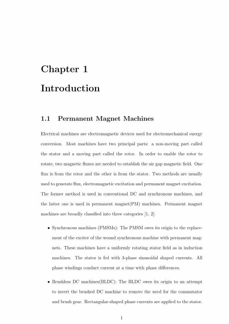
• Synchronous machines (PMSMs): The PMSM owes its origin to the replace-
ment of the exciter of the wound synchronous machine with permanent mag-
nets. These machines have a uniformly rotating stator field as in induction
machines. The stator is fed with 3-phase sinusoidal shaped currents. All
phase windings conduct current at a time with phase differences.
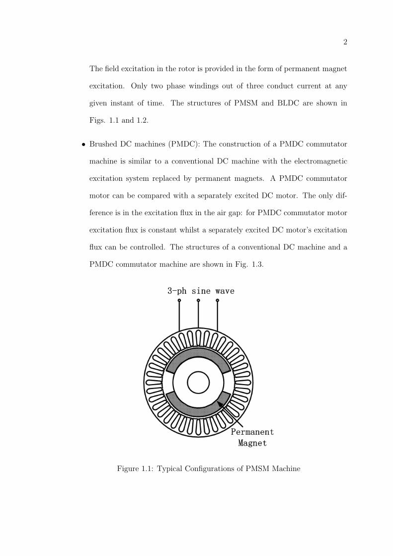
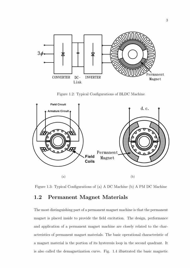
• Brushless DC machines(BLDC): The BLDC owes its origin to an attempt
to invert the brushed DC machine to remove the need for the commutator
and brush gear. Rectangular-shaped phase currents are applied to the stator.
1
2
The field excitation in the rotor is provided in the form of permanent magnet
excitation. Only two phase windings out of three conduct current at any
given instant of time. The structures of PMSM and BLDC are shown in
Figs. 1.1 and 1.2.
• Brushed DC machines (PMDC): The construction of a PMDC commutator
machine is similar to a conventional DC machine with the electromagnetic
excitation system replaced by permanent magnets. A PMDC commutator
motor can be compared with a separately excited DC motor. The only dif-
ference is in the excitation flux in the air gap: for PMDC commutator motor
excitation flux is constant whilst a separately excited DC motor’s excitation
flux can be controlled. The structures of a conventional DC machine and a
PMDC commutator machine are shown in Fig. 1.3.
Figure 1.1: Typical Configurations of PMSM Machine
3
Figure 1.2: Typical Configurations of BLDC Machine
(a) (b)
Figure 1.3: Typical Configurations of (a) A DC Machine (b) A PM DC Machine
1.2 Permanent Magnet Materials
The most distinguishing part of a permanent magnet machine is that the permanent
magnet is placed inside to provide the field excitation. The design, performance
and application of a permanent magnet machine are closely related to the char-
acteristics of permanent magnet materials. The basic operational characteristic of
a magnet material is the portion of its hysteresis loop in the second quadrant. It
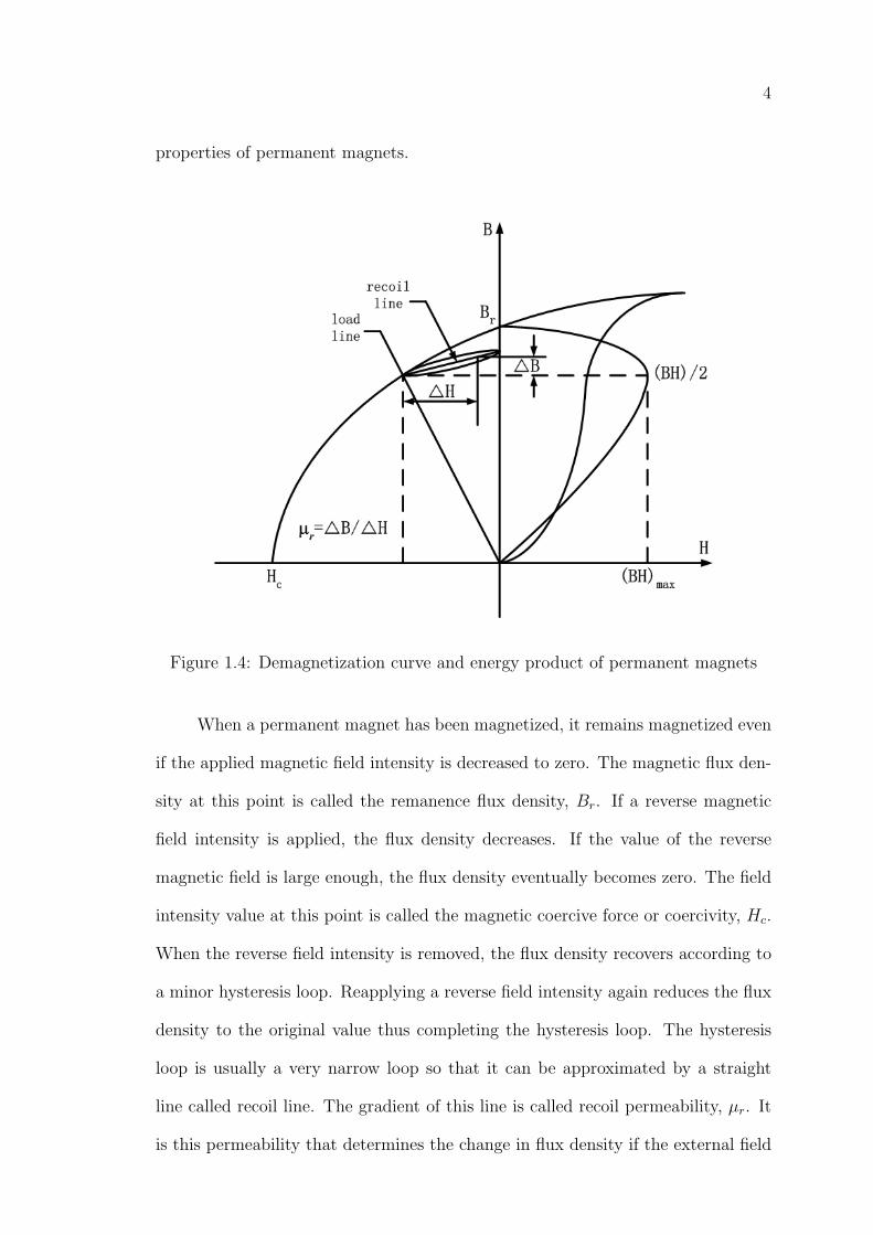
is also called the demagnetization curve. Fig. 1.4 illustrated the basic magnetic
4
properties of permanent magnets.
Figure 1.4: Demagnetization curve and energy product of permanent magnets
When a permanent magnet has been magnetized, it remains magnetized even
if the applied magnetic field intensity is decreased to zero. The magnetic flux den-
sity at this point is called the remanence flux density, Br. If a reverse magnetic
field intensity is applied, the flux density decreases. If the value of the reverse
magnetic field is large enough, the flux density eventually becomes zero. The field
intensity value at this point is called the magnetic coercive force or coercivity, Hc.
When the reverse field intensity is removed, the flux density recovers according to
a minor hysteresis loop. Reapplying a reverse field intensity again reduces the flux
density to the original value thus completing the hysteresis loop. The hysteresis
loop is usually a very narrow loop so that it can be approximated by a straight
line called recoil line. The gradient of this line is called recoil permeability, µr. It
is this permeability that determines the change in flux density if the external field
5
changes according to µr = ∆B/∆H. The operating point of a permanent magnet
is the intersection point of a B-H curve of the external magnetic circuit (load line)
and the demagnetisation curve of a permanent magnet. The operation point moves
along the demagnetisation curve with changes in the outer magnetic circuit. The
absolute value of the product of the flux density B and the field intensity H at
each point along the demagnetization curve can be represented by the energy prod-
uct and this quantity is one of the indexes of the strength of the permanent magnet.
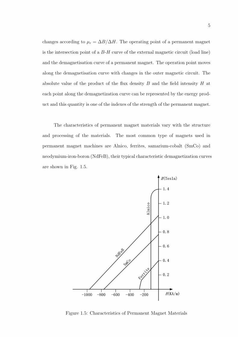
The characteristics of permanent magnet materials vary with the structure
and processing of the materials. The most common type of magnets used in
permanent magnet machines are Alnico, ferrites, samarium-cobalt (SmCo) and
neodymium-iron-boron (NdFeB), their typical characteristic demagnetization curves
are shown in Fig. 1.5.
Figure 1.5: Characteristics of Permanent Magnet Materials
6
Permanent magnets have been used in electric machines almost from the
beginning of the development of these machines as replacements for wound field
excitation systems. But the low energy densities of permanent magnets prevented
the use of permanent magnets in any types of machines other than very low power
control machines and signal transducers [3]. Modern permanent magnet machines
began with the development of Alnico magnets by Bell Labortories in the 1930’s.
This kind of magnets have the lowest temperature coefficient of Br and the highest
operating temperature. It has a Br value of up to 1.4 Tesla but with only a Hc
less than 120 kA/m. The applications of Alnico permanent magnet were limited.
However, the introduction of Alnico is the very start of widespread use of perma-
nent magnets in various devices.
Ferrite magnets were developed in 1950’s and have been used for decades. It
promoted the widespread use of permanent magnets in commercial and aerospace
applications. This kind of magnets has a Br value of around 0.3∼0.45 Tesla but
with a very high Hc up to 200 KA/m or more. Ferrite magnets have the lowest
cost and low core losses. They can be operational up to 100oC [4].
A revolution in permanent magnets commenced about 1960’s with the intro-
duction of samarium-cobalt (Sm-Co) family of hard magnets. It has a high value
of Br which is around 0.8∼1.1 Tesla and a strong Hc about 800 KA/m. However
the high cost of both samarium and cobalt makes this magnet one of the most
expensive magnetic materials in use today.
The revolution in magnetic materials accelerated with the discovery of an-
other new rare-earth magnet, neodymium-iron-boron (NdFeB) types. This kind of
magnets have higher Br values up to about 1.25 Tesla. The maximum tempera-
7
ture for NdFeB ranges from 100o to 180o depending on the detailed composition [4].
The cost of this magnet is still high but it is more efficient in terms of flux per dollar.
1.3 Line-Start Permanent Magnet Synchronous
Machines
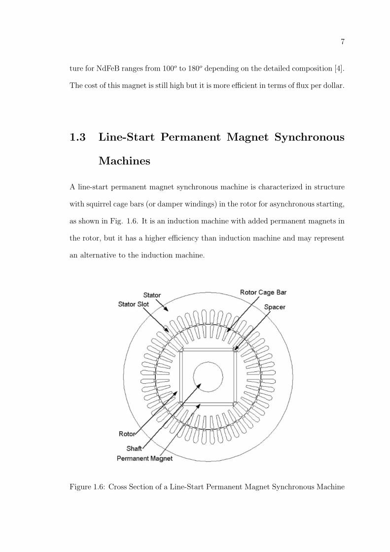
A line-start permanent magnet synchronous machine is characterized in structure
with squirrel cage bars (or damper windings) in the rotor for asynchronous starting,
as shown in Fig. 1.6. It is an induction machine with added permanent magnets in
the rotor, but it has a higher efficiency than induction machine and may represent
an alternative to the induction machine.
Figure 1.6: Cross Section of a Line-Start Permanent Magnet Synchronous Machine
8
Line-start permanent magnet synchronous machines have several advantages
for industrial applications. The presence of the magnets means that the magnetiz-
ing current is unnecessary, which improves the power factor of the machine. The
absence of field ohmic losses and the much lower rotor losses once synchronized
make the efficiency of the machine high.
When a line-start permanent magnet synchronous machine is run up from
zero speed to the rated speed, several factors have to be considered, such as start-
ing current, starting torque, run-up time, etc. The maximum current occurs at
run-up as in a normal induction machine. The heavy inrush of current at starting
may cause demagnetization of the magnets unless suitable precautions are taken
in the design of such machines. Although the squirrel cage bars can protect the
magnets from demagnetization during the transients associated with the start-up,
the magnet thickness must be designed such that it can withstand the maximum
possible demagnetization current. In practice, this high starting current should be
prevented from happening often so as to protect the permanent magnet. Therefore
frequent self-starting of the machine should be avoided or the machine should be
started at low voltage and light loads.
Starting torque is another important issue during the starting of a line-start
permanent magnet synchronous machine. Three different torques appear in the
process of starting [5]:
• braking torque due to the magnet;
• pulsating torque due to rotor saliency acting as a braking torque;
• accelerating torque due to the rotor bars.
9
The squirrel cage bars in the rotor can provide the accelerating torque that
drive the machine to near synchronous speed. The magnet torque is a braking
torque that opposes the cage torque during run-up. The stronger the magnet field,
the greater the braking torque. The accelerating torque must overcome, not only
the applied load torque, but also the generated magnet braking toques due to the
presence of the permanent magnet flux and the rotor saliency. As the motor ap-
proaches synchronous speed, the level of accelerating cage torque is lowered and
the magnet torque reverses its role and becomes the sole source of accelerating
torque. This synchronizing toque from the permanent magnet must be big enough
so as to pull the machine into synchronism. For large capacity machines, a stronger
magnet field is needed for the synchronism. However, this high magnetic field will
result in a big braking torque at low speed and prevent the machine from starting.
Therefore for some line-start permanent magnet synchronous machines, especially
some large capacity machines, the self-starting is quite difficult or even impossible.
The ability of starting and synchronizing a considerable load and inertia
against friction and windage is crucial for self-starting permanent magnet syn-
chronous machine. Bigger load inertia causes larger starting current which may
bring demagnetization to the permanent magnet. With bigger load inertia, stronger
magnetic field is required to pull the machine into synchronism, which may result
in a big braking torque at low speed.
Pulsating torque is caused by the machine saliency during the run-up. It will
bring oscillation to the speed and hence mechanical variation to the shaft. This
pulsation torque persists right up to the moment of pull-in. Such oscillation may
be severe and cause damage to the shaft during the starting process.
10
Heat is generated in the cage of the line start machines during start-up. This
heat is more of a problem in permanent magnet machines because of the proximity
of the cages to the magnets. Both the residual flux density and coercivity of some
permanent magnets reduce as a function of temperature. Indeed if the tempera-
ture excursion is beyond a certain value, permanent demagnetization can happen.
Therefore for permanent magnet synchronous machines with very high bar current
during the self-starting process, the heat effects brought along by the current may
cause the demagnetization of the permanent magnet. For such machines frequent
self-starting should not be applied.
The starting performance of a line-start permanent magnet synchronous ma-
chine from the moment of switch-on to the onset of stable synchronous running
forms an important part of the assessment of such machines for practical applica-
tions. The machine can be self-starting when connected to supply mains directly.
However, a few aspects as described above during the self-starting process have to
be considered, including the starting current, the demagnetization of permanent
magnet, the torque, etc. The machine can also be started with supply fed from
an inverter, where many starting quantities can be controlled, such as the starting
current, torque and frequency.
1.4 Computational Analysis of Permanent
Magnet Machines
Permanent magnet machines are widely used in industrial applications for their
superior performances. Performance simulation is vital to machine design as it is a
fast and low-cost way of predicting machine performances. The act of making and
remaking prototypes for actual testing, due to design changes, is both costly and

11
time consuming. This becomes especially important for large or special-purpose
equipment where trial and error methods are impossible or prohibitively expen-
sive. So analysis and simulation of machines are competitive when compared with
the experimental methods of development. It is for this reason that the study of
permanent magnet machine performance using mathematical methods has received
much attention in recent years [6] - [8]. Generally, two methods are used for evaluat-
ing the performance of electromagnetic devices: analytical and numerical methods.
1.4.1 Analytical Methods
Traditional analytical methods, such as lumped parameter models and equivalent
circuits, are computationally fast and designers can also have a good view of model
sensitivities to design parameters. These methods are simple and involved only a
few simple circuit equations to be evaluated. The circuit equations can be either
algebraic in a steady state condition or in the form of ordinary differential equations
in the transient conditions. Simple computer programs can also be easily written
for this purpose. Most available type of machines can be analyzed using a circuit
model once the machine parameters are known.
The main limitation of this method is that accurate determination of nec-
essary parameters is very difficult for permanent magnet machines. Most of the
standard methods used in conventional machines are not suitable for permanent
magnet machines because the field excitation cannot be varied or switched off.
Moreover, the parameters especially the transient parameters are dependent on
current and speed to some extent. So unless a proper method is developed to take
these factors into account it is impossible to determine all the machine parameters
accurately by experimental methods [9].
12
Other analytical methods, such as the method of images, can give us the solu-
tions to electromagnetic field problems [10]. These closed form solutions are usually
expressed through exact mathematical formulation. However, these methods can
only be used to solve the field problem with simple geometries. For example, the
method of images can only be applied to a range of problems in electrostatics and
magnetostatics when they involve relatively simple sources and possess an easily
identifiable symmetry. In reality, almost all the field problems are very compli-
cated. The resultant mathematical expressions may be too complicated for the
engineers to gain some intuitive feelings for the field behaviours. Sometimes it is
even difficult to obtain a mathematical expression just because of the complexity
of the problem [11].
1.4.2 Numerical Analysis
The limitations of the analytical methods require us to surrender the expectations
of closed form analytical solutions and to seek rigorous numerical field values di-
rectly. Using numerical methods, the solution of the field is not an analytical
expression, but the field values at some points in the field domain. If we can obtain
more such field points, we can find out more information about the field to be
solved. Although numerical methods are approximate by definition, high degrees
of accuracy are now possible.
In the analysis of electric machines, it is essential to be able to consider any
aspects of the design in great detail. Some critical factors, such as losses, tempera-
ture rise and efficiency, are dependent on the distribution of electromagnetic fields.
The computation of these fields to the accuracy now desired cannot be achieved by
13
analytical method. Numerical methods offer a more accurate and powerful design
tool. Most important aspects of the field computation, such as material properties,
non-linearities and structural details, can be taken into account. It is particularly
effective when dealing with such qualitative analysis as the optimization, demag-
netization and transient phenomena in the machine. With numerical methods few
simplifications are necessary. It is possible to calculate the field in the machine
very close to that in an actual operation.
1.5 Analysis of Electric Machines Using Finite
Element Method
Numerical methods are more suitable for the electromagnetic field analysis of per-
manent magnet machines. There are a number of numerical methods available
for the analysis of electromagnetic field problems. A few of them are, finite differ-
ence method (FDM) [12], boundary element method (BEM) [13] and finite element
method (FEM) [8]. These methods have their advantages and disadvantages. How-
ever, finite element method incorporates most of the advantages of the other two
methods without incurring significant disadvantages; especially for the analysis of
electric machines where many factors need to be considered, such as complex ge-
ometries, magnetic and electric materials, induced currents, coupling of thermal
and mechanical effects, etc.. In such cases, the finite element method is more suit-
able. For example, the finite difference method is not easily applicable to the field
involving rapid changes of the gradient or complex geometries. Nodal distribution
can be very inefficient. This is not so with finite elements. Equally, boundary ele-
ment method is not efficient at handling non-linear materials [14]. Finite element
method is well suited for the analysis involved with nonlinearities. It can be used

14
for solving both linear and non-linear field problems including simple and complex
geometries. Thus it is well recognized that finite element method offers consider-
able advantages in electrical machine analysis [14] - [16].
The finite element method was first introduced for the computation of mag-
netic field in nonlinear electromagnetic devices by Chari and Silvester in 1970’s
[17, 18]. It was mainly for solving nonlinear magnetostatic problems. Hannala and
MacDonald pioneered the numerical calculation of transient phenomenon during
the operation of electric machines [19]. They used time stepping techniques and
nodal method to predict the transient behavior of electric machines. The use of
time-stepping finite element method for analyzing nonlinear transient electromag-
netic field problems in electrical machines was presented by Tandon et al in the
1980’s [20].
In modern power systems, electric machines are often operated together with
the external circuits. The coupling of a comprehensive field analysis and circuit
analysis is necessary. Moreover, there are movable mechanical components in the
machine, like the rotor. Electromagnetic force determines the movement of these
components and the positions of these components in turn affect the electromag-
netic field within the machine. Therefore the coupling of mechanical movement
with the field and circuit analysis is also important.
Circuit equations are first applied to the steady state performance evaluation
of a turbine-generator by Brandl et al in 1975 [21]. A method of accounting for the
circuits in electric machines in the frequency domain was presented by Williamson
and Ralph in 1983 [22]. The direct coupling of fields and circuit equations in time
domain was applied by Nakata and Takahosi [23] in 1982. Later similar methods
15
were also used by many other researchers in the 1980’s [24]-[26].
An integrated approach to couple fields, circuits and mechanical motion was
first presented by Arkkio [27] and Istfan [28] in 1987. Then a detailed description
was given by Salon et al [29]. Given the machine geometry, winding connections,
material characteristics, applied voltage and the loading conditions, machine cur-
rents, fields and the motion can be computed accordingly. Such type of finite
element method is often referred to as field-circuit coupled time stepping method.
It has been widely used in the analysis of various electric machines [30]-[34].
Currently many commercial softwares, such as Flux2D [35], Maxwell [36] and
many others [37]-[40], are available to researchers for analysis of various complex
field problems of static and time varying nature.
The field-circuit coupled time stepping finite element method has been applied
to the computation of line-start permanent magnet synchronous machine before
[31, 41, 42]. Most of the application is for single phase line-start permanent magnet
synchronous machine as in [31]. The implementation of this method to the three
phase machines are presented in [41, 42]. However, the coupling of electromagnetic
field with the external circuit, such as inverter, is not included in these works.
1.6 Parameter Determination of Permanent
Magnet Synchronous Machines
Performance simulation is vital to machine analysis as it is a fast and low-cost
way of predicting machine performances. Traditional analytical methods, such as
lumped parameter models are computationally fast and simple in determining the
16
machine performances. The designers can also have a good view of model sensitiv-
ities to parameters. The analytical analysis requires machine parameters and the
accuracy of the analysis is wholly dependent on the accuracy of these parameters.
Therefore parameter determination is very important for performance evaluations
of electric machines.
Parameter determination is also important for the operations of machines.
Many synchronous machine drives are operated under various control schemes.
For example the flux weakening control is used in the synchronously rotating ref-
erence frame to actively vary the d-axis armature current as a function of loading
and speed. Such operation is realized with the knowledge of machine parameters.
It is for this reason that the accurate determination of machine parameters is in-
dispensable.
Many methods have been used for the determination of parameters of perma-
nent magnet synchronous machines [43] - [60], mainly focusing on the steady-state
synchronous reactances. Generally we can classify these methods as computational
methods and experimental methods. Computational methods, such as finite el-
ements [44, 45], allow assessment of parameters which are difficult to determine
experimentally and the estimation of various parameters even before the machine
prototype is made. But the limitation of computation modelling must be ap-
preciated [46]. The parameters of permanent magnet synchronous machines vary
nonlinearly due to the structural speciality of the rotor, the load condition and
current phase angle. Therefore the model should account for the parameter vari-
ations at different loading conditions and the iron saturation. Different authors
have proposed alternative methods to evaluate the variations of parameters with
iron saturation [47], [48]-[50]. However some assumptions have been made, such as
17
the constant permanent magnet flux linkage with load conditions [48, 49] and no
mutual coupling between the two axes [48]-[50].
Experimental methods, such as static test (locked rotor test) [51]-[54], no-
load tests [53, 55], load tests [43], [56]-[58] and other methods [59, 60] have been
applied by many researchers. Most of the methods are based on the steady state
two-axis model of permanent magnet synchronous machines and some necessary
simplifications. For example, it is assumed in the static test that parameters are
constant with one frequency. In no-load tests the variation of permanent magnet
flux linkage under different loading conditions is neglected. Some load tests take
into account the iron saturation but the issue of variable permanent magnet exci-
tation still cannot be solved.
1.7 Scope of the Thesis
This thesis presents the dynamic analysis of permanent magnet synchronous ma-
chines using field-circuit coupled time stepping finite element method. It also deals
with the parameter estimation of permanent magnet synchronous machines using
both experimental and computational methods.
A line-start interior permanent magnet synchronous machine is used in this
work. In modern power system, the line start interior permanent magnet syn-
chronous machine is often operated with external circuits. The coupling of a com-
prehensive field analysis and circuit analysis is necessary. Moreover, electric ma-
chines are electromagnetic devices for electro-mechanical energy conversion. The
electromagnetic field inside the motor affects the movement of the rotor and the po-
sition of the rotor in turn affects the electromagnetic field. Therefore the coupling
18
of mechanical movement with the field and circuit analysis is important. To ana-
lyze the dynamic performance of line-start permanent magnet synchronous machine
comprehensively, the field-circuit coupled time stepping finite element method is
implemented. The modelling of line-start permanent magnet synchronous machine
system is presented in Chapter 2. The finite element analysis is presented in Chap-
ter 3. As one of the dynamic performances, the starting process is computed and
presented in Chapter 5. This starting process includes both the self-starting and
the starting processes under different control schemes. The computational results
are validated by the experimental results.
Another important aspect in the analysis of permanent magnet synchronous
machines is the determination of its parameters, among which the most important
ones are the direct axis reactance Xd, the quadrature axis reactance Xq and the
permanent magnet excitation voltage E0. In Chapter 4 both the experimental
method and the computational method are discussed in combination to determine
these parameters. Two novel methods are proposed through the application of
linear regression and Hopfield neural network. Finite element analysis has been
used to compute the machine parameters as well.

Chapter 2
Mathematical Modelling ofLine-Start Permanent MagnetSynchronous Machines
2.1 Introduction
Line-start permanent magnet synchronous machines have complex geometrical con-
figurations consisting of magnets, conductors, barriers, etc. Precise analysis and
simulation of these machines are challenging tasks for those who design and use
these machines. The accomplishment of these tasks depends on the accurate com-
putation of electromagnetic fields in the machine using analytical or numerical
methods. Essentially the method selected has to be able to analyze the electric
machines in considerable detail, so that a near exactness may be obtained. Elec-
tric machines are complicated devices, with difficulties such as complex geometries,
nonlinearities of materials and eddy currents, which cannot be included in an an-
alytical method. However, the use of numerical analysis can easily overcome these
difficulties.
The fundamental basis of applying numerical methods is the modelling of
electric machines. Electric machines receive power from external sources through
electric circuits. This in turn requires the modelling of electromagnetic fields inside
19
20
the machine to be coupled with electric circuit analysis. Moreover electric machines
are electro-mechanical conversion devices. It is important to take into account also
the interaction of electromagnetic fields, mechanical forces and motions. Therefore
a comprehensive modelling of electromagnetic fields, circuits and mechanical mo-
tion of an electrical machine system should be considered together.
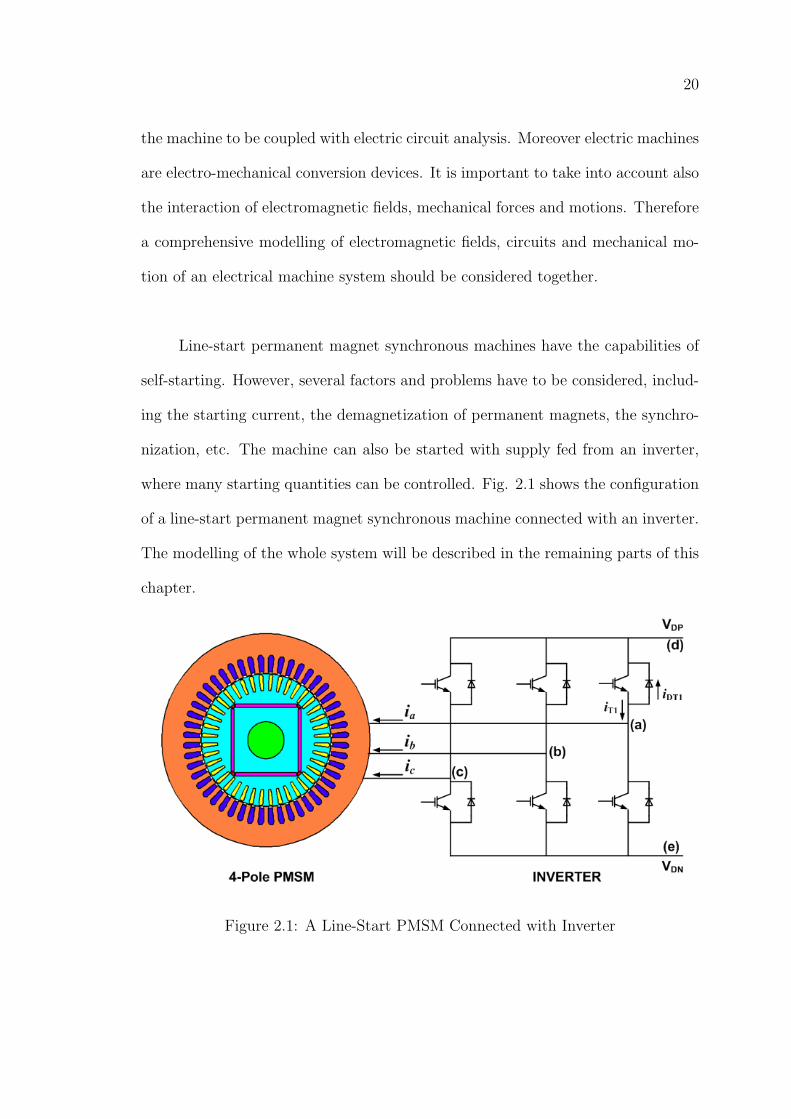
Line-start permanent magnet synchronous machines have the capabilities of
self-starting. However, several factors and problems have to be considered, includ-
ing the starting current, the demagnetization of permanent magnets, the synchro-
nization, etc. The machine can also be started with supply fed from an inverter,
where many starting quantities can be controlled. Fig. 2.1 shows the configuration
of a line-start permanent magnet synchronous machine connected with an inverter.
The modelling of the whole system will be described in the remaining parts of this
chapter.
Figure 2.1: A Line-Start PMSM Connected with Inverter
21
2.2 Representation of Permanent Magnets
The properties and performances of a permanent magnet machine are greatly af-
fected by the characteristics of permanent magnets. Therefore proper represen-
tation of permanent magnet is very important in the design and analysis of a
permanent magnet machine. Generally there are two models to represent perma-
nent magnets: a magnetization vector model [8] and an equivalent current sheet
model [61]. These two methods have different starting points but they result in the
same set of equations [8]. In this work the magnetization vector model has been
used.
Magnetic behavior of magnet materials is described in terms of three interre-
lated vectors: B− magnetic induction or flux density, H− magnetic field intensity
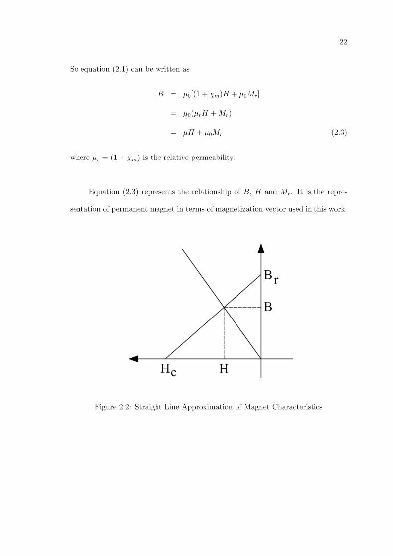
and M− magnetization. For a magnet material NdFeB operated in the second
quadrant of its normal hysteresis loop, it can be represented as a straight line as
shown in Fig. 2.2. The relationship of the three vectors B, H and M can be
expressed as [62]:
B = µ0H + µ0M (2.1)
where µ0 is the permeability of the free space.
While calculating distributed fields, it is usual to describe the vector M in
terms of its remanent value Mr ( when H = 0 ) and M ′ which is the function of
magnetic susceptibility χm and H :
M = M ′ +Mr
= χmH +Mr (2.2)
22
So equation (2.1) can be written as
B = µ0[(1 + χm)H + µ0Mr]
= µ0(µrH +Mr)
= µH + µ0Mr (2.3)
where µr = (1 + χm) is the relative permeability.
Equation (2.3) represents the relationship of B, H and Mr. It is the repre-
sentation of permanent magnet in terms of magnetization vector used in this work.
Figure 2.2: Straight Line Approximation of Magnet Characteristics
23
2.3 Modelling of Electromagnetic Fields
The electromagnetic field in an electric machine is governed by Maxwell’s equations:
∇×H = J (2.4)
∇× E = −∂B∂t
(2.5)
∇ ·B = 0 (2.6)
with the constitutive relationship:
J = σE (2.7)
and
B = µH (2.8)
where
J = current density
E = electric field intensity
σ = conductivity
Since
∇ ·B = 0,
we are able to find a vector A whose curl is equal to B and the ∇ ·B is assured to
be zero through ∇ · (∇× A) = 0. Thus
B = ∇× A (2.9)
and A is the magnetic vector potential.
24
Substituting equation (2.9) into equation (2.5) yields
∇× E = −∂(∇× A)
∂t= −∇× ∂A
∂t(2.10)
or
∇× (E +∂A
∂t) = 0. (2.11)
Since the curl of a gradient is identically zero, we can write
E +∂A
∂t= −∇ψ (2.12)
or
E = −∂A∂t
−∇ψ (2.13)
where ∇ψ is the gradient of a scalar quantity ψ called the scalar potential. Sub-
stituting equation (2.13) into equation (2.7), the current density vector becomes
J = σE = −σ(∂A
∂t+∇ψ). (2.14)
The current density in equation (2.14) includes two parts: one is induced quantity
∂A∂t
produced by electromagnetic induction and the other one is ∇ψ caused by the
effect of charge build up at the conductor end.
If we consider a current-carrying conductor of length l, its positive terminal is
point a and negative terminal is point b. If the difference in electric scalar potential
between point a and b is Vtz volts, we can write
Vtz = Va − Vb =
∫ b
a
Escaledl = −∫ b
a
∇ψdl. (2.15)
In two-dimensional field problems ∇ψ is considered to be constant in z−direction,
then equation (2.15) becomes
Vtz = −∇ψ · l (2.16)
or
∇ψ = −Vtz
l(2.17)
25
Therefore the current density vector for a stationary two-dimensional field is
J = −σ∂A∂t
+ σVtz
l(2.18)
When the field is moving with a relative velocity v, two reference frames
(coordinate systems) have to be defined. One frame O(x, y, z) is stationary and
the other frame O′(x′, y′, z′) is moving. Assuming the time t and t′ measured in
the two frame are same, then following relation exists for vector E [63]:
E ′ = E + v ×B (2.19)
Therefore the current density observed from the stationary frame O(x, y, z) is
J = σ(E + v ×B)
= −σ∂A∂t
+ σVtz
l+ σv ×B (2.20)
Combining with equation (2.4) yields
∇×H = −σ∂A∂t
+ σVtz
l+ σv ×B. (2.21)
Recalling equations (2.8) and (2.9),
B = µH
∇× A = B
then equation (2.21) becomes
∇× (ν∇× A) = −σ∂A∂t
+ σVtz
l+ σv ×B (2.22)
where ν = 1µ
is the reluctivity.
26
For permanent magnets which are represented by
B = µH + µ0Mr, (2.23)
∇×H = ∇× (νB)−∇× (νµ0Mr)
= ∇× (ν∇× A)−∇× (νµ0Mr).
Since
∇×H = J,
combining with equation (2.20) yields the governing equation for permanent mag-
net,
∇× (ν∇× A) = −σ∂A∂t
+ σVtz
l+ σv ×B +∇× (νµ0Mr). (2.24)
For soft magnetic materials, equation (2.24) is reduced to equation (2.22) since
no remanent magnetization (Mr = 0). Therefore equation (2.24) is taken as the
general governing equation for moving time-varying field problems.
Employing the moving frame as reference frame, the relative velocity v be-
comes zero and equation (2.24) can be simplified as:
∇× (ν∇× A) = −σ∂A∂t
+ σVtz
l+∇× (νµ0Mr) (2.25)
Equation (2.25) is the fundamental governing equation for the modelling of
various field problems. It can be solved for a wide class of field problems, involving
relative motion, non-linear material properties and time-variations. In the analysis
of electric machines, it is common to evaluate the field solution in two dimensions
considering the current density J and magnetic vector potential A having only z-
directed invariant components. This analysis is valid for most cases because the air
gap between the rotor and stator in an electrical machine is so small that for most
of the length of the machine, except the end regions, the machine is practically
27
two-dimensional in operation. Comparing with three dimensional technique, two-
dimensional technique distinctively saves the computational cost and time despite
the possible loss in accuracy. Three dimensional effects such as skewing and end
winding effect can somehow be compensated by employing correction factors to the
field solution or applying some other techniques, like multi-slice [64]. Thus for a
given a problem domain or region, equation (2.25) with B and H in x − y plane
becomes,
∂
∂x(ν∂A
∂x) +
∂
∂y(ν∂A
∂y) = σ
∂A
∂t− σ
Vtz
l−∇× (νµ0Mr) (2.26)
2.4 Circuit Equations
The analysis of electric machines depends on the accurate field analysis. The ap-
proach to analysis commonly involves two dimensional numerical methods with
specified current sources for the conductors. The knowledge of input currents is
essential for the successful field analysis of electrical devices. However in practice
electric devices are mostly connected to voltage sources instead of the ideal current
sources. The problem is further complicated by the connections of the conductors.
Therefore analysis of field problems with a voltage source and arbitrary waveforms
is preferred. Circuit equations that represent the relations of current and voltages
are needed. The coupling of circuit equations to the field analysis is necessary.
Modern electric machines are often operated under some external circuits
connected to a known voltage source. The behaviours of such circuits affect the
integrity and performance of all the connected devices. Unless the interactions of
these external circuits with the electric machines are considered, the analysis of the
electric machines cannot assumed to be complete. Thus it is necessary to include
the modelling and circuit description of such devices.
28
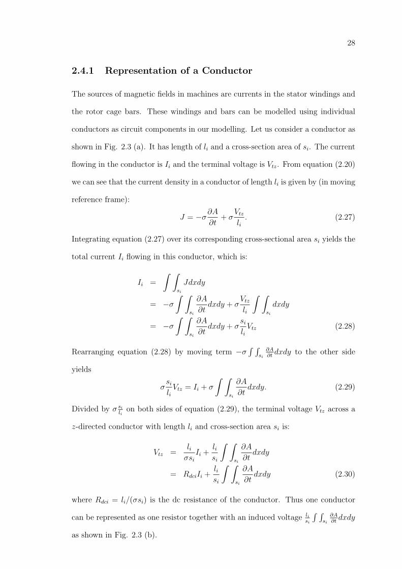
2.4.1 Representation of a Conductor
The sources of magnetic fields in machines are currents in the stator windings and
the rotor cage bars. These windings and bars can be modelled using individual
conductors as circuit components in our modelling. Let us consider a conductor as
shown in Fig. 2.3 (a). It has length of li and a cross-section area of si. The current
flowing in the conductor is Ii and the terminal voltage is Vtz. From equation (2.20)
we can see that the current density in a conductor of length li is given by (in moving
reference frame):
J = −σ∂A∂t
+ σVtz
li. (2.27)
Integrating equation (2.27) over its corresponding cross-sectional area si yields the
total current Ii flowing in this conductor, which is:
Ii =
∫ ∫si
Jdxdy
= −σ∫ ∫
si
∂A
∂tdxdy + σ
Vtz
li
∫ ∫si
dxdy
= −σ∫ ∫
si
∂A
∂tdxdy + σ
si
liVtz (2.28)
Rearranging equation (2.28) by moving term −σ∫ ∫
si
∂A∂tdxdy to the other side
yields
σsi
liVtz = Ii + σ
∫ ∫si
∂A
∂tdxdy. (2.29)
Divided by σ si
lion both sides of equation (2.29), the terminal voltage Vtz across a
z-directed conductor with length li and cross-section area si is:
Vtz =liσsi
Ii +lisi
∫ ∫si
∂A
∂tdxdy
= RdciIi +lisi
∫ ∫si
∂A
∂tdxdy (2.30)
where Rdci = li/(σsi) is the dc resistance of the conductor. Thus one conductor
can be represented as one resistor together with an induced voltage lisi
∫ ∫si
∂A∂tdxdy
as shown in Fig. 2.3 (b).
29
Figure 2.3: Representation of a Conductor
Both stator windings and rotor cage bars are made up of conductors con-
nected in series or in parallel. It is possible to model them using two-dimensional
models based on the modelling of one conductor. However some properties and fea-
tures due to the inherent three dimensional nature of electric machines have to be
taken into account. Among these features the most important ones are the stator
end-windings and rotor end rings. These end effects lie outside the jurisdiction of
two dimensional numerical models, which can only account for the currents flowing
in Z−direction. Therefore some means must be found to deal with these end effects.
Stator end-winding effects are dealt with simply by adding an appropriate
external impedance in the stator circuit equations [23]. For rotor end-ring effects,
Strangas [25] neatly combines the end-ring impedance with the field analysis by
means of rotor loop equations. These methods are quite effective when including
the three-dimensional effects into the two-dimensional field analysis. They have
been used frequently in the analysis of electric machines [27, 64].
30
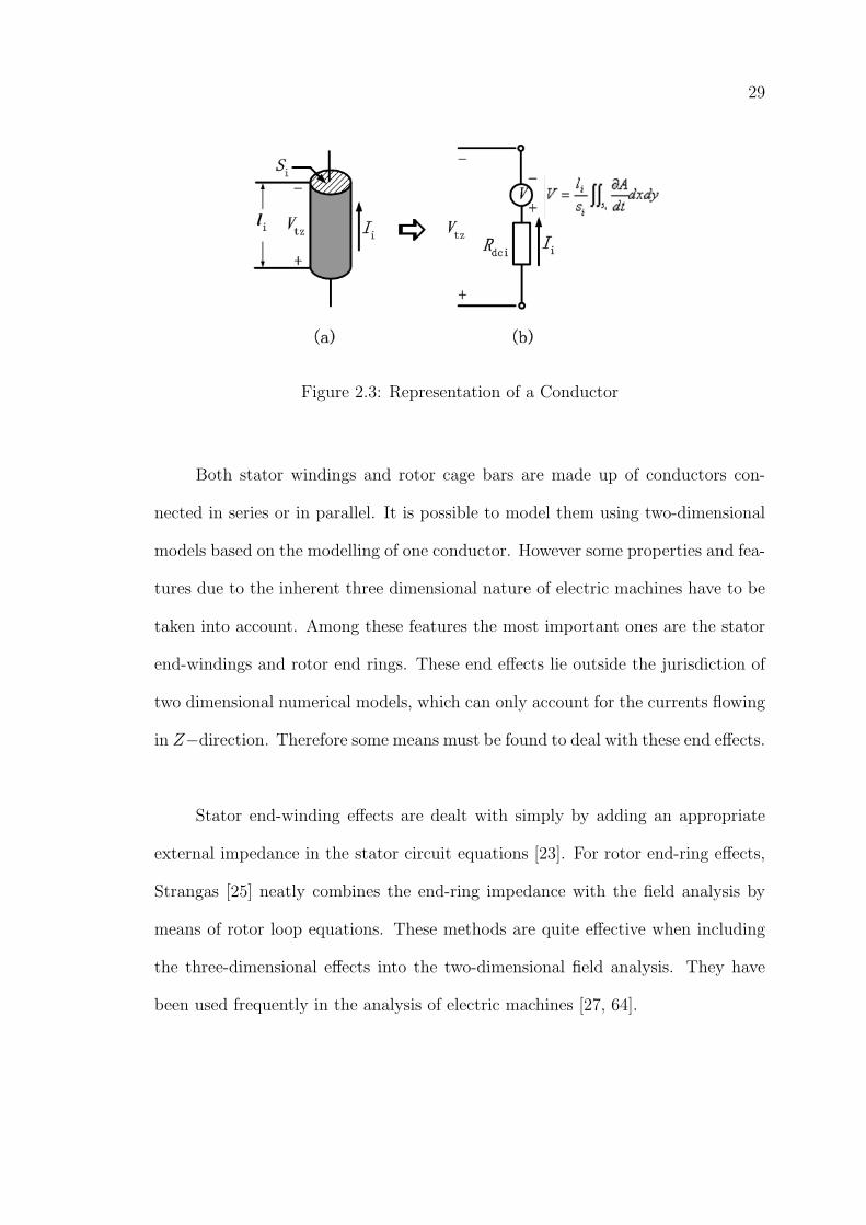
2.4.2 Equivalent Circuits of Stator Windings
Stator windings are made up by conductors connected in many turns. If we con-
sider a ’go’ and ’return’ loop of current-carrying conductors (Fig. 2.4) connected
to an external input voltage source Vext through an external resistance Rext and
inductance Lext, we can get:
Vext = V +tz − V −tz +RextiI + Lexti
dI
dt(2.31)
Figure 2.4: One Turn of ’Go’ and ’Return’ Loop of Conductors
Substituting equation (2.30) into equation (2.31) yields
Vext = R+dciI
+i −R−dciI
−i +
l+is+
i
∫ ∫s+i
∂A
∂tdxdy− l−i
s−i
∫ ∫s−i
∂A
∂tdxdy+RextiI+Lexti
dI
dt
(2.32)
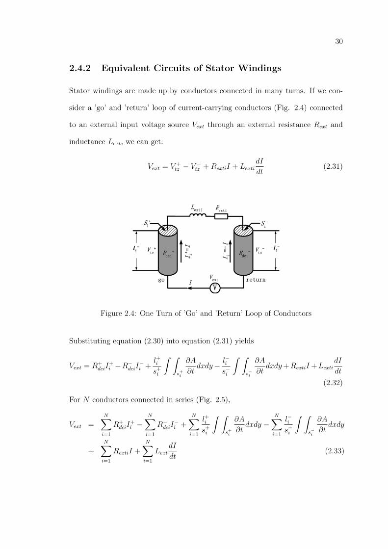
For N conductors connected in series (Fig. 2.5),
Vext =N∑
i=1
R+dciI
+i −
N∑i=1
R−dciI−i +
N∑i=1
l+is+
i
∫ ∫s+i
∂A
∂tdxdy −
N∑i=1
l−is−i
∫ ∫s−i
∂A
∂tdxdy
+N∑
i=1
RextiI +N∑
i=1
LextdI
dt(2.33)
31
When N is large, the representation of each conductor as shown above is
unrealistic to carry out in calculation. Under this condition a uniform current,
length and cross section area for each conductor are assumed:
I+1 = I+
2 = . . . = I+N = I
I−1 = I−2 = . . . = I−N = −I
l+1 = l+2 = . . . = l+N = l
l−1 = l−2 = . . . = l−N = l
s+1 = s+
2 = . . . = s+N = s = Stt/N
s−1 = s−2 = . . . = s−N = s = Stt/N (2.34)
Here
Stt = the total cross section area of the N−turn conductors
s = the average cross section area of one turn of conductor
and the insulation space between the turns are neglected
+ is for the ’go’ conductor
− is for the ’return’ conductor
Figure 2.5: N Turns of Conductors Connected in Series
32
Substituting equation (2.34) to equation (2.33) yields
Vext = (Rdc +Rext)I + LextdI
dt+l
s(
∫ ∫S+
tt
∂A
∂tdxdy −
∫ ∫S−tt
∂A
∂tdxdy) (2.35)
where
Rdc =∑N
i=1R+dci +R−dci = 2lN
σsis the total cross section area
of N -turn conductors
Rext =∑N
i=1Rexti is the total external resistance
Lext =∑n
i=1 Lexti is the total external inductance
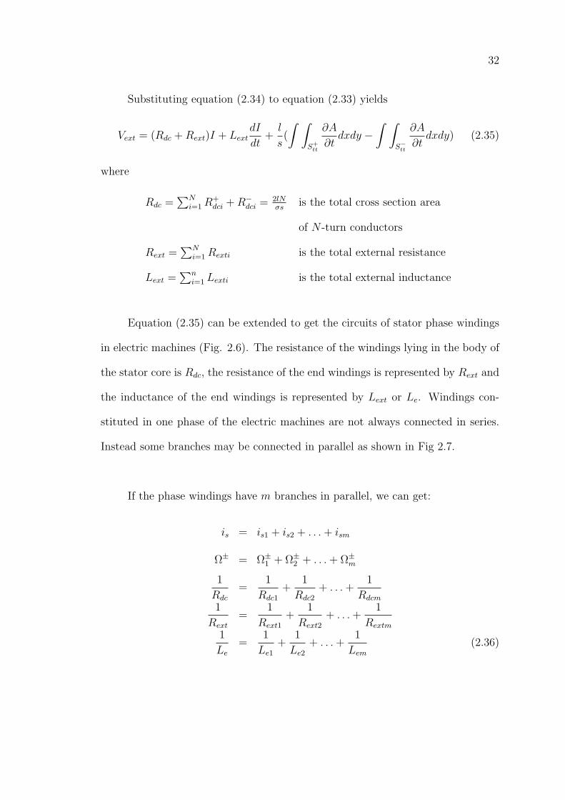
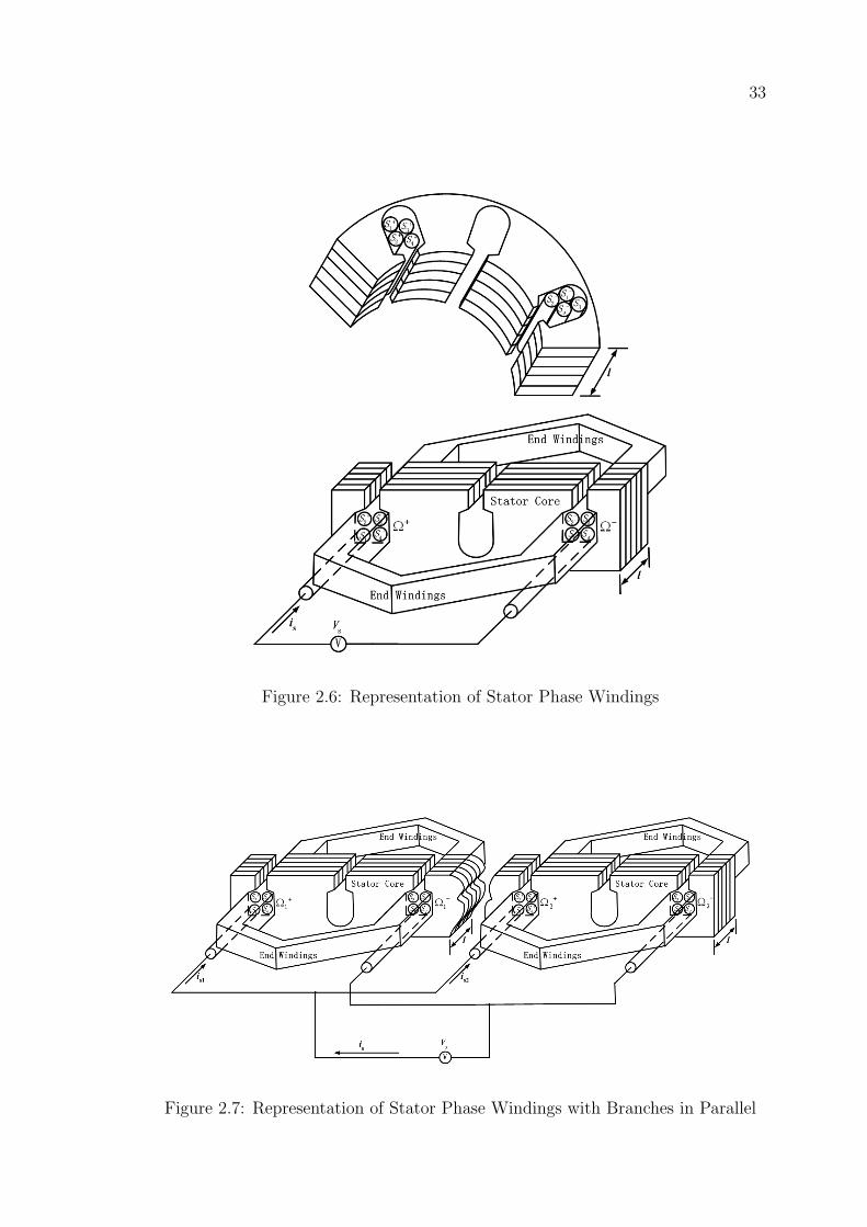
Equation (2.35) can be extended to get the circuits of stator phase windings
in electric machines (Fig. 2.6). The resistance of the windings lying in the body of
the stator core is Rdc, the resistance of the end windings is represented by Rext and
the inductance of the end windings is represented by Lext or Le. Windings con-
stituted in one phase of the electric machines are not always connected in series.
Instead some branches may be connected in parallel as shown in Fig 2.7.
If the phase windings have m branches in parallel, we can get:
is = is1 + is2 + . . .+ ism
Ω± = Ω±1 + Ω±2 + . . .+ Ω±m
1
Rdc
=1
Rdc1
+1
Rdc2
+ . . .+1
Rdcm
1
Rext
=1
Rext1
+1
Rext2
+ . . .+1
Rextm
1
Le
=1
Le1
+1
Le2
+ . . .+1
Lem
(2.36)
33
Figure 2.6: Representation of Stator Phase Windings
Figure 2.7: Representation of Stator Phase Windings with Branches in Parallel
34
Therefore the general governing equation for stator phase circuits in electrical
machines is:
Vs = (Rdc +Rext)is + Ledisdt
+l
ms(
∫ ∫Ω+
∂A
∂tdxdy −
∫ ∫Ω−
∂A
∂tdxdy)
= Rsis + Ledisdt
+l
ms(
∫ ∫Ω+
∂A
∂tdxdy −
∫ ∫Ω−
∂A
∂tdxdy)
= Rsis + Ledisdt
+ Vi (2.37)
where
Vs = applied stator phase voltage
is = stator phase current
Rs = total equivalent resistance per phase
Le = total equivalent inductance of end winding
l = the length of stator windings in Z−direction,
usually it uses the same value as the axial length of stator iron core
m = number of stator winding branches in parallel connection
s = equivalent cross section area of one turn of stator windings
Ω+,Ω− = total cross section area of ’go’ and ’return’ windings per phase respectively
Vi = induced voltage per phase
Equation (2.37) describes the relationship of external voltage source Vs, cor-
responding current is and vector potential A. Therefore we can calculate the field
value A directly from the external voltage source Vs. It is quite effective in the com-
putation of two dimensional electromagnetic fields with coupled external voltage
sources.
35
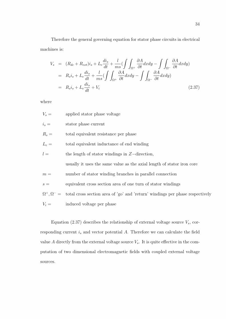
In three-phase electric machines, usually the stator phases are connected in
two different types of connections: a delta (4) connection or a star (Y ) connection
(Fig. 2.8). Representation of sources and circuits in the modelling process can be
achieved using common circuit laws such as Kirchoff’s voltage rule.
Figure 2.8: Connections of Stator Phase Windings (a) 4 - Connection (b)Y -
Connection
In Fig. 2.8, Vtk|k=1,2,3 are terminal voltages of the stator phases, ilk are line
currents and isk are phase currents. ilk and Vtk are measurable quantities from
outside. isk are the quantities used in the model of stator phases.
Taking loops around every two terminals of 4 connection yields,
Vt1 − Vt2 = Rs1is1 + Le1dis1dt
+ Vi1
Vt2 − Vt3 = Rs2is2 + Le2dis2dt
+ Vi2
Vt3 − Vt1 = Rs3is3 + Le3dis3dt
+ Vi3 (2.38)
and il1
il2
il3
=
1 0 −1
−1 1 0
0 −1 1
is1
is2
is3
(2.39)
36
Taking loops around every two terminals of Y connection yields,
Vt1 − Vt2 = Rs1is1 + Le1dis1dt
+ Vi1 − (Rs2is2 + Le2dis2dt
+ Vi2)
Vt2 − Vt3 = Rs2is2 + Le2dis2dt
+ Vi2 − (Rs3is3 + Le3dis3dt
+ Vi3)
Vt3 − Vt1 = Rs3is3 + Le3dis3dt
+ Vi3 − (Rs1is1 + Le1dis1dt
+ Vi1) (2.40)
and il1
il2
il3
=
1 0 0
0 1 0
0 0 1
is1
is2
is3
(2.41)
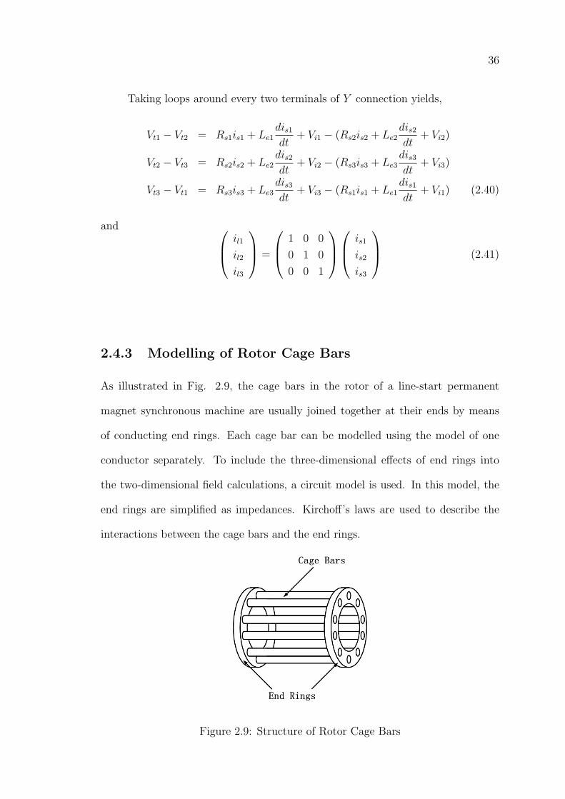
2.4.3 Modelling of Rotor Cage Bars
As illustrated in Fig. 2.9, the cage bars in the rotor of a line-start permanent
magnet synchronous machine are usually joined together at their ends by means
of conducting end rings. Each cage bar can be modelled using the model of one
conductor separately. To include the three-dimensional effects of end rings into
the two-dimensional field calculations, a circuit model is used. In this model, the
end rings are simplified as impedances. Kirchoff’s laws are used to describe the
interactions between the cage bars and the end rings.
Figure 2.9: Structure of Rotor Cage Bars
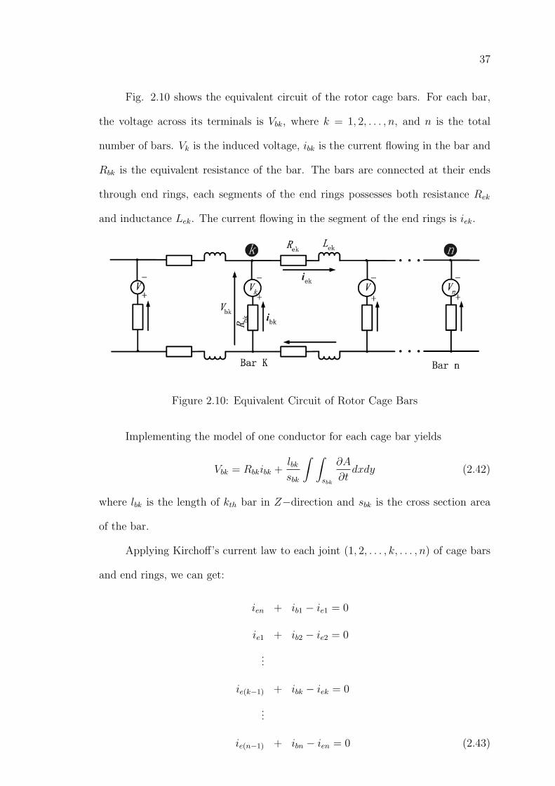
37
Fig. 2.10 shows the equivalent circuit of the rotor cage bars. For each bar,
the voltage across its terminals is Vbk, where k = 1, 2, . . . , n, and n is the total
number of bars. Vk is the induced voltage, ibk is the current flowing in the bar and
Rbk is the equivalent resistance of the bar. The bars are connected at their ends
through end rings, each segments of the end rings possesses both resistance Rek
and inductance Lek. The current flowing in the segment of the end rings is iek.
Figure 2.10: Equivalent Circuit of Rotor Cage Bars
Implementing the model of one conductor for each cage bar yields
Vbk = Rbkibk +lbksbk
∫ ∫sbk
∂A
∂tdxdy (2.42)
where lbk is the length of kth bar in Z−direction and sbk is the cross section area
of the bar.
Applying Kirchoff’s current law to each joint (1, 2, . . . , k, . . . , n) of cage bars
and end rings, we can get:
ien + ib1 − ie1 = 0
ie1 + ib2 − ie2 = 0
...
ie(k−1) + ibk − iek = 0
...
ie(n−1) + ibn − ien = 0 (2.43)
38
It can also be rewritten as:
[ib]− [C1][ie] = 0 (2.44)
where
[ib] =(ib1 ib2 . . . ibk . . . ibn
)tr
, (2.45)
[C1] =
1 . . . . . . . . . . . . −1
−1 1 . . . . . . . . . . . ....
......
......
...
. . . . . . −1 1 . . . . . ....
......
......
...
. . . . . . . . . . . . −1 1
n×n
, (2.46)
[ie](ie1 ie2 . . . iek . . . ien
)tr
, (2.47)
and ’()tr’ denotes the transpose operation of a matrix.
Applying Kirchoff’s voltage law to each loop surrounded by two segments of
end rings and two cage bars, we can get:
Vb1 + 2(Re1ie1 + Le1die1dt
)− Vb2 = 0
Vb2 + 2(Re2ie2 + Le2die2dt
)− Vb3 = 0
...
Vbk + 2(Rekiek + Lekdiekdt
)− Vb(k+1) = 0
...
Vbn + 2(Renien + Lendiendt
)− Vb1 = 0 (2.48)
Putting them in a matrix form yields:
[C2][Vb] + 2[Re] +d
dt[Le][ie] = 0 (2.49)
39
where
[C2] =
1 −1 . . . . . . . . . . . .
. . . 1 −1 . . . . . . . . ....
......
......
...
. . . . . . . . . 1 −1 . . ....
......
......
...
−1 . . . . . . . . . . . . 1
n×n
, (2.50)
[Vb] =(Vb1 Vb2 . . . Vbk . . . Vbn
)tr
, (2.51)
[Re] =(Re1 Re2 . . . Rek . . . Ren
)tr
, (2.52)
[Le] =(Le1 Le2 . . . Lek . . . Len
)tr
. (2.53)
Equations (2.42), (2.44) and (2.49) are three governing equations for the mod-
elling of cage bars. They cover the whole solution domain of the rotor cage bars.
Electric machines are geometrically symmetrical devices. With the intention
of saving computational efforts, usually only part of the problem domain is used in
the numerical computation. Under this condition, equations (2.44) and (2.49) will
have different formats. The main difference lies in the format of matrices [C1] and
[C2]. If there are only np(np ≤ n) bars involved in the computation, the current
and voltage of bar np and bar n have the following relationships,
ienp = δ · ien
ibnp = δ · ibn
Vbnp = δ · Vbn (2.54)
where δ = 1 or δ = −1. The value of δ depends on how many poles are included
in the computation domain. Two cases are illustrated below:
40
(1) Pairs of poles are included in the computation domain
The cage bars over pairs of poles pitch have identical currents and voltages. There-
fore if the domain to be investigated spans over pairs of poles in electric machine,
δ = 1. Under this condition, equation (2.43) becomes
ienp + ib1 − ie1 = 0
ie1 + ib2 − ie2 = 0
...
ie(k−1) + ibk − iek = 0
...
ie(np−1) + ibnp − ienp = 0 (2.55)
or
[ibp]− [C1p][iep ] = 0 (2.56)
where
[ibp] =(ib1 ib2 . . . ibk . . . ibnp
)tr
, (2.57)
[C1p] =
1 . . . . . . . . . . . . −1
−1 1 . . . . . . . . . . . ....
......
......
...
. . . . . . −1 1 . . . . . ....
......
......
...
. . . . . . . . . . . . −1 1
np×np
, (2.58)
[iep] =(ie1 ie2 . . . iek . . . ienp
)tr
. (2.59)
41
Similarly substituting equation (2.54) into equation (2.48) when δ = 1 yields,
Vb1 + 2(Re1ie1 + Le1die1dt
)− Vb2 = 0
Vb2 + 2(Re2ie2 + Le2die2dt
)− Vb3 = 0
...
Vbk + 2(Rekiek + Lekdiekdt
)− Vb(k+1) = 0
...
Vbnp + 2(Renpienp + Lenp
dienp
dt)− Vb1 = 0 (2.60)
or
[C2p][Vbp] + 2[Rep] +d
dt[Lep][iep] = 0 (2.61)
where
[C2p] =
1 −1 . . . . . . . . . . . .
. . . 1 −1 . . . . . . . . ....
......
......
...
. . . . . . . . . 1 −1 . . ....
......
......
...
−1 . . . . . . . . . . . . 1
np×np
, (2.62)
[Vbp] =(Vb1 Vb2 . . . Vbk . . . Vbnp
)tr
, (2.63)
[Rep] =(Re1 Re2 . . . Rek . . . Renp
)tr
, (2.64)
[Lep] =(Le1 Le2 . . . Lek . . . Lenp
)tr
. (2.65)
(2) Odd number of poles are included in the computation domain
On the other hand, the cage bars over one-pole pitch have equivalent current and
voltage in magnitude but in opposite direction. So if the domain to be investigated
spans over one pole in electric machine, δ = −1 for equation (2.54). Equation
42
(2.43) becomes
− ienp + ib1 − ie1 = 0
ie1 + ib2 − ie2 = 0
...
ie(k−1) + ibk − iek = 0
...
ie(np−1) + ibnp − ienp = 0 (2.66)
and matrix [C1p] becomes
[C1p] =
1 . . . . . . . . . . . . +1
−1 1 . . . . . . . . . . . ....
......
......
...
. . . . . . −1 1 . . . . . ....
......
......
...
. . . . . . . . . . . . −1 1
np×np
. (2.67)
Similarly equation (2.48) becomes
Vb1 + 2(Re1ie1 + Le1die1dt
)− Vb2 = 0
Vb2 + 2(Re2ie2 + Le2die2dt
)− Vb3 = 0
...
Vbk + 2(Rekiek + Lekdiekdt
)− Vb(k+1) = 0
...
−Vbnp + 2(Renpienp + Lenp
dienp
dt)− Vb1 = 0 (2.68)
and matrix [C2p] becomes
[C2p] =
1 −1 . . . . . . . . . . . .
. . . 1 −1 . . . . . . . . ....
......
......
...
. . . . . . . . . 1 −1 . . ....
......
......
...
+1 . . . . . . . . . . . . 1
np×np
. (2.69)
43
In summary, matrices [C1] and [C2] are:
[C1] =
1 . . . . . . . . . . . . ∓1
−1 1 . . . . . . . . . . . ....
......
......
...
. . . . . . . . . −1 1 . . ....
......
......
...
. . . . . . . . . . . . −1 1
np×np
, (2.70)
[C2] =
1 −1 . . . . . . . . . . . .
. . . 1 −1 . . . . . . . . ....
......
......
...
. . . . . . . . . 1 −1 . . ....
......
......
...
∓1 . . . . . . . . . . . . 1
np×np
, (2.71)
where np(np ≤ n) is the number of cage bars in the computation domain. If the
domain to be investigated spans over one pair of poles in electric machine, the signs
’∓’ in equations (2.70) and (2.71) should be ’-’. If the studied domain covers odd
number of poles, then the signs should be ’+’.
2.4.4 Modelling of External Circuit Components
A suitable simulation of the behavior of the machines and drives should take into
account the numerical models of electrical, electronic circuit and electromagnetic
fields. In the modelling of electronic circuits, the main difficulties lie in the mod-
elling of transistors, diodes and other active nonlinear semiconductor devices. The
method proposed by F. Piriou and A. Razek [65, 66] could be used to get the
simultaneous solution of the field equations and equations of the circuits with non-
linear semiconductor elements. This method basically is an application of Newton-
Raphson algorithm to both the magnetic core nonlinearity and the nonlinearity
of the semiconductor components. A. Demenko [67] simplified the method and
approximated the volt-ampere characteristics (the nonlinearity) of semiconductor
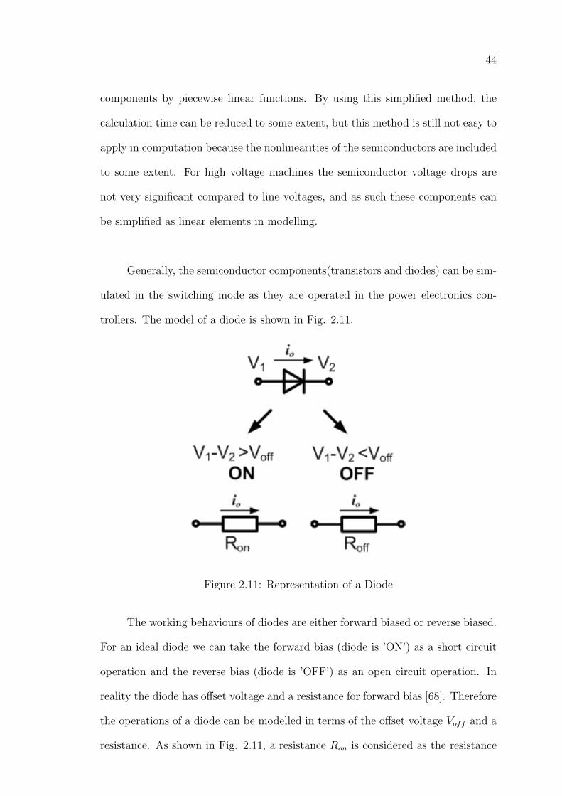
44
components by piecewise linear functions. By using this simplified method, the
calculation time can be reduced to some extent, but this method is still not easy to
apply in computation because the nonlinearities of the semiconductors are included
to some extent. For high voltage machines the semiconductor voltage drops are
not very significant compared to line voltages, and as such these components can
be simplified as linear elements in modelling.
Generally, the semiconductor components(transistors and diodes) can be sim-
ulated in the switching mode as they are operated in the power electronics con-
trollers. The model of a diode is shown in Fig. 2.11.
Figure 2.11: Representation of a Diode
The working behaviours of diodes are either forward biased or reverse biased.
For an ideal diode we can take the forward bias (diode is ’ON’) as a short circuit
operation and the reverse bias (diode is ’OFF’) as an open circuit operation. In
reality the diode has offset voltage and a resistance for forward bias [68]. Therefore
the operations of a diode can be modelled in terms of the offset voltage Voff and a
resistance. As shown in Fig. 2.11, a resistance Ron is considered as the resistance
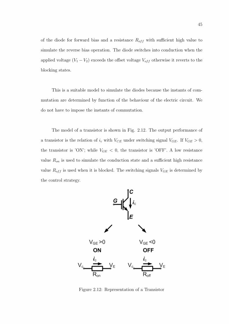
45
of the diode for forward bias and a resistance Roff with sufficient high value to
simulate the reverse bias operation. The diode switches into conduction when the
applied voltage (V1− V2) exceeds the offset voltage Voff otherwise it reverts to the
blocking states.
This is a suitable model to simulate the diodes because the instants of com-
mutation are determined by function of the behaviour of the electric circuit. We
do not have to impose the instants of commutation.
The model of a transistor is shown in Fig. 2.12. The output performance of
a transistor is the relation of ic with VCE under switching signal VGE. If VGE > 0,
the transistor is ’ON’; while VGE < 0, the transistor is ’OFF’. A low resistance
value Ron is used to simulate the conduction state and a sufficient high resistance
value Roff is used when it is blocked. The switching signals VGE is determined by
the control strategy.
Figure 2.12: Representation of a Transistor
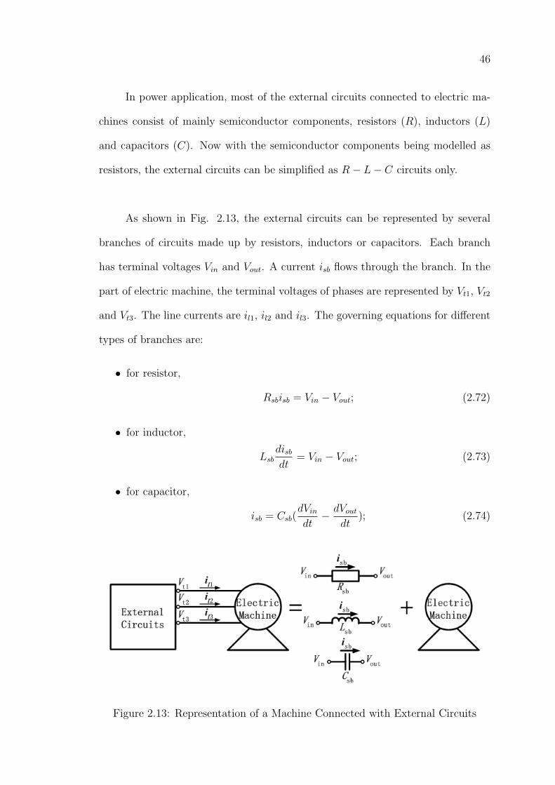
46
In power application, most of the external circuits connected to electric ma-
chines consist of mainly semiconductor components, resistors (R), inductors (L)
and capacitors (C). Now with the semiconductor components being modelled as
resistors, the external circuits can be simplified as R− L− C circuits only.
As shown in Fig. 2.13, the external circuits can be represented by several
branches of circuits made up by resistors, inductors or capacitors. Each branch
has terminal voltages Vin and Vout. A current isb flows through the branch. In the
part of electric machine, the terminal voltages of phases are represented by Vt1, Vt2
and Vt3. The line currents are il1, il2 and il3. The governing equations for different
types of branches are:
• for resistor,
Rsbisb = Vin − Vout; (2.72)
• for inductor,
Lsbdisbdt
= Vin − Vout; (2.73)
• for capacitor,
isb = Csb(dVin
dt− dVout
dt); (2.74)
Figure 2.13: Representation of a Machine Connected with External Circuits
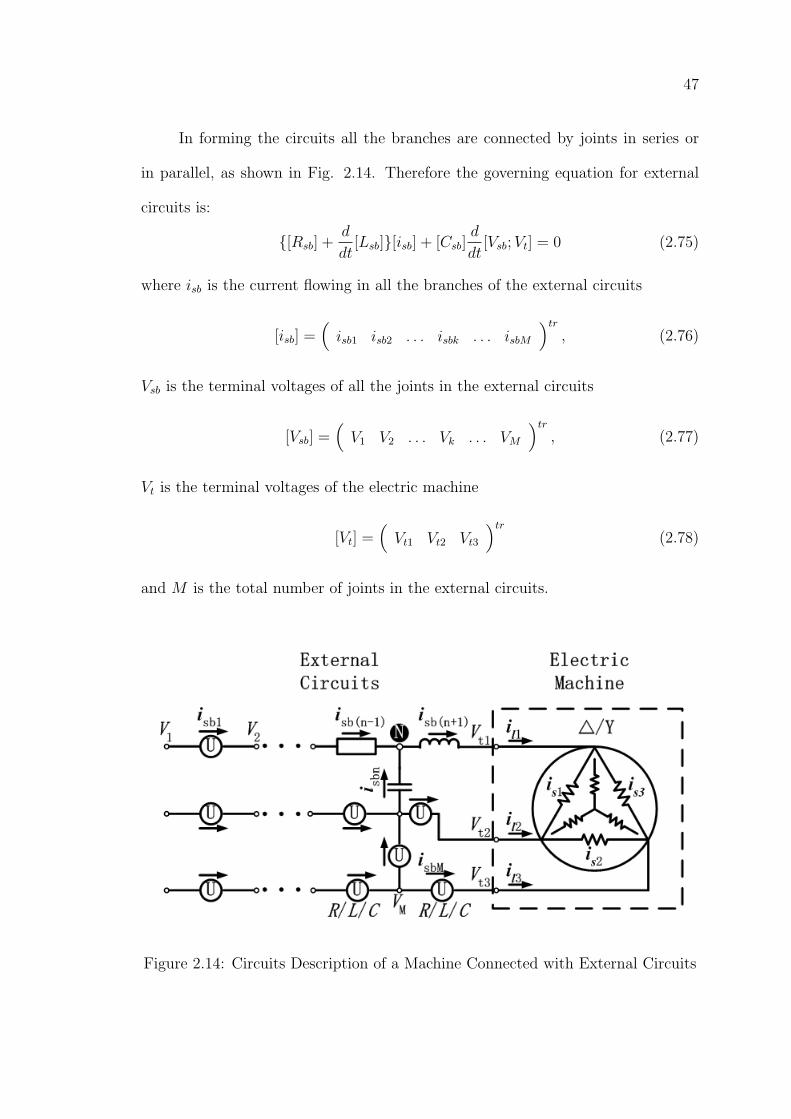
47
In forming the circuits all the branches are connected by joints in series or
in parallel, as shown in Fig. 2.14. Therefore the governing equation for external
circuits is:
[Rsb] +d
dt[Lsb][isb] + [Csb]
d
dt[Vsb;Vt] = 0 (2.75)
where isb is the current flowing in all the branches of the external circuits
[isb] =(isb1 isb2 . . . isbk . . . isbM
)tr
, (2.76)
Vsb is the terminal voltages of all the joints in the external circuits
[Vsb] =(V1 V2 . . . Vk . . . VM
)tr
, (2.77)
Vt is the terminal voltages of the electric machine
[Vt] =(Vt1 Vt2 Vt3
)tr
(2.78)
and M is the total number of joints in the external circuits.
Figure 2.14: Circuits Description of a Machine Connected with External Circuits
48
For each joint in the circuit, Kirchoff’s current law is applied. For example,
for joint ’N ’ in Fig. 2.14, the current equation is:
isb(n−1) + isbn − isb(n+1) = 0. (2.79)
The current equations for the whole circuit are:
[C3][isb] + [C4][is] = 0 (2.80)
where [is] is the stator phase currents
[is] =(is1 is2 is3
)tr
, (2.81)
[C3] is the coefficient matrix decided by the structure of the external circuits and
[C4] is the coefficient matrix decided by the ’4’ or ’Y ’ connection of stator phase
winding.
2.5 Equation of Motion
Rotating electric machines are one kind of electromagnetic devices for electro-
mechanical energy conversion. Normally the electric machines have two fundamen-
tal parts: the stator that is fixed and the rotor that is rotating mechanically. The
movement of the rotor is determined by the electromagnetic forces originated from
the interaction between the electromagnetic field in the air gap and the currents.
The positions of rotor is changed continuously with the movement, which in turn
affects the electromagnetic field within the machine. Therefore a complete analysis
of electric machine should take into account the dynamic mechanical movement of
the rotor.
49
The analysis of electric machines involves the continuous movement of the
rotor, which is governed by:
Jrdωm
dt= Tem − TL −Bfωm, (2.82)
dθm
dt= ωm (2.83)
where
Jr = the moment of inertia of the rotor
θm = the rotor position
ωm = the mechanical motor speed
Tem = the electromagnetic torque
TL = the applied load torque
Bf = the coefficient of friction
For a particular machine, Jr and Bf are taken as constants. The value of TL
is decided by the loading conditions of the machine. Equations (2.82) and (2.83)
are time-dependent. The values of θm, ωm and Tem vary with the instants of time.
2.6 Conclusion
This chapter presented the modelling of electric machines with coupled circuits
and motion. The governing equations for the magnetic field, the circuits and the
motion are summarized below:
• The field equation,
∂
∂x(ν∂A
∂x) +
∂
∂y(ν∂A
∂y) = σ
∂A
∂t− σ
Vtz
l−∇× (νµ0Mr)
50
• Stator phase equation,
Vs = Rsis + Ledisdt
+l
ms(
∫ ∫Ω+
∂A
∂tdxdy −
∫ ∫Ω−
∂A
∂tdxdy)
• Equations for cage bars,
Vbk = Rbkibk +lbksbk
∫ ∫sbk
∂A
∂tdxdy
[ib]− [C1][ie] = 0
[C2][Vb] + 2[Re] +d
dt[Le][ie] = 0
• Equations for external circuits,
[Rsb] +d
dt[Lsb][isb] + [Csb]
d
dt[Vsb;Vt] = 0
[C3][isb] + [C4][is] = 0
• Equations for mechanical motion,
Jrdωm
dt= Tem − Tf −Bfωm,
dθm
dt= ωm
Formulation of finite element computational procedures is based on the simul-
taneous solutions of these sets of equations. Detailed account of numerical analysis
are presented in the following chapters.
Chapter 3
Finite Element Analysis ofLine-Start Permanent MagnetSynchronous Machines WithCoupled Circuits and Motion
3.1 Introduction
Finite element method is a numerical tool used in solving partial differential equa-
tions in a given domain including the boundary conditions. Variational principle
or the method of weighted residuals is used to derive the finite element equations
[8]. The fundamental concept of the method is to divide the problem domain into
a number of small subregions or elements. The unknown field values are approx-
imated in those elements by simple shape functions, mostly linear or quadratic.
After the finite element formulation of governing equation in each element and the
assembly of all the elements, a large linear system of equations is generated. The
solution to this system of equations gives the field values of the whole problem
domain. Compared with other numerical methods, the main advantages of finite
element methods are its flexibility for modelling complex geometries, the capabil-
ity of handling nonlinearities and eddy currents, easy implementation and stable
solutions.
51

52
In general, the following steps are involved in the finite element method:
• Define the problem of interest by partial differential equations;
• Subdivide the problem field region into many small subregions;
• Choose the interpolation function in terms of the nodal vales of the elements;
• Derive the finite element equations within each element in terms of energy-
related functions or weighted residual expressions;
• Assembly of the element equations and the global system of equations is
generated;
• Impose boundary conditions;
• Solve the global system of equations with appropriate methods;
• Convert the field solutions to useful design quantities.
When the finite element field analysis is coupled with the circuit analysis and the
mechanical motion, the following steps should also be included:
• the discretization of equations in time domain;
• the combination of field equations with the circuit equations;
• the simulation of the rotor motion.
3.2 Summary of the Equations
Finite element analysis of electric machines is based on the proper definition or the
modelling of the problem. A complete model of an electric machine should include:
(1) the electromagnetic field,
(2) the circuits that transfer the external power to the field,
53
(3) the motion of rotor that have interaction with the field.
The governing equations for the field, circuit and motion have been derived
in Chapter 2 and they are listed as follows:
• The field equation,
∂
∂x(ν∂A
∂x) +
∂
∂y(ν∂A
∂y) = σ
∂A
∂t− σ
Vtz
l−∇× (νµ0Mr) (3.1)
• Stator phase equation,
Vs = Rsis + Ledisdt
+l
ms(
∫ ∫Ω+
∂A
∂tdxdy −
∫ ∫Ω−
∂A
∂tdxdy) (3.2)
• Equations for cage bars,
Vbk = Rbkibk +lbksbk
∫ ∫sbk
∂A
∂tdxdy (3.3)
[ib]− [C1][ie] = 0 (3.4)
[C2][Vb] + 2[Re] +d
dt[Le][ie] = 0 (3.5)
• Equations for external circuits,
[Rsb] +d
dt[Lsb][isb] + [Csb]
d
dt[Vsb;Vt] = 0 (3.6)
[C3][isb] + [C4][is] = 0 (3.7)
• Equations for mechanical motion,
Jrdωm
dt= Tem − Tf −Bfωm, (3.8)
dθm
dt= ωm (3.9)
Equations (3.1)-(3.3) are directly field-dependent. Finite element formulations of
these equations are needed. Equations (3.4)-(3.9) are indirectly related to the field
values. Therefore they can be taken as constraints and finite element formulations
are unnecessary.

54
3.3 Domain Discretization
To discretize the domain into subregions (finite elements) is the first step in finite
element method. The shapes, sizes and the configurations of the elements may
vary, but a few important points must be taken into consideration during the mesh
generation process:
(a) the nodes should be placed within the region and on the boundary of the field
domain;
(b) the density of the nodes should be high in those areas where the field varies
rapidly and the elements could be large while the field is uniform;
(c) the elements cannot overlap meanwhile no empty spaces can be left;
(d) for a region composed of different materials, the separating lines should be
represented by the boundaries of elements;
(e) in order to reduce the storage and bandwidth of the resultant global matrix,
the numbering of the nodes should be optimized [69].
There are many types and shapes of elements that can be used for the dis-
cretization of a domain. Fig. 3.1 shows some two and three dimensional finite
elements. In the two-dimensional electromagnetic field analysis of electric ma-
chines, triangular elements are usually used. The best in triangular elements are
the free topology irregular triangular meshes. Any complicated geometry can fi-
nally be represented without any undue mathematical complexity [9]. Because of
their shapes, triangular elements are one of the most suitable class of elements
which can represent accurately a very complicated machine geometry. This type
of element has been used extensively in the analysis of electric machine problems
[18, 19, 20, 64].
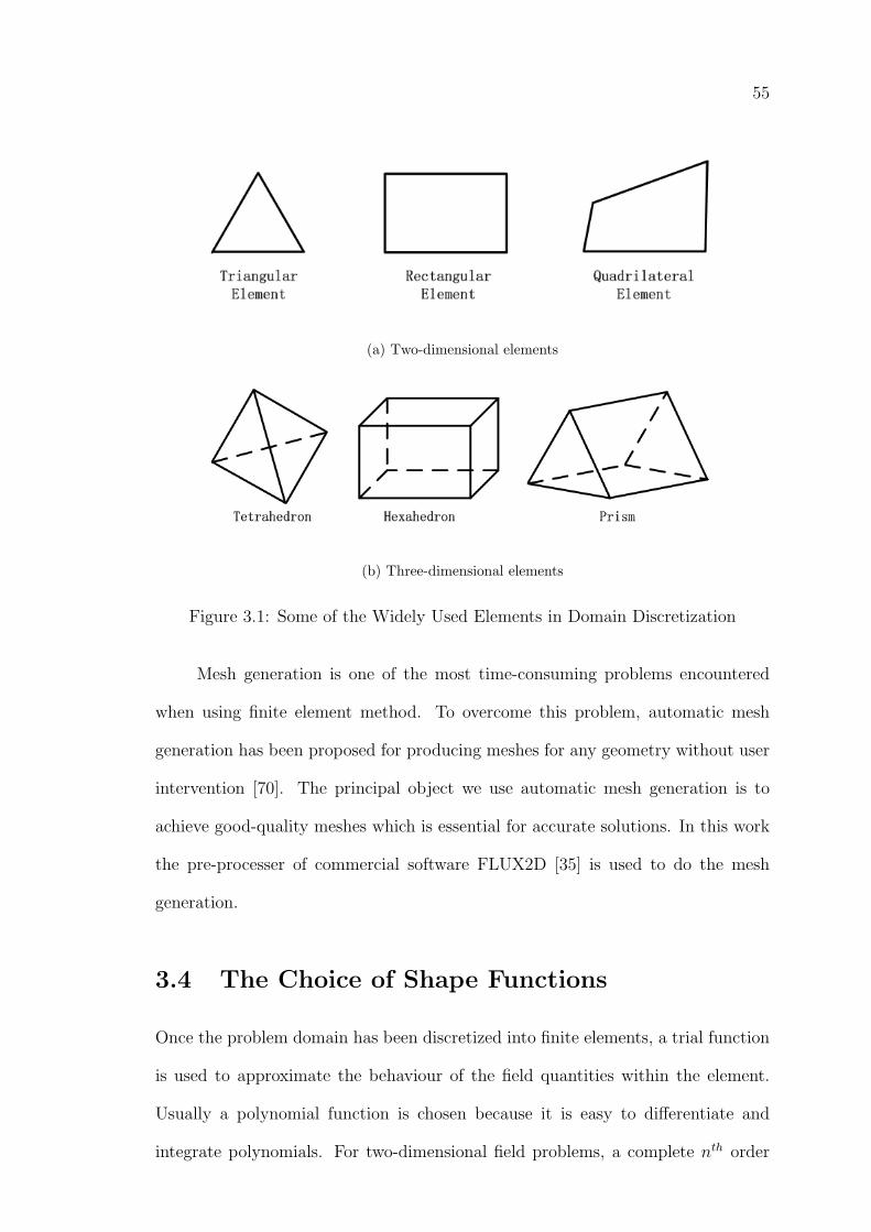
55
(a) Two-dimensional elements
(b) Three-dimensional elements
Figure 3.1: Some of the Widely Used Elements in Domain Discretization
Mesh generation is one of the most time-consuming problems encountered
when using finite element method. To overcome this problem, automatic mesh
generation has been proposed for producing meshes for any geometry without user
intervention [70]. The principal object we use automatic mesh generation is to
achieve good-quality meshes which is essential for accurate solutions. In this work
the pre-processer of commercial software FLUX2D [35] is used to do the mesh
generation.
3.4 The Choice of Shape Functions
Once the problem domain has been discretized into finite elements, a trial function
is used to approximate the behaviour of the field quantities within the element.
Usually a polynomial function is chosen because it is easy to differentiate and
integrate polynomials. For two-dimensional field problems, a complete nth order
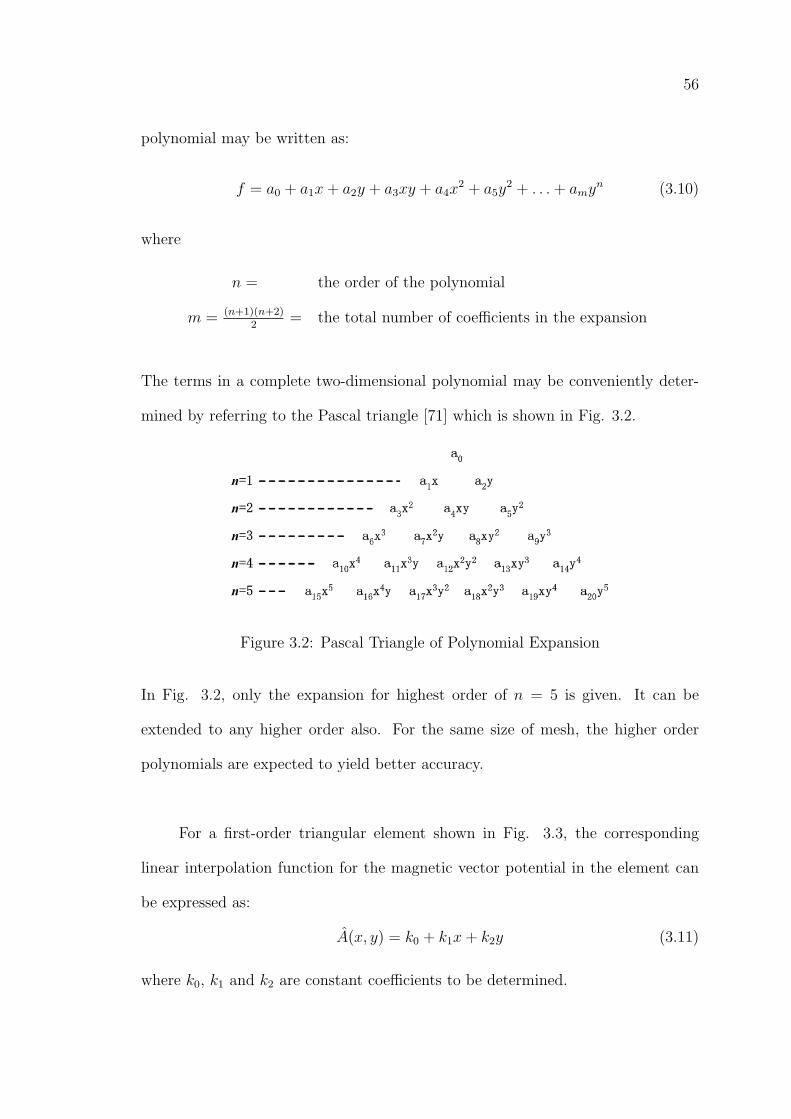
56
polynomial may be written as:
f = a0 + a1x+ a2y + a3xy + a4x2 + a5y
2 + . . .+ amyn (3.10)
where
n = the order of the polynomial
m = (n+1)(n+2)2
= the total number of coefficients in the expansion
The terms in a complete two-dimensional polynomial may be conveniently deter-
mined by referring to the Pascal triangle [71] which is shown in Fig. 3.2.
Figure 3.2: Pascal Triangle of Polynomial Expansion
In Fig. 3.2, only the expansion for highest order of n = 5 is given. It can be
extended to any higher order also. For the same size of mesh, the higher order
polynomials are expected to yield better accuracy.
For a first-order triangular element shown in Fig. 3.3, the corresponding
linear interpolation function for the magnetic vector potential in the element can
be expressed as:
A(x, y) = k0 + k1x+ k2y (3.11)
where k0, k1 and k2 are constant coefficients to be determined.
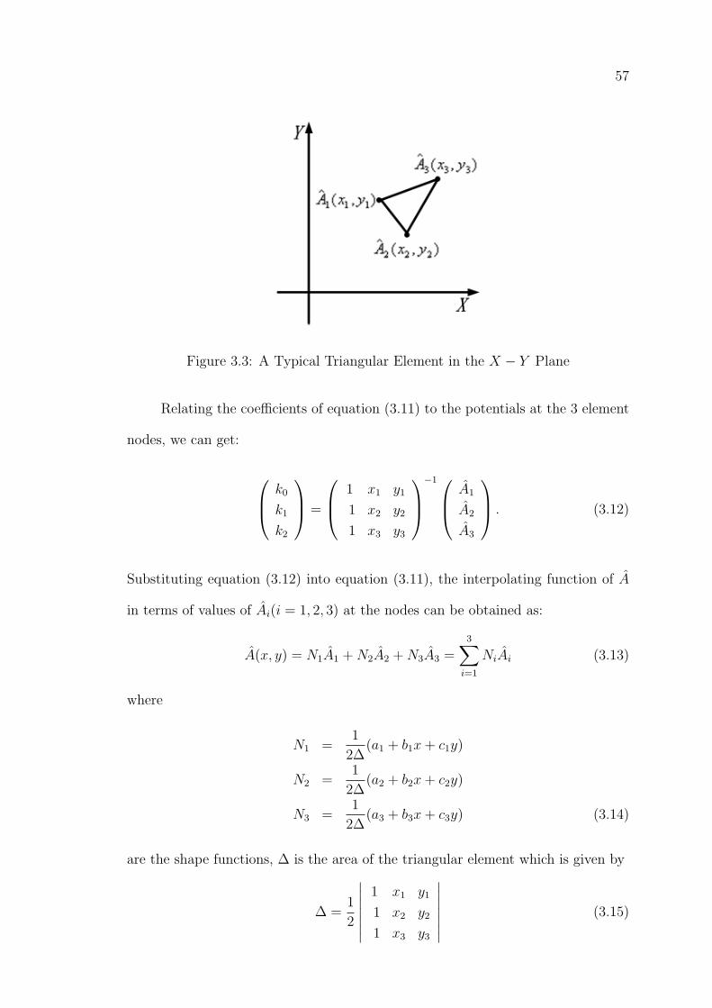
57
Figure 3.3: A Typical Triangular Element in the X − Y Plane
Relating the coefficients of equation (3.11) to the potentials at the 3 element
nodes, we can get:
k0
k1
k2
=
1 x1 y1
1 x2 y2
1 x3 y3
−1 A1
A2
A3
. (3.12)
Substituting equation (3.12) into equation (3.11), the interpolating function of A
in terms of values of Ai(i = 1, 2, 3) at the nodes can be obtained as:
A(x, y) = N1A1 +N2A2 +N3A3 =3∑
i=1
NiAi (3.13)
where
N1 =1
2∆(a1 + b1x+ c1y)
N2 =1
2∆(a2 + b2x+ c2y)
N3 =1
2∆(a3 + b3x+ c3y) (3.14)
are the shape functions, ∆ is the area of the triangular element which is given by
∆ =1
2
∣∣∣∣∣∣∣1 x1 y1
1 x2 y2
1 x3 y3
∣∣∣∣∣∣∣ (3.15)
58
and
a1 = x2y3 − y2x3; a2 = x3y1 − y3x1; a3 = x1y2 − y1x2;
b1 = y2 − y3; b2 = y3 − y1; b3 = y1 − y2;
c1 = x3 − x2; c2 = x1 − x3; c3 = x2 − x1;
In the two dimensional finite element analysis, the magnetic vector potential A has
only invariant z-directed components in the x, y, z-coordinates. Therefore we can
get
A = Az. (3.16)
Since the flux density is the derivative of the vector potential
B = ∇× A =
∣∣∣∣∣∣∣x y z∂∂x
∂∂y
∂∂z
0 0 Az
∣∣∣∣∣∣∣ =∂Az
∂y· x− ∂Az
∂x· y, (3.17)
Combination of equations (3.16) and (3.17) yields:
Bx =∂A
∂y(3.18)
By = −∂A∂x
. (3.19)
Substituting equation (3.13) into equations (3.18) and (3.19) yields the x and y
components of flux density
Bx =1
2∆(b1A1 + b2A2 + b3A3) (3.20)
By = − 1
2∆(c1A1 + c2A2 + c3A3) (3.21)
From equations (3.20) and (3.21), we can see that the flux density is constant
within each element.
59
3.5 Deriving Finite Element Equations Based on
the Method of Weighted Residuals
When the unknown field quantities of equation (3.1)-(3.3) are substituted by the
approximate function A =∑3
i=1NiAi in each element, the residual R or an error
of approximation is unavoidable. For example, for field equation (3.1), the residual
is
R =∂
∂x(ν∂A
∂x) +
∂
∂y(ν∂A
∂y)− σ
∂A
∂t+ σ
Vtz
l+∇× (νµ0Mr) (3.22)
If the residual R in the whole domain tends to zero, the A can be regarded as an
acceptable approximate solution. There are several principle of error minimization,
such as principle of weighted residuals [72], orthogonal projection principle [73] and
variational principle [72, 74]. In numerical methods the most often used ones are the
principle of weighted residuals or the variational principle. The variational method
is based on the equivalent functional of the governing equation. The weighted
residual approach is based on the operator equation directly. Although these two
principles are based on different starting equations, they yield the same set of
equations. The principle of weighted residual can be used for all numerical meth-
ods. Based on the choice of weighting functions, shape functions and the approach
to discretization, different methods are formulated, including sub-domain method,
collocation method, Galerkin’s method and least-square method [75]. The most
often used method for deriving finite element equations is the Galerkin’s method.
The method of weighted residual involves finding the unknown parameters
contained in the approximate solution such that the residual is as close to zero as
possible. This usually means determining the parameters such that some weighted
integral of the residual over the whole problem domain is zero. For our problem,
60
one would require that, ∫ ∫Ω
WRdxdy = 0. (3.23)
where
W = the weighting function
Ω = the area of the whole domain
This surface integral may be broken into summations over small areas. The whole
domain is replaced with small sub-domains so called finite elements, and integration
can easily be performed over the individual elements. Therefore we can get∫ ∫Ω
WRdxdy =M∑
e=1
∫ ∫Ωe
[W e]Redxdy = 0. (3.24)
where
M = the number of finite element in the domain
Ωe = the area of one individual element
[W e] = the weighting function of one individual element
Re = the residual of one one individual element
According to the principle of the Galerkin’s method, the weighting functions are
chosen to be the same as the shape functions
[W e] = [N ei ] =
N1
N2
N3
. (3.25)
61
3.5.1 Finite Element Formulation of Field Equations
The residual of field equation given in equation (3.22) and the combination of
equations (3.22)-(3.25) leads to the integral equation for individual element∫ ∫Ωe
[W e]Redxdy =
∫ ∫Ωe
[N ei ][
∂
∂x(ν∂A
∂x) +
∂
∂y(ν∂A
∂y)− σ
∂A
∂t+ σ
Vtz
l
+∇× (νµ0Mr)]dxdy
=
∫ ∫Ωe
[N ei ][
∂
∂x(ν∂A
∂x) +
∂
∂y(ν∂A
∂y)]dxdy
−∫ ∫
Ωe
[N ei ](σ
∂A
∂t)dxdy
+
∫ ∫Ωe
[N ei ](σ
Vtz
l)dxdy
+
∫ ∫Ωe
[N ei ][∇× (νµ0Mr)]dxdy
= 0. (3.26)
Equation (3.26) has four terms. The integration of these four terms gives the ele-
ment matrix equation for field equation (3.1).
(a) Integration of the first term of equation (3.26)∫ ∫
Ωe[N e
i ][ ∂∂x
(ν ∂A∂x
) +
∂∂y
(ν ∂A∂y
)]dxdy
Integrating the first term by parts,
∫ ∫Ωe
[N ei ][
∂
∂x(ν∂A
∂x)+
∂
∂y(ν∂A
∂y)]dxdy =
∮Γ
ν[N ei ]∂A
∂ndΓ−
∫ ∫Ωe
ν(∂[N e
i ]
∂x
∂A
∂x+∂[N e
i ]
∂y
∂A
∂y)dxdy.
(3.27)
The line integral in equation (3.27) is only employed over elements which have a
side common with the boundary Γ. By imposing the natural boundary condition,
i.e., ∂A∂n
= 0, this integral is vanished. Then equation (3.27) becomes∫ ∫Ωe
[N ei ][
∂
∂x(ν∂A
∂x) +
∂
∂y(ν∂A
∂y)]dxdy = −
∫ ∫Ωe
ν(∂[N e
i ]
∂x
∂A
∂x+∂[N e
i ]
∂y
∂A
∂y)dxdy.
(3.28)
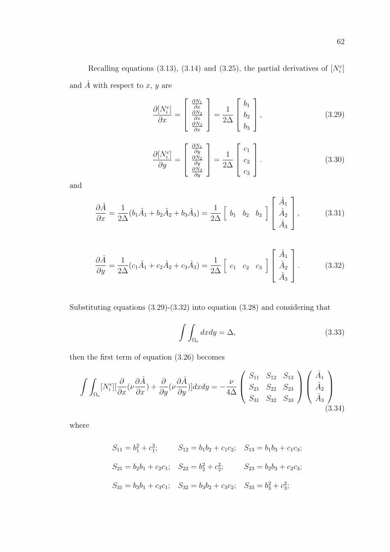
62
Recalling equations (3.13), (3.14) and (3.25), the partial derivatives of [N ei ]
and A with respect to x, y are
∂[N ei ]
∂x=
∂N1
∂x∂N2
∂x∂N3
∂x
=1
2∆
b1
b2
b3
, (3.29)
∂[N ei ]
∂y=
∂N1
∂y∂N2
∂y∂N3
∂y
=1
2∆
c1
c2
c3
. (3.30)
and
∂A
∂x=
1
2∆(b1A1 + b2A2 + b3A3) =
1
2∆
[b1 b2 b3
] A1
A2
A3
, (3.31)
∂A
∂y=
1
2∆(c1A1 + c2A2 + c3A3) =
1
2∆
[c1 c2 c3
] A1
A2
A3
. (3.32)
Substituting equations (3.29)-(3.32) into equation (3.28) and considering that∫ ∫Ωe
dxdy = ∆, (3.33)
then the first term of equation (3.26) becomes
∫ ∫Ωe
[N ei ][
∂
∂x(ν∂A
∂x) +
∂
∂y(ν∂A
∂y)]dxdy = − ν
4∆
S11 S12 S13
S21 S22 S23
S31 S32 S33
A1
A2
A3
(3.34)
where
S11 = b21 + c21; S12 = b1b2 + c1c2; S13 = b1b3 + c1c3;
S21 = b2b1 + c2c1; S22 = b22 + c22; S23 = b2b3 + c2c3;
S31 = b3b1 + c3c1; S32 = b3b2 + c3c2; S33 = b23 + c23;
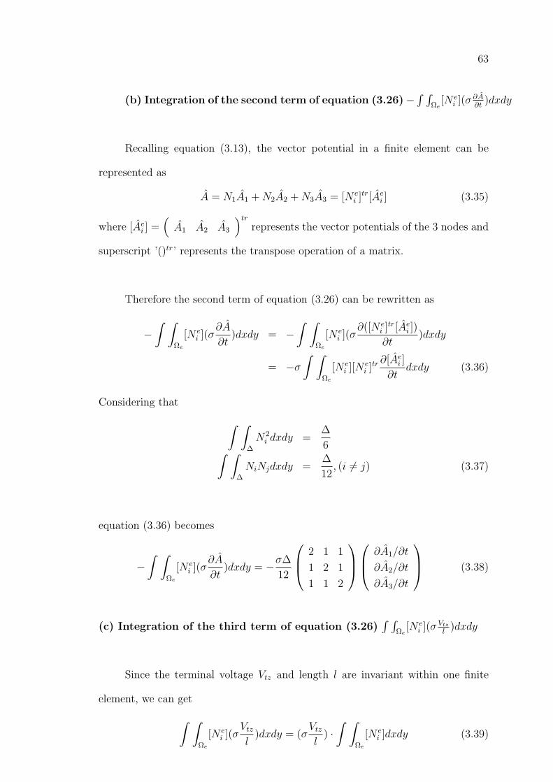
63
(b) Integration of the second term of equation (3.26)−∫ ∫
Ωe[N e
i ](σ ∂A∂t
)dxdy
Recalling equation (3.13), the vector potential in a finite element can be
represented as
A = N1A1 +N2A2 +N3A3 = [N ei ]tr[Ae
i ] (3.35)
where [Aei ] =
(A1 A2 A3
)tr
represents the vector potentials of the 3 nodes and
superscript ’()tr’ represents the transpose operation of a matrix.
Therefore the second term of equation (3.26) can be rewritten as
−∫ ∫
Ωe
[N ei ](σ
∂A
∂t)dxdy = −
∫ ∫Ωe
[N ei ](σ
∂([N ei ]tr[Ae
i ])
∂t)dxdy
= −σ∫ ∫
Ωe
[N ei ][N e
i ]tr∂[Ae
i ]
∂tdxdy (3.36)
Considering that ∫ ∫∆
N2i dxdy =
∆
6∫ ∫∆
NiNjdxdy =∆
12, (i 6= j) (3.37)
equation (3.36) becomes
−∫ ∫
Ωe
[N ei ](σ
∂A
∂t)dxdy = −σ∆
12
2 1 1
1 2 1
1 1 2
∂A1/∂t
∂A2/∂t
∂A3/∂t
(3.38)
(c) Integration of the third term of equation (3.26)∫ ∫
Ωe[N e
i ](σ Vtz
l)dxdy
Since the terminal voltage Vtz and length l are invariant within one finite
element, we can get∫ ∫Ωe
[N ei ](σ
Vtz
l)dxdy = (σ
Vtz
l) ·∫ ∫
Ωe
[N ei ]dxdy (3.39)
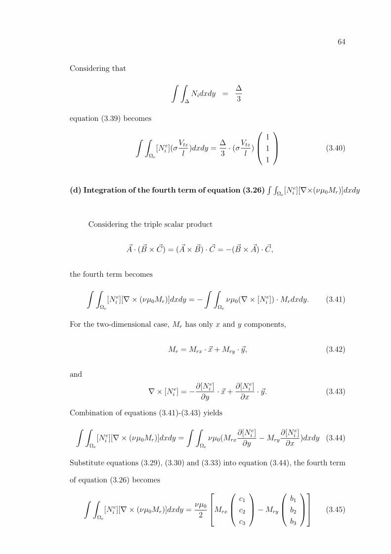
64
Considering that ∫ ∫∆
Nidxdy =∆
3
equation (3.39) becomes
∫ ∫Ωe
[N ei ](σ
Vtz
l)dxdy =
∆
3· (σVtz
l)
1
1
1
(3.40)
(d) Integration of the fourth term of equation (3.26)∫ ∫
Ωe[N e
i ][∇×(νµ0Mr)]dxdy
Considering the triple scalar product
~A · ( ~B × ~C) = ( ~A× ~B) · ~C = −( ~B × ~A) · ~C,
the fourth term becomes∫ ∫Ωe
[N ei ][∇× (νµ0Mr)]dxdy = −
∫ ∫Ωe
νµ0(∇× [N ei ]) ·Mrdxdy. (3.41)
For the two-dimensional case, Mr has only x and y components,
Mr = Mrx · ~x+Mry · ~y, (3.42)
and
∇× [N ei ] = −∂[N e
i ]
∂y· ~x+
∂[N ei ]
∂x· ~y. (3.43)
Combination of equations (3.41)-(3.43) yields∫ ∫Ωe
[N ei ][∇× (νµ0Mr)]dxdy =
∫ ∫Ωe
νµ0(Mrx∂[N e
i ]
∂y−Mry
∂[N ei ]
∂x)dxdy (3.44)
Substitute equations (3.29), (3.30) and (3.33) into equation (3.44), the fourth term
of equation (3.26) becomes
∫ ∫Ωe
[N ei ][∇× (νµ0Mr)]dxdy =
νµ0
2
Mrx
c1
c2
c3
−Mry
b1
b2
b3
(3.45)
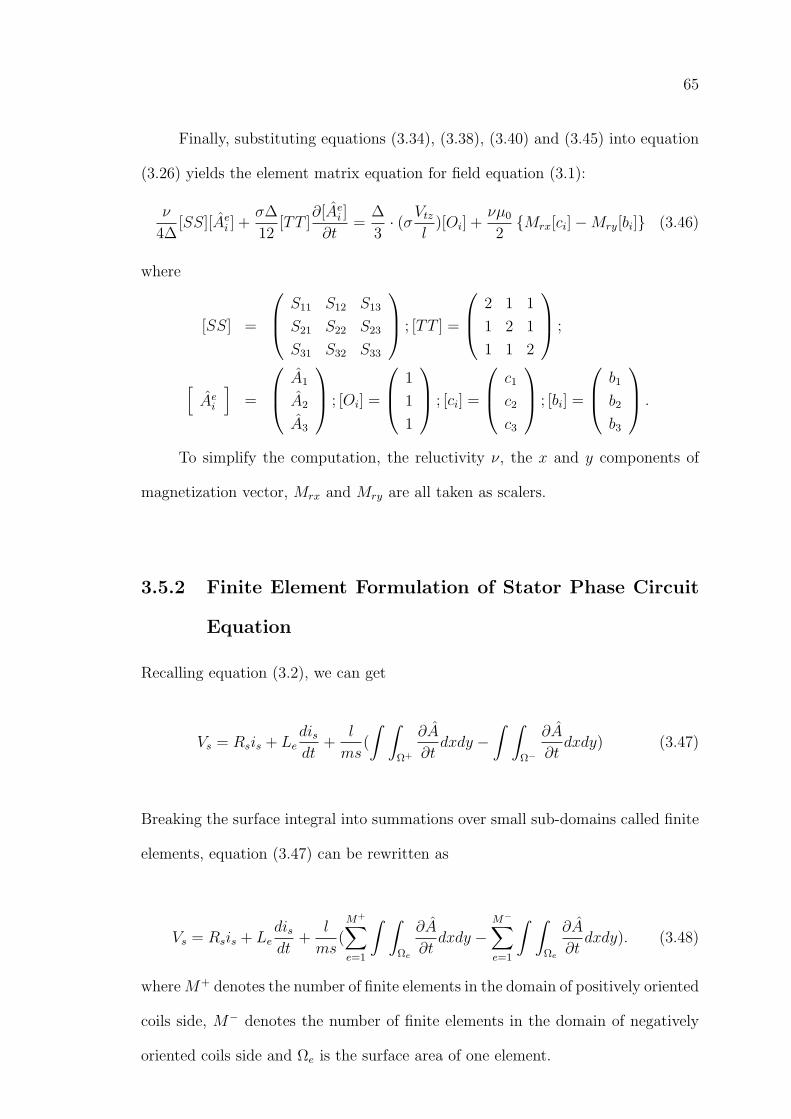
65
Finally, substituting equations (3.34), (3.38), (3.40) and (3.45) into equation
(3.26) yields the element matrix equation for field equation (3.1):
ν
4∆[SS][Ae
i ] +σ∆
12[TT ]
∂[Aei ]
∂t=
∆
3· (σVtz
l)[Oi] +
νµ0
2Mrx[ci]−Mry[bi] (3.46)
where
[SS] =
S11 S12 S13
S21 S22 S23
S31 S32 S33
; [TT ] =
2 1 1
1 2 1
1 1 2
;
[Ae
i
]=
A1
A2
A3
; [Oi] =
1
1
1
; [ci] =
c1
c2
c3
; [bi] =
b1
b2
b3
.
To simplify the computation, the reluctivity ν, the x and y components of
magnetization vector, Mrx and Mry are all taken as scalers.
3.5.2 Finite Element Formulation of Stator Phase Circuit
Equation
Recalling equation (3.2), we can get
Vs = Rsis + Ledisdt
+l
ms(
∫ ∫Ω+
∂A
∂tdxdy −
∫ ∫Ω−
∂A
∂tdxdy) (3.47)
Breaking the surface integral into summations over small sub-domains called finite
elements, equation (3.47) can be rewritten as
Vs = Rsis + Ledisdt
+l
ms(
M+∑e=1
∫ ∫Ωe
∂A
∂tdxdy −
M−∑e=1
∫ ∫Ωe
∂A
∂tdxdy). (3.48)
whereM+ denotes the number of finite elements in the domain of positively oriented
coils side, M− denotes the number of finite elements in the domain of negatively
oriented coils side and Ωe is the surface area of one element.
66
Since
A = [N ei ]tr[Ae
i ],
equation (3.48) becomes
Vs = Rsis + Ledisdt
+l
ms
(M+∑e=1
∫ ∫Ωe
∂([N ei ]tr[Ae
i ])
∂tdxdy −
M−∑e=1
∫ ∫Ωe
∂([N ei ]tr[Ae
i ])
∂tdxdy
)= Rsis + Le
disdt
+l
ms
(M+∑e=1
∫ ∫Ωe
[N ei ]tr
∂[Aei ]
∂tdxdy −
M−∑e=1
∫ ∫Ωe
[N ei ]tr
∂[Aei ]
∂tdxdy
). (3.49)
As ∫ ∫∆
Nidxdy =∆
3
equation (3.49) becomes
Vs = Rsis + Ledisdt
+l
ms
(M+∑e=1
∆
3
∂[Aei ]
∂t−
M−∑e=1
∆
3
∂[Aei ]
∂t
), (3.50)
or
Rsis + Ledisdt
+l
ms[KK]sp
∂[A]sp∂t
− Vs = 0 (3.51)
where
[KK]sp =(. . . ±∆
3±∆
3±∆
3. . .),[
A]
sp=
(. . . A1 A2 A3 . . .
)tr
.
The sign ’±’ is ’+’ when the triangle element is in the domain of positively oriented
coils side, and it is ’−’ when the element is in the domain of negatively oriented
coils side. Matrices [KK]sp and [A]sp are only used for those elements that locate
in the region of stator phase windings.
67
3.5.3 Finite Element Formulation of Cage Bar Equation
Recalling equation (3.3), we can get
Vbk = Rbkibk +lbksbk
∫ ∫sbk
∂A
∂tdxdy (3.52)
Breaking the surface integral into summations over the finite elements, equation
(3.52) can be rewritten as
Vbk = Rbkibk +lbksbk
Mcb∑e=1
∫ ∫Ωe
∂A
∂tdxdy (3.53)
Since
A = [N ei ]tr[Ae
i ],
equation (3.53) becomes
Vbk = Rbkibk +lbksbk
Mcb∑e=1
∫ ∫Ωe
∂([N ei ][Ae
i ])
∂tdxdy
= Rbkibk +lbksbk
Mcb∑e=1
∫ ∫Ωe
[N ei ]∂[Ae
i ]
∂tdxdy (3.54)
where Mcb is the number of finite elements in this cage bar.
As ∫ ∫∆
Nidxdy =∆
3
equation (3.54) becomes
Vbk = Rbkibk +lbksbk
Mcb∑e=1
∆
3
∂[Aei ]
∂t, (3.55)
or
Rbkibk +lbksbk
[KK]cb∂[A]cb∂t
− Vbk = 0 (3.56)
68
where
[KK]cb =(. . . ∆
3∆3
∆3
. . .),[
A]
cb=
(. . . A1 A2 A3 . . .
)tr
.
Matrices [KK]cb and [A]cb are only used for those elements that locate in the region
of cage bars.
Other equations (3.4)∼(3.9), describe the cage bar circuits, external circuit
and mechanical motions. They are not field-dependent directly. Therefore the
finite element formulation of these equations are not necessary.
3.6 Discretization of Governing Equations in Time
Domain
As shown in equations (3.1)-(3.9), electric machines are often modelled in terms of
a complete set of partial differential equations or linear algebraic equations with
solution functions expressed in the space and time domains. The space solution
is determined by the finite element technique while the time solution is evalu-
ated by time-stepping methods that consist of implicit or explicit time-integration
procedures [76]-[78]. The time-stepping method is the method that solves a time-
dependent quantity by discretizing the time at short time intervals ∆t and evalu-
ating the quantitiy at times t1, t2, t3, . . ., (tk+1 = tk + ∆t). The accuracy of the
solution depends on the particular time-stepping algorithm applied, as well as the
size of the time step used. The most often used time-stepping algorithms are:
69
• Explicit algorithm (Forward Euler’s method)
∂At
∂t=A(t+∆t) − At
∆t(3.57)
If the value of A and its time derivative at t are known, its value at (t+ ∆t)
is obtainable using equations (3.57).
• Implicit algorithm
– Crank-Nicholson Algorithm
1
2(∂A(t+∆t)
∂t+∂At
∂t) =
A(t+∆t) − At
∆t(3.58)
The time derivatives at t and (t+ ∆t) are used to find the value of A at
(t+ ∆t), A(t+∆t).
– Backward difference scheme (Backward Euler’s method)
∂A(t+∆t)
∂t=A(t+∆t) − At
∆t(3.59)
If the value of A and its time derivative at (t+ ∆t) are known, its value
at (t+ ∆t) is obtainable using equations (3.59).
It has been shown that implicit algorithms have distinct advantages over the explicit
ones, due to higher degree of numerical stability and larger time step possibility
[76]-[80]. Inside the group of implicit algorithm, Tsukerman [80, 81] examined the
stabilities of Crank-Nicholson algorithm and Backward Euler’s algorithm in coupled
field-circuit problems. It was shown that Backward Euler’s method is stable while
the Crank-Nicholson scheme generates undamped or in some cases even divergent
oscillations. Therefore, in this work the Backward Euler’s method is chosen in the
time discretization of the governing equations.
70
3.6.1 Discretization of Field Equation
Recalling the element matrix equation for field (3.46),
ν
4∆[SS][Ae
i ]t+∆t+
σ∆
12[TT ]
∂[Aei ]
t+∆t
∂t=
∆
3·(σV
(t+∆t)tz
l)[Oi]+
νµ0
2Mrx[ci]−Mry[bi]
(3.60)
According to equation (3.59),
∂[Aei ]
(t+∆t)
∂t=
[Aei ]
(t+∆t) − [Aei ]
t
∆t, (3.61)
the element matrix equation for field becomes,
(ν
4∆[SS] +
σ∆
12[TT ]
)· [Ae
i ]t+∆t − [Ae
i ]t
∆t− ∆
3· (σV
(t+∆t)tz
l)[Oi]
=νµ0
2Mrx[ci]−Mry[bi] . (3.62)
Rearranging terms to isolate the (t+ ∆t) term yields,
ν
4∆[SS] +
σ∆
12∆t[TT ]
[Ae
i ]t+∆t − ∆
3· (σV
(t+∆t)tz
l)[Oi]
=σ∆
12∆t[TT ][Ae
i ]t +
νµ0
2Mrx[ci]−Mry[bi] . (3.63)
Equation (3.63) shows that as long as the values at t are known, the values at
(t + ∆t) can be calculated readily by solving this equation. In other words, a dy-
namic process can be evaluated in steps or the dynamic behaviours of a device can
be analyzed using time-stepping method.
71
3.6.2 Discretization of Equation for Stator Phase Circuit
Recalling equation (3.51) and considering that,
di(t+∆t)s
dt=
i(t+∆t)s − its
∆t
∂[A]t+∆t
sp
∂t=
[A]t+∆t
sp−[A]t
sp
∆t
the equation for stator phase circuit becomes,
(Rs +Le
∆t)i(t+∆t)
s +l
ms
[KK]sp∆t
[A]t+∆tsp − V (t+∆t)
s =Le
∆tits +
l
ms
[KK]sp∆t
[A]tsp (3.64)
3.6.3 Discretization of Governing Equations for Cage Bars
Equation (3.56) can be discretized as:
Rbk[ibk]t+∆t +
lbksbk
[KK]cb∆t
[A]t+∆tcb − [Vbk]
t+∆t =lbksbk
[KK]cb∆t
[A]tcb (3.65)
Recalling equation (3.4) and considering that it is not time-dependent, it is kept
unchanged in time domain:
[ib]t+∆t − [C1][ie]
t+∆t = 0 (3.66)
Equation (3.5) can be discretized as:
[C2][Vb]t+∆t + 2[Re] +
[Le]
∆t[ie]t+∆t = 2
[Le]
∆t[ie]
t (3.67)
72
3.6.4 Discretization of Equations for External Circuits
Equation (3.6) can be discretized as:
[Rsb] +[Lsb]
∆t[isb]t+∆t +
[Csb]
∆t[Vsb;Vt]
t+∆t =[Lsb]
∆t[isb]
t +[Csb]
∆t[Vsb;Vt]
t (3.68)
Recalling equation (3.7) and considering that it is not time-dependent, it is kept
unchanged in time domain:
[C3][isb]t+∆t + [C4][is]
t+∆t = 0 (3.69)
3.6.5 Discretization of Equations for Mechanical Motion
Equation (3.8) can be discretized as:
(Jr
∆t+Bf )ω
t+∆tm =
Jr
∆t· ωt
m + Tem − Tf (3.70)
and equation (3.9) can be discretized as:
1
∆tθt+∆t
m − ωt+∆tm =
1
∆tθt
m (3.71)
73
3.7 Solving the Nonlinear Equations
In the analysis of electric machines the problems are almost always nonlinear due to
the presence of ferromagnetic materials in the rotor and stator iron cores. Generally
the iron material is characterized by a nonlinear curve relating the magnetic field
intensity H to the magnetic flux density B. Mathematically it is represented by
the permeability parameter µ at each point of the iron domain,
µ =B
H(3.72)
If the distribution of B is known, the value of H can be found according to the
nonlinear B − H curve; then µ can be calculated using equation (3.72). Thus
the value of magnetic permeability µ is field-dependent, which is characterized as
ν = 1µ
= f(B). To treat the nonlinearities of the materials, two methods are
usually used [8, 14, 28]:
1. The simple iteration method
A set of permeability values µ is assumed firstly. In the light of the field
solution values obtained, adjust the µ with the following equation
µn+1 = µn−1 + k(µn − µn−1) (3.73)
where k (0 < k < 1) is a real number and n is the iteration step number.
The above solve-adjust cycle is continued until satisfactory convergence is
obtained.
This method is very simple in implementation. However the method con-
verges rather slowly and may need considerable computation time. In ad-
dition, no known estimate of k may guarantee stability without slowing the
iterative process [28].
74
2. The Newton-Raphson method
The method utilizes the rate of change of error with potential to obtain new
estimates of potential. For a set of equations
[f ]k×1 = [K]k×k[X]k×1 = [Q]k×1,
an initial value [X](0) is assumed as the estimate of solution. The solution is
updated iteratively with equation
[X](n+1) = [X](n) + [J ](n)−1[Q]− [f ](n) (3.74)
where [J ] = ∂fi
∂Xj, (i, j = 1, 2, . . . , k) is the Jacobian matrix and n is the iter-
ation step number. The iteration is continued until satisfactory convergence
is obtained. The detailed algorithm of the Newton-Raphson method and the
description of Jacobian matrix [J ] are presented in Appendix A.
Particularly when [Q] = 0, the Newton-Raphson algorithm is:
∂f(n)i
∂X(n)1
∆X(n+1)1 +
∂f(n)i
∂X(n)2
∆X(n+1)2 + . . .+
∂f(n)i
∂X(n)k
∆X(n+1)k = −f (n)
i (3.75)
The Newton-Raphson method gives more certain and quicker convergence.
It is particularly suitable for a nonlinear system of equations.
The application of the Newton-Raphson method to the solution of the non-
linear finite element equations requires extension to matrix equations and was first
demonstrated by Chari and Silvester [17]. Then it has been extensively used in the
solution of finite element problems by many others [18]-[20],[22]-[30].
75
3.7.1 Linearization of Field Equation
Recalling equation (3.63) and let
[PP ] =
P1
P2
P3
=σ∆
12∆t[TT ][Ae
i ]t +
νµ0
2Mrx[ci]−Mry[bi] , (3.76)
then equation (3.63) becomesν
4∆[SS] +
σ∆
12∆t[TT ]
[Ae
i ]t+∆t − ∆
3· (σV
(t+∆t)tz
l)[Oi] = [PP ]. (3.77)
or ν
4∆
S11 S12 S13
S21 S22 S23
S31 S32 S33
+σ∆
12∆t
2 1 1
1 2 1
1 1 2
A1
A2
A3
t+∆t
−∆
3
σ
lV
(t+∆t)tz
1
1
1
=
P1
P2
P3
(3.78)
Let f1 = ν
4∆(S11A
t+∆t1 + S12A
t+∆t2 + S13A
t+∆t3 )
f2 = ν4∆
(S21At+∆t1 + S22A
t+∆t2 + S23A
t+∆t3 )
f3 = ν4∆
(S31At+∆t1 + S32A
t+∆t2 + S33A
t+∆t3 )
(3.79)
or
f1
f2
f3
=ν
4∆
S11 S12 S13
S21 S22 S23
S31 S32 S33
A1
A2
A3
t+∆t
, (3.80)
then equation (3.78) can be rewritten into 3 equations
F1 = f1 +σ∆
12∆t
(2 1 1
) A1
A2
A3
t+∆t
− ∆
3
σ
lV
(t+∆t)tz − P1 = 0 (3.81)
F2 = f2 +σ∆
12∆t
(1 2 1
) A1
A2
A3
t+∆t
− ∆
3
σ
lV
(t+∆t)tz − P2 = 0 (3.82)
76
F3 = f3 +σ∆
12∆t
(1 1 2
) A1
A2
A3
t+∆t
− ∆
3
σ
lV
(t+∆t)tz − P3 = 0 (3.83)
To find the derivatives necessary for the Newton-Raphson method, equations (3.81)-
(3.83) need to be differentiated with respect to the variables. The differentiation
of equation (3.81) gives
∂F1
∂A(t+∆t)1
=ν
4∆S11 +
f1
ν· ∂ν∂B
· ∂B
∂A(t+∆t)1
+σ∆
12∆t· 2 (3.84)
∂F1
∂A(t+∆t)2
=ν
4∆S12 +
f1
ν· ∂ν∂B
· ∂B
∂A(t+∆t)2
+σ∆
12∆t· 1 (3.85)
∂F1
∂A(t+∆t)3
=ν
4∆S13 +
f1
ν· ∂ν∂B
· ∂B
∂A(t+∆t)3
+σ∆
12∆t· 1 (3.86)
∂F1
∂V(t+∆t)tz
= −∆
3
σ
l(3.87)
Since (see Appendix B)
∂B
∂A(t+∆t)1
=f1
Bν∆
∂B
∂A(t+∆t)2
=f2
Bν∆
∂B
∂A(t+∆t)3
=f3
Bν∆
equations (3.84)-(3.86) become
∂F1
∂A(t+∆t)1
=ν
4∆S11 +
f1f1
ν2B∆· ∂ν∂B
+σ∆
12∆t· 2 (3.88)
77
∂F1
∂A(t+∆t)2
=ν
4∆S12 +
f1f2
ν2B∆· ∂ν∂B
+σ∆
12∆t· 1 (3.89)
∂F1
∂A(t+∆t)3
=ν
4∆S13 +
f1f3
ν2B∆· ∂ν∂B
+σ∆
12∆t· 1 (3.90)
Applying equation (3.75), the Newton-Raphson equation is
∂F1
∂A(t+∆t)1
· [∆A1](t+∆t)(n+1) +
∂F1
∂A(t+∆t)2
· [∆A2](t+∆t)(n+1)
+∂F1
∂A(t+∆t)3
· [∆A3](t+∆t)(n+1) +
∂F1
∂V(t+∆t)tz
· [∆Vtz](t+∆t)(n+1) = −F1. (3.91)
Substituting equations (3.87)-(3.90) into equation (3.91) yields the linearization of
equation F1
ν
4∆
(S11 S12 S13
) ∆A1
∆A2
∆A3
t+∆t
(n+1)
+σ∆
12∆t
(2 1 1
) ∆A1
∆A2
∆A3
t+∆t
(n+1)
+1
ν2B∆· ∂ν∂B
(f1f1 f1f2 f1f3
) ∆A1
∆A2
∆A3
t+∆t
(n+1)
− ∆
3
σ
l[∆Vtz]
(t+∆t)(n+1)
= − ν
4∆
(S11 S12 S13
) A1
A2
A3
t+∆t
(n)
− σ∆
12∆t
(2 1 1
) A1
A2
A3
t+∆t
(n)
+∆
3
σ
l[Vtz]
(t+∆t)(n) + P1 (3.92)
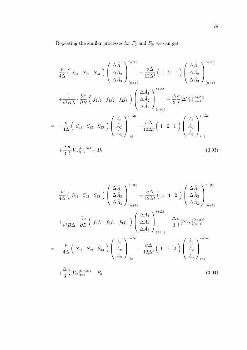
78
Repeating the similar processes for F2 and F3, we can get
ν
4∆
(S21 S22 S23
) ∆A1
∆A2
∆A3
t+∆t
(n+1)
+σ∆
12∆t
(1 2 1
) ∆A1
∆A2
∆A3
t+∆t
(n+1)
+1
ν2B∆· ∂ν∂B
(f2f1 f2f2 f2f3
) ∆A1
∆A2
∆A3
t+∆t
(n+1)
− ∆
3
σ
l[∆Vtz]
(t+∆t)(n+1)
= − ν
4∆
(S21 S22 S23
) A1
A2
A3
t+∆t
(n)
− σ∆
12∆t
(1 2 1
) A1
A2
A3
t+∆t
(n)
+∆
3
σ
l[Vtz]
(t+∆t)(n) + P2 (3.93)
ν
4∆
(S31 S32 S33
) ∆A1
∆A2
∆A3
t+∆t
(n+1)
+σ∆
12∆t
(1 1 2
) ∆A1
∆A2
∆A3
t+∆t
(n+1)
+1
ν2B∆· ∂ν∂B
(f3f1 f3f2 f3f3
) ∆A1
∆A2
∆A3
t+∆t
(n+1)
− ∆
3
σ
l[∆Vtz]
(t+∆t)(n+1)
= − ν
4∆
(S31 S32 S33
) A1
A2
A3
t+∆t
(n)
− σ∆
12∆t
(1 1 2
) A1
A2
A3
t+∆t
(n)
+∆
3
σ
l[Vtz]
(t+∆t)(n) + P3 (3.94)
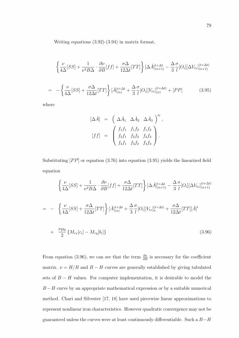
79
Writing equations (3.92)-(3.94) in matrix format,
ν
4∆[SS] +
1
ν2B∆· ∂ν∂B
[ff ] +σ∆
12∆t[TT ]
[∆A]t+∆t
(n+1) −∆
3
σ
l[Oi][∆Vtz]
(t+∆t)(n+1)
= −ν
4∆[SS] +
σ∆
12∆t[TT ]
[A]t+∆t
(n) +∆
3
σ
l[Oi][Vtz]
(t+∆t)(n) + [PP ] (3.95)
where
[∆A] =(
∆A1 ∆A2 ∆A3
)tr
,
[ff ] =
f1f1 f1f2 f1f3
f2f1 f2f2 f2f3
f3f1 f3f2 f3f3
.
Substituting [PP ] or equation (3.76) into equation (3.95) yields the linearized field
equationν
4∆[SS] +
1
ν2B∆· ∂ν∂B
[ff ] +σ∆
12∆t[TT ]
[∆A]t+∆t
(n+1) −∆
3
σ
l[Oi][∆Vtz]
(t+∆t)(n+1)
= −ν
4∆[SS] +
σ∆
12∆t[TT ]
[A]t+∆t
(n) +∆
3
σ
l[Oi][Vtz]
(t+∆t)n +
σ∆
12∆t[TT ][A]t
+νµ0
2Mrx[ci]−Mry[bi] (3.96)
From equation (3.96), we can see that the term ∂ν∂B
is necessary for the coefficient
matrix. ν = H/B and B −H curves are generally established by giving tabulated
sets of B − H values. For computer implementation, it is desirable to model the
B−H curve by an appropriate mathematical expression or by a suitable numerical
method. Chari and Silvester [17, 18] have used piecewise linear approximations to
represent nonlinear iron characteristics. However quadratic convergence may not be
guaranteed unless the curves were at least continuously differentiable. Such a B−H
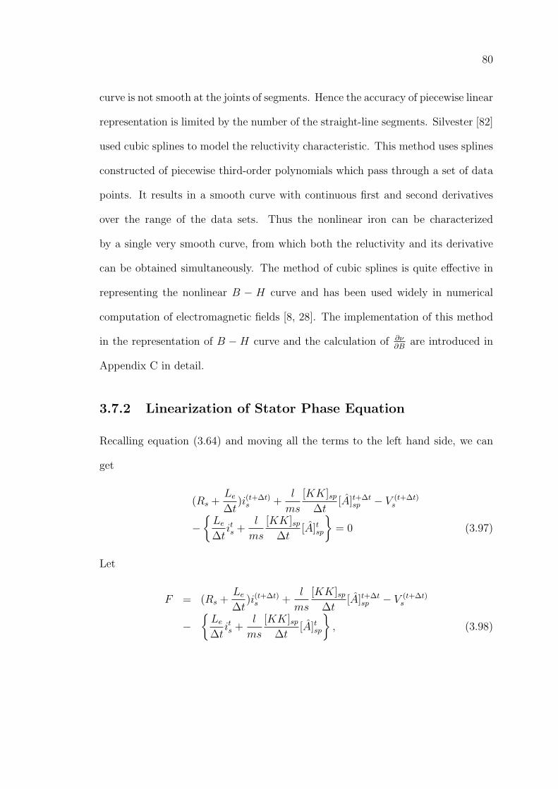
80
curve is not smooth at the joints of segments. Hence the accuracy of piecewise linear
representation is limited by the number of the straight-line segments. Silvester [82]
used cubic splines to model the reluctivity characteristic. This method uses splines
constructed of piecewise third-order polynomials which pass through a set of data
points. It results in a smooth curve with continuous first and second derivatives
over the range of the data sets. Thus the nonlinear iron can be characterized
by a single very smooth curve, from which both the reluctivity and its derivative
can be obtained simultaneously. The method of cubic splines is quite effective in
representing the nonlinear B − H curve and has been used widely in numerical
computation of electromagnetic fields [8, 28]. The implementation of this method
in the representation of B −H curve and the calculation of ∂ν∂B
are introduced in
Appendix C in detail.
3.7.2 Linearization of Stator Phase Equation
Recalling equation (3.64) and moving all the terms to the left hand side, we can
get
(Rs +Le
∆t)i(t+∆t)
s +l
ms
[KK]sp∆t
[A]t+∆tsp − V (t+∆t)
s
−Le
∆tits +
l
ms
[KK]sp∆t
[A]tsp
= 0 (3.97)
Let
F = (Rs +Le
∆t)i(t+∆t)
s +l
ms
[KK]sp∆t
[A]t+∆tsp − V (t+∆t)
s
−Le
∆tits +
l
ms
[KK]sp∆t
[A]tsp
, (3.98)
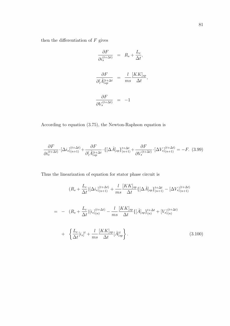
81
then the differentiation of F gives
∂F
∂i(t+∆t)s
= Rs +Le
∆t,
∂F
∂[A]t+∆tsp
=l
ms
[KK]sp∆t
,
∂F
∂V(t+∆t)s
= −1
According to equation (3.75), the Newton-Raphson equation is
∂F
∂i(t+∆t)s
·[∆is](t+∆t)(n+1) +
∂F
∂[A]t+∆tsp
·[∆A]spt+∆t(n+1)+
∂F
∂V(t+∆t)s
·[∆Vs](t+∆t)(n+1) = −F. (3.99)
Thus the linearization of equation for stator phase circuit is
(Rs +Le
∆t)[∆is]
(t+∆t)(n+1) +
l
ms
[KK]sp∆t
[∆A]spt+∆t(n+1) − [∆Vs]
(t+∆t)(n+1)
= − (Rs +Le
∆t)[is]
(t+∆t)(n) − l
ms
[KK]sp∆t
[A]spt+∆t(n) + [Vs]
(t+∆t)(n)
+
Le
∆t[is]
t +l
ms
[KK]sp∆t
[A]tsp
. (3.100)
82
3.7.3 Linearization of Equations for Cage Bars
Repeating the similar linearization process for equation (3.65) yields
Rbk[∆ibk]t+∆t(n+1) +
lbksbk
[KK]cb∆t
[∆A]cbt+∆t(n+1) − [∆Vbk]
t+∆t(n+1)
= − Rbk[ibk]t+∆t(n) − lbk
sbk
[KK]cb∆t
[A]cbt+∆t(n) + [Vbk]
t+∆t(n)
+lbksbk
[KK]cb∆t
[A]cbt. (3.101)
The linearization of equation (3.66) is
[∆ib]t+∆t(n+1) − [C1][∆ie]
t+∆t(n+1) = −[ib]
t+∆t(n) + [C1][ie]
t+∆t(n) (3.102)
The linearization of equation (3.67) is
[C2][∆Vb]t+∆t(n+1) + 2[Re] +
[Le]
∆t[∆ie]t+∆t
(n+1)
= −[C2][Vb]t+∆t(n) − 2[Re] +
[Le]
∆t[ie]t+∆t
(n) + 2[Le]
∆t[ie]
t (3.103)
83
3.7.4 Linearization of Equations for External Circuits
The linearization of equation (3.68) is
[Rsb] +[Lsb]
∆t[∆isb]t+∆t
(n+1) +[Csb]
∆t[∆Vsb; ∆Vt]
t+∆t(n+1)
= − [Rsb] +[Lsb]
∆t[isb]t+∆t
(n) − [Csb]
∆t[Vsb;Vt]
t+∆t(n)
+[Lsb]
∆t[isb]
t +[Csb]
∆t[Vsb;Vt]
t (3.104)
The linearization of equation (3.69) is
[C3][∆isb]t+∆t(n+1) + [C4][∆is]
t+∆t(n+1) = −[C3][isb]
t+∆t(n) − [C4][is]
t+∆t(n) (3.105)
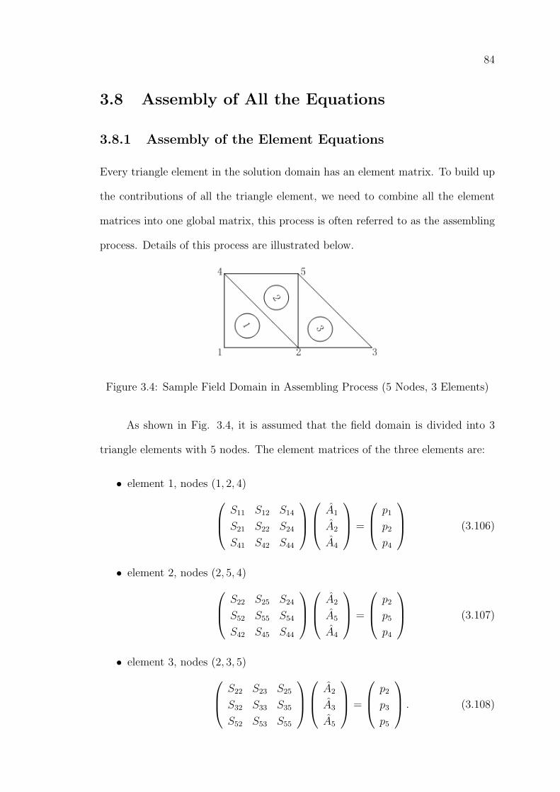
84
3.8 Assembly of All the Equations
3.8.1 Assembly of the Element Equations
Every triangle element in the solution domain has an element matrix. To build up
the contributions of all the triangle element, we need to combine all the element
matrices into one global matrix, this process is often referred to as the assembling
process. Details of this process are illustrated below.
Figure 3.4: Sample Field Domain in Assembling Process (5 Nodes, 3 Elements)
As shown in Fig. 3.4, it is assumed that the field domain is divided into 3
triangle elements with 5 nodes. The element matrices of the three elements are:
• element 1, nodes (1, 2, 4) S11 S12 S14
S21 S22 S24
S41 S42 S44
A1
A2
A4
=
p1
p2
p4
(3.106)
• element 2, nodes (2, 5, 4) S22 S25 S24
S52 S55 S54
S42 S45 S44
A2
A5
A4
=
p2
p5
p4
(3.107)
• element 3, nodes (2, 3, 5) S22 S23 S25
S32 S33 S35
S52 S53 S55
A2
A3
A5
=
p2
p3
p5
. (3.108)
85
Since there are 5 nodes totally, the size of the global coefficient matrix [S] is
5 × 5 and the size of force matrix [p] is 5 × 1. The initial value of [S] and [p] are
set to be 0,
[S] =
0 0 0 0 0
0 0 0 0 0
0 0 0 0 0
0 0 0 0 0
0 0 0 0 0
(3.109)
[p] =(
0 0 0 0 0)tr
(3.110)
Since element 1 is made up by nodes (1, 2, 4), the coefficients of its element matrix
will be added up to column 1, 2, 4 and row 1, 2, 4 of the global matrix. Equa-
tions (3.111) and (3.112) show the updated matrices [S] and [p] after element 1 is
assembled,
[S] =
S
(1)11 S
(1)12 0 S
(1)14 0
S(1)21 S
(1)22 0 S
(1)24 0
0 0 0 0 0
S(1)41 S
(1)42 0 S
(1)44 0
0 0 0 0 0
(3.111)
[p] =(p
(1)1 p
(1)2 0 p
(1)4 0
)tr
(3.112)
where the superscripts (1) denote the index number of the triangular elements, the
subscripts 11,12 , . . . denote the index number of the nodes and (. . .)tr denotes the
transpose operation of a matrix.
Repeating the similar process for element 2 and 3, the final global matrix
after assembly process is
[S][A] = [p] (3.113)
86
where
[S] =
S
(1)11 S
(1)12 0 S
(1)14 0
S(1)21 S
(1)+(2)+(3)22 S
(3)23 S
(1)+(2)24 S
(2)+(3)25
0 S(3)32 S
(3)33 0 S
(3)35
S(1)41 S
(1)+(2)42 0 S
(1)+(2)44 S
(2)45
0 S(2)+(3)52 S
(3)53 S
(2)54 S
(2)+(3)55
,
[A] =(A1 A2 A3 A4 A5
)tr
,
[p] =(p
(1)1 p
(1)+(2)+(3)2 p
(3)3 p
(1)+(2)4 p
(2)+(3)5
)tr
,
3.8.2 Global System of Equations
Applying the above assembly process for all the elemental equations (equation
(3.96) and combining with the other circuit equations (equations (3.100)-(3.103) )
yields a linear set of algebraic equations. In combination with the equations for
mechanical motion (equations (3.70) and (3.71)), we can get a global system of
equations
[GML][∆X]t+∆t(n+1) = [GMR1][X]]t+∆t
(n) + [GMR2][X]t + [SOURCE], (3.114)
and
(Jr
∆t+Bf )ω
t+∆tm =
Jr
∆t· ωt
m + Tem − Tf (3.115)
1
∆tθt+∆t
m − ωt+∆tm =
1
∆tθt
m (3.116)
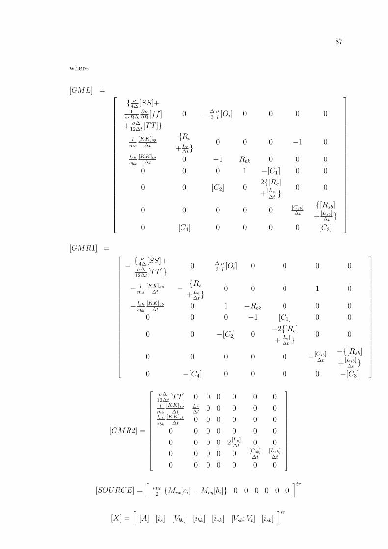
87
where
[GML] =
ν4∆
[SS]+1
ν2B∆∂ν∂B
[ff ]
+ σ∆12∆t
[TT ]0 −∆
3σl[Oi] 0 0 0 0
lms
[KK]sp
∆t
Rs
+Le
∆t
0 0 0 −1 0
lbk
sbk
[KK]cb
∆t0 −1 Rbk 0 0 0
0 0 0 1 −[C1] 0 0
0 0 [C2] 02[Re]
+ [Le]∆t
0 0
0 0 0 0 0 [Csb]∆t
[Rsb]
+ [Lsb]∆t
0 [C4] 0 0 0 0 [C3]
[GMR1] =
− ν
4∆[SS]+
σ∆12∆t
[TT ]0 ∆
3σl[Oi] 0 0 0 0
− lms
[KK]sp
∆t−
Rs
+Le
∆t
0 0 0 1 0
− lbk
sbk
[KK]cb
∆t0 1 −Rbk 0 0 0
0 0 0 −1 [C1] 0 0
0 0 −[C2] 0−2[Re]
+ [Le]∆t
0 0
0 0 0 0 0 − [Csb]∆t
−[Rsb]
+ [Lsb]∆t
0 −[C4] 0 0 0 0 −[C3]
[GMR2] =
σ∆12∆t
[TT ] 0 0 0 0 0 0l
ms
[KK]sp
∆tLe
∆t0 0 0 0 0
lbk
sbk
[KK]cb
∆t0 0 0 0 0 0
0 0 0 0 0 0 0
0 0 0 0 2 [Le]∆t
0 0
0 0 0 0 0 [Csb]∆t
[Lsb]∆t
0 0 0 0 0 0 0
[SOURCE] =
[νµ0
2Mrx[ci]−Mry[bi] 0 0 0 0 0 0
]tr[X] =
[[A] [is] [Vbk] [ibk] [iek] [Vsb;Vt] [isb]
]tr
88
[∆X] =[
[∆A] [∆is] [∆Vbk] [∆ibk] [∆iek] [∆Vsb; ∆Vt] [∆isb]]tr
The first line of equation (3.114) represents all the field equations. The second
line represent the equations for stator phase circuits. The third, fourth and fifth
lines represent all the equations for cage bars. The sixth and seventh lines represent
all the equations for external circuits. In the resultant matrix equation, [GML]
is the coefficient matrix. It is non-symmetrical due to the coupling of circuits
equations and mechanical motion equations. [∆X] is the solution vector where
n denotes the nth Newton-Raphson iteration
[∆A] denotes the incremental nodal vector potential solution
[∆is] denotes the incremental stator phase currents
[∆Vbk] denotes the incremental cage bar voltages
[∆ibk] denotes the incremental cage bar currents
[∆iek] denotes the incremental currents of the end rings
[∆Vsb; ∆Vt] denotes the incremental terminal voltages of the external circuits
and the electric machines
[∆isb] denotes the incremental currents of the external circuits
The solution vector [∆X] is updated at each Newton-Raphson iteration until
the incremental solution vector becomes within a prescribed tolerance. The known
input sources are the permanent magnet excitation νµ0
2Mrx[ci]−Mry[bi] and
some terminal voltages applied to the external circuits.
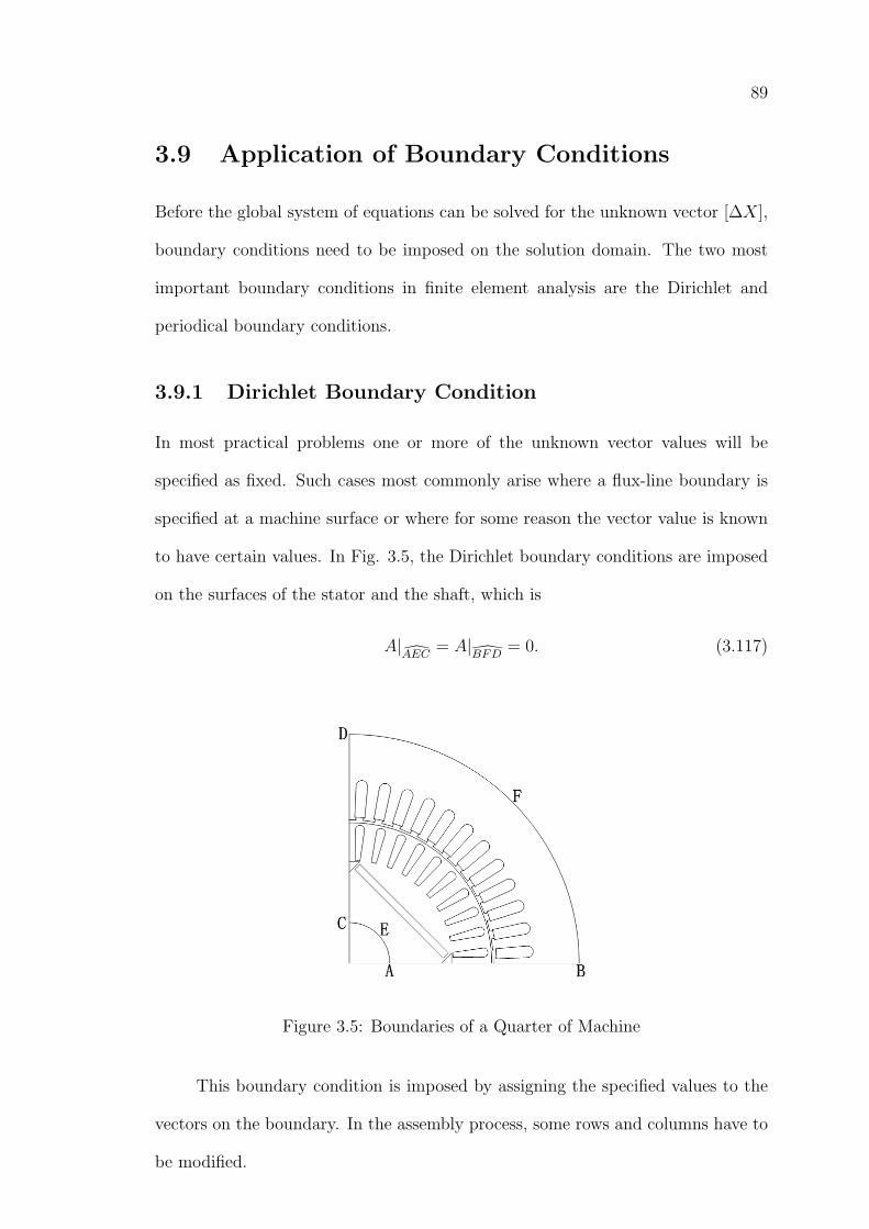
89
3.9 Application of Boundary Conditions
Before the global system of equations can be solved for the unknown vector [∆X],
boundary conditions need to be imposed on the solution domain. The two most
important boundary conditions in finite element analysis are the Dirichlet and
periodical boundary conditions.
3.9.1 Dirichlet Boundary Condition
In most practical problems one or more of the unknown vector values will be
specified as fixed. Such cases most commonly arise where a flux-line boundary is
specified at a machine surface or where for some reason the vector value is known
to have certain values. In Fig. 3.5, the Dirichlet boundary conditions are imposed
on the surfaces of the stator and the shaft, which is
A|AEC
= A|BFD
= 0. (3.117)
Figure 3.5: Boundaries of a Quarter of Machine
This boundary condition is imposed by assigning the specified values to the
vectors on the boundary. In the assembly process, some rows and columns have to
be modified.
90
Let the set of all the unknown vectors [X] be divided into two parts: the free
vectors [Xfr] and the vectors with fixed values [Xfi]. Recalling equation (3.74), we
can get the iterative process for the set of equations [f ]k×1 = [K]k×k[X]k×1 = [Q]k×1
is:
[X](n+1) = [X](n) + [J ](n)−1[Q]− [f ](n) (3.118)
where [J ] = ∂fi
∂Xj, (i, j = 1, 2, . . . , k) is the Jacobian matrix and n is the iteration
step number.
To include the vectors with fixed values into the iteration process, equation
(3.118) can be modified as
(Xfr
Xf i
)(n+1)
=
(Xfr
Xf i
)n
+
([J (n)] 0
0 [I]
)−1([Q]− [f ](n)
0
)(3.119)
where [I] is the identity matrix.
The inclusion of the segment of identity matrix with [J ] is necessary to guar-
antee that the modified Jacobian matrix is nonsingular and equation (3.119) is
solvable. From equation (3.119) we can see that the fixed vector values [Xfi] are
not altered by the iteration. In other words, the Dirichlet boundary condition is
satisfied using equation (3.119). In practice, if the row number of the global ma-
trix corresponds to a vector with a fixed value (or the vector meets the Dirichlet
boundary condition), the fixed value is assigned to this vector. In the iterative
process, row of the identity matrix is substituted in the Jacobian matrix and zero
entry is substituted in the right-hand vector.
91
3.9.2 Periodical Boundary Condition
In electric machine problems, there arise boundary conditions which do not cor-
respond to explicit knowledge of unknown vectors or derivatives, but merely state
that the vector value at one point is linearly related to the value at another point.
The most common occurrence of this kind of conditions arise in connection with
the analysis of loaded machines. When an electric machine operates under load and
at a power factor different from zero, the pole axis is no longer an axis of symmetry
and is not a flux line boundary. However the stator conductors in one pole pitch
carrying currents in one direction have their equivalent and identical conductors in
the next pole-pitch but carrying current in the opposite direction. As a result, the
vector potentials one pole pitch apart have equal magnitude but opposite sign. In
Fig. 3.5, the relationship between the potential values at different positions are:
A|AB = −A|CD. (3.120)
Similarly there occur other cases, in which the potentials of any two points are
identical both in magnitude and sign. All these purely periodic cases can be rep-
resented by the constraint
Ap1 = ±Ap2 (3.121)
where Ap1 and Ap2 are the potential values on the anti-periodical boundaries.
When imposing periodical boundary conditions one always deals with only
two triangles at a time. Hence it is only necessary to derive the matrix operation
involved in imposing such periodical condition on a pair of triangles only. Fig. 3.6
shows two triangles (1, 2, 3) and (4, 5, 6) having two nodes of each triangle on the
pole axis. Therefore,
A1 = ±A5,
A3 = ±A6. (3.122)
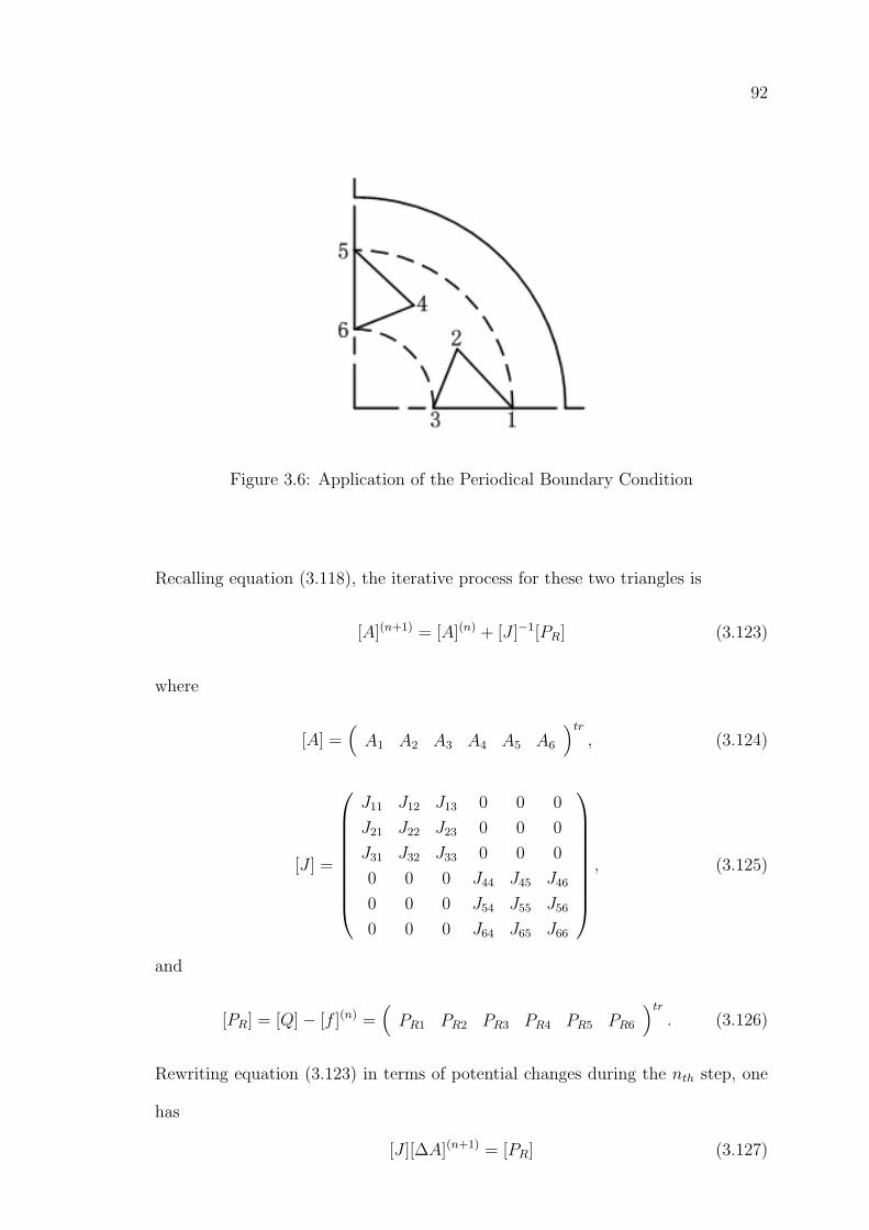
92
Figure 3.6: Application of the Periodical Boundary Condition
Recalling equation (3.118), the iterative process for these two triangles is
[A](n+1) = [A](n) + [J ]−1[PR] (3.123)
where
[A] =(A1 A2 A3 A4 A5 A6
)tr
, (3.124)
[J ] =
J11 J12 J13 0 0 0
J21 J22 J23 0 0 0
J31 J32 J33 0 0 0
0 0 0 J44 J45 J46
0 0 0 J54 J55 J56
0 0 0 J64 J65 J66
, (3.125)
and
[PR] = [Q]− [f ](n) =(PR1 PR2 PR3 PR4 PR5 PR6
)tr
. (3.126)
Rewriting equation (3.123) in terms of potential changes during the nth step, one
has
[J ][∆A](n+1) = [PR] (3.127)
93
If it is assumed that [∆A′] represents the total incremental vector potential
for the connected triangles and the sum of the individual incremental potential
vectors for the unconnected triangle is represented by [∆A], then these can be
related by a connection matrix [C] in the following manner
[∆A] = [C] · [∆A′] (3.128)
where
[∆A′] =
∆A1
∆A2
∆A3
∆A4
, [C] =
1 0 0 0
0 1 0 0
0 0 1 0
0 0 0 1
±1 0 0 0
0 0 ±1 0
, [∆A] =
∆A1
∆A2
∆A3
∆A4
∆A5
∆A6
.
The similar operations can be applied on the right hand side matrix [PR] and [P ′R]
can be used to represent the total connected vectors, thus
[P ′R] = [Ct] · [PR] (3.129)
where
[P ′R] =
P ′R1
P ′R2
P ′R3
P ′R4
=
PR1 ± PR5
PR2
PR3 ± PR6
PR4
, [Ct] =
1 0 0 0 ±1 0
0 1 0 0 0 0
0 0 1 0 0 ±1
0 0 0 1 0 0
.
Substituting equation (3.128) into equation (3.127) yields
[PR] = [J ][∆A] = [J ][C][∆A′] (3.130)
Combining equation (3.130) and (3.129) yields
[P ′R] = [Ct][PR] = [Ct][J ][C][∆A′]. (3.131)
94
Since
[P ′R] = [J ′] · [∆A′] (3.132)
where [J ′] is the Jacobian matrix after applying periodical boundary conditions,
then comparing equation (3.132) and (3.131) yields
[J ′] = [Ct][J ][C] =
J11 + J55 J12 J13 + J56 ±J54
J21 J22 J23 0
J31 + J65 J32 J33 + J66 ±J64
±J45 0 ±J46 J44
(3.133)
or
[J ′] =
J11 J12 J13 0
J21 J22 J23 0
J31 J32 J33 0
0 0 0 0
+
J55 0 J56 ±J54
0 0 0 0
J65 0 J66 ±J64
±J45 0 ±J46 J44
(3.134)
Therefore the iterative process after imposing periodical boundary condition is
[A′](n+1) = [A′](n) + [J ′]−1[P ′R] (3.135)
It can be seen that the inclusion of the periodical boundary conditions merely
requires that certain matrix segments be assembled with altered signs. The rows
and columns of these segments correspond to the nodes where periodical boundary
conditions are applied.
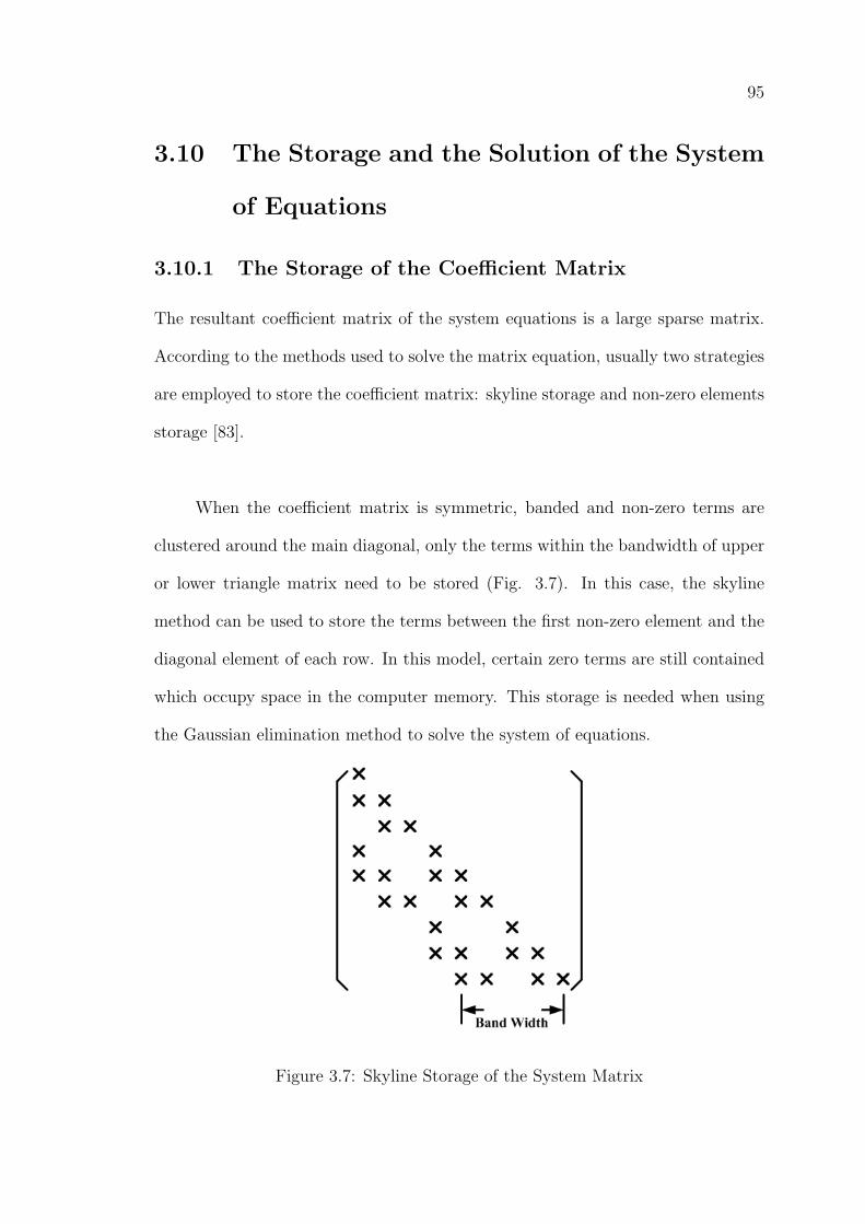
95
3.10 The Storage and the Solution of the System
of Equations
3.10.1 The Storage of the Coefficient Matrix
The resultant coefficient matrix of the system equations is a large sparse matrix.
According to the methods used to solve the matrix equation, usually two strategies
are employed to store the coefficient matrix: skyline storage and non-zero elements
storage [83].
When the coefficient matrix is symmetric, banded and non-zero terms are
clustered around the main diagonal, only the terms within the bandwidth of upper
or lower triangle matrix need to be stored (Fig. 3.7). In this case, the skyline
method can be used to store the terms between the first non-zero element and the
diagonal element of each row. In this model, certain zero terms are still contained
which occupy space in the computer memory. This storage is needed when using
the Gaussian elimination method to solve the system of equations.
Figure 3.7: Skyline Storage of the System Matrix
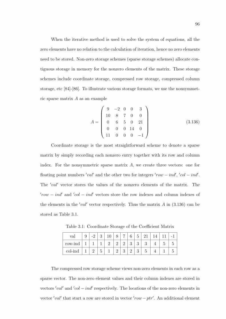
96
When the iterative method is used to solve the system of equations, all the
zero elements have no relation to the calculation of iteration, hence no zero elements
need to be stored. Non-zero storage schemes (sparse storage schemes) allocate con-
tiguous storage in memory for the nonzero elements of the matrix. These storage
schemes include coordinate storage, compressed row storage, compressed column
storage, etc [84]-[86]. To illustrate various storage formats, we use the nonsymmet-
ric sparse matrix A as an example
A =
9 −2 0 0 3
10 8 7 0 0
0 6 5 0 21
0 0 0 14 0
11 0 0 0 −1
(3.136)
Coordinate storage is the most straightforward scheme to denote a sparse
matrix by simply recording each nonzero entry together with its row and column
index. For the nonsymmetric sparse matrix A, we create three vectors: one for
floating point numbers ′val′ and the other two for integers ′row− ind′, ′col− ind′.
The ′val′ vector stores the values of the nonzero elements of the matrix. The
′row − ind′ and ′col − ind′ vectors store the row indexes and column indexes of
the elements in the ′val′ vector respectively. Thus the matrix A in (3.136) can be
stored as Table 3.1.
Table 3.1: Coordinate Storage of the Coefficient Matrix
val 9 -2 3 10 8 7 6 5 21 14 11 -1
row-ind 1 1 1 2 2 2 3 3 3 4 5 5
col-ind 1 2 5 1 2 3 2 3 5 4 1 5
The compressed row storage scheme views non-zero elements in each row as a
sparse vector. The non-zero element values and their column indexes are stored in
vectors ′val′ and ′col− ind′ respectively. The locations of the non-zero elements in
vector ′val′ that start a row are stored in vector ′row−ptr′. An additional element
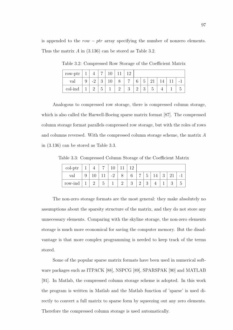
97
is appended to the row − ptr array specifying the number of nonzero elements.
Thus the matrix A in (3.136) can be stored as Table 3.2.
Table 3.2: Compressed Row Storage of the Coefficient Matrix
row-ptr 1 4 7 10 11 12
val 9 -2 3 10 8 7 6 5 21 14 11 -1
col-ind 1 2 5 1 2 3 2 3 5 4 1 5
Analogous to compressed row storage, there is compressed column storage,
which is also called the Harwell-Boeing sparse matrix format [87]. The compressed
column storage format parallels compressed row storage, but with the roles of rows
and columns reversed. With the compressed column storage scheme, the matrix A
in (3.136) can be stored as Table 3.3.
Table 3.3: Compressed Column Storage of the Coefficient Matrix
col-ptr 1 4 7 10 11 12
val 9 10 11 -2 8 6 7 5 14 3 21 -1
row-ind 1 2 5 1 2 3 2 3 4 1 3 5
The non-zero storage formats are the most general: they make absolutely no
assumptions about the sparsity structure of the matrix, and they do not store any
unnecessary elements. Comparing with the skyline storage, the non-zero elements
storage is much more economical for saving the computer memory. But the disad-
vantage is that more complex programming is needed to keep track of the terms
stored.
Some of the popular sparse matrix formats have been used in numerical soft-
ware packages such as ITPACK [88], NSPCG [89], SPARSPAK [90] and MATLAB
[91]. In Matlab, the compressed column storage scheme is adopted. In this work
the program is written in Matlab and the Matlab function of ’sparse’ is used di-
rectly to convert a full matrix to sparse form by squeezing out any zero elements.
Therefore the compressed column storage is used automatically.
98
3.10.2 Solving the Global System of Equations
The system of equations is non-symmetric linear. The solution algorithm of such
matrix equations can generally be classified as direct methods and iterative meth-
ods [83].
The most commonly used direct method for non-symmetric linear system of
equations is Gaussian elimination. Direct methods are characterized by always re-
quiring a constant amount of work. Another class of methods, iterative methods,
require a variable amount of work that depends on the problem being solved. The
appeal of iterative methods is that they may require less work than a direct method
for many problems. In particular, they are effective on large sparse linear systems.
Iterative methods are generally used to solve system of equations which is
too large to be handled by direct methods. Iterative methods do not guarantee a
solution for every system of equations. However, when they do yield a solution,
they are usually less expensive than direct methods. Iterative methods can be
expressed in the simple form
X(n+1) = T ·X(n) + C. (3.137)
Depending on the nature of T and C, iterative methods can be classified into two
main categories, stationary iterative methods and non-stationary iterative meth-
ods. In stationary method, the iterative matrix T and vector C stays the same
throughout the iteration, while a new iterative matrix T or vector C is generated
in every step of the non-stationary iterative methods. Conjugate gradient methods
for symmetric positive definite problems and conjugate gradient look-alike methods
for nonsymmetric problems are examples of nonstationary iterative methods [92].
99
Several conjugate gradient-like iterative solvers, such as bi-conjugate gra-
dient iteration (BiCG), bi-conjugate iteration stabilized (BiCGSTAB), conjugate
gradient squared iteration (CGS) and quasi minimal residual iteration (QMR), are
available for solving general non-symmetric system of linear equations. They are
particularly attractive to solve sparse matrices which are normally direct results
of spatial discretization of differential equations [92, 93]. In this work, method of
BiCG is used. The details of the method is shown in Appendix D.
3.11 The Calculation of Electromagnetic Torque
3.11.1 Introduction
Electromagnetic torque, Tem, is the motive that drive the rotor of a electric ma-
chine. The knowledge of the electromagnetic torque in terms of the rotation angle is
very important for the designer to evaluate the performances and operating qual-
ities of the machine. Electromagnetic forces and torques can be computed in a
variety of methods. The three basic methods often employed with finite element
analysis are Lorentz method [94], Energy methods [95, 96] and Maxwell’s stress
tensor method [8, 97].
Lorentz method is used to calculate electromagnetic forces acting on current
carrying structures only. Although it is easy to cooperate with the finite element
field solutions, it cannot be applied to determine forces acting on ferromagnetic
structures, except where the reaction force of a single coil appears on the iron. Due
to the limitation of the Lorentz method, it is ignored in our computation.
Electromagnetic torque can also be calculated by energy methods based on
the principle of conservation of energy. The force acting on a movable part of a
100
device may be derived from the variation of the stored magnetic energy, W , or
co-energy, W ′ of the entire device against small space displacement ∆θ [8, 95].
The flux linkage λ and current I are kept constant while derived from energy and
co-energy respectively. Although the method is quite straightforward and easy to
implement, it suffers from two major shortcomings. First, important numerical
errors may be introduced as a consequence of a small incremental choice of ∆θ.
Second, the field computation has to be performed twice for one torque value, caus-
ing the computation time doubled.
The Coulomb virtual work method overcomes these shortcomings by taking
direct, closed form differentiation of magnetic energy or co-energy of the free space
region between the moveable and the fixed parts of the system under consideration.
By this way, only one finite element solution is necessary.
Forces and torques can also be integrated using Maxwell stress tensor over any
closed surface surrounding the moving body [8, 97]. Both the Coulomb’s virtual
work method and the Maxwell stress tensor method can be used to calculate the
electromagnetic torque. These two methods have the following advantages [28, 96]:
(1) Both methods are applicable to any rigid body in the finite element problems.
(2) Both methods need only one field computation.
(3) Both methods require a single integration involving only air gap elements .
(4) Both methods can give similar results if a good surface is chosen for the Maxwell
stress tensor method [98, 96].
In this work the Maxwell stress tensor method is used to calculated the elec-
tromagnetic torque.
101
3.11.2 Calculation of Torque with Maxwell Stress Tensor
Method
The Maxwell stress tensor method is commonly used in the calculation of forces
and torques in the finite element analysis of electrical devices. The Maxwell tensor
can be expressed as
σ =1
µ0
(B · ~n)B − 1
2µ0
(B2~n). (3.138)
where σ is the Maxwell’s stress tensor, B is the flux density and ~n is the unit
normal vector
The torque applied to one part of the magnetic circuit can be obtained by
integrating the Maxwell stress tensor along a path Γ placed in the air and enclosing
this part. In the case of electric machines, this integration path is normally placed
in the air gap and the torque can be calculated by
T = L
∫Γ
(r × σ)dΓ (3.139)
where L is the axial length and r is the lever arm.
Since
B = Bn~n+Bt~t (3.140)
and
B2 = B2n +B2
t , (3.141)
substituting equations (3.140) and (3.141) into equation (3.138) yields
σ =1
2µ0
(B2n −B2
t )~n+1
µ0
(BnBt)~t (3.142)
where Bn and Bt are the normal and tangential components of flux density respec-
tively, ~t is the unit tangential vector.
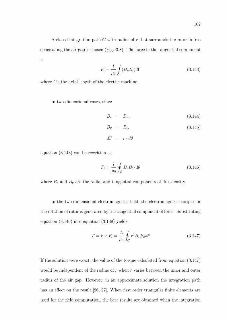
102
A closed integration path C with radius of r that surrounds the rotor in free
space along the air-gap is chosen (Fig. 3.8). The force in the tangential component
is
Ft =l
µ0
∫Γ
(BnBt)dΓ (3.143)
where l is the axial length of the electric machine.
In two-dimensional cases, since
Br = Bn, (3.144)
Bθ = Bt, (3.145)
dΓ = r · dθ
equation (3.143) can be rewritten as
Ft =l
µ0
∮C
BrBθrdθ (3.146)
where Br and Bθ are the radial and tangential components of flux density.
In the two-dimensional electromagnetic field, the electromagnetic torque for
the rotation of rotor is generated by the tangential component of force. Substituting
equation (3.146) into equation (3.139) yields
T = r × Ft =L
µ0
∮C
r2BrBθdθ (3.147)
If the solution were exact, the value of the torque calculated from equation (3.147)
would be independent of the radius of r when r varies between the inner and outer
radius of the air gap. However, in an approximate solution the integration path
has an effect on the result [96, 27]. When first order triangular finite elements are
used for the field computation, the best results are obtained when the integration
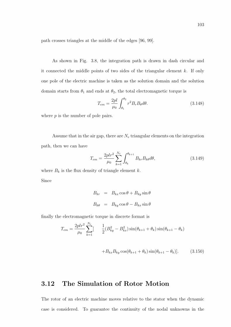
103
path crosses triangles at the middle of the edges [96, 99].
As shown in Fig. 3.8, the integration path is drawn in dash circular and
it connected the middle points of two sides of the triangular element k. If only
one pole of the electric machine is taken as the solution domain and the solution
domain starts from θ1 and ends at θ2, the total electromagnetic torque is
Tem =2pl
µ0
∫ θ2
θ1
r2BrBθdθ. (3.148)
where p is the number of pole pairs.
Assume that in the air gap, there areNe triangular elements on the integration
path, then we can have
Tem =2plr2
µ0
Ne∑k=1
∫ θk+1
θk
BkrBkθdθ, (3.149)
where Bk is the flux density of triangle element k.
Since
Bkr = Bkx cos θ +Bky sin θ
Bkθ = Bky cos θ −Bkx sin θ
finally the electromagnetic torque in discrete format is
Tem =2plr2
µ0
Ne∑k=1
[1
2(B2
ky −B2kx) sin(θk+1 + θk) sin(θk+1 − θk)
+BkxBky cos(θk+1 + θk) sin(θk+1 − θk)]. (3.150)
3.12 The Simulation of Rotor Motion
The rotor of an electric machine moves relative to the stator when the dynamic
case is considered. To guarantee the continuity of the nodal unknowns in the
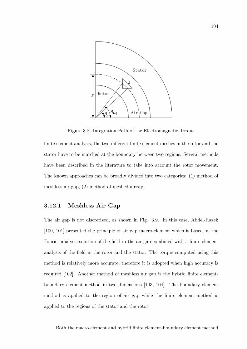
104
Figure 3.8: Integration Path of the Electromagnetic Torque
finite element analysis, the two different finite element meshes in the rotor and the
stator have to be matched at the boundary between two regions. Several methods
have been described in the literature to take into account the rotor movement.
The known approaches can be broadly divided into two categories: (1) method of
meshless air gap, (2) method of meshed airgap.
3.12.1 Meshless Air Gap
The air gap is not discretized, as shown in Fig. 3.9. In this case, Abdel-Razek
[100, 101] presented the principle of air gap macro-element which is based on the
Fourier analysis solution of the field in the air gap combined with a finite element
analysis of the field in the rotor and the stator. The torque computed using this
method is relatively more accurate, therefore it is adopted when high accuracy is
required [102]. Another method of meshless air gap is the hybrid finite element-
boundary element method in two dimensions [103, 104]. The boundary element
method is applied to the region of air gap while the finite element method is
applied to the regions of the stator and the rotor.
Both the macro-element and hybrid finite element-boundary element method

105
Figure 3.9: The Meshless Air Gap in Simulation of Rotor Motion
may reduce the number of unknowns and avoid the handling of triangular elements
in the air gap region. However the sparsity of the stiffness matrix is lost because of
the full matrix part contributed by the boundary element method and the analytical
method. Due to the long time spent on assembly process, the efficiency of these
methods are not guaranteed. This may be a disadvantage for dynamic problems,
thus these two methods are not considered in our computation.
3.12.2 Meshed Air Gap
The air gap is discretised, as shown in Fig. 3.10. In this case, the air gap is
subdivided into meshes and the rotation can take place by means of a layer of
finite element placed in the air gap. This layer can occupy all the air gap region
or just a part of it. Since the rotor is moving and the stator is fixed, this layer of
meshes will distort as time going on (Fig. 3.11).
To avoid the need of remeshing the distorted elements, the Lagrange mul-
tipliers techniques [105] is used which allows a finite element mesh to move with
respect to an adjacent mesh freely. At different positions, only the terms which
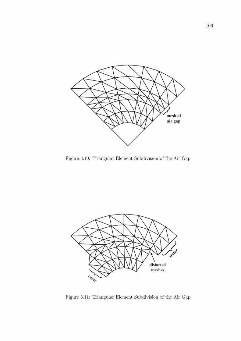
106
Figure 3.10: Triangular Element Subdivision of the Air Gap
Figure 3.11: Triangular Element Subdivision of the Air Gap
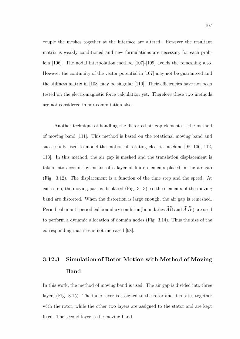
107
couple the meshes together at the interface are altered. However the resultant
matrix is weakly conditioned and new formulations are necessary for each prob-
lem [106]. The nodal interpolation method [107]-[109] avoids the remeshing also.
However the continuity of the vector potential in [107] may not be guaranteed and
the stiffness matrix in [108] may be singular [110]. Their efficiencies have not been
tested on the electromagnetic force calculation yet. Therefore these two methods
are not considered in our computation also.
Another technique of handling the distorted air gap elements is the method
of moving band [111]. This method is based on the rotational moving band and
successfully used to model the motion of rotating electric machine [98, 106, 112,
113]. In this method, the air gap is meshed and the translation displacement is
taken into account by means of a layer of finite elements placed in the air gap
(Fig. 3.12). The displacement is a function of the time step and the speed. At
each step, the moving part is displaced (Fig. 3.13), so the elements of the moving
band are distorted. When the distortion is large enough, the air gap is remeshed.
Periodical or anti-periodical boundary condition(boundaries AB and A′B′) are used
to perform a dynamic allocation of domain nodes (Fig. 3.14). Thus the size of the
corresponding matrices is not increased [98].
3.12.3 Simulation of Rotor Motion with Method of Moving
Band
In this work, the method of moving band is used. The air gap is divided into three
layers (Fig. 3.15). The inner layer is assigned to the rotor and it rotates together
with the rotor, while the other two layers are assigned to the stator and are kept
fixed. The second layer is the moving band.
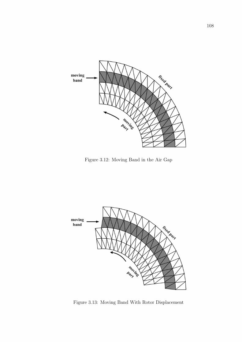
108
Figure 3.12: Moving Band in the Air Gap
Figure 3.13: Moving Band With Rotor Displacement
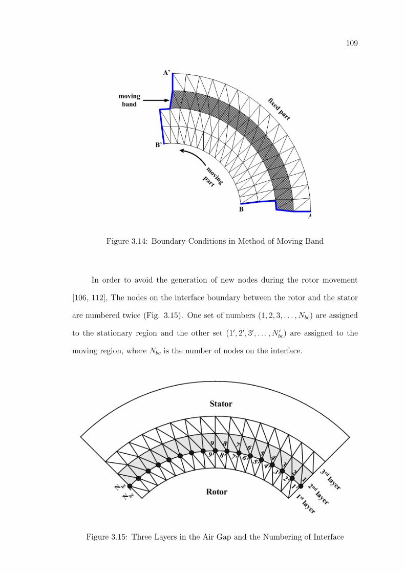
109
Figure 3.14: Boundary Conditions in Method of Moving Band
In order to avoid the generation of new nodes during the rotor movement
[106, 112], The nodes on the interface boundary between the rotor and the stator
are numbered twice (Fig. 3.15). One set of numbers (1, 2, 3, . . . , Nbc) are assigned
to the stationary region and the other set (1′, 2′, 3′, . . . , N ′bc) are assigned to the
moving region, where Nbc is the number of nodes on the interface.
Figure 3.15: Three Layers in the Air Gap and the Numbering of Interface
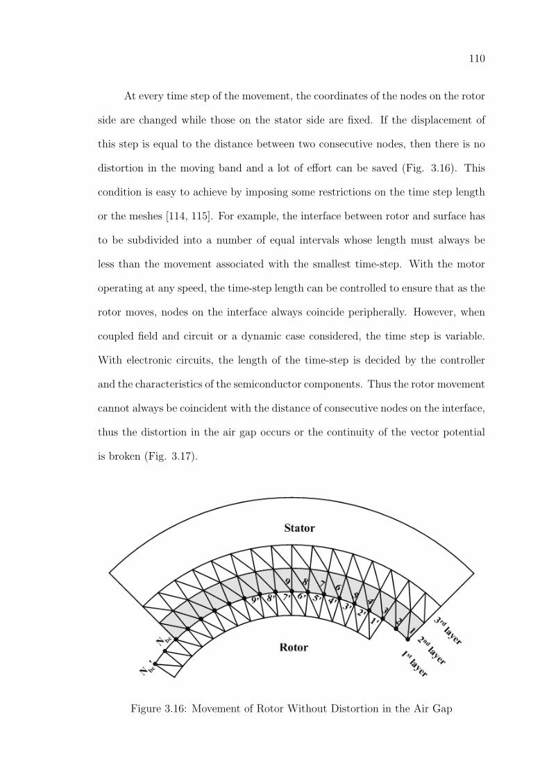
110
At every time step of the movement, the coordinates of the nodes on the rotor
side are changed while those on the stator side are fixed. If the displacement of
this step is equal to the distance between two consecutive nodes, then there is no
distortion in the moving band and a lot of effort can be saved (Fig. 3.16). This
condition is easy to achieve by imposing some restrictions on the time step length
or the meshes [114, 115]. For example, the interface between rotor and surface has
to be subdivided into a number of equal intervals whose length must always be
less than the movement associated with the smallest time-step. With the motor
operating at any speed, the time-step length can be controlled to ensure that as the
rotor moves, nodes on the interface always coincide peripherally. However, when
coupled field and circuit or a dynamic case considered, the time step is variable.
With electronic circuits, the length of the time-step is decided by the controller
and the characteristics of the semiconductor components. Thus the rotor movement
cannot always be coincident with the distance of consecutive nodes on the interface,
thus the distortion in the air gap occurs or the continuity of the vector potential
is broken (Fig. 3.17).
Figure 3.16: Movement of Rotor Without Distortion in the Air Gap
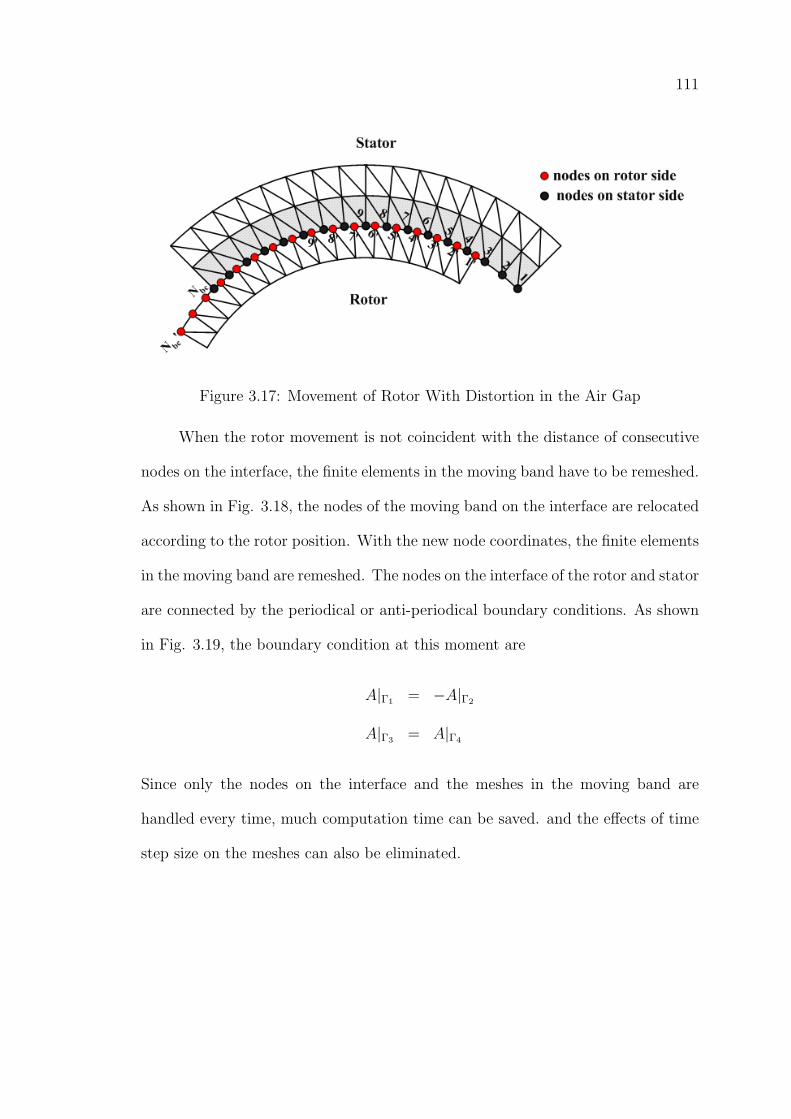
111
Figure 3.17: Movement of Rotor With Distortion in the Air Gap
When the rotor movement is not coincident with the distance of consecutive
nodes on the interface, the finite elements in the moving band have to be remeshed.
As shown in Fig. 3.18, the nodes of the moving band on the interface are relocated
according to the rotor position. With the new node coordinates, the finite elements
in the moving band are remeshed. The nodes on the interface of the rotor and stator
are connected by the periodical or anti-periodical boundary conditions. As shown
in Fig. 3.19, the boundary condition at this moment are
A|Γ1 = −A|Γ2
A|Γ3 = A|Γ4
Since only the nodes on the interface and the meshes in the moving band are
handled every time, much computation time can be saved. and the effects of time
step size on the meshes can also be eliminated.
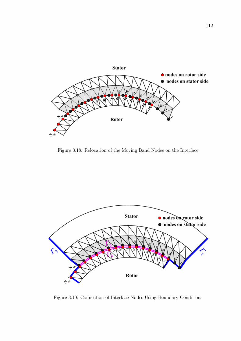
112
Figure 3.18: Relocation of the Moving Band Nodes on the Interface
Figure 3.19: Connection of Interface Nodes Using Boundary Conditions
113
3.13 Conclusion
This chapter presented the complete process of field-circuit coupled time stepping
finite element computation of line-start permanent magnet synchronous machine.
Most of the governing equations are space dependent or time dependent. The
space dependent quantities can be formulated by the method of weighted residual.
The time dependent quantities are evaluated by the time-stepping method and
the backward Euler’s method is recognized as one of the most stable ones. Since
nonlinear materials are used for the iron cores of the stator and the rotor, the re-
sultant global system of equations is nonlinear. Newton-Raphson iterative method
can be chosen to solve these nonlinear equations and the cubic splines are used to
represent the characteristics of the nonlinear materials. Because of the coupling
of circuit equations, the resultant global coefficient matrix is non-symmetric also.
To get the solution of this set of non-symmetrical linear equations, bi-conjugate
gradient method can be used in each Newton-Raphson iteration. With the electro-
magnetic field solution, the motor torque can be calculated using Maxwell stress
tensor method. Once the motor torque is available, the rotor speed and rotor po-
sition are obtainable with the mechanical motion equations. If we continue the
computation with the new time and new position, the dynamic performance of
the machine can be calculated step by step. The flow chart for this computation
process is shown in Appendix E.
In general, this field-circuit coupled time stepping finite element computation
process can be used to calculate the dynamics of any electric machine. It will be
used to calculate the dynamics of a line-start permanent magnet synchronous ma-
chine in Chapter 5.
Chapter 4
Parameter Estimation of theLine-Start Permanent MagnetSynchronous Machines
4.1 Introduction
Permanent magnet synchronous machines are receiving much attention due to their
high speed, power density and efficiency characteristics. New rotor configurations
and the commercial availability of high field strength permanent magnets have re-
duced the cost of these machines. Permanent magnet synchronous machines now
can provide a significant and affordable performance improvement in many applica-
tions. However, manufactures of such commercially available machines provide very
little information about the parameters which are very important for implement-
ing various types of controllers. Thus parameter estimation is extremely important
for the operators of modern drives to implement high performance control. It is
also invaluable for the machine designer and manufacturers wishing to do various
simulation and analysis before the prototypes are made.
The testing and analysis of permanent magnet synchronous machines are
based on the recognized equivalent circuit modelling. This equivalent circuit is
based on the classical two-axis model and the parameters of this two-axis model
114
115
are the ones of interest in this work. These machine parameters usually consist
of the synchronous reactance of direct axis Xd, the synchronous reactance of the
quadrant axis Xq and the magnet induced voltage E0.
The parameter determination of the permanent magnet synchronous ma-
chines are in principle similar to the procedures applied to conventional synchronous
motors with wound rotors and slip rings. However, because of the permanent mag-
net excitation, classical methods applied to conventional synchronous machines are
no longer appropriate. For example, without the ability to remove field excitation
of the permanent magnet from the permanent magnet synchronous machine, the
conventional methods of electrical parameter identification using the open circuit
saturation curve, the short circuit current curve, the zero power factor curve or the
slip test cannot be utilized [56].
To tackle the problems of parameter determination of permanent magnet
synchronous machines, various techniques and methods have been used by many
researchers [43] - [60]. In this work, the methods that were mostly used before
by other researchers are reviewed first. Then two new methods are proposed by
the implementation of linear regression and Hopfield neural network. Parameters
calculated by finite element method are also presented.
116
4.2 Lumped Parameter Model of Permanent
Magnet Synchronous Machines
The lumped parameter model of a permanent magnet synchronous machine is de-
rived from generalized electrical machine theory. The standard two-axis theory
with fixed rotor reference frame is used. A transformation that transforms the
three-phase model to such and equivalent two-phase description is needed. It is
desirable to utilize a particular transformation such that the representation of elec-
trical power in the machine is preserved. As a result, the developed torques are
invariant over the transformation. The Park’s transformation is used to transform
the variables from the stator reference frame abc to the rotor reference frame dq0
[116]. To keep the power invariant, the transformation is given by [117]:
fds
fqs
f0s
=
√2
3
sin θe sin(θe − 2π/3) sin(θe + 2π/3)
cos θe cos(θe − 2π/3) cos(θe + 2π/3)√1/2
√1/2
√1/2
fas
fbs
fcs
, (4.1)
where fds, fqs and f0s are the direct, quadrature and zero-sequence quantities, re-
spectively.
Fig. 4.1 shows the trigonometric interpretation of the change of stator vari-
ables using Park’s transformation. In Fig. 4.1, θm is the rotor angle, θe is the rotor
electrical angle, which equals to the number of pole pairs times θm. ωm denotes the
mechanical speed of the rotor and its positive direction is assumed to be counter-
clockwise. The rotor position is decided by
θm = θ0 +
∫ t
0
ωmdt (4.2)
where θ0 is the initial rotor position.
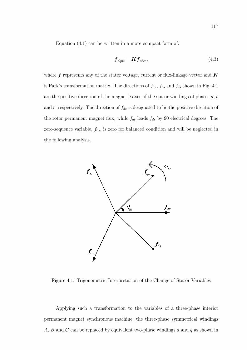
117
Equation (4.1) can be written in a more compact form of:
f dq0s = Kfabcs, (4.3)
where f represents any of the stator voltage, current or flux-linkage vector and K
is Park’s transformation matrix. The directions of fas, fbs and fcs shown in Fig. 4.1
are the positive direction of the magnetic axes of the stator windings of phases a, b
and c, respectively. The direction of fds is designated to be the positive direction of
the rotor permanent magnet flux, while fqs leads fds by 90 electrical degrees. The
zero-sequence variable, f0s, is zero for balanced condition and will be neglected in
the following analysis.
Figure 4.1: Trigonometric Interpretation of the Change of Stator Variables
Applying such a transformation to the variables of a three-phase interior
permanent magnet synchronous machine, the three-phase symmetrical windings
A, B and C can be replaced by equivalent two-phase windings d and q as shown in
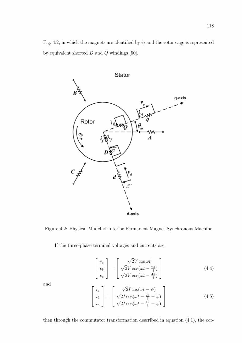
118
Fig. 4.2, in which the magnets are identified by if and the rotor cage is represented
by equivalent shorted D and Q windings [50].
Figure 4.2: Physical Model of Interior Permanent Magnet Synchronous Machine
If the three-phase terminal voltages and currents are
va
vb
vc
=
√
2V cosωt√2V cos(ωt− 2π
3)√
2V cos(ωt− 4π3
)
(4.4)
and ia
ib
ic
=
√
2I cos(ωt− ψ)√2I cos(ωt− 2π
3− ψ)√
2I cos(ωt− 4π3− ψ)
(4.5)
then through the commutator transformation described in equation (4.1), the cor-
119
responding voltages and currents in dq0 system are
vd
vq
v0
=√
3V
− sin(ωt− θe)
cos(ωt− θe)
0
=√
3V
− sin δ
cos δ
0
(4.6)
and id
iq
i0
=√
3I
− sin(ωt− θe − ψ)
cos(ωt− θe − ψ)
0
=√
3I
− sin(δ − ψ)
cos(δ − ψ)
0
=
√3I
cos(π2
+ δ − ψ)
sin(π2
+ δ − ψ)
0
(4.7)
where ω is the stator angular velocity, δ = ωt − θe is the torque angle and ψ is
power factor angle.
Let
β =π
2+ δ − ψ (4.8)
then equation (4.7) is rewritten as id
iq
i0
=√
3I
cos β
sin β
0
(4.9)
Assuming balanced operating conditions, with the model shown in Fig. 4.2,
the voltage equations are written as:
vd = dλd
dt− ωeλq + Rsid
vq = dλq
dt+ ωeλd + Rsiq
0 = dλD
dt+ RDiD
0 =dλQ
dt+ RQiQ
(4.10)
where λ is the flux linkage, ωe is the rotor angular velocity, suffixes d and q denote
the d−axis and q−axis quantities of the stator, suffixes D and Q denote the d−axis
120
and q−axis quantities of the rotor.
With the permanent magnet being represented by equivalent current if , the
flux linkages can be written as:
λd = Ldid + LmdiD + Lmdif
λq = Lqiq + LmqiQ
λD = LDiD + Lmdid + Lmdif
λQ = LQiQ + Lmqiq
(4.11)
where L denotes the inductances and suffix m denotes the mutual quantities.
Substituting equation (4.11) into equation (4.10) yields
[v] = [R][i] + [L]d[i]
dt+ ωe[G][i] + ωe[C]λf (4.12)
where
λf = Lmdif
[v] =[vd vq 0 0
]tr
[i] =[id iq iD iQ
]tr
[R] = diag(Rs, Rs, RD, RQ)
[L] =
Ld 0 Lmd 0
0 Lq 0 Lmq
Lmd 0 LD 0
0 Lmq 0 LQ
[G] =
0 −Lq 0 −Lmq
Ld 0 Lmd 0
0 0 0 0
0 0 0 0
121
[C] =[
0 1 0 0]tr
and ’diag’ means the diagonals of the matrix.
When the permanent magnet synchronous machine is running in steady state
or under synchronous operation, the rotor is synchronized with the stator, ωe = ω.
Therefore no current is induced in the rotor or iD = iQ = 0. Thus equation (4.12)
can be simplified asvd = −
√3V sin δ = −ωLqiq + Rsid
vq =√
3V cos δ = ωLdid + ωλf + Rsiq(4.13)
If E0 represents the induced phase voltage in abc system by the permanent
magnet under synchronous speed, then
√3E0 = ωλf (4.14)
Since the reactance of d and q axis under synchronous operation areXd = ωLd
Xq = ωLq
(4.15)
substituting equations (4.9), (4.14) and (4.15) into equation (4.13) yields
−√
3V sin δ = −Xq
√3I sin β + Rs
√3I cos β√
3V cos δ = Xd
√3I cos β + Rs
√3I sin β +
√3E0
(4.16)
or V sin δ = XqI sin β − RsI cos β
V cos δ = XdI cos β + RsI sin β + E0
(4.17)
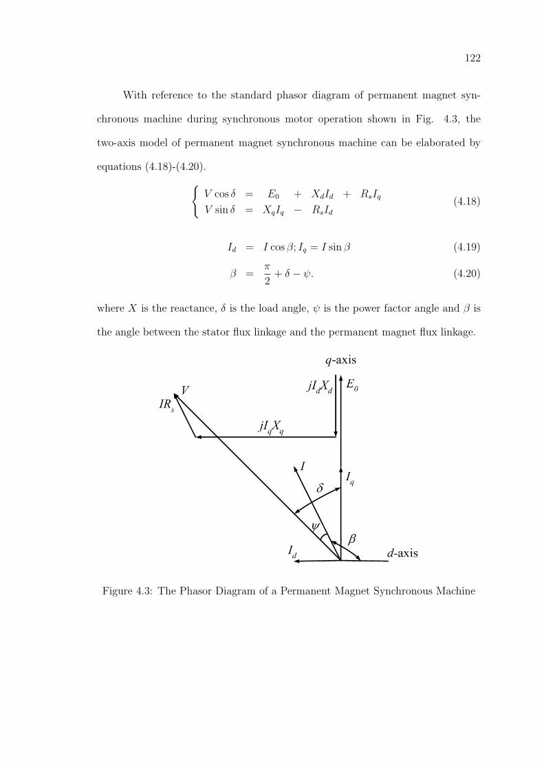
122
With reference to the standard phasor diagram of permanent magnet syn-
chronous machine during synchronous motor operation shown in Fig. 4.3, the
two-axis model of permanent magnet synchronous machine can be elaborated by
equations (4.18)-(4.20).V cos δ = E0 + XdId + RsIq
V sin δ = XqIq − RsId(4.18)
Id = I cos β; Iq = I sin β (4.19)
β =π
2+ δ − ψ. (4.20)
where X is the reactance, δ is the load angle, ψ is the power factor angle and β is
the angle between the stator flux linkage and the permanent magnet flux linkage.
Figure 4.3: The Phasor Diagram of a Permanent Magnet Synchronous Machine
123
4.3 Parameter Estimation of Line-Start
Permanent Magnet Synchronous Machine
The presence of permanent magnets in the permanent magnet synchronous ma-
chine prevents the use of the most conventional parameter measurement methods,
which are applicable to the wound field synchronous machines. To tackle this prob-
lem, various techniques and methods have been used by many researchers for the
determination of machine parameters. The experimental methods that were used
often are static test (locked rotor), sensorless no-load test and load test, while one
of the most popular computational methods is the finite element method.
The static tests are carried out with some assumptions, such as the constant
parameters with different frequencies or constant parameters with different load
conditions. These assumptions result in simple measurement procedure, but not
enough parameter information for machine dynamic operations. The conventional
sensorless no-load test and load test methods are based on the two-axis model
of permanent magnet synchronous machines. They have an important limit that
a constant value, E0, is assumed for the induced EMF due to permanent mag-
nets. Although the load test methods are modified later by taking into account of
the variation of E0, the results are still irregular. In this work, the experimental
methods that were used before by other researchers were reviewed. Based on the
modified load test method, two novel techniques through the implementation of
linear regression and Hopfield neural network are presented.
In the finite element analysis, the machine parameters can be calculated from
the stored magnetic energy or flux linkage. Different authors have proposed al-
ternative methods to evaluate the machine parameters and their variations with
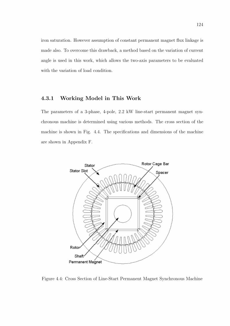
124
iron saturation. However assumption of constant permanent magnet flux linkage is
made also. To overcome this drawback, a method based on the variation of current
angle is used in this work, which allows the two-axis parameters to be evaluated
with the variation of load condition.
4.3.1 Working Model in This Work
The parameters of a 3-phase, 4-pole, 2.2 kW line-start permanent magnet syn-
chronous machine is determined using various methods. The cross section of the
machine is shown in Fig. 4.4. The specifications and dimensions of the machine
are shown in Appendix F.
Figure 4.4: Cross Section of Line-Start Permanent Magnet Synchronous Machine
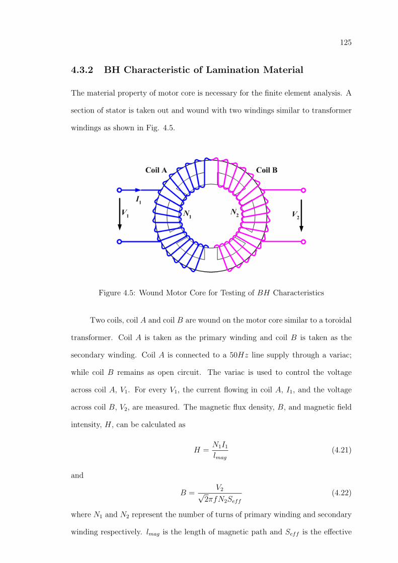
125
4.3.2 BH Characteristic of Lamination Material
The material property of motor core is necessary for the finite element analysis. A
section of stator is taken out and wound with two windings similar to transformer
windings as shown in Fig. 4.5.
Figure 4.5: Wound Motor Core for Testing of BH Characteristics
Two coils, coil A and coil B are wound on the motor core similar to a toroidal
transformer. Coil A is taken as the primary winding and coil B is taken as the
secondary winding. Coil A is connected to a 50Hz line supply through a variac;
while coil B remains as open circuit. The variac is used to control the voltage
across coil A, V1. For every V1, the current flowing in coil A, I1, and the voltage
across coil B, V2, are measured. The magnetic flux density, B, and magnetic field
intensity, H, can be calculated as
H =N1I1lmag
(4.21)
and
B =V2√
2πfN2Seff
(4.22)
where N1 and N2 represent the number of turns of primary winding and secondary
winding respectively. lmag is the length of magnetic path and Seff is the effective
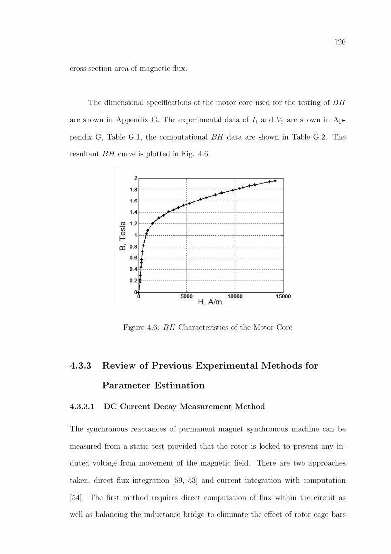
126
cross section area of magnetic flux.
The dimensional specifications of the motor core used for the testing of BH
are shown in Appendix G. The experimental data of I1 and V2 are shown in Ap-
pendix G, Table G.1, the computational BH data are shown in Table G.2. The
resultant BH curve is plotted in Fig. 4.6.
Figure 4.6: BH Characteristics of the Motor Core
4.3.3 Review of Previous Experimental Methods for
Parameter Estimation
4.3.3.1 DC Current Decay Measurement Method
The synchronous reactances of permanent magnet synchronous machine can be
measured from a static test provided that the rotor is locked to prevent any in-
duced voltage from movement of the magnetic field. There are two approaches
taken, direct flux integration [59, 53] and current integration with computation
[54]. The first method requires direct computation of flux within the circuit as
well as balancing the inductance bridge to eliminate the effect of rotor cage bars
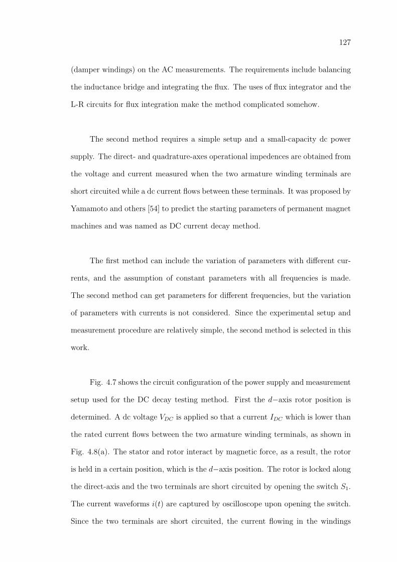
127
(damper windings) on the AC measurements. The requirements include balancing
the inductance bridge and integrating the flux. The uses of flux integrator and the
L-R circuits for flux integration make the method complicated somehow.
The second method requires a simple setup and a small-capacity dc power
supply. The direct- and quadrature-axes operational impedences are obtained from
the voltage and current measured when the two armature winding terminals are
short circuited while a dc current flows between these terminals. It was proposed by
Yamamoto and others [54] to predict the starting parameters of permanent magnet
machines and was named as DC current decay method.
The first method can include the variation of parameters with different cur-
rents, and the assumption of constant parameters with all frequencies is made.
The second method can get parameters for different frequencies, but the variation
of parameters with currents is not considered. Since the experimental setup and
measurement procedure are relatively simple, the second method is selected in this
work.
Fig. 4.7 shows the circuit configuration of the power supply and measurement
setup used for the DC decay testing method. First the d−axis rotor position is
determined. A dc voltage VDC is applied so that a current IDC which is lower than
the rated current flows between the two armature winding terminals, as shown in
Fig. 4.8(a). The stator and rotor interact by magnetic force, as a result, the rotor
is held in a certain position, which is the d−axis position. The rotor is locked along
the direct-axis and the two terminals are short circuited by opening the switch S1.
The current waveforms i(t) are captured by oscilloscope upon opening the switch.
Since the two terminals are short circuited, the current flowing in the windings
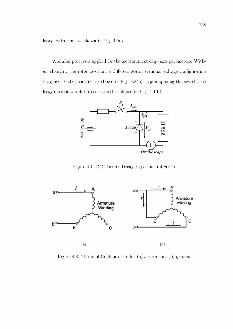
128
decays with time, as shown in Fig. 4.9(a).
A similar process is applied for the measurement of q−axis parameters. With-
out changing the rotor position, a different stator terminal voltage configuration
is applied to the machine, as shown in Fig. 4.8(b). Upon opening the switch, the
decay current waveform is captured as shown in Fig. 4.9(b).
Figure 4.7: DC Current Decay Experimental Setup
(a) (b)
Figure 4.8: Terminal Configuration for (a) d−axis and (b) q−axis
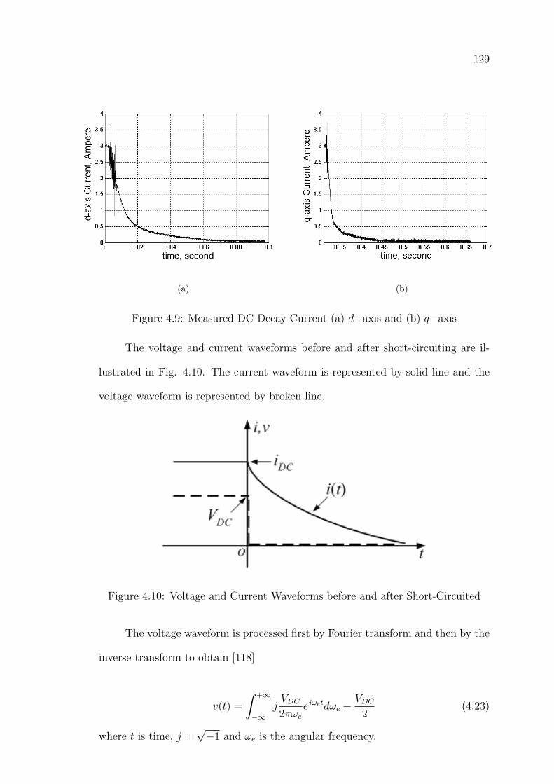
129
(a) (b)
Figure 4.9: Measured DC Decay Current (a) d−axis and (b) q−axis
The voltage and current waveforms before and after short-circuiting are il-
lustrated in Fig. 4.10. The current waveform is represented by solid line and the
voltage waveform is represented by broken line.
Figure 4.10: Voltage and Current Waveforms before and after Short-Circuited
The voltage waveform is processed first by Fourier transform and then by the
inverse transform to obtain [118]
v(t) =
∫ +∞
−∞jVDC
2πωe
ejωetdωe +VDC
2(4.23)
where t is time, j =√−1 and ωe is the angular frequency.
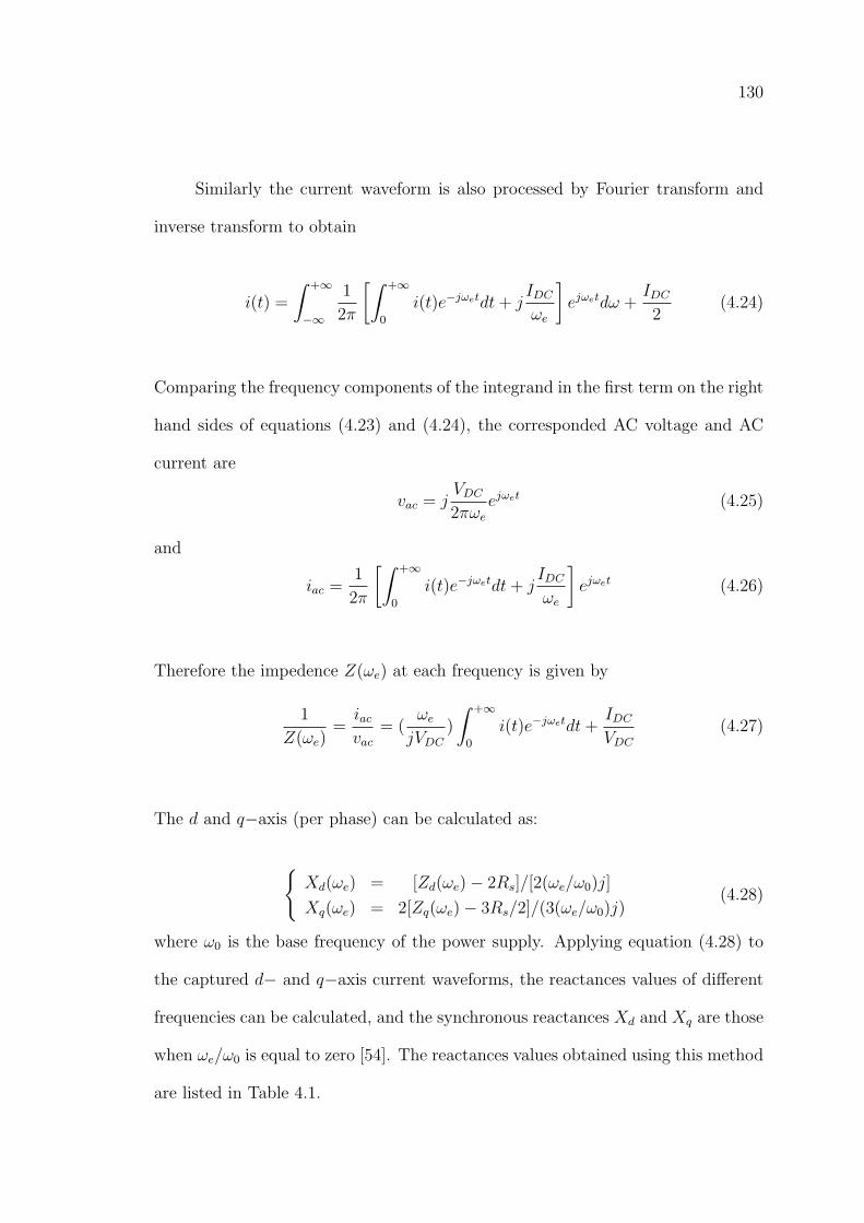
130
Similarly the current waveform is also processed by Fourier transform and
inverse transform to obtain
i(t) =
∫ +∞
−∞
1
2π
[∫ +∞
0
i(t)e−jωetdt+ jIDC
ωe
]ejωetdω +
IDC
2(4.24)
Comparing the frequency components of the integrand in the first term on the right
hand sides of equations (4.23) and (4.24), the corresponded AC voltage and AC
current are
vac = jVDC
2πωe
ejωet (4.25)
and
iac =1
2π
[∫ +∞
0
i(t)e−jωetdt+ jIDC
ωe
]ejωet (4.26)
Therefore the impedence Z(ωe) at each frequency is given by
1
Z(ωe)=iac
vac
= (ωe
jVDC
)
∫ +∞
0
i(t)e−jωetdt+IDC
VDC
(4.27)
The d and q−axis (per phase) can be calculated as:
Xd(ωe) = [Zd(ωe)− 2Rs]/[2(ωe/ω0)j]
Xq(ωe) = 2[Zq(ωe)− 3Rs/2]/(3(ωe/ω0)j)(4.28)
where ω0 is the base frequency of the power supply. Applying equation (4.28) to
the captured d− and q−axis current waveforms, the reactances values of different
frequencies can be calculated, and the synchronous reactances Xd and Xq are those
when ωe/ω0 is equal to zero [54]. The reactances values obtained using this method
are listed in Table 4.1.
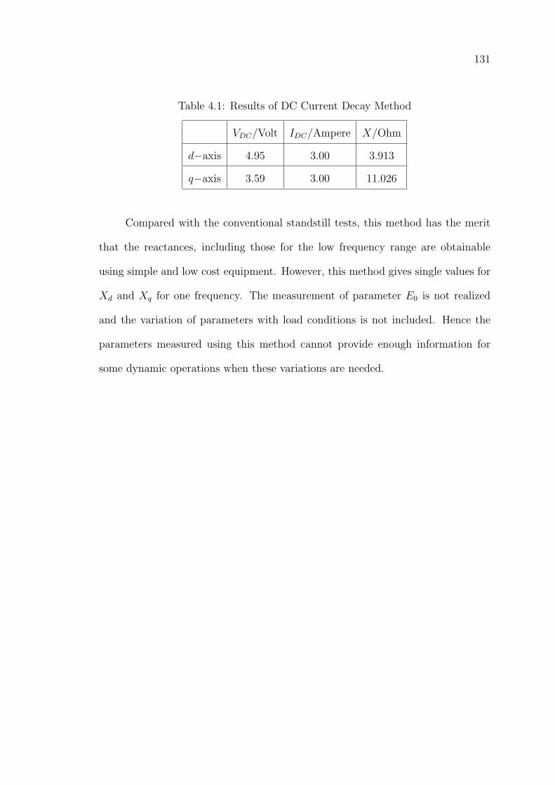
131
Table 4.1: Results of DC Current Decay Method
VDC/Volt IDC/Ampere X/Ohm
d−axis 4.95 3.00 3.913
q−axis 3.59 3.00 11.026
Compared with the conventional standstill tests, this method has the merit
that the reactances, including those for the low frequency range are obtainable
using simple and low cost equipment. However, this method gives single values for
Xd and Xq for one frequency. The measurement of parameter E0 is not realized
and the variation of parameters with load conditions is not included. Hence the
parameters measured using this method cannot provide enough information for
some dynamic operations when these variations are needed.
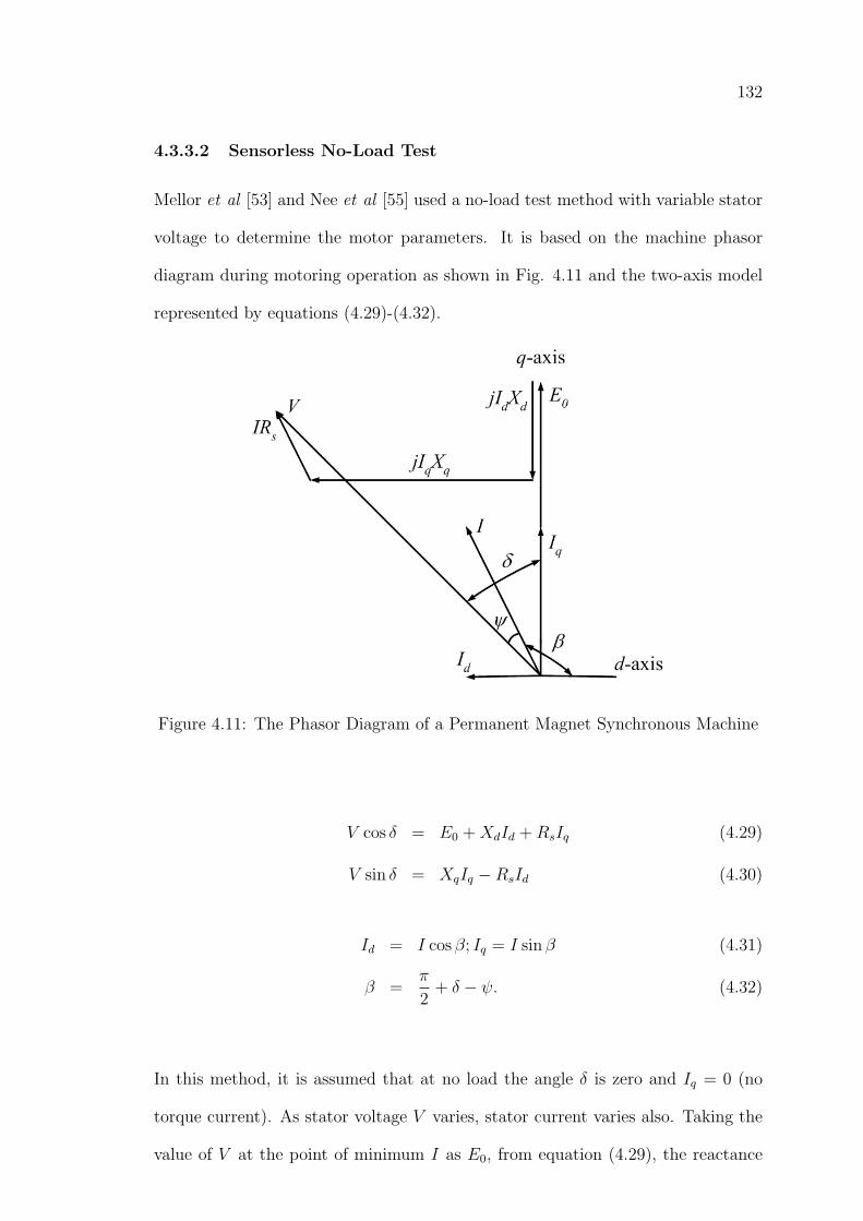
132
4.3.3.2 Sensorless No-Load Test
Mellor et al [53] and Nee et al [55] used a no-load test method with variable stator
voltage to determine the motor parameters. It is based on the machine phasor
diagram during motoring operation as shown in Fig. 4.11 and the two-axis model
represented by equations (4.29)-(4.32).
Figure 4.11: The Phasor Diagram of a Permanent Magnet Synchronous Machine
V cos δ = E0 +XdId +RsIq (4.29)
V sin δ = XqIq −RsId (4.30)
Id = I cos β; Iq = I sin β (4.31)
β =π
2+ δ − ψ. (4.32)
In this method, it is assumed that at no load the angle δ is zero and Iq = 0 (no
torque current). As stator voltage V varies, stator current varies also. Taking the
value of V at the point of minimum I as E0, from equation (4.29), the reactance
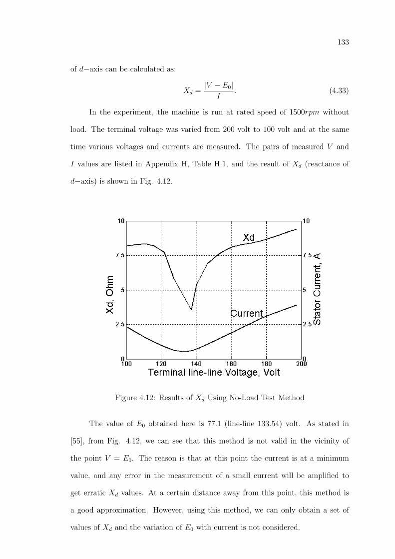
133
of d−axis can be calculated as:
Xd =|V − E0|
I. (4.33)
In the experiment, the machine is run at rated speed of 1500rpm without
load. The terminal voltage was varied from 200 volt to 100 volt and at the same
time various voltages and currents are measured. The pairs of measured V and
I values are listed in Appendix H, Table H.1, and the result of Xd (reactance of
d−axis) is shown in Fig. 4.12.
Figure 4.12: Results of Xd Using No-Load Test Method
The value of E0 obtained here is 77.1 (line-line 133.54) volt. As stated in
[55], from Fig. 4.12, we can see that this method is not valid in the vicinity of
the point V = E0. The reason is that at this point the current is at a minimum
value, and any error in the measurement of a small current will be amplified to
get erratic Xd values. At a certain distance away from this point, this method is
a good approximation. However, using this method, we can only obtain a set of
values of Xd and the variation of E0 with current is not considered.
134
4.3.3.3 Load Test Method
The load test method for PMSM was first proposed by Miller [59]. It is also based
on the two-axis model represented by equations (4.34)-(4.37).
V cos δ = E0 +XdId +RsIq (4.34)
V sin δ = XqIq −RsId (4.35)
Id = I cos β; Iq = I sin β (4.36)
β =π
2+ δ − ψ. (4.37)
The method is used to determine the Xd from the stator d−axis voltage component
and Xq from the q−axis component respectively. Once the data of applied voltage
V , current I, input power P and torque angle δ are known from the load test,
power factor angle can be easily obtained as
ψ = arccos(P
3IV) (4.38)
Thereafter other quantities, β, Id and Iq, can be calculated using equations (4.36)-
(4.37). From equation (4.35), the value of Xq can be easily obtained. However,
from equation (4.34), it is inadequate to evaluate the two unknown quantities E0
and Xd. To this end, E0 is assumed to be constant by Miller [59] and it is equal to
the open-circuit value. This assumption leads to the irregularity of Xd over a load
range where the armature reaction in direct axis is changing from magnetizing to
demagnetizing regions [59].
This load test was modified by Rahman and Zhou [57] by not making the
simplifying assumption that the permanent magnet excitation voltage E0 is con-
stant. Instead, an attempt was made to solve for Xd and E0 simultaneously by
getting two sets of readings while making a change of ∆β in angle β. With the
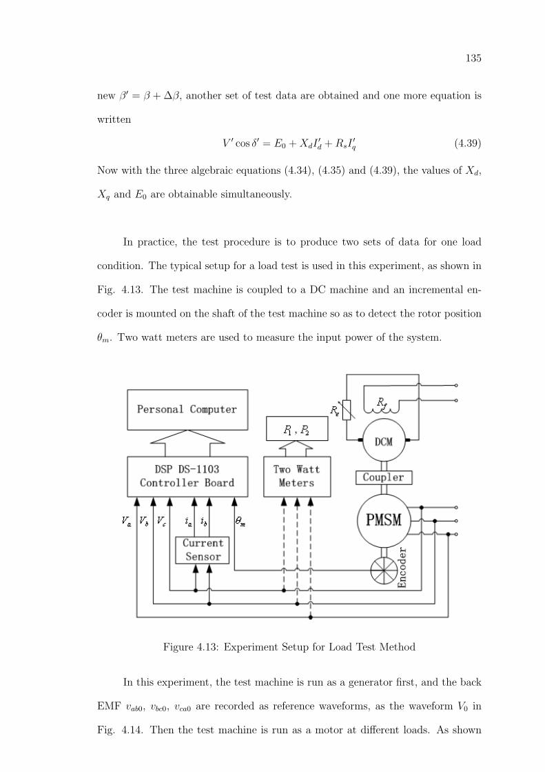
135
new β′ = β + ∆β, another set of test data are obtained and one more equation is
written
V ′ cos δ′ = E0 +XdI′d +RsI
′q (4.39)
Now with the three algebraic equations (4.34), (4.35) and (4.39), the values of Xd,
Xq and E0 are obtainable simultaneously.
In practice, the test procedure is to produce two sets of data for one load
condition. The typical setup for a load test is used in this experiment, as shown in
Fig. 4.13. The test machine is coupled to a DC machine and an incremental en-
coder is mounted on the shaft of the test machine so as to detect the rotor position
θm. Two watt meters are used to measure the input power of the system.
Figure 4.13: Experiment Setup for Load Test Method
In this experiment, the test machine is run as a generator first, and the back
EMF vab0, vbc0, vca0 are recorded as reference waveforms, as the waveform V0 in
Fig. 4.14. Then the test machine is run as a motor at different loads. As shown
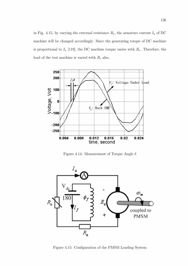
136
in Fig. 4.15, by varying the external resistance Re, the armature current Ia of DC
machine will be changed accordingly. Since the generating torque of DC machine
is proportional to Ia [119], the DC machine torque varies with Re. Therefore, the
load of the test machine is varied with Re also.
Figure 4.14: Measurement of Torque Angle δ
Figure 4.15: Configuration of the PMSM Loading System
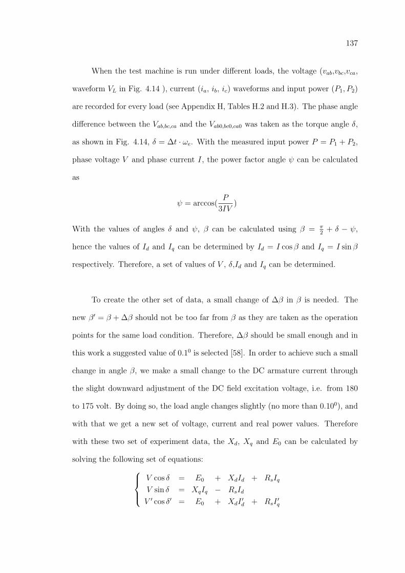
137
When the test machine is run under different loads, the voltage (vab,vbc,vca,
waveform VL in Fig. 4.14 ), current (ia, ib, ic) waveforms and input power (P1, P2)
are recorded for every load (see Appendix H, Tables H.2 and H.3). The phase angle
difference between the Vab,bc,ca and the Vab0,bc0,ca0 was taken as the torque angle δ,
as shown in Fig. 4.14, δ = ∆t · ωe. With the measured input power P = P1 + P2,
phase voltage V and phase current I, the power factor angle ψ can be calculated
as
ψ = arccos(P
3IV)
With the values of angles δ and ψ, β can be calculated using β = π2
+ δ − ψ,
hence the values of Id and Iq can be determined by Id = I cos β and Iq = I sin β
respectively. Therefore, a set of values of V , δ,Id and Iq can be determined.
To create the other set of data, a small change of ∆β in β is needed. The
new β′ = β + ∆β should not be too far from β as they are taken as the operation
points for the same load condition. Therefore, ∆β should be small enough and in
this work a suggested value of 0.10 is selected [58]. In order to achieve such a small
change in angle β, we make a small change to the DC armature current through
the slight downward adjustment of the DC field excitation voltage, i.e. from 180
to 175 volt. By doing so, the load angle changes slightly (no more than 0.100), and
with that we get a new set of voltage, current and real power values. Therefore
with these two set of experiment data, the Xd, Xq and E0 can be calculated by
solving the following set of equations:V cos δ = E0 + XdId + RsIq
V sin δ = XqIq − RsId
V ′ cos δ′ = E0 + XdI′d + RsI
′q
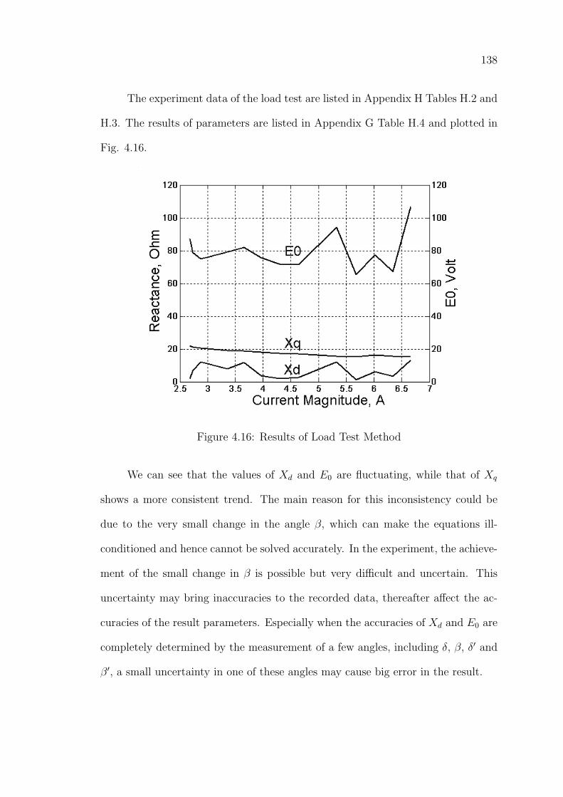
138
The experiment data of the load test are listed in Appendix H Tables H.2 and
H.3. The results of parameters are listed in Appendix G Table H.4 and plotted in
Fig. 4.16.
Figure 4.16: Results of Load Test Method
We can see that the values of Xd and E0 are fluctuating, while that of Xq
shows a more consistent trend. The main reason for this inconsistency could be
due to the very small change in the angle β, which can make the equations ill-
conditioned and hence cannot be solved accurately. In the experiment, the achieve-
ment of the small change in β is possible but very difficult and uncertain. This
uncertainty may bring inaccuracies to the recorded data, thereafter affect the ac-
curacies of the result parameters. Especially when the accuracies of Xd and E0 are
completely determined by the measurement of a few angles, including δ, β, δ′ and
β′, a small uncertainty in one of these angles may cause big error in the result.
139
4.3.4 New Methods for Parameter Determination
The DC current decay method is easy to carry out, but only single values of Xd and
Xq are obtained. The sensorless no-load test is also easy in implementation, but
only a group of Xd values are obtained. The load test suffers from the shortcoming
of the fact that we need a very small change of angle β. The change of such a
small margin in experiment is very difficult to achieve, and it could also lead to the
inconsistency of experimental results.
In order to overcome these drawbacks and difficulties, the load test is applied
in combination with a linear regression model and a Hopfield neural network model
respectively. By using the combined methods, one would avoid the measurement
of the load angle δ, and the power factor angle ψ, but the rotor position would be
required. Thus the load test processes become much simpler with the combination
techniques.
4.3.4.1 Combination of Load Test and Linear Regression
The main concept of linear regression model is to adapt parameters from input and
output data by searching for the minimum of the mean square error (MSE) [120].
For example, suppose d is the desired output of n inputs x1, x2, . . . , xn, the error
between the estimated output and the desired output is:
ε = d−n∑
k=0
hkxk
where hk(k = 0, 1, . . . , n) are the weights, h0 is the bias and x0 is 1. Hence the
MSE of m sample is:
J =1
2m
m∑i=1
(di −n∑
k=0
hkxik)2
140
The differential of J with respect to the unknowns (hk) is:
∇ = [∂J
∂h0
,∂J
∂h1
, . . . ,∂J
∂hn
] = CH −D
where
∂J
∂hk
|(k=0,1,...,n) =1
m[
n∑j=0
(hj
m∑i=1
xijxik)−m∑
i=1
dixik]
H = [h0, h1, . . . , hn]tr
The optimal H? is obtained by setting ∇ = 0. Therefore,
H? = C−1D. (4.40)
To apply this method for the processing of load test data, the oscillations
of stator currents in the steady state are taken into account. As the governing
equations of permanent magnet synchronous machine in the steady state are:
vd = Rsid − ωeLqiq + Lddiddt
(4.41)
vq = Rsiq + ωeLdid + Lqdiqdt
+√
3E0 (4.42)
By applying the sum (4.42)+(4.41) and the difference (4.42)−(4.41) of these two
equations, we can get Y1 = LdX11 + LqX12 + b0
Y2 = LdX21 + LqX22 + b0
whereY1 = (vd −Rsid) + (vq −Rsiq); X11 = ωeid + did
dt; X12 = diq
dt− ωeiq;
Y2 = (vq −Rsiq)− (vd −Rsid); X21 = ωeid − diddt
; X22 = diqdt
+ ωeiq;
b0 =√
3E0;
Taking X11, X12, X21 and X22 as the inputs, Y1 and Y2 as the desired outputs
and Ld, Lq and b0 as the weights, we try to find the best linear regression on all
the inputs using equation (4.40) so that we can determine the values of Ld, Lq and
E0.
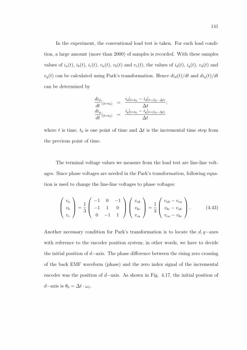
141
In the experiment, the conventional load test is taken. For each load condi-
tion, a large amount (more than 2000) of samples is recorded. With these samples
values of ia(t), ib(t), ic(t), va(t), vb(t) and vc(t), the values of id(t), iq(t), vd(t) and
vq(t) can be calculated using Park’s transformation. Hence did(t)/dt and diq(t)/dt
can be determined by
diddt|(t=t0) =
id|t=t0 − id|t=(t0−∆t)
∆t;
diqdt|(t=t0) =
iq|t=t0 − iq|t=(t0−∆t)
∆t
where t is time, t0 is one point of time and ∆t is the incremental time step from
the previous point of time.
The terminal voltage values we measure from the load test are line-line volt-
ages. Since phase voltages are needed in the Park’s transformation, following equa-
tion is used to change the line-line voltages to phase voltages:
va
vb
vc
=1
3
−1 0 −1
−1 1 0
0 −1 1
vab
vbc
vca
=1
3
vab − vca
vbc − vab
vca − vbc
. (4.43)
Another necessary condition for Park’s transformation is to locate the d, q−axes
with reference to the encoder position system; in other words, we have to decide
the initial position of d−axis. The phase difference between the rising zero crossing
of the back EMF waveform (phase) and the zero index signal of the incremental
encoder was the position of d−axis. As shown in Fig. 4.17, the initial position of
d−axis is θ0 = ∆t · ωe.
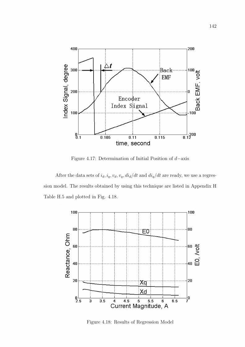
142
Figure 4.17: Determination of Initial Position of d−axis
After the data sets of id, iq, vd, vq, did/dt and diq/dt are ready, we use a regres-
sion model. The results obtained by using this technique are listed in Appendix H
Table H.5 and plotted in Fig. 4.18.
Figure 4.18: Results of Regression Model
143
Comparing with the Miller’s load test method, this combined technique has
the merit that the variation of E0 with load condition is taken into account. Com-
paring with the Zhou’s modified load test method, this technique overcomes the
difficulty of achieving a very small change in angle β during the experiment. The
uncertainties in angle measurements are lessened and the experiment procedure is
simplified.
Comparing Fig. 4.18 with Fig. 4.16, we can see that the zigzags in the re-
sults of load test method are removed by the new combination technique. All the
parameters obtained by the combination technique vary smoothly with the current
and the trends shown in the variations of waveforms are more obvious. The reason
is that Miller’s method and Zhou’s method are based on the solution of two or
three equations, the accuracies of the solved parameters are totally dependent on
a few data. A small mistake in one of these few data may lead to big unexpected
error in the resultant parameters. Especially in Zhou’s method, when the Xd and
E0 are determined by two sets of data (v, i, δ, β) and (v′, i′, δ′, β′) which are very
close to each other, the small uncertainties may cause the equations ill-conditioned
and produce inaccuracies in the results. The combination technique used in this
work overcomes this drawback by getting a optimal solution based on the linear
regression of thousands of samples. Therefore accuracies of the solved parameters
are improved greatly. This improvement can be very significant in the analysis for
dynamics and transients where accurate parameters are needed.
144
4.3.4.2 Combination of Load Test and Hopfield Neural Network
Hopfield neural network model was proposed by Hopfield [121] and was further
explored to solve some classes of optimization problems by Hopfield and Tank
[122] - [124]. In 1990, S. R. Chu et al [125] modified this network and applied it
successfully for identification of linear time invariant or time varying systems by
measuring the inputs, states and derivations of the states. In the following years,
this method was used by many researchers for system identification, state estima-
tion and control in various areas [126] - [130]. As for the application of Hopfield
neural network in the parameter estimation of electric machines, some work has
been done in induction machines and DC machines [127, 130, 131]. In order to get
more accurate machine parameters and also to overcome the difficulties of using
only load test, we have applied the Hopfield neural network in combination with
the load test.
Artificial neural networks (ANN) can be considered as highly interconnected
dynamical systems consisting of simple processing elements called neurons. Feed-
forward and recurrent type artificial neural network architectures are the two major
type of ANNs being investigated. The distinction between feedforward and recur-
rent type networks is that the former learns the function mapping by updating
its connection weights while the latter seeks to retain its minimum computational
energy as its neurons evolve in time [132]. Hopfield neural network is just one kind
of recurrent network.
The Hopfield neural network was proposed by John Hopfield of the California
Institute of Technology in 1982 . He devised an array of neurons that were fully
interconnected, with each neuron feeding its output to all others. The concept
was that all the neurons would transimit signals back and forth to each other in a
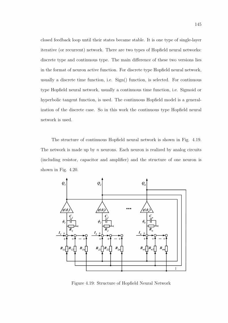
145
closed feedback loop until their states became stable. It is one type of single-layer
iterative (or recurrent) network. There are two types of Hopfield neural networks:
discrete type and continuous type. The main difference of these two versions lies
in the format of neuron active function. For discrete type Hopfield neural network,
usually a discrete time function, i.e. Sign() function, is selected. For continuous
type Hopfield neural network, usually a continuous time function, i.e. Sigmoid or
hyperbolic tangent function, is used. The continuous Hopfield model is a general-
ization of the discrete case. So in this work the continuous type Hopfield neural
network is used.
The structure of continuous Hopfield neural network is shown in Fig. 4.19.
The network is made up by n neurons. Each neuron is realized by analog circuits
(including resistor, capacitor and amplifier) and the structure of one neuron is
shown in Fig. 4.20.
Figure 4.19: Structure of Hopfield Neural Network
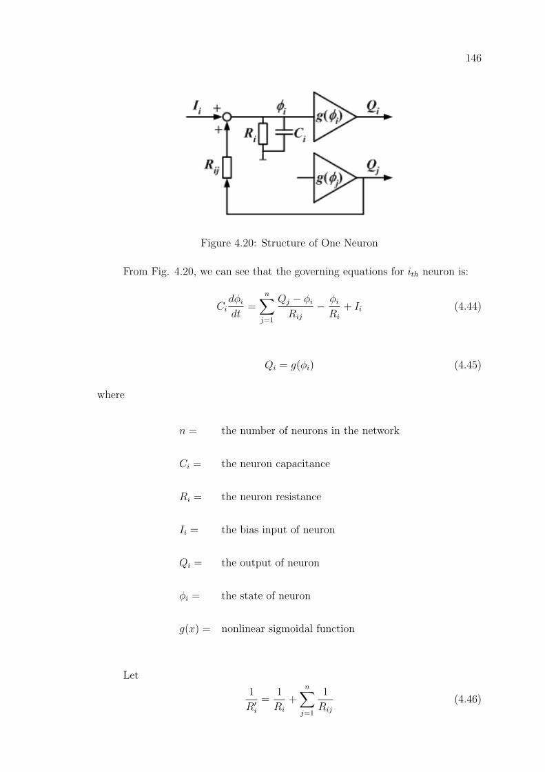
146
Figure 4.20: Structure of One Neuron
From Fig. 4.20, we can see that the governing equations for ith neuron is:
Cidφi
dt=
n∑j=1
Qj − φi
Rij
− φi
Ri
+ Ii (4.44)
Qi = g(φi) (4.45)
where
n = the number of neurons in the network
Ci = the neuron capacitance
Ri = the neuron resistance
Ii = the bias input of neuron
Qi = the output of neuron
φi = the state of neuron
g(x) = nonlinear sigmoidal function
Let
1
R′i=
1
Ri
+n∑
j=1
1
Rij
(4.46)
147
and
Tij =1
Rij
(4.47)
then we can get
Cidφi
dt= − 1
R′iφi +
n∑j=1
TijQj + Ii (4.48)
Considering the quantity
E = −1
2
n∑i=1
n∑j=1
TijQiQj −n∑
i=1
QiIi +n∑
i=1
1
R′i
∫ Q
0
g−1(Q)dQ (4.49)
where g−1(Q) is the inverse function of Q = g(φ).
Its differential with time is
∂E
∂t=
n∑i=1
∂E
∂Qi
∂Qi
∂t(4.50)
where
∂E
∂Qi
= −1
2
n∑j=1
TijQj −1
2
n∑j=1
TijQj − Ii +1
R′iφi (4.51)
If
Tij = Tji (4.52)
then equation (4.51) can be written as
∂E
∂Qi
= −n∑
j=1
TijQj − Ii +1
R′iφi (4.53)
Comparing equation (4.53) with equation (4.44), we can get
∂E
∂Qi
= −Cidφi
dt= −Ci
dφi
dQi
dQi
dt= −Ci(
dQt
dt)d
dQi
g−1(Qi) (4.54)
Substituting equation (4.54) into equation (4.50) yields
∂E
∂t= −
n∑i=1
Ci(dQi
dt)2 d
dQi
g−1(Qi) (4.55)
If function g(Qi) is mono-increasing, its inverse function g−1(Qi) is mono-increasing
also. In other words,
d
dQi
g−1(Qi) > 0 (4.56)
148
Therefore equation (4.50) becomes
∂E
∂t≤ 0 (4.57)
Equation (4.57) shows that the time evolution of the system is a motion in state
space that seeks out minima in E and comes to a stop at such point. E is a
Lyapunov function for the system and is taken as the computational energy of the
network.
For simplicity, we can always choose R′i = R and Ci = C, independent of i.
Dividing by C and redefining Tij/C and Ii/C as Tij and Ii, equations (4.48), (4.45)
and (4.49) become
dφi
dt=
n∑j=1
TijQj + Ii −φi
RC(4.58)
Qi = g(φi) (4.59)
and
E = −1
2
n∑i=1
n∑j=1
TijQiQj −n∑
i=1
QiIi +n∑
i=1
1
R
∫ Q
0
g−1(Q)dQ (4.60)
Equations (4.58)-(4.60) are the Hopfield neural network model and energy function
that are used often in various applications.
While the input resistance of each neuron R → ∞, the network dynamic
model and energy function can be further simplified as:
dφj
dt=
n∑i=1
TijQj + Ij (4.61)
Qj = g(φj), j = 1, . . . , n (4.62)
149
E = −1
2
n∑i=1
n∑j=1
TijQiQj −n∑
i=1
QiIi (4.63)
It has been shown in equations (4.52) and (4.56) that we can get the minima of
the energy function if Tij = Tji and function Qj = g(φj) is mono-increasing as well.
Generally, function g(φj) is selected as:
Qj = g(φj) = ρ1− e−kφj
1 + e−kφj(4.64)
Here k is the slope of the sigmoid nonlinearity, the ρ is such that when φj tends to
±∞, the function Qj = g(φj) tends to ±ρ.
Consider a dynamical system in state space as:
[x] = [At][x] + [Bt][u] (4.65)
The definition of [At], [Bt], [x] and [u] are list in equation 4.66, where [At] and [Bt]
are the system matrices, [x] is the state vector and [u] is the input.
[At]n×n =
a11 a12 . . . a1n
a21 a22 . . . a2n
...
an1 an2 . . . ann
, [x]n×1 =
x1
x2
...
xn
[Bt]n×m =
b11 b12 . . . b1m
b21 b22 . . . b2m
...
bn1 bn2 . . . bnm
, [u]n×1 =
u1
u2
...
um
(4.66)
The aim of system identification is to get [At] and [Bt] with known values of [x],[x]
and [u]. Suppose [As] and [Bs] are estimated parameter values of [At] and [Bt],
then the error between the real system and the estimated system is:
[e] = [x]− [As]x− [Bs]u
150
and the identification energy function is defined as
E =1
2t
∫ t
0
[e]tr[e]dt
=1
2t
∫ t
0
([x]− [As]x− [Bs]u)tr([x]− [As]x− [Bs]u)dt
When we compare this energy function with the standard energy function of Hop-
field neural network in equation 4.63, we can get the weight matrix [Tij] and the
bias matrix [Ij], which are crucial for the training of the neural network.
Defining [Q] as
[Q] = [a11, . . . , a1n, . . . , an1, . . . , ann, b11, . . . , b1m, . . . , bn1, . . . , bnm]tr,
the weight matrix [Tij] and bias matrix [Ij] can be computed using equation 4.67,
and the definition of the matrix elements in [PT ] is shown in equation 4.68. In
equation 4.68, ′diag′ means diagonals of the matrix. The other elements of matrices
[PT11],[PT12],[PT21] and [PT22] are all zeros except the diagonals.
[Tij] = −1
t
∫ t
0[PT ] dt = −1
t
∫ t
0
[PT11 PT12
PT21 PT22
]dt
[Ii] = 1t
∫ t
0
[x1 [x] , . . . , xn [x] , x1 [u] , . . . , xn [u]
]trdt
(4.67)
[PT11]n2×n2 = diag(
[x] [x]tr [x] [x]tr . . . [x] [x]tr)
[PT12]n2×nm = diag(
[x] [u]tr [x] [u]tr . . . [x] [u]tr)
[PT21]nm×n2 = diag(
[u] [x]tr [u] [x]tr . . . [u] [x]tr)
[PT22]nm×nm = diag(
[u] [u]tr [u] [u]tr . . . [u] [u]tr)
(4.68)
Therefore, for the sigmoid function shown in equation 4.64, the expression for the
evolution of [Q] can be obtained as
dQi
dt|(i=1,...,n2+nm) =
dQi
dφi
dφi
dt=k(ρ2 −Q2
i )
2ρ
[n2+nm∑
j=1
TijQj + Ii
]. (4.69)
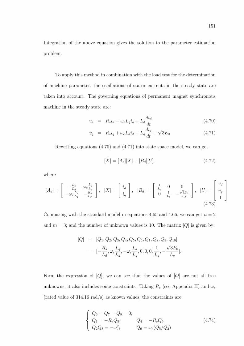
151
Integration of the above equation gives the solution to the parameter estimation
problem.
To apply this method in combination with the load test for the determination
of machine parameter, the oscillations of stator currents in the steady state are
taken into account. The governing equations of permanent magnet synchronous
machine in the steady state are:
vd = Rsid − ωeLqiq + Lddiddt
(4.70)
vq = Rsiq + ωeLdid + Lqdiqdt
+√
3E0 (4.71)
Rewriting equations (4.70) and (4.71) into state space model, we can get
[X] = [Ad][X] + [Bd][U ]. (4.72)
where
[Ad] =
[−Rs
Ldωe
Lq
Ld
−ωeLd
Lq−Rs
Lq
], [X] =
[id
iq
], [Bd] =
[1
Ld0 0
0 1Lq
−√
3E0
Lq
], [U ] =
vd
vq
1
(4.73)
Comparing with the standard model in equations 4.65 and 4.66, we can get n = 2
and m = 3; and the number of unknown values is 10. The matrix [Q] is given by:
[Q] = [Q1, Q2, Q3, Q4, Q5, Q6, Q7, Q8, Q9, Q10]
= [−Rs
Ld
, ωeLq
Ld
,−ωeLd
Lq
, 0, 0, 0,1
Lq
,−√
3E0
Lq
].
Form the expression of [Q], we can see that the values of [Q] are not all free
unknowns, it also includes some constraints. Taking Rs (see Appendix H) and ωe
(rated value of 314.16 rad/s) as known values, the constraints are:
Q6 = Q7 = Q8 = 0;
Q1 = −RsQ5; Q4 = −RsQ9
Q2Q3 = −ω2e ; Q9 = ωe(Q5/Q2)
(4.74)
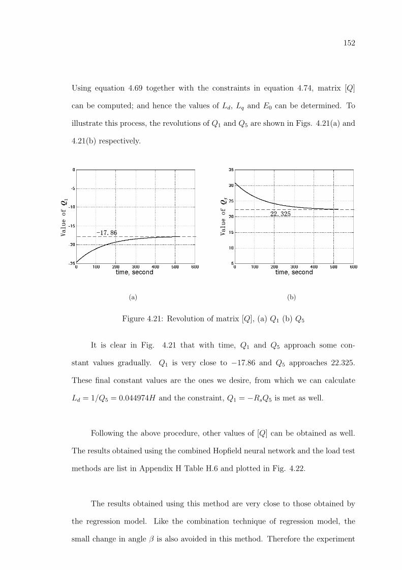
152
Using equation 4.69 together with the constraints in equation 4.74, matrix [Q]
can be computed; and hence the values of Ld, Lq and E0 can be determined. To
illustrate this process, the revolutions of Q1 and Q5 are shown in Figs. 4.21(a) and
4.21(b) respectively.
(a) (b)
Figure 4.21: Revolution of matrix [Q], (a) Q1 (b) Q5
It is clear in Fig. 4.21 that with time, Q1 and Q5 approach some con-
stant values gradually. Q1 is very close to −17.86 and Q5 approaches 22.325.
These final constant values are the ones we desire, from which we can calculate
Ld = 1/Q5 = 0.044974H and the constraint, Q1 = −RsQ5 is met as well.
Following the above procedure, other values of [Q] can be obtained as well.
The results obtained using the combined Hopfield neural network and the load test
methods are list in Appendix H Table H.6 and plotted in Fig. 4.22.
The results obtained using this method are very close to those obtained by
the regression model. Like the combination technique of regression model, the
small change in angle β is also avoided in this method. Therefore the experiment
153
procedure is simplified as well. Compared with the results obtained by Zhou’s load
test method, we can see that the zigzags of the results in load test method are
removed. The variations of all the parameters are very smooth and the variation
trends are more obvious. These improvements lie in the fact that the result pa-
rameters are identified on the basis of large amount of samples by minimizing the
estimation error. In comparison with method of load test only, the combination
technique is more optimized. The good results from this method also indicated
that the Hopfield neural network is a useful tool in the parameter estimation of
machine. Since this method can also be used for the identification of time-varying
systems [125], it may be explored for the online parameter estimation of machine
and drive systems as well.
Figure 4.22: Results of Hopfield Neural Network
154
4.3.5 Parameter Determination Using Finite Element Method
Finite element computation is expensive but provides an easy means of computing
machine parameters. Normally, this method can be used for benchmarking all other
experimental methods. However, the main limitation of finite element method is in
getting a correct and accurate model of the machine. Since finite element method
provides an extensive set of values for flux distributions all around, it is much more
transparent and can be used to compute machine parameters although many as-
pects, like eddy losses and hysteresis, are very difficult to represent in finite element
models.
4.3.5.1 Inductance Calculation Using Finite Element Method
The evaluation of reactances are realized through the calculation of inductances.
Usually, the finite element computation of the steady-state inductances are based
on the following two concepts:
• The number of flux linkages of the winding, divided by the current in the
winding.
• The energy stored in the inductor, divided by one-half the current squared.
Both concepts give identical results for linear inductances but not the same for
nonlinear inductances [45].
Demerdash et al and Zhu [133] - [136] have used current and energy pertur-
bation method to calculate the machine parameters. This method is based on the
calculation of the total energy stored in the magnetic field of a given device compris-
ing a few windings. On the other hand, many other researchers [49, 137, 138, 139]
have calculated the machine parameters on the basis of flux linkages. This method
155
is realized by applying the Stokes’ theorem in the processing of the magnetic field
solutions in terms of magnetic vector potentials. The inductance calculation in this
work is based on the calculation of flux linkage, current source is used and variation
of parameters with load conditions is taken into account as well.
The flux linked by a single turn of coil is
λ =
∫Ω
B · dΩ. (4.75)
where λ is flux linkage, B is flux density and Ω is the area.
Substituting ∇ × A = B into the above equation and applying the Stokes’
theorem, we can get
λ =
∮A · dl, (4.76)
where the integration is around the closed contour formed by the coil and A repre-
sents the magnetic vector potential. For the phases windings in machine, neglecting
the length at the end of the coil, the flux linkage of one turn of coil is
λ = l(A+ − A−), (4.77)
where the superscripts signs ′+′ and ′−′ stand for the ′go′ and ′return′ sides of the
coils, and l is the axil length of the machine. Therefore, for one phase with Ns
equivalent turns of coils, the flux linkages with phases are
λi|(i=a,b,c) = Nsl(
∫ ∫Ω+ A
+dΩ
Ω+−∫ ∫
Ω−A−dΩ
Ω−). (4.78)
where Ω+ and Ω− are the total cross areas of the positively and negatively oriented
coil sides of the phase conductors.
156
4.3.5.2 Evaluation of Machine Parameters by Applying a Small Change
in Current Angle
The method of calculating the machine parameters by varying the current angle
is based on the modified load test method used by Zhou [50, 57]. Zhou et al and
Chang [138] have used the method to estimate the machine parameters using two
finite element solutions for each point of operation.
When the permanent magnet synchronous machine is run in steady state, the
flux linkages in the d and q−axis can be represented by
λd = LdId + λf (4.79)
λq = LqIq (4.80)
where
Id = I cos β
Iq = I sin β
β =π
2+ δ − ψ
δ is the torque angle and ψ is the power factor angle.
Since the variation of parameters with load condition is taken into account in
the calculation, Ld, Lq and λf are unknowns. As equations (4.79) and (4.80) are
inadequate for 3 unknowns, a small change in angle β is exerted and a new β′ is
obtained. Therefore we can have another set of equations as:
λ′d = LdI′d + λf (4.81)
λ′q = LqI′q (4.82)
157
where
I ′d = I cos β′
I ′q = I sin β′
With the calculated d and q-axis flux linkage values and the injected current values,
Ld, Lq and E0 can be obtained by solving equations (4.79)-(4.82)
[Ld
λf
]=
[Id 1
I ′q 1
]−1 [λd
λ′d
], Lq =
λq + λ′qIq + I ′q
, E0 = ωeλf (4.83)
When a current is applied, the flux linkages of a, b, c−axis can be calculated using
equation (4.78), then Park’s transformation is used to change the flux linkages from
a, b, c−axis to d, q−axis. The results obtained using this method are shown in Fig.
4.23.
The results obtained by FEM are comparable with the experimental results,
but the values of Xd, Xq are higher and the value of E0 decreases faster than the
experimental values. This may be caused by the model that does not take into
account the various losses, such as hysteresis losses and eddy current losses. But
the results of FEM agree with the experimental results to some extent, which in-
dicated that FEM is applicable and useful in predicating the parameters of PMSM.
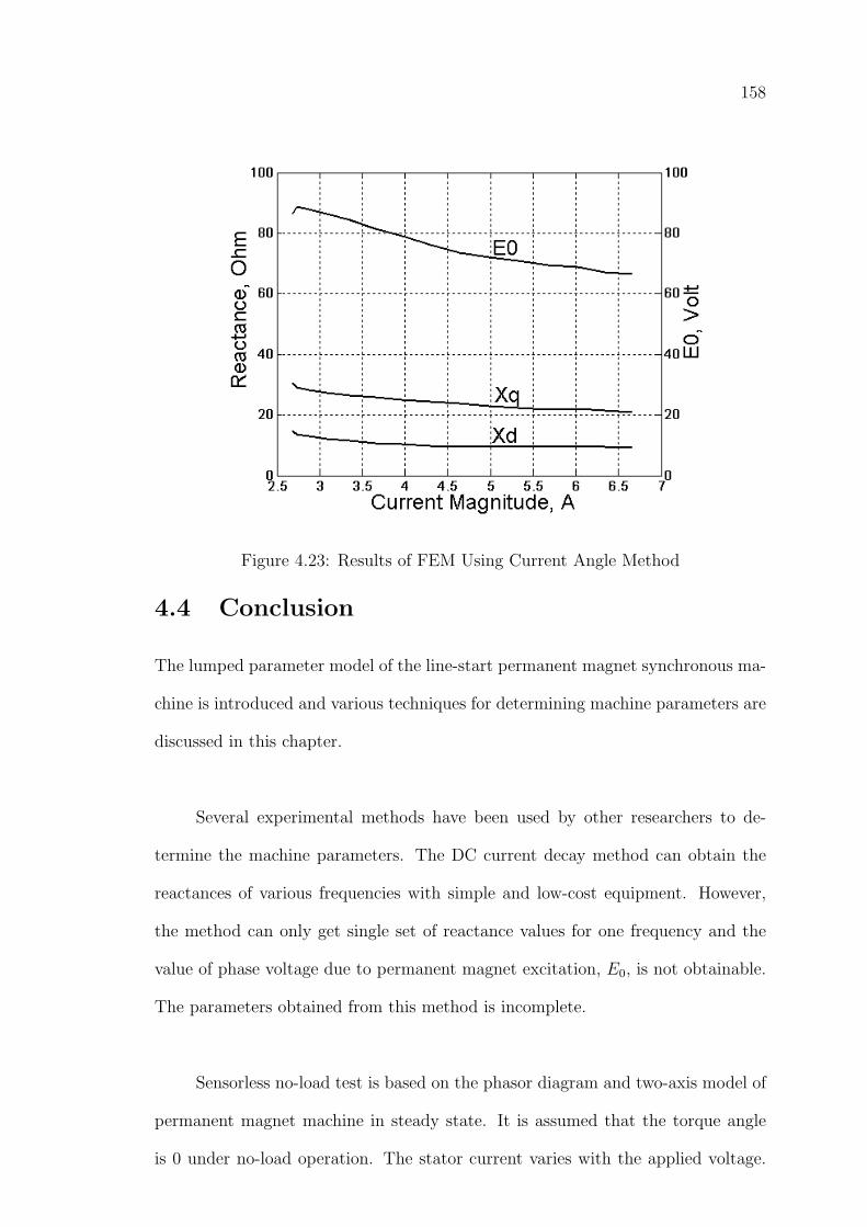
158
Figure 4.23: Results of FEM Using Current Angle Method
4.4 Conclusion
The lumped parameter model of the line-start permanent magnet synchronous ma-
chine is introduced and various techniques for determining machine parameters are
discussed in this chapter.
Several experimental methods have been used by other researchers to de-
termine the machine parameters. The DC current decay method can obtain the
reactances of various frequencies with simple and low-cost equipment. However,
the method can only get single set of reactance values for one frequency and the
value of phase voltage due to permanent magnet excitation, E0, is not obtainable.
The parameters obtained from this method is incomplete.
Sensorless no-load test is based on the phasor diagram and two-axis model of
permanent magnet machine in steady state. It is assumed that the torque angle
is 0 under no-load operation. The stator current varies with the applied voltage.
159
Phase voltage corresponding to the minimum stator current is E0. This method is
also easy in experimental implementation, and the variation of Xd with saturation
is considered. However only a set of Xd can be obtained and the variation of E0 is
neglected. The parameters obtained from this method is still incomplete.
The load test method makes improvement compared with DC current decay
method and no-load test method, because both the Xd and Xq can be obtained
simultaneously and their variations with loads are considered as well. However, the
conventional load test method cannot evaluate the variation of E0 with the the two
equations in two-axis model. The modified load test method overcomes this draw-
back by imposing a small displacement to the angle β. With one extra equation
from the new β, sets of parameters Xd, Xq and E0 under different load conditions
are obtainable. One of the shortcoming of the modified load test method is that
the achievement of a small change of β in experiment is very difficult. Another
critical shortcoming is that accuracies of the parameters in this method are totally
dependent on the measurement of a few experimental data. A small inaccuracy
in one data may bring along big mistake to the resultant parameters. Therefore
the parameters of Xd and E0 obtained from this method are fluctuating, which are
more likely to be caused by the inaccuracy of the small change in β.
To overcome the shortcomings of the modified load test method, two new
methods are proposed. One method is based on the combination of load test and
the technique of linear regression, the other is based on the combination of load
test and the Hopfield neural network.
The combination of load test and linear regression technique is quite effective
in parameter estimation. The difficulty of achieving the small change in β is avoided
160
so that the experiment procedure is simplified. Moreover, since the parameters are
evaluated on the basis of thousands of experimental samples, the accuracies of the
results are improved greatly. The fluctuation in load test is removed and the vari-
ation trend of parameters with load conditions becomes more obvious.
The combination of load test and Hopfield neural network also shows great im-
provement compared with the load test only. The results obtained by this method
are very close to those obtained by the technique of linear regression. One of the
main advantages of this method is the change of β is avoided as well. Since the
parameters are identified based on large amount of samples by minimizing the
estimation error, good accuracies are achieved. In addition, the Hopfield neural
network is applicable for both time-varying and time-invariant system, therefore
the method may be applied for the online parameter estimation of machines.
Finite element method (FEM) is used to compute the machine parameters
also. Finite element calculation fed with current source is implemented and the
variations of parameters with different load conditions are taken into account. The
results of FEM are comparable with the experimental results, which suggested that
the FEM is a useful means of predicting machine parameters.
Chapter 5
Dynamic Analysis of a Line-StartPermanent Magnet SynchronousMachines with Coupled Circuits
5.1 Introduction
A line-start permanent magnet synchronous machine has squirrel cage bars (or
damper windings) in the rotor for asynchronous starting. It is a very high effi-
ciency synchronous machine designed for fixed and variable frequency operations.
The excitation is provided partly by the magnets, which are mounted on the rotor,
and partly by the line current. The motor is initially started by the the accelerat-
ing torque generated in the cages, and finally sustained by the synchronous torque
which is due to the magnets and the saliency of the rotor.
When connected to a fixed frequency AC voltage supply, the line-start per-
manent magnet synchronous machines run up to the synchronous speed. However,
several factors have to be considered in the starting process, such as starting cur-
rent, accelerating toque, heating, synchronization, stability, etc. Some line-start
permanent magnet synchronous machines have high starting current and pulsating
torque during the self starting process. Frequent self-starting may cause damage
to the permanent magnets as well as to the mechanical parts. Synchronization
161

162
is another important issue that has to be tackled. The increase of the magnet
strength may lead to an increase in the synchronization process. However a strong
excitation magnetic field can result in a big braking torque and prevent the ma-
chine from starting. Particularly, for large capacity machines, the self-starting is
quite difficult or even impossible.
To avoid the problems and difficulties occuring during the self-starting pro-
cess, a line-start permanent magnet synchronous machine is usually used in appli-
cations where frequent self-starting are not common. To ensure the proper opera-
tion of the machine, usually external drive circuits become necessary; particulary
when adjustable frequency operations are required. Therefore a complete numeri-
cal analysis of the machine should include not only the machine itself, but also the
peripheral drive circuits.
The methodology of field-circuit coupled time-stepping finite element has
been presented in Chapter 3. The method is used here to analyze the dynamics
of a line-start permanent magnet synchronous machine. As one of the important
performances, the starting process is computed. Two kinds of starting processes
are implemented: a self starting process and starting under two different control
schemes.
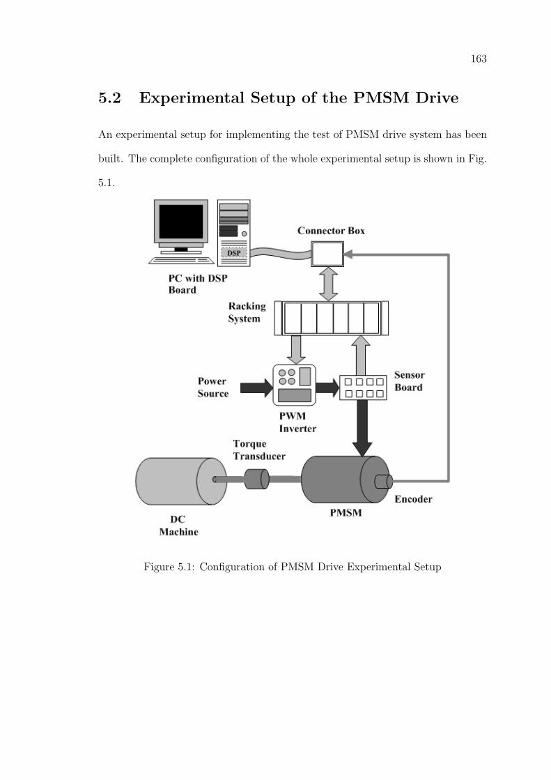
163
5.2 Experimental Setup of the PMSM Drive
An experimental setup for implementing the test of PMSM drive system has been
built. The complete configuration of the whole experimental setup is shown in Fig.
5.1.
Figure 5.1: Configuration of PMSM Drive Experimental Setup
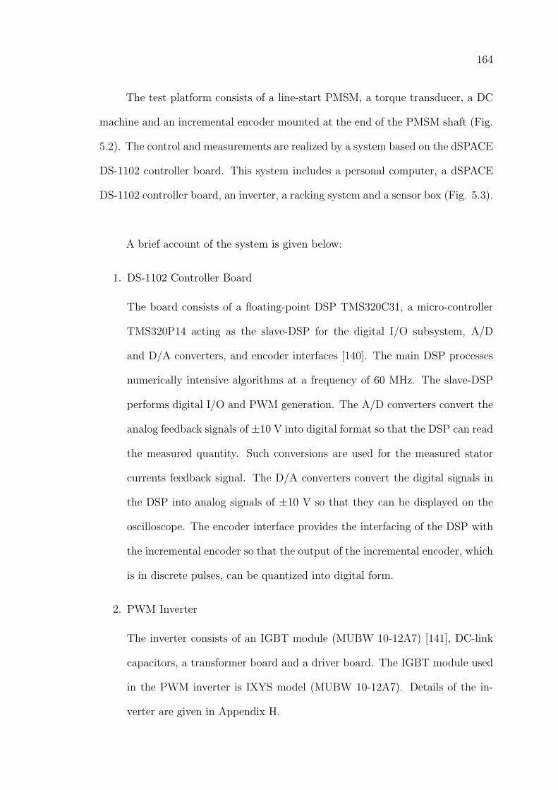
164
The test platform consists of a line-start PMSM, a torque transducer, a DC
machine and an incremental encoder mounted at the end of the PMSM shaft (Fig.
5.2). The control and measurements are realized by a system based on the dSPACE
DS-1102 controller board. This system includes a personal computer, a dSPACE
DS-1102 controller board, an inverter, a racking system and a sensor box (Fig. 5.3).
A brief account of the system is given below:
1. DS-1102 Controller Board
The board consists of a floating-point DSP TMS320C31, a micro-controller
TMS320P14 acting as the slave-DSP for the digital I/O subsystem, A/D
and D/A converters, and encoder interfaces [140]. The main DSP processes
numerically intensive algorithms at a frequency of 60 MHz. The slave-DSP
performs digital I/O and PWM generation. The A/D converters convert the
analog feedback signals of ±10 V into digital format so that the DSP can read
the measured quantity. Such conversions are used for the measured stator
currents feedback signal. The D/A converters convert the digital signals in
the DSP into analog signals of ±10 V so that they can be displayed on the
oscilloscope. The encoder interface provides the interfacing of the DSP with
the incremental encoder so that the output of the incremental encoder, which
is in discrete pulses, can be quantized into digital form.
2. PWM Inverter
The inverter consists of an IGBT module (MUBW 10-12A7) [141], DC-link
capacitors, a transformer board and a driver board. The IGBT module used
in the PWM inverter is IXYS model (MUBW 10-12A7). Details of the in-
verter are given in Appendix H.
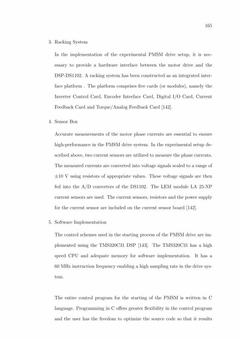
165
3. Racking System
In the implementation of the experimental PMSM drive setup, it is nec-
essary to provide a hardware interface between the motor drive and the
DSP-DS1102. A racking system has been constructed as an integrated inter-
face platform . The platform comprises five cards (or modules), namely the
Inverter Control Card, Encoder Interface Card, Digital I/O Card, Current
Feedback Card and Torque/Analog Feedback Card [142].
4. Sensor Box
Accurate measurements of the motor phase currents are essential to ensure
high-performance in the PMSM drive system. In the experimental setup de-
scribed above, two current sensors are utilized to measure the phase currents.
The measured currents are converted into voltage signals scaled to a range of
±10 V using resistors of appropriate values. These voltage signals are then
fed into the A/D converters of the DS1102. The LEM module LA 25-NP
current sensors are used. The current sensors, resistors and the power supply
for the current sensor are included on the current sensor board [142].
5. Software Implementation
The control schemes used in the starting process of the PMSM drive are im-
plemented using the TMS320C31 DSP [143]. The TMS320C31 has a high
speed CPU and adequate memory for software implementation. It has a
60 MHz instruction frequency enabling a high sampling rate in the drive sys-
tem.
The entire control program for the starting of the PMSM is written in C
language. Programming in C offers greater flexibility in the control program
and the user has the freedom to optimize the source code so that it results
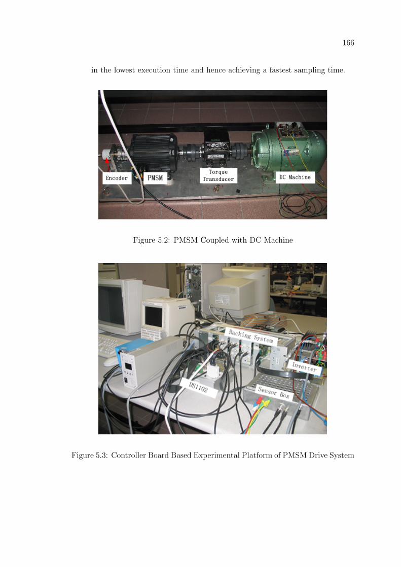
166
in the lowest execution time and hence achieving a fastest sampling time.
Figure 5.2: PMSM Coupled with DC Machine
Figure 5.3: Controller Board Based Experimental Platform of PMSM Drive System

167
5.3 Methodology and Modelling for Analysis
A two-dimensional finite element method is used for modelling the motor perfor-
mance. Maxwell’s equations, applied to the domains, give rise to the diffusion
equations. The non-linear field equations are solved simultaneously with the rotor,
stator and external circuit equations, allowing current distribution in the rotor bars
to be properly accounted for.
5.3.1 Modelling of the Fields
Recalling equation (2.26), the fundamental equations for the magnetic field are
represented in the two-dimensional rectangular coordinates as
∂
∂x(ν∂A
∂x) +
∂
∂y(ν∂A
∂y) = σ
∂A
∂t− σ
Vtz
l−∇× (νµ0Mr) (5.1)
For each domain in the machine, the field equation can be represented as:
• In the laminated iron where eddy current is neglected because of the lamina-
tion and in the air gap
∂
∂x(ν∂A
∂x) +
∂
∂y(ν∂A
∂y) = 0 (5.2)
• In the armature windings
∂
∂x(ν∂A
∂x) +
∂
∂y(ν∂A
∂y) = −is
s(5.3)
• In the rotor cage bars where the bars are solid conductors and the eddy
current is taken into account in the modelling.
∂
∂x(ν∂A
∂x) +
∂
∂y(ν∂A
∂y) = σ
∂A
∂t− σ
Vbk
lb(5.4)
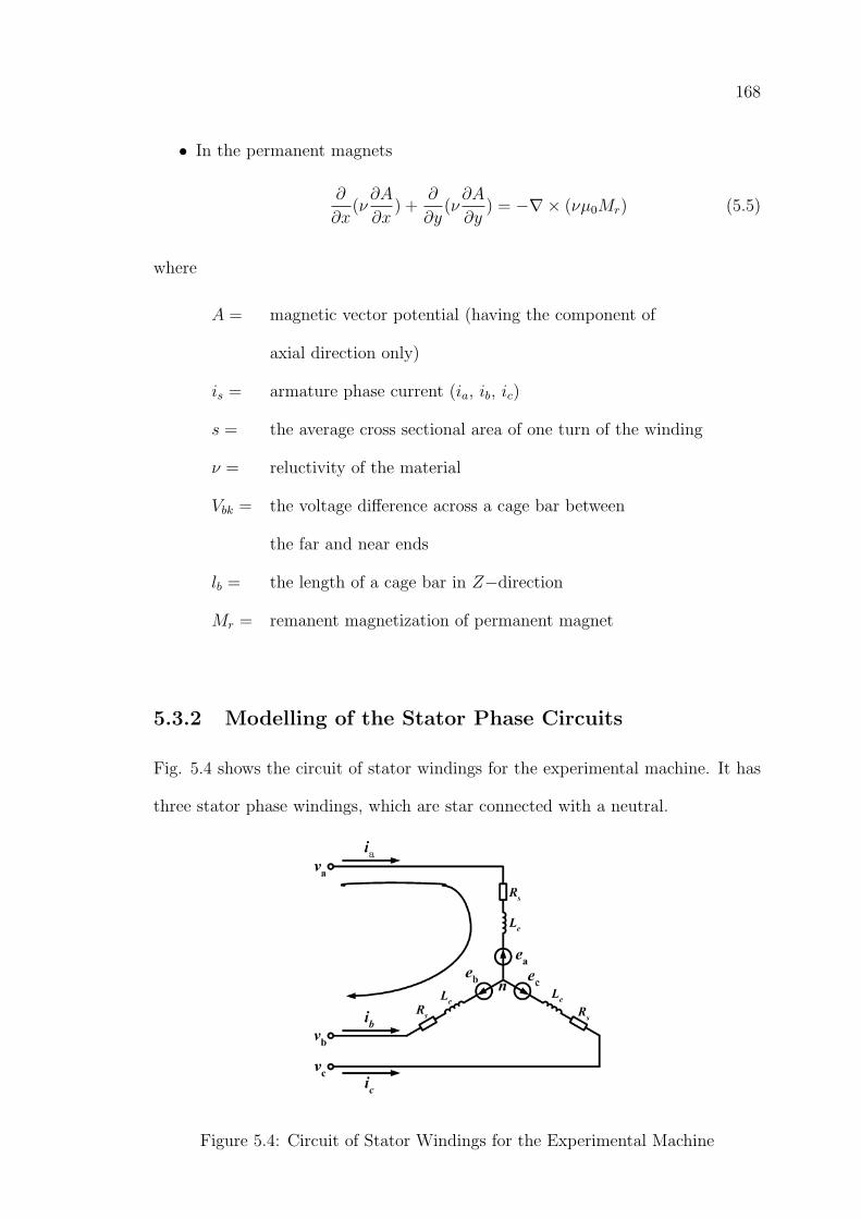
168
• In the permanent magnets
∂
∂x(ν∂A
∂x) +
∂
∂y(ν∂A
∂y) = −∇× (νµ0Mr) (5.5)
where
A = magnetic vector potential (having the component of
axial direction only)
is = armature phase current (ia, ib, ic)
s = the average cross sectional area of one turn of the winding
ν = reluctivity of the material
Vbk = the voltage difference across a cage bar between
the far and near ends
lb = the length of a cage bar in Z−direction
Mr = remanent magnetization of permanent magnet
5.3.2 Modelling of the Stator Phase Circuits
Fig. 5.4 shows the circuit of stator windings for the experimental machine. It has
three stator phase windings, which are star connected with a neutral.
Figure 5.4: Circuit of Stator Windings for the Experimental Machine
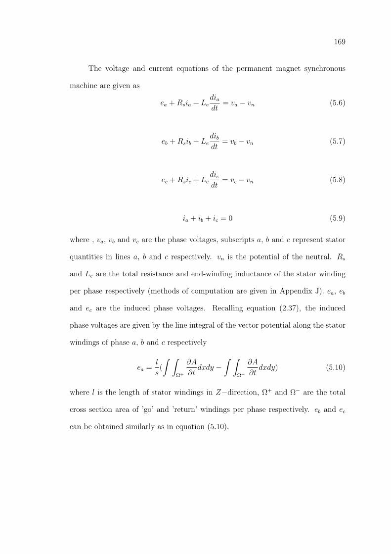
169
The voltage and current equations of the permanent magnet synchronous
machine are given as
ea +Rsia + Lediadt
= va − vn (5.6)
eb +Rsib + Ledibdt
= vb − vn (5.7)
ec +Rsic + Ledicdt
= vc − vn (5.8)
ia + ib + ic = 0 (5.9)
where , va, vb and vc are the phase voltages, subscripts a, b and c represent stator
quantities in lines a, b and c respectively. vn is the potential of the neutral. Rs
and Le are the total resistance and end-winding inductance of the stator winding
per phase respectively (methods of computation are given in Appendix J). ea, eb
and ec are the induced phase voltages. Recalling equation (2.37), the induced
phase voltages are given by the line integral of the vector potential along the stator
windings of phase a, b and c respectively
ea =l
s(
∫ ∫Ω+
∂A
∂tdxdy −
∫ ∫Ω−
∂A
∂tdxdy) (5.10)
where l is the length of stator windings in Z−direction, Ω+ and Ω− are the total
cross section area of ’go’ and ’return’ windings per phase respectively. eb and ec
can be obtained similarly as in equation (5.10).
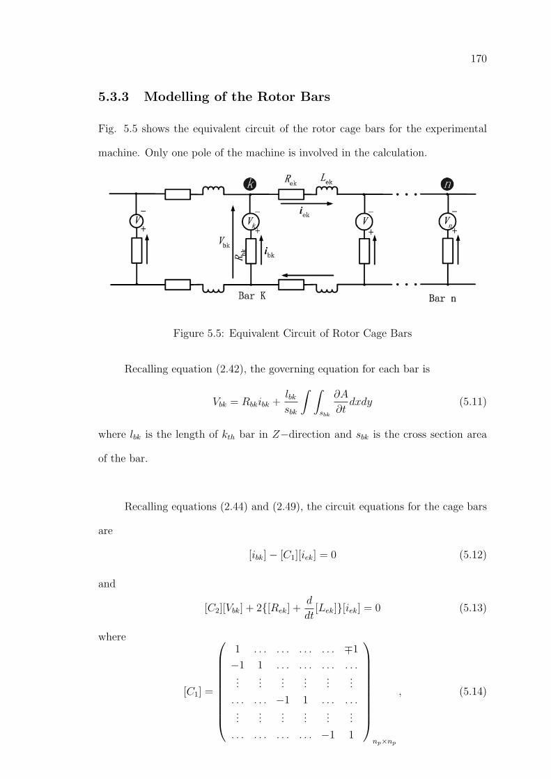
170
5.3.3 Modelling of the Rotor Bars
Fig. 5.5 shows the equivalent circuit of the rotor cage bars for the experimental
machine. Only one pole of the machine is involved in the calculation.
Figure 5.5: Equivalent Circuit of Rotor Cage Bars
Recalling equation (2.42), the governing equation for each bar is
Vbk = Rbkibk +lbksbk
∫ ∫sbk
∂A
∂tdxdy (5.11)
where lbk is the length of kth bar in Z−direction and sbk is the cross section area
of the bar.
Recalling equations (2.44) and (2.49), the circuit equations for the cage bars
are
[ibk]− [C1][iek] = 0 (5.12)
and
[C2][Vbk] + 2[Rek] +d
dt[Lek][iek] = 0 (5.13)
where
[C1] =
1 . . . . . . . . . . . . ∓1
−1 1 . . . . . . . . . . . ....
......
......
...
. . . . . . −1 1 . . . . . ....
......
......
...
. . . . . . . . . . . . −1 1
np×np
, (5.14)
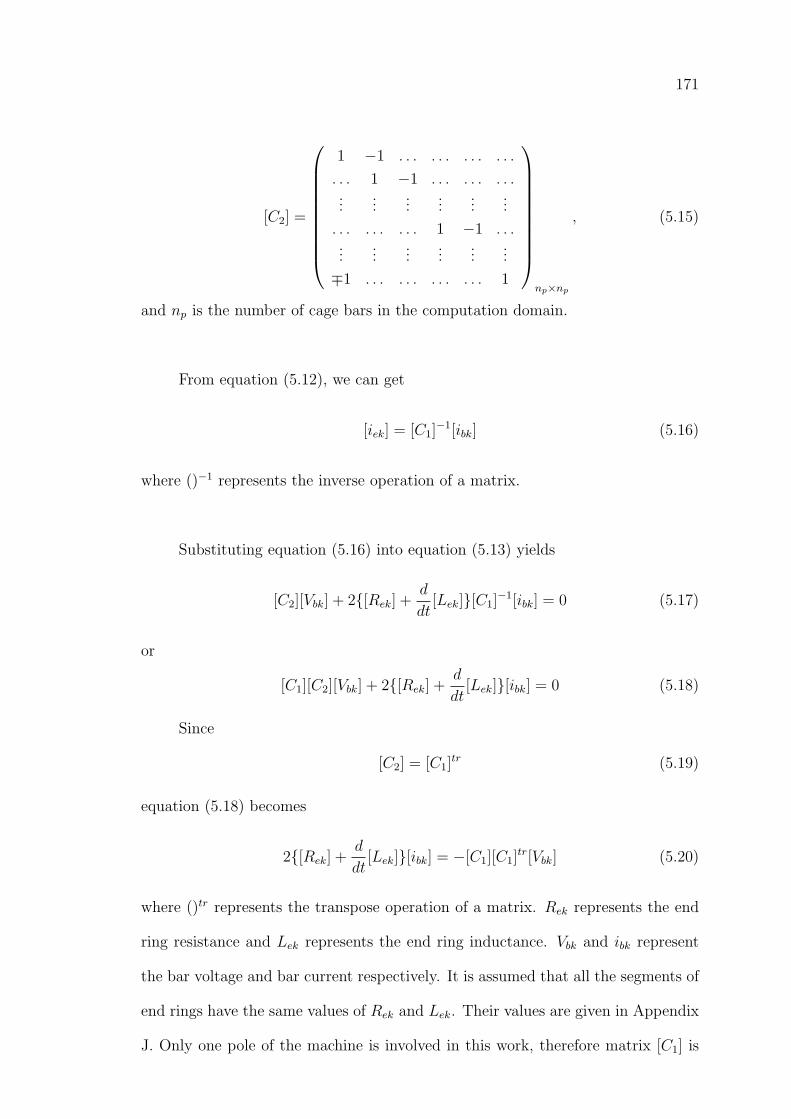
171
[C2] =
1 −1 . . . . . . . . . . . .
. . . 1 −1 . . . . . . . . ....
......
......
...
. . . . . . . . . 1 −1 . . ....
......
......
...
∓1 . . . . . . . . . . . . 1
np×np
, (5.15)
and np is the number of cage bars in the computation domain.
From equation (5.12), we can get
[iek] = [C1]−1[ibk] (5.16)
where ()−1 represents the inverse operation of a matrix.
Substituting equation (5.16) into equation (5.13) yields
[C2][Vbk] + 2[Rek] +d
dt[Lek][C1]
−1[ibk] = 0 (5.17)
or
[C1][C2][Vbk] + 2[Rek] +d
dt[Lek][ibk] = 0 (5.18)
Since
[C2] = [C1]tr (5.19)
equation (5.18) becomes
2[Rek] +d
dt[Lek][ibk] = −[C1][C1]
tr[Vbk] (5.20)
where ()tr represents the transpose operation of a matrix. Rek represents the end
ring resistance and Lek represents the end ring inductance. Vbk and ibk represent
the bar voltage and bar current respectively. It is assumed that all the segments of
end rings have the same values of Rek and Lek. Their values are given in Appendix
J. Only one pole of the machine is involved in this work, therefore matrix [C1] is
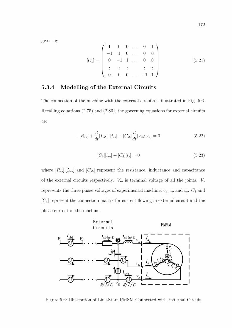
172
given by
[C1] =
1 0 0 . . . 0 1
−1 1 0 . . . 0 0
0 −1 1 . . . 0 0...
......
......
0 0 0 . . . −1 1
(5.21)
5.3.4 Modelling of the External Circuits
The connection of the machine with the external circuits is illustrated in Fig. 5.6.
Recalling equations (2.75) and (2.80), the governing equations for external circuits
are
[Rsb] +d
dt[Lsb][isb] + [Csb]
d
dt[Vsb;Vs] = 0 (5.22)
[C3][isb] + [C4][is] = 0 (5.23)
where [Rsb],[Lsb] and [Csb] represent the resistance, inductance and capacitance
of the external circuits respectively. Vsb is terminal voltage of all the joints. Vs
represents the three phase voltages of experimental machine, va, vb and vc. C3 and
[C4] represent the connection matrix for current flowing in external circuit and the
phase current of the machine.
Figure 5.6: Illustration of Line-Start PMSM Connected with External Circuit
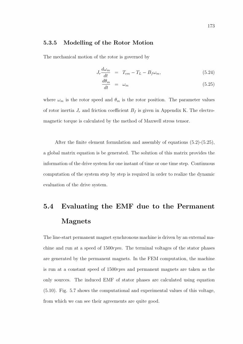
173
5.3.5 Modelling of the Rotor Motion
The mechanical motion of the rotor is governed by
Jrdωm
dt= Tem − TL −Bfωm, (5.24)
dθm
dt= ωm (5.25)
where ωm is the rotor speed and θm is the rotor position. The parameter values
of rotor inertia Jr and friction coefficient Bf is given in Appendix K. The electro-
magnetic torque is calculated by the method of Maxwell stress tensor.
After the finite element formulation and assembly of equations (5.2)-(5.25),
a global matrix equation is be generated. The solution of this matrix provides the
information of the drive system for one instant of time or one time step. Continuous
computation of the system step by step is required in order to realize the dynamic
evaluation of the drive system.
5.4 Evaluating the EMF due to the Permanent
Magnets
The line-start permanent magnet synchronous machine is driven by an external ma-
chine and run at a speed of 1500rpm. The terminal voltages of the stator phases
are generated by the permanent magnets. In the FEM computation, the machine
is run at a constant speed of 1500rpm and permanent magnets are taken as the
only sources. The induced EMF of stator phases are calculated using equation
(5.10). Fig. 5.7 shows the computational and experimental values of this voltage,
from which we can see their agreements are quite good.
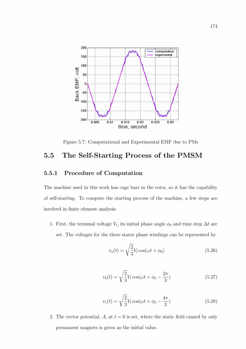
174
Figure 5.7: Computational and Experimental EMF due to PMs
5.5 The Self-Starting Process of the PMSM
5.5.1 Procedure of Computation
The machine used in this work has cage bars in the rotor, so it has the capability
of self-starting. To compute the starting process of the machine, a few steps are
involved in finite element analysis:
1. First, the terminal voltage Vl, its initial phase angle φ0 and time step ∆t are
set. The voltages for the three stator phase windings can be represented by
va(t) =
√2
3Vl cos(ωt+ φ0) (5.26)
vb(t) =
√2
3Vl cos(ωt+ φ0 −
2π
3) (5.27)
vc(t) =
√2
3Vl cos(ωt+ φ0 −
4π
3) (5.28)
2. The vector potential, A, at t = 0 is set, where the static field caused by only
permanent magnets is given as the initial value.
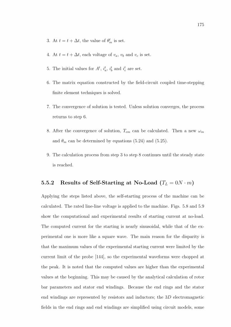
175
3. At t = t+ ∆t, the value of θtm is set.
4. At t = t+ ∆t, each voltage of va, vb and vc is set.
5. The initial values for At, ita, itb and itc are set.
6. The matrix equation constructed by the field-circuit coupled time-stepping
finite element techniques is solved.
7. The convergence of solution is tested. Unless solution converges, the process
returns to step 6.
8. After the convergence of solution, Tem can be calculated. Then a new ωm
and θm can be determined by equations (5.24) and (5.25).
9. The calculation process from step 3 to step 8 continues until the steady state
is reached.
5.5.2 Results of Self-Starting at No-Load (TL = 0N ·m)
Applying the steps listed above, the self-starting process of the machine can be
calculated. The rated line-line voltage is applied to the machine. Figs. 5.8 and 5.9
show the computational and experimental results of starting current at no-load.
The computed current for the starting is nearly sinusoidal, while that of the ex-
perimental one is more like a square wave. The main reason for the disparity is
that the maximum values of the experimental starting current were limited by the
current limit of the probe [144], so the experimental waveforms were chopped at
the peak. It is noted that the computed values are higher than the experimental
values at the beginning. This may be caused by the analytical calculation of rotor
bar parameters and stator end windings. Because the end rings and the stator
end windings are represented by resistors and inductors; the 3D electromagnetic
fields in the end rings and end windings are simplified using circuit models, some
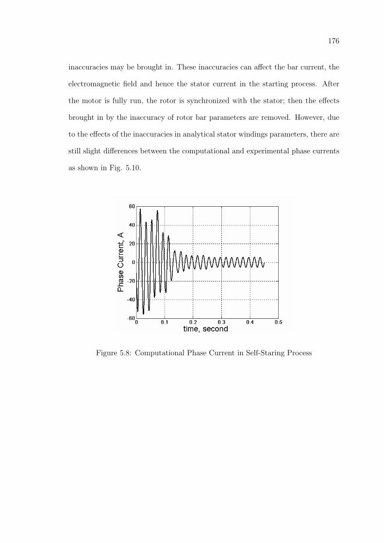
176
inaccuracies may be brought in. These inaccuracies can affect the bar current, the
electromagnetic field and hence the stator current in the starting process. After
the motor is fully run, the rotor is synchronized with the stator; then the effects
brought in by the inaccuracy of rotor bar parameters are removed. However, due
to the effects of the inaccuracies in analytical stator windings parameters, there are
still slight differences between the computational and experimental phase currents
as shown in Fig. 5.10.
Figure 5.8: Computational Phase Current in Self-Staring Process
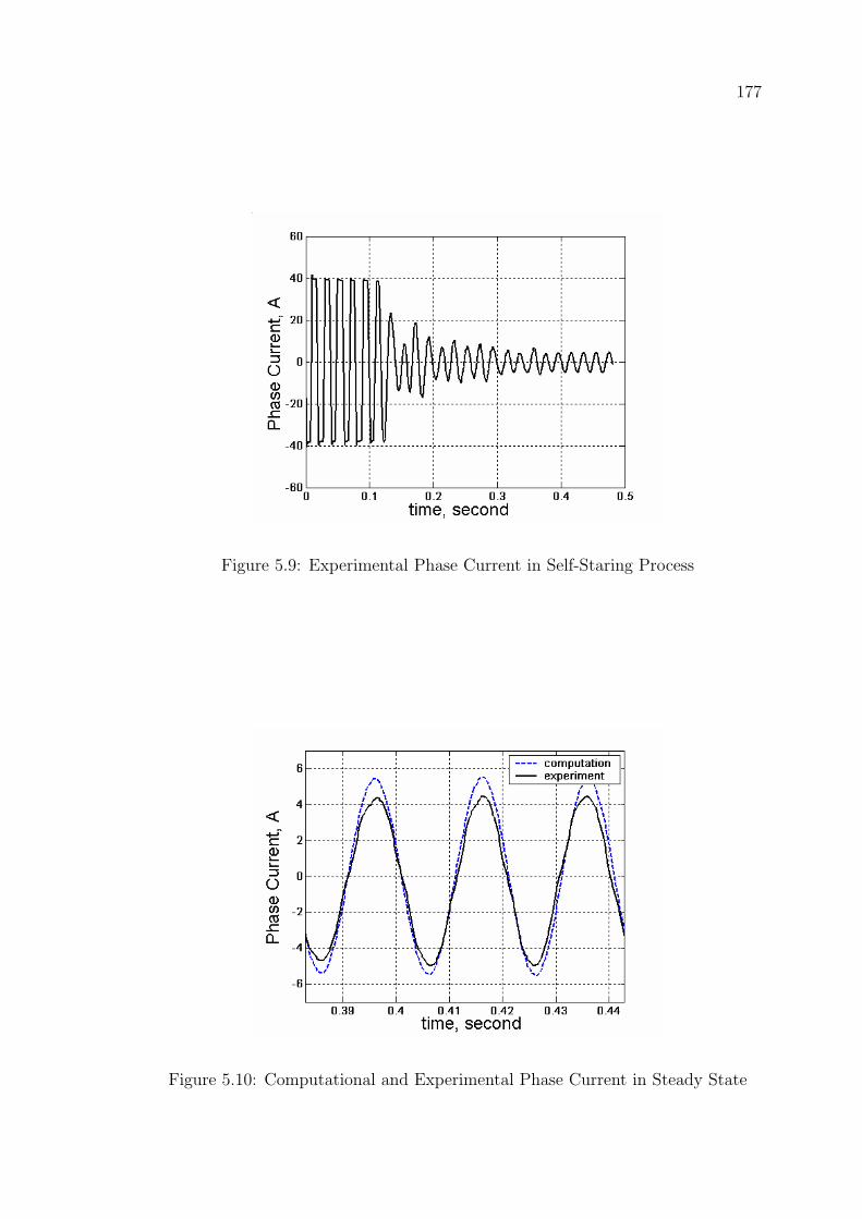
177
Figure 5.9: Experimental Phase Current in Self-Staring Process
Figure 5.10: Computational and Experimental Phase Current in Steady State
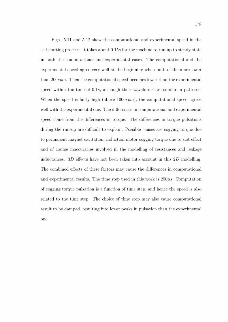
178
Figs. 5.11 and 5.12 show the computational and experimental speed in the
self-starting process. It takes about 0.15s for the machine to run up to steady state
in both the computational and experimental cases. The computational and the
experimental speed agree very well at the beginning when both of them are lower
than 200rpm. Then the computational speed becomes lower than the experimental
speed within the time of 0.1s, although their waveforms are similar in patterns.
When the speed is fairly high (above 1000rpm), the computational speed agrees
well with the experimental one. The differences in computational and experimental
speed come from the differences in torque. The differences in torque pulsations
during the run-up are difficult to explain. Possible causes are cogging torque due
to permanent magnet excitation, induction motor cogging torque due to slot effect
and of course inaccuracies involved in the modelling of resistances and leakage
inductances. 3D effects have not been taken into account in this 2D modelling.
The combined effects of these factors may cause the differences in computational
and experimental results. The time step used in this work is 250µs. Computation
of cogging torque pulsation is a function of time step, and hence the speed is also
related to the time step. The choice of time step may also cause computational
result to be damped, resulting into lower peaks in pulsation than the experimental
one.
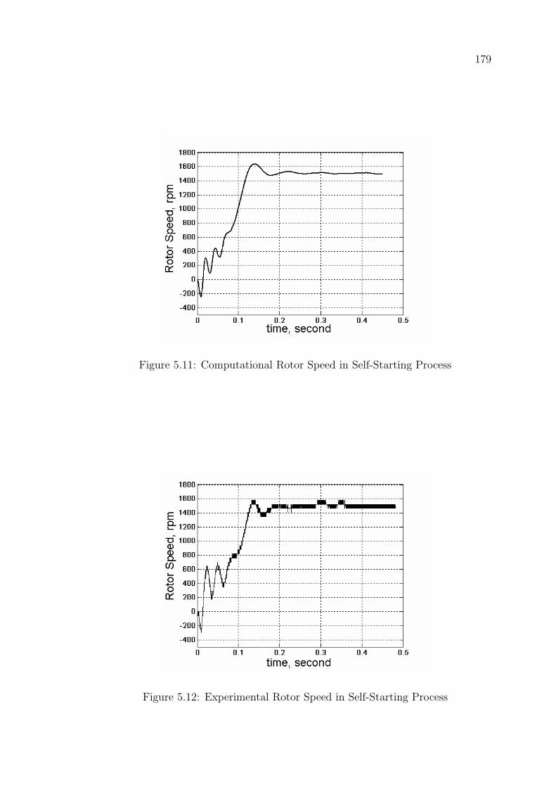
179
Figure 5.11: Computational Rotor Speed in Self-Starting Process
Figure 5.12: Experimental Rotor Speed in Self-Starting Process
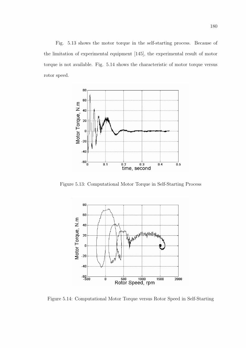
180
Fig. 5.13 shows the motor torque in the self-starting process. Because of
the limitation of experimental equipment [145], the experimental result of motor
torque is not available. Fig. 5.14 shows the characteristic of motor torque versus
rotor speed.
Figure 5.13: Computational Motor Torque in Self-Starting Process
Figure 5.14: Computational Motor Torque versus Rotor Speed in Self-Starting
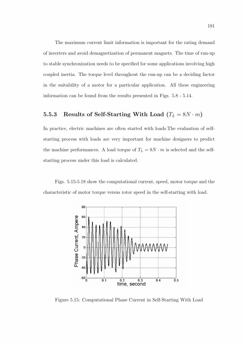
181
The maximum current limit information is important for the rating demand
of inverters and avoid demagnetization of permanent magnets. The time of run-up
to stable synchronization needs to be specified for some applications involving high
coupled inertia. The torque level throughout the run-up can be a deciding factor
in the suitability of a motor for a particular application. All these engineering
information can be found from the results presented in Figs. 5.8 - 5.14.
5.5.3 Results of Self-Starting With Load (TL = 8N ·m)
In practice, electric machines are often started with loads.The evaluation of self-
starting process with loads are very important for machine designers to predict
the machine performances. A load torque of TL = 8N ·m is selected and the self-
starting process under this load is calculated.
Figs. 5.15-5.18 show the computational current, speed, motor torque and the
characteristic of motor torque versus rotor speed in the self-starting with load.
Figure 5.15: Computational Phase Current in Self-Starting With Load
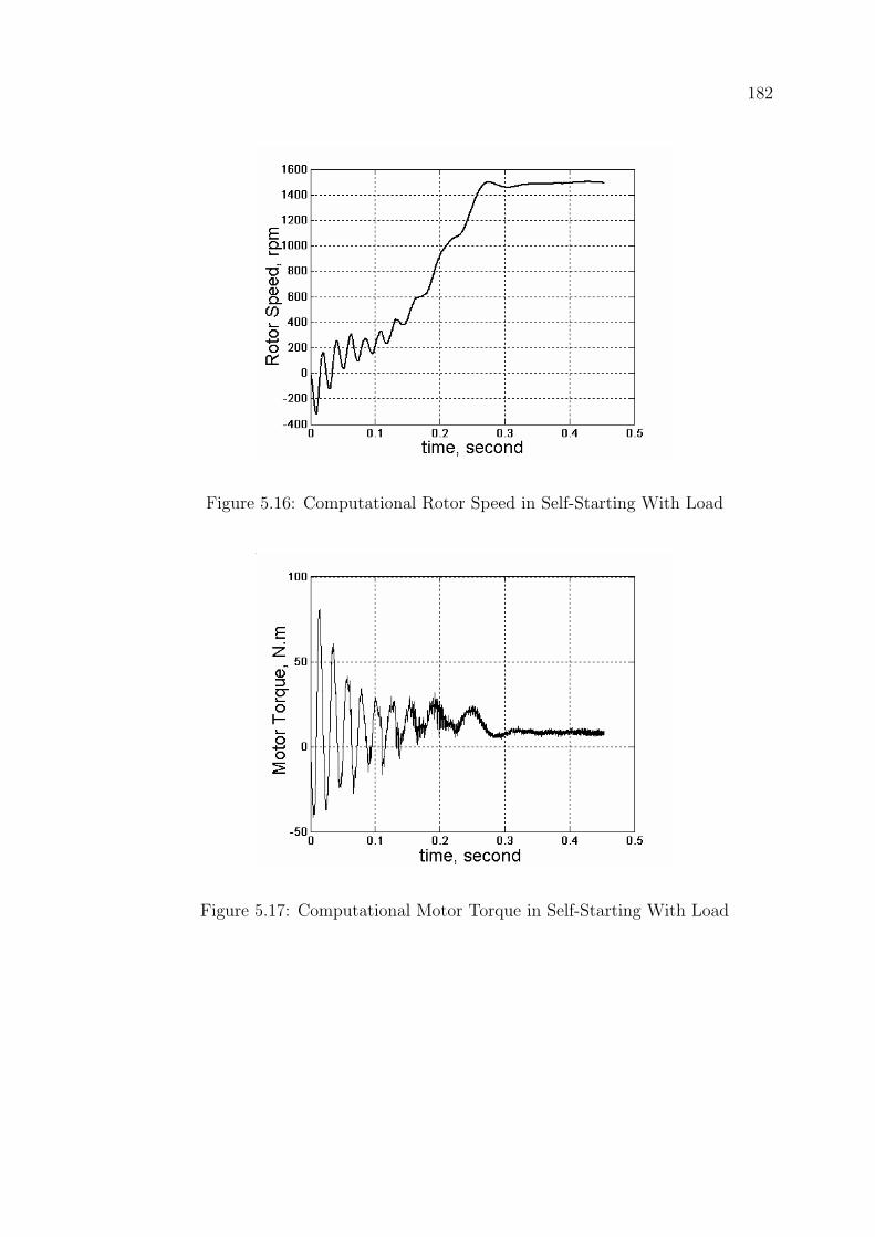
182
Figure 5.16: Computational Rotor Speed in Self-Starting With Load
Figure 5.17: Computational Motor Torque in Self-Starting With Load
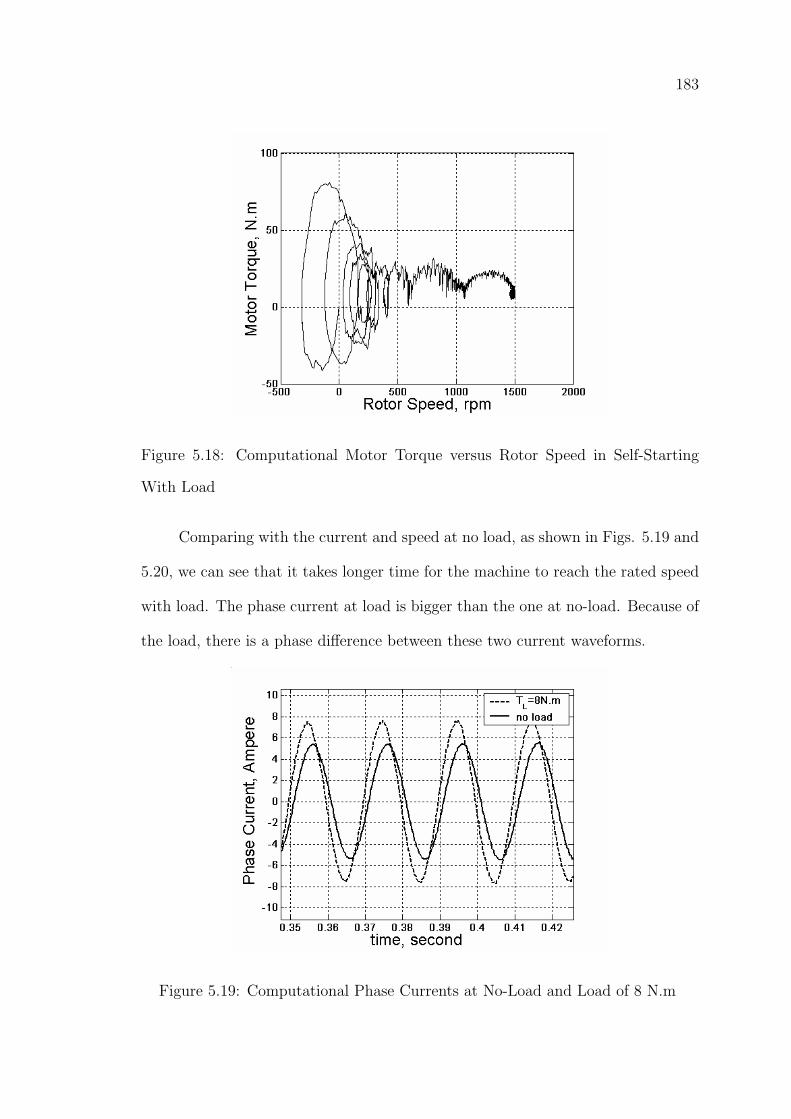
183
Figure 5.18: Computational Motor Torque versus Rotor Speed in Self-Starting
With Load
Comparing with the current and speed at no load, as shown in Figs. 5.19 and
5.20, we can see that it takes longer time for the machine to reach the rated speed
with load. The phase current at load is bigger than the one at no-load. Because of
the load, there is a phase difference between these two current waveforms.
Figure 5.19: Computational Phase Currents at No-Load and Load of 8 N.m
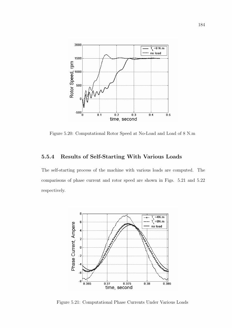
184
Figure 5.20: Computational Rotor Speed at No-Load and Load of 8 N.m
5.5.4 Results of Self-Starting With Various Loads
The self-starting process of the machine with various loads are computed. The
comparisons of phase current and rotor speed are shown in Figs. 5.21 and 5.22
respectively.
Figure 5.21: Computational Phase Currents Under Various Loads
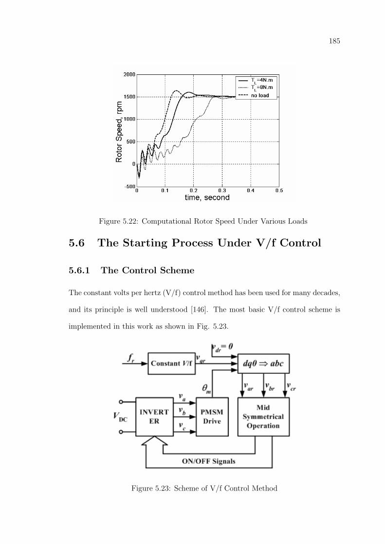
185
Figure 5.22: Computational Rotor Speed Under Various Loads
5.6 The Starting Process Under V/f Control
5.6.1 The Control Scheme
The constant volts per hertz (V/f) control method has been used for many decades,
and its principle is well understood [146]. The most basic V/f control scheme is
implemented in this work as shown in Fig. 5.23.
Figure 5.23: Scheme of V/f Control Method
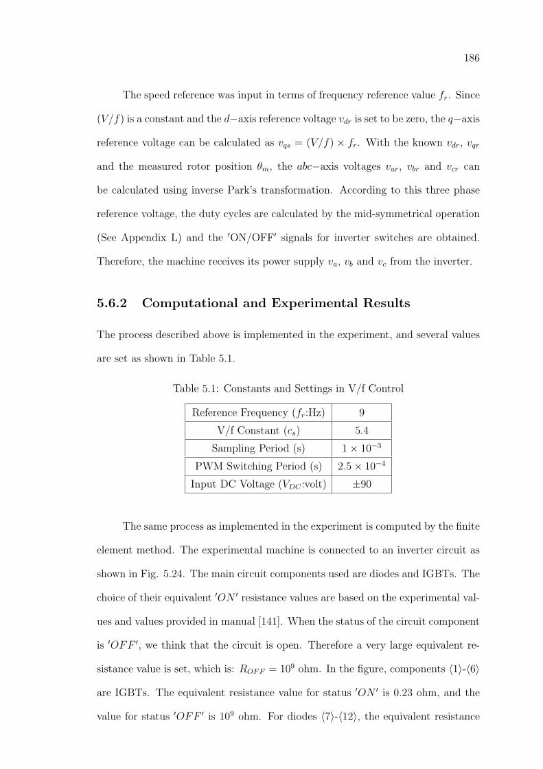
186
The speed reference was input in terms of frequency reference value fr. Since
(V/f) is a constant and the d−axis reference voltage vdr is set to be zero, the q−axis
reference voltage can be calculated as vqs = (V/f) × fr. With the known vdr, vqr
and the measured rotor position θm, the abc−axis voltages var, vbr and vcr can
be calculated using inverse Park’s transformation. According to this three phase
reference voltage, the duty cycles are calculated by the mid-symmetrical operation
(See Appendix L) and the ′ON/OFF′ signals for inverter switches are obtained.
Therefore, the machine receives its power supply va, vb and vc from the inverter.
5.6.2 Computational and Experimental Results
The process described above is implemented in the experiment, and several values
are set as shown in Table 5.1.
Table 5.1: Constants and Settings in V/f Control
Reference Frequency (fr:Hz) 9
V/f Constant (cs) 5.4
Sampling Period (s) 1× 10⁻³
PWM Switching Period (s) 2.5× 10⁻⁴
Input DC Voltage (VDC :volt) ±90
The same process as implemented in the experiment is computed by the finite
element method. The experimental machine is connected to an inverter circuit as
shown in Fig. 5.24. The main circuit components used are diodes and IGBTs. The
choice of their equivalent ′ON ′ resistance values are based on the experimental val-
ues and values provided in manual [141]. When the status of the circuit component
is ′OFF ′, we think that the circuit is open. Therefore a very large equivalent re-
sistance value is set, which is: ROFF = 109 ohm. In the figure, components 〈1〉-〈6〉
are IGBTs. The equivalent resistance value for status ′ON ′ is 0.23 ohm, and the
value for status ′OFF ′ is 109 ohm. For diodes 〈7〉-〈12〉, the equivalent resistance
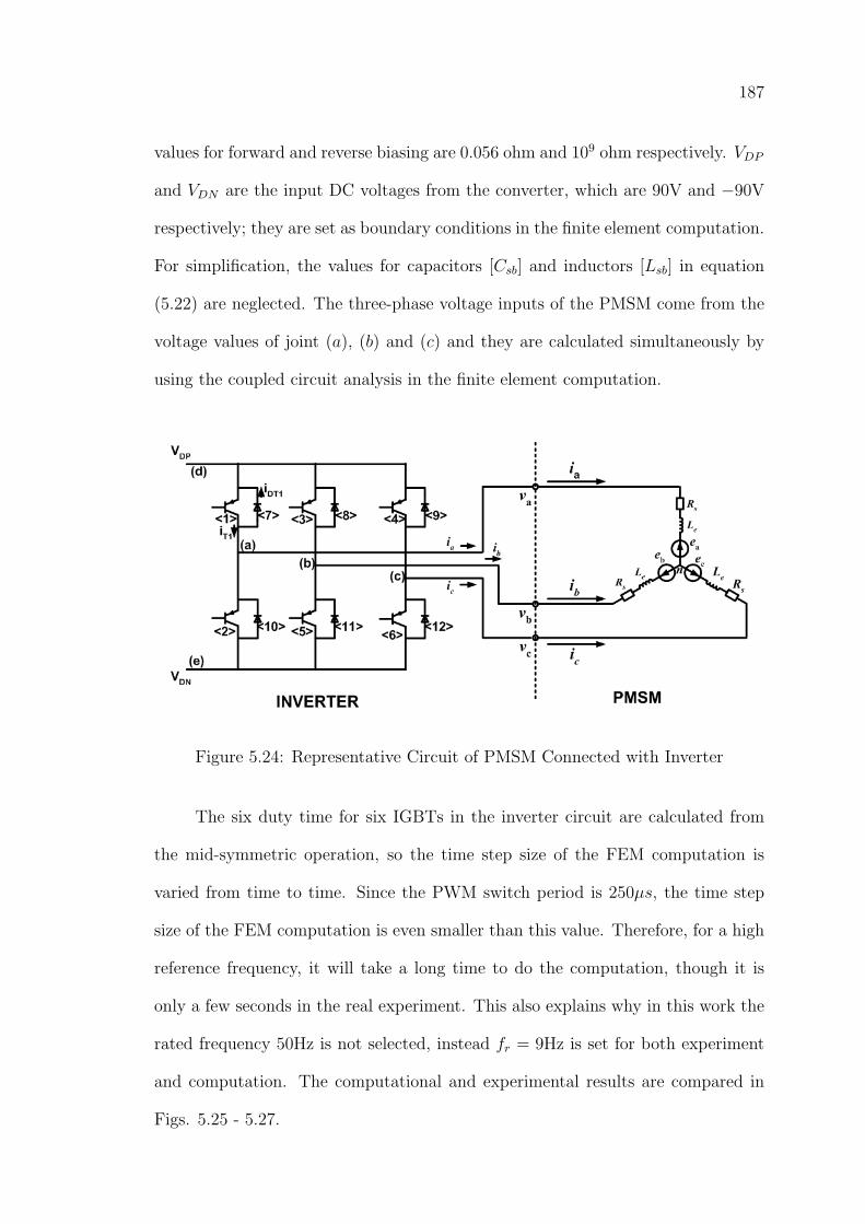
187
values for forward and reverse biasing are 0.056 ohm and 109 ohm respectively. VDP
and VDN are the input DC voltages from the converter, which are 90V and −90V
respectively; they are set as boundary conditions in the finite element computation.
For simplification, the values for capacitors [Csb] and inductors [Lsb] in equation
(5.22) are neglected. The three-phase voltage inputs of the PMSM come from the
voltage values of joint (a), (b) and (c) and they are calculated simultaneously by
using the coupled circuit analysis in the finite element computation.
Figure 5.24: Representative Circuit of PMSM Connected with Inverter
The six duty time for six IGBTs in the inverter circuit are calculated from
the mid-symmetric operation, so the time step size of the FEM computation is
varied from time to time. Since the PWM switch period is 250µs, the time step
size of the FEM computation is even smaller than this value. Therefore, for a high
reference frequency, it will take a long time to do the computation, though it is
only a few seconds in the real experiment. This also explains why in this work the
rated frequency 50Hz is not selected, instead fr = 9Hz is set for both experiment
and computation. The computational and experimental results are compared in
Figs. 5.25 - 5.27.
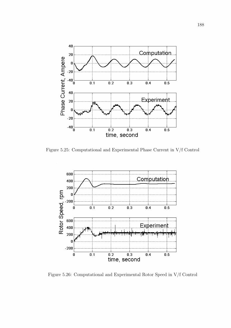
188
Figure 5.25: Computational and Experimental Phase Current in V/f Control
Figure 5.26: Computational and Experimental Rotor Speed in V/f Control
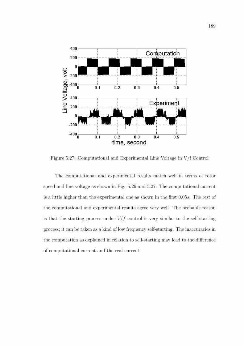
189
Figure 5.27: Computational and Experimental Line Voltage in V/f Control
The computational and experimental results match well in terms of rotor
speed and line voltage as shown in Fig. 5.26 and 5.27. The computational current
is a little higher than the experimental one as shown in the first 0.05s. The rest of
the computational and experimental results agree very well. The probable reason
is that the starting process under V/f control is very similar to the self-starting
process; it can be taken as a kind of low frequency self-starting. The inaccuracies in
the computation as explained in relation to self-starting may lead to the difference
of computational current and the real current.
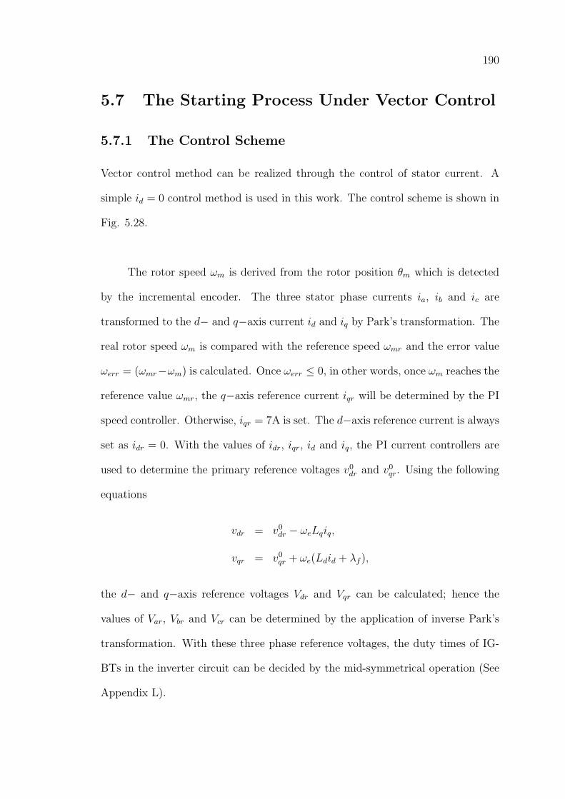
190
5.7 The Starting Process Under Vector Control
5.7.1 The Control Scheme
Vector control method can be realized through the control of stator current. A
simple id = 0 control method is used in this work. The control scheme is shown in
Fig. 5.28.
The rotor speed ωm is derived from the rotor position θm which is detected
by the incremental encoder. The three stator phase currents ia, ib and ic are
transformed to the d− and q−axis current id and iq by Park’s transformation. The
real rotor speed ωm is compared with the reference speed ωmr and the error value
ωerr = (ωmr−ωm) is calculated. Once ωerr ≤ 0, in other words, once ωm reaches the
reference value ωmr, the q−axis reference current iqr will be determined by the PI
speed controller. Otherwise, iqr = 7A is set. The d−axis reference current is always
set as idr = 0. With the values of idr, iqr, id and iq, the PI current controllers are
used to determine the primary reference voltages v0dr and v0
qr. Using the following
equations
vdr = v0dr − ωeLqiq,
vqr = v0qr + ωe(Ldid + λf ),
the d− and q−axis reference voltages Vdr and Vqr can be calculated; hence the
values of Var, Vbr and Vcr can be determined by the application of inverse Park’s
transformation. With these three phase reference voltages, the duty times of IG-
BTs in the inverter circuit can be decided by the mid-symmetrical operation (See
Appendix L).
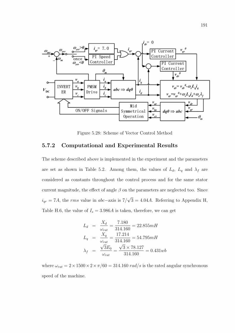
191
Figure 5.28: Scheme of Vector Control Method
5.7.2 Computational and Experimental Results
The scheme described above is implemented in the experiment and the parameters
are set as shown in Table 5.2. Among them, the values of Ld, Lq and λf are
considered as constants throughout the control process and for the same stator
current magnitude, the effect of angle β on the parameters are neglected too. Since
iqr = 7A, the rms value in abc−axis is 7/√
3 = 4.04A. Referring to Appendix H,
Table H.6, the value of Is = 3.986A is taken, therefore, we can get
Ld =Xd
ωrat
=7.180
314.160= 22.855mH
Lq =Xq
ωrat
=17.214
314.160= 54.795mH
λf =
√3E0
ωrat
=
√3× 78.127
314.160= 0.431wb
where ωrat = 2×1500×2×π/60 = 314.160 rad/s is the rated angular synchronous
speed of the machine.
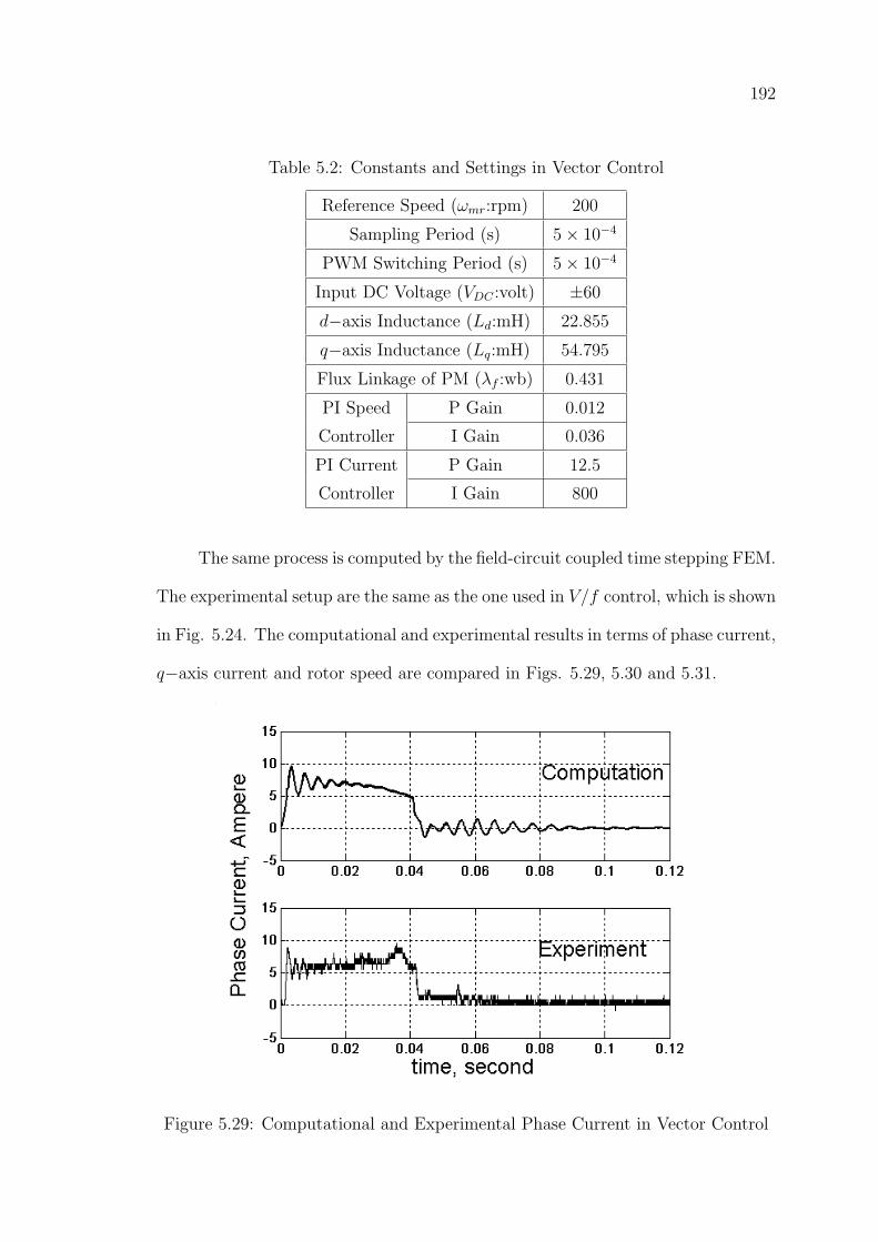
192
Table 5.2: Constants and Settings in Vector Control
Reference Speed (ωmr:rpm) 200
Sampling Period (s) 5× 10⁻⁴
PWM Switching Period (s) 5× 10⁻⁴
Input DC Voltage (VDC :volt) ±60
d−axis Inductance (Ld:mH) 22.855
q−axis Inductance (Lq:mH) 54.795
Flux Linkage of PM (λf :wb) 0.431
PI Speed P Gain 0.012
Controller I Gain 0.036
PI Current P Gain 12.5
Controller I Gain 800
The same process is computed by the field-circuit coupled time stepping FEM.
The experimental setup are the same as the one used in V/f control, which is shown
in Fig. 5.24. The computational and experimental results in terms of phase current,
q−axis current and rotor speed are compared in Figs. 5.29, 5.30 and 5.31.
Figure 5.29: Computational and Experimental Phase Current in Vector Control
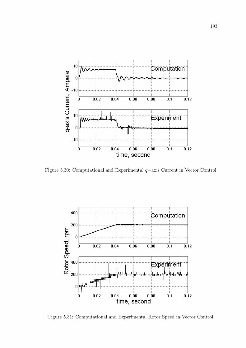
193
Figure 5.30: Computational and Experimental q−axis Current in Vector Control
Figure 5.31: Computational and Experimental Rotor Speed in Vector Control
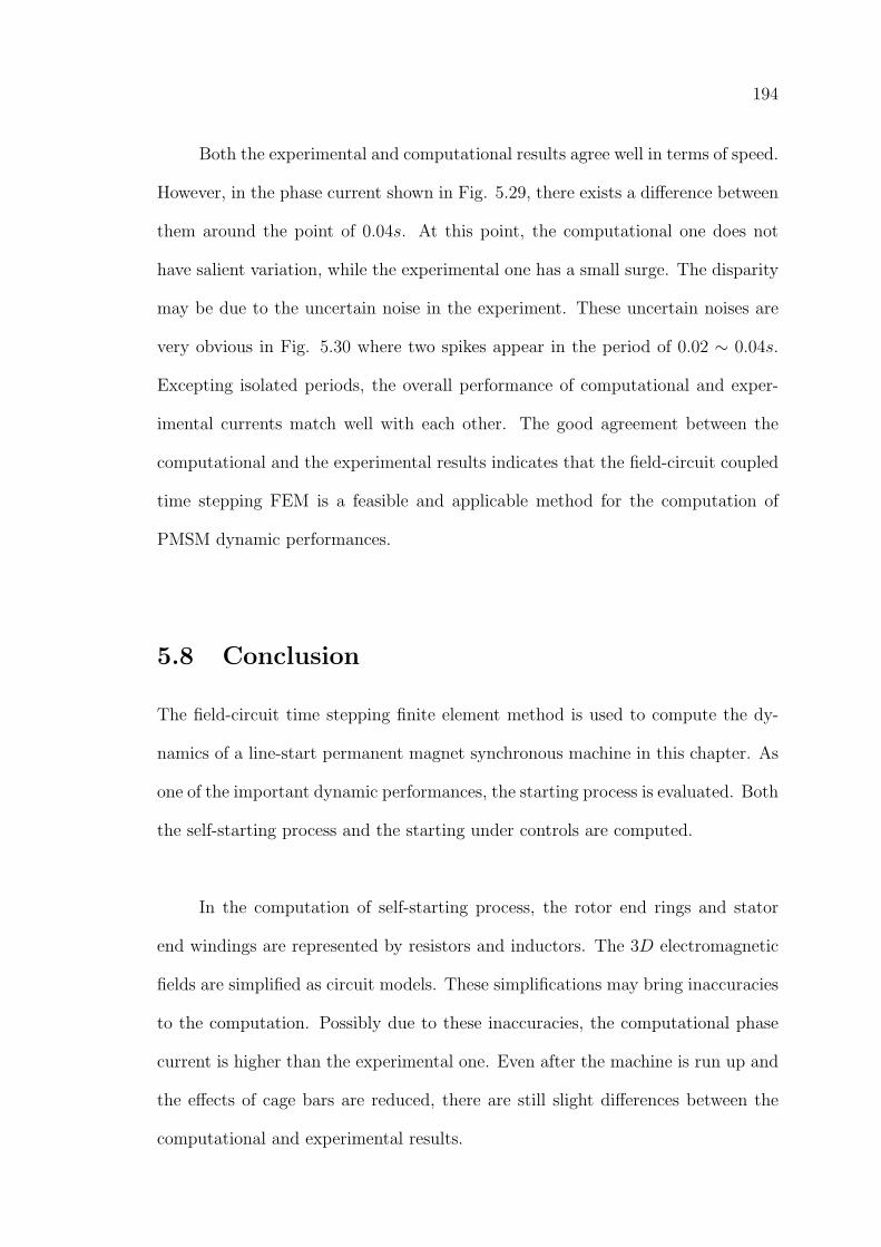
194
Both the experimental and computational results agree well in terms of speed.
However, in the phase current shown in Fig. 5.29, there exists a difference between
them around the point of 0.04s. At this point, the computational one does not
have salient variation, while the experimental one has a small surge. The disparity
may be due to the uncertain noise in the experiment. These uncertain noises are
very obvious in Fig. 5.30 where two spikes appear in the period of 0.02 ∼ 0.04s.
Excepting isolated periods, the overall performance of computational and exper-
imental currents match well with each other. The good agreement between the
computational and the experimental results indicates that the field-circuit coupled
time stepping FEM is a feasible and applicable method for the computation of
PMSM dynamic performances.
5.8 Conclusion
The field-circuit time stepping finite element method is used to compute the dy-
namics of a line-start permanent magnet synchronous machine in this chapter. As
one of the important dynamic performances, the starting process is evaluated. Both
the self-starting process and the starting under controls are computed.
In the computation of self-starting process, the rotor end rings and stator
end windings are represented by resistors and inductors. The 3D electromagnetic
fields are simplified as circuit models. These simplifications may bring inaccuracies
to the computation. Possibly due to these inaccuracies, the computational phase
current is higher than the experimental one. Even after the machine is run up and
the effects of cage bars are reduced, there are still slight differences between the
computational and experimental results.
195
The pattern of computational speed is the result of computational torque.
In the computation of self-starting process, the computational speed is lower than
the experimental speed at the beginning, although they are similar in patterns.
The differences may be caused by the combined inaccuracies in the computation
of cogging torque due to permanent magnet excitation, computation of cogging
torque due to slot effect, simplification of 3D effects and the choice of time step.
The starting process of machine under V/f control is very similar to the self-
starting process, which can be taken as a kind of low frequency self-starting. The
inaccuracies in the computation as explained in relation to self-starting may lead to
the difference of computational current and the real current in the starting process
under V/f control.
When the machine is started under current vector control, both the compu-
tational current and speed agree well with the experimental ones. The reason is
the frequency of supplies is always in synchronism with the rotor frequency, the
effects of cage bars are reduced greatly. Therefore good agreement can be achieved.
From the computation of the various starting processes, we can see that the
field-circuit time-stepping finite element method is applicable in evaluating the
dynamics of line-start permanent magnet synchronous machine. Most of the im-
portant factors in the starting process can be computed, including the starting
current, motor torque, rotor speed and starting time. However, possibly due to the
limitation of 2D modelling, differences still exists between the computational and
experimental results in some areas.
Chapter 6
Conclusions and Discussions
This thesis deals with the dynamic analysis of a line start permanent magnet syn-
chronous machines (PMSM) using field-circuit coupled time stepping finite element
method (FEM). This method has been widely used based on the 2D modelling of
machines. The 3D effects of the machine like the stator end windings and rotor
end rings are represented by resistors and inductors. The 3D electromagnetic field
is simplified using circuit models. 2D modelling is advantageous in simplifying
the formulation and saving computation time; particularly for the computation
of dynamic process. However, because of the inaccuracies brought along by the
simplifications in 2D modelling, some differences exist between the computational
results and the experimental results. In Chapter 5, we have shown that the tran-
sient computational current was higher than the experimental current. Even after
the machine was fully run, there were still slight difference in the computational
and experimental current due to the inaccuracies involved in the 2D modelling of
stator end windings. Fortunately the differences between them are not big, and
most of the important information for dynamic analysis can be achieved as well.
Electric machines are often operated with external drive circuits, therefore
the modelling of these circuits are necessary. The semiconductor components, such
as IGBTs and diodes, are simplified as resistors in this work. These resistors have
different values depending on their operation status. In other words, these com-
196
197
ponents are modelled as linear components and their transient characteristics are
neglected. This modelling is quite effective when coupling the effects of external
circuits into the electromagnetic fields computation. Accuracies are guaranteed as
shown in Chapter 5 where the starting processes under V/f control and vector
control were validated. Since the nonlinearities of the component characteristics
are neglected, much computation time are saved as well. It should also be noted
that for small capacity machine with quite low terminal voltages, the effects of the
semiconductor components in external circuits may be significant. Thus the simpli-
fication of neglecting their transient characteristics should be carefully considered.
In modelling the geometry by finite elements, triangular element is a widely-
recognized choice for electric machine problem. First order element is simple to
evaluate. However, if it is possible, higher order elements can be used since higher
order elements give a better representation of the field and more accurate results.
The number of nodes used in finite element computation is also very im-
portant. Not only the accuracies of the solution but also the time needed to get
the solution are dependent on the number of nodes. Larger number of nodes can
provide more detailed information about the field. Particularly in the region of
air gap, a large number of nodes are usually needed for good-quality meshes and
accurate motor torque calculation. However more nodes leads to bigger global
matrix, hence longer computation may be required. For dynamic analysis using
time-stepping method, time is a big issue. Therefore the good compromise between
computation accuracy and computation time should be achieved. In the absence
of available methods to determine the optimal number of nodes, we can start the
field computation with reasonable number of nodes. Then this number may be
increased until satisfactory field representation is achieved.
198
The choice of time step also affects the computation process of time-stepping
finite element method. A bigger time step means shorter computation time, but
some details of the dynamic process may be overlooked. As shown in Chapter
5, time step may be one of the causes in the differences of computational and
experimental speed in self-starting process. A smaller time step may make the
computation more close to the real dynamics, however excessive computation time
may be needed. In the author’s view, a time step of hundreds of micro-seconds
may be reasonable [151].
The resultant global matrix equation after the assembly process is non-symmetric,
biconjugate gradient (BICG) method is used in this work to get the solution. In-
complete Choleski conjugate method (ICCG), which is widely used in solving the
symmetrical linear system of equations, can also be applied. However, some modi-
fications must be made so as to change the non-symmetric matrix to a symmetrical
one. The comparisons between the efficiencies of the BICG and ICCG methods
need to be further explored.
The first application of the time-stepping finite element method in this work
has been the computation of the self-starting process of the machine. Possibly due
to the inaccuracies brought along by the simplified 2D model, the computational
current is higher than the experimental one when the slip frequency is high. After
the machine is run up, the computational current is very close to the experimental
one. However, due to the simplifications in modelling the effects of the stator end
windings, slight differences still exist between the computational and experimental
currents. Therefore, from the aspect of accuracy, 3D modelling is preferred. How-
ever, due to the excessive demand on computing time and storage requirement that
199
may be brought along by the 3D computation, the application of 3D modelling to
the time-stepping computation is not practical. The multi-slice model [64] may be
a compromise alternative, but so far the method is used mainly for the skew effects
and inter-bar current, instead of the 3D end effects. Therefore, 2D time-stepping
finite element method may still be the best choice for dynamic computation so far.
With the development of computing capacity of computer and the development
of advanced computing structure, i.e. parallel computing, the 3D model is more
promising for the dynamic computation.
The computational speed in self-starting process is lower than the experimen-
tal speed in some areas, although they are similar in pattern. The differences in
speed are the reflections of differences in torque. The causes of differences in com-
putational and experimental torque are difficult to explain. The proper reason is
the inaccuracies of cogging due to permanent magnets and slot effects. The simpli-
fied 2D model and the choice of time step may contribute to the differences as well.
The 2D time-stepping finite element model is also applied to compute the
starting process under V/f control. Due to the similar factors related to the inac-
curacies in self-starting process, the computational current in V/f control is also
higher than the experimental current. The effect of the 2D modelling of stator end
windings on stator current in steady state is not obvious.
The method is quite successful in evaluating the starting process under cur-
rent vector control. Because the rotor is always synchronized with the stator, both
the computational current and speed agree well with the experimental results.
This thesis also deals with the parameter determination of line-start perma-
200
nent magnet synchronous machine. Both computational and experimental methods
are used. The experimental methods include DC current decay method, sensor-
less no-load test method and load test method, while the computational method
is referred to as finite element method. Based on the load test method, two new
methods are also proposed in this work.
The DC current decay method is realized with simple experimental procedure
and low-cost experiment equipment. The direct- and quadrature-axis parameters
are obtained from the voltage and current measured when the two armature wind-
ing terminals are short circuited while a dc current flows between these terminals.
The parameters of various frequencies can be computed by Fourier transform. How-
ever only a single set of reactance values can be obtained for one frequency. The
saturation effect is neglected and the parameter of E0 is not obtainable.
Sensorless no-load test is based on the two-axis model of machine. It is as-
sumed that the torque angle under no load condition is zero. The stator current
varies with the variation of stator terminal voltage, and the phase voltage corre-
sponding to the minimum stator current is taken as the excitation voltage due to
permanent magnet, E0. The test can be implemented easily and a good approxi-
mation of parameter Xd can be obtained when the operation point is away from
the point of minimum current. However, the limitation is that only a set of values
for Xd is achieved and the variation of E0 with loads is not considered.
The effects of saturation in permanent magnet machine are profound. Sat-
uration causes Xd and Xq to vary with load, it leads to the variation of E0 with
load as well. To model and control the machine accurately, the variation of all the
parameters, Xd, Xq and E0, should be considered in the parameter determination.
201
The conventional load test method used by Miller can get a set of Xd and Xq si-
multaneously. However, it is still based on the assumption of constant E0 over all
the loads. Zhou modified this method by imposing a small change in angle β, the
variation of Xd, Xq and E0 with loads can be achieved simultaneously. Unfortu-
nately, this modified method suffered from the uncertainties brought by the small
change of angle β and the complexity of the experimental procedures. The values
of Xd and E0 are fluctuating.
To overcome the drawbacks of the old methods, two new methods were in-
troduced in this work based on the load test method. Linear regression model and
Hopfield neural network are used in combination with the load test to determine
the machine parameter. Since these two methods are implemented on the basis
of large number of experimental samples, the accuracy of results are improved
greatly. The fluctuations of the load test are removed and variation trends of the
parameters are more obvious. Moveover, since the small change in angle β and the
measurement of load angle are avoided, the experimental procedure is simplified.
These two new methods are quite effective in the parameter determination of ma-
chines; particulary the Hopfield neural network, which is applicable for both the
time-invariant and time varying systems.
Finite element method is also applied to calculate the machine parameters.
Current source is used and the variation of parameters with loads are considered
as well. The results obtained by finite element method are comparable with those
experimental results. However, the computational values for Xd and Xq are gen-
erally higher than the experimental results, and E0 decreases faster. The reason
for such differences are not known, but a number of factors may contribute to this,
such as the modelling inaccuracies, 3D effects, etc.
References
[1] Jack F. Giers and Mitchell Wing, “Permanent magnet motor technology:
design and applications (2nd edition),” Marcel Dekker, Inc. New York, 2002.
[2] T. M. Jahns, “Motion control with permanent magnet AC machines (Invited
Paper),” Proc. of the IEEE, vol. 82, no. 8, pp.1241-1251, Aug. 1994. .
[3] S. A. Nasar, I. Boldea and L. E. Unnewehr,“Permanent magnet, reluctance,
and self-synchronous motors,” Boca Raton, CRC Press, 1993.
[4] Iqbal Husain, “Electric and hybrid vechicles: design fundamentals,” Boca
Raton, FL: CRC Press, 2003.
[5] V. B. Honsinger, “Permanent magnet machines: asynchronous operation,”
IEEE Trans. on Power Apparatus and Systems, vol. PAS-99, no. 4, pp. 1503-
1509, July 1980.
[6] Thomas M. Jahns, Gerald B. Kliman and Thomas W. Neuman, “Interior
permanent magnet synchronous motors for adjustable speed drives,” IEEE
Trans. on Industry Applications, vol. IA-22, no. 4, pp. 738-747, July/August
1986.
[7] Pillay Pragasen, “Modelling simulation and analysis of permanent magnet
synchronous and burshless DC motor drives ,” Ph. D dissertation, Dept.
Elec. Eng., Virginia Polytechnic Institute and State University, USA, 1987.
202

[8] S. J. Salon, “Finite element analysis of electrical machines,” Kluwer Academic
Publishers, 1995.
[9] M. A. Jabbar, “Analysis of the performance of a permanent magnet A. C.
machine ,” Ph. D dissertation, Dept. Elec. Eng., University of Southhampton,
U.K., June 1977.
[10] Tapeng Tsao, “A concise course in electromagnetism for electrical engineer-
ing,” World Scientific Publishing, 1994.
[11] S. Ratnajeevan H. Hoole, “Finite elements, electromagnetics and design,”
Amsterdam; New York: Elsevier, 1995.
[12] K. J. Binns and P. J. Lawrenson, “Analysis and computation of electric and
magnetic field problems,” 2nd Edition, Oxford, New York, Pergamon Press,
1973.
[13] C. A. Brebbia and J. Dominguez, “Boundary elements: an introductory
course,” 2nd Edition, Southhampton, Boston: Computational Mechanics
Publications; New York: Copublished with McGraw-Hill, 1992.
[14] A. B. J. Reece and T. W. Preston, “Finite element methods in electrical
power engineering,” Oxford University Press Inc., New York, 2000.
[15] S. Williamson, L. H. Lim and M. J. Robinson, “Finite-element models for
cage induction motor analysis,” Conference Record of the IEEE Industry
Application Society Annual Meeting, vol. 1, pp. 23-30, 1-5 Oct. 1989.
[16] Edward P. Furlani, “Permanent magnet and electromechanical devices - ma-
terials,analysis and applications,” Academic Press, 2001.
203
[17] M. V. K. Chari and P. Silvester, “Analysis of turbo-alternator magnetic fields
by finite elements,”IEEE Transactions on Power Apparatus and Systems, vol.
PAS-90, no. 2, pp. 454-464,1971.
[18] M. V. K. Chari and P. Silvester, “Finite-element analysis of magnetically sat-
urated DC machines,”IEEE Transactions on Power Apparatus and Systems,
vol. PAS-90, pp. 2362-2372,1971.
[19] A. Y. Hannalla and D. C. MacDonald, “Numerical analysis of transient field
problems in electric machines,”IEE Proceedings, vol. 123, no. 9, pp. 893-898,
Sept. 1976.
[20] S. C. Tandon, A. f. Armor and M. V. K. Chari, “Nonlinear transient finite
element field computation for electrical machines and devices,”IEEE Trans.
on Power Apparatus and Systems, vol. PAS-102, no. 5, pp. 1089-1095, May
1983.
[21] P. Brandl, K. Reichert and W. Vogt, “Simulation of turbogenerators on
steady state load,”, Brown Bovery Review, vol. 9, pp. 444-449, 1975.
[22] S. Williamson and J. W. Ralph, “Finite-element analysis of an induction
motor fed from a constant-voltage source,”, IEE Proceedings (Pt. B), vol.
130, no. 1, pp. 18-24, Jan. 1983.
[23] T. Nakata and N. Takahashi, “Direct finite element analysis of flux and cur-
rent distributions under specific conditions,” IEEE Trans. On Magnetics, vol.
MAG-18, no. 2, pp. 325-330, March 1982.
[24] Philip G. Potter and Gregory K. Cambrell, “A combined finite element and
loop analysis for nonlinearly interacting fields and circuits,” IEEE Trans. On
Magnetics, vol. MAG-18, no. 6, pp. 2352-2355, Nov. 1983.
204
[25] Elias G. Strangas and Kenneth R. Theis, “Shaded pole motor design and
evaluation using coupled field and circuit equations,” IEEE Trans. On Mag-
netics, vol. MAG-21, no. 5, pp. 1880-1882, Sept. 1985.
[26] Elias G. Strangas, “Coupling the circuit equations to the non-linear time
dependent field solution in inverter driven induction motors,” IEEE Trans.
On Magnetics, vol. MAG-21, no. 6, pp. 2408-2411, Nov. 1985.
[27] A. Arkkio, “Analysis of induction motor based on the numerical solution of
the magnetic field and circuit equtions,” Helsinki Acta Polytechnica Scandi-
navica, Electrical Engineering Series, no. 59, 1987.
[28] Basim F. Istfan, “Extensions to the finite element method for nonlinear mag-
netic field problems,” Ph. D thesis, Rensselaer Polytechnic Institute, Troy,
New York, 1987.
[29] S. J. Salon, M. J. Debortoli and R. Palma, “Coupling of transient fields, cir-
cuits, and motion using finite element analysis ,” Journal of Electromagnetic
Waves and Applications, vol. 4, no. 11, pp. 1077-1106, 1990.
[30] S. L. Ho, W. N. Fu and H. C. Wong, “Estimation of stray losses of skewed
induction motors using coupled 2-D and 3-D time stepping finite element
models,” IEEE Trans. on Magnetics, vol. 34, no. 5, pp.3102-3105, Sept. 1998.
[31] Andrew M. Knight and Catherine I. McClay, “Design of high-efficiency line-
start motors,” IEEE Trans. on Industry Applications, vol. 36, no. 6, pp.
1555-1562, Nov./Dec. 2000.
[32] W. N. Fu, Z. J. Liu and C. Bi, “Dynamic model of the disk drive spindle
motor and its applications ,” IEEE Trans. on Magnetics, vol. 38, no. 2, pp.
973-976, March 2002.
205
[33] H. C. Karmaker, “Time-stepping finite element analysis of starting perfor-
mance of large salient-pole synchronous machines,” IEEE International Con-
ference on Electric Machines and Drives (IEMDC’03), vol. 3, pp. 1565-1570,
1-4 June 2003.
[34] Wei Wu, Bruce A. Kalan and Howard C. Lovatt, “Time-stepping analysis
of a switched reluctance motor by coupling electrical circuit and electromag-
netic finite element methods,” Sixth International Conference on Electrical
Machines and Systems (ICEMS 2003), vol. 2, pp.728-731, 9-11 Nov. 2003.
[35] Magsoft Corporation, “Finite Element Analysis Software Reference Manuals-
FLUX2D Version 7.40,” 2000. http://www.magsoft-flux.com
[36] Ansoft Corporation, “Maxwell 2D V10,” 2003. http://www.ansoft.com
[37] ANSYS, Inc., “ANSYS 8.1,” 2004. http://www.ansys.com
[38] David Meeker, “Finite Element Method Magnetics, Freeware Software for 2D
FEA,” http://femm.foster-miller.net
[39] Magneforce Software Systems, Inc., “MagneForce, FEA for rotating electric
machines ,” http://www.magneforcess.com
[40] Motorsoft Inc., “SPEEDCAD, Motor Design Software,”
http://www.motorsoft.net
[41] L. Lefevre and J. Soulard, “Finite element transient start of a line-start per-
manent magnet synchronous motor,” Proceedings of the International Con-
ference on Electrical Machines (ICEM 2000), Helsinki, Finland, August 2000.
[42] Kazumi Kurihara and M. Azizur Rahman, “High-Efficiency Line-Start Inte-
rior Permanent-Magnet Synchronous Motors,” IEEE Trans. on Magnetics,
Vol. 40, no. 3, pp. 789-796, MAY/JUNE 2004.
206
[43] Uwe Schaible and Barna Szabados, “Dynamic motor parameter identifica-
tion for high speed flux weakening operation of brushless permanent magnet
synchronous machines,” IEEE Trans. on Energy Conversion, vol. 14, no. 3,
pp. 486-492, Sept. 1999.
[44] B. Stumberger and b. Hribernik, “Calculation of two-axis parameters of syn-
chronous motor with permanent magnet using finite elements,” Proceedings of
IEEE International Conference on Electric Machines and Drives (IEMD’99)
, pp. 98-100, May. 1999.
[45] D. A. Lowther and P. P. Silvester, “Computer-aided design in magnetics,”
Berlin; New York : Springer-Verlag, 1986.
[46] D. W. Shimmin, J. Wang, N. Bennett and K. J. Binns, “Modelling and
stability analysis of a permanent-magnet synchronous machine taking into
account the effect of cage bars,” IEE Proc. Electr. Power Appl., vol. 142, no.
2, pp. 137-144, March 1995.
[47] Nicola Bianchi and Silverio Bolognani, “Magnetic models of saturated interior
permanent magnet motors based on finite element analysis,” The 33rd IEEE
Industry Application Conference, vol. 1, pp. 27-34, 12-15 Oct. 1998.
[48] Liuchen Chang, “Modeling, desing and control of a 30 HP permanent mag-
net synchronous motor ,” Ph. D dissertation, Dept. Electrical Engineering,
Queen’s University, Kingston, Ontario, Canada, 1991.
[49] Gyu-Hong Kang, Jung-Pyo Hong, Gyu-Tak Kim and Jung-Woo Park, “Im-
proved parameter modeling of interior permanent magnet synchronous mtor
based on finite element analysis,” IEEE Trans. on Magnetics, vol. 36, no. 4,
pp. 1867-870, July 2000.
207
[50] Ping Zhou, “Field and circuit combined analysis of permanent magnet syn-
chronous motors,” Ph. D dissertation, Faculty of Engineering and Applied
Science, Memorial University of Newfoundland, St. John’s, Newfoundland,
Canada, 1994.
[51] E. Eitelberg and R. G. Harley, “Estimating synchronous machine electrical
parameters from frequency response tests ,” IEEE Trans. on Energy Conver-
sion , vol. 2, no. 1, pp. 132-138, March 1987.
[52] IEEE Standard Procedures for Obtaining Synchronous Machine Parameters
by Standstill Frequency Response Testing, IEEE Std. 115A, 1987.
[53] P. H. Mellor, F. B. Chaaban and K. J. Binns,“Estimation of parameters and
performance of rare-earth permanent-magnet motors avoiding measurement
of load angle,” IEE Proceedings-B, vol. 138, no. 6, pp. 322-330, Nov. 1991.
[54] Shu Yamamoto, Takahiro Ara, Shoichi Oda and Kouki Matsuse, “Prediction
of starting performance of PM motors by DC decay testing method,” IEEE
Trans. on Industry Applications, vol. 36, no. 4, pp. 1053-1060, July/August
2000.
[55] Hans-Peter Nee, Louis Lefevre, Peter Thelin and Juliette Soulard, “Deter-
mination of d and q reactances of permanent-magnet synchronous motors
without measurements of the rotor position,” IEEE Trans. on Industry Ap-
plications, vol. 36, no. 5, pp. 1330-1335, Sept./Oct. 2000.
[56] S. F. Gorman, C. Chen and J. J. Cathey, “Determination of permanent
magnet synchronous motor parameters for use in brushless dc motor drive
analysis ,” IEEE Trans. on Energy Conversion, vol. 3, no. 3, pp. 674-681,
Sept. 1988.
208
[57] M. A. Rahman and Ping Zhou, “Accurate determination of PM motor pa-
rameters by digital torque angle measurement ,” Journal of Applied Physics
, vol. 76, no. 10, pp. 6868-6870, Nov. 1994.
[58] B. Stumberger, B. Kreca and B. Hribernik,“Determination of parameters
of synchronous motor with permanent magnets from measurement of load
conditions,” IEEE Trans. on Energy Conversion, vol. 14, no. 4, pp. 1413-
1416, Dec. 1999.
[59] T. J. E. Miller, “Methods for testing permanent magnet polyphase AC mo-
tors,” IEEE IAS Conf. Rec., 23D, pp. 494-499, 1981.
[60] B. J. Chalmers, S. A. Hamed and G. D. Baines,“Parameters and performance
of a high field permanent magnet synchronous motor for variable frequency
operation ,” IEE Proc. B, vol. 132, no. 3, pp. 117-124, 1985.
[61] F. A. Fouad, T. W. Nehl and N. A. Demerdash, “Permanenet mmagnet
modeling for use in vector potential finite element analysis in electrical ma-
chinery,” IEEE Trans. on Magnetics, vol. MAG-17, no. 6, pp. 3002-3004,
Nov. 1981.
[62] Peter Campbell, “Permanent magnet materials and their application,” Cam-
bridge University Press, Cambridge, 1994.
[63] Herbert H. Woodson and James R. Melcher, “Electromechanical dynamics,
Part I: discrete systems,” New York , Wiley, 1968.
[64] W. N. Fu, S. L. Ho, L. Li and H. C. Wong, “A multislice coupled finite
element method with uneven slice length division for the simulation study of
electric machines,” IEEE Trans. on Magnetics, vol. 39, no. 3, pp. 1566-1569,
May 2003.
209
[65] F. Piriou and A. Razek, “Coupling of saturated electromagnetic system to
nonlinear power electronic devices ,” IEEE Trans. on Magnetics, vol. 24, no.
1, pp. 274-277, Jan. 1988.
[66] F. Piriou and A. Razek, “Numerical simulation of non-conventional alternator
connected to a rectifier,” IEEE Trans. on Energy Conversion, vol. 5, no. 3,
pp. 512-518, Sept. 1990.
[67] A. Demenko, “Time-stepping FE analysis of electric motor drives with semi-
conductor converters,” IEEE Trans. on Magnetics, vol. 30, no. 5, pp. 3264-
3267, Sept. 1994.
[68] Paul B. Zbar, Albert P. Malvino and Michael A. Miller, “Basic electronics:
a text-lab manual,” New York, NY: Glencoe, 1994.
[69] P. P. Silvester and R. L. Ferrari, “Finite elements for electrical engineers (2nd
ed.),” Cambridge University Press, 1990.
[70] Knneth Baldwin (ed.), “Modern methods for automating finite element mesh
generation,” Proceedings of a session sponsored by Engineering Mechanics
Divison of the American Society of Civil Engineers in conjuction with the
ASCE National Convention, Boston, Massachusetts, Oct. 1986.
[71] Richard H. Gallagher, “Finite element analysis: fundamentals,” Englewood
Cliffs, New Jersey, Prentice-Hall, 1975.
[72] Bruce A. Finlayson, “The method of weighted residuals and the variational
principles, with application in fluid mechanics, heat and mass transfer,” New
York, Academic Press, 1972.
[73] Charles W. Steele, “Numerical computation of electric and magnetic fields,”
New York : Chapman & Hall : International Thomson Pub., 1997.
210
[74] Laurent Cairo and Theo Kahan (Trans. from French to English by G. D.
Sims), “Variational techniques in electromagnetism,” New York , Gordon
and Breach, 1965.
[75] Antonius Otto, “Methods in numerical simulation,” Physics Department,
University of Alaska, 2003. http://what.gi.alaska.edu/ao/sim/
[76] C. William Gear, “Numerical initial value problems in ordinary differential
equations,” Englewood Cliffs, N. J., Prentice-Hall, 1971.
[77] J. D. Lambert, “Computational methods in ordinary differential equations,”
London, New York, Wiley, 1973.
[78] T. J. R. Hughes and W. K. Liu, “Implicit-explicit finite elements in transient
analysis: stability theory,” Journal of Applied Mechanics, vol. 45, pp. 371-
374, 1978.
[79] W. H. Press, B. P. Flannery, S. A. Teukolsky and W. T. Vetterling ,“Numer-
ical recipes in FORTRAN: the art of scientific computing (2nd Edition) ,”
Cambridge, England, Cambridge University Press, p. 710, 1992.
[80] I. A. Tsukerman, A. Konrad, G. Bedrosian and M. V. K. Chari, “A survey of
numberical methods for transient eddy current problems,” IEEE Trans. on
Magnetics, vol. 29, no. 2, pp. 1711-1716, March 1993.
[81] Igor Tsukerman, “A stability paradox for time-stepping schemes in coupled
field-circuit problems,” IEEE Trans. on Magnetics, vol. 31, no. 3, pp. 1857-
1860, May 1995.
[82] P. Silvester, H. S. Cabayan and B. T. Browne, “Efficient techniques for finite
element analysis of electric machines,” IEEE Trans. on Power Apparatus and
Systems, vol. PAS-92, no. 4, pp. 1274-1281, July/August 1973.
211
[83] Pei-bai Zhou, “Numerical analysis of electromagnetic fields,” Berlin ; New
York : Springer-Verlag , c1993.
[84] Yousef Saad, “SPARSKIT, a basic tool-kit for sparse matrix com-
putations (Version 2),” University of Minnesota. http://www-
users.cs.umn.edu/ saad/software/SPARSKIT/sparskit.html.
[85] Victor Eijkhout, “Distributed sparse data sturctures for linear algebra op-
erations (UT-CS-92-169),” University of Tennessee, Knoxville, May 1992.
http://www.netlib.org/lapack/lawns/downloads/lawn50.pdf.
[86] Roldan Pozo, Karin A. Remington and Andrew Lumsdaine, “SparseLib++
v.1.5, Sparse Matrix Class Library Reference Guide,” National Institute of
Standards and Technology, and University of Notre Dame, April 1996.
[87] Iain S. Duff, Roger G. Grimes and John G. Lewis, “Sparse matrix test prob-
lems,” ACM Transactions on Mathematical Software, vol. 15, no. 1, pp. 1-14,
March 1989.
[88] David R. Kincaid, John R. Respess, David M. Young and Roger G. Grimes,
“Algorithm 586 - ITPACK 2C: A Fortran package for solving large sparse
linear systems by adaptive accelerated iterative methods,” ACM Transactions
on Mathematical Software, vol. 8, no. 3, pp. 302-322, September 1982.
[89] Thomas C. Oppe, Wayne D.Joubert and David R. Kincaid,
“NSPCG User’s Guide Version 1.0, A Package for Solving Large
Sparse Linear Systems by Various Iterative Methods,” Center for
Numerical Analysis, University of Texas at Austin, April 1988.
http://rene.ma.utexas.edu/CNA/NSPCG/manuals/usernsp/
[90] Alan George and Joseph W. H. Liu. , “Computer solution of large sparse
positive definite systems,” Englewood Cliffs, N.J. : Prentice-Hall, 1981.
212
[91] Matlab, The Language of Technical Computing, Version 6.0.0.88, Release 12,
The Mathworks, Inc.
[92] “Iterative Solvers for System of Linear Equations,” Joint Institute for
Computational Science, Computer Science and Mathematics Division, Oak
Ridge National Laboratory, the University of Tennessee, USA, Sept. 97.
http://www-jics.cs.utk.edu
[93] Jack Dongarra, Andrew Lumsdaine, Roldan Pozo and Karin A. Reming-
ton, “IML++ v.1.2, Iterative Methods Library Reference Guide,” Oak Ridge
National Laboratory and The University of Tennessee, University of Notre
Dame, National Institute of Standards and Technology, April 1996.
[94] J. Mizia, K. Adamiak, A. R. Eastham and G. E. Dawson, “Finite element
force calculation: comparsion of methods for electric machines,” IEEE Trans-
actions on Magnetics, vol. 24, no. 1, pp. 447-450, Jan. 1988.
[95] Eugene A. Aronson and John R. Brauer, “Magnetic torque or force calcula-
tion by direct differentiation of finite element coenergy ,” IEEE Transactions
on Magnetics, vol. 25, no. 5, pp. 3578-3580, Sept. 1989.
[96] J. L. Coulomb, “A methodology for the determination of global electrical
quantities from a finite element analysis and its application to the evaluation
of magnetic forces, torques and stiffness,” IEEE Transactions on Magnetics,
vol. MAG-19, no. 6, pp. 2514-2519, Nov. 1983.
[97] Tang Renyuan, “Modern permanent magnet machines - theory and design,”
Mechanical Industry Publishing, Beijing, P. R. China, 1997 (in Chinese).
[98] N. Sadowski, Y. Lefevre, M. Lajoie-Mazenc and J. Cros, “Finite element
torque calculation in electrical machines while considering the movement,”
IEEE Transactions on Magnetics, vol. 28, no. 2, pp. 1410-1413, March 1992.
213
[99] T. Tarnhuvud and K. Reichert, “Accuracy problems of force and torque cal-
culation in FE-systems,” IEEE Transactions on Magnetics, vol. 24, no. 1,
pp. 443-446, Jan. 1988.
[100] A. A. Abdel-Razek, J. L. Coulomb, M. Feliachi and J. C. Sabonnadiere, “The
calculation of electromagnetic torque in saturated electric machines within
combined numerical and analytical solutions of the field equations,” IEEE
Transactions on Magnetics, vol. MAG-17, no. 6, pp. 3250-3252, Nov. 1981.
[101] A. A. Abdel-Razek, J. L. Coulomb, M. Feliachi and J. C. Sabonnadiere,
“Concept of an air-gap element for the dynamic analysis of electromagnetic
field in electric machines,” IEEE Transactions on Magnetics, vol. MAG-18,
no. 2, pp. 655-659, March 1982.
[102] A. M. Knight and J. C. Salmon, “Using a finite element eddy-current for-
mulation to simulate the performance of a single-phase line-start permanent
magnet machine,” Proceedings of the 1999 IEEE Canadian Conference on
Electrical and Computer Engineering, pp. 306-311, Shaw Conference Center,
Edmonton, Alberta, Canada, May 9-12, 1999.
[103] S. J. Salon and J. M. Schneider, “A hybrid finite element-boundary element
integral formulation of the eddy current problem,” IEEE Trans. on Magnet-
ics, vol. 18, no. 2, pp. 461-466, Sept. 1982.
[104] T. Onuki, S. Wakao and T. Hattori, “Hybrid finite and boundary element
method applied to nonlinear magnetic field analysis,” IEEE Trans. on Mag-
netics, vol. 30, no. 5, pp. 2908-2911, Sept. 1994.
[105] D. Rodger, H. C. Lai and P. J. Leonard, “Coupled elements for problems
involving movement,” IEEE Trans. on Magnetics, vol. 26, no. 2, pp. 548-550,
March 1990.
214
[106] O. J. Antunes, J. P. A. Bastos and N. Sadowski, “Using high-order elements
in problems with movement ,” IEEE Trans. on Magnetics, vol. 40, no. 2, pp.
529-532, March 2004.
[107] Remy Perrin-Bit and Jean Louis Coulomb, “A three dimensional finite ele-
ment mesh connection for problems involving movement,” IEEE Trans. on
Magnetics, vol. 31, no. 3, pp. 1920-1923, May 1995.
[108] Y. Marechal, G. Meunier, J. L. Coulomb and H. Magnin, “A general purpose
tool for restoring inter-element continuity,” IEEE Trans. on Magnetics, vol.
28, no. 2, pp. 1728-1731, March 1992.
[109] S. L. Ho, Shiyou Yang, M. Rahman and H. C. Wong, “Transient analysis
of PWM inverter-fed AC motor dirves using finite element method coupling
with external circuit model,” IEEE 1999 International Conference on Power
Electronics and Drive Systems, PEDS’99, pp. 591-596, Hong Kong, July
1999.
[110] Igor A. Tsukerman, “Overlapping finite elements for problems with move-
ment,” IEEE Trans. on Magnetics, vol. 28, no. 5, pp. 2247-2249, Sept. 1992.
[111] B. Davat, Z. Ren and M. Lajoie-Mazenc, “The movement in field modeling,”
IEEE Trans. on Magnetics, vol. MAG-21, no. 6, pp. 2296-2298, Nov. 1985.
[112] D. Deas, P. Kuo-Peng, N. Sadowski, A. M. Oliveira, J. L. Roel and J. P. A.
Bastos, “2-D FEM modelling of the tubular linear induction motor taking
into account the movement,” IEEE Trans. on Magnetics, vol. 38, no. 2, pp.
1165-1168, March 2002.
[113] Mauricio V. Ferreira da Luz, Patrick Dular, Nelson Sadowski, Christophe
Geuzaine and J. P. A. Bastos, “Analysis of a permanent magnet generator
215
with dual formulations using periodicity conditions and moving band,” IEEE
Trans. on Magnetics, vol. 38, no. 2, pp. 961-964, March 2002.
[114] T. W. Preston, A. B. J. Reece and P. S. Sangha, “Induction motor analysis
by time-stepping techniques,” IEEE Trans. on Magnetics, vol. 24, no. 1, pp.
471-474, Jan. 1988.
[115] Tang Renyuan, Hu Yan, Lu Zhanhong, Yang Shiyou and Miao Lijie, “Com-
putation of transient electromagnetic torque in a turbogenerator under the
cases of different sudden short circuits,” IEEE Trans. on Magnetics, vol. 26,
no. 2, pp. 1042-1045, March 1990.
[116] Paul C. Krause, Oleg Wasynczuk and Scott D. Sudhoff, “Analysis of electric
machinery and drive systems,” New York : John Wiley and Sons ; Piscataway,
N.J. : IEEE Press, 2002.
[117] N. N. Hancock, “Matrix analysis of electrical machinery,” Oxford, New York,
Pergamon Press, 1974.
[118] Hiroshi Asano, Syu Yamamoto, Takahiro Ara, Shouichi Oda and Kouki Mat-
suse, “An estimation method of starting performance of squirrel-cage induc-
tion motor on DC decay testing method,” Conference Record of the 34th IAS
Annual Meeting, vol. 3, pp. 1559-1564, Oct. 1999.
[119] Gordon R. Slemon, “Electric Machines and Drives,” Addison-Wesley Pub-
lishing Company, INC., 1992.
[120] Jose C. Principe, Neil R. Euliano and W. Curt Lefebvre, “Neural and Adap-
tive Systems: Fundamentals Through Simulations,” John Wiley and Sons,
INC., 1999.
216
[121] J. J. Hopfield,“Neural networks and physical systems with emergent collective
computational abilities,” Proceedings of National Academy Sciences of United
States of America, vol. 79, no. 8, pp. 2554-2558, 1982.
[122] J. J. Hopfield,“Neurons with graded response have collective computational
properties like those of two-state neurons,” Proceedings of National Academy
Sciences of the United States of America, vol. 81, no. 10, pp. 3088-3092, 1984.
[123] J. J. Hopfield and D. W. Tank,“Neural computation of decisions in optimiza-
tion problems ,” Biological Cybernetics, vol. 52, pp. 141-152, 1985.
[124] D. W. Tank and J. J. Hopfield,“Simple neural optimization networks: an
A/D converter, signal decision circuit, and a linear programming circuit,”
IEEE Trans. on Circuits and Systems, vol. CAS-33, no. 5, pp. 533-541, 1986.
[125] S. Reynold Chu, Rahmat Shoureshi and Manoel Tenorio,“Neural networks
for system identification,” IEEE Control System Magnize, vol. 10, no. 3, pp.
31-35, 1990.
[126] Marc Karam and M. Sami Fadali,“System identification sing a
Fourier/Hopfield neural network,” Proceedings of the 44th IEEE 2001
Midwest Symposium on Circuits and Systems (MWSCAS 2001) , vol. 2, pp.
878-883, 2001.
[127] T. G. Park and K. S. Lee,“SMC-base adaptive input-output linearising con-
trol of induction motors,” IEE Proc. Control Theory Appl., vol. 145, no. 1,
pp. 55-62, 1998.
[128] J. R. Raol,“Neural network based parameter estimation of unstable aerospace
dynamic systems ,” IEE Proc. Control Theory Appl., vol. 141, no. 6, pp. 385-
388, 1994.
217
[129] Rahmat Shoureshi and S. Reynold Chu,“Hopfield-based adaptive state es-
timators,” IEEE International Conference on Neural Networks, vol. 3, pp.
1289-1294, 1993.
[130] Wang Lei, Xiao Yunshi, Zhou Guoxing and Wu Qidi,“Further discussion
of Hopfield neural network based DC drive system identification and con-
trol,”Proceedings of the 4th World Congress on Intelligent Control and Au-
tomation, pp. 1990-1993, June 10-14, Shanghai, P. R. China, 2002.
[131] Lei Wang, Guo-xing Zhou, Li-hong Xu and Qi-di Wu,“Hopfield neural net-
work based identification and control of induction otor drive system - part
I: identification,”Proceedings of the 14th World Congress, International Fed-
eration of Automatic Control (IFAC) , vol. O, pp. 279-283, Beijing, P. R.
China, 1999.
[132] Lin, Ching-Fang, “Advanced control systems design,” Englewood Cliffs, N.J.
: PTR Prentice Hall , c1994.
[133] N. A. Demerdash, F. A. Fouad,“Determination of winding inductances in
ferrite type permanent magnet electic machinery by finite elements,”IEEE
Trans. on Magnetics, vol. MAG-18, no. 6, pp. 1052-1054, Nov. 1982.
[134] N. A. Demerdash, T. M. Hijazi and A. A. Arkadan“Computation of winding
inductances of permanent magnet brushless DC motors with damper wind-
ings by energy perturbation ,”IEEE Trans. on Energy Conversion, vol. 3, no.
3, pp. 705-713, Sept. 1988.
[135] N. A. Demerdash and T. W. Nehl,“Electric machinery parameters and
torques by current and energy perturbation from field computation - part
I: theory and formulation ,”IEEE Trans. on Energy Conversion, vol. 14, no.
4, pp. 1507-1513, Dec. 1999.
218
[136] Zhu Z. Q., Howe D. and Mitchell J. K., “Magnetic field analysis and induc-
tances of brushless DC machines with surface-mounted and non-overlapping
stator windings ,”IEEE Trans. on Magnetics, vol. 31, no. 3, pp. 2115-2118,
July 1996.
[137] Francis Piriou and Adel Razek,“Calculation of saturated inductances for nu-
merical simulation of synchronous machines,”IEEE Trans. on Magnetics, vol.
MAG-19, no. 6, pp. 2628-2631, Nov. 1983.
[138] Liuchen Chang,“An improved FE inductance calculation for electric machines
,”IEEE Trans. on Magnetics, vol. 32, no. 4, pp. 3237-3245, July 1996.
[139] Jack F. Gieras, Ezio Santini and Mitchell Wing,“Calculation of synchronous
reactances of small permanent-magnet alternating-current motors: com-
parison of analytical approach and finite element method with measure-
ments,”IEEE Trans. on Magnetics, vol. 34, no. 5, pp. 3712-3720, Sept. 1998.
[140] dSPACE, Floating-Point Controller Board - DS1102, User’s Guide, v.3.3.1,
1996.
[141] Advanced Technical Information of IGBT Module-MUBW 10-12A7
(IXYS),1999.
[142] Liang Zhihong, Integrated Electric Drive Platform, User’s Guide, National
University of Singapore, Dec. 2000.
[143] Texas Instruments, TMS320C31 - User’s Guide, 1998.
[144] “YOKOGAWA 700937 High Frequency Current Probe,” YOKOGAWA Elec-
tric Corporation, 2002.
[145] “ONO SOKKI Torque Detecotr SS Series Standard Type (SS-200),” Ono
Sokki Co. Ltd..
219
[146] Philip L. Alger, “Induction Machines, Their Behavior and Uses,” 2nd Edition,
New York: Gordon and Breach, 1970.
[147] R. Fletcher, “Conjugate Gradient Methods for Indefinite Systems,” Proceed-
ings of Dundee Conference on Numerical Analysis 1975, Lecture Notes in
Mathematics 506, G. A. Watson, ed., Springer-Verlag, Berlin, pp. 73-89
(1976).
[148] D. A. H. Jacobs, “A generalization of the conjugate-gradient method to solve
complex systems,” IMA Journal of Numerial Analysis, vol. 6, pp. 447-452,
1986.
[149] Charles H. Tong, and Qiang Ye, “Analysis of the finite precision Bi-conjugate
gradient algorithm for nonsymmetric linear systems,” Mathematics of Com-
putation, vol. 69, no. 232, pp. 1559-1575, August 1999.
[150] Enrico Levi, “Polyphase Motors - A Direct Approach to Their Design,” John
Wiley and Sons, 1984.
[151] S.L.Ho, H.L.Li, W.N.Fu and H.C.Wong, “A novel approach to circuit-field-
torque coupled time stepping finite element modeling of electric machines,”
IEEE Trans. on Magnetics, vol. 36, no. 4, pp. 1886-1889, July 2000.
220
List of Publications
1. Dong Jing, M. A. Jabbar and Liu Zhejie, “Dynamic analysis of interior perma-
nent magnet synchronous machines,” in Proc. of the International Conference
on Electrical and Computer Engineering (ICECE 2002), Dhaka, Bangladesh,
Dec.26 - 28, 2002.
2. M. A. Jabbar, Zhejie Liu and Jing Dong, “Time-stepping finite element analy-
sis for the dynamic performance of a permanent magnet synchronous motor,”
in Proc. of the International Magnetics Conference (INTERMAG 2003), FP-
08, Boston, Massachusetts, March 30 - April 3, 2003.
3. M. A. Jabbar, Jing Dong and Zhejie Liu, “Dynamic analysis of a permanent
magnet synchronous motor under different starting schemes,” in Proc. of the
11th International Symposium on Applied Electromagnetics and Mechanics
(ISEM 2003), Versailles, France, May 12 - 14, 2003.
4. M. A. Jabbar, Zhejie Liu and Jing Dong, “Time-stepping finite-element anal-
ysis for the dynamic performance of a permanent magnet synchronous mo-
tor,” in IEEE Transactions on Magnetics, vol. 39, no. 5, pp. 2621-2623,
Sept. 2003.
5. M. A. Jabbar, Jing Dong and Zhejie Liu, “Dynamic analysis of a permanent
magnet synchronous motor under different starting schemes,” in International
Journal of Applied Electromagnetics and Mechanics, Vol. 19, pp. 79 - 85,
2004.
221
6. M. A. Jabbar, Jing Dong and Zhejie Liu, “Determination of machine param-
eters for internal permanent magnet synchronous motors,” Second Interna-
tional Conference on Power Electronics, Machines and Drives (PEMD 2004),
University of Edinburgh, UK, March 31 - April 2, 2004.
7. M. A. Jabbar, Jing Dong and Zhejie Liu, “Determination of parameters for
internal permanent magnet synchronous motors,” accepted by International
Electric Machines and Drives Conference (IEMDC 2005), San Antonio, TX,
May 15-18, 2005.
8. M. A. Jabbar, Jing Dong and Zhejie Liu, “Parameter determination for inter-
nal permanent magnet synchronous motors,” submitted to IEE Proceedings
- Electric Power Application, August, 2004.
222

Appendix A
The Newton-Raphson Method
A.1 Application to Single Nonlinear Equation
Given a nonlinear function
f(u) = k(u) · u = p, (A.1)
where u is the unknown variable, k is the function of u, and p is a constant. To find
the root of this equation, and initial value u(0) is assumed as the estimate of the
solution. Expanding equation (A.1) by a Taylor’s series about u(0) and ignoring
higher order terms, we can get
f(u) = p = f(u(0)) +∂f(u(0))
∂u(u(1) − u(0)) (A.2)
or,
∂f(u(0))
∂u(u(1) − u(0)) = p− f(u(0)). (A.3)
Therefore,
u(1) = u(0) + [∂f(u(0))
∂u]−1[p− f(u(0))] (A.4)
Using the above equation, we can get the first approximate solution to equa-
tion (A.1). Repeat the calculation at point u(1), the second iteration can be done
as
∂f(u(1))
∂u(u(2) − u(1)) = p− f(u(1)). (A.5)
223
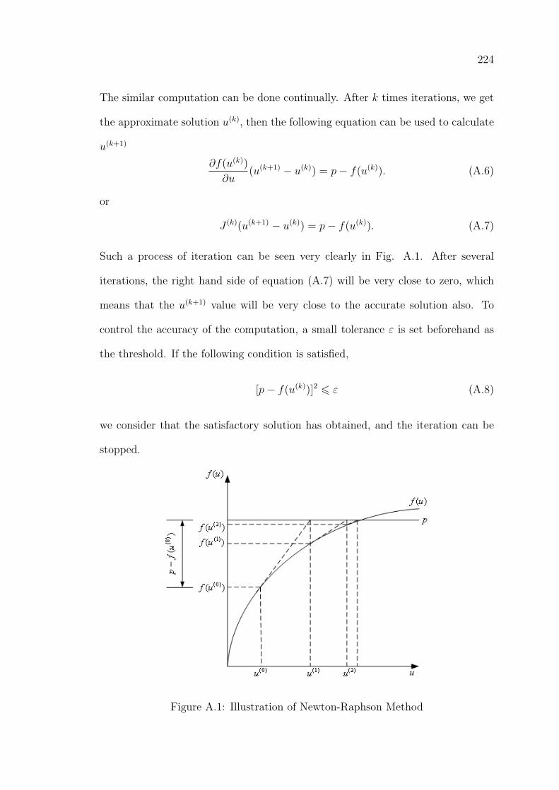
224
The similar computation can be done continually. After k times iterations, we get
the approximate solution u(k), then the following equation can be used to calculate
u(k+1)
∂f(u(k))
∂u(u(k+1) − u(k)) = p− f(u(k)). (A.6)
or
J (k)(u(k+1) − u(k)) = p− f(u(k)). (A.7)
Such a process of iteration can be seen very clearly in Fig. A.1. After several
iterations, the right hand side of equation (A.7) will be very close to zero, which
means that the u(k+1) value will be very close to the accurate solution also. To
control the accuracy of the computation, a small tolerance ε is set beforehand as
the threshold. If the following condition is satisfied,
[p− f(u(k))]2 6 ε (A.8)
we consider that the satisfactory solution has obtained, and the iteration can be
stopped.
Figure A.1: Illustration of Newton-Raphson Method
225
A.2 Application to a System of Equations
Based on the implementation of Newton-Raphson method to single nonlinear equa-
tion introduced above, we extend the application to a system of equations. Consider
a set of equations
[f ] = [K][X] = [Q], (A.9)
where [K] is the coefficient matrix, [X] is the matrix unknown variables and [Q] is
the matrix of known values. Then equation (A.9) can be rewritten as a group of
functions, which aref1 = K11X1 +K12X2 + . . .+K1nX1n = Q1
f2 = K21X1 +K22X2 + . . .+K2nX1n = Q2
. . .
fn = Kn1X1 +Kn2X2 + . . .+KnnX1n = Qn
(A.10)
Setting the initial value of [X] as [X](0), then we have
f(0)i =
n∑j=1
KijX(0)j , (i = 1, 2, . . . , n). (A.11)
Expanding every row of [f ] by a Taylor’s series and ignoring higher order terms,
following equations can be obtainedf1 = f
(0)1 +
∂f(0)1
∂X1(X
(1)1 −X
(0)1 ) +
∂f(0)1
∂X2(X
(1)2 −X
(0)2 ) + . . .+
∂f(0)1
∂Xn(X
(1)n −X
(0)n ) = Q1
f2 = f(0)2 +
∂f(0)2
∂X1(X
(1)1 −X
(0)1 ) +
∂f(0)2
∂X2(X
(1)2 −X
(0)2 ) + . . .+
∂f(0)2
∂Xn(X
(1)n −X
(0)n ) = Q2
. . . . . . . . . . . . . . .
fn = f(0)n + ∂f
(0)n
∂X1(X
(1)1 −X
(0)1 ) + ∂f
(0)n
∂X2(X
(1)2 −X
(0)2 ) + . . .+ ∂f
(0)n
∂Xn(X
(1)n −X
(0)n ) = Qn
(A.12)
When rewritten into matrix form it will become∂f
(0)1
∂X1
∂f(0)1
∂X2. . .
∂f(0)1
∂Xn
∂f(0)2
∂X1
∂f(0)2
∂X2. . .
∂f(0)2
∂Xn...
......
...∂f
(0)n
∂X1
∂f(0)n
∂X2. . . ∂f
(0)n
∂Xn
X
(1)1 −X
(0)1
X(1)2 −X
(0)2
...
X(1)n −X
(0)n
=
Q1 − f
(0)1
Q2 − f(0)2
...
Qn − f(0)n
(A.13)
or
[J ](0)([X](1) − [X](0)) = [Q]− [f ](0), (A.14)
226
where
[J ] =∂[f ]
∂[X]=
∂f1
∂X1
∂f1
∂X2. . . ∂f1
∂Xn∂f2
∂X1
∂f2
∂X2. . . ∂f2
∂Xn...
......
...∂fn
∂X1
∂fn
∂X2. . . ∂fn
∂Xn
(A.15)
is the Jacobian matrix. Using equation (A.14), we can get the value of ([X](1) −
[X](0)), thereby the value of [X](1)
[X](1) = [X](0) + [J ](0)−1[Q]− [f ](0) (A.16)
Take the value of [X](1) as initial value and repeat the above process described
in equations (A.12)-(A.16), the value of [X](2) can be calculated as
[X](2) = [X](1) + [J ](1)−1[Q]− [f ](1) (A.17)
Repeat the similar calculation process and after k iterations, the value of [X](k+1)
can be obtained by the following equation
[X](k+1) = [X](k) + [J ](k)−1[Q]− [f ](k) (A.18)
After several iterations, the term of [Q]− [f ](k) on the right hand side of equation
(A.18) will approach zero, which means the value of [X](k+1) will be very close to
the real solution. To control the accuracy of the approximate solution, a small
tolerance ε is set. At the kth iteration, when the criteria in equation (A.19) is met,
we think the result of this iteration is satisfactory for the approximation of solution
and the iteration can be stopped.
n∑i=1
(Qi − f(k)i )2 6 ε (A.19)
Appendix B
The Derivation of ∂B∂A
Recalling equation (4.19) and (4.20), the x and y component of the flux density in
one element are
Bx =1
2∆(b1A1 + b2A2 + b3A3) (B.1)
By = − 1
2∆(c1A1 + c2A2 + c3A3) (B.2)
and the flux density over the element is
B =√B2
x +B2y . (B.3)
Then the partial derivation of B with respect to Ai, (i = 1, 2, 3) is
∂B
∂Ai
|i=1,2,3 =1
2(B2
x +B2y)− 1
2 (2Bx∂Bx
∂Ai
+ 2By∂By
∂Ai
)
=1
B(Bx
∂Bx
∂Ai
+By∂By
∂Ai
)
=1
B(Bx
bi2∆
−Byci2∆
)
=1
B
[1
2∆(b1A1 + b2A2 + b3A3)
bi2∆
+1
2∆(c1A1 + c2A2 + c3A3)
ci2∆
]=
1
4∆2· 1
B[(b1bi + c1ci)A1 + (b2bi + c2ci)A2 + (b3bi + c3ci)A3] (B.4)
Therefore,
• when i = 1,
∂B
∂A1
=1
4∆2· 1
B
[(b21 + c21)A1 + (b2b1 + c2c1)A2 + (b3b1 + c3c1)A3
](B.5)
227
228
• when i = 2,
∂B
∂A2
=1
4∆2· 1
B
[(b1b2 + c1c2)A1 + (b22 + c22)A2 + (b3b2 + c3c2)A3
](B.6)
• when i = 3,
∂B
∂A3
=1
4∆2· 1
B
[(b1b3 + c1c3)A1 + (b2b3 + c2c3)A2 + (b23 + c23)A3
](B.7)
Recall equation (4.32) where
S11 = b21 + c21; S12 = b1b2 + c1c2; S13 = b1b3 + c1c3;
S21 = b2b1 + c2c1; S22 = b22 + c22; S23 = b2b3 + c2c3;
S31 = b3b1 + c3c1; S32 = b3b2 + c3c2; S33 = b23 + c23;
then equations (B.5)-(B.7) become
∂B
∂A1
=1
4∆2· 1
B· (S11A1 + S12A2 + S13A3)
∂B
∂A2
=1
4∆2· 1
B· (S21A1 + S22A2 + S23A3)
∂B
∂A3
=1
4∆2· 1
B· (S31A1 + S32A2 + S33A3) (B.8)
Let f1 = ν
4∆(S11A1 + S12A2 + S13A3)
f2 = ν4∆
(S21A1 + S22A2 + S23A3)
f3 = ν4∆
(S31A1 + S32A2 + S33A3)
(B.9)
or f1
f2
f3
=ν
4∆
S11 S12 S13
S21 S22 S23
S31 S32 S33
A1
A2
A3
, (B.10)
then equation (B.8) can be rewritten as
∂B
∂A1
=f1
Bν∆∂B
∂A2
=f2
Bν∆∂B
∂A3
=f3
Bν∆(B.11)
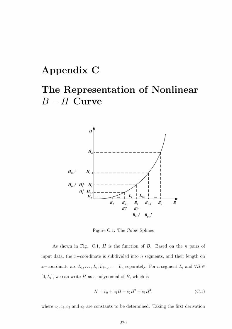
Appendix C
The Representation of NonlinearB −H Curve
Figure C.1: The Cubic Splines
As shown in Fig. C.1, H is the function of B. Based on the n pairs of
input data, the x−coordinate is subdivided into n segments, and their length on
x−coordinate are L1, . . . , Li, Li+1, . . . , Ln separately. For a segment Li and ∀B ∈
[0, Li], we can write H as a polynomial of B, which is
H = c0 + c1B + c2B2 + c3B
3, (C.1)
where c0, c1, c2 and c3 are constants to be determined. Taking the first derivation
229
230
on the both sides of the above equation, we can get
dH
dB= c1 + 2c2B + 3c3B
2. (C.2)
Substituting B = 0 and B = Li into equation C.1 and C.2 respectively and solving
the resulted 4 equations together, constants c0 ∼ c3 can be obtained asc0
c1
c2
c3
=
1 0 0 0
1 Li L2i L3
i
0 1 0 0
0 1 2Li 3L2i
−1
H0i
HLii
dH0i /dB
dHLii /dB
. (C.3)
Therefore,
H = (1− 3B2
L2i
+2B3
L3i
)H0i + (
3B2
L2i
− 2B3
)L3
i )HLii
+ (B − 2B2
Li
+B3
L2i
)dH0
i
dB+ (−B
2
Li
+B3
L2i
)dHLi
i
dB(C.4)
Taking the second derivation on the above equation yields
d2H
dB2= (− 6
L2i
+12B
L3i
)H0i + (
6
L2i
− 12B
L3i
)HLii
+ (− 4
Li
+6B
L2i
)dH0
i
dB+ (− 2
Li
+6B
L2i
)dHLi
i
dB.
As
d2HLii
dB2=d2H0
i+1
dB2
and
H0i = Hi−1, H
Lii = Hi
H0i+1 = Hi, H
Li+1
i+1 = Hi+1
the following equation can be obtained
2
Li
dHi−1
dB+
4
Li
dHi
dB+
4
Li+1
dHi
dB+
2
Li+1
dHi+1
dB=
6
L2i
(Hi −Hi−1) +6
L2i+1
(Hi+1 −Hi)
(C.5)
231
Consider boundary conditions
d2H01
dB2= 0,
d2HLnn
dB2= 0,
finally we can get equation C.6 from which the derivative coefficients dH/dB can
be calculated in terms of the values of H and B.
[LHS][dH/dB] = [RHS][H], (C.6)
where
[LHS] =
4L1
2L1
0 . . . . . . . . . . . .2
L1( 4
L1+ 4
L2) 2
L2. . . . . . . . . . . .
......
......
......
...
. . . . . . 2Li
( 4Li
+ 4Li+1
) 2Li+1
. . . . . ....
......
......
......
. . . . . . . . . . . . 2Ln−1
( 4Ln−1
+ 4Ln
) 2Ln
. . . . . . . . . . . . 0 2Ln
4Ln
[RHS] =
− 6L2
1
6L2
10 . . . . . . . . . . . .
− 6L2
1( 6
L21− 6
L22) 6
L22
. . . . . . . . . . . ....
......
......
......
. . . . . . − 6L2
i( 6
L2i− 6
L2i+1
) 6L2
i+1. . . . . .
......
......
......
...
. . . . . . . . . . . . − 6L2
n−1( 6
L2n−1
− 6L2
n) 6
L2n
. . . . . . . . . . . . 0 − 6L2
n
6L2
n
[dH/dB] =[dH0/dB dH1/dB . . . dHi−1/dB . . . dHn−1/dB dHn/dB
]tr
[dH/dB] =[H0 H1 . . . Hi−1 . . . Hn−1 Hn
]trAfter getting the values of [dH/dB], for a specific flux density value of B, the
corresponding value of dν/dB can be calculated by
dν
dB=dH
B
dB=
1
B
dH
dB− H
B2. (C.7)
Appendix D
The Method of BICG
After the assembly process of the finite element method, a large system of equa-
tions is generated. The number of unknowns involved in this system equations is
often several thousand. The bandwidth of the matrices is so large that the classi-
cal Gauss elimination algorithm and its modern variants are not efficient methods.
This suggests that the iterative methods should be used. The method used in
this work is the biconjugate gradient method (BICG). The method of BICG was
firstly described by Fletcher [147] for real nonsymmetric matrices and by Jacobs for
complex matrices [148]. The method has evolved many variations, such as CGS,
BiCGSTAB and QMR, each of which was specially designed to overcome some of
its inherent difficulties. However, BICG may still be competitive in terms of con-
vergence and convergence rates when compared with other methods [149].
Our concern is to get the solution of a system of real or complex linear
algebraic equations
Ax = b, (D.1)
where A is a nonsingular N × N matrix. x = (x1, . . . , xN)tr is the vector of un-
knowns, b = (b1, . . . , bN)tr and ()tr represents the transpose operation of a matrix.
The BICG algorithm for solving the linear system described in equation (D.1)
232
233
is implemented as
1. Input initial approximation x1;
2. Initialize
r1 = p1 = r1 = p1 = b− Ax1; (D.2)
and
ρ1 = rtr1 r1 (D.3)
3. For n = 1, 2 . . .
σn = ptrnApn (D.4)
αn =ρn
σn
(D.5)
rn+1 = rn − αnApn (D.6)
xn+1 = xn + αnpn (D.7)
rn+1 = rn − αnAtrpn (D.8)
ρn+1 = rtrn+1rn+1 (D.9)
βn+1 =ρn+1
ρn
(D.10)
pn+1 = rn+1 + βn+1pn (D.11)
pn+1 = rn+1 + βn+1pn (D.12)
end For

234
The sequence generated by the algorithm satisfies the following conditions:
rtrn rm = 0, ptr
nApm = 0, for(m 6= n) (D.13)
rn+1 is called the computed residual and it is equal to b − Axn+1. The iteration
process of BICG method described in equations (D.4)-(D.12) continues until the
residual is small enough.
Appendix E
The flowchart of the Field-CircuitCoupled Time Stepping FiniteElement Method
In Chapter 3, details of the time stepping finite element computation of the line-
start permanent magnet synchronous machine have been presented. The whole
process can be summarized by the flowchart shown in Fig. E.1.
235
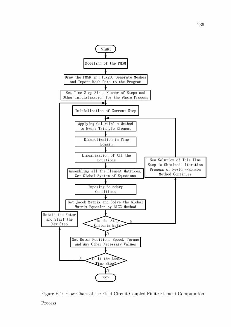
236
Figure E.1: Flow Chart of the Field-Circuit Coupled Finite Element Computation
Process

Appendix F
Motor Specifications andDimensions
1. PMSM Specifications
Table F.1: Ratings of the PMSM Used in This Research Work
Rated power (kW) 2.2
Rated speed (rpm) 1500
Rated voltage (line-to-line Vrms) 200
Rated current (Arms) 8.1
Number of phases 3
Number of poles 4
Number of stator slots 48
Number of rotor cage bars 40
Number of series turns per phase Ns 240
Winding connection Y
Winding layout Single layer
237
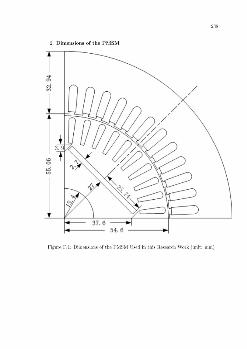
238
2. Dimensions of the PMSM
Figure F.1: Dimensions of the PMSM Used in this Research Work (unit: mm)
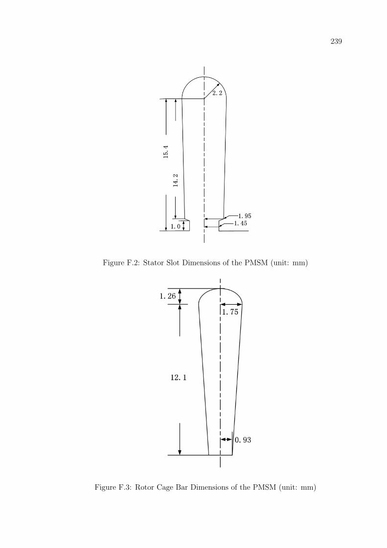
239
Figure F.2: Stator Slot Dimensions of the PMSM (unit: mm)
Figure F.3: Rotor Cage Bar Dimensions of the PMSM (unit: mm)
Appendix G
Determination of the B −HCharacteristic of the Stator Iron
The finite element solution program requires input material characteristics for all
magnetic materials in the part of pre-processing. All linear materials (air gap, spac-
ers, rotor bars and stator windings) are assigned the permeability of free space. The
solid rotor shaft is made by aluminium and has the permeability of free space. The
NdFeB permanent magnet is modelled with a straight line BH curve in the second
quadrant. The remanent flux density Br is 0.8 Tesla and the relative permeability
µr is 1.05.
Fig. G.1 shows the totoidal transformer used for testing BH characteristic
of motor core. The number of turns for primary winding is N1 = 576, the number
of turns for secondary winding is N2 = 116. The experimental data of I1 and V2
are shown in Table G.1. The computed BH data are shown in Table G.2.
240
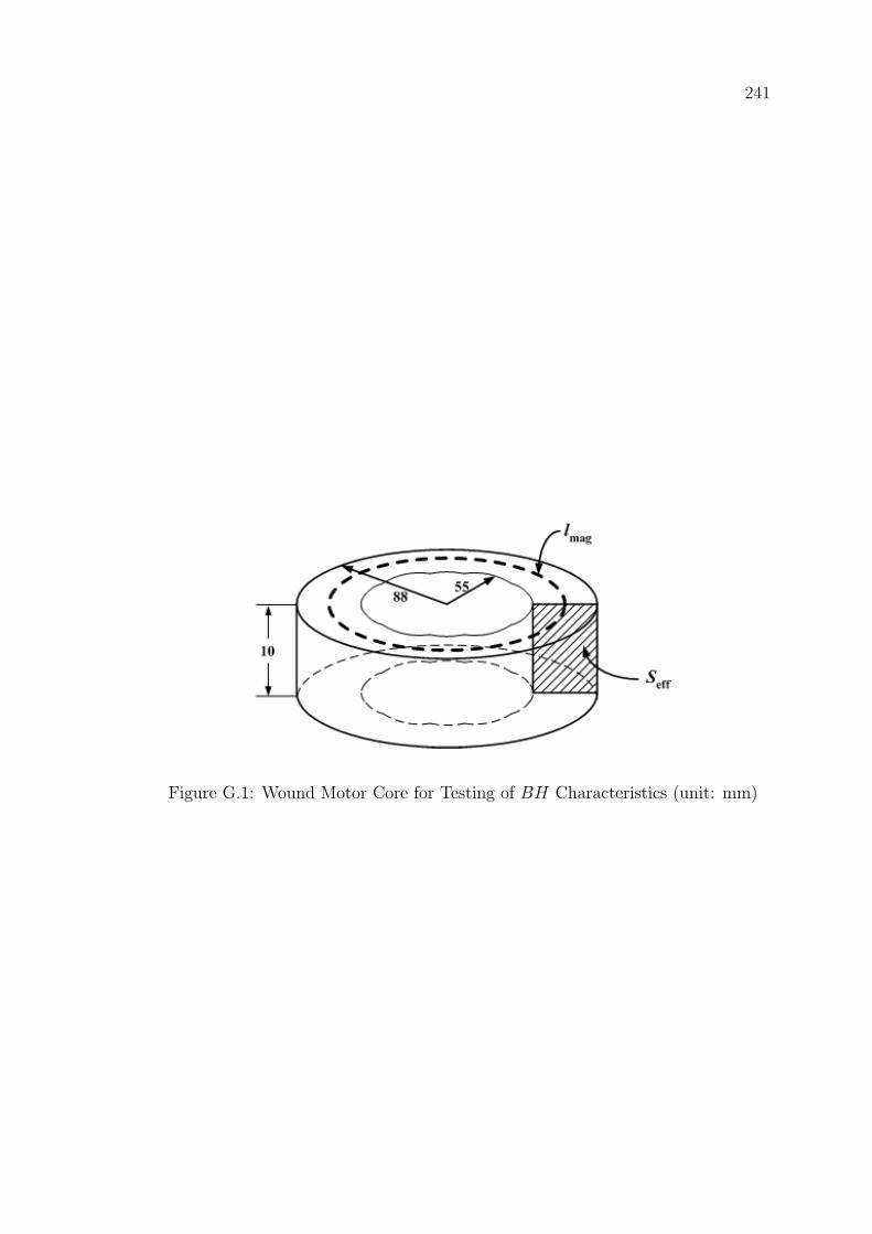
241
Figure G.1: Wound Motor Core for Testing of BH Characteristics (unit: mm)
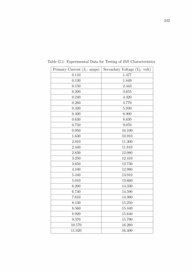
242
Table G.1: Experimental Data for Testing of BH Characteristics
Primary Current (I1: amps) Secondary Voltage (V2: volt)
0.110 1.477
0.130 1.849
0.150 2.443
0.200 3.655
0.240 4.320
0.260 4.770
0.320 5.930
0.400 6.900
0.630 8.630
0.750 9.070
0.950 10.100
1.630 10.910
2.010 11.300
2.440 11.810
2.830 12.080
3.250 12.410
3.650 12.730
4.100 12.980
5.440 13.910
5.010 13.660
6.200 14.330
6.740 14.590
7.610 14.990
8.130 15.250
8.560 15.440
8.920 15.640
9.370 15.790
10.570 16.260
11.020 16.400
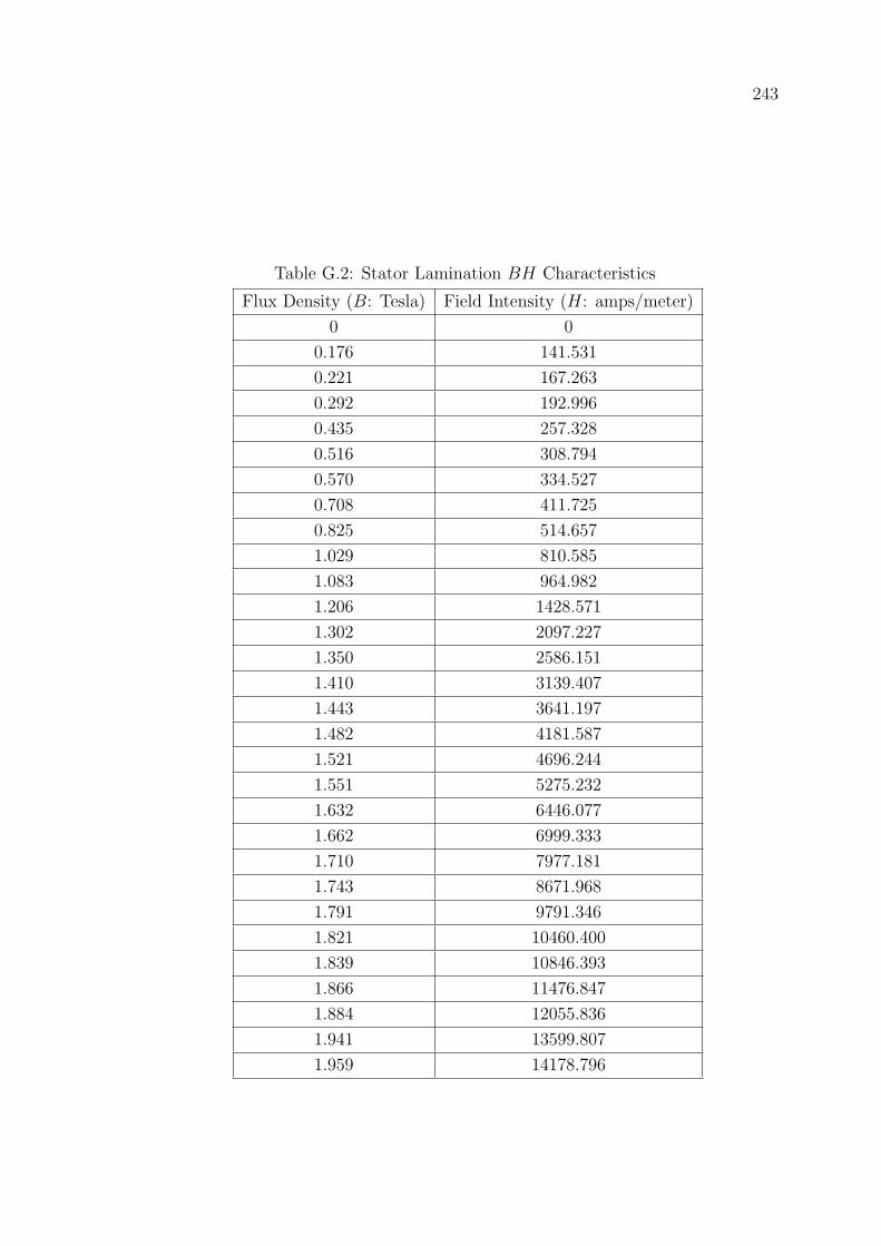
243
Table G.2: Stator Lamination BH Characteristics
Flux Density (B: Tesla) Field Intensity (H: amps/meter)
0 0
0.176 141.531
0.221 167.263
0.292 192.996
0.435 257.328
0.516 308.794
0.570 334.527
0.708 411.725
0.825 514.657
1.029 810.585
1.083 964.982
1.206 1428.571
1.302 2097.227
1.350 2586.151
1.410 3139.407
1.443 3641.197
1.482 4181.587
1.521 4696.244
1.551 5275.232
1.632 6446.077
1.662 6999.333
1.710 7977.181
1.743 8671.968
1.791 9791.346
1.821 10460.400
1.839 10846.393
1.866 11476.847
1.884 12055.836
1.941 13599.807
1.959 14178.796
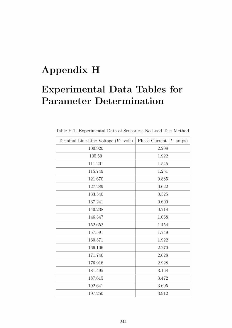
Appendix H
Experimental Data Tables forParameter Determination
Table H.1: Experimental Data of Sensorless No-Load Test Method
Terminal Line-Line Voltage (V : volt) Phase Current (I: amps)
100.920 2.298
105.59 1.922
111.201 1.545
115.749 1.251
121.670 0.885
127.289 0.622
133.540 0.525
137.241 0.600
140.238 0.718
146.347 1.068
152.652 1.454
157.591 1.749
160.571 1.922
166.106 2.270
171.746 2.628
176.916 2.928
181.495 3.168
187.615 3.472
192.641 3.695
197.250 3.912
244
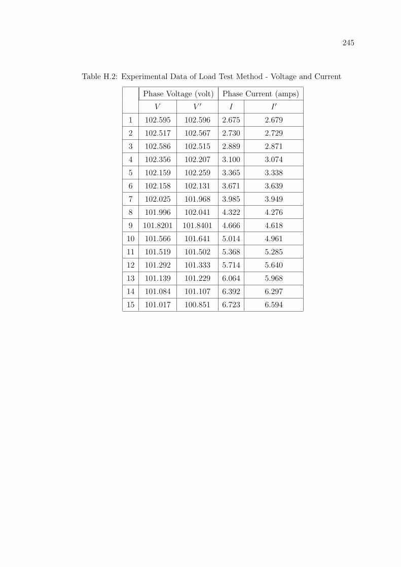
245
Table H.2: Experimental Data of Load Test Method - Voltage and Current
Phase Voltage (volt) Phase Current (amps)
V V ′ I I ′
1 102.595 102.596 2.675 2.679
2 102.517 102.567 2.730 2.729
3 102.586 102.515 2.889 2.871
4 102.356 102.207 3.100 3.074
5 102.159 102.259 3.365 3.338
6 102.158 102.131 3.671 3.639
7 102.025 101.968 3.985 3.949
8 101.996 102.041 4.322 4.276
9 101.8201 101.8401 4.666 4.618
10 101.566 101.641 5.014 4.961
11 101.519 101.502 5.368 5.285
12 101.292 101.333 5.714 5.640
13 101.139 101.229 6.064 5.968
14 101.084 101.107 6.392 6.297
15 101.017 100.851 6.723 6.594
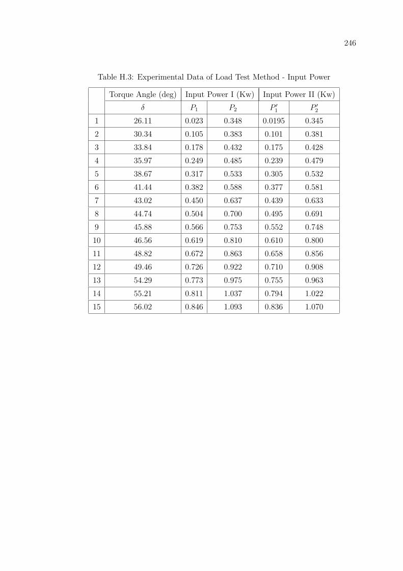
246
Table H.3: Experimental Data of Load Test Method - Input Power
Torque Angle (deg) Input Power I (Kw) Input Power II (Kw)
δ P1 P2 P ′1 P ′2
1 26.11 0.023 0.348 0.0195 0.345
2 30.34 0.105 0.383 0.101 0.381
3 33.84 0.178 0.432 0.175 0.428
4 35.97 0.249 0.485 0.239 0.479
5 38.67 0.317 0.533 0.305 0.532
6 41.44 0.382 0.588 0.377 0.581
7 43.02 0.450 0.637 0.439 0.633
8 44.74 0.504 0.700 0.495 0.691
9 45.88 0.566 0.753 0.552 0.748
10 46.56 0.619 0.810 0.610 0.800
11 48.82 0.672 0.863 0.658 0.856
12 49.46 0.726 0.922 0.710 0.908
13 54.29 0.773 0.975 0.755 0.963
14 55.21 0.811 1.037 0.794 1.022
15 56.02 0.846 1.093 0.836 1.070

247
Table H.4: Results of Load Test Method
Stator Current (ampere) Xd (ohm) Xq (ohm) E0 (volt)
1 2.677 2.060 21.771 87.090
2 2.729 6.960 21.153 78.701
3 2.880 12.256 20.467 75.083
4 3.087 -11.041 19.484 82.557
5 3.352 7.898 18.959 79.008
6 3.655 11.651 18.605 81.856
7 3.967 3.708 17.937 75.587
8 4.299 1.770 17.414 71.849
9 4.642 2.540 17.025 71.491
10 4.988 26.807 15.689 124.160
11 5.327 12.048 15.783 94.074
12 5.677 1.247 15.240 65.586
13 6.016 6.254 16.170 77.437
14 6.345 3.459 15.778 67.111
15 6.658 13.123 15.210 106.678
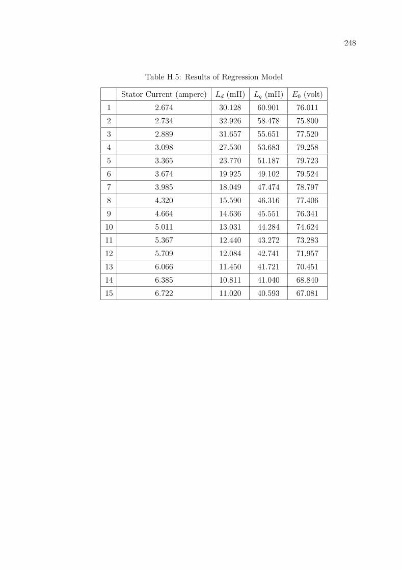
248
Table H.5: Results of Regression Model
Stator Current (ampere) Ld (mH) Lq (mH) E0 (volt)
1 2.674 30.128 60.901 76.011
2 2.734 32.926 58.478 75.800
3 2.889 31.657 55.651 77.520
4 3.098 27.530 53.683 79.258
5 3.365 23.770 51.187 79.723
6 3.674 19.925 49.102 79.524
7 3.985 18.049 47.474 78.797
8 4.320 15.590 46.316 77.406
9 4.664 14.636 45.551 76.341
10 5.011 13.031 44.284 74.624
11 5.367 12.440 43.272 73.283
12 5.709 12.084 42.741 71.957
13 6.066 11.450 41.721 70.451
14 6.385 10.811 41.040 68.840
15 6.722 11.020 40.593 67.081
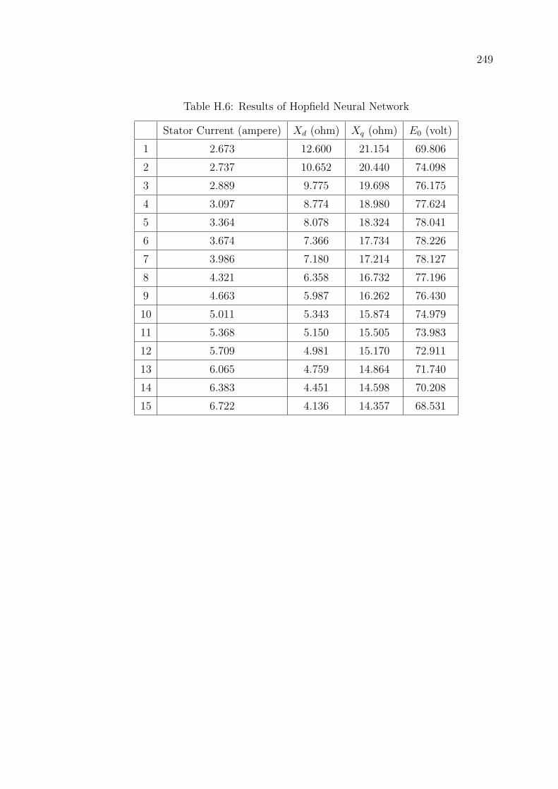
249
Table H.6: Results of Hopfield Neural Network
Stator Current (ampere) Xd (ohm) Xq (ohm) E0 (volt)
1 2.673 12.600 21.154 69.806
2 2.737 10.652 20.440 74.098
3 2.889 9.775 19.698 76.175
4 3.097 8.774 18.980 77.624
5 3.364 8.078 18.324 78.041
6 3.674 7.366 17.734 78.226
7 3.986 7.180 17.214 78.127
8 4.321 6.358 16.732 77.196
9 4.663 5.987 16.262 76.430
10 5.011 5.343 15.874 74.979
11 5.368 5.150 15.505 73.983
12 5.709 4.981 15.170 72.911
13 6.065 4.759 14.864 71.740
14 6.383 4.451 14.598 70.208
15 6.722 4.136 14.357 68.531
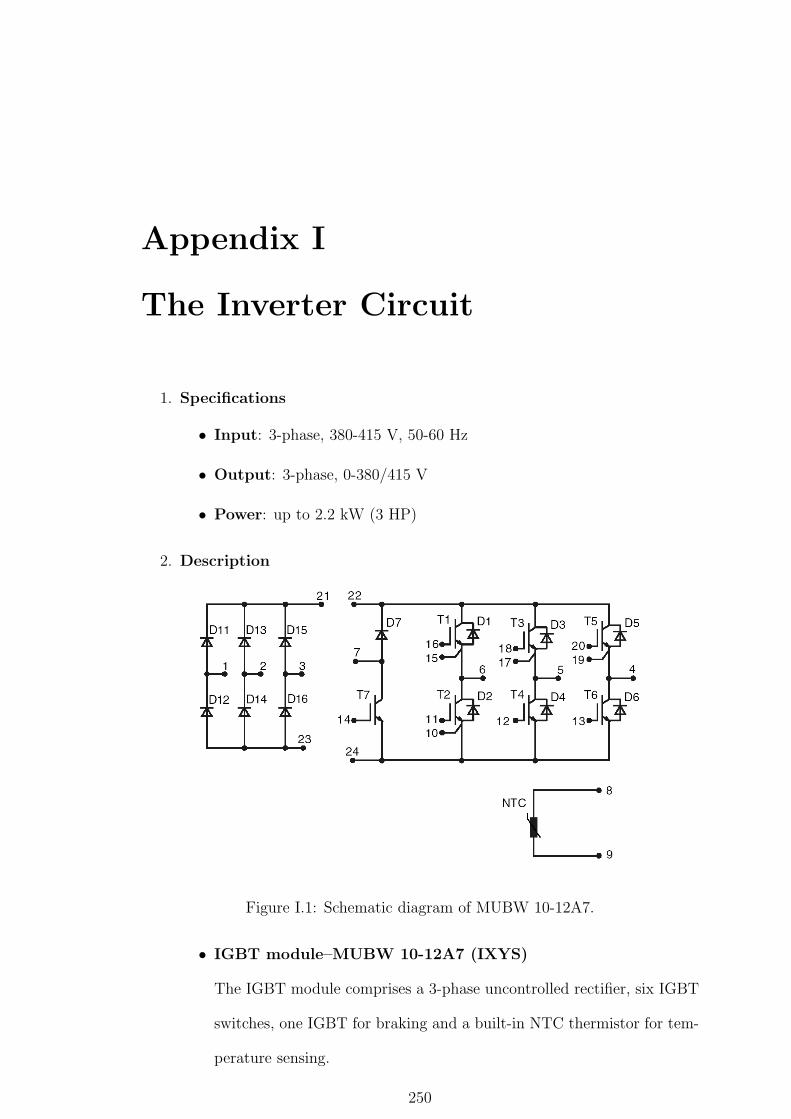
Appendix I
The Inverter Circuit
1. Specifications
• Input: 3-phase, 380-415 V, 50-60 Hz
• Output: 3-phase, 0-380/415 V
• Power: up to 2.2 kW (3 HP)
2. Description
Figure I.1: Schematic diagram of MUBW 10-12A7.
• IGBT module–MUBW 10-12A7 (IXYS)
The IGBT module comprises a 3-phase uncontrolled rectifier, six IGBT
switches, one IGBT for braking and a built-in NTC thermistor for tem-
perature sensing.
250
251
• DC-link capacitors & transformer board
Fig. I.1 shows the schematic diagram of IXYS module. The DC-link
capacitor is connected across pins 22-23. An NTC thermistor is con-
nected in between pins 21-22 to limit the in-rush current. A low ohmic
shunt is connected in between pins 23-24 for over-current sensing. Two
resistor are connected in series across pins 22-24 as a voltage divider for
over-voltage sensing. The transformers are powered from single-phase
mains and provide floating power sources to the driver board.
• Driver board
The driver board comprises voltage regulators (78L15), opto-couplers
(HCPL4503, H11L1), gate drivers (TC4429), braking control and pro-
tection circuits. The connections in between the driver board and the
IGBT module or transformer board are made by wires of twisted pairs.
The driver board is connected with the Control-PWM Card via a shield
flat-ribbon cable.
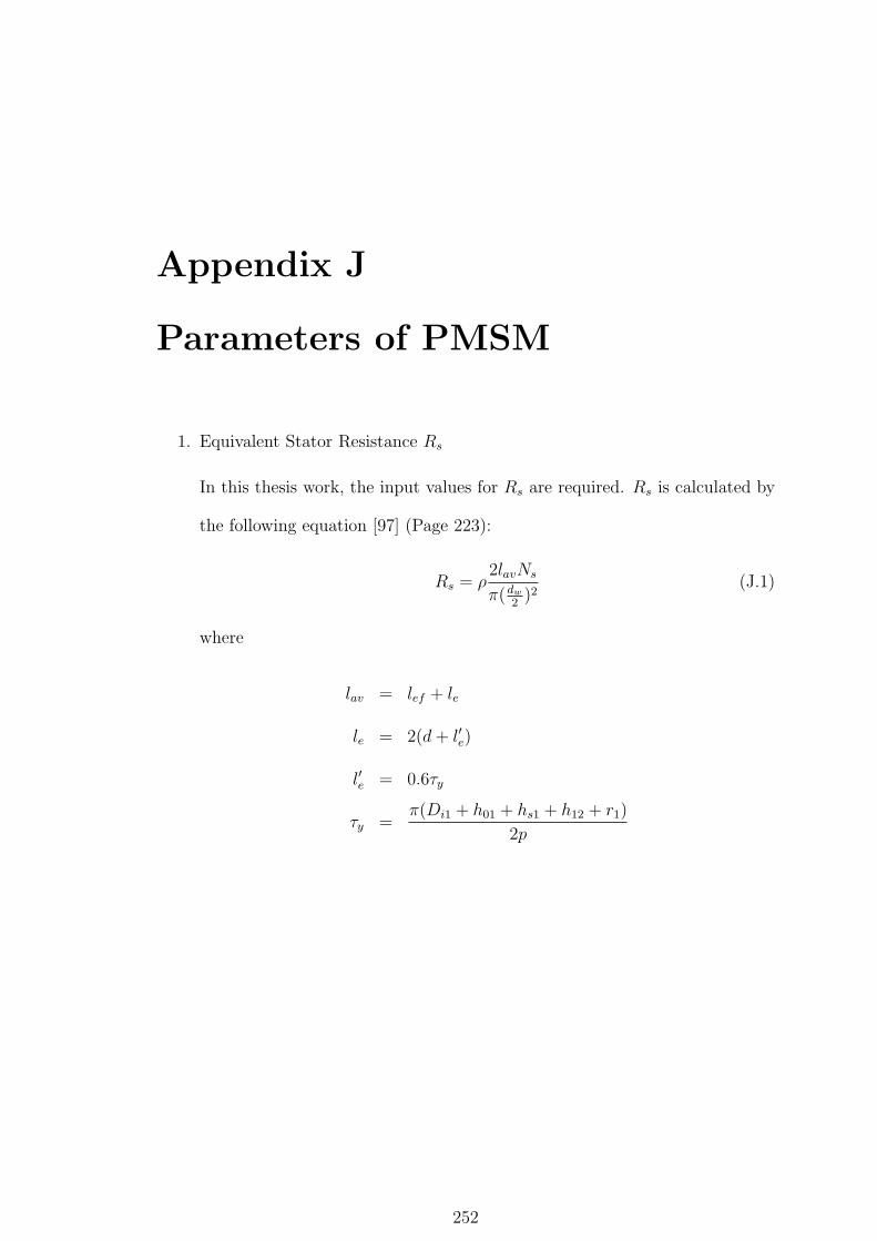
Appendix J
Parameters of PMSM
1. Equivalent Stator Resistance Rs
In this thesis work, the input values for Rs are required. Rs is calculated by
the following equation [97] (Page 223):
Rs = ρ2lavNs
π(dw
2)2
(J.1)
where
lav = lef + le
le = 2(d+ l′e)
l′e = 0.6τy
τy =π(Di1 + h01 + hs1 + h12 + r1)
2p
252

253
The definition of h01, hs1, h12 and r1 were shown in Fig. J.1, and
ρ resistivity of stator windings
dw diameter of the coil
lef axil length of stator
Ns equivalent number of turns per phase
p number of pole pairs
d extension length of windings
Di1 inner diameter of the stator
The calculated Rs value for the PMSM is 1.1430Ω per phase. The measured
Rs value is 0.8Ω per phase.
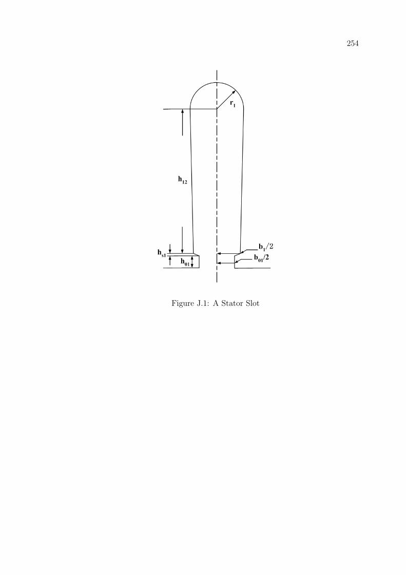
254
Figure J.1: A Stator Slot
255
2. Inductance of Stator End-Windings Le
The reactance of stator end-windings Xe1 was calculated first and Le =
Xe1/ωe, where ωe is the angular synchronous speed of the PMSM. Xe was
calculated by the following equation [97] (Page 225):
Xe1 = 0.67(le − 0.64τylefK2
dp
)Cx (J.2)
where
Cx =4πfµ0lef (KdpNs)
2
p
Kdp = Kd ·Kp ·Ks
and
µ0 magnetic permeability in free space
f synchronous frequency
Kd winding distribution factor
Kp winding pitch factor
Ks skew factor
The calculated value of end-winding inductance is
Le = 8.496× 10⁻⁴H (J.3)
256
3. End-Ring Resistance Rek
The end-ring resistance Rek is calculated by [150] (Page 395):
Rek =ρRlRAR
1
(2 sin πpQ2
)2(J.4)
where
lR = 0.7πDR
Q2
and
Q2 number of rotor slots
ρR resistivity of the end ring
DR average diameter of the end ring
AR cross section area of the end ring
The calculated value of end-ring resistance is
Rek = 4.536× 10⁻⁶Ω (J.5)

257
4. End-Ring Inductance Lek
The end-ring inductance is calculated by [150] (Page 389):
Lek = µ0Q2
m1p× 2
3[(lB − l2) + ς
πDR
2p] (J.6)
where
m1 number of phases
lB axil length of the rotor bar
l2 axil length of rotor iron core
ς = 0.18 for p > 1
The calculated value of end-ring inductance is
Lek = 8.994× 10⁻⁸H (J.7)
Appendix K
Determination of Moment ofInertia and the Coefficient ofFriction
The movement of the rotor is governed by :
Jrdωm(t)
dt= Tem − Tf −Dωm(t), (K.1)
where Jr is the moment of inertia of the rotor, ωm is the mechanical motor speed,
Tem is the electromagnetic torque, Tf is the load torque, D is friction coefficient and
t is time. In order to compute the dynamic performances of the PMSM involving
the rotor movement, the parameters of Jr and D have to be determined. In this
work, both of these two parameters are determined by simple experiments.
1. Determination of D
Under no load condition, equation K.1 can be rewritten as
Jrdωm(t)
dt= Tem −Dωm(t). (K.2)
With the initial condition of ωm(0) = 0, the solution of equation K.2 is
ωm(t) =Tem
D(1− e−
DJr
t). (K.3)
Therefore, when t = ∞, ωm(t) = Tem/D. In other words, mathematically,
if we apply a torque of Tem to the rotor, with infinitely long time, the final
speed of the rotor is Tem/D. So if we can know Tem and ωm(t = ∞), D will
be attainable.
258
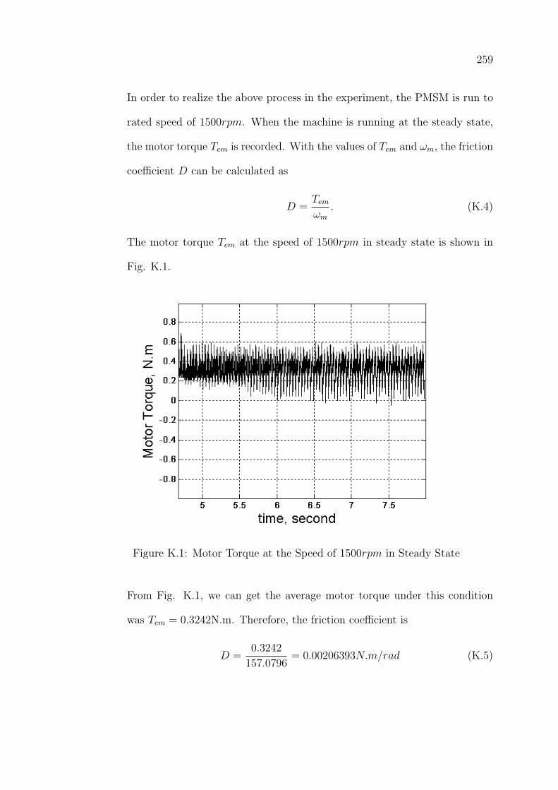
259
In order to realize the above process in the experiment, the PMSM is run to
rated speed of 1500rpm. When the machine is running at the steady state,
the motor torque Tem is recorded. With the values of Tem and ωm, the friction
coefficient D can be calculated as
D =Tem
ωm
. (K.4)
The motor torque Tem at the speed of 1500rpm in steady state is shown in
Fig. K.1.
Figure K.1: Motor Torque at the Speed of 1500rpm in Steady State
From Fig. K.1, we can get the average motor torque under this condition
was Tem = 0.3242N.m. Therefore, the friction coefficient is
D =0.3242
157.0796= 0.00206393N.m/rad (K.5)
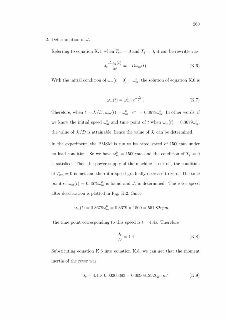
260
2. Determination of Jr
Referring to equation K.1, when Tem = 0 and Tf = 0, it can be rewritten as
Jrdωm(t)
dt= −Dωm(t). (K.6)
With the initial condition of ωm(t = 0) = ω0m, the solution of equation K.6 is
ωm(t) = ω0m · e−
DJr
t. (K.7)
Therefore, when t = Jr/D, ωm(t) = ω0m · e−1 = 0.3679ω0
m. In other words, if
we know the initial speed ω0m and time point of t when ωm(t) = 0.3679ω0
m,
the value of Jr/D is attainable, hence the value of Jr can be determined.
In the experiment, the PMSM is run to its rated speed of 1500rpm under
no load condition. So we have ω0m = 1500rpm and the condition of Tf = 0
is satisfied. Then the power supply of the machine is cut off, the condition
of Tem = 0 is met and the rotor speed gradually decrease to zero. The time
point of ωm(t) = 0.3679ω0m is found and Jr is determined. The rotor speed
after deceleration is plotted in Fig. K.2. Since
ωm(t) = 0.3679ω0m = 0.3679× 1500 = 551.82rpm,
the time point corresponding to this speed is t = 4.4s. Therefore
Jr
D= 4.4 (K.8)
Substituting equation K.5 into equation K.8, we can get that the moment
inertia of the rotor was
Jr = 4.4× 0.00206393 = 0.009081292kg ·m2 (K.9)
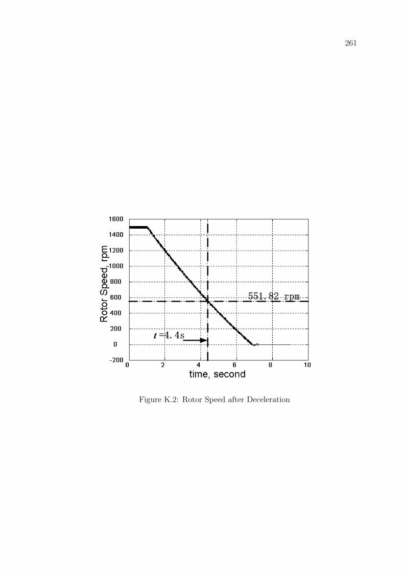
261
Figure K.2: Rotor Speed after Deceleration
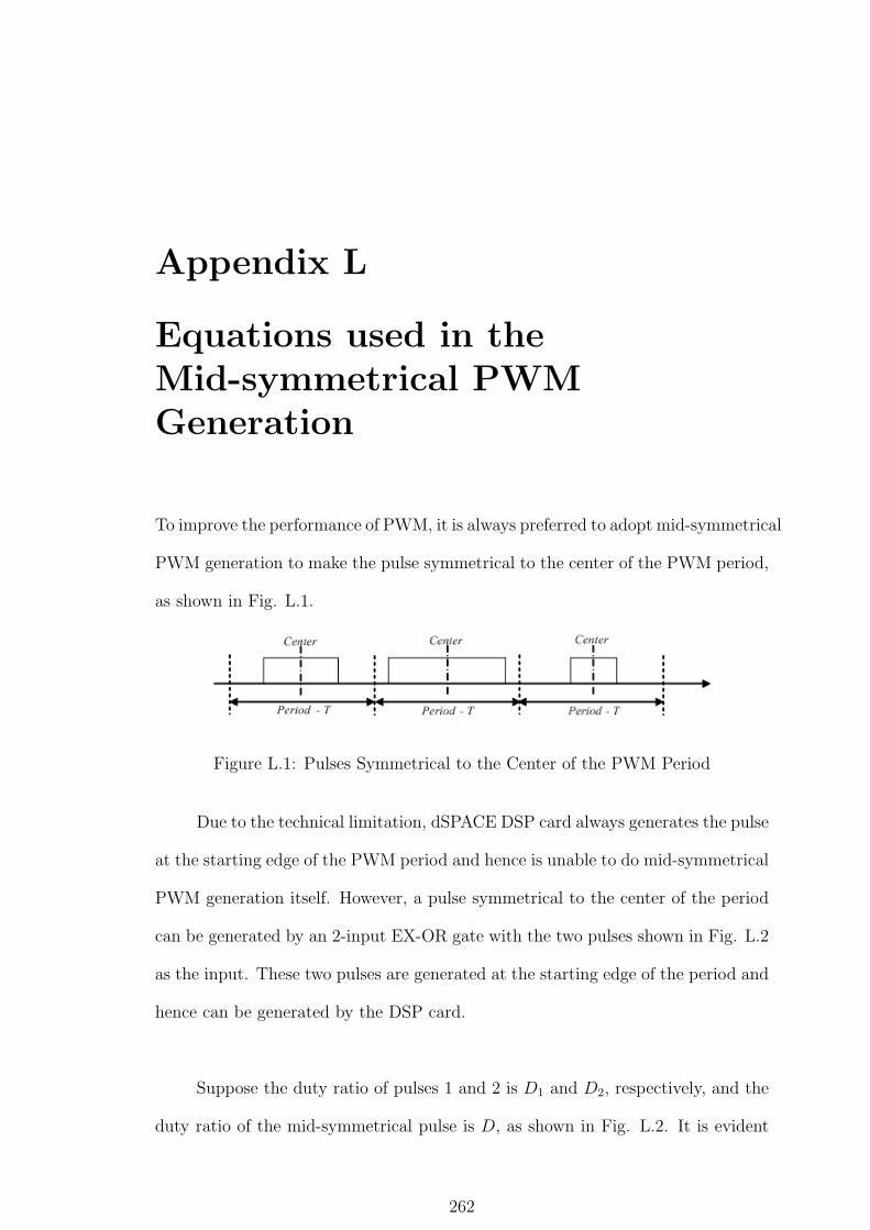
Appendix L
Equations used in theMid-symmetrical PWMGeneration
To improve the performance of PWM, it is always preferred to adopt mid-symmetrical
PWM generation to make the pulse symmetrical to the center of the PWM period,
as shown in Fig. L.1.
Figure L.1: Pulses Symmetrical to the Center of the PWM Period
Due to the technical limitation, dSPACE DSP card always generates the pulse
at the starting edge of the PWM period and hence is unable to do mid-symmetrical
PWM generation itself. However, a pulse symmetrical to the center of the period
can be generated by an 2-input EX-OR gate with the two pulses shown in Fig. L.2
as the input. These two pulses are generated at the starting edge of the period and
hence can be generated by the DSP card.
Suppose the duty ratio of pulses 1 and 2 is D1 and D2, respectively, and the
duty ratio of the mid-symmetrical pulse is D, as shown in Fig. L.2. It is evident
262
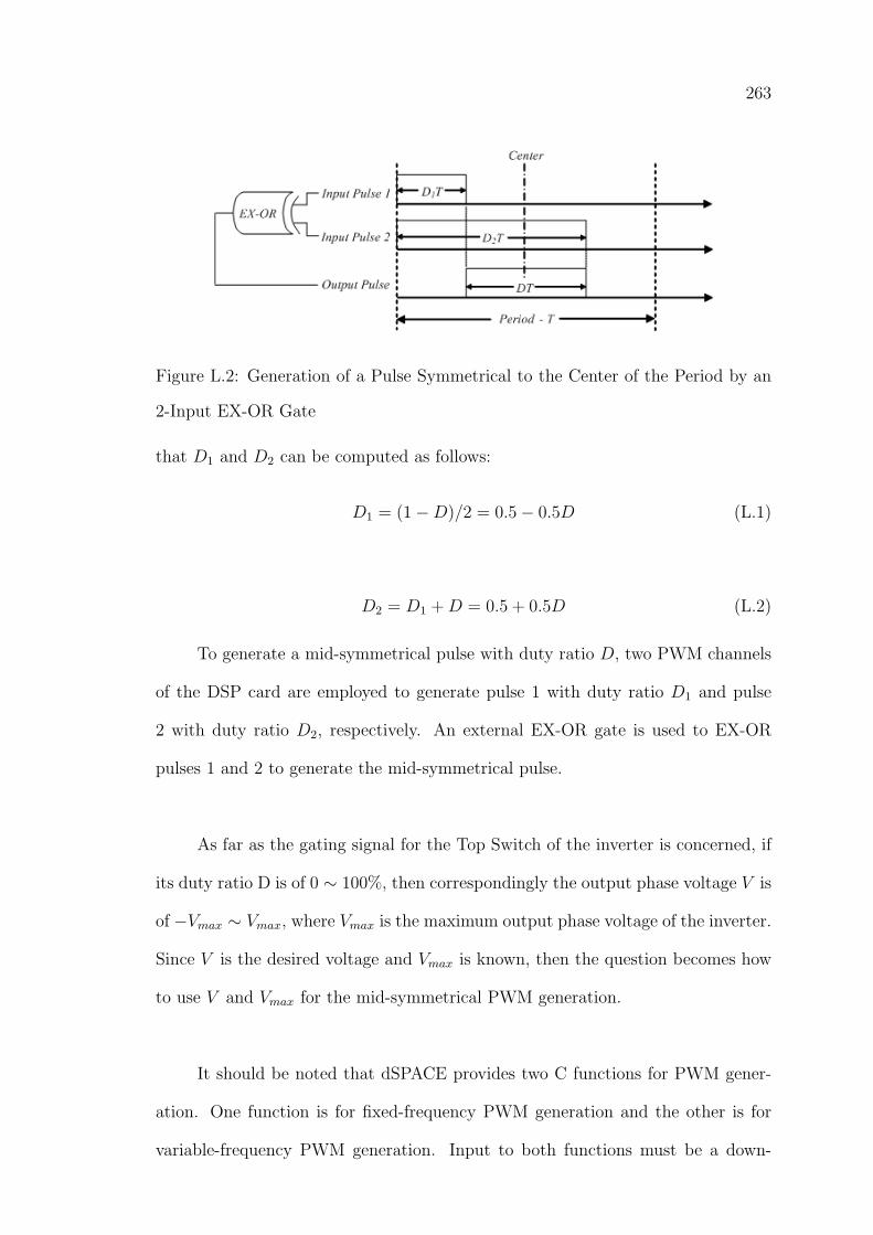
263
Figure L.2: Generation of a Pulse Symmetrical to the Center of the Period by an
2-Input EX-OR Gate
that D1 and D2 can be computed as follows:
D1 = (1−D)/2 = 0.5− 0.5D (L.1)
D2 = D1 +D = 0.5 + 0.5D (L.2)
To generate a mid-symmetrical pulse with duty ratio D, two PWM channels
of the DSP card are employed to generate pulse 1 with duty ratio D1 and pulse
2 with duty ratio D2, respectively. An external EX-OR gate is used to EX-OR
pulses 1 and 2 to generate the mid-symmetrical pulse.
As far as the gating signal for the Top Switch of the inverter is concerned, if
its duty ratio D is of 0 ∼ 100%, then correspondingly the output phase voltage V is
of −Vmax ∼ Vmax, where Vmax is the maximum output phase voltage of the inverter.
Since V is the desired voltage and Vmax is known, then the question becomes how
to use V and Vmax for the mid-symmetrical PWM generation.
It should be noted that dSPACE provides two C functions for PWM gener-
ation. One function is for fixed-frequency PWM generation and the other is for
variable-frequency PWM generation. Input to both functions must be a down-
264
scaled value, but the ranges of the scaling for the two functions are different.
For fixed-frequency PWM generation, the input to the C function should be
scaled down within −1 ∼ 1, which is corresponding to duty ratio of 0 ∼ 100%. For
variable-frequency PWM generation, the input to the C function should be scaled
down within 0 ∼ 1, which is corresponding to duty ratio of 0 ∼ 100%. The Simulink
block for PWM channels given by RTI of dSPACE is for variable-frequency PWM
generation, hence requires its input to be scaled down within 0 ∼ 1.
To use V and Vmax for PWM generation, define a variable u in terms of V
and Vmax. For fixed-frequency PWM generation, u = V/Vmax so that u is within
−1 ∼ 1. For variable-frequency PWM generation, u = 0.5(1 + V/Vmax) so that
u is within 0 ∼ 1. If conventional PWM generation would be used, then u could
directly be used by the C function/Simulink block as input. The duty ratio D is
hence as follows:
• For fixed-frequency PWM generation:D = 0.5(1 + u)
• For variable-frequency PWM generation: D = u
However, to carry out mid-symmetrical PWM generation, u is not used di-
rectly as the input but split into two components, which are then used by the C
function / Simulink block as the inputs. Let them be u1 and u2 corresponding to
duty ratio D1 and D2, respectively.
1. For fixed-frequency PWM generation, since the input of −1 ∼ 1 is corre-
sponding to duty ratio of 0 ∼ 100%, then it can be known that:
D1 = 0.5(1 + u1) (L.3)
D2 = 0.5(1 + u2) (L.4)
265
Substituting equations (L.3) and (L.4) into equations (L.1) and (L.2), we can
get
u1 = −0.5− 0.5u (L.5)
u2 = 0.5 + 0.5u (L.6)
2. For variable-frequency PWM generation, since the input of 0 ∼ 1 is corre-
sponding to duty ratio of 0 ∼ 100%, then it can be known that:
D1 = u1 (L.7)
D2 = u2 (L.8)
Substituting equations (L.3) and (L.4) into equations (L.1) and (L.2), we can
get
u1 = 0.5− 0.5uu2 = 0.5 + 0.5u (L.9)