COMPLEXITY AND AESTHETIC PREFERENCE

FOR DIVERSE VISUAL STIMULI

DOCTORAL THESIS

AUTHOR: Marcos Nadal Roberts

DIRECTOR: Camilo José Cela Conde and Gisèle Marty

Departament de Psicologia

Universitat de les Illes Balears

2007

i

Contents

Presentation ...................................................................................................................iv

1. Introduction...............................................................................................................1

1.1. The study of the determinants of aesthetic preference

during the initial period of experimental aesthetics ..........................................2

1.1.1. The birth of a new field: The work

of Gustav Fechner................................................................................3

1.1.2. Birkhoff’s aesthetic measure.....................................................8

1.1.3. Eysenck’s measure of aesthetic preference.............................10

1.2. The study of the determinants of aesthetic preference since

the “new experimental aesthetics” ......................................................................13

1.2.1. The framework created by Daniel Berlyne .............................14

1.2.2. Testing Berlyne’s hypothesis ....................................................19

1.2.3. The concept of complexity and its measure...........................47

1.2.4. Criticisms to Berlyne’s framework...........................................61

1.3. Aesthetic preference ......................................................................................71

1.3.1. Cognitive processes involved in aesthetic preference ...........72

1.3.2. The dimensional nature of aesthetic preference ....................77

1.3.3. The influence of personality traits and cognitive styles ........95

1.3.4. The influence of art training.....................................................114

1.3.5. The influence of sex...................................................................134

ii

1.4. Summary, objectives, and hypotheses.........................................................144

2. Method ......................................................................................................................149

2.1. Participants .....................................................................................................150

2.1.1. Description of the sample of participants involved

in the preparation of the materials ......................................................151

2.1.2. Description of the sample of participants involved

in the actual testing of our hypotheses ...............................................154

2.2. Materials ..........................................................................................................157

2.2.1. Stimuli ...........................................................................................158

2.2.2. Stimuli selection and modification............................................159

2.2.3. Hardware and software ..............................................................159

2.3. Procedure ........................................................................................................162

2.3.1. Creation of a suitable set of stimuli ..........................................163

2.3.2. Aesthetic preference ...................................................................165

2.3.3. Dimensions of visual complexity ..............................................167

3. Results ......................................................................................................................175

3.1. Creation of three complexity levels .............................................................176

3.2. The influence of independent variables on aesthetic preference.............184

3.2.1. Descriptive statistics ..................................................................185

3.2.2. Analyses of main effects and interactions...............................194

3.3. The concept of visual complexity................................................................208

3.3.1. Discriminant analyses ................................................................211

3.3.2. Factor analysis ............................................................................241

3.3.3. Exploratory study of the relation between

complexity dimensions and beauty ratings........................................251

iii

4. Discussion..................................................................................................................263

4.1. The influence of complexity on aesthetic preference ...............................264

4.2. The concept of complexity...........................................................................269

4.2.1. Relevance of complexity dimensions

for complexity judgments.....................................................................271

4.2.2. Relations among complexity dimensions.................................272

4.2.3. Relation between complexity dimensions

and beauty ratings..................................................................................274

4.3. General conclusions ......................................................................................278

Resumen (Spanish summary) ......................................................................................281

1. Introducción ......................................................................................................282

2. Método ...............................................................................................................291

3. Resultados ..........................................................................................................303

4. Discusión............................................................................................................323

References ......................................................................................................................337

Annex A ......................................................................................................................359

Annex B ......................................................................................................................381

Annex C ......................................................................................................................399

Annex D ......................................................................................................................417

iv

Presentation

Even a superficial familiarity with the field of empirical aesthetics is enough

to realize that there is a considerable amount of conceptual confusion. For

instance, aesthetic judgment and aesthetic preference are often used with no prior explicit

definition. Whereas some authors seem to consider that they are interchangeable,

others consider that they should be used to designate different phenomena. In the

present work I have chosen to follow McWhinnie's (1968) criterion of using

aesthetic preference to refer to the degree with which people like a particular visual

stimulus or not, how much they prefer it to another, or how they rate its beauty.

Conversely, aesthetic judgment will be used to refer to the assessment someone does

of the aesthetic or artistic value of a certain visual stimulus. Whereas the goodness

of someone’s aesthetic judgment can be gauged using external criteria provided by

expert’s appraisals –though these have certainly varied throughout history-, there

can be no yardstick to determine how “good” someone’s aesthetic preference is,

given that it is an entirely subjective and personal matter. Finally, aesthetic

appreciation will be used to refer to the human capacity to divide the world into

beautiful and ugly things, to prefer a blue car to a red one, and to like blond men

more than others. We believe that this capacity was present at least at the time of

our species’ birth, though it probably built on pre-existing cognitive and affective

processes. It led the first Homo sapiens to decorate their bodies and to make

necklaces, enabled our upper Palaeolithic ancestors to create breath-taking murals

on cave walls, drove Michelangelo to sculpt David, and allows us to admire all of

this. But it also allowed our ancestors to avoid settling in resourceless

environments, feeling attracted by sick-looking people, and it allows us to avoid

living in bare-walled houses, and wearing brown with red.

v

The work presented here, structured as a standard journal paper, is mostly

concerned with aesthetic preference for visual stimuli, though there are many

previous studies on aesthetic judgment and aesthetic appreciation which cast light

on how people develop aesthetic preferences for visual stimuli. In fact, the

question of the factors that govern these preferences is one of the oldest in the

field of empirical aesthetics, and one of its chiefs objectives has been to articulate a

sort of predictive mathematical formula that describes an underlying relation

between certain attributes of visual stimuli and people’s reaction to them. After

briefly reviewing early attempts to formulate this relation, we will present Daniel

Berlyne’s framework, which stimulated research in the field since the 1970s. The

main aim of our work is to explore the reasons behind the divergence of results

obtained by studies attempting to verify Berlyne’s predicted relation between

complexity and aesthetic preference. We look at three main possibilities: (i) studies

have varied as to the proportion of male and female participants, (ii) studies have

used different kinds of stimuli (abstract, representational, artistic, geometric

figures, and so on), (iii) studies have used different measures of complexity. As we

mentioned, we are concerned solely with visual stimuli. Generalization of our

results to auditory stimuli could be possible, though we have left this interesting

issue for a later occasion.

Carrying out this project has been satisfying and thrilling most of the time,

and disheartening at certain moments. However, I am sure it would not have been

completed without the help and encouragement from my colleagues at the

Deparatment de Psicologia and the Departament de Filosofia i Treball Social at the

Universitat de les Illes Balears. To them I am deeply grateful. Thank you to my

supervisors, Camilo José Cela Conde and Gisèle Marty, who I greatly admire and

respect, for inspiring and enthusing me. Support, patience, and understanding

from my friends and family were as essential as air, food, and water to me during

this venture.

1

1

Introduction

2

1.1 The study of the determinants of aesthetic

preference during the initial period of

experimental aesthetics

Abstract

In this section we briefly review the early empirical approaches to aesthetic and artistic phenomena. We begin by presenting Fechner’s work, which constitutes the foundation of the field of empirical aesthetics. Among many methodological and theoretical contributions, he formulated his principle of “unitary connection”, which argues that pleasant stimuli achieve a balance between complexity and order. These two factors, complexity and order, were later considered by Birkhoff as the bases of the measure of the aesthetics of objects. From his point of view, this measure was greatest for ordered and simple stimuli, and decreased with disorder or complexity. However, Birkhoff’s formulation received mixed empirical support. In fact, the results of Eysenck’s experiments showed that both order and complexity were positively related with aesthetic preference. These early efforts to develop a predictive framework for aesthetic preference based on properties of the stimuli paved the way for Berlyne’s integrative approach, which we review in section 1.2.

3

1.1.1. The birth of a new field: The work of Gustav Fechner

As many other intellectual issues, the questions related with art and

aesthetics have been continuously debated since they were initially asked by

ancient Greek philosophers. Until relatively recently the answers to these

questions, as well as those concerning other psychological phenomena, were

mostly based on the experiences of the authors themselves. In this case, the

experiences were their own reactions when viewing artworks and the daily

observation of other people. These are extremely poor bases to ground

explanatory theories, and leave a great amount of issues unaddressed, which in

many occasions are not detected until new and more rigorous research methods

are used.

It is usually considered that experimental means of testing insights and

hypotheses regarding art and aesthetics began in 1879 with the work Gustav

Fechner, who also founded the field of psychophysics (Cupchik, 1986). Although

aesthetic and artistic phenomena are probably among the most complex within the

domain of psychology, they were among the first to be addressed by experimental

psychology, more than a century ago, giving birth to the field of empirical

aesthetics (Carreras, 1998; Marty, 1997). The first serious empirical study of

reactions to artworks was performed in 1871, when two versions of Holbein’s

(1497–1543) painting Madonna with Burgomaster Meyer were exhibited at the Dresden

Museum. At the time there was certain controversy regarding the authenticity of

these two versions. Experimental and other empirical methods had proven unable

to resolve the question, but Fechner realized he could study a different matter.

Specifically, he designed a method to determine which of the two paintings was

valued best by spectators, which involved asking the museum visitors to write

down their impressions. Ultimately, the experiment did not reach its goal. In fact,

4

only a small part of the visitors accepted the invitation to participate, many of

which were unable to correctly carry out the instructions, and their answers were

not taken into account. He later carried out a series of empirical studies designed

to determine which types of form, proportions, and colours were considered the

most beautiful or pleasant (Carreras, 1998).

In spite of the fact that some authors have noted that the methods used by

Fechner in experimental aesthetics were less elaborate than those used in

psychophysics (Pratt, 1961), there is a broad agreement that his greatest

innovation was a methodological one. He introduced the practice of addressing

psychological questions related with art by means of the registration of reactions

of a sample of subjects representing a certain population. His book Elements of

Aesthetics, published in 1876, included reports of various experiments carried out in

more rigorous conditions than the Dresden experiment. Fechner (1876)

characterized the new experimental aesthetics he was proposing as a kind of

aesthetics from below. He meant that it had to begin with particular facts and then

gradually grow towards generalization, which contrasted with the type of aesthetics

carried out by philosophers. The reflections of a single individual were substituted

by averaged responses given by a group of participants. Instead of studying a

single artwork in depth, large numbers of objects were used to determine

collective attributes of classes of stimuli (Cupchik, 1986). In fact, Fechner’s work

is considered as the beginning of the transition from traditional humanist

perspectives towards a scientific and experimental approach.

Fechner developed three methods to be used in empirical aesthetics, all of

which have been used ever since. First, the choice method consisted in asking

various participants to compare the pleasingness of a number of objects. Different

variants of this method have dominated experimental psychology of aesthetics

since its first implementation. Second, in the method of production participants

were required to produce, by means of drawing or the manipulation of certain

devices, an object conforming to their own taste or liking. Third, the method of

5

use consisted in the examination of artworks or other objects under the premise

that the features that appear most frequently are preferred by the society which

originated them.

Since the publication of Fechner’s book, many experiments have sought to

elicit indicative responses of the preferences of samples of participants. Artistic

materials, such as reproductions of paintings, photographs of sculptures or

façades, and musical excerpts have been used on some occasions. Most of the

times, however, researchers have used much simpler materials: colours, geometric

forms, or isolated sounds. The first kind of stimuli has the advantage of enabling

the study of the reactions to true art, but the disadvantage that any two artworks

may differ in any number of features, such that it becomes difficult to identify the

factor that is truly responsible for any differences in the reactions to them. The use

of simple artificial materials overcomes this problem because it allows

manipulating a single dimension. Nonetheless, this kind of material has been

criticised for being very far from anything like art and, hence, could prevent the

identification of essential components of the true aesthetic behaviour.

In time, the procedures designed to obtain and register participants’

preferences have multiplied and have become more varied. For instance, later

studies have used the ordering method, which requires participants to order a

series of objects according to their preference for them. Another popular method

is known as paired comparisons, in which the objects to be rated are presented in

pairs. Participants are asked to indicate which of the two elements they prefer.

Finally, one of the most common methods used in empirical aesthetics is to ask

participants to choose a number that represents their degree of preference or

liking for each object in the presented set.

As Cupchik (1986) noted, the kind of approach to aesthetic phenomena

initiated by Fechner is eminently empirical, quantitative, determinist, and

reductionist. This tradition has been criticised from other perspectives precisely

because of these biases. The Gestalt psychologists, for instance, noted the extreme

6

limitation of the phenomena addressed by Fechner’s approach, as well as the

restriction of the methods he applied. Philosophers have often made similar

criticisms, related mainly with these methodological restrictions and the fact that

cultural and historical aspects are usually left aside. We will further develop these

criticisms in subsection 1.2.3.

Despite these limitations, Fechner’s work anticipated many of the elements

that characterize the motivational and cognitive traditions in modern psychology.

He expressed this motivational aspect in the belief that the search for pleasure is

an important element in the aesthetic response. He also studied, as we just

mentioned, the mental processes that could be associated with aesthetic responses,

including the effects of relative similarity, intensity, context, and sequence. Relative

similarity between stimuli and their intensity are two important parameters taken

into account by modern experimental aesthetics. They are an essential part of

Berlyne’s model, and, more generally, they are consistent with the widespread

approach within the field of addressing aesthetic phenomena through isolated

traits or dimensions of experimental stimuli. The effects of context and sequence

have been central to the approach of Gestalt psychologists. These factors

emphasize the holistic and global perspective of the aesthetic stimuli.

Fechner must also be credited for developing a series of theoretical

concepts to account for aesthetic preferences. For instance, his principle of the

aesthetic centre states that people will tolerate an intermediate degree of activation

more frequently and for a longer time than a very high or very low degree. This

leads them to feel neither over-stimulated nor unsatisfied by a lack of stimulation.

As we will soon see, this principle was reformulated by Berlyne, and constitutes

the explanatory mechanism of his model of aesthetic preference. Fechner’s

principle of unitary connection suggests that pleasant stimuli must provide an

adequate balance between complexity -a multiplicity of fixation points- and order -

unitary connection- (Cupchik, 1986). Again, this is another of the pillars of

modern experimental aesthetics.

7

One of the most important questions that have been addressed by

experimental aesthetics is how to measure the relation between an object’s features

and its aesthetic value. The focus of Fechner’s initial proposals was almost

exclusively based on studies of rectangle proportions. However, this issue was

dealt in a novel and revolutionary way during the 1930s.

8

1.1.2. Birkhoff’s aesthetic measure

According to a very old belief, which was reformulated by Fechner, beauty

is a function of two distinct factors. One of these is usually associated with such

concepts as order, unity, or harmony. The other is usually understood as a

synonym of complexity, multiplicity, or diversity. Since the Greek philosophers,

most authors have believed beauty to result from the balance of these two factors,

a notion expressed in the principle of unity in variety (Boselie & Leeuwenberg,

1985). However, it was George Birkhoff (1932) who first transformed this

intuition into a mathematical formula. He proposed a means to compare, in a

rational fashion, diverse aesthetic objects. From his perspective, the aesthetic value

of an object is given by the relation between its order and its complexity, such that

ordered and simple objects, including artworks, have the highest aesthetic

measures. He based his formula on the hypothesis that the effort made by

someone to attend to a certain configuration grows proportionally to the amount

of complexity of the visual details of the object. The measure of the aesthetic value

refers to the feeling that reinforces this attentional effort.

Hence, features related with order (O) contribute positively to his aesthetic

measure (M), while aspects related with complexity (C) contribute negatively. He

supported this formulation with an analogy from economics: any business requires

a certain investment and provides a certain benefit. The relation between one and

the other determines the success of the business. Likewise, the perception of any

object requires an attentional effort, measured by C, which is rewarded by the

object’s resulting order, measured by O. In this case, the invested effort should

also be compensated by the reward. Hence, the best estimation of the aesthetic

measure is the relation between order and complexity. This is the reasoning

behind Birkhoff’s (1932) well-known formula:

9

!

M =O

C

Birkhoff was very specific with his definition of the terms order and

complexity for various classes of objects, such as polygonal figures, or vase

contours, the rhythmical structure of poetry or musical melodies. Among the

elements of order for polygonal figures Birkhoff included vertical symmetry,

balance, radial symmetry, relation to a vertical-horizontal grid, and unsatisfactory

form (small distances between vertices, angles too close to 0º or 180º and other

ambiguities). He defined complexity as the number of independent straight lines

that contain all the sides of the polygon. Additionally, he specified a protocol to

assign numerical values for each of the elements of order and complexity, and

published a series of 90 polygons, each with its M values.

Birkhoff himself did not carry out any rigorous study to contrast the

predictions of his model with the ratings made by different groups of participants.

However, his formula has been tested by other authors. These efforts yielded

contradictory results. For instance, Brighouse (1939) and Meier's (1942)

conclusions supported Birkhoff’s predicted relation between complexity and

order. Conversely, the results of the studies performed by Weber (1927), Beebe-

Center and Pratt (1930), Davis (1936) and Eysenck (1942) did not conform to the

predicted values. In any case, as noted by McWhinnie (1968), although

correlations between scores awarded by participants and the predicted values was

usually positive, the truth is that they were considerably low. The broadest study

aimed at contrasting Birkhoff’s measure was carried out by Eysenck and Castle

(1970b), who showed a series of polygons to more that 1100 participants,

including art students and people without art education, and asked them to rate

their preference for the figures. The correlation of scores awarded by both groups

of participants with Birkhoff’s M was r = .28 for art students and r = .04 for

laypeople.

10

1.1.3. Eysenck’s measure of aesthetic preference

The fact that there was a great deal of variation in the results of studies that

had been carried out to determine whether Birkhoff’s (1932) aesthetic measure

could in actual fact predict the preference of humans for simple polygons, and that

most of the correlations were quite low, led Eysenck (1941b) to develop an

empirical aesthetic formula. In order to do so he used 64 of Birkhoff's original

polygons, trying to include at least one of the different classes and avoiding those

that had very obvious associations, such as the swastika or the Jewish star, divided

into two equivalent samples. He thereafter asked seven men and seven women,

which included artists, students, professionals, teachers and psychologists, to rank

the stimuli in each set in order of preference. The rankings for each of the two sets

of polygons were correlated subjected to statistical analysis. Two factors were

extracted from each table of correlations: a general factor with positive loadings

throughout, and a bipolar factor with roughly equal positive and negative loadings.

The structure of these factors will be commented in a different section below.

Eysenck (1941b) studied the features of the polygons that had strong correlations

with the general factor. These included vertical or horizontal symmetry, rotational

symmetry, angles close to 90 or 180 degrees, and number of non-parallel sides of

the polygon. Using the squares of the correlations as weights in a regression

equation, he derived an empirical formula that could predict preference for simple

geometrical forms:

!

M = 20x1 + 24x 2 + 8x 3 + 7x 4 + 5x 5 + 3x 6 + 3x 7 + 2x 8 +1x 9 " 2x10 " 8x11"15x12

In this formula, x1 is “vertical or horizontal symmetry”, x2 is “rotational

symmetry”, x3 is “equilibrium”, x4 is “repetition”, x5 is “compact figure”, x6 is

“more than 6 non-parallel sides”, x7 is “both vertical and horizontal symmetry”, x8

is “pointed top and/or base”, x9 is “between three and six non-parallel sides”, x10

11

is “two non-parallel sides”, x11 is “re-entrant angles”, x12 is “angles close to 90 or

180 degrees” (Eysenck, 1941b).

He tested the accuracy of this formula by correlating the average orders

received by the polygons in each of the sets and their expected values given by the

formula. This procedure showed that the formula accounted for over 80% of the

factors influencing preference judgments for polygons. An additional validation of

the formula with different participants and different polygons from Birkhoff's

work revealed that, again, 80% of the variance is accounted for by the formula.

The terms in Eysenck's (1941b) formula seemed to be different

manifestations of order and complexity. These are the same two principles Gestalt

psychologists considered to be the determinants of aesthetic appreciation, as well

as the two terms that Birkhoff included in his mathematical measure of aesthetic

preference. However, contrary to what Birkhoff had predicted, the terms in

Eysenck's (1941b) formula associated with complexity showed positive, and not

negative, correlations with liking for polygons. As a first approximation, Eysenck

(1942) suggested that the following formula would be a better predictor of human

preferences for polygons:

!

M = O "C

He also noted that the final formula would probably be much more

complicated, because it would have to accommodate different kinds of objects, as

well as the relations between the fundamental elements of those objects and the

whole. Nevertheless, this represented the first serious effort to quantify the “good

Gestalt”. Goodness is thus defined as a combination of order and complexity.

But the precise definition of the terms of order and complexity was left for future

studies.

Eysenck (1968) addressed this issue by asking 160 male industrial

apprentices to rank Birkhoff's 90 polygons, divided in two sets, in order of

preference. The comparison of the mean ranking for each polygons and the

12

predictive value using Birkhoff's formula yielded a positive, albeit non-significant

correlation. The analysis of the results allowed Eysenck (1968) to ratify the

simplification of his original formula (Eysenck, 1941b) to his more manageable

prediction of

!

M = O "C (Eysenck 1942) by reducing order elements down to some

form of symmetry (vertical, horizontal, rotational), and complexity to the number

of sides and the presence of angles other than 90º. Eysenck believed that this

conception of order and complexity refers specifically to polygons, and that the

specific elements contributing to the order and complexity of other kinds of visual

materials should be determined empirically. However, he predicted that the

presence of elements of order and complexity would both contribute positively to

aesthetic preference in any set of visual stimuli. This prediction was supported by

his analysis of the preference ratings for geometrical designs and devices other

than polygons (Eysenck, 1968), which suggested that

!

M = O "C was a much better

predictor than

!

M =O

C

13

1.2 The study of the determinants of

aesthetic preference since the

“new experimental aesthetics”

Abstract

In this section we review Berlyne’s contribution to the study of the relation between complexity and aesthetic preference. His view is usually summarized as the prediction that preference for intermediately complex stimuli will be greater than for simple or highly complex ones. However, studies that have tested this prediction using non-artistic and artistic stimuli have not always yielded results supporting it. In fact, a great number of them have found a linear relation between complexity and aesthetic preference. We have devoted better part of this section to give an overview of these studies, and to offer a sample of studies that have attempted to clarify the nature of the concept of complexity. We finally review some of the criticisms made to Berlyne’s theoretical and methodological approach.

14

1.2.1. The framework created by Daniel Berlyne

We owe Daniel Berlyne the current framing of most the questions

addressed by Fechner. Berlyne is undoubtedly one of the most prominent figures

contributing to the revitalization of the study of psychological phenomena related

with art and aesthetics. During the 1960s and 1970s, he developed a broad

research program, known as Psychobiological Aesthetics, which became the

starting point for contemporary experimental aesthetics. Its main objective was to

detail a set of hedonic laws that could explain the preference of people, as well as

other animals, for certain kinds of stimuli.

Berlyne’s work is mainly a theoretical integration of several different

perspectives of his time (Konecni, 1978). His efforts were driven by the will to

develop an explanation for a broad range of human and animal behaviours in

terms of a reduced number of motivational principles. Many authors have

considered him as a motivational psychologist because his main interest was to

understand why organisms show curiosity and explore their environment, why

they seek knowledge and information, and why some of them like looking at

paintings and listening to music. He approached these question from the

framework constituted by the collative theory of motivation, which focused on the

hedonic effects of changes in the organisms’ arousal as a result of their exposure

to stimuli varying in such features as novelty, complexity, surprise, and so on.

These stimulus dimensions were called collative properties because their effects

are related with operations that include the comparison of current stimuli with

past ones, and the comparison of current stimuli with the expected ones.

His book Conflict, Arousal and Curiosity, published in 1960, is usually

considered his most important contribution (Konecni, 1978). It is there where he

integrated his own work related with exploratory behaviour, arousal, and curiosity,

15

with classical behaviourist approaches. Berlyne (1960) laid down the bases of his

motivational theories and anticipated some aspects of its application to art,

humour, and intellectual processes, which he developed later. The book is a

serious attempt to integrate collative motivation theory, the latest advances in

neurophysiology, and the very young information theory. Towards the end of the

1960s his interest shifted to the application of collative motivation to aesthetic

phenomena, and in 1971 he published Aesthetics and Psychobiology, which had a

capital role in the articulation of an empirically-oriented psychology of art

(Konecni, 1978). This was followed in 1974 by Studies in the New Experimental

Aesthetics, a collection of studies carried out by himself and his colleagues that

explored different possible applications of motivation theory to aesthetics.

There is no question that Berlyne’s work still influences contemporary

research in empirical aesthetics and the psychology of art (Jacobsen, 2006). Silvia

(2005) wrote that “Modern research on experimental aesthetics still take

inspiration from Berlyne’s ideas about how collative variables affect arousal,

interest, and preference. The influence of the Berlyne tradition may be best seen in

the intensity of debates about alternative theories of aesthetic response” (Silvia,

2005, p. 119). Databases afford more of a quantitative assessment. For instance, a

search of the ISI Web of Knowledge on may 12th 2007 revealed that, during the

last five years, Aesthetics and Psychobiology (Berlyne, 1971) has been cited an average

21 times each year in journals with impact factor, Studies in the New Experimental

Aesthetics, (Berlyne, 1974) has been cited an average 12 times, and his paper Novelty,

complexity, and hedonic value (Berlyne, 1970), has been cited an average 9 times each

year. Hence, it seems clear that Berlyne’s work is still highly regarded by

researchers publishing in high-profile journals. We now briefly review his model of

aesthetic preference, which is the starting point of the present work.

On the grounds of neurobiological findings on motivational and emotional

systems Berlyne (1971) argued that the motivational state of an organism is the

product of the activity of three neural systems: (i) a primary reward system, (ii) an

16

aversion system, and (iii) a secondary reward system, whose activity inhibits the

aversion system. The activity of the three systems depends on the organism’s

degree of arousal (see figure 1.1), which in turn depends, among other factors, on

the configuration of stimuli from the environment. The degree in which a given

stimulus can increase arousal is known as arousal potential.

Adapted from Berlyne (1971)

Figure 1.1. Activity of the primary reward and aversion systems as a function of arousal potential

Given that the primary reward system is the most sensitive to the

organism’s arousal, moderate increases of arousal during a relatively low arousal

state are usually pleasant. The aversion system’s threshold is somewhat higher (A),

such that if arousal continues to grow it becomes active, counteracting the effects

of the primary reward system. If the arousal becomes very high, the activity of the

aversion system can exceed that of the primary reward system (D>C). For each

degree of arousal the resultant hedonic tone can be calculated by means of the

algebraic sum of the activity curves of the primary reward and aversion systems.

Hence, moderate increases of arousal in a resting organism increase its positive

hedonic tone up to a given point, beyond which additional increases in arousal

potential do not modify the activity of the primary reward system. At a certain

point (A), and because of the initiation of the activity of the aversion system,

increases in arousal produce a decrease of the overall hedonic tone. This can even

lead to a negative hedonic state if arousal pushes the activity of the aversion

17

system beyond a given threshold that corresponds to the maximum level of

activity of the primary reward system (B). This is illustrated in figure 1.2:

Adapted from Berlyne (1971)

Figure 1.2. Resulting hedonic tone as a function of arousal potential

From this point of view, the hedonic tone induced by a stimulus, defined

as the capacity to reward an operant response and to generate preference or

pleasure expressed through verbal assessments (Berlyne, 1971), depends on the

level of arousal that it is capable of eliciting and the organism’s current arousal

level. Given that organisms tend to search for the optimal hedonic value, they will

tend to expose themselves to different stimuli as a function of their arousal

potential. Berlyne (1971) noted three classes of variables that determine a given

stimulus’ arousal potential, mainly through the amount of information transmitted

to the organism. These are: (i) psychophysical variables, such as brightness,

saturation, predominant wavelength, and so on; (ii) ecological variables, including

those elements that might have acquired associations with biologically relevant

events or activities; (iii) collative variables, such as novelty, surprise, complexity,

ambiguity, or asymmetry.

In relation to aesthetics and art, Berlyne suggested that interest and

preference for an image depend primarily on how complex such a stimulus

18

appears to the viewer (Berlyne, 1963; Berlyne, Ogilvie, & Parham, 1968). Perceived

complexity, in turn, is related with such factors as the regularity of the pattern, the

amount of elements that form the scene, their heterogeneity, or the irregularity of

the forms (Berlyne, 1970). Thus, in normal conditions, that is to say, with an

intermediate level of arousal, people are expected to prefer intermediately complex

artworks over highly complex or very simple ones.

There has been a great amount of subsequent attempts to test the

predictions derived from this framework. We next review some of these studies, a

number of which have used non-artistic, decorative, or artificially generated

stimuli, whereas others have used artistic stimuli. Their contradictory results

constitute the grounds for the hypotheses tested in the present work.

19

1.2.2. Testing Berlyne’s hypothesis

1.2.2.1. The use of non-artistic stimuli

As mentioned above, Berlyne (1963) noted that the concept of complexity,

as commonly used, included different aspects: the irregularity of the arrangement

of elements, the amount of elements, their heterogeneity, the irregularity of the

shapes, the degree with which the different elements are perceived as a unit,

asymmetry, and incongruence of the elements. In order to determine whether

these variables influence exploratory behaviour, the judgments of pleasingness,

and the judgments of interest, and to clarify the relation between pleasingness and

interest, Berlyne (1963) presented four groups of participants with pairs of slides

illustrating the aforementioned dimensions. One of the stimulus in each pair was

high in a complexity dimension, while the other was low in the same complexity

dimension. The four groups of participants viewed the same slides, though for

different time intervals: .5, 1, 3, and 4 seconds. In a first experiment, participants

were asked to choose one of the two stimuli in each slide to see again. Results

showed that the stimuli participants chose most often to see again were the high

complexity ones. This tendency was significantly greater for the two groups of

participants with the shorter exposure times than for the two groups of

participants with greater exposure times.

In the second experiment, the same stimuli were shown to two different

groups of participants. One of the groups was asked to rate the interest of each of

the stimuli on a 7-point Likert scale, whereas the second group was asked to rate

the pleasingness of the stimuli on the same kind of scale. Highly complex stimuli

received higher scores on the interest scale, while low complexity stimuli received

the greatest scores on pleasingness.

20

From both sets of results Berlyne (1963) concluded that the collative

properties of the stimuli patterns influenced the level of arousal, independently of

the content. Arousal increased with the initial contact with a stimulus, and this

increase was driven further by the features that distinguished the least complex

patterns from the most complex patterns used in the experiment. Such features as

an orderly spatial arrangement of the elements, their coherent grouping, repetition,

and redundancy reduce the level arousal and allow a faster recovery. The results of

the second experiment suggest that the scores awarded by participants on the

interest scales reflect processes related with properties that increase arousal, while

scores awarded on the pleasingness scale reflect processes related with arousal

reducing properties.

Berlyne (1963) explained these results in accordance with theories of

exploratory behaviour. When participants were presented with stimuli for very

short intervals, they exhibited a type of exploratory behaviour known as specific

exploration, which is seen in situations in which there is an increase in arousal

because of conflicts arising from the reception of incomplete information. In these

cases, arousal is conceived as perceptual curiosity. The continued or repeated

exposure to the stimulus that produced this curiosity reduces arousal, with a

consequent reinforcing effect, which is proportional to the magnitude of the

reduction. Participants who were presented with stimuli for a longer time

exhibited a different kind of exploratory behaviour, known as diversive exploration.

This kind of exploration is not directed towards any particular source of

stimulation. It is driven by stimuli with optimal collative properties, independently

of the source or the content. Berlyne (1963) argued that most forms of aesthetic

behaviour could be considered as instances of diversive exploration. Given that long

initial exposure times would have afforded participants to satisfy their levels of

perceptual curiosity, they should tend to choose the least complex patterns. These

were, as described above, the results obtained by Berlyne (1963).

21

Based on Berlyne’s framework, Munsinger and Kessen (1964) carried out a

series of experiments to study the relation between preference and complexity of

visual stimuli. They predicted that participants would award higher preference

scores to intermediately complex stimuli than to very simple or highly complex

ones. They noted in their predictions that the perceived complexity of the stimuli

depends on features of the stimuli themselves, such as the number of independent

turns in a polygon, and on the cognitive structure of the viewer. In fact, they

expected that for random shapes, such as those used in their experiments, such

features of the stimuli would be the greatest determinants. The authors also

predicted that the point of maximal preference could be shifted by changing the

features of the stimuli that contributed to its perceived complexity or by helping

participants to code the stimuli. In order to test these predictions, the authors

created two sets of random shapes to be used as stimuli in their experiments, one

of asymmetrical figures and the other of symmetrical ones. They did so using a

variation of Attneave's (1957) method. Ten thousand holes were drilled on a 1m2

square-shaped board at the intersections of 100 vertical and 100 horizontal lines

drawn at 1 cm intervals. Thereafter, points were randomly connected to form a

polygon containing a specified number of independent turns, which varied from 3

to 40. The stimuli included in the symmetric set required and additional step. The

authors reflected the polygon on a vertical axis had passed through the centre of

the board. This did not change the total number of turns in the shape, but it

substantially reduced the number of independent turns. The resultant shapes were

traced on paper and then photographed for their projection to the participants. To

test the hypothesis that participants, 92 men and 44 women, would prefer

intermediate levels of complexity they used the asymmetrical shapes, including 12

levels varying from 3 to 40 turns. Results show that preferences of both men and

women increased from low scores given to polygons with five turns to a

maximum score for polygons with about 10 turns, and then decreased again as the

number of turns increased to about 20 (Munsinger & Kessen, 1964).

22

However, there were two departures from this inverted-U-like trend.

Shapes with three and four turns were more preferred than shapes with five turns,

and preference seemed to increase with the number of turns for shapes beyond 20

turns. In order to analyse the reasons behind these two departures, the authors

designed to additional experiments. First, they hypothesised that the high scores

received by the three and four sided shapes were due to the fact that they were

easily classified as triangles and quadrilaterals. In order to test this explanation, the

authors asked 20 participants to rate their preference for a set of 3-, 4-, and 5-turn

regular and random polygons presented in a variety of orientations. Results

showed no significant differences between the preferences of the participants for

the regular and random three and four sided shapes. However, there were very

large differences between preference for the regular and random shapes with five

turns. The authors believed that this showed that the departure from the inverted-

U-like trend observed for the preference ratings given to shapes with very few

sides was, indeed, due to the ease with which 3- and 4-turn shapes are classified as

triangles or quadrilaterals, whereas shapes with more turns are not as easily

classified (Munsinger & Kessen, 1964).

Second, they wished to verify whether the increasing preference for

polygons with more than 20 turns owed to the increasing meaningfulness of the

shapes. Forty-eight male participants were asked to judge the meaningfulness of

the shapes ranging from 5 to 40 turns used in the previous experiment by

indicating the amount of things each of the shapes reminded them of. Results

showed that the meaningfulness ratings for the shapes with 25, 31 and 40 was

much higher than those given to the intermediate range of shapes. This suggests

that the departure from the inverted-U-like trend for the shapes with the most

sides is the result of meaningfulness of the shapes reducing the amount of

perceived complexity. The authors concluded that the results show that preference

for stimuli varying in complexity is determined by the number of independent

features of the stimuli and meaningfulness, that is to say, a factor related with the

23

number and variability of the elements, and a factor related with the overall

structure of the elements.

Munsinger and Kessen (1964) also wished to assess the impact of

symmetry on preference for this kind of stimuli. They constructed asymmetrical

figures, varying from eight to 46 turns, according to the method described above

and asked 40 female and 8 male participants to rate their preference for these

stimuli, as well as the number of ideas or things they remind them of, that is, their

meaningfulness. The results of this experiment showed that preference for

symmetric random shapes increased monotonically with the number of turns, and

that symmetrical shapes were rated much more meaningful than asymmetrical

shapes. Thus, perceived complexity was reduced by decreasing the number

independent units, and by increasing meaningfulness. Hence, overall, these results

show that there is an inverted U-like relation between preference and complexity

of random shapes. This trend is disrupted by the ease with which 3- and 4-sided

shapes are seen as triangles and quadrilaterals, by the meaningfulness of very

complex polygons, and by the reduction of complexity by symmetry (Munsinger &

Kessen, 1964).

Day (1967) designed a different study to uncover the relations between

perceived complexity, interestingness, and pleasingness at different levels of

objective complexity. He used black solid polygons varying in number of sides

presented on a white background, which were created by using a similar method to

that used by Attneave (1957). In his first study he asked 245 students to rate seven

polygons varying from four to 40 sides on one of three dimensions: complexity,

interestingness, and pleasingness. A third part of the participants rated subjective

complexity, another third rated interest, and the rest rated pleasingness. A paired-

comparison method was used, so each possible combination of two polygons was

presented to each participant.

Results show that the relation between the number of sides of the polygons

and their perceived complexity is an increasing linear one (Day, 1967). However,

24

there were two deviations from linearity: the 6-sided figure seemed less complex

than the 4-sided one, and the 40-sided figure was rated as complex as the 28-sided

one. The ratings of interest raised up to the 28-sided figure and then dropped

slightly, whereas pleasingness ratings showed great fluctuations and a small

tendency to decrease with increasing complexity. These two tendencies were

interrupted by a very low score awarded to the 20-sided figure. Additional studies

were carried out with the intention of clarifying these anomalous instances. They

showed that the plateau that had appeared at the 40-side level was a peculiarity of

the specific figure used in the first study. When the figure was substituted for

another one, and further figures with up to 90 sides were added, ratings for

complexity continued to rise monotonically. When the number of sides was

increased to 160, results showed that subjective complexity continued to rise with

number of sides, whereas interestingness and pleasingness reached a peak at 28

sides and then gradually decreased. On the other hand, when the scores for

pleasingness and interestingness were laid over the scores for subjective

complexity, interestingness seemed to increase gradually and pleasingness showed

an inverted-U pattern, although both trends exhibited great fluctuations,

suggesting they were susceptible to factors other than complexity (Day, 1967).

Based on these findings that supported the notion that people reject very

complex stimuli in aesthetic preference tasks, Eisenman (1967) carried out a study

to assess the relation between complexity and symmetry in determining people’s

preference for visual stimuli. In order to test the hypothesis of a greater preference

for symmetry and rejection of complexity he created a set of twelve geometric

figures which varied in symmetry and complexity, measured by the number of

vertices of the polygons. In the first part of his experiment Eisenman (1967) asked

a group of 58 men and women without formal art training to choose their three

most and the three least preferred figures. The results showed that participants

mostly preferred symmetric figures to the asymmetric ones.

25

In the second part of the experiment, for which he recruited 28 different

participants, he eliminated the symmetric figures and repeated the procedure with

the 9 asymmetric figures. These results showed that most of the high preference

scores were awarded to simple and intermediately complex figures. Eisenman

(1967) concluded that when people are offered a choice between symmetric and

asymmetric figures they tend to choose the former, whereas when they are not

given the chance to choose symmetry, they express their preference for simplicity

by rejecting complexity. However, we believe that an important limitation of this

study is that symmetric and asymmetric figures were taken from different studies,

specifically from Birkhoff (1932) and Vanderplas and Garvin (1959), respectively.

These results called for an additional experiment in which the materials

included stimuli which varied simultaneously in complexity and symmetry.

Eisenman and Gillens (1968) created a slide with four rows of three geometric

figures each. Crossing the simple-complex and symmetric-asymmetric dimensions

produced four kinds of figures presented in each of the four lines in the slide:

complex symmetric, complex asymmetric, simple symmetric, and simple

asymmetric. Here, complexity was calculated on the grounds of the number of

vertices of the figures: the complex ones had 24 vertices, while the simple ones

had 3 or 9. Participants were asked to choose the three figures they preferred the

most. Results showed a strong tendency to prefer the complex symmetric figures.

This result was unexpected in the light of Eisenman's (1967) previous study, which

suggested people had a strong preference for simplicity. Eisenman and Gillens

(1968) concluded that symmetry had acted by reducing the complexity introduced

by the number of vertices of the figures.

Nicki (1972) carried out a series of experiments aimed to uncover the

relations between an objective measure of complexity (uncertainty), arousal,

preference, and EEG desychronization. In the first experiment, he asked 120

female students to press one of two switches, which projected two possible

stimuli. Participants were divided into six groups. Three of them carried out the

26

procedure wearing earphones that delivered white noise, known to increase

arousal, while the other three groups were delivered no sound. Within each of the

two sound levels, one group would be shown medium or low complexity visual

stimuli (checkerboard-like displays), depending on the switch pressed by the

participant. The second group in each sound level would have to choose between

medium or high complexity visual stimuli, while the third could choose between

seeing stimuli with low or high complexity. Here complexity was defined on the

basis of the grain of the checkerboards, which were randomly filled with about

50% of black squares: low complexity stimuli were 2 x 2 checkerboards, medium

complexity stimuli were 6 x 6 checkerboards, and high complexity stimuli were 30

x 30 checkerboards. The advantage of using this kind of material is that it allowed

a very precise measure of complexity in terms of information. Low, medium and

high complexity slides had 4, 36 and 900 bits, respectively. The aim of this first

experiment was to ascertain whether arousal level and complexity would influence

participants’ choice of the stimuli they wished to see. Results showed that

participants preferred to view medium rather than high, and medium rather than

low complexity stimuli. There was no trend apparent in the choices made by

participants offered low or high complexity stimuli. Furthermore, there was no

appreciable effect of arousal on the responses of the participants. Nicki (1972)

attributed this to the possible inadequacy of the design and of the measure of

arousal used in this experiment (GSR). In order to determine whether this was the

case, he carried out an additional experiment.

In the second experiment Nicki (1972) asked 60 male and female to look at

some of the stimuli used in the previous experiment (10 low, 10 medium, and 10

highly complex images), while their brain activity was recorded by means of an

electroencephalograph. Berlyne’s model predicted a linear relation between

complexity and arousal, specified here as EEG desychronization. However, the

results showed that this was not the case. There was an inverted U relation

between both variables, with EEG desychronization reaching a peak with

27

intermediate levels of complexity, whereas both low and high complexity stimuli

were associated with low EEG desychronization (Nicki, 1972).

Another attempt to clarify the influence of the complexity of visual stimuli

on ratings of their pleasingness and interest, as well as the relation between these

two scales, was carried out by Aitken (1974). The author created 5 sets of 10

random polygons generated using the procedure described by Attneave (1957),

corresponding to 10 levels of complexity. These levels were defined in accordance

with the number of sides of the polygons, which varied between 4 and 40. Each

complexity level included polygons with 4 more sides than the level immediately

below. Participants were asked to order the 10 stimuli in each set from those they

found least pleasing to those they found the most pleasing. The procedure was

then repeated, but participants were instead asked to order the stimuli based on

the interest of the figures. The order in which the sets of stimuli were presented

and the task participants performed was counterbalanced.

The results of Aitken's (1974) study suggests that scores on pleasingness

and interest increase with complexity to a certain asymptotic limit. Scores on the

pleasingness scale reach this limit before the interest scale. However, Aitken

(1974) reported that results at the group level masked several particular scoring

tendencies in which scores on pleasingness and interest decreased with complexity.

Besides this small number of participants, the scores of most of the participants

increased monotonically or had an inverted u shape.

On the other hand, the highest scores awarded on the pleasingness scale

correspond to stimuli that are less complex than those receiving the highest scores

on the interest scale. This finding is compatible with Berlyne’s (1966) view that

stimuli that are somewhat more complex than those that produce the maximum

level of hedonic value can seem interesting because they hold the promise of

arousal reduction through their assimilation. There was, however, no support for

an inverted U distribution of preference. Additionally, Aitken (1974) made an

interesting finding in the interviews carried out after the participants had

28

performed all the tasks. They revealed that the criteria that participants used to

order the stimuli according to pleasingness and interest included other aspects in

addition to the number of sides. Some of the participants had based their

responses on the associations between the polygons and common objects,

whereas others based their answers on organizational aspects of the overall aspect

of the stimulus, such as how cutting or compact they seemed.

Grounded on the firm conviction that complexity cannot be reduced to a

single dimension, Kreitler, Zigler, and Kreitler (1974) drew on Berlyne, Ogilvie,

and Parham's (1968) work and attempted to clarify the relations between different

forms of complexity and aesthetic preference. Kreitler et al. (1974) asked 42 boys

and 42 girls between 6 and 8 years old to look at Berlyne’s figures (Berlyne, 1963,

1974a, 1974c; Berlyne & Ogilvie, 1974; Berlyne et al., 1968; Berlyne & Peckham,

1966). This set varied in five complexity dimensions: heterogeneity of elements,

irregularity of the disposition of the elements, the amount of elements, irregularity

of the shape, and incongruence of the juxtaposition of the elements. The authors

recorded the time participants spent observing each stimuli and their stated

preference for them. Their results revealed no clear relation between any of the

complexity dimensions and the two measures of aesthetic preference. In fact, the

authors found no differences in the responses given by participants to simple and

complex stimuli for most of the pairs, and no prevalent trend when differences did

exist (Kreitler et al., 1974).

Building on these authors’ strategy, Francès (1976) designed a study

intended to clarify the relations between aesthetic preference and complexity,

albeit not just one measure of complexity, but several different dimensions. In

order to do so he carried out two experiments involving two groups of

participants with different educational levels, and materials varying in six different

kinds of complexity. These were: number of elements, heterogeneity of elements,

regularity and symmetry of the designs, regularity of the disposition of the

elements, incongruity, and incongruous juxtaposition. Materials were presented as

29

pairs of designs which varied only in one of these six dimensions. In the first

experiment, he asked 36 university students and 36 manual workers to indicate

their preferred design in each pair and the one they found most interesting. The

second experiment involved the same procedure, but instead of designs,

photographs were used. Results of both experiments were identical. They revealed

that both groups of participants showed a greater interest in the most complex

designs. However, whereas students also preferred the complex designs, manual

workers tended to prefer the simple designs. The results of this experiment showed

that these forms of complexity were tolerated best, or more preferred by university

students than by manual workers, who clearly rejected them (Francès, 1976).

Thomas Jacobsen and Lea Höfel (2002) recently performed a study to

verify whether the main structural dimensions of visual stimuli predict ratings on

aesthetic preference tasks, as suggested by Berlyne (1970, 1971) and to disentangle

the roles of symmetry and complexity in the determination of aesthetic preference.

In order to do so, they created graphic material that varied in two dimensions:

symmetry and complexity, understood as the number of elements that conform

the pattern. Beginning from a fixed pattern with a black circle in which there was

an empty square placed like a rhombus, Jacobsen and Höfel (2002) created 252

different stimuli. The different patterns were created within the empty square by

means of arranging between 86 and 88 small black triangles. Half of the stimuli

were symmetric. The complexity of the stimuli was measured by counting the

amount of geometric elements constructed by means of triangle combinations.

Fifty-five participants without artistic education, of which 15 were men, were

asked to classify each of the stimuli in three categories: beautiful, ugly, and

indifferent. Their initial hypothesis was that participants would award higher

preference scores to symmetric stimuli than to the asymmetric ones, and that

complex stimuli would receive higher preference scores than the simple ones.

Jacobsen and Höfel's (2002) results showed that symmetry was the best

predictor of the aesthetic preference of participants, who, overall, tended to

30

classify symmetric stimuli as beautiful more often than asymmetric figures. The

complexity of the stimuli was the second predictor of aesthetic preference. Stimuli

which were generally classified as beautiful were constituted by more distinct

elements than those generally classified as ugly. The authors note, however, that

these tendencies are by no means representative of the whole sample. Specifically,

symmetry was used as the sole criterion of aesthetic preference by 22 of the

participants, 4 of which consistently preferred asymmetric stimuli. Twenty of the

participants exclusively based their responses on complexity, 3 of which preferred

the simple figures. In light of these results, Jacobsen and Höfel (2002) argued that

there are substantial individual differences among aesthetic preference, and that

ignoring them by averaging participants’ results is to loose a very valuable

information, as well as an overestimation of within-group agreement.

Vitz (1966) carried out two experiments to determine whether the

preference for certain visual stimuli rises with complexity to a certain point after

which it decreases. However, Vitz's (1966) approach to the relation between visual

complexity and aesthetic preference differs slightly in posited the causal

mechanism. From his point of view, the ease with which perceptual experience

can be processed is inversely related to a stimulus’ complexity or uncertainty. And

given that the processing and organization of stimuli is reinforcing, people are

motivated to process stimuli that are close to the maximum limit of our perceptual

system.

The two experiments reported by Vitz (1966) were very similar in all

aspects, except that he used different kinds of randomly generated geometrical

stimuli, and that he used 8 stimuli in the first experiment and 6 in the second. The

complexity of each stimulus was calculated based on the ratings by 6 and 5

participants in the first and second experiments, respectively. Participants –fifty six

and 48, respectively- were asked to perform two tasks. First, they were required to

order the set of stimuli along a dimension of decreasing preference. Second, they

were asked to select the stimuli they most preferred in a pairwise comparison

31

presentation. The general results of both experiments are quite similar, so we will

comment them jointly. Overall, the simplest and most complex stimuli received

lower scores than the intermediately complex stimuli. This was true for the

majority of participants –close to 60%-, but there were also other individual

preference patterns. Vitz (1966) attributed these deviations from the expected

distribution to the influence of variables related with the meaning participants

attributed to the stimuli. For some participants these interpretative processes seem

to have been more salient than the perceived complexity in the determination of

their preference.

Chevrier and Delorme (1980) carried on this exploration of the mediating

role of perceptual ability between the complexity of visual stimuli and people’s

aesthetic preference for them. They designed an experiment aimed at determining

whether there is any relation between the level of complexity preferred by

participants and their perceptual abilities. This experiment was grounded on the

belief that aesthetic preferences are based, at least in part, on the pleasure obtained

from the quality in the functioning of perceptual abilities during the viewing of

aesthetic stimuli. Aesthetic pleasure would be caused by an easy functioning of

perceptual processes, whereas displeasure would be caused by their difficult

functioning. At the same time, they took a developmental point of view and

examined how this relation changes with age. The participants that took part in

this experiment were 40 boys and 40 girls equally distributed in four age groups

(average 6, 8, 11, and 14 years old). The authors created five stimuli varying in

complexity, created from the same 6 transparent rectangles. The only variable

aspect was the number of intersections among them. Aesthetic preference was

recorded by means of a paired comparisons ranking procedure. Perceptual ability

was measured using an overlapping figures test and an embedded figures test.

They both involve the same kind of perceptual difficulty as the aesthetic

preference task, that is to say, isolating figures within a complex general structure.

32

Results showed that participants seemed to use the activity of their

perceptual system as a criterion to guide their aesthetic preferences. Chevrier and

Delorme (1980) suggested that children felt well when they were able to isolate the

figures that composed each stimulus. When the task got harder due to the increase

in the number of intersections, that is to say, the increase of the stimulus’

complexity, it was only pleasurable for those participants whose perceptual

abilities were mature enough to isolate the components of those stimuli. For those

participants whose abilities had not developed to that point, elevated complexity

levels reduced the task’s pleasure and the stimulus was seen as less pleasing.

However, there was a great variability in relation to the figure preferred by

participants with low perceptual abilities. Chevrier and Delorme (1980) suggested

that, given that their capability to manage the complexity of the stimuli, small

children base their preference solely on numerousness, and only later will they

attend to organizational aspects.

1.2.2.2. The use of artistic stimuli

In this subsection we review studies that have used artistic to test Berlyne’s

hypothesized relation between aesthetic preference and complexity. As formulated

by Berlyne (1971), the predicted inverted U function of aesthetic preference over

complexity should hold for artistic stimuli as well as for simple geometric forms

and random shapes, as those we reviewed in the previous subsection. As we

mentioned before, the challenge with this new kind of stimuli is to adequately

control such variables as complexity, familiarity, or style.

One of the earliest attempts was carried out by Wohlwill (1968), whose

main objective was to determine whether the influence of complexity on aesthetic

preference for artworks is similar to what was reported in similar studies to those

we reviewed in the previous subsection. Five judges were asked to rate 48 initial

33

reproductions of landscape paintings on a 1 to 7 scale on five complexity

dimensions: colour, form, direction of dominant lines, texture, and natural-

artificial. Complexity was defined as the degree of variation on each of the

dimensions. The same procedure was followed for a set of abstract art

reproductions, except that the natural-artificial dimension was not included.

Thereafter, 14 stimuli of each kind were selected, which were pairs belonging to

each of the 7 complexity levels. Aesthetic preference was measured by two

dependent variables: the amount of voluntary exploration and scores awarded by

participants on a semantic judgment scale. The 28 stimuli were first presented to

28 participants by means of a tachistoscope for half a second. Participants were

asked to press a button as many times as they wanted to see each of the slides. In

the second phase, participants were asked to rate the extent to which they liked

each of the slides on a 1 to 7 scale.

Results revealed that, for both landscape and abstract artworks, both

preference measures had different relations with complexity. The number of times

participant chose to expose themselves to each stimulus grew monotonically with

their complexity. Wohlwill (1968) interpreted this as a reflection of the interest

elicited by the stimuli, and related this result with Berlyne’s specific exploration.

Preference scores awarded by participants to the stimuli increase with complexity

to a certain extent, after which they decrease somewhat. Wohlwill (1968) suggested

that, according to the perspective of diversive exploration, after that point, the

effort required to process information reduces the interest, which leads to a

decrease in preference.

Osborne and Farley (1970) were also interested in examining the relation

between aesthetic preference and the complexity of abstract works of art, as well

as the influence of other variables, such as gender, formal art education, and

certain personality traits, including extroversion and sensation seeking. Twenty

participants, half psychology students and half art students (5 men and 5 women

in each group), rated the complexity of 62 reproductions of very well known

34

abstract artworks. Complexity was defined in this study as the way in which the

formal elements of line, direction, form, size, colour, tone, and texture, had been

used to achieve harmony, contrast, dominance, rhythm, and balance. These ratings

were used to create three complexity levels –high, intermediate, and low

complexity- with five stimuli in each of them. Thereafter, 15 psychology students

and 15 art students (8 male and 7 female participants in each) were asked to assign

a high, intermediate, or low aesthetic preference to each of the stimuli.

Osborne and Farley's (1970) results revealed that there were no differences

relating to the participants’ sex, personality, or training in art. On the other hand,

participants tended to assign the highest preference scores to the most complex

stimuli. However, the greatest difference appeared between intermediate and low

complexity stimuli, with the latter receiving very low preference scores. These

results support Eysenck (1941b) and Taylor and Eisenman's (1964) predictions of

a linear relation between complexity and aesthetic preference, though given the

celebrity of the paintings used as materials, it is difficult to say to what extent

subjects’ familiarity with the stimuli influenced these results.

Saklofske (1975) asked 30 female infirmary students to rate the complexity

of a series of portraits. Based on these ratings the author selected 5 simple stimuli,

5 intermediately complex stimuli, and 5 highly complex ones, such that the average

complexity of each level was significantly different from that of the other two.

These portraits were then presented to 60 different women, also infirmary

students, who were able to view them as long as they wanted to. They were asked

to rate their pleasingness, interest and liking for each of the stimuli on a 7-point

Likert scale. This experiment’s results revealed that complexity has a significant

effect on ratings of pleasingness, interest, and liking. Interest scores increased with

the complexity of the paintings, whereas scores on liking and pleasingness were

significantly greater for intermediately complex stimuli than for simple or highly

complex ones. Portraits of intermediate complexity were also those which

participants chose to view for a longer time. These results, hence, support

35

Berlyne’s model. They come to show, according to Saklofske (1975), that when

people are presented with visual stimuli for a long enough time as to alleviate

perceptual curiosity and uncertainty, they seek to extent their exposure to stimuli

with an optimal arousal potential –a case of diverse exploration.

In addition to examining the relation between three different measures of

complexity, which we will review in the following subsection, Nicki and Moss

(1975) carried out a study aimed at clarifying the influence of these measures on

three dependent variables related with aesthetic preference. The first of the

complexity measures, which the authors named judged complexity, was obtained

by averaging the ratings awarded by 12 participants to 30 abstract artworks on four

7-point Likert scales ranging from “little or no variation” to “much variation”:

colour, form, texture, and direction of the dominant lines. Based on these ratings

the authors selected 18 of the original stimuli with the highest degree of agreement

among participants and which represented a balanced distribution of complexity.

The second complexity measure referred to redundancy. It was calculated with the

aid of 24 different participants and the 18 selected stimuli. Participants were

presented with the stimuli missing two square regions and they were asked to fill-

in the missing areas. Thereafter, five additional participants judged, as a

percentage, the accuracy of the participants’ responses. The average of the five

accuracy ratings for each stimulus was considered as the measure of its

redundancy. The third measure of complexity, considered by Nicki and Moss

(1975) as subjective complexity, was calculated on the basis of the number of

answers given when participants were asked to write down the names of objects

they associated with each of the stimuli.

As we just mentioned, aesthetic preference was measured by means of

three dependent variables: the number of times participants chose to expose

themselves to .5 second presentations of each stimulus, the rating of interest on a

7-point Likert scale, and the rating of liking on a 7-point Likert scale. These tasks

were carried out by 12 male and 12 female participants for each of the 18

36

reproductions of abstract artworks. The results of the analysis of variance revealed

that the three complexity measures had significant effects on the three measures of

aesthetic preference. In all three cases, there was a linear relation between

complexity and aesthetic preference, such that as complexity increased, so did

aesthetic preference (Nicki & Moss, 1975). However, in the case of pleasingness,

there was also a significant curvilinear relation with the three complexity measures.

These results are in general agreement with those obtained by Wohlwill (1968).

Nonetheless, only the linear relation between measures of pleasingness and

interest and several complexity indicators was confirmed by a subsequent

experiment (Nicki & Gale, 1977). In this case, the authors included a measure of

physiologic activity: the abundance of alpha waves in the electroencephalogram.

They asked 34 participants (male and female students, housewives, children, and

so on) aged between 12 and 46 to view each of the 18 stimuli used in the previous

experiment. Stimuli were presented for 27 seconds, with a 3 second interstimuli

interval, while electroencephalographic activity was being registered. In a different

experimental session, the stimuli were presented again to the participants with the

instruction of rating their complexity, liking and interest. As we advanced, their

results support an increasing linear relation between complexity and liking and

interest. On the other hand, and contrary to Berlyne’s model, the abundance of

alpha waves showed a decreasing relation with the complexity of the artworks, as

measured by means of judged complexity and redundancy (Nicki & Gale, 1977).

Later, Nicki, Lee, and Moss (1981) carried out a series of experiments to

determine the influence of ambiguity on aesthetic preference. The materials they

used in these experiments were 20 reproductions of cubist artworks by Picasso,

Braque, and Gris. A numerical value for ambiguity had been previously obtained

from the word associations elicited by the stimuli in 40 students. Ambiguity was

high for those stimuli eliciting the greatest variety of associations, and low for

those stimuli which were associated with few items. Stimuli were thereafter divided

in two sets: low ambiguity and high ambiguity. Subjects were sat in front of the

37

screen and instructed to press the ‘view’ button if they wanted to see the picture

again, which was presented for 1 second, and to press the ‘change’ button if they

wanted to go on to the next image. The aim of this experiment was to ascertain

whether participants would prefer to expose themselves to images of low

ambiguity or high ambiguity. Results showed that participants pressed the ‘view’

button more often for the high ambiguity images than the low ambiguity ones,

though the difference was not significant. The division of images into more levels

of ambiguity yielded no significant effects either (Nicki, Lee, & Moss, 1981).

In the second experiment, 30 male and female students were asked to carry

out the same task, only that half of them were asked to guess what the main object

depicted in the artwork was. In this case, participants who had to guess chose to

expose themselves to each stimulus much more than participants who did not

have to guess. This difference was much greater for highly ambiguous stimuli.

Specifically, participants who were guessing chose to view highly ambiguous

stimuli significantly more than paintings with low ambiguity. In the last

experiment, 43 male and 57 female participants were asked to rate the interest and

pleasingness of the 20 stimuli. Results show that low ambiguity images were rated

as more pleasing and interesting than the highly ambiguous artworks. Nicki and

colleagues (1981) believe that the lack of an inverted U function of the verbal

ratings over ambiguity owes to the fact that images of extremely low ambiguity

were not included in the materials, and they speculate that doing so might have

produced low interest and pleasingness ratings for these barely ambiguous stimuli,

rendering a possible preference peak for the intermediate ambiguity stimuli (the

ones they referred to as low ambiguity artworks in their actual experiments).

Farley and Weinstock (1980) conducted an experiment to study the

influence of complexity on children’s aesthetic preferences. They divided the

sample of 18 girls and 21 boys –aged around 8- into four groups. Each group was

asked to carry out a different task: rating the complexity of original woodcuts,

rating their liking for original woodcuts, rating the complexity of photographs of

38

the woodcuts, rating their liking for photographs of the woodcuts. Results

revealed that greater preferences scores were awarded to stimuli of intermediate

complexity, for original works as well as their photographs. Very complex and

very simple originals and reproductions received lower scores (Farley &

Weinstock, 1980).

Neperud and Marschalek (1988) conducted an experiment aimed at

assessing the influence of amount of information contained in an artwork and

aesthetic preference for it. Materials included two unaltered early 20th century

black and white artworks by Pankok and Gris, as well as two modified versions of

each obtained by removing different amounts of elements (black lines and shapes).

The authors asked 26 college students with no formal art training or experience to

rate the six stimuli on a semantic differential including the following adjective

pairs: pleasing-annoying, beautiful-ugly, weak-strong, powerful-powerless, active-

passive, noisy-quiet. The first two scales represented the evaluative dimension, and

were equated with hedonic value, the third and fourth scales represented the

potency dimension and were interpreted as measures of arousal, and the final two

scales represent the activity dimension, and were considered as measures of

uncertainty. Additional adjective pairs included complex-simple, dense-sparse,

cohesive-diffuse, and pleasant-unpleasant.

Results revealed that, with the exception of the cohesion scale, scores on

all other variables were influenced by the information levels created by the

alterations to the original artworks (Neperud & Marschalek, 1988). Specifically, a

linear relation was found between arousal (potency scales) and level of

information. Ratings for the two higher information levels on uncertainty was

higher than for the modified versions of lower information level. Scores on the

evaluative scales were higher for the two modified versions (low and intermediate

information levels) than for the unaltered (high information level). Finally,

preference ratings were greatest for low levels of uncertainty and equally low for

the unaltered and the intermediate information level (Neperud & Marschalek,

39

1988). Thus, these results provide very limited support for Berlyne’s general

framework. Although measures of arousal did consistently grow with the amount

of information, preference ratings seem to decrease with stimuli density. One

possible explanation for the failure to support Berlyne’s expected inverted U

distribution of preference is that the removal of structural elements, such as lines

and shapes, might have increased semantic uncertainty. If this assumption is true,

Neperud and Marschalek's (1988) attempt to manipulate one complexity factor by

reducing the amount of elements resulted in the inadvertent modification of

another: the increase of unintelligibility of the overall painting.

Krupinski and Locher (1988) aimed to clarify the relation between

complexity, arousal, and aesthetic judgment. The aspect of complexity they

focused on was symmetry. Their materials included 15 unaltered non-

representational artworks by Vasarely, Rothko, Braque, Matisse, Mondrian,

Kandinsky, and so on, as well as 4 similar artworks by Hoffman, Duchamp, Klee,

and Pollock that had been subjected to two modifications by applying two

symmetrical transformations: reflecting one half of the picture to create a

representation with perfect vertical symmetry, and then, subjecting this version to

a further horizontal symmetry transformation. Thus, from each of these four

originals two altered versions were created, one by means of a single symmetry

transformation, and the other by means of a double symmetry transformation.

The non-redundant elements contained by the symmetrical versions were fewer

and less varied than the originals, though the authors felt that rather than variety, it

was the reduction in overall elements that contributed to the reduction in

complexity of the altered versions. Eight female and 5 male participants were

asked to examine each painting carefully and to rate it for inclusion in an art show

from 1 (definitively not to be included in the show) to 5 (definitively to be

included in the show), based on composition, complexity, and creativity. Skin

conductance levels were measured while participants carried out this task

40

The results of Krupinski and Locher's (1988) experiment revealed

significant differences in the skin conductance levels when participants were

viewing the unaltered reproductions, the single-axis symmetry versions, and the

double-axis versions. Contrasts suggested that the arousal induced by unaltered

artworks, this is, the most complex stimuli, was greater than that induced by

versions produced by the single symmetry transformation, with intermediate

complexity, and that these induced more arousal than the double-symmetry

versions. On the other hand, the ratings made by the participants also followed

this trend. Ratings were significantly greater for the unaltered than for the two

kinds of transformations, and ratings for the single symmetry versions were

greater than for the double symmetry versions. Krupinski and Locher (1988)

interpreted these results as a support for Berlyne’s model, in spite of the fact that

their results showed preference to be a linear function of arousal and complexity.

They believe their stimuli represent only a low to intermediate range of

complexity, and thus, their results would only reflect the ascending trend of

Berlyne’s predicted inverted U relation between complexity/arousal and

preference (Krupinski & Locher, 1988).

Messinger (1998) carried out an experiment to determine the relations

between perceived complexity, pleasure and interest in artworks. The author asked

92 participants to view 6 paintings varying in era (ranging from the fourteen-

hundreds to the nineteen fifties), style, and genre, by Hans Memling (The

Annunciation), George Tooker (The subway), Diego Rivera (Zapata, the Peasant

Leader), Pablo Picasso (Les Demoiselles d’Avignon), Georges de la Tour (The Fortune

Teller), and Salvador Dalí (The Persistence of Memory). Additionally, participants were

asked to fill out a semantic differential adapted from Berlyne’s (1974) work that

measured perceived complexity, pleasure, and interest. Messinger's (1998) results

showed an inverted U function of pleasure over interest. However, there was no

appreciable relationship whatsoever between perceived complexity and pleasure.

The author suggested that these results might be due to the fact that the ratings of

complexity might actually reflect an inability to process the material, and not the

41

process that was taking place, and concluded that interest might be a better

measure of involvement with the stimuli. However, besides the small number of

stimuli, we believe that the absence of a relation between complexity and pleasure

is due to the interference of a variable the author did not take into account: the

familiarity with the materials included in this study, a necessary precaution pointed

out by Eysenck (1940) and Berlyne (1970, 1971) himself. Most of the works

(Messinger, 1998) included are by authors with a very conspicuous style, and,

furthermore, the particular artworks are probably among their best known

productions.

More recent studies that have assessed the relation between aesthetic

preference and complexity have been carried out in applied settings, such as

architecture or landscape design. For instance, Imamoglu (2000) carried out an

experiment designed to test Berlyne’s (1971) prediction of an inverted U function

of preference over complexity in the realm of architecture. The author produced

two series of drawings of facades of two-storey buildings which varied from the

very simple to the very complex. One series represented traditional Turkish

façades, while the other represented modern facades. The simplest items in each

set render only the most basic elements of the façades, such as the windows,

windowsills, and chimneys. Complexity was increased by adding additional

elements, such as shutters, wooden lining, and different degrees of tiling detail.

Fifteen male and 19 female architect students, and 21 male and 17 female students

without architectural or artistic training were asked to rate each stimulus, in

addition to five buffer items which were not taken into account for the analysis,

on a series of 7-point scales. These included three scales to measure preference

(beautiful-ugly, pleasant-unpleasant, like-did not like), two measuring complexity

(simple-complex, plain-ornate) and one to assess familiarity (familiar-unfamiliar).

With regards to the ratings on complexity, scores were collapsed into three

complexity levels. Imamoglu's (2000) results showed that the ratings of all groups

of participants followed a linear relation with the level of complexity, that is, they

42

rated the highly complex façades as more complex than the intermediate ones, and

these as more complex than the simple ones. This was true for both styles of

houses (traditional and modern). Regarding the preference ratings, the combined

measure of the three scales was greater for the intermediately complex houses than

for the highly complex or very simple ones. This was true for men and women,

and architecture students and other students, as well as for modern and traditional

façades (Imamoglu, 2000). This result clearly supports Berlyne’s prediction of an

inverted U function of preference across levels of complexity.

Nasar (2002) designed a study to assess the influence of factors such as

complexity, order, historical significance, and prototypicality on preferences for

presidential libraries. The author selected six colour photographs of different

buildings from a large sample, two of which had conspicuous historical elements,

such as arches, ornaments and a roof typical of older buildings. The stimuli

represented several architectural styles and their size were just about right to pass

as a presidential library. Before the main study was carried out, the author asked

eight graduate students in city planning to judge the complexity, order,

prototypicality, and historical significance of the six buildings. The analysis of their

responses indicated a high reliability of the scales. In the main experiment, 130

participants were included, varying in political views, education, and occupation.

There were just about the same amount of men and women, and they were all

interviewed in their homes. Half of them were asked to pick the building they

liked most and then the one they liked least. For the other half this order was

reversed. Thereafter, they were all asked to rate how attractive, expensive, public,

complex, ordered, and impressive they felt each of the buildings was on a 7-point

scale.

The analysis of the data collected by Nasar (2002) revealed that two factors

accounted for a large portion of the variance. The first one received high loadings

from attractive, expensive, impressive, and public, while the second factor received

high loadings only from complexity. The analysis of the relation between

43

attractiveness and complexity revealed that people had tended to rate

intermediately complex buildings as the most attractive, and that they had rated

simple and highly complex buildings as less attractive. On the other hand, there

was a surprising result concerning the relation between attractiveness and order.

The most attractive buildings had received an intermediate score for order, while

the most orderly and disorderly buildings had both received low attractiveness

ratings. This result is contrary to views that preference is a linear function of order

(Birkhoff, 1932; Eysenck, 1942). Nasar (2002) concluded that these results support

Berlyne’s prediction concerning the relation between preference and complexity,

and suggested that the unexpected result for order might be due to participants

confounding order with simplicity. However, we believe the confounding effect

might already be present in the stimuli, given that order and complexity were not

manipulated independently of each other. Another of the limitations of Nasar's

(2002) study is that materials were not controlled for factors such as shades, size

of the building in relation to the photograph, perspective, amount of the building

appearing in the photograph, and other features of the surroundings, such as

vegetation or fountains. Because these aspects have not been controlled, the

extent to which participants responded to features of the buildings themselves, or

the photographs, is uncertain.

However, other studies of preference for architectural designs within

Berlyne’s framework have failed to produce the expected inverted U distribution

of preference over complexity. Heath, Smith and Lim (2000) also framed their

research into architectural aesthetics within Berlyne’s framework. Their main

objective was to study the impact of skyline complexity on aesthetic preference.

They considered two dimensions of the skyline complexity, one related with the

building silhouette, and the other with the articulation of the building surface, or

the façade detail. Given that photographs of skylines of actual cities presented

many disadvantages, such as difficulty to control many variables or their

familiarity, the materials used in this study were designed and constructed by the

authors according to the two dimensions of complexity they considered. Heath

44

and colleagues (2000) generated nine monochrome images based on a common

scene of several tall buildings rising above a common baseline of low waterfront

buildings. The generated stimuli varied in three levels of each of the two

complexity dimensions. Before the main study was performed, the authors made

sure that perceived complexity as rated by a test group correlated highly with the

objective levels of complexity. Thereafter, Heath and colleagues (2000) asked 32

women and 28 men, all psychology students, to look at the set of nine images and

complete an affect grid with the two crossing dimensions of arousal and pleasure.

Additionally, half of the participants were asked to rate the images’ complexity

(after having been instructed to attend the complexity of the silhouette and the

façades) and the other half to rate their preference for each of the stimulus.

Results revealed a significant effect of silhouette complexity and façade

complexity on perceived complexity. Highly complex silhouettes were rated as

more complex than the simpler silhouettes, and highly and intermediately complex

façades were rated as more complex than the simpler façades. There were also

significant effects of silhouette, but not façade, complexity on preference ratings.

Highly complex silhouettes were more preferred than intermediate or simple

silhouettes. Arousal and pleasure also showed this monotonic increasing relation

with complexity levels of silhouette, but not façade. Heath et al. (2000) concluded

that, concerning distant views of skylines, architects should work on silhouette

development rather than the façade in order to generate acceptance for the

buildings, and that increasing silhouette complexity would lead to greater positive

attitudes. The authors acknowledge that these conclusions are limited by several

factors, including their non-applicability to close views. But there is an additional

limitation which is more interesting to our purposes. It concerns the stimuli used

in this study. Inspection of this material suggests that, as noted by Heath et al.

(2000), the range of complexity is rather limited. Expanding the upper range, as

well as increasing the differences between complexity levels, might reveal a

decrease in preference ratings, producing the inverted U distribution.

45

Stamps (2002) designed a study with the purpose of clarifying the relations

between the entropy of visual stimuli and ratings for pleasure and diversity.

Results were intended to add to the field architectural aesthetics and contribute to

its regulation. An important aspect of this study was the use of entropy as an

independent variable. The concept of entropy, developed initially as a measure of

physical disorder, was redefined by information theoreticians as a measure of

information disorder. His design addressed to main issues: whether visual entropy

is a good predictor of subjective ratings of visual diversity, and whether preference

is an inverted U-like function of visual entropy. Thirty female and 27 male

participants were asked to view a series of scenes portraying a line of houses and

rate each scene on two semantic differentials: pleasant-unpleasant and uniform-

diverse. The scenes were all composed of 7 aligned houses, and varied in the

amount of colours, the variation in the size of the houses, and the variation in the

shape of the houses. The resultant measure of entropy ranged from 0.0 bits for the

scene with houses the same colour, size, and shape, to 5.6 bits, for the scene with

all houses different in colour, size and shape.

Stamps' (2002) results revealed that the data relating entropy and

preference, as well as entropy and rated diversity, could be best accommodated by

either a linear or asymptotic function. Hence, entropy as defined in this study

seems to be a good predictor of rated diversity. The author suggests that these

results support building policies that depart from total uniformity towards greater

amounts of diversity. On the other hand, there was no support for an inverted U

relation between preference and entropy. This is interpreted by Stamps (2002) as

the result of using stimuli with low entropy measures, and suggests the possibility

that the use of stimuli with greater entropy might produce the expected inverted U

function. There are three reasons why we believe this might not be the case. First,

if entropy is a measure of disorder, Berlyne’s (1971) predictions do not necessarily

apply, because complexity is not just random chaos (Sambrook & Whiten, 1997).

Second, the expected inverted U distribution of preference was posited to be a

function of subjective or perceived complexity, not an objective measure of

46

information. Third, variety is only one form of increasing complexity. When

Berlyne (1963) developed his model he referred to other additional forms of

complexity, such as the irregularity of arrangement, or the amount of elements, to

name only two. These factors were kept constant in Stamps' (2002) experiment,

which precludes clarifying whether other forms of complexity, or any combination

of them, could have produced the expected distribution

47

1.2.3. The concept of complexity and its measure

In this section we will review the ways in which the concept of complexity

has been defined and used to test Berlyne’s predicted relation between complexity

and aesthetic preference. A general review of the development of the study of

visual complexity throughout the 20th century from Gestalt psychologists to

current approaches was provided by Donderi (2006), which complemented by

Sambrook & Whiten's (1997) thoughtful conceptual discussion on complexity and

its role in cognitive and behavioural sciences. These general issues will not be

repeated here, given that our focus is much narrower.

1.2.3.1. The relation between objective and subjective complexity

Berlyne (1971) explicitly asserted that the hedonic value of a stimulus was

not directly determined by objective complexity features, but by subjective

complexity. The latter is undoubtedly related with the former (Attneave, 1957;

Chipman, 1977; Chipman & Mendelson, 1979; Hall, 1969), in that it varies, to a

certain extent, with such aspects as the number of elements or the redundancy in

visual stimuli. However, the complexity perceived by each individual depends on

the way he or she perceptually organizes the scene:

The collative variables are actually subjective, in the sense that they depend on the relations between physical and statistical properties of stimulus objects and processes within the organism. A pattern can be more novel, complex, or ambiguous for one person than for another or, for the same person, at one time than at another. Nevertheless, many experiments, using rating scales and other techniques, have confirmed that collative properties and subjective informational variables tend, as one would expect, to vary concomitantly with the corresponding objective measures of classical information theory (Berlyne, 1974b, p.19).

48

Other contemporary researchers realized the importance of distinguishing

objective from subjective measures of complexity. Heckhausen (1964), for

instance, argued that the attempts to relate complexity, as conceived from

information theory and based on elemental aspects of the stimulus, such as the

number, size, or location of the elements, and aesthetic preference are inherently

flawed. Heckhausen (1964) stated that the behaviour of experimental participants,

and people in general, does not depend on the complexity of the stimulus itself,

but the way complexity is perceived: “Only what is perceived –the perceptual

object- can have activating or motivating effects upon behaviour” (Heckhausen,

1964, p. 168). He suggested that instead of considering the smallest isolatable

elements, researchers should focus on “natural parts”, that is to say, those that

encompass elements as they are perceived, as observed, for instance, in the

relations between figure and ground. Additionally, the informational content of an

image would also contain the different relations between these “natural parts”,

which is to say, the grouping of parts into sets. Unexpected and surprising

reorganizations can result from these phenomenal processes. Heckhausen (1964)

believed that what was required was a multidimensional phenomenology of

complexity.

Recent experimental studies have actually demonstrated that subjective

complexity, as Berlyne (1971) had argued, does not only depend on the amount of

elements, or their heterogeneity. It also depends on how people organize those

elements to form a coherent scene (Hogeboom & van Leeuwen, 1997; Strother &

Kubovy, 2003). This process of construction of a global and meaningful scene

based on the interaction of different perceptual elements, such as lines, angles, or

surfaces, is known as perceptual organization.

Phenomena related with perceptual organization were initially studied by

Gestalt psychologists, who concluded that the overall organization of the scene is

not reducible to the combination of its parts. They proposed a series of principles

that were thought to promote the performance of different cognitive operations,

49

such as figure-ground segregation and grouping, which would contribute to

perceptual organization. Some of these proposals include the principles of

proximity, similarity, common destiny, orientation, continuity, closure, common

region, or connectivity. Additionally, a general guiding principle was posited,

known as the principle of figural goodness. This principle maintains that “out of

all possible organizations for a given stimulus, the simplest will be perceived, that

which minimizes its complexity” (Crespo León, 1999). This simplest organization

is known as good form. Later studies have revealed some interesting details about

perceptual organization, such as the fact that it cannot be explained in virtue of a

single discrete processing stage. Instead, as suggested by results from psychological

studies (Palmer, Brooks, & Nelson, 2003), neuroimaging experiments (Altmann &

Bülthoff, 2003; Murray, Schrater, & Kersten, 2004), and neuropsychological tests

(Behrmann & Kimchi, 2003), the assembling of distinct elements into an

organized scene occurs at different levels of perceptual processing.

Not many studies have addressed questions related with perceptual

organization using artworks. The closest approximation is the work of Paul

Locher (2003a; 2003b; 2004; Locher, Smith, & Smith, 2001), who has developed

several procedures to study the influence of such features as balance and the

disposition of the elements on the perception of works of art. However, the

question of how the processes postulated by Gestalt psychologists lead to

perceptual organization has not been directly addressed from this perspective. For

instance, the possible differential role of the different Gestalt principles on the

perceptual organization of abstract and representational artworks has not been

explored.

Most of the studies that have explored phenomena related with perceptual

organization in the last fifty years have taken the principle of figural goodness as

the starting point. The main difficulty they have found lies in the absence of a

clear and non-circular definition of terms such as simple or complex, given that, as

we mentioned above, the properties that make a stimulus simple or complex do

50

not completely reside in that stimulus (Pomerantz & Kubovy, 1981). The

definition of good form has also been a source of discussion. For instance, Garner

(1970) defined it as that organization of elements that offers the least alternatives

of perception. Attneave (1981) has conceived it as the most economic form in

terms of information required to describe the stimulus. Palmer (1982, 1991) has

argued that the good form is that organization which remains invariant in spite of

the different transformations to which it may be subjected.

Given that the present study is concerned with the influence of complexity

on aesthetic preference, we can leave the debates surrounding the most adequate

way in which to conceive figural goodness to one side. However, we do need to

review how prior studies have conceived and measured complexity and simplicity. We

explore this question in the remainder of this section, and we will deal with

aesthetic preference and the cognitive and affective processes it involves further

below.

Within a broad effort to explore the applications of information theory in

psychology, Attneave (1957) explored the relation between different physical

attributes of non-representational figures and subjective judgments people made

about their complexity. He constructed a series of figures by randomly joining

different marks in several matrices. He used matrices formed by 8, 16, 32, and 64

marks. In addition to this variable, which he referred to as the grain of the

matrices, he included others, such as the curvature, symmetry, or the number of

turns (vertices or curves). His results showed that close to 80% of the variance of

people’s judgments of the complexity a given polygon was explained by its

number of turns. Conversely, the remaining variables hardly had any predictive

value of the subjective judgments of complexity.

In addition to revealing that the number of vertices of a non-

representational figure determines to a great extent the complexity people attribute

to that figure, Attneave's (1957) study is of great importance to the present work

for pointing out that the judgment of the complexity of a visual stimulus is not

51

completely determined by the amount of information contained in it. This is

illustrated by two findings. First, although figures constructed from matrices with

64 marks contain a greater amount of information than those constructed from

matrices with 8 marks, this variable had no appreciable influence on complexity

judgments. Second, the kind of turn had also no effect on complexity ratings. This

is true despite the fact that in order to create a vertex of α degrees only two

numbers are required to place it in a bidimensional space, whereas the creation of

a curve of α degrees, in addition to the spatial coordinates, requires a measure of

the curvature radius. Hence, curved turns contain more information that vertices,

but the complexity of curved, angular, and mixed figures was rated very similarly.

These findings led the author to conclude that “the amount of information

contained in a stimulus (from the experimenter’s point of view) may be varied

greatly without changing the apparent complexity of the stimulus” (Attneave,

1957, p. 225).

Berlyne, Ogilvie and Parham (1968) carried out another study to attempt to

clarify the conceptual structure of complexity ratings. They created stimuli varying

in several objective measures of complexity and designed a study to assess the way

in which each of these variables contributed to subjective judgments of

complexity. Twenty participants were presented with 16 figures varying in the

following complexity dimensions: irregularity of the disposition of the elements,

amount of elements, their heterogeneity, irregularity of the shapes, degree with

which the different elements were perceived as a unity, asymmetry, and

incongruence. Their results revealed that two factors explained most of the

variance. The first factor was the number of independent elements. This

dimension accounts for between 70 and 90% of the variance (Berlyne et al., 1968).

The second factor was more difficult to conceptualize, but the authors defined it

as unity versus articulation of easily recognizable parts.

Hall's (1969) attempt to validate physical variables related with geometrical

figures as measures of subjective complexity was the first to examine the role of

52

colour. He created 30 random geometrical figures that varied in the number of

segments used to construct them, from 4 to 20. Ten female participants were

asked to rate the “visual complexity” of each of the figures, and ten other women

were asked to perform the same task with the same stimuli whose lines had been

coloured with different pairs of colours. The results showed that colours did not

represent an important factor in the complexity judgments. On the other hand, the

author found that the correlation between the complexity ratings awarded by the

participants to the stimuli and the number of intersections of the segments was

very high (.98), as was the correlation between the ratings and the number of

vertices of the contour (.85) (Hall, 1969).

Nicki (1972) carried out a series of experiments aimed to uncover the

relations between an objective measure of complexity, arousal, preference, and

EEG desychronization, and subjective complexity. The results concerning the

relation between complexity, arousal, and preference were commented in the

previous section. Here we will concentrate on the results that bear on the relation

between objective and subjective complexity. Let us recall that Nicki (1972)

defined complexity on the basis of the grain of the checkerboards, which were

randomly filled with about 50% of black squares: low complexity stimuli were 2 x

2 checkerboards, medium complexity stimuli were 6 x 6 checkerboards, and high

complexity stimuli were 30 x 30 checkerboards. The advantage of using this kind

of material is that it allowed a very precise measure of complexity in terms of

information. Low, medium and high complexity slides had 4, 36 and 900 bits,

respectively. Conversely, subjective complexity was measured by the number of

free associations elicited by a pattern and the strength of those associations.

Thirty-six male and female participants were asked to look and 30 checkerboard-

like patterns (10 low, 10 medium, and 10 high in complexity) and to say all the

names of things he or she was reminded of. Thereafter, participants were asked to

rate the strength of those associations. Results showed a U-shaped relation

between objective and subjective complexity, with 4- and 900-bit images eliciting

53

the greatest amount and strongest associations, while 36-bit images received the

lowest subjective complexity scores (Nicki, 1972).

1.2.3.2. Visual complexity: a multidimensional concept

Most of the studies exploring the relation between complexity and

aesthetic preference that we reviewed in the previous section created a set of

materials by manipulating only one aspect of the visual stimuli, such as the number

of polygon sides or symmetry (Aitken, 1974; Day, 1967; Eisenman, 1967;

Eisenman & Gillens, 1968; Imamoglu, 2000; Jacobsen & Höfel, 2002; Krupinski &

Locher, 1988; Munsinger & Kessen, 1964; Nicki, 1972). Others quantified the

complexity of their stimuli by asking participants to rate them on a general

complexity scale (Farley & Weinstock, 1980; Messinger, 1998; Nasar, 2002;

Saklofske, 1975). Yet others gathered ratings from participants on different

dimensions of complexity and then collapsed them into a single measure (Osborne

& Farley, 1970; Stamps, 2002; Wohlwill, 1968). However, there is reason to believe

that not all aspects of a visual stimulus, such as number of elements, variety of

colours, asymmetry, and so forth, contribute equally to subjective complexity.

Hence, general ratings of complexity, might mask the effects of different

contributing features.

Rump (1968) empirically examined the assumption that different aspects of

visual complexity are intercorrelated. He compared people’s preference for stimuli

varying in asymmetry, multiplicity, and heterogeneity, using different materials for

each test, designed to vary in only one of the dimensions. He registered the

preference scores awarded to the stimuli by 66 women and 45 men and found that

there was no correlation between the three scores. That is, people that preferred

asymmetrical figures did not necessarily prefer pictures with many elements, nor

figures with different elements. The author interpreted these results as an

54

indication that a general concept of complexity is meaningless. Instead, researchers

should specify the specific dimension of complexity manipulated in the study.

Moreover, Rump (1968) suggested that people’s assessment of the complexity of

an image may differ depending on the feature they focus on primarily.

Kreitler, Zigler and Kreitler (1974) were very critical with previous

attempts to measure visual complexity in terms of a single dimension reflecting

uncertainty. They pointed three main inadequacies of these attempts, some of

which are still applicable to the current state of the matter. In the first place,

researchers have not agreed on the single adequate measure to reflect the

complexity of visual patterns. This point was also emphasized by Siebold (1972)

when comparing his results with those from previous studies:

Since no clear definition of complexity (applicable to all the stimuli in question) is presently available, the relative complexity levels of the stimuli employed by Berlyne and those used in the present study cannot be assessed. It seems, therefore, that until a general means of scaling complexity is devised, no definitive statement regarding the relationship of preference to stimulus complexity and familiarity can be made (Siebold, 1972, p. 263).

Second, Kreitler, Zigler and Kreitler (1974) argued that despite efforts to

design patterns to vary along certain measure of complexity, they often end up

varying on other features that may affect several dependent measures, such as

preference ratings or exploration time, which was also noted by Long and Wurst

(1984). Third, it has been shown that complexity judgments performed by

participants in different experiments correspond to several features of the stimuli

and not to a single dimension (Attneave, 1957; Berlyne et al., 1968; Day, 1967).

In view of these issues, Kreitler, Zigler, and Kreitler (1974) argued that

visual complexity is best conceived as a multidimensional concept. In order to

begin characterizing the structure of this concept they designed a study which

picked up on the work carried out by Berlyne and colleagues (1968). They asked

42 boys and 42 girls between 6 and 8 years old to look at Berlyne’s figures

(Berlyne, 1963, 1974a, 1974c; Berlyne & Ogilvie, 1974; Berlyne et al., 1968; Berlyne

& Peckham, 1966). This set varied in five complexity dimensions: heterogeneity of

55

elements, irregularity of the disposition of the elements, the amount of elements,

irregularity of the shape, and incongruence of the juxtaposition of the elements.

Two measures of preference were recorded: looking time and numerical rating.

The analysis of their results led Kreitler and colleagues (1974) to conclude

that the stimuli, which had been designed to reflect variation in a certain

complexity dimension, varied in other features which had a serious impact on the

dependent variables. These other features most often referred to the global

structure of the stimulus, mainly its organization. They argued that a stimulus

which facilitates the organization of its meaning and its forms into an overall

structure can be rated as simpler than a stimulus with fewer elements, or more

homogeneous, but which are harder to integrate or organize into a coherent

whole. Hence, the first great implication of this study was the need to revise the

concept of complexity to reflect the degree of organization of the stimuli’s

patterns. Another important implication derived from the finding that the

relations between the five complexity dimensions that were taken into account in

this study were very low. Kreitler and colleagues (1974) suggested this could be

evidence that the dimensions could refer to very different aspects of the stimuli,

some of which, or even all, could be unrelated to complexity as defined in

previous studies. Another possibility suggested by the authors is that the five

dimensions are related with five complementary, but different, aspects of

complexity. If this were finally the case, the authors argue that subsequent studies

need to separately take into account the five dimensions, and not in combination.

Most of the subsequent studies that addressed the question of the relation

between objective and subjective measures of complexity did in actual fact

consider the multidimensional nature of complexity. However, there is a wide

variation in the procedures, materials, and participants they selected to explore this

relation and the specific dimensions they studied.

For instance, Nicki and Moss (1975) examined the relation between three

different measures of the visual complexity of abstract works of art and the effects

56

that each of them had on the time participants need to reconstruct puzzles

representing those paintings. The first of the complexity measures, which the

authors named judged complexity, was obtained by averaging the ratings awarded

by 12 participants to 30 abstract artworks on four 7-point Likert scales ranging

from “little or no variation” to “much variation”: colour, form, texture, and

direction of the dominant lines. Based on these ratings the authors selected 18 of

the original stimuli with the highest degree of agreement among participants and

which represented a balanced distribution of complexity. The second complexity

measure referred to redundancy. It was calculated with the aid of 24 different

participants and the 18 selected stimuli. Participants were presented with the

stimuli missing two square regions and they were asked to fill-in the missing areas.

Thereafer, five additional participants judged, as a percentage, the accuracy of the

participants’ responses. The average of the five accuracy ratings for each stimulus

was considered as the measure of its redundancy. The third measure of

complexity, what the authors considered as subjective complexity was calculated

on the basis of the number of answers given when participants were asked to write

down the names of objects they associated with each of the stimuli. In a second

part of the experiment the authors presented the stimuli in the form of puzzles to

24 new participants and measured the time they took to complete them.

Results showed there was a significant positive correlation between the

stimuli’s judged complexity and subjective complexity. Redundancy correlated

significantly, though negatively, with the other two measures of complexity.

Regarding the effects of the different measures of complexity on the time

participants took to make the puzzles, results showed that the three measures had

significant effects. However, whereas completion time was linearly related with

redundancy and judged complexity, there was a curvilinear relation between time

and subjective complexity. Specifically, the puzzles of intermediate complexity

artworks took participants longer to make than puzzles of low complexity (those

which reminded of few objects) and those of high complexity (that had received

many associations). Nicki and Moss (1975) suggested these results indicated the

57

existence of two complexity factors: a perceptual kind, related with the number

and variety of elements, and a cognitive kind of complexity, related with the

amount of associations or cognitive tags elicited by visual stimuli.

Chipman (1977) adopted quite a different approach to the same issue. In a

series of seven experiments she explored the determinants of the perceived

complexity of visual patterns. The materials she used in all the experiments was

composed by a series of 45 stimuli from a 6 x 6 black and white square matrix.

Each stimulus contained 12 black squares. Some of the stimuli were randomly

created, whereas other were created by the author by arranging the black squares

to form a variety of patterns and symmetries. The subjective complexity of each of

the stimulus was gathered by means of verbally expressed scores. Each participant

was asked to estimate the complexity of a sample of the stimuli. On the other

hand, computer programs calculated a series of complexity measures for each

stimulus. These measures included the number of corners, (perimeter)2/area,

horizontal symmetry, diagonal symmetry, opposition symmetry (opposite colours),

repetitions, and rotations. Overall, the results reveal that there are two important

components in relation to the subjective determination of the visual complexity of

a stimulus. The first one has a marked quantitative character, and it corresponds

mainly to the number of turns in the stimuli, in this case, the number of corners.

The second component refers to structural aspects, and it is related with

symmetry, rotation, and the repetition of motifs. The analysis of her results led

Chipman (1977) to conclude that the first component fixes an upper limit for the

complexity of a given pattern, and that the different structural aspects of the

second component act by reducing perceived complexity. This conclusion is

similar to what Eisenman and Gillens (1968) had noted for the number of vertices

and symmetry. It is interesting to note, however, that by selecting a broader range

of organizational processes, Chipman's (1977) study allowed her to determine that

the relation between structural aspects of the second component need not be

additive, they can function as alternatives.

58

Chipman and Mendelson (1979) gathered additional evidence supporting

the notion of two distinct complexity components. Additionally, they showed that

the sensibility to the different kinds of structure of the second complexity

component develop at different rates. The complexity reducing effects exerted by

double symmetry and vertical symmetry appear first throughout development,

around the age of five. The effects of horizontal symmetry, diagonal symmetry,

and chequered patterns appear at later ages, between seven and eight. The

sensibility to the organization created by the rotation of the stimulus’ elements

seemed to be incompletely developed even in the oldest participants in this study,

which were eleven years old (Chipman & Mendelson, 1979). Thus, as children

grow they gradually become able to use all structures to assess the complexity of

visual stimuli. These results were supported by a later study in which Mendelson

(1984) asked 8, 10, and 12 year old children, as well as young adults with an

average age of 23, to order a series of visual patterns according to any property

they wished. These figures varied in the amount of contour and visual

organization (unstructured, simple symmetries, multiple symmetries, and so on).

The results of this study again showed that small children attend to the amount of

contour, and that attention to structural aspects increases with age. This suggests

that quantitative aspects of complexity perception may be associated with different

underlying cognitive processes which are different to those involved in the

detection of structural relations and their contribution to the perception of visual

complexity. This is in complete agreement with Chevrier and Delorme's (1980)

suggestion that children’s capability to manage the complexity of visual stimuli has

a deep impact on their perception of complexity. Small children base their

preference solely on numerousness, and only later will they attend to

organizational aspects of the stimuli.

Additional evidence for different cognitive processes involved in different

kinds of complexity was offered by Francès' (1976) study we mentioned above.

The author designed a study intended to clarify the relations between aesthetic

preference and complexity, albeit not just one measure of complexity, but several

59

different dimensions. In order to do so he recruited two groups of participants

with different educational levels, and materials varying in six different kinds of

complexity. These were: number of elements, heterogeneity of elements, regularity

and symmetry of the designs, regularity of the disposition of the elements,

incongruity, and incongruous juxtaposition. Materials were presented as pairs of

designs or photographs which varied only in one of these six dimensions. The

author asked 36 university students and 36 manual workers to indicate their

preferred design in each pair. Results revealed that whereas students preferred the

complex designs, manual workers tended to prefer the simple designs. When

responses were analyzed separately for each complexity dimension, it was found

that the number of elements and their heterogeneity had an identical impact on

both groups’ preferences. However, the effects of aesthetic preference of

regularity of the elements, the regularity of their disposition, incongruity, and

incongruous juxtaposition seem to be mediated by educational level. The fact that

some forms of complexity are sensitive to educational level, and, thus, familiarity

with such materials, while other are not, suggests that they are not all processed in

the same manner (Francès, 1976).

Additional evidence for this dual nature of visual complexity was obtained

by Ichikawa (1985), who designed a study to determine the quantitative and

qualitative variables that affect judgments of the complexity of visual patterns. The

results of this study indicated that general ratings of complexity could be explained

by the number of the figure’s turns (quantitative variable) and its degree of

symmetry (structural variable). Ichikawa (1985) hypothesized that the effects of

the structural and quantitative factors are the result of two different kinds of

processing. A primary processing would be responsible for the estimation of

quantitative features, and a higher-order processing is assumed to be involved in

the discovery of structure. The results suggest that only quantitative aspects play a

role in very short complexity judgments, whereas both quantitative and qualitative

aspects play a role when there is no time limit for the judgment. The author

proposed that both processes are carried out in parallel, but the one related with

60

structural features lasts longer than the other. Due to this, short exposures lead to

the interruption of the assessment of the structural aspect. These results are

compatible, and can be seen as an extension of Chipman’s (1977) work.

1.2.3.3. Summary

In this section we have reviewed studies that show subjective complexity

cannot be directly equated with objective measures of complexity (Attneave,

1957). However, there have been several attempts to derive objective measures of

complexity that could predict subjective ratings. These measures include Berlyne

and colleagues' (1968) irregularity of element disposition, amount of elements,

their heterogeneity, irregularity of the shapes, unity, asymmetry, and incongruence,

Hall’s (1969) number of segments constituting random polygons, Nicki's (1972)

checkerboard grain, and so on. However, we have also reviewed evidence that cast

doubts on the validity of a unitary and general concept of complexity. In fact,

several studies have shown that different measures of objective complexity may

refer to completely different aspects of complexity, and that they might even be

independent. Hence, it is possible that the divergence among the results yielded by

studies of the relation between complexity and aesthetic preference owes to the

use and manipulation of different forms of complexity. However, at present this

possibility remains to be tested.

61

1.2.4. Criticisms to Berlyne’s framework

Several problems with Daniel Berlyne’s framework have been noted from

empirical and theoretical points of view. In this section we will briefly review three

kinds criticisms: (i) those that have questioned the validity of the concept of

arousal, (ii) those that have questioned the special relevance awarded to complexity

in aesthetic preference for visual stimuli, and (iii) those that have focused on the

shortcomings of the general approach of empirical aesthetics.

The concept of arousal

Neiss (1988) reviewed the history of the concept of arousal and its

application to research in motor performance. He pointed out that the reason for

the initial success of the concept of arousal was that it substituted the traditional

concepts of emotion, drive, and motivation, whose definition and relations were

much more complex. However, psychophysiological and neurophysiological

research has shown that arousal can no longer be conceived as a one-dimensional

construct. It became apparent that there were different forms of arousal. Some

proposals distinguished input-related arousal from preparatory activation and

effort. Other proposals distinguished between externally and internally directed

arousal. Yet others drew a distinction between appetitive and aversive arousal.

Additionally, we now know that there are multiple arousal mechanisms (Mong,

Easton, Kow, & Pfaff, 2003), related with different neural nuclei (Jones, 2003).

Furthermore, the indicators used to measure arousal do not consistently

show correlated activity, they seem to function independently, a phenomenon

62

known as directional fractionation (Lacey, 1967), and they show idiosyncratic

patterns in different people (Lacey & Lacey, 1958). In fact, they exhibit different

patterns in relation to different affective states (Lang, Greenwald, Bradley, &

Hamm, 1993) and are related to different neural structures which interact in

complex ways (Derryberry & Tucker, 1992).

Berlyne’s conceived arousal as an intervening variable, which was defined

based on its relations with antecedents and consequents. Due to this, arousal has

not been manipulated as an independent variable, and thus, its effects on

performance have not been directly tested. In fact Neiss (1988) has suggested that

although the inverted-U hypothesis is refutable in principle, it has become

immune to falsification. As we saw in the studies reviewed above, on finding that

preference increased in a linear fashion with complexity, some researchers believed

this was evidence for the ascending part of the curve, and that their stimuli were

insufficiently complex to produce the expected curve (Krupinski & Locher, 1988;

Nicki, Lee, & Moss, 1981; Stamps, 2002).

In light of these issues, Neiss (1988) suggested substituting arousal-based

explanations for others grounded on current knowledge of cognition and affect.

Silvia (2005) has began this task of reformulating and testing hypotheses in

empirical aesthetics based on recent theories explaining the dynamics of emotional

responses, such as appraisal-based models of emotion.

One of Berlyne’s legacies is a narrow view of the possible responses to art. Research to date has emphasized ratings of enjoyment and interest (…), the responses that figured in Berlyne’s research. But there are a lot of emotions, and the emotions evoked by art extend beyond interest and enjoyment. An appraisal model can make predictions about other “epistemological emotions” (…), such as wonder and awe, as well as emotions like anxiety, shame, confusion, disgust, and anger (…). The traditional psychobiological model, in contrast, has little to say about the broader set of emotions that can be experienced in the context of art. (Silvia, 2005, p. 128).

These recent approaches suggest that the explanatory role Berlyne awarded

the concept of arousal in the mediation between complexity and aesthetic

preference was inadequate. However, as we saw in our review, the fact is that

63

visual complexity has been repeatedly shown to influence aesthetic preference,

presumably by virtue of other underlying processes, such as those outlined in

section 1.3, below. A different question, the one we are exploring in the present

work, is that different studies have found different relations between complexity

and aesthetic preference, and this lack of congruence requires an explanation.

Complexity or prototypicality?

One of the most important alternatives to Berlyne’s framework was

elaborated by Colin Martindale (1984, 1988). He and his colleagues carried out a

number of experiments designed to test predictions derived from Berlyne’s

framework. Some of this work questioned the role of arousal in aesthetic

preference (Martindale, Moore, & Anderson, 2005), but as we mentioned before,

we will not concentrate on this aspect of Berlyne’s work. In any case, the bulk of

Martindale’s criticism is directed towards the influence of complexity and other

collative variables on aesthetic preference. For instance, Martindale, Moore and

West (1988) compared the importance of novelty, one of Berlyne’s collative

variables, and prototypicality, the core of Martindale’s framework, in determining

aesthetic preference. In order to do so, the authors asked a group of female

participants to rate their liking for each word in a set of 171 items, which were

controlled for typicality and usage frequency, on a +10 to -10 scale. The results

showed that when the effects of frequency were removed, typicality explained

43% of the variance in preference ratings. Conversely, when the effects of

typicality were removed, usage frequency accounted only for 8.1 of the variance.

Furthermore, there was no trace of an inverted U function of aesthetic preference

and novelty, as predicted by Berlyne’s (1971) model.

Martindale, Moore and Borkum (1990) carried out a series of seven

experiments designed to assess the relative importance of collative, ecological and

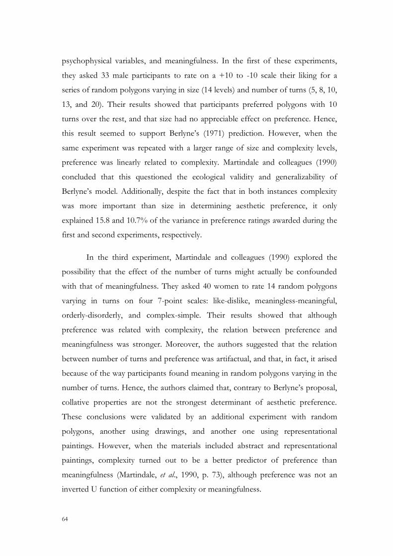
64

psychophysical variables, and meaningfulness. In the first of these experiments,

they asked 33 male participants to rate on a +10 to -10 scale their liking for a

series of random polygons varying in size (14 levels) and number of turns (5, 8, 10,

13, and 20). Their results showed that participants preferred polygons with 10

turns over the rest, and that size had no appreciable effect on preference. Hence,

this result seemed to support Berlyne’s (1971) prediction. However, when the

same experiment was repeated with a larger range of size and complexity levels,

preference was linearly related to complexity. Martindale and colleagues (1990)

concluded that this questioned the ecological validity and generalizability of

Berlyne’s model. Additionally, despite the fact that in both instances complexity

was more important than size in determining aesthetic preference, it only

explained 15.8 and 10.7% of the variance in preference ratings awarded during the

first and second experiments, respectively.

In the third experiment, Martindale and colleagues (1990) explored the

possibility that the effect of the number of turns might actually be confounded

with that of meaningfulness. They asked 40 women to rate 14 random polygons

varying in turns on four 7-point scales: like-dislike, meaningless-meaningful,

orderly-disorderly, and complex-simple. Their results showed that although

preference was related with complexity, the relation between preference and

meaningfulness was stronger. Moreover, the authors suggested that the relation

between number of turns and preference was artifactual, and that, in fact, it arised

because of the way participants found meaning in random polygons varying in the

number of turns. Hence, the authors claimed that, contrary to Berlyne’s proposal,

collative properties are not the strongest determinant of aesthetic preference.

These conclusions were validated by an additional experiment with random

polygons, another using drawings, and another one using representational

paintings. However, when the materials included abstract and representational

paintings, complexity turned out to be a better predictor of preference than

meaningfulness (Martindale, et al., 1990, p. 73), although preference was not an

inverted U function of either complexity or meaningfulness.

65

Martindale considered that these results raised serious questions regarding

Berlyne’s framework and that they were congruent with his own model of

aesthetic preference (Martindale, 1984, 1988). The main pillar of his model is the

assumption that the mind can be adequately modelled as a large network of

interconnected cognitive units, segregated into a number of so-called analyzers.

This theory posits a sensory analyzer for each of the senses, whose output

constitutes the input for a number of perceptual or gnostic analyzers. It is believed

that there is a distinct perceptual analyzer for each class of recognizable objects.

These perceptual analyzers include a series of cognitive units at the lower levels

which code the distinctive features. Specific excitement patterns of feature units

define units in the next level, and so on up the hierarchy in the perceptual

analyzers. Hence, a reduced number of feature units are able to define a vast

amount of unitary percepts. The output from perceptual analyzers enter the

semantic analyzer, where it is hypothesized that there is one cognitive unit for each

concept a person has. Activity from here is passed on to the episodic analyzer,

which contains memories. This analyzer produces outputs which correspond to

events coded propositionally. Whereas sensory and perceptual analyzers are

modality-specific, the others are conceptual.

When using this general model of cognition to explain aesthetic

appreciation, Martindale noted that it addresses only “disinterested or aesthetic

pleasure” (Martindale, 1988, p. 26). When the arousal or limbic systems become

unusually active, pleasure and displeasure is mainly determined by the activity of

these systems. Conversely, under conditions of “disinterested pleasure”, usually

associated with aesthetic experiences, preference is determined by the cognitive

system we just summarized:

Apprehension of a work of art of any sort will involve activation of cognitive units in sensory, gnostic, semantic, and episodic analyzers. (…) the pleasure engendered by a work of art will be a positive monotonic function of how activated this entire ensemble of cognitive units is. The more activated the ensemble of units, the more pleasurable an observer will find the stimulus to be. (Martindale, 1988, p. 26).

66

Martindale (1984, 1988) hypothesized that prototypical stimuli are encoded

by stronger cognitive units. And given that aesthetic pleasure is a function of the

activation level of cognitive units, prototypical and meaningful stimuli are

predicted to be associated with higher levels of aesthetic preference than stimuli

which are atypical. Hence, Martindale, Moore and West (1988) and Martindale,

Moore and Borkum's (1990) results are considered to represent strong support for

this model.

However, Martindale’s work has not gone without criticisms either. North

and Hargreaves (2000) suggested that the results which Martindale uses to ground

his rejection of Berlyne’s framework and the proposal of meaningfulness and

prototypicality as central to aesthetic preference may be biased by the use of

materials that varied more on typicality than on complexity. This would explain

the different percentages of variance accounted for by complexity and typicality.

But North and Hargreaves (2000) pointed out another problem related with the

materials. They argued that the manipulation of typicality cannot be done without

confounding other aspects, including complexity, and thus, the contribution of

both presumed determinants cannot be disentangled. Boselie (1991) noted several

methodological problems with Martindale’s approach. For instance, given that

Martindale’s studies have primarily been correlational, there has been no way to

show that prototypicality has a causal role in aesthetic preference. Boselie (1991)

even cites evidence supporting the notion that preference might influence

typicality ratings. Boselie (1991) also pointed out some problems with the

interpretation of the data in Martindale and Moore (1988) and Martindale and

colleagues' (1988). Prototypicality cannot be such a great determinant of aesthetic

preference when it explains such a little amount of the variance in the results

reported in those studies. On the other hand, Boselie (1991) also questioned that

the task Martindale et al. (1988) asked their participants to perform was actually an

aesthetic preference task. And in relation with this, Boselie (1991) also noted that

it is not clear what feature of the stimuli participants are responding to. Are they

67

rating the prototypicality of the object as a painting, as a cubist artwork, or as the

depicted object?

From a very different perspective, Humphrey (1973) also came to conclude

that the key to explaining why people find certain objects or representations more

beautiful than other was more closely related with prototypicality than other

features. In exploring the natural origin of humans’ ability to find beauty in things,

and its possible biological adaptiveness, he identified a quality which beautiful

things have in common and suggested a reason why we feel attracted to the

presence of that quality:

Considered as a biological phenomenon, aesthetic preferences stem from a predisposition among animals and men to seek out experiences through which they may learn to classify the objects in the world about them. Beautiful ‘structures’ in nature or in art are those which facilitate the task of classification by presenting evidence of the ‘taxonomic’ relations between things in a way which is informative and easy to grasp (Humphrey, 1973, p. 432).

He reasoned that an effective classification, the organization of sensory

information as an economical description of the world, must divide entities into

discrete categories according to a series of criteria “which make an object’s

membership of any particular class a relevant datum for guiding behaviour”

(Humphrey, 1973, p. 433). Just as other vital functions, Humphrey reasoned that

classification became a source of pleasure throughout evolution. This pleasure is

minimal with repetitive examples of the same object, or with exemplars which are

so different from everything else that lie beyond the scope of the classification.

Pleasure is greatest for objects that, while resembling others in the classification

system, show certain peculiarities, and act as “sources of new insight into how

things are related and divided” (Humphrey, 1973, p. 434).

Hence, from this point of view, it seems that we should find that people

prefer viewing intermediately typical representations. This prediction was

supported by Hekkert, Snelders, and van Wieringen's (2003) study of the relation

between typicality and novelty, that showed people’s preference is greatest for

novel objects, providing they are typical, and for typical objects, providing they are

68

reasonably novel. Hence, this study reconciles the importance of meaningfulness

and collative properties in the determination of aesthetic preference, a view

advocated by Hekkert and van Wieringen (1990) and North and Hargreaves

(2000).

The shortcomings of empirical aesthetics

Cupchik (1986) has reviewed some of the criticisms made to the general

strategy of empirical aesthetics. George Dickie (1962), for instance, considers

aesthetics as a discipline in which philosophers deal with logical consideration that

encompasses the meaning of critical concepts and the truth of descriptive and

evaluative critical statements. According to this author, the psychological approach

could be useful to address questions related with behavioural or cognitive aspects

involved in the creative experience or the perception of artworks. However,

Dickie (1962) believes these issues are irrelevant for aesthetics.

Margolis (1980) has been a little more specific in his arguments against

some of the bases and procedures of empirical aesthetics. Margolis (1980) believes

that it is problematic to reduce aesthetic materials to mere physical elements or the

transmission of information without reference to its content. This leads to the loss

of a fundamental quality related with cultural and intentional aspects of the

materials. A true science of aesthetics cannot be reductionist in any sense,

including informational, neurophysiological, and behavioural. He argued that the

roots of aesthetic comprehension should be cultural relativism, conventionalism,

and the influences of history and language on perception and learning. Styles and

ways of producing and appreciating art are strongly influenced by cultural

particularities and historical moments. Margolis (1980) believes that artists and

spectators are not restricted by their nervous systems to interpret or produce art in

specific ways.

69

On a different note, Cupchik (1986) and Cupchik and Heinrichs (1981)

have criticised the passive role assigned to the spectator and the artist, as well as

the fractionation of an artwork into a collection of elements in order to ease the

quantification of informational content. Cupchik (1986) noted that this approach

does not take into account the decisional and organizing role of the artist.

Furthermore, denies the viewer an active role, “stressing instead the competition

among ‘bits’ of information for the attention of a passive viewer” (Cupchik, 1986,

p. 353). This distortion, introduced by experimental procedures moves the

researcher away from the natural processes of creation and appreciation. The fact

that the impact of an artwork is produced by the structuring of component

elements diminishes the validity of the conclusions reached through these

strategies. Appreciating art cannot be conceived as a passive observation of the

accumulation of visual contents. Instead, people actively organize those contents

searching for an aesthetic and personal meaning. The strategies developed by

Fechner and Berlyne emphasize those elemental aspects of aesthetic appreciation.

However, there are many other kinds of cognitive and affective processes related

with this search for meaning.

One of Arnheim's (1966) most noted achievements was to apply the

viewpoint of Gestalt psychology to the realm of art and aesthetics, countering

Fechner and Berlyne’s atomism. One of the issues Arnheim (1966) strongly

criticised was Fechner and Berlyne’s conception of art as a source of pleasure and

the hedonistic perspective that has shaped research in aesthetics. He objected to

the reduction of the complicated processes that occur when people perceive,

organize, and understand artworks to a single quantitative variable measured by

means of a pleasant-unpleasant scale. However, according to this author, the

emphasis on pleasure has prevented realizing that there are differences between

aesthetic pleasure and pleasure related with other kinds of stimuli, such as food or

sex. Another of Arnheim’s criticisms refers to the belief that concepts used to

research in empirical aesthetics can be isolated and have a precise meaning. Such

70

terms as interest, complexity, and pleasure are examples of multidimensional

concepts, as we already mentioned above.

Cupchik (1986) has underlined the need for creating a broad framework

that reconciles the approach of empirical aesthetics, as created by Fechner and

reformulated by Berlyne, and the historical and sociological perspectives

advocated by Margolis (1980) and Cupchik (1986; Cupchik & Heinrichs, 1981).

Cupchik (1986) suggested considering, within this broad frame, the meeting of

spectator and artwork as a search for meaning based on the application of

perceptual and cognitive schemes. He considers these schemes to be hierarchically

organized at two poles. Culturally and historically specified schemes, related with

artistic styles and rules are at one of them. They allow viewers to understand

artistic innovations and conventions. These schemes change with time, gradually

or suddenly. Spectators familiarized with artistic culture have acquired an aesthetic

competence by means of these schemes that allow them to understand the

meaning of an artwork, to understand its message completely. Innate

psychobiological restrictions that guide the processing of visual information from

the world would be at the opposite pole. These processes are general and they are

involved in the perception of aesthetic and non-aesthetic objects. These innate

schemes would be the reflection of the structure of the nervous system, they

operate automatically, without the involvement of the spectators’ attention. These

lower processes are related with the psychophysical properties of the stimulus, and

they can also reflect gestalt-like processes.

This point of view conceives that comprehending the meaning of an

artwork requires the interaction of schemes operating at both levels. Hence, it

considers that both divergent perspectives mentioned above as parts of the same

process. In the next section we will review recent models that have developed this

integrated perspective. They consider that aesthetic preference involves a number

of affective and cognitive processes and that it is closely related with other

personal, cultural, and historical factors.

71

1.3 Aesthetic preference

Abstract

Although complexity, among other variables, has been shown to have a great influence on aesthetic preference, the psychobiological mechanisms proposed by Berlyne (1971) are now known to be too simplistic. A great deal of current research in the field of empirical aesthetics is aimed at determining the cognitive and affective processes involved in aesthetic preference. In this section, we review two recent approaches to this issue and discuss their differences and similarities. We then turn to the question of the dimensional structure of aesthetic preference, trying to ascertain whether the complexity of this phenomenon can be reduced to a simple but meaningful measure. This framework will serve us to present studies that evidenced the influence of several variables on aesthetic preference. Specifically, we present evidence suggesting several personality traits and cognitive styles have a very small role in determining aesthetic preferences. Conversely, there is strong support for the notion that art education plays a pivotal role in aesthetic preference. Finally, the extent to which sex and aesthetic preference are related is unclear.

72

1.3.1. Cognitive processes involved in aesthetic preference

Thirty years ago Hardiman and Zernich (1977) performed a review of 20

studies that had explored people’s preference for artistic visual stimuli. These

authors showed that although some of the reviewed studies attempted to relate

their results with some kind of theoretical framework, most of them did not

present explanations that went beyond simple intuition. Hardiman and Zernich

(1977) concluded that preference for visual arts should be considered as an

unresolved question. They also pointed out three issues that were not adequately

taken into account by most of the studies. First, they lacked and adequate control

over the properties of the stimuli, including reproductions of images belonging to

different artistic styles, with a different degree of abstraction, and ignoring

differences related with the emotional content of the artworks, their popularity or

the presence of human figures. Second, the authors noted the lack of a common

method of registering the responses of the participants. Whereas some studies

used questionnaires to record their answers, others used paired comparisons, and

others used Likert scales. Finally, Hardiman and Zernich (1977) underlined the

little generalizability of the results of these studies, given that all the samples of

participants were strictly composed of university students.

The authors suggested two courses of action for the future. The first one

was to closely examine the meaningful dimensions related with the appreciation of

artworks to ground future studies. Their second proposal was to frame research

into aesthetic preference within a theoretical structure that can serve as the base

for the interpretation of the results (Hardiman & Zernich, 1977). As we noted in

previous sections, although many of the studies that were carried out subsequently

show the same shortcomings that they pointed out about previous work, there

73

have been significant contributions to clarify the cognitive and affective processes

involved in aesthetic preference, as well as the relations among them.

Leder et al. (2004) have recently proposed a comprehensive model of visual

aesthetic judgment and perception. It includes five processing stages that might

run in parallel or in series. The first of them, perceptual analysis of the visual

stimulus, includes operations related with perceptual organization, such as

grouping, the analysis of symmetry and complexity, and other perceptual features

that influence aesthetic judgment. The second stage, implicit memory integration,

encompasses the effects of familiarity, prototypicality and meaningfulness. The

third stage, explicit classification, includes cognitive operations related with the

style and content of the stimulus. The following stage, cognitive mastering,

includes art-specific and self-related interpretations. Finally, the last stage sees the

emergence of a cognitive state, resulting from previous stages, and an affective

state, that results from the continuous interactions between previous stages and

affective systems in the brain. The cognitive state is the source of aesthetic

judgment, while aesthetic emotion is grounded on the affective state.

Chatterjee’s (2003) model of visual aesthetics represents a recent

neuroscientific framework for investigating aesthetic experience. Chatterjee (2003)

has suggested that aesthetic experiences related to visual objects involve three

visual processing stages common to the perception of any visual stimulus, as well

as an emotional response, a decision, and the modulating effect of attention. In

the first stage early visual processes break the stimulus down into simple

components, such as colour, shape, and so on, which are extracted and analyzed in

different brain areas. The second stage, intermediate vision, includes a series of

operations that segregate some elements and group others, forming coherent

representations. In late visual stages, included under the representational domain

in this model, certain regions of the object are selected for further scrutiny. At this

moment, memories are activated, and objects are recognized and associated with

meanings. This visual analysis leads to emotions associated with the aesthetic

74

experience, and it grounds decisions about the stimulus. However, this is not a

strictly linear model. In fact, it posits an important feedback flow of information

via attentional processes, from higher visual and emotional levels towards early

visual processing.

A comparison of the models proposed by Leder and colleagues (2004) and

Chatterjee (2003) reveals similarities and differences. Both models acknowledge

the importance of early and late visual processes in the generation of an emotional

response and the elaboration of a decision. They also take into consideration the

influence of complexity, order, grouping, and many other variables familiar to

experimental aestheticians, as well as the interaction between affective and

cognitive processes such as the activation of memories and the search for

meaning. Additionally, both models suggest two different outputs: an emotional

response or aesthetic emotion versus a decision or aesthetic judgment. However,

at a more specific level, these models have emphasized different aspects of

aesthetic experience. Chatterjee’s (2003) model deals extensively with perceptual

processes, but makes little mention of higher cognitive processes, such as

interpretation or classification. In contrast, Leder and colleagues (2004) subsumed

all perceptual processes in a single stage and did not explicitly consider a function

for attention, instead specifying higher cognitive processes in detail, and awarding

them a central role in the aesthetic experience. Figure 1.3 shows a combined

representation of both models, illustrating their similarities and differences.

75

Figure 1.3. Combined representation of Leder and colleagues’ (2004) and Chatterjee’s (2003) models of aesthetic appreciation. Grey boxes, white arrows and italic text correspond to the stages suggested by Leder et al. (2004),

and white boxes, black arrows and regular text correspond to Chatterjee’s (2003) stages.

There could be several reasons behind the differences between Chatterjee’s

and Leder and colleagues’ models. First, Chatterjee’s (2003) objective was to create

a framework for neuroaesthetics that was firmly based on findings from visual

neuroscience. In his model, the processes involved in visual object recognition

constitute the starting point for visual aesthetics, so it is not surprising that they

figure so prominently in his model. This is also the reason why attention is

awarded a central role: It is known to exert top-down modulation of early visual

processing. On the other hand, Leder and colleagues (2004) aimed to present an

information-processing model of the stages involved in the aesthetic processing of

visual artistic stimuli. In this sense, the starting point of the model was their

analysis of modern art (Leder et al., 2004, p. 491). They believe that understanding

plays a critical role in the aesthetic experience of modern art, in the sense that

comprehending an artwork alters the way in which it is experienced.

However, there is also a deeper difference between the two models, and it

refers to the way in which they conceive of the aesthetic experience itself.

Chatterjee (2003) believes the notion of disinterested interest adequately captures

the aesthetic experience such that “the viewer experiences pleasure without

obvious utilitarian consequences of this pleasure” (Chatterjee, 2003, p.55). From

76

this perspective “judgments about an aesthetic object might be considered outside

the core aesthetic experience” (Chatterjee, 2003, p. 56). In fact, the model seems

to include a decision phase only as an approach to laboratory settings, where

participants are usually asked to state their preferences or make decisions about a

certain aspect of the stimulus. Conversely, Leder and colleagues (2004) believe

aesthetic experiences arise when “exposure to art provides the perceiver with a

challenging situation to classify, understand and cognitively master the artwork

successfully” (Leder et al., 2004, p. 493). This successful mastering of the artwork

involves, especially in relation to modern art, style-related processing, which

results from the acquisition of expertise. In this model, the judgment of the

aesthetic object is an important element; in fact, together with aesthetic emotion, it

is the main output of the model. In sum, whereas Chatterjee’s (2003) proposal can

be considered as a neuroscientific model of aesthetic preference for a broad range of visual

objects, Leder and colleagues’ (2004) proposal is an information-processing model of

aesthetic judgment of visual works of art.

In any case, there is currently a broad agreement among researchers that

aesthetic preference involves a number of cognitive and affective processes. Some

of these are related with perceptual analysis, others with recognition and other

mnemonic processes, others with decision-making, and other with analyzing the

affective value of the stimulus. In the remainder of this section we will use this

general framework to address two issues. First, if aesthetic preference involves

such a complex interplay of cognitive and affective operations, can it be adequately

studied in laboratory conditions which require simple responses from participants?

Second, what are the main personal variables that influence these cognitive and

affective processes, and therefore, the performance on aesthetic preference tasks?

77

1.3.2. The dimensional nature of aesthetic preference

Research of aesthetic preference usually entails the recording of

participants’ responses to different kinds of objects. However, these responses

may refer to a broad variety of aspects of the material used in the experiment or

the response scales, such as novelty, originality, pleasantness, complexity,

interestingness, order, liking, or beauty, among many other possibilities. However,

when the aesthetic experience of participants is studied in an experimental setting

with the objective of relating it with different variables, such experience must be

reduced to a manageable, and preferably quantifiable, magnitude. In spite of the

need to simplify this admittedly complex human experience, and accepting the loss

of information in the process, researchers need to make sure that the resulting

measure is not completely devoid of meaning, that is to say, that it is

representative of the phenomenon being studied. Hence, we need to ask

participants to communicate their aesthetic experience in a meaningful but simple

way.

The issue of whether there is a simple rating scale that might best represent

the aesthetic experience was initially addressed by researchers during the early

twentieth century and has been carried on to the present using different

experimental and statistical approaches. This line of research was born from the

need of art schools and vocational psychologists for a valid and reliable test of

artistic capacity that could be used as an entrance examination or as a tool for

estimating a candidate’s suitability for an artistic career. The following paragraph

by one of the pioneers in this endeavour clearly illustrates the parallels existing

between the aims of these vocational psychologists and empirical aestheticians:

If we are to seek a single test-measurement for ‘artistic appreciation’, whatever that may be, it is important first of all to inquire whether any single central factor exists which mainly determines the artistic judgments of different persons

78

(…). There may be, too, and almost certainly are, many other specific factors, each of them perhaps influencing certain persons or certain groups. The chief questions, therefore, are: do these irrelevant factors have sufficient weight to obscure and overlay any general or universal tendency that may operate, and do the standards and criteria differ so completely from one competent judge to another that no single test is conceivable? (Dewar, 1938; p 32).

1.3.2.1. A general factor of aesthetic preference?

The first empirical attempts at determining the existence of a general factor

underlying aesthetic preference were based on Cyril Burt’s (1924, 1933) work on

the creation of adequate instruments to select pupils for art schools. Burt arranged

a sample of 50 postcards including “reproductions from classical masters, second-

rate pictures by second-rate painters, every variety and type down to the crudest

and the most flashy birthday-card that I could find at a paper-shop in the slums”

(Burt, 1933, p. 290). His first objective was to establish a standard for comparison

by asking competent artists and art critics to arrange the cards in order of

preference. Burt (1933) recounts the experience in the following words:

Nearly all of them began by protesting that such a standard was impossible. The Royal Academician declared that the modernist would completely reverse his order; and both were quite sure that any approach to agreement was wholly out of the question. To my amazement, their actual orders were much the same throughout. The average correlation was nearly .9. All that happened was that the Royal Academician would put a landscape by Leader rather near the top, whereas the modernist might put it tenth or fifteenth –but well above the commercial horrors of the stationer’s shop. Some put Raphael first, and the primitives fourth or fifth; others put the primitives first, yet Raphael was never far down. It became clear that the differences in their taste and judgment were far smaller than their warm disputes and discussions would lead one to suppose. The conclusion, in short, was irresistible: that there was something fundamental guiding their general choice, although their special theories or private points of view might produce a few minor divergences (Burt, 1933, p. 290).

He thereafter asked children and untrained adults to rate their liking for

each of the postcards in the set. He observed that the preferences of these

participants were much more influenced by “irrelevant factors”, such as the

subject matter of the pictures. He correlated the order preferred by each of these

79

participants with the standard order suggested by the art experts, and took this as

the measure for each individual’s taste. Two observations were critical. First, that

scores increased with age, though untrained adults still fell short of the experts’

standard. Second, despite the difference regarding experts, “the coefficients were

almost invariably positive: thus there seemed to be some one, general, underlying

factor influencing the artistic judgments of all” (Burt, 1933, p. 292). As Pickford

(1955) noted, this was the first time such a factor was mentioned. Subsequent

studies including older participants confirmed this finding. The use of new factor

analysis techniques suggested the existence of bipolar factors related with certain

kinds of artistic appreciation. The same kind of results were obtained from

studying the aesthetic preference of men and women with different social

backgrounds using a broad range of test materials, including several different

objects with aesthetic value, such as furniture, vases and china, dressing

complements, and so on.

Heather Dewar (1938) followed this line of research with her study of the

responses to several artistic tests given by both laymen and experts. She asked her

participants to complete The Meier Seashore Art Judgment Test, The McAdory Art Test,

which measured appreciation of form, colour and distribution of light and shade,

as well as modified versions of two of the tests used by Burt (1933), one of which

was the aforementioned Picture Postcard Test. Her results showed that her

participants had tended to place the pictures varying in aesthetic merit in

approximately the same order of liking in the four tests they performed. The

factorial analysis of the data revealed that, even eliminating the influence of

intelligence, a single general factor accounted for over 70% of the variance in the

responses of the participants to the tests. Additionally, as previously suggested by

Burt (1933), there was indication of some factors that seemed to be specific of

different kinds of aesthetic appreciation (objective or classical versus subjective or

romantic). Hence, the arrangement of the cards of the different tests afforded

information about the general degree of taste individuals had and the direction in

which his or her preference tend. An interesting issue raised by this study was that

80

the second factor seemed to be different for experts and non-experts. This factor

separated the former group of participants into those with a higher appreciation

for classical art from those preferring romantic art. But when the general factor

was eliminated from the scores given by laymen, the bipolar factor seemed to

indicate the extent to which untrained people were influenced by subjective

associations in their judgment. Two types of persons were distinguished: those

who based their judgments on the stimuli actually shown and exhibited a critical

stance, and those who based their judgements on the effects of the object on

themselves –emotions, associations and memories elicited by the test stimuli. In a

footnote, Dewar (1938) pointed out the resemblance between this division and the

Jungian distinction between extroverts and introverts.

It must be noted that at this early research period the appreciation of

pictorial art was not the only area to be explored with factorial techniques.

Williams, Winter and Woods (1938) carried out a similar investigation to the

aforementioned studies using literary materials. Their results revealed a general

factor underlying literary appreciation and a bipolar factor which distinguished

romantic from classical writing styles. Furthermore, they also reported that there

was a correlation between the appreciation for literary, musical and pictorial

materials. Overall, thus, as early as the beginning of the nineteen forties there were

several studies that suggested the existence of a general factor underlying the

appreciation of pictorial arts, and possibly musical and literary, as well as some

indications of bipolar factors associated with specific styles or kinds of artistic

expression.

However, Hans Eysenck (1940) was not completely convinced by the

procedures of the studies we have just summarized. Specifically, he believed that

the materials used by the researchers did not meet relevant criteria for factor

analyses. Eysenck's (1940) concerns were mainly related with three issues. First,

the influence of culture –meaning teaching, traditions and so on- had not been

completely controlled. Second, some of the material sets varied in the technical

81

merit of the stimuli. Third, familiarity was also not taken into account, which

would lead to greater preference for familiar pictures, artists or art schools. Thus,

in order to carry out a diligent study of the factorial structure of aesthetic

preference, researchers should avoid materials for which preference might be

susceptible to teaching or tradition, materials including stimuli of uneven

execution, and which might stand out as familiar.

Taking these criteria into account Eysenck (1940) asked eighteen

participants with a variety of social and educational background (typists, students,

painters, teachers, bank clerks, psychologists and a professor of Aesthetics) to rank

the pictures in each one of eighteen sets of stimuli. These sets, which included an

average of fifteen elements were: portraits, reproductions of statues of Roman

emperors, reproductions of book bindings, pencil drawings by the same artist,

pictures used in advertising, photographs of vases, reproductions of Malayan

masks, Japanese paintings, photographs of steamships, Japanese landscape

paintings, picture sets, reproductions of pieces of embroidery, curves of

mathematical functions, reproductions of modern statues, coloured photographs

of flowers, coloured reproductions of Eastern pottery, reproductions of silver

plate, and pictures of medieval clocks. The results showed that for each of the

stimuli sets, the order preferred by each participant was significantly correlated

with the average order, which suggests that a general factor underlies the

responses to each of the tests. In order to make sure that in effect it was the same

factor for all of the eighteen tests, Eysenck ran a correlation between the tests, and

found another very statistically significant value. This, he believed, was evidence

for the existence a general objective factor of aesthetic appreciation. He referred

to this factor as “general” because it seemed to cover a broad range of visual

stimuli, just as Spearman’s “g” covers at least most cognitive tests, and “objective”

because it had been shown to be largely independent of individual taste. He named

this factor T, because he believed this factor was behind what is usually known as

“good taste”. This factor exhibited insignificant correlations with measures of

intelligence, which suggested that T could not be explained entirely in terms of

82

general cognitive ability. On the other hand, the fact that this general factor

correlates with the ranks awarded to odoriferous substances, several colours and a

variety of polygonal figures led Eysenck to “surmise that we are dealing here with

a perceptual factor that derives directly from the nature of the nervous system”

(Eysenck, 1940). Most importantly for the present research, Eysenck stated that

“as related to pictures, [T] accounts for what we call ‘beauty’” (Eysenck, 1940,

p100).

The nature of the bipolar factor was studied in detail in a subsequent paper

(Eysenck, 1941c) aimed at reducing the relevance of the general factor by

eliminating better part of the variation in artistic merit among the stimuli included

in the materials. Thus, the stimuli in each of the five sets used in that study were

characterized by a similar artistic merit. Materials included two sets of 51

landscape paintings, a set of 51 black and white landscape photographs, a set of 32

portrait paintings, and a set of 32 photographs of statues. Fifteen participants,

seven men and eight women, including artists, university students, teachers, bank

clerks, and typists, were asked to rank the pictures in each one of the five sets in

order of liking, using a grouping strategy which created a normal-like distribution.

The results of this study confirmed that standardizing the artistic merit of the

stimuli used as material favoured the emergence of bipolar factors for each of the

stimuli sets. This factor separated participants preferring modern, impressionistic,

colourful pictures of landscapes and portraits, and those who preferred the older,

more conventional, less colourful ones. In relation to photographs, the factor

distinguished participants who preferred sunny, bright, happy landscapes with

trees and clear skies from those preferring dark landscapes with overcast and

cloudy skies. Finally, it opposed those who liked sculptures with perfect forms

from those emphasizing character or content. The correlation of the five bipolar

factors suggested that there is one factor running through all the five tests.

Eysenck (1941c) named it the K factor, and suggested that it might have a

significant relation with education and temperamental qualities, which we will

examine in the following sections of this chapter.

83

What is the relation between the T and K factors? Eysenck and Hawker,

(1994) asked art-trained and untrained participants to complete two visual

preference tests. The first test, VAST (Götz, Borisy, Lynn, & Eysenck, 1979), had

been designed to measure the T-factor, and consists of a series of high aesthetic

quality non-representational pictures paired with a very similar altered version

which is aesthetically flawed. The task of the participant is to identify the correct

version of each picture. The second test, designed to measure preference for

complexity, and thus, closely related to the K factor, was the Barron-Welsh Art

Scale (Barron & Welsh, 1952). The results showed no significant correlations for

either group of participants, which suggests the two factors are independent of

each other, and that art training does not alter this fact.

To what extent do these two factors underlying aesthetic preference

generalize to other kinds of stimuli? There is evidence that these results may be

generalized to quite a broad range of visual stimuli, including colours and

geometrical designs. Eysenck (1941a) asked 6 men and 6 women to rank 10

colours in order of preference and to respond to a test of the T factor. His results

showed a considerable agreement in the preferences for colours, and furthermore,

two factors were extracted from the table of correlations. The first of these, with

positive saturations throughout, accounted for 34% of the total variance, while the

second factor, which was bipolar, accounted for only 4%. The correlation between

the saturation of the ratings awarded by these 12 participants with their scores on

the T factor test was .53, which led him to conclude that the first factor of colour

appreciation could be a manifestation of the underlying general factor of aesthetic

appreciation we mentioned above. The second factor simply divided those

participants who preferred saturated colours from those who preferred

unsaturated colours. Eysenck's (1941a) study also included the assessment of sex

differences. He repeated the procedure with a different sample of 15 men and 15

women, to find the preferences among these participants were virtually identical,

and coincident with those of the smaller group of participants.

84

Eysenck (1971a) also provided evidence to support the involvement of the

general factor when people are asked to express their preferences for geometrical

designs. He asked 179 participants with no specific art training to rate their liking

for a series of 131 geometrical designs on a 5-point scale, which ranged from

“Don’t like” to “Like very much indeed”. The stimuli were a broad range of

designs representing elaborate variations of geometrical forms, such as squares,

triangles, circles, hexagons, and so on. Factor analysis revealed three major kinds

of factors across which stimuli could be distinguished. The first kind of factors

separated stimuli according to their shape into circles, rings, squares, stars, and so

on. The second type of factors was related to the presentation of the stimuli and

included shadings, and three-dimensional appearance, among others. The last type

of factor separated simple designs from complex ones. In addition to this, and

closer to our present interests, Eysenck's (1971a) participants showed a great

agreement, which suggested the involvement, yet again, of the general factor of

aesthetic preference. In order to verify this, he had his participants rate their liking

for 135 Birkhoff-like polygons, as a sort of T test. For each participant two scores

were obtained, one which represented their agreement with the mean average of

designs, and the other their agreement with the mean average of polygons. The

correlation between both scores was .525, which “demonstrates at a high level of

statistical significance that a person showing ‘conformity’ or ‘taste’ on one test

does so also on the other, while a person lacking in this quality on one test is also

found lacking on the other” (Eysenck, 1971a, p. 163.). Hence, it seems that the

general factor underlies, to a certain extent, aesthetic preferences for a wide range

of visual stimuli.

The notion that the coincident ordering by participants of diverse visual

stimuli on preference scales might actually represent the aesthetic value of those

stimuli was questioned by Child (1962). He asked two groups of 22 participants

with no artistic training to order each of the 60 pictures in each of 12 sets

according to how much they liked or disliked them. The picture sets included still

lifes, pictures of animals, landscapes, religious themes, abstract pictures, depictions

85

of single men, depictions of single women, and so on. A third group of

participants, art students in this case, was asked to perform a different task in

order to obtain a criterion for aesthetic value of the pictures. They had to “judge

the aesthetic merit of the pictures (i.e., how good they are as works of art)” (Child,

1962, p. 499). According to the author, the results from his study question that

group preference reflects aesthetic value and that the proximity of individual

agreement with that group preference can be considered as a measure of aesthetic

sensitivity. However, Eysenck (1971b) noted three reasons why Child’s (1962)

results do not represent actual criticisms of his previous work (Eysenck, 1940).

First, the group of art students were asked to perform a different judgment to the

other two groups of participants. Eysenck (1971) argued that there was no reason

to assume that preference and aesthetic judgment would coincide even for a single

group of participants, and thus, that Child’s results might merely show that

different instructions lead to different results. Second, the stimuli used by Child do

not meet the three criteria established by Eysenck (1940). Thus, the kinds of

interfering effects mentioned above cannot be discarded. Finally, whereas Child

(1962) assumed the existence of an external criterion of aesthetic value provided

by experts, Eysenck (1971) was not willing to accept this in the absence of

empirical proof. Eysenck naturally agreed that experts, such as those included in

Child’s (1962) third group of participants, possess knowledge of criteria used to

assess artworks, but he stressed that agreement on these criteria does not

necessarily amount to good taste or aesthetic sensitivity.

Together with other works, the literature reviewed above led Pickford

(1955) to feel that it was well established at the time that there is a general factor

of aesthetic appreciation. This factor, as stated by Eysenck (1940) is closely related

with the appreciation of beauty. This would suggest that beauty represents an

adequate scale to summarize aesthetic experiences of participants carrying out

experimental procedures in laboratory settings. This early conclusion has been

ratified by recent studies using different approaches. One of these studies was

carried out by Marty, Cela-Conde, Munar, Rosselló, Roca and Escudero (2003),

86

who were faced with a similar issue we are dealing with here: to find a simple way

of recording the aesthetic experience of participants in neuroimaging procedures.

They asked 100 university students to rate 96 images on four semantic

differentials: beautiful-ugly, interesting-uninteresting, original-common, and pleasant-

unpleasant. Their set of materials included black and white High Art and Popular

Art images, both abstract and representational, and were selected according to

Eysenck’s (1940) criteria. The factorial analysis they carried out revealed the

existence of a general factor explaining 62.3% of the whole variance, with the

beauty scale having the greatest loadings. The authors concluded that these results

are in agreement with Eysenck’s (1940) characterization of a general factor

underlying aesthetic appreciation, and allow the reduction of aesthetic appreciation

to relatively simple questions about the beauty of the stimuli presented in

neuroimaging and cognitive experiments.

Jacobsen, Buchta, Köler, and Schröger (2004) carried out another recent

study aimed at disclosing the most representative dimension of aesthetic

appreciation, although they used quite a different approach from those reviewed

above. In contrast to the other studies, they moved away from theoretical

perspectives of what constitutes aesthetic experiences and focused on what

people’s ordinary idea of aesthetics was. They asked the people participating in

their study -84 male and 227 female non-art undergraduate students- to write

down adjectives that could be used to describe the aesthetics of objects for two

minutes. The analysis of the 590 different words produced by the participants

revealed that “beautiful” was clearly the most frequent answer to the

questionnaire, written by 91.6% of them. The second most frequent answer was

“ugly”, appearing in 42% of the answer sheets. The remaining responses were

much less common, and included such adjectives as pretty (27%), elegant (23%),

small (18%), repulsive (12%), stylish (10%), interesting (7%), and so on. The

authors correlated the frequency with which these words appeared in the

responses of their participants and the frequency with which they appeared in

common language use. This showed that general use accounted for less than 6%

87

of the answers to the questionnaire, excluding the possibility that they had

responded based on the common usage of the adjectives. These results show that

“a bipolar beautiful-ugly dimension clearly appears to be the primary and

prototypical descriptive dimension for the aesthetics of objects” (Jacobsen,

Buchta, Köler, & Schröger, 2004, p.1258).

In sum, experimental results support the notion of a general underlying

capability of aesthetic preference. Beauty ratings have been shown to adequately

represent this general factor in experimental settings using a broad diversity of

stimuli. However, to show that this general factor is a biological property of our

species is a different question. This issue has been traditionally studied by

attempting to determine whether there are aesthetic universals by means of cross-

cultural research methods.

1.3.2.2. Cross-cultural research

The anthropologist Robert Lowie (1921) was the among the first to carry

out a quantitative research aimed at establishing whether aesthetic preferences are

universal. Stimulated by the results obtained by contemporary psychologists

showing that occidental participants tended to prefer rectangles with proportions

close to the golden section, Lowie (1921) studied the distribution of rectangular

forms in the decorative art of a tribe of North American Indians, the Crow. He

also compared some of these elements with similar ones created by another tribe,

the Shoshoni, expecting to find a mix of common features, resulting from a

putative universal aesthetic norm, and distinctive motives in each tradition. The

measurements of the proportions of 20 Crow and 20 Shoshoni items revealed that

the former tribe seemed to prefer somewhat thinner rectangles that the latter.

Furthermore, his results revealed that the dimensions of the most prevalent

rectangular figures in Indian art did not conform to those established by the

88

golden section. In fact, the Crow’s norm was below this proportion, whereas the

Shoshoni’s was above it (Lowie, 1921).

A possible explanation for this failure in finding common aesthetic values

in different cultures may reside in the use of extremely simple materials. At around

the mid nineteenth century researchers began using other kinds of materials, such

as those collected by Eysenck (1940), and with participants from cultures with

very little mutual contact and with notoriously different beauty criteria. The

objective of these studies was to identify indications of agreement in aesthetic

preferences which were resistant to the influence of culture. McElroy (1952) and

Lawlor's (1955) studies are considered as pioneers in this line. McElroy (1952)

registered preference scores of 40 Australian aborigines and 20 Caucasian students

and Sidney University for similar materials to those used by Eysenck (1940):

drawings of flowers, butterflies, fish, landscapes, reproductions of works by Paul

Klee, and so on. His results yielded high correlations among participants

belonging to each group. However, correlation between the scores awarded by

Caucasians and aborigines was lower than expected and in many instances below

statistical significance levels. Correlation between the general factors extracted for

each group varied depending on the specific test. Correlation values varied from

non-significance (Birds, Flowers, Landscapes, Paul Klee, Polygons, Portraits of

Caucasians) to significantly positive (Fishes, Colours) to significantly negative

(Tartans, Portraits of Africans). In no case, however, were cross-cultural

correlations as high as within each group of participants. The author concluded

that his results “provide much evidence in favour of the view that the ‘beauty’ of a

visual object is almost entirely determined by the cultural conditioning of

perception” (McElroy, 1952, p. 94), and that the data he collected

appear to offer little support to Eysenck’s inter-racial “good taste” or “inherited predisposition” as accounting for the tendency to agreement between judges with material satisfying his three conditions of freedom from “irrelevant associations” (McElroy, 1952, p. 93).

Lawlor (1955) compared the preference scores awarded by 56 European

and 56 West African participants to 8 East African decorative elements

89

reproduced from motifs appearing on woodcuts, metal figures, earrings, necklaces,

and fabrics. Although she found an elevated agreement among the opinions of

people belonging to each of the participating groups, there was no indication of

intercultural agreement. This, again, suggested that if there is in fact a universal

aesthetic preference factor, it is largely superseded by cultural experience.

Child and Siroto (1965) attributed the results of these experiments to the

fact that the people included in the samples, those whose preference was recorded,

were not selected for their interest in art. They were representative of the general

community. Child and Siroto (1965) believe that there is no reason whatsoever to

expect that aesthetic values are shared even by the members of the same

community. From their perspective, preferences of laypeople are not necessarily

coincident with traditional aesthetic values, which have to do with the assessment

of stimuli in relation to their adequacy to satisfy a certain kind of interest that

people may have developed or not. In this sense, “It is possible that esthetic

evaluations may be made by or known to only some people in each society, and

yet that agreement will be found between such people in various societies (Child &

Siroto, 1965, p. 350). Hence, according to these authors, the question about the

existence of aesthetic universals refers to whether the preference of people

interested in art in one culture will coincide with the preference of people

interested in art in a different culture.

In order to test these assertions, Child and Siroto (1965) gathered a series

of 39 photographs of BaKwele masks used in different rituals. They asked 13

North American experts to judge the aesthetic value of each stimulus. These

experts were advanced art students and other people considered by the researchers

to be capable of performing such judgments. They also recruited 16 BaKwele

participants, male elders that had made masks, or that had participated in rituals

involving masks, as well as young men interested in masks, who were asked to

state which masks they preferred. Child and Siroto's (1965) results revealed a

reasonable agreement between both groups of judges: the images that had been

90

judged as having a greater aesthetic value by American experts were also those

which were most preferred by BaKwele judges. The authors interpreted these

results as a preliminary indication that the masks “do really vary one from another

in general suitability for arousing and sustaining interest in anyone who enjoys

visual art, and both sets of judges are sensitive to this variation” (Child & Siroto,

1965, p. 357).

Ford, Prothro and Child's (1966) results also support Child’s notion of an

agreement among aesthetic judgments which is unaffected by cultural factors,

though only in certain people who exhibit a specific aesthetic sensibility. In this

study, though, they registered the opinions of North American judges about

abstract artworks, artistic still lifes, and so on. These participants were required to

judge the artistic merit of the stimuli. The other participant groups were

constituted by artisans living on a remote Fiji island, and on a remote Greek

island.

In our opinion there is a serious conceptual problem with these two

studies: the task carried out by American participants is different to the one the

researchers asked the other participants to perform. American experts judged the

aesthetic value of the stimuli, whereas the other participants had to choose the

most beautiful one, or the one they preferred. If aesthetic judgment is defined, as

Child and Siroto (1965) do, as the judgment of the quality of a stimulus as a work

of art, it is clear that participants who were asked to rate the beauty of each

stimulus were not carrying out the same task as the American participants.

In a subsequent study, Iwao and Child (1966) gathered a larger set of

stimuli and recruited a larger number of participants. The objective was to find out

the extent to which aesthetic judgments of traditional Japanese potters would

coincide with those American experts. They used pairs of black and white

photographs of artworks of the same type, style, and content, and pairs of full-

colour artistic abstract paintings. Each pair represented artworks that had been

judged as unequal regarding artistic quality by at least 12 out of 14 American

91

experts. In this study, Japanese potters were asked to perform the same task as

American experts had. Results revealed that there was a statistically significant

agreement between American experts and Japanese potters in their choices: 61 and

57.5% for black and white reproductions and abstract works, respectively.

Although the researchers expected the values of agreement to be much greater

that the 50% chance value, and that there was a great variation in the extent to

which Japanese participants agreed with American ones, Iwao and Child (1966)

concluded that the data reflect a tendency of people interested in art to agree on

their aesthetic judgment, irrespective of their particular traditions.

In a follow-up study, Iwao, Child and García (1969) showed the same

materials to 31 additional Japanese participants related with the practice or

teaching of at least one Japanese artistic tradition, including flower arranging, the

tea ceremony, textile dying, manufacture of dolls, woodcutting, painting, and

calligraphy. However, agreement with American experts was even lower than in

the previous study Iwao and Child (1966): 58.5 and 51.5% for black and white and

abstract materials, respectively. In spite of these low agreement values, the second

of which does not even reach statistical significance, the authors concluded that

these results add to the evidence that aesthetic valuing by people involved in

artistic activities in two different traditions tend to coincide (Iwao, Child, &

García, 1969). These results and conclusions are very similar to those obtained by

Anwar and Child's (1972) attempt to extend this line of research to other cultures.

Eysenck’s perspective on cross-cultural research into aesthetic universals

differs from Child’s in two important aspects. First, western art is discarded as

materials for experiments, and stimuli which are less culturally biased are used:

polygons and simple designs, which are not familiar to any of the participant

groups. Second, the opinion of experts is abandoned as a reference point for

cross-cultural comparisons. Eysenck’s work is based on the premise that if there

actually is a universal aesthetic value, it will be revealed by the coincidence in the

aesthetic preference of the majority of the participants, including laypeople.

92

With these considerations in mind, Eysenck began articulating his cross-

cultural comparison of aesthetic preference. Soueif and Eysenck (1971) recruited a

broad set of British and Egyptian art students and laypeople, who were asked to

rate the pleasingness of each of Birkhoff's (1932) original 90 polygons. Their

results revealed that whereas British art students preferred simple figures, British

participants without art education preferred the complex figures. There were no

significant differences between both groups of Egyptian participants, though the

tendency was the opposite of British groups. Although the cross-cultural

differences were somewhat greater than those found in Child’s studies, Soueif and

Eysenck (1971) did not believe that their data support considerably large

differences in aesthetic preference between both cultures.

In a subsequent experiment Soueif and Eysenck (1972) studied whether the

factorial structure of the scores awarded by Egyptian participants to Birkhoff's

(1932) 90 polygons was comparable to the one revealed by a previous study

involving only British participants (Eysenck & Castle, 1970a). Soueif and

Eysenck's (1972) results showed that the factors underlying the aesthetic

preference of Egyptian participants were very similar to those underlying the

preference of British participants: rectangular figures, with radial symmetry, cross-

like, elliptic, triangular, circular, and so on. Hence, the authors believed that, in

addition to a predisposition to prefer certain polygonal figures to others, the

causes of this preference seem to be the same in both cultures. This suggests “the

possibility of a more deeply based, biologically determined cause for aesthetic

judgments” (Soueif & Eysenck, 1972, p. 153).

Eysenck and Iwawaki (1971) performed a study to ascertain whether this

coincidence in aesthetic preferences of British and Egyptian participants could be

extended to other cultural groups, specifically Japanese people. In order to do this,

they used a very similar procedure as in Soueif and Eysenck's (1971) study. The

only difference is that they compared how much British and Japanese participants

liked Birkhoff’s polygons and a set of 131 simple geometric designs. Results

93

showed no significant differences between the scores of both groups of

participants. The correlation between the scores awarded to polygons by both

groups was .8 and to designs was .6. However, there was a tendency for British

participants to score the designs somewhat higher that the Japanese, and the

opposite tendency for polygons.

Just as in the comparison between British and Egyptian participants,

Eysenck and Iwawaki (1975) wanted to know whether the features of the stimuli

that determined aesthetic preference were the same for Japanese and British

participants. Their results revealed a great similarity in the factors underlying the

preference of people from different cultures, and support the notion of the

universality of the processes that determine the aesthetic preference of human

beings.

Eysenck’s line of research was further explored by Farley and Ahn (1973),

who carried out a study aimed at comparing the aesthetic preference for polygons

varying in complexity by participants from 5 different cultures. In order to do so

they recruited participants from the United States, Korea, China, India, and

Turkey who were at the time studying at the same university in the US.

Participants belonging to the last four groups were residing in the US temporally.

None of the participants had formal training in art, and they all had similar social

and economic backgrounds. Twelve polygons varying in the number of sides,

from 4 to 160, were used as materials. Participants were asked to indicate the four

polygons they preferred most and the four they preferred least. Their analysis

revealed that there were no significant differences among the groups of

participants regarding the most or least preferred levels of complexity. Hence,

these results are in agreement with the existence of aesthetic universals, in which

complexity has a similar influence in different cultures. However, the results and

conclusion of this last study are limited by the fact that the data were collected in

the United States. This means that all participants had been exposed to a greater or

94

lesser degree to North American culture, evidenced by the fact that they all had

mastered English enough as to study in the US.

1.3.2.3. Summary

The main objective of this section was to examine whether aesthetic

preference could be adequately measured in a simple and direct way in a laboratory

setting, given that it is a broad phenomenon with many aspects to it, and which

requires the participation of a varied set of cognitive and affective processes. Early

studies suggested that there was a single factor underlying aesthetic preference.

However, Eysenck’s factor analyses uncovered two main factors he named T and

K. The former was conceived as a general and universal factor of aesthetic

preference very closely related with our perception of beauty. The latter was

related with our liking for modern or traditional representation. Subsequent

studies using different methods and different kinds of stimuli have corroborated

the primacy of beauty ratings as an adequate representation of aesthetic

preference. However, cross-cultural studies have provided weak evidence, at best,

for the notion that this general factor of aesthetic preference is universal. This

could be due to methodological inadequacies of those studies or to the fact that

cultural particulars override the effects of this general factor, making it virtually

impossible to detect it using cross-cultural designs.

In spite of the support for a single general factor underlying aesthetic

preference, whether it be universal or not, a number of studies have shown that

there is a considerable degree of variation among people’s aesthetic preference.

Researchers have attempted to explain this variation as a function of a number of

personality traits, general cultural background, specific art education, and sex,

among other variables. We will review some of these explanations in the following

sections.

95

1.3.3. The influence of personality traits and cognitive styles

A great deal of work has been carried out in relation to the notion that

individual differences influence aesthetic appreciation of visual, as well as auditory,

stimuli. The first modern approach to this issue was based on the findings made

by Alfred Binet (1903). He distinguished four different kinds of people depending

on the way they apprehended visual objects. The first kind of people, who he

termed descriptive type, tend to arrive at a pure description of the object’s details,

and do not seek to grasp its meaning or significance in relation to other objects.

The second type of people, the observers, assess the expressive and significant

features of an object, they realize that not all features are equally important and

that they hold specific relations with other aspects and with the whole. The third

type, which he called erudite, do not focus their attention on the impression caused

by the object, but on the associated or remembered facts called up by it. The last

type, known as emotional or imaginative, do not focus on the visible details of the

object, but on its emotional meaning.

Although this typology was derived from the study of children’s

description of visual stimuli, which had no aesthetic purpose, Edward Bullough

(1921) was the first to realize that such individual differences might lead to

measurable differences in aesthetic preference. Based on his studies of the

appreciation of colours, he distinguished among four kinds of appreciation:

objective, intra-subjective, associative, and character. The first of these is characterized by

an impersonal attitude towards the colours and the grounding of appreciation on

saturation, luminosity and its consistency with preconceived standards. The colour

appreciation of the second type is influenced by mood and bodily sensations,

viewing colours as depressing, warm, stimulating, or relaxing. The third type

96

expresses preference for colour as a function of the power of the colour to call up

associations or images of past events. For the fourth type, colours have moods

and personalities: they can be happy, active, serious, funny, and so on. It is this

character attributed to the colour that determines the appreciation of it. There is

no straightforward equivalence between Binet’s and Bullough’s classifications.

However, the latter author suggested that his objective type incorporates features of

Binet’s descriptive and erudite, the intra-subjective shares peculiarities with the observer

and the emotional, Bullough’s associative type is a combination of the observer, emotional

and erudite, and finally, the character type shares features with the French author’s

emotional and observer kinds.

Subsequent research, summarized by Burt (1933), highlighted two main

issues. First, that the types of colour preferences could also be found for music,

which suggested that they might not be completely bound by perceptual processes.

Second, although Bullough (1921) had suggested that the types he described were

more than transitory attitudes of the subject, that they were fundamental and

permanent ways of appreciating colour, it later became apparent that each of the

four tendencies may be discerned in most people, and the difference is the result

of predominance or degree, and not a strict definition of clear-cut groups of

people.

This work paved the path for subsequent approaches which made use of

psychometric tools and factor analyses, represented by Burt (1933) and Eysenck's

(1941c) studies. Whereas the first author’s starting point were personality types

which were subsequently tested for differences in aesthetic preference, the latter’s

starting point was the identification of type factors in aesthetic preference which

were later compared with personality factors. Burt's (1933) studies report the

analysis of aesthetic preferences of people with extreme scores on two personality

dimensions: extraversion and stability. He found that unstable extraverts prefer

dramatic and romantic art, depictions of human figures rather than landscapes or

still lifes. They prefer vivid colours with strong contrasts and vital flowing curves.

97

Instead of the emotional aspects, the second type, stable extraverts, emphasize the

rational, realistic and practical features of pictures, and is more attracted to solidity

and mass than to decoration and flowing curves. The third kind of people,

unstable introverts, prefer impressionist art, subjects related with the mystical and

supernatural, and prefer landscapes –especially if they are surrounded by an air of

mysticism- to portraits. People in the last category, stable introverts, show a

marked intellectual attitude and prefer clear renderings, good drawing, and

chiaroscuro to colours, the theatrical and sentimental.

We already mentioned Eysenck's (1941c) work on aesthetic preference

type-factors in the section concerning the dimensional nature of aesthetic

preference. We noted that this bipolar K factor separated people who preferred

simple and ordered polygons from those who preferred complex and less

organized polygons and shapes. Subsequent studies involving several groups of

participants revealed significant correlations between the K factor and

extraversion-introversion –as Dewar (1938) had previously suggested- and

radicalism-conservatism, with extroverts and radicals liking bright and modern

stimuli the most and introverts and conservatives, the older masters.

In 1947, Welsh constructed a test to aid in the detection of psychiatric

disorders consisting of 200 drawings and administered it to large groups of

psychiatric patients and non-patients. This test, known as the Welsh Figure Preference

Test, required participants to indicate whether they liked each of the drawings. The

factor analysis revealed two factors: a general acceptance factor, related with the

general tendency of the participant to either like or dislike the drawings, and a

bipolar factor, orthogonal to the previous one, related to the preference for

simple-symmetrical figures or for complex-asymmetrical figures. It was noted at

the time that healthy participants tended to form two distinct groups with

markedly different personality traits. Those who preferred simple and symmetrical

figures were conservative and conventional, while those who preferred the other

kind of stimuli were eccentric, cynical, and radical (Barron, 1952).

98

The Welsh test was thereafter enlarged to 400 stimuli and a specific scale

which could discriminate between the preference of artists and non-artists was

extracted and used independently. This is known as the Barron-Welsh Art Scale

(Barron & Welsh, 1952), and was used by Barron (1952) to verify whether

promising people with a great deal of potential success would better discriminate

the good from the poor drawings than those who showed little promise and

potential. It was expected, thus, that their preferences would more closely parallel

those of artists than those of non-artists. Accordingly, 40 psychology students

were asked to go through the scale, 20 of which had been highly rated by the

faculties on qualities like originality and personal soundness, promise and

potential, whereas the other 20 students had been rated as low in originality,

personal soundness and potential success.

Contrary to the original hypothesis, the distribution of both groups of

participants was approximately even between both simple-symmetrical and

complex-asymmetrical pictures. However, two groups of participants did appear

towards the poles of the simplicity-complexity continuum. In a subsequent phase

of the study, participants had to express their preference for reproductions of a

variety of artworks. It was found that the group who had preferred simple-

symmetrical drawings also preferred paintings portraying good breeding, religious

motifs, and scenes reflecting a certain degree of authority, and rejected paintings

with esoteric, unnatural and openly sensual contents. Conversely, the group of

people who had expressed a greater appreciation for the more complex drawings

also gave higher ratings to modern, experimental paintings, those with primitive or

sensual content, and disliked those related with religion, aristocracy, tradition, and

emotional control.

Barron (1952) suggested that the differences observed in the preferences

for drawings varying in complexity and paintings with diverse content might be

explained by the different views both groups of participants have of themselves

and the world. The analysis of their responses on a checklist of adjectives they

99

could use to describe themselves revealed that they had different attitudes towards

the perception of stability, predictability, balance, symmetry, and the use of simple

general principles, as well as towards tradition, religion, authority and sensuality.

The group that preferred simple-symmetric figures described themselves as

contented, gentle, conservative, unaffected, patient, and peaceable, while the group

who had preferred complex-asymmetric figures described themselves as unstable,

dissatisfied, pessimistic, emotional, pleasure-seeking, and irritable. These results

add to the increasing consistency of the suggestion that the extroversion-

introversion and conservatism-radicalism dimensions contribute to the preference

for visual stimuli varying in complexity.

On the grounds laid down by these pioneering studies, research on the

influence of personality on aesthetic phenomena took two very related, but

distinct, forms. On the one hand, further work was done to identify personality

traits that explained differences in aesthetic preference. On the other hand, a new line

was opened by Irvin Child: the study of personality influence on aesthetic judgment.

Given that our main interest for the present research is in aesthetic preference, our

review of studies concerning aesthetic judgment will be much more concise. In

fact, we will report only two studies, one by Child, who pioneered this research

field, and a very recent one by Adrian Furnham. This will afford a brief historical

perspective, while allowing us to quickly turn to aesthetic preference.

In a similar way to McWhinnie's (1968) definition of aesthetic judgment we

have adopted in the present work, Irvin Child conceived it as “the extent to which,

when a person judges the esthetic value of works of art, his judgments agree with

an appropriate external standard of their esthetic value. The external standard used

here is provided by the judgment of experts.” (Child, 1965, p. 476). Child (1965)

asked 138 male students with no special formal education in art to look at 120

pairs of artworks and decide “which of the two works of art is better esthetically –

that is, the better work of art.” (Child, 1965, p. 477). The pairs had previously been

prepared mostly by art and art history graduate students. Each pair represented the

100

same subject matter and most of them were done in the same artistic style. Pairs

were then shown to 14 art experts who were asked to choose the better work of

art in each pair. Only pairs for which expert agreement was high were finally

selected for the experiment. The participants in the experiment were also

administered a large amount of questionnaires, behavioural measures, and

standardized tests. These measured, among other variables, background in art

(including art education, experience in galleries and museums, art-related hobbies,

and family attitudes towards art), skill in the perception of visual forms, tolerance

for complexity, tolerance for ambiguity, scanning, sharpening, field dependence,

independence of judgment, Jungian measures of cognitive orientation

(introversion-extroversion, intuition-sensation, perception-judgment), masculinity-

femininity, originality, and colour preferences.

Results revealed that, while some of the measured variables showed

significant relations with aesthetic judgment, others did not. It is surprising to find

some variables among the latter, such as skill in the perception of visual form, skill

in the perception of human meaning in ambiguous stimuli, and originality. On the

other hand, it is not as striking to learn that others, like masculinity-femininity, and

some behavioural measures of cognitive style, were unrelated to aesthetic

judgment, mainly because of conceptual weakness or the way in which they were

measured. Measures of artistic background showed very strong relations with

aesthetic judgment, especially formal education in at and experience in visiting art

galleries and museums. Turning now to personality dimensions, the variables that

showed strong relations to aesthetic judgment were tolerance for complexity,

scanning (awareness of events outside the main focus of attention), independence

of judgment (preference for the development of one’s own views on matters as

opposed to conformity with others’), regression in the service of the ego

(psychodynamic concept referring to the positive use of relatively immature

functions in the development of mature ones), intuition rather than sensation

(going beyond what is strictly perceived rather than limiting oneself to what is

actually presented), perception rather than judgment. From these results Child

101

(1965) advanced a description of people who showed good aesthetic judgment,

i.e., that tended to agree with art experts about which of the two paintings in each

pair represents a better work of art:

a person of actively inquiring mind, seeking out experience that may be challenging because of complexity or novelty, ever alert to the potential experience offered by stimuli not already in the focus of attention, interested in understanding each experience thoroughly and for its own sake rather than contemplating it superficially and promptly filing it away in a category, and able to do this with respect to the world inside himself as well as the world outside.” (Child, 1965, p. 508).

This description suggests that people who approach new experiences with

an open attitude should “be capable a better aesthetic judgment”. Based on Child's

(1965) results, as well as on many other studies, Furnham and Chamorro-Premuzic

(2004) carried out an experiment to examine the relation between aesthetic

judgment and the personality traits measured by the NEO Five-Factor Inventory

(FFI) (Costa & McCrae, 1992), as well as intelligence. They predicted that two of

these traits would be related with aesthetic preference, as measured by the Maitland

Graves Judgment Test: Openness to Experience and Conscientiousness. The first of

these relations was predicted to be positive, while the second was expected to be

negative. They asked 28 male and 46 female participants to carry out the Maitland

Graves Judgment Test, which consists of 90 slides presented in pairs or trios, of

which one represents the best design. Stimuli are black, white and green regular

and abstract figures. Participants were also administered the NEO FFI, a test of

general intelligence, and a questionnaire on art interests, activities, and knowledge.

Correlational analysis revealed significant positive correlations among the

three aspects of experience with art (interests, activities, and knowledge). In

addition, these three measures were positively correlated with Openness to

experience. Knowledge of art was negatively correlated with Conscientiousness.

Finally, scores on the aesthetic judgment test were positively correlated with

Extraversion and the measure of general intelligence (Furnham & Chamorro-

Premuzic, 2004). Regression analyses were performed to clarify the predictors for

art interests, activities, and knowledge, on one hand, and aesthetic judgment on

102

the other. Results showed that the Big Five personality inventory accounted for

15.5%, 25.7%, and 21.1%, of art interests, activities, and knowledge, respectively.

In all three cases, the only significant predictor in the model was Openness to

Experience. The second regression analysis showed that the combination of the

Big Five (mainly Extraversion and Conscientiousness –negatively) and intelligence

scores were the best predictors of aesthetic judgment, though in this case the

model did not reach strict significance levels. The authors concluded that their

study supported the notion that personality, especially Openness to Experience,

and experience with art are strongly related. However, and contrary to Child's,

(1965) predictions, Openness to Experience seems to be quite unrelated with

aesthetic judgment (Furnham & Chamorro-Premuzic, 2004). We feel that

Furnham and Chamorro-Premuzic's (2004) meticulous study suggests that Child's

(1965) results concerning the relation between openness and aesthetic judgment

might be confounded by participants’ prior artistic interests, activities, and/or

knowledge. In this sense, people who are open to novel experiences, and feel

challenged by them, tend to show greater interest in art, participate in more artistic

activities, and develop greater knowledge of art, than those who score low on

Openness to Experience, but do not necessarily show a better aesthetic judgment.

After examining the work by Child and other authors that have followed in

his research into the relation between personality and aesthetic judgment, let us

turn now to the studies that continued Barron's (1952) work on the relation

between personality traits and aesthetic preference. The early study conducted by

Knapp and Wulff (1963) was aimed at assessing the relation between certain

individual differences and preference for abstract and representational works of

art. Their first objective was to determine whether preferences for abstract and

representational artworks was related to values, scores on the sensation-intuition

continuum, and several measures of academic achievement. They asked 88 male

students to rate 36 still lifes varying in their degree of abstraction for “their degree

of pleasingness as aesthetic objects” (Knapp & Wulff, 1963, p. 257). Based on the

agreement among three judges, stimuli were included in three groups: abstract

103

(with works by Picasso, Braque, Gris, and Rivera), intermediate (with works by

Renoir, Cezanne, Matisse, and Gaugin, among others), and representational (with

paintings by Chardin, Zurbaran, and Harnett, among others). The analysis of the

data collected by the authors revealed significant differences between participants

who held strong religious values, who tended to prefer representational artworks,

and those who held strong aesthetic values, who showed greater preference for

abstract paintings. Additionally, participants high on intuitiveness showed a greater

appreciation for the abstract stimuli than those high on sensation. Furthermore,

preference for abstract art was also greater for participants with “superior verbal

and mathematical abilities, a family background of greater intellectual cultivation,

and, finally, superior performance at the precollegiate level.” (Knapp & Wulff,

1963, p. 261). However, generalization of their results must be cautious, given that

the experiment only included still lifes and male participants.

Kloss and Dreger (1971) designed an experiment to determine whether

aesthetic preferences are related to temperament. They asked 64 male and 66

female participants with no specific art education to express their liking for 25

slides of modern abstract works of art on a 7-point scale. Materials included

paintings by Miró, Mondrian, Kandinsky, Pollock, Guston, and Hartung, among

others. Additionally, participants were administered the Guilford-Zimmerman

Temperament Survey, which measures General Activity, Restraint, Ascendance,

Sociability, Emotional Stability, Objectivity, Friendliness, Thoughtfulness,

Personal Relations, and Masculinity. Factor analysis of the participants’ responses

revealed three underlying factors. The first one included paintings which primed

the geometrical and cool blue and green colours. Paintings with high loadings on

the second factor were created with subtle strokes placed across the whole canvas,

lacking a focal point and a specific form. The third factor included the abstract

expressionists, which were characterized by broad blows across the canvas with

mostly warm colours. There was a strong negative correlation between factor 1

and both 2 and 3, which showed a strong positive correlation between them. This

suggested a non-geometric second order factor in opposition to the geometrical

104

first order factor for abstract artworks. With regards to the relation between the

preference judgments clustered in the three factors and the temperament factors,

only two correlations reached significance at the .10 level. Specifically, preference

for geometric art (factor 1) was correlated with poor personal relations, and

preference for abstract expressionism (factor 3) was associated with lower scores

in the restraint scale. The authors attributed the lack of significant relations

between temperament and aesthetic preference to two possibilities. Either the

traits measured by the psychometric tool they used are not relevant to aesthetic

preference, or the relation between temperament and aesthetic preference is not

very strong: “Most studies have shown that art preferences are influenced

considerably by talent and by training, neither of which is central to temperament”

(Kloss & Dreger, 1971, p. 377).

Wilson, Ausman and Mathews' (1973) experiment was designed to assess

the relation between conservatism and aesthetic preference. Here, conservatism,

understood as having conventional, conformist, dogmatic, superstitious, and

antiscientific attitudes, among others, is viewed as the consequence of “a

generalized susceptibility to feeling threat or anxiety in the face of uncertainty”

(Wilson, Ausman, & Mathews, 1973, p. 286). The authors assumed that if stimulus

uncertainty was just as aversive to conservatives, then this might reflect on

aesthetic preference as a rejection for abstract and complex art. In order to test

this assumption 16 female and 14 male participants were asked to rate their

personal preference on a 7-point liking scale, as well as complete Wilson and

Patterson’s Conservatism Scale. Materials consisted of twenty artworks divided

into four categories: simple representational, simple abstract, complex

representational, and complex abstract. The choice of the five paintings in each

category was made by an art expert. Complexity was defined as the amount and

density of elements (objects, shapes, lines, colours, and so on), and abstraction was

defined as a function of the degree with which the elements were identifiable and

the extent to which the painting corresponded to visual reality. The analysis of the

collected data showed that conservatives’ preference for simple representational

105

was greater than liberals’, and that the preference of liberals for complex

representational and complex abstract was greater than that of conservatives. In

fact, conservatives did not show a mere smaller preference for paintings in both

categories of complex art, but the average score they awarded was within the

dislike pole of the rating scale. The authors concluded that these results provide

support for the notion that conservatism represents a reaction against

environmental complexity and uncertainty (Wilson et al., 1973).

Savarese and Miller (1979) designed a study to clarify the relation between

cognitive style and aesthetic preference. Specifically, they set out to determine

whether there would be any relation between participants’ preference for paintings

varying on the linear-painterly dimension and their performance on an embedded

figures and an incomplete pictures tests. These tests require participants to find a

single figure confounded within a complex pattern, and to find out the identity of

an object drawn with some of its parts are missing, respectively. High scores on

these tests require different perceptual styles. Persons who are capable of ignoring

the whole and attend to the parts do well on embedded figures, while those who

are able to synthesize parts into wholes do well on incomplete figures. In order to

establish the relation between these cognitive styles and aesthetic perception, the

authors created an Art Preference Test by pairing 36 paintings and sketches of

similar subject, but created in two different styles. Paintings and sketches done in

the linear style had clear forms, with easily identifiable elements, and a strong

emphasis on the outlines. Paintings created in the painterly style stressed mass

over contour, elements were not clearly distinguished, and there were no strong

boundaries whatsoever. In order to mask the dimension under consideration, an

additional 23 pairs were added. In this case, both paintings were done in the same

style.

One hundred and thirty seven female and 141 male participants carried out

an embedded figures and incomplete pictures task. Thereafter they were asked to

choose their preferred painting in each of the total 59 pairs that constituted the

106

Art Preference Test. Results of this experiment showed that participants with high

scores on the embedded figures test tended to show a greater preference for the

painterly stimuli than those who had obtained a low score on that test. This

association was significant for the male participants, but not for the female ones.

There were no significant results in relation with the incomplete figure test. The

authors interpreted these results as showing that men who have difficulties in

identifying objects in a complex visual field prefer artistic stimuli that places strong

emphasis on contours, and thus, makes the elements more salient: “The clear

outlines and boundary definitions of linear art in a sense do the perceptual work

for these individuals (…) On the other hand, males who do well at disengaging a

smaller part from its whole (…) may find the structure of linear art redundant or

may simply not have as great a need for it” (Savarese & Miller, 1979, p. 49).

Tobacyk, Myers and Bailey (1981) carried out a study designed to clarify

the relation between aesthetic preference and individual differences in cognitive

style and personality: field-dependence and sensation-seeking. The first of these

constructs distinguishes people who have a more analytic approach to perception

and cognition, and who are able to impose structure on unstructured stimuli, from

those who are less analytic in their perception and cognition, and who are less able

to structure stimuli lacking an inherent structure. The second construct

distinguishes people in regards to their optimal arousal level. Higher sensation-

seeking is found in people who prefer novel and varied experiences. Eighty-eight

female and 122 male participants with no specific art education were asked to rate

40 paintings, presented as slides, on a 5-point scale ranging from a strong liking to

a strong disliking. They were also administered standardized field dependence and

sensation-seeking measures. Materials were chosen “based upon theoretical

considerations, so as to, hopefully, form clear dimensions of painting preference

that would be related to field-dependence and sensation-seeking.” (Tobacyk et al.,

1981, p. 270). Thus materials belonged to several categories: representational

paintings of aggressive scenes, representational landscape scenes, representational

107

still-life paintings, and several forms of abstract art, such as minimalist, futurist

cubist, and impressionist.

The first step in data analysis consisted in a factor analysis of the responses

given by participants on the liking scale, expecting factors to correspond with the

chosen stimuli categories. The procedure resulted in 7 interpretable factors:

aggression, abstract minimalism, landscape, abstract futurist, portrait, hunting

scenes, and abstract impressionism. Thereafter, the authors related the scores on

field dependence and sensation-seeking with each of these dimensions. It was

hypothesized that participants scoring high on field dependence would show

greater preference for the representational categories (landscape, portrait, and

hunting) –those with greater structure- and less preference for the abstract

categories than participants scoring low on field dependence. It was also

hypothesized that participants with high scores on sensation-seeking would prefer

abstract categories and the representational paintings rendering aggressive themes

than participants low in sensation-seeking. Results showed support for some of

these expectations. Specifically, highly field-dependent participants showed greater

preference for representational landscape, portrait, and hunting paintings, but did

not show less preference for paintings in the abstract categories. Additionally,

participants with high scores on sensation-seeking awarded higher ratings to

aggressive, abstract futurist, and abstract impressionist pictures, than participants

low in sensation-seeking, but there were no significant differences for the other

painting categories. Although these results support the influence of cognitive styles

and personality traits on aesthetic preference, we feel there are two aspects of the

present study that suggest caution. First, given that stimuli were deliberately

chosen by the experimenter to create meaningful differences between participants

scoring high and low in both measures of individual differences, there is a chance

that their results might not generalize to a broader range of artistic stimuli. Second,

the largest amount of variance accounted for by either measure on any category

was only 9% (Tobacyk, Myers, & Bailey, 1981).

108

Heinrichs and Cupchik (1985) carried out a study to clarify the relation

between personality and aesthetic preference. Three aspects distinguish this effort

from the ones we have just described. First, the authors wished to contrast

responses to realist vs. abstract art, to representations of specific content

(sexuality, aggression) created in different styles: idealized (emphasis on form and

conveying proportion and perfection) vs. expressionist (emphasis on the

subjective and conveying emotions), and linear (emphasis on outline) vs. painterly

(emphasis on mass). Second, participants’ responses were recorded on two

preference dimensions: interest and pleasure. Third, they did not rely on standard

personality inventories, but used a combination of questionnaires, as well as a

series of measures of background in art. Materials were constituted by 48

paintings, 32 of which had been rated by judges as to emphasis on sexuality or

aggression, and idealization vs. expressionism. There were 8 stimulus in each

category resulting from crossing these two dimensions. An additional 16 stimuli

were included. These were 4 linear, 4 painterly, 4 representational, and 4 abstract

artworks. The 24 male and female participants were asked to view the whole set of

materials, presented in pairs, and rate the pleasingness and interest of each

stimulus on an 8-point scale: “The subjective set consisted of instructions to view

the pairs of paintings in a ‘very emotional manner’. Subjects were asked to use

their emotional reactions as a guide in indicating on bipolar 8-point scales which

painting in a pair was more pleasing and which painting they would like to see

again. Under the objective set subjects were encouraged to ‘analyse the paintings

in terms of composition, style, etc.’ in an objective manner.” (Heinrichs &

Cupchik, 1985, p. 508).

The results of this study revealed significant relations within the sexual and

aggression subject dimensions, as well as within the linear-painterly and abstract-

representational dimensions. Given the conceptual weakness of some of the

independent variables, and the amount of interactions that are difficult to

interpret, we will concentrate on the most significant and straightforward results.

Participants’ ratings of paintings with sexual and aggressive content in the

109

subjective set were predicted by two variables: memories of emotionally

inexpressive mothers and emotional lability (intense experiences elicited by

affectively charged imagery). Objective ratings were predicted by sex, memories of

unaffective fathers, and trait-anxiety. Turning to results concerning the linear-

painterly dimension, it was found that participants who showed a great subjective

preference for the painterly style, also scored higher on trait-anxiety, felt closer to

their mothers than fathers, and reported feeling comfortable in social situations.

There were no significant relations for the objective preference ratings. Finally,

preference for abstract art was governed by emotional lability, in that people who

awarded higher subjective preference ratings to abstract art also tended to report

stronger reactions to affectively charged imagery. No significant relations were

found for objective preference on the abstract-representational dimension

(Heinrichs & Cupchik, 1985).

Furnham and Walker's (2001) study attempted to clarify the relation

between aesthetic preference and measures of sensation seeking, conservatism,

and the Big Five personality traits. Specifically, the authors set out to show that

aesthetic preference for artworks is influenced by conservatism, sensation seeking,

neuroticism, openness, agreeableness, conscientiousness, and exposure to art. In

order to do so, the authors asked 71 female and 30 male psychology students to

express their preferences for 40 paintings, which included traditional

representational artworks, abstract paintings, pop art pictures, and 18th and 19th

century Japanese paintings. There were five rating scales: how much would they

like the painting in an art gallery, how much would they like it in their living room,

talent of the artist, how much would they pay for the painting, and their familiarity

with it. Additionally, participants were administered a test of art knowledge, a

sensation seeking scale, the five factor inventory, and an attitude inventory.

Correlational analyses revealed that scores on Extraversion and

Agreeableness were unrelated to preference ratings for the four stimuli categories.

On the other hand, participants with high scores on Disinhibition considered pop

110

art and Japanese artists as more talented than low scorers on this scale.

Participants who scored high on Thrill and Adventure Seeking considered abstract

artists to be more talented, and showed a greater preference for abstract art, than

did participants that scored low. Openness to experience was also positively

related with preference for pop art and abstract paintings. Conscientiousness was

negatively correlated with preference for pop art, but, contrary to original

hypotheses, high scorers on this scale rated the talent of representational artists

lower than participants with low scores. Finally, Conservatism was negatively

related to preference for abstract, Japanese, and pop art. In fact, the negative

relation between Conservatism and preference for art which is not traditional or

representational, turned out to be the most consistent finding of the study.

However, several combinations of Conservatism, sex, familiarity and measures of

experience with art explain only between 16 and 32% of the overall variation in

preference scores (Furnham & Walker, 2001).

Feist and Brady's (2004) experiment was carried out to study how

personality and non-conformist attitudes are related with aesthetic preference for

abstract and representational artworks. Based on different theoretical approaches,

as well as on prior empirical results, Feist and Brady (2004) expected that, in

general, their participants would prefer representational art over abstract art. They

predicted, however, that abstract art would be especially preferred by participants

with high scores on measures of openness, liberal attitudes, and tolerance for drug

use. The selection of participants with high and low scores on openness produced

a sample including 55 highly open participants, 36 of which were women and 19

were men, and 49 participants scoring low in openness, 32 women and 16 men. In

this case, openness was computed by combining scores on an experience-seeking

scale (part of a sensation-seeking test) and an openness scale. Attitudinal

information was retrieved by means of an especially designed questionnaire.

Participants were asked to rate how much they liked each of the 45 artworks that

constituted this experiment’s material on a 9-point Likert scale. Stimuli had

111

previously been classified into three categories: abstract, representational, and

ambiguous.

Results of this experiment showed that, overall, representational artworks

were preferred more than abstract and ambiguous ones. In regards to the

magnitude of this effect, the authors report that the degree of abstraction

explained 29% of the variance in art preference. Concerning the individual

differences studied in this experiment, results also showed that participants with

high scores on openness preferred all kinds of art more than participants with low

openness scores. This difference was especially marked for the abstract artworks.

However, the magnitude of the interaction effect between openness and

abstraction explained less than 5% of the variance of preference scores. Finally,

liberal attitudes were also associated with a greater preference for abstract art.

Demographic variables such as age or sex did not show any significant effects on

preference ratings for abstract art (Feist & Brady, 2004). The authors took their

results as supporting the notion that people who approach novel events with an

open attitude are more appreciative of art in general, and of abstract art in

particular.

1.3.3.1. Summary

Some of the studies we have just gone over suggest there might be a

relation between certain personality traits or cognitive styles and aesthetic

preference. However, these personality traits vary from study to study, especially

in the early ones. For instance, whereas Knapp and Wulff's (1963) study suggested

the relevant traits were intuitiveness vs. sensation and holding strong religious vs.

aesthetic values, Wilson, Ausman and Mathews' (1973) results show conservatism

to have a significant impact on aesthetic preference. Subsequent studies have

supported the notion that conservatism determines, at least to a certain extent, the

112

responses participants give in aesthetic preference tasks (Feist & Brady, 2004;

Furnham & Walker, 2001), though they have also added other significant traits,

such as openness (Feist & Brady, 2004), and sensation-seeking (Furnham &

Walker, 2001; Tobacyk, Myers, & Bailey, 1981). Some cognitive styles have also

been shown to influence aesthetic preference, such as analytic vs. synthetic

(Savarese & Miller, 1979), or field dependence (Tobacyk, Myers, & Bailey, 1981).

However, not all the studies have found significant effects of personality

on aesthetic preference. Kloss and Dreger (1971) found no relation between

personality and aesthetic preference, and Furnham and Chamorro-Premuzic's

(2004) model predicting aesthetic preference by a combination of the Big 5

personality traits and intelligence did not reach significance levels. Even in those

cases that have found a significant relation between both variables, it seems to be a

rather weak one. Furnham and Walker's (2001) study accounted for between 16

and 32% of the variance in aesthetic preference scores, whereas Tobacyk and

colleagues' (1981) study did so just for 9%, and Feist and Brady (2004) only for

5%. This has also been noted in previous reviews of studies on the relation

between personality measures and aesthetic preference (Hekkert & Wieringen,

1996a). Heinrichs and Cupchik (1985) wrote that “One notable limitation of these

and similar studies is the finding that personality measures rarely account for more

than a small amount of variability in preferences for different kinds of paintings.”

(Heinrichs & Cupchik, 1985, p. 503). Hardiman & Zernich (1977) reviewed several

early studies attempting to draw relations between aesthetic preference and

personality. They noted that their results range from no evidence of such relation

to a significant correlation between preference scores and certain personality traits.

However, the majority of the studies have produced only small correlations

between these two measures. Hardiman & Zernich (1977) concluded that “These

studies bring little clarity to the hypothesized relationships between preference and

personality. Although several studies used personality assessment instruments that

are reliable and valid, there was no generalizability of the stimulus dimensions used

to elicit these preference judgments.” (Hardiman & Zernich, 1977, p. 469).

113

Heinrichs and Cupchik (1985) noted that cultural background and general

educational level have shown to influence aesthetic appreciation, and that these

factors might better explain aesthetic preferences. For instance, Knapp, Brimner

and White (1959) found that social class predicted aesthetic preference for

Scottish tartan designs. Whereas middle class adolescents showed strong

preferences for complex designs without saturated colours or striking contrasts,

lower class adolescents preferred simple designs with saturated colours and strong

contrasts. Francès (1976) recorded the aesthetic preferences of participants with

high and low general educational background for stimuli varying on six kinds of

complexity. Results showed that, overall, participants with a high educational

background preferred complex stimuli over simple ones, whereas participants with

little general education showed the opposite preference trend. Whereas number

and variety of elements produced no significant differences between the

preferences of both groups, regularity and incongruity produced very significant

differences (Francès, 1976).

However, effects of class and educational level on aesthetic preference are

not as strong as the influence of art-specific education. It has been suggested that

the observed effects of general background are actually due to differences in the

amount of specific art education (Hekkert & Wieringen, 1996a). It is interesting to

recall that some of the studies we have reviewed above suggest that personality

might have a greater impact on artistic interests and activities than on aesthetic

judgment and preference per se (Furnham & Chamorro-Premuzic, 2004). Thus,

certain personality traits, such as Openness to experience and Conservatism, might

attract people towards and away from artistic interests and experience. It is this

experience with art, be it formal or informal, which seems to have a greater impact

on aesthetic preferences, especially for those styles which are more unfamiliar,

such as abstract painting. Let us review some of the studies that have examined

this influence of art education on aesthetic preference.

114

1.3.4. The influence of art training

In this section we will review studies that have searched for differences in

aesthetic preference for visual stimuli between groups of people with and without

artistic education. Given the objectives of the present work, we will emphasize

studies that have taken into account the complexity of stimuli in the determination

of aesthetic preference.

The main objective of Eysenck and Castle's (1970b) study was to assess

whether participants with and without artistic training would agree in their

preference for Birkhoff's (1932) 90 polygons. They asked a very large number of

participants to rate the aesthetic pleasingness of each figure on a 7-point scale.

Their groups were composed by 369 male and 408 female artists, and 176 male

and 180 female controls. The group of artists included people who were attending

or had attended courses in graphic, typographic, textile, industrial, interior, stained

glass or fashion design, fine arts (painting and sculpture), architectural studies,

photography, cinematography, and so on, as well as some professional artists. The

group of controls included students enrolled in law, accounting, electrical

engineering, catering, hairdressing, surveying, retailing, among other careers. The

main finding of this study was that participants with artistic training prefer forms

which are characterized by simplicity and order, while the control group seemed to

give higher preference ratings to figures which were more complex. Similar results

were obtained later Eysenck and Castle (1971) with similar groups of participants

but using a different set of stimuli, namely the Maitland Graves Design Judgment Test.

There are two possible explanations for these results, but these studies were not

designed to decide between them. First, training in arts might lead people to

develop an appreciation for simplicity and order. Second, people who appreciate

115

simplicity and order are especially proficient in artistic activities. Although only a

longitudinal study could actually settle this question, the fact that the scores of

artistically trained participants on three different measures of aesthetic sensitivity

showed low correlations, led Eysenck (1971b) to tentatively favour the first

option.

Bezrucsko and Schroeder (1994) were able to carry out a similar study with

even a larger sample of art-trained and untrained participants. They recruited 1,578

people, approximately the same number of men and women, with little or no art

training or experience, 107 participants, also almost even numbers of men and

women, with some art training and experience, and 62 professional artists whose

main activity was the design and production of visual artworks at the time of the

study. The latter groups included slightly more women than men, but the main

occupation of all of them was painting, sculpting, architecture, or stage and film

production. They were all asked to complete a series of artistic judgment scales as

well as a battery of cognitive aptitude tests. The former set included the Design

Judgment Test, the Visual Designs Test, and the Proportion Appraisal task. The first one,

which we have already mentioned, is composed of ninety items, each of which

presents the examinees with three visual designs, two of which violate such basic

aesthetic principles as balance, symmetry, proportion, unity, and so on. The viewer

is asked to indicate which one of the three designs he or she prefers or likes the

most. The final score reflects the number of choices that match the one

considered by the test’s authors to be artistically superior. The second test also

requires participants to indicate which stimuli they like most. In this case, they

have to choose among stimuli varying in complexity, defined as the number of

elements, and order, defined as the degree of repetition of the pattern. The last

tests measures preferences for 50 sets of 3 visual designs that differ in their

proportions, such as the ratio of width to length of parabolic curves. The set of

aptitude tests participants were asked to complete included the assessment of

colour perception, several modes of reasoning, numerical abilities, visualization of

three-dimensional forms, rotation of two-dimensional shapes, several forms of

116

memory and motor ability, among others. The results of this study showed

significant differences between the preferences of professional artists and non-

artists on the following dimensions: symmetry, complexity, order, and shape. The

most relevant results for our study include: (i) the finding that whereas artists

tended to prefer the asymmetrical designs, non-artists preferred the more

symmetrical ones; (ii) artists preferred less complex designs than non-artists; (iii)

artists preference for unordered designs was higher than that of non-artists; and

finally, (iv) the scores of artists on inductive reasoning, spatial ability, visual

memory and dexterity were higher than those of non-artists.

However, Eysenck's (1971b; Eysenck & Castle, 1970b) and Bezrucsko and

Schroeder's (1994) results are in sharp contrast with studies that have suggested

that artistically trained participants tend to prefer more complex stimuli than

untrained participants. This trend appeared in the study performed by Barron and

Welsh (1952), which had a twofold objective: to discover systematic differences

between artists and non-artists in preferences for figures and to construct a scale

of artistic discrimination. They asked a group of 37 artists and art students and a

group of 150 people without artistic training, who varied in educational and

occupational background, to sort 400 figures according to their preference for

them. Thereafter, the authors selected 40 items which were consistently disliked by

artists more often than non-artists and 25 which were preferred by artists but not

by laypeople, making sure that the differences were statistically significant. The

study of these figures revealed that all 40 figures disliked by the artist group were

simple and symmetrical, while all the figures they preferred, but non-artists

rejected, were complex and asymmetrical. The set of 65 figures were used to

construct a scale, such that agreement with preferences expressed by the art group

awarded examinees a high score. This scale effectively separated the original

participating groups, with scores of 16.9 and 40.25 for non-artists and artists

respectively. Its application to two different groups also separated artists from

non-artists, with scores of 18.37 and 39.07, a highly significant difference. Thus, it

is suggested that people with art training or professional artists have a higher

117

preference for complexity than those who do not have art education or carry out

artistic activities.

Munsinger and Kessen (1964) designed a series of experiments to study

preference for random polygons varying in complexity, determined by the number

of turns, which ranged from 3 to 40. They compared the preferences of art

students, who had extensive experience with painting and graphic design, with

those of inexperienced participants. Results showed that whereas the latter group’s

preferences increased with the complexity of the polygons to a certain point –

around ten turns-, and then decreased for more complex polygons, art students

gave very low preference ratings for simple polygons and very high ratings for the

most complex polygons. The authors concluded that

The almost linear relation between preference and number of turns suggests that the art students’ past experience with patterns and shapes has changed their preference for variability from that of the unsophisticated observer. This difference can be taken as evidence that experience increases one’s ability to group independent characteristics of stimuli and thereby reduce cognitive uncertainty (Munsinger & Kessen, 1964, p. 16).

The study carried out by Taylor and Eisenman (1964) lead to similar

conclusions. In this case, however, only art students were included in the

experiment, but they varied in creativity (as rated by a member of an art faculty)

and experience with arts. Participants were asked to indicate which three polygons

he or she preferred most and least out of a set of twelve varying from 4 to 24

vertices. Overall, participants tended to prefer the more complex polygons.

However, significant differences were observed between participants rated as

highly creative and with greater experience and those rated as less creative and

lacking experience in arts. Creative participants showed a tendency to choose more

complex figures than the less creative participants. Eisenman and Cofee (1964)

attempted to verify whether there were differences between the preference for

polygons of art students and mathematics students, who were also familiar with

geometrical forms, although from quite a different perspective. They asked 10 art

students and 10 mathematics students to express their aesthetic preference for 5

118

symmetrical and 5 asymmetrical polygons, each of which had six points. Their

results showed that the first choice of all art students was an asymmetrical

polygon, whereas the first choice of each mathematics student was a symmetrical

polygon. The authors concluded that, given that asymmetrical polygons are more

complex than their symmetrical counterparts, artists prefer more complex forms

than non-artists.

Hare (1974) framed his study of the influence of expertise in the arts on

the relation between complexity and aesthetic preference within Berlyne’s

conceptual structure. As an explanation for the fact that stimuli preferred by

artistically experienced participants tend to be more complex than those preferred

by laypeople, as revealed by the studies we have just commented (Barron & Welsh,

1952; Eisenman & Cofee, 1964; Taylor & Eisenman, 1964), he suggested that

experience with a variety of artistic stimuli might improve the ability to process

more complex stimuli, which may increase the amount of complexity required to

produce an optimal hedonic tone. Hare's (1974) aim was to verify whether the

preference for complexity was limited to the most familiar stimuli class, or

whether it would extend to other classes. First he studied the differences between

the ratings of complexity, pleasingness and interest for 12 sound sequences

varying in uncertainty made by a group of 24 fine art students (enrolled in painting

and sculpture courses) and 24 psychology students with not art background. His

results showed that the complexity and interest ratings of both groups of

participants grew linearly with the uncertainty of the sound sequences. Importantly

for our purposes, there were no significant differences between complexity ratings

made by participants with and without artistic education. However, preference

scores awarded by art students to stimuli with high uncertainty were significantly

higher than those awarded by psychology students. A second experiment

paralleled this one, but assessed the ratings of random polygons varying in number

of sides from 3 to 146 by music and psychology students. Again, participants were

asked to rate the stimuli on pleasingness, complexity and interest. Although in this

case scores in the three scales increased with the number of sides, there were no

119

significant differences between music and psychology students. Although this

study suggests a certain cross-modal transfer of complexity preference, the choice

of materials might be masking interesting relations, and the reader is left

wondering why the first experiment did not include a group of music students and

the second one a group of fine art students, which would have provided an

interesting reference point.

More recently, Hekkert, Peper and Van Wieringen (1994) designed an

experiment to clarify the influence of the instructions given by the experimenter

on differences between artistically trained and untrained participants’ ratings of

rectangles varying in proportions. They created two counterbalanced conditions.

In one of them, twelve participants with art education and twelve with no art-

related experience, were asked to express their (subjective) aesthetic preference for

a series of rectangles presented in a paired comparison procedure. Specifically,

they had to choose the one they found more pleasing or attractive. In the other

condition, participants were asked to make an (objective) aesthetic judgment by

choosing the one they believed was better proportioned or more balanced. The

analysis of the participants’ responses indicated that in the subjective condition

both groups showed a preference peak for proportions close to the golden

section, with trained participants exhibiting an additional peak for proportions

close to the square. Under the objective condition both groups of participants

showed a maximum preference for rectangle proportions close to the square.

Thus, it seems that differences between groups of participants varying in

experience with art are especially large when they are asked to rate their

preferences. These differences tend to disappear when they are asked to conform

to some external objective criterion (Hekkert, Peper, & Van Wieringen, 1994).

Neperud (1986) asked seventeen art students, 4 of which were male, and 31

non-art students, including 7 males, to rate representational and abstract pictures,

collages, and patterns on a series of bipolar adjective scales designed to measure

pleasingness, hedonic tone, arousal, and uncertainty. Evaluative ratings (which

120

were taken to represent hedonic tone) of art students were higher than non-art

students. The ratings on pleasingness given by art students to abstract stimuli were

also significantly higher than those given by non-art students. There were no

significant differences between these two groups of participants on the arousal and

uncertainty scores, nor on the pleasingness scores given to representational

pictures. These results were interpreted by the author as evidence that artistic

education provides information about art styles, the structure and organization of

compositions, that results in differences in the way art is viewed and valued

(Neperud, 1986).

Winston and Cupchik's (1992) work represents one of the best-designed

studies of the effects of art education on aesthetic preference, and stimulated

further research in this area with more ecologically valid stimuli. They recruited 17

male and 14 female Psychology students, who had never undergone any art-related

courses, and 10 male and 15 female art students, who had taken at least five art

history or studio art courses. All participants were asked to rate 50 stimuli on four

7-point scales: pleasant-unpleasant, simple-complex, warm-cold, and like-dislike.

Half of the stimuli used in this study belonged to the popular art category, and the

other were exemplars of high art. The former included sentimental, anecdotal

paintings and wildlife prints, country scenes and children, while the latter included

works exhibited in great museums and collections of the world, and are valued by

art critics and curators. Whereas popular pictures emphasize the pleasing effects of

the represented subject, providing soothing emotions for the viewer, high art

pictures achieve a balance between subject matter and style, and explore a greater

variety of emotional effects (Winston & Cupchik, 1992).

Results showed significant differences between art-trained and untrained

participants on some of the measurements. Whereas untrained participants

expressed a greater liking for popular art than for high art, experienced

participants expressed the opposite preference. Furthermore, untrained

participants found popular art to be warm and pleasant and high art to be more

121

unpleasant and colder, while there were no significant differences between ratings

of art-trained participants on warmth and pleasantness for high art and popular

art. The last significant difference on the scales refers to the ratings of complexity.

Untrained participants did not rate high art and popular art differently, but

experienced participants rated the complexity of high art stimuli higher than that

of popular art (Winston & Cupchik, 1992).

Hekkert and Wieringen (1996b) compared the ratings of a group of non-

experts (university students lacking experience or interest in art), a group of

relative experts (senior industrial design students), and a group of experts (senior

art school students with at least two years of education and experience related with

visual arts) on a series of scales. These included three referring to colour, as well as

like-dislike, abstract-figurative, balanced-unbalanced, and complex-simple. The

materials used in this study consisted of 12 postimpressionist paintings, 12 black

and white versions of the same paintings, 12 distorted versions of the same

paintings which appeared abstract, and 12 black and white versions of the

distorted pictures. The analysis of these ratings led to several interesting results.

First, the liking scores given by non-experts and relative experts to

representational stimuli were significantly greater than those given to abstract

stimuli. However, this difference was not significant for the group of art experts,

which suggests that as expertise increases, the preference of the representational

over the abstract versions decreases. Second, whereas art experts expressed similar

liking for the colour and black and white versions, non-experts and relative experts

preferred the colour versions.

Hekkert and Wieringen's (1996a) study is characterized by a series of

interesting issues. First, whereas other similar studies have recorded participants’

preferences or liking scores, here participants were asked to rate the stimuli along

dimensions which represent criteria commonly used to discuss the merit of

artworks. Second, the material used in this study is composed of a set of works

created by young artists beginning their careers. This choice aimed at offering

122

participants with unfamiliar stimuli that would also reach standard artistic qualities.

Stimuli ranged from representational to abstract and from traditional to avant-

garde works. The third feature has to do with the degree of expertise of the

participants rating the stimuli. In this case, the group of experts included 16 well-

established artists and 18 gallery directors, curators and art critics, whereas the

group of non-experts included 26 people with professions unrelated to art, but

who showed a certain interest in art, that is to say, they regularly visited museums

and art galleries, read art reviews in magazines, or carried out amateur artistic

activities. Participants were asked to rate the material on several scales, including

complexity, craftsmanship, expressive power, interest, quality, originality, concept

richness, and so on, as well as an average quality score. The analysis of the scores

awarded on these scales by both groups of participants revealed that artists relied

most heavily on concept richness, craftsmanship and originality when awarding

the mean score. Conversely, non-artists relied mainly on craftsmanship and

development of individual style. Furthermore, experts and non-experts showed

significant differences in their ratings of concept richness, expressive power,

interest and quality, although they agreed on complexity, dynamics, coherence and

originality.

Furnham and Walker (2001) asked 71 female and 30 male psychology

students varying in experience and interest in art to rate 40 paintings, including

traditional, abstract, pop art, and 18th and 19th century Japanese relatively unknown

artworks, on five different scales. These were: (i) how much they would like the

painting in a gallery; (ii) how much they would like the painting in their living

room; (iii) how talented did they consider the artist; (iv) how much would they pay

for the painting; (v) how familiar they were with the painting. They also asked their

participants to complete a demographic questionnaire, a test of their knowledge of

art, as well as some personality scales. The results of this study showed that those

participants who had studied art more and those who regularly went to museums

tended to award higher talent scores to pop art and abstract stimuli. The authors

concluded that people who have studied some art, attend exhibitions, or visit

123

galleries, are more likely to have a better grasp of the meaning of works of art, and

have developed skills related with the interpretation of art, such as an

understanding of the intention of artists or the historical relevance of certain art

movements.

The objective of the study carried out by Locher, Smith and Smith (2001)

was to assess the impact of different format presentations when asking trained and

untrained participants to rate certain features of artworks. The same nine works of

art were presented to three sets of artistically trained and untrained participants in

a gallery (20 trained and 20 untrained participants), on slides (20 trained and 30

untrained), and by means of a computer (20 trained and 25 untrained). Participants

were asked to rate the stimuli’s complexity, symmetry, familiarity, interest, and

pleasingness, among other features, on 9-point scales. We will not discuss the

results related with format presentation; instead, we will focus on the significant

effects found between the expert and non-expert groups. The authors found main

effects for training and a single instance of interaction between presentation

format and viewer training (for the similar-contrasting rating scale), and

considered this as a spurious result. Regarding the differences between the two

groups, and irrespectively of format, trained participants found the stimuli to be

more complex, varied, asymmetrical, contrasting, interesting and pleasant than the

untrained participants.

Despite the studies reviewed until now, not all experiments have produced

significant differences between art-trained and untrained participants. A good

example of this is the work carried out by Neperud and Marschalek (1988) and

Lindauer (1990). Neperud and Marschalek (1988) asked 26 participants with no art

education and 14 participants who had received a considerable amount of artistic

education to rate 20 black and white stimuli on the following 7-point scales:

beautiful-ugly (taken as a measure of hedonic tone), powerful-powerless (taken as

a measure of arousal), active-passive (considered as a measure of uncertainty), and

pleasant-unpleasant (a measure of aesthetic preference). Stimuli consisted of four

124

original paintings (a male portrait, a female portrait, a landscape, and a cityscape),

and four altered versions of each. These versions were obtained by increasing and

reducing the number of black pixels by 10 and 20%. Thus, stimuli were graded

according to information density, with the original representing the intermediate

level of information. As we just mentioned, the results of this study revealed no

differences between both groups of participants. In both cases the measure of

arousal showed an asymptotic tendency to grow with information density, and in

both cases hedonic tone and preference ratings were not influenced by level of

information (Neperud & Marschalek, 1988). Very similar results were obtained

with an additional group of 21 participants with art education and another of 21

without. We believe that the lack of differences due to artistic education lie in the

kind of stimuli manipulation performed to produce the information levels. The

authors equated information density with complexity, and thus, expected to find

an inverted U distribution of preference. However, inspection of the example of

materials provided in the paper suggests that the increase and reduction of black

pixel percentage might have two opposite effects on perceived complexity. On

one hand, increasing pixels does indeed result in increased information, but most

of it is redundant. On the other hand, the reduction of pixels does reduce

information density, but it also increases the uncertainty as to what is represented.

Hence, the authors might have used a kind of transformation that leads to effects

that cancel themselves out, producing no real effect on perceived complexity.

Lindauer (1990) studied the aesthetic appreciation of mass-produced art by

art-trained and untrained people. This is an affordable form of art found in

offices, hotels, homes, and public places. It sometimes resembles high art, but it is

not found in museums. It is based on borrowed ideas with little originality, and it

is produced mainly to be sold in large amounts. Despite all of this, it undoubtedly

has a broad audience. Materials included 24 reproductions of this kind of art,

twelve of which had been rated in a previous study as highly liked by a group of

untrained participants, and twelve had been negatively rated. In the current study

participants included a group of 12 art students (2 men), 15 dance students (1

125

man), and 15 students with no art or dance education (10 men). They were asked

to rate how much they liked each of the stimuli on a 7-point scale ranging from

least liked to most liked. Contrary to the author’s original hypothesis, which

suggested art students –and maybe dance students- would give lower ratings than

non-art students, the three groups of participants gave higher ratings to the

paintings previously catalogued as most liked than to those pre-classified as least

liked. The only difference to be found was that positive ratings by art students

were lower than those by the other two groups. The author concluded that this

kind of decorative art is “highly regarded by people of all backgrounds” (Lindauer,

1990, p. 106).

Most of the studies we have reviewed in this section provide evidence that

ratings of preference and artistic merit differ between participants with and

without art education. What is the reason for these differences? In the remainder

of the present section we will consider several possible explanations: (i) differences

in the attributes on which participants base their judgments; (ii) differences in the

visual exploration of the stimuli; (iii) differences in visual cognition proficiency;

(iv) differences in the cognitive representation of the stimuli; (v) differences in the

appraisal of the stimuli. All of these differences are believed to contribute to a

greater tolerance of art-trained participants for complexity, and are reviewed

below.

O'Hare (1976) used multidimensional scaling techniques to assess whether

trained and untrained art viewers attend to different attributes or artworks when

judging their similarity and when expressing their preference for them. Participants

included an initial 16 undergraduate students in their first year of psychology and

19 first-year art students who had been studying art full-time for at least three

years. After familiarizing all the participants with the twelve projected

reproductions of landscape paintings created in a variety of styles which served as

material, he asked both groups to make judgments of the degree of similarity for

every pair of pictures. Thereafter they were asked to rank the pictures they had

126

seen in order of preference. The examination of the reliability of the similarity

judgments revealed that sixteen participants did not reach the established criterion

and their judgments and ratings were not considered further, which left a sample

of 9 participants with art education and 10 without. The analysis of the similarity

judgments revealed two main underlying dimensions. The first one distinguished

highly realist landscapes from the less representational ones, and the second set

the stimuli apart according to their clarity of detail. It was shown that whereas art-

trained participants tended to prefer the less realist but clearer paintings, the

untrained participants tended to prefer the highly realist but indefinite stimuli.

Furthermore, it was also noted that art-trained participants relied more heavily

than the others on the clarity dimension to carry out the similarity task, while the

untrained participants based their similarity judgments mostly on the degree of

realism.

Hekkert and Wieringen (1996b) results also suggested that differences

between the aesthetic rating of visual stimuli by participants with and without

artistic training owe to the two groups emphasizing different aspects of the works

presented. It seems that untrained people rely more on semantic features, such as

the content or the themes of the pictures, and colour properties, and their way of

perceiving is regarded as an extension of common perception. Non-expert

participants have generally shown realistic works of art over abstract ones. These

participants only rely on formal aspects when rating abstract images. Conversely,

the reliance of art-trained participants on content is minimal, whereas they

emphasize formal, stylistic and relational properties. Their responses take into

account elements which are specific to the fields of the arts, and their aesthetic

perception seems to be different from common perception (Hekkert & Wieringen,

1996b).

These conclusions were supported and expanded by Winston and

Cupchik's (1992) aforementioned study. High art and popular art stimuli were

presented in subject-matched pairs, and participants were asked to choose their

127

preferred item and to indicate the reasons for their choices among 13 possibilities

that included such factors as ‘expressiveness’, ‘realism’, ‘familiarity’, ‘induces

happiness’, ‘reminiscent of things in their lives’, and so on. Afterwards,

participants responded to a questionnaire about art philosophy, whose scores load

on two factors: interpretative challenge and the viewer’s experience of pleasure.

The different preference of the two groups for the different kinds of stimuli we

noted above was confirmed by the choice trial results, which indicated that the

most frequent choice of untrained participants had been popular art, and that

trained participants had most often chosen the high art alternative. The reasons

given by experienced participants tended to be originality, abstraction,

expressiveness, complexity and dynamism. Untrained participants tended to base

their response on warmth, realism, reminiscent of daily things or events and

peacefulness. Hence, it seems that naïve participants responded to qualities of

artworks which provide pleasant feelings, while experienced participants

responded to abstract and expressive qualities of the stimuli. The questionnaire

also revealed that “Pleasure is more important for naïve viewers, and forms the

basis for their valuing of popular art and rejection of high art. Challenge is more

salient for experienced viewers, and governs their rejection of popular art and

preference for high art” (Winston & Cupchik, 1992, p. 11). So, participants with

art education seem to have developed a different conception of the purpose of art,

constituted around the belief that art should challenge the viewer’s view of the

world, express deep feelings of the artist, and require effort from the viewers.

Untrained participants, conversely, believe paintings should evoke peaceful and

tender feelings, and happy memories, give immediate pleasure and appeal to a

large number of people. This difference in art philosophy may be the cause of the

observed differences between the responses to artistic and decorative stimuli by

both groups of participants. While untrained viewers generalize from everyday

perception and search for the familiar and moderately stimulating, art-trained

people go beyond the immediate represented meaning and objects, and search for

128

the indications of harmony, composition, contrast, texture, and emotional

expressiveness.

Hence, the studies by O'Hare (1976), Hekkert and Wieringen (1996b), and

Winston and Cupchik (1992) suggest that differences in aesthetic preference

between participants with and without art training or experience are related at least

with the fact that both groups of participants base their preference ratings on

different attributes of the presented stimuli. However, as we mentioned above,

there are additional factors explaining the effects of art training on aesthetic

preference. Nodine, Locher and Krupinski (1993) designed a study to determine

whether there is a relation between the differences in preference ratings between

participants with and without art education and differences in the strategies of

visual exploration of artistic materials. The analysis of eye-fixation patterns while

participants scan visual stimuli is able to distinguish two distinct kinds of

exploration. Dispersed and sparse clusters of eye-fixations are usually associated

with extracting information from global pictorial features, such as symmetry or the

relation between the compositional elements (diversive exploration). Patterns

revealing clearer high-density clusters are associated with a different information-

gathering strategy. They are believed to reflect an interest on the semantic aspect

of certain specific elements of the artwork (specific exploration). The general trend

of scanning visual stimuli shows that the first pattern is most common during the

initial stages of visual processing, while the second one progressively becomes

more relevant during later stages.

Nodine, Locher and Krupinski (1993) created a set of stimuli by altering

the formal balance of six paintings by renowned artists, namely Seurat, Mondrian,

Bellow, Cézanne and Gauguin, such that the elements in one version exhibited a

more formal geometric arrangement than in the other. They then asked seven

untrained participants and seven other participants who had received formal art

training, were professional artists, or were working in art-related fields, to view

each of the twelve stimuli for 12 seconds while their eye movements were

129

recorded. After viewing each of the six pairs, the participants were asked to say

which version they preferred “in terms of aesthetic and pleasing expressions of

harmony and beauty” (Nodine et al., 1993, p. 222). The results of this study

showed there are differences between trained and untrained participants in two

main aspects: the kind of exploration and the design area preferentially attended

to. First, art trained participants exhibited a greater degree of diversive exploration

for the unbalanced versions than for the balanced versions, whereas the untrained

participants carried out more diversive exploration for the balanced versions.

These results are interpreted by the authors as implying that “training leading to

the recognition of design structure can lead to faster attainment of equilibrium.

Certainly, untrained viewers were less prepared to separate issues of form and

balance from issues of content in judging aesthetic value than were art-trained

viewers” (Nodine et al., 1993, p. 224). Second, results also showed that art-trained

participants spent more time looking at background features, whereas untrained

participants spent more time focusing on central and foreground figures. Given

that assessing the relations among shapes, colours, and space requires information

about background features, the authors believe that art-trained participants

attended primarily to the relationships among objects, and the untrained group

attended mostly to the objects as individual elements. “Thus, formal art training

results in a shift of purpose of perceptual scanning away from local feature analysis

and information gathering to global recognition of pictorial structures and their

relationship to narrative themes (i.e. from picture-driven to schema-driven

purposes)” (Nodine et al., 1993, p. 227).

The third factor behind art-trained and naïve participants diverging

aesthetic preferences, namely that visual artists differ from non-artists in visual

cognition, was tested by Kozbelt (2001). He asked 46 participants varying in

training and practice with drawing to complete four perception tasks, in addition

to seven drawing tasks which we will not consider here. Participants recruited for

this study included 17 first-year art students, 13 fourth-year art students, and 16

first-and fourth-year students who majored in other subjects and had no

130

experience with drawing. The four perception tasks required participants to

identify the subject of an out-of-focus picture (out-of-focus picture task), identify

the subject of a drawing with missing visual information (Gestalt completion task),

find a simple shape hidden within a complex pattern (embedded figure task), and

to compare two block figures to determine whether they can be matched through

rotation (mental rotation task). Results showed that experienced participants, even

first-year art students, significantly outperformed inexperienced ones in every

single perception test. Kozbelt (2001) suggested that these results owe to the great

experience of artists with the demands of drawing and other artistic activities,

which would have led them to develop a greater declarative knowledge about the

visual world, as well as flexible procedures for understanding key structural

characteristics of visual representations.

Cela-Conde, Marty, Munar, Nadal and Burges (2002) assessed the validity

of the fourth explanation for differences between the preferences of participants

with and without art training. Their study was designed to verify whether there

were differences in the way in which art-trained and untrained participants

encoded visual artistic and non-artistic representations, both abstract and

representational. They recruited 50 participants with art education, fourth- and

fifth-year art history students, and 50 participants with no artistic background,

fourth- and fifth-year psychology students. The materials they used were

composed of 48 relatively unknown High Art and 48 Popular Art black and white

reproductions. Half of the stimuli of each kind were abstract and the other half

were representational. This made a total of 96 images equally divided in four

categories (abstract High Art, representational High Art, abstract Popular Art,

representational High Art). Images were selected such that they could be

assembled into 48 pairs of target and distracter, according to their role in the

recognition task. Distracters were selected according to the following criteria: they

were created by the same author in the same period and exhibited the same theme

as the targets. In an initial session, participants were asked to look carefully at

each of the target stimuli. Twenty-four hours later, participants were randomly

131

presented with the whole set of targets and distracters, and were asked to mark

each of them as seen or unseen the previous day. Results show that whereas all

participants were better at detecting High Art representational targets than High

Art abstract targets, there was no difference in the detection of abstract and

representational Popular Art targets. The difference between art-trained and

untrained participants appeared only for High Art stimuli. Here, the detection of

abstract targets by untrained participants was significantly worse than their

detection of representational ones. Conversely, there were no significant

differences between trained participants’ detection of abstract and representational

targets. This was interpreted by the authors as revealing that art-trained

participants were more capable of finding semantic content in the abstract High

Art stimuli than untrained participants.

The last possible reason for differences in aesthetic preference related with

art education was tested by Silvia (2005), whose approach represents an ongoing

effort to explain the affective components of aesthetic experience by means of

appraisal theories of emotion, which suggests that emotions arise from the

subjective evaluations people make of objects and situations. Silvia (2006)

explained why aesthetic preferences of artistically trained and untrained

participants differ. Although his research focus has been on interest, rather than

beauty, he presents an interesting case in favour of the notion that the

aforementioned differences stem from differences in the appraisals made by

trained and untrained participants. Prior research had shown that interest has a

relatively simple appraisal structure, consisting of two basic appraisals: novelty-

complexity and coping potential. Silvia (2006) designed to experiments to verify

whether experience and art affects appraisals relevant to interest. It could be that

trained participants of finding complex art more interesting because they view it as

more complex, easier to understand, or both.

He asked 50 participants, only eight of which were men, to rate a set of 12

pictures. Half of the participants were students of art, art history, graphic design,

132

or interior architecture. The other half had taken no college classes in art, and

expressed a low interest in art. The materials used included stimuli that had been

previously rated as very simple and six stimuli that had been previously rated as a

very complex. Participants were asked to rate their impressions on 6 semantic

scales, two of which measured interest (interesting-uninteresting and boring-

exciting), one measured appraised complexity (simple-complex), and 3 measured

coping potential (comprehensible-incomprehensible, coherent-incoherent, easy to

understand-hard to understand). Results showed an interaction for training in art

and complexity, in that training did not affect interest in simple pictures but it did

increase interest in complex pictures, just as the literature we have reviewed above

would suggest. The analysis of the data pertaining to appraisals showed that

training had an insignificant effect on appraised complexity, but a significant effect

on the appraised ability to understand (average of the three coping potential

scales). Both groups of participants expressed a lower ability to understand

complex pictures than simple pictures, although in both cases trained participants

expressed the highest appraised ability to understand. Hence, Silvia (2006)

concluded that they increase interest shown by art-trained participants owes to the

fact that they feel more capable of understanding the visual stimuli.

1.3.4.1. Summary

In this section we have reviewed a number of studies showing that formal

art education influences aesthetic preference for diverse visual stimuli varying in

complexity. Although some of these suggest that participants with art education

prefer simpler materials than uneducated participants (Bezrucsko & Schroeder,

1994; Eysenck & Castle, 1970b), most of them have presented results favouring

the opposite pattern, that is to say, that scores awarded by educated participants to

complex stimuli are higher than those awarded by uneducated participants.

Conversely, laypeople tend to express greater preference for simple stimuli than

133

experts (Barron & Welsh, 1952; Hekkert et al, 1994; Munsinger & Kessen, 1964;

Neperud, 1986; Taylor & Eisenman, 1964; Winston & Cupchik, 1992). These

differences could owe to the influence of cognitive processes in any of the stages

identified by Leder and colleagues (2004), such as differences in visual exploration

strategies, visual cognition, attributes attended to, cognitive representation, and

appraisals (Cela-Conde et al., 2002; Kozbelt, 2001; Nodine, Locher, & Krupinski,

1993; O'Hare, 1976; Silvia, 2005; Winston & Cupchik, 1992).

134

1.3.5. The influence of sex

The final factor influencing aesthetic judgment that we will review in the

present work is sex. Here we use the term “sex” and not “gender” following

Ashmore's (1990) distinction between these concepts. Thus, here we will take the

former to refer to the set of biological and evolutionary factors that contribute to

the ways in which men and women appear, behave, think, and feel. Gender, on the

other hand, will be understood as the set of differences between the cultural

constructs “male” and “female”. Given that our primary interest lies in the

performance of cognitive and affective processes in aesthetic judgment and

preference tasks, and not in the cultural aspect of male and female roles, we feel

the use of the term “sex” to refer to differences between women and men is more

appropriate.

Several studies have suggested that there are significant differences

between the aesthetic behaviour of women and men. These differences refer, on

the one hand, to women’s greater aesthetic sensitivity, as reflected, for instance, in

their higher scores on the Maitland Graves Design Judgment Test (Eysenck & Castle,

1971) and on the Visual Aesthetic Sensitivity Test (Chan, Eysenck, & Götz, 1980;

Frois & Eysenck, 1995), although the significance of these differences varies

across the studies, some even showing non-significant differences (Bernard, 1972;

Götz, Borisy, Lynn, & Eysenck, 1979). On the other hand, differences have also

been observed in regard to aesthetic preference. Although these differences do not

seem to emerge with very simple stimuli, such as colours (Eysenck, 1941a), some

studies have revealed differences between men and women’s preference for more

complex stimuli. We will review some of these studies in greater depth, given that

135

the present work is concerned with aesthetic preference and involves the use of

more complex stimuli.

However, before we delve into this review, we must acknowledge the fact

that the general study of sex differences has been the object of criticisms on

various fronts. Although this is not the place to spell out these objections, we

must at least take them into account when reviewing the specific literature on sex

differences in aesthetic appreciation. Ashmore (1990) pointed out the lack of

agreement among studies of sex differences concerning the existence and extent

of such differences as one of the field’s most obvious weaknesses. This

disagreement arises from many procedural variations in the literature. For instance,

the characteristics of the participants in the studies –most notably age-, the

instruments used to measure differences, the different weights awarded to culture

and biology, as well as the studied variables themselves, are often a source of

incoherence among the results of different experiments. The methodological and

conceptual problems related with the results of studies on sex differences has led

some researchers to call for the restriction or elimination of reports on this topic.

However, instead of ignoring the work that has been carried out in relation to the

objective of our present study, we believe that a careful analysis is called for. Thus,

in agreement with Ashmore (1990), if only to point out possible ways to improve

the design of future work, it is profitable to review some of the most significant

literature on sex differences in aesthetic preference, but we must not be oblivious

to the problematic issues we mentioned above.

One of the first experimental studies of sex differences in preference for

aesthetic stimuli or artworks was carried out by Frumkin (1963). He asked 228

male and 302 female undergraduate students to numerically express their

appreciation for 30 colour reproductions of paintings by renowned artists

representing a broad spectrum of styles, ranging from traditional to avant-garde.

The results of this study showed that the general appreciative scores awarded by

women were significantly higher than those awarded by men. This general

136

tendency was particularly marked for modern paintings. Although this study

merits recognition for the recruitment of a large amount of participants, there

seems to have been no causal hypothesis to test, and the author suggests no

explanation for the identified differences. Furthermore, there is no way to tell

whether the differences are related to the fact that stimuli were artistic, or they are

common to other forms of visual stimuli. In addition, the study reports no

demographical information concerning the participants other than they were

college students. The lack of information about art background and interest, as

well as the absence of a theoretical framework, makes it difficult to go beyond the

conclusion that, overall, the men and women who participated in the study

differed in the kinds of artworks they preferred.

Johnson and Knapp's (1963) study represents a more sophisticated

attempt, in that they analyzed aesthetic preferences of men and women for three

different art forms: verbal imagery used in poetry, visual artistic stimuli and tartan

designs, and music. Although our main focus will be on the results they obtained

using visual stimuli, it might be useful to frame them within the results they

obtained using other materials. Their study of preference for poetic metaphor

revealed that men and women’s preference for metaphors is greatly influenced by

the subject. Whereas men tended to prefer powerful and aggressive images,

women preferred metaphors of containment and self-improvement. Although

these differences were statistically significant, the authors noted that they are not

as influential as other variables, such as social background and interest in art.

Differences in preference for music were, for the most part, non-significant. As

the authors suggested, this could be due to the low number of participants –thirty-

two men and twenty-eight women- and to the limited range of stylistic variation of

the compositions they used as materials –sixteen musical selections from 19th

century composers.

Turning now to their work with visual stimuli, Johnson and Knapp (1963)

performed two studies, one using abstract paintings and the other with tartan

137

designs. In both cases, the choice of materials aimed to minimize the possible

influence of subject matter. For the first study they recruited 100 participants,

equally distributed between male and female students enrolled in art-related and

unrelated courses, and asked them to express their preference for 25 abstract

artworks produced by renowned artists. The results of this experiment showed

that there were no significant differences between art-trained men and women.

Conversely, the comparison of the preference scores of untrained men and

women revealed significant differences. This difference owes mostly to the fact

that untrained male participants tended to prefer clean, geometrical styles, with

round and curvilinear features more than untrained women did. Interestingly,

differences between untrained women and the trained participants (both men and

women) were much smaller than the differences between untrained men and the

trained participants.

As we mentioned above, these authors carried out a second experiment

using visual stimuli: tartan designs. In this case, four groups of participants,

distributed as in the previous experiment, were asked to rate their preference for

each of 30 tartan plaids reproduced in colour prints. These had been classified by

the authors in four kinds: warm colour (red, orange, yellow) with an open broad

design, warm colour with a closed fine design, cold colour (blue, green) with an

open broad design, cold colour with a closed fine design. The results of this study

revealed that men preferred warmer colours than women did. However, whereas

this difference is significant for participants without art training, it is not for the

art-trained groups. Furthermore, the preference ratings awarded by men to closed

fine designs were higher than women’s. Again, this difference was non-significant

for the art students and highly significant for the non-art students.

The study carried out by Bernard (1972) is interesting both in its

methodology, which emphasized ecological validity, and in that it is one of the

first to be explicitly designed to assess sex differences in aesthetic preference. The

author did not require participants to score or rate several stimuli on given scales,

138

but studied the purchases of 78 single men and 80 single women, chosen from the

clients of an art reproduction gallery in Paris. The results show noteworthy

differences between men and women regarding the painting style and the

represented subject matter. There were few differences between male and female

choice of classic paintings, but the preference of women for impressionist

artworks was greater that that of men, who seemed to prefer modern works,

expressionist and cubist. The greatest difference concerned abstract works of art,

which represented 10% of their total purchases, whereas women did not purchase

a single abstract painting. Regarding the represented content, there was a striking

difference in men and women’s preference for sceneries, the former preferring

harbours and aquatic landscapes, and the latter showing a greater appreciation for

city scenes.

More conventional laboratory procedures were used in subsequent studies.

Let us comment here Savarese and Miller's (1979) results concerning sex

differences. In their experiment, 137 female and 141 male participants carried out

an “embedded figures” task and an “incomplete pictures” task. Thereafter they

were asked to choose a painting from each of the 59 pairs that constituted the Art

Preference Test. These stimuli varied on a painterly-linear dimension. As we

mentioned before, the results of this experiment revealed that male participants

with high scores on the embedded figures test tended to show a greater preference

for the painterly stimuli than those who had obtained a low score on that test. This

association was not significant for the female participants. Thus, performance on

an embedded figures test could predict men’s preference for painterly or linear art,

but not women’s. The authors concluded that “female preferences for linear or

painterly art are based on strategies that are at least in part different from the

strategies used by males.” (Savarese & Miller, 1979, p. 49).

Polzella (2000) asked 38 men and 55 women enrolled in an introductory

course to Psychology to rate reproductions of 40 representational artworks on 12

seven-point scales, which included complexity, interestingness, pleasingness,

139

beauty, among others. Materials included samples of five artistic periods

(Renaissance, Rococo, Impressionist, Post-Impressionist and Modern Art) and of

four subjects (portraits, landscapes, still lifes and depictions of behaviours). The

analysis of the data revealed no main effect for sex in any of the rating scales, but

there was a significant interaction between sex and artistic period in some of the

scales. Namely, women found the Rococo and Impressionist paintings more

pleasing than did men, and they rated Impressionist stimuli as more pleasurable

and relaxing than did men. Ratings of beauty also showed a significant interaction

between sex and period, with women rating the beauty of Impressionist and

Rococo higher than men, and Modern Art lower than men. However, these

differences did not survive the significance level correction for multiple

comparisons. Finally, there were no significant differences between the scores

awarded by men and women to the stimuli in regards to complexity.

The study carried out by Furnham and Walker (2001) we mentioned in

section 1.3.4 also revealed some interesting results in relation to sex. Let us recall

that they asked 71 female and 30 male participants to rate 40 paintings, including

traditional, abstract, pop art, and Japanese ones, on five different scales: how

much they would like it in a gallery, how much they would like it in their living-

room, talent of the artist, how much would they pay, and their familiarity with

each painting. Significant differences between the sexes appeared in several scales.

Specifically, women would like traditional, pop art, and Japanese paintings in their

living room less than men would. They also rated pop artists as less talented than

men did, and rated pop art as less valuable than men.

It must be noted that not all studies that have addressed sex differences in

aesthetic appreciation have found differences between male and female

preferences. For instance, sex differences were studied in Lindauer's (1990)

research on aesthetic appreciation for mass-produced art. Let us recall that

materials included 24 reproductions of this kind of art, twelve of which had been

rated in a previous study as highly liked by a group of untrained participants, and

140

twelve had been negatively rated. Participants included a group of 12 art students

(2 men), 15 dance students (1 man), and 15 students with no art or dance

education (10 men). They were asked to rate how much they liked each of the

stimuli on a 7-point scale ranging from least liked to most liked. The results of this

study revealed that “Sex differences played no role in these judgments. Men and

women equally liked the paintings, either the set as a whole, or the works divided

into those relatively liked or disliked” (Lindauer, 1990, p. 99).

Farrell and Rogers (1982) designed an experiment to determine the

influence of age, sex, and IQ on aesthetic appreciation. They recruited three

groups of twenty participants from fourth, seventh, and eleventh grades and asked

them to choose some words from a pre-selected list of 10 items to describe each

of 11 stimuli and their reactions to them. The stimuli were postcard-sized

reproductions of samples of western art considered masterpieces, but were quite

unfamiliar to the participants. The words that participants could select from were:

funny, warm, heavy, calm, serious, sad, weird, soft, old, and loud. The results of

this experiment revealed no differences owing to sex, age or IQ, and the words

chosen by the participants seemed to be mainly determined by the paintings

themselves. We think that the contrast between this study’s results and the others

mentioned above might be related to two facts. First, this is the only study we

have reviewed in this section in which aesthetic responses were elicited from

children. Second, the sample of materials is constituted by a small number of

stimuli, and the words the participants had to choose from did not include any

related to beauty or preference, such as nice, pleasant, beautiful and so on.

1.3.5.1. Summary

We have reviewed a number of studies which give more or less complete

descriptions of how the aesthetic preferences of men and women differ. But when

141

attempting to put forward an explanation for these differences there is not much

to draw on. In fact, if we take Leder and colleagues’ (2004) five stage model as a

guideline of cognitive processes involved in aesthetic appreciation, we must

conclude that, at present, there is no way to determine whether sex differences in

aesthetic preference owe to perceptual, mnemonic, semantic or affective

processes, or any combination of them. However, there is data from other fields

of inquiry suggesting that men and women might differ in all of these processes,

and in the integration of cognitive and affective information.

There is evidence to support that men and women differ in their

performance on tasks involving the cognitive processes included in Leder and

colleagues' (2004) first stage, perceptual analysis. Moving beyond discussions

about whether these differences owe to biological or social factors, McGuinness

(1976) and Richardson's (1997) reviews of the literature, as well as Voyer, Voyer

and Bryden's (1995) metaanalysis, suggested that men perform better than women

on certain measures of spatial ability. There is also strong evidence showing that

these perceptual differences are related with differences in brain activity. For

instance, Georgopoulos and colleagues (2001) found that when performing an

object construction task men engage the right hemisphere predominantly, while

women tended to show a left hemisphere lateralization. Bell, Willson, Wilman,

Dave and Silverstone (2006) found significant differences between male and

female’s neural correlates of the performance of a word generation task, a spatial

attention task, and a working memory task. These differences were apparent even

in instances when performance in these tasks did not vary. In addition, they also

suggested that sometimes differences in performance might not be reflected in the

neural correlates.

The role of memory in aesthetic preference was also pointed out by Leder

and colleagues (2004) and Chatterjee (2003). Gender differences in memory and its

neural correlates have been identified in several studies, mainly in those involving

the recognition of affective stimuli (Mackiewicz, Sarinopoulos, Cleven, &

142

Nitschke, 2006). Nevertheless, there is also evidence for sex-related differences in

autobiographical memory (P. J. Davis, 1999; Fujita, Diener, & Sanvik, 1991). In

fact, Piefke, Weiss, Markowitsch and Fink's (2005) results suggest that even when

behavioural differences are not apparent in the access to autobiographical

information, differences in neural activity are still observed.

The role of affective processes in aesthetic preference was underscored by

both Leder and colleagues (2004) and Chatterjee (2003). There is a great amount

of evidence showing sex-related differences in emotion and affective disorders

(APA, 1994; Bradley, Codispoti, Sabatinelli, & Lang, 2001; Brody, 1993).

Moreover, it seems that these differences in the processing and expression of

emotions are accompanied by differences at a neurobiological level. For instance,

Tranel, Damasio, Denburg and Bechara (2005) found evidence suggesting that

women tend to use verbally-mediated strategies during the processing of

emotional information more than men. The results of Kemp, Silberstein,

Armstrong and Nathan's (2004) study showed that despite there were no

significant differences in subjective mood or ratings of pleasantness of a set of

images taken from the IAPS (International Affective Picture System),

electrophysiological differences were registered. These differences appeared

preferentially before negatively-valued visual stimuli, and women’s activity was

interpreted by Kemp and colleagues (2004) as consistent with the widespread

observation that women are more susceptible to negative life experiences and

more prone to mood disorders.

There also seem to be sex-related differences in cognitive and neural

processes related with attention, decision-making, planning, and other executive

functions which were considered by Leder and colleagues (2004) and Chatterjee

(2003) as essential processes in the later stages of aesthetic preference. Chatterjee

(2003) in particular noted the importance of attentional processes in aesthetic

preference, which was later illustrated by Vartanian and Goel's (2004)

neuroimaging results. McGuinness (1976) reviewed a number of studies showing

143

sex-related differences in attentional tasks. In addition, Tranel, Damasio, Denburg,

and Bechara's (2005) results suggest that whereas men tend to use holistic or

gestalt-type strategies in decision-making, women seem to rely on analytic and

verbally guided strategies to solve the same problems, tendencies that are also

apparent when presented with humorous stimuli (Azim, Mobbs, Jo, Menon, &

Reiss, 2005). With regards to planning, Boghi et al. (2006) found that when

carrying out the Tower of London task, men rely primarily on visuospatial abilities

and women on executive processes. Similar conclusions were presented by Haier,

Jung, Yeo, Head and Alkire (2005), whose results suggest that men and women

obtain similar scores on IQ tests with the involvement of different brain regions.

In sum, the studies that we have reviewed in this section suggest that men

and women differ in their preference for various artistic styles. Women seem to

prefer impressionist and rococo styles more than men (Bernard, 1972; Polzella,

2000). Men, in turn, seem to prefer expressionism, cubism, pop art, and

abstraction more than women (Bernard, 1972; Furnham & Walker, 2001; Polzella,

2000). In spite of the fact that other studies have found no significant differences

between men and women’s aesthetic preference (Farrell & Rogers, 1982; Lindauer,

1990), there is evidence supporting the notion that men and women differ in their

performance of many of the cognitive and affective processes involved in aesthetic

preference, including perceptual analysis, attention, recognition, classification,

affective evaluation, and decision-making. The study carried out by Savarese and

Miller (1979) suggests that men and women might be using different strategies, or

relying on different cognitive processes to carry out aesthetic preference tasks,

though their performance on these may not differ that much. It remains for future

studies to determine the extent to which and how these strategies or reliance on

certain cognitive and affective influence aesthetic preference, as well as the way in

which they interact with each other.

144

1.4 Summary, objectives, and hypotheses

145

Although the birth of empirical aesthetics is usually associated with Gustav

Fechner’s methodological and theoretical contributions, current research in the

field derives directly from Daniel Berlyne’s reformulation. This new perspective

was grounded on the notion of arousal and its influence on organisms’ behaviour.

Organisms choose to expose themselves to environmental stimuli depending on

their capacity to increase or decrease their level of arousal. This general framework

was seen as an adequate explanation of aesthetic behaviour. In this case,

complexity was considered one of the most important features of visual stimuli in

the determination of aesthetic preference. Berlyne (1971) reasoned that people

would tend to prefer intermediately complex stimuli to very simple or highly

complex ones. Subsequent attempts to verify this theoretical proposal have

produced confusing results. Whereas some of them have corroborated Berlyne’s

(1971) formulation, other have found that aesthetic preference increases linearly

with complexity, and yet other have found that people seem to prefer simple

visual stimuli over complex ones.

The main objective of the present work is to ascertain the reasons for this

divergence in the results of prior studies that have attempted to verify Berlyne’s

(1971) predicted inverted U function of aesthetic preference as the complexity of

visual stimuli increases. Here we suggest three possible factors behind the

aforementioned divergence:

1. The use of different kinds of materials in the studies designed to

verify Berlyne’s (1971) hypothesis. Some of the studies reviewed in the

introduction used reproductions of works that are exhibited in museums, whereas

other used figures which were created with no artistic intentions whatsoever.

Additionally, these studies vary in the proportion of abstract versus

representational stimuli. The results of a number of results suggest that the use of

different proportions of artistic and non-artistic, as well as abstract and

representational, stimuli may be a plausible explanation for the contradictory

results of studies attempting to verify Berlyne’s (1971) predicted relation between

146

complexity and aesthetic preference. Hardiman & Zernich (1977) reviewed a large

amount of studies and concluded that, especially for adults, the degree of realism

is an important determinant of aesthetic preference. This was later corroborated

by Heinrichs and Cupchik (1985), Kettlewell and colleagues (1990), Furnham and

Walker (2001), and Feist and Brady (2004), who found that preferences were

higher for representational than for abstract or ambiguous works of art. Hekkert

and Wieringen (1996a) provided an explanation for these differences. They found

that naïve viewers base their preference ratings on formal qualities only in the

absence of explicit content (abstract works of art). When the content is easily

identified, semantic features guide their decisions. It has even been suggested that

there might be neuropsychological differences between people who preferred

abstract paintings and those who preferred representational ones (Kettlewell &

Lipscomb, 1992). Additionally, Neperud (1986) and Cela-Conde and colleagues'

(2002) results suggest that the relations between preference, sex, and degree of

abstraction may differ for artistic and non-artistic stimuli.

2. The recruitment of different proportions of male and female

participants. As we saw in section 1.3.5 of the present work, there is some

evidence of differences in the aesthetic preference of men and women. Even

though it can be argued that the performance of men and women on aesthetic

preference tasks is not too different, there is reason to believe that there are

differences in the way they carry out cognitive and affective strategies underlying

aesthetic preference, and in their neural correlates. Hence, it could be the case that,

when deciding about the beauty or ugliness of visual stimuli, men and women rely

to a different extent on certain cognitive and affective processes.

3. The use of different conceptions and measures of visual

complexity. As we mentioned in section 1.2.3 of the present work, studies that

have explored the relation between complexity and aesthetic preference have

defined complexity in a variety of different ways to mean, for instance,

numerousness, heterogeneity, disorder, asymmetry, and so on. We suggest that

147

these are not merely different ways of viewing the same concept of complexity,

but that they are in fact different kinds of visual complexity. Additionally, we

suggest that these different kinds of complexity might have different effects on

aesthetic preference. For instance, we believe that it is possible that people prefer

visual stimuli with many elements to those with very few elements and all the

intermediate possibilities, and that they might prefer highly ordered stimuli over

intermediately or completely disordered images. In short, we are suggesting three

points in relation to complexity: (i) that people base their subjective impression of

visual complexity on a variety of different features depending on their sex and the

degree of abstraction and artistry of the stimuli; (ii) that these features are not

equal or reducible to a single measure of complexity; and (iii) that these complexity

dimensions are related with aesthetic preference in different ways.

In order to carry out these objectives we suggested the following null

hypotheses:

I.I. Aesthetic preference for diverse visual stimuli of low, intermediate, and high

complexity will be equal.

I.II. Aesthetic preference for abstract and representational stimuli will be the same.

I.III. Aesthetic preference for artistic and decorative stimuli will be the same.

II. Men and women’s aesthetic preference for diverse visual will be equal.

III.I. The sex of the participant and the kind of stimuli do not influence the

features people use to judge the complexity of visual stimuli.

III.II. All features of complexity are reducible to a single measure.

III.III. All features of complexity are related with aesthetic preference in the same

way.

Although the experiment designed to test these hypotheses is described in

detail in the following section, we feel it necessary to advance here our decisions

148

regarding two factors whose influence on aesthetic preference we have reviewed in

this section, but are not reflected in our hypotheses. In regards to art training, we

have chosen to control the effects of this variable by only including participants

with no formal art education. Conversely, given that the reviewed literature

suggests that personality and cognitive style have very small effects on aesthetic

preference, we have not controlled the effects of these variables.

149

2

Method

150

2.1 Participants

Abstract

Two samples of participants were included in the present study. A sample of 240 men and women, in approximately the same number, volunteered to take part in the first phase of the study, aimed at creating an adequate set of stimuli to test our hypotheses. The second sample was constituted by 38 men and 56 women. They took part in the actual testing of the hypotheses concerning the influence of the kind of stimuli, sex, and complexity dimensions on aesthetic preference. In this section we describe both samples in detail.

151

All the participants in this part of the study were students at the Universitat

de les Illes Balears, in their last two terms of psychology, philosophy, or history.

Those who reported having received formal training in any form of art or art

history were excluded. This was an important requirement, given the results of

previous studies reviewed in the introduction (see section 1.3.4). Two groups of

participants took part in the present work. The first group was involved in the

creation of an adequate sample of materials to be used in the second phase of the

study. The second group of participants, who took part in the second phase, were

involved in the actual testing of the hypotheses outlined in the section 1.4.

2.1.1. Description of the sample of participants involved in the

preparation of the materials

Two hundred and forty participants took part in the selection of an

adequate sample of materials to be used in the actual experiment carried out to test

our hypotheses. This sample included 112 men and 128 women. Participants in

this initial phase were divided into eight groups as described in the procedure

section, below. Table 2.1 shows the composition of the 8 groups that participated

in the material preparation phase. The whole sample included slightly more

women than men (53.3% to 46.7%, respectively). Within groups, however, it was

not always possible to achieve a balanced number of male and female participants.

The most unbalanced of the groups, number 3, included 36.7% of men and 63.3%

of women. The opposite trend appears in group 7, in which men and women

represented 60% and 40%, respectively.

152

Table 2.1. Composition of the 8 groups in relation to sex

Table 2.2 shows the descriptive statistics for the age of the whole sample of

240 participants. Their ages ranged from 18 to 44, with a mean of 22.03 and a

standard deviation of 3.75 years. Table 2.3 shows that the ages of male and female

participants included in this part of the study were very similar, though the mean

average age of males was slightly higher than that of females. This is probably due

to the inclusion of some older men and the smaller standard deviation of women’s

scores. Figure 2.1, showing histograms for the ages of male and female

participants, reveals that the age distributions for men and women are also very

similar.

Table 2.2. Descriptive statistics for age of the whole sample of participants

Table 2.3. Descriptive statistics for age of male and female participants

153

Figure 2.1. Age distributions of the 112 male and 128 female participants

Despite the similarity in age distributions of men and women, they depart

from normality in two aspects, shown in table 2.4. Men and women’s age

distributions are both positively skewed, with women’s being slightly more

asymmetric. With regards to kurtosis, coefficients show that both distributions are

leptokurtic. This is much more evident in the case of women. Normality tests

performed on these distributions reveal they significantly depart from this trend

(see table 2.5).

Skewness Std. Error Kurtosis Std. Error

Men 2.283 .228 7.581 .453

Women 2.768 .214 13.164 .425

Table 2.4. Asymmetry and Kurtosis coefficients for men and women age distributions

Table 2.5. Normality tests for men and women’s age distributions

154

Studying the age of male and female participants in each of the 8 group

reveals certain differences. This is reflected in the descriptive statistics included in

table 2.6. The youngest group were women in group 2 (mean age 19.59 years),

while the oldest group were men in group 5 (mean age 23.67). The average ages of

the rest of the groups of participants are between these two values. Table 2.6. also

reveals a great variation in the age ranges of the groups. These differences are

mostly determined by the maximum value, which varies from 23 to 44, rather than

the minimum, which varies from 19 to 21 years of age.

Table 2.6. Descriptive statistics for the age of men and women in each of the 8 groups

2.1.2. Description of the sample of participants involved in the actual

testing of our hypotheses

Ninety-four participants voluntarily took part in the second phase of the

present study. Thirty-eight of them were men and 56 were women, representing

close to 40% and 60%, respectively (table 2.7). Eighty-four of the participants

were psychology students, 9 philosophy students, and one history student. Men

and women were not represented uniformly in each degree. About 64% of

155

psychology students were female, while only close to 22% of philosophy students

were female (see table 2.8). The sole history student was male.

Table 2.7 Composition of the sample in relation to sex

Table 2.8. Degree of male and female participants

The mean age of the whole sample of participants was 22.41, with a

standard deviation of 4.1 years. The youngest participant was 18 and the oldest

was 46 years old. The age distribution is skewed to the right and highly leptokurtic

(see figure 2.2 and table 2.9).

Figure 2.2. Age histogram for all participants Table 2.9. Descriptive statistics for all participants

156

With regards to the age distributions of male and female participants taken

separately, table 2.10 shows that on average men were older than women, and that

there was a greater homogeneity among the ages of the former than the latter. The

sample of female participants included two women with noticeably greater ages

than the majority. There is also a similar case in the sample of male participants,

though the departure from the central tendency is less marked, as can be seen in

figure 2.3. Tables 2.11 and 2.12 show that both age distributions are skewed to the

right and highly leptokurtic. This is especially true in the case of females.

Table 2.10. Descriptive statistics for male and female age distributions

Figure 2.3. Age histograms for male (left) and female (right) participants.

Table 2.11. Skewness and Kurtosis coefficients for the age distribution of male participants

Table 2.12. Skewness and Kurtosis coefficients for the age distribution of female participants

157

2.2 Materials

Abstract

The materials used in the present study include the stimuli and computer hardware and software. Stimuli were selected from a pool of over 1500 digitalized images. In this section we describe the criteria used to select the stimuli and the procedures we implemented to control the effects of strange variables. We also describe the computer program that was used to present the stimuli to the participants and to register their responses, as well as the hardware on which this program ran.

158

2.2.1. Stimuli

The initial pool of stimuli was a set of over 1500 digitalized images,

including abstract and representational, as well as artistic and decorative stimuli.

Studies reviewed in the introduction suggested the need of including stimuli of

each of these types. Our distinction between artistic and decorative stimuli is

equivalent to Winston and Cupchik's (1992) classification of High art versus

Popular art. They noted that Popular art emphasizes the pleasing aspects of the

subject matter, whereas High art explores a broader range of emotions and strives

towards a balance between content and style. Specifically, in our case, artistic

stimuli refer to reproductions of catalogued pieces created by renowned artists and

exhibited in museums. Following Heinrichs and Cupchik's (1985)

recommendations we also included images belonging to a broad array of styles,

such as realism, cubism, impressionism, as well as others that have been articulated

by art historians. We used included selected from the collection Movements in

Modern Art of the Tate Gallery, London, adding European XVII and XVIII

Centuries and American Art pictures. Decorative stimuli included photographs of

landscapes, artefacts, urban scenes, and so forth, taken from the book series Boring

Postcards, Phaidon Press, London, and photographs taken by us, together with a

sample of images from the Master Clips Premium Image Collection (IMSI, San

Rafael, CA), which are used in industrial design, illustrating books, and so on. On

the other hand, the distinction between abstract and decorative images followed

the usual criterion of the presence or absence of explicit content.

159

2.2.2. Stimuli selection and modification

The original set of materials was subjected to a series of modifications in

order to eliminate the influence of strange variables. Aiming to avoid the influence

of other collative variables, such as novelty, or the celebrity of the artworks, only

relatively unknown pieces were selected. In order to avoid the influence of

ecological variables we eliminated those stimuli that contained clear views of

human figures and human faces, as well as those stimuli portraying scenes that

could elicit emotional responses. To avoid the undesired influence of

psychophysical variables, all stimuli were adjusted to the same resolution of 150

ppi and set to the same size of 9 by 12 cm. Additionally, the colour spectrum was

adjusted in all images. Values of extreme illumination and shadow in each picture

were adjusted to reach a global tone range allowing the best detail. Stimuli were

classified according to their dominant tone (dark, medium, or light), and those

with a mean distribution of pixels concentrated in both the left (dark) and right

(light) extremes of the histogram were discarded. Thereafter the luminance of the

remaining stimuli was adjusted to between 370 and 390 lx. Stimuli that could not

be reasonably modified in this sense were discarded. Finally, the signature was

removed from all signed pictures. This process of stimuli selection and

modification was carried out such that we were left with 800 images, of which 200

were abstract artistic, 200 were abstract decorative, 200 were representational

artistic, and 200 were representational decorative.

2.2.3. Hardware and software

Stimuli modifications were carried out by means of Photoshop 7.0 running

on a PowerBook G4 computer. The luminance of the stimuli was measured in a

dark room, by means of a Minolta Auto Meter IV F digital photometer placed 40

160

cm from the screen with an accessory for 40° reflected light. All stimuli were

presented by means of a specifically designed software running on Compaq

EVO300 Pentium IV / 1,7 GHz computers with Windows 2000 SP4. When

participants opened this program they were presented with a screen which

required them to fill in demographic and other kinds of information: name and

surnames, age, sex, degree, and the date. After this section was completed they

went on to a screen with the instructions of the task they had to carry out. For the

first phase this task was rating the complexity of the stimuli, for the second phase

it was rating the beauty of the stimuli, and finally, in the third phase it was rating

one of seven complexity dimensions, as explained below in the procedure section.

These instructions were clearly written. Only in the first phase were participants

presented with examples to illustrate what was meant by complexity.

Examples given to participants of low and high complexity

After participants had read and understood the instructions they pressed

the begin button. This led to a 2-second masking screen. Thereafter the first

stimulus was presented. All stimuli were presented within a grey frame. In the

upper segment of the frame there was a brief reminder of the task they were asked

to perform. In the lower segment of the frame there was a reminder of the scale

they were required to use.

Based on previous studies that showed no effect of viewing time on

aesthetic preference (McWhinnie, 1993; Smith, Bousquet, Chang, & Smith, 2006),

161

it had been decided not to impose a time limit on participants’ responses. Hence,

each stimulus was presented until participants responded. They did so by pressing

a key between 1 and 9 in the first and third phases, and a key between 1 and 5 in

the second phase. If participants pressed any other key there was no response

from the program. If the response was correct it was fed-back on to the screen for

1.5 seconds, after which the 2-second masking screen appeared again. This same

pattern was repeated for the 100, 120, and 60 stimuli in the first, second, and third

phases, respectively (see below in the procedure section). The computer program

registered all the demographic information given by the participants and each of

their responses to the stimuli in each phase.

162

2.3 Procedure

Abstract

The present work was structured in three phases. The first phase was aimed at obtaining a set of stimuli to test our hypotheses. This set had to include artistic, decorative, abstract and representational stimuli belonging to three complexity levels: low, intermediate, and high. The objective of the second phase was to test our hypotheses concerning the effects of the kind of stimuli and the sex of the participants on their aesthetic preferences. Hence, participants were asked to rate the beauty of the stimuli selected in the previous phase. Finally, the third phase was designed to explore the conceptual nature of visual complexity. We selected half of the stimuli used in the previous phase and asked the same participants to rate them on seven complexity dimensions. These ratings were then used to determine which of the dimensions were the best predictors of the judgment of general complexity, to clarify the relations among the different complexity dimensions, and to probe the relations between each of the complexity dimensions and the beauty ratings.

163

In order to test the hypotheses listed at the end of the introduction we

structured the present work into three stages. The first stage was designed to

create a set of stimuli suitable to carry out the aforementioned tests. The second

stage consisted in the actual testing of the hypotheses concerning the relation

between complexity and aesthetic preference, namely hypotheses I.I, I.II, I.III, and

II, by means of an aesthetic preference task using the set of stimuli created in the

first phase. Finally, the objective of the third stage was to test the hypotheses

relating to the conceptual structure of visual complexity: hypotheses III.I, III.II,

and III.III.

2.3.1. Creation of a suitable set of stimuli

The test of hypotheses I.I, I.II, and I.III required a sample of stimuli

varying in complexity, and which includes both abstract and representational, as

well as artistic and decorative stimuli. Our aim in this first phase of the study was

to obtain a set of 120 stimuli equally divided into three complexity levels: low,

intermediate, and high. Each of these complexity levels would include 10 abstract

artistic (AA), 10 abstract decorative (AD), 10 representational artistic (RA), and 10

representational decorative (RD) stimuli.

As previously described, the 240 participants recruited for this stage were

divided into 8 different groups of 30 individuals, attempting to balance each of

them in relation to sex. The set of 800 stimuli was randomly divided into 8 groups

of 100, using a stratified randomized method, such that there were 25 stimuli of

each kind (AA, AD, RA, RD). Each set of stimuli was randomized and presented

to all participants in the same order. The participants in each group were asked to

rate the complexity of a different set of 100 images (25 AA, 25 AD, 25 RA, 25

RD) on a 1 to 9 Likert scale. In order to avoid biasing the participants’ responses

164

towards any given feature of complexity, this concept was not explicitly defined by

the experimenter. He only clarified that it related to the image and its contents, not

to how difficult participants though each stimulus must have been to achieve, and

emphasized that we were looking for their first subjective impression of the

stimuli.

The 8 groups took part in the procedure on different days at the same time

during the morning and in a mildly illuminated and noise-isolated room. The 30

participants in each group were sat at different computers and collectively given

the instructions before they began. The experimenter answered any doubts before

beginning the testing. Presentation of the stimuli was individual, as were their

responses. Although participants did not have a time limit for their responses, and

thus, the rhythm of stimuli presentation was controlled by each of them, the

experimenter encouraged participants to answer based on their initial subjective

impression of each stimulus.

After all eight groups of participants had carried out this task, their

responses were collected. Two statistics were calculated for each stimulus: the

average rating awarded by the 30 participants, and the standard deviation. The first

measure was considered as the complexity score for each stimulus, and the second

one was considered as the measure of agreement of participants regarding that

score.

The selection of stimuli for each complexity level was based on their

complexity score and measure of agreement. The selection was carried out

separately for each of the stimuli types (AA, AD, RA, RD) according to the

following procedure. Each of the four sets of 200 images was ordered according

to their complexity score. To select stimuli for the low complexity level the

experimenter began at the bottom of the list of stimuli (those with the lowest

complexity score). If the standard deviation for the stimulus was below .80 it was

selected. If it was .81 or above, the stimulus was discarded and the operation was

repeated with the stimulus immediately above in complexity score. This process

165

was carried out for each of the four stimuli types until 10 stimuli of each particular

type had been selected. In order to select stimuli for the high complexity level the

same procedure was followed, except that it began at the top of the list and moved

down the complexity scores. Again, this finished when 10 stimuli had been

selected for each stimuli type. In order to select stimuli for the intermediate level

of complexity, the median of the complexity scores was calculated for each stimuli

kind. The experimenter started the selection at that point, using the same

agreement criterion as mentioned above, only that he alternatively moved up and

down the list to select or discard the stimuli. When the 10 images of each kind

were selected, the process was ended.

This procedure was followed with the objective of maximizing the

difference between complexity levels and to minimize the difference in complexity

within levels. Choosing images whose complexity score showed a small standard

deviation was aimed at including stimuli for which people tend to agree on their

degree of complexity. Hence, our sample of 120 stimuli to be used to test our

hypotheses would be composed of stimuli that belonged to complexity levels that

were actually different, within which stimuli were virtually indistinguishable as to

their complexity. Moreover, there was a great level of agreement among

participants regarding this distribution.

2.3.2. Aesthetic preference

The objective of this stage was to test hypotheses I.I, I.II, I.III, and II, as

outlined at the end of the introduction (See section 1.4). These hypotheses refer to

the relation between complexity and aesthetic preference, abstraction and aesthetic

preference, artistry and aesthetic preference, and the influence of sex on aesthetic

preference. As argued in the introduction, beauty ratings are the best measure of

aesthetic preference. Thus, the group of 94 participants described above was asked

166

to rate the beauty of the 120 stimuli selected in the previous phase on a 1 to 5

Likert scale. Stimuli were randomized and presented in the same order to all

participants. They took part in this procedure at the same time in a mildly

illuminated and sound-isolated room. They were sat at different computers and

collectively given the instructions before they began. The following instructions

were given in written and spoken format:

A series of images will now be presented. Your task is to score, according to your own criterion, the beauty of each of the images. Please use the following rating scale:

1: very ugly 2: ugly 3: indifferent 4: beautiful 5: very beautiful

Please try to use value 3 as little as possible. If you have understood the instructions, you can begin the test.

The experimenter then answered any doubts before beginning the

procedure. Presentation of the stimuli was individual, as were their responses.

Participants did not have a time limit for their responses, and thus, controlled the

rhythm of stimuli presentation. The experimenter encouraged participants to

answer based on their subjective and personal impression of each stimulus.

After all participants had finished the task, their ratings were collected. The

average rating awarded by male participants and the average rating awarded by

female participants were calculated for each stimulus. These were the two

dependent variables that were used in our analysis of the influence of the three

independent variables that were taken into account: (i) Complexity, an ordinal

variable with three levels (low, intermediate, high); (ii) Abstraction, a nominal

variable with two levels (abstract and representational); (iii) Artistry, a nominal

variable with two levels (artistic and decorative). Thus, there were 120 cases (the

rated stimuli), three independent variables (Complexity, Abstraction, Artistry), and

two dependent variables (male beauty ratings and female beauty ratings). To avoid

an excessively complex design, it was decided not to include sex as an independent

variable, and to consider the influence of independent on dependent variables for

167

men and women separately. This meant that the test of this variable’s influence

was, in essence, only indirect and exploratory. This design solely allows assessing

whether the influence of the independent variables on men and women’s

responses is comparable. The results of this analysis are presented in the results

section, below.

Complexity

Abstraction Artistry Low Intermediate High

Artistic mbr wbr mbr wbr mbr wbr Abstract

Decorative mbr wbr mbr wbr mbr wbr

Artistic mbr wbr mbr wbr mbr wbr Representational

Decorative mbr wbr mbr wbr mbr wbr

mbs: men’s beauty rating wbs: women’s beauty rating

2.3.3. Dimensions of visual complexity

The objective of this stage was to test hypotheses III.I, III.II, III.III, as

outlined at the end of the introduction. These hypotheses refer to the influence of

different features of visual stimuli on judgments of complexity, the relations

between these features, and their relation with aesthetic preference. In order to

test these hypotheses we selected 60 of the 120 stimuli used in the previous

section. This subset was constituted by including five stimuli from each of the four

kinds in each level of complexity from those that had been selected for the 120

stimuli set during the first stage of the study. The median value of complexity was

calculated for each of the twelve subgroups. We included the stimuli

corresponding to the median value and the two adjacent stimuli on both sides.

168

Based on our review of the literature on visual complexity and its influence

on aesthetic preference, we selected seven complexity dimensions we believed

could relate to different aspects of visual complexity. These dimensions were:

Dimension 1: Unintelligibility of the elements. How difficult it is to identify

the elements in the image.

Dimension 2: Disorganization. How difficult it is to organize the elements into

a coherent scene.

Dimension 3: Amount of elements. Numerousness of the elements in the

image.

Dimension 4: Variety of elements. Heterogeneity of the elements in the image.

Dimension 5: Asymmetry. How unbalanced is the image.

Dimension 6: Variety of colours. Heterogeneity of the colours present in the

image.

Dimension 7: Three-dimensional appearance. How three-dimensional does

the image look.

In order to illustrate what was meant by each of the dimensions, the

following table contains examples for each dimension examples of stimuli

expected to receive low and high scores on each dimension. Examples include

abstract and representational images, though only artistic. It must be noted that

these examples were not presented to participants.

169

Dim Kind Expected low scores Expected high scores

Abs

trac

t

Uni

ntel

ligib

ility

of t

he e

lem

ents

Rep

rese

ntat

iona

l

Abs

trac

t

Dis

orga

niza

tion

Rep

rese

ntat

iona

l

Abs

trac

t

Am

ount

of e

lem

ents

Rep

rese

ntat

iona

l

170

Abs

trac

t

Var

iety

of e

lem

ents

Rep

rese

ntat

iona

l

Abs

trac

t

Asy

mm

etry

Rep

rese

ntat

iona

l

Abs

trac

t

Var

iety

of c

olou

rs

Rep

rese

ntat

iona

l

171

Abs

trac

t

Thr

ee-d

imen

sion

al a

ppea

ranc

e

Rep

rese

ntat

iona

l

The same group of 94 participants as in the previous stage took part in this

third and last stage. In this case they were asked to rate each stimulus on a 1 to 9

Likert scale for each of the seven scales detailed above. All the stimuli in the

subset were rated on each scale separately. Stimuli were presented in a different

random order for each rating scale. Before rating them on each particular

dimension, participants received written and verbal instructions and the same brief

definition we included above. These were the instructions given before

participants rated the first dimension (italics indicates the part of the instructions

that varied from one rating scale to the other):

A series of images will now be presented. Your task is to score, according to your own criterion, how difficult it is to identify the elements in each of the images. Please use the following rating scale:

Please try to use value 5 as little as possible. If you have understood the instructions, you can begin the test.

High difficulty Low difficulty

1 2 3 4 5 6 7 8 9

172

All participants took part in this procedure at the same time in a mildly

illuminated and sound-isolated room. They were sat at different computers and

collectively given the instructions before they began. The experimenter answered

any doubts before beginning the procedure. Presentation of the stimuli was

individual, as were their responses. Participants did not have a time limit for their

responses, and thus, controlled the rhythm of stimuli presentation. The

experimenter encouraged participants to answer based on their subjective and

personal impression of each stimulus. Images were presented within a grey frame.

In the upper part of the frame there was a written reminder of the task they were

required to perform, and in the lower part of the frame there was a reminder of

the rating scale they were asked to use.

After all participants had finished the task, their ratings were collected.

The average rating awarded by male participants and the average rating awarded by

female participants on each dimension were calculated for each stimulus. Hence,

there were 14 dependent variables: men’s ratings on dimension 1, women’s ratings

on dimension 1, men’s ratings on dimension 2, women’s ratings on dimension 2,

and so on for the seven dimensions. These variables were used in three different

ways in order to test hypotheses III.I (regarding the impact of each dimension on

general complexity ratings), III.II (regarding the relations among the dimensions),

and III.III (regarding the relation between the dimensions and beauty ratings).

In order to test hypothesis III.I a series of discriminant analyses were

carried out. This technique is used to ascertain which among a series of

quantitative variables predict the values of an ordinal variable with the greatest

accuracy. In this case, this variable was the complexity level (low, intermediate,

high). We first tested which of the seven complexity dimensions as rated by men

predicted the complexity scores of the overall sample of 60 stimuli. We then

repeated the procedure with scores awarded by women on each of the dimensions.

Thereafter we carried out both analyses for each kind of stimulus (AA, AD, RA,

RD) separately. In each case, the complexity level of each stimulus served as the

173

grouping value, and men or women’s ratings on each complexity dimension were

entered as independent variables.

In order to test hypothesis III.II we performed two factor analyses. This

procedure allows simplifying relations among variables, our complexity

dimensions, by identifying underlying factors that explain the greatest possible

amount of original information. Factor analysis has the advantage over other data

reduction procedures of yielding a small number of easily interpretable factors. We

carried out separate analyses for men and women’s scores on the seven complexity

dimensions.

Finally, a preliminary and exploratory assessment of hypothesis III.III was

carried out by means of a series of curve estimation tests. We took each of the

seven complexity dimensions separately as independent variables and the beauty

scores awarded by men and women collected in the prior phase as the dependent

variable. The fit of linear, quadratic, and cubic functions was assessed separately

for men and women’s scores.

174

175

3

Results

176

3.1

Creation of three complexity levels

Abstract

This section is divided into three parts. First we will present the results concerning the creation of the three complexity levels in each stimulus category. Here we will describe the resulting set of 120 stimuli used to examine the influence of complexity on aesthetic preference and the nature of complexity judgments themselves. The second section is devoted to reporting the effects of complexity, abstraction and artistry on aesthetic preference of men and women. The third and final section is devoted to the exploration of the concept of visual complexity. Here we report the results of the discriminant analysis that allows to determine which of the 7 complexity dimensions is the best predictor of complexity judgments for each kind of stimulus. The relations among the complexity dimensions were explored by means of factor analysis. These results are also reported here. Finally, we will also report the results of the exploratory analysis of the different relations between the seven complexity dimensions and men and women’s beauty ratings.

177

The objective of this first part of the study was to create a set of stimuli

with three levels of complexity which could be used to study the effects of

complexity on aesthetic preference, and to clarify what the main aspects

influencing complexity ratings are. The results related with these two issues are

presented in sections 3.2 and 3.3, respectively.

Here we provide a brief description of the scores awarded by participants

to stimuli belonging to each stimulus category. Table 3.1a, which includes

descriptive statistics of the complexity scores awarded to the four kinds of stimuli,

shows that participants felt that, overall, abstract artistic stimuli were the most

complex. Conversely, they scored abstract decorative as the least complex of the

four stimuli kinds. The ranges of the scores are similar, and range from 2.9 for

abstract artistic stimuli to 3.46 for representational artistic images.

Table 3.1a. Descriptive statistics of the complexity scores awarded to the four kinds of stimuli

Table 3.1b shows the percentile distributions for the complexity scores

participants awarded to stimuli within each category. Here the differences in the

scores received by abstract artistic and decorative images becomes very clear. Only

abstract decorative stimuli with the 5% highest complexity scores come close to

the abstract artistic stimuli with the lowest 5% complexity scores. The overlap

between complexity scores awarded to the two kinds of representational stimuli is

larger. For instance, whereas complexity scores above 3.5 were awarded to about

178

50% of the representational artistic images, they were awarded to only about 20%

of representational decorative stimuli.

Table 3.1b. Percentile distributions for complexity scores awarded to each stimulus kind

Frequencies of complexity scores awarded to stimuli belonging to each

category by participants are reflected in figure 3.1. There are striking differences

between the distributions of the complexity ratings of abstract artistic and

decorative stimuli, with the former receiving scores in the high end of the

complexity scale, and the latter receiving low scores in general. Conversely,

distributions of representational artistic and decorative stimuli are more similar,

and participants seem to have tended to award intermediate complexity scores. In

regards to symmetry, the distribution of complexity scores awarded to abstract

decorative stimuli is skewed to the right, whereas the other three distributions are

slightly skewed to the left (see table 3.2). The distributions of complexity scores

awarded to artistic stimuli, both representational and abstract, are very slightly

leptokurtic. The distribution of complexity scores awarded to abstract decorative

stimuli is quite leptokurtic, whereas the distribution of representational decorative

stimuli is slightly platykurtic. Tests of normality carried out on the four

distributions reveal that none of them conform to a normal distribution (see table

3.3).

179

Figure 3.1. Histograms of the complexity scores awarded to stimuli in each kind

Table 3.2. Skewness and Kurtosis coefficients for complexity ratings for each stimulus category

180

Table 3.3. Normality tests for complexity ratings for each stimulus category

One hundred and twenty images were selected out of the initial set of 800

following the criteria mentioned in the procedure section. Table 3.4 shows the

descriptive statistics of this set of stimuli for each complexity level by stimuli kind

and style.

Artistic Decorative Complexity

Level Style n m s Style n m s

A 10 4.66 .15 A 10 2.98 .44 High

R 10 4.37 .16 R 10 3.75 .19

A 10 3.47 .06 A 10 2.09 .04 Intermediate

R 10 3.49 .03 R 10 2.52 .15

A 10 2.48 .20 A 10 1.19 .03 Low

R 10 2.68 .12 R 10 1.40 .08

Table 3.4. Descriptive statistics of the composition of the three complexity levels for each stimulus kind (A stands

for abstract and R for representational).

181

Levene’s test of equality of variances was performed to test the null

hypothesis that the variance of Complexity is equal across all groups. Results of

this test are presented in table 3.5.

Table 3.5. Levene’s test of equality of variances

Both subsequent phases, those designed to study the influence of

complexity on aesthetic appreciation and to clarify the concept of complexity,

required three sets of stimuli differing in complexity. Given the fact that normality

could not be assumed, and neither could variance equality, a series of Kruskal-

Wallis tests were carried out to make sure that the three sets of images were well

suited to use in these additional sessions. As table 3.6 shows, there were significant

differences between complexity scores of stimuli included in the high,

intermediate, and low complexity levels.

Complexity levels mean ranks Stimuli

Low Interm High

χ2 d.f. p

AA 5.50 15.50 25.50 25.94 2 < .001

AD 5.50 15.50 25.50 25.97 2 < .001

RA 5.50 15.50 25.50 26.02 2 < .001

RD 5.50 15.50 25.50 25.88 2 < .001

All 29.56 57.13 94.81 71.02 2 < .001

Abstract 16.17 29.50 45.83 28.97 2 < .001

Representational 14.80 26.83 49.88 41.76 2 < .001

182

Artistic 10.50 30.50 50.50 52.78 2 < .001

Decorative 10.50 30.83 50.17 51.67 2 < .001

Table 3.6. Results of the non-parametric mean comparisons for the different stimuli categories

Pairwise comparisons revealed that scores of stimuli included in the high

complexity level were significantly greater than those in the other two levels.

Likewise, stimuli included in the intermediate levels had been rated higher than

those included in the low level. This is true for each of the stimuli categories and

the whole set of stimuli taken together (see table 3.7). Hence, the objective of the

first experimental session, the creation of a set of stimuli belonging to different

categories and grouped in three distinct levels of complexity, had been

accomplished. Reproductions of these 120 stimuli, as well as their complexity

score and beauty ratings by men and women can be found in Annex A.

Contrasts Stimuli

Mr1 Mr2 Z p

1-2 5.5 15.5 3.811 < .001

1-3 5.5 15.5 3.782 < .001 AA

2-3 5.5 15.5 3.811 < .001

1-2 5.5 15.5 3.820 < .001

1-3 5.5 15.5 3.800 < .001 AD

2-3 5.5 15.5 3.803 < .001

1-2 5.5 15.5 3.832 < .001

1-3 5.5 15.5 3.788 < .001 RA

2-3 5.5 15.5 3.823 < .001

183

Table 3.7. Results for the pairwise comparisons between complexity levels in each stimulus category.

1-2 5.5 15.5 3.795 < .001

1-3 5.5 15.5 3.791 < .001 RD

2-3 5.5 15.5 3.790 < .001

1-2 28.63 52.38 4.578 < .001

1-3 21.44 59.56 7.339 < .001 All

2-3 25.25 55.75 5.879 < .001

1-2 15.5 25.5 2.711 .006

1-3 11.18 29.83 5.049 < .001 Abstract

2-3 14.5 26.5 3.252 < .001

1-2 14.8 26.2 3.093 .002

1-3 10.5 30.5 5.414 < .001 Representational

2-3 11.13 29.88 5.084 < .001

1-2 10.5 30.5 5.465 < .001

1-3 10.5 30.5 5.413 < .001 Artistic

2-3 10.5 30.5 5.464 < .001

1-2 10.5 30.5 5.421 < .001

1-3 10.5 30.5 5.416 < .001 Decorative

2-3 10.82 30.17 5.240 < .001

184

3.2 The influence of independent

variables on aesthetic

preference

Abstract

This section includes the results of the analyses carried out to test the hypotheses listed at the end of the introduction concerning the influence of the kind of stimuli and the sex of the participant on the relation between visual complexity and aesthetic preference. After presenting the descriptive statistics, we show the results of the non-parametric techniques that were applied to clarify these relations.

185

3.2.1. Descriptive statistics

In this subsection we describe the beauty ratings given by male and female

participants to the four classes of stimuli: abstract artistic, abstract decorative,

representational artistic, and representational decorative. First, we graphically

present frequency distributions of men and women’s beauty ratings to stimuli in

each category. Thereafter, we analyze outliers and extreme values. After explaining

how these cases were dealt with, central tendency and dispersion statistics are

presented.

Figure 4.1 shows the histograms of men’s beauty ratings to stimuli in each

category. It can be seen that the four are quite different. Whereas men’s ratings of

the beauty of abstract artistic stimuli tend to be concentrated around the

intermediate values, they were generally high for representational artistic stimuli.

Conversely, beauty ratings of abstract decorative stimuli fall for the most part on

the lower part of the scale. Finally, men awarded representational decorative

stimuli low, intermediate, and high scores in about equal measure. These trends

are also present in women’s beauty scores, though the rejection of abstract

decorative stimuli does not seem as extreme (see figure 4.2).

186

Figure 4.1. Men’s beauty ratings for the four classes of stimuli

Figure 4.2. Women’s beauty ratings for the four classes of stimuli

187

Let us turn now to the study of outliers and extreme values. Figure 4.3.

presents the boxplots for men and women’s beauty scores to each kind of

stimulus belonging to each of the three complexity levels.

Figure 4.3. Boxplots of men and women’s beauty ratings to each kind of stimulus in the three complexity levels

As figure 2.5 reveals, outliers and extreme values are only present for

distributions with very small interquartile ranges. For this reason, it was decided to

keep outlying values, but to eliminate extreme values. Two extreme values were

found in male ratings for abstract decorative stimuli. They corresponded to images

188

3121 and 3123 (see Annex A), rated with scores of 2.83 and 2.47 respectively,

which were above the exterior frontier, i.e., more than three times the interquartile

range above the first quartile. These values were removed and were considered

missing in the ensuing data analysis.

Now we turn to central tendency and dispersion statistics. Men and

women’s first, second, and third quartiles of their beauty ratings of each kind of

stimulus in each of the three complexity levels, are reported in tables 4.1 and 4.2,

respectively.

Complexity Realism Type Q1 Q2 Q3

A 2.19 2.55 3.08 Abs

D 1.66 1.76 1.97

A 3.21 3.57 3.83 Low

Rep D 1.67 2.30 2.41

A 2.36 2.61 3.18 Abs

D 1.58 1.84 2.20

A 3.09 3.54 4.12 Intermediate

Rep D 2.23 2.76 3.38

A 2.72 2.86 3.30 Abs

D 1.71 1.84 1.88

A 2.92 3.61 4.22 High

Rep D 3.33 3.63 4.26

Table 4.1. Quartile distribution of men’s beauty ratings for the different categories of stimuli (Abs: Abstract; Rep:

Representational; A: Artistic; D: Decorative).

189

Complexity Realism Type Q1 Q2 Q3

A 2.27 2.74 3.06 Abs

D 1.75 1.85 2.00

A 3.15 3.41 3.67 Low

Rep D 1.53 2.05 2.54

A 2.37 2.67 3.44 Abs

D 1.68 2.09 2.49

A 2.95 3.49 3.74 Intermediate

Rep D 2.02 2.71 3.46

A 2.41 2.80 3.35 Abs

D 2.00 2.15 2.68

A 3.00 3.49 3.97 High

Rep D 3.01 3.65 3.97

Table 4.2. Quartile distribution of women’s beauty ratings for the different categories of stimuli (Abs: Abstract;

Rep: Representational; A: Artistic; D: Decorative).

Mean scores, and their standard deviation, awarded to each kind of

stimulus belonging to the three complexity levels by men and women are shown in

tables 4.3 and 4.4, respectively. Minimum and maximum scores, as well as the

range are also shown.

190

Complexity Realism Type n m s Max Min Rng

A 10 2.64 .61 3.89 1.86 2.03 Abs

D 10 1.80 .22 2.21 1.42 0.79

A 10 3.45 .46 3.95 2.41 1.54 Low

Rep D 10 2.14 .46 2.92 1.51 1.41

A 10 2.71 .44 3.39 2.17 1.22 Abs

D 10 1.19 .40 2.78 1.53 1.25

A 10 3.58 .59 4.49 2.67 1.82 Intermediate

Rep D 10 2.82 .70 3.93 1.72 2.21

A 10 3.01 .41 3.84 2.58 1.26 Abs

D 10 1.78 .13 1.89 1.51 0.38

A 10 3.62 .61 4.49 2.87 1.62 High

Rep D 10 3.66 .57 4.30 2.53 1.77

Table 4.3. Descriptive statistics for men’s beauty ratings for each category of stimuli (Abs: Abstract; Rep:

Representational; A: Artistic; D: Decorative).

191

Complexity Realism Type n m s Max Min Rng

A 10 2.72 .45 3.46 2.18 1.28 Abs

D 10 1.87 .25 2.29 1.41 .88

A 10 3.37 .42 3.86 2.43 1.43 Low

Rep D 10 2.08 .59 3.09 1.36 1.73

A 10 2.81 .48 3.52 2.29 1.23 Abs

D 10 2.16 .55 3.38 1.52 1.86

A 10 3.41 .53 4.34 2.52 1.82 Intermediate

Rep D 10 2.68 .77 3.64 1.50 2.14

A 10 2.90 .54 3.79 2.27 1.52 Abs

D 10 2.29 .47 3.09 1.55 1.54

A 10 3.47 .55 4.32 2.64 1.68 High

Rep D 10 3.47 .60 4.25 2.29 1.96

Table 4.4. Descriptive statistics for women’s beauty ratings for each category of stimuli (Abs: Abstract; Rep:

Representational; A: Artistic; D: Decorative).

Tests of normality were performed on men and women’s ratings of stimuli

in each level of the three independent variables: complexity, abstraction, and

artistry. Results for these tests are presented in tables 4.5 and 4.6 for male and

female participants, respectively.

192

Kolmogorov-Smirnov Shapiro-Wilk

Complexity Statistic df Sig. Statistic df Sig.

Low .128 40 .099 .922 40 .009

Medium .082 40 .200 .967 40 .297

High .127 38 .129 .950 38 .089

Kolmogorov-Smirnov Shapiro-Wilk

Abstraction Statistic df Sig. Statistic df Sig.

Abstract .159 58 .001 .159 58 .004

Decorative .089 60 .200 .089 60 .127

Kolmogorov-Smirnov Shapiro-Wilk

Artistry Statistic df Sig. Statistic df Sig.

Artistic .069 60 .200 .981 60 .480

Decorative .179 58 .000 .865 58 .000

Table 4.5. Normality tests for men’s beauty ratings to stimuli in each variable level

193

Kolmogorov-Smirnov Shapiro-Wilk

Complexity Statistic df Sig. Statistic df Sig.

Low .100 40 .200 .954 40 .101

Medium .127 40 .106 .966 40 .274

High .116 38 .200 .969 38 .364

Kolmogorov-Smirnov Shapiro-Wilk

Abstraction Statistic df Sig. Statistic df Sig.

Abstract .103 58 .200 .103 58 .069

Decorative .113 60 .053 .113 60 .013

Kolmogorov-Smirnov Shapiro-Wilk

Artistry Statistic df Sig. Statistic df Sig.

Artistic .097 60 .200 .097 60 .102

Decorative .142 58 .005 .142 58 .001

Table 4.6. Normality tests for women’s beauty ratings to stimuli in each variable level

194

3.2.2. Analyses of main effects and interactions

Given that the normality could not be assumed (see section 3.2.1, above),

and that Box’s test of equality of variances is susceptible to departures from

normality, we carried out Levene’s tests for men and women’s scores awarded to

the different kinds of stimuli in the three complexity levels. Results show that

equality of variances cannot be assumed, at least for men’s scores (table 4.7).

Table 4.7. Results of Levene’s test of equality of variances for men (left) and women’s (right) scores.

Given that homogeneity of variances cannot be assumed for men’s scores,

and that some of the distributions of beauty ratings cannot be considered to

approach normality, we have used non-parametric techniques to test our

hypotheses regarding the influence of complexity on the ratings men and women

award to the beauty of visual stimuli varying in abstraction and artistry (hypotheses

I.I, I.II, I.III, and II; see section 1.4).

195

3.2.2.1. Main effects

We carried out a series of non-parametric tests in order to determine

whether any of the independent variables –Complexity, Abstraction, Artistry- had

main effects on the dependent variables –Men’s beauty rating, and Women’s

beauty rating. Under this heading we will present these results, and the study of

interactions will be presented further below.

Main effects of Complexity

We performed a Kuskal-Wallis test to study the influence of complexity on

the beauty ratings awarded by men and women to all 120 stimuli. Both dependent

variables –men’s beauty scores and women’s beauty scores- were entered as test

variables in the SPSS k independent samples tool included under the nonparametric tests

option. Complexity was included as the grouping variable, with range as

complexity levels 1 to 3 (low, medium, and high).

Table 4.8. Kruskal Wallis test of the influence of Complexity on men and women’s beauty ratings

196

Results presented in table 4.8 reveal that complexity has a statistically

significant effect both on men (χ2 = 8.963, p<.05) and women’s (χ2 = 8.939,

p<.05) beauty ratings of visual stimuli. In order to determine the levels between

which there were differences we performed a series of contrasts by means of non-

parametric Mann-Whitney tests. With the correction for multiple comparisons1,

the significance level is

!

" =.05

6= .0083

Table 4.9 shows the results for the contrast between men and women’s

beauty scores awarded to the stimuli belonging to low and intermediate complexity

levels. Men’s results revealed that there were no significant differences between

beauty scores given to stimuli in low and intermediate complexity levels (Z = -

1.448, ns). The same was true for women’s beauty scores (Z = -1.574, ns).

Table 4.9. Mann-Whitney test of the differences between men and women’s beauty ratings awarded to stimuli from low and medium complexity levels

1 Following Clark-Carter (1997), throughout this work we have corrected for multiple

comparisons using the following adjustment:

!

"* ="

k # (k $1)

197

Table 4.10 shows the results for the contrast between men and women’s

beauty scores awarded to the stimuli belonging to intermediate and high

complexity levels. Men’s results revealed that there were no significant differences

between beauty scores given to stimuli in intermediate and high complexity levels

(Z = -1.795, ns). The same was true for women’s beauty scores (Z = -1.516, ns).

Table 4.10. Mann-Whitney test of the differences between men and women’s beauty ratings awarded to stimuli from medium and high complexity levels

Table 4.11 shows the results for the contrast between men and women’s

beauty scores awarded to the stimuli belonging to complexity levels low and high.

Men’s results revealed that in this case there were significant differences between

beauty scores given to stimuli in complexity levels low and high (Z = -2.859

p<.0083). The same was true for women’s beauty scores (Z = -2.930 p<.0083).

For both men and women, beauty scores awarded to high complexity stimuli were

significantly greater than those awarded to low complexity stimuli.

198

Table 4.11. Mann-Whitney test of the differences between men and women’s beauty ratings awarded to stimuli from low and high complexity levels

Main effects of Abstraction

We performed a Mann-Whitney test to study the influence of Abstraction

of visual stimuli on the beauty ratings awarded by men and women to all 120

pictures. Both dependent variables –men’s beauty scores and women’s beauty

scores- were entered as test variables in the SPSS 2 independent samples tool included

under the nonparametric tests option. Abstraction was included as the grouping

variable, with range as abstraction levels 1 and 2 (abstract and representational).

Table 4.12 shows the results of the test to determine the influence of the

degree of abstraction on men and women’s beauty ratings. Men’s results revealed

that there were significant differences between beauty scores given to abstract and

representational stimuli (Z = -5.658, p<.001). The same was true for women’s

beauty scores (Z = -4.646, p<.001). For both men and women, beauty scores

awarded to representational stimuli were significantly greater than those awarded

to abstract stimuli.

199

Table 4.12. Mann-Whitney test of the influence of Abstraction on men and women’s beauty ratings

Main effects of Artistry

We performed a Mann-Whitney test to study the influence of Artistry of

visual stimuli on the beauty ratings awarded by men and women to all 120

pictures. Both dependent variables –men’s beauty scores and women’s beauty

scores- were entered as test variables in the SPSS 2 independent samples tool included

under the nonparametric tests option. Artistry was included as the grouping variable,

with range as artistry levels 1 and 2 (artistic and decorative).

Table 4.13 shows the results of the test to determine the influence of the

degree of artistry on men and women’s beauty ratings. Men’s results revealed that

there were significant differences between beauty scores given to artistic and

decorative stimuli (Z = -5.381 p<.001). The same was true for women’s beauty

scores (Z = -5.160, p<.001). For both men and women, beauty scores awarded to

artistic stimuli were significantly greater than those awarded to decorative stimuli.

200

Table 4.13. Mann-Whitney test of the influence of Artistry on men and women’s beauty ratings

3.2.2.2. Interaction effects

Given that triple interaction effects appeared for both men and women’s

beauty scores, we will not report double interactions (see Annex C). In this section

we will report results for differences between levels of complexity for each kind of

stimulus category, resulting from the crossing of both levels of Abstraction and

Artistry (for other triple interactions, see Annex D). Here the correction for

multiple comparisons renders a significance level of

!

" =.05

12= .0042

Abstract artistic stimuli

We performed a Kuskal-Wallis test to study the influence of Complexity

on the beauty ratings awarded by men and women to abstract artistic stimuli. Both

dependent variables –men’s beauty scores and women’s beauty scores- were

201

entered as test variables in the SPSS k independent samples tool included under the

nonparametric tests option. Complexity was included as the grouping variable, with

range as complexity levels 1 to 3 (low, intermediate, and high).

Table 4.14 shows the results for the contrast between men and women’s

beauty scores awarded to abstract artistic stimuli belonging to the three complexity

levels. Men’s results revealed that there were no statistically significant differences

between beauty scores given to stimuli in the three complexity levels (χ2 = 4.257,

ns). The same was true for women’s beauty scores (χ2 = .795, ns).

Table 4.14. Kruskal Wallis test of the influence of Complexity on men and women’s beauty ratings of abstract artistic stimuli

Abstract decorative stimuli

We performed a Kuskal-Wallis test to study the influence of Complexity

on the beauty ratings awarded by men and women to abstract decorative stimuli.

Both dependent variables –men’s beauty scores and women’s beauty scores- were

entered as test variables in the SPSS k independent samples tool included under the

202

nonparametric tests option. Complexity was included as the grouping variable, with

range as complexity levels 1 to 3 (low, intermediate, and high).

Table 4.15 shows the results for the contrast between men and women’s

beauty scores awarded to abstract decorative stimuli belonging to the three

complexity levels. Men’s results revealed that there were no statistically significant

differences between beauty scores given to abstract decorative stimuli in the three

complexity levels (χ2 = .254, ns). The same was true for women’s beauty scores

(χ2 = 4.611, ns).

Table 4.15. Kruskal Wallis test of the influence of Complexity on men and women’s beauty ratings of abstract decorative stimuli

Representational artistic stimuli

A Kuskal-Wallis test was performed to study the influence of Complexity

on the beauty ratings awarded by men and women to representational artistic

stimuli. Both dependent variables –men’s beauty scores and women’s beauty

scores- were entered as test variables in the SPSS k independent samples tool

203

included under the nonparametric tests option. Complexity was included as the

grouping variable, with range as complexity levels 1 to 3 (low, intermediate, and

high).

Table 4.16 shows the results for the contrast between men and women’s

beauty scores awarded to representational artistic stimuli belonging to the three

complexity levels. Men’s results revealed that there were no statistically significant

differences between beauty scores given to representational artistic stimuli in the

three complexity levels (χ2 = .214, ns). The same was true for women’s beauty

scores (χ2 = .051, ns).

Table 4.16. Kruskal Wallis test of the influence of Complexity on men and women’s beauty ratings of representational artistic stimuli

Representational decorative stimuli

A Kuskal-Wallis test was performed to study the influence of Complexity

on the beauty ratings awarded by men and women to representational decorative

stimuli. Both dependent variables –men’s beauty scores and women’s beauty

204

scores- were entered as test variables in the SPSS k independent samples tool

included under the nonparametric tests option. Complexity was included as the

grouping variable, with range as complexity levels 1 to 3 (low, intermediate, and

high).

Table 4.17 shows the results for the contrast between men and women’s

beauty scores awarded to representational decorative stimuli belonging to the three

complexity levels. Men’s results revealed that in this case there were statistically

significant differences between beauty scores given to representational decorative

stimuli in the three complexity levels (χ2 = 16.235 p<.0042). The same was true

for women’s beauty scores (χ2 = 13.194 p<.0042).

Table 4.17. Kruskal Wallis test of the influence of Complexity on men and women’s beauty ratings of representational artistic stimuli

In order to determine the complexity levels between which there are

differences we performed a series of contrasts by means of non-parametric Mann-

Whitney tests. With the correction for multiple comparisons, the significance level

is

!

" =.05

6= .0083

205

Table 4.18 shows the results for the contrast between men and women’s

beauty scores awarded to the representational decorative stimuli belonging to low

and medium complexity levels. Men’s results revealed that there were no

significant differences between beauty scores given to representational decorative

stimuli in low and intermediate complexity levels (Z = -2.155, ns). The same was

true for women’s beauty scores (Z = -1.816, ns).

Table 4.18. Mann-Whitney test of the differences between men and women’s beauty ratings awarded to representational decorative stimuli from low and intermediate complexity levels

Table 4.19 shows the results for the contrast between men and women’s

beauty scores awarded to the representational decorative stimuli belonging to

intermediate and high complexity levels. Men’s results revealed that there were no

significant differences between beauty scores given to representational decorative

stimuli in intermediate and high complexity levels (Z = -2.419, ns). The same was

true for women’s beauty scores (Z = -2.307, ns).

206

Table 4.19. Mann-Whitney test of the differences between men and women’s beauty ratings awarded to representational decorative stimuli from intermediate and high complexity levels

Table 4.20 shows the results for the contrast between men and women’s

beauty scores awarded to the representational decorative stimuli belonging to low

and high complexity levels. Men’s results revealed that in this case there were

significant differences between beauty scores given to representational decorative

stimuli in low and high complexity levels (Men Z = -2.704, p<.0083). The same

was true for women’s beauty scores (Women Z = -3.326, p<.0083). Results reveal

that for both men and women, beauty scores awarded to highly complex

representational decorative stimuli were greater than those awarded to simple

representational decorative stimuli.

207

Table 4.20. Mann-Whitney test of the differences between men and women’s beauty ratings awarded to representational decorative stimuli from low and high complexity levels

3.2.3.3. Summary of the results

Analysis of the main effects revealed that the three independent variables

had a significant influence on beauty scores awarded by men and women.

Specifically, high complexity stimuli were awarded higher beauty scores than low

complexity stimuli (p<.01), representational stimuli were awarded higher beauty

scores than abstract stimuli (p<.001), and artistic stimuli were awarded higher

beauty scores that decorative stimuli (p<.001). However, the study of interactions

suggested that these results were driven by scores given to a certain kind of

stimuli. Specifically, high complexity representational decorative stimuli were rated

as being more beautiful than low complexity representational decorative stimuli

(p<.001). These results apply to both men and women.

208

3.3 The concept of visual complexity

Abstract

In this section we present the results of the tests of hypotheses III.I, III.II, and III.III, concerning the concept of visual complexity. In relation to hypothesis III.I, our results suggest that, overall, the amount of elements in a stimulus is the best predictor of general complexity ratings. However, except for abstract decorative stimuli, men and women seem to base their ratings of general complexity on different features of the stimuli, which vary for different kinds of stimuli. With regards to hypothesis III.II, our results show that the seven complexity dimensions we have studied in the present work can be reduced to three factors which refer to: (i) the amount and variety of elements in a visual stimulus, (ii) the organization of the stimulus, (iii) asymmetry. Finally, our exploratory approach to hypothesis III.III suggests that each of these three complexity factors may be related in a different way to aesthetic preference.

209

In this section we deal with the concept of visual complexity. Specifically,

we have broken down the concept of complexity into a series of more operative

dimensions to address the following questions: (i) which of these dimensions are

the best predictors of general complexity scores of each kind of stimulus

(subsection 3.3.1)? (ii) how do these dimensions relate to each other (subsection

3.3.2)? (iii) how are these complexity dimensions related with beauty scores

(subsection 3.3.3)? We explore each of these issues for men and women separately.

In order to do so, as stated in section 2.3.3 of the procedure, we used the set of 60

visual stimuli selected from the pool of 120 (described in sections 2.2 and 3.1).

Reproductions of each of the 60 stimuli, as well as men and women’s scores

awarded to each of them on the seven complexity dimensions can be found in

Annex B. Before we turn to the results of our hypotheses tests, a description of

the scores awarded to each stimulus kind on each dimension by male and female

participants is presented in tables 5.1 and 5.2, respectively.

Table 5.1. Scores awarded to each stimulus kind on each complexity dimension by male participants

210

Table 5.2. Scores awarded to each stimulus kind on each complexity dimension by female participants

211

3.3.1. Discriminant analyses

The objective of these analyses was to determine whether ratings on any

set of complexity dimensions could adequately predict the complexity level (low,

intermediate, high) to which different kinds of stimuli belonged. In order to test

this possibility we performed a series of discriminant analyses, a technique used to

ascertain which among a series of quantitative variables predict the values of an

ordinal variable with the greatest accuracy. We were interested in obtaining results

for the whole set of 60 stimuli and for each stimulus kind in particular.

Discriminant analysis requires at least: (i) the existence of two or more

groups, (ii) the existence of two or more cases in each group, (iii) that the number

of discriminant variables does not exceed the number of cases minus two, (iv) that

discriminant variables are not be linear combinations of each other, (v) that the

group-defining variable is nominal and the discriminants must be scale variables,

(vi) that covariance matrices of each group are approximately equal, (vii) that

discriminant variables do not significantly depart from normality (Lévy Mangin &

Varela Mallou, 2003). Although it has been pointed out that the robusticity of this

technique allows for the infringement of the last two conditions (Lévy Mangin &

Varela Mallou, 2003), we will explore normality and Covariance matrix

homogeneity before we turn to the results of the discriminant analysis.

The results of the tests for normality carried out with the ratings of all 60

stimuli on the seven complexity dimensions awarded by men and women are

shown in tables 5.3 and 5.4 respectively. As these results reveal, the scores on

most of the dimensions significantly depart from normality. Tables 5.5. and 5.6

present the results for the test of homogeneity of covariance matrices for scores

awarded by male and female participants, respectively. These results indicate that

212

there is not reason enough to assume they are not homogeneous. However, this

test is sensitive to violations of the normality assumption. In any case, as

mentioned above, violations of the normality assumption do not seem to affect

the procedure to a great extent, and neither do violations of sphericity, so

discriminant analysis was performed as described.

Table 5.3. Results for the normality tests carried out on men’s ratings for each complexity factor

213

Table 5.4. Results for the normality tests carried out on women’s ratings for each complexity factor

Box’s M F df1 df2 Sig

74.711 1.096 56 9280.32 .290

Table 5.5. Results for Box’s test for equality of covariance matrices for men

Box’s M F df1 df2 Sig

80.139 1.176 56 9280.32 .174

Table 5.6. Results for Box’s test for equality of covariance matrices for women

We now turn to the results of the discriminant analyses. First we present

the results that address the issue of whether scores on any combination of

complexity dimensions can accurately predict the complexity level of the whole set

of sixty stimuli. Men and women’s results are presented separately. Thereafter we

present the results of the analyses addressing the issue of whether complexity

214

dimensions which accurately predict the complexity level differ for each kind of

stimulus. Here, men and women’s results are also presented separately.

Due to its parsimonious results, we chose Wilks’ Lambda stepwise method.

It indicates which of the predictor variables have the greatest discriminant power,

and includes the least possible number of them in the model. The procedure is

carried out according to an algorithm that includes variables according to their

discriminant capacity along a series of steps. At each step this algorithm checks

that all the included variables comply with the permanence criterion and, at the

same time, a new variable which satisfies the entry criterion is included. The

procedure ends when no variables satisfying the entry criterion remain and, at the

same time, all those included comply with the permanence criterion. We fixed our

entry criterion at an F value of 3.84 (5%) and the removal criterion at an F value

of 2.71 (10%).

3.3.1.1. Discriminant analysis of men’s complexity ratings on the

seven predictor variables for all stimuli

The complexity level of each stimulus served as the grouping value, and the

average of men’s scores to each stimulus on each complexity dimension were

entered as independent variables. As shown in table 5.7, men’s scores on

dimensions 3 and 4 –amount of elements and variety of elements- is the best

parsimonious combination of dimensions to predict the complexity level of the

whole set of stimuli. In fact, the F-tests reveal that the scores men awarded on

dimensions 3 and 4 to stimuli belonging to the three complexity levels differ

significantly.

215

Table 5.7. Predictor variables for men’s ratings of all stimuli

Together with the standardized canonical discriminant function

coefficients, Wilks’ Lambda for men’s discriminant scores is presented in table 5.8.

This statistic expresses the proportion of total variance of discriminant scores that

is not explained by differences among groups. In this case, differences among

complexity levels accounts for just under 60% of the variance among discriminant

scores derived from factors 3 and 4. The associated Chi-square statistic tests the

null hypotheses that there are no differences between the discriminant function of

stimuli belonging to the three complexity levels. The results of this test reveal

there are highly significant differences between complexity levels in the results of

the first discriminant function, but not the second.

Table 5.8. Standardized canonical discriminant function coefficients and Wilks’ Lambda

As shown in table 5.9, the first discriminant function has a high eigenvalue,

the quotient between the between-groups sum of squares and the within-groups

sum of squares. It also shows that the first discriminant function explains 97% of

the overall variance.

216

Table 5.9. Eigenvalues and percentage of variance explained by the discriminant functions

Table 5.10 shows the correspondence between the complexity levels

predicted using men’s ratings on dimensions 3 and 4 and the original complexity

levels to which stimuli belonged. The discriminant function correctly classified

70% of low complexity stimuli, 60% of intermediate complexity stimuli, and 75%

of high complexity stimuli. Most low complexity stimuli that were erroneously

classified were placed in the intermediate level. Most of the intermediate

complexity stimuli that were erroneously classified were placed in the high

complexity level. And most of the high complexity stimuli that were erroneously

classified were placed in the intermediate level. Overall, 68.3% of the stimuli were

correctly classified.

Table 5.10. Classification results of stimuli in three complexity levels based on dimensions 3 and 4

In order to obtain a significance value for the accuracy of this classification

we calculated the Kappa index between the predicted level of complexity and the

actual complexity level to which stimuli belonged. Cohen’s Kappa index provides

the percentage of agreement between both variables after correcting for chance.

As shown in table 5.11, after correcting for chance, there is a 52.5% agreement

217

between the actual complexity level and the predicted complexity level based on

men’s ratings of the whole set of stimuli on factors 3 and 4.

Table 5.11. Cohen’s Kappa between predicted and actual complexity levels

3.3.1.2. Discriminant analysis of women’s complexity ratings on the

seven predictor variables for all stimuli

The complexity level of each stimulus served as the grouping value, and the

average of women’s scores to each stimulus on each complexity dimension were

entered as independent variables. As shown in table 5.12, women’s scores on

dimensions 3 and 6 –amount of elements and variety of colours- represent the

best parsimonious combination to predict the complexity level of the whole set of

stimuli. In fact, the F-tests reveal that the scores women awarded on dimensions 3

and 6 to stimuli belonging to the three complexity levels differ significantly.

Table 5.12. Predictor variables for women’s ratings of all stimuli

218

Together with the standardized canonical discriminant function

coefficients, Wilks’ Lambda for women’s discriminant scores is presented in table

5.13. In this case, differences among complexity levels account for approximately

66% of the variance among discriminant scores derived from factors 3 and 6. The

result of the associated Chi-square this test reveals there are highly significant

differences between complexity levels in the results of the first discriminant

function, but not the second.

Table 5.13. Standardized canonical discriminant function coefficients and Wilks’ Lambda

As shown in table 5.14, the first discriminant function has a high

eigenvalue, the quotient between the between-groups sum of squares and the

within-groups sum of squares. It also shows that the first discriminant function

explains 99.8% of the overall variance.

Table 5.14. Eigenvalues and percentage of variance explained by the discriminant functions

Table 5.15 shows the correspondence between the complexity levels

predicted using women’s ratings on dimensions 3 and 6 and the original

complexity levels to which stimuli belonged. The discriminant function correctly

classified 85% of low complexity stimuli, 65% of intermediate complexity stimuli,

and 80% of high complexity stimuli. All of the low complexity stimuli that were

erroneously classified were predicted to belong to the intermediate level. Four of

the intermediate complexity stimuli that were erroneously classified were placed in

the high complexity level, and three were predicted to belong to the low

219

complexity level. Finally, half of the high complexity stimuli that were erroneously

classified were placed in the intermediate level and the other in the low complexity

level. Overall, 76.7% of the stimuli were correctly classified.

Table 5.15. Classification results of stimuli in three complexity levels based on dimensions 3 and 6

In order to obtain a significance value for the accuracy of this classification

we calculated the Kappa index between the predicted level of complexity and the

actual complexity level to which stimuli belonged. As shown in table 5.16, after

correcting for chance, there is a 65% agreement between the actual complexity

level and the predicted complexity level based on women’s ratings of the whole set

of stimuli on factors 3 and 6.

Table 5.16. Cohen’s Kappa between predicted and actual complexity levels

3.3.1.3. Discriminant analysis for each stimulus category

Abstract artistic: men

The complexity level of each stimulus served as the grouping value, and the

average of men’s scores awarded to each of the 15 abstract artistic stimuli on each

220

complexity dimension were entered as independent variables. As shown in table

5.17, men’s scores on dimension 4 –variety of elements- represents the best

parsimonious combination to predict the complexity level of the subset of abstract

artistic stimuli. In fact, the F-test reveal that the scores men awarded on dimension

4 to stimuli belonging to the three complexity levels differ significantly.

Table 5.17. Predictor variables for men’s ratings of abstract artistic stimuli

Together with the standardized canonical discriminant function

coefficients, Wilks’ Lambda for men’s discriminant scores is presented in table

5.18. In this case, differences among complexity levels accounts for almost 94% of

the variance among discriminant scores derived from dimension 4. The result of

the associated Chi-square this test reveals there are highly significant differences

between complexity levels in the results of the sole discriminant function.

Table 5.18. Standardized canonical discriminant function coefficients and Wilks’ Lambda

As shown in table 5.19, the discriminant function has a very high

eigenvalue, the quotient between the between-groups sum of squares and the

within-groups sum of squares. It also shows that the first discriminant function

explains 100% of the overall variance.

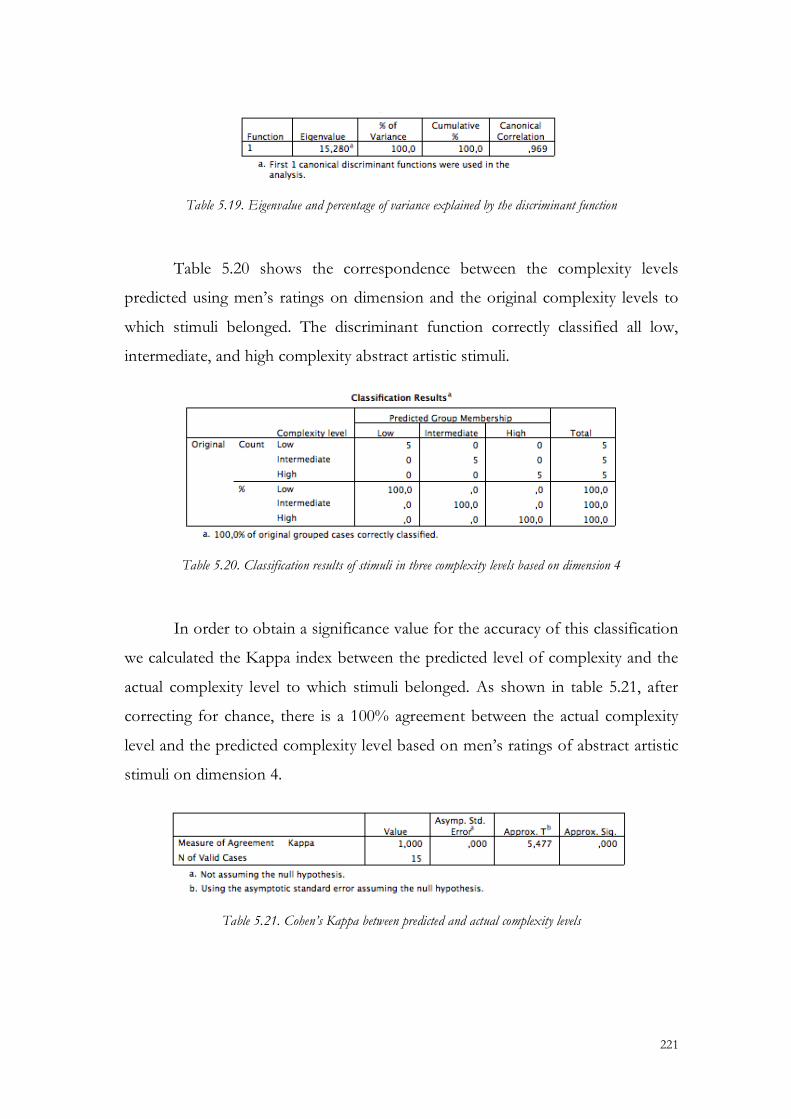
221

Table 5.19. Eigenvalue and percentage of variance explained by the discriminant function

Table 5.20 shows the correspondence between the complexity levels

predicted using men’s ratings on dimension and the original complexity levels to

which stimuli belonged. The discriminant function correctly classified all low,

intermediate, and high complexity abstract artistic stimuli.

Table 5.20. Classification results of stimuli in three complexity levels based on dimension 4

In order to obtain a significance value for the accuracy of this classification

we calculated the Kappa index between the predicted level of complexity and the

actual complexity level to which stimuli belonged. As shown in table 5.21, after

correcting for chance, there is a 100% agreement between the actual complexity

level and the predicted complexity level based on men’s ratings of abstract artistic

stimuli on dimension 4.

Table 5.21. Cohen’s Kappa between predicted and actual complexity levels

222

Abstract artistic: women

The complexity level of each stimulus served as the grouping value, and the

average of women’s scores to each of the 15 abstract artistic stimuli on each

complexity dimension were entered as independent variables. As shown in table

5.22, women’s scores on dimensions 1 and 3 –unintelligibility of the elements and

variety of elements- represent the best parsimonious combination of dimensions

to predict the complexity level of the subset of abstract artistic stimuli. In fact, the

F-tests reveal that the scores women awarded on dimensions 1 and 3 to stimuli

belonging to the three complexity levels differ significantly.

Table 5.22. Predictor variables for women’s ratings of abstract artistic stimuli

Together with the standardized canonical discriminant function

coefficients, Wilks’ Lambda for women’s discriminant scores is presented in table

5.23. In this case, differences among complexity levels accounts for over 95% of

the variance among discriminant scores derived from dimensions 1 and 3. The

result of the associated Chi-square this test reveals there are highly significant

differences between complexity levels in the results of the first discriminant

function, though not the second.

Table 5.23. Standardized canonical discriminant function coefficients and Wilks’ Lambda

223

As shown in table 5.24, the first discriminant function has a very high

eigenvalue, the quotient between the between-groups sum of squares and the

within-groups sum of squares. It also shows that the first discriminant function

explains over 98% of the overall variance.

Table 5.24. Eigenvalues and percentage of variance explained by the discriminant functions

Table 5.25 shows the correspondence between the complexity levels

predicted using women’s ratings on dimensions 1 and 3 and the original

complexity levels to which stimuli belonged. The discriminant function correctly

classified all low, and intermediate complexity abstract artistic stimuli. However, it

erroneously classified one of the five high complexity abstract artistic stimuli in the

intermediate level. Overall, the discriminant function based on women’s scores on

dimensions 1 and 3 correctly classified 93.3% of abstract artistic stimuli.

Table 5.25. Classification results of stimuli in three complexity levels based on dimensions 1 and 3

In order to obtain a significance value for the accuracy of this classification

we calculated the Kappa index between the predicted level of complexity and the

actual complexity level to which stimuli belonged. As shown in table 5.26, after

correcting for chance, there is a 90% agreement between the actual complexity

224

level and the predicted complexity level based on women’s ratings of abstract

artistic stimuli on dimensions 1 and 3.

Table 5.26. Cohen’s Kappa between predicted and actual complexity levels

Abstract decorative: men

The complexity level of each stimulus served as the grouping value, and the

average of men’s scores to each of the 15 abstract decorative stimuli on each

complexity dimension were entered as independent variables. As shown in table

5.27, men’s scores on dimension 3 –amount of elements- represents the best

parsimonious combination to predict the complexity level of the subset of abstract

decorative stimuli. In fact, the F-test reveal that the scores men awarded on

dimension 3 to stimuli belonging to the three complexity levels differ significantly.

Table 5.27. Predictor variables for men’s ratings of abstract decorative stimuli

Together with the standardized canonical discriminant function

coefficients, Wilks’ Lambda for men’s discriminant scores is presented in table

5.28. In this case, differences among complexity levels account for over 81% of

the variance among discriminant scores derived from factor 3. The result of the

associated Chi-square this test reveals there are highly significant differences

between complexity levels in the results of the sole discriminant function.

225

Table 5.28. Standardized canonical discriminant function coefficients and Wilks’ Lambda

As shown in table 5.29, the first discriminant function has a very high

eigenvalue, the quotient between the between-groups sum of squares and the

within-groups sum of squares. It also shows that the first discriminant function

explains over 98% of the overall variance.

Table 5.29. Eigenvalue and percentage of variance explained by the discriminant function

Table 5.30 shows the correspondence between the complexity levels

predicted using men’s ratings on dimension and the original complexity levels to

which stimuli belonged. The discriminant function correctly classified all low

complexity stimuli. Four of the five intermediately complex abstract decorative

stimuli were correctly classified, while the other was predicted to belong to the

high complexity level. The worse classification results relate to the high complexity

stimuli, two of which were predicted to belong to the intermediate level. Overall,

the discriminant function based on men’s scores on dimension 3 correctly

classified 80% of abstract decorative stimuli.

Table 5.30. Classification results of stimuli in three complexity levels based on dimension 3

226

In order to obtain a significance value for the accuracy of this classification

we calculated the Kappa index between the predicted level of complexity and the

actual complexity level to which stimuli belonged. As shown in table 5.26, after

correcting for chance, there is a 70% agreement between the actual complexity

level and the predicted complexity level based on men’s ratings of abstract

decorative stimuli on dimension 3.

Table 5.31. Cohen’s Kappa between predicted and actual complexity levels

Abstract decorative: women

The complexity level of each stimulus served as the grouping value, and the

average of women’s scores to each of the 15 abstract decorative stimuli on each

complexity dimension were entered as independent variables. As shown in table

5.32, women’s scores on dimension 3 –amount of elements- represents the best

parsimonious combination of factors to predict the complexity level of the subset

of abstract decorative stimuli. In fact, the F-test reveal that the scores women

awarded on dimension 3 to stimuli belonging to the three complexity levels differ

significantly.

Table 5.32. Predictor variables for women’s ratings of abstract decorative stimuli

227

Together with the standardized canonical discriminant function

coefficients, Wilks’ Lambda for women’s discriminant scores is presented in table

5.33. In this case, differences among complexity levels account for almost 75% of

the variance among discriminant scores derived from dimension 3. The result of

the associated Chi-square this test reveals there are highly significant differences

between complexity levels in the results of the sole discriminant function.

Table 5.33. Standardized canonical discriminant function coefficients and Wilks’ Lambda

As shown in table 5.34, the first discriminant function has a very high

eigenvalue, the quotient between the between-groups sum of squares and the

within-groups sum of squares. It also shows that the first discriminant function

explains over 98% of the overall variance.

Table 5.34. Eigenvalue and percentage of variance explained by the discriminant function

Table 5.35 shows the correspondence between the complexity levels

predicted using women’s ratings on dimension 3 and the original complexity levels

to which stimuli belonged. The discriminant function correctly classified all low

complexity stimuli. Four of the five intermediately complex abstract decorative

stimuli were correctly classified, while the other was predicted to belong to the

high complexity level. The worse classification results relate to the high complexity

stimuli, two of which were predicted to belong to the intermediate level. Overall,

228

the discriminant function based on women’s scores on dimension 3 correctly

classified 80% of abstract decorative stimuli.

Table 5.35. Classification results of stimuli in three complexity levels based on dimension 3

In order to obtain a significance value for the accuracy of this classification

we calculated the Kappa index between the predicted level of complexity and the

actual complexity level to which stimuli belonged. As shown in table 5.36, after

correcting for chance, there is a 70% agreement between the actual complexity

level and the predicted complexity level based on women’s ratings of abstract

decorative stimuli on factor 3.

Table 5.36. Cohen’s Kappa between predicted and actual complexity levels

Representational artistic: men

The complexity level of each stimulus served as the grouping value, and the

average of men’s scores to each of the 15 representational artistic stimuli on each

complexity dimension were entered as independent variables. As shown in table

5.37, men’s scores on dimensions 2, 3, 4, and 5 –disorganization, number of

elements, variety of elements, and symmetry- represent the best parsimonious

combination of dimensions to predict the complexity level of the subset of

229

representational artistic stimuli. In fact, the F-tests reveal that the scores men

awarded on dimensions 2, 3, 4, and 5 to stimuli belonging to the three complexity

levels differ significantly.

Table 5.37. Predictor variables for men’s rating of representational artistic stimuli

Together with the standardized canonical discriminant function

coefficients, Wilks’ Lambda for men’s discriminant scores is presented in table

5.38. In this case, the first discriminant function leads to differences among

complexity levels which account for over 98% of the variance among discriminant

scores derived from factors 2, 3, 4, and 5. The result of the associated Chi-square

this test reveals there are highly significant differences between complexity levels

in the results of the first discriminant function. The second discriminant function

also provides significantly different results when calculated for ratings awarded to

stimuli belonging to the three complexity levels, though it accounts for just over

66% of the between group differences.

Table 5.38. Standardized canonical discriminant function coefficients and Wilks’ Lambda

230

As shown in table 5.39, the first discriminant function has a very high

eigenvalue, the quotient between the between-groups sum of squares and the

within-groups sum of squares. It also shows that the first discriminant function

explains 89.9% of the overall variance. In regards to the second discriminant

function, though its eigenvalue is above 1, it is certainly much smaller than that of

the first function. The variance explained by this function is very small, a mere

10.1%.

Table 5.39. Eigenvalue and percentage of variance explained by the discriminant functions

Table 5.40 shows the correspondence between the complexity levels

predicted using men’s ratings on dimensions 2, 3, 4 and 5, and the original

complexity levels to which stimuli belonged. All representational artistic stimuli

were correctly classified.

Table 5.40. Classification results of stimuli in three complexity levels based on dimensions 2, 3, 4 and 5

In order to obtain a significance value for the accuracy of this classification

we calculated the Kappa index between the predicted level of complexity and the

actual complexity level to which stimuli belonged. As shown in table 5.41, after

correcting for chance, there is a 100% agreement between the actual complexity

231

level and the predicted complexity level based on men’s ratings of representational

artistic stimuli on dimensions 2, 3, 4, and 5.

Table 5.41. Cohen’s Kappa between predicted and actual complexity levels

Representational artistic: women

The complexity level of each stimulus served as the grouping value, and the

average of women’s scores to each of the 15 representational artistic stimuli on

each complexity dimension were entered as independent variables. As shown in

table 5.42, women’s scores on dimensions 3 and 5 –number of elements and

symmetry- represents the best parsimonious combination of factors to predict the

complexity level of the subset of representational artistic stimuli. In fact, the F-

tests reveal that the scores women awarded on dimensions 3 and 5 to stimuli

belonging to the three complexity levels differ significantly.

Table 5.42. Predictor variables for women’s rating of representational artistic stimuli

Together with the standardized canonical discriminant function

coefficients, Wilks’ Lambda for women’s discriminant scores is presented in table

5.43. In this case, the first discriminant function leads to differences among

232

complexity levels which account for over 90% of the variance among discriminant

scores derived from dimensions 3 and 5. The result of the associated Chi-square

this test reveals there are highly significant differences between complexity levels

in the results of the first discriminant function. The second discriminant function

does not yield significantly different results when calculated for ratings awarded to

stimuli belonging to the three complexity levels, and accounts for less than 15% of

the between-group differences.

Table 5.43. Standardized canonical discriminant function coefficients and Wilks’ Lambda

As shown in table 5.44, the first discriminant function has a very high

eigenvalue, the quotient between the between-groups sum of squares and the

within-groups sum of squares. It also shows that the first discriminant function

explains 98% of the overall variance. In regards to the second discriminant

function, its eigenvalue is well below 1, and it only explains 2% of the variance.

Table 5.44. Eigenvalue and percentage of variance explained by the discriminant functions

Table 5.45 shows the correspondence between the complexity levels

predicted using women’s ratings on dimensions 3 and 5, and the original

complexity levels to which stimuli belonged. All intermediate complexity

representational artistic stimuli were correctly classified. One of the five high

complexity stimuli was misclassified as intermediate, as was one of the high

complexity representational artistic stimuli.

233

Table 5.45. Classification results of stimuli in three complexity levels based on dimensions 3 and 5

In order to obtain a significance value for the accuracy of this classification

we calculated the Kappa index between the predicted level of complexity and the

actual complexity level to which stimuli belonged. As shown in table 5.46, after

correcting for chance, there is an 80% agreement between the actual complexity

level and the predicted complexity level based on women’s ratings of

representational artistic stimuli on dimensions 3 and 5.

Table 5.46. Cohen’s Kappa between predicted and actual complexity levels

Representational decorative: men

The complexity level of each stimulus served as the grouping value, and the

average of men’s scores to each of the 15 representational decorative stimuli on

each complexity dimension were entered as independent variables. As shown in

table 5.47, men’s scores on dimensions 3 –number of elements- represent the best

parsimonious combination of factors to predict the complexity level of the subset

of representational decorative stimuli. In fact, the F-test reveal that the scores men

awarded on dimension 3 to stimuli belonging to the three complexity levels differ

significantly.

234

Table 5.47. Predictor variables for men’s rating of representational decorative stimuli

Together with the standardized canonical discriminant function

coefficients, Wilks’ Lambda for men’s discriminant scores is presented in table

5.48. In this case, the sole discriminant function leads to differences among

complexity levels which account for over 92% of the variance among discriminant

scores derived from dimension 3. The result of the associated Chi-square test

reveals there are highly significant differences between complexity levels in the

results of the discriminant function.

Table 5.48. Standardized canonical discriminant function coefficients and Wilks’ Lambda

As shown in table 5.49, the discriminant function has a very high

eigenvalue, the quotient between the between groups sum of squares and the

within groups sum of squares. It also shows that the discriminant function

explains 100% of the overall variance.

Table 5.49. Eigenvalue and percentage of variance explained by the discriminant functions

235

Table 5.50 shows the correspondence between the complexity levels

predicted using men’s ratings on dimension 3, and the original complexity levels to

which stimuli belonged. All representational decorative stimuli were correctly

classified.

Table 5.50. Classification results of stimuli in three complexity levels based on dimension 3

In order to obtain a significance value for the accuracy of this classification

we calculated the Kappa index between the predicted level of complexity and the

actual complexity level to which stimuli belonged. As shown in table 5.51, after

correcting for chance, there is a 100% agreement between the actual complexity

level and the predicted complexity level based on men’s ratings of representational

decorative stimuli on dimension 3.

Table 5.51. Cohen’s Kappa between predicted and actual complexity levels

Representational decorative: women

The complexity level of each stimulus served as the grouping value, and the

average of women’s scores to each of the 15 representational decorative stimuli on

each complexity dimension were entered as independent variables. As shown in

table 5.52, women’s scores on dimensions 3 and 5 –number of elements and

236

symmetry- represent the best parsimonious combination to predict the complexity

level of the subset of representational decorative stimuli. In fact, the F-tests reveal

that the scores women awarded on dimensions 3 and 5 to stimuli belonging to the

three complexity levels differ significantly.

Table 5.52. Predictor variables for women’s rating of representational decorative stimuli

Together with the standardized canonical discriminant function

coefficients, Wilks’ Lambda for women’s discriminant scores is presented in table

5.53. In this case, the first discriminant function leads to differences among

complexity levels which account for over 95% of the variance among discriminant

scores derived from dimensions 3 and 5. The result of the associated Chi-square

test reveals there are highly significant differences between complexity levels in the

results of the first discriminant function. The second discriminant function

accounts for under 10% of the variance among discriminant scores on dimensions

3 and 5. Furthermore, discriminant scores do not differ significantly among

complexity levels.

Table 5.53. Standardized canonical discriminant function coefficients and Wilks’ Lambda

As shown in table 5.54, the first discriminant function has a very high

eigenvalue, the quotient between the between-groups sum of squares and the

237

within-groups sum of squares. It also shows that the discriminant function

explains 99.5% of the overall variance. The second discriminant function has an

extremely low eigenvalue and explains a mere .5% of the variance.

Table 5.54. Eigenvalue and percentage of variance explained by the discriminant functions

Table 5.55 shows the correspondence between the complexity levels

predicted using women’s ratings on dimensions 3 and 5, and the original

complexity levels to which stimuli belonged. All representational decorative stimuli

were correctly classified.

Table 5.55. Classification results of stimuli in three complexity levels based on dimensions 3 and 5

In order to obtain a significance value for the accuracy of this classification

we calculated the Kappa index between the predicted level of complexity and the

actual complexity level to which stimuli belonged. As shown in table 5.56, after

correcting for chance, there is a 100% agreement between the actual complexity

level and the predicted complexity level based on women’s ratings of

representational decorative stimuli on dimensions 3 and 5.

238

Table 5.56. Cohen’s Kappa between predicted and actual complexity levels

239

3.3.1.4. Summary table

Stimuli Sex PV EV(%) CC (%) Kappa

Men 3 & 4 97 68.3 .525* All taken together

Women 3 & 6 99.8 76.7 .650*

Men 4 100 100 1* Abstract Artistic

Women 1 & 3 98.6 93.3 .90*

Men 3 100 80 .70* Abstract Decorative

Women 3 100 80 .70*

Men 2, 3, 4 & 5 89.9 100 1* Representational Artistic

Women 3 & 5 98 86.7 .80*

Men 3 100 100 1* Representational Decorative

Women 3 & 5 99.5 100 1*

*p < .001

PV: Predictor complexity factors. EV: Explained variance. CC: Correct classification. Kappa: Agreement between the predicted and actual complexity levels.

Dimensio n 1: Unintelligibility of the elements. Dimensio n 2: Disorganization. Dimensio n 3: Amount of elements. Dimensio n 4: Variety of elements. Dimensio n 5: Symmetry. Dimensio n 6: Variety of colours. Dimensio n 7: Three-dimensional appearance.

These results suggest that the complexity levels of stimuli in the overall

sample can be predicted based on men’s scores on dimensions 3 and 4 –amount

of elements and variety of elements, respectively. Conversely, in the case of

women, the complexity levels for the overall sample of stimuli can be predicted

from their ratings of the amount of elements and the variety of colours

(dimensions 3 and 6). When predicting the complexity levels of stimuli belonging

240

to each kind (AA, AD; RA, RD), the most accurate complexity dimensions vary

according to the kind of stimulus and the sex of the participants. The complexity

of abstract artistic stimuli is adequately predicted by men’s scores to dimension 4,

variety of elements, and women’s ratings on dimensions 1 and 3, unintelligibility of

the elements and amount of elements. Both men and women’s ratings of amount

of elements (dimensions 3) are the best predictors of complexity level of abstract

decorative stimuli. In order to predict the complexity level of representational

artistic stimuli from men’s ratings to the predictor variables, dimensions 2, 3, 4,

and 5, disorganization, amount and variety of elements, and symmetry, need to be

taken into account. Conversely, women’s ratings on dimensions 3 and 5, amount

of elements and asymmetry, suffice to make adequate predictions. Finally,

dimension 3, amount of elements, is necessary to predict the complexity level of

representational decorative stimuli from men and women’s scores. But dimension

5, asymmetry, is also required for the prediction to be accurate in the case of

scores awarded by female participants. Overall, dimension 3, the amount of

elements seems to be the most common predictor variable, and factor 7, three-

dimensional appearance, has no predictive value at all, as well as dimension 6,

variety of colours, when analyzing different kinds of stimuli separately.

241

3.3.2. Factor analysis

Factor analysis was performed in order to assess the relations among the

seven dimensions of complexity. This procedure allows simplifying those relations

by identifying underlying factors that explain the greatest possible amount of

original information. Factor analysis has the advantage over other data reduction

procedures of yielding a small number of easily interpretable factors.

Here we have used principal components to estimate the factorial model,

one of the most common procedures in this kind of analysis. In order to aid in the

interpretation of the resulting factors we have used Varimax rotation of factors.

This additional step strengthens correlations among the original variables included

in each factor and weakens those with variables included in other factors. The

same procedure has been carried out on men and women’s ratings of the 60

stimuli on the 7 complexity dimensions. These stimuli were selected, as stated in

section 2.3.3, among the original set of 120, as described in sections 2.2 and 3.1.

Originally only factors with eigenvalues over 1 were extracted. This

resulted in two factors which explained 48.669% and 31.854% of the variance in

scores awarded by male participants and 47.351% and 31.426% in scores awarded

by female participants. For both groups of participants factor 1 received high

loadings from complexity dimensions 3 (amount of elements), 4 (variety of

elements), 6 (variety of colours), and 7 (three-dimensional appearance). For men

and women factor 2 received high loadings from dimensions 1 (unintelligibility of

the elements) and 2 (disorganization). Additionally, for both groups of participants

dimensions 5 (asymmetry) showed unsatisfactory relations with both factors.

Inspection of its relation with additional factors revealed it was related with a

factor whose eigenvalue was .975. Given the importance of the symmetry-

242

asymmetry dimension in the study of the relation between complexity and the

appreciation of beauty, outlined in the introduction, as well as the potential

advantages of understanding its relation with other dimensions of complexity, it

was decided to lower the factor extraction criterion from eigenvalues over 1 to

eigenvalues over .97. Although it is not common to lower this threshold, the fact

that the factor with the next highest eigenvalues had very low values, .212 for men

and .314 for women, suggests that this choice did not prejudice the extraction of

additional factors. This solution is compatible with an alternative approach to

deciding on how many factors to extract, known as the scree test. This procedure

involves retaining all factors with eigenvalues on the sharp descent part of the

scree plot before they begin to level. For both men and women the scree test

recommends extracting three factors (see figure 6.1).

Figure 6.1. Scree plots for the eigenvalues of factors extracted from men’s (left) and women’s (right) ratings on the 7 complexity dimensions

Hence, in this section we present the results of factor analysis of men and

women’s ratings on the seven complexity dimensions by means of principal

components extracting factors with eigenvalues over .97 and including a Varimax

orthogonal rotation.

243

3.3.2.1. Factor analysis for men’s rating of the 7 complexity

dimensions

Mean scores awarded by men to each stimulus on each of the seven

complexity dimensions were entered as variables into the factor analysis application

of the SPSS. Varimax was chosen as the rotation method. The selected descriptives

of the correlation matrix were KMO and Bartlett’s test of sphericity, determinant, and

anti-image matrix. Selected extraction options were to use the principal components

method, to analyze the correlation matrix, and to extract factors with eigenvalues

over .97, as indicated above. We begin by presenting the measures of adequacy,

and then we present the results of the factor analysis.

KMO is a measure of the adequacy of the data for a factor analysis. In the

case of men’s scores on the seven complexity dimensions, its value is quite high,

indicating that the adequacy of the data is reasonably high (see table 6.1). Batlett’s

procedure tests the null hypothesis that the initial variables are not correlated.

These results indicate that there is a high degree of correlation among the

dimensions, which is an important requirement for factor analysis. However, the

fact that the distribution of scores awarded by male participants on some of the

dimensions departs from normality, reduces the trustworthiness of this measure.

Table 6.1. KMO measure and Bartlett’s test of sphericity

Additional measures of adequacy were calculated for ratings awarded by

men on the seven complexity dimensions (see table 6.2): (i) the determinant of the

correlation matrix, with smaller values indicating a high correlation among the

244

variables, a requirement of the principal component procedure, and (ii) the anti-

image correlation matrix, which provide partial correlation coefficients between

each pair of variables. In this second case, low values are necessary for values to

share common factors. Elements in the main diagonal are akin to the KMO

measure for each pair of variables, and higher values indicate a greater adequacy.

Table 6.2. Determinant of the correlation matrix and anti-image matrices for men’s scores on the 7 complexity dimensions

As seen in table 6.2, the determinant of the correlation matrix has a very

low value, suggesting that, overall, men’s ratings on the complexity dimensions are

relatively correlated. More specifically, the adequacy of men’s ratings on

dimensions 1 and 2 is acceptable, around .55. The adequacy of their ratings on

dimensions 3 and 4 is good, around .75. The adequacy of scores awarded on

dimensions 6 and 7 is very good, in fact it is over .9. The worse adequacy score

was obtained by complexity dimension 5, probably related with its low eigenvalue.

The results of the factor analysis of men’s scores on the seven complexity

dimensions appear in table 6.3. Three components met the aforementioned

criteria and, hence, were extracted. The first two components explained over 48%

and over 31% of the variance, respectively. Cumulative explained variance is just

245

over 80%. The third component explains close to 14% of the variance. Thus, if

this component is accepted, the overall explained variance is raised to over 94%.

Table 6.3. Extracted components and variance explained

Commonalities, which are presented below in table 6.4, inform about the

extent to which the variables are well represented by the extracted factors. That is,

the extent to which their variance is reproduced by the common factors. In the

case of men’s ratings on the seven complexity dimensions, all results are very

positive, with values over 95%, except for dimensions 6 (90.6%) and 7 (84.9%).

Hence, as a whole, the variance of the seven complexity dimensions as rated by

men is accurately reproduced by the common factors.

Table 6.4. Commonalities for men’s ratings on the seven complexity dimensions

Table 6.5 presents the component matrix and the rotated component

matrix. After the factors had been rotated, it became very clear that the first one

received high loadings from dimensions 3, 4, 6, and to a slightly lesser degree,

dimension 7. Loadings from the other three dimensions were negligible. The

second factor received high loadings from dimensions 1 and 2. Dimension 3 had a

very slight positive loading on this factor, and dimension 7 a moderate negative

246

loading. Finally, the only complexity dimension to load on the third factor is

number 5. The remaining dimensions have negligible loadings on this factor.

Table 6.5. Component matrix (left) and rotated component matrix (right)

Table 6.6 presents the component score coefficient matrix, which

reinforces the aforementioned results. Dimensions 3, 4, 6, and 7 (amount of

elements, variety of elements, variety of colours, three-dimensional appearance)

have high coefficients for factor 1. Dimensions 1 and 2 (unintelligibility of the

elements and disorganization) have high coefficients on the second factor.

Dimension 7 has also a slight negative coefficient for the second factor. Finally,

dimension 5 –asymmetry- is the sole high coefficient for the third factor.

Table 6.6. Component score coefficient matrix

247

3.3.2.2. Factor analysis for women’s rating of the 7 complexity

dimensions

Mean scores awarded by women to each stimulus on each of the seven

complexity dimensions were entered as variables into the factor analysis application

of the SPSS. Varimax was chosen as the rotation method. The selected descriptives

of the correlation matrix were KMO and Bartlett’s test of sphericity, determinant, and

anti-image matrix. Selected extraction options were to use the principal components

method, to analyze the correlation matrix, and to extract factors with eigenvalues

over .97, as indicated above. We begin by presenting the measures of adequacy,

and then we present the results of the factor analysis.

The KMO is a measure of the adequacy of the data for a factor analysis. In

the case of women’s scores on the seven complexity dimensions, its value is quite

high, indicating that the adequacy of the data is reasonably high (see table 6.7).

Batlett’s procedure tests the null hypothesis that the initial variables are not

correlated. These results indicate that there is a high degree of correlation among

the dimensions, which is an important requirement for factor analysis. However,

the fact that the distribution of scores awarded by female participants on some of

the dimensions departs from normality, reduces the trustworthiness of this

measure.

Table 6.7. KMO measure and Bartlett’s test of sphericity

Additional measures of adequacy were calculated for ratings awarded by

women on the seven complexity dimensions (see table 6.8): (i) the determinant of

the correlation matrix, with smaller values indicating a high correlation among the

248

variables, a requirement of the principal component procedure, and (ii) the anti-

image correlation matrix, which provide partial correlation coefficients between

each pair of variables. In this second case, low values are necessary for values to

share common factors. Elements in the main diagonal are akin to the KMO

measure for each pair of variables, and higher values indicate a greater adequacy.

Table 6.8. Determinant of the correlation matrix and anti-image matrices for women’s scores on the 7 complexity dimensions

As seen in table 6.8, the determinant of the correlation matrix has a very

low value, suggesting that overall, women’s ratings on the complexity dimensions

are relatively correlated. More specifically, the adequacy of women’s ratings on

dimensions 1 and 2 is acceptable, around .54. The adequacy of their ratings on

dimensions 3 and 4 is good, around .75. The adequacy of scores awarded on

dimensions 6 and 7 is very good, in fact it is over .85. The worse adequacy score

was obtained by complexity dimension 5 (.31), probably related with its low

eigenvalue.

The results of the factor analysis of women’s scores on the seven

complexity dimensions appear in table 6.9. Three components met the

aforementioned extraction criteria and were extracted. The first two components

explained over 47% and over 31% of the variance, respectively. Cummulative

249

explained variance is just over 78%. The third component explains close to 14%

of the variance. Thus, if this component is accepted, the overall explained variance

is raised to over 92%.

Table 6.9. Extracted components and variance explained

Commonalities, which are presented below in table 6.10 inform about the

extent to which the variables are well represented by the extracted factors. That is,

the extent to which their variance is reproduced by the common factors. In the

case of women’s ratings on the seven complexity dimensions, most of the results

are very positive, with values over 95%. Under this threshold we find dimensions

4 (93.2%), 6 (87.1%) and 7 (78.9%). Hence, overall, the variance of the seven

complexity dimensions as rated by women is accurately reproduced by the

common factors.

Table 6.10. Commonalities for women’s ratings on the seven complexity dimensions

Table 6.11 presents the component matrix and the rotated component

matrix. After the factors had been rotated, it became very clear that the first one

received high loadings from dimensions 3, 4, 6, and to a slightly lesser degree,

250

dimension 7. Loadings from the other three dimensions were negligible. The

second factor received high loadings from dimensions 1 and 2. Dimensions 3 and

4 had very slight positive loadings on this factor, and dimension 7 a moderate

negative loading. Finally, the only complexity dimension to load on the third factor

is number 5. The remaining dimensions have negligible or very low loadings on

this factor.

Table 6.11. Component matrix (left) and rotated component matrix (right)

Table 6.12 presents the component score coefficient matrix, which

reinforces the aforementioned results. Dimensions 3, 4, 6, and 7 (amount of

elements, variety of elements, variety of colours, three-dimensional appearance)

have high coefficients for factor 1. Dimensions 1 and 2 (unintelligibility of the

elements and disorganization) have high coefficients on the second factor.

Dimension 7 has also a moderately high negative coefficient for the second factor.

Finally, dimension 5, asymmetry, is the sole high coefficient for the third factor.

Table 6.12. Component score coefficient matrix

251

3.3.3. Exploratory study of the relation between complexity

dimensions and beauty ratings.

In the introduction we suggested that a possible reason for the lack of

agreement among studies of the relation between complexity and aesthetic

preference was the use of different concepts and measurements of complexity.

Although the present study was not designed to address this issue experimentally,

but only in an exploratory fashion, it could be the case that the seven complexity

factors that we have considered here might have different effects on the ratings of

the beauty of visual stimuli. In this section we will use the data we collected to

explore this possibility in a very preliminary manner.

Curve estimation tests were carried out taking each of the seven complexity

factors separately as independent variables and the beauty scores as the dependent

variable. The fit of linear, quadratic, and cubic functions was assessed. The results

of this analysis are provided below for each of the factors, along with a plot of

beauty scores as a function of each of them. The significant function is overlaid on

the graphs. When more than one or no solution turned out to reach significance,

only the solution with the lowest significance value was plotted. When all

significance values were equal, only the function with the highest F value was

plotted. This procedure was carried out separately for men and women, and the

results for both groups are presented sequentially.

252

3.3.3.1. Curve fit between men’s complexity factors and beauty scores

Complexity dimension 1: Unintelligibility of the elements

The curve fit procedure indicated that the only function to reach

significance is the cubic one. Figure 7.1 shows that the highest beauty scores

awarded by men were received by those stimuli that were later rated as low or high

on unintelligibility of the elements present in the picture. Stimuli rated with an

intermediate unintelligibility of the elements tended to receive the lowest beauty

scores.

Figure 7.1. Curve fit between men’s scores on “Unintelligibility of the elements” and “Beauty”

Complexity dimension 2: Disorganization

In this case, linear, quadratic and cubic functions fit the relation between

men’s scores on complexity dimension 2, disorganization, and beauty. However,

the quadratic function reached the best significance levels. In a similar way to

unintelligibility of the elements, low and high scores on disorganization were

associated to the highest beauty scores. However, beauty ratings associated with

higher scores on the present complexity dimension were slightly lower than beauty

ratings associated with the lower scores on disorganization (see figure 7.2).

253

Figure 7.2. Curve fit between men’s scores on “Disorganization” and “Beauty”

Complexity dimension 3: Amount of elements

Here, linear, quadratic, and cubic functions fit the relation between men’s

scores on amount of elements and beauty. Given that all significance levels are the

same, only the linear function has been plotted. Overall, higher beauty scores were

awarded by men to stimuli rated to have more elements, and lower beauty scores

were awarded to stimuli with fewer elements (see figure 7.3).

Figure 7.3. Curve fit between men’s scores on “Amount of elements” and “Beauty”

254

Complexity dimension 4: Element heterogeneity

Here, linear, quadratic, and cubic functions again fit the relation between

men’s scores on variety of elements and beauty. Given that all significance levels

are the same, only the linear function has been plotted. Overall, higher beauty

scores were awarded by men to stimuli rated to have more elements, and lower

beauty scores were awarded to stimuli with fewer elements (see figure 7.4).

Figure 7.4. Curve fit between men’s scores on “Element heterogeneity” and “Beauty”

Complexity dimension 5: Asymmetry

There is no satisfactory relation between men’s rating of asymmetry and

beauty. None of the three functions reached significance. We have chosen to plot

the one with the best significance: the quadratic function. In this case, men seem

to have awarded higher beauty scores to stimuli rated as intermediately asymmetric

than to those stimuli rated as very symmetric or very asymmetric (see figure 7.5).

255

Figure 7.5. Curve fit between men’s scores on “Asymmetry” and “Beauty”

Complexity dimension 6: Colour variety

Here, linear, quadratic, and cubic functions again fit the relation between

men’s scores on colour variety and beauty. Given that all significance levels are the

same, only the linear function has been plotted. Overall, higher beauty scores were

awarded by men to stimuli rated to have a broader range of colours, and lower

beauty scores were awarded to stimuli with fewer colours (see figure 7.6).

Figure 7.6. Curve fit between men’s scores on “Colour variety” and “Beauty”

256

Complexity dimension 7: Three-dimensional appearance

Linear, quadratic, and cubic functions again fit the relation between men’s

scores on three-dimensional appearance and beauty. Given that all significance

levels are the same, only the linear function has been plotted. Overall, men

awarded higher beauty scores to stimuli rated to have a greater three-dimensional

appearance than to those rated as having a lower three-dimensional appearance

(see figure 7.7).

Figure 7.7. Curve fit between men’s scores on “Three-dimensional appearance” and “Beauty”

3.3.3.2. Curve fit between women’s complexity factors and beauty

scores

Complexity dimension 1: Unintelligibility of the elements

The curve fit procedure indicated that the linear, quadratic and cubic

functions reach significance, though the latter one’s significance value is the

smallest. Figure 7.8 shows that the highest beauty scores awarded by women were

received by those stimuli that were later rated as very low or very high on

unintelligibility of the elements present in the picture. Stimuli rated with an

257

intermediate unintelligibility of the elements received the lowest beauty scores. For

women, however, this tendency is not as marked as for men.

Figure 7.8. Curve fit between women’s scores on “Unintelligibility of the elements” and “Beauty”

Complexity dimension 2: Disorganization

In this case, linear, quadratic and cubic functions showed an adequate fit

the relation between women’s scores on complexity dimension 2, disorganization,

and beauty. However, the quadratic function reached the best significance levels.

In a similar way to unintelligibility of the elements, low and high scores on

disorganization were associated to the highest beauty scores. However, beauty

ratings associated with higher scores on the present complexity dimension were

lower than beauty ratings associated with the lower scores on disorganization (see

figure 7.9).

258

Figure 7.9. Curve fit between women’s scores on “Disorganization” and “Beauty”

Complexity dimension 3: Amount of elements

Here, linear, quadratic, and cubic functions fit the relation between

women’s scores on amount of elements and beauty. Given that all significance

levels are the same, only the linear function has been plotted. Overall, higher

beauty scores were awarded by women to stimuli rated to have more elements,

and lower beauty scores were awarded to stimuli with fewer elements (see figure

7.10).

Figure 7.10. Curve fit between women’s scores on “Amount of elements” and “Beauty”

259

Complexity dimension 4: Element heterogeneity

Here, linear, quadratic, and cubic functions again fit the relation between

women’s scores on variety of elements and beauty. Given that all significance

levels are the same, only the linear function has been plotted. Overall, women

awarded higher beauty scores to stimuli rated to have more elements, and lower

beauty scores to stimuli with fewer elements (see figure 7.11).

Figure 7.11. Curve fit between women’s scores on “Element heterogeneity” and “Beauty”

Complexity dimension 5: Asymmetry

There is no satisfactory relation between women’s rating of asymmetry and

beauty. None of the three functions reached significance. We have chosen to plot

the one with the best significance: the quadratic function. In this case, women

seem to have awarded higher beauty scores to stimuli rated as intermediately

asymmetric than to those stimuli rated as very symmetric or very asymmetric (see

figure 7.12).

260

Figure 7.12. Curve fit between women’s scores on “Asymmetry” and “Beauty”

Complexity dimension 6: Colour variety

Here, linear, quadratic, and cubic functions again fit the relation between

women’s scores on colour variety and beauty. Given that all significance levels are

the same, only the linear function has been plotted. Overall, higher beauty scores

were awarded by women to stimuli rated to have a broader range of colours, and

lower beauty scores were awarded to stimuli with fewer colours (see figure 7.13).

Figure 7.13. Curve fit between women’s scores on “Colour variety” and “Beauty”

261

Complexity dimension 7: Three-dimensional appearance

Linear, quadratic, and cubic functions again fit the relation between

women’s scores on three-dimensional appearance and beauty. Given that all

significance levels are the same, only the linear function has been plotted. Overall,

women awarded higher beauty scores to stimuli rated to have a greater three-

dimensional appearance than to those rated as having a lower three-dimensional

appearance (see figure 7.14).

Figure 7.14. Curve fit between women’s scores on “Three-dimensional appearance” and “Beauty”

3.3.3.3. Summary table

The following table summarizes the results of relating men and women’s

beauty ratings with their scores on each complexity dimension. Two issues stand

out at a glance. First, that trends for men and women are very similar. Second, that

trends for dimensions 1 and 2 are virtually identical, as are trends for dimensions

3, 4, 6, and 7. The relation between dimension 5 and beauty ratings is different to

all the rest.

262

Dimension Men Women

1

Unintelligibility of the elements

2

Disorganization

3

Amount of elements

4

Element heterogeneity

5

Asymmetry

6

Colour variety

7

Three-dimensional appearance

263

4

Discussion

264

4.1 The influence of complexity on

aesthetic preference

Abstract

In this section we discuss the results of our tests of hypotheses I.I, I.II, I.III and II. Our results suggest that both men and women prefer highly complex stimuli to simple ones, artistic to decorative stimuli, and representational to abstract stimuli. However, closer inspection of the data revealed that the effects of complexity were driven mainly by the scores awarded to representational decorative stimuli. We feel that these results support our initial assumption that divergence among the results of studies carried out to test Berlyne’s predicted relation between complexity and aesthetic preference could, to a certain extent, be due to their use of different kinds of materials. However, our results do not support our initial prediction that the composition of the groups of participants in relation to sex might have also played a role in the aforementioned divergence.

265

Daniel Berlyne was one of the most influential researchers in empirical

aesthetics. His work integrated some aspects of Fechner’s legacy with behavioural

science, neuroscience, and information theory. One of his most lasting

contributions was his study of the role of collative variables, particularly

complexity, on aesthetic preference. As we saw in the introduction to the present

work, Berlyne’s framework predicted that, given a choice of visual stimuli varying

in complexity, people would prefer intermediately complex pictures than very

simple or very complex ones. Since its formulation, there have been many

attempts to test this prediction. Some studies have found that indeed, participants

preferred intermediate levels of complexity. However, a substantial portion of the

studies that have examined this question have found that aesthetic preference

increases with complexity.

The main objective of the present work was to determine the causes of the

discrepancies in studies testing Berlyne’s predicted relation between complexity

and preference. We hypothesized that, to a certain point, the use of different kinds

of materials, such as abstract or representational stimuli, and reproductions of

artworks or non-artistic pictures, could explain the divergence in results. We also

suggested that the composition of participant groups in relation to sex could lead

to studies arriving at different results. Finally, we argued that the use of different

definitions and measures of “complexity” could have also played a part in the lack

of congruence in the reviewed results. In order to test these hypotheses, we

designed a study in which male and female participants were asked to rate the

beauty of abstract, representational, artistic, and decorative visual stimuli varying in

complexity. Thereafter, they were also asked to rate visual stimuli varying in

complexity on a series of possible dimensions of complexity.

In this subsection we will discuss the results in relation to the first two

hypotheses, those that have to do with the role of the kind of stimulus and the

participants’ sex on the relation between the complexity of those stimuli and the

266

aesthetic preference expressed by those participants. We will discuss the results

relating to the influence of the conception of complexity for the subsequent

subsection.

The results yielded by our statistical tests revealed that both men and

women awarded higher beauty scores to highly complex visual stimuli than to

simple ones. In addition, male and female participants found representational

stimuli to be more beautiful than the abstract ones. Finally, both groups of

participants rated the beauty of artistic stimuli higher than decorative stimuli.

However, when the analysis was carried out separately for each type of stimulus, it

turned out that the influence of complexity on aesthetic preference we just noted

was not felt for any of the stimuli types, except for representational decorative

images. In fact, the results suggest that the great difference in aesthetic preference

for very complex and simple representational decorative stimuli might actually be

driving the aforementioned main effects, together with other triple interactions

(commented in Annex D).

Closer inspection of the data and the stimuli suggests a possible

explanation for the strong influence of complexity on aesthetic preferences for

representational decorative stimuli. Boxplots in figure 4.3 and tables 4.3 and 4.4

clearly show that both men and women rated highly complex representational

decorative stimuli as beautiful as artistic representational stimuli. The comparison

of low complexity and high complexity representational decorative stimuli (see

Annex A, images 1221 to 1220 and images 3221 to 3220, respectively) reveals a

clear difference between both groups of stimuli. Low complexity representational

decorative stimuli are simple or schematic drawings or photographs of individual

objects, such as a car, a biker, bananas, a pencil, and so on. Conversely, high

complexity representational decorative stimuli are, for the most part, paintings or

photographs of natural sceneries, such as landscapes or seascapes. Hence, it seems

that the beauty ratings awarded by our participants without artistic training reflect

a tendency to consider the art-looking postcards or illustratioins as artistic and to

267

reject simple depictions of individual objects. This suggests that our category of

decorative stimuli could probably be subdivided into a category of what Lindauer

(1990) and Winston and Cupchik (1992) might consider cheap or popular art and a

category of what we could call icons or objects.

On the other hand, the fact that all of our results were virtually identical for

men and women, suggest that, contrary to what we predicted, the role of sex

seems to be small in the mediation of the influence of complexity on aesthetic

preference. The fact that we were unable to find any evidence that the influence of

complexity on aesthetic preference differs for men and women suggests that the

composition of participant groups in relation to sex is not a relevant factor behind

the diverging results of prior studies examining the relation between complexity

and aesthetic preference.

Our results, thus, support prior studies that found a linear relation between

the complexity of non-artistic representational stimuli and aesthetic preference,

suggesting that people prefer complex representational decorative over simple

ones (Francès, 1976; Heath et al., 2000; Stamps, 2002). Our results are contrary to

Berlyne's (1963) finding that aesthetic preference for non-artistic representational

stimuli decreased with complexity, and to studies finding an inverted U

distribution for this kind of images (Imamoglu, 2000; Nasar, 2002). Additionally,

we found no evidence to support the notion that complexity influences people’s

aesthetic preference of artistic stimuli, as suggested by Krupinski and Locher

(1988), Messinger (1998), Neperud and Marschalek (1988), Nicki and colleagues

(1981), Nicki and Moss (1975), Osborne and Farley (1970), Saklofske (1975), and

Wohlwill (1968). Finally, we found no evidence for the influence of complexity on

aesthetic preference for non-artistic abstract images that had been noted by Aitken

(1974), Day (1967), Eisenman (1967), Munsinger and Kessen (1964), and Nicki

and Gale (1977).

Our finding of different effects of complexity on aesthetic preference as a

function of stimuli type suggests that the composition of the materials used in

268

studies testing Berlyne’s prediction is a factor that can explain why they have

arrived at diverging results. Hence, it would seem that the role of complexity on

aesthetic preference is mediated by the kind of visual stimuli used to study the

relation between these two variables.

However, although our results showed that complexity was an important

determinant of people’s aesthetic preference for non-artistic representational

visual stimuli, the fact remains that for the other kinds of stimuli used in the

present study, aesthetic preference was unrelated to complexity. This suggests that

other variables might have played a larger role than we previously suspected.

These uncontrolled variables might include the degree of prototypicality of the

stimuli, certain personality traits and cognitive style of the participants, their

informal experience with art, and so on.

Additionally, it is possible that a single general measure of complexity is

simply an invalid concept. With few exceptions, attempts to explore the relation

between complexity and aesthetic preference have made use of a single measure of

complexity, most often the number of elements (angles, lines, intersections,

geometrical figures, and so on). This means that they have not controlled other

features that possibly have an impact on the perceived complexity of the stimuli.

We explore this possibility in the next subsection.

269

4.2 The concept of complexity

Abstract

In this section we discuss the results of our tests of hypotheses III.I, III.II, and III.III. These results suggest, first, that men and women base their judgments of complexity of visual stimuli on different features. Furthermore, the kind of stimuli also plays a role in determining the relevant features on which participants base their general complexity ratings. Second, there seem to be three main factors behind these ratings: the amount and variety of elements, their organization, and symmetry. We suggest that these three factors could be related with different perceptual and cognitive processes, and that a general concept of complexity is invalid because it masks the different contributions of these three forms of complexity. Finally, the three complexity factors seem to be related differently with beauty ratings.

270

Berlyne and colleagues (1968) distinguished various features of visual

stimuli that contributed to the subjective impression of complexity. These

included the amount of elements, their heterogeneity, the irregularity of their

shapes, the irregularity of their disposition, the degree with which the different

elements are perceived as a unit, asymmetry, and incongruence. Since this initial

classification there has not been much work aimed at determining whether these

features impact subjective complexity in the same way and to the same extent. In

addition, there has been little research on the relation among the complexity

features themselves. It could be, for instance, that Berlyne and colleagues’ (1968)

complexity features were completely independent, or, conversely, that some of

them were more closely related than others. Finally, there has been no attempt at

determining whether different complexity features affect aesthetic preference in

the same way or to the same extent. In fact, most research in empirical aesthetics

and visual perception has regarded complexity as a one-dimensional concept.

Although many studies have dealt with the relation between complexity and

aesthetic preference, their specification of complexity has not always emphasized

the same aspect of complexity. Whereas some studies have conceived complexity

as the amount of elements in a stimulus –lines, angles, turns, and so on- other

have regarded it as the degree of asymmetry, or the degree of incongruity. This

obviously creates problems when comparing their results, which may differ

precisely because complexity refers to different things in different cases.

Here we have tentatively explored the conceptual structure of complexity

ratings in three ways: (i) by trying to ascertain whether any of the dimensions is

more salient that others as a function of the sex of the participants and the kind of

stimuli when performing judgments of complexity, (ii) by exploring how the

complexity dimensions are related among themselves, and (iii) by exploring how

each of them is related to beauty ratings. In what follows, we discuss the results of

these three explorations and we then finish with a general discussion.

271

4.2.1. Relevance of complexity dimensions for complexity judgments

In order to study the relative importance of complexity dimensions on the

ratings of visual stimuli on subjective complexity we performed a series of

discriminant analyses. The results of these analyses revealed that the complexity

level of each kind of visual stimuli could be predicted very reliably from solely one

or two dimensions. However, the predictive dimensions varied according to the

sex of the participants and the kind of stimulus.

Specifically, the only instance in which more than two dimensions were

required to reach an accurate prediction was that constituted by men’s ratings of

artistic representational stimuli, for which four dimensions were required. Overall,

and in agreement with Berlyne and colleagues’ (1968) results, the dimension which

most often appeared among the predictor variables, alone or in combination with

others, was the amount of elements. When we studied the contribution of the

complexity dimensions to the rating of complexity of the different stimuli types, it

became clear that the variety of their colours and their three-dimensional

appearance was of little relevance. This is in agreement with Hall's (1969) results,

which suggested that the variety of colours did not represent an important factor

when rating the complexity of linear stimuli. Two other results were striking. First,

the heterogeneity of elements was among the reliable predictors of men’s

complexity rating of artistic stimuli, both abstract and representational.

Conversely, it did not appear among the predictors of their rating of decorative

stimuli, neither abstract nor representational. Second, amount of elements and

asymmetry predict women’s complexity ratings of representational stimuli, both

artistic and decorative. Conversely, asymmetry does not appear to be an adequate

predictor of women’s complexity rating of abstract stimuli.

These tentative results suggest hypotheses that require future experimental

testing under rigorously controlled conditions and with stimuli specifically

manipulated to this end:

272

The amount of elements has a great influence on men and women’s ratings

of complexity of artistic and decorative abstract and representational

stimuli.

The variety of colours and the three-dimensional appearance have little

influence on men and women’s ratings of complexity of artistic and

decorative abstract and representational stimuli.

The heterogeneity of elements is a good predictor of men’s rating of artistic

but not decorative stimuli.

Asymmetry is a good predictor of women’s rating of representational but

not abstract stimuli.

4.2.2. Relations among complexity dimensions

We studied the relation between the seven complexity dimensions by

means of factor analysis, which allows simplifying those relations by identifying

underlying factors that explain the greatest possible amount of original

information. Factor analysis has the advantage over other data reduction

procedures of yielding a small number of easily interpretable factors. We carried

out separate analyses for men and women’s ratings, although the final results were

very similar. The present discussion, hence, applies to both sets of results.

Our results indicated the existence of two factors that explained most of

the variance, and a third one which we included to account for asymmetry. The

first factor received high loadings from the following dimensions: amount of

elements, element heterogeneity, variety of colours, and three-dimensional

appearance. The second factor received high loadings from unintelligibility of the

elements and disorganization. And the third factor, as we just mentioned, received

273

high loadings only from asymmetry. We refer these three factors as elements –which

has to do with the amount and variety of the elements-, organization –related with

how the elements are grouped to form identifiable objects and how these are

organized into a coherent scene-, and asymmetry.

Based on men’s ratings, elements accounted for 48.33% of the variance,

organization accounted for 31.69% of the variance, and asymmetry for 14.43%.

Overall, thus, the three factors accounted for 94.45% of the variance of men’s

ratings on the seven complexity dimensions. When the calculations are based on

women’s ratings, elements accounted for 47.01% of the variance, organization

explained 31.17%, whereas asymmetry explained 14.54%. Overall, the three factors

explained 92.71% of the variance of women’s ratings on the seven complexity

dimensions. Hence, loadings on factors based on men and women’s ratings are

very similar.

These results are in line with prior studies. For instance Berlyne and

colleagues' (1968) factor analysis indicated the existence of two main factors, one

related with the amount of elements and another which was a composite of

various of the dimensions he had taken into account, and named it unity versus

articulation into easily recognizable parts. It stands out that these two factors are

very similar, or even equivalent, to our elements and organization factors. However, in

contrast to our results, his first factor accounted for between 70 and 90% of the

variance. This difference in the relevance of the amount of elements on

complexity ratings might be due to the fact that the stimuli used by Berlyne and

colleagues (1968) were simple line drawings in which the constituting elements

were much more salient that in most of the stimuli used in the present study.

Other studies have also found subjective complexity to depend on two

kinds of features. Nicki and Moss (1975) interpreted their results suggesting there

might be two kinds of complexity factors, a “perceptual” one related with the

number and variety of elements, and a “cognitive” one related with the amount of

associations or cognitive tags elicited by stimuli. Chipman (1977) distinguished

274

between a qualitative component of complexity judgments, determined largely by

the amount of elements, and a structural component, related with symmetry, the

repetition of motifs and other organizational processes. Chipman (1977) made a

very interesting suggestion. She noted that the first factor, related to the amount of

elements, seems to set an upper threshold of perceived complexity and the second

one can act reducing this impression. By varying presentation times Ichikawa

(1985) found experimental data to back this.

Thus, our results add further support to the idea that two or three

processes contribute to the formation of subjective visual complexity. Probably

the most important one is the determination of the number and variety of

elements. The second one refers to the difficulty with which the elements are

identified and organized into a coherent scene. Although previous studies have

subsumed asymmetry within organizational processes, our results showed this was

not an adequate solution for our data, and hence, we chose to include it as a

separate factor. The temporal sequence of cognitive processes related with these

factors remains to be elucidated, though based on Ichikawa's (1985) results, a

plausible hypotheses is that the different features are processed in parallel, but that

those related with elements are faster than those related with organization, which

finish later.

4.2.3. Relation between complexity dimensions and beauty ratings

The final part of this study was a tentative exploration of the possibility

that the different dimensions of complexity are related in different ways to beauty

ratings. If this were the case, it could explain some of the diverging results

reviewed in the introduction, which manipulated different features of the stimuli

to create their complexity levels. In order to address this issue we plotted men and

women’s beauty ratings against their rating of each of the complexity dimensions.

275

This can only be regarded as a very tentative exploration because stimuli were not

manipulated independently on each of the complexity dimensions. Despite this

limitation, our results revealed that complexity dimensions were not related in the

same way to beauty.

Dimensions 1 and 2, unintelligibility of the elements and disorganization,

seem to have a U-shaped or descending relation to beauty. Specifically, stimuli

receiving extremely low values on this dimensions were rated as more beautiful

than those receiving intermediate and high scores. In contrast, dimensions 3, 4, 6,

and 7, amount of elements, element heterogeneity, variety of colours, and three-

dimensional appearance, have a linear relation to beauty: images considered to be

most beautiful were also rated higher on these four dimensions. Finally, our results

suggest that dimension 5, asymmetry, seems to have an inverted U shape relation

to beauty: images rated as intermediately asymmetric were considered to be more

beautiful than those rated as extremely asymmetric or extremely symmetric.

This grouping of dimensions according to their relation with beauty ratings

mirrors their loadings on the three factors we commented above. Complexity

dimensions related with the factor elements have a linear relation to beauty.

Complexity dimensions related with the factor organization have a U shaped

relation to beauty. Asymmetry has an inverted U shaped relation to beauty.

Is it possible that the diversity of relations between complexity and beauty

that have been found in previous studies owes to their emphasis on different

factors? Our review of the literature suggests that this might be the case. Out of

the studies we reviewed in the introduction to this work, we selected those that

utilized some sort of specific complexity measure, and we left out those that

assessed complexity by means of a general complexity rating scale. Out of the

studies we were left with, six designed or employed stimuli which varied along the

elements factor (Aitken, 1974; Day, 1967; Heath et al., 2000; Nicki, 1972; Nicki &

Moss, 1975; Stamps, 2002), five designed or used stimuli which varied along the

organization factor (Krupinski & Locher, 1988; Neperud & Marschalek, 1988; Nicki

276

et al., 1981; Nicki & Moss, 1975; Osborne & Farley, 1970), one used stimuli

varying only in asymmetry (Krupinski & Locher, 1988), three used stimuli which

varied in asymmetry as well as elements (Eisenman, 1967; Imamoglu, 2000; Munsinger

& Kessen, 1964), and one used stimuli varying in all three factors (Francès, 1976).

If our reasoning were sound, we would expect those studies that have varied

complexity by manipulating the amount or variety of elements to have found an

increasing relation between complexity and preference. We would expect to find

that studies manipulating complexity by means of organizational features obtained

decreasing or U-like distributions between complexity and preference. Finally, we

would expect prior studies that specified complexity along a symmetry-asymmetry

dimension to have produced the expected inverted U distribution of preferences

over complexity.

In order to test this retrospective prediction we discarded the study by

Francès (1976) due to its combined use of measures related with the three factors.

We also pooled the studies that had conceived complexity as asymmetry or the

combination of asymmetry and number of elements into a single category. For

each of the fifteen studies, we summarized its main conclusion as supporting an

increasing, inverted-U, or decreasing, relation of preference and complexity. Table

8.1 shows the crosstabulation of the main factors manipulated by these studies

with their main conclusion, together with the corresponding Chi-square test.

Table 8.1. Crosstabulation of the main factor manipulated by previous studies and their resultant relation between beauty and complexity

The results of the Chi-square test are highly significant, suggesting that the

choice of complexity factor among Elements, Organization, and Symmetry, has an

impact on the shape of the resulting distribution of beauty over complexity. It is

important to note that just as our results had suggested, most studies manipulating

277

the number or variety of elements found an increasing relation between

complexity and preference, most of those manipulating organizational features had

found a descending relation, and most of those that had manipulated symmetry

found an inverted U distribution. Additionally, directional measures were

calculated in order to assess the strength of the association, which are presented in

table 8.2.

Table 8.2. Directional measures of association between manipulated complexity factor and main result

Hence, there is a strong relation between the way in which previous studies

have specified complexity and their resulting distribution of beauty scores as a

function of complexity. Moreover, as the measures of association show, the kind

of distribution can be predicted from the complexity factor manipulated by the

experimenter with an acceptable degree of accuracy.

278

4.3 General conclusions

Abstract

This work explored several possible reasons for the diverging results of studies aimed to clarify the relation between visual complexity and aesthetic preference. Our results suggested that the use of different kinds of stimuli might have led to some of those divergences. However, contrary to our original assumption, the proportion of men and women participating in those studies seems to have played a very small role. Finally, we suggest that the main reason behind the lack of agreement on the influence of complexity on aesthetic preference is the use and manipulation of different kinds of complexity.

279

This work was carried out with the purpose of determining the reasons for

the divergence in the results of studies testing Berlyne’s hypothesized inverted U

relation between complexity and aesthetic preference of visual stimuli. We had

originally conjectured that differences in the proportion of male and female

participants, in the composition of materials, and in the definition and

measurement of visual complexity among these studies could explain why

Berlyne’s prediction has received such mixed support.

Our results, however, suggest that the proportion of male and female

participants might have had little effect on the results of the studies reviewed in

the introduction. Furthermore, our results also lend limited support to the

possibility that the use of different kinds of visual stimuli, such as artistic vs.

decorative, or abstract vs. representational, might have led to the aforementioned

divergent results. We have also suggested that the role of individual differences in

personality, cognitive style, and informal artistic experience might be more

relevant than we originally surmised.

The results yielded by our study suggest that the most probable cause

behind the diverging results is the different definitions of complexity on which the

researchers grounded their studies. We found that complexity is better understood

as a multidimensional concept. People tend to base their rating of the complexity

of visual stimuli on different aspects, depending on their sex and the kind of

stimulus. Our results suggest that there are three main kinds of aspects: (i) those

related with the amount and variety of elements, (ii) those related with object

recognition and scene organization, and (iii) asymmetry. These three aspects of

complexity seem to be related in different ways to general ratings of the

complexity and to ratings of beauty of visual stimuli, though this needs to be

experimentally tested. We have shown that it is possible that prior studies have

280

designed or used stimuli that emphasized different particular aspects of

complexity. These differences seem to have conditioned the diverging relations

between complexity and aesthetic preference found by the studies we reviewed in

the introduction to this work.

281

Resumen

(Spanish summary)

De todas las aportaciones de Daniel Berlyne a la estética experimental, la que ha tenido un impacto más duradero fue su hipótesis de que las personas tenderían a preferir estímulos visuales de complejidad intermedia por encima de estímulos muy complejos o muy simples. Desde entonces se han llevado a cabo un gran número de estudios que han pretendido verificar esta propuesta. Mientras que los resultados de algunos de ellos han corroborado la hipotetizada relación entre complejidad visual y preferencia estética, otros han hallado que la preferencia aumenta con la complejidad de manera lineal. El objetivo principal de este trabajo es explorar las posibles razones de esta divergencia entre los resultados de los mencionados estudios. Contemplamos tres posibilidades: (i) el uso de materiales distintos en cuanto a su grado de realismo y calidad artística, (ii) la composición diferente de los grupos de participantes en cuanto al sexo, y (iii) distintas concepciones y formas de medir la complejidad visual de los estímulos. Nuestros resultados sugieren que el tipo de materiales y la composición de los grupos de participantes han jugado un papel limitado en la divergencia de resultados entre los estudios anteriores. Por el contrario, nuestros resultados apuntan a que el factor más relevante ha sido la adopción de distintas concepciones de complejidad en los diversos estudios.

282

1. Introducción

Las cuestiones relacionadas con el arte y la estética se han debatido

continuamente desde que fueron planteadas inicialmente por los filósofos de la

antigua Grecia. Hasta hace relativamente poco, las respuestas a estas preguntas, así

como las que atañen a otros fenómenos psicológicos, estaban basadas casi

exclusivamente en las experiencias de los propios autores. En el caso del arte y la

estética, estas experiencias eran sus propias reacciones al contemplar obras

artísticas y la observación cotidiana de las reacciones de otros espectadores. Este

método constituye una base extremadamente pobre para asentar teorías

explicativas, y deja un gran número de temas sin plantear, que a menudo no se

detectan hasta que se aplican métodos más novedosos y rigurosos.

La aplicación de métodos experimentales para la verificación de hipótesis

relacionadas con el arte y la estética comenzó con los trabajos de Gustav Fechner,

considerado también como fundador del campo de la psicofísica. En su libro

Elementos de Estética, Fechner (1876) describía varios experimentos en los que se

estudiaron las respuestas estéticas de muestras de participantes representativos de

diversas poblaciones a diversos tipos de materiales visuales. Las reflexiones e

introspecciones de un único individuo fueron sustituidas por promedios de

respuestas dadas por grupos de participantes, y en lugar de estudiar una obra de

arte en profundidad se empezaron a usar numerosos objetos para determinar

atributos colectivos relacionados con determinadas respuestas.

Los nuevos métodos experimentales introducidos por Fechner permitieron

la formulación rigurosa de hipótesis y su comprobación en condiciones

controladas. Uno de los puntos de mayor interés de esta estética experimental fue

desarrollar un método que permitiera cuantificar la medida estética de un abanico

amplio de objetos. En esta línea, es bien conocida la aportación del matemático

Birkhoff (1932) en la que introducía una fórmula matemática que permitía calcular

283

la medida estética (M) de objetos visuales en virtud del orden (O) y la complejidad

(C):

!

M = OC

De esta manera, cuanto más ordenados y sencillos sean los

estímulos visuales, mayor será su medida estética.

A pesar de que Birkhoff (1932) acompañó esta fórmula de unas precisas

definiciones de orden y complejidad y ejemplos para un amplio número de

polígonos, él mismo no llevó a cabo experimentos para validar que la relación

entre estos dos componentes era, en efecto, una medida adecuada de la cualidad

estética de los objetos. Experimentos realizados con posterioridad produjeron

resultados contradictorios. El estudio más amplio realizado para esclarecer la

validez de esta relación halló una correlación entre la medida estética calculada con

la fórmula y las puntuaciones asignadas por participantes sin educación artística de

0,04, y de 0,28 en el caso de participantes con educación artística (Eysenck y

Castle, 1970b). En busca de una alternativa más satisfactoria, Eysenck (1941b)

estudió las respuestas dadas por participantes en una tarea de preferencia estética a

un amplio número de figuras geométricas. Sus resultados sugirieron que distintas

características de estos objetos, efectivamente relacionados con la complejidad y el

orden, podían usarse para predecir las preferencias de sujetos humanos por ellas.

Sin embargo, la relación entre estas características no era la que había formulado

Birkhoff (1932). En una simplificación de su fórmula original, Eysenck (1942)

sugirió, que la contribución de la complejidad a la preferencia estética no era

negativa, sino positiva:

!

M = O "C

Dos décadas más tarde Daniel Berlyne inició un programa de investigación,

conocido como Estética Psicobiológica, que tiene claras implicaciones en relación a

los determinantes del juicio estético. Su objetivo final era detallar un conjunto de

leyes hedónicas que pudieran explicar las preferencias de las personas, así como

del resto de animales, por ciertos tipos de estímulos. Basándose en los hallazgos

neurobiológicos sobre los sistemas motivacionales y emocionales propuso que el

estado motivacional de un organismo está relacionado con la actividad de tres

sistemas neuronales: (i) un sistema primario de refuerzo, (ii) un sistema de aversión

284

y (iii) un sistema secundario de refuerzo, que opera inhibiendo el sistema de

aversión. La actividad de los tres sistemas depende del grado de activación del

organismo, que a su vez depende, en cierta medida, de la configuración de los

estímulos procedentes del medio. Las propiedades de los estímulos que tienden a

aumentar la activación, es decir, el grado con el que pueden inducir un estado de

alerta en el organismo, se conoce como potencial de activación. Son tres las clases

de variables que determinan, principalmente mediante la cantidad de información

que transmiten al organismo, este potencial de activación (Berlyne, 1971): (i)

variables psicofísicas, como el brillo, la saturación, el tamaño o la longitud de onda

predominante; (ii) variables ecológicas, que incluyen todos aquellos elementos que

puedan haber adquirido asociaciones con eventos o actividades biológicamente

relevantes; (iii) variables colativas, como la novedad, sorpresa, complejidad,

ambigüedad o la asimetría.

El sistema primario de refuerzo es el más sensible a la activación del

organismo, por lo que incrementos moderados de activación durante un estado de

activación relativamente baja suelen resultar placenteros. El umbral del sistema de

aversión es algo más elevado, por lo que si la activación continúa creciendo se

pone en funcionamiento, contrarrestando los efectos del sistema primario de

refuerzo o, si la activación es muy elevada, sobrepasándolos. Para cada grado de

activación del organismo, el tono hedónico resultante se puede calcular mediante

la suma algebraica de las curvas de actividad del sistema primario de refuerzo y de

aversión (ver figura 9.1).

Figura 9.1. Actividad de los sistemas primario de refuerzo y aversivo en función del potencial de activación

285

De esta manera, los incrementos moderados de la activación del organismo

a partir del punto de reposo incrementan el valor hedónico positivo hasta un nivel

dado, a partir del cual incrementos en el potencial de activación no modifican la

actividad del sistema primario de refuerzo. En cierto momento (X1), y como

resultado de la puesta en marcha del sistema aversivo, al haberse superado el

umbral de potencial de activación, los incrementos de activación producen un

decremento del valor hedónico global, pudiendo llegar a resultar en un estado

hedónico negativo si la activación sobrepasa determinado umbral (X2) igual a la

actividad del sistema primario de refuerzo (ver figura 9.2).

Figura 9.2. Valor hedónico resultante en función del potencial de activación

Desde este punto de vista, el valor hedónico de un estímulo depende del

nivel de actividad que es capaz de inducir y del nivel de activación actual del

organismo. Dado que los organismos tienden a buscar el punto óptimo de valor

hedónico, tenderán a exponerse en mayor o menor medida a los diferentes

estímulos en función de su potencial de activación.

En relación con la estética y el arte, Berlyne propuso que los juicios sobre el

interés y agrado de una imagen, o un sonido, depende, de manera primordial, del

286

juicio de la complejidad de ese estímulo (Berlyne, 1963; Berlyne, Ogilvie, y

Parham, 1968), que a la vez está relacionado con factores tales como la regularidad

del patrón, la cantidad de elementos que forman la escena, su heterogeneidad o la

irregularidad de las formas (Berlyne, 1970). Así pues, en condiciones normales, es

decir, de activación media, es de esperar que las personas prefieran obras de arte

de complejidad intermedia sobre estímulos de complejidad baja o alta.

Berlyne (1971) afirmó explícitamente que el valor hedónico no quedaba

determinado directamente los por factores objetivos de complejidad, sino por la

complejidad subjetiva. La segunda depende indudablemente de la primera

(Attneave, 1957; Chipman, 1977; Chipman y Mendelson, 1979; Hall, 1969), en

cuanto varía, en cierta medida, de acuerdo con el número de elementos y la

redundancia que hay en una imagen, pero es de esperar que la complejidad que

percibe cada individuo dependa de la manera en la que organice perceptivamente

la escena. En efecto, se ha constatado que la complejidad subjetiva, tal y como

indicaba Berlyne (1971), no depende sólo de la cantidad de elementos, o de su

disimilitud, sino de cómo cada una de las personas organiza esos elementos para

formar una escena coherente (Hogeboom y van Leeuwen, 1997; Strother y

Kubovy, 2003).

Con la finalidad de contrastar esta hipótesis en relación con estímulos

visuales, la investigación sobre las preferencias estéticas y los juicios de belleza se

ha llevado a cabo principalmente con materiales simples que pueden ser

manipulados experimentalmente: objetos geométricos (Aitken, 1974; Katz, 2002;

Vitz, 1966), o imágenes generadas artificialmente (Heath, Smith, y Lim, 2000;

Ichikawa, 1985; Markovic y Gvozdenovic, 2001; Stamps III, 1998). Si bien es

cierto que no se puede negar que el uso de materiales sencillos permite un mejor

control de las variables relativas a los estímulos, en la mayoría de los estudios no

queda clara la implicación de procesos cognitivos relacionados con la estética

durante la realización de la tarea que se propone al participante. Los experimentos

en los que se pide a los sujetos que valoren estéticamente figuras geométricas no

287

están, con seguridad, captando la esencia del juicio estético. Algunos estudios han

pretendido contrastar el modelo de Berlyne utilizando estímulos artísticos, aunque

normalmente se han incluido materiales de una sola clase, como cuadros

abstractos (Krupinski y Locher, 1988; Nicki y Moss, 1975; Osborne y Farley,

1970), obras de arte cubistas (Nicki, Lee, y Moss, 1981), imágenes figurativas

(Messinger, 1998) o retratos (Saklofske, 1975). Además, en la mayoría de los casos,

el número de participantes era bajo (en algunos experimentos tan pocos como 8

por condición) o el número de estímulos era muy bajo (en ocasiones sólo 5).

Adicionalmente, la metodología que se ha utilizado en la inmensa mayoría de esas

investigaciones es de tipo correlacional.

Por otro lado, estos estudios llegan a conclusiones contradictorias. Unos

hallan la esperada distribución de preferencias en forma de u invertida, mientras

que otros hallan que la preferencia por los estímulos crece, o decrece, linealmente

con su complejidad. Es posible que esta disparidad se deba a diferencias en el

material utilizado, a la inclusión de distinto número de hombres y mujeres en las

muestras de participantes, o al uso de distintas concepciones y formas de

manipular la complejidad de las imágenes, además de algunos problemas en los

diseños experimentales, como el no controlar variables psicofísicas, o el grado de

celebridad de las diferentes obras de arte. En definitiva, actualmente no se ha

contrastado satisfactoriamente la hipótesis de Berlyne con estímulos artísticos, ni

sabemos si la complejidad está relacionada con la preferencia de manera diferente

en función de los estilos artísticos, el sexo y distintas formas de complejidad.

Sin embargo, existe un problema adicional referido a la poca claridad con la

que se ha considerado el propio concepto de complejidad visual. Berlyne (1971)

afirmó explícitamente que el valor hedónico de un estímulo no venía determinado

por los rasgos objetivos de complejidad, sino por la complejidad subjetiva. La

segunda guarda, sin duda, alguna relación con la primera (Attneave, 1957;

Chipman, 1977; Chipman y Mendelson, 1979; Hall, 1969), en tanto que varía, en

cierta medida, con aspectos como el número de elementos, o la redundancia de un

288

estímulo visual. Sin embargo, la complejidad percibida por cada individuo depende

de la manera en la que organice la escena (Hogeboom y van Leeuwen, 1997;

Strother y Kubovy, 2003). Por ejemplo, el estudio de Attneave (1957) mostró que

aunque aproximadamente el 80% de la varianza de los juicios subjetivos de

complejidad de polígonos venía explicada por el número de giros, habían dos

resultados que ilustraban la relativa independencia entre las medidas objetivas y

subjetivas de complejidad. En primer lugar, aunque los polígonos construidos a

partir de matrices con más puntos contienen más información que los polígonos

construidos a partir de matrices con menos puntos, esta variable no tuvo efectos

apreciables sobre el juicio de complejidad realizado por los participantes. Segundo,

a pesar de que los giros curvos contienen más información que los vértices (en los

que no existe información sobre el radio del giro), este factor tampoco tuvo

efectos sobre los juicios de complejidad. Estos resultados llevaron al autor a

concluir que “la cantidad de información contenida en un estímulo (desde el punto

de vista del experimentador) puede variarse en gran medida sin cambiar la

complejidad aparente del estímulo” (Attneave, 1957, p 225).

Se han realizado muchos otros experimentos para clarificar el concepto de

complejidad visual y la relación entre rasgos objetivos y juicios subjetivos. A pesar

de que la mayoría de estudios de la relación entre complejidad y belleza han usado

una única medida de complejidad, lo cierto es que la bibliografía sugiere que tales

medidas pueden careced de validez. Por ejemplo, Berlyne y colaboradores (1968)

distinguieron entre varias formas de complejidad: irregularidad de la disposición de

los elementos, cantidad de elementos, su heterogeneidad, la irregularidad de las

formas, el grado en el que distintos elementos se perciben como una unidad, y la

incongruencia. Rump (1968) halló que las puntuaciones dadas por sus

participantes a estímulos visuales en escalas de asimetría, numerosidad y

heterogeneidad no correlacionaban significativamente, por lo que podrían referirse

a formas de complejidad completamente diferentes. Es más, Rump (1968) sugirió

que las personas podrían otorgar puntuaciones diversas en escalas generales de

complejidad en función de la característica a la que prestasen más atención. Estas

289

conclusiones fueron más tarde extendidas por Kreitler et al. (1974) a los mismos

materiales y dimensiones utilizados por Berlyne et al. (1968).

El interesante estudio de Chipman (1977) sugiere que habría dos grandes

formas de complejidad: una cuantitativa relacionada con el número de elementos y

una estructural que tendría que ver con la simetría y la organización. La primera de

estas formas determinaría el límite superior de la complejidad de los estímulos,

mientras que la segunda actuaría reduciendo en distinta medida esa impresión. Los

estudios de Chipman y Mendelson (1979) y Francès (1976) demuestran que las

diversas formas de complejidad tienen cursos de desarrollo distintos, y que son

susceptibles a la educación en distinta medida. Esto sugiere que los procesos

perceptivos y cognitivos relacionados con las distintas formas de complejidad

podrían variar, cuestionando la validez de las medidas generales de complejidad.

El objetivo principal de la tesis que se propone es la de clarificar las razones

por las que los resultados de los estudios que han tratado de verificar la relación

entre preferencia y complejidad en forma de U invertida predicha por Berlyne

(1971) han resultado ser divergentes. Aquí proponemos tres posibles factores que

explicarían esta discrepancia:

1. El uso de materiales diferentes para testar la mencionada hipótesis

(estímulos abstractos frente a representacionales, artísticos frente a decorativos).

2. La composición de los grupos de participantes en cuanto al sexo.

3. La adopción de distintas definiciones del concepto de complejidad y el

desarrollo de distintos modos de operativizar, medir, y manipular este concepto.

Para cumplir nuestro objetivo diseñamos un experimento, descrito más

abajo, dirigido a testar las siguientes hipótesis nulas:

I.I. La preferencia estética de los participantes será igual para estímulos

visuales de complejidad baja, intermedia y alta.

290

I.II La preferencia estética para estímulos abstractos y representacionales

será igual.

I.III. La preferencia estética para estímulos artísticos y decorativos será

igual.

II. La preferencia estética de hombres y mujeres por estímulos visuales

diversos será igual.

III.I. El sexo de los participantes y el tipo de estímulo no influyen en los

rasgos que usan los participantes para juzgar la complejidad de estímulos visuales.

III.II. Todos los rasgos de complejidad son reducibles a una única medida.

III.III. Todos los rasgos de complejidad están relacionados con la

preferencia estética de la misma manera.

Una de las cuestiones más controvertidas en el campo de la estética

experimental es el de poder estudiar la preferencia estética en condiciones de

laboratorio. Sin embargo, basándonos en los trabajos de Eysenck (1942), Marty et

al. (2003) y Jacobsen et al. (2004), que mostraron mediante métodos diversos que

las puntuaciones de la belleza era la mejor aproximación a la preferencia estética,

en este trabajo tomaremos como medida de la preferencia estética precisamente las

puntuaciones otorgadas por los participantes en una escala de belleza.

A pesar de que algunos estudios han sugerido que ciertos rasgos de

personalidad, como el conservadurismo, la apertura o la búsqueda de sensaciones

(Feist y Brady, 2004; Furnham y Walker, 2001), y ciertos estilos cognitivos

(Tobacyk et al., 1981), pueden tener influencia sobre la preferencia estética, lo

cierto es que en la mayor parte de estos estudios estas relaciones o no son

significativas, o explican una proporción muy baja de la varianza de las

puntuaciones en preferencia estética (Hardiman y Zernich, 1977; Heinrichs y

Cupchik, 1985). Se ha sugerido, incluso, que las débiles relaciones entre las

mencionadas diferencias individuales y la preferencia estética pueden deberse más

291

a la experiencia con actividades artísticas que con rasgos de personalidad en sí

(Furnham y Chamorro-Premuzic, 2004; Hekkert y Wieringen, 1996a). De hecho,

existe una gran cantidad de literatura que demuestra que la educación artística tiene

un gran peso sobre la preferencia estética (Barron y Welsh, 1952; Cela-Conde et al.,

2002; Hekkert et al., 1994; Munsinger y Kessen, 1964; Neperud, 1986; Nodine et

al., 1993; Silvia, 2005; Winston y Cupchik, 1992). Otra de las variables que se han

apuntado como relevantes en preferencia estética es el sexo (Bernard, 1972;

Furnham y Walter, 2001; Polzella, 2000). Aunque estos estudios han hallado

algunas diferencias entre los estilos preferidos por hombres y mujeres, otros no

han halado tales diferencias (Farrel y Rogers, 1982; Lindauer, 1990). Por estos

motivos, en este estudio se controlarán las variables de educación y sexo de los

participantes, pero no sus rasgos de personalidad y otras diferencias individuales.

2. Método

Participantes

Todos los participantes en este estudio eran estudiantes en la Universitat de

les Illes Balears que cursaban cuarto o quinto de las licenciaturas de psicología,

filosofía, o historia. Aquellos que informaron haber recibido educación formal de

ate o historia del arte fueron excluidos. Tomaron parte en el estudio dos grupos de

participantes. El primero de ellos lo hizo en la primera fase de creación de un

conjunto de estímulos para ser usado en la segunda y tercera fases. En estas

últimas, en las que se pusieron a prueba nuestras hipótesis, tomó parte el segundo

grupo de participantes.

292

Descripción de la muestra de participantes implicados en la

preparación de los materiales

Un total de 240 personas participaron en la selección de una muestra

adecuada de estímulos visuales para ser usada en el posterior experimento en el

que se pusieron a prueba nuestras hipótesis. Esta muestra estaba integrada por 112

hombres (46,7%) y 128 mujeres (53,3%). Las edades de estos participantes iban de

18 a 44 años, con una media de 22,03 y una desviación estándar de 3,75.

Descripción de la muestra de participantes implicados en la

verificación de nuestras hipótesis

En la segunda y tercera fases participaron 94 personas, 38 hombres

(40,4%) y 56 mujeres (59,6%). Del total de participantes, 84 estudiaban psicología

(89,4%), 9 eran estudiantes de filosofía (9,6%) y uno estudiaba historia (1,1%).

Mientras que las mujeres representaban el 64,3% de estudiantes de psicología, en

el caso de filosofía eran únicamente un 22,2%. El único estudiante de historia era

varón. La edad de los participantes estaba comprendida entre los 18 y 46 años, con

una media de 22,41 y desviación estándar de 4,1. El conjunto de participantes

varones resultó ser algo más mayor que el de mujeres (23,24 años frente a 21,86,

respectivamente).

Materiales

Estímulos visuales

El conjunto inicial de estímulos visuales estaba formado por más de 1500

imágenes digitalizadas, incluyendo estímulos abstractos y representacionales,

artísticos y no artísticos. La distinción entre estímulos abstractos y

representacionales se hizo de acuerdo al criterio habitual de ausencia y presencia

de contenido explícito, respectivamente. La distinción entre estímulos artísticos y

293

no artísticos, que aquí denominaremos decorativos, es análoga a la que hicieron

Winston y Cupchik (1992) entre High Art y Popular Art. Desde este punto de vista,

la diferencia estriba en que las obras decorativas enfatizan los aspectos placenteros

del tema representado, mientras que las obras artísticas exploran un abanico más

amplio de emociones y buscan conseguir un equilibrio entre el contenido y el

estilo. Específicamente, en nuestro caso los estímulos artísticos eran

reproducciones de piezas catalogadas creadas por artistas célebres y exhibidas en

museos. Siguiendo las recomendaciones de Heinrichs y Cupchik (1985), incluimos

imágenes pertenecientes a diversos estilos y escuelas, como realismo, cubismo,

impresionismo. Para ello se usó como guía el compendio Movements in Modern Art

de la Tate Gallery, London, añadiendo además reproducciones de obras americanas y

europeas de los siglos XVII y XVIII. Los estímulos decorativos incluían postales,

fotografías de paisajes, artefactos, escenas urbanas, etc., tomadas de la serie de

libros Boring Postcards, Phaidon Press, Londres, fotografías tomadas por nosotros

mismos, junto con imágenes de la colección Master Clips Premium Image Collection

(ISMI, San Rafael, CA), utilizadas en diseño industrial, la ilustración de libros, etc.

Selección y modificación de los estímulos

El conjunto original de materiales fue sometido a una serie de

modificaciones destinadas a eliminar la influencia de variables extrañas. Para evitar

la influencia de otras variables colativas, como la novedad, o la celebridad de las

obras de arte, se incluyeron solo trabajos poco conocidos. Para evitar la influencia

de variables ecológicas se eliminaron aquellos estímulos que contenían claras

ilustraciones de figuras y caras humanas, así como aquellos que representaban

escenas que pudieran evocar reacciones emocionales. Para evitar la influencia de

variables psicofísicas, se ajustó la resolución de todos los estímulos a 150 ppp y su

tamaño a 9 x 12 centímetros. Se ajustó el espectro de color de todas las imágenes,

modificando los valores extremos de iluminación y sombra para alcanzar un tono

global que permitiera el mejor detalle. Aquellos estímulos que contenían grandes

294

proporciones de píxeles claros u oscuros fueron eliminados. La luminancia de cada

uno de los estímulos restantes se ajustó a entre 370 y 390 lx, y los estímulos que no

pudieron modificarse razonablemente bien para acomodarse a este intervalo

fueron eliminados. Finalmente, se eliminó la firma de todos aquellos estímulos que

la llevaran. Este proceso de modificación y eliminación se llevó a cabo tal que

quedaron 800 imágenes, 200 de las cuales eran abstractas artísticas, 200 eran

abstractas decorativas, 200 eran representacionales artísticas, y 200 eran

representacionales decorativas.

Material informático

Todos los estímulos se presentaron mediante un programa informático

implementado sobre ordenadores Compaq EVO300 Pentium IV / 1,7 GHz en un

entorno Windows 2000 SP4. Cuando los participantes ejecutaban el programa se

encontraban primero con una pantalla en la que se les pedía que rellenaran

información principalmente demográfica: nombre y apellidos, edad, sexo, estudios

y la fecha. Tras cumplimentar esta sección, el programa les llevaba a una pantalla

en la que se les presentaba las instrucciones de la tarea que tenían que realizar.

Como se detallará más abajo en la sección de procedimiento, en la primera fase de

este estudio la tarea consistía en puntuar la complejidad de los estímulos, en la

segunda se les pidió que puntuaran la belleza de los estímulos, y finalmente, en la

tercera fase, la tarea consistió en puntuar cada estímulo en una serie de siete

dimensiones de complejidad. Las instrucciones aparecían escritas sobre la pantalla

y se leyeron en voz alta. Una vez leídas y entendidas las instrucciones, los

participantes hacían clic sobre comenzar. En este momento aparecía una pantalla de

enmascaramiento durante 2 segundos, tras la cual aparecía el primer estímulo.

Todos los estímulos se presentaban dentro de un marco gris. En el segmento

superior del marco aparecía un breve recordatorio de la tarea que se les había

pedido. En el segmento inferior aparecía un recordatorio de la escala que debían

usar.

295

Basándonos en estudios previos que habían mostrado que el tiempo de

exposición no ejerce una influencia significativa sobre la preferencia estética

(McWhinnie, 1993; Smith, Bousquet, Chang y Smith, 2006), se decidió no imponer

un límite temporal a las respuestas de los participantes. Así, cada participante vio

cada uno de los estímulos hasta que optó por una respuesta. En las fases primera y

tercera su respuesta consistía en apretar una tecla del ordenador entre el 1 al 9 y

del 1 al 5 en la segunda. Si los participantes apretaban otra tecla no se producía

reacción por parte del programa. En cambio, si la respuesta era adecuada aparecía

en la pantalla durante 1,5 segundos, tras los cuales volvía a aparecer la pantalla de

enmascaramiento durante 2 segundos. Este mismo patrón se repitió para cada uno

de los 100, 120 y 60 estímulos de las fases primera, segunda y tercera,

respectivamente (ver más abajo, en la sección de procedimiento). El programa de

ordenador registraba toda la información demográfica dada por los participantes y

cada una de sus respuestas a los estímulos en cada fase.

Procedimiento

De cara a someter a prueba las hipótesis listadas al final de la introducción,

estructuramos el presente trabajo en tres fases. La primera tenía como objeto la

creación de un conjunto de estímulos adecuado para poner a prueba las

mencionadas hipótesis. La segunda fase se diseñó para evaluar las hipótesis sobre

la relación entre la complejidad y la preferencia estética, específicamente las

hipótesis I.I, I.II, I.III, y II, mediante una tarea de preferencia estética usando el

conjunto de estímulos creado en la primera fase. Finalmente, el objetivo de la

tercera fase fue el de examinar las hipótesis relacionadas con la estructura

conceptual de la complejidad visual: las hipótesis III.I, III.II, III.III.

296

Creación de un conjunto adecuado de estímulos

El someter a pruebas las hipótesis I.I, I.II y I.III requería un conjunto de

estímulos que varíen en complejidad, y que incluyese estímulos abstractos y

representacionales, artísticos y decorativos. Nuestro objetivo en esta primera fase

era obtener 120 estímulos visuales divididos por igual en tres niveles de

complejidad: baja, intermedia y alta. Cada uno de estos niveles debía incluir 10

estímulos abstractos artísticos (AA), 10 abstractos decorativos (AD), 10

representacionales artísticos (RA) y 10 representacionales decorativos (RD).

Los 240 participantes en esta fase fueron divididos en 8 grupos de 30

personas, intentando en lo posible equiparar cada uno en relación al sexo. El

conjunto de 800 estímulos fue dividido en 8 conjuntos de 100, mediante un

procedimiento aleatorio estratificado, tal que había 25 estímulos de cada tipo (AA,

AD, RA, RD). Cada conjunto de estímulos se aleatorizó y presentó a los

participantes de cada grupo en el mismo orden. Por tanto, se pidió a los

participantes de cada grupo que puntuaran la complejidad de un conjunto distinto

de 100 imágenes (25 AA, 25 AD, 25 RA, 25 RD) en una escala Likert de 9 puntos.

Con la intención de no sesgar las respuestas de los participantes hacia un

determinado aspecto de complejidad, el experimentador no dio ninguna definición

explícita de complejidad a los participantes. Simplemente clarificó que estaba

relacionado con las imágenes y su contenido, y no con lo difícil que parecía

haberlas producido, y enfatizó que lo que se buscaba era la primera impresión

subjetiva asociada a cada estímulo.

Los 8 grupos de participantes llevaron a cabo el procedimiento en distintos

días a la misma hora de la mañana en una sala iluminada modestamente y bien

aislada del ruido. Los 30 participantes de cada grupo se sentaron en ordenadores

distintos y recibieron las instrucciones colectivamente por parte del

experimentador, quien respondió a cualquier duda antes de empezar. La

297

presentación de los estímulos y el registro de las respuestas fue completamente

individual.

Una vez que los 8 grupos habían realizado esta tarea, se recogieron sus

respuestas. Para cada uno de los 800 estímulos se calcularon dos estadísticos: el

promedio de las puntuaciones otorgadas por los 30 participantes, y su desviación

estándar. La primera medida fue considerada como la puntuación de complejidad

de cada estímulo, mientras que la segunda se consideró como la medida de

acuerdo de los participantes en cuanto a esa puntuación.

La selección de los estímulos para cada nivel de complejidad se basó en su

puntuación de complejidad y la medida de acuerdo. Esta selección se realizó por

separado para cada tipo de estímulo (AA, AD, RA, RD), de acuerdo con el

procedimiento que se explica a continuación. Se ordenaron cada uno de los cuatro

conjuntos de 200 imágenes de acuerdo a su puntuación de complejidad. Para la

selección de los estímulos de baja complejidad el experimentador comenzó en la

parte inferior de la lista (aquellos con la menor puntuación en complejidad). Si la

desviación estándar estaba por debajo de 0,8 el estímulo fue seleccionado,

mientras que si era 0,81 o mayor el estímulo fue descartado y la operación se

realizó con el estímulo inmediatamente superior en puntuación de complejidad.

Este procedimiento se llevó a cabo con cada uno de los cuatro tipos de estímulos

hasta que se hubieron seleccionado 10 de cada. Para seleccionar los estímulos de

alta complejidad se siguió el mismo procedimiento, excepto que se empezó en la

parte superior de la lista y la selección se hizo en un sentido descendente. De

nuevo, se finalizó cuando se tenían 10 estímulos de cada tipo. Para seleccionar los

estímulos de complejidad intermedia se calculó la mediana de complejidad para

cada tipo de estímulo, punto que sirvió al experimentador para iniciar su selección

de estímulos, usando los mismos criterios que se han mencionado arriba, sólo que

se alternó hacia arriba y hacia abajo en la lista para la selección o rechazo de los

estímulos. Cuando se hubieron seleccionado 10 estímulos de cada tipo se dio por

concluido el proceso de selección de los estímulos.

298

Se siguió este procedimiento con el objeto de maximizar las diferencias

entre los niveles de complejidad y minimizar las diferencias en la complejidad de

los estímulos de cada nivel. La elección de imágenes cuya puntuación de

complejidad mostrara una baja desviación estándar tenía el fin de seleccionar sólo

estímulos para los que la gente mostrara un elevado acuerdo en cuanto a su

complejidad. Así, nuestra muestra de 120 estímulos para poner a prueba nuestras

hipótesis estaba compuesta por estímulos que realmente pertenecieran a niveles

distintos de complejidad, dentro de los cuales eran prácticamente indistinguibles

en cuanto a esta característica. Es más, nos aseguramos un alto grado de acuerdo

entre participantes en cuanto a esta distribución.

Preferencia estética

El objetivo de esta fase era poner a prueba las hipótesis I.I, I.II, I.III y II,

tal y como se detallaron al final de la introducción. Estas hipótesis se refieren a la

relación entre la complejidad y la preferencia estética, el grado de abstracción y la

preferencia estética, la cualidad artística y la preferencia estética, y el sexo y la

preferencia estética. Se pidió, pues, a los 94 participantes descritos arriba que

puntuaran la belleza de los 120 estímulos seleccionados en la fase anterior en una

escala Likert de 5 puntos. Los estímulos se aleatorizaron y se presentaron en el

mismo orden a todos los participantes. Tomaron parte en esta fase al mismo

tiempo en una sala moderadamente iluminada y aislada del ruido. Los participantes

se sentaron delante de distintos ordenadores y escucharon las instrucciones

colectivamente antes de empezar. Se dieron las siguientes instrucciones de forma

escrita y oral:

A continuación se presentará una serie de imágenes. Tu tarea consiste en puntuar, de acuerdo a tu propio criterio, la belleza de cada una de las imágenes. Por favor usa la siguiente escala de puntuación:

1: muy fea 2: fea 3: indiferente 4: bella 5: muy bella

Por favor trata de utilizar el valor 3 lo menos posible. Si has entendido las instrucciones, puedes empezar la prueba.

299

A continuación el experimentador contestó a cualquier duda antes de

empezar el procedimiento. La presentación de estímulos era individual, así como

las respuestas de los participantes. Una vez que los participantes hubieron acabado

su tarea, se recogieron las puntuaciones. Para cada estímulo se calculó el promedio

de las puntuaciones dadas por los hombres y las puntuaciones dadas por las

mujeres, las dos variables dependientes contempladas en el análisis de la varianza.

Se tomaron en cuenta tres variables independientes: (i) Complejidad, ordinal con

tres niveles (baja, intermedia, alta), (ii) Abstracción, nominal con dos niveles

(abstractos, representacionales), (iii) Arte, nominal con dos niveles (artísticos,

decorativos). Así, habían 120 casos (los estímulos), tres variables independientes

(Complejidad, Abstracción, Arte) y dos variables dependientes (puntuaciones de

belleza dadas por los hombres, puntuaciones de belleza dadas por las mujeres).

Para evitar complicar en exceso el diseño experimental se decidió no incluir el sexo

como una variable independiente, y llevar a cabo el procedimiento por separado

para hombres y mujeres. Esto significaba que la prueba de la influencia de esta

variable fue, sólo indirecta y exploratoria, puesto que nuestro diseño permitía

únicamente determinar si la influencia de las variables independientes sobre las

puntuaciones de hombres y mujeres era comparable. Ilustramos nuestro diseño

experimental en el siguiente cuadro:

Complejidad

Abstracción Arte Baja Intermedia Alta

Artísticos pbh pbm pbh pbm pbh pbm Abstractos

Decorativos pbh pbm pbh pbm pbh pbm

Artísticos pbh pbm pbh pbm pbh pbm Representacionales

Decorativos pbh pbm pbh pbm pbh pbm

pbh: puntuación en belleza hombres pbm: puntuación belleza mujeres

300

Dimensiones de la complejidad visual

El objetivo de esta tercera fase era poner a prueba las hipótesis III.I, III.II y

III.III, enunciadas al final del apartado de introducción. Estas hipótesis se refieren

a la influencia de diferentes rasgos de los estímulos visuales sobre los juicios de

complejidad, las relaciones entre esos rasgos, y su relación con la preferencia

estética. Para llevar a cabo estas pruebas se seleccionaron 60 de los estímulos

utilizados en la fase anterior. Para cada una de las cuatro categorías de estímulos en

cada nivel de complejidad se escogieron 5 imágenes. Se calculó para cada uno de

los 12 subgrupos la mediana de complejidad. Se eligió el estímulo correspondiente

a ese valor y los dos correspondientes a los dos valores siguientes, tanto por arriba

como por abajo.

Basándonos en nuestra revisión de la literatura sobre complejidad visual y

su influencia sobre la preferencia estética, seleccionamos siete dimensiones de

complejidad que creímos relacionadas con rasgos distintos de la complejidad

visual. Estas dimensiones eran:

Dimensión 1: Ininteligibilidad de los elementos. Dificultad con la que se

identifican los elementos

Dimensión 2: Desorganización. Dificultad con la que los elementos forman una

escena coherente

Dimensión 3: Cantidad de elementos. Cuantía de elementos

Dimensión 4: Variedad de elementos. Heterogeneidad de los elementos

Dimensión 5: Asimetría. Desequilibrio de la imagen.

Dimensión 6: Diversidad de colores. Heterogeneidad de los colores presentes

en la imagen.

Dimensión 7: Apariencia de tridimensionalidad. Aspecto tridimensional de la

imagen.

301

En esta tercera y última fase participaron las mismas 94 personas que en la

fase anterior. En este caso se les pidió que puntuaran cada estímulo sobre una

escala Likert de 9 puntos cada una de las dimensiones detalladas arriba. Todos los

estímulos del subconjunto de 60 fueron puntuados separadamente en cada escala y

presentados en un orden aleatorio distinto cada vez. Antes de puntuar los

estímulos en cada dimensión concreta, los participantes recibieron instrucciones

escritas y habladas. A continuación se presenta un ejemplo de las instrucciones

dadas antes de que los participantes puntuaran la primera dimensión (en cursiva

aparece la parte de las instrucciones que varió de una escala a otra):

A continuación se presentarán una serie de imágenes. Tu tarea consiste en puntuar, de acuerdo con tu propio criterio, la dificultad con la que se identifican los elementos representados en cada una de las imágenes. Realiza tu valoración de acuerdo a la siguiente escala:

Procura utilizar la valoración 5 lo menos posible. Si has entendido las instrucciones, puedes empezar la prueba.

Al igual que en la fase anterior, los participantes que tomaron parte en este

procedimiento lo hicieron al mismo tiempo en una sala iluminada moderadamente

y aislada del ruido. Se sentaron frente a ordenadores distintos, la presentación de

estímulos y las respuestas eran individuales, pero recibieron las instrucciones

colectivamente antes de empezar. Aunque no había límite de tiempo para

responder, el experimentador animó a los participantes a responder basándose en

su primera impresión subjetiva de cada estímulo. Las imágenes se presentaron

dentro de un marco gris, en cuyo segmento superior aparecía un breve

recordatorio de la tarea que debían realizar, y en el inferior la escala que debían

utilizar para puntuar.

1 2 3 4 5 6 7 8 9

Dificultad alta Dificultad baja

302

Después de que los participantes acabaran sus tareas, se recogieron las

puntuaciones que habían dado. Para cada estímulo se calculó el promedio de las

puntuaciones dadas por hombres y mujeres, por separado, en cada una de las siete

dimensiones. Así, se recogieron 14 variables dependientes: las puntuaciones de los

hombres en la dimensión 1, las puntuaciones de las mujeres en la dimensión 1, las

puntuaciones de los hombres en la dimensión 2, las puntuaciones de las mujeres

en la dimensión 2, y así sucesivamente para las 7 dimensiones.

Estas variables se usaron de formas diversas para poner a prueba las

hipótesis III.I (referida a la importancia de cada dimensión sobre las puntuaciones

generales de complejidad), III.II (referida a la relación entre las dimensiones) y

III.III (referente a la relación entre las dimensiones de complejidad y las

puntuaciones de belleza).

Para poner a prueba la hipótesis III.I se llevaron a cabo varios análisis

discriminantes. Esta técnica permite averiguar cuál o cuáles de entre una serie de

variables cuantitativas predicen los valores de una variable ordinal con la mayor

precisión. En este caso, esta variable ordinal era el nivel de complejidad (bajo,

intermedio, alto) y las predictoras eran las siete dimensiones de complejidad. Se

llevó a cabo el estudio referido al subconjunto de 60 imágenes y además para cada

tipo de estímulo (AA, AD, RA, RD) por separado. Esto se hizo usando primero

las puntuaciones otorgadas por hombres y luego por las otorgadas por las mujeres.

En cada caso, el nivel de complejidad de cada estímulo se usó como la variable

agrupadora, y las puntuaciones de hombres o mujeres en cada una de las

dimensiones de complejidad se usaron como variables independientes.

Para poner a prueba la hipótesis III.II se llevaron a cabo dos análisis

factoriales. Este procedimiento permite la simplificación de las relaciones entre

variables al identificar factores subyacentes que explican la mayor cantidad posible

de información original. El análisis factorial tiene la ventaja sobre otros

procedimientos de reducción de datos que produce un número pequeño de

303

factores fácilmente interpretables. Se llevaron a cabo análisis separados para las

puntuaciones de hombres y mujeres en las siete dimensiones de complejidad.

Finalmente, se desarrolló una evaluación inicial y exploratoria de la

hipótesis III.III mediante una serie de pruebas de ajuste de curvas. Tomamos cada

una de las siete dimensiones de complejidad por separado como variables

independientes y las puntuaciones de belleza recogidas en la fase anterior como la

variable dependiente. Se evaluó el ajuste de funciones lineales, cuadráticas y

cúbicas para las puntuaciones otorgadas por los hombres y las mujeres por

separado.

3. Resultados

Creación de los tres niveles de complejidad

El objetivo de esta primera parte de este estudio era crear un conjunto de

estímulos con tres niveles de complejidad que puedan ser usados para evaluar los

efectos de la complejidad sobre la preferencia estética, así como clarificar cuáles

son los rasgos principales que determinan las puntuaciones generales de

complejidad y las relaciones entre ellos y con la preferencia estética.

El resultado de la selección de 120 estímulos de entre los 800 iniciales, tal y

como se describió arriba produjo la distribución de imágenes resumida en la tabla

9.1:

304

Artísticos Decorativos Nivel de complejidad

Estilo n m s Estilo n m s

A 10 4,66 0,15 A 10 2,98 0,44 Alta

R 10 4,37 0,16 R 10 3,75 0,19

A 10 3,47 0,06 A 10 2,09 0,04 Intermedia

R 10 3,49 0,03 R 10 2,52 0,15

A 10 2,48 0,20 A 10 1,19 0,03 Baja

R 10 2,68 0,12 R 10 1,40 0,08

Tabla 9.1. Composición de los grupos de complejidad

Las dos fases siguientes requerían que hubiera diferencias reales entre las

diferentes clases de estímulos pertenecientes a los tres niveles en cuanto a su

complejidad. Para verificar el cumplimiento de este requisito se realizaron una

serie de pruebas de Kruskal-Wallis2. Como muestra la tabla 9.2, en la que se

presentan los resultados de estas pruebas, existen diferencias significativas entre las

puntuaciones de complejidad de los estímulos incluidos en los tres niveles. Esto es

así para todas las clases de estímulos (AA, AD, RA, RD) como para las

agrupaciones en abstractos, representacionales, artísticos, decorativos, como para

todas las clases tomadas conjuntamente.

2 Se optó por la vía no paramétrica al no cumplirse los supuestos de aplicación de las pruebas paramétricas. Véase la sección 3.1 de la versión inglesa para más detalles.

305

Rango medio de los niveles de complejidad Estímulos

Baja Interm alta

χ2 g.l. p

AA 5,50 15,50 25,50 25,94 2 < ,001

AD 5,50 15,50 25,50 25,97 2 < ,001

RA 5,50 15,50 25,50 26,02 2 < ,001

RD 5,50 15,50 25,50 25,88 2 < ,001

Abstractos 16,17 29,50 45,83 28,97 2 < ,001

Representacionales 14,80 26,83 49,88 41,76 2 < ,001

Artísticos 10,50 30,50 50,50 52,78 2 < ,001

Decorativos 10,50 30,83 50,17 51,67 2 < ,001

Todos 29,56 57,13 94,81 71,02 2 < ,001

Tabla 9.2. Resultados de las pruebas Kruskal-Wallis de diferencias entre niveles de complejidad para cada tipo de

estímulos

De cara a determinar si las diferencias detectadas mediante las pruebas

anteriores se producían entre los niveles de complejidad bajo e intermedio,

intermedio y alto, así como bajo y alto, se llevaron a cabo una serie de contrastes

mediante la prueba U de Mann-Whitney. Los resultados de estos contrastes se

muestran en la tabla 9.3. Como se ve, para todos los tipos de estímulos y todas las

combinaciones, aparecen diferencias significativas de complejidad entre los

estímulos incluidos en los niveles de complejidad baja e intermedia, entre los

estímulos incluidos en los niveles de complejidad intermedia y alta, así como entre

los estímulos de complejidad baja y alta. Podemos concluir, por tanto, que los

objetivos de la primera fase están cumplidos con los estímulos seleccionados3.

3 Las reproducciones de cada uno de estos 120 estímulos, así como su puntuación de complejidad y las puntuaciones de belleza otorgadas por hombres y mujeres pueden hallarse en el anexo A.

306

Contrastes Estímulos

Rm1 Rm2 Z p

1-2 5,5 15,5 3,811 < 0,001

1-3 5,5 15,5 3,782 < 0,001 AA

2-3 5,5 15,5 3,811 < 0,001

1-2 5,5 15,5 3,820 < 0,001

1-3 5,5 15,5 3,800 < 0,001 AD

2-3 5,5 15,5 3,803 < 0,001

1-2 5,5 15,5 3,832 < 0,001

1-3 5,5 15,5 3,788 < 0,001 RA

2-3 5,5 15,5 3,823 < 0,001

1-2 5,5 15,5 3,795 < 0,001

1-3 5,5 15,5 3,791 < 0,001 RD

2-3 5,5 15,5 3,790 < 0,001

1-2 15,5 25,5 2,711 0,006

1-3 11,18 29,83 5,049 <0,001 Abstractos

2-3 14,5 26,5 3,252 < 0,001

1-2 14,8 26,2 3,093 0,002

1-3 10,5 30,5 5,414 < 0,001 Representacionales

2-3 11,13 29,88 5,084 < 0,001

1-2 10,5 30,5 5,465 < 0,001

1-3 10,5 30,5 5,413 < 0,001 Artísticos

2-3 10,5 30,5 5,464 < 0,001

307

Tabla 9.3. Resultados de los contrastes entre niveles de complejidad para cada tipo de estímulo. Rm1 y Rm2 se

refieren al rango medio del miembro primero y segundo de cada pareja.

Influencia de las variables independientes sobre la

preferencia estética

En la tabla 9.4 se presentan los estadísticos descriptivos de las

puntuaciones de preferencia estética otorgadas por los participantes varones a cada

tipo de estímulo en los tres niveles de complejidad.

Complejidad Abstracción Arte n m s Max Min Rng

A 10 2,64 0,61 3,89 1,86 2,03 Abs

D 10 1,80 0,22 2,21 1,42 0,79

A 10 3,45 0,46 3,95 2,41 1,54 Baja

Rep D 10 2,14 0,46 2,92 1,51 1,41

A 10 2,71 0,44 3,39 2,17 1,22 Intermedia Abs

D 10 1,19 0,40 2,78 1,53 1,25

1-2 10,5 30,5 5,421 < 0,001

1-3 10,5 30,5 5,416 < 0,001 Decorativos

2-3 10,82 30,17 5,240 < 0,001

1-2 28,63 52,38 4,578 < 0,001

1-3 21,44 59,56 7,339 < 0,001 Todos

2-3 25,25 55,75 5,879 < 0,001

308

A 10 3,58 0,59 4,49 2,67 1,82 Rep

D 10 2,82 0,70 3,93 1,72 2,21

A 10 3,01 0,41 3,84 2,58 1,26 Abs

D 10 1,78 0,13 1,89 1,51 0,38

A 10 3,62 0,61 4,49 2,87 1,62 Alta

Rep D 10 3,66 0,57 4,30 2,53 1,77

Tabla 9.4. Estadísticos descriptivos de las puntuaciones otorgadas por los hombres a cada tipo de estímulo en los

tres niveles de complejidad (Abs: Abstractos, Rep: Representacionales, A: Artísticos, D: Decorativos)

En la tabla 9.5 se presentan los estadísticos descriptivos de las

puntuaciones de preferencia estética otorgadas por las mujeres a cada tipo de

estímulo en los tres niveles de complejidad.

Complejidad Abstracción Arte n m s Max Min Rng

A 10 2,72 0,45 3,46 2,18 1,28 Abs

D 10 1,87 0,25 2,29 1,41 ,88

A 10 3,37 0,42 3,86 2,43 1,43 Baja

Rep D 10 2,08 0,59 3,09 1,36 1,73

A 10 2,81 0,48 3,52 2,29 1,23 Abs

D 10 2,16 0,55 3,38 1,52 1,86

A 10 3,41 0,53 4,34 2,52 1,82 Intermedia

Rep D 10 2,68 0,77 3,64 1,50 2,14

Alta Abs A 10 2,90 0,54 3,79 2,27 1,52

309

D 10 2,29 0,47 3,09 1,55 1,54

A 10 3,47 0,55 4,32 2,64 1,68

Rep D 10 3,47 0,60 4,25 2,29 1,96

Tabla 9.5. Estadísticos descriptivos de las puntuaciones otorgadas por las mujeres a cada tipo de estímulo en los

tres niveles de complejidad (Abs: Abstractos, Rep: Representacionales, A: Artísticos, D: Decorativos)

El estudio de la normalidad y de la homogeneidad de la varianza mostró

que no se puede asumir el cumplimiento ninguno de estos dos supuestos del

análisis de la varianza4. Por tanto, se optó por realizar el estudio de la influencia de

las variables independientes (Complejidad, Abstracción, Arte) sobre las

dependientes (preferencia estética de hombres, preferencia estética de mujeres)

mediante pruebas no paramétricas. A continuación se presentan los resultados de

estas pruebas para los efectos principales y, después, para las interacciones5.

Estudio de efectos principales

Complejidad

Llevamos a cabo una prueba de Kruskal-Wallis para estudiar la influencia

de la variable Complejidad sobre las puntuaciones de belleza otorgadas por

hombres y mujeres a los 120 estímulos. Los resultados indican que la complejidad

tiene un efecto significativo sobre las puntuaciones de belleza que dieron tanto

hombres (χ2 = 8,962, p<0,05) como mujeres (χ2 = 8,939, p<0,05). Para

determinar los niveles entre los que aparecen estas diferencias se llevaron a cabo

4 Los resultados de estas pruebas pueden consultarse en las secciones 3.2.2 y 3.2.3 de la versión inglesa de este estudio.

5 Una presentación más detallada de estos resultados puede encontrarse en la sección 3.2.3 del presente estudio.

310

una serie de contrastes por medio de pruebas no paramétricas de Mann-Whitney.

La corrección de la significación para comparaciones múltiples sitúa el nivel en

!

" =0,05

6= 0,0083

Los resultados de estos contrastes mostraron que no había diferencias

significativas entre las puntuaciones de belleza dadas a estímulos de complejidad

baja e intermedia, tanto en el caso de los hombres (Z = 1,448, ns) como el de las

mujeres (Z = 1,574, ns). Tampoco aparecieron diferencias significativas entre las

puntuaciones dadas a estímulos de complejidad intermedia y alta (Z = 1,795, ns;

Z= 1,516, ns; para hombres y mujeres respectivamente). En cambio, las diferencias

entre las puntuaciones de belleza dadas a estímulos de baja y alta complejidad sí

resultaron ser significativas, tanto para hombres (Z = 2,859, p<0,0083) como para

mujeres (Z = 2,930, p<0,0083). En ambos casos los participantes prefirieron los

estímulos de alta complejidad por encima de los estímulos de complejidad baja.

Abstracción

Llevamos a cabo una prueba de Mann-Whitney para estudiar la influencia

de la variable Abstracción sobre las puntuaciones de belleza otorgadas por

hombres y mujeres a los 120 estímulos. Los resultados indican que las

puntuaciones de belleza recibidas por los estímulos representacionales eran

significativamente mayores que las recibidas por los estímulos abstractos, tanto en

el caso de los hombres (Z = 5,658, p<0,001) como de las mujeres (Z = 4,646,

p<0,001).

Arte

Llevamos a cabo una prueba de Mann-Whitney para estudiar la influencia

de la variable Arte sobre las puntuaciones de belleza otorgadas por hombres y

mujeres a los 120 estímulos. Los resultados indican que las puntuaciones de

belleza recibidas por los estímulos artísticos eran significativamente mayores que

311

las recibidas por los estímulos decorativos, tanto en el caso de los hombres (Z =

5,381, p<0,001) como de las mujeres (Z = 5,160, p<0,001).

Estudio de las interacciones

Dado que aparecieron interacciones triples, no comentaremos aquí los

resultados relacionados con las interacciones dobles, aunque estos resultados

figuran en el anexo C. Por tanto, nos concentraremos aquí en los resultados

referidos a las interacciones triples, específicamente a los efectos de la complejidad

dentro de cada nivel de Abstracción x Arte. Dado que esta fase del trabajo tiene

como principal interés el de estudiar los efectos de la complejidad para cada tipo

de estímulos, no comentaremos el resto de interacciones triples, que quedan

recogidas en el anexo D. En la tabla 9.6 se presentan, de forma resumida, los

resultados de nuestro análisis de las interacciones triples.

χ2 Kruskal-Wallis Significación

Hombres Mujeres Hombres Mujeres

Artísticos 4,257 0,795 ns ns Abstractos

Decorativos 0,254 4,611 ns ns

Artísticos 0,214 0,051 ns ns Representacionales

Decorativos 16,235 13,194 p<0,001 p<0,001

Tabla 9.6. Resultado del análisis de las interacciones triples.

Corrección por comparaciones múltiples:

!

" =0,05

12= 0,0042

Por tanto, nuestros resultados sugieren que la complejidad influye sobre la

preferencia estética únicamente de estímulos representacionales decorativos, tanto

en el caso de los hombres como en el de las mujeres (p<0,001). Con la finalidad de

312

determinar los niveles entre los que se producían estas diferencias llevamos a cabo

una serie de contrastes entre las puntuaciones dadas a estímulos representacionales

decorativos pertenecientes a los tres niveles de complejidad mediante pruebas de

Mann-Whitney. Como se puede apreciar en la tabla 9.7, tanto para los hombres

como para las mujeres, las puntuaciones otorgadas a los estímulos

representacionales decorativos de alta complejidad son significativamente mayores

que las dadas a los estímulos de la misma clase de baja complejidad (p<0,001).

Niveles de complejidad contrastados (Mann-Whitney)

Baja-intermedia Intermedia-alta Baja-alta

Estímulos

representacionales

decorativos Z p Z p Z p

Hombres 1,816 ns 2,307 ns 3,326 <0,001

Mujeres 2,155 ns 2,419 ns 2,704 <0,001

Tabla 9.7. Contraste entre las puntuaciones dadas a los estímulos representacionales decorativos en los tres niveles

de complejidad por hombres y mujeres. Corrección por comparaciones múltiples:

!

" =0,05

6= 0,0083

Resumen

En análisis de efectos principales reveló que las tres variables

independientes tenían una influencia significativa sobre las puntuaciones de belleza

otorgadas por los hombres y las mujeres. Específicamente, los estímulos de alta

complejidad recibieron puntuaciones más altas que los estímulos de baja

complejidad (p<0,001), los estímulos representacionales recibieron mayores

puntuaciones de belleza que los estímulos abstractos (p<0,001), y los estímulos

artísticos fueron valorados como más bellos que los decorativos (p<0,001). Sin

embargo, el estudio de las interacciones sugiere que estos resultados se pueden

explicar por las puntuaciones dadas a un único tipo de estímulos. En concreto, los

estímulos representacionales decorativos de alta complejidad fueron puntuados

como más bellos que los estímulos representacionales decorativos de baja

complejidad (p<0,001), tanto por los hombres como por las mujeres.

313

El concepto de complejidad visual

En esta sección se presentan los resultados relacionados con el concepto

de complejidad visual. Específicamente, hemos desglosado este concepto en una

serie de dimensiones más operativas para tratas las siguientes cuestiones: (i) ¿cuáles

de estas dimensiones son las mejores predoctoras de las puntuaciones generales de

complejidad para cada tipo de estímulo?, (ii) ¿cómo están relacionadas entre ellas

estas dimensiones?, (iii) ¿cómo se relacionan estas dimensiones con las

puntuaciones de belleza otorgadas en la fase anterior? Para explorar estas

cuestiones, recordemos, habíamos seleccionado 60 de los 120 estímulos utilizados

en la sección anterior, tal y como se ha descrito arriba.

Relevancia de las dimensiones de complejidad

La primera de las cuestiones planteadas en relación con el concepto de

complejidad se refiere a la posibilidad de que los hombres y las mujeres se fijen en

aspectos distintos a la hora de juzgar la complejidad de diferentes tipos de

estímulos visuales. Para estudiar esta cuestión hemos realizado una serie de análisis

discriminantes, que permiten determinar cuál o cuáles, de entre una serie de

variables independientes, predicen mejor la pertenencia de un estímulo a una de

varias posibles categorías. En nuestro caso, estamos interesados por averiguar si

las puntuaciones otorgadas por hombres y mujeres en alguna de las 7 dimensiones

de complejidad pueden usarse para predecir el nivel de complejidad (bajo,

314

intermedio, alto) al que pertenecen diversos tipos de estímulos (AA, AD, RA,

RD). En la tabla 9.8 se presenta un resumen de estos resultados6:

Estímulos Grupo DP VE(%) CC (%) Kappa

Hombres 3 y 4 97 68,3 0,525* Todos

Mujeres 3 y 6 99,8 76,7 0,650*

Hombres 4 100 100 1* Abstractos artísticos

Mujeres 1 y 3 98,6 93,3 0,90*

Hombres 3 100 80 0,70* Abstractos decorativos

Mujeres 3 100 80 0,70*

Hombres 2, 3, 4 y 5 89,9 100 1* Representacionales artísticos

Mujeres 3 y 5 98 86,7 0,80*

Hombres 3 100 100 1* Representacionales decorativos

Mujeres 3 y 5 99,5 100 1*

Tabla 9.8. Resumen de los análisis discriminantes * p<0,001

DP: Dimensiones con valor predictivo Dimensió n 1: Ininteligibilidad de los elementos VE: Varianza explicada Dimensió n 2: Desorganización CC: Clasificación correcta Dimensió n 3: Cantidad de elementos Kappa: Acuerdo entre los niveles predicho Dimensió n 4: Variedad de elementos y real Dimensió n 5: Asimetría Dimensió n 6: Variedad de colores Dimensió n 7: Apariencia tridimensional

6 Para una información más detallada sobre estos resultados puede consultarse la sección 3.3.1 de la versión en inglés de este trabajo.

315

Estos resultados indican que las puntuaciones que otorgaron los hombres al

conjunto de 60 estímulos en las dimensiones 3 y 4 (cantidad de elementos y variedad

de elementos) pueden usarse para predecir el nivel de complejidad al que pertenece

cada uno de los estímulos. En el caso de las mujeres las dimensiones predictivas son

la 3 y la 6 (cantidad de elementos y variedad de colores). También indican, sin

embargo, que para estímulos diversos (AA, AD, RA, RD), las variables predictoras

son distintas, y que el sexo juega un papel importante.

Relaciones entre las dimensiones de complejidad

En esta sección se presentan los resultados referidos la hipótesis III.II, en la

que se planteaban las relaciones entre las dimensiones de complejidad. Para ello nos

hemos servido del análisis factorial a través del método de componentes factoriales

para estimar el modelo factorial. Además, para facilitar la interpretación de los

factores resultantes hemos aplicado una rotación de factores Varimax. Este paso

adicional refuerza las correlaciones entre las variables originales incluidas en cada

factor y debilita aquellas entre variables incluidas en factores distintos. Hemos

seguido el mismo procedimiento por separado para las puntuaciones dadas por

hombres y mujeres en las 7 dimensiones de complejidad a los 60 estímulos,

seleccionados de entre el conjunto original de 120, como se explicó más arriba.

Para determinar el número de factores a extraer seguimos el procedimiento

conocido como el test de sedimentación. De acuerdo con este procedimiento, se

deben extraer todos los factores con valores propios situados en la parte

pronunciada de la pendiente de la gráfica de sedimentación, antes de que empiece a

reducirse la pendiente. Tanto en el caso de los hombres como el de las mujeres este

procedimiento recomienda la extracción de tres factores (véase figura 9.3). A pesar

de que en ambos casos el tercer valor propio está por debajo de 1 (0,975) se decidió

mantener el criterio recomendado por el test de sedimentación, dado que en un

estudio preliminar se reveló que la dimensión de complejidad 5, asimetría,

únicamente saturaba de forma satisfactoria en este tercer factor. Creemos que esta

316

decisión queda justificada por el relevante papel que ha jugado la asimetría en el

estudio de la relación entre complejidad y preferencia estética, así como el hecho de

que los valores propios de los siguientes cuatro factores eran muy inferiores a 1.

Figura 9.3. Gráficos de sedimentación para los valores propios de los 7 factores iniciales extraídos de las puntuaciones en las 7 dimensiones de complejidad otorgados por hombres (izquierda) y mujeres (derecha).

Así pues, en esta sección presentamos los resultados del análisis factorial de

las puntuaciones otorgadas por hombres y mujeres a las 7 dimensiones de

complejidad mediante componentes principales incluyendo una rotación ortogonal

Varimax y extrayendo tres factores7.

Análisis factorial de las puntuaciones dadas por los hombres

En la tabla 9.9 aparecen los resultados del análisis factorial de las

puntuaciones dadas por los hombres a los 60 estímulos en las 7 dimensiones de

7 Las medidas de adecuación de los datos al procedimiento de análisis factorial para hombres y mujeres se presentan en las secciones 3.3.2.1 y 3.3.2.2, respectivamente, de la versión inglesa de este estudio.

317

complejidad. Como se ve, los dos primeros componentes explicaron más del 48% y

del 31% de la varianza, respectivamente. De forma acumulada explicaron algo más

del 80%, mientras que el tercer componente explica cerca del 14%, con lo que el

modelo completo explica más del 94% de la varianza.

Tabla 9.9. Componentes extraídos y varianza explicada

Las comunalidades, presentadas en la tabla 9.10, informan sobre el grado con

el que las variables originales, las 7 dimensiones de complejidad, están bien

representadas por los factores extraídos. Es decir, el grado con el que su varianza es

reproducida por los factores comunes. En el caso de las puntuaciones dadas por los

hombres en las siete dimensiones de complejidad, todas los resultados son muy

positivos, con valores superiores al 95%, excepto las dimensiones 6 (90.6%) y 7

(84.9%). Por tanto, en general, la varianza de las puntuaciones de los hombres en las

siete dimensiones de complejidad se reproduce bien por los factores comunes.

Tabla 9.10 Comunalidades para las puntuaciones dadas por los hombres en las 7 dimensiones de complejidad

En la tabla 9.11 se muestran la matriz de componentes y la matriz de

componentes rotada. Tras la rotación se hizo muy patente que el primer factor

recibía saturaciones de las dimensiones 3, 4, 6, y en menor grado de la 7, mientras

318

que la saturación del resto de dimensiones era despreciable. El segundo factor

recibió saturaciones positivas de las dimensiones 1 y 2. La dimensión 3 resultó tener

una saturación positiva muy baja en este factor, y la dimensión 7 una saturación

moderada negativa. Finalmente, la única dimensión de complejidad que saturaba en

el tercer factor era la 5, mientras que la saturación del resto de dimensiones era

despreciable.

Tabla 9.11 Matriz de componentes (izquierda) y matriz de componentes rotada (derecha)

La tabla 9.12 presenta la matriz de coeficientes, confirmando los resultados

que acabamos de mencionar. Los coeficientes de las dimensiones 3, 4, 6, y 7

(cantidad de elementos, variedad de elementos, variedad de colores, apariencia

tridimensional) para el factor 1 son altos. Las dimensiones 1 y 2 (ininteligibilidad de

los elementos y desorganización) tienen altos coeficientes en el segundo factor. La

dimensión 7 tiene también un pequeño coeficiente negativo en este segundo factor.

Finalmente, la dimensión 5 (asimetría) tiene el único coeficiente alto para el tercer

factor.

Tabla 9.12. Matriz de coeficientes

319

Análisis factorial de las puntuaciones dadas por las mujeres

Los resultados del análisis factorial de las puntuaciones dadas por las mujeres

a las siete dimensiones de complejidad aparecen en la tabla 9.13. Los dos primeros

componentes explicaron más del 47% y del 31% de la varianza, respectivamente.

Así, ambos explican algo más del 78% de la varianza. El tercer componente explica

cerca del 14%, lo que hace un total de 92% de la varianza explicada por los tres

factores.

Tabla 9.13. Componentes extraídos y varianza explicada

En cuanto a las comunalidades, en el caso de las puntuaciones de las mujeres

en las 7 dimensiones de complejidad, la mayoría de los resultados son muy

positivos, con valores superiores al 95%. Por debajo de este umbral encontramos las

dimensiones 4 (93.2%), 6 (87.1%) y 7 (78.9%). Por tanto, en general, podemos decir

que la varianza de las puntuaciones otorgadas por las mujeres en las siete

dimensiones de complejidad, es reproducida aceptablemente por los factores

comunes (ver tabla 9.14).

Tabla 9.14 Comunalidades para las puntuaciones dadas por las mujeres en las 7 dimensiones de complejidad

320

En la tabla 9.15 se muestran la matriz de componentes y la matriz de

componentes rotada. Al igual que en el caso de los hombres, tras la rotación se hizo

muy patente que el primero de ellos recibía saturaciones de las dimensiones 3, 4, 6, y

en menor grado de la 7, mientras que la saturación del resto de dimensiones era

despreciable. El segundo factor recibió saturaciones positivas de las dimensiones 1 y

2. La dimensión 3 resultó tener una saturación positiva muy baja en este factor, y la

dimensión 7 una saturación moderada negativa. Finalmente, la única dimensión de

complejidad que saturaba en el tercer factor era la 5, mientras que la saturación del

resto de dimensiones era despreciable.

Tabla 9.15 Matriz de componentes (izquierda) y matriz de componentes rotada (derecha)

La tabla 9.16 presenta la matriz de coeficientes, que, de nuevo, al igual que en

el caso de los hombres, muestra que los coeficientes de las dimensiones 3, 4, 6, y 7

(cantidad de elementos, variedad de elementos, variedad de colores, apariencia

tridimensional) para el factor 1 son altos. Las dimensiones 1 y 2 (ininteligibilidad de

los elementos y desorganización) tienen altos coeficientes en el segundo factor. La

dimensión 7 tiene también un pequeño coeficiente negativo en este segundo factor.

Finalmente, la dimensión 5 (asimetría) tiene el único coeficiente alto para el tercer

factor.

321

Tabla 9.16. Matriz de coeficientes

Estudio exploratorio de la relación entre las dimensiones de

complejidad y la preferencia estética

En la introducción sugerimos que un posible motivo para la falta de acuerdo

entre los estudios que exploraron la relación entre la complejidad y la preferencia

estética era el uso de distintos conceptos y mediciones de complejidad. Aunque el

presente estudio no fue diseñado para tratar este tema de forma experimental, sino

solo de forma exploratoria, podría darse el caso de que los siete factores de

complejidad que hemos considerado tengan distintos efectos sobre las puntuaciones

de la belleza de los estímulos visuales. En esta sección presentamos los resultados de

nuestra utilización de los datos recogidos para explorar esta posibilidad de forma

muy preliminar.

Se llevaron a cabo pruebas de estimación de curvas tomando cada una de los

siete factores por separado como variables independientes y las puntuaciones de

belleza como la variable dependiente. Se examinó el ajuste de las funciones lineal,

cuadrática y cúbica. La relación entre cada uno de los factores y las puntuaciones de

preferencia estética se muestran de forma gráfica, con la función significativa

superpuesta. En el caso en que más de una de las funciones, o ninguna, produjese

un ajuste significativo, hemos superpuesto la solución de mayor significación.

Cuando todos los valores de significación eran iguales, hemos superpuesto sólo la

322

función con el mayor valor de F. Este procedimiento se realizó por separado para

hombres y mujeres, y los resultados se resumen en la tabla 9.178:

Dimensión Hombres Mujeres

1

2

3

4

5

8 Una descripción más detallada del procedimiento y de los resultados de este análisis puede consultarse en la sección 3.3.3 de la versión inglesa de este trabajo.

323

6

7

Tabla 9.17. Resumen del estudio exploratorio de la relación entre cada una de las dimensiones de complejidad y la preferencia estética de hombres y mujeres

4. Discusión

Relación entre la complejidad visual y la preferencia

estética

Daniel Berlyne fue uno de los investigadores más influyentes en el campo de

la estética experimental. Su trabajo integró algunos de los aspectos del legado de

Fechner con las ciencias del comportamiento, neurociencia y la teoría de la

información. Una de sus contribuciones más duraderas fue el estudio de la

influencia de las variables colativas sobre la preferencia estética, en particular de la

complejidad. Como se ha visto en la introducción a este trabajo, el marco teórico de

Berlyne predecía que las personas preferirían estímulos visuales de complejidad

intermedia por encima de los muy simples o muy complejos. Desde la formulación

de esta hipótesis se han llevado a cabo numerosos estudios para ponerla a prueba. A

pesar de que, ciertamente, algunos estudios han verificado que sus participantes

324

prefirieron estímulos visuales de complejidad intermedia, muchos de estos trabajos

han hallado que la preferencia aumenta con la complejidad.

El principal objetivo del presente estudio era determinar las causas de las

discrepancias entre los resultados de los estudios que han puesto a prueba la

hipótesis de Berlyne. Propusimos que, hasta cierto punto, el uso de distintos tipos

de materiales, como estímulos abstractos o representacionales, reproducciones de

obras de arte o imágenes no artísticas, podía explicar la divergencia en los resultados.

También propusimos que la composición de los participantes en relación al sexo

podía producir diferencias en los resultados. Finalmente, hemos explorado la

posibilidad de que el uso de distintas definiciones y medidas operativas de

“complejidad” podrían haber jugado un importante papel en esta falta de

congruencia entre los resultados de la bibliografía revisada.

En relación a la primera de nuestras explicaciones, el uso de materiales

diversos, los resultados de nuestras pruebas estadísticas mostraron que tanto

hombres como mujeres otorgaron mayores puntuaciones de belleza a los estímulos

de alta complejidad que a los de baja complejidad, a los representacionales que a los

abstractos, y a los artísticos que a los decorativos. Sin embargo, cuando se analizó la

influencia de la complejidad para cada tipo de estímulo por separado, quedó patente

que la influencia de la complejidad sobre la preferencia estética no era significativa,

excepto para las imágenes representacionales decorativas. Un examen detenido de

los datos y los estímulos sugiere una posible explicación de la fuerte influencia de la

complejidad sobre la preferencia estética de los estímulos representacionales y

decorativos. Se ve que tanto los hombres como las mujeres puntuaron la belleza de

los estímulos representacionales decorativos de alta complejidad al mismo nivel que

cuando puntuaron la belleza de los estímulos artísticos representacionales. La

comparación de los estímulos representacionales decorativos de baja y alta

complejidad (véase anexo A, imágenes 1221 a 1220 y 3221 a 3220, respectivamente)

revela una clara diferencia entre ambos grupos de estímulos. Los estímulos

representacionales decorativos de baja complejidad son dibujos o fotos simples o

325

esquemáticos de objetos individuales, como un coche, un ciclista, plátanos, un lápiz,

etc. Por el contrario, los estímulos representacionales decorativos son, en su

mayoría, pinturas o fotografías de paisajes naturales, montañas, escenas marinas, etc.

Por tanto, parece que las puntuaciones de belleza otorgadas por nuestros

participantes sin formación artística reflejan una tendencia a considerar las postales

de apariencia artística como obras de arte y a rechazar ilustraciones simples de

objetos individuales. Esto sugiere que nuestra categoría de estímulos decorativos

podría probablemente subdividirse en una categoría de lo que Lindauer (1990) y

Winston y Cupchik (1992) considerarían arte barato o popular, y una categoría que

podríamos denominar de objetos o iconos.

Estos resultados respaldan estudios anteriores que hallaron una relación

lineal entre la complejidad de estímulos representacionales no artísticos y la

preferencia estética, apuntando que las personas prefieren estímulos

representacionales decorativos complejos a los simples (Francès, 1976; Heath et al.,

2000; Stamps, 2002). Nuestros resultados son contrarios a los de Berlyne (1963), que

apuntaban a que la preferencia por los estímulos representacionales no artísticos

decrecía con la complejidad, y a los estudios que hallaron una distribución en forma

de U invertida para este tipo de imágenes (Imamoglu, 2000; Nasar, 2002). Por otro

lado no hallamos apoyo para la noción de que la complejidad influye sobre la

preferencia estética de estímulos artísticos, como sugirieron Krupinski y Locher

(1988), Messinger (1998), Neperud y Marschalek (1988), Nicki y colaboradores

(1981), Nicki y Moss (1975), Osborne y Farley (1970), Saklofske (1975), y Wohlwill

(1968). Finalmente, tampoco hallamos evidencia de que la complejidad influyera

sobre la preferencia estética de estímulos abstractos no artísticos, como habían

apuntado Aitken (1974), Day (1967), Eisenman (1967), Munsinger y Kessen (1964),

y Nicki y Gale (1977).

El hallazgo de que la complejidad tiene efectos diferentes sobre la

preferencia estética dependiendo del tipo de estímulos sugiere que la composición

de los materiales utilizados en los estudios que han puesto a prueba la hipótesis de

326

Berlyne pone de manifiesto que, al menos en parte, este puede ser un factor que

explique por qué llegaron a resultados tan dispares. Parece, por tanto, que el papel

de la complejidad en la preferencia estética está mediado por el tipo de estímulo

visual utilizado para estudiar la relación entre estas dos variables. Por otro lado, el

hecho de que todos nuestros resultados fueran iguales para hombres y mujeres

sugiere que, en contra de nuestras suposiciones originales, el papel del sexo parece

ser pequeño en la mediación de la influencia de la complejidad sobre la preferencia

estética. El que no hayamos hallado evidencia alguna de que la influencia de la

complejidad sobre la preferencia estética difiere en hombres y mujeres indica que la

composición de los grupos de participantes en relación al sexo no es un factor

relevante en la explicación de la divergencia de los resultados obtenidos por

anteriores estudios que examinaron la relación entre complejidad y preferencia

estética.

Sin embargo, aunque nuestros resultados mostraron que la complejidad era

un determinante importante de la preferencia estética de las personas por estímulos

visuales representacionales no artísticos, lo cierto es que para los otros tres tipos de

estímulos usados en este estudio la preferencia estética no guardó relaciones

significativas con la complejidad. Esto hace pensar que otras variables pueden haber

jugado un papel más relevante que lo que supusimos originalmente. Estas variables

no controladas incluyen el grado de tipicidad de los estímulos, ciertos rasgos de

personalidad o estilos cognitivos de nuestros participantes, así como su experiencia

informal con el arte, etc. Además, es posible que una única medida de complejidad

sea, sencillamente, un concepto inválido. Con pocas excepciones, los intentos de

explorar la relación entre la complejidad y la preferencia estética han empleado una

única medida de complejidad, en la mayor parte el número de elementos (ángulos,

líneas, intersecciones, figuras geométricas, etc.). Esto significa que no han

controlado otros rasgos que podrían tener influencia sobre la complejidad percibida

del estímulo. Exploramos esta posibilidad a continuación.

327

El concepto de complejidad visual

Berlyne y colaboradores (1968) distinguieron varios rasgos de los estímulos

que contribuían a la impresión subjetiva de complejidad, incluyendo la cantidad de

elementos, su heterogeneidad, la irregularidad de sus formas, la irregularidad de su

disposición, el grado con el que los diferentes elementos se perciben como una

unidad, la asimetría, y la incongruencia. Desde esta clasificación inicial no se ha

hecho mucho trabajo para determinar si estos rasgos influyen sobre la complejidad

subjetiva del mismo modo y en el mismo grado. Asimismo, tampoco han habido

muchos estudios que hayan investigado cómo se relacionan estos rasgos entre sí ni

con la preferencia estética. De hecho, la mayor parte de los estudios realizados

dentro del campo de la estética experimental han considerado la complejidad como

un concepto unidimensional. En este trabajo hemos explorado tentativamente la

estructura conceptual de la complejidad de tres maneras: (i) tratando de determinar

si alguna o algunas de las dimensiones es más saliente que otras en función del sexo

y del tipo de estímulo a la hora de puntuar la complejidad, (ii) explorando cómo se

relacionan las dimensiones de complejidad entre ellas, y (iii) explorando cómo cada

una de ellas está relacionada con las puntuaciones de belleza.

Relevancia de las dimensiones en los juicios de complejidad

De cara a estudiar la importancia relativa de las dimensiones de complejidad

en la tarea de puntuar la complejidad de estímulos visuales llevamos a cabo una serie

de análisis discriminantes. Los resultados de estos análisis mostraron que el nivel de

complejidad de los estímulos de cada tipo podían ser, en la mayor parte de los cases,

predichos con un alto grado de exactitud a partir de las puntuaciones en una o dos

de las dimensiones. Sin embargo, estas dimensiones variaban en función del sexo y

del tipo de estímulo.

328

Específicamente, el único caso en el que requirieron más de dos dimensiones

para llegar a una predicción exacta es el de las puntuaciones dadas por los hombres a

los estímulos representacionales artísticos, para los que se requirieron cuatro

dimensiones. En general, y de acuerdo con los resultados de Berlyne y

colaboradores (1968), la dimensión que apareció con mayor frecuencia ente las

variables predictoras, sola o en combinación con otras, era el número de elementos.

Cuando se estudió la contribución de las dimensiones de complejidad a las

puntuaciones de complejidad de los distintos tipos de estímulo, se hizo claro que la

variedad de colores y la apariencia tridimensional eran muy poco relevantes, lo que

está de acuerdo con los resultados obtenidos por Hall (1969). Dos resultados

adicionales merecen ser destacados aquí. En primer lugar, para los hombres la

heterogeneidad de los elementos apareció entre los predoctores fiables de las

puntuaciones de complejidad de los estímulos artísticos, tanto abstractos como

representacionales. Por el contrario, no apareció entre las predictoras de su

puntuación de los estímulos decorativos, ni abstractos ni representacionales. En

segundo lugar, las puntuaciones de las mujeres dadas a la cantidad de elementos y la

asimetría predicen la pertenencia de estímulos representacionales, tanto artísticos

como decorativos, a los tres niveles de complejidad. Sin embargo, la asimetría parece

jugar un papel mucho menor en la predicción de la complejidad de los estímulos

abstractos.

Relaciones entre las dimensiones de complejidad

Estudiamos la relación entre las siete dimensiones de complejidad mediante

un análisis factorial. Dado que los resultados partiendo de las puntuaciones dadas

por los hombres y las mujeres son muy similares, los discutiremos conjuntamente.

Nuestros resultados indican la existencia de tres factores que explicaban la mayor

parte de la variancia. El primer factor recibió altas saturaciones de las siguientes

dimensiones: cantidad de elementos, heterogeneidad de elementos, variedad de

colores, y apariencia tridimensional. En el segundo factor saturaban las dimensiones

329

de ininteligibilidad de los elementos y desorganización. Finalmente, el tercer factor

recibía saturación de una única dimensión: asimetría. Podríamos llamar a estos tres

factores elementos –relacionado con la cantidad y variedad de los elementos-,

organización –que tiene que ver con cómo se agrupan los elementos para formar

objetos identificables y cómo estos se organizan en una escena coherente-, y

asimetría.

En función de las puntuaciones otorgadas por los hombres, el factor elementos

explicó el 48,33% de la varianza, organización el 31,69%, y asimetría el 14,43%. En

general, pues, los tres factores explican el 94,45% de la varianza de las puntuaciones

de los hombres en las 7 dimensiones de complejidad. Cuando los cálculos se basan

en las puntuaciones otorgadas por las mujeres, elementos explicaba el 47,01% de la

varianza, organización el 31,17%, y asimetría el 14,54%. En conjunto, los tres factores

explicaron el 92,71% de la varianza de las puntuaciones otorgadas por las mujeres en

las siete dimensiones de complejidad.

Estos resultados están en línea con los de estudios anteriores. Por ejemplo, el

análisis factorial realizado por Berlyne et al. (1968) indicó la existencia de dos

factores principales, uno relacionado con la cantidad de elementos y otro que era un

compuesto de varias dimensiones que habían tenido en cuenta, y al que

denominaron unidad frente a articulación en partes fácilmente reconocibles. Las

similitudes entre estos dos factores y nuestros elementos y organización salta a la vista.

Sin embargo, en contraste con nuestros resultados, el primer factor de Berlyne et al.

(1968) explicaba entre un 70 y un 90% de la varianza. Esta diferencia en la

relevancia de la cantidad de los elementos para las puntuaciones de complejidad

puede deberse al hecho de que los estímulos usados por Berlyne et al. (1968) eran

dibujos lineales simples en los que los elementos constituyentes eran mucho más

salientes que en la mayoría de los estímulos usados en el presente estudio.

Otros estudios también han hallado que las puntuaciones subjetivas de

complejidad dependen de dos tipos de características. Nicki y Moss (1975)

interpretaron sus resultados sugiriendo que podrían haber dos tipos de factores de

330

complejidad, uno “perceptivo”, relacionado con el número y variedad de elementos,

y uno “cognitivo”, relacionado con la cantidad de asociaciones o términos elicitados

por el estímulo. Chipman (1977) distinguió entre un componente cualitativo de los

juicios de complejidad, determinado en gran medida por la cantidad de elementos,

un componente estructural, relacionado con la simetría, la repetición de motivos y

otros procesos organizativos. Chipman (1977) sugirió que el primer factor,

relacionado con la cantidad de elementos, fija un umbral máximo de complejidad

percibido, y que el segundo actúa reduciendo esta impresión. Al variar los tiempos

de presentación, Ichikawa (1985) proporcionó datos experimentales que respaldaban

esta hipótesis.

Así, nuestros resultados aportan un nuevo apoyo a la idea de que dos o tres

procesos distintos contribuyen a la formación de la complejidad visual subjetiva.

Probablemente el más importante de estos procesos es la determinación del número

y variedad de elementos. El segundo se refiere a la dificultad con la que estos

elementos se identifican y organizan para formar una escena coherente. Aunque los

estudios anteriores han incluido la asimetría dentro de los procesos organizacionales,

nuestros análisis revelaron que esta solución no era adecuada para nuestros datos. La

secuencia temporal de los procesos cognitivos relacionados con estos factores queda

por dilucidarse, aunque basándonos en los resultados de Ichikawa (1985), es

plausible que los distintos rasgos se procesen en paralelo, pero que los relacionados

con el factor elementos sean más rápidos que los relacionados con organizacón, que

acaban más tarde.

Relación entre las dimensiones de complejidad y la preferencia

estética

En la última parte de este trabajo se realizó una exploración tentativa de la

posibilidad de que las diferentes dimensiones de complejidad estén relacionadas de

formas distintas con las puntuaciones de belleza. De ser así, podría explicar la

divergencia en los resultados de los estudios revisados en la introducción, que

331

manipularon distintos rasgos de los estímulos para crear sus niveles de complejidad.

Para investigar esta posibilidad relacionamos las puntuaciones dadas en cada una de

las dimensiones de complejidad con las de belleza otorgadas por hombres y mujeres.

Esto sólo puede considerarse como una exploración muy tentativa porque los

estímulos no fueron manipulados independientemente en cada uno de las

dimensiones de complejidad. A pesar de estas limitaciones, nuestros resultados

sugieren que las variaciones de complejidad en cada una de las dimensiones pueden

tener efectos distintos sobre la preferencia estética.

Las dimensiones 1 y 2, ininteligibilidad de los elementos y desorganización,

parecen estar relacionadas con la belleza según una función descendente o en forma

de U. Específicamente, los estímulos que recibieron puntuaciones muy bajas en

estas dimensiones de complejidad fueron las más apreciados que los estímulos que

recibieron puntuaciones intermedias o altas. Por el contrario, las dimensiones 3, 4, 6

y 7, cantidad de elementos, heterogeneidad de los elementos, variedad de colores y

apariencia tridimensional guardan una relación lineal con la belleza: las imágenes

consideradas como más bellas son las que recibieron puntuaciones más altas en estas

dimensiones. Finalmente, nuestros resultados sugieren que la preferencia estética es

una función con forma de U invertida de la dimensión 5, asimetría: las imágenes con

puntuaciones intermedias en complejidad fueron consideraras como más bellas que

las puntuadas como extremadamente asimétricas o extremadamente simétricas.

Este agrupamiento de las dimensiones de acuerdo a su relación con las

puntuaciones en belleza sigue el mismo patrón que sus saturaciones en cada uno de

los tres factores comentados arriba. Las dimensiones de complejidad relacionadas

con el factor elementos guardan una relación lineal con la belleza. La relación entre las

dimensiones de complejidad relacionadas con el factor organización y las

puntuaciones de belleza parece tener forma de U. Por el contrario, la relación entre

la asimetría y la preferencia estética parece tener forma de U invertida.

¿Es posible que la diversidad de relaciones entre complejidad y belleza que se

han hallado en estudios previos se deba a su énfasis sobre distintos factores de

332

complejidad? Nuestra revisión de la literatura sugiere que éste puede ser el caso. De

los estudios que examinamos en la introducción a este trabajo seleccionamos

aquellos que usaron algún tipo de medida específica de complejidad, y dejamos de

lado los que usaron una escala general de complejidad. Entre estos primeros

estudios seis diseñaron o utilizaron estímulos que variaban en el factor elementos

(Aitken, 1974; Day, 1967; Heath et al., 2000; Nicki, 1972; Nicki & Moss, 1975;

Stamps, 2002), cinco diseñaron o usaron estímulos que variaban en organización

(Krupinski y Locher, 1988; Neperud y Marschalek, 1988; Nicki et al., 1981; Nicki y

Moss, 1975; Osborne y Farley, 1970), uno usó estímulos que variaban sólo en

asimetría (Krupinski y Locher, 1988), tres usaron estímulos que variaban en asimetría y

elementos (Eisenman, 1967; Imamoglu, 2000; Munsinger & Kessen, 1964), y uno usó

estímulos que variaban en los tres factores (Francès, 1976). Si nuestra hipótesis es

correcta, deberíamos esperar que aquellos estudios que manipularon la complejidad

variando el número o heterogeneidad de los elementos hubieran encontrado una

relación lineal creciente entre complejidad y preferencia. Esperaríamos hallar

también que los estudios que manipularon la complejidad mediante rasgos

relacionados con la organización hubieran obtenido una relación lineal decreciente o

en forma de U entre complejidad y preferencia. Finalmente esperaríamos hallar que

estudios previos que operativizaron la complejidad a lo largo de un continuo

simetría-asimetría reportaran la esperada relación entre complejidad y preferencia en

forma de U invertida.

De cara a someter a prueba esta predicción retrospectiva descartamos el

estudio de Francès (1976) debido su uso combinado de las medidas relacionadas con

los tres factores. También reunimos en una única categoría los estudios que

concibieron la complejidad como asimetría o como la combinación de asimetría y

número de elementos. Para cada uno de estos quince estudios resumimos su

principal conclusión como un apoyo a una relación ente preferencia y complejidad

monótona creciente, en forma de U invertida, o decreciente (o en forma de U). La

tabla 9.18 muestra el cruce entre los tres factores principales manipulados por estos

estudios y su conclusión principal, junto con la correspondiente prueba ji-cuadrado.

333

Tabla 9.18. Relación entre el principal factor manipulado por estudios anteriores y la forma de la función belleza-complejidad resultante

Los resultados de la prueba ji-cuadrado son altamente significativos, lo que

sugiere que la elección del factor de complejidad ente elementos, organización y

simetría está muy relacionado con la forma de la distribución resultante de belleza y

complejidad. Así, de acuerdo con nuestras expectativas, la mayoría de los estudios

que han manipulado el número o la variedad de los elementos hallaron una relación

monótona creciente entre complejidad y preferencia, la mayoría de los que

manipularon aspectos organizacionales obtuvieron una relación decreciente o en

forma de U, y la mayoría de los que manipularon la simetría hallaron una

distribución en forma de U invertida. Además, calculamos algunas medias de

asociación direccionales para valorar la fuerza de la asociación, presentadas en la

tabla 9.19:

Tabla 9.19. Medidas de asociación direccionales entre la forma de complejidad manipulada y el resultado principal

Estos resultados muestran que hay una fuerte relación entre la manera en la

que estudios anteriores han especificado y operativizado el concepto de complejidad

y la forma de la distribución de las puntuaciones de belleza en función de la

334

complejidad. Más aún, las medidas de asociación nos permiten predecir el tipo de

distribución resultante partiendo del conocimiento del factor manipulado por el

experimentador con un alto grado de precisión.

Conclusiones

Este trabajo se llevó a cabo con el objetivo de determinar los motivos de la

divergencia en los resultados de estudios que han puesto a prueba la hipotetizada

relación en forma de U invertida entre preferencia y complejidad de estímulos

visuales. Inicialmente conjeturamos que las diferencias en la proporción de

participantes varones y mujeres, en la composición de los materiales, y en la

definición y operativización de la complejidad visual entre estos estudios podían

explicar por qué la predicción de Berlyne ha recibido un apoyo tan desigual.

Sin embargo, nuestros resultados apuntan a que la diferencia en la

proporción de participantes varones y mujeres ha tenido un efecto muy pequeño

sobre los resultados de los estudios revisados en la introducción. Además, nuestros

resultados también prestan un apoyo muy limitado a la posibilidad de que el uso de

distintos tipos de estímulos visuales, como artísticos frente a decorativos, o

abstractos frente a representacionales, haya llevado a los mencionados resultados

divergentes. También hemos sugerido que el papel de las diferencias individuales en

personalidad, estilo cognitivo y la experiencia artística informal puede ser más

relevante que lo que supusimos inicialmente.

Los resultados ofrecidos por nuestro estudio sugieren que la causa más

probable de la divergencia en los resultados es la adopción de distintas definiciones

de complejidad y formas de operativizar este concepto sobre las que los distintos

investigadores han fundamentado sus trabajos. Hemos mostrado que la complejidad

se entiende mejor como un concepto multidimensional. Las personas tienden a

335

basar sus juicios sobre la complejidad visual en distintos aspectos, en función del

sexo y del tipo de estímulo. Nuestros hallazgos apuntan que hay tres tipos

principales de aspectos: (i) aquellos relacionados con la cantidad y variedad de

elementos, (ii) aquellos relacionados con el reconocimiento de objetos y de

organización de la escena, y (iii) la asimetría. Estos tres aspectos de la complejidad

visual parecen estar relacionados de formas distintas a las puntuaciones de belleza,

aunque esto requiere todavía confirmación experimental. Finalmente, hemos

mostrado que los estudios anteriores que han explorado la relación entre

complejidad y preferencia han hecho uso de materiales que variaban en distintos

aspectos particulares de complejidad, y que estas diferencias son, posiblemente, el

mayor determinante de la falta de coincidencia en los resultados de los estudios que

han explorado la relación entre la complejidad y preferencia por estímulos visuales.

336

337

References

338

Aitken, P. P. (1974). Judgments of pleasingness and interestingness as functions of

visual complexity. Journal of Experimental Psychology, 103, 240-244.

Altmann, C. F., & Bülthoff, H. H. (2003). Perceptual organization of local elements

into global shapes in the human visual cortex. Current Biology, 13, 342-349.

Anwar, M. P., & Child, I. L. (1972). Personality and esthetic sensitivity in an Islamic

culture. The Journal of Social Psychology, 87, 21-28.

Arnheim, R. (1966). Toward a psychology of art. Berkeley, CA: The University of

California Press.

Ashmore, R. D. (1990). Sex, Gender, and the Individual. In L. A. Pervin (Ed.),

Handbook of personality. Theory and research (pp. 486-526). New York: The

Guilford Press.

APA. (1994). Diagnostic and Statistic Manual of Mental Disorders DSM-IV. Washington,

DC: American Psychiatric Association.

Attneave, F. (1957). Physical determinants of the judged complexity of shapes.

Journal of Experimental Psychology, 53, 221-227.

Azim, E., Mobbs, D., Jo, B., Menon, V., & Reiss, A. L. (2005). Sex differences in

brain activation elicited by humor. Proceedings of the National Academy of Sciences

USA, 102, 16496-16501.

Barron, F. (1952). Personality style and perceptual choice. Journal of Personality, 20,

385-401.

Barron, F., & Welsh, G. S. (1952). Artistic perception as a possible factor in

personality style: Its measurement by a figure preference test. The Journal of

Psychology, 33, 199-203.

Beebe-Center, J. H., & Pratt, C. C. (1930). A test of Birkhoff's aesthetic measure.

Journal of General Psychology, 17, 335-350.

339

Behrmann, M., & Kimchi, R. (2003). What does visual agnosia tell us about

perceptual organization and its relationship to object perception? Journal of

Experimental Psychology: Human Perception and Performance, 29, 19-42.

Bell, E. C., Willson, M. C., Wilman, A. H., Dave, S., & Silverstone, P. H. (2006).

Males and females differ in brain activation during cognitive tasks.

Neuroimage, 30, 529-538.

Berlyne, D. E. (1960). Conflict, arousal and curiosity. New York: McGraw-Hill.

Berlyne, D. E. (1963). Complexity and incongruity variables as determinants of

exploratory choice and evaluative ratings. Canadian Journal of Psychology, 17,

274-290.

Berlyne, D. E. (1970). Novelty, complexity, and hedonic value. Perception &

Psychophysics, 8, 279-286.

Berlyne, D. E. (1971). Aesthetics and Psychobiology. New York: Appleton-Century-

Crofts.

Berlyne, D. E. (1974a). Novelty, complexity, and interestingness. In D. E. Berlyne

(Ed.), Studies in the new experimental aesthetics: Steps toward an objective psychology of

aesthetic appreciation (pp. 175-180). Washington, D. C.: Hemisphere Publishing

Corporation.

Berlyne, D. E. (1974b). The new experimental aesthetics. In D. E. Berlyne (Ed.),

Studies in the new experimental aesthetics: Steps toward an objective psychology of aesthetic

appreciation (pp. 1-26). Washington, D. C.: Hemisphere Publishing

Corporation.

Berlyne, D. E. (1974c). Verbal and exploratory responses to visual patterns varying

in uncertainty and in redundancy. In D. E. Berlyne (Ed.), Studies in the new

experimental aesthetics: Steps toward an objective psychology of aesthetic appreciation (pp.

121-158). Washington, D. C.: Hemisphere Publishing Corporation.

340

Berlyne, D. E., & Ogilvie, J. C. (1974). Dimensions of perception of paintings. In D.

E. Berlyne (Ed.), Studies in the new experimental aesthetics: Steps toward an objective

psychology of aesthetic appreciation (pp. 181-226). Washington, D. C.: Hemisphere

Publishing Corporation.

Berlyne, D. E., Ogilvie, J. C., & Parham, L. C. C. (1968). The dimensionality of

visual complexity, interestingness, and pleasingness. Canadian Journal of

Psychology, 22, 376-387.

Berlyne, D. E., & Peckham, S. (1966). The semantic differential and other measures

of reaction to visual complexity. Canadian Journal of Psychology, 20, 125-135.

Bernard, Y. (1972). Sex influence in aesthetic behavior. Perceptual and Motor Skills, 34,

663-666.

Bezrucsko, N., & Schroeder, D. H. (1994). Differences in visual preferences and

cognitive aptitudes of professional artists and nonartists. Empirical Studies of

the Arts, 12, 19-39.

Binet, A. (1903). Etude expérimentale de l’Intelligence. Paris: Sleicher frères.

Birkhoff, G. D. (1932). Aesthetic Measure. Cambridge, Mass.: Harvard University

Press.

Boghi, A., Rasetti, R., Avidano, F., Manzone, C., Orsi, L., D'Agata, F., et al. (2006).

The effect of gender on planning: An fMRI study using the Tower of

London task. Neuroimage, 33, 999-1010.

Boselie, F. (1991). Against prototypicality as a central concept in aesthetics. Empirical

Studies of the Arts, 9, 65-73.

Boselie, F., & Leeuwenberg, E. (1985). Birkhoff revisited: Beauty as a function of

effect and means. American Journal of Psychology, 98, 1-39.

341

Bradley, M. M., Codispoti, M., Sabatinelli, D., & Lang, P. J. (2001). Emotion and

motivation II: sex differences in picture processing. Emotion, 1, 300-319.

Brighouse, G. (1939). Variability in preference for simple forms. Psychological

Monographs, 51, 68-74.

Bullough, E. (1921). Recent work in experimental aesthetics. British Journal of

Psychology, 12, 76-99.

Burt, C. (1924). Psychological Tests of Educable Capacity, Chapter I. In Report of the

Consultative Committee of the Board of Education. London.

Burt, C. (1933). The Psychology of Art. In C. Burt (Ed.), How the Mind Works (pp.

Chapter 15). London: Allen and Unwin.

Carreras, P. (1998). De Fechner a Berlyne: 100 años de estética experimental. Revista

de Historia de la Psicología, 19, 323-332.

Cela-Conde, C. J., Marty, G., Munar, E., Nadal, M., & Burges, L. (2002). The "style

scheme" grounds perception of paintings. Perceptual and Motor Skills, 95, 91-

100.

Chan, J., Eysenck, H. J., & Götz, K. O. (1980). A new visual aesthetic sensitivity

test: III Cross-cultural comparison between Hong Kong children and adults,

and English and Japanese samples. Perceptual and Motor Skills, 50, 1325-1326.

Chatterjee, A. (2003). Prospects for a Cognitive Neuroscience of Visual Aesthetics.

Bulletin of Psychology of the Arts, 4, 55-60.

Chevrier, J., & Delorme, A. (1980). Aesthetic preferences: Influence of perceptual

ability, age and complexity of stimulus. Perceptual and Motor Skills, 50, 839-849.

Child, I. L. (1962). Personal preferences as an expression of aesthetic sensitivity.

Journal of Personality, 30, 496-512.

342

Child, I. L. (1965). Personality correlates of esthetic judgment in college students.

Journal of Personality, 33, 476-511.

Child, I. L., & Siroto, L. (1965). BaKwele and American esthetic evaluations

compared. Ethnology, 4, 349-360.

Chipman, S. F. (1977). Complexity and structure in visual patterns. Journal of

Experimental Psychology: General, 106, 269-301.

Chipman, S. F., & Mendelson, M. J. (1979). Influence of six types of visual structure

on complexity judgments in children and adults. Journal of Experimental

Psychology: Human Perception and Performance, 5, 365-378.

Clark-Carter, D. (1997/2002). Investigación cuantitativa en psicología. Del diseño

experimental al reporte de investigación. Méjico: Oxford University Press.

Costa, P., & McCrae, R. (1992). NEO-PI-R: Revised NEO Personality Inventory (NEO-

PI-R). Odessa, Fl.: Psychological Assessment Resources.

Crespo León, A. (1999). Organización perceptual y reconocimiento visual del

objeto. In E. Munar, J. Rosselló & A. Sánchez-Cabaco (Eds.), Atención y

Percepción (pp. 339-377). Madrid: Alianza.

Cupchik, G. C. (1986). A decade after Berlyne. New directions in Experimental

Aesthetics. Poetics, 15, 345-369.

Cupchik, G. C., & Heinrichs, R. W. (1981). Toward an integrated theory of aesthetic

perception. In H. Day (Ed.), Advances in intrinsic motivation and aesthetics. New

York: Plenum.

Davis, P. J. (1999). Gender differences in autobiographical memory for childhood

emotional experiences. Journal of Personality and Social Psychology, 76, 498-510.

Davis, R. C. (1936). An evaluation and test of Birkhoff's aesthetic measure. Journal of

General Psychology, 15, 231-240.

343

Day, H. (1967). Evaluations of subjective complexity, pleasingness and

interestingness for a series of random polygons varying in complexity.

Perception & Psychophysics, 2, 281-286.

Derryberry, D., & Tucker, D. M. (1992). Neural mechanisms of emotion. Journal of

Consulting and Clinical Psychology, 60, 329-338.

Dewar, H. (1938). A Comparison of Tests of Aesthetic Appreciation. British Journal

of Educational Psychology, 8, 29-49.

Dickie, G. (1962). Is Psychology relevant to Aesthetics? The Philosophical Review, 71,

285-302.

Donderi, D. C. (2006). Visual Complexity: A review. Psychological Bulletin, 132, 73-97.

Eisenman, R. (1967). Complexity-simplicity: I. Preference for symmetry and

rejection of complexity. Psychonomic Science, 8(4), 169-170.

Eisenman, R., & Cofee, S. (1964). Aesthetic preferences of art students and

mathematics students. The Journal of Psychology, 58, 375-378.

Eisenman, R., & Gillens, H. (1968). Preferences for complexity-simplicity and

symmetry-asymmetry. Perceptual and Motor Skills, 26, 888-890.

Eysenck, H. J. (1940). The ‘general factor’ in aesthetic judgements. British Journal of

Psychology, 31, 94-102.

Eysenck, H. J. (1941a). A critical and experimental study of colour preferences.

American Journal of Psychology, 54, 385-394.

Eysenck, H. J. (1941b). The empirical determination of an aesthetic formula.

Psychological Review, 48, 83-92.

Eysenck, H. J. (1941c). 'Type'-Factors in aesthetic judgments. British Journal of

Psychology, 31, 262-270.

344

Eysenck, H. J. (1942). The experimental study of the 'Good Gestalt' - A new

approach. Psychological Review, 49, 344-363.

Eysenck, H. J. (1968). An experimental study of aesthetic preference for polygonal

figures. The Journal of General Psychology, 79, 3-17.

Eysenck, H. J. (1971a). Factors determining aesthetic preferences for geometrical

designs and devices. British Journal of Aesthetics, 11, 154-166.

Eysenck, H. J. (1971b). Personal preferences, aesthetic sensitivity and personality in

trained and untrained subjects. Journal of Personality, 39, 544-557.

Eysenck, H. J., & Castle, M. (1970a). A factor-analytic study of the Barron-Welsh

Art Scale. The Psychological Record, 20, 523-525.

Eysenck, H. J., & Castle, M. (1970b). Training in art as a factor in the determination

of preference judgments for polygons. British Journal of Psychology, 61, 65-81.

Eysenck, H. J., & Castle, M. (1971). Comparative study of artists and nonartists on

the Maitland Graves Design Judgment Test. Journal of Applied Psychology, 55,

389-392.

Eysenck, H. J., & Hawker, G. W. (1994). The taxonomy of visual aesthetic

preferences: An empirical study. Empirical Studies of the Arts, 12, 95-101.

Eysenck, H. J., & Iwawaki, S. (1971). Cultural relativity in aesthetic judgments: An

empirical study. Perceptual and Motor Skills, 32, 817-818.

Eysenck, H. J., & Iwawaki, S. (1975). The determination of aesthetic judgment by

race and sex. The Journal of Social Psychology, 96, 11-20.

Farley, F., & Ahn, S.-H. (1973). Experimental aesthetics: Visual aesthetic preference

in five cultures. Studies in Art Education, 15, 44-48.

345

Farley, F. H., & Weinstock, C. A. (1980). Experimental aesthetics: Children's

complexity preference in original art and photoreproductions. Bulletin of the

Psychonomic Society, 15, 194-196.

Farrell, E., & Rogers, P. (1982). Is aesthetic response independent of age, sex, and

IQ? Journal of Aesthetic Education, 16, 96-98.

Fechner, G. T. (1876). Vorschule der Ästhetik. Leipzig: Breitkopf und Härtel.

Feist, G. J., & Brady, T. R. (2004). Openness to experience, non-conformity, and the

preference for abstract art. Empirical Studies of the Arts, 22, 77-89.

Ford, C. S., Prothro, E. T., & Child, I. L. (1966). Some transcultural comparisons of

esthetic judgment. Journal of Social Psychology, 68, 19-26.

Francès, R. (1976). Comparative effects of six collative variables on interest and

preference in adults of different educational levels. Journal of Personality and

Social Psychology, 33, 62-79.

Frois, J. P., & Eysenck, H. J. (1995). The visual aesthetic sensitivity test applied to

Portuguese children and fine art students. Creativity Research Journal, 8, 277-

284.

Frumkin, R. M. (1963). Sex, familiarity, and dogmatism as factors in painting

preferences. Perceptual and Motor Skills, 17, 12.

Fujita, F., Diener, E., & Sanvik, E. (1991). Gender differences in negative affect and

well-baing: the case for emotional intensity. Journal of Personality and Social

Psychology, 61, 427-434.

Furnham, A., & Chamorro-Premuzic, T. (2004). Personality, intelligence and, art.

Personality and Individual Differences, 36, 705-715.

346

Furnham, A., & Walker, J. (2001). The influence of personality traits, previous

experience of art, and demographic variables on artistic preference. Personality

and Individual Differences, 31, 997-1017.

Garner, W. R. (1970). Good patterns have few alternatives. American Scientist, 58, 34-

42.

Georgopoulos, A. P., Whang, K., Georgopoulos, M.-A., Tagaris, G. A., Amirikian,

B., Richter, W., et al. (2001). Functional magnetic resonance imaging of

visual object construction and shape discrimination: Relations among task,

hemispheric lateralization, and gender. Journal of Cognitive Neuroscience, 13, 72-

89.

Götz, K. O., Borisy, A. R., Lynn, R., & Eysenck, H. J. (1979). A new visual aesthetic

sensitivity test: I Construction and psychometric properties. Perceptual and

Motor Skills, 49, 795-802.

Haier, R. J., Jung, R. E., Yeo, R. A., Head, K., & Alkire, M. T. (2005). The

neuroanatomy of general intelligence: sex matters. Neuroimage, 25, 320-327.

Hall, A. C. (1969). Measures of the complexity of random black and white and

coloured stimuli. Perceptual and Motor Skills, 29, 773-774.

Hardiman, G. W., & Zernich, T. (1977). Preferences for the visual arts: A review of

recent studies. Perceptual and Motor Skills, 44, 455-463.

Hare, F. G. (1974). Artistic training and responses to visual and auditory patterns

varying in uncertainty. In D. E. Berlyne (Ed.), Studies in the new experimental

aesthetics: Steps toward an objective psychology of aesthetic appreciation (pp. 159-168).

Washington, D. C.: Hemisphere Publishing Corporation.

Heath, T., Smith, S. G., & Lim, B. (2000). Tall buildings and the urban skyline. The

effect of visual complexity on preferences. Environment and Behavior, 32, 541-

556.

347

Heckhausen, H. (1964). Complexity in perception: Phenomenal criteria and

information theoretic calculus -a note on D. E. Berlyne's "complexity

effects". Canadian Journal of Psychologyº, 18, 168-173.

Heinrichs, R. W., & Cupchik, G. C. (1985). Individual differences as predictors of

preference in visual art. Journal of Personality, 53, 502-515.

Hekkert, P., Peper, C. E., & Van Wieringen, P. C. W. (1994). The effect of verbal

instruction and artistic background on the aesthetic judgment of rectangles.

Empirical Studies of the Arts, 12, 185-203.

Hekkert, P., Snelders, D., & van Wieringen, P. C. W. (2003). 'Most advanced, yet

acceptable': Typicality and novelty as joint predictors of aesthetic preference

in industrial design. British Journal of Psychology, 94, 111-124.

Hekkert, P., & Wieringen, P. C. W. (1990). Complexity and prototipicality as

determinants of the appraisal of cubist paintings. British Journal of Psychology,

81, 483-495.

Hekkert, P., & Wieringen, P. C. W. v. (1996a). Beauty in the eye of the expert and

nonexpert beholders: A study in the appraisal of art. American Journal of

Psychology, 109, 389-407.

Hekkert, P., & Wieringen, P. C. W. v. (1996b). The impact of level of expertiese on

the evaluation of original and altered versions of post-impressionistic

paintings. Acta Psychologica, 94, 117-131.

Hogeboom, M., & van Leeuwen, C. (1997). Visual search strategy and perceptual

organization covary with individual preference and structural complexity.

Acta Psychologica, 95, 141-164.

Humphrey, N. K. (1973). The illusion of beauty. Perception, 2, 429-429.

Ichikawa, S. (1985). Quantitative and structural factors in the judgment of pattern

complexity. Perception & Psychophysics, 38, 101-109.

348

Imamoglu, C. (2000). Complexity, liking and familiarity: Architecture and non-

architecture Turkish students' assessments of traditional and modern house

facades. Journal of Environmental Psychology, 20, 5-16.

Iwao, S., & Child, I. L. (1966). Comparison of esthetic judgments by American

experts and by Japanese potters. The Journal of Social Psychology, 68, 27-33.

Iwao, S., Child, I. L., & García, M. (1969). Further evidence of agreement between

Japanese and American esthetic evaluations. The Journal of Social Psychology, 78,

11-15.

Jacobsen, T. (2006). Bridging the arts and sciences: A framework for the Psychology

of Aesthetics. Leonardo, 39, 155-162.

Jacobsen, T., Buchta, K., Köler, M., & Schröger, E. (2004). The primacy of beauty

in judging the aesthetics of objects. Psychological Reports, 94, 1253-1260.

Jacobsen, T., & Höfel, L. (2002). Aesthetic judgments of novel graphic patterns:

Analyses of individual judgments. Perceptual and Motor Skills, 95, 755-766.

Johnson, O., & Knapp, R. H. (1963). Sex differences in aesthetic preferences. The

Journal of Social Psychology, 61, 279-301.

Jones, B. E. (2003). Arousal Systems. Frontiers in Bioscience, 8, s438-s451.

Katz, B. F. (2002). What makes a polygon pleasing? Empirical studies of the Arts, 20, 1-

19.

Kemp, A. H., Silberstein, R. B., Armstrong, S. M., & Nathan, P. J. (2004). Gender

differences in the cortical electrophysiological processing of visual emotional

stimuli. NeuroImage, 16, 632-646.

Kettlewell, N., & Lipscomb, S. (1992). Neuropsychological correlates for realism-

abstraction, a dimension of aesthetics. Perceptual and Motor Skills, 75, 1023-

1026.

349

Kettlewell, N., Lipscomb, S., Evans, L., & Rosston, K. (1990). The effect of subject

matter and degree of realism on aesthetic preferences for paintings. Empirical

Studies of the Arts, 8, 85-93.

Kloss, M. G., & Dreger, R. M. (1971). Abstract art preferences and temperament

traits: A study in the psychology of aesthetics. Journal of Personality Assessment,

35, 375-378.

Knapp, R. H., Brimner, J., & White, M. (1959). Educational level, class status, and

aesthetic preference. Journal of Social Psychology, 50, 277-284.

Knapp, R. H., & Wulff, A. (1963). Preferences for abstract and representational art.

The Journal of Social Psychology, 60, 255-262.

Konecni, V. J. (1978). Daniel E. Berlyne: 1924-1976. American Journal of Psychology,

91(1), 133-137.

Kozbelt, A. (2001). Artists as experts in visual cognition. Visual Cognition, 8, 705-723.

Kreitler, S., Zigler, E., & Kreitler, H. (1974). The complexity of complexity. Human

Development, 17, 54-73.

Krupinski, E., & Locher, P. (1988). Skin conductance and aesthetic evaluative

responses to non representational works of art varying in symmetry. Bulletin

of the Psychonomic Society, 26, 355-358.

Lacey, J. I. (1967). Somatic response patterning of stress: Some revisions of

activation theory. In M. Appley & R. Trumbell (Eds.), Psychological Stress. New

York: Appleton.

Lacey, J. I., & Lacey, B. C. (1958). Verification and extension of the principle of

autonomic response-stereotypy. American Journal of Psychology, 71, 50-73.

350

Lang, P. J., Greenwald, M. K., Bradley, M. M., & Hamm, A. O. (1993). Looking at

pictures: Affective, facial, visceral, and behavioral reactions. Psychophysiology,

30, 261-273.

Lawlor, M. (1955). Cultural influences on preference for designs. Journal of Abnormal

and Social Psychology, 61, 690-692.

Leder, H., Belke, B., Oeberst, A., & Augustin, D. (2004). A model of aesthetic

appreciation and aesthetic judgments. British Journal of Psychology, 95, 489-508.

Lévy Mangin, J. P., & Varela Mallou, J. (Eds.). (2003). Análisis multivariable para las

ciencias sociales. Madrid: Pearson.

Lindauer, M. S. (1990). Reactions to cheap art. Empirical Studies of the Arts, 8, 95-110.

Locher, P. J. (2003a). Experimental techniques for investigating the contribution of

pictorial balance to the creation and perception of visual displays. Empirical

Studies of the Arts, 21, 127-235.

Locher, P. J. (2003b). An empirical investigation of the visual rightness theory of

picture perception. Acta Psychologica, 114, 147-164.

Locher, P. J. (2004). Factors contributing to the percieved dynamic quality of static

abstract designs. In J. P. Frois, P. Andrade & J. F. Marques (Eds.), Art and

Science. Proceedings of the XVIII Congress of the International Association of Empirical

Aesthetics (pp. 188-191). Lisboa: Jorge Fernandes.

Locher, P. J., Smith, K. S., & Smith, L. F. (2001). The influence of presentation

format and viewer training in the visual arts on the perception of pictorial

and aesthetic qualities of paintings. Perception, 30, 449-465.

Long, G. M., & Wurst, S. A. (1984). Complexity effects on reaction-time measures

of visual persistence: Evidence for peripheral and central contributions.

American Journal of Psychology, 97, 537-561.

351

Lowie, R. H. (1921). A note on aesthetics. American Anthropologist, 23, 170-174.

Mackiewicz, K. L., Sarinopoulos, I., Cleven, K. L., & Nitschke, J. B. (2006). The

effect of anticipation and the specificity of sex differences for amygdala and

hippocampus function in emotional memory. Proceedings of the National

Academy of Sciences, USA, 103, 14200-15205.

Margolis, J. (1980). Prospects for a science of aesthetic perception. In J. Fisher

(Ed.), Perceiving artworks. Philadelphia, PA: Temple University Press.

Martindale, C. (1984). The pleasures of thought: A theory of cognitive hedonics. The

Journal of Mind and Behavior, 5, 49-80.

Martindale, C. (1988). Aesthetics, Psychobiology, and Cognition. In F. Farley & R.

Neperud (Eds.), The foundations of aesthetics, art, and art education (pp. 7-42).

Nueva York: Praeger.

Martindale, C., & Moore, K. (1988). Priming, prototypicality, and preference. Journal

of Experimental Psychology: Human Perception and Performance, 14, 661-670.

Martindale, C., Moore, K., & Anderson, K. (2005). The effect of extraneous

stimulation on aesthetic preference. Empirical Studies of the Arts, 23, 83-91.

Martindale, C., Moore, K., & Borkum, J. (1990). Aesthetic preference: Anomalous

findings for Berlyne's Psychobiological Theory. American Journal of Psychology,

103, 53-80.

Martindale, C., Moore, K., & West, A. (1988). Relationship of preference judgments

to typicality, novelty, and mere exposure. Empirical Studies of the Arts, 6, 79-96.

Marty, G. (1997). Hacia la Psicología del Arte. Psicothema, 9, 57-68.

Marty, G., Cela-Conde, C. J., Munar, E., Rosselló, J., Roca, M., & Escudero, J. T.

(2003). Dimensiones factoriales de la experiencia estética. Psicothema, 15, 478-

483.

352

McElroy, W. A. (1952). Aesthetic appreciation in aborigigines of Arnhem Land: A

comparative experimental study. Oceania, 23, 81-95.

McGuinness, D. (1976). Sex differences in the organization of perception and

cognition. In Lloyd & Archer (Eds.), Exploring sex differences (pp. 123-156).

London: Academic Press.

McWhinnie, H. J. (1968). A review of research on aesthetic measure. Acta

Psychologica, 28, 363-375.

McWhinnie, H. J. (1993). Response time and aesthetic preference. Perceptual and

Motor Skills, 76, 336-338.

Meier, N. C. (1942). Art in human affairs. New York: McGraw-Hill.

Mendelson, M. J. (1984). Attention to quantitative and configural properties of

abstract visual patterns by children and adults. Child development, 55, 1789-

1798.

Messinger, S. M. (1998). Pleasure and Complexity: Berlyne revisited. The Journal of

Psychology, 132, 558-560.

Mong, J., Easton, A., Kow, L.-M., & Pfaff, D. (2003). Neural, hormonal and genetic

mechanisms for the activation of brain and behavior. European Journal of

Pharmacology, 480, 229-231.

Munsinger, H., & Kessen, W. (1964). Uncertainty, structure, and preference.

Psychological Monographs: General and Applied, 78, 1-24.

Murray, S. O., Schrater, P., & Kersten, D. (2004). Perceptual grouping and the

interactions between visual cortical areas. Neural Networks, 17, 695-705.

Nasar, J. L. (2002). What design for a presidential library? Complexity, typicality,

order, and historical significance. Empirical Studies of the Arts, 20, 83-99.

353

Neiss, R. (1988). Reconceptualizing arousal: Psychobiological states in motor

performance. Psychological Bulletin, 103, 345-366.

Neperud, R. W. (1986). The relationship of art training and sex differences to

aesthetic valuing. Visual Arts Research, 12, 11-19.

Neperud, R. W., & Marschalek, D. G. (1988). Informational and affect bases of

aesthetic response. Leonardo, 21, 305-312.

Nicki, R. M. (1972). Arousal increment and degree of complexity as incentive. British

Journal of Psychology, 63, 165-171.

Nicki, R. M., & Gale, A. (1977). EEG, measures of complexity, and preference for

nonrepresentational works of art. Perception, 6, 281-286.

Nicki, R. M., Lee, P. L., & Moss, V. (1981). Ambiguity, cubist works of art, and

preference. Acta Psychologica, 49, 27-41.

Nicki, R. M., & Moss, V. (1975). Preference for non-representational art as a

function of various measures of complexity. Canadian Journal of Psychology, 29,

237-249.

Nodine, C. F., Locher, P. J., & Krupinski, E. A. (1993). The role of formal art

training on perception and aesthetic judgment of art compositions. Leonardo,

26, 219-227.

North, A. C., & Hargreaves, D. J. (2000). Collative variables versus prototipicality.

Empirical Studies of the Arts, 18, 13-17.

O'Hare, D. (1976). Individual differences in perceived similarity and preference for

visual art: A multidimensional scaling analysis. Perception & Psychophysics, 20,

445-452.

Osborne, J. W., & Farley, F. H. (1970). The relationship between aesthetic

preference and visual complexity in abstract art. Psychonomic Science, 19, 69-70.

354

Palmer, S. E. (1982). Symmetry, transformation, and the structure of perceptual

systems. In J. Beck (Ed.), Organization and Representation in Perception (pp. 95-

144). Hillsdale, NJ: Lawrence Erlbaum Associates.

Palmer, S. E. (1991). Goodness, Gestalt, groups, and Garner. Local symmetry

sobgroups as a theory of figural goodness. In G. R. Lockhead & J. R.

Pomerantz (Eds.), The perception of structure. Essays in honor of Wendell R. Garner

(pp. 23-39). Washington DC: APA Press.

Palmer, S. E., Brooks, J. L., & Nelson, R. (2003). When does grouping happen? Acta

Psychologica, 114, 311-330.

Pickford, R. W. (1955). Factorial studies of aesthetic judgments. In A. A. Roback

(Ed.), Present-Day Psychology (pp. 913-929). New York: Philosophical Library.

Piefke, M., Weiss, P. H., Markowitsch, H. J., & Fink, G. R. (2005). Gender

differences in the functional neuroanatomy of emotional episodic

autobiographical memory. Human Brain Mapping, 24, 313-324.

Polzella, D. J. (2000). Differences in reactions to paintings by male and female

college students. Perceptual and Motor Skills, 91, 251-258.

Pomerantz, J. R., & Kubovy, M. (1981). Perceptual Organization: An Overview. In

M. Kubovy & J. R. Pomerantz (Eds.), Perceptual Organization (pp. 423-456).

Hillsdale, NJ: Lawrence Erlbaum Associates.

Pratt, C. C. (1961). Aesthetics. Annual Review of Psychology, 12, 71-92.

Richardson, J. T. E. (1997). Conclusions from the study of gender differences in

cognition. In C. e. al. (Ed.), Gender Differences in Human Cognition (pp. 131-169).

New York: Oxford University Press.

Rump, E. E. (1968). Is there a general factor of preference for complexity? Perception

& Psychophysics, 3, 346-348.

355

Saklofske, D. H. (1975). Visual aesthetic complexity, attractiveness and diverse

exploration. Perceptual and Motor Skills, 41, 813-814.

Sambrook, T., & Whiten, A. (1997). On the nature of complexity in cognitive and

behavioural science. Theory & Psychology, 7, 191-213.

Savarese, J. M., & Miller, R. J. (1979). Artistic preferences and cognitive-perceptual

style. Studies in Art Education, 20, 45-41.

Siebold, J. R. (1972). Children`s rating responses as related to amount and recency

of stimulus familiarization and stimulus complexity. Journal of Experimental

Child Psychology, 14, 257-264.

Silvia, P. J. (2005). Cognitive appraisals and interest in visual art: Exploring an

appraisal theory of aesthetic emotions. Empirical Studies of the Arts, 23, 119-

133.

Silvia, P. J. (2006). Artistic training and interest in visual art: Applying the appraisal

model of aesthetic emotions. Empirical Studies of the Arts, 24, 139-161.

Smith, L., Bousquet, S. G., Chang, G., & Smith, J. K. (2006). Effects of time and

information on perception of art. Empirical Studies of the Arts, 2, 229-242.

Soueif, M. I., & Eysenck, H. J. (1971). Cultural differences in aesthetic preferences.

International Journal of Psychology, 6, 293-298.

Soueif, M. I., & Eysenck, H. J. (1972). Factors in the determination of preference

judgments for polygonal figures: A comparative study. International Journal of

Psychology, 7, 145-153.

Stamps, A. E., III. (2002). Entropy, visual diversity, and preference. The Journal of

General Psychology, 129, 300-320.

Strother, L., & Kubovy, M. (2003). Perceived complexity and the grouping effect in

band patterns. Acta Psychologica, 114, 229-244.

356

Taylor, R. E., & Eisenman, R. (1964). Perception and production of complexity by

creative art students. The Journal of Psychology, 57, 239-242.

Tobacyk, J. J., Myers, H., & Bailey, L. (1981). Field-dependence, sensation-seeking,

and preference for paintings. Journal of Personality Assessment, 45, 270-277.

Tranel, D., Damasio, H., Denburg, N. L., & Bechara, A. (2005). Does gender play a

role in functional asymmetry of ventromedial prefrontal cortex? Brain, 128,

2872-2881.

Vanderplas, J. M., & Garvin, E. A. (1959). The association value of random shapes.

Journal of Experimental Psychology, 57, 147-154.

Vartanian, O., & Goel, V. (2004). Neuroanatomical correlates of aesthetic

preference for paintings. Neuroreport, 15, 893-897.

Vitz, P. C. (1966). Preference for different amounts of visual complexity. Behavioral

Science, 11, 105-114.

Voyer, D., Voyer, S., & Bryden, M. P. (1995). Magnitude of sex differences in spatial

abilities: A meta-analysis and consideratioin of critical variables. Psychological

Bulletin, 117, 250-270.

Weber, C. O. (1927). Aesthetics of rectangles and theories of affection. Journal of

Applied Psychology, 15, 310-318.

Williams, E. D., Winter, L., & Woods, J. M. (1938). Tests of Literary Appreciation.

British Journal of Educational Psychology, 8, 265-284.

Wilson, G. D., Ausman, J., & Mathews, T. R. (1973). Conservatism and art

preferences. Journal of Personality and Social Psychology, 25, 286-288.

Winston, A. S., & Cupchik, G. C. (1992). The evaluation of high art and popular art

by naive and experienced viewers. Visual Arts Research, 18, 1-14.

357

Wohlwill, J. F. (1968). Amount of stimulus exploration and preference as differential

functions of stimulus complexity. Perception & Psychophysics, 4, 307-312.

358

359

Annex A

360

In this Annex we present reproductions of the 120 images selected in the first

phase to be used in subsequent phases. The “Scores” column includes the

complexity score of each stimulus, as well as the average scores awarded by men

and women. Complexity levels are 1: low, 2: intermediate, 3: high. Abstraction

levels are 1: abstract, 2: representational. Artistry levels are 1: artistic, 2: decorative.

Code Image Scores

Com

plex

ity

leve

l

Abs

trac

tion

Art

istr

y

1111

Complexity: 2.61

Beauty (men): 3.89

Beauty (women): 3.30

1 1 1

1112

Complexity: 2.58

Beauty (men): 2.43

Beauty (women): 2.50

1 1 1

1113

Complexity: 2.42

Beauty (men): 2.50

Beauty (women): 2.29

1 1 1

1114

Complexity: 2.39

Beauty (men): 1.91

Beauty (women): 2.20

1 1 1

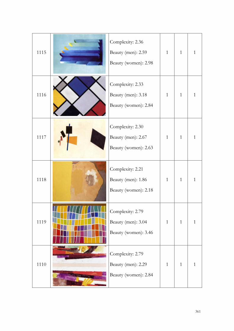
361

1115

Complexity: 2.36

Beauty (men): 2.59

Beauty (women): 2.98

1 1 1

1116

Complexity: 2.33

Beauty (men): 3.18

Beauty (women): 2.84

1 1 1

1117

Complexity: 2.30

Beauty (men): 2.67

Beauty (women): 2.63

1 1 1

1118

Complexity: 2.21

Beauty (men): 1.86

Beauty (women): 2.18

1 1 1

1119

Complexity: 2.79

Beauty (men): 3.04

Beauty (women): 3.46

1 1 1

1110

Complexity: 2.79

Beauty (men): 2.29

Beauty (women): 2.84

1 1 1

362

1121

Complexity: 1.24

Beauty (men): 1.95

Beauty (women): 1.86

1 1 2

1122

Complexity: 1.24

Beauty (men): 2.21

Beauty (women): 2.20

1 1 2

1123

Complexity: 1.21

Beauty (men): 2.04

Beauty (women): 2.29

1 1 2

1124

Complexity: 1.21

Beauty (men): 1.76

Beauty (women): 1.84

1 1 2

1125

Complexity: 1.18

Beauty (men): 1.67

Beauty (women): 1.70

1 1 2

1126

Complexity: 1.18

Beauty (men): 1.76

Beauty (women): 1.88

1 1 2

363

1127

Complexity: 1.18

Beauty (men): 1.71

Beauty (women): 1.93

1 1 2

1128

Complexity: 1.18

Beauty (men): 1.83

Beauty (women): 1.82

1 1 2

1129

Complexity: 1.15

Beauty (men): 1.62

Beauty (women): 1.77

1 1 2

1120

Complexity: 1.15

Beauty (men): 1.42

Beauty (women): 1.41

1 1 2

1211

Complexity: 2.94

Beauty (men): 3.82

Beauty (women): 3.86

1 2 1

1212

Complexity: 2.76

Beauty (men): 3.32

Beauty (women): 3.23

1 2 1

364

1213

Complexity: 2.70

Beauty (men): 3.54

Beauty (women): 3.13

1 2 1

1214

Complexity: 2.70

Beauty (men): 3.26

Beauty (women): 3.46

1 2 1

1215

Complexity: 2.67

Beauty (men): 3.70

Beauty (women): 3.36

1 2 1

1216

Complexity: 2.67

Beauty (men): 3.86

Beauty (women): 3.61

1 2 1

1217

Complexity: 2.67

Beauty (men): 2.41

Beauty (women): 2.43

1 2 1

1218

Complexity: 2.61

Beauty (men): 3.05

Beauty (women): 3.16

1 2 1

365

1219

Complexity: 2.52

Beauty (men): 3.59

Beauty (women): 3.63

1 2 1

1210

Complexity: 2.52

Beauty (men): 3.95

Beauty (women): 3.80

1 2 1

1221

Complexity: 1.48

Beauty (men): 2.28

Beauty (women): 1.96

1 2 2

1222

Complexity: 1.45

Beauty (men): 1.53

Beauty (women): 1.54

1 2 2

1223

Complexity: 1.42

Beauty (men): 1.51

Beauty (women): 1.36

1 2 2

1224

Complexity: 1.36

Beauty (men): 1.71

Beauty (women): 1.50

1 2 2

366

1225

Complexity: 1.30

Beauty (men): 2.34

Beauty (women): 2.48

1 2 2

1226

Complexity: 1.48

Beauty (men): 2.39

Beauty (women): 2.45

1 2 2

1227

Complexity: 1.45

Beauty (men): 2.47

Beauty (women): 2.70

1 2 2

1228

Complexity: 1.45

Beauty (men): 2.33

Beauty (women): 2.14

1 2 2

1229

Complexity: 1.42

Beauty (men): 2.92

Beauty (women): 3.09

1 2 2

1220

Complexity: 1.24

Beauty (men): 1.89

Beauty (women): 1.59

1 2 2

367

2111

Complexity: 3.36

Beauty (men): 2.28

Beauty (women): 2.80

2 1 1

2112

Complexity: 3.36

Beauty (men): 3.12

Beauty (women): 3.46

2 1 1

2113

Complexity: 3.48

Beauty (men): 2.68

Beauty (women): 2.63

2 1 1

2114

Complexity: 3.48

Beauty (men): 2.41

Beauty (women): 2.59

2 1 1

2115

Complexity: 3.48

Beauty (men): 2.39

Beauty (women): 2.70

2 1 1

2116

Complexity: 3.48

Beauty (men): 2.54

Beauty (women): 2.39

2 1 1

368

2117

Complexity: 3.52

Beauty (men): 2.17

Beauty (women): 2.32

2 1 1

2118

Complexity: 3.52

Beauty (men): 3.36

Beauty (women): 3.43

2 1 1

2119

Complexity: 3.52

Beauty (men): 3.39

Beauty (women): 3.52

2 1 1

2110

Complexity: 3.52

Beauty (men): 2.72

Beauty (women): 2.29

2 1 1

2121

Complexity: 2.15

Beauty (men): 1.67

Beauty (women): 1.55

2 1 2

2122

Complexity: 2.15

Beauty (men): 2.78

Beauty (women): 3.38

2 1 2

369

2123

Complexity: 2.09

Beauty (men): 1.76

Beauty (women): 1.95

2 1 2

2124

Complexity: 2.09

Beauty (men): 1.59

Beauty (women): 2.48

2 1 2

2125

Complexity: 2.09

Beauty (men): 1.54

Beauty (women): 1.73

2 1 2

2126

Complexity: 2.09

Beauty (men): 1.91

Beauty (women): 2.05

2 1 2

2127

Complexity: 2.06

Beauty (men): 1.53

Beauty (women): 1.52

2 1 2

2128

Complexity: 2.06

Beauty (men): 2.17

Beauty (women): 2.50

2 1 2

370

2129

Complexity: 2.06

Beauty (men): 1.91

Beauty (women): 2.14

2 1 2

2120

Complexity: 2.03

Beauty (men): 2.28

Beauty (women): 2.25

2 1 2

2211

Complexity: 3.52

Beauty (men): 4.12

Beauty (women): 3.71

2 2 1

2212

Complexity: 3.52

Beauty (men): 4.49

Beauty (women): 4.34

2 2 1

2213

Complexity: 3.52

Beauty (men): 3.54

Beauty (women): 3.83

2 2 1

2214

Complexity: 3.52

Beauty (men): 4.00

Beauty (women): 3.59

2 2 1

371

2215

Complexity: 3.52

Beauty (men): 3.09

Beauty (women): 2.93

2 2 1

2216

Complexity: 3.48

Beauty (men): 2.67

Beauty (women): 2.52

2 2 1

2217

Complexity: 3.48

Beauty (men): 3.13

Beauty (women): 3.39

2 2 1

2218

Complexity: 3.48

Beauty (men): 3.53

Beauty (women): 2.95

2 2 1

2219

Complexity: 3.42

Beauty (men): 3.09

Beauty (women): 3.13

2 2 1

2210

Complexity: 3.48

Beauty (men): 4.13

Beauty (women): 3.68

2 2 1

372

2221

Complexity: 2.91

Beauty (men): 2.72

Beauty (women): 2.34

2 2 2

2222

Complexity: 2.52

Beauty (men): 2.28

Beauty (women): 2.14

2 2 2

2223

Complexity: 2.45

Beauty (men): 2.79

Beauty (women): 2.91

2 2 2

2224

Complexity: 2.42

Beauty (men): 3.26

Beauty (women): 3.46

2 2 2

2225

Complexity: 2.36

Beauty (men): 3.05

Beauty (women): 3.20

2 2 2

2226

Complexity: 2.55

Beauty (men): 3.75

Beauty (women): 3.46

2 2 2

373

2227

Complexity: 2.52

Beauty (men): 3.93

Beauty (women): 3.64

2 2 2

2228

Complexity: 2.52

Beauty (men): 1.72

Beauty (women): 1.50

2 2 2

2229

Complexity: 2.48

Beauty (men): 2.62

Beauty (women): 2.50

2 2 2

2220

Complexity: 2.48

Beauty (men): 2.07

Beauty (women): 1.66

2 2 2

3111

Complexity: 4.82

Beauty (men): 2.67

Beauty (women): 3.27

3 1 1

3112

Complexity: 4.79

Beauty (men): 2.78

Beauty (women): 3.00

3 1 1

374

3113

Complexity: 4.76

Beauty (men): 2.79

Beauty (women): 2.57

3 1 1

3114

Complexity: 4.42

Beauty (men): 2.97

Beauty (women): 2.29

3 1 1

3115

Complexity: 4.73

Beauty (men): 3.20

Beauty (women): 2.59

3 1 1

3116

Complexity: 4.70

Beauty (men): 2.93

Beauty (women): 2.27

3 1 1

3117

Complexity: 4.70

Beauty (men): 3.58

Beauty (women): 3.59

3 1 1

3118

Complexity: 4.67

Beauty (men): 3.84

Beauty (women): 3.79

3 1 1

375

3119

Complexity: 4.39

Beauty (men): 2.74

Beauty (women): 2.45

3 1 1

3110

Complexity: 4.64

Beauty (men): 2.58

Beauty (women): 3.26

3 1 1

3121

Complexity: 3.79

Beauty (men): 2.83

Beauty (women): 2.61

3 1 2

3122

Complexity: 3.70

Beauty (men): 1.82

Beauty (women): 2.16

3 1 2

3123

Complexity: 3.15

Beauty (men): 2.47

Beauty (women): 3.09

3 1 2

3124

Complexity: 3.00

Beauty (men): 1.51

Beauty (women): 1.55

3 1 2

376

3125

Complexity: 2.88

Beauty (men): 1.70

Beauty (women): 2.39

3 1 2

3126

Complexity: 2.73

Beauty (men): 1.75

Beauty (women): 1.86

3 1 2

3127

Complexity: 2.73

Beauty (men): 1.88

Beauty (women): 2.14

3 1 2

3128

Complexity: 2.70

Beauty (men): 1.86

Beauty (women): 2.05

3 1 2

3129

Complexity: 2.58

Beauty (men): 1.89

Beauty (women): 2.13

3 1 2

3120

Complexity: 2.55

Beauty (men): 1.86

Beauty (women): 2.88

3 1 2

377

3211

Complexity: 4.67

Beauty (men): 2.91

Beauty (women): 3.11

3 2 1

3212

Complexity: 4.58

Beauty (men): 3.45

Beauty (women): 3.36

3 2 1

3213

Complexity: 4.45

Beauty (men): 4.14

Beauty (women): 3.93

3 2 1

3214

Complexity: 4.42

Beauty (men): 2.87

Beauty (women): 2.93

3 2 1

3215

Complexity: 4.33

Beauty (men): 3.71

Beauty (women): 3.61

3 2 1

3216

Complexity: 4.30

Beauty (men): 2.92

Beauty (women): 3.02

3 2 1

378

3217

Complexity: 4.27

Beauty (men): 3.50

Beauty (women): 2.64

3 2 1

3218

Complexity: 4.24

Beauty (men): 3.74

Beauty (women): 3.68

3 2 1

3219

Complexity: 4.21

Beauty (men): 4.49

Beauty (women): 4.32

3 2 1

3210

Complexity: 4.18

Beauty (men): 4.47

Beauty (women): 4.09

3 2 1

3221

Complexity: 3.85

Beauty (men): 3.49

Beauty (women): 3.23

3 2 2

3222

Complexity: 3.82

Beauty (men): 2.53

Beauty (women): 2.29

3 2 2

379

3223

Complexity: 3.76

Beauty (men): 3.58

Beauty (women): 3.04

3 2 2

3224

Complexity: 3.52

Beauty (men): 3.14

Beauty (women): 2.91

3 2 2

3225

Complexity: 3.36

Beauty (men): 3.67

Beauty (women): 3.66

3 2 2

3226

Complexity: 3.94

Beauty (men): 3.97

Beauty (women): 3.68

3 2 2

3227

Complexity: 3.91

Beauty (men): 3.39

Beauty (women): 3.63

3 2 2

3228

Complexity: 3.91

Beauty (men): 4.29

Beauty (women): 4.02

3 2 2

380

3229

Complexity: 3.76

Beauty (men): 4.30

Beauty (women): 4.25

3 2 2

3220

Complexity: 3.67

Beauty (men): 4.25

Beauty (women): 3.95

3 2 2

381

Annex B

382

In this Annex we include reproductions of the 60 stimuli used in the third phase of

this work, related with the clarification of the concept of complexity. We also

include the average scores awarded by men and women to each stimulus on each of

the 7 complexity dimensions.

Code Image Complexity dimensions M W

1113

Unintelligibility of the elements

Disorganization

Amount of elements

Element heterogeneity

Asymmetry

Colour variety

Three-dimensionality

6.53

6.63

3.71

2.95

6.71

2.82

1.97

6.14

6.25

2.82

3.07

6.20

2.38

2.51

1114

Unintelligibility of the elements

Disorganization

Amount of elements

Element heterogeneity

Asymmetry

Colour variety

Three-dimensionality

5.76

6.76

3.34

3.63

7.00

3.82

1.61

5.57

6.15

3.32

4.18

7.07

4.27

2.15

1115

Unintelligibility of the elements

Disorganization

Amount of elements

Element heterogeneity

Asymmetry

Colour variety

Three-dimensionality

3.13

4.66

3.92

3.29

4.34

3.76

6.13

3.52

4.58

4.13

2.91

4.68

3.96

6.26

383

1116

Unintelligibility of the elements

Disorganization

Amount of elements

Element heterogeneity

Asymmetry

Colour variety

Three-dimensionality

3.66

3.47

3.76

2.92

4.76

4.37

1.82

3.25

3.95

3.52

2.66

4.02

5.00

2.23

1117

Unintelligibility of the elements

Disorganization

Amount of elements

Element heterogeneity

Asymmetry

Colour variety

Three-dimensionality

4.39

5.82

2.95

2.39

3.13

2.89

3.00

4.07

5.80

2.98

3.07

3.29

3.72

3.94

1122

Unintelligibility of the elements

Disorganization

Amount of elements

Element heterogeneity

Asymmetry

Colour variety

Three-dimensionality

3.87

3.76

1.61

1.26

2.79

1.42

1.18

2.82

3.30

1.52

1.11

3.18

1.16

1.40

1123

Unintelligibility of the elements

Disorganization

Amount of elements

Element heterogeneity

Asymmetry

Colour variety

Three-dimensionality

4.92

5.76

1.21

1.53

6.05

1.28

1.24

3.95

4.67

1.20

1.30

6.39

1.14

1.34

384

1124

Unintelligibility of the elements

Disorganization

Amount of elements

Element heterogeneity

Asymmetry

Colour variety

Three-dimensionality

4.50

5.63

1.13

1.42

8.37

1.38

1.22

4.21

4.93

1.30

1.43

7.86

1.20

1.26

1125

Unintelligibility of the elements

Disorganization

Amount of elements

Element heterogeneity

Asymmetry

Colour variety

Three-dimensionality

4.82

5.26

1.45

1.42

8.53

1.26

1.11

3.98

4.56

1.50

1.21

8.43

1.10

1.25

1126

Unintelligibility of the elements

Disorganization

Amount of elements

Element heterogeneity

Asymmetry

Colour variety

Three-dimensionality

5.11

5.74

1.50

1.68

2.61

1.63

1.24

4.34

4.93

1.61

2.14

2.80

1.30

1.41

1213

Unintelligibility of the elements

Disorganization

Amount of elements

Element heterogeneity

Asymmetry

Colour variety

Three-dimensionality

2.26

1.58

3.39

3.79

3.66

4.63

6.24

1.71

1.95

3.18

3.20

3.96

3.86

5.82

385

1214

Unintelligibility of the elements

Disorganization

Amount of elements

Element heterogeneity

Asymmetry

Colour variety

Three-dimensionality

2.29

1.82

4.18

4.34

4.37

4.79

6.81

1.86

2.00

3.91

3.66

3.96

4.58

6.61

1215

Unintelligibility of the elements

Disorganization

Amount of elements

Element heterogeneity

Asymmetry

Colour variety

Three-dimensionality

2.68

1.95

6.11

6.95

7.13

7.37

7.35

1.86

2.20

6.18

7.21

7.36

7.28

6.64

1216

Unintelligibility of the elements

Disorganization

Amount of elements

Element heterogeneity

Asymmetry

Colour variety

Three-dimensionality

2.47

2.08

4.82

4.45

5.61

5.92

6.89

1.96

2.54

4.45

4.63

5.36

5.19

6.45

1217

Unintelligibility of the elements

Disorganization

Amount of elements

Element heterogeneity

Asymmetry

Colour variety

Three-dimensionality

3.42

3.32

4.97

5.03

6.26

6.59

4.86

2.43

2.85

4.63

5.09

6.14

6.46

4.39

386

1222

Unintelligibility of the elements

Disorganization

Amount of elements

Element heterogeneity

Asymmetry

Colour variety

Three-dimensionality

4.42

4.95

2.24

2.24

4.42

2.68

1.61

4.46

5.14

2.68

2.66

4.66

2.92

2.00

1223

Unintelligibility of the elements

Disorganization

Amount of elements

Element heterogeneity

Asymmetry

Colour variety

Three-dimensionality

1.16

1.45

1.74

2.18

5.82

2.23

2.11

1.34

1.58

1.63

2.30

5.68

2.53

2.20

1224

Unintelligibility of the elements

Disorganization

Amount of elements

Element heterogeneity

Asymmetry

Colour variety

Three-dimensionality

1.21

2.21

2.00

2.32

6.79

2.45

1.50

1.21

1.86

2.27

3.07

6.68

2.32

1.85

1225

Unintelligibility of the elements

Disorganization

Amount of elements

Element heterogeneity

Asymmetry

Colour variety

Three-dimensionality

1.66

1.45

1.50

1.95

5.13

2.16

1.49

1.39

1.67

1.27

1.46

6.02

2.10

1.89

387

1226

Unintelligibility of the elements

Disorganization

Amount of elements

Element heterogeneity

Asymmetry

Colour variety

Three-dimensionality

1.61

2.26

2.21

2.39

5.82

2.33

5.00

1.43

2.09

1.84

2.00

5.80

2.00

4.55

2112

Unintelligibility of the elements

Disorganization

Amount of elements

Element heterogeneity

Asymmetry

Colour variety

Three-dimensionality

6.68

7.50

4.05

3.95

6.82

4.97

2.45

7.13

6.59

4.29

4.71

6.43

5.23

2.67

2113

Unintelligibility of the elements

Disorganization

Amount of elements

Element heterogeneity

Asymmetry

Colour variety

Three-dimensionality

6.79

7.37

6.16

4.61

3.76

3.69

2.28

6.96

6.96

5.54

5.23

4.30

3.96

2.59

2114

Unintelligibility of the elements

Disorganization

Amount of elements

Element heterogeneity

Asymmetry

Colour variety

Three-dimensionality

6.58

7.13

5.58

4.61

4.05

4.66

3.05

6.96

7.14

5.63

5.41

4.45

5.16

3.49

388

2115

Unintelligibility of the elements

Disorganization

Amount of elements

Element heterogeneity

Asymmetry

Colour variety

Three-dimensionality

6.34

7.24

5.61

4.58

5.55

5.11

6.18

6.07

6.38

5.34

4.41

5.77

4.96

6.38

2116

Unintelligibility of the elements

Disorganization

Amount of elements

Element heterogeneity

Asymmetry

Colour variety

Three-dimensionality

7.03

7.32

5.53

5.00

3.58

3.97

3.03

7.11

6.96

5.09

4.57

3.98

3.54

3.38

2123

Unintelligibility of the elements

Disorganization

Amount of elements

Element heterogeneity

Asymmetry

Colour variety

Three-dimensionality

3.68

3.58

3.58

1.63

4.26

1.29

1.71

3.66

4.09

3.50

1.93

3.86

1.20

2.71

2124

Unintelligibility of the elements

Disorganization

Amount of elements

Element heterogeneity

Asymmetry

Colour variety

Three-dimensionality

5.32

6.53

4.32

2.95

5.08

4.66

2.14

4.54

5.16

4.05

3.23

5.48

6.14

2.68

389

2125

Unintelligibility of the elements

Disorganization

Amount of elements

Element heterogeneity

Asymmetry

Colour variety

Three-dimensionality

4.71

6.00

3.61

3.26

6.29

3.26

2.45

5.54

6.18

4.88

3.82

5.41

3.39

2.85

2126

Unintelligibility of the elements

Disorganization

Amount of elements

Element heterogeneity

Asymmetry

Colour variety

Three-dimensionality

5.58

6.76

3.42

2.66

6.03

1.74

2.55

5.68

6.18

3.34

3.09

6.27

1.65

4.23

2127

Unintelligibility of the elements

Disorganization

Amount of elements

Element heterogeneity

Asymmetry

Colour variety

Three-dimensionality

5.03

6.03

3.89

3.45

3.87

2.92

1.62

4.73

6.04

4.14

3.11

4.34

4.24

2.02

2212

Unintelligibility of the elements

Disorganization

Amount of elements

Element heterogeneity

Asymmetry

Colour variety

Three-dimensionality

2.76

1.82

6.58

5.97

5.55

7.00

7.32

2.50

2.34

6.43

6.14

6.18

7.00

7.26

390

2213

Unintelligibility of the elements

Disorganization

Amount of elements

Element heterogeneity

Asymmetry

Colour variety

Three-dimensionality

2.82

2.26

5.97

5.68

5.55

6.72

7.24

2.32

2.45

5.79

6.46

5.84

6.42

7.08

2214

Unintelligibility of the elements

Disorganization

Amount of elements

Element heterogeneity

Asymmetry

Colour variety

Three-dimensionality

2.68

2.71

7.03

6.47

7.11

6.47

6.78

2.38

2.45

7.02

6.45

7.00

7.04

6.40

2215

Unintelligibility of the elements

Disorganization

Amount of elements

Element heterogeneity

Asymmetry

Colour variety

Three-dimensionality

4.08

4.63

5.58

4.45

5.63

4.29

6.47

3.66

4.02

5.18

4.05

4.98

4.06

6.10

2216

Unintelligibility of the elements

Disorganization

Amount of elements

Element heterogeneity

Asymmetry

Colour variety

Three-dimensionality

4.66

4.63

6.82

6.29

5.95

5.69

5.41

4.89

4.87

6.38

6.43

5.89

6.19

4.85

391

2223

Unintelligibility of the elements

Disorganization

Amount of elements

Element heterogeneity

Asymmetry

Colour variety

Three-dimensionality

2.63

3.34

3.79

3.39

3.37

4.87

1.92

2.46

3.18

4.70

5.11

3.77

5.61

2.58

2224

Unintelligibility of the elements

Disorganization

Amount of elements

Element heterogeneity

Asymmetry

Colour variety

Three-dimensionality

1.97

2.00

3.95

4.63

4.53

3.59

6.32

1.73

1.87

4.14

5.04

4.57

3.85

5.60

2225

Unintelligibility of the elements

Disorganization

Amount of elements

Element heterogeneity

Asymmetry

Colour variety

Three-dimensionality

1.79

1.53

3.26

2.26

7.58

3.56

3.61

1.64

1.80

2.73

2.13

6.98

3.42

3.66

2226

Unintelligibility of the elements

Disorganization

Amount of elements

Element heterogeneity

Asymmetry

Colour variety

Three-dimensionality

2.13

1.58

5.32

5.42

4.00

5.37

7.92

1.61

1.84

5.11

5.27

4.38

5.33

7.23

392

2227

Unintelligibility of the elements

Disorganization

Amount of elements

Element heterogeneity

Asymmetry

Colour variety

Three-dimensionality

1.71

1.29

5.13

4.89

6.13

5.66

7.84

1.57

1.93

4.71

5.68

5.23

5.50

7.57

3112

Unintelligibility of the elements

Disorganization

Amount of elements

Element heterogeneity

Asymmetry

Colour variety

Three-dimensionality

8.05

7.53

7.84

7.00

4.92

7.15

2.92

7.88

7.13

7.71

7.13

4.52

7.37

3.17

3113

Unintelligibility of the elements

Disorganization

Amount of elements

Element heterogeneity

Asymmetry

Colour variety

Three-dimensionality

8.18

7.79

7.24

6.05

3.55

4.79

3.11

6.89

6.41

7.41

5.13

2.82

4.69

3.28

3114

Unintelligibility of the elements

Disorganization

Amount of elements

Element heterogeneity

Asymmetry

Colour variety

Three-dimensionality

7.16

7.26

7.76

6.76

5.95

5.45

4.32

7.86

7.69

7.45

6.64

6.48

5.04

4.63

393

3115

Unintelligibility of the elements

Disorganization

Amount of elements

Element heterogeneity

Asymmetry

Colour variety

Three-dimensionality

7.53

7.13

7.00

6.39

3.95

5.89

5.84

7.30

6.73

6.14

6.21

4.07

5.31

6.17

3116

Unintelligibility of the elements

Disorganization

Amount of elements

Element heterogeneity

Asymmetry

Colour variety

Three-dimensionality

7.13

7.47

8.18

7.08

4.16

5.55

5.14

7.64

7.53

7.88

7.13

4.23

4.94

4.80

3122

Unintelligibility of the elements

Disorganization

Amount of elements

Element heterogeneity

Asymmetry

Colour variety

Three-dimensionality

4.29

4.03

4.63

2.42

3.11

5.33

6.71

4.54

4.38

6.14

3.13

3.09

5.30

7.11

3123

Unintelligibility of the elements

Disorganization

Amount of elements

Element heterogeneity

Asymmetry

Colour variety

Three-dimensionality

6.11

6.97

3.00

2.61

6.21

2.42

4.21

6.41

5.80

3.30

2.64

5.82

2.68

5.15

394

3124

Unintelligibility of the elements

Disorganization

Amount of elements

Element heterogeneity

Asymmetry

Colour variety

Three-dimensionality

6.92

7.82

5.26

4.32

4.89

4.97

2.61

6.30

6.98

5.54

4.30

4.59

5.31

2.71

3125

Unintelligibility of the elements

Disorganization

Amount of elements

Element heterogeneity

Asymmetry

Colour variety

Three-dimensionality

5.87

7.16

4.82

4.47

7.39

4.05

2.24

6.29

6.96

6.04

5.18

6.95

4.38

3.26

3126

Unintelligibility of the elements

Disorganization

Amount of elements

Element heterogeneity

Asymmetry

Colour variety

Three-dimensionality

4.61

6.03

3.03

2.71

4.58

2.79

1.58

4.13

5.70

3.09

3.13

4.43

3.02

2.44

3212

Unintelligibility of the elements

Disorganization

Amount of elements

Element heterogeneity

Asymmetry

Colour variety

Three-dimensionality

5.42

6.66

7.89

7.18

4.55

7.76

6.37

6.02

6.35

7.91

6.89

3.98

7.90

6.30

395

3213

Unintelligibility of the elements

Disorganization

Amount of elements

Element heterogeneity

Asymmetry

Colour variety

Three-dimensionality

3.13

2.47

8.13

7.95

4.13

7.58

7.32

3.38

2.73

8.13

8.09

4.50

7.70

7.65

3214

Unintelligibility of the elements

Disorganization

Amount of elements

Element heterogeneity

Asymmetry

Colour variety

Three-dimensionality

6.21

6.32

7.26

6.71

4.76

5.49

5.86

6.30

6.20

7.23

6.18

4.54

5.25

5.64

3215

Unintelligibility of the elements

Disorganization

Amount of elements

Element heterogeneity

Asymmetry

Colour variety

Three-dimensionality

5.08

6.58

7.37

7.34

6.39

7.18

4.28

4.95

6.00

7.55

7.70

6.46

7.20

4.45

3216

Unintelligibility of the elements

Disorganization

Amount of elements

Element heterogeneity

Asymmetry

Colour variety

Three-dimensionality

6.55

6.37

6.34

5.66

3.13

4.58

5.24

7.13

6.47

6.70

5.93

4.20

4.92

5.65

396

3223

Unintelligibility of the elements

Disorganization

Amount of elements

Element heterogeneity

Asymmetry

Colour variety

Three-dimensionality

2.42

2.13

6.26

5.66

5.34

6.71

6.89

2.25

2.50

6.73

5.88

5.05

6.68

7.13

3224

Unintelligibility of the elements

Disorganization

Amount of elements

Element heterogeneity

Asymmetry

Colour variety

Three-dimensionality

2.53

2.50

6.76

7.16

6.58

7.15

7.46

2.29

2.47

6.84

7.52

6.59

7.35

7.02

3225

Unintelligibility of the elements

Disorganization

Amount of elements

Element heterogeneity

Asymmetry

Colour variety

Three-dimensionality

2.39

1.71

6.24

6.47

5.26

6.92

7.18

2.09

2.15

6.63

6.71

4.96

7.10

7.13

3226

Unintelligibility of the elements

Disorganization

Amount of elements

Element heterogeneity

Asymmetry

Colour variety

Three-dimensionality

2.82

2.24

6.66

4.97

6.16

4.26

7.42

2.32

2.44

5.93

4.86

6.71

3.94

7.09

397

3227

Unintelligibility of the elements

Disorganization

Amount of elements

Element heterogeneity

Asymmetry

Colour variety

Three-dimensionality

2.34

2.16

7.24

6.50

4.53

6.32

7.70

2.02

2.48

7.71

6.07

3.93

5.88

7.11

398

399

Annex C

400

In this Annex we present the results of our analysis of double interactions between

our three independent variables (Complexity, Abstraction, Artistry) on men and

women’s beauty scores.

Abstraction x Artistry

Artistry in Abstraction (

!

"* =.05

2= .025)

Abstract stimuli: Are there differences between beauty scores awarded to artistic and

decorative abstract stimuli?

Artistic abstract stimuli were rated more beautiful than decorative abstract

stimuli by both men and women (p<.025).

401

Representational stimuli: Are there differences between beauty scores awarded to

artistic and decorative representational stimuli?

Artistic representational stimuli were rated more beautiful than decorative

representational stimuli by both men and women (p<.025).

402

Abstraction in Artistry (

!

"* =.05

2= .025)

Artistic stimuli: Are there differences between beauty scores awarded to abstract and

representational artistic stimuli?

Representational artistic stimuli were rated more beautiful than abstract

artistic stimuli by both men and women (p<.025).

403

Decorative stimuli: Are there differences between beauty scores awarded to abstract

and representational decorative stimuli?

Representational decorative stimuli were rated more beautiful than abstract

decorative stimuli by both men and women (p<.025).

404

Abstraction x Complexity

Complexity in Abstraction (

!

"* =.05

2= .025)

Abstract stimuli: Are there differences among the beauty scores awarded to low,

intermediate, and high complexity abstract stimuli?

There were no statistical differences among the beauty scores awarded to

low, intermediate, and high complexity abstract stimuli

405

Representational stimuli: Are there differences among the beauty scores awarded to

low, intermediate, and high complexity representational stimuli?

There were statistical differences among the beauty scores awarded to low,

intermediate, and high complexity abstract stimuli, for both men and women

(p<.025). We carried out pairwise contrasts using the Mann-Whitney test to

determine the complexity levels between which beauty scores differed

(

!

"* =.05

6= .0083).

406

Both men and women rated the beauty of high complexity representational

stimuli higher than low complexity representational stimuli (p<.0083).

407

Abstraction in Complexity (

!

"* =.05

6= .0083)

Low complexity stimuli: Are there differences between beauty scores awarded to

abstract and representational low complexity stimuli?

For both men and women, differences between beauty scores awarded to

abstract and representational low complexity stimuli were not significant.

408

Intermediate complexity stimuli: Are there differences between beauty scores

awarded to abstract and representational intermediate complexity stimuli?

Both men and women rated the beauty of representational intermediate

complexity stimuli higher than abstract intermediate complexity stimuli (p<.0083).

409

High complexity stimuli: Are there differences between beauty scores awarded to

abstract and representational high complexity stimuli?

Both men and women rated the beauty of representational high complexity

stimuli higher than abstract high complexity stimuli (p<.0083).

410

Artistry x Complexity

Complexity in Artistry (

!

"* =.05

2= .025)

Artistic stimuli: Are there differences among the beauty scores awarded to low,

intermediate, and high complexity artistic stimuli?

For both men and women differences among the beauty scores awarded to

low, intermediate, and high complexity artistic stimuli were non-significant.

411

Decorative stimuli: Are there differences among the beauty scores awarded to low,

intermediate, and high complexity decorative stimuli?

Whereas differences among the beauty scores awarded by men to low,

intermediate, and high complexity decorative stimuli were non-significant, they

reached statistical significance levels in the case of women (p<.025). Pairwise

contrasts between complexity levels were carried out (

!

"* =.05

6= .0083) by means of

Mann-Whitney tests.

412

Hence, women awarded higher beauty scores to high complexity decorative

stimuli than to low complexity decorative stimuli (p<.0083).

413

Artistry in Complexity (

!

"* =.05

6= .0083)

Low complexity stimuli: Are there differences between beauty scores awarded to

artistic and decorative low complexity stimuli?

Both men and women rated the beauty of artistic low complexity stimuli

higher than the beauty of decorative low complexity stimuli (p<.0083).

414

Intermediate complexity stimuli: Are there differences between beauty scores

awarded to artistic and decorative intermediate complexity stimuli?

Both men and women rated the beauty of artistic intermediate complexity

stimuli higher than the beauty of decorative intermediate complexity stimuli

(p<.0083).

415

High complexity stimuli: Are there differences between beauty scores awarded to

artistic and decorative high complexity stimuli?

For both men and women, differences between beauty scores awarded to

artistic and decorative high complexity stimuli were not significant.

416

417

Annex D

418

In this Annex we present the results of our analysis of triple interactions between

our three independent variables (Complexity, Abstraction, Artistry) on men and

women’s beauty scores, except for the analysis of the effects of Complexity in

Abstraction x Artistry, which was included in the main text of this work.

Artistry in abstraction x complexity

!

("* =.05

30= .0016)

Abstract stimuli

Low complexity abstract stimuli: Are there any differences between beauty scores

awarded to artistic and decorative low complexity abstract stimuli?

Both men and women awarded higher beauty scores to artistic low

complexity abstract stimuli than to decorative low complexity abstract stimuli

(p<.0016).

419

Intermediate complexity abstract stimuli: Are there any differences between beauty

scores awarded to artistic and decorative intermediate complexity abstract stimuli?

Men awarded higher beauty scores to artistic intermediate complexity

abstract stimuli than to decorative intermediate complexity abstract stimuli

(p<.0016). However, differences did not reach statistical significance levels in the

case of women.

420

High complexity abstract stimuli: Are there any differences between beauty scores

awarded to artistic and decorative high complexity abstract stimuli?

Both men and women awarded higher beauty scores to artistic high

complexity abstract stimuli than to decorative high complexity abstract stimuli

(p<.0016).

421

Representational stimuli

Low complexity representational stimuli: Are there any differences between beauty

scores awarded to artistic and decorative low complexity representational stimuli?

Both men and women awarded higher beauty scores to artistic low

complexity representational stimuli than to decorative low complexity

representational stimuli (p<.0016).

422

Intermediate complexity representational stimuli: Are there any differences between

beauty scores awarded to artistic and decorative intermediate complexity

representational stimuli?

For both men and women, differences between beauty scores awarded to

artistic and decorative intermediate complexity representational stimuli did not reach

statistical significance.

423

High complexity representational stimuli: Are there any differences between beauty

scores awarded to artistic and decorative high complexity representational stimuli?

For both men and women, differences between beauty scores awarded to

artistic and decorative high complexity representational stimuli did not reach

statistical significance.

424

Abstraction in artistry x complexity

!

("* =.05

30= .0016)

Artistic stimuli

Low complexity artistic stimuli: Are there any differences between beauty scores

awarded to abstract and representational low complexity artistic stimuli?

For both men and women, differences between beauty scores awarded to

abstract and representational low complexity artistic stimuli did not reach statistical

significance.

425

Intermediate complexity artistic stimuli: Are there any differences between beauty

scores awarded to abstract and representational intermediate complexity artistic

stimuli?

For both men and women, differences between beauty scores awarded to

abstract and representational intermediate complexity artistic stimuli did not reach

statistical significance.

426

High complexity artistic stimuli: Are there any differences between beauty scores

awarded to abstract and representational high complexity artistic stimuli?

For both men and women, differences between beauty scores awarded to

abstract and representational high complexity artistic stimuli did not reach statistical

significance.

427

Decorative stimuli

Low complexity decorative stimuli: Are there any differences between beauty scores

awarded to abstract and representational low complexity decorative stimuli?

For both men and women, differences between beauty scores awarded to

abstract and representational low complexity decorative stimuli did not reach

statistical significance.

428

Intermediate complexity decorative stimuli: Are there any differences between

beauty scores awarded to abstract and representational intermediate complexity

decorative stimuli?

For both men and women, differences between beauty scores awarded to

abstract and representational intermediate complexity decorative stimuli did not

reach statistical significance.

429

High complexity decorative stimuli: Are there any differences between beauty scores

awarded to abstract and representational high complexity decorative stimuli?

Both men and women awarded higher beauty ratings to representational

high complexity decorative stimuli than to abstract high complexity decorative

stimuli (p<.0016)