compit'17 - hiper
TRANSCRIPT
16th
Conference on
Computer and IT Applications in the Maritime Industries
COMPIT’17
Cardiff, 15-17 May 2017

1
16th International Conference on
Computer and IT Applications in the Maritime Industries
COMPIT’17
Cardiff, 15-17 May 2017
Edited by Volker Bertram

2
Sponsored by
www.dnvgl.com
www.beta-cae.com www.siemens.com/marine
www.ensight.com www.ssi-corporate.com / www.ndar.com
www.aveva.com www.cadmatic.com
www.spectec.net www.lr.org
www.foran.es www.dell.com/IoT

3
16th International Conference on Computer and IT Applications in the Maritime
Industries, Cardiff, 15-17 May 2017, Hamburg, Technische Universität Hamburg-Harburg,
2017, ISBN 978-3-89220-701-6
© Technische Universität Hamburg-Harburg
Schriftenreihe Schiffbau
Schwarzenbergstraße 95c
D-21073 Hamburg
http://www.tuhh.de/vss

4
Index
Volker Bertram, Tracy Plowman
Maritime Training in the 21st Century
7
Volker Bertram
Future of Shipbuilding and Shipping - A Technology Vision
17
Knud Benedict, Michael Gluch, Sandro Fischer, Matthias Kirchhoff, Michèle Schaub,
Michael Baldauf, Burkhard Müller
Innovative Fast Time Simulation Tools for Briefing/Debriefing in Advanced Ship Handling
Simulator Training for Cruise Ship Operation
31
Yogang Singh, Sanjay Sharma, Robert Sutton, Daniel Hatton
Path Planning of an Autonomous Surface Vehicle based on Artificial Potential Fields in a Real
Time Marine Environment
48
Marius Brinkmann, Axel Hahn, Bjørn Åge Hjøllo
Physical Testbed for Highly Automated and Autonomous Vessels
55
David Andrews
The Key Ship Design Decision - Choosing the Style of a New Design
69
Hideo Orihara, Hisafumi Yoshida, Ichiro Amaya
Big Data Analysis for Service Performance Evaluation and Ship Design
83
Azriel Rahav
Case Study - Totem Fully Autonomous Navigation System
97
Marco Bibuli, Gabriele Bruzzone, Massimo Caccia, Davide Chiarella, Roberta Ferretti, Angelo
Odetti, Andrea Ranieri, Enrica Zereik
Cutting-Edge Underwater Robotics - CADDY Project Challenges, Results and Future Steps
101
Leo Sakari, Seppo Helle, Sirpa Korhonen, Tero Säntti, Olli Heimo, Mikko Forsman, Mika
Taskinen, Teijo Lehtonen
Virtual and Augmented Reality Solutions to Industrial Applications
115
Denis Morais, Mark Waldie, Darren Larkins
The Evolution of Virtual Reality in Shipbuilding
128
Siebe Cieraad, Etienne Duchateau, Ruben Zandstra, Wendy van den Broek-de Bruijn
A Packing Approach Model in Support of the Conceptual Design of Naval Submarines
139
Greta Levišauskaitė, Henrique Murilo Gaspar, Bernt-Aage Ulstein
4GD Framework in Ship Design
155
Gianandrea Mannarini, Giovanni Coppini, Rita Lecci, Giuseppe Turrisi
Sea Currents and Waves for Optimal Route Planning with VISIR
170
Hasan Deeb, Mohamed Abdelaal, Axel Hahn
Pre-Crash Advisor – Decision Support System for Mitigating Collision Damage
180
George Korbetis, Serafim Chatzimoisiadis, Dimitrios Drougkas
EPILYSIS, a new solver for Finite Element Analysis
190

5
Mark J. Roth, Koen Droste, Austin A. Kana
Analysis of General Arrangements Created by the TU Delft Packing Approach
201
Anna Lito Michala, Ioannis Vourganas
A Smart Modular Wireless System for Condition Monitoring Data Acquisition
212
Rodrigo Perez Fernandez, Jesus A. Muñoz
Change and Access Control Management to Provide Sister Ships Applicability Capability
226
Marianne Hagaseth, Ulrike Moser
Ontology Based Integration of Ship Inspection Data
238
André Keane, Per Olaf Brett, Ali Ebrahimi, Henrique M. Gaspar, Jose Jorge Garcia Agis
Preparing for a Digital Future – Experiences and Implications from a Maritime Domain
Perspective
253
Natalie Cariaga Costa Rodrigues, Rodrigo Uchoa Simões, Luiz Antônio Vaz Pinto,
Luiz Felipe Assis, Jean-David Caprace
A Vessel Weather Routing Scheduler to Minimize the Voyage Time
270
Maricruz A. F. Cepeda, Rodrigo Uchoa Simões, João Vitor Marques de Oliveira Moita, Luiz
Felipe Assis, Luiz Antônio Vaz Pinto, Jean-David Caprace
Big Data Analysis of AIS Records to Provide Knowledge for Offshore Logistic Simulation
280
Byeongseop Kim, Yong-Kuk Jeong, Philippe Lee, Yonggil Lee, Jong Hun Woo
The Extended Process-centric Modeling Method for Logistics Simulation in Shipyards
considering Stock Areas
291
Stephan Procee, Clark Borst, Rene van Paasen, Max Mulder
Toward Functional Augmented Reality in Marine Navigation: A Cognitive Work Analysis
298
Gunnar Brink, Gaurav Mulay
Fast Leaps and Deep Dives towards Autonomous, Fast, and High-Resolution Deep-Sea Ocean
Exploration
313
Lode Huijgens, Frank Verhelst, Jenny Coenen
Prediction of Work Content in Shipbuilding Projects Using Extrapolation Methods
323
Sabah Alwan, Kevin Koosup Yum, Sverre Steen, Eilif Pedersen
Multidisciplinary Process Integration and Design Optimization of a Hybrid Marine Power
System Applied to a VLCC
336
Bart Van Lierde, Wim Cardoen, Dejan Radosavljevic
Predictive Engineering Analytics for Shipbuilding - An Overview
351
Rachel Pawling, Nikolaos Kouriampalis, Syavash Esbati, Nick Bradbeer, David Andrews
Expanding the Scope of Early Stage Computer Aided Ship Design
362
Scott Patterson, Peter Barton
Secure Wireless Options in the Smart Ship
377
Patrick Müller
Marine 4.0 - Condition Monitoring for the Future
394

6
Martin Kurowski, Agnes U. Schubert, Torsten Jeinsch
Generic Control Strategy for Future Autonomous Ship Operations
401
Howard Tripp, Richard Daltry
The Path to Real World Autonomy for Autonomous Surface Vehicles
413
Heinrich Grümmer, Stefan Harries, Andrés Cura Hochbaum
Optimization of a Self-Righting Hull and a Thruster Unit for an Autonomous Surface Vehicle
419
Henrique M. Gaspar
JavaScript Applied to Maritime Design and Engineering
428
Christian Cabos, Viktor Wolf, Przemyslaw Feiner
Remote Hull Surveys with Virtual Reality
444
Jesus Mediavilla Varas, Spyros Hirdaris, Renny Smith, Paolo Scialla, Walter Caharija, Zakirul
Bhuiyan, Terry Mills, Wasif Naeem, Liang Hu, Ian Renton, David Motson, Eshan Rajabally
MAXCMAS Project - Autonomous COLREGs Compliant Ship Navigation
454
Carl S.P. Hunter
The Ungoverned Space of Marine Fire Safety
465
Ted Jaspers, Austin A. Kana
Elucidating Families of Ship Designs using Clustering Algorithms
474
Mary Etienne
Six Steps to using the IoT to Steer Ships into the Digital Future – Keeping Vessels “Ship
Shape” with Predictive Maintenance Efficiency
486
Mark Deverill
Big Data – Processing Global AIS in Real Time to Produce Market Insight
492
Index of authors 498
Call for Papers for next year
7
Maritime Training in the 21st Century
Volker Bertram, Tracy Plowman, DNV GL, Hamburg/Germany,
{volker.bertram,tracy.plowman}@dnvgl.com
Abstract
The paper discusses expected or desirable changes in teaching engineering, in particular post-
graduate and professional training in maritime technologies. Several factors drive the developments:
changes in students, changes in technology, changes in expectations from industry and governments.
These factors determine what we need to teach and how we need to teach. A different teaching infra-
structure with possibly different providers is expected to evolve. The paper discusses both market and
technological aspects, highlighting challenges and pitfalls of new technologies commonly referred to
as “e-learning”. The paper argues in favor of pedagogy-driven education rather than technology-
driven education.
1. Introduction
A new method to the 3d flow around a ship on shallow water and in oblique waves is a safe topic for
an engineering conference. An estimated three colleagues may be interested to start with. A suitable
mixture of complex equations, daunting diagrams and colorful displays will evoke admiration, little
interest and no aggression. In comparison, education in engineering is a dangerous topic. All engi-
neers have been exposed to the topic (as students). It is a bit like soccer:
It used to be better in the past.
The players (students) today just do not want to work anymore. Shame on them!
The coaches (professors) are incompetent. We could do a better job.
It is still great fun to talk about…
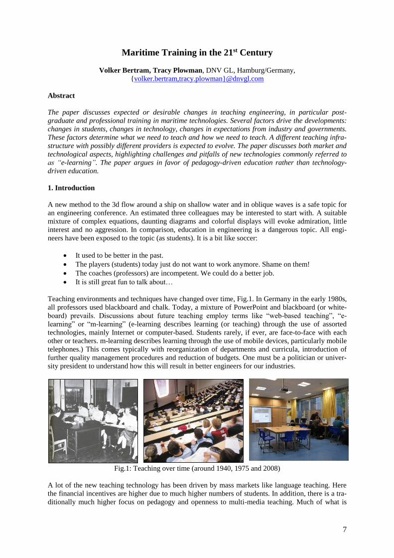
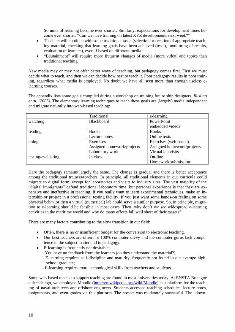
Teaching environments and techniques have changed over time, Fig.1. In Germany in the early 1980s,
all professors used blackboard and chalk. Today, a mixture of PowerPoint and blackboard (or white-
board) prevails. Discussions about future teaching employ terms like “web-based teaching”, “e-
learning” or “m-learning” (e-learning describes learning (or teaching) through the use of assorted
technologies, mainly Internet or computer-based. Students rarely, if ever, are face-to-face with each
other or teachers. m-learning describes learning through the use of mobile devices, particularly mobile
telephones.) This comes typically with reorganization of departments and curricula, introduction of
further quality management procedures and reduction of budgets. One must be a politician or univer-
sity president to understand how this will result in better engineers for our industries.
Fig.1: Teaching over time (around 1940, 1975 and 2008)
A lot of the new teaching technology has been driven by mass markets like language teaching. Here
the financial incentives are higher due to much higher numbers of students. In addition, there is a tra-
ditionally much higher focus on pedagogy and openness to multi-media teaching. Much of what is
8
now discussed for maritime teaching has been tested in other fields like language teaching, law, and
medicine. Highly specialized engineering (like graduate and post-graduate training in maritime tech-
nologies) is different from these fields in required skills, available market size, and other aspects.
Some approaches that work for example in English language teaching do not work for teaching naval
architecture.
Despite changes in students and technologies, there are some constants in our fundamental guidelines
to teaching:
You learn by doing and face-to-face time with teachers is expensive. So we need to encourage
students to work outside class time.
Students should use tools that they are familiar with. For our generation, that meant books. For
the new generation of students, this may increasingly mean computers and even smart phones.
Communication with peers should be encouraged. This happened too little in classical engi-
neering training, where frontal teaching has ruled supreme. Internet technology allows virtual
meeting spaces for students. While popular for “net-working” (gossiping), we are not aware of
any real academic benefits in the maritime field. However, traditional teamwork continues to
work well and team communication is then automatically based on internet and mobile phones.
Modern teaching approaches advocate: Make teaching competitive, make it fun! We are sup-
posed to move from education to edutainment, where students are entertained while learning
quasi without noticing it. This is easier in language education than in engineering. Material sci-
ence was no fun 30 years ago, still is no fun, and is unlikely to ever be fun. No pain, no gain.
2. Changing conditions
The introduction has already mentioned several of the driving factors shaping our teaching: budgets,
technology, and politics. The demographic and political changes are fairly universal. They will be
discussed in the following subsections.
2.1. Different students
“Students these days are not what they used to be.” We heard this sentence when we were students
from our professors. We hear it today, and it is the same the world over:
They do not want to study as much as we did.
They cannot write properly even in their mother tongue.
They only want to play with computers; they are not interested in “real” science (i.e. the
mathematics involved in fluid or structural analyses).
These are not senile professors ranting, with a selective memory of their past. There are real changes,
due to changes in the way of life and upbringing of children. Today’s children are exposed to comput-
ers before they go to school. Prensky (2001,2011) calls them “digital natives”: “Today’s average col-
lege grads [in the USA] have spent less than 5,000 hours of their lives reading, but over 10,000 play-
ing video games […] It is very likely that our students’ brains have physically changed […] .” These
digital natives are our raw material and they are different from us, with strengths and weaknesses:
They are used to getting information fast. They google rather than open 20 books in a library.
They prefer graphics to texts.
They prefer random access to information (like hypertext links).
They function best when networked.
They thrive on instant gratification.
They prefer games to serious work.
9
Does any of this sound familiar? Our generation of teachers is called “digital immigrants” by Prensky
(2001). We are always one generation behind in the latest technology tools. Digital Immigrants have
to teach Digital Natives. We cannot change the students or course participants we get. Instead, we
should work on understanding them better and try to adapt our teaching to them, without sacrificing
our goal to teach them what we know (or believe) to be important in their professional careers.
2.2. Changing political frameworks
Several political trends influence the evolution of teaching in general:
There is an increasing demand for life-long training, with upgrades on new developments in
legislation and technology. Industry engineers looking for continuous professional develop-
ment are willing to spend more money, but less time and will favor on-site training rather
than on-campus training. The demand for distance learning will increase.
The transition towards a unified bachelor-master-PhD system in Europe (following the Bolo-
gna treaty) has reduced thresholds between the various states in making university degree
compatible. This means that students will have more choice in where they can study. The
winners of the resulting competition between universities are likely to be large Anglophone
universities.
Funding for education is reduced in most countries. There is a trend to “privatize” state uni-
versities, cutting their budgets and encouraging them to generate more own income.
2.3. New media
“New” media invariably involve computer technology. Technology develops and new terms come and
go. After initial hype and large investments, universities and other higher learning institutes frequently
experience a sobering disillusion.
An example may illustrate the problems encountered: “Self-access centers” (SACs) are educational
facilities designed for student learning that are at least partially, if not fully self-directed. Several web-
sites promote SACs as follows: “Self-access learning gives you the opportunity to develop initiative,
responsibility, self-awareness, confidence and independence in learning. It is about making choices
and having flexibility in learning.” This sounds great in theory, but SACs often do not live up to these
expectations, for a variety of reasons:
It is expensive to set up a good SAC. Learning institutes like to boast having an SAC, but do
not want to pay much. Token efforts are a waste of money when it comes to SACs.
SACs are frequently poorly staffed. Some existing teacher or technician gets tasked with
running the new multi-media lab. There is no budget for hiring a dedicated expert or even for
training the person responsible.
Material gets stolen or vandalized.
SACs are set up as a once-off prestige object, often with external once-off funding. There is
no budget for maintenance and upgrades. As a result, half the computers do not work after a
short period or have outdated and incompatible software.
Students have no time or no motivation to use SACs, at least not for studying.
3. Challenges and Trends
The requirements for future engineering teaching involve some changes in infrastructure and teacher
profiles:
More teaching will have to be based on e-learning and short courses. We have observed
course times moving from 1 week, to one day with demand increasing for 5 to 45 minutes e-
learning solutions to respond to industry demand for continuous professional development.
10
So units of learning become ever shorter. Similarly, expectations for development times be-
come ever shorter: “Can we have training on latest XYZ developments next week?”
Teachers will continue with some traditional tasks (selection or creation of appropriate teach-
ing material, checking that learning goals have been achieved (tests), monitoring of results,
evaluation of learners), even if based on different media.
“Edutainment” will require more frequent changes of media (more video) and topics than
traditional teaching.
New media may or may not offer better ways of teaching, but pedagogy comes first. First we must
decide what to teach, and then we can decide how best to teach it. Poor pedagogy results in poor train-
ing, regardless what media is employed. No doubt we have all seen more than enough useless e-
learning courses.
The appendix lists some goals compiled during a workshop on training future ship designers, Rusling
et al. (2005). The elementary learning techniques to teach these goals are (largely) media independent
and migrate naturally into web-based teaching:
Traditional e-learning
watching Blackboard PowerPoint
embedded videos
reading Books
Lecture notes
Books
Online texts
doing Exercises
Assigned homework/projects
Laboratory work
Exercises (web-based)
Assigned homework/projects
Virtual lab visits
testing/evaluating In class On-line
Homework submission
Here the pedagogy remains largely the same. The change is gradual and there is better acceptance
among the traditional trainers/teachers. In principle, all traditional elements in our curricula could
migrate to digital form, except for laboratories and visits to industry sites. The vast majority of the
“digital immigrants” defend traditional laboratory time, but personal experience is that they are ex-
pensive and ineffective in teaching. If you really want to learn experimental techniques, make an in-
ternship or project in a professional testing facility. If you just want some hands-on feeling on some
physical behavior then a virtual (numerical) lab could serve a similar purpose. So, in principle, migra-
tion to e-learning should be feasible in most cases. Then, why don’t we see widespread e-learning
activities in the maritime world and why do many efforts fall well short of their targets?
There are many factors contributing to the slow transition in our field:
Often, there is no or insufficient budget for the conversion to electronic teaching.
Our best teachers are often not 100% computer savvy and the computer gurus lack compe-
tence in the subject matter and in pedagogy.
E-learning is frequently not desirable:
- You have no feedback from the learners (do they understand the material?)
- E-learning requires self-discipline and maturity, frequently not found in our average high-
school graduate;
- E-learning requires more technological skills from teachers and students.
Some web-based means to support teaching are found in most universities today. At ENSTA Bretagne
a decade ago, we employed Moodle (http://en.wikipedia.org/wiki/Moodle) as a platform for the teach-
ing of naval architects and offshore engineers. Students accessed teaching schedules, lecture notes,
assignments, and even grades via this platform. The project was moderately successful. The “down-
11
load” center was readily accepted. Moodle also made it easier to integrate special students who were
part time in industry (in other cities) and followed part-time courses at ENSTA Bretagne.
In Germany, four universities offering naval architecture and ocean engineering at graduate level and
the research group “instructional design and interactive media” joined forces within the multi-million
project mar-ing to develop e-learning infrastructure and material, Bronsart and Müsebeck (2007).
Some years later, the video conference facilities were used for occasional lectures by visiting lecturers
from industry or academia. Each university continued to use the developed material, but no mention
of core lectures being offered in distance learning could be found.
We should not be surprised. The same mechanisms have prevented a text book culture in our field:
The considerable effort to develop and update material for specialized topics cannot be recu-
perated.
Teachers like to use their own material, because some topics are not covered in a book, or not
explained in a way the teacher likes.
We will therefore not see a rapid e-learning development as e.g. in English language teaching. Still,
the demand (and pressure) is there to develop web-based courses, which may come in the form of e-
learning or webinars or evolving other forms. As universities do not reward effective teaching, much
of this development towards web-based training will be driven mainly by industry providers.
4. Our own experience
Until fairly recently, DNV GL’s Academy and our own training experience was based on classroom
courses, where frontal teaching is interspersed with various tasks to actively involve and engage the
learners who are usually limited to 15- 20 people to allow small-group interaction. Over the past few
years, our Academy has responded to the increasing demand for “e-learning”, which is a frequently
used term by our customers expressing “something on the computer where my employees don’t have
to travel and sit in your classroom”. Often the real training need and most suitable form of training
require further elucidation through discussion of available options and constraints. We discuss our
experience with various options in the following subchapters.
4.1. Classical e-learning courses
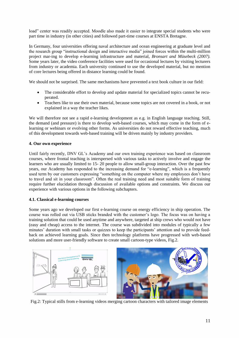
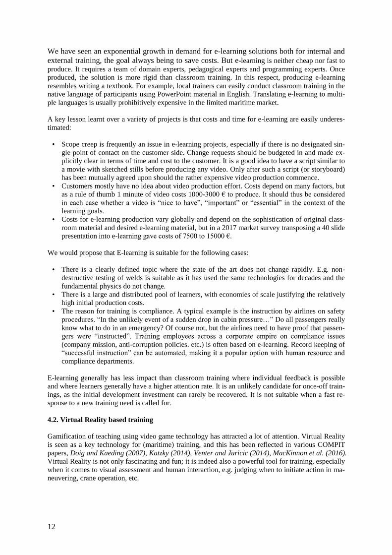
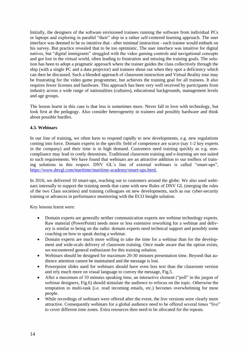
Some years ago we developed our first e-learning course on energy efficiency in ship operation. The
course was rolled out via USB sticks branded with the customer’s logo. The focus was on having a
training solution that could be used anytime and anywhere, targeted at ship crews who would not have
(easy and cheap) access to the internet. The course was subdivided into modules of typically a few
minutes’ duration with small tasks or quizzes to keep the participants’ attention and to provide feed-
back on achieved learning goals. Since then technology platforms have progressed with web-based
solutions and more user-friendly software to create small cartoon-type videos, Fig.2.
Fig.2: Typical stills from e-learning videos merging cartoon characters with tailored image elements
12
We have seen an exponential growth in demand for e-learning solutions both for internal and
external training, the goal always being to save costs. But e-learning is neither cheap nor fast to
produce. It requires a team of domain experts, pedagogical experts and programming experts. Once
produced, the solution is more rigid than classroom training. In this respect, producing e-learning
resembles writing a textbook. For example, local trainers can easily conduct classroom training in the
native language of participants using PowerPoint material in English. Translating e-learning to multi-
ple languages is usually prohibitively expensive in the limited maritime market.
A key lesson learnt over a variety of projects is that costs and time for e-learning are easily underes-
timated:
• Scope creep is frequently an issue in e-learning projects, especially if there is no designated sin-
gle point of contact on the customer side. Change requests should be budgeted in and made ex-
plicitly clear in terms of time and cost to the customer. It is a good idea to have a script similar to
a movie with sketched stills before producing any video. Only after such a script (or storyboard)
has been mutually agreed upon should the rather expensive video production commence.
• Customers mostly have no idea about video production effort. Costs depend on many factors, but
as a rule of thumb 1 minute of video costs 1000-3000 € to produce. It should thus be considered
in each case whether a video is “nice to have”, “important” or “essential” in the context of the
learning goals.
• Costs for e-learning production vary globally and depend on the sophistication of original class-
room material and desired e-learning material, but in a 2017 market survey transposing a 40 slide
presentation into e-learning gave costs of 7500 to 15000 €.
We would propose that E-learning is suitable for the following cases:
• There is a clearly defined topic where the state of the art does not change rapidly. E.g. non-
destructive testing of welds is suitable as it has used the same technologies for decades and the
fundamental physics do not change.
• There is a large and distributed pool of learners, with economies of scale justifying the relatively
high initial production costs.
• The reason for training is compliance. A typical example is the instruction by airlines on safety
procedures. “In the unlikely event of a sudden drop in cabin pressure…” Do all passengers really
know what to do in an emergency? Of course not, but the airlines need to have proof that passen-
gers were “instructed”. Training employees across a corporate empire on compliance issues
(company mission, anti-corruption policies. etc.) is often based on e-learning. Record keeping of
“successful instruction” can be automated, making it a popular option with human resource and
compliance departments.
E-learning generally has less impact than classroom training where individual feedback is possible
and where learners generally have a higher attention rate. It is an unlikely candidate for once-off train-
ings, as the initial development investment can rarely be recovered. It is not suitable when a fast re-
sponse to a new training need is called for.
4.2. Virtual Reality based training
Gamification of teaching using video game technology has attracted a lot of attention. Virtual Reality
is seen as a key technology for (maritime) training, and this has been reflected in various COMPIT
papers, Doig and Kaeding (2007), Katzky (2014), Venter and Juricic (2014), MacKinnon et al. (2016).
Virtual Reality is not only fascinating and fun; it is indeed also a powerful tool for training, especially
when it comes to visual assessment and human interaction, e.g. judging when to initiate action in ma-
neuvering, crane operation, etc.

13
However, the price of developing Virtual Reality-based training is high. Creating virtual worlds has
become easier, faster and cheaper, but it is still far from being easy, fast and cheap. Models need to
have the right level of detail, balancing realism and response time. Import/export from CAD systems
or other models (e.g. finite-element models) may save time, but in our experience is never as straight-
forward as hoped for or promised by vendors. Having a ship modelled over several decks, along with
equipment, interactivity, etc. may run into 5 or 6 digits of Euros. Such an investment needs either
subsidizing from R&D projects or a suitable mass market willing to pay premium fees for training,
such as firefighting. Often solutions have been developed for larger industries and are then adapted to
maritime applications, reducing the development effort.
DNV GL has developed a Virtual Reality-based training solution for ship inspections, called SuSi
(Survey Simulator), https://www.dnvgl.com/services/survey-simulator-for-ship-surveyor-training-in-
virtual-reality-shipmanager-survey-simulator-2173. SuSi provides realistic and cost-efficient 3D train-
ing software for survey inspections, using Virtual Reality technology and detailed models of ships and
offshore structures, Fig.3. The virtual inspection gets trainees exposed to deficiencies that would take
years for a surveyor to experience in real life. An inspection run can be recorded and discussed in a
debriefing with an experienced supervisor/trainer, pointing out oversights and errors by the trainee.
Fig.3: Level of detail in SuSi (Virtual Reality based survey simulator)
SuSi offers a variety of interactive elements, such as a virtual camera, virtual smartphone with product
data information and access to DNV GL Rules, virtual spray to mark deficiencies, Fig.4, and obvious-
ly navigation control to explore the virtual ship or offshore platform.
Fig.4: Virtual Reality based training with DNV GL’s SuSi (Surveyor Simulator)
14
Initially, the designers of the software envisioned trainees running the software from individual PCs
or laptops and exploring in parallel “their” ship in a rather self-centered learning approach. The user
interface was deemed to be so intuitive that - after minimal instruction - each trainee would embark on
his survey. But practice revealed that to be too optimistic. The user interface was intuitive for digital
natives, but “digital immigrants” struggled with the video gaming controls and navigational concepts
and got lost in the virtual world, often leading to frustration and missing the training goals. The solu-
tion has been to adopt a pragmatic approach where the trainer guides the class collectively through the
ship (with a single PC and a data projector) and trainees shout out when they spot a deficiency which
can then be discussed. Such a blended approach of classroom instruction and Virtual Reality tour may
be frustrating for the video game programmer, but achieves the training goal for all trainees. It also
requires fewer licenses and hardware. This approach has been very well received by participants from
industry across a wide range of nationalities (cultures), educational backgrounds, management levels
and age groups.
The lesson learnt in this case is that less is sometimes more. Never fall in love with technology, but
look first at the pedagogy. Also consider heterogeneity in trainees and possibly hardware and think
about possible hurdles.
4.3. Webinars
In our line of training, we often have to respond rapidly to new developments, e.g. new regulations
coming into force. Domain experts in the specific field of competence are scarce (say 1-2 key experts
in the company) and their time is in high demand. Customers need training quickly as e.g. non-
compliance may lead to costly detentions. Traditional classroom training and e-learning are not suited
to such requirements. We have found that webinars are an attractive addition to our toolbox of train-
ing solutions in this respect. DNV GL’s line of external webinars is called “smart-ups”,
https://www.dnvgl.com/maritime/maritime-academy/smart-ups.html.
In 2016, we delivered 10 smart-ups, reaching out to customers around the globe. We also used webi-
nars internally to support the training needs that came with new Rules of DNV GL (merging the rules
of the two Class societies) and training colleagues on new developments, such as our cyber-security
training or advances in performance monitoring with the ECO Insight solution.
Key lessons learnt were:
Domain experts are generally neither communication experts nor webinar technology experts.
Raw material (PowerPoint) needs more or less extensive reworking for a webinar and deliv-
ery is similar to being on the radio: domain experts need technical support and possibly some
coaching on how to speak during a webinar.
Domain experts are much more willing to take the time for a webinar than for the develop-
ment and wide-scale delivery of classroom training. Once made aware that the option exists,
we encountered general enthusiasm for this training solution.
Webinars should be designed for maximum 20-30 minutes presentation time. Beyond that au-
dience attention cannot be maintained and the message is lost.
Powerpoint slides used for webinars should have even less text than the classroom version
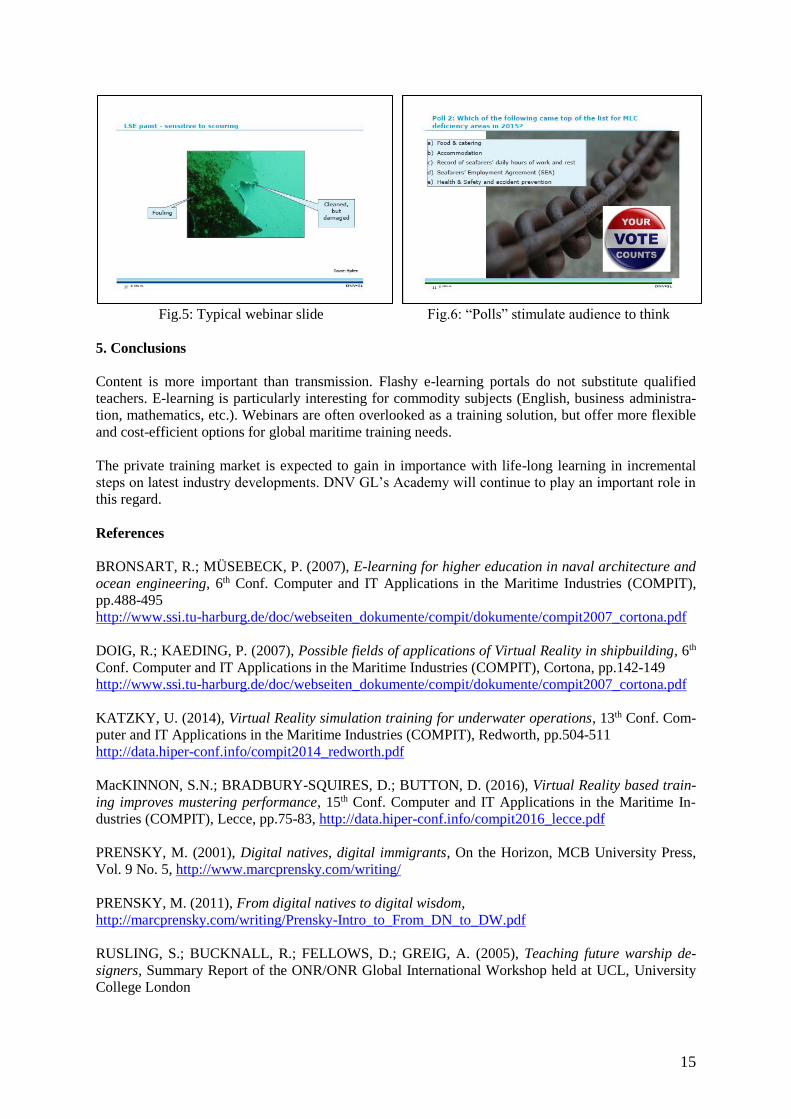
and rely much more on visual language to convey the message, Fig.5.
After a maximum of 10 minutes speaking time, an interactive element (“poll” in the jargon of
webinar designers, Fig.6) should stimulate the audience to refocus on the topic. Otherwise the
temptation to multi-task (i.e. read incoming emails, etc.) becomes overwhelming for most
people.
While recordings of webinars were offered after the event, the live versions were clearly more
attractive. Consequently webinars for a global audience need to be offered several times “live”
to cover different time zones. Extra resources then need to be allocated for the repeats.
15
Fig.5: Typical webinar slide Fig.6: “Polls” stimulate audience to think
5. Conclusions
Content is more important than transmission. Flashy e-learning portals do not substitute qualified
teachers. E-learning is particularly interesting for commodity subjects (English, business administra-
tion, mathematics, etc.). Webinars are often overlooked as a training solution, but offer more flexible
and cost-efficient options for global maritime training needs.
The private training market is expected to gain in importance with life-long learning in incremental
steps on latest industry developments. DNV GL’s Academy will continue to play an important role in
this regard.
References
BRONSART, R.; MÜSEBECK, P. (2007), E-learning for higher education in naval architecture and
ocean engineering, 6th Conf. Computer and IT Applications in the Maritime Industries (COMPIT),
pp.488-495
http://www.ssi.tu-harburg.de/doc/webseiten_dokumente/compit/dokumente/compit2007_cortona.pdf
DOIG, R.; KAEDING, P. (2007), Possible fields of applications of Virtual Reality in shipbuilding, 6th
Conf. Computer and IT Applications in the Maritime Industries (COMPIT), Cortona, pp.142-149
http://www.ssi.tu-harburg.de/doc/webseiten_dokumente/compit/dokumente/compit2007_cortona.pdf
KATZKY, U. (2014), Virtual Reality simulation training for underwater operations, 13th Conf. Com-
puter and IT Applications in the Maritime Industries (COMPIT), Redworth, pp.504-511
http://data.hiper-conf.info/compit2014_redworth.pdf
MacKINNON, S.N.; BRADBURY-SQUIRES, D.; BUTTON, D. (2016), Virtual Reality based train-
ing improves mustering performance, 15th Conf. Computer and IT Applications in the Maritime In-
dustries (COMPIT), Lecce, pp.75-83, http://data.hiper-conf.info/compit2016_lecce.pdf
PRENSKY, M. (2001), Digital natives, digital immigrants, On the Horizon, MCB University Press,
Vol. 9 No. 5, http://www.marcprensky.com/writing/
PRENSKY, M. (2011), From digital natives to digital wisdom,
http://marcprensky.com/writing/Prensky-Intro_to_From_DN_to_DW.pdf
RUSLING, S.; BUCKNALL, R.; FELLOWS, D.; GREIG, A. (2005), Teaching future warship de-
signers, Summary Report of the ONR/ONR Global International Workshop held at UCL, University
College London

16
VENTER, A.; JURICIC, I. (2014), Virtual Reality for crew education in on-board operational and
emergency conditions, 13th Conf. Computer and IT Applications in the Maritime Industries (COM-
PIT), Redworth, pp.437-447, http://data.hiper-conf.info/compit2014_redworth.pdf
Appendix: Requirements for Naval Architects
The following is based on an ONR workshop on Future Warship Designers, Rusling (2005). In dis-
cussion between (mostly US American) representatives of industry and academia, the following items
were listed as guidelines for future curricula for naval architecture:
Good base in naval architecture / engineering principles
- strength analyses, structural design and production
- hydrostatics / stability and ship design (rules, layout, estimation methods)
- hydrodynamics
- marine engineering
Computer literate
- CAD proficiency seen as main gap
- Level of competence (hours spent with specific software) should be recorded
- Naval architecture is increasingly applied computer science and less mechanical en-
gineering
Hands-on experience
- as worker and as engineer
- at sea / at shipyard
more specialized knowledge 7 more mathematics at post-grad level
soft skills
- ability to study independently
- creative with feel for viability of solutions
- enthusiastic
- team capability
management skills
- project management
- communication
- basic legal frameworks for contract / work laws
- motivation
engineering English
- vocabulary (incl. mathematical expressions)
- technical / scientific communication in English
17
Future of Shipbuilding and Shipping - A Technology Vision
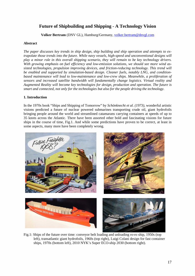
Volker Bertram (DNV GL), Hamburg/Germany, [email protected] Abstract The paper discusses key trends in ship design, ship building and ship operation and attempts to ex-trapolate those trends into the future. While navy vessels, high-speed and unconventional designs will play a minor role in this overall shipping scenario, they will remain to be key technology drivers. With growing emphasis on fuel efficiency and low-emission solutions, we should see more wind as-sisted technologies, propulsion improving devices, and friction-reducing technology. This trend will be enabled and supported by simulation-based design. Cleaner fuels, notably LNG, and condition-based maintenance will lead to low-maintenance and low-crew ships. Meanwhile, a proliferation of sensors and increased satellite bandwidth will fundamentally change logistics. Virtual reality and Augmented Reality will become key technologies for design, production and operation. The future is smart and connected, not only for the technologies but also for the people driving the technology. 1. Introduction In the 1970s book “Ships and Shipping of Tomorrow” by Schönknecht et al. (1973), wonderful artistic visions predicted a future of nuclear powered submarines transporting crude oil, giant hydrofoils bringing people around the world and streamlined catamarans carrying containers at speeds of up to 35 knots across the Atlantic. There have been assorted other bold and fascinating visions for future ships in the course of time, Fig.1. And while some predictions have proven to be correct, at least in some aspects, many more have been completely wrong.
Fig.1: Ships of the future over time: conveyor belt loading and unloading ro-ro ship, 1950s (top left), transatlantic giant hydrofoils, 1960s (top right), Luigi Colani design for fast container ships, 1970s (bottom left), 2010 NYK’s Super ECO-ship 2030 (bottom right).
18
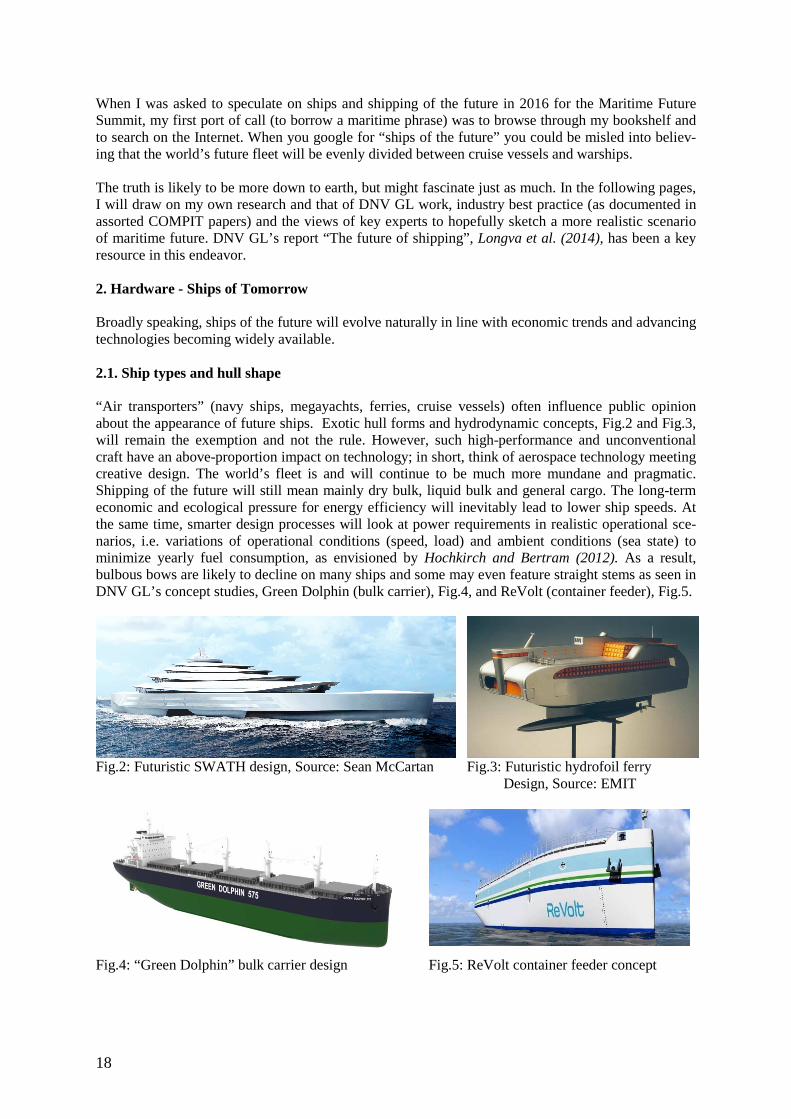
When I was asked to speculate on ships and shipping of the future in 2016 for the Maritime Future Summit, my first port of call (to borrow a maritime phrase) was to browse through my bookshelf and to search on the Internet. When you google for “ships of the future” you could be misled into believ-ing that the world’s future fleet will be evenly divided between cruise vessels and warships. The truth is likely to be more down to earth, but might fascinate just as much. In the following pages, I will draw on my own research and that of DNV GL work, industry best practice (as documented in assorted COMPIT papers) and the views of key experts to hopefully sketch a more realistic scenario of maritime future. DNV GL’s report “The future of shipping”, Longva et al. (2014), has been a key resource in this endeavor. 2. Hardware - Ships of Tomorrow Broadly speaking, ships of the future will evolve naturally in line with economic trends and advancing technologies becoming widely available. 2.1. Ship types and hull shape “Air transporters” (navy ships, megayachts, ferries, cruise vessels) often influence public opinion about the appearance of future ships. Exotic hull forms and hydrodynamic concepts, Fig.2 and Fig.3, will remain the exemption and not the rule. However, such high-performance and unconventional craft have an above-proportion impact on technology; in short, think of aerospace technology meeting creative design. The world’s fleet is and will continue to be much more mundane and pragmatic. Shipping of the future will still mean mainly dry bulk, liquid bulk and general cargo. The long-term economic and ecological pressure for energy efficiency will inevitably lead to lower ship speeds. At the same time, smarter design processes will look at power requirements in realistic operational sce-narios, i.e. variations of operational conditions (speed, load) and ambient conditions (sea state) to minimize yearly fuel consumption, as envisioned by Hochkirch and Bertram (2012). As a result, bulbous bows are likely to decline on many ships and some may even feature straight stems as seen in DNV GL’s concept studies, Green Dolphin (bulk carrier), Fig.4, and ReVolt (container feeder), Fig.5.
Fig.2: Futuristic SWATH design, Source: Sean McCartan Fig.3: Futuristic hydrofoil ferry
Design, Source: EMIT
Fig.4: “Green Dolphin” bulk carrier design Fig.5: ReVolt container feeder concept
19
2.2. Materials Most likely, ship hulls will continue to be made of steel, simply because steel is cheap, strong and easy to recycle. Better coatings and inspection programs will compensate for steel’s main shortcom-ing, namely, corrosion. More ductile steel alloys will lead to more collision-resistant structures. Intel-ligent condition monitoring schemes will provide the appropriate technologies to extend the average life-span of steel structures while reducing (if not avoiding completely) the risk of structural failure:
• Big Data: embedded monitoring systems and conventional surveying schemes will generate huge volumes of data across fleets of ships in service and offshore platforms. Cross-referencing this data will support future intelligent condition monitoring systems.
• Image Processing: image processing techniques are likely to be used to automatically detect and quantify paint defects, extent of corrosion and cracks, for example, Mavi et al. (2012). The progression of such defects will likely be mapped and quantified through the use of im-ages from different time periods. The availability of cheap miniature cameras (as embedded in mobile phones) is also likely to lead to wide-spread installation and automatic surveying schemes.
• Corrosion Prediction Schemes: using Artificial Intelligence techniques, classical corrosion prediction schemes will be improved, providing a more accurate prediction of location, extent and type of corrosion. De Masi et al. (2016) provide an example of pipelines.
• Simulation technology: using 3D ship product models and fast finite-element modelling tech-niques, the as-is condition of a ship will be capable of being simulated at any time, as envi-sioned in Wilken et al. (2011).
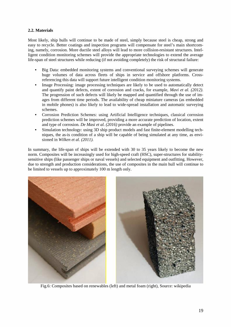
In summary, the life-span of ships will be extended with 30 to 35 years likely to become the new norm. Composites will be increasingly used for high-speed craft (HSC), super-structures for stability-sensitive ships (like passenger ships or naval vessels) and selected equipment and outfitting. However, due to strength and production considerations, the use of composites in the main hull will continue to be limited to vessels up to approximately 100 m length only.
Fig.6: Composites based on renewables (left) and metal foam (right), Source: wikipedia
20
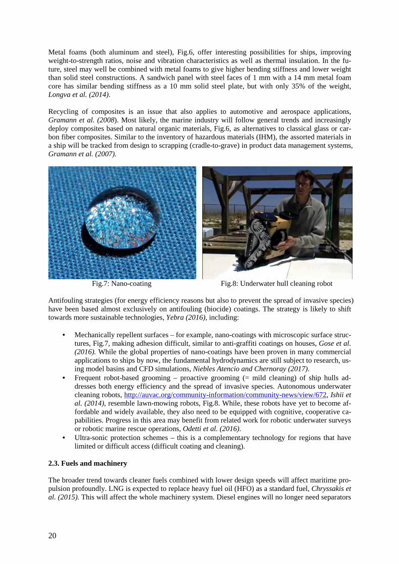
Metal foams (both aluminum and steel), Fig.6, offer interesting possibilities for ships, improving weight-to-strength ratios, noise and vibration characteristics as well as thermal insulation. In the fu-ture, steel may well be combined with metal foams to give higher bending stiffness and lower weight than solid steel constructions. A sandwich panel with steel faces of 1 mm with a 14 mm metal foam core has similar bending stiffness as a 10 mm solid steel plate, but with only 35% of the weight, Longva et al. (2014). Recycling of composites is an issue that also applies to automotive and aerospace applications, Gramann et al. (2008). Most likely, the marine industry will follow general trends and increasingly deploy composites based on natural organic materials, Fig.6, as alternatives to classical glass or car-bon fiber composites. Similar to the inventory of hazardous materials (IHM), the assorted materials in a ship will be tracked from design to scrapping (cradle-to-grave) in product data management systems, Gramann et al. (2007).
Fig.7: Nano-coating Fig.8: Underwater hull cleaning robot
Antifouling strategies (for energy efficiency reasons but also to prevent the spread of invasive species) have been based almost exclusively on antifouling (biocide) coatings. The strategy is likely to shift towards more sustainable technologies, Yebra (2016), including:
• Mechanically repellent surfaces – for example, nano-coatings with microscopic surface struc-tures, Fig.7, making adhesion difficult, similar to anti-graffiti coatings on houses, Gose et al. (2016). While the global properties of nano-coatings have been proven in many commercial applications to ships by now, the fundamental hydrodynamics are still subject to research, us-ing model basins and CFD simulations, Niebles Atencio and Chernoray (2017).
• Frequent robot-based grooming – proactive grooming (= mild cleaning) of ship hulls ad-dresses both energy efficiency and the spread of invasive species. Autonomous underwater cleaning robots, http://auvac.org/community-information/community-news/view/672, Ishii et al. (2014), resemble lawn-mowing robots, Fig.8. While, these robots have yet to become af-fordable and widely available, they also need to be equipped with cognitive, cooperative ca-pabilities. Progress in this area may benefit from related work for robotic underwater surveys or robotic marine rescue operations, Odetti et al. (2016).
• Ultra-sonic protection schemes – this is a complementary technology for regions that have limited or difficult access (difficult coating and cleaning).
2.3. Fuels and machinery The broader trend towards cleaner fuels combined with lower design speeds will affect maritime pro-pulsion profoundly. LNG is expected to replace heavy fuel oil (HFO) as a standard fuel, Chryssakis et al. (2015). This will affect the whole machinery system. Diesel engines will no longer need separators
21
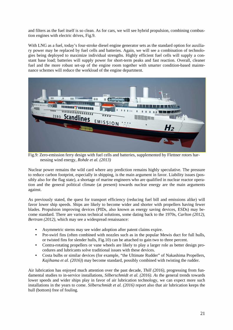
and filters as the fuel itself is so clean. As for cars, we will see hybrid propulsion, combining combus-tion engines with electric drives, Fig.9. With LNG as a fuel, today’s four-stroke diesel engine generator sets as the standard option for auxilia-ry power may be replaced by fuel cells and batteries. Again, we will see a combination of technolo-gies being deployed to maximize individual strengths. Highly efficient fuel cells will supply a con-stant base load; batteries will supply power for short-term peaks and fast reaction. Overall, cleaner fuel and the more robust set-up of the engine room together with smarter condition-based mainte-nance schemes will reduce the workload of the engine department.
Fig.9: Zero-emission ferry design with fuel cells and batteries, supplemented by Flettner rotors har- nessing wind energy, Rohde et al. (2013) Nuclear power remains the wild card where any prediction remains highly speculative. The pressure to reduce carbon footprint, especially in shipping, is the main argument in favor. Liability issues (pos-sibly also for the flag state), a shortage of marine engineers who are qualified in nuclear reactor opera-tion and the general political climate (at present) towards nuclear energy are the main arguments against. As previously stated, the quest for transport efficiency (reducing fuel bill and emissions alike) will favor lower ship speeds. Ships are likely to become wider and shorter with propellers having fewer blades. Propulsion improving devices (PIDs, also known as energy saving devices, ESDs) may be-come standard. There are various technical solutions, some dating back to the 1970s, Carlton (2012), Bertram (2012), which may see a widespread renaissance:
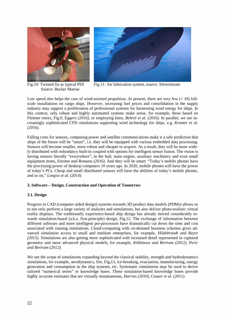
• Asymmetric sterns may see wider adoption after patent claims expire. • Pre-swirl fins (often combined with nozzles such as in the popular Mewis duct for full hulls,
or twisted fins for slender hulls, Fig.10) can be attached to gain two to three percent. • Contra-rotating propellers or vane wheels are likely to play a larger role as better design pro-
cedures and lubricants solve traditional issues with these devices. • Costa bulbs or similar devices (for example, “the Ultimate Rudder” of Nakashima Propellers,
Kajihama et al. (2016)) may become standard, possibly combined with twisting the rudder. Air lubrication has enjoyed much attention over the past decade, Thill (2016), progressing from fun-damental studies to in-service installations, Silberschmidt et al. (2016). As the general trends towards lower speeds and wider ships play in favor of air lubrication technology, we can expect more such installations in the years to come. Silberschmidt et al. (2016) report also that air lubrication keeps the hull (bottom) free of fouling.
22
Fig.10: Twisted fin as typical PDI Source: Becker Marine
Fig.11: Air lubrication system, source: Silverstream
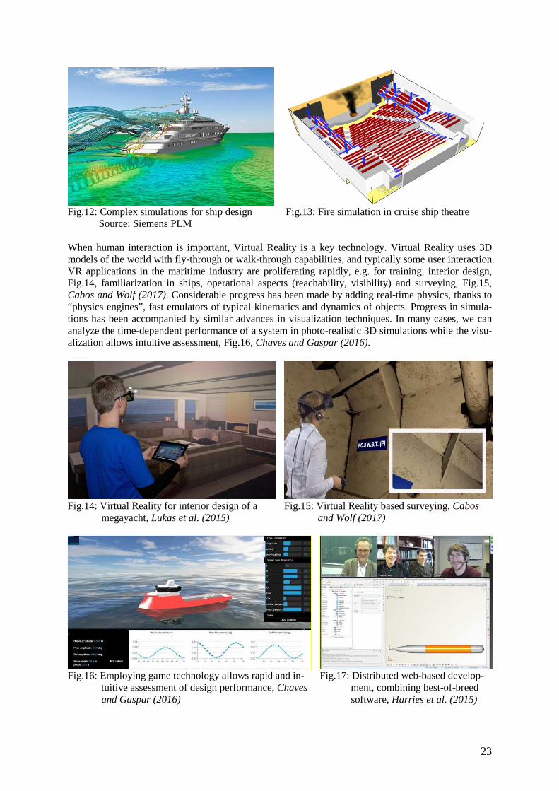
Low speed also helps the case of wind-assisted propulsion. At present, there are very few (< 10) full-scale installations on cargo ships. However, increasing fuel prices and consolidation in the supply industry may support a proliferation of professional systems for harnessing wind energy for ships. In this context, only robust and highly automated systems make sense, for example, those based on Flettner rotors, Fig.9, Eggers (2016), or employing kites, Behrel et al. (2016). In parallel, we see in-creasingly sophisticated CFD simulations supporting wind technology for ships, e.g. Kramer et al. (2016). Falling costs for sensors, computing power and satellite communications make it a safe prediction that ships of the future will be “smart”, i.e. they will be equipped with various embedded data processing. Sensors will become smaller, more robust and cheaper to acquire. As a result, they will be more wide-ly distributed with redundancy built-in coupled with options for intelligent sensor fusion. The vision is having sensors literally “everywhere”, in the hull, main engine, auxiliary machinery and even small equipment items, Etienne and Romano (2016). And they will be smart. “Today’s mobile phones have the processing power of desktop computers 10 years ago. In 2020, mobile phones will have the power of today’s PCs. Cheap and small distributed sensors will have the abilities of today’s mobile phones, and so on,” Longva et al. (2014). 3. Software – Design, Construction and Operation of Tomorrow 3.1. Design Progress in CAD (computer aided design) systems towards 3D product data models (PDMs) allows us to not only perform a large variety of analyses and simulations, but also deliver photo-realistic virtual reality displays. The traditionally experience-based ship design has already moved considerably to-wards simulation-based (a.k.a. first-principle) design, Fig.12. The exchange of information between different software and more intelligent pre-processors have dramatically cut down the time and cost associated with running simulations. Cloud-computing with on-demand business schemes gives ad-vanced simulation access to small and medium enterprises, for example, Hildebrandt and Reyer (2015). Simulations are also getting more sophisticated with increased detail represented in captured geometry and more advanced physical models, for example, Köhlmoos and Bertram (2012), Peric and Bertram (2012). We see the scope of simulations expanding beyond the classical stability, strength and hydrodynamics simulations, for example, aerodynamics, fire, Fig,13, ice-breaking, evacuation, manufacturing, energy generation and consumption in the ship systems, etc. Systematic simulations may be used to derive tailored “numerical series” or knowledge bases. These simulation-based knowledge bases provide highly accurate estimates that are virtually instantaneous, Harries (2010), Couser et al. (2011).
23
Fig.12: Complex simulations for ship design Source: Siemens PLM
Fig.13: Fire simulation in cruise ship theatre
When human interaction is important, Virtual Reality is a key technology. Virtual Reality uses 3D models of the world with fly-through or walk-through capabilities, and typically some user interaction. VR applications in the maritime industry are proliferating rapidly, e.g. for training, interior design, Fig.14, familiarization in ships, operational aspects (reachability, visibility) and surveying, Fig.15, Cabos and Wolf (2017). Considerable progress has been made by adding real-time physics, thanks to “physics engines”, fast emulators of typical kinematics and dynamics of objects. Progress in simula-tions has been accompanied by similar advances in visualization techniques. In many cases, we can analyze the time-dependent performance of a system in photo-realistic 3D simulations while the visu-alization allows intuitive assessment, Fig.16, Chaves and Gaspar (2016).
Fig.14: Virtual Reality for interior design of a megayacht, Lukas et al. (2015)
Fig.15: Virtual Reality based surveying, Cabos and Wolf (2017)
Fig.16: Employing game technology allows rapid and in- tuitive assessment of design performance, Chaves and Gaspar (2016)
Fig.17: Distributed web-based develop- ment, combining best-of-breed software, Harries et al. (2015)
24
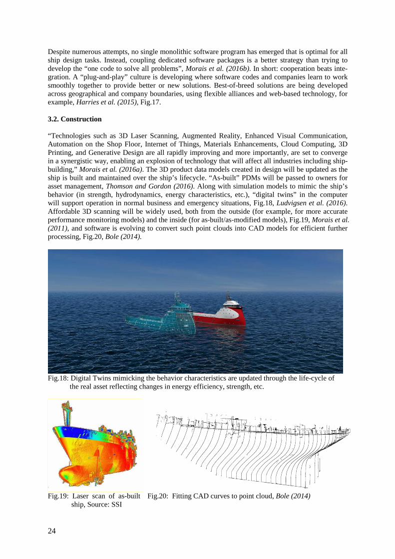
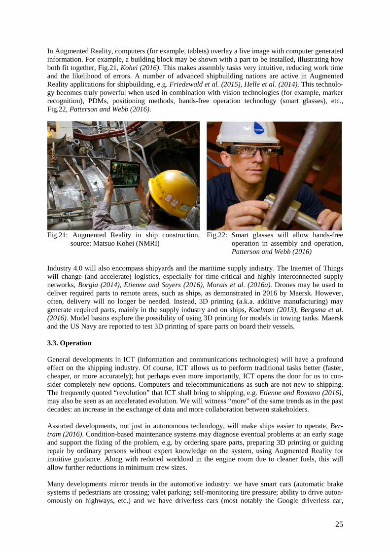
Despite numerous attempts, no single monolithic software program has emerged that is optimal for all ship design tasks. Instead, coupling dedicated software packages is a better strategy than trying to develop the “one code to solve all problems”, Morais et al. (2016b). In short: cooperation beats inte-gration. A “plug-and-play” culture is developing where software codes and companies learn to work smoothly together to provide better or new solutions. Best-of-breed solutions are being developed across geographical and company boundaries, using flexible alliances and web-based technology, for example, Harries et al. (2015), Fig.17. 3.2. Construction “Technologies such as 3D Laser Scanning, Augmented Reality, Enhanced Visual Communication, Automation on the Shop Floor, Internet of Things, Materials Enhancements, Cloud Computing, 3D Printing, and Generative Design are all rapidly improving and more importantly, are set to converge in a synergistic way, enabling an explosion of technology that will affect all industries including ship-building,” Morais et al. (2016a). The 3D product data models created in design will be updated as the ship is built and maintained over the ship’s lifecycle. “As-built” PDMs will be passed to owners for asset management, Thomson and Gordon (2016). Along with simulation models to mimic the ship’s behavior (in strength, hydrodynamics, energy characteristics, etc.), “digital twins” in the computer will support operation in normal business and emergency situations, Fig.18, Ludvigsen et al. (2016). Affordable 3D scanning will be widely used, both from the outside (for example, for more accurate performance monitoring models) and the inside (for as-built/as-modified models), Fig.19, Morais et al. (2011), and software is evolving to convert such point clouds into CAD models for efficient further processing, Fig.20, Bole (2014).
Fig.18: Digital Twins mimicking the behavior characteristics are updated through the life-cycle of the real asset reflecting changes in energy efficiency, strength, etc.
Fig.19: Laser scan of as-built
ship, Source: SSI Fig.20: Fitting CAD curves to point cloud, Bole (2014)
25
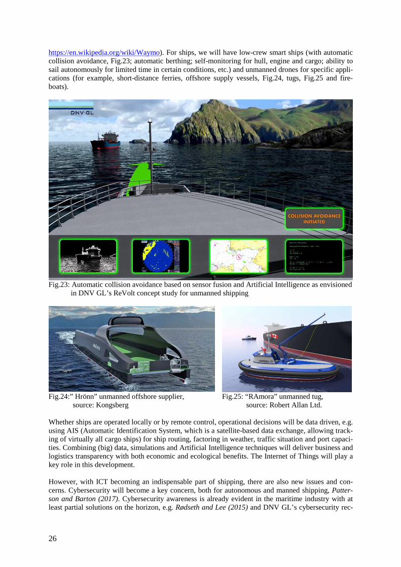
In Augmented Reality, computers (for example, tablets) overlay a live image with computer generated information. For example, a building block may be shown with a part to be installed, illustrating how both fit together, Fig.21, Kohei (2016). This makes assembly tasks very intuitive, reducing work time and the likelihood of errors. A number of advanced shipbuilding nations are active in Augmented Reality applications for shipbuilding, e.g. Friedewald et al. (2015), Helle et al. (2014). This technolo-gy becomes truly powerful when used in combination with vision technologies (for example, marker recognition), PDMs, positioning methods, hands-free operation technology (smart glasses), etc., Fig.22, Patterson and Webb (2016).
Fig.21: Augmented Reality in ship construction,
source: Matsuo Kohei (NMRI) Fig.22: Smart glasses will allow hands-free
operation in assembly and operation, Patterson and Webb (2016)
Industry 4.0 will also encompass shipyards and the maritime supply industry. The Internet of Things will change (and accelerate) logistics, especially for time-critical and highly interconnected supply networks, Borgia (2014), Etienne and Sayers (2016), Morais et al. (2016a). Drones may be used to deliver required parts to remote areas, such as ships, as demonstrated in 2016 by Maersk. However, often, delivery will no longer be needed. Instead, 3D printing (a.k.a. additive manufacturing) may generate required parts, mainly in the supply industry and on ships, Koelman (2013), Bergsma et al. (2016). Model basins explore the possibility of using 3D printing for models in towing tanks. Maersk and the US Navy are reported to test 3D printing of spare parts on board their vessels. 3.3. Operation General developments in ICT (information and communications technologies) will have a profound effect on the shipping industry. Of course, ICT allows us to perform traditional tasks better (faster, cheaper, or more accurately); but perhaps even more importantly, ICT opens the door for us to con-sider completely new options. Computers and telecommunications as such are not new to shipping. The frequently quoted “revolution” that ICT shall bring to shipping, e.g. Etienne and Romano (2016), may also be seen as an accelerated evolution. We will witness “more” of the same trends as in the past decades: an increase in the exchange of data and more collaboration between stakeholders. Assorted developments, not just in autonomous technology, will make ships easier to operate, Ber-tram (2016). Condition-based maintenance systems may diagnose eventual problems at an early stage and support the fixing of the problem, e.g. by ordering spare parts, preparing 3D printing or guiding repair by ordinary persons without expert knowledge on the system, using Augmented Reality for intuitive guidance. Along with reduced workload in the engine room due to cleaner fuels, this will allow further reductions in minimum crew sizes. Many developments mirror trends in the automotive industry: we have smart cars (automatic brake systems if pedestrians are crossing; valet parking; self-monitoring tire pressure; ability to drive auton-omously on highways, etc.) and we have driverless cars (most notably the Google driverless car,
26
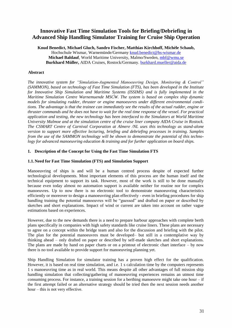
https://en.wikipedia.org/wiki/Waymo). For ships, we will have low-crew smart ships (with automatic collision avoidance, Fig.23; automatic berthing; self-monitoring for hull, engine and cargo; ability to sail autonomously for limited time in certain conditions, etc.) and unmanned drones for specific appli-cations (for example, short-distance ferries, offshore supply vessels, Fig.24, tugs, Fig.25 and fire-boats).
Fig.23: Automatic collision avoidance based on sensor fusion and Artificial Intelligence as envisioned in DNV GL’s ReVolt concept study for unmanned shipping
Fig.24:” Hrönn” unmanned offshore supplier, source: Kongsberg
Fig.25: “RAmora” unmanned tug, source: Robert Allan Ltd.
Whether ships are operated locally or by remote control, operational decisions will be data driven, e.g. using AIS (Automatic Identification System, which is a satellite-based data exchange, allowing track-ing of virtually all cargo ships) for ship routing, factoring in weather, traffic situation and port capaci-ties. Combining (big) data, simulations and Artificial Intelligence techniques will deliver business and logistics transparency with both economic and ecological benefits. The Internet of Things will play a key role in this development. However, with ICT becoming an indispensable part of shipping, there are also new issues and con-cerns. Cybersecurity will become a key concern, both for autonomous and manned shipping, Patter-son and Barton (2017). Cybersecurity awareness is already evident in the maritime industry with at least partial solutions on the horizon, e.g. Rødseth and Lee (2015) and DNV GL’s cybersecurity rec-

27
ommended practice, https://www.dnvgl.com/maritime/dnvgl-rp-0496-recommended-practice-cyber-security-download.html. The technology on ships will largely follow the cybersecurity technology employed for other large assets, such as power plants, traffic control centers, etc. 4. Conclusions Stand-alone techniques have already reached a high degree of maturity and further progress is best obtained by partnerships and an appropriate combination of technologies and techniques, as illustrated in the individual chapters. We see this trend continuing swiftly: simulation tools with Virtual Reality displays and Artificial Intelligence for user guidance, Big Data using Artificial Intelligence to derive trends for profiles used in formal optimization, etc. In short, it is all about getting smart and connected – as is the COMPIT conference. Acknowledgments This paper is the result of countless contributions to the COMPIT conferences and the last HIPER conference, where over the years I have seen the arrival and application of new technologies. The papers, but perhaps even more the discussions, have shaped my view of our industry and the assorted IT developments. For this insight, I am very grateful. If I have overlooked key publications in my already long list of publications, I beg your indulgence. References BEHREL, M.; BIGI, N.; RONCIN, K.; GRELON, D.; MONTEL, F.; NEME, A.; LEROUX, J.B.; JOCHUM, C.; PARLIER, Y. (2016), Measured performance of a 50-m2 kite on a trawler, 10th HIPER Conf., Cortona, pp.443-457, http://data.hiper-conf.info/Hiper2016_cortona.pdf BERGSMA, J.M.; ZALM, M.v.d.; PRUYN, J.F.J. (2016), 3D-printing and the maritime construction sector, 10th HIPER Conf., Cortona, pp.428-442, http://data.hiper-conf.info/Hiper2016_cortona.pdf BERTRAM, V. (2012), Practical Ship Hydrodynamics, Butterworth & Heinemann BERTRAM, V. (2016), Unmanned & Autonomous Shipping – A Technology Review, 10th HIPER Conf., Cortona, pp.10-24, http://data.hiper-conf.info/Hiper2016_cortona.pdf BOLE, M. (2014), Regenerating hull design definition from poor surface definitions and other geo-metric representations, 13th COMPIT Conf., Redworth, pp.193-208, http://data.hiper-conf.info/compit2014_redworth.pdf BORGIA, E. (2014), The Internet of Things vision: Key features, applications and open issues, Com-puter Communications 54, pp.1-31 https://www.semanticscholar.org/paper/The-Internet-of-Things-vision-Key-features-Borgia/2e5924dbb26cf9c3b5533bdf1c96885befbb265d/pdf CABOS, C.; WOLF, V. (2017), Virtual Reality aided remote hull inspection,16th COMPIT, Cardiff CARLTON, J. (2012), Marine Propeller and Propulsion, Butterworth & Heinemann CHAVES, O.; GASPAR, H. (2016), A web based real-time 3D simulator for ship design virtual pro-totype and motion prediction, 15th COMPIT Conf., Lecce, pp.410-419, http://data.hiper-conf.info/compit2016_lecce.pdf CHRYSSAKIS, C.; BRINKS, H.; KING, T. (2015), The fuel trilemma, Position Paper, DNV GL, Høvik, https://www.dnvgl.com/Images/DNV GL_Position Paper on Fuel Trilemma_tcm8-25973.pdf

28
COUSER, P.; HARRIES, S.; TILLIG, F. (2011), Numerical hull series for calm water and sea-keeping, 10th COMPIT Conf., Berlin, pp.206-220, http://data.hiper-conf.info/compit2011_berlin.pdf DE MASI, G.; GENTILE, M.; VICHI, R.; BRUSCHI, R.; GABETTA, G. (2016), Corrosion predic-tion by hierarchical neural networks, 15th COMPIT, Lecce, pp.146-160, http://data.hiper-conf.info/compit2016_lecce.pdf EGGERS, R. (2016), Operational performance of wind assisted ships, 10th HIPER Conf., Cortona, pp.366-379, http://data.hiper-conf.info/Hiper2016_cortona.pdf ETIENNE, M.; ROMANO, A. (2016), The Internet of Things for smarter, safer, connected ships, 10th HIPER Conf., Cortona, pp.164-171, http://data.hiper-conf.info/Hiper2016_cortona.pdf FRIEDEWALD, A.; LÖDDING, H.; TITOV, F. Augmented Reality for the retrofit of ships, 15th COMPIT, Lecce, pp.236-246, http://data.hiper-conf.info/compit2016_lecce.pdf GOSE, J.W.; OLOVIN, K.; BARROS, J.; SCHULTZ, M.; TUTEJA, A.; CECCIO, S.L.; PERLIN, M. (2016), Biomimetic super-hydrophobic coatings for friction reduction, 10th HIPER Conf., Cortona, pp.477-490, http://data.hiper-conf.info/Hiper2016_cortona.pdf GRAMANN, H.; KÖPKE, M.; FLÜGGE, M.; GRAFE, W. (2007), Data management for better ship-care and recycling, 6th COMPIT, Cortona, pp.33-41, http://data.hiper-conf.info/compit2007_cortona.pdf GRAMANN, H.; KRAPP, R.; BERTRAM, V. (2008), Disposal and recycling of HSC materials, 6th HIPER Conf., Naples, pp.271-280, http://data.hiper-conf.info/Hiper2008_Naples.pdf HARRIES, S. (2010), Investigating multi-dimensional design spaces using first principle methods, 7th
HIPER Conf., Melbourne, pp.179-194, http://data.hiper-conf.info/Hiper2010_Melbourne.pdf HARRIES, S.; MacPHERSON, D.; EDMONDS, A. (2015), Speed-power optimized AUV design by coupling CAESES and NavCad, 14th COMPIT Conf., Ulrichshusen, pp.247-256, http://data.hiper-conf.info/compit2015_ulrichshusen.pdf HELLE, S.; KORHONEN, S.; EURANTO, A.; KAUSTINEN, M.; LAHDENOJA, O.; LEHTONEN, T. (2014), Benefits achieved by applying Augmented Reality technology in marine industry, 13th COMPIT Conf., Redworth, pp.86-97, http://data.hiper-conf.info/compit2014_redworth.pdf HILDEBRANDT, T.; REYER, M. (2015), Business and Technical Adaptivity in Marine CFD Simula-tions - Bridging the Gap, 14th COMPIT Conf., Ulrichshusen, pp.394-405, http://data.hiper-conf.info/compit2015_ulrichshusen.pdf HOCHKIRCH, K.; BERTRAM, V. (2012), Hull optimization for fuel efficiency – Past, present and future, 11th COMPIT, Liege, pp.39-49, http://data.hiper-conf.info/compit2012_liege.pdf ISHII, K.; NASSIRAEI, A.A.F.; SONODA, T. (2014), Design concept of an underwater robot for ship hull cleaning, 13th COMPIT Conf., Redworth, pp.540-545, http://data.hiper-conf.info/compit2014_redworth.pdf KAJIHAMA, T.; TACHIKAWA, T.; KATAYAMA, K.; OKADA, Y .; OKAZAKI, A. (2016), Inno-vative energy saving device designed by virtual prototyping method, 10th HIPER Conf., Cortona, pp.380-385, http://data.hiper-conf.info/Hiper2016_cortona.pdf KÖHLMOOS, A.; BERTRAM, V. (2012), Advanced simulations for high-performance megayachts, 8th HIPER Conf., Duisburg, pp.38-50, http://data.hiper-conf.info/Hiper2012_Duisburg.pdf

29
KOELMAN, H.J. (2013), A mid-term outlook on computer aided ship design, 12th COMPIT Conf., Cortona, pp.110-119, http://data.hiper-conf.info/compit2013_cortona.pdf KRAMER, J.A.; STEEN, S.; SAVIO, L. (2016), Drift forces – Wingsails vs Flettner rotors, 10th HIPER Conf., Cortona, pp.202-216, http://data.hiper-conf.info/Hiper2016_cortona.pdf LONGVA, T.; HOLMVANG, P.; GUTTORMSEN, V.J. (2014), The Future of Shipping, DNV GL report, Høvik, https://www.dnvgl.com/publications/the-future-of-shipping-april-2014--14230 LUDVIGSEN, K.B.; JAMT, L.K.; Nicolai HUSTELI, SMOGELI, Ø. (2016), Digital twins for design, testing and verification throughout a vessel’s life cycle, 15th COMPIT, Lecce, pp.448-457, http://data.hiper-conf.info/compit2016_lecce.pdf LUKAS, U.v.; RUTH, T.; DEISTUNG, E.; HUBER, L. (2015), Leveraging the potential of 3D data in the ship lifecycle with open formats and interfaces, 14th COMPIT Conf., Ulrichshusen, pp.318-330, http://data.hiper-conf.info/compit2015_ulrichshusen.pdf MATSUO, K. (2016), Augmented reality assistance for outfitting works in shipbuilding, 15th COM-PIT, Lecce, pp.234-239, http://data.hiper-conf.info/compit2016_lecce.pdf MAVI, A.; KAUR, G.; KAUR, N. (2012), Paint defect detection using a machine vision system – A review, Int. J. Research in Management & Technology 2/3, pp.334-337, http://www.iracst.org/ijrmt/papers/vol2no32012/11vol2no3.pdf MORAIS, D.; WALDIE, M.; LARKINS, D. (2011), Driving the adoption of cutting edge technology in shipbuilding, 10th COMPIT, Berlin, pp.523-535, http://data.hiper-conf.info/compit2016_lecce.pdf MORAIS, D.; WALDIE, M.; DANESE, N. (2016b), Open architecture applications: The key to best-of-breed solutions, 15th COMPIT, Lecce, pp.223-233, http://data.hiper-conf.info/compit2016_lecce.pdf MORAIS, D.; DANESE, N.; WALDIE, M. (2016a), Ship design, engineering and construction in 2030 and beyond, 15th COMPIT, Lecce, pp.223-233, 10th HIPER Conf., Cortona, pp.297-310, http://data.hiper-conf.info/Hiper2016_cortona.pdf NIEBLES ATENCIO, B.; CHERNORAY, V. (2017), Measurements and prediction of friction drag of hull coatings, 2nd HullPIC Conf., Ulrichshusen ODETTI, A.; BIBULI, M.; BRUZZONE, G.; CACCIA, M.; RANIERI, A.; ZEREIK, E. (2016), Co-operative robotics – Technology for future underwater cleaning, 1st HullPIC Conf., Pavone, pp.163-177, http://data.hullpic.info/HullPIC2016.pdf PATTERSON, S.; WEBB, A. (2016), Augmented reality assistance for outfitting works in shipbuild-ing, 15th COMPIT, Lecce, pp.186-194, http://data.hiper-conf.info/compit2016_lecce.pdf PATTERSON, S.; BARTON, P. (2017), Secure wireless options in the smart ship, 16th COMPIT Conf., Cardiff PERIC, M.; BERTRAM, V. (2012), Trends in advanced CFD applications for high-performance marine vehicles, 8th HIPER Conf., Duisburg, pp.51-61, http://data.hiper-conf.info/Hiper2012_Duisburg.pdf RØDSETH, Ø.J.; LEE, K.I. (2015), Secure communication for e-navigation and remote control of unmanned ships, 14th COMPIT, Ulrichshusen, pp.44-56, http://data.hiper-conf.info/compit2015_ulrichshusen.pdf

30
ROHDE, F.; PAPE, B.; NIKOLAJSEN, C. (2013), Zero-emission ferry concept for Scandlines, STG Ship Efficiency Conf., Hamburg, http://www.ship-efficiency.org/onTEAM/pdf/07 Fridtjof Rohde.pdf ETIENNE, M.; SAYERS, A. (2016), The Internet of Things for Smarter, Safer, Connected Ships, 15th COMPIT, Lecce, pp.353-360, http://data.hiper-conf.info/compit2016_lecce.pdf SCHÖNKNECHT, R.; LÜSCH, R.; SCHELZEL, M.; OBENAUS, H. (1973), Schiffe und Schiffahrt von Morgen, VEB Verlag Technik Berlin, translated (1983) as Ships and shipping of tomorrow, MacGregor Publ. SILBERSCHMIDT, N.; TASKER, D.; PAPPAS, T.; JOHANNESSON, J. (2016), Silverstream sys-tem – Air-lubrication performance verification and design development, 10th HIPER Conf., Cortona, pp.236-246, http://data.hiper-conf.info/Hiper2016_cortona.pdf THILL, C. (2016), Air lubrication technology – Past, present and future, 10th HIPER Conf., Cortona, pp.317-330, http://data.hiper-conf.info/Hiper2016_cortona.pdf THOMSON, D.; GORDON, A. (2016), Maritime asset visualisation, 15th COMPIT, Lecce, pp.387-391, http://data.hiper-conf.info/compit2016_lecce.pdf WILKEN, M.; EISEN, H.; KRÖMER, M.; CABOS, C. (2011), Hull structure assessment for ships in operation, 10th COMPIT Conf., Berlin, pp.501-515, http://data.hiper-conf.info/compit2011_berlin.pdf
YEBRA, D.M. (2016), Future directions towards low-friction hulls, 10th HIPER Conf., Cortona, pp.217-224, http://data.hiper-conf.info/Hiper2016_cortona.pdf
31
Innovative Fast Time Simulation Tools for Briefing/Debriefing in
Advanced Ship Handling Simulator Training for Cruise Ship Operation
Knud Benedict, Michael Gluch, Sandro Fischer, Matthias Kirchhoff, Michèle Schaub,
Hochschule Wismar, Warnemünde/Germany [email protected]
Michael Baldauf, World Maritime University, Malmo/Sweden, [email protected]
Burkhard Müller, AIDA Cruises, Rostock/Germany. [email protected]
Abstract
The innovative system for “Simulation-Augmented Manoeuvring Design, Monitoring & Control”
(SAMMON), based on technology of Fast Time Simulation (FTS), has been developed in the Institute
for Innovative Ship Simulation and Maritime Systems (ISSIMS) and is fully implemented in the
Maritime Simulation Centre Warnemuende MSCW. The system is based on complex ship dynamic
models for simulating rudder, thruster or engine manoeuvres under different environmental condi-
tions. The advantage is that the trainee can immediately see the results of the actual rudder, engine or
thruster commands and he does not have to wait for the real time response of the vessel. For practical
application and testing, the new technology has been interfaced to the Simulators at World Maritime
University Malmoe and at the simulation centre of the cruise liner company AIDA Cruise in Rostock.
The CSMART Centre of Carnival Corporation at Almere /NL uses this technology as stand-alone
version to support more effective lecturing, briefing and debriefing processes in training. Samples
from the use of the SAMMON technology will be shown to demonstrate the potential of this techno-
logy for advanced manoeuvring education & training and for further application on board ships.
1. Description of the Concept for Using the Fast Time Simulation FTS
1.1. Need for Fast Time Simulation (FTS) and Simulation Support
Manoeuvring of ships is and will be a human centred process despite of expected further
technological developments. Most important elements of this process are the human itself and the
technical equipment to support its task. However, most of the work is still to be done manually
because even today almost no automation support is available neither for routine nor for complex
manoeuvres. Up to now there is no electronic tool to demonstrate manoeuvring characteristics
efficiently or moreover to design a manoeuvring plan effectively - even in briefing procedures for ship
handling training the potential manoeuvres will be “guessed” and drafted on paper or described by
sketches and short explanations. Impact of wind or current are taken into account on rather vague
estimations based on experiences.
However, due to the new demands there is a need to prepare harbour approaches with complete berth
plans specifically in companies with high safety standards like cruise liners. These plans are necessary
to agree on a concept within the bridge team and also for the discussion and briefing with the pilot.
The plan for the potential manoeuvres must be developed– but still in a contemplative way by
thinking ahead – only drafted on paper or described by self-made sketches and short explanations.
The plans are made by hand on paper charts or on a printout of electronic chart interface – by now
there is no tool available to provide support for manoeuvring planning yet.
Ship Handling Simulation for simulator training has a proven high effect for the qualification.
However, it is based on real time simulation, and i.e. 1 s calculation time by the computers represents
1 s manoeuvring time as in real world. This means despite all other advantages of full mission ship
handling simulation that collecting/gathering of manoeuvring experiences remains an utmost time
consuming process. For instance, a training session for a berthing manoeuvre might take one hour – if
the first attempt failed or an alternative strategy should be tried then the next session needs another
hour – this is not very effective.
32
For increasing the effectiveness of training and also the safety and efficiency for manoeuvring real
ships the method of Fast Time Simulation will be used in future – Even with standard computers it
can be achieved to simulate in 1 second computing time a manoeuvre lasting about to 20 min using
innovative simulation methods. These Fast Time Simulation tools were initiated in research activities
of the Institute for Innovative Ship Simulation and Maritime System ISSIMS at the Maritime
Simulation Centre Warnemuende, which is a part of the Department of Maritime Studies of
Hochschule Wismar, University of Applied Sciences - Technology, Business & Design in Germany.
They have been further developed by the start-up company Innovative Ship Simulation and Maritime
Systems (ISSIMS GmbH, https://www.issims-gmbh.com).
1.2. Overview on the software modules for the Fast Time Simulation (FTS)
A brief overview is given for the modules of the FTS tools and its potential application:
SAMMON is the brand name of the innovative system for “Simulation Augmented Manoeuvring –
Design, Monitoring & Conning”, consisting of four software modules for Manoeuvring Design &
Planning, Monitoring & Conning with Multiple Dynamic Prediction and for Simulation & Trial:
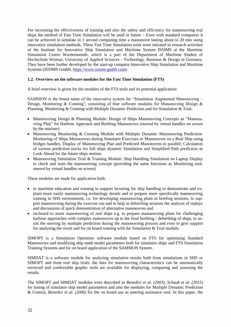
Manoeuvring Design & Planning Module: Design of Ships Manoeuvring Concepts as “Manoeu-
vring Plan” for Harbour Approach and Berthing Manoeuvres (steered by virtual handles on screen
by the mariner)
Manoeuvring Monitoring & Conning Module with Multiple Dynamic Manoeuvring Prediction:
Monitoring of Ships Manoeuvres during Simulator Exercises or Manoeuvres on a Real Ship using
bridges handles, Display of Manoeuvring Plan and Predicted Manoeuvres in parallel; Calculation
of various prediction tracks for full ships dynamic Simulation and Simplified Path prediction as
Look Ahead for the future ships motion.
Manoeuvring Simulation Trial & Training Module: Ship Handling Simulation on Laptop Display
to check and train the manoeuvring concept (providing the same functions as Monitoring tool;
steered by virtual handles on screen)
These modules are made for application both:
in maritime education and training to support lecturing for ship handling to demonstrate and ex-
plain more easily manoeuvring technology details and to prepare more specifically manoeuvring
training in SHS environment, i.e. for developing manoeuvring plans in briefing sessions, to sup-
port manoeuvring during the exercise run and to help in debriefing sessions the analysis of replays
and discussions of quick demonstration of alternative manoeuvres and
on-board to assist manoeuvring of real ships e.g. to prepare manoeuvring plans for challenging
harbour approaches with complex manoeuvres up to the final berthing / deberthing of ships, to as-
sist the steering by multiple prediction during the manoeuvring process and even to give support
for analysing the result and for on board training with the Simulation & Trial module.
SIMOPT is a Simulation Optimiser software module based on FTS for optimising Standard
Manoeuvres and modifying ship math model parameters both for simulator ships and FTS Simulation
Training Systems and for on board application of the SAMMON System.
SIMDAT is a software module for analysing simulation results both from simulations in SHS or
SIMOPT and from real ship trials: the data for manoeuvring characteristics can be automatically
retrieved and comfortable graphic tools are available for displaying, comparing and assessing the
results.
The SIMOPT and SIMDAT modules were described in Benedict et al. (2003), Schaub et al. (2015)
for tuning of simulator ship model parameters and also the modules for Multiple Dynamic Prediction
& Control, Benedict et al. (2006) for the on board use as steering assistance tool. In this paper, the
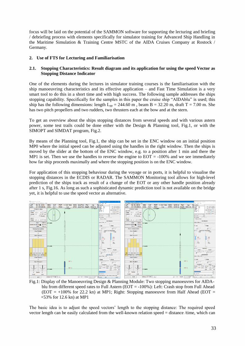
33
focus will be laid on the potential of the SAMMON software for supporting the lecturing and briefing
/ debriefing process with elements specifically for simulator training for Advanced Ship Handling in
the Maritime Simulation & Training Centre MSTC of the AIDA Cruises Company at Rostock /
Germany.
2. Use of FTS for Lecturing and Familiarisation
2.1. Stopping Characteristics: Result diagram and its application for using the speed Vector as
Stopping Distance Indicator
One of the elements during the lectures in simulator training courses is the familiarisation with the
ship manoeuvring characteristics and its effective application – and Fast Time Simulation is a very
smart tool to do this in a short time and with high success. The following sample addresses the ships
stopping capability. Specifically for the samples in this paper the cruise ship “AIDAblu” is used; this
ship has the following dimensions: length Lpp = 244.60 m , beam B = 32.20 m, draft T = 7.00 m. She
has two pitch propellers and two rudders, two thrusters each at the bow and at the stern.
To get an overview about the ships stopping distances from several speeds and with various astern
power, some test trails could be done either with the Design & Planning tool, Fig.1, or with the
SIMOPT and SIMDAT program, Fig.2.
By means of the Planning tool, Fig.1, the ship can be set in the ENC window on an initial position
MP0 where the initial speed can be adjusted using the handles in the right window. Then the ships is
moved by the slider at the bottom of the ENC window, e.g. to a position after 1 min and there the
MP1 is set. Then we use the handles to reverse the engine to EOT = -100% and we see immediately
how far ship proceeds maximally and where the stopping position is on the ENC window.
For application of this stopping behaviour during the voyage or in ports, it is helpful to visualise the
stopping distances in the ECDIS or RADAR. The SAMMON Monitoring tool allows for high-level
prediction of the ships track as result of a change of the EOT or any other handle position already
after 1 s, Fig.16. As long as such a sophisticated dynamic prediction tool is not available on the bridge
yet, it is helpful to use the speed vector as alternative.
Fig.1: Display of the Manoeuvring Design & Planning Module: Two stopping manoeuvres for AIDA-
blu from different speed rates to Full Astern (EOT = -100%): Left: Crash stop from Full Ahead
(EOT = +100% for 22.2 kn) at MP1; Right: Stopping manoeuvre from Half Ahead (EOT =
+53% for 12.6 kn) at MP1
The basic idea is to adjust the speed vectors’ length to the stopping distance: The required speed
vector length can be easily calculated from the well-known relation speed = distance /time, which can
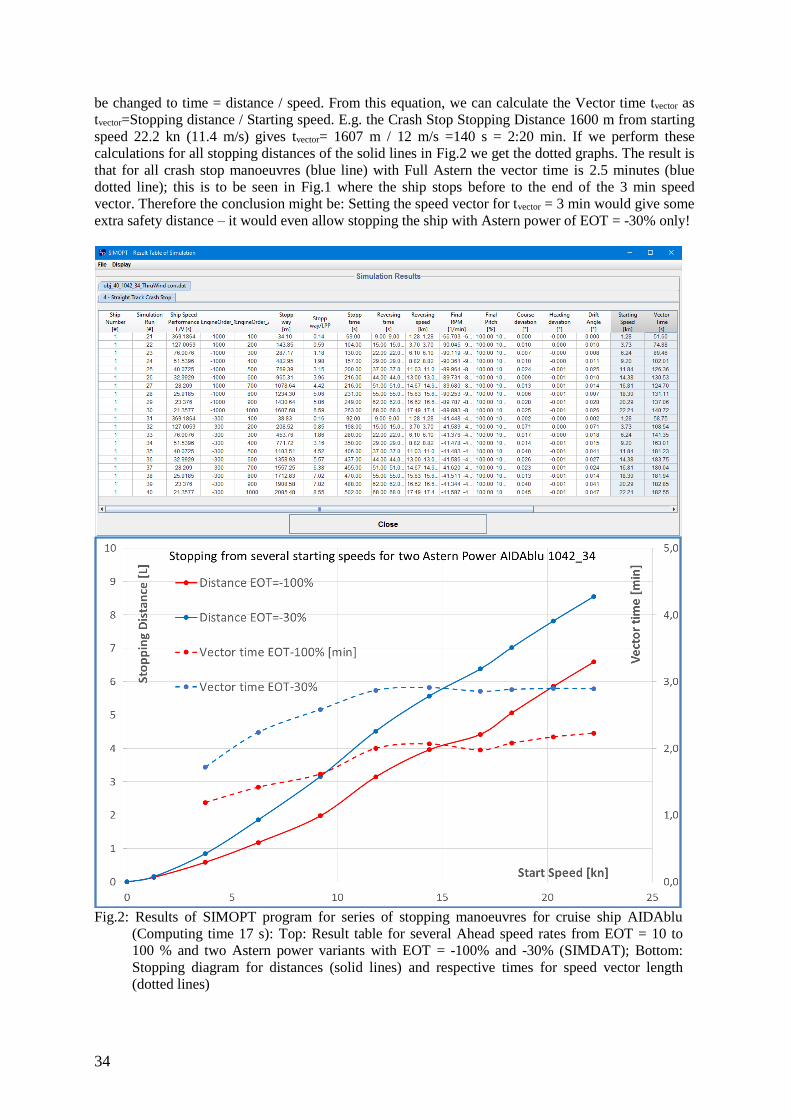
34
be changed to time = distance / speed. From this equation, we can calculate the Vector time tvector as
tvector=Stopping distance / Starting speed. E.g. the Crash Stop Stopping Distance 1600 m from starting
speed 22.2 kn (11.4 m/s) gives tvector= 1607 m / 12 m/s =140 s = 2:20 min. If we perform these
calculations for all stopping distances of the solid lines in Fig.2 we get the dotted graphs. The result is
that for all crash stop manoeuvres (blue line) with Full Astern the vector time is 2.5 minutes (blue
dotted line); this is to be seen in Fig.1 where the ship stops before to the end of the 3 min speed
vector. Therefore the conclusion might be: Setting the speed vector for tvector = 3 min would give some
extra safety distance – it would even allow stopping the ship with Astern power of EOT = -30% only!
Fig.2: Results of SIMOPT program for series of stopping manoeuvres for cruise ship AIDAblu
(Computing time 17 s): Top: Result table for several Ahead speed rates from EOT = 10 to
100 % and two Astern power variants with EOT = -100% and -30% (SIMDAT); Bottom:
Stopping diagram for distances (solid lines) and respective times for speed vector length
(dotted lines)
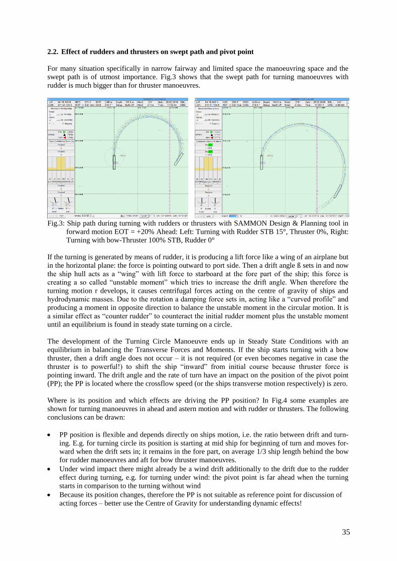
35
2.2. Effect of rudders and thrusters on swept path and pivot point
For many situation specifically in narrow fairway and limited space the manoeuvring space and the
swept path is of utmost importance. Fig.3 shows that the swept path for turning manoeuvres with
rudder is much bigger than for thruster manoeuvres.
Fig.3: Ship path during turning with rudders or thrusters with SAMMON Design & Planning tool in
forward motion EOT = +20% Ahead: Left: Turning with Rudder STB 15°, Thruster 0%, Right:
Turning with bow-Thruster 100% STB, Rudder 0°
If the turning is generated by means of rudder, it is producing a lift force like a wing of an airplane but
in the horizontal plane: the force is pointing outward to port side. Then a drift angle ß sets in and now
the ship hull acts as a “wing” with lift force to starboard at the fore part of the ship; this force is
creating a so called “unstable moment” which tries to increase the drift angle. When therefore the
turning motion r develops, it causes centrifugal forces acting on the centre of gravity of ships and
hydrodynamic masses. Due to the rotation a damping force sets in, acting like a “curved profile” and
producing a moment in opposite direction to balance the unstable moment in the circular motion. It is
a similar effect as “counter rudder” to counteract the initial rudder moment plus the unstable moment
until an equilibrium is found in steady state turning on a circle.
The development of the Turning Circle Manoeuvre ends up in Steady State Conditions with an
equilibrium in balancing the Transverse Forces and Moments. If the ship starts turning with a bow
thruster, then a drift angle does not occur – it is not required (or even becomes negative in case the
thruster is to powerful!) to shift the ship “inward” from initial course because thruster force is
pointing inward. The drift angle and the rate of turn have an impact on the position of the pivot point
(PP); the PP is located where the crossflow speed (or the ships transverse motion respectively) is zero.
Where is its position and which effects are driving the PP position? In Fig.4 some examples are
shown for turning manoeuvres in ahead and astern motion and with rudder or thrusters. The following
conclusions can be drawn:
PP position is flexible and depends directly on ships motion, i.e. the ratio between drift and turn-
ing. E.g. for turning circle its position is starting at mid ship for beginning of turn and moves for-
ward when the drift sets in; it remains in the fore part, on average 1/3 ship length behind the bow
for rudder manoeuvres and aft for bow thruster manoeuvres.
Under wind impact there might already be a wind drift additionally to the drift due to the rudder
effect during turning, e.g. for turning under wind: the pivot point is far ahead when the turning
starts in comparison to the turning without wind
Because its position changes, therefore the PP is not suitable as reference point for discussion of
acting forces – better use the Centre of Gravity for understanding dynamic effects!
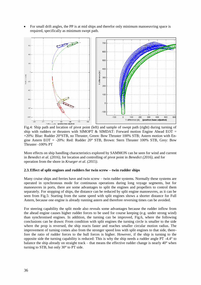
36
For small drift angles, the PP is at mid ships and therefor only minimum manoeuvring space is
required, specifically as minimum swept path.
Fig.4: Ship path and location of pivot point (left) and sample of swept path (right) during turning of
ship with rudders or thrusters with SIMOPT & SIMDAT: Forward motion Engine Ahead EOT =
+20%: Blue: Rudder 20°STB, no Thruster, Green: Bow Thruster 100% STB; Astern motion with En-
gine Astern EOT = -20%: Red: Rudder 20° STB, Brown: Stern Thruster 100% STB, Grey: Bow
Thruster -100% PT
More effects on ship handling characteristics explored by SAMMON can be seen for wind and current
in Benedict et al. (2016), for location and controlling of pivot point in Benedict (2016), and for
operation from the shore in Krueger et al. (2015).
2.3. Effect of split engines and rudders for twin screw – twin rudder ships
Many cruise ships and ferries have and twin screw – twin rudder systems. Normally these systems are
operated in synchronous mode for continuous operations during long voyage segments, but for
manoeuvres in ports, there are some advantages to split the engines and propellers to control them
separately. For stopping of ships, the distance can be reduced by split engine manoeuvres, as it can be
seen from Fig.5: Starting from the same speed with split engines shows a shorter distance for Full
Astern, because one engine is already running astern and therefore reversing times can be avoided.
For steering capability the split mode also reveals some advantages because the rudder inflow from
the ahead engine causes higher rudder forces to be used for course keeping (e.g. under strong wind)
than synchronised engines. In addition, the turning can be improved, Fig.6, where the following
conclusions can be drawn: From condition with split engines the turning circle is smaller to the side
where the prop is reversed, the ship reacts faster and reaches smaller circular motion radius. The
improvement of turning comes also from the stronger speed loss with split engines to that side, there-
fore the ratio of rudder forces to the hull forces is higher. However, if the ship is turning to the
opposite side the turning capability is reduced: This is why the ship needs a rudder angle PT -4.4° to
balance the ship already on straight track – that means the effective rudder change is nearly 40° when
turning to STB, but only 30° to PT side.
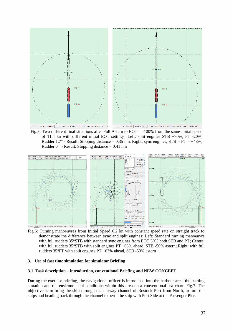
37
Fig.5: Two different final situations after Full Astern to EOT = -100% from the same initial speed
of 11.4 kn with different initial EOT settings: Left: split engines STB +70%, PT -20%,
Rudder 1.7° - Result: Stopping distance = 0.35 nm, Right: sync engines, STB = PT = +48%;
Rudder 0° - Result: Stopping distance = 0.41 nm
Fig.6: Turning manoeuvres from Initial Speed 6.2 kn with constant speed rate on straight track to
demonstrate the difference between sync and split engines: Left: Standard turning manoeuvre
with full rudders 35°STB with standard sync engines from EOT 30% both STB and PT; Centre:
with full rudders 35°STB with split engines PT +63% ahead, STB -50% astern; Right: with full
rudders 35°PT with split engines PT +63% ahead, STB -50% astern
3. Use of fast time simulation for simulator Briefing
3.1 Task description – introduction, conventional Briefing and NEW CONCEPT
During the exercise briefing, the navigational officer is introduced into the harbour area, the starting
situation and the environmental conditions within this area on a conventional sea chart, Fig.7. The
objective is to bring the ship through the fairway channel of Rostock Port from North, to turn the
ships and heading back through the channel to berth the ship with Port Side at the Passenger Pier.
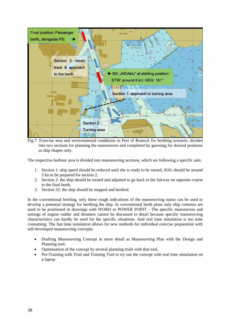
38
Fig.7: Exercise area and environmental conditions in Port of Rostock for berthing scenario, divided
into two sections for planning the manoeuvres and completed by guessing for desired positions
as ship shapes only.
The respective harbour area is divided into manoeuvring sections, which are following a specific aim:
1. Section 1: ship speed should be reduced until she is ready to be turned, SOG should be around
3 kn to be prepared for section 2.
2. Section 2: the ship should be turned and adjusted to go back in the fairway on opposite course
to the final berth.
3. Section 32: the ship should be stopped and berthed.
In the conventional briefing, only these rough indications of the manoeuvring status can be used to
develop a potential strategy for berthing the ship. In conventional berth plans only ship contours are
used to be positioned in drawings with WORD or POWER POINT - The specific manoeuvres and
settings of engine rudder and thrusters cannot be discussed in detail because specific manoeuvring
characteristics can hardly be used for the specific situations. And real time simulation is too time
consuming. The fast time simulation allows for new methods for individual exercise preparation with
self-developed manoeuvring concepts:
Drafting Manoeuvring Concept in more detail as Manoeuvring Plan with the Design and
Planning tool;
Optimisation of the concept by several planning trials with that tool,
Pre-Training with Trial and Training Tool to try out the concept with real time simulation on
a laptop

39
3.2 Briefing by means of the “Manoeuvre Planning & Design Module”
3.2.1. Basic exercise with no wind and current
With the new fast time Simulation there is the chance for designing a Manoeuvre Plan as a detailed
strategy with the specific settings at distinguished positions called the Manoeuvring Points MP. Some
basic functions and interface displays for the Fast Time Simulation within the Design and Planning
Tool are shown in the next figures. Fig.8 explains the method in a sea chart environment represented
by an interface, which combines
the electronic navigational chart ENC window (centre),
the interface window for the steering panel of the ship (right) for adjusting the controls for the
selected manoeuvring point MP and the
interface to display the status of the current actual ship manoeuvring controls (left) at the po-
sition of the next manoeuvring point MP which is indicated as ship shape in red colour in the
ENC.
In the following, the course of actions is described in a series of figures to make a full manoeuvring
plan by means of the control actions at the manoeuvring points MP – this will be done first for easy
conditions with no wind and current to explain the procedure of fast time planning: In Fig.8 the initial
position MP 0 is to be seen where the instructor has set the ship in the centre of the fairway. The ship
has already been moved by the slider at the ENC bottom to set the next manoeuvring point MP 1:
there the stopping manoeuvre is started with EOT -30%. The prediction already shows that the ship
would lose speed according to the handle positions.
Fig.8: Fast time planning in sea chart: Initial ship position at MP0 and prediction for the stopping
manoeuvre at MP1: The prediction already shows that the ship reduces speed to the set
handle positions.
In Fig.10 the ship is nearly stopped and turns by means of the thrusters – the contour is shifted to a
position where the thrusters are stopped and the engines speed up to return to the fairway with
opposite course. In Fig.11 the vessel is brought close to the berth and at MP5 the engines are reversed
to reduce speed and to stop the ships at a position parallel to the berth to be shifted by thrusters to the
pier from the next MP 6. Afterwards the plan needs a further MP in order to reduce the transversal
speed shortly before berthing.
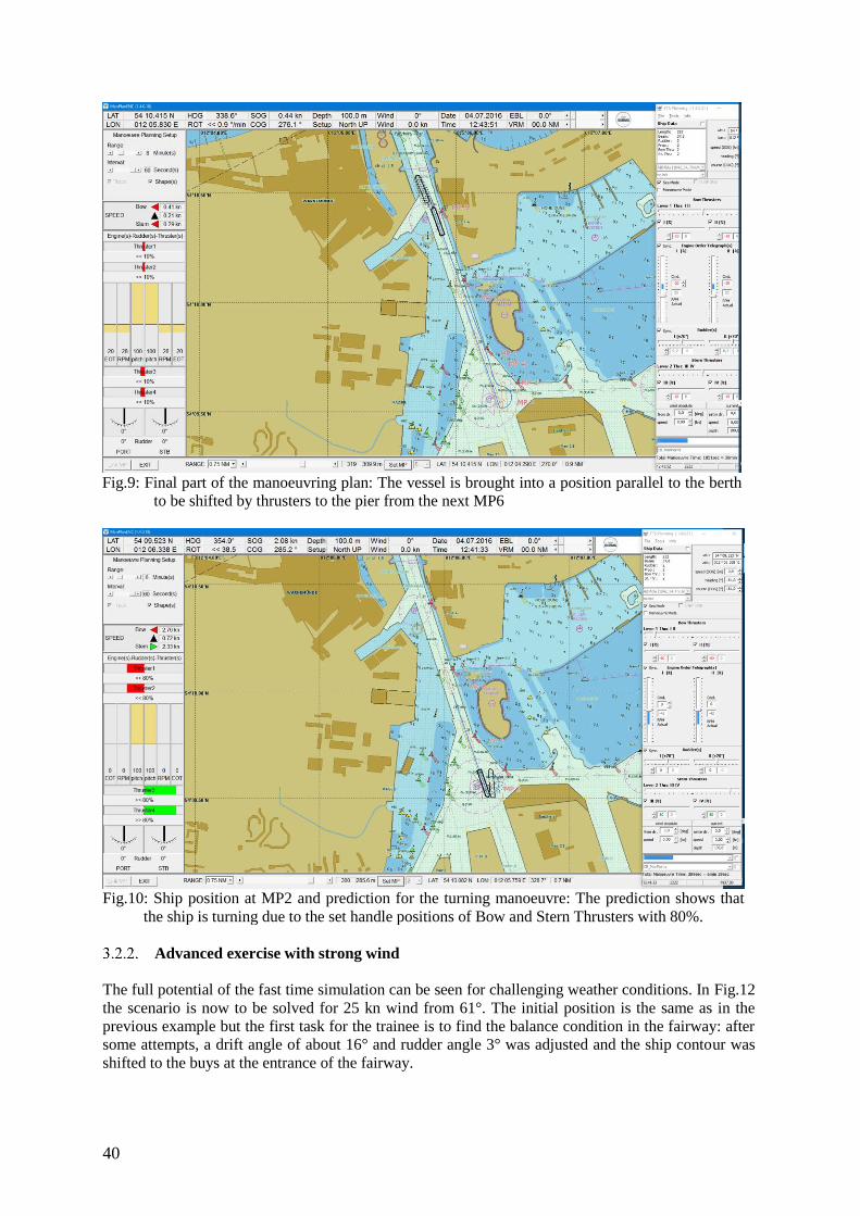
40
Fig.9: Final part of the manoeuvring plan: The vessel is brought into a position parallel to the berth
to be shifted by thrusters to the pier from the next MP6
Fig.10: Ship position at MP2 and prediction for the turning manoeuvre: The prediction shows that
the ship is turning due to the set handle positions of Bow and Stern Thrusters with 80%.
Advanced exercise with strong wind
The full potential of the fast time simulation can be seen for challenging weather conditions. In Fig.12
the scenario is now to be solved for 25 kn wind from 61°. The initial position is the same as in the
previous example but the first task for the trainee is to find the balance condition in the fairway: after
some attempts, a drift angle of about 16° and rudder angle 3° was adjusted and the ship contour was
shifted to the buys at the entrance of the fairway.
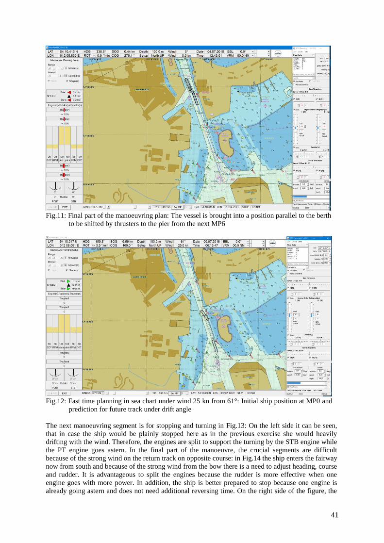
41
Fig.11: Final part of the manoeuvring plan: The vessel is brought into a position parallel to the berth
to be shifted by thrusters to the pier from the next MP6
Fig.12: Fast time planning in sea chart under wind 25 kn from 61°: Initial ship position at MP0 and
prediction for future track under drift angle
The next manoeuvring segment is for stopping and turning in Fig.13: On the left side it can be seen,
that in case the ship would be plainly stopped here as in the previous exercise she would heavily
drifting with the wind. Therefore, the engines are split to support the turning by the STB engine while
the PT engine goes astern. In the final part of the manoeuvre, the crucial segments are difficult
because of the strong wind on the return track on opposite course: in Fig.14 the ship enters the fairway
now from south and because of the strong wind from the bow there is a need to adjust heading, course
and rudder. It is advantageous to split the engines because the rudder is more effective when one
engine goes with more power. In addition, the ship is better prepared to stop because one engine is
already going astern and does not need additional reversing time. On the right side of the figure, the
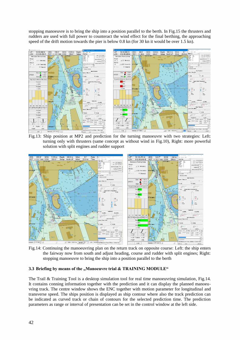
42
stopping manoeuvre is to bring the ship into a position parallel to the berth. In Fig.15 the thrusters and
rudders are used with full power to counteract the wind effect for the final berthing, the approaching
speed of the drift motion towards the pier is below 0.8 kn (for 30 kn it would be over 1.5 kn).
Fig.13: Ship position at MP2 and prediction for the turning manoeuvre with two strategies: Left:
turning only with thrusters (same concept as without wind in Fig.10), Right: more powerful
solution with split engines and rudder support
Fig.14: Continuing the manoeuvring plan on the return track on opposite course: Left: the ship enters
the fairway now from south and adjust heading, course and rudder with split engines; Right:
stopping manoeuvre to bring the ship into a position parallel to the berth
3.3 Briefing by means of the „Manoeuvre trial & TRAINING MODULE“
The Trail & Training Tool is a desktop simulation tool for real time manoeuvring simulation, Fig.14.
It contains conning information together with the prediction and it can display the planned manoeu-
vring track. The centre window shows the ENC together with motion parameter for longitudinal and
transverse speed. The ships position is displayed as ship contour where also the track prediction can
be indicated as curved track or chain of contours for the selected prediction time. The prediction
parameters as range or interval of presentation can be set in the control window at the left side.
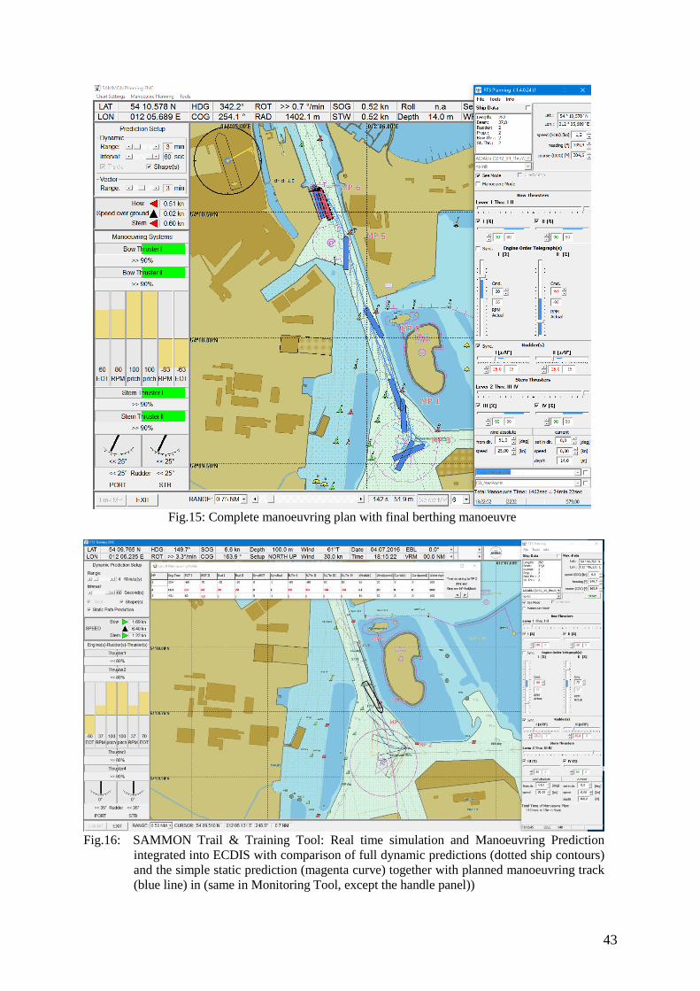
43
Fig.15: Complete manoeuvring plan with final berthing manoeuvre
Fig.16: SAMMON Trail & Training Tool: Real time simulation and Manoeuvring Prediction
integrated into ECDIS with comparison of full dynamic predictions (dotted ship contours)
and the simple static prediction (magenta curve) together with planned manoeuvring track
(blue line) in (same in Monitoring Tool, except the handle panel))
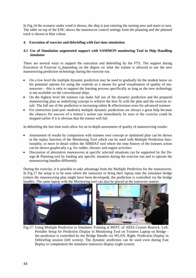
44
In Fig.14 the scenario under wind is shown, the ship is just entering the turning area and starts to turn.
The table on top of the ENC shows the manoeuvre control settings from the planning and the planned
track is shown in blue colour.
4. Execution of exercise and debriefing with fast time simulation
4.1 Use of Simulation augmented support with SAMMON monitoring Tool in Ship Handling
simulator
There are several ways to support the execution and debriefing by the FTS. The support during
Execution of Exercise is depending on the degree on what the trainee is allowed to use the new
manoeuvring prediction technology during the exercise run.
On a low level the multiple dynamic prediction may be used to gradually let the student know on
his potential options for using the controls as a means for good visualisation of quality of ma-
noeuvres – this is only to support the learning process specifically as long as the new technology
is not available on the conventional ships
On the highest level the trainees can make full use of the dynamic prediction and the prepared
manoeuvring plan as underlying concept to achieve the best fit with the plan and the exercise re-
sult. The full use of the prediction is increasing safety & effectiveness even for advanced trainees
For instructors (and peer students) multiple dynamic predictions are always a great help because
the chances for success of a trainee’s action can immediately be seen or the exercise could be
stopped earlier if it is obvious that the trainee will fail.
In debriefing the fast time tools allow for an in-depth assessment of quality of manoeuvring results:
Assessment of results by comparison with trainees own concept or optimised plan can be shown
in the replay function of the Monitoring Tool which can be used with Multiple Prediction func-
tionality; or more in detail within the SIMDAT tool where the time history of the trainees action
can be shown graphically e.g. for rudder, thruster and engine activities
Discussion of alternative manoeuvres at specific selected situations can be supported by the De-
sign & Planning tool by loading any specific situation during the exercise run and to operate the
manoeuvring handles differently.
During the exercise, it is possible to take advantage from the Multiple Prediction for the manoeuvres.
In Fig.17 the setup is to be seen where the instructor or bring their laptop onto the simulator bridge
(where the manoeuvring plan might have been developed), the prediction is controlled via the bridge
handles. The same laptop with the Monitoring tool can also be placed at the instructor station.
Fig.17: Using Multiple Prediction in Simulator Training at MSTC of AIDA Cruises Rostock. Left:
Portable Setup for Prediction Display in Monitoring Tool on Trainees Laptop on Bridge -
the prediction is controlled by the Bridge Handle via WLAN. Right: Prediction Display in
Debriefing session (left screen): The dynamic prediction can be used even during Fast
Replay to complement the simulator instructor display (right screen)
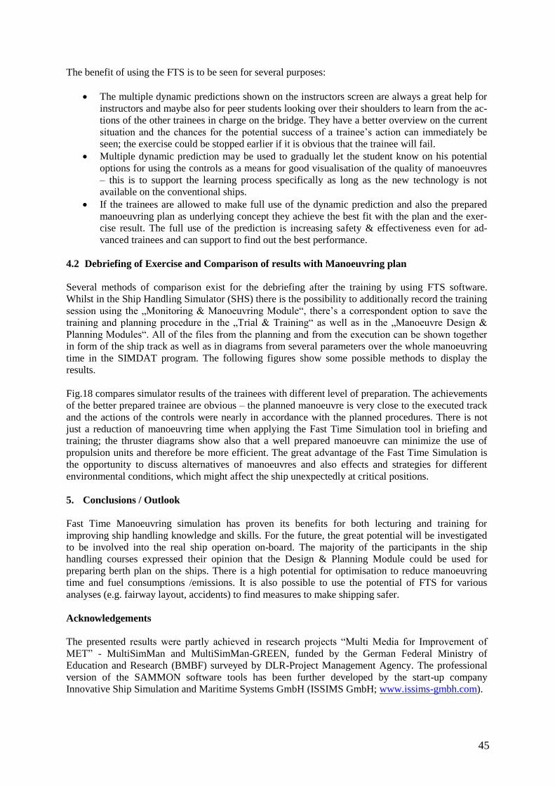
45
The benefit of using the FTS is to be seen for several purposes:
The multiple dynamic predictions shown on the instructors screen are always a great help for
instructors and maybe also for peer students looking over their shoulders to learn from the ac-
tions of the other trainees in charge on the bridge. They have a better overview on the current
situation and the chances for the potential success of a trainee’s action can immediately be
seen; the exercise could be stopped earlier if it is obvious that the trainee will fail.
Multiple dynamic prediction may be used to gradually let the student know on his potential
options for using the controls as a means for good visualisation of the quality of manoeuvres
– this is to support the learning process specifically as long as the new technology is not
available on the conventional ships.
If the trainees are allowed to make full use of the dynamic prediction and also the prepared
manoeuvring plan as underlying concept they achieve the best fit with the plan and the exer-
cise result. The full use of the prediction is increasing safety & effectiveness even for ad-
vanced trainees and can support to find out the best performance.
4.2 Debriefing of Exercise and Comparison of results with Manoeuvring plan
Several methods of comparison exist for the debriefing after the training by using FTS software.
Whilst in the Ship Handling Simulator (SHS) there is the possibility to additionally record the training
session using the „Monitoring & Manoeuvring Module“, there’s a correspondent option to save the
training and planning procedure in the „Trial & Training“ as well as in the „Manoeuvre Design &
Planning Modules“. All of the files from the planning and from the execution can be shown together
in form of the ship track as well as in diagrams from several parameters over the whole manoeuvring
time in the SIMDAT program. The following figures show some possible methods to display the
results.
Fig.18 compares simulator results of the trainees with different level of preparation. The achievements
of the better prepared trainee are obvious – the planned manoeuvre is very close to the executed track
and the actions of the controls were nearly in accordance with the planned procedures. There is not
just a reduction of manoeuvring time when applying the Fast Time Simulation tool in briefing and
training; the thruster diagrams show also that a well prepared manoeuvre can minimize the use of
propulsion units and therefore be more efficient. The great advantage of the Fast Time Simulation is
the opportunity to discuss alternatives of manoeuvres and also effects and strategies for different
environmental conditions, which might affect the ship unexpectedly at critical positions.
5. Conclusions / Outlook
Fast Time Manoeuvring simulation has proven its benefits for both lecturing and training for
improving ship handling knowledge and skills. For the future, the great potential will be investigated
to be involved into the real ship operation on-board. The majority of the participants in the ship
handling courses expressed their opinion that the Design & Planning Module could be used for
preparing berth plan on the ships. There is a high potential for optimisation to reduce manoeuvring
time and fuel consumptions /emissions. It is also possible to use the potential of FTS for various
analyses (e.g. fairway layout, accidents) to find measures to make shipping safer.
Acknowledgements
The presented results were partly achieved in research projects “Multi Media for Improvement of
MET” - MultiSimMan and MultiSimMan-GREEN, funded by the German Federal Ministry of
Education and Research (BMBF) surveyed by DLR-Project Management Agency. The professional
version of the SAMMON software tools has been further developed by the start-up company
Innovative Ship Simulation and Maritime Systems GmbH (ISSIMS GmbH; www.issims-gmbh.com).
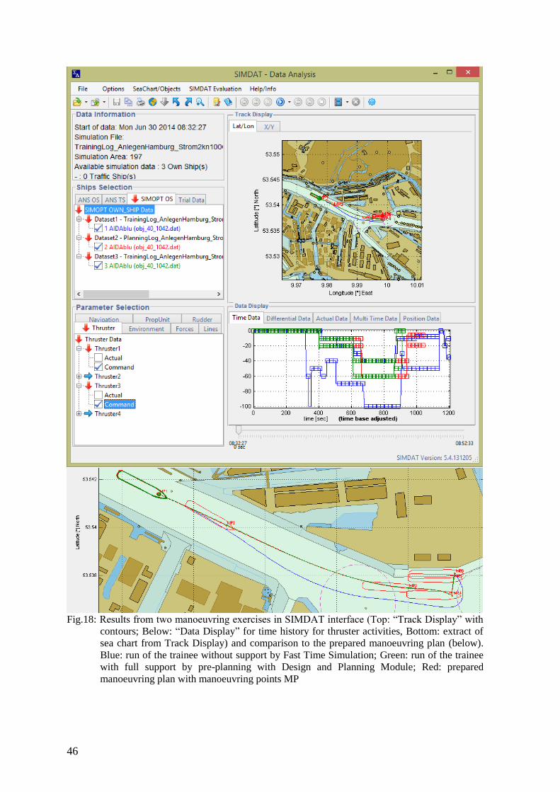
46
Fig.18: Results from two manoeuvring exercises in SIMDAT interface (Top: “Track Display” with
contours; Below: “Data Display” for time history for thruster activities, Bottom: extract of
sea chart from Track Display) and comparison to the prepared manoeuvring plan (below).
Blue: run of the trainee without support by Fast Time Simulation; Green: run of the trainee
with full support by pre-planning with Design and Planning Module; Red: prepared
manoeuvring plan with manoeuvring points MP

47
References
BENEDICT, K. (2016), Control your pivot point position in ship handling - Multimedia approach by
Fast Time Simulation, IMSF 2016 AGM Seminar, Ilawa
BENEDICT, K.; BALDAUF, M.; FELSENSTEIN, C.; KIRCHHOFF, M. (2003), Computer-based
support for the evaluation of ship handling simulator exercise results, Int. Conf. Marine Simulation
and Ship Manoeuvrability (MARSIM), Kanazawa
BENEDICT, K.; BALDAUF, M.; FISCHER, S.; GLUCH, M.; KIRCHHOFF, M.; SCHAUB, M.;
KLAES, S. (2012), Fast time manoeuvring simulation as decision support for planning and monitor-
ing of ship handling processes for ship operation on-board and training in simulators, Int. Conf. Ma-
rine Simulation and Ship Manoeuvrability (MARSIM), Singapore
BENEDICT, K.; BALDAUF, M.; FISCHER, S.; GLUCH, M.; KIRCHHOFF, M.; SCHAUB, M.;
KRÜGER, C-P.; KLAES, S. (2016), Simulation technology brings new visualisation of the future
ships path – and advanced use of the well-known speed vector, 24th Int. Maritime Lecturers Associa-
tion Conf. “Quality Standards in Maritime Education”, Galveston
BENEDICT, K.; BALDAUF, M.; KIRCHHOFF, M.; KOEPNICK, W.; EYRICH R. (2006), Combin-
ing fast-time simulation and automatic assessment for tuning of simulator ship models, Int. Conf. Ma-
rine Simulation and Ship Manoeuvrability (MARSIM), Terschelling
KRÜGER, C.-M.; SCHAUB, M.; BENEDICT, K.; KIRCHHOFF, M.; GLUCH, M.; FISCHER, S.
(2015), Simulation-augmented manoeuvring support for ship handling on board and from shore, 14th
Int. Conf. Computer and IT Applications in the Maritime Industries (COMPIT), Ulrichshusen, pp.74-
88
SCHAUB, M.; BENEDICT, K.; GLUCH, M.; MILBRADT, G.; TUSCHLING, G.; KIRCHHOFF, M.
(2015), Modelling of ships for simulator-training and simulation-augmented manoeuvring support on
board and from the shore, Int. Conf. Marine Simulation and Ship Manoeuvrability (MARSIM), New-
castle
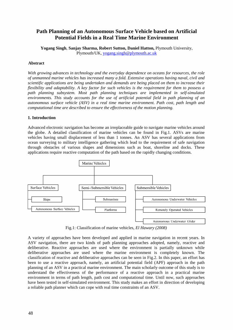
48
Path Planning of an Autonomous Surface Vehicle based on Artificial Potential Fields in a Real Time Marine Environment
Yogang Singh, Sanjay Sharma, Robert Sutton, Daniel Hatton, Plymouth University,
Plymouth/UK, [email protected]
Abstract
With growing advances in technology and the everyday dependence on oceans for resources, the role of unmanned marine vehicles has increased many a fold. Extensive operations having naval, civil and scientific applications are being undertaken and demands are being placed on them to increase their flexibility and adaptability. A key factor for such vehicles is the requirement for them to possess a path planning subsystem. Most path planning techniques are implemented in self-simulated environments. This study accounts for the use of artificial potential field in path planning of an autonomous surface vehicle (ASV) in a real time marine environment. Path cost, path length and computational time are described to ensure the effectiveness of the motion planning.
1. Introduction Advanced electronic navigation has become an irreplaceable guide to navigate marine vehicles around the globe. A detailed classification of marine vehicles can be found in Fig.1. ASVs are marine vehicles having small displacement of less than 1 tonnes. An ASV has several applications from ocean surveying to military intelligence gathering which lead to the requirement of safe navigation through obstacles of various shapes and dimensions such as boat, shoreline and docks. These applications require reactive computation of the path based on the rapidly changing conditions.
Fig.1: Classification of marine vehicles, El Hawary (2008)
A variety of approaches have been developed and applied in marine navigation in recent years. In ASV navigation, there are two kinds of path planning approaches adopted, namely, reactive and deliberative. Reactive approaches are used where the environment is partially unknown while deliberative approaches are used where the marine environment is completely known. The classification of reactive and deliberative approaches can be seen in Fig.2. In this paper, an effort has been to use a reactive approach, namely, an artificial potential field (APF) approach in the path planning of an ASV in a practical marine environment. The main scholarly outcome of this study is to understand the effectiveness of the performance of a reactive approach in a practical marine environment in terms of path length, path cost and computational time. Until now, such approaches have been tested in self-simulated environment. This study makes an effort in direction of developing a reliable path planner which can cope with real time constraints of an ASV.
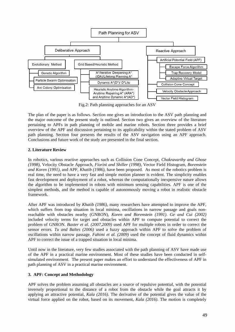
49
Fig.2: Path planning approaches for an ASV
The plan of the paper is as follows. Section one gives an introduction to the ASV path planning and the major outcome of the present study is outlined. Section two gives an overview of the literature pertaining to APFs in path planning of mobile and marine robots. Section three provides a brief overview of the APF and discussion pertaining to its applicability within the stated problem of ASV path planning. Section four presents the results of the ASV navigation using an APF approach. Conclusions and future work of the study are presented in the final section. 2. Literature Review In robotics, various reactive approaches such as Collision Cone Concept, Chakravarthy and Ghose (1998), Velocity Obstacle Approach, Fiorini and Shiller (1998), Vector Field Histogram, Borenstein and Koren (1991), and APF, Khatib (1986), have been proposed. As most of the robotics problem is real time, the need to have a very fast and simple motion planner is evident. The simplicity enables fast development and deployment of a robot, whereas the computationally inexpensive nature allows the algorithm to be implemented in robots with minimum sensing capabilities. APF is one of the simplest methods, and the method is capable of autonomously moving a robot in realistic obstacle framework. After APF was introduced by Khatib (1986), many researchers have attempted to improve the APF, which suffers from trap situation in local minima, oscillations in narrow passage and goals non-reachable with obstacles nearby (GNRON), Koren and Borenstein (1991). Ge and Cui (2002) included velocity terms for target and obstacles within APF to compute potential to correct the problem of GNRON. Baxter et al. (2007,2009) used APF for multiple robots in order to correct the sensor errors. Tu and Baltes (2006) used a fuzzy approach within APF to solve the problem of oscillations within narrow passage. Fahimi et al. (2009) used the concept of fluid dynamics within APF to correct the issue of a trapped situation in local minima. Until now in the literature, very few studies associated with the path planning of ASV have made use of the APF in a practical marine environment. Most of these studies have been conducted in self-simulated environment. The present paper makes an effort to understand the effectiveness of APF in path planning of ASV in a practical marine environment. 3. APF: Concept and Methodology APF solves the problem assuming all obstacles are a source of repulsive potential, with the potential inversely proportional to the distance of a robot from the obstacle while the goal attracts it by applying an attractive potential, Kala (2016). The derivative of the potential gives the value of the virtual force applied on the robot, based on its movement, Kala (2016). The motion is completely
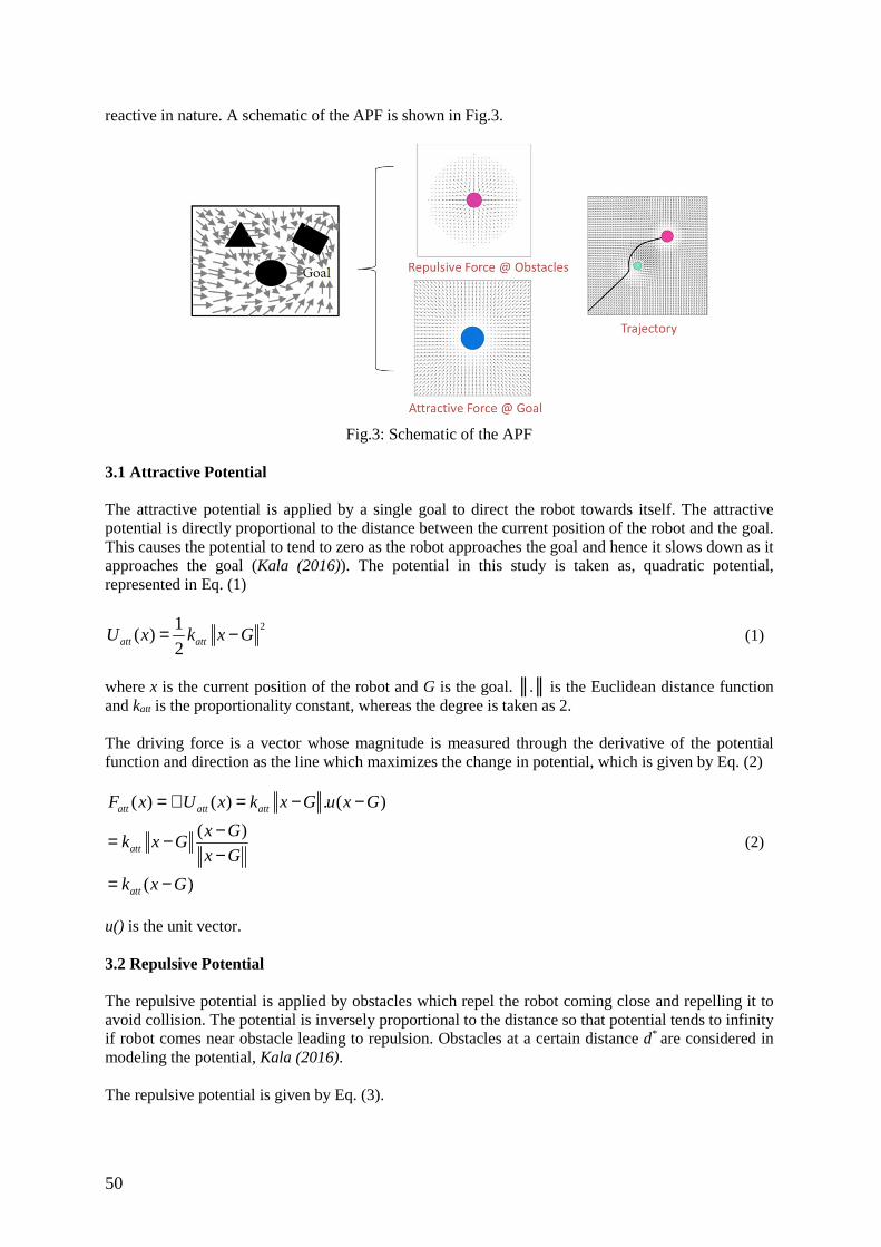
50
reactive in nature. A schematic of the APF is shown in Fig.3.
Fig.3: Schematic of the APF
3.1 Attractive Potential The attractive potential is applied by a single goal to direct the robot towards itself. The attractive potential is directly proportional to the distance between the current position of the robot and the goal. This causes the potential to tend to zero as the robot approaches the goal and hence it slows down as it approaches the goal (Kala (2016)). The potential in this study is taken as, quadratic potential, represented in Eq. (1)
21( )
2att attU x k x G= − (1)
where x is the current position of the robot and G is the goal. ║.║ is the Euclidean distance function and katt is the proportionality constant, whereas the degree is taken as 2. The driving force is a vector whose magnitude is measured through the derivative of the potential function and direction as the line which maximizes the change in potential, which is given by Eq. (2)
( ) ( ) . ( )
( )
( )
att att att
att
att
F x U x k x G u x G
x Gk x G
x G
k x G
= ∇ = − −−= −−
= −
(2)
u() is the unit vector. 3.2 Repulsive Potential The repulsive potential is applied by obstacles which repel the robot coming close and repelling it to avoid collision. The potential is inversely proportional to the distance so that potential tends to infinity if robot comes near obstacle leading to repulsion. Obstacles at a certain distance d* are considered in modeling the potential, Kala (2016). The repulsive potential is given by Eq. (3).
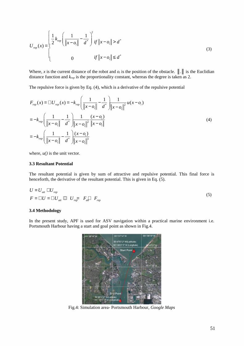
51
2
**
*
1 1 1
2( )
0
repii
rep
i
kif x o dx o d
U x
if x o d
− − >− = − ≤
(3)
Where, x is the current distance of the robot and oi is the position of the obstacle. ║.║ is the Euclidian distance function and krep is the proportionality constant, whereas the degree is taken as 2. The repulsive force is given by Eq. (4), which is a derivative of the repulsive potential
2*
2*
3*
1 1 1( ) ( ) ( )
( )1 1 1
( )1 1
rep rep rep ii i
irep
i ii
irep
i i
F x U x k u x ox o d x o
x ok
x o d x ox o
x ok
x o d x o
= ∇ = − − − − −
−= − − − −−
−= − − − −
(4)
where, u() is the unit vector. 3.3 Resultant Potential The resultant potential is given by sum of attractive and repulsive potential. This final force is henceforth, the derivative of the resultant potential. This is given in Eq. (5).
att rep
att rep att rep
U U U
F U U U F F
= +
= ∇ = ∇ + ∇ = + (5)
3.4 Methodology In the present study, APF is used for ASV navigation within a practical marine environment i.e. Portsmouth Harbour having a start and goal point as shown in Fig.4.
Fig.4: Simulation area- Portsmouth Harbour, Google Maps
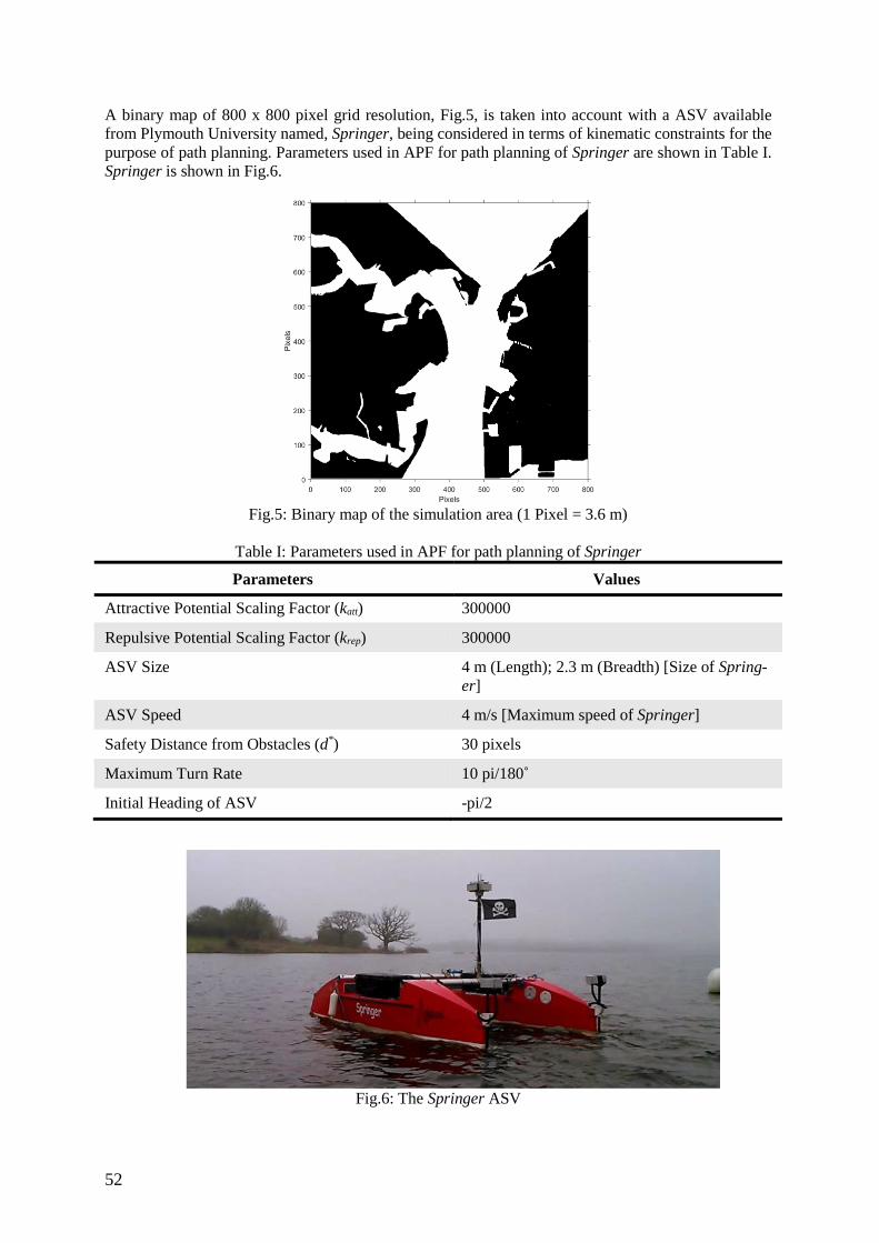
52
A binary map of 800 x 800 pixel grid resolution, Fig.5, is taken into account with a ASV available from Plymouth University named, Springer, being considered in terms of kinematic constraints for the purpose of path planning. Parameters used in APF for path planning of Springer are shown in Table I. Springer is shown in Fig.6.
Fig.5: Binary map of the simulation area (1 Pixel = 3.6 m)
Table I: Parameters used in APF for path planning of Springer
Parameters Values
Attractive Potential Scaling Factor (katt) 300000
Repulsive Potential Scaling Factor (krep) 300000
ASV Size 4 m (Length); 2.3 m (Breadth) [Size of Spring-er]
ASV Speed 4 m/s [Maximum speed of Springer]
Safety Distance from Obstacles (d*) 30 pixels
Maximum Turn Rate 10 pi/180˚
Initial Heading of ASV -pi/2
Fig.6: The Springer ASV
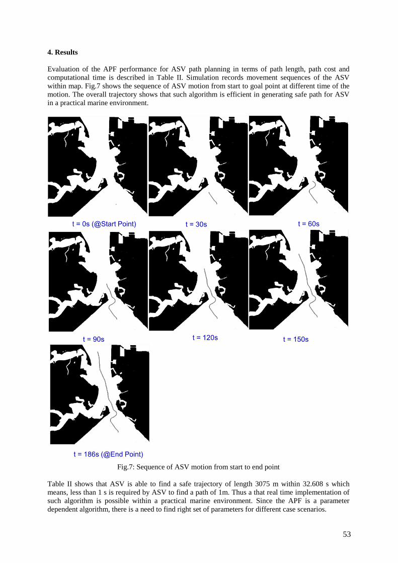
53
4. Results Evaluation of the APF performance for ASV path planning in terms of path length, path cost and computational time is described in Table II. Simulation records movement sequences of the ASV within map. Fig.7 shows the sequence of ASV motion from start to goal point at different time of the motion. The overall trajectory shows that such algorithm is efficient in generating safe path for ASV in a practical marine environment.
Fig.7: Sequence of ASV motion from start to end point
Table II shows that ASV is able to find a safe trajectory of length 3075 m within 32.608 s which means, less than 1 s is required by ASV to find a path of 1m. Thus a that real time implementation of such algorithm is possible within a practical marine environment. Since the APF is a parameter dependent algorithm, there is a need to find right set of parameters for different case scenarios.

54
Table II: Performance of APF in Springer navigation Parameters Value
Path Length 3.075 Km Path Cost (1 Pixel = £20) 854.315 Pixels CPU Time 32.608 s
5. Conclusions and future work The paper introduced and discussed APF algorithm for ASV path planning in a practical marine environment. The algorithm is found robust in terms of computational time and real time implementation in a static environment and can be extended in a dynamic environment. Furthermore, international collision avoidance regulation COLREGs can be incorporated within the algorithm to make it suitable for maritime manoeuvring. APF and its several variants have been widely implemented in path planning of mobile robotics for safe navigation. Although, conventional APF is prone to several disadvantages but recent variants of APF take care of those infelicities. For future work, this can be extended towards navigation of multiple ASVs. This will help in increasing autonomy of ASVs, which is the goal of the future research in ASV navigation. References BAXTER, J.L.; BURKE, E.K.; GARIBALDI, J.M.; NORMAN, M. (2007), Multi-robot search and rescue: A potential field based approach, Autonomous Robots and Agents, Springer, pp.9-16 BAXTER, J.L.; BURKE, E.K.; GARIBALDI, J.M.; NORMAN, M. (2009), Shared potential fields and their place in a multi-robot co-ordination taxonomy, Robotics and Autonomous Systems 57(10), pp. 1048-1055 BORENSTEIN, J.; KOREN, Y. (1991), The vector field histogram-fast obstacle avoidance for mobile robots, IEEE Trans. Robotics and Automation 7, pp. 278-288 CHAKRAVARTHY, A; GHOSE, D. (1998), Obstacle avoidance in a Dynamic Environment: A Col-lision Cone Approach, IEEE Trans. Systems, Man and Cybernetics, Part A: Systems and Humans 28, pp. 562-74 El-HAWARY, F. (2000), The Ocean Engineering Handbook, CRC Press, pp.1-416 FAHIMI, F.; NATARAJ, C.; ASHRAFIUON, H. (2009), Real-time obstacle avoidance for multiple mobile robots, Robotica 27(2), pp.189-198 FIORINI, P.; SHILLER, Z. (1998), Motion planning in dynamic environments using velocity obsta-cles, Int. J. Robotics Research 17, pp.760-772 GE, S.S.; CUI, Y.J. (2002), Dynamic motion planning for mobile robots using potential field meth-od, Autonomous Robots 13(3), pp.207-222 KALA, R. (2016), Potential-Based Planning, On-Road Intelligent Vehicles, Ch.11, pp.318-356 KHATIB, O. (1986), Real time obstacle avoidance for manipulators and mobile robots, Int. J. Robot-ic Research 5, pp. 90-98 TU, K.; BALTES, J. (2006), Fuzzy potential energy for a map approach to robot navigation, J. Robotics and Autonomous Systems 54(7), pp. 574-589
55
Physical Testbed for Highly Automated and Autonomous Vessels
Marius Brinkmann , University of Oldenburg, Germany, [email protected] Axel Hahn, University of Oldenburg, Germany, [email protected]
Bjørn Åge Hjøllo, Navtor AS, Norway, [email protected]
Abstract Technology is changing the way of transportation. Thus, the development of new safety-critical driving systems increases the complexity of testing. To facilitate these efforts, suitable engineering and safety/risk assessment methods are required. The maritime physical testbed LABSKAUS implements components such as a research vessel, sensor infrastructure and a reference waterway. This paper describes methods to support the development of new e-Navigation technologies by verification and validation. It gives an overview on the requirements based on the conceptual architecture for driving and reflects current maritime testbeds. Concepts and components of LABSKAUS are presented and evaluated by testing a shore-based bridge.
1. Introduction Maritime research facilities and industries started developing highly automated and autonomous maritime systems (e. g. autopilots) to provide solutions for the present and future challenges to make seafaring more efficient, safer and sustainable. Based on upcoming technologies or strategies for an optimized information exchange between ship and shore as well as a safe voyage from berth to berth, the (civil) maritime transportation sector faces a time of change to meet the increasing demands of the global logistic processes. For example, NN (2012) reports that more than 75% of all worldwide maritime accidents are caused by human factor. Next to the safety argumentation, governmental sustainability plans such as the Paris Agreement establish universal bindings for a global climate deal to reduce emissions, http://ec.europa.eu/clima/policies/international/negotiations/paris_en. There is evidence of a trend towards developing high automated vessel assistance systems with an outlook for the future describing autonomous seafaring to achieve these aims of increased safety and environmental sustainability. As seen from a technical perspective, the development of automation technology for shipping (as well as other transportation types) involves various disciplines. Components such as sensors, actuators, software and the communication infrastructure technologies form a maritime cyber-physical system (mCPS) that is necessary to enable the development of highly automated and autonomous shipping. While autonomous shipping may affect (human) errors and critical situations, it is a safety-critical issue and needs to follow overarching functional safety related rules. Understanding maritime transportation as a sociotechnical (human and machine) system allows the usage of system-engineering methods. There is the need for a holistic testing approach to consider the sociotechnical system in its environment containing technology, processes, human factors and regulations. Today’s certification tests verify functional properties according to conformance standards (e.g. the range of navigational lights, correct data by AIS system). This does not last for intelligent assistance systems which must evaluate complex situations. The development of safety-critical systems such as highly-automated and autonomous vessel brings the need to establish a test environment (or ‘testbed’) close to the real world in addition to simulative test environments. New systems can be tested in simulations. Simulators enable the replication of real-life conditions for systems like bridge simulators such as the Korean in Mokpo or big scaled environment planning/control algorithms like the Maritime Traffic Simulator, Hahn (2015). Nevertheless, a prototype must be validated regarding its functionality within a real physical environment to prove the concept for real-life applications. For the evaluation of intelligent assistance systems, a testbed can provide complex maritime situations to analyse the behaviour of the whole system “vessel” considering the components and subsystems.
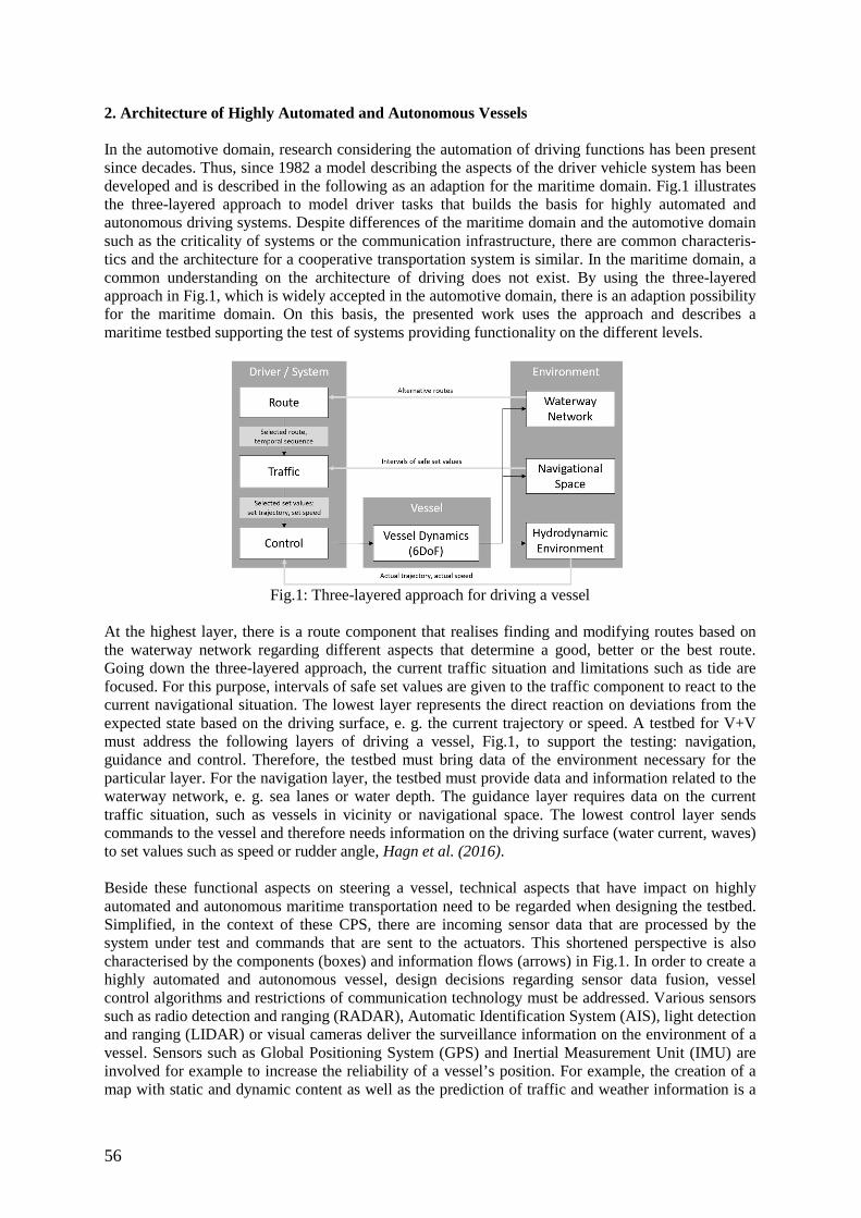
56
2. Architecture of Highly Automated and Autonomous Vessels In the automotive domain, research considering the automation of driving functions has been present since decades. Thus, since 1982 a model describing the aspects of the driver vehicle system has been developed and is described in the following as an adaption for the maritime domain. Fig.1 illustrates the three-layered approach to model driver tasks that builds the basis for highly automated and autonomous driving systems. Despite differences of the maritime domain and the automotive domain such as the criticality of systems or the communication infrastructure, there are common characteris-tics and the architecture for a cooperative transportation system is similar. In the maritime domain, a common understanding on the architecture of driving does not exist. By using the three-layered approach in Fig.1, which is widely accepted in the automotive domain, there is an adaption possibility for the maritime domain. On this basis, the presented work uses the approach and describes a maritime testbed supporting the test of systems providing functionality on the different levels.
Fig.1: Three-layered approach for driving a vessel
At the highest layer, there is a route component that realises finding and modifying routes based on the waterway network regarding different aspects that determine a good, better or the best route. Going down the three-layered approach, the current traffic situation and limitations such as tide are focused. For this purpose, intervals of safe set values are given to the traffic component to react to the current navigational situation. The lowest layer represents the direct reaction on deviations from the expected state based on the driving surface, e. g. the current trajectory or speed. A testbed for V+V must address the following layers of driving a vessel, Fig.1, to support the testing: navigation, guidance and control. Therefore, the testbed must bring data of the environment necessary for the particular layer. For the navigation layer, the testbed must provide data and information related to the waterway network, e. g. sea lanes or water depth. The guidance layer requires data on the current traffic situation, such as vessels in vicinity or navigational space. The lowest control layer sends commands to the vessel and therefore needs information on the driving surface (water current, waves) to set values such as speed or rudder angle, Hagn et al. (2016). Beside these functional aspects on steering a vessel, technical aspects that have impact on highly automated and autonomous maritime transportation need to be regarded when designing the testbed. Simplified, in the context of these CPS, there are incoming sensor data that are processed by the system under test and commands that are sent to the actuators. This shortened perspective is also characterised by the components (boxes) and information flows (arrows) in Fig.1. In order to create a highly automated and autonomous vessel, design decisions regarding sensor data fusion, vessel control algorithms and restrictions of communication technology must be addressed. Various sensors such as radio detection and ranging (RADAR), Automatic Identification System (AIS), light detection and ranging (LIDAR) or visual cameras deliver the surveillance information on the environment of a vessel. Sensors such as Global Positioning System (GPS) and Inertial Measurement Unit (IMU) are involved for example to increase the reliability of a vessel’s position. For example, the creation of a map with static and dynamic content as well as the prediction of traffic and weather information is a
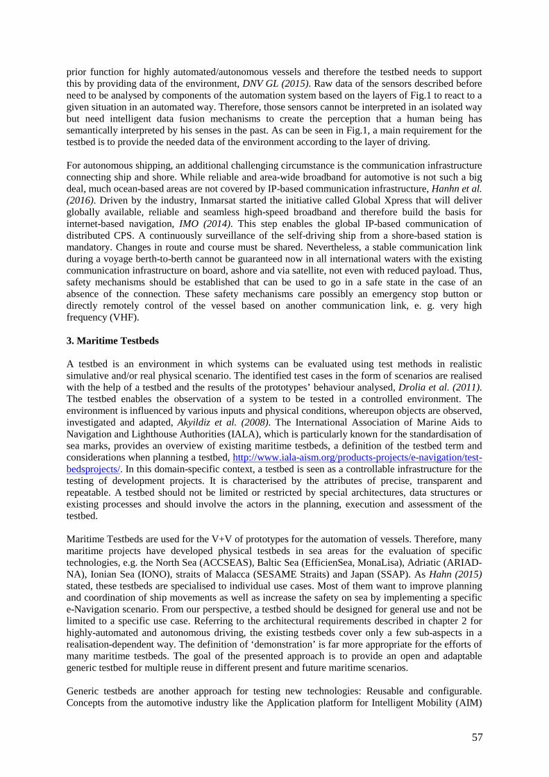
57
prior function for highly automated/autonomous vessels and therefore the testbed needs to support this by providing data of the environment, DNV GL (2015). Raw data of the sensors described before need to be analysed by components of the automation system based on the layers of Fig.1 to react to a given situation in an automated way. Therefore, those sensors cannot be interpreted in an isolated way but need intelligent data fusion mechanisms to create the perception that a human being has semantically interpreted by his senses in the past. As can be seen in Fig.1, a main requirement for the testbed is to provide the needed data of the environment according to the layer of driving. For autonomous shipping, an additional challenging circumstance is the communication infrastructure connecting ship and shore. While reliable and area-wide broadband for automotive is not such a big deal, much ocean-based areas are not covered by IP-based communication infrastructure, Hanhn et al. (2016). Driven by the industry, Inmarsat started the initiative called Global Xpress that will deliver globally available, reliable and seamless high-speed broadband and therefore build the basis for internet-based navigation, IMO (2014). This step enables the global IP-based communication of distributed CPS. A continuously surveillance of the self-driving ship from a shore-based station is mandatory. Changes in route and course must be shared. Nevertheless, a stable communication link during a voyage berth-to-berth cannot be guaranteed now in all international waters with the existing communication infrastructure on board, ashore and via satellite, not even with reduced payload. Thus, safety mechanisms should be established that can be used to go in a safe state in the case of an absence of the connection. These safety mechanisms care possibly an emergency stop button or directly remotely control of the vessel based on another communication link, e. g. very high frequency (VHF). 3. Maritime Testbeds A testbed is an environment in which systems can be evaluated using test methods in realistic simulative and/or real physical scenario. The identified test cases in the form of scenarios are realised with the help of a testbed and the results of the prototypes’ behaviour analysed, Drolia et al. (2011). The testbed enables the observation of a system to be tested in a controlled environment. The environment is influenced by various inputs and physical conditions, whereupon objects are observed, investigated and adapted, Akyildiz et al. (2008). The International Association of Marine Aids to Navigation and Lighthouse Authorities (IALA), which is particularly known for the standardisation of sea marks, provides an overview of existing maritime testbeds, a definition of the testbed term and considerations when planning a testbed, http://www.iala-aism.org/products-projects/e-navigation/test-bedsprojects/. In this domain-specific context, a testbed is seen as a controllable infrastructure for the testing of development projects. It is characterised by the attributes of precise, transparent and repeatable. A testbed should not be limited or restricted by special architectures, data structures or existing processes and should involve the actors in the planning, execution and assessment of the testbed. Maritime Testbeds are used for the V+V of prototypes for the automation of vessels. Therefore, many maritime projects have developed physical testbeds in sea areas for the evaluation of specific technologies, e.g. the North Sea (ACCSEAS), Baltic Sea (EfficienSea, MonaLisa), Adriatic (ARIAD-NA), Ionian Sea (IONO), straits of Malacca (SESAME Straits) and Japan (SSAP). As Hahn (2015) stated, these testbeds are specialised to individual use cases. Most of them want to improve planning and coordination of ship movements as well as increase the safety on sea by implementing a specific e-Navigation scenario. From our perspective, a testbed should be designed for general use and not be limited to a specific use case. Referring to the architectural requirements described in chapter 2 for highly-automated and autonomous driving, the existing testbeds cover only a few sub-aspects in a realisation-dependent way. The definition of ‘demonstration’ is far more appropriate for the efforts of many maritime testbeds. The goal of the presented approach is to provide an open and adaptable generic testbed for multiple reuse in different present and future maritime scenarios. Generic testbeds are another approach for testing new technologies: Reusable and configurable. Concepts from the automotive industry like the Application platform for Intelligent Mobility (AIM)
58
build an orientation. AIM is a component based testbed for land traffic, Schnieder and Krenkel (2015). It has mobile components like a car fleet or structural components like a research crossway, research railway crossing or reference way Car2X. It also offers driving or virtual reality simulators. These components are test carrier for new technologies. The data gathered can be used later for simulations or other research. If a new traffic observation or management requires a testbed, it can be implemented in the AIM testbed. The virtual reality laboratory is built around a modular mock-up car which allows the integration of new driver assistance systems. This scenario allows evaluating in a static environment. The target of AIM is to be a versatile test environment for broad diversity of land transportation technologies. A major contribution to the previously described scope is a maritime testbed architecture which can realise the previously described requirements of the highly automated and autonomous driving functionality for the maritime domain. This paper describes a similar approach for the maritime domain. 4. Integrated Testbed 4.1 Supporting the Development Process In this chapter, the approach of a seamless testing environment considering various test methods for the whole development lifecycle will be presented. Since physical testing on rough sea is very costly and complex, the main part of testing is carried out in virtual simulation environments. Nevertheless, virtual tests must be supplemented by tests in the real world. Fig.2 illustrates the holistic perspective on the development process from early stages of requirement engineering to a real physical usage. Each of the development processes can be supported by either virtual and/or physical testbeds. Depending on the respective development process, different test methods are provided for a seamless testing, such as maritime traffic simulations for virtual testing or a mobile bridge and a research vessel for physical testing.
Fig.2: Supporting the Development Process by Testbeds
Firstly, V+V scenario definitions are created on the basis of requirements. When developing safety-critical systems such as highly automated and autonomous driving systems, well established development processes based on a methodological approach are used. Therefore, the key international standard IEC 61508 (Functional safety of electrical, electronic and programmable electronic (E/E/PE) safety-related systems) has been adapted by many industrial sectors as a guideline for development. As an example of the automotive sector, the ISO 26262 (“Road vehicles – functional safety”) is an adaption of the IEC 61508 and had hit the light as a draft in 2009. The ISO 17894 (“Ships and marine technology – General principles for the development and use of programmable electronic systems in marine applications”) adapts the standard and others for the maritime domain. The IEC 61508 and thus all adaptions focus on safety requirements, hazard analysis, adequate V+V methods and risk assessment. Therefore, the V+V scenario definition based on information of the early requirements and conceptual development process phase is mandatory for a testbed. A virtual testbed providing complex simulation environments supports the early testing of new maritime technologies. Along the development process, a seamless transfer of the simulated tested
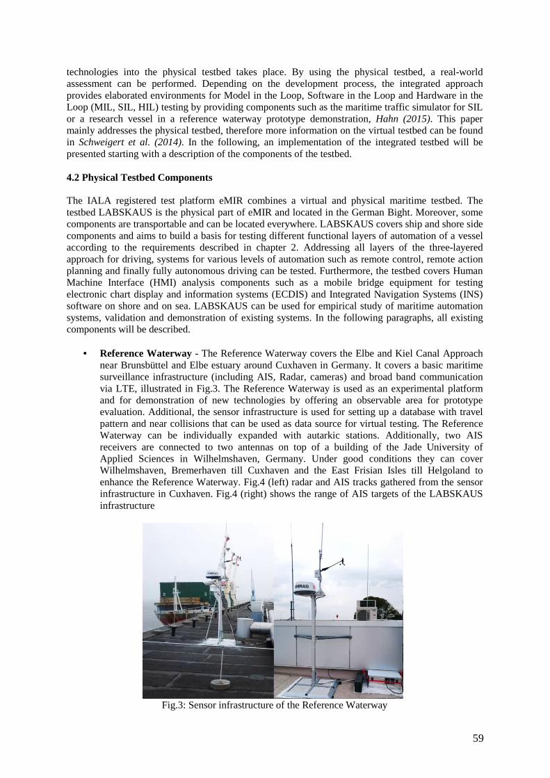
59
technologies into the physical testbed takes place. By using the physical testbed, a real-world assessment can be performed. Depending on the development process, the integrated approach provides elaborated environments for Model in the Loop, Software in the Loop and Hardware in the Loop (MIL, SIL, HIL) testing by providing components such as the maritime traffic simulator for SIL or a research vessel in a reference waterway prototype demonstration, Hahn (2015). This paper mainly addresses the physical testbed, therefore more information on the virtual testbed can be found in Schweigert et al. (2014). In the following, an implementation of the integrated testbed will be presented starting with a description of the components of the testbed. 4.2 Physical Testbed Components The IALA registered test platform eMIR combines a virtual and physical maritime testbed. The testbed LABSKAUS is the physical part of eMIR and located in the German Bight. Moreover, some components are transportable and can be located everywhere. LABSKAUS covers ship and shore side components and aims to build a basis for testing different functional layers of automation of a vessel according to the requirements described in chapter 2. Addressing all layers of the three-layered approach for driving, systems for various levels of automation such as remote control, remote action planning and finally fully autonomous driving can be tested. Furthermore, the testbed covers Human Machine Interface (HMI) analysis components such as a mobile bridge equipment for testing electronic chart display and information systems (ECDIS) and Integrated Navigation Systems (INS) software on shore and on sea. LABSKAUS can be used for empirical study of maritime automation systems, validation and demonstration of existing systems. In the following paragraphs, all existing components will be described.
• Reference Waterway - The Reference Waterway covers the Elbe and Kiel Canal Approach near Brunsbüttel and Elbe estuary around Cuxhaven in Germany. It covers a basic maritime surveillance infrastructure (including AIS, Radar, cameras) and broad band communication via LTE, illustrated in Fig.3. The Reference Waterway is used as an experimental platform and for demonstration of new technologies by offering an observable area for prototype evaluation. Additional, the sensor infrastructure is used for setting up a database with travel pattern and near collisions that can be used as data source for virtual testing. The Reference Waterway can be individually expanded with autarkic stations. Additionally, two AIS receivers are connected to two antennas on top of a building of the Jade University of Applied Sciences in Wilhelmshaven, Germany. Under good conditions they can cover Wilhelmshaven, Bremerhaven till Cuxhaven and the East Frisian Isles till Helgoland to enhance the Reference Waterway. Fig.4 (left) radar and AIS tracks gathered from the sensor infrastructure in Cuxhaven. Fig.4 (right) shows the range of AIS targets of the LABSKAUS infrastructure
Fig.3: Sensor infrastructure of the Reference Waterway
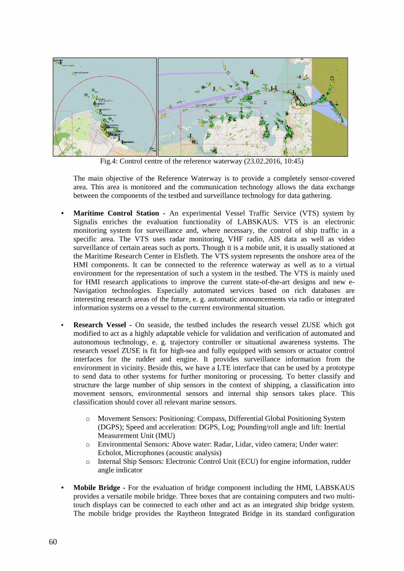
60
Fig.4: Control centre of the reference waterway (23.02.2016, 10:45)
The main objective of the Reference Waterway is to provide a completely sensor-covered area. This area is monitored and the communication technology allows the data exchange between the components of the testbed and surveillance technology for data gathering.
• Maritime Control Station - An experimental Vessel Traffic Service (VTS) system by
Signalis enriches the evaluation functionality of LABSKAUS. VTS is an electronic monitoring system for surveillance and, where necessary, the control of ship traffic in a specific area. The VTS uses radar monitoring, VHF radio, AIS data as well as video surveillance of certain areas such as ports. Though it is a mobile unit, it is usually stationed at the Maritime Research Center in Elsfleth. The VTS system represents the onshore area of the HMI components. It can be connected to the reference waterway as well as to a virtual environment for the representation of such a system in the testbed. The VTS is mainly used for HMI research applications to improve the current state-of-the-art designs and new e-Navigation technologies. Especially automated services based on rich databases are interesting research areas of the future, e. g. automatic announcements via radio or integrated information systems on a vessel to the current environmental situation.
• Research Vessel - On seaside, the testbed includes the research vessel ZUSE which got modified to act as a highly adaptable vehicle for validation and verification of automated and autonomous technology, e. g. trajectory controller or situational awareness systems. The research vessel ZUSE is fit for high-sea and fully equipped with sensors or actuator control interfaces for the rudder and engine. It provides surveillance information from the environment in vicinity. Beside this, we have a LTE interface that can be used by a prototype to send data to other systems for further monitoring or processing. To better classify and structure the large number of ship sensors in the context of shipping, a classification into movement sensors, environmental sensors and internal ship sensors takes place. This classification should cover all relevant marine sensors.
o Movement Sensors: Positioning: Compass, Differential Global Positioning System (DGPS); Speed and acceleration: DGPS, Log; Pounding/roll angle and lift: Inertial Measurement Unit (IMU)
o Environmental Sensors: Above water: Radar, Lidar, video camera; Under water: Echolot, Microphones (acoustic analysis)
o Internal Ship Sensors: Electronic Control Unit (ECU) for engine information, rudder angle indicator
• Mobile Bridge - For the evaluation of bridge component including the HMI, LABSKAUS
provides a versatile mobile bridge. Three boxes that are containing computers and two multi-touch displays can be connected to each other and act as an integrated ship bridge system. The mobile bridge provides the Raytheon Integrated Bridge in its standard configuration
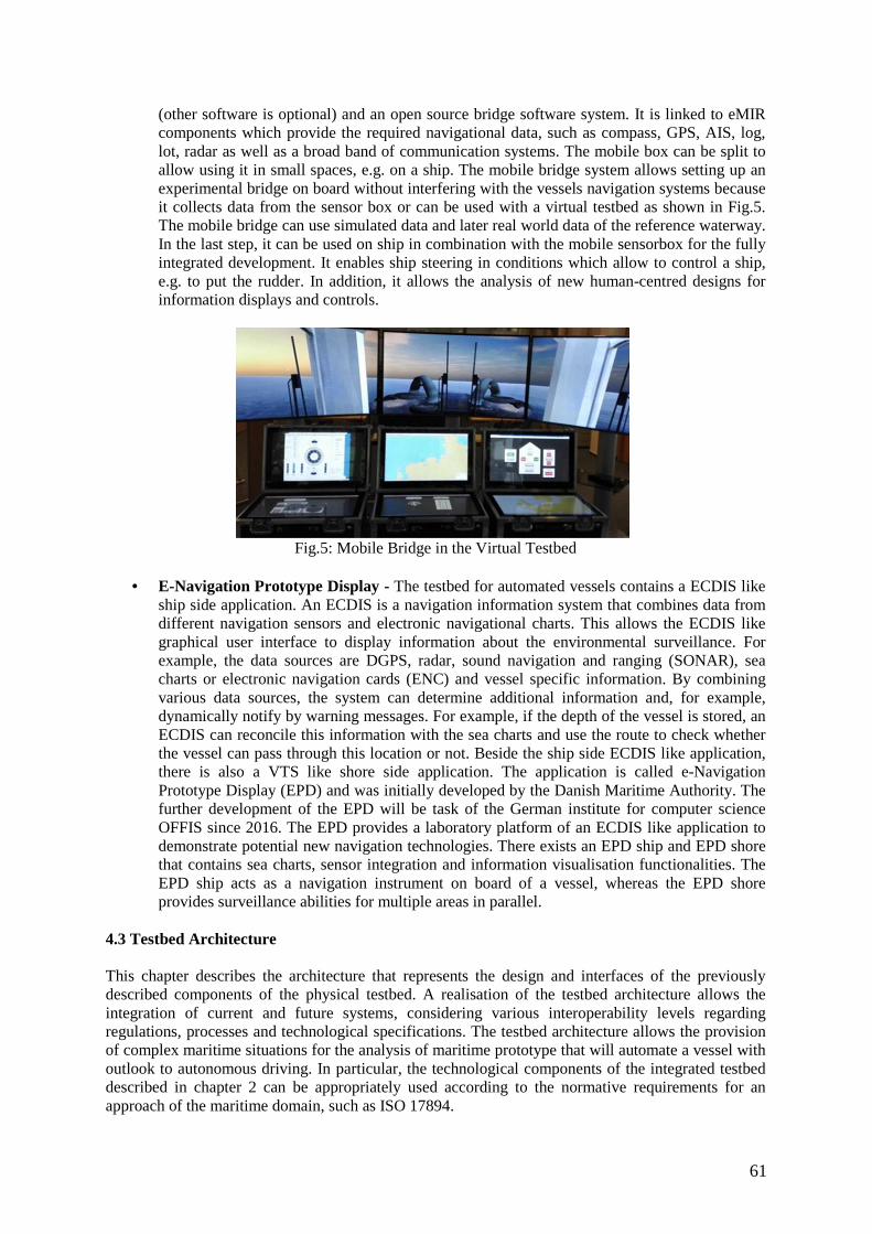
61
(other software is optional) and an open source bridge software system. It is linked to eMIR components which provide the required navigational data, such as compass, GPS, AIS, log, lot, radar as well as a broad band of communication systems. The mobile box can be split to allow using it in small spaces, e.g. on a ship. The mobile bridge system allows setting up an experimental bridge on board without interfering with the vessels navigation systems because it collects data from the sensor box or can be used with a virtual testbed as shown in Fig.5. The mobile bridge can use simulated data and later real world data of the reference waterway. In the last step, it can be used on ship in combination with the mobile sensorbox for the fully integrated development. It enables ship steering in conditions which allow to control a ship, e.g. to put the rudder. In addition, it allows the analysis of new human-centred designs for information displays and controls.
Fig.5: Mobile Bridge in the Virtual Testbed
• E-Navigation Prototype Display - The testbed for automated vessels contains a ECDIS like
ship side application. An ECDIS is a navigation information system that combines data from different navigation sensors and electronic navigational charts. This allows the ECDIS like graphical user interface to display information about the environmental surveillance. For example, the data sources are DGPS, radar, sound navigation and ranging (SONAR), sea charts or electronic navigation cards (ENC) and vessel specific information. By combining various data sources, the system can determine additional information and, for example, dynamically notify by warning messages. For example, if the depth of the vessel is stored, an ECDIS can reconcile this information with the sea charts and use the route to check whether the vessel can pass through this location or not. Beside the ship side ECDIS like application, there is also a VTS like shore side application. The application is called e-Navigation Prototype Display (EPD) and was initially developed by the Danish Maritime Authority. The further development of the EPD will be task of the German institute for computer science OFFIS since 2016. The EPD provides a laboratory platform of an ECDIS like application to demonstrate potential new navigation technologies. There exists an EPD ship and EPD shore that contains sea charts, sensor integration and information visualisation functionalities. The EPD ship acts as a navigation instrument on board of a vessel, whereas the EPD shore provides surveillance abilities for multiple areas in parallel.
4.3 Testbed Architecture This chapter describes the architecture that represents the design and interfaces of the previously described components of the physical testbed. A realisation of the testbed architecture allows the integration of current and future systems, considering various interoperability levels regarding regulations, processes and technological specifications. The testbed architecture allows the provision of complex maritime situations for the analysis of maritime prototype that will automate a vessel with outlook to autonomous driving. In particular, the technological components of the integrated testbed described in chapter 2 can be appropriately used according to the normative requirements for an approach of the maritime domain, such as ISO 17894.
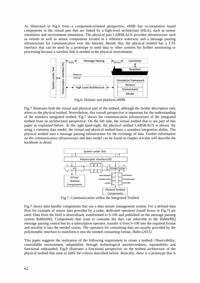
62
As illustrated in Fig.6 from a component-oriented perspective, eMIR has co-simulation based components in the virtual part that are linked by a high-level architecture (HLA), such as sensor simulation and environment simulation. The physical part LABSKAUS provides infrastructure such as vessels as well as sensor components located in a reference waterway and a message passing infrastructure for communication over the Internet. Beside this, the physical testbed has a LTE interface that can be used by a prototype to send data to other systems for further monitoring or processing because a wireless link is needed in the physical environment.
Fig.6: Holistic test platform eMIR
Fig.7 illustrates both the virtual and physical part of the testbed, although the further description only refers to the physical testbed. Nevertheless, this overall perspective is important for the understanding of the seamless integrated testbed. Fig.7 shows the communication infrastructure of the integrated testbed from an architectural perspective. On the left side, the virtual testbed that is not part of this paper as explained before. At the right hand-sight, the physical testbed LABSKAUS is shown. By using a common data model, the virtual and physical testbed have a seamless integration ability. The physical testbed uses a message passing infrastructure for the exchange of data. Further information on the communication infrastructure and data model can be found in chapter 4.4 that will describe the backbone in detail.
Fig.7: Communication within the Integrated Testbed
Fig.7 shows data handler components that use a data stream management system. For a defined data flow for example of sensor data provided by a radar, dedicated operators (small boxes in Fig.7) are used. Data from the field is deserialised, transformed to S-100 and published on the message passing system RabbitMQ. Components that want to consume the data can subscribe to the RabbitMQ message passing central bus by a subscription operator, transfer it from S-100 into the required format and serialise it into the needed syntax. The operators for consuming data are usually provided by the polymorphic interface to transform it into the needed consuming format, Hahn (2015). This paper suggests the realisation of the following requirement to create a testbed: Observability, controllable environment, adaptability through technological unrestrictedness, repeatability and functional unbounded. Fig.8 illustrates a functional perspective on the testbed architecture of the physical testbed that aims to fulfil the criteria described before. Basically, there is a prototype that is
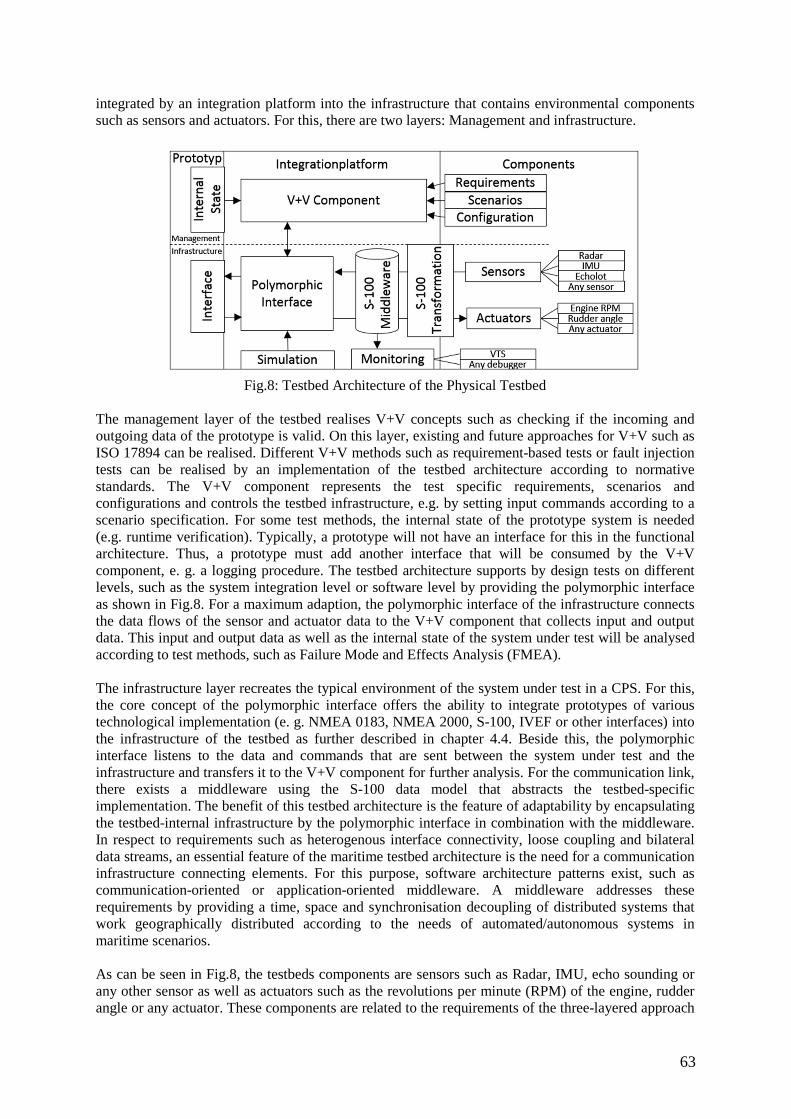
63
integrated by an integration platform into the infrastructure that contains environmental components such as sensors and actuators. For this, there are two layers: Management and infrastructure.
Fig.8: Testbed Architecture of the Physical Testbed
The management layer of the testbed realises V+V concepts such as checking if the incoming and outgoing data of the prototype is valid. On this layer, existing and future approaches for V+V such as ISO 17894 can be realised. Different V+V methods such as requirement-based tests or fault injection tests can be realised by an implementation of the testbed architecture according to normative standards. The V+V component represents the test specific requirements, scenarios and configurations and controls the testbed infrastructure, e.g. by setting input commands according to a scenario specification. For some test methods, the internal state of the prototype system is needed (e.g. runtime verification). Typically, a prototype will not have an interface for this in the functional architecture. Thus, a prototype must add another interface that will be consumed by the V+V component, e. g. a logging procedure. The testbed architecture supports by design tests on different levels, such as the system integration level or software level by providing the polymorphic interface as shown in Fig.8. For a maximum adaption, the polymorphic interface of the infrastructure connects the data flows of the sensor and actuator data to the V+V component that collects input and output data. This input and output data as well as the internal state of the system under test will be analysed according to test methods, such as Failure Mode and Effects Analysis (FMEA). The infrastructure layer recreates the typical environment of the system under test in a CPS. For this, the core concept of the polymorphic interface offers the ability to integrate prototypes of various technological implementation (e. g. NMEA 0183, NMEA 2000, S-100, IVEF or other interfaces) into the infrastructure of the testbed as further described in chapter 4.4. Beside this, the polymorphic interface listens to the data and commands that are sent between the system under test and the infrastructure and transfers it to the V+V component for further analysis. For the communication link, there exists a middleware using the S-100 data model that abstracts the testbed-specific implementation. The benefit of this testbed architecture is the feature of adaptability by encapsulating the testbed-internal infrastructure by the polymorphic interface in combination with the middleware. In respect to requirements such as heterogenous interface connectivity, loose coupling and bilateral data streams, an essential feature of the maritime testbed architecture is the need for a communication infrastructure connecting elements. For this purpose, software architecture patterns exist, such as communication-oriented or application-oriented middleware. A middleware addresses these requirements by providing a time, space and synchronisation decoupling of distributed systems that work geographically distributed according to the needs of automated/autonomous systems in maritime scenarios. As can be seen in Fig.8, the testbeds components are sensors such as Radar, IMU, echo sounding or any other sensor as well as actuators such as the revolutions per minute (RPM) of the engine, rudder angle or any actuator. These components are related to the requirements of the three-layered approach
64
of chapter 2 and represent the environment and the vehicle parameters. The native interfaces of these sensors and actuators are heterogeneous, such as NMEA 0183 or NMEA 2000. Therefore, a transformation into the canonical data model of the testbed infrastructure S-100 will be done according to the data handler description in Fig.7. The testbed needs some information to perform the tests. Typically, this information results from requirements and specifications. E.g. pre-conditions, post-conditions, environmental factors and the steps of the scenarios are needed to set up the testbed and perform the test cases. As can be seen in Fig.8, there is a monitoring component that streams information of the testbed infrastructure to a VTS for visual evaluation or any debugger. The non-modified data of the testbed communication infrastructure can be used for diagnosis of errors or analysis of a system’s behaviour based on raw data. The detailed implementation of the components of the backbone according to the testbed architecture will be described in the following chapter. 4.4 Backbone The backbone is a sensor box to integrate the naval sensors, an open communication system based on open source message passing implementation and S-100 conform data representation according to the testbed architecture presented in chapter 4.3.
• Sensorbox - The component which integrates the sensors is called ‘Navibox’. It is a compact sensor data hub which provides navigational data on board as well as data for maritime surveillance systems. It provides LAN, WLAN and broadband WAN communication facilities. The minimum setup consists of a radar, an Automatic Identification System (AIS) antenna and a wind sensor. The AIS is a core technology based on a radio system for the exchange of navigation information and ship data in the shipping industry. The objective pursued by the use of AIS is to improve the safety and control of shipping by sending various static and dynamic data via radio. All sensors which are sending data appropriate to the communication standard NMEA 0183 or NMEA 2000 and Ethernet can be attached. In case of a different communication standard, an adapter will be implemented to integrate the sensor into the Navibox. The AIS receiver receives all AIS messages from the AIS transceiver equipped systems in a 35-100 km radius dependent on the antenna height. The AIS messages include static, dynamic and journey vessel information. A wind sensor is able to gather wind speed as well as angle and is connected to the NMEA 2000 bus. An Industrial PC (IPC) takes over the sensor stream management and processing. It houses a message passing broker for the publish/subscribe mechanism of the testbed communication infrastructure. The Navibox software gathers and handles all sensor data. A Navibox is configured to be remotely controlled via network (LTE).
The stationary variant of the Navibox has a sturdy pole to carry the sensor head. Two of the stationary Naviboxes are implemented in the reference waterway located at the roof of buildings that are near to the coast. The setup in Cuxhaven is additionally equipped with optical surveillance technologies to track objects and observe water current/surface behaviour. In the future, an echo sounder will be attached to track movements and ship dynamics under water. An energy autarkic version of the Navibox station is added to run tests on any coast location.
To collect data at the location of a vessel there is the mobile Navibox. It adds a JRC JRL-21 Differential GPS (DGPS) System that can not only add the position, course over ground and speed over ground, but also the true heading and rate of turn to replace a compass. A chart and multifunctional display allows monitoring sensor data on board. The sensor pole will be attached to a vessel and gathers sensor data independent of the ship navigation electronics.
• Data Model - The physical testbed exchanges data based on S-100 over the message passing
bus, DNV GL (2015). S-100 is a universal hydrographic data model that was developed by the International Hydrographic Organization (IHO) in 2010. This new standard replaces the past IHO standard S-57 due to a lack of flexibility. For example, a limitation of S-57 is the
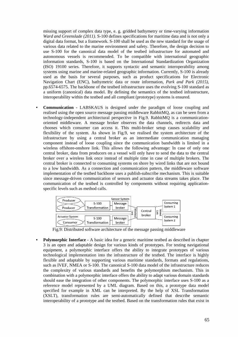
65
missing support of complex data type, e. g. gridded bathymetry or time-varying information Ward and Greenslade (2011). S-100 defines specifications for maritime data and is not only a digital data format, but a framework. S-100 shall be used as the new standard for the usage of various data related to the marine environment and safety. Therefore, the design decision to use S-100 for the canonical data model of the testbed infrastructure for automated and autonomous vessels is recommended. To be compatible with international geographic information standards, S-100 is based on the International Standardization Organization (ISO) 19100 series. Therefore, it supports syntactic and semantic interoperability among systems using marine and marine-related geographic information. Currently, S-100 is already used as the basis for several purposes, such as product specifications for Electronic Navigation Chart (ENC), bathymetric data or route information, Park and Park (2015), pp.6574-6575. The backbone of the testbed infrastructure uses the evolving S-100 standard as a uniform (canonical) data model. By defining the semantics of the testbed infrastructure, interoperability within the testbed and all compliant (prototype) systems is ensured.
• Communication - LABSKAUS is designed under the paradigm of loose coupling and
realised using the open source message passing middleware RabbitMQ, as can be seen from a technology-independent architectural perspective in Fig.9. RabbitMQ is a communication-oriented middleware. A message broker observes the data channels, redirects data and chooses which consumer can access it. This multi-broker setup causes scalability and flexibility of the system. As shown in Fig.9, we realised the system architecture of the infrastructure by using a central broker as an intermediate communication managing component instead of loose coupling since the communication bandwidth is limited in a wireless offshore-onshore link. This allows the following advantage: In case of only one central broker, data from producers on a vessel will only have to send the data to the central broker over a wireless link once instead of multiple time in case of multiple brokers. The central broker is connected to consuming systems on shore by wired links that are not bound to a low bandwidth. As a connection and communication pattern, the middleware software implementation of the testbed backbone uses a publish-subscribe mechanism. This is suitable since message-driven communication of sensors and actuator data streams takes place. The communication of the testbed is controlled by components without requiring application-specific levels such as method calls.
Fig.9: Distributed software architecture of the message passing middleware
• Polymorphic Interface - A basic idea for a generic maritime testbed as described in chapter
3 is an open and adaptable design for various kinds of prototypes. For testing navigational equipment, a polymorphic interface offers the ability to integrate prototypes of various technological implementation into the infrastructure of the testbed. The interface is highly flexible and adaptable by supporting various maritime standards, formats and regulations, such as IVEF, NMEA or S-100. The canonical S-100 data model of the infrastructure reduces the complexity of various standards and benefits the polymorphism mechanism. This in combination with a polymorphic interface offers the ability to adapt various domain standards should ease the integration of other components. The polymorphic interface uses S-100 as a reference model represented by a UML diagram. Based on this, a prototype data model specified for example in XML can be interpreted. By the help of XSL Transformation (XSLT), transformation rules are semi-automatically defined that describe semantic interoperability of a prototype and the testbed. Based on the transformation rules that exist in
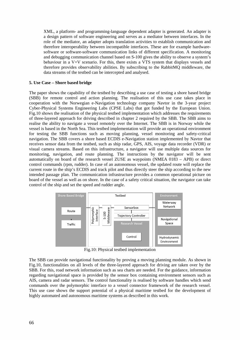
66
XML, a platform- and programming-language dependent adapter is generated. An adapter is a design pattern of software engineering and serves as a mediator between interfaces. In the role of the mediator, an adapter adopts translation activities to establish communication and therefore interoperability between incompatible interfaces. These are for example hardware-software or software-software communication links of different specification. A monitoring and debugging communication channel based on S-100 gives the ability to observe a system’s behaviour in a V+V scenario. For this, there exists a VTS system that displays vessels and therefore provides observability abilities. By subscribing to the RabbitMQ middleware, the data streams of the testbed can be intercepted and analysed.
5. Use Case – Shore based bridge The paper shows the capability of the testbed by describing a use case of testing a shore based bridge (SBB) for remote control and action planning. The realisation of this use case takes place in cooperation with the Norwegian e-Navigation technology company Navtor in the 3-year project Cyber-Physical Systems Engineering Labs (CPSE Labs) that got funded by the European Union. Fig.10 shows the realisation of the physical testbed implementation which addresses the requirements of three-layered approach for driving described in chapter 2 required by the SBB. The SBB aims to realise the ability to navigate a vessel remotely over the Internet. The SBB is in Norway while the vessel is based in the North Sea. This testbed implementation will provide an operational environment for testing the SBB functions such as moving planning, vessel monitoring and safety-critical navigation. The SBB covers a shore based ECDIS e-Navigation station implemented by Navtor that receives sensor data from the testbed, such as ship radar, GPS, AIS, voyage data recorder (VDR) or visual camera streams. Based on this infrastructure, a navigator will use multiple data sources for monitoring, navigation, and route planning. The instructions by the navigator will be sent automatically on board of the research vessel ZUSE as waypoints (NMEA 0183 – APB) or direct control commands (rpm, rudder). In case of an autonomous vessel, the updated route will replace the current route in the ship’s ECDIS and track pilot and thus directly steer the ship according to the new intended passage plan. The communication infrastructure provides a common operational picture on board of the vessel as well as on shore. In the case of a safety critical situation, the navigator can take control of the ship and set the speed and rudder angle.
Fig.10: Physical testbed implementation
The SBB can provide navigational functionality by proving a moving planning module. As shown in Fig.10, functionalities on all levels of the three-layered approach for driving are taken over by the SBB. For this, road network information such as sea charts are needed. For the guidance, information regarding navigational space is provided by the sensor box containing environment sensors such as AIS, camera and radar sensors. The control functionality is realised by software handles which send commands over the polymorphic interface to a vessel connector framework of the research vessel. This use case shows the support potential of a physical maritime testbed for the development of highly automated and autonomous maritime systems as described in this work.
67
6. Conclusion This paper gives an overview on the implementation and usage of testbeds for highly automated and autonomous vessels. The requirements for a maritime testbed were described that result by the three-layered approach for driving. Furthermore, an overview of present related testbeds was given. This work introduces the test platform eMIR with special focus on the physical testbed LABSKAUS. Firstly, the potential was described from a development perspective to continue describing the individual components of the physical testbed and finally present the complete testbed architecture. LABSKAUS provides components such as a research vessel, reference waterway and mobile bridge aiming to support the V+V by providing services. These testbed components address a wide field of sensor sources, sinks and an infrastructure to build the testbed for V+V. The wide scope of possible tests for highly automated and autonomous technologies offers an open as well as extendable platform for research and industry. Using this approach, various test and demonstration environments can be set up. A use case shows the potential of the presented approach by setting up a test environ-ment for a shore based bridge. The use case realised the remote monitoring and control functionality of a vessel by using a modified ECDIS based in Norway and the physical testbed. In future, the eMIR testbed will be expanded for the development and research of technology for highly-automated and autonomous vessels which seem to be the future of e-Navigation.
Acknowledgements The work presented in this paper is supported by numerous projects. The application of this approach is supported by European Union’s Horizon 2020 research and innovation programme under grant agreement No 644400 (CPSE Labs). References AKYILDIZ, I.F.; MELODIA, T.; CHOWDHURY, K.R. (2008), Wireless Multimedia Sensor Net-works: Applications and Testbeds, IEEE 96 (10), pp.1588-1605 DNV GL (2015), Ship Connectivity, Position Paper, DNV GL, Høvik, https://www.dnvgl.com/publications/ship-connectivity-28107 DROLIA, U.; WANG, Z.Y.; PANT, Y.V.; MANGHARAM, R. (2011), AutoPlug: An Automotive Test-Bed for Electronic Controller Unit Testing and Verification, ITSC Conf. http://repository.upenn.edu/cgi/viewcontent.cgi?article=1045&context=mlab_papers HAHN, A. (2015), Simulation environment for risk assessment of e-navigation systems, OMAE Conf. HAHN, A.; BOLLES, A.; FRÄNZLE, M.; FRÖSCHLE, S.; PARK, J.H. (2016), Requirements for E-Navigation Architectures, Int. J. E-Navigation and Maritime Economy 5, pp.1-20 IMO (2014), Development of an e-navigation Strategy Implementation Plan, Sub-Committee on navi-gation communications and search and rescue, Report of the Correspondence Group on e-Navigation, International Maritime Organization, London NN (2012), Safety and Shipping 1912-2012, Report, Allianz Global Corporate & Specialty SE, http://www.agcs.allianz.com/assets/PDFs/Reports/AGCS_safety_and_shipping_report.pdf PARK, D.W.; PARK, S.Y. (2015), E-Navigation-supporting data management system for variant S-100-based data, Multimedia Tools and Applications 74(16), pp.6573-6588 SCHNIEDER, L.; KRENKEL, R. (2015), Betreibermodell einer Forschungsinfrastruktur für die Entwicklung intelligenter Mobilitätsdienste im realen Verkehrsumfeld, 16. Symp. Automatisie-rungssysteme, Assistenzsysteme und eingebettete Systeme für Transportmittel (AAET), Braun-

68
schweig, pp.108-116 SCHWEIGERT, S.; GOLLÜCKE, V.; HAHN, A.; BOLLES, A. (2014), HAGGIS: A modelling and simulation platform for e-maritime technology assessment, 2nd Int. Symp. Naval Architecture and Maritime (INTNAM), Istanbul, pp.733-742 WARD, R.; GREENSLADE, B. (2011), IHO S-100 - The Universal Hydrographic Data Model, https://www.iho.int/mtg_docs/com_wg/TSMAD/TSMAD_Misc/S-100InfoPaper_FinalJan2011.pdf
69
The Key Ship Design Decision - Choosing the Style of a New Design
David Andrews, University College London, London/UK, [email protected]
Abstract
A paper to COMPIT 2013 presented a description of the ship design process in terms of the important decisions a ship designer makes, consciously or unconsciously, in order to produce a new design. The first real decision that has to be made by the designer in order to proceed was said to be selecting the “style” of the design study or a specific design option. This term was adopted in order to distinguish not just a host of design issues and standards implicit in a given study but also, at this very initial step, the overall characteristics of any particular study. So, the term style could be said to be doubly im-portant. The paper considers the nature of the early ship design process for complex multi-functional vessels, referring to the 2013 paper, and then retracing the origins of the particular use of the term, where it was seen as the last of the five elements in Brown and Andrews’ 1980 encapsulation of the ship design issues that matter to the naval architect, incorporated in the term “S to the 5th”. This leads on to consideration of the various aspects of design style, many of which could be considered “transver-sals” as they apply across the naval architectural sub-disciplines and to the component material sub-systems comprising a ship. One of the distinctive advantages of the architecturally driven ship synthesis or Design Building Block approach is that it can address many of the style issues in the earliest descrip-tions of an emergent design study. Examples are provided showing both different top-level style char-acteristics and how the impact of specific component style aspects can be investigated in early stage ship design using the UCL DBB approach. This enables the paper to demonstrate why the choice of “style” is seen to be The Key Design Decision.
1. Introduction - Style in Early Stage Ship Design “Style” was explicitly incorporated as a characteristic of a ship design by Brown and Andrews (1980) as the fifth “S” in the “S5” ship design characteristics, the others being Speed (really Resistance and Propulsion), Seakeeping, Stability, and Strength. However the exact nature of style, as a type of infor-mation or design characteristic, that set it apart from other characteristics (or even the sub-disciplines of naval architecture), such as Speed or structural strength, was not so clear. Pawling et al. (2013) proposed at COMPIT 2013 that the design issues generally grouped under style, see below, are conceptually dif-ferent to the other naval architectural disciplines not because many are unsuited to mathematical analysis (the same was once true of Seakeeping or structural vibration analysis) but because style is a cross-cutting concept, in that a decision on an aspect of style explicitly influences a wide range of solution features. Stylistic information also has the key property of being able to accommodate uncertainty, con-taining both “hard” knowledge (such as adoption of specific structural standards) and “soft” knowledge (such as guidance on ship internal layout). Such knowledge can then be conceptually connected or grouped. In addition, style choices may also be reflected in the weighting factors chosen given multiple criteria when the ship designer is selecting a design preference. An example of a transversal style choice would be the level and extent of survivability adopted in a naval ship design. A decision on the level of survivability can influence a wide range of overall and detailed design features, such as the choice of signatures and defensive systems (to prevent a hit), the spacing of bulkheads (to resist weapon effects and subsequent flooding), the mutual arrangement of compartments (to protect vital spaces and aid in recovering from damage) and structural details (to resist the result of underwater shock on the structural hull girder). This particular example also illustrates another feature of style in that it is cross cutting across the responsibilities of the engineering disciplines involved in a ship design (such as naval architecture, marine engineering and combatant system engi-neering). In this regard, style choices could be said to be particularly critical in decision-making at the crucial earliest stages of complex ship design. It could be argued, however, that the difference between style and the other components of “S5” is a matter of degree, given that all the aspects of ship design interact to a greater or lesser degree with each other.
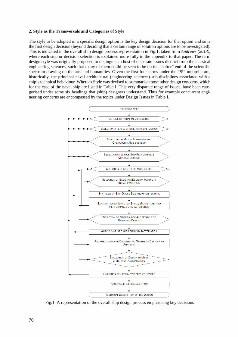
70
2. Style as the Transversals and Categories of Style The style to be adopted in a specific design option is the key design decision for that option and so is the first design decision (beyond deciding that a certain range of solution options are to be investigated). This is indicated in the overall ship design process representation in Fig.1, taken from Andrews (2013), where each step or decision selection is explained more fully in the appendix to that paper. The term design style was originally proposed to distinguish a host of disparate issues distinct from the classical engineering sciences, such that many of them could be seen to be on the “softer” end of the scientific spectrum drawing on the arts and humanities. Given the first four terms under the “S5” umbrella are, historically, the principal naval architectural (engineering sciences) sub-disciplines associated with a ship’s technical behaviour. Whereas Style was devised to summarise those other design concerns, which for the case of the naval ship are listed in Table I. This very disparate range of issues, have been cate-gorised under some six headings that (ship) designers understand. Thus for example concurrent engi-neering concerns are encompassed by the topics under Design Issues in Table I.
Fig.1: A representation of the overall ship design process emphasising key decisions
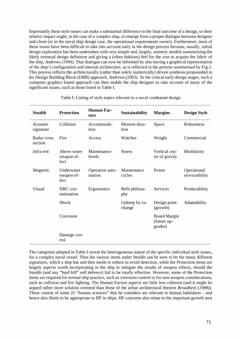
71
Importantly these style issues can make a substantial difference to the final outcome of a design, so their relative impact ought, in the case of a complex ship, to emerge from a proper dialogue between designer and client (or in the naval ship design case, the operational requirements owner). Furthermore, most of these issues have been difficult to take into account early in the design process because, usually, initial design exploration has been undertaken with very simple and, largely, numeric models summarising the likely eventual design definition and giving a (often dubious) feel for the cost to acquire the fabric of the ship, Andrews (1994). That dialogue can now be informed by also having a graphical representation of the ship’s configuration and internal architecture, as is reflected in the process summarised by Fig.1. This process reflects the architecturally (rather than solely numerically) driven synthesis propounded in his Design Building Block (DBB) approach, Andrews (2003). At the critical early design stages, such a computer graphics based approach can then enable the ship designer to take account of many of the significant issues, such as those listed in Table I.
Table I: Listing of style topics relevant to a naval combatant design
Stealth Protection Human Fac-tors Sustainability Margins Design Style
Acoustic signature
Collision Accommoda-tion
Mission dura-tion
Space Robustness
Radar cross section
Fire Access Watches Weight Commercial
Infra-red Above water weapon ef-fect
Maintenance levels
Stores Vertical cen-tre of gravity
Modularity
Magnetic Underwater weapon ef-fect
Operation auto-mation
Maintenance cycles
Power Operational serviceability
Visual NBC con-tamination
Ergonomics Refit philoso-phy
Services Producability
Shock Upkeep by ex-change
Design point (growth)
Adaptability
Corrosion Board Margin (future up-grades)
Damage con-trol
The categories adopted in Table I reveal the heterogeneous nature of the specific individual style issues, for a complex naval vessel. Thus the various items under Stealth can be seen to be the many different signatures, which a ship has and then needs to reduce to avoid detection, while the Protection items are largely aspects worth incorporating in the ship to mitigate the results of weapon effects, should the Stealth (and any “hard kill” self defence) fail to be totally effective. However, some of the Protection items are required for normal ship practice, such as corrosion control or for non-weapon considerations, such as collision and fire fighting. The Human Factors aspects are little less coherent (and it might be argued rather more solution oriented than those of the urban architectural theorist Broadbent (1988)). These consist of some 21 “human sciences” that he considers are relevant to human habitation – and hence also likely to be appropriate to HF in ships. HF concerns also relate to the important growth area
72
of automation, which along with micro-ergonomics (e.g. console design) has a strong input to the Pro-tection category, specifically in regard to modern bridge design. Sustainability is a major consideration in naval ship design and could be said to be a major driver, and hence a key hidden decision in the ship’s style from the beginning of any ship design study. The list of Margins just makes the point that there are many features and considerations beyond simple margins on the weight/VCG to ensure the ship’s sta-bility is adequate beyond the day it is accepted into service. Table I also distinguishes those margins required for unplanned (but consistently observed) growth in weight and rise in VCG in-service from Design Margins. The latter are more rightly a Design Issue in Table I, given they address many measures of uncertainty in design estimates. These margins, across all the weight/space groups, are intended to be absorbed, but not exceeded, through out the design and build process to completion. The last category in Table I is clearly the most broad and heterogeneous. Also, generally, such topics have the biggest impact on the final ship design. But this means they need to be recognised as choices and then properly considered with the owner/requirements team from the beginning of studying any design option. Some of these have been the objects of particular investigations by our research group at UCL and are discussed further in Section 5 as examples of design impact of considering separately some of these particular issues, where each could be as the specific driver of a design from its initiation. It is noticeable that certain of these issues can only be adequately investigated in the Concept Phase if the architectural synthesis assumed in Fig.1 is adopted. The other aspect to most of the Design Issues listed is that they have a qualitative or fuzzy nature. Thus, say, Robustness implies a greater degree of that quality than the “norm” for that type of vessel. This then raises the point that such a “norm” for a given new design option ought itself be defined but is often just accepted (or inferred) as being “current prac-tice” or by the adoption of existing standards. There are also exceptions in the listing of the Design Issues category, like Aesthetics, which for most vessels, other than mega yachts and some cruise ships, is seen to be “a luxury”. However, even this can be seen to be a simplification, as in the Cold War there was considerable debate in the US naval ship community as to whether the physical appearance of such a ship was part of it’s political “armament”, Roach et al. (1979).
Table II: Types of Ship Design in terms of Design Novelty
Type Example
second (stretched) batch
RN Batch 2 Type 22 frigate and Batch 3 Type 42
destroyer
simple type ship Most commercial vessels and many naval auxiliary
vessels
evolutionary design
a family of designs, such as
VT corvettes or OCL container ships
simple (numerical) synthesis
UCL student designs
architectural synthesis
UCL (DRC) design studies (see below)
radical configuration SWATH, Trimaran
radical technology US Navy Surface Effect
Ship of 1970s
The nature of the design of complex ships, such as cruise ships and naval combatants, is such that the need to emphasise the importance and difficulty of early representation of style issues is seen to be a
73
further complication in the practice of designing such vessels. This is due to there being, additionally, a wide range in the practice of such design. This arises from the degree of design novelty adopted in a specific design option, as is indicated by Table II. This shows a set of examples, across the field of ship design, where the sophistication in the design undertaken ranges from a simple modification of an ex-isting ship, through ever more extensive variations in design practice, to designs adopting, firstly, radical configurations and, beyond that, radical technologies. Although in first of the latter two categories of Table II current technology is often adopted, such options are still rarely built, due to the risk of un-knowns (usually exacerbated by the lack of a real prototype), while radical technology solutions are even more rarely pursued. In part this rarity arises because such radical technology solutions require recourse to design and, indeed, manufacturing practice much more akin to that appropriate to the aero-space industry. Thus, new major aircraft projects, typically, require massive development costs (includ-ing full scale physical prototypes, some tested to destruction) and additionally need tooling and manu-facturing facilities to also be specifically designed and then built, before extensive series production of each new aircraft design can commence. This is of course quite unlike most ship design, be it the ubiq-uitous bulker or the most sophisticated naval vessel. Such distinctions as those of Table II for the design of complex ships suggest any discussion of style needs, at least, to recognise the spectrum of design approach resulting from the novelty of the specific design option being pursued. Such choice on design novelty is key to the initial style choice for a given design study or a variant option in a properly con-ducted concept exploration, Andrews (2013). 3. Examples of Style Choices in Actual Ship Designs The following are brief summaries of a series of built naval ships, where style in an overall configuration has been a distinct choice and also some more specific style choices have been adopted, reflecting some of the more significant issues amongst those listed in Table I.
• 1st and 2nd Rate Royal Navy (R.N.) Ship Designs In an early study into the nature of ship cost, Brown and Andrews (1980) drew on a series of R.N. ship designs to point out that ship classes, which had been specifically designated “First rate” or “Second rate” designs, invariably showed that the latter were poor value for money (VFM). This applied to the Queen Elisabeth Class and Revenge Class Battleships, where the latter ”cheaper” versions were far less effective and clearly less value for money, in their ina-bility to be upgraded over a thirty years life. In WWII, the early convoy escorts, the Flower Class corvettes were again poor VFM compared to the later Castles and Lochs. Post War first and second class frigate classes were produced and, while the former led to the very successful Leander Class, the latter (Blackwoods) were soon disposed of. All these comparative designs are excellent examples of the overall style choice being made from which all the capabilities followed.
• HMS OCEAN
Commercial standards were mandated for this helicopter carrier without this being assessed through any proper concept and feasibility studies, because of the adoption of a false costing based on belief in a potential merchant ship conversion option. The Project Manager (the author in 1986-1990) fought the naval staff over adopting such non-naval standards for an essentially high value unit (given its “cargo” of hundreds of troops plus associated equipment and 12 Com-mando helicopters). The PM managed to raise the purchase budget but not sufficiently enough to cover the incorporation of limited naval standards. The eventual purchase was subsequently criticised by the Ministry of Defence chief marine engineer as this commercial practice substan-tially increased the engine support requirement for the fleet (due to this one ship’s unique engine fit). Of course, these support costs were not shown in original cost based decision, given this was obsessed with direct initial procurement cost rather than the “true ownership cost” of the design solution. Interestingly, many have argued that HMS OCEAN has been “good value for money”, however it has not been used in naval warfare (rather than usefully in peace keeping), so the jury must be out as to whether this constitutes, as a “cheap” solution for such a major naval capability. The extent to which many of the detailed “style issues”, largely listed in Table
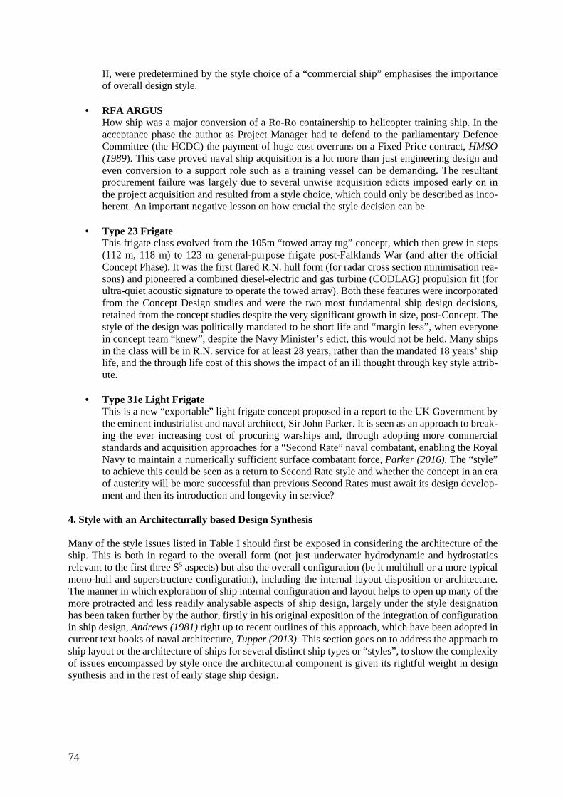
74
II, were predetermined by the style choice of a “commercial ship” emphasises the importance of overall design style.
• RFA ARGUS
How ship was a major conversion of a Ro-Ro containership to helicopter training ship. In the acceptance phase the author as Project Manager had to defend to the parliamentary Defence Committee (the HCDC) the payment of huge cost overruns on a Fixed Price contract, HMSO (1989). This case proved naval ship acquisition is a lot more than just engineering design and even conversion to a support role such as a training vessel can be demanding. The resultant procurement failure was largely due to several unwise acquisition edicts imposed early on in the project acquisition and resulted from a style choice, which could only be described as inco-herent. An important negative lesson on how crucial the style decision can be.
• Type 23 Frigate
This frigate class evolved from the 105m “towed array tug” concept, which then grew in steps (112 m, 118 m) to 123 m general-purpose frigate post-Falklands War (and after the official Concept Phase). It was the first flared R.N. hull form (for radar cross section minimisation rea-sons) and pioneered a combined diesel-electric and gas turbine (CODLAG) propulsion fit (for ultra-quiet acoustic signature to operate the towed array). Both these features were incorporated from the Concept Design studies and were the two most fundamental ship design decisions, retained from the concept studies despite the very significant growth in size, post-Concept. The style of the design was politically mandated to be short life and “margin less”, when everyone in concept team “knew”, despite the Navy Minister’s edict, this would not be held. Many ships in the class will be in R.N. service for at least 28 years, rather than the mandated 18 years’ ship life, and the through life cost of this shows the impact of an ill thought through key style attrib-ute.
• Type 31e Light Frigate
This is a new “exportable” light frigate concept proposed in a report to the UK Government by the eminent industrialist and naval architect, Sir John Parker. It is seen as an approach to break-ing the ever increasing cost of procuring warships and, through adopting more commercial standards and acquisition approaches for a “Second Rate” naval combatant, enabling the Royal Navy to maintain a numerically sufficient surface combatant force, Parker (2016). The “style” to achieve this could be seen as a return to Second Rate style and whether the concept in an era of austerity will be more successful than previous Second Rates must await its design develop-ment and then its introduction and longevity in service?
4. Style with an Architecturally based Design Synthesis Many of the style issues listed in Table I should first be exposed in considering the architecture of the ship. This is both in regard to the overall form (not just underwater hydrodynamic and hydrostatics relevant to the first three S5 aspects) but also the overall configuration (be it multihull or a more typical mono-hull and superstructure configuration), including the internal layout disposition or architecture. The manner in which exploration of ship internal configuration and layout helps to open up many of the more protracted and less readily analysable aspects of ship design, largely under the style designation has been taken further by the author, firstly in his original exposition of the integration of configuration in ship design, Andrews (1981) right up to recent outlines of this approach, which have been adopted in current text books of naval architecture, Tupper (2013). This section goes on to address the approach to ship layout or the architecture of ships for several distinct ship types or “styles”, to show the complexity of issues encompassed by style once the architectural component is given its rightful weight in design synthesis and in the rest of early stage ship design.
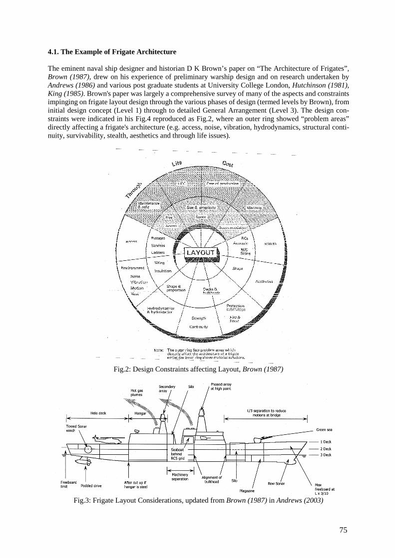
75
4.1. The Example of Frigate Architecture The eminent naval ship designer and historian D K Brown’s paper on “The Architecture of Frigates”, Brown (1987), drew on his experience of preliminary warship design and on research undertaken by Andrews (1986) and various post graduate students at University College London, Hutchinson (1981), King (1985). Brown's paper was largely a comprehensive survey of many of the aspects and constraints impinging on frigate layout design through the various phases of design (termed levels by Brown), from initial design concept (Level 1) through to detailed General Arrangement (Level 3). The design con-straints were indicated in his Fig.4 reproduced as Fig.2, where an outer ring showed “problem areas” directly affecting a frigate's architecture (e.g. access, noise, vibration, hydrodynamics, structural conti-nuity, survivability, stealth, aesthetics and through life issues).
Fig.2: Design Constraints affecting Layout, Brown (1987)
Fig.3: Frigate Layout Considerations, updated from Brown (1987) in Andrews (2003)
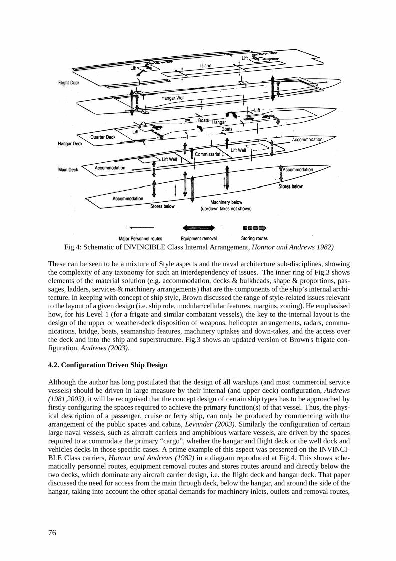
76
Fig.4: Schematic of INVINCIBLE Class Internal Arrangement, Honnor and Andrews 1982)
These can be seen to be a mixture of Style aspects and the naval architecture sub-disciplines, showing the complexity of any taxonomy for such an interdependency of issues. The inner ring of Fig.3 shows elements of the material solution (e.g. accommodation, decks & bulkheads, shape & proportions, pas-sages, ladders, services & machinery arrangements) that are the components of the ship’s internal archi-tecture. In keeping with concept of ship style, Brown discussed the range of style-related issues relevant to the layout of a given design (i.e. ship role, modular/cellular features, margins, zoning). He emphasised how, for his Level 1 (for a frigate and similar combatant vessels), the key to the internal layout is the design of the upper or weather-deck disposition of weapons, helicopter arrangements, radars, commu-nications, bridge, boats, seamanship features, machinery uptakes and down-takes, and the access over the deck and into the ship and superstructure. Fig.3 shows an updated version of Brown's frigate con-figuration, Andrews (2003). 4.2. Configuration Driven Ship Design Although the author has long postulated that the design of all warships (and most commercial service vessels) should be driven in large measure by their internal (and upper deck) configuration, Andrews (1981,2003), it will be recognised that the concept design of certain ship types has to be approached by firstly configuring the spaces required to achieve the primary function(s) of that vessel. Thus, the phys-ical description of a passenger, cruise or ferry ship, can only be produced by commencing with the arrangement of the public spaces and cabins, Levander (2003). Similarly the configuration of certain large naval vessels, such as aircraft carriers and amphibious warfare vessels, are driven by the spaces required to accommodate the primary “cargo”, whether the hangar and flight deck or the well dock and vehicles decks in those specific cases. A prime example of this aspect was presented on the INVINCI-BLE Class carriers, Honnor and Andrews (1982) in a diagram reproduced at Fig.4. This shows sche-matically personnel routes, equipment removal routes and stores routes around and directly below the two decks, which dominate any aircraft carrier design, i.e. the flight deck and hangar deck. That paper discussed the need for access from the main through deck, below the hangar, and around the side of the hangar, taking into account the other spatial demands for machinery inlets, outlets and removal routes,
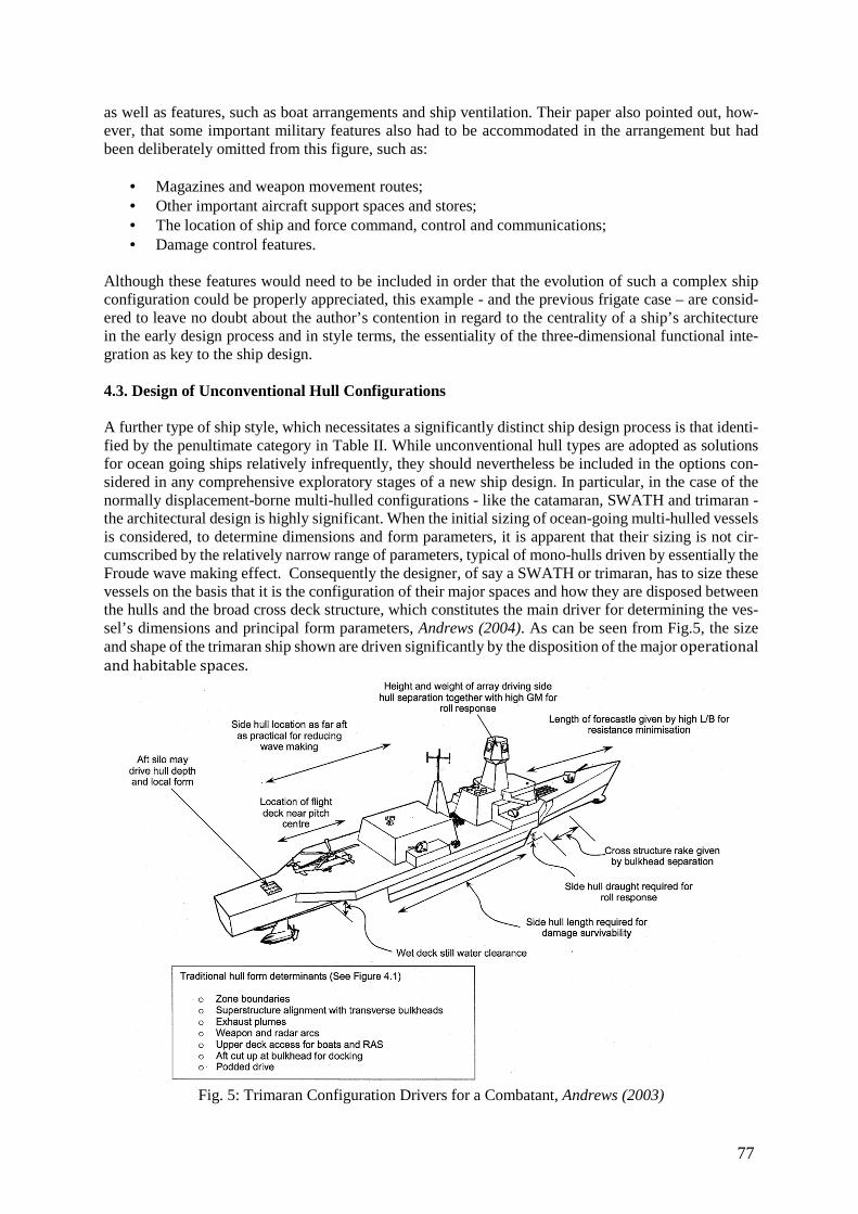
77
as well as features, such as boat arrangements and ship ventilation. Their paper also pointed out, how-ever, that some important military features also had to be accommodated in the arrangement but had been deliberately omitted from this figure, such as:
• Magazines and weapon movement routes; • Other important aircraft support spaces and stores; • The location of ship and force command, control and communications; • Damage control features.
Although these features would need to be included in order that the evolution of such a complex ship configuration could be properly appreciated, this example - and the previous frigate case – are consid-ered to leave no doubt about the author’s contention in regard to the centrality of a ship’s architecture in the early design process and in style terms, the essentiality of the three-dimensional functional inte-gration as key to the ship design. 4.3. Design of Unconventional Hull Configurations A further type of ship style, which necessitates a significantly distinct ship design process is that identi-fied by the penultimate category in Table II. While unconventional hull types are adopted as solutions for ocean going ships relatively infrequently, they should nevertheless be included in the options con-sidered in any comprehensive exploratory stages of a new ship design. In particular, in the case of the normally displacement-borne multi-hulled configurations - like the catamaran, SWATH and trimaran - the architectural design is highly significant. When the initial sizing of ocean-going multi-hulled vessels is considered, to determine dimensions and form parameters, it is apparent that their sizing is not cir-cumscribed by the relatively narrow range of parameters, typical of mono-hulls driven by essentially the Froude wave making effect. Consequently the designer, of say a SWATH or trimaran, has to size these vessels on the basis that it is the configuration of their major spaces and how they are disposed between the hulls and the broad cross deck structure, which constitutes the main driver for determining the ves-sel’s dimensions and principal form parameters, Andrews (2004). As can be seen from Fig.5, the size and shape of the trimaran ship shown are driven significantly by the disposition of the major operational
and habitable spaces.
Fig. 5: Trimaran Configuration Drivers for a Combatant, Andrews (2003)
78
5. Examples of UCL Concept Studies exploring aspects of Style This section gets results of investigations into a selected set of the topics in Table 1, which have been the subject of discrete ship design studies by the author’s research team at UCL over the last two dec-ades. The items outlined are not a comprehensive analysis of the Table I topics, but are intended to show how these various design issues are key design choices over which the ship designer ought to be more informed. Thus the designer could make the key first decision step in the ship design process summa-rised in Fig.1 more overtly and better informed, as a result of such studies for new ship designs.
• Margins An exploration into the validity of the Design Spiral, as a representation of the nature of ship design especially in ESSD, considered Growth and Board Margins for a naval combatant study, Andrews et al. (2012). Two distinct design styles were investigated: a conventional frigate style and a large hulled/small superstructure variant. The former showed a linear behaviour in solu-tion size with increasing Board Margin, while the latter showed a distinct step change in size with the same variable. Thus the choice of overall style was shown to be key to any such inves-tigations and was only revealed by the use of the DBB approach, rather than simple numerically ship synthesis, which had been undertaken on a frigate study several decades previously.
• Commercial structure versus Shock Robustness
In considering the extent to which commercial standards might be introduced into naval ship design, in the search for reductions in initial (procurement) cost, this UK EPSRC CASE funded project, Bradbeer and Andrews (2010) first considered the effect of missile attack on a small frigate built to commercial standards. It was found that survivability was affected by the density of outfitting, which could be considered a style decision, akin to building in robustness or adapt-ability. A second investigation, Bradbeer and Andrews (2012), looked at the effect of underwa-ter shock and varied the structural style from normal naval scantlings to commercial practice. This meant changing from closely spaced “Tee bar” stiffeners adopted to reduce the structural weight fraction to wider spaced larger bulb and flat bar stiffeners. The survivability to very high (hull lethality) shock levels due to adopting such differing scantling styles, yet with the same longitudinal bending strength, was found to be considerably less for the heavier but less struc-turally effective commercial style. This is an example of more detailed analysis than would normally be undertaken in ESSD, but reveals that a style decision taken early in design can make a major difference in a key ship’s capability, which has been seen to be fundamental in a naval combatant.
• Design for Production – design style dominated
In a research project funded by the UK Shipbuilders and Ship-repairers’ Association, Andrews et al. (2005) a study was undertaken on both commercial vessel and naval ship ESSD to improve the architecture of ships to reduce the cost of outfitting. This was a novel study in that much of large commercial ship cost is in steelwork, whereas for complex ships, such as the Offshore Support Vessel (OSV) and the Corvette in this study, much of the cost is in outfitting, and hence amenable to architectural exploration. The styles of both ship types were investigated, with re-arranged machinery location and more spacious passageways to fleet in modular cabins, respec-tively, which could be seen as specific style choices.
• Offshore Patrol Vessel (OPV) configuration Style
This ESSD investigation, Pawling and Andrews (2010), was undertaken to show that in addition to the conventional OPV, based on the style of small naval combatants, it was worth exploring more radical ship configurations, such as the OSV commercial design, a trimaran OPV and a very wide stern (Ramform like) mono-hull. These alternative configurations could be seen to be addressing style issues, such as commercial design style and different hull forms, in exploring solutions which might be more appropriate for stowing and deploying sizeable autonomous ve-hicles, especially launch and recovery from the vessel’s stern.
79
• Mothership Configuration/operational style A novel solution to the fast Littoral Combatant concept was seen to be the transporting of several small craft on a large fast vessel. This study, Andrews and Pawling (2004), presented some five radically different ship configurations with different launch and recovery methods (e.g. crane, heavy lift, well dock and stern gantry). These alternative styles were proposed to explore the operational options but clearly introduced distinct ship configurations which were both synthe-sised and the compared using the UCL DBB approach.
6. Recent Developments of Research into Ship Style A further feature of style is that, if it can influence multiple areas of design, then it must itself represent the “grouping” of multiple sources of information in some way. Developing an ontology and taxonomy for style is seen to offer potential advantages to the practice of ship concept design, as it could allow for more efficient storage, retrieval and application of potentially disparate pieces of information or deci-sions, Pawling et al. (2013). It has been proposed that this could be combined with the semi-automatic layout generation methods, such as that developed by TU Delft, van Oers (2011), to allow a broader exploration of the impact of stylistic decisions in ESSD than the point based architecturally design ap-proach using DBBs. From the some of the above examples of ship architecture, it is considered that these can be seen as highly stylistic, in that decisions such as the number of masts on a frigate, or how the various functions might be disposed around an enclosed hangar on an aircraft carrier (see Fig.3) are highly cross-cutting. This is because such style choices can have both direct and indirect impacts on a wide range of overall and detailed design features. There are seen to be two aspects where a more focused consideration of style might improve ESSD, Pawling et al. (2013). Firstly, the development of semi-automatic methods of generating sufficiently detailed designs but based on an initial crude layout, rather than ab initio and genetic algorithm based such as the TU Delft approach above, would allow the designer to better focus on the overall style of the arrangement. Secondly, a style taxonomy could be used as a method for describing and storing the data and rules that permit such semi-automatic tools to develop more detailed layouts. The designer could then apply a wide range of changes to a design by selecting a different style (e.g. different surviv-ability levels or extent of through life adaptability – see Table I). These could then be compared to give insights into major design and cost drivers in ESSD. 6.1. Proposed Integrated Approach to better Style driven design An approach, to better consideration of style choices, was made by the UCL team, in conjunction with its research partners the University of Michigan and TU Delft, Pawling et al. (2013). Current early stage design techniques for initial general arrangement definition focus predominantly on spatial compartment allocation. When evolving general arrangements, there is a lack of clarity, which should draw on the selected overall ship style, Fig.1. Given that style can be defined as the combination of whole ship performance metrics and local system metrics (see Table I), information is drawn from different do-mains, much of which may be ill-defined knowledge (such as HF aspects). Style is representative of design intent and the designer’s engineering judgment in the early stages of ship design constraint defi-nition, layout generation, and the evolving layout’s evaluations. With the ability to account for style definition, the designer could create concept designs that integrate a larger body of design intent, without the need to explicitly describe its characteristics. In an effort to incorporate style into the early stages of concept design, an iterative method using three primary levels in the design process was proposed. Fig.6 shows those levels as the style elucidation and input definition level, design layout generation method level, and post-generation style analysis level, respectively. Multiple components of coupled analysis would allow the cross cutting of knowledge to capture style attributes over multiple domains of the design within each level of the suggested process.
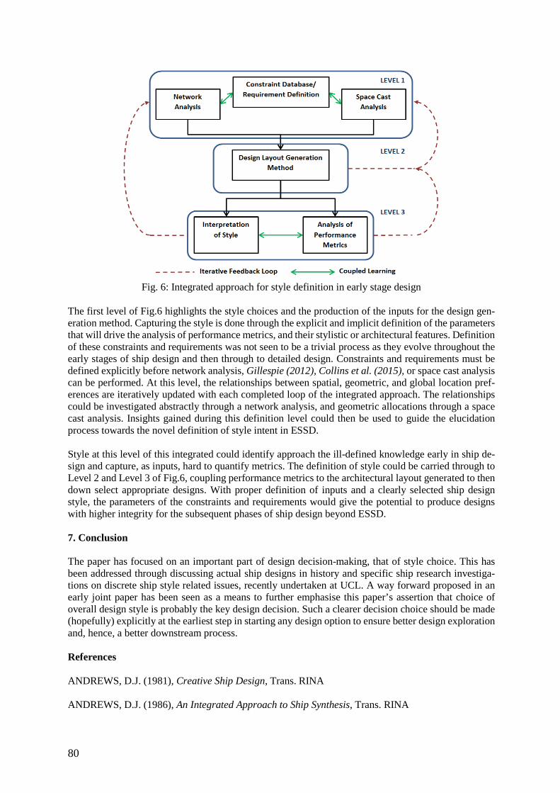
80
The first level of Fig.6 highlights the style choices and the production of the inputs for the design gen-eration method. Capturing the style is done through the explicit and implicit definition of the parameters that will drive the analysis of performance metrics, and their stylistic or architectural features. Definition of these constraints and requirements was not seen to be a trivial process as they evolve throughout the early stages of ship design and then through to detailed design. Constraints and requirements must be defined explicitly before network analysis, Gillespie (2012), Collins et al. (2015), or space cast analysis can be performed. At this level, the relationships between spatial, geometric, and global location pref-erences are iteratively updated with each completed loop of the integrated approach. The relationships could be investigated abstractly through a network analysis, and geometric allocations through a space cast analysis. Insights gained during this definition level could then be used to guide the elucidation process towards the novel definition of style intent in ESSD. Style at this level of this integrated could identify approach the ill-defined knowledge early in ship de-sign and capture, as inputs, hard to quantify metrics. The definition of style could be carried through to Level 2 and Level 3 of Fig.6, coupling performance metrics to the architectural layout generated to then down select appropriate designs. With proper definition of inputs and a clearly selected ship design style, the parameters of the constraints and requirements would give the potential to produce designs with higher integrity for the subsequent phases of ship design beyond ESSD. 7. Conclusion The paper has focused on an important part of design decision-making, that of style choice. This has been addressed through discussing actual ship designs in history and specific ship research investiga-tions on discrete ship style related issues, recently undertaken at UCL. A way forward proposed in an early joint paper has been seen as a means to further emphasise this paper’s assertion that choice of overall design style is probably the key design decision. Such a clearer decision choice should be made (hopefully) explicitly at the earliest step in starting any design option to ensure better design exploration and, hence, a better downstream process. References ANDREWS, D.J. (1981), Creative Ship Design, Trans. RINA ANDREWS, D.J. (1986), An Integrated Approach to Ship Synthesis, Trans. RINA
Fig. 6: Integrated approach for style definition in early stage design

81
ANDREWS, D.J. (1994), Preliminary Warship Design, Trans. RINA ANDREWS, D.J. (2003), A creative approach to ship architecture, Int. J. Maritime Eng. 145, Discussion and Author’s response in Int. J. Maritime Eng. 146 (2004) ANDREWS, D.J. (2004), Multi-Hulled Vessels, Ch.46 of "Ship Design and Construction", SNAME ANDREWS, D.J. (2013), The true nature of ship concept design – And what it means for the future development of CASD, 14th COMPIT Conf., Cortona ANDREWS, D.J.; PAWLING, R. (2003), SURFCON – A 21st century ship design tool, 8th Int. Marine Design Conf. (IMDC), Athens ANDREWS, D.J.; PAWLING, R. (2004), Fast motherships - A design challenge, RINA Conf. ‘Warship 2004: Littoral Warfare & the Expeditionary Force’, London ANDREWS, D.J.; BURGER, D.; ZHANG, J.W. (2005), Design for production using the design building block approach, Int. J. Maritime Eng. 147 ANDREWS, D.J.; DUCHATEAU, E.A.E.; GILLESPE, J.W.; HOPMAN, J.J.; PAWLING, R.G.; SINGER, D.J. (2012), Design for Layout, in DforX State of Art Report, 11th Int. Marine Design Conf. (IMDC), Glasgow BRADBEER, N.; ANDREWS, D.J. (2010), Vulnerability of a low cost combatant converted from a merchant ship, Int. Naval Eng. Conf. (INEC), Portsmouth BRADBEER, N.; ANDREWS, D.J. (2012), Shock response implications of lower-cost warship struc-tural styles, 11th Int. Marine Design Conf. (IMDC), Glasgow BROADBENT, G. (1988), Design in Architecture: Architecture and the Human Sciences, David Fulton BROWN, D.K. (1987), The architecture of frigates, RINA Symp. Anti-Submarine Warfare, London BROWN, D.K.; ANDREWS, D.J. (1980), The design of cheap warships, Int. Naval Technology Expo 80, Rotterdam, (Reprinted in J. Naval Science April 1981) COLLINS, L.; ANDREWS, D.; PAWLING, R. (2015), A new approach for the incorporation of radical technologies: Rim drive for large submarines, 12th Int. Marine Design Conf. (IMDC), Tokyo, pp.587-606 GILLESPIE, J.W. (2012), A network science approach to understanding and generating ship arrange-ments in early-stage design, PhD thesis, University of Michigan HMSO (1989), Supplementary Estimates Vote 1, Class II: Payments to Harland & Wolff PLC, House of Commons Defence Committee, Minutes of Evidence, 29th Nov 1989 HONNOR, A.F.; ANDREWS, D.J. (1982), HMS INVINCIBLE The first of a new genus of aircraft car-rying ships, Trans RINA Vol. 124 HUTCHINSON, G.A. (1981), Study of Internal configuration of Ships, MSc thesis, UCL KING, A.S. (1985), CAD Layout Exploration, MSc thesis, UCL LEVANDER, K. (2003), Innovative ship design, 8th Int. Marine Design Conf. (IMDC), Athens

82
PARKER, J. (2016), An Independent Report to Inform the UK National Shipbuilding Strategy, London, PAWLING, R.; ANDREWS, D.J. (2010), Three innovative OPV designs incorporating a modular pay-load for UXVs, RINA Conf. ‘Warship 2010: Advanced Technologies for Naval Design and Construc-tion’, London PAWLING, R.; ANDREWS, D.J.; PIKS, R.; SINGER, D.J.; DUCHATEAU, E.A.E.; HOPMAN, J.J. (2013), An integrated approach to style definition in early stage ship design, 14th COMPIT Conf., Cor-tona, pp. 248-263 ROACH, J.C.; MEIER, H.A. (1979), Visual effectiveness in modern warship design, Naval Eng. J. 91/6, pp.19-32 TUPPER, E.C. (2013), An Introduction to Naval Architecture, Butterworth-Heinemann VAN OERS, B. (2011), A packing approach for the early stage design of service vessels, PhD thesis, TU Delft
83
Big Data Analysis for Service Performance Evaluation and Ship Design
Hideo Orihara, Japan Marine United Corporation, Tsu/Japan, [email protected] Hisafumi Yoshida, Japan Marine United Corporation, Tsu/Japan, [email protected]
Ichiro Amaya, Japan Marine United Corporation, Tsu/Japan, [email protected]
Abstract
This paper describes our experiences in big data analysis of on-board ship performance monitoring data for the evaluation of ship’s service performance and the feedback to ship design. Full-scale performance monitoring and analysis method devised at Japan Marine United Corporation is presented, which has been developed mainly for the performance evaluation of large merchant ships in service, and which have been found to give satisfactory practical results over a number of years. Monitored full-scale performance data is analysed in a similar way as that employed in ship’s speed trials and the results are compared with performance predictions conducted at the design and development stages. Performance evaluations are made for a large bulk carrier. It is shown that by employing the newly developed monitoring and performance analysis method, full-scale performance can be evaluated with high degree of confidence and its results can effectively utilized in the ship design stage.
1. Introduction In recent years, large-size on-board performance data which cannot be obtained for commercial use in the past has become available for ship’s service performance analysis. Whilst these data may not be regarded strictly as Big Data as generally recognized, they possess similar characteristics as Big Data and require special data analysis procedures to deal with. Big Data is usually characterized by 3 Vs including “Volume”, “Velocity” and “Variety” which require specific technology and analytical methods for its transformation into value. From the ship performance monitoring point of view, posset ions of 3 Vs-like features can be admitted in the context in the drastic change in technologies in the on-board monitoring. In terms of “Volume”, growth in monitoring data size has been noticeable. Until quite recently service performance monitoring, in particular hull performance monitoring, has been conducted mainly from abstract logs or noon-report data with a daily sampling rate. At the present time, however, continuous automatic monitoring has increasingly employed and high-frequency monitoring with sampling rate of 1 Hz and above has been common practice on normal merchant vessels. Along with the increase in sampling rate, a size of monitoring items is also increased from the past normal practice of around 10 items to more than 100 items. As a result, a size of monitoring data has increased by an order of 106 and above over the past norm. As for “Velocity”, this is generally defined as availability of data in real-time manner. Recent service performance monitoring technology with the use of automatic data transmission capability to shore-side users follows exactly this definition. As for “Variety”, this denotes variety of data type and data source. Tendency to collect performance data from normal on-board equipment (such as VDR, EMS) bring about similar challenges concerning the way to deal with the variations in data collected. To cope with these radical transformations in on-board performance monitoring environment, we have established new monitoring and analysis procedures which can deal with the large size data. For on-board monitoring and automatic data transmission to the shore-side users, we have developed “Sea-Navi” voyage support system for on-board performance monitoring, Orihara and Yoshida (2010), Orihara et al..(2016). Monitoring is conducted continuously of items including ship’s position, speed, power, fuel consumption and weather conditions. Monitored performance data are statistically analysed in the on-board sub-system in an automatic manner for the specified duration of time to reduce data size and cost for analysis work. Statistically analysed data are sent shore-side sub-system and examined by means of physics-based rigorous analysis methods as will be described in the present study.
84
Reverting to the physical nature of ship’s service performance, In the course of its normal duties, merchant ships in service are continuously exposed to a variety of disturbances which can in one way or another affects its performance. In a seaway, wind and wave conditions combine to increase the propulsive performance necessary to maintain economical service speed. In addition, intentional steering and manoeuvring motion result in noticeable changes in performance from that in steady advancing on straight course. The full-scale performance of large merchant ships has long been predicted by extrapolating model-scale tank test results using some combination of correlation factors accounting for the scale effects between model and ship. Whilst this performance evaluation procedures has been effective for some ship types for which full-scale performance can be verified by new-building speed trials conducted in designed laden condition (e.g. tankers) and its results can be readily fed back to prediction at the design stage, accuracy of performance prediction is usually deteriorated considerably for most types of large merchant ships for which new-building speed trials are conducted only in light-load condition. So, for these types of ships, full-scale performance verification is compelled to rely on service performance data. It has been frequently stated that full-scale on-board performance data are so unreliable and inconsistent that, having in mind that the large amount of work involved for eliminate the effects of many disturbing factors, the detailed analysis of such data is not worthwhile compared to the analysis of new-building speed trials data, but this has not been the author’s experience. It is true that the performance data recorded on board is subject to the effects of a variety of disturbances and difficult to apply to detailed analysis on hydrodynamic bases. However, when a sufficient amount of data is available and appropriate analysis methods such as those presented in this paper is employed, high-quality performance evaluation with a comparable accuracy as those from normal new-building speed trials can be obtained. In any case, it is apparent that the final criterion of ship performance must obviously be the results that are consistently monitored and analysed in service, and the ship designer should finally accept this position. Service performance monitoring and analysis has long history and has been utilized for the management of ship operations over the years. Several works have been done in service performance analysis by utilizing abstract log data, e.g. Telfer (1926), Clements (1957), Logan (1960). In recent years, “Big Data Analysis” like works based on detailed on-board performance monitoring data which is similar to the present work has been reported, Furustam (2016), Gundemann and Dirksen (2016), Gunnsteinsoson and Clausen (2016), Solonen (2016). Most of these reference works are conducted mainly from a ship owner/operator’s point of view, and attentions has been devoted to the evaluation of the rate of ship’s performance deteriorations due to fouling and wind and wave disturbances with a time after delivery or out of dock. Whilst these evaluations are quite useful for economical operation of merchant ships, from the ship design point of view, more detailed service performance analysis applicable to the verification of design performance predictions. In normal full-scale ship performance predictions conducted at design stage, ship’s performance is evaluated under strictly defined weather conditions. In normal practice at the present day, still-water condition which means no wind and no waves are principal weather conditions for performance evaluation. In addition to it, specifically defined weather conditions such as Beaufort wind force scale based weather conditions are employed for the performance in a seaway. Thus the primary consideration in this paper is placed on the evaluation of full-scale performance under these specifically defined weather conditions and the verification of the design performance predictions. The next section describes the on-board monitoring system employed in the present full-scale perfor-mance analysis method. Then, the physics-based full-scale performance analysis method is described. After that, effectiveness of the proposed full-scale performance monitoring and analysis method is examined by evaluating the analysis results obtained on a bulk carrier in fully loaded condition in both still water and seaway. Analysed full-scale results are compared with performance characteristics predicted at the design and development stage. Brief conclusions are presented in the final section.
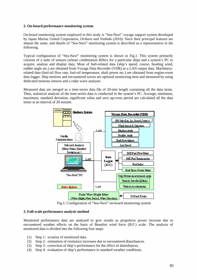
85
2. On-board performance monitoring system On-board monitoring system employed in this study is “Sea-Navi” voyage support system developed by Japan Marine United Corporation, Orihara and Yoshida (2010). Since their principal features are almost the same, and details of “Sea-Navi” monitoring system is described as a representative in the following. Typical configuration of “Sea-Navi” monitoring system is shown in Fig.1. This system primarily consists of a suite of sensors (whose combination differs for a particular ship) and a system’s PC to acquire, analyse and display data. Most of hull-related data (ship’s speed, course, heading wind, rudder angle etc.) are obtained from Voyage Data Recorder (VDR) as a LAN output data. Machinery-related data (fuel-oil flow rate, fuel-oil temperature, shaft power etc.) are obtained from engine-room data logger. Ship motions and encountered waves are optional monitoring item and measured by using dedicated motions sensors and a radar wave analyser. Measured data are merged as a time-series data file of 20-min length containing all the data items. Then, statistical analysis of the time-series data is conducted in the system’s PC. Average, minimum, maximum, standard deviation, significant value and zero up-cross period are calculated all the data items at an interval of 20-minute.
Fig.1: Configuration of “Sea-Navi” on-board monitoring system
3. Full-scale performance analysis method Monitored performance data are analysed to give results as propulsive power increase due to encountered weather effects on the basis of Beaufort wind force (B.F.) scale. The analysis of monitored data is divided into the following four steps:
(1) Step 1: scrutiny of monitored data. (2) Step 2: estimation of resistance increases due to encountered disturbances. (3) Step 3: correction of ship’s performance for the effect of disturbances. (4) Step 4: evaluation of ship’s performance in standard weather conditions.

86
3.1. Scrutiny of monitored data In order to remove uncertainty of data and conduct the analysis under equivalent basis to the extent possible, certain group of monitored data is selected for the analysis. For the performance analysis on still-water condition (i.e. no wind and wave condition), following criteria are specified in the data scrutiny:
(1) Propeller revolutions are greater than those corresponding to minimum output of the main engine capable of continuous running to eliminate the data during at excessively slow speeds such as harbour manoeuvres.
(2) Difference in propeller revolution during certain duration of time is within certain threshold value of maximum propeller revolution corresponding to MCO to eliminate the data during accelerating or decelerating operations.
(3) Average and standard deviation of rudder angle during certain duration of time are within certain threshold values to eliminate the data during intentional steering operations.
(4) True wind speed is less than certain threshold value to eliminate data under strong winds. (5) Significant wave height is less certain threshold value to eliminate data in large waves (6) Pitch and roll angle are less than certain threshold values to eliminate data in rough weather
conditions For the performance analysis in standard wind and wave conditions, only (1)~(3) of the above criteria is imposed. 3.2. Estimation of resistance increases due to encountered disturbances Ship’s resistance increases due to environmental and external disturbances such as wind, waves, steering and drifting are estimated. Resistance increase due to wind (dRWIND) is calculated by
( ) ( ){ }22,, 0
2
1GAARWINDRWINDAATaWIND VCVCAdR ⋅−⋅Ψ⋅⋅= ρ (1)
where ρa is the mass density of air, AT is the transverse projected area above the waterline including superstructure, CAA() is the wind resistance coefficient; CAA(0) means the wind coefficient in head wind, ΨWIND,R is the relative wind direction, VWIND,R is the relative wind speed, VG is the ship’s speed over ground. The wind resistance coefficient is based on the data derived from model tests in wind tunnel or data calculated by the method in ISO15016_ 2015, ISO (2015). Resistance increase due to wave (dRWAVE) is presented as a summation of resistance increases due to wind waves and swell and calculated by
( ){ WDWVmWDWVWDAWWDWVwWAVE TCHL
BgdR ,,
22
,χρ ⋅⋅
⋅⋅= ( ) }SWLLSWLLSLAWSWLL TCH ,,
2 χ⋅+ (2)
where ρw is the mass density of water, g is the acceleration of gravity, B is the ship’s breadth, L is the ship’s length, HWDWV is the significant height of wind waves, HSWLL is the height of swell, CAW,WD() is the coefficient for the added resistance due to wind waves, CAW,SL() is the coefficient for the added resistance due to swell, χWDWV is the encounter angle of wind waves; 0 means head waves, χSWLL is the encounter angle of swell; 0 means head swell, Tm,WDWV is the mean period of wind waves, TSWLL is the period of swell. CAW,WD() and CAW,SL() are calculated by linear superposition of the directional wave spectrum and the response function of the mean resistance increase in regular waves. Response function of the mean wave resistance increase in regular waves is based on the data derived from tests in ship model basin or data calculated by the method in ISO15016_ 2015, ISO (2015).
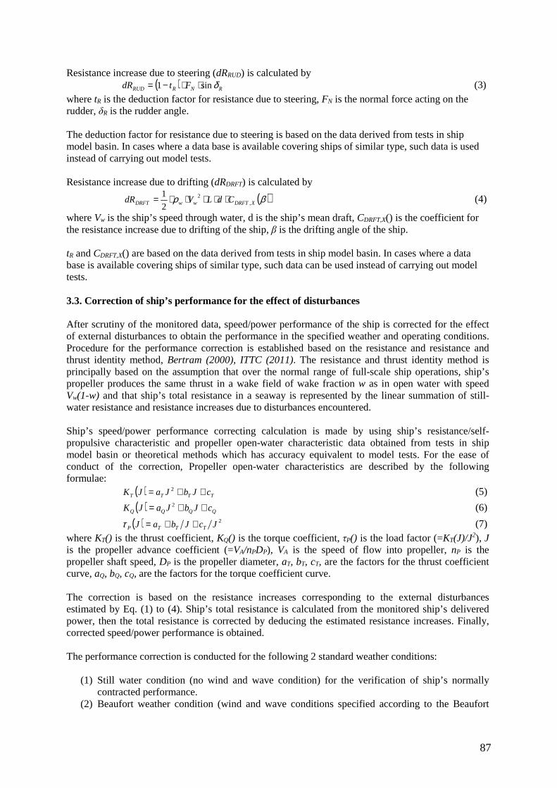
87
Resistance increase due to steering (dRRUD) is calculated by ( ) RNRRUD FtdR δsin1 ⋅⋅−= (3) where tR is the deduction factor for resistance due to steering, FN is the normal force acting on the rudder, δR is the rudder angle. The deduction factor for resistance due to steering is based on the data derived from tests in ship model basin. In cases where a data base is available covering ships of similar type, such data is used instead of carrying out model tests. Resistance increase due to drifting (dRDRFT) is calculated by
( )βρ XDRFTwwDRFT CdLVdR ,2
2
1 ⋅⋅⋅⋅⋅= (4)
where Vw is the ship’s speed through water, d is the ship’s mean draft, CDRFT,X() is the coefficient for the resistance increase due to drifting of the ship, β is the drifting angle of the ship. tR and CDRFT,X() are based on the data derived from tests in ship model basin. In cases where a data base is available covering ships of similar type, such data can be used instead of carrying out model tests. 3.3. Correction of ship’s performance for the effect of disturbances After scrutiny of the monitored data, speed/power performance of the ship is corrected for the effect of external disturbances to obtain the performance in the specified weather and operating conditions. Procedure for the performance correction is established based on the resistance and resistance and thrust identity method, Bertram (2000), ITTC (2011). The resistance and thrust identity method is principally based on the assumption that over the normal range of full-scale ship operations, ship’s propeller produces the same thrust in a wake field of wake fraction w as in open water with speed Vw(1-w) and that ship’s total resistance in a seaway is represented by the linear summation of still-water resistance and resistance increases due to disturbances encountered. Ship’s speed/power performance correcting calculation is made by using ship’s resistance/self-propulsive characteristic and propeller open-water characteristic data obtained from tests in ship model basin or theoretical methods which has accuracy equivalent to model tests. For the ease of conduct of the correction, Propeller open-water characteristics are described by the following formulae:
( ) TTTT cJbJaJK ++= 2 (5)
( ) QQQQ cJbJaJK ++= 2 (6)
( ) 2JcJbaJ TTTP ++=τ (7) where KT() is the thrust coefficient, KQ() is the torque coefficient, τP() is the load factor (=KT(J)/J2), J is the propeller advance coefficient (=VA/nPDP), VA is the speed of flow into propeller, nP is the propeller shaft speed, DP is the propeller diameter, aT, bT, cT, are the factors for the thrust coefficient curve, aQ, bQ, cQ, are the factors for the torque coefficient curve. The correction is based on the resistance increases corresponding to the external disturbances estimated by Eq. (1) to (4). Ship’s total resistance is calculated from the monitored ship’s delivered power, then the total resistance is corrected by deducing the estimated resistance increases. Finally, corrected speed/power performance is obtained. The performance correction is conducted for the following 2 standard weather conditions:
(1) Still water condition (no wind and wave condition) for the verification of ship’s normally contracted performance.
(2) Beaufort weather condition (wind and wave conditions specified according to the Beaufort
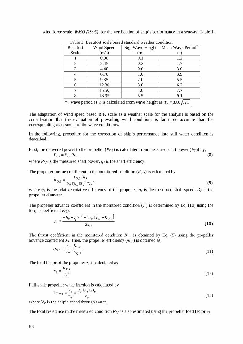
88
wind force scale, WMO (1995), for the verification of ship’s performance in a seaway, Table 1.
Table 1: Beaufort scale based standard weather condition Beaufort
Scale Wind Speed
(m/s) Sig. Wave Height
(m) Mean Wave Period*
(s) 1 0.90 0.1 1.2 2 2.45 0.2 1.7 3 4.40 0.6 3.0 4 6.70 1.0 3.9 5 9.35 2.0 5.5 6 12.30 3.0 6.7 7 15.50 4.0 7.7 8 18.95 5.5 9.1
* : wave period (Tm) is calculated from wave height as Wm HT 86.3=.
The adaptation of wind speed based B.F. scale as a weather scale for the analysis is based on the consideration that the evaluation of prevailing wind conditions is far more accurate than the corresponding assessment of the wave conditions. In the following, procedure for the correction of ship’s performance into still water condition is described. First, the delivered power to the propeller (PD,S) is calculated from measured shaft power (PS,S) by,
SSSSD PP η⋅= ,, (8)
where PS,S is the measured shaft power, ηS is the shaft efficiency. The propeller torque coefficient in the monitored condition (KQ,S) is calculated by
53,
,2 Psw
RSDSQ
Dn
PK
⋅⋅⋅
⋅=
ρπη
(9)
where ηR is the relative rotative efficiency of the propeller, nS is the measured shaft speed, DP is the propeller diameter. The propeller advance coefficient in the monitored condition (JS) is determined by Eq. (10) using the torque coefficient KQ,S,
( )Q
SQQQQQS a
KcabbJ
2
4 ,2 −⋅−−−
= (10)
The thrust coefficient in the monitored condition KT,S is obtained by Eq. (5) using the propeller advance coefficient JS. Then, the propeller efficiency (ηO,S) is obtained as,
SQ
STSSO K
KJ
,
,, 2
⋅=π
η (11)
The load factor of the propeller τS is calculated as
2,
S
STS
J
K=τ
(12)
Full-scale propeller wake fraction is calculated by
w
PSS
w
aS V
DnJ
V
Vw
⋅⋅==−1
(13)
where Vw is the ship’s speed through water. The total resistance in the measured condition RT,S is also estimated using the propeller load factor τS:
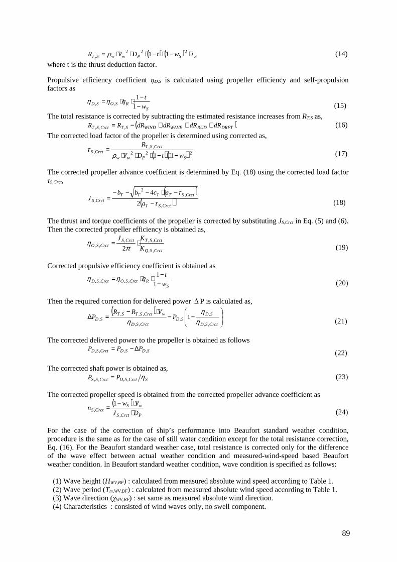
89
( ) ( ) SSPwwST wtDVR τρ ⋅−⋅−⋅⋅⋅= 222, 11 (14)
where t is the thrust deduction factor. Propulsive efficiency coefficient ηD,S is calculated using propeller efficiency and self-propulsion factors as
SRSOSD w
t
−−⋅⋅=
1
1,, ηηη
(15)
The total resistance is corrected by subtracting the estimated resistance increases from RT,S as, ( )DRFTRUDWAVEWINDSTCrctST dRdRdRdRRR +++−= ,,, (16)
The corrected load factor of the propeller is determined using corrected as,
( ) ( )222,,
,11 SPww
CrctSTCrctS
wtDV
R
−⋅−⋅⋅⋅=
ρτ
(17)
The corrected propeller advance coefficient is determined by Eq. (18) using the corrected load factor τS,Crct,
( )( )CrctST
CrctSTTTTCrctS a
acbbJ
,
,2
, 2
4
ττ
−
−⋅−−−=
(18)
The thrust and torque coefficients of the propeller is corrected by substituting JS,Crct in Eq. (5) and (6). Then the corrected propeller efficiency is obtained as,
CrctSQ
CrctSTCrctSCrctSO K
KJ
,,
,,,,, 2
⋅=π
η (19)
Corrected propulsive efficiency coefficient is obtained as
SRCrctSOCrctSD w
t
−−⋅⋅=
1
1,,,, ηηη
(20)
Then the required correction for delivered power ΔP is calculated as, ( )
−−
⋅−=∆
CrctSD
SDSD
CrctSD
wCrctSTSTSD P
VRRP
,,
,,
,,
,,,, 1
ηη
η (21)
The corrected delivered power to the propeller is obtained as follows
SDSDCrctSD PPP ,,,, ∆−= (22)
The corrected shaft power is obtained as,
SCrctSDCrctSS PP η,,,, = (23) The corrected propeller speed is obtained from the corrected propeller advance coefficient as
( )PCrctS
wSCrctS DJ
Vwn
⋅⋅−
=,
,1
(24)
For the case of the correction of ship’s performance into Beaufort standard weather condition, procedure is the same as for the case of still water condition except for the total resistance correction, Eq. (16). For the Beaufort standard weather case, total resistance is corrected only for the difference of the wave effect between actual weather condition and measured-wind-speed based Beaufort weather condition. In Beaufort standard weather condition, wave condition is specified as follows: (1) Wave height (HWV,BF) : calculated from measured absolute wind speed according to Table 1. (2) Wave period (Tm,WV,BF) : calculated from measured absolute wind speed according to Table 1. (3) Wave direction (χWV,BF) : set same as measured absolute wind direction. (4) Characteristics : consisted of wind waves only, no swell component.
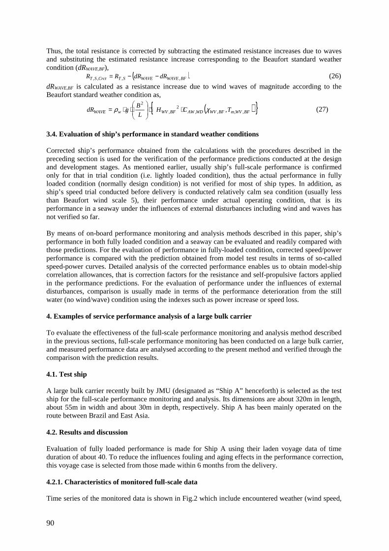
90
Thus, the total resistance is corrected by subtracting the estimated resistance increases due to waves and substituting the estimated resistance increase corresponding to the Beaufort standard weather condition (dRWAVE,BF),
( )BFWAVEWAVESTCrctST dRdRRR ,,,, −−= (26)
dRWAVE,BF is calculated as a resistance increase due to wind waves of magnitude according to the Beaufort standard weather condition as,
( ){ }BFWVmBFWVWDAWBFWVwWAVE TCHL
BgdR ,,,,
2,
2
,χρ ⋅⋅
⋅⋅=
(27)
3.4. Evaluation of ship’s performance in standard weather conditions Corrected ship’s performance obtained from the calculations with the procedures described in the preceding section is used for the verification of the performance predictions conducted at the design and development stages. As mentioned earlier, usually ship’s full-scale performance is confirmed only for that in trial condition (i.e. lightly loaded condition), thus the actual performance in fully loaded condition (normally design condition) is not verified for most of ship types. In addition, as ship’s speed trial conducted before delivery is conducted relatively calm sea condition (usually less than Beaufort wind scale 5), their performance under actual operating condition, that is its performance in a seaway under the influences of external disturbances including wind and waves has not verified so far. By means of on-board performance monitoring and analysis methods described in this paper, ship’s performance in both fully loaded condition and a seaway can be evaluated and readily compared with those predictions. For the evaluation of performance in fully-loaded condition, corrected speed/power performance is compared with the prediction obtained from model test results in terms of so-called speed-power curves. Detailed analysis of the corrected performance enables us to obtain model-ship correlation allowances, that is correction factors for the resistance and self-propulsive factors applied in the performance predictions. For the evaluation of performance under the influences of external disturbances, comparison is usually made in terms of the performance deterioration from the still water (no wind/wave) condition using the indexes such as power increase or speed loss. 4. Examples of service performance analysis of a large bulk carrier To evaluate the effectiveness of the full-scale performance monitoring and analysis method described in the previous sections, full-scale performance monitoring has been conducted on a large bulk carrier, and measured performance data are analysed according to the present method and verified through the comparison with the prediction results. 4.1. Test ship A large bulk carrier recently built by JMU (designated as “Ship A” henceforth) is selected as the test ship for the full-scale performance monitoring and analysis. Its dimensions are about 320m in length, about 55m in width and about 30m in depth, respectively. Ship A has been mainly operated on the route between Brazil and East Asia. 4.2. Results and discussion Evaluation of fully loaded performance is made for Ship A using their laden voyage data of time duration of about 40. To reduce the influences fouling and aging effects in the performance correction, this voyage case is selected from those made within 6 months from the delivery. 4.2.1. Characteristics of monitored full-scale data Time series of the monitored data is shown in Fig.2 which include encountered weather (wind speed,
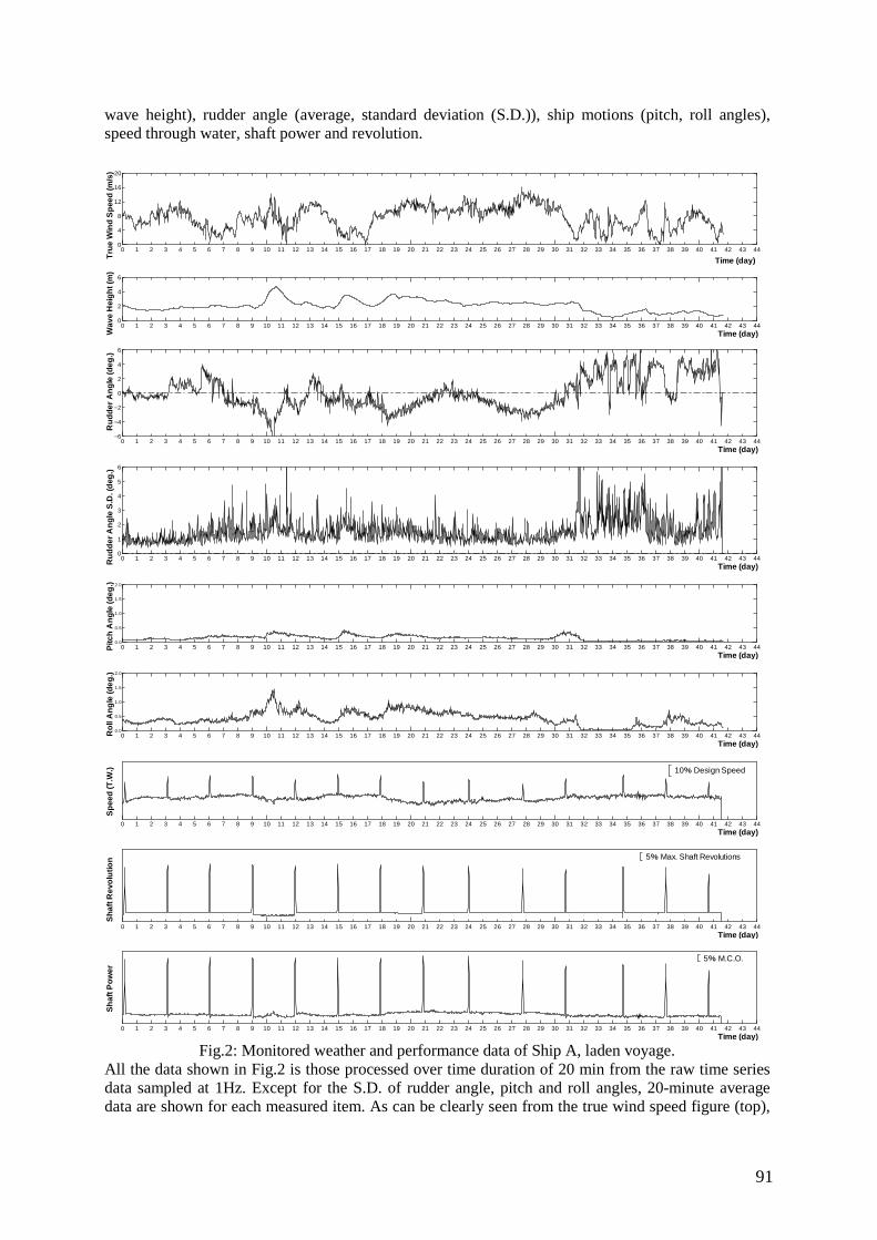
91
wave height), rudder angle (average, standard deviation (S.D.)), ship motions (pitch, roll angles), speed through water, shaft power and revolution.
Fig.2: Monitored weather and performance data of Ship A, laden voyage.
All the data shown in Fig.2 is those processed over time duration of 20 min from the raw time series data sampled at 1Hz. Except for the S.D. of rudder angle, pitch and roll angles, 20-minute average data are shown for each measured item. As can be clearly seen from the true wind speed figure (top),
0 1 2 3 4 5 6 7 8 9 10 11 12 13 14 15 16 17 18 19 20 21 22 23 24 25 26 27 28 29 30 31 32 33 34 35 36 37 38 39 40 41 42 43 440
4
8
12
16
20
Time (day)Tru
e W
ind
Sp
eed
(m/s
)
0 1 2 3 4 5 6 7 8 9 10 11 12 13 14 15 16 17 18 19 20 21 22 23 24 25 26 27 28 29 30 31 32 33 34 35 36 37 38 39 40 41 42 43 440
2
4
6
Wav
e H
eig
ht (
m)
Time (day)
0 1 2 3 4 5 6 7 8 9 10 11 12 13 14 15 16 17 18 19 20 21 22 23 24 25 26 27 28 29 30 31 32 33 34 35 36 37 38 39 40 41 42 43 44−6
−4
−2
0
2
4
6
Ru
dd
er A
ng
le (d
eg.)
Time (day)
0 1 2 3 4 5 6 7 8 9 10 11 12 13 14 15 16 17 18 19 20 21 22 23 24 25 26 27 28 29 30 31 32 33 34 35 36 37 38 39 40 41 42 43 440
1
2
3
4
5
6
Ru
dd
er A
ng
le S
.D. (
deg
.)
Time (day)
0 1 2 3 4 5 6 7 8 9 10 11 12 13 14 15 16 17 18 19 20 21 22 23 24 25 26 27 28 29 30 31 32 33 34 35 36 37 38 39 40 41 42 43 440.0
0.5
1.0
1.5
2.0
Pitc
h A
ng
le (d
eg.)
Time (day)
0 1 2 3 4 5 6 7 8 9 10 11 12 13 14 15 16 17 18 19 20 21 22 23 24 25 26 27 28 29 30 31 32 33 34 35 36 37 38 39 40 41 42 43 440.0
0.5
1.0
1.5
2.0
Ro
ll A
ng
le (d
eg.)
Time (day)
0 1 2 3 4 5 6 7 8 9 10 11 12 13 14 15 16 17 18 19 20 21 22 23 24 25 26 27 28 29 30 31 32 33 34 35 36 37 38 39 40 41 42 43 44
Time (day)
Sp
eed
(T.W
.) 10% Design Speed
0 1 2 3 4 5 6 7 8 9 10 11 12 13 14 15 16 17 18 19 20 21 22 23 24 25 26 27 28 29 30 31 32 33 34 35 36 37 38 39 40 41 42 43 44
Time (day)
Sh
aft R
evo
lutio
n 5% Max. Shaft Revolutions
0 1 2 3 4 5 6 7 8 9 10 11 12 13 14 15 16 17 18 19 20 21 22 23 24 25 26 27 28 29 30 31 32 33 34 35 36 37 38 39 40 41 42 43 44
Time (day)
Sh
aft P
ow
er
5% M.C.O.
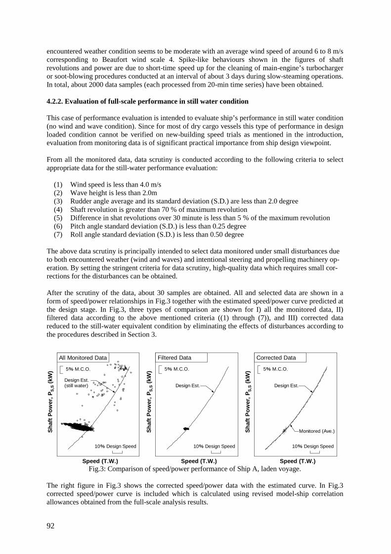
92
encountered weather condition seems to be moderate with an average wind speed of around 6 to 8 m/s corresponding to Beaufort wind scale 4. Spike-like behaviours shown in the figures of shaft revolutions and power are due to short-time speed up for the cleaning of main-engine’s turbocharger or soot-blowing procedures conducted at an interval of about 3 days during slow-steaming operations. In total, about 2000 data samples (each processed from 20-min time series) have been obtained. 4.2.2. Evaluation of full-scale performance in still water condition This case of performance evaluation is intended to evaluate ship’s performance in still water condition (no wind and wave condition). Since for most of dry cargo vessels this type of performance in design loaded condition cannot be verified on new-building speed trials as mentioned in the introduction, evaluation from monitoring data is of significant practical importance from ship design viewpoint. From all the monitored data, data scrutiny is conducted according to the following criteria to select appropriate data for the still-water performance evaluation:
(1) Wind speed is less than 4.0 m/s (2) Wave height is less than 2.0m (3) Rudder angle average and its standard deviation (S.D.) are less than 2.0 degree (4) Shaft revolution is greater than 70 % of maximum revolution (5) Difference in shat revolutions over 30 minute is less than 5 % of the maximum revolution (6) Pitch angle standard deviation (S.D.) is less than 0.25 degree (7) Roll angle standard deviation (S.D.) is less than 0.50 degree
The above data scrutiny is principally intended to select data monitored under small disturbances due to both encountered weather (wind and waves) and intentional steering and propelling machinery op-eration. By setting the stringent criteria for data scrutiny, high-quality data which requires small cor-rections for the disturbances can be obtained. After the scrutiny of the data, about 30 samples are obtained. All and selected data are shown in a form of speed/power relationships in Fig.3 together with the estimated speed/power curve predicted at the design stage. In Fig.3, three types of comparison are shown for I) all the monitored data, II) filtered data according to the above mentioned criteria ((1) through (7)), and III) corrected data reduced to the still-water equivalent condition by eliminating the effects of disturbances according to the procedures described in Section 3.
Fig.3: Comparison of speed/power performance of Ship A, laden voyage.
The right figure in Fig.3 shows the corrected speed/power data with the estimated curve. In Fig.3 corrected speed/power curve is included which is calculated using revised model-ship correlation allowances obtained from the full-scale analysis results.
Sh
aft
Po
wer
, PS
,S (
kW)
Speed (T.W.)
10% Design Speed
5% M.C.O.
All Monitored Data
Design Est. (still water)
Sh
aft
Po
wer
, P
S,S
(kW
)
Speed (T.W.)
10% Design Speed
5% M.C.O.
Filtered Data
Design Est.
Sh
aft
Po
wer
, P
S,S
(kW
)
Speed (T.W.)
10% Design Speed
5% M.C.O.
Corrected Data
Design Est.
Monitored (Ave.)
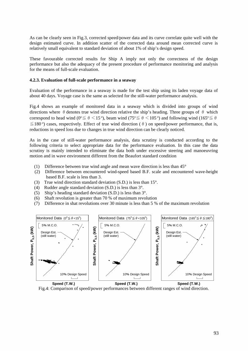
93
As can be clearly seen in Fig.3, corrected speed/power data and its curve correlate quite well with the design estimated curve. In addition scatter of the corrected data around mean corrected curve is relatively small equivalent to standard deviation of about 1% of ship’s design speed. These favourable corrected results for Ship A imply not only the correctness of the design performance but also the adequacy of the present procedure of performance monitoring and analysis for the means of full-scale evaluation. 4.2.3. Evaluation of full-scale performance in a seaway Evaluation of the performance in a seaway is made for the test ship using its laden voyage data of about 40 days. Voyage case is the same as selected for the still-water performance analysis. Fig.4 shows an example of monitored data in a seaway which is divided into groups of wind directions where θdenotes true wind direction relative the ship’s heading. Three groups of θ which correspond to head wind (0o
≦θ<15 o), beam wind (75o≦θ<105 o) and following wind (165o≦θ≦180 o) cases, respectively. Effect of true wind direction (θ) on speed/power performance, that is, reductions in speed loss due to changes in true wind direction can be clearly noticed. As in the case of still-water performance analysis, data scrutiny is conducted according to the following criteria to select appropriate data for the performance evaluation. In this case the data scrutiny is mainly intended to eliminate the data both under excessive steering and manoeuvring motion and in wave environment different from the Beaufort standard condition
(1) Difference between true wind angle and mean wave direction is less than 45° (2) Difference between encountered wind-speed based B.F. scale and encountered wave-height
based B.F. scale is less than 3. (3) True wind direction standard deviation (S.D.) is less than 15°. (4) Rudder angle standard deviation (S.D.) is less than 3°. (5) Ship’s heading standard deviation (S.D.) is less than 3°. (6) Shaft revolution is greater than 70 % of maximum revolution (7) Difference in shat revolutions over 30 minute is less than 5 % of the maximum revolution
Fig.4: Comparison of speed/power performances between different ranges of wind direction.
Sh
aft
Po
wer
, P
S,S
(kW
)
Speed (T.W.)
10% Design Speed
5% M.C.O.
Monitored Data
Design Est. (still water)
(0o≦θ<15o)
Sh
aft
Po
wer
, P
S,S
(kW
)
Speed (T.W.)
10% Design Speed
5% M.C.O.
Monitored Data
Design Est. (still water)
(75o≦θ<105o)
Sh
aft
Po
wer
, P
S,S
(kW
)
Speed (T.W.)
10% Design Speed
5% M.C.O.
Monitored Data
Design Est. (still water)
(165o≦θ≦180o)
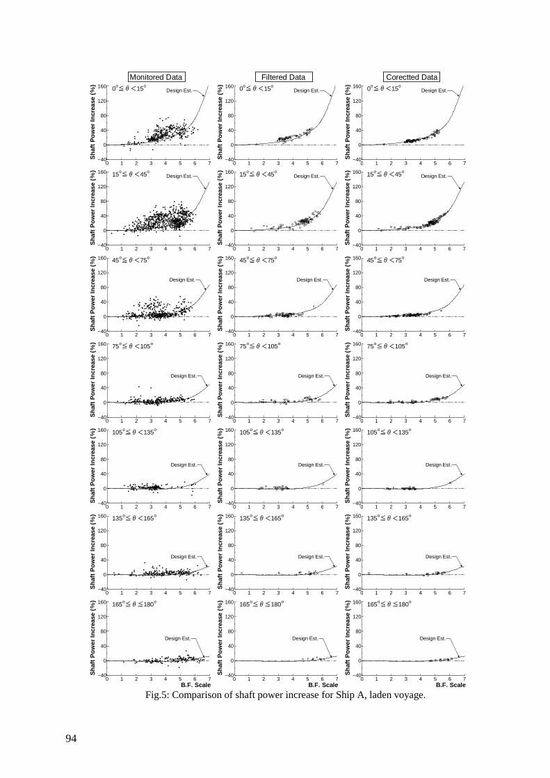
94
Fig.5: Comparison of shaft power increase for Ship A, laden voyage.
0 1 2 3 4 5 6 7−40
0
40
80
120
160 0o≦θ<15o
Sh
aft
Po
wer
Incr
ease
(%
)Design Est.
Monitored Data
0 1 2 3 4 5 6 7−40
0
40
80
120
160 0o≦θ<15o
Sh
aft
Po
wer
Incr
ease
(%
)
Design Est.
Filtered Data
0 1 2 3 4 5 6 7−40
0
40
80
120
160 0o≦θ<15o
Sh
aft
Po
wer
Incr
ease
(%
)
Design Est.
Corectted Data
0 1 2 3 4 5 6 7−40
0
40
80
120
160 15o≦θ<45o
Sh
aft
Po
wer
Incr
ease
(%
)
Design Est.
0 1 2 3 4 5 6 7−40
0
40
80
120
160 15o≦θ<45o
Sh
aft
Po
wer
Incr
ease
(%
)
Design Est.
0 1 2 3 4 5 6 7−40
0
40
80
120
160 15o≦θ<45o
Sh
aft
Po
wer
Incr
ease
(%
)
Design Est.
0 1 2 3 4 5 6 7−40
0
40
80
120
160 45o≦θ<75o
Sh
aft
Po
wer
Incr
ease
(%
)
Design Est.
0 1 2 3 4 5 6 7−40
0
40
80
120
160 45o≦θ<75o
Sh
aft
Po
wer
Incr
ease
(%
)
Design Est.
0 1 2 3 4 5 6 7−40
0
40
80
120
160 45o≦θ<75o
Sh
aft
Po
wer
Incr
ease
(%
)
Design Est.
0 1 2 3 4 5 6 7−40
0
40
80
120
160 75o≦θ<105o
Sh
aft
Po
wer
Incr
ease
(%
)
Design Est.
0 1 2 3 4 5 6 7−40
0
40
80
120
160 75o≦θ<105o
Sh
aft
Po
wer
Incr
ease
(%
)
Design Est.
0 1 2 3 4 5 6 7−40
0
40
80
120
160 75o≦θ<105o
Sh
aft
Po
wer
Incr
ease
(%
)
Design Est.
0 1 2 3 4 5 6 7−40
0
40
80
120
160 105o≦θ<135o
Sh
aft
Po
wer
Incr
ease
(%
)
Design Est.
0 1 2 3 4 5 6 7−40
0
40
80
120
160 105o≦θ<135o
Sh
aft
Po
wer
Incr
ease
(%
)
Design Est.
0 1 2 3 4 5 6 7−40
0
40
80
120
160 105o≦θ<135o
Sh
aft
Po
wer
Incr
ease
(%
)
Design Est.
0 1 2 3 4 5 6 7−40
0
40
80
120
160 135o≦θ<165o
Sh
aft
Po
wer
Incr
ease
(%
)
Design Est.
0 1 2 3 4 5 6 7−40
0
40
80
120
160 135o≦θ<165o
Sh
aft
Po
wer
Incr
ease
(%
)
Design Est.
0 1 2 3 4 5 6 7−40
0
40
80
120
160 135o≦θ<165o
Sh
aft
Po
wer
Incr
ease
(%
)
Design Est.
0 1 2 3 4 5 6 7−40
0
40
80
120
160 165o≦θ≦180o
B.F. Scale
Sh
aft
Po
wer
Incr
ease
(%
)
Design Est.
0 1 2 3 4 5 6 7−40
0
40
80
120
160 165o≦θ≦180o
B.F. Scale
Sh
aft
Po
wer
Incr
ease
(%
)
Design Est.
0 1 2 3 4 5 6 7−40
0
40
80
120
160 165o≦θ≦180o
B.F. Scale
Sh
aft
Po
wer
Incr
ease
(%
)
Design Est.
95
In this case of analysis, ship’s performance corrected for the difference of weather disturbances due to waves. That is, resistance increase due to waves is adjusted by substituting the estimated resistance increase under actual wave condition with that corresponding to the Beaufort standard condition based on the encountered true wind speed by means of Eq. (16). Corrected performance under Beaufort standard weather condition is evaluated in terms of shaft power increase which denotes the percent increase of power relative to the power in still water at same ship’s speed through water. Comparison of corrected performance with estimated shaft power increase curve is shown in Fig.5 for a group of wind/wave directions. In Fig.5, shaft power increase is presented against true-wind speed based B.F. scale. Three types of data consisting of raw monitored data (●), filtered data (○) and corrected data (□) are shown in the left, centre and right graph, respectively. By applying the scrutiny criteria ((1) through (7)), data size is reduced to about 50 percent of original data. Differences between filtered (○) and corrected (□) stand for the effect due to difference in wave conditions between actual weather and the Beaufort standard weather which assumes fully developed wind waves. Principle reasons for the corrections applied in this analysis are the effects of swell and the differences of mean periods and encounter directions of waves. In the case where swell effect is predominant, corrected sea margin is noticeably reduced from the monitored data. On the other hand, in the case where encounter directions of wind and waves differ by large amount, correction can be large because the resistance increase due to waves changes significantly with encounter angle. If the wave encounter direction is small (close to bow) than the encounter wave direction, wave resistance increase is corrected to a smaller value than that corresponding to the actual encountered wave condition. As shown in shown in Fig.5, corrected shaft power increases correlate quite well with the estimated curves. Also noted is that the corrections of shaft power increase data due to the difference in wave conditions is relatively small which is the order of corrections are less than 10% for most of filtered data. This implies that there exists a noticeable difference in wave conditions between actual weather and monitored wind-speed based Beaufort standard wave condition, and that ship’s performance evaluation in a seaway should be conducted by imposing stringent scrutiny criteria considering the actual wave conditions instead of evaluation solely based on wind-speed based Beaufort weather condition. These reasonable agreements between corrected results with the estimations in terms of shaft power increase in a seaway under wide range of wind and wave conditions imply that ship’s performance in service can be estimated using the present prediction approach which is based on the resistance and thrust identity method. Also should be stressed is that the speed/power performance is affected significantly from the effect of encountered waves and that the accurate evaluation of those effect is crucial in enhancing the accuracy of full-scale performance monitoring and analysis. 5. Conclusions In this paper, full-scale performance of large merchant ships is evaluated by means of newly developed on-board performance monitoring method. Full-scale performance monitoring and analysis method based on on-board performance monitoring has been developed for the performance evaluation of large merchant ships in service. Monitored full-scale performance data is analysed in a similar way as that employed in ship’s speed trials and the results are compared with performance predictions conducted at design and development stage. Performance evaluations are made in terms of still-water performance and seaway performance for a variety of 3 merchant ships of large bulk carrier. It is shown that by employing present monitoring and performance procedures, full-scale performance can be evaluated with high degree of confidence and its results can effectively utilized to improve the accuracy of performance predictions at design stage.

96
References BERTRAM, V. (2000), Practical Ship Hydrodynamics, Butterworth-Heinemann CLEMENTS, R.E. (1957). A method of analysing voyage data, Trans. North East Coast Inst. of Engineers & Shipbuilders 73/4, pp.197-230 FURUSTAM, J. (2016). On ways to collect and utilize data from ship operation in naval architecture, 15th Int. Conf. on Computer and IT Applications in the Maritime Industries (COMPIT), Lecce, pp.430-438 GUNDEMANN, D.; DIRKSEN, T. (2016). A statistical study of propulsion performance of ships and the effects of dry dockings, hull cleanings and propeller polishes on performance, 1st Hull Performance & Insight Conf. (HullPIC), Castello di Pavone, pp.282-291 GUNNSTEINSSON, S.; CLAUSEN, J.W. (2016). Enhancing performance through continuous monitoring, 15th Int. Conf. on Computer and IT Applications in the Maritime Industries (COMPIT), Lecce, pp.471-480 ISO15016_2015 (2015), Ships and marine technology – Guideline for the assessment of speed and power performance by analysis of speed trial data, Int. Standard Org. ITTC/RP.7.5.-02-07-02.2 (2011), ITTC-Recommended Procedures, Prediction of Power Increase in Irregular waves from Model Test, Int. Towing Tank Symp. LOGAN, A. (1960), Service performance of a fleet of tankers, Trans. North East Coast Inst. of Engineers & Shipbuilders 76/7, pp.s61-s78 ORIHARA, H.; YOSHIDA, H. (2010). Development of voyage support system “Sea-Navi” for lower fuel consumption and CO2 emissions, Int. Symp. on Ship Design and Operation for Environmental Sustainability, London, pp.315-328 ORIHARA, H.; YOSHIDA, H.; AMAYA, I (2016). Evaluation of full-scale performance of large merchant ships by means of on-board performance monitoring, 26th Int. Ocean and Polar Eng. Conf., Rhodes SOLONEN, A. (2016). Experiences with ISO-19030 and Beyond, 1st Hull Performance & Insight Conf. (HullPIC), Castello di Pavone, pp.152-162 TELFER, E.V. (1926), The practical analysis of merchant ship trials and service performance, Trans. North East Coast Inst. of Engineers & Shipbuilders 43/2, pp.123-177 WMO (1995), Manual of Codes, International Codes, Volume I.1, Part A-Alphanumeric Codes, WMO-No.306, World Meteorological Org.
97
Case Study - Totem Fully Autonomous Navigation System
Azriel Rahav, Totem plus, Ramat HaSharon/Israel, [email protected]
Abstract
The Totem Autonomous Navigation System enables a USV to operate on the waters without a crew
even when the vessel is without radio contact. The vessel can be operated in a fully autonomous way
with route keeping, collision avoidance and danger/obstruction avoidance capabilities as well as
interception functionality: (1) The built in, fully approved ECDIS uses vector electronic charts and
provides powerful route planning, monitoring capabilities and interception ability. The system can be
configured for the task in advance or change the task during the voyage by the control station. (2) The
integrated Track control system keeps the vessel on a selected pre-determined route with unlimited
number of waypoints. The route can be regular, cyclic, ASR etc. Dangers and cautions along the track
are automatically avoided. (3) Collision and Obstruction Avoidance capabilities: the system enables
safe sailing by automatically avoiding danger from collisions and obstructions. This aim is achieved
by analyzing automatically ALL the targets and obstructions within the selected range around the
ship, and applying change of course to steer or speed as required. The stipulations of the COLREGS
are taken into account and the advice is complying in full with the COLREGS. The system categorizes
the targets according to their status (crossing, overtaking, head-on etc.) and applies the requirements
of the COLREGS (Give Way, Stand On etc.) according to the required parameters. The system can
handle a multiple vessels scenario. Dangers along the new course are avoided automatically. (4)
Interception functionality: This function enables the user of the Control Station (CS) to select a
specific target on the map, and instruct the system to intercept it. The system calculates continuously
the required Intercept Course and Speed and follows the target according to its changing parameters.
1. Introduction
In a world quickly entering an era of driverless cars, or at least talking about it, it is only a matter of
time before the maritime industry will be faced with Unmanned Surface Vessels. Such USVs start
from remotely controlled vessels (without autonomous capability) and go all the way to fully
autonomous vessels, with a combination of both in the interim.
The incentive for unmanned ships can come from several aspects. The shipping community is faced
with rising difficulties to obtain good officers and crews, the life onboard is becoming less and less
appealing to young people, cost of crew are always a major expense, unfortunately humans tend to err
- and errors at sea result in lives lost and loss of assets. During 2013 alone there were more than 10
collisions between ships, more than 150 seamen lost their lives and more than 1000 tons of heavy fuel
polluted the sea - most of those accidents were attributed to Human Error; e.g. Allianz estimates 80%
of marine casualties are down to human error, NN (2015); Rothblum et al. (2002) estimate 75-96% of
marine casualties are caused, at least in part, by some form of human error. Further, certain tasks are
best done without risking people, for example patrolling in rough weather or mine sweeping in
dangerous waters.
Totem Plus is active in the Autonomous Vessels field for few years, during which the Totem
Autonomous Navigation System (TANS) was fine tuned to offer full autonomous control of a fast
unmanned craft. The TANS can provide track control for various pre-defined routes, offer obstruction
avoidance and collision avoidance by course and speed control, and much more. The system can be
fully autonomous but can also be remote controlled from a command center by radio communication.
2. Totem Autonomous Navigation System
Totem Autonomous Navigation System is based on Totem ECDIS, short for “Electronic Chart
Display and Information System”, with the additional features of track control, Collision Avoidance,
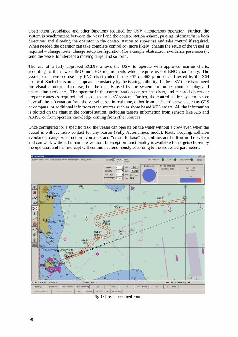
98
Obstruction Avoidance and other functions required for USV autonomous operation. Further, the
system is synchronized between the vessel and the control station ashore, passing information in both
directions and allowing the operator in the control station to supervise and take control if required.
When needed the operator can take complete control or (more likely) change the setup of the vessel as
required – change route, change setup configuration (for example obstruction avoidance parameters) ,
send the vessel to intercept a moving target and so forth.
The use of a fully approved ECDIS allows the USV to operate with approved marine charts,
according to the newest IMO and IHO requirements which require use of ENC charts only. The
system can therefore use any ENC chart coded in the S57 or S63 protocol and tested by the S64
protocol. Such charts are also updated constantly by the issuing authority. In the USV there is no need
for visual monitor, of course, but the data is used by the system for proper route keeping and
obstruction avoidance. The operator in the control station can see the chart, and can add objects or
prepare routes as required and pass it to the USV system. Further, the control station system ashore
have all the information from the vessel at sea in real time, either from on-board sensors such as GPS
or compass, or additional info from other sources such as shore based VTS radars. All the information
is plotted on the chart in the control station, including targets information from sensors like AIS and
ARPA, or from operator knowledge coming from other sources.
Once configured for a specific task, the vessel can operate on the water without a crew even when the
vessel is without radio contact for any reason (Fully Autonomous mode). Route keeping, collision
avoidance, danger/obstruction avoidance and “return to base” capabilities are built-in in the system
and can work without human intervention. Interception functionality is available for targets chosen by
the operator, and the intercept will continue autonomously according to the requested parameters.
Fig.1: Pre-determined route
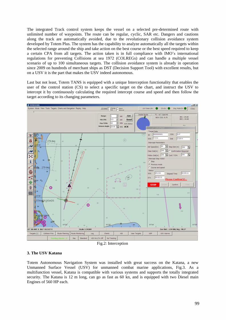
99
The integrated Track control system keeps the vessel on a selected pre-determined route with
unlimited number of waypoints. The route can be regular, cyclic, SAR etc. Dangers and cautions
along the track are automatically avoided, due to the revolutionary collision avoidance system
developed by Totem Plus. The system has the capability to analyze automatically all the targets within
the selected range around the ship and take action on the best course or the best speed required to keep
a certain CPA from all targets. The action taken is in full compliance with IMO’s international
regulations for preventing Collisions at sea 1972 (COLREGs) and can handle a multiple vessel
scenario of up to 100 simultaneous targets. The collision avoidance system is already in operation
since 2009 on hundreds of merchant ships as DST (Decision Support Tool) with excellent results, but
on a USV it is the part that makes the USV indeed autonomous.
Last but not least, Totem TANS is equipped with a unique Interception functionality that enables the
user of the control station (CS) to select a specific target on the chart, and instruct the USV to
intercept it by continuously calculating the required intercept course and speed and then follow the
target according to its changing parameters.
Fig.2: Interception
3. The USV Katana
Totem Autonomous Navigation System was installed with great success on the Katana, a new
Unmanned Surface Vessel (USV) for unmanned combat marine applications, Fig.3. As a
multifunction vessel, Katana is compatible with various systems and supports the totally integrated
security. The Katana is 12 m long, can go as fast as 60 kn, and is equipped with two Diesel main
Engines of 560 HP each.
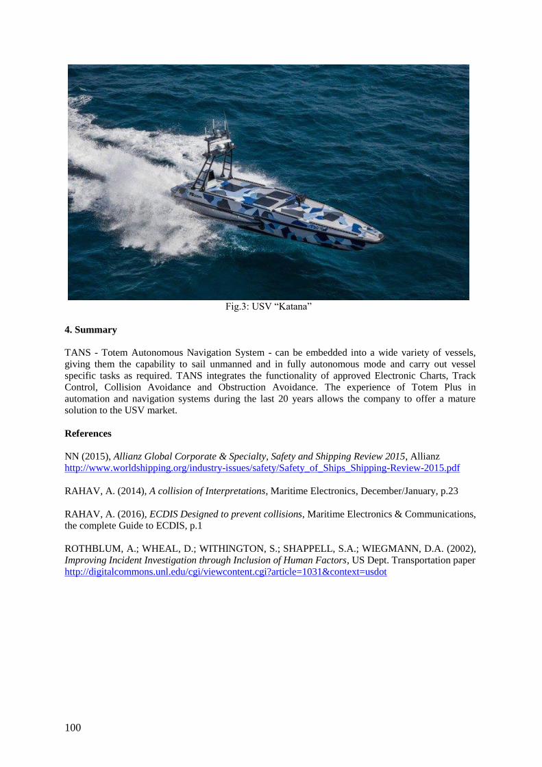
100
Fig.3: USV “Katana”
4. Summary
TANS - Totem Autonomous Navigation System - can be embedded into a wide variety of vessels,
giving them the capability to sail unmanned and in fully autonomous mode and carry out vessel
specific tasks as required. TANS integrates the functionality of approved Electronic Charts, Track
Control, Collision Avoidance and Obstruction Avoidance. The experience of Totem Plus in
automation and navigation systems during the last 20 years allows the company to offer a mature
solution to the USV market.
References
NN (2015), Allianz Global Corporate & Specialty, Safety and Shipping Review 2015, Allianz
http://www.worldshipping.org/industry-issues/safety/Safety_of_Ships_Shipping-Review-2015.pdf
RAHAV, A. (2014), A collision of Interpretations, Maritime Electronics, December/January, p.23
RAHAV, A. (2016), ECDIS Designed to prevent collisions, Maritime Electronics & Communications,
the complete Guide to ECDIS, p.1
ROTHBLUM, A.; WHEAL, D.; WITHINGTON, S.; SHAPPELL, S.A.; WIEGMANN, D.A. (2002),
Improving Incident Investigation through Inclusion of Human Factors, US Dept. Transportation paper
http://digitalcommons.unl.edu/cgi/viewcontent.cgi?article=1031&context=usdot
101
Cutting-Edge Underwater Robotics - CADDY Project Challenges, Results and Future Steps
Marco Bibuli , CNR-ISSIA, Genova/Italy, [email protected]
Gabriele Bruzzone, CNR-ISSIA, Genova/Italy, [email protected] Massimo Caccia, CNR-ISSIA, Genova/Italy, [email protected]
Davide Chiarella, CNR-ISSIA, Genova/Italy, [email protected] Roberta Ferretti, CNR-ISSIA, Genova/Italy, [email protected]
Angelo Odetti, CNR-ISSIA, Genova/Italy, [email protected] Andrea Ranieri, CNR-ISSIA, Genova/Italy, [email protected]
Enrica Zereik, CNR-ISSIA, Genova/Italy, [email protected]
Abstract
This paper describes results from the EU research project CADDY on cognitive autonomous robotics to support divers. The robot communicates with the diver by understanding gestures and acknowledges by light signals and task execution. Validation trials showed feasibility of the approach. In order to successfully achieve these beyond-the-state-of-the-art objectives, a number of specific features and functionalities have been designed and developed from scratch, integrated in the overall CADDY architecture and finally tested for validation. This paper focuses on the development on some of the game-changing techniques needed to face the scientific challenges of the projects. 1. Introduction The FP7 CADDY (Cognitive Autonomous Diving Buddy) project is funded by the European Com-mission and was started in January 2014, Miskovic et al. (2015). Seven partner institutions (University of Zagreb, Croatia; National Research Council, Italy; Instituto Superior Tecnico, Portugal; University of Newcastle, UK; Jacobs University, Germany; University of Vienna, Austria; Divers Alert Network Europe, Malta) came together to pursue collaborative R&D work aimed at enhancing cognitive robot-ics in the underwater arena; specifically, to develop robots capable of cooperating with divers. The main motivation for the CADDY project, Bibuli et al. (2016), was the fact that divers operate in harsh and poorly monitored environments in which the slightest unexpected disturbance, technical malfunction, or lack of attention can have catastrophic consequences. They manoeuvre in complex 3D environments and carry cumbersome equipment while performing their missions. To overcome these problems, CADDY aims to establish an innovative set–up between a diver and companion autono-mous robots (underwater and surface) that exhibit cognitive behaviour through learning, interpreting, and adapting to the diver’s behaviour, physical state, and actions. The CADDY framework, Fig.1, is composed by three components: an autonomous surface vehicle, an autonomous underwater vehicle, and the diver. The autonomous surface vehicle is responsible for communicating with the diver and the autonomous underwater robot, as well as serving as a commu-nication relay link to a command centre. It also plays the key role of navigation aid for the underwater agents – it must adapt its motion to optimize communication efficiency and navigational accuracy of underwater agents. The autonomous underwater vehicle, on the other hand, manoeuvres near the div-er, and exhibits cognitive behaviour with regard to the diver actions by determining the diver’s inten-tions and the state of the diver’s body. The CADDY project replaces a human buddy diver with an autonomous underwater vehicle and adds a new autonomous surface vehicle to improve monitoring, assistance, and safety of the diver’s mis-sion. The resulting system plays a threefold role similar to those that a human buddy diver should have:
i) the buddy “observer” that continuously monitors the diver;
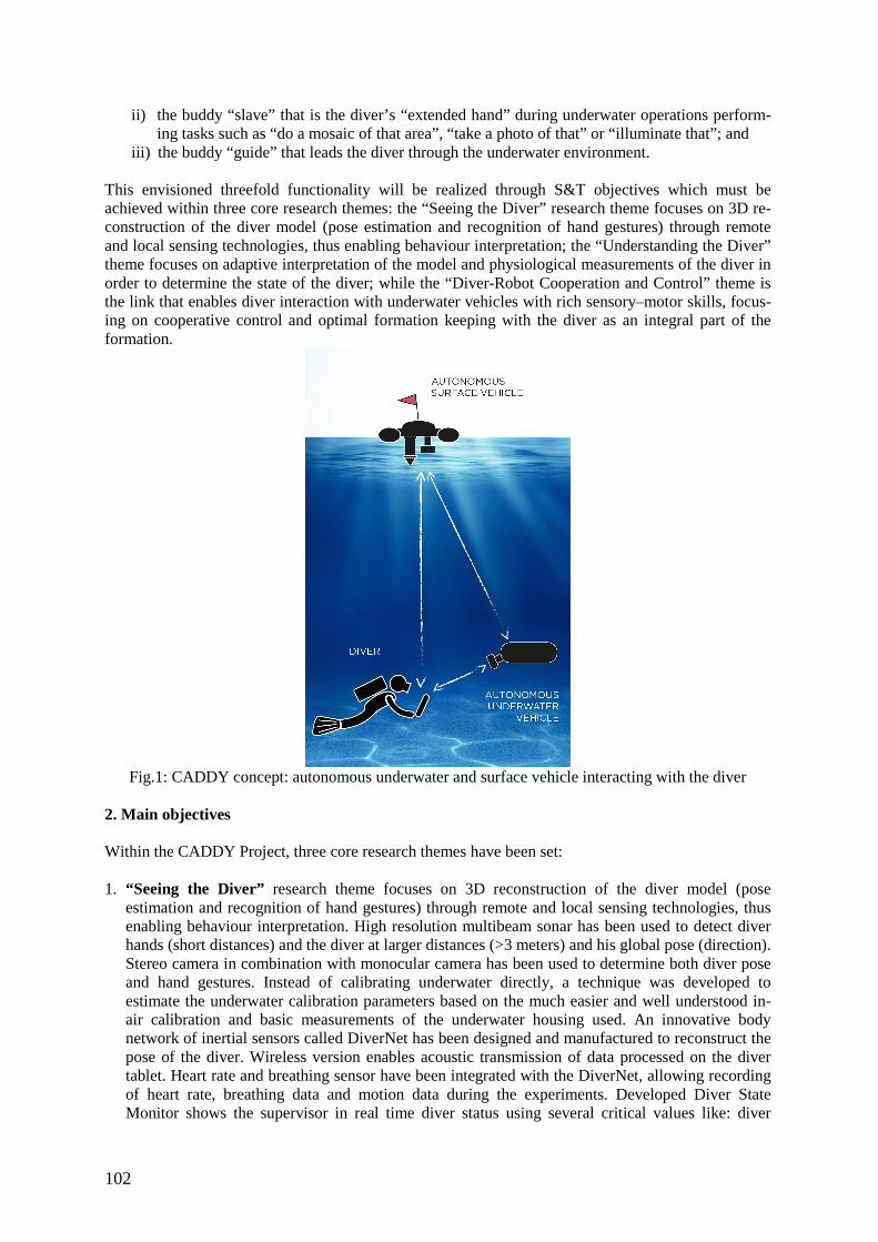
102
ii) the buddy “slave” that is the diver’s “extended hand” during underwater operations perform-ing tasks such as “do a mosaic of that area”, “take a photo of that” or “illuminate that”; and
iii) the buddy “guide” that leads the diver through the underwater environment. This envisioned threefold functionality will be realized through S&T objectives which must be achieved within three core research themes: the “Seeing the Diver” research theme focuses on 3D re-construction of the diver model (pose estimation and recognition of hand gestures) through remote and local sensing technologies, thus enabling behaviour interpretation; the “Understanding the Diver” theme focuses on adaptive interpretation of the model and physiological measurements of the diver in order to determine the state of the diver; while the “Diver-Robot Cooperation and Control” theme is the link that enables diver interaction with underwater vehicles with rich sensory–motor skills, focus-ing on cooperative control and optimal formation keeping with the diver as an integral part of the formation.
Fig.1: CADDY concept: autonomous underwater and surface vehicle interacting with the diver
2. Main objectives Within the CADDY Project, three core research themes have been set: 1. “Seeing the Diver” research theme focuses on 3D reconstruction of the diver model (pose
estimation and recognition of hand gestures) through remote and local sensing technologies, thus enabling behaviour interpretation. High resolution multibeam sonar has been used to detect diver hands (short distances) and the diver at larger distances (>3 meters) and his global pose (direction). Stereo camera in combination with monocular camera has been used to determine both diver pose and hand gestures. Instead of calibrating underwater directly, a technique was developed to estimate the underwater calibration parameters based on the much easier and well understood in-air calibration and basic measurements of the underwater housing used. An innovative body network of inertial sensors called DiverNet has been designed and manufactured to reconstruct the pose of the diver. Wireless version enables acoustic transmission of data processed on the diver tablet. Heart rate and breathing sensor have been integrated with the DiverNet, allowing recording of heart rate, breathing data and motion data during the experiments. Developed Diver State Monitor shows the supervisor in real time diver status using several critical values like: diver
103
depth, average flipper rate, heart rate, breathing rate, motion rate, PAD space, diver state alarms, and predefined chat messages.
2. “Understanding the Diver” theme focuses on adaptive interpretation of the model and physiological measurements of the diver to determine the state of the diver. Artificial neural networks were trained using the DiverNet data do detect different diver activities such as standing, sitting, T-pose, etc. Accuracy of around 90% was achieved allowing to transmit only this high-level diver activity data to the surface. A multilayer perceptron was trained to predict pleasure, arousal and control using breath rate, heart rate and motion rate measurements. This approach proved successful with classification rates reaching from 60% (dominance/control high) to only 18% (pleasure, neutral). Overall classification score was 40%. Language of communication between the diver and the robot based on gestures, called CADDIAN, has been developed – a total of 52 symbols have been defined, together with the “slang” group of symbols for better acceptance by the diving community. A fault tolerant symbolic language interpreter was developed, allowing robust interpretation of the commands issued by the diver to BUDDY. The following set of algorithms have been developed: hand gesture recognition using stereo camera imagery based on feature aggregation algorithm developed to cope with the highly variant underwater imagery; hand detection using multibeam sonar imagery to detect the number of extended diver fingers within sonar imagery; algorithms for diver pose recognition and localization from mono and stereo imagery, and algorithms for diver pose and localization recognition using the sonar to determine diver position and orientation relative to the BUDDY AUV.
3. “Diver-Robot Cooperation and Control” theme is the link that enables diver interaction with underwater vehicles with rich sensory-motor skills, focusing on cooperative control and optimal formation keeping with the diver, as an integral part of the formation. Diver-AUV cooperative controller was developed to ensure that the AUV is positioned in front of the diver regardless of the diver’s orientation. Diver-AUV-USV formation control was developed to ensure the surface vehicle is in an area close-by to improve, among other things, the acoustic communications with the underwater agents, while avoiding being on top of them, for safety purposes. Single beacon navigation algorithms based on extremum seeking and Fisher Matrix Inversion approach was implemented for navigation using only ranging devices, without angle measurements. Automatic selection system for the execution of the proper autonomous robotic tasks was developed with the aim of providing a compliant behaviour of the overall robotic system, with respect to the command issued by the diver. Modular framework of the mission controller based on Petri nets was designed and developed with the aim of managing the state tracking, task activations and reference generation that fulfils the requirements to support the diver operations.
In order to successfully achieve these beyond-the-state-of-the-art objectives, a number of specific features and functionalities have been designed and developed from scratch, integrated in the overall CADDY architecture and finally tested for validation. This paper focuses on the development on some of the game-changing techniques needed to face the scientific challenges of the projects. 3. Video-based diver recognition To comply with the requirement of diver operation support, the overall CADDY system must be able to detect and recognize the diver in the underwater environment. The problem is two-fold: i) the robotic system has firstly to be able to detect the diver pose, in such a way to move and position itself to some specific relative position with respect to the diver (usually the robot is required to stand in front of the diver to guarantee the recognition of hand gesture based commands as well as to be visible to the diver allowing safe operations); ii) the robotic platform requires the capability to recognize the hand-gesture commands issued by the diver in order to trigger the execution of specific mission operations. 3.1 Diver pose estimation Diver orientation estimation by means of stereo camera imagery was implemented for obtaining a pose estimation measure through computation on-board the AUV to perform a relative positioning
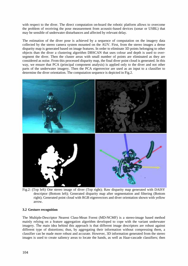
104
with respect to the diver. The direct computation on-board the robotic platform allows to overcome the problem of receiving the pose measurement from acoustic-based devices (sonar or USBL) that may be sensible of underwater disturbances and affected by relevant delay. The estimation of the diver pose is achieved by a sequence of computation on the imagery data collected by the stereo camera system mounted on the AUV. First, from the stereo images a dense disparity map is generated based on image features. In order to eliminate 3D points belonging to other objects than the diver a clustering algorithm DBSCAN that uses colour and depth is used to over-segment the diver. Then the cluster areas with small number of points are eliminated as they are considered as noise. From this processed disparity map, the final diver point cloud is generated. In this way, we ensure that PCA (principal component analysis) is applied only to the diver and not other parts of the underwater imagery. Then the PCA eigenvector are used as an input to a classifier to determine the diver orientation. The computation sequence is depicted in Fig.2.
Fig.2: (Top left) One stereo image of diver (Top right); Raw disparity map generated with DAISY
descriptor (Bottom left); Generated disparity map after segmentation and filtering (Bottom right); Generated point cloud with RGB eigenvectors and diver orientation shown with yellow arrow.
3.2 Gesture recognition The Multiple-Descriptor Nearest Class-Mean Forest (MD-NCMF) is a stereo-image based method mainly relying on a feature aggregation algorithm developed to cope with the variant underwater imagery. The main idea behind this approach is that different image descriptors are robust against different type of distortions; thus, by aggregating their information without compressing them, a classifier can be made more robust and accurate. However, 3D information generated from the stereo images is used to create saliency areas to locate the hands, as well as Haar-cascade classifiers; then
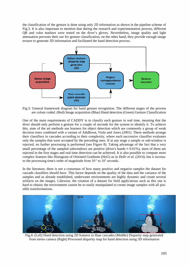
105
the classification of the gesture is done using only 2D information as shown in the pipeline scheme of Fig.3. It is also important to mention that during the research and experimentation process, different QR and color markers were tested on the diver’s gloves. Nevertheless, image quality and light attenuation prevents their use for gesture classification; on the other hand, they provide enough image texture to generate 3D information and facilitated the hand detection process.
Fig.3: General framework diagram for hand gesture recognition. The different stages of the process
are colour coded. (Red) Image acquisition (Blue) Hand detection (Green) Gesture Classification
One of the main requirements of CADDY is to classify each gesture in real time, meaning that the diver should only perform a gesture for a couple of seconds for the system to identify it. To achieve this, state of the art methods use learners for object detection which are commonly a group of weak decision trees combined with a variant of AdaBoost, Viola and Jones (2001). These methods arrange their classifiers in cascades according to their complexity, where each successive classifier evaluates only the samples that were accepted by the preceding ones. If at any stage a sample or sub-window is rejected, no further processing is performed (see Figure 8). Taking advantage of the fact that a very small percentage of the sampled subwindows are positive (diver's hands ≈ 0.01%), most of them are rejected in the first stages and real time detection can be achieved. It is also possible to compute more complex features like Histogram of Oriented Gradients (HoG) as in Dollr et al. (2014), but it increas-es the processing time's order of magnitude from 10-1 to 101 seconds. In the literature, there is not a consensus of how many positive and negative samples the dataset for cascade classifiers should have. This factor depends on the quality of the data and the variance of the samples and as already established, underwater environments are highly dynamic and create several artifacts on the images. Likewise, the creation of a dataset for field applications such as this one is hard to obtain; the environment cannot be so easily manipulated to create image samples with all pos-sible transformations.
Fig.4: (Left) Hand detection using 2D features in Haar cascades (Middle) Disparity map generated
from stereo camera (Right) Processed disparity map for hand detection using 3D information
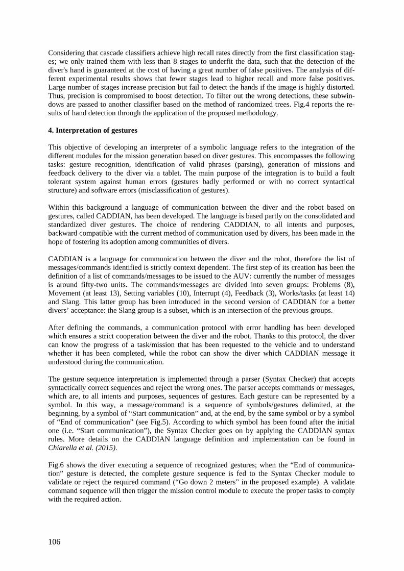
106
Considering that cascade classifiers achieve high recall rates directly from the first classification stag-es; we only trained them with less than 8 stages to underfit the data, such that the detection of the diver's hand is guaranteed at the cost of having a great number of false positives. The analysis of dif-ferent experimental results shows that fewer stages lead to higher recall and more false positives. Large number of stages increase precision but fail to detect the hands if the image is highly distorted. Thus, precision is compromised to boost detection. To filter out the wrong detections, these subwin-dows are passed to another classifier based on the method of randomized trees. Fig.4 reports the re-sults of hand detection through the application of the proposed methodology. 4. Interpretation of gestures This objective of developing an interpreter of a symbolic language refers to the integration of the different modules for the mission generation based on diver gestures. This encompasses the following tasks: gesture recognition, identification of valid phrases (parsing), generation of missions and feedback delivery to the diver via a tablet. The main purpose of the integration is to build a fault tolerant system against human errors (gestures badly performed or with no correct syntactical structure) and software errors (misclassification of gestures). Within this background a language of communication between the diver and the robot based on gestures, called CADDIAN, has been developed. The language is based partly on the consolidated and standardized diver gestures. The choice of rendering CADDIAN, to all intents and purposes, backward compatible with the current method of communication used by divers, has been made in the hope of fostering its adoption among communities of divers. CADDIAN is a language for communication between the diver and the robot, therefore the list of messages/commands identified is strictly context dependent. The first step of its creation has been the definition of a list of commands/messages to be issued to the AUV: currently the number of messages is around fifty-two units. The commands/messages are divided into seven groups: Problems (8), Movement (at least 13), Setting variables (10), Interrupt (4), Feedback (3), Works/tasks (at least 14) and Slang. This latter group has been introduced in the second version of CADDIAN for a better divers’ acceptance: the Slang group is a subset, which is an intersection of the previous groups. After defining the commands, a communication protocol with error handling has been developed which ensures a strict cooperation between the diver and the robot. Thanks to this protocol, the diver can know the progress of a task/mission that has been requested to the vehicle and to understand whether it has been completed, while the robot can show the diver which CADDIAN message it understood during the communication. The gesture sequence interpretation is implemented through a parser (Syntax Checker) that accepts syntactically correct sequences and reject the wrong ones. The parser accepts commands or messages, which are, to all intents and purposes, sequences of gestures. Each gesture can be represented by a symbol. In this way, a message/command is a sequence of symbols/gestures delimited, at the beginning, by a symbol of “Start communication” and, at the end, by the same symbol or by a symbol of “End of communication” (see Fig.5). According to which symbol has been found after the initial one (i.e. “Start communication”), the Syntax Checker goes on by applying the CADDIAN syntax rules. More details on the CADDIAN language definition and implementation can be found in Chiarella et al. (2015). Fig.6 shows the diver executing a sequence of recognized gestures; when the “End of communica-tion” gesture is detected, the complete gesture sequence is fed to the Syntax Checker module to validate or reject the required command (“Go down 2 meters” in the proposed example). A validate command sequence will then trigger the mission control module to execute the proper tasks to comply with the required action.
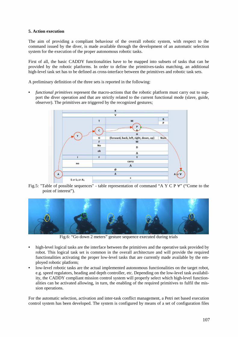
107
5. Action execution The aim of providing a compliant behaviour of the overall robotic system, with respect to the command issued by the diver, is made available through the development of an automatic selection system for the execution of the proper autonomous robotic tasks. First of all, the basic CADDY functionalities have to be mapped into subsets of tasks that can be provided by the robotic platforms. In order to define the primitives-tasks matching, an additional high-level task set has to be defined as cross-interface between the primitives and robotic task sets. A preliminary definition of the three sets is reported in the following: • functional primitives represent the macro-actions that the robotic platform must carry out to sup-
port the diver operation and that are strictly related to the current functional mode (slave, guide, observer). The primitives are triggered by the recognized gestures;
Fig.5: "Table of possible sequences" - table representation of command “A Y C P ∀” (“Come to the
point of interest”).
Fig.6: “Go down 2 meters” gesture sequence executed during trials
• high-level logical tasks are the interface between the primitives and the operative task provided by
robot. This logical task set is common in the overall architecture and will provide the required functionalities activating the proper low-level tasks that are currently made available by the em-ployed robotic platform;
• low-level robotic tasks are the actual implemented autonomous functionalities on the target robot, e.g. speed regulators, heading and depth controller, etc. Depending on the low-level task availabil-ity, the CADDY compliant mission control system will properly select which high-level function-alities can be activated allowing, in turn, the enabling of the required primitives to fulfil the mis-sion operations.
For the automatic selection, activation and inter-task conflict management, a Petri net based execution control system has been developed. The system is configured by means of a set of configuration files
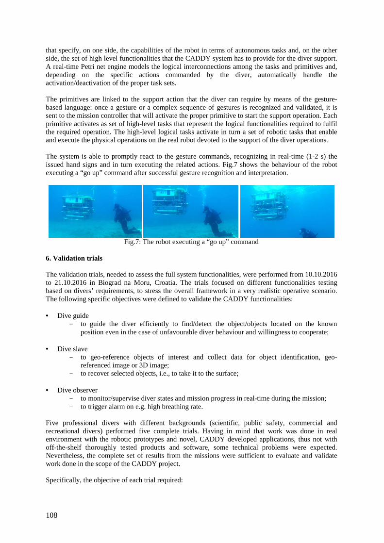
108
that specify, on one side, the capabilities of the robot in terms of autonomous tasks and, on the other side, the set of high level functionalities that the CADDY system has to provide for the diver support. A real-time Petri net engine models the logical interconnections among the tasks and primitives and, depending on the specific actions commanded by the diver, automatically handle the activation/deactivation of the proper task sets. The primitives are linked to the support action that the diver can require by means of the gesture-based language: once a gesture or a complex sequence of gestures is recognized and validated, it is sent to the mission controller that will activate the proper primitive to start the support operation. Each primitive activates as set of high-level tasks that represent the logical functionalities required to fulfil the required operation. The high-level logical tasks activate in turn a set of robotic tasks that enable and execute the physical operations on the real robot devoted to the support of the diver operations. The system is able to promptly react to the gesture commands, recognizing in real-time (1-2 s) the issued hand signs and in turn executing the related actions. Fig.7 shows the behaviour of the robot executing a “go up” command after successful gesture recognition and interpretation.
Fig.7: The robot executing a “go up” command
6. Validation trials The validation trials, needed to assess the full system functionalities, were performed from 10.10.2016 to 21.10.2016 in Biograd na Moru, Croatia. The trials focused on different functionalities testing based on divers’ requirements, to stress the overall framework in a very realistic operative scenario. The following specific objectives were defined to validate the CADDY functionalities: • Dive guide
- to guide the diver efficiently to find/detect the object/objects located on the known position even in the case of unfavourable diver behaviour and willingness to cooperate;
• Dive slave - to geo-reference objects of interest and collect data for object identification, geo-
referenced image or 3D image; - to recover selected objects, i.e., to take it to the surface;
• Dive observer
- to monitor/supervise diver states and mission progress in real-time during the mission; - to trigger alarm on e.g. high breathing rate.
Five professional divers with different backgrounds (scientific, public safety, commercial and recreational divers) performed five complete trials. Having in mind that work was done in real environment with the robotic prototypes and novel, CADDY developed applications, thus not with off-the-shelf thoroughly tested products and software, some technical problems were expected. Nevertheless, the complete set of results from the missions were sufficient to evaluate and validate work done in the scope of the CADDY project. Specifically, the objective of each trial required:
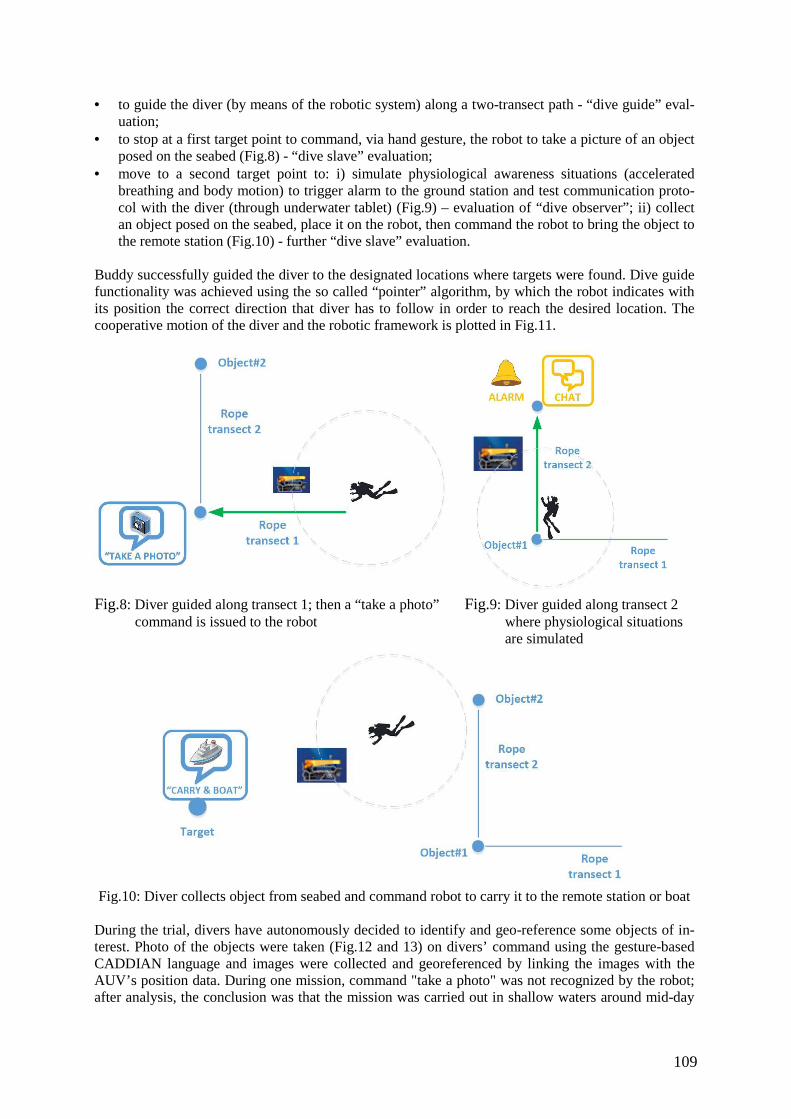
109
• to guide the diver (by means of the robotic system) along a two-transect path - “dive guide” eval-uation;
• to stop at a first target point to command, via hand gesture, the robot to take a picture of an object posed on the seabed (Fig.8) - “dive slave” evaluation;
• move to a second target point to: i) simulate physiological awareness situations (accelerated breathing and body motion) to trigger alarm to the ground station and test communication proto-col with the diver (through underwater tablet) (Fig.9) – evaluation of “dive observer”; ii) collect an object posed on the seabed, place it on the robot, then command the robot to bring the object to the remote station (Fig.10) - further “dive slave” evaluation.
Buddy successfully guided the diver to the designated locations where targets were found. Dive guide functionality was achieved using the so called “pointer” algorithm, by which the robot indicates with its position the correct direction that diver has to follow in order to reach the desired location. The cooperative motion of the diver and the robotic framework is plotted in Fig.11.
Fig.8: Diver guided along transect 1; then a “take a photo” command is issued to the robot
Fig.9: Diver guided along transect 2 where physiological situations are simulated
Fig.10: Diver collects object from seabed and command robot to carry it to the remote station or boat
During the trial, divers have autonomously decided to identify and geo-reference some objects of in-terest. Photo of the objects were taken (Fig.12 and 13) on divers’ command using the gesture-based CADDIAN language and images were collected and georeferenced by linking the images with the AUV’s position data. During one mission, command "take a photo" was not recognized by the robot; after analysis, the conclusion was that the mission was carried out in shallow waters around mid-day
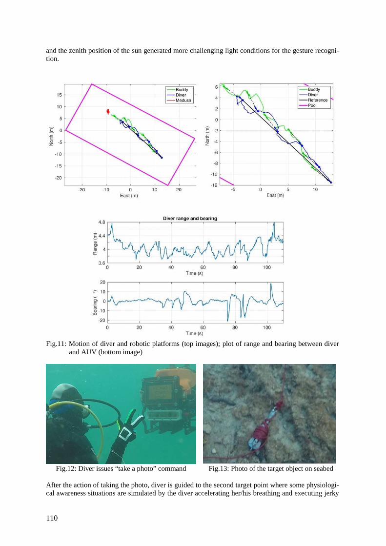
110
and the zenith position of the sun generated more challenging light conditions for the gesture recogni-tion.
Fig.11: Motion of diver and robotic platforms (top images); plot of range and bearing between diver
and AUV (bottom image)
Fig.12: Diver issues “take a photo” command Fig.13: Photo of the target object on seabed
After the action of taking the photo, diver is guided to the second target point where some physiologi-cal awareness situations are simulated by the diver accelerating her/his breathing and executing jerky
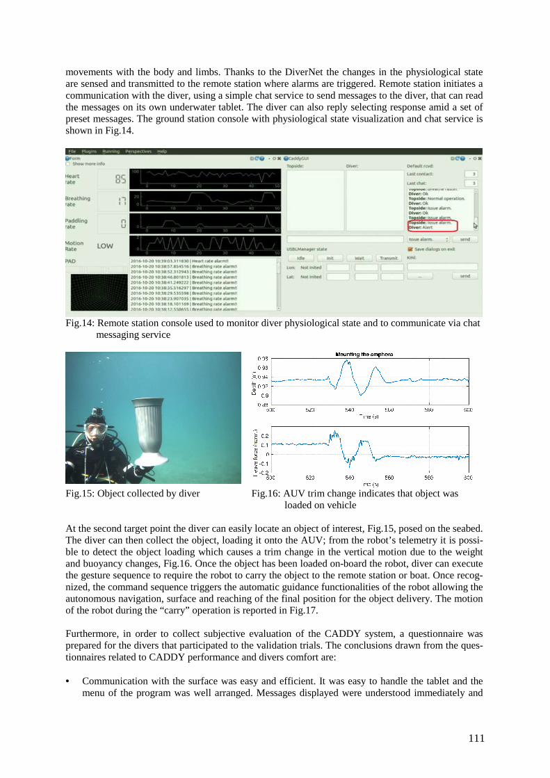
111
movements with the body and limbs. Thanks to the DiverNet the changes in the physiological state are sensed and transmitted to the remote station where alarms are triggered. Remote station initiates a communication with the diver, using a simple chat service to send messages to the diver, that can read the messages on its own underwater tablet. The diver can also reply selecting response amid a set of preset messages. The ground station console with physiological state visualization and chat service is shown in Fig.14.
Fig.14: Remote station console used to monitor diver physiological state and to communicate via chat messaging service
Fig.15: Object collected by diver Fig.16: AUV trim change indicates that object was
loaded on vehicle At the second target point the diver can easily locate an object of interest, Fig.15, posed on the seabed. The diver can then collect the object, loading it onto the AUV; from the robot’s telemetry it is possi-ble to detect the object loading which causes a trim change in the vertical motion due to the weight and buoyancy changes, Fig.16. Once the object has been loaded on-board the robot, diver can execute the gesture sequence to require the robot to carry the object to the remote station or boat. Once recog-nized, the command sequence triggers the automatic guidance functionalities of the robot allowing the autonomous navigation, surface and reaching of the final position for the object delivery. The motion of the robot during the “carry” operation is reported in Fig.17. Furthermore, in order to collect subjective evaluation of the CADDY system, a questionnaire was prepared for the divers that participated to the validation trials. The conclusions drawn from the ques-tionnaires related to CADDY performance and divers comfort are: • Communication with the surface was easy and efficient. It was easy to handle the tablet and the
menu of the program was well arranged. Messages displayed were understood immediately and
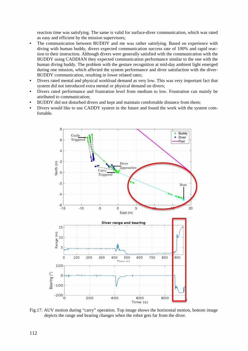
112
reaction time was satisfying. The same is valid for surface-diver communication, which was rated as easy and efficient by the mission supervisors;
• The communication between BUDDY and me was rather satisfying. Based on experience with diving with human buddy, divers expected communication success rate of 100% and rapid reac-tion to their instruction. Although divers were generally satisfied with the communication with the BUDDY using CADDIAN they expected communication performance similar to the one with the human diving buddy. The problem with the gesture recognition at mid-day ambient light emerged during one mission, which affected the system performance and diver satisfaction with the diver-BUDDY communication, resulting in lower related rates;
• Divers rated mental and physical workload demand as very low. This was very important fact that system did not introduced extra mental or physical demand on divers;
• Divers rated performance and frustration level from medium to low. Frustration can mainly be attributed to communication;
• BUDDY did not disturbed divers and kept and maintain comfortable distance from them; • Divers would like to use CADDY system in the future and found the work with the system com-
fortable.
Fig.17: AUV motion during “carry” operation. Top image shows the horizontal motion, bottom image
depicts the range and bearing changes when the robot gets far from the diver.
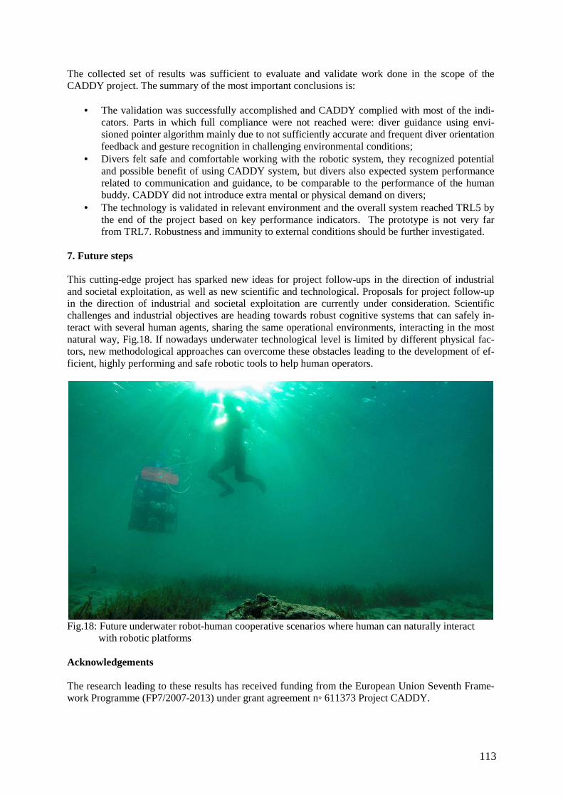
113
The collected set of results was sufficient to evaluate and validate work done in the scope of the CADDY project. The summary of the most important conclusions is:
• The validation was successfully accomplished and CADDY complied with most of the indi-cators. Parts in which full compliance were not reached were: diver guidance using envi-sioned pointer algorithm mainly due to not sufficiently accurate and frequent diver orientation feedback and gesture recognition in challenging environmental conditions;
• Divers felt safe and comfortable working with the robotic system, they recognized potential and possible benefit of using CADDY system, but divers also expected system performance related to communication and guidance, to be comparable to the performance of the human buddy. CADDY did not introduce extra mental or physical demand on divers;
• The technology is validated in relevant environment and the overall system reached TRL5 by the end of the project based on key performance indicators. The prototype is not very far from TRL7. Robustness and immunity to external conditions should be further investigated.
7. Future steps This cutting-edge project has sparked new ideas for project follow-ups in the direction of industrial and societal exploitation, as well as new scientific and technological. Proposals for project follow-up in the direction of industrial and societal exploitation are currently under consideration. Scientific challenges and industrial objectives are heading towards robust cognitive systems that can safely in-teract with several human agents, sharing the same operational environments, interacting in the most natural way, Fig.18. If nowadays underwater technological level is limited by different physical fac-tors, new methodological approaches can overcome these obstacles leading to the development of ef-ficient, highly performing and safe robotic tools to help human operators.
Fig.18: Future underwater robot-human cooperative scenarios where human can naturally interact with robotic platforms
Acknowledgements The research leading to these results has received funding from the European Union Seventh Frame-work Programme (FP7/2007-2013) under grant agreement n◦ 611373 Project CADDY.

114
References BIBULI, M.; BRUZZONE, G.; CHIARELLA, D.; CACCIA, M.; ODETTI, A.; RANIERI, A.; SAG-GINI, E.; ZEREIK, E. (2016), Underwater robotics for diver operations support: the CADDY project, 15th COMPIT Conf., Lecce DOLLR, P.; APPEL, R.; BELONGIE, S.; PERONA, P. (2014), Fast feature pyramids for object de-tection, IEEE Trans. Pattern Analysis and Machine Intelligence 36/8, pp.1532-1545 MISKOVIC, N.; BIBULI, M.; BIRK, A.; CACCIA, M.; EGI, M.; GRAMMER, K.; MARRONI, A.; NEASHAM, J.; PASCOAL, A.; VASILIJEVIC, A.; VUKIC, Z. (2015), Overview of the FP7 project CADDY - Cognitive Autonomous Diving Buddy, MTS/IEEE Oceans’15, Genova VIOLA, P.; JONES, M. (2001), Rapid object detection using a boosted cascade of simple features, IEEE Computer Society Conf. Computer Vision and Pattern Recognition, Vol. 1, pp.511-518
115
Virtual and Augmented Reality Solutions to Industrial Applications
Leo Sakari, Seppo Helle, Sirpa Korhonen, Tero Säntti, Olli Heimo, Mikko Forsman, Mika Taskinen, Teijo Lehtonen, University of Turku, Turku/Finland,
{leersa | seilhe | sikrko | teansa | olheimo | miolfo | mhjtas | tetale}@utu.fi Abstract This paper introduces a variety of virtual and augmented reality solutions for industrial applications. In addition the technologies and techniques required for producing these kind of solutions are presented. The issues studied in research projects referred here include data connectivity, processing and 3D visualization of construction models, positioning and tracking solutions and user experience design. An open database containing evaluations about available virtual and augmented reality platforms is also presented. 1. Introduction During the last few years, virtual reality and augmented reality have both been hot topics in the entertainment industry, but still the implementation of these technologies in industrial context has been lacking. While in industry various technological solutions are widely used with efficient results it is still usual to use tools that have been in use for over a decade. However there seems to be much to utilise in augmented reality (AR) and virtual reality (VR) technologies if one wishes to promote the information flow from the design bench to the construction process by enhancing the aforementioned processes with visual aids. Due to the requirements of the work processes, these solutions must be meticulously designed and have higher standards for current and correct information and thus they differ quite a lot from their entertainment counterparts. Virtual reality refers to technologies that are used to generate virtual images and sounds to simulate physical presence in another environment. In VR the content can be linked to the real world, but it does not have to be. The physical location of the user is irrelevant to the content per se, but in a large system the movements of the user can be tracked and reflected into the VR world. Some of the content can be real time sensory data, for instance the user can navigate a virtual model of a building on the other side of the Earth, and see the air flow in a given ventilation duct. This allows remote monitoring, without physical presence. In training and education VR provides a low-cost alternative to sending the learners on site. Additionally, VR allows simulated situations that would be hazardous to the user and costly to perform, like how to react in case a fire starts. Augmented reality involves superimposing virtual content on the user’s view of the real world. In AR, views from real-world environments are augmented with digital 3D-objects and/or other data in real time. The content can include real time data, e.g. the status of a given item, such as the temperature of a water pipe, or static data, like the material used for a given item. In the AR-case, the content is linked to the physical location of the user. Additionally, the user can be provided with access to further data, such as manuals or instruction for maintenance operations, based on the item(s) seen in the AR-view. Mixed reality (MR), https://developer.microsoft.com/en-us/windows/mixed-reality, can be imposed by changing incoming information from all senses. Usually MR uses at least visual and aural methods but also olfactory, gustatory, and haptic can be used, e.g. Ranasinghe et al. (2011), Colwell et al. (1998), Ischer et al. (1998). Visual effects can be e.g. computer-generated 2D and 3D images or information superimposed on the real-world view captured from the camera of a smartphone, computer or other device, Bujak et al. (2013), Heimo et al. (2017). Mixed image appears to its users as virtual and real objects coexisting simultaneously in the same space, Di Serio et al. (2013), Seppälä et al. (2016), Heimo et al. (2017). MR consists of various setups and combinations of levels of reality and digitally generated material. As
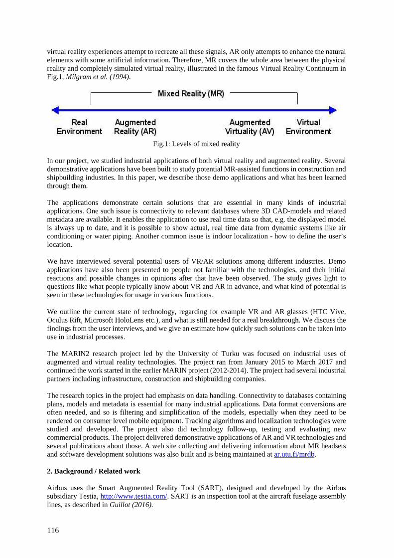
116
virtual reality experiences attempt to recreate all these signals, AR only attempts to enhance the natural elements with some artificial information. Therefore, MR covers the whole area between the physical reality and completely simulated virtual reality, illustrated in the famous Virtual Reality Continuum in Fig.1, Milgram et al. (1994).
Fig.1: Levels of mixed reality
In our project, we studied industrial applications of both virtual reality and augmented reality. Several demonstrative applications have been built to study potential MR-assisted functions in construction and shipbuilding industries. In this paper, we describe those demo applications and what has been learned through them. The applications demonstrate certain solutions that are essential in many kinds of industrial applications. One such issue is connectivity to relevant databases where 3D CAD-models and related metadata are available. It enables the application to use real time data so that, e.g. the displayed model is always up to date, and it is possible to show actual, real time data from dynamic systems like air conditioning or water piping. Another common issue is indoor localization - how to define the user’s location. We have interviewed several potential users of VR/AR solutions among different industries. Demo applications have also been presented to people not familiar with the technologies, and their initial reactions and possible changes in opinions after that have been observed. The study gives light to questions like what people typically know about VR and AR in advance, and what kind of potential is seen in these technologies for usage in various functions. We outline the current state of technology, regarding for example VR and AR glasses (HTC Vive, Oculus Rift, Microsoft HoloLens etc.), and what is still needed for a real breakthrough. We discuss the findings from the user interviews, and we give an estimate how quickly such solutions can be taken into use in industrial processes. The MARIN2 research project led by the University of Turku was focused on industrial uses of augmented and virtual reality technologies. The project ran from January 2015 to March 2017 and continued the work started in the earlier MARIN project (2012-2014). The project had several industrial partners including infrastructure, construction and shipbuilding companies. The research topics in the project had emphasis on data handling. Connectivity to databases containing plans, models and metadata is essential for many industrial applications. Data format conversions are often needed, and so is filtering and simplification of the models, especially when they need to be rendered on consumer level mobile equipment. Tracking algorithms and localization technologies were studied and developed. The project also did technology follow-up, testing and evaluating new commercial products. The project delivered demonstrative applications of AR and VR technologies and several publications about those. A web site collecting and delivering information about MR headsets and software development solutions was also built and is being maintained at ar.utu.fi/mrdb. 2. Background / Related work Airbus uses the Smart Augmented Reality Tool (SART), designed and developed by the Airbus subsidiary Testia, http://www.testia.com/. SART is an inspection tool at the aircraft fuselage assembly lines, as described in Guillot (2016).

117
SART is being used for inspection of mounting brackets in the aircraft fuselage. There are thousands of brackets in an airliner, and correct installation of each one must be inspected. An AR solution for this specific task was designed and implemented initially in 2010, and it has been in routine use since 2011, with further refinements and updates during the operational period. The application includes a reporting tool, integrating the inspection task into one device. With the AR application Airbus claims to have reduced the inspection time to one fifth of what is needed using the traditional method involving paper or laptop based inspection sheets and Excel/Word applications for reporting. Also quality improvements (decrease of non-conformities) are reported, http://www.manufacturing-summit.com/wp-content/uploads/2016/10/Aurelien-Cottet-Airbus.compressed.pdf. The SART process includes data processing where 3D-models and parts data are prepared to be run on a mobile device. This phase is done in the office before the actual inspection task. The inspection requires human approval for everything – according to aircraft industry regulations – as an automatic system can’t approve the inspection results. Thus SART is designed as an assistant for human operators, not as a fully automated system capable of unsupervised work. The actual SART tool runs on a tablet computer, with a specific camera module attached to it. In the inspection work, it uses a marker-based, in-house developed tracking method with millimetre scale accuracy. A markerless solution exists too, having lower accuracy, but being useful in some applications. The markers are set to place by the operator during the work task. Typically one marker every 3-5 m suffices, but it depends on individual working styles. The marker-based solution ensures good localization, although it also requires some effort from the operator. For example, an aircraft fuselage has a lot of repetitive elements, making correct localization by an automatic, markerless system very difficult. The tablet device is used with a light neck strap or harness, which makes carrying it relatively easy. The currently available AR glasses would be impractical and inconvenient for continued use. The tablet can be used continuously for half a workday, and its battery is changed or charged during the lunchbreak. Another example of the recent development would be the EdcAR system, developed for the European Space Agency (ESA) by Technical Research Centre of Finland (VTT), Thales Alenia Space, and Institute of Communications and Computer Systems, Greece. Helin (2016) presents the system, as well as two use-cases: (1) AR supported telecom payload coax cables assembly; (2) AR based on-board training and remote support for centralized cabin filter replacement in ISS. The EdcAR AR-system was designed to give a simple solution based on standards for portability and expandability. With this in mind, modularity and reusability were highlighted in the development. These were achieved by using the ALVAR 2D/3D tracking system, http://virtual.vtt.fi/virtual/proj2/multimedia/alvar/index.html, on top of the Unity engine with ROS (an open-source Robot Operating System) providing the platform support. The team reported the following lessons learnt:
• Point cloud tracking works well, but needs expertise in set-up • Main show-stopper is usability and processing power of AR-goggles • EdcAR system works with smart phones and tablets • A lot of resources was spent to the backend system and loading content in real time • A fully Unity-based system could show much better features of AR and would also enhance
performance Within the MARIN2 project several systematic literature reviews were conducted about subjects related to the industrial use of augmented and virtual reality solutions. One review collects information about use of depth sensors in augmented reality applications Taskinen et al. (2015). Usage of inertial sensors for movement tracking on a map is the theme in Kaustinen et al. (2015). Advances in monocular model-based tracking are analysed in Lahdenoja et al. (2015), while articles about hardware accelerated visual tracking algorithms are collected in Korhonen et al. (2015). Developments of user interaction technologies in mobile AR are presented in Härkänen et al. (2015). All these literature reviews are
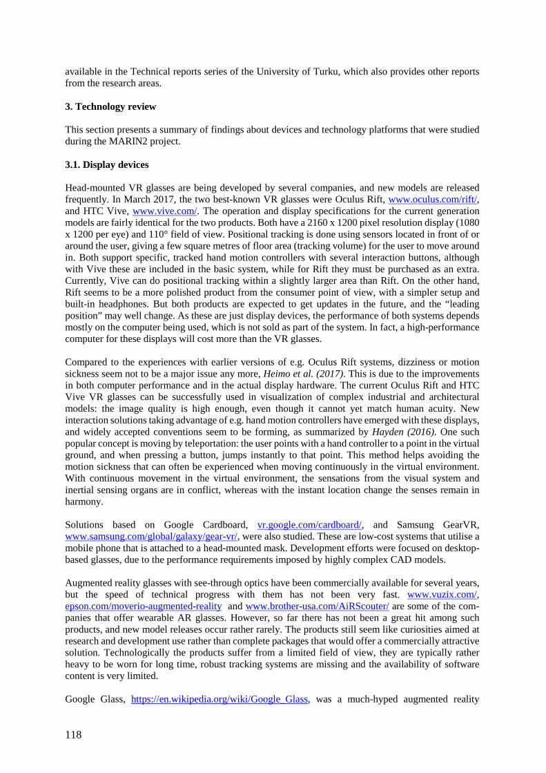
118
available in the Technical reports series of the University of Turku, which also provides other reports from the research areas. 3. Technology review This section presents a summary of findings about devices and technology platforms that were studied during the MARIN2 project. 3.1. Display devices Head-mounted VR glasses are being developed by several companies, and new models are released frequently. In March 2017, the two best-known VR glasses were Oculus Rift, www.oculus.com/rift/, and HTC Vive, www.vive.com/. The operation and display specifications for the current generation models are fairly identical for the two products. Both have a 2160 x 1200 pixel resolution display (1080 x 1200 per eye) and 110° field of view. Positional tracking is done using sensors located in front of or around the user, giving a few square metres of floor area (tracking volume) for the user to move around in. Both support specific, tracked hand motion controllers with several interaction buttons, although with Vive these are included in the basic system, while for Rift they must be purchased as an extra. Currently, Vive can do positional tracking within a slightly larger area than Rift. On the other hand, Rift seems to be a more polished product from the consumer point of view, with a simpler setup and built-in headphones. But both products are expected to get updates in the future, and the “leading position” may well change. As these are just display devices, the performance of both systems depends mostly on the computer being used, which is not sold as part of the system. In fact, a high-performance computer for these displays will cost more than the VR glasses. Compared to the experiences with earlier versions of e.g. Oculus Rift systems, dizziness or motion sickness seem not to be a major issue any more, Heimo et al. (2017). This is due to the improvements in both computer performance and in the actual display hardware. The current Oculus Rift and HTC Vive VR glasses can be successfully used in visualization of complex industrial and architectural models: the image quality is high enough, even though it cannot yet match human acuity. New interaction solutions taking advantage of e.g. hand motion controllers have emerged with these displays, and widely accepted conventions seem to be forming, as summarized by Hayden (2016). One such popular concept is moving by teleportation: the user points with a hand controller to a point in the virtual ground, and when pressing a button, jumps instantly to that point. This method helps avoiding the motion sickness that can often be experienced when moving continuously in the virtual environment. With continuous movement in the virtual environment, the sensations from the visual system and inertial sensing organs are in conflict, whereas with the instant location change the senses remain in harmony. Solutions based on Google Cardboard, vr.google.com/cardboard/, and Samsung GearVR, www.samsung.com/global/galaxy/gear-vr/, were also studied. These are low-cost systems that utilise a mobile phone that is attached to a head-mounted mask. Development efforts were focused on desktop-based glasses, due to the performance requirements imposed by highly complex CAD models. Augmented reality glasses with see-through optics have been commercially available for several years, but the speed of technical progress with them has not been very fast. www.vuzix.com/, epson.com/moverio-augmented-reality and www.brother-usa.com/AiRScouter/ are some of the com-panies that offer wearable AR glasses. However, so far there has not been a great hit among such products, and new model releases occur rather rarely. The products still seem like curiosities aimed at research and development use rather than complete packages that would offer a commercially attractive solution. Technologically the products suffer from a limited field of view, they are typically rather heavy to be worn for long time, robust tracking systems are missing and the availability of software content is very limited. Google Glass, https://en.wikipedia.org/wiki/Google_Glass, was a much-hyped augmented reality
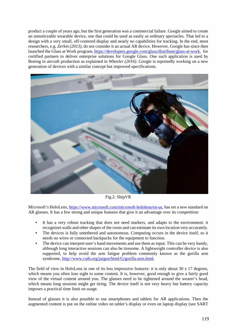
119
product a couple of years ago, but the first generation was a commercial failure. Google aimed to create an unnoticeable wearable device, one that could be used as easily as ordinary spectacles. That led to a design with a very small, off-centered display and nearly no capabilities for tracking. In the end, most researchers, e.g. Zerkin (2013), do not consider it an actual AR device. However, Google has since then launched the Glass at Work program, https://developers.google.com/glass/distribute/glass-at-work, for certified partners to deliver enterprise solutions for Google Glass. One such application is used by Boeing in aircraft production as explained in Wheeler (2016). Google is reportedly working on a new generation of devices with a similar concept but improved specifications.
Fig.2: ShipVR Microsoft’s HoloLens, https://www.microsoft.com/microsoft-hololens/en-us, has set a new standard on AR glasses. It has a few strong and unique features that give it an advantage over its competition:
• It has a very robust tracking that does not need markers, and adapts to the environment: it recognizes walls and other shapes of the room and can estimate its own location very accurately.
• The devices is fully untethered and autonomous. Computing occurs in the device itself, so it needs no wires or connected backpacks for the equipment to function.
• The device can interpret user’s hand movements and use them as input. This can be very handy, although long interactive sessions can also be tiresome. A lightweight controller device is also supported, to help avoid the arm fatigue problem commonly known as the gorilla arm syndrome, http://www.catb.org/jargon/html/G/gorilla-arm.html.
The field of view in HoloLens in one of its less impressive features: it is only about 30 x 17 degrees, which means you often lose sight to some content. It is, however, good enough to give a fairly good view of the virtual content around you. The glasses need to be tightened around the wearer’s head, which means long sessions might get tiring. The device itself is not very heavy but battery capacity imposes a practical time limit on usage. Instead of glasses it is also possible to use smartphones and tablets for AR applications. Then the augmented content is put on the online video on tablet’s display or even on laptop display (see SART
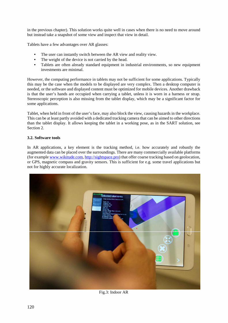
120
in the previous chapter). This solution works quite well in cases when there is no need to move around but instead take a snapshot of some view and inspect that view in detail. Tablets have a few advantages over AR glasses:
• The user can instantly switch between the AR view and reality view. • The weight of the device is not carried by the head. • Tablets are often already standard equipment in industrial environments, so new equipment
investments are minimal. However, the computing performance in tablets may not be sufficient for some applications. Typically this may be the case when the models to be displayed are very complex. Then a desktop computer is needed, or the software and displayed content must be optimized for mobile devices. Another drawback is that the user’s hands are occupied when carrying a tablet, unless it is worn in a harness or strap. Stereoscopic perception is also missing from the tablet display, which may be a significant factor for some applications. Tablet, when held in front of the user’s face, may also block the view, causing hazards in the workplace. This can be at least partly avoided with a dedicated tracking camera that can be aimed to other directions than the tablet display. It allows keeping the tablet in a working pose, as in the SART solution, see Section 2. 3.2. Software tools In AR applications, a key element is the tracking method, i.e. how accurately and robustly the augmented data can be placed over the surroundings. There are many commercially available platforms (for example www.wikitude.com, http://sightspace.pro) that offer coarse tracking based on geolocation, or GPS, magnetic compass and gravity sensors. This is sufficient for e.g. some travel applications but not for highly accurate localization.
Fig.3: Indoor AR
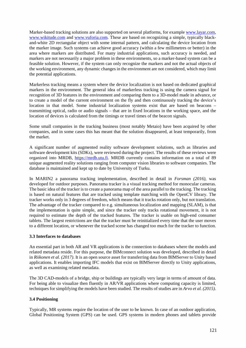
121
Marker-based tracking solutions are also supported on several platforms, for example www.layar.com, www.wikitude.com and www.vuforia.com. These are based on recognizing a simple, typically black-and-white 2D rectangular object with some internal pattern, and calculating the device location from the marker image. Such systems can achieve good accuracy (within a few millimetres or better) in the area where markers are distributed. For many industrial applications, such accuracy is needed, and markers are not necessarily a major problem in these environments, so a marker-based system can be a feasible solution. However, if the system can only recognize the markers and not the actual objects of the working environment, any dynamic changes in the environment are not considered, which may limit the potential applications. Markerless tracking means a system where the device localization is not based on dedicated graphical markers in the environment. The general idea of markerless tracking is using the camera signal for recognition of 3D features in the environment and comparing them to a 3D-model made in advance, or to create a model of the current environment on the fly and then continuously tracking the device’s location in that model. Some industrial localization systems exist that are based on beacons – transmitting optical, radio or audio signals – that are in fixed locations in the working space, and the location of devices is calculated from the timings or travel times of the beacon signals. Some small companies in the tracking business (most notably Metaio) have been acquired by other companies, and in some cases this has meant that the solution disappeared, at least temporarily, from the market. A significant number of augmented reality software development solutions, such as libraries and software development kits (SDKs), were reviewed during the project. The results of these reviews were organized into MRDB, https://mrdb.utu.fi. MRDB currently contains information on a total of 89 unique augmented reality solutions ranging from computer vision libraries to software companies. The database is maintained and kept up to date by University of Turku. In MARIN2 a panorama tracking implementation, described in detail in Forsman (2016), was developed for outdoor purposes. Panorama tracker is a visual tracking method for monocular cameras. The basic idea of the tracker is to create a panorama map of the area parallel to the tracking. The tracking is based on natural features that are tracked using template matching with the OpenCV library. The tracker works only in 3 degrees of freedom, which means that it tracks rotation only, but not translation. The advantage of the tracker compared to e.g. simultaneous localization and mapping (SLAM), is that the implementation is quite simple, and since the tracker only tracks rotational movement, it is not required to estimate the depth of the tracked features. The tracker is usable on high-end consumer tablets. The largest restrictions are that the tracker must be reinitialized every time that the user moves to a different location, or whenever the tracked scene has changed too much for the tracker to function. 3.3 Interfaces to databases An essential part in both AR and VR applications is the connection to databases where the models and related metadata reside. For this purpose, the BIMconnect solution was developed, described in detail in Riikonen et al. (2017). It is an open source asset for transferring data from BIMServer to Unity based applications. It enables importing IFC models that exist on BIMServer directly to Unity applications, as well as examining related metadata. The 3D CAD-models of a bridge, ship or buildings are typically very large in terms of amount of data. For being able to visualize then fluently in AR/VR applications where computing capacity is limited, techniques for simplifying the models have been studied. The results of studies are in Arvo et al. (2015). 3.4 Positioning Typically, MR systems require the location of the user to be known. In case of an outdoor application, Global Positioning System (GPS) can be used. GPS systems in modern phones and tablets provide
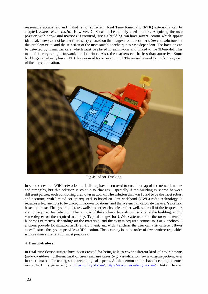
122
reasonable accuracies, and if that is not sufficient, Real Time Kinematic (RTK) extensions can be adapted, Sakari et al. (2016). However, GPS cannot be reliably used indoors. Acquiring the user position with non-visual methods is required, since a building can have several rooms which appear identical. These cannot be identified simply based on the images from the camera. Several solutions for this problem exist, and the selection of the most suitable technique is case dependent. The location can be detected by visual markers, which must be placed in each room, and linked to the 3D-model. This method is very straight forward, but laborious. Also, the markers can be less than attractive. Some buildings can already have RFID devices used for access control. These can be used to notify the system of the current location.
Fig.4: Indoor Tracking In some cases, the WiFi networks in a building have been used to create a map of the network names and strengths, but this solution is volatile to changes. Especially if the building is shared between different parties, each controlling their own networks. The solution that was found to be the most robust and accurate, with limited set up required, is based on ultra-wideband (UWB) radio technology. It requires a few anchors to be placed in known locations, and the system can calculate the user’s position based on those. The system tolerates walls and other obstacles rather well, since all of the frequencies are not required for detection. The number of the anchors depends on the size of the building, and to some degree on the required accuracy. Typical ranges for UWB systems are in the order of tens to hundreds of metres, depending on the materials, and the system requires contact to 3 or 4 anchors. 3 anchors provide localization in 2D environment, and with 4 anchors the user can visit different floors as well, since the system provides a 3D location. The accuracy is in the order of few centimetres, which is more than sufficient for most purposes. 4. Demonstrators In total nine demonstrators have been created for being able to cover different kind of environments (indoor/outdoor), different kind of users and use cases (e.g. visualization, reviewing/inspection, user instructions) and for testing some technological aspects. All the demonstrators have been implemented using the Unity game engine, https://unity3d.com/, https://www.unrealengine.com/. Unity offers an
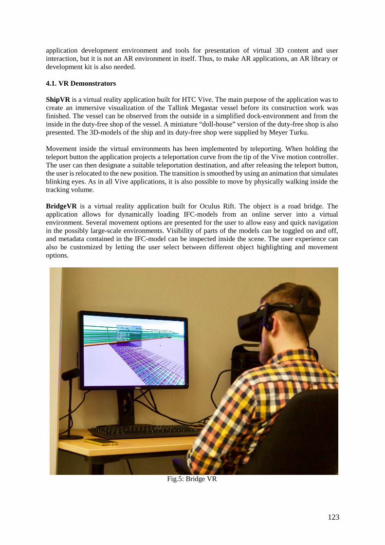
123
application development environment and tools for presentation of virtual 3D content and user interaction, but it is not an AR environment in itself. Thus, to make AR applications, an AR library or development kit is also needed. 4.1. VR Demonstrators ShipVR is a virtual reality application built for HTC Vive. The main purpose of the application was to create an immersive visualization of the Tallink Megastar vessel before its construction work was finished. The vessel can be observed from the outside in a simplified dock-environment and from the inside in the duty-free shop of the vessel. A miniature “doll-house” version of the duty-free shop is also presented. The 3D-models of the ship and its duty-free shop were supplied by Meyer Turku. Movement inside the virtual environments has been implemented by teleporting. When holding the teleport button the application projects a teleportation curve from the tip of the Vive motion controller. The user can then designate a suitable teleportation destination, and after releasing the teleport button, the user is relocated to the new position. The transition is smoothed by using an animation that simulates blinking eyes. As in all Vive applications, it is also possible to move by physically walking inside the tracking volume. BridgeVR is a virtual reality application built for Oculus Rift. The object is a road bridge. The application allows for dynamically loading IFC-models from an online server into a virtual environment. Several movement options are presented for the user to allow easy and quick navigation in the possibly large-scale environments. Visibility of parts of the models can be toggled on and off, and metadata contained in the IFC-model can be inspected inside the scene. The user experience can also be customized by letting the user select between different object highlighting and movement options.
Fig.5: Bridge VR

124
The application is controlled with an Xbox 360 or Xbox One controller. Movement inside the virtual environment has been implemented by using joysticks and gaze teleporting, while user interface elements and model objects can be selected with gaze. BIMServer and BIMconnect were used in conjunction to make dynamic loading of CAD-models possible. IFC-model data is streamed directly from BIMServer and the models are constructed one-by-one into Unity. BuildingVR is a virtual reality application that is based on BridgeVR. The main difference between BridgeVR and this is that as well as displaying static metadata contained in the loaded IFC-models, BuildingVR contains components that allow gathering data from the design databases. In this demo was used as an example Granlund Designer, a building information application by Granlund. The integration with Granlund Designer allows for combining the models of the buildings/spaces in the application with real-time sensor data contained in Granlund Designer. This means that inspecting e.g. the models of air conditioning systems gives the user real-time data about the state of the selected air conditioning components. 4.2. AR Demonstrators OutdoorAR is an augmented reality application built for high-end customer-grade tablets. The application can be used to augment a 3D-model in an outdoor scenario. The initial placement of the model can be done either manually, or by using a GPS based system that uses 2 distinct GPS locations. The tracking in the system is based on the panorama tracker, which is only capable to track the rotational movements of the device, so the tracker must be reset whenever the user moves to another location. Panorama tracker is a markerless tracker, so it doesn't require any markers or previous knowledge of the area, Forsman et al. (2016). IndoorAR is an Android tablet application that combined results from several different research areas. The application guides its user to the maintenance target with a dynamically updating indoor map, downloads the CAD-model of the maintenance target from a server, and allows the inspection of the maintenance target via augmented reality. Several objects can be selected for inspection, and static metadata from the IFC-model as well as real-time data from Granlund Designer are displayed to the user. The functionality of the application is based on several subsystems. Tracking is handled using the Vuforia SDK, https://mrdb.utu.fi, and the tablet's gyroscope as a backup. Vuforia's marker tracking and extended tracking are used to calculate the exact pose of the user, while the gyroscope of the tablet is used as a backup if the visual tracking system fails to determine the pose. Indoor localization is handled with an UWB (ultra-wideband) system that uses UWB beacons by Decawave. The system calculates distances to UWB beacons that are situated close by and then uses triangulation to determine the exact position of the user. Dynamic loading of CAD-models is made possible with a combination of a BIMServer and BIMconnect, in very much the same way it is done in BridgeVR and BuildingVR. Displaying real-time data from the environment is made possible with a component that communicates with the Granlund Designer API (application programming interface). The system extracts component identifiers from the metadata contained in the IFC-model and then uses those identifiers to request for component specific real-time data. 4.3. Small Scale Demonstrators HoloLensAR is a simple proof of concept created for Microsoft HoloLens. The application contains the 3D-model of the air conditioning system situated in the office building. The air conditioning system is positioned so that it is overlaid directly on top of the real-life system. After positioning the model, real-time data from the air conditioning system can be fetched from the relevant databases. In this case it was Granlund Designer.
125
PhoneAR is a proof of concept for using the commercial augmented reality SDK Vuforia in a device training/maintenance application for Android tablets. The application shows step-by-step visual instructions for the usage of a Cisco IP phone. The visual instructions are overlaid directly onto a live video feed. This is accomplished by recognizing the phone using the tracking functionality in the Vuforia SDK. OfficeVR is a virtual reality application that is based on BridgeVR. Most of the more complex functions of BridgeVR have been removed, but the graphical fidelity has been improved. The main purpose of the demo is architectural visualization using CAD-models and virtual reality tools. 4.4. User experience Three usability tests were carried out, all varying with different MR systems, different test subjects and different test settings. This was due the variance in the target groups, company aims and suitable times. The test settings include quantitative and qualitative testing as well as observing the use-situations. Preliminary results show positive feedback from most of the test subjects. According to the test subjects the potential to use VR and AR in industry seems good. Users saw that the technology could improve their work processes and they were eager to implement the solutions to their use. The was an interesting notion that the VR and AR development should be focused on their specific field where it would be a big improvement (but not necessarily to others) thus giving a hint that if everyone feels this way, perhaps they are suitable for many of those fields. While the larger analysis of the results is still on-going, we argue that these systems - when designed correctly - a) do not generate a large-scale user-resistance and b) will improve the work process of most of the stakeholders in the industrial field. 5. Conclusions In this paper, the current state of commercially available display hardware and software tools supporting augmented and virtual reality were discussed. The current level of sensor and display technology, even in consumer-oriented devices, allows creation of viable augmented and virtual reality solutions for industrial use. In the software field, more robust positioning and tracking solutions are wanted – this is especially the case with markerless tracking, for which a commercially available, truly efficient and robust solution seems to be missing. For coarse positioning, UWB technology offers a working solution, at least in cases where using a beacon system is acceptable. These AR and VR proof of concepts and prototypes implemented in the MARIN2 project covered several different areas. These solutions were rather easy to produce given the fact that no applications alike were produced before. During the 4-year research period the technology took huge leaps in both AR and VR of which the last leap – the Microsoft HoloLens – made the biggest impression. While before the tracking and other base-level programming took most work in the development of AR solutions, the new technology frees the resources for content creation. In addition, the VR technology has taken huge leaps in both quality and prize. Therefore, it seems likely that these solutions will get cheaper and thus more common in near future both in entertainment and industrial sectors. AR and VR solutions were tested by potential users from the partner companies in the project. Feedback from them supports the view that such tools would be useful and potentially could be taken as part of their work. Thus it seems that from both the perspective of work and workforce, as well as from the economical point of view, developing and implementing AR and VR as a part of industrial work processes seems an idea worth considering.
126
Acknowledgements The research was carried out during the MARIN2 project (Mobile Mixed Reality Applications for Professional Use) funded by Tekes (The Finnish Funding Agency for Innovation) in collaboration with partners; Defour, Destia, Granlund, Infrakit, Integration House, Lloyd’s Register, Nextfour Group, Meyer Turku, BuildingSMART Finland, Machine Technology Center Turku and Turku Science Park. References ARVO, J.; EURANTO, A.; JÄRVENPÄÄ, L.; LEHTONEN, T.; KNUUTILA, T. (2015), 3D mesh simplification - A survey of algorithms and CAD model simplification tests, University of Turku Technical Reports, No.3, http://urn.fi/URN:ISBN:978-951-29-6202-0 BUJAK, K.R.; RADU, I.; CATRAMBONE, R.; MacINTYRE, B.; ZHENG, R.; GOLUBSKIC, G. (2013), A psychological perspective on augmented reality in the mathematics classroom, Computers & Education 68, pp.536-544 COLWELL, C.; PETRIE, H.; KORNBROT, D.; HARDWICK, A.; FURNER, S. (1998), Haptic virtual reality for blind computer users, 3rd Int. ACM Conf. Assistive Technologies (Assets '98), pp.92-99 DISERIO, Á.; IBÁÑEZ, M.B.; KLOOS, C.D. (2013), Impact of an augmented reality system on students' motivation for a visual art course, Computers & Education 68, pp.586-596 FORSMAN, M. (2016), Applying Augmented Reality to Outdoors Industrial Use, Master’s Thesis, http://urn.fi/URN:NBN:fi-fe2016053013052 FORSMAN, M.; ARVO, J.; LEHTONEN, T. (2016), Extended panorama tracking algorithm for augmenting virtual 3d objects in outdoor environments, 22nd Int. Conf. on Virtual Systems & Multimedia GUILLOT, R. (2016), The assembly of the future is already a reality with TESTIA's SART system, Aviation World News, http://www.aviationworldnews.com/news/the-assembly-of-the-future-is-already-a-reality-with-testia-s-sart-system-40174 HEIMO, O.I.; KIMPPA, K.K.; YLI-SEPPÄLÄ, L.; VIINIKKALA, L.; KORKALAINEN, T.; MÄKILÄ, T.; LEHTONEN, T. (2017), Ethical problems in creating historically representative mixed reality make-belief, CEPE ETHICOMP 2017, Values in Emerging Science and Technology, Turin HEIMO, O.I.; SAKARI, L.; SÄNTTI, T.; LEHTONEN, T. (2017), User testing industrial mixed reality solutions, Unpublished manuscript HELIN, K. (2016), ESA EdcAR Augmented Reality system for space applications, presented in ARea16, Otaniemi HAYDEN, S. (2016), 7 ways to move users around in VR without making them sick, http://www.roadtovr.com/7-ways-move-users-around-vr-without-making-sick/ HÄRKÄNEN, L.; HELLE, S.; JÄRVENPÄÄ, L.; LEHTONEN, T. (2015), Novel interaction techniques for mobile augmented reality applications - A systematic literature review, University of Turku Technical Reports, No. 9, http://urn.fi/URN:ISBN:978-951-29-6214-3 ISCHER, M.; BARON, N.; MERMOUD, C.; CAYEUX, I.; PORCHEROT, C.; SANDER, D.; DELPLANQUE, S. (2014), How incorporation of scents could enhance immersive virtual experiences, Frontiers in Psychology 5, http://doi.org/10.3389/fpsyg.2014.00736

127
KAUSTINEN, M.; TASKINEN, M.; SÄNTTI, T.; ARVO, J.; LEHTONEN, T. (2015), Map matching by using inertial sensors: Literature review, University of Turku Technical Reports, No.6, http://urn.fi/URN:ISBN:978-951-29-6190-0 KORHONEN, S.; SAKARI, L.; SÄNTTI, T.; LAHDENOJA, O.; LEHTONEN, T. (2015), Hardware accelerated visual tracking algorithms - A systematic literature review, University of Turku Technical Reports, No. 5, http://urn.fi/URN:ISBN:978-951-29-6189-4 LAHDENOJA, O.; SUOMINEN, R.; SÄNTTI, T.; LEHTONEN, T. (2015), Recent advances in monocular model-based tracking: A systematic literature review, University of Turku Technical Reports, No. 8, http://urn.fi/URN:ISBN:978-951-29-6215-0 MILGRAM, P.; TAKEMURA, H.; UTSUMI, A.; KISHINO, F. (1994), Augmented Reality: A class of displays on the reality-virtuality continuum, Telemanipulator and Telepresence Technologies Conf., pp.2351-34 RANASINGHE, N.; KARUNANAYAKA, K.; CHEOK, A.D.; FERNANDO, O.N.N.; NII, H.; GOPA-LAKRISHNAKONE, P. (2011), Digital taste and smell communication, 6th Int. Conf. Body Area Networks (BodyNets'11), Brussels, pp.78-84. http://dl.acm.org/citation.cfm?id=2318795 RIIKONEN, P.; ARVO, J.; LEHTONEN, T. (2017), Data transfer from BIMserver to Unity 3D applications with the BIMconnect asset, Advanced Engineering Informatics SAKARI, L.; FORSMAN, M.; TASKINEN, M.; SÄNTTI, T.; LEHTONEN, T. (2016), Evaluation of the GPS accuracy of tablets, University of Turku Technical Reports, No.11, http://urn.fi/URN:ISBN:978-951-29-6561-8 SEPPÄLÄ, K.; HEIMO, O.I.; PÄÄKYLÄ, J.; LATVALA, J.; HELLE, S.; HÄRKÄNEN, L.; JOKELA, S.; JÄRVENPÄÄ, L.; SAUKKO, F.; VIINIKKALA, L.; MÄKILÄ, T.; LEHTONEN, T. (2016), Examining user experience in an augmented reality adventure game: Case Luostarinmäki Handicrafts Museum, 12th IFIP TC9 Human Choice and Computers Conf. TASKINEN, M.M.; LAHDENOJA, O.O.; SÄNTTI, T.T.; JOKELA, T.; LEHTONEN, T. (2015), Depth sensors in Augmented Reality solutions - Literature review, University of Turku Technical Reports, No.10, http://urn.fi/URN:ISBN:978-951-29-6225-9 WHEELER, A. (2016), Assembling airplanes with Google Glass, www.engineering.com/Hardware/ArticleID/12712/Assembling-Airplanes-with-Google-Glass.aspx ZERKIN, N. (2013), Is Google Glass an Augmented Reality device?, Integrated Realities, http://blog.integratedrealities.com/?p=261

128
The Evolution of Virtual Reality in Shipbuilding
Denis Morais, SSI, Victoria/Canada, [email protected]
Mark Waldie, SSI, Victoria/Canada, [email protected]
Darren Larkins, SSI, Victoria/Canada, [email protected]
Abstract
Virtual Reality (VR) has gone from being science fiction, to being realized in the research lab, to being
treated as a toy, to being used in practical applications, including shipbuilding. This paper examines
the history of VR technology as well as its current state. It then predicts the future of VR by analysing
the forces that have either hindered or promoted the implementation of Virtual Reality in the ship design
and construction industry. Challenges are identified as well as possible solutions, in the context of
technology, economics and organizational culture.
1. Introduction
The year is 1992. You are in a theatre to watch a science fiction/horror film starring Pierce Brosnan.
The movie is Lawn Mower Man. It opens with a black screen showing some scary, yet exciting
prophetic text:
“By the turn of the millennium, a technology known as VIRTUAL REALITY will be in widespread
use. It will allow you to enter computer generated artificial worlds as unlimited as the imagination itself.
Its creators foresee millions of positive uses- others fear it as a new form of mind control…”
Fig.1: Lawn Mower Man: Collector’s Edition Promotional Poster Image
The movie then proceeds to show how Brosnan, the scientist, does experiments using virtual reality
(VR) on a hapless simpleton who mows lawns for a living. The experiments involve head mounted
displays (HMDs) and haptic bodysuits to provide touch sensations. VR is so perfect as a training
medium that the lawn mower man becomes a genius; he even develops the ability of telepathy. VR was
thought to be that powerful.
It is just a movie, and much of it may seem laughable, yet at the time, it was not considered all that
unbelievable; VR was all the rage. In the early 1990s, there was a broad market for books, magazines
and newsletters about the subject. There was Ben Delaney’s ‘CyberEdge Journal’ which addressed the
business aspects of virtual reality. MIT launched ‘Presence’ to cover virtual environment research.
There was even a bimonthly magazine called ‘PCVR’ which was a how-to guide for building home VR
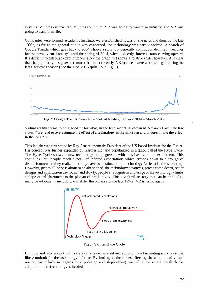
129
systems. VR was everywhere, VR was the future, VR was going to transform industry, and VR was
going to transform life.
Companies were formed. Academic institutes were established. It was on the news and then, by the late
1990s, as far as the general public was concerned, the technology was hardly noticed. A search of
Google Trends, which goes back to 2004, shows a slow, but generally continuous decline in searches
for the term “virtual reality” until the spring of 2014, when suddenly, interest starts curving upward.
It’s difficult to establish exact numbers since the graph just shows a relative scale; however, it is clear
that the popularity has grown so much that most recently, VR headsets were a hot tech gift during the
last Christmas season (See the Dec. 2016 spike up in Fig. 2).
Fig.2: Google Trends: Search for Virtual Reality, January 2004 – March 2017
Virtual reality seems to be a good fit for what, in the tech world, is known as Amara’s Law. The law
states, “We tend to overestimate the effect of a technology in the short run and underestimate the effect
in the long run.”
This insight was first stated by Roy Amara, formerly President of the US-based Institute for the Future.
His concept was further expanded by Gartner Inc. and popularized in a graph called the Hype Cycle.
The Hype Cycle shows a new technology being greeted with massive hype and excitement. This
continues until people reach a peak of inflated expectations which crashes down to a trough of
disillusionment as they realize that they have overestimated the technology (at least in the short run).
However, just as all hope is about to be abandoned, the technology advances, prices come down, better
designs and applications are found, and slowly, people’s recognition and usage of the technology climbs
a slope of enlightenment to the plateau of productivity. This is a familiar story that can be applied to
many developments including VR. After the collapse in the late 1990s, VR is rising again.
Fig.3: Gartner Hype Cycle
But how and why we got to this state of renewed interest and adoption is a fascinating story, as is the
likely outlook for the technology’s future. By looking at the forces affecting the adoption of virtual
reality, particularly in regards to ship design and shipbuilding, we will show where we think the
adoption of this technology is headed.
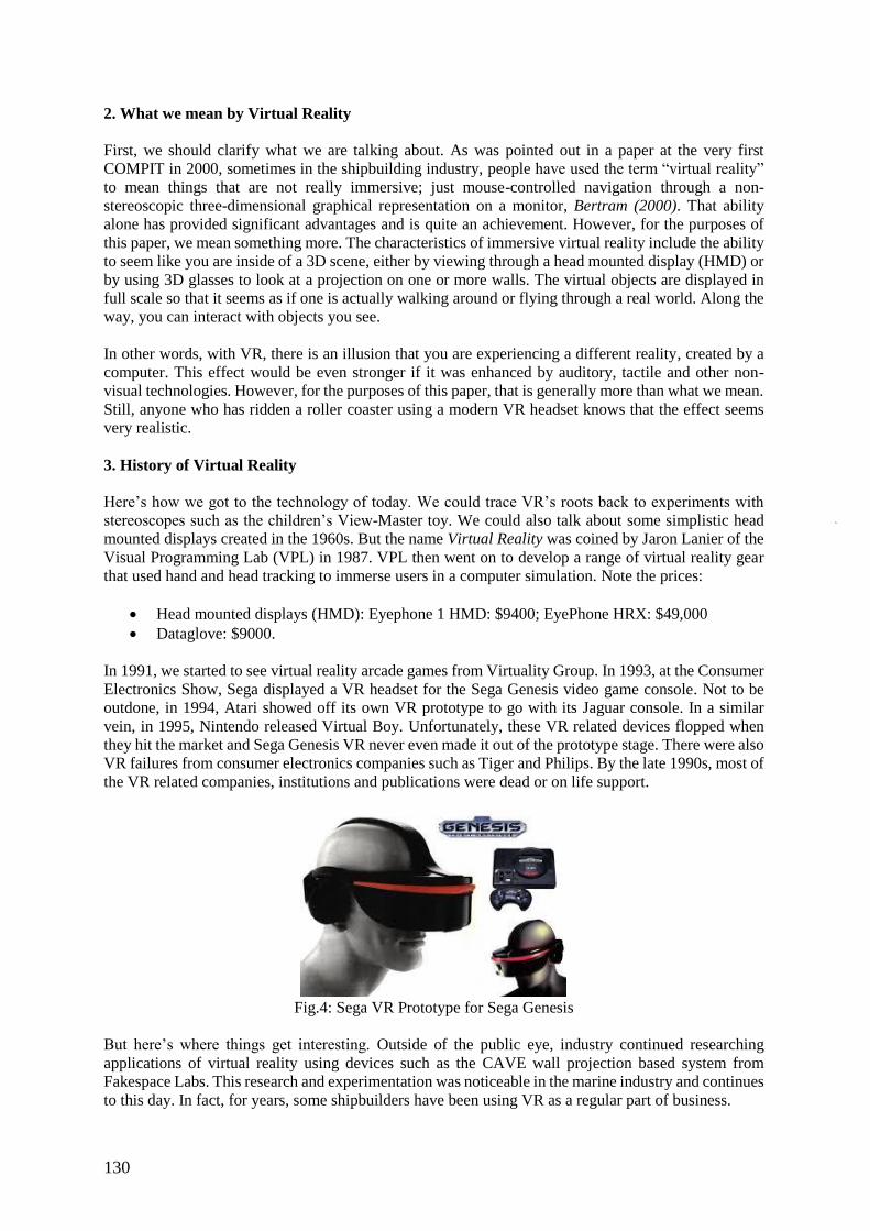
130
2. What we mean by Virtual Reality
First, we should clarify what we are talking about. As was pointed out in a paper at the very first
COMPIT in 2000, sometimes in the shipbuilding industry, people have used the term “virtual reality”
to mean things that are not really immersive; just mouse-controlled navigation through a non-
stereoscopic three-dimensional graphical representation on a monitor, Bertram (2000). That ability
alone has provided significant advantages and is quite an achievement. However, for the purposes of
this paper, we mean something more. The characteristics of immersive virtual reality include the ability
to seem like you are inside of a 3D scene, either by viewing through a head mounted display (HMD) or
by using 3D glasses to look at a projection on one or more walls. The virtual objects are displayed in
full scale so that it seems as if one is actually walking around or flying through a real world. Along the
way, you can interact with objects you see.
In other words, with VR, there is an illusion that you are experiencing a different reality, created by a
computer. This effect would be even stronger if it was enhanced by auditory, tactile and other non-
visual technologies. However, for the purposes of this paper, that is generally more than what we mean.
Still, anyone who has ridden a roller coaster using a modern VR headset knows that the effect seems
very realistic.
3. History of Virtual Reality
Here’s how we got to the technology of today. We could trace VR’s roots back to experiments with
stereoscopes such as the children’s View-Master toy. We could also talk about some simplistic head
mounted displays created in the 1960s. But the name Virtual Reality was coined by Jaron Lanier of the
Visual Programming Lab (VPL) in 1987. VPL then went on to develop a range of virtual reality gear
that used hand and head tracking to immerse users in a computer simulation. Note the prices:
Head mounted displays (HMD): Eyephone 1 HMD: $9400; EyePhone HRX: $49,000
Dataglove: $9000.
In 1991, we started to see virtual reality arcade games from Virtuality Group. In 1993, at the Consumer
Electronics Show, Sega displayed a VR headset for the Sega Genesis video game console. Not to be
outdone, in 1994, Atari showed off its own VR prototype to go with its Jaguar console. In a similar
vein, in 1995, Nintendo released Virtual Boy. Unfortunately, these VR related devices flopped when
they hit the market and Sega Genesis VR never even made it out of the prototype stage. There were also
VR failures from consumer electronics companies such as Tiger and Philips. By the late 1990s, most of
the VR related companies, institutions and publications were dead or on life support.
Fig.4: Sega VR Prototype for Sega Genesis
But here’s where things get interesting. Outside of the public eye, industry continued researching
applications of virtual reality using devices such as the CAVE wall projection based system from
Fakespace Labs. This research and experimentation was noticeable in the marine industry and continues
to this day. In fact, for years, some shipbuilders have been using VR as a regular part of business.

131
3.1 Virtual Reality in Shipbuilding Industry: COMPIT Papers
The marine industry’s interest in VR was apparent at the first COMPIT held in 2000. Furthermore, a
review of all the proceedings since then shows that with very few exceptions, almost every year the
conference has featured several papers on virtual reality. Admittedly, sometimes the papers are about
utilizing what one paper called “poor man’s” virtual reality, just 3D navigation on a monitor, Bertram
(2000). Still, it is interesting to review the history. Here is a sample of papers presented:
In 2000, there was discussion of using VR for CFD post-processing, Bertram (2000) and discussions
of how the Canadian Navy was using a virtual reality simulator for training on deep water manoeuvring,
Frutuoso and Soares (2000). In 2003, there was a paper on the advantages of using VR for engine room
design, Baier (2003). In 2005, a paper talked about using VR to enhance clarity in the design of ship
outfitting, Nedeß et al. (2005).
The focus between 2000 and 2005 seems generally to have been on simulation and design review for
manufacturing. Then, in 2006 and 2007, papers start talking about using VR more for sales and
marketing and training. In 2008, there is a paper on how the Brazilian Navy was using animations of
assembly sequencing to visualize possible problems in production, Santos (2008). In 2013 there is talk
about shop-floor 3D, supply chain collaboration, and integration with other software, Larkins et al.
(2013). More recent papers have been talking about VR’s close cousin, Augmented Reality (AR).
3.2 Current VR Usage in shipbuilding
That brings us to today. Currently, if one surveys the actual usage of immersive virtual reality in our
industry, two major players are Virtalis and Techviz. According to their websites, they have the
following major shipbuilding clients:
Technviz Clients:
DSNS (French Navy projects)
Keppel FELS (Offshore builder)
Hyundai Mipo Dockyard (one of the world’s largest shipbuilders)
Virtalis Clients: (Software: Visionary Render & VR for CAD)
BAE (British Navy projects)
Dalian (Big Chinese shipbuilder)
Irving and Fleetway (Canadian Navy Project)
Companies use VR for design review, shop floor 3D, sales, marketing and training.
In our survey of the market, something jumps out at us. The companies that use the big cave style
immersive VR systems are typically involved in defence or in very large-scale shipbuilding. Companies
building workboats, ferries and yachts are not typically using VR on this level. It’s true, they do often
use programs such as Autodesk Navisworks and other CAD software’s associated viewing applications.
However, head mounted displays and virtual reality viewing rooms are not typically used by anyone
but large organizations, especially those involved with defence.
4. Back in Time: Consumer VR from 1990s until Oculus Rift
So why isn’t immersive virtual reality used more often in our industry? Before answering that question,
let us turn back to the consumer world because to understand what has happened in the last few years,
you need to look at what happened from the 1990s until the development of the Oculus Rift.
Let us go back in time and look at why consumer grade VR died in the late 1990s. We’ll get into more
details later, but right now, it’s simple enough to say this: Back then, VR was extensively promoted to
the masses and there was a receptive audience. Unfortunately, the quality of what people experienced
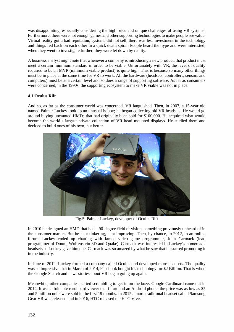
132
was disappointing, especially considering the high price and unique challenges of using VR systems.
Furthermore, there were not enough games and other supporting technologies to make people see value.
Virtual reality got a bad reputation, systems did not sell, there was less investment in the technology
and things fed back on each other in a quick death spiral. People heard the hype and were interested;
when they went to investigate further, they were let down by reality.
A business analyst might note that whenever a company is introducing a new product, that product must
meet a certain minimum standard in order to be viable. Unfortunately with VR, the level of quality
required to be an MVP (minimum viable product) is quite high. This is because so many other things
must be in place at the same time for VR to work. All the hardware (headsets, controllers, sensors and
computers) must be at a certain level and so does a range of supporting software. As far as consumers
were concerned, in the 1990s, the supporting ecosystem to make VR viable was not in place.
4.1 Oculus Rift
And so, as far as the consumer world was concerned, VR languished. Then, in 2007, a 15-year old
named Palmer Luckey took up an unusual hobby; he began collecting old VR headsets. He would go
around buying unwanted HMDs that had originally been sold for $100,000. He acquired what would
become the world’s largest private collection of VR head mounted displays. He studied them and
decided to build ones of his own, but better.
Fig.5: Palmer Luckey, developer of Oculus Rift
In 2010 he designed an HMD that had a 90-degree field of vision, something previously unheard of in
the consumer market. But he kept tinkering, kept improving. Then, by chance, in 2012, in an online
forum, Luckey ended up chatting with famed video game programmer, John Carmack (lead
programmer of Doom, Wolfenstein 3D and Quake). Carmack was interested in Luckey’s homemade
headsets so Luckey gave him one. Carmack was so amazed by what he saw that he started promoting it
in the industry.
In June of 2012, Luckey formed a company called Oculus and developed more headsets. The quality
was so impressive that in March of 2014, Facebook bought his technology for $2 Billion. That is when
the Google Search and news stories about VR began going up again.
Meanwhile, other companies started scrambling to get in on the buzz. Google Cardboard came out in
2014. It was a foldable cardboard viewer that fit around an Android phone; the price was as low as $5
and 5 million units were sold in the first 19 months. In 2015 a more traditional headset called Samsung
Gear VR was released and in 2016, HTC released the HTC Vive.
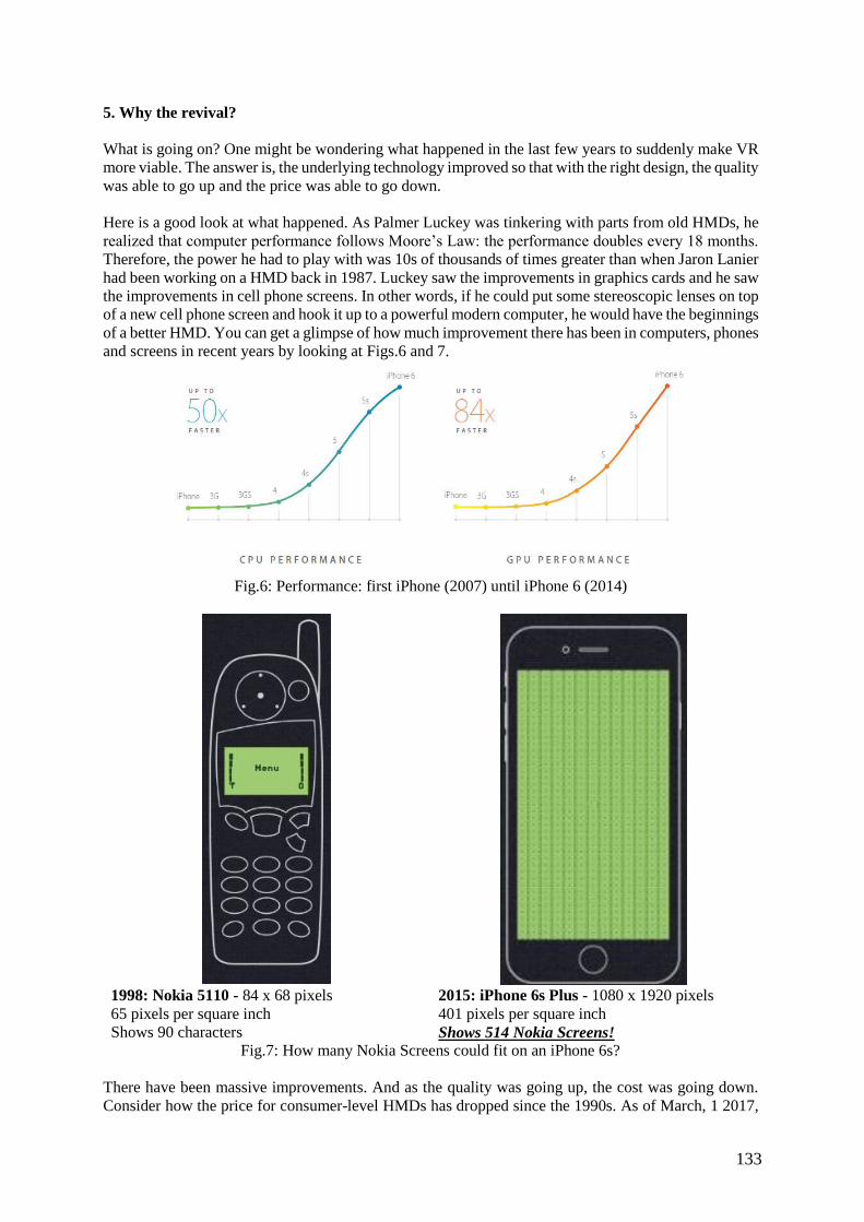
133
5. Why the revival?
What is going on? One might be wondering what happened in the last few years to suddenly make VR
more viable. The answer is, the underlying technology improved so that with the right design, the quality
was able to go up and the price was able to go down.
Here is a good look at what happened. As Palmer Luckey was tinkering with parts from old HMDs, he
realized that computer performance follows Moore’s Law: the performance doubles every 18 months.
Therefore, the power he had to play with was 10s of thousands of times greater than when Jaron Lanier
had been working on a HMD back in 1987. Luckey saw the improvements in graphics cards and he saw
the improvements in cell phone screens. In other words, if he could put some stereoscopic lenses on top
of a new cell phone screen and hook it up to a powerful modern computer, he would have the beginnings
of a better HMD. You can get a glimpse of how much improvement there has been in computers, phones
and screens in recent years by looking at Figs.6 and 7.
Fig.6: Performance: first iPhone (2007) until iPhone 6 (2014)
1998: Nokia 5110 - 84 x 68 pixels
65 pixels per square inch
Shows 90 characters
2015: iPhone 6s Plus - 1080 x 1920 pixels
401 pixels per square inch
Shows 514 Nokia Screens! Fig.7: How many Nokia Screens could fit on an iPhone 6s?
There have been massive improvements. And as the quality was going up, the cost was going down.
Consider how the price for consumer-level HMDs has dropped since the 1990s. As of March, 1 2017,
134
the Oculus Rift Headset is $499 USD and the associated Touch Controller is $99. The price of Jaron
Lanier’s inferior technology in the 1990s was over $18,000!
6. Consumer VR still not ready
Unfortunately however, VR still does not appear to be ready for mass adoption by consumers. Even
though in March 2014, Facebook’s Mark Zuckerberg was willing to spend $2 Billion on virtual reality,
in February of 2016 he said to ‘Business Insider’ that the technology remains a long way from reaching
the mass market; in fact, he thought that it would take at least 10 years.
There are several logical reasons for Zuckerberg’s caution. There are several challenges that still need
to be better addressed. First of all, even with the massive price reductions, the cost of VR equipment is
still higher than most consumers want to pay to play video games. Not only do you need a special
headset and controller, VR requires a more expensive computer than most people have. Then, there are
several other factors which you don’t think about until you start getting serious about VR: the headsets
are bulky and not comfortable for long periods of use; they mess up people’s hair and even their makeup.
Being tethered to a machine with cables is a tripping hazard and you must spend quite a bit of time
creating a controlled environment in an open space without furniture in the way. There are also sensors
to set up. People do not want to do all this work in their homes. All of this is a significant cost and
hassle, and what do consumers get out of it?
If quality is acceptable, the price is high, but if the price is low, the quality is poor. A lot of people were
excited to see that they could leverage their phones to get virtual reality cheaply via solutions such as
Google Daydream View ($99) or Samsung Gear ($69.99). Unfortunately, these are mostly just a
novelty; these products do not support scenes as complex as most people would like.
As for all consumer VR in general, the newness of the technology means there are few games or
applications available. The fragmentation of the market further makes it harder for consumers to know
which platform they should pick. All of this leads to a Catch-22: less games and applications are
developed, the price stays too high, and there is less of a reason for average consumers to spend on VR.
It is true that virtual reality games and devices experienced an exponential increase in sales in the 2016
Christmas season. However, that was still dwarfed by sales of other technology. Zuckerberg is probably
right; even though there have been exponential improvements, as far as consumers are concerned, VR
still has ways to go before it will become ubiquitous.
7. Industry will Drive Enhancements
On the other hand, the situation is totally different in the business world. In fact, we believe that industry
will lead the charge in VR development from here. This is in contrast to what we have been used to
seeing over the past decade where technology for the consumer market (e.g. cell phones and tablets)
has been driving development and later spinning off into business uses. Remember, unlike with the total
collapse in the consumer market in the late 1990s, industrial usage of virtual reality never went away.
A lot of the challenges and hassles that plagued products for consumers were not present, or at least,
not felt as strongly in the business world.
When a business uses VR, it is not doing it for casual entertainment; it is to solve real business
challenges. In the COMPIT papers over the last 17 years, it has repeatedly been noted that VR increases
quality and understanding during design reviews which prevents rework, increases efficiency in
production, and reduces costly errors. Still more benefit can be derived for training and sales. Therefore,
there is a potential for significant return on investment; buying a VR system for an industrial application
is not just something one does for amusement. This seriousness means that people working on high
value designs are a bit more willing to accept a certain amount of annoyance such as tethering, bulky
headsets, and even more prosaic problems such as mussing up one’s hair and makeup with an HMD.
Of course, these types of things still are concerns; they just do not have quite as high a weight as when
people are merely using VR for fun.
135
As for the issue of computing power, this is far less of a concern for industry. It may be true that only
1% of consumers have PCs that can support VR. However, if a company is doing engineering, this is
not the case. If a company is using CAD programs, it probably already has powerful VR capable
computers and is used to buying machines of that calibre. Admittedly, depending on the VR solution
deployed, they will probably need a separate machine for each graphics display node; however, buying
high powered computers is not a shock for engineers.
Another relative non-issue for industrial use-cases is the availability of applications. Programs such as
Virtalis Visionary Render or the software from TechViz already address several industry desires and
support input from a wide variety of CAD programs. It is nothing like the situation with consumer VR
where consumers are unwilling to buy VR hardware until more games are developed.
8. Challenges
Nevertheless, the fact that VR has not already been more widely adopted for business uses demonstrates
that there still are serious concerns, particularly in the shipbuilding industry.
8.1. Challenge: Lack of perceived benefit vs cost
First of all, there is the price or rather, the perceived benefit vs. the cost. It is hard to justify spending
money on virtual reality if it is not thought to be worth it. Below are some numbers:
With the price cut at the beginning of March 2017, you can buy an Oculus Rift and an associated Touch
motion controller for $598 USD. It is advertised as being plug and play but when engineering managers
go to experiment with it, they are shocked to find out that they probably need software for $17,000 (on
top of a $4000 computer). And that is just the beginning. If you start looking at wall systems, things
start to really add up. On top of the price of the high-end computer (actually, multiple high-end
computers, depending on the collaboration scenarios), there is the cost of the projector. A projector with
the necessary lumens and a resolution of 4K could be $150,000! If you start adding displays on the floor
and multiple walls, or if you want multiple HMDs, you need more computers, software and projectors.
On top of that is the construction (and preparation and dedication) of a special VR room itself.
Therefore, for many applications, the price of a virtual reality system can run well into the hundreds of
thousands of dollars. That is an order of magnitude more than the type of price that people these days
expect to pay for anything to do with computers and electronics so this can come as quite a shock.
You also must remember that the upfront dollars are just one “cost” of VR. Virtual reality always
involves at least some form of additional overhead, e.g. the hassle of putting on headsets and meeting
in a special room etc. Thus, in order to justify the usage of VR, there probably has to be significant
additional benefit to using it over the status quo. Indeed, the bigger the net benefit, the better.
8.1.1 Solution 1: 10x better
A good way to think of this is to use the 10x concept promoted by venture capitalist and PayPal founder
Peter Thiel. He only invests in companies that offer a solution that is ten times (10x) better than the
current way of doing things. Applying this concept to VR, we can see that in many scenarios, even if
utilizing VR was a natural extension of current processes, the advantages would likely be perceived as
being too small to create widespread adoption. Using VR for routine clash detection of geometry would
probably fall into this category so we would not expect shipbuilders to be sold on VR for that.
On the other hand, using VR for sales and marketing would provide a dramatically better experience
than looking at plain pictures. That is because VR allows better communication, especially with non-
technical people who, by using VR would have a way to navigate through a ship model naturally. Virtual
reality would thus be more likely to be adopted here.
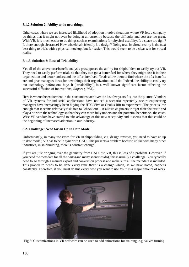
136
8.1.2 Solution 2: Ability to do new things
Other cases where we see increased likelihood of adoption involve situations where VR lets a company
do things that it might not even be doing at all currently because the difficulty and cost are too great.
With VR, it is much easier to do things such as examinations for physical usability. Is a space too tight?
Is there enough clearance? How wheelchair-friendly is a design? Doing tests in virtual reality is the next
best thing to trials with a physical mockup, but far easier. This would seem to be a clear win for virtual
reality.
8. 1.3. Solution 3: Ease of Trialability
Yet all of the above cost/benefit analysis presupposes the ability for shipbuilders to easily try out VR.
They need to easily perform trials so that they can get a better feel for where they might use it in their
organization and better understand the effort involved. Trials allow them to find where the 10x benefits
are and give managers ideas for new things their organization could do. Indeed, the ability to easily try
out technology before one buys it (“trialability”) is a well-known significant factor affecting the
successful diffusion of innovations, Rogers (1983).
Here is where the excitement in the consumer space over the last few years fits into the picture. Vendors
of VR systems for industrial applications have noticed a scenario repeatedly occur; engineering
managers have increasingly been buying the HTC Vive or Oculus Rift to experiment. The price is low
enough that it seems relatively risk-free to “check out”. It allows engineers to “get their feet wet” and
play a bit with the technology so that they can more fully understand the potential benefits vs. the costs.
Wise VR vendors have started to take advantage of this new receptivity and it seems that this could be
the beginning of increased adoption in our industry.
8.2. Challenge: Need for an Up to Date Model
Unfortunately, in many use cases for VR in shipbuilding, e.g. design reviews, you need to have an up
to date model; VR has to be in sync with CAD. This presents a problem because unlike with many other
industries, in shipbuilding, there is constant change.
If you are just bringing over the geometry from CAD into VR, this is less of a problem. However, if
you need the metadata for all the parts (and many scenarios do), this is usually a challenge. You typically
need to go through a manual export and conversion process and make sure all the metadata is included.
This procedure needs to be done every time there is a change which, as we have noted, happens
constantly. Therefore, if you must do this every time you want to use VR it is a major amount of work.
Fig.8: Customizations in VR software can be used to add animations for training, e.g. valves turning
137
And the problem is compounded once you start dealing with VR customizations. What we mean by VR
customizations is adding data in VR. For instance, to make a scene more realistic you might change
material properties. This helps when showing an owner or sales prospect what their ship might look
like. Similarly, to help with training or simulation, you might add animations to make a door open or a
valve turn. You would not want to lose all those customizations every time you updated the CAD model
because recreating these would take a lot of effort. Indeed, the inability for software solutions to handle
change is so significant that it often relegates VR usage to scenarios that change less often.
8.2.1. Solution: VR Must be a Natural Extension of CAD and Current Workflows
The solution to the challenge of change (and other problems, for that matter) is to make VR a natural
extension of CAD and current workflows. In other words, working in virtual reality should be a
seamless process. VR should be a natural way of viewing and interacting with the CAD data (including
all properties, not just geometry). It should always be accurate and up-to-date and should be able to
handle change without costly overhead. No special VR experts should be required to convert data into
the system and no special CAD expertise should be required for users of the VR program to easily find
the data. The entire process should be intuitive.
A key to realizing this solution would be linkages between the parts in CAD and VR. While in VR, you
would always be working on a current CAD model and you would be able to add animations and
enhance the scene, yet these changes would persist, even when the CAD model changed.
The linkages would bi-directional. This would allow you to be able to make annotations in the VR
program and these would not just be sent to a notepad file, they would actually feed back into the CAD
system so modellers would know of any changes that needed to be made. Everything would be as clear
as possible and as simple as possible. This would make VR a natural extension of current shipbuilding
software and thus speed the adoption of virtual reality in our industry.
12. Conclusion
In summary, we have witnessed continual improvement in computer performance and screen resolution
since VR’s short-lived consumer heyday in the 1990s. More recently, we have seen VR once again
explode into the public consciousness, including in the consciousness of shipbuilders who previously
considered virtual reality to be priced out of reach. From here, we see industry leading the charge in
terms of development because hassles that would deter consumers are of relatively smaller weight in a
business context.
The issue regarding perceived benefit vs. price can be addressed by finding scenarios where VR
contributes ten times the net advantage of the status quo, or by scenarios involving capabilities that a
shipyard never considered possible before. While performing this cost/ benefit analysis, the ability to
easily try the technology (“trialability”) will be crucial.
Many scenarios in shipbuilding will present a special challenge because they require and up to date
model and our industry involves constant changes to a design. Building a VR solution that is tightly
integrated with CAD via linkages will be a way of creating a solution that is a natural extension of CAD
and existing workflows. This will lead to increased adoption of virtual reality in our industry.
References
BAIER, C. (2003), Practical application of Virtual Reality in engine room design, 2nd Int. Conf.
Computer and IT Appl. Maritime Ind., Hamburg, pp.278-283
BERTRAM, V. (2000), Virtual Reality applications for CFD postprocessing, 1st Int. Conf. Computer
and IT Appl. Maritime Ind., Potsdam, pp.35-44

138
FRUTUOSO, M.S.; SOARES, C.G. (2000), 3D Virtual Environments for Ship Manoeuvring
Simulation, 1st Int. Conf. Computer and IT Appl. Maritime Ind., Potsdam, pp.438-448
LARKINS, D.; MORAIS, D.; WALDIE, M. (2013), Democratization of Virtual Reality in shipbuilding,
12th Int. Conf. Computer and IT Appl. Maritime Ind., Cortona, pp.316-326
LÖDDING, H.; FRIEDEWALD, A; HEINIG, M.; SCHLEUSENER, S. (2011), Virtual Reality
assembly planning in the shipbuilding industry, 10th Int. Conf. Computer and IT Appl. Maritime Ind.,
Berlin, pp.253-263
MORAIS, D.; LARKINS, D.; WALDIE, M. (2011), Driving the adoption of cutting edge technology
in shipbuilding, 10th Int. Conf. Computer and IT Appl. Maritime Ind., Berlin, pp.523-535
NEDESS, C.; FRIEDEWALD, A.; KERSE, N. (2005), Increasing customer’s benefit using Virtual
Reality (VR) – Technologies in the design of ship outfitting, 4th Int. Conf. Computer and IT Appl.
Maritime Ind., Hamburg, pp.113-122
ROGERS, E.M. (1983), Diffusion of Innovations, Free Press-Macmillan Publ., pp.21-233
SANTOS, C.V.M.S. (2008), Production simulation applied to military shipbuilding, 7th Int. Conf.
Computer and IT Appl. Maritime Ind., Liège, pp.302-313
139
A Packing Approach Model in Support of the Conceptual
Design of Naval Submarines
Siebe Cieraad, Defence Materiel Organisation, The Hague/The Netherlands, [email protected]
Etienne Duchateau, Defence Materiel Organisation, [email protected]
Ruben Zandstra, Defence Materiel Organisation, [email protected]
Wendy van den Broek-de Bruijn, Defence Materiel Organisation, [email protected]
Abstract
Concept exploration has proven to be useful in the early stage design of naval surface vessels,
especially when new operational concepts or complex design solutions are required. This paper
presents a design synthesis model for diesel-electric submarines, based on the 2.5D Packing-
Approach, which can automatically generate varying yet balanced designs. To do so, several new
developments have been implemented in the 2.5D Packing-Approach to facilitate the design and
balancing of submarine arrangements. The synthesis model was verified and validated with two test-
cases. It was first used to redesign the Walrus-class conventional submarine. Second, to assess the
models’ capabilities as a conceptual design aid, several variations of requirements were performed
and analysed. The results of these test-cases confirm that the synthesis model can be a valuable
resource in the conceptual design stage of submarines.
1. Introduction/background
The preliminary design stage of a vessel balances the ambitions and needs of the customer with the
technical feasibility and available budget. This is often done by exploring a broad number of designs
in which different levels of technical feasibility, budget, and customer ambitions are considered. A
process referred to as requirements elucidation or concept exploration, Andrews (2011; van Oers
(2015).
Generally, naval vessels are novel complex concepts that need to fulfil a specific purpose for which
multiple alternatives can be used. These alternatives can differ in the used components/systems and
the configuration of those components/systems. For example, a RHIB (rigid hull inflatable boat) can
be deployed from a vessel with a crane, a davit, or using a slipway, or a combination of these systems
to increase flexibility. Each alternative has its advantages and disadvantages and can be placed on
different locations on board the vessel which will result in a different vessel concept. Furthermore, the
characteristics of a design concept can only be properly predicted and compared with other design
concepts when a certain level of detail in the design is reached. Achieving this level of detail for a
complex vessel requires considerable design effort due to the complex relations intertwined in vessel
design itself and the complex systems for which the vessel acts as a platform. This effort, multiplied
with the large number of designs needed to conduct a thorough design exploration, together with the
generally limited time available, makes the design exploration of naval vessels a challenging
undertaking, Pawling (2007), van Oers (2011).
1.1. Conceptual submarine design
Concept exploration for a naval submarine requires even more effort. The relatively small size of a
submarine and the large amount of constrained components keep the diversity in the configuration of
a submarine relatively low when compared to surface vessels. However, in submarines even small
variations in the configuration can have large impact on the hydrostatic balance of the vessel.
The hydrostatic balance is the balance between the buoyancy and mass of any floating object. For
submarines the hydrostatic balance needs to be exactly right in order for the submarine to be neutrally
buoyant. Also, to make sure the submarine has no trim or roll angles the points of application of both
the buoyancy and mass need to be placed exactly above each other. Surface vessels also need to be
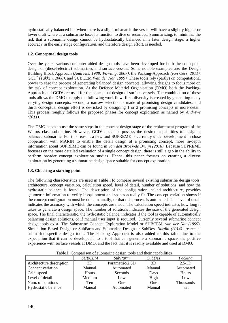
140
hydrostatically balanced but when there is a slight mismatch the vessel will have a slightly higher or
lower draft where as a submarine loses its function to dive or resurface. Summarizing, to minimize the
risk that a submarine design cannot be hydrostatically balanced in a later design stage, a higher
accuracy in the early stage configuration, and therefore design effort, is needed.
1.2. Conceptual design tools
Over the years, various computer aided design tools have been developed for both the conceptual
design of (diesel-electric) submarines and surface vessels. Some notable examples are: the Design
Building Block Approach (Andrews, 1988; Pawling, 2007), the Packing-Approach (van Oers, 2011),
GCD2 (Takken, 2008), and SUBCEM (van der Nat, 1999). These tools rely (partly) on computational
power to ease the process of generating balanced design concepts, allowing designs to focus more on
the task of concept exploration. At the Defence Materiel Organisation (DMO) both the Packing-
Approach and GCD2 are used for the conceptual design of surface vessels. The combination of these
tools allows the DMO to apply the following work flow: first, diversity is created by generating many
varying design concepts; second, a narrow selection is made of promising design candidates; and
third, conceptual design effort is de-risked by designing 1 or 2 promising concepts in more detail.
This process roughly follows the proposed phases for concept exploration as named by Andrews
(2011).
The DMO needs to use the same steps in the concept design stage of the replacement program of the
Walrus class submarine. However, GCD2 does not possess the desired capabilities to design a
balanced submarine. For this reason, a new tool SUPREME is currently under development in close
cooperation with MARIN to enable the detail design of a promising concept, more in-depth
information about SUPREME can be found in van den Broek-de Bruijn (2016). Because SUPREME
focusses on the more detailed evaluation of a single concept design, there is still a gap in the ability to
perform broader concept exploration studies. Hence, this paper focuses on creating a diverse
exploration by generating a submarine design space suitable for concept exploration.
1.3. Choosing a starting point
The following characteristics are used in Table I to compare several existing submarine design tools:
architecture, concept variation, calculation speed, level of detail, number of solutions, and how the
hydrostatic balance is found. The description of the configuration, called architecture, provides
geometric information to verify if equipment and spaces actually fit. The concept variation shows if
the concept configuration must be done manually, or that this process is automated. The level of detail
indicates the accuracy with which the concepts are made. The calculation speed indicates how long it
takes to generate a design space. The number of solutions indicates the size of the generated design
space. The final characteristic, the hydrostatic balance, indicates if the tool is capable of automatically
balancing design solutions, or if manual user input is required. Currently several submarine concept
design tools exist. The Submarine Concept Exploration Model or SUBCEM, van der Nat (1999),
Simulation Based Design or SubParm and Submarine Design or SubDes, Nordin (2014) are recent
submarine specific design tools. The Packing Approach is also added to this table due to the
expectation that it can be developed into a tool that can generate a submarine space, the positive
experience with surface vessels at DMO, and the fact that it is readily available and used at DMO.
Table I: Comparison of submarine design tools and their capabilities
SUBCEM SubParm SubDes Packing
Architecture description 3D Parametric/2.5D 3D 2.5/3D
Concept variation Manual Automated Manual Automated
Calc. speed Hours Seconds Days Hours
Level of detail Medium Low High Low
Num. of solutions Ten One One Thousands
Hydrostatic balance Manual Automated Manual n.a.
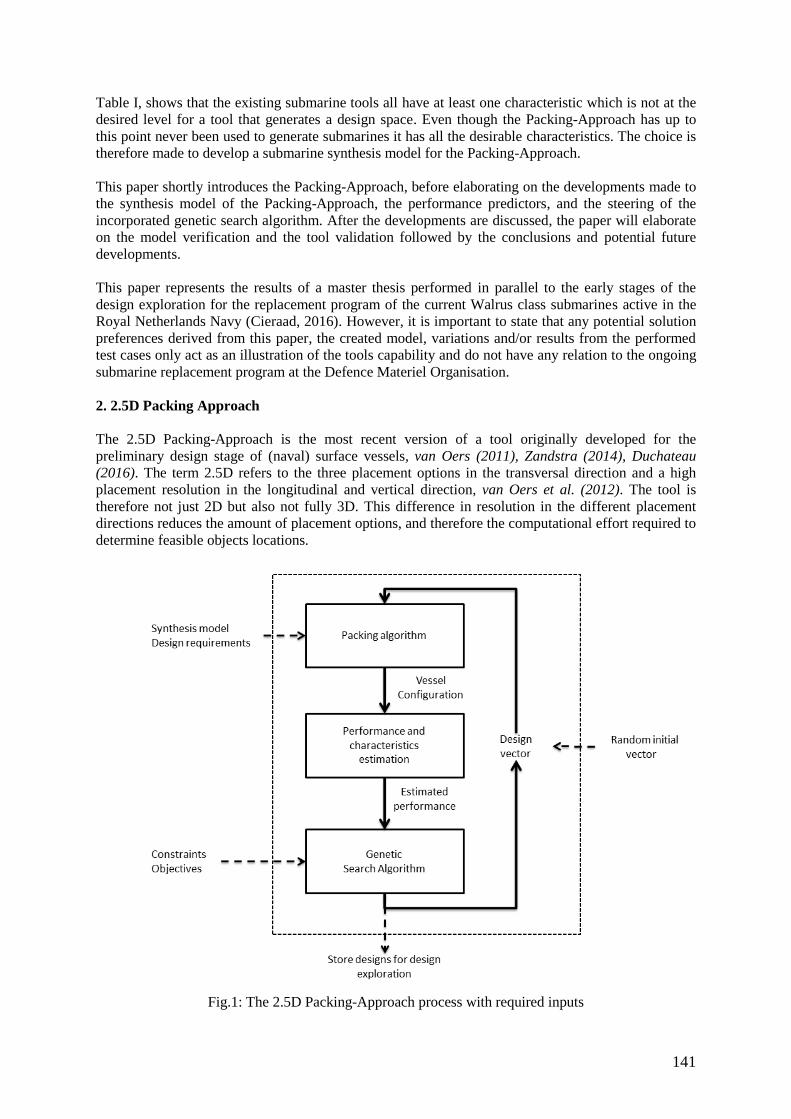
141
Table I, shows that the existing submarine tools all have at least one characteristic which is not at the
desired level for a tool that generates a design space. Even though the Packing-Approach has up to
this point never been used to generate submarines it has all the desirable characteristics. The choice is
therefore made to develop a submarine synthesis model for the Packing-Approach.
This paper shortly introduces the Packing-Approach, before elaborating on the developments made to
the synthesis model of the Packing-Approach, the performance predictors, and the steering of the
incorporated genetic search algorithm. After the developments are discussed, the paper will elaborate
on the model verification and the tool validation followed by the conclusions and potential future
developments.
This paper represents the results of a master thesis performed in parallel to the early stages of the
design exploration for the replacement program of the current Walrus class submarines active in the
Royal Netherlands Navy (Cieraad, 2016). However, it is important to state that any potential solution
preferences derived from this paper, the created model, variations and/or results from the performed
test cases only act as an illustration of the tools capability and do not have any relation to the ongoing
submarine replacement program at the Defence Materiel Organisation.
2. 2.5D Packing Approach
The 2.5D Packing-Approach is the most recent version of a tool originally developed for the
preliminary design stage of (naval) surface vessels, van Oers (2011), Zandstra (2014), Duchateau
(2016). The term 2.5D refers to the three placement options in the transversal direction and a high
placement resolution in the longitudinal and vertical direction, van Oers et al. (2012). The tool is
therefore not just 2D but also not fully 3D. This difference in resolution in the different placement
directions reduces the amount of placement options, and therefore the computational effort required to
determine feasible objects locations.
Fig.1: The 2.5D Packing-Approach process with required inputs
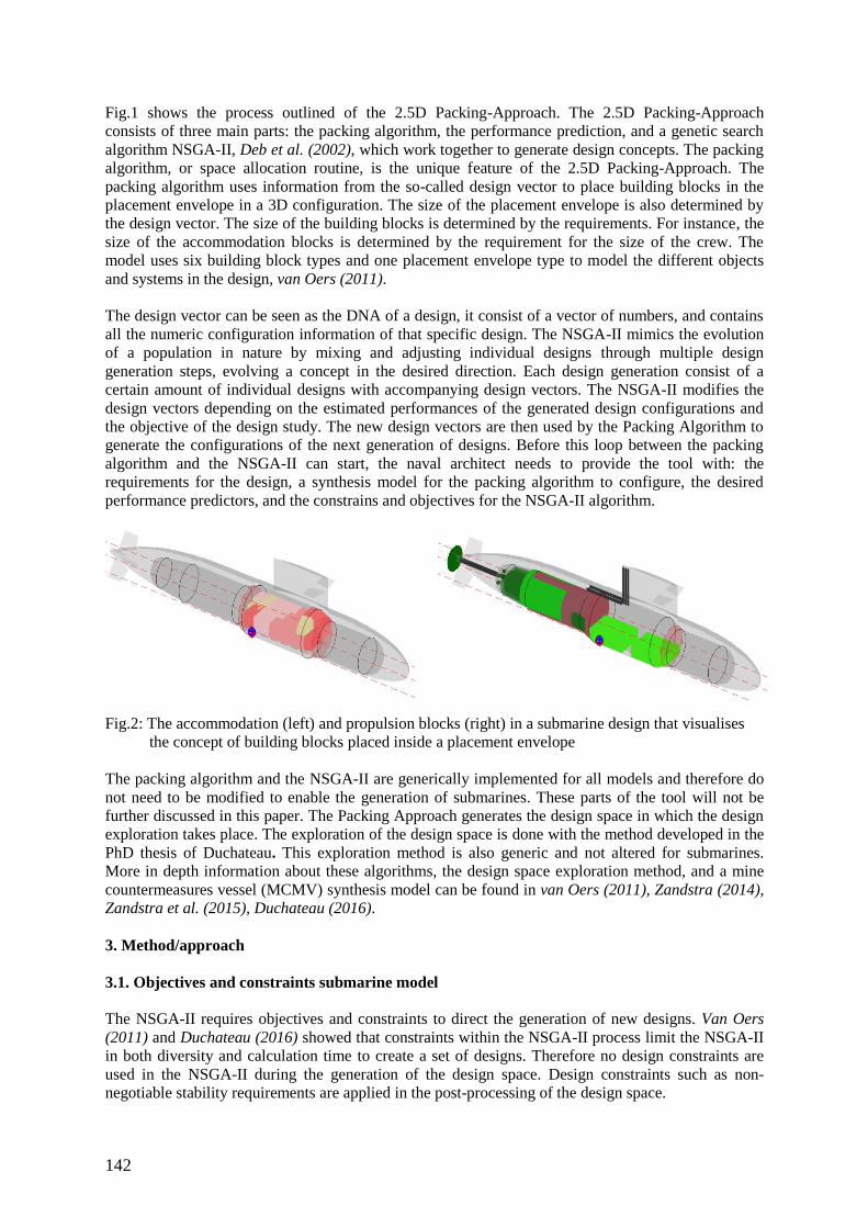
142
Fig.1 shows the process outlined of the 2.5D Packing-Approach. The 2.5D Packing-Approach
consists of three main parts: the packing algorithm, the performance prediction, and a genetic search
algorithm NSGA-II, Deb et al. (2002), which work together to generate design concepts. The packing
algorithm, or space allocation routine, is the unique feature of the 2.5D Packing-Approach. The
packing algorithm uses information from the so-called design vector to place building blocks in the
placement envelope in a 3D configuration. The size of the placement envelope is also determined by
the design vector. The size of the building blocks is determined by the requirements. For instance, the
size of the accommodation blocks is determined by the requirement for the size of the crew. The
model uses six building block types and one placement envelope type to model the different objects
and systems in the design, van Oers (2011).
The design vector can be seen as the DNA of a design, it consist of a vector of numbers, and contains
all the numeric configuration information of that specific design. The NSGA-II mimics the evolution
of a population in nature by mixing and adjusting individual designs through multiple design
generation steps, evolving a concept in the desired direction. Each design generation consist of a
certain amount of individual designs with accompanying design vectors. The NSGA-II modifies the
design vectors depending on the estimated performances of the generated design configurations and
the objective of the design study. The new design vectors are then used by the Packing Algorithm to
generate the configurations of the next generation of designs. Before this loop between the packing
algorithm and the NSGA-II can start, the naval architect needs to provide the tool with: the
requirements for the design, a synthesis model for the packing algorithm to configure, the desired
performance predictors, and the constrains and objectives for the NSGA-II algorithm.
Fig.2: The accommodation (left) and propulsion blocks (right) in a submarine design that visualises
the concept of building blocks placed inside a placement envelope
The packing algorithm and the NSGA-II are generically implemented for all models and therefore do
not need to be modified to enable the generation of submarines. These parts of the tool will not be
further discussed in this paper. The Packing Approach generates the design space in which the design
exploration takes place. The exploration of the design space is done with the method developed in the
PhD thesis of Duchateau. This exploration method is also generic and not altered for submarines.
More in depth information about these algorithms, the design space exploration method, and a mine
countermeasures vessel (MCMV) synthesis model can be found in van Oers (2011), Zandstra (2014),
Zandstra et al. (2015), Duchateau (2016).
3. Method/approach
3.1. Objectives and constraints submarine model
The NSGA-II requires objectives and constraints to direct the generation of new designs. Van Oers
(2011) and Duchateau (2016) showed that constraints within the NSGA-II process limit the NSGA-II
in both diversity and calculation time to create a set of designs. Therefore no design constraints are
used in the NSGA-II during the generation of the design space. Design constraints such as non-
negotiable stability requirements are applied in the post-processing of the design space.
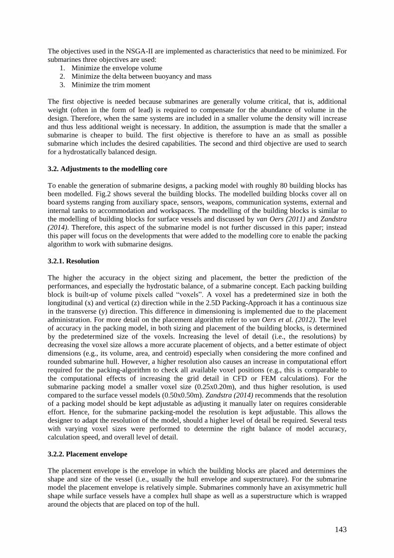
143
The objectives used in the NSGA-II are implemented as characteristics that need to be minimized. For
submarines three objectives are used:
1. Minimize the envelope volume
2. Minimize the delta between buoyancy and mass
3. Minimize the trim moment
The first objective is needed because submarines are generally volume critical, that is, additional
weight (often in the form of lead) is required to compensate for the abundance of volume in the
design. Therefore, when the same systems are included in a smaller volume the density will increase
and thus less additional weight is necessary. In addition, the assumption is made that the smaller a
submarine is cheaper to build. The first objective is therefore to have an as small as possible
submarine which includes the desired capabilities. The second and third objective are used to search
for a hydrostatically balanced design.
3.2. Adjustments to the modelling core
To enable the generation of submarine designs, a packing model with roughly 80 building blocks has
been modelled. Fig.2 shows several the building blocks. The modelled building blocks cover all on
board systems ranging from auxiliary space, sensors, weapons, communication systems, external and
internal tanks to accommodation and workspaces. The modelling of the building blocks is similar to
the modelling of building blocks for surface vessels and discussed by van Oers (2011) and Zandstra
(2014). Therefore, this aspect of the submarine model is not further discussed in this paper; instead
this paper will focus on the developments that were added to the modelling core to enable the packing
algorithm to work with submarine designs.
3.2.1. Resolution
The higher the accuracy in the object sizing and placement, the better the prediction of the
performances, and especially the hydrostatic balance, of a submarine concept. Each packing building
block is built-up of volume pixels called “voxels”. A voxel has a predetermined size in both the
longitudinal (x) and vertical (z) direction while in the 2.5D Packing-Approach it has a continuous size
in the transverse (y) direction. This difference in dimensioning is implemented due to the placement
administration. For more detail on the placement algorithm refer to van Oers et al. (2012). The level
of accuracy in the packing model, in both sizing and placement of the building blocks, is determined
by the predetermined size of the voxels. Increasing the level of detail (i.e., the resolutions) by
decreasing the voxel size allows a more accurate placement of objects, and a better estimate of object
dimensions (e.g., its volume, area, and centroid) especially when considering the more confined and
rounded submarine hull. However, a higher resolution also causes an increase in computational effort
required for the packing-algorithm to check all available voxel positions (e.g., this is comparable to
the computational effects of increasing the grid detail in CFD or FEM calculations). For the
submarine packing model a smaller voxel size (0.25x0.20m), and thus higher resolution, is used
compared to the surface vessel models (0.50x0.50m). Zandstra (2014) recommends that the resolution
of a packing model should be kept adjustable as adjusting it manually later on requires considerable
effort. Hence, for the submarine packing-model the resolution is kept adjustable. This allows the
designer to adapt the resolution of the model, should a higher level of detail be required. Several tests
with varying voxel sizes were performed to determine the right balance of model accuracy,
calculation speed, and overall level of detail.
3.2.2. Placement envelope
The placement envelope is the envelope in which the building blocks are placed and determines the
shape and size of the vessel (i.e., usually the hull envelope and superstructure). For the submarine
model the placement envelope is relatively simple. Submarines commonly have an axisymmetric hull
shape while surface vessels have a complex hull shape as well as a superstructure which is wrapped
around the objects that are placed on top of the hull.
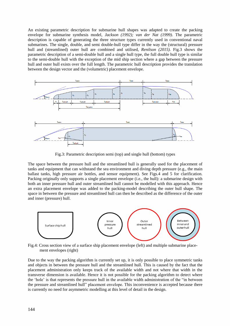
144
An existing parametric description for submarine hull shapes was adapted to create the packing
envelope for submarine synthesis model, Jackson (1992); van der Nat (1999). The parametric
description is capable of generating the three structure types currently used in conventional naval
submarines. The single, double, and semi double-hull type differ in the way the (structural) pressure
hull and (streamlined) outer hull are combined and utilised, Renilson (2015). Fig.3 shows the
parametric description of a semi-double hull and a single hull type, the full double hull type is similar
to the semi-double hull with the exception of the mid ship section where a gap between the pressure
hull and outer hull exists over the full length. The parametric hull description provides the translation
between the design vector and the (volumetric) placement envelope.
Fig.3: Parametric description semi (top) and single hull (bottom) types
The space between the pressure hull and the streamlined hull is generally used for the placement of
tanks and equipment that can withstand the sea environment and diving depth pressure (e.g., the main
ballast tanks, high pressure air bottles, and sensor equipment). See Figs.4 and 5 for clarification.
Packing originally only supports a single placement envelope (i.e., the hull): a submarine design with
both an inner pressure hull and outer streamlined hull cannot be modelled with this approach. Hence
an extra placement envelope was added to the packing-model describing the outer hull shape. The
space in between the pressure and streamlined hull can then be described as the difference of the outer
and inner (pressure) hull.
Fig.4: Cross section view of a surface ship placement envelope (left) and multiple submarine place-
ment envelopes (right)
Due to the way the packing algorithm is currently set up, it is only possible to place symmetric tanks
and objects in between the pressure hull and the streamlined hull. This is caused by the fact that the
placement administration only keeps track of the available width and not where that width in the
transverse dimension is available. Hence it is not possible for the packing algorithm to detect where
the ‘hole’ is that represents the pressure hull in the available width administration of the “in between
the pressure and streamlined hull” placement envelope. This inconvenience is accepted because there
is currently no need for asymmetric modelling at this level of detail in the design.
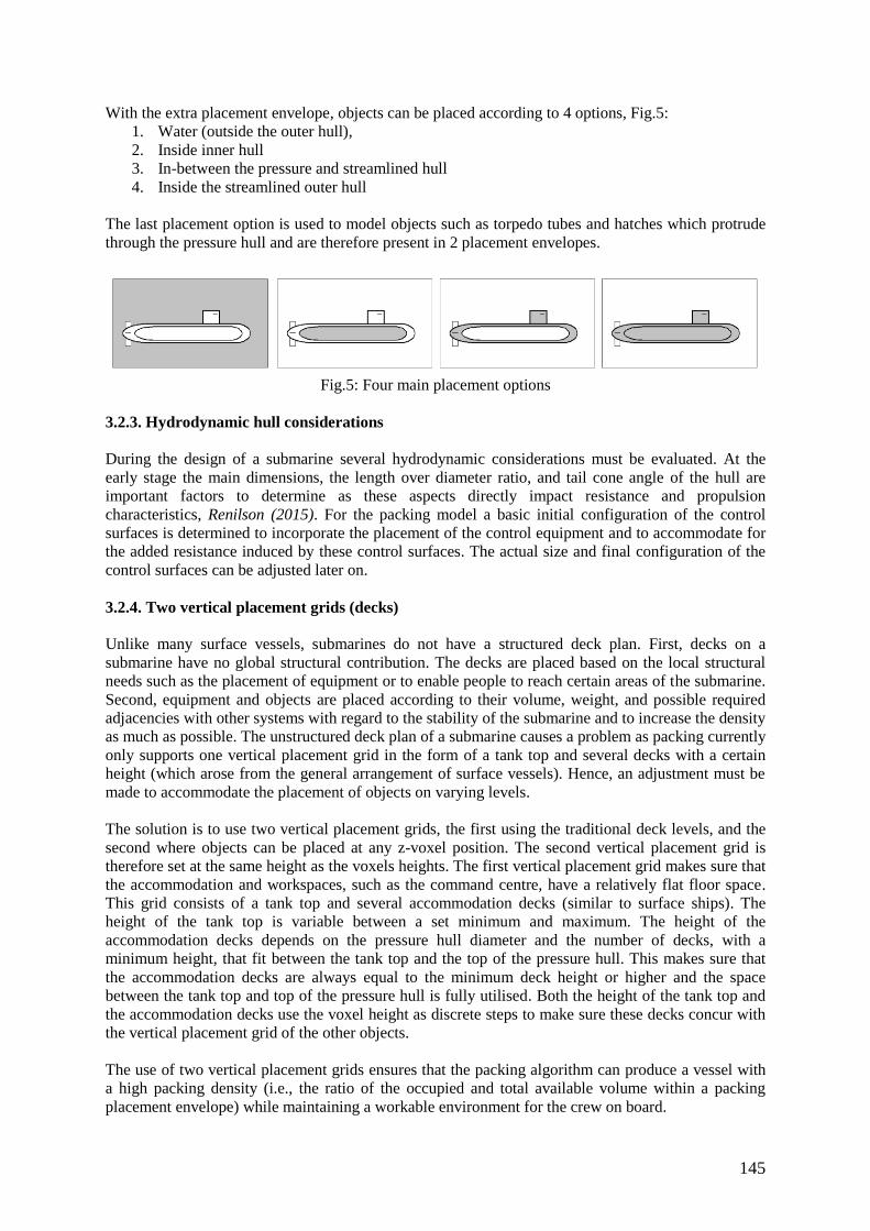
145
With the extra placement envelope, objects can be placed according to 4 options, Fig.5:
1. Water (outside the outer hull),
2. Inside inner hull
3. In-between the pressure and streamlined hull
4. Inside the streamlined outer hull
The last placement option is used to model objects such as torpedo tubes and hatches which protrude
through the pressure hull and are therefore present in 2 placement envelopes.
Fig.5: Four main placement options
3.2.3. Hydrodynamic hull considerations
During the design of a submarine several hydrodynamic considerations must be evaluated. At the
early stage the main dimensions, the length over diameter ratio, and tail cone angle of the hull are
important factors to determine as these aspects directly impact resistance and propulsion
characteristics, Renilson (2015). For the packing model a basic initial configuration of the control
surfaces is determined to incorporate the placement of the control equipment and to accommodate for
the added resistance induced by these control surfaces. The actual size and final configuration of the
control surfaces can be adjusted later on.
3.2.4. Two vertical placement grids (decks)
Unlike many surface vessels, submarines do not have a structured deck plan. First, decks on a
submarine have no global structural contribution. The decks are placed based on the local structural
needs such as the placement of equipment or to enable people to reach certain areas of the submarine.
Second, equipment and objects are placed according to their volume, weight, and possible required
adjacencies with other systems with regard to the stability of the submarine and to increase the density
as much as possible. The unstructured deck plan of a submarine causes a problem as packing currently
only supports one vertical placement grid in the form of a tank top and several decks with a certain
height (which arose from the general arrangement of surface vessels). Hence, an adjustment must be
made to accommodate the placement of objects on varying levels.
The solution is to use two vertical placement grids, the first using the traditional deck levels, and the
second where objects can be placed at any z-voxel position. The second vertical placement grid is
therefore set at the same height as the voxels heights. The first vertical placement grid makes sure that
the accommodation and workspaces, such as the command centre, have a relatively flat floor space.
This grid consists of a tank top and several accommodation decks (similar to surface ships). The
height of the tank top is variable between a set minimum and maximum. The height of the
accommodation decks depends on the pressure hull diameter and the number of decks, with a
minimum height, that fit between the tank top and the top of the pressure hull. This makes sure that
the accommodation decks are always equal to the minimum deck height or higher and the space
between the tank top and top of the pressure hull is fully utilised. Both the height of the tank top and
the accommodation decks use the voxel height as discrete steps to make sure these decks concur with
the vertical placement grid of the other objects.
The use of two vertical placement grids ensures that the packing algorithm can produce a vessel with
a high packing density (i.e., the ratio of the occupied and total available volume within a packing
placement envelope) while maintaining a workable environment for the crew on board.
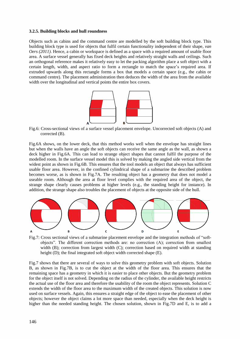
146
3.2.5. Building blocks and hull roundness
Objects such as cabins and the command centre are modelled by the soft building block type. This
building block type is used for objects that fulfil certain functionality independent of their shape, van
Oers (2011). Hence, a cabin or workspace is defined as a space with a required amount of usable floor
area. A surface vessel generally has fixed deck heights and relatively straight walls and ceilings. Such
an orthogonal reference makes it relatively easy to let the packing algorithm place a soft object with a
certain length, width, and aspect ratio to form a rectangle to match the space’s required area. If
extruded upwards along this rectangle forms a box that models a certain space (e.g., the cabin or
command centre). The placement administration then deduces the width of the area from the available
width over the longitudinal and vertical points the entire box covers.
Fig.6: Cross-sectional views of a surface vessel placement envelope. Uncorrected soft objects (A) and
corrected (B).
Fig.6A shows, on the lower deck, that this method works well when the envelope has straight lines
but when the walls have an angle the soft objects can receive the same angle as the wall, as shown a
deck higher in Fig.6A. This can lead to strange object shapes that cannot fulfil the purpose of the
modelled room. In the surface vessel model this is solved by making the angled side vertical from the
widest point as shown in Fig.6B. This ensures that the tool models an object that always has sufficient
usable floor area. However, in the confined cylindrical shape of a submarine the described problem
becomes worse, as is shown in Fig.7A. The resulting object has a geometry that does not model a
useable room. Although the area at floor level complies with the required area of the object, the
strange shape clearly causes problems at higher levels (e.g., the standing height for instance). In
addition, the strange shape also troubles the placement of objects at the opposite side of the hull.
Fig.7: Cross sectional views of a submarine placement envelope and the integration methods of “soft-
objects”. The different correction methods are: no correction (A); correction from smallest
width (B); correction from largest width (C); correction based on required width at standing
height (D); the final integrated soft object width corrected shape (E).
Fig.7 shows that there are several of ways to solve this geometry problem with soft objects. Solution
B, as shown in Fig.7B, is to cut the object at the width of the floor area. This ensures that the
remaining space has a geometry in which it is easier to place other objects. But the geometry problem
for the object itself is not solved. Depending on the radius of the cylinder, the available height restricts
the actual use of the floor area and therefore the usability of the room the object represents. Solution C
extends the width of the floor area to the maximum width of the created objects. This solution is now
used on surface vessels. Again, this ensures a straight edge of the object to ease the placement of other
objects; however the object claims a lot more space than needed, especially when the deck height is
higher than the needed standing height. The chosen solution, shown in Fig.7D and E, is to add a
147
minimum required standing height to the objects characteristics. The standing height is shown as a
line in Fig.7D and E. This ensures that the generated object contains a box with at least the required
floor area and minimum standing height while still keeping the flexible characteristics of a soft object.
The spaces above and besides the box are kept appointed to that object so this surplus in the objects
volume can be used to ensure that there is enough space in later design stages to include storage
space, cables, piping, and ventilation ducts within the design.
3.2.6. Compartmentalisation
The arrangement of surface vessels is, to a large extent, governed by the placement of the watertight
bulkheads. These are placed while considering the floodable length curve and divide the hull into
multiple compartments to ensure that there is enough reserve buoyancy in the case of damage. A
submarine needs to be exactly hydrostatically balanced; it therefore cannot have any surplus or
reserve buoyancy. The compartments on a submarine only act as a safe zone from which the
submariners can escape or be rescued in the case of an emergency. The number of bulkheads on a
submarine depends on the adopted safety design philosophy and corresponding number of water and
pressure tight compartments the naval architect has to implement. As there is no floodable length
curve to dictate the placement of the bulkheads, they are now placed by the NSGA-II within the
ranges that are determined by the adopted design safety philosophy.
3.2.7. Order of placement
The order of placement has influence on the “packability” and eventual design due to the fact that two
physical objects cannot be placed at the same location. The rules of thumb for creating a packing
placement order are, Zandstra (2014):
- Heavily constrained objects before unconstrained objects (e.g., the main electric motor is placed
early as its position is heavily constrained at the aft end of the pressure hull);
- Large objects before small objects (e.g., large fluid tanks are placed before smaller fluid tanks as
the latter are more easily placed in small gaps);
- Hard objects before soft objects (e.g., the “hard” diesel engines are placed before the “soft” fuel
tanks, as soft objects can change their shape to wrap around other objects).
In the synthesis model for surface vessels the placement of bulkheads is done before any other objects
are placed due to their fixed place according the floodable length curve. In the synthesis model for
submarines the bulkheads do not have this constraint while other objects do. The placement of
bulkheads is therefore performed after the placement of the torpedo tubes and adjacent to the torpedo
storage (located at the front end of the pressure hull). The adopted packing order used in the
submarine model is: envelope, decks, torpedo tubes and torpedo storage, bulkheads, propulsion
objects, trim and compensation tanks, sail equipment, accommodation and workspace spaces,
auxiliary spaces, internal tanks, external systems, and external tanks.
3.3 Adjusted performance predictors
Most of the needed performance predictions are the same for submarines as used for the surface
vessels. Those that required adjustments, or were added to correctly predict the performances of
submarines are discussed in the following sections.
3.3.1. Resistance
The resistance is, unlike the other performance predictors, estimated directly after the placement
envelope is generated and the geometry of the hull is known. With the resistance curve and
requirements, such as ranges, speeds, and endurance, it is possible to calculate the input parameters
for the sizing of objects such as: the fuel tanks, the batteries, the main electric motor and the diesel
generators. A submarine operates both at the surface and submerged, therefore resistance curves is are
148
needed for both conditions. The submerged resistance curve is predicted with the method described in
Jackson (1992). The surface resistance estimation method for surface vessels is unusable as the
submarine’s hull is optimized for submerged conditions and therefore has a completely different
shape. This mainly results in a lack of a fast and good prediction for the resulting wave making
resistance. This makes the prediction of the resistance of submarines at the surface very difficult.
During concept design, a first very rough estimate, at lower speeds, can be made by doubling the
submerged resistance at lower speeds.
3.3.2. Stability
As with the resistance, the stability of a submarine needs to be predicted for both submerged and
surfaced conditions. In surfaced conditions the stability prediction is roughly the same as for surface
vessels while submerged the contribution of the waterline area disappears as the entire vessel is
submerged. The submerged stability is therefore completely dependent on the vertical separation of
the buoyancy point (KB) and the centre of gravity (KG). This distance should lie between predefined
upper and lower stability limits.
The stability of the submarine when transitioning between the surface and submerged conditions is
extremely dynamic, non-linear, and depends on which way the transition takes place. Hence, the final
prediction of the stability conditions during the transition is therefore not done at this stage of the
design and the assumption is made that when the stability in the surfaced and submerged conditions is
sufficient, the stability during the transitions will also be sufficient, Renilson (2015).
3.4. Balancing the submarine
A submarine needs to be hydrostatically balanced in order for it to sail neutrally buoyant underwater.
This hydrostatic balance has a fixed part and a variable part. The fixed part is induced by the fixed
objects such as the submarines hull and the on-board equipment. The variable part is caused by
operational activities of the submarine. Due to the importance of the hydrostatic balance both these
parts must be considered accurately in the conceptual design stage.
3.4.1. Fixed part of the hydrostatic balance
For most submarine designs it is not possible to achieve an exact hydrostatic balance with only the
needed equipment and objects. A submarine design can have a surplus in volume, a surplus in mass,
and a resulting trim moment that needs to be compensated to achieve a hydrostatically balance design.
In the case the submarine has a surplus in mass, extra volume must be added. This generally means an
increase in size and a redesign of the vessel’s hull which, especially when the surplus in mass is noted
in a later design stages or even during construction, is a very expensive and time consuming exercise.
On the other hand, when there is a surplus in volume, extra mass must be added. This can relatively
easily be achieved by adding ballast in the form of lead. It is therefore important to make sure that the
submarine has a surplus in volume at the early stages of the design to act as buffer for potential weight
growth in the later design stages. This surplus in volume also enables the use of lead to correct the
trim moment.
3.4.2. Variable part of the hydrostatic balance
The hydrostatic balance of a submarine can change due to operational activities. Obvious aspects such
as firing a torpedo but also the consumption of fuel and stores, internal movement of weight, or a
different sea water density influence the hydrostatic balance and trim condition. These variations must
be compensated to ensure the submarine remains hydrostatically balanced and trimmed throughout a
voyage. This is done by the so called trim and compensation system. The trim polygon is used to
compare and check the capabilities of the trim and compensation system with the load variation due to
operational activities.
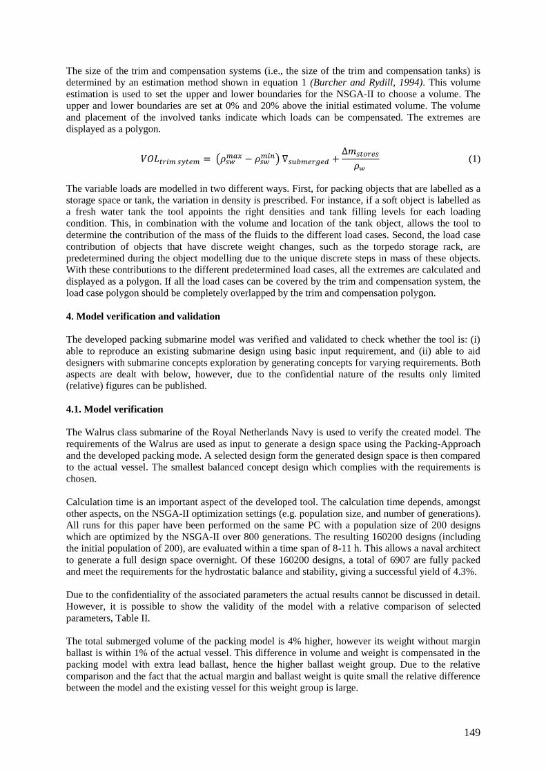
149
The size of the trim and compensation systems (i.e., the size of the trim and compensation tanks) is
determined by an estimation method shown in equation 1 (Burcher and Rydill, 1994). This volume
estimation is used to set the upper and lower boundaries for the NSGA-II to choose a volume. The
upper and lower boundaries are set at 0% and 20% above the initial estimated volume. The volume
and placement of the involved tanks indicate which loads can be compensated. The extremes are
displayed as a polygon.
𝑉𝑂𝐿𝑡𝑟𝑖𝑚 𝑠𝑦𝑡𝑒𝑚 = (𝜌𝑠𝑤𝑚𝑎𝑥 − 𝜌𝑠𝑤
𝑚𝑖𝑛) ∇𝑠𝑢𝑏𝑚𝑒𝑟𝑔𝑒𝑑 +∆𝑚𝑠𝑡𝑜𝑟𝑒𝑠
𝜌𝑤 (1)
The variable loads are modelled in two different ways. First, for packing objects that are labelled as a
storage space or tank, the variation in density is prescribed. For instance, if a soft object is labelled as
a fresh water tank the tool appoints the right densities and tank filling levels for each loading
condition. This, in combination with the volume and location of the tank object, allows the tool to
determine the contribution of the mass of the fluids to the different load cases. Second, the load case
contribution of objects that have discrete weight changes, such as the torpedo storage rack, are
predetermined during the object modelling due to the unique discrete steps in mass of these objects.
With these contributions to the different predetermined load cases, all the extremes are calculated and
displayed as a polygon. If all the load cases can be covered by the trim and compensation system, the
load case polygon should be completely overlapped by the trim and compensation polygon.
4. Model verification and validation
The developed packing submarine model was verified and validated to check whether the tool is: (i)
able to reproduce an existing submarine design using basic input requirement, and (ii) able to aid
designers with submarine concepts exploration by generating concepts for varying requirements. Both
aspects are dealt with below, however, due to the confidential nature of the results only limited
(relative) figures can be published.
4.1. Model verification
The Walrus class submarine of the Royal Netherlands Navy is used to verify the created model. The
requirements of the Walrus are used as input to generate a design space using the Packing-Approach
and the developed packing mode. A selected design form the generated design space is then compared
to the actual vessel. The smallest balanced concept design which complies with the requirements is
chosen.
Calculation time is an important aspect of the developed tool. The calculation time depends, amongst
other aspects, on the NSGA-II optimization settings (e.g. population size, and number of generations).
All runs for this paper have been performed on the same PC with a population size of 200 designs
which are optimized by the NSGA-II over 800 generations. The resulting 160200 designs (including
the initial population of 200), are evaluated within a time span of 8-11 h. This allows a naval architect
to generate a full design space overnight. Of these 160200 designs, a total of 6907 are fully packed
and meet the requirements for the hydrostatic balance and stability, giving a successful yield of 4.3%.
Due to the confidentiality of the associated parameters the actual results cannot be discussed in detail.
However, it is possible to show the validity of the model with a relative comparison of selected
parameters, Table II.
The total submerged volume of the packing model is 4% higher, however its weight without margin
ballast is within 1% of the actual vessel. This difference in volume and weight is compensated in the
packing model with extra lead ballast, hence the higher ballast weight group. Due to the relative
comparison and the fact that the actual margin and ballast weight is quite small the relative difference
between the model and the existing vessel for this weight group is large.
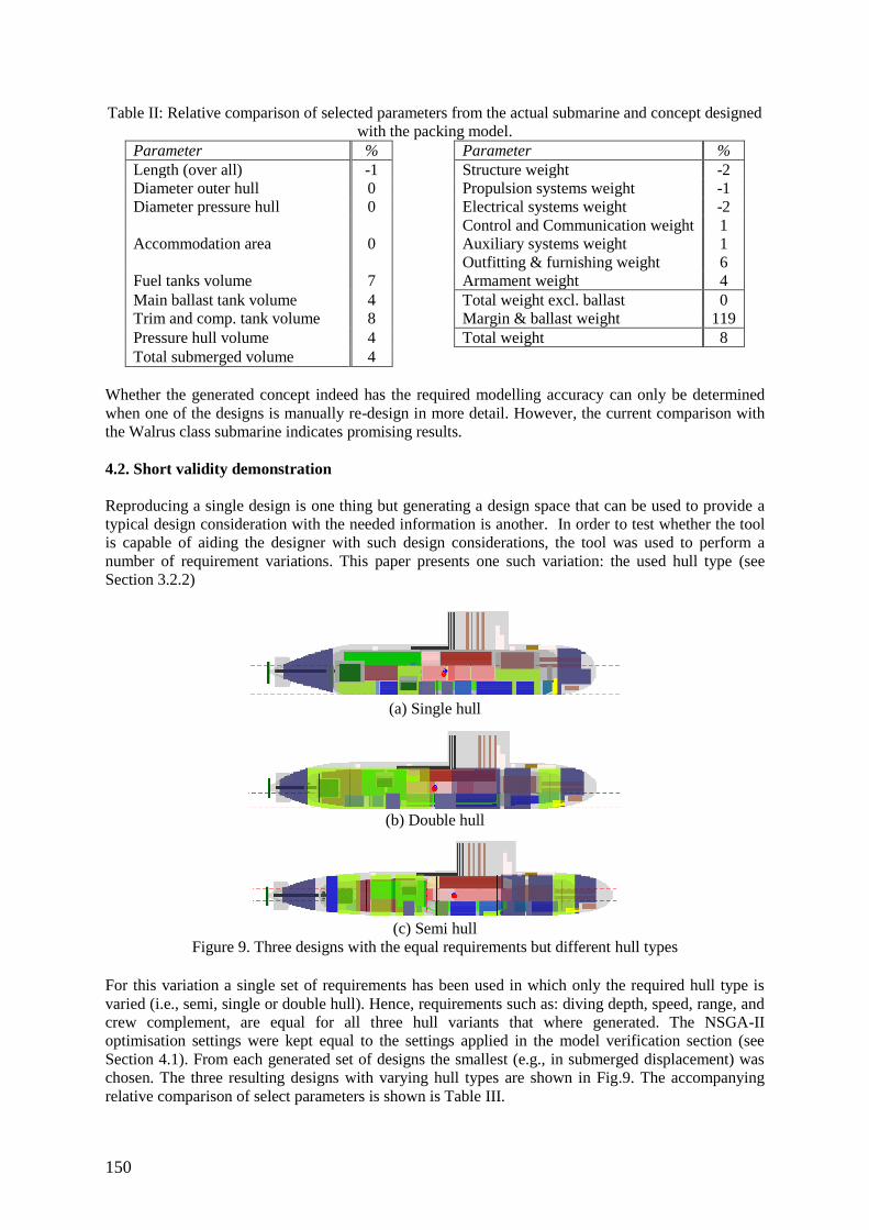
150
Table II: Relative comparison of selected parameters from the actual submarine and concept designed
with the packing model.
Parameter % Parameter %
Length (over all) -1 Structure weight -2
Diameter outer hull 0 Propulsion systems weight -1
Diameter pressure hull 0 Electrical systems weight -2
Control and Communication weight 1
Accommodation area 0 Auxiliary systems weight 1
Outfitting & furnishing weight 6
Fuel tanks volume 7 Armament weight 4
Main ballast tank volume 4 Total weight excl. ballast 0
Trim and comp. tank volume 8 Margin & ballast weight 119
Pressure hull volume 4 Total weight 8
Total submerged volume 4
Whether the generated concept indeed has the required modelling accuracy can only be determined
when one of the designs is manually re-design in more detail. However, the current comparison with
the Walrus class submarine indicates promising results.
4.2. Short validity demonstration
Reproducing a single design is one thing but generating a design space that can be used to provide a
typical design consideration with the needed information is another. In order to test whether the tool
is capable of aiding the designer with such design considerations, the tool was used to perform a
number of requirement variations. This paper presents one such variation: the used hull type (see
Section 3.2.2)
(a) Single hull
(b) Double hull
(c) Semi hull
Figure 9. Three designs with the equal requirements but different hull types
For this variation a single set of requirements has been used in which only the required hull type is
varied (i.e., semi, single or double hull). Hence, requirements such as: diving depth, speed, range, and
crew complement, are equal for all three hull variants that where generated. The NSGA-II
optimisation settings were kept equal to the settings applied in the model verification section (see
Section 4.1). From each generated set of designs the smallest (e.g., in submerged displacement) was
chosen. The three resulting designs with varying hull types are shown in Fig.9. The accompanying
relative comparison of select parameters is shown is Table III.
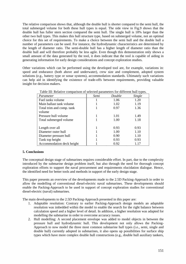
151
The relative comparison shows that, although the double hull is shorter compared to the semi hull, the
total submerged volume for both these hull types is equal. The side view in Fig.9 shows that the
double hull has fuller stern section compared the semi hull. The single hull is 18% larger than the
other two hull types. This makes this hull structure type, based on submerged volume, not an optimal
choice for this set of requirements. To make a choice between the semi hull and the double hull a
number of parameters can be used. For instance, the hydrodynamic characteristics are determined by
the length of diameter ratio. The semi-double hull has a higher length of diameter ratio than the
double hull and will therefore probably be less agile. Even though this demonstration only shows a
small amount of the data generated by the tool, it does indicate that the tool is capable of aiding in
generating information for early design considerations and concept exploration studies.
Other variations which can be performed using the developed tool are, for example, variations in:
speed and endurance (both above and underwater), crew size and complement, adopted system
solutions (e.g., battery type or sonar systems), accommodation standards. Ultimately such variations
can help aid in identifying the existence of trade-offs between requirements, providing valuable
insight for decision makers.
Table III: Relative comparison of selected parameters for different hull types.
Parameter Semi Double Single
Fuel tanks volume 1 1.06 1.20
Main ballast tank volume 1 1.02 1.19
Total trim and comp. tank
volume
1 0.97 1.36
Pressure hull volume 1 1.01 1.49
Total submerged volume 1 1.00 1.18
Length over all 1 0.93 0.93
Diameter outer hull 1 1.00 1.10
Diameter pressure hull 1 0.90 1.10
Tank top height 1 0.93 0.93
Accommodation deck height 1 0.92 1.17
5. Conclusions
The conceptual design stage of submarines requires considerable effort. In part, due to the complexity
introduced by the submarine design problem itself, but also through the need for thorough concept
exploration efforts to support the naval procurement and requirements elucidation dialogue. Hence,
the identified need for better tools and methods in support of the early design stage.
This paper presents an overview of the developments made to the 2.5D Packing-Approach in order to
allow the modelling of conventional diesel-electric naval submarines. These developments should
enable the Packing-Approach to be used in support of concept exploration studies for conventional
diesel-electric (naval) submarines.
The main developments to the 2.5D Packing-Approach presented in this paper are:
1. Adaptable resolution: Contrary to earlier Packing-Approach design models an adaptable
resolution was imbedded within the model to enable the search for the right balance between
calculation speed and a higher level of detail. In addition, a higher resolution was adapted for
modelling the submarine in order to overcome accuracy issues.
2. Hull modelling: A second placement envelope was added to model objects in between the
pressure hull and hydrodynamic hull. This development not only allows the Packing-
Approach to now model the three most common submarine hull types (i.e., semi, single and
double hull) currently adopted in submarines, it also opens up possibilities for surface ship
types which have more complex double hull constructions (e.g., double hull auxiliary tankers,
152
floating production storage and offloading units). Moreover, with additional modifications the
multiple placement envelope method could also be used to model multi-hull vessels.
3. Deck layout: To cope with the disjoint deck-layouts of submarines, two separate vertical
placement grids are implemented. This was done to enable a high system density inside the
submarine hull, while still making sure the crew spaces can be placed on logical deck levels.
4. Hull roundness: A minimum required standing height was introduced for soft objects. For
complex hull shapes, such as the round submarine pressure hull, this ensures that modelled
accommodation and workspace blocks have sufficient usable floor space including the
minimum standing height.
5. Adjusted performance predictors: A number of performance predictors were adjusted for
submarine design, such as resistance and stability calculations.
The above modifications enable the modelling of conventional diesel-electric submarines in the 2.5D
Packing-Approach tool.
To verify if the tool is indeed capable of producing designs with the required level of detail suitable
and necessary for the early design stages, several test-cases were performed. This paper presented
results of two of these test-cases:
1. The submarine packing model was verified by using it to redesign a Walrus class submarine
based on the actual design requirements (i.e., the original design requirements were used as a
basis to redesign the vessel with the new tool). Results of this verification study show that the
design tool can remodel the Walrus class design well with 10% of the actual values. Much
needed verification of the tool with other existing submarines is part of future work.
2. To demonstrate that the Packing-Approach with the new submarine model can be used in the
same fashion as the surface vessel model in support of early stage design, a typical design
requirement variation was also performed. Three submarines with equal requirements but
varying hull structure types were generated and assessed. Results of this test case show that
the tool is capable of aiding designers with typical early stage design considerations and
variations.
To summarize, the application of the 2.5D Packing-Approach to submarines shows that, with the
necessary modifications, the packing-based design approach can still successfully and time efficiently
balance requirements for space, arrangement, weight, and centre of gravity. This again proves the
Packing-Approach to be a versatile and generic tool during the conceptual design stages. In addition,
the tool now enables designers to evaluate a wide range of requirements and their accompanying
balanced submarine design alternatives in a short time-frame, supporting the requirements elucidation
dialogue between the Dutch Defence Staff and the Defence Materiel Organisation. Moreover, the tool
can also quickly provide solid starting points for more detailed designs and analysis using alternate,
more user-centric, design tools. Hence, the developed design tool greatly eases the conceptual design
process of diesel-electric naval submarines.
6. Future improvements
The model verification and validation results show that the submarine model is capable of achieving
the level of detail needed in conceptual submarine design. However, several improvements to the
existing model are envisioned:
- As presented in this paper, the model is verified with only one existing submarine. By verifying
the tool with more vessels, with varying requirements and sizes, the model can be fine-tuned
further.
- The parametric weight estimation for the non-discrete objects such as accommodation spaces and
the pressure hull structure are based on a limited amount of reference submarine designs. Due to
the confidential nature of submarines these figures are not publicly available and easily obtained.
153
The used reference submarines currently provide enough data, but increasing this number will
further improve the parametric weight estimation.
- The estimation used for the required auxiliary and switchboard space is performed based on the
previously mentioned example reference submarines, most of which were built and/or designed
several decades ago. Although advances in power electronics have made various items smaller
(e.g., from rotary to static converters), the assumption is made that the overall size of such
machinery spaces is still a valid reference. The validity of this assumption must be investigated if
the tool is to be used.
- Currently no cost estimation is incorporated within the performance predictors. This would make
it possible to provide additional information on the impact of potential requirement changes.
Acknowledgements
The authors would like to thank the Dutch Ministry of Defence’s Defence Materiel Organisation and
the Delft University of Technology for the support that led to the work presented in this paper.
References
ANDREWS, D.J. (1988), A comprehensive methodology for the design of ships (and other complex
systems), Proc. Royal Society London A, vol. 454, pp.187-211
ANDREWS, D.J. (2003), Marine design – Requirements elucidation rather than requirements
engineering, 8th Int. Marine Des. Conf. (IMDC)
ANDREWS, D.J. (2011), Marine requirements elucidation and the nature of preliminary ship design,
Int. J. of Maritime Eng., vol. 153(1), pp.A23-A39
VAN DEN BROEK DE BRUIJN, W.H. (2016), Submarine performance and requirements evaluation
method, Undersea Defense Technology Conference (UDT), Oslo
BURCHER, R.; RYDILL, L.J. (1994), Concepts in submarine design, Cambridge University Press
CIERAAD, J.S. (2016), Generating a design space for conventional naval submarines, MSc Thesis,
Delft University of Technology, Delft
DEB, K.; PRATAP, A.; AGARWAL, S.; MEYARIVAN, T. (2002), A fast and elitist multi-objective
genetic algorithm: NSGA-II, IEEE Trans. on Evolutionary Comp. 6(2), pp.182-197
DUCHATEAU, E.A.E. (2016), Interactive evolutionary concept exploration in preliminary ship
design, PhD Thesis, Delft University of Technology, Delft
JACKSON, H.A. (1992), Fundamentals of submarine concept design, SNAME Trans. 100, pp.419-
448
VAN DER NAT, C.G.J.M. (1999), A knowledge-based concept exploration method for submarine
design, PhD Thesis, Delft University of Technology, Delft
NORDIN, M. (2014), A novel submarine design method based on technical, economical and
operational factors of influence, PhD Thesis, Chalmers University of Technology, Goteborg
VAN OERS, B.J. (2011), A packing approach for the early stage design of service vessels, PhD
Thesis, Delft University of Technology, Delft
VAN OERS, B.J. (2012), Simpler and faster: A 2.5D packing-based approach for the early stage ship
design, 11th Int. Maritime Design Conf. (IMDC), Glasgow

154
PAWLING, R.J. (2007), The application of the design building block approach to innovative ship
design, PhD Thesis, University College London, London
RENILSON, M. (2015), Submarine Hydrodynamics, Springer Briefs in Applied Sciences and
Technology
TAKKEN, E. (2008), Concept design by using functional volume blocks with variable resolution,
MSc Thesis, Delft University of Technology, Delft
ZANDSTRA, R.J. (2014), Generating a large and diverse set of designs, MSc Thesis, Delft
University of Technology, Delft
ZANDSTRA, R.J.; DUCHATEAU, E.A.E.; VAN OERS, B.J. (2015), Concept exploration for a
mine-countermeasures vessel using a packing-based ship synthesis model, 5th World Maritime Tech.
Conf. (WMTC), Providence
155
4GD Framework in Ship Design
Greta Levišauskaitė, Ulstein Design & Solutions, Ulsteinvik/Norway, [email protected]
Henrique Murilo Gaspar, NTNU, Ålesund/Norway, [email protected]
Bernt-Aage Ulstein, Ulstein Design & Solutions, Ulsteinvik/Norway, [email protected]
Abstract
Shipbuilding companies are seeking innovation and production cost reduction by exploring the oppor-
tunities and capabilities of data management and modelling software. However, they yet struggle with
the combination of efficient 3D modelling tools and keeping high control on the product’s lifecycle.
Therefore, it is a significant matter for the maritime companies to have well-develop tools and ap-
proaches to efficiently manage vessel’s lifecycle and boost innovation. There are several commercial
software and approaches on how to manage vast amount of data during ship design, of which one of
the most current one is 4th Generation Design (4GD), that manages the design and product data in one
environment. In this context, this work intends to apply and investigate the 4GD approach in ship design
and evaluate if this is a beneficial approach in comparison with the traditional hierarchical approach.
Due to the wide range the maritime scope, our case is limited to the investigation of a simplified Plat-
form Supply Vessel (PSV) during basic design, specially for the exchange, improvement and 3D reuse
facilitation from the 3D designer point of view. The evaluation method is uniformly applied to the 4GD
and traditional assembly approach to perform a comparative analysis. The main case study of the re-
search comprises from the modelling and change processes of a PSV based on the challenges commonly
met in the industry. The results of the case study are summarizing the user’s experience working with
4GD and traditional assembly approach. A comparative analysis is performed on the two methods to
emphasize the advantages and disadvantages one against each other. Finally, the concluding remarks
suggests that 4GD has potential for innovation in ship design and is potentially beneficial for the ship-
building companies.
1. Introduction
Ship production processes, Fig.1, are highly collaborative, with the project planning coordinating con-
currently ship engineering, construction and maintenance from project development to outfitting, Cang
et al. (2013). Therefore, the challenge to combine rich product lifecycle management (PLM) systems
and efficient developed designing tools, as well as to perform 3D modelling of a ship with thousands
of units and parts arises. Currently, the maritime companies are struggling with one of the two cases,
and to manage both adequately an available solution is the implementation of a well-developed PLM
approach/software, configured to fit and manage the vessel’s lifecycle efficiently, NN (2013)..
As an integral part of PLM, product data management (PDM) allows to manage product data and pro-
cess-related information as one system by use of software, Kramer and Filius (2014), thus providing
easy accessibility for multiple teams across the company, such as CAD models, documents, standards,
manufacturing instructions, requirements and bill of materials. PDM allows each team working with
the project or assignment to access the data related to their needs in the appropriated context. PDM
allows the maritime companies to optimize operational resources, finding necessary data quickly, re-
ducing development cycle time, errors and costs. However, even if the usage of PDM in maritime in-
dustry exposes great advantages, the implementation of the system evokes difficulties due to the neces-
sity of well-established requirements, compatibility and expectations from the PLM/PDM system
from the ship design company as well as the shipyard.
To improve the ship design process, the virtual design environment (CAD representation) is paramount.
Specifically, in conceptual design phase it allows having a first look at the concept of a ship which gives
opportunity for the customer to view visualized product and improves sales argumentation, Andrade et
al. (2015). Likewise, accurate visualization in the detailed design phase is extremely important to eval-
uate interfaces, perform volume, motion or any other analyses on a product. 3D modelling ensures
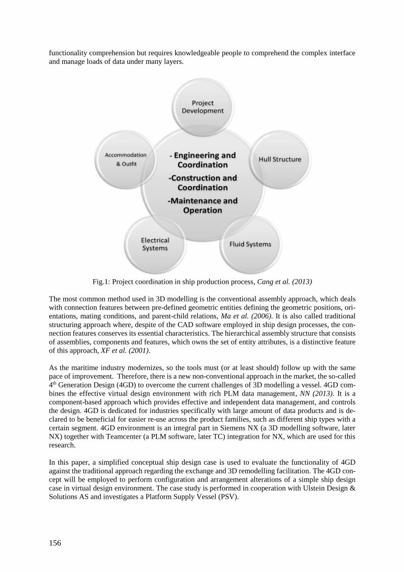
156
functionality comprehension but requires knowledgeable people to comprehend the complex interface
and manage loads of data under many layers.
Fig.1: Project coordination in ship production process, Cang et al. (2013)
The most common method used in 3D modelling is the conventional assembly approach, which deals
with connection features between pre-defined geometric entities defining the geometric positions, ori-
entations, mating conditions, and parent-child relations, Ma et al. (2006). It is also called traditional
structuring approach where, despite of the CAD software employed in ship design processes, the con-
nection features conserves its essential characteristics. The hierarchical assembly structure that consists
of assemblies, components and features, which owns the set of entity attributes, is a distinctive feature
of this approach, XF et al. (2001).
As the maritime industry modernizes, so the tools must (or at least should) follow up with the same
pace of improvement. Therefore, there is a new non-conventional approach in the market, the so-called
4th Generation Design (4GD) to overcome the current challenges of 3D modelling a vessel. 4GD com-
bines the effective virtual design environment with rich PLM data management, NN (2013). It is a
component-based approach which provides effective and independent data management, and controls
the design. 4GD is dedicated for industries specifically with large amount of data products and is de-
clared to be beneficial for easier re-use across the product families, such as different ship types with a
certain segment. 4GD environment is an integral part in Siemens NX (a 3D modelling software, later
NX) together with Teamcenter (a PLM software, later TC) integration for NX, which are used for this
research.
In this paper, a simplified conceptual ship design case is used to evaluate the functionality of 4GD
against the traditional approach regarding the exchange and 3D remodelling facilitation. The 4GD con-
cept will be employed to perform configuration and arrangement alterations of a simple ship design
case in virtual design environment. The case study is performed in cooperation with Ulstein Design &
Solutions AS and investigates a Platform Supply Vessel (PSV).
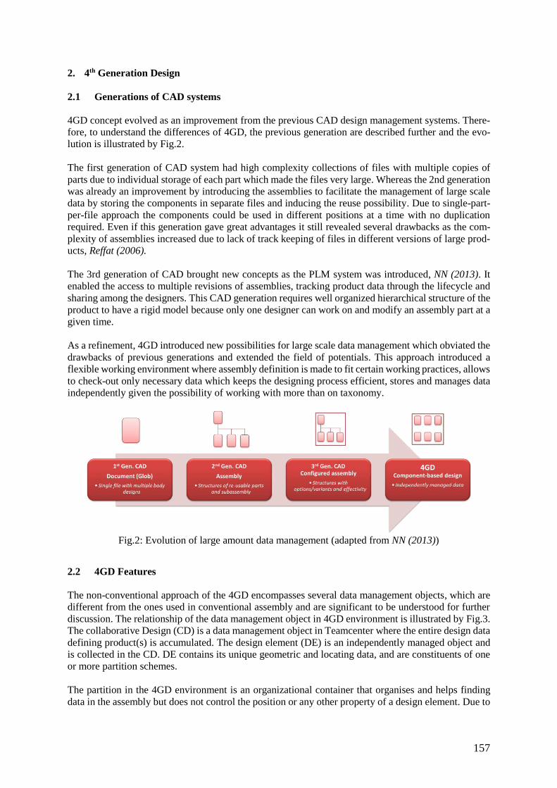
157
2. 4th Generation Design
2.1 Generations of CAD systems
4GD concept evolved as an improvement from the previous CAD design management systems. There-
fore, to understand the differences of 4GD, the previous generation are described further and the evo-
lution is illustrated by Fig.2.
The first generation of CAD system had high complexity collections of files with multiple copies of
parts due to individual storage of each part which made the files very large. Whereas the 2nd generation
was already an improvement by introducing the assemblies to facilitate the management of large scale
data by storing the components in separate files and inducing the reuse possibility. Due to single-part-
per-file approach the components could be used in different positions at a time with no duplication
required. Even if this generation gave great advantages it still revealed several drawbacks as the com-
plexity of assemblies increased due to lack of track keeping of files in different versions of large prod-
ucts, Reffat (2006).
The 3rd generation of CAD brought new concepts as the PLM system was introduced, NN (2013). It
enabled the access to multiple revisions of assemblies, tracking product data through the lifecycle and
sharing among the designers. This CAD generation requires well organized hierarchical structure of the
product to have a rigid model because only one designer can work on and modify an assembly part at a
given time.
As a refinement, 4GD introduced new possibilities for large scale data management which obviated the
drawbacks of previous generations and extended the field of potentials. This approach introduced a
flexible working environment where assembly definition is made to fit certain working practices, allows
to check-out only necessary data which keeps the designing process efficient, stores and manages data
independently given the possibility of working with more than on taxonomy.
Fig.2: Evolution of large amount data management (adapted from NN (2013))
2.2 4GD Features
The non-conventional approach of the 4GD encompasses several data management objects, which are
different from the ones used in conventional assembly and are significant to be understood for further
discussion. The relationship of the data management object in 4GD environment is illustrated by Fig.3.
The collaborative Design (CD) is a data management object in Teamcenter where the entire design data
defining product(s) is accumulated. The design element (DE) is an independently managed object and
is collected in the CD. DE contains its unique geometric and locating data, and are constituents of one
or more partition schemes.
The partition in the 4GD environment is an organizational container that organises and helps finding
data in the assembly but does not control the position or any other property of a design element. Due to
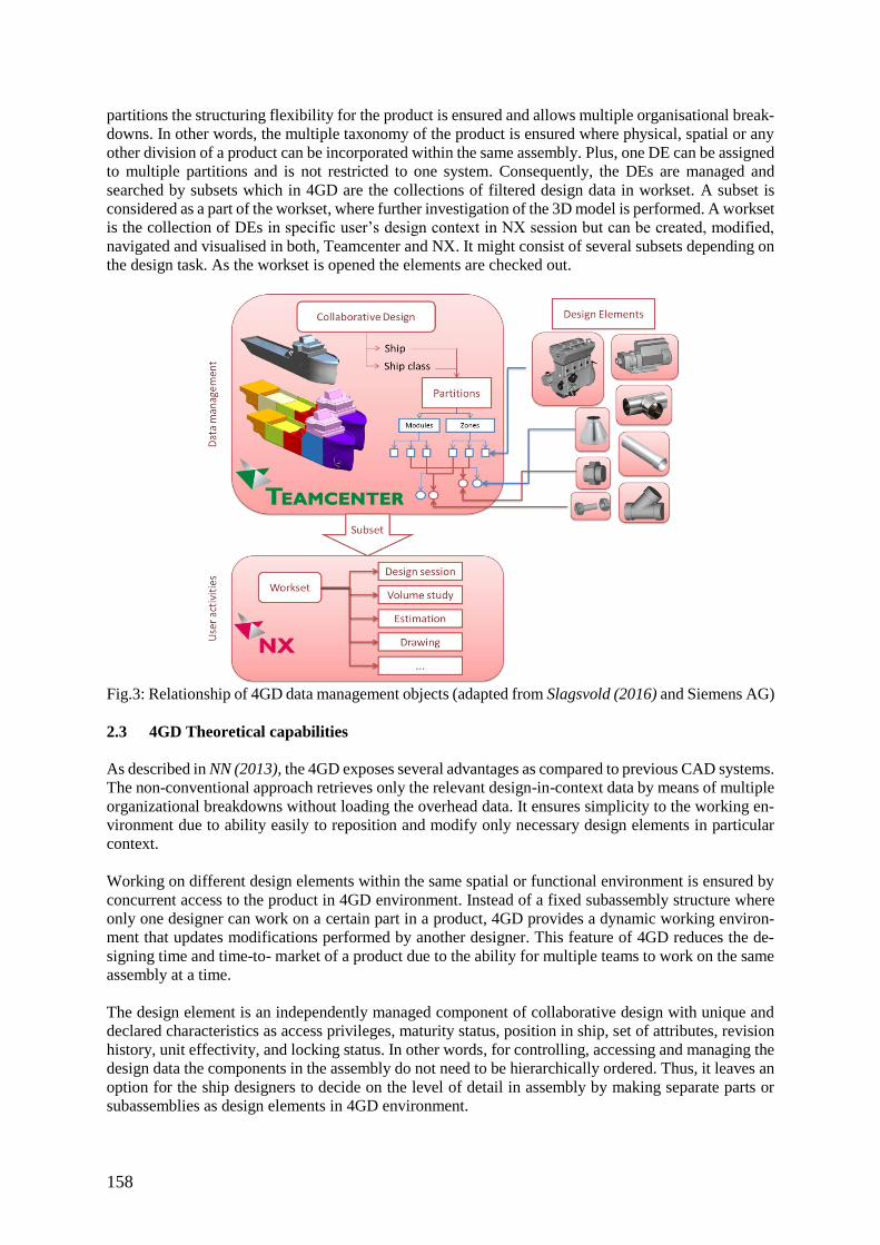
158
partitions the structuring flexibility for the product is ensured and allows multiple organisational break-
downs. In other words, the multiple taxonomy of the product is ensured where physical, spatial or any
other division of a product can be incorporated within the same assembly. Plus, one DE can be assigned
to multiple partitions and is not restricted to one system. Consequently, the DEs are managed and
searched by subsets which in 4GD are the collections of filtered design data in workset. A subset is
considered as a part of the workset, where further investigation of the 3D model is performed. A workset
is the collection of DEs in specific user’s design context in NX session but can be created, modified,
navigated and visualised in both, Teamcenter and NX. It might consist of several subsets depending on
the design task. As the workset is opened the elements are checked out.
Fig.3: Relationship of 4GD data management objects (adapted from Slagsvold (2016) and Siemens AG)
2.3 4GD Theoretical capabilities
As described in NN (2013), the 4GD exposes several advantages as compared to previous CAD systems.
The non-conventional approach retrieves only the relevant design-in-context data by means of multiple
organizational breakdowns without loading the overhead data. It ensures simplicity to the working en-
vironment due to ability easily to reposition and modify only necessary design elements in particular
context.
Working on different design elements within the same spatial or functional environment is ensured by
concurrent access to the product in 4GD environment. Instead of a fixed subassembly structure where
only one designer can work on a certain part in a product, 4GD provides a dynamic working environ-
ment that updates modifications performed by another designer. This feature of 4GD reduces the de-
signing time and time-to- market of a product due to the ability for multiple teams to work on the same
assembly at a time.
The design element is an independently managed component of collaborative design with unique and
declared characteristics as access privileges, maturity status, position in ship, set of attributes, revision
history, unit effectivity, and locking status. In other words, for controlling, accessing and managing the
design data the components in the assembly do not need to be hierarchically ordered. Thus, it leaves an
option for the ship designers to decide on the level of detail in assembly by making separate parts or
subassemblies as design elements in 4GD environment.
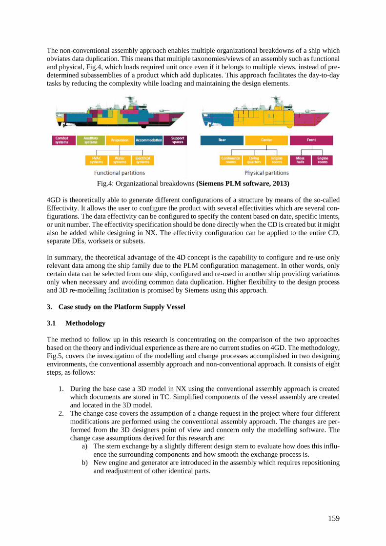
159
The non-conventional assembly approach enables multiple organizational breakdowns of a ship which
obviates data duplication. This means that multiple taxonomies/views of an assembly such as functional
and physical, Fig.4, which loads required unit once even if it belongs to multiple views, instead of pre-
determined subassemblies of a product which add duplicates. This approach facilitates the day-to-day
tasks by reducing the complexity while loading and maintaining the design elements.
Fig.4: Organizational breakdowns (Siemens PLM software, 2013)
4GD is theoretically able to generate different configurations of a structure by means of the so-called
Effectivity. It allows the user to configure the product with several effectivities which are several con-
figurations. The data effectivity can be configured to specify the content based on date, specific intents,
or unit number. The effectivity specification should be done directly when the CD is created but it might
also be added while designing in NX. The effectivity configuration can be applied to the entire CD,
separate DEs, worksets or subsets.
In summary, the theoretical advantage of the 4D concept is the capability to configure and re-use only
relevant data among the ship family due to the PLM configuration management. In other words, only
certain data can be selected from one ship, configured and re-used in another ship providing variations
only when necessary and avoiding common data duplication. Higher flexibility to the design process
and 3D re-modelling facilitation is promised by Siemens using this approach.
3. Case study on the Platform Supply Vessel
3.1 Methodology
The method to follow up in this research is concentrating on the comparison of the two approaches
based on the theory and individual experience as there are no current studies on 4GD. The methodology,
Fig.5, covers the investigation of the modelling and change processes accomplished in two designing
environments, the conventional assembly approach and non-conventional approach. It consists of eight
steps, as follows:
1. During the base case a 3D model in NX using the conventional assembly approach is created
which documents are stored in TC. Simplified components of the vessel assembly are created
and located in the 3D model.
2. The change case covers the assumption of a change request in the project where four different
modifications are performed using the conventional assembly approach. The changes are per-
formed from the 3D designers point of view and concern only the modelling software. The
change case assumptions derived for this research are:
a) The stern exchange by a slightly different design stern to evaluate how does this influ-
ence the surrounding components and how smooth the exchange process is.
b) New engine and generator are introduced in the assembly which requires repositioning
and readjustment of other identical parts.
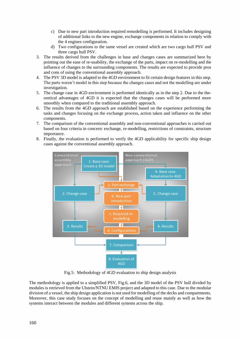
160
c) Due to new part introduction required remodelling is performed. It includes designing
of additional links to the new engine, exchange components in relation to comply with
the 4 engines configuration.
d) Two configurations to the same vessel are created which are two cargo hull PSV and
three cargo hull PSV.
3. The results derived from the challenges in base and changes cases are summarized here by
pointing out the ease of re-usability, the exchange of the parts, impact on re-modelling and the
influence of changes to the surrounding components. The results are expected to provide pros
and cons of using the conventional assembly approach.
4. The PSV 3D model is adapted to the 4GD environment to fit certain design features in this step.
The parts weren’t model in this step because the changes cases and not the modelling are under
investigation.
5. The change case in 4GD environment is performed identically as in the step 2. Due to the the-
oretical advantages of 4GD it is expected that the changes cases will be performed more
smoothly when compared to the traditional assembly approach.
6. The results from the 4GD approach are established based on the experience performing the
tasks and changes focusing on the exchange process, action taken and influence on the other
components.
7. The comparison of the conventional assembly and non-conventional approaches is carried out
based on four criteria in concern: exchange, re-modelling, restrictions of constraints, structure
importance.
8. Finally, the evaluation is performed to verify the 4GD applicability for specific ship design
cases against the conventional assembly approach.
Fig.5: Methodology of 4GD evaluation to ship design analysis
The methodology is applied to a simplified PSV, Fig.6, and the 3D model of the PSV hull divided by
modules is retrieved from the Ulstein/NTNU EMIS project and adapted to this case. Due to the modular
division of a vessel, the ship design application is not used for modelling of the decks and compartments.
Moreover, this case study focuses on the concept of modelling and reuse mainly as well as how the
systems interact between the modules and different systems across the ship.
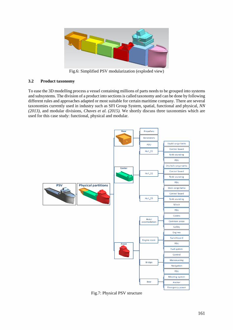
161
Fig.6: Simplified PSV modularization (exploded view)
3.2 Product taxonomy
To ease the 3D modelling process a vessel containing millions of parts needs to be grouped into systems
and subsystems. The division of a product into sections is called taxonomy and can be done by following
different rules and approaches adapted or most suitable for certain maritime company. There are several
taxonomies currently used in industry such as SFI Group System, spatial, functional and physical, NN
(2013), and modular divisions, Chaves et al. (2015). We shortly discuss three taxonomies which are
used for this case study: functional, physical and modular.
Fig.7: Physical PSV structure
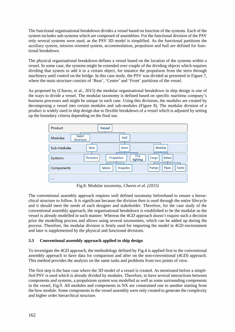
162
The functional organisational breakdown divides a vessel based on function of the systems. Each of the
system includes sub-systems which are composed of assemblies. For the functional division of the PSV
only several systems were used, as the PSV 3D model is simplified. As the functional partitions the
auxiliary system, mission oriented system, accommodation, propulsion and hull are defined for func-
tional breakdown.
The physical organisational breakdown defines a vessel based on the location of the systems within a
vessel. In some case, the systems might be extended over couple of the dividing objects which requires
dividing that system to add it to a certain object, for instance the propulsion from the stern through
machinery until control on the bridge. In this case study, the PSV was divided as presented in Figure 7,
where the main structure consists of ‘Rear’, ‘Centre’ and ‘Front’ partitions of the vessel.
As proposed by (Chaves, et al., 2015) the modular organisational breakdown in ship design is one of
the ways to divide a vessel. The modular taxonomy is defined based on specific maritime company’s
business processes and might be unique in each case. Using this divisions, the modules are created by
decomposing a vessel into certain modules and sub-modules (Figure 8). The modular division of a
product is widely used in ship design due to flexible breakdown of a vessel which is adjusted by setting
up the boundary criteria depending on the final use.
Fig.8: Modular taxonomy, Chaves et al. (2015)
The conventional assembly approach requires well defined taxonomy beforehand to ensure a hierar-
chical structure to follow. It is significant because the division then is used through the entire lifecycle
and it should meet the needs of each designer and stakeholder. Therefore, for the case study of the
conventional assembly approach, the organisational breakdown is established to be the modular as the
vessel is already modelled in such manner. Whereas the 4GD approach doesn’t require such a decision
prior the modelling process and allows using several taxonomies, which can be added up during the
process. Therefore, the modular division is firstly used for importing the model in 4GD environment
and later is supplemented by the physical and functional divisions.
3.3 Conventional assembly approach applied to ship design
To investigate the 4GD approach, the methodology defined by Fig.4 is applied first to the conventional
assembly approach to have data for comparison and after on the non-conventional (4GD) approach.
This method provides the analysis on the same tasks and problems from two points of view.
The first step is the base case where the 3D model of a vessel is created. As mentioned before a simpli-
fied PSV is used which is already divided by modules. Therefore, to have several interactions between
components and systems, a propulsions system was modelled as well as some surrounding components
in the vessel, Fig.9. All modules and components in NX are constrained one to another starting from
the bow module. Some components in the vessel assembly were only created to generate the complexity
and higher order hierarchical structure.
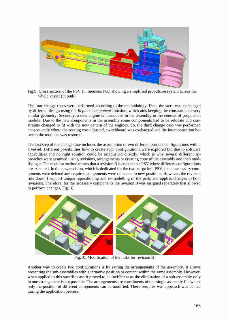
163
Fig.9: Cross section of the PSV (in Siemens NX) showing a simplified propulsion system across the
whole vessel (in pink)
The four change cases were performed according to the methodology. First, the stern was exchanged
by different design using the Replace component function, which aids keeping the constraints of very
similar geometry. Secondly, a new engine is introduced in the assembly in the context of propulsion
module. Due to the new components in the assembly some components had to be relocate and con-
straints changed to fit with the new pattern of the engines. So, the third change case was performed
consequently where the routing was adjusted, switchboard was exchanged and the interconnection be-
tween the modules was restored.
The last step of the change case includes the assumption of two different product configurations within
a vessel. Different possibilities how to create such configurations were explored but due to software
capabilities and no right solution could be established directly, which is why several different ap-
proaches were assumed: using revisions, arrangements or creating copy of the assembly and then mod-
ifying it. The revision method means that a revision B is created to a PSV where different configurations
are executed. In the new revision, which is dedicated for the two-cargo hull PSV, the unnecessary com-
ponents were deleted and required components were relocated to new positions. However, the revision
rule doesn’t support unique repositioning and re-modelling of the parts and applies changes to both
revisions. Therefore, for the necessary components the revision B was assigned separately that allowed
to perform changes, Fig.10.
Fig.10: Modification of the links for revision B
Another way to create two configurations is by setting the arrangements of the assembly. It allows
presenting the sub-assemblies with alternative position or content within the same assembly. However,
when applied to this specific case it proved to be inefficient as the elimination of a sub-assembly only
in one arrangement is not possible. The arrangements are constituents of one single assembly file where
only the position of different components can be modified. Therefore, this was approach was denied
during the application process.
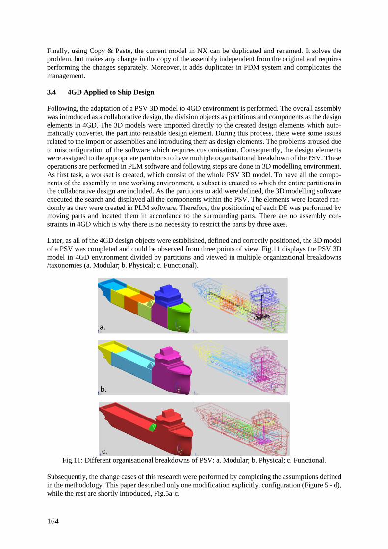
164
Finally, using Copy & Paste, the current model in NX can be duplicated and renamed. It solves the
problem, but makes any change in the copy of the assembly independent from the original and requires
performing the changes separately. Moreover, it adds duplicates in PDM system and complicates the
management.
3.4 4GD Applied to Ship Design
Following, the adaptation of a PSV 3D model to 4GD environment is performed. The overall assembly
was introduced as a collaborative design, the division objects as partitions and components as the design
elements in 4GD. The 3D models were imported directly to the created design elements which auto-
matically converted the part into reusable design element. During this process, there were some issues
related to the import of assemblies and introducing them as design elements. The problems aroused due
to misconfiguration of the software which requires customisation. Consequently, the design elements
were assigned to the appropriate partitions to have multiple organisational breakdown of the PSV. These
operations are performed in PLM software and following steps are done in 3D modelling environment.
As first task, a workset is created, which consist of the whole PSV 3D model. To have all the compo-
nents of the assembly in one working environment, a subset is created to which the entire partitions in
the collaborative design are included. As the partitions to add were defined, the 3D modelling software
executed the search and displayed all the components within the PSV. The elements were located ran-
domly as they were created in PLM software. Therefore, the positioning of each DE was performed by
moving parts and located them in accordance to the surrounding parts. There are no assembly con-
straints in 4GD which is why there is no necessity to restrict the parts by three axes.
Later, as all of the 4GD design objects were established, defined and correctly positioned, the 3D model
of a PSV was completed and could be observed from three points of view. Fig.11 displays the PSV 3D
model in 4GD environment divided by partitions and viewed in multiple organizational breakdowns
/taxonomies (a. Modular; b. Physical; c. Functional).
Fig.11: Different organisational breakdowns of PSV: a. Modular; b. Physical; c. Functional.
Subsequently, the change cases of this research were performed by completing the assumptions defined
in the methodology. This paper described only one modification explicitly, configuration (Figure 5 - d),
while the rest are shortly introduced, Fig.5a-c.
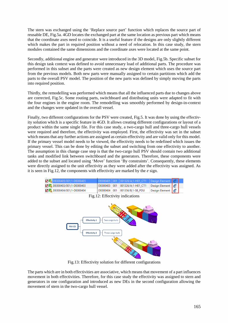
165
The stern was exchanged using the ‘Replace source part’ function which replaces the source part of
reusable DE, Fig.5a. 4GD locates the exchanged part at the same location as previous part which means
that the coordinate axes need to coincide. It is a useful feature if the designs are only slightly different
which makes the part in required position without a need of relocation. In this case study, the stern
modules contained the same dimensions and the coordinate axes were located at the same point.
Secondly, additional engine and generator were introduced in the 3D model, Fig.5b. Specific subset for
this design task context was defined to avoid unnecessary load of additional parts. The procedure was
performed in this subset and the parts were created as new design element which uses the source part
from the previous models. Both new parts were manually assigned to certain partitions which add the
parts to the overall PSV model. The position of the new parts was defined by simply moving the parts
into required position.
Thirdly, the remodelling was performed which means that all the influenced parts due to changes above
are corrected, Fig.5c. Some routing parts, switchboard and distributing units were adapted to fit with
the four engines in the engine room. The remodelling was smoothly performed by design-in-context
and the changes were updated in the overall vessel.
Finally, two different configurations for the PSV were created, Fig.5. It was done by using the effectiv-
ity solution which is a specific feature in 4GD. It allows creating different configurations or layout of a
product within the same single file. For this case study, a two-cargo hull and three-cargo hull vessels
were required and therefore, the effectivity was employed. First, the effectivity was set in the subset
which means that any further actions are assigned as certain effectivity and are valid only for this model.
If the primary vessel model needs to be viewed, the effectivity needs to be redefined which issues the
primary vessel. This can be done by editing the subset and switching from one effectivity to another.
The assumption in this change case step is that the two-cargo hull PSV should contain two additional
tanks and modified link between switchboard and the generators. Therefore, these components were
added to the subset and located using ‘Move’ function ‘By constraints’. Consequently, these elements
were directly assigned to the unit effectivity as they were added after the effectivity was assigned. As
it is seen in Fig.12, the components with effectivity are marked by the e sign.
Fig.12: Effectivity indications
Fig.13: Effectivity solution for different configurations
The parts which are in both effectivities are associative, which means that movement of a part influences
movement in both effectivities. Therefore, for this case study the effectivity was assigned to stern and
generators in one configuration and introduced as new DEs in the second configuration allowing the
movement of stern in the two-cargo hull vessel.
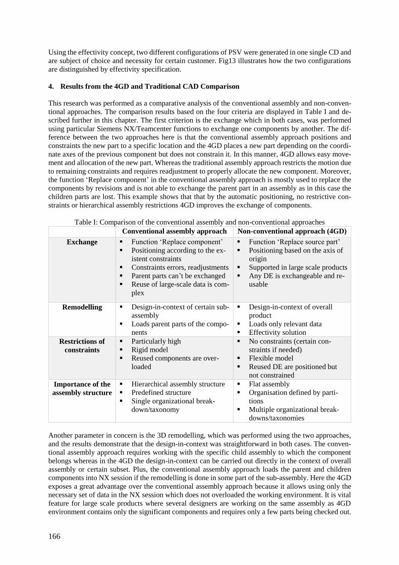
166
Using the effectivity concept, two different configurations of PSV were generated in one single CD and
are subject of choice and necessity for certain customer. Fig13 illustrates how the two configurations
are distinguished by effectivity specification.
4. Results from the 4GD and Traditional CAD Comparison
This research was performed as a comparative analysis of the conventional assembly and non-conven-
tional approaches. The comparison results based on the four criteria are displayed in Table I and de-
scribed further in this chapter. The first criterion is the exchange which in both cases, was performed
using particular Siemens NX/Teamcenter functions to exchange one components by another. The dif-
ference between the two approaches here is that the conventional assembly approach positions and
constraints the new part to a specific location and the 4GD places a new part depending on the coordi-
nate axes of the previous component but does not constrain it. In this manner, 4GD allows easy move-
ment and allocation of the new part. Whereas the traditional assembly approach restricts the motion due
to remaining constraints and requires readjustment to properly allocate the new component. Moreover,
the function ‘Replace component’ in the conventional assembly approach is mostly used to replace the
components by revisions and is not able to exchange the parent part in an assembly as in this case the
children parts are lost. This example shows that that by the automatic positioning, no restrictive con-
straints or hierarchical assembly restrictions 4GD improves the exchange of components.
Table I: Comparison of the conventional assembly and non-conventional approaches
Conventional assembly approach Non-conventional approach (4GD)
Exchange Function ‘Replace component’
Positioning according to the ex-
istent constraints
Constraints errors, readjustments
Parent parts can’t be exchanged
Reuse of large-scale data is com-
plex
Function ‘Replace source part’
Positioning based on the axis of
origin
Supported in large scale products
Any DE is exchangeable and re-
usable
Remodelling Design-in-context of certain sub-
assembly
Loads parent parts of the compo-
nents
Design-in-context of overall
product
Loads only relevant data
Effectivity solution
Restrictions of
constraints
Particularly high
Rigid model
Reused components are over-
loaded
No constraints (certain con-
straints if needed)
Flexible model
Reused DE are positioned but
not constrained
Importance of the
assembly structure
Hierarchical assembly structure
Predefined structure
Single organizational break-
down/taxonomy
Flat assembly
Organisation defined by parti-
tions
Multiple organizational break-
downs/taxonomies
Another parameter in concern is the 3D remodelling, which was performed using the two approaches,
and the results demonstrate that the design-in-context was straightforward in both cases. The conven-
tional assembly approach requires working with the specific child assembly to which the component
belongs whereas in the 4GD the design-in-context can be carried out directly in the context of overall
assembly or certain subset. Plus, the conventional assembly approach loads the parent and children
components into NX session if the remodelling is done in some part of the sub-assembly. Here the 4GD
exposes a great advantage over the conventional assembly approach because it allows using only the
necessary set of data in the NX session which does not overloaded the working environment. It is vital
feature for large scale products where several designers are working on the same assembly as 4GD
environment contains only the significant components and requires only a few parts being checked out.
167
One more way to reduce or avoid remodelling is the effectivity solution which might be employed
instead of remodelling in 4GD by creating an equivalent model in the same file which contains the same
information and is different where needed.
The restriction of constraints is another important criterion in consideration which proved to be unusu-
ally high in the conventional assembly approach. The constraints are defining the positioning of each
component in the assembly which makes any movement, modification or exchange of part complicated
and demands readjustments. It makes the assembly very rigid and any change influences surrounding
parts and constraints but at the same time, the constraints structure the assemblies and move components
together with the parent parts. Plus, the constraints might overload the assembly when some components
or assemblies are being reused. The sub-assembly comes with the existent constraints and might mix
up with the assembly constraints of the primary model. Whereas in 4GD, the reused DEs are positioned
at certain location and remain positioned until moved. As the 4GD doesn’t use constraints, it makes the
assembly a flexible structure but it also maintains the position of components. This research showed
that the 4GD exposes an advantage over the conventional assembly approach due to the absence of
constraints system but still sustaining the required position.
Finally, the importance of the assembly structure in the two approaches is compared. As stated previ-
ously, the hierarchical structure of the assembly is of high importance in the conventional assembly
approach and thus, this research verified this importance and influence the entire design process. The
assembly structure was pre-defined to have a product structure before modelling. Several components
were not considered and had to be inserted during the modelling process which complicated the inter-
actions between the assemblies, interrupted some constraints and order of the product. Therefore, in
large scale products the structure of assemblies and sub-assemblies needs to be clear and meet the re-
quirements of different design teams. In contrary, 4GD supports a flat assembly structure where the
parts are not necessary dependent one to each other but the dependency remains an option. The non-
conventional approach allows to decide the product structure at the beginning or during the design pro-
cess due to multiple organisational breakdowns and search capabilities to load only relevant data for
design teams. Therefore, it can be concluded that the high importance of the assembly structure in the
traditional structuring approach makes the product more rigid and requires well defined process as the
4GD provides flexibility and preparation process mistakes can be solved.
The fourth criteria described above were established to reflect the exchange and 3D reuse capabilities
in 4GD environment. It exposed the facilitation of exchange due to the multiple organisational break-
downs and flat assembly structure where each DE is independent. The 4GD provides a more flexible
assembly structure of a product which means that there are no constraints and very few restrictions to
position components in the assembly. Even the top-level elements that can’t be exchanged in conven-
tional assembly approach are exchangeable in the non-conventional approach and do not influence the
children parts.
As for the reuse, the comparison results showed that due to the effectivity solution in 4GD the estab-
lishment of a series of vessels with the same hull or the same propulsion system within the same col-
laborative design object is possible. The same configuration is reused across the vessel family which
makes it easier to gather the models and documentation from one large scale product to another. Plus,
the reuse is facilitated due to the reusable DEs, which allows the previous designs be directly reused in
a new vessel design.
The comparison of the two approaches showed that the modelling organisation and component man-
agement sequence in 4GD must be perceived distinct from the traditional assembly approach due to
absence of constraints and flat structure of the assembly. The 3D designer is required to change the
mindset from assemblies and components to collaborative design and design elements which are not
the same. Moreover, the data in 4GD is managed differently from the conventional approach by sorting
and viewing the DEs by partition schemes. Therefore, as the 4GD requires changing the working ap-
proach with product data from the maritime companies the investment risk arises due to demand of
168
competent resources for 4GD configuration, data population, training and deployment. This risk is cur-
rently observed with high criticism, especially due to the novelty of the method, with a lack of infor-
mation and examples of successful 4GD integration in maritime companies. That might be the factors
pulling back the maritime companies from implementing 4GD approach in their business processes.
5. Concluding Remarks and Further Work
The implementation and study of the 4GD framework in ship design in comparison to the conventional
structuring approach was the main goal of this research. To verify the applicability of the non-conven-
tional approach for improving the exchange and facilitating the reuse, design and change cases were
established as the framework for this analysis.
The case study of a simplified PSV 3D model revealed that working with the new 4GD approach re-
quires different perception of the 3D models, product assemblies and designing processes. The concept
of the components and features in 4GD is different from the conventional assembly approach. The
positioning of the components in 4GD environment is performed by moving the parts to required place
and changes are adopted without interruptions due to the absence of assembly constraints as well as the
flat assembly structure. These conditions are also significant for the exchange of components which
becomes a non-restrictive and fluent process in comparison to the conventional assembly approach.
Moreover, for different vessel configurations across the vessel family the effectivity proved to be an
efficient solution to avoid remodelling and instead, re-use the 3D models of previous products. In ship
design this approach, with a more flexible way of modelling, promises to bring innovative, cost effec-
tive, and time saving when handling large scale products such as ship’s systems, but requires an engi-
neer mind-set shifting on the understanding of the actual value-chain processes and on the integration
of multiple taxonomies, which can be cumbersome and face negative feedback from users working with
a single traditional hierarchical viewpoint of the vessel.
This research demonstrated that 4GD is a highly-advanced approach to model and organise the design
data requiring high competence people in programming, product management and modelling of the 3D
components. Moreover, the non-conventional approach demands well defined needs and requirements
to the software from the company to obtain the efficient employment and expected benefit out of the
4GD. Furthermore, it is important to ensure well-defined and customized configuration of PLM and 3D
modelling software. Therefore, it can be concluded that the verification of the 4GD suitability for con-
tinuous improvement in maritime industry should be assessed by application to a pilot project of de-
signing a full-scale vessel. However, even if applied to a simplified PSV 4GD exposed advantages over
the conventional assembly approach but significant improvements of the exchange and 3D re-use across
the vessel were not observed. For this reason, the research on 4GD has high potential for further inves-
tigation of a more complex vessel.
First, the case study of 4GD was performed from the 3D designer point of view, mainly working with
Siemens NX. Therefore, as a further step the investigation of the 4GD capabilities and differences in
the Teamcenter when compared to the traditional structuring approach should be carried out. The design
process involves people from different disciplines working with different tasks not only in Siemens NX
but also other legacy software (e.g. AutoCAD, Catia). The data management, structuring, views on the
Bill of Materials, the search of data and data population are maintained in 4GD Designer environment
in Teamcenter which is unlike the traditional data management in Teamcenter.
Secondly, it is relevant to analyse 4GD in context of large amount of data to get more reliable results.
So far, the 4GD was applied for a simplified PSV design with several sub-assemblies and components
only. Therefore, to verify the theoretical advantages of the flat assembly structure, effectivity, absence
of assembly constraints and other distinctive features of 4GD the approach should be used to model the
general arrangement of the concept design vessel.
Finally, to go on with this specific case study of changes in the traditional assembly approach and 4GD,
advanced Teamcenter functionalities should be employed. Teamcenter PLM tool Change Management

169
to work with changes in the vessel should be used that might influence the management of exchanged
components, design tasks and workflows. The change management tool used together with 4GD could
expose even greater advantages and development possibilities in comparison to the conventional as-
sembly approach.
Acknowledgments
This research uses relevant information from Siemens NX and Teamcenter software which is owned by
Siemens AG (Germany) and distributed in Norway by Digitread AS. Part of this work is based on the
MSc thesis Implementation of 4GD framework in Ship Design for improving exchange and 3D reuse,
NTNU 2016, written by the first author and under supervision of the co-authors.
References
ANDRADE, S.; MONTEIRO, T.; GASPAR, H. (2015), Product life-cycle management in ship design:
from concept to decommission in a virtual environment, ECMS, Varna
CANG, V.; BICH, V.; TUAN, N. (2013), 3D simulation-based support systems in PLM solution for
offshore and marine industry, Tuan Marine Engineering Frontiers 1(4)
CHAVES, O.; NICKELSEN, M.; GASPAR, H. (2015), Enhancing virtual prototype in ship design
using modular techniques, Varna
EYRES, D.J.; BRUCE, G.J. (2012), Ship Construction, Elsevier
KRAMER, H.; FILIUS, P. (2014), Integrating CAD/CAM in a PDM/ERP environment, SNAME Mar-
itime Convention
MA, Y.; BRITTON, G.; TOR, S.; JIN, L. (2006), Associative assembly design features: concept, im-
plementation and application, Springer
MOLLAND, A. F. (2008), A Guide to Ship Design, Construction and Operation, The Maritime Engi-
neering Reference Book, Elsevier, pp. 636-727
NN (2013), Providing the next-generation design paradigm for shipbuilders, White Paper, Siemens
PLM Software
REFFAT, R. (2006), Computing in architectural design: Reflections and an approach to new genera-
tions of CAAD, Information Technology in Construction, pp.655-668
SLAGSVOLD, M. (2016), 4th Generation design, Digitread AS, Alesund
XF, Z.; HJ, D.; JH, Q. (2001), Knowledge-based approach and system for assembly oriented design,
part I: The approach, Eng. Applications of Artificial Intelligence, p. 61-75
170
Sea Currents and Waves for Optimal Route Planning with VISIR
Gianandrea Mannarini, Giovanni Coppini, Rita Lecci, Giuseppe Turrisi, Fondazione CMCC, Lecce/Italy, [email protected]
Abstract
The open-source model for marine-weather ship routing VISIR (visir-model.net) was designed in a modular way for easily modifying and adding functionalities. In particular, the impact of ocean currents is the subject of the latest development. The model has been extended for using forecasts of surface sea currents from the European service CMEMS (marine.copernicus.eu). However, fields from other providers can be easily used. Currents are shown to have an impact in the percent range on route duration - even in presence of waves - and can also affect route topology in specific cases, demonstrating that even short-sea shipping could benefit from accounting for forecast ocean state.
1. Introduction Meteo-oceanographic forecasts may be exploited for optimising navigation between given end-points with respect to some strategic objective such as route duration or fuel oil consumption. The International Maritime Organization recommends to avoid "rough seas and head currents" among the ten measures within the Ship Energy Efficiency Management Plan (SEEMP), Bazari and Longva (2011). The SEEMP is one of the main instruments for the mitigation of the contribution of maritime transportation to climate change, Mannarini (2015a). A reconstruction of the Kuroshio current by means of drifter data is employed by Chang et al. (2013) for demonstrating that it can be exploited for time-savings when navigating between Taipei and Tokyo (about 1100 M distance (1 M = 1850 m)). In that work, suggested diversions from the great circle route are seemingly ad hoc chosen, without any automatic optimisation procedure. Nevertheless, the authors find that the proposed route, despite extra mileage, leads to savings in the 2-6% range for super-slow-steaming (12 kn) vessels. The largest savings are obtained for the south-west-bound route (against the Kuroshio). Lo and McCord (1995) report significant fuel savings in the Gulf Stream region (up to 6-9%) for routes with or against the main current direction. Per construction, routes of constant duration and constant speed through water (STW) were considered. The horizontal spacing of the current fields employed varied from 5 to 0.1 degree, with best performances in fuel savings at the highest spatial resolution. The same authors also developed an algorithm that tackles the problem of the predictability of ocean currents, especially where they are stronger and thus more dynamic, Lo and McCord (1998). Their approach is based on a stochastic variant of the dynamic programming technique by Chen (1978) or Zoppoli (1972). As such, there are inherent simplifications of the route geometry, e.g. it cannot sail trough the same longitude on more than a single waypoint (WP) and it is unclear how to deal with coastline and other topological restrictions. An exact method based on the level set equation has been developed by Lolla et al. (2014) and it can deal with generic time-dependent flows and vehicle speeds through the flow. It is based on two-step differential equations governing the propagation of the reachability front (a Hamilton-Jacobi level-set equation) and the time-optimal trajectory (a particle backnracking ordinary differential equation). The paper by Lolla et al. (2014) contains a careful analysis of the mathematical scheme and the com-putational cost. The level set approach was extended to deal with energy minimisation by Subramani et al. (2016) showing the potential of intentional speed reduction in a dynamic flow. This method appears to be quite promising, though is not yet employed in an operational environment. The above recognition of literature shows that the question of the impact of sea/ocean currents on navigation, despite its classical appearance, is still open. In fact, the available results are hardly
171
comparable to each other, since they employ different methods in different regions of the global ocean. Also, none of the cited works considers the impact of ocean currents and waves altogether. Finally, the published methods are just applied to case studies and are not operational. The latest development of the VISIR model Mannarini et al. (2016a,b,c) would like to contribute to these issues. The VISIR model is at the heart of an operational marine-weather routing system for the Mediterranean Sea, www.visir-nav.com. It has been applied also to sailboat routing in Mannarini et al. (2015b). Its algorithm for computing the shortest routes has been validated versus analytical results in case of static wave fields. VISIR is coded in MATLAB and its first version was released with a GPL licence, www.visir-model.net. 2. Model structure
The VISIR model was documented in highest detail in Mannarini et al. (2016b). The inclusion of ocean currents required a few developments that are summarized in this section. 2.1. Speed over ground Assuming that the vessel speed over ground (SOG) is given by the linear superposition of surface ocean current and vessel speed through water (STW, see Sect.2.2), the rudder can be employed to instantaneously adjust vessel heading for compensating the cross current. A formal definition of the above statement allows inferring following general features:
a) The cross flow always reduces the SOG, as part of vessel momentum has to be spent for compensating the drift. The flow component along the route instead may either increase or decrease the SOG;
b) The ratio of the cross flow to the magnitude of the STW determines the rudder angle. The SOG resulting from a) is then used by the VISIR routine for path optimization, as explained in Sect.2.3. 2.2. Speed through water The STW is defined as the SOG in the absence of ocean currents. Following Mannarini et al. (2016b), the STW is determined by the sea state only. In particular, the STW results from a balance of thrust and resistance at the propeller. In the resistance, a term related to calm water is distinguished from a “wave added resistance”. The calm water term depends on a dimensionless drag coefficient CT that, within VISIR, has a power-law dependence on STW: CT ~ (STW)q. For the wave added resistance, its directional and spectral dependence is neglected, and just the peak value of the radiation part is considered. The latter is obtained by Alexandersson (2009) as a function of vessel’s principal particulars, starting from a statistical reanalysis of simulations based on Gerritsma and Beukelman (1972)’s method. Finally, VISIR employs sea-state information also for performing a few checks of vessel intact stability, namely related to: parametric roll, pure loss of stability, and surfriding/broaching-to. The algorithm then constructs the optimal route by ensuring that vessel intact stability is always satisfied. 2.3. Discretisation and graph-search method The SOG obtained using both ocean currents (Sect.2.1) and the STW depending on sea state (Sect.2.2) are the key ingredients for the computation of the optimal routes. These routes result from a shortest path algorithm on a graph, whose edge weights are given by the rate between the distance between couples of graph nodes and the SOG. Since the SOG depends on time-dependent environmental fields (Sect.2.4), the edge weights too are functions of time. Thus, a classical shortest
172
path algorithm (Dijkstra's one, cf. Bertsekas (1998)) is adapted to time-dependent edge weights in Mannarini et al. (2016b). Furthermore, several variants of the edge weights are computed, each corresponding to a different value of the vessel’s engine throttle. The algorithm then selects the highest throttle leading to a vessel speed that is still compliant with the stability constraints (Sect.2.2). This way, an option of voluntary speed reduction is implemented into the algorithm.
Table I: Connectivity parameters for graphs with squared meshes Order of neighbours Min resolution Max resolution
2 26.6° 18.4° 4 14.0° 4.4°
In the VISIR version described in Mannarini et al. (2016b), a graph mesh with a 1/60 degree spacing (i.e., about 1 M in the meridional direction) and an angular resolution of about 27° were considered. Angular resolution affects route smoothness and, thus, route accuracy and duration. This is especially true in presence of ocean currents, since they form eddies with a radius of curvature about one of order of magnitude smaller than the typical extension of rough seas areas, www.sea-conditions.com, Fig.3. For this reason, the angular resolution of VISIR was improved by considering edges between all nodes up to the fourth and not just the second order of neighbors of a squared mesh. As reported in Table I, this implies that the angular resolution is now between about 14 and 5°, depending on direction. 2.4. Forecasts fields The developments of VISIR require hydrodynamic and sea-state forecast fields in input. They are both obtained from the CMEMS operational system, marine.copernicus.eu. However, fields from other providers can also be used, just adapting the VISIR functions for field reading. 2.4.1. Surface currents Forecast fields of surface ocean currents are employed. They are produced by an operational implementation of the hydrodynamic forecasting model NEMO in the Mediterranean Sea, Tonani et al. (2014,2015). The Cartesian components of the current field are horizontally discretized on a 1/16 degree (3.75 M in the meridional direction) mesh and the time-resolution of the output is hourly. 2.4.2. Waves Forecast fields of significant wave height, wave direction, and mean wave period are employed. They are produced by an operational implementation of the Wave Watch III (WW3) model in the Mediterranean Sea, delivered by INGV (Istituto Nazionale di Geofisica e Vulcanologia), see Clementi et al. (2017). The model is horizontally discretized on a 1/16 (3.75 M in the meridional direction) mesh and hourly output fields are employed. 3. Results In order to demonstrate the impact of ocean currents on optimal routes, we perform a case study in a marine region at the boundary between the Atlantic Ocean and the Mediterranean Sea. This region comprises the eastern part of the Gulf of Cadiz and most of the Alboran Sea, whose eastern boundary is conventionally set at about 1o W, Fourcy and Lorvelec (2012). The ventilation in the Alboran Sea is typically characterized by zonal winds: either westerly winds through Gibraltar or easterlies, Ardhuin et al. (2007), Macías et al. (2008). Both of them can easily lead to waves exceeding 3 m in significant height over distances of the order of 100 M. The surface circulation in the Alboran Sea is normally characterized by two main anticyclonic eddies
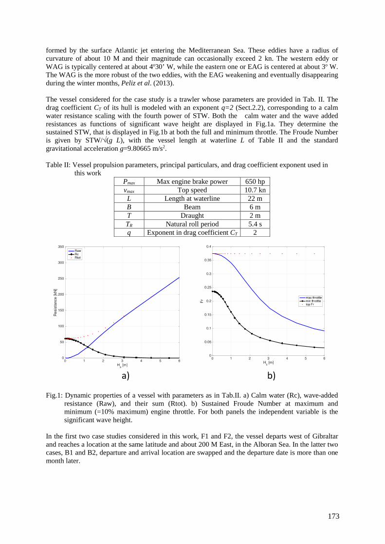
173
formed by the surface Atlantic jet entering the Mediterranean Sea. These eddies have a radius of curvature of about 10 M and their magnitude can occasionally exceed 2 kn. The western eddy or WAG is typically centered at about 4o30’ W, while the eastern one or EAG is centered at about 3o W. The WAG is the more robust of the two eddies, with the EAG weakening and eventually disappearing during the winter months, Peliz et al. (2013). The vessel considered for the case study is a trawler whose parameters are provided in Tab. II. The drag coefficient CT of its hull is modeled with an exponent q=2 (Sect.2.2), corresponding to a calm water resistance scaling with the fourth power of STW. Both the calm water and the wave added resistances as functions of significant wave height are displayed in Fig.1a. They determine the sustained STW, that is displayed in Fig.1b at both the full and minimum throttle. The Froude Number is given by STW/√(g L), with the vessel length at waterline L of Table II and the standard gravitational acceleration g=9.80665 m/s2.
Table II: Vessel propulsion parameters, principal particulars, and drag coefficient exponent used in this work
Pmax Max engine brake power 650 hp vmax Top speed 10.7 kn L Length at waterline 22 m B Beam 6 m T Draught 2 m TR Natural roll period 5.4 s q Exponent in drag coefficient CT 2
Fig.1: Dynamic properties of a vessel with parameters as in Tab.II. a) Calm water (Rc), wave-added
resistance (Raw), and their sum (Rtot). b) Sustained Froude Number at maximum and minimum (=10% maximum) engine throttle. For both panels the independent variable is the significant wave height.
In the first two case studies considered in this work, F1 and F2, the vessel departs west of Gibraltar and reaches a location at the same latitude and about 200 M East, in the Alboran Sea. In the latter two cases, B1 and B2, departure and arrival location are swapped and the departure date is more than one month later.
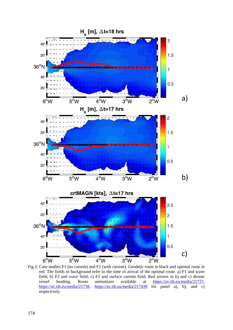
174
Fig.2: Case studies F1 (no current) and F2 (with current). Geodetic route in black and optimal route in
red. The fields in background refer to the time of arrival of the optimal route. a) F1 and wave field; b) F2 and wave field; c) F2 and surface current field. Red arrows in b) and c) denote vessel heading. Route animations available at https://av.tib.eu/media/21737, https://av.tib.eu/media/21738, https://av.tib.eu/media/217439 for panel a), b), and c) respectively.
a)
b)
c)
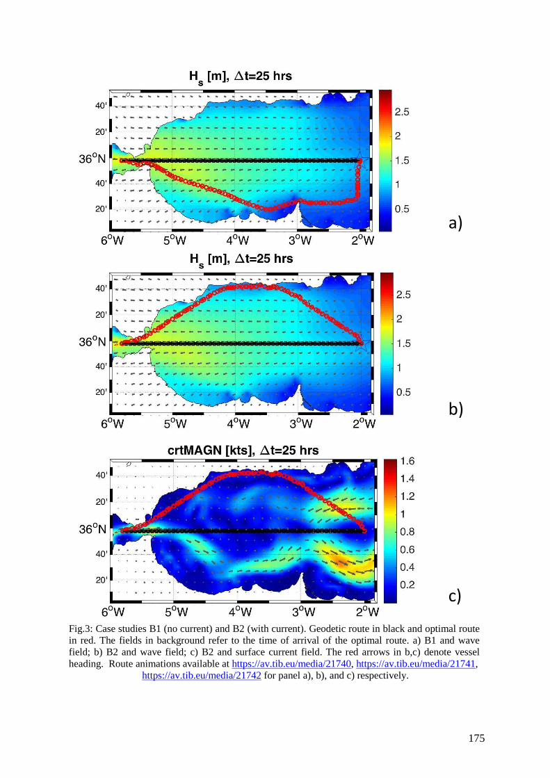
175
Fig.3: Case studies B1 (no current) and B2 (with current). Geodetic route in black and optimal route in red. The fields in background refer to the time of arrival of the optimal route. a) B1 and wave field; b) B2 and wave field; c) B2 and surface current field. The red arrows in b,c) denote vessel heading. Route animations available at https://av.tib.eu/media/21740, https://av.tib.eu/media/21741,
https://av.tib.eu/media/21742 for panel a), b), and c) respectively.
a)
b)
c)
176
For each case, both a geodetic and an optimal route are computed. The geodetic route (black markers in Fig.2 and Fig.3) is the shortest route keeping into account the coastline and the under keel clearance only. The optimal route (red markers in in Fig.2 and Fig.3) also considers the impact of the environmental fields (Sect.2.4) on STW and SOG and the dynamical constraints for vessel intact stability (Sect 2.2). The presentation strategy of the case studies is the following: first, the geodetic and the optimal route in presence of waves only are displayed on top of the significant wave height field (panels a in Fig.2 and Fig.3); then both routes in presence of waves and currents are displayed on top of either the significant wave height field (panels b) or the surface current field (panels c). The main computational and dynamical parameters of the routes are summarized in Table III and IV respectively. Table III: Computational parameters of case study routes. Departure date is on the day following the
model analysis date. The total CPU time does not include the time for the graphical rendering of maps and time series. The number of nodes and edges in the graph is respectively 19’271 and 1’468’703 for each case study.
Case study#
Currents considered?
Model analysis date
Depart time
#time-steps
Opt. route CPU time [s]
Total CPU time [s]
F1 No 2016-08-28 21:00 UTC
19 6.9 54.5 F2 Yes 18 7.0 61.9
B1 No 2016-12-28 03:00 UTC
26 8.2 123.6 B2 Yes 26 8.2 138.5
Table IV: Dynamical features of case study routes. ∆ is the relative change of metrics (length,
duration) of the optimal route with respect to the case with surface currents neglected. Case
study # Currents
considered? Length [m] Duration [hh:mm:ss]
Geodetic Optimal ∆ [%] Optimal ∆ [%] F1 No 184.9 188.2 0.0 18:00:06 0.0 F2 Yes 188.4 +0.1 17:28:01 -3.0 B1 No 223.0 0.0 25:28:33 0.0 B2 Yes 211.0 -5.4 25:24:30 -0.3
Table V: Route analysis dates and some marine weather features. Departure date is on the day
following the model analysis date. For each date departure times at 00:00, 03:00, 06:00, 09:00, 12:00, 15:00, 18:00, 21:00 UTC are considered, which makes the 40 dots per panel of Fig.4
Analysis date Case study
Prevailing wave direction WAG? EAG?
2016-08-28 F1, F2 eastbound Yes North-western meander only
2016-10-24 - East- and then southwestbound Yes Yes 2016-12-28 B1, B2 westbound southern
meander only cyclonic
2017-01-12 - eastbound Yes No 2017-01-25 - southwestbound Yes Yes
In the “wave-only” forward route, F1, the vessel sails with following waves. A northbound diversion (Fig.2a) instrumental in avoiding a condition of surfriding/broaching-to is computed (not shown). In the “wave¤t” forward route F2 instead a southbound diversion is observed (Fig.2b,c). This is not surprising, as the algorithm exploits the favorable eastbound jet (more than 2 kn velocity) of the Atlantic current that feeds the WAG. The optimal route is 3% faster than the case not considering currents, Table IV. In this case, the currents allow not just recovering the involuntary speed loss due

177
to the added resistance in waves, but even achieving a voyage-average speed of 10.8 kn, i.e. nearly 1% higher than the top speed of the vessel in calm waters, Table II. In the “wave-only” backward route, B1, a westbound route leg follows a sudden southbound diversion (Fig.3a), and this is due to avoidance of both pure loss of stability (not shown) and rough sea (cf. route animation at https://av.tib.eu/media/21740). The algorithm also computes throttle reductions down to 55% brake power (not shown). In the “wave¤t” backward route, B2, a large northbound diversion is found (Fig.3b,c). This allows avoiding a SOG penalty in sailing across and then against the southern meander of the WAG and allows exploiting the favorable northern meander of the EAG. The route then continues in the coastal waters of Andalusia where calm seas are encountered, realizing that “route refraction” that was already explained in Mannarini et al. (2016b) and aimed to benefitting from to the larger STW in calmer sea. During the crossing of the northern meander of the EAG, the rudder must be set more than 10° starboard of the Course Over Ground (COG, not shown). The B2 route is more than 5% shorter than the B1. However, the maximum SOG along B2 is about 1 kn less than along B1. 4. Conclusions The ship routing model VISIR has been generalized for accounting for both sea state variables and surface currents. If the vessel course is prescribed, currents affect both the SOG and the rudder angle of the vessel, while the STW is determined by the sea state only (specifically, by the significant wave height). Case studies in the Alboran Sea are discussed. VISIR attempts to maximize the sailing with currents and minimize navigation against or cross the currents. The duration of the resulting least-time routes can differ in percent range from the ones neglecting the currents and their topology can be dramatically different. However, the ocean circulation and the sea state obtained from data-assimilative forecasting models show such a variability to rule out not only the use of climatological currents and waves, but also to limit the conclusions drawn from individual time-dependent case studies. Thus, these numerical results from VISIR should be consolidated through a wider set of routes and vessel types in different regions of the global ocean. Nevertheless, these results already provide first evidence that, at least for not too fast fishing vessels, ocean currents may have a measurable impact on route duration and topology, even in presence of waves. Acknowledgements This work has received partial funding from the European Union's Horizon 2020 research and innovation programme under grant agreement No 633211 (“AtlantOS”). References ALEXANDERSSON, M. (2009), A study of methods to predict added resistance in waves, Master thesis, KNH Centre for Naval Architecture, Stockholm www.knh.se/polopoly_fs/1.151543!/Menu/general/column-content/attachment/Alexandersson.pdf ARDHUIN, F.; BERTOTTI, L.; BIDLOT, J.R.; CAVALERI, L.; FILIPETTO, V.; LEFEVRE, J.M.; WITTMANN, P. (2007), Comparison of wind and wave measurements and models in the Western Mediterranean Sea, Ocean Engineering 34(3), pp.526-541

178
BAZARI, Z.; LONGVA, T. (2011), Assessment of IMO mandated energy efficiency measures for international shipping, International Maritime Organization, http://www.imo.org/ BERTSEKAS, D.P. (1998), Network Optimization: Continuous and Discrete Models, Athena Scientific, http://web.mit.edu/dimitrib/www/netbook_Full_Book.pdf BREIVIK, Ø.; ALLEN, A.A. (2008), An operational search and rescue model for the Norwegian Sea and the North Sea, J. Marine Systems 69, pp.99-113, https://arxiv.org/pdf/1111.1102.pdf CHANG, Y.C.; TSENG, R.S.; CHEN, G.Y.; CHU, P.C.; SHEN, Y.T. (2013), Ship routing utilizing strong ocean currents, J. Navigation 66, pp.825-835, www.dtic.mil/dtic/tr/fulltext/u2/a587298.pdf CHEN, H.H. (1978), A dynamic program for minimum cost ship routing under uncertainty, Ph.D. thesis, Massachusetts Institute of Technology CLEMENTI, E.; ODDO, P.; DRUDI, M.; PINARDI, N.; KORRES, G.; GRANDI, A. (2017), Coupling hydrodynamic and wave models: first step and sensitivity experiments in the Mediterranean Sea, Ocean Dynamics FOURCY, D.; LORVELEC, O. (2012), A new digital map of limits of oceans and seas consistent with high-resolution global shorelines, J. Coastal Research 29(2), pp.471-477 GERRITSMA, J.; BEUKELMAN, W. (1972), Analysis of the resistance increase in waves of a fast cargo ship, International Shipbuilding Progress 19, pp.285-293 LO, H.K.; McCORD, M.R. (1995), Routing through dynamic ocean currents: General heuristics and empirical results in the Gulf stream region, Transportation Research Part B: Methodological 29, pp.109-124 LO, H.K.; McCORD, M.R. (1998), Adaptive ship routing through stochastic ocean currents: General formulations and empirical results, Transportation Research Part A: Policy and Practice 32, pp.547-561 LOLLA, T.; HALEY, P.J.; LERMUSIAUX, P.F. (2014), Time-optimal path planning in dynamic flows using level set equations: realistic applications, Ocean Dynamics 64, pp.1399-1417 MACÍAS, D.; BRUNO, M.; ECHEVARRÍA, F.; VÁZQUEZ, A.; GARCIA, C.M. (2008), Meteo-rologically-induced mesoscale variability of the North-western Alboran Sea (southern Spain) and related biological patterns, Estuarine, Coastal and Shelf Science 78(2), pp.250-266 MANNARINI, G. (2015a), The twofold aspect of climate change on navigation: the search for new maritime routes and the challenge of reducing the carbon footprint of ships, Tech. Rep. RP0252, CMCC, http://www.cmcc.it/wp-content/uploads/2015/03/rp0252-opa-03-2015.pdf MANNARINI, G.; LECCI, R.; COPPINI, G. (2015b), Introducing sailboats into ship routing system VISIR, 6th Int. Conf. Information, Intelligence, Systems and Applications, pp.1-6 MANNARINI, G.; PINARDI, N.; COPPINI, G. (2016a), VISIR: A free and open-source model for ship route optimization, COMPIT Conf., Lecce, http://data.hiper-conf.info/compit2016_lecce.pdf MANNARINI, G.; PINARDI, N.; COPPINI, G.; ODDO, P.; IAFRATI, A. (2016b), VISIR-I: small vessels – least-time nautical routes using wave forecasts, Geoscientific Model Development 9, pp.1597-1625, http://www.geosci-model-dev.net/9/1597/2016/gmd-9-1597-2016.pdf MANNARINI, G.; TURRISI, G.; D’ANCA, A.; SCALAS, M.; PINARDI, N.; COPPINI, G.; PALERMO, F.; CARLUCCIO, I.; SCURO, M.; CRET`ı, S.; LECCI, R.; NASSISI, P.; TEDESCO, L.

179
(2016c), VISIR: technological infrastructure of an operational service for safe and efficient navigation in the Mediterranean Sea, Natural Hazards and Earth System Sciences 16(8), pp.1791-1806, http://www.nat-hazards-earth-syst-sci.net/16/1791/2016/nhess-16-1791-2016.pdf PELIZ, A.; BOUTOV, D.; CARDOSO, R.M.; DELGADO, J; SOARES, P.M. (2013), The Gulf of Cadiz–Alboran Sea sub-basin: Model setup, exchange and seasonal variability, Ocean Modelling 61, pp.49-67 SUBRAMANI, D.N.; LERMUSIAUX, P.F. (2016), Energy-optimal path planning by stochastic dynamically orthogonal level-set optimization, Ocean Modeling 100, pp.55-57 TONANI, M.; ODDO, P.; KORRES, G.; CLEMENTI, E.; DOBRICIC, S.; DRUDI, M.; PISTOIA, J.; GUARNIERI, A.; ROMANIELLO, V.; GIRARDI, G.; GRANDI, A.; BONADUCE, A.; PINARDI, N. (2014), The Mediterranean Forecasting System: recent developments, EGU General Assembly Conference Abstracts 16, p.16899 TONANI, M.; BALMASEDA, M.; BERTINO, L.; BLOCKLEY, E.; BRASSINGTON, G.; DAVIDSON, F.; DRILLET, Y.; HOGAN, P.; KURAGANO, T.; LEE, T.; MEHRAK, A.; PARA-NATHARAL, F.; TANAJURAM, C.; WANG, H. (2015), Status and future of global and regional ocean prediction systems, J. Operational Oceanography 8, s201–s220 ZOPPOLI, R. (1972), Minimum-time routing as an N-stage decision process, J. Applied Met. 11, pp.429-435, http://journals.ametsoc.org/doi/pdf/10.1175/1520-0450(1972)011%3C0429:MTRAAS%3E2.0.CO%3B2
180
Pre-Crash Advisor –
Decision Support System for Mitigating Collision Damage
Hasan Deeb, Mohamed Abdelaal, Axel Hahn, University of Oldenburg, Oldenburg/Germany,
[email protected], [email protected], [email protected]
Abstract
This paper describes a decision support system looking at possible options minimizing ship accident
consequences for unavoidable collisions. The proposed algorithm takes in consideration the ship
maneuvering and collision scenarios. Ship maneuvering is represented using the first-order Nomoto
model with speed correction, and damage is constrained by the collision angle. The developed
approach predicts all the possible collision scenarios and proposes best rudder angle to minimize
damage.
1. Introduction
The International Maritime Organization (IMO) safety goal for passenger ships is: "ship is its best live
boat". From this goal mitigation of ship accident consequences comes as essential need. Risk of ship
collision is increasing with the increasing of the maritime transportation activities, where more than
90 percent of the international trading is done by ships. Ship collisions may cause human casualties,
economical loss and environmental pollution. Taking in consideration these serious consequences,
there is a need to investigate options in addition to risk assessment and collision avoidance, once
collision is inevitable. Many researches have been done concerning risk assessment and collision
avoidance using most advanced technologies. However, the number of ship collisions is still on a
constant, HELCOM (2013,2014). In addition to the trend for unmanned ships which put the maritime
traffic in challenge of absence of the crew experience.
Damage mitigation exists in maritime industry through regulations and standards developed by
classification societies regarding extent and location of damage due to collision and grounding Norsok
(2010), DNVGL (2015) Norsok (2004). The International Maritime Organization (IMO) also requires
the use of goal-based standards (GBSs) to improve ship’s hull resistance against collision damage.
Many research have been done in order to predict collision damage and ensure ship survivability in
case of ship accidents Hogström (2012), Wang (2002). Most of development on ship structure
regarding the improvement of ship safety came as reactive actions after certain catastrophic accidents.
The Risk-based design is a proactive research developed as an improved alternative to the traditional
design process to integrates safety as additional design objective Boulougouris and Papanikolaou
(2013). Another proposed solution to reduce collision damage is the concept of buffer bow developed
to minimize the damage along the struck ship, which supposed to absorb most of collision impact
Yamada and Pedersen (2008). In general these methods affect ship design, structural arrangement and
cost, it is based on statistical and probabilistic analyses. However, there is no research concerning
damage mitigation based on changing encountering situation using ship's maneuvering capabilities to
reduce collision impact.
2. Collision effect mitigation
2.1 Requirements and background
Ships collisions despite all applied advanced technologies are in a constant – see, for example, EMSA
(2015), HELCOM (2013,2014) – as ship collisions are a complex phenomenon consist of complicated
ship motion and structural damage, Tabri (2010). In normal navigation the situation can be shifted
from commonplace to critical in very short time. Accidents investigations show that poor judgment
and less than adequate communications, as well as lack of situational awareness are major reasons
which can lead to collisions. Mitigation of ship collision damage concerns a very critical phase of
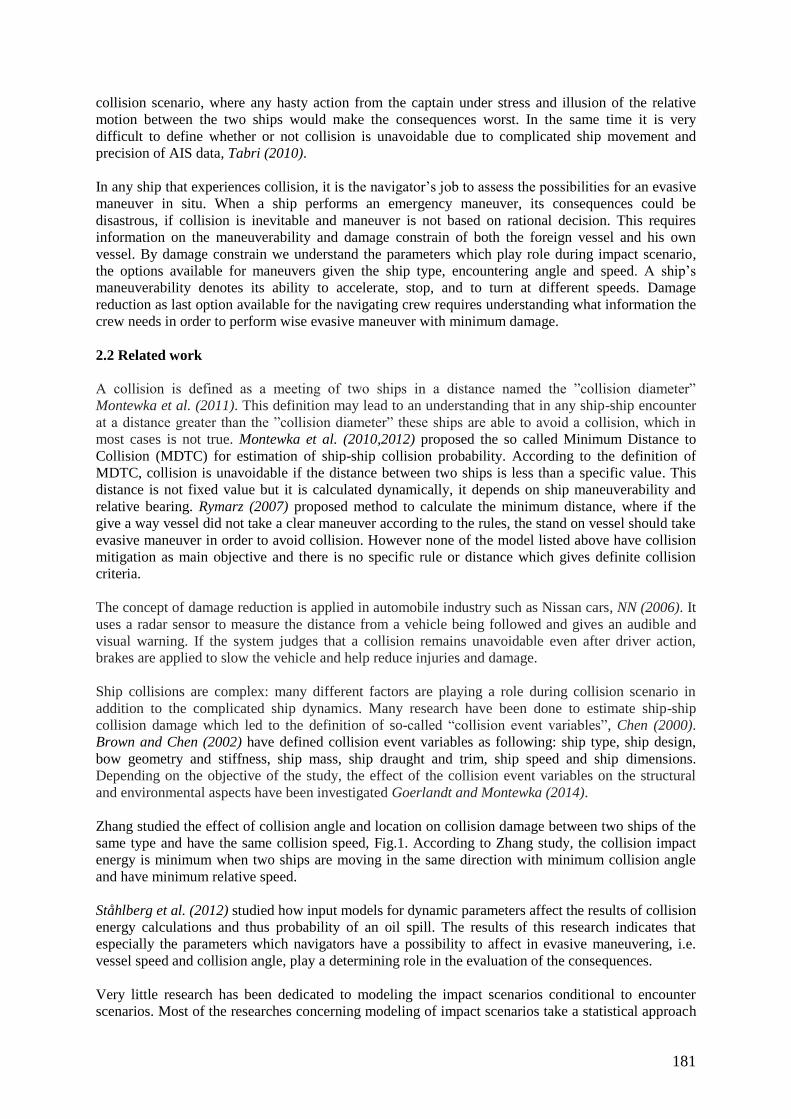
181
collision scenario, where any hasty action from the captain under stress and illusion of the relative
motion between the two ships would make the consequences worst. In the same time it is very
difficult to define whether or not collision is unavoidable due to complicated ship movement and
precision of AIS data, Tabri (2010).
In any ship that experiences collision, it is the navigator’s job to assess the possibilities for an evasive
maneuver in situ. When a ship performs an emergency maneuver, its consequences could be
disastrous, if collision is inevitable and maneuver is not based on rational decision. This requires
information on the maneuverability and damage constrain of both the foreign vessel and his own
vessel. By damage constrain we understand the parameters which play role during impact scenario,
the options available for maneuvers given the ship type, encountering angle and speed. A ship’s
maneuverability denotes its ability to accelerate, stop, and to turn at different speeds. Damage
reduction as last option available for the navigating crew requires understanding what information the
crew needs in order to perform wise evasive maneuver with minimum damage.
2.2 Related work
A collision is defined as a meeting of two ships in a distance named the ”collision diameter”
Montewka et al. (2011). This definition may lead to an understanding that in any ship-ship encounter
at a distance greater than the ”collision diameter” these ships are able to avoid a collision, which in
most cases is not true. Montewka et al. (2010,2012) proposed the so called Minimum Distance to
Collision (MDTC) for estimation of ship-ship collision probability. According to the definition of
MDTC, collision is unavoidable if the distance between two ships is less than a specific value. This
distance is not fixed value but it is calculated dynamically, it depends on ship maneuverability and
relative bearing. Rymarz (2007) proposed method to calculate the minimum distance, where if the
give a way vessel did not take a clear maneuver according to the rules, the stand on vessel should take
evasive maneuver in order to avoid collision. However none of the model listed above have collision
mitigation as main objective and there is no specific rule or distance which gives definite collision
criteria.
The concept of damage reduction is applied in automobile industry such as Nissan cars, NN (2006). It
uses a radar sensor to measure the distance from a vehicle being followed and gives an audible and
visual warning. If the system judges that a collision remains unavoidable even after driver action,
brakes are applied to slow the vehicle and help reduce injuries and damage.
Ship collisions are complex: many different factors are playing a role during collision scenario in
addition to the complicated ship dynamics. Many research have been done to estimate ship-ship
collision damage which led to the definition of so-called “collision event variables”, Chen (2000).
Brown and Chen (2002) have defined collision event variables as following: ship type, ship design,
bow geometry and stiffness, ship mass, ship draught and trim, ship speed and ship dimensions.
Depending on the objective of the study, the effect of the collision event variables on the structural
and environmental aspects have been investigated Goerlandt and Montewka (2014).
Zhang studied the effect of collision angle and location on collision damage between two ships of the
same type and have the same collision speed, Fig.1. According to Zhang study, the collision impact
energy is minimum when two ships are moving in the same direction with minimum collision angle
and have minimum relative speed.
Ståhlberg et al. (2012) studied how input models for dynamic parameters affect the results of collision
energy calculations and thus probability of an oil spill. The results of this research indicates that
especially the parameters which navigators have a possibility to affect in evasive maneuvering, i.e.
vessel speed and collision angle, play a determining role in the evaluation of the consequences.
Very little research has been dedicated to modeling the impact scenarios conditional to encounter
scenarios. Most of the researches concerning modeling of impact scenarios take a statistical approach
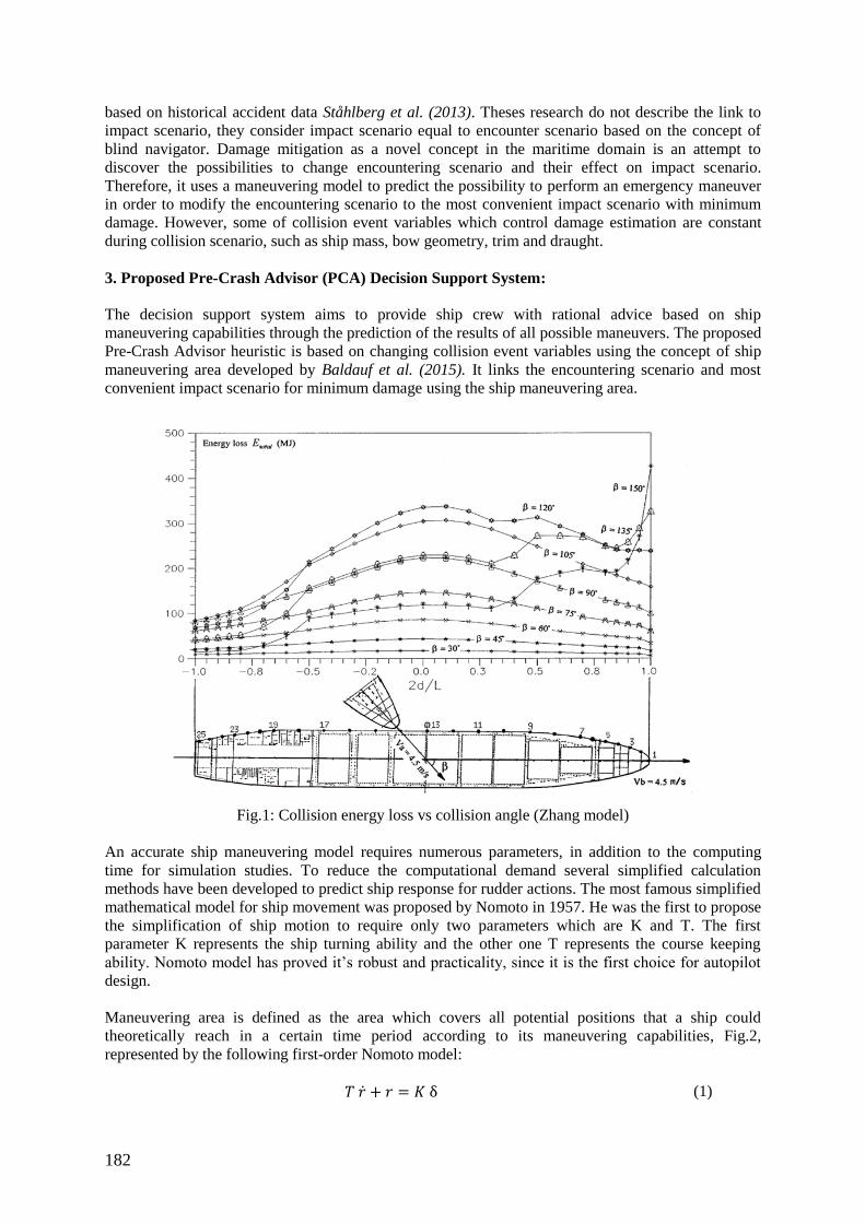
182
based on historical accident data Ståhlberg et al. (2013). Theses research do not describe the link to
impact scenario, they consider impact scenario equal to encounter scenario based on the concept of
blind navigator. Damage mitigation as a novel concept in the maritime domain is an attempt to
discover the possibilities to change encountering scenario and their effect on impact scenario.
Therefore, it uses a maneuvering model to predict the possibility to perform an emergency maneuver
in order to modify the encountering scenario to the most convenient impact scenario with minimum
damage. However, some of collision event variables which control damage estimation are constant
during collision scenario, such as ship mass, bow geometry, trim and draught.
3. Proposed Pre-Crash Advisor (PCA) Decision Support System:
The decision support system aims to provide ship crew with rational advice based on ship
maneuvering capabilities through the prediction of the results of all possible maneuvers. The proposed
Pre-Crash Advisor heuristic is based on changing collision event variables using the concept of ship
maneuvering area developed by Baldauf et al. (2015). It links the encountering scenario and most
convenient impact scenario for minimum damage using the ship maneuvering area.
Fig.1: Collision energy loss vs collision angle (Zhang model)
An accurate ship maneuvering model requires numerous parameters, in addition to the computing
time for simulation studies. To reduce the computational demand several simplified calculation
methods have been developed to predict ship response for rudder actions. The most famous simplified
mathematical model for ship movement was proposed by Nomoto in 1957. He was the first to propose
the simplification of ship motion to require only two parameters which are K and T. The first
parameter K represents the ship turning ability and the other one T represents the course keeping
ability. Nomoto model has proved it’s robust and practicality, since it is the first choice for autopilot
design.
Maneuvering area is defined as the area which covers all potential positions that a ship could
theoretically reach in a certain time period according to its maneuvering capabilities, Fig.2,
represented by the following first-order Nomoto model:
𝑇 �̇� + 𝑟 = 𝐾 δ (1)
183
where 𝑟 is the yaw velocity, 𝛿 is the rudder angle, and 𝐾 and 𝑇 are the ship hydrodynamics indices.
It has been used to predict ship paths according to possible rudder angle actions with the aid of the
ship simplified kinematics:
[
�̇��̇��̇�
] = [𝑈 cos (𝜑)𝑈 sin (𝜑)
𝑟]
(2)
Where 𝑈 is the assumed constant ship speed, 𝜑 is the heading angle, and 𝑥 and 𝑦 form the position
of the ship. Nomoto model is the one of the simplest mathematical models for ship maneuvering
dynamics as it is robust and fast model specially for damage mitigation, where time is an issue. All
the aforementioned equations are discretized using a proper sampling interval.
Fig.2: Concept of ship domain (rudder angle -30 to + 30 degrees)
Pre-Crash Advisor must be linked to the installed collision avoidance system. It is activated after
collision avoidance fails (i.e. when the distance between the two ships becomes less than specific
value (MDTC) and collision supposed to be inevitable Montewka et al. (2011)). But in order to define
the inevitable collision candidate Pre-Crash Advisor (PCA) updates its input data from the Automatic
Identification System (AIS). It calculates the expected initial collision point and angle using AIS data.
In the same time AIS provides other information such as ship length which is required for defining
striking and struck ship. The algorithm calculates and compares the distance between the two ships
with the (MDTC). In the current version of the PCA this distance is taken equal to struck ship length.
The hydrodynamic indices K and T which represent the manoeuvring capabilities of the striking ship
should be available from the manoeuvring test and stored in the PCA memory.
In the Pre-Crash Advisor, the algorithm generates ship manoeuvring area according to its definition
i.e. the prediction time is equal to the time required the ship according to its actual speed to turn 180°
with full rudder action, Baldauf et al. (2015), Fig.2. When the AIS data refer to certain threat or
collision candidate due to intersection between the two ship paths, it compares the distance between
each point of the manoeuvring area and the candidate collision ship. If this distance is smaller than the
MDTC, it gives an alarm about the paths and rudder angles which lead to collision. If the captain took
an action and its results always show that all possible manoeuvring paths lead to inevitable collision.
The algorithm calculates all the collision angles and proposes the rudder angle which gives the
minimum damage according the minimum damage criteria. A calculation of the collision angle is
done by finding the different between both ships heading angles at the collision point for all
manoeuvring paths.
The first developed scheme is working in the following order, see Fig.4:
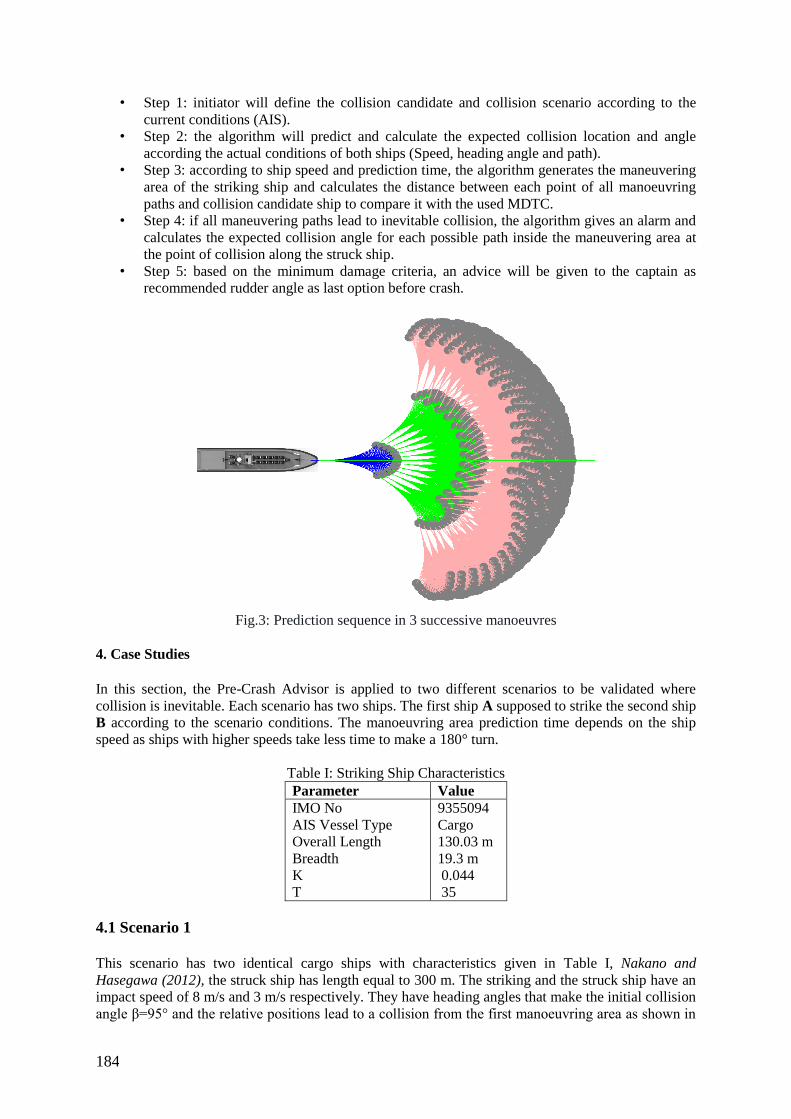
184
• Step 1: initiator will define the collision candidate and collision scenario according to the
current conditions (AIS).
• Step 2: the algorithm will predict and calculate the expected collision location and angle
according the actual conditions of both ships (Speed, heading angle and path).
• Step 3: according to ship speed and prediction time, the algorithm generates the maneuvering
area of the striking ship and calculates the distance between each point of all manoeuvring
paths and collision candidate ship to compare it with the used MDTC.
• Step 4: if all maneuvering paths lead to inevitable collision, the algorithm gives an alarm and
calculates the expected collision angle for each possible path inside the maneuvering area at
the point of collision along the struck ship.
• Step 5: based on the minimum damage criteria, an advice will be given to the captain as
recommended rudder angle as last option before crash.
Fig.3: Prediction sequence in 3 successive manoeuvres
4. Case Studies
In this section, the Pre-Crash Advisor is applied to two different scenarios to be validated where
collision is inevitable. Each scenario has two ships. The first ship A supposed to strike the second ship
B according to the scenario conditions. The manoeuvring area prediction time depends on the ship
speed as ships with higher speeds take less time to make a 180° turn.
Table I: Striking Ship Characteristics
Parameter Value
IMO No
AIS Vessel Type
Overall Length
Breadth
K
T
9355094
Cargo
130.03 m
19.3 m
0.044
35
4.1 Scenario 1
This scenario has two identical cargo ships with characteristics given in Table I, Nakano and
Hasegawa (2012), the struck ship has length equal to 300 m. The striking and the struck ship have an
impact speed of 8 m/s and 3 m/s respectively. They have heading angles that make the initial collision
angle β=95° and the relative positions lead to a collision from the first manoeuvring area as shown in
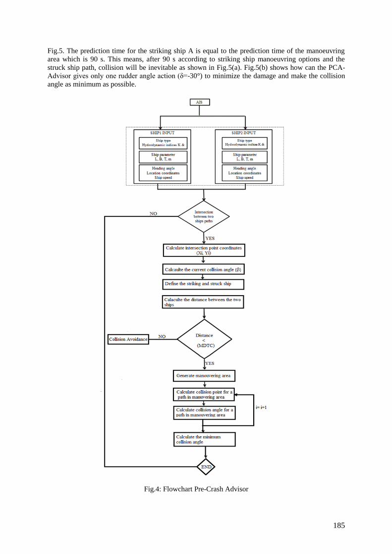
185
Fig.5. The prediction time for the striking ship A is equal to the prediction time of the manoeuvring
area which is 90 s. This means, after 90 s according to striking ship manoeuvring options and the
struck ship path, collision will be inevitable as shown in Fig.5(a). Fig.5(b) shows how can the PCA-
Advisor gives only one rudder angle action (δ=-30°) to minimize the damage and make the collision
angle as minimum as possible.
Fig.4: Flowchart Pre-Crash Advisor
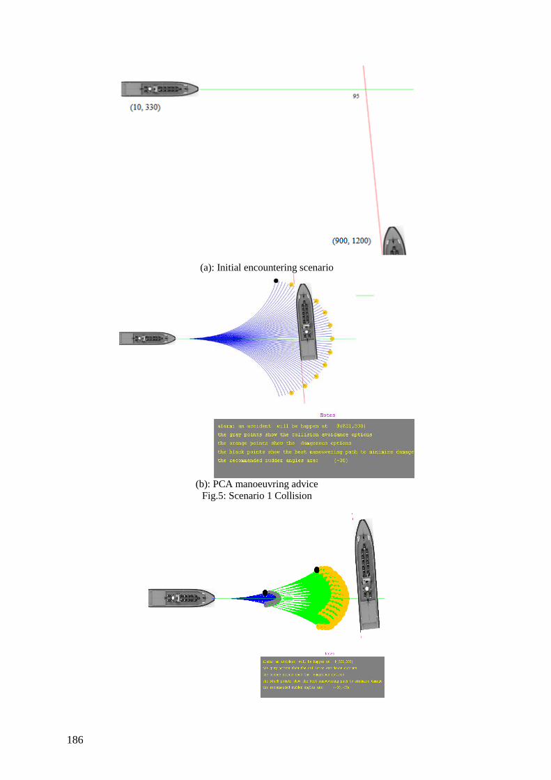
186
(a): Initial encountering scenario
(b): PCA manoeuvring advice
Fig.5: Scenario 1 Collision
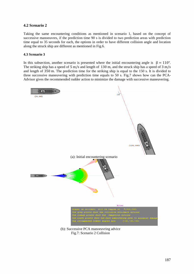
187
4.2 Scenario 2
Taking the same encountering conditions as mentioned in scenario 1, based on the concept of
successive manoeuvres, if the prediction time 90 s is divided to two prediction areas with prediction
time equal to 35 seconds for each, the options in order to have different collision angle and location
along the struck ship are different as mentioned in Fig.6.
4.3 Scenario 3
In this subsection, another scenario is presented where the initial encountering angle is β = 110°.
The striking ship has a speed of 5 m/s and length of 130 m, and the struck ship has a speed of 3 m/s
and length of 350 m. The prediction time for the striking ship is equal to the 150 s. It is divided to
three successive maneuvering with prediction time equals to 50 s. Fig.7 shows how can the PCA-
Advisor gives the recommended rudder action to minimize the damage with successive maneuvering.
(a): Initial encountering scenario
(b): Successive PCA manoeuvring advice
Fig.7: Scenario 2 Collision
188
5. Conclusion and discussion
The dynamic parameters at the moment of impact significantly affect the collision damage.
Modification of dynamic parameters at the moment of impact are nevertheless little discussed in
context of collision damage mitigation. Therefore, a decision support system for ship collision
damage mitigation is presented. This paper addresses the main aspects which must be considered for
the development of intelligent decision support system for ship-ship collision damage mitigation.
These aspects are:
1- Criteria for unavoidable collision (MDTC);
2- Collision event variables which effect collision damage (collision angle, speed and location);
3- Criteria for minimum damage during evasive manoeuvre;
4- Link between encountering scenario and impact scenario using maneuvering model.
Due to the absence of specific criteria that defines case when collision is unavoidable, the authors
propose that struck ship length is the criteria for unavoidable collision. The developed algorithm let
the door open to use any specific or dynamic value for MDTC, it can be chosen from the captain
according to his experience or value of risk he can accept.
Collision angle has been chosen due to its strong effect on collision damage according to Zhang
research. Nomoto model is used for the current version of PCA due to its robust and fast prediction
for the maneuvering area. The advantage of the maneuvering area that, it is dynamic area, its size
changes with ship type and speed. This comes in harmony with the definition of MDTC which
depends on different factors such as ship speed and relative bearing.
6. Future work
According to SOLAS, The International Convention for the Safety of Life at Sea, requires that ships
are fitted with transverse watertight bulkheads to provide the ship with a certain measure of survival
capability. In addition to the classification societies rules for collision bulkheads, DNVGL (2015),
Ståhl-berg et al. (2012). Collision location affects the damages according to the ship type, for
example, any structural damage along cargo area can lead to economical loss or pollution such as in
Tankers vessels or human casualties such as in passenger vessels.
As collision location and speed have important role in collision impact, the authors aim to use a three
degree of freedom (3-DOF) nonlinear model of the vessel to account for manipulating the engine
speed in addition to the rudder angle; this will give more freedom in damage reduction as a trade-off
between collision angle, location, and speed. The successive manoeuvres concept helps to optimise
damage mitigation; the authors aim to implement the PCA with successive maneuvers in real time
applications.
Acknowledgements
The work presented in this paper was supported by the Ministry of Science and Culture of Lower
Saxony as part of the Graduate School Safe Automation of Maritime Systems (SAMS) and the project
Critical Systems Engineering for Socio-Technical Systems (CSE).
References
BALDAUF, M.; MEHDI, R.; DEEB, H.; SCHRÖDER-HINRICHS, J.U.; BENEDICT, K.;
KRÜGER, C.; FISCHER, S.; GLUCH, M. (2015), Manoeuvring areas to adapt ACAS for the
maritime domain, Sci. J. Marit. Univ. Szczec. 43, pp.39-47
BOULOUGOURIS, E.; PAPANIKOLAOU, A. (2013), Risk-Based Design of Naval Combatants,

189
Ocean Eng. 65, pp.49-61
BROWN, A.; CHEN, D. (2002), Probabilistic method for predicting ship collision damage, Ocean
Engineering 6, pp.54-65
CHEN (2000), Simplified Ship Collision Model, PhD Thesis, Virginia Polytech, Blacksburg
DNVGL (2015), Rules for Classification Ships, Part 3 Hull Chapter 2 General Arrangement Design,
DNV GL, Hovik
GOERLANDT, F.; MONTEWKA, J. (2014), A probabilistic model for accidental cargo oil outflow
from product tankers in a ship-ship collision, Marine Pollution Bulletin 79(1-2), pp.130-44
HELCOM (2013), Annual Report on Shipping Accidents in the Baltic Sea Area during 2012,
Technical report, HELCOM – Baltic Marine Environment Protection Commission
HELCOM (2014), Annual Report on Shipping Accidents in the Baltic Sea Area during 2013,
Technical report, HELCOM – Baltic Marine Environment Protection Commission
HOGSTRÖM, P. (2012), RoPax Ship Collision - A Methodology for Survivability Analysis, PhD
Thesis, Chalmers University of Technology
MONTEWKA, J.; GOERLANDT, F.; KUJALA, P. (2011), A new definition of a collision zone for a
geometrical model for ship-ship collision probability estimation, TransNav 5(4), pp.497-504
NAKANO, T.; HASEGAWA, K. (2012), An attempt to predict manoeuvring indices using ais data
for automatic OD data acquisition, IFAC Proceedings Volumes (IFAC-PapersOnline) 9(PART 1),
pp.1-6
NN (2006), Nissan's approach to safety, Technology overview, Nissan, www.nissan-global.com/EN/
NORSOK (2004), NORSOK STANDARD N-004, Design of Steel Structures. Appendix A, Design
against Accidental Actions
RYMARZ, E.W. (2007), The Determination of a Minimum Critical Distance for Avoiding Action by a
Stand-on Vessel as Permitted by Rule 17a ) Ii ), 1, pp.63-68
STÅHLBERG, K.; GOERLANDT, F.; MONTEWKA J.; KUJALA, P. (2012), Uncertainty in
analytical collision dynamics model due to assumptions in dynamic parameters, TransNav 6(1),
pp.47-54
STÅHLBERG, K.; GOERLANDT, F.; EHLERS, S. (2013), Impact scenario models for probabilistic
risk-based design for ship – Ship collision, Marine Structures 33, pp.238-264
TABRI, K. (2010), Dynamics of Ship Collisions, PhD thesis, Aalto University
WANG, G.; SEAH, A.K.; YUNG, S. (2002), Predicting Ship Structure Performance in Accidents,
ABS Tech. Papers, pp.69-84
YAMADA, Y.; ENDO, H.; PEDERSEN, P.T. (2008), Effects of buffer bow structure in ship-ship
collision, Int. J. Offshore and Polar Eng. 18(2), pp.133-141
190
EPILYSIS, a New Solver for Finite Element Analysis
George Korbetis, Serafim Chatzimoisiadis, Dimitrios Drougkas, BETA CAE Systems,
Thessaloniki/Greece, [email protected]
Abstract
This paper introduces EPILYSIS, the new member of BETA CAE Systems software suite. EPILYSIS is
a solver for Finite Element Analysis, which comes to bridge the gap between pre- and post-
processing and offer a seamless operation in CAE workflow. Designed for large-scale model
analyses, it is ideal for the global strength assessment of large vessels and detailed strength
assessment of highly stressed areas. Additionally, direct and modal frequency response and non-
linear contact solutions allow more extensive and sophisticated analyses. EPILYSIS together with the
pre- and post- processors, ANSA and META, offer a valuable yet affordable tool to the Marine
Engineering sector. Two characteristic case studies are presented where EPILYSIS element accuracy
and results performance are compared with well-known solvers in the market.
1. Introduction
EPILYSIS is the new addition to the BETA CAE Systems analysis tools. Named after the Greek word
for "solution", EPILYSIS covers numerous solution types such as Structural, NVH, Optimization and
more. In this paper, two representative applications are presented, where the complete BETA CAE
Systems suite is used for the model preparation, process and results interpretation.
In the first part, a typical VLCC vessel is subjected to three different loading conditions. The main
target is the determination of the maximum stresses and the critical areas. The complete Model set-up
is conducted with the aid of the ANSA pre-processor. First, a detailed Finite Element model of the
hull structure is generated, complying with the meshing requirements set by Classification Societies.
Then, a series of useful and automated processes make the model "lighter", more sophisticated but
still realistic and suitable for the strength analysis. For each loading condition, the hydrostatic
equilibrium of the ship is computed and the corresponding hull deformations are calculated. The static
analyses are conducted using both the EPILYSIS and a well-known commercial solver.
In the second part, EPILYSIS solver is used on a nonlinear-contact strength analysis for a ship’s
rudder. The applied force which is produced by the water resistance, at specific speed and angle-
position of the rudder, is calculated by a simplified CFD analysis and used as the loading condition
for the structural analysis. The static problem set-up is performed using automated processes, such as
the results mapping, the contact pair definition and the batch meshing, which are provided by the
ANSA pre-processor. Several runs are performed with EPILYSIS and an industry standard solver.
The solvers are compared to each other concerning the performance and the results accuracy.
2. Static Analysis
2.1. Model set-up
The general characteristics of the studied VLCC are presented in Table I. At first, a Finite Element
(FE) model of the ship structure is automatically generated. In general, the ship is relatively large so,
coarse mesh should be applied to avoid very long simulation time. The whole structure is represented
by first-order shell elements; (a small amount of solid tetrahedral elements are used at the stern tube
region). A coarse mesh is generated for the whole structure (element length of 0.95 m), except from
selected areas, where finer mesh (e.g. 0.2 m) ensures better results accuracy. This mesh strategy was
selected to contribute to the solvers comparison.
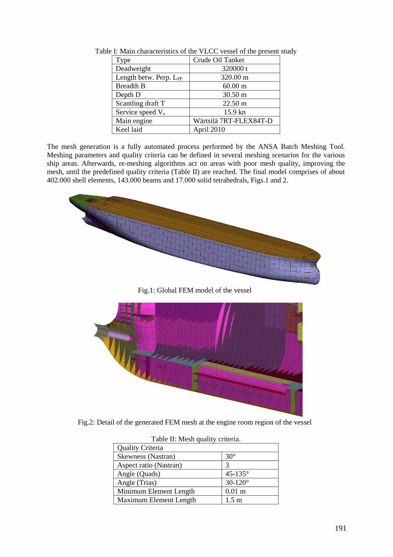
191
Table I: Main characteristics of the VLCC vessel of the present study
Type Crude Oil Tanker
Deadweight 320000 t
Length betw. Perp. LPP 320.00 m
Breadth B 60.00 m
Depth D 30.50 m
Scantling draft T 22.50 m
Service speed Vs 15.9 kn
Main engine Wärtsilä 7RT-FLEX84T-D
Keel laid April 2010
The mesh generation is a fully automated process performed by the ANSA Batch Meshing Tool.
Meshing parameters and quality criteria can be defined in several meshing scenarios for the various
ship areas. Afterwards, re-meshing algorithms act on areas with poor mesh quality, improving the
mesh, until the predefined quality criteria (Table II) are reached. The final model comprises of about
402.000 shell elements, 143.000 beams and 17.000 solid tetrahedrals, Figs.1 and 2.
Fig.1: Global FEM model of the vessel
Fig.2: Detail of the generated FEM mesh at the engine room region of the vessel
Table II: Mesh quality criteria.
Quality Criteria
Skewness (Nastran) 30°
Aspect ratio (Nastran) 3
Angle (Quads) 45-135°
Angle (Trias) 30-120°
Minimum Element Length 0.01 m
Maximum Element Length 1.5 m
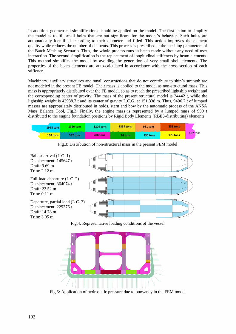
192
In addition, geometrical simplifications should be applied on the model. The first action to simplify
the model is to fill small holes that are not significant for the model’s behavior. Such holes are
automatically identified according to their diameter and filled. This action improves the element
quality while reduces the number of elements. This process is prescribed at the meshing parameters of
the Batch Meshing Scenario. Thus, the whole process runs in batch mode without any need of user
interaction. The second simplification is the replacement of longitudinal stiffeners by beam elements.
This method simplifies the model by avoiding the generation of very small shell elements. The
properties of the beam elements are auto-calculated in accordance with the cross section of each
stiffener.
Machinery, auxiliary structures and small constructions that do not contribute to ship’s strength are
not modeled in the present FE model. Their mass is applied to the model as non-structural mass. This
mass is appropriately distributed over the FE model, so as to reach the prescribed lightship weight and
the corresponding center of gravity. The mass of the present structural model is 34442 t, while the
lightship weight is 43938.7 t and its center of gravity L.C.G. at 151.338 m. Thus, 9496.7 t of lumped
masses are appropriately distributed in holds, stern and bow by the automatic process of the ANSA
Mass Balance Tool, Fig.3. Finally, the engine mass is represented by a lumped mass of 990 t
distributed to the engine foundation positions by Rigid Body Elements (RBE3-distributing) elements.
Fig.3: Distribution of non-structural mass in the present FEM model
Ballast arrival (L.C. 1)
Displacement: 145647 t
Draft: 9.69 m
Trim: 2.12 m
Full-load departure (L.C. 2)
Displacement: 364074 t
Draft: 22.52 m
Trim: 0.11 m
Departure, partial load (L.C. 3)
Displacement: 229276 t
Draft: 14.78 m
Trim: 3.05 m
Fig.4: Representative loading conditions of the vessel
Fig.5: Application of hydrostatic pressure due to buoyancy in the FEM model
168 tons
1360 tons
532 tons 208 tons
1334 tons 1205 tons
24 tons
911 tons
130 tons 167 tons
179 tons
358 tons 1918 tons
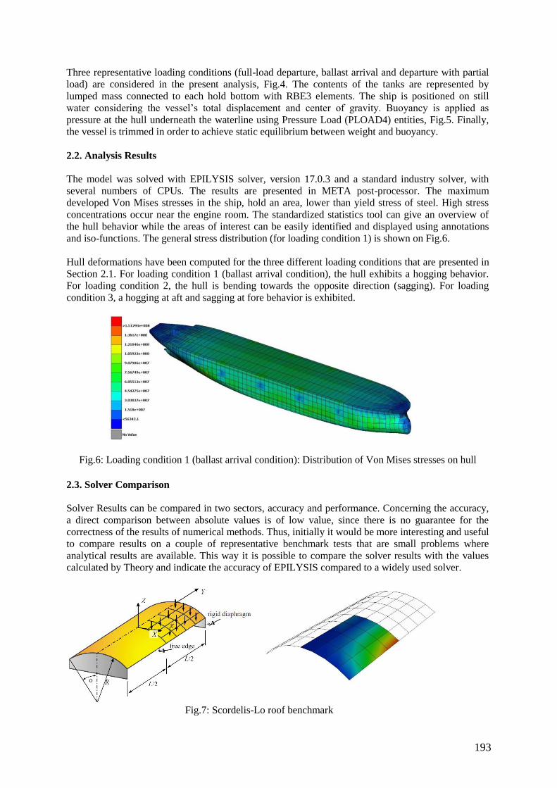
193
Three representative loading conditions (full-load departure, ballast arrival and departure with partial
load) are considered in the present analysis, Fig.4. The contents of the tanks are represented by
lumped mass connected to each hold bottom with RBE3 elements. The ship is positioned on still
water considering the vessel’s total displacement and center of gravity. Buoyancy is applied as
pressure at the hull underneath the waterline using Pressure Load (PLOAD4) entities, Fig.5. Finally,
the vessel is trimmed in order to achieve static equilibrium between weight and buoyancy.
2.2. Analysis Results
The model was solved with EPILYSIS solver, version 17.0.3 and a standard industry solver, with
several numbers of CPUs. The results are presented in META post-processor. The maximum
developed Von Mises stresses in the ship, hold an area, lower than yield stress of steel. High stress
concentrations occur near the engine room. The standardized statistics tool can give an overview of
the hull behavior while the areas of interest can be easily identified and displayed using annotations
and iso-functions. The general stress distribution (for loading condition 1) is shown on Fig.6.
Hull deformations have been computed for the three different loading conditions that are presented in
Section 2.1. For loading condition 1 (ballast arrival condition), the hull exhibits a hogging behavior.
For loading condition 2, the hull is bending towards the opposite direction (sagging). For loading
condition 3, a hogging at aft and sagging at fore behavior is exhibited.
Fig.6: Loading condition 1 (ballast arrival condition): Distribution of Von Mises stresses on hull
2.3. Solver Comparison
Solver Results can be compared in two sectors, accuracy and performance. Concerning the accuracy,
a direct comparison between absolute values is of low value, since there is no guarantee for the
correctness of the results of numerical methods. Thus, initially it would be more interesting and useful
to compare results on a couple of representative benchmark tests that are small problems where
analytical results are available. This way it is possible to compare the solver results with the values
calculated by Theory and indicate the accuracy of EPILYSIS compared to a widely used solver.
Fig.7: Scordelis-Lo roof benchmark
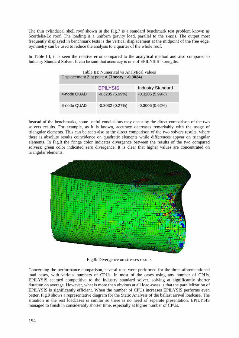
194
The thin cylindrical shell roof shown in the Fig.7 is a standard benchmark test problem known as
Scordelis-Lo roof. The loading is a uniform gravity load, parallel to the z-axis. The output most
frequently displayed in benchmark tests is the vertical displacement at the midpoint of the free edge.
Symmetry can be used to reduce the analysis to a quarter of the whole roof.
In Table III, it is seen the relative error compared to the analytical method and also compared to
Industry Standard Solver. It can be said that accuracy is one of EPILYSIS’ strengths.
Table III: Numerical vs Analytical values
Displacement Z at point A (Theory : -0.3024)
EPILYSIS Industry Standard
4-node QUAD -0.3205 (5.99%) -0.3205 (5.99%)
8-node QUAD -0.3032 (0.27%) -0.3005 (0.62%)
Instead of the benchmarks, some useful conclusions may occur by the direct comparison of the two
solvers results. For example, as it is known, accuracy decreases remarkably with the usage of
triangular elements. This can be seen also at the direct comparison of the two solvers results, where
there is absolute results coincidence on quadratic elements while differences appear on triangular
elements. In Fig.8 the fringe color indicates divergence between the results of the two compared
solvers; green color indicated zero divergence. It is clear that higher values are concentrated on
triangular elements.
Fig.8: Divergence on stresses results
Concerning the performance comparison, several runs were performed for the three aforementioned
load cases, with various numbers of CPUs. In most of the cases using any number of CPUs,
EPILYSIS seemed competitive to the Industry standard solver, solving at significantly shorter
duration on average. However, what is more than obvious at all load-cases is that the parallelization of
EPILYSIS is significantly efficient. When the number of CPUs increases EPILYSIS performs even
better. Fig.9 shows a representative diagram for the Static Analysis of the ballast arrival loadcase. The
situation in the rest loadcases is similar so there is no need of separate presentation. EPILYSIS
managed to finish in considerably shorter time, especially at higher number of CPUs.
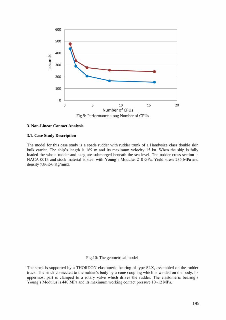
195
Fig.9: Performance along Number of CPUs
3. Non-Linear Contact Analysis
3.1. Case Study Description
The model for this case study is a spade rudder with rudder trunk of a Handysize class double skin
bulk carrier. The ship’s length is 169 m and its maximum velocity 15 kn. When the ship is fully
loaded the whole rudder and skeg are submerged beneath the sea level. The rudder cross section is
NACA 0015 and stock material is steel with Young’s Modulus 210 GPa, Yield stress 235 MPa and
density 7.86E-6 Kg/mm3.
Fig.10: The geometrical model
The stock is supported by a THORDON elastomeric bearing of type SLX, assembled on the rudder
truck. The stock connected to the rudder’s body by a cone coupling which is welded on the body. Its
uppermost part is clamped to a rotary valve which drives the rudder. The elastomeric bearing’s
Young’s Modulus is 440 MPa and its maximum working contact pressure 10~12 MPa.
0 5 10 15 20
0
100
200
300
400
500
600
Number of CPUs
seco
nd
sStandart Solver
EPILYSIS 17.0.3.
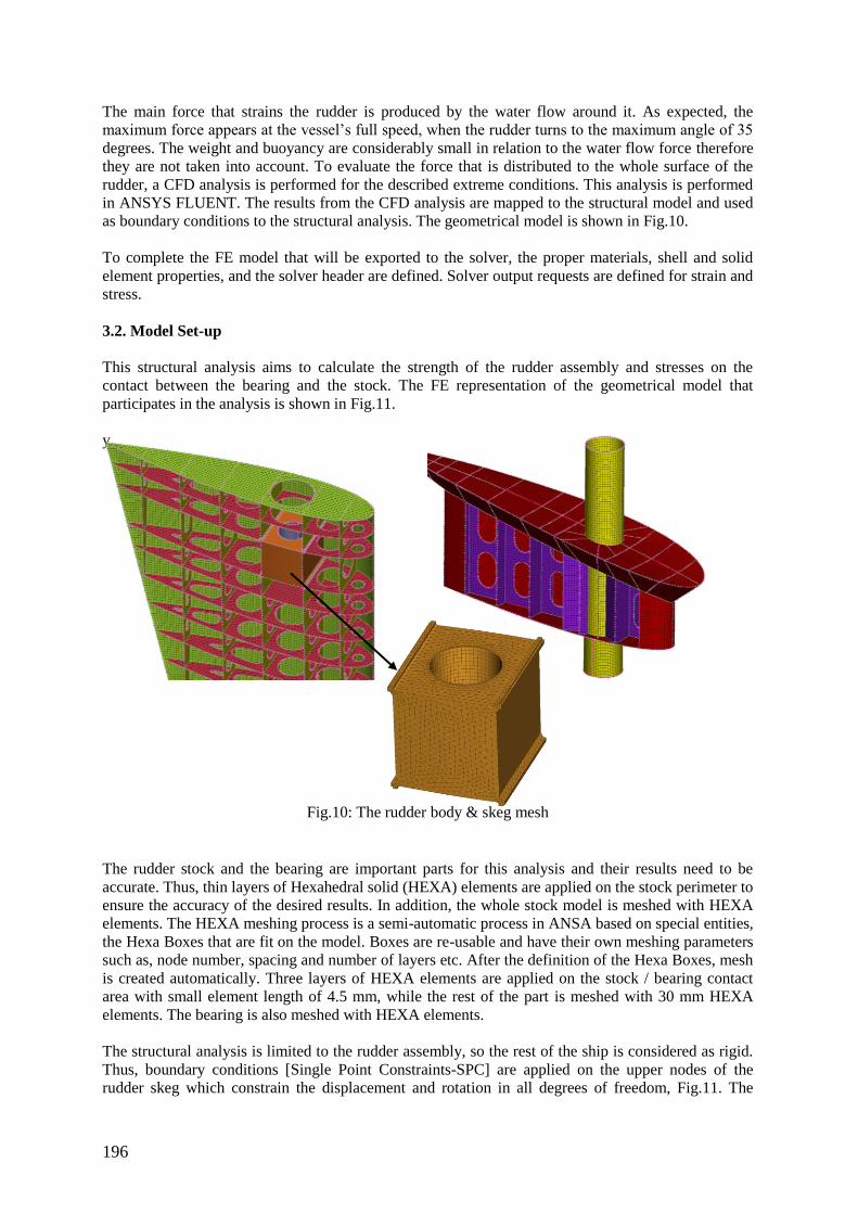
196
The main force that strains the rudder is produced by the water flow around it. As expected, the
maximum force appears at the vessel’s full speed, when the rudder turns to the maximum angle of 35
degrees. The weight and buoyancy are considerably small in relation to the water flow force therefore
they are not taken into account. To evaluate the force that is distributed to the whole surface of the
rudder, a CFD analysis is performed for the described extreme conditions. This analysis is performed
in ANSYS FLUENT. The results from the CFD analysis are mapped to the structural model and used
as boundary conditions to the structural analysis. The geometrical model is shown in Fig.10.
To complete the FE model that will be exported to the solver, the proper materials, shell and solid
element properties, and the solver header are defined. Solver output requests are defined for strain and
stress.
3.2. Model Set-up
This structural analysis aims to calculate the strength of the rudder assembly and stresses on the
contact between the bearing and the stock. The FE representation of the geometrical model that
participates in the analysis is shown in Fig.11.
y
Fig.10: The rudder body & skeg mesh
The rudder stock and the bearing are important parts for this analysis and their results need to be
accurate. Thus, thin layers of Hexahedral solid (HEXA) elements are applied on the stock perimeter to
ensure the accuracy of the desired results. In addition, the whole stock model is meshed with HEXA
elements. The HEXA meshing process is a semi-automatic process in ANSA based on special entities,
the Hexa Boxes that are fit on the model. Boxes are re-usable and have their own meshing parameters
such as, node number, spacing and number of layers etc. After the definition of the Hexa Boxes, mesh
is created automatically. Three layers of HEXA elements are applied on the stock / bearing contact
area with small element length of 4.5 mm, while the rest of the part is meshed with 30 mm HEXA
elements. The bearing is also meshed with HEXA elements.
The structural analysis is limited to the rudder assembly, so the rest of the ship is considered as rigid.
Thus, boundary conditions [Single Point Constraints-SPC] are applied on the upper nodes of the
rudder skeg which constrain the displacement and rotation in all degrees of freedom, Fig.11. The
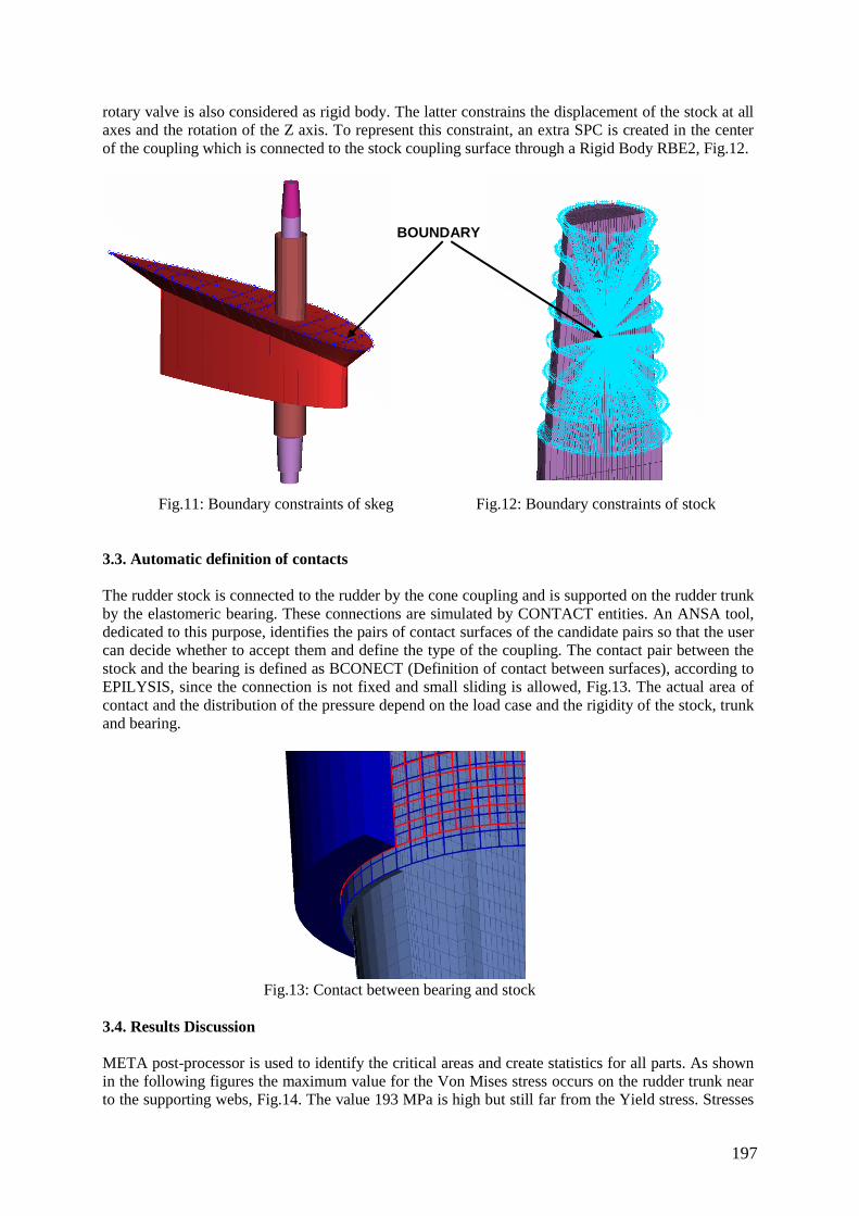
197
rotary valve is also considered as rigid body. The latter constrains the displacement of the stock at all
axes and the rotation of the Z axis. To represent this constraint, an extra SPC is created in the center
of the coupling which is connected to the stock coupling surface through a Rigid Body RBE2, Fig.12.
Fig.11: Boundary constraints of skeg Fig.12: Boundary constraints of stock
3.3. Automatic definition of contacts
The rudder stock is connected to the rudder by the cone coupling and is supported on the rudder trunk
by the elastomeric bearing. These connections are simulated by CONTACT entities. An ANSA tool,
dedicated to this purpose, identifies the pairs of contact surfaces of the candidate pairs so that the user
can decide whether to accept them and define the type of the coupling. The contact pair between the
stock and the bearing is defined as BCONECT (Definition of contact between surfaces), according to
EPILYSIS, since the connection is not fixed and small sliding is allowed, Fig.13. The actual area of
contact and the distribution of the pressure depend on the load case and the rigidity of the stock, trunk
and bearing.
Fig.13: Contact between bearing and stock
3.4. Results Discussion
META post-processor is used to identify the critical areas and create statistics for all parts. As shown
in the following figures the maximum value for the Von Mises stress occurs on the rudder trunk near
to the supporting webs, Fig.14. The value 193 MPa is high but still far from the Yield stress. Stresses
BOUNDARY
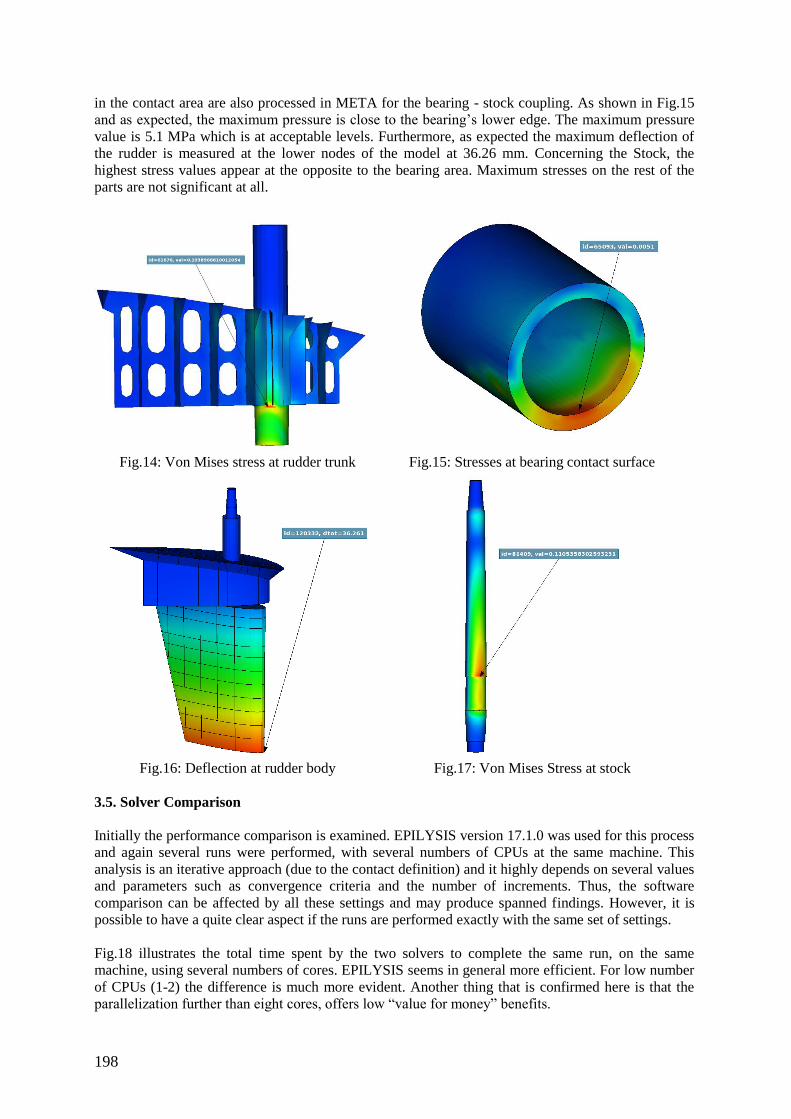
198
in the contact area are also processed in META for the bearing - stock coupling. As shown in Fig.15
and as expected, the maximum pressure is close to the bearing’s lower edge. The maximum pressure
value is 5.1 MPa which is at acceptable levels. Furthermore, as expected the maximum deflection of
the rudder is measured at the lower nodes of the model at 36.26 mm. Concerning the Stock, the
highest stress values appear at the opposite to the bearing area. Maximum stresses on the rest of the
parts are not significant at all.
Fig.14: Von Mises stress at rudder trunk Fig.15: Stresses at bearing contact surface
Fig.16: Deflection at rudder body Fig.17: Von Mises Stress at stock
3.5. Solver Comparison
Initially the performance comparison is examined. EPILYSIS version 17.1.0 was used for this process
and again several runs were performed, with several numbers of CPUs at the same machine. This
analysis is an iterative approach (due to the contact definition) and it highly depends on several values
and parameters such as convergence criteria and the number of increments. Thus, the software
comparison can be affected by all these settings and may produce spanned findings. However, it is
possible to have a quite clear aspect if the runs are performed exactly with the same set of settings.
Fig.18 illustrates the total time spent by the two solvers to complete the same run, on the same
machine, using several numbers of cores. EPILYSIS seems in general more efficient. For low number
of CPUs (1-2) the difference is much more evident. Another thing that is confirmed here is that the
parallelization further than eight cores, offers low “value for money” benefits.
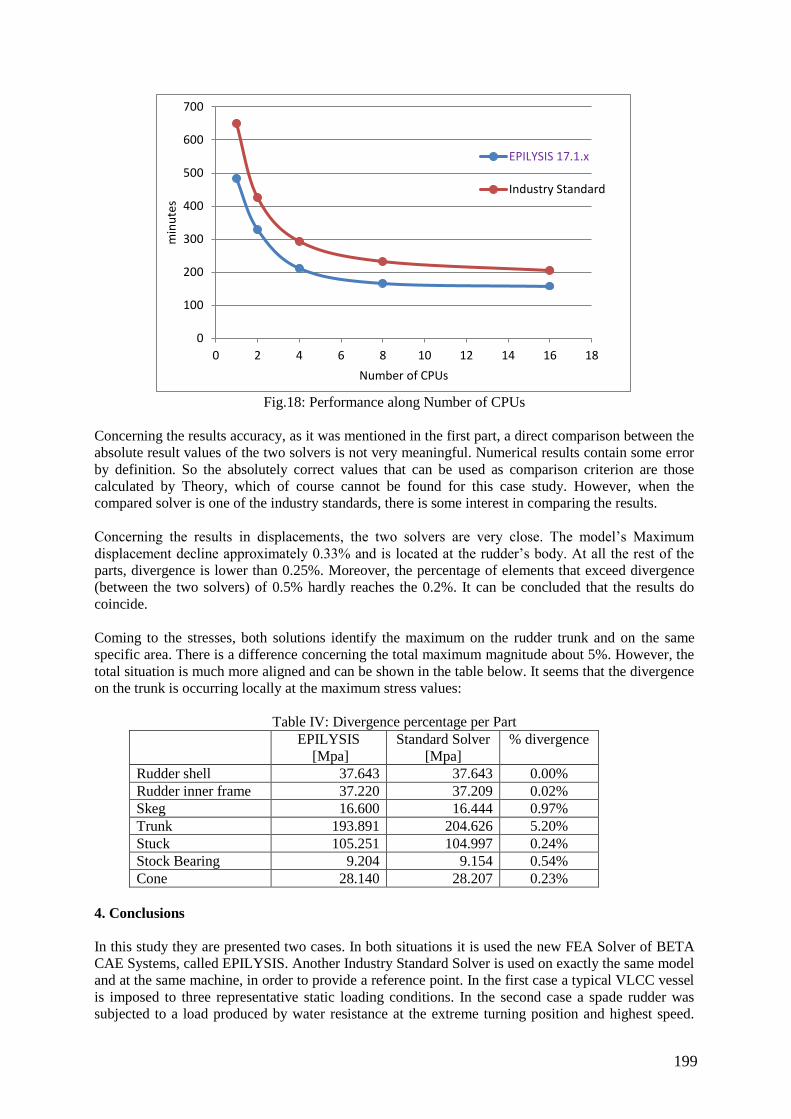
199
Fig.18: Performance along Number of CPUs
Concerning the results accuracy, as it was mentioned in the first part, a direct comparison between the
absolute result values of the two solvers is not very meaningful. Numerical results contain some error
by definition. So the absolutely correct values that can be used as comparison criterion are those
calculated by Theory, which of course cannot be found for this case study. However, when the
compared solver is one of the industry standards, there is some interest in comparing the results.
Concerning the results in displacements, the two solvers are very close. The model’s Maximum
displacement decline approximately 0.33% and is located at the rudder’s body. At all the rest of the
parts, divergence is lower than 0.25%. Moreover, the percentage of elements that exceed divergence
(between the two solvers) of 0.5% hardly reaches the 0.2%. It can be concluded that the results do
coincide.
Coming to the stresses, both solutions identify the maximum on the rudder trunk and on the same
specific area. There is a difference concerning the total maximum magnitude about 5%. However, the
total situation is much more aligned and can be shown in the table below. It seems that the divergence
on the trunk is occurring locally at the maximum stress values:
Table IV: Divergence percentage per Part
EPILYSIS
[Mpa]
Standard Solver
[Mpa]
% divergence
Rudder shell 37.643 37.643 0.00%
Rudder inner frame 37.220 37.209 0.02%
Skeg 16.600 16.444 0.97%
Trunk 193.891 204.626 5.20%
Stuck 105.251 104.997 0.24%
Stock Bearing 9.204 9.154 0.54%
Cone 28.140 28.207 0.23%
4. Conclusions
In this study they are presented two cases. In both situations it is used the new FEA Solver of BETA
CAE Systems, called EPILYSIS. Another Industry Standard Solver is used on exactly the same model
and at the same machine, in order to provide a reference point. In the first case a typical VLCC vessel
is imposed to three representative static loading conditions. In the second case a spade rudder was
subjected to a load produced by water resistance at the extreme turning position and highest speed.
0
100
200
300
400
500
600
700
0 2 4 6 8 10 12 14 16 18
min
ute
s
Number of CPUs
EPILYSIS 17.1.x
Industry Standard
200
What makes this analysis more special is the contact definition between the rudder stuck and a
bearing made of Thordon material. For the analysis set up of such big and detailed models the use of
sophisticated tools that automate and facilitate the simulation process (like Batch Meshing, Results
Mapper and Contact Wizard) turns to be a matter of great importance. ANSA and μETA pre- and
post- processors have been used successfully for the definition of CFD and structural analysis.
Analysis results, generated by the two solvers, referring mainly to the Stresses and Deformations, are
presented and analyzed by META post-processor and compared to each other. In terms of
Deformation there is absolute coincidence between the two Solvers. The stress results are also more
or less aligned for Quadratic elements while for Triangular elements there is much higher divergence.
It is also presented a performance comparison between the two Solvers, for both case studies. Even
though in the second case the performance strongly depends on the analyses’ characteristic values like
convergence criteria, mesh density, material characteristic values etc., in general it seems that
EPILYSIS solver reaches quite high performance standards for any number of CPUs. Additionally,
the parallelization of EPILYSIS seems quite more efficient especially in the first Linear Static case
study.
References
DAHLER G.; BRODIN, E.; VARTDAL, B.J.; CHISTENSEN, H.W.; JAKOBSEN, S.B.; OK, Y.K.;
HEO, J.H.; PARK, K.R. (2004), A study on flexible hulls, flexible engines, crank shaft deflections and
engine bearing loads for VLCC propulsion machinery, CIMAC Congress, Kyoto
DEVANNEY, J.; KENNEDY, M. (2003), The down ratchet and the deterioration of tanker new-
building standards, Center for Tankship Excellence
RAWSON, K.J.; TUPPER, E.C. (1997), Basic Ship Theory, Elsevier, pp.555-563
GL RULES and GUIDELINES (2011), Rudder and Manoeuvring Arrangement, Germanischer Lloyd,
Hamburg
GL RULES and GUIDELINES (2011), Steel Plates, Strips, Sections and Bars, Germanischer Lloyd,
Hamburg
201
Analysis of General Arrangements Created by the TU Delft
Packing Approach
Mark J. Roth, Delft University of Technology, [email protected]
Koen Droste, Delft University of Technology, [email protected]
Austin A. Kana, Delft University of Technology, [email protected]
Abstract
This paper applies network theory to understand the physical relationships in the general arrangements
generated by TU Delft packing approach. The generated arrangements are converted into weighted
graph networks. The authors have developed a new scoring metric using this network and have applied
this to quantitatively assess qualitative properties of the different arrangements, enabling direct
comparison between concept designs. Finding and understanding these specific physical properties of
the arrangements should lead to improved design space exploration of layout features of the designs
generated by the TU Delft packing approach.
1. Introduction
During the conceptual ship design phase, problems concerning the overall composition of the vessel
can be directly related to the arrangement of systems, compartments and components. Historically, these
arrangements have been compiled into detailed drawings of the vessels where the naval architect has
decided on the arrangement and connections between these compartments manually. These decisions
have been traditionally built upon design rules and the experience of the designer. Furthermore, the
designer can usually fall back to comparison vessels to have a decent understanding of the architectural
problems and to have a starting point for the current design. A problem occurs when new vessel classes
are being designed or in situations where a lack of experience is encountered, Andrews (1998).
Currently, projects are being undertaken for general arrangement optimization in an earlier stage of the
design process, such as the packing approach, Van Oers (2011) and Duchateau (2016), the Intelligent
Ship Arrangement platform, Parsons et al. (2008), and the Design Building Block approach, Andrews
and Dicks (1997). These projects all make the use of computing power to generate a concept exploration
space. By creating numerous design concepts, a solution space is created where the designer is able to
explore trade-offs and eventually select multiple concepts for further examination. This paper is
focusing specifically on the layouts generated by packing.
In the packing approach, the actual internal layout of the generated designs is mostly ignored, because
the overall quality of the generated arrangement has been considered to be fairly poor. Manual redesign
of the most promising design is deemed necessary to create a complete functional layout in later stages
of design. This paper seeks to create more insight and understanding into these generated arrangements,
facilitating the opportunity to transfer the generated designs into later design phases. To do this, an
assessment of physical locations and relationships as well as fundamental interactions between elements
of systems in the designs is necessary. One might be able to improve the arrangements out of the packing
algorithm by increasing the number of constraints in the model, but this will greatly limit the number
of feasible designs and so the explored design space. By allowing the model to have more freedom, the
design space should lead to more diversity in the set of designs. Developing a method that would be
able to directly compare the generated arrangements without ove rconstraining and the model would be
beneficial.
1.1 Introduction to the TU Delft Packing approach
The TU Delft packing approach is a method which uses a parametric model called the Ship Synthesis
Model (SSM) composed of ‘system objects’ describing the spaces and systems of the design. A packing
algorithm generates ship designs based on this SSM and calculates their performances. These
202
performances such as speed, weight or costs can be used to quantify how good a design is in terms of
those specific metrics. These performances are fed to a genetic search algorithm which uses them to
explore the design and performance space belonging to the SSM. Specific details of the SSM can be
found in van Oers (2011). This highly automated search process enables fast and extensive exploration
of the design space in an early design stage, Wagner (2009), Wagner et al. (2010), Zandstra (2014).
Duchateau (2016) extended the SSM method to the Interactive Evolutionary Concept Exploration
Method (IECEM) which allowed for a more interactive exploration of the design space by including
the designer in a feedback loop to the search process. Each of the designs exists of a set of performance
metrics, dimensions and a description of the layout of the design. Until recently the results were mainly
used to find the approximate dimensions of a vessel and to study the feasibility of a set of design
requirements. This work will present a method that aims to understand the layout features of designs.
The packing design is based on a parametric 2.5D ship-design, Van Oers and Hopman (2012). The 2.5D
design describes a set of multiple 2D configurations which include a centreline, a port and a starboard
slice. Objects in the vessels are placed mostly in the side-view, or x-z plane, of the design. The 2.5D
approach introduces a variable width for objects and an available width for every position in the side-
view of the design. This enables the packing-approach to fill a 2.5D space, instead of the necessity to
describe the entire 3D space. This 2.5D approach is introduced to speed up the packing algorithm, where
improvements in speed of a factor up to seven have been attainable, Van Oers and Hopman (2012).
This enables the packing algorithm to explore a wider design space by using a simpler model.
This study uses a design set generated for a small exploration cruise ship. The design set originates from
Droste (2016). As is discussed in detail in the following case study, the current set of designs showed
several flaws in the arrangement and raised the question of whether it would be possible to improve our
understanding of the relations between the systems and spaces within the packing approach.
1.2 Analysis of General Arrangements and Rationale Capturing
One of the biggest problems in generating general arrangements, is the analysis of the generated
arrangement, Hope (1981). When analysing multiple arrangements by hand, one might find a number
of mistakes or aberrations in the physical allocation in the arrangement that are either unhandy or non-
compliant to design prospects. For an experienced designer, it should be quite easy to disclose these
issues in the design by hand; however, integrating this into computer interactive methods might be quite
hard. Furthermore, analysing thousands of designs as generated by the packing approach is also
difficult. There may several conflicting interests within the design specifications that algorithms might
not be able to analyse in a coherent way. An automated way of general arrangement analysis would
need a scoring metric for the algorithm to evaluate the arrangement and to allow direct comparison. The
use of a comparative score improves the solutions in a spatial or topological model, as demonstrated by
Gillespie et al. (2013). They showed that analysis of a graph model of the design by partitioning and
spatial community preferences can give guidance to the arrangement process of the allocation
algorithms. To create a comparative score, quantitative assessment of qualitative properties of the
designs is necessary.
In order to do this quantitative assessment, one needs to know what qualitative properties are desired in
the design. Deciding what designs are either “good” or “bad” depends on personal preference and will
most certainly lead to different design decisions between different designers. Since there is no singular
“wrong” or “right” solution, but more commonly a “better” or “worse” approach to the problem, it is
very hard to describe the rationale behind certain decisions. DeNucci (2012) introduced a method of
capturing design rationale for complex ship general arrangement design. His method allows multiple
naval architects to evaluate both desirable and undesirable features presented in one or multiple designs,
accompanied by the underlying rationale. For instance, a generator room should not be placed adjacent
to accommodation space to minimise noise levels in accommodation rooms. Using DeNucci’s method
and rationale database as quality metrics, one can start to define what is the motivation between certain
design decisions and start to analyse which of these decisions are better or worse for the total design.
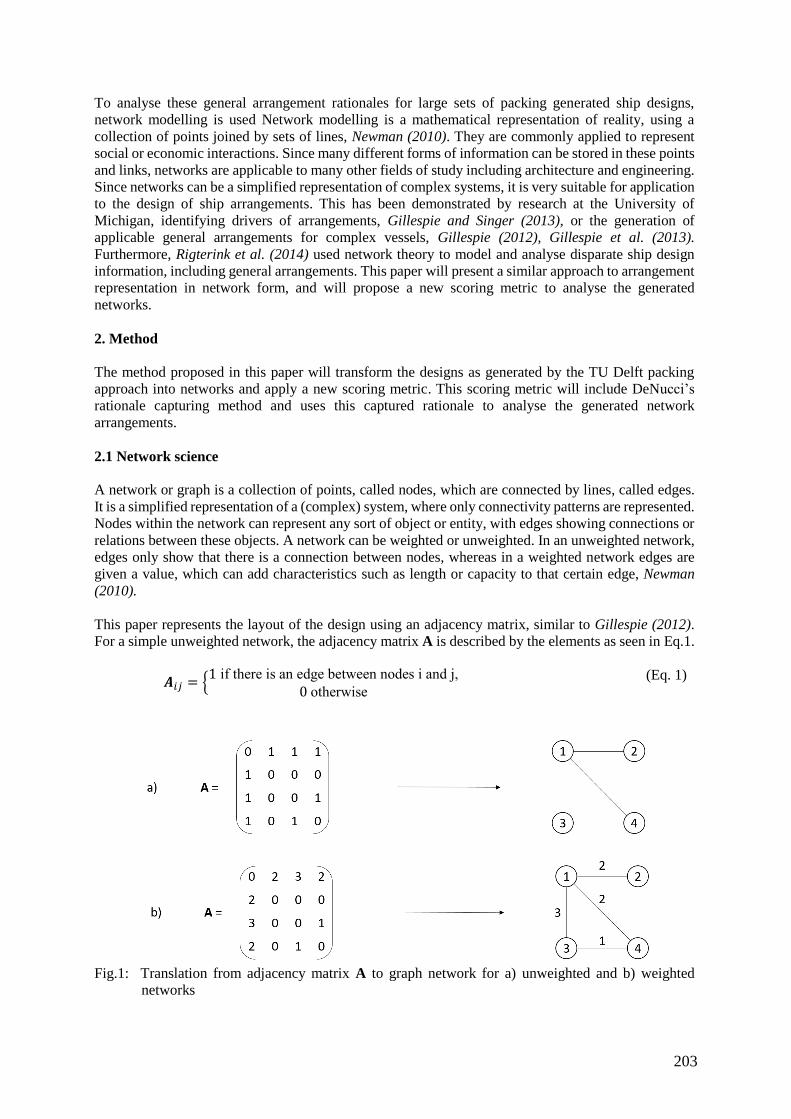
203
To analyse these general arrangement rationales for large sets of packing generated ship designs,
network modelling is used Network modelling is a mathematical representation of reality, using a
collection of points joined by sets of lines, Newman (2010). They are commonly applied to represent
social or economic interactions. Since many different forms of information can be stored in these points
and links, networks are applicable to many other fields of study including architecture and engineering.
Since networks can be a simplified representation of complex systems, it is very suitable for application
to the design of ship arrangements. This has been demonstrated by research at the University of
Michigan, identifying drivers of arrangements, Gillespie and Singer (2013), or the generation of
applicable general arrangements for complex vessels, Gillespie (2012), Gillespie et al. (2013).
Furthermore, Rigterink et al. (2014) used network theory to model and analyse disparate ship design
information, including general arrangements. This paper will present a similar approach to arrangement
representation in network form, and will propose a new scoring metric to analyse the generated
networks.
2. Method
The method proposed in this paper will transform the designs as generated by the TU Delft packing
approach into networks and apply a new scoring metric. This scoring metric will include DeNucci’s
rationale capturing method and uses this captured rationale to analyse the generated network
arrangements.
2.1 Network science
A network or graph is a collection of points, called nodes, which are connected by lines, called edges.
It is a simplified representation of a (complex) system, where only connectivity patterns are represented.
Nodes within the network can represent any sort of object or entity, with edges showing connections or
relations between these objects. A network can be weighted or unweighted. In an unweighted network,
edges only show that there is a connection between nodes, whereas in a weighted network edges are
given a value, which can add characteristics such as length or capacity to that certain edge, Newman
(2010).
This paper represents the layout of the design using an adjacency matrix, similar to Gillespie (2012).
For a simple unweighted network, the adjacency matrix A is described by the elements as seen in Eq.1.
𝑨𝑖𝑗 = {1 if there is an edge between nodes i and j,
0 otherwise
(Eq. 1)
Fig.1: Translation from adjacency matrix A to graph network for a) unweighted and b) weighted
networks
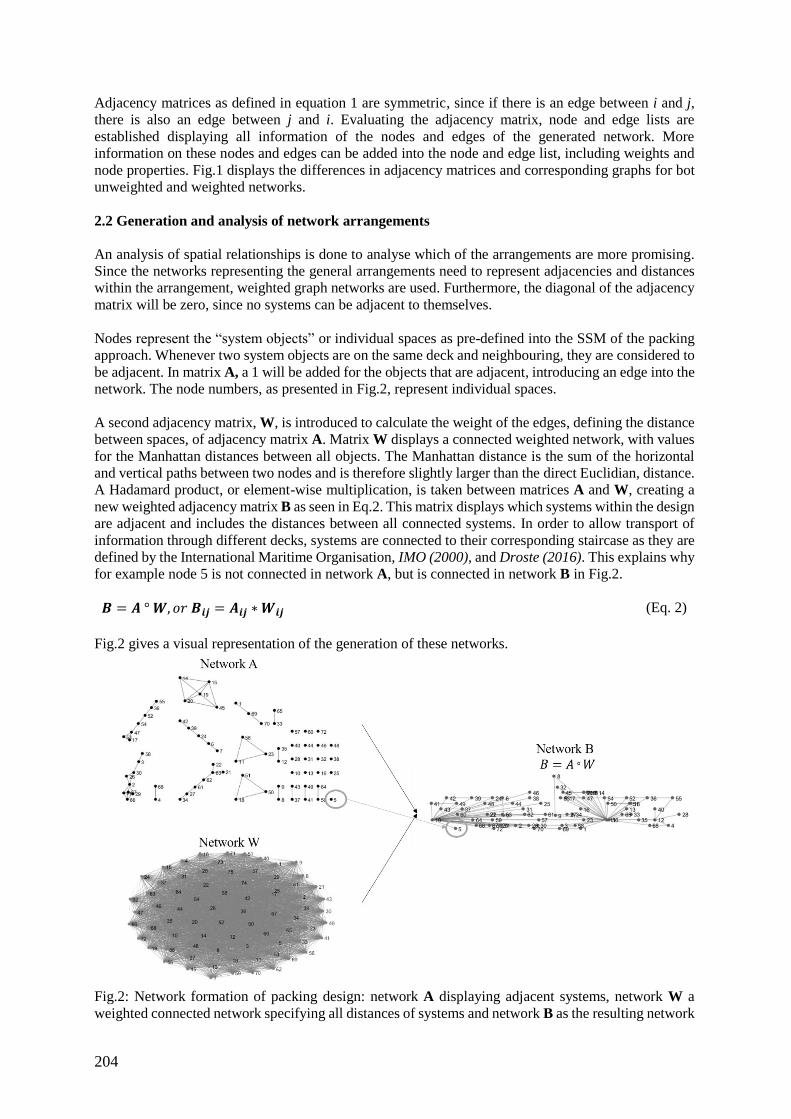
204
Adjacency matrices as defined in equation 1 are symmetric, since if there is an edge between i and j,
there is also an edge between j and i. Evaluating the adjacency matrix, node and edge lists are
established displaying all information of the nodes and edges of the generated network. More
information on these nodes and edges can be added into the node and edge list, including weights and
node properties. Fig.1 displays the differences in adjacency matrices and corresponding graphs for bot
unweighted and weighted networks.
2.2 Generation and analysis of network arrangements
An analysis of spatial relationships is done to analyse which of the arrangements are more promising.
Since the networks representing the general arrangements need to represent adjacencies and distances
within the arrangement, weighted graph networks are used. Furthermore, the diagonal of the adjacency
matrix will be zero, since no systems can be adjacent to themselves.
Nodes represent the “system objects” or individual spaces as pre-defined into the SSM of the packing
approach. Whenever two system objects are on the same deck and neighbouring, they are considered to
be adjacent. In matrix A, a 1 will be added for the objects that are adjacent, introducing an edge into the
network. The node numbers, as presented in Fig.2, represent individual spaces.
A second adjacency matrix, W, is introduced to calculate the weight of the edges, defining the distance
between spaces, of adjacency matrix A. Matrix W displays a connected weighted network, with values
for the Manhattan distances between all objects. The Manhattan distance is the sum of the horizontal
and vertical paths between two nodes and is therefore slightly larger than the direct Euclidian, distance.
A Hadamard product, or element-wise multiplication, is taken between matrices A and W, creating a
new weighted adjacency matrix B as seen in Eq.2. This matrix displays which systems within the design
are adjacent and includes the distances between all connected systems. In order to allow transport of
information through different decks, systems are connected to their corresponding staircase as they are
defined by the International Maritime Organisation, IMO (2000), and Droste (2016). This explains why
for example node 5 is not connected in network A, but is connected in network B in Fig.2.
𝑩 = 𝑨 ° 𝑾, 𝑜𝑟 𝑩𝒊𝒋 = 𝑨𝒊𝒋 ∗ 𝑾𝒊𝒋 (Eq. 2)
Fig.2 gives a visual representation of the generation of these networks.
Fig.2: Network formation of packing design: network A displaying adjacent systems, network W a
weighted connected network specifying all distances of systems and network B as the resulting network
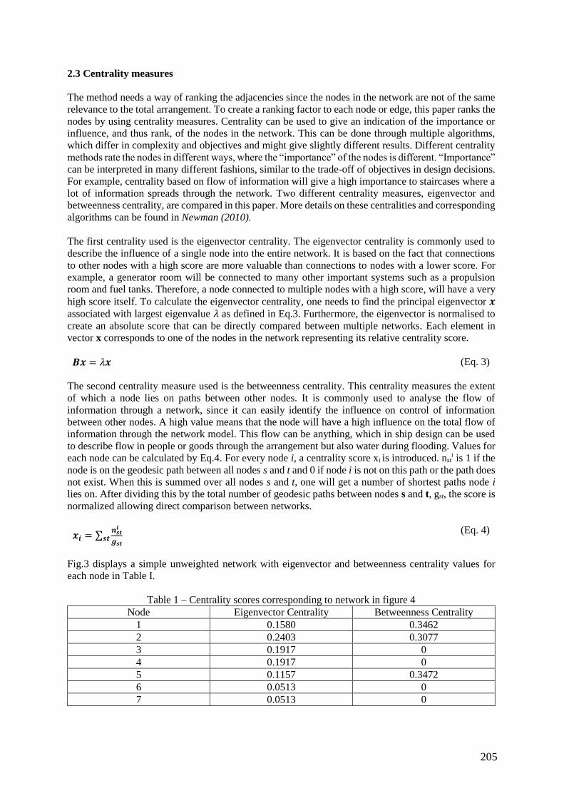
205
2.3 Centrality measures
The method needs a way of ranking the adjacencies since the nodes in the network are not of the same
relevance to the total arrangement. To create a ranking factor to each node or edge, this paper ranks the
nodes by using centrality measures. Centrality can be used to give an indication of the importance or
influence, and thus rank, of the nodes in the network. This can be done through multiple algorithms,
which differ in complexity and objectives and might give slightly different results. Different centrality
methods rate the nodes in different ways, where the “importance” of the nodes is different. “Importance”
can be interpreted in many different fashions, similar to the trade-off of objectives in design decisions.
For example, centrality based on flow of information will give a high importance to staircases where a
lot of information spreads through the network. Two different centrality measures, eigenvector and
betweenness centrality, are compared in this paper. More details on these centralities and corresponding
algorithms can be found in Newman (2010).
The first centrality used is the eigenvector centrality. The eigenvector centrality is commonly used to
describe the influence of a single node into the entire network. It is based on the fact that connections
to other nodes with a high score are more valuable than connections to nodes with a lower score. For
example, a generator room will be connected to many other important systems such as a propulsion
room and fuel tanks. Therefore, a node connected to multiple nodes with a high score, will have a very
high score itself. To calculate the eigenvector centrality, one needs to find the principal eigenvector 𝒙
associated with largest eigenvalue 𝜆 as defined in Eq.3. Furthermore, the eigenvector is normalised to
create an absolute score that can be directly compared between multiple networks. Each element in
vector x corresponds to one of the nodes in the network representing its relative centrality score.
𝑩𝒙 = 𝜆𝒙 (Eq. 3)
The second centrality measure used is the betweenness centrality. This centrality measures the extent
of which a node lies on paths between other nodes. It is commonly used to analyse the flow of
information through a network, since it can easily identify the influence on control of information
between other nodes. A high value means that the node will have a high influence on the total flow of
information through the network model. This flow can be anything, which in ship design can be used
to describe flow in people or goods through the arrangement but also water during flooding. Values for
each node can be calculated by Eq.4. For every node i, a centrality score xi is introduced. nsti is 1 if the
node is on the geodesic path between all nodes s and t and 0 if node i is not on this path or the path does
not exist. When this is summed over all nodes s and t, one will get a number of shortest paths node i
lies on. After dividing this by the total number of geodesic paths between nodes s and t, gst, the score is
normalized allowing direct comparison between networks.
𝒙𝒊 = ∑𝒏𝒔𝒕
𝒊
𝒈𝒔𝒕𝒔𝒕
(Eq. 4)
Fig.3 displays a simple unweighted network with eigenvector and betweenness centrality values for
each node in Table I.
Table 1 – Centrality scores corresponding to network in figure 4
Node Eigenvector Centrality Betweenness Centrality
1 0.1580 0.3462
2 0.2403 0.3077
3 0.1917 0
4 0.1917 0
5 0.1157 0.3472
6 0.0513 0
7 0.0513 0
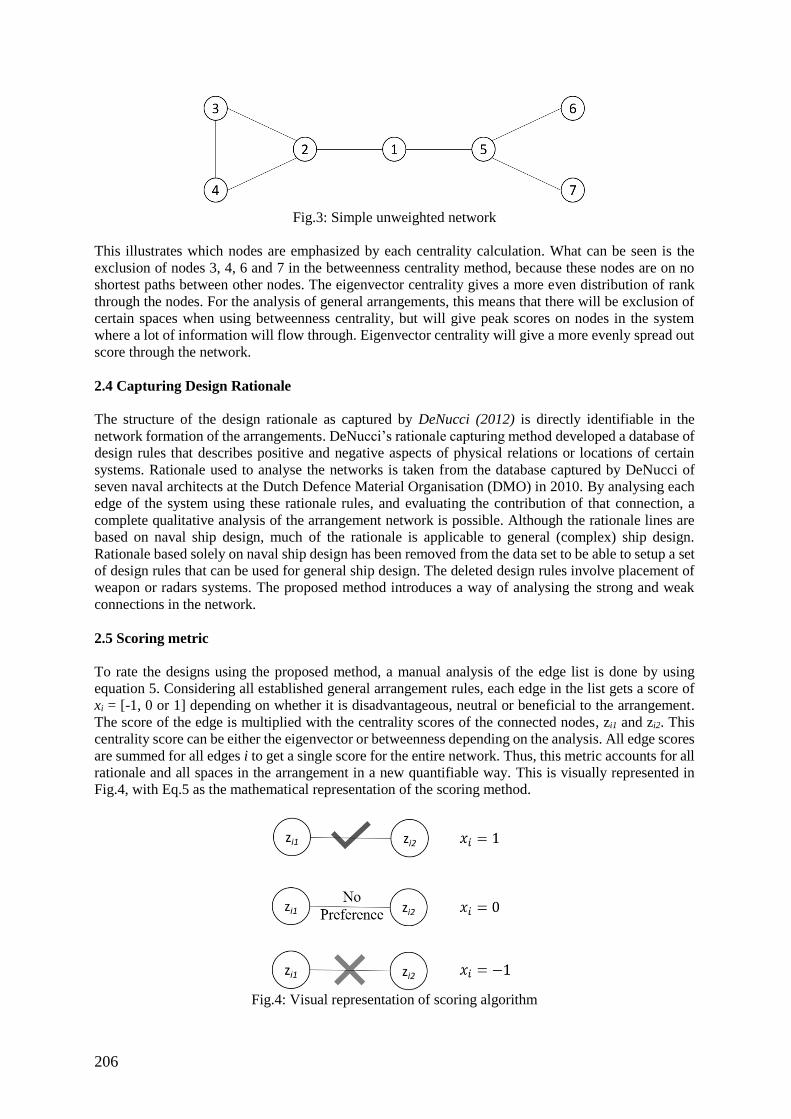
206
Fig.3: Simple unweighted network
This illustrates which nodes are emphasized by each centrality calculation. What can be seen is the
exclusion of nodes 3, 4, 6 and 7 in the betweenness centrality method, because these nodes are on no
shortest paths between other nodes. The eigenvector centrality gives a more even distribution of rank
through the nodes. For the analysis of general arrangements, this means that there will be exclusion of
certain spaces when using betweenness centrality, but will give peak scores on nodes in the system
where a lot of information will flow through. Eigenvector centrality will give a more evenly spread out
score through the network.
2.4 Capturing Design Rationale
The structure of the design rationale as captured by DeNucci (2012) is directly identifiable in the
network formation of the arrangements. DeNucci’s rationale capturing method developed a database of
design rules that describes positive and negative aspects of physical relations or locations of certain
systems. Rationale used to analyse the networks is taken from the database captured by DeNucci of
seven naval architects at the Dutch Defence Material Organisation (DMO) in 2010. By analysing each
edge of the system using these rationale rules, and evaluating the contribution of that connection, a
complete qualitative analysis of the arrangement network is possible. Although the rationale lines are
based on naval ship design, much of the rationale is applicable to general (complex) ship design.
Rationale based solely on naval ship design has been removed from the data set to be able to setup a set
of design rules that can be used for general ship design. The deleted design rules involve placement of
weapon or radars systems. The proposed method introduces a way of analysing the strong and weak
connections in the network.
2.5 Scoring metric
To rate the designs using the proposed method, a manual analysis of the edge list is done by using
equation 5. Considering all established general arrangement rules, each edge in the list gets a score of
xi = [-1, 0 or 1] depending on whether it is disadvantageous, neutral or beneficial to the arrangement.
The score of the edge is multiplied with the centrality scores of the connected nodes, zi1 and zi2. This
centrality score can be either the eigenvector or betweenness depending on the analysis. All edge scores
are summed for all edges i to get a single score for the entire network. Thus, this metric accounts for all
rationale and all spaces in the arrangement in a new quantifiable way. This is visually represented in
Fig.4, with Eq.5 as the mathematical representation of the scoring method.
Fig.4: Visual representation of scoring algorithm
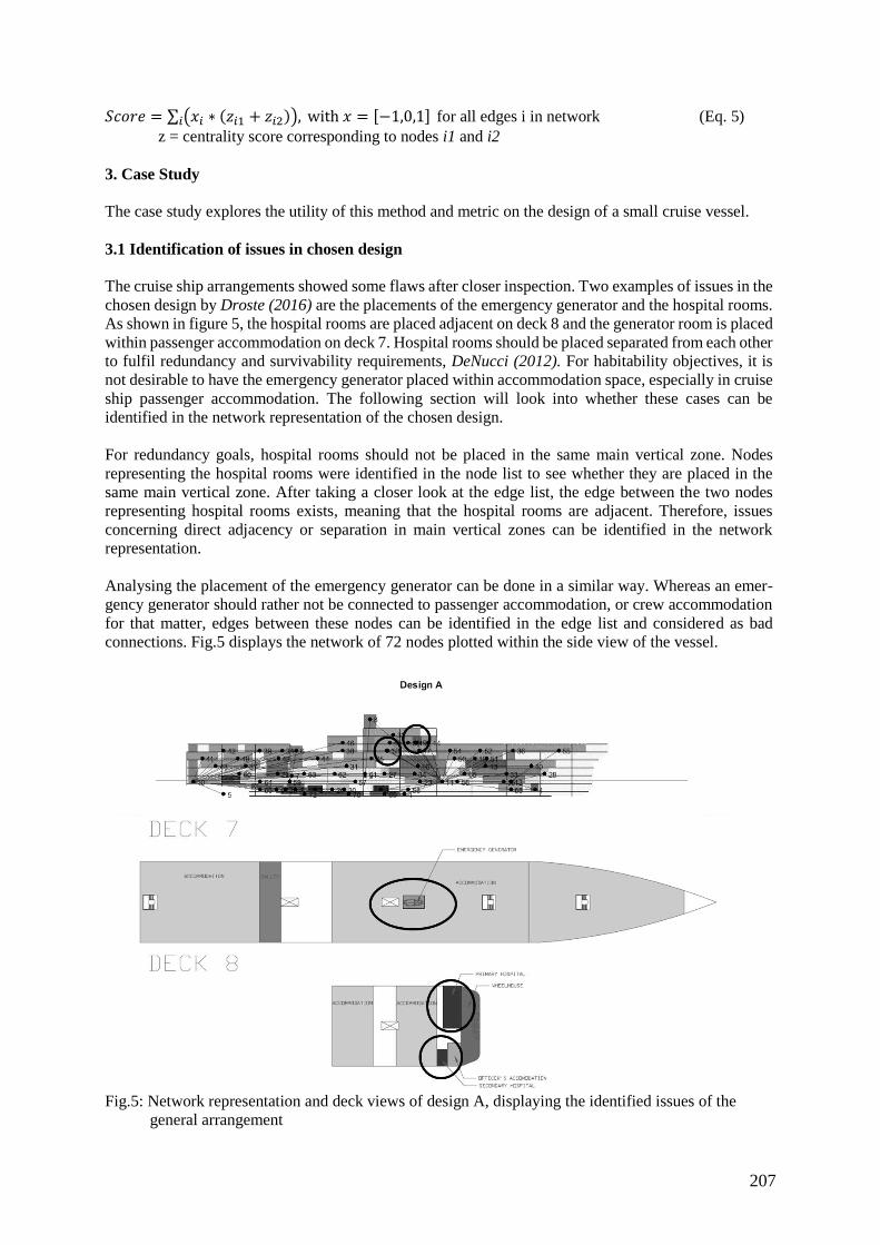
207
𝑆𝑐𝑜𝑟𝑒 = ∑ (𝑥𝑖 ∗ (𝑧𝑖1 + 𝑧𝑖2)), with 𝑥 = [−1,0,1]𝑖 for all edges i in network (Eq. 5)
z = centrality score corresponding to nodes i1 and i2
3. Case Study
The case study explores the utility of this method and metric on the design of a small cruise vessel.
3.1 Identification of issues in chosen design
The cruise ship arrangements showed some flaws after closer inspection. Two examples of issues in the
chosen design by Droste (2016) are the placements of the emergency generator and the hospital rooms.
As shown in figure 5, the hospital rooms are placed adjacent on deck 8 and the generator room is placed
within passenger accommodation on deck 7. Hospital rooms should be placed separated from each other
to fulfil redundancy and survivability requirements, DeNucci (2012). For habitability objectives, it is
not desirable to have the emergency generator placed within accommodation space, especially in cruise
ship passenger accommodation. The following section will look into whether these cases can be
identified in the network representation of the chosen design.
For redundancy goals, hospital rooms should not be placed in the same main vertical zone. Nodes
representing the hospital rooms were identified in the node list to see whether they are placed in the
same main vertical zone. After taking a closer look at the edge list, the edge between the two nodes
representing hospital rooms exists, meaning that the hospital rooms are adjacent. Therefore, issues
concerning direct adjacency or separation in main vertical zones can be identified in the network
representation.
Analysing the placement of the emergency generator can be done in a similar way. Whereas an emer-
gency generator should rather not be connected to passenger accommodation, or crew accommodation
for that matter, edges between these nodes can be identified in the edge list and considered as bad
connections. Fig.5 displays the network of 72 nodes plotted within the side view of the vessel.
Fig.5: Network representation and deck views of design A, displaying the identified issues of the
general arrangement
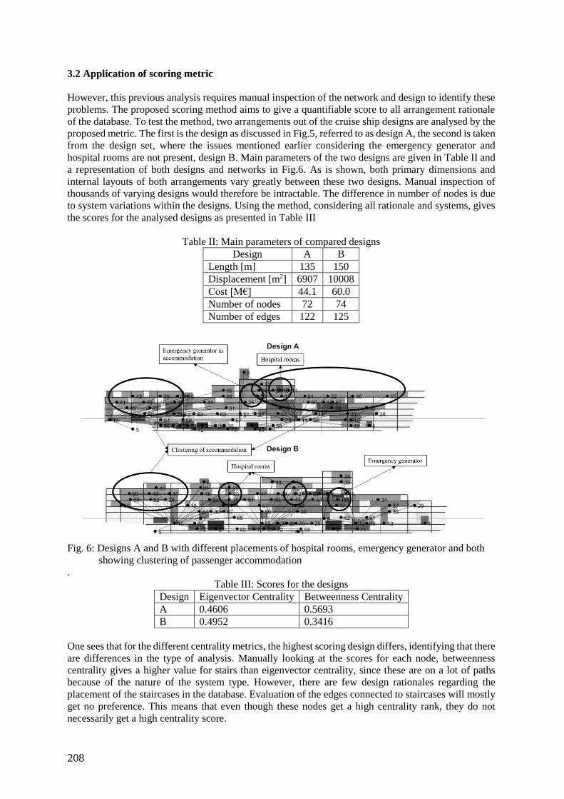
208
3.2 Application of scoring metric
However, this previous analysis requires manual inspection of the network and design to identify these
problems. The proposed scoring method aims to give a quantifiable score to all arrangement rationale
of the database. To test the method, two arrangements out of the cruise ship designs are analysed by the
proposed metric. The first is the design as discussed in Fig.5, referred to as design A, the second is taken
from the design set, where the issues mentioned earlier considering the emergency generator and
hospital rooms are not present, design B. Main parameters of the two designs are given in Table II and
a representation of both designs and networks in Fig.6. As is shown, both primary dimensions and
internal layouts of both arrangements vary greatly between these two designs. Manual inspection of
thousands of varying designs would therefore be intractable. The difference in number of nodes is due
to system variations within the designs. Using the method, considering all rationale and systems, gives
the scores for the analysed designs as presented in Table III
Table II: Main parameters of compared designs
Design A B
Length [m] 135 150
Displacement [m2] 6907 10008
Cost [M€] 44.1 60.0
Number of nodes 72 74
Number of edges 122 125
Fig. 6: Designs A and B with different placements of hospital rooms, emergency generator and both
showing clustering of passenger accommodation
.
Table III: Scores for the designs
Design Eigenvector Centrality Betweenness Centrality
A 0.4606 0.5693
B 0.4952 0.3416
One sees that for the different centrality metrics, the highest scoring design differs, identifying that there
are differences in the type of analysis. Manually looking at the scores for each node, betweenness
centrality gives a higher value for stairs than eigenvector centrality, since these are on a lot of paths
because of the nature of the system type. However, there are few design rationales regarding the
placement of the staircases in the database. Evaluation of the edges connected to staircases will mostly
get no preference. This means that even though these nodes get a high centrality rank, they do not
necessarily get a high centrality score.
209
Apparent is that passenger accommodation contributes a lot to the high score for design A. In the case
of betweenness centrality, analysis of the node list shows that accommodation accounts for 0.29 of the
total score. In design B, this value is only 0.11. This is likely due to accommodation systems being
more clustered in design A, as seen in Fig.6. A same trend can be found in crew accommodation,
although the difference is slightly smaller. This can be explained by the fact that there is less crew
accommodation than passenger accommodation present in the arrangements. Furthermore, design B has
two accommodation systems that are highly penalized by the betweenness centrality because of a
connection with a technical/auxiliary systems room. Looking at eigenvector centrality, the score for
accommodation placement is 0.16 for both designs. An overview of the breakdown of these scores can
be found in Table IV.
Other areas where design A scores better, especially on betweenness centrality, is the placement of the
generator rooms. As generator rooms are of high importance to the vessel, there are quite some rationale
rules based on the placement of generator rooms. Connections to the generator room are often regarded
as positive or negative instead of neutral and are therefore highly represented in the score.
The poor placement of the emergency generator room in design A does not get penalized by
betweenness centrality since it is not on any shortest paths, due to the transport through the
accommodation surrounding the generator. It is therefore not visible in the betweenness centrality score.
It is however penalized in the eigenvector centrality score, accounting for a subtraction of 0.01. This is
rather small when comparing to accommodation scores, which lies in the fact that it only involves one
node instead of twenty nodes in the case of passenger accommodation.
Because betweenness centrality can give a value of 0 for nodes on no shortest paths, the number of
evaluated nodes decreases. For design A, 30 nodes get a betweenness centrality of 0, for design B this
number is 38. This is about half of the total number of nodes, which is similar to the simple network in
Fig.3. Since these are nodes that are on the ends of paths, these are primarily propulsion rooms and
bridge or entertainment systems that are located on the ends of the vessel and are thus not reflected in
the betweenness centrality score.
Stating that design A is “better” than design B, depends on the designer’s view. Design B better
represents designer’s overall rationale as it pertains to the layout of the general arrangements, as is
shown by its eigenvector centrality score. However, if a specific designer is more interested in personnel
flow through staircases, design A would be preferred, according to betweenness centrality score. By
using this metric, one is now able to give a score to these properties of the general arrangements.
4. Discussion
The first question to be asked is whether quantitative assessment of qualitative properties of the
arrangement is possible. The answer to this is yes, using network analysis it is possible to give a score
to a general arrangement generated by the packing approach. In order to do this, general arrangement
design rationale has been applied, which can be captured in methods as described by DeNucci (2012).
This is an improvement in the current design decision process of the IECEM, as it now includes analysis
of interior design arrangement of the vessel. However, using a single score for the total analysis of the
design enables direct comparison, but makes traceability of high or low scores in different objectives
difficult without the use of sensitivity studies.
The second question is which of the compared centrality measures would be more promising.
Comparing eigenvector and betweenness centrality measures, eigenvector seems to be more applicable
for this type of arrangement analysis. This originates from the fact that it is commonly used as a
normalized rank and takes all nodes into account in a more similar value in comparison to the
betweenness centrality analysis. The betweenness centrality excludes nodes that are on no paths and
easily overrates certain nodes in the system that carry a lot of information, such as staircases.
Furthermore, the analysis is completely based on the user’s (in this case the authors’) interpretation of
the rationale database and implementation of the design rules. Overrating of nodes by betweenness
210
centrality does not seem to be a big problem, since nodes as staircases do not have a lot of beneficial
edges within the design rationale. It does however give a bigger penalty on poorly placed
accommodation due to the normalization of the betweenness centrality score. Betweenness centrality
analysis is applicable in other types of analysis, such as flow analysis in evacuation cases.
What makes concept design complicated, especially applied to complex ship design, is the fact that it
cannot directly be validated by existing ship design. Analysis is done in a preliminary ship design phase,
where there are still a lot of unknowns and uncertainties in the design and a lot of design decisions are
still to be taken. The new method allows the use of captured rationale and shows how certain decisions
score in the design trade-off.
5. Conclusion
The authors have developed a scoring metric, that is able to quantitatively identify qualitative properties
of designs generated by TU Delft packing approach or IECEM. By converting the designs into weighted
networks, a new representation of the packing generated designs is acquired. Using rationale captured
by DeNucci, edges in these networks are analysed and identified based on their influence on the
arrangement. This gives an overall score of the general arrangement of the packed design allowing the
designer to make decisions not merely on costs or primary parameters, but also take the interior design
of the vessel into account and allow direct comparison.
6. Recommendation for future work
The method proposes a beginning in the semi-automated analysis of the arrangements of packing
generated designs. Future work includes a higher level of understanding of the results of the scoring
metric. Understanding differences in scores between different networks should give more insight in
how this score can be used, for example as a filtering measure for lower quality arrangements. By
filtering, the designer would be able to improve awareness of the quality of the arrangement during
design decisions. The networks could be generated in different ways, implementing directed networks
or layered multiplex networking. It will be interesting to see if the method is also applicable to different
datasets of arrangements generated by the packing approach or other concept exploration methods.
Furthermore, the networks could be used together with a search tool algorithm as a filter to look for
those designs that either include or lack certain edges.
The biggest next step is the application of this method to an entire dataset. In order to do so, the design
rules need to be incorporated into the programming of the network generation. Being applied to the
entire dataset, one can use it as an extra objective function for Pareto optimization, or even as a
performance input in the genetic search algorithm in the packing approach. Furthermore, it can be used
to assess the quality of the layout and filter the dataset of poor quality arrangements.
References
ANDREWS, D.J. (1998), A comprehensive methodology for the design of ships (and other complex
systems), Proc. Royal Society: Mathematical, Physical and Engineering Sciences 454/1968, pp.187-211
ANDREWS, D.; DICKS, C. (1997) The building block design methodology applied to advanced naval
ship design, Int. Marine Design Conf., Newcastle, pp.3-19
DANIELS, A.; TAHMASBI, F.; SINGER, D.J. (2010) Intelligent ship arrangement passage variable
lattice network studies and results, Naval Engineers J. 122, pp.107-119
DENUCCI, T.W. (2012), Capturing Design: Improving conceptual ship design through the capture of
design rationale, PhD, Delft University of Technology, Delft
211
DROSTE, K. (2016), A new concept exploration method to support innovative cruise ship design, MSc
thesis, Delft University of Technology, Delft
DUCHATEAU, E.A.E. (2016), Interactive Evolutionary Concept Exploration in Preliminary Ship
Design, PhD Thesis, Delft University of Technology, Delft
GILLESPIE, J.W. (2012), A Network Science Approach to Understanding and Generating Ship
Arrangements in Early-stage Design, PhD Thesis, University of Michigan
GILLESPIE, J.W.; SINGER, D.J. (2013), Identifying drivers of general arrangements through the use
of network measures of centrality and hierarchy, Ocean Engineering 57, pp.230-239
GILLESPIE, J.W.; DANIELS A.S.; SINGER, D.J. (2013), Generating functional complex-based ship
arrangements using network partitioning and community preferences, Ocean Eng. 72, pp.107-115
HOPE, J.P. (1981), The process of naval ship general arrangement design and analysis, Naval
Engineers J., August
IMO (2000), IMO Resolution MSC.99(73), amendments to the International Convention for the Safety
of Life at Sea, 1974, as amended, 5 December 2000, International Maritime Organization
NEWMAN, M.E.J. (2010), Networks: An Introduction, Oxford University Press
PARKER, M.; SINGER, D. (2015), Comprehension of design synthesis utilizing network theory, Int.
Marine Design Conf., pp.425-438
PARSONS, M.; CHUNG, H.; NICK, E.; DANIELS, S.L.; PATEL, J. (2008), Intelligent ship
arrangements: A new approach to general arrangement, Naval Engineers J. 120, pp.51-65
RIGTERINK, D.; PIKS, R.; SINGER, D.J. (2014) The use of network theory to model disparate ship
design information, Int. J. Nav. Archit. Ocean Eng. 6, pp.484-495
RIGTERINK, D.T. (2014), Methods for Analyzing Early Stage Naval Distributed Systems Designs,
Employing Simplex, Multislice, and Multiplex Networks, PhD Thesis, University of Michigan
VAN OERS, B. (2011), A Packing Approach for the Early Stage Design of Service Vessels, PhD Thesis,
Delft University of Technology, Delft
VAN OERS, B.; H. HOPMAN (2012), Simpler and faster: A 2.5D-packing based approach for early
stage ship design, Delft University of Technology, Delft
WAGNER, K. (2009), Applicability of a configuration optimization routine to the conceptual design of
deepwater drilling vessels, Master’s thesis, Delft University of Technology, Delft
WAGNER, K., VAN OERS, B., WASSINK, A. (2010), Practical application of early stage ship
configuration optimization: Deepwater drillship design, Pract. Des. of Ship and Offshore Struct. Conf.
(PRADS), Portsmouth
ZANDSTRA, R.J. (2014), Generating a large and diverse set of designs, Master’s thesis, Delft
University of Technology, Delft
212
A Smart Modular Wireless System for
Condition Monitoring Data Acquisition
Anna Lito Michala, University of Strathclyde, Glasgow/UK, [email protected]
Ioannis Vourganas, University of Strathclyde, Glasgow/UK, [email protected]
Abstract
Smart sensors, big data, the cloud and distributed data processing are some of the most interning
changes in the way we collect, manage and treat data in recent years. These changes have not
significantly influenced the common practices in condition monitoring for shipping. In part this is due
to the reduced trust in data security, data ownership issues, lack of technological integration and
obscurity of direct benefit. This paper presents a method of incorporating smart sensor techniques
and distributed processing in data acquisition for condition monitoring to assist decision support for
maintenance actions addressing these inhibitors.
1. Introduction
Common practices in condition monitoring of the shipping industry have been resilient to change as
the industry in general is often reluctant to engage new technologies and computerised systems, DNV
GL (2014). Several barriers are often recognised with the most prominent being trust in the
technology, security, proprietary data and ownership as well as data transferring to shore, DNV GL
(2014), Latarche (2015). One of the main drivers also is that the direct benefit of implementing such
technologies is not clearly identified by several key stakeholders in the ship operator or ship owner
organisations, Adamson (2016a). However, despite the barriers, in 2015 Big Data growth and
importance for the industry has exceeded their predicted trends, Adamson (2015). In that respect, an
increasing need is expected for systems that manage and translate the collected data to information
that is relevant and useful for the industry.
An area that is particularly expected to generate a large amount of data in the upcoming years is
Condition Monitoring (CM). As more ships embrace the continuous monitoring approach the influx
of data is expected to exponentially increase. Several technological advances relevant to CM include
smart sensors, distributed data processing and the cloud. However, systems that utilise these are not
yet widely available in the shipping environment.
The system presented here is based on a smart sensor technique and distributed processing for condi-
tion monitoring. Also, it introduces the concept or sensor-servers. The sensors utilised are well
established technologies in the condition monitoring sector for marine engines. The presented
system’s approach is in collecting and pre-processing data relevant to vibration, temperature and
pressure prior to wirelessly transmitting it to a central collection point onboard a vessel. Moreover, the
smart collection unit (SmartDAQ) is able to derive events from the data at the remote location; thus,
prioritising messages based on importance. This reduces the amount of transmitted data and also
power required to operate the wireless communications chip. Furthermore, it tackles some of the most
prominent issues with modern wireless data recording systems such as false data and gaps in data
streams finding their way into the database. The data is then post-processed to assist decision support
(DS) for maintenance actions that engineers can take onboard the vessel. These actions are suggested
by the DS software based on the recorded condition. The system can connect to a server based
database allowing secure data transfers to shore over the internet for further processing if required.
As the system is based on a modular approach in both the components and the algorithms developed,
it is able to support integration of new technologies and provide a base for future large scale systems.
Hence, answering an existing need for low cost platforms for both academic and industrial projects.
For example, as the Cloud matures and internet on ships becomes a lower cost commodity, Adamson
(2016b), http://www.satbeams.com/satellites?id=2571, the system could incorporate a new module
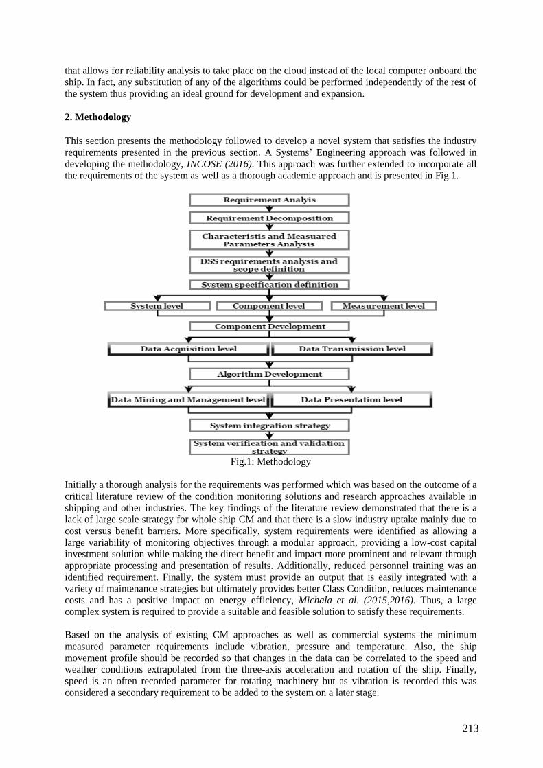
213
that allows for reliability analysis to take place on the cloud instead of the local computer onboard the
ship. In fact, any substitution of any of the algorithms could be performed independently of the rest of
the system thus providing an ideal ground for development and expansion.
2. Methodology
This section presents the methodology followed to develop a novel system that satisfies the industry
requirements presented in the previous section. A Systems’ Engineering approach was followed in
developing the methodology, INCOSE (2016). This approach was further extended to incorporate all
the requirements of the system as well as a thorough academic approach and is presented in Fig.1.
Fig.1: Methodology
Initially a thorough analysis for the requirements was performed which was based on the outcome of a
critical literature review of the condition monitoring solutions and research approaches available in
shipping and other industries. The key findings of the literature review demonstrated that there is a
lack of large scale strategy for whole ship CM and that there is a slow industry uptake mainly due to
cost versus benefit barriers. More specifically, system requirements were identified as allowing a
large variability of monitoring objectives through a modular approach, providing a low-cost capital
investment solution while making the direct benefit and impact more prominent and relevant through
appropriate processing and presentation of results. Additionally, reduced personnel training was an
identified requirement. Finally, the system must provide an output that is easily integrated with a
variety of maintenance strategies but ultimately provides better Class Condition, reduces maintenance
costs and has a positive impact on energy efficiency, Michala et al. (2015,2016). Thus, a large
complex system is required to provide a suitable and feasible solution to satisfy these requirements.
Based on the analysis of existing CM approaches as well as commercial systems the minimum
measured parameter requirements include vibration, pressure and temperature. Also, the ship
movement profile should be recorded so that changes in the data can be correlated to the speed and
weather conditions extrapolated from the three-axis acceleration and rotation of the ship. Finally,
speed is an often recorded parameter for rotating machinery but as vibration is recorded this was
considered a secondary requirement to be added to the system on a later stage.
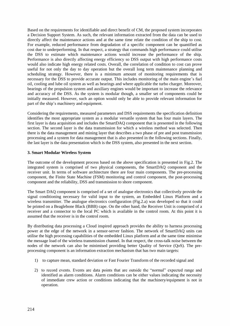
214
Based on the requirements for identifiable and direct benefit of CM, the proposed system incorporates
a Decision Support System. As such, the relevant information extracted from the data can be used to
directly affect the maintenance actions and at the same time relate the condition of the ship to cost.
For example, reduced performance from degradation of a specific component can be quantified as
cost due to underperforming. In that respect, a strategy that commands high performance could utilise
the DSS to estimate which maintenance actions would increase the performance of the ship.
Performance is also directly affecting energy efficiency so DSS output with high performance costs
would also indicate high energy related costs. Overall, the correlation of condition to cost can prove
useful for not only the day to day operation but the overall long term maintenance planning and
scheduling strategy. However, there is a minimum amount of monitoring requirements that is
necessary for the DSS to provide accurate output. This includes monitoring of the main engine’s fuel
oil, cooling and lube oil system as well as bearings and where applicable the turbo charger. Moreover,
bearings of the propulsion system and auxiliary engines would be important to increase the relevance
and accuracy of the DSS. As the system is modular though, a smaller set of components could be
initially measured. However, such an option would only be able to provide relevant information for
part of the ship’s machinery and equipment.
Considering the requirements, measured parameters and DSS requirements the specification definition
identifies the most appropriate system as a modular versatile system that has four main layers. The
first layer is data acquisition and includes the SmartDAQ component that is presented in the following
section. The second layer is the data transmission for which a wireless method was selected. Then
there is the data management and mining layer that describes a two phase of pre and post transmission
processing and a system for data management that is also presented in the following sections. Finally,
the last layer is the data presentation which is the DSS system, also presented in the next section.
3. Smart Modular Wireless System
The outcome of the development process based on the above specification is presented in Fig.2. The
integrated system is comprised of two physical components, the SmartDAQ component and the
receiver unit. In terms of software architecture there are four main components. The pre-processing
component, the Finite State Machine (FSM) monitoring and control component, the post-processing
component and the reliability, DSS and transmission to shore component.
The Smart DAQ component is comprised of a set of analogue electronics that collectively provide the
signal conditioning necessary for valid input to the system, an Embedded Linux Platform and a
wireless transmitter. The analogue electronics configuration (Fig.2.a) was developed so that it could
be printed on a Beaglebone Black (BBB) cape. On the other hand, the Receiver Unit is comprised of a
receiver and a connector to the local PC which is available in the control room. At this point it is
assumed that the receiver is in the control room.
By distributing data processing a Cloud inspired approach provides the ability to harness processing
power at the edge of the network in a sensor-server fashion. The network of SmartDAQ units can
utilise the high processing capabilities of the embedded Linux platform and at the same time minimise
the message load of the wireless transmission channel. In that respect, the cross-talk noise between the
nodes of the network can also be minimised providing better Quality of Service (QoS). The pre-
processing component is an information extraction mechanism that has two main targets:
1) to capture mean, standard deviation or Fast Fourier Transform of the recorded signal and
2) to record events. Events are data points that are outside the “normal” expected range and
identified as alarm conditions. Alarm conditions can be either values indicating the necessity
of immediate crew action or conditions indicating that the machinery/equipment is not in
operation.
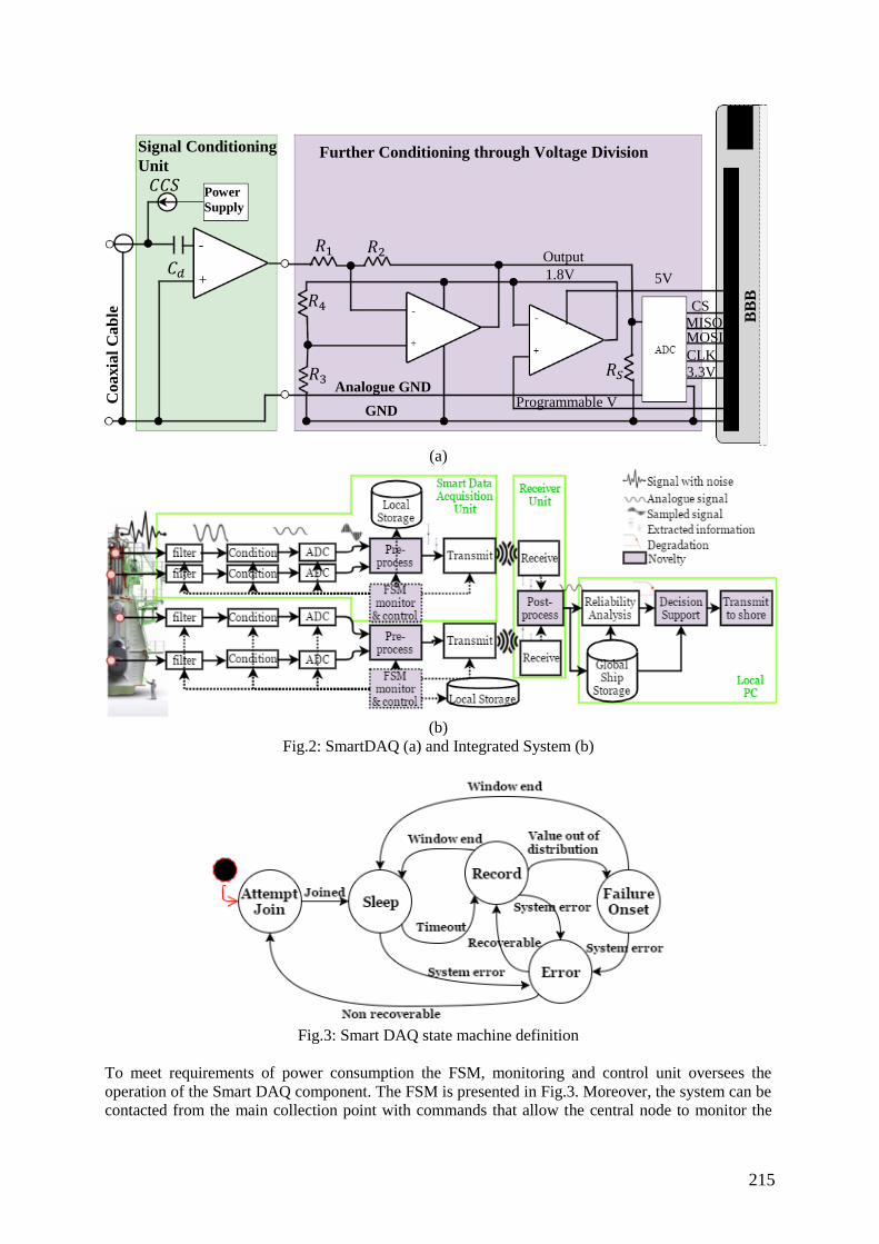
215
(a)
(b)
Fig.2: SmartDAQ (a) and Integrated System (b)
Fig.3: Smart DAQ state machine definition
To meet requirements of power consumption the FSM, monitoring and control unit oversees the
operation of the Smart DAQ component. The FSM is presented in Fig.3. Moreover, the system can be
contacted from the main collection point with commands that allow the central node to monitor the
Signal Conditioning
Unit
Co
axia
l C
ab
le
Power
Supply
𝐶𝐶𝑆
𝐶𝑑
Further Conditioning through Voltage Division
BB
B
𝑅1 𝑅2
𝑅4
𝑅3 𝑅𝑆
Output
5V 1.8V
GND Programmable V
-
+
Analogue GND
CS MISO
O MOSI
CLK 3.3V
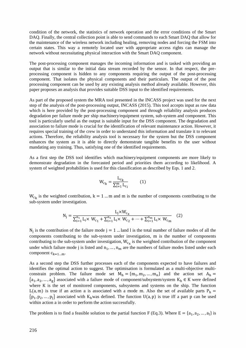
216
condition of the network, the statistics of network operation and the error conditions of the Smart
DAQ. Finally, the central collection point is able to send commands to each Smart DAQ that allow for
the maintenance of the wireless network including healing, removing nodes and forcing the FSM into
certain states. This way a remotely located user with appropriate access rights can manage the
network without necessitating physical interaction with the Smart DAQ component.
The post-processing component manages the incoming information and is tasked with providing an
output that is similar to the initial data stream recorded by the sensor. In that respect, the pre-
processing component is hidden to any components requiring the output of the post-processing
component. That isolates the physical components and their particulars. The output of the post
processing component can be used by any existing analysis method already available. However, this
paper proposes an analysis that provides suitable DSS input to the identified requirements.
As part of the proposed system the MRA tool presented in the INCASS project was used for the next
step of the analysis of the post-processing output, INCASS (2015). This tool accepts input as raw data
which is here provided by the post-processing component and through reliability analysis produces
degradation per failure mode per ship machinery/equipment system, sub-system and component. This
tool is particularly useful as the output is suitable input for the DSS component. The degradation and
association to failure mode is crucial for the identification of relevant maintenance action. However, it
requires special training of the crew in order to understand this information and translate it to relevant
actions. Therefore, the reliability analysis tool is necessary for the system but the DSS component
enhances the system as it is able to directly demonstrate tangible benefits to the user without
mandating any training. Thus, satisfying one of the identified requirements.
As a first step the DSS tool identifies which machinery/equipment components are more likely to
demonstrate degradation in the forecasted period and priorities them according to likelihood. A
system of weighted probabilities is used for this classification as described by Eqs. 1 and 2.
Wck=
Lck
∑ Lcimi=1
(1)
Wck is the weighted contribution, k = 1 … m and m is the number of components contributing to the
sub-system under investigation.
Nj =Lj×Wcx
∑ Li× n1i=1 Wc1
+ ∑ Li× n2i=1 Wc2
+ ⋯ + ∑ Li× nmi=1 Wcm
(2)
Nj is the contribution of the failure mode j = 1 … land l is the total number of failure modes of all the
components contributing to the sub-system under investigation, m is the number of components
contributing to the sub-system under investigation, Wcx is the weighted contribution of the component
under which failure mode j is listed and n1, … , nm are the numbers of failure modes listed under each
component ck=1…m.
As a second step the DSS further processes each of the components expected to have failures and
identifies the optimal action to suggest. The optimisation is formulated as a multi-objective multi-
constrain problem. The failure mode set Mh = {m1, m2, … , mn} and the action set Ah =
{a1, a2, … , ag} associated with a failure mode of component/subsystem/system Kh ∈ K were defined
where K is the set of monitored components, subsystems and systems on the ship. The function
L(a, m) is true if an action a is associated with a mode m. Also the set of available parts Ph =
{p1, p2, … , pj} associated with Khwas defined. The function U(a, p) is true iff a part p can be used
within action a in order to perform the action successfully.
The problem is to find a feasible solution to the partial function F (Eq.3). Where E = {a1, a2, … , al} is
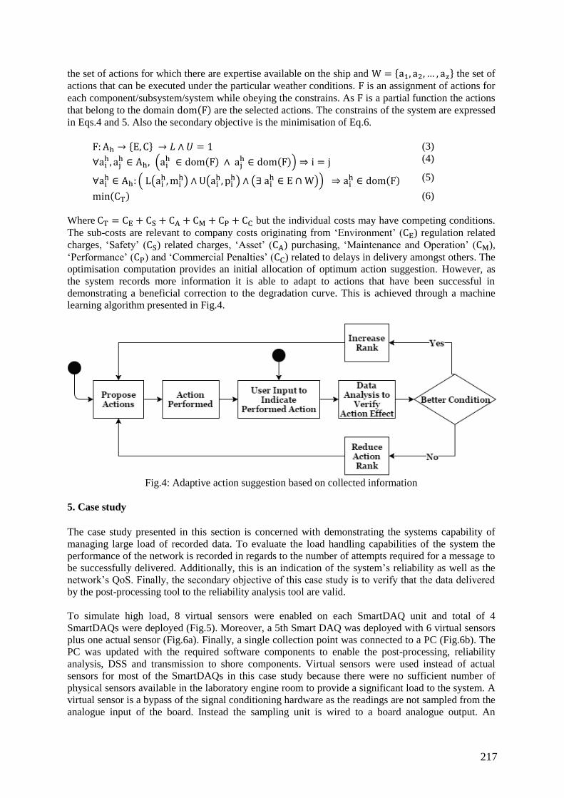
217
the set of actions for which there are expertise available on the ship and W = {a1, a2, … , az} the set of
actions that can be executed under the particular weather conditions. F is an assignment of actions for
each component/subsystem/system while obeying the constrains. As F is a partial function the actions
that belong to the domain dom(F) are the selected actions. The constrains of the system are expressed
in Eqs.4 and 5. Also the secondary objective is the minimisation of Eq.6.
F: Ah → {E, C} → 𝐿 ∧ 𝑈 = 1 (3)
∀aih, aj
h ∈ Ah, (aih ∈ dom(F) ∧ aj
h ∈ dom(F)) ⇒ i = j (4)
∀aih ∈ Ah: ( L(ai
h, mih) ∧ U(ai
h, pih) ∧ (∃ ai
h ∈ E ∩ W)) ⇒ aih ∈ dom(F) (5)
min(CT) (6)
Where CT = CE + CS + CA + CM + CP + CC but the individual costs may have competing conditions.
The sub-costs are relevant to company costs originating from ‘Environment’ (CE) regulation related
charges, ‘Safety’ (CS) related charges, ‘Asset’ (CA) purchasing, ‘Maintenance and Operation’ (CM),
‘Performance’ (CP) and ‘Commercial Penalties’ (CC) related to delays in delivery amongst others. The
optimisation computation provides an initial allocation of optimum action suggestion. However, as
the system records more information it is able to adapt to actions that have been successful in
demonstrating a beneficial correction to the degradation curve. This is achieved through a machine
learning algorithm presented in Fig.4.
Fig.4: Adaptive action suggestion based on collected information
5. Case study
The case study presented in this section is concerned with demonstrating the systems capability of
managing large load of recorded data. To evaluate the load handling capabilities of the system the
performance of the network is recorded in regards to the number of attempts required for a message to
be successfully delivered. Additionally, this is an indication of the system’s reliability as well as the
network’s QoS. Finally, the secondary objective of this case study is to verify that the data delivered
by the post-processing tool to the reliability analysis tool are valid.
To simulate high load, 8 virtual sensors were enabled on each SmartDAQ unit and total of 4
SmartDAQs were deployed (Fig.5). Moreover, a 5th Smart DAQ was deployed with 6 virtual sensors
plus one actual sensor (Fig.6a). Finally, a single collection point was connected to a PC (Fig.6b). The
PC was updated with the required software components to enable the post-processing, reliability
analysis, DSS and transmission to shore components. Virtual sensors were used instead of actual
sensors for most of the SmartDAQs in this case study because there were no sufficient number of
physical sensors available in the laboratory engine room to provide a significant load to the system. A
virtual sensor is a bypass of the signal conditioning hardware as the readings are not sampled from the
analogue input of the board. Instead the sampling unit is wired to a board analogue output. An
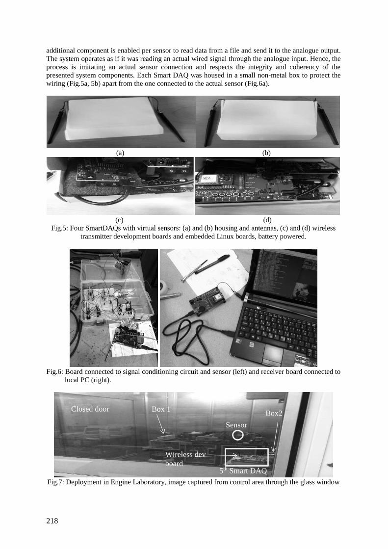
218
additional component is enabled per sensor to read data from a file and send it to the analogue output.
The system operates as if it was reading an actual wired signal through the analogue input. Hence, the
process is imitating an actual sensor connection and respects the integrity and coherency of the
presented system components. Each Smart DAQ was housed in a small non-metal box to protect the
wiring (Fig.5a, 5b) apart from the one connected to the actual sensor (Fig.6a).
(a) (b)
(c) (d)
Fig.5: Four SmartDAQs with virtual sensors: (a) and (b) housing and antennas, (c) and (d) wireless
transmitter development boards and embedded Linux boards, battery powered.
Fig.6: Board connected to signal conditioning circuit and sensor (left) and receiver board connected to
local PC (right).
Fig.7: Deployment in Engine Laboratory, image captured from control area through the glass window
Closed door Box 1 Box2
Sensor
5th Smart DAQ
Wireless dev
board
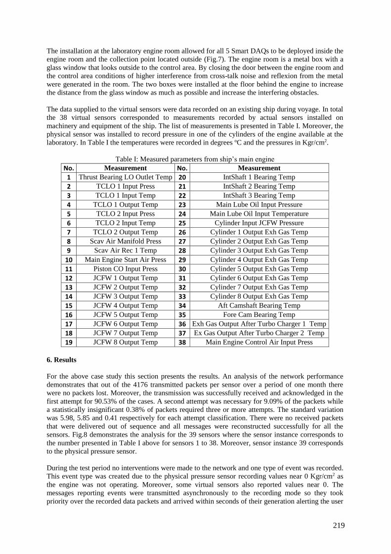
219
The installation at the laboratory engine room allowed for all 5 Smart DAQs to be deployed inside the
engine room and the collection point located outside (Fig.7). The engine room is a metal box with a
glass window that looks outside to the control area. By closing the door between the engine room and
the control area conditions of higher interference from cross-talk noise and reflexion from the metal
were generated in the room. The two boxes were installed at the floor behind the engine to increase
the distance from the glass window as much as possible and increase the interfering obstacles.
The data supplied to the virtual sensors were data recorded on an existing ship during voyage. In total
the 38 virtual sensors corresponded to measurements recorded by actual sensors installed on
machinery and equipment of the ship. The list of measurements is presented in Table I. Moreover, the
physical sensor was installed to record pressure in one of the cylinders of the engine available at the
laboratory. In Table I the temperatures were recorded in degrees oC and the pressures in Kgr/cm2.
Table I: Measured parameters from ship’s main engine
No. Measurement No. Measurement
1 Thrust Bearing LO Outlet Temp 20 IntShaft 1 Bearing Temp
2 TCLO 1 Input Press 21 IntShaft 2 Bearing Temp
3 TCLO 1 Input Temp 22 IntShaft 3 Bearing Temp
4 TCLO 1 Output Temp 23 Main Lube Oil Input Pressure
5 TCLO 2 Input Press 24 Main Lube Oil Input Temperature
6 TCLO 2 Input Temp 25 Cylinder Input JCFW Pressure
7 TCLO 2 Output Temp 26 Cylinder 1 Output Exh Gas Temp
8 Scav Air Manifold Press 27 Cylinder 2 Output Exh Gas Temp
9 Scav Air Rec 1 Temp 28 Cylinder 3 Output Exh Gas Temp
10 Main Engine Start Air Press 29 Cylinder 4 Output Exh Gas Temp
11 Piston CO Input Press 30 Cylinder 5 Output Exh Gas Temp
12 JCFW 1 Output Temp 31 Cylinder 6 Output Exh Gas Temp
13 JCFW 2 Output Temp 32 Cylinder 7 Output Exh Gas Temp
14 JCFW 3 Output Temp 33 Cylinder 8 Output Exh Gas Temp
15 JCFW 4 Output Temp 34 Aft Camshaft Bearing Temp
16 JCFW 5 Output Temp 35 Fore Cam Bearing Temp
17 JCFW 6 Output Temp 36 Exh Gas Output After Turbo Charger 1 Temp
18 JCFW 7 Output Temp 37 Ex Gas Output After Turbo Charger 2 Temp
19 JCFW 8 Output Temp 38 Main Engine Control Air Input Press
6. Results
For the above case study this section presents the results. An analysis of the network performance
demonstrates that out of the 4176 transmitted packets per sensor over a period of one month there
were no packets lost. Moreover, the transmission was successfully received and acknowledged in the
first attempt for 90.53% of the cases. A second attempt was necessary for 9.09% of the packets while
a statistically insignificant 0.38% of packets required three or more attempts. The standard variation
was 5.98, 5.85 and 0.41 respectively for each attempt classification. There were no received packets
that were delivered out of sequence and all messages were reconstructed successfully for all the
sensors. Fig.8 demonstrates the analysis for the 39 sensors where the sensor instance corresponds to
the number presented in Table I above for sensors 1 to 38. Moreover, sensor instance 39 corresponds
to the physical pressure sensor.
During the test period no interventions were made to the network and one type of event was recorded.
This event type was created due to the physical pressure sensor recording values near 0 Kgr/cm2 as
the engine was not operating. Moreover, some virtual sensors also reported values near 0. The
messages reporting events were transmitted asynchronously to the recording mode so they took
priority over the recorded data packets and arrived within seconds of their generation alerting the user
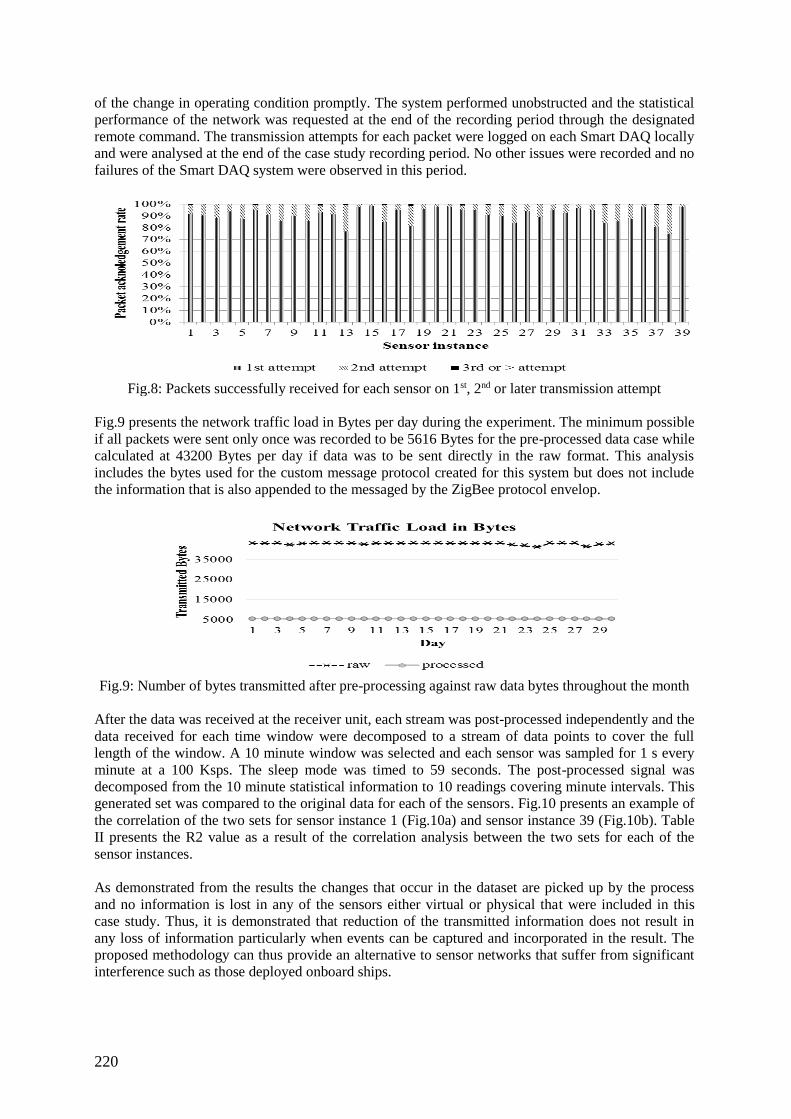
220
of the change in operating condition promptly. The system performed unobstructed and the statistical
performance of the network was requested at the end of the recording period through the designated
remote command. The transmission attempts for each packet were logged on each Smart DAQ locally
and were analysed at the end of the case study recording period. No other issues were recorded and no
failures of the Smart DAQ system were observed in this period.
Fig.8: Packets successfully received for each sensor on 1st, 2nd or later transmission attempt
Fig.9 presents the network traffic load in Bytes per day during the experiment. The minimum possible
if all packets were sent only once was recorded to be 5616 Bytes for the pre-processed data case while
calculated at 43200 Bytes per day if data was to be sent directly in the raw format. This analysis
includes the bytes used for the custom message protocol created for this system but does not include
the information that is also appended to the messaged by the ZigBee protocol envelop.
Fig.9: Number of bytes transmitted after pre-processing against raw data bytes throughout the month
After the data was received at the receiver unit, each stream was post-processed independently and the
data received for each time window were decomposed to a stream of data points to cover the full
length of the window. A 10 minute window was selected and each sensor was sampled for 1 s every
minute at a 100 Ksps. The sleep mode was timed to 59 seconds. The post-processed signal was
decomposed from the 10 minute statistical information to 10 readings covering minute intervals. This
generated set was compared to the original data for each of the sensors. Fig.10 presents an example of
the correlation of the two sets for sensor instance 1 (Fig.10a) and sensor instance 39 (Fig.10b). Table
II presents the R2 value as a result of the correlation analysis between the two sets for each of the
sensor instances.
As demonstrated from the results the changes that occur in the dataset are picked up by the process
and no information is lost in any of the sensors either virtual or physical that were included in this
case study. Thus, it is demonstrated that reduction of the transmitted information does not result in
any loss of information particularly when events can be captured and incorporated in the result. The
proposed methodology can thus provide an alternative to sensor networks that suffer from significant
interference such as those deployed onboard ships.
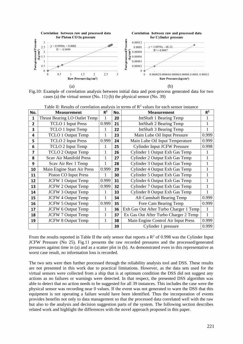
221
(a) (b)
Fig.10: Example of correlation analysis between initial data and post-process generated data for two
cases (a) the virtual sensor (No. 11) (b) the physical sensor (No. 39)
Table II: Results of correlation analysis in terms of R2 values for each sensor instance
No. Measurement R2 No. Measurement R2
1 Thrust Bearing LO Outlet Temp 1 20 IntShaft 1 Bearing Temp 1
2 TCLO 1 Input Press 0.999 21 IntShaft 2 Bearing Temp 1
3 TCLO 1 Input Temp 1 22 IntShaft 3 Bearing Temp 1
4 TCLO 1 Output Temp 1 23 Main Lube Oil Input Pressure 0.999
5 TCLO 2 Input Press 0.999 24 Main Lube Oil Input Temperature 0.999
6 TCLO 2 Input Temp 1 25 Cylinder Input JCFW Pressure 0.998
7 TCLO 2 Output Temp 1 26 Cylinder 1 Output Exh Gas Temp 1
8 Scav Air Manifold Press 1 27 Cylinder 2 Output Exh Gas Temp 1
9 Scav Air Rec 1 Temp 1 28 Cylinder 3 Output Exh Gas Temp 1
10 Main Engine Start Air Press 0.999 29 Cylinder 4 Output Exh Gas Temp 1
11 Piston CO Input Press 1 30 Cylinder 5 Output Exh Gas Temp 1
12 JCFW 1 Output Temp 0.999 31 Cylinder 6 Output Exh Gas Temp 1
13 JCFW 2 Output Temp 0.999 32 Cylinder 7 Output Exh Gas Temp 1
14 JCFW 3 Output Temp 1 33 Cylinder 8 Output Exh Gas Temp 1
15 JCFW 4 Output Temp 1 34 Aft Camshaft Bearing Temp 0.999
16 JCFW 5 Output Temp 0.999 35 Fore Cam Bearing Temp 0.999
17 JCFW 6 Output Temp 1 36 Exh Gas Out After Turbo Charger 1 Temp 1
18 JCFW 7 Output Temp 1 37 Ex Gas Out After Turbo Charger 2 Temp 1
19 JCFW 8 Output Temp 1 38 Main Engine Control Air Input Press 0.999
39 Cylinder 1 pressure 0.999
From the results reported in Table II the only sensor that reports a R2 of 0.998 was the Cylinder Input
JCFW Pressure (No 25). Fig.11 presents the raw recorded pressures and the processed/generated
pressures against time in (a) and as a scatter plot in (b). As demonstrated even in this representative as
worst case result, no information loss is recorded.
The two sets were then further processed through the reliability analysis tool and DSS. These results
are not presented in this work due to practical limitations. However, as the data sets used for the
virtual sensors were collected from a ship that is at optimum condition the DSS did not suggest any
actions as no failures or warnings were detected. In that respect, the presented DSS algorithm was
able to detect that no action needs to be suggested for all 39 instances. This includes the case were the
physical sensor was recording near 0 values. If the event was not generated to warn the DSS that this
equipment is not operating a failure would have been identified. Thus the incorporation of events
provides benefits not only to data management so that the processed data correlated well with the raw
but also to the analysis and decision suggestion parts of the system. The following section describes
related work and highlight the differences with the novel approach proposed in this paper.
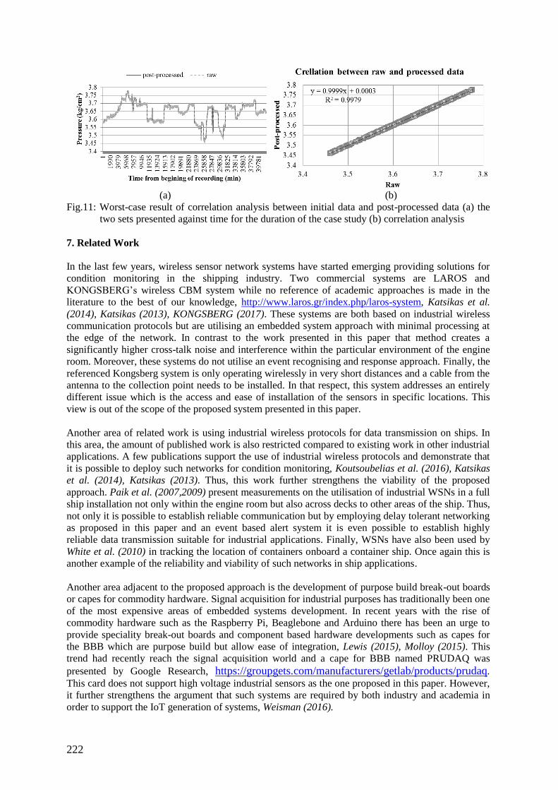
222
(a) (b)
Fig.11: Worst-case result of correlation analysis between initial data and post-processed data (a) the
two sets presented against time for the duration of the case study (b) correlation analysis
7. Related Work
In the last few years, wireless sensor network systems have started emerging providing solutions for
condition monitoring in the shipping industry. Two commercial systems are LAROS and
KONGSBERG’s wireless CBM system while no reference of academic approaches is made in the
literature to the best of our knowledge, http://www.laros.gr/index.php/laros-system, Katsikas et al.
(2014), Katsikas (2013), KONGSBERG (2017). These systems are both based on industrial wireless
communication protocols but are utilising an embedded system approach with minimal processing at
the edge of the network. In contrast to the work presented in this paper that method creates a
significantly higher cross-talk noise and interference within the particular environment of the engine
room. Moreover, these systems do not utilise an event recognising and response approach. Finally, the
referenced Kongsberg system is only operating wirelessly in very short distances and a cable from the
antenna to the collection point needs to be installed. In that respect, this system addresses an entirely
different issue which is the access and ease of installation of the sensors in specific locations. This
view is out of the scope of the proposed system presented in this paper.
Another area of related work is using industrial wireless protocols for data transmission on ships. In
this area, the amount of published work is also restricted compared to existing work in other industrial
applications. A few publications support the use of industrial wireless protocols and demonstrate that
it is possible to deploy such networks for condition monitoring, Koutsoubelias et al. (2016), Katsikas
et al. (2014), Katsikas (2013). Thus, this work further strengthens the viability of the proposed
approach. Paik et al. (2007,2009) present measurements on the utilisation of industrial WSNs in a full
ship installation not only within the engine room but also across decks to other areas of the ship. Thus,
not only it is possible to establish reliable communication but by employing delay tolerant networking
as proposed in this paper and an event based alert system it is even possible to establish highly
reliable data transmission suitable for industrial applications. Finally, WSNs have also been used by
White et al. (2010) in tracking the location of containers onboard a container ship. Once again this is
another example of the reliability and viability of such networks in ship applications.
Another area adjacent to the proposed approach is the development of purpose build break-out boards
or capes for commodity hardware. Signal acquisition for industrial purposes has traditionally been one
of the most expensive areas of embedded systems development. In recent years with the rise of
commodity hardware such as the Raspberry Pi, Beaglebone and Arduino there has been an urge to
provide speciality break-out boards and component based hardware developments such as capes for
the BBB which are purpose build but allow ease of integration, Lewis (2015), Molloy (2015). This
trend had recently reach the signal acquisition world and a cape for BBB named PRUDAQ was
presented by Google Research, https://groupgets.com/manufacturers/getlab/products/prudaq.
This card does not support high voltage industrial sensors as the one proposed in this paper. However,
it further strengthens the argument that such systems are required by both industry and academia in
order to support the IoT generation of systems, Weisman (2016).
223
Decision support systems have enjoyed varied attention in several industries of the past few decades.
It has been identified that DSS systems cannot be generic for all industries and all applications,
Makowski, (2011), Vallerio et al. (2015). Hence, publications in the condition monitoring of ship
applications have been reviewed. Jardine et al. (1997) presents one approach using hazard modelling
which takes into account cost and age models along with a system based on maximum likelihood
estimations advising strictly on replacement of parts. A control theory based approach is also
presented by Christer et al. (1997) again to identify the time for replacement of parts. Khac Tuan et
al. (2014) present a more sophisticated system that is based on degradation, threshold and failure
mode integration. However, the interaction between failure modes and components of a system is not
considered. A reliability analysis technique is presented by Dikis et al. (2016) and Lazakis et al.
(2016,2017) which considers these interactions but does not include vibration measurements.
However, none of the above consider constrains such as availability of parts, crew expertise and
weather conditions which may affect the decisions to be made as well as parameters such as
performance and energy efficiency. Such a DSS is not previously published in literature to the best of
our knowledge. This work proposes a DSS which is a multiple parameter multiple constrain
optimisation problem and allows for user defined constrains to be added to the system.
8. Conclusion
Through the proposed methodology some of the inhibitors in acceptance of this technology are
addressed such as increased security of data, ensuring data ownership and providing clear benefit to
both the engineers onboard the vessel and management through the DSS software. Furthermore, the
performance of the wireless network is demonstrating that the proposed system supports highly
reliable data transfer. Additionally, through the proposed system the particular noise and interference
conditions in the ship engine room are addressed without compromising data integrity, data quality,
security and safety onboard the vessel. The results demonstrate correlation between the data recorded
onboard a ship in voyage and the data that have been processed through the proposed approach. As
such, this novel system can be utilised in real industrial applications to support any post-processing
methodology while ensuring data integrity and security.
References
ADAMSON, K.D. (2015), Big Data & the new IT, 2015 Roundtable Series, Mayfair, London
ADAMSON, K.D. (2016a), Bits & Pieces, Future Nautics, The Maritime Future, pp.20-23
ADAMSON, K.D. (2016b), Maritime Satellite Communications & Applications, 2016 Research
White Pape, Mayfair, London
CHRISTER, A.; WANG, W.; SHARP, J. (1997), A state space condition monitoring model for
furnace erosion prediction and replacement, European J. Operational Research 101, pp.1-14
DIKIS, K.; LAZAKIS, I.; MICHALA, A.L.; RAPTODIMOS, Y.; THEOTOKATOS, G. (2016),
Dynamic risk and reliability assessment for ship machinery decision making, European Safety and
Reliability Conf., Glasgow
DNV GL (2014), Beyond condition monitoring in the maritime industry, DNV GL Strategic Research
& Innovation
INCASS (2015), Deliverable D4.4 Machinery and equipment assessment methodology at component
and system level, INCASS - Inspection Capabilities for Enhanced Ship Safety. EC FP7 Project
JARDINE, A.K.S.; BANJEVIC, D.; MAKIS, V. (1997), Optimal replacement policy and the
structure of software for condition‐ based maintenance, J. Quality in Maintenance Eng. 3, pp.109-119

224
KATSIKAS, S. (2013), An innovative system for vessels monitoring, diagnosis and prognosis and the
challenges to be faced, 1st Int. Conf. Case Studies in Advanced Engineering Design
KATSIKAS, S.; DIMAS, D.; DEFIGOS, A.; ROUTZOMANIS, A.; MERMIKL, K. (2014), Wireless
modular system for vessel engines monitoring, condition based maintenance and vessel’s
performance analysis, European Conf. Prognostics and Health Management Society, Nantes
KHAC TUAN, H.; TORRES CASTRO, I.; BARROS, A.; BERENGUER, C. (2014), On the use of
mean residual life as a condition index for condition-based maintenance decision-making, IEEE
Trans. Systems, Man, and Cybernetics 44, pp.877-893
KONGSBERG (2017), Wireless temperature monitoring for compressors,
https://www.km.kongsberg.com/ks/web/nokbg0240.nsf/AllWeb/6B5FEFE64164D3FBC12577CB003
EFDDA?OpenDocument
KOUTSOUBELIAS, M.; GRIGOROPOULOS, N.; LALIS, S.; LAMPSAS, P.; KATSIKAS, S.;
DIMAS, D. (2016), System support for the in situ testing of wireless sensor networks via programma-
ble virtual onboard sensors, IEEE Trans. Instrumentation And Measurement 65, pp.744-753
LATARCHE, M. (2015), The Connected Ship – DNV GL. https://www.shipinsight.com/the-
connected-ship-dnv-gl
LAZAKIS, I.; DIKIS, K.; MICHALA, A.L. (2016), Condition monitoring for enhanced inspection,
maintenance and decision making in ship operations, 13th Int. Symp. Practical Design of Ships and
Other Floating Structures. Copenhagen
LAZAKIS, I.; DIKIS, K.; MICHALA, A.L.; THEOTOKATOS, G. (2017), Advanced ship systems
condition monitoring for enhanced inspection, maintenance and decision making in ship operations,
Transportation Research Procedia 14, pp.1679-1688
LEWIS, B. (2015), 10 sensors, 3 protocols, 3 minutes, 1 dev kit for cloud-connected IoT apps.
OpenSystems Media http://embedded-computing.com/articles/10-sensors-3-protocols-3-minutes-1-
dev-kit-for-cloud-connected-iot-apps/#
MAKOWSKI, M. (2011), Multi-objective decision support including sensitivity analysis, UNESCO -
Encyclopedia Of Life Support System, Environmental Systems Vol III
MICHALA, A.L.; LAZAKIS, I.; THEOTOKATOS, G. (2015), Predictive maintenance decision
support system for enhanced energy efficiency of ship machinery, Int. Conf. of Shipping in Changing
Climates, Glasgow, pp.195-205
MICHALA, A.L.; LAZAKIS, I.; THEOTOKATOS, G.; VARELAS, T. (2016), Wireless condition
monitoring for ship applications, Smart Ship Technology Conf., London, pp.59-66
MOLLOY, D. (2015). Exploring BeagleBone, Tools and Technologies for Building with Embedded
Linux, Wiley, Inidianapolis
PAIK, B.G.; CHO, S.R.; PARK, B.J.; LEE, D.; YUN, J.H.; BAE, B.D. (2007), Employment of
wireless sensor networks for full-scale ship application, Int. Conf. Embedded and Ubiquitous
Computing, Taipei
PAIK, B.G.; CHO, S.R.; PARK, B.J.; LEE, D.; BAE, B.D.; YUN, J.H. (2009), Characteristics of
wireless sensor network for full-scale ship application, J. Marine Science and Technology 14, pp.115-
126

225
VALLERIO, M.; HUFKENS, J.; IMPE, J.V.; LOGIST, F. (2015), An interactive decision-support
system for multi-objective optimization of nonlinear dynamic processes with uncertainty, Expert Syst.
Appl. 42, pp.7710-7731
WEISMAN, D. (2016), Silicon labs to showcase IoT connectivity innovations at embedded world,
http://news.silabs.com/blog/silicon-labs-showcase-iot-connectivity-innovations-embedded-world-0
WHITE, J.; BROWN, J.; RAMASWAMY, S.; GEOGHAN, S.; ITMI, M. (2010), Securing P2P
wireless communications by deploying honeytokens in a cooperative maritime network, Technological
Developments in Networking, Education and Automation, Springer

226
Change and Access Control Management to Provide Sister Ships
Applicability Capability
Rodrigo Perez Fernandez, SENER, Madrid/Spain, [email protected]
Jesus A. Muñoz, SENER, Madrid/Spain, [email protected]
Abstract
The use of specialized shipbuilding CAD Systems in marine environments is crucial for the efficient
design and manufacturing of ships. The heart of a shipbuilding CAD System as FORAN is a relational
database where the vessel CAD product model is stored. The product model includes geometry,
topology, specialized technological and manufacturing information for all ship design disciplines and
many relationships between the ship items. The main objective of this paper is to describe how a
shipbuilding CAD System, as FORAN, supports management of Ship Unit Series of projects. For this
purpose, FORAN has been enhanced to allow the creation of a new ship series and the management of
the projects included in it, representing the different vessel units. This capability of handling sister ship
management in FORAN can be enhanced when using a complete FORAN-PLM integration, as FORAN
sister ship management is also considered in FORAN-PLM integration tools, so PLM can take
advantage of it.
1. Shipbuilding CAD Systems in naval environments
The use of specialized shipbuilding CAD Systems in naval environments is crucial for the efficient
design and manufacturing of surface ships and submarines, Perez and Gonzalez (2015). The heart of a
shipbuilding CAD System as FORAN is a relational database (ORACLE) where the vessel CAD prod-
uct model is stored. The product model includes geometry, topology, specialized technological and
manufacturing information for all vessel disciplines and many relationships between the vessel items.
Shipbuilding CAD Systems working in naval environments offer significant advantages over other ge-
neric CAD applications, some of which can be relevant for the purpose of this paper:
Specifically developed for shipbuilding.
Availability of shipbuilding smart modelling tools.
Incorporation of many years of shipbuilding knowledge.
Outputs adapted to shipbuilding manufacturing processes.
Proven scalability.
Proven performance.
Adapted to military shipbuilding requirements (Dunseath et al., 2015).
Reduction of design and manufacturing hours over generic CAD applications.
The scalability refers to both the number of CAD users and to the number of vessel items to be handled.
Military vessels are very complex products that may be composed of millions of items, requiring a large
number of designers, accessing concurrently to the vessel product model, Perez and Lee (2014). The
design cycles of these vessels are usually very long and there are many design changes along the whole
vessel lifecycle. Performance is another critical requirement, especially in the detail design and manu-
facturing stages, when the detail design is almost complete, there are hundreds of users working on the
model, model changes are constant and information for the production processes must be provided
continuously, Perez and Penas (2015).
2. Management of Ship Unit Series
The main objective is to enable FORAN to support management of Ship Unit Series of projects. For
this purpose, the FDBA utility (FORAN Database Administrator) has been enhanced to allow creating
a new ship series and the management of the projects included in it, representing the different ship units.
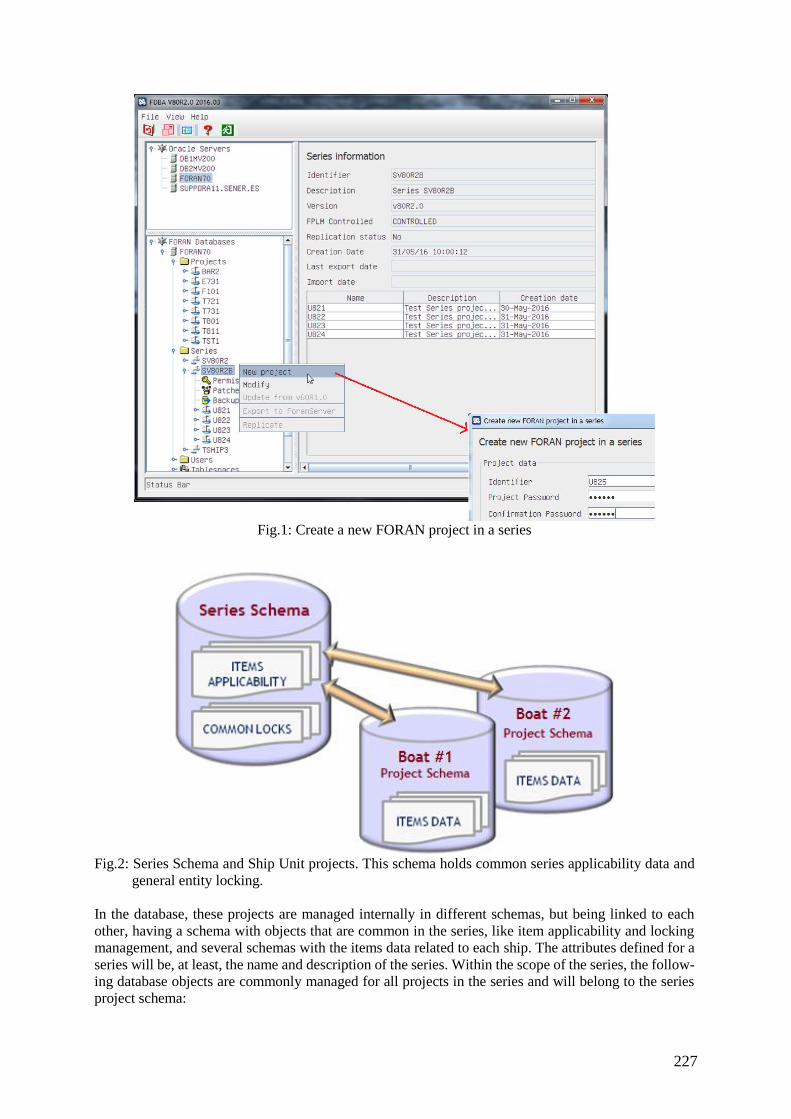
227
Fig.1: Create a new FORAN project in a series
Fig.2: Series Schema and Ship Unit projects. This schema holds common series applicability data and
general entity locking.
In the database, these projects are managed internally in different schemas, but being linked to each
other, having a schema with objects that are common in the series, like item applicability and locking
management, and several schemas with the items data related to each ship. The attributes defined for a
series will be, at least, the name and description of the series. Within the scope of the series, the follow-
ing database objects are commonly managed for all projects in the series and will belong to the series
project schema:

228
Oracle sequences
Table of projects included in the series
Locking tables
Applicability of items in the series (FORAN_APPLICABILITY). This table will include all related data
about the ship units in which the entities subject of applicability in a range exist.
2.1 Database Structure in a Multi-Ship Series
In the case of a multi-ship series, the FORAN database is structured in the following components:
The FORAN Series Schema.
The FORAN Project schemas. There is one specific FORAN project schema for each ship in
the series.
The FORAN Project Schemas in a series context are identical to those FORAN project schemas, except
that the COM_LOCK table is not used, as locking is controlled and centralized in the Series schema
COM_LOCK table. This is to ensure consistency when several users might be working in different
projects, but potentially could be accessing identical data among them, Each FORAN project schema
contains all model and PLM data for the ship it belongs to. The entities data identical among more than
one ship (sharing the applicability range), is copied identically and automatically by the multi-save
FORAN device when a user working in a particular project in the series saves the data.
Fig.3: Data controlled in Series Project
3. Changes in FORAN Design Modules
3.1 Storing Design Changes in Project Entities
When a user is working in a FORAN design module in a project belonging to a series and is going to
store the changes applied on an entity, the system behaves differently depending on the entity type. If
the entity is of a type not included in the applicability management, and so it is no subject of multi-
saving, then the data will only be stored in the working project. If the entity is of a type included in
applicability management, and so it is subject of multi-saving, the system obtains the information re-
lated to the ship units in the series that share the same applicability range with the current ship unit for
the entity, before saving takes place. Then, the changes to be stored are done identically in all database
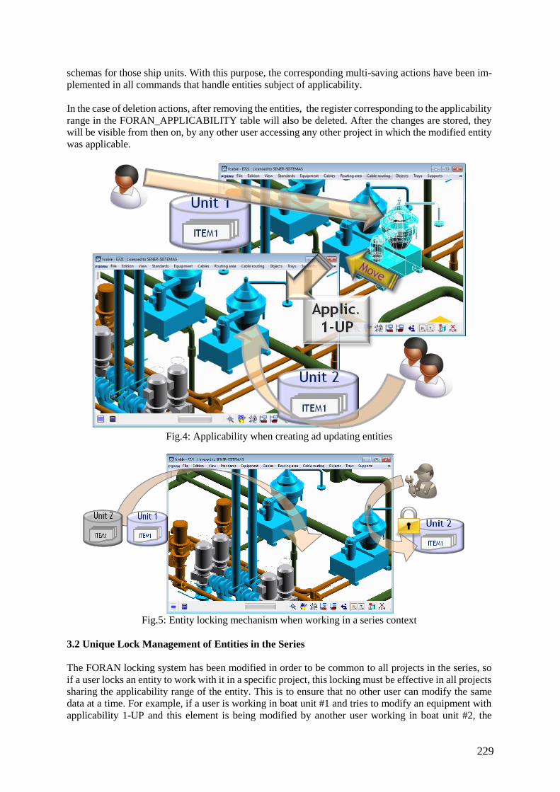
229
schemas for those ship units. With this purpose, the corresponding multi-saving actions have been im-
plemented in all commands that handle entities subject of applicability.
In the case of deletion actions, after removing the entities, the register corresponding to the applicability
range in the FORAN_APPLICABILITY table will also be deleted. After the changes are stored, they
will be visible from then on, by any other user accessing any other project in which the modified entity
was applicable.
Fig.4: Applicability when creating ad updating entities
Fig.5: Entity locking mechanism when working in a series context
3.2 Unique Lock Management of Entities in the Series
The FORAN locking system has been modified in order to be common to all projects in the series, so
if a user locks an entity to work with it in a specific project, this locking must be effective in all projects
sharing the applicability range of the entity. This is to ensure that no other user can modify the same
data at a time. For example, if a user is working in boat unit #1 and tries to modify an equipment with
applicability 1-UP and this element is being modified by another user working in boat unit #2, the

230
system will not allow the item edition by the first user and will show a message to this first user, as it
can be seen in the following images.
If this happens, the system does not allow the item edition by the first user. To enable this, it will be
necessary to add the applicability range to the existing locking keys in FORAN DB, This will apply to
all entity types subject of applicability as well as to the standards.
3.3 Managing Unique Identification of Entities in the Series
The general identification generator system will be modified to be common to all projects in the series,
so if a user creates an entity in a project of the series, the system will guarantee that the entity identifi-
cation will be also unique in all projects in the series.
This will apply to the manual introduction of identifications as well as to automatic numbering tem-
plates. If these uniqueness rules are violated when trying to create an entity, a message will be shown
to the user.
Fig.6: Warning message, when a user tries to reuse an existing identification
The default behaviour will be to not to allow the operation. However, there are some cases in which
this could be feasible:
The case in which an entity was created in the past and then was deleted. The system will allow
re-creation of the entity, depending on the entity type and the proper constraints that apply in
each case. If the entity was removed in all boat unit projects, it could be re-created again if no
other restrictions apply, but if the entity was removed within an applicability range but not in
another one, the entity will only be allowed to be re-created in the current working boat unit
project, in order to not interfere with the other projects in which it still exists. In all cases, the
entity will have to be of the same type as the former deleted one.
The case in which an entity never existed in the current boat unit project, but it does exist in
others with different applicability range. In this case, the entity will be allowed to be created,
except if some specific constraints apply to it, by default with applicability just in the current
boat unit project, but optionally in some others as well, with the only restriction of not being
applicable to other boat unit projects in which an entity of the same type and identification
already exists.
With respect to the restrictions and constraints that could prevent an entity, in one of the previous men-
tioned cases, to be created or re-created, they depend on the entity type and situation. Entities that rely
on the existence of other entities to exist (e.g. Cables) are more restricted than others than can exist by
themselves (e.g. Equipment Elements). In addition, this will also depend on the context. For example,
an Equipment Element can be created or re-created without further applicability constraints from FPIPE
module, but if it is created or re-created in a diagram in FSYSD, applicability has to be restricted to that
of the diagram, to avoid potential conflicts with other ship units in which the diagram is not applicable.
The detailed description of which creation operations could be done in each case, depending on the
entity type, will be incorporated to official FORAN documentation for each module. In case of entity
modification, if another entity of the same type already exists with the same identification, the operation
of changing the Id is not allowed.
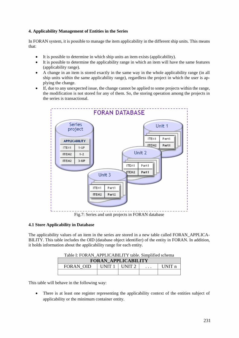
231
4. Applicability Management of Entities in the Series
In FORAN system, it is possible to manage the item applicability in the different ship units. This means
that:
It is possible to determine in which ship units an item exists (applicability).
It is possible to determine the applicability range in which an item will have the same features
(applicability range).
A change in an item is stored exactly in the same way in the whole applicability range (in all
ship units within the same applicability range), regardless the project in which the user is ap-
plying the change.
If, due to any unexpected issue, the change cannot be applied to some projects within the range,
the modification is not stored for any of them. So, the storing operation among the projects in
the series is transactional.
Fig.7: Series and unit projects in FORAN database
4.1 Store Applicability in Database
The applicability values of an item in the series are stored in a new table called FORAN_APPLICA-
BILITY. This table includes the OID (database object identifier) of the entity in FORAN. In addition,
it holds information about the applicability range for each entity.
Table I: FORAN_APPLICABILITY table. Simplified schema
FORAN_APPLICABILITY
FORAN_OID UNIT 1 UNIT 2 . . . UNIT n
This table will behave in the following way:
There is at least one register representing the applicability context of the entities subject of
applicability or the minimum container entity.
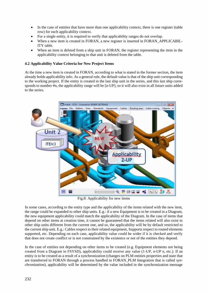
232
In the case of entities that have more than one applicability context, there is one register (table
row) for each applicability context.
For a single entity, it is required to verify that applicability ranges do not overlap.
When a new item is created in FORAN, a new register is inserted in FORAN_APPLICABIL-
ITY table.
When an item is deleted from a ship unit in FORAN, the register representing the item in the
applicability context belonging to that unit is deleted from the table.
4.2 Applicability Value Criteria for New Project Items
At the time a new item is created in FORAN, according to what is stated in the former section, the item
already holds applicability info. As a general rule, the default value is that of the ship unit corresponding
to the working project. If the entity is created in the last ship unit in the series, and this last ship corre-
sponds to number #n, the applicability range will be [n-UP], so it will also exist in all future units added
to the series.
Fig.8: Applicability for new items
In some cases, according to the entity type and the applicability of the items related with the new item,
the range could be expanded to other ship units. E.g.: if a new Equipment is to be created in a Diagram,
the new equipment applicability could match the applicability of the Diagram. In the case of items that
depend on other items at creation time, it cannot be guaranteed that the items related will also exist in
other ship units different from the current one, and so, the applicability will be by default restricted to
the current ship unit. E.g.: Cables respect to their related equipment, Supports respect to routed elements
supported, etc. Depending on each case, applicability value could be wider if it is checked and verify
that does not create conflict or is not constrained by the existence or not of the entities they depend.
In the case of entities not depending on other items to be created (e.g. Equipment elements not being
created from a Diagram in FSYSD), applicability could receive any value (1-UP, n-UP n, etc.). If an
entity is to be created as a result of a synchronization (changes on PLM entities properties and state that
are transferred to FORAN through a process handled in FORAN_PLM Integration that is called syn-
chronization), applicability will be determined by the value included in the synchronization message
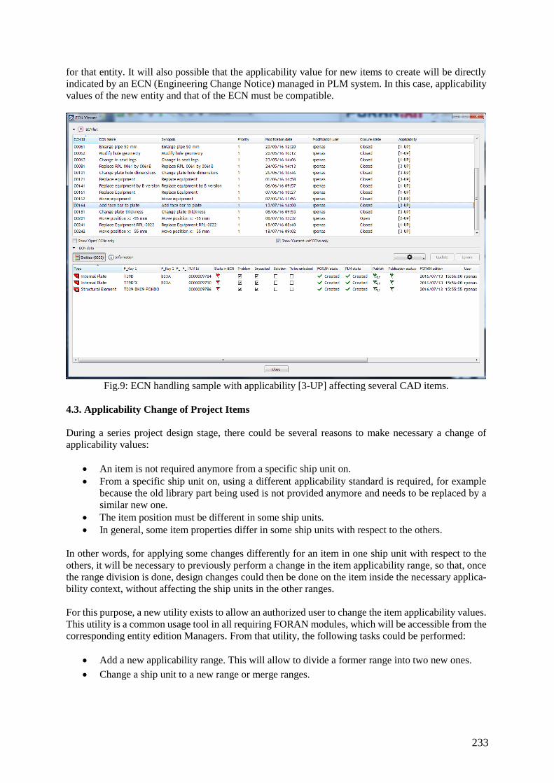
233
for that entity. It will also possible that the applicability value for new items to create will be directly
indicated by an ECN (Engineering Change Notice) managed in PLM system. In this case, applicability
values of the new entity and that of the ECN must be compatible.
Fig.9: ECN handling sample with applicability [3-UP] affecting several CAD items.
4.3. Applicability Change of Project Items
During a series project design stage, there could be several reasons to make necessary a change of
applicability values:
An item is not required anymore from a specific ship unit on.
From a specific ship unit on, using a different applicability standard is required, for example
because the old library part being used is not provided anymore and needs to be replaced by a
similar new one.
The item position must be different in some ship units.
In general, some item properties differ in some ship units with respect to the others.
In other words, for applying some changes differently for an item in one ship unit with respect to the
others, it will be necessary to previously perform a change in the item applicability range, so that, once
the range division is done, design changes could then be done on the item inside the necessary applica-
bility context, without affecting the ship units in the other ranges.
For this purpose, a new utility exists to allow an authorized user to change the item applicability values.
This utility is a common usage tool in all requiring FORAN modules, which will be accessible from the
corresponding entity edition Managers. From that utility, the following tasks could be performed:
Add a new applicability range. This will allow to divide a former range into two new ones.
Change a ship unit to a new range or merge ranges.
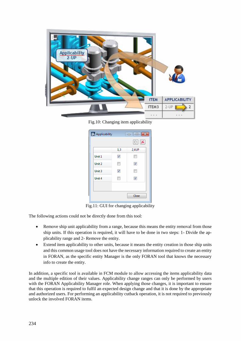
234
Fig.10: Changing item applicability
Fig.11: GUI for changing applicability
The following actions could not be directly done from this tool:
Remove ship unit applicability from a range, because this means the entity removal from those
ship units. If this operation is required, it will have to be done in two steps: 1- Divide the ap-
plicability range and 2- Remove the entity.
Extend item applicability to other units, because it means the entity creation in those ship units
and this common usage tool does not have the necessary information required to create an entity
in FORAN, as the specific entity Manager is the only FORAN tool that knows the necessary
info to create the entity.
In addition, a specific tool is available in FCM module to allow accessing the items applicability data
and the multiple edition of their values. Applicability change ranges can only be performed by users
with the FORAN Applicability Manager role. When applying those changes, it is important to ensure
that this operation is required to fulfil an expected design change and that it is done by the appropriate
and authorized users. For performing an applicability cutback operation, it is not required to previously
unlock the involved FORAN items.
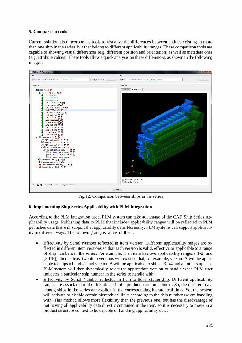
235
5. Comparison tools
Current solution also incorporates tools to visualize the differences between entities existing in more
than one ship in the series, but that belong to different applicability ranges. These comparison tools are
capable of showing visual differences (e.g. different position and orientation) as well as metadata ones
(e.g. attribute values). These tools allow a quick analysis on these differences, as shown in the following
images.
Fig.12: Comparison between ships in the series
6. Implementing Ship Series Applicability with PLM Integration
According to the PLM integration used, PLM system can take advantage of the CAD Ship Series Ap-
plicability usage. Publishing data to PLM that includes applicability ranges will be reflected in PLM
published data that will support that applicability data. Normally, PLM systems can support applicabil-
ity in different ways. The following are just a few of them:
Effectivity by Serial Number reflected in Item Version. Different applicability ranges are re-
flected in different item versions so that each version is valid, effective or applicable to a range
of ship numbers in the series. For example, if an item has two applicability ranges ([1-2] and
[3-UP]), then at least two item versions will exist so that, for example, version A will be appli-
cable to ships #1 and #2 and version B will be applicable to ships #3, #4 and all others up. The
PLM system will then dynamically select the appropriate version to handle when PLM user
indicates a particular ship number in the series to handle with.
Effectivity by Serial Number reflected in Item-to-Item relationship. Different applicability
ranges are associated to the link object in the product structure context. So, the different data
among ships in the series are explicit in the corresponding hierarchical links. So, the system
will activate or disable certain hierarchical links according to the ship number we are handling
with. This method allows more flexibility than the previous one, but has the disadvantage of
not having all applicability data directly contained in the item, so it is necessary to move in a
product structure context to be capable of handling applicability data.
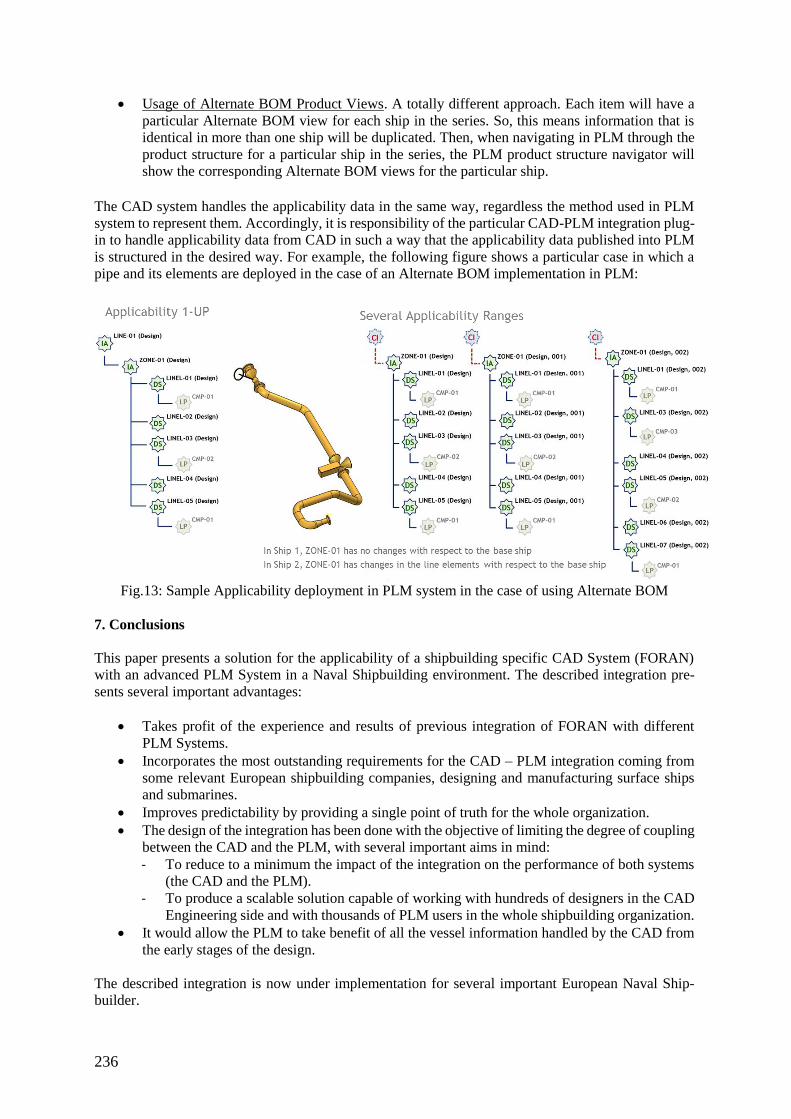
236
Usage of Alternate BOM Product Views. A totally different approach. Each item will have a
particular Alternate BOM view for each ship in the series. So, this means information that is
identical in more than one ship will be duplicated. Then, when navigating in PLM through the
product structure for a particular ship in the series, the PLM product structure navigator will
show the corresponding Alternate BOM views for the particular ship.
The CAD system handles the applicability data in the same way, regardless the method used in PLM
system to represent them. Accordingly, it is responsibility of the particular CAD-PLM integration plug-
in to handle applicability data from CAD in such a way that the applicability data published into PLM
is structured in the desired way. For example, the following figure shows a particular case in which a
pipe and its elements are deployed in the case of an Alternate BOM implementation in PLM:
Fig.13: Sample Applicability deployment in PLM system in the case of using Alternate BOM
7. Conclusions
This paper presents a solution for the applicability of a shipbuilding specific CAD System (FORAN)
with an advanced PLM System in a Naval Shipbuilding environment. The described integration pre-
sents several important advantages:
Takes profit of the experience and results of previous integration of FORAN with different
PLM Systems.
Incorporates the most outstanding requirements for the CAD – PLM integration coming from
some relevant European shipbuilding companies, designing and manufacturing surface ships
and submarines.
Improves predictability by providing a single point of truth for the whole organization.
The design of the integration has been done with the objective of limiting the degree of coupling
between the CAD and the PLM, with several important aims in mind:
- To reduce to a minimum the impact of the integration on the performance of both systems
(the CAD and the PLM).
- To produce a scalable solution capable of working with hundreds of designers in the CAD
Engineering side and with thousands of PLM users in the whole shipbuilding organization.
It would allow the PLM to take benefit of all the vessel information handled by the CAD from
the early stages of the design.
The described integration is now under implementation for several important European Naval Ship-
builder.

237
References
PEREZ, R.; LEE, D.J. (2014), An innovative approach for Korean CADres, The Naval Architect, pp.58-
61
DUNSEATH, B.; SEAR, C.; MURRAY, D.; McLAUCHLAN, J. (2007), Choosing CAD tools for the
21st Century, ICCAS 2007, Portsmouth pp.18-2.
PEREZ, R.; PENAS, R. (2015), Integration between shipbuilding CAD Systems and a generic PLM
tool in naval projects, Computer Science and Applications 2/5, pp.181-191
PEREZ, R.; GONZALEZ, C. (2015), History and evolution of shipbuilding oriented CAD tools, 14th
COMPIT, Ulrichshusen, pp.8-21
238
Ontology Based Integration of Ship Inspection Data
Marianne Hagaseth, SINTEF OCEAN, Trondheim/Norway, [email protected]
Ulrike Moser, DNV GL, Hamburg/Germany, [email protected]
Abstract
This paper describes how ontology based integration of heterogeneous ship data can be done to
provide risk models with consistent and up-to-date information, including ship particulars, inspection
results and AIS data. The purpose of the risk based inspection models is to calculate the overall risk
for each ship from a set of ships to select the one most relevant for inspection. The paper presents the
methodology to generate this ontology, an example ontology used in the SAFEPEC Tool to fetch
parameter values used by the various risk models, and the architecture of the Data Integration
Module that uses this ontology.
1. Introduction
1.1. Ontologies
An ontology formally represents the “knowledge” about a domain in a structured and computer-
readable way, Gruber (1993). With the introduction and standardization of technologies like RDFF
1,
RDF Schema and OWL1F
2 (Ontology Web Language), the possibilities of using ontologies in the field
of data integration and semantic web increased significantly, Allemang and Hendler (2008). Due to
these standards, the formal description of a domain by ontologies became executable. A digital object
(identified by an URI2F
3) has associated metadata represented by RDF. In RDF, information is
represented as a triplet containing a subject, a predicate and an object. A set of such triples is called a
RDF graph. These RDF statements make use of concepts described by an OWL ontology. The digital
objects can thus be classified by using this OWL ontology. The classification is supported by
additionally inferred RDF statements arising from the logic inside the OWL ontology, that is, the
relationships (object properties and data properties) and sub-classing defined in the OWL ontology.
The inferencing is done by components called OWL reasoners. By applying further ontologies to the
digital objects, they are classified and described with respect to these other ontologies. This means
that several ontologies can be linked to other related domains, Section 3.2.3. The OWL Ontology can
be queried using SPARQL3F
4, Section 2.2.
1.2. Challenges in Data Integration
Data integration is the task of combining different sources of data together to produce useful business
information, Underdahl (2014). In practise, these data sources may include legacy mainframe
databases, relational databases, desktop applications, social media comments, blog postings, data
fetched through web services, machine sensor data and so on. The various data sources are typically
heterogeneous, both when it comes to the structure and the semantics, Wache (2001). In addition, they
are distributed, and thus may be physically stored in different places. The interoperability problem
between the different heterogeneous data sources includes both structural and semantic heterogeneity
between the data sources. Structural heterogeneity means that the different sources has structured their
data in different data models. The difference can also be in how the physical representation of the data
is done, for instance in relational tables, xml files, web posts etc. Also, the data can be on different
level of structuration, that is, structured (e.g. relational databases), semi-structured (e.g. CSV, XML,
JSON documents, NoSQL databases) or unstructured (eg. text and multi-media content, e-mails, web
pages). Semantic heterogeneity means that the information content and the meaning of the data in the
1 RDF: standard representation for semantic data from W3C. 2 OWL: standard ontology language from the World Wide Web Consortium (W3C). 3 URI: Uniform Resource Identifier. 4 SPARQL: standard query language for semantic data from the W3C.
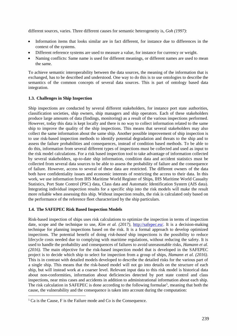
239
different sources, varies. Three different causes for semantic heterogeneity is, Goh (1997):
Information items that looks similar are in fact different, for instance due to differences in the
context of the systems.
Different reference systems are used to measure a value, for instance for currency or weight.
Naming conflicts: Same name is used for different meanings, or different names are used to mean
the same.
To achieve semantic interoperability between the data sources, the meaning of the information that is
exchanged, has to be described and understood. One way to do this is to use ontologies to describe the
semantics of the common concepts of several data sources. This is part of ontology based data
integration. 1.3. Challenges in Ship Inspection
Ship inspections are conducted by several different stakeholders, for instance port state authorities,
classification societies, ship owners, ship managers and ship operators. Each of these stakeholders
produce large amounts of data (findings, monitoring) as a result of the various inspections performed.
However, today this data is kept locally and there is no way to collect information related to the same
ship to improve the quality of the ship inspections. This means that several stakeholders may also
collect the same information about the same ship. Another possible improvement of ship inspection is
to use risk-based inspection methods to identify potential degradation and threats to the ship and to
assess the failure probabilities and consequences, instead of condition based methods. To be able to
do this, information from several different types of inspections must be collected and used as input to
the risk model calculations. For a risk based inspection tool to take advantage of information collected
by several stakeholders, up-to-date ship information, condition data and accident statistics must be
collected from several data sources to be able to assess the probability of failure and the consequence
of failure. However, access to several of these data are restricted. The different owners of the data
both have confidentiality issues and economic interests of restricting the access to their data. In this
work, we use information from IHS Maritime World Register of Ships, IHS Maritime World Casualty
Statistics, Port State Control (PSC) data, Class data and Automatic Identification System (AIS data).
Integrating individual inspection results for a specific ship into the risk models will make the result
more reliable when assessing this ship. Without inspection results, the risk is calculated only based on
the performance of the reference fleet characterized by the ship particulars.
1.4. The SAFEPEC Risk Based Inspection Models
Risk-based inspection of ships uses risk calculations to optimize the inspection in terms of inspection
date, scope and the technique to use, Kim et al. (2017), http://safepec.eu/. It is a decision-making
technique for planning inspections based on the risk. It is a formal approach to develop optimized
inspections. The potential benefit of doing risk-based ship inspections is the possibility to reduce
lifecycle costs needed due to complying with maritime regulations, without reducing the safety. It is
used to handle the probability and consequences of failures to avoid unreasonable risks, Hamann et al.
(2016). The main objective for the risk-based inspection model that is developed in the SAFEPEC
project is to decide which ship to select for inspection from a group of ships, Hamann et al. (2016).
This is in contrast with detailed models developed to describe the detailed risks for the various part of
a single ship. This means that the risk-based model will not go into details on the structure of each
ship, but will instead work at a coarser level. Relevant input data to this risk model is historical data
about non-conformities, information about deficiencies detected by port state control and class
inspections, near miss cases and accidents in addition to administrational information about each ship.
The risk calculation in SAFEPEC is done according to the following formulae5, meaning that both the
cause, the vulnerability and the consequence is taken into account during the computation:
5 Ca is the Cause, F is the Failure mode and Co is the Consequence.
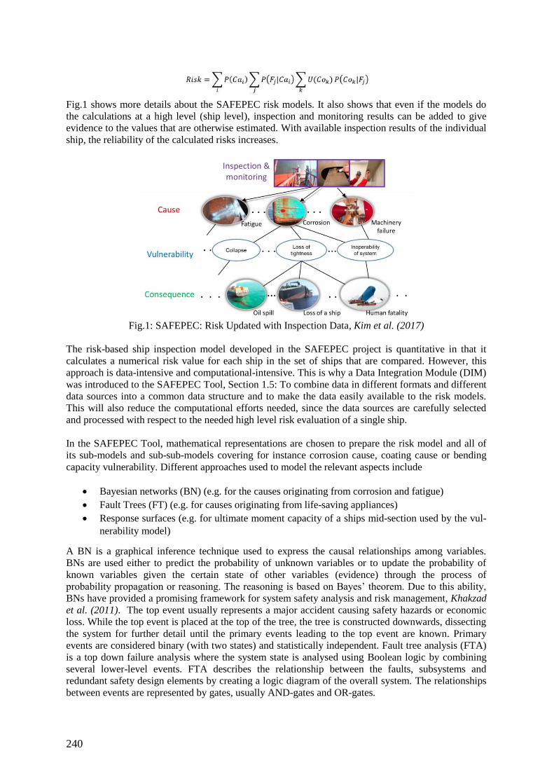
240
Fig.1 shows more details about the SAFEPEC risk models. It also shows that even if the models do
the calculations at a high level (ship level), inspection and monitoring results can be added to give
evidence to the values that are otherwise estimated. With available inspection results of the individual
ship, the reliability of the calculated risks increases.
Fig.1: SAFEPEC: Risk Updated with Inspection Data, Kim et al. (2017)
The risk-based ship inspection model developed in the SAFEPEC project is quantitative in that it
calculates a numerical risk value for each ship in the set of ships that are compared. However, this
approach is data-intensive and computational-intensive. This is why a Data Integration Module (DIM)
was introduced to the SAFEPEC Tool, Section 1.5: To combine data in different formats and different
data sources into a common data structure and to make the data easily available to the risk models.
This will also reduce the computational efforts needed, since the data sources are carefully selected
and processed with respect to the needed high level risk evaluation of a single ship.
In the SAFEPEC Tool, mathematical representations are chosen to prepare the risk model and all of
its sub-models and sub-sub-models covering for instance corrosion cause, coating cause or bending
capacity vulnerability. Different approaches used to model the relevant aspects include
Bayesian networks (BN) (e.g. for the causes originating from corrosion and fatigue)
Fault Trees (FT) (e.g. for causes originating from life-saving appliances)
Response surfaces (e.g. for ultimate moment capacity of a ships mid-section used by the vul-
nerability model)
A BN is a graphical inference technique used to express the causal relationships among variables.
BNs are used either to predict the probability of unknown variables or to update the probability of
known variables given the certain state of other variables (evidence) through the process of
probability propagation or reasoning. The reasoning is based on Bayes’ theorem. Due to this ability,
BNs have provided a promising framework for system safety analysis and risk management, Khakzad
et al. (2011). The top event usually represents a major accident causing safety hazards or economic
loss. While the top event is placed at the top of the tree, the tree is constructed downwards, dissecting
the system for further detail until the primary events leading to the top event are known. Primary
events are considered binary (with two states) and statistically independent. Fault tree analysis (FTA)
is a top down failure analysis where the system state is analysed using Boolean logic by combining
several lower-level events. FTA describes the relationship between the faults, subsystems and
redundant safety design elements by creating a logic diagram of the overall system. The relationships
between events are represented by gates, usually AND-gates and OR-gates.
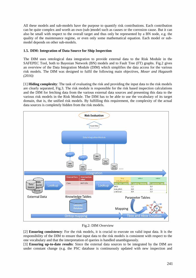
241
All these models and sub-models have the purpose to quantify risk contributions. Each contribution
can be quite complex and worth an own (sub-)model such as causes or the corrosion cause. But it can
also be small with respect to the overall target and thus only be represented by a BN node, e.g. the
quality of the maintenance regime, or even only some mathematical equation. Each model or sub-
model depends on other sub-models.
1.5. DIM: Integration of Data Source for Ship Inspection
The DIM uses ontological data integration to provide external data to the Risk Module in the
SAFEPEC Tool, both to Bayesian Network (BN) models and to Fault Tree (FT) graphs. Fig.2 gives
an overview of the Data Integration Module (DIM) which simplifies the data access for the various
risk models. The DIM was designed to fulfil the following main objectives, Moser and Hagaseth
(2016):
[1] Hiding complexity: The task of evaluating the risk and providing the input data to the risk models
are clearly separated, Fig.3. The risk module is responsible for the risk based inspection calculations
and the DIM for fetching data from the various external data sources and presenting this data to the
various risk models in the Risk Module. The DIM has to be able to use the vocabulary of its target
domain, that is, the unified risk models. By fulfilling this requirement, the complexity of the actual
data sources is completely hidden from the risk models.
Fig.2: DIM Overview
[2] Ensuring consistency: For the risk models, it is crucial to execute on valid input data. It is the
responsibility of the DIM to ensure that input data to the risk models is consistent with respect to the
one vocabulary and that the interpretation of queries is handled unambiguously.
[3] Ensuring up-to-date results: Since the external data sources to be integrated by the DIM are
under constant change (e.g. the PSC database is continuously updated with new inspection and
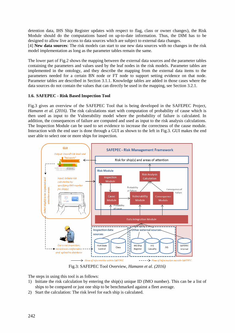
242
detention data, IHS Ship Register updates with respect to flag, class or owner changes), the Risk
Module should do the computations based on up-to-date information. Thus, the DIM has to be
designed to allow live access to data sources which are subject to external data changes.
[4] New data sources: The risk models can start to use new data sources with no changes in the risk
model implementation as long as the parameter tables remain the same.
The lower part of Fig.2 shows the mapping between the external data sources and the parameter tables
containing the parameters and values used by the leaf nodes in the risk models. Parameter tables are
implemented in the ontology, and they describe the mapping from the external data items to the
parameters needed for a certain BN node or FT node to support setting evidence on that node.
Parameter tables are described in Section 3.1.1. Knowledge tables are added in those cases where the
data sources do not contain the values that can directly be used in the mapping, see Section 3.2.1.
1.6. SAFEPEC - Risk Based Inspection Tool
Fig.3 gives an overview of the SAFEPEC Tool that is being developed in the SAFEPEC Project,
Hamann et al. (2016). The risk calculations start with computation of probability of cause which is
then used as input to the Vulnerability model where the probability of failure is calculated. In
addition, the consequences of failure are computed and used as input to the risk analysis calculations.
The Inspection Module can be used to set evidence to increase the correctness of the cause module.
Interaction with the end user is done through a GUI as shown to the left in Fig.3. GUI makes the end
user able to select one or more ships for inspection.
Fig.3: SAFEPEC Tool Overview, Hamann et al. (2016)
The steps in using this tool is as follows:
1) Initiate the risk calculation by entering the ship(s) unique ID (IMO number). This can be a list of
ships to be compared or just one ship to be benchmarked against a fleet average.
2) Start the calculation: The risk level for each ship is calculated.
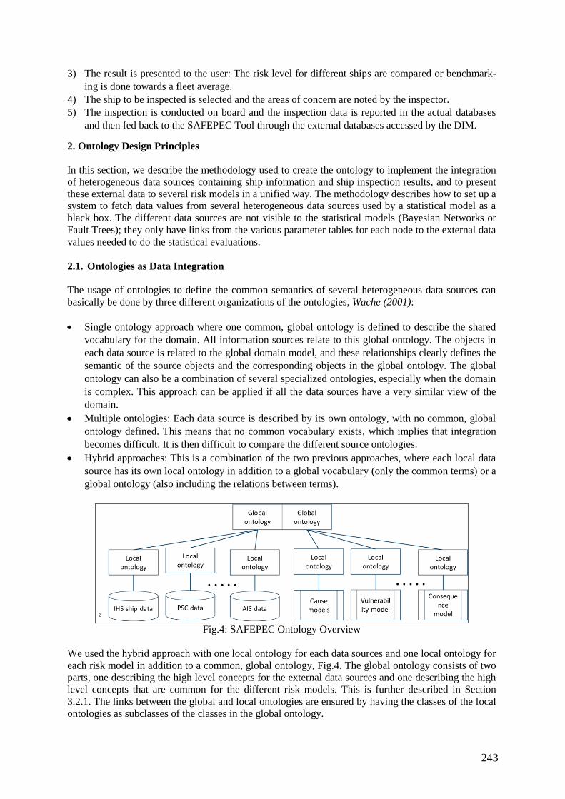
243
3) The result is presented to the user: The risk level for different ships are compared or benchmark-
ing is done towards a fleet average.
4) The ship to be inspected is selected and the areas of concern are noted by the inspector.
5) The inspection is conducted on board and the inspection data is reported in the actual databases
and then fed back to the SAFEPEC Tool through the external databases accessed by the DIM.
2. Ontology Design Principles
In this section, we describe the methodology used to create the ontology to implement the integration
of heterogeneous data sources containing ship information and ship inspection results, and to present
these external data to several risk models in a unified way. The methodology describes how to set up a
system to fetch data values from several heterogeneous data sources used by a statistical model as a
black box. The different data sources are not visible to the statistical models (Bayesian Networks or
Fault Trees); they only have links from the various parameter tables for each node to the external data
values needed to do the statistical evaluations.
2.1. Ontologies as Data Integration
The usage of ontologies to define the common semantics of several heterogeneous data sources can
basically be done by three different organizations of the ontologies, Wache (2001):
Single ontology approach where one common, global ontology is defined to describe the shared
vocabulary for the domain. All information sources relate to this global ontology. The objects in
each data source is related to the global domain model, and these relationships clearly defines the
semantic of the source objects and the corresponding objects in the global ontology. The global
ontology can also be a combination of several specialized ontologies, especially when the domain
is complex. This approach can be applied if all the data sources have a very similar view of the
domain.
Multiple ontologies: Each data source is described by its own ontology, with no common, global
ontology defined. This means that no common vocabulary exists, which implies that integration
becomes difficult. It is then difficult to compare the different source ontologies.
Hybrid approaches: This is a combination of the two previous approaches, where each local data
source has its own local ontology in addition to a global vocabulary (only the common terms) or a
global ontology (also including the relations between terms).
Fig.4: SAFEPEC Ontology Overview
We used the hybrid approach with one local ontology for each data sources and one local ontology for
each risk model in addition to a common, global ontology, Fig.4. The global ontology consists of two
parts, one describing the high level concepts for the external data sources and one describing the high
level concepts that are common for the different risk models. This is further described in Section
3.2.1. The links between the global and local ontologies are ensured by having the classes of the local
ontologies as subclasses of the classes in the global ontology.
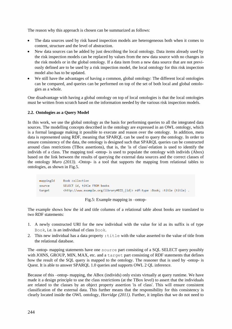
244
The reason why this approach is chosen can be summarized as follows:
The data sources used by risk based inspection models are heterogeneous both when it comes to
content, structure and the level of abstraction.
New data sources can be added by just describing the local ontology. Data items already used by
the risk inspection models can be replaced by values from the new data source with no changes in
the risk models or in the global ontology. If a data item from a new data source that are not previ-
ously defined are to be used by a risk inspection model, the local ontology for this risk inspection
model also has to be updated.
We still have the advantages of having a common, global ontology: The different local ontologies
can be compared, and queries can be performed on top of the set of both local and global ontolo-
gies as a whole.
One disadvantage with having a global ontology on top of local ontologies is that the local ontologies
must be written from scratch based on the information needed by the various risk inspection models.
2.2. Ontologies as a Query Model
In this work, we use the global ontology as the basis for performing queries to all the integrated data
sources. The modelling concepts described in the ontology are expressed in an OWL ontology, which
is a formal language making it possible to execute and reason over the ontology. In addition, meta
data is represented using RDF, meaning that SPARQL can be used to query the ontology. In order to
ensure consistency of the data, the ontology is designed such that SPARQL queries can be constructed
around class restrictions (TBox assertions), that is, the 'is of class'-relation is used to identify the
individs of a class. The mapping tool -ontop- is used to populate the ontology with individs (Abox)
based on the link between the results of querying the external data sources and the correct classes of
the ontology Muro (2013). -Ontop- is a tool that supports the mapping from relational tables to
ontologies, as shown in Fig.5.
Fig.5: Example mapping in –ontop-
The example shows how the id and title columns of a relational table about books are translated to
two RDF statements:
1. A newly constructed URI for the new individual with the value for id as its suffix is of type
Book, i.e. is an individual of class Book.
2. This new individual has a data property :title with the value asserted to the value of title from
the relational database.
The -ontop- mapping statements have one source part consisting of a SQL SELECT query possibly
with JOINS, GROUP, MIN, MAX, etc. and a target part consisting of RDF statements that defines
how the result of the SQL query is mapped to the ontology. The reasoner that is used by -ontop- is
Quest. It is able to answer SPARQL 1.0 queries and supports OWL 2 QL inference.
Because of this –ontop- mapping, the ABox (individs) only exists virtually at query runtime. We have
made it a design principle to use the class restrictions (at the TBox level) to assert that the individuals
are related to the classes by an object property assertion 'is of class'. This will ensure consistent
classification of the external data. This further means that the responsibility for this consistency is
clearly located inside the OWL ontology, Horridge (2011). Further, it implies that we do not need to
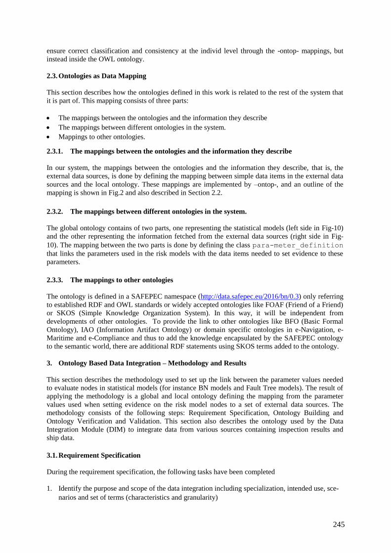
245
ensure correct classification and consistency at the individ level through the -ontop- mappings, but
instead inside the OWL ontology.
2.3. Ontologies as Data Mapping
This section describes how the ontologies defined in this work is related to the rest of the system that
it is part of. This mapping consists of three parts:
The mappings between the ontologies and the information they describe
The mappings between different ontologies in the system.
Mappings to other ontologies.
2.3.1. The mappings between the ontologies and the information they describe
In our system, the mappings between the ontologies and the information they describe, that is, the
external data sources, is done by defining the mapping between simple data items in the external data
sources and the local ontology. These mappings are implemented by –ontop-, and an outline of the
mapping is shown in Fig.2 and also described in Section 2.2.
2.3.2. The mappings between different ontologies in the system.
The global ontology contains of two parts, one representing the statistical models (left side in Fig-10)
and the other representing the information fetched from the external data sources (right side in Fig-
10). The mapping between the two parts is done by defining the class para-meter_definition
that links the parameters used in the risk models with the data items needed to set evidence to these
parameters.
2.3.3. The mappings to other ontologies
The ontology is defined in a SAFEPEC namespace (http://data.safepec.eu/2016/bn/0.3) only referring
to established RDF and OWL standards or widely accepted ontologies like FOAF (Friend of a Friend)
or SKOS (Simple Knowledge Organization System). In this way, it will be independent from
developments of other ontologies. To provide the link to other ontologies like BFO (Basic Formal
Ontology), IAO (Information Artifact Ontology) or domain specific ontologies in e-Navigation, e-
Maritime and e-Compliance and thus to add the knowledge encapsulated by the SAFEPEC ontology
to the semantic world, there are additional RDF statements using SKOS terms added to the ontology.
3. Ontology Based Data Integration – Methodology and Results
This section describes the methodology used to set up the link between the parameter values needed
to evaluate nodes in statistical models (for instance BN models and Fault Tree models). The result of
applying the methodology is a global and local ontology defining the mapping from the parameter
values used when setting evidence on the risk model nodes to a set of external data sources. The
methodology consists of the following steps: Requirement Specification, Ontology Building and
Ontology Verification and Validation. This section also describes the ontology used by the Data
Integration Module (DIM) to integrate data from various sources containing inspection results and
ship data.
3.1. Requirement Specification
During the requirement specification, the following tasks have been completed
1. Identify the purpose and scope of the data integration including specialization, intended use, sce-
narios and set of terms (characteristics and granularity)
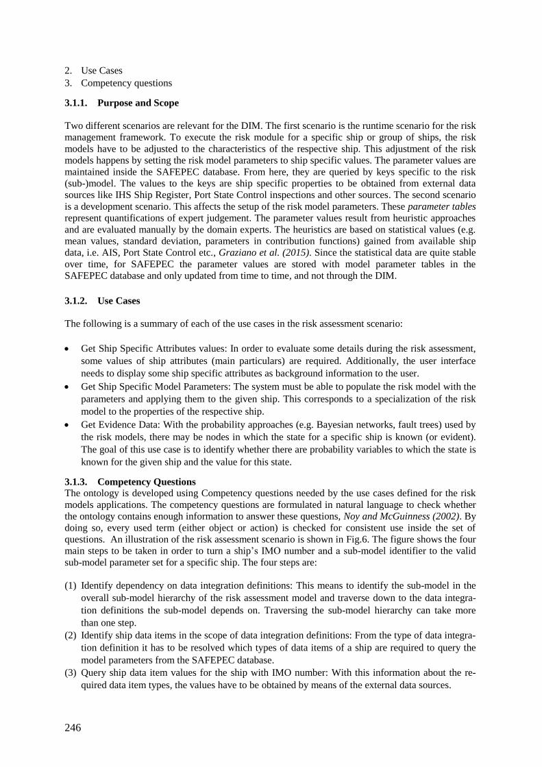
246
2. Use Cases
3. Competency questions
3.1.1. Purpose and Scope
Two different scenarios are relevant for the DIM. The first scenario is the runtime scenario for the risk
management framework. To execute the risk module for a specific ship or group of ships, the risk
models have to be adjusted to the characteristics of the respective ship. This adjustment of the risk
models happens by setting the risk model parameters to ship specific values. The parameter values are
maintained inside the SAFEPEC database. From here, they are queried by keys specific to the risk
(sub-)model. The values to the keys are ship specific properties to be obtained from external data
sources like IHS Ship Register, Port State Control inspections and other sources. The second scenario
is a development scenario. This affects the setup of the risk model parameters. These parameter tables
represent quantifications of expert judgement. The parameter values result from heuristic approaches
and are evaluated manually by the domain experts. The heuristics are based on statistical values (e.g.
mean values, standard deviation, parameters in contribution functions) gained from available ship
data, i.e. AIS, Port State Control etc., Graziano et al. (2015). Since the statistical data are quite stable
over time, for SAFEPEC the parameter values are stored with model parameter tables in the
SAFEPEC database and only updated from time to time, and not through the DIM.
3.1.2. Use Cases
The following is a summary of each of the use cases in the risk assessment scenario:
Get Ship Specific Attributes values: In order to evaluate some details during the risk assessment,
some values of ship attributes (main particulars) are required. Additionally, the user interface
needs to display some ship specific attributes as background information to the user.
Get Ship Specific Model Parameters: The system must be able to populate the risk model with the
parameters and applying them to the given ship. This corresponds to a specialization of the risk
model to the properties of the respective ship.
Get Evidence Data: With the probability approaches (e.g. Bayesian networks, fault trees) used by
the risk models, there may be nodes in which the state for a specific ship is known (or evident).
The goal of this use case is to identify whether there are probability variables to which the state is
known for the given ship and the value for this state.
3.1.3. Competency Questions
The ontology is developed using Competency questions needed by the use cases defined for the risk
models applications. The competency questions are formulated in natural language to check whether
the ontology contains enough information to answer these questions, Noy and McGuinness (2002). By
doing so, every used term (either object or action) is checked for consistent use inside the set of
questions. An illustration of the risk assessment scenario is shown in Fig.6. The figure shows the four
main steps to be taken in order to turn a ship’s IMO number and a sub-model identifier to the valid
sub-model parameter set for a specific ship. The four steps are:
(1) Identify dependency on data integration definitions: This means to identify the sub-model in the
overall sub-model hierarchy of the risk assessment model and traverse down to the data integra-
tion definitions the sub-model depends on. Traversing the sub-model hierarchy can take more
than one step.
(2) Identify ship data items in the scope of data integration definitions: From the type of data integra-
tion definition it has to be resolved which types of data items of a ship are required to query the
model parameters from the SAFEPEC database.
(3) Query ship data item values for the ship with IMO number: With this information about the re-
quired data item types, the values have to be obtained by means of the external data sources.
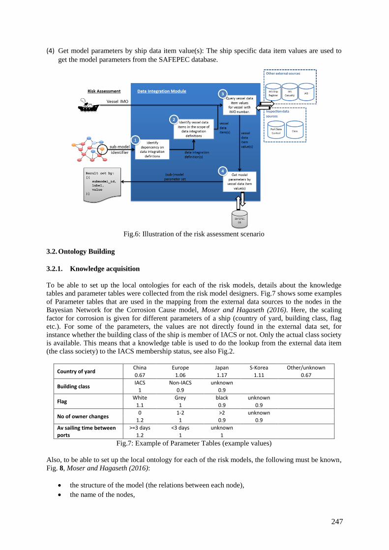
247
(4) Get model parameters by ship data item value(s): The ship specific data item values are used to
get the model parameters from the SAFEPEC database.
Fig.6: Illustration of the risk assessment scenario
3.2. Ontology Building
3.2.1. Knowledge acquisition
To be able to set up the local ontologies for each of the risk models, details about the knowledge
tables and parameter tables were collected from the risk model designers. Fig.7 shows some examples
of Parameter tables that are used in the mapping from the external data sources to the nodes in the
Bayesian Network for the Corrosion Cause model, Moser and Hagaseth (2016). Here, the scaling
factor for corrosion is given for different parameters of a ship (country of yard, building class, flag
etc.). For some of the parameters, the values are not directly found in the external data set, for
instance whether the building class of the ship is member of IACS or not. Only the actual class society
is available. This means that a knowledge table is used to do the lookup from the external data item
(the class society) to the IACS membership status, see also Fig.2.
Country of yard China Europe Japan S-Korea Other/unknown
0.67 1.06 1.17 1.11 0.67
Building class IACS Non-IACS unknown
1 0.9 0.9
Flag White Grey black unknown
1.1 1 0.9 0.9
No of owner changes 0 1-2 >2 unknown
1.2 1 0.9 0.9
Av sailing time between ports
>=3 days <3 days unknown
1.2 1 1
Fig.7: Example of Parameter Tables (example values)
Also, to be able to set up the local ontology for each of the risk models, the following must be known,
Fig. 8, Moser and Hagaseth (2016):
the structure of the model (the relations between each node),
the name of the nodes,
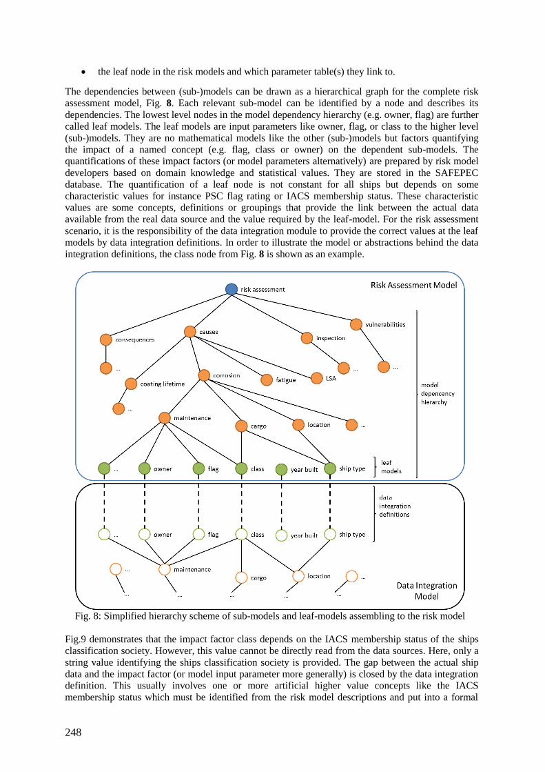
248
the leaf node in the risk models and which parameter table(s) they link to.
The dependencies between (sub-)models can be drawn as a hierarchical graph for the complete risk
assessment model, Fig. 8. Each relevant sub-model can be identified by a node and describes its
dependencies. The lowest level nodes in the model dependency hierarchy (e.g. owner, flag) are further
called leaf models. The leaf models are input parameters like owner, flag, or class to the higher level
(sub-)models. They are no mathematical models like the other (sub-)models but factors quantifying
the impact of a named concept (e.g. flag, class or owner) on the dependent sub-models. The
quantifications of these impact factors (or model parameters alternatively) are prepared by risk model
developers based on domain knowledge and statistical values. They are stored in the SAFEPEC
database. The quantification of a leaf node is not constant for all ships but depends on some
characteristic values for instance PSC flag rating or IACS membership status. These characteristic
values are some concepts, definitions or groupings that provide the link between the actual data
available from the real data source and the value required by the leaf-model. For the risk assessment
scenario, it is the responsibility of the data integration module to provide the correct values at the leaf
models by data integration definitions. In order to illustrate the model or abstractions behind the data
integration definitions, the class node from Fig. 8 is shown as an example.
Fig. 8: Simplified hierarchy scheme of sub-models and leaf-models assembling to the risk model
Fig.9 demonstrates that the impact factor class depends on the IACS membership status of the ships
classification society. However, this value cannot be directly read from the data sources. Here, only a
string value identifying the ships classification society is provided. The gap between the actual ship
data and the impact factor (or model input parameter more generally) is closed by the data integration
definition. This usually involves one or more artificial higher value concepts like the IACS
membership status which must be identified from the risk model descriptions and put into a formal
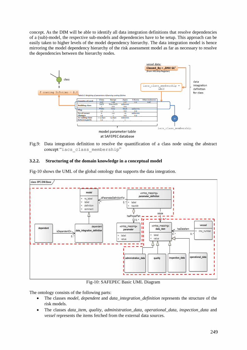
249
concept. As the DIM will be able to identify all data integration definitions that resolve dependencies
of a (sub)-model, the respective sub-models and dependencies have to be setup. This approach can be
easily taken to higher levels of the model dependency hierarchy. The data integration model is hence
mirroring the model dependency hierarchy of the risk assessment model as far as necessary to resolve
the dependencies between the hierarchy nodes.
Fig.9: Data integration definition to resolve the quantification of a class node using the abstract
concept “iacs_class_membership”
3.2.2. Structuring of the domain knowledge in a conceptual model
Fig-10 shows the UML of the global ontology that supports the data integration.
Fig-10: SAFEPEC Basic UML Diagram
The ontology consists of the following parts:
The classes model, dependent and data_integration_definition represents the structure of the
risk models.
The classes data_item, quality, administration_data, operational_data, inspection_data and
vessel represents the items fetched from the external data sources.
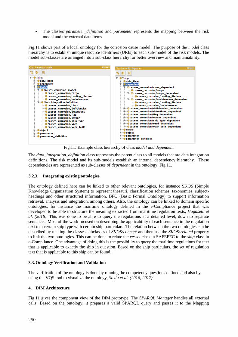
250
The classes parameter_definition and parameter represents the mapping between the risk
model and the external data items.
Fig.11 shows part of a local ontology for the corrosion cause model. The purpose of the model class
hierarchy is to establish unique resource identifiers (URIs) to each sub-model of the risk models. The
model sub-classes are arranged into a sub-class hierarchy for better overview and maintainability.
Fig.11: Example class hierarchy of class model and dependent
The data_integration_definition class represents the parent class to all models that are data integration
definitions. The risk model and its sub-models establish an internal dependency hierarchy. These
dependencies are represented as sub-classes of dependent in the ontology, Fig.11.
3.2.3. Integrating existing ontologies
The ontology defined here can be linked to other relevant ontologies, for instance SKOS (Simple
Knowledge Organization System) to represent thesauri, classification schemes, taxonomies, subject-
headings and other structured information, BFO (Basic Formal Ontology) to support information
retrieval, analysis and integration, among others. Also, the ontology can be linked to domain specific
ontologies, for instance the maritime ontology defined in the e-Compliance project that was
developed to be able to structure the meaning extracted from maritime regulation texts, Hagaseth et
al. (2016). This was done to be able to query the regulations at a detailed level, down to separate
sentences. Most of the work focused on describing the applicability of each sentence in the regulation
text to a certain ship type with certain ship particulars. The relation between the two ontologies can be
described by making the classes subclasses of SKOS:concept and then use the SKOS:related property
to link the two ontologies. This can be done to relate the vessel class in SAFEPEC to the ship class in
e-Compliance. One advantage of doing this is the possibility to query the maritime regulations for text
that is applicable to exactly the ship in question. Based on the ship particulars, the set of regulation
text that is applicable to this ship can be found.
3.3. Ontology Verification and Validation
The verification of the ontology is done by running the competency questions defined and also by
using the VQS tool to visualize the ontology, Soylu et al. (2016, 2017).
4. DIM Architecture
Fig.11 gives the component view of the DIM prototype. The SPARQL Manager handles all external
calls. Based on the ontology, it prepares a valid SPARQL query and passes it to the Mapping
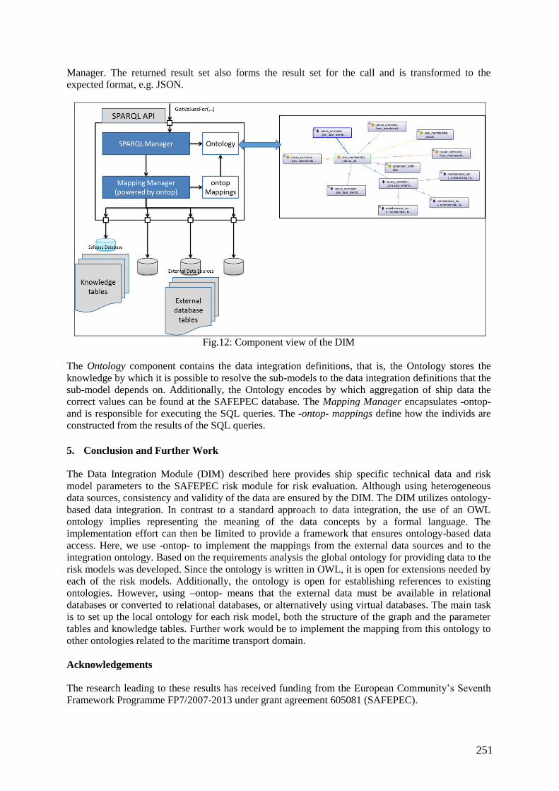
251
Manager. The returned result set also forms the result set for the call and is transformed to the
expected format, e.g. JSON.
Fig.12: Component view of the DIM
The Ontology component contains the data integration definitions, that is, the Ontology stores the
knowledge by which it is possible to resolve the sub-models to the data integration definitions that the
sub-model depends on. Additionally, the Ontology encodes by which aggregation of ship data the
correct values can be found at the SAFEPEC database. The Mapping Manager encapsulates -ontop-
and is responsible for executing the SQL queries. The -ontop- mappings define how the individs are
constructed from the results of the SQL queries.
5. Conclusion and Further Work
The Data Integration Module (DIM) described here provides ship specific technical data and risk
model parameters to the SAFEPEC risk module for risk evaluation. Although using heterogeneous
data sources, consistency and validity of the data are ensured by the DIM. The DIM utilizes ontology-
based data integration. In contrast to a standard approach to data integration, the use of an OWL
ontology implies representing the meaning of the data concepts by a formal language. The
implementation effort can then be limited to provide a framework that ensures ontology-based data
access. Here, we use -ontop- to implement the mappings from the external data sources and to the
integration ontology. Based on the requirements analysis the global ontology for providing data to the
risk models was developed. Since the ontology is written in OWL, it is open for extensions needed by
each of the risk models. Additionally, the ontology is open for establishing references to existing
ontologies. However, using –ontop- means that the external data must be available in relational
databases or converted to relational databases, or alternatively using virtual databases. The main task
is to set up the local ontology for each risk model, both the structure of the graph and the parameter
tables and knowledge tables. Further work would be to implement the mapping from this ontology to
other ontologies related to the maritime transport domain.
Acknowledgements
The research leading to these results has received funding from the European Community’s Seventh
Framework Programme FP7/2007-2013 under grant agreement 605081 (SAFEPEC).

252
References
ALLEMANG, D.; HENDLER, J. (2008), Semantic Web for the Working Ontologist, ISBN:
9780123859655
GOH, C.H. (1997), Representing and Reasoning about Semantic Conflicts in Heterogeneous Infor-
mation Sources, PhD Thesis, MIT
GRAZIANO, A. et al. (2015) SAFEPEC D1.1 - State of the art of ship safety-related data sources,
http://195.23.37.205/wp-content/uploads/2016/10/Executive-Summary-D1.1.pdf
GRUBER, T.R. (1993), A translation approach to portable ontology specifications, Knowledge Ac-
quisition 5(2), pp.199-220
HAGASETH, M.; LOHRMANN, P.; RUIZ, A.; OIKONOMOU, F.; ROYTHORNE, D.; RAYOT, S.
(2016), Digital maritime regulations: Applications to ships and ports, 7th Int. Conf. Maritime
Transport, Universitat Politècnica de Catalunya, pp.59-81
HAMANN, R.; KÄHLER, N.; STRAUB, D.; KIM, H.J.; VENTIKOS, N.; SOTIRALIS, N.;
VALKONEN, J. (2016), Generic risk models for ship inspection based on readily available
information, Int. Conf. Maritime Safety and Operations
HORRIDGE, M. (2011), A Practical Guide To Building OWL Ontologies Using Protégé 4 and CO-
ODE Tools Edition 1.3
http://mowl-power.cs.man.ac.uk/protegeowltutorial/resources/ProtegeOWLTutorialP4_v1_3.pdf .
KHAKZAD, N,.;KHAN, F.; AMYOTTE P. (2011), Safety analysis in process facilities: Comparison
of fault tree and Bayesian network approaches, Reliability Eng. and System Safety 96, pp.925-932
KIM, H.J.; HAMANN, R.; PESCHMANN J.; STRAUB D. (2017), Vulnerability and risk assessment
of ship structures via a Bayesian network model, 7th Int. Conf. Computational Methods in Marine
Engineering
MOSER, U.; HAGASETH M. (2016) SAFEPEC Deliverable D2.1: Standards for Exchange of Ship
Inspection Data, Report from SAFEPEC project
MURO, M. R. (2013) ontop: A Tutorial. http://de.slideshare.net/marianomx/ontop-a-tutorial
NOY, N.F.; McGUINNESS, D. L. (2002), Ontology Development 101: A Guide to Creating Your
First Ontology,
http://protege.stanford.edu/publications/ontology_development/ontology101-noy-mcguinness.html
SOYLU, A.; GIESE M.; JIMENEZ-RUIZ E.; VEGA-GORGOJO G.; HORROCKS I. (2016),
Experiencing OptiqueVQS: a multi-paradigm and ontology-based visual query system for end users,
Universal Access in the Information Society 15(1), pp.129-152
SOYLU, A.; KHARLAMOV, E.; ZHELEZNYAKOV, D; JIMENEZ-RUIZ, E.; GIESE, M.; SKJAE-
VELAND, M.G.; HOVLAND, D.; SCHLATTE, R.; BRANDT, S.; LIE, H.; HORROCKS, I. (2017),
OptiqueVQS: a Visual Query System over Ontologies for Industry, Semantic Web
UNDERDAHL, B. (2014), Data integration for dummies - Informatica special edition, Wiley & Sons
WACHE, H.; VÖGELE, T.; VISSER, U.; STUCKENSCHMIDT, H.; SCHUSTER, G.; NEUMANN,
H.; HÜBNER, S. (2001), Ontology-Based Integration of Information - A Survey of Existing
Approaches, http://ceur-ws.org/Vol-47/wache.pdf
253
Preparing for a Digital Future –
Experiences and Implications from a Maritime Domain Perspective
André Keane, Ulstein International, Ulsteinvik/Norway, [email protected]
Per Olaf Brett, Ulstein International, Ulsteinvik/Norway, [email protected]
Ali Ebrahimi, Ulstein International, Ulsteinvik/Norway, [email protected]
Henrique M. Gaspar, NTNU, Aalesund/Norway, [email protected]
Jose Jorge Garcia Agis, NTNU, Trondheim/Norway, [email protected]
Abstract
The re-emergence and subsequently increased credibility of big data analytics to support and enhance
effective decision-making in recent years, comes largely because of significantly increased available
computing power, which has consequently caused a dramatic spur in the generation of new applications
encroaching upon the normalcy of business processes and models. Maritime industries are often
attributed with an elaborate complexity, which often protrudes the difficulties of state-of-the-art
technology adaptations and implementations that have not been developed natively within the industry.
As such, there is a clear need for a modern, systemic, and methodological approach so that more
traditionally inclined industries not only can utilize such digital enhancements, but embrace it to further
contribute towards previously incomprehensible applications and provide enhanced sustainability
including but not limited to higher productivity and new business opportunities. This paper examines
the empirical and implicational facets of embracing digital technologies in the maritime domain from
a Big Data Analytics handling perspective. It presents an introduction on the emergence of digital
technology, discusses the challenge of integrating such innovations into the traditional maritime
business and presents a few examples from Ulstein digital experiences.
1. Extended Systems of Systems Boundaries and its Effect on Traditional Maritime Business
With over 90% of the world trade being carried by ships, the maritime industry is, more than ever, an
integral part of the process of globalization, which makes it strongly dependent of the world behaviour.
As such, the industry is influenced by factors such as economy, trade, production, consumption, politics,
financing, and technology that drive the demand and supply of manufactured goods, raw materials, and
shipping services, Stopford (2009).
Companies operating in the maritime business are challenged by much more extended and somehow
liquid system of systems boundaries, a VUCA world. Volatility, complexity, uncertainty, and ambiguity
(VUCA) coexist in many industries, Bennet and Lemoine (2014), maritime being one of them. VUCA
aspects characterize the technical and managerial development of firms, limiting innovation, and
challenging the implementation of new technologies, Corsi and Akhunov (2000). Fuel prices, market
supply or demand are volatile variables. They are influenced by a diverse list of factors that makes them
unpredictable. Although we know they are continuously changing, it is very difficult or impossible to
predict their exact behaviour. Volatility covers the expected but unpredictable. Fuel price is one of the
volatile factors with stronger influence in the maritime industries. Uncertainty, contrary to volatility,
refers to changes that are not expected. New regulations, new market entrants (products, services, or
business models) or natural disasters are typical examples of uncertainties affecting the maritime
industry. Both, volatility, and uncertainty can be assessed by simulation of future scenarios, Schoemaker
and van der Haijden (1992), which improves the agility of the company in reacting towards
unpredictable or unexpected changes. Data availability, storage capacity and increasing capability are
key drivers in mitigating future uncertainty, and the emergence of Big Data Analytics and Artificial
Intelligence (AI) bring with them capabilities that will undoubtedly further our understanding the
technology is matured.
The complexity of the maritime industry and its corresponding decision-making processes are a cause
of the large variety of operations, operational environments, and multitude of stakeholders. This
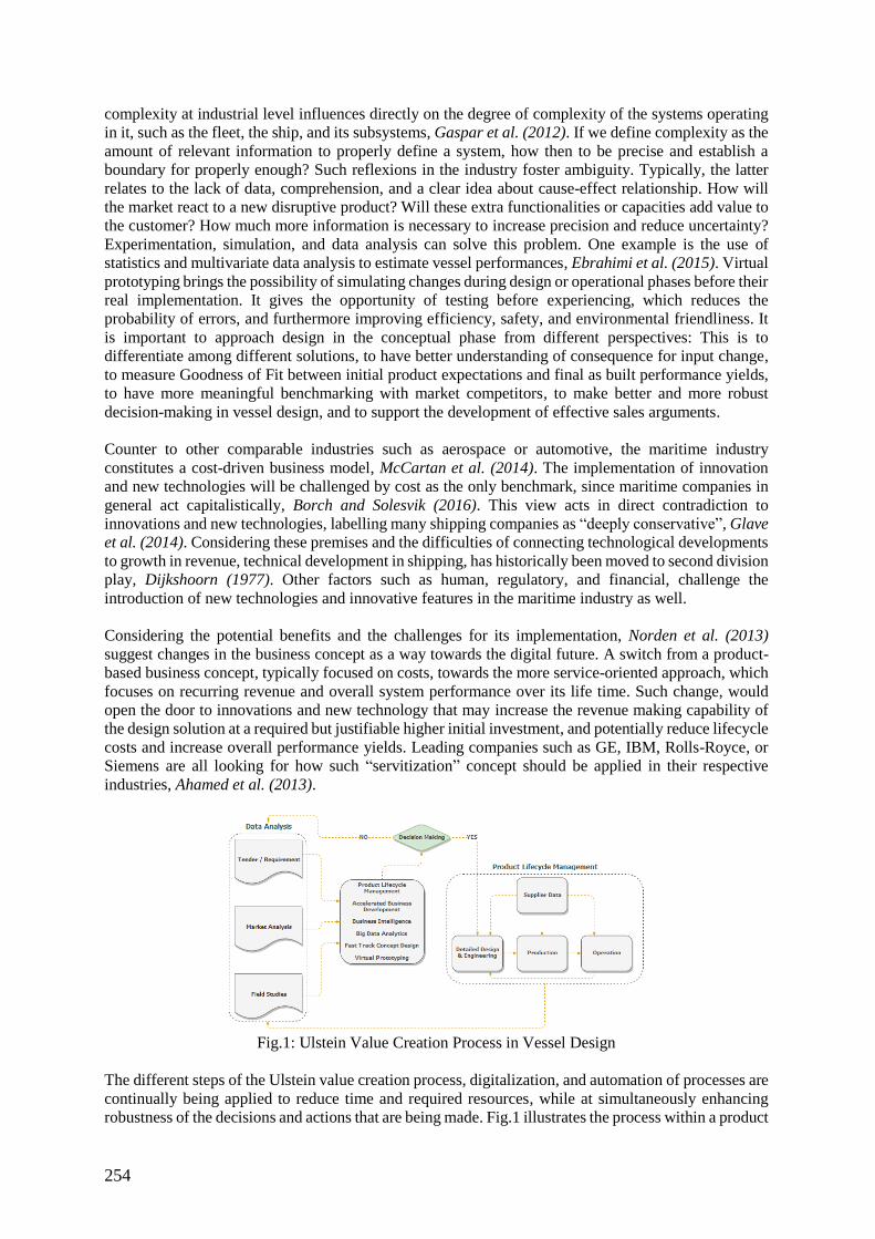
254
complexity at industrial level influences directly on the degree of complexity of the systems operating
in it, such as the fleet, the ship, and its subsystems, Gaspar et al. (2012). If we define complexity as the
amount of relevant information to properly define a system, how then to be precise and establish a
boundary for properly enough? Such reflexions in the industry foster ambiguity. Typically, the latter
relates to the lack of data, comprehension, and a clear idea about cause-effect relationship. How will
the market react to a new disruptive product? Will these extra functionalities or capacities add value to
the customer? How much more information is necessary to increase precision and reduce uncertainty?
Experimentation, simulation, and data analysis can solve this problem. One example is the use of
statistics and multivariate data analysis to estimate vessel performances, Ebrahimi et al. (2015). Virtual
prototyping brings the possibility of simulating changes during design or operational phases before their
real implementation. It gives the opportunity of testing before experiencing, which reduces the
probability of errors, and furthermore improving efficiency, safety, and environmental friendliness. It
is important to approach design in the conceptual phase from different perspectives: This is to
differentiate among different solutions, to have better understanding of consequence for input change,
to measure Goodness of Fit between initial product expectations and final as built performance yields,
to have more meaningful benchmarking with market competitors, to make better and more robust
decision-making in vessel design, and to support the development of effective sales arguments.
Counter to other comparable industries such as aerospace or automotive, the maritime industry
constitutes a cost-driven business model, McCartan et al. (2014). The implementation of innovation
and new technologies will be challenged by cost as the only benchmark, since maritime companies in
general act capitalistically, Borch and Solesvik (2016). This view acts in direct contradiction to
innovations and new technologies, labelling many shipping companies as “deeply conservative”, Glave
et al. (2014). Considering these premises and the difficulties of connecting technological developments
to growth in revenue, technical development in shipping, has historically been moved to second division
play, Dijkshoorn (1977). Other factors such as human, regulatory, and financial, challenge the
introduction of new technologies and innovative features in the maritime industry as well.
Considering the potential benefits and the challenges for its implementation, Norden et al. (2013)
suggest changes in the business concept as a way towards the digital future. A switch from a product-
based business concept, typically focused on costs, towards the more service-oriented approach, which
focuses on recurring revenue and overall system performance over its life time. Such change, would
open the door to innovations and new technology that may increase the revenue making capability of
the design solution at a required but justifiable higher initial investment, and potentially reduce lifecycle
costs and increase overall performance yields. Leading companies such as GE, IBM, Rolls-Royce, or
Siemens are all looking for how such “servitization” concept should be applied in their respective
industries, Ahamed et al. (2013).
Fig.1: Ulstein Value Creation Process in Vessel Design
The different steps of the Ulstein value creation process, digitalization, and automation of processes are
continually being applied to reduce time and required resources, while at simultaneously enhancing
robustness of the decisions and actions that are being made. Fig.1 illustrates the process within a product
255
lifecycle context for ships. This is a new product development process where different business
intelligence approaches, tools and techniques are applied to improve overall system effectiveness. The
exploration of these phenomenon and recent related developments of the maritime industry are
reviewed by this paper.
2. The Integration Challenge
2.1. PLM as an Umbrella
Products within the maritime domain not only must comply with a vast set of requirements governed
by national and international politics, rules and regulations, and vested stakeholder interests, but a high
performing asset also demands exceeding capabilities within aspects such as the commercial, technical,
and operational, Ulstein and Brett (2009). Such multi-faceted criteria as input to product development
requires a robust product development suite to supplement the human capability and to stay competitive
as a product supplier. Product lifecycle management (PLM) was introduced in the 1990s to better
manage information and expand the scope of computer aided tools throughout all phases of a product’s
lifecycle, which from a manufacturer’s standpoint is comprised of imagination, definition, realisation,
support, and retirement, Lee et al. (2008). Such an approach enhances the overall effectiveness of vessel
design, Ulstein and Brett (2015).
PLM is the business activity of managing a product from first idea to final retirement – cradle to grave,
Stark (2015), which furthermore can be viewed as an approach to integrate information, people,
processes, and business systems, Lee et al. (2008). Realising such an approach in practice, not only
encompasses an immense amount and variety of data in terms of volume, veracity, and compatibility,
but also requires interfaces to enable an efficient two-way communication channel for information
exchange among relevant stakeholders. Adding to the consideration an inherent complexity within ship
design, manufacturing, and operation, the challenge of integration is an intractable one.
Lee et al. (2008) argue that PLM originates from two main domains: The first being enterprise
management, which further consists of subdomains such as enterprise resource planning (ERP),
customer relationship management (CRM), and supply chain management (SCM); and the second
sourced from product information management. The latter largely pertains to computer aided design
and manufacturing, and product data management tools that have become imperative in the process of
product development, Sharma et al. (2012).
Taking a ship as a product-example from the maritime domain, the lifecycle phases pertaining to
product definition and generation in a PLM context serve to provide a complete product definition in
terms of both performance evaluation and input documentation for subsequent production activity. Each
module in the core product data model is composed of multidimensional sources of information in terms
of formatting, frequency, and compatibility to name a few, which, in turn, clearly exemplifies the extent
of the integration challenge to systematically manage the product’s lifecycle. From a shipbuilding
perspective, Morais et al. (2011) further elaborate regarding some of the main challenges of technology
adoption within the industry.
2.2. PLM as Basis for Emergent Technology
As increased competition among vendors thrive, an increase in demand drives complexity in modern
engineering design, which furthermore protrudes the nuanced and frail trade-off between technical,
operational performance, and commercial viability, Sharma et al. (2012). For a product in development
to meet or exceed customer expectations and simultaneously adhere to regulation, coordinate cross-
functional workloads, and deliver on budget, it would follow that through an increase in design
complexity, the resulting information produced to manage and govern the product’s total lifecycle
would increase proportionally. Mitigating potential model inconsistencies in the flow and management
of product information over the lifespan is stated as one of the major concerns and keys to a successful
PLM implementation, Thimm et al. (2006). Minimising the probability of inconsistency in such an
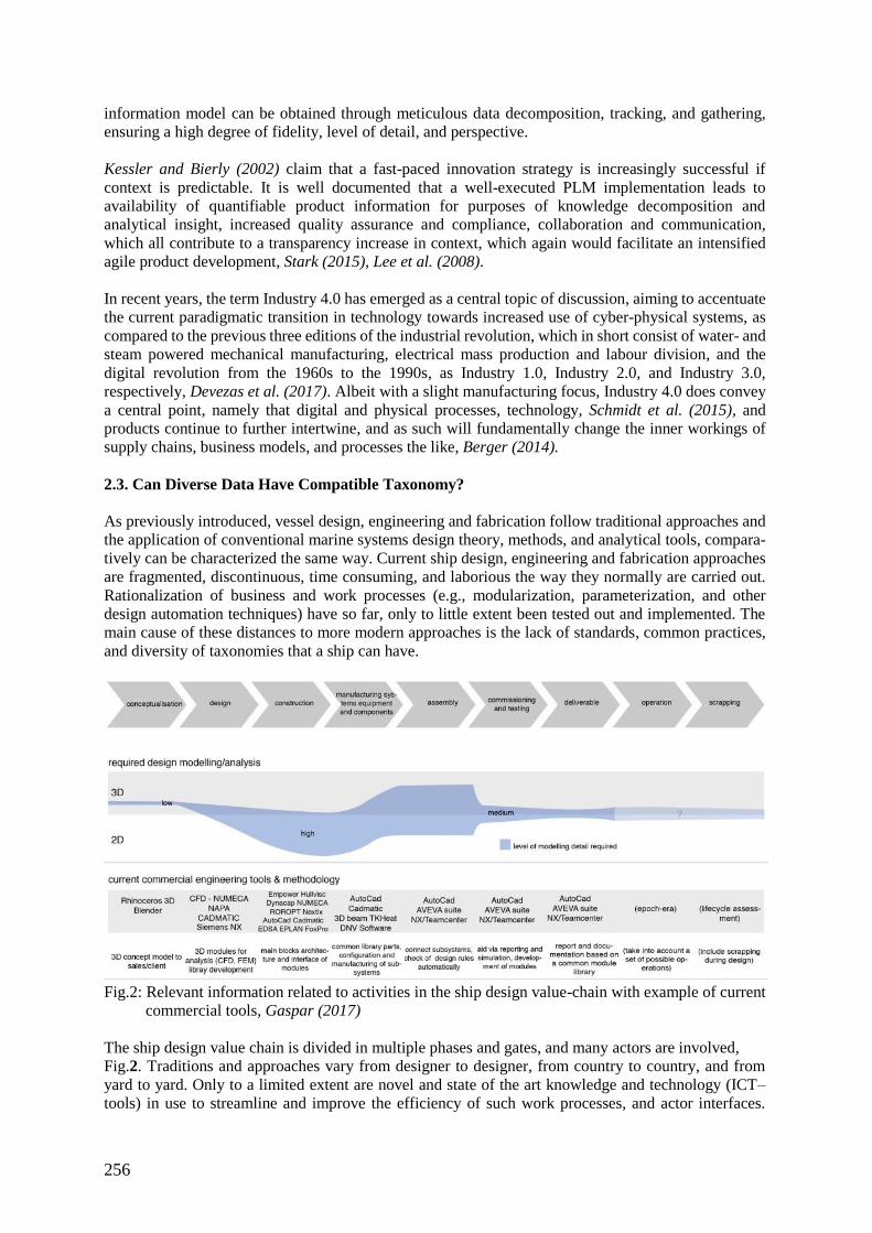
256
information model can be obtained through meticulous data decomposition, tracking, and gathering,
ensuring a high degree of fidelity, level of detail, and perspective.
Kessler and Bierly (2002) claim that a fast-paced innovation strategy is increasingly successful if
context is predictable. It is well documented that a well-executed PLM implementation leads to
availability of quantifiable product information for purposes of knowledge decomposition and
analytical insight, increased quality assurance and compliance, collaboration and communication,
which all contribute to a transparency increase in context, which again would facilitate an intensified
agile product development, Stark (2015), Lee et al. (2008).
In recent years, the term Industry 4.0 has emerged as a central topic of discussion, aiming to accentuate
the current paradigmatic transition in technology towards increased use of cyber-physical systems, as
compared to the previous three editions of the industrial revolution, which in short consist of water- and
steam powered mechanical manufacturing, electrical mass production and labour division, and the
digital revolution from the 1960s to the 1990s, as Industry 1.0, Industry 2.0, and Industry 3.0,
respectively, Devezas et al. (2017). Albeit with a slight manufacturing focus, Industry 4.0 does convey
a central point, namely that digital and physical processes, technology, Schmidt et al. (2015), and
products continue to further intertwine, and as such will fundamentally change the inner workings of
supply chains, business models, and processes the like, Berger (2014).
2.3. Can Diverse Data Have Compatible Taxonomy?
As previously introduced, vessel design, engineering and fabrication follow traditional approaches and
the application of conventional marine systems design theory, methods, and analytical tools, compara-
tively can be characterized the same way. Current ship design, engineering and fabrication approaches
are fragmented, discontinuous, time consuming, and laborious the way they normally are carried out.
Rationalization of business and work processes (e.g., modularization, parameterization, and other
design automation techniques) have so far, only to little extent been tested out and implemented. The
main cause of these distances to more modern approaches is the lack of standards, common practices,
and diversity of taxonomies that a ship can have.
Fig.2: Relevant information related to activities in the ship design value-chain with example of current
commercial tools, Gaspar (2017)
The ship design value chain is divided in multiple phases and gates, and many actors are involved,
Fig.2. Traditions and approaches vary from designer to designer, from country to country, and from
yard to yard. Only to a limited extent are novel and state of the art knowledge and technology (ICT–
tools) in use to streamline and improve the efficiency of such work processes, and actor interfaces.
257
Moreover, highly detailed 3D concepts are presented to the client prior to a signed contract despite
much of the engineering being remodelled in 2D, and few attempts to operate in 3D during the assembly
phase. This excessive re-modelling, blocks innovation and consumes unnecessary time. The cause can
mainly be attributed to the difference in boundary definition and placement for the parts and systems of
the ship between phases.
Hierarchization was once considered the solution for such lack of standard: it handles the complexity
on different layers and systems, such as the SFI group system in the 1970s, Manchinu and McConnel
(1977). Unfortunately, it also constrains the understanding of the system by a specific set of rules, which
may not work in a different context. A mapping between such stiff hierarchy and other more pragmatic
taxonomies is then necessary. The cumbersome task of handling multiple taxonomies and diverse tags
attributed to each part/system is now promised to be handled by modern PLM systems.
3. Emergent Technologies in the Maritime Industry
3.1. From PLM to Everything Else
PLM systems promise to keep control of products’ digital data structuring, using dedicated (and
expensive) software for improving the management and collaboration of the team throughout the
product development process. If modern PLM systems deliver on the promise of handling the
aforementioned challenges of multi-taxonomy/disciplinarily issues, it is reasonable to assume that we
can start to use PLM as a foundation towards handling and storing diverse data, and furthermore develop
other emergent technologies.
The drawbacks of a decision to go completely via PLM are, however, well known. It is vital to
understand how complicated and time consuming the implementation of a PLM project might become
depending on the company requirements. Often maritime companies consider PLM system as too time
and resource consuming before bringing benefits, and tend to avoid it or postpone its implementation.
Another drawback is the failures of previous implementation attempts, Levisauskaite (2016). PLM
systems have been promising implementation miracles for years. Many ship design companies faced
difficulties in the past, including Ulstein, when managing the large scale of data using 10-20 year old
PLM systems, and such a poor experience is clearly reflected when introduced to more modern and
agile software.
3.2. Cloud Computing and the Internet of Things
To circumvent sizeable capital expenditures and other typical challenges of on premise computing
solutions, such as required space and maintenance for hardware, or need for competency in conjunction
with advanced configuration, Cloud-computing has emerged as a viable solution. Aimed at providing
much of the same solution scope, and at greater convenience, such systems have become highly scalable
and personalised to the extent that many companies have chosen to outsource large, or all, parts of in-
house IT infrastructure in favour of cloud services, Willcocks and Lacity (2016). Complementarily,
there has been a similar development in the adoption of Internet of Things (IoT), defined as “a set of
interconnected things (humans, tags, sensors, and so on) over the Internet, which have the ability to
measure, communicate and act all over the world,” Díaz et al. (2016). Whereby Cloud computing has
virtually unlimited capabilities in terms of storage and processing power, IoT infrastructure
comparatively lacks the same features. As such, the inherent complementarity that enables IoT to be
abstracted from its limitations, and Cloud computing to fruition, has led to the Cloud of Things, Aazam
et al. (2014). Leveraging the combined strengths of these technologies has become a priority for many
solution providers, Díaz et al. (2016), https://news.microsoft.com/2016/07/11/ge-and-microsoft-
partner-to-bring-predix-to-azure-accelerating-digital-transformation-for-industrial-customers/, and has
certainly also minimized the barrier of entry for parties still considering whether to pursue such
technology in their organisation. The application of practical IoT use has been demonstrated in a vast
set of use-cases, such as the structural health of buildings, waste management systems, traffic
congestion monitoring, energy consumption monitoring, smart lighting, building automation, nursing
258
home patient monitoring, eating disorder mitigation, and indoor navigation for the blind, to name some,
Zanella et al. (2014), Al-Fuqaha et al. (2015). In the maritime domain, there have also been several
publicized initiatives spurred on by larger industry actors, e.g. Hyundai Heavy Industries, MarEx
(2016), Wärtsilä (2016), and DNV GL, Späth (2017).
3.3. Simulation and Virtual Prototyping
The rapid development of computational power and the need of robust, quantitative metrics have
progressively incentivized the implementation of simulation and virtual prototyping in the maritime
industries. Starting in academic environments as a way to generate knowledge, Haddara and Xu (1998),
and expanding lately to rule development, Glen (2001), training purposes, Pawlowski (1996),
conceptual design, Chaves and Gaspar (2016), Erikstad et al. (2015), construction, Karpowicz and
Simone (1987), and operational management, Ludvigsen et al. (2016).
In general, the ship design environment has been the one using the most simulation and virtual
prototyping within the maritime industry. The lack of information at early concept design stages,
together with influence on final performance of decisions taken at this stage – up to 80% of the costs
are fixed in the concept design, Erikstad (2007) – spurred the need of understanding the consequences
and implications of decisions in technical, operational, and commercial performances, Ulstein and Brett
(2015). Specific, single-attribute simulation tools could not solve this complexity problem, therefore
holistic, multi-attribute simulation tools have been the core focus of recent research. Concept design
workbenches developed both by universities and industry, pursue the acceleration of the concept design
development process and to increase the potential number of alternatives being evaluated during
consideration of changing contextual factors. These workbenches approach the concept design
development from an alternative perspective. Rather than focusing purely on design parameters their
approach embraces the selection of functional requirements, and which mission the vessel is intended
for, as a premise to design a better vessel: “it is only when having the correct set of requirements that
we can decide upon the correct vessel”, Gaspar et al. (2016).
VISTA (Virtual sea trial by simulating complex marine operations) is a simulation-based workbench to
assess operability performance of a design, Erikstad et al. (2015). Its goal is to shorten the time spent
in concept development and make it more efficient, by creating a template to configure alternative
designs and measure their performance. Notwithstanding, as a state-of-the-art simulation tool for ship
design, VISTA does lack a commercial perspective. Chaves and Gaspar (2016) present a similar
approach based on open-source web-based applications. As an alternative application, Li et al. (2016)
assess the value of implementing virtual prototyping to support the planning phase of offshore
operations though simulation of vessel’s manoeuvrability.
3.4. Big Data
Following the emergence of Industry 4.0, the prevalence of digitization, and the ensuing deluge of
information and knowledge that has surfaced because of it, the topic of Big Data has been at the centre
of many discussions in terms of defining what it is, and how it can be done. In that respect, De Mauro
et al. (2015) after a thorough review, suggest an entailing characterization of volume, velocity, and
variety in terms of the what, and “… specific Technology and Analytical Methods for its transformation
into Value” as to the how. The definition leaves little to interpretation in terms of compositional criteria,
but it does leave the innate content of said criteria still as a topic under development and one to be
further explored. More specifically, the technology used to gather, process, store, and distribute various
sources of data, as well as the methodology with which said data is transformed into insight and
subsequent value creation, are the components in need of attention and development to achieve the end
goal of spurring economic value. It is generally agreed that as the volume of data keeps growing,
opportunities for new discoveries increase thereafter, Manovich (2011). It is also anticipated to facilitate
and create substantial shifts in a range of different disciplines, bringing disruptive innovations into play
and potentially revamping how research is conducted, Kitchin (2014). Nevertheless, organizations are
still facing significant challenges in understanding the guiding principles and value proposition during
259
early stage adoption, Wamba et al. (2015). A main cited contributor is the multidisciplinary knowledge
required across topics such as statistics, programming, and other domain (industry) specific fields, to
effectively understand the business challenge at hand, and envisage the necessary solution scope that
will provide an economic surplus upon completion, Dumbill et al. (2013).
Considering prevalent Big Data technology, Hadoop was one of the first commonly available
frameworks developed for distributed storage and processing of Big Data. Since its inception in 2003,
it arguably has emancipated utilization of big data analytics (BDA), as it could be run by computer
clusters based on cheap commodity hardware. Over time, many competing, as well as complementary,
systems have been developed, many of which have been adopted by the Apache foundation to ensure
operational maintenance and further development, e.g. Apache Pig, Apache Hive, Apache Spark. The
latter has for several applications become a contender to be reckoned with, even though the two are not
mutually exclusive and can work together in some fashions, Gu and Li (2013). There are an untold
number of other technological solutions not mentioned herein, as a complete overview is beyond the
purpose and scope of this paper.
When considering methods and techniques of approach, implementing, and governing Big Data
initiatives, there are many options to consider. Prominent techniques used in the context of analysis and
prediction include data mining, clustering, regression, classification, association analysis, anomaly
detection, neural networks, generic algorithms, multivariate statistical analysis, optimization, heuristic
search, Chen et al. (2012).
As has been briefly touched upon in this paper, there are many variations of which to choose from when
evaluating technologies and methodologies for Big Data analytics (BDA). Notwithstanding, the most
impactful challenge lies in the implementation and embracement of BDA as a core part of the firm’s
business model as a quote from Henke et al. (2016) states: “the real power of analytics-enabled insights
comes when they become so fully embedded in the culture that their predictions and prescriptions drive
a company’s strategy and operations and reshape how the organization delivers on them.” These
initiatives are often easy to deprioritize as leadership is often focused on performance and the bottom
line based on individual projects or cases, whereas pivoting towards a more holistic perspective, and
aggregating each incremental gain, might depict a much larger benefit. Uncovering this value in the
early stages of BDA initiatives is paramount to gain traction and acceptance.
BDA in practice emanates from many fields and sectors, ranges from economic and business activities
to public administration, and from national security to scientific research, Chen and Zhang (2014).
State-of-the-art applications and use-cases are copiously being developed, including behaviour
prediction, healthcare analysis, content recommendation, and traffic forecasting, Lv et al. (2017). In
maritime, much of the focus has currently resided with geospatial analysis, Adland and Jia (2016),
logistics optimization, Xu et al. (2015), and condition based monitoring, Wang et al. (2015).
Additionally, the Japan Ship Technology Research Association has been reported to invest a substantial
amount of funding into a vast BDA system designed to analyse yard workers’ behavioural patterns by
gathering and analysing imagery, radio-frequency identification tags, and physical force gathered from
smartphone accelerometers, Wainright (2016).
3.5. Artificial Intelligence
The first reported work referencing artificial intelligence (AI) emerged in 1943 and touched upon
knowledge of basic physiology and functions of neurons in the brain; the formal analysis of proportional
logic; and Turing’s theory of computation, Russel and Norvig (1995). Both applications and research
have come a long way since then, and to portray how it currently can be utilized some explanations are
in order. The most prominent interrelationship between fields within AI research normally depict a
hierarchical structure showing AI at the top, Machine Learning (ML) in the middle, and Deep Learning
(DL) as the newest addition, http://blog.algorithmia.com/ai-why-deep-learning-matters/. Whereas the
term AI is commonly accepted as a machines capability of mimicking human intelligence, ML refers
to algorithms that allow computers to learn behaviours by generalizing from data, and DL a
260
representation-learning method with multiple levels of representation based on artificial neural
networks (ANN), Bravo et al. (2014).
Using ANNs to emulate how the brain functions, in conjunction with higher levels of representation,
enables the machine to identify features that have not been designed by human engineers, they are
learned, LeCun et al. (2015). Combined with the increased availability of high performance parallel
computing via the cloud, this methodology has become increasingly present in consumer products, such
as language translation, image context recognition, or purchasing recommendations. Recently, Google
created a novel approach using DL to replace large parts of their existing language translation service,
Johnson et al. (2016). Whereas most translation systems only work on a single pair of languages, this
method could handle multiple pairs despite not having been directly trained to do so. As such, based on
discovered patterns, the machine essentially created a new language that could translate via an
intermediary.
Within a maritime domain, the use of DL yields little results in terms of academic research literature.
Identified examples have shown application regarding image processing for ship detection, Tang et al.
(2015), and the response or load prediction of offshore floating structures, Mazaheri (2006), Uddin et
al. (2012), Maslin (2017).
4. Preparing for the Future – Ulstein Experiences
4.1. Decision Making in Ulstein
It is important to approach vessel design in the conceptual phase from different perspectives: i) To
differentiate among different solutions; ii) to have better understanding of consequence for any small
input change; iii) to measure goodness of fit between final product and requirements; iv) to have more
meaningful benchmarking with market competitors; v) to make better and more robust decision-making
in vessel design; and vi) to support the development of effective sales arguments of - what is a better
vessel. Furthermore, Ulstein appreciates that proper and effective decision making should be based on
the fact that ship design is a multi-variable-based decision making process, and big data oriented to
secure proper balancing of new vessel designs with appropriate trad-off among requirements to resolve
the inherent complexity of ship design. It is essential that the decision-making model can demonstrate,
separate and distinguish among the effects of design parameters (main dimensions, power, mission
attributes, machinery, etc.) on final vessel design performance yield, Ebrahimi et al. (2015). The Ulstein
approach typically, integrates both multi criteria evolutionary problems with multiple objective
optimization problems to come up with the better solution. Ulstein applies complementary methods for
benchmarking of ship designs: i) Ranking based vessel design including indices developed based on
vessel missions, scoring by indices, and ranking by statistics. Ulstein also apply Hierarchical
multivariate based vessel design benchmarking according to smarter, safer, and greener performance
perspectives by i) hierarchical factor categorization, ii) metric attribution of design factor causal map
matrices and iii) hierarchical comparative based ranking.
4.2. Data Integration in Practice
As has been highlighted previously the challenge of creating a centralized, organized, and maintained
single version of the truth, is a formidable yet increasingly surmountable task. Facilitated by new
storage and processing technologies such as Apache Hadoop and Microsoft Azure, NoSQL, or T-SQL,
and combined with modern processes of transformation, augmentation, and automation using languages
such as R, M (Power Query), Python, and PowerShell, Ulstein has initiated the creation of an integrated
ecosystem of information – the Ulstein Big Data Repository. Currently, the scope has largely covered
domains such as finance, market intelligence, and resource management much because of the
transaction based nature of residing information. Moving forward, the product and all aspects pertaining
to vessels and ship designs lifecycle will increasingly become a focal point, seeing as, in an ideal state,
the product is at the heart of all business activities. This drives the further development, integration, and
extension of PLM.
261
4.3. PLM as an Implementation
Implementation of modern PLM is a key success factor for modernization of the Ulstein processes and
methods in novel ship design. Ulstein experience is based on key implementations and testing of modern
established commercial software tools (e.g. Autodesk, Siemens), in conjunction with internal
proprietary knowledge. As an example, testing and implementation of the non-conventional 4GD
framework in ship design has been performed as a comparison to the conventional structuring approach
Levisauskaite (2016). Several design and change cases were evaluated and analysed, emphasizing
challenges in ship design like exchange, remodelling, alternatives, and reuse across vessels. The method
is described in detail in Levisauskaite et al. (2017), and proved to be a powerful tool for this research
to verify whether the 4GD improves the exchange and facilitates the 3D re-use.
The mentioned case study showed that the 4GD approach requires different thinking on the assemblies
and designing process as the components and features are distinct from a traditional assembly approach.
Due to the absence of assembly constraints together with flat assembly structure in 4GD, the positioning
of the parts becomes straightforward, and changes are accomplished smoothly. These features influence
the exchange of parts which are non-restrictive and a fluent process in comparison to the traditional
assembly approach. Additionally, the effectiveness in 4GD proved to be an efficient solution for
alternative vessels or various ship configurations across the vessel family. It supports the designers
towards avoiding remodelling, and instead reuses 3D models of previous products. In ship design, it is
a powerful tool that is innovative, cost effective, and time saving Levisauskaite (2016).
However, this implementation only scratched the surface of the 4GD framework from an entry level
point of view. 4GD is a highly-advanced approach to work and organise design data, which requires
advanced competence within programming, configuration and working with Teamcenter and Siemens
NX to gain sufficient benefit. Moreover, it requires well established needs and requirements to
efficiently employ and integrate 4GD into business processes. The installation and configuration must
be well set and customized. To verify whether 4GD is a beneficial approach for continuous
improvement in shipbuilding, it must be implemented and tested in maritime business and products.
Ulstein has plans to proceed along this experimental line of implementation initiatives.
4.4. Accelerated Business Development
Ulstein has over the years introduced and implemented an Accelerated Business Development
methodology (ABD) to enhance and strengthen our capability to effectively solicit relevant
stakeholders´ expectations and desires when it comes to the realization of ship designs and new building
projects, Ulstein and Brett (2009).
The core elements of the ABD approach, which aims to better guide ship designers, yards, cargo, and
ship owners in realizing a business opportunity within intermodal transport or offshore field
development work whereby ship design is utilized to achieve a competitive advantage. The approach
advocates that a new or improved solution system, where the ship plays a significant role, shall fulfil
the needs and expectations of all the involved stakeholders in the best possible way through the multi-
attribute decision making ABD-approach. This approach makes it possible to follow the complex and
normally fragmented processes of business development related to maritime transport, offshore oil &
gas field, and the pertinent ship design in a systemic and explicit way.
Traditionally, the big data oriented logistics-based requirements of a transport or offshore field system
have been included in the ship conceptualization and design often, in a non-structured and non-scientific
way. Knowledge about logistics is spread over many actors and subjects being involved in realizing the
transport system at hand where the ship design solutions are integral parts of the operation of such
systems, but seldom an integral part of the business development process. The actors in such processes
are ship operators, brokers, investors, designers, consultants, and companies managing transport chains.
None of these parties isolated have the full picture and specific knowledge on assessing a ship's
technical and operational performance in a broader business context. Traditions and specialization over
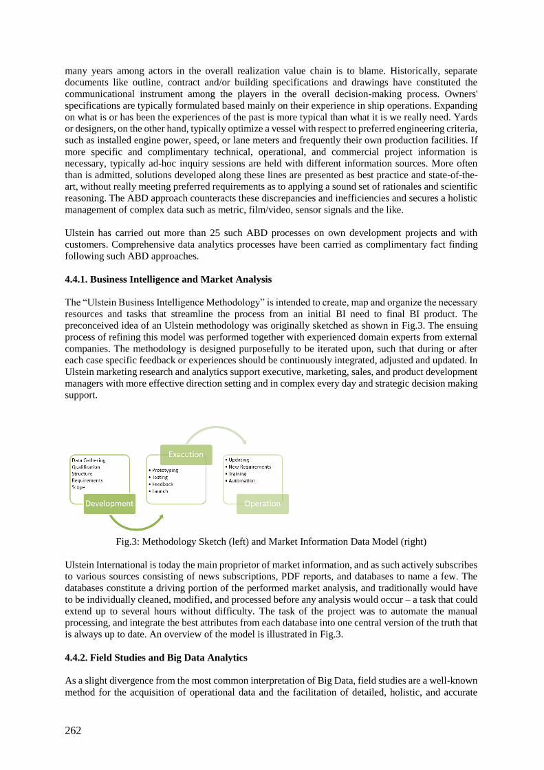
262
many years among actors in the overall realization value chain is to blame. Historically, separate
documents like outline, contract and/or building specifications and drawings have constituted the
communicational instrument among the players in the overall decision-making process. Owners'
specifications are typically formulated based mainly on their experience in ship operations. Expanding
on what is or has been the experiences of the past is more typical than what it is we really need. Yards
or designers, on the other hand, typically optimize a vessel with respect to preferred engineering criteria,
such as installed engine power, speed, or lane meters and frequently their own production facilities. If
more specific and complimentary technical, operational, and commercial project information is
necessary, typically ad-hoc inquiry sessions are held with different information sources. More often
than is admitted, solutions developed along these lines are presented as best practice and state-of-the-
art, without really meeting preferred requirements as to applying a sound set of rationales and scientific
reasoning. The ABD approach counteracts these discrepancies and inefficiencies and secures a holistic
management of complex data such as metric, film/video, sensor signals and the like.
Ulstein has carried out more than 25 such ABD processes on own development projects and with
customers. Comprehensive data analytics processes have been carried as complimentary fact finding
following such ABD approaches.
4.4.1. Business Intelligence and Market Analysis
The “Ulstein Business Intelligence Methodology” is intended to create, map and organize the necessary
resources and tasks that streamline the process from an initial BI need to final BI product. The
preconceived idea of an Ulstein methodology was originally sketched as shown in Fig.3. The ensuing
process of refining this model was performed together with experienced domain experts from external
companies. The methodology is designed purposefully to be iterated upon, such that during or after
each case specific feedback or experiences should be continuously integrated, adjusted and updated. In
Ulstein marketing research and analytics support executive, marketing, sales, and product development
managers with more effective direction setting and in complex every day and strategic decision making
support.
Fig.3: Methodology Sketch (left) and Market Information Data Model (right)
Ulstein International is today the main proprietor of market information, and as such actively subscribes
to various sources consisting of news subscriptions, PDF reports, and databases to name a few. The
databases constitute a driving portion of the performed market analysis, and traditionally would have
to be individually cleaned, modified, and processed before any analysis would occur – a task that could
extend up to several hours without difficulty. The task of the project was to automate the manual
processing, and integrate the best attributes from each database into one central version of the truth that
is always up to date. An overview of the model is illustrated in Fig.3.
4.4.2. Field Studies and Big Data Analytics
As a slight divergence from the most common interpretation of Big Data, field studies are a well-known
method for the acquisition of operational data and the facilitation of detailed, holistic, and accurate
263
information that typically is contained as tacit knowledge. They play an important role in acquiring
contextual, systems-oriented, and human-centered knowledge from on-site operations and during
execution generate an extensive amount of data. Sources of information include video, audio, pictures,
interviews, physiological monitoring, notes, diagrams, and models in addition to the plethora of both
on-board systems and provided third party sources such as the integrated automation system (IAS),
automation systems for winches and cranes, dynamic positioning system, accelerometers, cargo load
calculator, route planner, weather forecasts, radar imagery, task plans, operation logs, and so on.
Aggregated, these sources can generate upward of a terabyte of data per day in countless formats, and
as such counts significantly towards the data integration and big data analytics challenge as presented
previously in the paper. In cooperation with various research institutions, Ulstein has developed
methodology to handle the various challenges such an approach entails, and are in the process of
creating a corresponding infrastructure to convert the data into knowledge.
As one of the initial use-cases analysis of AIS (Automatic Identification System) information containing
data for nearly 6000 vessels, was performed. Gathering such data for integration and analysis improved
existing knowledge of design performance, that traditionally had been extracted from theoretical models
and simulations. Additionally, it provided an opportunity to compare aspects of operational features,
such as service speed and operating draft with design draft and speed, respectively. Containing 24 days
of on-site operation, the vessel data was processed and stored in the repository and then analysed.
Despite the relatively short period of evaluation, it showed that offshore vessels typically operate 30%
below designed service speed and 20% below design draft during most commercial operations. This
significant discrepancy between utilized and available capacities is an indication for further
investigation, development, and eventual design target resetting. This type of analysis provides new
opportunities for verifying actual performance including variation in motions, fuel consumption due to
respective weather conditions.
4.4.3. Fast Track Vessel Concept Design Analysis (FTCDA)
Companies operating in the design of maritime units are challenged by the need of incorporating
flexibility, innovation, speed, and agility to their business model, Ulstein and Brett (2009). The
conventional concept design development process, based on work processes relating to the traditional
design spiral for vessels has proven to be non-effective when it comes to ensuring very short customer
response time and robustness of the results. It is too time consuming and resource demanding, and
drastically limits the number of alternatives to potentially be evaluated for goodness of fit.
In response to this, Ulstein has developed a Fast-Track Concept Design Analysis tool (FTCDA). This
simulation tool combines multivariate statistics, network resources and design knowledge/expertise to
accelerate effective decision making in vessel concept design. The FTCDA is an integration tool which
gathers different modules of the conceptual design process in a unified digital platform. A holistic
approach, combining technical, commercial, and operational perspectives, ensures a more balanced and
robust design solution. The overall concept design development is benchmarked with peer vessel
alternatives, including existing vessels. Hence, the concept design is validated and potential points of
improvement can be identified and rectified to improve the overall performance of vessel design
solutions proposed.
This comprehensive approach requires a multi-disciplinary design platform, combining the different
aspects of maritime systems. Technical analyses such as stability, structural strength, and calm and
waves propulsion resistance. Hydrodynamic aspects such as seakeeping and operability, combined with
the evaluation of capacities and capabilities give the operational perspective. The feasibility analysis of
the configured solution, is assessed simultaneously in the tool, including the commercial perspective.
Newbuilding price and operational expenses are then contrasted with the potential revenue capability
and costs of the design solution. This fast-track evaluation of design performance enables designers and
decision makers to better perceive the implications and consequences of individual design changes such
as: main dimensions, mission equipment, operational environment, crew nationality, material, or build
country.
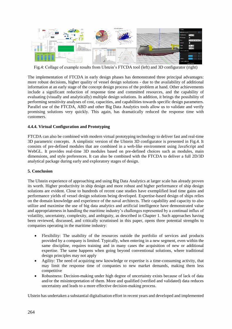
264
Fig.4: Collage of example results from Ulstein’s FTCDA tool (left) and 3D configurator (right)
The implementation of FTCDA in early design phases has demonstrated three principal advantages:
more robust decisions, higher quality of vessel design solutions - due to the availability of additional
information at an early stage of the concept design process of the problem at hand. Other achievements
include a significant reduction of response time and committed resources, and the capability of
evaluating (visually and analytically) multiple design solutions. In addition, it brings the possibility of
performing sensitivity analyses of cost, capacities, and capabilities towards specific design parameters.
Parallel use of the FTCDA, ABD and other Big Data Analytics tools allow us to validate and verify
promising solutions very quickly. This again, has dramatically reduced the response time with
customers.
4.4.4. Virtual Configuration and Prototyping
FTCDA can also be combined with modern virtual prototyping technology to deliver fast and real-time
3D parametric concepts. A simplistic version of the Ulstein 3D configurator is presented in Fig.4. It
consists of pre-defined modules that are combined in a web-like environment using JavaScript and
WebGL. It provides real-time 3D modules based on pre-defined choices such as modules, main
dimensions, and style preferences. It can also be combined with the FTCDA to deliver a full 2D/3D
analytical package during early and exploratory stages of design.
5. Conclusion
The Ulstein experience of approaching and using Big Data Analytics at larger scale has already proven
its worth. Higher productivity in ship design and more robust and higher performance of ship design
solutions are evident. Close to hundreds of recent case studies have exemplified lead time gains and
performance yields of vessel design solutions being developed. Expertise-based design of ships relies
on the domain knowledge and experience of the naval architects. Their capability and capacity to also
utilize and maximise the use of big data analytics and artificial intelligence have demonstrated value
and appropriateness in handling the maritime industry’s challenges represented by a continual influx of
volatility, uncertainty, complexity, and ambiguity, as described in Chapter 1. Such approaches having
been reviewed, discussed, and critically scrutinised in this paper, opens three potential strengths to
companies operating in the maritime industry:
Flexibility: The usability of the resources outside the portfolio of services and products
provided by a company is limited. Typically, when entering in a new segment, even within the
same discipline, requires training and in many cases the acquisition of new or additional
expertise. The same happens when going beyond conventional solutions, where traditional
design principles may not apply
Agility: The need of acquiring new knowledge or expertise is a time-consuming activity, that
may limit the response time of companies to new market demands, making them less
competitive
Robustness: Decision-making under high degree of uncertainty exists because of lack of data
and/or the misinterpretation of them. More and qualified (verified and validated) data reduces
uncertainty and leads to a more effective decision-making process.
Ulstein has undertaken a substantial digitalisation effort in recent years and developed and implemented
265
a set of new internally manufactured Big Data Analytics based tools and knowledge repositories to
enhance its ship design activity. It is envisaged that this effort is only a good start in exploring the
benefits and potential of Big Data Analytics and digitalisation of business and work processes. The
continuation of improvement activities will encompass, but not be restricted to such expansions such
as online web-based vessel configuration, algorithmic intelligence supported naval architecture and
vessel engineering work, and artificial intelligence based tools’ expansions. Continual improvement
work along these strategic avenues and steadily inclusion of new internally and externally developed
analytics tools are bound to happen, thus accelerating the effectiveness of Ulstein doings.
References
AAZAM, M.; KHAN, I.; ALSAFFAR, A.A.; HUH, E.N. (2014), Cloud of things: Integrating internet
of things and cloud computing and the issues involved, IEEE Conf., Anchorage, pp.414-419
ADLAND, R.O.; JIA, H. (2016), Vessel speed analytics using satellite-based ship position data, IEEE,
pp.1299-1303
AHAMED, Z.; INOHARA, T.; KAMOSHIDA, A. (2013), The Servitization of Manufacturing: An
Empirical Case Study of IBM, Int. J. Business Administration 4(2), pp.18-26
AL-FUQAHA, A.; GUIZANI, M.; MOHAMMADI, M.; ALEDHARI, M.; AYYASH, M. (2015),
Internet of things: A survey on enabling technologies, protocols, and applications, IEEE
Communications Surveys & Tutorials, pp.2347-2376.
BENNET, N.; LEMOINE, G.J. (2014), What a difference a word makes: Understanding threats to
performance in a VUCA world, Business Horizons 57, pp.311-317
BERGER, R. (2014), Industry 4.0. The new industrial revolution. How Europe will succeed, Roland
Berger strategy consultants
BORCH, O.J.; SOLESVIK, M.Z. (2016), Partner selection versus partner attraction in R&D strategic
alliances: the case of the Norwegian shipping industry, Int. J. Technology Marketing 11(4)
BRAVO, C.E.; SAPUTELLI, L.; RIVAS, F.; PÉREZ, A.G.; NICKOLAOU, M.; ZANGL, G.; DE
GUZMÁN, N.; MOHAGHEGH, S.D.; NUNEZ, G. (2014), State of the Art of Artificial Intelligence
and Predictive Analytics in the E&P Industry: A Technology Survey, SPE J. 19(4), pp.547-563
CHAVES, O.; GASPAR, H. (2016), A Web Based Real-Time 3D Simulator for Ship Design Virtual
Prototype and Motion Prediction, COMPIT Conf., Lecce, pp.410-419
CHEN, C.P.; ZHANG, C.Y. (2014), Data-intensive applications, challenges, techniques and techno-
logies: A survey on Big Data, Information Sciences 275, pp.314-347
CHEN, H.; CHIANG, R.H.; STOREY, V.C. (2012), Business intelligence and analytics: From big data
to big impact, MIS Quarterly 36(4), pp.1165-1188
CORSI, C.; AKHUNOV, A. (2000), Innovation and Market Globalization: The Position of SME's, IOS
Press
DE MAURO, A.; GRECO, M., GRIMALDI, M. (2015), What is big data? A consensual definition and
a review of key research topics, 4th Int. Conf. on Integrated Information, Madrid, pp.97-104.
DEVEZAS, T.; LEITÃO, J.; SARYGULOV, A. (2017), Industry 4.0: Entrepreneurship and Structural
Change in the New Digital Landscape, Springer

266
DÍAZ, M.; MARTÍN, C.; RUBIO, B. (2016), State-of-the-art, challenges, and open issues in the
integration of Internet of things and cloud computing, J. Network and Applications, pp.99-117
DIJKSHOORN, N. (1977), Interaction of costs and technological developments in the shipping
industry, Rotterdam
DUMBILL, E.; LIDDY, E.D.; STANTON, J.; MUELLER, K.; FARNHAM, S. (2013), Educating the
next generation of data scientists, Big Data 1(1), pp.21-27
EBRAHIMI, A.; BRETT, P.O.; GARCIA, J.J.; GASPAR, H.E.; KAMSVAG, O. (2015), Better
decision making to improve robustness of OCV designs, 12th IMDC Conf., Tokyo
EBRAHIMI, A.; BRETT, P.O.; GARCIA, J.J.; GASPAR, H.E.; KAMSVAG, O. (2015), Parametric
OSV design studies - precision and quality assurance via updated statistics, 12th IMDC Conf., Tokyo
ERIKSTAD, S.O. (2007), Efficient exploitation of existing corporate knowledge in conceptual ship
design, Ship Technology Research 54(4), pp.184-193
ERIKSTAD, S.O.; GRIMSTAD, A.; JOHNSEN, T.; BORGEN, H. (2015), VISTA (Virtual sea trial by
simulating complex marine operations): Assessing operability at the design stage, 12th IMDC Conf.,
Tokyo
GASPAR, H. (2017), EMIS Project: Final Report to the Research Council of Norway (RCN), NTNU,
Ålesund
GASPAR, H.M.; HAGEN, A.; ERIKSTAD, S.O. (2016), On designing a ship for complex value
robustness, Ship Technology Research 63, pp.14-25
GASPAR, H.M.; ROSS, A.M.; RHODES, D.H.; ERIKSTAD, S.O. (2012), Handling complexity
aspects in conceptual ship design, IMDC, Glasgow
GLAVE, T.; JOERSS, M.; SAXON, S. (2014), The hidden opportunity in container shipping,
McKinsey & Co., November
GLEN, I. (2001), Ship Evacuation Simulation: Challenges and Solutions, SNAME Trans. 109, pp.121-
139
GU, L.; LI, H. (2013), Memory or time: Performance evaluation for iterative operation on hadoop and
spark, IEEE Int. Conf. Embedded and Ubiquitous Computing, Zhangjiajie
HADDARA, M.; XU, J. (1998), On the identification of ship coupled heave-pitch motions using neural
networks, Ocean Engineering 26(5), pp.381-400
HENKE, N.; LIBARIKIAN, A.; WISEMAN, B. (2016), Straight talk about big data, McKinsey
Quarterly 10
JOHNSON, M.; SCHUSTER, M.; LE, Q.V.; KRIKUN, M.; WU, Y.; CHEN, Z.; HUGHES, M. (2016),
Google's Multilingual Neural Machine Translation System: Enabling Zero-Shot Translation. arXiv
preprint arXiv:1611.04558
KAHNEMAN, D.; KLEIN, G. (2009), Conditions for Intuitive Expertise: A Failure to Disagree.
American Psychologist 64(6), pp.515-526
KARPOWICZ, A.S.; SIMONE, V. (1987), An application of computer simulation methods in ship
production process, Computers in Industry 9(1), pp.37-51
267
KESSLER, E.H.; BIERLY, P.E. (2002), Is faster really better? An empirical test of the implications of
innovation speed, IEEE Trans. Engineering Management 49(1), pp.2-12
KITCHIN, R. (2014), Big Data, new epistemologies and paradigm shifts, Big Data & Society 1(1), p.
2053951714528481
KUDYBA, S. (2014), Big data, mining, and analytics: components of strategic decision making, CRC
Press
LECUN, Y.; BENGIO, Y.; HINTON, G. (2015), Deep learning, Nature 521(7553), pp.436-444
LEE, S.G.; MA, Y.S.; THIMM, G.L.; VERSTRAETEN, J. (2008), Product lifecycle management in
aviation maintenance, repair and overhaul, Computers in industry 59(2), pp.296-303
LEVISAUSKAITE, G. (2016), Implementation of 4GD framework in Ship Design for improving
exchange and 3D reuse, NTNU, Ålesund
LEVISAUSKAITE, G.; GASPAR, H.M.; ULSTEIN, B. (2017), 4GD framework in Ship Design, 16th
COMPIT Conf., Cardiff
LI, G.; SKOGENG, P.B.; DENG, Y.; HATLEDAL, L.I.; ZHANG, H. (2016), Towards a Virtual
Prototyping Framework for Ship Maneuvering in Offshore Operations, OCEANS Conf., Shanghai,
pp.1-6
LUDVIGSEN, K.B.; JAMT, L.K.; HUSTELI, N.; SMOGELI, Ø. (2016), Digital Twins for Design,
Testing and Verification Throughout a Vessel's Life Cycle, 15th COMPIT Conf., Lecce, pp.448-456
LV, Z.; SONG, H.; BASANTA-VAL, P.; STEED, A.; JO, M. (2017), Next-generation big data
analytics: State of the art, challenges, and future research topics, IEEE Trans. Industrial Informatics
99
MANCHINU, A.; MCCONNEL, F. (1977), The SFI Coding and Classification System for Ship
Information, REAPS Technical Symp.
MANOVICH, L. (2011), Trending: The promises and the challenges of big social data, Debates in the
Digital Humanities 2, pp.460-475
MAREX (2016), Shipbuilder Looks to Internet of Things for Future Business, http://www.maritime-
executive.com/article/shipbuilder-looks-to-internet-of-things-for-future-business
MASLIN, E. (2017), Neural networking by design, Offshore Engineer 1(3), pp.26-27
MAZAHERI, S. (2006), The Usage of Artificial Neural Networks in Hydrodynamic Analysis of Floating
Offshore Platforms, Int. J. Maritime Technology 3(4), pp.48-60
McCARTAN, S.; HARRIS, D.; VERHEIJDEN, B.; LUNDH, M.; LUNTZHOFT, M.; BOOTE, D.;
HOPMAN, J.J.; SMULDERS, F.E.H.M.; LURAAS, S.; NORDBY, K., (2014), European boat design
innovation group: The marine design manifesto, RINA Marine Design Conf., Coventry
MORAIS, D.; WALDIE, M.; LARKINS, D. (2011), Driving the Adoption of Cutting Edge Technology
in Shipbuilding, 10th COMPIT Conf., Berlin, pp.490-502
NORDEN, C.; HRIBERNIK, K.; GHRAIRI, Z.; THOBEN, K.D.; FUGGINI, C. (2013), New
approaches to through-life asset management in the maritime industry, Procedia CIRP 11, pp.219-224

268
PAWLOWSKI, J.S. (1996), Hydrodynamic modelling for ship manoeuvring simulation, Intl. Conf. on
Marine Simulation and Manoeuvrability, Copenhagen
RUSSEL, S.; NORVIG, P. (1995), Artificial Intelligence: A modern approach, Prentice-Hall,
Englewood Cliffs 25
SCHMIDT, R.; MÖHRING, M.; HÄRTING, R.C.; REICHSTEIN, C.; NEUMAIER, P.; JOZINOVIC,
P. (2015), Industry 4.0-potentials for creating smart products: empirical research results, Int. Conf. on
Business Information Systems, Springer International Publishing, pp.16-27
SCHOEMAKER, P.J.; VAN DER HEIJDEN, C.A. (1992), Integrating Scenarios into Strategic
Planning at Royal Dutch/Shell, Planning Review, 20(3), pp.41-46
SHARMA, R.; KIM, T.W.; STORCH, R.L.; HOPMAN, H.J.; ERIKSTAD, S.O. (2012), Challenges in
computer applications for ship and floating structure design and analysis, Computer-Aided Design,
44(3), pp.166-185
SPÄTH, N. (2017), DNV GL’s new Veracity industry platform unlocks the potential of big data,
https://www.dnvgl.com/news/dnv-gl-s-new-veracity-industry-platform-unlocks-the-potential-of-big-
data-85547
STARK, J. (2015), Product lifecycle management, Springer International Publishing
STOPFORD, M. (2009), Maritime Economics, Taylor & Francis
TANG, J.; DENG, C.; HUANG, G.B.; ZHAO, B. (2015), Compressed-domain ship detection on
spaceborne optical image using deep neural network and extreme learning machine, IEEE Transactions
on Geoscience and Remote Sensing 53(3), pp.1174-1185
THIMM, G.; LEE, S.G.; MA, Y.S. (2006), Towards unified modelling of product life-cycles, Computers
in Industry, 57(4), pp.331-341
TOMAR, G.S.; CHAUDHARI, N.S.; NARENDRA, S.; BHADORIA, R.S.; DEKA, G.C. (2016), The
Human Element of Big Data: Issues, Analytics, and Performance, Taylor & Francis
UDDIN, M.; JAMEEL, M.; RAZAK, H.A.; ISLAM, A.B.M. (2012), Response prediction of offshore
floating structure using artificial neural network, Advanced Science Letters, 14(1), pp.186-189
ULSTEIN, T.; BRETT, P.O. (2009), Seeing whats next in design solutions: Developing the capability
to develop a commercial growth engine in marine design, IMDC, Trondheim
ULSTEIN, T.; BRETT, P.O. (2015), What is a better ship? - It all depends..., IMDC, Tokyo
WAINRIGHT, D. (2016), Ship Sales, http://www.tradewindsnews.com/shipsales/774217/japans-
shipbuilders-look-to-technology-to-gain-edge
WAMBA, S.F.; AKTER, S.; EDWARDS, A.; CHOPIN, G.; GNANZOU, D. (2015), How ‘big data’
can make big impact: Findings from a systematic review and a longitudinal case study, Int. J.
Production Economics 165, pp.234-246
WANG, H.; OSEN, O.L.; LI, G.; LI, W.; DAI, H.N.; ZENG, W. (2015), Big data and industrial internet
of things for the maritime industry in northwestern Norway, TENCON IEEE Region 10 Conf., pp.1-5
WILLCOCKS, L.P.; LACITY, M.C. (2016), The new IT outsourcing landscape: from innovation to
cloud services, Springer

269
WÄRTSILÄ (2016), Optimising ship lifecycle efficiency, http://cdn.wartsila.com/docs/default-
source/services-documents/white-papers/w%c3%a4rtsil%c3%a4-bwp---optimising-ship-lifecycle-
efficiency.pdf?sfvrsn=2
XU, J.; HUANG, E.; CHEN, C.H.; LEE, L.H. (2015), Simulation optimization: a review and
exploration in the new era of cloud computing and big data, Asia-Pacific J. Operational Research 32(3),
pp.155019-34
ZANELLA, A.; BUI, N.; CASTELLANI, A.; VANGELISTA, L.; ZORZI, M. (2014), Internet of things
for smart cities, IEEE Internet of Things Journal, pp.22-32
270
A Vessel Weather Routing Scheduler to Minimize the Voyage Time
Natalie Cariaga Costa Rodrigues, UFRJ, Rio de Janeiro/Brazil, [email protected]
Rodrigo Uchoa Simões, UFRJ, Rio de Janeiro/Brazil, [email protected]
Luiz Antônio Vaz Pinto, UFRJ, Rio de Janeiro/Brazil, [email protected]
Luiz Felipe Assis, UFRJ, Rio de Janeiro/Brazil, [email protected]
Jean-David Caprace, UFRJ, Rio de Janeiro/Brazil, [email protected]
Abstract
Maintaining the efficiency and sustainability in sea transportation is essential to ensure cost
competitiveness of ship operations. The constant need to maximize profit motivates further
developments and improvements in voyage optimization and weather routing systems. Indeed, these
technologies may lead to a significant reduction of voyage time, fuel consumption and emissions. This
paper presents a weather routing scheduler based on Dijkstra’s algorithm. The model seeks the route
that minimize the voyage time considering the forecast of wave specific height and wave direction at
sea. Therefore, the optimal route is obtained by considering both voluntary and involuntary sailing
speed reduction. Validation of the model is performed comparing the results to standard routes. The
results demonstrate that the developments may lead to significant voyage time reduction. Future
developments to consider fuel consumption and emissions for ship constant speed are planned.
1. Introduction
It is well known that ship routing is a procedure to determine an optimal route for ocean voyages based
on weather forecasts, characteristics of a particular ship and sea conditions. The principles of ship
performance analysis, considering the problem of a routing algorithm for optimizing trajectory and the
advance in marine weather forecasting, has allowed the navigation industry to reduce voyage time, fuel
consumption and minimizing cargo and hull damages. Agencies of routing services based on weather
forecasts show results of structural damage reduction by 73%, an 80% in the voyage time, and damage
to cargo reduction by 87% Chen (2002).
This optimization problem has received attention of many researchers in past years, such as the calculus
of variations Bijlsma (1975) that aims to minimize or maximize functions, expressed as integrals, in
order to find extremals. The optimization is achieved through variation of the parameters that control
the trajectory, for example time or velocity. The isochrone method proposed by James (1957) is a
practical deterministic method for calculating the minimum time route. The optimization is determined
by varying ship headings while assuming constant engine power. The isopone method of Spaans
(1995), finds the optimal track by defining planes of equal fuel consumption (energy fronts) instead of
time fronts. In addition to above mentioned algorithms, recently there have been significant advances
in the modified isochrone method, Lin et. al. (2013) which has applied a 3D model that considers the
variation of sea conditions during voyage and avoids land. There is also the augmented Lagrange
multiplier Tsujimoto (2006), the genetic algorithm Bekker (2006) and the Dijkstra algorithm of
Takashima (2009) that will be used for this paper and discussed later.
This paper describes a ship weather routing scheduler for determining optimal route, taken as the
minimum time route, based on Dijkstra’s algorithm. In the routing algorithm are established weight
functions based on forecast of wave specific height and wave direction at sea, voluntary and involuntary
speed reductions. All possible routes will be taken into account and the algorithm must calculate the
one of minimum weight, obtaining de optimal track.
The reliability of the optimal route derived from the ship weather routing scheduler is based on the
following parameters: the accuracy of weather forecasted data and the estimated ship behaviour in such
ocean wave conditions.
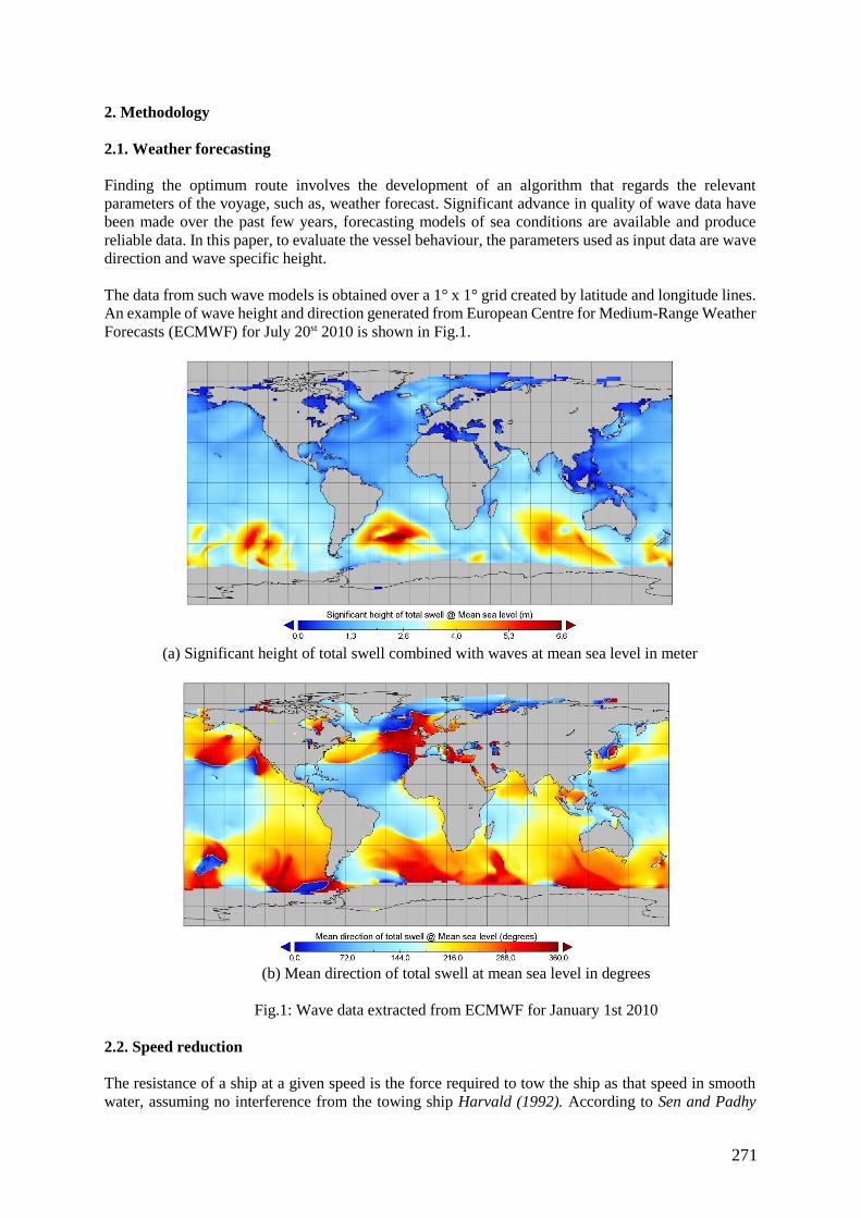
271
2. Methodology
2.1. Weather forecasting
Finding the optimum route involves the development of an algorithm that regards the relevant
parameters of the voyage, such as, weather forecast. Significant advance in quality of wave data have
been made over the past few years, forecasting models of sea conditions are available and produce
reliable data. In this paper, to evaluate the vessel behaviour, the parameters used as input data are wave
direction and wave specific height.
The data from such wave models is obtained over a 1° x 1° grid created by latitude and longitude lines.
An example of wave height and direction generated from European Centre for Medium-Range Weather
Forecasts (ECMWF) for July 20st 2010 is shown in Fig.1.
(a) Significant height of total swell combined with waves at mean sea level in meter
(b) Mean direction of total swell at mean sea level in degrees
Fig.1: Wave data extracted from ECMWF for January 1st 2010
2.2. Speed reduction
The resistance of a ship at a given speed is the force required to tow the ship as that speed in smooth
water, assuming no interference from the towing ship Harvald (1992). According to Sen and Padhy
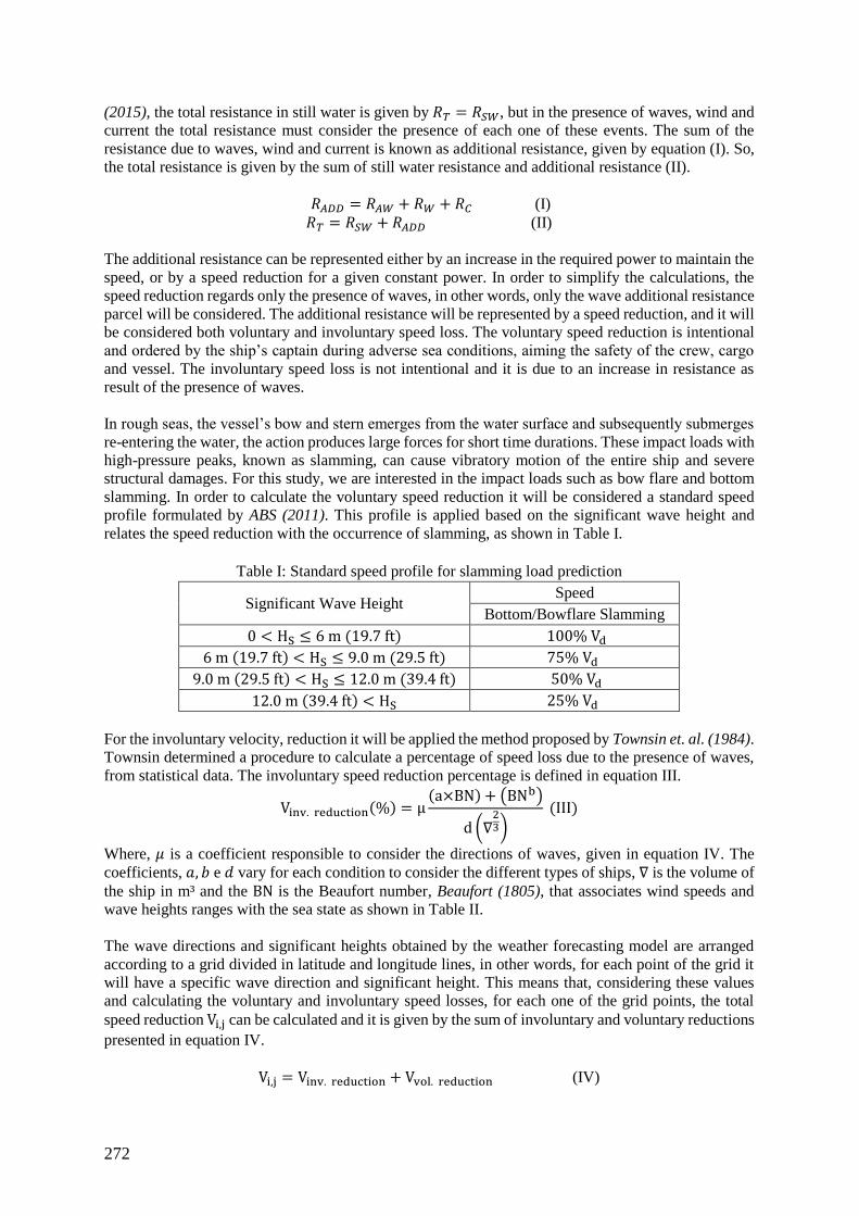
272
(2015), the total resistance in still water is given by 𝑅𝑇 = 𝑅𝑆𝑊, but in the presence of waves, wind and
current the total resistance must consider the presence of each one of these events. The sum of the
resistance due to waves, wind and current is known as additional resistance, given by equation (I). So,
the total resistance is given by the sum of still water resistance and additional resistance (II).
𝑅𝐴𝐷𝐷 = 𝑅𝐴𝑊 + 𝑅𝑊 + 𝑅𝐶 (I)
𝑅𝑇 = 𝑅𝑆𝑊 + 𝑅𝐴𝐷𝐷 (II)
The additional resistance can be represented either by an increase in the required power to maintain the
speed, or by a speed reduction for a given constant power. In order to simplify the calculations, the
speed reduction regards only the presence of waves, in other words, only the wave additional resistance
parcel will be considered. The additional resistance will be represented by a speed reduction, and it will
be considered both voluntary and involuntary speed loss. The voluntary speed reduction is intentional
and ordered by the ship’s captain during adverse sea conditions, aiming the safety of the crew, cargo
and vessel. The involuntary speed loss is not intentional and it is due to an increase in resistance as
result of the presence of waves.
In rough seas, the vessel’s bow and stern emerges from the water surface and subsequently submerges
re-entering the water, the action produces large forces for short time durations. These impact loads with
high-pressure peaks, known as slamming, can cause vibratory motion of the entire ship and severe
structural damages. For this study, we are interested in the impact loads such as bow flare and bottom
slamming. In order to calculate the voluntary speed reduction it will be considered a standard speed
profile formulated by ABS (2011). This profile is applied based on the significant wave height and
relates the speed reduction with the occurrence of slamming, as shown in Table I.
Table I: Standard speed profile for slamming load prediction
Significant Wave Height Speed
Bottom/Bowflare Slamming
0 < HS ≤ 6 m (19.7 ft) 100% Vd
6 m (19.7 ft) < HS ≤ 9.0 m (29.5 ft) 75% Vd
9.0 m (29.5 ft) < HS ≤ 12.0 m (39.4 ft) 50% Vd
12.0 m (39.4 ft) < HS 25% Vd
For the involuntary velocity, reduction it will be applied the method proposed by Townsin et. al. (1984).
Townsin determined a procedure to calculate a percentage of speed loss due to the presence of waves,
from statistical data. The involuntary speed reduction percentage is defined in equation III.
Vinv. reduction(%) = μ(a×BN) + (BNb)
d (∇23)
(III)
Where, 𝜇 is a coefficient responsible to consider the directions of waves, given in equation IV. The
coefficients, 𝑎, 𝑏 e 𝑑 vary for each condition to consider the different types of ships, ∇ is the volume of
the ship in m³ and the BN is the Beaufort number, Beaufort (1805), that associates wind speeds and
wave heights ranges with the sea state as shown in Table II.
The wave directions and significant heights obtained by the weather forecasting model are arranged
according to a grid divided in latitude and longitude lines, in other words, for each point of the grid it
will have a specific wave direction and significant height. This means that, considering these values
and calculating the voluntary and involuntary speed losses, for each one of the grid points, the total
speed reduction Vi,j can be calculated and it is given by the sum of involuntary and voluntary reductions
presented in equation IV.
Vi,j = Vinv. reduction + Vvol. reduction (IV)
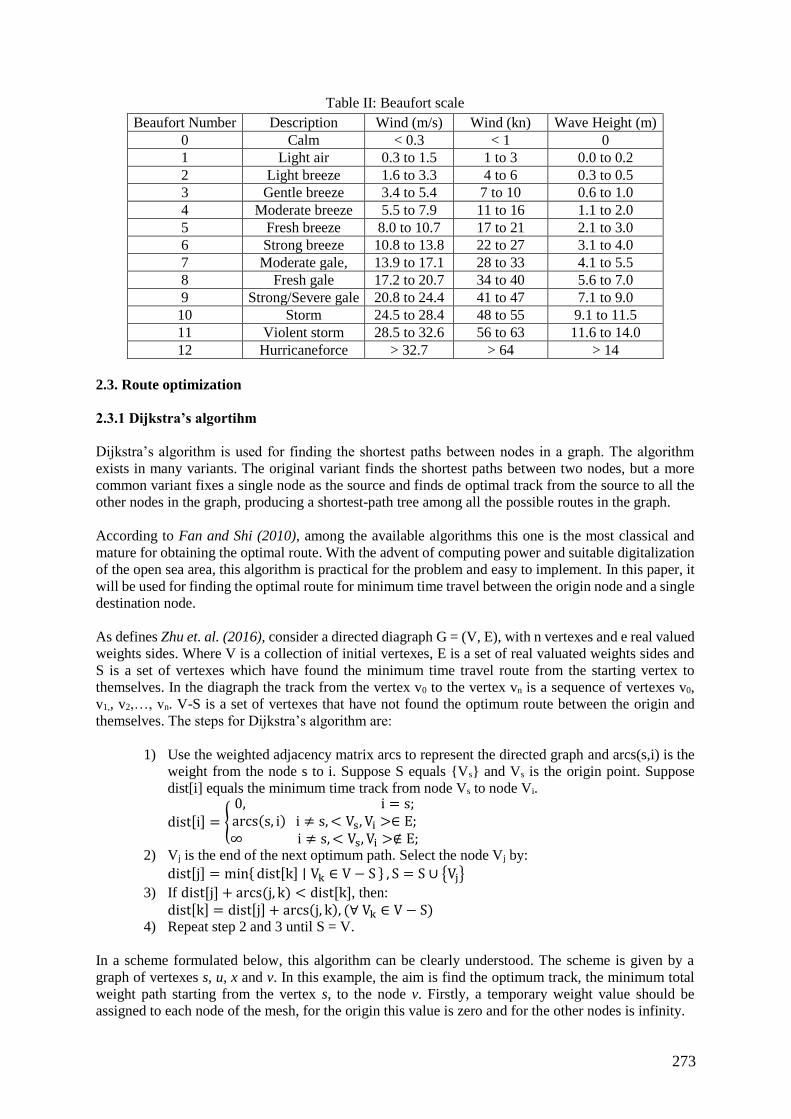
273
Table II: Beaufort scale
Beaufort Number Description Wind (m/s) Wind (kn) Wave Height (m)
0 Calm < 0.3 < 1 0
1 Light air 0.3 to 1.5 1 to 3 0.0 to 0.2
2 Light breeze 1.6 to 3.3 4 to 6 0.3 to 0.5
3 Gentle breeze 3.4 to 5.4 7 to 10 0.6 to 1.0
4 Moderate breeze 5.5 to 7.9 11 to 16 1.1 to 2.0
5 Fresh breeze 8.0 to 10.7 17 to 21 2.1 to 3.0
6 Strong breeze 10.8 to 13.8 22 to 27 3.1 to 4.0
7 Moderate gale, 13.9 to 17.1 28 to 33 4.1 to 5.5
8 Fresh gale 17.2 to 20.7 34 to 40 5.6 to 7.0
9 Strong/Severe gale 20.8 to 24.4 41 to 47 7.1 to 9.0
10 Storm 24.5 to 28.4 48 to 55 9.1 to 11.5
11 Violent storm 28.5 to 32.6 56 to 63 11.6 to 14.0
12 Hurricaneforce > 32.7 > 64 > 14
2.3. Route optimization
2.3.1 Dijkstra’s algortihm
Dijkstra’s algorithm is used for finding the shortest paths between nodes in a graph. The algorithm
exists in many variants. The original variant finds the shortest paths between two nodes, but a more
common variant fixes a single node as the source and finds de optimal track from the source to all the
other nodes in the graph, producing a shortest-path tree among all the possible routes in the graph.
According to Fan and Shi (2010), among the available algorithms this one is the most classical and
mature for obtaining the optimal route. With the advent of computing power and suitable digitalization
of the open sea area, this algorithm is practical for the problem and easy to implement. In this paper, it
will be used for finding the optimal route for minimum time travel between the origin node and a single
destination node.
As defines Zhu et. al. (2016), consider a directed diagraph G = (V, E), with n vertexes and e real valued
weights sides. Where V is a collection of initial vertexes, E is a set of real valuated weights sides and
S is a set of vertexes which have found the minimum time travel route from the starting vertex to
themselves. In the diagraph the track from the vertex v0 to the vertex vn is a sequence of vertexes v0,
v1,, v2,…, vn. V-S is a set of vertexes that have not found the optimum route between the origin and
themselves. The steps for Dijkstra’s algorithm are:
1) Use the weighted adjacency matrix arcs to represent the directed graph and arcs(s,i) is the
weight from the node s to i. Suppose S equals {Vs} and Vs is the origin point. Suppose
dist[i] equals the minimum time track from node Vs to node Vi.
dist[i] = {
0, i = s;arcs(s, i) i ≠ s, < Vs, Vi >∈ E;∞ i ≠ s, < Vs, Vi >∉ E;
2) Vj is the end of the next optimum path. Select the node Vj by:
dist[j] = min{ dist[k] ∣∣ Vk ∈ V − S } , S = S ∪ {Vj}
3) If dist[j] + arcs(j, k) < dist[k], then:
dist[k] = dist[j] + arcs(j, k), (∀ Vk ∈ V − S) 4) Repeat step 2 and 3 until S = V.
In a scheme formulated below, this algorithm can be clearly understood. The scheme is given by a
graph of vertexes s, u, x and v. In this example, the aim is find the optimum track, the minimum total
weight path starting from the vertex s, to the node v. Firstly, a temporary weight value should be
assigned to each node of the mesh, for the origin this value is zero and for the other nodes is infinity.
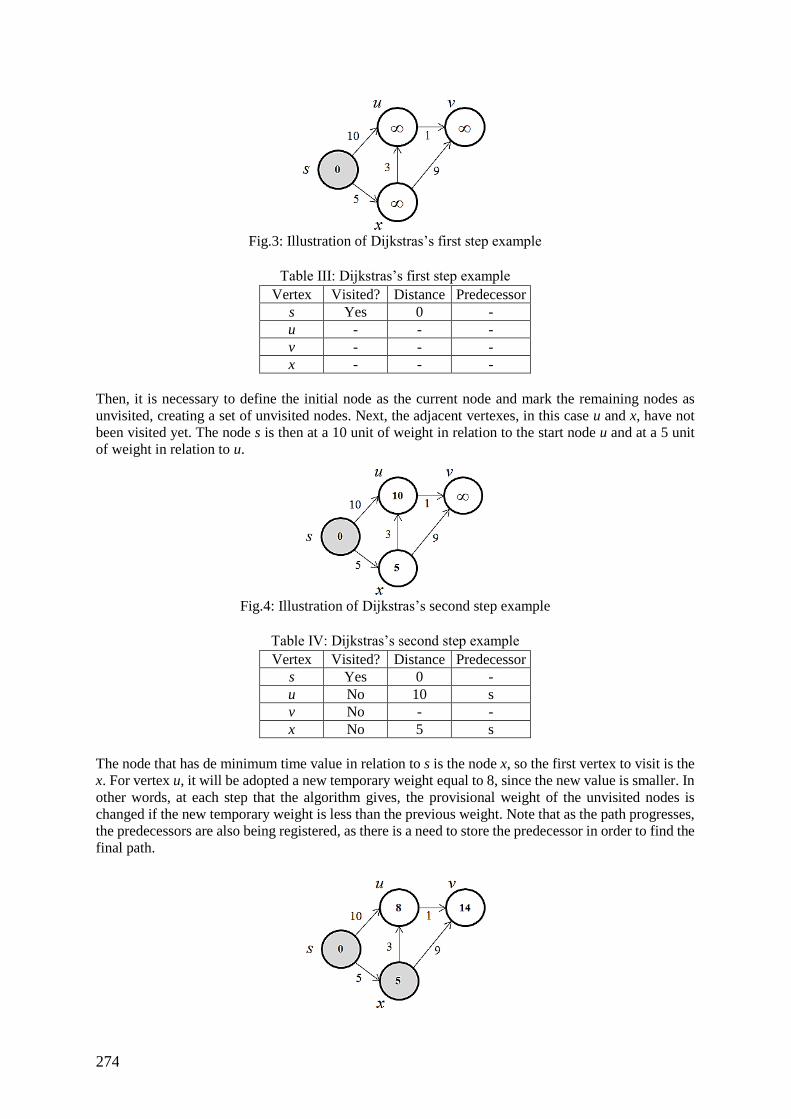
274
Fig.3: Illustration of Dijkstras’s first step example
Table III: Dijkstras’s first step example
Vertex Visited? Distance Predecessor
s Yes 0 -
u - - -
v - - -
x - - -
Then, it is necessary to define the initial node as the current node and mark the remaining nodes as
unvisited, creating a set of unvisited nodes. Next, the adjacent vertexes, in this case u and x, have not
been visited yet. The node s is then at a 10 unit of weight in relation to the start node u and at a 5 unit
of weight in relation to u.
Fig.4: Illustration of Dijkstras’s second step example
Table IV: Dijkstras’s second step example
Vertex Visited? Distance Predecessor
s Yes 0 -
u No 10 s
v No - -
x No 5 s
The node that has de minimum time value in relation to s is the node x, so the first vertex to visit is the
x. For vertex u, it will be adopted a new temporary weight equal to 8, since the new value is smaller. In
other words, at each step that the algorithm gives, the provisional weight of the unvisited nodes is
changed if the new temporary weight is less than the previous weight. Note that as the path progresses,
the predecessors are also being registered, as there is a need to store the predecessor in order to find the
final path.
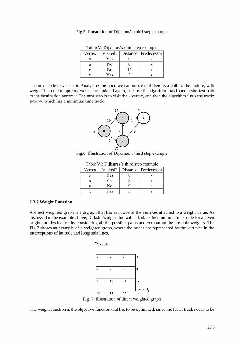
275
Fig.5: Illustration of Dijkstras’s third step example
Table V: Dijkstras’s third step example
Vertex Visited? Distance Predecessor
s Yes 0 -
u No 8 x
v No 14 x
x Yes 5 s
The next node to visit is u. Analysing the node we can notice that there is a path to the node v, with
weight 1, so the temporary values are updated again, because the algorithm has found a shortest path
to the destination vertex v. The next step is to visit the v vertex, and then the algorithm finds the track:
s-x-u-v, which has a minimum time track.
Fig.6: Illustration of Dijkstras’s third step example
Table VI: Dijkstras’s third step example
Vertex Visited? Distance Predecessor
s Yes 0 -
u Yes 8 x
v No 9 u
x Yes 5 s
2.3.2 Weight Function
A direct weighted graph is a digraph that has each one of the vertexes attached to a weight value. As
discussed in the example above, Dijkstra’s algorithm will calculate the minimum time route for a given
origin and destination by considering all the possible paths and comparing the possible weights. The
Fig.7 shows an example of a weighted graph, where the nodes are represented by the vertexes in the
interceptions of latitude and longitude lines.
Fig. 7: Illustration of direct weighted graph
The weight function is the objective function that has to be optimized, since the faster track needs to be
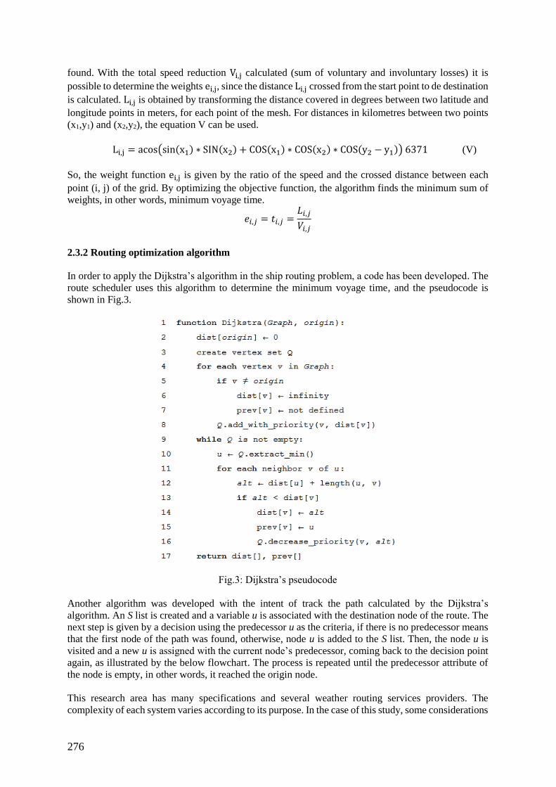
276
found. With the total speed reduction Vi,j calculated (sum of voluntary and involuntary losses) it is
possible to determine the weights ei,j, since the distance Li,j crossed from the start point to de destination
is calculated. Li,j is obtained by transforming the distance covered in degrees between two latitude and
longitude points in meters, for each point of the mesh. For distances in kilometres between two points
(x1,y1) and (x2,y2), the equation V can be used.
Li,j = acos(sin(x1) ∗ SIN(x2) + COS(x1) ∗ COS(x2) ∗ COS(y2 − y1)) 6371 (V)
So, the weight function ei,j is given by the ratio of the speed and the crossed distance between each
point (i, j) of the grid. By optimizing the objective function, the algorithm finds the minimum sum of
weights, in other words, minimum voyage time.
𝑒𝑖,𝑗 = 𝑡𝑖,𝑗 =𝐿𝑖,𝑗
𝑉𝑖,𝑗
2.3.2 Routing optimization algorithm
In order to apply the Dijkstra’s algorithm in the ship routing problem, a code has been developed. The
route scheduler uses this algorithm to determine the minimum voyage time, and the pseudocode is
shown in Fig.3.
Fig.3: Dijkstra’s pseudocode
Another algorithm was developed with the intent of track the path calculated by the Dijkstra’s
algorithm. An S list is created and a variable u is associated with the destination node of the route. The
next step is given by a decision using the predecessor u as the criteria, if there is no predecessor means
that the first node of the path was found, otherwise, node u is added to the S list. Then, the node u is
visited and a new u is assigned with the current node’s predecessor, coming back to the decision point
again, as illustrated by the below flowchart. The process is repeated until the predecessor attribute of
the node is empty, in other words, it reached the origin node.
This research area has many specifications and several weather routing services providers. The
complexity of each system varies according to its purpose. In the case of this study, some considerations
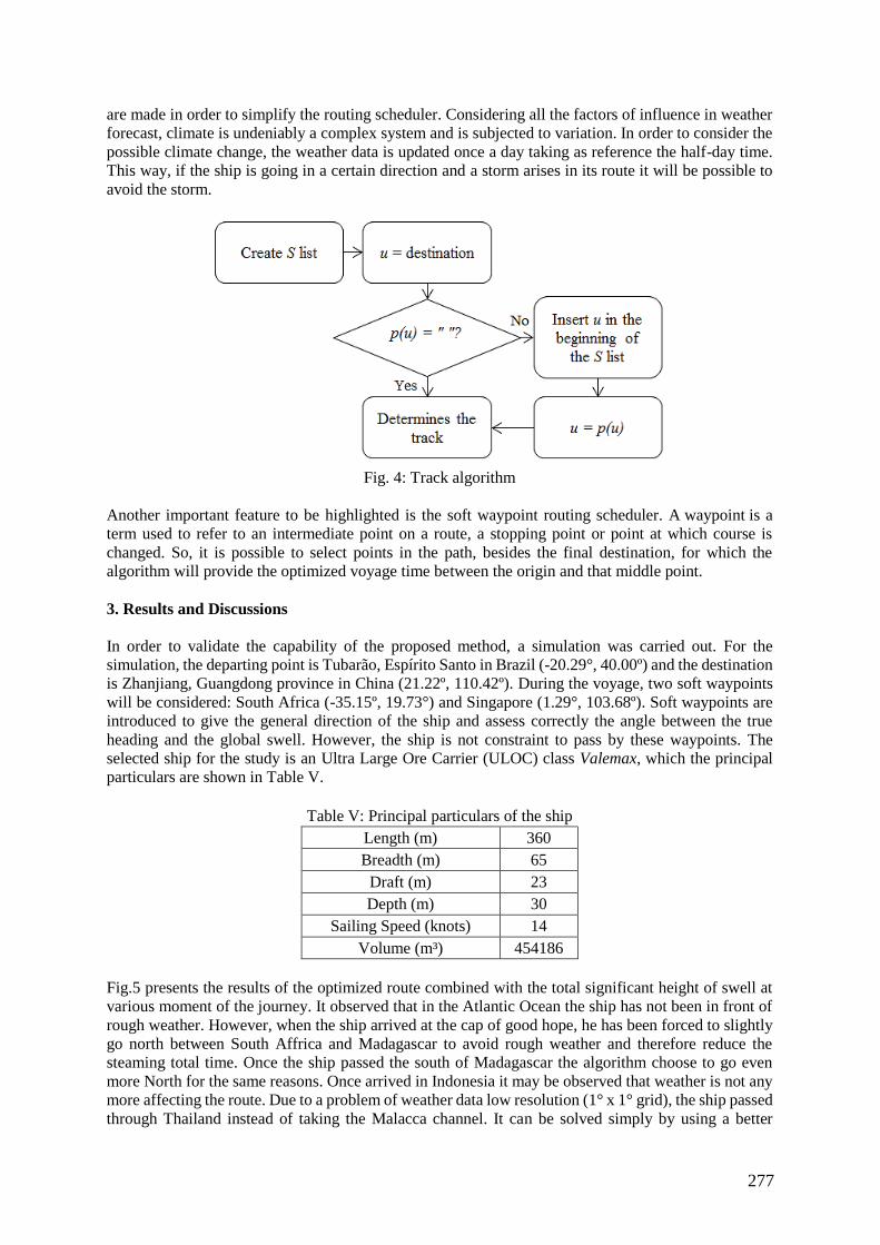
277
are made in order to simplify the routing scheduler. Considering all the factors of influence in weather
forecast, climate is undeniably a complex system and is subjected to variation. In order to consider the
possible climate change, the weather data is updated once a day taking as reference the half-day time.
This way, if the ship is going in a certain direction and a storm arises in its route it will be possible to
avoid the storm.
Fig. 4: Track algorithm
Another important feature to be highlighted is the soft waypoint routing scheduler. A waypoint is a
term used to refer to an intermediate point on a route, a stopping point or point at which course is
changed. So, it is possible to select points in the path, besides the final destination, for which the
algorithm will provide the optimized voyage time between the origin and that middle point.
3. Results and Discussions
In order to validate the capability of the proposed method, a simulation was carried out. For the
simulation, the departing point is Tubarão, Espírito Santo in Brazil (-20.29°, 40.00º) and the destination
is Zhanjiang, Guangdong province in China (21.22º, 110.42º). During the voyage, two soft waypoints
will be considered: South Africa (-35.15º, 19.73°) and Singapore (1.29°, 103.68º). Soft waypoints are
introduced to give the general direction of the ship and assess correctly the angle between the true
heading and the global swell. However, the ship is not constraint to pass by these waypoints. The
selected ship for the study is an Ultra Large Ore Carrier (ULOC) class Valemax, which the principal
particulars are shown in Table V.
Table V: Principal particulars of the ship
Length (m) 360
Breadth (m) 65
Draft (m) 23
Depth (m) 30
Sailing Speed (knots) 14
Volume (m³) 454186
Fig.5 presents the results of the optimized route combined with the total significant height of swell at
various moment of the journey. It observed that in the Atlantic Ocean the ship has not been in front of
rough weather. However, when the ship arrived at the cap of good hope, he has been forced to slightly
go north between South Affrica and Madagascar to avoid rough weather and therefore reduce the
steaming total time. Once the ship passed the south of Madagascar the algorithm choose to go even
more North for the same reasons. Once arrived in Indonesia it may be observed that weather is not any
more affecting the route. Due to a problem of weather data low resolution (1° x 1° grid), the ship passed
through Thailand instead of taking the Malacca channel. It can be solved simply by using a better
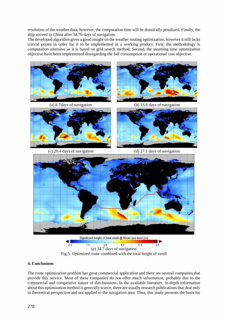
278
resolution of the weather data; however, the computation time will be drastically penalized. Finally, the
ship arrived in China after 34.76 days of navigation.
The developed algorithm gives a good insight on the weather routing optimization, however it still lacks
critical points in order for it to be implemented in a working product. First, the methodology is
computation intensive as it is based on grid search method. Second, the steaming time optimization
objective have been implemented disregarding the full consumption or operational cost objective.
(a) 6.7days of navigation
(b) 13.6 days of navigation
(c) 20.4 days of navigation
(d) 27.1 days of navigation
(e) 34.7 days of navigation
Fig.5: Optimized route combined with the total height of swell
4. Conclusions
The route optimization problem has great commercial application and there are several companies that
provide this service. Most of these companies do not offer much information, probably due to the
commercial and competitive nature of this business. In the available literature, in-depth information
about this optimization method is generally scarce, there are usually research publications that deal only
in theoretical perspective and not applied to the navigation area. Thus, this study presents the basis for
279
the ship routing problem elucidating the basic structure for the approach of an algorithm in the route
optimization problem.
This research can be extended in many directions. Future developments to consider fuel consumption,
operational costs and emissions for ship constant speed are planned. One of the limitations of this
approach is that the speed reduction regards only the wave additional resistance parcel, so the influence
of the wind and current should be considered in future improvements. Generally, in the wave data sites
the weather forecast is updated every 3 hours. To reduce computation time, the algorithm updated
weather data every 24 hours with a resolution of 1° x 1° grid. A suggestion for futures development is
to reduce the updating time and increase the resolution of the grid, keeping in mind that the shorter this
time is, the more accurate the results will be.
References
ABS (2011), Guide for Slamming Loads and Strength Assessment for Vessels, American Bureau of
Shipping, Houston
BEAUFORT, F. (1805), Beaufort Wind Scale, U.K. Royal Navy
BIJLSMA, S.J. (1975), On minimal-time ship routing, Delft University of Technology
CHEN, H. (2002), Weather routing: a new approach, Safety at Sea
FAN, D.; SHI, P. (2010), Improvement of Dijkstra's algorithm and its application in route planning,
7th Int. Conf. Fuzzy Systems and Knowledge Discovery (FSKD), Vol. 4, pp.1901-1904
HARVALD, S.A. (1992), Resistance and Propulsion of Ships, Wiley & Sons
JAMES, R.W. (1987), Application of wave forecast to marine navigation, US Navy Hydrographic
Office, Washington
LIN, Y.H.; FANG, M.C.; YEUNG, R.W. (2013), The optimization of ship weather routing algorithm
based on the composite influence of multi-dynamic elements. Appl. Ocean Res. 43, pp.184-94
SEN, D.; PADHY, C.P. (2015), An approach for development of a ship routing algorithm for
application in the North Indian Ocean region, Appl. Ocean Res. 50, pp.173-191
SPAANS, J.A. (1995), New developments in ship weather routing, Navigation 169, pp.95-106
TOWNSIN, R.L.; MEDHURST, J.S.; HAMLIN, N.A.; SEDAT, B.S. (1984), Progress in Calculating
the Resistance of Ships with Homogeneous or Distributed Roughness, Necies Centenary Conf. Marine
Propulsion
ZHU, X.; WANG, H.; SHEN, Z.; HONGJUN L.V. (2016), Ship weather routing based on modified
Dijkstra algorithm, 6th Int. Conf. Machinery, Materials, Environment, Biotechnology and Computer
(MMEBC 2016), pp.696-697
280
Big Data Analysis of AIS Records to Provide Knowledge for Offshore
Logistic Simulation
Maricruz A. F. Cepeda, COPPE, UFRJ, Rio de Janeiro/Brazil, [email protected]
Rodrigo Uchoa Simões, PENO, UFRJ, Rio de Janeiro/Brazil, [email protected]
João Vitor Marques de Oliveira Moita, PENO, UFRJ, Rio de Janeiro/Brazil, [email protected]
Luiz Felipe Assis, COPPE, UFRJ, Rio de Janeiro/Brazil, [email protected]
Luiz Antônio Vaz Pinto, COPPE, UFRJ, Rio de Janeiro/Brazil, [email protected]
Jean-David Caprace, COPPE, UFRJ, Rio de Janeiro/Brazil, [email protected]
Abstract
Today, Big Data is getting popular in shipping where large amounts of information is collected to
better understand and improve logistics, emissions, energy consumption and maintenance. In
shipping, the Automatic Identification System (AIS) records millions of information of ships
operations. However, to get the most of these big chunks of information specific technologies should
be applied to process these data within an acceptable time. This paper presents a model to extract
patterns from AIS records in the field of supply chain of offshore platforms. Here a solution using
distributed processing framework based on Hadoop Hive queries (map/reduce) and Hadoop
Distributed File Systems (HDFS) is developed. First, a short benchmark study is present to compare
performance of Big Data technology in front of former technology. Second, results of the pattern
extraction regarding navigational behaviour of Platform Supply Vessels are presented. Then, the new
knowledge is introduce in a stochastic simulation to mimic the supply chain management of offshore
platforms. The results shown that the proposed methodology is efficient to reproduce offshore logistic
activities taking into account uncertainties related to operational matters, as well as weather
uncertainties that affect the system. Moreover, big data technologies are greatly reducing time to
extract pattern from considerable amount of data.
1. Introduction
1.1. Contextualization
Offshore Oil and Gas (O&G) industry is one of the most important industries in the world with a di-
rect impact on the worldwide economies. According to annual world energy statistics, it is stated that
in 2014 approximately 55% of total energy consumed in the world has been produced from oil and
natural gas, IEA (2016). World oil demand grew more strongly in 2015 (+1.8 million barrels per day
(mb/d)), UK (2016). The profitability of O&G development activity depends on both the prices real-
ized by producers and the cost and productivity of present and newly developed wells. Prices, costs,
and field’s productivity have all experienced significant changes over the past decade, EIA (2016).
The collapse of oil prices in late 2014 forces the offshore oil key players to reduce their logistics costs
to recover competitiveness.
Most of Brazil oil reserves are nestled in offshore fields, a fact that has led the O&G activities to
achieve increasing depths. The logistic of Brazilian pre-salt fields are challenging due to the
considerable distance to coastline (~300 km).
Every day, 2.5 quintillion bytes of data are created. Datasets whose size is beyond the ability of
typical database software tools to capture, store, manage and analyse. This is known as Big Data, MGI
(2012). Big data is present in key sectors as health care, public sector administration, global personal
location data, retail, manufacturing, social personal and professional data, Zicari (2014).
Big data have revolutionized the industry over the past several years. Companies across the various
travel and transportation industry segments as airlines, airports, railways, freight logistics, hospitality
and others have been handling large amounts of data for years. In addition, today’s advanced analytics
281
technologies and techniques enable organizations to extract insights from data with previously
unachievable levels of sophistication, speed and accuracy, IBM (2014).
Today, Big Data is getting popular in shipping where large amounts of information is collected to
better understand and improve logistics, emissions, energy consumption and maintenance.
Using satellite navigation and sensors, trucks, airplanes or ships can be tracked in real-time. In
shipping, the Automatic Identification System (AIS), which is used for preventing collisions at sea
and by vessel traffic services (VTS), records millions of information of ships operations, between
vessels and between vessels and shore facilities. Historical AIS data is a valuable data source used for
vessel traffic analyses, port calling information, risk assessment and accident investigation. It may
also provide basement for decisions in offshore logistic.
1.2. Gap
Over the past few years, there has been a fundamental shift in data storage, management, and
processing. Companies are storing more data from more sources in more formats than ever before.
This is not just about being a “data package” but rather building products, features, and intelligence
predicated on knowing more about this information, Sammer (2012).
Organizations discovers new ways to use data that was previously believed to be of little value, or far
too expensive to keep, to better serve their clients. Sourcing and storing data is a part of the problem.
Processing that data to produce information is fundamental to the daily operations of any industry,
Sammer (2012).
However, to get the most of these big chunks of information specific technologies should be applied
to process these data within an acceptable time and resources. In order to efficiently extract value
from these data, the offshore oil key players need to find new tools and methods specialized for big
data processing.
1.3. State of the art
To deal with this huge quantity of data, common solutions may not be any more efficient or too time
consuming. Here a solution using distributed processing framework based on Hadoop Hive queries
(map/reduce) and Hadoop Distributed File Systems (HDFS) is developed. Hadoop is a useful platform
used in the last years where solutions have been developed for the industry with the use of big data.
In shipping industry, the use of big data is present in various studies. Bons and Wirdum (2016) de-
scribe how CoVadem introduces a big data solution that will add significant value to the inland ship-
ping industry in Europe with a cooperatively sourced big data from over 50 vessels (over 55.000.000
measured values a day). It is used to provide effective key performance indicators (KPI’s) to judge
actual performance and cater for the necessary metrics to analyse, interpret and decide upon im-
provement measures. With the right technical and organizational implementation a revolutionary basis
is introduced that allows for effective, continuous and holistic improvement, Bons and Wirdum
(2016).
Rødseth et al.(2016) present an overview of some of these issues and possible solutions about the con-
straints to the use of big data. New protocol standards may simplify the process of collecting and or-
ganizing the data, including in the e-navigation domain are reviewed. This paper references the exter-
nal ship monitoring as AIS and VTS. It indicates that AIS receivers can provide very valuable data on
ship movements due to ships will send AIS data quite frequently, normally minimum each 10 sec-
onds. Data that is transmitted is position, speed, course, true heading and rate of turn. This automated
ship reporting is a prioritized solution in the e-navigation strategic implementation plan, IMO (2014),
so one may expect some developments in this area in the coming years, Rødseth et al. (2016).
282
Ramsden et al. (2016) use a Big Data solution to predicting fouling on an underwater hull because
they consider that as a vital part of optimising the efficiency of a maritime vessel. They mash together
multiple data streams for relevant vessel attributes, positional data, environmental data and fouling
coating performance factor generated a dataset of over 3.5 Billon records, Ramsden et al. (2016).
The creation of realistic scenarios with simulation in maritime industry is important for training and
for testing of the developed tools. These scenarios are verified and validated with the reality. In the
shipping industry the use of simulation is present in various studies. Korte et al. (2012) present the
project Safe Offshore Operations about offshore training simulations where the main idea consists of
the development of an integrated operator assistance and information system based on a self-
organising wireless computer and sensor network, and also prolong the time frames for offshore
operations. The initial simulate scenarios and their verification shall be presented and discussed by the
study, Korte et al. (2012).
Shyshou et al. (2010) proposed a simulation model for offshore anchor handling operations related to
movement of offshore mobile units. The operations are performed by anchor handling tug supply
(AHTS) vessels, which can be hired either on the long-term basis or from the spot market. The
stochastic elements are weather conditions and spot-hire rates. The requirements on the weather
conditions are similar to the methodology developed in this paper. However, the authors are using
met-ocean data to assess theses distributions, Shyshou et al. (2010).
The work developed by Aneichyk (2009) covers the designing of a simulation model for offshore
supply process with the aim of creating a tool to plan the operations and fleet size. Some uncertainty
factors affecting the process are taken into account such as weather conditions, varying demand and
delays. A discrete-event simulation (DES) model is developed in order to model those uncertainties
with a stochastic approach. Results obtained show that simulation may be seen as an important tool to
develop new strategies under varying conditions and improve the efficiency of the process
dramatically. The authors stated that simulation has a promising future in offshore logistics field and
the usage will increase in near future, Aneichyk (2009).
The novel approach to use AIS data to feed DES input is original and the problem has not been previ-
ously studied in that way.
1.4. Purpose
This paper presents a model to extract patterns from AIS records in the field of supply chain of
offshore platforms. Big data technologies are greatly reducing time to extract pattern from
considerable amount of data. Then, DES methodology is used to simulate the offshore logistics. The
results shown that the proposed methodology is efficient to reproduce offshore logistic activities
taking into account uncertainties related to operational matters, as well as weather uncertainties that
affect the system.
2. Methodology
Apache Hadoop is a platform that provides pragmatic, cost-effective, scalable infrastructure for build-
ing many of the types of applications described earlier. It is an open source software that allows for
the distributed processing of large data sets across clusters of computers using a simple programming
model. It scales up from single servers to thousands of machines, each offering local computation and
storage, White (2009).
The Hadoop library is using a filesystem called Hadoop Distributed Filesystem (HDFS). HDFS was
built to support high throughput, streaming reads and writes of extremely large files. Sammer (2012).
HDFS uses a scale-out model based on JBOD (“Just a bunch of disks”) to achieve large-scale storage.
It uses replication of data to accomplish availability and high throughput.
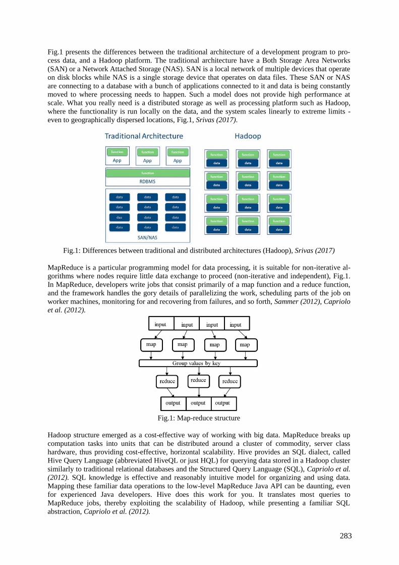
283
Fig.1 presents the differences between the traditional architecture of a development program to pro-
cess data, and a Hadoop platform. The traditional architecture have a Both Storage Area Networks
(SAN) or a Network Attached Storage (NAS). SAN is a local network of multiple devices that operate
on disk blocks while NAS is a single storage device that operates on data files. These SAN or NAS
are connecting to a database with a bunch of applications connected to it and data is being constantly
moved to where processing needs to happen. Such a model does not provide high performance at
scale. What you really need is a distributed storage as well as processing platform such as Hadoop,
where the functionality is run locally on the data, and the system scales linearly to extreme limits -
even to geographically dispersed locations, Fig.1, Srivas (2017).
Fig.1: Differences between traditional and distributed architectures (Hadoop), Srivas (2017)
MapReduce is a particular programming model for data processing, it is suitable for non-iterative al-
gorithms where nodes require little data exchange to proceed (non-iterative and independent), Fig.1.
In MapReduce, developers write jobs that consist primarily of a map function and a reduce function,
and the framework handles the gory details of parallelizing the work, scheduling parts of the job on
worker machines, monitoring for and recovering from failures, and so forth, Sammer (2012), Capriolo
et al. (2012).
Fig.1: Map-reduce structure
Hadoop structure emerged as a cost-effective way of working with big data. MapReduce breaks up
computation tasks into units that can be distributed around a cluster of commodity, server class
hardware, thus providing cost-effective, horizontal scalability. Hive provides an SQL dialect, called
Hive Query Language (abbreviated HiveQL or just HQL) for querying data stored in a Hadoop cluster
similarly to traditional relational databases and the Structured Query Language (SQL), Capriolo et al.
(2012). SQL knowledge is effective and reasonably intuitive model for organizing and using data.
Mapping these familiar data operations to the low-level MapReduce Java API can be daunting, even
for experienced Java developers. Hive does this work for you. It translates most queries to
MapReduce jobs, thereby exploiting the scalability of Hadoop, while presenting a familiar SQL
abstraction, Capriolo et al. (2012).
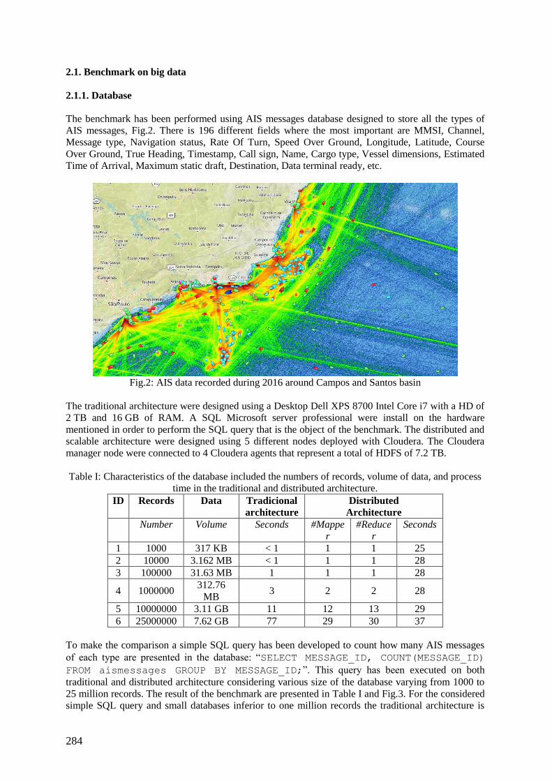
284
2.1. Benchmark on big data
2.1.1. Database
The benchmark has been performed using AIS messages database designed to store all the types of
AIS messages, Fig.2. There is 196 different fields where the most important are MMSI, Channel,
Message type, Navigation status, Rate Of Turn, Speed Over Ground, Longitude, Latitude, Course
Over Ground, True Heading, Timestamp, Call sign, Name, Cargo type, Vessel dimensions, Estimated
Time of Arrival, Maximum static draft, Destination, Data terminal ready, etc.
Fig.2: AIS data recorded during 2016 around Campos and Santos basin
The traditional architecture were designed using a Desktop Dell XPS 8700 Intel Core i7 with a HD of
2 TB and 16 GB of RAM. A SQL Microsoft server professional were install on the hardware
mentioned in order to perform the SQL query that is the object of the benchmark. The distributed and
scalable architecture were designed using 5 different nodes deployed with Cloudera. The Cloudera
manager node were connected to 4 Cloudera agents that represent a total of HDFS of 7.2 TB.
Table I: Characteristics of the database included the numbers of records, volume of data, and process
time in the traditional and distributed architecture.
ID Records Data Tradicional
architecture
Distributed
Architecture
Number Volume Seconds #Mappe
r
#Reduce
r
Seconds
1 1000 317 KB < 1 1 1 25
2 10000 3.162 MB < 1 1 1 28
3 100000 31.63 MB 1 1 1 28
4 1000000 312.76
MB 3 2 2 28
5 10000000 3.11 GB 11 12 13 29
6 25000000 7.62 GB 77 29 30 37
To make the comparison a simple SQL query has been developed to count how many AIS messages
of each type are presented in the database: “SELECT MESSAGE_ID, COUNT(MESSAGE_ID)
FROM aismessages GROUP BY MESSAGE_ID;”. This query has been executed on both
traditional and distributed architecture considering various size of the database varying from 1000 to
25 million records. The result of the benchmark are presented in Table I and Fig.3. For the considered
simple SQL query and small databases inferior to one million records the traditional architecture is
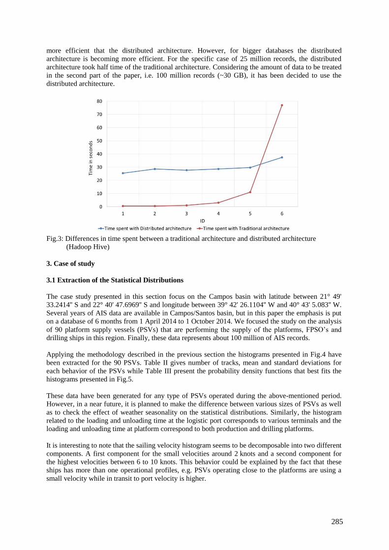
285
more efficient that the distributed architecture. However, for bigger databases the distributed
architecture is becoming more efficient. For the specific case of 25 million records, the distributed
architecture took half time of the traditional architecture. Considering the amount of data to be treated
in the second part of the paper, i.e. 100 million records (~30 GB), it has been decided to use the
distributed architecture.
Fig.3: Differences in time spent between a traditional architecture and distributed architecture
(Hadoop Hive)
3. Case of study
3.1 Extraction of the Statistical Distributions
The case study presented in this section focus on the Campos basin with latitude between 21° 49'
33.2414'' S and 22° 40' 47.6969'' S and longitude between 39° 42' 26.1104'' W and 40° 43' 5.083'' W.
Several years of AIS data are available in Campos/Santos basin, but in this paper the emphasis is put
on a database of 6 months from 1 April 2014 to 1 October 2014. We focused the study on the analysis
of 90 platform supply vessels (PSVs) that are performing the supply of the platforms, FPSO’s and
drilling ships in this region. Finally, these data represents about 100 million of AIS records.
Applying the methodology described in the previous section the histograms presented in Fig.4 have
been extracted for the 90 PSVs. Table II gives number of tracks, mean and standard deviations for
each behavior of the PSVs while Table III present the probability density functions that best fits the
histograms presented in Fig.5.
These data have been generated for any type of PSVs operated during the above-mentioned period.
However, in a near future, it is planned to make the difference between various sizes of PSVs as well
as to check the effect of weather seasonality on the statistical distributions. Similarly, the histogram
related to the loading and unloading time at the logistic port corresponds to various terminals and the
loading and unloading time at platform correspond to both production and drilling platforms.
It is interesting to note that the sailing velocity histogram seems to be decomposable into two different
components. A first component for the small velocities around 2 knots and a second component for
the highest velocities between 6 to 10 knots. This behavior could be explained by the fact that these
ships has more than one operational profiles, e.g. PSVs operating close to the platforms are using a
small velocity while in transit to port velocity is higher.
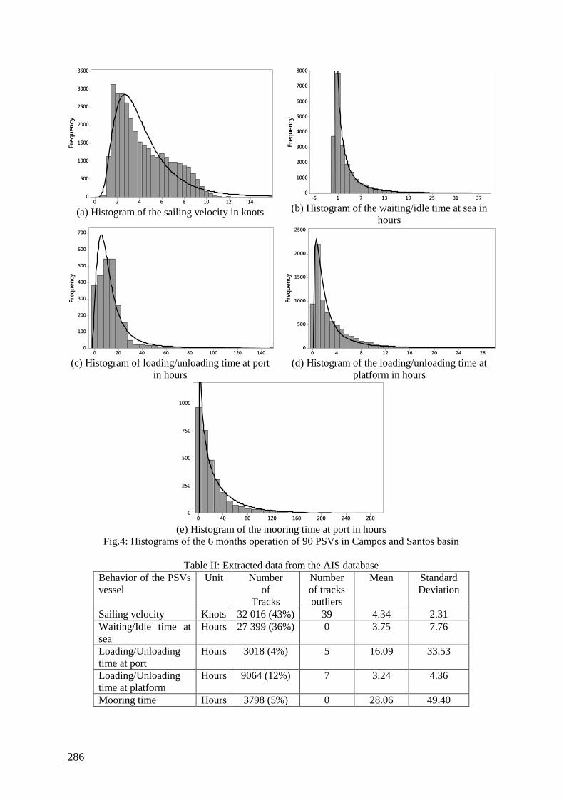
286
14121086420
3500
3000
2500
2000
1500
1000
500
0
Loc 1,306
Scale 0,5676
Thresh -0,03347
N 31975
Sailing
Fre
qu
en
cy
3-Parameter Lognormal
Histogram of Sailing
(a) Histogram of the sailing velocity in knots
373125191371-5
8000
7000
6000
5000
4000
3000
2000
1000
0
Loc 0,4431
Scale 1,338
Thresh -0,00125
N 22484
Waiting
Fre
qu
en
cy
3-Parameter Lognormal
Histogram of Waiting
(b) Histogram of the waiting/idle time at sea in
hours
140120100806040200
700
600
500
400
300
200
100
0
Loc 2,513
Scale 0,4639
Thresh -2,073
N 2535
Loading/Unloading - Port
Fre
qu
en
cy
3-Parameter Loglogistic
Histogram of Loading/Unloading - Port
(c) Histogram of loading/unloading time at port
in hours
2824201612840
2500
2000
1500
1000
500
0
Loc 0,5438
Scale 0,724
Thresh 0,01667
N 7992
Loading/Unloading - Platform
Fre
qu
en
cy
Histogram of Loading/Unloading - Platform3-Parameter Loglogistic
(d) Histogram of the loading/unloading time at
platform in hours
28024020016012080400
1000
750
500
250
0
Shape 0,5882
Scale 47,69
Thresh 0,01662
N 3238
Anchorage
Fre
qu
en
cy
3-Parameter Gamma
Histogram of Anchorage
(e) Histogram of the mooring time at port in hours
Fig.4: Histograms of the 6 months operation of 90 PSVs in Campos and Santos basin
Table II: Extracted data from the AIS database
Behavior of the PSVs
vessel
Unit Number
of
Tracks
Number
of tracks
outliers
Mean Standard
Deviation
Sailing velocity Knots 32 016 (43%) 39 4.34 2.31
Waiting/Idle time at
sea
Hours 27 399 (36%) 0 3.75 7.76
Loading/Unloading
time at port
Hours 3018 (4%) 5 16.09 33.53
Loading/Unloading
time at platform
Hours 9064 (12%) 7 3.24 4.36
Mooring time Hours 3798 (5%) 0 28.06 49.40
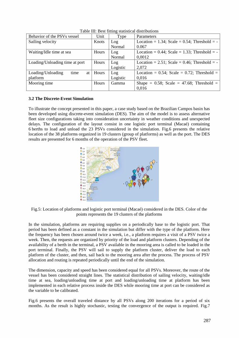
287
Table III: Best fitting statistical distributions
Behavior of the PSVs vessel Unit Type Parameters
Sailing velocity Knots Log
Normal
Location = 1.34; Scale = 0.54; Threshold = -
0.067
Waiting/Idle time at sea Hours Log
Normal
Location = 0.44; Scale = 1.33; Threshold = -
0,0012
Loading/Unloading time at port Hours Log
Logistic
Location = 2.51; Scale = 0.46; Threshold = -
2,072
Loading/Unloading time at
platform
Hours Log
Logistic
Location = 0.54; Scale = 0.72; Threshold =
0,016
Mooring time Hours Gamma Shape = 0.58; Scale = 47.68; Threshold =
0,016
3.2 The Discrete-Event Simulation
To illustrate the concept presented in this paper, a case study based on the Brazilian Campos basin has
been developed using discrete-event simulation (DES). The aim of the model is to assess alternative
fleet size configurations taking into consideration uncertainty in weather conditions and unexpected
delays. The configuration of the layout consist in one logistic port terminal (Macaé) containing
6 berths to load and unload the 23 PSVs considered in the simulation. Fig.6 presents the relative
location of the 38 platforms organized in 19 clusters (group of platforms) as well as the port. The DES
results are presented for 6 months of the operation of the PSV fleet.
Fig.5: Location of platforms and logistic port terminal (Macaé) considered in the DES. Color of the
points represents the 19 clusters of the platforms
In the simulation, platforms are requiring supplies on a periodically base to the logistic port. That
period has been defined as a constant in the simulation but differ with the type of the platform. Here
the frequency has been chosen around twice a week, i.e., a platform requires a visit of a PSV twice a
week. Then, the requests are organized by priority of the load and platform clusters. Depending of the
availability of a berth in the terminal, a PSV available in the mooring area is called to be loaded in the
port terminal. Finally, the PSV will sail to supply the platform cluster, deliver the load to each
platform of the cluster, and then, sail back to the mooring area after the process. The process of PSV
allocation and routing is repeated periodically until the end of the simulation.
The dimension, capacity and speed has been considered equal for all PSVs. Moreover, the route of the
vessel has been considered straight lines. The statistical distribution of sailing velocity, waiting/idle
time at sea, loading/unloading time at port and loading/unloading time at platform has been
implemented in each relative process inside the DES while mooring time at port can be considered as
the variable to be calibrated.
Fig.6 presents the overall traveled distance by all PSVs along 200 iterations for a period of six
months. As the result is highly stochastic, testing the convergence of the output is required. Fig.7
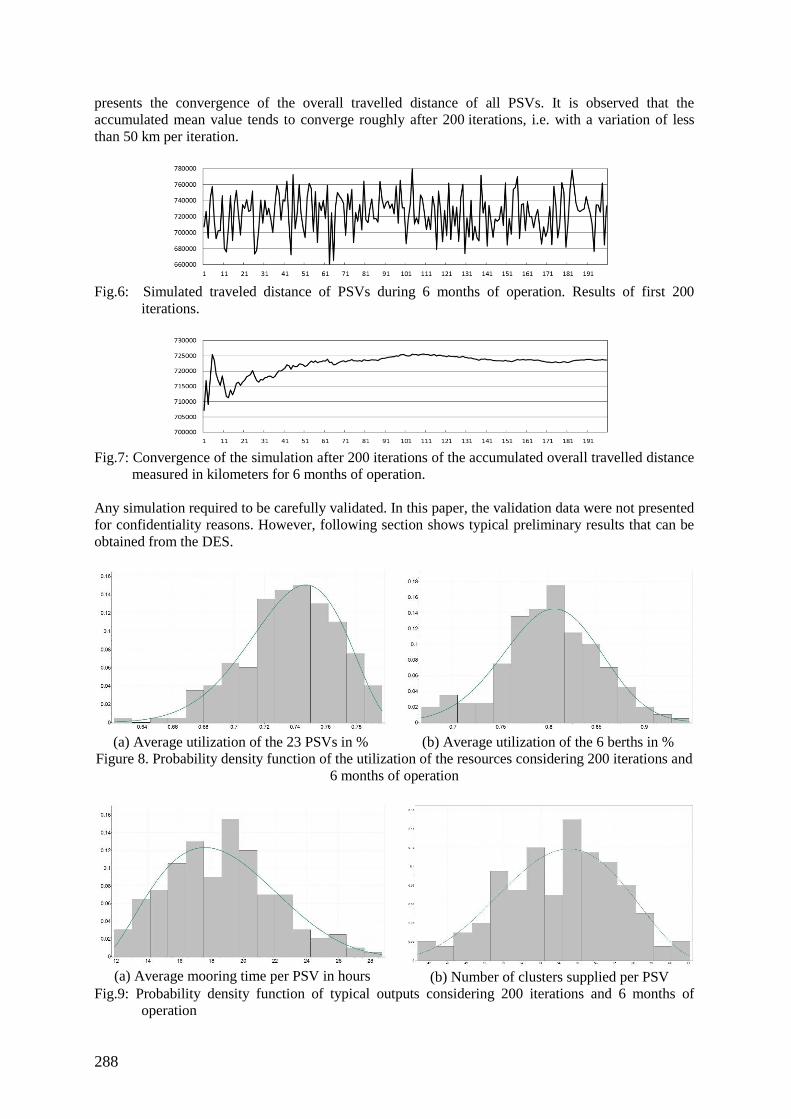
288
presents the convergence of the overall travelled distance of all PSVs. It is observed that the
accumulated mean value tends to converge roughly after 200 iterations, i.e. with a variation of less
than 50 km per iteration.
Fig.6: Simulated traveled distance of PSVs during 6 months of operation. Results of first 200
iterations.
Fig.7: Convergence of the simulation after 200 iterations of the accumulated overall travelled distance
measured in kilometers for 6 months of operation.
Any simulation required to be carefully validated. In this paper, the validation data were not presented
for confidentiality reasons. However, following section shows typical preliminary results that can be
obtained from the DES.
(a) Average utilization of the 23 PSVs in %
(b) Average utilization of the 6 berths in %
Figure 8. Probability density function of the utilization of the resources considering 200 iterations and
6 months of operation
(a) Average mooring time per PSV in hours (b) Number of clusters supplied per PSV
Fig.9: Probability density function of typical outputs considering 200 iterations and 6 months of
operation
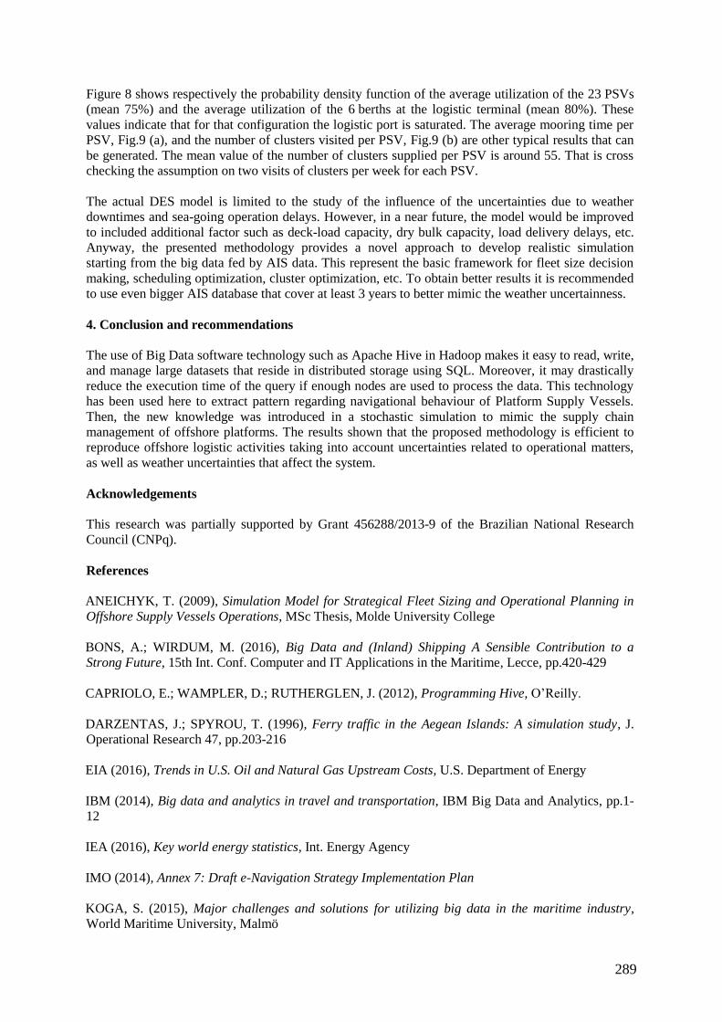
289
Figure 8 shows respectively the probability density function of the average utilization of the 23 PSVs
(mean 75%) and the average utilization of the 6 berths at the logistic terminal (mean 80%). These
values indicate that for that configuration the logistic port is saturated. The average mooring time per
PSV, Fig.9 (a), and the number of clusters visited per PSV, Fig.9 (b) are other typical results that can
be generated. The mean value of the number of clusters supplied per PSV is around 55. That is cross
checking the assumption on two visits of clusters per week for each PSV.
The actual DES model is limited to the study of the influence of the uncertainties due to weather
downtimes and sea-going operation delays. However, in a near future, the model would be improved
to included additional factor such as deck-load capacity, dry bulk capacity, load delivery delays, etc.
Anyway, the presented methodology provides a novel approach to develop realistic simulation
starting from the big data fed by AIS data. This represent the basic framework for fleet size decision
making, scheduling optimization, cluster optimization, etc. To obtain better results it is recommended
to use even bigger AIS database that cover at least 3 years to better mimic the weather uncertainness.
4. Conclusion and recommendations
The use of Big Data software technology such as Apache Hive in Hadoop makes it easy to read, write,
and manage large datasets that reside in distributed storage using SQL. Moreover, it may drastically
reduce the execution time of the query if enough nodes are used to process the data. This technology
has been used here to extract pattern regarding navigational behaviour of Platform Supply Vessels.
Then, the new knowledge was introduced in a stochastic simulation to mimic the supply chain
management of offshore platforms. The results shown that the proposed methodology is efficient to
reproduce offshore logistic activities taking into account uncertainties related to operational matters,
as well as weather uncertainties that affect the system.
Acknowledgements
This research was partially supported by Grant 456288/2013-9 of the Brazilian National Research
Council (CNPq).
References
ANEICHYK, T. (2009), Simulation Model for Strategical Fleet Sizing and Operational Planning in
Offshore Supply Vessels Operations, MSc Thesis, Molde University College
BONS, A.; WIRDUM, M. (2016), Big Data and (Inland) Shipping A Sensible Contribution to a
Strong Future, 15th Int. Conf. Computer and IT Applications in the Maritime, Lecce, pp.420-429
CAPRIOLO, E.; WAMPLER, D.; RUTHERGLEN, J. (2012), Programming Hive, O’Reilly.
DARZENTAS, J.; SPYROU, T. (1996), Ferry traffic in the Aegean Islands: A simulation study, J.
Operational Research 47, pp.203-216
EIA (2016), Trends in U.S. Oil and Natural Gas Upstream Costs, U.S. Department of Energy
IBM (2014), Big data and analytics in travel and transportation, IBM Big Data and Analytics, pp.1-
12
IEA (2016), Key world energy statistics, Int. Energy Agency
IMO (2014), Annex 7: Draft e-Navigation Strategy Implementation Plan
KOGA, S. (2015), Major challenges and solutions for utilizing big data in the maritime industry,
World Maritime University, Malmö

290
KORTE, H.; IHMELS, I.; RICHTER, J.; ZERHUSEN, B.; HAHN, A. (2012), Offshore training
simulations, 9th IFAC Conf. Manoeuvring and Control of Marine Craft, pp.37-42)
MGI, M.G. (2012), Big Data: The next frontier for innovation, competition, and productivity
RAMSDEN, R.; LELLIOT, P.; THOMASON, J.; ROERMUND, D. (2016), Project Helm: Insights
from AIS, Fouling Control and Big Data, 15th Int. Conf. Computer and IT Applications in the
Maritime, Lecce, pp.439-447
RØDSETH, Ø.; PERERA, L.; MO, B. (2016), Big Data in Shipping - Challenges and Opportunities,
15th Int. Conf. Computer and IT Applications in the Maritime, Lecce, pp.361-373
SAMMER, E. (2012), Hadoop Operations, O'Reilly
SHYSHOU, A.; GRIBKOVSKAIA, I.; BARCELÓ, J. (2010), A simulation study of the fleet sizing
problem arising in offshore anchor handling operations, European J. Operational Research 203(1),
pp.230-240
SRIVAS, M. (2017), Architecture matters for production success, MAPR, https://mapr.com/why-
hadoop/why-mapr/architecture-matters/
UK (2016), Oil & Gas UK’s Economic Report 2016
WHITE, T. (2009), Hadoop: The Definitive Guide, O’Reilly
ZICARI, R. (2014), Big Data: Challenges and Opportunities, Big Data Computing, Western Norway
Research Institute, , pp. 103-130
291
The Extended Process-Centric Modeling Method
for Logistics Simulation in Shipyards Considering Stock Areas
Byeongseop Kim, Seoul National University, Seoul/Korea, [email protected]
Yong-Kuk Jeong, Seoul National University, Seoul/Korea, [email protected]
Seunghyeok Son, Seoul National University, Seoul/Korea, [email protected]
Philippe Lee, Xinnos Co., Ltd., Seoul/Korea, [email protected]
Yonggil Lee, Korea Maritime and Ocean University, Busan/Korea, [email protected]
Jong Hun Woo, Korea Maritime and Ocean University, Busan/Korea, [email protected]
Abstract
Block logistic loads, such as those associated with transporters and stockers, are difficult to consider
in the planning stage for a shipyard. This study was conducted to calculate the block logistics load in
the planning stage using simulations and proposes an extended process-centric modeling method with
the concept of a logistic token being added to the conventional process-centric simulation method used
in the shipyard. The proposed method was validated first through a unit model and then with a logistics
model of an actual shipyard that was constructed from the validated model. As a result of the simulation,
usage result of stock area, transporter, and road for the plan was obtained.
1. Introduction
Ships are manufactured by a block construction, by assembling an intermediate product, usually in the
form of blocks, and then constructing the ship as a finished product by mounting the blocks at the dock.
After the assembly, blocks undergo processes such as outfitting, installation of pipe and electric devices,
and painting. Blocks wait in the stock area if there is a period of time remaining between the processes
before they can be mounted at the dock. Blocks are very large and heavy even though they are
intermediate products, and they are transported one by one using a special facility called a transporter.
Such transportation and stocking processes are referred to as block logistics in the shipyard.
Because the number of transporters and the space in the stock areas are limited, such logistic loads must
be considered in the planning stage for smooth production. In most cases, however, logistics plans
including transporter and stock area allocations are not set up in the planning stage and the block
transportation department just provides such direction in the actual production stage. Because the loads
of transporters and stock areas are not considered in the planning stage, even if the process equipment
capacity is sufficient, processes can be delayed by logistic loads in the production stage, Song and Kang
(2009).
In addition to the shipbuilding industry, logistical load issues within the plant are also experienced in
the automobile, semiconductor, and aviation industries, and many studies have been conducted to
calculate logistic loads using discrete-event system (DES) simulations. Most DES studies are based on
resource-centric modeling, which is a method of modeling facilities and products flows along facilities.
However, the resource-centric modeling method has a few problems when applied to shipyards, as
shipyards do not produce mass production. First, products of shipyards don’t flow through a certain
route, so modeling of route which is essential in resource-centric modeling is difficult. Second, it takes
much time to model the resources of a plant because the shipbuilding plant has very large space and
many facilities. Third, simulation results from the resource-centric model are not easy to analyze based
on schedule, but most decisions in the production stage of a shipyard are based on the schedule made
during production planning stage.
Due to these reasons, the DES simulation research of shipyards has focused on a process-centric
modeling method instead of a resource-centric modeling method, Lee et al. (2014). It has been
demonstrated that the process-centric modeling method is more appropriate for shipyards and has been
used in such cases as the validation of mid-term plans, Jeong et al. (2015). However, the conventional
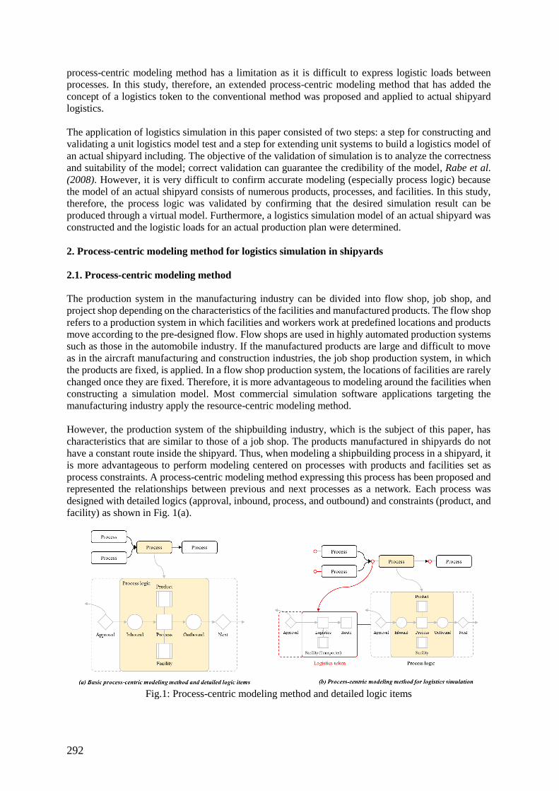
292
process-centric modeling method has a limitation as it is difficult to express logistic loads between
processes. In this study, therefore, an extended process-centric modeling method that has added the
concept of a logistics token to the conventional method was proposed and applied to actual shipyard
logistics.
The application of logistics simulation in this paper consisted of two steps: a step for constructing and
validating a unit logistics model test and a step for extending unit systems to build a logistics model of
an actual shipyard including. The objective of the validation of simulation is to analyze the correctness
and suitability of the model; correct validation can guarantee the credibility of the model, Rabe et al.
(2008). However, it is very difficult to confirm accurate modeling (especially process logic) because
the model of an actual shipyard consists of numerous products, processes, and facilities. In this study,
therefore, the process logic was validated by confirming that the desired simulation result can be
produced through a virtual model. Furthermore, a logistics simulation model of an actual shipyard was
constructed and the logistic loads for an actual production plan were determined.
2. Process-centric modeling method for logistics simulation in shipyards
2.1. Process-centric modeling method
The production system in the manufacturing industry can be divided into flow shop, job shop, and
project shop depending on the characteristics of the facilities and manufactured products. The flow shop
refers to a production system in which facilities and workers work at predefined locations and products
move according to the pre-designed flow. Flow shops are used in highly automated production systems
such as those in the automobile industry. If the manufactured products are large and difficult to move
as in the aircraft manufacturing and construction industries, the job shop production system, in which
the products are fixed, is applied. In a flow shop production system, the locations of facilities are rarely
changed once they are fixed. Therefore, it is more advantageous to modeling around the facilities when
constructing a simulation model. Most commercial simulation software applications targeting the
manufacturing industry apply the resource-centric modeling method.
However, the production system of the shipbuilding industry, which is the subject of this paper, has
characteristics that are similar to those of a job shop. The products manufactured in shipyards do not
have a constant route inside the shipyard. Thus, when modeling a shipbuilding process in a shipyard, it
is more advantageous to perform modeling centered on processes with products and facilities set as
process constraints. A process-centric modeling method expressing this process has been proposed and
represented the relationships between previous and next processes as a network. Each process was
designed with detailed logics (approval, inbound, process, and outbound) and constraints (product, and
facility) as shown in Fig. 1(a).
Fig.1: Process-centric modeling method and detailed logic items
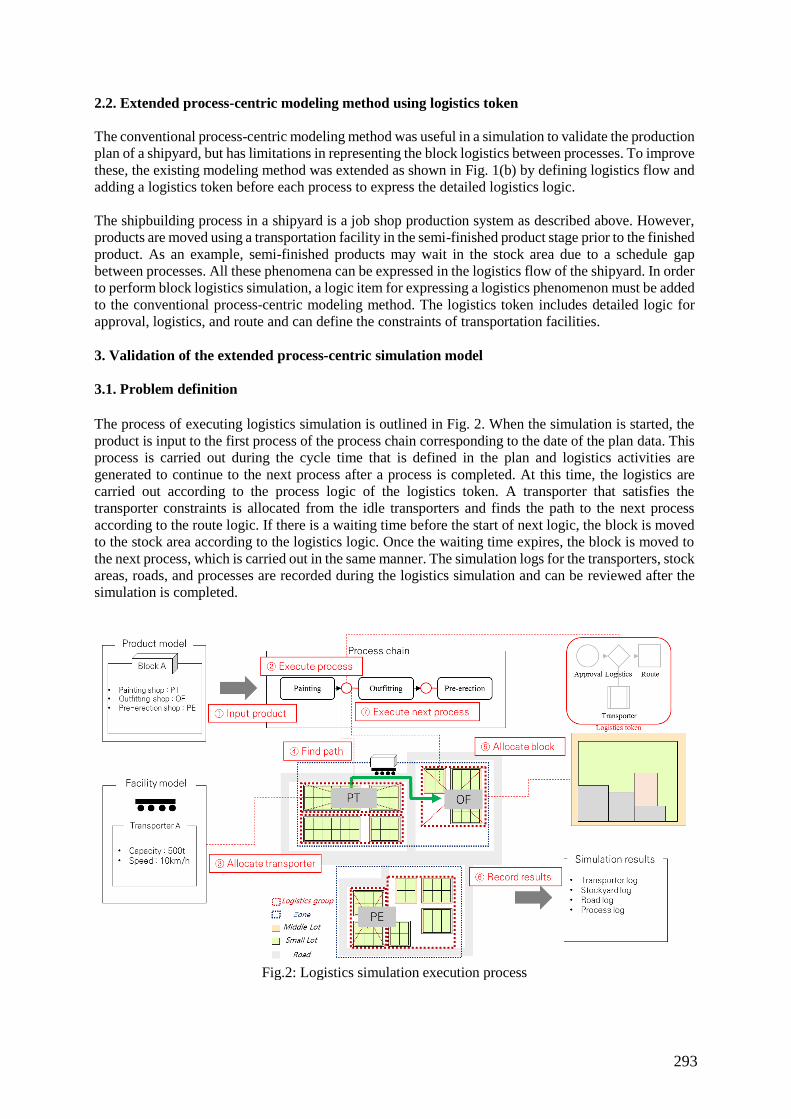
293
2.2. Extended process-centric modeling method using logistics token
The conventional process-centric modeling method was useful in a simulation to validate the production
plan of a shipyard, but has limitations in representing the block logistics between processes. To improve
these, the existing modeling method was extended as shown in Fig. 1(b) by defining logistics flow and
adding a logistics token before each process to express the detailed logistics logic.
The shipbuilding process in a shipyard is a job shop production system as described above. However,
products are moved using a transportation facility in the semi-finished product stage prior to the finished
product. As an example, semi-finished products may wait in the stock area due to a schedule gap
between processes. All these phenomena can be expressed in the logistics flow of the shipyard. In order
to perform block logistics simulation, a logic item for expressing a logistics phenomenon must be added
to the conventional process-centric modeling method. The logistics token includes detailed logic for
approval, logistics, and route and can define the constraints of transportation facilities.
3. Validation of the extended process-centric simulation model
3.1. Problem definition
The process of executing logistics simulation is outlined in Fig. 2. When the simulation is started, the
product is input to the first process of the process chain corresponding to the date of the plan data. This
process is carried out during the cycle time that is defined in the plan and logistics activities are
generated to continue to the next process after a process is completed. At this time, the logistics are
carried out according to the process logic of the logistics token. A transporter that satisfies the
transporter constraints is allocated from the idle transporters and finds the path to the next process
according to the route logic. If there is a waiting time before the start of next logic, the block is moved
to the stock area according to the logistics logic. Once the waiting time expires, the block is moved to
the next process, which is carried out in the same manner. The simulation logs for the transporters, stock
areas, roads, and processes are recorded during the logistics simulation and can be reviewed after the
simulation is completed.
Fig.2: Logistics simulation execution process

294
Fig.3: Factory Selection Logic
The workshop and stock area are created as part of the plant model that is mapped to spatial data. The
plant selection logic is performed in the logistics step of the logistics token and determines stocking by
comparing the simulation time and planned days. Fig. 3 shows a schematic of the routing path of blocks.
When the difference between work time and planned days is less than one day, the block is immediately
input to the workplace of the next process. If the block needs to be stocked, it is moved to and remains
at the stock area until being moved to the workshop of the next process on the starting date of the next
process.
The selection of a stock area can be considered as an important factor if stocking is required. The stock
area selection logic in the simulation has the preferred stock area information for each workshop
considering the logic of movements. During the selection of the stock area, the workshop of the next
process checks the preferred stock area and stocks the blocks in the corresponding stock area.
The facility capacity must be considered for efficient use of transporters. This capacity refers to the
maximum weight that can be transported. Transportation is impossible if the block weight is greater
than the capacity. The simulation is designed to select a facility that has the smallest capacity among
the facilities having a capacity greater than the block weight. The objective is to use the most efficient
facility to minimize the fuel consumption, as fuel efficiency is lower when the facility weight is greater.
Fig.4: Example of unit logistics simulation model
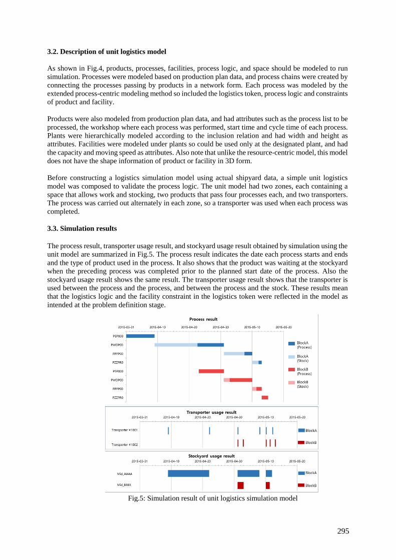
295
3.2. Description of unit logistics model
As shown in Fig.4, products, processes, facilities, process logic, and space should be modeled to run
simulation. Processes were modeled based on production plan data, and process chains were created by
connecting the processes passing by products in a network form. Each process was modeled by the
extended process-centric modeling method so included the logistics token, process logic and constraints
of product and facility.
Products were also modeled from production plan data, and had attributes such as the process list to be
processed, the workshop where each process was performed, start time and cycle time of each process.
Plants were hierarchically modeled according to the inclusion relation and had width and height as
attributes. Facilities were modeled under plants so could be used only at the designated plant, and had
the capacity and moving speed as attributes. Also note that unlike the resource-centric model, this model
does not have the shape information of product or facility in 3D form.
Before constructing a logistics simulation model using actual shipyard data, a simple unit logistics
model was composed to validate the process logic. The unit model had two zones, each containing a
space that allows work and stocking, two products that pass four processes each, and two transporters.
The process was carried out alternately in each zone, so a transporter was used when each process was
completed.
3.3. Simulation results
The process result, transporter usage result, and stockyard usage result obtained by simulation using the
unit model are summarized in Fig.5. The process result indicates the date each process starts and ends
and the type of product used in the process. It also shows that the product was waiting at the stockyard
when the preceding process was completed prior to the planned start date of the process. Also the
stockyard usage result shows the same result. The transporter usage result shows that the transporter is
used between the process and the process, and between the process and the stock. These results mean
that the logistics logic and the facility constraint in the logistics token were reflected in the model as
intended at the problem definition stage.
Fig.5: Simulation result of unit logistics simulation model
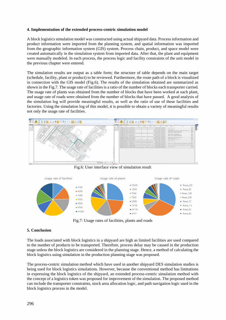
296
4. Implementation of the extended process-centric simulation model
A block logistics simulation model was constructed using actual shipyard data. Process information and
product information were imported from the planning system, and spatial information was imported
from the geographic information system (GIS) system. Process chain, product, and space model were
created automatically in the simulation system from imported data. After that, the plant and equipment
were manually modeled. In each process, the process logic and facility constraints of the unit model in
the previous chapter were entered.
The simulation results are output as a table form; the structure of table depends on the main target
(schedule, facility, plant or product) to be reviewed. Furthermore, the route path of a block is visualized
in connection with the GIS model (Fig.6). The results of the simulation obtained are summarized as
shown in the Fig.7. The usage rate of facilities is a ratio of the number of blocks each transporter carried.
The usage rate of plants was obtained from the number of blocks that have been worked at each plant,
and usage rate of roads were obtained from the number of blocks that have passed. A good analysis of
the simulation log will provide meaningful results, as well as the ratio of use of these facilities and
factories. Using the simulation log of this model, it is possible to obtain a variety of meaningful results
not only the usage rate of facilities.
Fig.6: User interface view of simulation result
Fig.7: Usage rates of facilities, plants and roads
5. Conclusion
The loads associated with block logistics in a shipyard are high as limited facilities are used compared
to the number of products to be transported. Therefore, process delay may be caused in the production
stage unless the block logistics are considered in the planning stage. Hence, a method of calculating the
block logistics using simulation in the production planning stage was proposed.
The process-centric simulation method which have used in another shipyard DES simulation studies is
being used for block logistics simulations. However, because the conventional method has limitations
in expressing the block logistics of the shipyard, an extended process-centric simulation method with
the concept of a logistics token was proposed for improvement of the simulation. The proposed method
can include the transporter constraints, stock area allocation logic, and path navigation logic used in the
block logistics process in the model.
297
In addition, to validate the proposed method and the process logic of logistics simulation, a unit model
was constructed. It was validated that this model produced the desired results for the usage of
transporters, stock areas, and roads and that the process logic of this model successfully reflected the
block logistics process. Next, the logistics simulation model of an actual shipyard was implemented
using schedule data and GIS data, and the validated process logic from the unit model. Such simulation
results as road usage, transporter usage, and stock area usage for an actual schedule could be calculated
using this model. These calculated logistics loads can be used in the production planning stage to
establish plans by considering logistics as constraints and can be also applied to the establishment of
transporter operation plans.
References
JEONG, Y.K.; WOO, J.H.; OH, D.K.; SHIN, J.G. (2016), A Shipyard Simulation System using the
Process-centric Simulation Modeling Methodology: Case Study of the Simulation Model for the
Shipyard Master Plan Validation, Trans. Society of CAD/CAM Engineers 21(2), pp.204-214
LEE, D.K.; KIM,Y.; HWANG, I.H.; OH, D.K.; SHIN, J.G. (2014), Study on a process-centric modeling
methodology for virtual manufacturing of ships and offshore structures in shipyards, Int. J. Advanced
Manufacturing Technology 71(1), pp.621-633
RABE, M.; SPIECKERMANN, S.; WENZEL, S. (2008), A new procedure model for verification and
validation in production and logistics simulation, 40th Conf. Winter Simulation, Miami, pp.1717-1726
SONG, C.S.; KANG, Y.W. (2009), Simulation of Block Logistics at a Big Shipyard, Korean J.
Computational Design and Engineering 14(6), pp.374-81
298
Toward Functional Augmented Reality in Marine Navigation:
A Cognitive Work Analysis
Stephan Procee, Maritiem Instituut Willem Barentsz, Terschelling/the Netherlands, [email protected] Clark Borst, Delft University of Technology, Delft/the Netherlands, [email protected]
René van Paassen, Delft Univ. of Technology, Delft/the Netherlands, [email protected] Max Mulder, Delft University of Technology, Delft/the Netherlands, [email protected]
Abstract
Augmented Reality, (AR) also known as vision-overlay, can help the navigator to visually detect a
dangerous target by the overlay of a synthetic image, thus providing a visual cue over the real world.
This is the first paper of a series about the practicalities and consequences of implementing AR in
marine navigation. A Cognitive Work Analysis is carried out to derive a scientific base for a func-
tional interface that best supports navigators in their work.
1. Introduction
The task of the watch officer (WO) can be described as systems process engineering. Long periods of
relative inactivity can suddenly change into a situation requiring heavy multitasking with a high level
of workload. It is no surprise then that, based on the number of navigational claims, the Swedish Club
has reported that in most accidents (69%), human error is an immediate cause. In this research, we
focus on the prevention from accidents related to navigation, collision and grounding. From the same
Swedish Club analysis it appears that lack of situation awareness is an immediate cause for collision
(38%) and groundings (55%).
Although several measures like Vessel Traffic Service (VTS), separating traffic, and the introduction
of electronic navigation have helped decrease the absolute number of accidents, the large annual
number of accidents and dramatic loss of life motivates research into ways to further improve. More-
over, statistics in transported tonnage show that the amount of transported goods by sea has more than
tripled since the 1950s and is expected to grow by approximately 2-3% per annum for the next decade
UNCTAD (2016). This justifies the effort spent on research and development to improve safety.
It is commonly accepted that technical malfunctioning of navigation equipment is seldom the cause of
accidents, therefore focusing on human factors is opportune, however, the work routines of the
navigator have barely changed over the last three or four decades. Morrel suggested already in 1960
that some form of expert aided decision support would be helpful in accident prevention, Morrel
(1960). Despite several studies into this field, automated Collision Avoidance (CA) or decision
support has still not been accepted. In the foreseeable future the human operator therefore remains the
only entity to control the ‘open’ process of navigation.
The research presented in this paper aims at creating a novel interface that best supports the human in
his or her role of decision maker. AR can contribute to this proposed Information Management Expert
Support system. By superimposing a virtual image on the outside world, the reality is enhanced by
visual cues. These cues can represent dangerous targets, however, in the E-navigation domain the
functionality needs not be limited to CA alone. Using AR, we also expect to speed up effective
information processing, although the practical implication of introducing this new technique is not at
all clear. Although several ways to portray AR already exist, and although hardware development is
ongoing, in this research we will use a Head Mounted Display (HMD) for testing.
An example of AR is shown in Fig.1 where the red projected box (c) points to a critical target, a red
projected fence (a) shows the area to be avoided and a route suggestion (b) is shown by the projection
of green 'runway' lighting. This projected information is corrected for the ship's attitude and motion
and also takes into account the position and viewing direction of the observer.
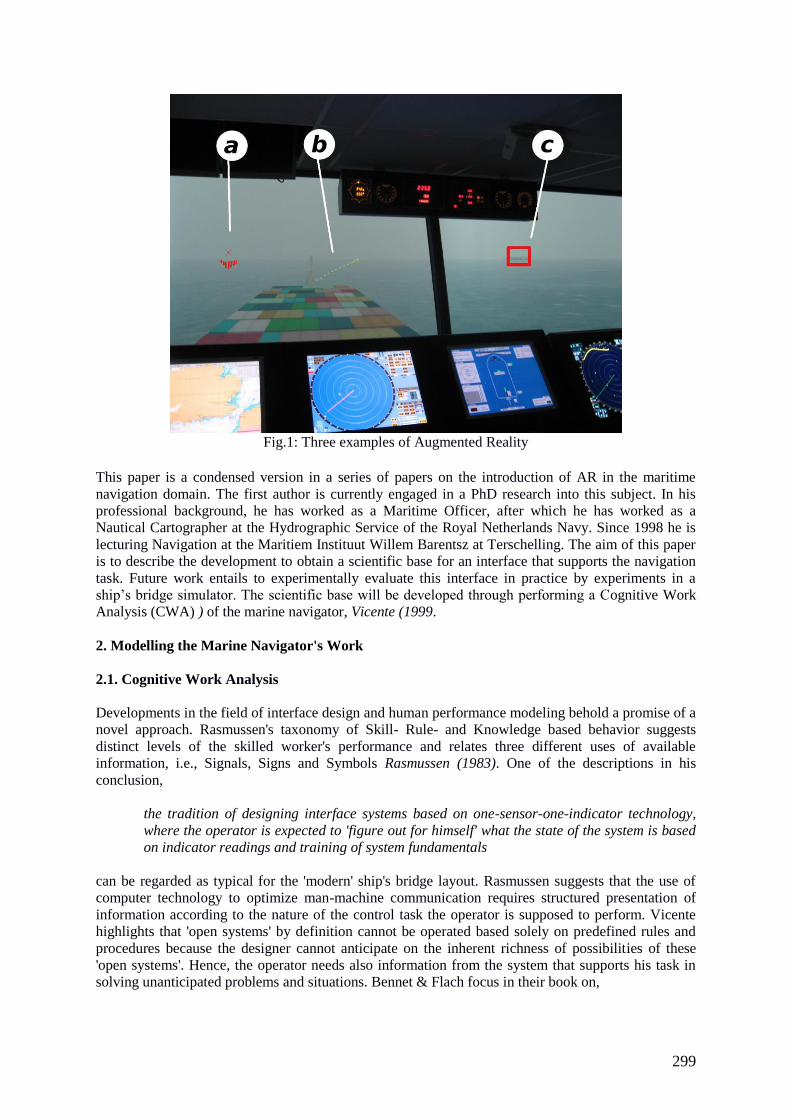
299
Fig.1: Three examples of Augmented Reality
This paper is a condensed version in a series of papers on the introduction of AR in the maritime
navigation domain. The first author is currently engaged in a PhD research into this subject. In his
professional background, he has worked as a Maritime Officer, after which he has worked as a
Nautical Cartographer at the Hydrographic Service of the Royal Netherlands Navy. Since 1998 he is
lecturing Navigation at the Maritiem Instituut Willem Barentsz at Terschelling. The aim of this paper
is to describe the development to obtain a scientific base for an interface that supports the navigation
task. Future work entails to experimentally evaluate this interface in practice by experiments in a
ship’s bridge simulator. The scientific base will be developed through performing a Cognitive Work
Analysis (CWA) ) of the marine navigator, Vicente (1999.
2. Modelling the Marine Navigator's Work
2.1. Cognitive Work Analysis
Developments in the field of interface design and human performance modeling behold a promise of a
novel approach. Rasmussen's taxonomy of Skill- Rule- and Knowledge based behavior suggests
distinct levels of the skilled worker's performance and relates three different uses of available
information, i.e., Signals, Signs and Symbols Rasmussen (1983). One of the descriptions in his
conclusion,
the tradition of designing interface systems based on one-sensor-one-indicator technology,
where the operator is expected to 'figure out for himself' what the state of the system is based
on indicator readings and training of system fundamentals
can be regarded as typical for the 'modern' ship's bridge layout. Rasmussen suggests that the use of
computer technology to optimize man-machine communication requires structured presentation of
information according to the nature of the control task the operator is supposed to perform. Vicente
highlights that 'open systems' by definition cannot be operated based solely on predefined rules and
procedures because the designer cannot anticipate on the inherent richness of possibilities of these
'open systems'. Hence, the operator needs also information from the system that supports his task in
solving unanticipated problems and situations. Bennet & Flach focus in their book on,
300
the primary purpose of an interface, to provide decision making and problem solving support
for a user who is completing work in a domain
In their book they adapt what they call a triadic approach, i.e., the design emphasis is put on the
functional demands of the work domain Bennet and Flach (2011). The underpinning Cognitive
Systems Engineering (CSE) concept finds a broad ground, and from that the concept of Ecological
Interface Design (EID) has been derived in the early 1990’s Flach et al. (1998). From Bainbridge
Bainbridge (1983) we may infer that maximizing the use of 'perceptual motor skills' and minimizing
the disruption of working memory may lead to a different balance in the distribution of mental
resources thus supporting problem solving tasks.
The multitude of tasks that the watch officer (WO) has to deal with, are visualized in Fig.2. The
navigation process of a ship can be characterized as dealing with a highly 'open' system, meaning that
it is subject to unpredictable external and internal influences. Although ships are overwhelmed by
Authorities’, Class Societies’, P&I clubs’ and Fleet Operators’ rules, requirements, procedures and
checklists, the work cannot really be characterized as 'normative'. Which means that, although some
of the tasks have been literally described in terms of instructions or checklists, the majority of work is
done at the WO's discretion within the boundaries of safe and effective operation.
Fig.2 is a representation of many of these boundaries and can therefore be regarded as a constraint-
based description of the WO's tasks, also known as 'task representation'. The quality assurance
systems in use primarily describe the responsibilities of the WO but not ‘how’ to fulfill these. So
when we analyze the work with the aim to develop an effective interface we should go further than
this constraint-based task representation. The reason for this wider scope is that the work domain, i.e.,
the ship, its controls and its natural environment, have a huge impact on the operation. Thus, the work
of the WO cannot solely be described by 'goals to be achieved', instead the possibilities and
limitations of the work domain should be taken into account as well. And, as said before, the
introduction of new technology, i.e., AR, requires us to design a new interface. The effectiveness of
this interface heavily depends on the 'meaning' of the portrayed information, in other words, it
depends on the provided or shown consequences, limitations and affordances of the system given its
state and its environment. Therefore, we have to analyze the work domain, and use this analysis
together with the task representation to come to an overarching framework in order to enable effective
interface design.
2.2. The Work Domain
The work domain consists of ships and sea. A ship can be defined as a floating self-propelling
controllable object, guided autonomously by a licensed watch keeper, with the purpose of undertaking
a voyage expeditiously. In this context the sea can be defined as any stretch of water, deep enough to
allow a ship to sail in and open for navigation.
Different from air navigation, traffic at sea is in principle unguided. However, there are situations
where the risk of grounding or collision is deemed so high that precautionary measures are taken. In
such cases the competent authority provides guidance by means of an established VTS or by
arranging compulsory pilotage. The competent authority can only rule within its own territory.
Outside territorial waters the principle of free sea rules since Hugo Grotius propounded this principle
in his 'Mare Liberum' in 1609 Grotius (1609).
Notwithstanding the principle of free sea, several arrangements have been accepted by international
agreement in order to regulate shipping in international waters to enhance safety and reduce pollution.
Amongst these are for instance the International Collision Regulations IMO (1972). These 'Rules of
the Road' focus primarily on the mutual conduct of ships. Ships have an obligation to act conformal to
the Rules, the ship's flag state is the only authority empowered to keep the law on board a vessel
sailing in international waters. The consequence of unguided shipping is that every vessel is free to
choose and sail its route. Although this routeing is strongly biased by cost-efficiency, the wide
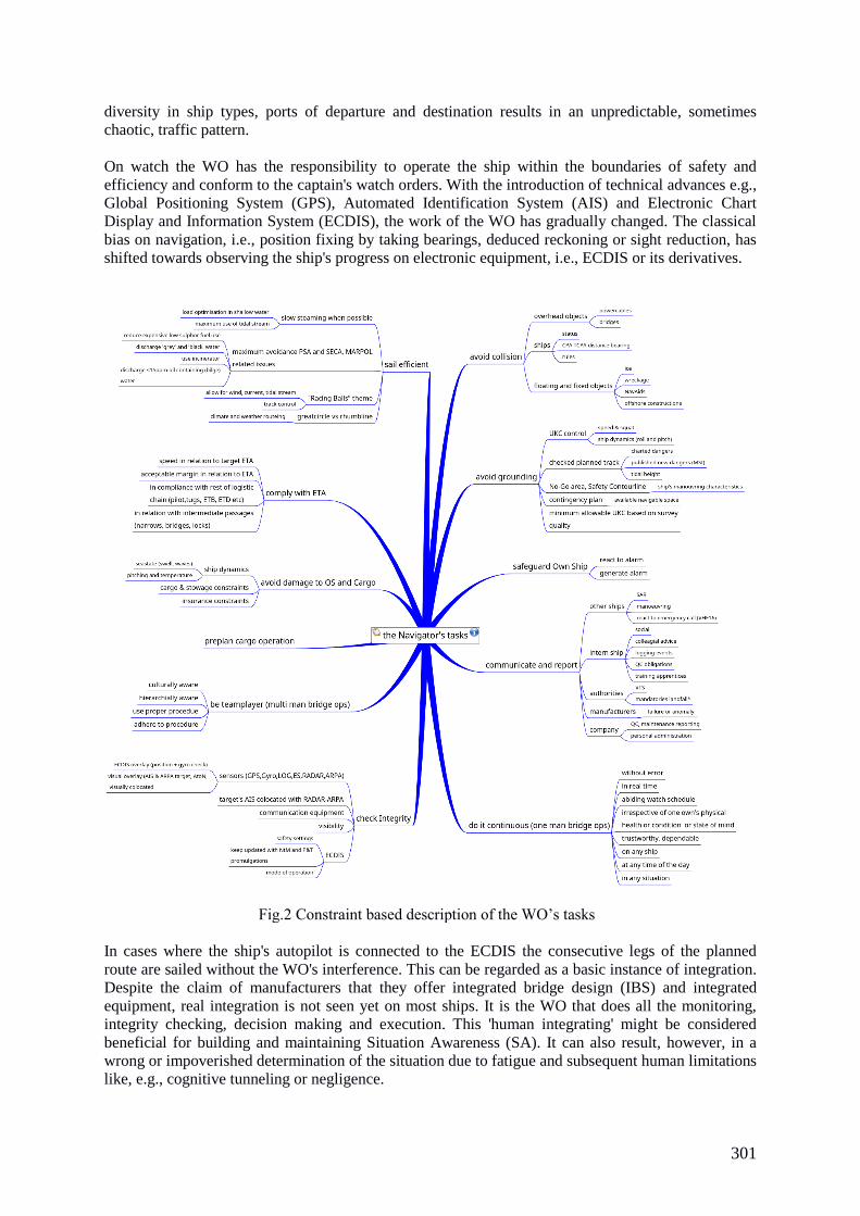
301
diversity in ship types, ports of departure and destination results in an unpredictable, sometimes
chaotic, traffic pattern.
On watch the WO has the responsibility to operate the ship within the boundaries of safety and
efficiency and conform to the captain's watch orders. With the introduction of technical advances e.g.,
Global Positioning System (GPS), Automated Identification System (AIS) and Electronic Chart
Display and Information System (ECDIS), the work of the WO has gradually changed. The classical
bias on navigation, i.e., position fixing by taking bearings, deduced reckoning or sight reduction, has
shifted towards observing the ship's progress on electronic equipment, i.e., ECDIS or its derivatives.
Fig.2 Constraint based description of the WO’s tasks
In cases where the ship's autopilot is connected to the ECDIS the consecutive legs of the planned
route are sailed without the WO's interference. This can be regarded as a basic instance of integration.
Despite the claim of manufacturers that they offer integrated bridge design (IBS) and integrated
equipment, real integration is not seen yet on most ships. It is the WO that does all the monitoring,
integrity checking, decision making and execution. This 'human integrating' might be considered
beneficial for building and maintaining Situation Awareness (SA). It can also result, however, in a
wrong or impoverished determination of the situation due to fatigue and subsequent human limitations
like, e.g., cognitive tunneling or negligence.
302
2.3. E-navigation developments in the work domain
The increase in the amount of worldwide transported goods by sea, the broadly felt public urge to
reduce the environmental impact of transport in general, and the reduced cost of continuous world-
wide satellite communication have led to the adoption of the E-Navigation concept by the IMO and
IALA. The agreed definition of E-navigation is: IMO (2017)
the harmonized collection, integration, exchange, presentation and analysis of marine
information on board and ashore by electronic means to enhance berth to berth navigation
and related services for safety and security at sea and protection of the marine environment.
An anticipated consequence of E-Navigation's safe communication possibilities is the exchange of the
planned route ahead. An already materialized prototype is called “Intended Route Exchange”. This
enables interacting ships to visually inform each other and even visually negotiate their planned
maneuvering within a limited time frame of approximately 20 to 30 minutes ACCSEAS (2015). This
will lead to unprecedented interaction between ships. An interaction based on the exchange of the
geographically referenced visualized planned route, and the visualized intention to deviate to avoid
collision.
Without going into all detailed examples of the more or less matured E-Navigation prototypes, it is
clear that the impact of these developments on the work domain will be tremendous. Whilst a
materialized E-Navigation proposition has not yet emerged, nor has it been internationally agreed or
adopted by IMO, we must focus on the existing work domain and keep in mind that within the next
decade a drastic shift will be necessary due to the adoption of E-Navigation.
2.4. Decomposition of the Task Representation
It is obvious from the complexity of Fig.2 that, in order to analyze the total span of the WO's
information needs, we have to decompose this task representation into subsets. The aim is to derive
such subsets that every subset covers a logical cluster of tasks which each relate to specific
information needs. From these information needs we can aggregate an overarching integrated
interface which effectively informs the WO and supports him in the execution of this subset of tasks.
Ultimately, the aggregation of each optimal interface should lead to an overarching interface design
supporting the WO in his or her work spanning the task representation, Fig.2.
The following subsections deal with the subset of CA. This subset can be decomposed into three areas
dealing with characteristic entities. All these entities are located on or above the sea surface, thus are,
in principle, visible and do impose a real danger to the vessel. The three characteristic entities relate to
the area of height restriction, e.g., bridges or overhead power cables, the area of other ships, and the
area of passive objects. The other subsets, e.g., grounding avoidance, efficient sailing and damage
avoidance will be covered in following papers.
2.5. Collision Avoidance, State Variables and State Dimension
In previous sections, we discussed the task representation of the WO, describing the boundaries
within which she has to perform his work, or within which he has to keep the system that he's
controlling. This system has its own characteristic and behavior which in its turn defines the possible
outcome of control, or the possible states that can be controlled. The State can be defined as a vector
in State Space describing the behavior of a system at a particular time. In the case of a ship this can be
seen as the set of relative position, course and speed and status of the ship, wherein State Variables,
such as course, speed, visual and oral declaration of the status and relative position can be used to
describe this State.
The state dimension specifies the space of possibilities, a multidimensional space which can be
regarded as the set of all Trajectories, hence, the description of all Behavior of a system over time.
303
The importance of describing the state dimension lies in understanding the intricate relation between
the boundaries within which to control the system and the state of the system which initiates the need
for control. The ship's State variables course and speed need not much explanation, both can be
defined relative to the water as well as to the ground. The combination of the two can be used to
predict the geographical position of the vessel.
The State Variable 'relative position' is used in relation to other traffic. This relative position has a
consequence for the obligatory conduct of ships when they interact, thus, when risk of collision exists
and ships are relatively close to each other. When the relative distance is large, however, ships are
considered not to be engaged and both can voluntarily choose an evasive measure in order to prevent
interaction at all.
The State Variable 'visual or oral declaration of status' applies to the special status that certain ships
have in relation to their work, e.g., fishing, or limited possibilities, e.g., deep-draught vessels. The
status of a vessel is made known to surrounding traffic by a visible daymark or light and can also be
transmitted through marine radio by speech or by AIS-code.
2.6. Work Domain Analysis, Abstraction Hierarchy (AH)
The work domain of the subset CA can be described by two distinct hierarchies. The part-whole or
decomposition hierarchy and the means-ends or Abstraction Hierarchy (AH). The former deals with
zooming in or out on the work domain, thus either showing parts or the larger whole. The latter deals
with relating structural means to achieve the higher-level ends, thus showing reasons for doing and
ways to accomplish. A first version of AH for the task of CA is shown in Fig.3.
The scope, CA, is chosen because it is of paramount importance for safe shipping and has a strong
relation with the introduction of AR as new technology in navigation. There is a relatively weak link
with the safety related goal of grounding avoidance because the quality of the terrain, i.e., shallow or
unsafe water, imposes a limitation in navigable space and therefore can have an impact on the CA
work domain. For the sake of simplicity grounding avoidance is left out of this analysis. At a later
stage this link will be revisited leading to an overarching integral work domain analysis for the
worker. The generic term worker is used on purpose, and can be considered as the bridge manning
varying from a team consisting of five professionals down to a single licensed watch keeper.
Unmanned bridge operation is currently illegal.
The Functional Purpose is the highest level in the AH, it can be interpreted as the purpose for which
the system is designed. Focusing on the nautical application we can state that a ship was designed in
order to accommodate crew and cargo, stay afloat, fight fire and support its energy needs to name just
a few. Of course the ship is also designed to propel itself to make progress and to manoeuvre to
separate from traffic and objects, as well as designed for a specific height and or draught restriction.
In this AH we discriminate three purposes that interrelate. The functional purpose of progress is
carried out by means of the abstract functions direction and speed, which are carried out by means of
the generalized function of Rate of Turn (ROT) and acceleration, respectively. These two functions
are carried out by means of lift and thrust. Lift is generated by means of a rudder, and thrust by means
of a propeller.
In this approach of maritime transport we analyze egocentric self-navigation applied to a conventional
ship with one rudder and a single fixed pitch propeller. Existing variants like e.g., azimuthal-
controlled propulsion, multiple propellers, bow-stern thrusters and active rudders are left out.
The other two functional purposes in this AH example are horizontal- and vertical separation. Both
are dealing with CA, and relate to progress, i.e., direction and speed as well. Horizontal separation is
carried out by means of a safe distance to a target, another ship, on the one hand, and on the other
hand by means of a safe distance to an object, e.g., a wreck, buoy, rock or iceberg.
304
Vertical separation is carried out by means of a safe Under Keel Clearance (UKC) with respect to the
ground and a safe Overhead Clearance (OHC) with respect to a fixed cultural object like an overhead
power cable or a bridge. The reason for this diversion is the characteristics of the mentioned three
object types and the different sources of information that are needed to plan for and take evasive
measures. Justification for this motivation is given in the next three paragraphs.
The first abstract function deals with the safe distance to targets. We use the term ‘target’ as a generic
name for active entities as opposed to objects which are passive. This function is carried out by means
of the COLREGs and subsequently by means of the Own Ship’s (OS) safety zone which on its turn is
defined by means of the OS’s particulars like length, breadth, speed, cargo, draught, etc. So, in order
to keep a target out of OS’s safety zone we apply the generalized function of the COLREGs to the end
of complying with the rules, which can be applied by means of the abstract functions direction and
speed. This illustrates the relation between the functional purpose of progress and horizontal
separation.
The second abstract function, horizontal distance to objects, deals with objects in the water. This
varies from charted aids to navigation, charted production gear like fish farms, dredge pipelines, wind
turbines and Single Point Moorings to uncharted floating dangers like debris, ice or wreckage. The
commonality is that these are passive objects usually in the vicinity of shipping routes, fairways and
harbours, and that their existence is not always known, so their position may not be charted, and their
actual presence is not always easily noticed.
Vertical separation can be realized by means of a safe UKC, which is realized by means of a sufficient
difference between the depth of the fairway and the ship’s draught which is realized by the vessel’s
displacement, the route, and date and time influencing tide and seastate. This in its turn is realized by
means of the vessel’s particulars, of which draught contributes most. Analyzing grounding avoidance
is left for later papers.
The other means of realizing vertical clearance is a safe OHC, which is realized by means of a
sufficient difference between the published safe height and the ship’s air-draught. As well as UKC,
this is realized by means of draught, tide and seastate.
The safe height of bridges and overhead power cables is found in nautical publications, i.e., Charts
and Pilots, and depends on the height of the water level. The height of the water level is, to a certain
extent, predictable, but can show unforeseen deviations due to the meteorological and natural
conditions, i.e., wind, air pressure, river down flow. The other variable, the vessel's air-draught, is
based on the vessel's dimension and present draught but is influenced by the ship's dynamics like
squat, trim, list and rolling. Despite these invariants and uncertainties, the number of ships colliding
with a bridge or hitting the bridgedeck with their superstructure grew to an average of three per year
Gluver and Olsen (1998).
2.7. Control Task Analysis, the Decision Ladder
The Control Task Analysis (CTA) is complementary to the Work Domain Analysis (WDA). CDA
aims at describing what needs to be done irrespective of worker or method. For this description the
decision ladder, developed by Rasmussen, is used Rasmussen (1987). This tool can be used to develop
control task models and provides the necessary flexibility to allow for the shortcuts and shunts that
experienced workers have developed over time in their strive to work effective and cognitively
efficient. Fig.4 shows an example for the task of CA. A box means action, a circle means knowledge.
Although action can start anywhere in the ladder, usually the detection of an object i.e., a bridge, ship
or buoy will lead to a state of alertness or alarm and starts subsequent actions. Observations are made
with independent, redundant, sensors to establish integrity of detection. From this, one knows that the
detected object really exists and is in the detected position, so it's not an anomaly.
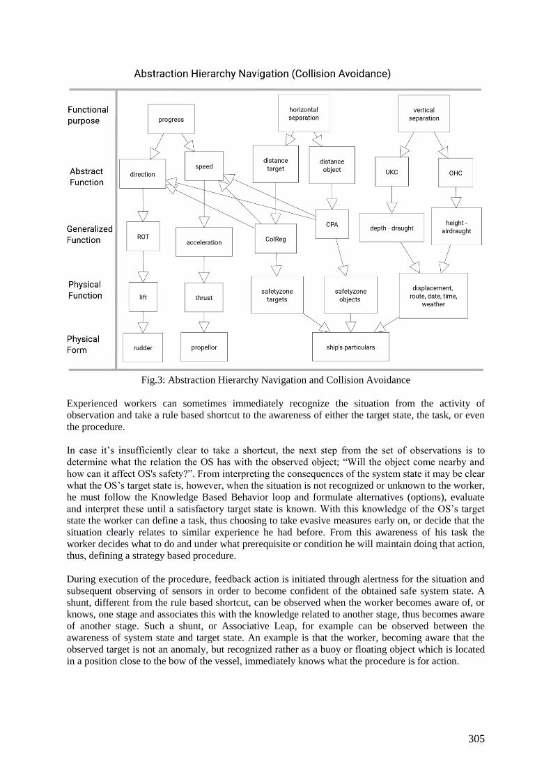
305
Fig.3: Abstraction Hierarchy Navigation and Collision Avoidance
Experienced workers can sometimes immediately recognize the situation from the activity of
observation and take a rule based shortcut to the awareness of either the target state, the task, or even
the procedure.
In case it’s insufficiently clear to take a shortcut, the next step from the set of observations is to
determine what the relation the OS has with the observed object; “Will the object come nearby and
how can it affect OS's safety?”. From interpreting the consequences of the system state it may be clear
what the OS’s target state is, however, when the situation is not recognized or unknown to the worker,
he must follow the Knowledge Based Behavior loop and formulate alternatives (options), evaluate
and interpret these until a satisfactory target state is known. With this knowledge of the OS’s target
state the worker can define a task, thus choosing to take evasive measures early on, or decide that the
situation clearly relates to similar experience he had before. From this awareness of his task the
worker decides what to do and under what prerequisite or condition he will maintain doing that action,
thus, defining a strategy based procedure.
During execution of the procedure, feedback action is initiated through alertness for the situation and
subsequent observing of sensors in order to become confident of the obtained safe system state. A
shunt, different from the rule based shortcut, can be observed when the worker becomes aware of, or
knows, one stage and associates this with the knowledge related to another stage, thus becomes aware
of another stage. Such a shunt, or Associative Leap, for example can be observed between the
awareness of system state and target state. An example is that the worker, becoming aware that the
observed target is not an anomaly, but recognized rather as a buoy or floating object which is located
in a position close to the bow of the vessel, immediately knows what the procedure is for action.
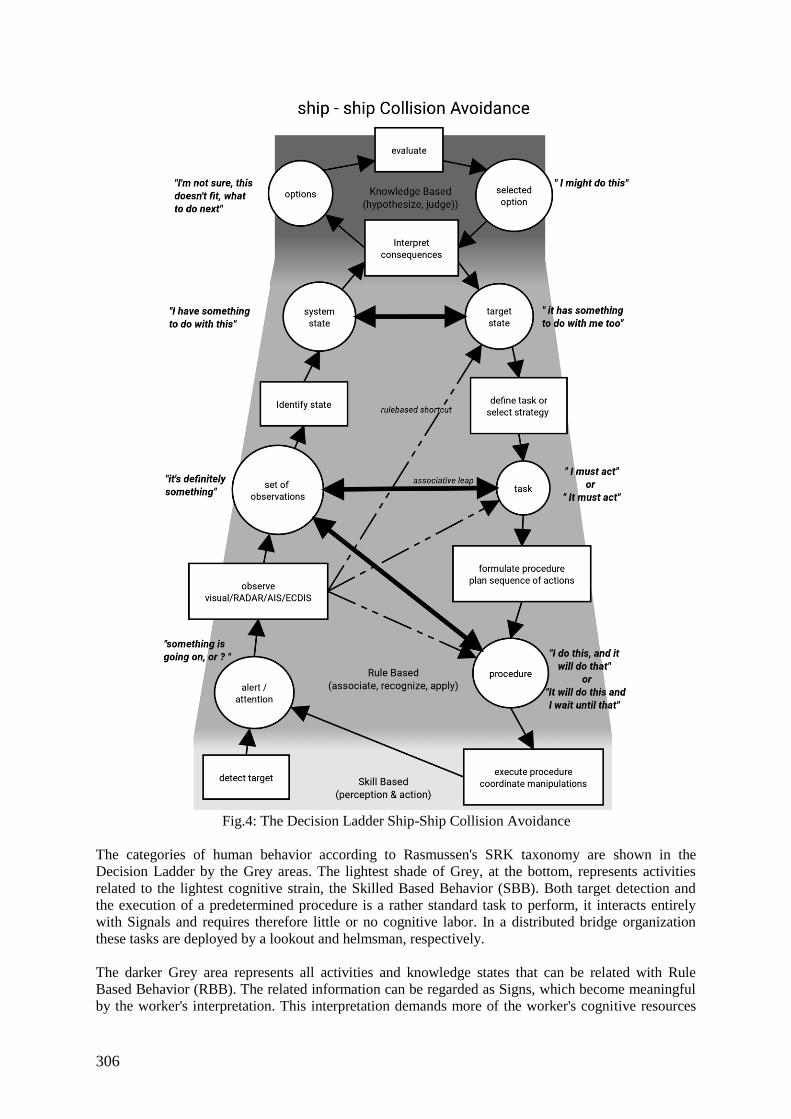
306
Fig.4: The Decision Ladder Ship-Ship Collision Avoidance
The categories of human behavior according to Rasmussen's SRK taxonomy are shown in the
Decision Ladder by the Grey areas. The lightest shade of Grey, at the bottom, represents activities
related to the lightest cognitive strain, the Skilled Based Behavior (SBB). Both target detection and
the execution of a predetermined procedure is a rather standard task to perform, it interacts entirely
with Signals and requires therefore little or no cognitive labor. In a distributed bridge organization
these tasks are deployed by a lookout and helmsman, respectively.
The darker Grey area represents all activities and knowledge states that can be related with Rule
Based Behavior (RBB). The related information can be regarded as Signs, which become meaningful
by the worker's interpretation. This interpretation demands more of the worker's cognitive resources
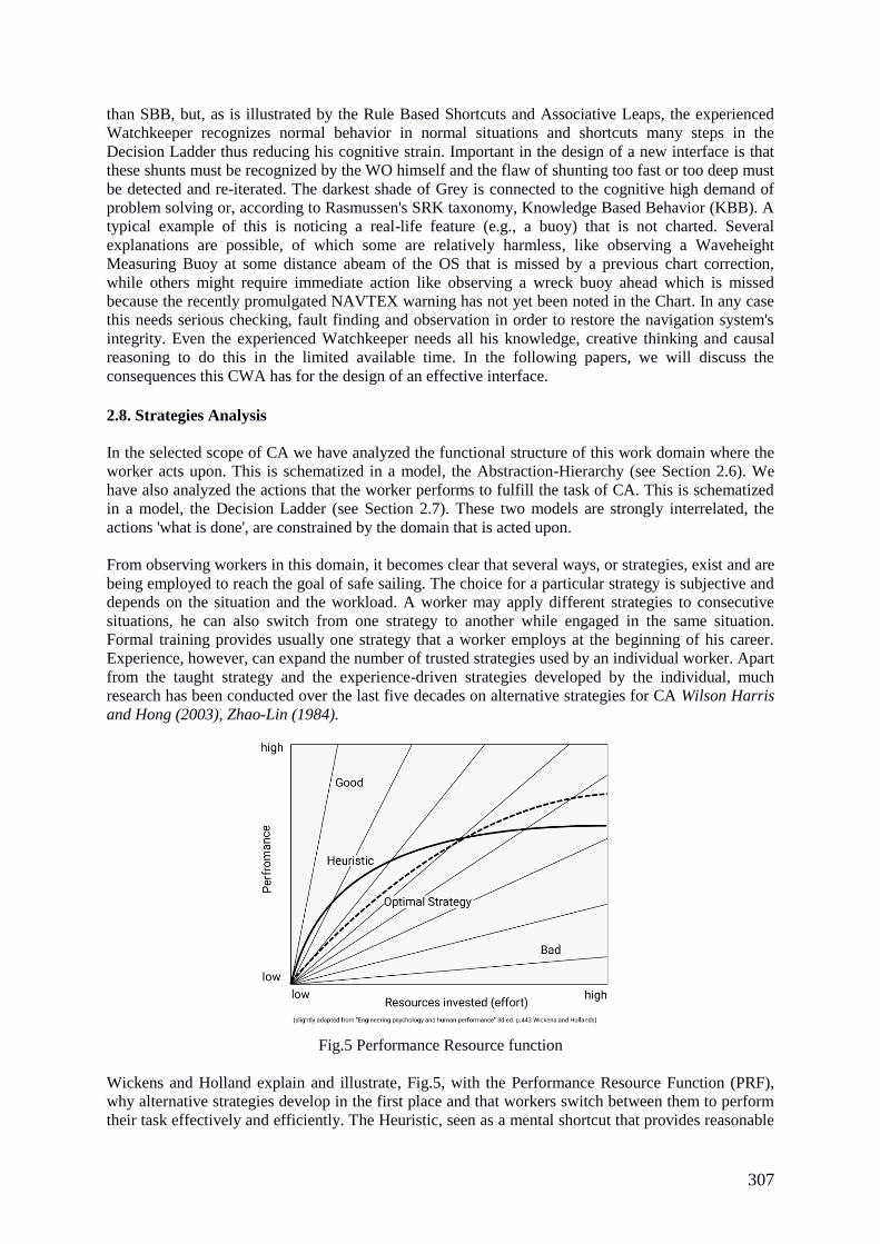
307
than SBB, but, as is illustrated by the Rule Based Shortcuts and Associative Leaps, the experienced
Watchkeeper recognizes normal behavior in normal situations and shortcuts many steps in the
Decision Ladder thus reducing his cognitive strain. Important in the design of a new interface is that
these shunts must be recognized by the WO himself and the flaw of shunting too fast or too deep must
be detected and re-iterated. The darkest shade of Grey is connected to the cognitive high demand of
problem solving or, according to Rasmussen's SRK taxonomy, Knowledge Based Behavior (KBB). A
typical example of this is noticing a real-life feature (e.g., a buoy) that is not charted. Several
explanations are possible, of which some are relatively harmless, like observing a Waveheight
Measuring Buoy at some distance abeam of the OS that is missed by a previous chart correction,
while others might require immediate action like observing a wreck buoy ahead which is missed
because the recently promulgated NAVTEX warning has not yet been noted in the Chart. In any case
this needs serious checking, fault finding and observation in order to restore the navigation system's
integrity. Even the experienced Watchkeeper needs all his knowledge, creative thinking and causal
reasoning to do this in the limited available time. In the following papers, we will discuss the
consequences this CWA has for the design of an effective interface. 2.8. Strategies Analysis
In the selected scope of CA we have analyzed the functional structure of this work domain where the
worker acts upon. This is schematized in a model, the Abstraction-Hierarchy (see Section 2.6). We
have also analyzed the actions that the worker performs to fulfill the task of CA. This is schematized
in a model, the Decision Ladder (see Section 2.7). These two models are strongly interrelated, the
actions 'what is done', are constrained by the domain that is acted upon.
From observing workers in this domain, it becomes clear that several ways, or strategies, exist and are
being employed to reach the goal of safe sailing. The choice for a particular strategy is subjective and
depends on the situation and the workload. A worker may apply different strategies to consecutive
situations, he can also switch from one strategy to another while engaged in the same situation.
Formal training provides usually one strategy that a worker employs at the beginning of his career.
Experience, however, can expand the number of trusted strategies used by an individual worker. Apart
from the taught strategy and the experience-driven strategies developed by the individual, much
research has been conducted over the last five decades on alternative strategies for CA Wilson Harris
and Hong (2003), Zhao-Lin (1984).
Fig.5 Performance Resource function
Wickens and Holland explain and illustrate, Fig.5, with the Performance Resource Function (PRF),
why alternative strategies develop in the first place and that workers switch between them to perform
their task effectively and efficiently. The Heuristic, seen as a mental shortcut that provides reasonable
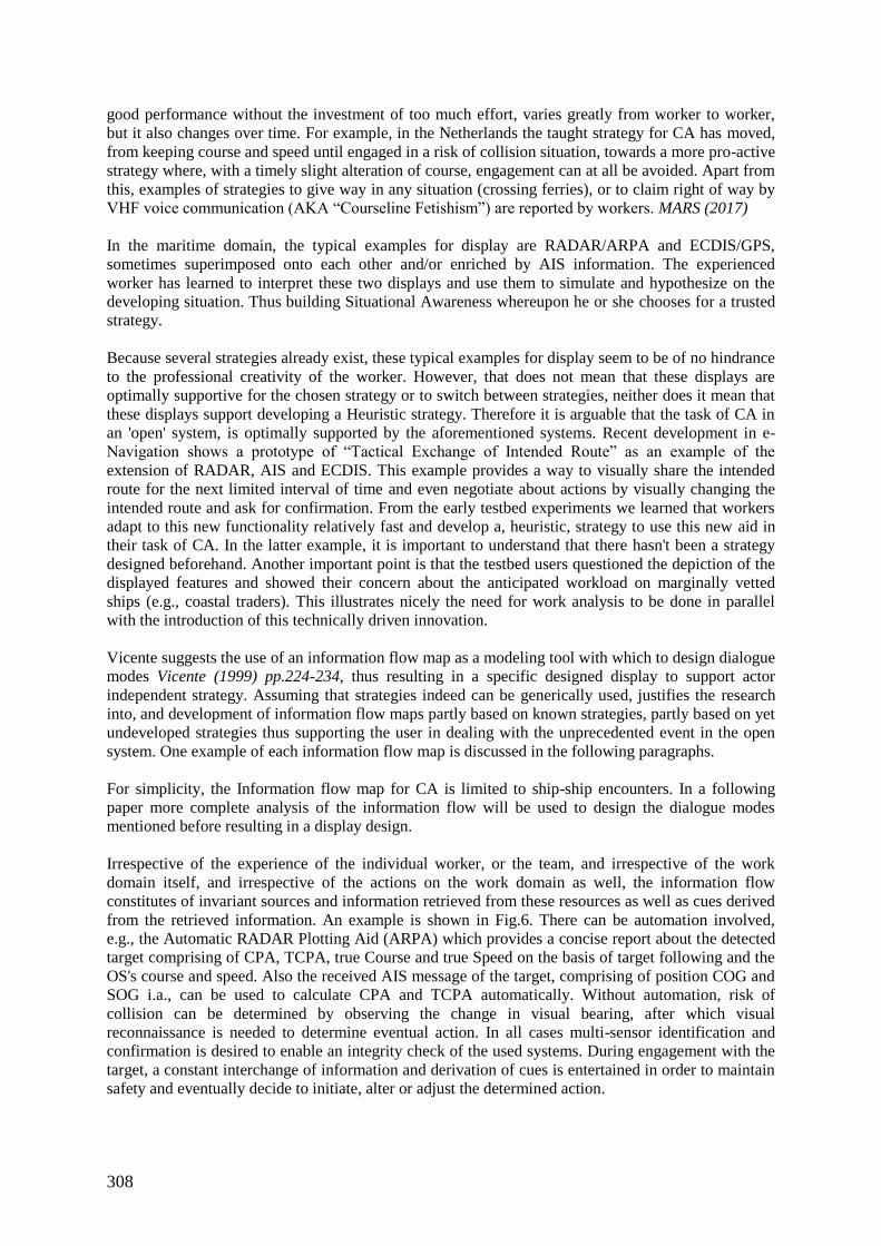
308
good performance without the investment of too much effort, varies greatly from worker to worker,
but it also changes over time. For example, in the Netherlands the taught strategy for CA has moved,
from keeping course and speed until engaged in a risk of collision situation, towards a more pro-active
strategy where, with a timely slight alteration of course, engagement can at all be avoided. Apart from
this, examples of strategies to give way in any situation (crossing ferries), or to claim right of way by
VHF voice communication (AKA “Courseline Fetishism”) are reported by workers. MARS (2017)
In the maritime domain, the typical examples for display are RADAR/ARPA and ECDIS/GPS,
sometimes superimposed onto each other and/or enriched by AIS information. The experienced
worker has learned to interpret these two displays and use them to simulate and hypothesize on the
developing situation. Thus building Situational Awareness whereupon he or she chooses for a trusted
strategy.
Because several strategies already exist, these typical examples for display seem to be of no hindrance
to the professional creativity of the worker. However, that does not mean that these displays are
optimally supportive for the chosen strategy or to switch between strategies, neither does it mean that
these displays support developing a Heuristic strategy. Therefore it is arguable that the task of CA in
an 'open' system, is optimally supported by the aforementioned systems. Recent development in e-
Navigation shows a prototype of “Tactical Exchange of Intended Route” as an example of the
extension of RADAR, AIS and ECDIS. This example provides a way to visually share the intended
route for the next limited interval of time and even negotiate about actions by visually changing the
intended route and ask for confirmation. From the early testbed experiments we learned that workers
adapt to this new functionality relatively fast and develop a, heuristic, strategy to use this new aid in
their task of CA. In the latter example, it is important to understand that there hasn't been a strategy
designed beforehand. Another important point is that the testbed users questioned the depiction of the
displayed features and showed their concern about the anticipated workload on marginally vetted
ships (e.g., coastal traders). This illustrates nicely the need for work analysis to be done in parallel
with the introduction of this technically driven innovation.
Vicente suggests the use of an information flow map as a modeling tool with which to design dialogue
modes Vicente (1999) pp.224-234, thus resulting in a specific designed display to support actor
independent strategy. Assuming that strategies indeed can be generically used, justifies the research
into, and development of information flow maps partly based on known strategies, partly based on yet
undeveloped strategies thus supporting the user in dealing with the unprecedented event in the open
system. One example of each information flow map is discussed in the following paragraphs.
For simplicity, the Information flow map for CA is limited to ship-ship encounters. In a following
paper more complete analysis of the information flow will be used to design the dialogue modes
mentioned before resulting in a display design.
Irrespective of the experience of the individual worker, or the team, and irrespective of the work
domain itself, and irrespective of the actions on the work domain as well, the information flow
constitutes of invariant sources and information retrieved from these resources as well as cues derived
from the retrieved information. An example is shown in Fig.6. There can be automation involved,
e.g., the Automatic RADAR Plotting Aid (ARPA) which provides a concise report about the detected
target comprising of CPA, TCPA, true Course and true Speed on the basis of target following and the
OS's course and speed. Also the received AIS message of the target, comprising of position COG and
SOG i.a., can be used to calculate CPA and TCPA automatically. Without automation, risk of
collision can be determined by observing the change in visual bearing, after which visual
reconnaissance is needed to determine eventual action. In all cases multi-sensor identification and
confirmation is desired to enable an integrity check of the used systems. During engagement with the
target, a constant interchange of information and derivation of cues is entertained in order to maintain
safety and eventually decide to initiate, alter or adjust the determined action.
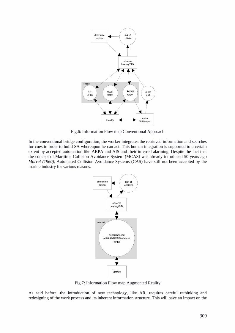
309
Fig.6: Information Flow map Conventional Approach
In the conventional bridge configuration, the worker integrates the retrieved information and searches
for cues in order to build SA whereupon he can act. This human integration is supported to a certain
extent by accepted automation like ARPA and AIS and their inferred alarming. Despite the fact that
the concept of Maritime Collision Avoidance System (MCAS) was already introduced 50 years ago
Morrel (1960), Automated Collision Avoidance Systems (CAS) have still not been accepted by the
marine industry for various reasons.
Fig.7: Information Flow map Augmented Reality
As said before, the introduction of new technology, like AR, requires careful rethinking and
redesigning of the work process and its inherent information structure. This will have an impact on the
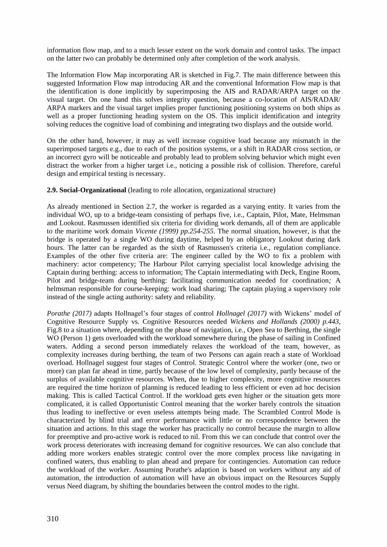
310
information flow map, and to a much lesser extent on the work domain and control tasks. The impact
on the latter two can probably be determined only after completion of the work analysis.
The Information Flow Map incorporating AR is sketched in Fig.7. The main difference between this
suggested Information Flow map introducing AR and the conventional Information Flow map is that
the identification is done implicitly by superimposing the AIS and RADAR/ARPA target on the
visual target. On one hand this solves integrity question, because a co-location of AIS/RADAR/
ARPA markers and the visual target implies proper functioning positioning systems on both ships as
well as a proper functioning heading system on the OS. This implicit identification and integrity
solving reduces the cognitive load of combining and integrating two displays and the outside world.
On the other hand, however, it may as well increase cognitive load because any mismatch in the
superimposed targets e.g., due to each of the position systems, or a shift in RADAR cross section, or
an incorrect gyro will be noticeable and probably lead to problem solving behavior which might even
distract the worker from a higher target i.e., noticing a possible risk of collision. Therefore, careful
design and empirical testing is necessary.
2.9. Social-Organizational (leading to role allocation, organizational structure)
As already mentioned in Section 2.7, the worker is regarded as a varying entity. It varies from the
individual WO, up to a bridge-team consisting of perhaps five, i.e., Captain, Pilot, Mate, Helmsman
and Lookout. Rasmussen identified six criteria for dividing work demands, all of them are applicable
to the maritime work domain Vicente (1999) pp.254-255. The normal situation, however, is that the
bridge is operated by a single WO during daytime, helped by an obligatory Lookout during dark
hours. The latter can be regarded as the sixth of Rasmussen's criteria i.e., regulation compliance.
Examples of the other five criteria are: The engineer called by the WO to fix a problem with
machinery: actor competency; The Harbour Pilot carrying specialist local knowledge advising the
Captain during berthing: access to information; The Captain intermediating with Deck, Engine Room,
Pilot and bridge-team during berthing: facilitating communication needed for coordination; A
helmsman responsible for course-keeping: work load sharing; The captain playing a supervisory role
instead of the single acting authority: safety and reliability.
Porathe (2017) adapts Hollnagel’s four stages of control Hollnagel (2017) with Wickens’ model of
Cognitive Resource Supply vs. Cognitive Resources needed Wickens and Hollands (2000) p.443,
Fig.8 to a situation where, depending on the phase of navigation, i.e., Open Sea to Berthing, the single
WO (Person 1) gets overloaded with the workload somewhere during the phase of sailing in Confined
waters. Adding a second person immediately relaxes the workload of the team, however, as
complexity increases during berthing, the team of two Persons can again reach a state of Workload
overload. Hollnagel suggest four stages of Control. Strategic Control where the worker (one, two or
more) can plan far ahead in time, partly because of the low level of complexity, partly because of the
surplus of available cognitive resources. When, due to higher complexity, more cognitive resources
are required the time horizon of planning is reduced leading to less efficient or even ad hoc decision
making. This is called Tactical Control. If the workload gets even higher or the situation gets more
complicated, it is called Opportunistic Control meaning that the worker barely controls the situation
thus leading to ineffective or even useless attempts being made. The Scrambled Control Mode is
characterized by blind trial and error performance with little or no correspondence between the
situation and actions. In this stage the worker has practically no control because the margin to allow
for preemptive and pro-active work is reduced to nil. From this we can conclude that control over the
work process deteriorates with increasing demand for cognitive resources. We can also conclude that
adding more workers enables strategic control over the more complex process like navigating in
confined waters, thus enabling to plan ahead and prepare for contingencies. Automation can reduce
the workload of the worker. Assuming Porathe's adaption is based on workers without any aid of
automation, the introduction of automation will have an obvious impact on the Resources Supply
versus Need diagram, by shifting the boundaries between the control modes to the right.
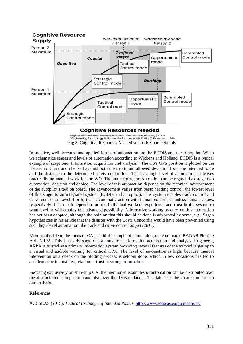
311
Fig.8: Cognitive Resources Needed versus Resource Supply
In practice, well accepted and applied forms of automation are the ECDIS and the Autopilot. When
we schematize stages and levels of automation according to Wickens and Holland, ECDIS is a typical
example of stage one,‘Information acquisition and analysis’. The OS's GPS position is plotted on the
Electronic Chart and checked against both the maximum allowed deviation from the intended route
and the distance to the determined safety contourline. This is a high level of automation, it leaves
practically no manual work for the WO. The latter form, the Autopilot, can be regarded as stage two
automation, decision and choice. The level of this automation depends on the technical advancement
of the autopilot fitted on board. The advancement varies from basic heading control, the lowest level
of this stage, to an integrated system (ECDIS and autopilot). This system enables track control and
curve control at Level 4 or 5, that is automatic action with human consent or unless human vetoes,
respectively. It is much dependent on the individual worker's experience and trust in the system to
what level he will employ this advanced possibility. A formative working practice on this automation
has not been adopted, although the opinion that this should be done is advocated by some, e.g., Sagen
hypothesizes in his article that the disaster with the Costa Concordia would have been prevented using
such high-level automation like track and curve control Sagen (2015).
More applicable to the focus of CA is a third example of automation, the Automated RADAR Plotting
Aid, ARPA. This is clearly stage one automation, information acquisition and analysis. In general,
ARPA is trusted as a primary information system providing several features of the tracked target up to
a visual and audible warning for critical CPA. The level of automation is high, because manual
intervention or a check on the plotting process is seldom done, which in few occasions has led to
accidents due to misinterpretation or trust in wrong information. Focusing exclusively on ship-ship CA, the mentioned examples of automation can be distributed over
the abstraction decomposition and also over the decision ladder. The latter has the greatest impact on
our analysis.
References
ACCSEAS (2015), Tactical Exchange of Intended Routes, http://www.accseas.eu/publications/

312
BENNET, K.B.; FLACH, J.M. (2011), Display and Interface Design, CRC Press
BAINBRIDGE, L. (1983), Ironies of Automation, Automatica 19/6, pp.775-779
BORST, C.; FLACH, J.M.; ELLERBROEK, J. (2015), Beyond Ecological Interface Design: Lessons
from Concerns and Misconceptions, IEEE Trans. Human-Machine Systems 45(2), pp.164-175
ENSTRÖM, J.; HULSMAN, A.; MALM, L.A. (2014), Navigational Claims 2014, The Swedish Club
FLACH, J.M.; VICENTE, K.J.; TANABE, F.; MONTA, K.; RASMUSSEN, J. (1998), An Ecological
Approach to Interface Design, Proceedings of the Human Factors and Ergonomics Society 42nd
annual meeting-1998
GLUVER H., OLSEN D. (Eds.) (1998). Ship Collision Analysis (Bridges), Balkema, Rotterdam; 1998
GRABOWSKI, M. (2015), Research on Wearable, Immersive, Augmented Reality (WIAR) Adoption
in Maritime Navigation, J. of Navigation 68, pp.453-464
GROTIUS, H. (1609), The Freedom of the Seas, MAGOFFIN transl., Oxford University Press 1916
HOLLNAGEL, E. (2017), Contextual Control Model, http://erikhollnagel.com
INTERNATIONAL MARITIME ORGANIZATION, IMO (1972), The International Regulations For
Preventing Collisions At Sea 1972, (COLREGs)
INTERNATIONAL MARITIME ORGANIZATION, IMO (2017), http://www.imo.org
The Nautical Institute (2017), Maritime Alerting and Reporting Scheme (MARS),
http://www.nautinst.org
MORREL, J.S. (1960), The Physics of Collision at Sea, J. Navigation XIV, pp.163-184 PORATHE, T. (2017) Display of e-Navigation information, http://www.iala-
aism.org/content/uploads/2016/09/1440-Thomas-Porathe-Display-of-e-nav-info.pdf
RASMUSSEN, J. (1983), Skills, Rules, and Knowledge; Signals Signs, ands Symbols, and other
distinctions in Human Performance Models, IEEE Trans. Systems Man and Cybernetics 13/3
SAGEN, A. (2015), ECDIS and the ISM Code, Seaways, October, p.3
UNITED NATIONS CONFERENCE ON TRADE AND DEVELOPMENT (2016), Review of
Maritime Transport, http://unctad.org/en/PublicationsLibrary/rmt2016_en.pdf, pp.24-26
VICENTE, K. J. (1999), Cognitive Work Analysis, CRC Press, ISBN 0-8058-2396-4
WICKENS, C.D.; HOLLANDS, J.G. (2000), Engineering Psychology and Human Performance, 3rd
Ed., Psychology Press
WILSON, P.A.; HARRIS, C.J.; HONG, X. (2003) A Line of Sight Counteraction Navigation
Algorithm for Ship Encounter Collision Avoidance, J. Navigation 56, pp.111-121 ZHAO-LIN, W. (1984), An Alternative System of Collision Avoidance, J. Navigation 37, pp.83-89
313
Fast Leaps and Deep Dives towards Autonomous,
Fast, and High-Resolution Deep-Sea Ocean Exploration
Gunnar Brink, IOSB Fraunhofer, Karlsruhe/Germany, [email protected]
Gaurav Mulay, IOSB Fraunhofer, Karlsruhe/Germany, [email protected]
Abstract
The global map of the Earth’s ocean floor is significantly less detailed when compared with maps of
other planetary bodies such as Mars, Venus, and the Moon. Thus, the aim of the Shell Ocean Discovery
XPRIZE involves resolving this issue, and it is a demanding ongoing global competition to advance
technologies for autonomous, fast, and high-resolution deep-sea ocean exploration. This study
describes the Arggonauts project that is part of the race to develop, build, and apply a fleet of AUVs
(autonomous underwater vehicles) and ASVs (autonomous surface vehicles) to explore and map the
deep-sea floor. Due to the ambitious timing, agile project management methods are being used and
improved for planning and implementation.
1. Introduction
It is often said that only 5% of the ocean floor of the Earth is mapped while in contrast, the surfaces of
the Moon, Mars, and Venus are thoroughly mapped. In this abbreviated form the statement is
misleading. Current maps of the ocean floor were gravimetrically created and represent all seas on
Earth, Sandwell et al. (2014), Fecher et al. (2015). The maps show several previously relatively
unknown details of the ocean floor. However, even extant maps are relatively crude and the observations
only include a resolution ranging from 1 km to 5 km such that it is not possible to detect objects like
crashed planes or shipwrecks on maps of this size. Additionally, many geological structures are
indistinguishable, and it is very difficult to analyse features of ecosystems at the fore-mentioned
resolution range. In contrast, knowledge of other celestial bodies is significantly more advanced, and
resolutions range from 100 m for Venus, Lee (2012), and 7 m for the Moon, Ren et al. (2014). This
discrepancy exists partly because taxpayers in several countries of the world spend a significantly
greater amount of funds on space travel when compared with that on deep-sea research. Another reason
which we as scientists and engineers have to cope with is that a thick layer of water surrounds the ocean
floor and increases the difficulty of explorations.
Satellite based gravimetry has a resolution of several kilometres. Acoustic measurements from hull
mounted sonars on boats on the surface are imprecise and require high sound pressure levels that can
adversely affect marine mammals apart from other drawbacks. Thus, it is necessary to bring sonar
systems very close to the ocean floor (by using autonomous underwater robotic explorers or tethered
instruments) to identify things that are only a few metres high from the ocean floor such as mineral
spires of submarine volcanoes or wrecks of crashed planes or sunken treasure ships. Currently,
approximately less than 0.05 percent of the ocean floor is mapped to the highest level of detail by sonars, http://moocs.southampton.ac.uk/. The Hubble Space Telescope is used to view stars and galaxies that
are billions of light years away. In contrast, the wreck of a MH370 plane that crashed several years ago
on our own planet is not located to date, Li et al. (2016).
An optimal method involves performing measurements from vehicles that travel distances ranging from
a few metres to 100 m over the ocean floor and to identify the relief of the ocean floor and the objects
lying on it by using optical methods or acoustic methods.
2. Challenges and Current Systems
The construction and operation of the fore-mentioned types of vehicles poses several difficulties. A
pressure of 400 bar exists at a water depth of 4,000 m, and this is equivalent to a force exerted by a
weight of approximately 4000 tons on one square metre.
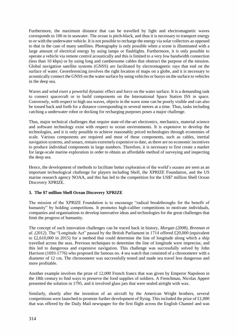
314
Furthermore, the maximum distance that can be travelled by light and electromagnetic waves
corresponds to 100 m in seawater. The ocean is pitch-black, and thus it is necessary to transport energy
to or with the underwater vehicle. It is not possible to recharge the energy via solar collectors as opposed
to that in the case of many satellites. Photography is only possible when a scene is illuminated with a
large amount of electrical energy by using lamps or flashlights. Furthermore, it is only possible to
operate a vehicle via remote control acoustically and this is limited to a very low bandwidth connection
(less than 10 kbps) or by using long and cumbersome cables that obstruct the purpose of the mission.
Global navigation satellite systems (GNSS) are facilitated by electromagnetic rays that end on the
surface of water. Georeferencing involves the right location of maps on a globe, and it is necessary to
acoustically connect the GNSS on the water surface by using vehicles or buoys on the surface to vehicles
in the deep sea.
Waves and wind exert a powerful dynamic effect and force on the water surface. It is a demanding task
to connect spacecraft or to build components on the International Space Station ISS in space.
Conversely, with respect to high sea waves, objects in the wave zone can be poorly visible and can also
be tossed back and forth for a distance corresponding to several metres at a time. Thus, tasks including
catching a underwater robot or docking for recharging purposes poses a major challenge.
Thus, major technical challenges that require state-of-the-art electronics, mechanics, material science
and software technology exist with respect to ocean environments. It is expensive to develop the
technologies, and it is only possible to achieve reasonably priced technologies through economies of
scale. Various components are required and most of these components, such as cables, inertial
navigation systems, and sonars, remain extremely expensive to date, as there are no economic incentives
to produce individual components in large numbers. Therefore, it is necessary to first create a market
for large-scale marine exploration in order to obtain an affordable method of surveying and inspecting
the deep sea.
Hence, the development of methods to facilitate better exploration of the world’s oceans are seen as an
important technological challenge for players including Shell, the XPRIZE Foundation, and the US
marine research agency NOAA, and this has led to the competition for the US$7 million Shell Ocean
Discovery XPRIZE.
3. The $7 million Shell Ocean Discovery XPRIZE
The mission of the XPRIZE Foundation is to encourage “radical breakthroughs for the benefit of
humanity” by holding competitions. It promotes high-calibre competitions to motivate individuals,
companies and organisations to develop innovative ideas and technologies for the great challenges that
limit the progress of humanity.
The concept of such innovation challenges can be traced back in history, Morgan (2008), Brennan et
al. (2012). The “Longitude Act” passed by the British Parliament in 1714 offered £20,000 (equivalent
to £2,610,000 in 2015) for a method that could determine the line of longitude along which a ship
travelled across the seas. Previous techniques to determine the line of longitude were imprecise, and
this led to dangerous and expensive navigation. This challenge was successfully solved by John
Harrison (1693-1776) who proposed the famous no. 4 sea watch that consisted of a chronometer with a
diameter of 12 cm. The chronometer was successfully tested and made sea travel less dangerous and
more profitable.
Another example involves the prize of 12,000 French francs that was given by Emperor Napoleon in
the 18th century to find ways to preserve the food supplies of soldiers. A Frenchman, Nicolas Appert
presented the solution in 1795, and it involved glass jars that were sealed airtight with wax.
Similarly, shortly after the invention of an aircraft by the American Wright brothers, several
competitions were launched to promote further development of flying. This included the prize of £1,000
that was offered by the Daily Mail newspaper for the first flight across the English Channel and was
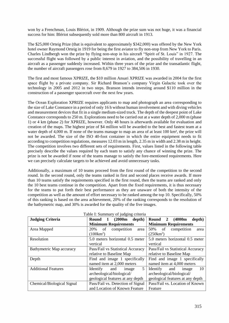
315
won by a Frenchman, Louis Blériot, in 1909. Although the prize sum was not huge, it was a financial
success for him: Blériot subsequently sold more than 800 aircraft in 1913.
The $25,000 Orteig Prize (that is equivalent to approximately $342,000) was offered by the New York
hotel owner Raymond Orteig in 1919 for being the first aviator to fly non-stop from New York to Paris.
Charles Lindbergh won the prize by flying non-stop in his aircraft “Spirit of St. Louis” in 1927. The
successful flight was followed by a public interest in aviation, and the possibility of travelling in an
aircraft as a passenger suddenly increased. Within three years of the prize and the transatlantic flight,
the number of aircraft passengers rose from 8,679 in 1927 to 384,506 in 1930.
The first and most famous XPRIZE, the $10 million Ansari XPRIZE was awarded in 2004 for the first
space flight by a private company. Sir Richard Branson’s company Virgin Galactic took over the
technology in 2005 and 2012 in two steps. Branson intends investing around $110 million in the
construction of a passenger spacecraft over the next few years.
The Ocean Exploration XPRIZE requires applicants to map and photograph an area corresponding to
the size of Lake Constance in a period of only 16 h without human involvement and with diving vehicles
and measurement devices that fit in a single medium-sized truck. The depth of the deepest point of Lake
Constance corresponds to 250 m. Explorations need to be carried out at a water depth of 2,000 m (phase
1) or 4 km (phase 2) for XPRIZE, however. Only 48 hours is afterwards available for evaluation and
creation of the maps. The highest prize of $4 million will be awarded to the best and fastest team at a
water depth of 4,000 m. If none of the teams manage to map an area of at least 100 km², the prize will
not be awarded. The size of the ISO 40-foot container in which the entire equipment needs to fit
according to competition regulations, measures 12.03 m in length, 2.35 m in width and 2.38 m in height.
The competition involves two different sets of requirements. First, values listed in the following table
precisely describe the values required by each team to satisfy any chance of winning the prize. The
prize is not be awarded if none of the teams manage to satisfy the fore-mentioned requirements. Here
we can precisely calculate targets to be achieved and avoid unnecessary tasks.
Additionally, a maximum of 10 teams proceed from the first round of the competition to the second
round. In the second round, only the teams ranked in first and second places receive awards. If more
than 10 teams satisfy the requirements specified in the first round, then the teams are ranked and only
the 10 best teams continue in the competition. Apart from the fixed requirements, it is thus necessary
for the teams to put forth their best performance as they are unaware of both the intensity of the
competition as well as the amount of effort necessary to be ranked among the top 10. Specifically, 50%
of this ranking is based on the area achievement, 20% of the ranking corresponds to the resolution of
the bathymetric map, and 30% is awarded for the quality of the five images.
Table I: Summary of judging criteria
Judging Criteria Round 1 (2000m depth)
Minimum Requirements
Round 2 (4000m depth)
Minimum Requirements
Area Mapped 20% of competition area
(100km2)
50% of competition area
(250km2)
Resolution 5.0 meters horizontal 0.5 meter
vertical
5.0 meters horizontal 0.5 meter
vertical
Bathymetric Map accuracy Pass/Fail vs Statistical Accuracy
relative to Baseline Map
Pass/Fail vs Statistical Accuracy
relative to Baseline Map
Depth Find and image 1 specifically
named item at 2,000 meters
Find and image 1 specifically
named item at 4,000 meters
Additional Features Identify and image 5
archeological/biological/
geological features at any depth
Identify and image 10
archeological/biological/
geological features at any depth
Chemical/Biological Signal Pass/Fail vs. Detection of Signal
and Location of Known Feature
Pass/Fail vs. Location of Known
Feature
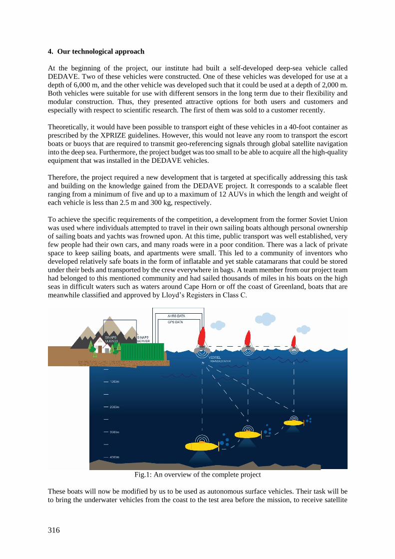
316
4. Our technological approach
At the beginning of the project, our institute had built a self-developed deep-sea vehicle called
DEDAVE. Two of these vehicles were constructed. One of these vehicles was developed for use at a
depth of 6,000 m, and the other vehicle was developed such that it could be used at a depth of 2,000 m.
Both vehicles were suitable for use with different sensors in the long term due to their flexibility and
modular construction. Thus, they presented attractive options for both users and customers and
especially with respect to scientific research. The first of them was sold to a customer recently.
Theoretically, it would have been possible to transport eight of these vehicles in a 40-foot container as
prescribed by the XPRIZE guidelines. However, this would not leave any room to transport the escort
boats or buoys that are required to transmit geo-referencing signals through global satellite navigation
into the deep sea. Furthermore, the project budget was too small to be able to acquire all the high-quality
equipment that was installed in the DEDAVE vehicles.
Therefore, the project required a new development that is targeted at specifically addressing this task
and building on the knowledge gained from the DEDAVE project. It corresponds to a scalable fleet
ranging from a minimum of five and up to a maximum of 12 AUVs in which the length and weight of
each vehicle is less than 2.5 m and 300 kg, respectively.
To achieve the specific requirements of the competition, a development from the former Soviet Union
was used where individuals attempted to travel in their own sailing boats although personal ownership
of sailing boats and yachts was frowned upon. At this time, public transport was well established, very
few people had their own cars, and many roads were in a poor condition. There was a lack of private
space to keep sailing boats, and apartments were small. This led to a community of inventors who
developed relatively safe boats in the form of inflatable and yet stable catamarans that could be stored
under their beds and transported by the crew everywhere in bags. A team member from our project team
had belonged to this mentioned community and had sailed thousands of miles in his boats on the high
seas in difficult waters such as waters around Cape Horn or off the coast of Greenland, boats that are
meanwhile classified and approved by Lloyd’s Registers in Class C.
Fig.1: An overview of the complete project
These boats will now be modified by us to be used as autonomous surface vehicles. Their task will be
to bring the underwater vehicles from the coast to the test area before the mission, to receive satellite
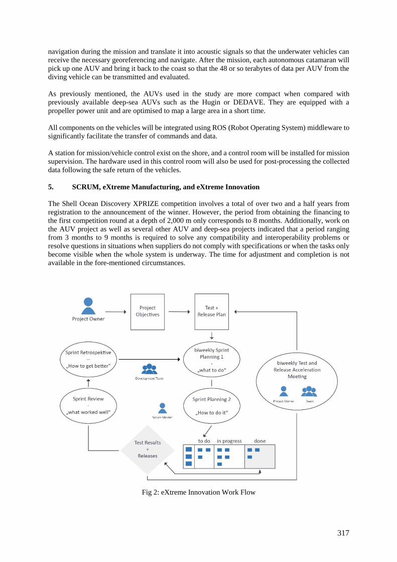
317
navigation during the mission and translate it into acoustic signals so that the underwater vehicles can
receive the necessary georeferencing and navigate. After the mission, each autonomous catamaran will
pick up one AUV and bring it back to the coast so that the 48 or so terabytes of data per AUV from the
diving vehicle can be transmitted and evaluated.
As previously mentioned, the AUVs used in the study are more compact when compared with
previously available deep-sea AUVs such as the Hugin or DEDAVE. They are equipped with a
propeller power unit and are optimised to map a large area in a short time.
All components on the vehicles will be integrated using ROS (Robot Operating System) middleware to
significantly facilitate the transfer of commands and data.
A station for mission/vehicle control exist on the shore, and a control room will be installed for mission
supervision. The hardware used in this control room will also be used for post-processing the collected
data following the safe return of the vehicles.
5. SCRUM, eXtreme Manufacturing, and eXtreme Innovation
The Shell Ocean Discovery XPRIZE competition involves a total of over two and a half years from
registration to the announcement of the winner. However, the period from obtaining the financing to
the first competition round at a depth of 2,000 m only corresponds to 8 months. Additionally, work on
the AUV project as well as several other AUV and deep-sea projects indicated that a period ranging
from 3 months to 9 months is required to solve any compatibility and interoperability problems or
resolve questions in situations when suppliers do not comply with specifications or when the tasks only
become visible when the whole system is underway. The time for adjustment and completion is not
available in the fore-mentioned circumstances.
Fig 2: eXtreme Innovation Work Flow
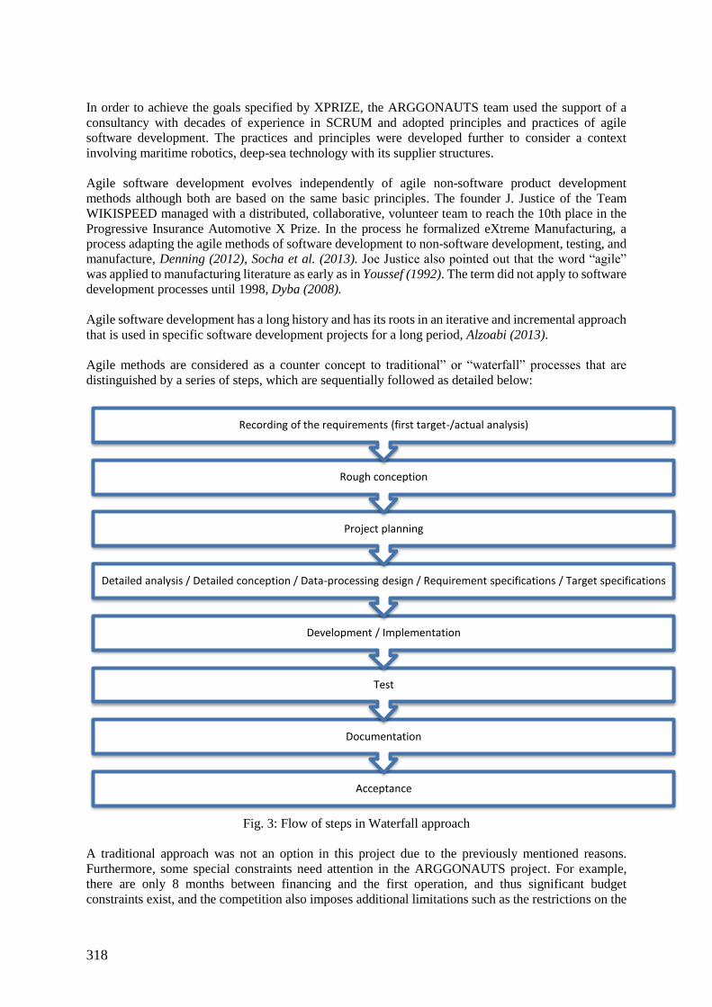
318
In order to achieve the goals specified by XPRIZE, the ARGGONAUTS team used the support of a
consultancy with decades of experience in SCRUM and adopted principles and practices of agile
software development. The practices and principles were developed further to consider a context
involving maritime robotics, deep-sea technology with its supplier structures.
Agile software development evolves independently of agile non-software product development
methods although both are based on the same basic principles. The founder J. Justice of the Team
WIKISPEED managed with a distributed, collaborative, volunteer team to reach the 10th place in the
Progressive Insurance Automotive X Prize. In the process he formalized eXtreme Manufacturing, a
process adapting the agile methods of software development to non-software development, testing, and
manufacture, Denning (2012), Socha et al. (2013). Joe Justice also pointed out that the word “agile”
was applied to manufacturing literature as early as in Youssef (1992). The term did not apply to software
development processes until 1998, Dyba (2008).
Agile software development has a long history and has its roots in an iterative and incremental approach
that is used in specific software development projects for a long period, Alzoabi (2013).
Agile methods are considered as a counter concept to traditional” or “waterfall” processes that are
distinguished by a series of steps, which are sequentially followed as detailed below:
Fig. 3: Flow of steps in Waterfall approach
A traditional approach was not an option in this project due to the previously mentioned reasons.
Furthermore, some special constraints need attention in the ARGGONAUTS project. For example,
there are only 8 months between financing and the first operation, and thus significant budget
constraints exist, and the competition also imposes additional limitations such as the restrictions on the
Acceptance
Documentation
Test
Development / Implementation
Detailed analysis / Detailed conception / Data-processing design / Requirement specifications / Target specifications
Project planning
Rough conception
Recording of the requirements (first target-/actual analysis)
319
entire volume of all parts and equipment as prescribed by competition rules (the limitations of a 40-foot
container). There was a lack of information (on where the other teams stand, where the test location
would be and on other parts of the project) at the beginning.. It is also necessary to account for delivery
times of some components that can correspond to a maximum of 5 months. Experience tells us that the
deliveries of parts will not always comply with the specifications, they frequently tended to describe
ideal values that are only valid in ideal circumstances, and unforeseen complications emerged when
parts were combined with other bought-in components. Therefore, the approach was modelled on
“effectuation”, which is a concept introduced by Saras Sarasvathy and is used by experienced
entrepreneurs in situations characterized by uncertainty, Sarasvathy (2001).
Effectuation runs contrary to decisions based on causal logic, which are based on justified predictions
of the future. Effectuation and causal logic differ in their basic assumption of the nature of the future.
Causal logic forms the basis of the above-mentioned waterfall model and assumes that it is only possible
to control an event that can be predicted. In contrast, effectuation is based on the attitude that it is not
necessary to predict everything that can be influenced by control. This attitude is compatible with the
current project. Sarasvathy related effectuation to the agile technology SCRUM, Schwaber and Beedle
(2002), as a method with effectuation principles.
The purchase of essential components requires a medium-term plan due to the delivery time and
compliance rules for procurement by public-sector organisations, and the fore-mentioned plan will
extend the SCRUM Sprints significantly into the future.
In SCRUM, the team acts as a unit. The name “scrum” is derived from rugby in the article “The New
New Product Development Game” by Hirotaka Takeuchi and Ikujiro Nonaka was published in the
Harvard Business Review in 1986 and inspired scrum for software. The authors compared the way in
which a rugby team moved forwards together by throwing the ball from an individual person to another
with sequential operations (such as a relay race) in traditional product development. They coined the
word “scrum” from the sport of rugby for the first time to describe that a team is formed to play together
and convey the ball forwards in which the general idea involved moving in a scrum as a unit on the
rugby field.
However, in our case team members only possessed partial knowledge on the entire project. Only some
of the team members had ever participated in the construction of an AUV, and these individuals were
largely committed to other projects. Only an individual possessed intensive maritime experience related
to months and years spent on small boats on the high seas. On the other side, this team member did not
possess any personal experience corresponding to deep sea projects.
According to SCRUM rules, a project team should preferably remain constant throughout the entire
project. Each worker should only work on a single project. Ideally, all team members would
communicate closely, and they can even maybe work together in the same room.
However, our team included students working on the project who were available all day during the
semester break but much less during the semester. Availability issues also existed for several permanent
employees who were involved on other projects at the beginning or intermittently or who were not
consistently available due to family commitments. Therefore, it was not possible to apply all SCRUM
steps in a one-to-one manner in the project.
In agile software development, every development step is regulated with the principle of timeboxing.
The process is concluded after the specified time period even if it is not possible to complete all the
planned contents involved in the process. Any outstanding parts are moved to a subsequent time box or
are cancelled. The fundamental time box of the development process is termed as a “Sprint”. In our
project, each Sprint lasts for exactly 14 days.
The following elements are adopted from the SCRUM in the present study:
Daily Scrums and biweekly Sprints
320
Sprint Review
Product Backlog Refinement
Project Burndown chart
In contrast to SCRUM, a few elements were introduced in the process developed in the present study
(which we termed as “eXtreme Innovation”).
In eXtreme Innovation the most important innovation is termed as “The Ship of Theseus”. This
metaphor is actually derived from philosophy and describes a problem of identity. According to the
metaphor, Theseus was a hero in ancient Greek mythology who possessed a fairly old yet seaworthy
ship. He decided to take the ship to a shipyard to restore it and asked the shipyard owner to replace all
the planks with new ones. The shipyard owner had several docks and thought it would be a pity to throw
away the old planks from the ship of Theseus. Thus, he decided to gradually replace the parts of the
ship of Theseus in Dock A and to take the old planks to Dock B where they were assembled in the
original order and in their original position to create a new ship.
In our approach, this metaphor describes a concept for a test-operated development of a project that
comprises of electronics hardware, software, and mechanical components to avoid waiting until the end
of the project to integrate individual parts. A testing object, a so called dummy, is built at the beginning
of the project, and it possesses only a few features of the finished product. This permits a trial of various
tasks, such as towing, releasing, and retrieving the AUV, by using the dummy. The dummy corresponds
to the Ship of Theseus in the present study. During the development project, a growing number of
components is replaced by new components that can be used in the finished product until eventually a
finished deep-sea vehicle is created. During this process it is subjected to various integration tests.
Another difference lies in the management of the Product Backlog, which corresponds to the usual list
of all the overriding work packages in SCRUM. In SCRUM, the Product Backlog is actually compiled
by the whole team but prioritised each time by the Product Owner during the Sprint. In SCRUM the
Backlog Owner makes a selection (ad hoc) with respect to the tasks that will be prioritised for the next
Sprint. The team processes as many of these tasks as it considers manageable.
In our “eXtreme Innovation” approach the team and the Product Owner together prioritise and structure
tasks towards the beginning of the project and then use this priority list as a test-and-release plan and
implementation checklist. The checklist is then revised and updated biweekly by the entire team in the
Product Backlog Refinement. The Product Owner is responsible for ensuring that sufficient capacity is
available or other solutions are found to work through the checklist.
Table II: Division of Scrum Features
Features of the SCRUM method taken over
by the ARGGONAUTS
Features of the ARGONNAUTS approach that
differed from SCRUM
Empowerment of the team, own decision as to
workload
The goals are specified by the XPRIZE competition.
The Product Owner is not responsible for the market
but for long-term planning and to ensure the various
aspects fit together.
Daily stand-ups with a SCRUM Master Test-driven:
Test-and-release plan
Ship of Theseus
Biweekly Sprints with a SCRUM Master Pow-wows for a content-related exchange of ideas
alternating with strict Sprint Planning in accordance
with SCRUM
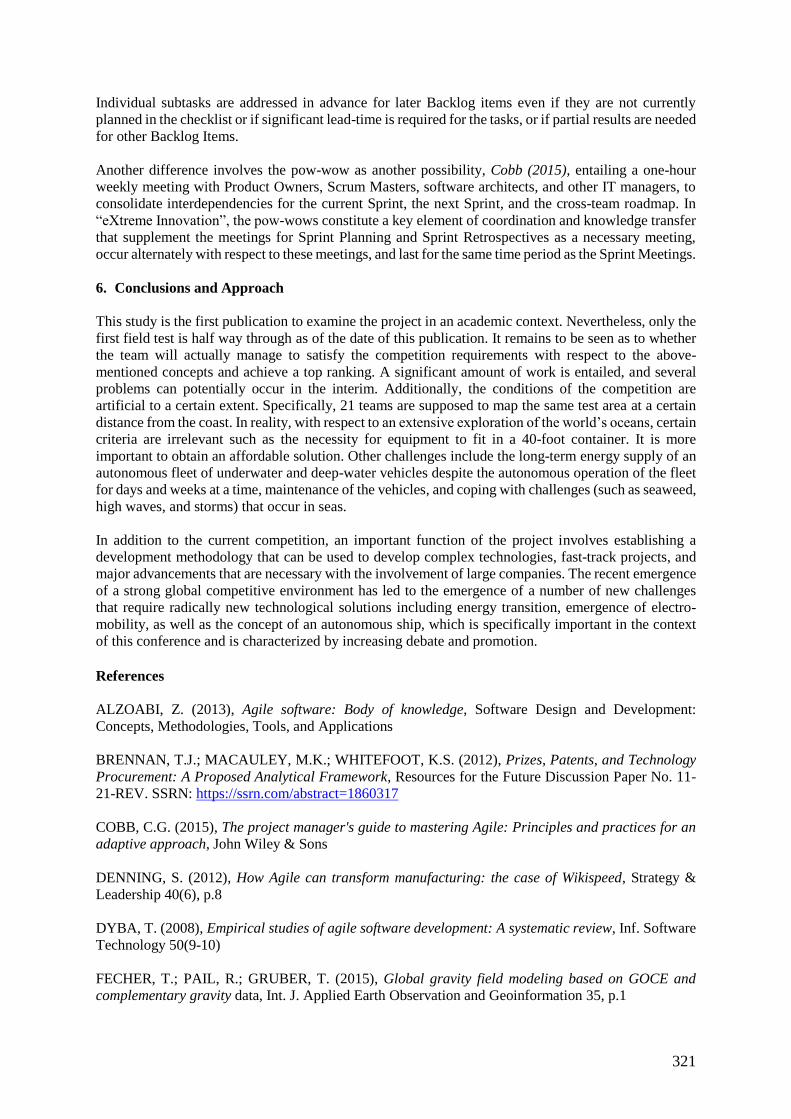
321
Individual subtasks are addressed in advance for later Backlog items even if they are not currently
planned in the checklist or if significant lead-time is required for the tasks, or if partial results are needed
for other Backlog Items.
Another difference involves the pow-wow as another possibility, Cobb (2015), entailing a one-hour
weekly meeting with Product Owners, Scrum Masters, software architects, and other IT managers, to
consolidate interdependencies for the current Sprint, the next Sprint, and the cross-team roadmap. In
“eXtreme Innovation”, the pow-wows constitute a key element of coordination and knowledge transfer
that supplement the meetings for Sprint Planning and Sprint Retrospectives as a necessary meeting,
occur alternately with respect to these meetings, and last for the same time period as the Sprint Meetings.
6. Conclusions and Approach
This study is the first publication to examine the project in an academic context. Nevertheless, only the
first field test is half way through as of the date of this publication. It remains to be seen as to whether
the team will actually manage to satisfy the competition requirements with respect to the above-
mentioned concepts and achieve a top ranking. A significant amount of work is entailed, and several
problems can potentially occur in the interim. Additionally, the conditions of the competition are
artificial to a certain extent. Specifically, 21 teams are supposed to map the same test area at a certain
distance from the coast. In reality, with respect to an extensive exploration of the world’s oceans, certain
criteria are irrelevant such as the necessity for equipment to fit in a 40-foot container. It is more
important to obtain an affordable solution. Other challenges include the long-term energy supply of an
autonomous fleet of underwater and deep-water vehicles despite the autonomous operation of the fleet
for days and weeks at a time, maintenance of the vehicles, and coping with challenges (such as seaweed,
high waves, and storms) that occur in seas.
In addition to the current competition, an important function of the project involves establishing a
development methodology that can be used to develop complex technologies, fast-track projects, and
major advancements that are necessary with the involvement of large companies. The recent emergence
of a strong global competitive environment has led to the emergence of a number of new challenges
that require radically new technological solutions including energy transition, emergence of electro-
mobility, as well as the concept of an autonomous ship, which is specifically important in the context
of this conference and is characterized by increasing debate and promotion. References
ALZOABI, Z. (2013), Agile software: Body of knowledge, Software Design and Development:
Concepts, Methodologies, Tools, and Applications
BRENNAN, T.J.; MACAULEY, M.K.; WHITEFOOT, K.S. (2012), Prizes, Patents, and Technology
Procurement: A Proposed Analytical Framework, Resources for the Future Discussion Paper No. 11-
21-REV. SSRN: https://ssrn.com/abstract=1860317
COBB, C.G. (2015), The project manager's guide to mastering Agile: Principles and practices for an
adaptive approach, John Wiley & Sons
DENNING, S. (2012), How Agile can transform manufacturing: the case of Wikispeed, Strategy &
Leadership 40(6), p.8
DYBA, T. (2008), Empirical studies of agile software development: A systematic review, Inf. Software
Technology 50(9-10)
FECHER, T.; PAIL, R.; GRUBER, T. (2015), Global gravity field modeling based on GOCE and
complementary gravity data, Int. J. Applied Earth Observation and Geoinformation 35, p.1

322
HIROTAKA, T.; IKUJIRO, N. (1986), The new new product development game, Harvard Business
Review 64(1), pp.137-146
LEE, H. (2012), Opposite-side radargrammetry of Magellan synthetic aperture radar on Venus,
Geosciences J. 16(2), pp.165-170
LI, B.; MORIDIAN, B.; MAHMOUDIAN, N. (2016), Underwater multi-robot persistent area
coverage mission planning, IEEE OCEANS 2016, Monterey, pp.1-6
MORGAN, J.G. (2008), Inducing innovation through prizes, Innovations 3(4), pp.105-117
REN, X.; LIU, J.J.; WANG, F.F.; WANG, W.R.; MU, L.L.; LI, H.H.; LI, C.L. (2014), A new lunar
global topographic map products from Chang’E - 2 Stereo Camera Image Data, European Planetary
Science Congress (EPSC2014 Abstracts Vol. 9)
SANDWELL, D.T.; MÜLLER, R.D.; SMITH, W.H.F.; GARCIA, E.; FRANCIS, R. (2014), New
global marine gravity model from CryoSat-2 and Jason-1 reveals buried tectonic structure, Science
345, pp.65-67
SARASVATHY, S.D. (2001), Causation and effectuation: Toward a theoretical shift from economic
inevitability to entrepreneurial contingency, Academy of Management Review 26(2), pp.243-263
SCHWABER, K.; BEEDLE, M. (2002), Agile software development with Scrum (Vol. 1), Prentice Hall
YOUSSEF, M. (1992), Agile manufacturing: a necessary condition for competing in global markets,
Ind. Eng. 24(12)
323
Prediction of Work Content in Shipbuilding Projects Using Extrapolation
Methods
Lode Huijgens, TU Delft, Delft/The Netherlands [email protected]
Frank Verhelst, Damen Schelde Naval Shipbuilding, Schelde/The Netherlands,
Jenny Coenen, TU Delft, Delft/The Netherlands, [email protected]
Abstract
A method to quantify manufacturing activities for shipbuilding projects is devised, based on extrapo-
lation of historical projects. Extrapolation rules are based on first principles and fine-tuned using
empirical data. A 4-tier hierarchical system structure is proposed, incorporating different types of
interrelations. Subsequently, it is investigated how design principles can be used to mathematically
define these relations, resulting in a substantiated work content estimation model. Several shipbuild-
ing projects, some of which recently executed, were used as data source to support the proposed theo-
ry. It is demonstrated that detailed production man hour estimations can be made using limited sets of
input data.
1. Introduction
In an open competitive environment, contracts are usually assigned to parties that are able to offer
what is perceived as the optimal combination of quality, price and delivery date. This implies that
information on these subjects is required already in the earliest phase of a project, and that this infor-
mation is usually considered as binding as it forms the motive for assignment of a contract.
Determination of a correct price, taking into account the production cost, can be especially challeng-
ing for one-off projects: even if the product incorporates nothing but proven technology, the compo-
nents have never before been assembled in the same combination, leading to uncertainty regarding
production work content.
In order to be able to obtain an early insight in work content related to production of shipbuilding
projects, and hence work force cost and throughput times, it was investigated how a method for ex-
trapolation of historical shipbuilding projects could be devised. Project data and practical knowledge
used in the described research were made available by Damen Schelde Naval Shipbuilding (DSNS), a
subsidiary of the Damen Shipyards concentrating on the naval market.
2. Research Objective and Scope
2.1. Research Objective
The objective of the research described in this paper is to devise a method which allows for generation
of an accurate estimation of work content in the earliest phase of a shipbuilding project. Such a meth-
od has to be able to generate a per-system indication of work content based on only a few input pa-
rameters. Historical data of previous projects can be used on the condition that sufficient similarities
exist between the systems considered. Therefore, output is given as non-dimensional factors express-
ing the ratio between work content of an evaluated project and a reference project.
To arrive at such a method, it was investigated how systems and components can be categorised as
well as the relations between these systems and components, and which set of formulas can be used to
describe these relations in an effective and standardised manner.
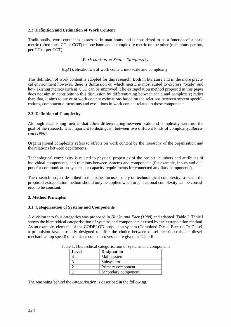
324
2.2. Definition and Estimation of Work Content
Traditionally, work content is expressed in man hours and is considered to be a function of a scale
metric (often tons, GT or CGT) on one hand and a complexity metric on the other (man hours per ton,
per GT or per CGT):
𝑊𝑜𝑟𝑘 𝑐𝑜𝑛𝑡𝑒𝑛𝑡 = 𝑆𝑐𝑎𝑙𝑒 ∙ 𝐶𝑜𝑚𝑝𝑙𝑒𝑥𝑖𝑡𝑦
Eq.(1): Breakdown of work content into scale and complexity
This definition of work content is adopted for this research. Both in literature and in the more practi-
cal environment however, there is discussion on which metric is most suited to express “Scale” and
how existing metrics such as CGT can be improved. The extrapolation method proposed in this paper
does not aim to contribute to this discussion by differentiating between scale and complexity; rather
than that, it aims to arrive at work content estimations based on the relations between system specifi-
cations, component dimensions and evolutions in work content related to these components.
2.3. Definition of Complexity
Although establishing metrics that allow differentiating between scale and complexity were not the
goal of the research, it is important to distinguish between two different kinds of complexity, Bacca-
rini (1996).
Organisational complexity refers to effects on work content by the hierarchy of the organisation and
the relations between departments.
Technological complexity is related to physical properties of the project: numbers and attributes of
individual components, and relations between systems and components (for example, inputs and out-
puts for communication systems, or capacity requirements for connected auxiliary components).
The research project described in this paper focuses solely on technological complexity; as such, the
proposed extrapolation method should only be applied when organisational complexity can be consid-
ered to be constant.
3. Method Principles
3.1. Categorisation of Systems and Components
A division into four categories was proposed in Hubka and Eder (1988) and adapted, Table I. Table I
shows the hierarchical categorisation of systems and components as used by the extrapolation method.
As an example, elements of the CODELOD propulsion system (Combined Diesel-Electric Or Diesel,
a propulsion layout usually designed to offer the choice between diesel-electric cruise or diesel-
mechanical top speed) of a surface combatant vessel are given in Table II.
Table 1: Hierarchical categorisation of systems and components
Level Designation
4 Main system
3 Subsystem
2 Primary component
1 Secondary component
The reasoning behind the categorisation is described in the following.
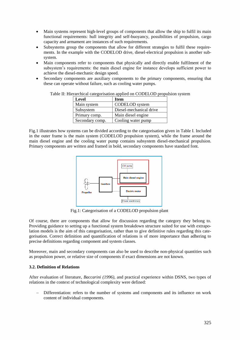
325
Main systems represent high-level groups of components that allow the ship to fulfil its main
functional requirements: hull integrity and self-buoyancy, possibilities of propulsion, cargo
capacity and armament are instances of such requirements.
Subsystems group the components that allow for different strategies to fulfil these require-
ments. In the example with the CODELOD drive, diesel-electrical propulsion is another sub-
system.
Main components refer to components that physically and directly enable fulfilment of the
subsystem’s requirements: the main diesel engine for instance develops sufficient power to
achieve the diesel-mechanic design speed.
Secondary components are auxiliary components to the primary components, ensuring that
these can operate without failure, such as cooling water pumps.
Table II: Hierarchical categorisation applied on CODELOD propulsion system
Level Item
Main system CODELOD system
Subsystem Diesel-mechanical drive
Primary comp. Main diesel engine
Secondary comp. Cooling water pump
Fig.1 illustrates how systems can be divided according to the categorisation given in Table I. Included
in the outer frame is the main system (CODELOD propulsion system), while the frame around the
main diesel engine and the cooling water pump contains subsystem diesel-mechanical propulsion.
Primary components are written and framed in bold, secondary components have standard font.
Fig.1: Categorisation of a CODELOD propulsion plant
Of course, there are components that allow for discussion regarding the category they belong to.
Providing guidance to setting up a functional system breakdown structure suited for use with extrapo-
lation models is the aim of this categorisation, rather than to give definitive rules regarding this cate-
gorisation. Correct definition and quantification of relations is of more importance than adhering to
precise definitions regarding component and system classes.
Moreover, main and secondary components can also be used to describe non-physical quantities such
as propulsion power, or relative size of components if exact dimensions are not known.
3.2. Definition of Relations
After evaluation of literature, Baccarini (1996), and practical experience within DSNS, two types of
relations in the context of technological complexity were defined:
Differentiation: refers to the number of systems and components and its influence on work
content of individual components.
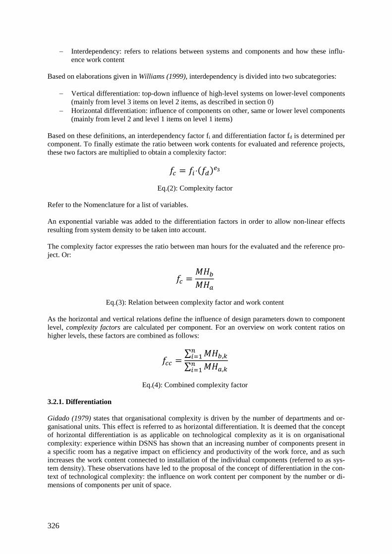
326
Interdependency: refers to relations between systems and components and how these influ-
ence work content
Based on elaborations given in Williams (1999), interdependency is divided into two subcategories:
Vertical differentiation: top-down influence of high-level systems on lower-level components
(mainly from level 3 items on level 2 items, as described in section 0)
Horizontal differentiation: influence of components on other, same or lower level components
(mainly from level 2 and level 1 items on level 1 items)
Based on these definitions, an interdependency factor fi and differentiation factor fd is determined per
component. To finally estimate the ratio between work contents for evaluated and reference projects,
these two factors are multiplied to obtain a complexity factor:
𝑓𝑐 = 𝑓𝑖(𝑓𝑑)𝑒3
Eq.(2): Complexity factor
Refer to the Nomenclature for a list of variables.
An exponential variable was added to the differentiation factors in order to allow non-linear effects
resulting from system density to be taken into account.
The complexity factor expresses the ratio between man hours for the evaluated and the reference pro-
ject. Or:
𝑓𝑐 =𝑀𝐻𝑏
𝑀𝐻𝑎
Eq.(3): Relation between complexity factor and work content
As the horizontal and vertical relations define the influence of design parameters down to component
level, complexity factors are calculated per component. For an overview on work content ratios on
higher levels, these factors are combined as follows:
𝑓𝑐𝑐 =∑ 𝑀𝐻𝑏,𝑘
𝑛𝑖=1
∑ 𝑀𝐻𝑎,𝑘𝑛𝑖=1
Eq.(4): Combined complexity factor
3.2.1. Differentiation
Gidado (1979) states that organisational complexity is driven by the number of departments and or-
ganisational units. This effect is referred to as horizontal differentiation. It is deemed that the concept
of horizontal differentiation is as applicable on technological complexity as it is on organisational
complexity: experience within DSNS has shown that an increasing number of components present in
a specific room has a negative impact on efficiency and productivity of the work force, and as such
increases the work content connected to installation of the individual components (referred to as sys-
tem density). These observations have led to the proposal of the concept of differentiation in the con-
text of technological complexity: the influence on work content per component by the number or di-
mensions of components per unit of space.
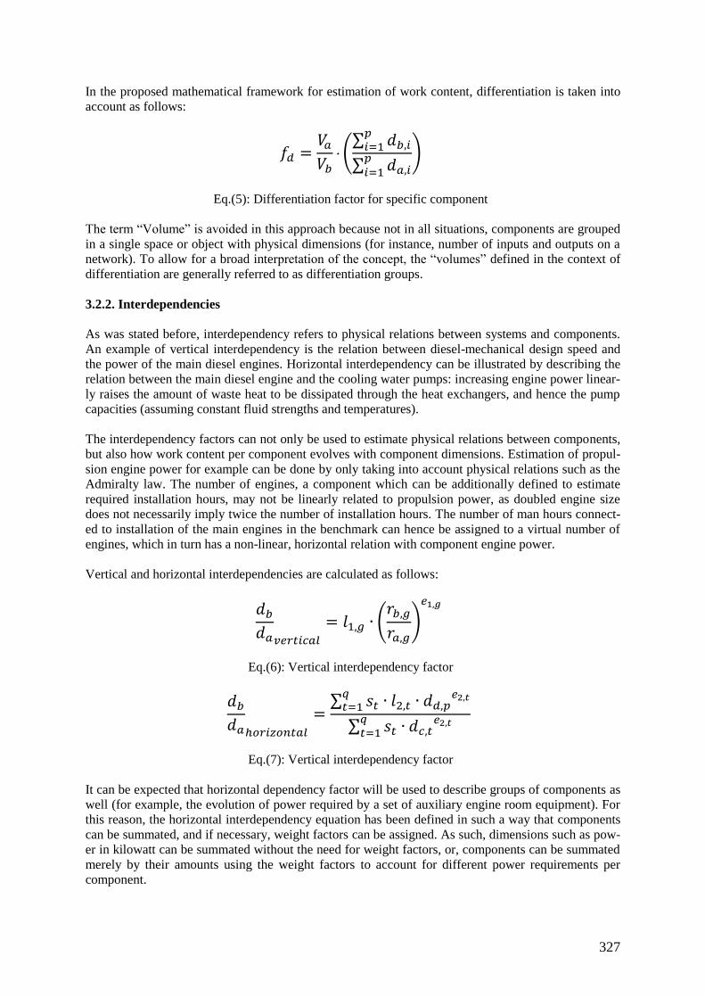
327
In the proposed mathematical framework for estimation of work content, differentiation is taken into
account as follows:
𝑓𝑑 =𝑉𝑎
𝑉𝑏(
∑ 𝑑𝑏,𝑖𝑝𝑖=1
∑ 𝑑𝑎,𝑖𝑝𝑖=1
)
Eq.(5): Differentiation factor for specific component
The term “Volume” is avoided in this approach because not in all situations, components are grouped
in a single space or object with physical dimensions (for instance, number of inputs and outputs on a
network). To allow for a broad interpretation of the concept, the “volumes” defined in the context of
differentiation are generally referred to as differentiation groups.
3.2.2. Interdependencies
As was stated before, interdependency refers to physical relations between systems and components.
An example of vertical interdependency is the relation between diesel-mechanical design speed and
the power of the main diesel engines. Horizontal interdependency can be illustrated by describing the
relation between the main diesel engine and the cooling water pumps: increasing engine power linear-
ly raises the amount of waste heat to be dissipated through the heat exchangers, and hence the pump
capacities (assuming constant fluid strengths and temperatures).
The interdependency factors can not only be used to estimate physical relations between components,
but also how work content per component evolves with component dimensions. Estimation of propul-
sion engine power for example can be done by only taking into account physical relations such as the
Admiralty law. The number of engines, a component which can be additionally defined to estimate
required installation hours, may not be linearly related to propulsion power, as doubled engine size
does not necessarily imply twice the number of installation hours. The number of man hours connect-
ed to installation of the main engines in the benchmark can hence be assigned to a virtual number of
engines, which in turn has a non-linear, horizontal relation with component engine power.
Vertical and horizontal interdependencies are calculated as follows:
𝑑𝑏
𝑑𝑎𝑣𝑒𝑟𝑡𝑖𝑐𝑎𝑙
= 𝑙1,𝑔 ∙ (𝑟𝑏,𝑔
𝑟𝑎,𝑔)
𝑒1,𝑔
Eq.(6): Vertical interdependency factor
𝑑𝑏
𝑑𝑎ℎ𝑜𝑟𝑖𝑧𝑜𝑛𝑡𝑎𝑙
=∑ 𝑠𝑡 ∙ 𝑙2,𝑡 ∙ 𝑑𝑑,𝑝
𝑒2,𝑡𝑞𝑡=1
∑ 𝑠𝑡𝑞𝑡=1 ∙ 𝑑𝑐,𝑡
𝑒2,𝑡
Eq.(7): Vertical interdependency factor
It can be expected that horizontal dependency factor will be used to describe groups of components as
well (for example, the evolution of power required by a set of auxiliary engine room equipment). For
this reason, the horizontal interdependency equation has been defined in such a way that components
can be summated, and if necessary, weight factors can be assigned. As such, dimensions such as pow-
er in kilowatt can be summated without the need for weight factors, or, components can be summated
merely by their amounts using the weight factors to account for different power requirements per
component.
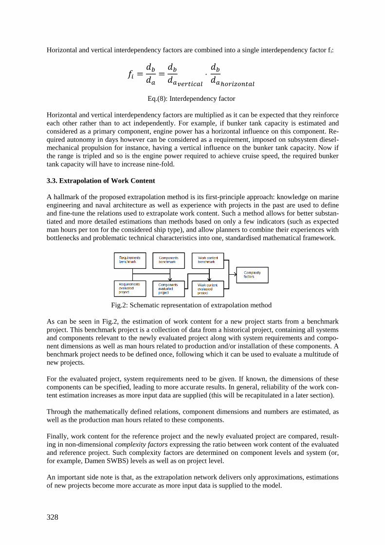
328
Horizontal and vertical interdependency factors are combined into a single interdependency factor fi:
𝑓𝑖 =𝑑𝑏
𝑑𝑎=
𝑑𝑏
𝑑𝑎𝑣𝑒𝑟𝑡𝑖𝑐𝑎𝑙
𝑑𝑏
𝑑𝑎ℎ𝑜𝑟𝑖𝑧𝑜𝑛𝑡𝑎𝑙
Eq.(8): Interdependency factor
Horizontal and vertical interdependency factors are multiplied as it can be expected that they reinforce
each other rather than to act independently. For example, if bunker tank capacity is estimated and
considered as a primary component, engine power has a horizontal influence on this component. Re-
quired autonomy in days however can be considered as a requirement, imposed on subsystem diesel-
mechanical propulsion for instance, having a vertical influence on the bunker tank capacity. Now if
the range is tripled and so is the engine power required to achieve cruise speed, the required bunker
tank capacity will have to increase nine-fold.
3.3. Extrapolation of Work Content
A hallmark of the proposed extrapolation method is its first-principle approach: knowledge on marine
engineering and naval architecture as well as experience with projects in the past are used to define
and fine-tune the relations used to extrapolate work content. Such a method allows for better substan-
tiated and more detailed estimations than methods based on only a few indicators (such as expected
man hours per ton for the considered ship type), and allow planners to combine their experiences with
bottlenecks and problematic technical characteristics into one, standardised mathematical framework.
Fig.2: Schematic representation of extrapolation method
As can be seen in Fig.2, the estimation of work content for a new project starts from a benchmark
project. This benchmark project is a collection of data from a historical project, containing all systems
and components relevant to the newly evaluated project along with system requirements and compo-
nent dimensions as well as man hours related to production and/or installation of these components. A
benchmark project needs to be defined once, following which it can be used to evaluate a multitude of
new projects.
For the evaluated project, system requirements need to be given. If known, the dimensions of these
components can be specified, leading to more accurate results. In general, reliability of the work con-
tent estimation increases as more input data are supplied (this will be recapitulated in a later section).
Through the mathematically defined relations, component dimensions and numbers are estimated, as
well as the production man hours related to these components.
Finally, work content for the reference project and the newly evaluated project are compared, result-
ing in non-dimensional complexity factors expressing the ratio between work content of the evaluated
and reference project. Such complexity factors are determined on component levels and system (or,
for example, Damen SWBS) levels as well as on project level.
An important side note is that, as the extrapolation network delivers only approximations, estimations
of new projects become more accurate as more input data is supplied to the model.
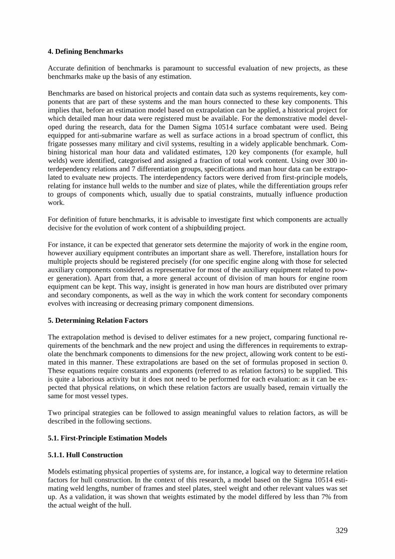
329
4. Defining Benchmarks
Accurate definition of benchmarks is paramount to successful evaluation of new projects, as these
benchmarks make up the basis of any estimation.
Benchmarks are based on historical projects and contain data such as systems requirements, key com-
ponents that are part of these systems and the man hours connected to these key components. This
implies that, before an estimation model based on extrapolation can be applied, a historical project for
which detailed man hour data were registered must be available. For the demonstrative model devel-
oped during the research, data for the Damen Sigma 10514 surface combatant were used. Being
equipped for anti-submarine warfare as well as surface actions in a broad spectrum of conflict, this
frigate possesses many military and civil systems, resulting in a widely applicable benchmark. Com-
bining historical man hour data and validated estimates, 120 key components (for example, hull
welds) were identified, categorised and assigned a fraction of total work content. Using over 300 in-
terdependency relations and 7 differentiation groups, specifications and man hour data can be extrapo-
lated to evaluate new projects. The interdependency factors were derived from first-principle models,
relating for instance hull welds to the number and size of plates, while the differentiation groups refer
to groups of components which, usually due to spatial constraints, mutually influence production
work.
For definition of future benchmarks, it is advisable to investigate first which components are actually
decisive for the evolution of work content of a shipbuilding project.
For instance, it can be expected that generator sets determine the majority of work in the engine room,
however auxiliary equipment contributes an important share as well. Therefore, installation hours for
multiple projects should be registered precisely (for one specific engine along with those for selected
auxiliary components considered as representative for most of the auxiliary equipment related to pow-
er generation). Apart from that, a more general account of division of man hours for engine room
equipment can be kept. This way, insight is generated in how man hours are distributed over primary
and secondary components, as well as the way in which the work content for secondary components
evolves with increasing or decreasing primary component dimensions.
5. Determining Relation Factors
The extrapolation method is devised to deliver estimates for a new project, comparing functional re-
quirements of the benchmark and the new project and using the differences in requirements to extrap-
olate the benchmark components to dimensions for the new project, allowing work content to be esti-
mated in this manner. These extrapolations are based on the set of formulas proposed in section 0.
These equations require constants and exponents (referred to as relation factors) to be supplied. This
is quite a laborious activity but it does not need to be performed for each evaluation: as it can be ex-
pected that physical relations, on which these relation factors are usually based, remain virtually the
same for most vessel types.
Two principal strategies can be followed to assign meaningful values to relation factors, as will be
described in the following sections.
5.1. First-Principle Estimation Models
5.1.1. Hull Construction
Models estimating physical properties of systems are, for instance, a logical way to determine relation
factors for hull construction. In the context of this research, a model based on the Sigma 10514 esti-
mating weld lengths, number of frames and steel plates, steel weight and other relevant values was set
up. As a validation, it was shown that weights estimated by the model differed by less than 7% from
the actual weight of the hull.
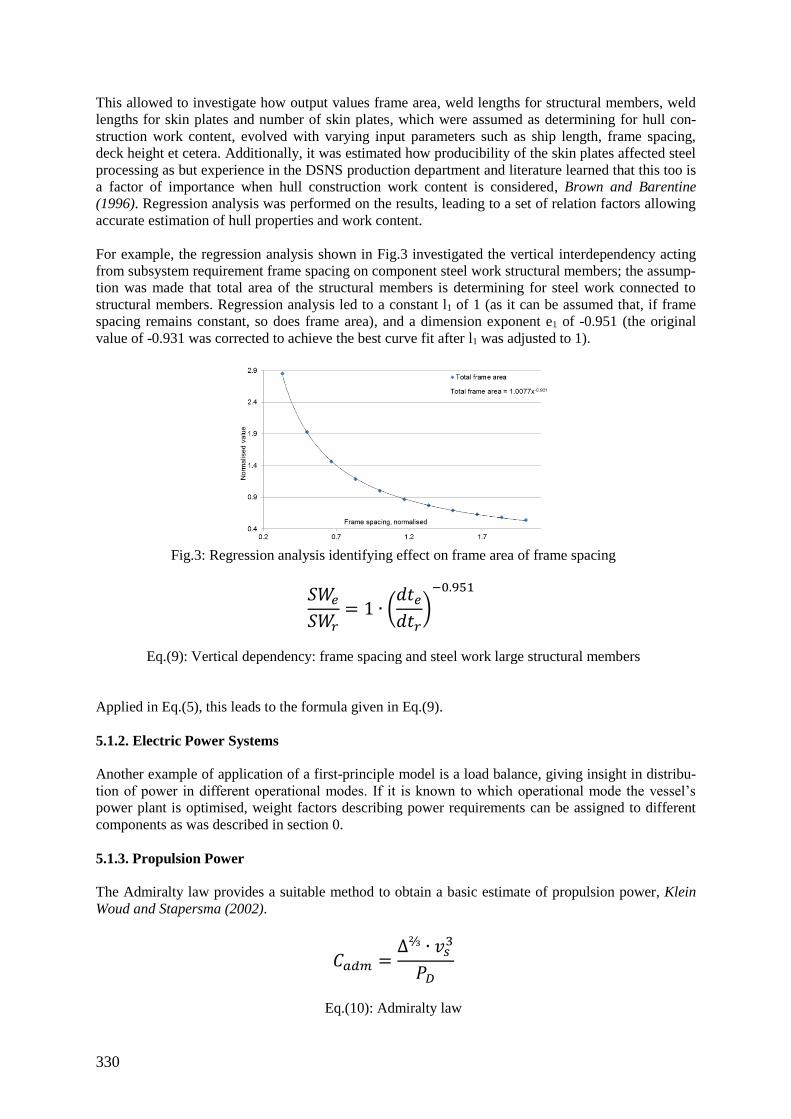
330
This allowed to investigate how output values frame area, weld lengths for structural members, weld
lengths for skin plates and number of skin plates, which were assumed as determining for hull con-
struction work content, evolved with varying input parameters such as ship length, frame spacing,
deck height et cetera. Additionally, it was estimated how producibility of the skin plates affected steel
processing as but experience in the DSNS production department and literature learned that this too is
a factor of importance when hull construction work content is considered, Brown and Barentine
(1996). Regression analysis was performed on the results, leading to a set of relation factors allowing
accurate estimation of hull properties and work content.
For example, the regression analysis shown in Fig.3 investigated the vertical interdependency acting
from subsystem requirement frame spacing on component steel work structural members; the assump-
tion was made that total area of the structural members is determining for steel work connected to
structural members. Regression analysis led to a constant l1 of 1 (as it can be assumed that, if frame
spacing remains constant, so does frame area), and a dimension exponent e1 of -0.951 (the original
value of -0.931 was corrected to achieve the best curve fit after l1 was adjusted to 1).
Fig.3: Regression analysis identifying effect on frame area of frame spacing
𝑆𝑊𝑒
𝑆𝑊𝑟= 1 ∙ (
𝑑𝑡𝑒
𝑑𝑡𝑟)
−0.951
Eq.(9): Vertical dependency: frame spacing and steel work large structural members
Applied in Eq.(5), this leads to the formula given in Eq.(9).
5.1.2. Electric Power Systems
Another example of application of a first-principle model is a load balance, giving insight in distribu-
tion of power in different operational modes. If it is known to which operational mode the vessel’s
power plant is optimised, weight factors describing power requirements can be assigned to different
components as was described in section 0.
5.1.3. Propulsion Power
The Admiralty law provides a suitable method to obtain a basic estimate of propulsion power, Klein
Woud and Stapersma (2002).
𝐶𝑎𝑑𝑚 =∆⅔ ∙ 𝑣𝑠
3
𝑃𝐷
Eq.(10): Admiralty law
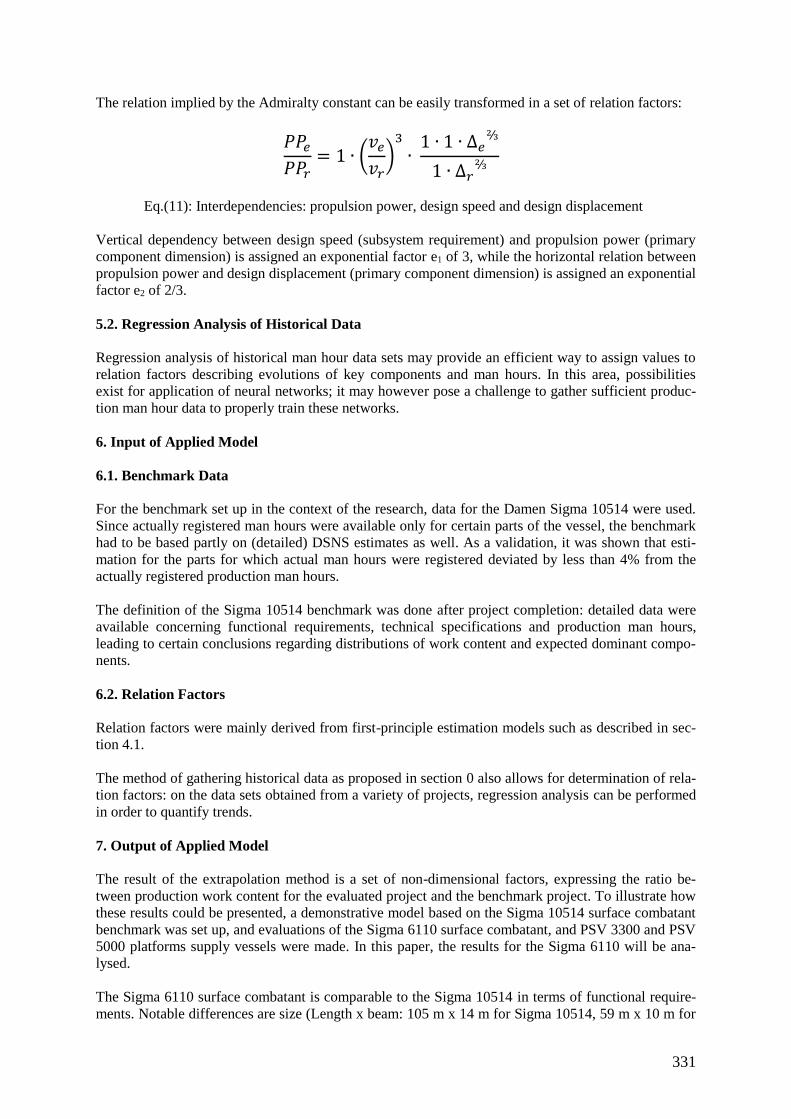
331
The relation implied by the Admiralty constant can be easily transformed in a set of relation factors:
𝑃𝑃𝑒
𝑃𝑃𝑟= 1 ∙ (
𝑣𝑒
𝑣𝑟)
3
∙ 1 ∙ 1 ∙ ∆𝑒
⅔
1 ∙ ∆𝑟⅔
Eq.(11): Interdependencies: propulsion power, design speed and design displacement
Vertical dependency between design speed (subsystem requirement) and propulsion power (primary
component dimension) is assigned an exponential factor e1 of 3, while the horizontal relation between
propulsion power and design displacement (primary component dimension) is assigned an exponential
factor e2 of 2/3.
5.2. Regression Analysis of Historical Data
Regression analysis of historical man hour data sets may provide an efficient way to assign values to
relation factors describing evolutions of key components and man hours. In this area, possibilities
exist for application of neural networks; it may however pose a challenge to gather sufficient produc-
tion man hour data to properly train these networks.
6. Input of Applied Model
6.1. Benchmark Data
For the benchmark set up in the context of the research, data for the Damen Sigma 10514 were used.
Since actually registered man hours were available only for certain parts of the vessel, the benchmark
had to be based partly on (detailed) DSNS estimates as well. As a validation, it was shown that esti-
mation for the parts for which actual man hours were registered deviated by less than 4% from the
actually registered production man hours.
The definition of the Sigma 10514 benchmark was done after project completion: detailed data were
available concerning functional requirements, technical specifications and production man hours,
leading to certain conclusions regarding distributions of work content and expected dominant compo-
nents.
6.2. Relation Factors
Relation factors were mainly derived from first-principle estimation models such as described in sec-
tion 4.1.
The method of gathering historical data as proposed in section 0 also allows for determination of rela-
tion factors: on the data sets obtained from a variety of projects, regression analysis can be performed
in order to quantify trends.
7. Output of Applied Model
The result of the extrapolation method is a set of non-dimensional factors, expressing the ratio be-
tween production work content for the evaluated project and the benchmark project. To illustrate how
these results could be presented, a demonstrative model based on the Sigma 10514 surface combatant
benchmark was set up, and evaluations of the Sigma 6110 surface combatant, and PSV 3300 and PSV
5000 platforms supply vessels were made. In this paper, the results for the Sigma 6110 will be ana-
lysed.
The Sigma 6110 surface combatant is comparable to the Sigma 10514 in terms of functional require-
ments. Notable differences are size (Length x beam: 105 m x 14 m for Sigma 10514, 59 m x 10 m for
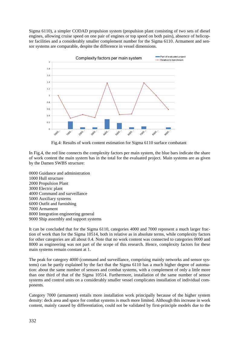
332
Sigma 6110), a simpler CODAD propulsion system (propulsion plant consisting of two sets of diesel
engines, allowing cruise speed on one pair of engines or top speed on both pairs), absence of helicop-
ter facilities and a considerably smaller complement number for the Sigma 6110. Armament and sen-
sor systems are comparable, despite the difference in vessel dimensions.
Fig.4: Results of work content estimation for Sigma 6110 surface combatant
In Fig.4, the red line connects the complexity factors per main system, the blue bars indicate the share
of work content the main system has in the total for the evaluated project. Main systems are as given
by the Damen SWBS structure:
0000 Guidance and administration
1000 Hull structure
2000 Propulsion Plant
3000 Electric plant
4000 Command and surveillance
5000 Auxiliary systems
6000 Outfit and furnishing
7000 Armament
8000 Integration engineering general
9000 Ship assembly and support systems
It can be concluded that for the Sigma 6110, categories 4000 and 7000 represent a much larger frac-
tion of work than for the Sigma 10514, both in relative as in absolute terms, while complexity factors
for other categories are all about 0.4. Note that no work content was connected to categories 0000 and
8000 as engineering was not part of the scope of this research. Hence, complexity factors for these
main systems remain constant at 1.
The peak for category 4000 (command and surveillance, comprising mainly networks and sensor sys-
tems) can be partly explained by the fact that the Sigma 6110 has a much higher degree of automa-
tion: about the same number of sensors and combat systems, with a complement of only a little more
than one third of that of the Sigma 10514. Furthermore, installation of the same number of sensor
systems and control units on a considerably smaller vessel complicates installation of individual com-
ponents.
Category 7000 (armament) entails more installation work principally because of the higher system
density: deck area and space for combat systems is much more limited. Although this increase in work
content, mainly caused by differentiation, could not be validated by first-principle models due to the
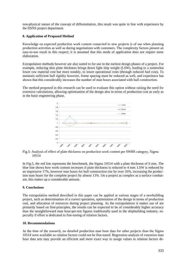
333
non-physical nature of the concept of differentiation, this result was quite in line with experience by
the DSNS project department.
8. Application of Proposed Method
Knowledge on expected production work content connected to new projects is of use when planning
production activities as well as during negotiations with customers. The complexity factors present an
easy-to-use result in this respect; it is assumed that this mode of application does not require more
elaboration.
Extrapolation methods however are also suited to for use in the earliest design phases of a project. For
example, reducing skin plate thickness brings down light ship weight (LSW), leading to a somewhat
lower raw material cost but more notably, to lower operational costs (through reduced fuel cost). To
maintain sufficient hull rigidity however, frame spacing must be reduced as well, and experience has
shown that this considerably increases the number of man hours associated with hull construction.
The method proposed in this research can be used to evaluate this option without raising the need for
extensive calculations, allowing optimisation of the design also in terms of production cost as early as
in the basic engineering phase.
Fig.5: Analysis of effect of plate thickness on production work content per SWBS category, Sigma
10514
In Fig.5, the red line represents the benchmark, the Sigma 10514 with a plate thickness of 6 mm. The
blue line shows how work content increases if plate thickness is reduced to 4 mm: LSW is reduced by
an impressive 17%, however man hours for hull construction rise by over 35%, increasing the produc-
tion man hours for the complete project by almost 13%. On a project as complex as a surface combat-
ant, this makes up a considerable amount.
9. Conclusions
The extrapolation method described in this paper can be applied at various stages of a newbuilding
project, such as determination of a correct quotation, optimisation of the design in terms of production
cost, and allocation of resources during project planning. As the extrapolations it makes use of are
primarily based on first-principles, the results can be expected to be of considerably higher accuracy
than the straightforward man hour-per-ton figures traditionally used in the shipbuilding industry, es-
pecially if effort is dedicated to fine-tuning of relation factors.
10. Recommendations
At the time of the research, no detailed production man hour data for other projects than the Sigma
10514 were available so relation factors could not be fine-tuned. Regression analysis of extensive man
hour data sets may provide an efficient and more exact way to assign values to relation factors de-
334
scribing evolutions of key components and man hours. In this area, possibilities exist for application
of neural networks; it may however pose a challenge to gather sufficient production man hour data to
properly train these networks.
When defining new benchmarks, it may be interesting to try an alternative approach: instead of basing
a new benchmark exclusively on available, historical data, it can be chosen to use these historical data
to identify, for example, a top-200 list of key components (including steel work related activities)
which represent the majority of work content. It can then be investigated how other equipment is
functionally related to these components. Subsequently, man hours can be tracked for these key com-
ponents, along with man hours for a selected group of functionally related equipment in order to gain
insight how this ancillary equipment evolves in terms of man hours.
These focused registrations of work content can be performed for multiple projects with differing
specifications, on the longer term leading to profound insight in which components drive production
work content and how these key components influence auxiliary components.
Abbreviations
CGT Compensated Gross Tonnage
CODAD Combined Diesel And Diesel
CODELOD Combined Diesel-Electric Or Diesel
DSNS Damen Schelde Naval Shipbuilding
GT Gross Tonnage
LSW Light Ship Weight
PSV
SWBS
Platform Supply Vessel
Ship Work Breakdown Structure
Nomenclature
fc = [-] complexity ratio for component
fi = [-] interdependency factor for component
fd = [-] differentiation factor for component
e3 = [-] differentiation – man hours exponent
da = [kW, kg, t, …] dimensions of influenced component in reference project
db = [kW, kg, t, …] dimensions of influenced component in evaluated project
Va = [m3, m, …] available space for component in reference project
Vb = [m3, m, …] available space for component in evaluated project
i = [-] index for components present in room
p = [-] number of components present in room
fcc = [-] combined complexity ratio for higher level
k = [-] index for lower level components, subsystems or main systems
n = [-] numbers of lower level components, subsystems or main systems
MHb = [hrs] estimated man hours for installation of evaluated component
MHa = [hrs] man hours for installation of reference component
l1 = [-] vertical dependency constant
ra = [kn, complement, …] system requirements for reference project
rb = [kn, complement, …] system requirements for evaluated project
e1 = [-] vertical dependency dimension exponent
s = [-] coefficient of effect (“weight factor”)
l2 = [-] horizontal dependency constant
dc = [kW, kg, t, …] dimensions of influencing components in reference project
dd = [kW, kg, t, …] dimensions of influencing components in evaluated project
t = [-] index for components of influence on horizontal dependency
q = [-] number of components of influence on horizontal dependency
e2 = [-] horizontal dependency exponent

335
SWe = [hrs] work content steel work large structural members, evaluated project
SWr = [hrs] work content steel work large structural members, reference project
dte = [m] transverse frame spacing, evaluated project
dtr = [m] transverse frame spacing, reference project
Cadm = [t2/3·kn3/kW] Admiralty constant
= [t] displacement
vs = [kn] ship speed
PD = [kW] power delivered to propulsors
PPe = [kW] propulsive power, evaluated project
PPr = [kW] propulsive power, reference project
ve = [kn] design speed, evaluated project
vr = [kn] design speed, reference project
∆e = [t] design displacement, evaluated project
∆r = [t] design displacement, reference project
References
BACCARINI, D. (1996), The Concept of Project Complexity - a Review, Int. J. Project Management
14, pp.201-204
BROWN, A.; BARENTINE, J. (1996), The Impact of Producibility on Cost and Performance in Na-
val Combatant Design, Massachusetts Institute of Technology
GIDADO, K. (1993), Numerical Index of Complexity in Building Construction with Particular Con-
sideration to its Effect on Production Time, PhD thesis, University of Brighton
HUBKA, M.; EDER, W. (1988), Practical Studies in Systematic Design, Butterworth-Heinemann,
KLEIN WOUD, H.; STAPERSMA, D. (2002), Design of Propulsion and Electric Power Generation
Systems. London: IMarEST.
WILLIAMS, T.M. (1999), The Need for New Paradigms for Complex Projects, Int. J. Project Man-
agement 17, pp.269-273
336
Multidisciplinary Process Integration and Design Optimization of a Hybrid
Marine Power System Applied to a VLCC
Sabah Alwan, NTNU, Trondheim/Norway, [email protected]
Kevin Koosup Yum, SINTEF Ocean, Trondheim/Norway, [email protected]
Sverre Steen, NTNU, Trondheim/Norway, [email protected]
Eilif Pedersen, NTNU, Trondheim/Norway, [email protected]
Abstract
In this paper, we explore the use of multidisciplinary and high-fidelity simulations for multi-objective
design optimization of a marine hybrid propulsion system with application to a very large crude oil
carrier (VLCC) tanker. The optimization is achieved by utilizing a process integration and design
optimization (PIDO) to support multidisciplinary design optimization (MDO). We performed a
minimum number of simulations to explore the design space through algorithm-guided design-of-
experiments (DoE). Based on those experiments, response surface models (RSMs) were constructed.
Further, sensitivity and correlation within design parameters and with the design objectives from the
simulations are simultaneously examined and elucidated. Subsequently, the quality of the RSMs is
validated using the simulation models. A multi-objective optimization is then carried out by utilizing
the RSMs rather than the high-fidelity simulation. Standard particle swarm optimization (sPSO) was
used with the RSMs while a very large number of design variation and alternatives are swiftly examined.
Remaining work is to test optimal design solutions for their reliability and robustness through sensitivity
to changes in operational requirements, changes in environmental conditions and imprecision in design
parameters.
1. Introduction
A ship is a complex system in which many designers develop and consider different aspects of the
system to meet various functional requirements. Traditionally design decisions are made in two
different levels, that is a system level and a component level. In the system level, often the optimization
objective is to make the ship as economic as possible, whereas in the component level, the objective is
to meet the component’s solitary functional requirements within the given constraints. In this paper, we
hope to shed light on the use of an integrated multidisciplinary simulation-based framework for multi-
objective design optimization of a vessel system performance rather than component based design and
optimization. These approaches are recently and widely in use within the aerospace and automotive
industries alike Frenzel, Heiserer et al. (2015) and Van der Auweraer, Donders et al. (2008), with lesser
usage in the maritime industry where its often discipline specific Liu and Collette (2014) and
Parsopoulos and Vrahatis (2002). Using a well-established approach from other industries can
potentially improve design outcomes de Weck, Agte et al. (2007) by simultaneously considering
different aspects of the system. Therefore, process integration and design optimization (PIDO) tools
are used to support multidisciplinary design optimization (MDO). In MDO, a metamodel is often
derived from performing a minimum number of multidisciplinary system simulations guided by smart
algorithm such as Latin Hypercube Eglajs and Audze (1977) or Factorial Design Box and Hunter (1961)
through design-of-experiment (DoE). In the system simulation, several domain specific virtual models
and processes are interlinked in accordance with the design task. In this paper, models include ship
operational model, metocean models, ship hydrodynamics, propulsion, electrical load and powering
models to simulate the total system performances. The metamodel can be in the form of a response
surface model (RSM) Box and Wilson (1992) that is constructed by a polynomial, support vector
machine (SVM) for supervised machine learning, a neural network, Kriging, etc. Subsequently, multi-
objective optimization is achieved by the utilization of the metamodel and varying design parameters
with optimization algorithms within some design constraints to achieve certain performance objectives.
Several optimization algorithms were tested and found to vary in their performance and convergence.
In this paper, we present an application of MDO using a PIDO platform for the design of a hybrid
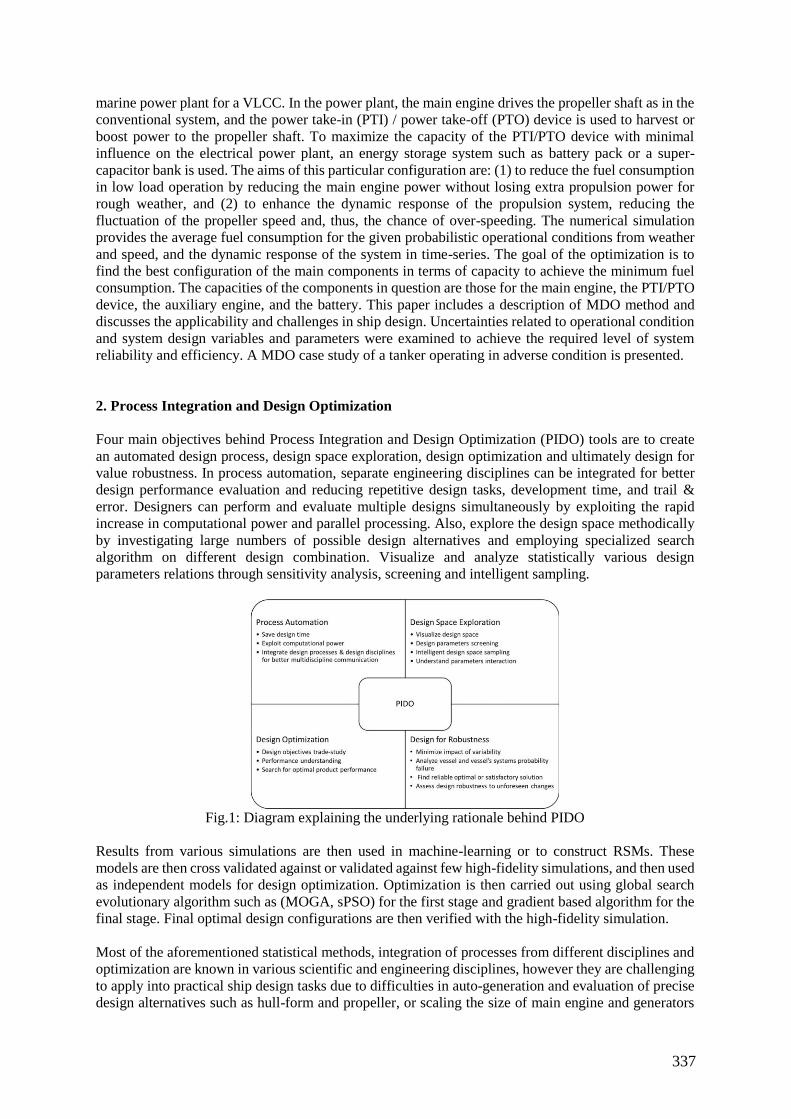
337
marine power plant for a VLCC. In the power plant, the main engine drives the propeller shaft as in the
conventional system, and the power take-in (PTI) / power take-off (PTO) device is used to harvest or
boost power to the propeller shaft. To maximize the capacity of the PTI/PTO device with minimal
influence on the electrical power plant, an energy storage system such as battery pack or a super-
capacitor bank is used. The aims of this particular configuration are: (1) to reduce the fuel consumption
in low load operation by reducing the main engine power without losing extra propulsion power for
rough weather, and (2) to enhance the dynamic response of the propulsion system, reducing the
fluctuation of the propeller speed and, thus, the chance of over-speeding. The numerical simulation
provides the average fuel consumption for the given probabilistic operational conditions from weather
and speed, and the dynamic response of the system in time-series. The goal of the optimization is to
find the best configuration of the main components in terms of capacity to achieve the minimum fuel
consumption. The capacities of the components in question are those for the main engine, the PTI/PTO
device, the auxiliary engine, and the battery. This paper includes a description of MDO method and
discusses the applicability and challenges in ship design. Uncertainties related to operational condition
and system design variables and parameters were examined to achieve the required level of system
reliability and efficiency. A MDO case study of a tanker operating in adverse condition is presented.
2. Process Integration and Design Optimization
Four main objectives behind Process Integration and Design Optimization (PIDO) tools are to create
an automated design process, design space exploration, design optimization and ultimately design for
value robustness. In process automation, separate engineering disciplines can be integrated for better
design performance evaluation and reducing repetitive design tasks, development time, and trail &
error. Designers can perform and evaluate multiple designs simultaneously by exploiting the rapid
increase in computational power and parallel processing. Also, explore the design space methodically
by investigating large numbers of possible design alternatives and employing specialized search
algorithm on different design combination. Visualize and analyze statistically various design
parameters relations through sensitivity analysis, screening and intelligent sampling.
Fig.1: Diagram explaining the underlying rationale behind PIDO
Results from various simulations are then used in machine-learning or to construct RSMs. These
models are then cross validated against or validated against few high-fidelity simulations, and then used
as independent models for design optimization. Optimization is then carried out using global search
evolutionary algorithm such as (MOGA, sPSO) for the first stage and gradient based algorithm for the
final stage. Final optimal design configurations are then verified with the high-fidelity simulation.
Most of the aforementioned statistical methods, integration of processes from different disciplines and
optimization are known in various scientific and engineering disciplines, however they are challenging
to apply into practical ship design tasks due to difficulties in auto-generation and evaluation of precise
design alternatives such as hull-form and propeller, or scaling the size of main engine and generators
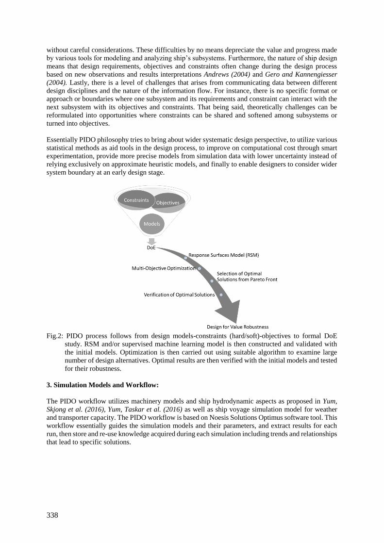
338
without careful considerations. These difficulties by no means depreciate the value and progress made
by various tools for modeling and analyzing ship’s subsystems. Furthermore, the nature of ship design
means that design requirements, objectives and constraints often change during the design process
based on new observations and results interpretations Andrews (2004) and Gero and Kannengiesser
(2004). Lastly, there is a level of challenges that arises from communicating data between different
design disciplines and the nature of the information flow. For instance, there is no specific format or
approach or boundaries where one subsystem and its requirements and constraint can interact with the
next subsystem with its objectives and constraints. That being said, theoretically challenges can be
reformulated into opportunities where constraints can be shared and softened among subsystems or
turned into objectives.
Essentially PIDO philosophy tries to bring about wider systematic design perspective, to utilize various
statistical methods as aid tools in the design process, to improve on computational cost through smart
experimentation, provide more precise models from simulation data with lower uncertainty instead of
relying exclusively on approximate heuristic models, and finally to enable designers to consider wider
system boundary at an early design stage.
Fig.2: PIDO process follows from design models-constraints (hard/soft)-objectives to formal DoE
study. RSM and/or supervised machine learning model is then constructed and validated with
the initial models. Optimization is then carried out using suitable algorithm to examine large
number of design alternatives. Optimal results are then verified with the initial models and tested
for their robustness.
3. Simulation Models and Workflow:
The PIDO workflow utilizes machinery models and ship hydrodynamic aspects as proposed in Yum,
Skjong et al. (2016), Yum, Taskar et al. (2016) as well as ship voyage simulation model for weather
and transporter capacity. The PIDO workflow is based on Noesis Solutions Optimus software tool. This
workflow essentially guides the simulation models and their parameters, and extract results for each
run, then store and re-use knowledge acquired during each simulation including trends and relationships
that lead to specific solutions.
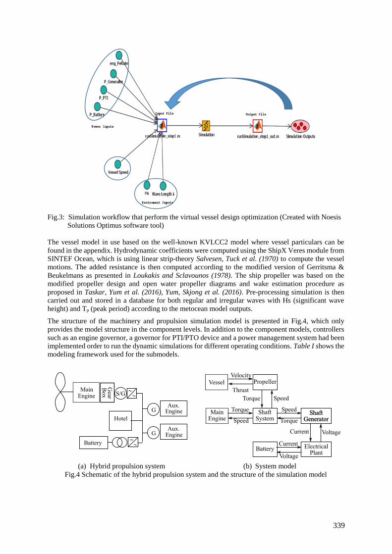
339
Fig.3: Simulation workflow that perform the virtual vessel design optimization (Created with Noesis
Solutions Optimus software tool)
The vessel model in use based on the well-known KVLCC2 model where vessel particulars can be
found in the appendix. Hydrodynamic coefficients were computed using the ShipX Veres module from
SINTEF Ocean, which is using linear strip-theory Salvesen, Tuck et al. (1970) to compute the vessel
motions. The added resistance is then computed according to the modified version of Gerritsma &
Beukelmans as presented in Loukakis and Sclavounos (1978). The ship propeller was based on the
modified propeller design and open water propeller diagrams and wake estimation procedure as
proposed in Taskar, Yum et al. (2016), Yum, Skjong et al. (2016). Pre-processing simulation is then
carried out and stored in a database for both regular and irregular waves with Hs (significant wave
height) and Tp (peak period) according to the metocean model outputs.
The structure of the machinery and propulsion simulation model is presented in Fig.4, which only
provides the model structure in the component levels. In addition to the component models, controllers
such as an engine governor, a governor for PTI/PTO device and a power management system had been
implemented order to run the dynamic simulations for different operating conditions. Table I shows the
modeling framework used for the submodels.
(a) Hybrid propulsion system (b) System model
Fig.4 Schematic of the hybrid propulsion system and the structure of the simulation model
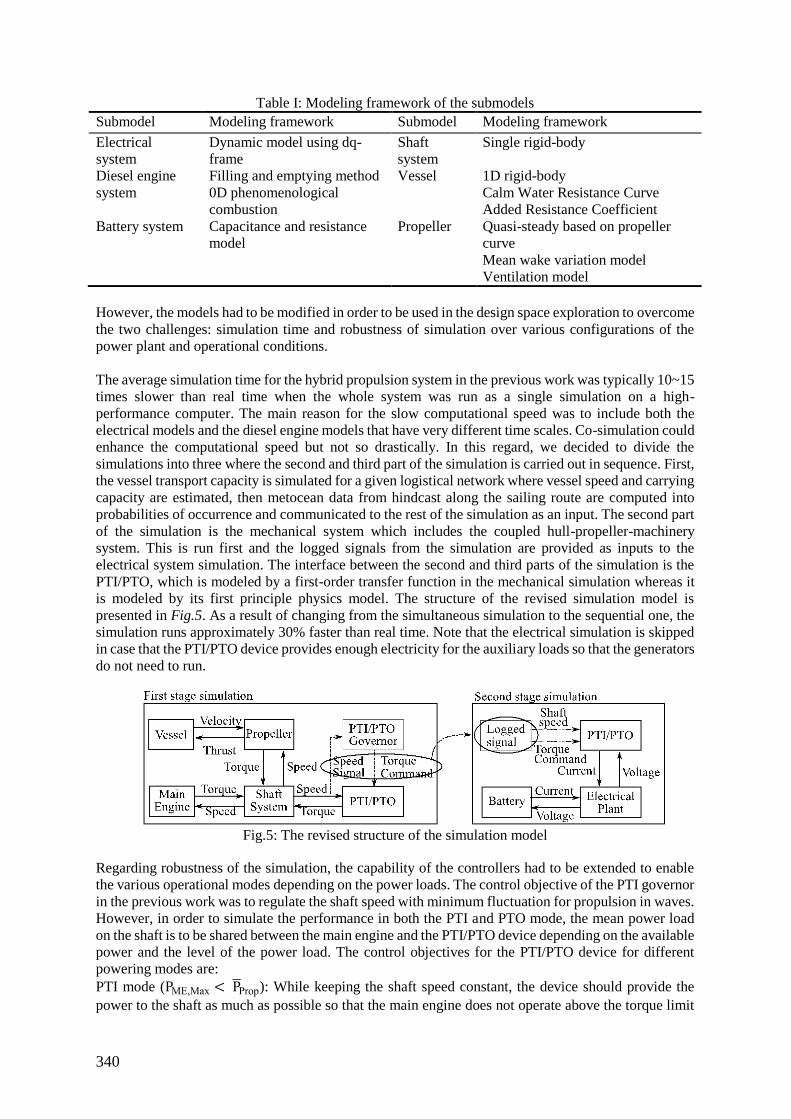
340
Table I: Modeling framework of the submodels
Submodel Modeling framework Submodel Modeling framework
Electrical
system
Dynamic model using dq-
frame
Shaft
system
Single rigid-body
Diesel engine
system
Filling and emptying method
0D phenomenological
combustion
Vessel 1D rigid-body
Calm Water Resistance Curve
Added Resistance Coefficient
Battery system Capacitance and resistance
model
Propeller Quasi-steady based on propeller
curve
Mean wake variation model
Ventilation model
However, the models had to be modified in order to be used in the design space exploration to overcome
the two challenges: simulation time and robustness of simulation over various configurations of the
power plant and operational conditions.
The average simulation time for the hybrid propulsion system in the previous work was typically 10~15
times slower than real time when the whole system was run as a single simulation on a high-
performance computer. The main reason for the slow computational speed was to include both the
electrical models and the diesel engine models that have very different time scales. Co-simulation could
enhance the computational speed but not so drastically. In this regard, we decided to divide the
simulations into three where the second and third part of the simulation is carried out in sequence. First,
the vessel transport capacity is simulated for a given logistical network where vessel speed and carrying
capacity are estimated, then metocean data from hindcast along the sailing route are computed into
probabilities of occurrence and communicated to the rest of the simulation as an input. The second part
of the simulation is the mechanical system which includes the coupled hull-propeller-machinery
system. This is run first and the logged signals from the simulation are provided as inputs to the
electrical system simulation. The interface between the second and third parts of the simulation is the
PTI/PTO, which is modeled by a first-order transfer function in the mechanical simulation whereas it
is modeled by its first principle physics model. The structure of the revised simulation model is
presented in Fig.5. As a result of changing from the simultaneous simulation to the sequential one, the
simulation runs approximately 30% faster than real time. Note that the electrical simulation is skipped
in case that the PTI/PTO device provides enough electricity for the auxiliary loads so that the generators
do not need to run.
Fig.5: The revised structure of the simulation model
Regarding robustness of the simulation, the capability of the controllers had to be extended to enable
the various operational modes depending on the power loads. The control objective of the PTI governor
in the previous work was to regulate the shaft speed with minimum fluctuation for propulsion in waves.
However, in order to simulate the performance in both the PTI and PTO mode, the mean power load
on the shaft is to be shared between the main engine and the PTI/PTO device depending on the available
power and the level of the power load. The control objectives for the PTI/PTO device for different
powering modes are:
PTI mode (PME,Max < P̅Prop): While keeping the shaft speed constant, the device should provide the
power to the shaft as much as possible so that the main engine does not operate above the torque limit
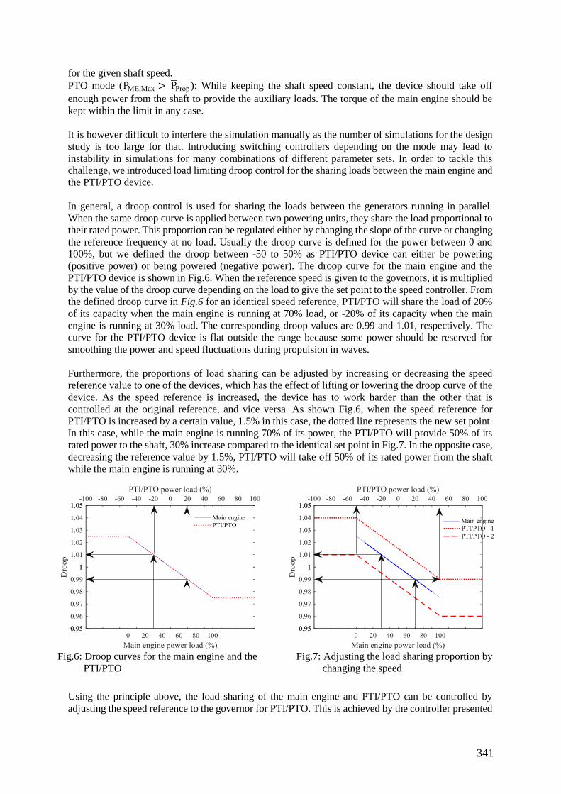
341
for the given shaft speed.
PTO mode (PME,Max > P̅Prop ): While keeping the shaft speed constant, the device should take off
enough power from the shaft to provide the auxiliary loads. The torque of the main engine should be
kept within the limit in any case.
It is however difficult to interfere the simulation manually as the number of simulations for the design
study is too large for that. Introducing switching controllers depending on the mode may lead to
instability in simulations for many combinations of different parameter sets. In order to tackle this
challenge, we introduced load limiting droop control for the sharing loads between the main engine and
the PTI/PTO device.
In general, a droop control is used for sharing the loads between the generators running in parallel.
When the same droop curve is applied between two powering units, they share the load proportional to
their rated power. This proportion can be regulated either by changing the slope of the curve or changing
the reference frequency at no load. Usually the droop curve is defined for the power between 0 and
100%, but we defined the droop between -50 to 50% as PTI/PTO device can either be powering
(positive power) or being powered (negative power). The droop curve for the main engine and the
PTI/PTO device is shown in Fig.6. When the reference speed is given to the governors, it is multiplied
by the value of the droop curve depending on the load to give the set point to the speed controller. From
the defined droop curve in Fig.6 for an identical speed reference, PTI/PTO will share the load of 20%
of its capacity when the main engine is running at 70% load, or -20% of its capacity when the main
engine is running at 30% load. The corresponding droop values are 0.99 and 1.01, respectively. The
curve for the PTI/PTO device is flat outside the range because some power should be reserved for
smoothing the power and speed fluctuations during propulsion in waves.
Furthermore, the proportions of load sharing can be adjusted by increasing or decreasing the speed
reference value to one of the devices, which has the effect of lifting or lowering the droop curve of the
device. As the speed reference is increased, the device has to work harder than the other that is
controlled at the original reference, and vice versa. As shown Fig.6, when the speed reference for
PTI/PTO is increased by a certain value, 1.5% in this case, the dotted line represents the new set point.
In this case, while the main engine is running 70% of its power, the PTI/PTO will provide 50% of its
rated power to the shaft, 30% increase compared to the identical set point in Fig.7. In the opposite case,
decreasing the reference value by 1.5%, PTI/PTO will take off 50% of its rated power from the shaft
while the main engine is running at 30%.
Fig.6: Droop curves for the main engine and the
PTI/PTO
Fig.7: Adjusting the load sharing proportion by
changing the speed
Using the principle above, the load sharing of the main engine and PTI/PTO can be controlled by
adjusting the speed reference to the governor for PTI/PTO. This is achieved by the controller presented
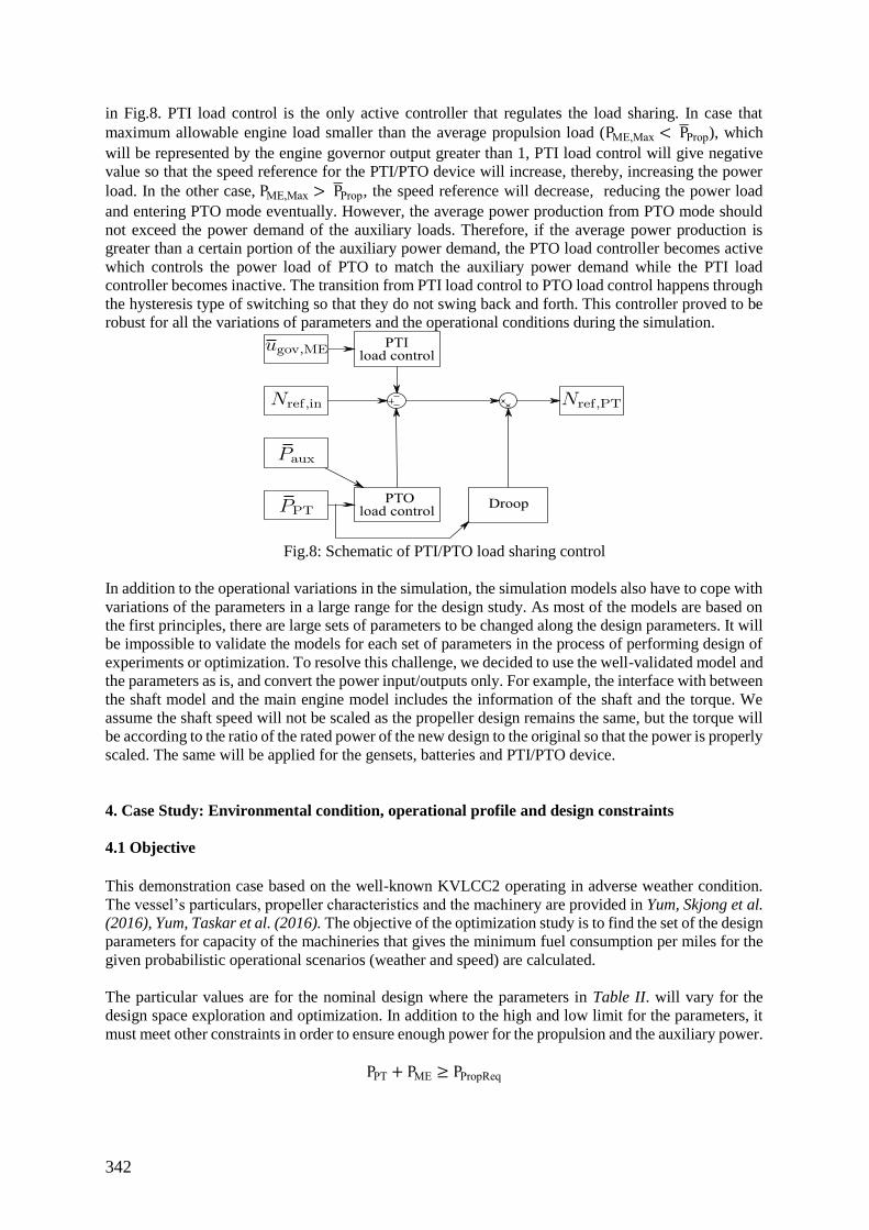
342
in Fig.8. PTI load control is the only active controller that regulates the load sharing. In case that
maximum allowable engine load smaller than the average propulsion load (PME,Max < P̅Prop), which
will be represented by the engine governor output greater than 1, PTI load control will give negative
value so that the speed reference for the PTI/PTO device will increase, thereby, increasing the power
load. In the other case, PME,Max > P̅Prop, the speed reference will decrease, reducing the power load
and entering PTO mode eventually. However, the average power production from PTO mode should
not exceed the power demand of the auxiliary loads. Therefore, if the average power production is
greater than a certain portion of the auxiliary power demand, the PTO load controller becomes active
which controls the power load of PTO to match the auxiliary power demand while the PTI load
controller becomes inactive. The transition from PTI load control to PTO load control happens through
the hysteresis type of switching so that they do not swing back and forth. This controller proved to be
robust for all the variations of parameters and the operational conditions during the simulation.
Fig.8: Schematic of PTI/PTO load sharing control
In addition to the operational variations in the simulation, the simulation models also have to cope with
variations of the parameters in a large range for the design study. As most of the models are based on
the first principles, there are large sets of parameters to be changed along the design parameters. It will
be impossible to validate the models for each set of parameters in the process of performing design of
experiments or optimization. To resolve this challenge, we decided to use the well-validated model and
the parameters as is, and convert the power input/outputs only. For example, the interface with between
the shaft model and the main engine model includes the information of the shaft and the torque. We
assume the shaft speed will not be scaled as the propeller design remains the same, but the torque will
be according to the ratio of the rated power of the new design to the original so that the power is properly
scaled. The same will be applied for the gensets, batteries and PTI/PTO device.
4. Case Study: Environmental condition, operational profile and design constraints
4.1 Objective
This demonstration case based on the well-known KVLCC2 operating in adverse weather condition.
The vessel’s particulars, propeller characteristics and the machinery are provided in Yum, Skjong et al.
(2016), Yum, Taskar et al. (2016). The objective of the optimization study is to find the set of the design
parameters for capacity of the machineries that gives the minimum fuel consumption per miles for the
given probabilistic operational scenarios (weather and speed) are calculated.
The particular values are for the nominal design where the parameters in Table II. will vary for the
design space exploration and optimization. In addition to the high and low limit for the parameters, it
must meet other constraints in order to ensure enough power for the propulsion and the auxiliary power.
PPT + PME ≥ PPropReq
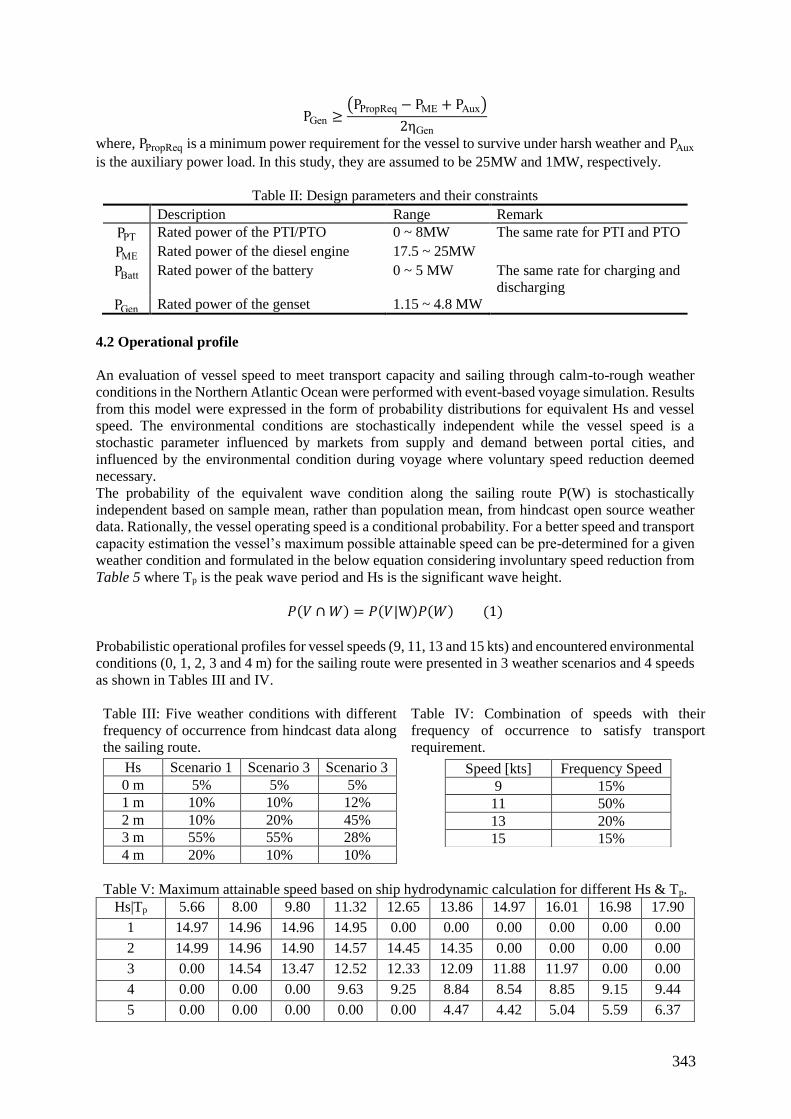
343
PGen ≥(PPropReq − PME + PAux)
2ηGen
where, PPropReq is a minimum power requirement for the vessel to survive under harsh weather and PAux
is the auxiliary power load. In this study, they are assumed to be 25MW and 1MW, respectively.
Table II: Design parameters and their constraints
Description Range Remark
PPT Rated power of the PTI/PTO 0 ~ 8MW The same rate for PTI and PTO
PME Rated power of the diesel engine 17.5 ~ 25MW
PBatt Rated power of the battery 0 ~ 5 MW The same rate for charging and
discharging
PGen Rated power of the genset 1.15 ~ 4.8 MW
4.2 Operational profile
An evaluation of vessel speed to meet transport capacity and sailing through calm-to-rough weather
conditions in the Northern Atlantic Ocean were performed with event-based voyage simulation. Results
from this model were expressed in the form of probability distributions for equivalent Hs and vessel
speed. The environmental conditions are stochastically independent while the vessel speed is a
stochastic parameter influenced by markets from supply and demand between portal cities, and
influenced by the environmental condition during voyage where voluntary speed reduction deemed
necessary.
The probability of the equivalent wave condition along the sailing route P(W) is stochastically
independent based on sample mean, rather than population mean, from hindcast open source weather
data. Rationally, the vessel operating speed is a conditional probability. For a better speed and transport
capacity estimation the vessel’s maximum possible attainable speed can be pre-determined for a given
weather condition and formulated in the below equation considering involuntary speed reduction from
Table 5 where Tp is the peak wave period and Hs is the significant wave height.
𝑃(𝑉 ∩ 𝑊) = 𝑃(𝑉|W)𝑃(𝑊) (1)
Probabilistic operational profiles for vessel speeds (9, 11, 13 and 15 kts) and encountered environmental
conditions (0, 1, 2, 3 and 4 m) for the sailing route were presented in 3 weather scenarios and 4 speeds
as shown in Tables III and IV.
Table III: Five weather conditions with different
frequency of occurrence from hindcast data along
the sailing route.
Hs Scenario 1 Scenario 3 Scenario 3
0 m 5% 5% 5%
1 m 10% 10% 12%
2 m 10% 20% 45%
3 m 55% 55% 28%
4 m 20% 10% 10%
Table IV: Combination of speeds with their
frequency of occurrence to satisfy transport
requirement.
Speed [kts] Frequency Speed
9 15%
11 50%
13 20%
15 15%
Table V: Maximum attainable speed based on ship hydrodynamic calculation for different Hs & Tp.
Hs|Tp 5.66 8.00 9.80 11.32 12.65 13.86 14.97 16.01 16.98 17.90
1 14.97 14.96 14.96 14.95 0.00 0.00 0.00 0.00 0.00 0.00
2 14.99 14.96 14.90 14.57 14.45 14.35 0.00 0.00 0.00 0.00
3 0.00 14.54 13.47 12.52 12.33 12.09 11.88 11.97 0.00 0.00
4 0.00 0.00 0.00 9.63 9.25 8.84 8.54 8.85 9.15 9.44
5 0.00 0.00 0.00 0.00 0.00 4.47 4.42 5.04 5.59 6.37
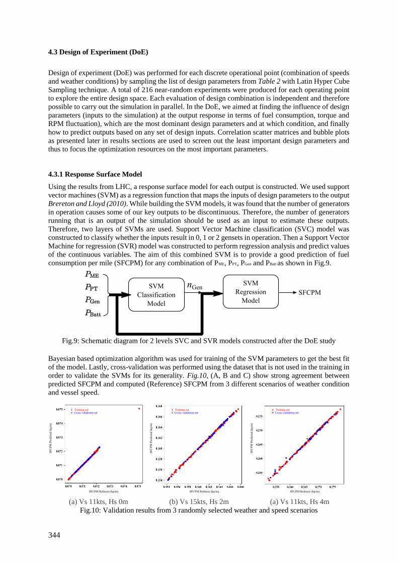
344
4.3 Design of Experiment (DoE)
Design of experiment (DoE) was performed for each discrete operational point (combination of speeds
and weather conditions) by sampling the list of design parameters from Table 2 with Latin Hyper Cube
Sampling technique. A total of 216 near-random experiments were produced for each operating point
to explore the entire design space. Each evaluation of design combination is independent and therefore
possible to carry out the simulation in parallel. In the DoE, we aimed at finding the influence of design
parameters (inputs to the simulation) at the output response in terms of fuel consumption, torque and
RPM fluctuation), which are the most dominant design parameters and at which condition, and finally
how to predict outputs based on any set of design inputs. Correlation scatter matrices and bubble plots
as presented later in results sections are used to screen out the least important design parameters and
thus to focus the optimization resources on the most important parameters.
4.3.1 Response Surface Model
Using the results from LHC, a response surface model for each output is constructed. We used support
vector machines (SVM) as a regression function that maps the inputs of design parameters to the output
Brereton and Lloyd (2010). While building the SVM models, it was found that the number of generators
in operation causes some of our key outputs to be discontinuous. Therefore, the number of generators
running that is an output of the simulation should be used as an input to estimate these outputs.
Therefore, two layers of SVMs are used. Support Vector Machine classification (SVC) model was
constructed to classify whether the inputs result in 0, 1 or 2 gensets in operation. Then a Support Vector
Machine for regression (SVR) model was constructed to perform regression analysis and predict values
of the continuous variables. The aim of this combined SVM is to provide a good prediction of fuel
consumption per mile (SFCPM) for any combination of PME, PPT, PGen and PBatt as shown in Fig.9.
Fig.9: Schematic diagram for 2 levels SVC and SVR models constructed after the DoE study
Bayesian based optimization algorithm was used for training of the SVM parameters to get the best fit
of the model. Lastly, cross-validation was performed using the dataset that is not used in the training in
order to validate the SVMs for its generality. Fig.10, (A, B and C) show strong agreement between
predicted SFCPM and computed (Reference) SFCPM from 3 different scenarios of weather condition
and vessel speed.
(a) Vs 11kts, Hs 0m (b) Vs 15kts, Hs 2m (a) Vs 11kts, Hs 4m
Fig.10: Validation results from 3 randomly selected weather and speed scenarios
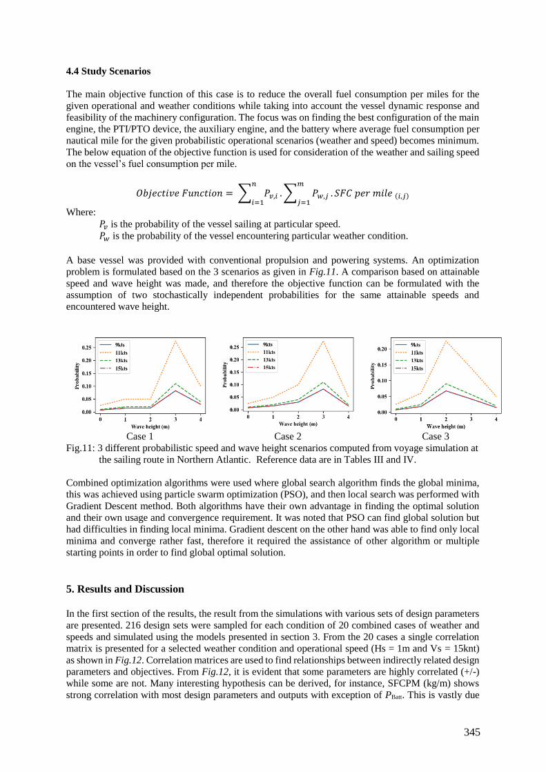
345
4.4 Study Scenarios
The main objective function of this case is to reduce the overall fuel consumption per miles for the
given operational and weather conditions while taking into account the vessel dynamic response and
feasibility of the machinery configuration. The focus was on finding the best configuration of the main
engine, the PTI/PTO device, the auxiliary engine, and the battery where average fuel consumption per
nautical mile for the given probabilistic operational scenarios (weather and speed) becomes minimum.
The below equation of the objective function is used for consideration of the weather and sailing speed
on the vessel’s fuel consumption per mile.
𝑂𝑏𝑗𝑒𝑐𝑡𝑖𝑣𝑒 𝐹𝑢𝑛𝑐𝑡𝑖𝑜𝑛 = ∑ 𝑃𝑣,𝑖
𝑛
𝑖=1. ∑ 𝑃𝑤,𝑗
𝑚
𝑗=1. 𝑆𝐹𝐶 𝑝𝑒𝑟 𝑚𝑖𝑙𝑒 (𝑖,𝑗)
Where:
𝑃𝑣 is the probability of the vessel sailing at particular speed.
𝑃𝑤 is the probability of the vessel encountering particular weather condition.
A base vessel was provided with conventional propulsion and powering systems. An optimization
problem is formulated based on the 3 scenarios as given in Fig.11. A comparison based on attainable
speed and wave height was made, and therefore the objective function can be formulated with the
assumption of two stochastically independent probabilities for the same attainable speeds and
encountered wave height.
Case 1 Case 2 Case 3
Fig.11: 3 different probabilistic speed and wave height scenarios computed from voyage simulation at
the sailing route in Northern Atlantic. Reference data are in Tables III and IV.
Combined optimization algorithms were used where global search algorithm finds the global minima,
this was achieved using particle swarm optimization (PSO), and then local search was performed with
Gradient Descent method. Both algorithms have their own advantage in finding the optimal solution
and their own usage and convergence requirement. It was noted that PSO can find global solution but
had difficulties in finding local minima. Gradient descent on the other hand was able to find only local
minima and converge rather fast, therefore it required the assistance of other algorithm or multiple
starting points in order to find global optimal solution.
5. Results and Discussion
In the first section of the results, the result from the simulations with various sets of design parameters
are presented. 216 design sets were sampled for each condition of 20 combined cases of weather and
speeds and simulated using the models presented in section 3. From the 20 cases a single correlation
matrix is presented for a selected weather condition and operational speed (Hs = 1m and Vs = 15knt)
as shown in Fig.12. Correlation matrices are used to find relationships between indirectly related design
parameters and objectives. From Fig.12, it is evident that some parameters are highly correlated (+/-)
while some are not. Many interesting hypothesis can be derived, for instance, SFCPM (kg/m) shows
strong correlation with most design parameters and outputs with exception of PBatt. This is vastly due
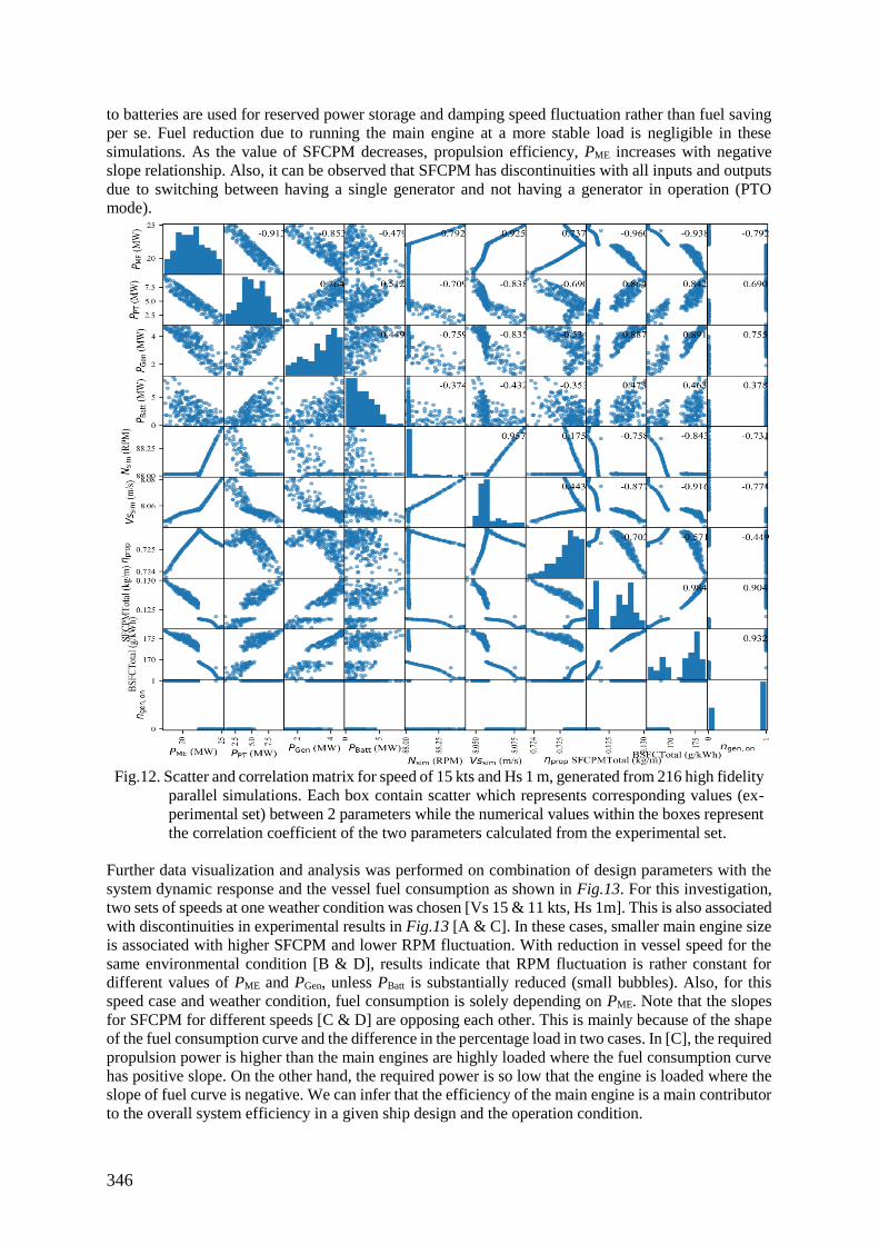
346
to batteries are used for reserved power storage and damping speed fluctuation rather than fuel saving
per se. Fuel reduction due to running the main engine at a more stable load is negligible in these
simulations. As the value of SFCPM decreases, propulsion efficiency, PME increases with negative
slope relationship. Also, it can be observed that SFCPM has discontinuities with all inputs and outputs
due to switching between having a single generator and not having a generator in operation (PTO
mode).
Fig.12. Scatter and correlation matrix for speed of 15 kts and Hs 1 m, generated from 216 high fidelity
parallel simulations. Each box contain scatter which represents corresponding values (ex-
perimental set) between 2 parameters while the numerical values within the boxes represent
the correlation coefficient of the two parameters calculated from the experimental set.
Further data visualization and analysis was performed on combination of design parameters with the
system dynamic response and the vessel fuel consumption as shown in Fig.13. For this investigation,
two sets of speeds at one weather condition was chosen [Vs 15 & 11 kts, Hs 1m]. This is also associated
with discontinuities in experimental results in Fig.13 [A & C]. In these cases, smaller main engine size
is associated with higher SFCPM and lower RPM fluctuation. With reduction in vessel speed for the
same environmental condition [B & D], results indicate that RPM fluctuation is rather constant for
different values of PME and PGen, unless PBatt is substantially reduced (small bubbles). Also, for this
speed case and weather condition, fuel consumption is solely depending on PME. Note that the slopes
for SFCPM for different speeds [C & D] are opposing each other. This is mainly because of the shape
of the fuel consumption curve and the difference in the percentage load in two cases. In [C], the required
propulsion power is higher than the main engines are highly loaded where the fuel consumption curve
has positive slope. On the other hand, the required power is so low that the engine is loaded where the
slope of fuel curve is negative. We can infer that the efficiency of the main engine is a main contributor
to the overall system efficiency in a given ship design and the operation condition.
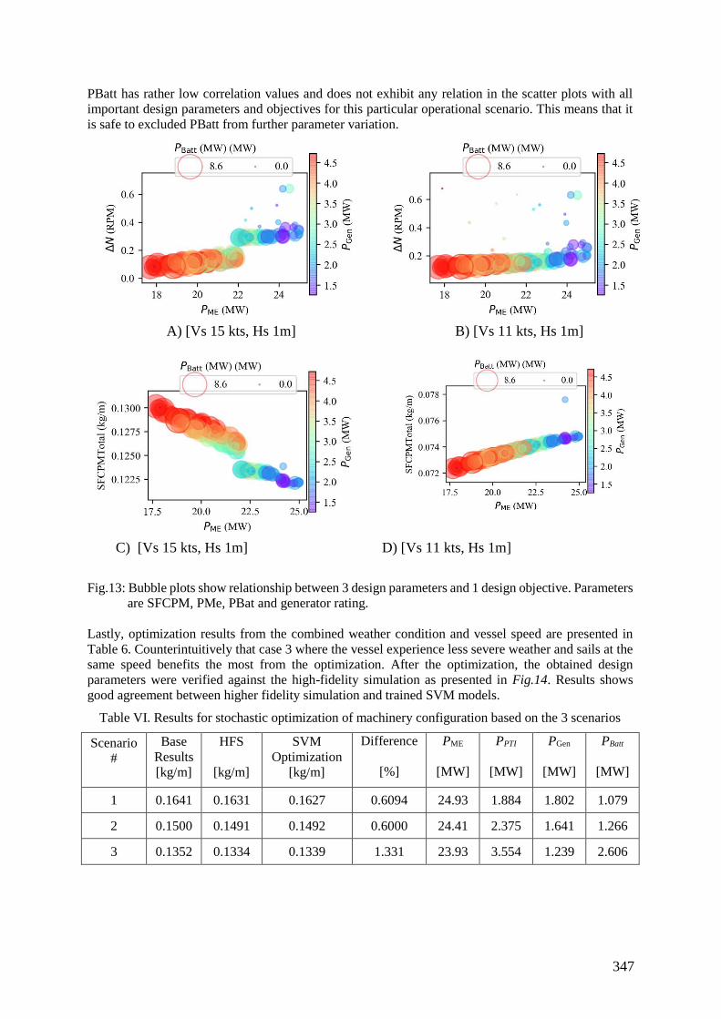
347
PBatt has rather low correlation values and does not exhibit any relation in the scatter plots with all
important design parameters and objectives for this particular operational scenario. This means that it
is safe to excluded PBatt from further parameter variation.
A) [Vs 15 kts, Hs 1m]
B) [Vs 11 kts, Hs 1m]
C) [Vs 15 kts, Hs 1m] D) [Vs 11 kts, Hs 1m]
Fig.13: Bubble plots show relationship between 3 design parameters and 1 design objective. Parameters
are SFCPM, PMe, PBat and generator rating.
Lastly, optimization results from the combined weather condition and vessel speed are presented in
Table 6. Counterintuitively that case 3 where the vessel experience less severe weather and sails at the
same speed benefits the most from the optimization. After the optimization, the obtained design
parameters were verified against the high-fidelity simulation as presented in Fig.14. Results shows
good agreement between higher fidelity simulation and trained SVM models.
Table VI. Results for stochastic optimization of machinery configuration based on the 3 scenarios
Scenario
#
Base
Results
[kg/m]
HFS
[kg/m]
SVM
Optimization
[kg/m]
Difference
[%]
PME
[MW]
PPTI
[MW]
PGen
[MW]
PBatt
[MW]
1 0.1641 0.1631 0.1627 0.6094 24.93 1.884 1.802 1.079
2 0.1500 0.1491 0.1492 0.6000 24.41 2.375 1.641 1.266
3 0.1352 0.1334 0.1339 1.331 23.93 3.554 1.239 2.606
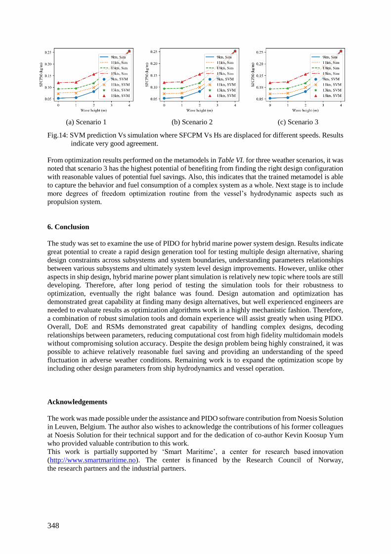
348
(a) Scenario 1 (b) Scenario 2 (c) Scenario 3
Fig.14: SVM prediction Vs simulation where SFCPM Vs Hs are displaced for different speeds. Results
indicate very good agreement.
From optimization results performed on the metamodels in Table VI. for three weather scenarios, it was
noted that scenario 3 has the highest potential of benefiting from finding the right design configuration
with reasonable values of potential fuel savings. Also, this indicates that the trained metamodel is able
to capture the behavior and fuel consumption of a complex system as a whole. Next stage is to include
more degrees of freedom optimization routine from the vessel’s hydrodynamic aspects such as
propulsion system.
6. Conclusion
The study was set to examine the use of PIDO for hybrid marine power system design. Results indicate
great potential to create a rapid design generation tool for testing multiple design alternative, sharing
design constraints across subsystems and system boundaries, understanding parameters relationships
between various subsystems and ultimately system level design improvements. However, unlike other
aspects in ship design, hybrid marine power plant simulation is relatively new topic where tools are still
developing. Therefore, after long period of testing the simulation tools for their robustness to
optimization, eventually the right balance was found. Design automation and optimization has
demonstrated great capability at finding many design alternatives, but well experienced engineers are
needed to evaluate results as optimization algorithms work in a highly mechanistic fashion. Therefore,
a combination of robust simulation tools and domain experience will assist greatly when using PIDO.
Overall, DoE and RSMs demonstrated great capability of handling complex designs, decoding
relationships between parameters, reducing computational cost from high fidelity multidomain models
without compromising solution accuracy. Despite the design problem being highly constrained, it was
possible to achieve relatively reasonable fuel saving and providing an understanding of the speed
fluctuation in adverse weather conditions. Remaining work is to expand the optimization scope by
including other design parameters from ship hydrodynamics and vessel operation.
Acknowledgements
The work was made possible under the assistance and PIDO software contribution from Noesis Solution
in Leuven, Belgium. The author also wishes to acknowledge the contributions of his former colleagues
at Noesis Solution for their technical support and for the dedication of co-author Kevin Koosup Yum
who provided valuable contribution to this work.
This work is partially supported by ‘Smart Maritime’, a center for research based innovation
(http://www.smartmaritime.no). The center is financed by the Research Council of Norway,
the research partners and the industrial partners.
349
References
Andrews, D. (2004). "Marine Design–Requirement Elucidation rather than Requirement
Engineering." Journal of Naval Engineering.
Box, G. E. and J. S. Hunter (1961). "The 2 k—p fractional factorial designs." Technometrics
3(3): 311-351.
Box, G. E. and K. Wilson (1992). On the experimental attainment of optimum conditions.
Breakthroughs in Statistics, Springer: 270-310.
Brereton, R. G. and G. R. Lloyd (2010). "Support vector machines for classification and
regression." Analyst 135(2): 230-267.
de Weck, O., et al. (2007). State-of-the-art and future trends in multidisciplinary design
optimization. 48th Aiaa/Asme/Asce/Ahs/Asc Structures, Structural Dynamics, and Materials
Conference.
Eglajs, V. and P. Audze (1977). "New approach to the design of multifactor experiments."
Problems of Dynamics and Strengths 35(1): 104-107.
Frenzel, M., et al. (2015). "Multidisciplinary optimization and integration requirements for
large-scale automotive and aerospace design work."
Gero, J. S. and U. Kannengiesser (2004). "Modelling expertise of temporary design teams."
Journal of Design Research 4(3): 1-13.
Liu, Y. and M. Collette (2014). "Surrogate-assisted robust design optimization considering
interval-type uncertainty." Maritime Technology and Engineering: 287-293.
Loukakis, T. and P. Sclavounos (1978). "Some extensions of the classical approach to strip
theory of ship motions, including the calculation of mean added forces and moments." Journal
of Ship Research 22(1).
Parsopoulos, K. E. and M. N. Vrahatis (2002). "Recent approaches to global optimization
problems through particle swarm optimization." Natural computing 1(2-3): 235-306.
Salvesen, N., et al. (1970). "Ship motions and sea loads." Trans. SNAME 78(8): 250-287.
Taskar, B., et al. (2016). "The effect of waves on engine-propeller dynamics and propulsion
performance of ships." Ocean Engineering 122: 262-277.
Van der Auweraer, H., et al. (2008). Breakthrough technologies for virtual prototyping of
automotive and aerospace structures. Product Engineering, Springer: 397-418.
Yum, K. K., et al. (2016). Simulation of a Hybrid Marine Propulsion System in Waves.
CIMAC Congress, CIMAC.
Yum, K. K., et al. (2016). "Simulation of a two-stroke diesel engine for propulsion in waves."
International Journal of Naval Architecture and Ocean Engineering.
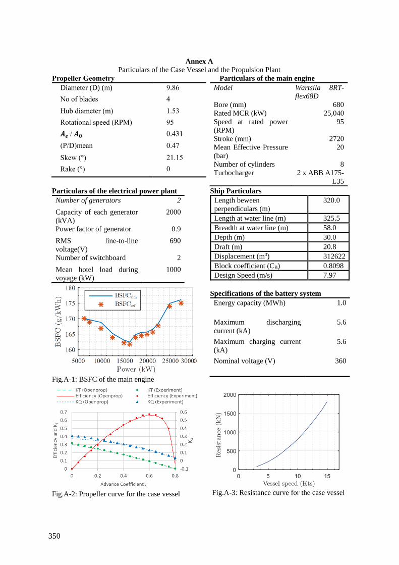
350
Annex A
Particulars of the Case Vessel and the Propulsion Plant
Propeller Geometry
Diameter (D) (m) 9.86
No of blades 4
Hub diameter (m) 1.53
Rotational speed (RPM) 95
𝑨𝒆 / 𝑨𝟎 0.431
(P/D)mean 0.47
Skew (°) 21.15
Rake (°) 0
Particulars of the main engine
Model Wartsila 8RT-
flex68D
Bore (mm) 680
Rated MCR (kW) 25,040
Speed at rated power
(RPM)
95
Stroke (mm) 2720
Mean Effective Pressure
(bar)
20
Number of cylinders 8
Turbocharger 2 x ABB A175-
L35
Particulars of the electrical power plant
Number of generators 2
Capacity of each generator
(kVA)
2000
Power factor of generator 0.9
RMS line-to-line
voltage(V)
690
Number of switchboard 2
Mean hotel load during
voyage (kW)
1000
Fig.A-1: BSFC of the main engine
Ship Particulars
Length beween
perpendiculars (m)
320.0
Length at water line (m) 325.5
Breadth at water line (m) 58.0
Depth (m) 30.0
Draft (m) 20.8
Displacement (m3) 312622
Block coefficient (CB) 0.8098
Design Speed (m/s) 7.97
Specifications of the battery system
Energy capacity (MWh) 1.0
Maximum discharging
current (kA)
5.6
Maximum charging current
(kA)
5.6
Nominal voltage (V) 360
Fig.A-2: Propeller curve for the case vessel
Fig.A-3: Resistance curve for the case vessel
351
Predictive Engineering Analytics for Shipbuilding - An Overview
Bart Van Lierde, Siemens PLM Software, Leuven/Belgium, [email protected]
Wim Cardoen, Siemens PLM Software, Leuven/Belgium, [email protected]
Dejan Radosavljevic, Siemens PLM Software, London/UK, [email protected]
Abstract
Modern ships operate increasingly autonomous through strongly interacting subsystems. Designing
such ships requires an efficient development approach that can consider the mutual interaction between
subsystems and the inherent multi-disciplinarity. Moreover, the overall vessel behaviour still needs to
be optimal. Product design and use need to be coupled, requiring traceability through a performant
data management system that spans the entire product lifecycle. Predictive Engineering Analytics
combines engineering simulation and testing with intelligent data analytics, to develop digital twins
that can predict real product behaviour throughout the entire lifecycle. This will help shipbuilders
develop and maintain complex vessels faster and better.
1. Introduction
Modern ships operate increasingly autonomous through strongly interacting subsystems. These systems
may be dedicated to a specific, primary objective of the vessel (such as special purpose, naval and
more) or may be part of the general essential ship operations. Between them, they exchange sensor data
and make coordinated operational decisions, ideally without any user interaction.
Designing such ships is complex, and requires an efficient development approach that can consider the
mutual interaction between subsystems and the inherent multi-disciplinarity from the very beginning.
Scalable simulation technologies must take the lead in this process. Whereas in the shipbuilding
industry, virtual modelling was for a long time limited to point solutions for specific problems such as
hydrodynamics and mechanics, it now must be applied on a much broader scale and drive development.
On top of that, the design of such ships doesn’t stop after delivery. Through software updates or because
of maintenance, subsystems can change. But the overall behaviour of the entire vessel still needs to be
optimal. To make sure of that, product design and product use need to be coupled. That requires
traceability through a performant data management system that spans the entire product lifecycle.
To deal with these challenges, Siemens PLM Software presents predictive engineering analytics (PEA).
PEA combines engineering simulation and testing with intelligent reporting and data analytics, to
develop digital twins that can predict real product behaviour throughout the entire lifecycle. This will
help shipbuilders develop and maintain complex vessels faster and with greater confidence.
2. Industry challenges and research trends
In response of today’s environmental and business challenges, companies across all manufacturing
industries are coming up with increasingly sophisticated products. These are conceived by applying
new design methods, new materials, combine mechanics with software, electronics and controls,
behave multi-physical and include intelligent systems. The development, creation and maintenance of
such products requires all stakeholders to dramatically change the way they do engineering.
Digitalization will play a crucial role in this. The application of new digital technologies will at the
same time enable a broad range of new product capabilities as well as disrupt how manufacturers work
in order to deliver them. For transportation industries, many innovations have their origins in sectors
with huge research and development (R&D) budgets, such as aerospace and automotive. But they could
easily find their ways to the others. The marine industry cannot afford to lag behind. The industry
challenges are similar, and so are the engineering trends and solutions to deal with them.
352
2.1. Increased pressure on energy efficiency and fuel economy
Together with safety and reliability, improved fleet performance and fuel economy are without question
the most function-critical design aspects for marine products. Not in the least because they directly
result in measureable economic added value for fleet owners and operators. But in addition to these
commercial aspects, public interests play a role.
The pressure we put on our planet is huge. In response to the entry into force of the Paris Agreement
on Climate Change, International Maritime Organization (IMO) regulations concerning emissions and
fuel efficiency have become stricter. Authorities have committed to numbers and percentages, and are
now counting on the industries to come up with innovations to make these happen. And as the entire
marine sector consumes the equivalent energy of a small country, it plays a significant role in this
matter. Showing social corporate responsibility (SCR) is becoming a must for companies that wish to
secure their future.
All new ships since 1st January 2013 have to be designed in accordance with IMO set EEDI (Energy
Efficiency Design Index). And all ships of 400 gross tonnage (gt) or more need to have an International
Energy Efficiency Certificate (IEEC). This requires for example a Ship Energy Efficiency Management
Plan (SEEMP) on board, incorporating best practices for fuel efficient operation of ships, such as speed
management throughout a voyage.
Speed management comes down to finding the best balance between vessel speed and fuel
consumption, taking into account operating environmental conditions such as the weather, sea state and
scheduling requirements. All this just to stress the importance of the topic.
It is clear that requirements like these make energy efficiency and fuel economy top priorities for ship
design. A good holistic vessel solution will need to have the most efficient individual components work
together as an integrated system in an optimal way.
2.1.1. New powering methods for propulsion systems
Modern ship designers and builders put huge efforts in exploring new ways to generate energy, both on
new vessels and for modernization of the current fleets. The typical large gas and diesel engines are
being replaced by electrical and hybrid solutions. And companies also investigate how to make optimal
use of natural resources like the sun or the wind on board.
Examples of new propulsion technologies are already in operation. In Norway for example, between
Lavik and Oppedal, a fully electric ferry with a capacity for 360 passengers and 120 vehicles crosses
the Sognefjord 34 times a day. On board, Siemens installed its BlueDrive PlusC system. It includes a
battery and steering system, thruster control for the propellers, an energy management system and an
integrated alarm system.
These types of intelligent systems combine mechanics with software, electronics and controls, and
become increasingly important to make sure the complete vessel propulsion as multi-physical system
performs in an optimal way. They obviously present a challenge during design, as they require
simultaneous optimization of various subsystems and their interaction starting from the very early stage
of concept design.
In future, new digital technologies will take the application of such systems to the next level. New
sensor types or more precise ones, more powerful microprocessors, better algorithms, data mining
capabilities and more will change the industry. These will allow intelligent systems to constantly
improve, also after delivery, through updates. This will completely change the way shipbuilders work,
as it will require a strong link between design and vessels in operation.
353
2.1.2. Optimizing performance of the vessel
Performance greatly depends on the fluid-structure interaction (FSI) of the entire vessel. Noise and
vibration as well as durability are also largely impacted by how smooth a vessel can advance and for
example how well peak loads on the propellers can be avoided. Optimizing this multi-domain behaviour
should capture all operational aspects and should be conducted at various scales, from smallest
component or equipment level, via various subsystem and system levels to a fully integrated holistic
view on the entire vessel. Indeed, full ship-level FSI simulations should become a mainstream activity.
And these should include real operating conditions. Doing so should eliminate the uncertainties related
to the extrapolation of model-scale measurements, and allow finding the best design for a particular
operating envelope. This will enable designers to achieve the most efficient design with the lowest
environmental impact while satisfying a full range of often contradictory requirements.
Using real conditions at sea for behavioural prediction should also allow engineers to look much more
accurately at extreme loading conditions. This will reduce uncertainties and improve the structural
design and safety. Linking to this, it should allow better design of control systems to let them give the
best possible response to these extreme conditions. As ships evolve towards ever more autonomy and
less human interaction, this will become critical for future safe operation.
Ultimately, to really fully exploit the strength of such full-scale, multi-domain simulations, it should be
possible to run hundreds of them at a time, in an automated way, to find the best compromise in design
trade-off. Such a capability, which is called design exploration, will allow engineers to use their time
and experience for selecting the best parameters for optimal vessel performance rather than for building
simulation models, testing whether they work and starting all over again when the smallest design
change is introduced.
Such multi-domain and automated vessel performance optimization will require a solid software
infrastructure with powerful simulation tools that can handle for example hydrodynamics along with
other physics such as structural integrity and acoustics. Even though some applications already reached
sufficient maturity to be part of standard development processes, simulation technologies will still need
to evolve during the coming decades to really reach digital design space exploration to its full extent.
2.1.3. Using new materials to reduce weight
The types of materials that are being used in the marine industry are rather diverse. Even though the
main requirements, being strong, light and easy to maintain, are clear and common to all, the
applicability of certain materials heavily depends on the vessel type, size and use. Nevertheless, there
is a clear trend to try and reduce weight (and thus the payload) in view of energy efficiency by using
new materials, of course without jeopardizing other priorities such as stability, manufacturability and
reparability.
Composite materials are already widely used in recreational and commercial boat building, and
gradually start to find their ways into the larger vessels like bulk carriers and containerships. The
advantages of composites are many, including lighter weight, tailored layup for optimum strength and
stiffness, improved fatigue life and corrosion resistance.
Fully composite large vessels will probably not be the standard as of tomorrow, but it can be expected
that the amount of composite parts will dramatically increase in the near future. This will have a big
impact on many engineering aspects: on design and development, on manufacturing, on maintenance,
and on the relation between all of these phases of the product lifecycle.
2.2. Adding value to the entire lifecycle
Another major challenge is related to the economic reality of the marine business. Equipment orders
are usually large investments that leave little margin after price negotiation. On top of that, late delivery
354
can lead to expensive penalties. It is critical for business success to have effective processes to turn the
demand into delivered products. This on itself already puts big pressure on product development and
manufacturing.
Besides, the shipping business is cyclic. Recessions usually result in a business slowdown, which comes
down to declined new vessel order rates and reduced maintenance, repair and operations expenditures.
To remain successful in such a harsh economic environment, shipbuilders must come up with extreme
value for money and with innovations that bring value to the fleet owners over the entire product
lifecycle.
This is where digital technologies that allow analytics on big data, advanced automation and smart
applications show enormous potential. In future, shipbuilders will offer fleet owners more than ‘just’ a
vessel, but rather a complete solution that allows them to manage their fleet efficiently and safely. The
development of a ship then won’t stop after delivery, but will continue while in operation.
2.2.1. Condition-based maintenance
One of such applications will be the ability to schedule maintenance on equipment based on measured
physical condition rather than on clock, calendar or runtime meters. This philosophy is called condition-
based maintenance (CBM), and will bring fleet owners a significant amount of cost savings, as safety
margins can dramatically be reduced. It will also allow to apply maintenance in a more targeted manner,
focusing on the root causes of potential failures.
Applying CBM could be automated by collecting data from sensors inside the vessel to continuously
monitor equipment performance, and sending it to an onshore center. Here, the data could be analyzed,
used for simulations or compared to statistics. Based on analysis, maintenance could then be scheduled.
This process will maximize the useful life and reduce cost by avoiding early replacement of functional
components.
2.2.2. Autonomous vessels
The ultimate goal of such applications would be the fully autonomous vessel that can monitor and report
on its own health, can gather information from its environment and use this information to make
autonomous decisions such as navigating safely and avoiding collisions. Even though big steps still
need to be taken to make this real, not in the least on the regulatory or legal side, this is most probably
the direction in which the shipbuilding industry will be going during the coming decades.
In fact, on the technology side, most components are already more or less available. The question is
rather how to combine various sensor technologies with operating and climatic conditions of a maritime
environment? Or how to program the interpretation of maritime regulations in the control algorithms?
And how to guarantee safe connectivity to and communication with a land based system at any time,
from anywhere?
2.2.3. A changing vision on doing business
Such innovations will change the entire marine business landscape during the coming decades. Design
engineers will need to stay much closer connected to the vessel after commissioning to follow-up on
monitoring, maintenance and updates. Shipbuilders will develop their products from a completely new
angle, making decisions based on an integrated view that spans the entire product.
Being able to deliver such lifecycle spanning solutions will require a different approach to engineering.
A product sale will no longer be the primary and ultimate achievement, but rather the beginning of a
long-term relationship. And in a market, that is typically limited to a finite set of customers, and where
incidents can have huge consequences, there will be little room for failure. To be successful,
shipbuilders must deploy watertight processes, first of all to bring their complex products to market
effectively, and secondly track if the functioning of all vessels meets the requirements cradle-to-grave.
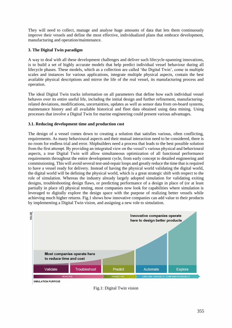
355
They will need to collect, manage and analyse huge amounts of data that lets them continuously
improve their vessels and define the most effective, individualized plans that embrace development,
manufacturing and operation/maintenance.
3. The Digital Twin paradigm
A way to deal with all these development challenges and deliver such lifecycle-spanning innovations,
is to build a set of highly accurate models that help predict individual vessel behaviour during all
lifecycle phases. These models, which as a collection are called ‘the Digital Twin’, come in multiple
scales and instances for various applications, integrate multiple physical aspects, contain the best
available physical descriptions and mirror the life of the real vessel, its manufacturing process and
operation.
The ideal Digital Twin tracks information on all parameters that define how each individual vessel
behaves over its entire useful life, including the initial design and further refinement, manufacturing-
related deviations, modifications, uncertainties, updates as well as sensor data from on-board systems,
maintenance history and all available historical and fleet data obtained using data mining. Using
processes that involve a Digital Twin for marine engineering could present various advantages.
3.1. Reducing development time and production cost
The design of a vessel comes down to creating a solution that satisfies various, often conflicting,
requirements. As many behavioural aspects and their mutual interaction need to be considered, there is
no room for endless trial and error. Shipbuilders need a process that leads to the best possible solution
from the first attempt. By providing an integrated view on the vessel’s various physical and behavioural
aspects, a true Digital Twin will allow simultaneous optimization of all functional performance
requirements throughout the entire development cycle, from early concept to detailed engineering and
commissioning. This will avoid several test-and-repair loops and greatly reduce the time that is required
to have a vessel ready for delivery. Instead of having the physical world validating the digital world,
the digital world will be defining the physical world, which is a great strategic shift with respect to the
role of simulation. Whereas the industry already largely adopted simulation for validating exiting
designs, troubleshooting design flaws, or predicting performance of a design in place of (or at least
partially in place of) physical testing, most companies now look for capabilities where simulation is
leveraged to digitally explore the design space with the purpose of realizing better vessels while
achieving much higher returns. Fig.1 shows how innovative companies can add value to their products
by implementing a Digital Twin vision, and assigning a new role to simulation.
Fig.1: Digital Twin vision
356
3.2. Reducing risk and improving performance by prediction
The ideal Digital Twin could include all the required information to continuously verify and forecast
the vessel’s performance and health, or the remaining useful life. It could also predict system response
to safety critical events and uncover previously unknown issues before they become critical by
comparing predicted and actual responses. An ultimate goal could be that systems on board of the
Digital Twin would be capable of mitigating damage or degradation autonomously. They could activate
self-healing mechanisms and thereby increase the vessel’s life span. Or they could suggests updates of
intelligent systems to improve performance and reduce fuel consumption.
3.3. Reducing product and operational cost
The standard approach in vessel design is to assume appropriately severe operational conditions and
subsequent usage, as well as rather large safety factors to account for deviations during the
manufacturing process. Such an approach is very conservative and leads to vessels that may be heavier
than they should be and require more frequent inspections than necessary. Thanks to the precision of
the available models, using a Digital Twin could reduce design tolerances, manufacturing uncertainties
and stochastic variabilities of vessel operation. This could result in a huge cost reduction in every
respect, including the use of materials during manufacturing, fuel consumption as well as a better plan
for inspection and maintenance.
3.4. Challenges to develop a Digital Twin to full extent
There is no such thing as a clear-cut and closing definition of a Digital Twin. It is rather a vision, a term
that refers to the linking of all activities related to advanced simulation and prediction and their
integration over the product lifecycle. If well-conceived, the Digital Twin should bring clear advantages
to product development, manufacturing and after delivery. But the extent to which the concept is
deployed still depends on what a company can or wants to do, and on what technologies are capable of.
In the marine industry, a lot of work still needs to be done in the coming decades, even though various
applications are already there. The industry looks forward to new methods and developments,
especially in the fields of modeling realism, computation speed, data management and the integration
between various activities that will enlarge the current scope of the Digital Twin.
3.4.1 Modelling realism
Current simulation processes are often still too separated. For example, there can be a computational
fluid dynamics (CFD) model, a structural model, a stress analysis model and fatigue cracking model.
And those can all be quite accurate for their specific use. But in reality, these physics are tightly coupled
and that needs to be reflected in the Digital Twin. Ship designers and builders must invest more in
developing parametrized multi-disciplinary models of their vessels. They should include all physics in
a single, unified simulation model that also includes controls, and that tightly couples various
disciplines. Ideally, these models come in various scales to allow both very detailed and very fast
analysis, for some applications even real-time.
A lot of research should be done on simulating the implications of using new materials and
manufacturing methods as well. Advanced modelling technologies should be able to capture the related
micro-structural behaviour. And as this varies for every product depending on the individual
manufacturing process and use history, the related parameters should be kept up-to-date for every
individual product over the entire lifecycle. And finally also the loading and boundary conditions should
become a lot more realistic than it is today. New FSI calculation methods and especially data measured
on real structures should help to prevent over-dimensioning of new designs and allow better damage
prediction. To successfully use a Digital Twin, it will not be sufficient to consult empirical load
databases. The Digital Twin should experience exactly the same as the real structure, including transient
events.
357
3.4.2 Calculation speed
While over the last decades computation technologies have really taken a flight, full-scale models that
include all geometrical and physical details of entire vessels are still a pain. Simulations that involve
tens of millions of degrees-of-freedom (DOFs) or cells require very smart solution schemes and solver
algorithms, as well as very powerful high-performance computing hardware. And still, for a true Digital
Twin that also includes fully coupled multi-physical behaviour, tens of millions of DOFs or cells are
not enough. All transportation industries count on both simulation software companies and computer
system manufacturers to join forces and come up with revolutionary improvements that will lead to an
exponential increase of capabilities. In the coming decades, new modelling methods combined with
exascale computing systems should allow simulations to stay ahead of the actual product use and enable
true model-based prediction and decision-making
3.4.3 Data management
The Digital Twin concept requires a strong connection between all models that are used during the
entire product lifecycle. Only a true digital thread can for example allow using the same 3D solid
models from design to manufacturing for numerically controlled programming, tracking parameter
changes for individual products during manufacturing and operation, or enable products in the field to
provide feedback to design and engineering teams. In practice, this means that an enormous amount of
data needs to be around for decades, constantly has to be updated and needs to be accessible for a large
number of different user profiles, located around the globe and often even spread over various
companies. To create and maintain a Digital Twin, ship designers and builders will need to deploy large
data storage infrastructure, powered by a very robust data management system.
4. Siemens PLM Software solutions for Digital Twin
As a world-leading provider of product lifecycle management solutions, Siemens PLM Software helps
thousands of companies across various industries and around the globe realize innovation by optimizing
their processes, from planning and development through manufacturing, production and support.
Converting the Digital Twin vision into an infrastructure with concrete solutions naturally fits these
activities. Siemens PLM Software clearly displays the intent of being able to offer ship designers and
builders the most comprehensive possible and state of the art solution set to build and maintain a Digital
Twin. This manifests itself in acquisitions of companies that cover missing pieces and in ambitious
development plans for more realistic simulation, accurate testing and powerful data management
applications, as well as the integration between those.
4.1. Building a Digital Twin during product development
Siemens PLM Software offers manufacturers a holistic set of methods and technologies to support them
during the entire development cycle and help them deliver innovations for complex products faster and
with greater confidence. Such a collection of solutions will allow ship designers and builders to
implement the Digital Twin philosophy, follow a more efficient design and commissioning process and
reduce the acquisition cost for their customers.
4.1.1. Predict real product behavior
With this comprehensive offering, Siemens wants to let the traditional development process evolve to
a new, predictive approach for systems-driven product development, called predictive engineering
analytics (PEA). In essence, PEA combines the application of multidisciplinary simulation and test with
intelligent reporting and data analytics in an integrated workflow with the ambition to build a Digital
Twin. PEA achieves higher modeling realism and simulation performance by removing the boundaries
between various development stakeholders. It integrates technologies such as 1D simulation, 3D
computer-aided engineering (CAE) including computational solid mechanics (CSM), finite element
analysis (FEA), computational fluid dynamics (CFD) and multibody dynamics, controls, physical
358
testing, visualization, multidisciplinary design exploration, and data analytics in a managed context.
Siemens has bundled all its solutions that underpin this vision in Simcenter™. This solutions portfolio
combines decades of experience by putting well-known products such as LMS Test.Lab, LMS
Imagine.Lab, NX Nastran, Femap, STAR-CCM+, Heeds and more under one umbrella. And it features
Simcenter 3D as the combined successor of NX CAE, LMS Virtual.Lab and LMS Samtech. Besides
these tools, PEA is also about a good alignment of processes. The following sections describe the
essentials for a successful implementation of a PEA approach.
4.1.2. Deploying closed-loop systems-driven product development
PEA supports closed-loop systems-driven product development, the fastest path to turn a set of
requirements into a vessel. In this multi-disciplinary simulation-based approach, the global vessel
design is considered as a collection of mutually interacting subsystems from the very beginning. From
the very early stages on, selected architectures are virtually tested for all critical functional performance
aspects simultaneously. These simulations use scalable modeling techniques, so that components can
be refined once the vessel configuration is defined and as data becomes available. This comes down to
creating a Digital Twin starting from the concept stage and gradually adding details. Closing the loop
refers in this context to concurrent development of mechanics with controls.
4.1.3. Increased use of 1D multi-physics system simulation
1D system simulation, also referred to as 1D CAE or mechatronics system simulation, allows scalable
modeling of multi-domain systems. The full system is presented in a schematic way, by connecting
validated analytical modeling blocks of electrical, hydraulic, pneumatic and mechanical subsystems
(including control systems). It helps engineers predict the behavior of concept designs of complex
mechatronics, either transient or steady-state. Manufacturers often have validated libraries available
that contain predefined components for different physical domains. Or Simcenter also contains a
complete set for various applications. Using those, the engineers can do concept performance
predictions very early, even before any computer-aided design (CAD) geometry is available. During
later stages, parameters can then be adapted. 1D system simulation calculations are very efficient. The
components are analytically defined, and have input and output ports. Causality is created by
connecting inputs of a component to outputs of another one (and vice versa). Models can have various
degrees of complexity, and can reach very high accuracy as they evolve. Because of their inherent
multi-physical nature, their scalability, their ability to become highly accurate and their outstanding
computational performance, 1D system simulation models are excellent and versatile components of a
Digital Twin. Some model versions may allow real-time simulation, which is particularly useful during
control systems development. Or later in the product lifecycle, as part of built-in predictive functionality
inside the product.
4.1.4. Multi-discipline 3D simulation technologies
3D CAE models can account for additional phenomena that naturally relate to 3D physics aspects, and
typically become highly detailed, computationally intensive representations that are usually very
application-specific. Over the last decades, various 3D CAE technologies have proved their value by
speeding up development and avoiding late-stage changes. Within a Digital Twin vision however, 3D
CAE will need to gain realism and performance, and be capable of pro-actively driving the decision-
making process more than today. In current research, big efforts are being spent in making revolutionary
improvements in this field. A lot of new capabilities arise on modeling, process and solver side. And
many more are expected to come in the near future. Simcenter features the state of the art for every
individual application, and bundles solutions for various functional performance aspects in a common
platform to facilitate multi-discipline analysis. It also captures industry knowledge and best practices
in application verticals. Simcenter includes very dedicated 3D solutions such as high-end CFD,
structural analysis, powerful acoustics, fatigue crack propagation modeling, composite analysis and
many more.
359
4.1.5. Strongly coupled 1D simulation, 3D simulation and controls engineering
As closed-loop systems-driven product development requires concurrent development of the entire
multi-physical system, including controls, the processes for 1D simulation, 3D simulation and control
algorithm development must be very well aligned. To achieve this, Simcenter offers various co-
simulation capabilities for Model in the Loop (MiL), Software-in-the-Loop (SiL) and Hardware-in-the-
Loop (HiL) simulations that combine various versions or scales of Digital Twin models in a coupled
analysis.
4.1.6. Combined simulation and physical testing
Working with a Digital Twin does not mean replacing physical testing completely by simulation during
vessel development. First of all because final certification still relies on sea trials. It will even become
more complex and time-consuming with all these multi-physics and controls involved. And secondly,
because lots of additional testing tasks will be required to reach the desired model realism, both during
development and after delivery. To successfully create and maintain a Digital Twin, test and simulation
engineers should collaborate and reinforce each other. Simcenter uniquely brings together a complete
series of physical testing applications and a comprehensive set of simulation solutions in a common
framework. This facilitates collaboration and data exchange between two traditionally very distinct
engineering domains. On both sides, engineers will see lots of benefits. Test engineers can use
simulation results to become more effective, whereas simulation engineers will have access to lots of
data to validate and improve their models.
Use simulation for more efficient certification testing
As the number of parameters and their mutual interaction explodes in vessels that include
control systems, efficiency is key during certification testing, both in terms of instrumentation
and definition of critical test cases. Simulation can help to analyse upfront which locations and
parameters can be more effective to measure a certain objective. And it also allows to
investigate the coupling between certain parameters, so that the amount of sensors and required
test conditions can be minimized. On top of that, simulation can be used as an observation tool
to derive certain parameters that cannot be measured directly. Here again, a close alignment
between simulation and testing activities is a must. Both 1D and 3D simulation models can
give access to many parameters that cannot directly reached with sensors. In fact, that is a huge
advantage of using a Digital Twin for product development.
Increase realism of simulation models using test input
Modal testing has for decades been a useful method to help improve structural finite element
models via correlation analysis and model updating. It greatly contributed to the success of for
example structural dynamics, vibro-acoustics and fatigue simulation analyses on mechanical
structures, and will continue doing so in the decades to come. Within the Digital Twin story,
modal testing will remain important, in particular for component validation. In addition to that,
the required fidelity of Digital Twin models calls for much more test-based validation and
input. Measurements also need to be capable of improving 3D CFD and 1D multi-physics
models for example. And they have to help defining realistic boundary conditions, loads and
all kinds of simulation parameters. In the Digital Twin context, a whole range of new testing
capabilities (some modal-based, some not) will become essential for success.
Create hybrid models that combine test with simulation
Test results can even replace entire components during simulation. Complex products are
usually combinations of subsystems which are not necessarily concurrently developed. As the
Digital Twin always strives for the best possible combination of accuracy and performance, it
can be beneficial during various development stages to create hybrid setups that include
hardware, simulation and test models. This will obviously require dedicated technologies as
well as a very good alignment between simulation (both 1D and 3D) and physical testing.
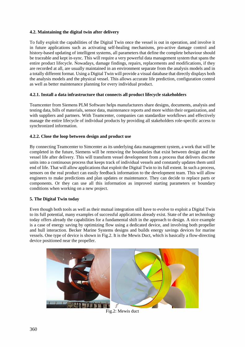
360
4.2. Maintaining the digital twin after delivery
To fully exploit the capabilities of the Digital Twin once the vessel is out in operation, and involve it
in future applications such as activating self-healing mechanisms, pro-active damage control and
history-based updating of intelligent systems, all parameters that define the complete behaviour should
be traceable and kept in-sync. This will require a very powerful data management system that spans the
entire product lifecycle. Nowadays, damage findings, repairs, replacements and modifications, if they
are recorded at all, are usually maintained in an environment separate from the analysis models and in
a totally different format. Using a Digital Twin will provide a visual database that directly displays both
the analysis models and the physical vessel. This allows accurate life prediction, configuration control
as well as better maintenance planning for every individual product.
4.2.1. Install a data infrastructure that connects all product lifecycle stakeholders
Teamcenter from Siemens PLM Software helps manufacturers share designs, documents, analysis and
testing data, bills of materials, sensor data, maintenance reports and more within their organization, and
with suppliers and partners. With Teamcenter, companies can standardize workflows and effectively
manage the entire lifecycle of individual products by providing all stakeholders role-specific access to
synchronized information.
4.2.2. Close the loop between design and product use
By connecting Teamcenter to Simcenter as its underlying data management system, a work that will be
completed in the future, Siemens will be removing the boundaries that exist between design and the
vessel life after delivery. This will transform vessel development from a process that delivers discrete
units into a continuous process that keeps track of individual vessels and constantly updates them until
end of life. That will allow applications that exploit the Digital Twin to its full extent. In such a process,
sensors on the real product can easily feedback information to the development team. This will allow
engineers to make predictions and plan updates or maintenance. They can decide to replace parts or
components. Or they can use all this information as improved starting parameters or boundary
conditions when working on a new project.
5. The Digital Twin today
Even though both tools as well as their mutual integration still have to evolve to exploit a Digital Twin
to its full potential, many examples of successful applications already exist. State of the art technology
today offers already the capabilities for a fundamental shift in the approach to design. A nice example
is a case of energy saving by optimizing flow using a dedicated device, and involving both propeller
and hull interaction. Becker Marine Systems designs and builds energy savings devices for marine
vessels. One type of device is shown in Fig.2. It is the Mewis Duct, which is basically a flow-directing
device positioned near the propeller.
Fig.2: Mewis duct

361
Crucial to the success of this Becker Marine’s product is to develop a particular shape of duct and fins
that provides the most energy savings, which depends on both the hull geometry and the propeller. In
order to do so, the engineers have created a process to calculate the flow field around the hull and
propeller. Then they automated this process to explore the design space varying 40 design parameters
that define the duct and fin geometry. They finally achieve a guaranteed 4.5% improvement in fuel
savings, with a project turnaround time of only 6 weeks. This is just one example of how accurate
simulation based on a holistic view that includes various subsystems can add value to a design, and via
fuel savings, to the entire vessel lifecycle.
6. Conclusion
The objective of this paper was to demonstrate how a Digital Twin vision can provide an answer to
today’s environmental and business challenges in the marine industry, and to the transformation vessel
designs will undergo in the decades to come. Even though both computational technologies and
infrastructure still need to evolve to reach a state in which they can fully support all applications the
ideal Digital Twin could allow for, state of the art solutions already bring lots of value in many aspects.
Siemens PLM Software is collecting all the pieces to put the Digital Twin puzzle together. By
combining product lifecycle management software, 1D system simulation, 3D CAE as well as physical
testing, Siemens has a holistic offering for Digital Twin. During the coming years, further work will be
invested in both integration between tools and extension and improvement of the individual
applications.
References
BERNDT, O.; LUKAS, U.v.; KUIJPER, A. (2015), Functional modelling and simulation of overall
system ship – virtual methods for engineering and commissioning shipbuilding, 29th ECMS, Varna
PEARCE, P.; HAUSE, M. (2012), ISO-15288, OOSEM and Model-Based Submarine Design, SETE
APCOSE 201
FERGUSON, S. (2016), designed with Star-CCM+: the Becker Mewis duct®, Marine Special Report
http://mdx.plm.automation.siemens.com/sites/all/themes/basic/assets/downloads/Marine%20spe-
cial%20report%20270916%20WEB.pdf
362
Expanding the Scope of Early Stage Computer Aided Ship Design
Rachel Pawling, UCL, London/UK, [email protected]
Nikolaos Kouriampalis, UCL, London/UK, [email protected]
Syavash Esbati, UCL, London/UK, [email protected]
Nick Bradbeer, UCL, London/UK, [email protected]
David Andrews, UCL, London/UK, [email protected]
Abstract
Previous papers by the authors have described the need for more holistic approaches to the early
stage design of ships, incorporating a wider range of aspects. This paper provides an overview of
some ongoing PhD projects in the UCL Marine Research Group (MRG) to use ubiquitous desktop
computers to apply methods from outside traditional Naval Architecture to further expand the range
of ship design and performance aspects that can be addressed in early stage design by the widest
range of practitioners. These include queuing theory, real options theory, on-line tools and Virtual
Reality. Possible impacts on ship design education are briefly discussed.
1. Introduction
The Marine Research Group (MRG) is a subdivision of the Department of Mechanical Engineering at
UCL (https://www.ucl.ac.uk/mecheng/research/marine). The MRG has a range of research interests in
the areas of Naval Architecture and Marine Engineering, including computer aided preliminary ship
design, and the use of computers in design education. The latter is related to the Department’s MSc
courses in both Naval Architecture and Marine Engineering. MRG interests encompass the use of
high-performance computing (generally for CFD), but, primarily driven by both teaching
requirements and involvement in ship design consultancies, there is a strong interest in methods and
tools that can be widely deployed using desktop hardware.
Computers have found application in all stages of ship design, and ship design has adopted a wide
range of modelling and analysis approaches from other domains to solve the many decision making,
design and engineering problems encountered in the design process. Some technologies are seeing
increasingly wider application, such as CFD, Bertram and Peric (2013) or genetic algorithms for use
in early stage design, Burger and Horner (2011), but still require some degree of dedicated computing
hardware (or time) to use. The ongoing development of ubiquitous desktop computers has made other
approaches far more accessible at the day-to-day level.
One example of this is the application of network science and analysis, first applied to ship design via
bespoke research software by MacCallum (1982) but now incorporated in free software tools, such as
nodeXL (http://research.microsoft.com/en-us/projects/nodexl/) and Pajek, Mrvar (2016). Pawling et
al. (2015,2016) describe the UCL application of network approaches to problems such as: under-
standing drivers in databases of expert ship layout preferences (inspired by Gillespie (2012)); eluci-
dating early stage ship sizing model structures; and internal blast vulnerability analysis. The combi-
nation of these readily available tools and the low computing overheads, required by network analy-
sis, offers the potential to widely use this for ship design approaches incorporating network science.
2. Architecturally Centred Ship Design tools for Research and Education
Previous papers by the authors have described the need for more holistic approaches to the early stage
design of ships, incorporating a wider range of aspects than straightforward numerical performance
analyses. This is particularly the case for complex service vessels, such as warships, survey ships and
vessels associated with offshore infrastructures. One key aspect of such a holistic approach is the
architecture or configuration of a ship and the fifth author proposed an approach, later termed the
Design Building Block approach (DBBa) to address this in early stage design, Andrews (1986). This
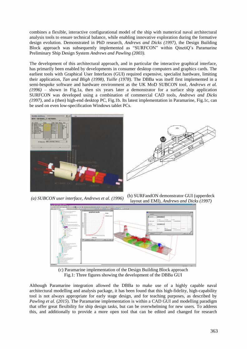
363
combines a flexible, interactive configurational model of the ship with numerical naval architectural
analysis tools to ensure technical balance, while enabling innovative exploration during the formative
design evolution. Demonstrated in PhD research, Andrews and Dicks (1997), the Design Building
Block approach was subsequently implemented as “SURFCON” within QinetiQ’s Paramarine
Preliminary Ship Design System Andrews and Pawling (2003).
The development of this architectural approach, and in particular the interactive graphical interface,
has primarily been enabled by developments in consumer desktop computers and graphics cards. The
earliest tools with Graphical User Interfaces (GUI) required expensive, specialist hardware, limiting
their application, Tan and Bligh (1998), Yuille (1978). The DBBa was itself first implemented in a
semi-bespoke software and hardware environment as the UK MoD SUBCON tool, Andrews et al.
(1996) – shown in Fig.1a, then six years later a demonstrator for a surface ship application
SURFCON was developed using a combination of commercial CAD tools, Andrews and Dicks
(1997), and a (then) high-end desktop PC, Fig.1b. Its latest implementation in Paramarine, Fig.1c, can
be used on even low-specification Windows tablet PCs.
(a) SUBCON user interface, Andrews et al. (1996) (b) SURFandON demonstrator GUI (upperdeck
layout and EMI), Andrews and Dicks (1997)
(c) Paramarine implementation of the Design Building Block approach
Fig.1: Three figures showing the development of the DBBa GUI
Although Paramarine integration allowed the DBBa to make use of a highly capable naval
architectural modelling and analysis package, it has been found that this high-fidelity, high-capability
tool is not always appropriate for early stage design, and for teaching purposes, as described by
Pawling et al. (2015). The Paramarine implementation is within a CAD GUI and modelling paradigm
that offer great flexibility for ship design tasks, but can be overwhelming for new users. To address
this, and additionally to provide a more open tool that can be edited and changed for research
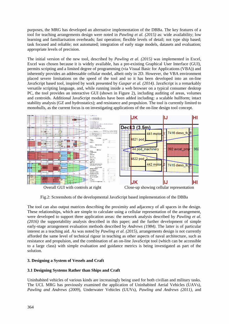
364
purposes, the MRG has developed an alternative implementation of the DBBa. The key features of a
tool for teaching arrangements design were noted in Pawling et al. (2015) as: wide availability; low
learning and familiarisation overheads; fast operation; flexible levels of detail; not type ship based;
task focused and reliable; not automated; integration of early stage models, datasets and evaluation;
appropriate levels of precision.
The initial version of the new tool, described by Pawling et al. (2015) was implemented in Excel,
Excel was chosen because it is widely available, has a pre-existing Graphical User Interface (GUI),
permits scripting and a limited degree of programming (via Visual Basic for Applications (VBA)) and
inherently provides an addressable cellular model, albeit only in 2D. However, the VBA environment
placed severe limitations on the speed of the tool and so it has been developed into an on-line
JavaScript based tool, inspired by work presented by Gaspar et al. (2014). JavaScript is a remarkably
versatile scripting language, and, while running inside a web browser on a typical consumer desktop
PC, the tool provides an interactive GUI (shown in Figure 2), including auditing of areas, volumes
and centroids. Additional JavaScript modules have been added including: a scalable hullform; intact
stability analysis (GZ and hydrostatics); and resistance and propulsion. The tool is currently limited to
monohulls, as the current focus is on investigating applications of the on-line design tool concept.
Overall GUI with controls at right Close-up showing cellular representation
Fig.2: Screenshots of the developmental JavaScript based implementation of the DBBa
The tool can also output matrices describing the proximity and adjacency of all spaces in the design.
These relationships, which are simple to calculate using a cellular representation of the arrangement,
were developed to support three application areas: the network analysis described by Pawling et al.
(2016) the supportability analysis described in this paper; and the further development of simple
early-stage arrangement evaluation methods described by Andrews (1984). The latter is of particular
interest as a teaching aid. As was noted by Pawling et al. (2015), arrangements design is not currently
afforded the same level of technical rigour in teaching as other aspects of naval architecture, such as
resistance and propulsion, and the combination of an on-line JavaScript tool (which can be accessible
to a large class) with simple evaluation and guidance metrics is being investigated as part of the
solution.
3. Designing a System of Vessels and Craft
3.1 Designing Systems Rather than Ships and Craft
Uninhabited vehicles of various kinds are increasingly being used for both civilian and military tasks.
The UCL MRG has previously examined the application of Uninhabited Aerial Vehicles (UAVs),
Pawling and Andrews (2009), Underwater Vehicles (UUVs), Pawling and Andrews (2011), and
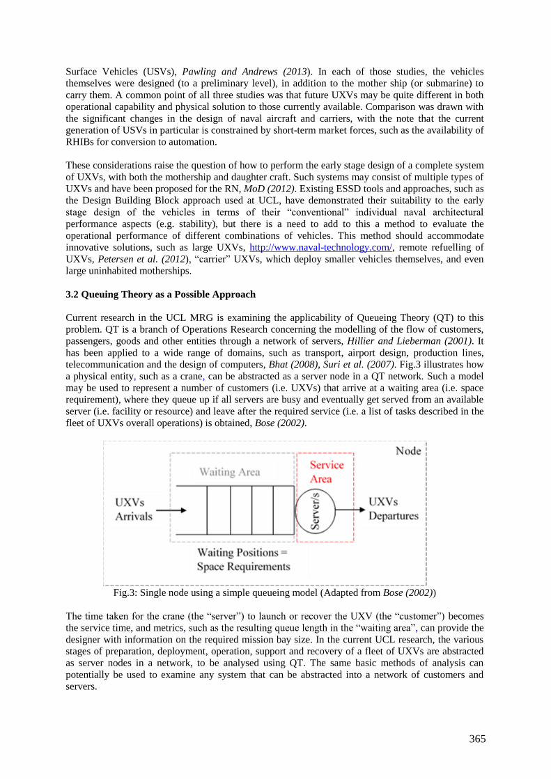
365
Surface Vehicles (USVs), Pawling and Andrews (2013). In each of those studies, the vehicles
themselves were designed (to a preliminary level), in addition to the mother ship (or submarine) to
carry them. A common point of all three studies was that future UXVs may be quite different in both
operational capability and physical solution to those currently available. Comparison was drawn with
the significant changes in the design of naval aircraft and carriers, with the note that the current
generation of USVs in particular is constrained by short-term market forces, such as the availability of
RHIBs for conversion to automation.
These considerations raise the question of how to perform the early stage design of a complete system
of UXVs, with both the mothership and daughter craft. Such systems may consist of multiple types of
UXVs and have been proposed for the RN, MoD (2012). Existing ESSD tools and approaches, such as
the Design Building Block approach used at UCL, have demonstrated their suitability to the early
stage design of the vehicles in terms of their “conventional” individual naval architectural
performance aspects (e.g. stability), but there is a need to add to this a method to evaluate the
operational performance of different combinations of vehicles. This method should accommodate
innovative solutions, such as large UXVs, http://www.naval-technology.com/, remote refuelling of
UXVs, Petersen et al. (2012), “carrier” UXVs, which deploy smaller vehicles themselves, and even
large uninhabited motherships.
3.2 Queuing Theory as a Possible Approach
Current research in the UCL MRG is examining the applicability of Queueing Theory (QT) to this
problem. QT is a branch of Operations Research concerning the modelling of the flow of customers,
passengers, goods and other entities through a network of servers, Hillier and Lieberman (2001). It
has been applied to a wide range of domains, such as transport, airport design, production lines,
telecommunication and the design of computers, Bhat (2008), Suri et al. (2007). Fig.3 illustrates how
a physical entity, such as a crane, can be abstracted as a server node in a QT network. Such a model
may be used to represent a number of customers (i.e. UXVs) that arrive at a waiting area (i.e. space
requirement), where they queue up if all servers are busy and eventually get served from an available
server (i.e. facility or resource) and leave after the required service (i.e. a list of tasks described in the
fleet of UXVs overall operations) is obtained, Bose (2002).
Fig.3: Single node using a simple queueing model (Adapted from Bose (2002))
The time taken for the crane (the “server”) to launch or recover the UXV (the “customer”) becomes
the service time, and metrics, such as the resulting queue length in the “waiting area”, can provide the
designer with information on the required mission bay size. In the current UCL research, the various
stages of preparation, deployment, operation, support and recovery of a fleet of UXVs are abstracted
as server nodes in a network, to be analysed using QT. The same basic methods of analysis can
potentially be used to examine any system that can be abstracted into a network of customers and
servers.
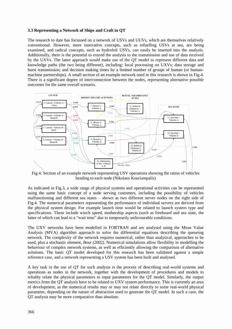
366
3.3 Representing a Network of Ships and Craft in QT
The research to date has focussed on a network of USVs and UUVs, which are themselves relatively
conventional. However, more innovative concepts, such as refuelling USVs at sea, are being
examined, and radical concepts, such as hydrofoil USVs, can easily be inserted into the analysis.
Additionally, there is the potential to extend the analysis to the transmission and use of data received
by the UXVs. The latter approach would make use of the QT model to represent different data and
knowledge paths (the two being different), including: local processing on UXVs; data storage and
burst transmission; and decision making times by a limited number of groups of human (or human-
machine partnerships). A small section of an example network used in this research is shown in Fig.4.
There is a significant degree of interconnection between the nodes, representing alternative possible
outcomes for the same overall scenario.
Fig.4: Section of an example network representing USV operations showing the ratios of vehicles
heading to each node (Nikolaos Kouriampalis)
As indicated in Fig.3, a wide range of physical systems and operational activities can be represented
using the same basic concept of a node serving customers, including the possibility of vehicles
malfunctioning and different sea states – shown as two different server nodes on the right side of
Fig.4. The numerical parameters representing the performance of individual servers are derived from
the physical system design. For example launch time would be related to launch system type and
specifications. These include winch speed, mothership aspects (such as freeboard and sea state, the
latter of which can lead to a “wait time” due to temporarily unfavourable conditions.
The UXV networks have been modelled in FORTRAN and are analysed using the Mean Value
Analysis (MVA) algorithm approach to solve the differential equations describing the queueing
network. The complexity of the network requires numerical, rather than analytical, approaches to be
used, plus a stochastic element, Bose (2002). Numerical simulations allow flexibility in modelling the
behaviour of complex network systems, as well as efficiently allowing the comparison of alternative
solutions. The basic QT model developed for this research has been validated against a simple
reference case, and a network representing a USV system has been built and analysed.
A key task in the use of QT for such analysis is the process of describing real-world systems and
operations as nodes in the network, together with the development of procedures and models to
reliably relate the physical parameters to input parameters for the QT model. Similarly, the output
metrics from the QT analysis have to be related to UXV system performance. This is currently an area
of development, as the numerical results may or may not relate directly to some real-world physical
parameter, depending on the nature of abstraction used to generate the QT model. In such a case, the
QT analysis may be more comparative than absolute.
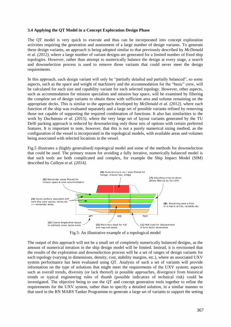
367
3.4 Applying the QT Model in a Concept Exploration Design Phase
The QT model is very quick to execute and thus can be incorporated into concept exploration
activities requiring the generation and assessment of a large number of design variants. To generate
these design variants, an approach is being adopted similar to that previously described by McDonald
et al. (2012), where a large number of variant designs are generated for a limited number of fixed ship
topologies. However, rather than attempt to numerically balance the design at every stage, a search
and downselection process is used to remove those variants that could never meet the design
requirements.
In this approach, each design variant will only be “partially detailed and partially balanced”, so some
aspects, such as the space and weight of machinery and the accommodation for the “basic” crew, will
be calculated for each size and capability variant for each selected topology. However, other aspects,
such as accommodation for mission specialists and mission bay space, will be examined by filtering
the complete set of design variants to obtain those with sufficient area and volume remaining on the
appropriate decks. This is similar to the approach developed by McDonald et al. (2012), where each
function of the ship was evaluated separately and a large set of possible variants refined by removing
those not capable of supporting the required combination of functions. It also has similarities to the
work by Duchateau et al. (2015), where the very large set of layout variants generated by the TU
Delft packing approach is reduced by downselecting only those sets of options with certain preferred
features. It is important to note, however, that this is not a purely numerical sizing method, as the
configuration of the vessel is incorporated in the topological models, with available areas and volumes
being associated with selected locations in the vessel.
Fig.5 illustrates a (highly generalised) topological model and some of the methods for downselection
that could be used. The primary reason for avoiding a fully iterative, numerically balanced model is
that such tools are both complicated and complex, for example the Ship Impact Model (SIM)
described by Calleya et al. (2014).
Fig.5: An illustrative example of a topological model
The output of this approach will not be a small set of completely numerically balanced designs, as the
amount of numerical iteration in the ship design model will be limited. Instead, it is envisioned that
the results of the exploration and downselection process will be a set of ranges of design variants for
each topology (varying in dimensions, density, cost, stability margins, etc.), where an associated UXV
system performance has been evaluated using QT. Analysis of such a set of variants will provide
information on the type of solutions that might meet the requirements of the UXV system; aspects
such as overall trends, diversity (or lack thereof) in possible approaches, divergence from historical
trends or typical engineering rules of thumb (possible indicators of technical risk) could be
investigated. The objective being to use the QT and concept generation tools together to refine the
requirements for the UXV system, rather than to specify a detailed solution, in a similar manner to
that used in the RN MARS Tanker Programme to generate a large set of variants to support the setting
368
of requirements for the industry bidders, who subsequently undertook the actual design of the ships,
Burger and Horner (2011).
4. Incorporating Supportability in Preliminary Ship Design
4.1 The Problem of Supportability in Preliminary Warship Design
Supportability is an important issue for all types of ships, but particularly for warships, with a
combination of long service lives, changing roles, bespoke equipment, high outfit complexity and a
complicated socio-technical support organization, made up of multiple groups of specialists. Although
technical design solutions have been developed to improve the supportability of naval vessels, it
remains a challenge to ensure that these are incorporated into the designs early enough to be used
effectively.
The increased availability of CAD modelling and analysis early in design does not seem to have
improved this situation by itself, with feedback from industry indicating that this is because the
problem is in part one of modelling fidelity. Ongoing PhD level research at UCL seeks to address
some of the many challenges in the incorporation of supportability into computer aided preliminary
ship design, Esbati (2016). The main aspects under investigation are;
- Representing and using expert knowledge and experience. Design practitioners will be familiar
with the phenomenon that, upon being shown a proposed general arrangement, experienced build-
ers, operators and maintainers will recount all manner of problems that occurred on previous, sim-
ilar configurations. The use of layouts to provoke such responses has been used successfully to
collect designer preferences for layout, DeNucci (2012). Formal subject-specific guidance docu-
ments are also maintained by some organisations, but is usually oriented towards procedures,
MoD (2015).
- Linking supportability to the ship layout and architecture. A long-running aspect of UCL MRG
research is the integration of the ships’ layout and other architectural aspects (such as the func-
tional connections between spaces) into ESSD. Although many areas of supportability relate to
the ship’s arrangement – both in terms of individual spaces and the overall layout – this is not ex-
plicitly captured in ship CAD models.
- Decision making under conditions of uncertainty. Design uncertainty in naval vessel design does
not only refer to the possibility of the design changing as the programme progresses, or of an
eventual failure to meet the performance requirements. It also refers to the uncertainty in the
ship’s role and the potential need for unforeseen refits and upgrades. An additional dimension that
has recently been illustrated by problems with the RN’s Type 45 destroyers, Fallon (2016), is
that, with naval vessels pushing the state of the art within a highly cost-constrained and politicized
procurement environment, there is further uncertainty regarding the likelihood and consequences
of some unforeseen class-wide technical issue.
4.2 The Research Area and Proposed Approach
It is acknowledged that warship supportability is a very broad topic, as indicated by the UK MoD
guidance, MoD (2015). Many aspects relate to detail issues, such as equipment selection and
compartment arrangement (ergonomics). To constrain this research to a scope practical for a single
PhD, the level of design definition has been limited to a typical early stage ship design: namely,
general arrangement, selection and location of major equipment; and initial structural design. The
approach being pursued is outlined in Fig.6 and some key points are described in more detail below.
1: Formulating and determining proxy supportability indicators. Direct and explicit
supportability performance indicators have proven difficult to define. However, consideration of the
type of experiential knowledge available on the subject has indicated that there are many features of
the design that can be used as proxy supportability indicators, in that they have a known effect on
supportability, and can be represented in a quantitative manner (albeit a simplified one).
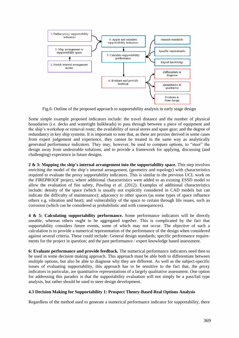
369
Fig.6: Outline of the proposed approach to supportability analysis in early stage design
Some simple example proposed indicators include: the travel distance and the number of physical
boundaries (i.e. decks and watertight bulkheads) to pass through between a piece of equipment and
the ship’s workshop or removal route; the availability of naval stores and spare gear; and the degree of
redundancy in key ship systems. It is important to note that, as these are proxies derived in some cases
from expert judgement and experience, they cannot be treated in the same way as analytically
generated performance indicators. They may, however, be used to compare options, to “steer” the
design away from undesirable solutions, and to provide a framework for applying, discussing (and
challenging) experience in future designs.
2 & 3: Mapping the ship’s internal arrangement into the supportability space. This step involves
enriching the model of the ship’s internal arrangement, (geometry and topology) with characteristics
required to evaluate the proxy supportability indicators. This is similar to the previous UCL work on
the FIREPROOF project, where additional characteristics were added to an existing ESSD model to
allow the evaluation of fire safety, Pawling et al. (2012). Examples of additional characteristics
include: density of the space (which is usually not explicitly considered in CAD models but can
indicate the difficulty of maintenance); adjacency to other spaces (as some types of space influence
others e.g. vibration and heat); and vulnerability of the space to certain through life issues, such as
corrosion (which can be considered as probabilistic and with consequences).
4 & 5: Calculating supportability performance. Some performance indicators will be directly
useable, whereas others ought to be aggregated together. This is complicated by the fact that
supportability considers future events, some of which may not occur. The objective of such a
calculation is to provide a numerical representation of the performance of the design when considered
against several criteria. These could include: General design standards; specific performance require-
ments for the project in question; and the past performance / expert knowledge based assessment.
6: Evaluate performance and provide feedback. The numerical performance indicators need then to
be used in some decision making approach. This approach must be able both to differentiate between
multiple options, but also be able to diagnose why they are different. As well as the subject-specific
issues of evaluating supportability, this approach has to be sensitive to the fact that, the proxy
indicators in particular, are quantitative representations of a largely qualitative assessment. One option
for addressing this paradox is that the supportability evaluation will not simply be a pass/fail type
analysis, but rather should be used to steer design development.
4.3 Decision Making for Supportability 1: Prospect Theory-Based Real Options Analysis
Regardless of the method used to generate a numerical performance indicator for supportability, there
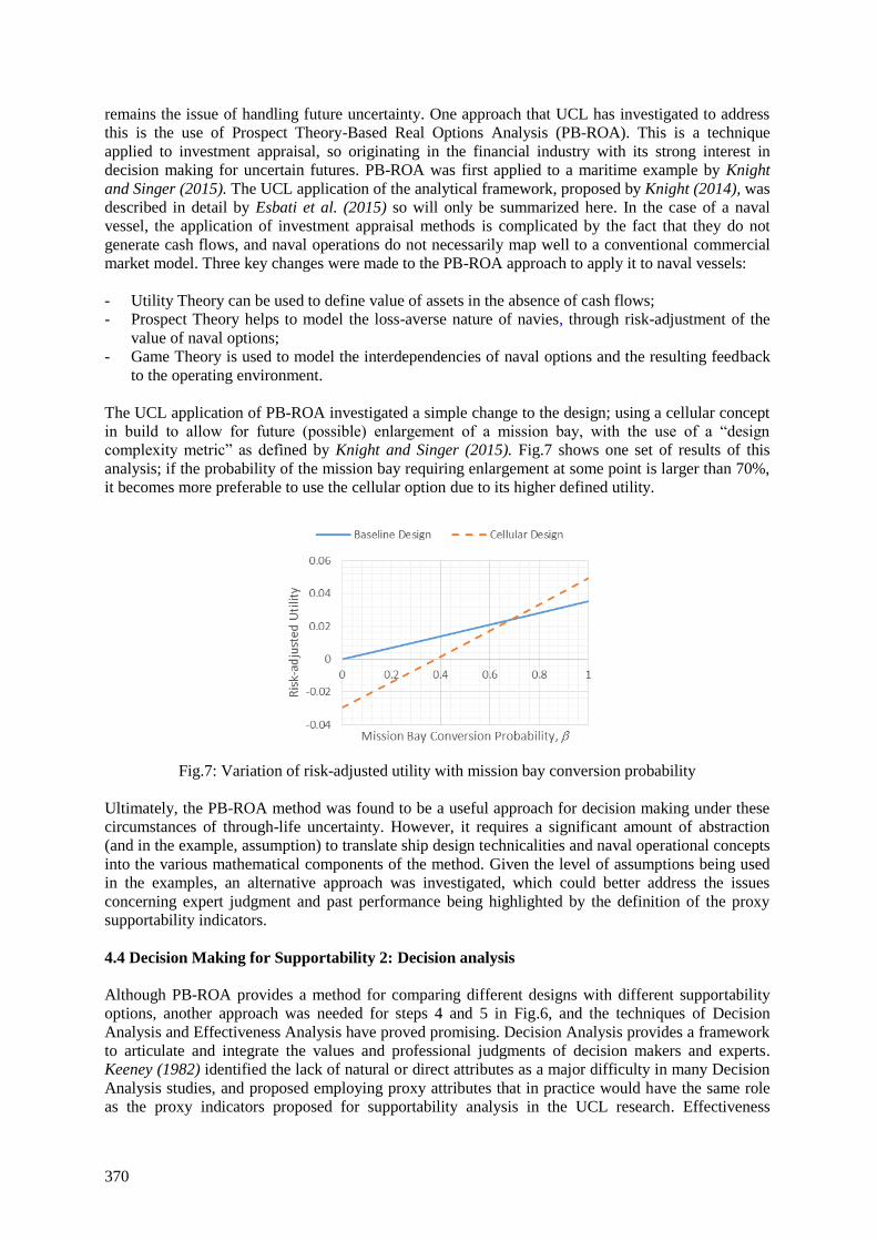
370
remains the issue of handling future uncertainty. One approach that UCL has investigated to address
this is the use of Prospect Theory-Based Real Options Analysis (PB-ROA). This is a technique
applied to investment appraisal, so originating in the financial industry with its strong interest in
decision making for uncertain futures. PB-ROA was first applied to a maritime example by Knight
and Singer (2015). The UCL application of the analytical framework, proposed by Knight (2014), was
described in detail by Esbati et al. (2015) so will only be summarized here. In the case of a naval
vessel, the application of investment appraisal methods is complicated by the fact that they do not
generate cash flows, and naval operations do not necessarily map well to a conventional commercial
market model. Three key changes were made to the PB-ROA approach to apply it to naval vessels:
- Utility Theory can be used to define value of assets in the absence of cash flows;
- Prospect Theory helps to model the loss-averse nature of navies, through risk-adjustment of the
value of naval options;
- Game Theory is used to model the interdependencies of naval options and the resulting feedback
to the operating environment.
The UCL application of PB-ROA investigated a simple change to the design; using a cellular concept
in build to allow for future (possible) enlargement of a mission bay, with the use of a “design
complexity metric” as defined by Knight and Singer (2015). Fig.7 shows one set of results of this
analysis; if the probability of the mission bay requiring enlargement at some point is larger than 70%,
it becomes more preferable to use the cellular option due to its higher defined utility.
Fig.7: Variation of risk-adjusted utility with mission bay conversion probability
Ultimately, the PB-ROA method was found to be a useful approach for decision making under these
circumstances of through-life uncertainty. However, it requires a significant amount of abstraction
(and in the example, assumption) to translate ship design technicalities and naval operational concepts
into the various mathematical components of the method. Given the level of assumptions being used
in the examples, an alternative approach was investigated, which could better address the issues
concerning expert judgment and past performance being highlighted by the definition of the proxy
supportability indicators.
4.4 Decision Making for Supportability 2: Decision analysis
Although PB-ROA provides a method for comparing different designs with different supportability
options, another approach was needed for steps 4 and 5 in Fig.6, and the techniques of Decision
Analysis and Effectiveness Analysis have proved promising. Decision Analysis provides a framework
to articulate and integrate the values and professional judgments of decision makers and experts.
Keeney (1982) identified the lack of natural or direct attributes as a major difficulty in many Decision
Analysis studies, and proposed employing proxy attributes that in practice would have the same role
as the proxy indicators proposed for supportability analysis in the UCL research. Effectiveness
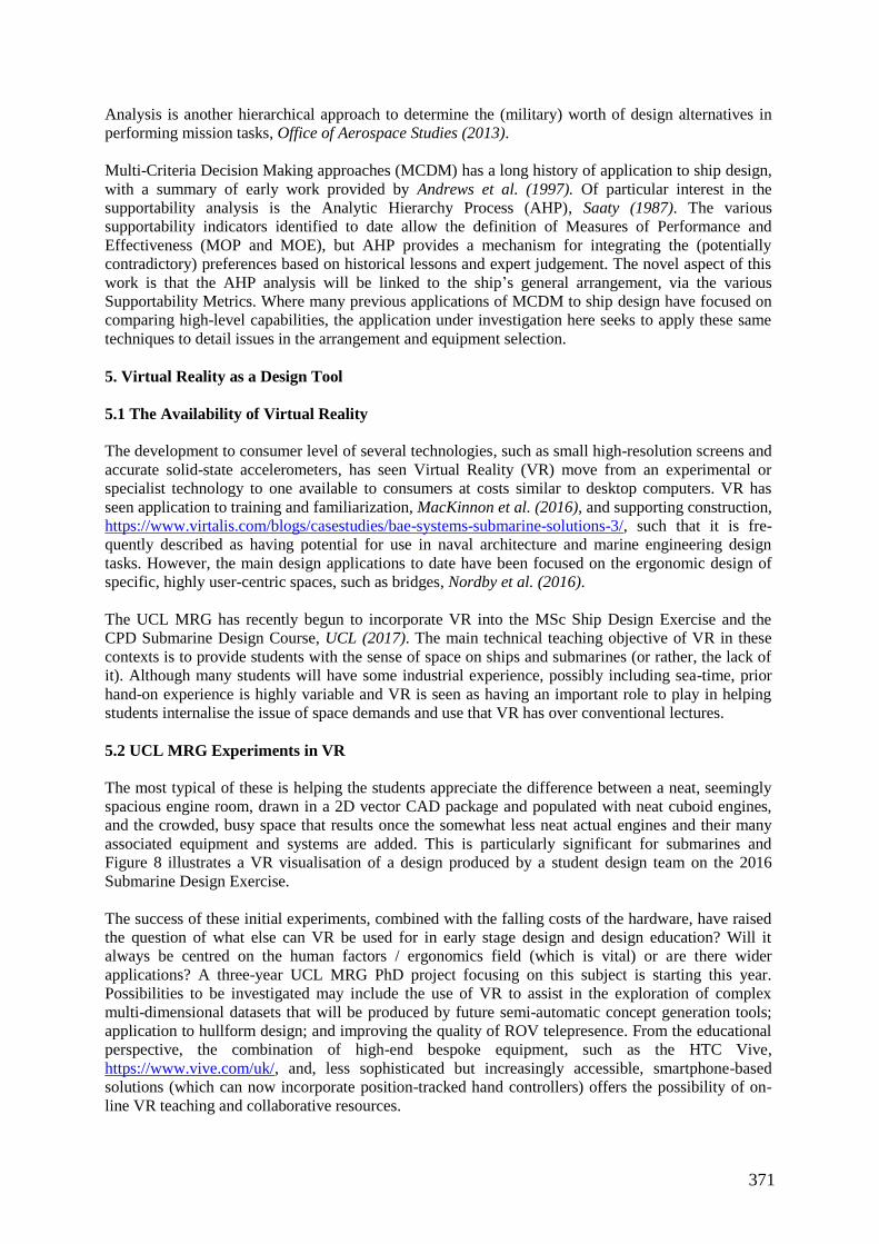
371
Analysis is another hierarchical approach to determine the (military) worth of design alternatives in
performing mission tasks, Office of Aerospace Studies (2013).
Multi-Criteria Decision Making approaches (MCDM) has a long history of application to ship design,
with a summary of early work provided by Andrews et al. (1997). Of particular interest in the
supportability analysis is the Analytic Hierarchy Process (AHP), Saaty (1987). The various
supportability indicators identified to date allow the definition of Measures of Performance and
Effectiveness (MOP and MOE), but AHP provides a mechanism for integrating the (potentially
contradictory) preferences based on historical lessons and expert judgement. The novel aspect of this
work is that the AHP analysis will be linked to the ship’s general arrangement, via the various
Supportability Metrics. Where many previous applications of MCDM to ship design have focused on
comparing high-level capabilities, the application under investigation here seeks to apply these same
techniques to detail issues in the arrangement and equipment selection.
5. Virtual Reality as a Design Tool
5.1 The Availability of Virtual Reality
The development to consumer level of several technologies, such as small high-resolution screens and
accurate solid-state accelerometers, has seen Virtual Reality (VR) move from an experimental or
specialist technology to one available to consumers at costs similar to desktop computers. VR has
seen application to training and familiarization, MacKinnon et al. (2016), and supporting construction,
https://www.virtalis.com/blogs/casestudies/bae-systems-submarine-solutions-3/, such that it is fre-
quently described as having potential for use in naval architecture and marine engineering design
tasks. However, the main design applications to date have been focused on the ergonomic design of
specific, highly user-centric spaces, such as bridges, Nordby et al. (2016).
The UCL MRG has recently begun to incorporate VR into the MSc Ship Design Exercise and the
CPD Submarine Design Course, UCL (2017). The main technical teaching objective of VR in these
contexts is to provide students with the sense of space on ships and submarines (or rather, the lack of
it). Although many students will have some industrial experience, possibly including sea-time, prior
hand-on experience is highly variable and VR is seen as having an important role to play in helping
students internalise the issue of space demands and use that VR has over conventional lectures.
5.2 UCL MRG Experiments in VR
The most typical of these is helping the students appreciate the difference between a neat, seemingly
spacious engine room, drawn in a 2D vector CAD package and populated with neat cuboid engines,
and the crowded, busy space that results once the somewhat less neat actual engines and their many
associated equipment and systems are added. This is particularly significant for submarines and
Figure 8 illustrates a VR visualisation of a design produced by a student design team on the 2016
Submarine Design Exercise.
The success of these initial experiments, combined with the falling costs of the hardware, have raised
the question of what else can VR be used for in early stage design and design education? Will it
always be centred on the human factors / ergonomics field (which is vital) or are there wider
applications? A three-year UCL MRG PhD project focusing on this subject is starting this year.
Possibilities to be investigated may include the use of VR to assist in the exploration of complex
multi-dimensional datasets that will be produced by future semi-automatic concept generation tools;
application to hullform design; and improving the quality of ROV telepresence. From the educational
perspective, the combination of high-end bespoke equipment, such as the HTC Vive,
https://www.vive.com/uk/, and, less sophisticated but increasingly accessible, smartphone-based
solutions (which can now incorporate position-tracked hand controllers) offers the possibility of on-
line VR teaching and collaborative resources.
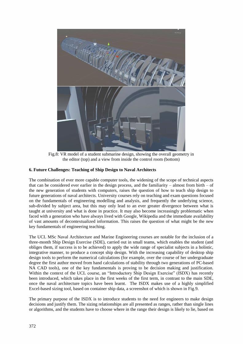
372
Fig.8: VR model of a student submarine design, showing the overall geometry in
the editor (top) and a view from inside the control room (bottom)
6. Future Challenges: Teaching of Ship Design to Naval Architects
The combination of ever more capable computer tools, the widening of the scope of technical aspects
that can be considered ever earlier in the design process, and the familiarity – almost from birth – of
the new generation of students with computers, raises the question of how to teach ship design to
future generations of naval architects. University courses rely on teaching and exam questions focused
on the fundamentals of engineering modelling and analysis, and frequently the underlying science,
sub-divided by subject area, but this may only lead to an ever greater divergence between what is
taught at university and what is done in practice. It may also become increasingly problematic when
faced with a generation who have always lived with Google, Wikipedia and the immediate availability
of vast amounts of decontextualized information. This raises the question of what might be the new
key fundamentals of engineering teaching.
The UCL MSc Naval Architecture and Marine Engineering courses are notable for the inclusion of a
three-month Ship Design Exercise (SDE), carried out in small teams, which enables the student (and
obliges them, if success is to be achieved) to apply the wide range of specialist subjects in a holistic,
integrative manner, to produce a concept ship design. With the increasing capability of desktop ship
design tools to perform the numerical calculations (for example, over the course of her undergraduate
degree the first author moved from hand calculations of stability through two generations of PC-based
NA CAD tools), one of the key fundamentals is proving to be decision making and justification.
Within the context of the UCL course, an “Introductory Ship Design Exercise” (ISDX) has recently
been introduced, which takes place in the first weeks of the first term, in contrast to the main SDE,
once the naval architecture topics have been learnt. The ISDX makes use of a highly simplified
Excel-based sizing tool, based on container ship data, a screenshot of which is shown in Fig.9.
The primary purpose of the ISDX is to introduce students to the need for engineers to make design
decisions and justify them. The sizing relationships are all presented as ranges, rather than single lines
or algorithms, and the students have to choose where in the range their design is likely to lie, based on
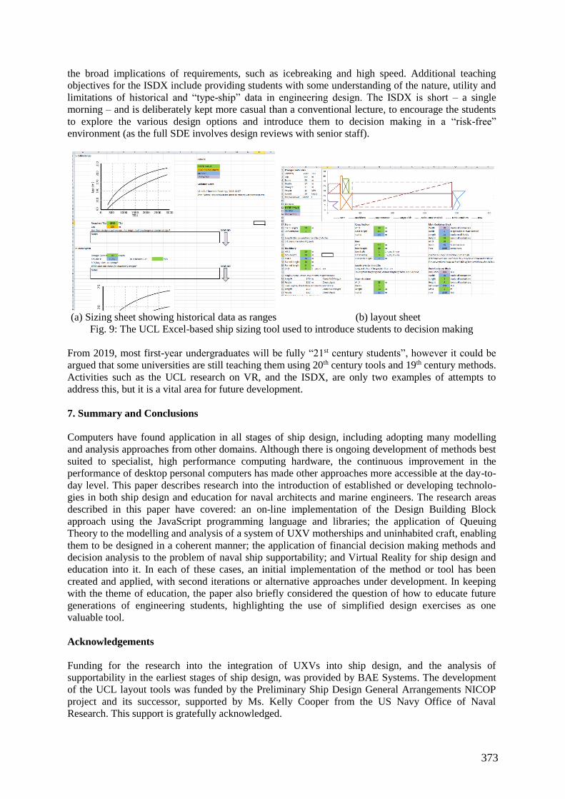
373
the broad implications of requirements, such as icebreaking and high speed. Additional teaching
objectives for the ISDX include providing students with some understanding of the nature, utility and
limitations of historical and “type-ship” data in engineering design. The ISDX is short – a single
morning – and is deliberately kept more casual than a conventional lecture, to encourage the students
to explore the various design options and introduce them to decision making in a “risk-free”
environment (as the full SDE involves design reviews with senior staff).
(a) Sizing sheet showing historical data as ranges (b) layout sheet
Fig. 9: The UCL Excel-based ship sizing tool used to introduce students to decision making
From 2019, most first-year undergraduates will be fully “21st century students”, however it could be
argued that some universities are still teaching them using 20th century tools and 19th century methods.
Activities such as the UCL research on VR, and the ISDX, are only two examples of attempts to
address this, but it is a vital area for future development.
7. Summary and Conclusions
Computers have found application in all stages of ship design, including adopting many modelling
and analysis approaches from other domains. Although there is ongoing development of methods best
suited to specialist, high performance computing hardware, the continuous improvement in the
performance of desktop personal computers has made other approaches more accessible at the day-to-
day level. This paper describes research into the introduction of established or developing technolo-
gies in both ship design and education for naval architects and marine engineers. The research areas
described in this paper have covered: an on-line implementation of the Design Building Block
approach using the JavaScript programming language and libraries; the application of Queuing
Theory to the modelling and analysis of a system of UXV motherships and uninhabited craft, enabling
them to be designed in a coherent manner; the application of financial decision making methods and
decision analysis to the problem of naval ship supportability; and Virtual Reality for ship design and
education into it. In each of these cases, an initial implementation of the method or tool has been
created and applied, with second iterations or alternative approaches under development. In keeping
with the theme of education, the paper also briefly considered the question of how to educate future
generations of engineering students, highlighting the use of simplified design exercises as one
valuable tool.
Acknowledgements
Funding for the research into the integration of UXVs into ship design, and the analysis of
supportability in the earliest stages of ship design, was provided by BAE Systems. The development
of the UCL layout tools was funded by the Preliminary Ship Design General Arrangements NICOP
project and its successor, supported by Ms. Kelly Cooper from the US Navy Office of Naval
Research. This support is gratefully acknowledged.

374
References
ANDREWS, D.J. (1984), Synthesis in Ship Design, PhD Thesis, University of London
ANDREWS, D.J. (1986), An integrated approach to ship synthesis, Trans. RINA.128
ANDREWS, D.J.; DICKS, C. (1997), The building block design methodology applied to advanced
naval ship design, 6th Int. Marine Design Conf. (IMDC), Newcastle
ANDREWS, D.J.; PAWLING, R.J. (2003), SURFCON - A 21st century ship design tool, 8th IMDC,
Athens
ANDREWS, D.J.; CUDMORE, A.C.; HUMBLE, P.; WILSON, D. (1996), SUBCON - A new
approach to submarine concept design, RINA Symp. Naval Submarines 5: The Total Weapons
System, London
ANDREWS, D.J. (Ed); ATLAR, M.; DRAKE, K.; GEE, N.; LEVANDER, K.J.; SEN, P.; SNAITH,
G.J. (1997), IMDC State of the Art Report on Design Methods, 6th IMDC, Newcastle
BERTRAM, V.; PERIC, M.; (2013), Advanced Simulations for Offshore Industry Applications, 12th
Int. Conf. Computer and IT Appl. Maritime Ind. (COMPIT), Cortona
BHAT, U.N. (2008), An Introduction to Queuing Theory - Modelling and Analysis in Applications,
Birkhauser Boston
BOSE, K.S. (2002), An Introduction to Queuing Systems, Springer
BURGER, D.; HORNER, D. (2011), The use of Paramarine and modeFRONTIER for ship design
space exploration, 10th COMPIT, Berlin
CALLEYA, J.; PAWLING, R.J.; GREIG, A. (2015), Ship impact model for technical assessment and
selection of carbon dioxide reducing technologies (CRTs), Ocean Engineering 97
DENUCCI, T.W. (2012), Capturing Design - Improving Conceptual Ship Design Through the
Capture of Design Rationale, PhD Thesis, Delft University of Technology
DUCHATEAU, E.A.E.; VAN OERS, B.J.; HOPMAN, J.J. (2015), Interactive steering of an
optimisation based ship synthesis model for concept exploration, 12th IMDC, Tokyo
ESBATI, S., (2016), Design for Support in the Initial Design of Naval Combatants, MPhil/PhD
Transfer Report, UCL
ESBATI, S.; PIPERAKIS, A.S.; PAWLING, R.J.; ANDREWS, D.J. (2015), Design for support in the
initial design of naval combatants, Int. Conf. Computer Applications in Shipbuilding, Bremen
FALLON, M. (2016), Letter to Chair of UK House of Commons Defence Committee, 3rd March
2016; http://www.parliament.uk/documents/commons-committees/defence/160303 SofS response -
Type 45 Destroyers(1).pdf
GASPAR, H.; P.O. BRETT, P.O.; EBRAHIM, A.; KEANE, A. (2014), Data-driven documents (D3)
applied to conceptual ship design knowledge, 13th COMPIT, Redworth
GILLESPIE, J. (2012), A Network Science Approach to Understanding and Generating Ship
Arrangements in Early-Stage Design, PhD thesis, University of Michigan

375
HILLIER S.F.; LIEBERMAN J.G. (2001), Introduction to Operations Research, McGraw-Hill
KEENEY, R.L. (1982), Decision Analysis: An Overview, Operations Research 30/5
KNIGHT J.T. (2014), A Prospect Theory-Based Real Option Analogy for Evaluating Flexible Systems
and Architectures in Naval Ship Design, PhD Thesis, University of Michigan
KNIGHT J.T.; SINGER D. J. (2015), Prospect theory-based real options analysis for non-
commercial assets, ASCE-ASME J. Risk and Uncertainty in Engineering Systems, Part B 1(1)
MacCALLUM, K.J. (1982), Understanding relationships in marine systems design, IMSDC, London
MacKINNON, S.N.; BRADBURY-SQUIRES, D.; BUTTON, D., (2016), Virtual reality based
training improves mustering performance, 15th COMPIT, Lecce
McDONALD, T.; ANDREWS, D.J.; PAWLING, R.J.; (2012), A demonstration of an advanced
library based approach to the initial design exploration of different hullform configurations,
Computer-Aided Design 44/3, pp.209-223
MRVAR, A. (2016), Pajek: analysis and visualization of large networks, http://mrvar.fdv.uni-
lj.si/pajek/
NORDBY, K.; BØRRESEN, S.; GERNEZ, E.; (2016), Efficient Use of Virtual and Mixed Reality in
Conceptual Design of Maritime Work Places, 15th COMPIT, Lecce
Office of Aerospace Studies (2013), Analysis of Alternatives (AoA) Handbook, 10th June 2013, USAF
Materiel Command
PAWLING, R.J; ANDREWS, D.J. (2009), The ship design challenge of naval unmanned aerial
vehicles, Warship 2009: Air power at sea, London
PAWLING, R.J; ANDREWS, D.J. (2011), A Submarine Concept Design – The Submarine as an UXV
Mothership, Warship 2011: Naval Submarines and UUVs, Bath
PAWLING, R.J; ANDREWS, D.J. (2013), Large Unmanned Vehicles and the Minor War Vessel,
Warship 2013: Minor Warships, Bath
PAWLING, R.J.; GRANDISON, A.; LOHRMANN, P.; MERMIRIS, G.; PEREIRA DIAS, C. (2012),
Methods and Tools for Risk-Based Approach to Fire Safety in Ship Design, Ship Technology
Research 59, pp.38-49
PAWLING, R.J.; PIPERAKIS, A.; ANDREWS, D.J. (2015), Developing architecturally oriented
concept ship design tools for research and education, 12th IMDC, Tokyo
PAWLING, R.J.; PIPERAKIS, A.; ANDREWS, D.J. (2016), Applications of network science in ship
design, 15th COMPIT, Lecce
PETERSEN, S.M.; GALWAY, R.J.; MICHELON, L.J.; HARRIS, D.B. (2012), The in situ replenish-
ment system, ASNE Launch and Recovery Symp., Linthicum
SAATY, R.W. (1987), The Analytic Hierarchy Process – What is it and How is it Used, Mathematical
Modelling 9/3-5
SURI, R.; SAHU, S.; VERNON, M. (2007), Approximate mean value analysis for closed queueing
networks with multiple-server stations, Industrial Engineering Research Conf., Pittsburgh

376
TAN, K.T.; BLIGH, T.P.; (1998), A New Approach to an Integrated CAD Method for Surface Ship
Design, Naval Engineers J. 110/1, pp.35-48
UCL (2017) https://www.ucl.ac.uk/mecheng/our-courses/other-courses/submarine_design
UK Ministry of Defence (2012), Joint Concept Note 1-12, Future ‘Black Sean’ Class Sloop-of-War: A
Group System
UK Ministry of Defence (2015), JSP 886: The Defence Logistics Support Chain Manual
YUILLE, I.M. (1978), The Forward Design System for Computer Aided Ship Design Using a Mini-
Computer, Trans. RINA 120
377
Secure Wireless Options in the Smart Ship
Scott Patterson, Babcock Analytic Solutions, [email protected]
Peter Barton, Babcock Analytic Solutions, [email protected]
Abstract
This paper presents a summary of the findings of a detailed study, conducted on behalf of the Ministry
of Defence, assessing wireless technologies with the potential to support secure communications on-
board Royal Naval platforms. Specific requirements and possible solutions were not in scope but the
security and interference implications of implementation of such networks in RN warships and
submarines were considered for a range of information types and classification levels. Design con-
siderations to limit exposure to threats are also discussed.
1. Introduction
Previous work on behalf of the MoD developed a Smart Platform Vision Demonstrator which
showcased a future state where on-board information (including equipment sensor data) was accessed
remotely at the point of use using mobile technologies, delivered over a wireless network bearer with
automated process flow and on-board analytics capability. This approach placed the Maintainer at the
heart of the solution and also highlighted the potential utility of Augmented Reality (AR) in an In-
Service support environment. The work presented how significant benefits could potentially be
achieved in the supportability maintenance environment by the use of secure wireless technologies in
a Smart Ship, including:
Improved access and exploitation of information by Ship Staff;
Improved feedback from the Platform to aid Design Authority and Waterfront decision
making;
More effective fault resolution and diagnostics, using digitally enabled equipment and
sensors;
Ability to deploy mobile applications and workflow automation, both shore side and within
platform environments.
However, there will be security and interference implications of installing and operating a wireless
communications system in an on-board platform environment. Wireless networks come with
increased Cyber risk, noting that they are generally easier for attackers to access than their wired
equivalents and can present an attractive, lower risk, path into a private network. If Cyber risks are not
managed adequately, an attacker can potentially intercept or transmit data at long range from a
position of safety, or deliberately jam the medium causing a network denial of service.
The selection of wireless technology solutions will be driven by specific requirements so, to avoid
being proscriptive, this paper summarises an assessment of a broad range of personal and local area
wireless communication technologies, particularly with respect to their potential utility in the
maritime environment. The security and interference implications of installing such networks on an
secure platform are considered for a range of information types and classification levels that may need
to be accessed. Additionally, design considerations to limit exposure to threats, including those of the
potential “Insider” to on-board systems, are discussed.
2. Background
2.1. Wireless Network Types
The evolution of wireless network communications has played a major role in shaping the ways in
which we work, play, socialise, are entertained and communicate in general. They offer location
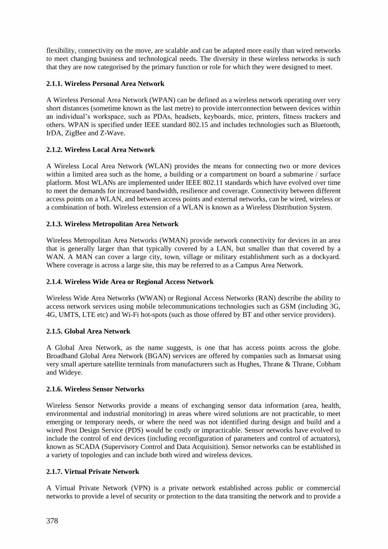
378
flexibility, connectivity on the move, are scalable and can be adapted more easily than wired networks
to meet changing business and technological needs. The diversity in these wireless networks is such
that they are now categorised by the primary function or role for which they were designed to meet.
2.1.1. Wireless Personal Area Network
A Wireless Personal Area Network (WPAN) can be defined as a wireless network operating over very
short distances (sometime known as the last metre) to provide interconnection between devices within
an individual’s workspace, such as PDAs, headsets, keyboards, mice, printers, fitness trackers and
others. WPAN is specified under IEEE standard 802.15 and includes technologies such as Bluetooth,
IrDA, ZigBee and Z-Wave.
2.1.2. Wireless Local Area Network
A Wireless Local Area Network (WLAN) provides the means for connecting two or more devices
within a limited area such as the home, a building or a compartment on board a submarine / surface
platform. Most WLANs are implemented under IEEE 802.11 standards which have evolved over time
to meet the demands for increased bandwidth, resilience and coverage. Connectivity between different
access points on a WLAN, and between access points and external networks, can be wired, wireless or
a combination of both. Wireless extension of a WLAN is known as a Wireless Distribution System.
2.1.3. Wireless Metropolitan Area Network
Wireless Metropolitan Area Networks (WMAN) provide network connectivity for devices in an area
that is generally larger than that typically covered by a LAN, but smaller than that covered by a
WAN. A MAN can cover a large city, town, village or military establishment such as a dockyard.
Where coverage is across a large site, this may be referred to as a Campus Area Network.
2.1.4. Wireless Wide Area or Regional Access Network
Wireless Wide Area Networks (WWAN) or Regional Access Networks (RAN) describe the ability to
access network services using mobile telecommunications technologies such as GSM (including 3G,
4G, UMTS, LTE etc) and Wi-Fi hot-spots (such as those offered by BT and other service providers).
2.1.5. Global Area Network
A Global Area Network, as the name suggests, is one that has access points across the globe.
Broadband Global Area Network (BGAN) services are offered by companies such as Inmarsat using
very small aperture satellite terminals from manufacturers such as Hughes, Thrane & Thrane, Cobham
and Wideye.
2.1.6. Wireless Sensor Networks
Wireless Sensor Networks provide a means of exchanging sensor data information (area, health,
environmental and industrial monitoring) in areas where wired solutions are not practicable, to meet
emerging or temporary needs, or where the need was not identified during design and build and a
wired Post Design Service (PDS) would be costly or impracticable. Sensor networks have evolved to
include the control of end devices (including reconfiguration of parameters and control of actuators),
known as SCADA (Supervisory Control and Data Acquisition). Sensor networks can be established in
a variety of topologies and can include both wired and wireless devices.
2.1.7. Virtual Private Network
A Virtual Private Network (VPN) is a private network established across public or commercial
networks to provide a level of security or protection to the data transiting the network and to provide a
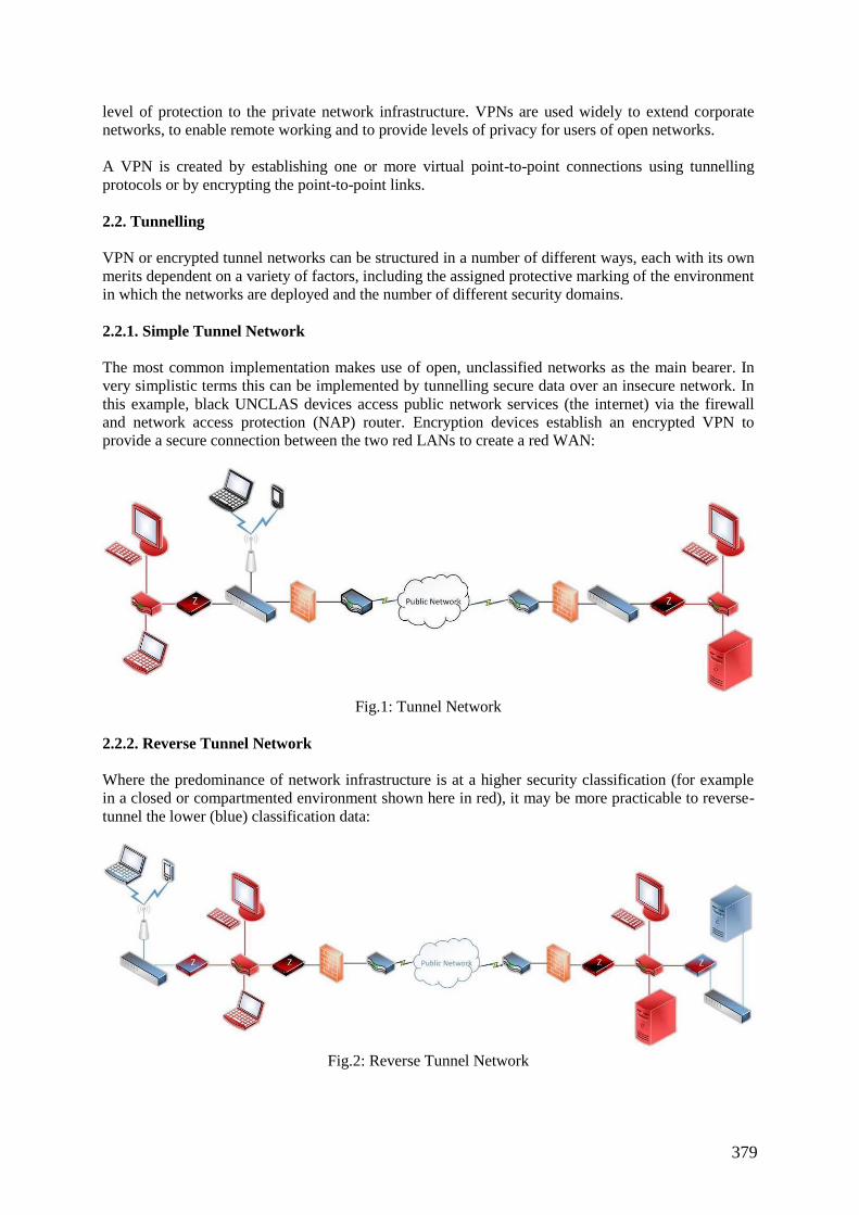
379
level of protection to the private network infrastructure. VPNs are used widely to extend corporate
networks, to enable remote working and to provide levels of privacy for users of open networks.
A VPN is created by establishing one or more virtual point-to-point connections using tunnelling
protocols or by encrypting the point-to-point links.
2.2. Tunnelling
VPN or encrypted tunnel networks can be structured in a number of different ways, each with its own
merits dependent on a variety of factors, including the assigned protective marking of the environment
in which the networks are deployed and the number of different security domains.
2.2.1. Simple Tunnel Network
The most common implementation makes use of open, unclassified networks as the main bearer. In
very simplistic terms this can be implemented by tunnelling secure data over an insecure network. In
this example, black UNCLAS devices access public network services (the internet) via the firewall
and network access protection (NAP) router. Encryption devices establish an encrypted VPN to
provide a secure connection between the two red LANs to create a red WAN:
Fig.1: Tunnel Network
2.2.2. Reverse Tunnel Network
Where the predominance of network infrastructure is at a higher security classification (for example
in a closed or compartmented environment shown here in red), it may be more practicable to reverse-
tunnel the lower (blue) classification data:
Fig.2: Reverse Tunnel Network
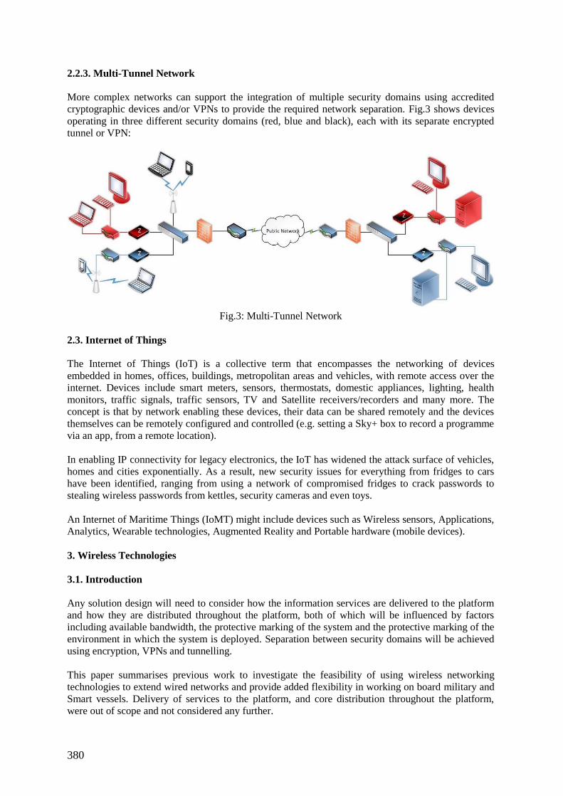
380
2.2.3. Multi-Tunnel Network
More complex networks can support the integration of multiple security domains using accredited
cryptographic devices and/or VPNs to provide the required network separation. Fig.3 shows devices
operating in three different security domains (red, blue and black), each with its separate encrypted
tunnel or VPN:
Fig.3: Multi-Tunnel Network
2.3. Internet of Things
The Internet of Things (IoT) is a collective term that encompasses the networking of devices
embedded in homes, offices, buildings, metropolitan areas and vehicles, with remote access over the
internet. Devices include smart meters, sensors, thermostats, domestic appliances, lighting, health
monitors, traffic signals, traffic sensors, TV and Satellite receivers/recorders and many more. The
concept is that by network enabling these devices, their data can be shared remotely and the devices
themselves can be remotely configured and controlled (e.g. setting a Sky+ box to record a programme
via an app, from a remote location).
In enabling IP connectivity for legacy electronics, the IoT has widened the attack surface of vehicles,
homes and cities exponentially. As a result, new security issues for everything from fridges to cars
have been identified, ranging from using a network of compromised fridges to crack passwords to
stealing wireless passwords from kettles, security cameras and even toys.
An Internet of Maritime Things (IoMT) might include devices such as Wireless sensors, Applications,
Analytics, Wearable technologies, Augmented Reality and Portable hardware (mobile devices).
3. Wireless Technologies
3.1. Introduction
Any solution design will need to consider how the information services are delivered to the platform
and how they are distributed throughout the platform, both of which will be influenced by factors
including available bandwidth, the protective marking of the system and the protective marking of the
environment in which the system is deployed. Separation between security domains will be achieved
using encryption, VPNs and tunnelling.
This paper summarises previous work to investigate the feasibility of using wireless networking
technologies to extend wired networks and provide added flexibility in working on board military and
Smart vessels. Delivery of services to the platform, and core distribution throughout the platform,
were out of scope and not considered any further.

381
A broad range of wireless options were considered from across the electromagnetic spectrum,
including the traditional Radio Frequency based technologies, such as Wi-Fi and Bluetooth, and those
operating in the Infrared, Visible Light and Ultraviolet bands. Ultraviolet was discounted immediately
as there are no developments for short range networks. Laser communications were considered
initially due to previous implementations in campus network solutions, however these devices are no
longer available and current developments are focused on space communications.
The remainder were considered to have potential utility in the maritime domain either now or in the
future and were assessed with respect to performance, security and maturity, the findings from which
are summarised below.
3.2. Wi-Fi
Wi-Fi is a technology that enables devices to connect wirelessly to Local Area Networks and is
specified under IEEE standard 802.11 for operation in the 900 MHz, 2.4GHz, 3.6GHz, 5GHz and
60GHz bands of the RF spectrum. Since its first implementation in the 1990s, the Wi-Fi standard has
undergone a number of revisions and developments; it is now a very well established open standard
offering reliable and secure wireless network extension that is capable of delivering sufficient
bandwidth to support most applications across multiple devices. Its popularity has ensured that
generic devices are readily available and Wi-Fi capability is often integrated in to many domestic,
industrial and commercial devices. This popularity does increase the risk of interference; however this
can be mitigated by careful network configuration and management.
Use of the Advanced Encryption Standard (AES) protocol means that Wi-Fi can be accredited for use
with some Government and military networks, but it is essential that robust key management is
implemented for this to meet the requirements of system security accreditors.
Wi-Fi networks are well suited to the delivery of welfare services where Bring Your Own Device
initiatives are supported, particularly as most service personnel will own Wi-Fi enabled smart phones
and tablets. Within an operational environment, consideration should be given to access point siting in
order to reduce the risk of targeted, standoff attacks. Solutions should also consider configuration
options that allow network access devices to be controlled in accordance with Emission Control
(EMCON) policies.
This type of network extension on board a platform could provide added flexibility and improve
efficiency of some working practices; however the structure of vessels is such that platform wide
coverage would require a considerable number of wireless access points. The use of PowerLine
technologies may help address this on existing platforms, however these would also need to be
assessed for Radio Frequency Interference (RFI), Electromagnetic Compatibility (EMC) and Security
Accreditation.
Wi-Fi standards have continued to develop in order to address emerging needs. The release to market
in 2016 of the first 802.11.ad devices, operating at 60GHz and offering significantly increased
bandwidth, may present opportunities for the employment of Wi-Fi in more sensitive and/or
bandwidth hungry environments.
3.3. Bluetooth
Bluetooth offers a suite of very well established, open standards which are used extensively in modern
communications and information systems (CIS) solutions to provide short-range connectivity
(typically less than 10m) between devices: including computers and their peripherals (keyboard,
mouse & printers), hands-free headsets, wireless speakers, media players and media centres, fitness
devices, remote controls, test equipment, medical equipment, bar code scanners and many modern
applications previously served by RS232 and other wired protocols. Governance by the Bluetooth
Special Interest Group (SIG) has helped ensure interoperability between different vendors’ devices
382
and developed user trust in the technology. Classic and Low Energy (LE) implementations of the
standards are well suited to applications requiring modest data rates (up to 3Mbps and 1Mbps
respectively) over relatively short distances (up to 10m). Later versions of the standard offer greater
throughput but rely on a hybrid Bluetooth/Wi-Fi solution to achieve this.
Bluetooth uses a frequency hopping standard which helps minimise the risk of interference with other
devices in the Industrial, Scientific & Medical (ISM) band and has the option to form mesh networks
which can be attractive for some applications such as sensor networks. The Bluetooth standards
include strong 128 bit AES encryption, however robust key management is critical to ensuring
connection integrity is maintained. Many low end devices, such as some headsets and keyboards,
employ weak pairing procedures and use fixed keys which can leave devices vulnerable to intercept or
cyber-attack.
The low transmit power levels of Bluetooth Classic and LE lends the technology to employment in
areas where minimising RF signatures is desirable and the risks of eavesdropping or interception are
concerns. Bluetooth headsets are currently used in operational environments where ease of movement
and freedom from wired devices is desirable. Current policies preclude the use of wireless devices at
higher classification levels, however where a suitable operational imperative can be justified and trials
results are able to demonstrate suitable risk mitigation (for example when deployed in metal clad
compartments providing sufficient RF screening) accreditation of such devices may be possible in the
future.
Bluetooth standards continue to develop, with V5 recently announced in December 2016. Despite
these progressions, Classic and LE versions continue to fill specific needs that V4 and V5 will not and
therefore device availability and support will not be affected.
3.4. ZigBee
ZigBee is an open specification, based on IEEE 802.15.4 for low-speed (250 kbps), short range (10m)
wireless personal area networks. ZigBee was conceived in 1998 and initially targeted at sensing and
control functions in the industrial and commercial sectors. Since then it has been adopted more widely
and is now also found in domestic and residential ‘smart home’ devices. Certification of ZigBee
products is undertaken by the ZigBee Alliance. ZigBee provides a meshed, small area network
capability, underpinned by predefined command libraries that could be adapted to meet many needs.
ZigBee delivers relatively low bandwidth of up to 250kbps at individual link ranges of up to 10m,
extendable up to 100m in a mesh.
The standard defines use of AES 128 bit encryption which, if correctly implemented, will provide
sufficient levels of security for use in most sensor networks. There are many development options
which make implementation of the standard for niche low bandwidth requirements a possibility. Easy
development of bespoke solutions, coupled with user definable options for key management and
ZigBee’s low power consumption, make it attractive for solutions which may need to be left
unattended for long periods, or where detection or the possibility of generating RFI with other devices
is a concern.
3.5. Z-Wave
Z-Wave was established by a small Danish start-up (acquired by Sigma Designs in 2008) as a home
automation wireless communications protocol intended to provide simple remote control functionality
for lighting, heating, air conditioning, security systems, windows, garage doors and access controls.
Z-Wave is a proprietary standard that operates outside the congested 2.4GHz ISM band, reducing the
risk of interference with other devices. Employing a mesh network topology provides a degree of
resilience which, coupled with AES 128 bit encryption, could make Z-Wave attractive for very low
bandwidth applications such as sensor networks.
383
The proprietary nature of Z-Wave is such that solutions rely on the use of chips that are only available
from a single manufacturer. AES encryption is not available on all chip sets and where it is, the
implementation is not generally very robust. This does not preclude Z-Wave from consideration for
future development options, but these would likely prove costly and require tie-in with a single chip
vendor. It is also likely that a requirement for which a Z-Wave solution might be implemented could
be met using an open standard based technology, such as ZigBee.
3.6. IrDA
The Infrared Data Association (IrDA) presents a mature set of standards for short range
communications (less than 1m) that were popular in the late 1990s and early 2000s to provide
connectivity between Laptops, Desktops and PDAs. However, a key limitation was the need for a line
of sight between the IrDA ‘ports’. The evolution of Wi-Fi and Bluetooth, which do not require a clear
line of sight, overtook IrDA in this application and its inclusion in new devices has largely fallen by
the wayside. Legacy support is still available for IrDA devices on some platforms, however research
was unable to reveal any vendor that incorporates IrDA ports or capability on their current devices.
Despite the IrDA association establishing Special Interest Groups for development of Giga-IR and IR-
USB there does not appear to have been any further development since 2012.
This lack of any development, market presence, or inclusion of encryption within the standards,
precludes IrDA from any recommendations for employment on military platforms or in any sensitive
environments at this time. Despite this, Infrared is used in PureLiFi’s LiFi-X solution and the ongoing
existence of the IrDA and its Special Interest Groups looking at developing speeds in excess of 1Gbps
may lead to the publication of new IrDA standards and a resurgence in the development and
production of IrDA devices.
3.7. LiFi
LiFi is a form of visible light communications theoretically capable of delivering full-duplex
bandwidth in excess of 200Gbps. It is intended to work by modulating the light emitted by common
household LED bulbs, which is picked up by photoelectric cells positioned within the beam of that
light. The aim is to provide easy access to computer networks in areas where Wi-Fi is not practicable
or where Wi-Fi bandwidth is insufficient. LiFi is a relatively immature technology which, although
underpinned by an IEEE standard, has so far only been implemented by individual vendors using
proprietary standards. Laboratory testing is reported to be achieving levels of performance that far
exceed those of RF based wireless solutions, however the small number offering commercial
solutions have failed to replicate this performance in the real world and none have achieved the
throughput that is available with Wi-Fi. LiFi offers advantages in presenting no EMC or RFI issues,
however performance in a range of different operating environments, with differing ambient light
levels can only be truly assessed with longer term independent testing.
LiFi does not yet offer any encryption or authentication on the air interface currently and is therefore
potentially vulnerable to intercept, denial of service and offensive cyber-attack. Interoperability
testing with other vendor solutions has not been conducted, however as each vendor’s solution is
proprietary, it is likely that a solution implemented using today’s technology would require single
vendor tie-in. Both factors present significant security and business risk to any solution.
LiFi is a technology in the very early stages of evolution; however despite the listed reservations it has
the potential to deliver significant increases in bandwidth, with utility in areas where RF solutions are
impracticable on safety, security or technological grounds. Significant progress has been made in the
5 years since the IEEE 802.15.7 standard was defined. Should commercial and private sector buy-in
start to escalate, now that products are becoming available, it seems likely that performance levels
will continue to increase rapidly in the coming years, providing a viable alternative to other wireless
technologies without the disadvantages of RF. Testing in controlled environments will provide
opportunities for technical authorities to have an early look at proposed solutions whilst also enabling
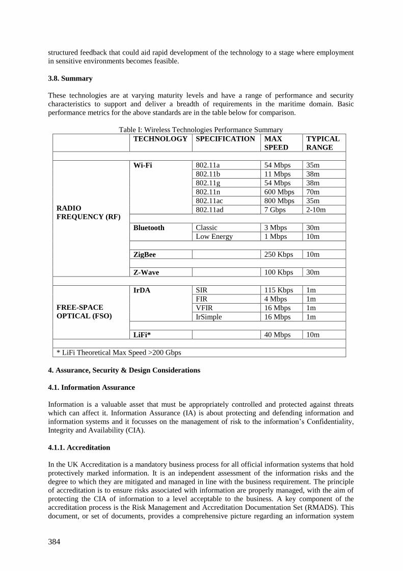
384
structured feedback that could aid rapid development of the technology to a stage where employment
in sensitive environments becomes feasible.
3.8. Summary
These technologies are at varying maturity levels and have a range of performance and security
characteristics to support and deliver a breadth of requirements in the maritime domain. Basic
performance metrics for the above standards are in the table below for comparison.
Table I: Wireless Technologies Performance Summary
TECHNOLOGY SPECIFICATION MAX
SPEED
TYPICAL
RANGE
RADIO
FREQUENCY (RF)
Wi-Fi 802.11a 54 Mbps 35m
802.11b 11 Mbps 38m
802.11g 54 Mbps 38m
802.11n 600 Mbps 70m
802.11ac 800 Mbps 35m
802.11ad 7 Gbps 2-10m
Bluetooth Classic 3 Mbps 30m
Low Energy 1 Mbps 10m
ZigBee 250 Kbps 10m
Z-Wave 100 Kbps 30m
FREE-SPACE
OPTICAL (FSO)
IrDA SIR 115 Kbps 1m
FIR 4 Mbps 1m
VFIR 16 Mbps 1m
IrSimple 16 Mbps 1m
LiFi* 40 Mbps 10m
* LiFi Theoretical Max Speed >200 Gbps
4. Assurance, Security & Design Considerations
4.1. Information Assurance
Information is a valuable asset that must be appropriately controlled and protected against threats
which can affect it. Information Assurance (IA) is about protecting and defending information and
information systems and it focusses on the management of risk to the information’s Confidentiality,
Integrity and Availability (CIA).
4.1.1. Accreditation
In the UK Accreditation is a mandatory business process for all official information systems that hold
protectively marked information. It is an independent assessment of the information risks and the
degree to which they are mitigated and managed in line with the business requirement. The principle
of accreditation is to ensure risks associated with information are properly managed, with the aim of
protecting the CIA of information to a level acceptable to the business. A key component of the
accreditation process is the Risk Management and Accreditation Documentation Set (RMADS). This
document, or set of documents, provides a comprehensive picture regarding an information system
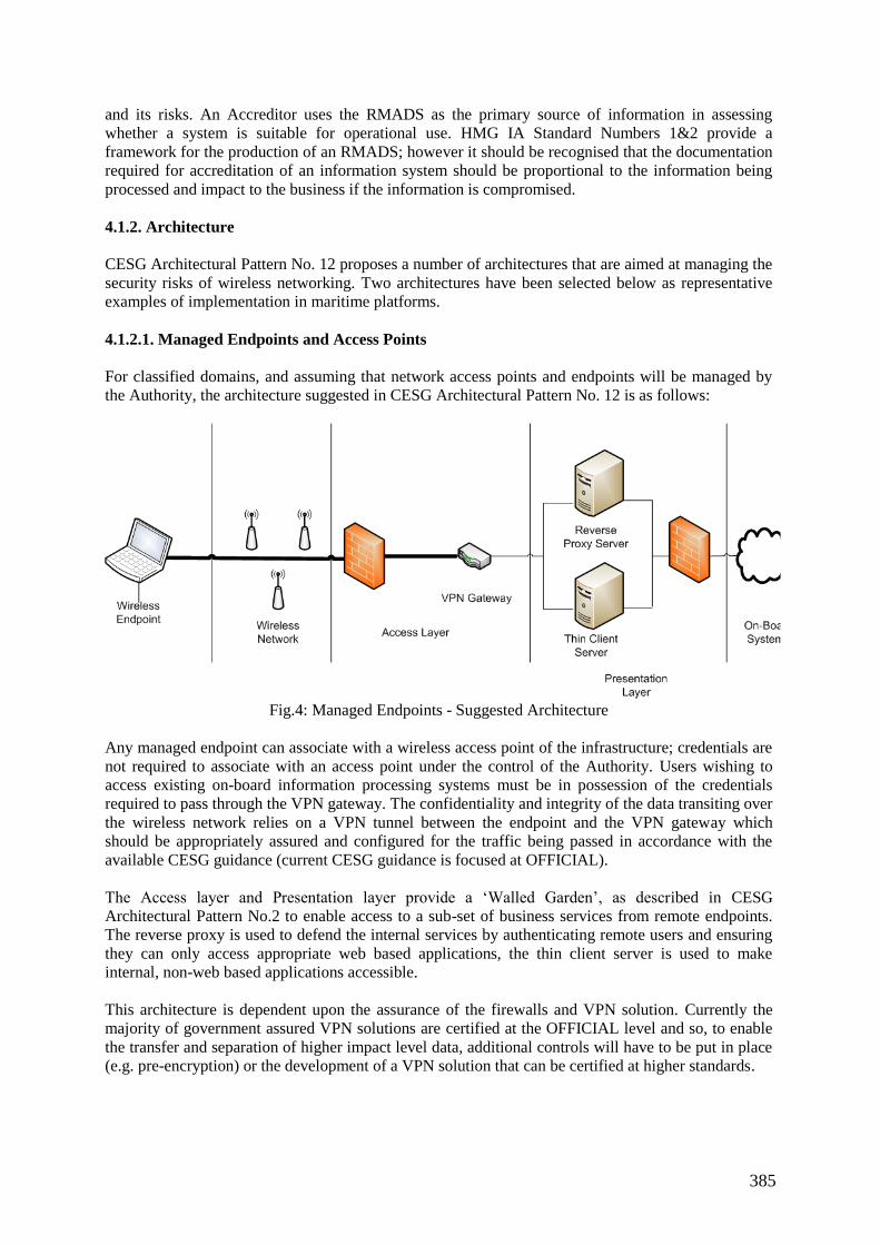
385
and its risks. An Accreditor uses the RMADS as the primary source of information in assessing
whether a system is suitable for operational use. HMG IA Standard Numbers 1&2 provide a
framework for the production of an RMADS; however it should be recognised that the documentation
required for accreditation of an information system should be proportional to the information being
processed and impact to the business if the information is compromised.
4.1.2. Architecture
CESG Architectural Pattern No. 12 proposes a number of architectures that are aimed at managing the
security risks of wireless networking. Two architectures have been selected below as representative
examples of implementation in maritime platforms.
4.1.2.1. Managed Endpoints and Access Points
For classified domains, and assuming that network access points and endpoints will be managed by
the Authority, the architecture suggested in CESG Architectural Pattern No. 12 is as follows:
Fig.4: Managed Endpoints - Suggested Architecture
Any managed endpoint can associate with a wireless access point of the infrastructure; credentials are
not required to associate with an access point under the control of the Authority. Users wishing to
access existing on-board information processing systems must be in possession of the credentials
required to pass through the VPN gateway. The confidentiality and integrity of the data transiting over
the wireless network relies on a VPN tunnel between the endpoint and the VPN gateway which
should be appropriately assured and configured for the traffic being passed in accordance with the
available CESG guidance (current CESG guidance is focused at OFFICIAL).
The Access layer and Presentation layer provide a ‘Walled Garden’, as described in CESG
Architectural Pattern No.2 to enable access to a sub-set of business services from remote endpoints.
The reverse proxy is used to defend the internal services by authenticating remote users and ensuring
they can only access appropriate web based applications, the thin client server is used to make
internal, non-web based applications accessible.
This architecture is dependent upon the assurance of the firewalls and VPN solution. Currently the
majority of government assured VPN solutions are certified at the OFFICIAL level and so, to enable
the transfer and separation of higher impact level data, additional controls will have to be put in place
(e.g. pre-encryption) or the development of a VPN solution that can be certified at higher standards.
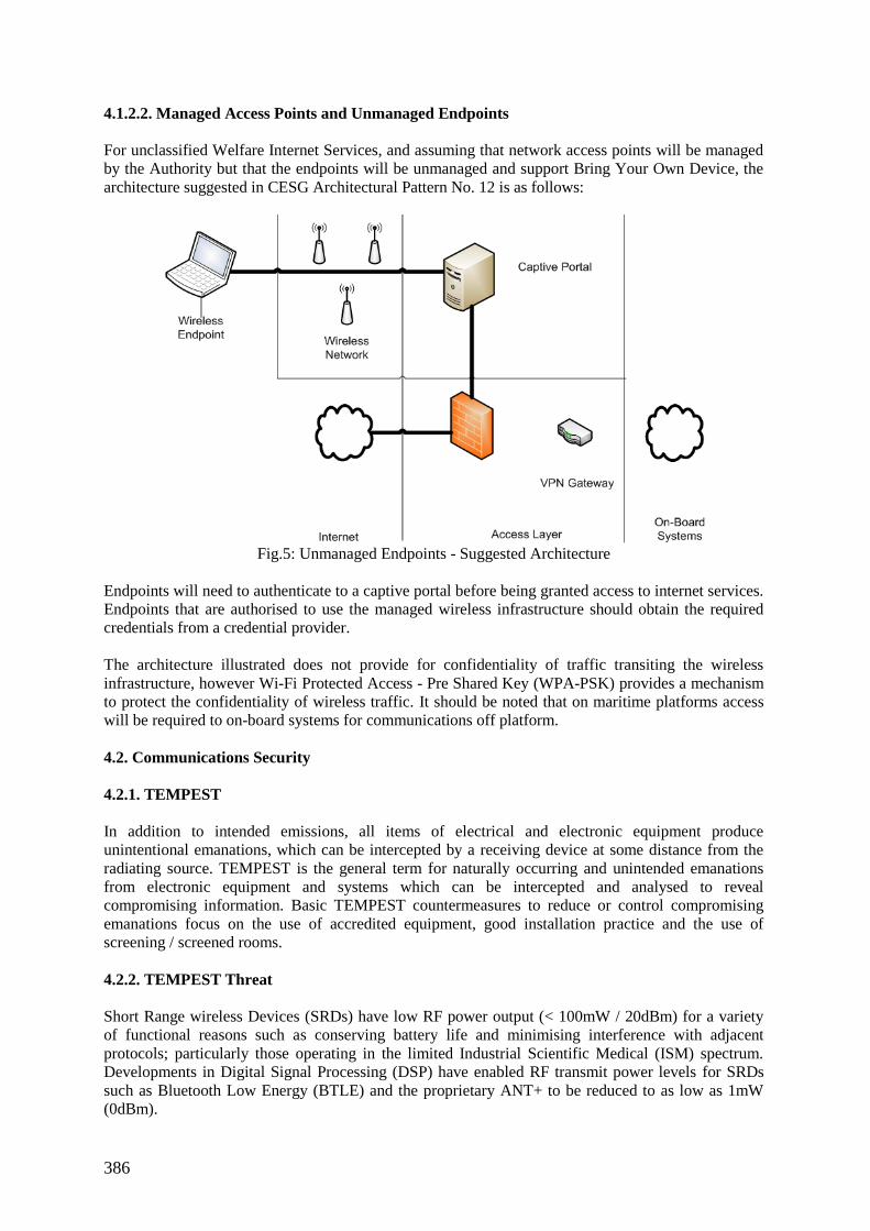
386
4.1.2.2. Managed Access Points and Unmanaged Endpoints
For unclassified Welfare Internet Services, and assuming that network access points will be managed
by the Authority but that the endpoints will be unmanaged and support Bring Your Own Device, the
architecture suggested in CESG Architectural Pattern No. 12 is as follows:
Fig.5: Unmanaged Endpoints - Suggested Architecture
Endpoints will need to authenticate to a captive portal before being granted access to internet services.
Endpoints that are authorised to use the managed wireless infrastructure should obtain the required
credentials from a credential provider.
The architecture illustrated does not provide for confidentiality of traffic transiting the wireless
infrastructure, however Wi-Fi Protected Access - Pre Shared Key (WPA-PSK) provides a mechanism
to protect the confidentiality of wireless traffic. It should be noted that on maritime platforms access
will be required to on-board systems for communications off platform.
4.2. Communications Security
4.2.1. TEMPEST
In addition to intended emissions, all items of electrical and electronic equipment produce
unintentional emanations, which can be intercepted by a receiving device at some distance from the
radiating source. TEMPEST is the general term for naturally occurring and unintended emanations
from electronic equipment and systems which can be intercepted and analysed to reveal
compromising information. Basic TEMPEST countermeasures to reduce or control compromising
emanations focus on the use of accredited equipment, good installation practice and the use of
screening / screened rooms.
4.2.2. TEMPEST Threat
Short Range wireless Devices (SRDs) have low RF power output (< 100mW / 20dBm) for a variety
of functional reasons such as conserving battery life and minimising interference with adjacent
protocols; particularly those operating in the limited Industrial Scientific Medical (ISM) spectrum.
Developments in Digital Signal Processing (DSP) have enabled RF transmit power levels for SRDs
such as Bluetooth Low Energy (BTLE) and the proprietary ANT+ to be reduced to as low as 1mW
(0dBm).
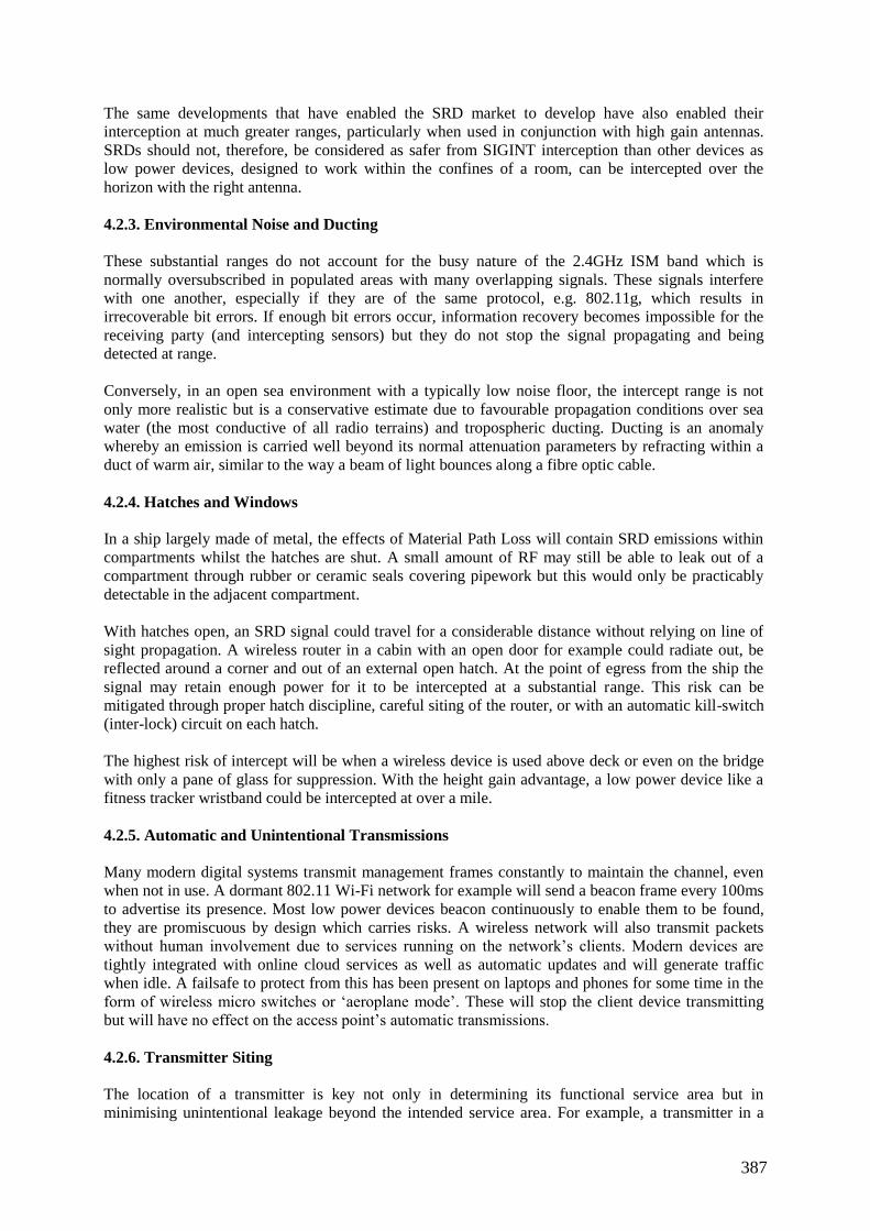
387
The same developments that have enabled the SRD market to develop have also enabled their
interception at much greater ranges, particularly when used in conjunction with high gain antennas.
SRDs should not, therefore, be considered as safer from SIGINT interception than other devices as
low power devices, designed to work within the confines of a room, can be intercepted over the
horizon with the right antenna.
4.2.3. Environmental Noise and Ducting
These substantial ranges do not account for the busy nature of the 2.4GHz ISM band which is
normally oversubscribed in populated areas with many overlapping signals. These signals interfere
with one another, especially if they are of the same protocol, e.g. 802.11g, which results in
irrecoverable bit errors. If enough bit errors occur, information recovery becomes impossible for the
receiving party (and intercepting sensors) but they do not stop the signal propagating and being
detected at range.
Conversely, in an open sea environment with a typically low noise floor, the intercept range is not
only more realistic but is a conservative estimate due to favourable propagation conditions over sea
water (the most conductive of all radio terrains) and tropospheric ducting. Ducting is an anomaly
whereby an emission is carried well beyond its normal attenuation parameters by refracting within a
duct of warm air, similar to the way a beam of light bounces along a fibre optic cable.
4.2.4. Hatches and Windows
In a ship largely made of metal, the effects of Material Path Loss will contain SRD emissions within
compartments whilst the hatches are shut. A small amount of RF may still be able to leak out of a
compartment through rubber or ceramic seals covering pipework but this would only be practicably
detectable in the adjacent compartment.
With hatches open, an SRD signal could travel for a considerable distance without relying on line of
sight propagation. A wireless router in a cabin with an open door for example could radiate out, be
reflected around a corner and out of an external open hatch. At the point of egress from the ship the
signal may retain enough power for it to be intercepted at a substantial range. This risk can be
mitigated through proper hatch discipline, careful siting of the router, or with an automatic kill-switch
(inter-lock) circuit on each hatch.
The highest risk of intercept will be when a wireless device is used above deck or even on the bridge
with only a pane of glass for suppression. With the height gain advantage, a low power device like a
fitness tracker wristband could be intercepted at over a mile.
4.2.5. Automatic and Unintentional Transmissions
Many modern digital systems transmit management frames constantly to maintain the channel, even
when not in use. A dormant 802.11 Wi-Fi network for example will send a beacon frame every 100ms
to advertise its presence. Most low power devices beacon continuously to enable them to be found,
they are promiscuous by design which carries risks. A wireless network will also transmit packets
without human involvement due to services running on the network’s clients. Modern devices are
tightly integrated with online cloud services as well as automatic updates and will generate traffic
when idle. A failsafe to protect from this has been present on laptops and phones for some time in the
form of wireless micro switches or ‘aeroplane mode’. These will stop the client device transmitting
but will have no effect on the access point’s automatic transmissions.
4.2.6. Transmitter Siting
The location of a transmitter is key not only in determining its functional service area but in
minimising unintentional leakage beyond the intended service area. For example, a transmitter in a
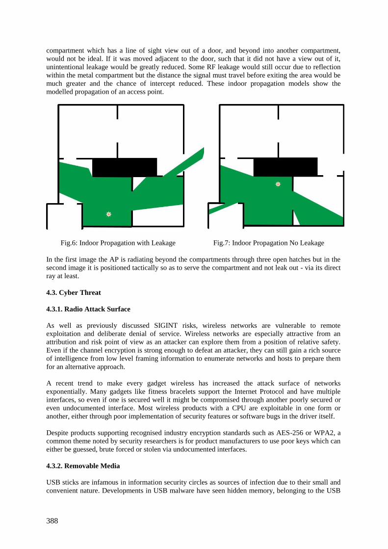
388
compartment which has a line of sight view out of a door, and beyond into another compartment,
would not be ideal. If it was moved adjacent to the door, such that it did not have a view out of it,
unintentional leakage would be greatly reduced. Some RF leakage would still occur due to reflection
within the metal compartment but the distance the signal must travel before exiting the area would be
much greater and the chance of intercept reduced. These indoor propagation models show the
modelled propagation of an access point.
Fig.6: Indoor Propagation with Leakage Fig.7: Indoor Propagation No Leakage
In the first image the AP is radiating beyond the compartments through three open hatches but in the
second image it is positioned tactically so as to serve the compartment and not leak out - via its direct
ray at least.
4.3. Cyber Threat
4.3.1. Radio Attack Surface
As well as previously discussed SIGINT risks, wireless networks are vulnerable to remote
exploitation and deliberate denial of service. Wireless networks are especially attractive from an
attribution and risk point of view as an attacker can explore them from a position of relative safety.
Even if the channel encryption is strong enough to defeat an attacker, they can still gain a rich source
of intelligence from low level framing information to enumerate networks and hosts to prepare them
for an alternative approach.
A recent trend to make every gadget wireless has increased the attack surface of networks
exponentially. Many gadgets like fitness bracelets support the Internet Protocol and have multiple
interfaces, so even if one is secured well it might be compromised through another poorly secured or
even undocumented interface. Most wireless products with a CPU are exploitable in one form or
another, either through poor implementation of security features or software bugs in the driver itself.
Despite products supporting recognised industry encryption standards such as AES-256 or WPA2, a
common theme noted by security researchers is for product manufacturers to use poor keys which can
either be guessed, brute forced or stolen via undocumented interfaces.
4.3.2. Removable Media
USB sticks are infamous in information security circles as sources of infection due to their small and
convenient nature. Developments in USB malware have seen hidden memory, belonging to the USB
389
stick’s own controller, used to store and deliver malware which cannot be detected or erased via
conventional methods, including full disk formatting of the stick. Mobile devices including phones,
wearables and media players are increasingly dangerous as many charge from a 500mA USB port as
standard (as well as being powerful computers in their own right). Despite not being permitted, their
owner’s will eventually give in to human nature and charge them discretely from the nearest available
USB port, even if that belongs to a classified system.
4.3.3. Bypassing USB Restrictions
Many secure hosts have USB disabled in the BIOS by policy. Some may accept only pre-approved
whitelisted devices for commercial or security reasons. A whitelist for a USB device will use its
idVendor and idProduct fields; however, these can be spoofed to bypass restrictions.
A single USB gadget can have multiple interfaces which it can present to the host; this is how a
smartphone is able to be reconfigured to perform multiple roles over a single USB interface. This
principle has been exploited by penetration testers to make a benign USB device appear to the host
computer as a trusted Human Interface Device (HID), such as a whitelisted keyboard from an
approved vendor. The fake ‘virtual’ keyboard can then issue keystrokes from a script, despite USB
whitelisting, and then re-role as a (trusted) USB storage device to receive the stolen data.
Any USB powered device, no matter how innocuous or basic is a threat.
4.3.4. Dormant Wireless Bridges
Classified computers do not historically have active wireless interfaces but do, increasingly, have
dormant adaptors on their circuit boards. These can be disabled at the hardware level by interfering
with the circuitry. However, this is made increasingly difficult due to miniaturisation and is thus
typically software disabled in a restricted menu like the BIOS. Any configuration change such as this
is not guaranteed to persist after software/firmware updates, or an unexpected power/memory failure.
Hence, there is a very real risk that a disabled (and accredited) wireless interface may become active
again in the future and expose the host to attack. Avoiding software updates as a strategy to protect
tightly configured secure networks is not recommended for obvious reasons.
4.3.5. Supply Chain
In a world of white labelled electronics where most vendors use common black-box components,
supply chain security is a huge problem. A secure system may be built by a contractor who employs a
sub-contractor who cuts corners and introduces counterfeit electronics into the supply chain; a largely
accidental problem, driven by a desire to maximise profit through cheap components where possible.
The risk to availability caused by counterfeit electronics is obvious, but if the weakness is known by
an adversary it could be remotely triggered. In the case of fake components in a US helicopter
programme, this could have allowed an adversary to blind a helicopter’s night optics permanently.
A greater concern is where hidden functionality is deliberately introduced into the supply chain. This
concern can be mitigated through very thorough and laborious reverse engineering, but the nature and
pace of modern technology means that code and computer chips are being minted faster than they can
be practically reviewed. There is a genuine risk that a computer chip on a secure computer may
contain a backdoor.
4.3.6. Software Bugs and Backdoors
On average, software applications have 10-20 bugs per 1000 lines of code. If a wireless device’s
circuit board is composed of a third party core, a network controller and a Digital Signal processor
(DSP) chip, with a total of 10,000 lines of code in their (proprietary) firmware, there will be at least
100 bugs before the manufacturer’s firmware is added on top. Most will be benign but some, when
390
triggered, could result in a denial of service or arbitrary code execution. A backdoor doesn’t have to
be a secret password or additional code; it could be a very subtle engineered vulnerability such as a
lack of bounds checking on an input buffer.
4.3.7. Insider Threat
The human is the weakest link in computer and network security. It must be accepted that there is
always a risk that a trusted individual will interfere with or exploit a (wireless) network for a variety
of reasons. Insider threat is defined as the risk of attacks to or security breaches of an organisation or
system from people within it. These could be permanent or temporary employees or even part of the
supply chain, but people who generally have access to critical systems, assets and information. Insider
attacks or breaches are complex events, influenced by a number of psychological and socio-cultural
drivers, which may be triggered by individuals with malicious intent or as an unintended consequence
of their actions.
The malicious insider is a real and prevalent threat and their deeper knowledge of the organisation's
systems allows them to better exploit known weaknesses and act 'under the radar' for longer periods of
time. Unfortunately, many industries do not have an insider threat programme in place and are
critically under-prepared for dealing with the threat. Similarly, there is too often a drive to solve the
issue purely with technology, when a more holistic approach that focusses on understanding the
human psychology and behaviour that underpins it is much more appropriate.
Unintentional insider threat is defined by harm to an organisation that is conducted or facilitated by an
unwilling, unknowing and non-malicious employee. Unintentional insider threat relates much more
closely to human error than it does to malicious behaviour. Whereas malicious behaviour is clearly
the fault of the person doing it, human error must be treated as an inherent human condition and
therefore not always the fault of the human. This can be mitigated through better system and
organisational design that supports the human in the system. Dealing with malicious and unintentional
insider threat in different ways shows an added appreciation and understanding of the risk and avoids
an inadequate ‘one size fits all' solution being rolled out.
The greatest risk to wireless networks comes from the unintentional insider threat and can take many
forms, including:
Unauthorised devices introduced onto the network (such as USB memory sticks, mobile
phones and smart jewellery) allow a malicious application to survey, intercept and exploit
local wireless networks, without the knowledge of the device’s owner.
Network security keys and certificates are compromised by the loss of a client device, such as
a tablet or laptop.
A confined signal could be unintentionally leaked out above deck, leading to unintended
interception and exploitation.
4.4. Electromagnetic Compatibility
Electromagnetic Compatibility is the ability of a device, equipment or system to function
satisfactorily in its intended operational electromagnetic environment without adversely affecting
anything else in that electromagnetic environment. It should also be able to operate without
intolerable electromagnetic disturbances, degradation of performance or malfunction. This is best
achieved by equipment being designed and built to meet a pre-determined electromagnetic
environment.
A major concern with introducing new wireless technologies in to a sensitive environment is EMC
and harmony with international and MoD allocated spectrum, as well as other technology already on-
board the platform such as SCADA devices. The EMC characteristics specific to individual wireless
391
standards vary but, in general, co-located wireless networks should be on different channels separated
by a guard channel to avoid interference. For 802.11, a channel has an overlap of 2 channels either
side.
5. Summary
5.1. Wireless Technologies
A broad range of wireless options were considered from across the electromagnetic spectrum,
including the traditional Radio Frequency based technologies, such as Wi-Fi and Bluetooth, and those
operating in the Infrared, Visible Light and Ultraviolet bands. Ultraviolet was discounted immediately
as there are no developments for short range networks. Laser communications were considered
initially due to previous implementations in campus network solutions, however these devices are no
longer available and current developments are focused on space communications.
The remainder (Wi-Fi, Bluetooth, ZigBee, Z-Wave, IrDA and LiFi) were considered to have potential
utility in the maritime domain either now or in the future. The technologies are at varying maturity
levels and have a range of performance and security characteristics to support and deliver a breadth of
requirements in the maritime domain.
5.2. Accreditation
Accreditation is a mandatory business process for all information systems that hold protectively
marked information. It is an independent assessment of the information risks and the degree to which
they are mitigated and managed in line with the business requirement. The principle of accreditation
is to ensure risks associated with information are properly managed, with the aim of protecting the
Confidentiality, Integrity and Availability (CIA) of information to a level acceptable to the business.
A key component of the accreditation process is the Risk Management and Accreditation
Documentation Set (RMADS). This document, or set of documents, provides a comprehensive picture
regarding an information system and its risks. An Accreditor uses the RMADS as the primary source
of information in the assessment as to whether a system is suitable for operational use. Identification
of information assets is fundamental to successful assurance; without understanding the information,
the risks to the information cannot be assessed and nor can the impact to the business of any
compromise. Without an understanding of the risk inappropriate controls could be implemented either
leaving vulnerabilities that could be exploited or, conversely overkill which would waste time and
resource.
5.3. TEMPEST
Basic TEMPEST countermeasures to reduce or control compromising emanations focus on the use of
accredited equipment, good installation practice and the use of screening / screened rooms. However,
modern technology enables the interception of relatively low power signals at significant ranges and
environmental noise, platform structure, transmitter siting and automatic / unintentional network
transmissions will all be important design considerations for future wireless projects.
5.4. Cyber Threat
In addition to SIGINT risks, wireless networks are also vulnerable to remote exploitation and
deliberate denial of service. Wireless computer networks are especially attractive from an attribution
and risk point of view as an attacker can explore networks from a position of relative safety. Even if
the channel encryption is strong enough to defeat an attacker, they can still gain a rich source of
intelligence from low level framing information to enumerate networks and hosts to prepare them for
an alternative approach. Removable media, software vulnerabilities, dormant wireless bridges and
supply chain weaknesses are all important considerations in threat assessment and design.
392
5.5. Insider Threat
The human is the weakest link in computer and network security and insider threat is defined as the
risk of attacks to or security breaches of an organisation or system from people within it. Insider
attacks or breaches are complex events, influenced by a number of psychological and socio-cultural
drivers, which may be triggered by individuals with malicious intent or as an unintended consequence
of their actions. The greatest risk to wireless networks comes from the unintentional insider threat and
can take many forms; unauthorised devices being introduced onto the network, network security keys
and certificates being compromised by the loss of a client device or a confined signal being
unintentionally leaked out above deck, leading to unintended interception and exploitation.
5.6. Electromagnetic Compatibility
A major concern with introducing new wireless technologies in to a sensitive environment is EMC
and harmony with international and government allocated spectrum as well as other technology
already on-board the platform such as SCADA devices. This is best achieved by equipment being
designed and built to meet a pre-determined electromagnetic environment.
References
HMG IA Standard 1&2 – Information Risk Management (08 Aug 2015)
HMG IA Standard 4 – Management of Cryptographic Systems (Oct 2013)
CESG Architectural Pattern No.2 – Walled Gardens for Remote Access (08 Aug 2016)
CESG Architectural Pattern No.12 – Wireless Networking (08 Aug 2016)
CESG Good Practice Guide No. 13 – Protective Monitoring for HMG ICT Systems (08 Aug 2016)
CESG Good Practice Guide 14 – Electromagnetic Security (08 Aug 2016)
CESG IA Implementation Guide 14 – TEMPEST and Electromagnetic Security (01 Aug 2016)
JSP 440 – Defence Manual of Security
JSP 604 – Defence Manual of Information and Communications Technology (20 Jun 2016)
BLUETOOTH SIG REGULATORY COMMITTEE, Bluetooth Core Specification V4, (30 Jun 2010)
BLUETOOTH SIG REGULATORY COMMITTEE, Bluetooth Low Energy Regulatory Aspects,
(Apr 2011)
NIST Special Publication 800-121, Guide to Bluetooth Security Rev 1 (Jun 2012)
Vishay Semiconductors, Ambient Light and Electromagnetic Interference, (20 Sep 2006)
ADEE, S. (2009), Ultraviolet Radios Beam to Life, IEEE Spectrum
EDDY, M. (2013), Android Remote Access Trojan AndroRAT is Cheaper and More Dangerous Than
Ever, PC Mag
FARRANT, A. (2016), Binary SMS - The old backdoor to your new thing, Context IS
FARRANT, A. (2015), Wireless Gridlock in the IOT, Context IS

393
HAATAJA, K.M.J, (2006), Security in Bluetooth, WLAN and IrDA: a comparison, University of
Kuopio
LESTER, S. (2015), The Emergence of Bluetooth Low Energy, Context IS
MAYNARD, J. (2014), Is X-Ray the Future of Communication and Navigation in Space?, James
Tech Times
PERSSON, K.E., (2009), A Protocol Suite For Wireless Personal Area Networks, University of
Kentucky Doctoral Dissertations
RODRÍGUEZ CRUZ, R.O.; SANTOS VÁZQUEZ, C.L. (2009), Ultraviolet Communication,
Bayamon Faculty
WILLNER, A.E. (2016), Twisted Light Could Dramatically Boost Data Rates, IEEE Spectrum
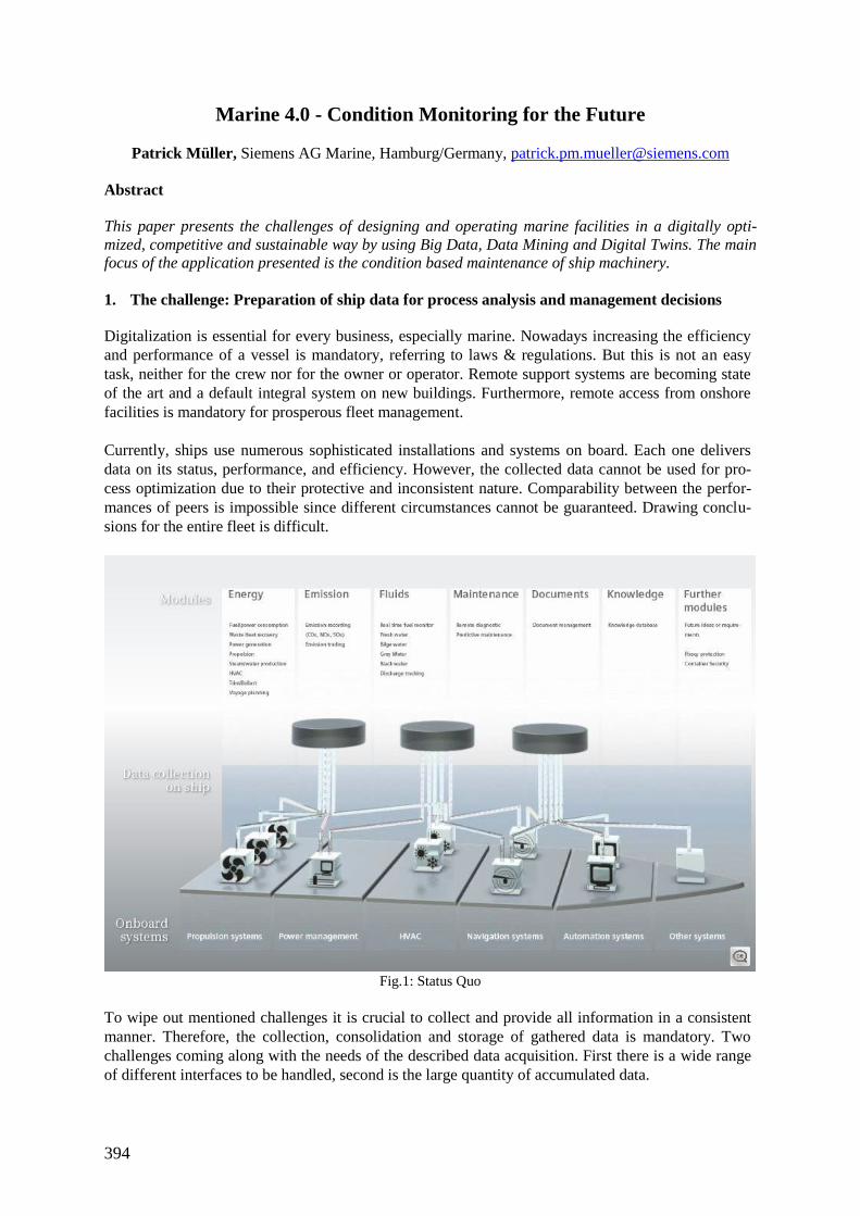
394
Marine 4.0 - Condition Monitoring for the Future
Patrick Müller, Siemens AG Marine, Hamburg/Germany, [email protected]
Abstract
This paper presents the challenges of designing and operating marine facilities in a digitally opti-
mized, competitive and sustainable way by using Big Data, Data Mining and Digital Twins. The main
focus of the application presented is the condition based maintenance of ship machinery.
1. The challenge: Preparation of ship data for process analysis and management decisions
Digitalization is essential for every business, especially marine. Nowadays increasing the efficiency
and performance of a vessel is mandatory, referring to laws & regulations. But this is not an easy
task, neither for the crew nor for the owner or operator. Remote support systems are becoming state
of the art and a default integral system on new buildings. Furthermore, remote access from onshore
facilities is mandatory for prosperous fleet management.
Currently, ships use numerous sophisticated installations and systems on board. Each one delivers
data on its status, performance, and efficiency. However, the collected data cannot be used for pro-
cess optimization due to their protective and inconsistent nature. Comparability between the perfor-
mances of peers is impossible since different circumstances cannot be guaranteed. Drawing conclu-
sions for the entire fleet is difficult.
Fig.1: Status Quo
To wipe out mentioned challenges it is crucial to collect and provide all information in a consistent
manner. Therefore, the collection, consolidation and storage of gathered data is mandatory. Two
challenges coming along with the needs of the described data acquisition. First there is a wide range
of different interfaces to be handled, second is the large quantity of accumulated data.
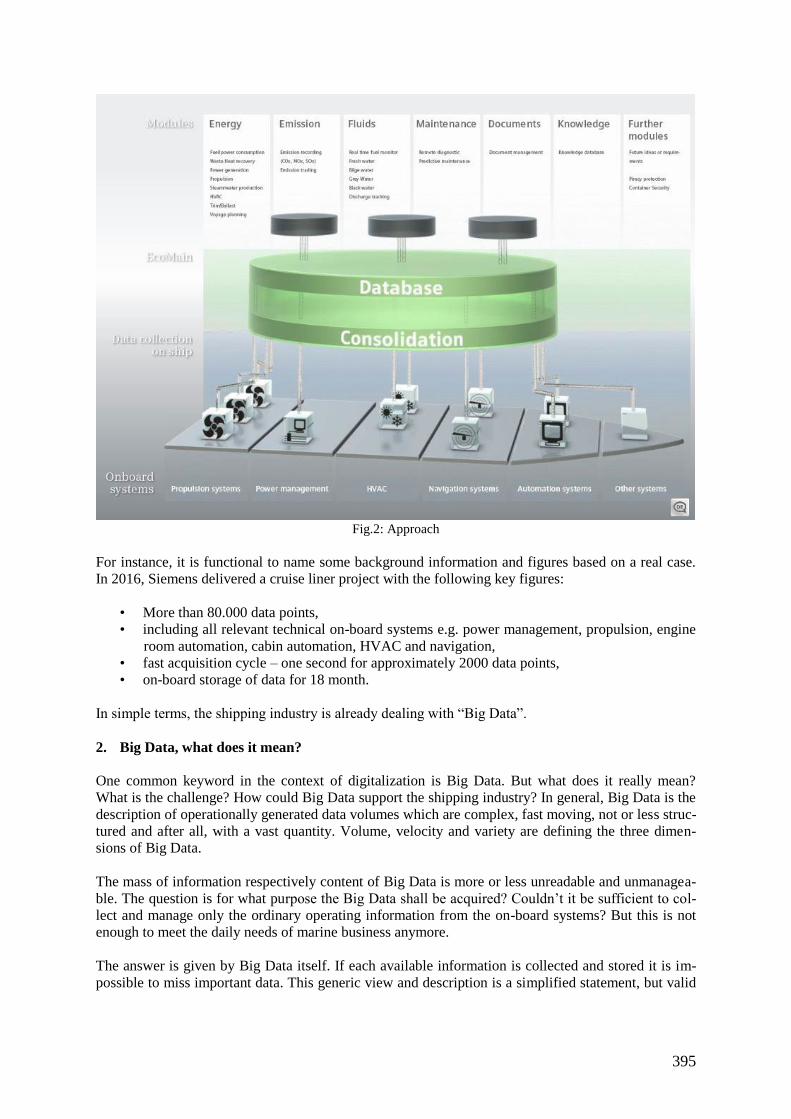
395
Fig.2: Approach
For instance, it is functional to name some background information and figures based on a real case.
In 2016, Siemens delivered a cruise liner project with the following key figures:
• More than 80.000 data points,
• including all relevant technical on-board systems e.g. power management, propulsion, engine
room automation, cabin automation, HVAC and navigation,
• fast acquisition cycle – one second for approximately 2000 data points,
• on-board storage of data for 18 month.
In simple terms, the shipping industry is already dealing with “Big Data”.
2. Big Data, what does it mean?
One common keyword in the context of digitalization is Big Data. But what does it really mean?
What is the challenge? How could Big Data support the shipping industry? In general, Big Data is the
description of operationally generated data volumes which are complex, fast moving, not or less struc-
tured and after all, with a vast quantity. Volume, velocity and variety are defining the three dimen-
sions of Big Data.
The mass of information respectively content of Big Data is more or less unreadable and unmanagea-
ble. The question is for what purpose the Big Data shall be acquired? Couldn’t it be sufficient to col-
lect and manage only the ordinary operating information from the on-board systems? But this is not
enough to meet the daily needs of marine business anymore.
The answer is given by Big Data itself. If each available information is collected and stored it is im-
possible to miss important data. This generic view and description is a simplified statement, but valid

396
for the industry and especially for the shipping industry in terms of the challenging environment of
marine business.
Fig.3: Big Data, where is the information?
3. Data Mining – How to extract useful information from Big Data
The huge variety of different data sources requires algorithms in order to fulfil the tasks humans are
not able to. These tools and methods automatically handle large quantities of data to extract previous-
ly unknown patterns and are known under the term “Data Mining”. Neither the data collection or the
data preparation, nor the result interpretation and reporting are parts of the Data Mining step. Addi-
tional applications are necessary to process the data towards the operators.
Fig.4: Data Mining - Finding the information you need
4. “Digital Twin”, the virtual asset
Another vital keyword in this context is Digital Twin. Generally, the naming itself, explains its func-
tion. The Digital Twin is a virtual copy of a real asset. This includes all mechanical and electrical
construction data, as well as its physical behavior. In addition, environmental conditions which are
subsequently added to the Digital Twin influence its behavior. To build up a complex ecosystem like
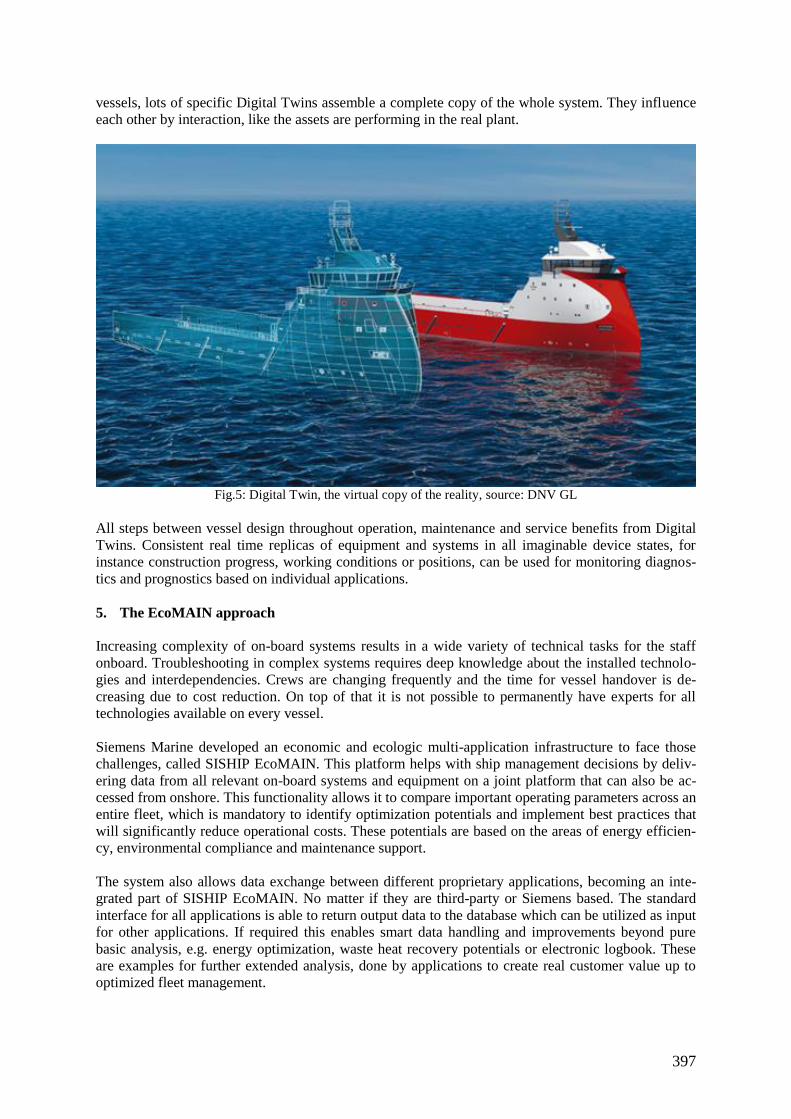
397
vessels, lots of specific Digital Twins assemble a complete copy of the whole system. They influence
each other by interaction, like the assets are performing in the real plant.
Fig.5: Digital Twin, the virtual copy of the reality, source: DNV GL
All steps between vessel design throughout operation, maintenance and service benefits from Digital
Twins. Consistent real time replicas of equipment and systems in all imaginable device states, for
instance construction progress, working conditions or positions, can be used for monitoring diagnos-
tics and prognostics based on individual applications.
5. The EcoMAIN approach
Increasing complexity of on-board systems results in a wide variety of technical tasks for the staff
onboard. Troubleshooting in complex systems requires deep knowledge about the installed technolo-
gies and interdependencies. Crews are changing frequently and the time for vessel handover is de-
creasing due to cost reduction. On top of that it is not possible to permanently have experts for all
technologies available on every vessel.
Siemens Marine developed an economic and ecologic multi-application infrastructure to face those
challenges, called SISHIP EcoMAIN. This platform helps with ship management decisions by deliv-
ering data from all relevant on-board systems and equipment on a joint platform that can also be ac-
cessed from onshore. This functionality allows it to compare important operating parameters across an
entire fleet, which is mandatory to identify optimization potentials and implement best practices that
will significantly reduce operational costs. These potentials are based on the areas of energy efficien-
cy, environmental compliance and maintenance support.
The system also allows data exchange between different proprietary applications, becoming an inte-
grated part of SISHIP EcoMAIN. No matter if they are third-party or Siemens based. The standard
interface for all applications is able to return output data to the database which can be utilized as input
for other applications. If required this enables smart data handling and improvements beyond pure
basic analysis, e.g. energy optimization, waste heat recovery potentials or electronic logbook. These
are examples for further extended analysis, done by applications to create real customer value up to
optimized fleet management.
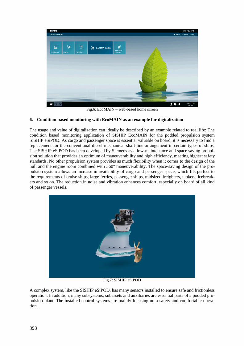
398
Fig.6: EcoMAIN – web-based home screen
6. Condition based monitoring with EcoMAIN as an example for digitalization
The usage and value of digitalization can ideally be described by an example related to real life: The
condition based monitoring application of SISHIP EcoMAIN for the podded propulsion system
SISHIP eSiPOD. As cargo and passenger space is essential valuable on board, it is necessary to find a
replacement for the conventional diesel-mechanical shaft line arrangement in certain types of ships.
The SISHIP eSiPOD has been developed by Siemens as a low-maintenance and space saving propul-
sion solution that provides an optimum of maneuverability and high efficiency, meeting highest safety
standards. No other propulsion system provides as much flexibility when it comes to the design of the
hull and the engine room combined with 360° maneuverability. The space-saving design of the pro-
pulsion system allows an increase in availability of cargo and passenger space, which fits perfect to
the requirements of cruise ships, large ferries, passenger ships, midsized freighters, tankers, icebreak-
ers and so on. The reduction in noise and vibration enhances comfort, especially on board of all kind
of passenger vessels.
Fig.7: SISHIP eSiPOD
A complex system, like the SISHIP eSiPOD, has many sensors installed to ensure safe and frictionless
operation. In addition, many subsystems, subassets and auxiliaries are essential parts of a podded pro-
pulsion plant. The installed control systems are mainly focusing on a safety and comfortable opera-
tion.
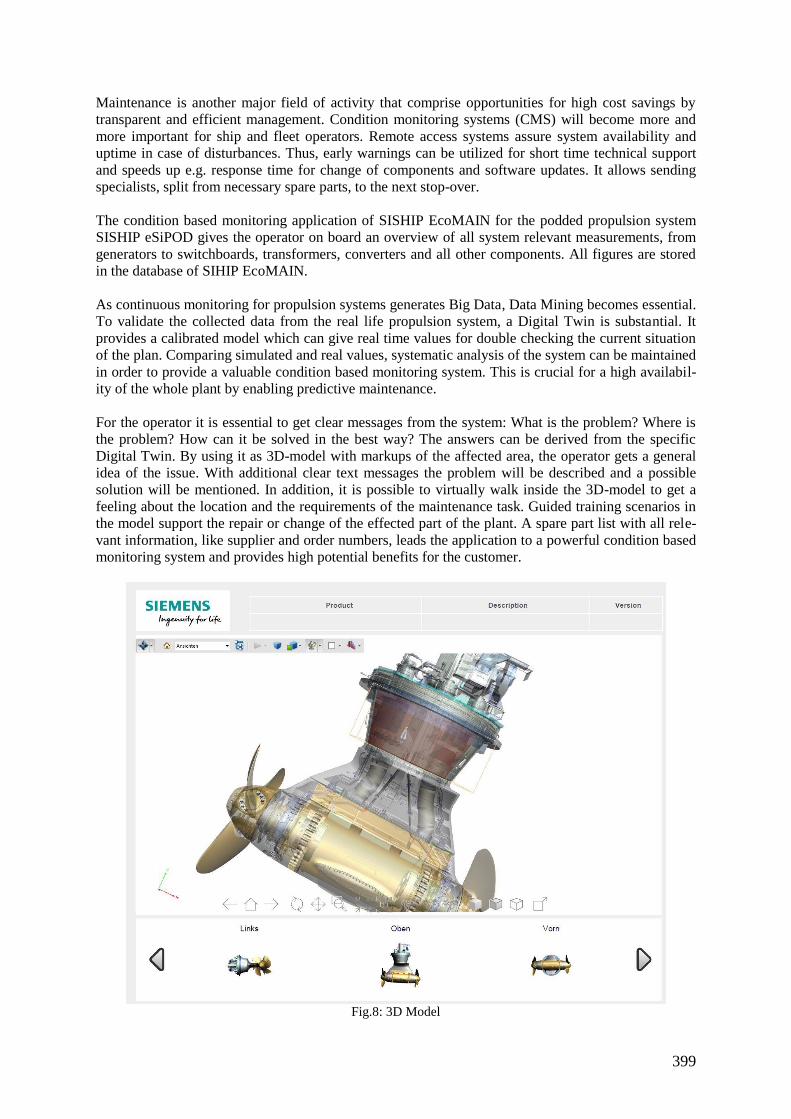
399
Maintenance is another major field of activity that comprise opportunities for high cost savings by
transparent and efficient management. Condition monitoring systems (CMS) will become more and
more important for ship and fleet operators. Remote access systems assure system availability and
uptime in case of disturbances. Thus, early warnings can be utilized for short time technical support
and speeds up e.g. response time for change of components and software updates. It allows sending
specialists, split from necessary spare parts, to the next stop-over.
The condition based monitoring application of SISHIP EcoMAIN for the podded propulsion system
SISHIP eSiPOD gives the operator on board an overview of all system relevant measurements, from
generators to switchboards, transformers, converters and all other components. All figures are stored
in the database of SIHIP EcoMAIN.
As continuous monitoring for propulsion systems generates Big Data, Data Mining becomes essential.
To validate the collected data from the real life propulsion system, a Digital Twin is substantial. It
provides a calibrated model which can give real time values for double checking the current situation
of the plan. Comparing simulated and real values, systematic analysis of the system can be maintained
in order to provide a valuable condition based monitoring system. This is crucial for a high availabil-
ity of the whole plant by enabling predictive maintenance.
For the operator it is essential to get clear messages from the system: What is the problem? Where is
the problem? How can it be solved in the best way? The answers can be derived from the specific
Digital Twin. By using it as 3D-model with markups of the affected area, the operator gets a general
idea of the issue. With additional clear text messages the problem will be described and a possible
solution will be mentioned. In addition, it is possible to virtually walk inside the 3D-model to get a
feeling about the location and the requirements of the maintenance task. Guided training scenarios in
the model support the repair or change of the effected part of the plant. A spare part list with all rele-
vant information, like supplier and order numbers, leads the application to a powerful condition based
monitoring system and provides high potential benefits for the customer.
Fig.8: 3D Model

400
The established CBM mechanism could be extended to the entire vessel. Due to this SISHIP Eco-
MAIN lays the foundation for efficient ship management on-board and supports green fleet manage-
ment over the entire fleet.
7. Conclusion
Together with the increasing digitalization of the whole vessel with more complex and higher sophis-
ticated equipment, like podded drives, the future of marine will go digital with the approach of all-
electric ships. Such solutions require incorporation of digital engineering over the whole lifecycle:
from design to construction to operation including training, maintenance and service – all over the
whole life cycle. Siemens is prepared for this by providing the fitting systems and solutions.
401
Generic Control Strategy
for Future Autonomous Ship Operations
Martin Kurowski, University of Rostock, Rostock/Germany, [email protected]
Agnes U. Schubert, MATNAV e.V., Rostock/Germany, [email protected] Torsten Jeinsch, University of Rostock, Rostock/Germany, [email protected]
Abstract
This paper describes a generic concept to control diverse marine vehicles. The approach is based on a
hybrid model of the vehicle motion while transiting, manoeuvring or station keeping mode, consisting
of modules of the propulsion and steering gears, the vessel dynamics as well as the disturbances. The
hybrid scheme was refined further by generalisation of the transition between two motion states within
one mode and between distinguished modes. The hybrid control structure is composed of the
feedforward and feedback control including allocation corresponding to the active model. The strategy
was applied to different marine vehicles; an ocean-going unmanned surface vehicle (USV) and a ferry
model in a ship handling simulator. The developed control structure belongs to the first results of the
cooperative project ‘GALILEOnautic’. By using satellite-based navigation and sensor data fusion, the
project contributes important tools for assisting safer and more efficient ship operations especially in
limited fairways with the vision to autonomous shipping.
1. Introduction
The maritime sector is facing substantial technological changes. Due to the ongoing globalisation, maritime trade is steadily growing despite the fluctuating sales of the oil and gas industry as well as of the shipbuilding sector. Besides that, the ship traffic is growing because of the increasing offshore activities. The key drivers are the alternative energy industry, especially by expanding offshore wind farms, and the exploiting new mineral deposits in the deep sea. The result is a higher traffic volume in harbours or narrow waterways with equivalent higher coordination effort. Additionally, the technological progress in the shipbuilding industry causes increasing size of vessels and operative changes such as fairway and passing limitations. Significant disturbances as wind, current or fog enhance the risk of collision or other hazardous situations. Statistics show that the number of accidents rises and therewith in principal the costs within the shipping industry. The largest percentage of accidents (75 - 96 %), was due to human failure including vehicle loss, collision or grounding, Fields (2012). The majority of these accidents could avoid by application of assistance systems in the nautical decision making process, Porretta et al. (2016). The subjects of recent research projects focus on unmanned ships to demonstrate the feasibility by application of common technologies, Burmeister et al. (2014). Primary, the transiting motion mode is investigated because the established methods of automatic control offers sufficient control quality in this speed range and there is enough space to solve encounter situations. However, the automatic manoeuvring is excluded in limited and safety-critical areas. Optionally, the unmanned vehicles will be remotely operated by land-based radio or satellite communication systems, Levander (2017). But, the autonomous systems are the future topic in all fields of global mobility. The investigations include assistance systems, innovative sensors and environment recognition systems, as well as a progressive digital interlinking to develop the basic infrastructure of safe and effective autonomous transport. 2. Problem formulation and related works
The joint project ‘GALILEOnautic’ especially aims to develop control systems for fully automated vessels cooperating with each other in areas with high safety and efficiency requirements, such as harbours, harbour entrances or narrow waterways. The particular institutions compile methods to coordinate autonomous vessels centrally as well as to ensure a safe automatic or closed-loop control of the vessels in different operation modes, also in error cases. The complete system includes modules for
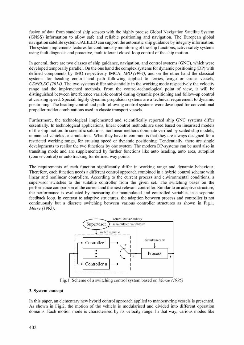
402
fusion of data from standard ship sensors with the highly precise Global Navigation Satellite System (GNSS) information to allow safe and reliable positioning and navigation. The European global navigation satellite system GALILEO can support the automatic ship guidance by integrity information. The system implements features for continuously monitoring of the ship functions, active safety systems using fault diagnosis and proactive, fault-tolerant closed-loop control of the ship motion. In general, there are two classes of ship guidance, navigation, and control systems (GNC), which were developed temporally parallel. On the one hand the complex systems for dynamic positioning (DP) with defined components by IMO respectively IMCA, IMO (1994), and on the other hand the classical systems for heading control and path following applied to ferries, cargo or cruise vessels, CENELEC (2014). The two systems differ substantially in the working mode respectively the velocity range and the implemented methods. From the control-technological point of view, it will be distinguished between interference variable control during dynamic positioning and follow-up control at cruising speed. Special, highly dynamic propulsion systems are a technical requirement to dynamic positioning. The heading control and path following control systems were developed for conventional propeller rudder combinations used in classic transport vessels. Furthermore, the technological implemented and scientifically reported ship GNC systems differ essentially. In technological applications, linear control methods are used based on linearised models of the ship motion. In scientific solutions, nonlinear methods dominate verified by scaled ship models, unmanned vehicles or simulations. What they have in common is that they are always designed for a restricted working range, for cruising speed or dynamic positioning. Tendentially, there are single developments to realise the two functions by one system. The modern DP-systems can be used also in transiting mode and are supplemented by further functions like auto heading, auto area, autopilot (course control) or auto tracking for defined way points. The requirements of each function significantly differ in working range and dynamic behaviour. Therefore, each function needs a different control approach combined in a hybrid control scheme with linear and nonlinear controllers. According to the current process and environmental conditions, a supervisor switches to the suitable controller from the given set. The switching bases on the performance comparison of the current and the next relevant controller. Similar to an adaptive structure, the performance is evaluated by measuring the manipulated and controlled variables in a separate feedback loop. In contrast to adaptive structures, the adaption between process and controller is not continuously but a discrete switching between various controller structures as shown in Fig.1, Morse (1995).
Fig.1: Scheme of a switching control system based on Morse (1995)
3. System concept
In this paper, an elementary new hybrid control approach applied to manoeuvring vessels is presented. As shown in Fig.2, the motion of the vehicle is modularised and divided into different operation domains. Each motion mode is characterised by its velocity range. In that way, various modes like
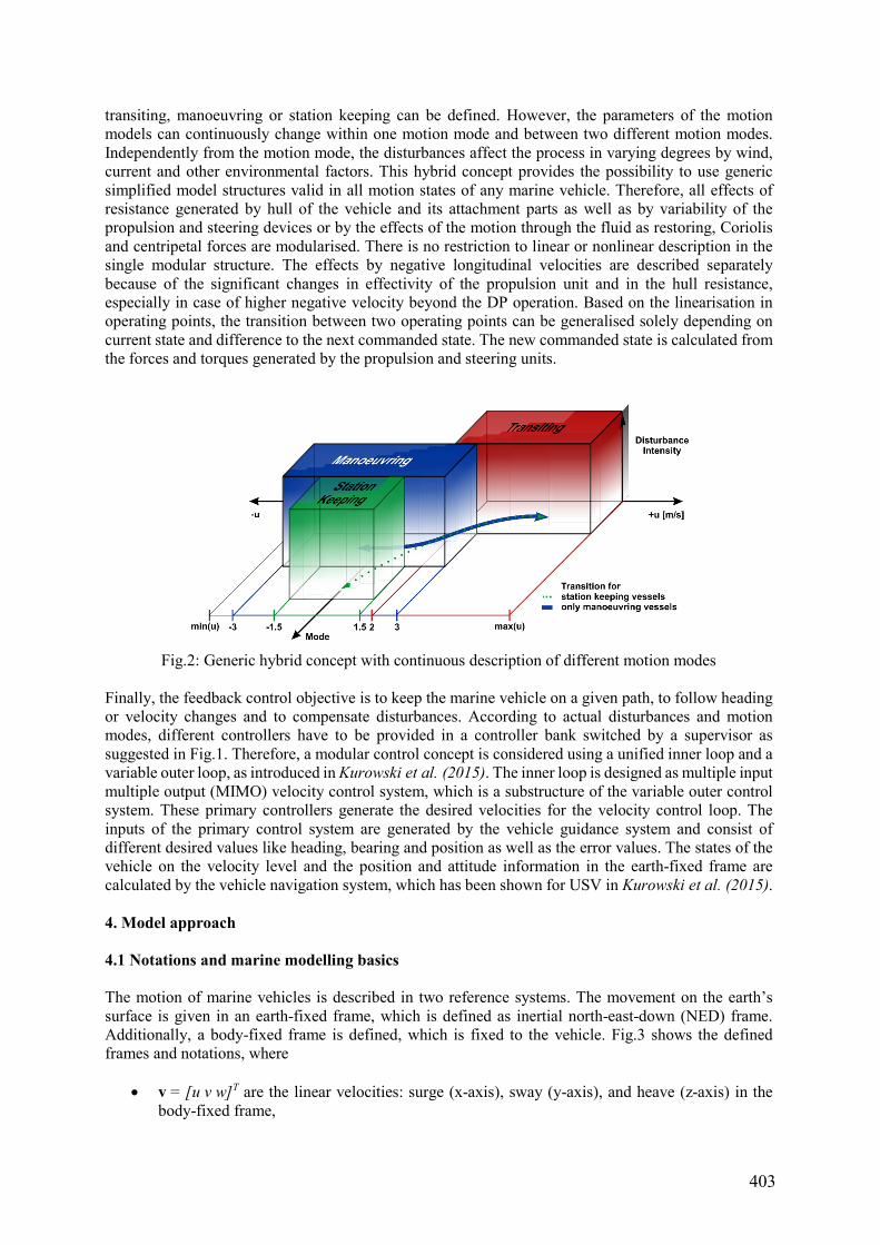
403
transiting, manoeuvring or station keeping can be defined. However, the parameters of the motion models can continuously change within one motion mode and between two different motion modes. Independently from the motion mode, the disturbances affect the process in varying degrees by wind, current and other environmental factors. This hybrid concept provides the possibility to use generic simplified model structures valid in all motion states of any marine vehicle. Therefore, all effects of resistance generated by hull of the vehicle and its attachment parts as well as by variability of the propulsion and steering devices or by the effects of the motion through the fluid as restoring, Coriolis and centripetal forces are modularised. There is no restriction to linear or nonlinear description in the single modular structure. The effects by negative longitudinal velocities are described separately because of the significant changes in effectivity of the propulsion unit and in the hull resistance, especially in case of higher negative velocity beyond the DP operation. Based on the linearisation in operating points, the transition between two operating points can be generalised solely depending on current state and difference to the next commanded state. The new commanded state is calculated from the forces and torques generated by the propulsion and steering units.
Fig.2: Generic hybrid concept with continuous description of different motion modes
Finally, the feedback control objective is to keep the marine vehicle on a given path, to follow heading or velocity changes and to compensate disturbances. According to actual disturbances and motion modes, different controllers have to be provided in a controller bank switched by a supervisor as suggested in Fig.1. Therefore, a modular control concept is considered using a unified inner loop and a variable outer loop, as introduced in Kurowski et al. (2015). The inner loop is designed as multiple input multiple output (MIMO) velocity control system, which is a substructure of the variable outer control system. These primary controllers generate the desired velocities for the velocity control loop. The inputs of the primary control system are generated by the vehicle guidance system and consist of different desired values like heading, bearing and position as well as the error values. The states of the vehicle on the velocity level and the position and attitude information in the earth-fixed frame are calculated by the vehicle navigation system, which has been shown for USV in Kurowski et al. (2015). 4. Model approach
4.1 Notations and marine modelling basics
The motion of marine vehicles is described in two reference systems. The movement on the earth’s surface is given in an earth-fixed frame, which is defined as inertial north-east-down (NED) frame. Additionally, a body-fixed frame is defined, which is fixed to the vehicle. Fig.3 shows the defined frames and notations, where
• v = [u v w]T are the linear velocities: surge (x-axis), sway (y-axis), and heave (z-axis) in the body-fixed frame,

404
• ω = [p q r]T are the angular velocities: roll, pitch, and yaw about the axes of the body-fixed frame, and
• x0 = [x0 y0 z0]T is the position of the vehicle according to the earth-fixed frame.
Fig.3: Definition of frames and notations
Additionally, the attitude of the vehicle is defined by the Euler angles Ω = [Φ Θ Ψ]T, which represent the relative angle between the body-fixed and the earth-fixed frame. Finally, the transformation from body-fixed to earth-fixed frame is done by using standard rotation matrices given in the literature. The dynamics of marine vehicles are described as slim rigid-bodies moving in the earth-fixed frame under the influence of forces F = [X Y Z]T and torques M = [K M N]T, which can be described by Newton's laws. Assuming that the origin of the body-fixed frame coincides with the center of gravity, the motion equations of a body in a fluid is transformed to the body-fixed frame using the so-called Kirchhoff equations, which lead to matrix representation of the equations of motion
, (1) where x = [vT ωT]T is the state vector of the nonlinear model. Mh describes the hydrodynamic inertia matrix, which consists of the vehicle mass and moment of inertia, and Ch is the Coriolis and Centripetal matrix including added inertia effects. On the right-hand side, the sum of external forces and moments acting on the vehicle presented by damping matrix Dh(x), stiffness matrix Sh(xe), using xe = [x0
T ΩT]T, actuators Ha, and disturbances Hd. In practice, it is a cumbersome task to identify the unknown parameters of the nonlinear model, due to strong couplings of the motion variables, measurement noise and unknown disturbances. Hence, the dynamics can be divided into different subspace models, e.g. uncoupled planar motion, roll motion, etc., which complies with the modular system concept. 4.2 Planar motion models
Due to the modular design approach, the planar motion model of a marine surface vehicle consists of three essential modules, the static gear, the disturbance and the dynamic module as shown in the model components of Fig.8. In static and dynamic modules, the vessel motion is described in a simplified form in three degrees of freedom (DoF) for the longitudinal (u), lateral (v) and rotational (r) velocity depicted in Fig.4. Eqs.(2)-(4) define the accelerating forces using the oriented masses and the inertial torque as the simple sum of actuator forces and moments (Xp, Yp, Np) as well as the overall resistance forces and moments (Xr, Yr, Nr) in the respective direction. The actuator forces and moments are the sum of resulting forces
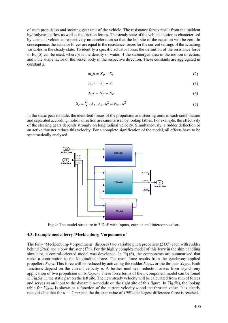
405
of each propulsion and steering gear unit of the vehicle. The resistance forces result from the incident hydrodynamic flow as well as the friction forces. The steady state of the vehicle motion is characterised by constant velocities respectively no acceleration so that the left site of the equation will be zero. In consequence, the actuator forces are equal to the resistance forces for the current settings of the actuating variables in the steady state. To identify a specific actuator force, the definition of the resistance force in Eq.(5) can be used, where ρ is the density of water, A the submerged area in the motion direction, and c the shape factor of the vessel body in the respective direction. These constants are aggregated in constant k.
(2)
(3)
(4)
(5)
In the static gear module, the identified forces of the propulsion and steering units in each combination and separated according motion direction are summarised by lookup tables. For example, the effectivity of the steering gears depends strongly on longitudinal velocity. Simultaneously, a rudder deflection or an active thruster reduce this velocity. For a complete signification of the model, all effects have to be systematically analysed.
Fig.4: The model structure in 3 DoF with inputs, outputs and interconnections
4.3. Example model ferry ‘Mecklenburg-Vorpommern’
The ferry ‘Mecklenburg-Vorpommern’ disposes two variable pitch propellers (EOT) each with rudder behind (Rud) and a bow thruster (Thr). For the highly complex model of this ferry in the ship handling simulator, a control-oriented model was developed. In Eq.(6), the components are summarised that make a contribution to the longitudinal force. The main force results from the synchrony applied propellers X2EOT. This force will be reduced by activating the rudder XdiffRud or the thruster XdiffThr. Both functions depend on the current velocity u. A further nonlinear reduction arises from asynchrony application of two propulsion units XdiffEOT. These force terms of the u-component model can be found in Fig.5a) in the static part on the left site. The new steady velocity will be calculated from sum of forces and serves as an input to the dynamic u-module on the right site of this figure. In Fig.5b), the lookup table for XdiffThr is shown as a function of the current velocity u and the thruster value. It is clearly recognisable that for u = -2 m/s and the thruster value of 100% the largest difference force is reached.
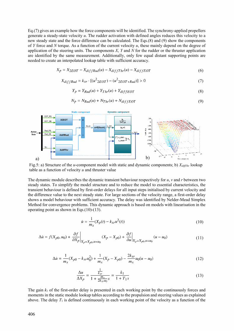
406
Eq.(7) gives an example how the force components will be identified. The synchrony-applied propellers generate a steady-state velocity u. The rudder activation with defined angles reduces this velocity to a new steady state and the force difference can be calculated. The Eqs.(8) and (9) show the components of Y force and N torque. As a function of the current velocity u, these mainly depend on the degree of application of the steering units. The components X, Y and N for the rudder or the thruster application are identified by the same measurement. Additionally, only few equal distant supporting points are needed to create an interpolated lookup table with sufficient accuracy.
(6)
(7)
(8)
(9)
Fig.5: a) Structure of the u-component model with static and dynamic components; b) XdiffThr lookup table as a function of velocity u and thruster value
The dynamic module describes the dynamic transient behaviour respectively for u, v and r between two steady states. To simplify the model structure and to reduce the model to essential characteristics, the transient behaviour is defined by first-order delays for all input steps initialised by current velocity and the difference value to the next steady state. For large sections of the velocity range, a first-order delay shows a model behaviour with sufficient accuracy. The delay was identified by Nelder-Mead Simplex Method for convergence problems. This dynamic approach is based on models with linearisation in the operating point as shown in Eqs.(10)-(13).
(10)
(11)
(12)
(13)
The gain k1 of the first-order delay is presented in each working point by the continuously forces and moments in the static module lookup tables according to the propulsion and steering values as explained above. The delay T1 is defined continuously in each working point of the velocity as a function of the
a) b)
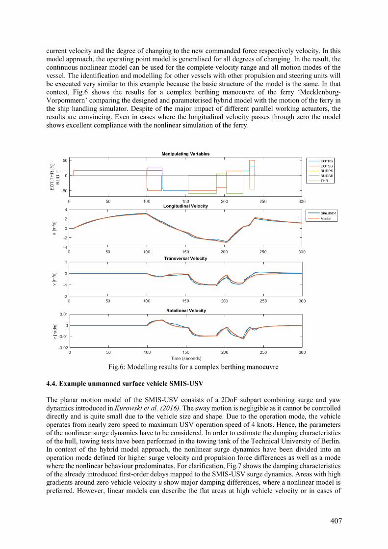
407
current velocity and the degree of changing to the new commanded force respectively velocity. In this model approach, the operating point model is generalised for all degrees of changing. In the result, the continuous nonlinear model can be used for the complete velocity range and all motion modes of the vessel. The identification and modelling for other vessels with other propulsion and steering units will be executed very similar to this example because the basic structure of the model is the same. In that context, Fig.6 shows the results for a complex berthing manoeuvre of the ferry ‘Mecklenburg-Vorpommern’ comparing the designed and parameterised hybrid model with the motion of the ferry in the ship handling simulator. Despite of the major impact of different parallel working actuators, the results are convincing. Even in cases where the longitudinal velocity passes through zero the model shows excellent compliance with the nonlinear simulation of the ferry.
Fig.6: Modelling results for a complex berthing manoeuvre 4.4. Example unmanned surface vehicle SMIS-USV
The planar motion model of the SMIS-USV consists of a 2DoF subpart combining surge and yaw dynamics introduced in Kurowski et al. (2016). The sway motion is negligible as it cannot be controlled directly and is quite small due to the vehicle size and shape. Due to the operation mode, the vehicle operates from nearly zero speed to maximum USV operation speed of 4 knots. Hence, the parameters of the nonlinear surge dynamics have to be considered. In order to estimate the damping characteristics of the hull, towing tests have been performed in the towing tank of the Technical University of Berlin. In context of the hybrid model approach, the nonlinear surge dynamics have been divided into an operation mode defined for higher surge velocity and propulsion force differences as well as a mode where the nonlinear behaviour predominates. For clarification, Fig.7 shows the damping characteristics of the already introduced first-order delays mapped to the SMIS-USV surge dynamics. Areas with high gradients around zero vehicle velocity u show major damping differences, where a nonlinear model is preferred. However, linear models can describe the flat areas at high vehicle velocity or in cases of
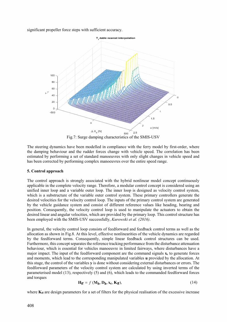
408
significant propeller force steps with sufficient accuracy.
Fig.7: Surge damping characteristics of the SMIS-USV
The steering dynamics have been modelled in compliance with the ferry model by first-order, where the damping behaviour and the rudder forces change with vehicle speed. The correlation has been estimated by performing a set of standard manoeuvres with only slight changes in vehicle speed and has been corrected by performing complex manoeuvres over the entire speed range. 5. Control approach
The control approach is strongly associated with the hybrid nonlinear model concept continuously applicable in the complete velocity range. Therefore, a modular control concept is considered using an unified inner loop and a variable outer loop. The inner loop is designed as velocity control system, which is a substructure of the variable outer control system. These primary controllers generate the desired velocities for the velocity control loop. The inputs of the primary control system are generated by the vehicle guidance system and consist of different reference values like heading, bearing and position. Consequently, the velocity control loop is used to manipulate the actuators to obtain the desired linear and angular velocities, which are provided by the primary loop. This control structure has been employed with the SMIS-USV successfully, Kurowski et al. (2016). In general, the velocity control loop consists of feedforward and feedback control terms as well as the allocation as shown in Fig.8. At this level, effective nonlinearities of the vehicle dynamics are regarded by the feedforward terms. Consequently, simple linear feedback control structures can be used. Furthermore, this concept separates the reference tracking performance from the disturbance attenuation behaviour, which is essential for vehicles manoeuvre in limited fairways, where disturbances have a major impact. The input of the feedforward component are the command signals xc to generate forces and moments, which lead to the corresponding manipulated variables u provided by the allocation. At this stage, the control of the variables y is done without considering external disturbances or errors. The feedforward parameters of the velocity control system are calculated by using inverted terms of the parameterised model (13), respectively (5) and (6), which leads to the commanded feedforward forces and torques
(14) where Kff are design parameters for a set of filters for the physical realisation of the excessive increase
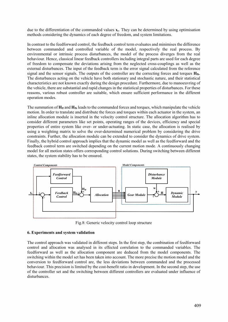
409
due to the differentiation of the commanded values xc. They can be determined by using optimisation methods considering the dynamics of each degree of freedom, and system limitations. In contrast to the feedforward control, the feedback control term evaluates and minimises the difference between commanded and controlled variable of the model, respectively the real process. By environmental or intrinsic process disturbances, the model of the process diverges from the real behaviour. Hence, classical linear feedback controllers including integral parts are used for each degree of freedom to compensate the deviations arising from the neglected cross-couplings as well as the external disturbances. The input of the feedback term is the error signal calculated from the reference signal and the sensor signals. The outputs of the controller are the correcting forces and torques Hfb. The disturbances acting on the vehicle have both stationary and stochastic nature, and their statistical characteristics are not known exactly during the design procedure. Furthermore, due to manoeuvring of the vehicle, there are substantial and rapid changes in the statistical properties of disturbances. For these reasons, various robust controller are suitable, which ensure sufficient performance in the different operation modes. The summation of Hff and Hfb leads to the commanded forces and torques, which manipulate the vehicle motion. In order to translate and distribute the forces and torques within each actuator in the system, an inline allocation module is inserted in the velocity control structure. The allocation algorithm has to consider different parameters like set points, operating ranges of the devices, efficiency and special properties of entire system like over- or under-actuating. In static case, the allocation is realised by using a weighting matrix to solve the over-determined numerical problem by considering the drive constraints. Further, the allocation module can be extended to consider the dynamics of drive system. Finally, the hybrid control approach implies that the dynamic model as well as the feedforward and the feedback control term are switched depending on the current motion mode. A continuously changing model for all motion states offers corresponding control solutions. During switching between different states, the system stability has to be ensured.
Fig.8: Generic velocity control loop structure 6. Experiments and system validation
The control approach was validated in different steps. In the first step, the combination of feedforward control and allocation was analysed in its effected correlation to the commanded variables. The feedforward as well as the allocation component are deduced from the model components. The switching within the model set has been taken into account. The more precise the motion model and the conversion to feedforward control are, the less deviations between commanded and the processed behaviour. This precision is limited by the cost-benefit ratio in development. In the second step, the use of the controller set and the switching between different controllers are evaluated under influence of disturbances.
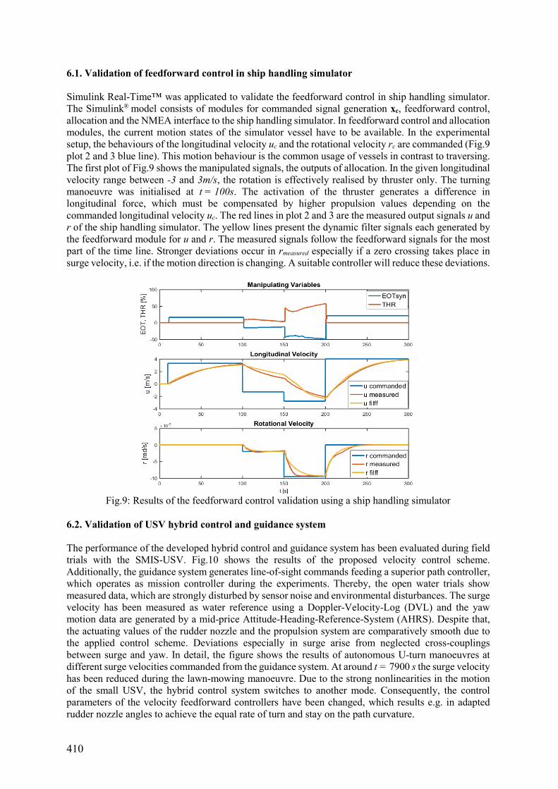
410
6.1. Validation of feedforward control in ship handling simulator
Simulink Real-Time™ was applicated to validate the feedforward control in ship handling simulator. The Simulink® model consists of modules for commanded signal generation xc, feedforward control, allocation and the NMEA interface to the ship handling simulator. In feedforward control and allocation modules, the current motion states of the simulator vessel have to be available. In the experimental setup, the behaviours of the longitudinal velocity uc and the rotational velocity rc are commanded (Fig.9 plot 2 and 3 blue line). This motion behaviour is the common usage of vessels in contrast to traversing. The first plot of Fig.9 shows the manipulated signals, the outputs of allocation. In the given longitudinal velocity range between -3 and 3m/s, the rotation is effectively realised by thruster only. The turning manoeuvre was initialised at t = 100s. The activation of the thruster generates a difference in longitudinal force, which must be compensated by higher propulsion values depending on the commanded longitudinal velocity uc. The red lines in plot 2 and 3 are the measured output signals u and r of the ship handling simulator. The yellow lines present the dynamic filter signals each generated by the feedforward module for u and r. The measured signals follow the feedforward signals for the most part of the time line. Stronger deviations occur in rmeasured especially if a zero crossing takes place in surge velocity, i.e. if the motion direction is changing. A suitable controller will reduce these deviations.
Fig.9: Results of the feedforward control validation using a ship handling simulator
6.2. Validation of USV hybrid control and guidance system
The performance of the developed hybrid control and guidance system has been evaluated during field trials with the SMIS-USV. Fig.10 shows the results of the proposed velocity control scheme. Additionally, the guidance system generates line-of-sight commands feeding a superior path controller, which operates as mission controller during the experiments. Thereby, the open water trials show measured data, which are strongly disturbed by sensor noise and environmental disturbances. The surge velocity has been measured as water reference using a Doppler-Velocity-Log (DVL) and the yaw motion data are generated by a mid-price Attitude-Heading-Reference-System (AHRS). Despite that, the actuating values of the rudder nozzle and the propulsion system are comparatively smooth due to the applied control scheme. Deviations especially in surge arise from neglected cross-couplings between surge and yaw. In detail, the figure shows the results of autonomous U-turn manoeuvres at different surge velocities commanded from the guidance system. At around t = 7900 s the surge velocity has been reduced during the lawn-mowing manoeuvre. Due to the strong nonlinearities in the motion of the small USV, the hybrid control system switches to another mode. Consequently, the control parameters of the velocity feedforward controllers have been changed, which results e.g. in adapted rudder nozzle angles to achieve the equal rate of turn and stay on the path curvature.
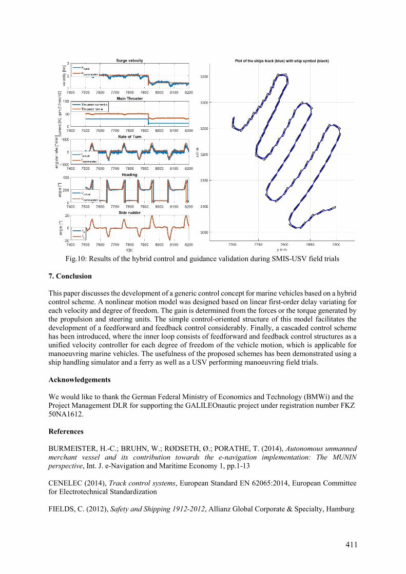
411
Fig.10: Results of the hybrid control and guidance validation during SMIS-USV field trials 7. Conclusion
This paper discusses the development of a generic control concept for marine vehicles based on a hybrid control scheme. A nonlinear motion model was designed based on linear first-order delay variating for each velocity and degree of freedom. The gain is determined from the forces or the torque generated by the propulsion and steering units. The simple control-oriented structure of this model facilitates the development of a feedforward and feedback control considerably. Finally, a cascaded control scheme has been introduced, where the inner loop consists of feedforward and feedback control structures as a unified velocity controller for each degree of freedom of the vehicle motion, which is applicable for manoeuvring marine vehicles. The usefulness of the proposed schemes has been demonstrated using a ship handling simulator and a ferry as well as a USV performing manoeuvring field trials. Acknowledgements
We would like to thank the German Federal Ministry of Economics and Technology (BMWi) and the Project Management DLR for supporting the GALILEOnautic project under registration number FKZ 50NA1612. References
BURMEISTER, H.-C.; BRUHN, W.; RØDSETH, Ø.; PORATHE, T. (2014), Autonomous unmanned
merchant vessel and its contribution towards the e-navigation implementation: The MUNIN
perspective, Int. J. e-Navigation and Maritime Economy 1, pp.1-13 CENELEC (2014), Track control systems, European Standard EN 62065:2014, European Committee for Electrotechnical Standardization FIELDS, C. (2012), Safety and Shipping 1912-2012, Allianz Global Corporate & Specialty, Hamburg

412
IMO (1994), Guidelines for vessels with dynamic positioning systems, Technical Report MSC/Circ.645, International Maritime Organization KUROWSKI, M.; HAGHANI, A.; KOSCHORREK, P.; JEINSCH, T. (2015), Guidance, navigation
and control of unmanned surface vehicles, at-Automatisierungstechnik 63/5, pp.355-367 KUROWSKI, M.; RENTZOW, E.; RITZ, S.; LAMPE, B.P.; JEINSCH, T. (2016), Modelling and
control of ASV acting as communication node for deep-sea applications, 10th IFAC CAMS, Trondheim, pp.291-296 LEVANDER, O. (2017), Autonomous ships on the high seas, IEEE Spectrum 54(2), pp.26-31 MORSE, A.S. (1995), Control using logic-based switching, Trends in control: A European Perspective, Springer, London, pp.69-113 PORRETTA, M.; BAÑOS, D.J.; CRISCI, M.; SOLARI, G.; FIUMARA, A. (2016), GNSS evolutions
for maritime, Inside GNSS magazine 11/3, pp.54-62
413
The Path to Real World Autonomy for Autonomous Surface Vehicles
Howard Tripp, ASV Global, Portchester/UK, [email protected]
Richard Daltry, ASV Global, Portchester/UK, [email protected]
Abstract
This paper presents a new autonomy architecture, developed and tested over the past two years which
has taken a “dumb” remote-controlled platform and built it into a state-of-the-art Autonomous Surface
Vehicle, able to navigate safely at high speeds in a COLREG aware manner, across some of the busiest
waterways in the world. The architecture is made up of a hierarchy of decision making components
sharing a common world model. These components consist of: a route planner, path planner and last
response engine. Each element of the hierarchy is working to reduce risk within decreasing time and
space horizons, ultimately providing a minimum risk navigational solution. MAST and the collision
avoidance system is now at the advanced prototype stage hence. Dstl and ASV welcome interest from
other organisations who would like to explore and experiment with running their systems either
onboard or otherwise in command.
1. Context
ASV Global has built a reputation as the leading manufacturer of Autonomous Surface Vehicles
(ASVs). In parallel to developing a wide product range of platforms, ASV Global has developed its
own autonomous control system, ASView. ASView has been in development for 9 years and is actively
used on over 80 platforms. It supports chart based operator situational awareness with pre-planned
vehicle actions. The system currently relies on human input with limited on-board decision making.
To fuel growth of the industry, the goal moving forward is to develop a commercially useful autonomy
system including and exceeding collision avoidance.
To ASV Global, real world autonomy means increasing the capability of the ASV to undertake decision
making and thus enabling the remote operator to focus on safety critical issues and utilise natural human
intuition. To provide the most efficient use of resources throughout the system as a whole, including
the human element. In pursuit of this goal, ASV Global has developed an architecture which provides
a robust foundation for the development of autonomy over the next decade. Throughout the design of
the architecture a key element is the capability for expandability and future improvement, ensuring the
system can meet current and future industry goals.
Initial tests and demonstrations of the system utilised data fused from radar, cameras and AIS sensors.
This has been used in proof of concept demonstrations and showcased at the recent Unmanned Warrior
naval exercise in the UK, deployed on multiple ASVs. Collision avoidance behaviours, taking into
account important aspects of the collision regulations at sea, have been a critical part of this early
development around which operational behaviours have been built.
These developments are accelerating the adoption of ASVs in the maritime industry by enabling
capabilities such as over the horizon operations and the control of fleets of ASVs with minimal human
input. Examples of applications spread across both military and commercial domains and include
ISTAR, hydrographic survey, support of underwater systems and in the future, commercial shipping.
The programme was directly funded by UK MoD through Dstl and led by ASV Global in partnership
with Roke Manor Research and Cambridge Pixel.
2. Project Introduction
The developed capability centred around the guiding vision of a high speed (>30 knots) Unmanned
Surface Vehicle (USV), notionally based outside Portsmouth Harbour, that could be tasked to
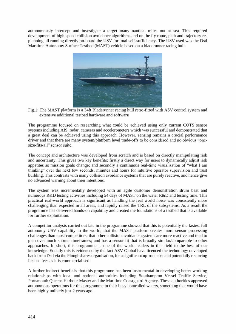
414
autonomously intercept and investigate a target many nautical miles out at sea. This required
development of high speed collision avoidance algorithms and on the fly route, path and trajectory re-
planning all running directly on-board the USV for total self-sufficiency. The USV used was the Dstl
Maritime Autonomy Surface Testbed (MAST) vehicle based on a bladerunner racing hull.
Fig.1: The MAST platform is a 34ft Bladerunner racing hull retro-fitted with ASV control system and
extensive additional testbed hardware and software
The programme focused on researching what could be achieved using only current COTS sensor
systems including AIS, radar, cameras and accelerometers which was successful and demonstrated that
a great deal can be achieved using this approach. However, sensing remains a crucial performance
driver and that there are many system/platform level trade-offs to be considered and no obvious “one-
size-fits-all” sensor suite.
The concept and architecture was developed from scratch and is based on directly manipulating risk
and uncertainty. This gives two key benefits: firstly a direct way for users to dynamically adjust risk
appetites as mission goals change; and secondly a continuous real-time visualisation of “what I am
thinking” over the next few seconds, minutes and hours for intuitive operator supervision and trust
building. This contrasts with many collision avoidance systems that are purely reactive, and hence give
no advanced warning about their intentions.
The system was incrementally developed with an agile customer demonstration drum beat and
numerous R&D testing activities including 54 days of MAST on the water R&D and testing time. This
practical real-world approach is significant as handling the real world noise was consistently more
challenging than expected in all areas, and rapidly raised the TRL of the subsystems. As a result the
programme has delivered hands-on capability and created the foundations of a testbed that is available
for further exploitation.
A competitor analysis carried out late in the programme showed that this is potentially the fastest full
autonomy USV capability in the world; that the MAST platform creates more sensor processing
challenges than most competitors; that other collision avoidance systems are more reactive and tend to
plan over much shorter timeframes; and has a sensor fit that is broadly similar/comparable to other
approaches. In short, this programme is one of the world leaders in this field to the best of our
knowledge. Equally this is evidenced by the fact ASV Global have licenced the technology developed
back from Dstl via the Ploughshares organisation, for a significant upfront cost and potentially recurring
license fees as it is commercialised.
A further indirect benefit is that this programme has been instrumental in developing better working
relationships with local and national authorities including Southampton Vessel Traffic Service,
Portsmouth Queens Harbour Master and the Maritime Coastguard Agency. These authorities approved
autonomous operations for this programme in their busy controlled waters, something that would have
been highly unlikely just 2 years ago.
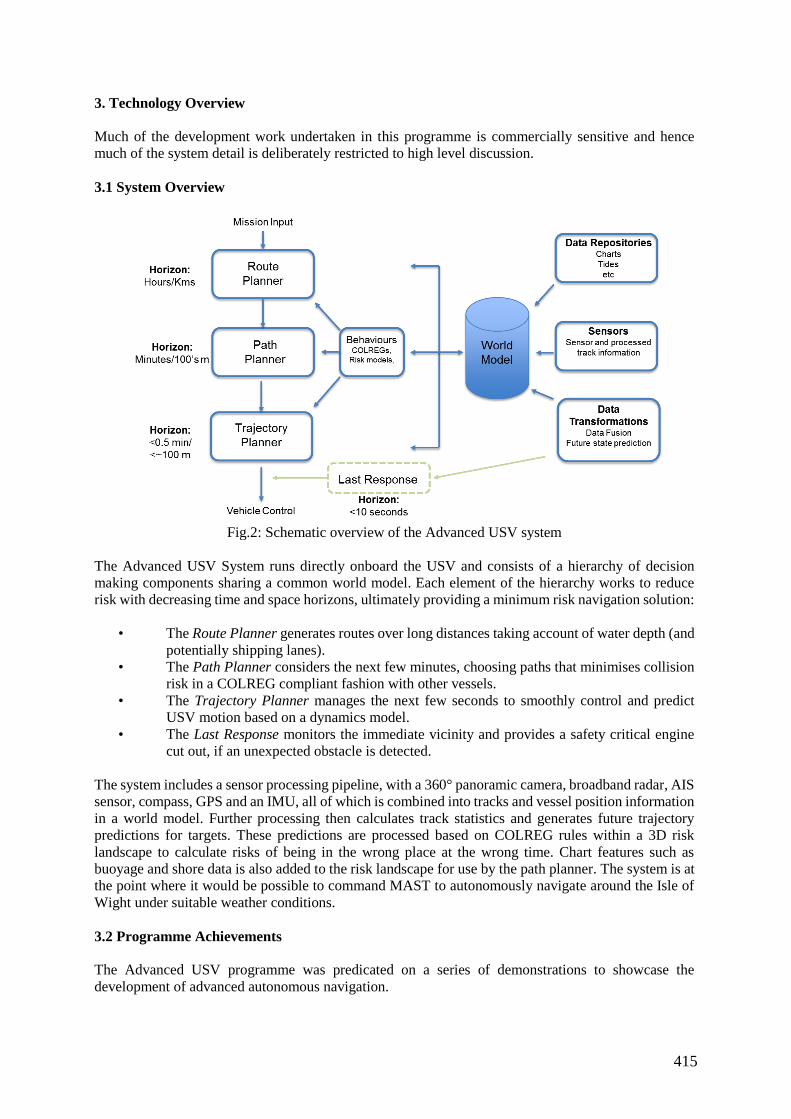
415
3. Technology Overview
Much of the development work undertaken in this programme is commercially sensitive and hence
much of the system detail is deliberately restricted to high level discussion.
3.1 System Overview
Fig.2: Schematic overview of the Advanced USV system
The Advanced USV System runs directly onboard the USV and consists of a hierarchy of decision
making components sharing a common world model. Each element of the hierarchy works to reduce
risk with decreasing time and space horizons, ultimately providing a minimum risk navigation solution:
• The Route Planner generates routes over long distances taking account of water depth (and
potentially shipping lanes).
• The Path Planner considers the next few minutes, choosing paths that minimises collision
risk in a COLREG compliant fashion with other vessels.
• The Trajectory Planner manages the next few seconds to smoothly control and predict
USV motion based on a dynamics model.
• The Last Response monitors the immediate vicinity and provides a safety critical engine
cut out, if an unexpected obstacle is detected.
The system includes a sensor processing pipeline, with a 360° panoramic camera, broadband radar, AIS
sensor, compass, GPS and an IMU, all of which is combined into tracks and vessel position information
in a world model. Further processing then calculates track statistics and generates future trajectory
predictions for targets. These predictions are processed based on COLREG rules within a 3D risk
landscape to calculate risks of being in the wrong place at the wrong time. Chart features such as
buoyage and shore data is also added to the risk landscape for use by the path planner. The system is at
the point where it would be possible to command MAST to autonomously navigate around the Isle of
Wight under suitable weather conditions.
3.2 Programme Achievements
The Advanced USV programme was predicated on a series of demonstrations to showcase the
development of advanced autonomous navigation.
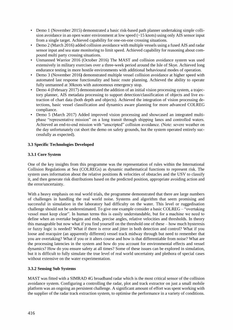
416
• Demo 1 (November 2015) demonstrated a basic risk-based path planner undertaking simple colli-
sion avoidance in an open water environment at low speed (~15 knots) using only AIS sensor input
from a single target. Achieved capability for one-on-one crossing situations.
• Demo 2 (March 2016) added collision avoidance with multiple vessels using a fused AIS and radar
sensor input and sea state monitoring to limit speed. Achieved capability for reasoning about com-
pound multi party crossing situations.
• Unmanned Warrior 2016 (October 2016) The MAST and collision avoidance system was used
extensively in military exercises over a three-week period around the Isle of Skye. Achieved long
endurance testing in more hostile environments with additional behavioural modes of operation.
• Demo 3 (November 2016) demonstrated multiple vessel collision avoidance at higher speed with
automated last response functionality and basic route planning. Achieved the ability to operate
fully unmanned at 30knots with autonomous emergency stop.
• Demo 4 (February 2017) demonstrated the addition of an initial vision processing system, a trajec-
tory planner, AIS metadata processing to support detection/classification of objects and live ex-
traction of chart data (both depth and objects). Achieved the integration of vision processing de-
tections, basic vessel classification and dynamics aware planning for more advanced COLREG
compliance.
• Demo 5 (March 2017) Added improved vision processing and showcased an integrated multi-
phase “representative mission” on a long transit through shipping lanes and controlled waters.
Achieved an end-to-end mission with “unscripted” collision avoidance. (Note: severe weather on
the day unfortunately cut short the demo on safety grounds, but the system operated entirely suc-
cessfully as expected).
3.3 Specific Technologies Developed
3.3.1 Core System
One of the key insights from this programme was the representation of rules within the International
Collision Regulations at Sea (COLREGs) as dynamic mathematical functions to represent risk. The
system uses information about the relative positions & velocities of obstacles and the USV to classify
it, and then generate risk distributions based on the predicted position, appropriate avoiding action and
the error/uncertainty.
With a heavy emphasis on real world trials, the programme demonstrated that there are large numbers
of challenges in handling the real world noise. Systems and algorithm that seem promising and
successful in simulation in the laboratory had difficulty on the water. This level or ruggedisation
challenge should not be underestimated. To give one example consider a basic COLREG – “overtaking
vessel must keep clear”. In human terms this is easily understandable, but for a machine we need to
define when an overtake begins and ends, precise angles, relative velocities and thresholds. In theory
this manageable but now what if you find yourself on the threshold one of these – how much hysteresis
or fuzzy logic is needed? What if there is error and jitter in both detection and control? What if you
loose and reacquire (an apparently different) vessel track midway through but need to remember that
you are overtaking? What if you or it alters course and how is that differentiable from noise? What are
the processing latencies in the system and how do you account for environmental effects and vessel
dynamics? How do you ensure safety at all times? Some of these issues can be explored in simulation,
but it is difficult to fully simulate the true level of real world uncertainty and plethora of special cases
without extensive on the water experimentation.
3.3.2 Sensing Sub Systems
MAST was fitted with a SIMRAD 4G broadband radar which is the most critical sensor of the collision
avoidance system. Configuring a controlling the radar, plot and track extractor on just a small mobile
platform was an ongoing an persistent challenge. A significant amount of effort was spent working with
the supplier of the radar track extraction system, to optimise the performance in a variety of conditions.
417
Fig.3: An example of AIS, radar & vision sensor outputs all being fused into tracks
The 360° panoramic Pt Grey LadyBug 5 camera was used for visual object detection. Work was
undertaken to explore various detection algorithms including: Image masking, Horizon detection,
Colour detector, Edge detector, Local Variance detector and particle probability hypothesis density
(PPHD) filter.
Other sensor related work undertaken included the numerous “enabling sensors” such as compasses and
GPS which again although seem conceptually simple had many challenges. Monitoring the vertical
acceleration of the boat using IMUs with FFT & physics based algorithms to infer maximum safe speed
was also developed.
Database algorithms were also developed to read and process electronic chart information for extraction
of information relevant to collision avoidance for example water depth information, tide data and chart
features such as buoys and marks.
3.3.3 Final Outcomes and Deliverables
An internal comparison with other research activities in the field was undertaken in December 2016.
This re-affirmed our belief that the work undertaken in this programme is at the forefront of the ongoing
research activities in the industry and highlighted:
• The capability developed under this project is potentially the fastest full autonomy capability in
the world.
• The light displacement, high speed platform creates more sensor processing challenges than most
competitors.
• Other collision avoidance systems are more reactive, operating over much shorter timeframes
(more like trajectory planners than path planners), whereas this system provides not just short term
planners but more longer range planning.
• The sensor fit on MAST is broadly similar to other products/projects.
Demo 5 (as noted in section 3.2 above) was the final deliverable of the project; a showcase of all the
technological developments made to date. Each leg of the scenario demonstrated a particular element
of the functionality that has been developed as part of the project.
The MAST USV was demonstrated operating autonomously (with full collision avoidance) from just
outside the entrance to Portsmouth Harbour out to the outer approaches of the Solent, this included
crossing the main shipping channel twice and operating at high speed. The Solent is one of the busiest
shipping areas in the world and this was a significant achievement for the project.
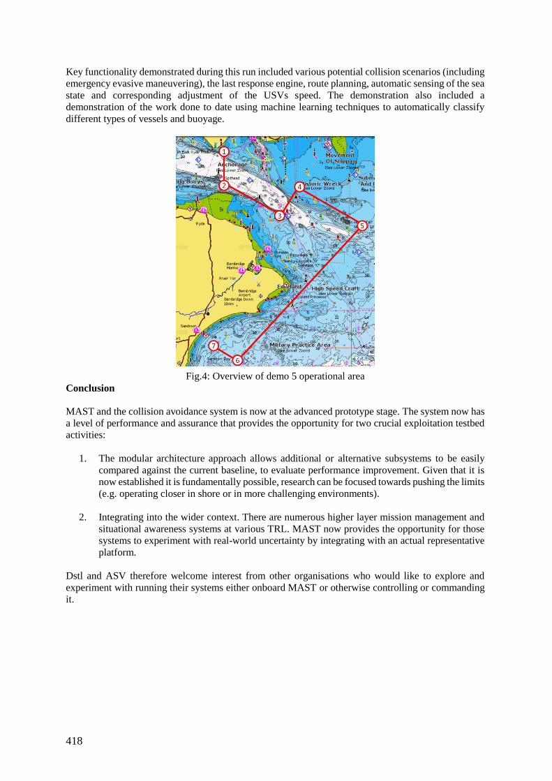
418
Key functionality demonstrated during this run included various potential collision scenarios (including
emergency evasive maneuvering), the last response engine, route planning, automatic sensing of the sea
state and corresponding adjustment of the USVs speed. The demonstration also included a
demonstration of the work done to date using machine learning techniques to automatically classify
different types of vessels and buoyage.
Fig.4: Overview of demo 5 operational area
Conclusion
MAST and the collision avoidance system is now at the advanced prototype stage. The system now has
a level of performance and assurance that provides the opportunity for two crucial exploitation testbed
activities:
1. The modular architecture approach allows additional or alternative subsystems to be easily
compared against the current baseline, to evaluate performance improvement. Given that it is
now established it is fundamentally possible, research can be focused towards pushing the limits
(e.g. operating closer in shore or in more challenging environments).
2. Integrating into the wider context. There are numerous higher layer mission management and
situational awareness systems at various TRL. MAST now provides the opportunity for those
systems to experiment with real-world uncertainty by integrating with an actual representative
platform.
Dstl and ASV therefore welcome interest from other organisations who would like to explore and
experiment with running their systems either onboard MAST or otherwise controlling or commanding
it.
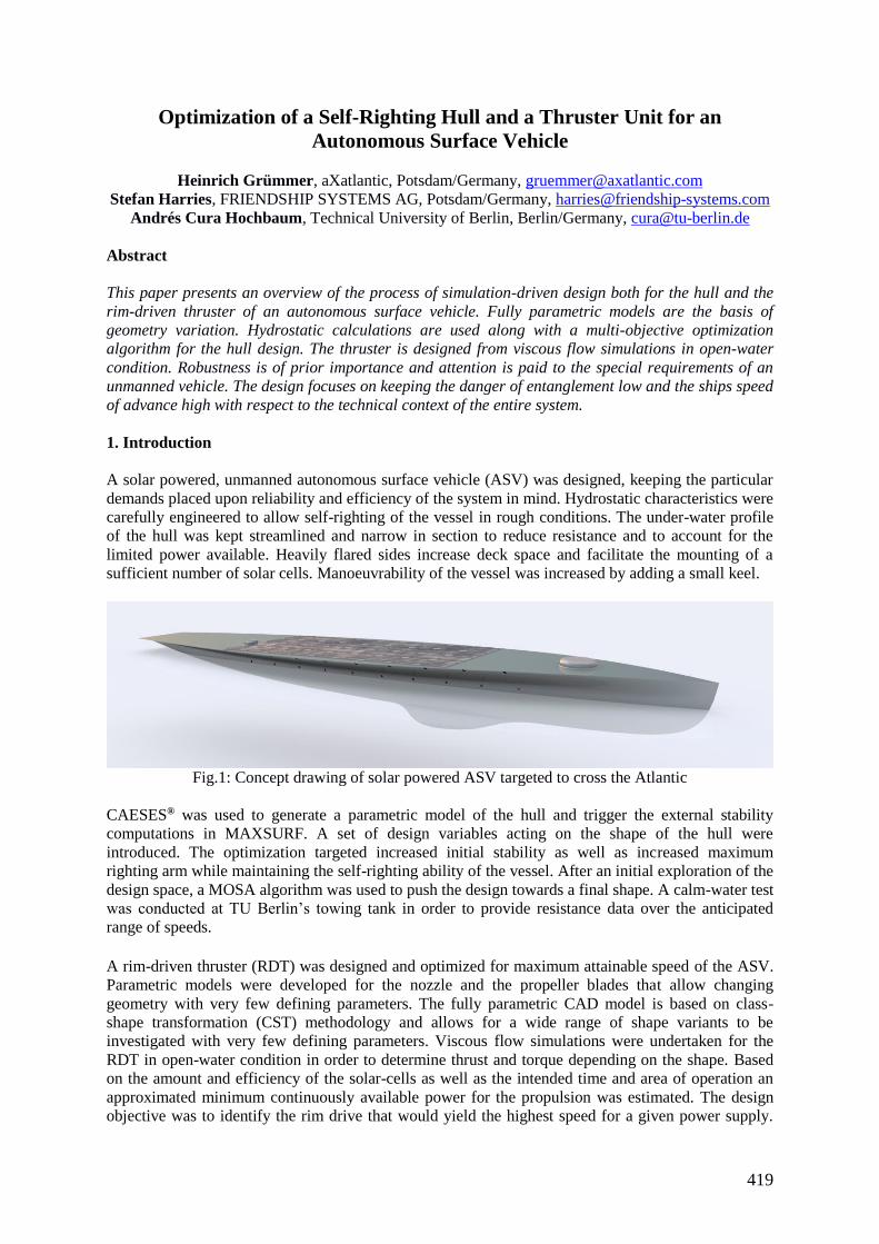
419
Optimization of a Self-Righting Hull and a Thruster Unit for an
Autonomous Surface Vehicle
Heinrich Grümmer, aXatlantic, Potsdam/Germany, [email protected] Stefan Harries, FRIENDSHIP SYSTEMS AG, Potsdam/Germany, [email protected]
Andrés Cura Hochbaum, Technical University of Berlin, Berlin/Germany, [email protected]
Abstract
This paper presents an overview of the process of simulation-driven design both for the hull and the
rim-driven thruster of an autonomous surface vehicle. Fully parametric models are the basis of
geometry variation. Hydrostatic calculations are used along with a multi-objective optimization
algorithm for the hull design. The thruster is designed from viscous flow simulations in open-water
condition. Robustness is of prior importance and attention is paid to the special requirements of an
unmanned vehicle. The design focuses on keeping the danger of entanglement low and the ships speed
of advance high with respect to the technical context of the entire system.
1. Introduction
A solar powered, unmanned autonomous surface vehicle (ASV) was designed, keeping the particular
demands placed upon reliability and efficiency of the system in mind. Hydrostatic characteristics were
carefully engineered to allow self-righting of the vessel in rough conditions. The under-water profile
of the hull was kept streamlined and narrow in section to reduce resistance and to account for the
limited power available. Heavily flared sides increase deck space and facilitate the mounting of a
sufficient number of solar cells. Manoeuvrability of the vessel was increased by adding a small keel.
Fig.1: Concept drawing of solar powered ASV targeted to cross the Atlantic
CAESES® was used to generate a parametric model of the hull and trigger the external stability
computations in MAXSURF. A set of design variables acting on the shape of the hull were
introduced. The optimization targeted increased initial stability as well as increased maximum
righting arm while maintaining the self-righting ability of the vessel. After an initial exploration of the
design space, a MOSA algorithm was used to push the design towards a final shape. A calm-water test
was conducted at TU Berlin’s towing tank in order to provide resistance data over the anticipated
range of speeds. A rim-driven thruster (RDT) was designed and optimized for maximum attainable speed of the ASV.
Parametric models were developed for the nozzle and the propeller blades that allow changing
geometry with very few defining parameters. The fully parametric CAD model is based on class-
shape transformation (CST) methodology and allows for a wide range of shape variants to be
investigated with very few defining parameters. Viscous flow simulations were undertaken for the
RDT in open-water condition in order to determine thrust and torque depending on the shape. Based
on the amount and efficiency of the solar-cells as well as the intended time and area of operation an
approximated minimum continuously available power for the propulsion was estimated. The design
objective was to identify the rim drive that would yield the highest speed for a given power supply.
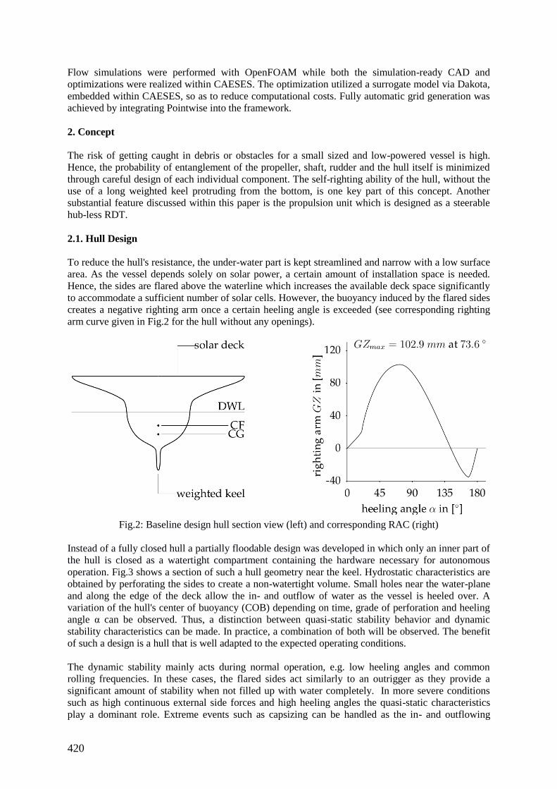
420
Flow simulations were performed with OpenFOAM while both the simulation-ready CAD and
optimizations were realized within CAESES. The optimization utilized a surrogate model via Dakota,
embedded within CAESES, so as to reduce computational costs. Fully automatic grid generation was
achieved by integrating Pointwise into the framework.
2. Concept
The risk of getting caught in debris or obstacles for a small sized and low-powered vessel is high.
Hence, the probability of entanglement of the propeller, shaft, rudder and the hull itself is minimized
through careful design of each individual component. The self-righting ability of the hull, without the
use of a long weighted keel protruding from the bottom, is one key part of this concept. Another
substantial feature discussed within this paper is the propulsion unit which is designed as a steerable
hub-less RDT.
2.1. Hull Design
To reduce the hull's resistance, the under-water part is kept streamlined and narrow with a low surface
area. As the vessel depends solely on solar power, a certain amount of installation space is needed.
Hence, the sides are flared above the waterline which increases the available deck space significantly
to accommodate a sufficient number of solar cells. However, the buoyancy induced by the flared sides
creates a negative righting arm once a certain heeling angle is exceeded (see corresponding righting
arm curve given in Fig.2 for the hull without any openings).
Fig.2: Baseline design hull section view (left) and corresponding RAC (right)
Instead of a fully closed hull a partially floodable design was developed in which only an inner part of
the hull is closed as a watertight compartment containing the hardware necessary for autonomous
operation. Fig.3 shows a section of such a hull geometry near the keel. Hydrostatic characteristics are
obtained by perforating the sides to create a non-watertight volume. Small holes near the water-plane
and along the edge of the deck allow the in- and outflow of water as the vessel is heeled over. A
variation of the hull's center of buoyancy (COB) depending on time, grade of perforation and heeling
angle α can be observed. Thus, a distinction between quasi-static stability behavior and dynamic
stability characteristics can be made. In practice, a combination of both will be observed. The benefit
of such a design is a hull that is well adapted to the expected operating conditions.
The dynamic stability mainly acts during normal operation, e.g. low heeling angles and common
rolling frequencies. In these cases, the flared sides act similarly to an outrigger as they provide a
significant amount of stability when not filled up with water completely. In more severe conditions
such as high continuous external side forces and high heeling angles the quasi-static characteristics
play a dominant role. Extreme events such as capsizing can be handled as the in- and outflowing
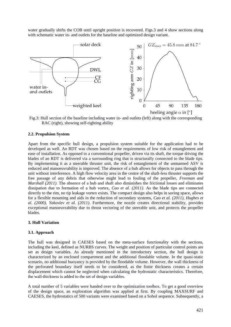
421
water gradually shifts the COB until upright position is recovered. Figs.3 and 4 show sections along
with schematic water in- and outlets for the baseline and optimized design variant.
Fig.3: Hull section of the baseline including water in- and outlets (left) along with the corresponding
RAC (right), showing self-righting ability
2.2. Propulsion System
Apart from the specific hull design, a propulsion system suitable for the application had to be
developed as well. An RDT was chosen based on the requirements of low risk of entanglement and
ease of installation. As opposed to a conventional propeller, driven via its shaft, the torque driving the
blades of an RDT is delivered via a surrounding ring that is structurally connected to the blade tips.
By implementing it as a steerable thruster unit, the risk of entanglement of the unmanned ASV is
reduced and manoeuvrability is improved. The absence of a hub allows for objects to pass through the
unit without interference. A high flow velocity area in the centre of the shaft-less thruster supports the
free passage of any debris that otherwise might lead to fouling of the propeller, Freeman and
Marshall (2011). The absence of a hub and shaft also diminishes the frictional losses and eliminates
dissipation due to formation of a hub vortex, Cao et al. (2011). As the blade tips are connected
directly to the rim, no tip leakage vortex exists. The compact design also helps in saving space, allows
for a flexible mounting and aids in the reduction of secondary systems, Cao et al. (2011), Hughes et
al. (2000), Yakovlev et al. (2011). Furthermore, the nozzle creates directional stability, provides
exceptional manoeuvrability due to thrust vectoring of the steerable unit, and protects the propeller
blades.
3. Hull Variation
3.1. Approach
The hull was designed in CAESES based on the meta-surface functionality with the sections,
including the keel, defined as NURBS curves. The weight and position of particular control points are
set as design variables. As already mentioned in the introductory section, the hull design is
characterized by an enclosed compartment and the additional floodable volume. In the quasi-static
scenario, no additional buoyancy is provided by the floodable volume. However, the wall thickness of
the perforated boundary itself needs to be considered, as the finite thickness creates a certain
displacement which cannot be neglected when calculating the hydrostatic characteristics. Therefore,
the wall-thickness is added to the set of design variables.
A total number of 5 variables were handed over to the optimization toolbox. To get a good overview
of the design space, an exploration algorithm was applied at first. By coupling MAXSURF and
CAESES, the hydrostatics of 500 variants were examined based on a Sobol sequence. Subsequently, a
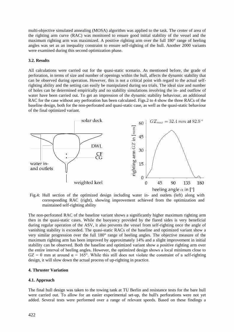
422
multi-objective simulated annealing (MOSA) algorithm was applied to the task. The center of area of
the righting arm curve (RAC) was monitored to ensure good initial stability of the vessel and the
maximum righting arm was maximized. A positive righting arm over the full 180° range of heeling
angles was set as an inequality constraint to ensure self-righting of the hull. Another 2000 variants
were examined during this second optimization phase.
3.2. Results
All calculations were carried out for the quasi-static scenario. As mentioned before, the grade of
perforation, in terms of size and number of openings within the hull, affects the dynamic stability that
can be observed during operation. However, this is not a critical point with regard to the actual self-
righting ability and the setting can easily be manipulated during sea trials. The ideal size and number
of holes can be determined empirically and no stability simulations involving the in- and outflow of
water have been carried out. To get an impression of the dynamic stability behaviour, an additional
RAC for the case without any perforation has been calculated. Figs.2 to 4 show the three RACs of the
baseline design, both for the non-perforated and quasi-static case, as well as the quasi-static behaviour
of the final optimized variant.
Fig.4: Hull section of the optimized design including water in- and outlets (left) along with
corresponding RAC (right), showing improvement achieved from the optimization and
maintained self-righting ability
The non-perforated RAC of the baseline variant shows a significantly higher maximum righting arm
then in the quasi-static cases. While the buoyancy provided by the flared sides is very beneficial
during regular operation of the ASV, it also prevents the vessel from self-righting once the angle of
vanishing stability is exceeded. The quasi-static RACs of the baseline and optimized variant show a
very similar progression over the full 180° range of heeling angles. The objective measure of the
maximum righting arm has been improved by approximately 14% and a slight improvement in initial
stability can be observed. Both the baseline and optimized variant show a positive righting arm over
the entire interval of heeling angles. However, the optimized design shows a local minimum close to
GZ = 0 mm at around α = 165°. While this still does not violate the constraint of a self-righting
design, it will slow down the actual process of up-righting in practice.
4. Thruster Variation
4.1. Approach
The final hull design was taken to the towing tank at TU Berlin and resistance tests for the bare hull
were carried out. To allow for an easier experimental set-up, the hull's perforations were not yet
added. Several tests were performed over a range of relevant speeds. Based on these findings a
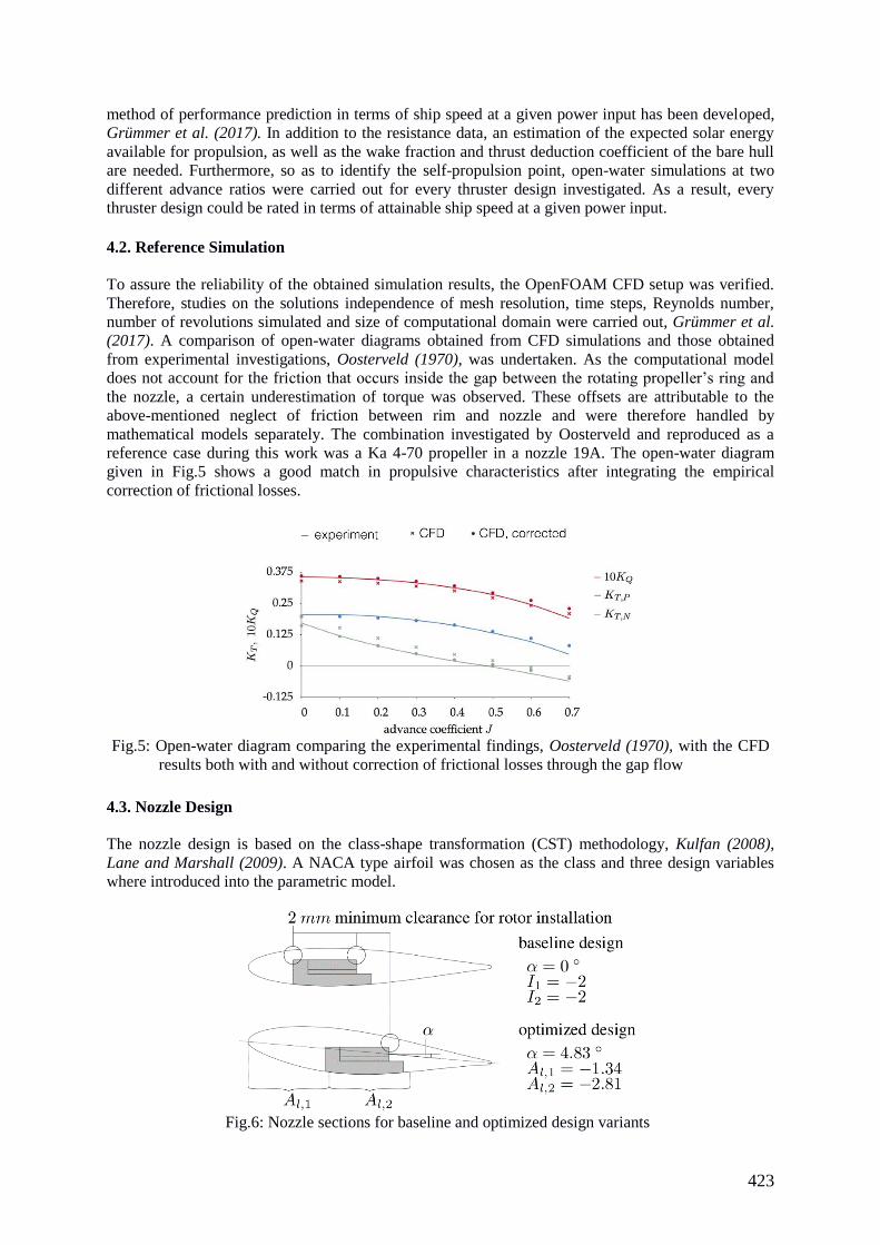
423
method of performance prediction in terms of ship speed at a given power input has been developed,
Grümmer et al. (2017). In addition to the resistance data, an estimation of the expected solar energy
available for propulsion, as well as the wake fraction and thrust deduction coefficient of the bare hull
are needed. Furthermore, so as to identify the self-propulsion point, open-water simulations at two
different advance ratios were carried out for every thruster design investigated. As a result, every
thruster design could be rated in terms of attainable ship speed at a given power input. 4.2. Reference Simulation
To assure the reliability of the obtained simulation results, the OpenFOAM CFD setup was verified.
Therefore, studies on the solutions independence of mesh resolution, time steps, Reynolds number,
number of revolutions simulated and size of computational domain were carried out, Grümmer et al.
(2017). A comparison of open-water diagrams obtained from CFD simulations and those obtained
from experimental investigations, Oosterveld (1970), was undertaken. As the computational model
does not account for the friction that occurs inside the gap between the rotating propeller’s ring and
the nozzle, a certain underestimation of torque was observed. These offsets are attributable to the
above-mentioned neglect of friction between rim and nozzle and were therefore handled by
mathematical models separately. The combination investigated by Oosterveld and reproduced as a
reference case during this work was a Ka 4-70 propeller in a nozzle 19A. The open-water diagram
given in Fig.5 shows a good match in propulsive characteristics after integrating the empirical
correction of frictional losses.
Fig.5: Open-water diagram comparing the experimental findings, Oosterveld (1970), with the CFD
results both with and without correction of frictional losses through the gap flow
4.3. Nozzle Design
The nozzle design is based on the class-shape transformation (CST) methodology, Kulfan (2008),
Lane and Marshall (2009). A NACA type airfoil was chosen as the class and three design variables
where introduced into the parametric model.
Fig.6: Nozzle sections for baseline and optimized design variants
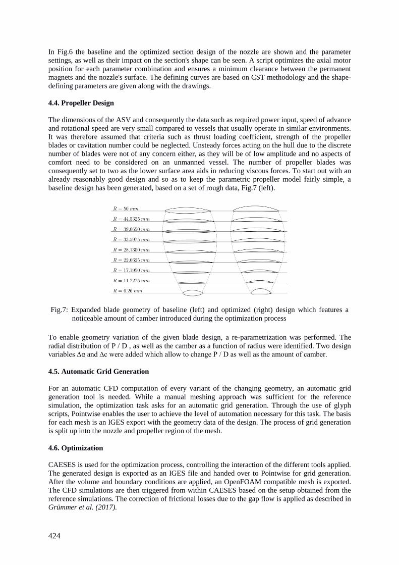
424
In Fig.6 the baseline and the optimized section design of the nozzle are shown and the parameter
settings, as well as their impact on the section's shape can be seen. A script optimizes the axial motor
position for each parameter combination and ensures a minimum clearance between the permanent
magnets and the nozzle's surface. The defining curves are based on CST methodology and the shape-
defining parameters are given along with the drawings.
4.4. Propeller Design
The dimensions of the ASV and consequently the data such as required power input, speed of advance
and rotational speed are very small compared to vessels that usually operate in similar environments.
It was therefore assumed that criteria such as thrust loading coefficient, strength of the propeller
blades or cavitation number could be neglected. Unsteady forces acting on the hull due to the discrete
number of blades were not of any concern either, as they will be of low amplitude and no aspects of
comfort need to be considered on an unmanned vessel. The number of propeller blades was
consequently set to two as the lower surface area aids in reducing viscous forces. To start out with an
already reasonably good design and so as to keep the parametric propeller model fairly simple, a
baseline design has been generated, based on a set of rough data, Fig.7 (left).
Fig.7: Expanded blade geometry of baseline (left) and optimized (right) design which features a
noticeable amount of camber introduced during the optimization process
To enable geometry variation of the given blade design, a re-parametrization was performed. The
radial distribution of P / D , as well as the camber as a function of radius were identified. Two design
variables ∆α and ∆c were added which allow to change P / D as well as the amount of camber.
4.5. Automatic Grid Generation
For an automatic CFD computation of every variant of the changing geometry, an automatic grid
generation tool is needed. While a manual meshing approach was sufficient for the reference
simulation, the optimization task asks for an automatic grid generation. Through the use of glyph
scripts, Pointwise enables the user to achieve the level of automation necessary for this task. The basis
for each mesh is an IGES export with the geometry data of the design. The process of grid generation
is split up into the nozzle and propeller region of the mesh.
4.6. Optimization
CAESES is used for the optimization process, controlling the interaction of the different tools applied.
The generated design is exported as an IGES file and handed over to Pointwise for grid generation.
After the volume and boundary conditions are applied, an OpenFOAM compatible mesh is exported.
The CFD simulations are then triggered from within CAESES based on the setup obtained from the
reference simulations. The correction of frictional losses due to the gap flow is applied as described in
Grümmer et al. (2017).
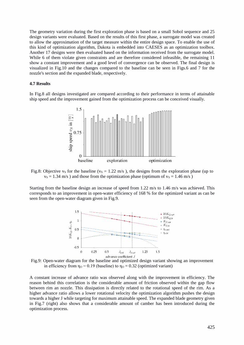
425
The geometry variation during the first exploration phase is based on a small Sobol sequence and 25
design variants were evaluated. Based on the results of this first phase, a surrogate model was created
to allow the approximation of the target measure within the entire design space. To enable the use of
this kind of optimization algorithm, Dakota is embedded into CAESES as an optimization toolbox.
Another 17 designs were then evaluated based on the information received from the surrogate model.
While 6 of them violate given constraints and are therefore considered infeasible, the remaining 11
show a constant improvement and a good level of convergence can be observed. The final design is
visualized in Fig.10 and the changes compared to the baseline can be seen in Figs.6 and 7 for the
nozzle's section and the expanded blade, respectively.
4.7 Results
In Fig.8 all designs investigated are compared according to their performance in terms of attainable
ship speed and the improvement gained from the optimization process can be conceived visually.
Fig.8: Objective vS for the baseline (vS = 1.22 m/s ), the designs from the exploration phase (up to
vS = 1.34 m/s ) and those from the optimization phase (optimum of vS = 1.46 m/s )
Starting from the baseline design an increase of speed from 1.22 m/s to 1.46 m/s was achieved. This
corresponds to an improvement in open-water efficiency of 168 % for the optimized variant as can be
seen from the open-water diagram given in Fig.9.
Fig.9: Open-water diagram for the baseline and optimized design variant showing an improvement
in efficiency from ηO = 0.19 (baseline) to ηO = 0.32 (optimized variant)
A constant increase of advance ratio was observed along with the improvement in efficiency. The
reason behind this correlation is the considerable amount of friction observed within the gap flow
between rim an nozzle. This dissipation is directly related to the rotational speed of the rim. As a
higher advance ratio allows a lower rotational velocity the optimization algorithm pushes the design
towards a higher J while targeting for maximum attainable speed. The expanded blade geometry given
in Fig.7 (right) also shows that a considerable amount of camber has been introduced during the
optimization process.
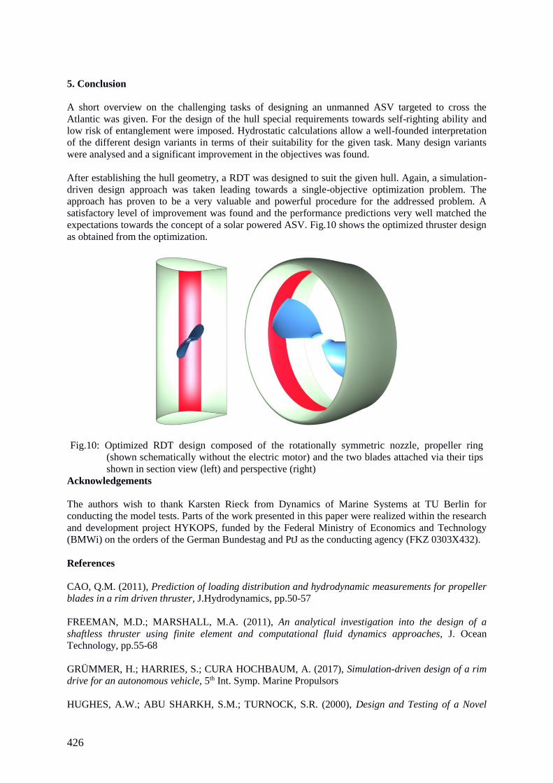
426
5. Conclusion
A short overview on the challenging tasks of designing an unmanned ASV targeted to cross the
Atlantic was given. For the design of the hull special requirements towards self-righting ability and
low risk of entanglement were imposed. Hydrostatic calculations allow a well-founded interpretation
of the different design variants in terms of their suitability for the given task. Many design variants
were analysed and a significant improvement in the objectives was found.
After establishing the hull geometry, a RDT was designed to suit the given hull. Again, a simulation-
driven design approach was taken leading towards a single-objective optimization problem. The
approach has proven to be a very valuable and powerful procedure for the addressed problem. A
satisfactory level of improvement was found and the performance predictions very well matched the
expectations towards the concept of a solar powered ASV. Fig.10 shows the optimized thruster design
as obtained from the optimization.
Fig.10: Optimized RDT design composed of the rotationally symmetric nozzle, propeller ring
(shown schematically without the electric motor) and the two blades attached via their tips
shown in section view (left) and perspective (right)
Acknowledgements
The authors wish to thank Karsten Rieck from Dynamics of Marine Systems at TU Berlin for
conducting the model tests. Parts of the work presented in this paper were realized within the research
and development project HYKOPS, funded by the Federal Ministry of Economics and Technology
(BMWi) on the orders of the German Bundestag and PtJ as the conducting agency (FKZ 0303X432).
References
CAO, Q.M. (2011), Prediction of loading distribution and hydrodynamic measurements for propeller
blades in a rim driven thruster, J.Hydrodynamics, pp.50-57
FREEMAN, M.D.; MARSHALL, M.A. (2011), An analytical investigation into the design of a
shaftless thruster using finite element and computational fluid dynamics approaches, J. Ocean
Technology, pp.55-68
GRÜMMER, H.; HARRIES, S.; CURA HOCHBAUM, A. (2017), Simulation-driven design of a rim
drive for an autonomous vehicle, 5th Int. Symp. Marine Propulsors
HUGHES, A.W.; ABU SHARKH, S.M.; TURNOCK, S.R. (2000), Design and Testing of a Novel

427
Electromagnetic Tip-Driven Thruster, School of Engineering Sciences, University of Southampton
(unpublished)
KULFAN, B. M. (2008), Universal parametric geometry representation method, J. Aircraft 45
LANE, K.A.; MARSHALL, D.D. (2009), A surface parameterization method for airfoil optimization
and high lift 2D geometries utilizing the CST methodology, 47th AIAA Aerospace Sciences Meeting
OOSTERVELD, M.W.C. (1970), Wake adapted ducted propellers, Ph.D. dissertation, Delft
University of Technology
YAKOVLEV, A.Y.; SOKOLOV, M.A.; MARINICH, N.V. (2011), Numerical design and
experimental verification of a rim-driven thruster, 2nd Int. Symp. Marine Propulsors
428
JavaScript Applied to Maritime Design and Engineering
Henrique M. Gaspar, NTNU, Alesund/Norway, [email protected]
Abstract
This paper proposes the use of JavaScript language as a key success factor when developing open
and collaborative software for maritime design and engineering. Among the many script languages
available for engineers, JavaScript stands out for the size of its community, easiness of learning and
wide spectrum of use, from traditional web applications to server management and mobile apps.
There is a resistance, however, to use and incorporate JS in engineering, usually connected to a
market trust/dominance on a traditional script-like language, such as Matlab, or lack of program-
ming skills when using a non-engineering tool to perform complex algorithms, such as using a
spreadsheet-like software for calculating CFD. The topic is introduced with a discussion on the main
advantages and disadvantages of JavaScript when compared to other languages in engineering,
focused on speed, compatibility, user interface and usage. A basic ship design example is presented as
a bridge to introduce JavaScript variables, objects, libraries and HTML document model object. Five
case studies of more complex maritime software developed in JavaScript are presented: dashboards
for resistance and motion calculation, a design layout tool, data-driven documents and a 3D
simulator. A call for JavaScript in engineering concludes the paper.
1. The Need for Script
The idea for the topics discussed in this paper came from the need to share design and simulation
developments with other academic and non-academic colleagues, as well as re-use computer-based
models without worrying about proprietary software and versioning. I cannot count the amount of
time wasted in meetings and classes because the results were presented in a non-interactive and closed
format. Worst, when files are copied from one computer to another, libraries are missing, software
versions are outdated, compilers are updated and the simulation suddenly does not run when the
audience requires it. Anyone that has tried to open a spreadsheet with a macro in another computer or
shared a complex Matlab code with someone else knows the feeling. Python presented itself as a
solution for this problem years ago, since it is one of the best and most versatile script (high-level)
languages available (www.python.org). It is free, intuitive, easy to learn and widely used in the
scientific community. But for simulation and visualization in engineering it lacks important features
that JavaScript (JS) has, such as simplicity to create an interactive interface, extensive 2D and 3D
graphic libraries and possibility to run and share a code with no external software installation. The
internet, or more precisely the web, on the other hand, has a pretty stable history of multi OS
compatibility. Sites like www.efunda.com or http://www.numericjs.com/ are providing reliable online
and interactive engineering/mathematic libraries for some years already.
Therefore, a disclaimer disguised as introduction: this paper will propose JS language as key success
to develop open and collaborative software in engineering. It keeps an informal writing tone with
unnecessary references to the first person, since that most of the examples are based on my personal
experience while developing and teaching with JS as an engineer. It expects to affect two kind of
readers: the ones that know about JS but never considered it a useful tool for engineers; and the
engineers that do not know JS. Computer scientists are out of the scope – this paper is too simplistic
for them – as well as engineers that do not develop any model-based simulation or prototype software
tools – the paper has no meaning if one just press buttons in a CAD tool and drink their coffee while a
3D fined CFD/FEM mesh is being processed. The scope is even narrower, given that most of the
examples from Section 4 are for maritime design and engineering. But it can be extended with no
damaged information to any kind of model-based engineering problem. In other (bolder) words, I
defend that, if one is considering develop an engineering software tool for data, analysis and/or
simulation that must be used, interacted, shared and developed by more than one person, using JS in a
web environment is a key success factor.
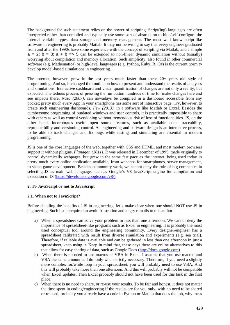
429
The background for such statement relies on the power of scripting. Script(ing) languages are often
interpreted rather than compiled and typically use some sort of abstraction to hide/self-configure the
internal variable types, data storage and memory management. The most well know script-like
software in engineering is probably Matlab. It may not be wrong to say that every engineer graduated
from and after the 1990s have some experience with the concept of scripting via Matlab, and a simple
a = 2; b = 3; a + b => 5 can be extended to non-linear dynamic simulation without (usually)
worrying about compilation and memory allocation. Such simplicity, also found in other commercial
software (e.g. Mathematica) or high-level languages (e.g. Python, Ruby, R, C#) is the current norm to
develop model-based simulations in engineering.
The internet, however, grew in the last years much faster than these 20+ years old style of
programming. And so, it changed the routine on how to present and understand the results of analyses
and simulations. Interactive dashboard and visual quantification of changes are not only a reality, but
expected. The tedious process of pressing the run button hundreds of time for make changes here and
see impacts there, Nasa (2007), can nowadays be compiled in a dashboard accessible from any
pocket; pretty much every App in your smartphone has some sort of interactive page. Try, however, to
create such engineering dashboards, Few (2013), in a software like Matlab or Excel. Besides the
cumbersome programing of outdated windows and user controls, it is practically impossible to share
with others as well as control versioning without tremendous risk of loss of functionalities. JS, on the
other hand, incorporates useful open source features, such as available code, traceability,
reproducibility and versioning control. As engineering and software design is an interactive process,
to be able to track changes and fix bugs while testing and simulating are essential in modern
programming.
JS is one of the core languages of the web, together with CSS and HTML, and most modern browsers
support it without plugins, Flanagan (2011). It was released in December of 1995, made originally to
control dynamically webpages, but grew in the same fast pace as the internet, being used today in
pretty much every online application available, from webapps for smartphones, server management,
to video game development. Besides community work, we cannot deny the role of big companies in
selecting JS as main web language, such as Google’s V8 JavaScript engine for compilation and
execution of JS (https://developers.google.com/v8/).
2. To JavaScript or not to JavaScript
2.1. When not to JavaScript?
Before detailing the benefits of JS in engineering, let’s make clear when one should NOT use JS in
engineering. Such list is required to avoid frustration and angry e-mails to this author.
a) When a spreadsheet can solve your problem in less than one afternoon. We cannot deny the
importance of spreadsheet-like programs such as Excel in engineering. It is probably the most
used conceptual tool around the engineering community. Every designer/engineer has a
spreadsheet calibrated with result from diverse simulation and experiments (e.g. sea trial).
Therefore, if reliable data is available and can be gathered in less than one afternoon in just a
spreadsheet, keep using it. Keep in mind that, these days there are online alternatives to this
that allow for easy sharing of data, such as Google Docs (http://docs.google.com).
b) When there is no need to use macros or VBA in Excel. I assume that you use macros and
VBA the same amount as I do: only when strictly necessary. Therefore, if you need a slightly
more complex for/while loop in your spreadsheet, you will probably need to use VBA. And
this will probably take more than one afternoon. And this will probably will not be compatible
when Excel updates. Then Excel probably should not have been used for this task in the first
place.
c) When there is no need to share, or re-use your results. To be fair and honest, it does not matter
the time spent in coding/engineering if the results are for you only, with no need to be shared
or re-used; probably you already have a code in Python or Matlab that does the job, why mess

430
it with JS if no one will ever see or re-use this simulation?
d) When the model does not require any graphic user interface (GUI). Anyone that tried to create
a GUI in Python, Matlab or Excel knows the limitations of these tools. One of the key
positive points from using JS is the possibility to combine mathematics with dynamic
elements of the HTML page. It means any kind of GUI, with buttons, figures, graphs as
customizable as there are different pages in the net. Creativity is the limit.
e) When one does not need to interact with the model/simulation parameters and/or data. In line
with the previous topic, interacting with data is much easier with a proper GUI. Parametric
models get easy with sliders and real-time visualization update. Such functionalities are one
of the core reasons for JS. If your model does not require the user changing variables, plotting
and replotting, creating and visualizing the data generated, JS may not be necessary.
f) When it is required to to control memory/events access and/or parallel computing. Although
modern JS engines such as Google V8 are as fast as C for certain tasks, JS is not the language
of choice when one wants to easily control memory access or distribute a large task among
multiple cores. True that modern JS packages take care of such events efficiently, such as
Node.js (https://nodejs.org), but I would only recommend this option if you are comfortable
with server management and JS. But if you do, then this paper is unnecessary.
g) When it can be solved without coding/computer (e.g. sketching by hand/board). Teaching
brought me many students knocking on my door with large models implemented in Matlab,
Excel or even JS asking coding questions. It is very common that an answer for their
problems relies not in the language of choice or ability to code, but on how the problem was
modelled and the algorithm sketched. One good hour of plain paper and pencil sketches can
be so efficient as hours of coding if both are done properly.
Experience shows that there is a large set of engineering cases that are not described on the excluding
conditions above, and does requires mathematical models with user interactivity, efficient GUI,
sharing and real time capacities. Therefore, JS benefits are described in the rest of this section.
2.2 Why JavaScript
2.2.1 Speed
When I started to use JS for simulation I got impressed by the speed of calculation. Having looping
for’s and if’s in vectors and matrices before in Matlab had brought me a certain time expectation
between the run and the results popping out in the screen. Such expectations reached a new level
when the simulation runs via a modern browser like Google Chrome in JS.
A benchmark from 2015 (https://julialang.org/benchmarks/) shows that for some basic operations,
such as parse_int, which parses a string from a user input or a table of values given in text file, and
transform this string in an integer number, JS can be over 130 times faster than Matlab. Even more
impressive, complex numbers calculations such as Mandelbrot Set and operations like the pi sum
series are faster than C, Fortran or Java, Fig.1. Given the pace of development and the fact that big
companies like Goggle are behind powerful JS engines, it is not wrong to speculate that in few years
the speed difference in other operations will be closer and closer to the C benchmark.
Speed to write and understand codes should also be considered. McLoone (2012) shows that JS
requires in average 3.4 times less lines of code than C and, impressively, requires 6 percent less lines
in average than an equivalent large task code in Matlab, Fig.2.
Although both benchmarks show that JS is not the fastest among all languages to process algorithms
or code typing, it is so efficient as other high-level languages (either open or proprietary), with the
extra functionalities from the web when combined with HTML and CSS.
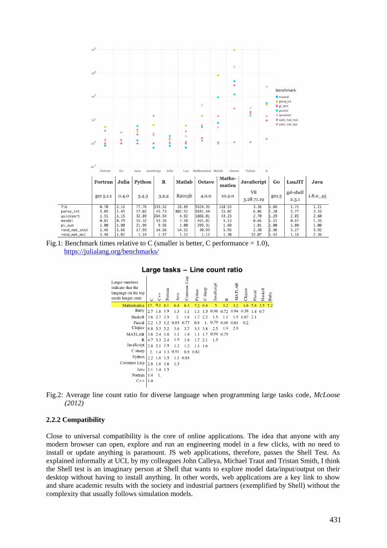
431
Fig.1: Benchmark times relative to C (smaller is better, C performance = 1.0),
https://julialang.org/benchmarks/
Fig.2: Average line count ratio for diverse language when programming large tasks code, McLoose
(2012)
2.2.2 Compatibility
Close to universal compatibility is the core of online applications. The idea that anyone with any
modern browser can open, explore and run an engineering model in a few clicks, with no need to
install or update anything is paramount. JS web applications, therefore, passes the Shell Test. As
explained informally at UCL by my colleagues John Calleya, Michael Traut and Tristan Smith, I think
the Shell test is an imaginary person at Shell that wants to explore model data/input/output on their
desktop without having to install anything. In other words, web applications are a key link to show
and share academic results with the society and industrial partners (exemplified by Shell) without the
complexity that usually follows simulation models.
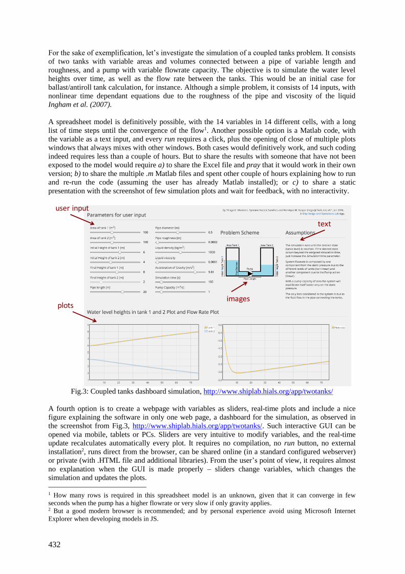
432
For the sake of exemplification, let’s investigate the simulation of a coupled tanks problem. It consists
of two tanks with variable areas and volumes connected between a pipe of variable length and
roughness, and a pump with variable flowrate capacity. The objective is to simulate the water level
heights over time, as well as the flow rate between the tanks. This would be an initial case for
ballast/antiroll tank calculation, for instance. Although a simple problem, it consists of 14 inputs, with
nonlinear time dependant equations due to the roughness of the pipe and viscosity of the liquid
Ingham et al. (2007).
A spreadsheet model is definitively possible, with the 14 variables in 14 different cells, with a long
list of time steps until the convergence of the flow1. Another possible option is a Matlab code, with
the variable as a text input, and every run requires a click, plus the opening of close of multiple plots
windows that always mixes with other windows. Both cases would definitively work, and such coding
indeed requires less than a couple of hours. But to share the results with someone that have not been
exposed to the model would require a) to share the Excel file and pray that it would work in their own
version; b) to share the multiple .m Matlab files and spent other couple of hours explaining how to run
and re-run the code (assuming the user has already Matlab installed); or c) to share a static
presentation with the screenshot of few simulation plots and wait for feedback, with no interactivity.
Fig.3: Coupled tanks dashboard simulation, http://www.shiplab.hials.org/app/twotanks/
A fourth option is to create a webpage with variables as sliders, real-time plots and include a nice
figure explaining the software in only one web page, a dashboard for the simulation, as observed in
the screenshot from Fig.3, http://www.shiplab.hials.org/app/twotanks/. Such interactive GUI can be
opened via mobile, tablets or PCs. Sliders are very intuitive to modify variables, and the real-time
update recalculates automatically every plot. It requires no compilation, no run button, no external
installation2, runs direct from the browser, can be shared online (in a standard configured webserver)
or private (with .HTML file and additional libraries). From the user’s point of view, it requires almost
no explanation when the GUI is made properly – sliders change variables, which changes the
simulation and updates the plots.
1 How many rows is required in this spreadsheet model is an unknown, given that it can converge in few
seconds when the pump has a higher flowrate or very slow if only gravity applies. 2 But a good modern browser is recommended; and by personal experience avoid using Microsoft Internet
Explorer when developing models in JS.
userinput
plots
text
images

433
2.2.3 User Interface
A clean user interface is not a merit of JS, but of the powerful combination of HTML and CSS.
Different from commercial software that have a GUI constrained by cells (e.g. Excel) or predefined
windows and buttons (e.g. Matlab), the browser always start from a blank page, where text, image,
video, buttons, charts and most of the interactive digital commands that we are used to can be placed
with large freedom on style and interface. Since 2003 CSS Zen Garden presents, for instance, the
versatility of the HTML + CSS with examples of a same HTML code controlled by different CSS
styles, http://www.csszengarden.com/.
Considering the example from Fig.3, we can observe that pretty much every element of the page can
be customized, from colours to fonts, graphs to buttons, text, and images. A single page dashboard
was the main objective in that app, with key information of the whole simulation condensed in one
page. Deliberately range slides were used for user input, to facilitate parametric changes, instead of a
traditional text input box. By the side of the slider is placed an image exemplifying the problem,
followed by a text of the assumptions. Results of the real-time simulation are presented below the
variables, with the two main plots that adjusts automatically to the maximum and minimum axis value
until the convergence is reached. Most of the elements in the page, such as sliders and plots, are ready
made via HTML5 or JS libraries, highly customizable for adapt to any application. Try to imagine
creating the same dashboard, with the same efficiency, in any other software.
The fact that everyone knows how to use a browser is another benefit. A clean dashboard requires
little or no training. Sliders instead of buttons instigates interactivity and the real-time calculation
eliminate the need of pressing the run button every time that a parameter is changed. The concept of
buttons, sliders, tabs, hyperlinks are already part of the everyday life of not only engineers, but all
stakeholders from a simulation model. In this sense, to create a GUI that is understood and can be
interacted by a wider range of people is an advancement.
2.2.4 Usage
Looking for similar examples in the internet is the first way to solve any difficulty while modelling.
From ‘How to do a scatter plot in Excel’ from ‘genetic algorithms in Python’, this is how must of us
and our students looks for a solution nowadays. Github (https://github.com/) is probably the largest
repository for codes available online. A study from 2014 shows that JS is by far the most used
language in Github (http://githut.info). It means software, tutorias and examples made available by
millions of collaborators to re-use and contribute, with an extensive qualified community that shares
its developments and results openly. Data Driven Documents library (D3 - https://d3js.org/), for
instance, keeps an impressively neat page of examples, tutorials and documentation available in
Github, with ready-made codes for most of the visualizations presented.
Such large community of developers means an extensive number of ready to use JS libraries available
online. There is no best choice, since that usually the selection of a JS library is strongly connected to
the needs, Does simulation X requires a real time plot of variables or a 3D object moving in the
screen, or both? For the sake of exemplification, my personal suggestion, with list of JS libraries
useful for engineers is presented as follows:
Data storage: JSON (https://www.w3schools.com/js/js_json_intro.asp)3
Data handling and interactivity: D3 (https://d3js.org/)
2D Plots: Flot (http://www.flotcharts.org/) and Chart.js (http://www.chartjs.org/)
3D Plots: Plotly (https://plot.ly/javascript/)
3 JSON is not a library, but a syntax for storing and exchanging data, written in JS object notation. Although
data can be easily converted from XML, CSV and even Excel XLXS to JSON, understanding JSON notation
saves precious time when testing and using JS libraries.
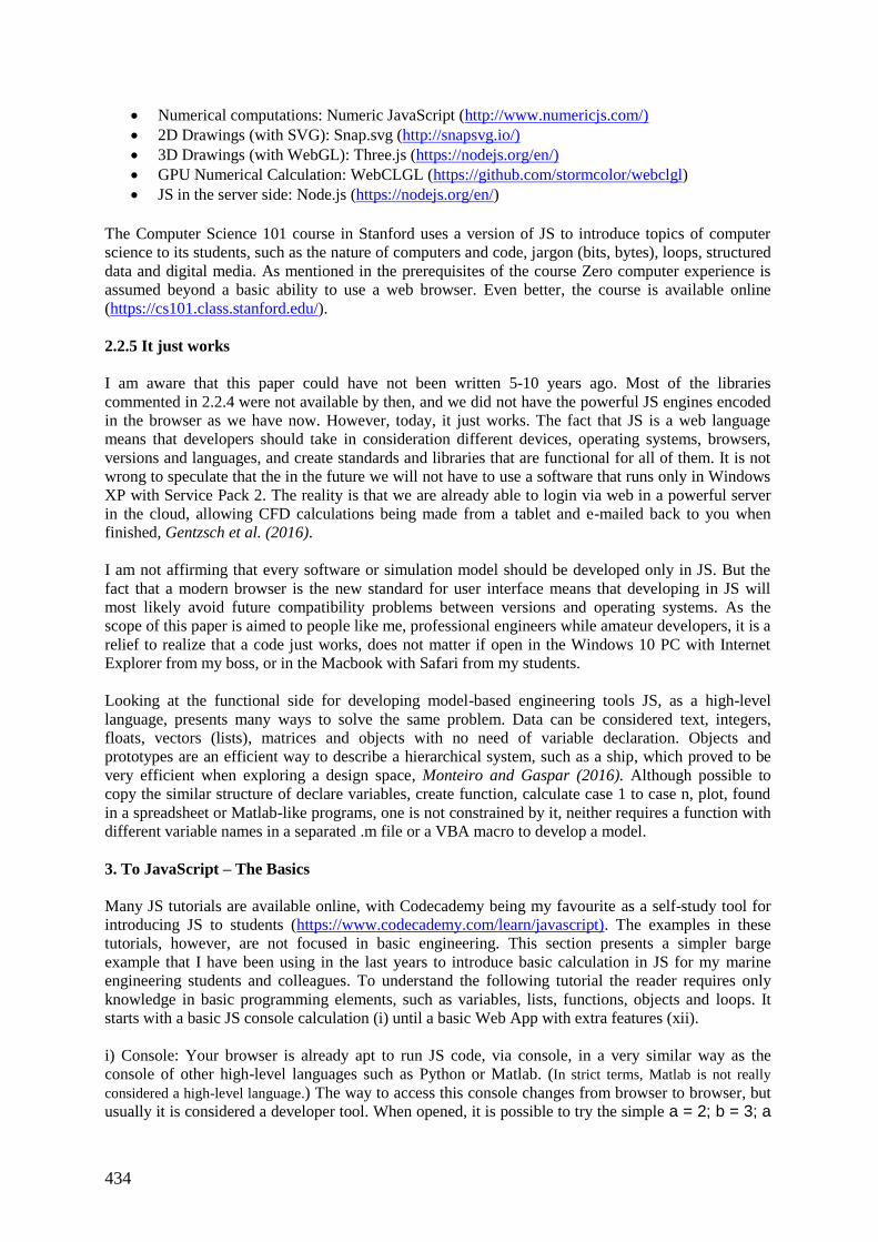
434
Numerical computations: Numeric JavaScript (http://www.numericjs.com/)
2D Drawings (with SVG): Snap.svg (http://snapsvg.io/)
3D Drawings (with WebGL): Three.js (https://nodejs.org/en/)
GPU Numerical Calculation: WebCLGL (https://github.com/stormcolor/webclgl)
JS in the server side: Node.js (https://nodejs.org/en/)
The Computer Science 101 course in Stanford uses a version of JS to introduce topics of computer
science to its students, such as the nature of computers and code, jargon (bits, bytes), loops, structured
data and digital media. As mentioned in the prerequisites of the course Zero computer experience is
assumed beyond a basic ability to use a web browser. Even better, the course is available online
(https://cs101.class.stanford.edu/).
2.2.5 It just works
I am aware that this paper could have not been written 5-10 years ago. Most of the libraries
commented in 2.2.4 were not available by then, and we did not have the powerful JS engines encoded
in the browser as we have now. However, today, it just works. The fact that JS is a web language
means that developers should take in consideration different devices, operating systems, browsers,
versions and languages, and create standards and libraries that are functional for all of them. It is not
wrong to speculate that the in the future we will not have to use a software that runs only in Windows
XP with Service Pack 2. The reality is that we are already able to login via web in a powerful server
in the cloud, allowing CFD calculations being made from a tablet and e-mailed back to you when
finished, Gentzsch et al. (2016).
I am not affirming that every software or simulation model should be developed only in JS. But the
fact that a modern browser is the new standard for user interface means that developing in JS will
most likely avoid future compatibility problems between versions and operating systems. As the
scope of this paper is aimed to people like me, professional engineers while amateur developers, it is a
relief to realize that a code just works, does not matter if open in the Windows 10 PC with Internet
Explorer from my boss, or in the Macbook with Safari from my students.
Looking at the functional side for developing model-based engineering tools JS, as a high-level
language, presents many ways to solve the same problem. Data can be considered text, integers,
floats, vectors (lists), matrices and objects with no need of variable declaration. Objects and
prototypes are an efficient way to describe a hierarchical system, such as a ship, which proved to be
very efficient when exploring a design space, Monteiro and Gaspar (2016). Although possible to
copy the similar structure of declare variables, create function, calculate case 1 to case n, plot, found
in a spreadsheet or Matlab-like programs, one is not constrained by it, neither requires a function with
different variable names in a separated .m file or a VBA macro to develop a model.
3. To JavaScript – The Basics
Many JS tutorials are available online, with Codecademy being my favourite as a self-study tool for
introducing JS to students (https://www.codecademy.com/learn/javascript). The examples in these
tutorials, however, are not focused in basic engineering. This section presents a simpler barge
example that I have been using in the last years to introduce basic calculation in JS for my marine
engineering students and colleagues. To understand the following tutorial the reader requires only
knowledge in basic programming elements, such as variables, lists, functions, objects and loops. It
starts with a basic JS console calculation (i) until a basic Web App with extra features (xii).
i) Console: Your browser is already apt to run JS code, via console, in a very similar way as the
console of other high-level languages such as Python or Matlab. (In strict terms, Matlab is not really
considered a high-level language.) The way to access this console changes from browser to browser, but
usually it is considered a developer tool. When opened, it is possible to try the simple a = 2; b = 3; a
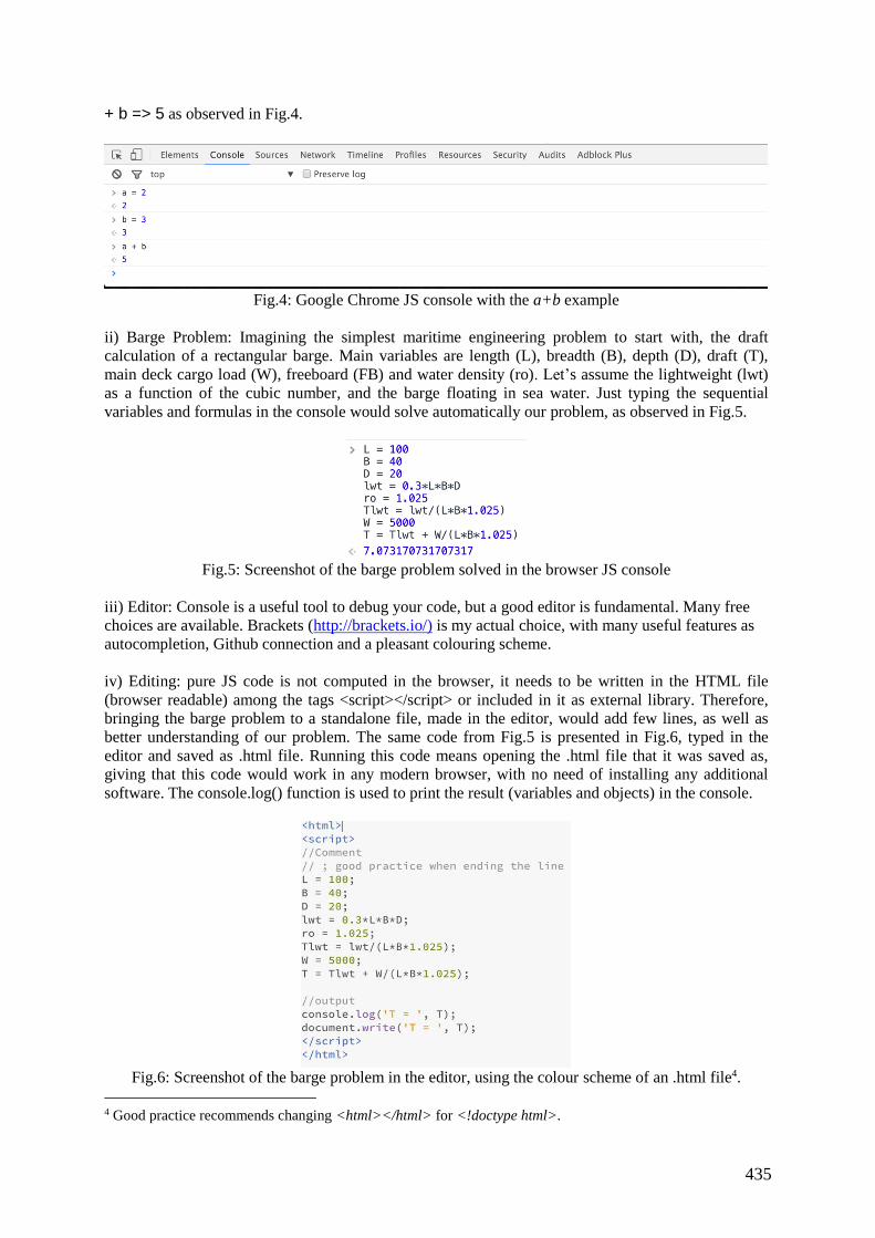
435
+ b => 5 as observed in Fig.4.
Fig.4: Google Chrome JS console with the a+b example
ii) Barge Problem: Imagining the simplest maritime engineering problem to start with, the draft
calculation of a rectangular barge. Main variables are length (L), breadth (B), depth (D), draft (T),
main deck cargo load (W), freeboard (FB) and water density (ro). Let’s assume the lightweight (lwt)
as a function of the cubic number, and the barge floating in sea water. Just typing the sequential
variables and formulas in the console would solve automatically our problem, as observed in Fig.5.
Fig.5: Screenshot of the barge problem solved in the browser JS console
iii) Editor: Console is a useful tool to debug your code, but a good editor is fundamental. Many free
choices are available. Brackets (http://brackets.io/) is my actual choice, with many useful features as
autocompletion, Github connection and a pleasant colouring scheme.
iv) Editing: pure JS code is not computed in the browser, it needs to be written in the HTML file
(browser readable) among the tags <script></script> or included in it as external library. Therefore,
bringing the barge problem to a standalone file, made in the editor, would add few lines, as well as
better understanding of our problem. The same code from Fig.5 is presented in Fig.6, typed in the
editor and saved as .html file. Running this code means opening the .html file that it was saved as,
giving that this code would work in any modern browser, with no need of installing any additional
software. The console.log() function is used to print the result (variables and objects) in the console.
Fig.6: Screenshot of the barge problem in the editor, using the colour scheme of an .html file4.
4 Good practice recommends changing <html></html> for <!doctype html>.
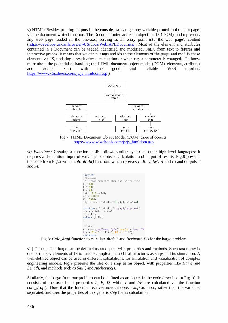
436
v) HTML: Besides printing outputs in the console, we can get any variable printed in the main page,
via the document.write() function. The Document interface is an object model (DOM), and represents
any web page loaded in the browser, serving as an entry point into the web page's content
(https://developer.mozilla.org/en-US/docs/Web/API/Document). Most of the element and attributes
contained in a Document can be tagged, identified and modified, Fig.7, from text to figures and
interactive graphs. It means that we can put tags and ids in the elements of the page, and modify these
elements via JS, updating a result after a calculation or when e.g. a parameter is changed. (To know
more about the potential of handling the HTML document object model (DOM), elements, attributes
and events, start with the good and reliable W3S tutorials,
https://www.w3schools.com/js/js_htmldom.asp.)
Fig.7: HTML Document Object Model (DOM) three of objects,
https://www.w3schools.com/js/js_htmldom.asp
vi) Functions: Creating a function in JS follows similar syntax as other high-level languages: it
requires a declaration, input of variables or objects, calculation and output of results. Fig.8 presents
the code from Fig.6 with a calc_draft() function, which receives L, B, D, lwt, W and ro and outputs T
and FB.
Fig.8: Calc_draft function to calculate draft T and freeboard FB for the barge problem
vii) Objects: The barge can be defined as an object, with properties and methods. Such taxonomy is
one of the key elements of JS to handle complex hierarchical structures as ships and its simulation. A
well-defined object can be used in different calculations, for simulation and visualization of complex
engineering models. Fig.9 presents the idea of a ship as an object, with properties like Name and
Length, and methods such as Sail() and Anchoring().
Similarly, the barge from our problem can be defined as an object in the code described in Fig.10. It
consists of the user input properties L, B, D, while T and FB are calculated via the function
calc_draft(). Note that the function receives now an object ship as input, rather than the variables
separated, and uses the properties of this generic ship for its calculation.
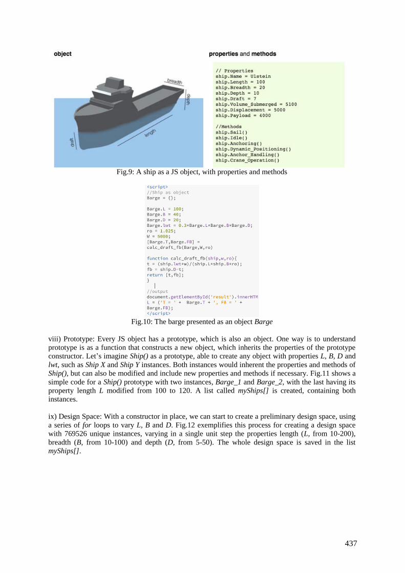
437
Fig.9: A ship as a JS object, with properties and methods
Fig.10: The barge presented as an object Barge
viii) Prototype: Every JS object has a prototype, which is also an object. One way is to understand
prototype is as a function that constructs a new object, which inherits the properties of the prototype
constructor. Let’s imagine Ship() as a prototype, able to create any object with properties L, B, D and
lwt, such as Ship X and Ship Y instances. Both instances would inherent the properties and methods of
Ship(), but can also be modified and include new properties and methods if necessary. Fig.11 shows a
simple code for a Ship() prototype with two instances, Barge_1 and Barge_2, with the last having its
property length L modified from 100 to 120. A list called myShips[] is created, containing both
instances.
ix) Design Space: With a constructor in place, we can start to create a preliminary design space, using
a series of for loops to vary L, B and D. Fig.12 exemplifies this process for creating a design space
with 769526 unique instances, varying in a single unit step the properties length (L, from 10-200),
breadth (B, from 10-100) and depth (D, from 5-50). The whole design space is saved in the list
myShips[].
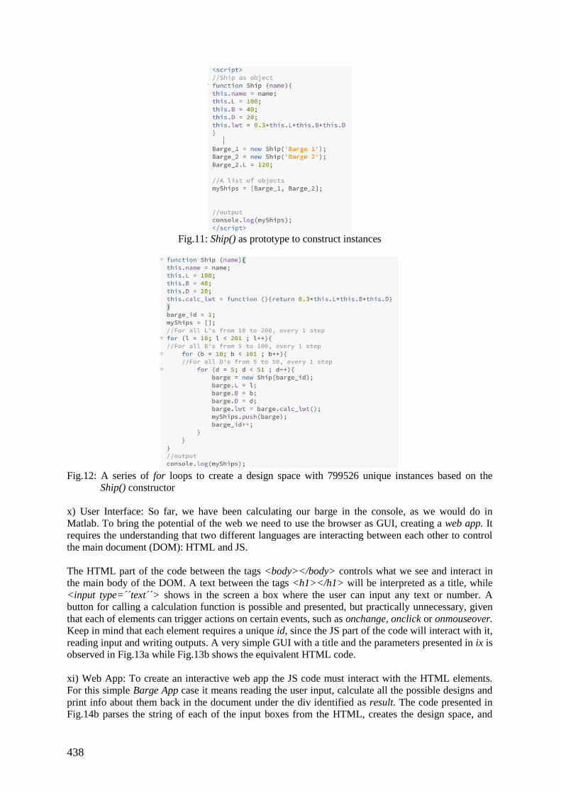
438
Fig.11: Ship() as prototype to construct instances
Fig.12: A series of for loops to create a design space with 799526 unique instances based on the
Ship() constructor
x) User Interface: So far, we have been calculating our barge in the console, as we would do in
Matlab. To bring the potential of the web we need to use the browser as GUI, creating a web app. It
requires the understanding that two different languages are interacting between each other to control
the main document (DOM): HTML and JS.
The HTML part of the code between the tags <body></body> controls what we see and interact in
the main body of the DOM. A text between the tags <h1></h1> will be interpreted as a title, while
<input type=´´text´´> shows in the screen a box where the user can input any text or number. A
button for calling a calculation function is possible and presented, but practically unnecessary, given
that each of elements can trigger actions on certain events, such as onchange, onclick or onmouseover.
Keep in mind that each element requires a unique id, since the JS part of the code will interact with it,
reading input and writing outputs. A very simple GUI with a title and the parameters presented in ix is
observed in Fig.13a while Fig.13b shows the equivalent HTML code.
xi) Web App: To create an interactive web app the JS code must interact with the HTML elements.
For this simple Barge App case it means reading the user input, calculate all the possible designs and
print info about them back in the document under the div identified as result. The code presented in
Fig.14b parses the string of each of the input boxes from the HTML, creates the design space, and
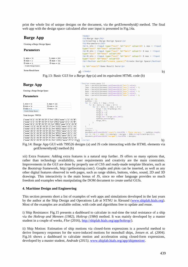
439
print the whole list of unique designs on the document, via the getElementbyid() method. The final
web app with the design space calculated after user input is presented in Fig.14a.
a) b)
Fig.13: Basic GUI for a Barge App (a) and its equivalent HTML code (b)
a) b)
Fig.14: Barge App GUI with 799526 designs (a) and JS code interacting with the HTML elements via
getElementbyid() method (b)
xii) Extra Features: Adding extra features is a natural step further. JS offers so many options that,
rather than technology availability, user requirements and creativity are the main constraints.
Improvements in the GUI are done by properly use of CSS and ready-made template libraries, such as
the Bootstrap framework, http://getbootstrap.com/). Graphs and plots can be inserted, as well as any
other digital features observed in web pages, such as range sliders, buttons, video, sound, 2D and 3D
drawings. This interactivity is the main bonus of JS, since no other language provides so much
freedom and examples when manipulating the DOM document to create useful GUIs.
4. Maritime Design and Engineering
This section presents short a list of examples of web apps and simulations developed in the last years
by the author at the Ship Design and Operations Lab at NTNU in Ålesund (www.shiplab.hials.org).
Most of the examples are available online, with code and algorithms free to update and reuse.
i) Ship Resistance: Fig.15 presents a dashboard to calculate in real-time the total resistance of a ship
via the Holtrop and Mennen (1982), Holtrop (1984) method. It was mainly developed by a master
student in a couple of weeks, Flor (2016), http://shiplab.hials.org/app/holtrop/).
ii) Ship Motion: Estimation of ship motions via closed-form expressions is a powerful method to
derive frequency responses for the wave-induced motions for monohull ships, Jensen et. al. (2004).
Fig.16 shows a dashboard to calculate motion and acceleration using closed-form expressions,
developed by a master student, Andrade (2015), www.shiplab.hials.org/app/shipmotion/.
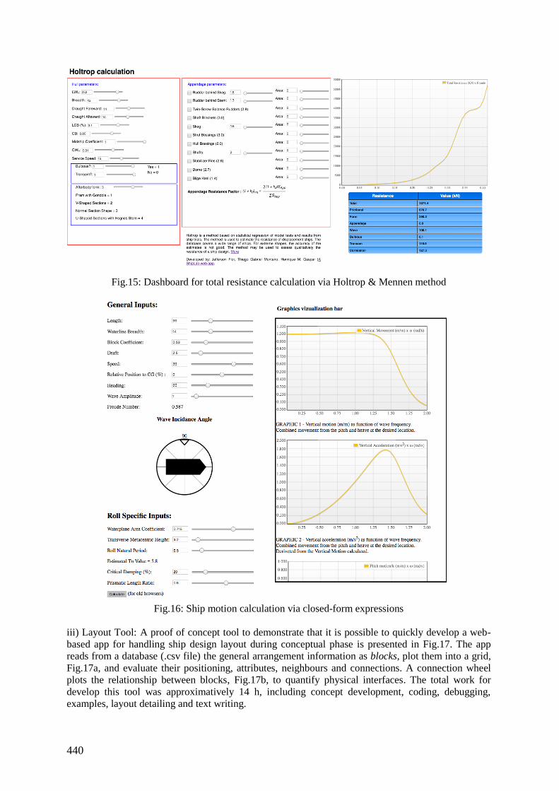
440
Fig.15: Dashboard for total resistance calculation via Holtrop & Mennen method
Fig.16: Ship motion calculation via closed-form expressions
iii) Layout Tool: A proof of concept tool to demonstrate that it is possible to quickly develop a web-
based app for handling ship design layout during conceptual phase is presented in Fig.17. The app
reads from a database (.csv file) the general arrangement information as blocks, plot them into a grid,
Fig.17a, and evaluate their positioning, attributes, neighbours and connections. A connection wheel
plots the relationship between blocks, Fig.17b, to quantify physical interfaces. The total work for
develop this tool was approximatively 14 h, including concept development, coding, debugging,
examples, layout detailing and text writing.
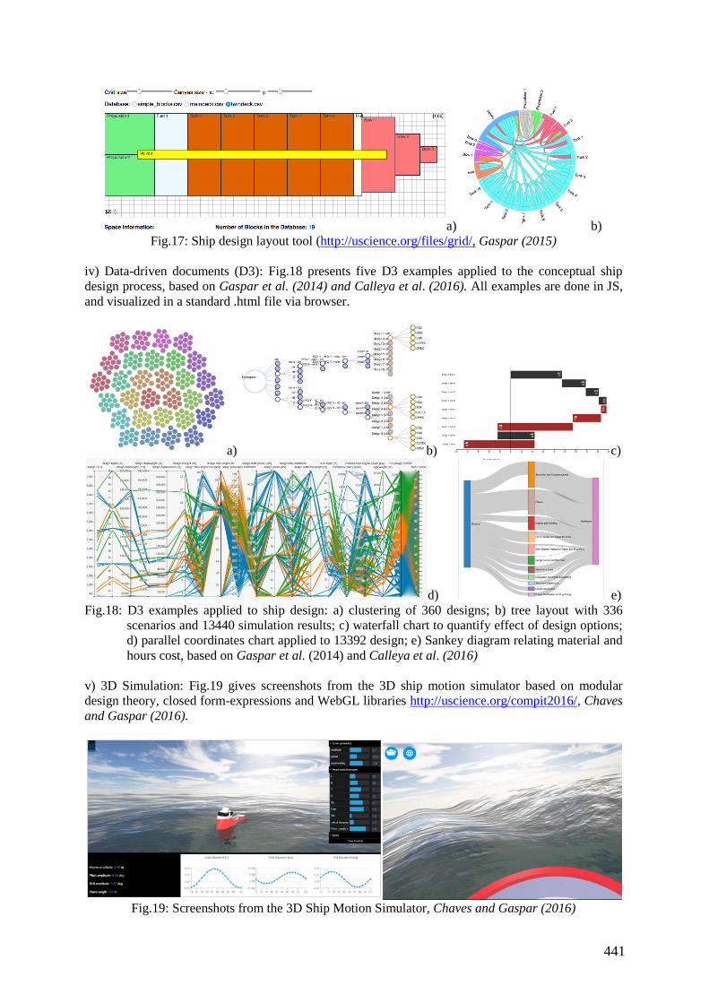
441
a) b)
Fig.17: Ship design layout tool (http://uscience.org/files/grid/, Gaspar (2015)
iv) Data-driven documents (D3): Fig.18 presents five D3 examples applied to the conceptual ship
design process, based on Gaspar et al. (2014) and Calleya et al. (2016). All examples are done in JS,
and visualized in a standard .html file via browser.
a) b) c)
d) e)
Fig.18: D3 examples applied to ship design: a) clustering of 360 designs; b) tree layout with 336
scenarios and 13440 simulation results; c) waterfall chart to quantify effect of design options;
d) parallel coordinates chart applied to 13392 design; e) Sankey diagram relating material and
hours cost, based on Gaspar et al. (2014) and Calleya et al. (2016)
v) 3D Simulation: Fig.19 gives screenshots from the 3D ship motion simulator based on modular
design theory, closed form-expressions and WebGL libraries http://uscience.org/compit2016/, Chaves
and Gaspar (2016).
Fig.19: Screenshots from the 3D Ship Motion Simulator, Chaves and Gaspar (2016)
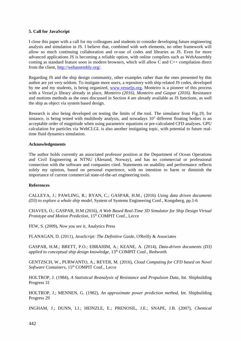
442
5. Call for JavaScript
I close this paper with a call for my colleagues and students to consider developing future engineering
analysis and simulation in JS. I believe that, combined with web elements, no other framework will
allow so much continuing collaboration and re-use of codes and libraries as JS. Even for more
advanced applications JS is becoming a reliable option, with online compilers such as WebAssembly
coming as standard feature soon in modern browsers, which will allow C and C++ compilation direct
from the client, http://webassembly.org/.
Regarding JS and the ship design community, other examples rather than the ones presented by this
author are yet very seldom. To instigate more users, a repository with ship related JS codes, developed
by me and my students, is being organized, www.vesseljs.org. Monteiro is a pioneer of this process
with a Vessel.js library already in place, Monteiro (2016), Monteiro and Gaspar (2016). Resistance
and motions methods as the ones discussed in Section 4 are already available as JS functions, as well
the ship as object via system based design.
Research is also being developed on testing the limits of the tool. The simulator from Fig.19, for
instance, is being tested with multibody analysis, and nowadays 103 different floating bodies is an
acceptable order of magnitude when using parametric equations or pre-calculated CFD analyses. GPU
calculation for particles via WebCLGL is also another instigating topic, with potential to future real-
time fluid dynamics simulation.
Acknowledgements
The author holds currently an associated professor position at the Department of Ocean Operations
and Civil Engineering at NTNU (Ålesund, Norway), and has no commercial or professional
connection with the software and companies cited. Statements on usability and performance reflects
solely my opinion, based on personal experience, with no intention to harm or diminish the
importance of current commercial state-of-the-art engineering tools.
References
CALLEYA, J.; PAWLING, R.; RYAN, C.; GASPAR, H.M.; (2016) Using data driven documents
(D3) to explore a whole ship model, System of Systems Engineering Conf., Kongsberg, pp.1-6
CHAVES, O.; GASPAR, H.M (2016), A Web Based Real-Time 3D Simulator for Ship Design Virtual
Prototype and Motion Prediction, 15th COMPIT Conf., Lecce
FEW, S. (2009), Now you see it, Analytics Press
FLANAGAN, D. (2011), JavaScript: The Definitive Guide, O'Reilly & Associates
GASPAR, H.M.; BRETT, P.O.; EBRAHIM, A.; KEANE, A. (2014), Data-driven documents (D3)
applied to conceptual ship design knowledge, 13th COMPIT Conf., Redworth
GENTZSCH, W., PURWANTO, A.; REYER, M. (2016), Cloud Computing for CFD based on Novel
Software Containers, 15th COMPIT Conf., Lecce
HOLTROP, J. (1984), A Statistical Reanalysis of Resistance and Propulsion Data, Int. Shipbuilding
Progress 31
HOLTROP, J.; MENNEN, G. (1982), An approximate power prediction method, Int. Shipbuilding
Progress 29
INGHAM, J.; DUNN, I.J.; HEINZLE, E.; PRENOSIL, J.E.; SNAPE, J.B. (2007), Chemical

443
Engineering Dynamics, Wiley
JENSEN, J.J.; MANSOUR, A.E.; OLSEN, A.S. (2004), Estimation of ship motions using closed-form
expressions, Ocean Engineering 31/1, pp.61-85
McLOOSE, J. (2012), Code length measured in 14 languages, Wolfram
http://blog.wolfram.com/2012/11/14/code-length-measured-in-14-languages/
MONTEIRO, T. (2016), A Knowledge-Based Approach for an Open Object Oriented Library in Ship
Design, MSc Thesis, NTNU, Trondheim
MONTEIRO, T.; GASPAR, H. M. (2016), An Open Source Approach for a Conceptual Ship Design
Tools Library, 10th HIPER Conf., Cortona
NASA (2007) NASA Systems Engineering Handbook, NASA
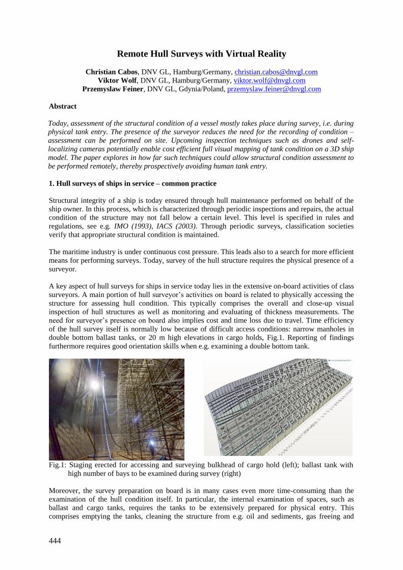
444
Remote Hull Surveys with Virtual Reality
Christian Cabos, DNV GL, Hamburg/Germany, [email protected]
Viktor Wolf, DNV GL, Hamburg/Germany, [email protected]
Przemyslaw Feiner, DNV GL, Gdynia/Poland, [email protected]
Abstract
Today, assessment of the structural condition of a vessel mostly takes place during survey, i.e. during
physical tank entry. The presence of the surveyor reduces the need for the recording of condition –
assessment can be performed on site. Upcoming inspection techniques such as drones and self-
localizing cameras potentially enable cost efficient full visual mapping of tank condition on a 3D ship
model. The paper explores in how far such techniques could allow structural condition assessment to
be performed remotely, thereby prospectively avoiding human tank entry.
1. Hull surveys of ships in service – common practice
Structural integrity of a ship is today ensured through hull maintenance performed on behalf of the
ship owner. In this process, which is characterized through periodic inspections and repairs, the actual
condition of the structure may not fall below a certain level. This level is specified in rules and
regulations, see e.g. IMO (1993), IACS (2003). Through periodic surveys, classification societies
verify that appropriate structural condition is maintained.
The maritime industry is under continuous cost pressure. This leads also to a search for more efficient
means for performing surveys. Today, survey of the hull structure requires the physical presence of a
surveyor.
A key aspect of hull surveys for ships in service today lies in the extensive on-board activities of class
surveyors. A main portion of hull surveyor’s activities on board is related to physically accessing the
structure for assessing hull condition. This typically comprises the overall and close-up visual
inspection of hull structures as well as monitoring and evaluating of thickness measurements. The
need for surveyor’s presence on board also implies cost and time loss due to travel. Time efficiency
of the hull survey itself is normally low because of difficult access conditions: narrow manholes in
double bottom ballast tanks, or 20 m high elevations in cargo holds, Fig.1. Reporting of findings
furthermore requires good orientation skills when e.g. examining a double bottom tank.
Fig.1: Staging erected for accessing and surveying bulkhead of cargo hold (left); ballast tank with
high number of bays to be examined during survey (right)
Moreover, the survey preparation on board is in many cases even more time-consuming than the
examination of the hull condition itself. In particular, the internal examination of spaces, such as
ballast and cargo tanks, requires the tanks to be extensively prepared for physical entry. This
comprises emptying the tanks, cleaning the structure from e.g. oil and sediments, gas freeing and
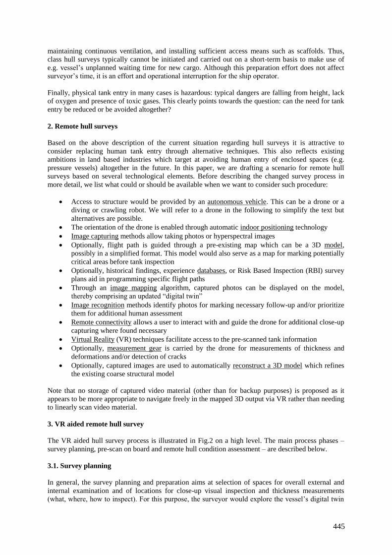
445
maintaining continuous ventilation, and installing sufficient access means such as scaffolds. Thus,
class hull surveys typically cannot be initiated and carried out on a short-term basis to make use of
e.g. vessel’s unplanned waiting time for new cargo. Although this preparation effort does not affect
surveyor’s time, it is an effort and operational interruption for the ship operator.
Finally, physical tank entry in many cases is hazardous: typical dangers are falling from height, lack
of oxygen and presence of toxic gases. This clearly points towards the question: can the need for tank
entry be reduced or be avoided altogether?
2. Remote hull surveys
Based on the above description of the current situation regarding hull surveys it is attractive to
consider replacing human tank entry through alternative techniques. This also reflects existing
ambitions in land based industries which target at avoiding human entry of enclosed spaces (e.g.
pressure vessels) altogether in the future. In this paper, we are drafting a scenario for remote hull
surveys based on several technological elements. Before describing the changed survey process in
more detail, we list what could or should be available when we want to consider such procedure:
Access to structure would be provided by an autonomous vehicle. This can be a drone or a
diving or crawling robot. We will refer to a drone in the following to simplify the text but
alternatives are possible.
The orientation of the drone is enabled through automatic indoor positioning technology
Image capturing methods allow taking photos or hyperspectral images
Optionally, flight path is guided through a pre-existing map which can be a 3D model,
possibly in a simplified format. This model would also serve as a map for marking potentially
critical areas before tank inspection
Optionally, historical findings, experience databases, or Risk Based Inspection (RBI) survey
plans aid in programming specific flight paths
Through an image mapping algorithm, captured photos can be displayed on the model,
thereby comprising an updated “digital twin”
Image recognition methods identify photos for marking necessary follow-up and/or prioritize
them for additional human assessment
Remote connectivity allows a user to interact with and guide the drone for additional close-up
capturing where found necessary
Virtual Reality (VR) techniques facilitate access to the pre-scanned tank information
Optionally, measurement gear is carried by the drone for measurements of thickness and
deformations and/or detection of cracks
Optionally, captured images are used to automatically reconstruct a 3D model which refines
the existing coarse structural model
Note that no storage of captured video material (other than for backup purposes) is proposed as it
appears to be more appropriate to navigate freely in the mapped 3D output via VR rather than needing
to linearly scan video material.
3. VR aided remote hull survey
The VR aided hull survey process is illustrated in Fig.2 on a high level. The main process phases –
survey planning, pre-scan on board and remote hull condition assessment – are described below.
3.1. Survey planning
In general, the survey planning and preparation aims at selection of spaces for overall external and
internal examination and of locations for close-up visual inspection and thickness measurements
(what, where, how to inspect). For this purpose, the surveyor would explore the vessel’s digital twin
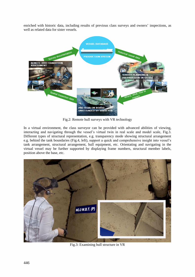
446
enriched with historic data, including results of previous class surveys and owners’ inspections, as
well as related data for sister vessels.
Fig.2: Remote hull surveys with VR technology
In a virtual environment, the class surveyor can be provided with advanced abilities of viewing,
interacting and navigating through the vessel’s virtual twin in real scale and model scale, Fig.3.
Different types of structural representation, e.g. transparency mode showing structural arrangement
e.g. behind the tank boundaries (Fig.4, left), support a quick and comprehensive insight into vessel’s
tank arrangement, structural arrangement, hull equipment, etc. Orientating and navigating in the
virtual vessel may be further supported by displaying frame numbers, structural member labels,
position above the base, etc.
Fig.3: Examining hull structure in VR
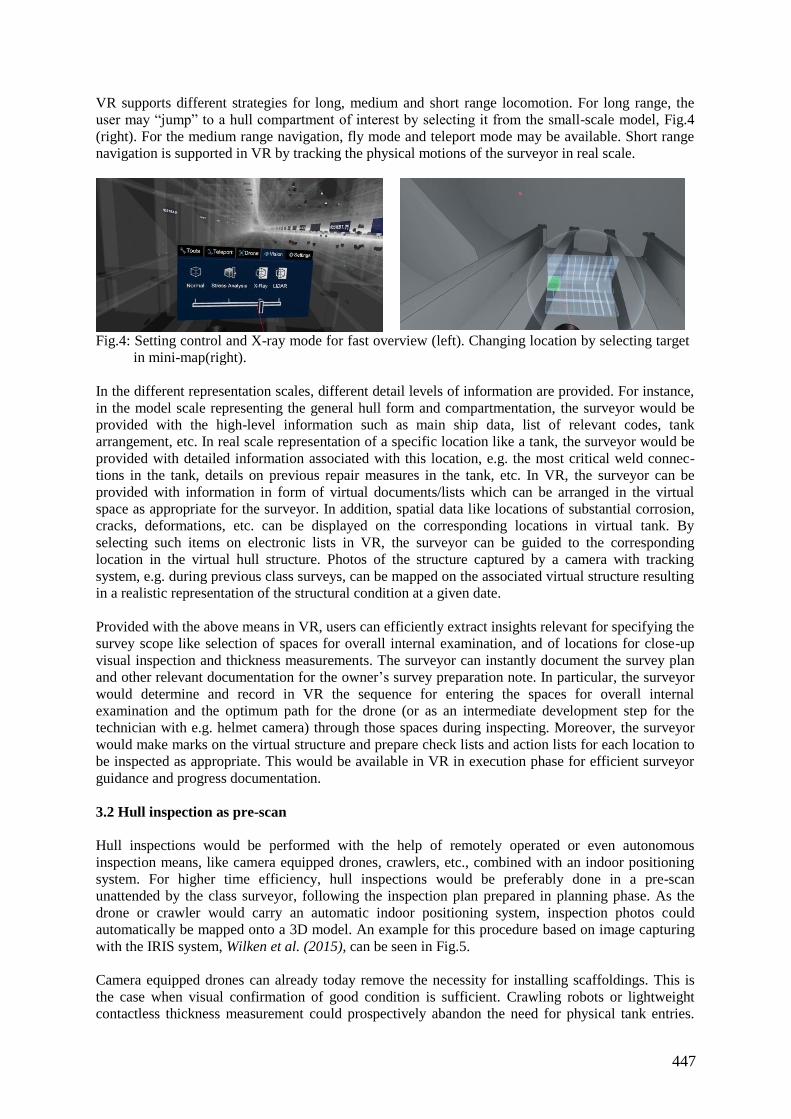
447
VR supports different strategies for long, medium and short range locomotion. For long range, the
user may “jump” to a hull compartment of interest by selecting it from the small-scale model, Fig.4
(right). For the medium range navigation, fly mode and teleport mode may be available. Short range
navigation is supported in VR by tracking the physical motions of the surveyor in real scale.
Fig.4: Setting control and X-ray mode for fast overview (left). Changing location by selecting target
in mini-map(right).
In the different representation scales, different detail levels of information are provided. For instance,
in the model scale representing the general hull form and compartmentation, the surveyor would be
provided with the high-level information such as main ship data, list of relevant codes, tank
arrangement, etc. In real scale representation of a specific location like a tank, the surveyor would be
provided with detailed information associated with this location, e.g. the most critical weld connec-
tions in the tank, details on previous repair measures in the tank, etc. In VR, the surveyor can be
provided with information in form of virtual documents/lists which can be arranged in the virtual
space as appropriate for the surveyor. In addition, spatial data like locations of substantial corrosion,
cracks, deformations, etc. can be displayed on the corresponding locations in virtual tank. By
selecting such items on electronic lists in VR, the surveyor can be guided to the corresponding
location in the virtual hull structure. Photos of the structure captured by a camera with tracking
system, e.g. during previous class surveys, can be mapped on the associated virtual structure resulting
in a realistic representation of the structural condition at a given date.
Provided with the above means in VR, users can efficiently extract insights relevant for specifying the
survey scope like selection of spaces for overall internal examination, and of locations for close-up
visual inspection and thickness measurements. The surveyor can instantly document the survey plan
and other relevant documentation for the owner’s survey preparation note. In particular, the surveyor
would determine and record in VR the sequence for entering the spaces for overall internal
examination and the optimum path for the drone (or as an intermediate development step for the
technician with e.g. helmet camera) through those spaces during inspecting. Moreover, the surveyor
would make marks on the virtual structure and prepare check lists and action lists for each location to
be inspected as appropriate. This would be available in VR in execution phase for efficient surveyor
guidance and progress documentation.
3.2 Hull inspection as pre-scan
Hull inspections would be performed with the help of remotely operated or even autonomous
inspection means, like camera equipped drones, crawlers, etc., combined with an indoor positioning
system. For higher time efficiency, hull inspections would be preferably done in a pre-scan
unattended by the class surveyor, following the inspection plan prepared in planning phase. As the
drone or crawler would carry an automatic indoor positioning system, inspection photos could
automatically be mapped onto a 3D model. An example for this procedure based on image capturing
with the IRIS system, Wilken et al. (2015), can be seen in Fig.5.
Camera equipped drones can already today remove the necessity for installing scaffoldings. This is
the case when visual confirmation of good condition is sufficient. Crawling robots or lightweight
contactless thickness measurement could prospectively abandon the need for physical tank entries.
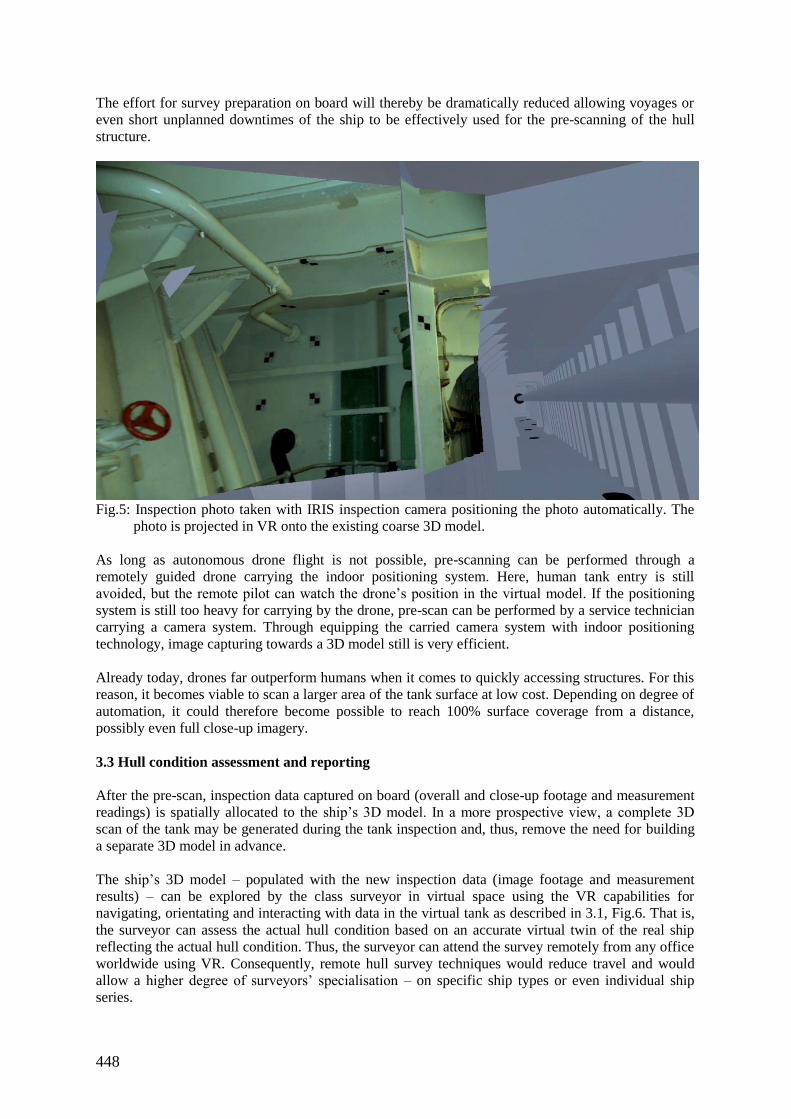
448
The effort for survey preparation on board will thereby be dramatically reduced allowing voyages or
even short unplanned downtimes of the ship to be effectively used for the pre-scanning of the hull
structure.
Fig.5: Inspection photo taken with IRIS inspection camera positioning the photo automatically. The
photo is projected in VR onto the existing coarse 3D model.
As long as autonomous drone flight is not possible, pre-scanning can be performed through a
remotely guided drone carrying the indoor positioning system. Here, human tank entry is still
avoided, but the remote pilot can watch the drone’s position in the virtual model. If the positioning
system is still too heavy for carrying by the drone, pre-scan can be performed by a service technician
carrying a camera system. Through equipping the carried camera system with indoor positioning
technology, image capturing towards a 3D model still is very efficient.
Already today, drones far outperform humans when it comes to quickly accessing structures. For this
reason, it becomes viable to scan a larger area of the tank surface at low cost. Depending on degree of
automation, it could therefore become possible to reach 100% surface coverage from a distance,
possibly even full close-up imagery.
3.3 Hull condition assessment and reporting
After the pre-scan, inspection data captured on board (overall and close-up footage and measurement
readings) is spatially allocated to the ship’s 3D model. In a more prospective view, a complete 3D
scan of the tank may be generated during the tank inspection and, thus, remove the need for building
a separate 3D model in advance.
The ship’s 3D model – populated with the new inspection data (image footage and measurement
results) – can be explored by the class surveyor in virtual space using the VR capabilities for
navigating, orientating and interacting with data in the virtual tank as described in 3.1, Fig.6. That is,
the surveyor can assess the actual hull condition based on an accurate virtual twin of the real ship
reflecting the actual hull condition. Thus, the surveyor can attend the survey remotely from any office
worldwide using VR. Consequently, remote hull survey techniques would reduce travel and would
allow a higher degree of surveyors’ specialisation – on specific ship types or even individual ship
series.
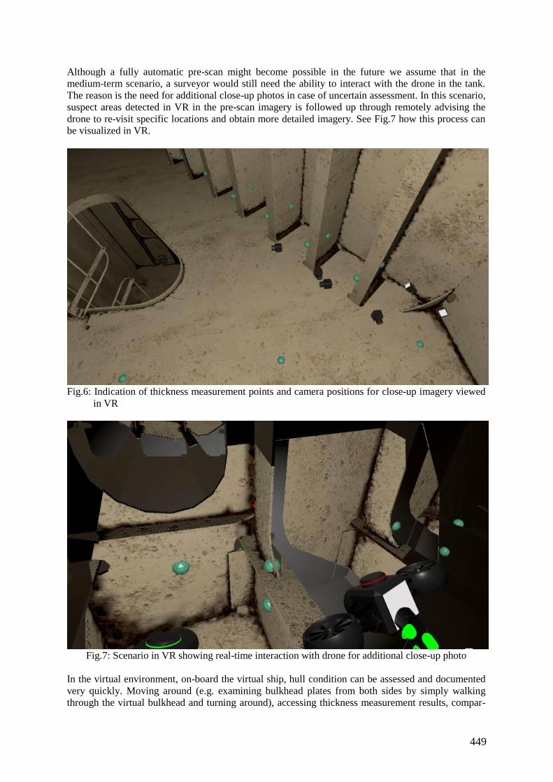
449
Although a fully automatic pre-scan might become possible in the future we assume that in the
medium-term scenario, a surveyor would still need the ability to interact with the drone in the tank.
The reason is the need for additional close-up photos in case of uncertain assessment. In this scenario,
suspect areas detected in VR in the pre-scan imagery is followed up through remotely advising the
drone to re-visit specific locations and obtain more detailed imagery. See Fig.7 how this process can
be visualized in VR.
Fig.6: Indication of thickness measurement points and camera positions for close-up imagery viewed
in VR
Fig.7: Scenario in VR showing real-time interaction with drone for additional close-up photo
In the virtual environment, on-board the virtual ship, hull condition can be assessed and documented
very quickly. Moving around (e.g. examining bulkhead plates from both sides by simply walking
through the virtual bulkhead and turning around), accessing thickness measurement results, compar-
450
ing to previous records, etc. becomes fast and easy. Automated algorithms for image recognition can
direct the surveyor to locations with suspected cracks, deformations, heavy corrosion wastage,
coating break-down, etc. and would therefore accelerate the process of hull condition assessment.
Inside the virtual tank, the surveyor is efficiently guided in terms of all relevant data from vessel
database like design analysis data, risk-critical areas, ship operation history (trading pattern,
encountered wave climate, loading pattern), survey and inspection history (condition of hull at last
survey), condition of sister ships, etc. In complicated cases, an expert from helpdesk can be brought
into the same virtual space for decision support.
Findings, repair measures, memo to surveyor, etc. can directly be recorded on the structure and linked
to the production system. Voice notes and text dictation further facilitate instant reporting. No addi-
tional work is necessary for the surveyor after leaving the virtual ship – documentation is done when
survey is done.
Results can be presented and necessity of possible maintenance and repair measures can be explained
to the superintendent/ship owner representative in a virtual meeting on-board the virtual ship in an
efficient and most intuitive way.
4. Remote hull surveys – technological status
Today, hull inspection techniques using remote means like camera-equipped drones are starting to be
accepted on a case-by-case basis. They might e.g. be used for the overall and close-up visual
inspections of large hull compartments. Drone inspections currently require two persons to be present
during the survey: the drone pilot with clear line of sight to the drone and the surveyor interpreting
the screen image. The surveyor also needs the line of sight to the drone to understand its current
position. Drone inspection techniques for narrow spaces – where no line of sight to the drone is
possible – are a matter of research.
From the perspective of a class surveyor, thickness measurements in the context of class hull surveys
are performed today de facto remotely as well: third party technicians carry out the thickness
measurement at designated locations inside the hull compartments, while the class surveyor monitors
the thickness measurement process and later evaluates the measurement results. Prospectively,
remotely operated or even autonomously operating robots may play a key role for remote thickness
measurement techniques and for avoiding human tank entry. Currently, crawling/rolling robots (using
magnets), diving robots, and floating robots (internal examination through gradually filling tanks) are
tested and partially used in the industry for thickness measurements. Thickness measurements via
drones are in an early development stage.
While remote inspection devices like drones and robots equipped with cameras and sensors are
fundamental prerequisites for remote hull inspections, the automated spatial allocation of imagery and
measurement data captured e.g. inside a ballast tank is essential for efficient documentation and
(visual) representation of the hull condition. Accordingly, several systems for automated indoor
positioning of cameras and sensors are currently under development. For instance, the IRIS system
enables photos captured in closed spaces to be properly associated to 3D models, Wilken (2015). The
same technique would allow the drone to orient itself in space. Further development of indoor
positioning technologies for cameras and sensors (e.g. UTM sensors) is needed regarding their
precision and portability by drones and robots. As an intermediate development step, IRIS or other
existing systems can be used by inspectors/surveyors for capturing (visual) inspection data inside hull
compartments.
Remote connectivity can further leverage performing remote hull surveys. As stated above,
techniques for remote inspections of closed spaces available today and those under development are
expected to reduce the need for physical tank entries by humans in the near future. The remote
connectivity between back office and ship capable of two-way audio and video transmission would
451
even enable the hull survey (as a follow-up to pre-scan) to be performed in real time remotely from
the back office. Although technology for two-way communication between surveyor in the office and
persons in closed spaces on board has already been tested, the capability of remote connectivity
technology of data transfer at rates appropriate for large amount of inspection data is uncertain today.
In particular, live connectivity to a ship on voyage would require further technological progress.
In the medium term, follow-up to hull pre-scan would be performed by the surveyor being on-board.
Without the need to enter the tank, the on-board surveyor could connect to the drone flying in the tank
and guide it to suspect areas for further close-up.
5. The role of VR
The technologies described above are in different development stages – between prototype and testing
– their further development in the near future is expected. The detailed scenario how remote surveys
could be realized will very much depend on actual availability and maturity of each technology over
time. Eventually, remote hull condition assessment would be enabled based on visualisation of spatial
inspection data, captured by (autonomous) drones and robots inside the hull compartments, by
mapping them on a ship’s 3D model. Thus, the need for physical tank entries and even for surveyor’s
presence on board would be avoided in many cases. This would not merely increase the time
efficiency of hull surveys but also reduce the health risks surveyors and inspectors are facing today
when working inside the tanks.
On the other hand, being outside the tank and, thus, being not able to use all human senses, see
section 6, involves potential difficulties for the surveyors to comprehend the inspection data and draw
insights regarding the actual hull condition. The unique capabilities of VR technology for
visualisation and interaction with spatial data can be used to partially compensate for this deficiency.
The realistic immersive simulating of an interactive environment with VR enables an accurate
replication of e.g. ballast and cargo tanks in a virtual space. It allows the surveyors to be immersed in
a virtual tank populated by imagery and measurement data captured inside the real tank, and to
explore it in the most natural and safe way. In other words, VR brings the remotely captured (spatial)
inspection data closer again to surveyors’ human senses. Moreover, VR combines the natural human
perception with augmented spatial data sets and improves surveyors’ ability to draw insights from
multiple data sources. For instance, in VR, the current hull inspection data can be aggregated and
compared e.g. with the data from previous inspections, including sister vessels, or with strength
calculation data from the design phase.
The potential of VR technology is not limited to enhancing the remote hull condition assessment
only. Benefit with respect to time efficiency and quality is also seen in the use of VR for survey
planning enabling quick insights e.g. into required survey scope and critical locations inside the tanks
under consideration. In addition, surveyors can be provided with all necessary (virtual) tools for
instant, largely automated recording and reporting of findings during the hull condition assessment in
the virtual tank. Thus, follow-up activities for survey documentation after the survey, which make up
a significant portion the total survey process today, could be substantially reduced. Finally, VR offers
new opportunities for collaborative working. Surveyors can invite other users like Helpdesk experts
or ship owner representatives, who are physically somewhere else, into the same virtual space for e.g.
decision support and sharing insights.
6. Can a drone replace physical tank entry?
A class surveyor, being physically present on board during survey, uses more than his/her visual
sense:
Touching/feeling objects and substances to examine their condition and nature (Is the surface
smooth? Is it wet? Is this water or oil?)
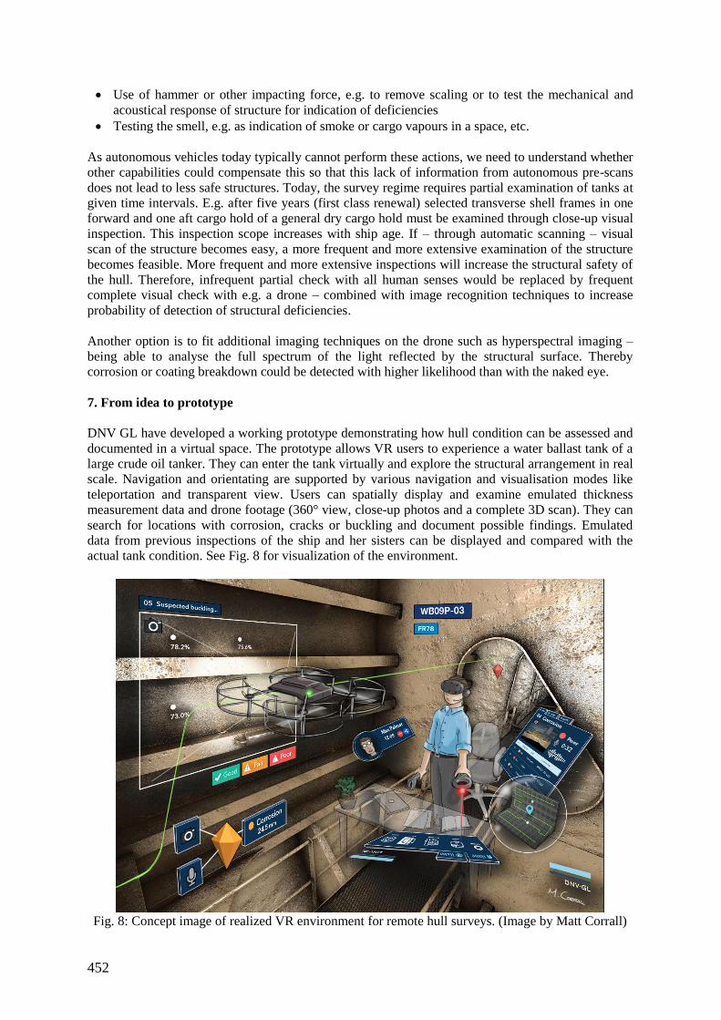
452
Use of hammer or other impacting force, e.g. to remove scaling or to test the mechanical and
acoustical response of structure for indication of deficiencies
Testing the smell, e.g. as indication of smoke or cargo vapours in a space, etc.
As autonomous vehicles today typically cannot perform these actions, we need to understand whether
other capabilities could compensate this so that this lack of information from autonomous pre-scans
does not lead to less safe structures. Today, the survey regime requires partial examination of tanks at
given time intervals. E.g. after five years (first class renewal) selected transverse shell frames in one
forward and one aft cargo hold of a general dry cargo hold must be examined through close-up visual
inspection. This inspection scope increases with ship age. If – through automatic scanning – visual
scan of the structure becomes easy, a more frequent and more extensive examination of the structure
becomes feasible. More frequent and more extensive inspections will increase the structural safety of
the hull. Therefore, infrequent partial check with all human senses would be replaced by frequent
complete visual check with e.g. a drone – combined with image recognition techniques to increase
probability of detection of structural deficiencies.
Another option is to fit additional imaging techniques on the drone such as hyperspectral imaging –
being able to analyse the full spectrum of the light reflected by the structural surface. Thereby
corrosion or coating breakdown could be detected with higher likelihood than with the naked eye.
7. From idea to prototype
DNV GL have developed a working prototype demonstrating how hull condition can be assessed and
documented in a virtual space. The prototype allows VR users to experience a water ballast tank of a
large crude oil tanker. They can enter the tank virtually and explore the structural arrangement in real
scale. Navigation and orientating are supported by various navigation and visualisation modes like
teleportation and transparent view. Users can spatially display and examine emulated thickness
measurement data and drone footage (360° view, close-up photos and a complete 3D scan). They can
search for locations with corrosion, cracks or buckling and document possible findings. Emulated
data from previous inspections of the ship and her sisters can be displayed and compared with the
actual tank condition. See Fig. 8 for visualization of the environment.
Fig. 8: Concept image of realized VR environment for remote hull surveys. (Image by Matt Corrall)
453
For actual inspections performed by a person using the IRIS self-localizing camera system, photos
can be uploaded to the ShipManager Hull model of the vessel. The photo results can be examined in
VR using the developed prototype. Therefore, without drones the system can be used in pilot studies
on-board real ships.
8. Summary and conclusions
Avoiding human entry into enclosed spaces is a valuable ambition. Technological developments in
many areas deliver the elements which will make this possible while at the same time reducing cost
level and service interruptions of the ship. By automating hull pre-scans with the help of drones, the
surface coverage and frequency of inspections could be increased. This, and the use of new imaging
and image recognition technology then has the potential to compensate for the missing human
perception of the tank environment. Thereby, the proposed procedure could result in the same or a
higher safety level than reached today through assessing the less frequent inspections carried out by
crew, superintendents, UTM operators and class surveyors.
It is not yet clear when a full autonomous scan of a ship compartment might become reality. But the
maritime industry is clearly working towards this. Further conceptual work should be performed to
investigate safety equivalence. VR will bring the captured images as close to physical presence as
possible. Thereby, VR might turn out to be an important element in making remote hull surveys
possible.
Acknowledgements
The authors wish to thank Max Palmer, Justin Roberts, and Matt Corrall for their excellent work on
VR design and implementation which also resulted in the images shown in this publication. This
work has thankfully built on top of the achievements of the Survey Simulator team in DNV GL
Software, Gdynia.
References
DNV GL (2017), Rules for Classification, Ships, Part 7 Fleet in service, Chapter 1 Survey
requirements for fleet in service
IACS, Recommendation 87: Guidelines for Coating Maintenance & Repairs for Ballast Tanks and
Combined Cargo/Ballast Tanks on Oil Tankers
IACS (2003), URZ, Requirements concerning Survey and Classification,
IMO (1993), A.744 (18), Guidelines on the enhanced programme of inspections during surveys of
bulk carriers and oil tankers
IMO (2001), Condition Assessment Scheme, Resolution MEPC.94(46)
WILKEN, M.; CABOS, C.; BAUMBACH, D.; BUDER, M.; CHOINOWSKI, A.; GRIESSBACH,
D.; ZUEV, S. (2015), IRIS - an innovative inspection system for maritime hull structures, ICCAS
Conf., Bremen
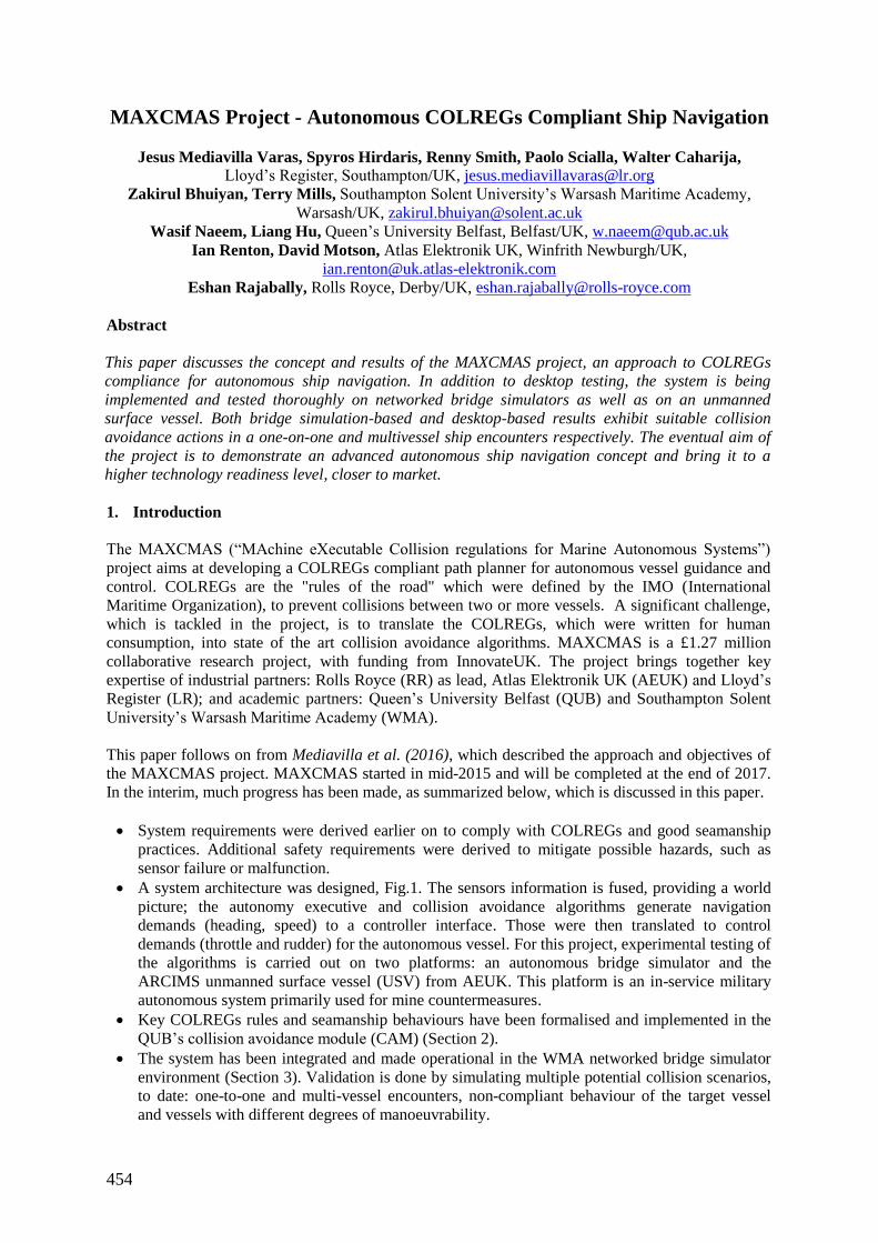
454
MAXCMAS Project - Autonomous COLREGs Compliant Ship Navigation
Jesus Mediavilla Varas, Spyros Hirdaris, Renny Smith, Paolo Scialla, Walter Caharija,
Lloyd’s Register, Southampton/UK, [email protected]
Zakirul Bhuiyan, Terry Mills, Southampton Solent University’s Warsash Maritime Academy,
Warsash/UK, [email protected]
Wasif Naeem, Liang Hu, Queen’s University Belfast, Belfast/UK, [email protected]
Ian Renton, David Motson, Atlas Elektronik UK, Winfrith Newburgh/UK,
Eshan Rajabally, Rolls Royce, Derby/UK, [email protected]
Abstract
This paper discusses the concept and results of the MAXCMAS project, an approach to COLREGs
compliance for autonomous ship navigation. In addition to desktop testing, the system is being
implemented and tested thoroughly on networked bridge simulators as well as on an unmanned
surface vessel. Both bridge simulation-based and desktop-based results exhibit suitable collision
avoidance actions in a one-on-one and multivessel ship encounters respectively. The eventual aim of
the project is to demonstrate an advanced autonomous ship navigation concept and bring it to a
higher technology readiness level, closer to market.
1. Introduction
The MAXCMAS (“MAchine eXecutable Collision regulations for Marine Autonomous Systems”)
project aims at developing a COLREGs compliant path planner for autonomous vessel guidance and
control. COLREGs are the "rules of the road" which were defined by the IMO (International
Maritime Organization), to prevent collisions between two or more vessels. A significant challenge,
which is tackled in the project, is to translate the COLREGs, which were written for human
consumption, into state of the art collision avoidance algorithms. MAXCMAS is a £1.27 million
collaborative research project, with funding from InnovateUK. The project brings together key
expertise of industrial partners: Rolls Royce (RR) as lead, Atlas Elektronik UK (AEUK) and Lloyd’s
Register (LR); and academic partners: Queen’s University Belfast (QUB) and Southampton Solent
University’s Warsash Maritime Academy (WMA).
This paper follows on from Mediavilla et al. (2016), which described the approach and objectives of
the MAXCMAS project. MAXCMAS started in mid-2015 and will be completed at the end of 2017.
In the interim, much progress has been made, as summarized below, which is discussed in this paper.
System requirements were derived earlier on to comply with COLREGs and good seamanship
practices. Additional safety requirements were derived to mitigate possible hazards, such as
sensor failure or malfunction.
A system architecture was designed, Fig.1. The sensors information is fused, providing a world
picture; the autonomy executive and collision avoidance algorithms generate navigation
demands (heading, speed) to a controller interface. Those were then translated to control
demands (throttle and rudder) for the autonomous vessel. For this project, experimental testing of
the algorithms is carried out on two platforms: an autonomous bridge simulator and the
ARCIMS unmanned surface vessel (USV) from AEUK. This platform is an in-service military
autonomous system primarily used for mine countermeasures.
Key COLREGs rules and seamanship behaviours have been formalised and implemented in the
QUB’s collision avoidance module (CAM) (Section 2).
The system has been integrated and made operational in the WMA networked bridge simulator
environment (Section 3). Validation is done by simulating multiple potential collision scenarios,
to date: one-to-one and multi-vessel encounters, non-compliant behaviour of the target vessel
and vessels with different degrees of manoeuvrability.
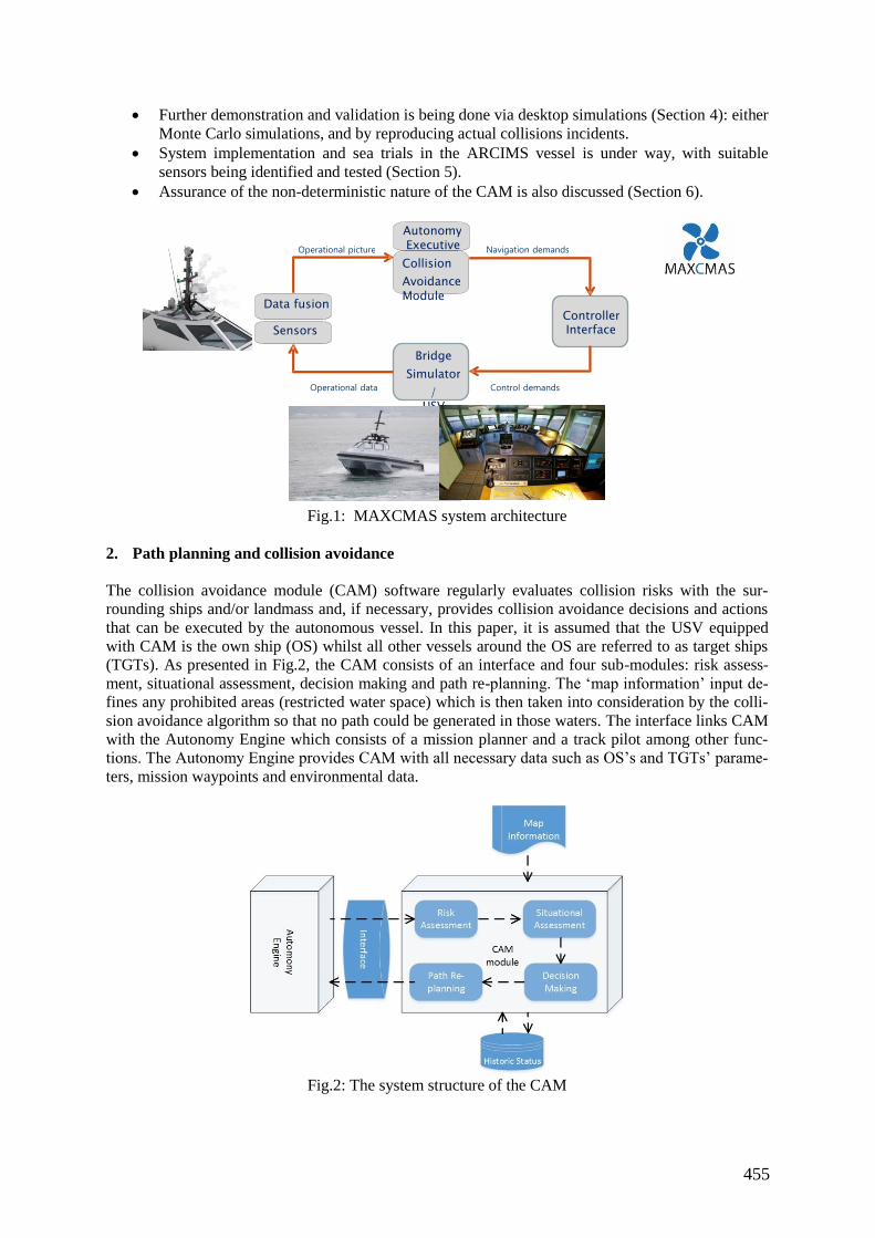
455
Further demonstration and validation is being done via desktop simulations (Section 4): either
Monte Carlo simulations, and by reproducing actual collisions incidents.
System implementation and sea trials in the ARCIMS vessel is under way, with suitable
sensors being identified and tested (Section 5).
Assurance of the non-deterministic nature of the CAM is also discussed (Section 6).
Fig.1: MAXCMAS system architecture
2. Path planning and collision avoidance
The collision avoidance module (CAM) software regularly evaluates collision risks with the sur-
rounding ships and/or landmass and, if necessary, provides collision avoidance decisions and actions
that can be executed by the autonomous vessel. In this paper, it is assumed that the USV equipped
with CAM is the own ship (OS) whilst all other vessels around the OS are referred to as target ships
(TGTs). As presented in Fig.2, the CAM consists of an interface and four sub-modules: risk assess-
ment, situational assessment, decision making and path re-planning. The ‘map information’ input de-
fines any prohibited areas (restricted water space) which is then taken into consideration by the colli-
sion avoidance algorithm so that no path could be generated in those waters. The interface links CAM
with the Autonomy Engine which consists of a mission planner and a track pilot among other func-
tions. The Autonomy Engine provides CAM with all necessary data such as OS’s and TGTs’ parame-
ters, mission waypoints and environmental data.
Fig.2: The system structure of the CAM
Autonomy Executive
Controller Interface
Bridge
Simulator
/ USV
Sensors
Navigation demands
Control demands Operational data
Operational picture Collision
Avoidance Module
Data fusion
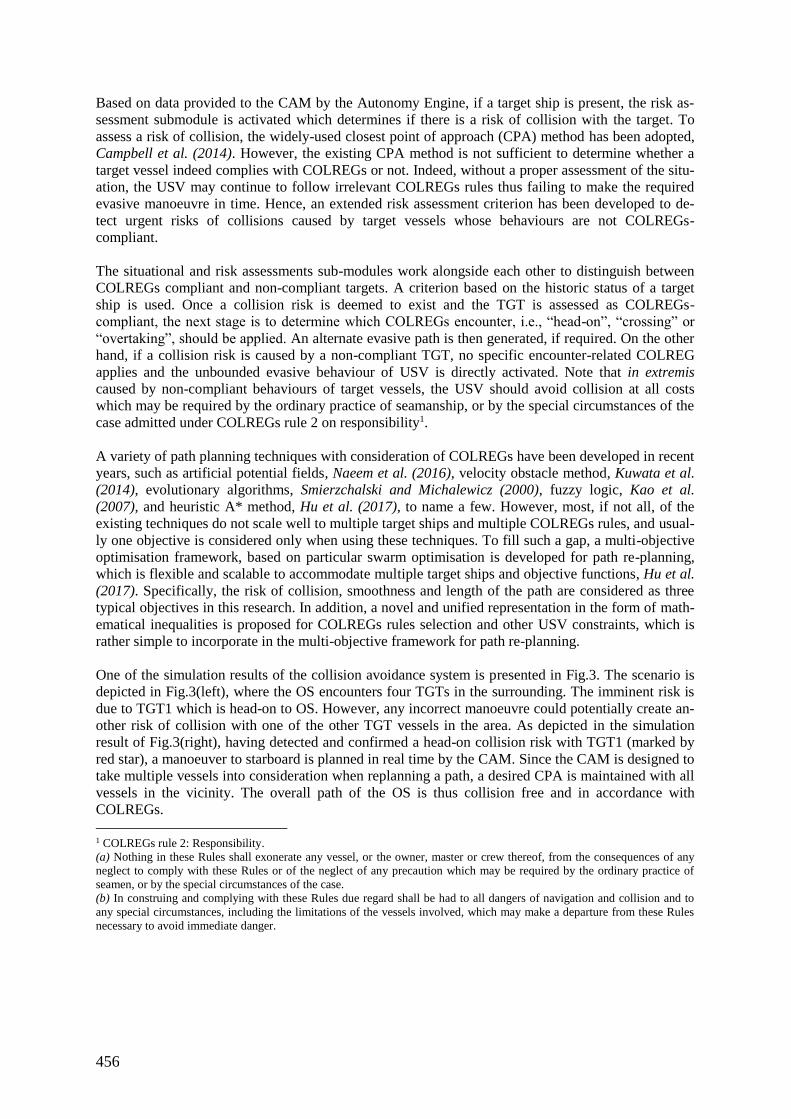
456
Based on data provided to the CAM by the Autonomy Engine, if a target ship is present, the risk as-
sessment submodule is activated which determines if there is a risk of collision with the target. To
assess a risk of collision, the widely-used closest point of approach (CPA) method has been adopted,
Campbell et al. (2014). However, the existing CPA method is not sufficient to determine whether a
target vessel indeed complies with COLREGs or not. Indeed, without a proper assessment of the situ-
ation, the USV may continue to follow irrelevant COLREGs rules thus failing to make the required
evasive manoeuvre in time. Hence, an extended risk assessment criterion has been developed to de-
tect urgent risks of collisions caused by target vessels whose behaviours are not COLREGs-
compliant.
The situational and risk assessments sub-modules work alongside each other to distinguish between
COLREGs compliant and non-compliant targets. A criterion based on the historic status of a target
ship is used. Once a collision risk is deemed to exist and the TGT is assessed as COLREGs-
compliant, the next stage is to determine which COLREGs encounter, i.e., “head-on”, “crossing” or
“overtaking”, should be applied. An alternate evasive path is then generated, if required. On the other
hand, if a collision risk is caused by a non-compliant TGT, no specific encounter-related COLREG
applies and the unbounded evasive behaviour of USV is directly activated. Note that in extremis
caused by non-compliant behaviours of target vessels, the USV should avoid collision at all costs
which may be required by the ordinary practice of seamanship, or by the special circumstances of the
case admitted under COLREGs rule 2 on responsibility1.
A variety of path planning techniques with consideration of COLREGs have been developed in recent
years, such as artificial potential fields, Naeem et al. (2016), velocity obstacle method, Kuwata et al.
(2014), evolutionary algorithms, Smierzchalski and Michalewicz (2000), fuzzy logic, Kao et al.
(2007), and heuristic A* method, Hu et al. (2017), to name a few. However, most, if not all, of the
existing techniques do not scale well to multiple target ships and multiple COLREGs rules, and usual-
ly one objective is considered only when using these techniques. To fill such a gap, a multi-objective
optimisation framework, based on particular swarm optimisation is developed for path re-planning,
which is flexible and scalable to accommodate multiple target ships and objective functions, Hu et al.
(2017). Specifically, the risk of collision, smoothness and length of the path are considered as three
typical objectives in this research. In addition, a novel and unified representation in the form of math-
ematical inequalities is proposed for COLREGs rules selection and other USV constraints, which is
rather simple to incorporate in the multi-objective framework for path re-planning.
One of the simulation results of the collision avoidance system is presented in Fig.3. The scenario is
depicted in Fig.3(left), where the OS encounters four TGTs in the surrounding. The imminent risk is
due to TGT1 which is head-on to OS. However, any incorrect manoeuvre could potentially create an-
other risk of collision with one of the other TGT vessels in the area. As depicted in the simulation
result of Fig.3(right), having detected and confirmed a head-on collision risk with TGT1 (marked by
red star), a manoeuver to starboard is planned in real time by the CAM. Since the CAM is designed to
take multiple vessels into consideration when replanning a path, a desired CPA is maintained with all
vessels in the vicinity. The overall path of the OS is thus collision free and in accordance with
COLREGs.
1 COLREGs rule 2: Responsibility.
(a) Nothing in these Rules shall exonerate any vessel, or the owner, master or crew thereof, from the consequences of any
neglect to comply with these Rules or of the neglect of any precaution which may be required by the ordinary practice of
seamen, or by the special circumstances of the case.
(b) In construing and complying with these Rules due regard shall be had to all dangers of navigation and collision and to
any special circumstances, including the limitations of the vessels involved, which may make a departure from these Rules
necessary to avoid immediate danger.
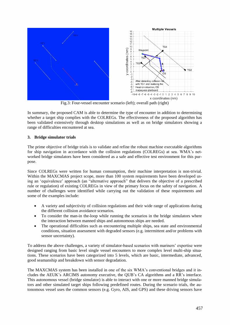
457
Fig.3: Four-vessel encounter scenario (left); overall path (right)
In summary, the proposed CAM is able to determine the type of encounter in addition to determining
whether a target ship complies with the COLREGs. The effectiveness of the proposed algorithm has
been validated extensively through desktop simulations as well as on bridge simulators showing a
range of difficulties encountered at sea.
3. Bridge simulator trials
The prime objective of bridge trials is to validate and refine the robust machine executable algorithms
for ship navigation in accordance with the collision regulations (COLREGs) at sea. WMA’s net-
worked bridge simulators have been considered as a safe and effective test environment for this pur-
pose.
Since COLREGs were written for human consumption, their machine interpretation is non-trivial.
Within the MAXCMAS project scope, more than 100 system requirements have been developed us-
ing an ‘equivalence’ approach (an “alternative approach” that delivers the objective of a prescribed
rule or regulation) of existing COLREGs in view of the primary focus on the safety of navigation. A
number of challenges were identified while carrying out the validation of these requirements and
some of the examples include:
A variety and subjectivity of collision regulations and their wide range of applications during
the different collision avoidance scenarios.
To consider the man-in the-loop while running the scenarios in the bridge simulators where
the interaction between manned ships and autonomous ships are needed.
The operational difficulties such as encountering multiple ships, sea state and environmental
conditions, situation assessment with degraded sensors (e.g. intermittent and/or problems with
sensor uncertainty).
To address the above challenges, a variety of simulator-based scenarios with mariners’ expertise were
designed ranging from basic level single vessel encounters to more complex level multi-ship situa-
tions. These scenarios have been categorized into 5 levels, which are basic, intermediate, advanced,
good seamanship and breakdown with sensor degradation.
The MAXCMAS system has been installed in one of the six WMA’s conventional bridges and it in-
cludes the AEUK’s ARCIMS autonomy executive, the QUB’s CA algorithms and a RR’s interface.
This autonomous vessel (bridge simulator) is able to interact with one or more manned bridge simula-
tors and other simulated target ships following predefined routes. During the scenario trials, the au-
tonomous vessel uses the common sensors (e.g. Gyro, AIS, and GPS) and these driving sensors have
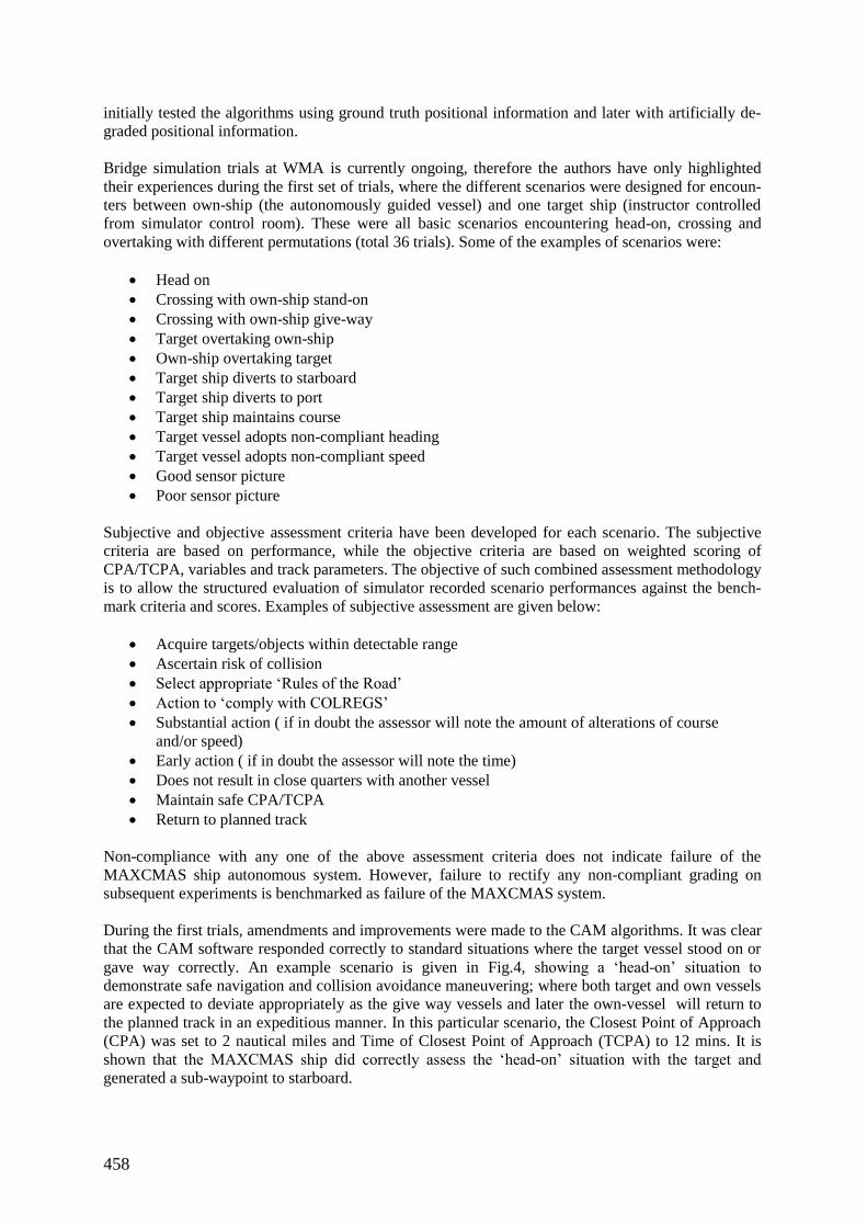
458
initially tested the algorithms using ground truth positional information and later with artificially de-
graded positional information.
Bridge simulation trials at WMA is currently ongoing, therefore the authors have only highlighted
their experiences during the first set of trials, where the different scenarios were designed for encoun-
ters between own-ship (the autonomously guided vessel) and one target ship (instructor controlled
from simulator control room). These were all basic scenarios encountering head-on, crossing and
overtaking with different permutations (total 36 trials). Some of the examples of scenarios were:
Head on
Crossing with own-ship stand-on
Crossing with own-ship give-way
Target overtaking own-ship
Own-ship overtaking target
Target ship diverts to starboard
Target ship diverts to port
Target ship maintains course
Target vessel adopts non-compliant heading
Target vessel adopts non-compliant speed
Good sensor picture
Poor sensor picture
Subjective and objective assessment criteria have been developed for each scenario. The subjective
criteria are based on performance, while the objective criteria are based on weighted scoring of
CPA/TCPA, variables and track parameters. The objective of such combined assessment methodology
is to allow the structured evaluation of simulator recorded scenario performances against the bench-
mark criteria and scores. Examples of subjective assessment are given below:
Acquire targets/objects within detectable range
Ascertain risk of collision
Select appropriate ‘Rules of the Road’
Action to ‘comply with COLREGS’
Substantial action ( if in doubt the assessor will note the amount of alterations of course
and/or speed)
Early action ( if in doubt the assessor will note the time)
Does not result in close quarters with another vessel
Maintain safe CPA/TCPA
Return to planned track
Non-compliance with any one of the above assessment criteria does not indicate failure of the
MAXCMAS ship autonomous system. However, failure to rectify any non-compliant grading on
subsequent experiments is benchmarked as failure of the MAXCMAS system.
During the first trials, amendments and improvements were made to the CAM algorithms. It was clear
that the CAM software responded correctly to standard situations where the target vessel stood on or
gave way correctly. An example scenario is given in Fig.4, showing a ‘head-on’ situation to
demonstrate safe navigation and collision avoidance maneuvering; where both target and own vessels
are expected to deviate appropriately as the give way vessels and later the own-vessel will return to
the planned track in an expeditious manner. In this particular scenario, the Closest Point of Approach
(CPA) was set to 2 nautical miles and Time of Closest Point of Approach (TCPA) to 12 mins. It is
shown that the MAXCMAS ship did correctly assess the ‘head-on’ situation with the target and
generated a sub-waypoint to starboard.
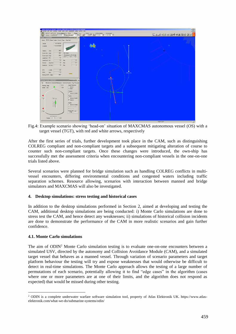
459
Fig.4: Example scenario showing ‘head-on’ situation of MAXCMAS autonomous vessel (OS) with a
target vessel (TGT), with red and white arrows, respectively
After the first series of trials, further development took place in the CAM, such as distinguishing
COLREG compliant and non-compliant targets and a subsequent mitigating alteration of course to
counter such non-compliant targets. Once these changes were introduced, the own-ship has
successfully met the assessment criteria when encountering non-compliant vessels in the one-on-one
trials listed above.
Several scenarios were planned for bridge simulation such as handling COLREG conflicts in multi-
vessel encounters, differing environmental conditions and congested waters including traffic
separation schemes. Resource allowing, scenarios with interaction between manned and bridge
simulators and MAXCMAS will also be investigated.
4. Desktop simulations: stress testing and historical cases
In addition to the desktop simulations performed in Section 2, aimed at developing and testing the
CAM, additional desktop simulations are being conducted: i) Monte Carlo simulations are done to
stress test the CAM, and hence detect any weaknesses; ii) simulations of historical collision incidents
are done to demonstrate the performance of the CAM in more realistic scenarios and gain further
confidence.
4.1. Monte Carlo simulations
The aim of ODIN2 Monte Carlo simulation testing is to evaluate one-on-one encounters between a
simulated USV, directed by the autonomy and Collision Avoidance Module (CAM), and a simulated
target vessel that behaves as a manned vessel. Through variation of scenario parameters and target
platform behaviour the testing will try and expose weaknesses that would otherwise be difficult to
detect in real-time simulations. The Monte Carlo approach allows the testing of a large number of
permutations of each scenario, potentially allowing it to find “edge cases” in the algorithm (cases
where one or more parameters are at one of their limits, and the algorithm does not respond as
expected) that would be missed during other testing.
2 ODIN is a complete underwater warfare software simulation tool, property of Atlas Elektronik UK. https://www.atlas-
elektronik.com/what-we-do/submarine-systems/odin/
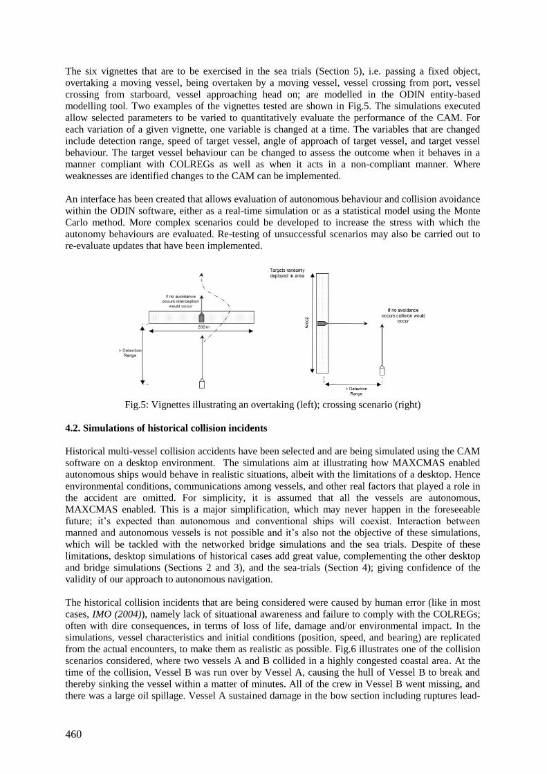
460
The six vignettes that are to be exercised in the sea trials (Section 5), i.e. passing a fixed object,
overtaking a moving vessel, being overtaken by a moving vessel, vessel crossing from port, vessel
crossing from starboard, vessel approaching head on; are modelled in the ODIN entity-based
modelling tool. Two examples of the vignettes tested are shown in Fig.5. The simulations executed
allow selected parameters to be varied to quantitatively evaluate the performance of the CAM. For
each variation of a given vignette, one variable is changed at a time. The variables that are changed
include detection range, speed of target vessel, angle of approach of target vessel, and target vessel
behaviour. The target vessel behaviour can be changed to assess the outcome when it behaves in a
manner compliant with COLREGs as well as when it acts in a non-compliant manner. Where
weaknesses are identified changes to the CAM can be implemented.
An interface has been created that allows evaluation of autonomous behaviour and collision avoidance
within the ODIN software, either as a real-time simulation or as a statistical model using the Monte
Carlo method. More complex scenarios could be developed to increase the stress with which the
autonomy behaviours are evaluated. Re-testing of unsuccessful scenarios may also be carried out to
re-evaluate updates that have been implemented.
Fig.5: Vignettes illustrating an overtaking (left); crossing scenario (right)
4.2. Simulations of historical collision incidents
Historical multi-vessel collision accidents have been selected and are being simulated using the CAM
software on a desktop environment. The simulations aim at illustrating how MAXCMAS enabled
autonomous ships would behave in realistic situations, albeit with the limitations of a desktop. Hence
environmental conditions, communications among vessels, and other real factors that played a role in
the accident are omitted. For simplicity, it is assumed that all the vessels are autonomous,
MAXCMAS enabled. This is a major simplification, which may never happen in the foreseeable
future; it’s expected than autonomous and conventional ships will coexist. Interaction between
manned and autonomous vessels is not possible and it’s also not the objective of these simulations,
which will be tackled with the networked bridge simulations and the sea trials. Despite of these
limitations, desktop simulations of historical cases add great value, complementing the other desktop
and bridge simulations (Sections 2 and 3), and the sea-trials (Section 4); giving confidence of the
validity of our approach to autonomous navigation.
The historical collision incidents that are being considered were caused by human error (like in most
cases, IMO (2004)), namely lack of situational awareness and failure to comply with the COLREGs;
often with dire consequences, in terms of loss of life, damage and/or environmental impact. In the
simulations, vessel characteristics and initial conditions (position, speed, and bearing) are replicated
from the actual encounters, to make them as realistic as possible. Fig.6 illustrates one of the collision
scenarios considered, where two vessels A and B collided in a highly congested coastal area. At the
time of the collision, Vessel B was run over by Vessel A, causing the hull of Vessel B to break and
thereby sinking the vessel within a matter of minutes. All of the crew in Vessel B went missing, and
there was a large oil spillage. Vessel A sustained damage in the bow section including ruptures lead-
461
ing to flooding, but no casualties to her crew. Visibility was good weather conditions were not an is-
sue. Post-mortem analysis revealed that Vessel A did not keep proper lookout, infringing rule 5 3, and
neither of the two vessels significantly alteration course and or speed to avoid collision, infringing
rule 8 4.
Fig.6: Trajectories of vessels A and B before and after collision (left); vessel A breaking the hull of
vessel B (right).
At the moment of the writing, simulation work is underway which will illustrate how MAXCMAS
autonomous vessels would have behave in nearly the same situation, demonstrating COLREGs com-
pliance and seamanship, and thus avoiding collision, albeit with the simplifications earlier mentioned.
The simulations adopt the same planned route and the same initial speed and bearing as in the actual
collision, until a risk threshold is reached; at which point the CAM triggers a collision avoiding ac-
tion, to finally returning to the original route.
5. USV sea trials
The aim of the sea trials is to exercise the Collision Avoidance Module (CAM) in a real environment
under true platform motion, sensor performance and environmental conditions. One goal from this
type of testing is to validate the results observed in simulated testing and gain an understanding of the
differences between real and synthetic trials. A further goal is to assert the performance of the CAM
or expose any additional weaknesses that have not been observed in other testing that will be fed in to
algorithm refinement.
Since one of the primary goals of the sea trials is to validate testing already conducted in simulation,
the test scenarios that will be exercised will replicate scenarios tested during the bridge simulation
trials (Section 3) as well as the Monte Carlo stress testing (Section 4). This involves execution of six
vignettes involving one-on-one encounters between the autonomous USV and a target vessel or
obstacle. The six vignettes to be executed are as follows: passing a fixed object, overtaking a moving
vessel, being overtaken by a moving vessel, vessel crossing from port, vessel crossing from starboard,
vessel approaching head on.
Initially the target vessel will be virtual and is presented as having been detected with perfect sensor
data. This approach allows the motion and manoeuvring of the USV to be the first factor to be
considered when compared against entirely synthetics trials results. Following testing against a
synthetic target a real target will be introduced. The real target will be a channel marker, for
avoidance of a fixed obstacle, and then a RIB (rigid inflatable boat) fitted with a radar reflector for a
moving target.
3 COLREGs rule 5: Lookout.
Every vessel shall at all times maintain a proper look-out by sight and hearing as well as by all available means appropriate
in the prevailing circumstances and conditions so as to make a full appraisal of the situation and of the risk of collision. 4 COLREGS rule 8: Action to avoid collision.
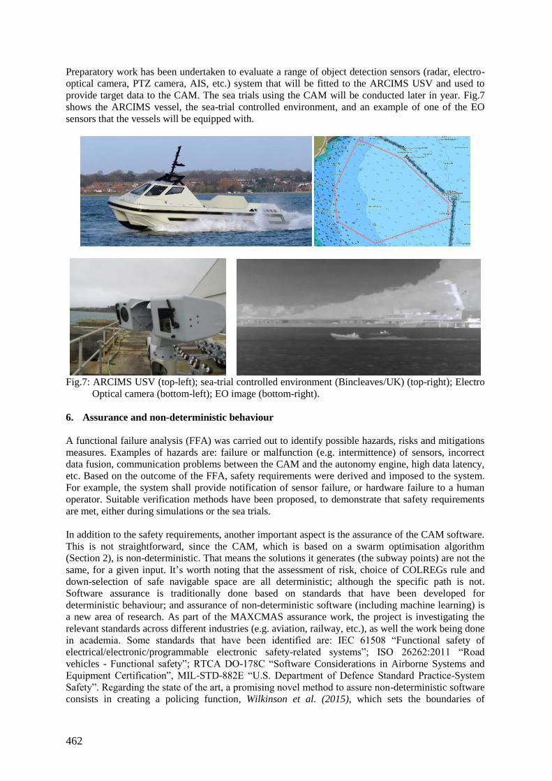
462
Preparatory work has been undertaken to evaluate a range of object detection sensors (radar, electro-
optical camera, PTZ camera, AIS, etc.) system that will be fitted to the ARCIMS USV and used to
provide target data to the CAM. The sea trials using the CAM will be conducted later in year. Fig.7
shows the ARCIMS vessel, the sea-trial controlled environment, and an example of one of the EO
sensors that the vessels will be equipped with.
Fig.7: ARCIMS USV (top-left); sea-trial controlled environment (Bincleaves/UK) (top-right); Electro
Optical camera (bottom-left); EO image (bottom-right).
6. Assurance and non-deterministic behaviour
A functional failure analysis (FFA) was carried out to identify possible hazards, risks and mitigations
measures. Examples of hazards are: failure or malfunction (e.g. intermittence) of sensors, incorrect
data fusion, communication problems between the CAM and the autonomy engine, high data latency,
etc. Based on the outcome of the FFA, safety requirements were derived and imposed to the system.
For example, the system shall provide notification of sensor failure, or hardware failure to a human
operator. Suitable verification methods have been proposed, to demonstrate that safety requirements
are met, either during simulations or the sea trials.
In addition to the safety requirements, another important aspect is the assurance of the CAM software.
This is not straightforward, since the CAM, which is based on a swarm optimisation algorithm
(Section 2), is non-deterministic. That means the solutions it generates (the subway points) are not the
same, for a given input. It’s worth noting that the assessment of risk, choice of COLREGs rule and
down-selection of safe navigable space are all deterministic; although the specific path is not.
Software assurance is traditionally done based on standards that have been developed for
deterministic behaviour; and assurance of non-deterministic software (including machine learning) is
a new area of research. As part of the MAXCMAS assurance work, the project is investigating the
relevant standards across different industries (e.g. aviation, railway, etc.), as well the work being done
in academia. Some standards that have been identified are: IEC 61508 “Functional safety of
electrical/electronic/programmable electronic safety-related systems”; ISO 26262:2011 “Road
vehicles - Functional safety”; RTCA DO-178C “Software Considerations in Airborne Systems and
Equipment Certification”, MIL-STD-882E “U.S. Department of Defence Standard Practice-System
Safety”. Regarding the state of the art, a promising novel method to assure non-deterministic software
consists in creating a policing function, Wilkinson et al. (2015), which sets the boundaries of
463
operation of the non-deterministic behaviour. The advantage of such an approach is that the policing
function can be assured using existing standards. Work is in progress, to identify the degree of non-
deterministic behaviour of the CAM software, the applicability of these standards and the policing
function, the knowledge gaps and what further work would be required.
7. Conclusions and future work
Since the last paper presented at COMPIT2016, much progress has been made in the MAXCMAS
project. A considerable amount of effort has been dedicated to deriving appropriate functional and
safety requirements to ensure COLREGs compliant behaviour, which has been implemented in the
CAM. The system architecture, with the CAM, has been seamlessly integrated in a bridge simulator
environment. The system is being thoroughly tested under a multitude of scenarios using desktop and
bridge simulators, to demonstrate its robustness, and prove that the different requirements are met.
The WMA bridge simulators have provided a unique platform to help develop and test the
MAXCMAS autonomous vessel, in a near real environment, with one-to-one and multi-vessel en-
counters and different types of vessels. Desktop simulations have proven to be quite useful, to com-
plement the bridge simulations in an inexpensive and fast manner.
Future work will deal with: conflicting rules, interaction of autonomous and manned vessels, poor or
degraded sensor picture, manoeuvring in restricted waters. Preparations are underway to test the sys-
tem at sea using the ARCIMS USV in a controlled environment, with virtual and real targets, using a
range of advanced sensors. The MAXCMAS project is in fact bringing up an advanced autonomous
ship navigation concept closer to commercialization.
Acknowledgments
We would like to thank all the MAXCMAS partners: Atlas Elektronik UK, Queen’s University Bel-
fast, Rolls Royce, Southampton Solent University’s Warsash Maritime Academy and Lloyd’s Regis-
ter, for their input, and great contributions to the project. This project would have not been possible
without the support of InnovateUK, under grant number 50121-378137, which is greatly acknowl-
edged.
References
CAMPBELL, S.; ABU-TAIR, M.; NAEEM, W. (2014), An automatic COLREGs compliant obstacle
avoidance system for an unmanned surface vehicle, Proc. Inst. Mechanical Engineers
HU, L.; NAEEM, W.; RAJABALLY, E.; MILLS, T.; WATSON, G. (2017), COLREGs-compliant
path planning for autonomous surface vehicles: a multi-objective optimization approach,
IMO (1972), International Regulations for Preventing Collisions at Sea (COLREGs), Int. Maritime
Org., London
IMO (2004), Casualties statistics and investigations - Very serious and serious casualties for the
2001, Int. Maritime Org., London
KAO, K.S.; LEE, K.C.; KO, M. (2007), A fuzzy logic method for collision avoidance in vessel traffic
service, J. Navigation 160, pp.17-31
KUWATA, Y.; WOLF, M.T.; ZARZHITSKY, D.; HUNTSBERGER, T.L. (2014), Safe maritime au-
tonomous navigation with COLREGS using velocity obstacles, IEEE J. Oceanic Eng. 39, pp.110-119
MEDIAVILLA VARAS, J.; CAHARIJA, W.; SMITH, R.; BHUIYAN, Z.; NAEEM, W.; CARTER,
P.; RENTON, I. (2016), Autonomous COLREGs compliant ship navigation, using bridge simulators
and an unmanned vessel, 15th COMPIT Conf., Lecce

464
NAEEM, W.; CAMPBELL, S.; HU, L. (2016), A reactive COLREGs-compliant navigation strategy
for autonomous maritime navigation, IFAC-PapersOnLine 49/23, pp.207-213
SMIERZCHALSKI, R.; MICHALEWICZ, Z. (2000), Modeling of ship trajectory in collision situa-
tions by an evolutionary algorithm, IEEE Trans. Evolutionary Computation14, pp.227-241
WILKINSON, T.; BUTLER, M.; PAXTON, M.; WALDRON, X. (2015), A formal approach to mul-
ti-UAV route validation, 4th Int. Workshop on Formal Techniques for Safety-Critical Systems
CAMPBELL, S.; NAEEM, W.; IRWIN, G. (2012), A review on improving the autonomy of un-
manned surface vehicles through intelligent collision avoidance manoeuvres, Annual Reviews in
Control 136, pp.267-283
465
The Ungoverned Space of Marine Fire Safety
Carl S.P. Hunter, Coltraco Ultrasonics, London/UK, [email protected]
Abstract
This paper explores the trending topic of harnessing data from improved and continuous monitoring
on smart ships in order to, primarily, increase safety and secondly, to make economical savings, with
regard to the “Ungoverned Space” of fire safety. Going above and beyond regulation compliance to
secure additional benefits are vital to increasingly high value and safety critical vessels in terms of fire
safety. The Shipping, Naval and Oil and Gas Industries among others, are all safety critical sectors
which can have catastrophic and expensive results in the event of fire. The size of vessels and the on-
board technology have been subject to a constant process of optimization. But safety measures,
particularly with respect of fire protection, have been left lagging behind in the face of ever bigger,
ever better ships.
1. Introduction
Over the last few decades cargo has generally been increasingly transported in containers rather than as
open bulk cargo, thus mistakenly leading shipping companies to disregard the importance of fire
protection systems, instead focusing on transporting greater quantities facilitated by the container
system. However, this outlook is dangerous and misplaced. The risk of fire is significant with growing
incidences of fire events exposed in the trade press, posing a risk both to expensive cargo and to human
life on-board the ships. With a movement towards autonomous shipping systems and smart-ships, the
importance of remotely monitored fire-fighting systems could grow exponentially, providing the
opportunity to monitor vessels from an external location. Technological developments and companies
such as Coltraco Ultrasonics, are working towards this end goal. The current on-board fire-fighting
facilities remain inadequate in the face of the capacity of such large vessels. Fire therefore remains an
ever-present risk on the high seas.
2. Economic risks
Traditionally, the maritime industry treats fire protection systems as a necessary expenditure, rather
than a means to safeguard valuable crew and cargo and maintain business continuity of the vessel.
Owners focus on systems delivered at the most competitive rates rather than seeing fire protection as
an investment. The definition of a free market is an idealised form of a market economy in which buyers
and sellers are allowed to transact freely based on a mutual agreement on price without state intervention
in the form of taxes, subsidies or regulation. The competitiveness of the free market places great
pressure on cost cutting: to deliver systems which often only minimally comply with regulations, and
deliver asset protection at the most economical budget. With the value of assets, vessels and importance
of business continuity growing, insurers are asked to underwrite almost incalculably high risk.
Unquestionably, the first priority of fire safety systems is to protect human life. Having said that, the
economic benefits of a truly integrated, continuous, ultrasonic monitoring system in the future would
be significant. Cargo damage remains an important negative result of on-ship fires, with 2 of the top 5
most expensive cargo claims on container ships in the last 10 years being fire-related according to
www.swedishclub.com/media_upload/files/Publications/P%26I%20Claims%20Analysis%20web.pdf.
Fire protection measures should hence be understood as a worthwhile business investment. Yet we
accept minimally compliant fire systems. Given both the crew lives and cargo are at stake, it seems
unfathomable that regulations do not mandate fire systems should be permanently monitored rather than
certified typically just once a year, if that, particularly since it is a regulatory obligation and or
recommendation to ensure that crew can check these themselves.
466
3. What is the “ungoverned space”?
Who would build a ship or offshore platform and install a power generating or auxiliary machinery
without installing emergency power systems or monitoring their condition states? Who today would
consider installing an alarm system without monitoring its overall status, not only its actuation, and
integrating the whole system into the ship safety management system, with central monitoring being an
essential part of it? These are basic engineering principles: building in redundancy and constantly
monitoring critical systems.
Traditionally, the industry cares little about this ungoverned space, with too few qualified engineers
considered subject matter experts. Yet when it comes to marine fire maintenance, never mind
continuous monitoring, of gaseous fire extinguishing systems, there is a lack of knowledge amongst the
-majority of the industry, regarding the potential risks. Awareness should exist about the huge expenses
incurred by fire, both in terms of costs upfront from the damage and long-term due to reputation and
unknown losses or damage to seafarers, vessel integrity, and cost of downtime and recovery. Above all
is the risk to human life presented by fire. Poor maintenance of suppression systems risk accidental
fatalities due to lack of training about the lethal properties of CO2 (the predominant suppressant agent
used on vessels, because it is the cheapest whilst being highly effective): when released it reduces
oxygen levels to extinguish fire. Limited appreciation of the need for room integrity testing of protected
spaces leads to minimal regulation compliance which could mean a failure of the fire system
suppressing a fire because the room is unable to hold the discharged gas due to leaks of the space into
which it actuates.
4. Fire Extinguishing Systems
Gaseous extinguishing/suppression systems are installed to protect against special hazards in critical
infrastructure at sea. They deliver the infrastructure resilience our advanced maritime society requires.
If the hazard is special and the vessel is critical, then this is the case for the constant monitoring of the
fire systems that aim to deliver their protection. There is a lack of knowledge of the characteristics of
the various extinguishants and the types of fire for which they are suitable. For too many years the
industry has been left to too few brilliant experts to determine safe outcome.
Two broad categories of ship and offshore extinguishing systems exist: sprinkler systems and
pressurised gaseous systems. While the former can suffer leakage, the latter can cause catastrophic
effect due to their pressures. These large gas cylinders are pressurised liquefied gases or non-liquefied
gases that are pressurised on actuation. CO2 is permanently under 720 psi or 49 bar of pressure, i.e.
nearly 50 times atmospheric pressure (by comparison a cup of water at sea level exists at 1 bar or 14.5
psi). Its’ state changes under increased temperatures to one that is neither a liquid nor a gas. Gases under
pressure are often effectively considered by the industry as single and passive cylinder columns of solid
material from the perspective of their monitoring following installation. Whereas being under pressure
and constantly changing under temperature they should be considered as active and dynamic systems
requiring constant monitoring. These are not passive systems therefore; they are dynamic ones, and all
dynamic systems under pressure need constant monitoring to ensure their effectiveness and longevity.
An engineered marine fire system typically lasts 20 years, longer than some vessels!
4.1. Traditional Cylinder Testing Methods
Typical methods for on-ship regular cylinder inspection primarily consists of trained professionals
weighing the chosen cylinder, to assess if there has been weight loss due to gas leakage. However,
although this method is widely used, it ultimately holds risk as an unsafe practice in reality, requiring
constant handling of tanks in a delicate, high-pressure state. Whilst weighing is the most commonly
cited method, it may be practical in the light of new and improved technology to add ultrasound as a
recommended method.
467
4.1.1. Poor Maintenance Practice
Marine servicing companies bid to service a ships CO2 system; this can comprise 200-600 x 45 kg CO2
cylinders per ship. They can discharge accidentally. One of the highest probabilities of discharge occurs
during their maintenance. Some service companies estimate that at one time 20% of a ships CO2
cylinders have discharged or partially leaked their contents and there are over 55000 commercial vessels
at sea at any time. On average, each cylinder will take 40 minutes to dismantle, weigh, record and re-
install. Too many times therefore, even good servicing companies may not have the physical time to
perform the inspection required, because the vessel may only provide them a few hours. But alongside
them there are other companies who are said to randomly check some cylinders and then place “tested
stickers” on the rest. Because the normal design concentration of CO2 of 34-72 v/v % is above the nearly
immediate acute lethality level an extremely narrow safety margin exists for these systems. Its
mechanism of fire suppression is through oxygen dilution to 8-15%, rather than the chemical disruption
of the catalytic combustion chain as with other clean agents.
4.1.2. Anecdotal experiences
• Safety pins being retained in position in the cylinder valves after installation.
• Marine CO2 systems with 20% of the CO2 cylinders installed on commercial shipping being
empty or partially filled.
• Over-filled and under-filled cylinders.
• Pipework and cylinders freshly painted but with severe internal corrosion.
• Room integrity testing with questionable results and with the room integrity remaining un-
monitored after testing.
• Liquefied extinguishants being confused by installers with Inert gas systems.
• There exists a lack of understanding of the organic compounds of some liquid extinguishants
and their corrosive effect on the cylinder in the event of condensate ingress.
• Shipping companies not implementing the FSS code of the IMO SOLAS regulations.
• We have been regularly asked how to operate portable Portalevel™ liquid level indicators on
dry powder extinguishers.
• WIKA Instrument discovered 25% of pressure gauges failed in an audit of 250 plants.
The problems cannot be denied. The International Maritime Risk Rating Agency (2016) has declared
fire safety to be the most common deficiency on tankers in October 2016, with 126 incidents.
5. Regulations
5.1. Fire Extinguishing Systems
International Maritime Organisation (IMO) Safety of Life at Sea (SOLAS) International Fire
Safety Systems (FSS) Code Chapter 5, 2.1.1.3 specifies that “means shall be provided for the
crew to safely check the quantity of the fire extinguishing medium in the containers.”
MSC.1-Circ.1432 REVISED GUIDELINES FOR THE MAINTENANCE AND INSPEC-
TION OF FIRE PROTECTION SYSTEMS AND APPLIANCES, also discusses the need to
inspect the contents of fire-protection systems’ cylinders.
CO2 UK Marine Equipment Directive (MED) UK/EU legislation with US Coast Guard Mutual
Recognition 7.3.2.6: “Means should be provided to verify the liquid level in all the cylinders,
either by weighing the cylinders or by using a suitable liquid level detector.”
United States Coast Guard Marine Safety Alert – May 27, 2015 “Receive adequate training to
perform routine inspections of their vessel’s fixed CO2 systems and fully understand their op-
eration, particularly those protecting large spaces or multiple areas.”
NFPA 12 code 4.8.3.4.2 specifies that if, at any time, a container shows a loss in net content of
more than 10 percent, it shall be refilled or replaced.
468
It can be argued that the existence of regulation (including but not limited to the examples above) guides
– and occasionally curbs – the direction taken by the free market. This then means that the current state
of the market, where ‘price is king’ is either due to unwillingness on the part of the regulators to create
an environment where safe engineering is rewarded or because the industry itself is unaware of new
technology that will help them meet both the spirit and letter of the regulation.
5.2 Protected Space Integrity
Compartment room integrity testing is essential under ISO 14520 where gaseous extinguishing systems
have to be designed in relation to the discharging agent hold-time (if the room cannot hold the agent
because of leaks the agent will disperse and not extinguish the fire) and discharging agent peak pressure
(if the pressure is too high for partition walls or suspended ceilings they will be blown apart or damaged
and possibly destroying the room integrity). If the room contains leakages, slowing down the process
to achieve the required flooding concentration, the CO2 extinguishing system would be unable to
achieve the desired concentration in the time limit proposed. IMO SOLAS Chapter II-2 Regulation 10,
G23.3 states, “The Regulations require that 85% of the required concentrations for machinery spaces
and cargo pump rooms is achieved in such spaces within two minutes.” ISO 1452 requires testing of a
compartments integrity every 12 months to ensure the fire extinguishing system will still be effective,
however in reality checks are necessary far more regularly.
6. Safeship® Technology
In shipping, unless a fatality occurs, it is left un-reported. This does not seem accurate or correct
considering the aforementioned assumption that systems leak and protected space integrity changes.
New smart ship technology counters the environment in which a “safety first” culture remains un-
pursued and unrewarded. With multiple ships sailing with partially-filled, over-filled or empty
cylinders, and unpublished instances of accidental discharges or slow seepages, there is a real cause for
concern – now there is an impetus to change.
6.1. Case Study 1
On 07 September 2015, a fire was detected inside one of the cargo holds of Barzan, a Maltese registered
container ship. At the time, the vessel was about 60 nm off Cabo Finisterre. The crew responded and
commenced fire-fighting with boundary cooling and the use of the water drenching system on board.
Subsequently, the fixed CO2 system was used but due to several leaks in the CO2 line, the required
amount of gas did not reach the cargo hold to be effective to smother the fire. The starboard fire main
line then developed a large leak at a joint in the under deck passage way and had to be isolated. This
restricted the fire-fighting efforts to only the port side, and rendered the starboard side water drenching
system unusable. What if more care and attention had been placed on the CO2 fire-fighting system?
6.2. Case Study 2
With delicate electrical systems, semi-open decks that may restrict fire suppression effectiveness and a
culture of undeclared cargo, Ro-Ro vessels have been identified as one of the highest fire risk marine
vessels. On 28 April 2015, Sorrento caught fire whilst on a voyage from Palma de Mallorca to Valencia.
The ship was 15 nm off Mallorca when a fire was discovered on one of the car decks. An emergency
was declared and several vessels went to the assistance of Sorrento, including the ferries Publia and
Visemar One. Publia rescued most of the 156 passengers and crew, who had left the ship by lifeboat.
Four crew were injured, and there was a fear that the entire ship would sink. According to lawyers in
Greece and Italy the fire was caused by a number of ‘oversights and mistakes’ on the part of crew. Once
the fire had broken out, it has been said that poor training and a lack of understanding of the fire extin-
guishing systems by the crew members restricted their ability to adequately extinguish the fire. There
were also ‘violations of protocol’ when it came to managing the fire extinguishing systems, managing
the incident itself and evacuating the ship. Raising awareness, education and training are key, hence the
development of easy to use, advanced technology like Portalevel®.
469
7. Innovative Measuring Solutions
However, with the impact of fire being more widely recognised, new research and development
explores ultrasonic technology to monitor the extinguishing systems through inspection and integrated,
continuous monitoring with alarm relay and remote diagnostics. The latter gives eyes to shore-based
operators at a time of fewer, poorly trained crew and a trend towards autonomous shipping.
One of the key advantages of ultrasonic measuring solutions is they allow a comprehensive maintenance
program to be implemented as part of a strategic approach to business continuity and reducing the risk
of accidental discharges and leaks not being picked up. Further reducing areas of ungoverned or
regulated space within the industry, ensuring a safer working environment for all.
7.1 Constant monitoring of fire extinguishing systems
Permalevel® Multiplex is the first system worldwide that is capable of monitoring the liquid level of
critical fire suppression cylinder systems on a constant basis. It gives a vessel total visibility on the real-
time status of all their critical fire systems. The Permalevel® Multiplex is designed to ensure that fire
suppression systems are always fully operational and that no accidental discharge has occurred, which
could affect the effectiveness of the overall fire protection system in the event that it is required for use.
The most critical point of a pressurised cylinder is the meeting of the cylinder neck with its valve. For
over 100 years the industry has monitored and permanently weighs (even suspends) cylinder pressure
and weight of contents at that critical point. The assumption is that the cylinder pressure gauge is of
high, almost MIL-SPEC quality, but they are often not and commercial pressures under a bidding
process can incline some to select low-end budget, minimally compliant gauge mechanisms.
Technologies will soon exist to monitor both liquefied gaseous content and non-liquefied gaseous
pressure safely - from the external sides of the cylinder rather than within it – in both fixed and portable
forms.
7.2 Ultrasound: An Under-Appreciated Technology
One of the sciences being harnessed by innovators in the fire safety sector is that of ultrasound: i.e.
acoustic (sound) energy in the form of waves of high frequency that are above the human audible range.
Although the shipping world largely sees it as a tool to gauge thickness, it has seen far more varied use
across military, medical and industrial fields and is now being put to more advanced, innovative uses
in shipping for fire safety solutions too.
Many will know this as SONAR in the UK from the military where it was first developed by the British
by ASDIC in WWI. Ultrasound is sound beyond our audible range. Sound is, in itself, vibrations that
propagate as a mechanical wave or pressure and transmit through solid, liquid or gaseous mediums. We
are familiar with it through our hospitals during pregnancy scanning or the BBC when we “hear”
dolphins and bats using it to communicate and navigate on wildlife programmes. We only hear that on
our televisions as the ultrasound is hetrodyned to convert the ultrasound into something we can hear.
But just as sound travels more quickly through water than air we understand how it travels through
both. And its speed of travel can be measured. And because a gaseous system contains liquid or gas and
it discharges into a protected space, so too can ultrasound be used to monitor all 3 of these. Coltraco is
one of a number of companies using these fundamental physical principles to design and manufacture
products and systems that can be used by fire engineers and their customer installations.
7.3 How Ultrasonic Technology works
This technology uses the attenuation of the ultrasound as it travels through different materials. It is the
extent of this attenuation and its energy dissipation that differentiates between different materials.
Instrumentation such as Coltraco Ultrasound’s Portalevel® MAX handheld liquid level indicator and
its Permalevel® Multiplex constant monitoring system convert electrical energy into ultrasonic waves
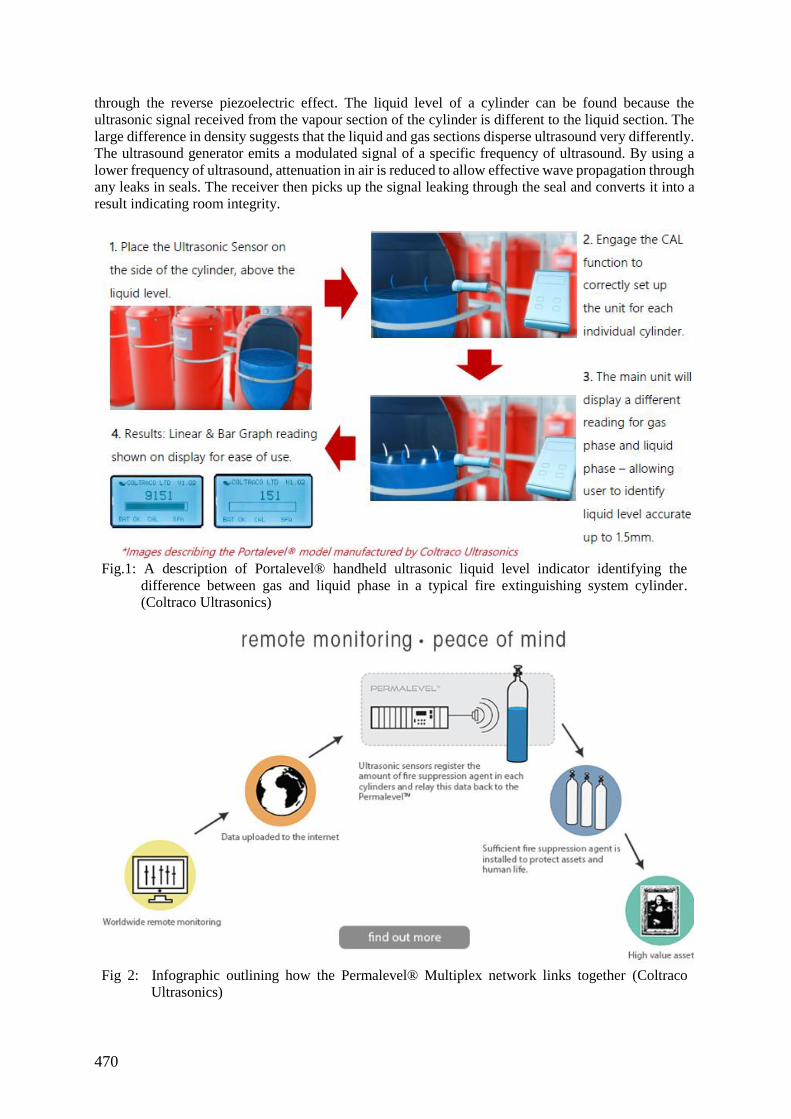
470
through the reverse piezoelectric effect. The liquid level of a cylinder can be found because the
ultrasonic signal received from the vapour section of the cylinder is different to the liquid section. The
large difference in density suggests that the liquid and gas sections disperse ultrasound very differently.
The ultrasound generator emits a modulated signal of a specific frequency of ultrasound. By using a
lower frequency of ultrasound, attenuation in air is reduced to allow effective wave propagation through
any leaks in seals. The receiver then picks up the signal leaking through the seal and converts it into a
result indicating room integrity.
Fig.1: A description of Portalevel® handheld ultrasonic liquid level indicator identifying the
difference between gas and liquid phase in a typical fire extinguishing system cylinder.
(Coltraco Ultrasonics)
Fig 2: Infographic outlining how the Permalevel® Multiplex network links together (Coltraco
Ultrasonics)
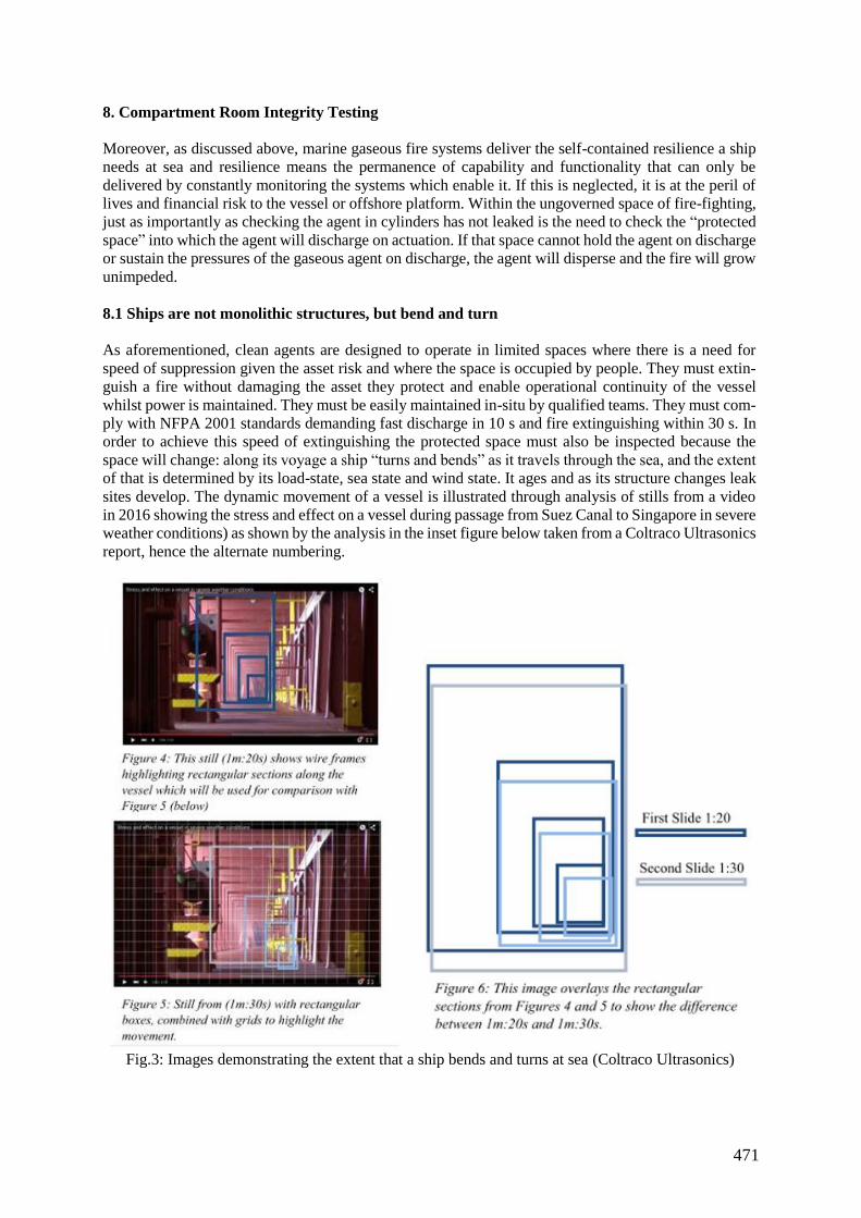
471
8. Compartment Room Integrity Testing
Moreover, as discussed above, marine gaseous fire systems deliver the self-contained resilience a ship
needs at sea and resilience means the permanence of capability and functionality that can only be
delivered by constantly monitoring the systems which enable it. If this is neglected, it is at the peril of
lives and financial risk to the vessel or offshore platform. Within the ungoverned space of fire-fighting,
just as importantly as checking the agent in cylinders has not leaked is the need to check the “protected
space” into which the agent will discharge on actuation. If that space cannot hold the agent on discharge
or sustain the pressures of the gaseous agent on discharge, the agent will disperse and the fire will grow
unimpeded.
8.1 Ships are not monolithic structures, but bend and turn
As aforementioned, clean agents are designed to operate in limited spaces where there is a need for
speed of suppression given the asset risk and where the space is occupied by people. They must extin-
guish a fire without damaging the asset they protect and enable operational continuity of the vessel
whilst power is maintained. They must be easily maintained in-situ by qualified teams. They must com-
ply with NFPA 2001 standards demanding fast discharge in 10 s and fire extinguishing within 30 s. In
order to achieve this speed of extinguishing the protected space must also be inspected because the
space will change: along its voyage a ship “turns and bends” as it travels through the sea, and the extent
of that is determined by its load-state, sea state and wind state. It ages and as its structure changes leak
sites develop. The dynamic movement of a vessel is illustrated through analysis of stills from a video
in 2016 showing the stress and effect on a vessel during passage from Suez Canal to Singapore in severe
weather conditions) as shown by the analysis in the inset figure below taken from a Coltraco Ultrasonics
report, hence the alternate numbering.
Fig.3: Images demonstrating the extent that a ship bends and turns at sea (Coltraco Ultrasonics)
472
8.2 Maintenance & Testing
Testing is essential under ISO 14520 where gaseous extinguishing systems have to be designed in
relation to -the discharging agent hold-time (if the room cannot hold the agent because of leaks the
agent will disperse and not extinguish the fire) and discharging agent peak pressure (if the pressure is
too high for partition walls or suspended ceilings they will be blown apart or damaged and possibly
destroying the room integrity). At the design stage of a fire extinguishing system protected spaces are
tested for room integrity by positively pressurising a room and detecting escaping pressure, to verify
that the room itself into which the gaseous extinguishant discharges on actuation, can both hold the
agent after its discharge and hold its pressure on actuation. The fire system is then installed and
commissioned.
Regulations may require the protected space to be tested every year, and it should be tested after every
major change to the room. Any changes to the compartments state could result in leak sites developing
which would stop the effectiveness of clean agent fire suppression systems should a fire occur. In order
to ensure these fire extinguishing systems maintain their effectiveness over long periods of time, regular
inspection is required. Inspection and constant monitoring of the compartment room integrity is now
possible with products such as Coltraco Ultrasonics’ Portascanner® 520.
As part of the testing procedure and to ensure unknown leak-sites do not develop, ultrasonic technology
can help assess the relevant compartment and detect and precisely locate any leak sites. Products such
as the Portascanner™ WATERTIGHT integrity test indicator is able not only to pinpoint precise leak
locations, but to determine their leak apertures as small as 0.06 mm with a tolerance of ±0.02 mm,
making it the most accurate device for this function. The Portascanner™ also provides an interpretation
of the seal for desired locations, the results signifying them either watertight, weather tight or full leak
site as appropriate. The advantages of being able to accurately detect the exact leak locations and size
are self-evident when considered alongside the importance of reaching Peak Pressure for clean agent
fire suppression to be effective.
9. Conclusion
The science of a marine gaseous extinguishing system is a complex one. The mathematics that underpin
its science are demanding ones. But in simple terms gaseous systems are pressurised and in that they
are dynamic not passive ones. They are there to protect critical marine structures in a safe and
expeditious manner in the only way that a gaseous system can, complemented by the integrity of the
protected space.
Ultrasonic Technology provides an opportunity to use technological advances to monitor these gaseous
fire extinguishing systems and ensure the safety of crew and vessel, in both onshore and offshore
situations. To leave a gaseous cylinder unchecked creates enormous risk which is easily preventable
using ultrasonic technology. Ultrasonic liquid level indicators are portable, require little training and
provide accurate results. Partnering with other readily available products provides recordable data,
providing quantifiable measurements which can be used to accurately assess the quality of fire systems
and its relevant protected spaces to ensure they will be effective. Through inspection and integrated,
continuous monitoring with alarm relay and remote diagnostics facilitated by ultrasonic technology,
smart ships can have an efficient and safe fire extinguishing system with longevity. The use of remote
diagnostics in particular gives eyes to shore-based operators at a time of fewer crew and hopes for
autonomous shipping.
As the world changes, so must our industry integrate technological solutions to provide a bulwark
against wider industry misinterpretation and minimal, even occasional and flagrant, disregard in the
application of standards and good global engineering practice, creating standards which all can
understand and apply. This “Ungoverned Space of Marine Fire Engineering” can be addressed today,
with minimal education and cost, to create a “safety first” culture where owners and operates are
rewarded for pursuing above and beyond regulation compliance.

473
Acknowledgements
With thanks to all who contributed from Coltraco Ultrasonics, Durham University, Warwick University
especially.
474
Elucidating Families of Ship Designs using Clustering Algorithms
Ted Jaspers, TU Delft, Delft/Netherlands, [email protected]
Austin A. Kana, TU Delft, Delft/Netherlands, [email protected]
Abstract
This paper proposes a method to elucidate families of ship designs generated by the TU Delft packing
approach using data clustering algorithms. The authors explore whether commonly used data science
techniques can extract new information from the existing data. To test this hypothesis this paper applies
data clustering algorithms to a test case of layouts of a Mine Counter Measures Vessel (MCMV)
generated by the packing approach. Results look to improve the understanding of the multidimensional
structure of the data, as well as to improve the comprehension and visualization of the complex
interactions between the design and performance space.
1. Background
Early stage design is the initial phase in ship design where the balance between the different desired
performances of the ship is explored. In ship design this process is often initiated by performing concept
exploration, where various design solutions are explored in order to acquire knowledge about the
interactions between design and performance space. Especially during concept exploration of complex
ships, new requirements and/or new relationships between requirements can be elucidated. This results
in an iterative process called requirement elucidation Andrews (2013). On top of that, the traditional
method of manually iterating through the design spiral is very time consuming. These aspects cause
that in general only a small part of the design space is explored, which leads to an increased probability
of converging to a suboptimal design, Vasudevan (2008), Duchateau (2016). In order to explore the
design space more extensively, the ‘packing approach’ was developed at the Delft University of
Technology, which automatically generates tens of thousands of coarse feasible ship designs. By
dividing this design space into ship design families, which share common design features and
performance characteristics, the designer may then be able to better understand interactions between
design and performance space. Think for instance of a ship where you can choose for either a long and
narrow design corresponding to low resistance and low initial stability or short and beamy
corresponding to high resistance and high initial stability. This paper explores the use of clustering
algorithms to study the presence of ship design families stemming from the packing approach.
1.1 The packing approach
The packing approach is a tool that assists in enhancing the concept exploration process. The idea is to
automatically generate a vast number of low level of detail feasible ship designs that cover a significant
part of the design space. This is obtained by using a genetic algorithm on a parametric model of the
desired ship, where all compartments in the ship are represented by building blocks. The designs are
thus coarse, but detailed enough to calculate some performance measures (such as cost, speed,
displacement, etc). Details on this approach can be found in van Oers (2011), van Oers (2012). The
resulting data set may consist of tens of thousands of designs, where each design has hundreds of design
and performance attributes. This data is then structured and visualized so that information about the
relation between design and performance space can be extracted Rowley (2007). One visualization
method applied to the packing approach is described in Duchateau (2016). He proposed a method of
displaying the data in matrix scatter plots, where numerical and architectural constraints could
interactively be added. In Fig.1, L, B, GM and packing density are plotted, and the constraint added is
that designs have deck 4 as damage control deck (dcd) instead of deck 5. Several results can be deducted
from this figure. It shows for instance that the length and packing density are negatively correlated. The
reason is that since a longer design has more space available, it has therefore more empty space to fit
the same number of objects. Furthermore a higher dcd results in a lower GM, since objects (such as the
main gun) should be above dcd, which raises the center of gravity.
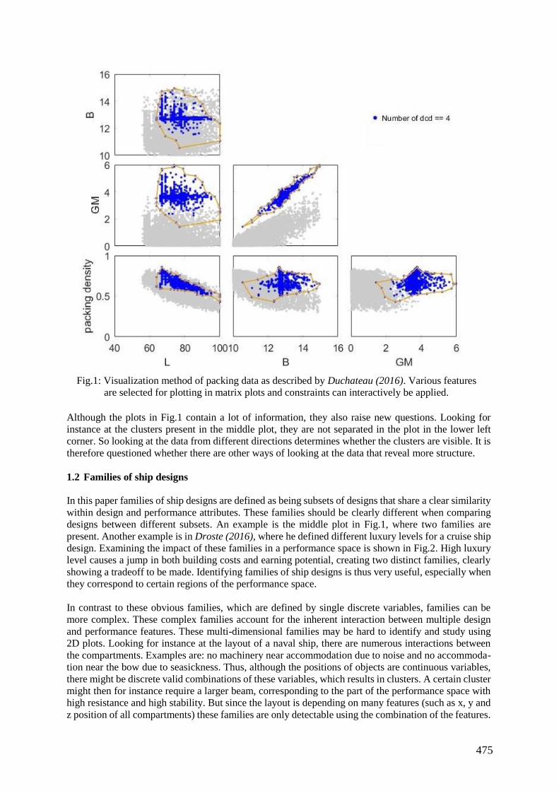
475
Fig.1: Visualization method of packing data as described by Duchateau (2016). Various features
are selected for plotting in matrix plots and constraints can interactively be applied. Although the plots in Fig.1 contain a lot of information, they also raise new questions. Looking for
instance at the clusters present in the middle plot, they are not separated in the plot in the lower left
corner. So looking at the data from different directions determines whether the clusters are visible. It is
therefore questioned whether there are other ways of looking at the data that reveal more structure.
1.2 Families of ship designs
In this paper families of ship designs are defined as being subsets of designs that share a clear similarity
within design and performance attributes. These families should be clearly different when comparing
designs between different subsets. An example is the middle plot in Fig.1, where two families are
present. Another example is in Droste (2016), where he defined different luxury levels for a cruise ship
design. Examining the impact of these families in a performance space is shown in Fig.2. High luxury
level causes a jump in both building costs and earning potential, creating two distinct families, clearly
showing a tradeoff to be made. Identifying families of ship designs is thus very useful, especially when
they correspond to certain regions of the performance space.
In contrast to these obvious families, which are defined by single discrete variables, families can be
more complex. These complex families account for the inherent interaction between multiple design
and performance features. These multi-dimensional families may be hard to identify and study using
2D plots. Looking for instance at the layout of a naval ship, there are numerous interactions between
the compartments. Examples are: no machinery near accommodation due to noise and no accommoda-
tion near the bow due to seasickness. Thus, although the positions of objects are continuous variables,
there might be discrete valid combinations of these variables, which results in clusters. A certain cluster
might then for instance require a larger beam, corresponding to the part of the performance space with
high resistance and high stability. But since the layout is depending on many features (such as x, y and
z position of all compartments) these families are only detectable using the combination of the features.
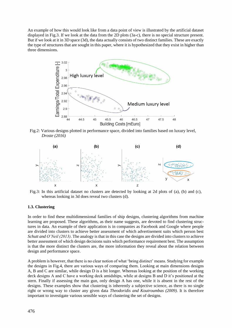
476
An example of how this would look like from a data point of view is illustrated by the artificial dataset
displayed in Fig.3. If we look at the data from the 2D plots (3a-c), there is no special structure present.
But if we look at it in 3D space (3d), the data actually consists of two distinct families. These are exactly
the type of structures that are sought in this paper, where it is hypothesized that they exist in higher than
three dimensions.
Fig.2: Various designs plotted in performance space, divided into families based on luxury level,
Droste (2016)
Fig.3: In this artificial dataset no clusters are detected by looking at 2d plots of (a), (b) and (c),
whereas looking in 3d does reveal two clusters (d). 1.3. Clustering
In order to find these multidimensional families of ship designs, clustering algorithms from machine
learning are proposed. These algorithms, as their name suggests, are devoted to find clustering struc-
tures in data. An example of their application is in companies as Facebook and Google where people
are divided into clusters to achieve better assessment of which advertisement suits which person best
Schutt and O’Neil (2013). The analogy is that in this case the designs are divided into clusters to achieve
better assessment of which design decisions suits which performance requirement best. The assumption
is that the more distinct the clusters are, the more information they reveal about the relation between
design and performance space.
A problem is however, that there is no clear notion of what ‘being distinct’ means. Studying for example
the designs in Fig.4, there are various ways of comparing them. Looking at main dimensions designs
A, B and C are similar, while design D is a bit longer. Whereas looking at the position of the working
deck designs A and C have a working deck amidships, while at designs B and D it’s positioned at the
stern. Finally if assessing the main gun, only design A has one, while it is absent in the rest of the
designs. These examples show that clustering is inherently a subjective science, as there is no single
right or wrong way to cluster any given data Theodoridis and Koutroumbas (2009). It is therefore
important to investigate various sensible ways of clustering the set of designs.
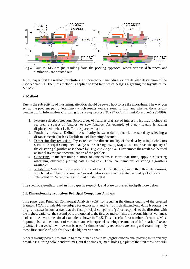
477
Fig.4: Four MCMV-designs resulting from the packing approach, where various differences and
similarities are pointed out.
In this paper first the method for clustering is pointed out, including a more detailed description of the
used techniques. Then this method is applied to find families of designs regarding the layouts of the
MCMV.
2. Method
Due to the subjectivity of clustering, attention should be payed how to use the algorithms. The way you
set up the problem partly determines which results you are going to find, and whether these results
contain useful information. Clustering is a six step process (See Theodoridis and Koutroumbas (2009)):
1. Feature selection/creation: Select a set of features that are of interest. This may include all
features, a subset of features, or new features. An example of a new feature is adding
displacement, when L, B, T and 𝑐𝐵 are available.
2. Proximity measure: Define how similarity between data points is measured by selecting a
distance metric (such as Euclidean and Hamming distance).
3. Dimensionality reduction: Try to reduce the dimensionality of the data by using techniques
such as Principal Component Analysis or Self-Organizing Maps. This improves the quality of
the clustering algorithm as is shown by Ding and He (2004). Furthermore the result can be used
as initial investigation/visualization of the problem.
4. Clustering: If the remaining number of dimensions is more than three, apply a clustering
algorithm, otherwise plotting data is possible. There are numerous clustering algorithms
available.
5. Validation: Validate the clusters. This is not trivial since there are more than three dimensions,
which makes it hard to visualize. Several metrics exist that indicate the quality of clusters.
6. Interpretation: When the result is valid, interpret it.
The specific algorithms used in this paper in steps 3, 4, and 5 are discussed in-depth more below.
2.1. Dimensionality reduction: Principal Component Analysis
This paper uses Principal Component Analysis (PCA) for reducing the dimensionality of the selected
features. PCA is a valuable technique for exploratory analysis of high dimensional data. It rotates the
original dataset in such a way that the first principal component (pc) corresponds to the direction with
the highest variance, the second pc is orthogonal to the first pc and contains the second highest variance,
and so on. A two-dimensional example is shown in Fig.5. This is useful for a number of reasons. Most
important is that the amount of variance can be interpreted as being the amount of information Linsker
(1989). This reveals how PCA can be used for dimensionality reduction: Selecting and examining only
those first couple of pc’s that have the highest variance.
Since it is only possible to plot up to three dimensional data (higher dimensional plotting is technically
possible (i.e. using colour and/or time), but the same argument holds.), a plot of the first three pc’s will
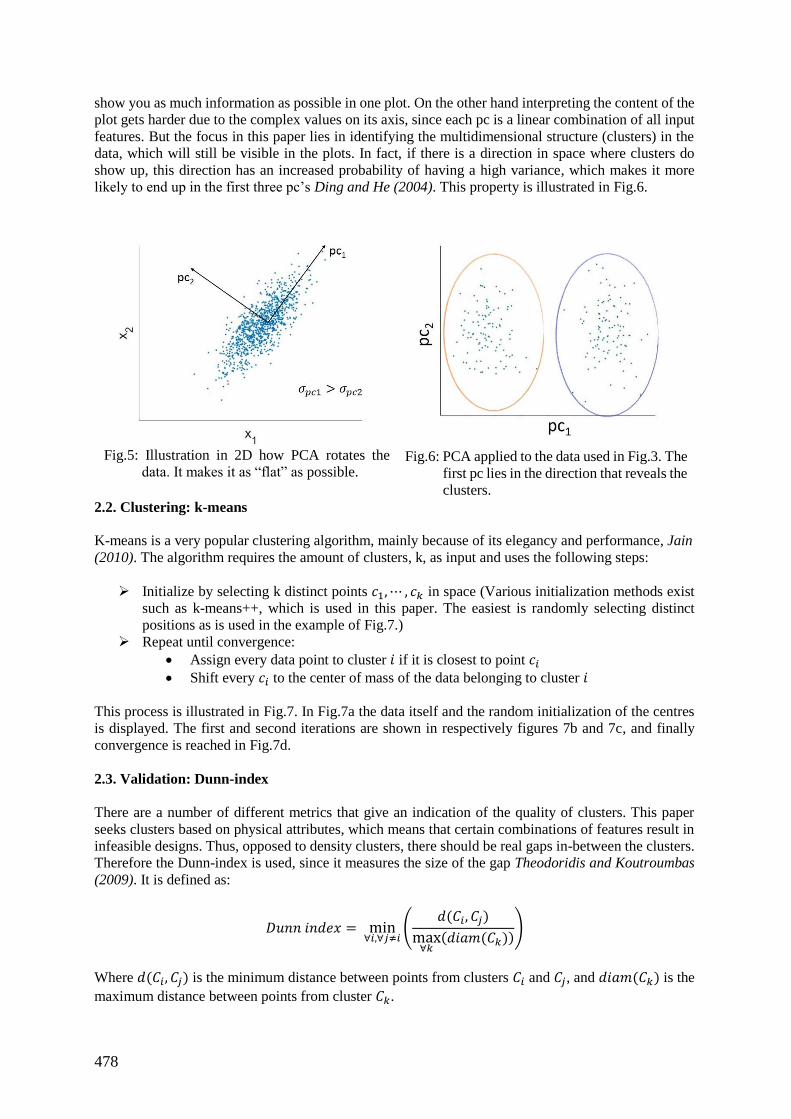
478
show you as much information as possible in one plot. On the other hand interpreting the content of the
plot gets harder due to the complex values on its axis, since each pc is a linear combination of all input
features. But the focus in this paper lies in identifying the multidimensional structure (clusters) in the
data, which will still be visible in the plots. In fact, if there is a direction in space where clusters do
show up, this direction has an increased probability of having a high variance, which makes it more
likely to end up in the first three pc’s Ding and He (2004). This property is illustrated in Fig.6.
Fig.5: Illustration in 2D how PCA rotates the
data. It makes it as “flat” as possible.
Fig.6: PCA applied to the data used in Fig.3. The
first pc lies in the direction that reveals the
clusters. 2.2. Clustering: k-means
K-means is a very popular clustering algorithm, mainly because of its elegancy and performance, Jain
(2010). The algorithm requires the amount of clusters, k, as input and uses the following steps:
Initialize by selecting k distinct points 𝑐1, ⋯ , 𝑐𝑘 in space (Various initialization methods exist
such as k-means++, which is used in this paper. The easiest is randomly selecting distinct
positions as is used in the example of Fig.7.)
Repeat until convergence:
Assign every data point to cluster 𝑖 if it is closest to point 𝑐𝑖
Shift every 𝑐𝑖 to the center of mass of the data belonging to cluster 𝑖
This process is illustrated in Fig.7. In Fig.7a the data itself and the random initialization of the centres
is displayed. The first and second iterations are shown in respectively figures 7b and 7c, and finally
convergence is reached in Fig.7d.
2.3. Validation: Dunn-index
There are a number of different metrics that give an indication of the quality of clusters. This paper
seeks clusters based on physical attributes, which means that certain combinations of features result in
infeasible designs. Thus, opposed to density clusters, there should be real gaps in-between the clusters.
Therefore the Dunn-index is used, since it measures the size of the gap Theodoridis and Koutroumbas
(2009). It is defined as:
𝐷𝑢𝑛𝑛 𝑖𝑛𝑑𝑒𝑥 = min∀𝑖,∀𝑗≠𝑖
(𝑑(𝐶𝑖, 𝐶𝑗)
max∀𝑘
(𝑑𝑖𝑎𝑚(𝐶𝑘)))
Where 𝑑(𝐶𝑖, 𝐶𝑗) is the minimum distance between points from clusters 𝐶𝑖 and 𝐶𝑗, and 𝑑𝑖𝑎𝑚(𝐶𝑘) is the
maximum distance between points from cluster 𝐶𝑘.
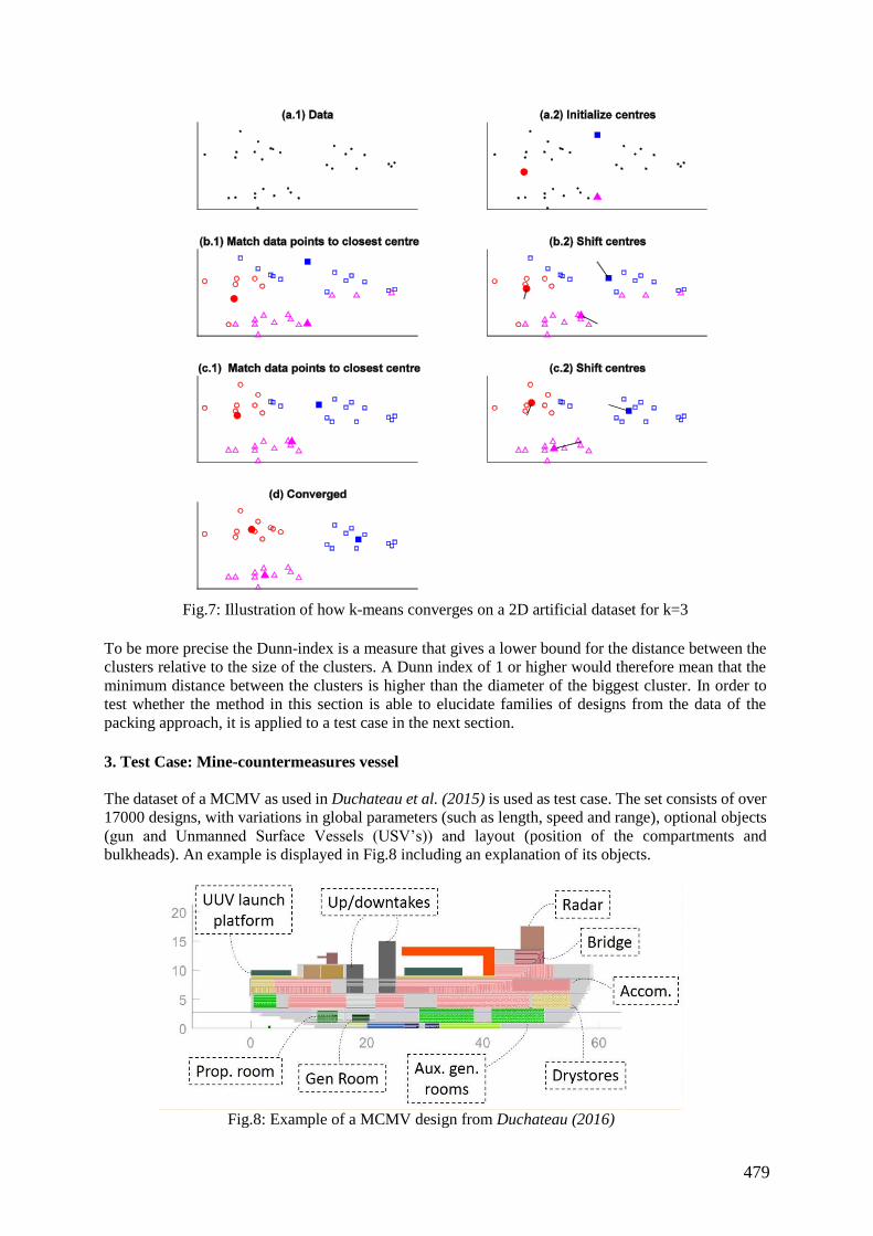
479
Fig.7: Illustration of how k-means converges on a 2D artificial dataset for k=3
To be more precise the Dunn-index is a measure that gives a lower bound for the distance between the
clusters relative to the size of the clusters. A Dunn index of 1 or higher would therefore mean that the
minimum distance between the clusters is higher than the diameter of the biggest cluster. In order to
test whether the method in this section is able to elucidate families of designs from the data of the
packing approach, it is applied to a test case in the next section.
3. Test Case: Mine-countermeasures vessel
The dataset of a MCMV as used in Duchateau et al. (2015) is used as test case. The set consists of over
17000 designs, with variations in global parameters (such as length, speed and range), optional objects
(gun and Unmanned Surface Vessels (USV’s)) and layout (position of the compartments and
bulkheads). An example is displayed in Fig.8 including an explanation of its objects.
Fig.8: Example of a MCMV design from Duchateau (2016)
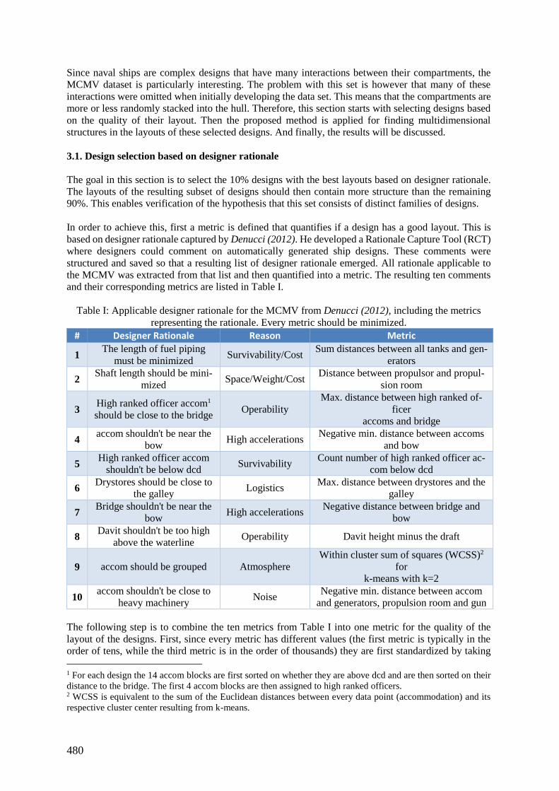
480
Since naval ships are complex designs that have many interactions between their compartments, the
MCMV dataset is particularly interesting. The problem with this set is however that many of these
interactions were omitted when initially developing the data set. This means that the compartments are
more or less randomly stacked into the hull. Therefore, this section starts with selecting designs based
on the quality of their layout. Then the proposed method is applied for finding multidimensional
structures in the layouts of these selected designs. And finally, the results will be discussed.
3.1. Design selection based on designer rationale
The goal in this section is to select the 10% designs with the best layouts based on designer rationale.
The layouts of the resulting subset of designs should then contain more structure than the remaining
90%. This enables verification of the hypothesis that this set consists of distinct families of designs.
In order to achieve this, first a metric is defined that quantifies if a design has a good layout. This is
based on designer rationale captured by Denucci (2012). He developed a Rationale Capture Tool (RCT)
where designers could comment on automatically generated ship designs. These comments were
structured and saved so that a resulting list of designer rationale emerged. All rationale applicable to
the MCMV was extracted from that list and then quantified into a metric. The resulting ten comments
and their corresponding metrics are listed in Table I.
Table I: Applicable designer rationale for the MCMV from Denucci (2012), including the metrics
representing the rationale. Every metric should be minimized.
# Designer Rationale Reason Metric
1 The length of fuel piping
must be minimized Survivability/Cost
Sum distances between all tanks and gen-
erators
2 Shaft length should be mini-
mized Space/Weight/Cost
Distance between propulsor and propul-
sion room
3 High ranked officer accom1
should be close to the bridge Operability
Max. distance between high ranked of-
ficer
accoms and bridge
4 accom shouldn't be near the
bow High accelerations
Negative min. distance between accoms
and bow
5 High ranked officer accom
shouldn't be below dcd Survivability
Count number of high ranked officer ac-
com below dcd
6 Drystores should be close to
the galley Logistics
Max. distance between drystores and the
galley
7 Bridge shouldn't be near the
bow High accelerations
Negative distance between bridge and
bow
8 Davit shouldn't be too high
above the waterline Operability Davit height minus the draft
9 accom should be grouped Atmosphere
Within cluster sum of squares (WCSS)2
for
k-means with k=2
10 accom shouldn't be close to
heavy machinery Noise
Negative min. distance between accom
and generators, propulsion room and gun
The following step is to combine the ten metrics from Table I into one metric for the quality of the
layout of the designs. First, since every metric has different values (the first metric is typically in the
order of tens, while the third metric is in the order of thousands) they are first standardized by taking
1 For each design the 14 accom blocks are first sorted on whether they are above dcd and are then sorted on their
distance to the bridge. The first 4 accom blocks are then assigned to high ranked officers. 2 WCSS is equivalent to the sum of the Euclidean distances between every data point (accommodation) and its
respective cluster center resulting from k-means.
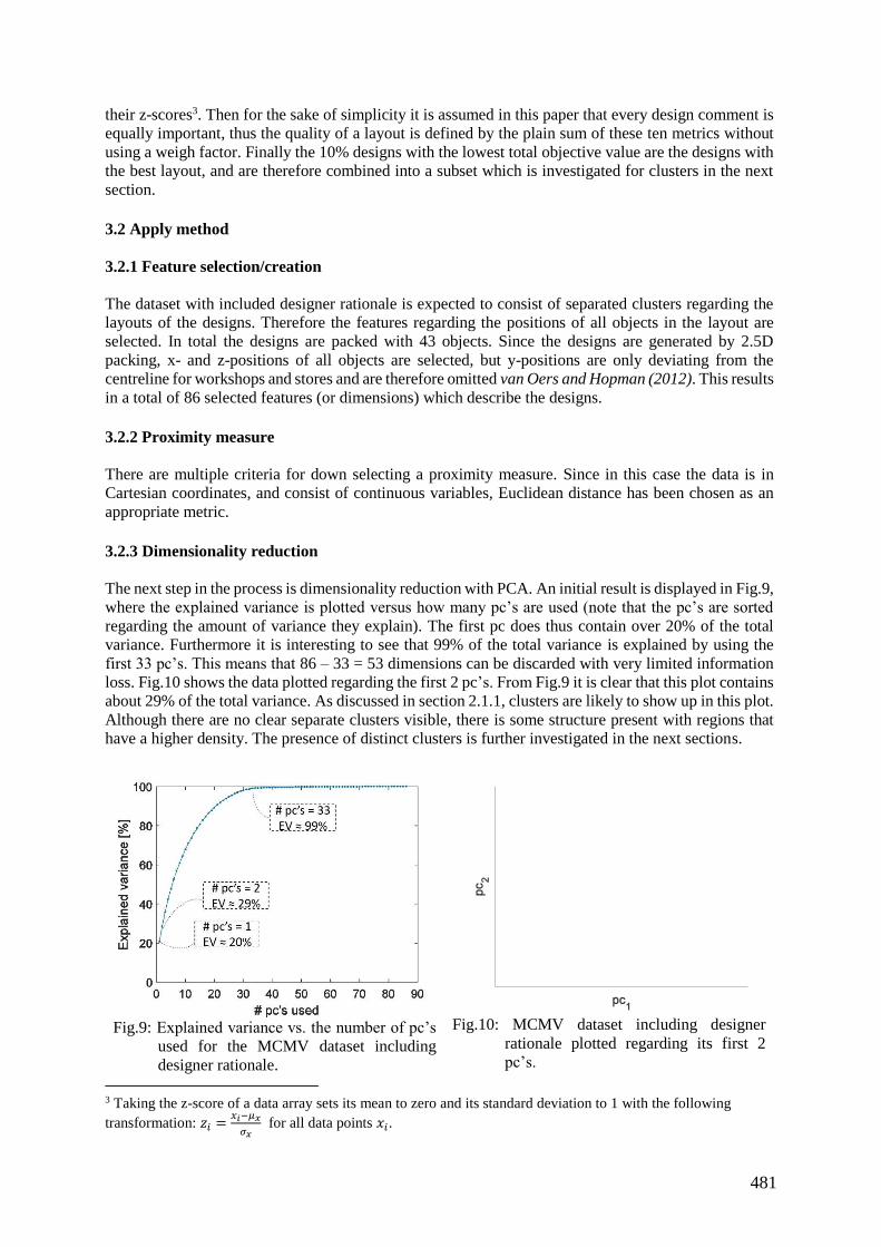
481
their z-scores3. Then for the sake of simplicity it is assumed in this paper that every design comment is
equally important, thus the quality of a layout is defined by the plain sum of these ten metrics without
using a weigh factor. Finally the 10% designs with the lowest total objective value are the designs with
the best layout, and are therefore combined into a subset which is investigated for clusters in the next
section.
3.2 Apply method
3.2.1 Feature selection/creation
The dataset with included designer rationale is expected to consist of separated clusters regarding the
layouts of the designs. Therefore the features regarding the positions of all objects in the layout are
selected. In total the designs are packed with 43 objects. Since the designs are generated by 2.5D
packing, x- and z-positions of all objects are selected, but y-positions are only deviating from the
centreline for workshops and stores and are therefore omitted van Oers and Hopman (2012). This results
in a total of 86 selected features (or dimensions) which describe the designs.
3.2.2 Proximity measure
There are multiple criteria for down selecting a proximity measure. Since in this case the data is in
Cartesian coordinates, and consist of continuous variables, Euclidean distance has been chosen as an
appropriate metric. 3.2.3 Dimensionality reduction
The next step in the process is dimensionality reduction with PCA. An initial result is displayed in Fig.9,
where the explained variance is plotted versus how many pc’s are used (note that the pc’s are sorted
regarding the amount of variance they explain). The first pc does thus contain over 20% of the total
variance. Furthermore it is interesting to see that 99% of the total variance is explained by using the
first 33 pc’s. This means that 86 – 33 = 53 dimensions can be discarded with very limited information
loss. Fig.10 shows the data plotted regarding the first 2 pc’s. From Fig.9 it is clear that this plot contains
about 29% of the total variance. As discussed in section 2.1.1, clusters are likely to show up in this plot.
Although there are no clear separate clusters visible, there is some structure present with regions that
have a higher density. The presence of distinct clusters is further investigated in the next sections.
Fig.9: Explained variance vs. the number of pc’s
used for the MCMV dataset including
designer rationale.
Fig.10: MCMV dataset including designer
rationale plotted regarding its first 2
pc’s.
3 Taking the z-score of a data array sets its mean to zero and its standard deviation to 1 with the following
transformation: 𝑧𝑖 =𝑥𝑖−𝜇𝑥
𝜎𝑥 for all data points 𝑥𝑖.
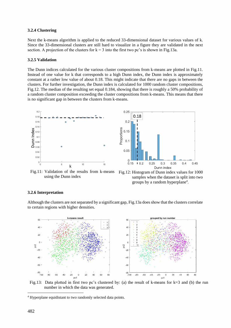
482
3.2.4 Clustering
Next the k-means algorithm is applied to the reduced 33-dimensional dataset for various values of k.
Since the 33-dimensional clusters are still hard to visualize in a figure they are validated in the next
section. A projection of the clusters for k = 3 into the first two pc’s is shown in Fig.13a.
3.2.5 Validation
The Dunn indices calculated for the various cluster compositions from k-means are plotted in Fig.11.
Instead of one value for k that corresponds to a high Dunn index, the Dunn index is approximately
constant at a rather low value of about 0.18. This might indicate that there are no gaps in between the
clusters. For further investigation, the Dunn index is calculated for 1000 random cluster compositions,
Fig.12. The median of the resulting set equal 0.184, showing that there is roughly a 50% probability of
a random cluster composition exceeding the cluster compositions from k-means. This means that there
is no significant gap in between the clusters from k-means.
Fig.11: Validation of the results from k-means
using the Dunn index
Fig.12: Histogram of Dunn index values for 1000
samples when the dataset is split into two
groups by a random hyperplane4. 3.2.6 Interpretation
Although the clusters are not separated by a significant gap, Fig.13a does show that the clusters correlate
to certain regions with higher densities.
Fig.13: Data plotted in first two pc’s clustered by: (a) the result of k-means for k=3 and (b) the run
number in which the data was generated. 4 Hyperplane equidistant to two randomly selected data points.
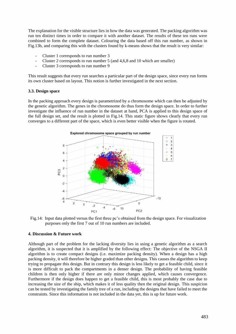
483
The explanation for the visible structure lies in how the data was generated. The packing algorithm was
run ten distinct times in order to compare it with another dataset. The results of these ten runs were
combined to form the complete dataset. Colouring the data based off this run number, as shown in
Fig.13b, and comparing this with the clusters found by k-means shows that the result is very similar:
- Cluster 1 corresponds to run number 3
- Cluster 2 corresponds to run number 5 (and 4,6,8 and 10 which are smaller)
- Cluster 3 corresponds to run number 9
This result suggests that every run searches a particular part of the design space, since every run forms
its own cluster based on layout. This notion is further investigated in the next section.
3.3. Design space
In the packing approach every design is parametrized by a chromosome which can then be adjusted by
the genetic algorithm. The genes in the chromosome do thus form the design space. In order to further
investigate the influence of run number in the dataset at hand, PCA is applied to this design space of
the full design set, and the result is plotted in Fig.14. This static figure shows clearly that every run
converges to a different part of the space, which is even better visible when the figure is rotated.
4. Discussion & Future work
Although part of the problem for the lacking diversity lies in using a genetic algorithm as a search
algorithm, it is suspected that it is amplified by the following effect: The objective of the NSGA II
algorithm is to create compact designs (i.e. maximize packing density). When a design has a high
packing density, it will therefore be higher graded than other designs. This causes the algorithm to keep
trying to propagate this design. But in contrary this design is less likely to get a feasible child, since it
is more difficult to pack the compartments in a denser design. The probability of having feasible
children is then only higher if there are only minor changes applied, which causes convergence.
Furthermore if the design does happen to get a feasible child, this is most probably the case due to
increasing the size of the ship, which makes it of less quality then the original design. This suspicion
can be tested by investigating the family tree of a run, including the designs that have failed to meet the
constraints. Since this information is not included in the data yet, this is up for future work.
Fig.14: Input data plotted versus the first three pc’s obtained from the design space. For visualization
purposes only the first 7 out of 10 run numbers are included.
484
5. Conclusion
In this paper clustering algorithms were used to search for families of ship designs generated by the TU
Delft packing approach. Therefore a clustering method was applied to a test case of layouts from a
MCMV. Unfortunately the results seem to be dominated by the fact that the dataset was built by
combining data from ten distinct runs of the packing approach.
Although families of ship designs based on physical aspects of the designs were not clearly visible, the
techniques used in this paper did reveal information on how the model generated the data. It shows that
despite the effort of using the NSGA II algorithm as a search algorithm by setting its mutation rate
rather high Duchateau (2016), the diversity for a single packing run is still limited.
It would have been difficult to ascertain this behaviour using other techniques. The clustering method
allows to look at the data from a different point of view than ordinary plotting variables, and therefore
creates new insights and hypotheses. The authors are therefore convinced that its application will remain
useful, revealing information about both the model as the relation between design and performance
space.
Acknowledgements
We gratefully thank Bijan Ranjbarsahraei for supporting us by sharing his wisdom on the various tech-
niques and methods from the field of data science in regular meetings.
References
ANDREWS, D.J. (2013), The true nature of ship concept design – and what it means for the future
development of CASD, COMPIT 2013, Cortona, pp.33-50
DENUCCI, T.W. (2012), Capturing design: Improving conceptual design through the capture of design
rationale, PhD Thesis, Delft University of Technology
DING, C.H.Q.; HE, X. (2004), k-means clustering via principal component analysis, 21st Int. Conf.
Machine Learning, Alberta, pp.29
DROSTE, K. (2016), A new concept exploration method to support innovative cruise ship design,
Master Thesis, Delft University of Technology
DUCHATEAU, E.A.E.; OERS van, B.J.; HOPMAN, J.J. (2015), Interactive steering of an
optimisation-based ship synthesis model for concept exploration, 12th IMDC, Tokyo
DUCHATEAU, E.A.E. (2016), Interactive evolutionary concept exploration in preliminary ship
design, PhD Thesis, Delft University of Technology
JAIN, A.K. (2010), Data clustering: 50 years beyond K-means, Pattern Recognition Letters 31/8,
pp.651-666
LINSKER, R. (1989), Self-organization in a perceptual network, Computer 21/3, pp.105-117
OERS van, B.J. (2011), A packing approach for the early stage ship design of service vessels, PhD
Thesis, Delft University of Technology
OERS van, B.J.; HOPMAN, J.J. (2012), Simpler and faster: A 2.5D packing-based approach for early
stage ship design, 11th IMDC, Glasgow
ROWLEY, J. (2007), The wisdom hierarchy: representations of the DIKW hierarchy, J. Information

485
Science 33/2, pp.163-180
SCHUTT, R.; O’NEIL, C. (2013), Doing data science: Straight talk from the frontline, O’Reilly Media
THEODORIDIS, S.; KOUTROUMBAS, K. (2009), Pattern Recognition (4th ed.), Elsevier
VASUDEVAN, S. (2008), Utility of the pareto-front approach in elucidating ship requirements during
concept design, PhD Thesis, University College London
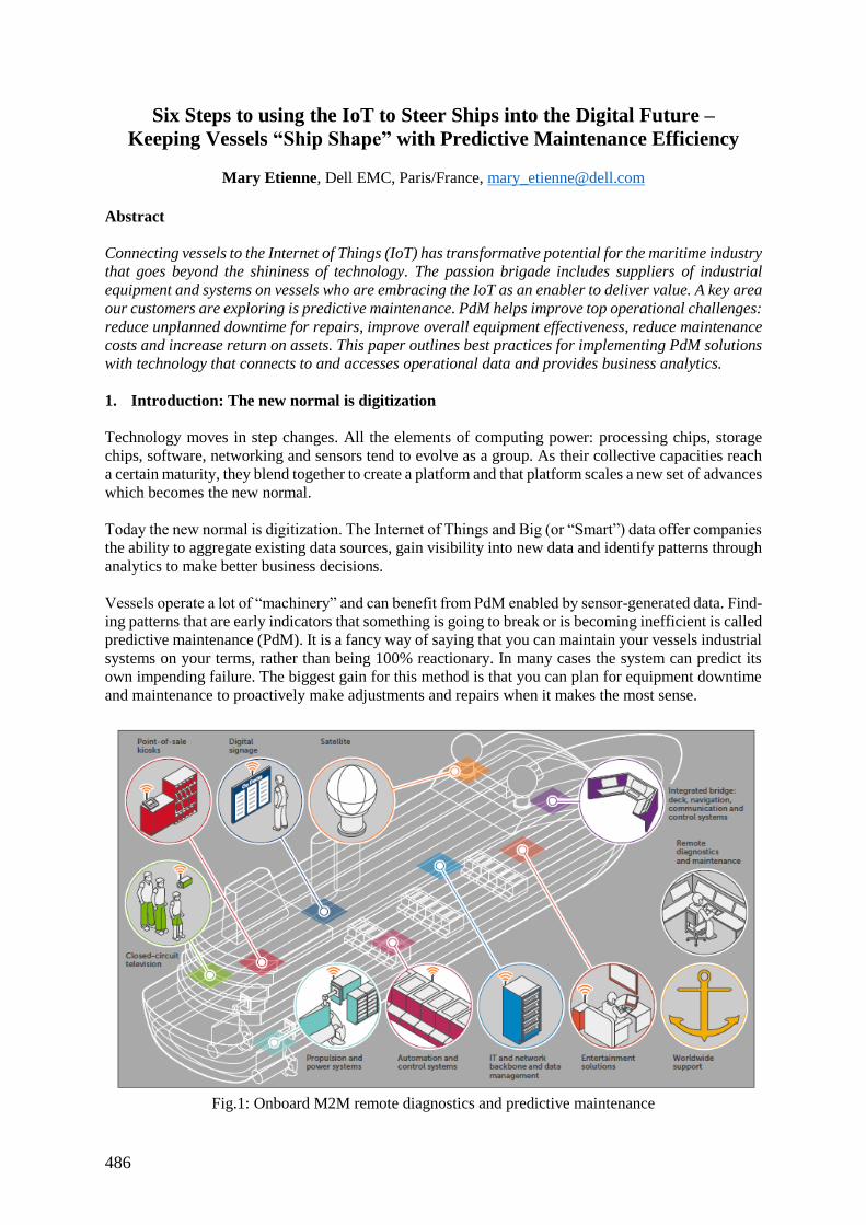
486
Six Steps to using the IoT to Steer Ships into the Digital Future –
Keeping Vessels “Ship Shape” with Predictive Maintenance Efficiency
Mary Etienne, Dell EMC, Paris/France, [email protected]
Abstract
Connecting vessels to the Internet of Things (IoT) has transformative potential for the maritime industry
that goes beyond the shininess of technology. The passion brigade includes suppliers of industrial
equipment and systems on vessels who are embracing the IoT as an enabler to deliver value. A key area
our customers are exploring is predictive maintenance. PdM helps improve top operational challenges:
reduce unplanned downtime for repairs, improve overall equipment effectiveness, reduce maintenance
costs and increase return on assets. This paper outlines best practices for implementing PdM solutions
with technology that connects to and accesses operational data and provides business analytics.
1. Introduction: The new normal is digitization
Technology moves in step changes. All the elements of computing power: processing chips, storage
chips, software, networking and sensors tend to evolve as a group. As their collective capacities reach
a certain maturity, they blend together to create a platform and that platform scales a new set of advances
which becomes the new normal.
Today the new normal is digitization. The Internet of Things and Big (or “Smart”) data offer companies
the ability to aggregate existing data sources, gain visibility into new data and identify patterns through
analytics to make better business decisions.
Vessels operate a lot of “machinery” and can benefit from PdM enabled by sensor-generated data. Find-
ing patterns that are early indicators that something is going to break or is becoming inefficient is called
predictive maintenance (PdM). It is a fancy way of saying that you can maintain your vessels industrial
systems on your terms, rather than being 100% reactionary. In many cases the system can predict its
own impending failure. The biggest gain for this method is that you can plan for equipment downtime
and maintenance to proactively make adjustments and repairs when it makes the most sense.
Fig.1: Onboard M2M remote diagnostics and predictive maintenance
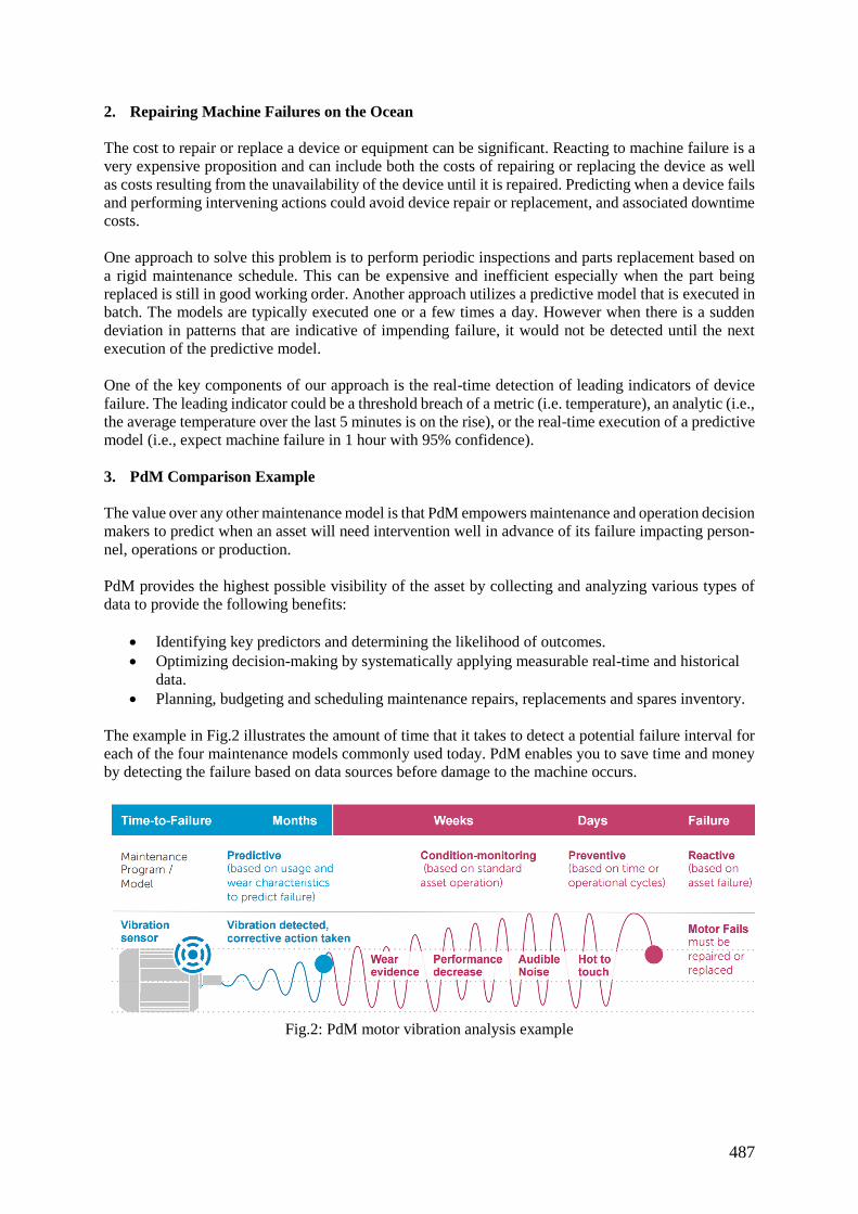
487
2. Repairing Machine Failures on the Ocean
The cost to repair or replace a device or equipment can be significant. Reacting to machine failure is a
very expensive proposition and can include both the costs of repairing or replacing the device as well
as costs resulting from the unavailability of the device until it is repaired. Predicting when a device fails
and performing intervening actions could avoid device repair or replacement, and associated downtime
costs.
One approach to solve this problem is to perform periodic inspections and parts replacement based on
a rigid maintenance schedule. This can be expensive and inefficient especially when the part being
replaced is still in good working order. Another approach utilizes a predictive model that is executed in
batch. The models are typically executed one or a few times a day. However when there is a sudden
deviation in patterns that are indicative of impending failure, it would not be detected until the next
execution of the predictive model.
One of the key components of our approach is the real-time detection of leading indicators of device
failure. The leading indicator could be a threshold breach of a metric (i.e. temperature), an analytic (i.e.,
the average temperature over the last 5 minutes is on the rise), or the real-time execution of a predictive
model (i.e., expect machine failure in 1 hour with 95% confidence).
3. PdM Comparison Example
The value over any other maintenance model is that PdM empowers maintenance and operation decision
makers to predict when an asset will need intervention well in advance of its failure impacting person-
nel, operations or production.
PdM provides the highest possible visibility of the asset by collecting and analyzing various types of
data to provide the following benefits:
Identifying key predictors and determining the likelihood of outcomes.
Optimizing decision-making by systematically applying measurable real-time and historical
data.
Planning, budgeting and scheduling maintenance repairs, replacements and spares inventory.
The example in Fig.2 illustrates the amount of time that it takes to detect a potential failure interval for
each of the four maintenance models commonly used today. PdM enables you to save time and money
by detecting the failure based on data sources before damage to the machine occurs.
Fig.2: PdM motor vibration analysis example
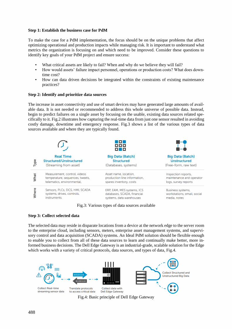
488
Step 1: Establish the business case for PdM
To make the case for a PdM implementation, the focus should be on the unique problems that affect
optimizing operational and production impacts while managing risk. It is important to understand what
metrics the organization is focusing on and which need to be improved. Consider these questions to
identify key goals of your PdM project and ensure success:
• What critical assets are likely to fail? When and why do we believe they will fail?
• How would assets’ failure impact personnel, operations or production costs? What does down-
time cost?
• How can data driven decisions be integrated within the constraints of existing maintenance
practices?
Step 2: Identify and prioritize data sources
The increase in asset connectivity and use of smart devices may have generated large amounts of avail-
able data. It is not needed or recommended to address this whole universe of possible data. Instead,
begin to predict failures on a single asset by focusing on the usable, existing data sources related spe-
cifically to it. Fig.2 illustrates how capturing the real-time data from just one sensor resulted in avoiding
costly damage, downtime and emergency response. Fig.3 shows a list of the various types of data
sources available and where they are typically found.
Fig.3: Various types of data sources available
Step 3: Collect selected data
The selected data may reside in disparate locations from a device at the network edge to the server room
to the enterprise cloud, including sensors, meters, enterprise asset management systems, and supervi-
sory control and data acquisition (SCADA) systems. An Ideal PdM solution should be flexible enough
to enable you to collect from all of these data sources to learn and continually make better, more in-
formed business decisions. The Dell Edge Gateway is an industrial-grade, scalable solution for the Edge
which works with a variety of critical protocols, data sources, and types of data, Fig.4.
Fig.4: Basic principle of Dell Edge Gateway
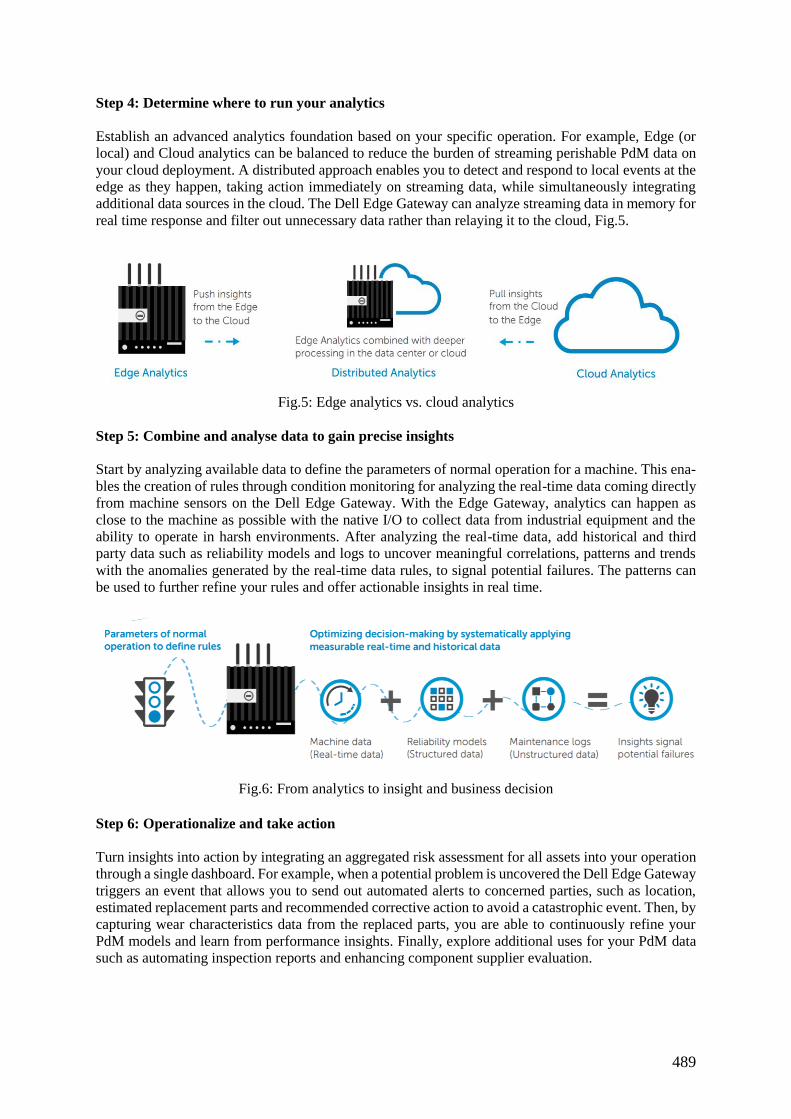
489
Step 4: Determine where to run your analytics
Establish an advanced analytics foundation based on your specific operation. For example, Edge (or
local) and Cloud analytics can be balanced to reduce the burden of streaming perishable PdM data on
your cloud deployment. A distributed approach enables you to detect and respond to local events at the
edge as they happen, taking action immediately on streaming data, while simultaneously integrating
additional data sources in the cloud. The Dell Edge Gateway can analyze streaming data in memory for
real time response and filter out unnecessary data rather than relaying it to the cloud, Fig.5.
Fig.5: Edge analytics vs. cloud analytics
Step 5: Combine and analyse data to gain precise insights
Start by analyzing available data to define the parameters of normal operation for a machine. This ena-
bles the creation of rules through condition monitoring for analyzing the real-time data coming directly
from machine sensors on the Dell Edge Gateway. With the Edge Gateway, analytics can happen as
close to the machine as possible with the native I/O to collect data from industrial equipment and the
ability to operate in harsh environments. After analyzing the real-time data, add historical and third
party data such as reliability models and logs to uncover meaningful correlations, patterns and trends
with the anomalies generated by the real-time data rules, to signal potential failures. The patterns can
be used to further refine your rules and offer actionable insights in real time.
Fig.6: From analytics to insight and business decision
Step 6: Operationalize and take action
Turn insights into action by integrating an aggregated risk assessment for all assets into your operation
through a single dashboard. For example, when a potential problem is uncovered the Dell Edge Gateway
triggers an event that allows you to send out automated alerts to concerned parties, such as location,
estimated replacement parts and recommended corrective action to avoid a catastrophic event. Then, by
capturing wear characteristics data from the replaced parts, you are able to continuously refine your
PdM models and learn from performance insights. Finally, explore additional uses for your PdM data
such as automating inspection reports and enhancing component supplier evaluation.
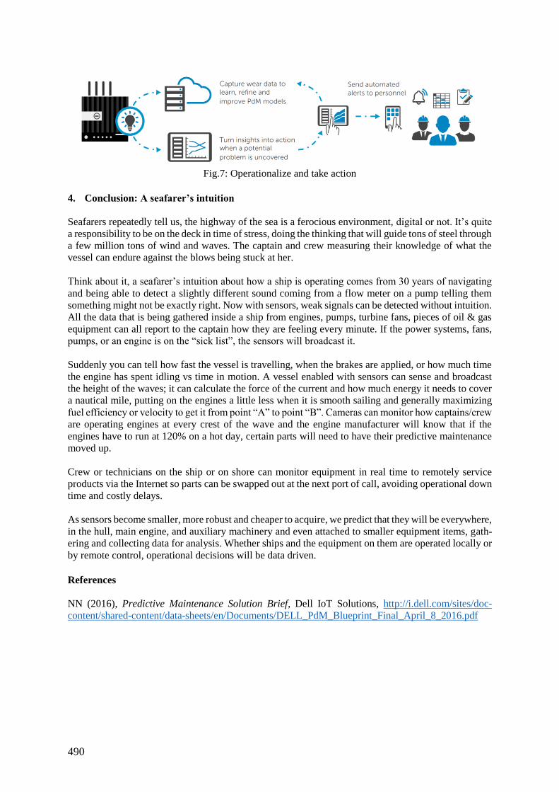
490
Fig.7: Operationalize and take action
4. Conclusion: A seafarer’s intuition
Seafarers repeatedly tell us, the highway of the sea is a ferocious environment, digital or not. It’s quite
a responsibility to be on the deck in time of stress, doing the thinking that will guide tons of steel through
a few million tons of wind and waves. The captain and crew measuring their knowledge of what the
vessel can endure against the blows being stuck at her.
Think about it, a seafarer’s intuition about how a ship is operating comes from 30 years of navigating
and being able to detect a slightly different sound coming from a flow meter on a pump telling them
something might not be exactly right. Now with sensors, weak signals can be detected without intuition.
All the data that is being gathered inside a ship from engines, pumps, turbine fans, pieces of oil & gas
equipment can all report to the captain how they are feeling every minute. If the power systems, fans,
pumps, or an engine is on the “sick list”, the sensors will broadcast it.
Suddenly you can tell how fast the vessel is travelling, when the brakes are applied, or how much time
the engine has spent idling vs time in motion. A vessel enabled with sensors can sense and broadcast
the height of the waves; it can calculate the force of the current and how much energy it needs to cover
a nautical mile, putting on the engines a little less when it is smooth sailing and generally maximizing
fuel efficiency or velocity to get it from point “A” to point “B”. Cameras can monitor how captains/crew
are operating engines at every crest of the wave and the engine manufacturer will know that if the
engines have to run at 120% on a hot day, certain parts will need to have their predictive maintenance
moved up.
Crew or technicians on the ship or on shore can monitor equipment in real time to remotely service
products via the Internet so parts can be swapped out at the next port of call, avoiding operational down
time and costly delays.
As sensors become smaller, more robust and cheaper to acquire, we predict that they will be everywhere,
in the hull, main engine, and auxiliary machinery and even attached to smaller equipment items, gath-
ering and collecting data for analysis. Whether ships and the equipment on them are operated locally or
by remote control, operational decisions will be data driven.
References
NN (2016), Predictive Maintenance Solution Brief, Dell IoT Solutions, http://i.dell.com/sites/doc-
content/shared-content/data-sheets/en/Documents/DELL_PdM_Blueprint_Final_April_8_2016.pdf

491
Appendix: Predictive Maintenance Solutions Blueprints
Dell EMC has developed flexible architectures around the Edge Gateway 5000 with qualified partners
for complete PdM solutions. For more detailed information on our Predictive Maintenance Reference
Architectures, see:
Dell | SAP IFM PdM Reference Architecture
http://en.community.dell.com/techcenter/blueprints/m/resources/20442877
This document is intended for both Information Technology and Operations Technology audiences in
asset intensive industries such as manufacturing, transportation, energy, and others. It is ideal for audi-
ences exploring how IoT-enabled predictive maintenance could be effectively deployed in their envi-
ronment. Readers who have some familiarity with concepts including IoT, device protocols, streaming
analytics, and predictive analytics will gain a deeper understanding of how these concepts can come
together to increase maintenance efficiencies in your business.
Dell Software AG Kepware PdM Reference Architecture
http://en.community.dell.com/techcenter/blueprints/m/resources/20442878
Big Data Streaming Analytics at the Edge for Predictive Maintenance Reference Architecture. This
paper presents a reference architecture for a Predictive Maintenance solution that runs on a Dell Edge
Gateway 5000 and associated best practices in leveraging this architecture. The architecture leverages
Kepware’s KEPServerEX® connectivity platform for device protocol translation and Software AG
Apama for streaming analytics and real-time predictive model execution.
492
Big Data – Processing Global AIS in Real Time to Produce Market Insight
Mark Deverill, Genscape Vesseltracker, London/UK, [email protected]
Abstract
This paper presents how Genscape Vesseltracker process 500 million daily AIS messages in real time,
filtering for all types of ship events, merging the information with a detailed geographical database of
maritime locations and facilities, and filtering against databases of ship, terminal and company
information to provide unique, actionable market insight.
1. Introduction
Vesseltracker, www.vesseltracker.com, has been pushing the boundaries of how AIS data can be used
to gain business advantage for over 10 years. While running probably the biggest commercial AIS
network for tracking ships globally, we recognise that AIS alone is no longer enough to gain the best
business advantage from ship tracking. Vesseltracker is now part of Genscape Maritime utilising
machine learning and the expertise of Genscape’s market analysts. Genscape’s new ship events engine
enables building market orientated views to mine specific information relevant to fleets and markets,
www.genscape.com/maritime, www.genscape.com/blog.
2. Ship Events based products
Genscape Vesseltracker parses AIS data in real-time to create a stream of ship events in a new suite of
products called Periscope. Periscope products provide detailed insight into specific market activities
from the past, present, and future. The history of these events is used to recognise trends and provide
insight to future market activity.
2.1. Events Processing Engine Overview
The Ship Events Engine parses the real-time stream of AIS and other data to identify events such as
floating storage, ship bunkering and other ship-to-ship (STS) transfers. This history of different events
builds a concise and readily available summary of the ship’s activity. The Events Processing Engine
consumes 500,000,000 daily AIS position and voyage messages, referencing a database of 150,000
ships and a geographical database of 3,400 ports. 1,900 ports have specific terminal or anchorage
information. The Events Processing Engine outputs more than 2,200 polygon events per minute and
more than 100 STS events per minute.
2.2. Ship-to-Ship Events
Ship-to-Ship (STS) events capture includes:
STS transfers
Bunker deliveries STS
Bunker tanker loadings from floating storage
Tug activity
Pilot Boat engagements
Supply and service ships
2.3. Voyage Periscope & Voyage Events
Ships calling at detailed locations
Changes in voyage information, destination, estimated times of arrival
Changes in draft – deriving ballast or laden status - leading to delivery or loading at ports
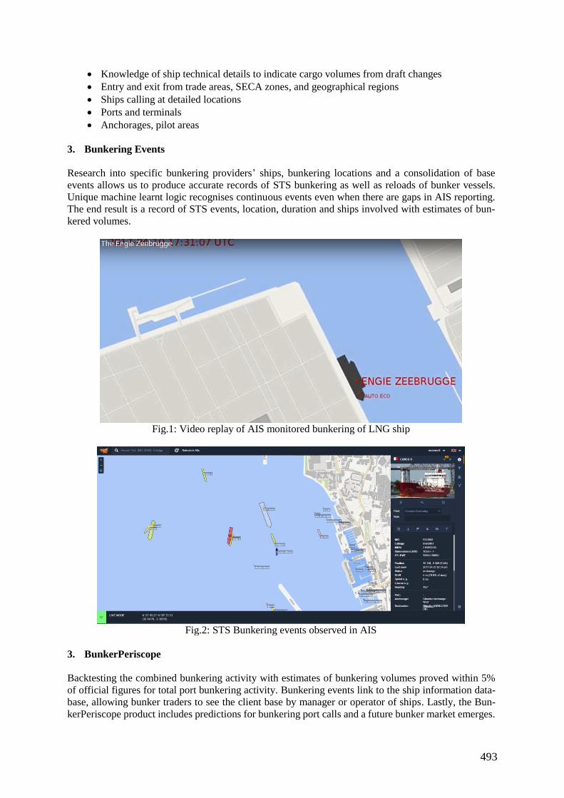
493
Knowledge of ship technical details to indicate cargo volumes from draft changes
Entry and exit from trade areas, SECA zones, and geographical regions
Ships calling at detailed locations
Ports and terminals
Anchorages, pilot areas
3. Bunkering Events
Research into specific bunkering providers’ ships, bunkering locations and a consolidation of base
events allows us to produce accurate records of STS bunkering as well as reloads of bunker vessels.
Unique machine learnt logic recognises continuous events even when there are gaps in AIS reporting.
The end result is a record of STS events, location, duration and ships involved with estimates of bun-
kered volumes.
Fig.1: Video replay of AIS monitored bunkering of LNG ship
Fig.2: STS Bunkering events observed in AIS
3. BunkerPeriscope
Backtesting the combined bunkering activity with estimates of bunkering volumes proved within 5%
of official figures for total port bunkering activity. Bunkering events link to the ship information data-
base, allowing bunker traders to see the client base by manager or operator of ships. Lastly, the Bun-
kerPeriscope product includes predictions for bunkering port calls and a future bunker market emerges.
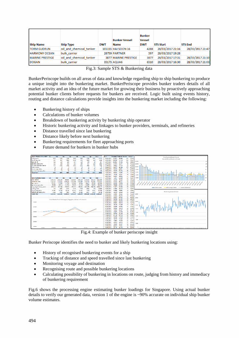
494
Fig.3: Sample STS & Bunkering data
BunkerPeriscope builds on all areas of data and knowledge regarding ship to ship bunkering to produce
a unique insight into the bunkering market. BunkerPeriscope provides bunker traders details of all
market activity and an idea of the future market for growing their business by proactively approaching
potential bunker clients before requests for bunkers are received. Logic built using events history,
routing and distance calculations provide insights into the bunkering market including the following:
Bunkering history of ships
Calculations of bunker volumes
Breakdown of bunkering activity by bunkering ship operator
Historic bunkering activity and linkages to bunker providers, terminals, and refineries
Distance travelled since last bunkering
Distance likely before next bunkering
Bunkering requirements for fleet approaching ports
Future demand for bunkers in bunker hubs
Fig.4: Example of bunker periscope insight
Bunker Periscope identifies the need to bunker and likely bunkering locations using:
History of recognised bunkering events for a ship
Tracking of distance and speed travelled since last bunkering
Monitoring voyage and destination
Recognising route and possible bunkering locations
Calculating possibility of bunkering in locations on route, judging from history and immediacy
of bunkering requirement
Fig.6 shows the processing engine estimating bunker loadings for Singapore. Using actual bunker
details to verify our generated data, version 1 of the engine is ~90% accurate on individual ship bunker
volume estimates.
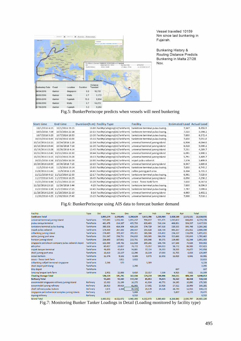
495
Fig.5: BunkerPeriscope predicts when vessels will need bunkering
Fig.6: BunkerPeriscope using AIS data to forecast bunker demand
Fig.7: Monitoring Bunker Tanker Loadings in Detail (Loading monitored by facility type)
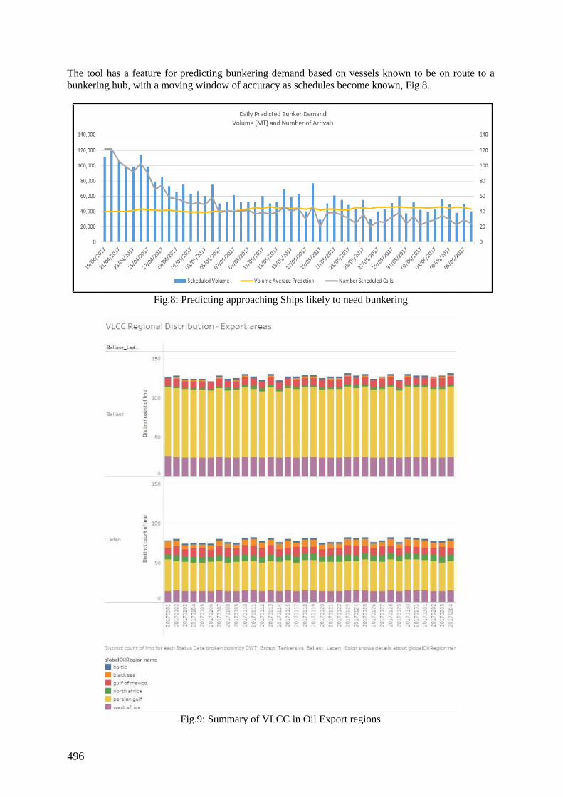
496
The tool has a feature for predicting bunkering demand based on vessels known to be on route to a
bunkering hub, with a moving window of accuracy as schedules become known, Fig.8.
Fig.8: Predicting approaching Ships likely to need bunkering
Fig.9: Summary of VLCC in Oil Export regions

497
4. Ship Status Events
The events engine builds up a detailed minute by minute history of all information and can provide a
current status covering all areas of ship activity at any specified time. This can be used to query current
status across multiple types of data not previously viewed together and also to take an aggregation of
this information across global or specific market regions and produce analysis of fleet activity, distri-
bution and deployment trends, Fig.9.
5. Summary
This approach to building business intelligence and market insight using all sets of available maritime
information for tracking, ships, companies, and facilities is proving highly valuable to the bunkering
sector.
All event engine based data sets are available through API services for integration to corporate
information systems.
Genscape believes that equal value can be created for other sectors of the maritime world, varying from
service providers such as tug companies, fleet operators, and bunker buyers.
Genscape also sees opportunities for port and national authorities to monitor maritime activity at a
detailed level, both for planning purposes and compliance checks.

498
Index by Authors
Abdelaal 180
Alwan 336
Amaya 83
Andrews 69,362
Assis 270,280
Baldauf 31
Barton 377
Benedict 31
Bertram 7
Bhuiyan 454
Bibuli 101
Borst 298
Bradbeer 362
Brett 253
Brink 313
Brinkmann 55
Broek-De Bruin 139
Bruzzone 101
Cabos 444
Caccia 101
Caharija 454
Caprace 270,280
Cardoen 351
Cepeda 280
Chatzimoisiadis 190
Chiarella 101
Cieraad 139
Coenen 323
Coppini 170
Costa 270
Cura 419
Daltry 413
Deeb 180
Deverill 492
Droste 201
Drougkas 190
Duchateau 139
Ebrahimi 253
Esbati 362
Etienne 484
Feiner 444
Ferretti 101
Fischer 31
Forsman 115
Garcia 253
Gaspar 155,253,428
Gluch 31
Grümmer 419
Hagaseth 238
Hahn 55,180
Harries 419
Hatton 48
Heimo 115
Helle 115
Hirdaris 454
Hjollo 55
Huijgens 323
Hu 454
Hunter 465
Jaspers 474
Jeinsch 401
Jeong 291
Kana 201,474
Keane 253
Kim 291
Kirchhoff 31
Korbetis 190
Korhonen 115
Kouriampalis 362
Kurowski 401
Larkins 128
Lecci 170
Lehtonen 115
Lee 291
Levišauskaitė 155
Lierde 351
Mannarini 170
Marques de Oliviera 280
Mediavilla 454
Michala 212
Mills 454
Morais 128
Moser 238
Motson 454
Müller 31,394
Mulay 313
Mulder 298
Munoz 226
Naeem 454
Odetti 101
Orihara 83
Paasen 298
Patterson 377
Pawling 362
Pedersen 336
Perez 226
Plowman 7
Proceee 298
Radosavljevic 351
Rahav 97
Rajabally 454
Ranieri 101
Renton 454
Roth 201
Sakari 115
Säntti 115
Schaub 31
Schubert 401
Scialla 454
Sharma 48
Singh 48
Smith 454
Steen 336
Sutton 48
Taskinen 115
Tripp 413
Turrisi 170
Uchoa Simões 270,280
Vaz 270,280
Verhelst 323
Vourganas 212
Waldie 128
Wolf 444
Woo 291
Yoshida 83
Yum 336
Zandstra 139
Zereik 101

17th Conference on
Computer Applications and Information Technology in the Maritime Industries
COMPIT'18 Pavone / Italy, 14-16 May 2018
Topics: Artificial Intelligence / Autonomous Technology / CAX Techniques / PLM / Robotics / Simulations / Smart Yards & Ships / Virtual & Augmented Reality / Web Technology / Big Data
In Design, Production and Operation of Maritime Systems
Organiser: Volker Bertram ([email protected])
Advisory Committee:
Volker Bertram Marcus Bole Andrea Caiti Jean-David Caprace Nick Danese
Tutech, Germany AVEVA, UK Univ Pisa, Italy COPPE, Brazil NDAR, France
Stein Ove Erikstad Augusto Gomez Stefan Harries Darren Larkins
NTNU, Norway SENER, Spain Friendship Systems, Germany SSI, Canada
Samuel Saltiel Ulf Siwe Julie Stark Giampiero Soncini Bastiaan Veelo
BETA CAE Systems, Greece Swed. Mar. Adm., Sweden US Navy, USA SpecTec, Cyprus SARC, Netherlands
Venue: The conference will be held at the Castello di Pavone in Pavone (near Turin/Italy)
Format: Papers to the above topics are invited and will be selected by a committee.
Deadlines: anytime Optional “early warning” of intent to submit paper 19.12.2017 First round of abstract selection (1/3 of available slots) 20.1.2018 Final round of abstract selection (remaining 2/3 of slots) 25.3.2018 Payment due for authors 25.3.2018 Final papers due (50 € surcharge for late submission)
Fees: 600 € / 300 € regular / PhD student – early registration (by 25.3.2017) 700 € / 350 € regular / PhD student – late registration Fees are subject to VAT (reverse charge mechanism in Europe) Fees include proceedings, lunches, coffee breaks and conference dinner
Sponsors: Aveva, DNV GL, Sener, SSI (further sponsors to be announced)
Information: www.compit.info