competitive online approximation of the optimal search ratio

Copyright © by SIAM. Unauthorized reproduction of this article is prohibited.

SIAM J. COMPUT. c© 2008 Society for Industrial and Applied MathematicsVol. 38, No. 3, pp. 881–898

COMPETITIVE ONLINE APPROXIMATION OF THE OPTIMALSEARCH RATIO∗

RUDOLF FLEISCHER† , TOM KAMPHANS‡ , ROLF KLEIN§ , ELMAR LANGETEPE§ ,

AND GERHARD TRIPPEN¶

Abstract. How efficiently can we search an unknown environment for a goal in an unknownposition? How much would it help if the environment were known? We answer these questions forsimple polygons and for undirected graphs by providing online search strategies that are as good asthe best offline search algorithms, up to a constant factor. For other settings we prove that no suchonline algorithms exist. We introduce a natural measure which gives reasonable results and is morerealistic than pure pessimistic competitive analysis.

Key words. online motion planning, competitive ratio, searching, exploration, natural measure

AMS subject classifications. 68Q17, 68Q25, 68W40

DOI. 10.1137/060662204

1. Introduction. One of the recurring tasks in life is to search one’s environmentfor an object whose location is—at least temporarily—unknown. This problem comesin different variations. The searcher may have vision, or be limited to sensing bytouch. The environment may be a simple polygon, for example, an apartment, or agraph, like a street network. Finally, the environment may be known to the searcheror be unknown.

Such search problems have attracted a lot of interest in online motion planning;see, for example, the survey by Berman [5]. Usually the cost of a search is measuredby the length of the search path traversed; this, in turn, is compared against thelength of the shortest path from the start position to the point where the goal isreached. The maximum quotient of these values, taken over all environments and allgoal positions within an environment, is the competitive ratio of the search algorithm.

Most prominent is the problem of searching two half-lines emanating from a com-mon start point. The “doubling” strategy visits the half-lines alternatingly, each timedoubling the depth of exploration. This way, the goal point is reached after traversinga path at most 9 times as long as its distance from the start, and the competitiveratio of 9 is optimal for this problem; see Baeza-Yates, Culberson, and Rawlins [4]and Alpern and Gal [2]. This doubling approach frequently appears as a subroutine

∗Received by the editors June 7, 2006; accepted for publication (in revised form) February 8, 2008;published electronically June 6, 2008. A preliminary version of this paper appeared at ESA 2004 [15].The work described in this paper was partially supported by a grant from the National NaturalScience Fund China (grant 60573025), by a grant from the Research Grants Council of the HongKong Special Administrative Region, China (project HKUST6010/01E), and by a grant from theGermany/Hong Kong Joint Research Scheme sponsored by the Research Grants Council of HongKong and the German Academic Exchange Service (project G-HK024/02).

http://www.siam.org/journals/sicomp/38-3/66220.html†Shanghai Key Laboratory of Intelligent Information Processing, Department of Computer Science

and Engineering, Fudan University, Shanghai 200433, China ([email protected]).‡Computer Science, Algorithms Group, Technical University of Braunschweig, 38106 Braun-

schweig, Germany ([email protected]).§Institute of Computer Science I, University of Bonn, D-53117 Bonn, Germany (rolf.klein@

uni-bonn.de, [email protected]).¶Sauder School of Business, The University of British Columbia, 2329 West Mall, Vancouver, BC

Canada ([email protected]).

881


882 FLEISCHER, KAMPHANS, KLEIN, LANGETEPE, AND TRIPPEN

in more complex navigation strategies.In searching m > 2 half-lines, a constant ratio with respect to the distance from

the start can no longer be achieved. Indeed, even if the half-lines were replaced bysegments of the same finite length, the goal could be placed at the end of the segmentvisited last, causing the ratio to be at least 2m − 1. Exponentially increasing theexploration depth by m/m− 1 is known [4, 2] to lead to an optimal competitive ratioof

C(m) = 1 + 2m

(m

m− 1

)m−1

≤ 1 + 2me.

Much less is known about more realistic settings. Suppose a searcher with visionwants to search an unknown simple polygon for a goal in unknown position. Hecould employ the m-way technique from above: By exploring the shortest paths fromthe start to the m reflex vertices of the polygon—ignoring their tree structure—acompetitive ratio of C(m) can easily be achieved [23]. Schuierer [27] has refined thismethod and obtained a ratio of C(2k), where k denotes the smallest number of convexand concave chains into which the polygon’s boundary can be decomposed.

But these results do not completely settle the problem. For one, it is not clearwhy the numbers m or k should measure the difficulty of searching a polygon. Also,human searchers can often outperform m-way search, because they make educatedguesses about the shape of those parts of the polygon not yet visited.

In this paper we take the following approach: Let π be a search path for a fixedpolygon P , i.e., a path from the start point, s, through P from which each point pinside P will eventually be visible. Let pπ be the first point on π where this happensfor a point p. The cost of getting to p via π is equal to the length of π from s to pπ,plus the Euclidean distance from pπ to p. We divide this value by the length of theshortest s-to-p path in P . The supremum of these ratios, over all p ∈ P , is the searchratio of π. The lowest search ratio possible, over all search paths, is the optimumsearch ratio of P ; it measures the “searchability” of P .

Apparently, this definition was first given by Koutsoupias, Papadimitriou, andYannakakis [24]. They studied graphs with unit length edges where the goal can belocated only at vertices, and they studied only the offline case where the graph is com-pletely known a priori. They showed that computing the optimal search ratio offlineis an NP-complete problem, and gave a polynomial time 8-approximation algorithmbased on the doubling heuristic.

The crucial question we are considering in this paper is the following: Is it possibleto design an online search strategy whose search ratio stays within a constant factorof the optimum search ratio for arbitrary instances of the environment? Surprisingly,the answer is positive for simple polygons as well as for undirected graphs. (However,for polygons with holes, and for graphs with unit edge length, where the goal positionsare restricted to the vertices, no such online strategy exists.)

Observe that this way of measuring performance is one step beyond competitiv-ity. Although the definitions of the search ratio and the competitive factor are quitesimilar, the concepts are different. In the competitive framework, we simply comparethe online path from the start to the goal to the shortest s-to-t path. For an approx-imation of the optimal search ratio, we compare the online path to the best possibleoffline path, which, in turn, may already have a bad competitive ratio.

To exemplify the given concept let us consider another simple environment: arbi-trary trees with a common root as a starting point. For a fixed tree, T , there will be


APPROXIMATION OF THE OPTIMAL SEARCH RATIO 883

a strategy S(T ) which attains the best competitive search performance C(T ) amongall possible goals on T . We know that an optimal strategy S(T ) exists, but we donot know what it looks like. Furthermore, for arbitrary trees it can be shown thatthe performance C(T ) of S(T ) can increase arbitrarily, though S(T ) is not known.Therefore, constant competitive searching is impossible for arbitrary trees T . But wecan try to approximate the strategy S(T ) for any tree T by a simple strategy A(T ).In this paper we will show that we can design an approximation strategy A(T ) sothat A(T ) is only a constant time worse than S(T ). This means that the competitiveratio of A(T ) is smaller than c · C(T ) for every T and a fixed constant c. Note thatc = 4 will be shown for this example in section 4.2.1. Thus, although the best searchstrategy is not known, we can approximate it efficiently. If the environment is known(but the goal is still unknown), sometimes the factor c can be slightly improved.

The idea of considering realistic ratios rather than pure pessimistic competitive ra-tios was also examined in the field of scheduling; see, for example, Edmonds et al. [13],Kalyanasundaram and Pruhs [22], or Berman and Coulston [6]. To compete with theoptimal offline algorithm in a constant competitive sense, the online scheduler is al-lowed to have more power in speed or number of processors (or whatever). Theincrease of power is mainly represented by a parameter which, in turn, influences thecompetitive ratio. In our framework we increase the power of the agent only in theoffline setting where the environment is known but the goal still has to be found. Inthe online setting we do not change the power balance between agent and adversaryat all.

The search strategies we will present use, as building blocks, modified versions ofconstant-competitive strategies for online exploration, namely, the exploration strat-egy by Hoffmann et al. [21] for simple polygons and the tethered graph explorationstrategy by Duncan, Kobourov, and Kumar [12].

At first glance it seems quite natural to employ an exploration strategy in search-ing—after all, either task involves looking at each point of the environment. Butthere is a serious difference in performance evaluation! In searching an environment,we compete against shortest start-to-goal paths, so we have to proceed in a breadthfirst search (BFS) manner.1 In exploration, we are up against the shortest round tripfrom which each point is visible; this means that once we have entered some remotepart of the environment we should finish it, in a depth first search (DFS) manner,before moving on.2 However, we can fit these exploration strategies to our searchproblem by restricting them to a bounded part of the environment. This will be shownin section 3, where we present our general framework, which turns out to be quiteelegant despite the complex definitions. The framework can be applied to both onlineand offline search ratio approximations. In section 2 we review basic definitions andnotation. Our framework will then be applied to searching in various environmentslike trees, (planar) graphs, and (rectilinear) polygonal environments with and withoutholes in sections 4 and 5. In section 6 we give a construction scheme for lower boundson the search ratio. Finally, in section 7, we conclude with a summary of our results.

2. Definitions. We want to find a good search path in some given environmentE . This may be a tree, a (planar) graph, or a (rectangular) polygon with or without

1But, as opposed to searching a data structure, we do not have pointers that allow us to jumpto a different location for free.

2Observe, however, that neither plain BFS nor DFS would work! BFS is lacking the doublingelement, and DFS, in a simple polygon, would tend to follow a long convex chain even though asmall step to the side could be sufficient to see its endpoint.



π

s

pπ

p

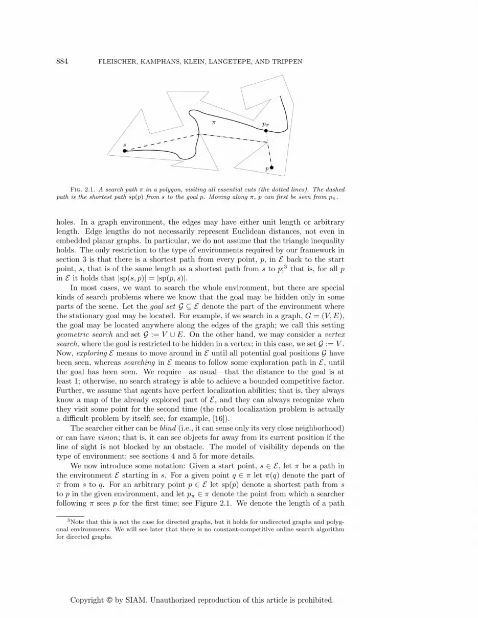
Fig. 2.1. A search path π in a polygon, visiting all essential cuts (the dotted lines). The dashedpath is the shortest path sp(p) from s to the goal p. Moving along π, p can first be seen from pπ.

holes. In a graph environment, the edges may have either unit length or arbitrarylength. Edge lengths do not necessarily represent Euclidean distances, not even inembedded planar graphs. In particular, we do not assume that the triangle inequalityholds. The only restriction to the type of environments required by our framework insection 3 is that there is a shortest path from every point, p, in E back to the startpoint, s, that is of the same length as a shortest path from s to p;3 that is, for all pin E it holds that |sp(s, p)| = |sp(p, s)|.

In most cases, we want to search the whole environment, but there are specialkinds of search problems where we know that the goal may be hidden only in someparts of the scene. Let the goal set G ⊆ E denote the part of the environment wherethe stationary goal may be located. For example, if we search in a graph, G = (V,E),the goal may be located anywhere along the edges of the graph; we call this settinggeometric search and set G := V ∪ E. On the other hand, we may consider a vertexsearch, where the goal is restricted to be hidden in a vertex; in this case, we set G := V .Now, exploring E means to move around in E until all potential goal positions G havebeen seen, whereas searching in E means to follow some exploration path in E , untilthe goal has been seen. We require—as usual—that the distance to the goal is atleast 1; otherwise, no search strategy is able to achieve a bounded competitive factor.Further, we assume that agents have perfect localization abilities; that is, they alwaysknow a map of the already explored part of E , and they can always recognize whenthey visit some point for the second time (the robot localization problem is actuallya difficult problem by itself; see, for example, [16]).

The searcher either can be blind (i.e., it can sense only its very close neighborhood)or can have vision; that is, it can see objects far away from its current position if theline of sight is not blocked by an obstacle. The model of visibility depends on thetype of environment; see sections 4 and 5 for more details.

We now introduce some notation: Given a start point, s ∈ E , let π be a path inthe environment E starting in s. For a given point q ∈ π let π(q) denote the part ofπ from s to q. For an arbitrary point p ∈ E let sp(p) denote a shortest path from sto p in the given environment, and let pπ ∈ π denote the point from which a searcherfollowing π sees p for the first time; see Figure 2.1. We denote the length of a path

3Note that this is not the case for directed graphs, but it holds for undirected graphs and polyg-onal environments. We will see later that there is no constant-competitive online search algorithmfor directed graphs.



segment π(p) by |π(p)|. Paths computed by some algorithm A will be named A, too.In particular, we write |A| for the length of the tour computed by A. The mainconcept in our paper is the following.

Definition 2.1. Let E be an environment, G ⊆ E a goal set, and s ∈ E a pointin the environment. A search path, π, with start point s is a path which starts in sand allows a searcher following π to see every goal position in G from at least onepoint on π. The search ratio, sr(π), is defined as

sr(π) := supp∈G

|π(pπ)| + |pπp||sp(p)| .

In other words, we compare the path walked by a searcher to the shortest path andtake the worst ratio among all possible targets as the search ratio of our search path.

An optimal search path, πopt, is a search path with a minimum search ratioamong all possible paths in the environment. We denote the optimal search ratio bysropt; that is, sropt := sr(πopt). For blind agents, p = pπ holds for every p ∈ E;

therefore, the search ratio can be computed as sr(π) := supp∈G|π(p)||sp(p)| .

As the optimal search path seems hard to compute [24], we are interested in findinggood approximations of the optimal search path in offline and online scenarios. We saya search algorithm A is search-competitive with factor C—or C–search-competitivefor short—if there are constants C ≥ 1 and B ≥ 0, so that sr(πA) ≤ C ·sropt+B holdsfor every path πA computed by A. Note that πA is then a C · sr(πopt)-competitivesearch path in the usual competitive sense. We use the term C–search-competitivealso for the approximation factor of offline approximation algorithms. If there is noC–search-competitive algorithm for any constant C, we call this type of environmenthard-searchable.

In the following, we want to use existing exploration algorithms to approximatethe optimal search path. We assume that every exploration algorithm returns to thestart point when the whole environment is explored.

Definition 2.2. For a given environment E and d ≥ 1, let E(d) denote thepart of E within distance at most d from s, and OPT(d) the optimal exploration forE(d). Further, let Expl be an—online or offline—algorithm for the exploration ofenvironments of the given type. Expl is called depth-restrictable if for every d ≥ 1 itis possible to modify the algorithm Expl to an algorithm Expl(d) that explores E(d)(i.e., the algorithm sees at least all potential goal positions of distance at most d—andmaybe some more—before it returns to the start point), and there are constants β > 0and Cβ ≥ 1, so that

(2.1) |Expl(d)| ≤ Cβ · |OPT(β · d)|

holds for every environment of the given type (i.e., Expl(d) is Cβ-competitive withrespect to OPT(β · d)).

For example, the DFS traversal for trees is depth-restrictable with β = 1 andCβ = 1: In every step we know exactly the distance to the tree’s root. Thus, we candecide whether we can explore the children of the current node or cannot explore thetree more deeply, because we have reached depth d. Obviously, DFS is optimal alsofor depth-restricted exploration.

In the usual competitive framework, we would compare Expl(d) to the optimalalgorithm OPT(d) (i.e., β = 1). As we will see later, our more general definitionsometimes makes it easier to find depth-restrictable exploration algorithms. Usually,



we cannot just take an exploration algorithm Expl for E and restrict it to pointswithin distance at most d from s. This way, we might miss useful shortcuts outsideof E(d). Even worse, it may not be possible to determine in an online setting whichparts of the environment belong to E(d), making it difficult to explore the right partof E . In sections 4 and 5 we will derive depth-restricted exploration algorithms forgraphs and polygons by carefully adapting existing exploration algorithms for theentire environment.

3. A general approximation framework. In this section, we show how totransform a depth-restrictable exploration algorithm, offline or online, into a searchalgorithm, without losing too much on the approximation factor.

Let E be the given environment and πopt an optimal search path. Rememberthat we assume that, for any point p, we can reach s from p on a path of length atmost sp(p).

Let Expl be an exploration algorithm for E , and for d ≥ 1, let Expl(d) be thecorresponding depth-restricted exploration algorithm for E(d). Let OPT and OPT(d)denote the corresponding optimal offline depth-restricted exploration algorithms. Weassume that the exploration strategies will always return to the start.

To obtain a search algorithm for E , we use the well-known doubling paradigm andsuccessively apply our given exploration strategy with increasing exploration depth;that is, we successively run Expl(2i), each iteration starting and ending in the startpoint, s.

Theorem 3.1. The doubling strategy based on a depth-restrictable explorationalgorithm with factors Cβ and β is a 4βCβ–search-competitive search algorithm forblind agents and an 8βCβ–search-competitive search algorithm for agents with vision.

Proof. Consider one iteration of the doubling strategy with search radius d ≥ 1.The optimal search path πopt for E must in particular explore all possible goal po-sitions within distance at most d from s. Let lastd be the point on πopt from whichwe see the last point within distance at most d from s when moving along πopt.Returning from lastd to s closes an exploration tour of E(d); therefore,

|OPT(d)| ≤ |πopt(lastd)| + |sp(lastd)| .In contrast to blind searchers, lastd may be located outside E(d) for agents with

vision; thus, we distinguish between blind agents and agents with vision to bound|sp(lastd)|. A blind agent can detect lastd only by visiting it, so we have sp(lastd) ≤ d.Thus,

(3.1) sropt ≥|πopt(lastd)|

d≥ |OPT(d)| − d

d⇐⇒ |OPT(d)| ≤ d · (sropt + 1) .

The worst case for the search ratio of the doubling strategy occurs when weexplore the environment up to some distance 2j+1 while the goal is within distance2j +ε for some small ε > 0. Thus, the search ratio of the doubling strategy is boundedby

sr(π) ≤∑j+1

i=1 |Expl(2i)|2j + ε

.

Expl is depth-restrictable with factor Cβ , so we can apply (2.1):

sr(π) ≤ Cβ

2j·j+1∑i=1

|OPT(β · 2i)| .



Finally, with (3.1) we get

sr(π) ≤ Cβ

2j·j+1∑i=1

β · 2i · (sropt + 1)

≤ βCβ ·(

2j+2 − 2

2j

)· (sropt + 1)

≤ 4β Cβ · (sropt + 1) .

If the agent has vision, it may see the last point within distance at most d fromsomewhere else, so we cannot guarantee sp(lastd) ≤ d. We know only |sp(lastd)| ≤|πopt(lastd)| (i.e., the return path to s cannot be longer than the path the agenttraveled along πopt). Thus,

sropt ≥|πopt(lastd)|

d≥ |OPT(d)|

2d⇐⇒ |OPT(d)| ≤ 2d · sropt .

Further, we detect the goal by applying the exploration strategy with depth 2j+1

and return to the start; then we still have to move to the goal. Similar to the case ofblind agents, we obtain for the search ratio an upper bound of

2j +∑j+1

i=1 |Expl(2i)|2j

≤ 1 + Cβ ·∑j+1

i=1 |OPT(β2i)|2j

≤ 1 + 2Cβ ·∑j+1

i=1 β2i sropt

2j

≤ 1 + 8βCβ · sropt .

In the next two sections we will apply our framework to various types of en-vironments and agents. The difficult part is always to find good depth-restrictableexploration algorithms.

4. Searching graphs. We distinguish between graphs with unit length andarbitrary length edges, planar and nonplanar graphs, directed and undirected graphs,as well as vertex and geometric search. We consider only blind agents: Located at avertex of a (directed) graph, the agent senses only the number of outgoing edges, butneither their lengths nor the positions of the other vertices are known. Incoming edgescannot be sensed; see Deng and Papadimitriou [10]. Blind agents must eventually visitall points in the goal set. In the vertex search problem, we assume w.l.o.g. that graphsdo not have parallel edges. Otherwise, there can be no constant–search-competitivevertex search algorithm: In Figure 4.1(i), the optimal search path s → v → t → s haslength 3, whereas any online search path can be forced to cycle often between s andv before traversing the edge v → t. Note that we can also use undirected edges.

4.1. Hard-searchable graphs. First, we show that for many graph classesthere is no constant–search-competitive online search algorithm. Incidentally, thereis also no constant-competitive online exploration algorithm for these graph classes.Note that we have the following implications for hard-searchable graphs:

• If planar graphs are hard-searchable, then so are nonplanar graphs.• If graphs with unit length edges are hard-searchable, then so are graphs with

arbitrary length edges.• If undirected graphs are hard-searchable, then so are directed graphs (we can

replace each undirected edge with directed edges in both directions).Theorem 4.1. For blind agents, there is no constant–search-competitive online

algorithm in the following settings:



(ii)

tv

s

(i)

Fig. 4.1. There is no constant–search-competitive vertex search algorithm for (i) graphs withparallel edges, (ii) vertex search in nonplanar graphs.

s v

(i)

1 1

1 1w

s t

(ii)

ε

εε

...

Fig. 4.2. There is no constant–search-competitive vertex search algorithm for (i) vertex searchand geometric search in directed graphs (the nodes ◦ occur only in the case of unit-length edges),(ii) vertex search in planar graphs with arbitrary edge length (the arrows denote the points on theedges where the searcher decides to return to s).

1. Vertex search in nonplanar graphs.2. Vertex search and geometric search in directed planar graphs.3. Vertex search in planar graphs with arbitrary edge lengths.

Proof.

1. Consider the graph in Figure 4.1(ii) with unit length edges. It is a k-clique,where each vertex has a sibling that has only one connection to the clique.The optimal search ratio is Θ(k): We successively visit every clique vertexand explore its sibling before proceeding to the next clique vertex. This yieldsa path of length 3k. On the other hand, any online search algorithm can beforced to travel Ω(k2) before reaching the last vertex, so it has search ratioΩ(k2). Thus, it is not better than k-competitive.Note that in a k-clique without siblings a BFS traversal achieves the optimalsearch ratio.

2. For vertex search, consider the planar graph in Figure 4.2(i) with a very longedge from s to w. The optimal search path, s → v → w, has search ratio 1.However, any online algorithm can be forced to first explore the long edgefrom s to w, resulting in a very high search ratio.If we are restricted to unit length edges, we can add more vertices along thelong edge (marked with ◦ in Figure 4.2(i)). Then the optimal search pathexplores this long path after exploring the short cycle s → w → s. Becausein the worst case the goal is hidden on the first vertex of the long path, thispath achieves a search ratio of 5.For a geometric search, with unit length edges or arbitrary edges, we can usethe same planar graph. Again, we force the online algorithm to explore thelong edge at first. In contrast, the optimal strategy visits the cycle s → w → sbefore exploring the long edge. The optimal strategy achieves its worst case



if the goal is hidden within distance 1 on the long edge.3. For any given online search algorithm, we construct a planar graph as in

Figure 4.2(ii) with k outgoing edges at the start vertex, s. An online algorithmvisits one of the k edges at first. If the algorithm does not return to s whileexploring this edge, the currently visited edge is the only long edge in thegraph and all other edges are very short. The optimal strategy visits onlyshort edges; thus, this algorithm can be arbitrarily bad.Hence, to achieve a good approximation factor, an online algorithm must atsome point decide to stop exploring the first edge and to return to s (thesmall arrows in the figure indicate this point). We place the endpoint of thecurrently visited edge immediately behind the last visited point and continuesimilarly with the next k − 2 edges. The last edge ends in vertex t, and itslength is the minimum length among the first k − 1 edges. Then we connectthe endpoints of the first k−1 edges to t by an edge of length ε, where ε > 0 issome very small number. The optimal search path in this graph first travelsthe last edge and then visits every other vertex quickly from t. Thus, itssearch ratio is close to 1. On the other hand, the online algorithm has searchratio at least k. Note that we introduced all the edge endpoints (instead ofhaving the edges ending in t) because we assumed that there are no paralleledges.

Note that there is an O(D8)-competitive exploration for directed graphs by Fleis-cher and Trippen [17]. D denotes the deficiency of the given graph, that is, theminimum number of edges that must be added to get an Euler graph. This exampleshows that there are settings where there is no constant–search-competitive onlinealgorithm, although there is an O(D8)–competitive exploration algorithm. The prob-lem is that this algorithm is not depth-restrictable. Besides, directed graphs do notfulfill |sp(s, p)| = |sp(p, s)| for all p in E , so we cannot apply our framework to directedgraphs, anyway.

4.2. Competitive search in graphs. In this subsection, we present search-competitive online and offline search algorithms for the remaining graph classes. Notethat we consider only undirected graphs.

4.2.1. Trees. On trees, DFS is a 1-competitive online exploration algorithmfor vertex and geometric search that is depth-restrictable; it is still 1-competitivewhen restricted to search depth d for any d ≥ 1. Thus, the doubling strategy givesa polynomial time 4–search-competitive search algorithm for trees—offline as wellas online. On the other hand, it is an open problem whether the computation ofan optimal vertex or geometric search path in trees with unit length edges is NP-complete [24].

4.2.2. Vertex search in graphs with unit length edges. Now, we givecompetitive search algorithms for vertex search in planar graphs with unit length edgesand—in the next section—for geometric search in undirected graphs with arbitrarylength edges. Both algorithms are based on an online algorithm for tethered graphexploration.

In the tethered exploration problem the agent is fixed to the start point by arope of restricted length. An optimal solution to this problem was given by Duncan,Kobourov, and Kumar [12]. Their algorithm, closest first exploration (CFX), exploresan unknown graph with unit length edges in 2|E|+ (4 + 16

α )|V | edge traversals, usinga rope length of (1 +α)d, where d is the distance of the point farthest away from the



start point and α > 0 is some parameter. Note that CFX explores the whole graphin spite of the tethered restriction.

CFX explores the graph in a mixture of depth-bounded DFS on G, DFS onspanning trees of parts of G, and recursive calls to explore certain large subgraphs.The basic idea of CFX is to maintain a set, T , of edge-disjoint, partially4 exploredsubtrees—more precisely, spanning trees of incomplete graph parts—that fulfill certainconditions on minimum size and maximal depth. Initially, T consists of one treecontaining only the start node, s. The strategy successively selects the subtree nearestto s and walks to its root. Then, CFX traverses the subtree using DFS. For eachencountered, incompletely explored vertex, CFX starts a depth-bounded DFS. In thisprocess, new vertices are discovered and new subtrees are added to T , possibly splitinto several smaller subtrees if they do not fulfill the conditions.

The costs for applying CFX sum up from relocation from s to the roots of thesubtrees and back to s, the DFS traversals, and the costs for the depth-bounded DFSstarting in unexplored vertices. The latter traverses only unexplored edges; thus, wehave costs 2|E| for this part. For a subtree, T , with |T | vertices, we have costs 2|T |for the DFS traversal. The size restrictions for the subtrees ensure that we can boundthe relocation costs by 8

α |T |. As the subtrees may overlap, we can bound the sum ofall vertices in the subtrees by 2|V |. Altogether, we get

2|E| +(

2 +8

α

)∑T

|T | ≤ 2|E| +(

2 +8

α

)· 2|V | = 2|E| +

(4 +

16

α

)|V | .

As Duncan, Kobourov, and Kumar pointed out, the algorithm can be used evenif the necessary rope length, d, is not known: They explore the whole graph bysuccessively applying CFX and doubling d in every step. The important part is thatthe analysis still holds in this case. Particularly, we can apply CFX for a depth-restricted exploration (i.e., explore only a subgraph of G). For d ≥ 1, let G(d) denotethe subgraph5 of G = (V,E) where all points p ∈ V ∪E have distance at most (1+α)dfrom s. For convenience, let G∗ = (V ∗, E∗) := G((1 + α)d). To explore all vertices inG(d)—and maybe some additional vertices from G((1 + α)d)—using a rope of length(1 + α)d, the number of edge traversals is bounded by

2|E∗| +(

4 +16

α

)|V ∗| .

Let us call this algorithm CFX(d). We have the following lemma.Lemma 4.2. In planar graphs with unit length edges, CFX is a depth-restrictable

algorithm for online vertex exploration with β = 1 + α and Cβ = 10 + 16α .

Proof. As G∗ is planar, we have |E∗| ≤ 3|V ∗| − 6 by Euler’s formula. Thus, thenumber of edge traversals of CFX(d) is at most

2 |E∗| +(

4 +16

α

)|V ∗| ≤ 6 |V ∗| +

(4 +

16

α

)|V ∗| =

(10 +

16

α

)|V ∗| .

On the other hand, we have OPT((1 + α)d) ≤ |V ∗|, because the optimal algorithmmust visit each vertex in V ∗ at least once.

4That is, there are vertices that are already discovered but still have unvisited incident edges.5In the case of unit-length edges, we omit all edges with length < 1 in the subgraph G(d). Such

edges occur if d is not an integer value.



Now, we can apply our framework with CFX.Theorem 4.3. The doubling strategy based on CFX(d) is a 206–search-competitive

online vertex search algorithm for blind agents in planar graphs with unit length edges.Proof. By Lemma 4.2, CFX(d) is depth-restrictable with β = 1 + α and Cβ =

10 + 16α . By Theorem 3.1, the doubling strategy based on CFX is 4βCβ-competitive.

Altogether, we have

4 · β · Cβ = 4 · (1 + α) ·(

10 +16

α

)= 104 + 40α +

64

α.

By simple analysis, we get the minimal competitive ratio of 205.192 . . . attained for

α =√

85 .

4.2.3. Geometric search in graphs with arbitrary length edges. We notethat CFX(d) can be modified to work on graphs with arbitrary length edges: Insteadof counting the number of edge traversals, the algorithm has to track the length of thetraversed edges. Now, it may happen that the maximal rope length is reached on anedge somewhere between two vertices. In this case, we interrupt the edge traversal,add an auxiliary vertex, and split the edge into two parts. Note that the added vertexis incompletely explored, so CFX will return to this vertex in a successive stage. Let�(E) denote the total length of all edges in E. It is possible to adapt the proofs byDuncan, Kobourov, and Kumar [12] to prove the following lemma.

Lemma 4.4. In graphs with arbitrary length edges, CFX (d) explores all edges andvertices in G(d) using a rope of length (1 + α)d at a cost of at most (4 + 8

α ) · �(E∗).Proof (sketch). The proof is similar to the unit-length case, but we can no longer

use the number of visited vertices to bound the number of traversed edges. Instead,we bound the costs for the depth-bounded DFS by 2 �(E∗). As the subtrees areedge disjoint, we can bound the costs for the DFS traversals by 2 �(E∗), too. Thesize restriction on the subtrees still ensures that the relocation costs are bound by8α �(E∗). Altogether, we get (4+ 8

α ) · �(E∗). Note that we have no additional costs forthe auxiliary vertices, because we count only edge lengths, and by inserting auxiliaryvertices we split one edge into two smaller edges whose total length is the same as theoriginal edge.

Lemma 4.5. In undirected graphs with arbitrary length edges, CFX is a depth-restrictable online geometric exploration algorithm with β = 1 + α and Cβ = 4 + 8

α .Proof. The total cost of CFX(d) is at most (4+ 8

α ) · �(E∗) by Lemma 4.4. On theother hand, OPT((1 + α)d) must traverse each edge in E∗ at least once.

Theorem 4.6. The doubling strategy based on CFX (d) is a 94–search-competitiveonline geometric search algorithm for blind agents in undirected graphs with arbitrarylength edges.

Proof. By Lemma 4.5, CFX(d) is depth-restrictable with β = 1+α and Cβ = 4+ 8α .

Thus, by Theorem 3.1 the doubling strategy is 4βCβ-competitive, and we have

4 · β · Cβ = 4 · (1 + α) ·(

4 +8

α

)= 48 + 16α +

32

α.

Simple analysis shows that this factor is minimal for α =√

2, yielding a factor of93.254 . . . .

4.2.4. Offline searching. In the offline setting, the searcher knows the graphbut still does not know the location of the target. Thus, we want to compute (orapproximate) an optimal search path in a known graph.



Computing an optimal search path in a known graph is NP-hard [24], but wecan use our framework to give an approximation. Given a graph G = (V,E) and anexploration depth d ≥ 1, we can compute the subgraph G(d). Now, we have to findan appropriate exploration strategy for G(d). In the case of a vertex search, exploringG(d) amounts to finding a traveling salesperson (TSP) tour on G(d). This problemis NP-hard, too, but we can approximate a TSP tour within factor Cβ = 2 using themimimum–spanning-tree heuristic,6 or we can use one of the 1+ ε approximations byGrigni, Koutsoupias, and Papadimitriou [18], Arora [3], or Mitchell [25].

The problem of finding a minimum-length tour that visits every edge of a givengraph at least once is known as the Chinese postman problem and can be solved inpolynomial time for graphs that are either directed or undirected [14, 26]. In thiscase, we have Cβ = β = 1. Altogether we have the following theorem.

Theorem 4.7. There is a 4–search-competitive strategy for offline geometricsearch and an 8–search-competitive strategy for offline vertex search.

5. Searching polygons.

5.1. Simple polygons. A simple polygon, P , is given by a closed, noninter-secting polygonal chain. Our searcher is equipped with ideal, unlimited vision; thatis, it is provided with the full visibility polygon with respect to the searcher’s currentposition.

To apply our framework, we need a depth-restrictable online exploration algo-rithm. The best known algorithm, PolyExplore, for the online exploration of a simplepolygon by Hoffmann et al. [21] achieves a competitive ratio of 26.5.

Let P (d) ⊆ P denote the part of the polygon P where all points have a distanceat most d from the start. We can modify PolyExplore to explore P (d): During theexploration, an unseen part of P always lies behind a cut cv emanating from a reflexvertex, v. These reflex vertices are called unexplored as long as we have not visitedthe corresponding cut cv. The algorithm maintains a list of unexplored reflex verticesand successively visits the corresponding cuts. While exploring a reflex vertex (alonga sequence of line segments and circular arcs), more unexplored reflex vertices maybe detected or unexplored reflex vertices may become explored. These vertices areinserted into or deleted from the list, respectively. In PolyExplore(d), unexploredreflex vertices within a distance greater than d from the start are simply ignored; thatis, although they may be detected they will not be inserted into the list. Let OPT(d)be the shortest path that sees all points in P (d).

Note that both PolyExplore(d) and OPT(d) may exceed P (d), as shown in Fig-ure 5.1. In (i) PolyExplore(d) successively explores the vertices vr and v�, but OPT(d)visits the cuts outside P (d). In (ii) PolyExplore(d) leaves P (d) in e4. However, we canenlarge P (d) to P ′(d) by a well-defined region so that the resulting polygon containsPolyExplore(d) as well as OPT(d); see Figure 5.1.

More precisely, let d′ be the maximal distance from PolyExplore(d) and OPT(d)to s; then we simply define P ′(d) := P (d′). Newly inserted reflex vertices in P ′(d)cannot influence the paths of OPT(d) and PolyExplore(d) in P ′(d). Thus, the analysisof PolyExplore by Hoffmann et al. still holds for OPT(d) and PolyExplore(d) in P ′(d),and we have the following lemma.

Lemma 5.1. In a simple polygon, PolyExplore is a depth-restrictable onlineexploration algorithm with β = 1 and Cβ = 26.5.

6Note that we cannot apply the Christofides heuristic [8], because the triangle-inequality is notfulfilled in arbitrary graphs.



(3)

(ii)(i)

(4) (2)

(1)vrv�

P (d)

s

s

P (d)

e1

e2

e4r2

OPT(d)P ′(d)

e3

PolyExplore(d)

P ′(d)

Fig. 5.1. (i) PolyExplore(d) explores the right reflex vertex vr along a circular arc (1), returnsto the start (2), and explores the left reflex vertex v� likewise (3)–(4). OPT(d) (dashed line) leavesP (d). (ii) PolyExplore(d) leaves P (d), whereas the shortest exploration path for P (d) lies inside P (d).In both cases, we can extend P (d) (dark gray) to P ′(d) (light gray) containing both PolyExplore(d)and OPT(d).

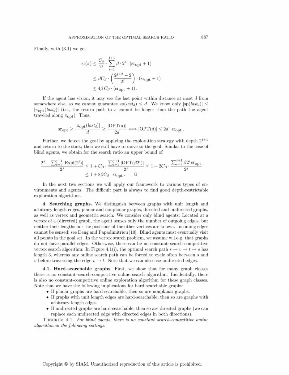
Theorem 5.2. The doubling strategy based on PolyExplore(d) is a 212–search-competitive online search algorithm for an agent with vision in a simple polygon.There is also a polynomial time 8–search-competitive offline search algorithm.

Proof. The online search-competitiveness follows from Lemma 5.1 and Theo-rem 3.1.

If we know the polygon, we can compute OPT(d) in polynomial time by adaptinga corresponding algorithm for P . Every known polynomial time offline explorationalgorithm visits the essential cuts in a certain sequence; see, for example, [7, 29, 28, 11].Any of these algorithms can be used in our framework. As an optimal algorithm hasapproximation factor C = 1, our framework yields an approximation of the optimalsearch path with a factor of 8.

The overall running time of the algorithm seems to depend on the distance to thefarthest reflex vertex of the polygon. However, we skip a step with distance 2i if thereis no reflex vertex within a distance between 2i−1 and 2i. Thus, we always explore atleast one new vertex in every iteration of the doubling strategy. Altogether, the totalrunning time is bounded by a polynomial in the number of the vertices of P .

Note that there is a considerable gap between the upper bound given by Hoffmannet al. [21] and the best known lower bound of 1.2825 [20]. The authors conjecturethat the actual performance of PolyExplore is below 10 [21]; the worst case known sofar is 5 [19]. Under this assumption, the search-competitivity of a doubling strategybased on PolyExplore can be expected to be below 80.

Now the question arises whether there is a polynomial time algorithm that com-putes the optimal search path in a simple polygon. We have to visit every essentialcut, so we can try to visit them in any possible order. Anyway, we do not knowexactly which point on the cut we should visit. We are not sure whether there areonly a few possibilities as in the shortest watchman route problem. In other words, itis unknown whether this subproblem is discrete at all. So the problem of computingan optimal search path in a polygon is still open.

Even for rectilinear simple polygons no polynomial time algorithm for the optimalsearch path is known, but we can find better online algorithms.

Theorem 5.3. For an agent with vision in a simple rectilinear polygon there is



OPT

2k

recursive subproblem

k

k

s′

s

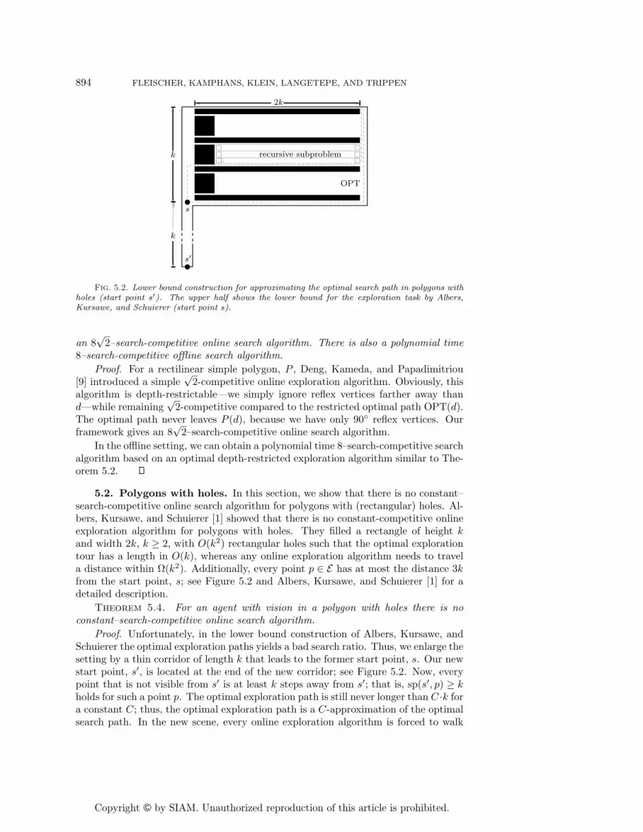
Fig. 5.2. Lower bound construction for approximating the optimal search path in polygons withholes (start point s′). The upper half shows the lower bound for the exploration task by Albers,Kursawe, and Schuierer (start point s).

an 8√

2–search-competitive online search algorithm. There is also a polynomial time8–search-competitive offline search algorithm.

Proof. For a rectilinear simple polygon, P , Deng, Kameda, and Papadimitriou[9] introduced a simple

√2-competitive online exploration algorithm. Obviously, this

algorithm is depth-restrictable—we simply ignore reflex vertices farther away thand—while remaining

√2-competitive compared to the restricted optimal path OPT(d).

The optimal path never leaves P (d), because we have only 90◦ reflex vertices. Ourframework gives an 8

√2–search-competitive online search algorithm.

In the offline setting, we can obtain a polynomial time 8–search-competitive searchalgorithm based on an optimal depth-restricted exploration algorithm similar to The-orem 5.2.

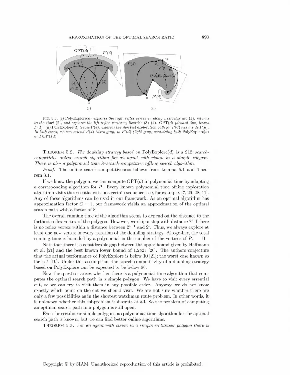
5.2. Polygons with holes. In this section, we show that there is no constant–search-competitive online search algorithm for polygons with (rectangular) holes. Al-bers, Kursawe, and Schuierer [1] showed that there is no constant-competitive onlineexploration algorithm for polygons with holes. They filled a rectangle of height kand width 2k, k ≥ 2, with O(k2) rectangular holes such that the optimal explorationtour has a length in O(k), whereas any online exploration algorithm needs to travela distance within Ω(k2). Additionally, every point p ∈ E has at most the distance 3kfrom the start point, s; see Figure 5.2 and Albers, Kursawe, and Schuierer [1] for adetailed description.

Theorem 5.4. For an agent with vision in a polygon with holes there is noconstant–search-competitive online search algorithm.

Proof. Unfortunately, in the lower bound construction of Albers, Kursawe, andSchuierer the optimal exploration paths yields a bad search ratio. Thus, we enlarge thesetting by a thin corridor of length k that leads to the former start point, s. Our newstart point, s′, is located at the end of the new corridor; see Figure 5.2. Now, everypoint that is not visible from s′ is at least k steps away from s′; that is, sp(s′, p) ≥ kholds for such a point p. The optimal exploration path is still never longer than C ·k fora constant C; thus, the optimal exploration path is a C-approximation of the optimalsearch path. In the new scene, every online exploration algorithm is forced to walk



a path of length in Ω(k2). Because every online approximation of the optimal searchpath is also an online exploration algorithm, there are points that are discovered afterwalking a path length in Ω(k2), although their distance to s′ is within O(k). Thus,no online approximation is able to achieve a constant approximation factor.

Since the offline exploration problem is NP-complete (by straightforward reduc-tion from planar TSP) we cannot use our framework to get a polynomial time approx-imation algorithm of the optimal search path. However, there is an exponential time8-approximation algorithm. We can list the essential cuts of OPT(d) in any order tofind the best one. Applying our framework gives an approximation factor of 8 for theoptimal search ratio.

The results of Koutsoupias, Papadimitriou, and Yannakakis [24] imply that theoffline problem of computing an optimal search path in a known polygon with holesis NP-complete.

6. A general lower bound. We have seen that for certain types of environ-ments there exists an approximation for the optimal search path if there exists adepth-restrictable, competitive exploration strategy. Further, we have seen that poly-gons with holes are hard-searchable. Now, we want to generalize the latter result; thatis, we want to show that—under a certain condition—there is no approximation upto a constant factor if there is no competitive exploration strategy for environmentsof the given type.

Usually, the nonexistence of competitive exploration strategies is shown by givinga lower bound—a scenario in which every exploration strategy is forced to walk apath whose length exceeds the length of the optimal exploration path by more than aconstant factor. To transfer such a result to search path approximations, we requirethat the scenario can be extended around the start point, such that the start pointmoves further away from the original scenario. We used this technique in section 5.2.One might think of an arbitrary large narrow corridor which is added to a givenenvironment.

Definition 6.1. Let E be an environment of arbitrary type and s be a startpoint in E. We call E s-extendable if we can enlarge E locally around the start point;that is, it is possible to choose a new start point, s′, outside E and enlarge E toE ′ such that s′ is contained in E ′ and every path from s′ to a point in E passes s.Additionally, we require that along any path from s′ to s all targets in the extensionwill be (successively) detected—but no target ouside the extension. And we can designE ′ so that the shortest path from s to s′ has arbitrary length.

Beyond this rather technical condition some additional properties of a lower boundconstruction should hold.

We consider environments E of a given type such that |sp(s, p)| = |sp(p, s)| holds.This was already one of our main requirements; see section 2. Let us now assumethat there is an optimal exploration strategy OPT for E but in general there is noconstant competitive online exploration strategy. We assume that this is shown by alower bound construction L(n), where n indicates the size of L(n). More precisely,we assume that any online exploration strategy A has path length |A(L(n))| ≥ C(n) ·|OPT(L(n))| in the environment L(n) and C(n) is unbounded in n.

Furthermore, the length of the shortest path to any goal in L(n) should bebounded by K · |OPT(L(n))|, where K is a constant. Obviously, the last conditionalways holds for blind agents.

Under the given conditions we can prove the following general result.Theorem 6.2. If there is no constant-competitive online exploration algorithm



for environments of a given type as indicated above, and the corresponding lowerbound is s-extendable and additionally fulfills the properties above, then there is nocompetitive online approximation of the optimal search path.

Proof. Any online approximation, A, of the optimal search path is also an onlineexploration strategy; therefore, we have |A(L(n))| ≥ C(n) · |OPT(L(n))|, and C(n)is unbounded in n. We extend L(n) by placing a new start point, s′, outside L(n)with distance |OPT(L(n))| and connecting it to the former start point s. Adding theshortest path from s to s′ to OPT(L(n)), this offline algorithm obviously has constantsearch ratio. The targets in the extension are detected optimally, and every target inL(n) has a shortest distance of at least |OPT(L(n))| from s′. For visiting a detectedgoal t in L(n) the extended version of OPT(L(n)) might first run to its end and backto the start and then runs along the shortest path to t. This always gives a constantratio.

On the other hand, for every online approximation, A, there are some goals twhich are detected after a path length greater than or equal to C(n) · |OPT(L(n))|,but the shortest path to the goal t is not longer than (K + 1) · |OPT(L(n))| for a

constant K. Thus, there is a search ratio of at least C(n)K+1 which is still unbounded

in n.

7. Conclusion and open problems. There are environments where no onlinesearch strategy can achieve a constant competitive factor. Therefore, we used thesearch ratio as a parameter of a given environment that gives a measure for theenvironment’s searchability. A search strategy is considered “good” if it achieves agood approximation of the optimal search ratio; that is, the search ratio of an onlinestrategy is at most a constant factor worse than the optimal search ratio.

We showed that we can use depth-restrictable exploration strategies—explorationstrategies that can be modified to explore the environment only up to a certain depthwhile they are still competitive—to approximate the optimal search path by succes-sively applying the exploration with exponentially increasing exploration depths. Forblind agents we showed that there are 4βCβ-approximations and for searchers withvision 8βCβ-approximations, where β and Cβ are parameters that depend on themodifications to turn an exploration algorithm into a depth-restricted exploration.We applied our results to various types of graphs and polygons; see Table 7.1.

Further, we showed that there is no constant–search-competitive strategy for poly-gons with holes. The main idea for this proof—enlarging the environment close tothe start point—can be generalized for environments that fulfill a certain conditionwe called s-extendable. We also showed that some graph settings—including directedgraphs—are hard-searchable.

Altogether, we showed a close relation between searching and exploring: Forenvironments fulfilling |sp(s, p)| = |sp(p, s)| for all p in E there is some equivalencebetween constant-competitive exploring and searching if the exploration strategy isdepth-restrictable and the lower bounds are s-extendable (among some other naturalproperties). Naturally, these results lead to the question of whether there is a strongerconnection. More precisely, can we omit at least the prerequisites “depth-restrictable”and “s-extendable” and show the following conjecture?

Conjecture 1. For a given type of environment that fulfills ∀p ∈ E : |sp(s, p)| =|sp(p, s)|, there is a constant–search-competitive strategy if and only if there exists aconstant-competitive online exploration for environments of this type.

Proving this conjecture would show a closer relation between exploration andsearching: We are able to approximate the optimal search path—in other words,



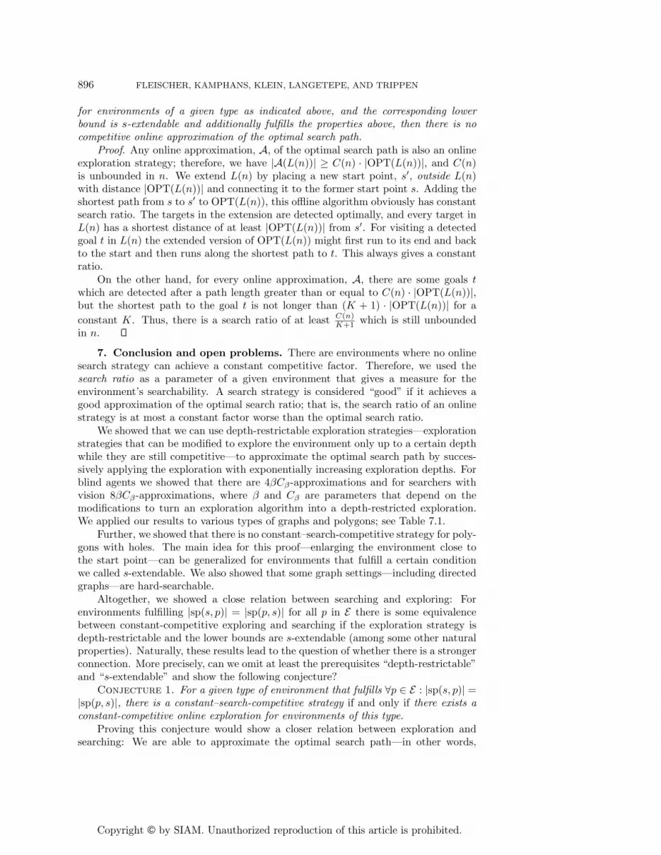
Table 7.1

Summary of our approximation results. The entry marked with * had earlier been proven byKoutsoupias, Papadimitriou, and Yannakakis [24]. They had also shown that computing the optimalsearch path is NP-complete for (planar) graphs. It is also NP-complete for polygons with holes,whereas it is not known to be NP-complete for trees and polygons without holes.

Polytime approximation ratioEnvironment Edge length Goal

Online Offline

Tree unit, arbitrary vertex, geometric 4 4

Planar graph arbitrary vertex no search-compet. alg. 8

Planar graph unit vertex 205.192 . . . 8

Undirected graph unit, arbitrary vertex no search-compet. alg. 8∗

Undirected graph arbitrary geometric 93.254 . . . 4

Simple polygon 212 8

Rect. simple polygon 8√

2 8

Polygon with holes no search-compet. alg. ?

we can find a good search strategy—if there is a constant-competitive explorationstrategy. And, vice versa, we have no chance of finding a good search strategy if noconstant-competitive exploration is possible. Note that the sp-condition is necessary,anyway, not only because our approximation framework relies on it, but also becauseit seems to be hard to find depth-restrictable exploration strategies for environmentswithout the sp-condition. For example, there is a competitive exploration strategy fordirected graphs (see Fleischer and Trippen [17]) which does not fulfill the sp-conditionand is not depth-restrictable.

Acknowledgment. We would like to thank the anonymous referees for helpfulcomments and suggestions for improvements.

REFERENCES

[1] S. Albers, K. Kursawe, and S. Schuierer, Exploring unknown environments with obstacles,in Proceedings of the 10th ACM-SIAM Symposium of Discrete Algorithms, ACM, NewYork, SIAM, Philadelphia, 1999, pp. 842–843.

[2] S. Alpern and S. Gal, The Theory of Search Games and Rendezvous, Kluwer AcademicPublishers, Boston, 2003.

[3] S. Arora, Polynomial time approximation schemes for Euclidean traveling salesman and othergeometric problems, J. ACM, 45 (1998), pp. 753–782.

[4] R. Baeza-Yates, J. Culberson, and G. Rawlins, Searching in the plane, Inform. and Com-put., 106 (1993), pp. 234–252.

[5] P. Berman, On-line searching and navigation, in Online Algorithms (Schloss Dagstuhl, 1996),A. Fiat and G. Woeginger, eds., Springer-Verlag, Berlin, 1998, pp. 232–241.

[6] P. Berman and C. Coulston, Speed is more powerful than clairvoyance, Nordic. J. Comput.,6 (1999), pp. 181–193.

[7] W.-P. Chin and S. Ntafos, Shortest watchman routes in simple polygons, Discrete Comput.Geom., 6 (1991), pp. 9–31.

[8] N. Christofides, Worst-case analysis of a new heuristic for the traveling salesman problem,in Proceedings of the Symposium on New Directions and Recent Results in Algorithmsand Complexity, J. F. Traub, ed., Academic Press, New York, 1976, p. 441.



[9] X. Deng, T. Kameda, and C. Papadimitriou, How to learn an unknown environment I: Therectilinear case, J. ACM, 45 (1998), pp. 215–245.

[10] X. Deng and C. H. Papadimitriou, Exploring an unknown graph, J. Graph Theory, 32 (1999),pp. 265–297.

[11] M. Dror, A. Efrat, A. Lubiw, and J. S. B. Mitchell, Touring a sequence of polygons, inProceedings of the 35th Annual ACM Symposium on Theory of Computing, ACM, NewYork, 2003, pp. 473–482.

[12] C. A. Duncan, S. G. Kobourov, and V. S. A. Kumar, Optimal constrained graph exploration,ACM Trans. Algorithms, 2 (2006), pp. 380–402.

[13] J. Edmonds, D. D. Chinn, T. Brecht, and X. Deng, Non-clairvoyant multiprocessor schedul-ing of jobs with changing execution characteristics, J. Scheduling, 6 (2003), pp. 231–250.

[14] J. Edmonds and E. L. Johnson, Matching, Euler tours and the Chinese postman, Math.Programming, 5 (1973), pp. 88–124.

[15] R. Fleischer, T. Kamphans, R. Klein, E. Langetepe, and G. Trippen, Competitive onlineapproximation of the optimal search ratio, in Proceedings of the 12th Annual EuropeanSymposium on Algorithms, Lecture Notes in Comput. Sci. 3221, Springer-Verlag, NewYork, 2004, pp. 335–346.

[16] R. Fleischer, K. Romanik, S. Schuierer, and G. Trippen, Optimal robot localization intrees, Inform. and Comput., 171 (2001), pp. 224–247.

[17] R. Fleischer and G. Trippen, Exploring an unknown graph efficiently, in Proceedings of the13th Annual European Symposium on Algorithms, Lecture Notes in Comput. Sci. 3669,Springer-Verlag, New York, 2005, pp. 11–22.

[18] M. Grigni, E. Koutsoupias, and C. H. Papadimitriou, An approximation scheme for pla-nar graph TSP, in Proceedings of the 36th Annual IEEE Symposium on Foundations ofComputer Science, IEEE Computer Society, Washington, DC, 1995, pp. 640–645.

[19] R. Hagius, Untere Schranken fur das Online-Explorationsproblem, Diplomarbeit, FernUniver-sitat Hagen, Fachbereich Informatik, Hagen, Germany, 2002.

[20] R. Hagius, C. Icking, and E. Langetepe, Lower bounds for the polygon exploration problem,in Abstracts of the 20th European Workshop on Computational Geometry, Universidad deSevilla, Seville, Spain, 2004, pp. 135–138.

[21] F. Hoffmann, C. Icking, R. Klein, and K. Kriegel, The polygon exploration problem, SIAMJ. Comput., 31 (2001), pp. 577–600.

[22] B. Kalyanasundaram and K. Pruhs, Speed is as powerful as clairvoyance, J. ACM, 47 (2000),pp. 617–643.

[23] R. Klein, Algorithmische Geometrie, 2nd ed., Springer-Verlag, Heidelberg, 2005.[24] E. Koutsoupias, C. H. Papadimitriou, and M. Yannakakis, Searching a fixed graph, in Pro-

ceedings of the 23rd International Colloquium on Automata, Languages, and Programming,Lecture Notes in Comput. Sci. 1099, Springer-Verlag, New York, 1996, pp. 280–289.

[25] J. S. B. Mitchell, Guillotine subdivisions approximate polygonal subdivisions: A simplepolynomial-time approximation scheme for geometric TSP, k-MST, and related problems,SIAM J. Comput., 28 (1999), pp. 1298–1309.

[26] C. H. Papadimitriou, On the complexity of edge traversing, J. ACM, 23 (1976), pp. 544–554.[27] S. Schuierer, On-line searching in simple polygons, in Sensor Based Intelligent Robots, Lecture

Notes in Artificial Intelligence 1724, H. Christensen, H. Bunke, and H. Noltemeier, eds.,Springer-Verlag, New York, 1999, pp. 220–239.

[28] X. Tan, T. Hirata, and Y. Inagaki, Corrigendum to “An incremental algorithm for con-structing shortest watchman routes,” Internat. J. Comput. Geom. Appl., 9 (1999), pp.319–323.

[29] X. H. Tan, T. Hirata, and Y. Inagaki, An incremental algorithm for constructing shortestwatchman routes, Internat. J. Comput. Geom. Appl., 3 (1993), pp. 351–365.

competitive online approximation of the optimal search ratio

Documents