1

A summary of the article entitled:

“Comparing seven candidate mission configurations for temporal gravity field retrieval

through full-scale numerical simulation”

Journal of Geodesy (2014) 88:31 – 43,

DOI 10.1007/s00190-013-0665-9

Basem Elsaka1,5

, Jean-Claude Raimondo2, Phillip Brieden

3, Tilo Reubelt

4, Jürgen Kusche

1,

Frank Flechtner2, Siavash Iran Pour

4, Nico Sneeuw

4 and Jürgen Müller

3

1- IGG - Institute of Geodesy and Geoinformation, University of Bonn, Germany

2- GFZ – German Research Centre for Geoscience, Oberpfaffenhofen, Germany

3- IfE, Institute of Geodesy, University of Hannover, Germany

4- GIS, Institute of Geodesy, University of Stuttgart, Germany

5- National Research Institute of Astronomy and Geophysics, Helwan, Cairo, Egypt

2

Abstract

The goal of this contribution is to focus on improving the quality of gravity field models in

the form of spherical harmonic representation via alternative configuration scenarios applied

in future gravimetric satellite missions. We performed full-scale simulations of various

mission scenarios within the frame work of the German joint research project “Concepts for

future gravity field satellite missions” as part of the Geotechnologies Program, funded by the

German Federal Ministry of Education and Research (BMBF) and the German Research

Foundation (DFG).

In contrast to most previous simulation studies including our own previous work, we

extended the simulated time span from one to three consecutive months in order to improve

the robustness of the assessed performance. New is that we performed simulations for seven

dedicated satellite configurations in addition to the GRACE scenario, serving as a reference

baseline. These scenarios include a “GRACE Follow-on” mission (with some modifications

to the currently implemented GRACE-FO mission), and an in-line “Bender” mission, in

addition to five mission scenarios that include additional cross-track and radial information.

Our results clearly confirm the benefit of radial and cross-track measurement information

compared to the GRACE along-track observable: The gravity fields recovered from the

related alternative mission scenarios are superior in terms of error level and error isotropy. In

fact, one of our main findings is that although the noise levels achievable with the particular

configurations do vary between the simulated months, their order of performance remains the

same. Our findings show also that the advanced pendulums provide the best performance of

the investigated single formations, however an accuracy reduced by about 2-4 times in the

important long-wavelength part of the spectrum (for spherical harmonic degrees < 50),

compared to the Bender mission, can be observed. Concerning state-of-the-art mission

constraints, in particular the severe restriction of heterodyne lasers on maximum range-rates,

only the moderate Pendulum and the Bender-mission are beneficial options, of course in

addition to GRACE and GRACE-FO.

Furthermore, a Bender-type constellation would result in the most accurate gravity field

solution by a factor of about 12 at long wavelengths (up to degree/order 40) and by a factor of

about 200 at short wavelengths (up to degree/order 120) compared to the present GRACE

solution. Finally, we suggest the Pendulum and the Bender missions as candidate mission

configurations depending on the available budget and technological progress.

Keywords. Numerical simulation, future gravity missions, temporal gravity field.

3

1. Introduction

During the past decade, the CHAMP (CHAllenging Minisatellite Payload), GRACE (Gravity

Recovery and Climate Experiment) and GOCE (Gravity recovery and steady-state Ocean

Circulation Explorer) missions have strongly improved the accuracy, spatial resolution, and

temporal resolution of the Earth’s gravity potential models. Nevertheless, further

improvements may be still expected when a next generation of gravimetric satellites will be

launched in formations different from the GRACE leader-follower configuration.

In the context of finding optimal scenarios, various studies were published in the last

years, e.g. by Sharifi et al. (2007), Sneeuw et al. (2008), Wiese et al. (2009), Elsaka (2010),

Elsaka et al. (2012), Elsaka (2013), and Iran Pour et al. (2013), which have investigated the

performance of certain single pair satellite formation missions, while the arrangement of a

second, inclined satellite pair in a Bender design was studied by Bender et al. (2008), Wiese et

al. (2011), and Wiese et al. (2012). For instance, Sharifi et al. (2007) compared the

performance of four basic (single pair) types of satellite formations (GRACE, pendulum,

Cartwheel and LISA-type) and found that the latter three missions would provide a lower

error spectrum with improved isotropy. Wiese et al. (2009) investigated the performance of

two and four inline-tandem constellations (i.e. GRACE-like) and Cartwheel missions. In two

ESA funded studies (Anselmi et al. 2011 and NG2 Team 2011), the capability of single and

multiple inline formation mission scenarios with identical and different inclinations (the so-

called “Bender-design”, Bender et al. 2008, see Fig. 1 bottom-right) was studied as well as the

performance and technical realization of different formations and double satellite pairs in

Bender design. The arrangement of a second, inclined satellite pair in a Bender design was

studied by Wiese et al. (2011), where a Monte-Carlo method was applied to sample the

enormous parameter search space mentioned above. Alternative future formations were

studied e.g. in Elsaka et al. (2012) and Elsaka (2013), where concepts of two-satellite and

multi-satellite missions were investigated. As a common result, all these studies show that a

significant increase in accuracy and sensitivity is expected when a future formation will be

launched in an alternative configuration, different from the GRACE leader-follower scheme.

In 2009, the project “Concepts for future gravity field satellite missions”, funded by the

‘Geotechnologies Program’ of the German Federal Ministry of Education and Research

(BMBF) and the German Research Foundation (DFG), was established in a partnership

between various German scientific and industry partners. One of the main project goals was to

define stable formation configurations to optimize time-variable gravity field recovery. To

4

this end, in the first step a catalogue of suitable orbit and formation parameters was defined

while potential future developments (aim: year 2020) of metrology and system design are

considered. Eight satellite formation designs have been investigated in detail including the

GRACE mission as reference: a modified version (with a small cross-track component and a

lower orbit) of the currently implemented GRACE Follow-on (GRACE-FO) mission

(Flechtner et al. 2013), a moderate Pendulum (with a small cross-track angle < 30°,

abbreviated as “mod. Pend.”), a Cartwheel, a Helix (cf. LISA-type in Elsaka et al. 2012) and

an in-line Bender configuration (Bender et al. 2008) (see Fig. 1) in addition to two advanced

Pendulum configurations (with a larger cross-track angle of 45°, labeled “adv. Pend. 1” and

“adv. Pend. 2”). All mission scenarios have been assumed as drag-free except for the GRACE

and GRACE-FO missions.

Simulated measurements are derived using GFZ’s EPOS (Earth Parameter and Orbit

System) software for different types of sensors, such as SST (satellite-to-satellite tracking)

instruments and accelerometers. Both sensor types provide a major contribution to gravity

field determination and their performance affects the results in different frequencies. While

long-wavelength gravity field signals are currently limited by accelerometer noise, short-wave

signal components are limited by SST noise. Therefore, to simulate the reality as close as

possible, we computed colored noise time series from PSDs (power spectral density) of the

involved sensors and added these to the simulated error-free measurements.

Finally, full-scale gravity recovery has been performed using the IGG’s GROOPS

(Gravity Recovery Object Oriented Programming System) software (Mayer-Gürr 2006), and

the results ’recovered minus true’ are analyzed in the spectral and spatial domain.

It is worth noting that in most of the above-mentioned studies (Sharifi et al. 2007,

Sneeuw et al. 2008, Wiese et al. 2009, Elsaka 2010 and Elsaka et al. 2012) only a time span of

one month was analyzed, mostly due to computational reasons. It is not clear how robust their

assessments with respect to changing orbital patterns, differing noise realization, and other

effects (that may change over time) really are. Therefore, we decided to implement a three-

month simulation (March – May 2004) to examine time-variable gravity recovery from our

mission scenarios.

The paper is organized as follows: section 2 reviews the orbital characteristics and

parameters selected for our mission configuration scenarios. Then, the methodology of the

full-scale simulation, which consists of forward and backward procedures, is described in

section 3. In the context of section 3, we also illustrate the generation of the colored noise

5

applied to the SST instruments and accelerometers. Our obtained gravity results are presented

in section 4. Finally, conclusions relevant for FGM (future gravity mission) scenarios are

provided in section 5.

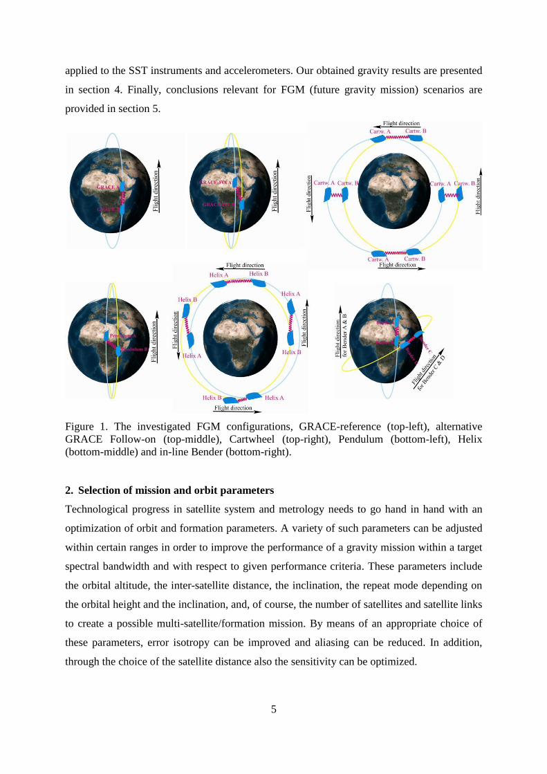
Figure 1. The investigated FGM configurations, GRACE-reference (top-left), alternative

GRACE Follow-on (top-middle), Cartwheel (top-right), Pendulum (bottom-left), Helix

(bottom-middle) and in-line Bender (bottom-right).

2. Selection of mission and orbit parameters

Technological progress in satellite system and metrology needs to go hand in hand with an

optimization of orbit and formation parameters. A variety of such parameters can be adjusted

within certain ranges in order to improve the performance of a gravity mission within a target

spectral bandwidth and with respect to given performance criteria. These parameters include

the orbital altitude, the inter-satellite distance, the inclination, the repeat mode depending on

the orbital height and the inclination, and, of course, the number of satellites and satellite links

to create a possible multi-satellite/formation mission. By means of an appropriate choice of

these parameters, error isotropy can be improved and aliasing can be reduced. In addition,

through the choice of the satellite distance also the sensitivity can be optimized.

6

Based on the results of the previous studies mentioned in Sec. 1, for this study the

pendulum, Cartwheel and Helix (LISA-like) formations have been selected as basic mission

scenarios as well as a two-inline-formation mission in a Bender design. For the latter, the

inclination for the second pair was chosen as i = 63° (Bender et al. 2008 and Anselmi et al.

2011). As a reference for the evaluation of these basic missions, two scenarios similar to the

current GRACE mission (orbit height h ≈ 460 km, SST range ρ ≈ 220 km) and the

“alternative” GRACE-FO (a moderate pendulum at h = 420 km with an along-track range ρx

= 220 km and a cross-track range ρy = 25 km) were added to the basic missions. It should be

noted that the latter “alternative” GRACE-FO configuration differs from the official one

planned to be launched in 2017 (Flechtner et al. 2013) at an initial altitude of 490 km, with an

inclination of 89.0° and an eccentricity less than 0.0025 in a co-planar orbit. Moreover, the K-

Band ranging instrument is the primary measuring instrument in the “official” GRACE-FO

mission, and the laser ranging device represents a demonstration experiment. In contrast, the

laser interferometer is assumed to be the main instrument for our “alternative” GRACE-FO.

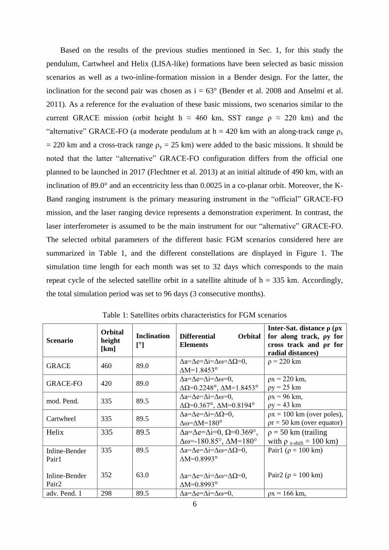
The selected orbital parameters of the different basic FGM scenarios considered here are

summarized in Table 1, and the different constellations are displayed in Figure 1. The

simulation time length for each month was set to 32 days which corresponds to the main

repeat cycle of the selected satellite orbit in a satellite altitude of h = 335 km. Accordingly,

the total simulation period was set to 96 days (3 consecutive months).

Table 1: Satellites orbits characteristics for FGM scenarios

Scenario

Orbital

height

[km]

Inclination

[°]

Differential Orbital

Elements

Inter-Sat. distance ρ (ρx

for along track, ρy for

cross track and ρr for

radial distances)

GRACE 460 89.0 Δa=Δe=Δi=Δω=ΔΩ=0,

ΔM=1.8453°

ρ = 220 km

GRACE-FO 420 89.0 Δa=Δe=Δi=Δω=0,

ΔΩ=0.2248°, ΔM=1.8453°

ρx = 220 km,

ρy = 25 km

mod. Pend. 335 89.5 Δa=Δe=Δi=Δω=0,

ΔΩ=0.367°, ΔM=0.8194°

ρx = 96 km,

ρy = 43 km

Cartwheel 335 89.5 Δa=Δe=Δi=ΔΩ=0,

Δω=ΔM=180°

ρx = 100 km (over poles),

ρr = 50 km (over equator)

Helix 335 89.5 Δa=Δe=Δi=0, Ω=0.369°,

Δω=-180.85°, ΔM=180°

ρ = 50 km (trailing

with ρ x-shift = 100 km)

Inline-Bender

Pair1

Inline-Bender

Pair2

335

352

89.5

63.0

Δa=Δe=Δi=Δω=ΔΩ=0,

ΔM=0.8993°

Δa=Δe=Δi=Δω=ΔΩ=0,

ΔM=0.8993°

Pair1 (ρ = 100 km)

Pair2 (ρ = 100 km)

adv. Pend. 1 298 89.5 Δa=Δe=Δi=Δω=0, ρx = 166 km,

7

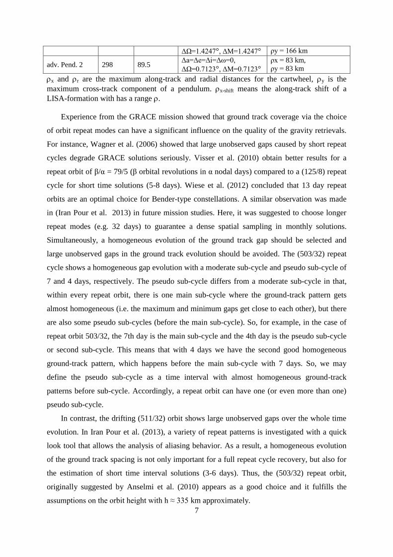
ΔΩ=1.4247°, ΔM=1.4247° ρy = 166 km

adv. Pend. 2 298 89.5 Δa=Δe=Δi=Δω=0,

ΔΩ=0.7123°, ΔM=0.7123°

ρx = 83 km,

ρy = 83 km

x and r are the maximum along-track and radial distances for the cartwheel, y is the

maximum cross-track component of a pendulum. x-shift means the along-track shift of a

LISA-formation with has a range .

Experience from the GRACE mission showed that ground track coverage via the choice

of orbit repeat modes can have a significant influence on the quality of the gravity retrievals.

For instance, Wagner et al. (2006) showed that large unobserved gaps caused by short repeat

cycles degrade GRACE solutions seriously. Visser et al. (2010) obtain better results for a

repeat orbit of β/α = 79/5 (β orbital revolutions in α nodal days) compared to a (125/8) repeat

cycle for short time solutions (5-8 days). Wiese et al. (2012) concluded that 13 day repeat

orbits are an optimal choice for Bender-type constellations. A similar observation was made

in (Iran Pour et al. 2013) in future mission studies. Here, it was suggested to choose longer

repeat modes (e.g. 32 days) to guarantee a dense spatial sampling in monthly solutions.

Simultaneously, a homogeneous evolution of the ground track gap should be selected and

large unobserved gaps in the ground track evolution should be avoided. The (503/32) repeat

cycle shows a homogeneous gap evolution with a moderate sub-cycle and pseudo sub-cycle of

7 and 4 days, respectively. The pseudo sub-cycle differs from a moderate sub-cycle in that,

within every repeat orbit, there is one main sub-cycle where the ground-track pattern gets

almost homogeneous (i.e. the maximum and minimum gaps get close to each other), but there

are also some pseudo sub-cycles (before the main sub-cycle). So, for example, in the case of

repeat orbit 503/32, the 7th day is the main sub-cycle and the 4th day is the pseudo sub-cycle

or second sub-cycle. This means that with 4 days we have the second good homogeneous

ground-track pattern, which happens before the main sub-cycle with 7 days. So, we may

define the pseudo sub-cycle as a time interval with almost homogeneous ground-track

patterns before sub-cycle. Accordingly, a repeat orbit can have one (or even more than one)

pseudo sub-cycle.

In contrast, the drifting (511/32) orbit shows large unobserved gaps over the whole time

evolution. In Iran Pour et al. (2013), a variety of repeat patterns is investigated with a quick

look tool that allows the analysis of aliasing behavior. As a result, a homogeneous evolution

of the ground track spacing is not only important for a full repeat cycle recovery, but also for

the estimation of short time interval solutions (3-6 days). Thus, the (503/32) repeat orbit,

originally suggested by Anselmi et al. (2010) appears as a good choice and it fulfills the

assumptions on the orbit height with h ≈ 335 km approximately.

8

We mention that the selection of an average satellite distance ρavg of 100 km together

with the orbit height of h = 335 km (for most considered future scenarios, see Table 1) is

based on the rule that the best sensitivity is reached for a large SST distance and a low orbital

height (Reubelt et al. 2011). However, a too large inter-satellite distance will cause problems

for laser technology (e.g. pointing issues, signal strength, noise) and a too low orbital height

appears problematic due to a higher air drag limiting the mission lifetime. Therefore, the

selected satellite distance and orbit height have to guarantee a compromise between

technological feasibility and geodetic sensitivity. Furthermore, Reubelt et al. (2011) showed

that the increase of accuracy is quite low for SST-distances larger than 100 km, where the

impact of the distance dependent laser noise becomes more important.

When considering such formations as the pendulum, cartwheel or LISA/helix, certain

technological constraints imposed by the relative motion of satellites have to be taken into

account. The main constraints concerning state-of-the-art technology are (Reubelt et al, 2014):

- the maximum range-rate should be kept within ±10 m/s,

- the line-of-sight angle between the two satellites should be kept within ±30° in yaw-

/pitch-direction.

The first constraint arises from the application of heterodyne lasers (Sheard et al. 2012) in

SST-links, which are already in an advanced technological level. The second constraint is

important to keep the energy consumption (because of, e.g., active satellite tracking for

satellite fine-pointing and enlarged air-drag due to slanted satellite) in a moderate state and

thus enable long mission lifetimes (please see Reubelt et al., 2014).

The first constraint is only fulfilled by GRACE, GRACE-FO and the moderate

pendulum, for the latter the maximum pendulum angle is fixed to 24° in order to keep the

range-rates below ±10 m/s. These three designs also fulfill the second constraint. Cartwheel

and LISA/helix formations are much more critical concerning the constraints due to the radial

component in their formation. The second constraint is impossible to be fulfilled by

cartwheels and LISA (due to their circular/elliptical relative motion), and apart from this, also

the first constraint appears to be problematic. Cartwheels show a large range variety due to

the 2:1 elliptical motion (Sharifi et al. 2007), and the range-rate criteria can only be met by

cartwheels with short baseline lengths (avg = 13.5 km) which lead to a severe loss of

sensitivity (Reubelt et al. 2011). The LISA formation seems optimal in fulfilling the first

constraint due to the nominal circular motion (range-rate = 0). Due to the perigee drift

induced by the Earth’s flattening the LISA motion deforms to an ellipse and the range-rates

9

again exceed the postulated limits, which can be overcome again only by too short baseline

lengths. One trick to make cartwheel and LISA formations fulfill the second constraint is to

shift one of the satellites out of the relative ellipse by a certain distance in along-track, which

leads to so-called trailing cartwheels/LISA. Of course, by such a manipulation isotropy is lost

due to a dominating along-track component, but on the benefit of fulfilling the second

constraint. In our contribution we implemented a trailing LISA (instead of LISA itself) which

is called helix due to its characteristic relative motion. If a satellite in a LISA-formation with

an inter-satellite distance is shifted with x-shift = 2 then the yaw angle is kept within ±30°

(pitch angle within ±15°). The cartwheel is taken as non-trailing formation and it can be

considered as an option in case of future developments, where the second constraint might not

be restrictive anymore. However, due to the introduced offset x-shift in along track direction

the helix satellite distance is not constant anymore (even if perigee drift is neglected) and thus

experiences strong range-rates, exceeding the range-rate constraint of

10m/s by far. To

keep the range-rate within this constraint, an average satellite distance of avg = 16 km similar

as for the cartwheel has to be selected, which would mean a clear decrease in sensitivity. In

order to establish formations with reasonable sensitivity, we selected a cartwheel and helix

with longer average inter-satellite distances avg = 78 km and avg = 112 km, respectively,

producing maximum range-rates of approximately = ±60 m/s. These two formations may

be regarded as unfeasible concerning the discussed heterodyne lasers (Sheard et al. 2012) but

might be possible with future laser technology. An option, which is under investigation, is

frequency comb laser systems (Coddington et al. 2009), which do not suffer from strict range-

rate constraints.

In summary, the investigated missions can be classified in three groups:

1) Feasible missions, with no or only minor relative motion of the satellites. This

group is represented by the Bender mission consisting of two inline pairs. This

formation has already been established with GRACE and is regarded as

unproblematic, although the four satellites would increase the mission costs.

2) Missions fulfilling the constraints: these are the two pendulum missions with a

smaller pendulum angle, namely the moderate pendulum and GRACE-FO. Although

they fulfill the constraints, they have to be regarded as a challenge due to their relative

motion, which imposes strong demands in formation control, laser instruments and

active satellite tracking.

10

3) Challenging missions: the mission exceeding the constraints, especially those for

the maximum range-rates. These are cartwheel and helix, and two versions of

challenging pendulums (adv. Pend. 1 and 2) with a larger pendulum angle of 45° and

average satellite distances of avg = 200/150 km leading to approximate maximum

range-rates of 80/60 m/s, respectively. For their implementation advanced future laser

technology is necessary, and system design and control systems are opposed to much

higher demands as the previous group. It has to be mentioned that for the challenging

pendulums additionally lower orbit heights are chosen, enabling higher resolution, but

increasing problems of insufficient mission lifetimes due to enlarged air-drag.

3. Methodology of full-scale simulation

3.1. Forward simulation process

For all the above-mentioned mission scenarios, simulated satellite orbits and true observations

were generated using GFZ’s Earth Parameter and Orbit System (EPOS) software package.

EPOS consists of a collection of tools built around the core module OC (Orbit Computation),

and it is able to simulate many observation types such as GPS (Global Positioning System),

GRACE K-band SST, SLR (Satellite Laser Ranging), DORIS (Doppler Orbitography and

Radiopositioning Integrated by Satellite) or altimetry.

The forward simulation is then performed by integrating sequentially the satellite orbits

in the formation over the complete 96 days period, while applying true background models,

cf. Table 2, and dedicated models for non-gravitational accelerations (only for GRACE and

GRACE-FO, see Table 2). The orbit integrator yields not only the 96 days long orbit files but

also the “measured” and error-free surface forces computed from the non-gravitational force

models (pseudo accelerometer data), the inter-satellite range-rate measurements as well as the

star camera data (attitude data), which are then used by GROOPS, as input to the gravity field

recovery, after adding noise for SST and accelerometer data (see below). The star camera

data, generated by the EPOS software, are used by the GROOPS software as error-free data.

It is important to mention here that in the frame of our project “Concepts for future

gravity field satellite missions”, we have compared all the gravitational and non-gravitational

accelerations at discrete points on the orbit between the GFZ-EPOS and the IGG-GROOPS

software packages. We have found that the agreement was at the level of 1.e-14 m/s/s or

better. For such comparison between GFZ-EPOS and IGG-GROOPS, please see Reubelt et

al., (2014).

11

3.2. Backward simulation process

The backward simulation process (gravity analysis step) implemented through the IGG-

GROOPS software is based on the solution of the Newton-Euler's equation of motion,

formulated as a boundary value problem of a Fredholm-type integral equation for setting up

the observation equations (Mayer-Gürr 2006). In fact, many strategies may be (and will be,

undoubtly) exploited for gravity recovery with future missions, however we choose to adhere

as close as possibly to the analysis as performed at IGG for real GRACE data (Mayer-Gürr et

al. 2005 and Mayer-Gürr 2006).

First, all observations including satellite orbits, accelerometer, inter-satellite range-rate

and attitude data files have been split into arcs of 35 minutes based on the short arc approach

that is implemented at IGG for analysis of real GRACE data. Here, “short” means a fraction

of a satellite orbit significantly less than one revolution. The short arc technique reduces the

accumulated effects of the perturbing forces acting on a satellite orbit. Moreover, it enables to

use the positions, range and the range-rate measurements as observations directly, and also

allows for data gaps. The observation equations are then set up for each short arc as a

linearized Gauss-Markov model as

2 -1= + with = ,l Ax ε C(ε) σ P [1]

with l containing the range-rate observations, A the design matrix (composed of partial

derivatives obtained by differentiating the range-rates w.r.t. the unknown parameters), x the

sought-for gravity parameters, ε the error vector, and C(ε) its corresponding covariance

matrix. σ2 stands for the variance factor for each satellite arc and P represents the weight

matrix of the observations. The least-squares solution of Eq. [1] leads to the following system

of normal equations (Koch and Kusche 2001),

T Twith and .Nx=n N= A PA n= A Pl [2]

The solution of the normal equations yields the estimation of the unknown parameters as

-1 T -1 T= =( ) .x N n A PA A Pl [3]

The normal equations can be directly accumulated from the individual arc-wise blocks as

m mT T

i i i i i i

i=1 i=1

= = and = = . N A P A n A Pl

[4]

In a next step, according to Eq. [4], the normal equations are directly solved via

Cholesky decomposition (Koch 1997). The output is then a set of spherical harmonic

12

coefficients which can be compared to the true coefficients (of the EIGEN-GL04C model) and

their differences are visualized in spectral and spatial domains.

In order to simulate the process of gravity recovery in the presence of realistic

background model errors, mean and time-variable background models applied in the forward

simulation step have been substituted in the backward simulation step by different models,

where the difference between both represents the current known model error level. Table 2

shows the models used for the ‘forward’ simulation and those substituted in the ‘backward’

simulation.

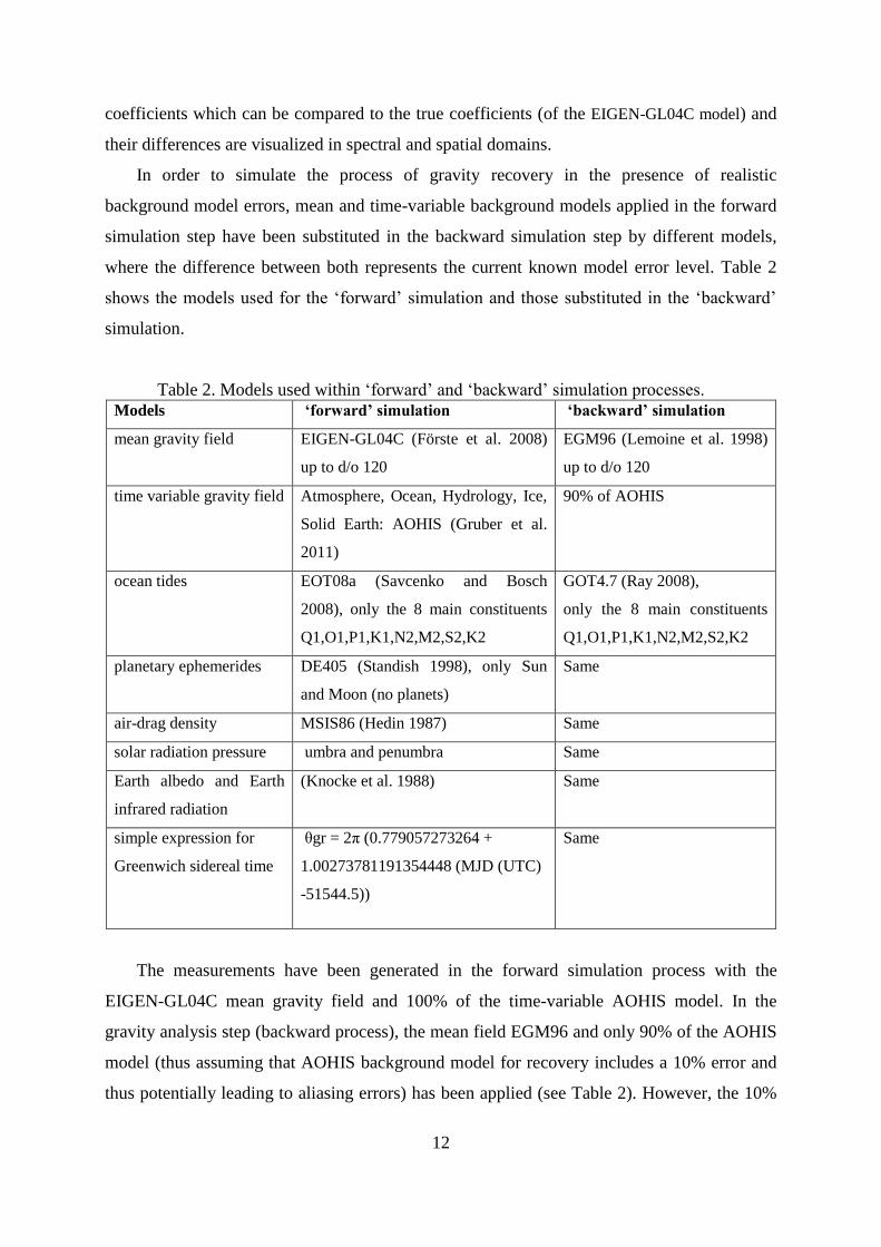
Table 2. Models used within ‘forward’ and ‘backward’ simulation processes.

Models ‘forward’ simulation ‘backward’ simulation

mean gravity field EIGEN-GL04C (Förste et al. 2008)

up to d/o 120

EGM96 (Lemoine et al. 1998)

up to d/o 120

time variable gravity field Atmosphere, Ocean, Hydrology, Ice,

Solid Earth: AOHIS (Gruber et al.

2011)

90% of AOHIS

ocean tides EOT08a (Savcenko and Bosch

2008), only the 8 main constituents

Q1,O1,P1,K1,N2,M2,S2,K2

GOT4.7 (Ray 2008),

only the 8 main constituents

Q1,O1,P1,K1,N2,M2,S2,K2

planetary ephemerides DE405 (Standish 1998), only Sun

and Moon (no planets)

Same

air-drag density MSIS86 (Hedin 1987) Same

solar radiation pressure umbra and penumbra Same

Earth albedo and Earth

infrared radiation

(Knocke et al. 1988) Same

simple expression for

Greenwich sidereal time

θgr = 2π (0.779057273264 +

1.00273781191354448 (MJD (UTC)

-51544.5))

Same

The measurements have been generated in the forward simulation process with the

EIGEN-GL04C mean gravity field and 100% of the time-variable AOHIS model. In the

gravity analysis step (backward process), the mean field EGM96 and only 90% of the AOHIS

model (thus assuming that AOHIS background model for recovery includes a 10% error and

thus potentially leading to aliasing errors) has been applied (see Table 2). However, the 10%

13

signal not removed in the backward analysis contains a monthly mean, which does not

contribute to temporal aliasing and should be picked up by the analysis and transformed into

the mean estimated model, which in turn means that this mean needs to be considered when

comparing estimated and true monthly models. In addition, for simplicity, no relativity,

precession, nutation, polar motion or Earth and pole tides have been applied during both

forward and backward simulations. This does not affect the overall simulation conclusions.

In order to simulate gravity recovery as close to reality as possible, colored noise in terms

of PSD (power spectral density) from the involved sensors was added to the noise-free

observations, provided by the forward step, during the gravity field determination. In the

following, the generation of colored noise time series is thoroughly described.

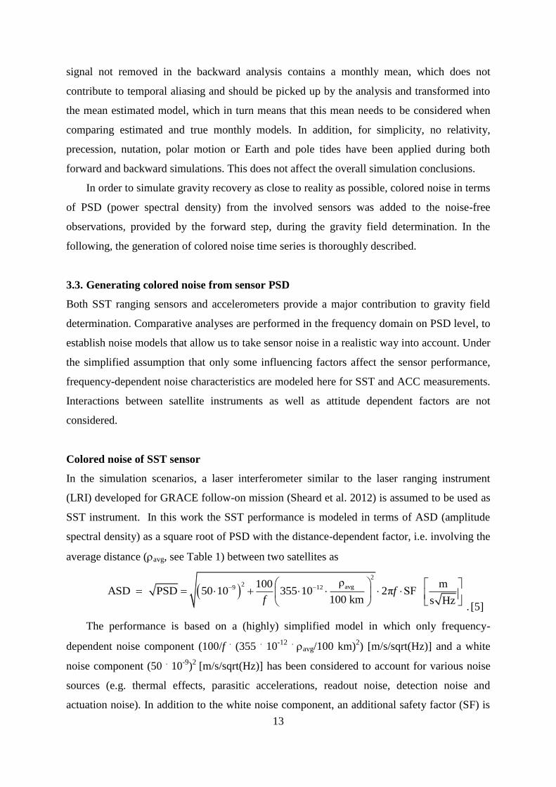
3.3. Generating colored noise from sensor PSD

Both SST ranging sensors and accelerometers provide a major contribution to gravity field

determination. Comparative analyses are performed in the frequency domain on PSD level, to

establish noise models that allow us to take sensor noise in a realistic way into account. Under

the simplified assumption that only some influencing factors affect the sensor performance,

frequency-dependent noise characteristics are modeled here for SST and ACC measurements.

Interactions between satellite instruments as well as attitude dependent factors are not

considered.

Colored noise of SST sensor

In the simulation scenarios, a laser interferometer similar to the laser ranging instrument

(LRI) developed for GRACE follow-on mission (Sheard et al. 2012) is assumed to be used as

SST instrument. In this work the SST performance is modeled in terms of ASD (amplitude

spectral density) as a square root of PSD with the distance-dependent factor, i.e. involving the

average distance (avg, see Table 1) between two satellites as

2

2 avg9 12ρ100 m

ASD PSD 50 10 355 10 2π SF100 km s Hz

ff

. [5]

The performance is based on a (highly) simplified model in which only frequency-

dependent noise component (100/f . (355

. 10

-12

. avg/100 km)

2) [m/s/sqrt(Hz)] and a white

noise component (50 . 10

-9)2

[m/s/sqrt(Hz)] has been considered to account for various noise

sources (e.g. thermal effects, parasitic accelerations, readout noise, detection noise and

actuation noise). In addition to the white noise component, an additional safety factor (SF) is

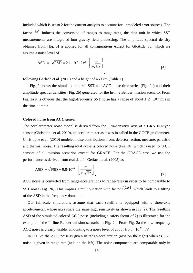
14

included which is set to 2 for the current analysis to account for unmodeled error sources. The

factor f2 induces the conversion of ranges to range-rates, the data unit in which SST

measurements are integrated into gravity field processing. The amplitude spectral density

obtained from [Eq. 5] is applied for all configurations except for GRACE, for which we

assume a noise level of

6 mASD PSD 2.1 10 2π

s Hzf

,

[6]

following Gerlach et al. (2005) and a height of 460 km (Table 1).

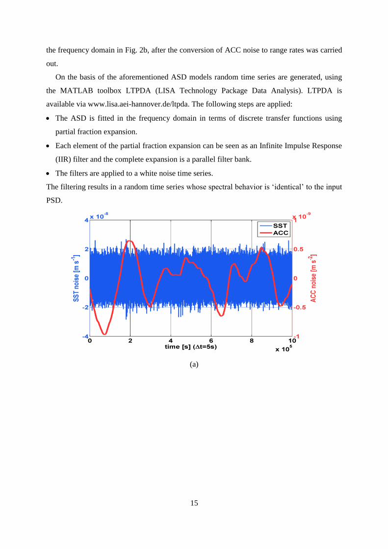
Fig. 2 shows the simulated colored SST and ACC noise time series (Fig. 2a) and their

amplitude spectral densities (Fig. 2b) generated for the In-line Bender mission scenario. From

Fig. 2a it is obvious that the high-frequency SST noise has a range of about ± 2 ∙ 10-8

m/s in

the time domain.

Colored noise from ACC sensor

The accelerometer noise model is derived from the ultra-sensitive axis of a GRADIO-type

sensor (Christophe et al. 2010), an accelerometer as it was installed in the GOCE gradiometer.

Christophe et al. (2010) modeled noise contributions from: detector, action, measure, parasitic

and thermal noise. The resulting total noise is colored noise (Fig. 2b) which is used for ACC

sensors of all mission scenarios except for GRACE. For the GRACE case we use the

performance as derived from real data in Gerlach et al. (2005) as

9

2

mASD PSD 9.8 10

s Hz

. [7]

ACC noise is converted from range-accelerations to range-rates in order to be comparable to

SST noise (Fig. 2b). This implies a multiplication with factor f21 , which leads to a tilting

of the ASD in the frequency domain.

Our full-scale simulations assume that each satellite is equipped with a three-axis

accelerometer, whose axes share the same high sensitivity as shown in Fig. 2a. The resulting

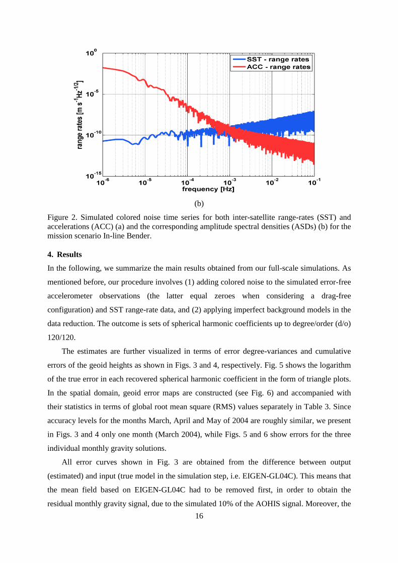
ASD of the simulated colored ACC noise (including a safety factor of 2) is illustrated for the

example of the In-line Bender mission scenario in Fig. 2b. From Fig. 2a the low-frequency

ACC noise is clearly visible, amounting to a noise level of about ± 0.5 ∙ 10-9

m/s2.

In Fig. 2a the ACC noise is given in range-acceleration (axis on the right) whereas SST

noise is given in range-rate (axis on the left). The noise components are comparable only in

15

the frequency domain in Fig. 2b, after the conversion of ACC noise to range rates was carried

out.

On the basis of the aforementioned ASD models random time series are generated, using

the MATLAB toolbox LTPDA (LISA Technology Package Data Analysis). LTPDA is

available via www.lisa.aei-hannover.de/ltpda. The following steps are applied:

The ASD is fitted in the frequency domain in terms of discrete transfer functions using

partial fraction expansion.

Each element of the partial fraction expansion can be seen as an Infinite Impulse Response

(IIR) filter and the complete expansion is a parallel filter bank.

The filters are applied to a white noise time series.

The filtering results in a random time series whose spectral behavior is ‘identical’ to the input

PSD.

(a)

16

(b)

Figure 2. Simulated colored noise time series for both inter-satellite range-rates (SST) and

accelerations (ACC) (a) and the corresponding amplitude spectral densities (ASDs) (b) for the

mission scenario In-line Bender.

4. Results

In the following, we summarize the main results obtained from our full-scale simulations. As

mentioned before, our procedure involves (1) adding colored noise to the simulated error-free

accelerometer observations (the latter equal zeroes when considering a drag-free

configuration) and SST range-rate data, and (2) applying imperfect background models in the

data reduction. The outcome is sets of spherical harmonic coefficients up to degree/order (d/o)

120/120.

The estimates are further visualized in terms of error degree-variances and cumulative

errors of the geoid heights as shown in Figs. 3 and 4, respectively. Fig. 5 shows the logarithm

of the true error in each recovered spherical harmonic coefficient in the form of triangle plots.

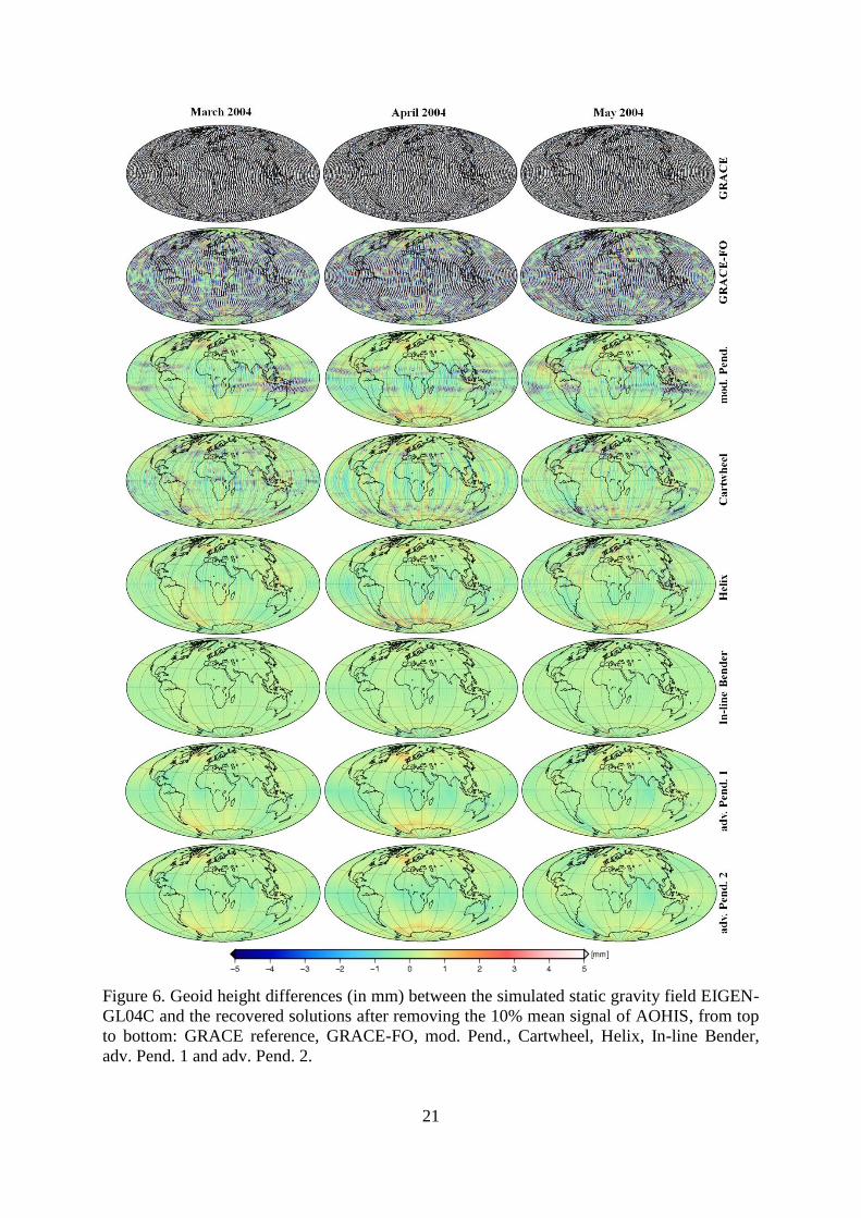
In the spatial domain, geoid error maps are constructed (see Fig. 6) and accompanied with

their statistics in terms of global root mean square (RMS) values separately in Table 3. Since

accuracy levels for the months March, April and May of 2004 are roughly similar, we present

in Figs. 3 and 4 only one month (March 2004), while Figs. 5 and 6 show errors for the three

individual monthly gravity solutions.

All error curves shown in Fig. 3 are obtained from the difference between output

(estimated) and input (true model in the simulation step, i.e. EIGEN-GL04C). This means that

the mean field based on EIGEN-GL04C had to be removed first, in order to obtain the

residual monthly gravity signal, due to the simulated 10% of the AOHIS signal. Moreover, the

17

mean signal of this 10% AOHIS field needs to be subtracted from the monthly recovered

solution in order to assess the error level of each satellite; resulting mainly from simulated

instrument noise and aliasing effects (see Figs. 5 and 6).

As expected, the estimated solutions for all alternative FGM scenarios perform

approximately one to two orders of magnitude better than the GRACE reference solution,

especially at the short wavelength range as seen in Fig. 3. The reason is that they add

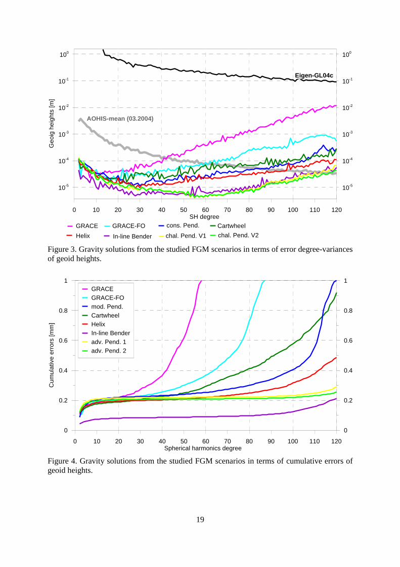
measurement information in cross-track and/or radial directions. This becomes apparent in

Fig. 5, which shows the error of each spherical harmonic coefficient. Additionally, the lower

orbital height and the improved sensors of all alternative FGMs, when compared to GRACE,

increase the signal-to-noise ratio and hence provide significant improvements.

North-south striping pattern still contaminates gravity recovery with our GRACE-FO

mission as seen in Fig. 6. However, the small cross-track component, besides the lower orbital

height and the laser instrument implemented in the GRACE-FO (see Table 1) formation

helped in reducing the aliasing errors by one order of magnitude w.r.t. the GRACE reference

solution, which displays a stronger striping pattern, as expected. As seen in Fig. 3, GRACE-

FO provides improvements at short wavelengths by a factor of about 10 (see also Table 3).

Increasing the cross-track inter-satellite separation angle, from 7° in case of the GRACE-FO

mission to 25° in case of the “mod. Pend.” mission, also improves the recovery; global errors

associated with the GRACE-FO solution could be reduced with the mod. Pend. solution (see

Fig. 6).

Besides the configurations which include a cross-track component, also the Cartwheel

and Helix mission scenarios which contain radial information perform better than the

GRACE-FO mission. The Helix solution provides a lower cumulative geoid error level for all

three months compared to the “mod. Pend.” and Cartwheel scenarios. The reason is likely that

the Helix-measured range-rate is the only observable we considered that senses in all three

space directions.

As may be expected, the best overall solutions for all cases are obtained by using more

than one pair of satellites that conduct SST via the In-line Bender configuration (see Table 3).

The error curve of the In-line Bender configuration crosses the mean signal of the AOHIS

temporal field at d/o 110 (see Fig. 3), meaning that the In-line Bender configuration would not

only be able to reduce aliasing errors but also to resolve the temporal signal better. From Fig.

6, it becomes obvious as well that the In-line Bender solution provides the most isotropic

error distribution and least errors especially in the long wavelengths across all considered

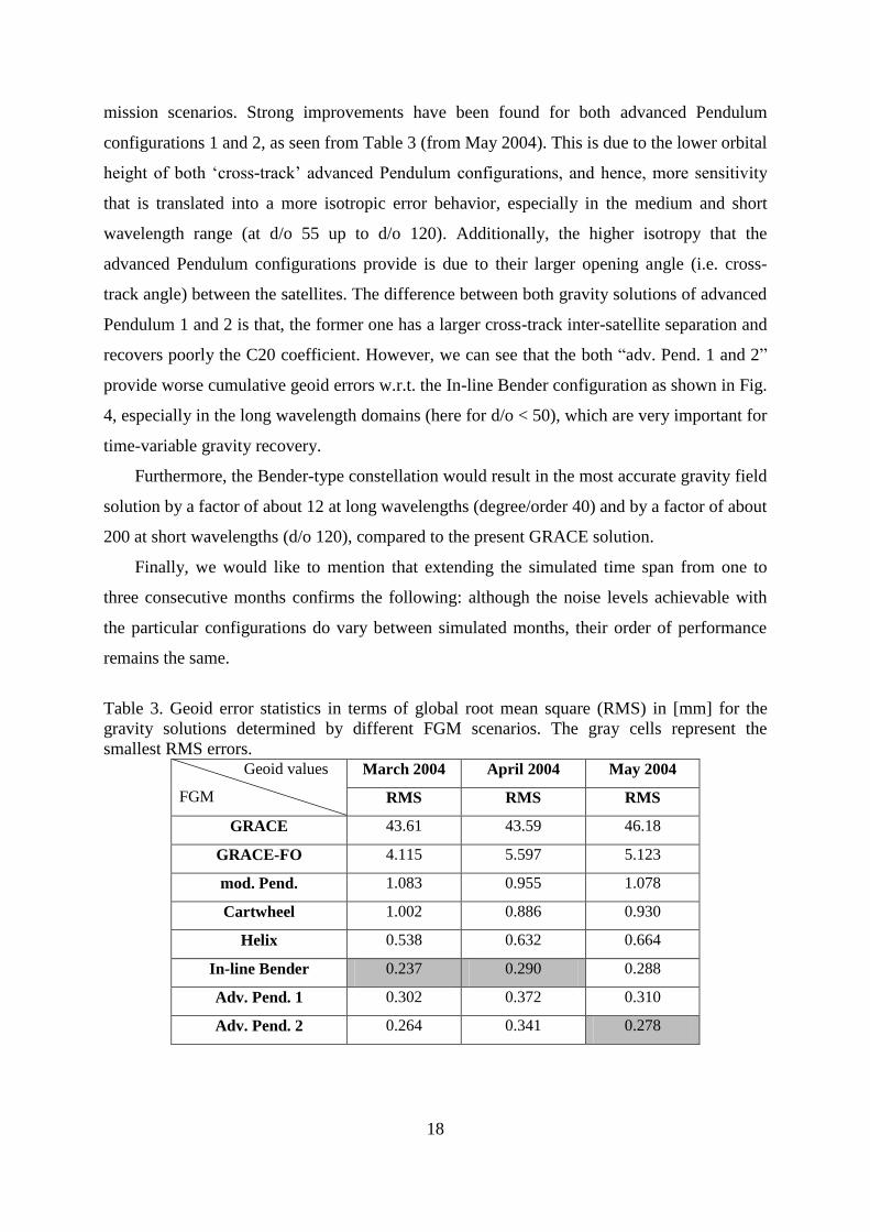
18

mission scenarios. Strong improvements have been found for both advanced Pendulum

configurations 1 and 2, as seen from Table 3 (from May 2004). This is due to the lower orbital

height of both ‘cross-track’ advanced Pendulum configurations, and hence, more sensitivity

that is translated into a more isotropic error behavior, especially in the medium and short

wavelength range (at d/o 55 up to d/o 120). Additionally, the higher isotropy that the

advanced Pendulum configurations provide is due to their larger opening angle (i.e. cross-

track angle) between the satellites. The difference between both gravity solutions of advanced

Pendulum 1 and 2 is that, the former one has a larger cross-track inter-satellite separation and

recovers poorly the C20 coefficient. However, we can see that the both “adv. Pend. 1 and 2”

provide worse cumulative geoid errors w.r.t. the In-line Bender configuration as shown in Fig.

4, especially in the long wavelength domains (here for d/o < 50), which are very important for

time-variable gravity recovery.

Furthermore, the Bender-type constellation would result in the most accurate gravity field

solution by a factor of about 12 at long wavelengths (degree/order 40) and by a factor of about

200 at short wavelengths (d/o 120), compared to the present GRACE solution.

Finally, we would like to mention that extending the simulated time span from one to

three consecutive months confirms the following: although the noise levels achievable with

the particular configurations do vary between simulated months, their order of performance

remains the same.

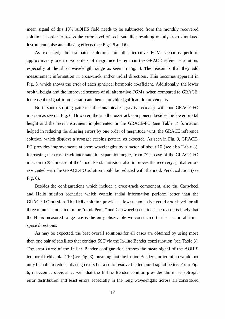
Table 3. Geoid error statistics in terms of global root mean square (RMS) in [mm] for the

gravity solutions determined by different FGM scenarios. The gray cells represent the

smallest RMS errors. Geoid values

FGM

March 2004 April 2004 May 2004

RMS RMS RMS

GRACE 43.61 43.59 46.18

GRACE-FO 4.115 5.597 5.123

mod. Pend. 1.083 0.955 1.078

Cartwheel 1.002 0.886 0.930

Helix 0.538 0.632 0.664

In-line Bender 0.237 0.290 0.288

Adv. Pend. 1 0.302 0.372 0.310

Adv. Pend. 2 0.264 0.341 0.278

19

0 10 20 30 40 50 60 70 80 90 100 110 120SH degree

10-5

10-4

10-3

10-2

10-1

100

Ge

oig

he

ights

[m

]

10-5

10-4

10-3

10-2

10-1

100

GRACE GRACE-FO cons. Pend. Cartwheel

Helix In-line Bender chal. Pend. V1 chal. Pend. V2

AOHIS-mean (03.2004)

Eigen-GL04c

Figure 3. Gravity solutions from the studied FGM scenarios in terms of error degree-variances

of geoid heights.

0 10 20 30 40 50 60 70 80 90 100 110 120Spherical harmonics degree

0

0.2

0.4

0.6

0.8

1

Cu

mula

tive e

rro

rs [m

m]

0

0.2

0.4

0.6

0.8

1

GRACE

GRACE-FO

mod. Pend.

Cartwheel

Helix

In-line Bender

adv. Pend. 1

adv. Pend. 2

Figure 4. Gravity solutions from the studied FGM scenarios in terms of cumulative errors of

geoid heights.

20

Figure 5. True errors in each spherical harmonic coefficient, from comparing the simulated

static gravity field EIGEN-GL04C and the recovered solutions after removing the 10% mean

signal of AOHIS. From top to bottom: GRACE reference, GRACE-FO, mod. Pend.,

Cartwheel, Helix, In-line Bender, adv. Pend. 1 and adv. Pend. 2. The colorbar is in

logarithmic scale of the coefficient absolute value.

21

Figure 6. Geoid height differences (in mm) between the simulated static gravity field EIGEN-

GL04C and the recovered solutions after removing the 10% mean signal of AOHIS, from top

to bottom: GRACE reference, GRACE-FO, mod. Pend., Cartwheel, Helix, In-line Bender,

adv. Pend. 1 and adv. Pend. 2.

22

5. Conclusion

In the course of this contribution, we have provided an assessment of seven candidate

scenarios for a future gravity mission based on full-scale simulations, which consist of

forward simulation by GFZ EPOS software, backward simulation by IGG GROOPS software,

and include the consideration of realistic colored accelerometer and ranging noise and

background model errors.

In line with earlier studies, we conclude that the gravity recovery improves significantly

in terms of the error levels and more isotropic noise distribution if moderate cross-track

and/or radial components are added to the SST observable. This is in principle possible by a

variety of formations, i.e. satellite pairs that orbit the Earth in alternative configurations.

We have also found that extending the simulated time span from one to three consecutive

months improves the robustness of the performance assessments, in a way that though the

noise levels of the particular configurations are varying between simulated months, their order

of performance remains the same.

We can confirm earlier findings that the GRACE formation is sub-optimal in terms of the

gravity field recovery. We find that simulation results are to some extent sensitive with

respect to the particular ‘monthly noise model’. This may explain a part of the differences

seen in the growing literature on simulation studies. It also means that such studies should be

based on longer simulated data sets.

The best performance of the investigated single formations was obtained by the advanced

pendulums, however an accuracy reduced by about 2-4 times in the important long-

wavelength part of the spectrum (for spherical harmonic degrees < 50), compared to the

Bender mission, can be observed.

Concerning state-of-the-art mission constraints, in particular the severe restriction of

heterodyne lasers on maximum range-rates, only the moderate Pendulum and the Bender-

mission are beneficial options, of course in addition to GRACE and GRACE-FO. Here, the

moderate pendulum shows the best performance of the considered single formation missions

with a significant gain of up to one order of magnitude (and more) compared to GRACE and

GRACE-FO. Again, as mentioned before, the Bender constellation, though economically

likely much more challenging shows the best performance of all missions. It would

outperform the moderate pendulum by more than half an order of magnitude, and would

indeed result in a significantly improved solution in the short and medium spectral range, with

23

a geoid accuracy better than 1 mm when spherical harmonic expansion up to degree 120 is

considered.

Depending on the available budget and technological progress we suggest the following

missions for future realisation:

- if the budget allows for the launch of two satellite pairs, the Bender constellation is

suggested. Furthermore, this mission seems feasible concerning technological issues (i.e. two

inline formations)

- if the budget allows only for the launch of one pair, a pendulum is proposed. Depending

on the technological progress, e.g. in laser technology, system and satellite design, the

maximum pendulum angle can be chosen.

Acknowledgements:

The authors would like to thank the reviewers for their valuable comments. We gratefully

acknowledge Dr. Pavel Ditmar, the Editor, for his valuable comments and corrections to

improve this manuscript. Additionally, the financial support of the German Federal Ministry

for Education and Research (BMBF) and the German Research Foundation (DFG) within the

frame work of the German joint research project “Concepts for future gravity field satellite

missions” as part of the Geotechnologies Program (grant 03G0729) is acknowledged.

References

Anselmi, A., Cesare, S., Visser, P., Van Dam, T., Sneeuw, N., Gruber, T., Altes, B.,

Christophe, B., Cossu, F., Ditmar, P., Murboeck, M., Parisch, M., Renard, M., Reubelt,

T., Sechi, G. and Texieira Da Encarnacao, JG. (2011) Assessment of a next generation

gravity mission to monitor the variations of Earth’s gravity field. ESA Contract No.

22643/09/NL/AF, Executive Summary, Thales Alenia Space report SD-RP-AI-0721, March

2011.

Bender, P. , Wiese, D. and Nerem, R. (2008) A possible dual-GRACE mission with 90

degree and 63 degree inclination orbits, paper presented at Third International Symposium on

Formation Flying, Eur. Space Agency, Noordwijk, Netherlands, 23–25 April.

Christophe, B., Marque, J.-P. and Foulon, B. (2010) Accelerometers for the ESA GOCE

Mission: one year of in-orbit results. Presentation at EGU 2010, Vienna, available on the ESA

GOCE website, http://earth.esa.int/pub/ESA_DOC/GOCE/Accelerometers for the ESA

GOCE Mission - one year of in-orbit results.pdf, Last accessed 24 September 2012

24

Coddington, I., Swann, W. C., Nenadovic, L. and Newbury, N. R. (2009) Rapid and

precise absolute distance measurements at long range. Nature Photonics Vol 3, 351–356,

doi:10.1038/nphoton.2009.94.

Elsaka, B. (2010) Simulated Satellite Formation Flights for Detecting the Temporal

Variations of the Earth’s Gravity Field. Ph.D. Dissertation, University of Bonn, Germany.

Elsaka, B., Kusche, J. and Ilk, K.-H. (2012) Recovery of the Earth’s gravity field from

formation-flying satellites: Temporal aliasing issues. Advances in Space Research, 50: 1534-

1552. doi.org/10.1016/j.asr.2012.07.016.

Elsaka, B. (2013) Sub-month Gravity Field Recovery from Simulated Multi-GRACE Mission

Type. Acta Geophysica (Accepted, Jul 2013).

Flechtner, F., Watkins, M., Morton, P. and Webb, F. (2013): Status of the GRACE

Follow-on Mission. Proceedings of the International Association of Geodesy Symposia

Gravity, Geoid and Height System (GGHS2012), 9.-11.10.2012, Venice, Italy, IAGS-D-12-

00141 (accepted).

Förste, C., Schmidt, R., Stubenvoll, R., Flechtner, F., Meyer, U., Koenig, R., Neu-mayer,

H., Biancale, R., Lemoine, J., Bruinsma, S., Loyer, S., Barthelmes, F. and Esselborn, S.

(2008) The GeoForschungsZentrum Potsdam/Groupe de Recherche de Ge-odesie Spatiale

satellite-only and combined gravity field models: EIGEN-GL04S1 and EIGEN-GL04C. J

Geod, 82, 6, 331-346, doi:10.1007/s00190-007-0183-8.

Gerlach. C., Flury, J., Frommknecht, B., Flechtner, F. and Rummel, R. (2005) GRACE

performance study and sensor analysis. Proceedings of the Joint CHAMP/GRACE Science

Meeting, GeoForschungsZentrum Potsdam, July 6-8, 2004, p.6.1, http://www-app2.gfz-

potsdam.de/pb1/JCG/Gerlach-etal_jcg.pdf.

Gruber, T., Bamber, J., Bierkens, M., Dobslaw, H., Murböck, M., Thomas, M., van

Beek, L., van Dam, T., Vermeersen, L.L.A. and Visser, P. (2011) Simulation of the time-

variable gravity field by means of coupled geophysical models. Earth System Science Data,

3:19–35, doi:10.5194/essd-3-19-2011.

Hedin, A. (1987) MSIS-86 Thermospheric Model. JGR, Vol. 92, No. A5, pp. 4649-4662,

doi:10.1029/JA092iA05p04649.

Iran Pour, S., Reubelt, T. and Sneeuw, N. (2013) Quality assessment of sub-Nyquist

recovery from future gravity satellite missions. Journal of Advances in Space Research

Volume 52, Issue 5, Pages 916–929.

25

Knocke, P., Ries, J. and Tapley, B. (1988) Earth Radiation Pressure Effects on Satellites.

Proceedings of the AIAA/AAS Astrodynamics Specialist Conference, Washington DC, 1988,

pp. 577-586.

Koch, K. R. (1997) Parameterschätzung und Hypothesentests. Dümmler, Bonn.

Koch, K. R. and Kusche, J. (2001) Regularization of geopotential determination from

satellite data by variance components. Journal of Geodesy, 76(5):641_652.

Kusche, J. (2002) A Monte-Carlo technique for weight estimation in satellite geodesy. J

Geod 76 (11), 641-652.

Lemoine, F., Kenyon, S., Factor, J., Trimmer, R., Pavlis, N., Cox, C., Klos-ko, S.,

Luthcke, S., Torrence, M., Wang, Y., Williamson, R., Pavlis, E., Rapp, R. and Olson, T.

(1998) The Development of the Joint NASA GSFC and the Na-tional Imagery and Mappping

Agency (NIMA) Geopotential Model EGM96. NASA/TP-1998-206861, July, 1998.

Mayer-Gürr, T., Ilk, K.-H., Eicker, A. and Feuchtinger, M. (2005) ITG-CHAMP01: A

CHAMP Gravitiy Field Model from Short Kinematical Arcs of a One-Year Observation

Period. Journal of Geodesy, 78:462-480.

Mayer-Gürr, T. (2006) Gravitationsfeldbestimmung aus der Analyse kurzer Bahnbögen am

Beispiel der Satellitenmissionen CHAMP und GRACE. Ph.D. Dissertation, University of

Bonn, Germany.

NG2 Team (2011) Assessment of a Next Generation Gravity Mission to Monitor the

Variations of Earth's Gravity Field. Final Report, ESTEC Contract No.: 22672/09/NL/AF.

Doc. No.: NG2-ASG-FR, Issue 1, 10 Oct. 2011.

Ray, R. (2008) GOT4.7 (private communication). Extension of Ray R (1999) A global ocean

tide model from Topex/Poseidon altimetry GOT99.2. NASA Tech Memo 209478, Sept. 1999.

Reubelt, T., Sneeuw, N. and Sharifi, M. (2010) Future Mission Design Options for Spatio-

Temporal Geopotential Recovery. In: Mertikas SP (ed) Gravity, Geoid and Earth Observation.

IAG Commission 2: Gravity Field, Chania, Crete, Greece, 23-27 June 2008. International

Association of Geodesy Symposia, Vol. 135, Springer.

Reubelt, T., Sneeuw, N. and Iran Pour, S. (2011) Quick-look gravity field analysis of

formation scenarios selection. In: Münch U, Dransch W (eds) Observation of the System

Earth from Space, GEOTECHNOLOGIEN Science Report No. 17, Status Seminar, 4 October

2010, Rheinische Friedrich Wilhelms Universität Bonn, Koordinierungsbüro

GEOTECHNOLOGIEN, Potsdam.

26

Reubelt, T., Sneeuw, N., Iran Pour, S., Hirth, M., Fichter, W., Müller, J., Brieden, Ph.,

Flechtner, F., Raimondo, J.-C., Kusche, J., Elsaka, B., Gruber, T., Pail, R., Murböck,

M., Doll, B., Sand, R., Wang, X., Klein, V., Lezius, M., Danzmann, K., Heinzel, G.,

Sheard, B., Rasel, E., Gilowski, M., Schubert, C., Schäfer, W., Rathke, A., Dittus, H. and

Pelivan, I. (2014): Future Gravity Field Satellite Missions. Flechtner, F., Sneeuw, N., Schuh,

W.-D. (Eds.), Observation of the System Earth from Space - CHAMP, GRACE, GOCE and

future missions. GEOTECHNOLOGIEN Science Report No. 20, Series "Advanced

Technologies in Earth Sciences", Springer, ISBN 978-3-642-32134-4 (in press 2014).

Savcenko, R. and Bosch, W. (2008) EOT08a – empirical ocean tide model from mul-ti-

mission satellite altimetry. Report No. 81, Deutsches Geodätisches Forschung-sinstitut

(DGFI), München.

Sharifi, M., Sneeuw, N., and Keller, W. (2007) Gravity Recovery capability of four generic

satellite formations. In Proc. Kilicoglu, A. and R. forsberg (Eds.), Gravity Field of the Earth.

General Command of Mapping, ISSN 1300-5790, Special issue 18, 211–216.

Sheard, B., Heinzel, G., Danzmann, K., Shaddock, D., Klipstein, W. and Folkner, W.

(2012) Intersatellite laser ranging instrument for the GRACE follow-on mission. Journal of

Geodesy, Vol. 86, Number 12, Page 1083.

Sneeuw, N., Sharifi, M., and Keller, W. (2008) Gravity Recovery from Formation Flight

Missions. Xu, Peiliang, Jingnan Liu and Athanasios Dermanis (Eds.), VI Hotine-Marussi

Symposium on Theoretical and Computational Geodesy, Vol. 132, Springer, Berlin

Heidelberg, 29–34.

Standish, E. M. (1998) JPL Planetary and Lunar Ephemerides, “DE405/LE405”. IOM 312.F-

98-048, August 26 1998.

van Dam, T., Visser, P., Sneeuw, N., Losch, M., Gruber, T., Bamber, J., Bierkens, M.

King, M. and Smit, M. (2008) Monitoring and Modelling Individual Sources of Mass

Distribution and Transport in the Earth System by Means of Satellites ESA-contract 20403,

Final Report.

Visser, P., Sneeuw, N., Reubelt, T., Losch, M. and van Dam, T. (2010) Space-borne

gravimetric satellite constellations and ocean tides: aliasing effects. Geophys. J. Int. (2010)

181, 789–805.

27

Wagner, C., McAdoo, D., Klokočník, J. and Kostelecký, J. (2006) Degradation of geo-

potential recovery from short repeat-cycle orbits: application to GRACE monthly fields. J

Geod 80(2):94–103.

Wiese, D., Folkner, W. and Nerem, R. (2009) Alternative mission architectures for a gravity

recovery satellite mission. Journal of Geodesy, 83, 569-581, DOI 10.1007/s00, 190-008-0274-

1.

Wiese, D., Nerem, R. and Han, S.-C. (2011) Expected improvements in determining

continental hydrology, ice mass variations, ocean bottom pressure signals, and earthquakes

using two pairs of dedicated satellites for temporal gravity recovery. Journal of Geophysical

Research, Vol. 116, B11 405, doi:10.1029/2011JB008375.

Wiese, D., Nerem, R. and Lemoine, F. (2012) Design considerations for a dedicated gravity

recovery satellite mission consisting of two pairs of satellites. Journal of Geodesy, 86:81-98,

DOI 10.1007/s00190-011-0493-8.