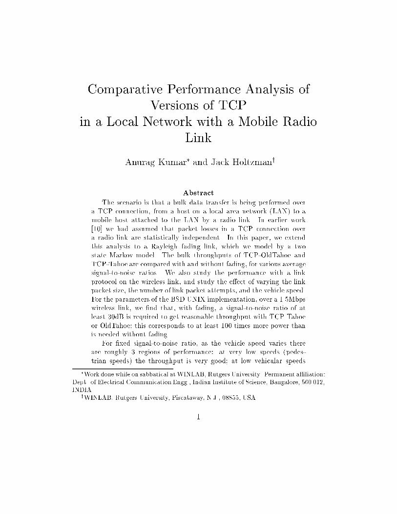
Comparative Performance Analysis ofVersions of TCPin a Local Network with a Mobile RadioLinkAnurag Kumar� and Jack HoltzmanyAbstractThe scenario is that a bulk data transfer is being performed overa TCP connection, from a host on a local area network (LAN) to amobile host attached to the LAN by a radio link. In earlier work[10] we had assumed that packet losses in a TCP connection overa radio link are statistically independent. In this paper, we extendthis analysis to a Rayleigh fading link, which we model by a twostate Markov model. The bulk throughputs of TCP-OldTahoe andTCP-Tahoe are compared with and without fading, for various averagesignal-to-noise ratios. We also study the performance with a linkprotocol on the wireless link, and study the e�ect of varying the linkpacket size, the number of link packet attempts, and the vehicle speed.For the parameters of the BSD UNIX implementation, over a 1.5Mbpswireless link, we �nd that, with fading, a signal-to-noise ratio of atleast 30dB is required to get reasonable throughput with TCP Tahoeor OldTahoe; this corresponds to at least 100 times more power thanis needed without fading.For �xed signal-to-noise ratio, as the vehicle speed varies thereare roughly 3 regions of performance: at very low speeds (pedes-trian speeds) the throughput is very good; at low vehicular speeds�Work done while on sabbatical atWINLAB, Rutgers University. Permanent a�liation:Dept. of Electrical Communication Engg., Indian Institute of Science, Bangalore, 560 012,INDIA.yWINLAB, Rutgers University, Piscataway, N.J., 08855, USA.1

LAN host

IP

TCP

IP

TCP

IP

modem modem

local area network

intermediate system (IS)

randompacketlosses

link link

mobile terminalFigure 1: A LAN host with a TCP connection to a mobile host.the throughput deteriorates, and again becomes very good at highervehicle speeds. The speeds corresponding to the various regions de-pend on the parameters of the link protocol.1 IntroductionThe network scenario (Figure 1) is motivated by the many recent experimen-tal studies of TCP performance over wireless mobile links [1, 2, 3]. We areinterested in the data throughput, from the LAN host to the mobile termi-nal, that can be achieved by various versions of TCP, when the wireless linkintroduces random packet losses. In our earlier work on this problem [10](see also [12], [14]), a simple loss model was assumed: TCP packets weretransmitted in their entirety over the wireless channel, and each packet waslost independently of anything else with probability p (i.e., the Bernoulli lossmodel). The Bernoulli loss model would correspond to a nonfading channelwith additive white Gaussian receiver noise. It is well known ([9, 15]) thatwhen the mobile and the transmitter are not in line-of-sight, the mobile re-ceiver antenna observes a superposition of multiple re ected and di�ractedsignals that are out of phase with each other. The phase relationship be-tween the interfering multipath signals is continuously changing as the vehi-cle moves. Destructive interference of these signals leads to \fading". Thefade durations depend on the velocity of the vehicle and the radio carrierfrequency. For high speed radio transmission (e.g., 1.5Mbps), typical carrierfrequencies (e.g., 900Mhz), and the usual vehicle speeds, the fade durationsare comparable to the transmission times of TCP packets, or are multiplesof transmission times of typical link packets. Thus the packet losses cannotbe modelled as being independent of each other.2

In this paper, we model the losses using a two state Markov model. Weassume that a packet succeeds with probability 1 in the Good state, and withprobability 0 in the Bad state. The TCP protocol alternates between packettransmission periods and loss recovery periods. It was shown in [10] thatthe TCP packet transmission process can be modelled as a Markov Renewal-Reward process [20], the Markov renewal instants being the epochs at whichthe �rst packet loss occurs in a transmission period, and the \reward" corre-sponding to successful packet transmissions. With the simple fading model,this Markov renewal-reward analysis is easily adapted. We obtain numericalresults for the same parameters as in [10].In previous work, Gilbert has used a two state Markov model to modelbursty error rates in digital transmission links [7]. Wang and Moayeri [19]have studied multistate Markov chain models for radio channels, and have,in particular, developed a �nite state Markov model for a Rayleigh fadingchannel. Recently, in [4], the authors analyse a wide area TCP connectionin which the receiver end system is connected to the wireline network by awireless mobile link. A Rayleigh fading model is assumed for the wirelesslink, and a two state Markov model is used. It is assumed that the linkprotocol on the wireless channel repeatedly retransmits the link packets un-til they succeed. Since this implies an increase in the e�ective transmissiontime of TCP packets, the main concern in the paper is the additional bu�errequirement (at the wireline-to-wireless router) as a result of wireless channellosses. It is argued that for a Markovian fading model (implying exponen-tially distributed fade durations) TCP will yield reasonable throughputs ifthe bu�er space grows only as fast as the logarithm of the bandwidth-delayproduct.In our analysis, we assume that there are adequate bu�ers at the wirelessrouter so that bu�er over ow is not a concern. On the other hand, wepermit the possibility of packet loss on the wireless link, either because thereis no link protocol, or because the link protocol limits the number of retries.The e�ect of losses on the TCP throughput is studied. We provide resultsfor throughput performance of TCP-OldTahoe and Tahoe as the signal-to-noise ratio varies, and compare the situations with and without Rayleighfading. For �xed signal-to-noise ratio, we then study the variation of TCPthroughput with the vehicle speed. Varying the vehicle speed e�ectivelyvaries the duration of the fades and the good periods on the radio link, andresults in interesting behaviour of the TCP throughput as a function of thevehicle speed.This paper is organised as follows. In Section 2 we develop the two stateMarkov loss model. In Section 3 we describe TCP's window adaptationprotocol. In Section 4 we adapt the throughput analysis developed in [10]to the Markov loss model. In Section 5 some numerical results and theirdiscussion are presented. 3

2 A Markov Model for Rayleigh Fading2.1 Review of the Rayleigh Fading ModelThe radio carrier is digitally modulated; for Pulse Amplitude Modulation(PAM), the transmitted signal is written asx(t) = p2 Re 8<: 1Xk=�1 skej�kp(t � kT )ej2�fct9=;where p(�) is the baseband pulse, fc is the carrier frequency, and (sk; �k) isthe complex modulating sequence (see, for example, [13]). Analysis of thesuperposition of multipath signals, in the presence of receiver mobility, yieldsthe following model for the received signal ([16]):y(t) = p2 Re 8<: 1Xk=�1 skr(t)ej(�k+�(t))�p(t� kT )ej2�fcto (1)where r(t) is the random attenuation and �(t) is the random phase noiseprocess. If the slower fading phenomena (power law attenuation, and log-normal fading [16]) are compensated for by power control, and the multipathphenomenon is spatially homogenous, then the process r(t) is stationary witha Rayleigh marginal distribution R, with densitypR(r) = r�2 exp � r22�2!We note that E(R2) = 2�2. The time variations in the process r(t) are of theorder of the Doppler frequency fd, which is related to the carrier frequencyfc, and the vehicle speed v, by the formulafd = vfcc (2)where c is the speed of light. For a 900Mhz carrier frequency, for example, theabove formula yields a Doppler frequency of 3Hz/m/sec, or 10.8Hz/km/hr.Thus, for the signalling rates used in high speed wireless transmission (e.g.,Mbps), Rayleigh fading can be taken to be roughly constant over several bits(see also [16, pages 165{166]). 4

From Equation 1, the predetection signal-to-noise ratio (SNR), say (t),at the receiver is given by (t) = (r(t))2 �EbN0�xmit (3)where �EbN0�xmit is the \transmitted" SNR. Denote the marginal random vari-able for the stationary process (t) by ; then we have = R2 �EbN0�xmit (4)where R is the marginal of the process r(t), as de�ned above. The averagee�ective received SNR is then given byE() = 2�2 �EbN0�xmit=: �EbN0�In dB units we can now write Equation 4 as()dB = �EbN0�dB + (A)dB (5)where A := R22�2 , and the distribution of A is known to be given by P (A >a) = e(�a) ([16]). As observed above, the SNR (t) varies slowly as comparedto the signalling rate. When the SNR is low (i.e., a large negative values of(A)dB), this situation persists for a while and the bit error rate (BER) ishigh; then the SNR improves and stays high for a while, yielding a low BER.This view motivates a Markov model for packet loss; we develop the modelin the next subsection.2.2 The Markov Packet Loss ModelFor a given average SNR �EbN0� (say 30dB) we determine the amount by whichthe SNR must drop below the average so that the channel enters the \Bad"state (say 20dB, i.e., a factor of .01); call this \margin" �, in dB units. Then,de�ning � := 10� �10 (i.e., � = :01 for � = 20dB), the fraction of time that thechannel is in the Bad state is given by P (A � �) = 1 � e��. Thus, �xing �5

Good Bad

γ

β

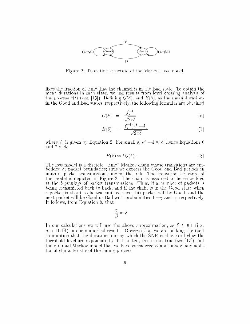
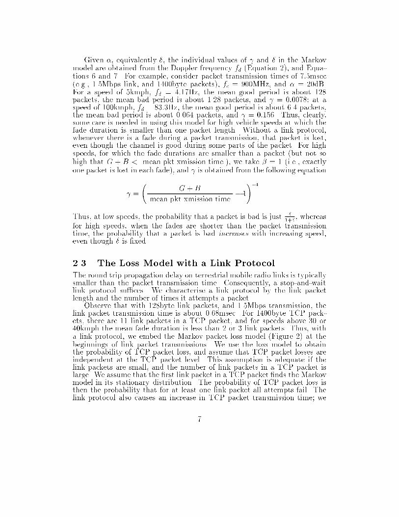
(1−γ) (1−β)Figure 2: Transition structure of the Markov loss model.�xes the fraction of time that the channel is in the Bad state. To obtain themean durations in each state, we use results from level crossing analysis ofthe process r(t) (see, [15]). De�ning G(�), and B(�), as the mean durationsin the Good and Bad states, respectively, the following formulas are obtainedG(�) = f�1dp2�� (6)B(�) = f�1d (e� � 1)p2�� (7)where fd is given by Equation 2. For small �, e� � 1 � �, hence Equations 6and 7 yield B(�) � �G(�): (8)The loss model is a discrete \time" Markov chain whose transitions are em-bedded at packet boundaries; thus we express the Good and Bad periods inunits of packet transmission time on the link. The transition structure ofthe model is depicted in Figure 2. The chain is assumed to be embeddedat the beginnings of packet transmissions. Thus, if a number of packets isbeing transmitted back to back, and if the chain is in the Good state whena packet is about to be transmitted then this packet will be Good, and thenext packet will be Good or Bad with probabilities 1� and , respectively.It follows, from Equation 8, that � � �In our calculations we will use the above approximation, as � � 0:1 (i.e.,� > 10dB) in our numerical results. Observe that we are making the tacitassumption that the durations during which the SNR is above or below thethreshold level are exponentially distributed; this is not true (see [17]), butthe minimal Markov model that we have considered cannot model any addi-tional characteristic of the fading process.6

Given �, equivalently �, the individual values of and � in the Markovmodel are obtained from the Doppler frequency fd (Equation 2), and Equa-tions 6 and 7. For example, consider packet transmission times of 7:5msec(e.g., 1.5Mbps link, and 1400byte packets), fc = 900MHz, and � = 20dB.For a speed of 5kmph, fd = 4:17Hz, the mean good period is about 128packets, the mean bad period is about 1.28 packets, and = 0:0078; at aspeed of 100kmph, fd = 83:3Hz, the mean good period is about 6.4 packets,the mean bad period is about 0.064 packets, and = 0:156. Thus, clearly,some care is needed in using this model for high vehicle speeds at which thefade duration is smaller than one packet length. Without a link protocol,whenever there is a fade during a packet transmission, that packet is lost,even though the channel is good during some parts of the packet. For highspeeds, for which the fade durations are smaller than a packet (but not sohigh that G + B < mean pkt xmission time ), we take � = 1 (i.e., exactlyone packet is lost in each fade), and is obtained from the following equation = G +Bmean pkt xmission time � 1!�1Thus, at low speeds, the probability that a packet is bad is just �1+� , whereasfor high speeds, when the fades are shorter than the packet transmissiontime, the probability that a packet is bad increases with increasing speed,even though � is �xed.2.3 The Loss Model with a Link ProtocolThe round trip propagation delay on terrestrial mobile radio links is typicallysmaller than the packet transmission time. Consequently, a stop-and-waitlink protocol su�ces. We characterise a link protocol by the link packetlength and the number of times it attempts a packet.Observe that with 128byte link packets, and 1.5Mbps transmission, thelink packet transmission time is about 0.68msec. For 1400byte TCP pack-ets, there are 11 link packets in a TCP packet, and for speeds above 30 or40kmph the mean fade duration is less than 2 or 3 link packets. Thus, witha link protocol, we embed the Markov packet loss model (Figure 2) at thebeginnings of link packet transmissions. We use the loss model to obtainthe probability of TCP packet loss, and assume that TCP packet losses areindependent at the TCP packet level. This assumption is adequate if thelink packets are small, and the number of link packets in a TCP packet islarge. We assume that the �rst link packet in a TCP packet �nds the Markovmodel in its stationary distribution. The probability of TCP packet loss isthen the probability that for at least one link packet all attempts fail. Thelink protocol also causes an increase in TCP packet transmission time; we7

use the link level Markov loss model to obtain the in ated mean TCP packettransmission time.Let N denote the maximum number of attempts of a link packet; andL denote the number of link packets in a TCP packet. Recalling that theMarkov process is embedded at the beginnings of link packet transmissions,we de�nepn = Probfat least 1 out of n link packets fails, given that the initial stateis Goodgq(k)n = Probfat least 1 out of n link packets fails, given that the �rst linkpacket has already had k(< N) bad attempts and the initial state isBadgp = Probfa TCP packet is bad gAssuming that the �rst link packet in a TCP packet �nds the Markov processin its stationary distribution, we havep = � + �pL + + �q0LThe values of pn; 1 � n � L and q(k)n ; 1 � n � L; 0 � k � N � 1 areeasily obtained from the following equations by recursive substitution, withthe boundary conditions: p1 = 0, q(N�1)n = 1; 1 � n � N , and q(k)1 =(1� �)((N�1)�k); 0 � k � (N � 1). For n > 1 and 0 � k < N � 1pn = (1� )pn�1 + q(0)n�1q(k)n = �pn + (1� �)q(k+1)nFor obtaining the mean e�ective TCP packet transmission time, taking intoaccount the link retransmissions, de�neln = mean number of link packets that will be sent for transmitting a TCPpacket of length n link packets, given that the state at the beginningis Goodm(k)n = mean number of link packets that will be sent for transmitting a TCPpacket of length n link packets, given that k link packets have alreadybeen sent for the �rst link packet and the current state is Badl = mean number of link packets that will be sent for transmitting a TCPpacket of length L link packets 8

As for the loss probability, we havel = � + � lL + + �m0LWith the boundary conditions l1 = 1 and m(N�1)1 = 1, we have the followingequations, for n � 1 and 0 � k < N � 1,m(k)n = 1 + (1 � �)m(k+1)n + �lnln = 1 + (1 � )ln�1 + m(0)n�1m(N�1)n = 1 + (1 � �)m(0)n�1 + �ln�1These equations can also be solved recursively.3 TCP Window AdaptationAt any time t there is a lower window edge A(t), which means that all datanumbered up to, and including, A(t)� 1 has been transmitted and acknowl-edged. The transmitter can send data numbered A(t) onwards. There is alsothe transmitter's congestion window W (t), which, at time t, is the maximumamount of data that the transmitter is permitted to send, starting from A(t).Under normal data transfer, A(t) has nondecreasing sample paths, whereasthe adaptive window mechanism causes W (t) to increase or decrease, butnever exceed Wmax. The receipt of an ack packet that acknowledges somedata will cause a jump in A(t) equal to the amount of data acknowledged,but the change in W (t) would depend on the particular version of TCP andthe state of the congestion control process.At the transmitter, round-trip time measurements of some packets areused to obtain a running estimate of the packet round-trip time (rtt) on theconnection. Each time a new packet is transmitted, the transmitter starts atimer and resets the already running transmission timer, if any. The timer isset for a round-trip time-out (rto) value that is derived from the rtt estimationprocedure. Whenever a time-out occurs, retransmission is initiated fromthe next packet after the last acknowledged packet (i.e., from the sequencenumber A(t)). It is important to note that the TCP transmitter processmeasures time and sets timeouts only in multiples of a timer granularity;for example, BSD UNIX based systems have a timer granularity of 500ms.Further, there is a minimum timeout duration of 2 or 3 timer \ticks" inmost implementations. We will see, in the analysis, that coarse timers havea signi�cant impact on TCP performance. For details on rtt estimation, andthe setting of rto values, see [5] or [18].9

The following basic window adaptation procedure [8] is common to allthe TCP versions; our description follows that of [12]. At all times t thefollowing are de�ned for all the protocol versions:W (t) = the transmitter's congestion window at time tWth(t) = the slow-start threshold at time tThe evolution of these processes is triggered by acks (only �rst acks; notduplicate acks) and timeouts as follows.1. If W (t) < Wth(t), each ack from the receiver causes W (t) to be incre-mented by 1. This is called the slow start phase.2. If W (t) � Wth(t), each ack from the receiver causes W (t) to be incre-mented by 1W (t). This is called the congestion avoidance phase.3. If timeout occurs at the transmitter, at epoch t, W (t+) is set to 1,Wth(t+) is set to lW (t)2 m, and the transmitter begins retransmissionfrom the packet after the last packet acknowledged.Note that the transmissions after a timeout always start with the �rstlost packet. We will call the \window" of packets transmitted from the lostpacket onwards, but before retransmission starts as the loss window.If a packet is lost, then the ack number from the receiver will cease tobe advanced, and the transmitter at the LAN host will continue sendingpackets until the current window is exhausted, or a packet gets through tothe receiver and an ack is received.. The last packet transmitted will have atimeout associated with it; in TCP-OldTahoe, retransmission will start onlyupon the expiry of this timer. Later versions of TCP, i.e., Tahoe, Reno,and NewReno, implement a fast-retransmit scheme. Observe that, even if apacket is lost, if subsequent packets get through, the receiver will continueto send back acks, but the \expected packet" number is not incremented. Ifseveral (an integer parameter K, e.g., 3) such \duplicate" acks are receivedat the LAN host, then it can assume that the loss is a random loss, and notdue to congestion. When the number of duplicate acks received reaches thethreshold K, then the packet next expected by the receiver is retransmitted.A complicated recovery phase then follows. In particular, in TCP Tahoe [6]if the transmitter receives the Kth duplicate ack at time t, before the timerexpires, then the transmitter behaves as if a timeout has occurred and beginsretransmission, with W (t+) and Wth(t+) as given by the basic algorithm.10

4 TCP Throughput Analysis with the MarkovLoss ModelAssume that, at t = 0 the connection starts with W (0) = 1 and Wth(0) =lWmax2 m, where Wmax is the maximum window limit set by the receiver; thisusually depends on the receiver's bu�er size (typical values are 32Kbytes or64Kbytes, i.e., several 10's of TCP packets). The protocol starts at time 0in slow start. Let `1 be the epoch at which the �rst packet loss occurs, andlet U1 =W (`1). As described above, timeout or fast recovery follows, and atsome later epoch transmission resumes with the �rst lost packet. If this epoch�nds the wireless channel in its Bad state, then a loss occurs immediately, thetimeout is doubled, and the next cycle starts with W = 1 and Wth = 2, theminimum value of Wth ([18]). No successful packet is sent in such a period.Hence, we merge such periods, if any, into the recovery period of the previouscycle. Thus at the beginning of the next cycle, denoted by t1, the channelis in the Good state. Again an epoch `2 can be identi�ed at which the �rstloss occurs in this transmission cycle. For k � 1, let tk denote the kth epochat which a new transmission cycle starts as described above. For k � 1,we call the interval (tk�1; tk] the kth cycle. In the kth cycle, let `k be theepoch at which the �rst packet is lost in the cycle (this is an end of a packettransmission epoch from the router). Further, for k � 1, let Uk = W (`k)denote the transmitter's window size at which packet loss takes place. Wetake U0 = Wmax. Since the �rst packet transmitted in each cycle is alwaysgood, the state space of the process fUkg is f2; 3; : : : ;Wmaxg.If the �rst retransmission after a recovery period �nds the channel in thegood state, then for TCP-OldTahoe and Tahoe, the value of Uk determinesthe values of W (t+k ) and Wth(t+k ), according to W (t+k ) = 1 and Wth(t+k ) =lUk2 ; mWe know that at the beginning of the transmission of the packet that islost, the channel is in the Bad state. It is thus clear that the evolution of thecongestion window process after the �rst loss epoch in the kth cycle dependsonly on the value of Uk; thus the process fUkg is a discrete time Markovchain over the state space f2; : : : ;Wmaxg. We can obtain the stationarydistribution of this chain. Note that a more complex analysis ensues if lossescan occur in either state of the channel.The mean number of packets successfully transmitted in each cycle, beforethe �rst lost packet, is just 1 . When a loss occurs at the lossy link, therewould be some packets queued in the lossy link transmitter, and the TCPtransmitter at the LAN host will continue sending packets till the congestionwindow (Uk) is exhausted (even if fast-retransmit is implemented, by the time3 duplicate acks are received, a fast sender would already have exhausted thewindow). Some of the packets that are transmitted on the lossy link, after11

the �rst lost packet, will get through, and will not need to be resent. Wedenote the mean number of such packets as residual good.Thus, for each TCP version, we have a Markov renewal reward process[20], embedded at the epochs t0; t1; t2; : : :, the reward being the number ofgood packets put through in each cycle. Then the throughput T is given byT = 1 + residual goodmean cycle duration (9)With a link protocol, and high vehicle speeds, we assume a Bernoulli lossmodel at the TCP packet level. Hence, for this case the analysis in [10] carriesthrough directly, after accounting for the fact that TCP packet transmissiontimes are longer.We will assume that the minimum timeout is large compared to the othertime scales in the local network; this is true for the numerical parametersthat we used in [10] (0.75sec minimum timeout, as in BSD, and 7.5msecpacket transmission time). Then, if the loss in a cycle is followed by atimeout, we assume that the beginning of the next cycle �nds the Markov lossprocess in its stationary distribution. This is always the case for OldTahoe,since it recovers only after a timeout. In the case of Tahoe, however, if fastretransmission takes place then we need to know the state of the Markov lossprocess at the beginning of the next cycle.The following analysis also assumes that the LAN host can transmit muchfaster than the wireless link. Hence, during the packet transmission periods ina cycle, the wireless link is assumed to be continuously busy. This assumptionfacilitates the carrying over of the channel state from one packet to the next.4.1 Analysis of the Markov Chain fUkgOwing to the above viewpoint, the transition probabilities of fUkg are slightlydi�erent from those in [10]. For M 2 f2; : : : ;Wmaxg, de�ne�M = Probfthe next cycle starts withWth = dM2 e, given that the loss windowin this cycle is Mg�M = Probfthe next cycle is forced to start with Wth = 2, owing to ad-ditional timeouts, given that the loss window in this cycle is M (=1� �M)gFollowing the development in [10] we can now write down the transitionprobabilities. Given that Uk =M 2 f2; : : : ;Wmaxg (and m := max(2; lM2 m)),12

recalling the Markov loss model, and writing = 1� , de�ne two transitionprobability matrices P and Q as follows:pM;j = 8>>><>>>: (j�1)�1 2 � j � m� 1 d(k)�1(1� m+k) j = m+ k,0 � k � (Wmax � 1�m) d(Wmax�m)�1 j =WmaxqM;j = p3;j(= p2;j = p4;j) for 2 � j � Wmaxwhere d(k) = (k + 1)((m� 1) + k2 )Note that P corresponds to the case in which the next cycle starts withWth = dM2 e, and Q corresponds to the case in which the next cycle is forcedto start with Wth = 2. Finally, we de�ne the vector� = (�2; : : : ; �Wmax);and then the transition probability matrix of fUkg is written asdiag(�)P + (I � diag(�))Q; (10)where I is the (Wmax � 1) � (Wmax � 1) identity matrix.The matrices P and Q are common to the OldTahoe and Tahoe versionswith the same values of Wmax and Markov loss model transition probabilities and �; as shown below � depends on and � for both OldTahoe andTahoe.OldTahoe: Since we assume that after a timeout the Markov channel modelis found in its stationary distribution, for M 2 f2; : : : ;Wmaxg,�M = � + � = 1� �MTahoe: De�ne, for M 2 f2; : : : ;Wmaxg,�M = Probfthe good transmission period in a cycle is followed by fast re-transmission, if the loss window is Mg�(G)M = Probfthe good transmission period in a cycle is followed by fast trans-mission, and at this epoch the channel is in the Good stateg13

�(B)M = Probfthe good transmission period in a cycle is followed by fasttransmission, and at this epoch the channel is in the Bad state (i.e.,�(B)M = �M � �(G)M )gIt follows that �M = �(G)M + (1� �M ) � + �Recursive equations were developed for computing �(G)M and �(B)M ; owing tolack of space here we refer the reader to the full paper [11].Thus the transition probabilities of the process fUkg can be calculatedby �rst computing �M ; �(G)M ; �(B)M , and �M , and �nally using Equation 10.The stationary distribution can be obtained by any of the many standardtechniques. Denote the stationary distribution byuM ; 2 �M � Wmax4.2 Throughput AnalysisGiven that the loss window is M , the probability that k � (M � 1) of theremaining packets get through is just g(k)M�1+b(k)M�1. Given the stationary dis-tribution uM ; 2 �M � Wmax; the mean number of good packets transmittedin a cycle after the �rst loss occurs can thus be calculated. This is what wehad called residual good (see Equation 9).We adopt the approximate mean cycle time analysis discussed in Sec-tion 4.2 of [10]. Letting Z denote the mean of the loss window distribution,we take the average window during packet transmissions to be 0.75Z, andtake the network throughput to be r = r(�; 0:75Z) (� is the LAN packettransmission rate normalised to the wireless link transmission rate), wherer(�;w) = (�(w+1)��)(�(w+1)�1) , if � 6= 1, and r(1; w) = w1+w .We assume that the timeout is always the minimum timeout (rto min) (agood assumption for a large coarse timeout and the local network situation).It follows that the recovery time due to repeated, exponentially growingtimeouts, is given by rto min1�2 +� (for this equation to hold, we must have +� <0:5).It follows that the throughput of OldTahoe is given byTOldTahoe = 1 + residual good1 r + rto min1�2 +�14

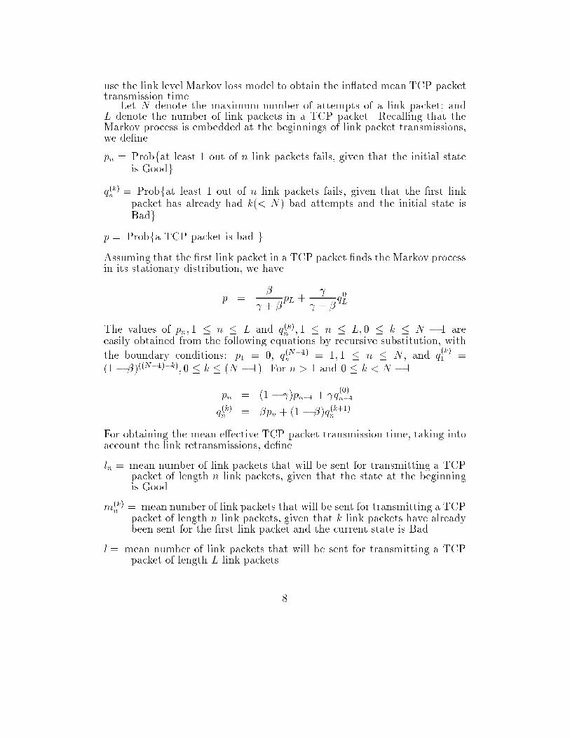
where the �rst term in the denominator is the mean time for transmitting 1 good packets. The throughput of Tahoe is given byTOldTahoe = (1 + residual good)�0@ 1 r + WmaxXM=2 uM 0@(1� �M) rto min1 � 2 +� +�(G)M Mr + �(B)M (Mr + rto min1 � 2 +� )1A1AHere the second term in the denominator is an expectation over the losswindow distribution; the term corresponding to each M is the sum of therecovery durations for three possibilities: the �rst if fast retransmit fails, thesecond if fast retransmit succeeds and the next cycle �nds the channel in theGood state, and the last if fast retransmit succeeds but the channel is foundin the Bad state, necessitating a timeout based recovery.5 Numerical Results and DiscussionWe present numerical results for the same numerical parameters as in [10].The wireless link speed is 1.5Mbps (all rates are normalised to this rate) andthe LAN host can transmit at 5 times the wireless link rate (i.e., � = 5). TheTCP packet length is 1400 bytes; i.e., its transmission time on the wirelesslink is 7.5ms; various times are normalised to this transmission time. Theminimum timeout is 750ms; or 100 packet service times on the wireless link.The fast retransmit threshold is K = 3. The carrier frequency fc is taken tobe 900Mhz.We consider DPSK (di�erential phase shift keying) modulation. In thisanalysis we do not consider forward error correction coding, or bit interleav-ing. The link protocol operates directly over the modulation scheme, andhas an error detection code. With AWGN the BER for DPSK is given by� = 0:5 exp(�EbN0 ) (11)Thus without a link protocol, in AWGN, the TCP packets can be assumedto be lost independently with probability p given byp = 1 � (1 � �)packet length (12)We will provide numerical results with AWGN for comparison purposes. In15

oldtahoe; no fading

tahoe: K=3; no fading

oldtahoe; fade=1 pkts

tahoe: K=3; fade=1 pkts

oldtahoe; fade=2 pkts

tahoe: K=3; fade=2 pkts

limit, speed−>0

10 15 20 25 30 35 400

0.1

0.2

0.3

0.4

0.5

0.6

0.7

0.8

0.9

1

Mean Signal to Noise Ratio (Eb/No dB)

Pac

ket t

hrup

ut, n

orm

alis

ed to

spe

ed o

f wire

less

link

TCP Thruput vs. Mean SNR, Wmax=24, link1= 5 x link2, min t.o.=100

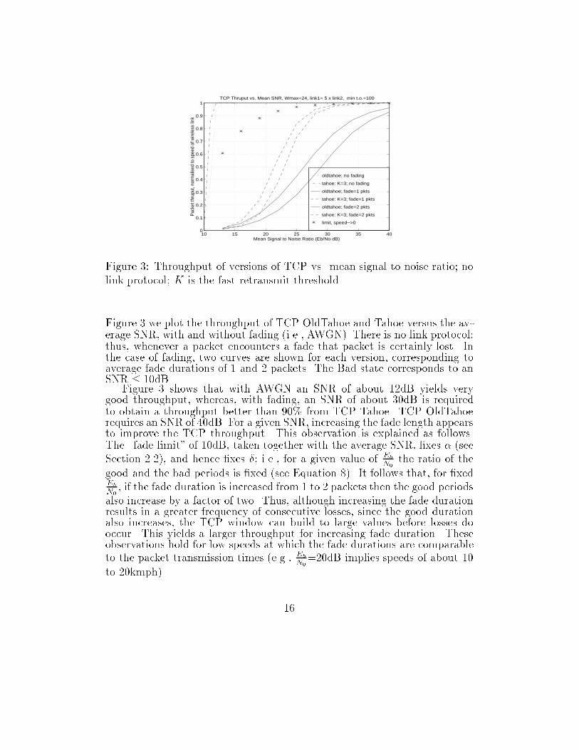
Figure 3: Throughput of versions of TCP vs. mean signal to noise ratio; nolink protocol; K is the fast retransmit threshold.Figure 3 we plot the throughput of TCP OldTahoe and Tahoe versus the av-erage SNR, with and without fading (i.e., AWGN). There is no link protocol;thus, whenever a packet encounters a fade that packet is certainly lost. Inthe case of fading, two curves are shown for each version, corresponding toaverage fade durations of 1 and 2 packets. The Bad state corresponds to anSNR � 10dB.Figure 3 shows that with AWGN an SNR of about 12dB yields verygood throughput, whereas, with fading, an SNR of about 30dB is requiredto obtain a throughput better than 90% from TCP Tahoe. TCP OldTahoerequires an SNR of 40dB. For a given SNR, increasing the fade length appearsto improve the TCP throughput. This observation is explained as follows.The \fade limit" of 10dB, taken together with the average SNR, �xes � (seeSection 2.2), and hence �xes �; i.e., for a given value of EbN0 the ratio of thegood and the bad periods is �xed (see Equation 8). It follows that, for �xedEbN0 , if the fade duration is increased from 1 to 2 packets then the good periodsalso increase by a factor of two. Thus, although increasing the fade durationresults in a greater frequency of consecutive losses, since the good durationalso increases, the TCP window can build to large values before losses dooccur. This yields a larger throughput for increasing fade duration. Theseobservations hold for low speeds at which the fade durations are comparableto the packet transmission times (e.g., EbN0=20dB implies speeds of about 10to 20kmph). 16

oldtahoe tahoe: K=3

0 20 40 60 80 100 120 140 1600.2

0.3

0.4

0.5

0.6

0.7

0.8

0.9

1

Vehicle Speed (Kmph)

Pac

ket t

hrup

ut, n

orm

alis

ed to

spe

ed o

f wire

less

link

TCP Thruput vs. Vehicle Speed, Wmax=24, link1= 5 x link2, min t.o.=100

Eb/No=30dB, fade limit=10dB

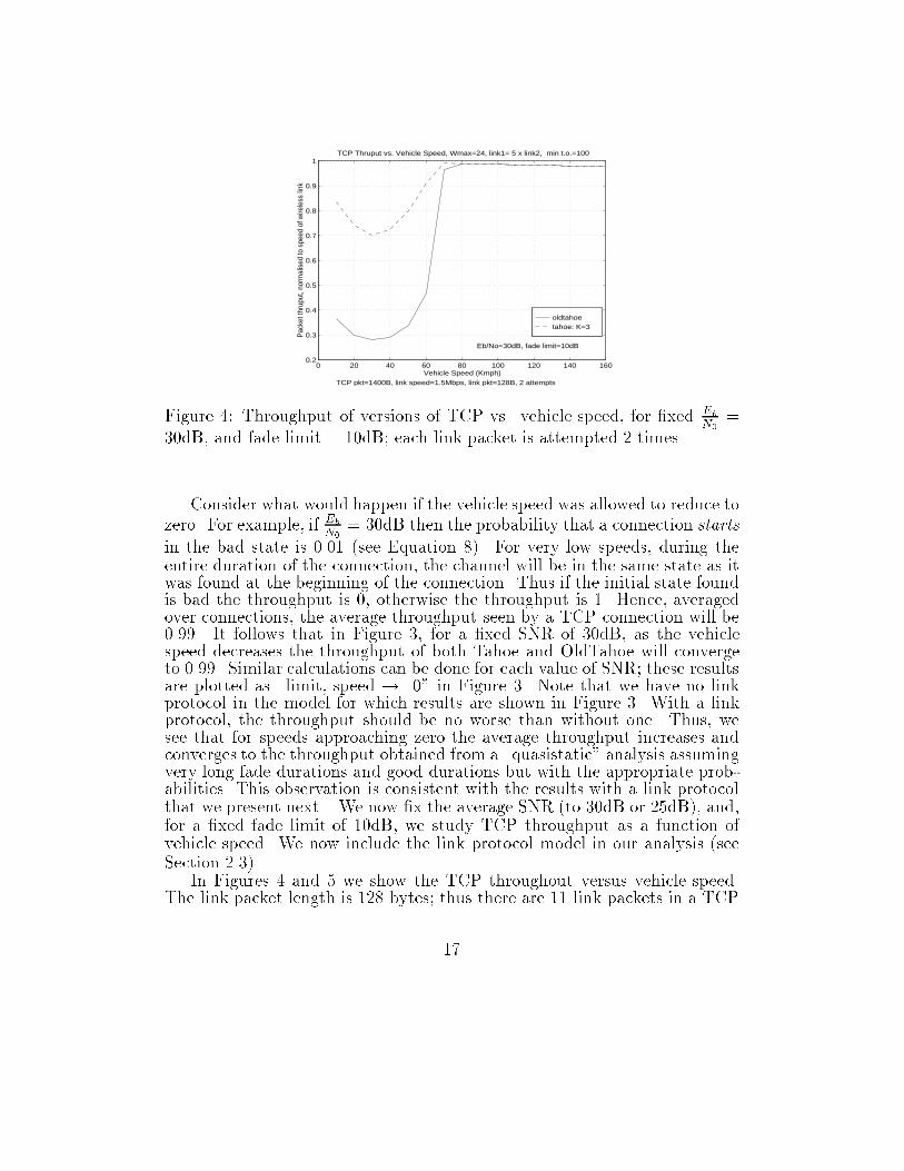
TCP pkt=1400B, link speed=1.5Mbps, link pkt=128B, 2 attemptsFigure 4: Throughput of versions of TCP vs. vehicle speed, for �xed EbN0 =30dB, and fade limit = 10dB; each link packet is attempted 2 times.Consider what would happen if the vehicle speed was allowed to reduce tozero. For example, if EbN0 = 30dB then the probability that a connection startsin the bad state is 0.01 (see Equation 8). For very low speeds, during theentire duration of the connection, the channel will be in the same state as itwas found at the beginning of the connection. Thus if the initial state foundis bad the throughput is 0, otherwise the throughput is 1. Hence, averagedover connections, the average throughput seen by a TCP connection will be0.99. It follows that in Figure 3, for a �xed SNR of 30dB, as the vehiclespeed decreases the throughput of both Tahoe and OldTahoe will convergeto 0.99. Similar calculations can be done for each value of SNR; these resultsare plotted as \limit, speed ! 0" in Figure 3. Note that we have no linkprotocol in the model for which results are shown in Figure 3. With a linkprotocol, the throughput should be no worse than without one. Thus, wesee that for speeds approaching zero the average throughput increases andconverges to the throughput obtained from a \quasistatic" analysis assumingvery long fade durations and good durations but with the appropriate prob-abilities. This observation is consistent with the results with a link protocolthat we present next. We now �x the average SNR (to 30dB or 25dB), and,for a �xed fade limit of 10dB, we study TCP throughput as a function ofvehicle speed. We now include the link protocol model in our analysis (seeSection 2.3).In Figures 4 and 5 we show the TCP throughout versus vehicle speed.The link packet length is 128 bytes; thus there are 11 link packets in a TCP17

oldtahoe tahoe: K=3

0 20 40 60 80 100 120 140 1600.55

0.6

0.65

0.7

0.75

0.8

0.85

0.9

0.95

1

Vehicle Speed (Kmph)

Pac

ket t

hrup

ut, n

orm

alis

ed to

spe

ed o

f wire

less

link

TCP Thruput vs. Vehicle Speed, Wmax=24, link1= 5 x link2, min t.o.=100

Eb/No=30dB, fade limit=10dB

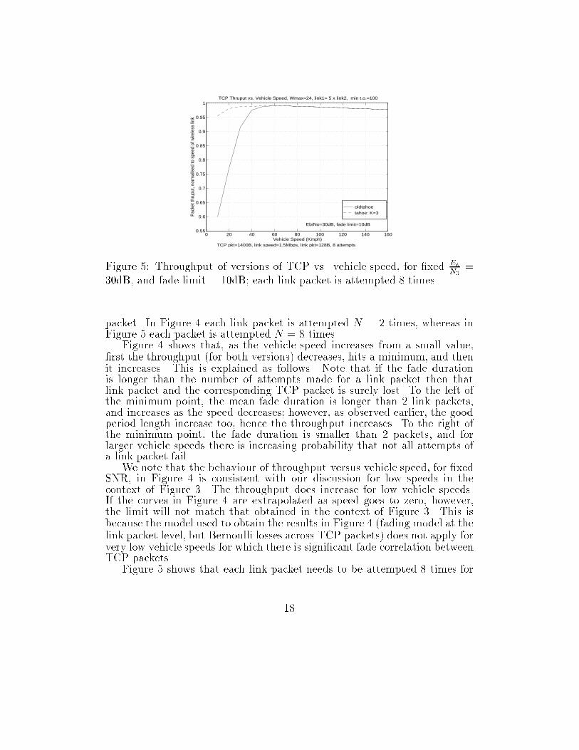
TCP pkt=1400B, link speed=1.5Mbps, link pkt=128B, 8 attemptsFigure 5: Throughput of versions of TCP vs. vehicle speed, for �xed EbN0 =30dB, and fade limit = 10dB; each link packet is attempted 8 times.packet. In Figure 4 each link packet is attempted N = 2 times, whereas inFigure 5 each packet is attempted N = 8 times.Figure 4 shows that, as the vehicle speed increases from a small value,�rst the throughput (for both versions) decreases, hits a minimum, and thenit increases. This is explained as follows. Note that if the fade durationis longer than the number of attempts made for a link packet then thatlink packet and the corresponding TCP packet is surely lost. To the left ofthe minimum point, the mean fade duration is longer than 2 link packets,and increases as the speed decreases; however, as observed earlier, the goodperiod length increase too, hence the throughput increases. To the right ofthe minimum point, the fade duration is smaller than 2 packets, and forlarger vehicle speeds there is increasing probability that not all attempts ofa link packet fail.We note that the behaviour of throughput versus vehicle speed, for �xedSNR, in Figure 4 is consistent with our discussion for low speeds in thecontext of Figure 3. The throughput does increase for low vehicle speeds.If the curves in Figure 4 are extrapolated as speed goes to zero, however,the limit will not match that obtained in the context of Figure 3. This isbecause the model used to obtain the results in Figure 4 (fading model at thelink packet level, but Bernoulli losses across TCP packets) does not apply forvery low vehicle speeds for which there is signi�cant fade correlation betweenTCP packets.Figure 5 shows that each link packet needs to be attempted 8 times for18

oldtahoe tahoe: K=3

0 20 40 60 80 100 120 140 1600.2

0.3

0.4

0.5

0.6

0.7

0.8

0.9

1

Vehicle Speed (Kmph)

Pac

ket t

hrup

ut, n

orm

alis

ed to

spe

ed o

f wire

less

link

TCP Thruput vs. Vehicle Speed, Wmax=24, link1= 5 x link2, min t.o.=100

Eb/No=25dB, fade limit=10dB

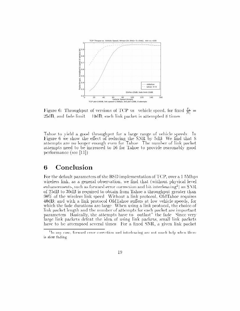
TCP pkt=1400B, link speed=1.5Mbps, link pkt=128B, 8 attemptsFigure 6: Throughput of versions of TCP vs. vehicle speed, for �xed EbN0 =25dB, and fade limit = 10dB; each link packet is attempted 8 times.Tahoe to yield a good throughput for a large range of vehicle speeds. InFigure 6 we show the e�ect of reducing the SNR by 5dB. We �nd that 8attempts are no longer enough even for Tahoe. The number of link packetattempts need to be increased to 16 for Tahoe to provide reasonably goodperformance (see [11]).6 ConclusionFor the default parameters of the BSD implementation of TCP, over a 1.5Mbpswireless link, as a general observation, we �nd that (without physical levelenhancements, such as forward error correction and bit interleaving1) an SNRof 25dB to 30dB is required to obtain from Tahoe a throughput greater than90% of the wireless link speed. Without a link protocol, OldTahoe requires40dB; and with a link protocol OldTahoe su�ers at low vehicle speeds, forwhich the fade durations are large. When using a link protocol, the choice oflink packet length and the number of attempts for each packet are importantparameters. Basically, the attempts have to \outlast" the fade. Since verylarge link packets defeat the idea of using link packets, small link packetshave to be attempted several times. For a �xed SNR, a given link packet1In any case, forward error correction and interleaving are not much help when thereis slow fading. 19

length, and a given number of link packet attempts, we �nd that throughputvaries in an interesting way with vehicle speed. At very low speeds (e.g.,pedestrian speeds) the throughput is high; it decreases with increasing ve-hicular speed until the fade durations become shorter than the number oflink packet attempts. Beyond this speed, again the throughput increases,and is limited only by the expansion of the TCP packet transmission timeowing to link-level retransmissions.Much work remains to be done to develop more comprehensive protocolanalyses even with the simple two state Markov loss model. Our analysisat present does not apply to many situations of interest; e.g., link protocolsat very low speeds, or with large link packets. The Markov model can alsobe enhanced to include a nonzero loss probability in the Good state. Boththese situations will require a more complex analysis, as the state of theMarkov loss model will need to be included in the evolution of the TCPwindow process. Such enhancements of the analysis will be fruitful as futureresearch. Other TCP versions, such as Reno and NewReno, also need to beanalysed.

20

References[1] A. Bakre and B.R. Badrinath, \I-TCP: Indirect TCP for mobile hosts,"Proc. 15th IEEE International Conf. on Distributed Computing Systems(ICDCS), pp 136-143, May 1995.[2] H. Balakrishnan, V.N. Padmanabhan, S. Seshan, and R.H. Katz, \Acomparison of mechanisms for improving TCP performance over wirelesslinks," IEEE/ACM Transactions on Networking, Vol 5, No. 6, pp 756-769, December 1997.[3] R. C�aceres, and L. Iftode, \Improving the performance of reliable trans-port protocols in mobile computing environments," IEEE Journal onSelected Areas in Communications, Vol. 13, No. 5, pp 850-857, June1995.[4] H. Chaskar, T.V. Lakshman, U. Madhow, \On the design of interfacesfor TCP/IP over wireless," Proc. IEEE MILCOM'96.[5] A. Desimone, M.C. Chuah, and O.C. Yue, \Throughput performance oftransport layer protocols over wireless LANs." Proc. IEEE Globecom'93,December 1993.[6] K. Fall, and S. Floyd, \Comparisons of Tahoe, Reno, and Sack TCP,"manuscript, ftp://ftp.ee.lbl.gov, March 1996.[7] E.N. Gilbert, \Capacity of a burst-noise channel," Bell Systems Techni-cal Journal, Vol. 39, pp. 1253-1265, Sept. 1960.[8] V. Jacobson, \Congestion avoidance and control," Proc. ACM Sigcomm'88, August 1988.[9] William C. Jakes, Microwave Mobile Communications, John Wiley andSons, New York, 1974.[10] Anurag Kumar, \Comparative performance analysis of versions ofTCP in a local network with a lossy link," WINLAB Technical Re-port No. 129, Rutgers University, October 1996. Also to appear inIEEE/ACM Transactions on Networking, Vol 6, No. 4, August 1998.[11] Anurag Kumar and J.M. Holtzman, \Comparative performance analysisof versions of TCP in a local network with a lossy link: Rayleigh Fad-ing Mobile Radio Link," WINLAB Technical Report No. 133, RutgersUniversity, November 1996. 21

[12] T.V. Lakshman and U. Madhow, \The peformance of TCP/IP fornetworks with high-bandwidth delay products and random loss,"IEEE/ACM Transactions on Networking, Vol. 5, No. 3, pp 336-351,June 1997.[13] Edward A. Lee and David G. Messerschmitt, Digital Communication,Kluwer Academic Publishers, Boston, 1988.[14] P.P. Mishra, D. Sanghi, and S.K. Tripathi, \TCP Flow Control inLossy Networks: Analysis and Enhancements," in IFIP TransactionsC-13 Computer Networks, Architecture and Applications, S.V. Ragha-van, G.v. Bochmann, and G. Pujolle (eds.), Elsevier North Holland, pp.181-193, Amsterdam, 1993.[15] J.D. Parsons, The Mobile Radio Propagation Channel, Pentech Press,London, 1992.[16] T.S. Rappaport, Wireless Communications, IEEE Press, New York,1996.[17] S.O. Rice, \Distribution of the duration of fades in radio transmission,"Bell Syst. Tech. Jour, Vol. 37, pp. 581-635, May 1958.[18] W.R. Stevens, TCP/IP Illustrated, Volume 1, Addison-Wesley, Reading,Mass., Nov. 1994.[19] Hong Shen Wang and Nader Moayeri, \Finite-state Markov channel {a useful model for radio communication channels," IEEE Transactionson Vehicular Technology, vol. 44, no. 1, pp 163-171, February 1995.[20] R.W. Wol�, Stochastic Modelling and the Theory of Queues, PrenticeHall, Englewood Cli�s, N.J., 1990.22