compactness and finite forcibility of graphons
TRANSCRIPT

arX
iv:1
309.
6695
v4 [
mat
h.C
O]
11
Mar
201
4
Compactness and finite forcibility of graphons∗
Roman Glebov† Daniel Kral’‡ Jan Volec§
Abstract
Graphons are analytic objects associated with convergent sequences ofgraphs. Problems from extremal combinatorics and theoretical computerscience led to a study of graphons determined by finitely many subgraphdensities, which are referred to as finitely forcible. Following the intuitionthat such graphons should have finitary structure, Lovasz and Szegedy con-jectured that the topological space of typical vertices of a finitely forciblegraphon is always compact. We disprove the conjecture by constructing afinitely forcible graphon such that the associated space is not compact. Inour construction, the space fails to be even locally compact.
1 Introduction
Recently, a theory of limits of combinatorial structures emerged and attractedsubstantial attention. The most studied case is that of limits of dense graphsinitiated by Borgs, Chayes, Lovasz, Sos, Szegedy and Vesztergombi [6–8, 22, 24],which we also address in this paper. A sequence of graphs is convergent if thedensity of every graph as a subgraph in the graphs contained in the sequenceconverges. A convergent sequence of graphs can be associated with an analyticobject (graphon) which is a symmetric measurable function from the unit square[0, 1]2 to [0, 1]. Graph limits and graphons are also closely related to flag alge-bras introduced by Razborov [28], which were successfully applied to numerousproblems in extremal combinatorics [1–4, 12–17, 26–30]. The development of thegraph limit theory is also reflected in a recent monograph by Lovasz [19].
∗The work leading to this invention has received funding from the European Research Coun-cil under the European Union’s Seventh Framework Programme (FP7/2007-2013)/ERC grantagreement no. 259385.
†Department of Mathematics, ETH, 8092 Zurich, Switzerland. E-mail:[email protected]. Previous affiliation: Mathematics Institute and DIMAP,University of Warwick, Coventry CV4 7AL, UK.
‡Mathematics Institute, DIMAP and Department of Computer Science, University of War-wick, Coventry CV4 7AL, UK. E-mail: [email protected].
§Mathematics Institute and DIMAP, University of Warwick, Coventry CV4 7AL, UK. E-mail: [email protected].
1

In this paper, we are concerned with finitely forcible graphons, i.e., those thatare uniquely determined (up to a natural equivalence) by finitely many subgraphdensities. Such graphons are related to uniqueness of extremal configurations inextremal graph theory as well as to other problems. For example, the classicalresult of Chung, Graham and Wilson [9] asserting that a large graph is pseudo-random if and only if the homomorphic densities of K2 and C4 are the same asin the Erdos-Renyi random graph Gn,1/2 can be cast in the language of graphonsas follows: The graphon identically equal to 1/2 is uniquely determined by ho-momorphic densities of K2 and C4, i.e., it is finitely forcible. Another examplethat can be cast in the language of finite forcibility is the asymptotic version ofthe theorem of Turan [31]: There exists a unique graphon with edge density r−1
r
and zero density of Kr+1, i.e., it is finitely forcible.The result of Chung, Graham, and Wilson [9] was generalized by Lovasz and
Sos [20] who proved that any graphon that is a stepfunction is finitely forcible.This result was further extended and a systematic study of finitely graphonswas initiated by Lovasz and Szegedy [21] who found first examples of finitelyforcible graphons that are not stepfunctions. In particular, they observed thatevery example of a finitely forcible graphon that they found had a somewhatfinite structure. Formalizing this intuition, they associated typical vertices of agraphon W with the topological space T (W ) ⊆ L1[0, 1] and observed that theirexamples of finitely forcible graphonsW have compact and at most 1-dimensionalT (W ). This led them to make the following conjectures [21, Conjectures 9 and10].
Conjecture 1 (Lovasz and Szegedy). If W is a finitely forcible graphon, thenT (W ) is a compact space.
They noted that they could not even prove that T (W ) had to be locallycompact. We give a construction of a finitely forcible graphon W such thatT (W ) fails to be locally compact, in particular, T (W ) is not compact.
Theorem 1. There exists a finitely forcible graphon WR such that the topologicalspace T (WR) is not locally compact.
They also made the following conjecture on the dimension of T (W ) of a finitelyforcible graphon W .
Conjecture 2 (Lovasz and Szegedy). If W is a finitely forcible graphon, thenT (W ) is finite dimensional.
Lovasz and Szegedy noted in their paper that they did not want to specifythe notion of dimension they had in mind. Since every non-compact subsetof L1[0, 1] has infinite Minkowski dimension, Theorem 1 also provides a partialanswer to Conjecture 2. Since we believe that other notions of dimension thanthe Minkowski dimension (e.g., the Lebesgue dimension) are more appropriate
2

measures of dimension for T (W ), we do not claim to disprove this conjecture inthis paper. We discuss Conjecture 2 in more details in Section 6, where we alsomention other applications of techniques used in this paper.
2 Notation
In this section, we introduce notation related to concepts used in this paper. Agraph is a pair (V,E) where E ⊆
(
V2
)
. The elements of V are called verticesand the elements of E are called edges . The order of a graph G is the numberof its vertices and it is denoted by |G|. The density d(H,G) of H in G is theprobability that |H| randomly chosen distinct vertices of G induce a subgraphisomorphic to H . If |H| > |G|, we set d(H,G) = 0. A sequence of graphs (Gi)i∈Nis convergent if the sequence (d(H,Gi))i∈N converges for every graph H .
We now present basic notions from the theory of dense graph limits as devel-oped in [6–8,22]. A graphon W is a symmetric measurable function from [0, 1]2 to[0, 1]. Here, symmetric stands for the property that W (x, y) =W (y, x) for everyx, y ∈ [0, 1]. A W -random graph of order k is obtained by sampling k randompoints x1, . . . , xk ∈ [0, 1] uniformly and independently and joining the i-th andthe j-th vertex by an edge with probability W (xi, xj). Since the points of [0, 1]play the role of vertices, we refer to them as to vertices of W . To simplify ournotation further, if A ⊆ [0, 1] is measurable, we use |A| for its measure. Thedensity d(H,W ) of a graph H in a graphon W is equal to the probability that aW -random graph of order |H| is isomorphic to H . Clearly, the following holds:
d(H,W ) =|H|!
|Aut(H)|
∫
[0,1]|H|
∏
(i,j)∈E(H)
W (xi, xj)∏
(i,j)6∈E(H)
(1−W (xi, xj)) dλ|H|,
where Aut(H) is the automorphism group of H . One of the key results in thetheory of dense graph limits asserts that for every convergent sequence (Gi)i∈N ofgraphs with increasing orders, there exists a graphon W (called the limit of thesequence) such that for every graph H ,
d(H,W ) = limi→∞
d(H,Gi) .
Conversely, if W is a graphon, then the sequence of W -random graphs withincreasing orders converges with probability one and its limit is W .
Every graphon can be assigned a topological space corresponding to its typicalvertices [23]. For a graphon W , define for x ∈ [0, 1] a function fWx (y) =W (x, y).For an open set A ⊆ L1[0, 1], we write AW for
{
x ∈ [0, 1], fWx ∈ A}
. Let T (W )be the set formed by the functions f ∈ L1[0, 1] such that
∣
∣UW∣
∣ > 0 for everyneighborhood U of f . The set T (W ) inherits topology from L1[0, 1]. The verticesx ∈ [0, 1] with fWx ∈ T (W ) are called typical vertices of a graphon W . Noticethat almost every vertex is typical [23].
3

Two graphons W1 and W2 are weakly isomorphic if d(H,W1) = d(H,W2)for every graph H . If ϕ : [0, 1] → [0, 1] is a measure preserving map, then thegraphon W ϕ(x, y) := W (ϕ(x), ϕ(y)) is always weakly isomorphic to W . Theopposite is true in the following sense [5]: if two graphons W1 and W2 are weaklyisomorphic, then there exist measure measure preserving maps ϕ1 : [0, 1] → [0, 1]and ϕ2 : [0, 1] → [0, 1] such that W ϕ1
1 = W ϕ2
2 almost everywhere.A graphon W is finitely forcible if there exist graphs H1, . . . , Hk such that
every graphon W ′ satisfying d(Hi,W ) = d(Hi,W′) for i ∈ {1, . . . , k} is weakly
isomorphic to W . For example, the result of Diaconis, Homes, and Janson [10]asserts that the half graphon W∆(x, y) defined as W∆(x, y) = 1 if x+ y ≥ 1, andW∆ = 0, otherwise, is finitely forcible. Also see [21] for further results.
When dealing with a finitely forcible graphon, we usually give a set of equalityconstraints that uniquely determines W instead of specifying the finitely manysubgraphs that uniquely determine W . A constraint is an equality between twodensity expressions where a density expression is recursively defined as follows:a real number or a graph H are density expressions, and if D1 and D2 are twodensity expression, then the sum D1 + D2 and the product D1 · D2 are alsodensity expressions. The value of the density expression is the value obtainedby substituting for every subgraph H its density in the graphon. Observe thatif W is a unique (up to weak isomorphism) graphon that satisfies a finite set Cof constraints, then it is finitely forcible. In particular, W is the unique (up toweak isomorphism) graphon with densities of subgraphs appearing in C equal totheir densities in W . This holds since any graphon with these densities satisfiesall constraints in C and thus it must be weakly isomorphic to W .
We extend the notion of density expressions to rooted density expressionsfollowing the ideas from the concept of flag algebras from [28]. A subgraph isrooted if it has m distinguished vertices labeled with numbers 1, . . . , m. Thesevertices are referred to as roots while the other vertices are non-roots. Two rootedgraphs are compatible if the subgraphs induced by their roots are isomorphicthrough an isomorphism mapping the roots with the same label to each other.Similarly, two rooted graphs are isomorphic if there exists an isomorphism thatmaps the i-th root of one of them to the i-th root of the other.
A rooted density expression is a density expression such that all graphs thatappear in it are mutually compatible rooted graphs. We will also speak aboutcompatible rooted density expressions to emphasize that the rooted graphs in allof them are mutually compatible. The value of a rooted density expression isdefined in the next paragraph.
Fix a rooted graph H . Let H0 be the graph induced by the roots of H , andlet m = |H0|. For a graphon W with d(H0,W ) > 0, we let the auxiliary functionc : [0, 1]m → [0, 1] denote the probability that an m-tuple (x1, . . . , xm) ∈ [0, 1]m
4

induces a copy of H0 in W respecting the labeling of vertices of H0:
c(x1, . . . , xm) =
∏
(i,j)∈E(H0)
W (xi, xj)
·
∏
(i,j)6∈E(H0)
(1−W (xi, xj))
.
We next define a probability measure µ on [0, 1]m. If A ⊆ [0, 1]m is a Borel set,then:
µ(A) =
∫
A
c(x1, . . . , xm)dλm∫
[0,1]mc(x1, . . . , xm)dλm
.
When x1, . . . , xm ∈ [0, 1] are fixed, then the density of a graph H with rootvertices x1, . . . , xm is the probability that a random sample of non-roots yields acopy of H conditioned on the roots inducing H0. Noticing that an automorphismof a rooted graph has all roots as fixed points, we obtain that this is equal to
(|H| −m)!
|Aut(H)|
∫
[0,1]|H|−m
∏
(i,j)∈E(H)\E(H0)
W (xi, xj)∏
(i,j)6∈E(H)∪(H02 )
(1−W (xi, xj))dλ|H|−m.
For different choices of x1, . . . , xm, we obtain different values. The value of arooted density expression is a random variable determined by the choice of theroots according to the probability distribution µ.
We now consider a constraint such that both left and right hand sides Dand D′ are compatible rooted density expression. Such a constraint should beinterpreted to mean that it holdsD−D′ = 0 with probability one. It can be shown(see, e.g., [28]) that the expected value of a rooted density expression D withroots inducing H0 is equal to JDK /d(H0,W ), where JDK is an ordinary densityexpression independent of W . Observe that if D and D′ are compatible rooteddensity expressions, then a graphon satisfies D = D′ if and only if it satisfiesthe (ordinary) constraint J(D −D′)× (D −D′)K = 0 . Since this allows us toexpress constraints involving rooted density expressions as ordinary constraints,we will not distinguish between the two types of constraints in what follows.
3 Partitioned graphons
In this section, we introduce partitioned graphons. Some of the methods pre-sented in this section are analogous to those used by Lovasz and Sos in [20] andby Norine [25] (see the construction in Section 6). In particular, they used sim-ilar types of arguments to specialize their constraints to parts of graphons theywere forcing as we do in this section. However, since it is hard to refer to anyparticular lemma in their paper instead of presenting a full argument, we decidedto give all details.
5
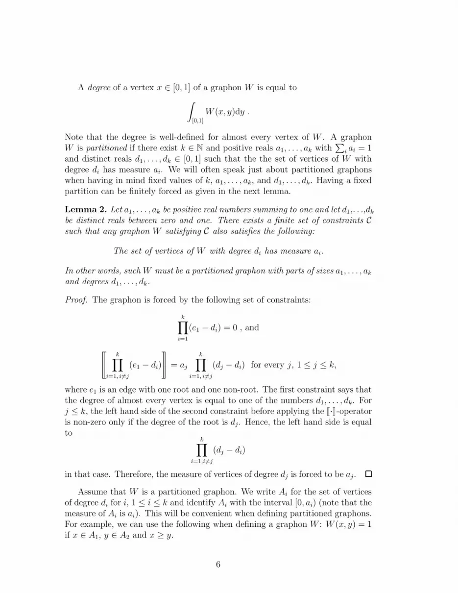
A degree of a vertex x ∈ [0, 1] of a graphon W is equal to
∫
[0,1]
W (x, y)dy .
Note that the degree is well-defined for almost every vertex of W . A graphonW is partitioned if there exist k ∈ N and positive reals a1, . . . , ak with
∑
i ai = 1and distinct reals d1, . . . , dk ∈ [0, 1] such that the the set of vertices of W withdegree di has measure ai. We will often speak just about partitioned graphonswhen having in mind fixed values of k, a1, . . . , ak, and d1, . . . , dk. Having a fixedpartition can be finitely forced as given in the next lemma.
Lemma 2. Let a1, . . . , ak be positive real numbers summing to one and let d1,. . .,dkbe distinct reals between zero and one. There exists a finite set of constraints Csuch that any graphon W satisfying C also satisfies the following:
The set of vertices of W with degree di has measure ai.
In other words, suchW must be a partitioned graphon with parts of sizes a1, . . . , akand degrees d1, . . . , dk.
Proof. The graphon is forced by the following set of constraints:
k∏
i=1
(e1 − di) = 0 , and
tk∏
i=1, i 6=j
(e1 − di)
|= aj
k∏
i=1, i 6=j
(dj − di) for every j, 1 ≤ j ≤ k,
where e1 is an edge with one root and one non-root. The first constraint says thatthe degree of almost every vertex is equal to one of the numbers d1, . . . , dk. Forj ≤ k, the left hand side of the second constraint before applying the J·K-operatoris non-zero only if the degree of the root is dj. Hence, the left hand side is equalto
k∏
i=1,i 6=j
(dj − di)
in that case. Therefore, the measure of vertices of degree dj is forced to be aj.
Assume that W is a partitioned graphon. We write Ai for the set of verticesof degree di for i, 1 ≤ i ≤ k and identify Ai with the interval [0, ai) (note that themeasure of Ai is ai). This will be convenient when defining partitioned graphons.For example, we can use the following when defining a graphon W : W (x, y) = 1if x ∈ A1, y ∈ A2 and x ≥ y.
6

H1= + =
A2 A3 A2 A3 A2 A3
Figure 1: The graph H1 from the proof of Lemma 3 if H is an edge with rootsdecorated with A2 and A3.
A graph H is decorated if its vertices are labeled with parts A1, . . . , Ak. Thedensity of a decorated graph H is the probability that randomly chosen |H|vertices induce a subgraph isomorphic to H with its vertices contained in theparts corresponding to the labels. For example, if H is an edge with verticesdecorated with parts A1 and A2, then the density of H is the density of edgesbetween A1 and A2, i.e.,
d(H,W ) =
∫
A1
∫
A2
W (x, y) dx dy .
Similarly as in the case of non-decorated graphs, we can define rooted decoratedsubgraphs. A constraint that uses (rooted or non-rooted) decorated subgraphs isreferred to as decorated.
The next lemma shows that decorated constraints are not more powerful thannon-decorated ones, and therefore they can be used to show that a graphon isfinitely forcible. We will always apply this lemma after forcing a graphon W tobe partitioned using Lemma 2. Before proving it, we introduce convention fordrawing density expressions: edges of graphs are always drawn solid, non-edgesdashed, and if two vertices are not joined, then the picture represents the sumover both possibilities. If a graph contains some roots, the roots are depicted bysquare vertices, and the non-root vertices by circles. If there are more roots fromthe same part, then the squares are rotated to distinguish the roots. Decorationsof vertices are always drawn inside vertices.
Lemma 3. Let k ∈ N, and let a1, . . . , ak be positive real numbers summing toone and let d1, . . . , dk be distinct reals between zero and one. If W is a partitionedgraphon with k parts formed by vertices of degree di and measure ai each, then anydecorated (rooted or non-rooted) constraint can be expressed as a non-decoratedconstraint, i.e., W satisfies the decorated constraint if and only if it satisfies thenon-decorated constraint.
Proof. By the argument analogous to the non-decorated case, it is enough toshow that the density of a non-rooted decorated subgraph can be expressed asa combination of densities of non-decorated subgraphs. Let H be a non-rooted
7

decorated subgraph with vertices v1, . . . , vn such that vi is labeled with a part Aℓi .Let Hi be the sum of all rooted non-decorated graphs on n + 1 vertices with nroots such that the roots induce H with the j-th vertex being vj for j = 1, . . . , nand the only non-root is always adjacent to vi (an example is given in Figure 1).We claim that the density of H is equal to the following:
|H|!
|Aut(H)|
tn∏
i=1
k∏
j=1, j 6=ℓi
Hi − djdℓi − dj
|. (1)
Indeed, if the n roots are chosen on a copy of H such that the i-th root is notfrom Aℓi, then the second product of the above expression is zero. Otherwise,the second product is one, possibly except for a set of measure zero. Hence, thevalue of (1) is exactly the probability that randomly chosen n vertices induce alabeled copy of H such that the i-th vertex belong to Aℓi .
Since decorated constraints are not more powerful than non-decorated ones,we will not distinguish between decorated and non-decorated constraints in whatfollows.
We finish this section with two lemmas that are straightforward corollaries ofLemma 3. The first one says that we can finitely force a finitely forcible graphonon a part of a partitioned graphon.
Lemma 4. Let W0 be a finitely forcible graphon. Then for every choice of k ∈ N,positive reals a1, . . . , ak summing to one, distinct reals d1, . . . , dk between zero andone, and ℓ ≤ k, there exists a finite set of constraints C such that the graphoninduced by the ℓ-th part of every graphon W that is a partitioned graphon with kparts A1, . . . , Ak of measures a1, . . . , ak and degrees d1, . . . , dk, respectively, andthat satisfies C is weakly isomorphic to W0. More precisely, there exist measurepreserving maps ϕ and ϕ′ from Aℓ to itself such that W0(ϕ(x)/|Aℓ|, ϕ(y)/|Aℓ|) =W (ϕ′(x), ϕ′(y)) for almost every x, y ∈ Aℓ.
Proof. Assume that W0 is forced by constraints of the form
d(Hi,W ) = di
for i ∈ [m]. The set C is then formed by constraints of the form
d(H ′i,W ) = a
|Hi|ℓ di ,
where H ′i is the graph Hi with all vertices decorated with Aℓ.
The second lemma asserts finite forcibility of pseudorandom bipartite graphsbetween different parts of a partitioned graphon.
8

Aℓ Aℓ Aℓ Aℓ Aℓ
Aℓ′ Aℓ′ Aℓ′
= aℓ′p = aℓ′p2 = aℓ′p
2
Figure 2: The constraints used in the proof of Lemma 5.
Lemma 5. For every choice of k ∈ N, positive reals a1, . . . , ak summing to one,distinct reals d1, . . . , dk between zero and one, ℓ, ℓ′ ≤ k, ℓ 6= ℓ′, and p ∈ [0, 1],there exists a finite set of constraints C such that every graphon W that is apartitioned graphon with k parts A1, . . . , Ak of measures a1, . . . , ak and degreesd1, . . . , dk, respectively, and that satisfies C also satisfies that W (x, y) = p foralmost every x ∈ Aℓ and y ∈ Aℓ′.
Proof. Let H be a rooted edge with the root decorated with Aℓ and the non-rootdecorated with Aℓ′, let H1 be a triangle with two roots such that the roots aredecorated with Aℓ and the non-root with Aℓ′, and let H2 be a cherry (a path onthree vertices) with two roots on its non-edge such that the roots are decoratedwith Aℓ and the non-root with Aℓ′ . The set C is formed by three constraints:H = p, H1 = p2, and H2 = p2 (also see Figure 2). These constraints imply that
∫
Aℓ′
W (x, y) dy = aℓ′p and
∫
Aℓ′
W (x, y) ·W (x′, y) dy = aℓ′p2
for almost every x, x′ ∈ Aℓ. Following the reasoning given in [21, proof of Lemma3.3], the second equation implies that
∫
Aℓ′
W 2(x, y) dy = aℓ′p2
for almost every x ∈ Aℓ. Cauchy-Schwarz inequality yields that W (x, y) = p foralmost every x ∈ Aℓ and y ∈ Aℓ′.
4 Rademacher Graphon
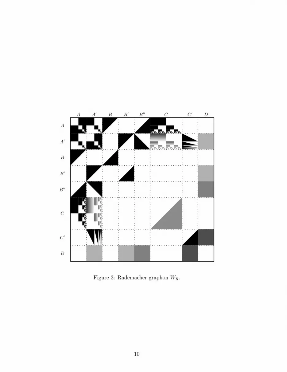
In this section, we introduce a graphon WR which we refer to as Rademachergraphon. The name comes from the fact that the adjacencies between its parts Aand C resembles Rademacher system of functions (such adjacencies also appearin [19, Example 13.30]). We establish its finite forcibility in the next section.
The graphon WR has eight parts. Instead of using A1, . . . , A8 for its parts,we use A, A′, B, B′, B′′, C, C ′ and D. All the parts except for C have the samesize a = 1/9; the size of C is 2a = 2/9.
9
A A′ B B′ B′′ C C ′ D
A
A′
B
B′
B′′
C
C ′
D
Figure 3: Rademacher graphon WR.
10

Part A A′ B B′ B′′ C C ′ DDegree 3a 3.2a a 1.2a 1.4a 1.5a 1.8a 1.6a
3/9 16/45 1/9 2/15 7/45 1/12 1/5 8/45
Table 1: The degrees of vertices in the nine parts of Rademacher graphon WR.
For x ∈ [0, 1), let us denote by [x] the smallest integer k such that x+2−k < 1.The graphon WR is then defined as follows (also see Figure 3). Let x and y betwo of its vertices. The value WR(x, y) is equal to 1 in the following cases:
• x, y ∈ A and [x/a] 6= [y/a],
• x, y ∈ A′ and [x/a] 6= [y/a],
• x ∈ A, y ∈ A′ and [x/a] = [y/a],
• x ∈ A, y ∈ B and x+ y ≤ a,
• x ∈ A, y ∈ B′′ and x+ y ≥ a,
• x ∈ A′, y ∈ B′ and x+ y ≤ a,
• x ∈ A′, y ∈ B′′ and y ≤ x,
• x, y ∈ B and x+ y ≥ a,
• x, y ∈ B′ and x+ y ≥ a,
• x ∈ A, y ∈ C and⌊
y2a
· 2[x/a]⌋
is even,
• x ∈ A′, y ∈ C ′ and (1− 2−[x/a] − x/a)2[x/a] + y/a ≤ 1,
• x, y ∈ C ′ and x+ y ≥ a.
If x ∈ A′, y ∈ C and⌊
y2a
· 2[x/a]⌋
is even, then WR(x, y) = (1−2−[x/a]−x/a)2[x/a].If x, y ∈ C, then WR(x, y) = 3/4 if x+ y ≥ 2a. If y ∈ D, then
WR(x, y) =
0.2 if x ∈ A′ or x ∈ B′,0.4 if x ∈ B′′, and0.8 if x ∈ C ′.
Finally, WR(x, y) = 0 if neither (x, y) nor the symmetric pair fall in any of thedescribed cases.
The degrees of vertices in the eight parts of Rademacher graphon WR areroutine to compute and they are given in Table 1.
We finish this section with establishing that Rademacher graphon, assumingits finite forcibility, yields Theorem 1.
11

Proposition 6. The topological space T (WR) is not locally compact.
Proof. We understand the interval [0, 1] to be partitioned by the intervals A, A′,B, B′, B′′, C, C ′ and D. Let g : [0, 1] → [0, 1] be the function defined as follows:
g(x) =
1 if x ∈ A′ ∪ B′′ ∪ C ′,0.2 if x ∈ D, and0 otherwise.
Further, let gi,δ : [0, 1] → [0, 1] for i ∈ N and δ ∈ [0, 1] be defined as follows:
gi,δ(x) =
1 if x ∈ A and [x/a] = i,1 if x ∈ A′ and [x/a] 6= i,1 if x ∈ B′ and x ≤ (1 + δ)2−i,1 if x ∈ B′′ and x ≤ 1− (1 + δ)2−i,δ if x ∈ C and ⌊2i · x/2a⌋ is even,1 if x ∈ C ′ and x/a ≤ 1− δ,0.2 if x ∈ D, and0 otherwise.
Observe that WR (x, 2/9− (1 + δ)2−i) = gi,δ(x) for every i ∈ N, δ ∈ (0, 1), andx ∈ [0, 1]. The following two estimates on the distances between g and gi,δ arestraightforward to obtain:
‖gi,δ − g‖1 = (4+2δ)·2−i+2δ9
‖gi,δ − gi′,δ′‖1 > δ+δ′
18for i 6= i′.
Hence, since gi,δ ∈ T (WR) for every i ∈ N and δ ∈ (0, 1), we obtain that g ∈T (WR). However, for every ε > 0, all the functions gi,ε with i > log2 ε
−1 are atL1-distance at most ε from g and the L1-distance between any pair of them is atleast ε/9. We conclude that no neighborhood of g in T (W ) is compact.
5 Forcing
In this section, we prove that Rademacher graphon WR is finitely forcible. Wefirst describe the set of constraints. We give names to the different kinds of theseconstraints to refer to them later. The whole set of constraints is denoted by CRin what follows.
• The partition constraints forcing the existence of eight parts of sizes as inWR and with vertex degrees as in WR (the existence of such constraintsfollows from Lemma 2),
12

(a) (b) (c) (d) (e)
(f) (g) (h) (i)
A A
B B
=0
A A
B′′ B′′
=0
A′ A′
B′ B′
=0
A′ A′
B′′ B′′
=0
A′ A′
C′ C′
=0
B B
A A A
=0B′ B′
A′ A′ A′
=0A
A A
=0
A′
A′ A′
=0
Figure 4: The monotonicity constraints.
• the zero constraints setting the edge density inside B′′ and D to zero as wellas setting the edge density between the following pairs of parts to zero: Aand C ′, A and D, A′ and B, B and B′, B and B′′, B and C, B and C ′, Band D, B′ and B′′, B′ and C, B′ and C ′, B′′ and C, B′′ and C ′, and C andD,
• the triangular constraints forcing the half graphons on B, B′, C, and C ′
with densities 1, 1, 1 and 3/4 (see Lemma 4 and [21, Corollaries 3.15 and5.2] for their existence), respectively,
• the pseudorandom constraints forcing the pseudorandom bipartite graphbetween D and the parts A′, B′, B′′, and C ′ with densities 0.2, 0.2, 0.4,and 0.8, respectively (see Lemma 5 for their existence),
• the monotonicity constraints depicted in Figure 4,
• the split constraints depicted in Figure 5,
• the infinitary constraints depicted in Figure 6, and
• the orthogonality constraints depicted in Figure 7.
The existence of the corresponding monotonicity, split, infinitary, and orthogo-nality constraints as ordinary constraints follows from Lemma 3. Also note thatthe first five monotonicity constraints imply that the graphon has values zero andone almost everywhere between the corresponding parts (also see [21, Lemma 3.3]for further details).
Theorem 7. If W is a graphon satisfying all constraints in CR, then there existmeasure preserving maps ϕ, ψ : [0, 1] → [0, 1] such that W ϕ and W ψ
R are equalalmost everywhere.
13

(a) (b) (c) (d)
(e) (f) (h)
A
A
A
A′
A
B
A
B′′
A′
A
A′
A′
A′
B′
A′
B′′
A
A′ A′
A
A′ A′
C
C
C
A
+ = 1
9+ = 1
9+ = 1
9+ = 1
9
=0 =0 + 3
2= 1
6
Figure 5: The split constraints.
(a) (b)
(c) (d)
A B A
A
A B A
A
A
A
==1/243
A′ B′ A′
A′
A′ B′ A′
A′
A′
A′
==1/243
Figure 6: The infinitary constraints.
14

(a) (b) (c)
(d)
(e)
A
C
A A
C
A A′
C
A′
C
A′
A′
A′
A′ B′
A′ A′
C
A′ A′
A′
A′ A′
B′ A′
A′ A′
A′ B′
= 1
9= 1
9=0
92
2× =
2 2
92
4× = ×
2 4
Figure 7: The orthogonality constraints.
Proof. SinceW satisfies the partition constraints contained in CR, Lemma 2 yieldsthat the interval [0, 1] can be partitioned into eight parts all but one havingmeasure 1/9 and the remaining one with measure 2/9 such that almost all verticesin the parts have degrees as those in the corresponding parts ofWR. In particular,there exists a measure preserving map ϕ : [0, 1] → [0, 1] such that the subintervalsof [0, 1] corresponding to the parts of WR are mapped to the corresponding partsof W . From now on, we use A, A′, B, B′, B′′, C, C ′, and D for the subintervalsof [0, 1] corresponding to the parts.
We next construct a measure preserving map ψ consisting of measure pre-serving maps on the intervals A, A′, B, B′, B′′, C and C ′. We choose these mapssuch that there exist decreasing functions fA : A → [0, 1] and fA′ : A′ → [0, 1],and increasing functions fB : B → [0, 1], fB′ : B′ → [0, 1], fB′′ : B′′ → [0, 1],fC : C → [0, 1] and fC′ : C ′ → [0, 1] such that the following holds almosteverywhere (the existence of such maps and functions follows from MonotoneReordering Theorem):
∀x ∈ A fA(ψ(x)) =∫
B
W ϕ(x, y)dy ∀x ∈ A′ fA′(ψ(x)) =∫
B′
W ϕ(x, y)dy
∀x ∈ B fB(ψ(x)) =∫
B
W ϕ(x, y)dy ∀x ∈ B′ fB′(ψ(x)) =∫
B′
W ϕ(x, y)dy
∀x ∈ B′′ fB′′(ψ(x)) =∫
A
W ϕ(x, y)dy
∀x ∈ C fC(ψ(x)) =∫
C
W ϕ(x, y)dy ∀x ∈ C ′ fC′(ψ(x)) =∫
C′
W ϕ(x, y)dy
15

In the rest of the proof, we establish that W ϕ and W ψR are equal almost every-
where.The pseudorandom and zero constraints in CR imply that W ϕ and W ψ
R agreealmost everywhere onD×[0, 1] and [0, 1]×D. The zero and triangular constraintsand the choice of ψ on B, B′, C, and C ′ yield the same conclusion for (B ∪B′ ∪B′′ ∪ C ∪ C ′)2, A× B′, A′ ×B, B × A′, and B′ × A.
Let us now introduce some additional notation. If x is a vertex and Y is oneof the parts, let NY (x) denote the set of y ∈ Y such that W ϕ(x, y) > 0. If xand y belong to the same part, then we write x � y iff ψ(x) ≤ ψ(y). Observethat the monotonicity constraint (a) from Figure 4 and the choice of ψ impliesthe existence of a set Z of measure zero such that NB(x
′) \ NB(x) has measurezero for x, x′ ∈ A \ Z if and only if x � x′. Since the degree of every vertexin B is 1/9, this yields that the graphons W ϕ and W ψ
R agree almost everywhereon A × B. The same reasoning applies to A′ and B′. Thus, we conclude thatthe graphons W ϕ and W ψ
R agree almost everywhere on (A ∪ A′)× (B ∪ B′) and(B ∪ B′)× (A ∪ A′).
We now apply the same reasoning using the monotonicity constraint (b) andthe split constraints (b) to deduce the existence of a zero measure set Z such thatNB′′(x) \ NB′′(x′) has measure zero if and only if x � x′ for x, x′ ∈ A \ Z. Themonotonicity constraint also imply that W ϕ has only values zero and one almosteverywhere on A×B′′. Since the measure of NB(x)∪NB′′(x) is 1/9 for almost allx ∈ A by the split constraint (b), the choice of ψ on B′′ implies that the graphonsW ϕ and W ψ
R agree almost everywhere on A × B′′. The degree regularity in B′′,the split constraint (d), and the monotonicity constraint (d), which yields thatW ϕ has values zero and one almost everywhere on A′ ×B′′, yield the agreementalmost everywhere on A′ ×B′′. Symmetrically, they agree almost everywhere onB′′ × (A ∪A′).
We now focus on the graphon W ϕ on A2. Observe first that the measure ofNB(x) is equal to ψ(x) for almost all x ∈ A. The monotonicity constraints (f)and (h) from Figure 4 imply that there exists a set Z of measure zero such thatevery point x ∈ A \Z can be associated with a unique open interval Jx ⊆ A suchthat W ϕ(x, x′) = 0 for almost every x′ ∈ ψ−1(Jx), and W
ϕ(x, x′) = 1 for almostevery x′ ∈ A\ψ−1(Jx). The interval Jx can be empty for some choice of x. Recallthat |Jx| is the measure of the interval Jx, and let J be the set of all intervals Jx,x ∈ A, with |Jx| > 0. Since the intervals in J are disjoint, the set J is equippedwith a natural linear order.
Let us now focus on the infinitary constraint (b) from Figure 6. Fix threevertices (two from A and one from B) as in the figure and let x be the left vertexfrom A. Observe that if x ∈ A is fixed, then the set of choices of the other twovertices has non-zero measure unless ψ(x) = sup Jx. The left hand side of theconstraint is equal to the measure of Jx, i.e., sup Jx− inf Jx. The right hand sideis equal to 1/9− sup Jx. We conclude that inf Jx = 1/9−2|Jx|. This implies thatthe set J is well-ordered and countable.
16

Let us write Jk for the k-th interval contained in J . Furthermore, for k ≥ 1,define
βk =2(1− 9 inf Jk+1)
1− 9 inf Jk=
2|Jk+1|
|Jk|,
and let β0 be equal to 1−9 inf J1. Note that by the observations made in the lastparagraph and since inf Jk+1 ≥ sup Jk, we obtain βk ≤ 1 for every k ≥ 0. In casethat J is finite, we define βk = 0 for k > |J |. We can now express the densityof non-edges with both end-vertices in A as
∑
J∈J
|J |2 =∞∑
k=1
(
1
9 · 2k
k−1∏
k′=0
βk′
)2
.
Since the sum is forced to be 1/243 by the infinitary constraint (a), we get that
βk = 1 for every k. This implies that for every k, Jk =(
1−2−k+1
9, 1−2−k
9
)
. In
particular, the graphons W ϕ and W ψR agree almost everywhere on A2.
The same reasoning as for A2 yields that the graphons W ϕ and W ψR agree
almost everywhere on A′2. Let J ′ be the corresponding set of intervals for A′ andlet J ′
1, J′2, . . . be their ordering. The split constraints (e) and (f) from Figure 5
imply that for almost every x ∈ A with |NA′(x)| > 0, there exists J ′ ∈ J ′
such that NA′(x)∆ψ−1(J ′) has measure zero and W ϕ(x, y) = 1 for almost everyy ∈ ψ−1(J ′).
Let x ∈ ψ−1(Jk). The split constraint (a) from Figure 5 yields that |NA′(x)| =1
2k·9. Consequently, NA′(x)∆ψ−1(J ′
k) has measure zero for almost every x ∈ψ−1(Jk) and W (x, x′) = 1 for almost every x ∈ ψ−1(Jk) and x′ ∈ ψ−1(J ′
k). Weconclude that the graphons W ϕ and W ψ
R agree almost everywhere on A×A′ andA′ ×A.
The orthogonality constraints (a) and (b) from Figure 7 yield that there existmeasurable subsets Ik ⊆ C with |Ik| = 1/9 for every k ≥ 1 such that it holdsfor almost every x ∈ ψ−1(Jk) that NC(x) differs from Ik on a set of measure zeroand W ϕ(x, y) = 1 for almost every y ∈ Ik. The construction of ψ and the splitconstraint (h) from Figure 5 imply that |NA(x)| = 1/9−ψ(x)/2 for almost everyx ∈ C. Since ψ−1(J1) \ NA(x) has measure zero for almost every x ∈ I1, we getthat |J1| ≤ |NA(x)| for almost every x ∈ I1. This implies that I1 and ψ
−1([0, 1/9])differ on a set of measure zero (also see Figure 8). Since ψ−1(J2) \ NA(x) hasmeasure zero for almost every x ∈ I2 and J1 ∩ J2 has measure zero, we get that|J1| + |J2| ≤ |NA(x)| for almost every x ∈ I1 ∩ I2 and that |J2| ≤ |NA(x)| foralmost every x ∈ I2 \ I1. This implies that I2 and ψ
−1([0, 1/18]∪ [1/9, 1/6]) differon a set of measure zero. Iterating the argument, we obtain that Ik differs fromthe preimage with respect to ψ of the set
2k−1⋃
i=1
[
2i− 2
9 · 2k−1,2i− 1
9 · 2k−1
]
17

C
0 2/9
1/9
|NA(x)|
|J1|
C
0 2/9
1/9
|NA(x) \ ψ−1(J1)|
|J2|
Figure 8: Illustration of the argument used in the proof of Theorem 7 to establishthat the graphons W ϕ and W ψ
R agree almost everywhere on A× C.
on a set of measure zero for every k ∈ N. This yields that the graphons W ϕ andW ψR agree almost everywhere on A× C.The orthogonality constraint (c) from Figure 7 implies that (C \ NC(x)) ∩
NC(x′) has measure zero for every k, almost every x ∈ A \ ψ−1(Jk), and al-
most every x′ ∈ ψ−1(J ′k). In particular, almost every x′ ∈ ψ−1(J ′
k) satisfies thatNC(x
′) \ Ik has measure zero, i.e., W ϕ(x′, y) = 0 for almost every x′ ∈ ψ−1(J ′k)
and y 6∈ Ik.We now interpret the orthogonality constraint (d) from Figure 7. Fix an
integer k ≥ 1 and a typical vertex x′ ∈ ψ−1(J ′k). The left term in the product
on the left hand side of the constraint is equal to the square of∫
C
W ϕ(x′, y)dy =∫
Ik
W ϕ(x′, y)dy . The right term in the product is equal to the square of |J ′k| =
2−[ψ(x′)/a]/9. The term on the right hand side is equal to the probability thatrandomly chosen x′′ and y satisfy x′′ ∈ A′, y ∈ B′, x′′ ∈ ψ−1(J ′
k), and ψ(x′) ≤ψ(y) < ψ(x′′). This is equal to
(
1− 2−[ψ(x′)/a] − ψ(x′)/a)2
2 · 92.
We deduce that almost every x′ ∈ ψ−1(J ′k) satisfies
∫
Ik
W ϕ(x′, y)dy =1− 2−[ψ(x′)/a] − ψ(x′)/a
9 · 2−[ψ(x′)/a]. (2)
We apply the same reasoning to the orthogonality constraint (e) from Figure 7and deduce that almost every pair of vertices x′, x′′ ∈ ψ−1(J ′
k) satisfies
92
4·
(
∫
Ik
W ϕ(x′, y)W ϕ(x′′, y)dy
)2
·(
2−[ψ(x′)/a])4
=
(
1−2−[ψ(x′)/a]−ψ(x′)/a)2
2·
(
1−2−[ψ(x′′)/a]−ψ(x′′)/a)2
2.
18

This implies (similarly as in the proof of Lemma 5) that almost every x′ ∈ ψ−1(J ′k)
satisfies:
∫
Ik
W ϕ(x′, y)2dy
1/2
=1− 2−[ψ(x′)/a] − ψ(x′)/a
3 · 2−[ψ(x′)/a]. (3)
Using Cauchy-Schwartz Inequality, we deduce from (2) and (3) (recall that |Ik| =1/9) that the following holds for almost every x′ ∈ ψ−1(J ′
k) and y ∈ Ik,
W ϕ(x′, y) =1− 2−[ψ(x′)/a] − ψ(x′)/a
2−[ψ(x′)/a].
In other words, W ϕ(x′, y) is constant almost everywhere on Ik for almost everyx′ ∈ ψ−1(J ′
k) and its value linearly decreases from one to zero almost everywhereinside ψ−1(J ′
k). Hence, the graphons W ϕ and W ψR agree almost everywhere on
A′ ×C and C ×A′ (recall that W ϕ(x′, y) = 0 for almost every pair x′ ∈ ψ−1(J ′k)
and y 6∈ Ik).The monotonicity constraint (e) from Figure 4 yields that at least one of
the sets NC′(x) \ NC′(x′) or NC′(x′) \ NC′(x) has measure zero for every k andalmost every pair x, x′ ∈ A′ and the graphon W ϕ has values zero and one almosteverywhere on A′ × C ′. This and the regularity on A′ imply that the graphonsW ϕ and W ψ
R agree almost everywhere on A′ ×C ′. Since the graphon W ϕ is zeroalmost everywhere on A×C ′ by one of the zero constraints, we have shown thatthe graphons W ϕ and W ψ
R agree almost everywhere on (A ∪ A′)× (C ∪ C ′) and(C ∪ C ′) × (A ∪ A′). Since these were the last subsets of their domains thatremained to be analyzed, we proved that the graphon W ϕ is equal to W ψ
R almosteverywhere.
Theorem 7 immediately yields the following.
Corollary 8. The graphon WR is finitely forcible.
6 Conclusion
It is quite clear that the construction of Rademacher graphon can be modified toyield other graphons W with non-compact T (W ). Some of these modificationscan yield such graphons with a smaller number of parts at the expense of makingthe argument that the graphon is finitely forcible less transparent.
In [21], Lovasz and Szegedy considered finite forcibility inside two classes offunctions. Conjecture 1, which we addressed in this paper, relates to the classthey refer to as W0. This class consists of symmetric measurable functions from[0, 1]2 to [0, 1]. A larger class referred to as W in [21] is the class containingall symmetric measurable functions from [0, 1]2 to R. It is not hard to see thatRademacher graphon WR is also finitely forcible inside this larger class. Also
19

note that stronger constraints involving multigraphs were used in [21] but wehave used only constraints involving simple graphs in this paper.
In [19], an analogue of the space T (W ) with respect to the following metricis also considered. If f, g ∈ L1[0, 1], then
dW (f, g) :=
∫
[0,1]
∣
∣
∣
∣
∣
∣
∣
∫
[0,1]
W (x, y)(f(y)− g(y))dy
∣
∣
∣
∣
∣
∣
∣
dx .
However, the appropriate closure of T (W ) always form a compact space [19,Corollary 13.28].
As mentioned in Section 1, Rademacher graphon WR also provides a par-tial answer to [21, Conjecture 10] in the sense that the Minkowski dimension ofT (WR) is infinite. However, the dimension is finite when several other notionsof dimension are considered. For instance, its Lebesgue dimension is only one.In [11], the first two authors and Klimosova disprove Conjecture 2 in a more con-vincing way: they construct a finitely forcible graphonW such that a subspace ofT (W ) is homeomorphic to [0, 1]∞. The construction is also based on partitionedgraphons used in this paper.
We finish by presenting a construction of a finitely forcible graphonWd with apart of T (Wd) positive measure isomorphic to [0, 1]d; the construction is analogousto one found earlier by Norine [25]. Fix a positive integer d. We construct agraphon Wd with 2d+ 2 parts A, B1, . . . , B2d, and C, each of size (2d+ 2)−1. Ifx, y ∈ Bi, then Wd(x, y) = 1 if x + y ≥ (2d + 2)−1, i.e., Wd is the half graphonon each B2
i . If x ∈ Bi and y ∈ C, then Wd(x, y) = Wd(y, x) = i/4d. Fix nowa measure preserving map ϕ from [0, 1] to [0, 1]d. If x ∈ A and y ∈ Bi, i ≤ d,then Wd(x, y) =Wd(y, x) = 1 if ϕ((2d+ 2)x)i ≥ (2d+ 2)y. Finally, if x ∈ A andy ∈ Bi, i ≥ d+ 1, then Wd(x, y) = Wd(y, x) = 1 if 1− ϕ((2d+ 2)x)i ≥ (2d+ 2)y.The graphon Wd is equal to zero for other pairs of vertices. Clearly, Wd is apartitioned graphon with 2d + 2 parts with vertices inside each part having thesame degree and vertices in different parts having different degrees. Using thetechniques presented in this paper and generalizing arguments from [18], one canshow that Wd is finitely forcible. Since the subspace of T (Wd) formed by typicalvertices from A is homeomorphic to [0, 1]d, the Lebesgue dimension of T (Wd) isat least d. This shows that finitely forcible graphons can have arbitrary largefinite dimension.
Acknowledgements
The authors would like to thank Jan Hladky, Tereza Klimosova, Serguei Norine,and Vojtech Tuma for their comments on the topics discussed in the paper.
20

References
[1] R. Baber: Turan densities of hypercubes, preprint available onhttp://arxiv.org/abs/1201.3587.
[2] R. Baber and J. Talbot: Hypergraphs do jump, Combinatorics, Probabilityand Computing 20 (2011), 161–171.
[3] R. Baber and J. Talbot: A solution to the 2/3 conjecture, preprint availableon http://arxiv.org/abs/1306.6202.
[4] J. Balogh, P. Hu, B. Lidicky, and H. Liu: Upper bounds on the size of 4-and 6-cycle-free subgraphs of the hypercube, to appear in European Journalon Combinatorics.
[5] C. Borgs, J.T. Chayes, and L. Lovasz: Moments of two-variable functionsand the uniqueness of graph limits, Geometric and Functional Analysis 19
(2010), 1597–1619.
[6] C. Borgs, J.T. Chayes, L. Lovasz, V.T. Sos, and K. Vesztergombi: Conver-gent sequences of dense graphs I: Subgraph frequencies, metric propertiesand testing, Advances in Mathematics 219 (2008), 1801–1851.
[7] C. Borgs, J.T. Chayes, L. Lovasz, V.T. Sos, and K. Vesztergombi: Con-vergent sequences of dense graphs II. Multiway cuts and statistical physics,Annals of Mathematics 176 (2012), 151–219.
[8] C. Borgs, J. Chayes, L. Lovasz, V.T. Sos, B. Szegedy, and K. Vesztergombi:Graph limits and parameter testing, in: Proceedings of the 38rd Annual ACMSymposium on the Theory of Computing (STOC), ACM, New York, 2006,261–270.
[9] F.R.K. Chung, R.L. Graham, and R.M.Wilson: Quasi-random graphs, Com-binatorica 9 (1989), 345–362.
[10] P. Diaconis, S. Holmes, and S. Janson: Threshold graph limits and randomthreshold graphs, Internet Mathematics 5 (2009), 267–318.
[11] R. Glebov, T. Klimosova, and D. Kral’: Infinite dimensional finitely forciblegraphon, in preparation.
[12] R. Glebov, D. Kral’, J. Volec: A problem of Erdos and Sos on 3-graphs,preprint available on http://arxiv.org/abs/1303.7372.
[13] A. Grzesik: On the maximum number of five-cycles in a triangle-free graph,Journal of Combinatorial Theory, Series B, 102 (2012), 1061–1066.
21

[14] H. Hatami, J. Hladky, D. Kral’, S. Norine, and A. Razborov: Non-three-colorable common graphs exist, Combinatorics, Probability and Computing21 (2012), 734–742.
[15] H. Hatami, J. Hladky, D. Kral’, S. Norine, and A. Razborov: On the numberof pentagons in triangle-free graphs, Journal of Combinatorial Theory, SeriesA, 120 (2013), 722–732.
[16] D. Kral’, C.-H. Liu, J.-S. Sereni, P. Whalen, and Z. Yilma: A new bound forthe 2/3 conjecture, Combinatorics, Probability and Computing 22 (2013),384–393.
[17] D. Kral’, L. Mach, and J.-S. Sereni: A new lower bound based on Gro-movs method of selecting heavily covered points, Discrete & ComputationalGeometry 48 (2012), 487–498.
[18] D. Kral’, O. Pikhurko: Quasirandom permutations are characterized by 4-point densities, Geometric and Functional Analysis 23 (2013), 570–579.
[19] L. Lovasz: Large networks and graph limits, AMS, Providence, RI,2012.
[20] L. Lovasz and V.T. Sos: Generalized quasirandom graphs, Journal of Com-binatorial Theory, Series B, 98 (2008), 146–163.
[21] L. Lovasz and B. Szegedy: Finitely forcible graphons, Journal of Combina-torial Theory, Series B, 101 (2011), 269–301.
[22] L. Lovasz and B. Szegedy: Limits of dense graph sequences, Journal ofCombinatorial Theory, Series B, 96 (2006), 933–957.
[23] L. Lovasz and B. Szegedy: Regularity partitions and the topology ofgraphons, in: I. Barany, J. Solymosi (eds.): An Irregular Mind. Szemeredi is70, Springer J. Bolyai Mathematical Society, 2010, 415–446.
[24] L. Lovasz and B. Szegedy: Testing properties of graphs and functions, IsraelJournal of Mathematics 178 (2010), 113–156.
[25] S. Norine: private communication.
[26] O. Pikhurko and A. Razborov: Asymptotic structure of graphswith the minimum number of triangles, preprint available onhttp://arxiv.org/abs/1204.2846.
[27] O. Pikhurko and E.R. Vaughan: Minimum number of k-cliques ingraphs with bounded independence number, preprint available onhttp://arxiv.org/abs/1203.4393.
22
[28] A. Razborov: Flag algebras, Journal of Symbolic Logic 72 (2007), 1239–1282.
[29] A. Razborov: On the minimal density of triangles in graphs, Combinatorics,Probability and Computing 17 (2008), 603–618.
[30] A. Razborov: On 3-hypergraphs with forbidden 4-vertex configurations,SIAM Journal on Discrete Mathematics 24 (2010), 946–963.
[31] P. Turan: On an extremal problem in graph theory, Matematikai es FizikaiLapok 48 (1941), 436–452. [in Hungarian] (Also see: On the theory of graphs,Colloquium Mathematicum 3 (1954), 19–30.)
23