Combining path-breaking with bidirectional nonequilibrium simulations to improveefficiency in free energy calculationsEdoardo Giovannelli, Cristina Gellini, Giangaetano Pietraperzia, Gianni Cardini, and Riccardo Chelli

Citation: The Journal of Chemical Physics 140, 064104 (2014); doi: 10.1063/1.4863999 View online: http://dx.doi.org/10.1063/1.4863999 View Table of Contents: http://scitation.aip.org/content/aip/journal/jcp/140/6?ver=pdfcov Published by the AIP Publishing Articles you may be interested in Path-breaking schemes for nonequilibrium free energy calculations J. Chem. Phys. 138, 214109 (2013); 10.1063/1.4808037 Density-dependent analysis of nonequilibrium paths improves free energy estimates II. A Feynman–Kacformalism J. Chem. Phys. 134, 034117 (2011); 10.1063/1.3541152 Density-dependent analysis of nonequilibrium paths improves free energy estimates J. Chem. Phys. 130, 204102 (2009); 10.1063/1.3139189 Rosenbluth-sampled nonequilibrium work method for calculation of free energies in molecular simulation J. Chem. Phys. 122, 204104 (2005); 10.1063/1.1906209 Efficient FreeEnergy Calculations by the Simulation of Nonequilibrium Processes Comput. Sci. Eng. 2, 88 (2000); 10.1109/5992.841802

This article is copyrighted as indicated in the article. Reuse of AIP content is subject to the terms at: http://scitation.aip.org/termsconditions. Downloaded to IP:

150.217.154.46 On: Wed, 20 Aug 2014 08:50:46

THE JOURNAL OF CHEMICAL PHYSICS 140, 064104 (2014)

Combining path-breaking with bidirectional nonequilibrium simulationsto improve efficiency in free energy calculations

Edoardo Giovannelli, Cristina Gellini, Giangaetano Pietraperzia, Gianni Cardini,and Riccardo Chellia)

Dipartimento di Chimica, Università di Firenze, Via della Lastruccia 3, I-50019 Sesto Fiorentino,Italy and European Laboratory for Non-linear Spectroscopy (LENS), Via Nello Carrara 1,I-50019 Sesto Fiorentino, Italy

(Received 22 November 2013; accepted 17 January 2014; published online 11 February 2014)

An important limitation of unidirectional nonequilibrium simulations is the amount of realizationsof the process necessary to reach suitable convergence of free energy estimates via Jarzynski’s re-lationship [C. Jarzynski, Phys. Rev. Lett. 78, 2690 (1997)]. To this regard, an improvement of themethod has been achieved by means of path-breaking schemes [R. Chelli et al., J. Chem. Phys. 138,214109 (2013)] based on stopping highly dissipative trajectories before their normal end, under thefounded assumption that such trajectories contribute marginally to the work exponential averages.Here, we combine the path-breaking scheme, called probability threshold scheme, to bidirectionalnonequilibrium methods for free energy calculations [G. E. Crooks, Phys. Rev. E 61, 2361 (2000);R. Chelli and P. Procacci, Phys. Chem. Chem. Phys. 11, 1152 (2009)]. The method is illustrated andtested on a benchmark system, i.e., the helix-coil transition of deca-alanine. By using path-breakingin our test system, the computer time needed to carry out a series of nonequilibrium trajectories canbe reduced up to a factor 4, with marginal loss of accuracy in free energy estimates. © 2014 AIPPublishing LLC. [http://dx.doi.org/10.1063/1.4863999]

I. INTRODUCTION

In the framework of computer simulation methods tocompute free energy differences, an interesting scenario hasbeen disclosed by two nonequilibrium work relations: theJarzynski equality1 and the Crooks fluctuation theorem.2, 3

These theorems relate the free energy difference between twothermodynamic states to the external work performed in anensemble of realizations switching the system between suchstates. The switching procedure is accomplished by a con-trol parameter correlated to some collective coordinate ofthe system (e.g., an interatomic distance, a torsional angle,and the morphing coordinate in alchemical transformations).Computer simulations based on these techniques are typicallyknown as steered simulations.4–7 In such calculations, it is ofbasic importance to improve the efficiency of path sampling,which globally increases by lowering the work dissipated dur-ing the realizations. To this aim, several approaches based onrational path sampling have been developed.8–22 The basicdifference between methods which exploit Jarzynski equal-ity and Crooks fluctuation theorem is that, while the formerinvolve nonequilibrium simulations in only one direction ofthe process, the latter make use of both directions of the pro-cess. For such a reason, these techniques are often referredto as unidirectional and bidirectional nonequilibrium meth-ods. In the last decade, several strategies based on bidirec-tional methods have been proposed to compute free energydifferences3, 23–26 and the potential of mean force (PMF) as afunction of collective variables of the system.27–31

a)Electronic mail: riccardo.chelli@unifi.it

Recently, we have introduced a method, called path-breaking, to speed up free energy calculations via nonequi-librium unidirectional Monte Carlo and molecular dynamicssimulations.32 Path-breaking is based on checking the dissi-pated work periodically during the nonequilibrium realiza-tions of the process and to stop the highly dissipative tra-jectories before their normal end. The contribution of thesebroken paths to the work exponential average is neglectedunder the founded assumption that such an average is dom-inated by paths with low dissipated work.33 As the methodrelies on estimates of the dissipated work at various check-points along the path, we need to determine somehow thefree energy at the same points during the realizations of theprocess, a task which is accomplished with a self-consistentprocedure. We remark that, once the simulation setup to re-alize pulling trajectories is given, which basically consists insetting the total number of trajectories and the pulling veloc-ity, path-breaking is not aimed at improving path samplingwith respect to the conventional approach, but rather at elimi-nating “as soon as possible” the most dissipative trajectories,which would contribute marginally to the Jarzynski equality.Two path-breaking schemes, called fixed threshold schemeand probability threshold scheme, were designed,32 whosedifference lies in the criterion to establish whether a nonequi-librium simulated trajectory must or must not be stopped at agiven check-point during the pulling path. In the fixed thresh-old scheme, an upper threshold limit for the dissipated work atthe check-points is established and trajectories exceeding thislimit are stopped. In the probability threshold scheme, an ac-ceptance probability of overcoming the check-point is insteadevaluated on the basis of the dissipated work. We have shown

0021-9606/2014/140(6)/064104/8/$30.00 © 2014 AIP Publishing LLC140, 064104-1

This article is copyrighted as indicated in the article. Reuse of AIP content is subject to the terms at: http://scitation.aip.org/termsconditions. Downloaded to IP:

150.217.154.46 On: Wed, 20 Aug 2014 08:50:46

064104-2 Giovannelli et al. J. Chem. Phys. 140, 064104 (2014)

that these schemes are comparable in accuracy, if we set simu-lation conditions that provide similar computational efficien-cies. However, as probability threshold scheme does not re-quire introduction of any arbitrary threshold for the dissipatedwork, it would be preferred in those cases (practically all) inwhich the amount of dissipation is unknown. The method wassuccessfully applied to the calculation of the PMF of deca-alanine with respect to the end-to-end collective coordinateand the PMF of two methane molecules in water solution withrespect to their mutual distance.32

In this article we extend the path-breaking machinery tobidirectional techniques. In particular, we focus on the Ben-nett method,34 generalized to nonequilibrium simulations byCrooks,3 and on a PMF estimator based on work exponen-tial averages.30 Moreover, owing to the considerable advan-tages of the probability threshold scheme with respect to thefixed threshold scheme, the present treatment is limited to theformer scheme. Following the guidelines of this study, for-mulation and implementation of a bidirectional version of thefixed threshold scheme appears straightforward. For consis-tency with Ref. 32, tests have been performed on the calcula-tion of the free energy difference between folded and unfoldedforms of deca-alanine (using the Bennett method3), as well ason the estimate of the PMF with respect to the end-to-end dis-tance of the peptide (using the bidirectional PMF estimator ofRef. 30).

The outline of the article is as follows. In Sec. II A, wedescribe the path-breaking algorithm for unidirectional sim-ulations developed in Ref. 32. In Sec. II B, we introduce atheoretical justification of path-breaking in the context ofbidirectional nonequilibrium simulations. In Sec. III, wepresent the calculation of the free energy difference betweenelongated and helix forms of deca-alanine, along with thePMF related to the end-to-end distance. Concluding remarksare given in Sec. IV.

II. THEORETICAL BACKGROUND

A. Path-breaking in unidirectionalnonequilibrium simulations

Path-breaking schemes for unidirectional nonequilibriumsimulations have been developed and tested elsewhere,32

but, to make the article self-consistent, we summarize herethe basic points of the algorithm. However, we refer toRef. 32 for a deeper illustration of theoretical and other prac-tical aspects of the method. Unidirectional nonequilibriumsimulations, also known as steered molecular dynamics orsteered Monte Carlo simulations,4–7 can be combined withthe Jarzynski equality1 to estimate the PMF along a collectivecoordinate. Nonequilibrium trajectories are realized by asso-ciating a collective coordinate ζ (q)35 with a control parameterλ through an external potential with typical harmonic form:V (q; λ) = k[ζ (q) − λ]2. During pulling realizations, the con-trol parameter λ varies from an initial value λ1 to a finalvalue λ2 and the work performed on the system is stored forsubsequent analysis.

Two path-breaking schemes, called fixed thresholdscheme and probability threshold scheme, were designed,32

whose basic difference lies in the criterion to establishwhether a nonequilibrium simulated trajectory must or mustnot be stopped at a given check-point during the pulling path.We thoroughly discussed on the convenience of using theprobability threshold scheme instead of the fixed thresholdscheme, especially due to the lower number of arbitrary pa-rameters introduced in the former approach. In this study,we therefore limit ourselves to report on results of the prob-ability threshold scheme. According to such a scheme, anonequilibrium trajectory is broken at a check-point located atλ = �, on the basis of the work dissipated as the collectivecoordinate is driven from λ1 to �. The dissipated work at the� check-point can be determined if we know the free energydifference �F� = F (�) − F (λ1),36 which can be computedby adopting a self-consistent procedure. The algorithm can besummarized as follows.

(i) Choose the collective coordinate ζ (q) associated with thecontrol parameter λ.

(ii) Sample the initial microstates from an equilibrium simu-lation by keeping fixed the control parameter to the initialvalue λ1.

Steps (i) and (ii) initialize the procedure without introducingany substantial modification to the standard approach. Nextsteps (iii) to (vii) describe how the pulling protocol is imple-mented to account for path-breaking.(iii) Choose the number and positions of the check-points

along the pathway, say �1, �2, . . . , �M.(iv) Generate a guess for the free energies �F�1 ,�F�2 ,

. . . ,�F�M, by exploiting the first few unbroken

trajectories into Jarzynski equality: exp(−β�F�n)

= N−1g

∑Ng

i=1 exp(−βWi(�n)), where β−1 = kBT is theinverse temperature, the average is over the first Ng tra-jectories, and Wi(�n) corresponds to the work performedon the system to drive the collective coordinate from theinitial value λ1 to �n during the ith trajectory. In prin-ciple, even a single trajectory can be used to get a freeenergy guess, i.e., Ng = 1.

(v) For a generic trajectory i, when a check-point �n isreached during the pulling path, the quantity p(Wi(�n))is calculated using the current value of �F�n

:

p(Wi(�n)) = min(1, e−β[Wi (�n)−�F�n ]

). (1)

(Note that Wi(�n) − �F�ncorresponds to the dissipated

work.) Then, a number r is randomly picked in the in-terval [0, 1]. If p(Wi(�n)) ≥ r then the trajectory i iscontinued toward the next check-point �n + 1 or the fi-nal step λ2. Otherwise, it is stopped and the trajectory i+ 1 is started. In both cases, the acceptance probabilityp(Wi(�n)) is recorded to update the value of �F�n

, asdescribed in step (vi).

(vi) The free energies at the check-points, i.e., �F�1 ,

�F�2 , . . . ,�F�M, are updated with established fre-

quency by exploiting all the available work values intothe following equations:

�F�n= −β−1 ln

(N−1

Nn−1∑i=1

F−1n−1,i e−βWi (�n)

), (2)

This article is copyrighted as indicated in the article. Reuse of AIP content is subject to the terms at: http://scitation.aip.org/termsconditions. Downloaded to IP:

150.217.154.46 On: Wed, 20 Aug 2014 08:50:46

064104-3 Giovannelli et al. J. Chem. Phys. 140, 064104 (2014)

F−1n−1,i =

⎡⎣n−1∏

j=1

p(Wi(�j ))

⎤⎦

−1

=n−1∏j=1

max(1, eβ[Wi (�j )−�F�j

]), (3)

where N is the number of (broken plus unbroken)trajectories realized till the current stage of the pullingcalculations and Nn − 1 is the number of trajectories thatovercome the �n − 1 check-point and hence reach the �n

check-point. We point out that for n = 1, the statementsF−1

n−1,i ≡ F−10,i = 1 and N0 = N hold because the first

check-point is surely reached by all trajectories. Notethat in Eq. (2), as well as in the following Eqs. (4), (6),(9), and (10), the trajectories have an ordered labeling,namely highest indexes are assigned to trajectories whichare broken later in the path.

(i) The procedure continues by adopting the new freeenergies, �F�1 ,�F�2 , . . . ,�F�M

, to check trajectorybreaking at step (v).

At the end of the nonequilibrium simulations, the PMF atλ, i.e., �Fλ, is computed exploiting the quantities p(Wi(�n))and Wi(λ) for each i = 1, 2, . . . , N. For convenience of pre-sentation, we report the related equation in Sec. II B (Eq. (4),or equivalently, Eq. (6)).

B. Path-breaking in bidirectionalnonequilibrium simulations

While in unidirectional nonequilibrium techniques(Sec. II A) only one of the two directions of the process isemployed, bidirectional methodologies3, 27, 30 make use of twoindependent sets of trajectories to calculate free energy differ-ences and PMFs. The first set is produced evolving the controlparameter λ from a value λ1 to a value λ2 under establishedtemporal protocol, whereas the second is produced varying λ

from λ2 to λ1 with inverted protocol. In both cases, startingsystem configurations are sampled at equilibrium, holding λ

fixed to the respective initial value (λ1 for the former and λ2

for the latter set of trajectories). The trajectories of the twosets are arbitrarily defined as forward and backward, with theonly aim of distinguishing the direction of the process, underthe assumption that λ1 < λ2. We point out that in the followingtreatment pulling simulations are supposed to be performedin the regime of stiff spring approximation,4 so that PMFwith respect to the control parameter λ can be considered tomatch the PMF with respect to the physical collective coordi-nate. Although extension of path-breaking to steered molec-ular dynamics simulations with soft driving potentials24, 37 isstraightforward, we will not address it, as it has been shownthat the best performances are usually obtained by using stiffdriving potentials.38

In the present article, we extend the probability thresh-old scheme of path-breaking technique to two bidirectionalnonequilibrium methods, specifically the Bennett method forthe calculation of free energy differences3, 34, 39 and the ap-proach to PMF of Ref. 30. Path-breaking adaptation of the

Minh-Adib PMF estimator27 is given in the supplementarymaterial,40 but the related PMFs are not reported here be-cause they almost match those obtained by means of the PMFestimator of Ref. 30.

In order to combine path-breaking with bidirectionalmethods, we must employ the unidirectional probabilitythreshold scheme32 to carry on a set of Nf forward trajecto-ries and a set of Nb backward trajectories. Before illustratingthe path-breaking relations for bidirectional methods, we needto introduce some notation to take into account the two direc-tions of the process. The work performed on the system inthe segment λ1 → λ of the ith forward trajectory is denotedas Wf,i(λ), while the work performed on the system in thesegment λ2 → λ of the jth backward trajectory is denoted asWb,j (λ). The nth check-point in forward direction and the mthcheck-point in backward direction are indicated with �f, n and�b, m, respectively.41 Without loss of generality, for the for-ward direction we consider the generic λ value in the range�f, n < λ ≤ �f, n + 1. According to the probability thresh-old scheme,32 the expression of the PMF based on forwardtrajectories is (see also Eqs. (2) and (3))

Ff (λ) = −β−1 ln

⎛⎝N−1

f

Nf,n∑i=1

F−1n,i e−βWf,i (λ)

⎞⎠ , (4)

where Nf, n is the number of forward trajectories that over-come the �f, n check-point thus reaching λ, and

F−1n,i =

⎡⎣ n∏

j=1

p(Wf,i(�f,j ))

⎤⎦

−1

, (5)

p(Wf,i(�f,j )) being computed through Eq. (1). Analogously,assuming that �b, m + 1 ≤ λ < �b, m, the expression ofthe PMF based on backward trajectories is (see also Eqs. (2)and (3))

Fb(λ) = −β−1 ln

⎛⎝N−1

b

Nb,m∑i=1

B−1m,i e−βWb,i (λ)

⎞⎠ , (6)

where Nb, m is the number of backward trajectories that over-come the �b, m check-point thus reaching λ, and

B−1m,i =

⎡⎣ m∏

j=1

p(Wb,i(�b,j ))

⎤⎦

−1

. (7)

As usual, p(Wb,i(�b,j )) comes from Eq. (1). We remark thatFf(λ) and Fb(λ) are PMF estimates based on unidirectionalnonequilibrium simulations such that Ff(λ1) = 0 and Fb(λ2)= 0. As shown in Ref. 30, the two independent free energyprofiles obtained from unidirectional forward and backwardsimulations, together with a suitable estimate of the free en-ergy difference �F = F(λ2) − F(λ1), can be combined torecover a more accurate PMF estimate as

e−βF (λ) = e−βFf (λ) + e−β�F e−βFb(λ), (8)

where Ff(λ) and Fb(λ) are the PMFs estimated by using theJarzynski equality in forward and backward directions, re-spectively. Thus, employing the path-breaking estimates of

This article is copyrighted as indicated in the article. Reuse of AIP content is subject to the terms at: http://scitation.aip.org/termsconditions. Downloaded to IP:

150.217.154.46 On: Wed, 20 Aug 2014 08:50:46

064104-4 Giovannelli et al. J. Chem. Phys. 140, 064104 (2014)

Ff(λ) and Fb(λ) into Eq. (8), we can write

e−βF (λ) = N−1f

Nf,n∑i=1

F−1n,i e−βWf,i (λ)

+ e−β�F N−1b

Nb,m∑j=1

B−1m,j e−βWb,j (λ). (9)

A suitable estimate of �F can be obtained from theBennett method,30 including only the contributions of trajec-tories which complete their path (only complete trajectoriescan actually be employed in the Bennett method39). However,as these trajectories will reach the end point with a biasedprobability due to the check-points along the path (step (v) inSec. II A), we need to reweight the contributions of the singletrajectories by the inverse of the probability of overcoming thelast check-point, i.e., F−1

Mf ,i for a generic ith forward trajectory

and B−1Mb,j

for a generic jth backward trajectory (note that Mf

and Mb correspond to the numbers of check-points in forwardand backward directions). The modified Bennett equation cantherefore be written as

Nf,Mf∑i=1

[1 + Nf

Nb

eβ(Wf,i (λ2)−�F)]−1

F−1Mf ,i

−Nb,Mb∑j=1

[1 + Nb

Nf

eβ(Wb,j (λ1)+�F)]−1

B−1Mb,j

= 0, (10)

where Nf,Mfand Nb,Mb

are the numbers of complete forwardand backward trajectories. �F can be evaluated from Eq. (10)by using an iterative procedure. We notice that the trajectoriesbroken before their natural end do not contribute to the sumsof Eq. (10). On the other side, neglecting these trajectoriesis not expected to affect the sums significantly, since break-ing arises, on average, from large dissipation, which leads tolarge exponential functions and ultimately to negligible val-ues of the terms in square brackets. We finally outline that thestandard version of the Bennett equation3, 39 corresponds toEq. (10) in which Nf,Mf

= Nf , Nb,Mb= Nb, F−1

Mf ,i = 1, and

B−1Mb,j

= 1.

III. APPLICATION OF PATH-BREAKING TOHELIX-COIL TRANSITION OF DECA-ALANINE

A. Simulation details

As stated in Sec. II, classifying one of the two pulling di-rections as forward or backward is arbitrary. In this context,trajectories that produce deca-alanine unfolding are classifiedas forward, while refolding is obtained by means of backwardtrajectories.5 We point out that forward trajectories were alsoused in Ref. 32 to test path-breaking (PB) schemes in uni-directional nonequilibrium simulations. In order to comparestandard and PB procedures under sampling protocols thatproduce identical nonequilibrium paths, PB has been applieda posteriori on full-length trajectories performed in the con-ventional way. Therefore, in the next paragraph, we discusstechnical details of standard pulling simulations, while detailson the PB application are given in the last part of the currentsubsection.

Constant-volume constant-temperature steered molecu-lar dynamics simulations of one deca-alanine molecule havebeen carried out in vacuum by enforcing a temperature of300 K through a Nosé-Hoover thermostat,42 without applica-tion of periodic boundary conditions. The force field is takenfrom Ref. 43, treating the electrostatic forces with the conven-tional Coulomb’s law. The N atom of the N-terminus residuehas been constrained to a fixed position, while the N atomof the C-terminus residue has been restrained to move alonga fixed direction by an external harmonic potential. Hence,the collective coordinate (end-to-end distance) corresponds tothe distance between the N atoms of the two terminal amidegroups. Forward pulling is accomplished by a linear time vari-ation of the end-to-end distance from 1.55 to 3.15 nm, whilethe reverse protocol is employed for the backward direction.Both types of trajectories have been realized by setting theharmonic force constant to 8 × 104 kcal mol−1 nm−2, a valuelarge enough to assume the stiff spring approximation beingvalid.4 The starting configurations of pulling trajectories wererandomly picked from two equilibrium molecular dynamicssimulations using a time-independent harmonic potential onthe end-to-end distance, with its equilibrium value fixed to1.55 and 3.15 nm for the forward and backward trajectories,respectively. The same force constant of pulling simulationshas been adopted.

All the free energy differences and PMFs reported herehave been obtained exploiting 104 forward and 104 backwardtrajectories, both directions being characterized by the samepulling velocity v. Three representative pulling velocities5

have been considered, namely v = 32, 53.3, 160 m s−1.44

In applying PB to forward and backward trajectories, thesame number Mf = Mb = M of check-points has been en-forced, namely M = 1, 4, 9. Even if the check-point positionscan be displaced arbitrarily along the pulling coordinate, herewe choose an arrangement which divides the end-to-end co-ordinate into equal segments. The free energy guess at thecheck-points is calculated using the first 5 full-length trajec-tories, while the free energies at the check-points are updatedevery 5 trajectories.

Making use of work functions along forward and back-ward trajectories, we have obtained several estimates ofthe free energy difference between folded and unfoldeddeca-alanine (by using the standard and PB-based Bennettmethod3) and of the PMF as a function of the end-to-enddistance (by using the standard and PB-based PMF estima-tor of Ref. 30). In the former case, estimates obtained withstandard and PB methods are generically indicated with �Fst

and �Fpb, respectively, while the notations Fst(λ) and Fpb(λ)are used for the PMF. To evaluate the free energy uncertainty,a block average procedure45 has been applied. In particular,for each direction of the process, we have built 20 disjointedblocks of 500 trajectories each. Then, �Fst, �Fpb, Fst(λ), andFpb(λ) have been recovered as averages of the estimates ob-tained from all possible pairs of blocks, one in forward andthe other in backward direction, for a total of 20 × 20 = 400block pairs. The error has been evaluated as twice the standarddeviation. This approach has been repeated for all the simula-tion setups, which may differ each other for pulling velocityand/or check-point number.

This article is copyrighted as indicated in the article. Reuse of AIP content is subject to the terms at: http://scitation.aip.org/termsconditions. Downloaded to IP:

150.217.154.46 On: Wed, 20 Aug 2014 08:50:46

064104-5 Giovannelli et al. J. Chem. Phys. 140, 064104 (2014)

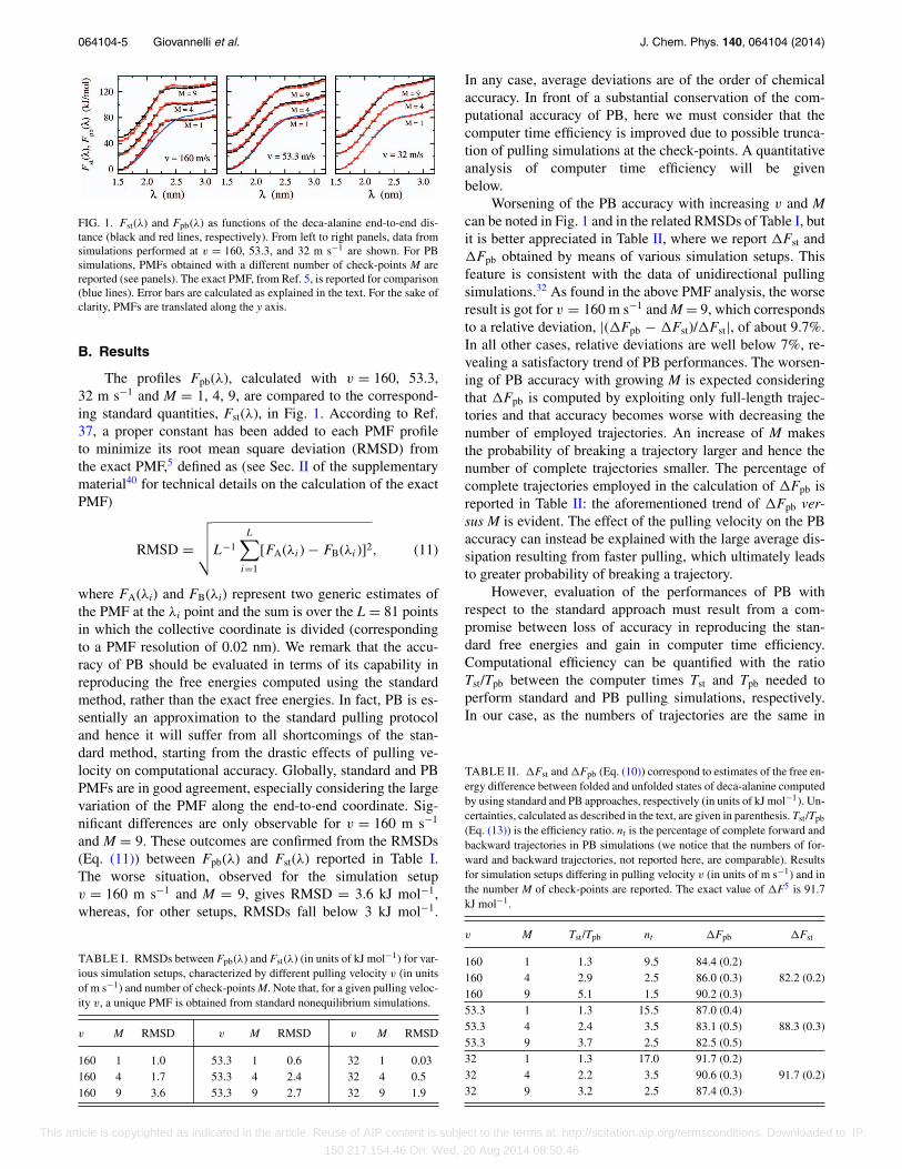
FIG. 1. Fst(λ) and Fpb(λ) as functions of the deca-alanine end-to-end dis-tance (black and red lines, respectively). From left to right panels, data fromsimulations performed at v = 160, 53.3, and 32 m s−1 are shown. For PBsimulations, PMFs obtained with a different number of check-points M arereported (see panels). The exact PMF, from Ref. 5, is reported for comparison(blue lines). Error bars are calculated as explained in the text. For the sake ofclarity, PMFs are translated along the y axis.

B. Results

The profiles Fpb(λ), calculated with v = 160, 53.3,32 m s−1 and M = 1, 4, 9, are compared to the correspond-ing standard quantities, Fst(λ), in Fig. 1. According to Ref.37, a proper constant has been added to each PMF profileto minimize its root mean square deviation (RMSD) fromthe exact PMF,5 defined as (see Sec. II of the supplementarymaterial40 for technical details on the calculation of the exactPMF)

RMSD =√√√√L−1

L∑i=1

[FA(λi) − FB(λi)]2, (11)

where FA(λi) and FB(λi) represent two generic estimates ofthe PMF at the λi point and the sum is over the L = 81 pointsin which the collective coordinate is divided (correspondingto a PMF resolution of 0.02 nm). We remark that the accu-racy of PB should be evaluated in terms of its capability inreproducing the free energies computed using the standardmethod, rather than the exact free energies. In fact, PB is es-sentially an approximation to the standard pulling protocoland hence it will suffer from all shortcomings of the stan-dard method, starting from the drastic effects of pulling ve-locity on computational accuracy. Globally, standard and PBPMFs are in good agreement, especially considering the largevariation of the PMF along the end-to-end coordinate. Sig-nificant differences are only observable for v = 160 m s−1

and M = 9. These outcomes are confirmed from the RMSDs(Eq. (11)) between Fpb(λ) and Fst(λ) reported in Table I.The worse situation, observed for the simulation setupv = 160 m s−1 and M = 9, gives RMSD = 3.6 kJ mol−1,whereas, for other setups, RMSDs fall below 3 kJ mol−1.

TABLE I. RMSDs between Fpb(λ) and Fst(λ) (in units of kJ mol−1) for var-ious simulation setups, characterized by different pulling velocity v (in unitsof m s−1) and number of check-points M. Note that, for a given pulling veloc-ity v, a unique PMF is obtained from standard nonequilibrium simulations.

v M RMSD v M RMSD v M RMSD

160 1 1.0 53.3 1 0.6 32 1 0.03160 4 1.7 53.3 4 2.4 32 4 0.5160 9 3.6 53.3 9 2.7 32 9 1.9

In any case, average deviations are of the order of chemicalaccuracy. In front of a substantial conservation of the com-putational accuracy of PB, here we must consider that thecomputer time efficiency is improved due to possible trunca-tion of pulling simulations at the check-points. A quantitativeanalysis of computer time efficiency will be givenbelow.

Worsening of the PB accuracy with increasing v and Mcan be noted in Fig. 1 and in the related RMSDs of Table I, butit is better appreciated in Table II, where we report �Fst and�Fpb obtained by means of various simulation setups. Thisfeature is consistent with the data of unidirectional pullingsimulations.32 As found in the above PMF analysis, the worseresult is got for v = 160 m s−1 and M = 9, which correspondsto a relative deviation, |(�Fpb − �Fst)/�Fst|, of about 9.7%.In all other cases, relative deviations are well below 7%, re-vealing a satisfactory trend of PB performances. The worsen-ing of PB accuracy with growing M is expected consideringthat �Fpb is computed by exploiting only full-length trajec-tories and that accuracy becomes worse with decreasing thenumber of employed trajectories. An increase of M makesthe probability of breaking a trajectory larger and hence thenumber of complete trajectories smaller. The percentage ofcomplete trajectories employed in the calculation of �Fpb isreported in Table II: the aforementioned trend of �Fpb ver-sus M is evident. The effect of the pulling velocity on the PBaccuracy can instead be explained with the large average dis-sipation resulting from faster pulling, which ultimately leadsto greater probability of breaking a trajectory.

However, evaluation of the performances of PB withrespect to the standard approach must result from a com-promise between loss of accuracy in reproducing the stan-dard free energies and gain in computer time efficiency.Computational efficiency can be quantified with the ratioTst/Tpb between the computer times Tst and Tpb needed toperform standard and PB pulling simulations, respectively.In our case, as the numbers of trajectories are the same in

TABLE II. �Fst and �Fpb (Eq. (10)) correspond to estimates of the free en-ergy difference between folded and unfolded states of deca-alanine computedby using standard and PB approaches, respectively (in units of kJ mol−1). Un-certainties, calculated as described in the text, are given in parenthesis. Tst/Tpb

(Eq. (13)) is the efficiency ratio. nt is the percentage of complete forward andbackward trajectories in PB simulations (we notice that the numbers of for-ward and backward trajectories, not reported here, are comparable). Resultsfor simulation setups differing in pulling velocity v (in units of m s−1) and inthe number M of check-points are reported. The exact value of �F5 is 91.7kJ mol−1.

v M Tst/Tpb nt �Fpb �Fst

160 1 1.3 9.5 84.4 (0.2)160 4 2.9 2.5 86.0 (0.3) 82.2 (0.2)160 9 5.1 1.5 90.2 (0.3)53.3 1 1.3 15.5 87.0 (0.4)53.3 4 2.4 3.5 83.1 (0.5) 88.3 (0.3)53.3 9 3.7 2.5 82.5 (0.5)32 1 1.3 17.0 91.7 (0.2)32 4 2.2 3.5 90.6 (0.3) 91.7 (0.2)32 9 3.2 2.5 87.4 (0.3)

This article is copyrighted as indicated in the article. Reuse of AIP content is subject to the terms at: http://scitation.aip.org/termsconditions. Downloaded to IP:

150.217.154.46 On: Wed, 20 Aug 2014 08:50:46

064104-6 Giovannelli et al. J. Chem. Phys. 140, 064104 (2014)

forward and backward directions, i.e., Nf = Nb = N, the timespent in standard pulling simulations is Tst = 2Nt, t being thetime necessary to complete a single forward or backward tra-jectory. In PB simulations, considering that Mf = Mb = M,the time Tpb is given by

Tpb = Nt

M + 1

(M∑

k=0

�f,k +M∑l=0

�b,l

), (12)

where �f, k and �b, l correspond to the fractions of forward andbackward trajectories that overcome the �f, k and �b, l check-points, respectively. Note that �f, 0 and �b, 0 refer to the firstsegments of coordinate, going from the starting point to thefirst check-point (this implies that �f, 0 = �b, 0 = 1). Thus, theefficiency ratio is given by the relation

Tst

Tpb= 2(M + 1)∑M

k=0 �f,k + ∑Ml=0 �b,l

. (13)

Just as in unidirectional pulling simulations,32 the efficiencyratio lies in the interval [1, M + 1]. The minimum efficiency,Tst/Tpb = 1, occurs as no trajectory is broken and hence PBconverges to the standard procedure (�f, k = �b, l = 1, ∀ k, l).The maximum efficiency, Tst/Tpb = M + 1, virtually occurswhen all trajectories are broken at the first check point (�f, 0

= �b, 0 = 1 and �f, k = �b, l = 0 for k > 1 and l > 1). Note,however, that the latter case is not suitable for free energycalculations, because at least one forward and one backwardtrajectory must reach its natural end. This implies that themaximum efficiency ratio for suitable calculations must be(M + 1)/(1 + M/N) [in our calculations M/N is of the orderof 0.01, so that (M + 1)/(1 + M/N) � M + 1]. The efficiencyratio is reported in Table II. It is significant that the computa-tional efficiency, which ranges from 1.3 to 5.1, becomes worseas accuracy increases and vice versa. In any case, we maysafely state that improving the computational efficiency up toa factor 3 or 4 does not lead to relevant deviations between�Fpb and �Fst.

The gain in computational efficiency obtainable with PBgives us the opportunity of decreasing the pulling velocity bykeeping unchanged the overall simulation time with respect tothe standard method. This is possible because in PB simula-tions the growth of computational time arising from loweringthe pulling velocity can be balanced by making the number ofcheck-points larger. In conditions of having similar computa-tional efficiency, i.e., Tst/Tpb � 1, which can be realized usinga proper combination of v and M in PB simulations, it is there-fore possible to compare directly the accuracies of Fst(λ) andFpb(λ) in reproducing the exact PMF. Different pulling veloci-ties for standard and PB simulations yield different simulationtimes per trajectory that we can denote as tst and tpb, respec-tively. The expression of Tst/Tpb (Eq. (13)) is thus modified asfollows:46

Tst

Tpb= tst

tpb

2(M + 1)∑Mk=0 �f,k + ∑M

l=0 �b,l

. (14)

Obviously, as Tpb depends on both v and M, it is possibleto find different combinations of these parameters such thatstandard and PB computational efficiencies are comparable,i.e., Tst/Tpb � 1. The combinations that enforce the condition

TABLE III. RMSDst and RMSDpb are the root mean square deviations be-tween the exact PMF5 and the PMFs computed by using standard and PBmethods, respectively (in units of kJ mol−1). For standard and PB methods,the reported combinations of v (in units of m s−1) and M yield comparableefficiency, as quantified by the ratio Tst/Tpb. For example, standard simula-tions performed at v = 80 m s−1 have computational efficiency compara-ble to PB simulations performed at (i) v = 32 m s−1 and M = 5 and (ii) v

= 53.3 m s−1 and M = 2 (for these simulation setups Tst/Tpb = 1.01 and1.12, respectively). Note that, for a given pulling velocity v, a unique PMF isobtained from standard nonequilibrium simulations.

Standard simulations Path-breaking simulations

v RMSDst v M RMSDpb Tst/Tpb

160 6.66 53.3 7 4.94 1.08160 6.66 32 26 2.36 1.0480 5.28 53.3 2 3.36 1.1280 5.28 32 5 1.64 1.0153.3 2.31 32 3 0.93 1.1653.3 2.31 16 13 0.16 1.01

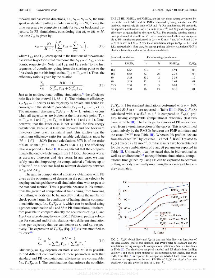
Tst/Tpb � 1 for standard simulations performed with v = 160,80, and 53.3 m s−1 are reported in Table III. In Fig. 2, Fst(λ)calculated with v = 53.3 m s−1 is compared to Fpb(λ) pro-files having comparable computational efficiency (last tworows in Table III). The better performances of PB are evidenteven from a visual inspection of the curves. This is confirmedquantitatively by the RMSDs between the PMF estimates andthe exact PMF5 (see Table III). Whereas PB profiles deviatefrom the exact PMF by less than 1 kJ mol−1, RMSD related toFst(λ) exceeds 2 kJ mol−1. Similar results have been obtainedfor the other combinations of v and M parameters reported inTable III. Ultimately, it can be stated that, in bidirectional aswell as unidirectional32 nonequilibrium simulations, compu-tational time gained by using PB can be exploited to decreasepulling velocity, eventually improving the accuracy of free en-ergy estimates.

FIG. 2. Fst(λ) (black line) and Fpb(λ) (red and blue lines) as functions ofthe deca-alanine end-to-end distance. The PMFs refer to standard and PBsimulations having comparable computational efficiency (see last two linesin Table III). The simulation setups of standard and PB simulations (pullingvelocity v and check-point number M) are reported in the legend. The exactPMF, from Ref. 5, is reported for comparison (dashed line). Error bars arecalculated as explained in the text. RMSDs of Fst(λ) and Fpb(λ) from theexact PMF are also given (in units of kJ mol−1).

This article is copyrighted as indicated in the article. Reuse of AIP content is subject to the terms at: http://scitation.aip.org/termsconditions. Downloaded to IP:

150.217.154.46 On: Wed, 20 Aug 2014 08:50:46

064104-7 Giovannelli et al. J. Chem. Phys. 140, 064104 (2014)

IV. CONCLUDING REMARKS AND PERSPECTIVES

A major shortcoming of free energy calculations vianonequilibrium molecular dynamics simulations4 is the rel-atively large number of realizations of the process (simula-tions) necessary to reach a suitable convergence of free energyor potential of mean force estimates. Such an aspect can haveimpact on the feasibility of a calculation as the time neededfor a single realization is large owing to the complexity ofthe system. This problem is particularly relevant in unidirec-tional nonequilibrium methods,1 because of the difficulty tosample pulling trajectories with low dissipated work.33 Path-breaking techniques,32 based on breaking strongly dissipativetrajectories before their natural end, give us the opportunityof a considerable computer-time saving, since only impor-tant nonequilibrium trajectories, i.e., the less dissipative, areretained.

In this article, the path-breaking variant called probabil-ity threshold scheme, applied to unidirectional steered molec-ular dynamics simulations in Ref. 32, is extended to the caseof bidirectional nonequilibrium simulations. We specificallyfocus on two relations to compute free energy: the Bennettmethod3 employed to compute the free energy difference be-tween two states and the potential of mean force estimatorbased on work exponential averages proposed in Ref. 30.Combining path-breaking with bidirectional methodologiesdoes not require execution of specific additional protocols inperforming nonequilibrium pulling simulations. These can berealized by applying the unidirectional path-breaking proce-dure independently to both forward and backward sets of tra-jectories. Reweighting relations for free energy evaluation areapplied a posteriori to the data stored during the nonequi-librium simulations. As in the unidirectional case,32 bidirec-tional adaptation of path-breaking has been tested on the es-timate of the free energy profile of deca-alanine as a functionof the end-to-end distance of the peptide, which may rangefrom a α-helix to a fully elongated conformation. Results arecompared with free energy estimates obtained from nonequi-librium standard methods in the same operating conditions.The enhancement of computer-time efficiency with respect tothe standard approach has been shown to range from a factor1.5 to 5, without significant changes in the accuracy of theresults.

An important advantage of path-breaking, also inthis bidirectional version, is the almost complete compat-ibility with most of path-sampling techniques developedin the framework of nonequilibrium simulation schemes.An example of such a compatibility has been shown inRef. 32 through the methane pulling process, which has beenrealized combining path-breaking with the configurationalfreezing approach.20, 21

We point out that, in the framework of methodologiesaimed at improving nonequilibrium path-sampling, other ef-fective strategies have been devised to eliminate highly dis-sipative trajectories. In particular, we mention the variantof the method annealed importance sampling47, 48 suppliedby trajectory-resampling.49 Although annealed importancesampling with trajectory-resampling is inherently a unidi-rectional technique in which thermal changes are realized,

extension to mechanical changes and bidirectional nonequi-librium schemes appears straightforward.

In perspective, path-breaking could be exploitedin replica exchange50–52 or serial generalized-ensemblesimulations53, 54 with trial exchanges realized by means ofnonequilibrium work simulations.55, 56 To generate a trialexchange using nonequilibrium simulations, the molecularsystem undergoes a simulation governed by a time-dependentHamiltonian that changes in a nonequilibrium fashion fromthe current Hamiltonian into the target Hamiltonian overa prescribed period of time. The probability of acceptingthe transition to the new Hamiltonian depends on the workdissipated during the nonequilibrium trial exchange. Thetime needed for these trial exchanges is the most criticalaspect of the method because, in the case of rejection of thetrial move, it would be lost. This approach is similar to thatemployed in nonequilibrium candidate Monte Carlo,57, 58 atechnique to perform equilibrium simulations which exploitsfinite-time rather than instantaneous switching moves to drivethe dynamics of important degrees of freedom. In this respect,unidirectional and bidirectional path-breaking schemes59

could be used to truncate nonequilibrium trial exchangeswhen the dissipated work exceeds a given threshold, withevident gain of computer time. Possibility of applicationof path-breaking is envisaged in both replica exchangesimulations50–52 and serial generalized-ensemble simulationswith self-consistent determination of weights.60–62 Futurestudies will be devoted to this subject.

ACKNOWLEDGMENTS

The authors are grateful to Pierluigi Cresci for techni-cal support. This work was supported by European UnionContract No. RII3-CT-2003-506350 and by the Italian Minis-tero dell’Istruzione, dell’Università e della Ricerca (No. PRIN2010-2011).

1C. Jarzynski, Phys. Rev. Lett. 78, 2690 (1997).2G. E. Crooks, J. Stat. Phys. 90, 1481 (1998).3G. E. Crooks, Phys. Rev. E 61, 2361 (2000).4S. Park and K. Schulten, J. Chem. Phys. 120, 5946 (2004).5P. Procacci, S. Marsili, A. Barducci, G. F. Signorini, and R. Chelli, J. Chem.Phys. 125, 164101 (2006).

6C. Chatelain, J. Stat. Mech.: Theor. Exp. P04011 (2007).7S. Mitternacht, S. Luccioli, A. Torcini, A. Imparato, and A. Irbäck, Bio-phys. J. 96, 429 (2009).

8F. M. Ytreberg and D. M. Zuckerman, J. Chem. Phys. 120, 10876 (2004).9S. X. Sun, J. Chem. Phys. 118, 5769 (2003).

10P. L. Geissler and C. Dellago, J. Phys. Chem. B 108, 6667 (2004).11D. Wu and D. A. Kofke, J. Chem. Phys. 122, 204104 (2005).12S. Vaikuntanathan and C. Jarzynski, Phys. Rev. Lett. 100, 190601 (2008).13T. Schmiedl and U. Seifert, Phys. Rev. Lett. 98, 108301 (2007).14W. Lechner, H. Oberhofer, C. Dellago, and P. L. Geissler, J. Chem. Phys.

124, 044113 (2006).15C. Jarzynski, Phys. Rev. E 65, 046122 (2002).16T. Z. Mordasini and J. A. McCammon, J. Phys. Chem. B 104, 360 (2000).17R. Bitetti-Putzer, W. Yang, and M. Karplus, Chem. Phys. Lett. 377, 633

(2003).18C. Oostenbrink and W. F. van Gunsteren, J. Comput. Chem. 24, 1730

(2003).19P. Nicolini and R. Chelli, Phys. Rev. E 80, 041124 (2009).20P. Nicolini, D. Frezzato, and R. Chelli, J. Chem. Theory Comput. 7, 582

(2011).21R. Chelli, J. Chem. Theory Comput. 8, 4040 (2012).

This article is copyrighted as indicated in the article. Reuse of AIP content is subject to the terms at: http://scitation.aip.org/termsconditions. Downloaded to IP:

150.217.154.46 On: Wed, 20 Aug 2014 08:50:46

064104-8 Giovannelli et al. J. Chem. Phys. 140, 064104 (2014)

22P. Nicolini, D. Frezzato, C. Gellini, M. Bizzarri, and R. Chelli, J. Comput.Chem. 34, 1561 (2013).

23M. R. Shirts and V. S. Pande, J. Chem. Phys. 122, 144107 (2005).24G. Hummer and A. Szabo, Proc. Natl. Acad. Sci. U.S.A. 98, 3658 (2001).25P. Maragakis, M. Spichty, and M. Karplus, Phys. Rev. Lett. 96, 100602

(2006).26R. Chelli, J. Chem. Phys. 130, 054102 (2009).27D. D. L. Minh and A. B. Adib, Phys. Rev. Lett. 100, 180602 (2008).28R. Chelli, S. Marsili, and P. Procacci, Phys. Rev. E 77, 031104 (2008).29E. H. Feng and G. E. Crooks, Phys. Rev. E 79, 012104 (2009).30R. Chelli and P. Procacci, Phys. Chem. Chem. Phys. 11, 1152 (2009).31T. N. Do, P. Carloni, G. Varani, and G. Bussi, J. Chem. Theory Comput. 9,

1720 (2013).32R. Chelli, C. Gellini, G. Pietraperzia, E. Giovannelli, and G. Cardini, J.

Chem. Phys. 138, 214109 (2013).33J. Gore, F. Ritort, and C. Bustamante, Proc. Natl. Acad. Sci. U.S.A. 100,

12564 (2003).34C. H. Bennett, J. Comput. Phys. 22, 245 (1976).35Here, q denotes the whole set or a subset of the atomic coordinates of the

system involved in the definition of the collective coordinate, which canbe an interatomic distance, a dihedral angle formed by covalently bondedatoms, the coordination number of an atom, etc.

36Dissipated work is defined as W (�) − �F�.37P. Nicolini, P. Procacci, and R. Chelli, J. Phys. Chem. B 114, 9546 (2010).38F. M. Ytreberg, J. Chem. Phys. 130, 164906 (2009).39M. R. Shirts, E. Bair, G. Hooker, and V. S. Pande, Phys. Rev. Lett. 91,

140601 (2003).40See supplementary material at http://dx.doi.org/10.1063/1.4863999 for the

implementation of path-breaking in the Minh-Adib potential of mean forceestimator (Sec. I) and for technical details on the calculation of the exactpotential of mean force of the deca-alanine system (Sec. II).

41Note that the numbers of check-points along the collective coordinate λ inforward and backward directions may not be identical.

42W. G. Hoover, Phys. Rev. A 31, 1695 (1985).

43A. D. MacKerell, Jr., D. Bashford, M. Bellot, R. L. Dunbrack, Jr., J.D. Evanseck, M. J. Field, S. Fisher, J. Gao, H. Guo, S. Ha, D. Joseph-McCarthy, L. Kuchnir, K. Kuczera, F. T. K. Lau, C. Mattos, S. Mich-nick, T. Ngo, D. T. Nguyen, B. Prodhom, W. E. Reiher III, B. Roux, M.Schlenkrich, J. C. Smith, R. Stote, J. Straub, M. Watanabe, J. Wiórkiewicz-Kuczera, D. Yin, and M. Karplus, J. Phys. Chem. B 102, 3586 (1998).

44These pulling velocities correspond to driven trajectories lasting 50, 30, and10 ps, respectively.

45D. M. Zuckerman and T. B. Woolf, Chem. Phys. Lett. 351, 445 (2002).46Equation (14) is obtained by setting Tst = 2ntst, while Tpb is from Eq. (12)

with t = tpb.47R. M. Neal, Stat. Comput. 11, 125 (2001).48E. Lyman and D. M. Zuckerman, J. Chem. Phys. 127, 065101 (2007).49E. Lyman and D. M. Zuckerman, J. Chem. Phys. 130, 081102 (2009).50U. H. E. Hansmann, Chem. Phys. Lett. 281, 140 (1997).51Y. Sugita and Y. Okamoto, Chem. Phys. Lett. 314, 141 (1999).52Y. Okamoto, J. Mol. Graphics Modell. 22, 425 (2004).53E. Marinari and G. Parisi, Europhys. Lett. 19, 451 (1992).54A. P. Lyubartsev, A. A. Martsinovski, S. V. Shevkunov, and P. N.

Vorontsov-Velyaminov, J. Chem. Phys. 96, 1776 (1992).55A. J. Ballard and C. Jarzynski, Proc. Natl. Acad. Sci. U.S.A. 106, 12224

(2009).56R. M. Dirks, H. Xu, and D. E. Shaw, J. Chem. Theory Comput. 8, 162

(2012).57J. P. Nilmeier, G. E. Crooks, D. D. L. Minh, and J. D. Chodera, Proc. Natl.

Acad. Sci. U.S.A. 108, E1009 (2011).58J. P. Nilmeier, G. E. Crooks, D. D. L. Minh, and J. D. Chodera, Proc. Natl.

Acad. Sci. U.S.A. 109, 9665 (2012).59In the case of nonequilibrium candidate Monte Carlo, only unidirectional

path-breaking can be used.60R. Chelli, J. Chem. Theory Comput. 6, 1935 (2010).61R. Chelli and G. F. Signorini, J. Chem. Theory Comput. 8, 830 (2012).62R. Chelli and G. F. Signorini, J. Chem. Theory Comput. 8, 2552

(2012).

This article is copyrighted as indicated in the article. Reuse of AIP content is subject to the terms at: http://scitation.aip.org/termsconditions. Downloaded to IP:

150.217.154.46 On: Wed, 20 Aug 2014 08:50:46