color classification of natural color images

Shoji Tominaga Faculty of Engineering Osaka Electro-Communication University Neyagawa, Osaka 572 Japan

Color Classification of Natural Color Images

The present article describes a color classifcation method that purtitions a color image into a set of uniform color regions. The input image data are Jirst mapped from device coordinates into the CIE L*a*b* color space, un approximately uniform perceptual color space. Colors used to represent u nuturai color itnuge are clussi- jied by means of cluster detection in the uniform color space. The basic process of color classifcation is bused on histogram analysis to detect color clusters sequentially. The principal components o j a color distribution are extracted f o r effective discrimination ojclusters. We present an algorithm jor sequential detection of color clusters in the uniform color space, and the related algorithms f o r region processing and color computation. The performance of the method is discussed in an experiment using three kinds of natural color images. 0 1992 John Wiley & Sons, Inc.

INTRODUCTION

This article describes a color classification method for partitioning a natural color image into a set of perceptually uniform color regions. The color classification algorithm accepts high-resolution color images as input and yields a new representation of the data in the form of a small set of spatial regions, each described by a single color value. The ability to classify spatial regions of an input image into a small number of uniform color regions can be useful for essential problems of color image analysis, including image segmentation and image representation.',2

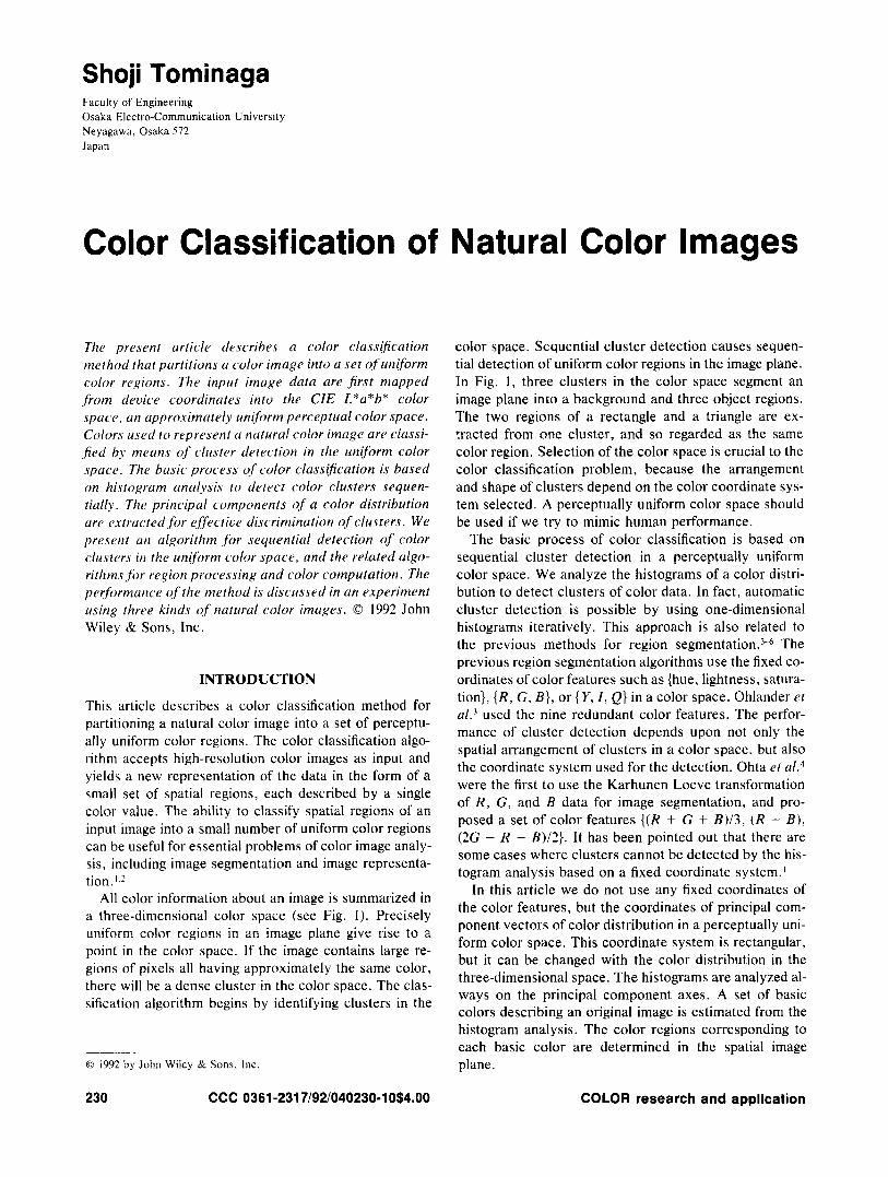
All color information about an image is summarized in a three-dimensional color space (see Fig. I) . Precisely uniform color regions in an image plane give rise to a point in the color space. If the image contains large regions of pixels all having approximately the same color, there will be a dense cluster in the color space. The classification algorithm begins by identifying clusters in the

Q I992 by John Wiley & Sons, lnc.

230 CCC 0361 -231 7/92/040230-10$4.00

color space. Sequential cluster detection causes sequential detection of uniform color regions in the image plane. In Fig. 1, three clusters in the color space segment an image plane into a background and three object regions. The two regions of a rectangle and a triangle are extracted from one cluster, and so regarded as the same color region. Selection of the color space is crucial to the color classification problem, because the arrangement and shape of clusters depend on the color coordinate system selected. A perceptually uniform color space should be used if we try to mimic human performance.

The basic process of color classification is based on sequential cluster detection in a perceptually uniform color space. We analyze the histograms of a color distribution to detect clusters of color data. In fact, automatic cluster detection is possible by using one-dimensional histograms iteratively. This approach is also related to the previous methods for region ~egmentation.~" The previous region segmentation algorithms use the fixed coordinates of color features such as (hue, lightness, satura- tion}, { R , G , B } , or { Y , I , Q} in a color space. Ohlander et ulS3 used the nine redundant color features. The performance of cluster detection depends upon not only the spatial arrangement of clusters in a color space, but also the coordinate system used for the detection. Ohta et ~ 1 . ~ were the first to use the Karhunen Loeve transformation of R , G , and B data for image segmentation, and proposed a set of color features { ( R + G + B ) / 3 , ( R - B ) , (2G - R - B)/2}. It has been pointed out that there are some cases where clusters cannot be detected by the histogram analysis based on a fixed coordinate system.'

In this article we do not use any fixed coordinates of the color features, but the coordinates of principal component vectors of color distribution in a perceptually uniform color space. This coordinate system is rectangular, but it can be changed with the color distribution in the three-dimensional space. The histograms are analyzed always on the principal component axes. A set of basic colors describing an original image is estimated from the histogram analysis. The color regions corresponding to each basic color are determined in the spatial image plane.

COLOR research and application

a* = 500[(X/Xo)”3 - ( Y/Yo)I13],

b* = 200[( Y/ yop3 - (z/zo)l/3i, ( 2 )

(3)

where the constants X o , Yo , and 2, are the tristimulus values of the standard white. This space defines a uniform metric-space representation of color so that a perceptual color difference is represented by the Euclidian distance.

A drum scanner is used for precise measurement of color pictures. The observed RGB values from the scanner are transformed into the tristimulus values. The fast transformation can be performed by a matrix multiplica- tion. Our method is summarized as follows (e.g., see Refs. 8 and 9): First, we obtain the effective reflectance (pR , p G , p s ) of the RGB values from the imaging device. The effective reflectances p, (i = R , G , B ) are defined by the ratios of reflected light intensity Zoi to incident light intensity Zi for the respective color components, namely, the normalized RGB values Zoi/Ii to a white standard. Here we express the measured color signals and the corresponding tristimulus values by three-dimensional vectors as

s = [ P R 9 P C , PSI‘, (4)

p = [ X , Y , Z ] ‘ . ( 5 )

These are column vectors, and t denotes matrix (vector) transposition. By assuming a linear relationship between s and p, the mapping is described in the form p = Ts, where T is a 3 x 3 transformation matrix. We determine the transformation matrix T based on real measurements of many color samples like Munsell color chips. Thus the approximated value of L*a*b* for each pixel of the measured image is computed from the matrix T and the above equations.

color space

image plane

FIG. 1. Color clusters and image partition.

In the subsequent sections, we first briefly describe color specification in a uniform color space. We then outline the basic process of our color classification. Next, we describe the classification method and its algorithm in detail. Finally, experimental results are shown, and feasibility of the proposed method is demonstrated.

COLOR SPECIFICATION IN A UNIFORM COLOR SPACE

Mapping of a measured image into a perceptually uniform color space is normally based on a nonlinear transformation of the observed RGB values. In this article the CIE L*a*b* color system is used as a uniform color space.’ This system approximates a uniform color space in terms of the tristimulus values X , Y , and 2. The space is pro- duced by plotting in rectangular coordinates the quanti- ties L*, a*, and b* defined by

(1) L* = 116(Y/Yo)113 - 16,

OVERVIEW OF COLOR CLASSIFICATION PROCESS

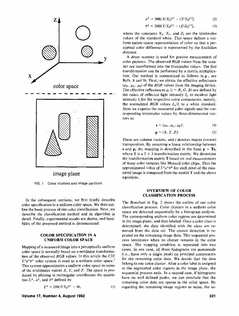
The flowchart in Fig. 2 shows the outline of our color classification process. Color clusters in a uniform color space are detected sequentially by a histogram analysis. The corresponding uniform color regions are determined in the image plane, and then labeled. Once a color class is determined, the data identified with the class are re- moved from the data set. The cluster detection is re- peated on the remaining image data. This sequential process terminates when no cluster remains in the color space. The stopping condition is separated into two cases. In one case, all three histograms are monomode (i.e., have only a single peak) on principal components for the remaining color data. We decide that the data belong to one color cluster. After a color label is assigned to the segmented color regions in the image plane, the sequential process ends. In a second case, if histograms have no well defined peaks, we can conclude that the remaining color data are sparse in the color space. By regarding the remaining image regions as noise, the se-

Volume 17, Number 4, August 1992 231

Remove labeled region from color space

Cluster remains in color space?

No

Post-processing

FIG. 2. Outline of the basic color classification process.

quential process ends. In post-processing these noisy regions are merged into spatially neighboring regions with any color label.

In the post-processing part, we first treat the remaining pixels without color labels, and then apply smoothing operation to all the segmented regions. These processes are a type of region merging. The segmented image is smoothed out by merging small noisy regions into spatially adjacent regions with small color difference. Next, representative colors are computed for each label of the classified colors. Thus we can determine a basic set of different colors, which compose an original image, and also obtain the segmented image, which consists of uniform color regions defined by the basic colors.

COLOR CLASSIFICATION ALGORITHM

Coordinate Transformation for Color Cluster Detection

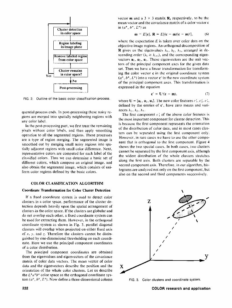
If a fixed coordinate system is used to detect color clusters in a color space, performance of the cluster detection depends heavily upon the spatial arrangement of clusters in the color space. If the clusters are globular and do not overlap each other, a fixed coordinate system can be used for extracting them. However, in the orthogonal coordinate system as shown in Fig. 3, parallel diagonal clusters will overlap when projected on either fixed axis of x, y , and t. Therefore the clusters cannot be distin- guished by one-dimensional thresholding on each coordinate. Here we use the principal component coordinates of a color distribution.

The principal component coordinates are obtained from the eigenvalues and eigenvectors of the covariance matrix of color data vectors. The mean vector of color data and the eigenvectors describe the position and the orientation of the whole color clusters. Let us describe the L*u*b* color space as the orthogonal coordinate system (a * , h*, L * ) . Now define a three-dimensional column

vector m and a 3 x 3 matrix R, respectively, to be the mean vector and the covariance matrix of a color vector c in (a* , h*, t*) as

m = E[cl, R = E[(c - m)(c - m)'], (6)

where the expectation E is taken over color data on the objective image regions. An orthogonal decomposition of R gives us the eigenvalues A l , A ? , A 3 , arranged in de- scending order ( A i 2 and the corresponding eigenvectors uI , u2, u3 . These eigenvectors are the unit vectors of the principal component axes for the given data set. Then we have a linear transformation for transform- ing the color vector c in the original coordinate system (a*, h*, L*) into a vector c' in the new coordinate system of the principal component axes. This transformation is expressed in the equation

c' = U'(c - m), (7)

where U = [u, , u2, u3]. The new color features c;, c;, c i , defined by the entries of c', have zero means and vari- ances A , , A ? , A,.

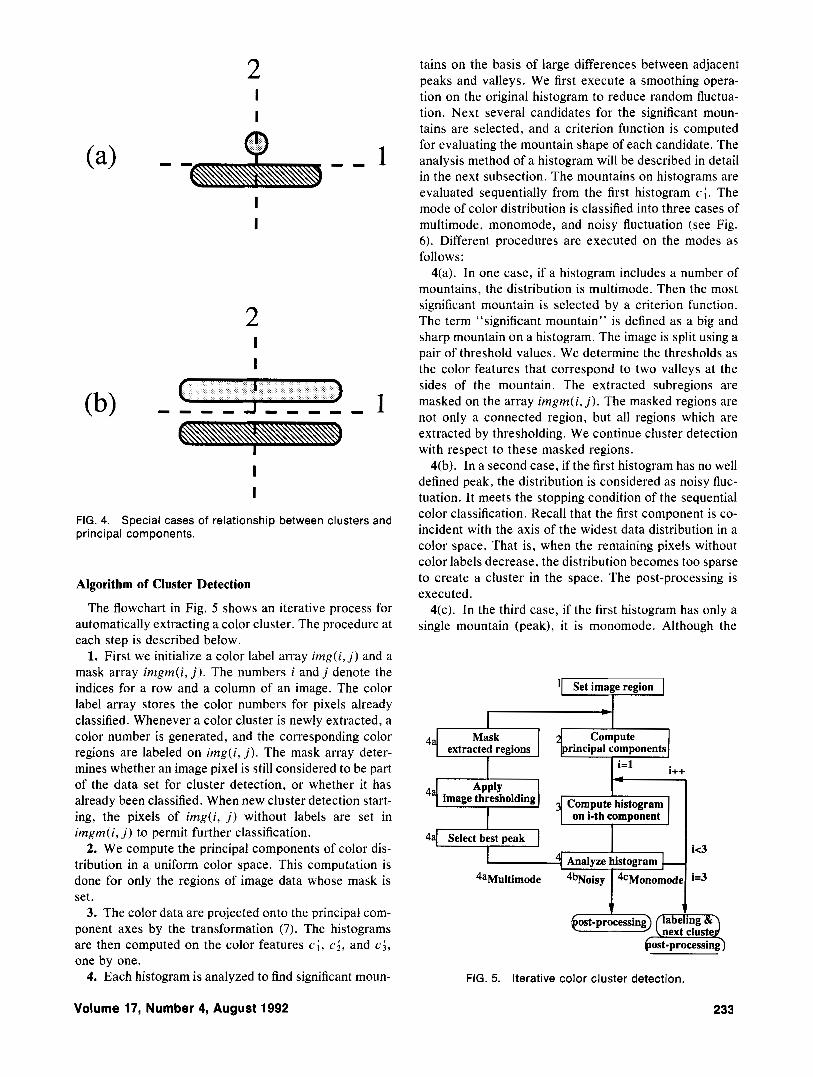
The first component c ; of the above color features is the most important component for cluster detection. This is because the first component represents the orientation of the distribution of color data, and in most cases clusters can be separated using the first component only. However, in rare cases we have to use the other component that is orthogonal to the first component. Figure 4 shows the two special cases. In both cases, two clusters cannot be separated by the first component axis, although the widest distribution of the whole clusters stretches along the first axis. Both clusters are separable by the second component axis. Therefore, in our algorithm, histograms are analyzed not only on the first component, but also on the second and third components successively.

\

Z

t / /

/ /

/ /

/

FIG. 3. Color clusters and coordinate system.

232 COLOR research and application

2 I I

2 I I

I 1

II 1

FIG. 4. Special cases of relationship between clusters and principal components.

Algorithm of Cluster Detection

The flowchart in Fig. 5 shows an iterative process for automatically extracting a color cluster. The procedure at each step is described below.

1. First we initialize a color label array img( i , j ) and a mask array irngrn(i, j ) . The numbers i and j denote the indices for a row and a column of an image. The color label array stores the color numbers for pixels already classified. Whenever a color cluster is newly extracted, a color number is generated, and the corresponding color regions are labeled on irng(i, j ) . The mask array deter- mines whether an image pixel is still considered to be part of the data set for cluster detection, or whether it has already been classified. When new cluster detection start- ing, the pixels of img(i, j ) without labels are set in imgrn(i, j ) to permit further classification.

2. We compute the principal components of color distribution in a uniform color space. This computation is done for only the regions of image data whose mask is set.

3. The color data are projected onto the principal component axes by the transformation (7). The histograms are then computed on the color features c ; , ci, and c ; , one by one.

4. Each histogram is analyzed to find significant moun-

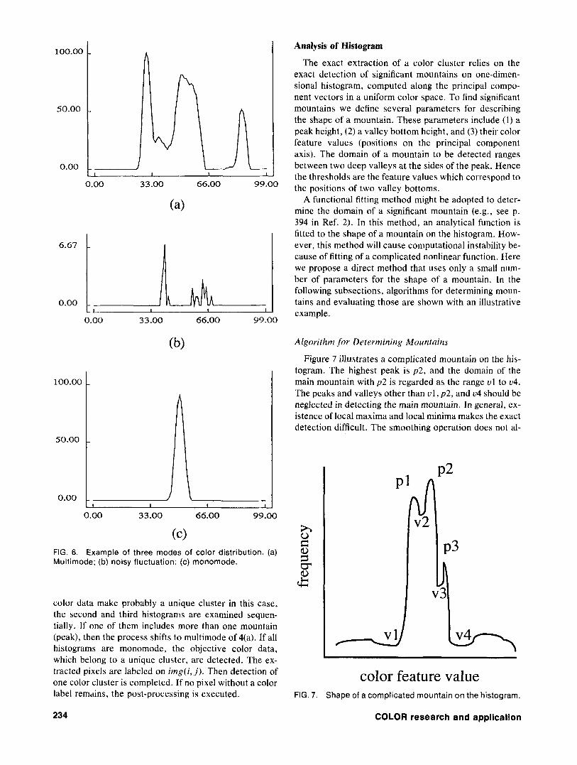
tains on the basis of large differences between adjacent peaks and valleys. We first execute a smoothing operation on the original histogram to reduce random fluctuation. Next several candidates for the significant mountains are selected, and a criterion function is computed for evaluating the mountain shape of each candidate. The analysis method of a histogram will be described in detail in the next subsection. The mountains on histograms are evaluated sequentially from the first histogram c ; . The mode of color distribution is classified into three cases of multimode, monomode, and noisy fluctuation (see Fig. 6). Different procedures are executed on the modes as follows:

4(a). In one case, if a histogram includes a number of mountains, the distribution is multimode. Then the most significant mountain is selected by a criterion function. The term “significant mountain” is defined as a big and sharp mountain on a histogram. The image is split using a pair of threshold values. We determine the thresholds as the color features that correspond to two valleys at the sides of the mountain. The extracted subregions are masked on the array irngrn(i,j). The masked regions are not only a connected region, but all regions which are extracted by thresholding. We continue cluster detection with respect to these masked regions.

4(b). In a second case, if the first histogram has no well defined peak, the distribution is considered as noisy fluctuation. It meets the stopping condition of the sequential color classification. Recall that the first component is co- incident with the axis of the widest data distribution in a color space. That is, when the remaining pixels without color labels decrease, the distribution becomes too sparse to create a cluster in the space. The post-processing is executed.

4(c). In the third case, if the first histogram has only a single mountain (peak), it is monomode. Although the

11 Set i m a y region I

.. .

44 i m a g e t i , i n g l j& 1 on i-th component

44 i m a g e t i , i n g l j& 1 on i-th component

4 4

FIG. 5. Iterative color cluster detection.

233 Volume 17, Number 4, August 1992

100.00

50.00

0.00

0.00 33.00 66.00 99.00

(a)

0.00 33.00 66.00 99.00

100.00

50.00

0.00

0.00 33.00 66.00 99.00

FIG. 6. Example of three modes of color distribution. (a) Multimode; (b) noisy fluctuation; (c) monomode.

color data make probably a unique cluster in this case, the second and third histograms are examined sequentially. If one of them includes more than one mountain (peak), then the process shifts to multimode of 4(a). If all histograms are monomode, the objective color data, which belong to a unique cluster, are detected. The extracted pixels are labeled on img( i , j ) . Then detection of one color cluster is completed. If no pixel without a color label remains, the post-processing is executed.

234

Analysis of Histogram

The exact extraction of a color cluster relies on the exact detection of significant mountains on one-dimensional histogram, computed along the principal component vectors in a uniform color space. To find significant mountains we define several parameters for describing the shape of a mountain. These parameters include ( I ) a peak height, (2) a valley bottom height, and (3) their color feature values (positions on the principal component axis). The domain of a mountain to be detected ranges between two deep valleys at the sides of the peak. Hence the thresholds are the feature values which correspond to the positions of two valley bottoms.

A functional fitting method might be adopted to determine the domain of a significant mountain (e.g., see p. 394 in Ref. 2) . In this method, an analytical function is fitted to the shape of a mountain on the histogram. How- ever, this method will cause computational instability because of fitting of a complicated nonlinear function. Here we propose a direct method that uses only a small number of parameters for the shape of a mountain. In the following subsections, algorithms for determining mountains and evaluating those are shown with an illustrative example.

Algorithm for Determining Mountains

Figure 7 illustrates a complicated mountain on the histogram. The highest peak is p 2 , and the domain of the main mountain with p 2 is regarded as the range u l to u4. The peaks and valleys other than u l , p 2 , and u4 should be neglected in detecting the main mountain. In general, ex- istence of local maxima and local minima makes the exact detection difficult. The smoothing operation does not al-

P l AP2 lJ v2

color feature value FIG. 7. Shape of a complicated mountain on the histogram.

COLOR research and application

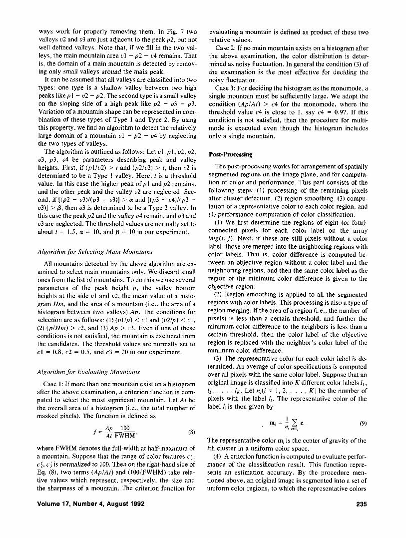
ways work for properly removing them. In Fig. 7 two valleys u2 and u3 are just adjacent to the peak p2 , but not well defined valleys. Note that, if we fill in the two valleys, the main mountain area ul - p 2 - u4 remains. That is, the domain of a main mountain is detected by removing only small valleys around the main peak.

It can be assumed that all valleys are classified into two types: one type is a shallow valley between two high peaks likepl - 712 - p 2 . The second type is a small valley on the sloping side of a high peak like p2 - u3 - p 3 . Variation of a mountain shape can be represented in com- bination of these types of Type 1 and Type 2. By using this property, we find an algorithm to detect the relatively large domain of a mountain ul - p 2 - u4 by neglecting the two types of valleys.

The algorithm is outlined as follows: Let u l , p l , u2, p2 , u3, p 3 , u4 be parameters describing peak and valley heights. First, if (p l lu2) > t and ( p 2 / u 2 ) > t , then u2 is determined to be a Type 1 valley. Here, t is a threshold value. In this case the higher peak of p l and p2 remains, and the other peak and the valley u2 are neglected. Sec- ond, if [ ( p 2 - u 3 ) / ( p 3 - u3)] > a and [ ( p 3 - u 4 ) / ( p 3 - u3)] > p, then u3 is determined to be a Type 2 valley. In this case the peak p 2 and the valley u4 remain, and p 3 and u3 are neglected. The threshold values are normally set to about t = 1.5, a = 10, and p = 10 in our experiment.

Algorithm for Selecting Main Mountains

All mountains detected by the above algorithm are examined to select main mountains only. We discard small ones from the list of mountains. To do this we use several parameters of the peak height p , the valley bottom heights at the side ul and u2, the mean value of a histogram Hm, and the area of a mountain (i.e., the area of a histogram between two valleys) A p . The conditions for selection are as follows: (1) ( u l l p ) < c l and (u2/p) < c l , (2) ( p / H m ) > c2, and (3) Ap > c3 . Even if one of these conditions is not satisfied, the mountain is excluded from the candidates. The threshold values are normally set to cl = 0.8, c2 = 0.5 , and c3 = 20 in our experiment.

Algorithm for Evaluating Mountains

Case 1: If more than one mountain exist on a histogram after the above examination, a criterion function is computed to select the most significant mountain. Let At be the overall area of a histogram (Lee, the total number of masked pixels). The function is defined as

Ap 100 At FWHM’

f = -~

where FWHM denotes the full-width at half-maximum of a mountain. Suppose that the range of color features c i , c i , c ; is normalized to 100. Then on the right-hand side of Eq. (S), two terms (Ap lAt ) and (100/FWHM) take relative values which represent, respectively, the size and the sharpness of a mountain. The criterion function for

evaluating a mountain is defined as product of these two relative values.

Case 2: If no main mountain exists on a histogram after the above examination, the color distribution is determined as noisy fluctuation. In general the condition ( 3 ) of the examination is the most effective for deciding the noisy fluctuation.

Case 3: For deciding the histogram as the monomode, a single mountain must be sufficiently large. We adopt the condition (AplAt) > c4 for the monomode, where the threshold value c4 is close to 1, say c4 = 0.97. If this condition is not satisfied, then the procedure for multimode is executed even though the histogram includes only a single mountain.

Post-Processing

The post-processing works for arrangement of spatially segmented regions on the image plane, and for computation of color and performance. This part consists of the following steps: (1) processing of the remaining pixels after cluster detection, ( 2 ) region smoothing, ( 3 ) computation of a representative color to each color region, and (4) performance computation of color classification.

(1) We first determine the regions of eight (or four)- connected pixels for each color label on the array img(i, j ) . Next, if these are still pixels without a color label, those are merged into the neighboring regions with color labels. That is, color difference is computed between an objective region without a color label and the neighboring regions, and then the same color label as the region of the minimum color difference is given to the objective region.

( 2 ) Region smoothing is applied to all the segmented regions with color labels. This processing is also a type of region merging. If the area of a region (i.e., the number of pixels) is less than a certain threshold, and further the minimum color difference to the neighbors is less than a certain threshold, then the color label of the objective region is replaced with the neighbor’s color label of the minimum color difference.

(3) The representative color for each color label is determined. An average of color specifications is computed over all pixels with the same color label. Suppose that an original image is classified into K different color labels I , , 1 2 , . . . , f K . Let ni(i = 1, 2, . . . , K ) be the number of pixels with the label 1;. The representative color of the label li is then given by

(9)

The representative color mi is the center of gravity of the ith cluster in a uniform color space.

( 4 ) A criterion function is computed to evaluate performance of the classification result. This function represents an estimation accuracy. By the procedure men- tioned above, an original image is segmented into a set of uniform color regions, to which the representative colors

Volume 17, Number 4, August 1992

are assigned. Therefore an average color difference is computed between the original image and the estimated one, which is represented by the representative colors only. The criterion function is defined as

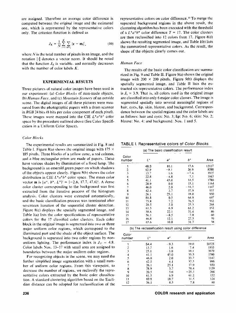
representative colors on color difference.l0 To merge the separated background regions in the above result, the clustering algorithm has been executed with the threshold of a L*a*b* color difference T = 17. The color clusters are then reclassified into 12 colors from 17. Figure 8(d) shows the resulting segmented image, and Table I(b) lists the summarized representative colors. As the result, the shape of the objects clearly comes out.

(10)

where N is the total number of pixels in an image, and the notation 11.11 denotes a vector norm. It should be noted that the function J K is variable, and normally decreases with the number of color labels K ,

l K J K = c c IIC - mill,

1 = I C€/,

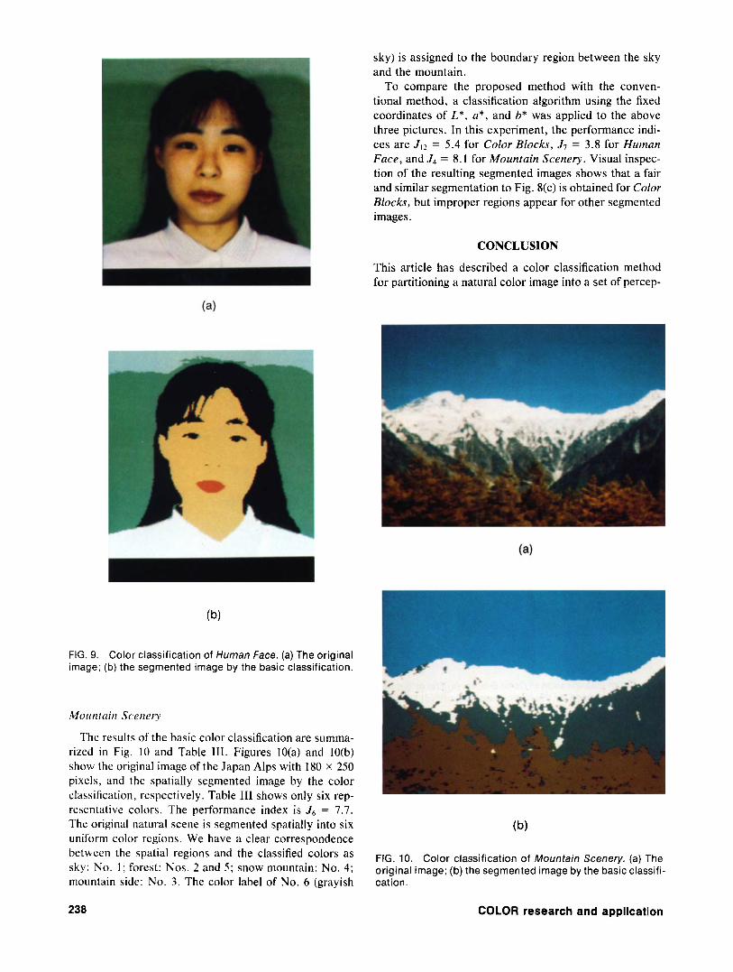
Human Face

The results of the basic color classification are summarized in Fig. 9 and Table 11. Figure 9(a) shows the original

EXPERIMENTAL RESULTS

Three pictures of natural color images have been used in our experiment: (a) Cotor Blocks of man-made objects, (b) Human Face, and (c) Mountain Scenery of an outside scene. The digital images of all these pictures were measured from the photographic papers with a drum scanner in RGB 24 bits (8 bits per color component of each pixel). These images were mapped into the CIE L*a*b* color space by the procedure outlined above (See Color Specifi- cation in a Uniform Color Space).

Color Blocks

The experimental results are summarized in Fig. 8 and Table I . Figure 8(a) shows the original image with 175 x 185 pixels. Three blocks of a yellow cone, a red column, and a blue rectangular prism are made of papers. These have various shades by illumination of a flood lamp. The background is an emerald green paper on which shadows of the objects appear clearly. Figure 8(b) shows the color distribution in CIE L*u*h* color space. The mean color vector m is [a*, b*, ,*]I = [-2.6, 17.7, 47.61'. A dense color cluster corresponding to the background was first extracted from the iterative process of the histogram analysis. Color clusters were extracted automatically, and the basic classification process was terminated after seventeen iteration of the sequential cluster detection. Figure 8(c) displays the spatially segmented image, and Table I(a) lists the color specifications of representative colors for the 17 classified color clusters. Each color block in the original image is segmented into two or three

image with 200 x 200 pixels. Figure 9(b) displays the spatially segmented image, and Table I1 lists the extracted six representative colors. The performance index is .Ib = 3.9. That is, all colors used in the original image are classified into only 6 major color classes. The image is segmented spatially into several meaningful regions of hair, eyes, lip, skin, blouse, and background. Correspon- dence between the spatial regions and the color labels are as follows: hair and eyes: No. 3; lip: No. 6; skin: No. 2; blouse: No. 4; and background: Nos. I and 5 .

TABLE I. Representative colors of Color Blocks. (a) The basic classification result

number L* a' b' Area Color

1 2 3 4 5 6 7 8 9

10 1 1 12 13 14 15 16 17

48.3 62.9 13.7 22.8 41.1 28.9 46.0 42.4 26.1 81.8 75.8 20.5 61.5 58.6 56.1 46.8 65.6

- 10.1 -8.1 -1.6 -4.8 45.0 -0.0

2.0 3.7

25.1 0.5 7.2 5.0 6.9

22. I -8.5 12.1 10.8

17.6 20.9 -7.4

7.1 33.5 15.1

-33.7 37.9 18.0 64.9 76.5 25.3 61.2 31.4

27.5 31.7

-7.8

12137 8588 1935 1915 1780 1 I64 I I47 957 950 607 552 268 152 86 60 39 38

major uniform color regions, which correspond to the illuminated part and the shade of the object surface. The

(b) The reclassification result using color difference

Color -. ~

background is senarated into two color regions bv non- number L' a* b' Area - - uniform lighting. The performance index is .Il7 = 4.8. 1 54.4 -9.3 19.0 20725 Color labels Nos. 13-17 with small area are assigned to 2 13.7 -1.6 -7.4 1935 boundaries between the major uniform color regions.

For recognizing objects in the scene, we may need the further simplified image segmentation with a small number of uniform color regions. From this viewpoint, to decrease the number of regions, we reclassify the representative colors extracted by the basic color classification. A standard clustering algorithm based on the Eucli- dian distance can be adopted for reclassification of the

3 4 5 6 7 8 9

10 11 12

25.1 41.1 46.0 42.5 26.1 78.9 20.5 61.5 60.8 56.1

-3.0 45.0

2.0 4. I

25. I 3.7 5.0 6.9

18.7 -8.5

10.1 33.5

-33.7 37.5 17.9 70.4

-25.3 61.2 31.5

-7.8

3079 1780 1 I47 996 950

1159 268 I52 124 60 -


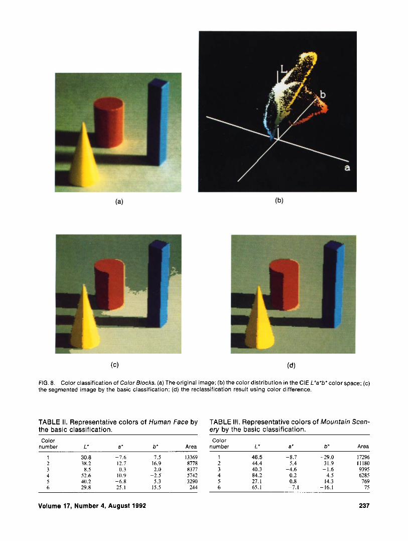
FIG. 8. Color classification of Color Blocks. (a) The original image; (b) the color distribution in the CIE L*a*b'color space; (c) the segmented image by the basic classification; (d) the reclassification result using color difference.

TABLE II. Representative colors of Human Face by the basic class if i cat ion.

TABLE Ill. Representative colors of Mountain Scen- ery by the basic classification.

Color number L' a* b* Area

Color number L* a* b* Area

1 30.8 -7.6 7.5 13369 2 38.2 12.7 16.9 8778 3 8.5 0.3 2.0 8377 4 52.6 10.9 -2.5 5742 5 40.2 -6.8 5.3 3290 6 29.8 25.1 15.5 244

1 46.5 -8.7 -29.0 17296 2 44.4 5.4 31.9 1 1 180 3 40.3 -4.6 -1.6 9395 4 84.2 0.2 4.5 6285 5 27.1 0.8 14.3 769 6 65.1 -7.1 -16.1 75


sky) is assigned to the boundary region between the sky and the mountain.

To compare the proposed method with the conven- tional method, a classification algorithm using the fixed coordinates of L*, a * , and b* was applied to the above three pictures. In this experiment, the performance indices are J I 2 = 5.4 for Color Blocks, 5, = 3.8 for Human Face, and J4 = 8. I for Mountain Scenery. Visual inspection of the resulting segmented images shows that a fair and similar segmentation to Fig. 8(c) is obtained for Color Blocks, but improper regions appear for other segmented images.

CONCLUSION

This article has described a color classification method for partitioning a natural color image into a set of percep-

FIG. 9. Color classification of Human Face. (a) The original image; (b) the segmented image by the basic classification.

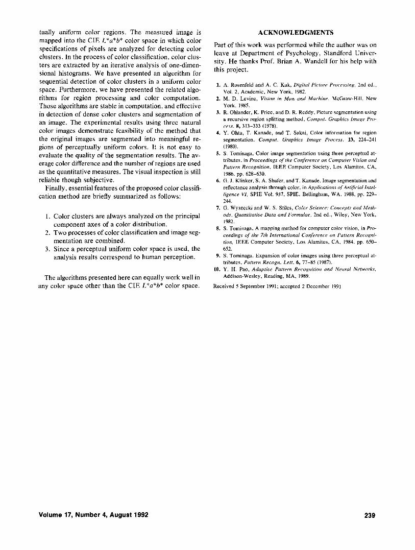
Mounfmin Scenery

The results of the basic color classification are summarized in Fig. 10 and Table 111. Figures IO(a) and 10(b) show the original image of the Japan Alps with 180 x 250 pixels, and the spatially segmented image by the color classification, respectively. Table Ill shows only six representative colors. The performance index is Jh = 7.7. The original natural scene is segmented spatially into six uniform color regions. We have a clear correspondence between the spatial regions and the classified colors as sky: No. 1 ; forest: Nos. 2 and 5 ; snow mountain: No. 4; mountain side: No. 3 . The color label of No. 6 (grayish

FIG. 10. Color classification of Mountain Scenery. (a) The original image; (b) the segmented image by the basic classification.


tually uniform color regions. The measured image is mapped into the CIE L*a*b* color space in which color specifications of pixels are analyzed for detecting color clusters. In the process of color classification, color clusters are extracted by an iterative analysis of one-dimensional histograms. We have presented an algorithm for sequential detection of color clusters in a uniform color space. Furthermore, we have presented the related algorithms for region processing and color computation. Those algorithms are stable in computation, and effective in detection of dense color clusters and segmentation of an image. The experimental results using three natural color images demonstrate feasibility of the method that the original images are segmented into meaningful regions of perceptually uniform colors. It is not easy to evaluate the quality of the segmentation results. The average color difference and the number of regions are used as the quantitative measures. The visual inspection is still reliable though subjective.

Finally, essential features of the proposed color classification method are briefly summarized as follows:

Color clusters are always analyzed on the principal component axes of a color distribution. Two processes of color classification and image segmentation are combined. Since a perceptual uniform color space is used, the analysis results correspond to human perception.

The algorithms presented here can equally work well in any color space other than the CIE L*a*b* color space.

ACKNOWLEDGMENTS

Part of this work was performed while the author was on leave at Department of Psychology, Standford Univer- sity. He thanks Prof. Brian A. Wandell for his help with this project.

1. A. Rosenfeld and A. C. Kak, Digital Picture Processing, 2nd ed., Vol. 2, Academic, New York, 1982.

2. M. D. Levine, Vision in Man and Machine, McGraw-Hill, New York, 1985.

3. R. Ohlander, K. Price, and D. R. Reddy, Picture segmentation using a recursive region splitting method, Comput. Graphics Image Pro- cess. 8, 313-333 (1978).

4. Y. Ohta, T. Kanade, and T. Sakai, Color information for region segmentation, Comput. Graphics Image Process. 13, 224-241 ( 1980).

5. S. Tominaga, Color image segmentation using three perceptual at- tributes, in Proceedings of the Conference on Computer Vision and Pattern Recognition, IEEE Computer Society, Los Alamitos, CA, 1986, pp. 628-630.

6. G . J . Klinker, S. A. Shafer, and T. Kanade, Image segmentation and reflectance analysis through color, in Applications of Artificial Intel- ligence VI, SPIE Vol. 937, SPIE, Bellingham, WA, 1988, pp. 229- 244.

1. G. Wyszecki and W. S. Stiles, Color Science: Concepts and Meth- ods, Quantitative Data and Formulae, 2nd ed., Wiley, New York, 1982.

8. S. Tominaga, A mapping method for computer color vision, in Pro- ceedings of the 7th International Conference on Pattern Recogni- tion, IEEE Computer Society, Los Alamitos, CA, 1984, pp. 650- 652.

9. S. Tominaga, Expansion of color images using three perceptual at- tributes, Pattern Recogn. Lett. 6 , 77-85 (1987).

10. Y. H. Pao, Adaptive Pattern Recogniiion and Neural Networks, Addison-Wesley, Reading, MA, 1989.

Received 5 September 1991; accepted 2 December 1991


color classification of natural color images

Documents