cold nuclear matter effects in drell-yan process and
TRANSCRIPT
HAL Id: tel-03121565https://tel.archives-ouvertes.fr/tel-03121565
Submitted on 26 Jan 2021
HAL is a multi-disciplinary open accessarchive for the deposit and dissemination of sci-entific research documents, whether they are pub-lished or not. The documents may come fromteaching and research institutions in France orabroad, or from public or private research centers.
L’archive ouverte pluridisciplinaire HAL, estdestinée au dépôt et à la diffusion de documentsscientifiques de niveau recherche, publiés ou non,émanant des établissements d’enseignement et derecherche français ou étrangers, des laboratoirespublics ou privés.
Cold nuclear matter effects in Drell-Yan process andcharmonium production
Charles-Joseph Naïm
To cite this version:Charles-Joseph Naïm. Cold nuclear matter effects in Drell-Yan process and charmonium production.High Energy Physics - Phenomenology [hep-ph]. Université Paris-Saclay, 2020. English. �NNT :2020UPASP038�. �tel-03121565�
Thès
e de
doc
tora
tN
NT:
2020U
PASP038
Cold nuclear matter effects inDrell-Yan process and
charmonium production
Thèse de doctorat de l’université Paris-Saclay
École doctorale n� 576, Particules, Hadrons, Energie,Noyau, Instrumentation, Imagerie, Cosmos et Simulation
(PHENIICS)Spécialité de doctorat: Physique
Unité de recherche: Université Paris-Saclay, CEA, Département dePhysique Nucléaire, 91191, Gif-sur-Yvette, France
Référent: Faculté des sciences d’Orsay
Thèse présentée et soutenue en visioconférence totale le30/10/2020 par
Charles-Joseph Naïm
Composition du jury:
Elena Ferreiro PrésidenteProfesseure, Universidade de Santiago de Compostela,SpainGinés Martinez Garcia Rapporteur & ExaminateurDirecteur de recherche, Subatech (CNRS)Ingo Schienbein Rapporteur & ExaminateurMaître de Conférences, Université Grenoble AlpesEmilie Maurice ExaminatriceProfesseure Assistant, Laboratoire Leprince-Ringuet(Ecole Polytechnique)Stefano Panebianco ExaminateurIngénieur chercheur, CEA/SaclayStéphane Peigné ExaminateurChargé de recherche, Subatech (CNRS)
Stéphane Platchkov Directeur de thèseIngénieur chercheur, CEA/SaclayFrançois Arleo Co-directeur de thèseChargé de recherche, Laboratoire Leprince-Ringuet(CNRS)

Le courage, c’est d’aimer la vie et de regarder la mort d’un regard tranquille ; c’estd’aller à l’idéal et de comprendre le réel ; c’est d’agir et de se donner aux grandescauses sans savoir quelle récompense réserve à notre effort l’univers profond, ni s’illui réserve une récompense. Le courage, c’est de chercher la vérité et de la dire ; c’estde ne pas subir la loi du mensonge triomphant qui passe, et de ne pas faire écho, denotre âme, de notre bouche et de nos mains aux applaudissements imbéciles et auxhuées fanatiques.
— Jean Jaurès, « Discours à la Jeunesse », Albi (France), 1903.

Remerciements
Jean Jaurès incarna avec splendeur l’idéal républicain. Baigné par la justice, il cherchacontinument à faire jaillir l’espoir d’un monde meilleur. Pacifiste, fédérateur et réformateur,il fut un défenseur omniprésent de la République sociale. La flamme de son héritage demeuretoujours veillée par toute la patrie reconnaissante. Voici par les mots de qui j’ai voulu débuter cemanuscrit. La définition du courage qu’il légua à la jeunesse de France en 1903 à Albi constituaune source profonde d’inspiration. Encore aujourd’hui, elle est pour moi l’écho de cet universprofond face aux tumultes de l’existence. Alors merci pour ces mots qui ornent mon jardin, ilsont été si souvent réconfortants...
Voilà maintenant l’instant le plus difficile, du moins le plus délicat. Comment résumer en quelqueslignes l’ensemble des interactions qui m’ont amené aujourd’hui à écrire ces remerciements ? Bienque la motivation soit un moteur indispensable à l’accomplissement des plus vastes projets, ellen’est pas suffisante, loin de là. Les rencontres, parfois sous l’auspice du fabuleux hasard, et lesproches en constituent le second moteur. Et je crois que l’idée de m’engager vers la physique mefut donnée par Mme Charliat dont j’ai eu l’honneur de croiser le chemin. Elle fut ma professeurede mathématiques en classe de 4ème au collège St-Joseph de Reims. Une professeure dont on sesouvient aisément tant elle marqua le jeune esprit, parfois rêveur, que j’étais. De là, je remercieégalement M. Kalité, mon professeur de physique de lycée, pour m’avoir poussé au travail et à larigueur ainsi que Mme Alardet, ma professeure d’anglais, pour sa bienveillance et ses précieuxconseils. Le premier aperçu de la recherche en physique me fut donné lors de mon stage de3ème à l’Institut d’Astrophysique de Paris (IAP). Je remercie donc chaleureusement ElisabethVangioni pour m’avoir donné l’opportunité de concrétiser ce qui n’était encore qu’imaginé.
Plus tard, pendant mes premières années à Sorbonne Université (ex-Université Pierre et MarieCurie), j’y ai découvert un lieu où la richesse individuelle nourrit une richesse collective. Unendroit où l’autonomie et la curiosité sont au service de la réussite. Je remercie l’ensemble del’équipe pédagogique, et en particulier le Professeur Patrick Boissé, pour m’avoir donné la chancede grandir dans un environnement scientifique de très haute qualité.
La présente thèse n’aurait pas pu voir le jour sans ma rencontre en master 1 avec StéphanePlatchkov qui fut par la suite mon co-directeur. Tu as été le premier lien entre la physique desparticules et moi : ta patience, ta bienveillance et ta richesse scientifique ont permis à un jeuneétudiant de s’orienter vers une thèse de doctorat. Alors merci ! Ta rencontre avec François Arleo,
bien loin d’ici, au Chili, a donné naissance à une superbe collaboration qui nous a tous les troisréunis. Je crois que je ne pouvais pas rêver d’un meilleur encadrement, donc merci de m’avoirdonné la possibilité de travailler à vos côtés pendant ces 3 années. Merci à toi François pourm’avoir donné l’opportunité d’apercevoir ton travail au quotidien : tu m’as transmis le sens etl’intuition physique nécessaire à tout physicien. Stéphane, merci à toi, tu m’as appris la rigueurqu’impose une mesure expérimentale. Votre apport complémentaire à ma formation scientifiquefut colossal. L’articulation entre l’aspect expérimental et théorique m’a permis d’avoir une visionlarge et fidèle du métier de physicien. Cette expérience très enrichissante a été nourrie par votretrès grande expertise scientifique et surtout votre patience.
Je remercie l’ensemble du jury pour avoir pris le temps de commenter et juger mes travaux derecherche. Ce fut un honneur.
Merci aussi à vous, Fabienne, Yann, Nicole et Damien, pour m’avoir apporté un environnementscientifique au quotidien de très haute qualité.
Thank you also to the entire COMPASS collaboration: working within an international col-laboration was much more than an asset, it was structuring both from a human and a scientificpoint of view! I would like to express my deep appreciation to Professor Wen-Chen Chang,Chia-Yu, Yu-Shiang, Marco, Vincent, Evgenii, Catarina and Bakur: working by your side wasexciting!
Rien de tout cela n’aurait été possible sans le CEA. Grâce à qui, j’ai pu réaliser ma thèsedans de parfaites conditions, alors merci à vous Franck, Christophe et Hervé M.. Merci àl’ensemble du département : vous avez chacun d’entre vous participé à l’obtention de ce diplôme.Un profond merci à toi, Danielle : ta bienveillance et ton attention ont été indispensables au bondéroulement de cette thèse. Je ne compte pas le nombre de cafés pris dans ton bureau tant tonécoute fut essentielle. Merci à toi Isabelle, c’est grâce à des gens comme toi qu’on prend plaisir à(re)venir au travail ! Merci aussi à l’École Polytechnique ainsi qu’au LLR pour leurs accueils.Je tiens également à remercier l’Université Paris-Saclay et le Labex P2IO pour leurs soutiensmatériels et financiers.
Merci à toi, Marine, pour m’avoir donné l’occasion de travailler à tes côtés pendant les Travauxen Laboratoire. Ton dynamisme, ta gentillesse, ta rigueur et ta pédagogie m’ont beaucoup appris.Merci à toi, Michael, pour ta bienveillance, ta passion pour la physique fut très enrichissante !
Un profond merci à toi, Christopher, pour ta gentillesse, ton courage, ton aide constanteet ta bonne humeur permanente. Merci à toi Antoine V. pour toutes ces discussions, ces momentsde partage et de rire. Merci Benjamin pour ton écoute et ces cafés. L’humain est au cœur de lapratique scientifique et ces 3 ans à tes côtés me l’ont démontré. Merci à vous, Robin et Florian,
pour toutes ces aventures et ces bières. Merci à vous tous et toutes, Brian, Vladimir, Zoé, HervéD., Aurore, Medhi, Eve, Noëlie, Pierre et Nancy, pour votre présence !
Une profonde reconnaissance pour toi, Stefano. Ton intelligence scientifique et humaine m’onttouché, je te remercie infiniment pour ta présence dans les moments de doute. Ton regardpercutant, sensible et sincère m’a été indispensable.
Merci à toutes les personnes qui m’ont accompagné tout au long de ces 3 années et mêmebien plus. Leur soutien indéfectible m’a montré combien la vie n’est pas un processus solitaire.Bien au contraire. Rien de tout cela n’aurait été possible sans elles.
Merci à ma famille, ma grand-mère, mes parents, mes frères, Héloïse, Jean-Marc et toutescelles et ceux qui ne sont plus. Vous avez chacun à votre manière participé à ce que je suisdevenu. Le temps passe ou plutôt, les choses passent dans le temps et pourtant, votre appuireste permanant malgré les éclats des vieilles tempêtes. Merci à mes proches dont la présencequotidienne a été décisive et remarquable. Un incommensurable respect à Antoine R., Kevin etClémence. Je vous dois tout.
Je ne pouvais pas conclure ces remerciements sans mentionner Quiberon, ces longs instantsdevant l’océan et son horizon apaisant ; merci pour tous ces moments.
Enfin, un insondable remerciement à cet univers profond pour m’avoir donné la possibilitéde croiser le chemin de personnes extraordinaires.

Figure 1: Côte Sauvage de la presqu’île de Quiberon.

Divisant la hauteur d’un arbre incertain, un invisible oiseau s’ingéniait à fairetrouver la journée courte, explorait d’une note prolongée la solitude environnante,mais il recevait d’elle une réplique si unanime, un choc en retour si redoublé de silenceet d’immobilité qu’on aurait dit qu’il venait d’arrêter pour toujours l’instant qu’ilavait cherché à faire passer plus vite.
— Marcel Proust, « Du côté de chez Swann », 1913.
Résumé en français
Introduction
Le phénomène de perte d’énergie des quarks et des gluons se propageant dans un milieu eninteraction forte a été mis en évidence pour la première fois dans les collisions d’ions lourdspar les expériences auprès des accélérateurs RHIC et LHC. Une autre manière de sonder lespropriétés de la matière nucléaire est d’étudier la production de processus durs dans les collisionshadron-noyau. En effet, dans ce cas, le milieu nucléaire est simple : sa densité ainsi que sa taillesont connues. Dans cette thèse, le processus Drell-Yan et la production de J/ψ ont été étudiés àtravers une analyse expérimentale et phénoménologique. La collaboration COMPASS au CERNa collecté un nombre significatif d’événements Drell-Yan et J/ψ en utilisant un faisceau de pionsnégatifs d’énergie égale à 190 GeV sur deux cibles nucléaires ; l’une composée de noyaux légers,l’aluminium (A=27) et l’autre, de noyaux lourds, le tungstène (A=184).
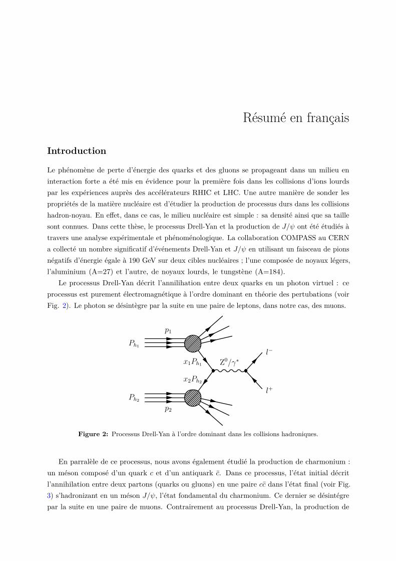
Le processus Drell-Yan décrit l’annilihation entre deux quarks en un photon virtuel : ceprocessus est purement électromagnétique à l’ordre dominant en théorie des pertubations (voirFig. 2). Le photon se désintègre par la suite en une paire de leptons, dans notre cas, des muons.
p1
p2
Z0/γ∗
Ph2
Ph1
l+
l−
x2Ph2
x1Ph1
Figure 2: Processus Drell-Yan à l’ordre dominant dans les collisions hadroniques.
En parralèle de ce processus, nous avons également étudié la production de charmonium :un méson composé d’un quark c et d’un antiquark c. Dans ce processus, l’état initial décritl’annihilation entre deux partons (quarks ou gluons) en une paire cc dans l’état final (voir Fig.3) s’hadronizant en un méson J/ψ, l’état fondamental du charmonium. Ce dernier se désintégrepar la suite en une paire de muons. Contrairement au processus Drell-Yan, la production de
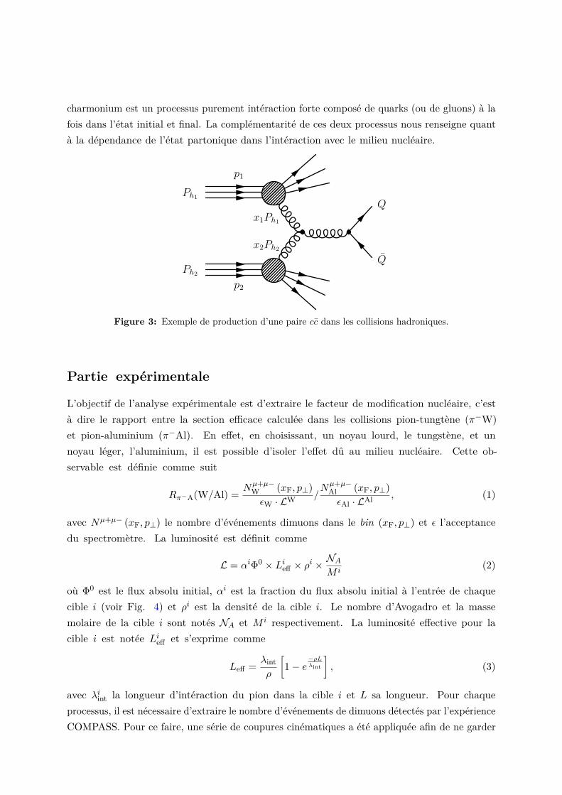
charmonium est un processus purement intéraction forte composé de quarks (ou de gluons) à lafois dans l’état initial et final. La complémentarité de ces deux processus nous renseigne quantà la dépendance de l’état partonique dans l’intéraction avec le milieu nucléaire.
p1
p2
Ph2
Ph1
Q
Q
x2Ph2
x1Ph1
Figure 3: Exemple de production d’une paire cc dans les collisions hadroniques.
Partie expérimentale
L’objectif de l’analyse expérimentale est d’extraire le facteur de modification nucléaire, c’està dire le rapport entre la section efficace calculée dans les collisions pion-tungtène (π−W)et pion-aluminium (π−Al). En effet, en choisissant, un noyau lourd, le tungstène, et unnoyau léger, l’aluminium, il est possible d’isoler l’effet dû au milieu nucléaire. Cette ob-servable est définie comme suit
Rπ−A(W/Al) = Nµ+µ−W (xF, p⊥)εW · LW
/Nµ+µ−
Al (xF, p⊥)εAl · LAl
, (1)
avec Nµ+µ− (xF, p⊥) le nombre d’événements dimuons dans le bin (xF, p⊥) et ε l’acceptancedu spectromètre. La luminosité est définit comme
L = αiΦ0 × Lieff × ρi ×NAM i
(2)
où Φ0 est le flux absolu initial, αi est la fraction du flux absolu initial à l’entrée de chaquecible i (voir Fig. 4) et ρi est la densité de la cible i. Le nombre d’Avogadro et la massemolaire de la cible i sont notés NA et M i respectivement. La luminosité effective pour lacible i est notée Lieff et s’exprime comme
Leff = λintρ
[1− e
−ρLλint
], (3)
avec λiint la longueur d’intéraction du pion dans la cible i et L sa longueur. Pour chaqueprocessus, il est nécessaire d’extraire le nombre d’événements de dimuons détectés par l’expérienceCOMPASS. Pour ce faire, une série de coupures cinématiques a été appliquée afin de ne garder
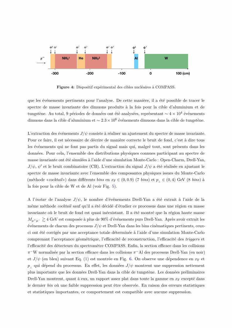
Figure 4: Dispositif expérimental des cibles nucléaires à COMPASS.
que les événements pertinents pour l’analyse. De cette manière, il a été possible de tracer lespectre de masse invariante des dimuons produits à la fois pour la cible d’aluminium et detungstène. Au total, 9 périodes de données ont été analysées, représentant ∼ 4× 10⁴ événementsdimuons dans la cible d’aluminium et ∼ 2.3×10⁶ événements dimuons dans la cible de tungstène.
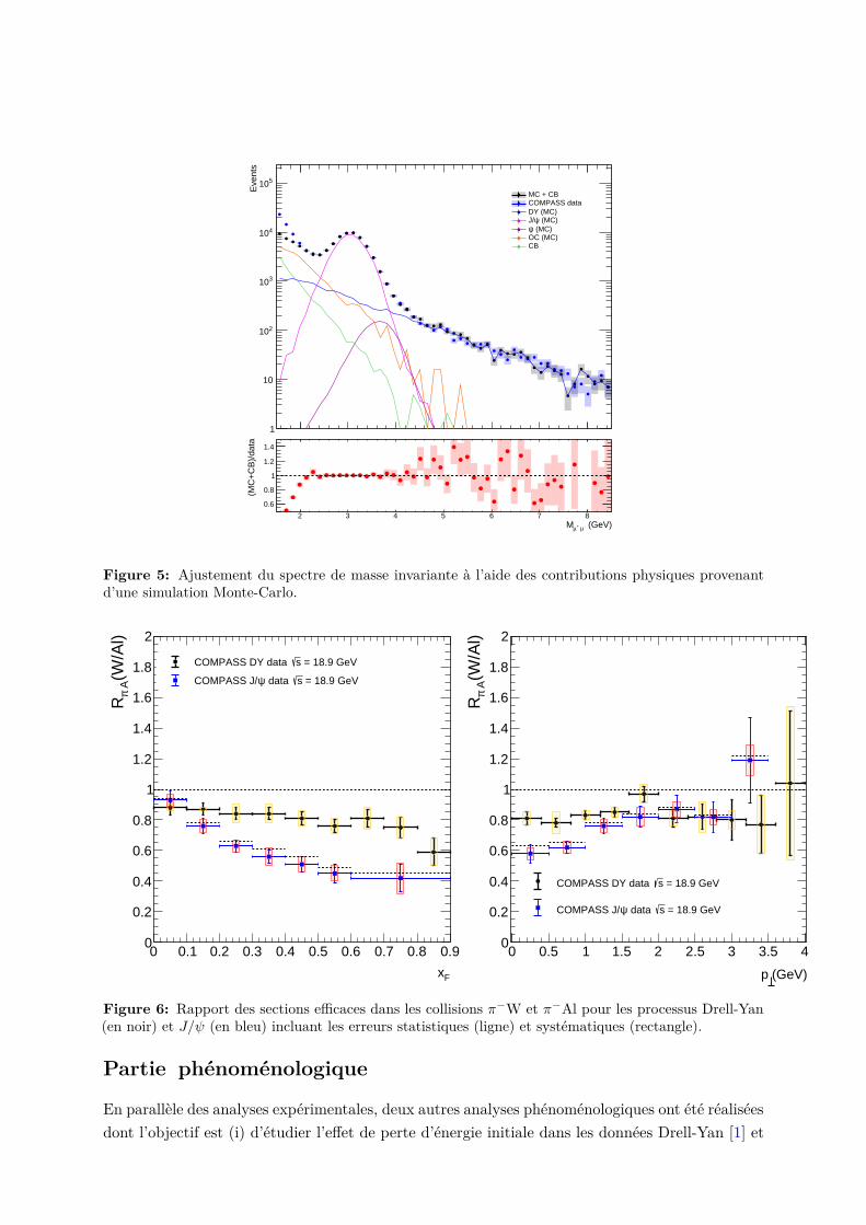
L’extraction des événements J/ψ consiste à réaliser un ajustement du spectre de masse invariante.Pour ce faire, il est nécessaire de décrire de manière correcte le bruit de fond, c’est à dire tousles événements qui ne font pas partis du signal mais qui, malgré tout, sont présents dans lesdonnées. Pour cela, l’ensemble des distributions physiques connues participant au spectre demasse invariante ont été simulées à l’aide d’une simulation Monte-Carlo : Open-Charm, Drell-Yan,J/ψ, ψ′ et le bruit combinatoire (CB). L’extraction du signal J/ψ a été réalisée en ajustant lespectre de masse invariante avec l’ensemble des composantes physiques issues du Monte-Carlo(méthode «cocktail») dans différents bins en xF ∈ (0, 0.9) (7 bins) et p⊥ ∈ (0, 4) GeV (8 bins) àla fois pour la cible de W et de Al (voir Fig. 5).
A l’instar de l’analyse J/ψ, le nombre d’événements Drell-Yan a été extrait à l’aide de lamême méthode cocktail sauf qu’il a été décidé d’étudier ce processus dans une région en masseinvariante où le bruit de fond est quasi inéexistant. Il a été montré que la région haute masseMµ+µ− & 4 GeV est composée à plus de 90% d’événements purs Drell-Yan. Après avoir extrait lesévénements de chacun des processus J/ψ et Drell-Yan dans les bins cinématiques pertinents, ceux-ci ont été corrigés par une acceptance totale déterminée à l’aide d’une simulation Monte-Carlocomprenant l’acceptance géométrique, l’efficacité de reconstruction, l’efficacité des triggers etl’efficacité des détecteurs du spectromètre COMPASS. Enfin, la section efficace dans les collisionsπ−W normalisée par la section efficace dans les collisions π−Al des processus Drell-Yan (en noir)et J/ψ (en bleu) suivant Eq. (1) est montrée en Fig. 6. On observe une dépendence en xF etp⊥ qui dépend du processus. En effet, les données J/ψ montrent une suppression nettementplus importante que les données Drell-Yan dans la cible de tungstène. Les données préliminairesDrell-Yan montrent, quant à eux, un rapport assez plat dans toute la gamme en xF excepté dansle dernier bin où une faible suppression peut être observée. En raison des erreurs statistiqueset statistiques importantes, ce comportement est compatible avec aucune suppression.
Eve
nts
1
10
210
310
410
510MC + CBCOMPASS dataDY (MC)
(MC)ψJ/ (MC)ψ
OC (MC)CB
(GeV)-µ +µM2 3 4 5 6 7 8
(MC
+C
B)/
data
0.6
0.8
1
1.2
1.4
Figure 5: Ajustement du spectre de masse invariante à l’aide des contributions physiques provenantd’une simulation Monte-Carlo.
0 0.1 0.2 0.3 0.4 0.5 0.6 0.7 0.8 0.9
Fx
0
0.2
0.4
0.6
0.8
1
1.2
1.4
1.6
1.8
2
(W/A
l) Aπ
R
= 18.9 GeVsCOMPASS DY data
= 18.9 GeVs data ψCOMPASS J/
0 0.5 1 1.5 2 2.5 3 3.5 4
(GeV)p
0
0.2
0.4
0.6
0.8
1
1.2
1.4
1.6
1.8
2
(W/A
l) Aπ
R
= 18.9 GeVsCOMPASS DY data
= 18.9 GeVs data ψCOMPASS J/
Figure 6: Rapport des sections efficaces dans les collisions π−W et π−Al pour les processus Drell-Yan(en noir) et J/ψ (en bleu) incluant les erreurs statistiques (ligne) et systématiques (rectangle).
Partie phénoménologique
En parallèle des analyses expérimentales, deux autres analyses phénoménologiques ont été réaliséesdont l’objectif est (i) d’étudier l’effet de perte d’énergie initiale dans les données Drell-Yan [1] et
(ii) d’extraire une valeur précise du coefficient de transport (noté q0) en analysant l’ensemble desdonnées ∆p2
⊥1 des processus Drell-Yan et J/ψ existantes [2].
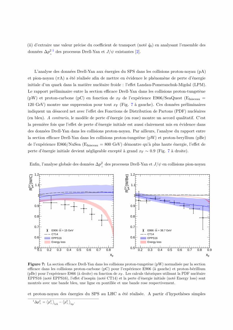
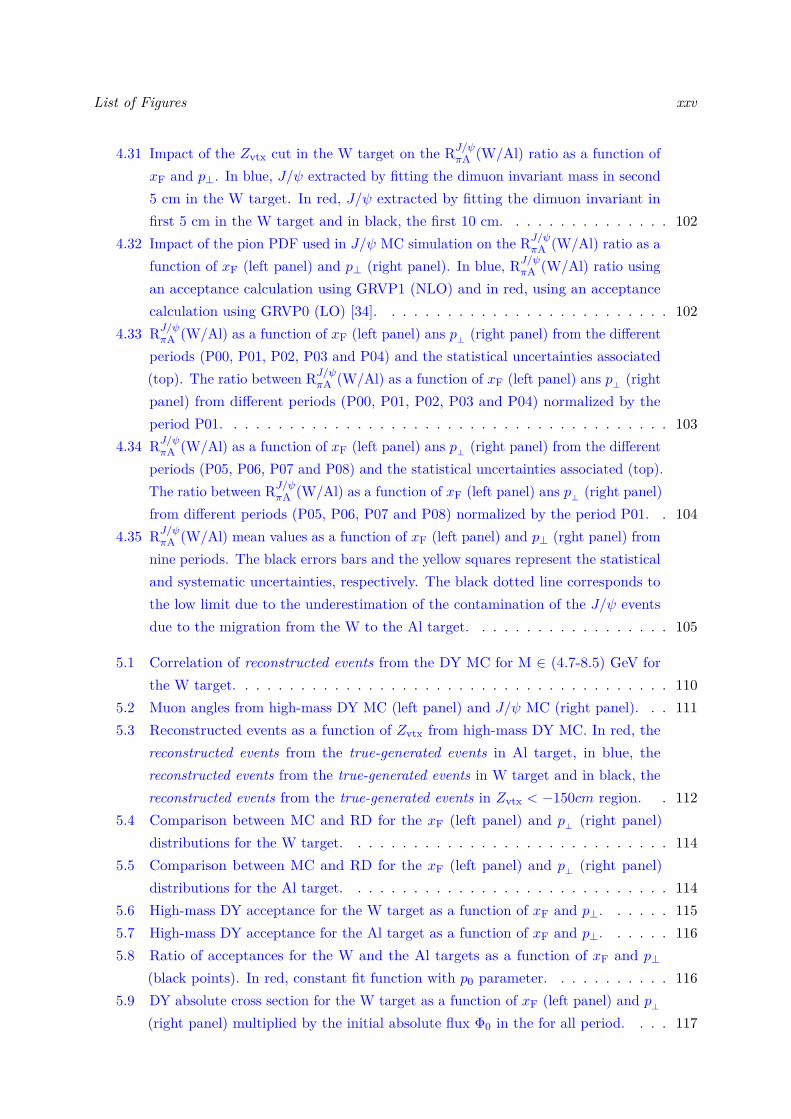
L’analyse des données Drell-Yan aux énergies du SPS dans les collisions proton-noyau (pA)et pion-noyau (πA) a été réalisée afin de mettre en évidence le phénomène de perte d’énergieinitiale d’un quark dans la matière nucléaire froide : l’effet Landau-Pomeranchuk-Migdal (LPM).Le rapport préliminaire entre la section efficace Drell-Yan dans les collisions proton-tungstène(pW) et proton-carbone (pC) en fonction de xF de l’expérience E906/SeaQuest (Efaisceau =120 GeV) montre une suppression pour tout xF (Fig. 7 à gauche). Ces données préliminairesindiquent un désacord net avec l’effet des Fonctions de Distribution de Partons (PDF) nucléaires(en bleu). A contrario, le modèle de perte d’énergie (en rose) montre un accord qualitatif. C’estla première fois que l’effet de perte d’énergie initiale est aussi clairement mis en évidence dansdes données Drell-Yan dans les collisions proton-noyau. Par ailleurs, l’analyse du rapport entrela section efficace Drell-Yan dans les collisions proton-tungstène (pW) et proton-beryllium (pBe)de l’expérience E866/NuSea (Efaisceau = 800 GeV) démontre qu’à plus haute énergie, l’effet deperte d’énergie initiale devient négligeable excepté à grand xF ∼ 0.9 (Fig. 7 à droite).
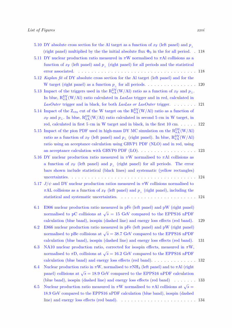
Enfin, l’analyse globale des données ∆p2⊥des processus Drell-Yan et J/ψ en collisions pion-noyau
0.1 0.2 0.3 0.4 0.5 0.6 0.7 0.8
Fx
0.5
0.6
0.7
0.8
0.9
1
1.1
1.2
(W/C
)pAD
YR
= 15 GeVsE906 CT14
EPPS16
Energy loss
0.2 0.3 0.4 0.5 0.6 0.7 0.8 0.9
Fx
0.5
0.6
0.7
0.8
0.9
1
1.1
1.2
(W/B
e)pAD
YR
= 38.7 GeVsE866 CT14
EPPS16
Energy loss
Figure 7: La section efficace Drell-Yan dans les collisions proton-tungstène (pW) normalisée par la sectionefficace dans les collisions proton-carbone (pC) pour l’expérience E906 (à gauche) et proton-bérillium(pBe) pour l’expérience E866 (à droite) en fonction de xF. Les calculs théoriques utilisant la PDF nucléaireEPPS16 (noté EPPS16), l’effet d’isospin (noté CT14) et la perte d’énergie initiale (noté Energy loss) sontmontrés avec une bande bleu, une ligne en pontillée et une bande rose respectivement.
et proton-noyau des énergies du SPS au LHC a été réalisée. A partir d’hypothèses simples1∆p2
⊥ =⟨p2⊥⟩
hA−⟨p2⊥⟩
hp.
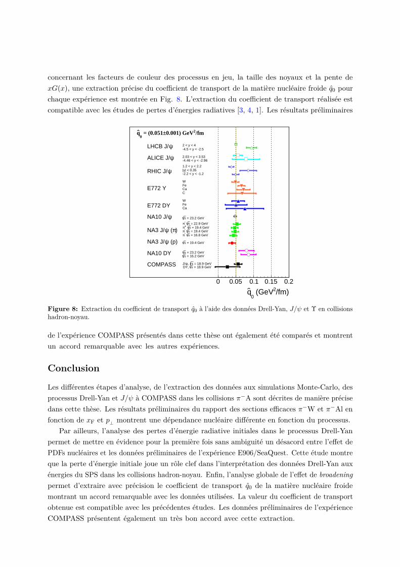
concernant les facteurs de couleur des processus en jeu, la taille des noyaux et la pente dexG(x), une extraction précise du coefficient de transport de la matière nucléaire froide q0 pourchaque expérience est montrée en Fig. 8. L’extraction du coefficient de transport réalisée estcompatible avec les études de pertes d’énergies radiatives [3, 4, 1]. Les résultats préliminaires
/fm)2 (GeV0
q
COMPASS = 18.9 GeVs, ψJ/ = 18.9 GeVsDY,
NA10 DY = 23.2 GeVs = 16.2 GeVs
(p)ψNA3 J/ = 19.4 GeVs
)π (ψNA3 J/ = 22.9 GeVs -π = 19.4 GeVs +π
= 19.4 GeVs -π = 16.8 GeVs -π
ψNA10 J/ = 23.2 GeVs
E772 DYWFeCa
ΥE772 WFeCaC
ψRHIC J/1.2 < y < 2.2|y| < 0.35-2.2 < y < -1.2
ψALICE J/ 2.03 < y < 3.53-4.46 < y < -2.96
ψLHCB J/ 2 < y < 4-4.5 < y < -2.5
/fm20.001) GeV± = (0.0510
q
0 0.05 0.1 0.15 0.2
Figure 8: Extraction du coefficient de transport q0 à l’aide des données Drell-Yan, J/ψ et Υ en collisionshadron-noyau.
de l’expérience COMPASS présentés dans cette thèse ont également été comparés et montrentun accord remarquable avec les autres expériences.
Conclusion
Les différentes étapes d’analyse, de l’extraction des données aux simulations Monte-Carlo, desprocessus Drell-Yan et J/ψ à COMPASS dans les collisions π−A sont décrites de manière précisedans cette thèse. Les résultats préliminaires du rapport des sections efficaces π−W et π−Al enfonction de xF et p⊥ montrent une dépendance nucléaire différente en fonction du processus.
Par ailleurs, l’analyse des pertes d’énergie radiative initiales dans le processus Drell-Yanpermet de mettre en évidence pour la première fois sans ambiguité un désacord entre l’effet dePDFs nucléaires et les données préliminaires de l’expérience E906/SeaQuest. Cette étude montreque la perte d’énergie initiale joue un rôle clef dans l’interprétation des données Drell-Yan auxénergies du SPS dans les collisions hadron-noyau. Enfin, l’analyse globale de l’effet de broadeningpermet d’extraire avec précision le coefficient de transport q0 de la matière nucléaire froidemontrant un accord remarquable avec les données utilisées. La valeur du coefficient de transportobtenue est compatible avec les précédentes études. Les données préliminaires de l’expérienceCOMPASS présentent également un très bon accord avec cette extraction.
Contents
List of Figures xx
1 Dilepton production in hadron-hadron collisions 11.1 Introduction . . . . . . . . . . . . . . . . . . . . . . . . . . . . . . . . . . . . . . . 1
1.1.1 Historical remarks . . . . . . . . . . . . . . . . . . . . . . . . . . . . . . . 11.1.2 Parton Model . . . . . . . . . . . . . . . . . . . . . . . . . . . . . . . . . . 21.1.3 Running coupling constant . . . . . . . . . . . . . . . . . . . . . . . . . . 31.1.4 QCD improved Parton Model . . . . . . . . . . . . . . . . . . . . . . . . . 41.1.5 Perturbative QCD corrections . . . . . . . . . . . . . . . . . . . . . . . . . 51.1.6 Parton distribution functions extraction from global fit . . . . . . . . . . . 6
1.2 Drell-Yan production . . . . . . . . . . . . . . . . . . . . . . . . . . . . . . . . . . 81.2.1 Leading order in αs (LO) . . . . . . . . . . . . . . . . . . . . . . . . . . . 81.2.2 NLO corrections . . . . . . . . . . . . . . . . . . . . . . . . . . . . . . . . 91.2.3 Kinematics definition in hadron-hadron collisions . . . . . . . . . . . . . . 13
1.3 Quarkonium production . . . . . . . . . . . . . . . . . . . . . . . . . . . . . . . . 141.3.1 Color state . . . . . . . . . . . . . . . . . . . . . . . . . . . . . . . . . . . 151.3.2 Color Evaporation Model . . . . . . . . . . . . . . . . . . . . . . . . . . . 151.3.3 Color-Singlet model . . . . . . . . . . . . . . . . . . . . . . . . . . . . . . 161.3.4 Non-Relativistic QCD model . . . . . . . . . . . . . . . . . . . . . . . . . 17
1.4 Phenomenological aspects of the Drell-Yan and quarkonium production . . . . . 171.4.1 Drell-Yan production . . . . . . . . . . . . . . . . . . . . . . . . . . . . . . 171.4.2 Quarkonia production . . . . . . . . . . . . . . . . . . . . . . . . . . . . . 18
2 Nuclear effects in dilepton production 212.1 A-dependence . . . . . . . . . . . . . . . . . . . . . . . . . . . . . . . . . . . . . . 22
2.1.1 Isospin effect . . . . . . . . . . . . . . . . . . . . . . . . . . . . . . . . . . 222.1.2 Antiquark flavor asymmetry in the nucleon sea . . . . . . . . . . . . . . . 232.1.3 Drell-Yan cross sections ratio . . . . . . . . . . . . . . . . . . . . . . . . . 252.1.4 Charmonium cross sections ratio . . . . . . . . . . . . . . . . . . . . . . . 25
2.2 Nuclear parton distribution function . . . . . . . . . . . . . . . . . . . . . . . . . 262.2.1 EPPS16 and EPS09 global fit . . . . . . . . . . . . . . . . . . . . . . . . . 292.2.2 nCTEQ global fit . . . . . . . . . . . . . . . . . . . . . . . . . . . . . . . . 312.2.3 DSSZ global fit . . . . . . . . . . . . . . . . . . . . . . . . . . . . . . . . . 31
xvi
Contents xvii
2.3 Nuclear absorption . . . . . . . . . . . . . . . . . . . . . . . . . . . . . . . . . . . 332.4 Parton energy loss in a QCD medium . . . . . . . . . . . . . . . . . . . . . . . . 35
2.4.1 Transport coefficient and broadening effect . . . . . . . . . . . . . . . . . 362.4.2 Energy loss regimes . . . . . . . . . . . . . . . . . . . . . . . . . . . . . . 37
2.5 Empirical observations . . . . . . . . . . . . . . . . . . . . . . . . . . . . . . . . . 382.5.1 Data . . . . . . . . . . . . . . . . . . . . . . . . . . . . . . . . . . . . . . . 382.5.2 Data interpretation . . . . . . . . . . . . . . . . . . . . . . . . . . . . . . . 412.5.3 Phenomenological approach . . . . . . . . . . . . . . . . . . . . . . . . . . 42
3 COMPASS experiment 453.1 Introduction . . . . . . . . . . . . . . . . . . . . . . . . . . . . . . . . . . . . . . . 453.2 Beam . . . . . . . . . . . . . . . . . . . . . . . . . . . . . . . . . . . . . . . . . . 463.3 Targets . . . . . . . . . . . . . . . . . . . . . . . . . . . . . . . . . . . . . . . . . 47
3.3.1 NH3 targets . . . . . . . . . . . . . . . . . . . . . . . . . . . . . . . . . . . 473.3.2 Al and W targets . . . . . . . . . . . . . . . . . . . . . . . . . . . . . . . . 483.3.3 Beam attenuation . . . . . . . . . . . . . . . . . . . . . . . . . . . . . . . 49
3.4 Spectrometer . . . . . . . . . . . . . . . . . . . . . . . . . . . . . . . . . . . . . . 513.4.1 Very Small Area Tracking . . . . . . . . . . . . . . . . . . . . . . . . . . . 523.4.2 Small Angle Trackers . . . . . . . . . . . . . . . . . . . . . . . . . . . . . . 523.4.3 Large Area Trackers . . . . . . . . . . . . . . . . . . . . . . . . . . . . . . 543.4.4 Muon identification . . . . . . . . . . . . . . . . . . . . . . . . . . . . . . 56
3.5 Trigger and veto system . . . . . . . . . . . . . . . . . . . . . . . . . . . . . . . . 573.6 Data acquisition . . . . . . . . . . . . . . . . . . . . . . . . . . . . . . . . . . . . 58
3.6.1 Reconstruction . . . . . . . . . . . . . . . . . . . . . . . . . . . . . . . . . 593.7 The Drift Chamber detector . . . . . . . . . . . . . . . . . . . . . . . . . . . . . . 59
3.7.1 Characteristics . . . . . . . . . . . . . . . . . . . . . . . . . . . . . . . . . 593.7.2 Formation and processing of the electrical signal . . . . . . . . . . . . . . 613.7.3 Calibration . . . . . . . . . . . . . . . . . . . . . . . . . . . . . . . . . . . 62
4 Analysis of J/ψ production in πA collisions 664.1 Observable . . . . . . . . . . . . . . . . . . . . . . . . . . . . . . . . . . . . . . . 674.2 Data sample . . . . . . . . . . . . . . . . . . . . . . . . . . . . . . . . . . . . . . . 67
4.2.1 Event selection . . . . . . . . . . . . . . . . . . . . . . . . . . . . . . . . . 684.2.2 Dimuon invariant mass . . . . . . . . . . . . . . . . . . . . . . . . . . . . 69
4.3 J/ψ signal extraction . . . . . . . . . . . . . . . . . . . . . . . . . . . . . . . . . . 704.3.1 Invariant mass reconstruction . . . . . . . . . . . . . . . . . . . . . . . . . 714.3.2 Fit procedure . . . . . . . . . . . . . . . . . . . . . . . . . . . . . . . . . . 774.3.3 J/ψ resolution estimation from Monte-Carlo simulation . . . . . . . . . . 804.3.4 J/ψ 2D extraction method . . . . . . . . . . . . . . . . . . . . . . . . . . 82
4.4 J/ψ cross section extraction method . . . . . . . . . . . . . . . . . . . . . . . . . 90
Contents xviii
4.4.1 2D acceptance as a function of p⊥ and xF . . . . . . . . . . . . . . . . . . 924.4.2 J/ψ cross section as a function of p⊥ and xF . . . . . . . . . . . . . . . . 954.4.3 Ratio of cross sections for J/ψ production for the W and Al targets . . . 964.4.4 Nuclear transverse momentum broadening . . . . . . . . . . . . . . . . . . 98
4.5 Systematic uncertainties estimation . . . . . . . . . . . . . . . . . . . . . . . . . . 994.5.1 Signal extraction . . . . . . . . . . . . . . . . . . . . . . . . . . . . . . . . 994.5.2 Impact of the Zvtx position in the W target . . . . . . . . . . . . . . . . . 1014.5.3 Acceptance systematic error . . . . . . . . . . . . . . . . . . . . . . . . . . 1014.5.4 Period compatibility . . . . . . . . . . . . . . . . . . . . . . . . . . . . . . 1034.5.5 Results . . . . . . . . . . . . . . . . . . . . . . . . . . . . . . . . . . . . . 104
4.6 Conclusion . . . . . . . . . . . . . . . . . . . . . . . . . . . . . . . . . . . . . . . 106
5 Analysis of Drell-Yan production in πA collisions 1075.1 Observable . . . . . . . . . . . . . . . . . . . . . . . . . . . . . . . . . . . . . . . 1075.2 Drell-Yan signal extraction . . . . . . . . . . . . . . . . . . . . . . . . . . . . . . 108
5.2.1 Data sample . . . . . . . . . . . . . . . . . . . . . . . . . . . . . . . . . . 1085.2.2 Monte-Carlo simulation . . . . . . . . . . . . . . . . . . . . . . . . . . . . 1095.2.3 Validity of the Monte-Carlo simulation . . . . . . . . . . . . . . . . . . . . 113
5.3 Drell-Yan cross section . . . . . . . . . . . . . . . . . . . . . . . . . . . . . . . . . 1135.3.1 2D acceptance as a function of xF and p⊥ . . . . . . . . . . . . . . . . . . 1145.3.2 Drell-Yan cross section as a function of xF and p⊥ . . . . . . . . . . . . . 1175.3.3 Ratios of nuclear cross sections . . . . . . . . . . . . . . . . . . . . . . . . 1175.3.4 Nuclear transverse momentum broadening . . . . . . . . . . . . . . . . . . 119
5.4 Systematic uncertainties . . . . . . . . . . . . . . . . . . . . . . . . . . . . . . . . 1205.4.1 Impact of the trigger selection . . . . . . . . . . . . . . . . . . . . . . . . 1205.4.2 Impact of Zvtx position in W target . . . . . . . . . . . . . . . . . . . . . 1225.4.3 Acceptance systematic error . . . . . . . . . . . . . . . . . . . . . . . . . . 1235.4.4 Results . . . . . . . . . . . . . . . . . . . . . . . . . . . . . . . . . . . . . 123
5.5 Conclusion . . . . . . . . . . . . . . . . . . . . . . . . . . . . . . . . . . . . . . . 125
6 Initial-state energy loss effects in the Drell-Yan process 1266.1 Initial-state energy loss model . . . . . . . . . . . . . . . . . . . . . . . . . . . . . 1276.2 Uncertainties computation . . . . . . . . . . . . . . . . . . . . . . . . . . . . . . . 1286.3 DY Rapidity dependence . . . . . . . . . . . . . . . . . . . . . . . . . . . . . . . . 128
6.3.1 E906 experiment . . . . . . . . . . . . . . . . . . . . . . . . . . . . . . . . 1286.3.2 E866 experiment . . . . . . . . . . . . . . . . . . . . . . . . . . . . . . . . 1306.3.3 NA10 experiment . . . . . . . . . . . . . . . . . . . . . . . . . . . . . . . . 1306.3.4 COMPASS experiment . . . . . . . . . . . . . . . . . . . . . . . . . . . . . 1326.3.5 E615 experiment . . . . . . . . . . . . . . . . . . . . . . . . . . . . . . . . 1346.3.6 Discussion about meson PDF at large x . . . . . . . . . . . . . . . . . . . 136
6.4 x2 scaling in Drell-Yan production . . . . . . . . . . . . . . . . . . . . . . . . . . 1376.5 Conclusion . . . . . . . . . . . . . . . . . . . . . . . . . . . . . . . . . . . . . . . 138
Contents xix
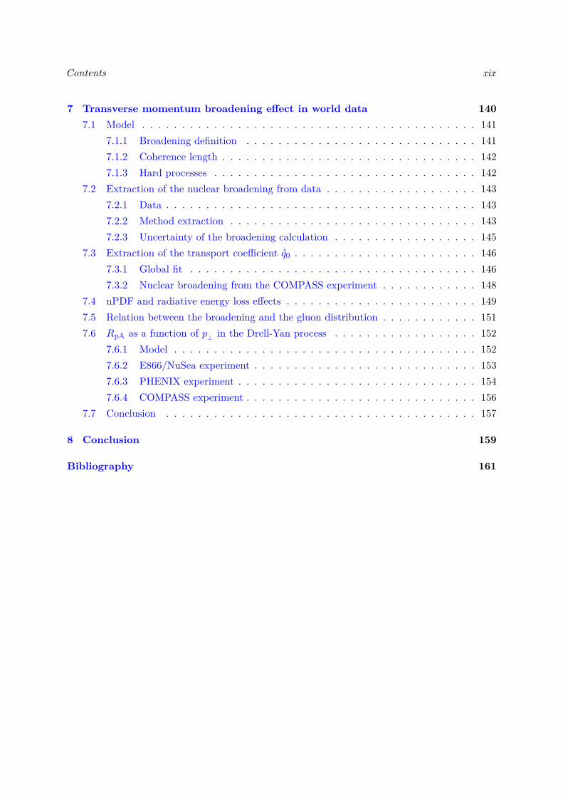
7 Transverse momentum broadening effect in world data 1407.1 Model . . . . . . . . . . . . . . . . . . . . . . . . . . . . . . . . . . . . . . . . . . 141
7.1.1 Broadening definition . . . . . . . . . . . . . . . . . . . . . . . . . . . . . 1417.1.2 Coherence length . . . . . . . . . . . . . . . . . . . . . . . . . . . . . . . . 1427.1.3 Hard processes . . . . . . . . . . . . . . . . . . . . . . . . . . . . . . . . . 142
7.2 Extraction of the nuclear broadening from data . . . . . . . . . . . . . . . . . . . 1437.2.1 Data . . . . . . . . . . . . . . . . . . . . . . . . . . . . . . . . . . . . . . . 1437.2.2 Method extraction . . . . . . . . . . . . . . . . . . . . . . . . . . . . . . . 1437.2.3 Uncertainty of the broadening calculation . . . . . . . . . . . . . . . . . . 145
7.3 Extraction of the transport coefficient q0 . . . . . . . . . . . . . . . . . . . . . . . 1467.3.1 Global fit . . . . . . . . . . . . . . . . . . . . . . . . . . . . . . . . . . . . 1467.3.2 Nuclear broadening from the COMPASS experiment . . . . . . . . . . . . 148
7.4 nPDF and radiative energy loss effects . . . . . . . . . . . . . . . . . . . . . . . . 1497.5 Relation between the broadening and the gluon distribution . . . . . . . . . . . . 1517.6 RpA as a function of p⊥ in the Drell-Yan process . . . . . . . . . . . . . . . . . . 152
7.6.1 Model . . . . . . . . . . . . . . . . . . . . . . . . . . . . . . . . . . . . . . 1527.6.2 E866/NuSea experiment . . . . . . . . . . . . . . . . . . . . . . . . . . . . 1537.6.3 PHENIX experiment . . . . . . . . . . . . . . . . . . . . . . . . . . . . . . 1547.6.4 COMPASS experiment . . . . . . . . . . . . . . . . . . . . . . . . . . . . . 156
7.7 Conclusion . . . . . . . . . . . . . . . . . . . . . . . . . . . . . . . . . . . . . . . 157
8 Conclusion 159
Bibliography 161
List of Figures
1 Côte Sauvage de la presqu’île de Quiberon. . . . . . . . . . . . . . . . . . . . . . vii2 Processus Drell-Yan à l’ordre dominant dans les collisions hadroniques. . . . . . . x3 Exemple de production d’une paire cc dans les collisions hadroniques. . . . . . . xi4 Dispositif expérimental des cibles nucléaires à COMPASS. . . . . . . . . . . . . . xii5 Ajustement du spectre de masse invariante à l’aide des contributions physiques
provenant d’une simulation Monte-Carlo. . . . . . . . . . . . . . . . . . . . . . . xiii6 Rapport des sections efficaces dans les collisions π−W et π−Al pour les processus
Drell-Yan (en noir) et J/ψ (en bleu) incluant les erreurs statistiques (ligne) etsystématiques (rectangle). . . . . . . . . . . . . . . . . . . . . . . . . . . . . . . . xiii
7 La section efficace Drell-Yan dans les collisions proton-tungstène (pW) normaliséepar la section efficace dans les collisions proton-carbone (pC) pour l’expérienceE906 (à gauche) et proton-bérillium (pBe) pour l’expérience E866 (à droite) enfonction de xF. Les calculs théoriques utilisant la PDF nucléaire EPPS16 (notéEPPS16), l’effet d’isospin (noté CT14) et la perte d’énergie initiale (noté Energyloss) sont montrés avec une bande bleu, une ligne en pontillée et une bande roserespectivement. . . . . . . . . . . . . . . . . . . . . . . . . . . . . . . . . . . . . . xiv
8 Extraction du coefficient de transport q0 à l’aide des données Drell-Yan, J/ψ et Υen collisions hadron-noyau. . . . . . . . . . . . . . . . . . . . . . . . . . . . . . . xv
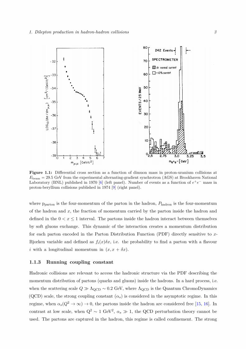
1.1 Differential cross section as a function of dimuon mass in proton-uranium collisionsat Ebeam = 29.5 GeV from the experimental alternating-gradient synchrotron(AGS) at Brookhaven National Laboratory (BNL) published in 1970 [6] (leftpanel). Number of events as a function of e+e− mass in proton-beryllium collisionspublished in 1974 [9] (right panel). . . . . . . . . . . . . . . . . . . . . . . . . . . 3
1.2 Differential cross section for neutral current e±p → e±X as a function of Q2
(GeV2) from the H1 collaboration [17]. . . . . . . . . . . . . . . . . . . . . . . . . 41.3 Graphical representation of the LO splitting functions Pqq, Pqg, Pgq and Pgg. . . 61.4 Parton distribution functions xf(x) and their associated uncertainties at Q2= 10
GeV2 (left) and Q2= 10000 GeV2 (right) at NLO using the CT14 parametrization[28]. . . . . . . . . . . . . . . . . . . . . . . . . . . . . . . . . . . . . . . . . . . . 7
1.5 Distribution functions of the partons xf(x) for π− meson at Q2 = 10 GeV2 atNLO from SMRS [30], GRV [34] and JAM [38] groups. . . . . . . . . . . . . . . . 8
1.6 Drell-Yan process at leading order (LO). . . . . . . . . . . . . . . . . . . . . . . . 9
xx
List of Figures xxi
1.7 Drell-Yan differential cross section as a function of p⊥ at NLO (in red) and NNLO(in magenta) using the DYNNLO software [43] in proton-proton (pp) collisionsat√s = 200 GeV. In the calculation the CT14 proton PDFs [28] are used by
varying the energy scale M/2 < µr, µf < 2M . The calculations are compared tothe Drell-Yan differential cross section data as a function of p⊥ collected by thePHENIX experiment in pp collisions at
√s = 200 GeV (blue) [44]. . . . . . . . . 11
1.8 Calculation of the ratio between NLO in αs and LO of DY cross section as afunction of xF using the DYNNLO software [43] using CT14 proton PDF [28] at√s = 50 GeV (in blue) and
√s = 20 GeV (in red) in pp collisions. . . . . . . . . 12
1.9 Drell-Yan differential cross section as a function of p⊥ at NNLL calculation usingthe DYRES software [48] in pp collisions at
√s = 200 GeV using CT14 proton
PDF and DY differential cross section as a function of p⊥ collected by PHENIXexperiment in pp collisions at
√s = 200 GeV (blue) [44] (left panel). Drell-Yan
differential cross section as a function of xF at NLO and NLL in pp collisions at√s = 200 GeV using CT14 proton PDF (right panel). . . . . . . . . . . . . . . . 13
1.10 Example of QQ pair production in hadron-hadron collisions. . . . . . . . . . . . . 151.11 Comparison between Drell-Yan data from E866, E772, E605 experiments as a
function of dimuon invariant mass M and xF for different collisions system pp,pD and pCu from [60] and NLO in αs calculation. . . . . . . . . . . . . . . . . . 18
1.12 Comparison between ICEM model [51] (in orange) and data as a function of p⊥from prompt J/ψ production in pp collisions at
√s = 200 GeV and
√s = 7 TeV
from RHIC experiment at mid rapidity [66] and from LHCb experiment at forwardrapidity [67] respectively. . . . . . . . . . . . . . . . . . . . . . . . . . . . . . . . 19
1.13 Comparison between J/ψ production model calculation at NLO, NRQCD (inorange), CSM (in blue) and CSM at NNLO neglecting a part of the logarithmicterms (in yellow) and prompt J/ψ data in pp collisions at
√s = 8 TeV as a
function of p⊥ from LHCb experiment [68]. . . . . . . . . . . . . . . . . . . . . . 20
2.1 Parton distribution functions of uAv (x) and dAv (x) normalised by A times x andtheir associated uncertainties at Q2= 25 GeV2 for deuterium nucleus (left panel)and tungsten nucleus (right panel) at Next-to-Leading Order (NLO) using CT14parameterization [28]. . . . . . . . . . . . . . . . . . . . . . . . . . . . . . . . . . 23
2.2 Ratio of DY cross section between pp and pd collisions from E866/NuSea experi-ment using a proton beam at Ebeam = 800 GeV (in black) [69] and from calculationusing nCTEQ15 (in red) [70], NNPDF31 (in blue) [29] and CT14 (in magenta)[28] free proton PDF at NLO neglecting nuclear effect due to deuterium nucleus. 24
2.3 Differential J/ψ cross section using the CEM model at LO at Ebeam=190 GeV inπ−A collisions using the GRV (left panel) and JAM pion PDFs (right panel). . . 27
2.4 nPDF ratio fp/W(x,Q)/fp(x,Q), their associated uncertainties (blue band) withthe central set (black line) and all error sets (blue lines) at Q2= 10 GeV2 usingEPPS16 NLO parameterization [78]. . . . . . . . . . . . . . . . . . . . . . . . . . 30
List of Figures xxii
2.5 nPDF ratio fp/W(x,Q)/fp(x,Q), their associated uncertainties (green band) withthe central set (green line) and all error sets (green lines) at Q2= 10 GeV2 usingEPS09 NLO parameterization [90]. . . . . . . . . . . . . . . . . . . . . . . . . . . 30
2.6 nPDF ratio fp/W(x,Q)/fp(x,Q), their associated uncertainties (red band) withthe central set (black line) and all error sets (red lines) at Q2= 10 GeV2 usingnCTEQ15 NLO parameterizations [70]. . . . . . . . . . . . . . . . . . . . . . . . 32
2.7 xabsF as a function Ebeam for different J/ψ formation time τJ/ψhad = 0.2, 0.3 and0.4 fm (left panel) and J/ψ production at length Lprod
J/ψ fm as a function of xFassuming τJ/ψhad = 0.3 fm (right panel). . . . . . . . . . . . . . . . . . . . . . . . . 34
2.8 Typical diagram for collisional (left panel) and gluon energy loss radiation (rightpanel) of an energetic quark travelling in a nuclear medium. . . . . . . . . . . . . 35
2.9 Cartoon of radiative energy loss and broadening effect from a hard parton withan energy E and a transverse momentum p⊥ scattering a QCD medium. . . . . . 37
2.10 Ratio of DY (in blue) (4 < M < 8.5 GeV) and J/ψ (in red) data measured in pAcollisions at
√s=38.7 GeV as a function of the xF from E866/NuSea experiment
in Fe (left panel) and W (right panel) nucleus, both normalised to the Be target. 402.11 Ratio of DY (in blue) data (4 < M < 8.5 GeV) and J/ψ (in red) data (0.3 ≤ xF ≤
0.93) measured in pA collisions at√s=38.7 GeV as a function of the dimuon p⊥
from E866/NuSea experiment. . . . . . . . . . . . . . . . . . . . . . . . . . . . . 412.12 Comparison between E866/NuSea J/ψ data (in red) and Rg(W/Be) ratio of W
and Be gluon nPDFs from EPPS16 (in blue) at NLO as a function of xF. . . . . 422.13 Comparison between RpA (W/Be) from E866 J/ψ data [86] and energy loss model
in FCEL regime from [4] as a function of xF. . . . . . . . . . . . . . . . . . . . . 432.14 Comparison between RpA (W/Be) from E866 J/ψ data [86] and broadening/energy
loss model in FCEL regime from [129] as a function of p⊥. . . . . . . . . . . . . . 43
3.1 Layout of the BMS at the end of the M2 beam line [134]. The BMS detectors arein green boxes, the bend 6 magnet is in red triangle labelled B6 and quadruplemagnets are in white boxes. . . . . . . . . . . . . . . . . . . . . . . . . . . . . . . 47
3.2 An illustration of targets position in DY COMPASS setup. . . . . . . . . . . . . 473.3 Illustration of the hadron absorber [135]. . . . . . . . . . . . . . . . . . . . . . . . 493.4 An illustration of the beam attenuation as a function of target length (cm) for W,
Al, NH13 and NH2
3 targets based on Eq.(4.3). . . . . . . . . . . . . . . . . . . . . . 503.5 COMPASS setup used for the DY data taking. . . . . . . . . . . . . . . . . . . . 523.6 Micromegas detector. . . . . . . . . . . . . . . . . . . . . . . . . . . . . . . . . . . 543.7 Sketch of alarge pixelised Micromegas. . . . . . . . . . . . . . . . . . . . . . . . . 543.8 Schema of the detection principle of a charged particle crossing a Drift Chamber. 553.9 Location of trigger system hodoscopes downstream of the target and veto system
hodoscopes upstream of the target during DY data taking. The figure shows theproduction of a dimuon correlated pair (in black line) and one muon from thebeam decay (dotted black line) rejected by the veto system. . . . . . . . . . . . 57
List of Figures xxiii
3.10 Typical dimuon events distribution as a function of pZ in all dimuon invariantmass phase space M ∈ (1;10) GeV from DY data taking. . . . . . . . . . . . . . . 58
3.11 Location of the DCs in the DY COMPASS setup in the LAS part. . . . . . . . . 603.12 Plan of the DC04 chamber [139]. . . . . . . . . . . . . . . . . . . . . . . . . . . . 603.13 Drift time distribution for DC00U1 (in red) and DC01U1 (in blue) at high flux as
a function of TDC channel (128 ps per channel). . . . . . . . . . . . . . . . . . . 623.14 Relation between time (ns) and the wire distance R (cm) for the DC04U1 plane
at high flux intensity during the DY data taking in 2015. . . . . . . . . . . . . . 633.15 Efficiency map of DC04U at high flux during the DY data taking. . . . . . . . . 643.16 Double residue distribution of DC04U1 and DC04U2 in a high flux data taking run. 65
4.1 Radial vertex distribution in the W target. . . . . . . . . . . . . . . . . . . . . . 694.2 Dimuon events as a function of the invariant mass M (GeV) for the W (in red),
Al (in blue), NH13 (in black) and NH2
3 (in magenta) targets in the period P01. . . 704.3 Open-Charm MC dimuon reconstructed events for the W target . . . . . . . . . . 724.4 J/ψ (left panel) and ψ′ (right panel) MC distributions as a function of dimuon
invariant mass. . . . . . . . . . . . . . . . . . . . . . . . . . . . . . . . . . . . . . 744.5 J/ψ MC distribution in the W (in blue), Al (in magenta) and NH2
3 (in red) targets. 754.6 Dimuon mass distribution including total dimuon pairs with opposite sign (in red),
uncorrelated dimuon pairs with same sign (in green and yellow), combinatorialbackground calculation (in blue). . . . . . . . . . . . . . . . . . . . . . . . . . . . 76
4.7 Drell-Yan MC dimuon reconstructed events in the W target . . . . . . . . . . . . 774.8 Invariant mass for the period P01 and the W target (top) and ratio between MC
calculation and RD (bottom). . . . . . . . . . . . . . . . . . . . . . . . . . . . . . 784.9 Invariant mass for the period P01 and the Al target (top) and the ratio between
the MC simulation and RD (bottom). . . . . . . . . . . . . . . . . . . . . . . . . 804.10 Difference between true-generated events and reconstructed events associated, ∆xF,
for xF kinematic variable. In blue, the Gaussian function used to estimate thekinematic resolution in the W target. In green, the Gaussian function used toestimate the background caused by the mis-associations. . . . . . . . . . . . . . 82
4.11 Number of J/ψ events as a function of the dimuon mass for different p⊥ bins forxF ∈ (0.1− 0.2) extracted thanks an invariant mass fit with "cocktail" method forthe period P01 in the W target. . . . . . . . . . . . . . . . . . . . . . . . . . . . . 83
4.12 Number of J/ψ events as a function of p⊥ and xF extracted using an invariantmass fit with "cocktail" method for the period P01 for the W target. . . . . . . . 84
4.13 Number of J/ψ events collected during the period P01 for the W target as afunction of xF and p⊥. . . . . . . . . . . . . . . . . . . . . . . . . . . . . . . . . . 85
4.14 Number of J/ψ events as a function of p⊥ and xF extracted using an invariantmass fit with "cocktail" method for the period P01 for the Al target. . . . . . . . 85
List of Figures xxiv
4.15 Number of J/ψ events collected during the period P01 for the Al target as afunction of xF and p⊥. . . . . . . . . . . . . . . . . . . . . . . . . . . . . . . . . . 86
4.16 Reconstructed dimuon events as a function of Zvtx from the J/ψ MC simulation.In red, reconstructed events from true-generated events associated inside Al targetand in blue, reconstructed events from true-generated events associated inside Wtarget. . . . . . . . . . . . . . . . . . . . . . . . . . . . . . . . . . . . . . . . . . . 87
4.17 θµ− muon polar angle as a function of xF (left panel) and p⊥ (right panel) from
the J/ψ MC for the W target. . . . . . . . . . . . . . . . . . . . . . . . . . . . . 884.18 Comparison between the J/ψ MC (blue) and the P01 RD (black) forM ∈ (3−3.3)
events normalised by the integral of the respective distributions as a function ofZvtx. . . . . . . . . . . . . . . . . . . . . . . . . . . . . . . . . . . . . . . . . . . . 89
4.19 Reconstructed events as a function of dimuon mass from the J/ψ MC. In red, thereconstructed events from the true-generated events in the Al target, in blue, thereconstructed events from the true-generated events in the W target and in blackthe reconstructed events from the true-generated events in Zvtx < −150cm region. 90
4.20 Illustration of MC and RD phase space as a function of p⊥ and xF. . . . . . . . . 924.21 Correlation of reconstructed events from prompt-J/ψ MC for the W target. . . . 934.22 Acceptance for the W target as a function of xF and p⊥. . . . . . . . . . . . . . 934.23 Acceptance for the Al target as a function of xF and p⊥ calculated with J/ψ MC
simulation. . . . . . . . . . . . . . . . . . . . . . . . . . . . . . . . . . . . . . . . 944.24 In black, ratio of ε acceptance in the W and Al targets as a function of xF and p⊥.
In red, zero degree polynomial fit function with p0 parameter. . . . . . . . . . . . 954.25 Absolute cross section as a function of xF (left panel) and p⊥ (right panel)
multiplied by the initial absolute flux Φ0 for the W target in the period P01. . . 964.26 Absolute cross section as a function of xF (left panel) and p⊥ (right panel)
multiplied by the initial absolute flux Φ0 for the Al target in the period P01. . . 964.27 J/ψ nuclear production ratio measured in πW normalised to πAl collisions as a
function of xF (left panel) and p⊥ (right panel) for the period P01. The error barsinclude statistical uncertainties only. . . . . . . . . . . . . . . . . . . . . . . . . . 97
4.28 Kaplan fit of the absolute cross section as a function of p⊥ (GeV) multiplied bythe initial absolute flux Φ0 for the Al (left panel) and the W (right panel) targetin the P01. The error bars include statistical uncertainties only. The p0, p1 andp2 are respectively the parameters to the fit results corresponding to N , p0 and min Eq. (7.8). . . . . . . . . . . . . . . . . . . . . . . . . . . . . . . . . . . . . . . . 98
4.29 Dimuon invariant mass fit between 1.5 et 8.5 GeV for the Al (left panel) and the W(right panel) targets using the "cocktail" method by leaving free CB normalisation.100
4.30 Impact of the mass range fit on the RJ/ψπA (W/Al) ratio as a function of xF (leftpanel) and p⊥ (right panel). In blue, J/ψ extracted by fitting the dimuon invariantmass between 1.5 and 8.5 GeV and in red, J/ψ extracted by fitting the dimuoninvariant mass between 2 and 8.5 GeV. . . . . . . . . . . . . . . . . . . . . . . . . 101
List of Figures xxv
4.31 Impact of the Zvtx cut in the W target on the RJ/ψπA (W/Al) ratio as a function ofxF and p⊥. In blue, J/ψ extracted by fitting the dimuon invariant mass in second5 cm in the W target. In red, J/ψ extracted by fitting the dimuon invariant infirst 5 cm in the W target and in black, the first 10 cm. . . . . . . . . . . . . . . 102
4.32 Impact of the pion PDF used in J/ψ MC simulation on the RJ/ψπA (W/Al) ratio as afunction of xF (left panel) and p⊥ (right panel). In blue, RJ/ψπA (W/Al) ratio usingan acceptance calculation using GRVP1 (NLO) and in red, using an acceptancecalculation using GRVP0 (LO) [34]. . . . . . . . . . . . . . . . . . . . . . . . . . 102
4.33 RJ/ψπA (W/Al) as a function of xF (left panel) ans p⊥ (right panel) from the differentperiods (P00, P01, P02, P03 and P04) and the statistical uncertainties associated(top). The ratio between RJ/ψπA (W/Al) as a function of xF (left panel) ans p⊥ (rightpanel) from different periods (P00, P01, P02, P03 and P04) normalized by theperiod P01. . . . . . . . . . . . . . . . . . . . . . . . . . . . . . . . . . . . . . . . 103
4.34 RJ/ψπA (W/Al) as a function of xF (left panel) ans p⊥ (right panel) from the differentperiods (P05, P06, P07 and P08) and the statistical uncertainties associated (top).The ratio between RJ/ψπA (W/Al) as a function of xF (left panel) ans p⊥ (right panel)from different periods (P05, P06, P07 and P08) normalized by the period P01. . 104
4.35 RJ/ψπA (W/Al) mean values as a function of xF (left panel) and p⊥ (rght panel) fromnine periods. The black errors bars and the yellow squares represent the statisticaland systematic uncertainties, respectively. The black dotted line corresponds tothe low limit due to the underestimation of the contamination of the J/ψ eventsdue to the migration from the W to the Al target. . . . . . . . . . . . . . . . . . 105
5.1 Correlation of reconstructed events from the DY MC for M ∈ (4.7-8.5) GeV forthe W target. . . . . . . . . . . . . . . . . . . . . . . . . . . . . . . . . . . . . . . 110
5.2 Muon angles from high-mass DY MC (left panel) and J/ψ MC (right panel). . . 1115.3 Reconstructed events as a function of Zvtx from high-mass DY MC. In red, the
reconstructed events from the true-generated events in Al target, in blue, thereconstructed events from the true-generated events in W target and in black, thereconstructed events from the true-generated events in Zvtx < −150cm region. . 112
5.4 Comparison between MC and RD for the xF (left panel) and p⊥ (right panel)distributions for the W target. . . . . . . . . . . . . . . . . . . . . . . . . . . . . 114
5.5 Comparison between MC and RD for the xF (left panel) and p⊥ (right panel)distributions for the Al target. . . . . . . . . . . . . . . . . . . . . . . . . . . . . 114
5.6 High-mass DY acceptance for the W target as a function of xF and p⊥. . . . . . 1155.7 High-mass DY acceptance for the Al target as a function of xF and p⊥. . . . . . 1165.8 Ratio of acceptances for the W and the Al targets as a function of xF and p⊥
(black points). In red, constant fit function with p0 parameter. . . . . . . . . . . 1165.9 DY absolute cross section for the W target as a function of xF (left panel) and p⊥
(right panel) multiplied by the initial absolute flux Φ0 in the for all period. . . . 117
List of Figures xxvi
5.10 DY absolute cross section for the Al target as a function of xF (left panel) and p⊥(right panel) multiplied by the the initial absolute flux Φ0 in the for all period. . 118
5.11 DY nuclear production ratio measured in πW normalised to πAl collisions as afunction of xF (left panel) and p⊥ (right panel) for all periods and the statisticalerror associated. . . . . . . . . . . . . . . . . . . . . . . . . . . . . . . . . . . . . 118
5.12 Kaplan fit of DY absolute cross section for the Al target (left panel) and for theW target (right panel) as a function p⊥ for all periods. . . . . . . . . . . . . . . . 120
5.13 Impact of the triggers used in the RDYπA (W/Al) ratio as a function of xF and p⊥.
In blue, RDYπA (W/Al) ratio calculated in LasLas trigger and in red, calculated in
LasOuter trigger and in black, for both LasLas or LasOuter trigger. . . . . . . . 1215.14 Impact of the Zvtx cut of the W target on the RDY
πA (W/Al) ratio as a function ofxF and p⊥. In blue, RDY
πA (W/Al) ratio calculated in second 5 cm in W target, inred, calculated in first 5 cm in W target and in black, in the first 10 cm. . . . . . 122
5.15 Impact of the pion PDF used in high-mass DY MC simulation on the RDYπA (W/Al)
ratio as a function of xF (left panel) and p⊥ (right panel). In blue, RDYπA (W/Al)
ratio using an acceptance calculation using GRVP1 PDF (NLO) and in red, usingan acceptance calculation with GRVP0 PDF (LO). . . . . . . . . . . . . . . . . . 123
5.16 DY nuclear production ratio measured in πW normalised to πAl collisions asa function of xF (left panel) and p⊥ (right panel) for all periods. The errorbars shown include statistical (black lines) and systematic (yellow rectangles)uncertainties. . . . . . . . . . . . . . . . . . . . . . . . . . . . . . . . . . . . . . . 124
5.17 J/ψ and DY nuclear production ratios measured in πW collisions normalised toπAL collisions as a function of xF (left panel) and p⊥ (right panel), including thestatistical and systematic uncertainties. . . . . . . . . . . . . . . . . . . . . . . . 124
6.1 E906 nuclear production ratio measured in pFe (left panel) and pW (right panel)normalised to pC collisions at
√s = 15 GeV compared to the EPPS16 nPDF
calculation (blue band), isospin (dashed line) and energy loss effects (red band). 1296.2 E866 nuclear production ratio measured in pFe (left panel) and pW (right panel)
normalised to pBe collisions at√s = 38.7 GeV compared to the EPPS16 nPDF
calculation (blue band), isospin (dashed line) and energy loss effects (red band). 1316.3 NA10 nuclear production ratio, corrected for isospin effects, measured in πW,
normalised to πD, collisions at√s = 16.2 GeV compared to the EPPS16 nPDF
calculation (blue band) and energy loss effects (red band). . . . . . . . . . . . . . 1326.4 Nuclear production ratio in πW, normalised to πNH3 (left panel) and to πAl (right
panel) collisions at√s = 18.9 GeV compared to the EPPS16 nPDF calculation
(blue band), isospin (dashed line) and energy loss effects (red band) . . . . . . . 1336.5 Nuclear production ratio measured in πW normalised to πAl collisions at
√s =
18.9 GeV compared to the EPPS16 nPDF calculation (blue band), isospin (dashedline) and energy loss effects (red band). . . . . . . . . . . . . . . . . . . . . . . . 134
List of Figures xxvii
6.6 Nuclear production ratio measured in pPb normalised to pp, collisions at√s =
115 GeV compared to isospin (dashed line) and energy loss effects (red band) . . 1356.7 Nuclear production ratio measured in π+W normalised to π−W collisions at
√s = 21.7 GeV compared to nPDF effect (blue band) and energy loss effects (red
band). . . . . . . . . . . . . . . . . . . . . . . . . . . . . . . . . . . . . . . . . . . 1356.8 DY nuclear production ratio measured in K−Pt normalised to π−Pt collisions at
√s = 16.7 GeV from NA3 experiment [157] (left panel) and the impact of α and
β values on the initial-state energy loss model calculation at LO using Pt nucleusat√s = 16.7 GeV (right panel). . . . . . . . . . . . . . . . . . . . . . . . . . . . . 137
6.9 Comparison between DY nuclear production ratio measured by E772 [85], E866 [124],E906 [118] and NLO calculation using the central set of EPPS16 nPDF, plottedas a function of x2. . . . . . . . . . . . . . . . . . . . . . . . . . . . . . . . . . . . 138
7.1 Sketch of the nuclear broadening at small coherence length. . . . . . . . . . . . . 1417.2 Scaling of the nuclear p⊥-broadening in DY and quarkonium production in octet
and singlet state to the left and the right panel respectively using the colorassumptions in Table 7.2. . . . . . . . . . . . . . . . . . . . . . . . . . . . . . . . 147
7.3 Extracted values of q0 from each measurement of ∆p2⊥. Experiments are plotted
in descending order of√s energy, data points in ascending order of atomic number
(E772) and rapidity (PHENIX, ALICE, LHCb). . . . . . . . . . . . . . . . . . . . 1487.4 Extracted values of q0 from each measurement of ∆p2
⊥including preliminary results
from the COMPASS experiment (in black). Experiments are plotted in descendingorder of
√s energy, data points in ascending order of atomic number (E772) and
rapidity (PHENIX, ALICE, LHCb). . . . . . . . . . . . . . . . . . . . . . . . . . 1507.5 R
J/ψpA (Pb/p) as a function of p⊥ calculated with the EPPS16 nPDF and FCEL
effects at√s = 8160 GeV in backward, −4.5 < y < −2.5, (left panel) and forward,
2 < y < 4 (right panel) rapidity. . . . . . . . . . . . . . . . . . . . . . . . . . . . . 1527.6 Scaling of the nuclear p⊥-broadening in DY and quarkonium production using
the CT14 LO gluon distribution (left panel). Fit of the gluon distribution xG(x)between 10−6 < x2 < 10−4 using CT14 PDF set at LO [28] (right panel) . . . . . 153
7.7 Fit of the absolute cross section as a function of p⊥ from E722 experiment integratedin 5 < M < 6 GeV dimuon invariant mass range. . . . . . . . . . . . . . . . . . . 154
7.8 Comparison between DY RpA as a function of p⊥ from E866/NuSea experiment forFe/Be (left panel) and W/Be (right panel) ratios with the broadening calculationusing q0 ∈ (0.05, 0.075, 0.09) GeV2/fm and the nPDF effect using the central setfrom EPPS16. . . . . . . . . . . . . . . . . . . . . . . . . . . . . . . . . . . . . . . 155
7.9 Fit of absolute cross section as a function of p⊥ from PHENIX experimentintegrated in 4.8 < M < 8.2 GeV dimuon invariant mass range at forwardrapidity 1.2 < y < 2.2. . . . . . . . . . . . . . . . . . . . . . . . . . . . . . . . . . 155
List of Figures xxviii
7.10 Comparison between DY RpA as a function of p⊥ from PHENIX experiment forAu/d ratio with the broadening using q0 ∈ (0.05, 0.075, 0.09) GeV2/fm and thenPDF effect using the central set from EPPS16. . . . . . . . . . . . . . . . . . . . 156
7.11 Comparison between DY RpA as a function of p⊥ from the COMPASS experimentfor W/Al ratio with the broadening using q0 ∈ (0.05, 0.075, 0.09) GeV2/fm andthe nPDF effect using the central set from EPPS16. . . . . . . . . . . . . . . . . 157
1Dilepton production in hadron-hadron collisions
Contents
1.1 Introduction . . . . . . . . . . . . . . . . . . . . . . . . . . . . . . . . . 11.1.1 Historical remarks . . . . . . . . . . . . . . . . . . . . . . . . . . . . . . 11.1.2 Parton Model . . . . . . . . . . . . . . . . . . . . . . . . . . . . . . . . . 21.1.3 Running coupling constant . . . . . . . . . . . . . . . . . . . . . . . . . 31.1.4 QCD improved Parton Model . . . . . . . . . . . . . . . . . . . . . . . . 41.1.5 Perturbative QCD corrections . . . . . . . . . . . . . . . . . . . . . . . . 51.1.6 Parton distribution functions extraction from global fit . . . . . . . . . . 6
1.2 Drell-Yan production . . . . . . . . . . . . . . . . . . . . . . . . . . . . 81.2.1 Leading order in αs (LO) . . . . . . . . . . . . . . . . . . . . . . . . . . 81.2.2 NLO corrections . . . . . . . . . . . . . . . . . . . . . . . . . . . . . . . 91.2.3 Kinematics definition in hadron-hadron collisions . . . . . . . . . . . . . 13
1.3 Quarkonium production . . . . . . . . . . . . . . . . . . . . . . . . . . 141.3.1 Color state . . . . . . . . . . . . . . . . . . . . . . . . . . . . . . . . . . 151.3.2 Color Evaporation Model . . . . . . . . . . . . . . . . . . . . . . . . . . 151.3.3 Color-Singlet model . . . . . . . . . . . . . . . . . . . . . . . . . . . . . 161.3.4 Non-Relativistic QCD model . . . . . . . . . . . . . . . . . . . . . . . . 17
1.4 Phenomenological aspects of the Drell-Yan and quarkonium pro-duction . . . . . . . . . . . . . . . . . . . . . . . . . . . . . . . . . . . . . 17
1.4.1 Drell-Yan production . . . . . . . . . . . . . . . . . . . . . . . . . . . . . 171.4.2 Quarkonia production . . . . . . . . . . . . . . . . . . . . . . . . . . . . 18
1.1 Introduction
1.1.1 Historical remarks
In 1970, a group working at the Alternating-gradient Synchrotron (AGS) at Brookhaven NationalLaboratory (BNL) proposed to study the massive dimuon pair production in hadronic collisionsusing a proton beam on uranium (U) target, pU → µ+µ− + X at Ebeam = 22 to 29.5 GeV
1
1. Dilepton production in hadron-hadron collisions 2
[5]. The differential cross section measured was found to follow a simple power law as afunction of the dimuon mass like [6]
dσdM ≈ 10−32
M5µ+µ−
cm2/(GeV/c2
). (1.1)
A few months earlier that same year, Sidney Drell and Tung-Mao Yan [7] introduced aformalism based on the newly proposed parton model (Feynman, 1969 [8]). This formalismdescribes the production of a virtual photon decaying into two leptons in hadron-hadroncollisions. The data were then compatible with the predicted continuum. This process isnow known as the Drell-Yan process.
On the other hand, in addition to the presence of this continuum, the collected data did notexhibit a resonant structure but a shoulder around M ∼ 3 GeV. The latter was interpreted asbeing a phase space effect. It was probably due to a bad mass resolution due to the thicknessof the uranium target.1 Few years later, in November 1974, new data in proton-beryllium(Be) collisions, pBe → e+e− + X, using a proton beam with Ebeam = 30 GeV highlighted aresonance state in the e+e− invariant mass spectrum in the same mass region M ∼ 3 GeV [9].The lack of dilepton continuum observed was therefore inconsistent with the Drell-Yan crosssection calculation and more generally with the parton model. This discovery was independentlydiscovered by the same observation in e+e− collisions at the Stanford Linear Accelerator Center(SLAC) [10]. This major discovery was called the November revolution.2
Later, this particle was identified as a bound state composed by a charm (c) and an anti-charmquark (c) [12]. Since, it has been called J/ψ meson, the ground state of the charmonium meson,with mJ/ψ ≈ 3.091 GeV. The first excited state, ψ′, was discovered some time after in the sameyear in e+e− collisions with mψ′ ≈ 3.695 GeV at SLAC [13]. In the rest of this chapter, theformalism to describe the Drell-Yan and charmonium productions in hadron-proton collisions isintroduced. I will expose their interest but also the questions which are still under study.
1.1.2 Parton Model
In the Breit frame or infinite momentum frame3, where the partons are considered free in thehadrons i.e. Q2 → ∞, the longitudinal momentum fraction x is defined as [14]
pparton = xPhadron, (1.2)1When the pair of muons is produced, it crosses a length of the target. The muons lose energy, proportionally
to the atomic number of the target, due to elastic collisions. It is therefore difficult to precisely reconstruct theenergy of the pair of muons from the hard process. Due to this uncertainty, the energy resolution can be degradedand therefore attenuate the expected peak resulting from the disintegration of a bound nuclear state. I will returnto this point in detail later in this thesis.
2Bjorken said then of this revolution [11]: "The November revolution just set everything in motion toward thestandard model that we have now."
3Where the hadron mass can be neglected in the collision with Eh � mh. In addition, the parton transvervemomentum component according to the direction of propagation of the hadron is considered negligible.
1. Dilepton production in hadron-hadron collisions 3
Figure 1.1: Differential cross section as a function of dimuon mass in proton-uranium collisions atEbeam = 29.5 GeV from the experimental alternating-gradient synchrotron (AGS) at Brookhaven NationalLaboratory (BNL) published in 1970 [6] (left panel). Number of events as a function of e+e− mass inproton-beryllium collisions published in 1974 [9] (right panel).
where pparton is the four-momentum of the parton in the hadron, Phadron is the four-momentumof the hadron and x, the fraction of momentum carried by the parton inside the hadron anddefined in the 0 < x ≤ 1 interval. The partons inside the hadron interact between themselvesby soft gluons exchange. This dynamic of the interaction creates a momentum distributionfor each parton encoded in the Parton Distribution Function (PDF) directly sensitive to x-Bjorken variable and defined as fi(x)δx, i.e. the probability to find a parton with a flavouri with a longitudinal momentum in (x, x + δx).
1.1.3 Running coupling constant
Hadronic collisions are relevant to access the hadronic structure via the PDF describing themomentum distribution of partons (quarks and gluons) inside the hadrons. In a hard process, i.e.when the scattering scale Q� ΛQCD ∼ 0.2 GeV, where ΛQCD is the Quantum ChromoDynamics(QCD) scale, the strong coupling constant (αs) is considered in the asymptotic regime. In thisregime, when αs(Q2 →∞)→ 0, the partons inside the hadron are considered free [15, 16]. Incontrast at low scale, when Q2 ∼ 1 GeV2, αs � 1, the QCD perturbation theory cannot beused. The partons are captured in the hadron, this regime is called confinement. The strong
1. Dilepton production in hadron-hadron collisions 4
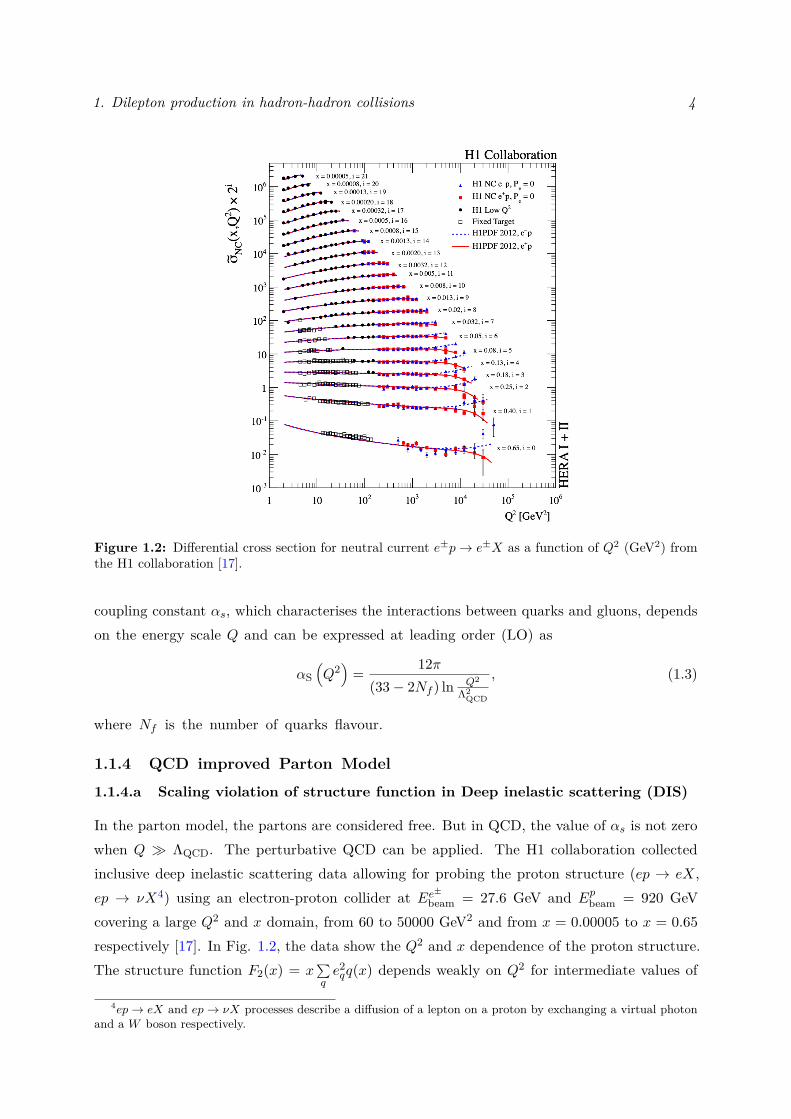
Figure 1.2: Differential cross section for neutral current e±p→ e±X as a function of Q2 (GeV2) fromthe H1 collaboration [17].
coupling constant αs, which characterises the interactions between quarks and gluons, dependson the energy scale Q and can be expressed at leading order (LO) as
αS(Q2)
= 12π(33− 2Nf ) ln Q2
Λ2QCD
, (1.3)
where Nf is the number of quarks flavour.
1.1.4 QCD improved Parton Model
1.1.4.a Scaling violation of structure function in Deep inelastic scattering (DIS)
In the parton model, the partons are considered free. But in QCD, the value of αs is not zerowhen Q � ΛQCD. The perturbative QCD can be applied. The H1 collaboration collectedinclusive deep inelastic scattering data allowing for probing the proton structure (ep → eX,ep → νX4) using an electron-proton collider at Ee±beam = 27.6 GeV and Epbeam = 920 GeVcovering a large Q2 and x domain, from 60 to 50000 GeV2 and from x = 0.00005 to x = 0.65respectively [17]. In Fig. 1.2, the data show the Q2 and x dependence of the proton structure.The structure function F2(x) = x
∑qe2qq(x) depends weakly on Q2 for intermediate values of
4ep→ eX and ep→ νX processes describe a diffusion of a lepton on a proton by exchanging a virtual photonand a W boson respectively.
1. Dilepton production in hadron-hadron collisions 5
x ∼ 10−1. For both large and small x values, a clear Q2 dependence is observed highlightinga scaling violation in the proton structure. This observation leads to the conclusion that thestructure functions do not only depend on x but also on the energy scale Q at which it isprobed. The dynamics of the evolution as a function of Q2 of the hadronic structure5 lies in theinteraction of quarks and gluons between them, via the gluons exchange. In the next section,the perturbative QCD corrections will be introduced allowing to predict the scale evolutionthe structure functions and more generally of the PDF.
1.1.5 Perturbative QCD corrections
In hadron-hadron collisions, the hard partonic cross section σij has a perturbative expansion in αssuch as [18]
σ(h1h2) =∞∑n=0
αns
(µ2r
)∑i,j
∫dx1dx2fi
(x1, µ
2f
)fj(x2, µ
2f
)σ
(n)ij
(x1x2s, µ
2r , µ
2f
)(1.4)
where x1 and x2 are the Bjorken variables of the hadrons. The σij partonic cross sectiondepends on a non-physical parameter: the renormalisation scale µr. This scale is linked tothe energy scale which characterises the physical process. Mathematically, it is possible toregularize Ultra-Violet (UV) divergences typically from the parton loop correction when partonmomenta k →∞. The factorisation scale µf enables to separate PDFs from the hard partoniccross section, i.e. to separate the long-distance and short-distance physics. This scale isintroduced in order to cancel out another type of divergences: InfraRed (IR) divergences i.e.when momenta become soft k → 0. In a cross section calculation, it is generally common tochoose a common value for the scales µ2
r ≈ µ2f ≈ Q2 to avoid the appearance of large logarithms
terms ln(Q/µ)� 1. To estimate an uncertainty on the perturbative calculation, the scales areusually varied between (µ2
r , µ2f ) ∈ (Q2/4, 4Q2). The expansion in αs of σ(n)
ij takes into accountthe QCD corrections with respect to the LO σ
(0)ij cross section. These QCD corrections will
be detailed more precisely in the Drell-Yan process in Sec. 1.1.5.
1.1.5.a DGLAP equations
The Q2 dependence of the PDFs is described by the following DGLAP evolution equations [19, 20],
dqi(x,Q2)
d lnQ2 = αs2π
∫ 1
x
dx′x′
[qi(x′, Q2
)Pqq
(x
x′
)+ g
(x′, Q2
)Pqg
(x
x′
)],
dg(x,Q2)
d lnQ2 = αs2π
∫ 1
x
dx′x′
[qi(x′, Q2
)Pgq
(x
x′
)+ g
(x′, Q2
)Pgg
(x
x′
)] (1.5)
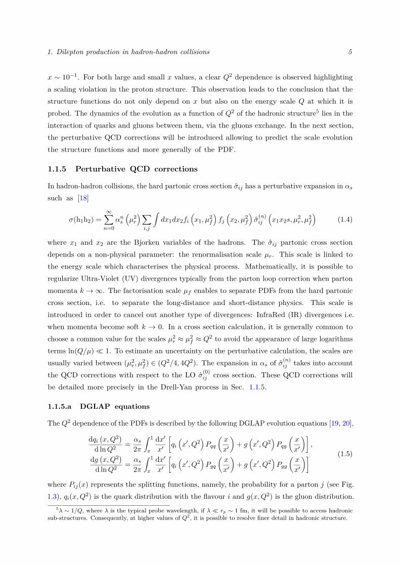
where Pij(x) represents the splitting functions, namely, the probability for a parton j (see Fig.1.3), qi(x,Q2) is the quark distribution with the flavour i and g(x,Q2) is the gluon distribution.
5λ ∼ 1/Q, where λ is the typical probe wavelength, if λ � rp ∼ 1 fm, it will be possible to access hadronicsub-structures. Consequently, at higher values of Q2, it is possible to resolve finer detail in hadronic structure.
1. Dilepton production in hadron-hadron collisions 6
These splitting functions are calculable in perturbation theory at any order in O (αns ) (see the
3-loop calculations in [21, 22, 23]). At LO in αs, these are given by [24]
P (LO)qq (z) = 4
3
[1 + z2
(1− z)++ 3
2δ(1− z)], (1.6)
P (LO)qg (z) = 1
2[z2 + (1− z)2
], (1.7)
P (LO)gq (z) = 4
3
[1 + (1− z)2
z
], (1.8)
P (LO)gg (z) = 6
[z
(1− z)++ 1− z
z+ z(1− z) +
(1112 −
Nf
18
)δ(1− z)
]. (1.9)
The plus prescription is defined as (see Eq. (3.2) in [25])
[f(x)]+ ≡ limβ→e
{f(x)Θ(1− x− β)− δ(1− x− β)
∫ 1−β
0dzf(z)
}. (1.10)
The Q2 evolution of the quarks and gluon PDFs is related by the coupled differential equations
x′
x
Pqq
x′
x
Pqg
x′
x
Pgq
x′
x
Pgg
Figure 1.3: Graphical representation of the LO splitting functions Pqq, Pqg, Pgq and Pgg.
in Eq. (1.5). Consequently, the information carried by the quarks PDFs at a given x and Q2
also give an information about the gluon PDF at the same x and Q2 and vice versa.
1.1.6 Parton distribution functions extraction from global fit
DGLAP equations can be numerically solved once the fi(x,Q20) are given as an input at the
starting scale Q20.6 The PDFs are extracted by performing a global fit of experimental data
to determine their shape at a given Q2 & Q20. The order in αs of the extracted PDF will
depend on the perturbative development in αs used to compute the partonic cross section of
the hard process and the loop order of the splitting functions. The extraction of the proton
and pion PDFs will now be briefly discussed.6Typically, the starting scale is defined as Q2
0 ' 1− 2 GeV2 at the limit where the DGLAP evolution equationsremains valid.
1. Dilepton production in hadron-hadron collisions 7
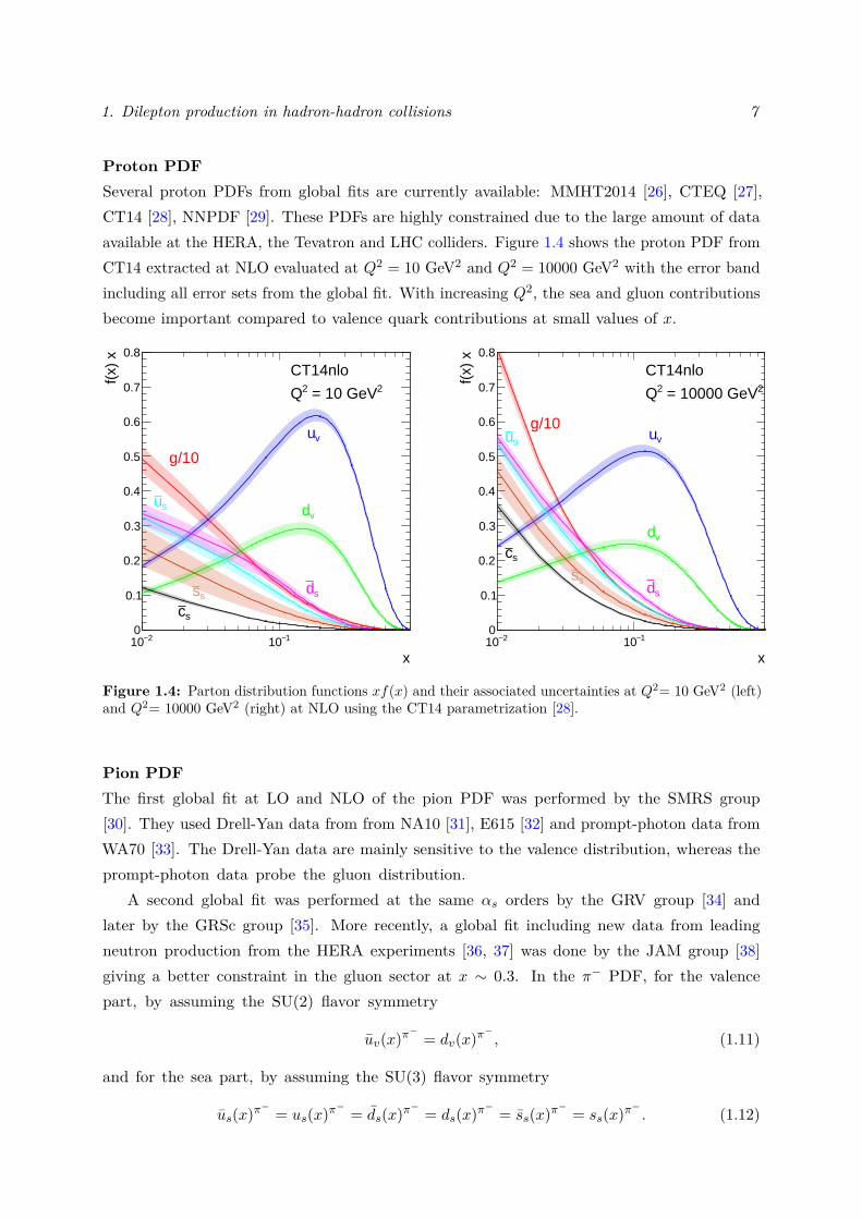
Proton PDFSeveral proton PDFs from global fits are currently available: MMHT2014 [26], CTEQ [27],CT14 [28], NNPDF [29]. These PDFs are highly constrained due to the large amount of dataavailable at the HERA, the Tevatron and LHC colliders. Figure 1.4 shows the proton PDF fromCT14 extracted at NLO evaluated at Q2 = 10 GeV2 and Q2 = 10000 GeV2 with the error bandincluding all error sets from the global fit. With increasing Q2, the sea and gluon contributionsbecome important compared to valence quark contributions at small values of x.
2−10 1−10x
0
0.1
0.2
0.3
0.4
0.5
0.6
0.7
0.8
f(x)
x
CT14nlo2 = 10 GeV2Q
g/10vu
vd
sd
su
ss
sc
2−10 1−10x
0
0.1
0.2
0.3
0.4
0.5
0.6
0.7
0.8
f(x)
x
CT14nlo2 = 10000 GeV2Q
g/10vu
vd
sd
su
sssc
Figure 1.4: Parton distribution functions xf(x) and their associated uncertainties at Q2= 10 GeV2 (left)and Q2= 10000 GeV2 (right) at NLO using the CT14 parametrization [28].
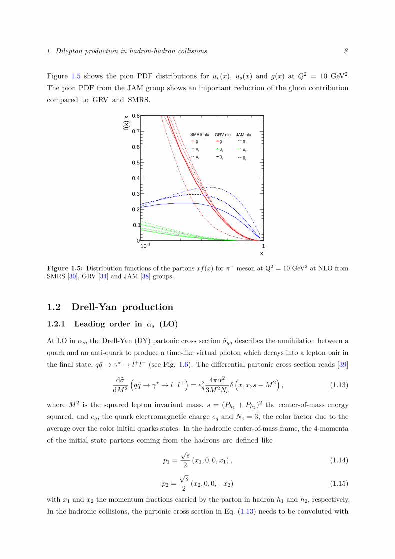
Pion PDFThe first global fit at LO and NLO of the pion PDF was performed by the SMRS group[30]. They used Drell-Yan data from from NA10 [31], E615 [32] and prompt-photon data fromWA70 [33]. The Drell-Yan data are mainly sensitive to the valence distribution, whereas theprompt-photon data probe the gluon distribution.
A second global fit was performed at the same αs orders by the GRV group [34] andlater by the GRSc group [35]. More recently, a global fit including new data from leadingneutron production from the HERA experiments [36, 37] was done by the JAM group [38]giving a better constraint in the gluon sector at x ∼ 0.3. In the π− PDF, for the valencepart, by assuming the SU(2) flavor symmetry
uv(x)π− = dv(x)π− , (1.11)
and for the sea part, by assuming the SU(3) flavor symmetry
us(x)π− = us(x)π− = ds(x)π− = ds(x)π− = ss(x)π− = ss(x)π− . (1.12)
1. Dilepton production in hadron-hadron collisions 8
Figure 1.5 shows the pion PDF distributions for uv(x), us(x) and g(x) at Q2 = 10 GeV2.The pion PDF from the JAM group shows an important reduction of the gluon contributioncompared to GRV and SMRS.
1−10 1x
0
0.1
0.2
0.3
0.4
0.5
0.6
0.7
0.8
f(x)
x
g
su
vu
g
su
vu
JAM nloGRV nloSMRS nlo
g
su
vu
Figure 1.5: Distribution functions of the partons xf(x) for π− meson at Q2 = 10 GeV2 at NLO fromSMRS [30], GRV [34] and JAM [38] groups.
1.2 Drell-Yan production
1.2.1 Leading order in αs (LO)
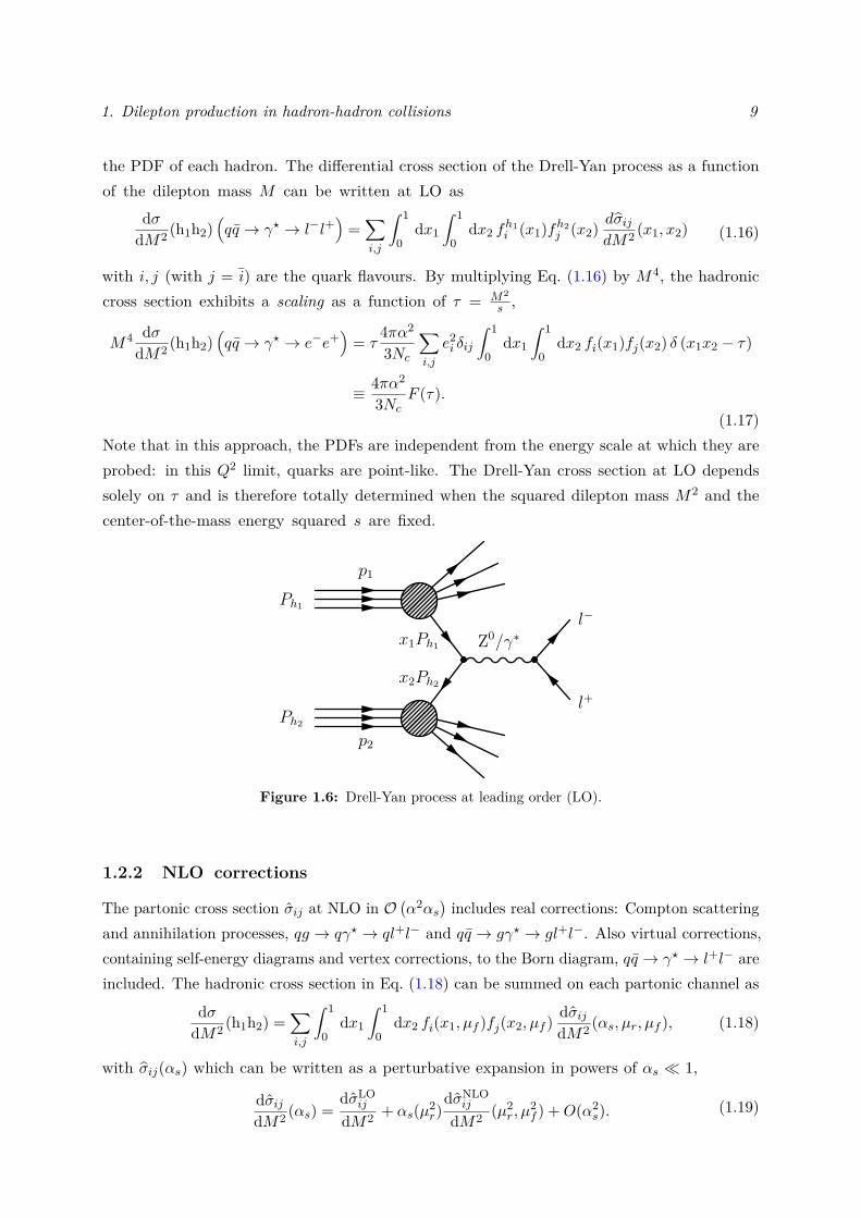
At LO in αs, the Drell-Yan (DY) partonic cross section σqq describes the annihilation between aquark and an anti-quark to produce a time-like virtual photon which decays into a lepton pair inthe final state, qq → γ? → l+l− (see Fig. 1.6). The differential partonic cross section reads [39]
dσdM2
(qq → γ? → l−l+
)= e2
q
4πα2
3M2Ncδ(x1x2s−M2
), (1.13)
where M2 is the squared lepton invariant mass, s = (Ph1 + Ph2)2 the center-of-mass energysquared, and eq, the quark electromagnetic charge eq and Nc = 3, the color factor due to theaverage over the color initial quarks states. In the hadronic center-of-mass frame, the 4-momentaof the initial state partons coming from the hadrons are defined like
p1 =√s
2 (x1, 0, 0, x1) , (1.14)
p2 =√s
2 (x2, 0, 0,−x2) (1.15)
with x1 and x2 the momentum fractions carried by the parton in hadron h1 and h2, respectively.In the hadronic collisions, the partonic cross section in Eq. (1.13) needs to be convoluted with
1. Dilepton production in hadron-hadron collisions 9
the PDF of each hadron. The differential cross section of the Drell-Yan process as a functionof the dilepton mass M can be written at LO as
dσdM2 (h1h2)
(qq → γ? → l−l+
)=∑i,j
∫ 1
0dx1
∫ 1
0dx2 f
h1i (x1)fh2
j (x2) dσijdM2 (x1, x2) (1.16)
with i, j (with j = i) are the quark flavours. By multiplying Eq. (1.16) by M4, the hadroniccross section exhibits a scaling as a function of τ = M2
s ,
M4 dσdM2 (h1h2)
(qq → γ? → e−e+
)= τ
4πα2
3Nc
∑i,j
e2i δij
∫ 1
0dx1
∫ 1
0dx2 fi(x1)fj(x2) δ (x1x2 − τ)
≡ 4πα2
3NcF (τ).
(1.17)Note that in this approach, the PDFs are independent from the energy scale at which they areprobed: in this Q2 limit, quarks are point-like. The Drell-Yan cross section at LO dependssolely on τ and is therefore totally determined when the squared dilepton mass M2 and thecenter-of-the-mass energy squared s are fixed.
p1
p2
Z0/γ∗
Ph2
Ph1
l+
l−
x2Ph2
x1Ph1
Figure 1.6: Drell-Yan process at leading order (LO).
1.2.2 NLO corrections
The partonic cross section σij at NLO in O(α2αs
)includes real corrections: Compton scattering
and annihilation processes, qg → qγ? → ql+l− and qq → gγ? → gl+l−. Also virtual corrections,containing self-energy diagrams and vertex corrections, to the Born diagram, qq → γ? → l+l− areincluded. The hadronic cross section in Eq. (1.18) can be summed on each partonic channel as
dσdM2 (h1h2) =
∑i,j
∫ 1
0dx1
∫ 1
0dx2 fi(x1, µf )fj(x2, µf ) dσij
dM2 (αs, µr, µf ), (1.18)
with σij(αs) which can be written as a perturbative expansion in powers of αs � 1,
dσijdM2 (αs) =
dσLOij
dM2 + αs(µ2r)
dσNLOij
dM2 (µ2r , µ
2f ) +O(α2
s). (1.19)
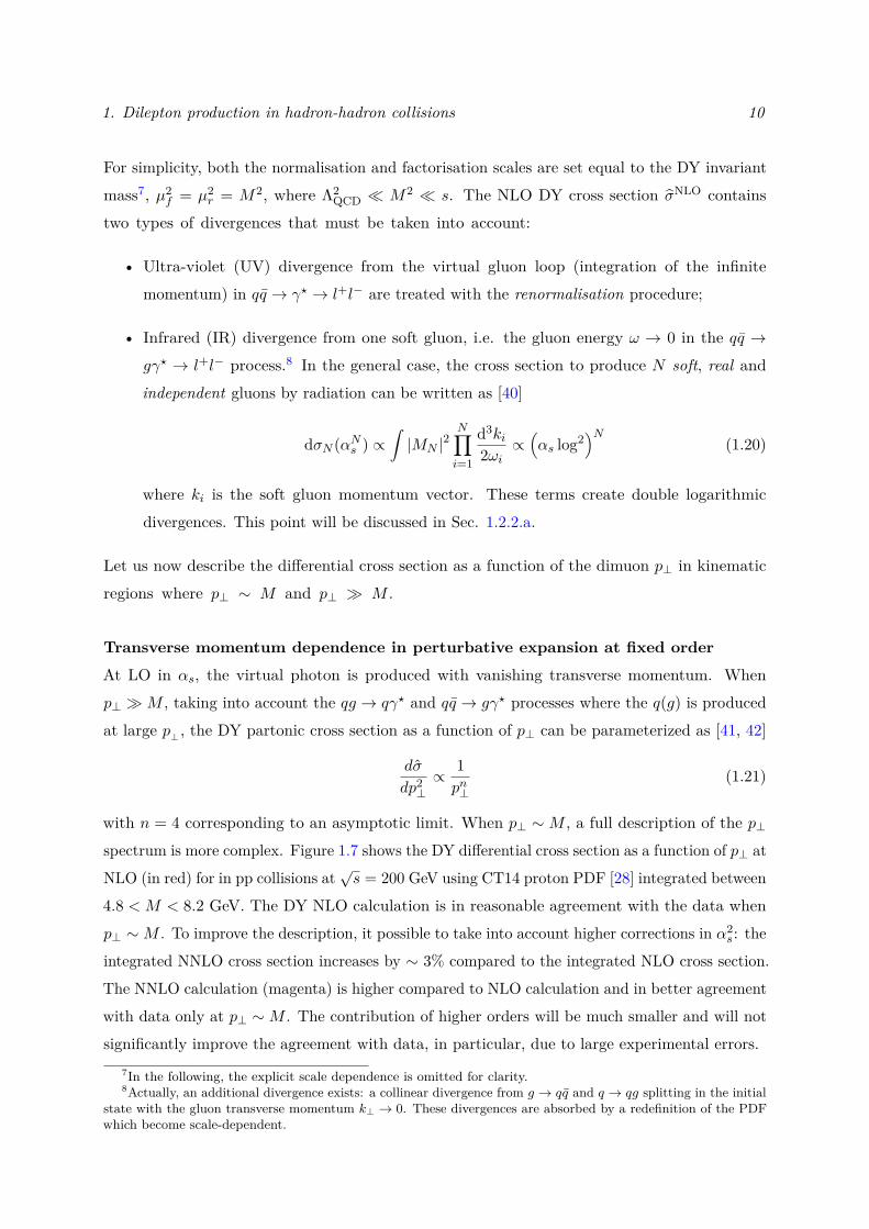
1. Dilepton production in hadron-hadron collisions 10
For simplicity, both the normalisation and factorisation scales are set equal to the DY invariantmass7, µ2
f = µ2r = M2, where Λ2
QCD � M2 � s. The NLO DY cross section σNLO containstwo types of divergences that must be taken into account:
• Ultra-violet (UV) divergence from the virtual gluon loop (integration of the infinitemomentum) in qq → γ? → l+l− are treated with the renormalisation procedure;
• Infrared (IR) divergence from one soft gluon, i.e. the gluon energy ω → 0 in the qq →gγ? → l+l− process.8 In the general case, the cross section to produce N soft, real andindependent gluons by radiation can be written as [40]
dσN (αNs ) ∝∫|MN |2
N∏i=1
d3ki2ωi
∝(αs log2
)N(1.20)
where ki is the soft gluon momentum vector. These terms create double logarithmicdivergences. This point will be discussed in Sec. 1.2.2.a.
Let us now describe the differential cross section as a function of the dimuon p⊥ in kinematicregions where p⊥ ∼ M and p⊥ � M .
Transverse momentum dependence in perturbative expansion at fixed order
At LO in αs, the virtual photon is produced with vanishing transverse momentum. Whenp⊥ �M , taking into account the qg → qγ? and qq → gγ? processes where the q(g) is producedat large p⊥ , the DY partonic cross section as a function of p⊥ can be parameterized as [41, 42]
dσ
dp2⊥∝ 1pn⊥
(1.21)
with n = 4 corresponding to an asymptotic limit. When p⊥ ∼ M , a full description of the p⊥spectrum is more complex. Figure 1.7 shows the DY differential cross section as a function of p⊥ atNLO (in red) for in pp collisions at
√s = 200 GeV using CT14 proton PDF [28] integrated between
4.8 < M < 8.2 GeV. The DY NLO calculation is in reasonable agreement with the data whenp⊥ ∼M . To improve the description, it possible to take into account higher corrections in α2
s: theintegrated NNLO cross section increases by ∼ 3% compared to the integrated NLO cross section.The NNLO calculation (magenta) is higher compared to NLO calculation and in better agreementwith data only at p⊥ ∼M . The contribution of higher orders will be much smaller and will notsignificantly improve the agreement with data, in particular, due to large experimental errors.
7In the following, the explicit scale dependence is omitted for clarity.8Actually, an additional divergence exists: a collinear divergence from g → qq and q → qg splitting in the initial
state with the gluon transverse momentum k⊥ → 0. These divergences are absorbed by a redefinition of the PDFwhich become scale-dependent.
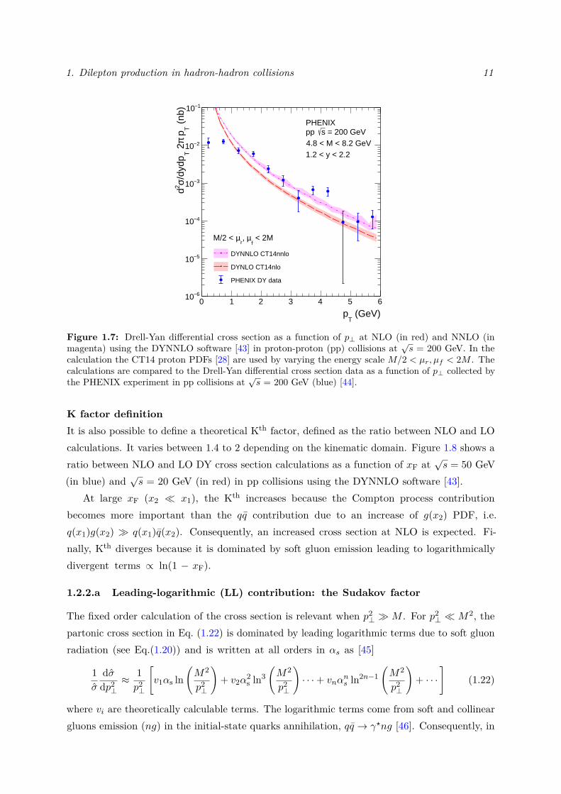
1. Dilepton production in hadron-hadron collisions 11
0 1 2 3 4 5 6
(GeV)T
p
6−10
5−10
4−10
3−10
2−10
1−10
(nb
)T
pπ 2
T/d
ydp
σ2 d
DYNNLO CT14nnlo
DYNLO CT14nlo
PHENIX DY data
PHENIX = 200 GeV spp
4.8 < M < 8.2 GeV1.2 < y < 2.2
< 2Mf
µ, r
µM/2 <
Figure 1.7: Drell-Yan differential cross section as a function of p⊥ at NLO (in red) and NNLO (inmagenta) using the DYNNLO software [43] in proton-proton (pp) collisions at
√s = 200 GeV. In the
calculation the CT14 proton PDFs [28] are used by varying the energy scale M/2 < µr, µf < 2M . Thecalculations are compared to the Drell-Yan differential cross section data as a function of p⊥ collected bythe PHENIX experiment in pp collisions at
√s = 200 GeV (blue) [44].
K factor definitionIt is also possible to define a theoretical Kth factor, defined as the ratio between NLO and LOcalculations. It varies between 1.4 to 2 depending on the kinematic domain. Figure 1.8 shows aratio between NLO and LO DY cross section calculations as a function of xF at
√s = 50 GeV
(in blue) and√s = 20 GeV (in red) in pp collisions using the DYNNLO software [43].
At large xF (x2 � x1), the Kth increases because the Compton process contributionbecomes more important than the qq contribution due to an increase of g(x2) PDF, i.e.q(x1)g(x2) � q(x1)q(x2). Consequently, an increased cross section at NLO is expected. Fi-nally, Kth diverges because it is dominated by soft gluon emission leading to logarithmicallydivergent terms ∝ ln(1 − xF).
1.2.2.a Leading-logarithmic (LL) contribution: the Sudakov factor
The fixed order calculation of the cross section is relevant when p2⊥ � M . For p2
⊥ � M2, thepartonic cross section in Eq. (1.22) is dominated by leading logarithmic terms due to soft gluonradiation (see Eq.(1.20)) and is written at all orders in αs as [45]
1σ
dσdp2⊥≈ 1p2⊥
[v1αs ln
(M2
p2⊥
)+ v2α
2s ln3
(M2
p2⊥
)· · ·+ vnα
ns ln2n−1
(M2
p2⊥
)+ · · ·
](1.22)
where vi are theoretically calculable terms. The logarithmic terms come from soft and collineargluons emission (ng) in the initial-state quarks annihilation, qq → γ?ng [46]. Consequently, in
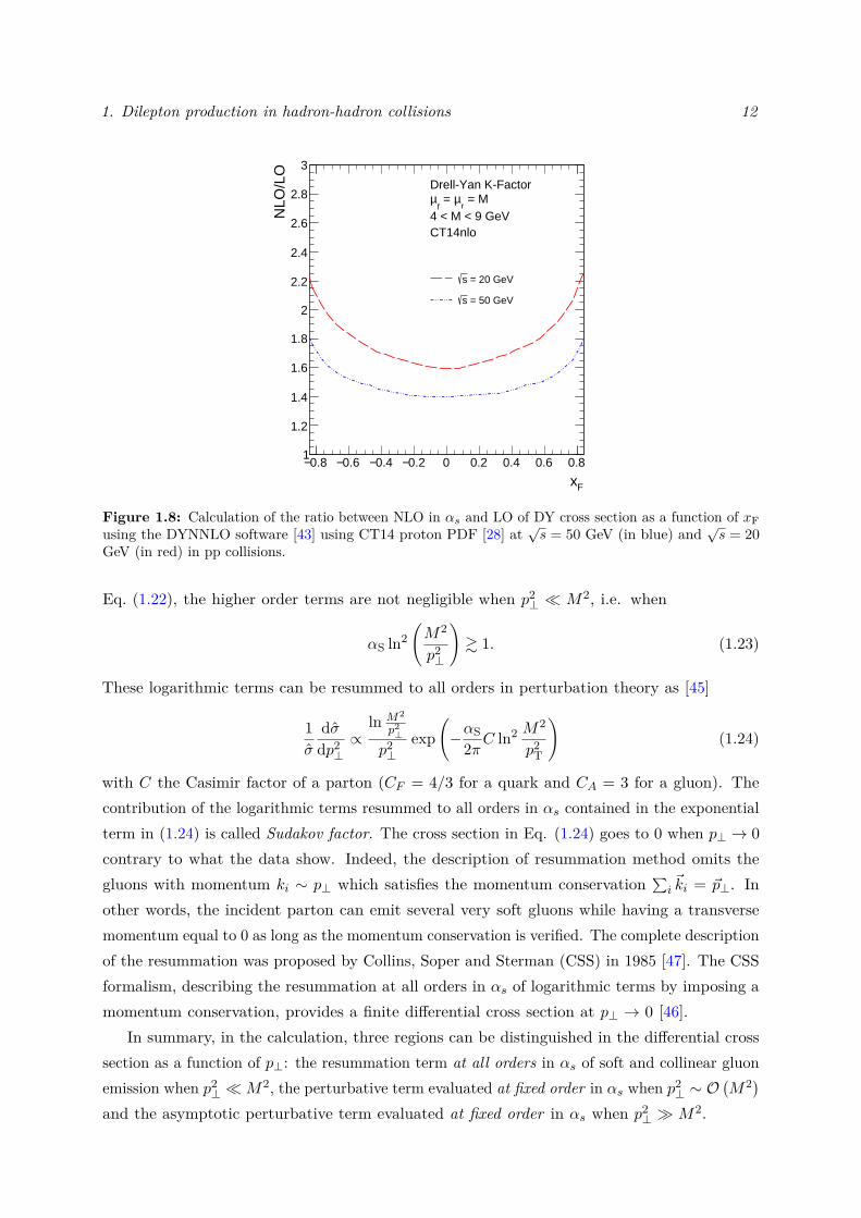
1. Dilepton production in hadron-hadron collisions 12
0.8− 0.6− 0.4− 0.2− 0 0.2 0.4 0.6 0.8
Fx
1
1.2
1.4
1.6
1.8
2
2.2
2.4
2.6
2.8
3
NLO
/LO
= 20 GeVs
= 50 GeVs
Drell-Yan K-Factor = M
rµ =
fµ4 < M < 9 GeVCT14nlo
Figure 1.8: Calculation of the ratio between NLO in αs and LO of DY cross section as a function of xFusing the DYNNLO software [43] using CT14 proton PDF [28] at
√s = 50 GeV (in blue) and
√s = 20
GeV (in red) in pp collisions.
Eq. (1.22), the higher order terms are not negligible when p2⊥ � M2, i.e. when
αS ln2(M2
p2⊥
)& 1. (1.23)
These logarithmic terms can be resummed to all orders in perturbation theory as [45]
1σ
dσdp2⊥∝
ln M2
p2⊥
p2⊥
exp(−αS
2πC ln2 M2
p2T
)(1.24)
with C the Casimir factor of a parton (CF = 4/3 for a quark and CA = 3 for a gluon). Thecontribution of the logarithmic terms resummed to all orders in αs contained in the exponentialterm in (1.24) is called Sudakov factor. The cross section in Eq. (1.24) goes to 0 when p⊥ → 0contrary to what the data show. Indeed, the description of resummation method omits thegluons with momentum ki ∼ p⊥ which satisfies the momentum conservation ∑i
~ki = ~p⊥. Inother words, the incident parton can emit several very soft gluons while having a transversemomentum equal to 0 as long as the momentum conservation is verified. The complete descriptionof the resummation was proposed by Collins, Soper and Sterman (CSS) in 1985 [47]. The CSSformalism, describing the resummation at all orders in αs of logarithmic terms by imposing amomentum conservation, provides a finite differential cross section at p⊥ → 0 [46].
In summary, in the calculation, three regions can be distinguished in the differential crosssection as a function of p⊥: the resummation term at all orders in αs of soft and collinear gluonemission when p2
⊥ �M2, the perturbative term evaluated at fixed order in αs when p2⊥ ∼ O
(M2)
and the asymptotic perturbative term evaluated at fixed order in αs when p2⊥ � M2.
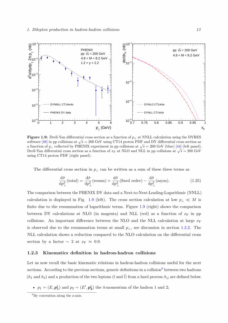
1. Dilepton production in hadron-hadron collisions 13
0 1 2 3 4 5 6
(GeV)T
p
6−10
5−10
4−10
3−10
2−10
1−10
(nb
)T
pπ 2
T/d
ydp
σ2 d
DYNNLL CT14nnlo
PHENIX DY data
PHENIX = 200 GeV spp
4.8 < M < 8.2 GeV1.2 < y < 2.2
0.7 0.75 0.8 0.85 0.9 0.95 1
Fx
5−10
4−10
3−10
2−10
1−10
(nb
)F
/dx
σd
DYNLO CT14nlo
DYNLL CT14nlo
PHENIX = 200 GeV spp
4.8 < M < 8.2 GeV
Figure 1.9: Drell-Yan differential cross section as a function of p⊥ at NNLL calculation using the DYRESsoftware [48] in pp collisions at
√s = 200 GeV using CT14 proton PDF and DY differential cross section as
a function of p⊥ collected by PHENIX experiment in pp collisions at√s = 200 GeV (blue) [44] (left panel).
Drell-Yan differential cross section as a function of xF at NLO and NLL in pp collisions at√s = 200 GeV
using CT14 proton PDF (right panel).
The differential cross section in p⊥ can be written as a sum of these three terms as
dσdp2⊥
(total) = dσdp2⊥
(resum) + dσdp2⊥
(fixed order)− dσdp2⊥
(asym). (1.25)
The comparison between the PHENIX DY data and a Next-to-Next-Leading-Logarithmic (NNLL)calculation is displayed in Fig. 1.9 (left). The cross section calculation at low p⊥ � M isfinite due to the resummation of logarithmic terms. Figure 1.9 (right) shows the comparisonbetween DY calculations at NLO (in magenta) and NLL (red) as a function of xF in ppcollisions. An important difference between the NLO and the NLL calculation at large xFis observed due to the resummation terms at small p⊥, see discussion in section 1.2.2. TheNLL calculation shows a reduction compared to the NLO calculation on the differential crosssection by a factor ∼ 2 at xF ≈ 0.9.
1.2.3 Kinematics definition in hadron-hadron collisions
Let us now recall the basic kinematic relations in hadron-hadron collisions useful for the nextsections. According to the previous sections, generic definitions in a collision9 between two hadrons(h1 and h2) and a production of the two leptons (l and l) from a hard process σij are defined below.
• p1 = (E,pi1) and p2 = (E′,pi2) the 4-momentum of the hadron 1 and 2;9By convention along the z-axis.
1. Dilepton production in hadron-hadron collisions 14
• s = (p1 + p2)2 the s-channel variable,√s the center-of-mass energy in the hadronic frame;
• x1p1 and x2p2 the 4-momentum of the parton 1 and 2 respectively;
• xF = pzpmaxz≈ x1 − x2 the fraction of the maximum longitudinal momentum carried by the
dilepton pair;
• M = √x1x2s the invariant mass of the dilepton pair;
• M⊥ =√M2 + p2
⊥, the transverse invariant mass of the dilepton pair;
• y = 12 ln
(E+pzE−pz
)= ln
(E+pzM⊥
), the rapidity of dilepton pair.
Bjorken x
The definition of the variables x1 and x2 depends on the domain in p⊥ of the dilepton pairproduced in a hard process. Indeed, if p⊥ is less than M , the scattering energy scale toprobe the physical process is equal to the invariant mass of the dilepton pair where p⊥ islarge compared to M , the relevant scattering energy scale becomes dependent on p⊥. Threedifferent kinematics can be defined as
• kinematic 2→ 1 (ij → k → l−l+ +X) namely when 0 < p⊥ .M : x1/2 'Me±y/√s,
• kinematic 2→ 2 (ij → kl→ l−l+ +X) when p⊥ &M : x1/2 ' (MT + p⊥)e±y/√s
• kinematic 2→ 2 (ij → kl→ l−l+ +X) when p⊥ �M : x1/2 ' 2p⊥e±y/√s.
1.3 Quarkonium production
In this section, we will introduce a second hard process of purely strong interaction: thequarkonium production. The quarkonium production in hadron-hadron collisions proceedsthrough the QCD scattering of the two partons, as illustrated in Fig. 1.10, in the gluon fusionchannel. In the J/ψ case, the ground state of the charmonium meson, the mass of the cc pairproduced of about 3 GeV is much larger than ΛQCD. Therefore, it is in principle possible to usethe perturbative QCD tools combined with factorisation theorems. But, unlike the DY processdescribed above, the quarkonium production is more complex, because it is necessary to describecorrectly the hadronisation part. Most quarkonium production models are based on a collinearfactorisation between the heavy quark pair QQ production and its subsequent hadronizaton intoa charmonium meson. Although the complete description of the production of quarkonium is stilla puzzle difficult to solve, the main existing models will be briefly described in the next sections.
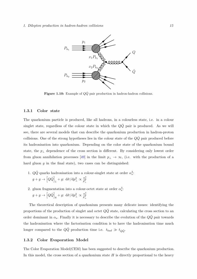
1. Dilepton production in hadron-hadron collisions 15
p1
p2
Ph2
Ph1
Q
Q
x2Ph2
x1Ph1
Figure 1.10: Example of QQ pair production in hadron-hadron collisions.
1.3.1 Color state
The quarkonium particle is produced, like all hadrons, in a colourless state, i.e. in a coloursinglet state, regardless of the colour state in which the QQ pair is produced. As we willsee, there are several models that can describe the quarkonium production in hadron-protoncollisions. One of the strong hypotheses lies in the colour state of the QQ pair produced beforeits hadronisation into quarkonium. Depending on the color state of the quarkonium boundstate, the p⊥ dependence of the cross section is different. By considering only lowest orderfrom gluon annihilation processes [49] in the limit p⊥ → ∞, (i.e. with the production of ahard gluon g in the final state), two cases can be distinguished:
1. QQ quarks hadronisation into a colour-singlet state at order α3s:
g + g →[QQ
]1
+ g: dσ/dp2⊥ ∝
α3s
p8⊥
2. gluon fragmentation into a colour-octet state at order α3s:
g + g →[QQ
]8
+ g: dσ/dp2⊥ ∝
α3s
p4⊥
The theoretical description of quarkonium presents many delicate issues: identifying theproportions of the production of singlet and octet QQ state, calculating the cross section to anorder dominant in αs. Finally it is necessary to describe the evolution of the QQ pair towardsthe hadronisation where the factorisation condition is to have the hadronisation time muchlonger compared to the QQ production time i.e. thad � tQQ.
1.3.2 Color Evaporation Model
The Color Evaporation Model(CEM) has been suggested to describe the quarkonium production.In this model, the cross section of a quarkonium state H is directly proportional to the heavy
1. Dilepton production in hadron-hadron collisions 16
quark pair production cross section integrated between the free QQ mass pair (2mQ) and open-heavy-flavour hadron pair mass (2mD,B). The quarkonium production cross section in theCEM model can be written as [50]
σ[H +X] = FH∫ 2mD,B
2mQ
dσ[QQ+X]dmQQ
dmQQ, (1.26)
where σ[H +X] is the production cross section of state H and dσ[QQ+X]dm
QQthe differential cross
section to produce a heavy quark pair (QQ) calculable in the perturbative theory. The factor FHis determined in a purely phenomenological approach and is related to the fraction of dσ[H +X]that produces the quarkonium state H. This model assumes the factorisation between theperturbative production of a QQ pair and the non-perturbative hadronisation process. It is areasonable assumption in the J/ψ case because tf ∼ 1/(2mcc) ∼ 0.1 fm� 1/(2(Mψ −MJ/ψ)),where tf is the H bound state formation time, Mψ and MJ/ψ, the ψ and J/ψ bound statemasses respectively. Otherwise, the CEM is an average over all color and spin states of theQQ produced. It therefore cannot predict the quantum numbers of the produced bound stateJ/ψ. On the other hand, a recent improvement of this model (ICEM) was performed to describethe polarisation dependence of the produced quarkonium state H [51]. The ICEM modelincludes interactions by many soft gluons between QQ and various color sources between itsproduction and its hadronisation into a bound state.
1.3.3 Color-Singlet model
The Color-Singlet Model (CSM) [52] is used to describe the production of a quarkonium stateH without evolution of the quantum states between the heavy-quark QQ pair production andits hadronisation. The model assumptions are:
• the QQ pair is produced at a scale µ2 ∼M2QQ� Λ2
QCD justifying a pQCD treatment;
• the QQ pair is produced in the non-relativistic limit with v � 1, with v the relative velocityof the heavy quarks;
• the state of quarkonium H is produced with the same spin, color and angular-momentumquantum numbers as the QQ pair in a color-singlet 3S
[1]1 state.
The cross section of quarkonium H production in the CSM model can be written
σ[H +X] ∝ σh1h2→(QQ)1|RH(0)|2 . (1.27)
with |RH(0)|, the non-perturbative parameters describing the hadronisation part and corre-sponding to the probability of the pair (QQ)1 in singlet-state to access to the bound stateH. Recently [53], it was shown that O
(α4s
)and O
(α5s
)corrections to CSM model participate
significantly to the total cross section calculation and lead to a relatively good agreement withdata at Tevatron and LHC energies in pp collisions at large p⊥ � MJ/ψ.
As we will be described in the next section, the NRQCD model proposes a more completedescription that encapsulates the CSM model.
1. Dilepton production in hadron-hadron collisions 17
1.3.4 Non-Relativistic QCD model
The Color-Octet Mechanism (COM) in the Non-Relativistic QCD (NRQCD) formalism givesa similar approach as the CSM model. This approach is also based on a factorisation betweenthe hard and soft part. However, the information on the hadronisation part is contained inlong distance matrix elements (LDMEs). The cross section of a quarkonium state H productionin NRQCD model can be written as [54]
dσ[H +X] ∝ σh1h2→(QQ)n 〈OnH〉 . (1.28)
where σh1h2→(QQ)n is the hadronic cross section part describing the production of QQ pair inspin, color and orbital-angular momentum state denoted n and 〈OnH〉, the non-perturbativeparameters describing the hadronisation part and correspond to the probability of the pairQQ to access to the bound state H in a quantum state n. The color-singlet matrix are takenfrom potential model calculation [55, 56] whereas the octet-matrix elements are extracted inthe experimental data [57, 58] at p⊥ � MJ/ψ. In contrast to the CEM model, the NRQCDmodel includes the radiative decays of exciting states to the J/ψ state. 10 The J/ψ totalproduction cross section can be written as
σJ/ψ = σdirJ/ψ +
2∑J=0
B (χcJ → J/ψ +X)σχcJ +B(ψ′ → J/ψ +X
)σψ′ , (1.29)
where B (Q→ J/ψ +X) is the branching ratio of excited quarkonium state H to J/ψ. Generally,none of the models cited in this section provides a complete description of the production ofquarkonium. In particular, the most complete NRQCD model does not reproduce low-energydata at fixed targets [59] especially the quarkonium polarisation.
1.4 Phenomenological aspects of the Drell-Yan and quarkoniumproduction
In this chapter, the framework to describe the production of the Drell-Yan and quarkoniumin pp collisions is discussed. These two processes of different but complementary nature makeit possible to study the hadronic structure.
1.4.1 Drell-Yan production
As mentioned in Sec. 1.2.2, it is possible to calculate in perturbation theory the DY process inall p⊥ regions. At moderate p⊥ ∼ M and large p⊥ � M values at fixed order in αs, the DYcross section is calculated up to NNLO corrections [43] but also at small p⊥ � M values, bytaking into account the logarithmic corrections up to NNLL corrections [48]. The perturbativecalculations allow for reproducing perfectly all observables in pp collisions, as a function ofthe dilepton mass, rapidity (xF) or p⊥. To illustrate this point, some comparisons betweenDY calculations and experimental results will be briefly shown.
10For more simplicity, the J/ψ quarkonium state is taken for example.
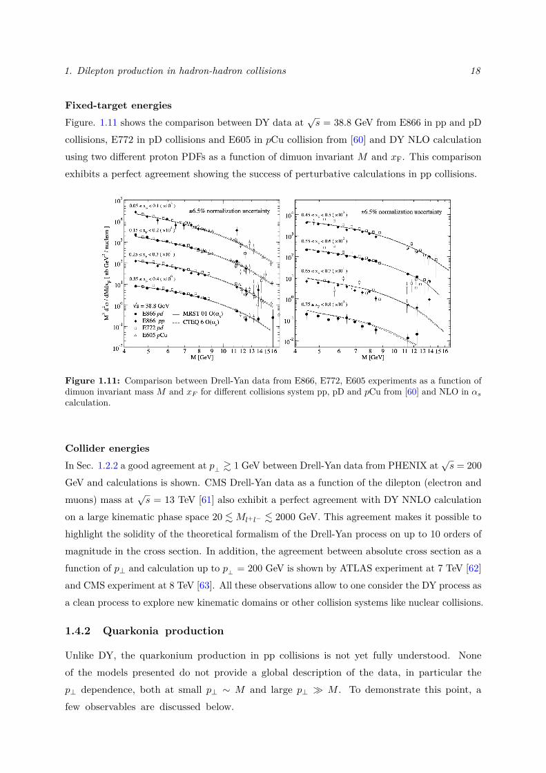
1. Dilepton production in hadron-hadron collisions 18
Fixed-target energiesFigure. 1.11 shows the comparison between DY data at
√s = 38.8 GeV from E866 in pp and pD
collisions, E772 in pD collisions and E605 in pCu collision from [60] and DY NLO calculationusing two different proton PDFs as a function of dimuon invariant M and xF. This comparisonexhibits a perfect agreement showing the success of perturbative calculations in pp collisions.
Figure 1.11: Comparison between Drell-Yan data from E866, E772, E605 experiments as a function ofdimuon invariant mass M and xF for different collisions system pp, pD and pCu from [60] and NLO in αscalculation.
Collider energiesIn Sec. 1.2.2 a good agreement at p⊥ & 1 GeV between Drell-Yan data from PHENIX at
√s = 200
GeV and calculations is shown. CMS Drell-Yan data as a function of the dilepton (electron andmuons) mass at
√s = 13 TeV [61] also exhibit a perfect agreement with DY NNLO calculation
on a large kinematic phase space 20 .Ml+l− . 2000 GeV. This agreement makes it possible tohighlight the solidity of the theoretical formalism of the Drell-Yan process on up to 10 orders ofmagnitude in the cross section. In addition, the agreement between absolute cross section as afunction of p⊥ and calculation up to p⊥ = 200 GeV is shown by ATLAS experiment at 7 TeV [62]and CMS experiment at 8 TeV [63]. All these observations allow to one consider the DY process asa clean process to explore new kinematic domains or other collision systems like nuclear collisions.
1.4.2 Quarkonia production
Unlike DY, the quarkonium production in pp collisions is not yet fully understood. Noneof the models presented do not provide a global description of the data, in particular thep⊥ dependence, both at small p⊥ ∼ M and large p⊥ � M . To demonstrate this point, afew observables are discussed below.
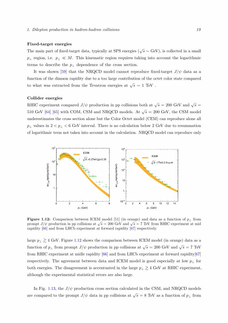
1. Dilepton production in hadron-hadron collisions 19
Fixed-target energiesThe main part of fixed-target data, typically at SPS energies (
√s ∼ GeV), is collected in a small
p⊥ region, i.e. p⊥ � M . This kinematic region requires taking into account the logarithmicterms to describe the p⊥ dependence of the cross section.
It was shown [59] that the NRQCD model cannot reproduce fixed-target J/ψ data as afunction of the dimuon rapidity due to a too large contribution of the octet color state comparedto what was extracted from the Tevatron energies at
√s ∼ 1 TeV .
Collider energiesRHIC experiment compared J/ψ production in pp collisions both at
√s = 200 GeV and
√s =
510 GeV [64] [65] with COM, CSM and NRQCD models. At√s = 200 GeV, the CSM model
underestimates the cross section alone but the Color Octet model (CEM) can reproduce alone allp⊥ values in 2 < p⊥ < 6 GeV interval. There is no calculation below 2 GeV due to resummationof logarithmic term not taken into account in the calculation. NRQCD model can reproduce only
Figure 1.12: Comparison between ICEM model [51] (in orange) and data as a function of p⊥ fromprompt J/ψ production in pp collisions at
√s = 200 GeV and
√s = 7 TeV from RHIC experiment at mid
rapidity [66] and from LHCb experiment at forward rapidity [67] respectively.
large p⊥ & 4 GeV. Figure 1.12 shows the comparison between ICEM model (in orange) data as afunction of p⊥ from prompt J/ψ production in pp collisions at
√s = 200 GeV and
√s = 7 TeV
from RHIC experiment at midle rapidity [66] and from LHCb experiment at forward rapidity[67]respectively. The agreement between data and ICEM model is good especially at low p⊥ forboth energies. The disagreement is accentuated in the large p⊥ & 4 GeV at RHIC experiment,although the experimental statistical errors are also large.
In Fig. 1.13, the J/ψ production cross section calculated in the CSM, and NRQCD modelsare compared to the prompt J/ψ data in pp collisions at
√s = 8 TeV as a function of p⊥ from
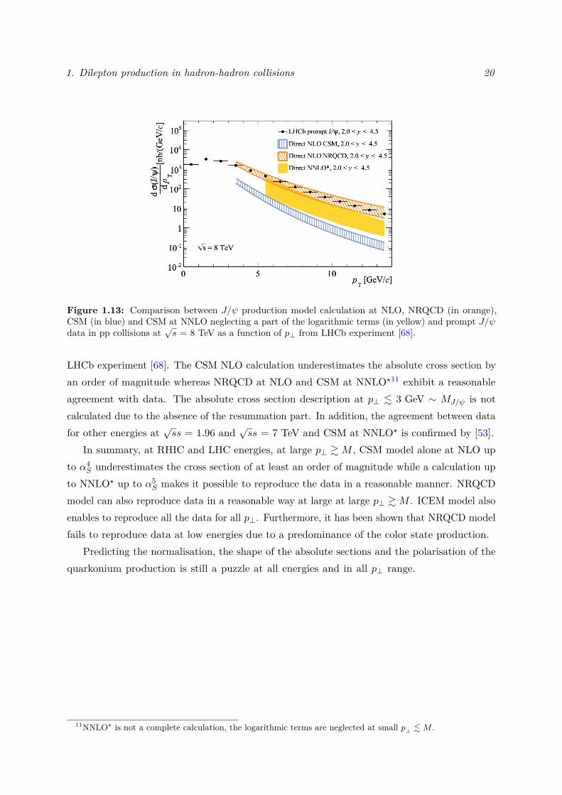
1. Dilepton production in hadron-hadron collisions 20
Figure 1.13: Comparison between J/ψ production model calculation at NLO, NRQCD (in orange),CSM (in blue) and CSM at NNLO neglecting a part of the logarithmic terms (in yellow) and prompt J/ψdata in pp collisions at
√s = 8 TeV as a function of p⊥ from LHCb experiment [68].
LHCb experiment [68]. The CSM NLO calculation underestimates the absolute cross section byan order of magnitude whereas NRQCD at NLO and CSM at NNLO?11 exhibit a reasonableagreement with data. The absolute cross section description at p⊥ . 3 GeV ∼ MJ/ψ is notcalculated due to the absence of the resummation part. In addition, the agreement between datafor other energies at
√ss = 1.96 and
√ss = 7 TeV and CSM at NNLO? is confirmed by [53].
In summary, at RHIC and LHC energies, at large p⊥ & M , CSM model alone at NLO upto α4
S underestimates the cross section of at least an order of magnitude while a calculation upto NNLO? up to α5
S makes it possible to reproduce the data in a reasonable manner. NRQCDmodel can also reproduce data in a reasonable way at large at large p⊥ &M . ICEM model alsoenables to reproduce all the data for all p⊥. Furthermore, it has been shown that NRQCD modelfails to reproduce data at low energies due to a predominance of the color state production.
Predicting the normalisation, the shape of the absolute sections and the polarisation of thequarkonium production is still a puzzle at all energies and in all p⊥ range.
11NNLO? is not a complete calculation, the logarithmic terms are neglected at small p⊥ .M .
2Nuclear effects in dilepton production
Contents
2.1 A-dependence . . . . . . . . . . . . . . . . . . . . . . . . . . . . . . . . . 222.1.1 Isospin effect . . . . . . . . . . . . . . . . . . . . . . . . . . . . . . . . . 222.1.2 Antiquark flavor asymmetry in the nucleon sea . . . . . . . . . . . . . . 232.1.3 Drell-Yan cross sections ratio . . . . . . . . . . . . . . . . . . . . . . . . 252.1.4 Charmonium cross sections ratio . . . . . . . . . . . . . . . . . . . . . . 25
2.2 Nuclear parton distribution function . . . . . . . . . . . . . . . . . . . 262.2.1 EPPS16 and EPS09 global fit . . . . . . . . . . . . . . . . . . . . . . . . 292.2.2 nCTEQ global fit . . . . . . . . . . . . . . . . . . . . . . . . . . . . . . . 312.2.3 DSSZ global fit . . . . . . . . . . . . . . . . . . . . . . . . . . . . . . . . 31
2.3 Nuclear absorption . . . . . . . . . . . . . . . . . . . . . . . . . . . . . 332.4 Parton energy loss in a QCD medium . . . . . . . . . . . . . . . . . . 35
2.4.1 Transport coefficient and broadening effect . . . . . . . . . . . . . . . . 362.4.2 Energy loss regimes . . . . . . . . . . . . . . . . . . . . . . . . . . . . . 37
2.5 Empirical observations . . . . . . . . . . . . . . . . . . . . . . . . . . . 382.5.1 Data . . . . . . . . . . . . . . . . . . . . . . . . . . . . . . . . . . . . . . 382.5.2 Data interpretation . . . . . . . . . . . . . . . . . . . . . . . . . . . . . . 412.5.3 Phenomenological approach . . . . . . . . . . . . . . . . . . . . . . . . . 42
Cold nuclear matter can be studied in hadron-nucleus collisions from fixed-target energies(√s ∼ GeV) to colliders (
√s ∼ TeV) energies. Indeed, the nuclear matter is static with a known
density. In this thesis, I am interested in the nuclear dependence of the DY and charmoniumproduction via the ratio of nuclear cross sections defined as
RhA (A/B, y) ≡ BA
(dσ(hA)dy
)×(dσ(hB)
dy
)−1(2.1)
and
RhA (A/B, p⊥) ≡ BA
(dσ(hA)dp⊥
)×(dσ(hB)
dp⊥
)−1(2.2)
21
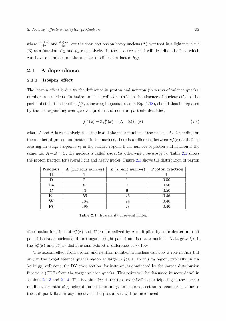
2. Nuclear effects in dilepton production 22
where dσ(hA)dy and dσ(hA)
dp⊥are the cross sections on heavy nucleus (A) over that in a lighter nucleus
(B) as a function of y and p⊥ respectiveky. In the next sections, I will describe all effects whichcan have an impact on the nuclear modification factor RhA.
2.1 A-dependence
2.1.1 Isospin effect
The isospin effect is due to the difference in proton and neutron (in terms of valence quarks)number in a nucleus. In hadron-nucleus collisions (hA) in the absence of nuclear effects, theparton distribution function fh2
j , appearing in general case in Eq. (1.18), should thus be replacedby the corresponding average over proton and neutron partonic densities,
fAj (x) = Zfpj (x) + (A− Z)fnj (x) (2.3)
where Z and A is respectively the atomic and the mass number of the nucleus A. Depending onthe number of proton and neutron in the nucleus, there is a difference between uAv (x) and dAv (x)creating an isospin-asymmetry in the valence region. If the number of proton and neutron is thesame, i.e. A− Z = Z, the nucleus is called isoscalar otherwise non-isoscalar. Table 2.1 showsthe proton fraction for several light and heavy nuclei. Figure 2.1 shows the distribution of parton
Nucleus A (nucleons number) Z (atomic number) Proton fractionH 1 1 1D 2 1 0.50Be 8 4 0.50C 12 6 0.50Fe 56 26 0.46W 184 74 0.40Pt 195 78 0.40
Table 2.1: Isoscalarity of several nuclei.
distribution functions of uAv (x) and dAv (x) normalized by A multiplied by x for deuterium (leftpanel) isoscalar nucleus and for tungsten (right panel) non-isoscalar nucleus. At large x & 0.1,the uAv (x) and dAv (x) distributions exhibit a difference of ∼ 15%.
The isospin effect from proton and neutron number in nucleus can play a role in RhA butonly in the target valence quarks region at large x2 & 0.1. In this x2 region, typically, in πA(or in pp) collisions, the DY cross section, for instance, is dominated by the parton distributionfunctions (PDF) from the target valence quarks. This point will be discussed in more detail insections 2.1.3 and 2.1.4. The isospin effect is the first trivial effect participating in the nuclearmodification ratio RhA being different than unity. In the next section, a second effect due tothe antiquark flavour asymmetry in the proton sea will be introduced.
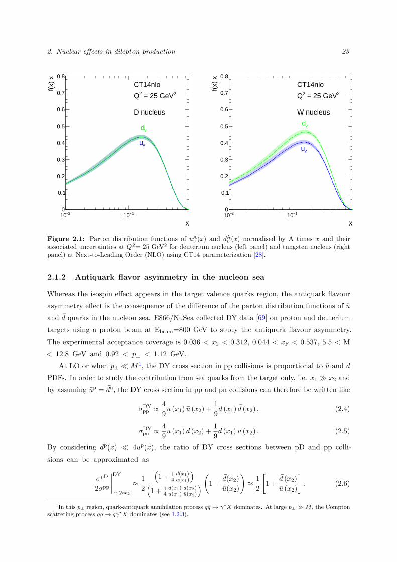
2. Nuclear effects in dilepton production 23
2−10 1−10x
0
0.1
0.2
0.3
0.4
0.5
0.6
0.7
0.8
f(x)
x
CT14nlo2 = 25 GeV2Q
D nucleus
vu
vd
2−10 1−10x
0
0.1
0.2
0.3
0.4
0.5
0.6
0.7
0.8
f(x)
x
CT14nlo2 = 25 GeV2Q
W nucleus
vu
vd
Figure 2.1: Parton distribution functions of uAv (x) and dA
v (x) normalised by A times x and theirassociated uncertainties at Q2= 25 GeV2 for deuterium nucleus (left panel) and tungsten nucleus (rightpanel) at Next-to-Leading Order (NLO) using CT14 parameterization [28].
2.1.2 Antiquark flavor asymmetry in the nucleon sea
Whereas the isospin effect appears in the target valence quarks region, the antiquark flavourasymmetry effect is the consequence of the difference of the parton distribution functions of uand d quarks in the nucleon sea. E866/NuSea collected DY data [69] on proton and deuteriumtargets using a proton beam at Ebeam=800 GeV to study the antiquark flavour asymmetry.The experimental acceptance coverage is 0.036 < x2 < 0.312, 0.044 < xF < 0.537, 5.5 < M< 12.8 GeV and 0.92 < p⊥ < 1.12 GeV.
At LO or when p⊥ �M1, the DY cross section in pp collisions is proportional to u and dPDFs. In order to study the contribution from sea quarks from the target only, i.e. x1 � x2 andby assuming up = dn, the DY cross section in pp and pn collisions can therefore be written like
σDYpp ∝49u (x1) u (x2) + 1
9d (x1) d (x2) , (2.4)
σDYpn ∝49u (x1) d (x2) + 1
9d (x1) u (x2) . (2.5)
By considering dp(x) � 4up(x), the ratio of DY cross sections between pD and pp colli-sions can be approximated as
σpD
2σpp
∣∣∣∣∣DY
x1�x2
≈ 12
(1 + 1
4d(x1)u(x1)
)(1 + 1
4d(x1)u(x1)
d(x2)u(x2)
) (1 + d(x2)u(x2)
)≈ 1
2
[1 + d (x2)
u (x2)
]. (2.6)
1In this p⊥ region, quark-antiquark annihilation process qq → γ∗X dominates. At large p⊥ �M , the Comptonscattering process qg → qγ?X dominates (see 1.2.3).
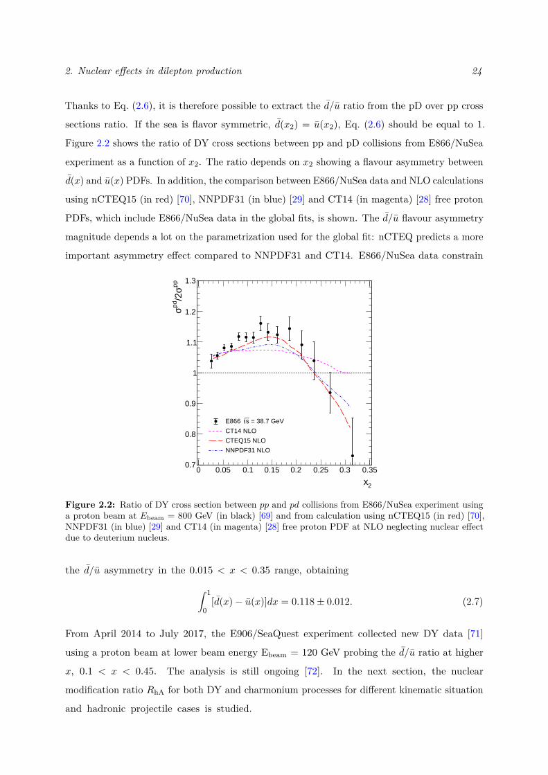
2. Nuclear effects in dilepton production 24
Thanks to Eq. (2.6), it is therefore possible to extract the d/u ratio from the pD over pp cross
sections ratio. If the sea is flavor symmetric, d(x2) = u(x2), Eq. (2.6) should be equal to 1.
Figure 2.2 shows the ratio of DY cross sections between pp and pD collisions from E866/NuSea
experiment as a function of x2. The ratio depends on x2 showing a flavour asymmetry between
d(x) and u(x) PDFs. In addition, the comparison between E866/NuSea data and NLO calculations
using nCTEQ15 (in red) [70], NNPDF31 (in blue) [29] and CT14 (in magenta) [28] free proton
PDFs, which include E866/NuSea data in the global fits, is shown. The d/u flavour asymmetry
magnitude depends a lot on the parametrization used for the global fit: nCTEQ predicts a more
important asymmetry effect compared to NNPDF31 and CT14. E866/NuSea data constrain
0 0.05 0.1 0.15 0.2 0.25 0.3 0.35
2x
0.7
0.8
0.9
1
1.1
1.2
1.3
pp σ/2
pd σ
= 38.7 GeVsE866
CT14 NLO
CTEQ15 NLO
NNPDF31 NLO
Figure 2.2: Ratio of DY cross section between pp and pd collisions from E866/NuSea experiment usinga proton beam at Ebeam = 800 GeV (in black) [69] and from calculation using nCTEQ15 (in red) [70],NNPDF31 (in blue) [29] and CT14 (in magenta) [28] free proton PDF at NLO neglecting nuclear effectdue to deuterium nucleus.
the d/u asymmetry in the 0.015 < x < 0.35 range, obtaining
∫ 1
0[d(x)− u(x)]dx = 0.118± 0.012. (2.7)
From April 2014 to July 2017, the E906/SeaQuest experiment collected new DY data [71]
using a proton beam at lower beam energy Ebeam = 120 GeV probing the d/u ratio at higher
x, 0.1 < x < 0.45. The analysis is still ongoing [72]. In the next section, the nuclear
modification ratio RhA for both DY and charmonium processes for different kinematic situation
and hadronic projectile cases is studied.
2. Nuclear effects in dilepton production 25
2.1.3 Drell-Yan cross sections ratio
At large positive xF > 0, or x1 � x2, typically in fixed-target configuration, the DY cross section atLO is dominated by the parton distribution functions of the valence quarks from the beam hadron.2
In pA collisions, the DY cross section is related to the sea quark distributions of the target,
σDYpA ∝49u
p(x1)uA(x2) + 19d
p(x1)dA(x2). (2.8)
The cross sections ratio in pA collisions can be written as
RDYpA ∝
8uA(x2) + dA(x2)8uB(x2) + dB(x2)
, (2.9)
by assuming up(x1) ≈ 2dp(x1) when x1 is the order O (10−1) in the proton. In π−A collisions, theDY cross section is dominated by valence quark contributions from the beam and from the target,
σDYπ−A ∝49 u
π−(x1)uAv (x2) + 19d
π−(x1)dB(x2). (2.10)
The ratio of nuclear cross sections can be express as
RDYπ−A ∝
4uA(x2) + dA(x2)4uB(x2) + dB(x2)
, (2.11)
by assuming uπ−(x1) = dπ−(x1) in the pion. Consequently, at forward rapidity (xF > 0) in
the pion beam case, the valence quarks of the target are essentially probed. Consequently, thisregion is sensitive to the isospin effect. While in pA, the sea quarks of the target is probedmainly sensitive to antiquark flavour asymmetry in the nucleon sea.
2.1.4 Charmonium cross sections ratio
In pA collisions, when xF ≈ 0 or x1 ≈ x2 � 1, the gluon PDF contribution is dominantcompared to quark PDFs contribution, g(x2) � q(x2) ' q(x2), the J/ψ 3 process in allproduction models can be written as,
gpgA → QQ→ J/ψ +X. (2.12)
The quarkonium production cross section in pA collisions is directly sensitive to the gluon PDFof the target. Assuming QCD factorisation, it can be written (see Eq. (2.13)) as a product ofthe gluon PDF from the beam4 and the nucleus and the quarkonium cross section,
dσ(pA)dy [J/ψ +X] =
∫ 1
0dx1
∫ 1
0dx2
∫dsgp
(x1, µ
2F
)gA(x2, µ
2F
) dσgg→J/ψ+Xdy δ (x1x2s− s)
(2.13)2At xF < 0, it is the opposite case, the DY cross section at LO is dominated by the PDFs of the valence quarks
from the target hadron.3To simplify, the J/ψ meson as the charmonium state is chosen.4It was shown in [73] in Υ data collected by E866/NuSea experiment in pp and pD collisions σ(pD →
Y)/2σ(pp→ Y) ≈ 12
(1 + g(x2)n
g(x2)p
)≈ 1 with integrated ratio equal to 0.984± 0.026(stat)± 0.01(sys) compatible
with g(x2)n = g(x2)p.
2. Nuclear effects in dilepton production 26
where µ2F ∼ M2
J/ψ. When x2 � 1, the cross sections ratio is equal to the ratio of the gluonPDFs of the nucleus A and the nucleus B,
RJ/ψpA ∝
gA(x2)gB(x2) . (2.14)
On the other hand, when xF & 0.85, the qq sub-process dominates [50].In π−A collisions, the dominant partonic sub-process depends on the pion PDF parametri-
sation as discussed in Sec. 1.1.6. However, at large xF ∼ x1, the cross section is dominatedby the valence quark PDFs from the pion beam. The shape of g(x) in the pion decreasesquickly at large x like xg(x)π ∼ (1 − x)3 [74] whereas the shape of qπ(x) decreases likexq(x) ∼ (1− x) [30]. Consequently, when the qq partonic sub-process dominates, it is reasonableto write the cross sections ratio as
RJ/ψπ−A ∝
uA(x2) + dA(x2)uB(x2) + uB(x2) . (2.15)
Between these two limits, i.e. 0 < xF � 1, the case is more complex to simply write the crosssections ratio because the relative contribution of qq and gg partonic sub-processes depend stronglyon which pion PDF is used6. The J/ψ cross section at LO can be written as a sum of two terms,
σπ−A[J/ψ +X] = σπ
−Agg [J/ψ +X] + σπ
−Aqq [J/ψ +X]. (2.16)
Figure 2.3 shows a calculation in the CEM model at LO for π−A collisions at the COMPASSexperiment with beam energy Ebeam = 190 GeV using two different pion PDFs: GRV [34] and themore recent pion PDF extraction from JAM [38]. Using GRV gives gluon fusion as a dominantchannel except at large xF ∼ 0.8. In contrast, JAM gives u(x1)u(x2) � g(x1)g(x2) at all xF.However, JAM pion PDF gives a better constraint in the gluon sector at x ∼ 0.3 thanks toleading neutron data from the HERA experiment [36, 37]. Consequently, as illustrated in Fig. 1.5,the gluon contribution from JAM is lower compared to GRV.
In π−A collisions, the uncertainty of the initial partonic state will have an impact on theinterpretation of the experimental data discussed in Sec. 2.5.
2.2 Nuclear parton distribution function
The EMC collaboration highlighted the Nuclear parton distribution function (nPDF) effectin DIS data in 1981 [75]. These data indicated for the first time that the proton PDF in anucleus (nPDF) is modified compared to the free proton PDF: fp/Ai (x,Q2) 6= fpi (x,Q2), wherefp/Ai is defined as the PDF of the parton of flavour i inside a proton bound in a nucleus. Thenuclear modification factor is defined as RA
j ≡ fp/Aj /fpj . The magnitude of this nuclear effect
5This value is modified at very low beam energy.6Certainly, the pion PDF and the hard process order will also change the relative contribution of these two
sub-processes.
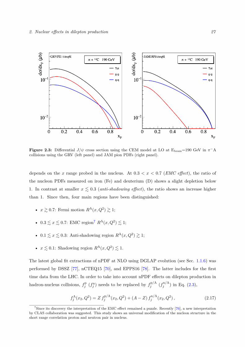
2. Nuclear effects in dilepton production 27
Figure 2.3: Differential J/ψ cross section using the CEM model at LO at Ebeam=190 GeV in π−Acollisions using the GRV (left panel) and JAM pion PDFs (right panel).
depends on the x range probed in the nucleus. At 0.3 < x < 0.7 (EMC effect), the ratio ofthe nucleon PDFs measured on iron (Fe) and deuterium (D) shows a slight depletion below1. In contrast at smaller x . 0.3 (anti-shadowing effect), the ratio shows an increase higherthan 1. Since then, four main regions have been distinguished:
• x & 0.7: Fermi motion RA(x,Q2) & 1;
• 0.3 . x . 0.7: EMC region7 RA(x,Q2) . 1;
• 0.1 . x . 0.3: Anti-shadowing region RA(x,Q2) & 1;
• x . 0.1: Shadowing region RA(x,Q2) . 1.
The latest global fit extractions of nPDF at NLO using DGLAP evolution (see Sec. 1.1.6) wasperformed by DSSZ [77], nCTEQ15 [70], and EPPS16 [78]. The latter includes for the firsttime data from the LHC. In order to take into account nPDF effects on dilepton production inhadron-nucleus collisions, fpj (fnj ) needs to be replaced by fp/Aj (fn/Aj ) in Eq. (2.3),
fAj (x2, Q
2) = Z fp/Aj (x2, Q
2) + (A− Z) fn/Aj (x2, Q2) , (2.17)
7Since its discovery the interpretation of the EMC effect remained a puzzle. Recently [76], a new interpretationby CLAS collaboration was suggested. This study shows an universal modification of the nucleon structure in theshort range correlation proton and neutron pair in nucleus.
2. Nuclear effects in dilepton production 28
where the bound neutron fn/Aj nPDF is determined by assuming SU(2) isospin symmetry as,
fn/Au,u
(x,Q2) = f
p/Ad,d
(x,Q2),
fn/Ad,d
(x,Q2) = f
p/Au,u
(x,Q2),
fn/Ai
(x,Q2) = f
p/Ai
(x,Q2) for other flavours.
. (2.18)
Let us now briefly describe the data used in different collisions to extract nPDFs:
• DIS data from EMC, SLAC, NMC and CHORUS experiments [78] (`A→ `+ X) describea scattering of a lepton (`) on a nucleus (A) via the production of space-like virtual photonor W boson (in νl diffusion). This process enables to probe the quark distributions ofthe nucleus. Depending on the collision energy, they data help to constrain both sea andvalence quark distributions at rather large x, 10−2 . x . 1. The largest amount of dataused for the nPDF extraction comes from this process [78, 70].
• π0 production (hA → π0 + X) at p⊥ . 16 GeV from PHENIX and STAR experiments[79, 80] at PHENIX (
√s = 200 GeV). These data can a priori be used to probe the gluon
sector nPDF around 10−2 . x . 10−1 at mid rapidity for instance.
• Z/W production (pA → Z and pA → W via ud→W+ and du→W−) are measured atLHC energies by the ATLAS and CMS experiments at
√s = 5.02 TeV and
√s = 8.16 TeV
[81, 82, 83]. These data constrain the quark nPDFs in the shadowing and antishadowingregion for 10−3 . x . 10−1 depending on the decay lepton rapidity.
• Dijet data from CMS experiment [84] at√s = 5.02 GeV at large p⊥ & 30 GeV. These
data constrain quark and gluon nPDFs at x ∼ 10−2 and x ∼ 10−1 depending on thepseudo-rapidity ηdijet8 probed.
• DY data in pA collisions from E772 [85] and E866 [86] fixed-target experiments at√s = 38.7
GeV collected in dilepton mass range 4 < M < 8 GeV. These data constrain sea quarknPDFs mainly in the shadowing region around x ∼ 0.1. In addition, DY data in πAcollisions from NA10 [87], NA3 [88] and E615 [89] fixed-target experiments from
√s = 16.2
to 23.1 GeV are used. In these collisions, DY production is sensitive to the valence quarkPDFs of the target. These data a priori constrain valence quark nPDFs in the EMC andanti-shadowing region for 0.1 . x . 0.5.
A summary of the data used by each group is shown in Table 2.2. In the next sections,I will discuss four different parameterizations of recent nPDFs from the EPPS16, EPS09[90], nCTEQ and DSSZ groups.
8The pseudo-rapidity is defined like η = − ln (tan(θ/2)) , where θ is the polar angle with respect to the protonbeam direction. In ulta-relativistic limit, y = η.
2. Nuclear effects in dilepton production 29
EPS09 DSSZ nCTEQ EPPS16e-DIS X X X Xν-DIS X XDY pA X X X X
RHIC hadrons X X X XLHC data XDY πA X
Flavor decomposition X XBaseline CTEQ6.1 MSTW2008 CT14
Table 2.2: Recent global analysis of nuclear PDFs.
2.2.1 EPPS16 and EPS09 global fit
The EPPS16 group used all data discussed above, in particular including the DY data in πAcollisions and the data from LHC. Each nPDF is constructed from CT14 free proton PDF[28], named baseline, by fitting the nPDF ratio as
RAi
(x,Q2
0
)=
a0 + a1 (x− xa)2 x ≤ xab0 + b1x
α + b2x2α + b3x
3α xa ≤ x ≤ xec0 + (c1 − c2x) (1− x)−β xe ≤ x ≤ 1
(2.19)
where ai, bi, ci are free parameters and determined by the asymptotic small x limit at y0 =RAi
(x→ 0, Q2
0), the antishadowing maximum and the EMC minimum are defnined as ya =
RAi
(xa, Q
20)and ye = RA
i
(xe, Q
20)respectively and α = 10xa. The EPPS16 nPDF A-dependence
of y0, ya and ye are parametrized as
yi(A) = yi (Aref)( AAref
)γi[yi(Aref)−1](2.20)
where the initial energy scale is Q0 = 1.3 GeV, Aref = 12 and γi ≥ 0 is a positive parameter.Figure 2.4 shows the nPDF ratio RA
j for the W nucleus at Q2 = 10 GeV2 (Q2 ∼M2J/ψ) at NLO
for several parton flavours (uv(x), dv(x), g(x), us(x) and ds(x))9 including the error band (blueband), the individual error sets (blue line) and the best fit extraction (black line). The globalfits are performed using 20 free parameters including 5 additional parameters compared to theprevious EPS09 nPDF extraction in order to take into account the flavour dependence of quarknPDFs observed in LHC data.10 EPS09 nuclear modification factor is also shown in Fig. 2.5 forcomparison. The EPPS16 nPDFs error band increases, compared to EPS09 as illustrated in Figs.2.5 and 2.4, because of the additional fit parameters included for each parton flavour to take intoaccount the flavour dependence highlighted in W and Z bosons production at LHC [81, 82, 83].
9The v and s labels denote respectively valence and sea.10In Z/W production measured at LHC energies, the data point to a difference between d and u nPDFs
[81, 82, 83].
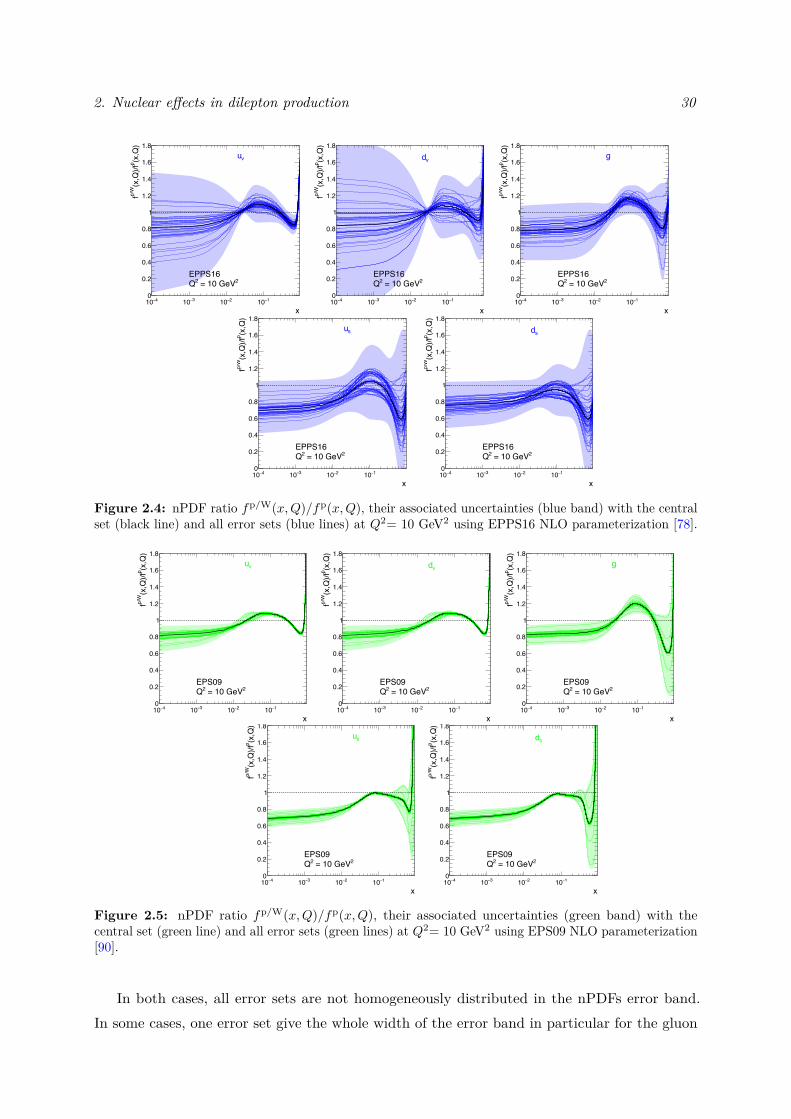
2. Nuclear effects in dilepton production 30
4−10 3−10 2−10 1−10x
0
0.2
0.4
0.6
0.8
1
1.2
1.4
1.6
1.8
(x,Q
)p
(x,Q
)/fp/
Wf
EPPS162 = 10 GeV2Q
sd
4−10 3−10 2−10 1−10x
0
0.2
0.4
0.6
0.8
1
1.2
1.4
1.6
1.8
(x,Q
)p
(x,Q
)/fp/
Wf
EPPS162 = 10 GeV2Q
vd
4−10 3−10 2−10 1−10x
0
0.2
0.4
0.6
0.8
1
1.2
1.4
1.6
1.8
(x,Q
)p
(x,Q
)/fp/
Wf
EPPS162 = 10 GeV2Q
g
4−10 3−10 2−10 1−10x
0
0.2
0.4
0.6
0.8
1
1.2
1.4
1.6
1.8
(x,Q
)p
(x,Q
)/fp/
Wf
EPPS162 = 10 GeV2Q
su
4−10 3−10 2−10 1−10x
0
0.2
0.4
0.6
0.8
1
1.2
1.4
1.6
1.8(x
,Q)
p(x
,Q)/f
p/W
f
EPPS162 = 10 GeV2Q
vu
Figure 2.4: nPDF ratio fp/W(x,Q)/fp(x,Q), their associated uncertainties (blue band) with the centralset (black line) and all error sets (blue lines) at Q2= 10 GeV2 using EPPS16 NLO parameterization [78].
4−10 3−10 2−10 1−10x
0
0.2
0.4
0.6
0.8
1
1.2
1.4
1.6
1.8
(x,Q
)p
(x,Q
)/fp/
Wf
EPS092 = 10 GeV2Q
su
4−10 3−10 2−10 1−10x
0
0.2
0.4
0.6
0.8
1
1.2
1.4
1.6
1.8
(x,Q
)p
(x,Q
)/fp/
Wf
EPS092 = 10 GeV2Q
sd
4−10 3−10 2−10 1−10x
0
0.2
0.4
0.6
0.8
1
1.2
1.4
1.6
1.8
(x,Q
)p
(x,Q
)/fp/
Wf
EPS092 = 10 GeV2Q
vd
4−10 3−10 2−10 1−10x
0
0.2
0.4
0.6
0.8
1
1.2
1.4
1.6
1.8
(x,Q
)p
(x,Q
)/fp/
Wf
EPS092 = 10 GeV2Q
vu
4−10 3−10 2−10 1−10x
0
0.2
0.4
0.6
0.8
1
1.2
1.4
1.6
1.8
(x,Q
)p
(x,Q
)/fp/
Wf
EPS092 = 10 GeV2Q
g
Figure 2.5: nPDF ratio fp/W(x,Q)/fp(x,Q), their associated uncertainties (green band) with thecentral set (green line) and all error sets (green lines) at Q2= 10 GeV2 using EPS09 NLO parameterization[90].
In both cases, all error sets are not homogeneously distributed in the nPDFs error band.In some cases, one error set give the whole width of the error band in particular for the gluon
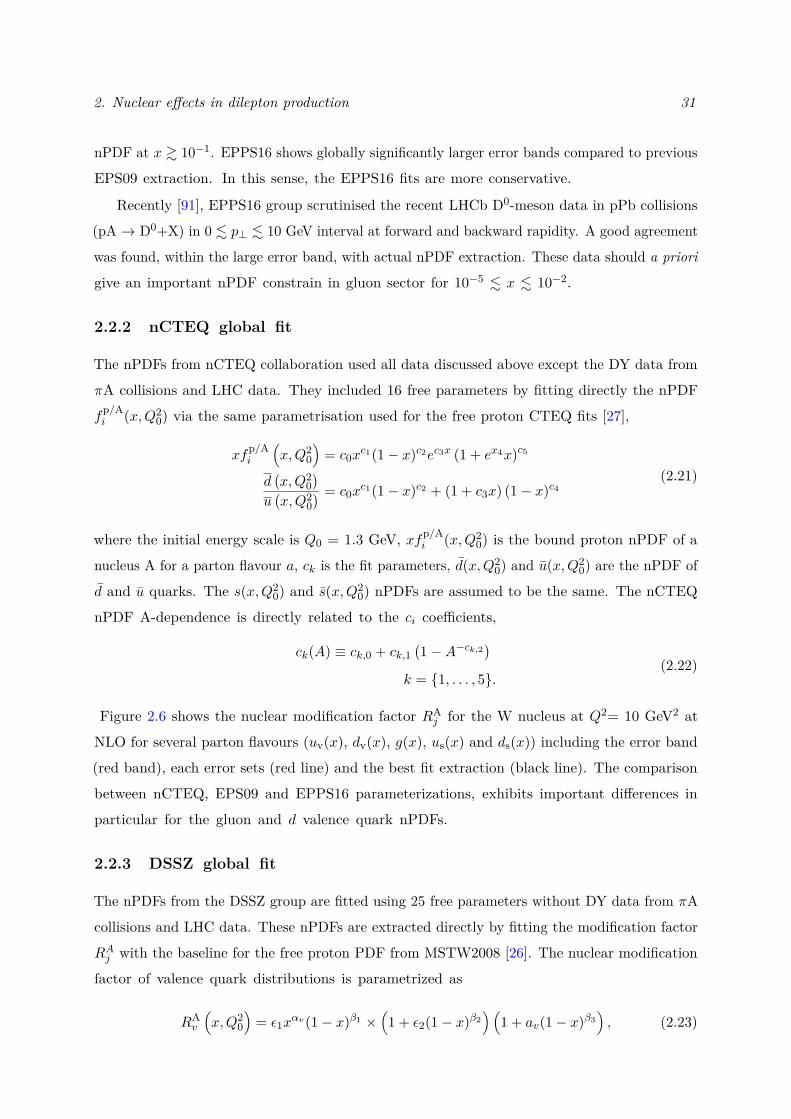
2. Nuclear effects in dilepton production 31
nPDF at x & 10−1. EPPS16 shows globally significantly larger error bands compared to previous
EPS09 extraction. In this sense, the EPPS16 fits are more conservative.
Recently [91], EPPS16 group scrutinised the recent LHCb D0-meson data in pPb collisions
(pA→ D0+X) in 0 . p⊥ . 10 GeV interval at forward and backward rapidity. A good agreement
was found, within the large error band, with actual nPDF extraction. These data should a priori
give an important nPDF constrain in gluon sector for 10−5 . x . 10−2.
2.2.2 nCTEQ global fit
The nPDFs from nCTEQ collaboration used all data discussed above except the DY data from
πA collisions and LHC data. They included 16 free parameters by fitting directly the nPDF
fp/Ai (x,Q2
0) via the same parametrisation used for the free proton CTEQ fits [27],
xfp/Ai
(x,Q2
0
)= c0x
c1(1− x)c2ec3x (1 + ex4x)c5
d(x,Q2
0)
u(x,Q2
0) = c0x
c1(1− x)c2 + (1 + c3x) (1− x)c4(2.21)
where the initial energy scale is Q0 = 1.3 GeV, xfp/Ai (x,Q20) is the bound proton nPDF of a
nucleus A for a parton flavour a, ck is the fit parameters, d(x,Q20) and u(x,Q2
0) are the nPDF of
d and u quarks. The s(x,Q20) and s(x,Q2
0) nPDFs are assumed to be the same. The nCTEQ
nPDF A-dependence is directly related to the ci coefficients,
ck(A) ≡ ck,0 + ck,1(1−A−ck,2
)k = {1, . . . , 5}.
(2.22)
Figure 2.6 shows the nuclear modification factor RAj for the W nucleus at Q2= 10 GeV2 at
NLO for several parton flavours (uv(x), dv(x), g(x), us(x) and ds(x)) including the error band
(red band), each error sets (red line) and the best fit extraction (black line). The comparison
between nCTEQ, EPS09 and EPPS16 parameterizations, exhibits important differences in
particular for the gluon and d valence quark nPDFs.
2.2.3 DSSZ global fit
The nPDFs from the DSSZ group are fitted using 25 free parameters without DY data from πA
collisions and LHC data. These nPDFs are extracted directly by fitting the modification factor
RAj with the baseline for the free proton PDF from MSTW2008 [26]. The nuclear modification
factor of valence quark distributions is parametrized as
RAv
(x,Q2
0
)= ε1x
αv(1− x)β1 ×(1 + ε2(1− x)β2
) (1 + av(1− x)β3
), (2.23)
2. Nuclear effects in dilepton production 32
4−10 3−10 2−10 1−10x
0
0.2
0.4
0.6
0.8
1
1.2
1.4
1.6
1.8
(x,Q
)p
(x,Q
)/fp/
Wf
nCTEQ2 = 10 GeV2Q
g
4−10 3−10 2−10 1−10x
0
0.2
0.4
0.6
0.8
1
1.2
1.4
1.6
1.8
(x,Q
)p
(x,Q
)/fp/
Wf
nCTEQ2 = 10 GeV2Q
su
4−10 3−10 2−10 1−10x
0
0.2
0.4
0.6
0.8
1
1.2
1.4
1.6
1.8
(x,Q
)p
(x,Q
)/fp/
Wf
nCTEQ2 = 10 GeV2Q
sd
4−10 3−10 2−10 1−10x
0
0.2
0.4
0.6
0.8
1
1.2
1.4
1.6
1.8
(x,Q
)p
(x,Q
)/fp/
Wf
nCTEQ2 = 10 GeV2Q
vd
4−10 3−10 2−10 1−10x
0
0.2
0.4
0.6
0.8
1
1.2
1.4
1.6
1.8(x
,Q)
p(x
,Q)/f
p/W
f
nCTEQ2 = 10 GeV2Q
vu
Figure 2.6: nPDF ratio fp/W(x,Q)/fp(x,Q), their associated uncertainties (red band) with the centralset (black line) and all error sets (red lines) at Q2= 10 GeV2 using nCTEQ15 NLO parameterizations [70].
and for the gluon and sea quark distributions, the nuclear modification factor is parametrized usingEq. (2.23) as
RAs
(x,Q2
0
)= RA
v
(x,Q2
0
) εsε1
1 + asxαs
as + 1
RAg
(x,Q2
0
)= RA
v
(x,Q2
0
) εgε1
1 + agxαg
ag + 1
(2.24)
with the initial energy scale Q0 = 1 GeV and αs, αg, as and ag are free parameters. The s(x,Q20)
and s(x,Q20) nPDFs are assumed to be the same. The A-dependence nPDF is determined via
ξ = γξ + λξAδε (2.25)
with γξ, λξ and δξ and ξ ∈ {αv, αs, αg, β1, β2, β3, av, as, ag}, the additional free parameters toreproduce the A-dependence. Moreover DSSZ group includes, in neutral pion production data[79, 80], the medium modified fragmentation function in the pion hadronization described in[92]. DSSZ nPDFs show a compatibility with EPS09 nPDF for valence quark distributions. Butthe more important differences come from the gluon nPDF where the shadowing effect is muchlower in DSSZ compared to EPPS16, EPS09 and nCTEQ nPDFs. In particular at x ∼ 10−4
where RAg (x,Q2 = 10) ≈ 111 as shown in Fig. (14) in [77]. In addition, the anti-shadowing and
EMC effects for sea quark distributions predicted by EPPS16, EPS09 and nCTEQ nPDFs isconsiderable compared to the DSSZ nPDF exhibiting moderate nuclear corrections.
11At low scale Q ∼ 1 GeV, DSSZ group shows an important dependence on Q and predicts an important effectin this energy scale region.
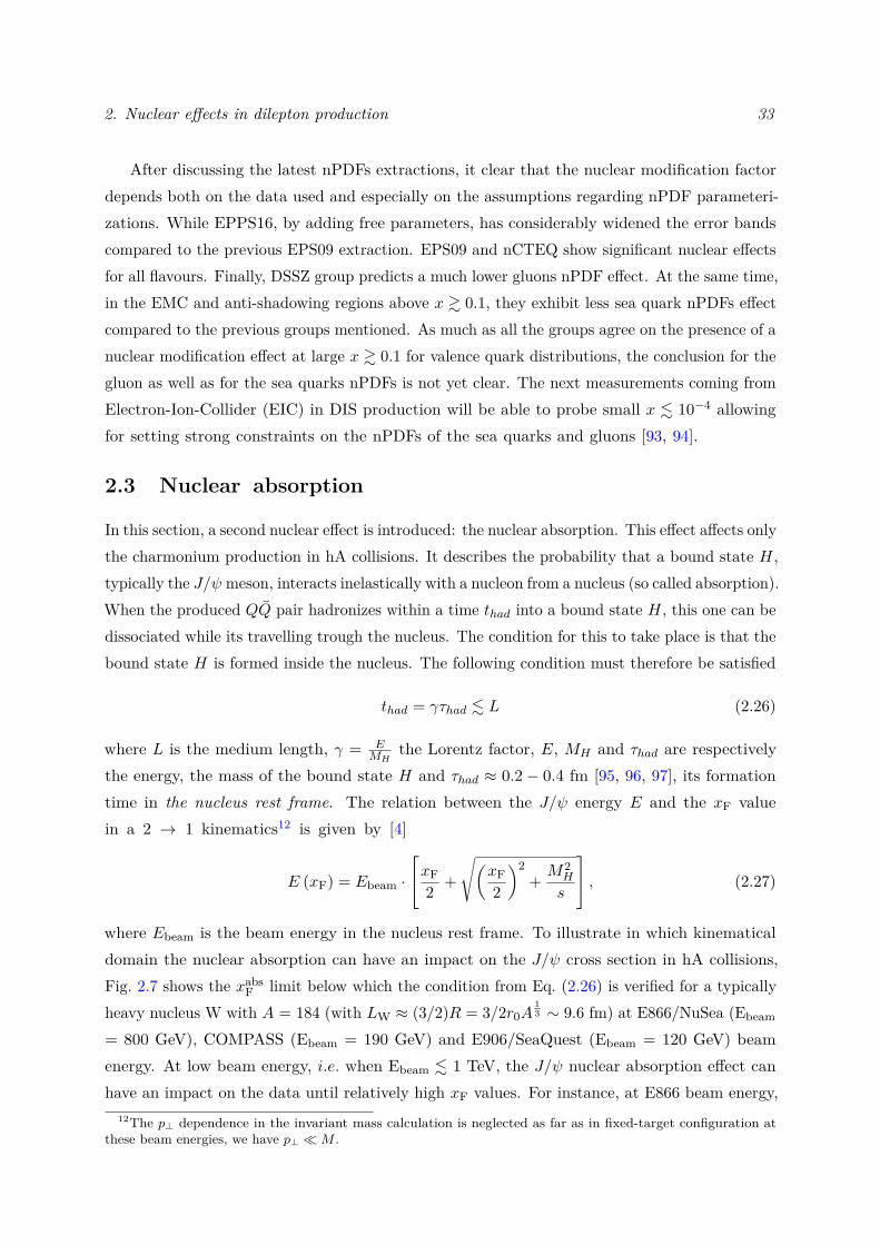
2. Nuclear effects in dilepton production 33
After discussing the latest nPDFs extractions, it clear that the nuclear modification factordepends both on the data used and especially on the assumptions regarding nPDF parameteri-zations. While EPPS16, by adding free parameters, has considerably widened the error bandscompared to the previous EPS09 extraction. EPS09 and nCTEQ show significant nuclear effectsfor all flavours. Finally, DSSZ group predicts a much lower gluons nPDF effect. At the same time,in the EMC and anti-shadowing regions above x & 0.1, they exhibit less sea quark nPDFs effectcompared to the previous groups mentioned. As much as all the groups agree on the presence of anuclear modification effect at large x & 0.1 for valence quark distributions, the conclusion for thegluon as well as for the sea quarks nPDFs is not yet clear. The next measurements coming fromElectron-Ion-Collider (EIC) in DIS production will be able to probe small x . 10−4 allowingfor setting strong constraints on the nPDFs of the sea quarks and gluons [93, 94].
2.3 Nuclear absorption
In this section, a second nuclear effect is introduced: the nuclear absorption. This effect affects onlythe charmonium production in hA collisions. It describes the probability that a bound state H,typically the J/ψ meson, interacts inelastically with a nucleon from a nucleus (so called absorption).When the produced QQ pair hadronizes within a time thad into a bound state H, this one can bedissociated while its travelling trough the nucleus. The condition for this to take place is that thebound state H is formed inside the nucleus. The following condition must therefore be satisfied
thad = γτhad . L (2.26)
where L is the medium length, γ = EMH
the Lorentz factor, E, MH and τhad are respectivelythe energy, the mass of the bound state H and τhad ≈ 0.2 − 0.4 fm [95, 96, 97], its formationtime in the nucleus rest frame. The relation between the J/ψ energy E and the xF valuein a 2 → 1 kinematics12 is given by [4]
E (xF) = Ebeam ·
xF2 +
√(xF2
)2+ M2
H
s
, (2.27)
where Ebeam is the beam energy in the nucleus rest frame. To illustrate in which kinematicaldomain the nuclear absorption can have an impact on the J/ψ cross section in hA collisions,Fig. 2.7 shows the xabsF limit below which the condition from Eq. (2.26) is verified for a typicallyheavy nucleus W with A = 184 (with LW ≈ (3/2)R = 3/2r0A
13 ∼ 9.6 fm) at E866/NuSea (Ebeam
= 800 GeV), COMPASS (Ebeam = 190 GeV) and E906/SeaQuest (Ebeam = 120 GeV) beamenergy. At low beam energy, i.e. when Ebeam . 1 TeV, the J/ψ nuclear absorption effect canhave an impact on the data until relatively high xF values. For instance, at E866 beam energy,
12The p⊥ dependence in the invariant mass calculation is neglected as far as in fixed-target configuration atthese beam energies, we have p⊥ �M .
2. Nuclear effects in dilepton production 34
the nuclear absorption has an impact only for xF . 0.1, whereas the more the beam energydecreases, the more this limit shifts towards larger xF. By taking τJ/ψhad = 0.3 fm, the J/ψ isproduced systematically higher than the length (LW) of the nucleus, LW . thad at positive xF,except at very low beam energy at Ebeam=190 GeV, where the thad . LW when xF . 0.5 (seeFig. 2.7). This limit changes to xF . 0.8 at the beam energy of E906 experiment. Note that itis difficult to estimate the exact value of xabsF limit where the condition in Eq. (2.26) is verifiedbecause of the uncertainty on the J/ψ formation time. However, this makes it possible to givea reasonable order of magnitude. Knowing the xF region where this effect can play a role, the
0 0.1 0.2 0.3 0.4 0.5 0.6 0.7 0.8 0.9 1absFx
0
100
200
300
400
500
600
700
800
900
1000
(G
eV)
beam
E
E866
COMPASS
E906
= 0.2 fmψJ/τ
= 0.3 fmψJ/τ
= 0.4 fmψJ/τ
0 0.1 0.2 0.3 0.4 0.5 0.6 0.7 0.8 0.9 1
Fx
0
2
4
6
8
10
12
14 (fm
)ψ
J/prod
L E866
COMPASS
E906
WL
WR
Figure 2.7: xabsF as a function Ebeam for different J/ψ formation time τJ/ψhad = 0.2, 0.3 and 0.4 fm (left
panel) and J/ψ production at length LprodJ/ψ fm as a function of xF assuming τJ/ψhad = 0.3 fm (right panel).
absorption survival probability by the medium can be computed as [50],
S(σabs, lA) = e−ρσabslA (2.28)
where σabs is the nuclear absorption cross section, lA the medium length crossed by the J/ψcalculated from the Glauber model [98] and ρ = 0.17 fm−3 the nuclear density. The globaldata analysis from SPS to RHIC experiments was done by [99, 100] and the best fit gave theJ/ψ nuclear absorption cross section equal to σJ/ψNabs = 3.5± 0.2 mb. According to Eq. (2.28),the J/ψ cross section in hA can be written as
dσhA[J/ψ +X]dy = S(σabs, lA)× dσhp[J/ψ +X]
dy ×A. (2.29)
For illustration, S(σabs, lA) is evaluated for a W nucleus, by taking lA = RW ∼ 6.4 fm andσJ/ψNabs = 3.5 ± 0.2 mb. The cross section ratio due to nuclear absorption is equal to
RJ/ψ,abshA = 0.68± 0.02. (2.30)
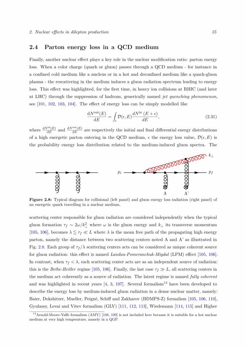
2. Nuclear effects in dilepton production 35
2.4 Parton energy loss in a QCD medium
Finally, another nuclear effect plays a key role in the nuclear modification ratio: parton energyloss. When a color charge (quark or gluon) passes through a QCD medium - for instance ina confined cold medium like a nucleus or in a hot and deconfined medium like a quark-gluonplasma - the rescattering in the medium induces a gluon radiation spectrum leading to energyloss. This effect was highlighted, for the first time, in heavy ion collisions at RHIC (and laterat LHC) through the suppression of hadrons, generically named jet quenching phenomenon,see [101, 102, 103, 104]. The effect of energy loss can be simply modelled like
dNout(E)dE =
∫εD(ε, E)dN
in (E + ε)dE
, (2.31)
where dN in(E)dE and dNout(E)
dE are respectively the initial and final differential energy distributionsof a high energetic parton entering in the QCD medium, ε the energy loss value, D(ε, E) isthe probability energy loss distribution related to the medium-induced gluon spectra. The
pi pf
k⊥
A’AFigure 2.8: Typical diagram for collisional (left panel) and gluon energy loss radiation (right panel) ofan energetic quark travelling in a nuclear medium.
scattering center responsible for gluon radiation are considered independently when the typicalgluon formation τf ∼ 2ω/k2
⊥ where ω is the gluon energy and k⊥ its transverse momentum[105, 106], becomes λ . τf � L where λ is the mean free path of the propagating high energyparton, namely the distance between two scattering centers noted A and A’ as illustrated inFig. 2.8. Each group of τf/λ scattering centers acts can be considered as unique coherent sourcefor gluon radiation: this effect is named Landau-Pomeranchuk-Migdal (LPM) effect [105, 106].In contrast, when τf < λ, each scattering center acts are as an independent source of radiation:this is the Bethe-Heitler regime [105, 106]. Finally, the last case τf � L, all scattering centers inthe medium act coherently as a source of radiation. The latest regime is named fully coherentand was highlighted in recent years [4, 3, 107]. Several formalism13 have been developed todescribe the energy loss by medium-induced gluon radiation in a dense nuclear matter, namely:Baier, Dokshitzer, Mueller, Peigné, Schiff and Zakharov (BDMPS-Z) formalism [105, 106, 110],Gyulassy, Levai and Vitev formalism (GLV) [111, 112, 113], Wiedemann [114, 115] and Higher
13Arnold-Moore-Yaffe formalism (AMY) [108, 109] is not included here because it is suitable for a hot nuclearmedium at very high temperature, namely in a QGP.
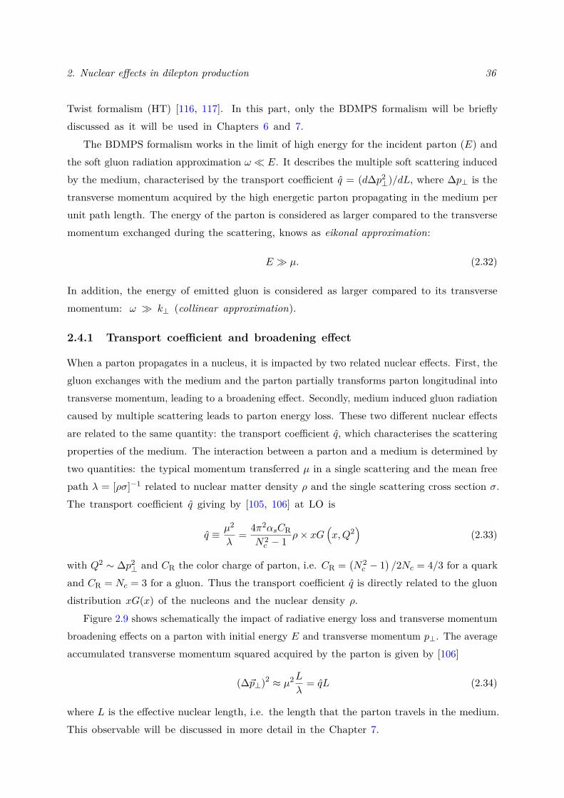
2. Nuclear effects in dilepton production 36
Twist formalism (HT) [116, 117]. In this part, only the BDMPS formalism will be brieflydiscussed as it will be used in Chapters 6 and 7.
The BDMPS formalism works in the limit of high energy for the incident parton (E) andthe soft gluon radiation approximation ω � E. It describes the multiple soft scattering inducedby the medium, characterised by the transport coefficient q = (d∆p2
⊥)/dL, where ∆p⊥ is thetransverse momentum acquired by the high energetic parton propagating in the medium perunit path length. The energy of the parton is considered as larger compared to the transversemomentum exchanged during the scattering, knows as eikonal approximation:
E � µ. (2.32)
In addition, the energy of emitted gluon is considered as larger compared to its transversemomentum: ω � k⊥ (collinear approximation).
2.4.1 Transport coefficient and broadening effect
When a parton propagates in a nucleus, it is impacted by two related nuclear effects. First, thegluon exchanges with the medium and the parton partially transforms parton longitudinal intotransverse momentum, leading to a broadening effect. Secondly, medium induced gluon radiationcaused by multiple scattering leads to parton energy loss. These two different nuclear effectsare related to the same quantity: the transport coefficient q, which characterises the scatteringproperties of the medium. The interaction between a parton and a medium is determined bytwo quantities: the typical momentum transferred µ in a single scattering and the mean freepath λ = [ρσ]−1 related to nuclear matter density ρ and the single scattering cross section σ.The transport coefficient q giving by [105, 106] at LO is
q ≡ µ2
λ= 4π2αsCR
N2c − 1 ρ× xG
(x,Q2
)(2.33)
with Q2 ∼ ∆p2⊥ and CR the color charge of parton, i.e. CR =
(N2c − 1
)/2Nc = 4/3 for a quark
and CR = Nc = 3 for a gluon. Thus the transport coefficient q is directly related to the gluondistribution xG(x) of the nucleons and the nuclear density ρ.
Figure 2.9 shows schematically the impact of radiative energy loss and transverse momentumbroadening effects on a parton with initial energy E and transverse momentum p⊥. The averageaccumulated transverse momentum squared acquired by the parton is given by [106]
(∆~p⊥)2 ≈ µ2L
λ= qL (2.34)
where L is the effective nuclear length, i.e. the length that the parton travels in the medium.This observable will be discussed in more detail in the Chapter 7.
2. Nuclear effects in dilepton production 37
Figure 2.9: Cartoon of radiative energy loss and broadening effect from a hard parton with an energy Eand a transverse momentum p⊥ scattering a QCD medium.
2.4.2 Energy loss regimes
The radiative energy loss induces a gluon radiation spectra. The probability that a parton ofenergy E radiates n gluons with a total energy ε has been determined by [105, 106].
Depending on the hard process and therefore the gluon formation time τf compared to thelength of the medium crossed L, the average energy loss will be different. Two situations standsout:
• The LPM regime, i.e. λ . τf � L, corresponds to the case where an incoming or outgoinghigh-energy parton crosses the nucleus from a hard collision. The first case is associated tothe DY production (hA→ γ?) and the second case to the SIDIS production (lA→ l + h).The probability D(ε) to lose an energy ε, based on independent and soft gluons radiations,reads
D(ε) =∞∑n=0
1n!
[n∏i=1
∫dωi
dI (ωi)dω
]δ
(ε−
n∑i=1
ωi
)· exp
[−∫ +∞
0dωdI(ω)dω
], (2.35)
with n, the number of gluon emission emitted by the hard parton and dI(ωi)dω is the medium-
induced gluon spectrum [105],
(ωdI
dω
)LPM
∼ αsNcL
τf= αsNc
π
√qL2
ω. (2.36)
In the LPM regime when λ . τf � L, the average energy loss is [105, 106]
〈ε〉LPM ≡∫ ∞
0dεD(ε)ε ∝ αsq L2. (2.37)
The effects of initial-state (or, final-state) energy loss in nuclear matter should be negligibleat high energy, 〈ε〉LPM � E, as the particle energy in the nucleus rest frame gets large,E ∝ s leading to ∆E/E → 0. The LPM regime in DY process will be studied in moredetail in Chapter 6.
2. Nuclear effects in dilepton production 38
• The Fully Coherent Energy Loss (FCEL) regime [4, 3, 107], i.e. τf � L, has an impactin the case where one incoming and one outgoing high-energy parton is produced in thenucleus. While the two partons undergo the initial and final LPM energy loss, the FCELenergy loss dynamic is generated by the interference term between the both partonic states.The medium-induced gluon spectrum in this regime is [4](
ωdIdω
)FCEL
= Ncαsπ
{ln(
1 + ∆q2⊥E
2
M2⊥ω
2
)− ln
(1 +
Λ2pE
2
M2⊥ω
2
)}Θ(∆q2⊥ − Λ2
p
), (2.38)
withM⊥ =(M2 + p2
⊥) 2
2 the transverse mass momentum and Λ2p = max
(Λ2
QCD,∆q2⊥
). The
FCEL energy loss average leads to
〈ε〉FCEL ∝√qL/M⊥ · E. (2.39)
This energy loss regime plays a role in the hadron production14 in hA→ q/g(→ h′) +X
collisions. The LPM energy loss regime is significantly lower than the FCEL regime in highenergy limit, 〈ε〉LPM � 〈ε〉FCEL. Since the mean energy loss in LPM regime is independentof parton energy E whereas the mean energy loss FCEL regime depends on it.
Energy loss Process Regime 〈ε〉Initial-state hA→ `+`− +X (LO DY) τf . L (LPM) ∝ qL2
Final-state eA→ e+ h+X (SIDIS) τf . L (LPM) ∝ qL2
Fully coherent hA→ [QQ(g)]8 +X τf � L ∝√qL/M · E
(quarkonium)
Table 2.3: LPM and FCEL energy loss regimes.
2.5 Empirical observations
2.5.1 Data
In this section, the nuclear dependence as a function of the rapidity (or xF) and the transversemomentum of DY and charmonium data from fixed-target to collider experiments will becommented in light of the nuclear effects introduced previously. The fixed target configurationprovides a higher luminosity compared to colliders allowing for data samples within largestatistics. In addition, thanks to the boost of the center-of-mass of the reaction, the collecteddata make it possible to access very large values of xF in the 0 . xF . 1 interval. A systematiccomparison will be made between the nuclear dependence of DY and J/ψ data. Below aresome observations from the data displayed in Table 2.4.
14Typically in J/ψ production.14These data will be available in the future.
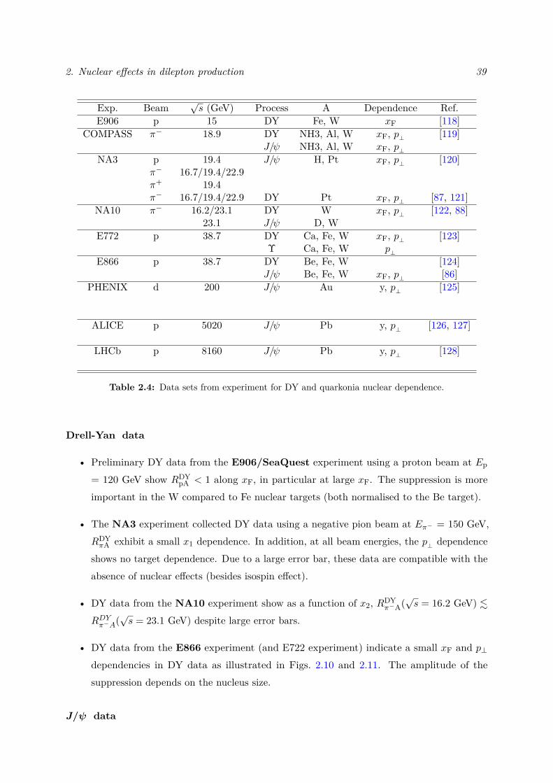
2. Nuclear effects in dilepton production 39
Exp. Beam√s (GeV) Process A Dependence Ref.
E906 p 15 DY Fe, W xF [118]COMPASS π− 18.9 DY NH3, Al, W xF, p⊥ [119]
J/ψ NH3, Al, W xF, p⊥NA3 p 19.4 J/ψ H, Pt xF, p⊥ [120]
π− 16.7/19.4/22.9π+ 19.4π− 16.7/19.4/22.9 DY Pt xF, p⊥ [87, 121]
NA10 π− 16.2/23.1 DY W xF, p⊥ [122, 88]23.1 J/ψ D, W
E772 p 38.7 DY Ca, Fe, W xF, p⊥ [123]Υ Ca, Fe, W p⊥
E866 p 38.7 DY Be, Fe, W [124]J/ψ Be, Fe, W xF, p⊥ [86]
PHENIX d 200 J/ψ Au y, p⊥ [125]
ALICE p 5020 J/ψ Pb y, p⊥ [126, 127]
LHCb p 8160 J/ψ Pb y, p⊥ [128]
Table 2.4: Data sets from experiment for DY and quarkonia nuclear dependence.
Drell-Yan data
• Preliminary DY data from the E906/SeaQuest experiment using a proton beam at Ep
= 120 GeV show RDYpA < 1 along xF, in particular at large xF. The suppression is more
important in the W compared to Fe nuclear targets (both normalised to the Be target).
• The NA3 experiment collected DY data using a negative pion beam at Eπ− = 150 GeV,RDYπA exhibit a small x1 dependence. In addition, at all beam energies, the p⊥ dependence
shows no target dependence. Due to a large error bar, these data are compatible with theabsence of nuclear effects (besides isospin effect).
• DY data from the NA10 experiment show as a function of x2, RDYπ−A(
√s = 16.2 GeV) .
RDYπ−A(√s = 23.1 GeV) despite large error bars.
• DY data from the E866 experiment (and E722 experiment) indicate a small xF and p⊥dependencies in DY data as illustrated in Figs. 2.10 and 2.11. The amplitude of thesuppression depends on the nucleus size.
J/ψ data
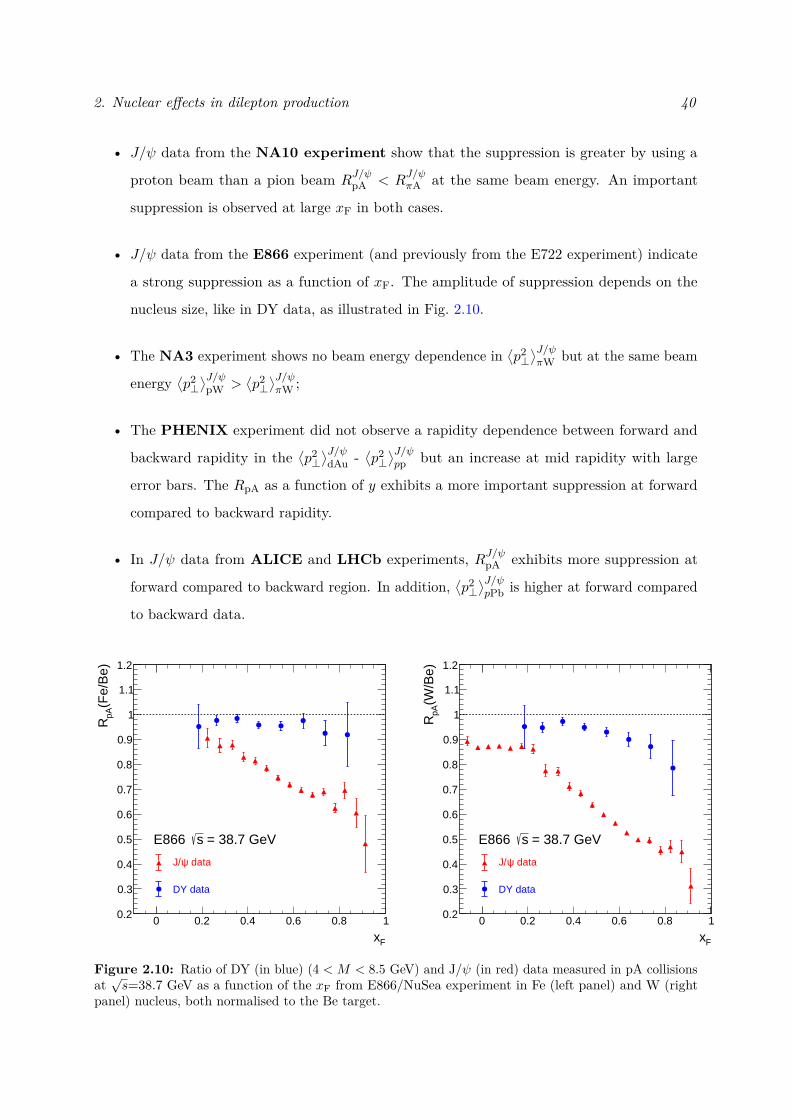
2. Nuclear effects in dilepton production 40
• J/ψ data from the NA10 experiment show that the suppression is greater by using a
proton beam than a pion beam RJ/ψpA < R
J/ψπA at the same beam energy. An important
suppression is observed at large xF in both cases.
• J/ψ data from the E866 experiment (and previously from the E722 experiment) indicate
a strong suppression as a function of xF. The amplitude of suppression depends on the
nucleus size, like in DY data, as illustrated in Fig. 2.10.
• The NA3 experiment shows no beam energy dependence in⟨p2⊥⟩J/ψπW but at the same beam
energy⟨p2⊥⟩J/ψ
pW >⟨p2⊥⟩J/ψπW ;
• The PHENIX experiment did not observe a rapidity dependence between forward and
backward rapidity in the⟨p2⊥⟩J/ψdAu -
⟨p2⊥⟩J/ψpp but an increase at mid rapidity with large
error bars. The RpA as a function of y exhibits a more important suppression at forward
compared to backward rapidity.
• In J/ψ data from ALICE and LHCb experiments, RJ/ψpA exhibits more suppression at
forward compared to backward region. In addition,⟨p2⊥⟩J/ψpPb is higher at forward compared
to backward data.
0 0.2 0.4 0.6 0.8 1
Fx
0.2
0.3
0.4
0.5
0.6
0.7
0.8
0.9
1
1.1
1.2
(Fe/
Be)
pAR
= 38.7 GeVsE866
dataψJ/
DY data
0 0.2 0.4 0.6 0.8 1
Fx
0.2
0.3
0.4
0.5
0.6
0.7
0.8
0.9
1
1.1
1.2
(W/B
e)pA
R
= 38.7 GeVsE866
dataψJ/
DY data
Figure 2.10: Ratio of DY (in blue) (4 < M < 8.5 GeV) and J/ψ (in red) data measured in pA collisionsat√s=38.7 GeV as a function of the xF from E866/NuSea experiment in Fe (left panel) and W (right
panel) nucleus, both normalised to the Be target.
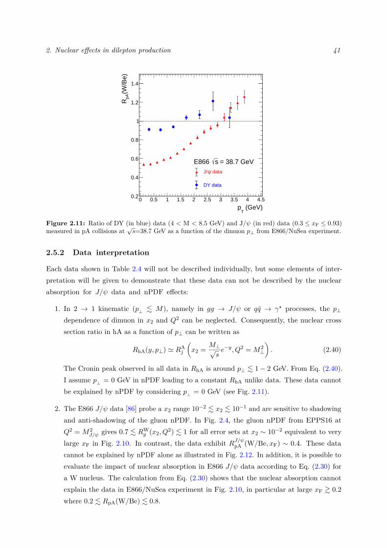
2. Nuclear effects in dilepton production 41
0 0.5 1 1.5 2 2.5 3 3.5 4 4.5
(GeV)T
p
0.2
0.4
0.6
0.8
1
1.2
1.4
(W/B
e)pA
R
= 38.7 GeVsE866 dataψJ/
DY data
Figure 2.11: Ratio of DY (in blue) data (4 < M < 8.5 GeV) and J/ψ (in red) data (0.3 ≤ xF ≤ 0.93)measured in pA collisions at
√s=38.7 GeV as a function of the dimuon p⊥ from E866/NuSea experiment.
2.5.2 Data interpretation
Each data shown in Table 2.4 will not be described individually, but some elements of inter-pretation will be given to demonstrate that these data can not be described by the nuclearabsorption for J/ψ data and nPDF effects:
1. In 2 → 1 kinematic (p⊥ . M), namely in gg → J/ψ or qq → γ? processes, the p⊥dependence of dimuon in x2 and Q2 can be neglected. Consequently, the nuclear crosssection ratio in hA as a function of p⊥ can be written as
RhA(y, p⊥) ' RAj
(x2 = M⊥√
se−y, Q2 = M2
⊥
). (2.40)
The Cronin peak observed in all data in RhA is around p⊥ . 1− 2 GeV. From Eq. (2.40).I assume p⊥ = 0 GeV in nPDF leading to a constant RhA unlike data. These data cannotbe explained by nPDF by considering p⊥ = 0 GeV (see Fig. 2.11).
2. The E866 J/ψ data [86] probe a x2 range 10−2 . x2 . 10−1 and are sensitive to shadowingand anti-shadowing of the gluon nPDF. In Fig. 2.4, the gluon nPDF from EPPS16 atQ2 = M2
J/ψ gives 0.7 . RWg (x2, Q
2) . 1 for all error sets at x2 ∼ 10−2 equivalent to verylarge xF in Fig. 2.10. In contrast, the data exhibit RJ/ψpA (W/Be, xF) ∼ 0.4. These datacannot be explained by nPDF alone as illustrated in Fig. 2.12. In addition, it is possible toevaluate the impact of nuclear absorption in E866 J/ψ data according to Eq. (2.30) fora W nucleus. The calculation from Eq. (2.30) shows that the nuclear absorption cannotexplain the data in E866/NuSea experiment in Fig. 2.10, in particular at large xF & 0.2where 0.2 . RpA(W/Be) . 0.8.
2. Nuclear effects in dilepton production 42
3. The preliminary E906 DY data [118] probe a x2 range 0.1 . x2 . 0.3 and are sensitive toanti-shadowing of mainly of the u(x2) nPDF where RA
u (x2) & 1 is expected but at large xFequivalent to x2 ∼ 0.1, the data show RpA(W/Be, xF) ∼ 0.75.
0 0.1 0.2 0.3 0.4 0.5 0.6 0.7 0.8 0.9
Fx
0
0.2
0.4
0.6
0.8
1
1.2(W
/Be)
g pAR
EPPS162 = 10 GeV2Q
= 38.7 GeVs data - E866 ψJ/
Figure 2.12: Comparison between E866/NuSea J/ψ data (in red) and Rg(W/Be) ratio of W and Begluon nPDFs from EPPS16 (in blue) at NLO as a function of xF.
2.5.3 Phenomenological approach
Throughout this chapter, the most important nuclear effects have been introduced. Some elementsshowed that the J/ψ data for example could neither be explained by nPDF or by nuclearabsorption alone. Recent phenomenological energy loss studies carried out had a great success inexplaining J/ψ suppression data from fixed-target to LHC energies following the highlighting ofa new energy loss dynamics in quarkonia production in these collisions: FCEL effect [4, 3, 107].
Figure 2.13 shows the comparison between nuclear cross sections ratios RpA (W/Be) fromE866 J/ψ data [86] and a calculation including only the FCEL effect from [4] as a function ofxF. The energy loss model alone can explain the suppression of the J/ψ data as a function ofxF. A precise value of the transport coefficient was extracted by fitting these data obtaininga reference value q = 0.075 GeV2/fm. As discussed in Sec. 2.2, it is possible to have a nPDFeffect in these data due to shadowing effect contributing to the normalisation mainly of RpA (seeFig. 2.12). The nPDF and radiative energy loss effects may appear as a product [4]
RpA(xF) = RE.losspA (xF)×RnPDF
g (xF) (2.41)
where RnPDFg is the gluon nuclear modification factor in the J/ψ pA data case. The nPDF effect
contributes to RpA normalisation by ∼ 10% using the EPPS16 nPDF central set [78] .In Fig. 2.14, the p⊥ dependence of RpA (W/Be) from the E866 J/ψ data is reproduced by
taking into account the both broadening and energy loss effect from [129]. The radiative energy
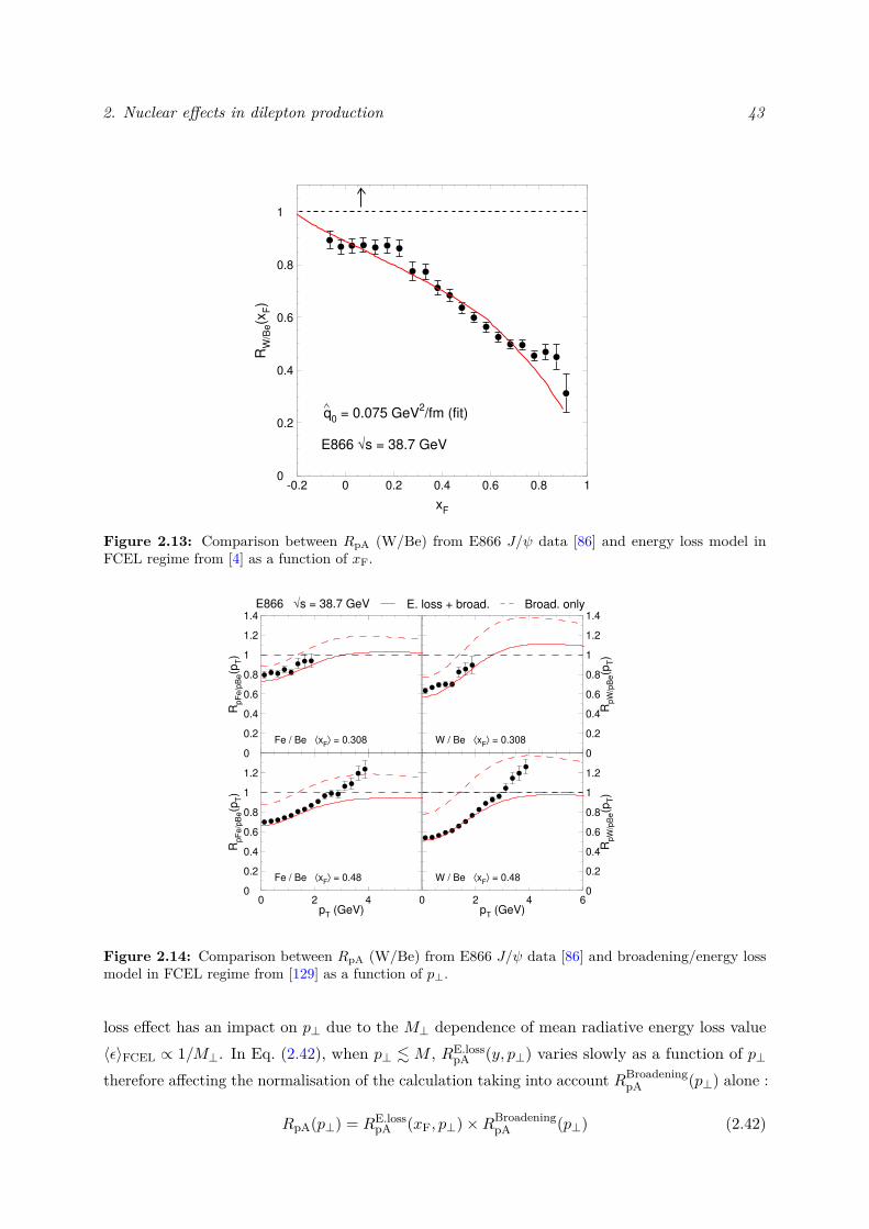
2. Nuclear effects in dilepton production 43
0
0.2
0.4
0.6
0.8
1
-0.2 0 0.2 0.4 0.6 0.8 1
xF
RW
/Be(x
F)
E866 √s = 38.7 GeV
∧q0 = 0.075 GeV
2/fm (fit)
Figure 2.13: Comparison between RpA (W/Be) from E866 J/ψ data [86] and energy loss model inFCEL regime from [4] as a function of xF.
0
0.2
0.4
0.6
0.8
1
1.2
1.4
RpF
e/p
Be(p
T)
Fe / Be ⟨xF⟩ = 0.308
0
0.2
0.4
0.6
0.8
1
1.2
1.4R
pW
/pB
e(p
T)
W / Be ⟨xF⟩ = 0.308
0
0.2
0.4
0.6
0.8
1
1.2
0 2 4pT (GeV)
RpF
e/p
Be(p
T)
Fe / Be ⟨xF⟩ = 0.48
0
0.2
0.4
0.6
0.8
1
1.2
0 2 4 6pT (GeV)
RpW
/pB
e(p
T)
W / Be ⟨xF⟩ = 0.48
E866 √s = 38.7 GeV E. loss + broad. Broad. only
Figure 2.14: Comparison between RpA (W/Be) from E866 J/ψ data [86] and broadening/energy lossmodel in FCEL regime from [129] as a function of p⊥.
loss effect has an impact on p⊥ due to the M⊥ dependence of mean radiative energy loss value〈ε〉FCEL ∝ 1/M⊥. In Eq. (2.42), when p⊥ . M , RE.loss
pA (y, p⊥) varies slowly as a function of p⊥therefore affecting the normalisation of the calculation taking into account RBroadening
pA (p⊥) alone :
RpA(p⊥) = RE.losspA (xF, p⊥)×RBroadening
pA (p⊥) (2.42)
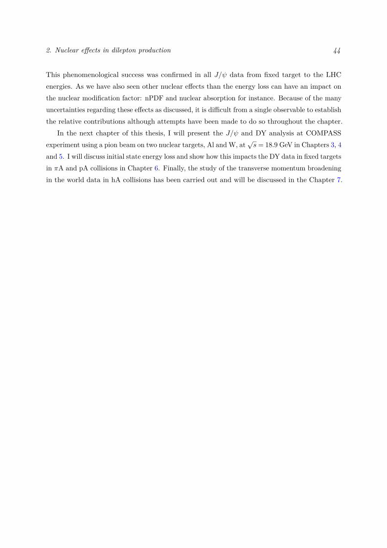
2. Nuclear effects in dilepton production 44
This phenomenological success was confirmed in all J/ψ data from fixed target to the LHCenergies. As we have also seen other nuclear effects than the energy loss can have an impact onthe nuclear modification factor: nPDF and nuclear absorption for instance. Because of the manyuncertainties regarding these effects as discussed, it is difficult from a single observable to establishthe relative contributions although attempts have been made to do so throughout the chapter.
In the next chapter of this thesis, I will present the J/ψ and DY analysis at COMPASSexperiment using a pion beam on two nuclear targets, Al and W, at
√s = 18.9 GeV in Chapters 3, 4
and 5. I will discuss initial state energy loss and show how this impacts the DY data in fixed targetsin πA and pA collisions in Chapter 6. Finally, the study of the transverse momentum broadeningin the world data in hA collisions has been carried out and will be discussed in the Chapter 7.
3COMPASS experiment
Contents
3.1 Introduction . . . . . . . . . . . . . . . . . . . . . . . . . . . . . . . . . 453.2 Beam . . . . . . . . . . . . . . . . . . . . . . . . . . . . . . . . . . . . . . 463.3 Targets . . . . . . . . . . . . . . . . . . . . . . . . . . . . . . . . . . . . . 47
3.3.1 NH3 targets . . . . . . . . . . . . . . . . . . . . . . . . . . . . . . . . . . 473.3.2 Al and W targets . . . . . . . . . . . . . . . . . . . . . . . . . . . . . . . 483.3.3 Beam attenuation . . . . . . . . . . . . . . . . . . . . . . . . . . . . . . 49
3.4 Spectrometer . . . . . . . . . . . . . . . . . . . . . . . . . . . . . . . . . 513.4.1 Very Small Area Tracking . . . . . . . . . . . . . . . . . . . . . . . . . . 523.4.2 Small Angle Trackers . . . . . . . . . . . . . . . . . . . . . . . . . . . . . 523.4.3 Large Area Trackers . . . . . . . . . . . . . . . . . . . . . . . . . . . . . 543.4.4 Muon identification . . . . . . . . . . . . . . . . . . . . . . . . . . . . . 56
3.5 Trigger and veto system . . . . . . . . . . . . . . . . . . . . . . . . . . 573.6 Data acquisition . . . . . . . . . . . . . . . . . . . . . . . . . . . . . . . 58
3.6.1 Reconstruction . . . . . . . . . . . . . . . . . . . . . . . . . . . . . . . . 593.7 The Drift Chamber detector . . . . . . . . . . . . . . . . . . . . . . . . 59
3.7.1 Characteristics . . . . . . . . . . . . . . . . . . . . . . . . . . . . . . . . 593.7.2 Formation and processing of the electrical signal . . . . . . . . . . . . . 613.7.3 Calibration . . . . . . . . . . . . . . . . . . . . . . . . . . . . . . . . . . 62
3.1 Introduction
COMPASS/NA58 (COmmon Muon and Proton Apparatus for Structure and Spectroscopy)is a fixed target experiment located in the north area at CERN. It uses hadron and muonbeams produced by the Super Proton Synchrotron (SPS). Dedicated to hadron structure andspectroscopy, the COMPASS experiment is contributing to many still open QCD problems. Thefirst COMPASS experiment proposal was accepted in 1998. One of its main goals was to measuredirectly the gluon polarisation [130, 131]. In 2010, an addendum to the experimental program
45
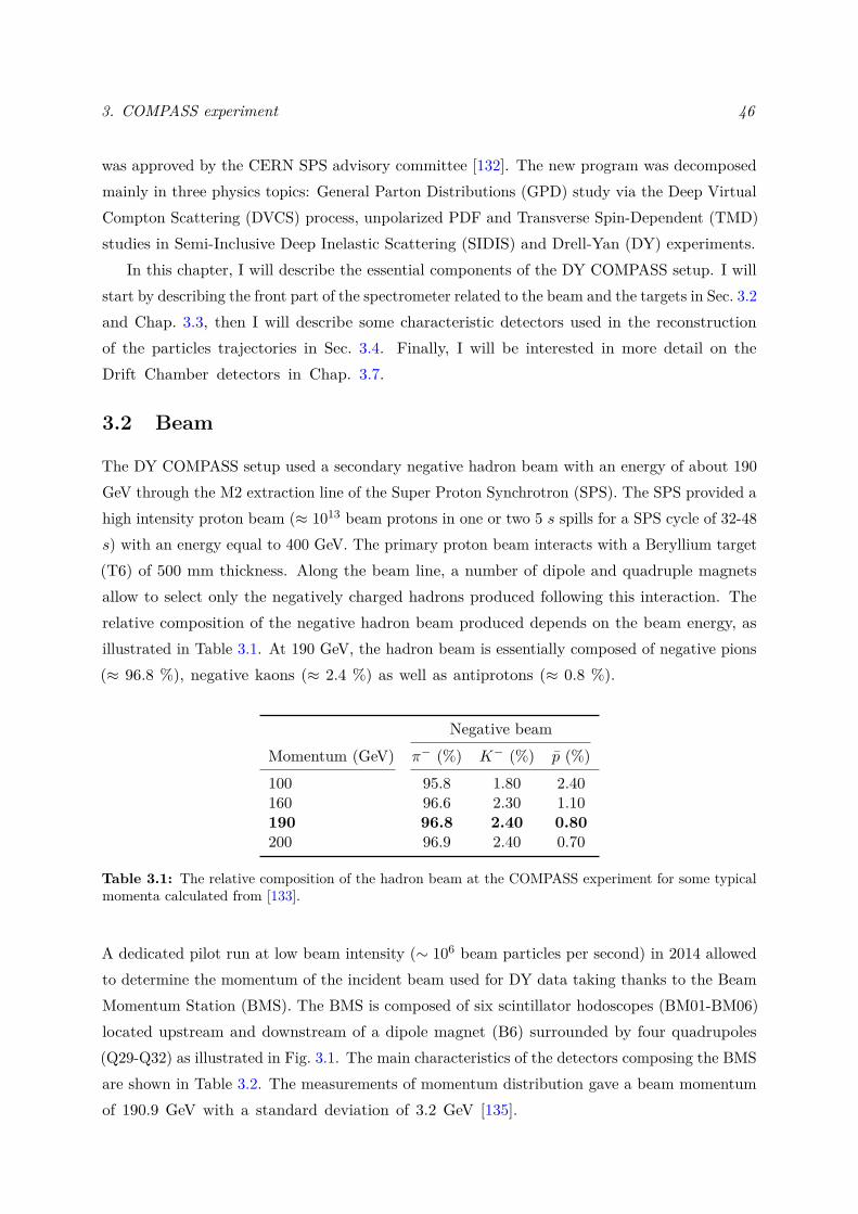
3. COMPASS experiment 46
was approved by the CERN SPS advisory committee [132]. The new program was decomposedmainly in three physics topics: General Parton Distributions (GPD) study via the Deep VirtualCompton Scattering (DVCS) process, unpolarized PDF and Transverse Spin-Dependent (TMD)studies in Semi-Inclusive Deep Inelastic Scattering (SIDIS) and Drell-Yan (DY) experiments.
In this chapter, I will describe the essential components of the DY COMPASS setup. I willstart by describing the front part of the spectrometer related to the beam and the targets in Sec. 3.2and Chap. 3.3, then I will describe some characteristic detectors used in the reconstructionof the particles trajectories in Sec. 3.4. Finally, I will be interested in more detail on theDrift Chamber detectors in Chap. 3.7.
3.2 Beam
The DY COMPASS setup used a secondary negative hadron beam with an energy of about 190GeV through the M2 extraction line of the Super Proton Synchrotron (SPS). The SPS provided ahigh intensity proton beam (≈ 1013 beam protons in one or two 5 s spills for a SPS cycle of 32-48s) with an energy equal to 400 GeV. The primary proton beam interacts with a Beryllium target(T6) of 500 mm thickness. Along the beam line, a number of dipole and quadruple magnetsallow to select only the negatively charged hadrons produced following this interaction. Therelative composition of the negative hadron beam produced depends on the beam energy, asillustrated in Table 3.1. At 190 GeV, the hadron beam is essentially composed of negative pions(≈ 96.8 %), negative kaons (≈ 2.4 %) as well as antiprotons (≈ 0.8 %).
Negative beamMomentum (GeV) π− (%) K− (%) p (%)100 95.8 1.80 2.40160 96.6 2.30 1.10190 96.8 2.40 0.80200 96.9 2.40 0.70
Table 3.1: The relative composition of the hadron beam at the COMPASS experiment for some typicalmomenta calculated from [133].
A dedicated pilot run at low beam intensity (∼ 106 beam particles per second) in 2014 allowedto determine the momentum of the incident beam used for DY data taking thanks to the BeamMomentum Station (BMS). The BMS is composed of six scintillator hodoscopes (BM01-BM06)located upstream and downstream of a dipole magnet (B6) surrounded by four quadrupoles(Q29-Q32) as illustrated in Fig. 3.1. The main characteristics of the detectors composing the BMSare shown in Table 3.2. The measurements of momentum distribution gave a beam momentumof 190.9 GeV with a standard deviation of 3.2 GeV [135].
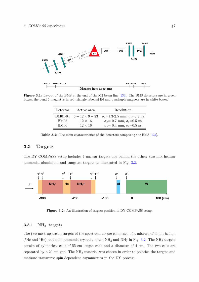
3. COMPASS experiment 47
Figure 3.1: Layout of the BMS at the end of the M2 beam line [134]. The BMS detectors are in greenboxes, the bend 6 magnet is in red triangle labelled B6 and quadruple magnets are in white boxes.
Detector Active area ResolutionBM01-04 6− 12× 9− 23 σs=1.3-2.5 mm, σt=0.3 nsBM05 12× 16 σs= 0.7 mm, σt=0.5 nsBM06 12× 16 σs= 0.4 mm, σt=0.5 ns
Table 3.2: The main characteristics of the detectors composing the BMS [134].
3.3 Targets
The DY COMPASS setup includes 4 nuclear targets one behind the other: two mix helium-ammonia, aluminium and tungsten targets as illustrated in Fig. 3.2.
Figure 3.2: An illustration of targets position in DY COMPASS setup.
3.3.1 NH3 targets
The two most upstream targets of the spectrometer are composed of a mixture of liquid helium(3He and 4He) and solid ammonia crystals, noted NH1
3 and NH23 in Fig. 3.2. The NH3 targets
consist of cylindrical cells of 55 cm length each and a diameter of 4 cm. The two cells areseparated by a 20 cm gap. The NH3 material was chosen in order to polarize the targets andmeasure transverse spin-dependent asymmetries in the DY process.
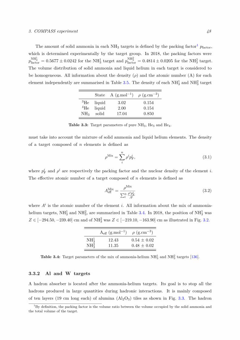
3. COMPASS experiment 48
The amount of solid ammonia in each NH3 targets is defined by the packing factor1 pfactor,which is determined experimentally by the target group. In 2018, the packing factors werepNH1
3factor = 0.5677 ± 0.0242 for the NH1
3 target and pNH23
factor = 0.4814 ± 0.0205 for the NH23 target.
The volume distribution of solid ammonia and liquid helium in each target is considered tobe homogeneous. All information about the density (ρ) and the atomic number (A) for eachelement independently are summarised in Table 3.5. The density of each NH1
3 and NH23 target
State A (g.mol−1) ρ (g.cm−3)3He liquid 3.02 0.1544He liquid 2.00 0.154NH3 solid 17.04 0.850
Table 3.3: Target parameters of pure NH3, He3 and He4.
must take into account the mixture of solid ammonia and liquid helium elements. The densityof a target composed of n elements is defined as
ρMix =n∑i
ρipiF, (3.1)
where piF and ρi are respectively the packing factor and the nuclear density of the element i.The effective atomic number of a target composed of n elements is defined as
AMixeff = ρMix∑n
iρipiFAi
(3.2)
where Ai is the atomic number of the element i. All information about the mix of ammonia-helium targets, NH1
3 and NH23, are summarized in Table 3.4. In 2018, the position of NH1
3 wasZ ∈ [−294.50,−239.40] cm and of NH2
3 was Z ∈ [−219.10,−163.90] cm as illustrated in Fig. 3.2.
Aeff (g.mol−1) ρ (g.cm−3)NH1
3 12.43 0.54 ± 0.02NH2
3 11.35 0.48 ± 0.02
Table 3.4: Target parameters of the mix of ammonia-helium NH13 and NH2
3 targets [136].
3.3.2 Al and W targets
A hadron absorber is located after the ammonia-helium targets. Its goal is to stop all thehadrons produced in large quantities during hadronic interactions. It is mainly composedof ten layers (19 cm long each) of alumina (Al2O3) tiles as shown in Fig. 3.3. The hadron
1By definition, the packing factor is the volume ratio between the volume occupied by the solid ammonia andthe total volume of the target.
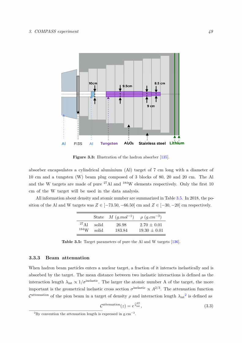
3. COMPASS experiment 49
Figure 3.3: Illustration of the hadron absorber [135].
absorber encapsulates a cylindrical aluminium (Al) target of 7 cm long with a diameter of10 cm and a tungsten (W) beam plug composed of 3 blocks of 80, 20 and 20 cm. The Aland the W targets are made of pure 27Al and 184W elements respectively. Only the first 10cm of the W target will be used in the data analysis.
All information about density and atomic number are summarized in Table 3.5. In 2018, the po-sition of the Al and W targets was Z ∈ [−73.50,−66.50] cm and Z ∈ [−30,−20] cm respectively.
State M (g.mol−1) ρ (g.cm−3)27Al solid 26.98 2.70 ± 0.01184W solid 183.84 19.30 ± 0.01
Table 3.5: Target parameters of pure the Al and W targets [136].
3.3.3 Beam attenuation
When hadron beam particles enters a nuclear target, a fraction of it interacts inelastically and isabsorbed by the target. The mean distance between two inelastic interactions is defined as theinteraction length λint ∝ 1/σinelastic. The larger the atomic number A of the target, the moreimportant is the geometrical inelastic cross section σinelastic ∝ A2/3. The attenuation functionCattenuation of the pion beam in a target of density ρ and interaction length λint2 is defined as
Cattenuation(z) = e−ρzλint , (3.3)
2By convention the attenuation length is expressed in g.cm−2.
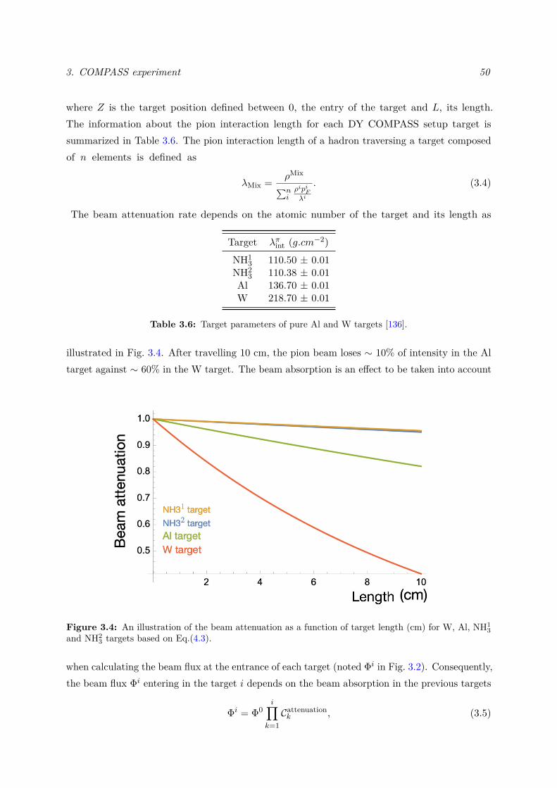
3. COMPASS experiment 50
where Z is the target position defined between 0, the entry of the target and L, its length.The information about the pion interaction length for each DY COMPASS setup target issummarized in Table 3.6. The pion interaction length of a hadron traversing a target composedof n elements is defined as
λMix = ρMix∑niρipiFλi
. (3.4)
The beam attenuation rate depends on the atomic number of the target and its length as
Target λπint (g.cm−2)NH1
3 110.50 ± 0.01NH2
3 110.38 ± 0.01Al 136.70 ± 0.01W 218.70 ± 0.01
Table 3.6: Target parameters of pure Al and W targets [136].
illustrated in Fig. 3.4. After travelling 10 cm, the pion beam loses ∼ 10% of intensity in the Altarget against ∼ 60% in the W target. The beam absorption is an effect to be taken into account
Figure 3.4: An illustration of the beam attenuation as a function of target length (cm) for W, Al, NH13
and NH23 targets based on Eq.(4.3).
when calculating the beam flux at the entrance of each target (noted Φi in Fig. 3.2). Consequently,the beam flux Φi entering in the target i depends on the beam absorption in the previous targets
Φi = Φ0i∏
k=1Cattenuationk , (3.5)
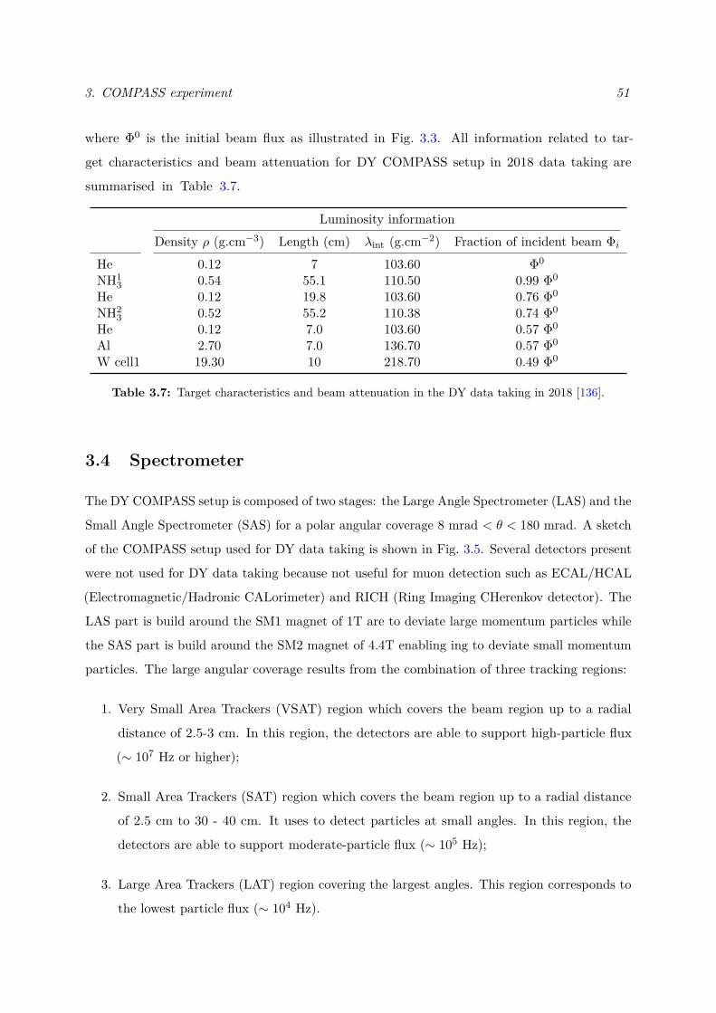
3. COMPASS experiment 51
where Φ0 is the initial beam flux as illustrated in Fig. 3.3. All information related to tar-
get characteristics and beam attenuation for DY COMPASS setup in 2018 data taking are
summarised in Table 3.7.
Luminosity informationDensity ρ (g.cm−3) Length (cm) λint (g.cm−2) Fraction of incident beam Φi
He 0.12 7 103.60 Φ0
NH13 0.54 55.1 110.50 0.99 Φ0
He 0.12 19.8 103.60 0.76 Φ0
NH23 0.52 55.2 110.38 0.74 Φ0
He 0.12 7.0 103.60 0.57 Φ0
Al 2.70 7.0 136.70 0.57 Φ0
W cell1 19.30 10 218.70 0.49 Φ0
Table 3.7: Target characteristics and beam attenuation in the DY data taking in 2018 [136].
3.4 Spectrometer
The DY COMPASS setup is composed of two stages: the Large Angle Spectrometer (LAS) and the
Small Angle Spectrometer (SAS) for a polar angular coverage 8 mrad < θ < 180 mrad. A sketch
of the COMPASS setup used for DY data taking is shown in Fig. 3.5. Several detectors present
were not used for DY data taking because not useful for muon detection such as ECAL/HCAL
(Electromagnetic/Hadronic CALorimeter) and RICH (Ring Imaging CHerenkov detector). The
LAS part is build around the SM1 magnet of 1T are to deviate large momentum particles while
the SAS part is build around the SM2 magnet of 4.4T enabling ing to deviate small momentum
particles. The large angular coverage results from the combination of three tracking regions:
1. Very Small Area Trackers (VSAT) region which covers the beam region up to a radial
distance of 2.5-3 cm. In this region, the detectors are able to support high-particle flux
(∼ 107 Hz or higher);
2. Small Area Trackers (SAT) region which covers the beam region up to a radial distance
of 2.5 cm to 30 - 40 cm. It uses to detect particles at small angles. In this region, the
detectors are able to support moderate-particle flux (∼ 105 Hz);
3. Large Area Trackers (LAT) region covering the largest angles. This region corresponds to
the lowest particle flux (∼ 104 Hz).
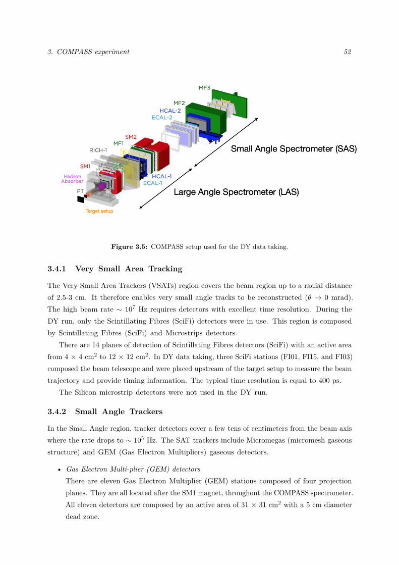
3. COMPASS experiment 52
Figure 3.5: COMPASS setup used for the DY data taking.
3.4.1 Very Small Area Tracking
The Very Small Area Trackers (VSATs) region covers the beam region up to a radial distanceof 2.5-3 cm. It therefore enables very small angle tracks to be reconstructed (θ → 0 mrad).The high beam rate ∼ 107 Hz requires detectors with excellent time resolution. During theDY run, only the Scintillating Fibres (SciFi) detectors were in use. This region is composedby Scintillating Fibres (SciFi) and Microstrips detectors.
There are 14 planes of detection of Scintillating Fibres detectors (SciFi) with an active areafrom 4 × 4 cm2 to 12 × 12 cm2. In DY data taking, three SciFi stations (FI01, FI15, and FI03)composed the beam telescope and were placed upstream of the target setup to measure the beamtrajectory and provide timing information. The typical time resolution is equal to 400 ps.
The Silicon microstrip detectors were not used in the DY run.
3.4.2 Small Angle Trackers
In the Small Angle region, tracker detectors cover a few tens of centimeters from the beam axiswhere the rate drops to ∼ 105 Hz. The SAT trackers include Micromegas (micromesh gaseousstructure) and GEM (Gas Electron Multipliers) gaseous detectors.
• Gas Electron Multi-plier (GEM) detectorsThere are eleven Gas Electron Multiplier (GEM) stations composed of four projectionplanes. They are all located after the SM1 magnet, throughout the COMPASS spectrometer.All eleven detectors are composed by an active area of 31 × 31 cm2 with a 5 cm diameterdead zone.
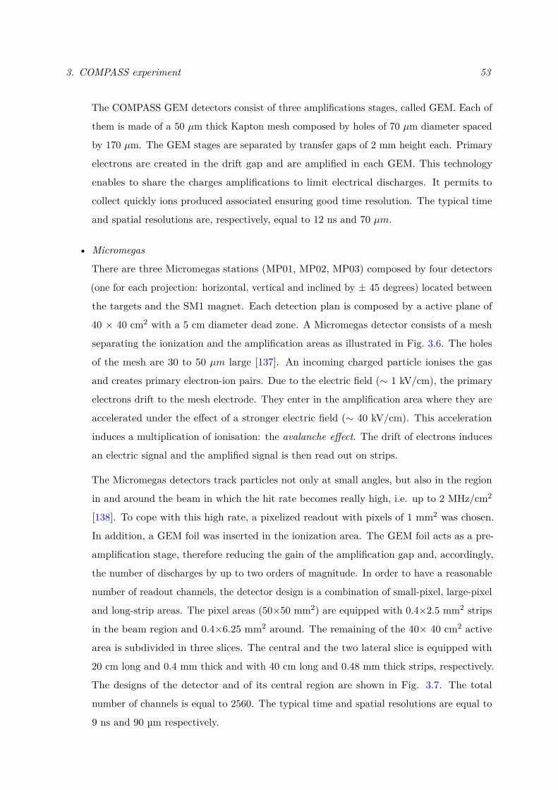
3. COMPASS experiment 53
The COMPASS GEM detectors consist of three amplifications stages, called GEM. Each of
them is made of a 50 µm thick Kapton mesh composed by holes of 70 µm diameter spaced
by 170 µm. The GEM stages are separated by transfer gaps of 2 mm height each. Primary
electrons are created in the drift gap and are amplified in each GEM. This technology
enables to share the charges amplifications to limit electrical discharges. It permits to
collect quickly ions produced associated ensuring good time resolution. The typical time
and spatial resolutions are, respectively, equal to 12 ns and 70 µm.
• Micromegas
There are three Micromegas stations (MP01, MP02, MP03) composed by four detectors
(one for each projection: horizontal, vertical and inclined by ± 45 degrees) located between
the targets and the SM1 magnet. Each detection plan is composed by a active plane of
40 × 40 cm2 with a 5 cm diameter dead zone. A Micromegas detector consists of a mesh
separating the ionization and the amplification areas as illustrated in Fig. 3.6. The holes
of the mesh are 30 to 50 µm large [137]. An incoming charged particle ionises the gas
and creates primary electron-ion pairs. Due to the electric field (∼ 1 kV/cm), the primary
electrons drift to the mesh electrode. They enter in the amplification area where they are
accelerated under the effect of a stronger electric field (∼ 40 kV/cm). This acceleration
induces a multiplication of ionisation: the avalanche effect. The drift of electrons induces
an electric signal and the amplified signal is then read out on strips.
The Micromegas detectors track particles not only at small angles, but also in the region
in and around the beam in which the hit rate becomes really high, i.e. up to 2 MHz/cm2
[138]. To cope with this high rate, a pixelized readout with pixels of 1 mm2 was chosen.
In addition, a GEM foil was inserted in the ionization area. The GEM foil acts as a pre-
amplification stage, therefore reducing the gain of the amplification gap and, accordingly,
the number of discharges by up to two orders of magnitude. In order to have a reasonable
number of readout channels, the detector design is a combination of small-pixel, large-pixel
and long-strip areas. The pixel areas (50×50 mm2) are equipped with 0.4×2.5 mm2 strips
in the beam region and 0.4×6.25 mm2 around. The remaining of the 40× 40 cm2 active
area is subdivided in three slices. The central and the two lateral slice is equipped with
20 cm long and 0.4 mm thick and with 40 cm long and 0.48 mm thick strips, respectively.
The designs of the detector and of its central region are shown in Fig. 3.7. The total
number of channels is equal to 2560. The typical time and spatial resolutions are equal to
9 ns and 90 µm respectively.
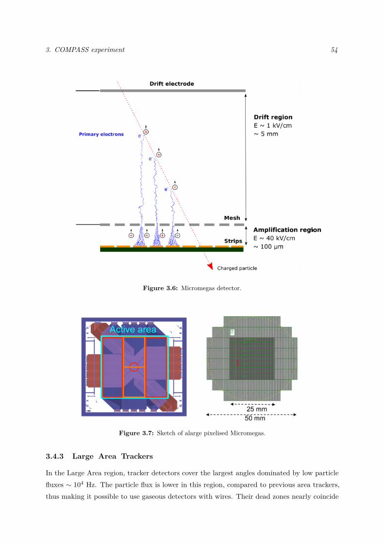
3. COMPASS experiment 54
Figure 3.6: Micromegas detector.
Figure 3.7: Sketch of alarge pixelised Micromegas.
3.4.3 Large Area Trackers
In the Large Area region, tracker detectors cover the largest angles dominated by low particlefluxes ∼ 104 Hz. The particle flux is lower in this region, compared to previous area trackers,thus making it possible to use gaseous detectors with wires. Their dead zones nearly coincide
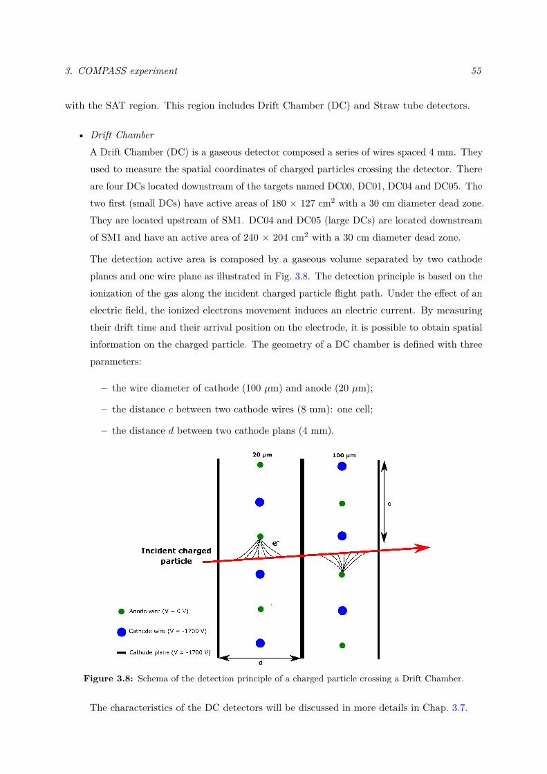
3. COMPASS experiment 55
with the SAT region. This region includes Drift Chamber (DC) and Straw tube detectors.
• Drift ChamberA Drift Chamber (DC) is a gaseous detector composed a series of wires spaced 4 mm. Theyused to measure the spatial coordinates of charged particles crossing the detector. Thereare four DCs located downstream of the targets named DC00, DC01, DC04 and DC05. Thetwo first (small DCs) have active areas of 180 × 127 cm2 with a 30 cm diameter dead zone.They are located upstream of SM1. DC04 and DC05 (large DCs) are located downstreamof SM1 and have an active area of 240 × 204 cm2 with a 30 cm diameter dead zone.
The detection active area is composed by a gaseous volume separated by two cathodeplanes and one wire plane as illustrated in Fig. 3.8. The detection principle is based on theionization of the gas along the incident charged particle flight path. Under the effect of anelectric field, the ionized electrons movement induces an electric current. By measuringtheir drift time and their arrival position on the electrode, it is possible to obtain spatialinformation on the charged particle. The geometry of a DC chamber is defined with threeparameters:
– the wire diameter of cathode (100 µm) and anode (20 µm);
– the distance c between two cathode wires (8 mm): one cell;
– the distance d between two cathode plans (4 mm).
Figure 3.8: Schema of the detection principle of a charged particle crossing a Drift Chamber.
The characteristics of the DC detectors will be discussed in more details in Chap. 3.7.
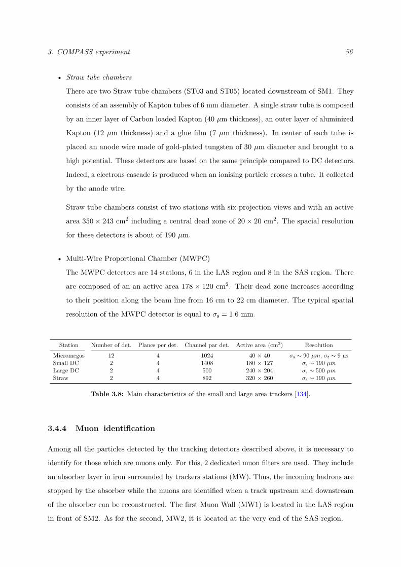
3. COMPASS experiment 56
• Straw tube chambers
There are two Straw tube chambers (ST03 and ST05) located downstream of SM1. They
consists of an assembly of Kapton tubes of 6 mm diameter. A single straw tube is composed
by an inner layer of Carbon loaded Kapton (40 µm thickness), an outer layer of aluminized
Kapton (12 µm thickness) and a glue film (7 µm thickness). In center of each tube is
placed an anode wire made of gold-plated tungsten of 30 µm diameter and brought to a
high potential. These detectors are based on the same principle compared to DC detectors.
Indeed, a electrons cascade is produced when an ionising particle crosses a tube. It collected
by the anode wire.
Straw tube chambers consist of two stations with six projection views and with an active
area 350× 243 cm2 including a central dead zone of 20× 20 cm2. The spacial resolution
for these detectors is about of 190 µm.
• Multi-Wire Proportional Chamber (MWPC)
The MWPC detectors are 14 stations, 6 in the LAS region and 8 in the SAS region. There
are composed of an an active area 178 × 120 cm2. Their dead zone increases according
to their position along the beam line from 16 cm to 22 cm diameter. The typical spatial
resolution of the MWPC detector is equal to σs = 1.6 mm.
Station Number of det. Planes per det. Channel par det. Active area (cm2) ResolutionMicromegas 12 4 1024 40 × 40 σs ∼ 90 µm, σt ∼ 9 nsSmall DC 2 4 1408 180 × 127 σs ∼ 190 µmLarge DC 2 4 500 240 × 204 σs ∼ 500 µmStraw 2 4 892 320 × 260 σs ∼ 190 µm
Table 3.8: Main characteristics of the small and large area trackers [134].
3.4.4 Muon identification
Among all the particles detected by the tracking detectors described above, it is necessary to
identify for those which are muons only. For this, 2 dedicated muon filters are used. They include
an absorber layer in iron surrounded by trackers stations (MW). Thus, the incoming hadrons are
stopped by the absorber while the muons are identified when a track upstream and downstream
of the absorber can be reconstructed. The first Muon Wall (MW1) is located in the LAS region
in front of SM2. As for the second, MW2, it is located at the very end of the SAS region.
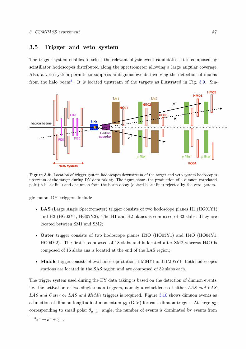
3. COMPASS experiment 57
3.5 Trigger and veto system
The trigger system enables to select the relevant physic event candidates. It is composed byscintillator hodoscopes distributed along the spectrometer allowing a large angular coverage.Also, a veto system permits to suppress ambiguous events involving the detection of muonsfrom the halo beam3. It is located upstream of the targets as illustrated in Fig. 3.9. Sin-
Figure 3.9: Location of trigger system hodoscopes downstream of the target and veto system hodoscopesupstream of the target during DY data taking. The figure shows the production of a dimuon correlatedpair (in black line) and one muon from the beam decay (dotted black line) rejected by the veto system.
gle muon DY triggers include
• LAS (Large Angle Spectrometer) trigger consists of two hodoscope planes H1 (HG01Y1)and H2 (HG02Y1, HG02Y2). The H1 and H2 planes is composed of 32 slabs. They arelocated between SM1 and SM2;
• Outer trigger consists of two hodoscope planes H3O (HO03Y1) and H4O (HO04Y1,HO04Y2). The first is composed of 18 slabs and is located after SM2 whereas H4O iscomposed of 16 slabs ans is located at the end of the LAS region;
• Middle trigger consists of two hodoscope stations HM04Y1 and HM05Y1. Both hodoscopesstations are located in the SAS region and are composed of 32 slabs each.
The trigger system used during the DY data taking is based on the detection of dimuon events,i.e. the activation of two single-muon triggers, namely a coincidence of either LAS and LAS,LAS and Outer or LAS and Middle triggers is required. Figure 3.10 shows dimuon events asa function of dimuon longitudinal momentum pZ (GeV) for each dimuon trigger. At large pZ,corresponding to small polar θµ+µ− angle, the number of events is dominated by events from
3π− → µ− + νµ− .
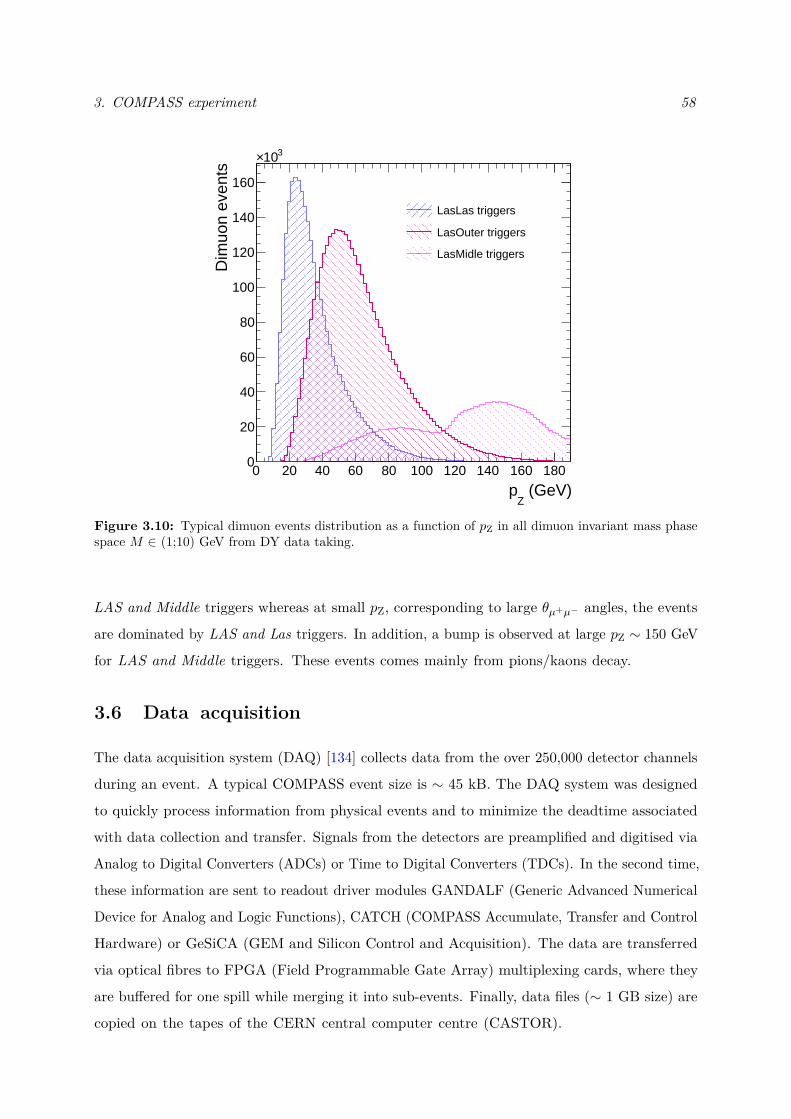
3. COMPASS experiment 58
0 20 40 60 80 100 120 140 160 180
(GeV)Z
p
0
20
40
60
80
100
120
140
160
310×
Dim
uon
even
tsLasLas triggers
LasOuter triggers
LasMidle triggers
Figure 3.10: Typical dimuon events distribution as a function of pZ in all dimuon invariant mass phasespace M ∈ (1;10) GeV from DY data taking.
LAS and Middle triggers whereas at small pZ, corresponding to large θµ+µ− angles, the events
are dominated by LAS and Las triggers. In addition, a bump is observed at large pZ ∼ 150 GeV
for LAS and Middle triggers. These events comes mainly from pions/kaons decay.
3.6 Data acquisition
The data acquisition system (DAQ) [134] collects data from the over 250,000 detector channels
during an event. A typical COMPASS event size is ∼ 45 kB. The DAQ system was designed
to quickly process information from physical events and to minimize the deadtime associated
with data collection and transfer. Signals from the detectors are preamplified and digitised via
Analog to Digital Converters (ADCs) or Time to Digital Converters (TDCs). In the second time,
these information are sent to readout driver modules GANDALF (Generic Advanced Numerical
Device for Analog and Logic Functions), CATCH (COMPASS Accumulate, Transfer and Control
Hardware) or GeSiCA (GEM and Silicon Control and Acquisition). The data are transferred
via optical fibres to FPGA (Field Programmable Gate Array) multiplexing cards, where they
are buffered for one spill while merging it into sub-events. Finally, data files (∼ 1 GB size) are
copied on the tapes of the CERN central computer centre (CASTOR).
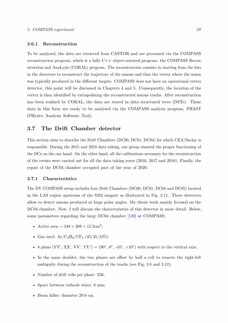
3. COMPASS experiment 59
3.6.1 Reconstruction
To be analysed, the data are retrieved from CASTOR and are processed via the COMPASSreconstruction program, which is a fully C++ object-oriented program: the COMPASS Recon-struction and AnaLysis (CORAL) program. The reconstruction consists in starting from the hitsin the detectors to reconstruct the trajectory of the muons and thus the vertex where the muonwas typically produced in the different targets. COMPASS does not have an operational vertexdetector, this point will be discussed in Chapters 4 and 5. Consequently, the location of thevertex is then identified by extrapolating the reconstructed muons tracks. After reconstructionhas been realised by CORAL, the data are stored in data structured trees (DSTs). Thesedata in this form are ready to be analysed via the COMPASS analysis program, PHAST(PHysics Analysis Software Tool).
3.7 The Drift Chamber detector
This section aims to describe the Drift Chambers (DC00, DC01, DC04) for which CEA/Saclay isresponsible. During the 2015 and 2018 data taking, our group ensured the proper functioning ofthe DCs on the one hand. On the other hand, all the calibrations necessary for the reconstructionof the events were carried out for all the data taking years (2016, 2017 and 2018). Finally, therepair of the DC04 chamber occupied part of the year of 2020.
3.7.1 Characteristics
The DY COMPASS setup includes four Drift Chambers (DC00, DC01, DC04 and DC05) locatedin the LAS region upstream of the SM2 magnet as illustrated in Fig. 3.11. These detectorsallow to detect muons produced at large polar angles. My thesis work mainly focused on theDC04 chamber. Now, I will discuss the characteristics of this detector in more detail. Below,some parameters regarding the large DC04 chamber [139] at COMPASS:
• Active area ∼ 248× 208× 12.5cm3;
• Gaz used: Ar/C2H6/CF4 (45/45/10%)
• 8 plans (YY’, XX’, VV’, UU’) = (90◦, 0◦, -10◦, +10◦) with respect to the vertical axis;
• In the same doublet, the two planes are offset by half a cell to remove the right-leftambiguity during the reconstruction of the tracks (see Fig. 3.8 and 3.12);
• Number of drift cells per plane: 256;
• Space between cathode wires: 8 mm;
• Beam killer: diameter 28.6 cm.
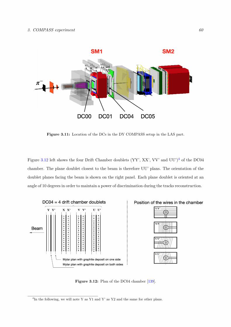
3. COMPASS experiment 60
Figure 3.11: Location of the DCs in the DY COMPASS setup in the LAS part.
Figure 3.12 left shows the four Drift Chamber doublets (YY’, XX’, VV’ and UU’)4 of the DC04
chamber. The plane doublet closest to the beam is therefore UU’ plans. The orientation of the
doublet planes facing the beam is shown on the right panel. Each plane doublet is oriented at an
angle of 10 degrees in order to maintain a power of discrimination during the tracks reconstruction.
Figure 3.12: Plan of the DC04 chamber [139].
4In the following, we will note Y as Y1 and Y’ as Y2 and the same for other plans.
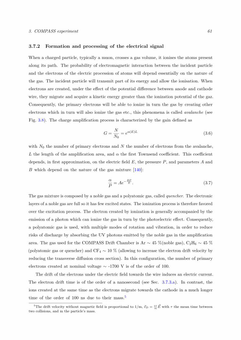
3. COMPASS experiment 61
3.7.2 Formation and processing of the electrical signal
When a charged particle, typically a muon, crosses a gas volume, it ionises the atoms present
along its path. The probability of electromagnetic interaction between the incident particle
and the electrons of the electric procession of atoms will depend essentially on the nature of
the gas. The incident particle will transmit part of its energy and allow the ionisation. When
electrons are created, under the effect of the potential difference between anode and cathode
wire, they migrate and acquire a kinetic energy greater than the ionization potential of the gaz.
Consequently, the primary electrons will be able to ionize in turn the gas by creating other
electrons which in turn will also ionize the gas etc., this phenomena is called avalanche (see
Fig. 3.8). The charge amplification process is characterized by the gain defined as
G = N
N0= eα(E)L (3.6)
with N0 the number of primary electrons and N the number of electrons from the avalanche,
L the length of the amplification area, and α the first Townsend coefficient. This coefficient
depends, in first approximation, on the electric field E, the pressure P , and parameters A and
B which depend on the nature of the gas mixture [140]:
α
P= Ae−
BPE . (3.7)
The gas mixture is composed by a noble gas and a polyatomic gas, called quencher. The electronic
layers of a noble gas are full so it has few excited states. The ionization process is therefore favored
over the excitation process. The electron created by ionization is generally accompanied by the
emission of a photon which can ionize the gas in turn by the photoelectric effect. Consequently,
a polyatomic gas is used, with multiple modes of rotation and vibration, in order to reduce
risks of discharge by absorbing the UV photons emitted by the noble gas in the amplification
area. The gas used for the COMPASS Drift Chamber is Ar ∼ 45 %(noble gas), C2H6 ∼ 45 %
(polyatomic gas or quencher) and CF4 ∼ 10 % (allowing to increase the electron drift velocity by
reducing the transverse diffusion cross section). In this configuration, the number of primary
electrons created at nominal voltage ∼ -1700 V is of the order of 100.
The drift of the electrons under the electric field towards the wire induces an electric current.
The electron drift time is of the order of a nanosecond (see Sec. 3.7.3.a). In contrast, the
ions created at the same time as the electrons migrate towards the cathode in a much longer
time of the order of 100 ns due to their mass.5
5The drift velocity without magnetic field is proportional to 1/m, ~vD = eτm~E with τ the mean time between
two collisions, and m the particle’s mass.
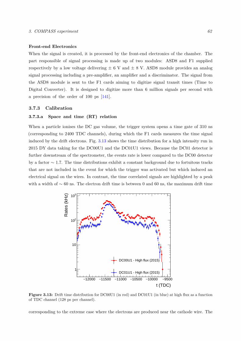
3. COMPASS experiment 62
Front-end ElectronicsWhen the signal is created, it is processed by the front-end electronics of the chamber. Thepart responsible of signal processing is made up of two modules: ASD8 and F1 suppliedrespectively by a low voltage delivering ± 6 V and ± 8 V. ASD8 module provides an analogsignal processing including a pre-amplifier, an amplifier and a discriminator. The signal fromthe ASD8 module is sent to the F1 cards aiming to digitize signal transit times (Time toDigital Converter). It is designed to digitize more than 6 million signals per second witha precision of the order of 100 ps [141].
3.7.3 Calibration
3.7.3.a Space and time (RT) relation
When a particle ionises the DC gas volume, the trigger system opens a time gate of 310 ns(corresponding to 2400 TDC channels), during which the F1 cards measures the time signalinduced by the drift electrons. Fig. 3.13 shows the time distribution for a high intensity run in2015 DY data taking for the DC00U1 and the DC01U1 views. Because the DC01 detector isfurther downstream of the spectrometer, the events rate is lower compared to the DC00 detectorby a factor ∼ 1.7. The time distributions exhibit a constant background due to fortuitous tracksthat are not included in the event for which the trigger was activated but which induced anelectrical signal on the wires. In contrast, the time correlated signals are highlighted by a peakwith a width of ∼ 60 ns. The electron drift time is between 0 and 60 ns, the maximum drift time
12000− 11500− 11000− 10500− 10000− 9500−
t (TDC)
1
10
210
310
Rat
es (
kHz)
DC00U1 - High flux (2015)
DC01U1 - High flux (2015)
Figure 3.13: Drift time distribution for DC00U1 (in red) and DC01U1 (in blue) at high flux as a functionof TDC channel (128 ps per channel).
corresponding to the extreme case where the electrons are produced near the cathode wire. The
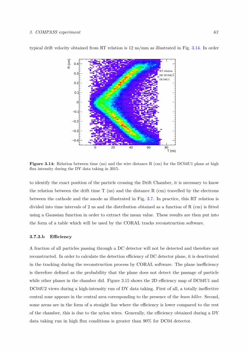
3. COMPASS experiment 63
typical drift velocity obtained from RT relation is 12 ns/mm as illustrated in Fig. 3.14. In order
0 20 40 60 80T (ns)
0.4−
0.3−
0.2−
0.1−
0
0.1
0.2
0.3
0.4R
(cm
)RT relation
HF DC04U1
DC04U1
Figure 3.14: Relation between time (ns) and the wire distance R (cm) for the DC04U1 plane at highflux intensity during the DY data taking in 2015.
to identify the exact position of the particle crossing the Drift Chamber, it is necessary to know
the relation between the drift time T (ns) and the distance R (cm) travelled by the electrons
between the cathode and the anode as illustrated in Fig. 3.7. In practice, this RT relation is
divided into time intervals of 2 ns and the distribution obtained as a function of R (cm) is fitted
using a Gaussian function in order to extract the mean value. These results are then put into
the form of a table which will be used by the CORAL tracks reconstruction software.
3.7.3.b Efficiency
A fraction of all particles passing through a DC detector will not be detected and therefore not
reconstructed. In order to calculate the detection efficiency of DC detector plane, it is deactivated
in the tracking during the reconstruction process by CORAL software. The plane inefficiency
is therefore defined as the probability that the plane does not detect the passage of particle
while other planes in the chamber did. Figure 3.15 shows the 2D efficiency map of DC04U1 and
DC04U2 views during a high-intensity run of DY data taking. First of all, a totally ineffective
central zone appears in the central area corresponding to the presence of the beam killer. Second,
some areas are in the form of a straight line where the efficiency is lower compared to the rest
of the chamber, this is due to the nylon wires. Generally, the efficiency obtained during a DY
data taking run in high flux conditions is greater than 90% for DC04 detector.
3. COMPASS experiment 64
100− 50− 0 50 100Position (cm)
100−
50−
0
50
100
Pos
ition
(cm
)
0
0.1
0.2
0.3
0.4
0.5
0.6
0.7
0.8
0.9
1
High flux - DC04U1
100− 50− 0 50 100Position (cm)
100−
50−
0
50
100
Pos
ition
(cm
)
0
0.1
0.2
0.3
0.4
0.5
0.6
0.7
0.8
0.9
1
High flux - DC04U2
Figure 3.15: Efficiency map of DC04U at high flux during the DY data taking.
3.7.3.c Spatial resolution
The spatial resolution of a detector σa can be calculated from the spatial resolution of the residualand the uncertainty of track reconstruction position thanks to other detectors. These sources ofuncertainty are completely independent and can be summed up in a quadratic way as
σ2 = σ2a + σ2
t . (3.8)
In order to get rid of the uncertainty of track reconstruction position depending on the setof detectors of the spectrometer, it is possible to use the fact that each view is divided in2 planes (see Fig. 3.12). The two planes from each view are staggered by a half a cell, i.e.4 mm. The uncertainty of reconstruction of the track for these two planes can therefore beconsidered to be identical. Consequently, it possible to define the double layer residual todetermine the spatial resolution of each detector plane as
δ∆udouble residual = (uplane 1 − utrack )− (uplane 2 − utrack ) = ustateplane 1 − uplane 2 (3.9)
where uplane 1(2) is the hit position on plane 1(2) and utrack is the hit position determinedfrom reconstruction. The double layer residual is independent of the track resolution and onlydependent of the difference of hit position between the plane 1 and plane 2. Figure 3.16 shows thedouble residual for the plane DC04U1 during the 2015 DY data taking in high flux condition. Todetermine the resolution, the distribution is fitted with one Gaussian function and one constantto reproduce the background. In Fig. 3.16, a Gaussian function is fitted on the distribution inorder to extract the value of the resolution of the plane. The resolution of the DC04U plane canbe written by assuming that the distribution of the residuals are the same for the two planes as
σ2double residual = σ2
plane 1 + σ2plane 2 = 2σ2
plane 1 = 2σ2a (3.10)
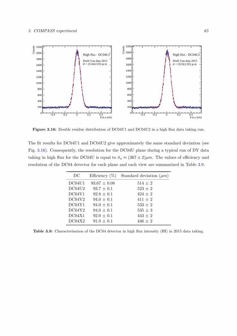
3. COMPASS experiment 65
0.4− 0.2− 0 0.2 0.4 u (cm)∆ δ
0
200
400
600
800
1000
1200
1400
1600
1800
2000
2200
Cou
nts
High flux - DC04U1
Drell-Yan data 2015 mµ2.03) ± = (514σ
0.4− 0.2− 0 0.2 0.4 u (cm)∆ δ
0
200
400
600
800
1000
1200
1400
1600
1800
2000
2200
Cou
nts
High flux - DC04U2
Drell-Yan data 2015 mµ2.05) ± = (523σ
Figure 3.16: Double residue distribution of DC04U1 and DC04U2 in a high flux data taking run.
The fit results for DC04U1 and DC04U2 give approximately the same standard deviation (seeFig. 3.16). Consequently, the resolution for the DC04U plane during a typical run of DY datataking in high flux for the DC04U is equal to σa ≈ (367± 2)µm. The values of efficiency andresolution of the DC04 detector for each plane and each view are summarized in Table 3.9.
DC Efficiency (%) Standard deviation (µm)DC04U1 93.67 ± 0.08 514 ± 2DC04U2 93.7 ± 0.1 523 ± 2DC04V1 92.8 ± 0.1 424 ± 2DC04V2 94.0 ± 0.1 411 ± 2DC04Y1 94.0 ± 0.1 533 ± 2DC04Y2 94.0 ± 0.1 535 ± 3DC04X1 92.0 ± 0.1 443 ± 2DC04X2 91.0 ± 0.1 446 ± 2
Table 3.9: Characterisation of the DC04 detector in high flux intensity (HI) in 2015 data taking.
4Analysis of J/ψ production in πA collisions
Contents
4.1 Observable . . . . . . . . . . . . . . . . . . . . . . . . . . . . . . . . . . 674.2 Data sample . . . . . . . . . . . . . . . . . . . . . . . . . . . . . . . . . 67
4.2.1 Event selection . . . . . . . . . . . . . . . . . . . . . . . . . . . . . . . . 684.2.2 Dimuon invariant mass . . . . . . . . . . . . . . . . . . . . . . . . . . . 69
4.3 J/ψ signal extraction . . . . . . . . . . . . . . . . . . . . . . . . . . . . 704.3.1 Invariant mass reconstruction . . . . . . . . . . . . . . . . . . . . . . . . 714.3.2 Fit procedure . . . . . . . . . . . . . . . . . . . . . . . . . . . . . . . . . 774.3.3 J/ψ resolution estimation from Monte-Carlo simulation . . . . . . . . . 804.3.4 J/ψ 2D extraction method . . . . . . . . . . . . . . . . . . . . . . . . . 82
4.4 J/ψ cross section extraction method . . . . . . . . . . . . . . . . . . . 904.4.1 2D acceptance as a function of p⊥ and xF . . . . . . . . . . . . . . . . . 924.4.2 J/ψ cross section as a function of p⊥ and xF . . . . . . . . . . . . . . . 954.4.3 Ratio of cross sections for J/ψ production for the W and Al targets . . 964.4.4 Nuclear transverse momentum broadening . . . . . . . . . . . . . . . . . 98
4.5 Systematic uncertainties estimation . . . . . . . . . . . . . . . . . . . 994.5.1 Signal extraction . . . . . . . . . . . . . . . . . . . . . . . . . . . . . . . 994.5.2 Impact of the Zvtx position in the W target . . . . . . . . . . . . . . . . 1014.5.3 Acceptance systematic error . . . . . . . . . . . . . . . . . . . . . . . . . 1014.5.4 Period compatibility . . . . . . . . . . . . . . . . . . . . . . . . . . . . . 1034.5.5 Results . . . . . . . . . . . . . . . . . . . . . . . . . . . . . . . . . . . . 104
4.6 Conclusion . . . . . . . . . . . . . . . . . . . . . . . . . . . . . . . . . . 106
In this chapter, I present the data analysis for the J/ψ production in π−A collisions, for the
W and the Al targets nuclei. Results for the ratio of nuclear cross section W/Al are given as a
function of xF and p⊥ . The analysis is based on real data (RD) accumulated in 2018. It includes
the selection of events, the calculation of the acceptance of the setup using a Monte-Carlo (MC)
simulation, the extraction of the cross-sections ratio and the study of systematic errors.
66
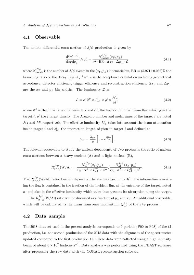
4. Analysis of J/ψ production in πA collisions 67
4.1 Observable
The double differential cross section of J/ψ production is given by
d2σπ−A
dxFdp⊥(J/ψ) = N
J/ψevents (xF, p⊥)
εA · BR ·∆xF ·∆p⊥ · L(4.1)
whereNJ/ψevents is the number of J/ψ events in the (xF, p⊥) kinematic bin, BR = (5.971±0.032)% the
branching ratio of the decay J/ψ → µ+µ−, ε is the acceptance calculation including geometricalacceptance, detector efficiency, trigger efficiency and reconstruction efficiency, ∆xF and ∆p⊥are the xF and p⊥ bin widths. The luminosity L is
L = αiΦ0 × Lieff × ρi ×NAM i
(4.2)
where Φ0 is the initial absolute beam flux and αi, the fraction of initial beam flux entering in thetarget i, ρi the i target density. The Avogadro number and molar mass of the target i are notedNA and M i respectively. The effective luminosity Lieff takes into account the beam attenuationinside target i and λiint the interaction length of pion in target i and defined as
Leff = λintρ
[1− e
−ρLλint
]. (4.3)
The relevant observable to study the nuclear dependence of J/ψ process is the ratio of nuclearcross sections between a heavy nucleus (A) and a light nucleus (B),
RJ/ψπ−A(W/Al) = N
J/ψW (xF, p⊥)
εW · αA × LWeff × ρW
/NJ/ψAl (xF, p⊥)
εAl · αAl × LAleff × ρAl
. (4.4)
The RJ/ψπ−A(W/Al) ratio does not depend on the absolute beam flux Φ0. The information concern-ing the flux is contained in the fraction of the incident flux at the entrance of the target, notedα, and also in the effective luminosity which takes into account its absorption along the target.
The RJ/ψπ−A(W/Al) ratio will be discussed as a function of p⊥ and xF. An additional observable,which will be calculated, is the mean transverse momentum, 〈p2
⊥〉 of the J/ψ process.
4.2 Data sample
The 2018 data set used in the present analysis corresponds to 9 periods (P00 to P08) of the t2production, i.e. the second production of the 2018 data with the alignment of the spectrometerupdated compared to the first production t1. These data were collected using a high intensitybeam of about 6× 10⁷ hadrons.s−1. Data analysis was performed using the PHAST softwareafter processing the raw data with the CORAL reconstruction software.
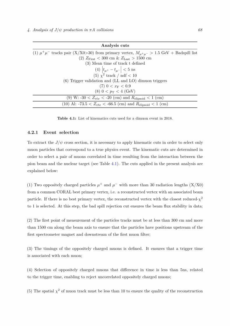
4. Analysis of J/ψ production in πA collisions 68
Analysis cuts
(1) µ+µ− tracks pair (X/X0>30) from primary vertex, Mµ+µ− > 1.5 GeV + Badspill list(2) ZFirst < 300 cm & ZLast > 1500 cm
(3) Mean time of track t defined(4)
∣∣∣tµ+ − tµ−∣∣∣ < 5 ns
(5) χ2 track / ndf < 10(6) Trigger validation and (LL and LO) dimuon triggers
(7) 0 < xF < 0.9(8) 0 < pT < 4 (GeV)
(9) W: -30 < Zvtx < -20 (cm) and Relipsoid < 1 (cm)(10) Al: -73.5 < Zvtx < -66.5 (cm) and Relipsoid < 1 (cm)
Table 4.1: List of kinematics cuts used for a dimuon event in 2018.
4.2.1 Event selection
To extract the J/ψ cross section, it is necessary to apply kinematic cuts in order to select onlymuon particles that correspond to a true physics event. The kinematic cuts are determined inorder to select a pair of muons correlated in time resulting from the interaction between thepion beam and the nuclear target (see Table 4.1). The cuts applied in the present analysis areexplained below:
(1) Two oppositely charged particles µ+ and µ− with more than 30 radiation lengths (X/X0)from a common CORAL best primary vertex, i.e. a reconstructed vertex with an associated beamparticle. If there is no best primary vertex, the reconstructed vertex with the closest reduced-χ2
to 1 is selected. At this step, the bad spill rejection cut ensures the beam flux stability in data;
(2) The first point of measurement of the particles tracks must be at less than 300 cm and morethan 1500 cm along the beam axis to ensure that the particles have positions upstream of thefirst spectrometer magnet and downstream of the first muon filter;
(3) The timings of the oppositely charged muons is defined. It ensures that a trigger timeis associated with each muon;
(4) Selection of oppositely charged muons that difference in time is less than 5ns, relatedto the trigger time, enabling to reject uncorrelated oppositely charged muons;
(5) The spatial χ2 of muon track must be less than 10 to ensure the quality of the reconstruction
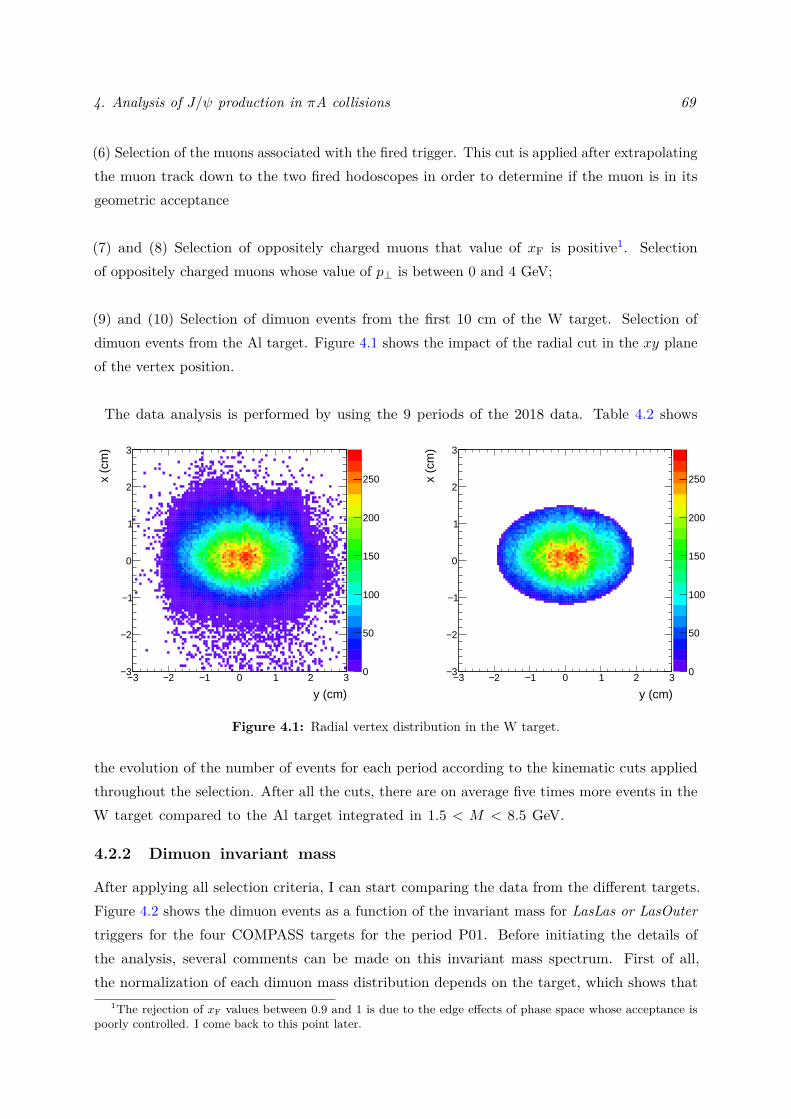
4. Analysis of J/ψ production in πA collisions 69
(6) Selection of the muons associated with the fired trigger. This cut is applied after extrapolatingthe muon track down to the two fired hodoscopes in order to determine if the muon is in itsgeometric acceptance
(7) and (8) Selection of oppositely charged muons that value of xF is positive1. Selectionof oppositely charged muons whose value of p⊥ is between 0 and 4 GeV;
(9) and (10) Selection of dimuon events from the first 10 cm of the W target. Selection ofdimuon events from the Al target. Figure 4.1 shows the impact of the radial cut in the xy planeof the vertex position.
The data analysis is performed by using the 9 periods of the 2018 data. Table 4.2 shows
3− 2− 1− 0 1 2 3
y (cm)
3−
2−
1−
0
1
2
3
x (c
m)
0
50
100
150
200
250
3− 2− 1− 0 1 2 3
y (cm)
3−
2−
1−
0
1
2
3
x (c
m)
0
50
100
150
200
250
Figure 4.1: Radial vertex distribution in the W target.
the evolution of the number of events for each period according to the kinematic cuts appliedthroughout the selection. After all the cuts, there are on average five times more events in theW target compared to the Al target integrated in 1.5 < M < 8.5 GeV.
4.2.2 Dimuon invariant mass
After applying all selection criteria, I can start comparing the data from the different targets.Figure 4.2 shows the dimuon events as a function of the invariant mass for LasLas or LasOutertriggers for the four COMPASS targets for the period P01. Before initiating the details ofthe analysis, several comments can be made on this invariant mass spectrum. First of all,the normalization of each dimuon mass distribution depends on the target, which shows that
1The rejection of xF values between 0.9 and 1 is due to the edge effects of phase space whose acceptance ispoorly controlled. I come back to this point later.
4. Analysis of J/ψ production in πA collisions 70
Selections P00 P01 P02 P03 P04 P05 P06 P07 P08General selections of dimuon events
(1) 1.55301e+07 7.99067e+06 1.61287e+07 1.21514e+07 1.09503e+07 7.15226e+06 8.18908e+06 1.39557e+07 5.02053e+06(2) 1.50536e+07 7.73835e+06 1.55943e+07 1.17552e+07 1.06538e+07 6.87648e+06 7.91197e+06 1.34766e+07 4.8452e+06(3) 1.49459e+07 7.67827e+06 1.54764e+07 1.16661e+07 1.05882e+07 6.82165e+06 7.8539e+06 1.33773e+07 4.8084e+06(4) 1.05282e+07 5.86996e+06 1.2101e+07 9.15094e+06 1.0509e+07 5.26634e+06 6.05618e+06 1.02259e+07 3.6605e+06(5) 1.0444e+07 5.82692e+06 1.2011e+07 9.08981e+06 8.13291e+06 5.22888e+06 6.01657e+06 1.01561e+07 3.63419e+06(6) 8.32992e+06 4.7662e+06 9.84962e+06 7.37048e+06 8.07781e+06 4.3115e+06 5.01756e+06 8.43529e+06 3.05939e+06(7) 6.04522e+06 3.50942e+06 7.32899e+06 5.49105e+06 4.93754e+06 3.21985e+06 3.77516e+06 6.3174e+06 2.28976e+06(8) 6.04264e+06 3.50817e+06 7.32644e+06 5.48917e+06 4.93615e+06 3.21874e+06 3.77393e+06 6.31523e+06 2.289e+06
Al target selections(09) 54328 36786 76401 56982 50839 34012 39374 66479 23987
W target selections(10) 276905 192656 404666 298319 267741 179285 212733 351660 127813
Table 4.2: The statistics of the dimuon events for each of the 9 periods, following the cuts defined inTable 4.1.
2 3 4 5 6 7 8 9 10
(GeV)-µ +µM
1
10
210
310
410
510
Dim
uon
even
ts
(LasLas || LasOuter) triggers
P01 period
W target
Al target
target13NH
target23NH
Figure 4.2: Dimuon events as a function of the invariant mass M (GeV) for the W (in red), Al (in blue),NH1
3 (in black) and NH23 (in magenta) targets in the period P01.
the acceptance of the spectrometer and the luminosity will be important corrective factorsto access to the J/ψ absolute cross section. In addition, the resolution of the J/ψ peakaround M ∼ 3 GeV varies depending on the target as well worsensing when going fromthe lighter to the heavier targets.
4.3 J/ψ signal extraction
In order to extract the number of J/ψ events for each target, there are essentially two methods.The first consists in finding a parametrization of the background and the J/ψ signal as a functionof the dimuon invariant mass. This method is model-dependent insofar as a strong assumptionis made concerning the values of the background. Often, the background evolves accordingto kinematic variables, it is sometimes difficult to find a single parameterization. The second
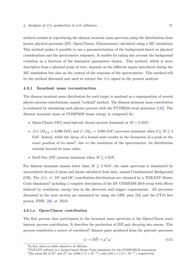
4. Analysis of J/ψ production in πA collisions 71
method consists in reproducing the dimuon invariant mass spectrum using the distributions fromknown physical processes (DY, Open-Charm, Charmonium) calculated using a MC simulation.This method makes it possible to use a parameterization of the background based on physicalconsiderations and the spectrometer responses. It enables for taking into account the backgroundevolution as a function of the kinematic parameters chosen. This method, which is moredescriptive from a physical point of view, depends on the different inputs introduced during theMC simulation but also on the control of the response of the spectrometer. This method willbe the method discussed and used to extract the J/ψ signal in the present analysis.
4.3.1 Invariant mass reconstruction
The dimuon invariant mass distribution for each target is analysed as a superposition of severalphysics process contributions, named "cocktail" method. The dimuon invariant mass contributionis evaluated by simulating each physics process with the PYTHIA8 event generator [142]. Thedimuon invariant mass at COMPASS beam energy is composed by:
• Open-Charm (OC) semi-leptonic decays process dominant at M ∼ 2 GeV;
• J/ψ (MJ/ψ = 3.096 GeV) and ψ′ (Mψ′ = 3.686 GeV) processes dominant when 2 .M . 4GeV. Indeed, while the decay of a bound state results in the formation of a peak at theexact position of its mass2, due to the resolution of the spectrometer, its distributionextends beyond its mass value;
• Drell-Yan (DY) process dominant when M & 4 GeV.
For dimuon invariant masses lower than M . 2 GeV, the mass spectrum is dominated byuncorrelated decays of pions and kaons calculated from data, named Combinatorial Background(CB). The J/ψ, ψ′, DY and OC contribution distributions are obtained by a TGEANT Monte-Carlo simulation3 including a complete description of the DY COMPASS 2018 setup with effectsinduced by resolution, energy loss in the detectors and trigger requirements. All processesdiscussed in the next section are simulated by using the GRV pion [34] and the CT14 freeproton PDFs [28] at NLO.
4.3.1.a Open-Charm contribution
The first process that participates in the invariant mass spectrum is the Open-Charm semi-leptonic process contribution. It describes the production of DD pair decaying into muons. Thisprocess constitutes a source of correlated4 dimuon pairs produced from the partonic processes
ij → DD → µ+µ− (4.5)2In fact, there is width related to its lifetime.3TGEANT software is a Geant4 based Monte Carlo simulation for the COMPASS-II experiment.4The mean life of D± and D0 are (1040± 7)× 10−15 s and (410.1± 1.5)× 10−15 s respectively.
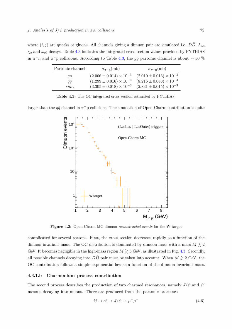
4. Analysis of J/ψ production in πA collisions 72
where (i, j) are quarks or gluons. All channels giving a dimuon pair are simulated i.e. DD, Λcc,χc and ωc0 decays. Table 4.3 indicates the integrated cross section values provided by PYTHIA8in π−n and π−p collisions. According to Table 4.3, the gg partonic channel is about ∼ 50 %
Partonic channel σπ−p(mb) σπ−n(mb)gg (2.006± 0.014)× 10−3 (2.010± 0.013)× 10−3
qq (1.299± 0.016)× 10−3 (8.216± 0.083)× 10−4
sum (3.305± 0.018)× 10−3 (2.831± 0.015)× 10−3
Table 4.3: The OC integrated cross section estimated by PYTHIA8.
larger than the qq channel in π−p collisions. The simulation of Open-Charm contribution is quite
1 2 3 4 5 6 7 8
(GeV)-µ +µM
1
10
210
310
Dim
uon
even
ts
W target
(LasLas || LasOuter) triggers
Open-Charm MC
Figure 4.3: Open-Charm MC dimuon reconstructed events for the W target
complicated for several reasons. First, the cross section decreases rapidly as a function of thedimuon invariant mass. The OC distribution is dominated by dimuon mass with a mass M . 2GeV. It becomes negligible in the high-mass regionM & 5 GeV, as illustrated in Fig. 4.3. Secondly,all possible channels decaying into DD pair must be taken into account. When M & 2 GeV, theOC contribution follows a simple exponential law as a function of the dimuon invariant mass.
4.3.1.b Charmonium process contribution
The second process describes the production of two charmed resonances, namely J/ψ and ψ′
mesons decaying into muons. There are produced from the partonic processes
ij → cc→ J/ψ → µ+µ− (4.6)
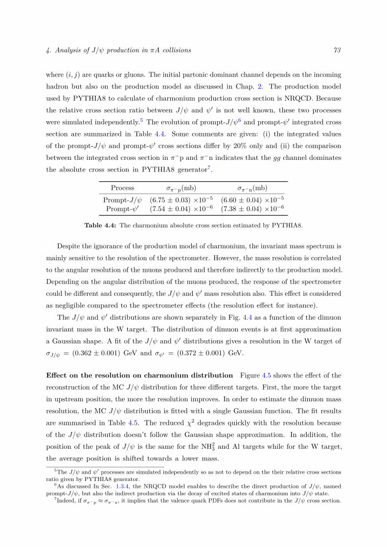
4. Analysis of J/ψ production in πA collisions 73
where (i, j) are quarks or gluons. The initial partonic dominant channel depends on the incominghadron but also on the production model as discussed in Chap. 2. The production modelused by PYTHIA8 to calculate of charmonium production cross section is NRQCD. Becausethe relative cross section ratio between J/ψ and ψ′ is not well known, these two processeswere simulated independently.5 The evolution of prompt-J/ψ6 and prompt-ψ′ integrated crosssection are summarized in Table 4.4. Some comments are given: (i) the integrated valuesof the prompt-J/ψ and prompt-ψ′ cross sections differ by 20% only and (ii) the comparisonbetween the integrated cross section in π−p and π−n indicates that the gg channel dominatesthe absolute cross section in PYTHIA8 generator7.
Process σπ−p(mb) σπ−n(mb)Prompt-J/ψ (6.75 ± 0.03) ×10−5 (6.60 ± 0.04) ×10−5
Prompt-ψ′ (7.54 ± 0.04) ×10−6 (7.38 ± 0.04) ×10−6
Table 4.4: The charmonium absolute cross section estimated by PYTHIA8.
Despite the ignorance of the production model of charmonium, the invariant mass spectrum ismainly sensitive to the resolution of the spectrometer. However, the mass resolution is correlatedto the angular resolution of the muons produced and therefore indirectly to the production model.Depending on the angular distribution of the muons produced, the response of the spectrometercould be different and consequently, the J/ψ and ψ′ mass resolution also. This effect is consideredas negligible compared to the spectrometer effects (the resolution effect for instance).
The J/ψ and ψ′ distributions are shown separately in Fig. 4.4 as a function of the dimuoninvariant mass in the W target. The distribution of dimuon events is at first approximationa Gaussian shape. A fit of the J/ψ and ψ′ distributions gives a resolution in the W target ofσJ/ψ = (0.362 ± 0.001) GeV and σψ′ = (0.372 ± 0.001) GeV.
Effect on the resolution on charmonium distribution Figure 4.5 shows the effect of thereconstruction of the MC J/ψ distribution for three different targets. First, the more the targetin upstream position, the more the resolution improves. In order to estimate the dimuon massresolution, the MC J/ψ distribution is fitted with a single Gaussian function. The fit resultsare summarised in Table 4.5. The reduced χ2 degrades quickly with the resolution becauseof the J/ψ distribution doesn’t follow the Gaussian shape approximation. In addition, theposition of the peak of J/ψ is the same for the NH2
3 and Al targets while for the W target,the average position is shifted towards a lower mass.
5The J/ψ and ψ′ processes are simulated independently so as not to depend on the their relative cross sectionsratio given by PYTHIA8 generator.
6As discussed In Sec. 1.3.4, the NRQCD model enables to describe the direct production of J/ψ, namedprompt-J/ψ, but also the indirect production via the decay of excited states of charmonium into J/ψ state.
7Indeed, if σπ−p ≈ σπ−n, it implies that the valence quark PDFs does not contribute in the J/ψ cross section.
4. Analysis of J/ψ production in πA collisions 74
1 2 3 4 5 6 7 8
(GeV)-µ +µM
1
10
210
310
410
Dim
uon
even
ts
W target
(LasLas || LasOuter) triggers
MCψJ/
1 2 3 4 5 6 7 8
(GeV)-µ +µM
1
10
210
310
410
Dim
uon
even
ts
W target
(LasLas || LasOuter) triggers
' MCψ
Figure 4.4: J/ψ (left panel) and ψ′ (right panel) MC distributions as a function of dimuon invariantmass.
Target 〈M〉 (GeV) σJ/ψ (MeV) χ2/ndfNH2
3 3.135 ± 0.006 194 ± 0.06 144Al 3.135 ± 0.006 212 ± 0.02 44W 3.095 ± 0.017 362 ± 0.01 19
Table 4.5: Estimation of the J/ψ resolution for NH13, Al and W targets by fitting the dimuon invariant
mass from MC with a Gaussian function.
Secondly, at low dimuon invariant masses M . 2 GeV, a shoulder appears for the Al target.While the distribution decreases more smoothly in the NH2
3 target. This effect is less pronouncedin the W target. It is explained by the fact that the muons produced lose their energy dependingon their polar angles, the energy losses in the the absorber are different.
4.3.1.c Uncorrelated background contribution
The dominant background for M ∼ 2 GeV is due to the decay of kaons and pions via
π+ → µ+ + νµ
π− → µ− + νµ
K+ → µ+ + νµ
K− → µ− + νµ.
(4.7)
Uncorrelated muons can accidentally be combined in the track reconstruction and satisfy thetrigger and cut requirements generating the uncorrelated background events, named CombinatorialBackground (CB). After collecting the single muons, the number of dimuons is calculated via the
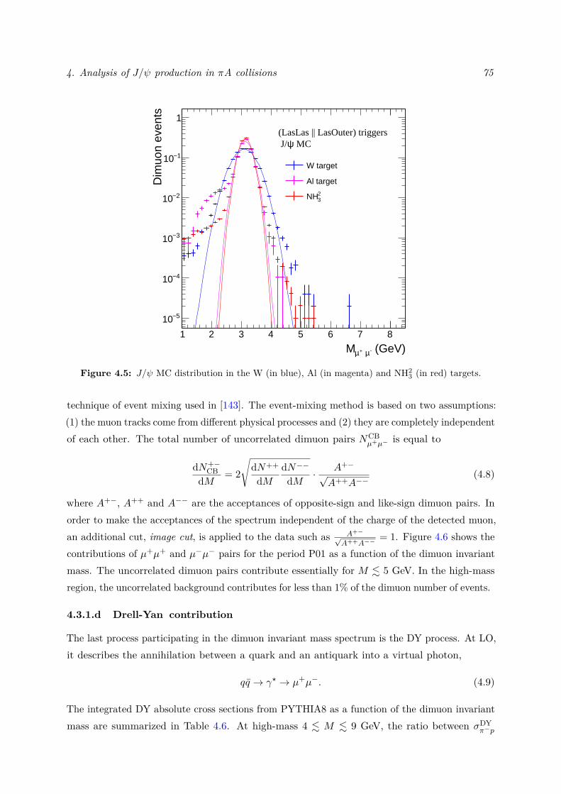
4. Analysis of J/ψ production in πA collisions 75
1 2 3 4 5 6 7 8
(GeV)-µ +µM
5−10
4−10
3−10
2−10
1−10
1
Dim
uon
even
tsW target
Al target23NH
(LasLas || LasOuter) triggers MCψJ/
Figure 4.5: J/ψ MC distribution in the W (in blue), Al (in magenta) and NH23 (in red) targets.
technique of event mixing used in [143]. The event-mixing method is based on two assumptions:(1) the muon tracks come from different physical processes and (2) they are completely independentof each other. The total number of uncorrelated dimuon pairs NCB
µ+µ− is equal to
dN+−CB
dM = 2
√dN++
dMdN−−dM · A+−
√A++A−−
(4.8)
where A+−, A++ and A−− are the acceptances of opposite-sign and like-sign dimuon pairs. Inorder to make the acceptances of the spectrum independent of the charge of the detected muon,an additional cut, image cut, is applied to the data such as A+−
√A++A−−
= 1. Figure 4.6 shows thecontributions of µ+µ+ and µ−µ− pairs for the period P01 as a function of the dimuon invariantmass. The uncorrelated dimuon pairs contribute essentially for M . 5 GeV. In the high-massregion, the uncorrelated background contributes for less than 1% of the dimuon number of events.
4.3.1.d Drell-Yan contribution
The last process participating in the dimuon invariant mass spectrum is the DY process. At LO,it describes the annihilation between a quark and an antiquark into a virtual photon,
qq → γ? → µ+µ−. (4.9)
The integrated DY absolute cross sections from PYTHIA8 as a function of the dimuon invariantmass are summarized in Table 4.6. At high-mass 4 . M . 9 GeV, the ratio between σDYπ−p
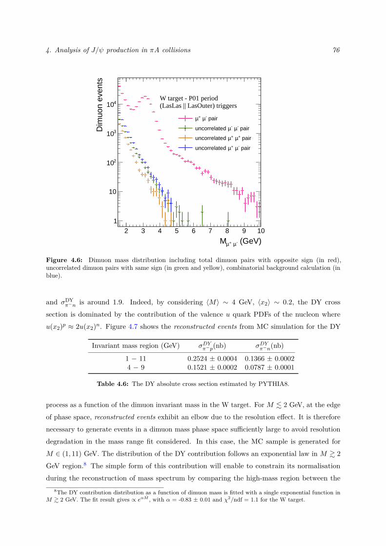
4. Analysis of J/ψ production in πA collisions 76
2 3 4 5 6 7 8 9 10
(GeV)-µ +µM
1
10
210
310
410D
imuo
n ev
ents
(LasLas || LasOuter) triggersW target - P01 period
pair-µ +µ
pair-µ -µuncorrelated
pair+µ +µuncorrelated
pair-µ +µuncorrelated
Figure 4.6: Dimuon mass distribution including total dimuon pairs with opposite sign (in red),uncorrelated dimuon pairs with same sign (in green and yellow), combinatorial background calculation (inblue).
and σDYπ−n is around 1.9. Indeed, by considering 〈M〉 ∼ 4 GeV, 〈x2〉 ∼ 0.2, the DY crosssection is dominated by the contribution of the valence u quark PDFs of the nucleon whereu(x2)p ≈ 2u(x2)n. Figure 4.7 shows the reconstructed events from MC simulation for the DY
Invariant mass region (GeV) σDYπ−p(nb) σDYπ−n(nb)
1 − 11 0.2524 ± 0.0004 0.1366 ± 0.00024 − 9 0.1521 ± 0.0002 0.0787 ± 0.0001
Table 4.6: The DY absolute cross section estimated by PYTHIA8.
process as a function of the dimuon invariant mass in the W target. For M . 2 GeV, at the edgeof phase space, reconstructed events exhibit an elbow due to the resolution effect. It is thereforenecessary to generate events in a dimuon mass phase space sufficiently large to avoid resolutiondegradation in the mass range fit considered. In this case, the MC sample is generated forM ∈ (1, 11) GeV. The distribution of the DY contribution follows an exponential law in M & 2GeV region.8 The simple form of this contribution will enable to constrain its normalisationduring the reconstruction of mass spectrum by comparing the high-mass region between the
8The DY contribution distribution as a function of dimuon mass is fitted with a single exponential function inM & 2 GeV. The fit result gives ∝ eαM , with α = -0.83 ± 0.01 and χ2/ndf = 1.1 for the W target.
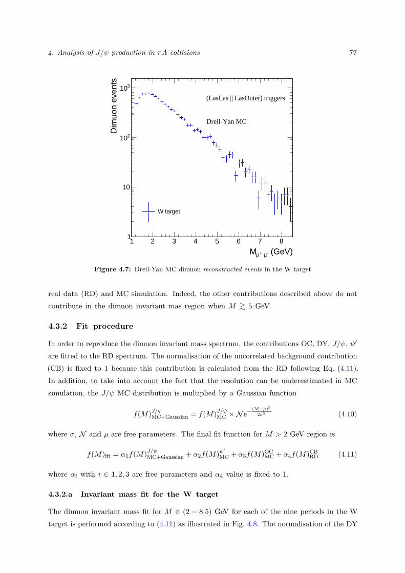
4. Analysis of J/ψ production in πA collisions 77
1 2 3 4 5 6 7 8
(GeV)-µ +µM
1
10
210
310
Dim
uon
even
ts
W target
(LasLas || LasOuter) triggers
Drell-Yan MC
Figure 4.7: Drell-Yan MC dimuon reconstructed events in the W target
real data (RD) and MC simulation. Indeed, the other contributions described above do notcontribute in the dimuon invariant mas region when M & 5 GeV.
4.3.2 Fit procedure
In order to reproduce the dimuon invariant mass spectrum, the contributions OC, DY, J/ψ, ψ′
are fitted to the RD spectrum. The normalisation of the uncorrelated background contribution(CB) is fixed to 1 because this contribution is calculated from the RD following Eq. (4.11).In addition, to take into account the fact that the resolution can be underestimated in MCsimulation, the J/ψ MC distribution is multiplied by a Gaussian function
f(M)J/ψMC+Gaussian = f(M)J/ψMC ×N e−(M−µ)2
2σ2 (4.10)
where σ, N and µ are free parameters. The final fit function for M > 2 GeV region is
f(M)fit = α1f(M)J/ψMC+Gaussian + α2f(M)ψ′
MC + α3f(M)OCMC + α4f(M)CBRD (4.11)
where αi with i ∈ 1, 2, 3 are free parameters and α4 value is fixed to 1.
4.3.2.a Invariant mass fit for the W target
The dimuon invariant mass fit for M ∈ (2 − 8.5) GeV for each of the nine periods in the Wtarget is performed according to (4.11) as illustrated in Fig. 4.8. The normalisation of the DY
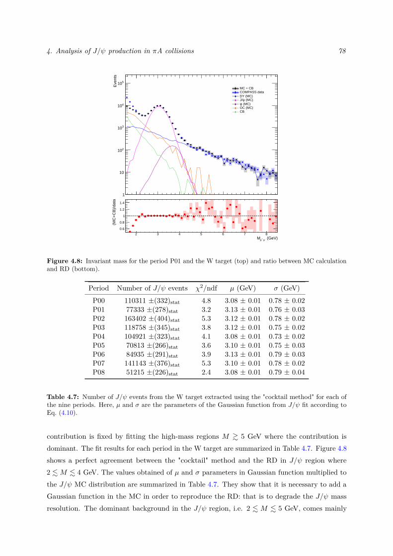
4. Analysis of J/ψ production in πA collisions 78
Eve
nts
1
10
210
310
410
510MC + CBCOMPASS dataDY (MC)
(MC)ψJ/ (MC)ψ
OC (MC)CB
(GeV)-µ +µM2 3 4 5 6 7 8
(MC
+C
B)/
data
0.6
0.8
1
1.2
1.4
Figure 4.8: Invariant mass for the period P01 and the W target (top) and ratio between MC calculationand RD (bottom).
Period Number of J/ψ events χ2/ndf µ (GeV) σ (GeV)P00 110311 ±(332)stat 4.8 3.08 ± 0.01 0.78 ± 0.02P01 77333 ±(278)stat 3.2 3.13 ± 0.01 0.76 ± 0.03P02 163402 ±(404)stat 5.3 3.12 ± 0.01 0.78 ± 0.02P03 118758 ±(345)stat 3.8 3.12 ± 0.01 0.75 ± 0.02P04 104921 ±(323)stat 4.1 3.08 ± 0.01 0.73 ± 0.02P05 70813 ±(266)stat 3.6 3.10 ± 0.01 0.75 ± 0.03P06 84935 ±(291)stat 3.9 3.13 ± 0.01 0.79 ± 0.03P07 141143 ±(376)stat 5.3 3.10 ± 0.01 0.78 ± 0.02P08 51215 ±(226)stat 2.4 3.08 ± 0.01 0.79 ± 0.04
Table 4.7: Number of J/ψ events from the W target extracted using the "cocktail method" for each ofthe nine periods. Here, µ and σ are the parameters of the Gaussian function from J/ψ fit according toEq. (4.10).
contribution is fixed by fitting the high-mass regions M & 5 GeV where the contribution isdominant. The fit results for each period in the W target are summarized in Table 4.7. Figure 4.8shows a perfect agreement between the "cocktail" method and the RD in J/ψ region where2 .M . 4 GeV. The values obtained of µ and σ parameters in Gaussian function multiplied tothe J/ψ MC distribution are summarized in Table 4.7. They show that it is necessary to add aGaussian function in the MC in order to reproduce the RD: that is to degrade the J/ψ massresolution. The dominant background in the J/ψ region, i.e. 2 . M . 5 GeV, comes mainly
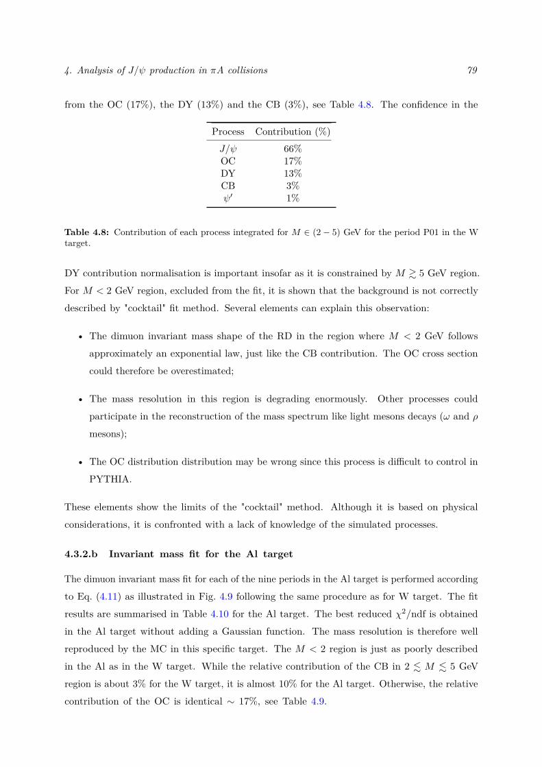
4. Analysis of J/ψ production in πA collisions 79
from the OC (17%), the DY (13%) and the CB (3%), see Table 4.8. The confidence in the
Process Contribution (%)J/ψ 66%OC 17%DY 13%CB 3%ψ′ 1%
Table 4.8: Contribution of each process integrated for M ∈ (2− 5) GeV for the period P01 in the Wtarget.
DY contribution normalisation is important insofar as it is constrained by M & 5 GeV region.For M < 2 GeV region, excluded from the fit, it is shown that the background is not correctlydescribed by "cocktail" fit method. Several elements can explain this observation:
• The dimuon invariant mass shape of the RD in the region where M < 2 GeV followsapproximately an exponential law, just like the CB contribution. The OC cross sectioncould therefore be overestimated;
• The mass resolution in this region is degrading enormously. Other processes couldparticipate in the reconstruction of the mass spectrum like light mesons decays (ω and ρmesons);
• The OC distribution distribution may be wrong since this process is difficult to control inPYTHIA.
These elements show the limits of the "cocktail" method. Although it is based on physicalconsiderations, it is confronted with a lack of knowledge of the simulated processes.
4.3.2.b Invariant mass fit for the Al target
The dimuon invariant mass fit for each of the nine periods in the Al target is performed accordingto Eq. (4.11) as illustrated in Fig. 4.9 following the same procedure as for W target. The fitresults are summarised in Table 4.10 for the Al target. The best reduced χ2/ndf is obtainedin the Al target without adding a Gaussian function. The mass resolution is therefore wellreproduced by the MC in this specific target. The M < 2 region is just as poorly describedin the Al as in the W target. While the relative contribution of the CB in 2 . M . 5 GeVregion is about 3% for the W target, it is almost 10% for the Al target. Otherwise, the relativecontribution of the OC is identical ∼ 17%, see Table 4.9.
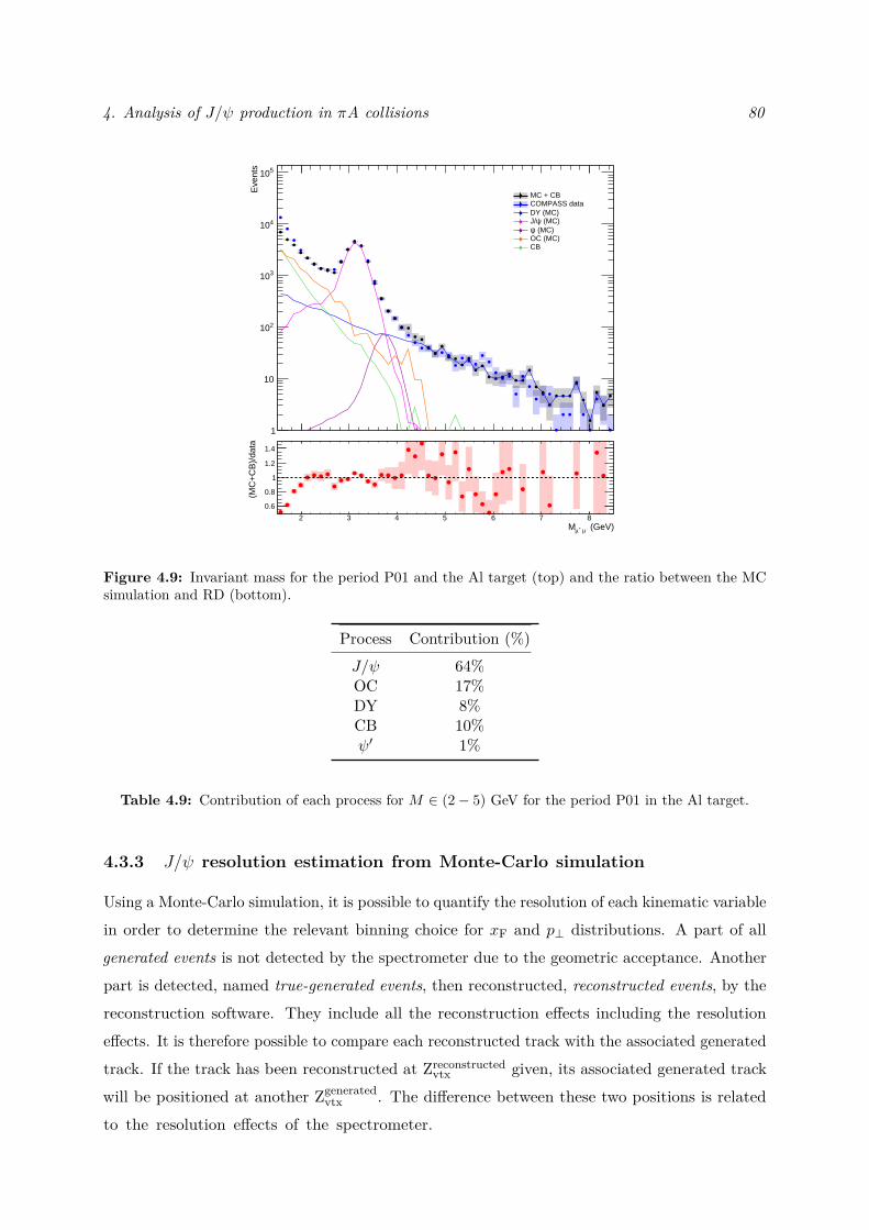
4. Analysis of J/ψ production in πA collisions 80
Eve
nts
1
10
210
310
410
510
MC + CBCOMPASS dataDY (MC)
(MC)ψJ/ (MC)ψ
OC (MC)CB
(GeV)-µ +µM2 3 4 5 6 7 8
(MC
+C
B)/
data
0.6
0.8
1
1.2
1.4
Figure 4.9: Invariant mass for the period P01 and the Al target (top) and the ratio between the MCsimulation and RD (bottom).
Process Contribution (%)J/ψ 64%OC 17%DY 8%CB 10%ψ′ 1%
Table 4.9: Contribution of each process for M ∈ (2− 5) GeV for the period P01 in the Al target.
4.3.3 J/ψ resolution estimation from Monte-Carlo simulation
Using a Monte-Carlo simulation, it is possible to quantify the resolution of each kinematic variablein order to determine the relevant binning choice for xF and p⊥ distributions. A part of allgenerated events is not detected by the spectrometer due to the geometric acceptance. Anotherpart is detected, named true-generated events, then reconstructed, reconstructed events, by thereconstruction software. They include all the reconstruction effects including the resolutioneffects. It is therefore possible to compare each reconstructed track with the associated generatedtrack. If the track has been reconstructed at Zreconstructed
vtx given, its associated generated trackwill be positioned at another Zgenerated
vtx . The difference between these two positions is relatedto the resolution effects of the spectrometer.
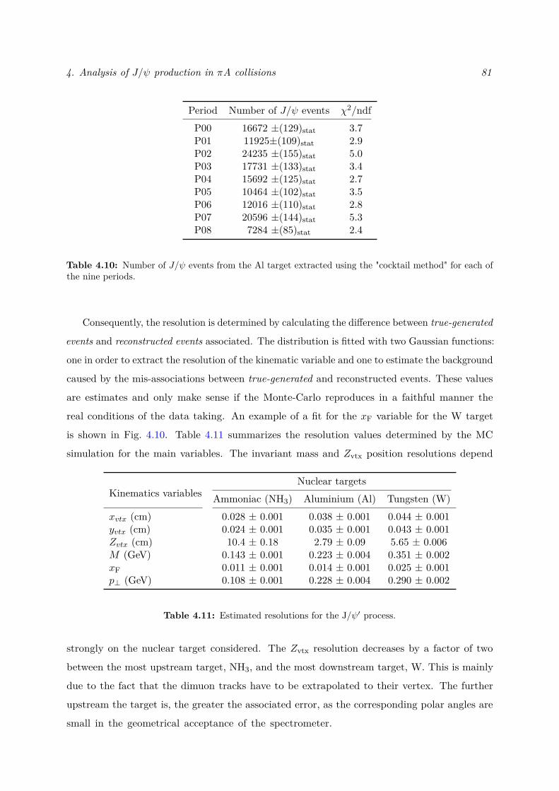
4. Analysis of J/ψ production in πA collisions 81
Period Number of J/ψ events χ2/ndfP00 16672 ±(129)stat 3.7P01 11925±(109)stat 2.9P02 24235 ±(155)stat 5.0P03 17731 ±(133)stat 3.4P04 15692 ±(125)stat 2.7P05 10464 ±(102)stat 3.5P06 12016 ±(110)stat 2.8P07 20596 ±(144)stat 5.3P08 7284 ±(85)stat 2.4
Table 4.10: Number of J/ψ events from the Al target extracted using the "cocktail method" for each ofthe nine periods.
Consequently, the resolution is determined by calculating the difference between true-generated
events and reconstructed events associated. The distribution is fitted with two Gaussian functions:
one in order to extract the resolution of the kinematic variable and one to estimate the background
caused by the mis-associations between true-generated and reconstructed events. These values
are estimates and only make sense if the Monte-Carlo reproduces in a faithful manner the
real conditions of the data taking. An example of a fit for the xF variable for the W target
is shown in Fig. 4.10. Table 4.11 summarizes the resolution values determined by the MC
simulation for the main variables. The invariant mass and Zvtx position resolutions depend
Kinematics variablesNuclear targets
Ammoniac (NH3) Aluminium (Al) Tungsten (W)xvtx (cm) 0.028 ± 0.001 0.038 ± 0.001 0.044 ± 0.001yvtx (cm) 0.024 ± 0.001 0.035 ± 0.001 0.043 ± 0.001Zvtx (cm) 10.4 ± 0.18 2.79 ± 0.09 5.65 ± 0.006M (GeV) 0.143 ± 0.001 0.223 ± 0.004 0.351 ± 0.002xF 0.011 ± 0.001 0.014 ± 0.001 0.025 ± 0.001p⊥ (GeV) 0.108 ± 0.001 0.228 ± 0.004 0.290 ± 0.002
Table 4.11: Estimated resolutions for the J/ψ′ process.
strongly on the nuclear target considered. The Zvtx resolution decreases by a factor of two
between the most upstream target, NH3, and the most downstream target, W. This is mainly
due to the fact that the dimuon tracks have to be extrapolated to their vertex. The further
upstream the target is, the greater the associated error, as the corresponding polar angles are
small in the geometrical acceptance of the spectrometer.
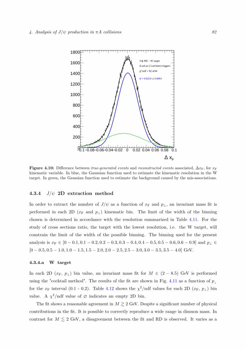
4. Analysis of J/ψ production in πA collisions 82
0.1− 0.08− 0.06− 0.04− 0.02− 0 0.02 0.04 0.06 0.08 0.1
F x∆
0
200
400
600
800
1000
1200
1400
1600
1800
MC - W targetψJ/
(LasLas || LasOuter) triggers
0.0001± = 0.0254 σ
/ndf = 82.4/942χ
Figure 4.10: Difference between true-generated events and reconstructed events associated, ∆xF, for xFkinematic variable. In blue, the Gaussian function used to estimate the kinematic resolution in the Wtarget. In green, the Gaussian function used to estimate the background caused by the mis-associations.
4.3.4 J/ψ 2D extraction method
In order to extract the number of J/ψ as a function of xF and p⊥, an invariant mass fit isperformed in each 2D (xF and p⊥) kinematic bin. The limit of the width of the binningchosen is determined in accordance with the resolution summarized in Table 4.11. For thestudy of cross sections ratio, the target with the lowest resolution, i.e. the W target, willconstrain the limit of the width of the possible binning. The binning used for the presentanalysis is xF ∈ [0 − 0.1, 0.1 − 0.2, 0.2 − 0.3, 0.3 − 0.4, 0.4 − 0.5, 0.5 − 0.6, 0.6 − 0.9] and p⊥ ∈[0 − 0.5, 0.5 − 1.0, 1.0 − 1.5, 1.5 − 2.0, 2.0 − 2.5, 2.5 − 3.0, 3.0 − 3.5, 3.5 − 4.0] GeV.
4.3.4.a W target
In each 2D (xF, p⊥) bin value, an invariant mass fit for M ∈ (2 − 8.5) GeV is performedusing the "cocktail method". The results of the fit are shown in Fig. 4.11 as a function of p⊥for the xF interval (0.1 - 0.2). Table 4.12 shows the χ2/ndf values for each 2D (xF, p⊥) binvalue. A χ2/ndf value of ø indicates an empty 2D bin.
The fit shows a reasonable agreement in M & 2 GeV. Despite a significant number of physicalcontributions in the fit. It is possible to correctly reproduce a wide range in dimuon mass. Incontrast for M . 2 GeV, a disagreement between the fit and RD is observed. It varies as a
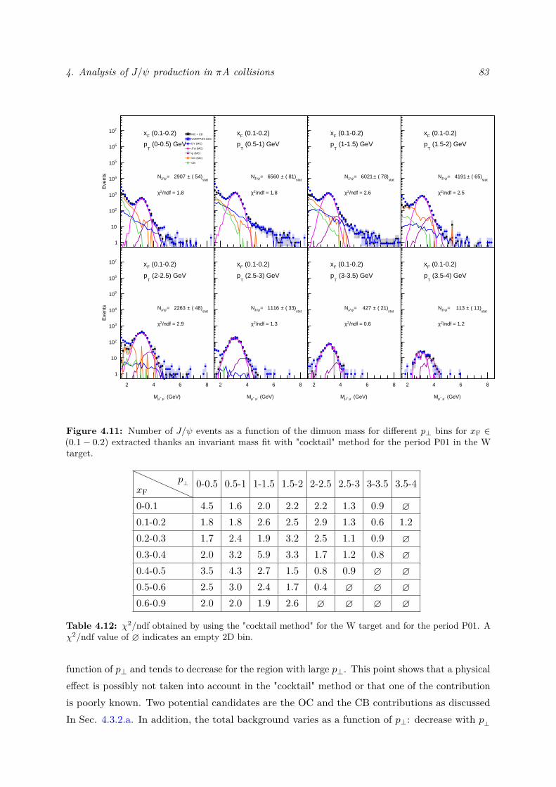
4. Analysis of J/ψ production in πA collisions 83
2 4 6 8
(GeV)-µ +µM
1
10
210
310
410
510
610
710
Eve
nts
(2-2.5) GeVT
p
stat ( 48)±= 2263 ψJ/N
/ndf = 2.92χ
(0.1-0.2)Fx
2 4 6 8
(GeV)-µ +µM
1
10
210
310
410
510
610
710
Eve
nts
(0-0.5) GeVT
p
stat ( 54)±= 2907 ψJ/N
/ndf = 1.82χ
(0.1-0.2)Fx MC + CB
COMPASS data
DY (MC)
(MC)ψJ/
(MC)ψ
OC (MC)
CB
2 4 6 8
(GeV)-µ +µM
1
10
210
310
410
510
610
710
Eve
nts
(2.5-3) GeVT
p
stat ( 33)±= 1116 ψJ/N
/ndf = 1.32χ
(0.1-0.2)Fx
2 4 6 8
(GeV)-µ +µM
1
10
210
310
410
510
610
710
Eve
nts
(0.5-1) GeVT
p
stat ( 81)±= 6560 ψJ/N
/ndf = 1.82χ
(0.1-0.2)Fx
2 4 6 8
(GeV)-µ +µM
1
10
210
310
410
510
610
710
Eve
nts
(3-3.5) GeVT
p
stat ( 21)±= 427 ψJ/N
/ndf = 0.62χ
(0.1-0.2)Fx
2 4 6 8
(GeV)-µ +µM
1
10
210
310
410
510
610
710
Eve
nts
(1-1.5) GeVT
p
stat ( 78)±= 6021 ψJ/N
/ndf = 2.62χ
(0.1-0.2)Fx
2 4 6 8
(GeV)-µ +µM
1
10
210
310
410
510
610
710
Eve
nts
(3.5-4) GeVT
p
stat ( 11)±= 113 ψJ/N
/ndf = 1.22χ
(0.1-0.2)Fx
2 4 6 8
(GeV)-µ +µM
1
10
210
310
410
510
610
710
Eve
nts
(1.5-2) GeVT
p
stat ( 65)±= 4191 ψJ/N
/ndf = 2.52χ
(0.1-0.2)Fx
Figure 4.11: Number of J/ψ events as a function of the dimuon mass for different p⊥ bins for xF ∈(0.1 − 0.2) extracted thanks an invariant mass fit with "cocktail" method for the period P01 in the Wtarget.
xFp⊥ 0-0.5 0.5-1 1-1.5 1.5-2 2-2.5 2.5-3 3-3.5 3.5-4
0-0.1 4.5 1.6 2.0 2.2 2.2 1.3 0.9 ø0.1-0.2 1.8 1.8 2.6 2.5 2.9 1.3 0.6 1.20.2-0.3 1.7 2.4 1.9 3.2 2.5 1.1 0.9 ø0.3-0.4 2.0 3.2 5.9 3.3 1.7 1.2 0.8 ø0.4-0.5 3.5 4.3 2.7 1.5 0.8 0.9 ø ø0.5-0.6 2.5 3.0 2.4 1.7 0.4 ø ø ø0.6-0.9 2.0 2.0 1.9 2.6 ø ø ø ø
Table 4.12: χ2/ndf obtained by using the "cocktail method" for the W target and for the period P01. Aχ2/ndf value of ø indicates an empty 2D bin.
function of p⊥ and tends to decrease for the region with large p⊥. This point shows that a physicaleffect is possibly not taken into account in the "cocktail" method or that one of the contributionis poorly known. Two potential candidates are the OC and the CB contributions as discussedIn Sec. 4.3.2.a. In addition, the total background varies as a function of p⊥: decrease with p⊥
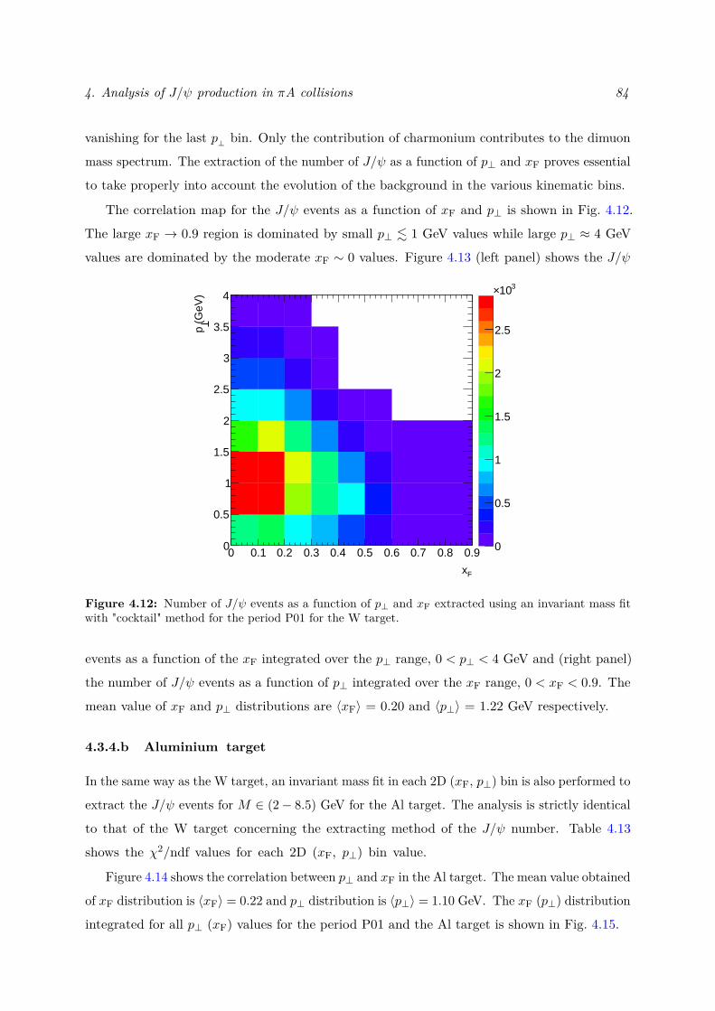
4. Analysis of J/ψ production in πA collisions 84
vanishing for the last p⊥ bin. Only the contribution of charmonium contributes to the dimuon
mass spectrum. The extraction of the number of J/ψ as a function of p⊥ and xF proves essential
to take properly into account the evolution of the background in the various kinematic bins.
The correlation map for the J/ψ events as a function of xF and p⊥ is shown in Fig. 4.12.
The large xF → 0.9 region is dominated by small p⊥ . 1 GeV values while large p⊥ ≈ 4 GeV
values are dominated by the moderate xF ∼ 0 values. Figure 4.13 (left panel) shows the J/ψ
0 0.1 0.2 0.3 0.4 0.5 0.6 0.7 0.8 0.9
Fx
0
0.5
1
1.5
2
2.5
3
3.5
4
(G
eV)
p
0
0.5
1
1.5
2
2.5
310×
Figure 4.12: Number of J/ψ events as a function of p⊥ and xF extracted using an invariant mass fitwith "cocktail" method for the period P01 for the W target.
events as a function of the xF integrated over the p⊥ range, 0 < p⊥ < 4 GeV and (right panel)
the number of J/ψ events as a function of p⊥ integrated over the xF range, 0 < xF < 0.9. The
mean value of xF and p⊥ distributions are 〈xF〉 = 0.20 and 〈p⊥〉 = 1.22 GeV respectively.
4.3.4.b Aluminium target
In the same way as the W target, an invariant mass fit in each 2D (xF, p⊥) bin is also performed to
extract the J/ψ events for M ∈ (2− 8.5) GeV for the Al target. The analysis is strictly identical
to that of the W target concerning the extracting method of the J/ψ number. Table 4.13
shows the χ2/ndf values for each 2D (xF, p⊥) bin value.
Figure 4.14 shows the correlation between p⊥ and xF in the Al target. The mean value obtained
of xF distribution is 〈xF〉 = 0.22 and p⊥ distribution is 〈p⊥〉 = 1.10 GeV. The xF (p⊥) distribution
integrated for all p⊥ (xF) values for the period P01 and the Al target is shown in Fig. 4.15.
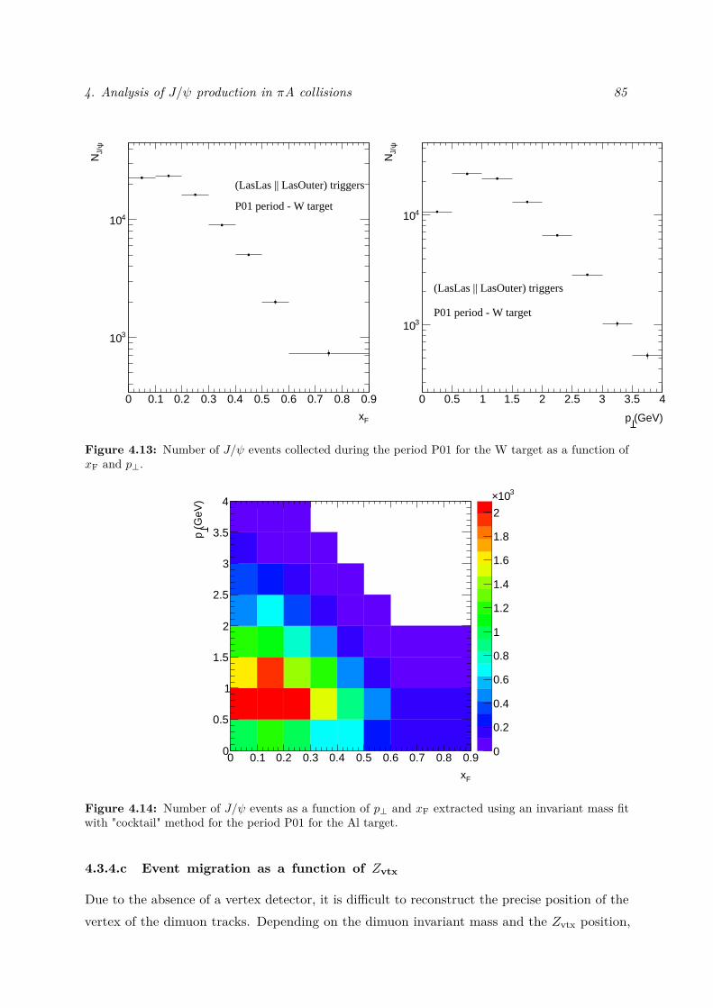
4. Analysis of J/ψ production in πA collisions 85
0 0.1 0.2 0.3 0.4 0.5 0.6 0.7 0.8 0.9
Fx
310
410
ψJ/
N
(LasLas || LasOuter) triggers
P01 period - W target
0 0.5 1 1.5 2 2.5 3 3.5 4
(GeV)p
310
410
ψJ/
N
(LasLas || LasOuter) triggers
P01 period - W target
Figure 4.13: Number of J/ψ events collected during the period P01 for the W target as a function ofxF and p⊥.
0 0.1 0.2 0.3 0.4 0.5 0.6 0.7 0.8 0.9
Fx
0
0.5
1
1.5
2
2.5
3
3.5
4
(G
eV)
p
0
0.2
0.4
0.6
0.8
1
1.2
1.4
1.6
1.8
2
310×
Figure 4.14: Number of J/ψ events as a function of p⊥ and xF extracted using an invariant mass fitwith "cocktail" method for the period P01 for the Al target.
4.3.4.c Event migration as a function of Zvtx
Due to the absence of a vertex detector, it is difficult to reconstruct the precise position of thevertex of the dimuon tracks. Depending on the dimuon invariant mass and the Zvtx position,
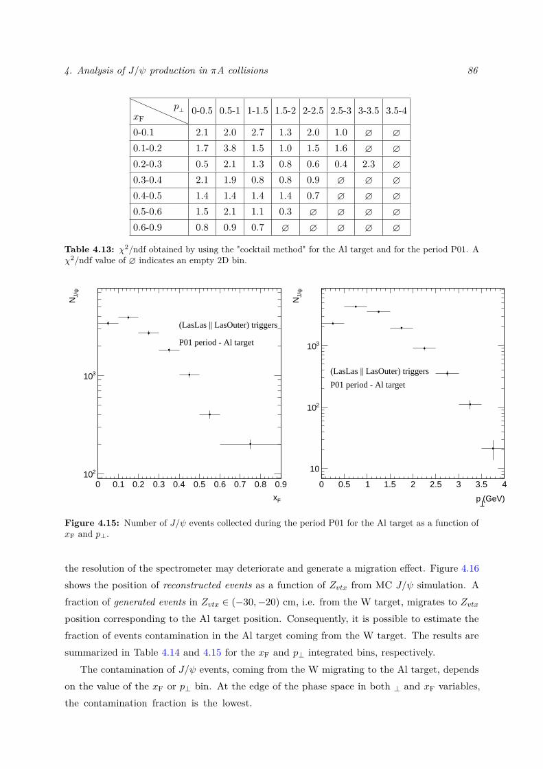
4. Analysis of J/ψ production in πA collisions 86
xFp⊥ 0-0.5 0.5-1 1-1.5 1.5-2 2-2.5 2.5-3 3-3.5 3.5-4
0-0.1 2.1 2.0 2.7 1.3 2.0 1.0 ø ø0.1-0.2 1.7 3.8 1.5 1.0 1.5 1.6 ø ø0.2-0.3 0.5 2.1 1.3 0.8 0.6 0.4 2.3 ø0.3-0.4 2.1 1.9 0.8 0.8 0.9 ø ø ø0.4-0.5 1.4 1.4 1.4 1.4 0.7 ø ø ø0.5-0.6 1.5 2.1 1.1 0.3 ø ø ø ø0.6-0.9 0.8 0.9 0.7 ø ø ø ø ø
Table 4.13: χ2/ndf obtained by using the "cocktail method" for the Al target and for the period P01. Aχ2/ndf value of ø indicates an empty 2D bin.
0 0.1 0.2 0.3 0.4 0.5 0.6 0.7 0.8 0.9
Fx
210
310
ψJ/
N
(LasLas || LasOuter) triggers
P01 period - Al target
0 0.5 1 1.5 2 2.5 3 3.5 4
(GeV)p
10
210
310
ψJ/
N
(LasLas || LasOuter) triggers
P01 period - Al target
Figure 4.15: Number of J/ψ events collected during the period P01 for the Al target as a function ofxF and p⊥.
the resolution of the spectrometer may deteriorate and generate a migration effect. Figure 4.16shows the position of reconstructed events as a function of Zvtx from MC J/ψ simulation. Afraction of generated events in Zvtx ∈ (−30,−20) cm, i.e. from the W target, migrates to Zvtxposition corresponding to the Al target position. Consequently, it is possible to estimate thefraction of events contamination in the Al target coming from the W target. The results aresummarized in Table 4.14 and 4.15 for the xF and p⊥ integrated bins, respectively.
The contamination of J/ψ events, coming from the W migrating to the Al target, dependson the value of the xF or p⊥ bin. At the edge of the phase space in both ⊥ and xF variables,the contamination fraction is the lowest.
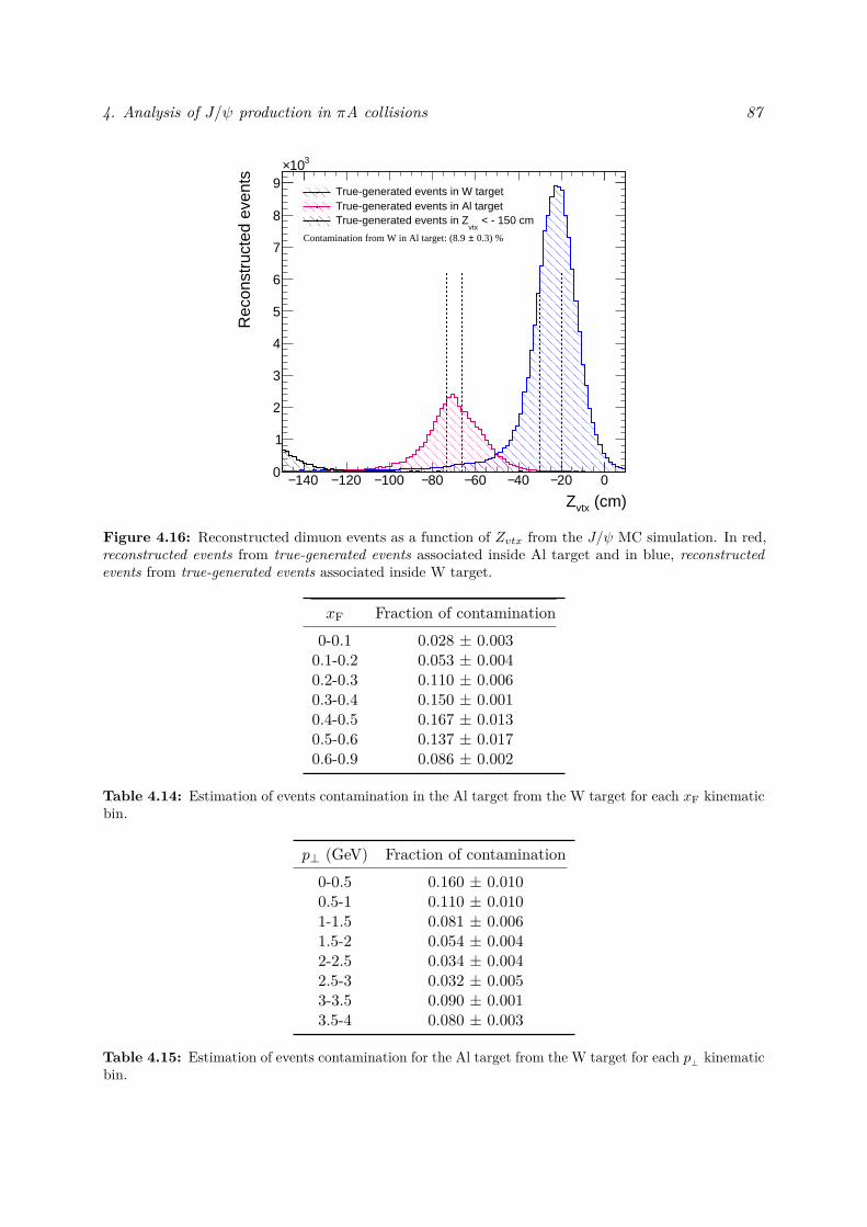
4. Analysis of J/ψ production in πA collisions 87
140− 120− 100− 80− 60− 40− 20− 0
(cm)vtxZ
0
1
2
3
4
5
6
7
8
9
310×
Rec
onst
ruct
ed e
vent
s
Monte-Carlo 2018ψJ/ 0.3) %±Contamination from W in Al target: (8.9
True-generated events in W targetTrue-generated events in Al target
< - 150 cmvtx
True-generated events in Z
Figure 4.16: Reconstructed dimuon events as a function of Zvtx from the J/ψ MC simulation. In red,reconstructed events from true-generated events associated inside Al target and in blue, reconstructedevents from true-generated events associated inside W target.
xF Fraction of contamination0-0.1 0.028 ± 0.0030.1-0.2 0.053 ± 0.0040.2-0.3 0.110 ± 0.0060.3-0.4 0.150 ± 0.0010.4-0.5 0.167 ± 0.0130.5-0.6 0.137 ± 0.0170.6-0.9 0.086 ± 0.002
Table 4.14: Estimation of events contamination in the Al target from the W target for each xF kinematicbin.
p⊥ (GeV) Fraction of contamination0-0.5 0.160 ± 0.0100.5-1 0.110 ± 0.0101-1.5 0.081 ± 0.0061.5-2 0.054 ± 0.0042-2.5 0.034 ± 0.0042.5-3 0.032 ± 0.0053-3.5 0.090 ± 0.0013.5-4 0.080 ± 0.003
Table 4.15: Estimation of events contamination for the Al target from the W target for each p⊥ kinematicbin.
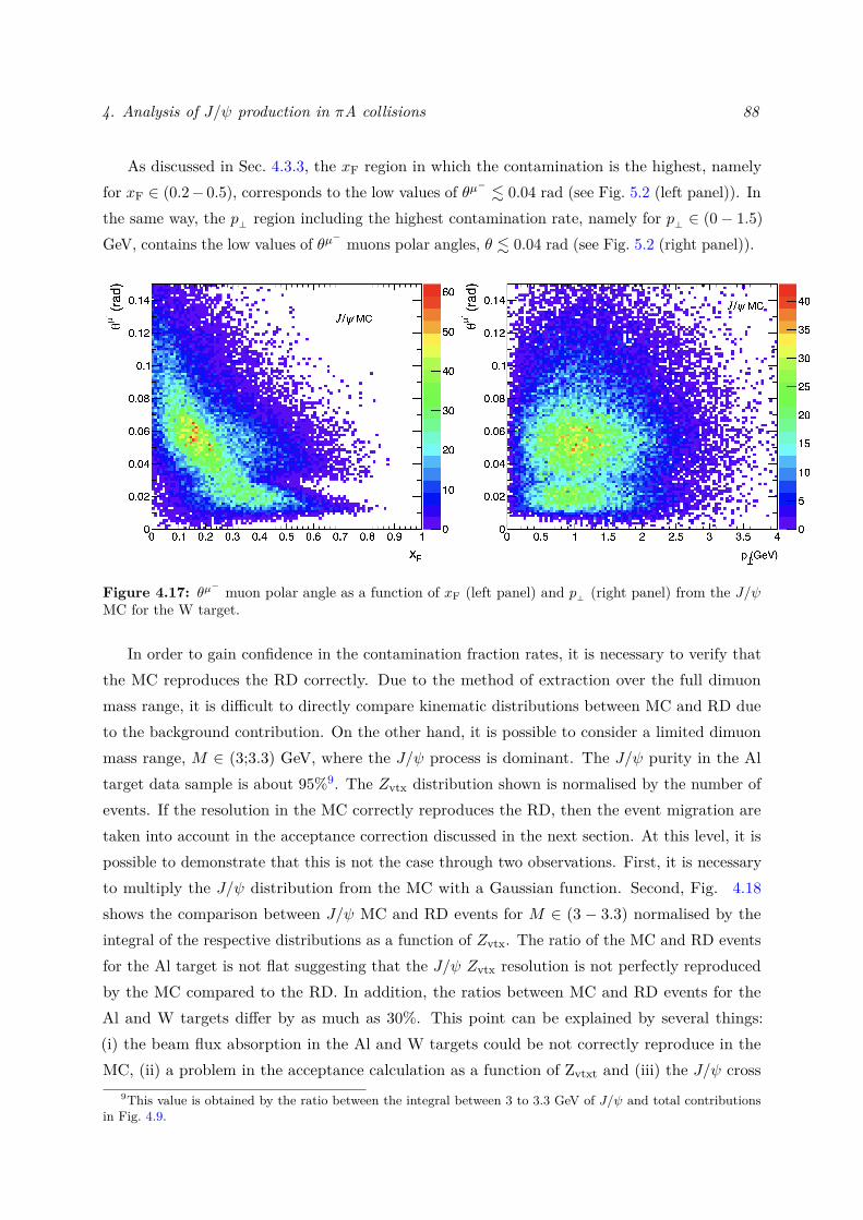
4. Analysis of J/ψ production in πA collisions 88
As discussed in Sec. 4.3.3, the xF region in which the contamination is the highest, namelyfor xF ∈ (0.2− 0.5), corresponds to the low values of θµ− . 0.04 rad (see Fig. 5.2 (left panel)). Inthe same way, the p⊥ region including the highest contamination rate, namely for p⊥ ∈ (0− 1.5)GeV, contains the low values of θµ− muons polar angles, θ . 0.04 rad (see Fig. 5.2 (right panel)).
Figure 4.17: θµ− muon polar angle as a function of xF (left panel) and p⊥ (right panel) from the J/ψMC for the W target.
In order to gain confidence in the contamination fraction rates, it is necessary to verify thatthe MC reproduces the RD correctly. Due to the method of extraction over the full dimuonmass range, it is difficult to directly compare kinematic distributions between MC and RD dueto the background contribution. On the other hand, it is possible to consider a limited dimuonmass range, M ∈ (3;3.3) GeV, where the J/ψ process is dominant. The J/ψ purity in the Altarget data sample is about 95%9. The Zvtx distribution shown is normalised by the number ofevents. If the resolution in the MC correctly reproduces the RD, then the event migration aretaken into account in the acceptance correction discussed in the next section. At this level, it ispossible to demonstrate that this is not the case through two observations. First, it is necessaryto multiply the J/ψ distribution from the MC with a Gaussian function. Second, Fig. 4.18shows the comparison between J/ψ MC and RD events for M ∈ (3 − 3.3) normalised by theintegral of the respective distributions as a function of Zvtx. The ratio of the MC and RD eventsfor the Al target is not flat suggesting that the J/ψ Zvtx resolution is not perfectly reproducedby the MC compared to the RD. In addition, the ratios between MC and RD events for theAl and W targets differ by as much as 30%. This point can be explained by several things:(i) the beam flux absorption in the Al and W targets could be not correctly reproduce in theMC, (ii) a problem in the acceptance calculation as a function of Zvtxt and (iii) the J/ψ cross
9This value is obtained by the ratio between the integral between 3 to 3.3 GeV of J/ψ and total contributionsin Fig. 4.9.
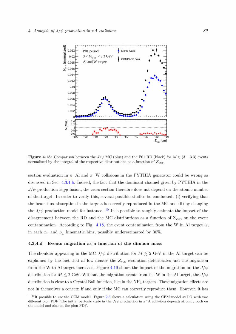
4. Analysis of J/ψ production in πA collisions 89
0
0.002
0.004
0.006
0.008
0.01
0.012
0.014
0.016
0.018
0.02
0.022
(no
rmal
ized
)µ µ
N
Monte-Carlo
COMPASS data
P01 period
< 3.3 GeV+µ -µ3 < M
Al and W targets
100− 90− 80− 70− 60− 50− 40− 30− 20− 10− [cm]vtxZ
0.60.8
11.21.4
MC
/RD
Figure 4.18: Comparison between the J/ψ MC (blue) and the P01 RD (black) for M ∈ (3− 3.3) eventsnormalised by the integral of the respective distributions as a function of Zvtx.
section evaluation in π−Al and π−W collisions in the PYTHIA generator could be wrong asdiscussed in Sec. 4.3.1.b. Indeed, the fact that the dominant channel given by PYTHIA in theJ/ψ production is gg fusion, the cross section therefore does not depend on the atomic numberof the target. In order to verify this, several possible studies be conducted: (i) verifying thatthe beam flux absorption in the targets is correctly reproduced in the MC and (ii) by changingthe J/ψ production model for instance. 10 It is possible to roughly estimate the impact of thedisagreement between the RD and the MC distributions as a function of Zvtxt on the eventcontamination. According to Fig. 4.18, the event contamination from the W in Al target is,in each xF and p⊥ kinematic bins, possibly underestimated by 30%.
4.3.4.d Events migration as a function of the dimuon mass
The shoulder appearing in the MC J/ψ distribution for M . 2 GeV in the Al target can beexplained by the fact that at low masses the Zvtx resolution deteriorates and the migrationfrom the W to Al target increases. Figure 4.19 shows the impact of the migration on the J/ψdistribution for M . 2 GeV. Without the migration events from the W in the Al target, the J/ψdistribution is close to a Crystal Ball function, like in the NH3 targets. These migration effects arenot in themselves a concern if and only if the MC can correctly reproduce them. However, it has
10It possible to use the CEM model. Figure 2.3 shows a calculation using the CEM model at LO with twodifferent pion PDF. The initial partonic state in the J/ψ production in π−A collisions depends strongly both onthe model and also on the pion PDF.
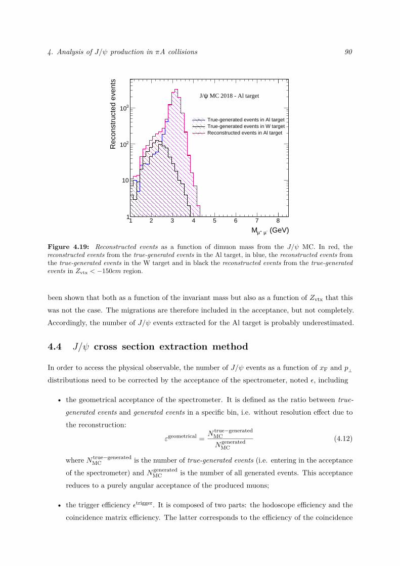
4. Analysis of J/ψ production in πA collisions 90
1 2 3 4 5 6 7 8
(GeV)-µ +µM
1
10
210
310R
econ
stru
cted
eve
nts
True-generated events in Al targetTrue-generated events in W targetReconstructed events in Al target
MC 2018 - Al targetψJ/
Figure 4.19: Reconstructed events as a function of dimuon mass from the J/ψ MC. In red, thereconstructed events from the true-generated events in the Al target, in blue, the reconstructed events fromthe true-generated events in the W target and in black the reconstructed events from the true-generatedevents in Zvtx < −150cm region.
been shown that both as a function of the invariant mass but also as a function of Zvtx that thiswas not the case. The migrations are therefore included in the acceptance, but not completely.Accordingly, the number of J/ψ events extracted for the Al target is probably underestimated.
4.4 J/ψ cross section extraction method
In order to access the physical observable, the number of J/ψ events as a function of xF and p⊥distributions need to be corrected by the acceptance of the spectrometer, noted ε, including
• the geometrical acceptance of the spectrometer. It is defined as the ratio between true-generated events and generated events in a specific bin, i.e. without resolution effect due tothe reconstruction:
εgeometrical = N true−generatedMCNgenerated
MC(4.12)
where N true−generatedMC is the number of true-generated events (i.e. entering in the acceptance
of the spectrometer) and NgeneratedMC is the number of all generated events. This acceptance
reduces to a purely angular acceptance of the produced muons;
• the trigger efficiency εtrigger. It is composed of two parts: the hodoscope efficiency and thecoincidence matrix efficiency. The latter corresponds to the efficiency of the coincidence
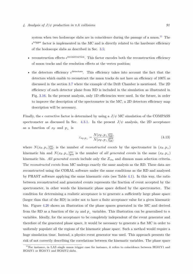
4. Analysis of J/ψ production in πA collisions 91
system when two hodoscope slabs are in coincidence during the passage of a muon.11 Theεtrigger factor is implemented in the MC and is directly related to the hardware efficiencyof the hodoscope slabs as described in Sec. 3.5;
• reconstruction effects εreconstruction. This factor encodes both the reconstruction efficiencyof muon tracks and the resolution effects at the vertex position;
• the detectors efficiency εdetectors. This efficiency takes into account the fact that thedetectors which enable to reconstruct the muon tracks do not have an efficiency of 100% asdiscussed in the section 3.7 where the example of the Drift Chamber is mentioned. The 2Defficiency of each detector plane from RD is included in the simulation as illustrated inFig. 3.16. In the present analysis, only 1D efficiencies were used. In the future, in orderto improve the description of the spectrometer in the MC, a 2D detectors efficiency mapdescription will be necessary.
Finally, the ε corrective factor is determined by using a J/ψ MC simulation of the COMPASSspectrometer as discussed In Sec. 4.3.1. In the present J/ψ analysis, the 2D acceptanceas a function of xF and p⊥ is
εxF,p⊥ = N(xF, p⊥)recMC
N(xF, p⊥)genMC
(4.13)
where N(xF, p⊥)recMC is the number of reconstructed events by the spectrometer in (xF, p⊥)
kinematic bin and N(xF, p⊥)recgen is the number of all generated events in the same (xF, p⊥)
kinematic bin. All generated events include only the Zvtx and dimuon mass selection criteria.The reconstructed events from MC undergo exactly the same analysis as the RD. These data arereconstructed using the CORAL software under the same conditions as the RD and analysedby PHAST software applying the same kinematic cuts (see Table 4.1). In this way, the ratiobetween reconstructed and generated events represents the fraction of event accepted by thespectrometer, in other words the kinematic phase space defined by the spectrometer. Thecondition for determining a realistic acceptance is to generate a sufficiently large phase space(larger than that of the RD) in order not to have a finite acceptance value for a given kinematicbin. Figure 4.20 shows an illustration of the phase spaces generated in the MC and derivedfrom the RD as a function of the xF and p⊥ variables. This illustration can be generalised to nvariables. Ideally, for the acceptance to be completely independent of the event generator andtherefore of the generated phase space, it would be necessary to generate a flat MC in order touniformly populate all the regions of the kinematic phase space. Such a method would require ahuge simulation time. Instead, a physics event generator was used. This approach presents therisk of not correctly describing the correlations between the kinematic variables. The phase space
11For instance, in LAS single muon trigger case for instance, it refers to coincidence between HG01Y1 andHG02Y1 or HG01Y1 and HG02Y2 slabs.
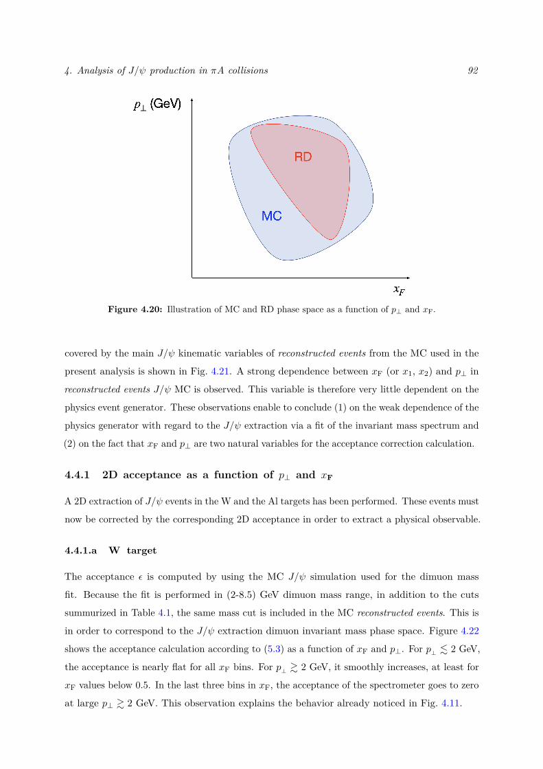
4. Analysis of J/ψ production in πA collisions 92
Figure 4.20: Illustration of MC and RD phase space as a function of p⊥ and xF.
covered by the main J/ψ kinematic variables of reconstructed events from the MC used in the
present analysis is shown in Fig. 4.21. A strong dependence between xF (or x1, x2) and p⊥ in
reconstructed events J/ψ MC is observed. This variable is therefore very little dependent on the
physics event generator. These observations enable to conclude (1) on the weak dependence of the
physics generator with regard to the J/ψ extraction via a fit of the invariant mass spectrum and
(2) on the fact that xF and p⊥ are two natural variables for the acceptance correction calculation.
4.4.1 2D acceptance as a function of p⊥ and xF
A 2D extraction of J/ψ events in the W and the Al targets has been performed. These events must
now be corrected by the corresponding 2D acceptance in order to extract a physical observable.
4.4.1.a W target
The acceptance ε is computed by using the MC J/ψ simulation used for the dimuon mass
fit. Because the fit is performed in (2-8.5) GeV dimuon mass range, in addition to the cuts
summurized in Table 4.1, the same mass cut is included in the MC reconstructed events. This is
in order to correspond to the J/ψ extraction dimuon invariant mass phase space. Figure 4.22
shows the acceptance calculation according to (5.3) as a function of xF and p⊥. For p⊥ . 2 GeV,
the acceptance is nearly flat for all xF bins. For p⊥ & 2 GeV, it smoothly increases, at least for
xF values below 0.5. In the last three bins in xF, the acceptance of the spectrometer goes to zero
at large p⊥ & 2 GeV. This observation explains the behavior already noticed in Fig. 4.11.
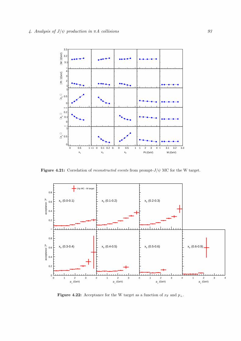
4. Analysis of J/ψ production in πA collisions 93
0 0.5 1
1x
0
0.5
1
⟩ 1 x⟨
0 0.5 11x
0.1−
0
0.1
0.2
0.3
⟩ 2
x⟨
0 0.5 11x
0
0.5
1
⟩ F
x⟨
0 0.5 11x
1
2
3
4
(G
eV)
⟩ P
t ⟨
0 0.5 11x
3
3.1
3.2
3.3
(G
eV)
⟩ M
⟨
0.1− 0 0.1 0.2 0.3
2x
0
0.5
1
⟩ 1 x⟨
0.1− 0 0.1 0.2 0.32x
0.1−
0
0.1
0.2
0.3
⟩ 2
x⟨
0.1− 0 0.1 0.2 0.32x
0
0.5
1⟩
F x⟨
0.1− 0 0.1 0.2 0.32x
1
2
3
4
(G
eV)
⟩ P
t ⟨
0.1− 0 0.1 0.2 0.32x
3
3.1
3.2
3.3
(G
eV)
⟩ M
⟨
0 0.5 1
Fx
0
0.5
1
⟩ 1 x⟨
0 0.5 1Fx
0.1−
0
0.1
0.2
0.3⟩
2 x⟨
0 0.5 1Fx
0
0.5
1
⟩ F
x⟨
0 0.5 1Fx
1
2
3
4
(G
eV)
⟩ P
t ⟨
0 0.5 1Fx
3
3.1
3.2
3.3
(G
eV)
⟩ M
⟨
1 2 3 4
Pt (GeV)
0
0.5
1
⟩ 1 x⟨
1 2 3 4Pt (GeV)
0.1−
0
0.1
0.2
0.3
⟩ 2
x⟨
1 2 3 4Pt (GeV)
0
0.5
1
⟩ F
x⟨
1 2 3 4Pt (GeV)
1
2
3
4
(G
eV)
⟩ P
t ⟨
1 2 3 4Pt (GeV)
3
3.1
3.2
3.3
(G
eV)
⟩ M
⟨
3 3.1 3.2 3.3
M (GeV)
0
0.5
1
⟩ 1 x⟨
3 3.1 3.2 3.3 M (GeV)
0.1−
0
0.1
0.2
0.3
⟩ 2
x⟨
3 3.1 3.2 3.3 M (GeV)
0
0.5
1
⟩ F
x⟨
3 3.1 3.2 3.3 M (GeV)
1
2
3
4
(G
eV)
⟩ P
t ⟨
3 3.1 3.2 3.3 M (GeV)
3
3.1
3.2
3.3
(G
eV)
⟩ M
⟨
Figure 4.21: Correlation of reconstructed events from prompt-J/ψ MC for the W target.
0 1 2 3 4
(GeV)T
p
0
0.2
0.4
0.6
0.8
W ∈ac
cept
ance
(0.3-0.4)Fx
0 1 2 3 4 (GeV)
Tp
0
0.2
0.4
0.6
0.8
W ∈ac
cept
ance
(0.0-0.1)Fx
MC - W targetψJ/
0 1 2 3 4
(GeV)T
p
0
0.2
0.4
0.6
0.8
W ∈ac
cept
ance
(0.4-0.5)Fx
0 1 2 3 4 (GeV)
Tp
0
0.2
0.4
0.6
0.8
W ∈ac
cept
ance
(0.1-0.2)Fx
0 1 2 3 4
(GeV)T
p
0
0.2
0.4
0.6
0.8
W ∈ac
cept
ance
(0.5-0.6)Fx
0 1 2 3 4 (GeV)
Tp
0
0.2
0.4
0.6
0.8
W ∈ac
cept
ance
(0.2-0.3)Fx
0 1 2 3 4
(GeV)T
p
0
0.2
0.4
0.6
0.8
W ∈ac
cept
ance
(0.6-0.9)Fx
Figure 4.22: Acceptance for the W target as a function of xF and p⊥.
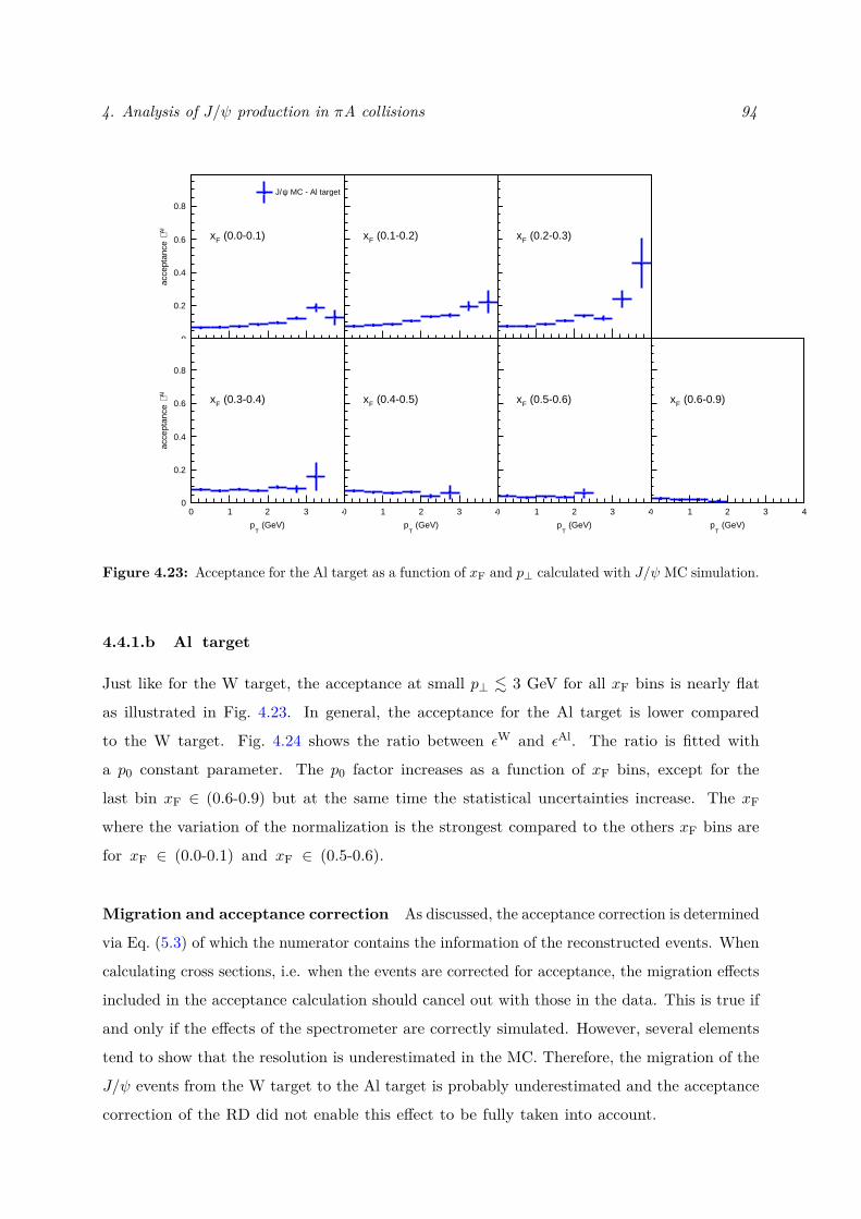
4. Analysis of J/ψ production in πA collisions 94
0 1 2 3 4
(GeV)T
p
0
0.2
0.4
0.6
0.8
Al
∈ac
cept
ance
(0.3-0.4)Fx
0 1 2 3 4 (GeV)
Tp
0
0.2
0.4
0.6
0.8
Al
∈ac
cept
ance
(0.0-0.1)Fx
MC - Al targetψJ/
0 1 2 3 4
(GeV)T
p
0
0.2
0.4
0.6
0.8
Al
∈ac
cept
ance
(0.4-0.5)Fx
0 1 2 3 4 (GeV)
Tp
0
0.2
0.4
0.6
0.8
Al
∈ac
cept
ance
(0.1-0.2)Fx
0 1 2 3 4
(GeV)T
p
0
0.2
0.4
0.6
0.8
Al
∈ac
cept
ance
(0.5-0.6)Fx
0 1 2 3 4 (GeV)
Tp
0
0.2
0.4
0.6
0.8
Al
∈ac
cept
ance
(0.2-0.3)Fx
0 1 2 3 4
(GeV)T
p
0
0.2
0.4
0.6
0.8
Al
∈ac
cept
ance
(0.6-0.9)Fx
Figure 4.23: Acceptance for the Al target as a function of xF and p⊥ calculated with J/ψ MC simulation.
4.4.1.b Al target
Just like for the W target, the acceptance at small p⊥ . 3 GeV for all xF bins is nearly flat
as illustrated in Fig. 4.23. In general, the acceptance for the Al target is lower compared
to the W target. Fig. 4.24 shows the ratio between εW and εAl. The ratio is fitted with
a p0 constant parameter. The p0 factor increases as a function of xF bins, except for the
last bin xF ∈ (0.6-0.9) but at the same time the statistical uncertainties increase. The xFwhere the variation of the normalization is the strongest compared to the others xF bins are
for xF ∈ (0.0-0.1) and xF ∈ (0.5-0.6).
Migration and acceptance correction As discussed, the acceptance correction is determined
via Eq. (5.3) of which the numerator contains the information of the reconstructed events. When
calculating cross sections, i.e. when the events are corrected for acceptance, the migration effects
included in the acceptance calculation should cancel out with those in the data. This is true if
and only if the effects of the spectrometer are correctly simulated. However, several elements
tend to show that the resolution is underestimated in the MC. Therefore, the migration of the
J/ψ events from the W target to the Al target is probably underestimated and the acceptance
correction of the RD did not enable this effect to be fully taken into account.
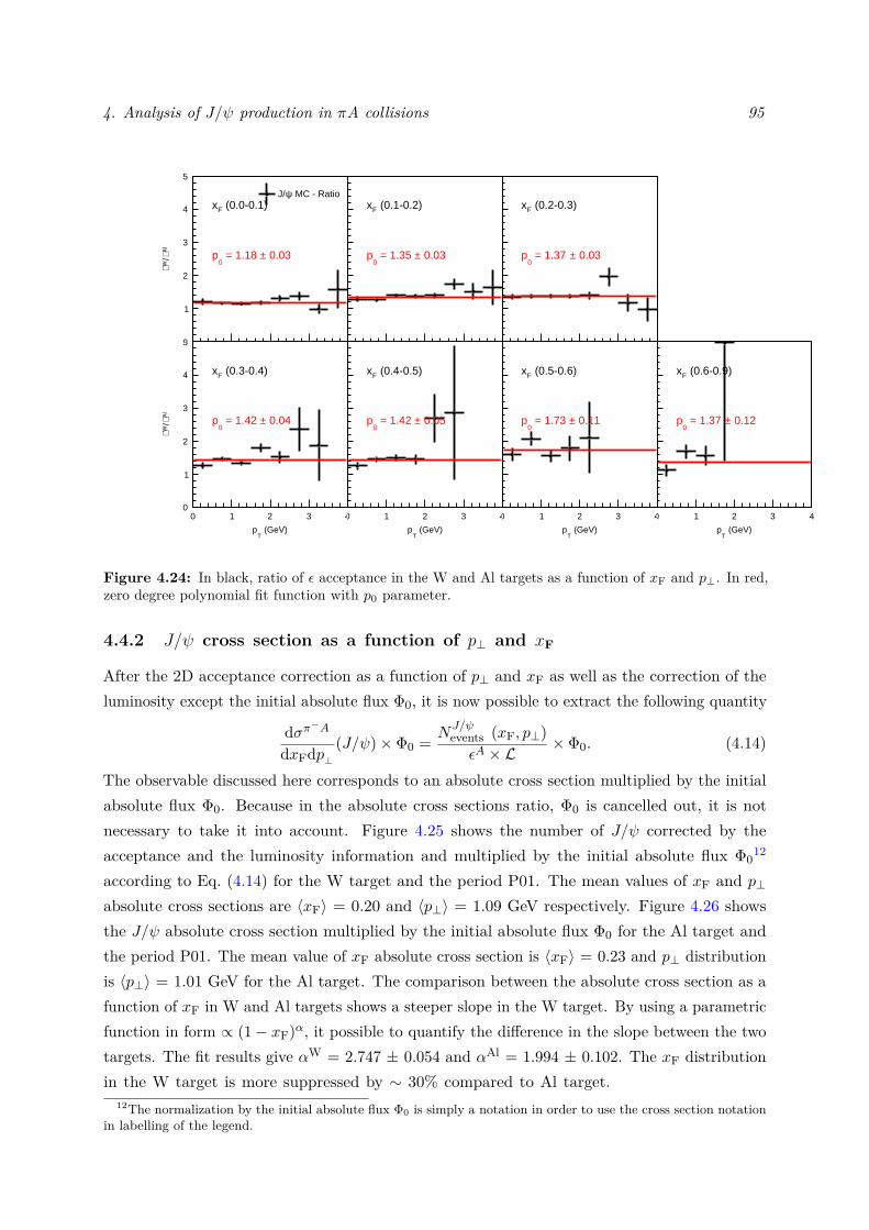
4. Analysis of J/ψ production in πA collisions 95
0 1 2 3 4
(GeV)T
p
0
1
2
3
4
5
Al
∈/W ∈
(0.3-0.4)Fx
0.04± = 1.42 0
p
0 1 2 3 4 (GeV)
Tp
0
1
2
3
4
5
Al
∈/W ∈
(0.0-0.1)Fx
0.03± = 1.18 0
p
MC - Ratio ψJ/
0 1 2 3 4
(GeV)T
p
0
1
2
3
4
5
Al
∈/W ∈
(0.4-0.5)Fx
0.05± = 1.42 0
p
0 1 2 3 4 (GeV)
Tp
0
1
2
3
4
5
Al
∈/W ∈
(0.1-0.2)Fx
0.03± = 1.35 0
p
0 1 2 3 4
(GeV)T
p
0
1
2
3
4
5
Al
∈/W ∈
(0.5-0.6)Fx
0.11± = 1.73 0
p
0 1 2 3 4 (GeV)
Tp
0
1
2
3
4
5
Al
∈/W ∈
(0.2-0.3)Fx
0.03± = 1.37 0
p
0 1 2 3 4
(GeV)T
p
0
1
2
3
4
5
Al
∈/W ∈
(0.6-0.9)Fx
0.12± = 1.37 0
p
Figure 4.24: In black, ratio of ε acceptance in the W and Al targets as a function of xF and p⊥. In red,zero degree polynomial fit function with p0 parameter.
4.4.2 J/ψ cross section as a function of p⊥ and xF
After the 2D acceptance correction as a function of p⊥ and xF as well as the correction of theluminosity except the initial absolute flux Φ0, it is now possible to extract the following quantity
dσπ−AdxFdp⊥
(J/ψ)× Φ0 = NJ/ψevents (xF, p⊥)εA × L
× Φ0. (4.14)
The observable discussed here corresponds to an absolute cross section multiplied by the initialabsolute flux Φ0. Because in the absolute cross sections ratio, Φ0 is cancelled out, it is notnecessary to take it into account. Figure 4.25 shows the number of J/ψ corrected by theacceptance and the luminosity information and multiplied by the initial absolute flux Φ0
12
according to Eq. (4.14) for the W target and the period P01. The mean values of xF and p⊥absolute cross sections are 〈xF〉 = 0.20 and 〈p⊥〉 = 1.09 GeV respectively. Figure 4.26 showsthe J/ψ absolute cross section multiplied by the initial absolute flux Φ0 for the Al target andthe period P01. The mean value of xF absolute cross section is 〈xF〉 = 0.23 and p⊥ distributionis 〈p⊥〉 = 1.01 GeV for the Al target. The comparison between the absolute cross section as afunction of xF in W and Al targets shows a steeper slope in the W target. By using a parametricfunction in form ∝ (1− xF)α, it possible to quantify the difference in the slope between the twotargets. The fit results give αW = 2.747 ± 0.054 and αAl = 1.994 ± 0.102. The xF distributionin the W target is more suppressed by ∼ 30% compared to Al target.
12The normalization by the initial absolute flux Φ0 is simply a notation in order to use the cross section notationin labelling of the legend.
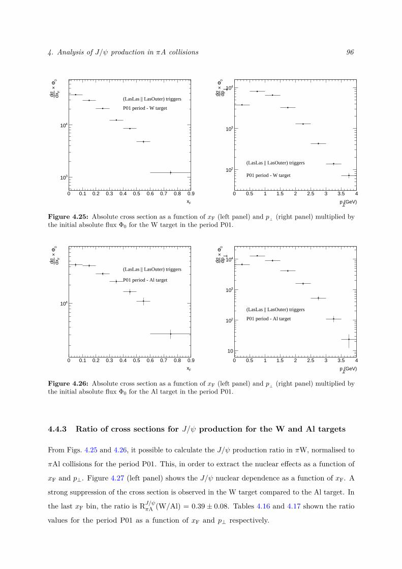
4. Analysis of J/ψ production in πA collisions 96
0 0.1 0.2 0.3 0.4 0.5 0.6 0.7 0.8 0.9
Fx
310
410
0Φ ×
Fdx
σd
(LasLas || LasOuter) triggers
P01 period - W target
0 0.5 1 1.5 2 2.5 3 3.5 4
(GeV)p
210
310
410
0Φ ×
dpσd
(LasLas || LasOuter) triggers
P01 period - W target
Figure 4.25: Absolute cross section as a function of xF (left panel) and p⊥ (right panel) multiplied bythe initial absolute flux Φ0 for the W target in the period P01.
0 0.1 0.2 0.3 0.4 0.5 0.6 0.7 0.8 0.9
Fx
410
0Φ ×
Fdx
σd
(LasLas || LasOuter) triggers
P01 period - Al target
0 0.5 1 1.5 2 2.5 3 3.5 4
(GeV)p
10
210
310
410
0Φ ×
dpσd
(LasLas || LasOuter) triggers
P01 period - Al target
Figure 4.26: Absolute cross section as a function of xF (left panel) and p⊥ (right panel) multiplied bythe initial absolute flux Φ0 for the Al target in the period P01.
4.4.3 Ratio of cross sections for J/ψ production for the W and Al targets
From Figs. 4.25 and 4.26, it possible to calculate the J/ψ production ratio in πW, normalised to
πAl collisions for the period P01. This, in order to extract the nuclear effects as a function of
xF and p⊥. Figure 4.27 (left panel) shows the J/ψ nuclear dependence as a function of xF. A
strong suppression of the cross section is observed in the W target compared to the Al target. In
the last xF bin, the ratio is RJ/ψπA (W/Al) = 0.39± 0.08. Tables 4.16 and 4.17 shown the ratio
values for the period P01 as a function of xF and p⊥ respectively.
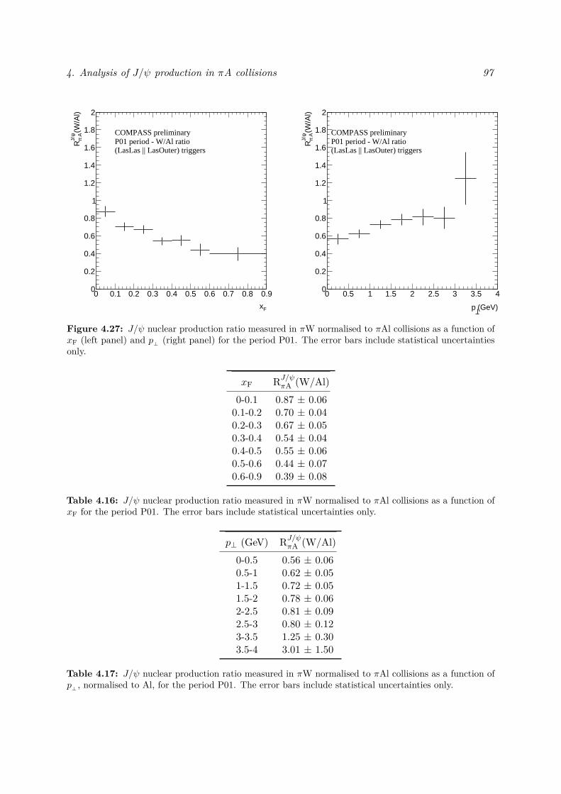
4. Analysis of J/ψ production in πA collisions 97
0 0.1 0.2 0.3 0.4 0.5 0.6 0.7 0.8 0.9
Fx
0
0.2
0.4
0.6
0.8
1
1.2
1.4
1.6
1.8
2
(W/A
l)ψ
J/ Aπ
R
COMPASS preliminaryP01 period - W/Al ratio(LasLas || LasOuter) triggers
0 0.5 1 1.5 2 2.5 3 3.5 4
(GeV)p
0
0.2
0.4
0.6
0.8
1
1.2
1.4
1.6
1.8
2
(W/A
l)ψ
J/ Aπ
R
COMPASS preliminaryP01 period - W/Al ratio(LasLas || LasOuter) triggers
Figure 4.27: J/ψ nuclear production ratio measured in πW normalised to πAl collisions as a function ofxF (left panel) and p⊥ (right panel) for the period P01. The error bars include statistical uncertaintiesonly.
xF RJ/ψπA (W/Al)0-0.1 0.87 ± 0.060.1-0.2 0.70 ± 0.040.2-0.3 0.67 ± 0.050.3-0.4 0.54 ± 0.040.4-0.5 0.55 ± 0.060.5-0.6 0.44 ± 0.070.6-0.9 0.39 ± 0.08
Table 4.16: J/ψ nuclear production ratio measured in πW normalised to πAl collisions as a function ofxF for the period P01. The error bars include statistical uncertainties only.
p⊥ (GeV) RJ/ψπA (W/Al)0-0.5 0.56 ± 0.060.5-1 0.62 ± 0.051-1.5 0.72 ± 0.051.5-2 0.78 ± 0.062-2.5 0.81 ± 0.092.5-3 0.80 ± 0.123-3.5 1.25 ± 0.303.5-4 3.01 ± 1.50
Table 4.17: J/ψ nuclear production ratio measured in πW normalised to πAl collisions as a function ofp⊥ , normalised to Al, for the period P01. The error bars include statistical uncertainties only.
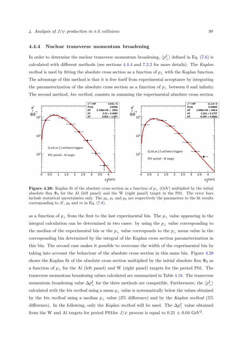
4. Analysis of J/ψ production in πA collisions 98
4.4.4 Nuclear transverse momentum broadening
In order to determine the nuclear transverse momentum broadening,⟨p2⊥⟩defined in Eq. (7.6) is
calculated with different methods (see sections 4.4.4 and 7.2.2 for more details). The Kaplanmethod is used by fitting the absolute cross section as a function of p⊥ with the Kaplan function.The advantage of this method is that it is free itself from experimental acceptance by integratingthe parameterization of the absolute cross section as a function of p⊥ between 0 and infinity.The second method, bin method, consists in summing the experimental absolute cross section
0 0.5 1 1.5 2 2.5 3 3.5 4
(GeV)p
210
310
410
0Φ ×
dpσd
/ ndf 2χ 3.041 / 5Prob 0.6936p0 1933± 2.748e+04 p1 0.4085± 3.31 p2 1.807± 9.802
/ ndf 2χ 3.041 / 5Prob 0.6936p0 1933± 2.748e+04 p1 0.4085± 3.31 p2 1.807± 9.802
(LasLas || LasOuter) triggers
P01 period - Al target
0 0.5 1 1.5 2 2.5 3 3.5 4
(GeV)p
210
310
410
0Φ ×
dpσd
/ ndf 2χ 11.14 / 5Prob 0.04863p0 446.6± 1.668e+04 p1 0.1757± 3.161 p2 0.6864± 8.209
/ ndf 2χ 11.14 / 5Prob 0.04863p0 446.6± 1.668e+04 p1 0.1757± 3.161 p2 0.6864± 8.209
(LasLas || LasOuter) triggers
P01 period - W target
Figure 4.28: Kaplan fit of the absolute cross section as a function of p⊥ (GeV) multiplied by the initialabsolute flux Φ0 for the Al (left panel) and the W (right panel) target in the P01. The error barsinclude statistical uncertainties only. The p0, p1 and p2 are respectively the parameters to the fit resultscorresponding to N , p0 and m in Eq. (7.8).
as a function of p⊥ from the first to the last experimental bin. The p⊥ value appearing in theintegral calculation can be determined in two cases: by using the p⊥ value corresponding tothe median of the experimental bin or the p⊥ value corresponds to the p⊥ mean value in thecorresponding bin determined by the integral of the Kaplan cross section parameterization inthis bin. The second case makes it possible to overcome the width of the experimental bin bytaking into account the behaviour of the absolute cross section in this same bin. Figure 4.28shows the Kaplan fit of the absolute cross section multiplied by the initial absolute flux Φ0 asa function of p⊥ for the Al (left panel) and W (right panel) targets for the period P01. Thetransverse momentum broadening values calculated are summarized in Table 4.18. The transversemomentum broadening value ∆p2
⊥ for the three methods are compatible. Furthermore, the⟨p2⊥⟩
calculated with the bin method using a mean p⊥ value is systematically below the values obtainedby the bin method using a median p⊥ value (3% difference) and by the Kaplan method (5%difference). In the following, only the Kaplan method will be used. The ∆p2
⊥ value obtainedfrom the W and Al targets for period P01for J/ψ process is equal to 0.21 ± 0.04 GeV2.
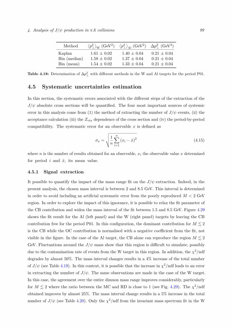
4. Analysis of J/ψ production in πA collisions 99
Method⟨p2⊥⟩W (GeV2)
⟨p2⊥⟩Al (GeV2) ∆p2
⊥ (GeV2)Kaplan 1.61 ± 0.02 1.40 ± 0.04 0.21 ± 0.04Bin (median) 1.58 ± 0.02 1.37 ± 0.04 0.21 ± 0.04Bin (mean) 1.54 ± 0.02 1.33 ± 0.04 0.21 ± 0.04
Table 4.18: Determination of ∆p2⊥ with different methods in the W and Al targets for the period P01.
4.5 Systematic uncertainties estimation
In this section, the systematic errors associated with the different steps of the extraction of theJ/ψ absolute cross sections will be quantified. The four most important sources of systemicerror in this analysis come from (1) the method of extracting the number of J/ψ events, (ii) theacceptance calculation (iii) the Zvtx dependence of the cross section and (iv) the period-by-periodcompatibility. The systematic error for an observable x is defined as
σx =
√√√√ 1n
n∑i=1
(xi − x)2 (4.15)
where n is the number of results obtained for an observable, xi the observable value x determinedfor period i and x, its mean value.
4.5.1 Signal extraction
It possible to quantify the impact of the mass range fit on the J/ψ extraction. Indeed, in thepresent analysis, the chosen mass interval is between 2 and 8.5 GeV. This interval is determinedin order to avoid including an artificial systematic error from the poorly reproduced M < 2 GeVregion. In order to explore the impact of this ignorance, it is possible to relax the fit parameter ofthe CB contribution and widen the mass interval of the fit between 1.5 and 8.5 GeV. Figure 4.29shows the fit result for the Al (left panel) and the W (right panel) targets by leaving the CBcontribution free for the period P01. In this configuration, the dominant contribution for M . 2is the CB while the OC contribution is normalised with a negative coefficient from the fit, notvisible in the figure. In the case of the Al target, the CB alone can reproduce the region M . 2GeV. Fluctuations around the J/ψ mass show that this region is difficult to simulate, possiblydue to the contamination rate of events from the W target in this region. In addition, the χ2/ndfdegrades by almost 50%. The mass interval changes results in a 4% increase of the total numberof J/ψ (see Table 4.19). In this context, it is possible that the increase in χ2/ndf leads to an errorin extracting the number of J/ψ. The same observations are made in the case of the W target.In this case, the agreement over the entire dimuon mass range improves considerably, particularlyfor M . 2 where the ratio between the MC and RD is close to 1 (see Fig. 4.29). The χ2/ndfobtained improves by almost 25%. The mass interval change results in a 5% increase in the totalnumber of J/ψ (see Table 4.20). Only the χ2/ndf from the invariant mass spectrum fit in the W
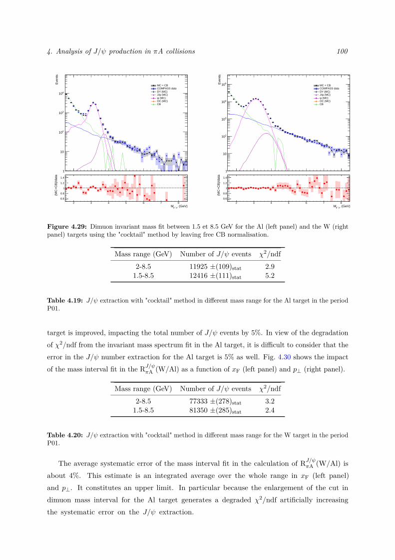
4. Analysis of J/ψ production in πA collisions 100E
vent
s
1
10
210
310
410
MC + CBCOMPASS dataDY (MC)
(MC)ψJ/ (MC)ψ
OC (MC)CB
(GeV)-µ +µM2 3 4 5 6 7 8
(MC
+C
B)/
data
0.6
0.8
1
1.2
1.4
Eve
nts
1
10
210
310
410
510 MC + CBCOMPASS dataDY (MC)
(MC)ψJ/ (MC)ψ
OC (MC)CB
(GeV)-µ +µM2 3 4 5 6 7 8
(MC
+C
B)/
data
0.6
0.8
1
1.2
1.4
Figure 4.29: Dimuon invariant mass fit between 1.5 et 8.5 GeV for the Al (left panel) and the W (rightpanel) targets using the "cocktail" method by leaving free CB normalisation.
Mass range (GeV) Number of J/ψ events χ2/ndf2-8.5 11925 ±(109)stat 2.91.5-8.5 12416 ±(111)stat 5.2
Table 4.19: J/ψ extraction with "cocktail" method in different mass range for the Al target in the periodP01.
target is improved, impacting the total number of J/ψ events by 5%. In view of the degradationof χ2/ndf from the invariant mass spectrum fit in the Al target, it is difficult to consider that theerror in the J/ψ number extraction for the Al target is 5% as well. Fig. 4.30 shows the impactof the mass interval fit in the RJ/ψπA (W/Al) as a function of xF (left panel) and p⊥ (right panel).
Mass range (GeV) Number of J/ψ events χ2/ndf2-8.5 77333 ±(278)stat 3.21.5-8.5 81350 ±(285)stat 2.4
Table 4.20: J/ψ extraction with "cocktail" method in different mass range for the W target in the periodP01.
The average systematic error of the mass interval fit in the calculation of RJ/ψπA (W/Al) isabout 4%. This estimate is an integrated average over the whole range in xF (left panel)and p⊥. It constitutes an upper limit. In particular because the enlargement of the cut indimuon mass interval for the Al target generates a degraded χ2/ndf artificially increasingthe systematic error on the J/ψ extraction.
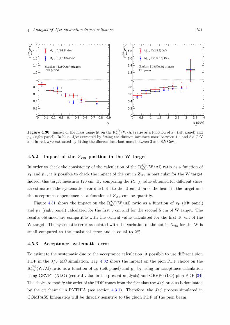
4. Analysis of J/ψ production in πA collisions 101
0 0.1 0.2 0.3 0.4 0.5 0.6 0.7 0.8 0.9
Fx
0
0.2
0.4
0.6
0.8
1
1.2
1.4
1.6
1.8
2
(W/A
l)ψ
J/ AπR
(LasLas || LasOuter) triggersP01 period
(2-8.5) GeV∈ -µ +µM
(1.5-8.5) GeV∈ -µ +µM
0 0.5 1 1.5 2 2.5 3 3.5 4
(GeV)p
0
0.2
0.4
0.6
0.8
1
1.2
1.4
1.6
1.8
2
(W/A
l)ψ
J/ AπR
(LasLas || LasOuter) triggersP01 period
(2-8.5) GeV∈ -µ +µM
(1.5-8.5) GeV∈ -µ +µM
Figure 4.30: Impact of the mass range fit on the RJ/ψπA (W/Al) ratio as a function of xF (left panel) andp⊥ (right panel). In blue, J/ψ extracted by fitting the dimuon invariant mass between 1.5 and 8.5 GeVand in red, J/ψ extracted by fitting the dimuon invariant mass between 2 and 8.5 GeV.
4.5.2 Impact of the Zvtx position in the W target
In order to check the consistency of the calculation of the RJ/ψπA (W/Al) ratio as a function ofxF and p⊥, it is possible to check the impact of the cut in Zvtx in particular for the W target.Indeed, this target measures 120 cm. By comparing the Rπ−A value obtained for different slices,an estimate of the systematic error due both to the attenuation of the beam in the target andthe acceptance dependence as a function of Zvtx can be quantify.
Figure 4.31 shows the impact on the RJ/ψπA (W/Al) ratio as a function of xF (left panel)and p⊥ (right panel) calculated for the first 5 cm and for the second 5 cm of W target. Theresults obtained are compatible with the central value calculated for the first 10 cm of theW target. The systematic error associated with the variation of the cut in Zvtx for the W issmall compared to the statistical error and is equal to 2%.
4.5.3 Acceptance systematic error
To estimate the systematic due to the acceptance calculation, it possible to use different pionPDF in the J/ψ MC simulation. Fig. 4.32 shows the impact on the pion PDF choice on theRJ/ψπA (W/Al) ratio as a function of xF (left panel) and p⊥ by using an acceptance calculationusing GRVP1 (NLO) (central value in the present analysis) and GRVP0 (LO) pion PDF [34].The choice to modify the order of the PDF comes from the fact that the J/ψ process is dominatedby the gg channel in PYTHIA (see section 4.3.1). Therefore, the J/ψ process simulated inCOMPASS kinematics will be directly sensitive to the gluon PDF of the pion beam.
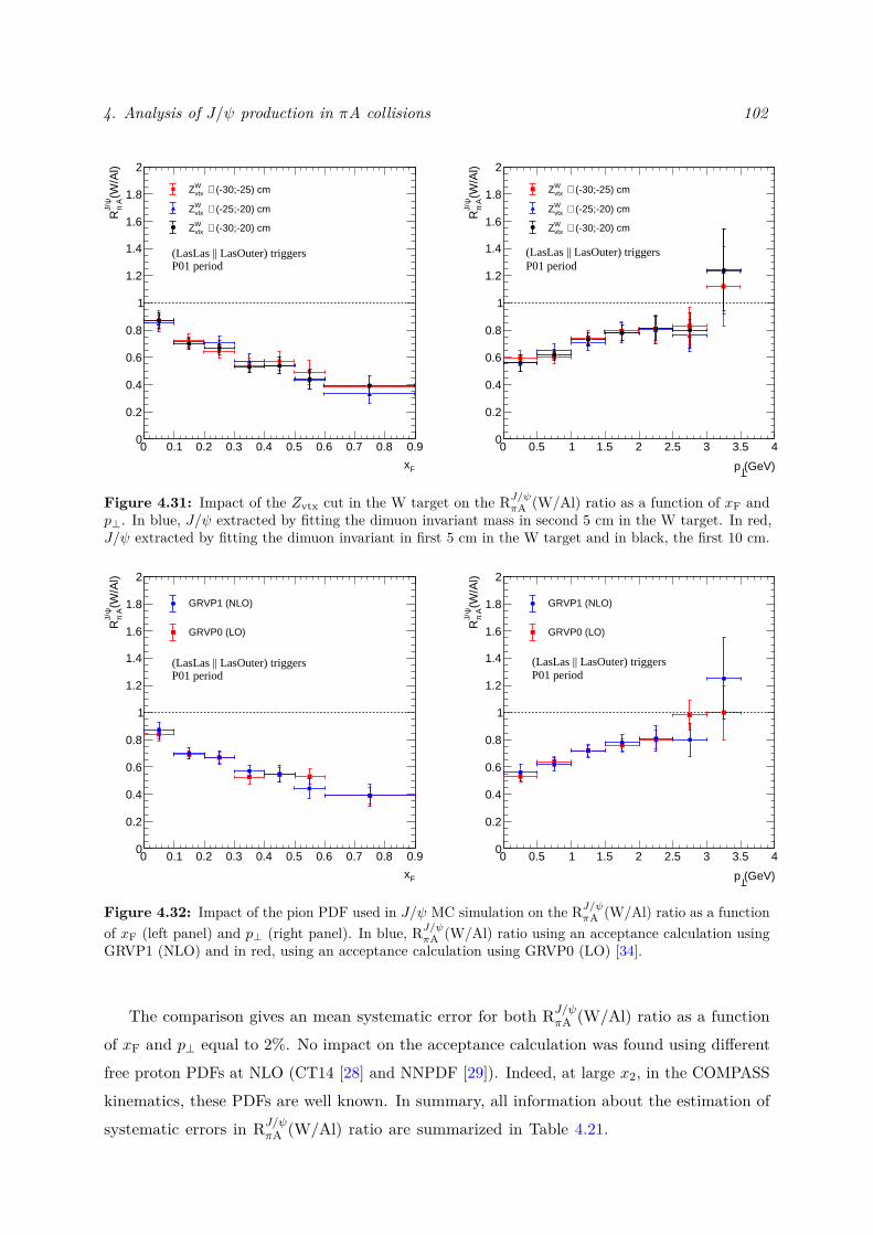
4. Analysis of J/ψ production in πA collisions 102
0 0.1 0.2 0.3 0.4 0.5 0.6 0.7 0.8 0.9
Fx
0
0.2
0.4
0.6
0.8
1
1.2
1.4
1.6
1.8
2
(W/A
l)ψ
J/ AπR
(LasLas || LasOuter) triggersP01 period
(-30;-25) cm∈ WvtxZ
(-25;-20) cm∈ WvtxZ
(-30;-20) cm∈ WvtxZ
0 0.5 1 1.5 2 2.5 3 3.5 4
(GeV)p
0
0.2
0.4
0.6
0.8
1
1.2
1.4
1.6
1.8
2
(W/A
l)ψ
J/ AπR
(LasLas || LasOuter) triggersP01 period
(-30;-25) cm∈ WvtxZ
(-25;-20) cm∈ WvtxZ
(-30;-20) cm∈ WvtxZ
Figure 4.31: Impact of the Zvtx cut in the W target on the RJ/ψπA (W/Al) ratio as a function of xF andp⊥. In blue, J/ψ extracted by fitting the dimuon invariant mass in second 5 cm in the W target. In red,J/ψ extracted by fitting the dimuon invariant in first 5 cm in the W target and in black, the first 10 cm.
0 0.1 0.2 0.3 0.4 0.5 0.6 0.7 0.8 0.9
Fx
0
0.2
0.4
0.6
0.8
1
1.2
1.4
1.6
1.8
2
(W/A
l)ψ
J/ AπR
(LasLas || LasOuter) triggersP01 period
GRVP1 (NLO)
GRVP0 (LO)
0 0.5 1 1.5 2 2.5 3 3.5 4
(GeV)p
0
0.2
0.4
0.6
0.8
1
1.2
1.4
1.6
1.8
2
(W/A
l)ψ
J/ AπR
(LasLas || LasOuter) triggersP01 period
GRVP1 (NLO)
GRVP0 (LO)
Figure 4.32: Impact of the pion PDF used in J/ψ MC simulation on the RJ/ψπA (W/Al) ratio as a functionof xF (left panel) and p⊥ (right panel). In blue, RJ/ψπA (W/Al) ratio using an acceptance calculation usingGRVP1 (NLO) and in red, using an acceptance calculation using GRVP0 (LO) [34].
The comparison gives an mean systematic error for both RJ/ψπA (W/Al) ratio as a functionof xF and p⊥ equal to 2%. No impact on the acceptance calculation was found using differentfree proton PDFs at NLO (CT14 [28] and NNPDF [29]). Indeed, at large x2, in the COMPASSkinematics, these PDFs are well known. In summary, all information about the estimation ofsystematic errors in RJ/ψπA (W/Al) ratio are summarized in Table 4.21.
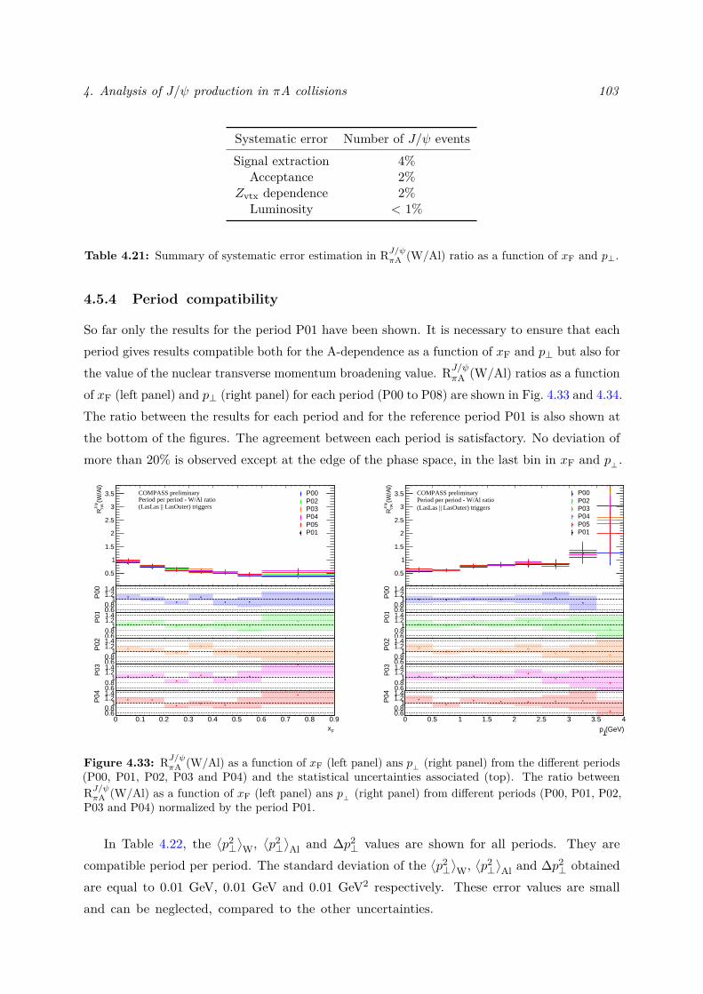
4. Analysis of J/ψ production in πA collisions 103
Systematic error Number of J/ψ eventsSignal extraction 4%
Acceptance 2%Zvtx dependence 2%
Luminosity < 1%
Table 4.21: Summary of systematic error estimation in RJ/ψπA (W/Al) ratio as a function of xF and p⊥.
4.5.4 Period compatibility
So far only the results for the period P01 have been shown. It is necessary to ensure that eachperiod gives results compatible both for the A-dependence as a function of xF and p⊥ but also forthe value of the nuclear transverse momentum broadening value. RJ/ψπA (W/Al) ratios as a functionof xF (left panel) and p⊥ (right panel) for each period (P00 to P08) are shown in Fig. 4.33 and 4.34.The ratio between the results for each period and for the reference period P01 is also shown atthe bottom of the figures. The agreement between each period is satisfactory. No deviation ofmore than 20% is observed except at the edge of the phase space, in the last bin in xF and p⊥ .
0.5
1
1.5
2
2.5
3
3.5
(W/A
l)ψ
J/
AπR
P00P02P03P04P05P01
COMPASS preliminaryPeriod per period - W/Al ratio(LasLas || LasOuter) triggers
0.60.8
11.21.4
P00
0.60.8
11.21.4
P01
0.60.8
11.21.4
P02
0.60.8
11.21.4
P03
0 0.1 0.2 0.3 0.4 0.5 0.6 0.7 0.8 0.9
Fx
0.60.8
11.21.4
P04
0.5
1
1.5
2
2.5
3
3.5
(W/A
l)ψ
J/
AπR
P00P02P03P04P05P01
COMPASS preliminaryPeriod per period - W/Al ratio(LasLas || LasOuter) triggers
0.60.8
11.21.4
P00
0.60.8
11.21.4
P01
0.60.8
11.21.4
P02
0.60.8
11.21.4
P03
0 0.5 1 1.5 2 2.5 3 3.5 4 (GeV)p
0.60.8
11.21.4
P04
Figure 4.33: RJ/ψπA (W/Al) as a function of xF (left panel) ans p⊥ (right panel) from the different periods(P00, P01, P02, P03 and P04) and the statistical uncertainties associated (top). The ratio betweenRJ/ψπA (W/Al) as a function of xF (left panel) ans p⊥ (right panel) from different periods (P00, P01, P02,P03 and P04) normalized by the period P01.
In Table 4.22, the⟨p2⊥⟩W,
⟨p2⊥⟩Al and ∆p2
⊥ values are shown for all periods. They arecompatible period per period. The standard deviation of the
⟨p2⊥⟩W,
⟨p2⊥⟩Al and ∆p2
⊥ obtainedare equal to 0.01 GeV, 0.01 GeV and 0.01 GeV2 respectively. These error values are smalland can be neglected, compared to the other uncertainties.
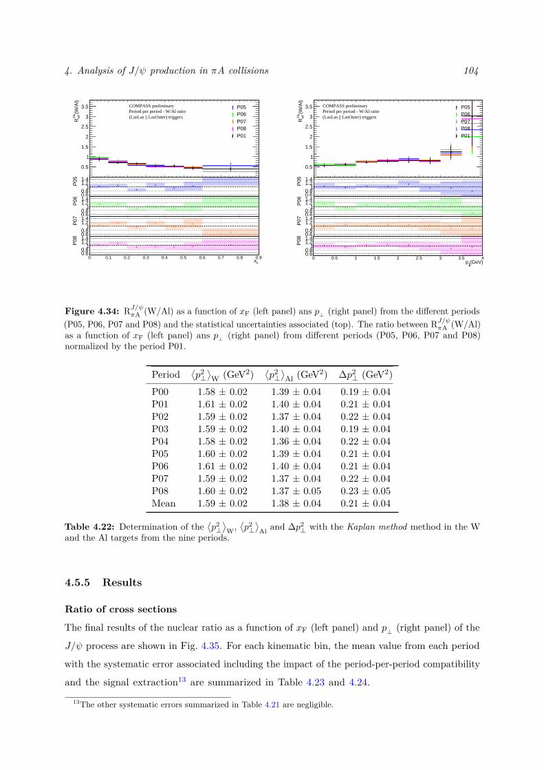
4. Analysis of J/ψ production in πA collisions 104
0.5
1
1.5
2
2.5
3
3.5
(W/A
l)ψ
J/
AπR
P05P06P07P08P01
COMPASS preliminaryPeriod per period - W/Al ratio(LasLas || LasOuter) triggers
0.60.8
11.21.4
P05
0.60.8
11.21.4
P06
0.60.8
11.21.4
P07
0 0.1 0.2 0.3 0.4 0.5 0.6 0.7 0.8 0.9Fx
0.60.8
11.21.4
P08
0.5
1
1.5
2
2.5
3
3.5
(W/A
l)ψ
J/
AπR
P05P06P07P08P01
COMPASS preliminaryPeriod per period - W/Al ratio(LasLas || LasOuter) triggers
0.60.8
11.21.4
P05
0.60.8
11.21.4
P06
0.60.8
11.21.4
P07
0 0.5 1 1.5 2 2.5 3 3.5 4 (GeV)p
0.60.8
11.21.4
P08
Figure 4.34: RJ/ψπA (W/Al) as a function of xF (left panel) ans p⊥ (right panel) from the different periods(P05, P06, P07 and P08) and the statistical uncertainties associated (top). The ratio between RJ/ψπA (W/Al)as a function of xF (left panel) ans p⊥ (right panel) from different periods (P05, P06, P07 and P08)normalized by the period P01.
Period⟨p2⊥⟩W (GeV2)
⟨p2⊥⟩Al (GeV2) ∆p2
⊥ (GeV2)P00 1.58 ± 0.02 1.39 ± 0.04 0.19 ± 0.04P01 1.61 ± 0.02 1.40 ± 0.04 0.21 ± 0.04P02 1.59 ± 0.02 1.37 ± 0.04 0.22 ± 0.04P03 1.59 ± 0.02 1.40 ± 0.04 0.19 ± 0.04P04 1.58 ± 0.02 1.36 ± 0.04 0.22 ± 0.04P05 1.60 ± 0.02 1.39 ± 0.04 0.21 ± 0.04P06 1.61 ± 0.02 1.40 ± 0.04 0.21 ± 0.04P07 1.59 ± 0.02 1.37 ± 0.04 0.22 ± 0.04P08 1.60 ± 0.02 1.37 ± 0.05 0.23 ± 0.05Mean 1.59 ± 0.02 1.38 ± 0.04 0.21 ± 0.04
Table 4.22: Determination of the⟨p2⊥⟩
W,⟨p2⊥⟩
Al and ∆p2⊥ with the Kaplan method method in the W
and the Al targets from the nine periods.
4.5.5 Results
Ratio of cross sections
The final results of the nuclear ratio as a function of xF (left panel) and p⊥ (right panel) of the
J/ψ process are shown in Fig. 4.35. For each kinematic bin, the mean value from each period
with the systematic error associated including the impact of the period-per-period compatibility
and the signal extraction13 are summarized in Table 4.23 and 4.24.
13The other systematic errors summarized in Table 4.21 are negligible.
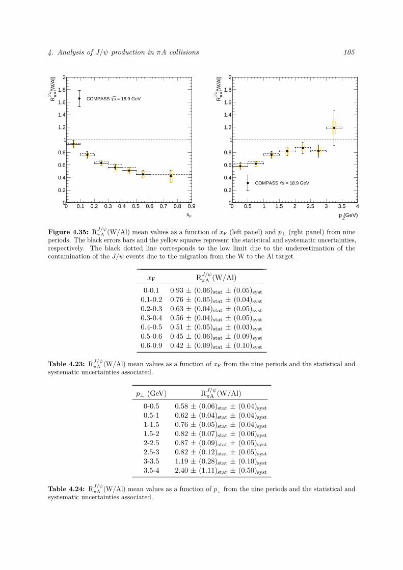
4. Analysis of J/ψ production in πA collisions 105
0 0.1 0.2 0.3 0.4 0.5 0.6 0.7 0.8 0.9
Fx
0
0.2
0.4
0.6
0.8
1
1.2
1.4
1.6
1.8
2
(W/A
l)ψ
J/ AπR = 18.9 GeVsCOMPASS
0 0.5 1 1.5 2 2.5 3 3.5 4
(GeV)p
0
0.2
0.4
0.6
0.8
1
1.2
1.4
1.6
1.8
2
(W/A
l)ψ
J/ AπR
= 18.9 GeVsCOMPASS
Figure 4.35: RJ/ψπA (W/Al) mean values as a function of xF (left panel) and p⊥ (rght panel) from nineperiods. The black errors bars and the yellow squares represent the statistical and systematic uncertainties,respectively. The black dotted line corresponds to the low limit due to the underestimation of thecontamination of the J/ψ events due to the migration from the W to the Al target.
xF RJ/ψπA (W/Al)0-0.1 0.93 ± (0.06)stat ± (0.05)syst0.1-0.2 0.76 ± (0.05)stat ± (0.04)syst0.2-0.3 0.63 ± (0.04)stat ± (0.05)syst0.3-0.4 0.56 ± (0.04)stat ± (0.05)syst0.4-0.5 0.51 ± (0.05)stat ± (0.03)syst0.5-0.6 0.45 ± (0.06)stat ± (0.09)syst0.6-0.9 0.42 ± (0.09)stat ± (0.10)syst
Table 4.23: RJ/ψπA (W/Al) mean values as a function of xF from the nine periods and the statistical andsystematic uncertainties associated.
p⊥ (GeV) RJ/ψπA (W/Al)0-0.5 0.58 ± (0.06)stat ± (0.04)syst0.5-1 0.62 ± (0.04)stat ± (0.04)syst1-1.5 0.76 ± (0.05)stat ± (0.04)syst1.5-2 0.82 ± (0.07)stat ± (0.06)syst2-2.5 0.87 ± (0.09)stat ± (0.05)syst2.5-3 0.82 ± (0.12)stat ± (0.05)syst3-3.5 1.19 ± (0.28)stat ± (0.10)syst3.5-4 2.40 ± (1.11)stat ± (0.50)syst
Table 4.24: RJ/ψπA (W/Al) mean values as a function of p⊥ from the nine periods and the statistical andsystematic uncertainties associated.
4. Analysis of J/ψ production in πA collisions 106
Nuclear transverse momentum broadeningThe mean values from each period are
⟨p2⊥⟩W = (1.59 ± 0.02) GeV2,
⟨p2⊥⟩Al = (1.38 ± 0.04)
GeV2 and ∆p2⊥ = 0.21 ± 0.04 GeV2.
4.6 Conclusion
In this chapter, preliminary J/ψ data of the COMPASS experiment were analysed. From theevent selection to the Monte-Carlo (MC) analysis, the extraction of the J/ψ cross sections ratiobetween π−W and π−Al collisions was discussed. The J/ψ extraction was performed by fittingthe dimuon mass spectrum using the "cocktail" method for different xF and p⊥ bins. Thismethod enables to take into account the background evolution.
A good agreement was found in a large dimuon mass fit interval, M ∈ (2− 8.5) GeV in bothAl and W targets data sample. However, some tensions appeared in the low dimuon mass regionM ∈ (1.5− 2.0) GeV due to several reasons: (i) a large event migration ∼ 10% from the W to Altargets was highlighted, (ii) the low dimuon mass region is dominated by the Open-Charm (OC)contribution that is not very well known in the PYTHIA generator and (iii) the low dimuon massregion could contain other processes not included in the "cocktail" method like the decay of lightmesons (ω and φ mesons). Nevertheless, the variation of the dimuon mass interval fit changesslightly ∼ 4% the extraction of the J/ψ cross sections ratio between π−W and π−Al collisions.
The preliminary J/ψ data show a strong suppression as a function of xF and p⊥ in π−Wcompared to π−Al collisions. Otherwise, the transverse momentum broadening effect betweenπ−W and π−Al collisions is equal to ∆p2
⊥ = 0.21 ± 0.04 GeV2. It exhibits an importantnuclear effect due to the W target. These preliminary results highlight strong nuclear effectsin the J/ψ data. In Chap. 6 and 7, an interpretation of these data based on the theoreticalframework exposed in Chap. 2 will be proposed.
5Analysis of Drell-Yan production in πA collisions
Contents
5.1 Observable . . . . . . . . . . . . . . . . . . . . . . . . . . . . . . . . . . 1075.2 Drell-Yan signal extraction . . . . . . . . . . . . . . . . . . . . . . . . . 108
5.2.1 Data sample . . . . . . . . . . . . . . . . . . . . . . . . . . . . . . . . . 1085.2.2 Monte-Carlo simulation . . . . . . . . . . . . . . . . . . . . . . . . . . . 1095.2.3 Validity of the Monte-Carlo simulation . . . . . . . . . . . . . . . . . . . 113
5.3 Drell-Yan cross section . . . . . . . . . . . . . . . . . . . . . . . . . . . 1135.3.1 2D acceptance as a function of xF and p⊥ . . . . . . . . . . . . . . . . . 1145.3.2 Drell-Yan cross section as a function of xF and p⊥ . . . . . . . . . . . . 1175.3.3 Ratios of nuclear cross sections . . . . . . . . . . . . . . . . . . . . . . . 1175.3.4 Nuclear transverse momentum broadening . . . . . . . . . . . . . . . . . 119
5.4 Systematic uncertainties . . . . . . . . . . . . . . . . . . . . . . . . . . 1205.4.1 Impact of the trigger selection . . . . . . . . . . . . . . . . . . . . . . . 1205.4.2 Impact of Zvtx position in W target . . . . . . . . . . . . . . . . . . . . 1225.4.3 Acceptance systematic error . . . . . . . . . . . . . . . . . . . . . . . . . 1235.4.4 Results . . . . . . . . . . . . . . . . . . . . . . . . . . . . . . . . . . . . 123
5.5 Conclusion . . . . . . . . . . . . . . . . . . . . . . . . . . . . . . . . . . 125
5.1 Observable
The double differential cross of Drell-Yan (DY) production is
d2σπ−A
dxFdp⊥(DY) = N
J/ψevents (xF, p⊥)
εA ·∆xF ·∆p⊥ · L(5.1)
where NDYevents is the number of Drell-Yan events in the (xF, p⊥) kinematic bin, ε is the acceptance
calculation including reconstruction efficiency, trigger efficiency, geometrical efficiency anddetectors efficiency, ∆xF and ∆p⊥ are the xF and p⊥ bin width. The luminosity L is defined
107
5. Analysis of Drell-Yan production in πA collisions 108
in Eq. (4.3). The nuclear dependence for the DY process can be accessed when considering theratio between the W and the Al target as a function of xF and p⊥ :
RDYπ−A(W/Al) = NDY
W (xF, p⊥)εW · αWΦ0 × LW
eff × ρW/
NDYAl (xF, p⊥)
εAl · αAlΦ0 × LAleff × ρAl
. (5.2)
As for the J/ψ analysis, the initial absolute flux Φ0 cancels out in (5.2). The informationconcerning the flux is contained in the fraction of the incident flux at the entrance of thetarget, α, and also in the effective luminosity which is taken into account using the effectivetarget length, Leff (see Eq. (4.3)).
In this chapter, the extraction of the DY nuclear cross section ratios between the W targetand the Al target will be discussed. All the steps of the analysis, from the extraction of DYevents to the calculation of acceptance thanks to the Monte-Carlo simulation (MC), will bedetailed. Finally, the preliminary results of Rπ−A as a function of xF and p⊥ will be shown.
5.2 Drell-Yan signal extraction
As discussed in the Sec 4, the dimuon mass spectrum consists of a mixture of different physicalcontributions: Open-Charm (OC), Combinatorial Background (CB), Charmonium (J/ψ andψ′) and DY. In order to study a specific process, it is necessary to evaluate the signal tobackground ratio in order (i) to minimise the systematic errors due to the background extractionand (ii) to maximise the signal number of events.
In the high-mass region M & 4 GeV, the dimuon mass spectrum is dominated by the DYcontribution in both W and Al targets (see Fig. 4.8 and Fig. 4.9). This very clean dimuon massregion is suitable for studying the DY process. The choice of the best dimuon mass intervalfor this study will depend on the evaluation of the DY process purity level.
5.2.1 Data sample
In order to determine the number of DY events, it is necessary to select the relevant invariantdimuon mass region where the purity of DY is high enough to minimise the systematic errordue to the background subtraction. From the invariant mass fit shown in Fig. 4.9 for the Altarget and in Fig. 4.8 for the W target, the integral of each physical contribution is calculated.The information about the background as a function of dimuon invariant mass is shown inTable 5.2 for the Al target and in Table 5.1 for the W target.
The dimuon invariant mass region best suited to study the DY process is 4.4 < M < 8.5 GeV forthe Al target and 4.7 < M < 8.5 GeV for the W target. It is therefore obvious that the target whichhas the most restrictive dimuon mass interval constrains the final mass cut, i.e. 4.7 < M < 8.5 GeV.The DY number of events after the final dimuon invariant mass cut are summarised in Table 5.3.
After applying all selection criteria, the extracted kinematic distributions contain only DYevents. The background is already subtracted thanks to the dimuon mass cut. A bin by bin DY
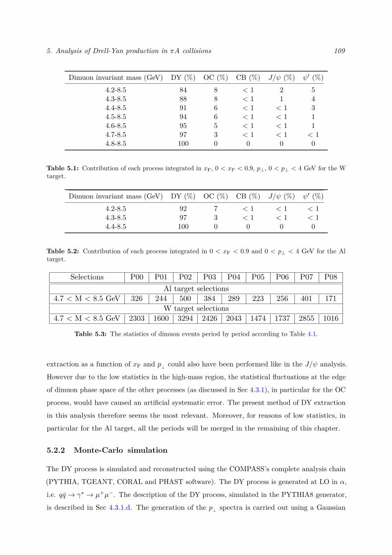
5. Analysis of Drell-Yan production in πA collisions 109
Dimuon invariant mass (GeV) DY (%) OC (%) CB (%) J/ψ (%) ψ′ (%)4.2-8.5 84 8 < 1 2 54.3-8.5 88 8 < 1 1 44.4-8.5 91 6 < 1 < 1 34.5-8.5 94 6 < 1 < 1 14.6-8.5 95 5 < 1 < 1 14.7-8.5 97 3 < 1 < 1 < 14.8-8.5 100 0 0 0 0
Table 5.1: Contribution of each process integrated in xF, 0 < xF < 0.9, p⊥, 0 < p⊥ < 4 GeV for the Wtarget.
Dimuon invariant mass (GeV) DY (%) OC (%) CB (%) J/ψ (%) ψ′ (%)4.2-8.5 92 7 < 1 < 1 < 14.3-8.5 97 3 < 1 < 1 < 14.4-8.5 100 0 0 0 0
Table 5.2: Contribution of each process integrated in 0 < xF < 0.9 and 0 < p⊥ < 4 GeV for the Altarget.
Selections P00 P01 P02 P03 P04 P05 P06 P07 P08Al target selections
4.7 < M < 8.5 GeV 326 244 500 384 289 223 256 401 171W target selections
4.7 < M < 8.5 GeV 2303 1600 3294 2426 2043 1474 1737 2855 1016
Table 5.3: The statistics of dimuon events period by period according to Table 4.1.
extraction as a function of xF and p⊥ could also have been performed like in the J/ψ analysis.
However due to the low statistics in the high-mass region, the statistical fluctuations at the edge
of dimuon phase space of the other processes (as discussed in Sec 4.3.1), in particular for the OC
process, would have caused an artificial systematic error. The present method of DY extraction
in this analysis therefore seems the most relevant. Moreover, for reasons of low statistics, in
particular for the Al target, all the periods will be merged in the remaining of this chapter.
5.2.2 Monte-Carlo simulation
The DY process is simulated and reconstructed using the COMPASS’s complete analysis chain
(PYTHIA, TGEANT, CORAL and PHAST software). The DY process is generated at LO in α,
i.e. qq → γ? → µ+µ−. The description of the DY process, simulated in the PYTHIA8 generator,
is described in Sec 4.3.1.d. The generation of the p⊥ spectra is carried out using a Gaussian
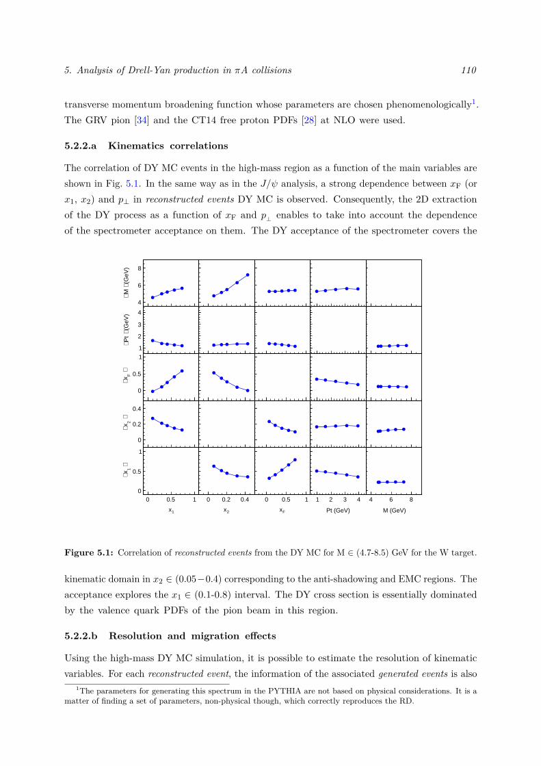
5. Analysis of Drell-Yan production in πA collisions 110
transverse momentum broadening function whose parameters are chosen phenomenologically1.The GRV pion [34] and the CT14 free proton PDFs [28] at NLO were used.
5.2.2.a Kinematics correlations
The correlation of DY MC events in the high-mass region as a function of the main variables areshown in Fig. 5.1. In the same way as in the J/ψ analysis, a strong dependence between xF (orx1, x2) and p⊥ in reconstructed events DY MC is observed. Consequently, the 2D extractionof the DY process as a function of xF and p⊥ enables to take into account the dependenceof the spectrometer acceptance on them. The DY acceptance of the spectrometer covers the
0 0.5 1
1x
0
0.5
1
⟩ 1 x⟨
0 0.5 11x
0
0.2
0.4
⟩ 2
x⟨
0 0.5 11x
0
0.5
1
⟩ F
x⟨
0 0.5 11x
1
2
3
4
(G
eV)
⟩ P
t ⟨
0 0.5 11x
4
6
8
(G
eV)
⟩ M
⟨
0 0.2 0.4
2x
0
0.5
1
⟩ 1 x⟨
0 0.2 0.42x
0
0.2
0.4
⟩ 2
x⟨
0 0.2 0.42x
0
0.5
1
⟩ F
x⟨
0 0.2 0.42x
1
2
3
4
(G
eV)
⟩ P
t ⟨
0 0.2 0.42x
4
6
8
(G
eV)
⟩ M
⟨
0 0.5 1
Fx
0
0.5
1
⟩ 1 x⟨
0 0.5 1Fx
0
0.2
0.4
⟩ 2
x⟨
0 0.5 1Fx
0
0.5
1
⟩ F
x⟨
0 0.5 1Fx
1
2
3
4
(G
eV)
⟩ P
t ⟨
0 0.5 1Fx
4
6
8
(G
eV)
⟩ M
⟨
1 2 3 4
Pt (GeV)
0
0.5
1
⟩ 1 x⟨
1 2 3 4Pt (GeV)
0
0.2
0.4
⟩ 2
x⟨
1 2 3 4Pt (GeV)
0
0.5
1
⟩ F
x⟨
1 2 3 4Pt (GeV)
1
2
3
4
(G
eV)
⟩ P
t ⟨
1 2 3 4Pt (GeV)
4
6
8
(G
eV)
⟩ M
⟨
4 6 8
M (GeV)
0
0.5
1
⟩ 1 x⟨
4 6 8 M (GeV)
0
0.2
0.4
⟩ 2
x⟨
4 6 8 M (GeV)
0
0.5
1⟩
F x⟨
4 6 8 M (GeV)
1
2
3
4
(G
eV)
⟩ P
t ⟨
4 6 8 M (GeV)
4
6
8
(G
eV)
⟩ M
⟨
Figure 5.1: Correlation of reconstructed events from the DY MC for M ∈ (4.7-8.5) GeV for the W target.
kinematic domain in x2 ∈ (0.05−0.4) corresponding to the anti-shadowing and EMC regions. Theacceptance explores the x1 ∈ (0.1-0.8) interval. The DY cross section is essentially dominatedby the valence quark PDFs of the pion beam in this region.
5.2.2.b Resolution and migration effects
Using the high-mass DY MC simulation, it is possible to estimate the resolution of kinematicvariables. For each reconstructed event, the information of the associated generated events is also
1The parameters for generating this spectrum in the PYTHIA are not based on physical considerations. It is amatter of finding a set of parameters, non-physical though, which correctly reproduces the RD.
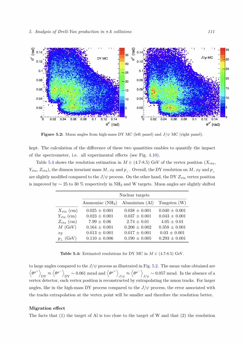
5. Analysis of Drell-Yan production in πA collisions 111
Figure 5.2: Muon angles from high-mass DY MC (left panel) and J/ψ MC (right panel).
kept. The calculation of the difference of these two quantities enables to quantify the impactof the spectrometer, i.e. all experimental effects (see Fig. 4.10).
Table 5.4 shows the resolution estimation in M ∈ (4.7-8.5) GeV of the vertex position (Xvtx,Yvtx, Zvtx), the dimuon invariant massM , xF and p⊥ . Overall, the DY resolution onM , xF and p⊥are slightly modified compared to the J/ψ process. On the other hand, the DY Zvtx vertex positionis improved by ∼ 25 to 30 % respectively in NH3 and W targets. Muon angles are slightly shifted
Nuclear targetsAmmoniac (NH3) Aluminium (Al) Tungsten (W)
Xvtx (cm) 0.025 ± 0.001 0.038 ± 0.001 0.040 ± 0.001Yvtx (cm) 0.023 ± 0.001 0.037 ± 0.001 0.043 ± 0.001Zvtx (cm) 7.99 ± 0.06 2.74 ± 0.01 4.05 ± 0.01M (GeV) 0.164 ± 0.001 0.206 ± 0.002 0.358 ± 0.001xF 0.013 ± 0.001 0.017 ± 0.001 0.03 ± 0.001p⊥ (GeV) 0.110 ± 0.006 0.190 ± 0.005 0.293 ± 0.001
Table 5.4: Estimated resolutions for DY MC in M ∈ (4.7-8.5) GeV.
to large angles compared to the J/ψ process as illustrated in Fig. 5.2. The mean value obtained are⟨θµ
+⟩DY≈⟨θµ−⟩DY∼ 0.061 mrad and
⟨θµ
+⟩J/ψ≈⟨θµ−⟩J/ψ∼ 0.057 mrad. In the absence of a
vertex detector, each vertex position is reconstructed by extrapolating the muon tracks. For largerangles, like in the high-mass DY process compared to the J/ψ process, the error associated withthe tracks extrapolation at the vertex point will be smaller and therefore the resolution better.
Migration effectThe facts that (1) the target of Al is too close to the target of W and that (2) the resolution
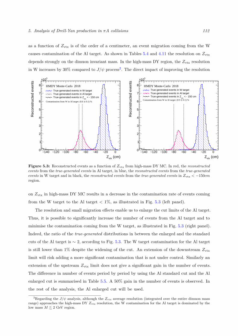
5. Analysis of Drell-Yan production in πA collisions 112
as a function of Zvtx is of the order of a centimeter, an event migration coming from the W
causes contamination of the Al target. As shown in Tables 5.4 and 4.11 the resolution on Zvtx
depends strongly on the dimuon invariant mass. In the high-mass DY region, the Zvtx resolution
in W increases by 30% compared to J/ψ process2. The direct impact of improving the resolution
140− 120− 100− 80− 60− 40− 20− 0
(cm)vtxZ
0
1
2
3
4
5
6
7
8
310×
Rec
onst
ruct
ed e
vent
s
HMDY Monte-Carlo 2018
0.1) %±Contamination from W in Al target: (0.6
True-generated events in W targetTrue-generated events in Al target
< - 150 cmvtx
True-generated events in Z
140− 120− 100− 80− 60− 40− 20− 0
(cm)vtxZ
0
1
2
3
4
5
6
7
8
310×
Rec
onst
ruct
ed e
vent
s
HMDY Monte-Carlo 2018
0.1) %±Contamination from W in Al target: (0.9
True-generated events in W targetTrue-generated events in Al target
< - 150 cmvtx
True-generated events in Z
Figure 5.3: Reconstructed events as a function of Zvtx from high-mass DY MC. In red, the reconstructedevents from the true-generated events in Al target, in blue, the reconstructed events from the true-generatedevents in W target and in black, the reconstructed events from the true-generated events in Zvtx < −150cmregion.
on Zvtx in high-mass DY MC results in a decrease in the contamination rate of events coming
from the W target to the Al target < 1%, as illustrated in Fig. 5.3 (left panel).
The resolution and small migration effects enable us to enlarge the cut limits of the Al target.
Thus, it is possible to significantly increase the number of events from the Al target and to
minimise the contamination coming from the W target, as illustrated in Fig. 5.3 (right panel).
Indeed, the ratio of the true-generated distributions in between the enlarged and the standard
cuts of the Al target is ∼ 2, according to Fig. 5.3. The W target contamination for the Al target
is still lower than 1% despite the widening of the cut. An extension of the downstream Zvtx
limit will risk adding a more significant contamination that is not under control. Similarly an
extension of the upstream Zvtx limit does not give a significant gain in the number of events.
The difference in number of events period by period by using the Al standard cut and the Al
enlarged cut is summarised in Table 5.5. A 50% gain in the number of events is observed. In
the rest of the analysis, the Al enlarged cut will be used.
2Regarding the J/ψ analysis, although the Zvtx average resolution (integrated over the entire dimuon massrange) approaches the high-mass DY Zvtx resolution, the W contamination for the Al target is dominated by thelow mass M . 2 GeV region.
5. Analysis of Drell-Yan production in πA collisions 113
Selections P00 P01 P02 P03 P04 P05 P06 P07 P08Al target selection -73.5 < Zzvtx < -66.5 cm
4.7 < M < 8.5 GeV 326 244 500 384 289 223 256 401 171Al enlarge target selection -80 < Zzvtx < -60 cm
4.7 < M < 8.5 GeV 696 462 999 756 590 455 512 832 320
Table 5.5: The statistics of dimuon events period by period for the Al target after applying the dimuonmass cut.
5.2.3 Validity of the Monte-Carlo simulation
In order to ensure the validity of the MC in this analysis, a comparison between the high-massDY MC and the Real Data (RD) is mandatory. The comparison must be made for identicalkinematics conditions. Therefore, the same kinematic cuts are applied both in the reconstructedevents from the high-mass DY MC and in the RD (Tables 4.1 and 5.5).
W targetFigure 5.4 shows the comparison between the MC and RD data as a function of xF (left panel)and p⊥ (right panel) for the W target. All distributions are normalised according to their integral.In this way, it is possible to get rid of the luminosity factor in the simulation and to controlthe shape of the distributions directly. The agreement between MC and RD data is satisfactory(less than 10% disagreement) in most of the xF range. Except at very large xF & 0.8, where thedisagreement reaches approximately 20%. We note that the agreement between MC and RD asa function of p⊥ is also reasonable.3 A disagreement by 10-20% is observed for p⊥ . 0.5 GeVand p⊥ ∼ 2-2.5 GeV. Overall, the generated phase space is in good agreement with the RD.
Al targetFigure 5.5 shows the comparison between the MC and RD as a function of xF (left panel) andp⊥ (right panel) for the Al target. The same observations can be made compared to the Wtarget. The disagreement between MC and RD for the Al target is slightly more pronouncedcompared to the W target. Overall, the agreement is satisfactory.
5.3 Drell-Yan cross section
After extracting the number of DY events as a function of xF and p⊥ , these distributions must becorrected for the acceptance of the spectrometer as well for the luminosity factor. The differentsteps to determine the DY cross section are detailed below.
3The tuning of the p⊥ spectrum in order to improve the agreement between the MC and RD has not beencarried out within the framework of this thesis work.

5. Analysis of Drell-Yan production in πA collisions 114
0
0.02
0.04
0.06
0.08
0.1
(no
rmal
ized
)µ µ
N
Monte-Carlo
COMPASS data
(LasLas || LasOuter) triggers < 8.5 GeV+µ -µ4.7 < M
W target
0 0.1 0.2 0.3 0.4 0.5 0.6 0.7 0.8 0.9
Fx
0.60.8
11.21.4
MC
/RD
0
0.05
0.1
0.15
0.2
0.25
0.3
(no
rmal
ized
)µ µ
N
Monte-Carlo
COMPASS data
(LasLas || LasOuter) triggers < 8.5 GeV+µ -µ4.7 < M
W target
0 0.5 1 1.5 2 2.5 3 3.5 4
(GeV)p
0.60.8
11.21.4
MC
/RD
Figure 5.4: Comparison between MC and RD for the xF (left panel) and p⊥ (right panel) distributionsfor the W target.
0
0.02
0.04
0.06
0.08
0.1
(no
rmal
ized
)µ µ
N
Monte-Carlo
COMPASS data
(LasLas || LasOuter) triggers < 8.5 GeV+µ -µ4.7 < M
< -60 cmvtx
Al target, -80 < Z
0 0.1 0.2 0.3 0.4 0.5 0.6 0.7 0.8 0.9
Fx
0.60.8
11.21.4
MC
/RD
0
0.05
0.1
0.15
0.2
0.25
0.3
0.35
(no
rmal
ized
)µ µ
N
Monte-Carlo
COMPASS data
(LasLas || LasOuter) triggers < 8.5 GeV+µ -µ4.7 < M
< -60 cmvtx
Al target, -80 < Z
0 0.5 1 1.5 2 2.5 3 3.5 4
(GeV)p
0.60.8
11.21.4
MC
/RD
Figure 5.5: Comparison between MC and RD for the xF (left panel) and p⊥ (right panel) distributionsfor the Al target.
5.3.1 2D acceptance as a function of xF and p⊥
The 2D acceptance as a function of xF and p⊥ including both geometrical acceptance, triggerefficiencies and resolution effects of the spectrometer is defined as
εxF,p⊥ = N(xF, p⊥)recMC
N(xF, p⊥)genMC
, (5.3)
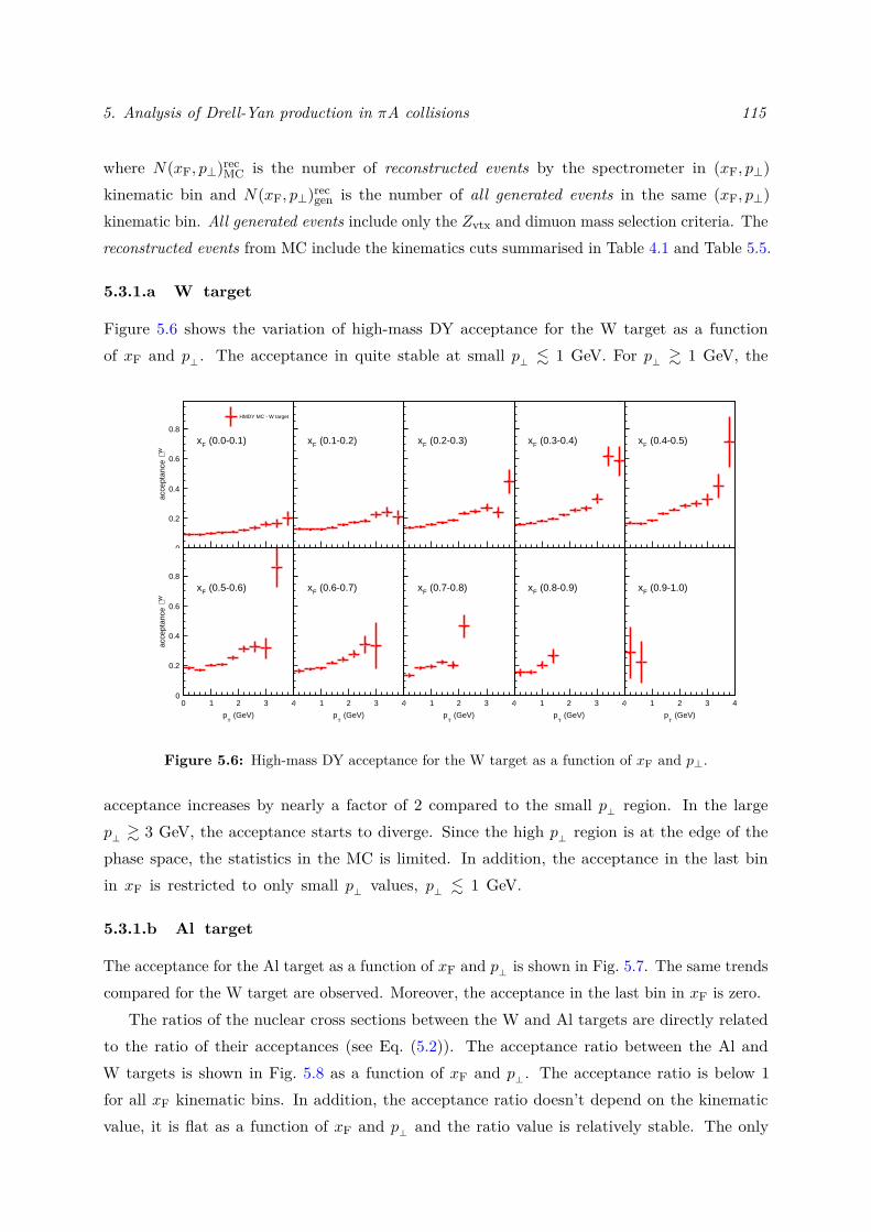
5. Analysis of Drell-Yan production in πA collisions 115
where N(xF, p⊥)recMC is the number of reconstructed events by the spectrometer in (xF, p⊥)
kinematic bin and N(xF, p⊥)recgen is the number of all generated events in the same (xF, p⊥)
kinematic bin. All generated events include only the Zvtx and dimuon mass selection criteria. Thereconstructed events from MC include the kinematics cuts summarised in Table 4.1 and Table 5.5.
5.3.1.a W target
Figure 5.6 shows the variation of high-mass DY acceptance for the W target as a functionof xF and p⊥ . The acceptance in quite stable at small p⊥ . 1 GeV. For p⊥ & 1 GeV, the
0 1 2 3 4
(GeV)T
p
0
0.2
0.4
0.6
0.8
W ∈ac
cept
ance
(0.5-0.6)Fx
0 1 2 3 4 (GeV)
Tp
0
0.2
0.4
0.6
0.8
W ∈ac
cept
ance
(0.0-0.1)Fx
HMDY MC - W target
0 1 2 3 4
(GeV)T
p
0
0.2
0.4
0.6
0.8
W ∈ac
cept
ance
(0.6-0.7)Fx
0 1 2 3 4 (GeV)
Tp
0
0.2
0.4
0.6
0.8
W ∈ac
cept
ance
(0.1-0.2)Fx
0 1 2 3 4
(GeV)T
p
0
0.2
0.4
0.6
0.8
W ∈ac
cept
ance
(0.7-0.8)Fx
0 1 2 3 4 (GeV)
Tp
0
0.2
0.4
0.6
0.8
W ∈ac
cept
ance
(0.2-0.3)Fx
0 1 2 3 4
(GeV)T
p
0
0.2
0.4
0.6
0.8
W ∈ac
cept
ance
(0.8-0.9)Fx
0 1 2 3 4 (GeV)
Tp
0
0.2
0.4
0.6
0.8
W ∈ac
cept
ance
(0.3-0.4)Fx
0 1 2 3 4
(GeV)T
p
0
0.2
0.4
0.6
0.8
W ∈ac
cept
ance
(0.9-1.0)Fx
0 1 2 3 4 (GeV)
Tp
0
0.2
0.4
0.6
0.8
W ∈ac
cept
ance
(0.4-0.5)Fx
Figure 5.6: High-mass DY acceptance for the W target as a function of xF and p⊥.
acceptance increases by nearly a factor of 2 compared to the small p⊥ region. In the largep⊥ & 3 GeV, the acceptance starts to diverge. Since the high p⊥ region is at the edge of thephase space, the statistics in the MC is limited. In addition, the acceptance in the last binin xF is restricted to only small p⊥ values, p⊥ . 1 GeV.
5.3.1.b Al target
The acceptance for the Al target as a function of xF and p⊥ is shown in Fig. 5.7. The same trendscompared for the W target are observed. Moreover, the acceptance in the last bin in xF is zero.
The ratios of the nuclear cross sections between the W and Al targets are directly relatedto the ratio of their acceptances (see Eq. (5.2)). The acceptance ratio between the Al andW targets is shown in Fig. 5.8 as a function of xF and p⊥ . The acceptance ratio is below 1for all xF kinematic bins. In addition, the acceptance ratio doesn’t depend on the kinematicvalue, it is flat as a function of xF and p⊥ and the ratio value is relatively stable. The only
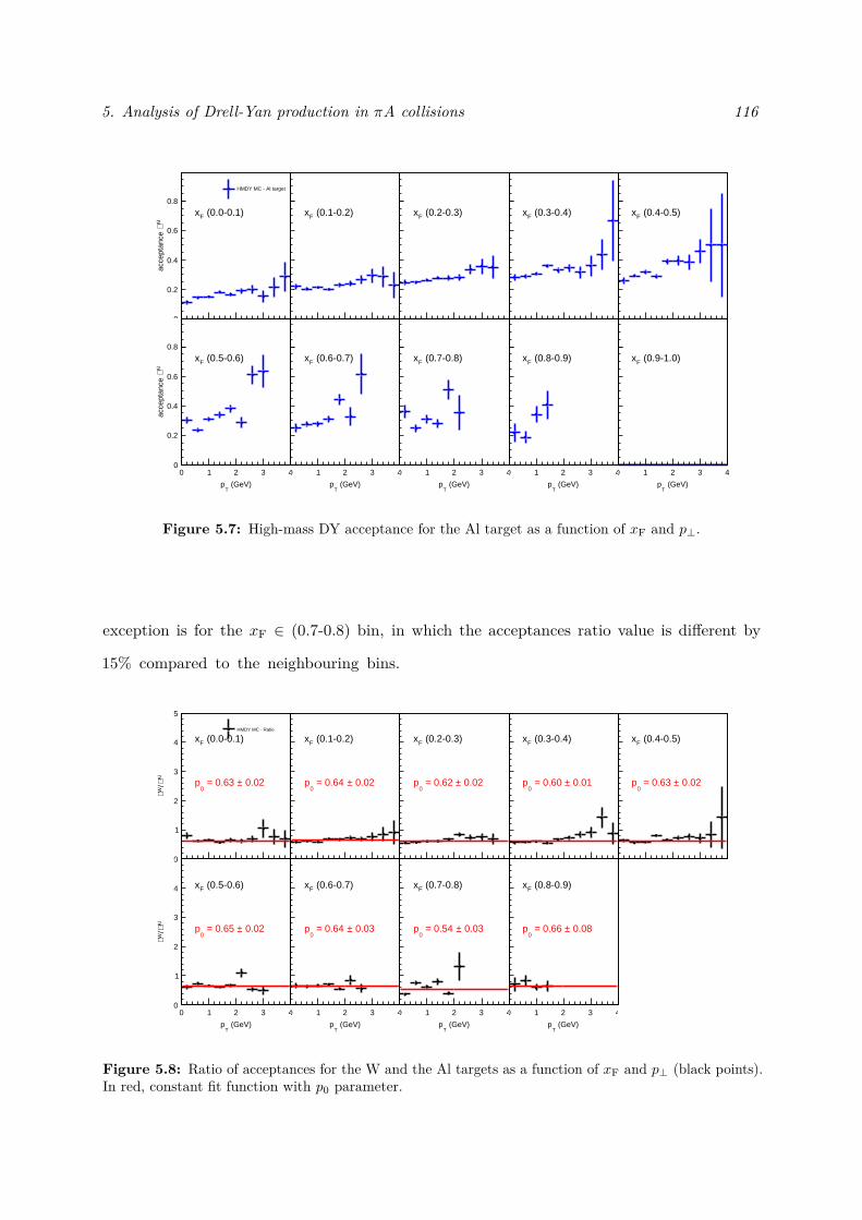
5. Analysis of Drell-Yan production in πA collisions 116
0 1 2 3 4
(GeV)T
p
0
0.2
0.4
0.6
0.8
Al
∈ac
cept
ance
(0.5-0.6)Fx
0 1 2 3 4 (GeV)
Tp
0
0.2
0.4
0.6
0.8
Al
∈ac
cept
ance
(0.0-0.1)Fx
HMDY MC - Al target
0 1 2 3 4
(GeV)T
p
0
0.2
0.4
0.6
0.8
Al
∈ac
cept
ance
(0.6-0.7)Fx
0 1 2 3 4 (GeV)
Tp
0
0.2
0.4
0.6
0.8
Al
∈ac
cept
ance
(0.1-0.2)Fx
0 1 2 3 4
(GeV)T
p
0
0.2
0.4
0.6
0.8
Al
∈ac
cept
ance
(0.7-0.8)Fx
0 1 2 3 4 (GeV)
Tp
0
0.2
0.4
0.6
0.8
Al
∈ac
cept
ance
(0.2-0.3)Fx
0 1 2 3 4
(GeV)T
p
0
0.2
0.4
0.6
0.8
Al
∈ac
cept
ance
(0.8-0.9)Fx
0 1 2 3 4 (GeV)
Tp
0
0.2
0.4
0.6
0.8
Al
∈ac
cept
ance
(0.3-0.4)Fx
0 1 2 3 4
(GeV)T
p
0
0.2
0.4
0.6
0.8
Al
∈ac
cept
ance
(0.9-1.0)Fx
0 1 2 3 4 (GeV)
Tp
0
0.2
0.4
0.6
0.8
Al
∈ac
cept
ance
(0.4-0.5)Fx
Figure 5.7: High-mass DY acceptance for the Al target as a function of xF and p⊥.
exception is for the xF ∈ (0.7-0.8) bin, in which the acceptances ratio value is different by
15% compared to the neighbouring bins.
0 1 2 3 4
(GeV)T
p
0
1
2
3
4
5
Al
∈/W ∈
(0.5-0.6)Fx
0.02± = 0.65 0
p
0 1 2 3 4 (GeV)
Tp
0
1
2
3
4
5
Al
∈/W ∈
(0.0-0.1)Fx
0.02± = 0.63 0
p
HMDY MC - Ratio
0 1 2 3 4
(GeV)T
p
0
1
2
3
4
5
Al
∈/W ∈
(0.6-0.7)Fx
0.03± = 0.64 0
p
0 1 2 3 4 (GeV)
Tp
0
1
2
3
4
5
Al
∈/W ∈
(0.1-0.2)Fx
0.02± = 0.64 0
p
0 1 2 3 4
(GeV)T
p
0
1
2
3
4
5
Al
∈/W ∈
(0.7-0.8)Fx
0.03± = 0.54 0
p
0 1 2 3 4 (GeV)
Tp
0
1
2
3
4
5
Al
∈/W ∈
(0.2-0.3)Fx
0.02± = 0.62 0
p
0 1 2 3 4
(GeV)T
p
0
1
2
3
4
5
Al
∈/W ∈
(0.8-0.9)Fx
0.08± = 0.66 0
p
0 1 2 3 4 (GeV)
Tp
0
1
2
3
4
5
Al
∈/W ∈
(0.3-0.4)Fx
0.01± = 0.60 0
p
0 1 2 3 4 (GeV)
Tp
0
1
2
3
4
5
Al
∈/W ∈
(0.4-0.5)Fx
0.02± = 0.63 0
p
Figure 5.8: Ratio of acceptances for the W and the Al targets as a function of xF and p⊥ (black points).In red, constant fit function with p0 parameter.
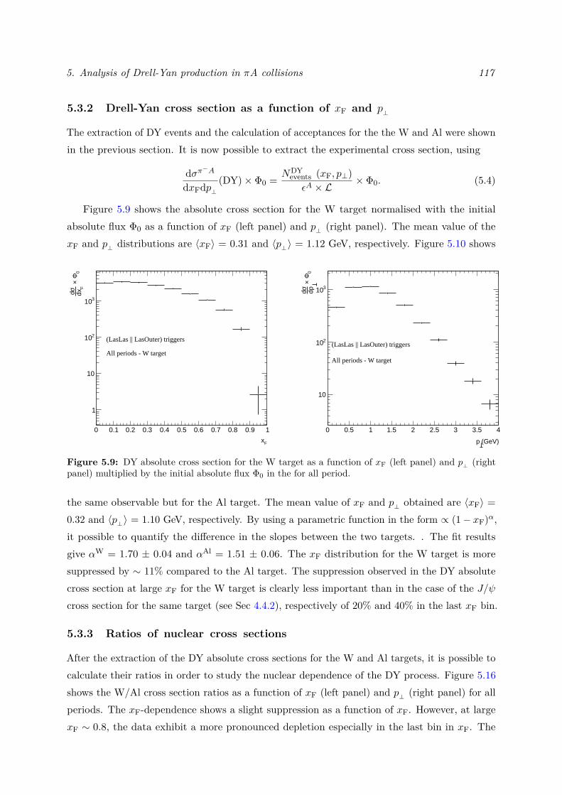
5. Analysis of Drell-Yan production in πA collisions 117
5.3.2 Drell-Yan cross section as a function of xF and p⊥
The extraction of DY events and the calculation of acceptances for the the W and Al were shownin the previous section. It is now possible to extract the experimental cross section, using
dσπ−AdxFdp⊥
(DY)× Φ0 = NDYevents (xF, p⊥)εA × L
× Φ0. (5.4)
Figure 5.9 shows the absolute cross section for the W target normalised with the initialabsolute flux Φ0 as a function of xF (left panel) and p⊥ (right panel). The mean value of thexF and p⊥ distributions are 〈xF〉 = 0.31 and 〈p⊥〉 = 1.12 GeV, respectively. Figure 5.10 shows
0 0.1 0.2 0.3 0.4 0.5 0.6 0.7 0.8 0.9 1
Fx
1
10
210
310
0Φ ×
Fdx
σd
All periods - W target
(LasLas || LasOuter) triggers
0 0.5 1 1.5 2 2.5 3 3.5 4
(GeV)p
10
210
310
0Φ ×
dpσd
All periods - W target
(LasLas || LasOuter) triggers
Figure 5.9: DY absolute cross section for the W target as a function of xF (left panel) and p⊥ (rightpanel) multiplied by the initial absolute flux Φ0 in the for all period.
the same observable but for the Al target. The mean value of xF and p⊥ obtained are 〈xF〉 =0.32 and 〈p⊥〉 = 1.10 GeV, respectively. By using a parametric function in the form ∝ (1− xF)α,it possible to quantify the difference in the slopes between the two targets. . The fit resultsgive αW = 1.70 ± 0.04 and αAl = 1.51 ± 0.06. The xF distribution for the W target is moresuppressed by ∼ 11% compared to the Al target. The suppression observed in the DY absolutecross section at large xF for the W target is clearly less important than in the case of the J/ψcross section for the same target (see Sec 4.4.2), respectively of 20% and 40% in the last xF bin.
5.3.3 Ratios of nuclear cross sections
After the extraction of the DY absolute cross sections for the W and Al targets, it is possible tocalculate their ratios in order to study the nuclear dependence of the DY process. Figure 5.16shows the W/Al cross section ratios as a function of xF (left panel) and p⊥ (right panel) for allperiods. The xF-dependence shows a slight suppression as a function of xF. However, at largexF ∼ 0.8, the data exhibit a more pronounced depletion especially in the last bin in xF. The
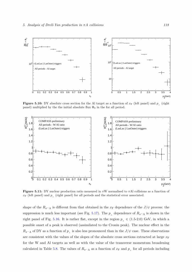
5. Analysis of Drell-Yan production in πA collisions 118
0 0.1 0.2 0.3 0.4 0.5 0.6 0.7 0.8 0.9 1
Fx
310
0Φ ×
Fdx
σd
All periods - Al target
(LasLas || LasOuter) triggers
0 0.5 1 1.5 2 2.5 3 3.5 4
(GeV)p
10
210
310
0Φ ×
dpσd
All periods - Al target
(LasLas || LasOuter) triggers
Figure 5.10: DY absolute cross section for the Al target as a function of xF (left panel) and p⊥ (rightpanel) multiplied by the the initial absolute flux Φ0 in the for all period.
0 0.1 0.2 0.3 0.4 0.5 0.6 0.7 0.8 0.9 1
Fx
0
0.2
0.4
0.6
0.8
1
1.2
1.4
1.6
1.8
2
(W/A
l)D
Y AπR
COMPASS preliminaryAll periods - W/Al ratio(LasLas || LasOuter) triggers
0 0.5 1 1.5 2 2.5 3 3.5 4
(GeV)p
0
0.2
0.4
0.6
0.8
1
1.2
1.4
1.6
1.8
2
(W/A
l)D
Y AπR
COMPASS preliminaryAll periods - W/Al ratio(LasLas || LasOuter) triggers
Figure 5.11: DY nuclear production ratio measured in πW normalised to πAl collisions as a function ofxF (left panel) and p⊥ (right panel) for all periods and the statistical error associated.
shape of the Rπ−A is different from that obtained in the xF dependence of the J/ψ process: thesuppression is much less important (see Fig. 5.17). The p⊥ dependence of Rπ−A is shown in theright panel of Fig. 5.16. It is rather flat, except in the region p⊥ ∈ (1.5-2.0) GeV, in which apossible onset of a peak is observed (assimilated to the Cronin peak). The nuclear effect in theRπ−A of DY as a function of p⊥ is also less pronounced than in the J/ψ case. These observationsare consistent with the values of the slopes of the absolute cross sections extracted at large xFfor the W and Al targets as well as with the value of the transverse momentum broadeningcalculated in Table 5.8. The values of Rπ−A as a function of xF and p⊥ for all periods including
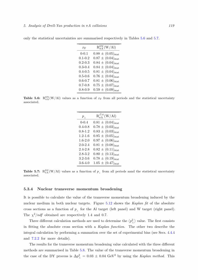
5. Analysis of Drell-Yan production in πA collisions 119
only the statistical uncertainties are summarised respectively in Tables 5.6 and 5.7.
xF RDYπA (W/Al)
0-0.1 0.88 ± (0.05)stat0.1-0.2 0.87 ± (0.04)stat0.2-0.3 0.84 ± (0.04)stat0.3-0.4 0.84 ± (0.04)stat0.4-0.5 0.81 ± (0.04)stat0.5-0.6 0.76 ± (0.04)stat0.6-0.7 0.81 ± (0.06)stat0.7-0.8 0.75 ± (0.07)stat0.8-0.9 0.59 ± (0.09)stat
Table 5.6: RDYπA (W/Al) values as a function of xF from all periods and the statistical uncertainty
associated.
p⊥ RJ/ψπA (W/Al)0-0.4 0.81 ± (0.04)stat0.4-0.8 0.78 ± (0.03)stat0.8-1.2 0.83 ± (0.03)stat1.2-1.6 0.85 ± (0.05)stat1.6-2.0 0.97 ± (0.06)stat2.0-2.4 0.81 ± (0.08)stat2.4-2.8 0.82 ± (0.11)stat2.8-3.2 0.80 ± (0.13)stat3.2-3.6 0.78 ± (0.19)stat3.6-4.0 1.05 ± (0.47)stat
Table 5.7: RDYπA (W/Al) values as a function of p⊥ from all periods aand the statistical uncertainty
associated.
5.3.4 Nuclear transverse momentum broadening
It is possible to calculate the value of the transverse momentum broadening induced by thenuclear medium in both nuclear targets. Figure 5.12 shows the Kaplan fit of the absolutecross sections as a function of p⊥ for the Al target (left panel) and W target (right panel).The χ2/ndf obtained are respectively 1.4 and 0.7.
Three different calculation methods are used to determine the⟨p2⊥⟩value. The first consists
in fitting the absolute cross section with a Kaplan function. The other two describe theintegral calculation by performing a summation over the set of experimental bins (see Secs. 4.4.4and 7.2.2 for more details).
The results for the transverse momentum broadening value calculated with the three differentmethods are summarised in Table 5.8. The value of the transverse momentum broadening inthe case of the DY process is ∆p2
⊥ = 0.03 ± 0.04 GeV2 by using the Kaplan method. This
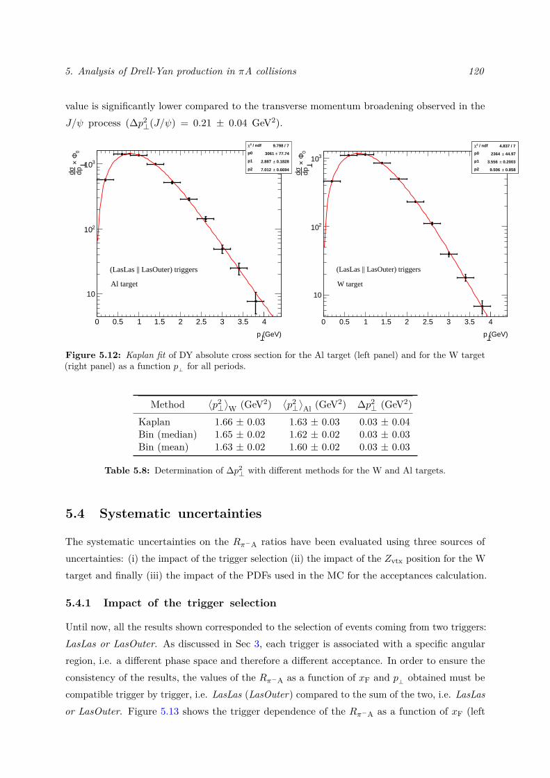
5. Analysis of Drell-Yan production in πA collisions 120
value is significantly lower compared to the transverse momentum broadening observed in theJ/ψ process (∆p2
⊥(J/ψ) = 0.21 ± 0.04 GeV2).
0 0.5 1 1.5 2 2.5 3 3.5 4
(GeV)p
10
210
310
0Φ ×
dpσd
/ ndf 2χ 9.798 / 7
p0 77.74± 3061
p1 0.1828± 2.887
p2 0.6694± 7.012
/ ndf 2χ 9.798 / 7
p0 77.74± 3061
p1 0.1828± 2.887
p2 0.6694± 7.012
(LasLas || LasOuter) triggers
Al target
0 0.5 1 1.5 2 2.5 3 3.5 4
(GeV)p
10
210
310
0Φ ×
dpσd
/ ndf 2χ 4.837 / 7
p0 44.97± 2364
p1 0.2003± 3.556
p2 0.858± 9.506
/ ndf 2χ 4.837 / 7
p0 44.97± 2364
p1 0.2003± 3.556
p2 0.858± 9.506
(LasLas || LasOuter) triggers
W target
Figure 5.12: Kaplan fit of DY absolute cross section for the Al target (left panel) and for the W target(right panel) as a function p⊥ for all periods.
Method⟨p2⊥⟩W (GeV2)
⟨p2⊥⟩Al (GeV2) ∆p2
⊥ (GeV2)Kaplan 1.66 ± 0.03 1.63 ± 0.03 0.03 ± 0.04Bin (median) 1.65 ± 0.02 1.62 ± 0.02 0.03 ± 0.03Bin (mean) 1.63 ± 0.02 1.60 ± 0.02 0.03 ± 0.03
Table 5.8: Determination of ∆p2⊥ with different methods for the W and Al targets.
5.4 Systematic uncertainties
The systematic uncertainties on the Rπ−A ratios have been evaluated using three sources ofuncertainties: (i) the impact of the trigger selection (ii) the impact of the Zvtx position for the Wtarget and finally (iii) the impact of the PDFs used in the MC for the acceptances calculation.
5.4.1 Impact of the trigger selection
Until now, all the results shown corresponded to the selection of events coming from two triggers:LasLas or LasOuter. As discussed in Sec 3, each trigger is associated with a specific angularregion, i.e. a different phase space and therefore a different acceptance. In order to ensure theconsistency of the results, the values of the Rπ−A as a function of xF and p⊥ obtained must becompatible trigger by trigger, i.e. LasLas (LasOuter) compared to the sum of the two, i.e. LasLasor LasOuter. Figure 5.13 shows the trigger dependence of the Rπ−A as a function of xF (left
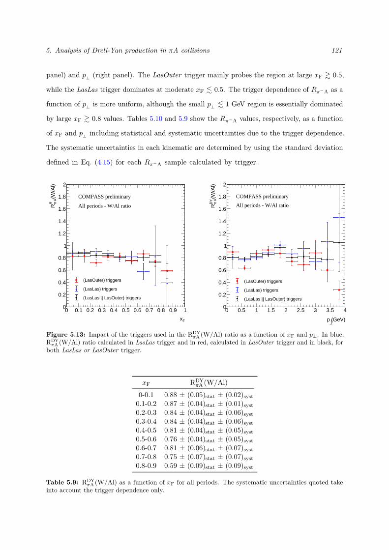
5. Analysis of Drell-Yan production in πA collisions 121
panel) and p⊥ (right panel). The LasOuter trigger mainly probes the region at large xF & 0.5,
while the LasLas trigger dominates at moderate xF . 0.5. The trigger dependence of Rπ−A as a
function of p⊥ is more uniform, although the small p⊥ . 1 GeV region is essentially dominated
by large xF & 0.8 values. Tables 5.10 and 5.9 show the Rπ−A values, respectively, as a function
of xF and p⊥ including statistical and systematic uncertainties due to the trigger dependence.
The systematic uncertainties in each kinematic are determined by using the standard deviation
defined in Eq. (4.15) for each Rπ−A sample calculated by trigger.
0 0.1 0.2 0.3 0.4 0.5 0.6 0.7 0.8 0.9 1
Fx
0
0.2
0.4
0.6
0.8
1
1.2
1.4
1.6
1.8
2
(W/A
l)ψ Aπ
R
COMPASS preliminary
All periods - W/Al ratio
(LasOuter) triggers
(LasLas) triggers
(LasLas || LasOuter) triggers
0 0.5 1 1.5 2 2.5 3 3.5 4
(GeV)p
0
0.2
0.4
0.6
0.8
1
1.2
1.4
1.6
1.8
2
(W/A
l)D
Y AπR
COMPASS preliminary
All periods - W/Al ratio
(LasOuter) triggers
(LasLas) triggers
(LasLas || LasOuter) triggers
Figure 5.13: Impact of the triggers used in the RDYπA (W/Al) ratio as a function of xF and p⊥. In blue,
RDYπA (W/Al) ratio calculated in LasLas trigger and in red, calculated in LasOuter trigger and in black, for
both LasLas or LasOuter trigger.
xF RDYπA (W/Al)
0-0.1 0.88 ± (0.05)stat ± (0.02)syst0.1-0.2 0.87 ± (0.04)stat ± (0.01)syst0.2-0.3 0.84 ± (0.04)stat ± (0.06)syst0.3-0.4 0.84 ± (0.04)stat ± (0.06)syst0.4-0.5 0.81 ± (0.04)stat ± (0.05)syst0.5-0.6 0.76 ± (0.04)stat ± (0.05)syst0.6-0.7 0.81 ± (0.06)stat ± (0.07)syst0.7-0.8 0.75 ± (0.07)stat ± (0.07)syst0.8-0.9 0.59 ± (0.09)stat ± (0.09)syst
Table 5.9: RDYπA (W/Al) as a function of xF for all periods. The systematic uncertainties quoted take
into account the trigger dependence only.
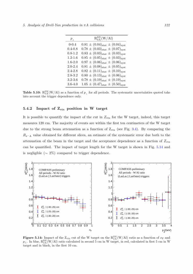
5. Analysis of Drell-Yan production in πA collisions 122
p⊥ RDYπA (W/Al)
0-0.4 0.81 ± (0.04)stat ± (0.04)syst0.4-0.8 0.78 ± (0.03)stat ± (0.07)syst0.8-1.2 0.83 ± (0.03)stat ± (0.03)syst1.2-1.6 0.85 ± (0.05)stat ± (0.03)syst1.6-2.0 0.97 ± (0.06)stat ± (0.06)syst2.0-2.4 0.81 ± (0.08)stat ± (0.05)syst2.4-2.8 0.82 ± (0.11)stat ± (0.10)syst2.8-3.2 0.80 ± (0.13)stat ± (0.06)syst3.2-3.6 0.78 ± (0.19)stat ± (0.19)syst3.6-4.0 1.05 ± (0.47)stat ± (0.50)syst
Table 5.10: RDYπA (W/Al) as a function of p⊥ for all periods. The systematic uncertainties quoted take
into account the trigger dependence only.
5.4.2 Impact of Zvtx position in W target
It is possible to quantify the impact of the cut in Zvtx for the W target, indeed, this targetmeasures 120 cm. The majority of events are within the first ten centimeters of the W targetdue to the strong beam attenuation as a function of Zvtx (see Fig. 3.4). By comparing theRπ−A value obtained for different slices, an estimate of the systematic error due both to theattenuation of the beam in the target and the acceptance dependence as a function of Zvtx
can be quantified. The impact of target length for the W target is shown in Fig. 5.14 andis negligible (∼ 2%) compared to trigger dependence.
0 0.1 0.2 0.3 0.4 0.5 0.6 0.7 0.8 0.9 1
Fx
0
0.2
0.4
0.6
0.8
1
1.2
1.4
1.6
1.8
2
(W/A
l)D
Y AπR
COMPASS preliminaryAll periods - W/Al ratio(LasLas || LasOuter) triggers
(-30;-25) cm∈ WvtxZ
(-25;-20) cm∈ WvtxZ
(-30;-20) cm∈ WvtxZ
0 0.5 1 1.5 2 2.5 3 3.5 4
(GeV)p
0
0.2
0.4
0.6
0.8
1
1.2
1.4
1.6
1.8
2
(W/A
l)D
Y AπR
COMPASS preliminaryAll periods - W/Al ratio(LasLas || LasOuter) triggers
(-30;-25) cm∈ WvtxZ
(-25;-20) cm∈ WvtxZ
(-30;-20) cm∈ WvtxZ
Figure 5.14: Impact of the Zvtx cut of the W target on the RDYπA (W/Al) ratio as a function of xF and
p⊥. In blue, RDYπA (W/Al) ratio calculated in second 5 cm in W target, in red, calculated in first 5 cm in W
target and in black, in the first 10 cm.
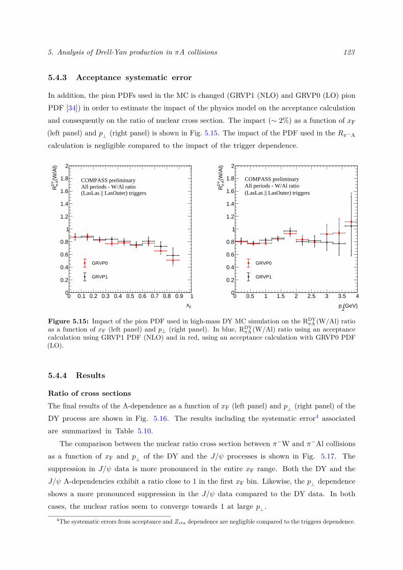
5. Analysis of Drell-Yan production in πA collisions 123
5.4.3 Acceptance systematic error
In addition, the pion PDFs used in the MC is changed (GRVP1 (NLO) and GRVP0 (LO) pionPDF [34]) in order to estimate the impact of the physics model on the acceptance calculationand consequently on the ratio of nuclear cross section. The impact (∼ 2%) as a function of xF(left panel) and p⊥ (right panel) is shown in Fig. 5.15. The impact of the PDF used in the Rπ−A
calculation is negligible compared to the impact of the trigger dependence.
0 0.1 0.2 0.3 0.4 0.5 0.6 0.7 0.8 0.9 1
Fx
0
0.2
0.4
0.6
0.8
1
1.2
1.4
1.6
1.8
2
(W/A
l)D
Y AπR
COMPASS preliminaryAll periods - W/Al ratio(LasLas || LasOuter) triggers
GRVP0
GRVP1
0 0.5 1 1.5 2 2.5 3 3.5 4
(GeV)p
0
0.2
0.4
0.6
0.8
1
1.2
1.4
1.6
1.8
2
(W/A
l)D
Y AπR
COMPASS preliminaryAll periods - W/Al ratio(LasLas || LasOuter) triggers
GRVP0
GRVP1
Figure 5.15: Impact of the pion PDF used in high-mass DY MC simulation on the RDYπA (W/Al) ratio
as a function of xF (left panel) and p⊥ (right panel). In blue, RDYπA (W/Al) ratio using an acceptance
calculation using GRVP1 PDF (NLO) and in red, using an acceptance calculation with GRVP0 PDF(LO).
5.4.4 Results
Ratio of cross sectionsThe final results of the A-dependence as a function of xF (left panel) and p⊥ (right panel) of theDY process are shown in Fig. 5.16. The results including the systematic error4 associatedare summarized in Table 5.10.
The comparison between the nuclear ratio cross section between π−W and π−Al collisionsas a function of xF and p⊥ of the DY and the J/ψ processes is shown in Fig. 5.17. Thesuppression in J/ψ data is more pronounced in the entire xF range. Both the DY and theJ/ψ A-dependencies exhibit a ratio close to 1 in the first xF bin. Likewise, the p⊥ dependenceshows a more pronounced suppression in the J/ψ data compared to the DY data. In bothcases, the nuclear ratios seem to converge towards 1 at large p⊥ .
4The systematic errors from acceptance and Zvtx dependence are negligible compared to the triggers dependence.
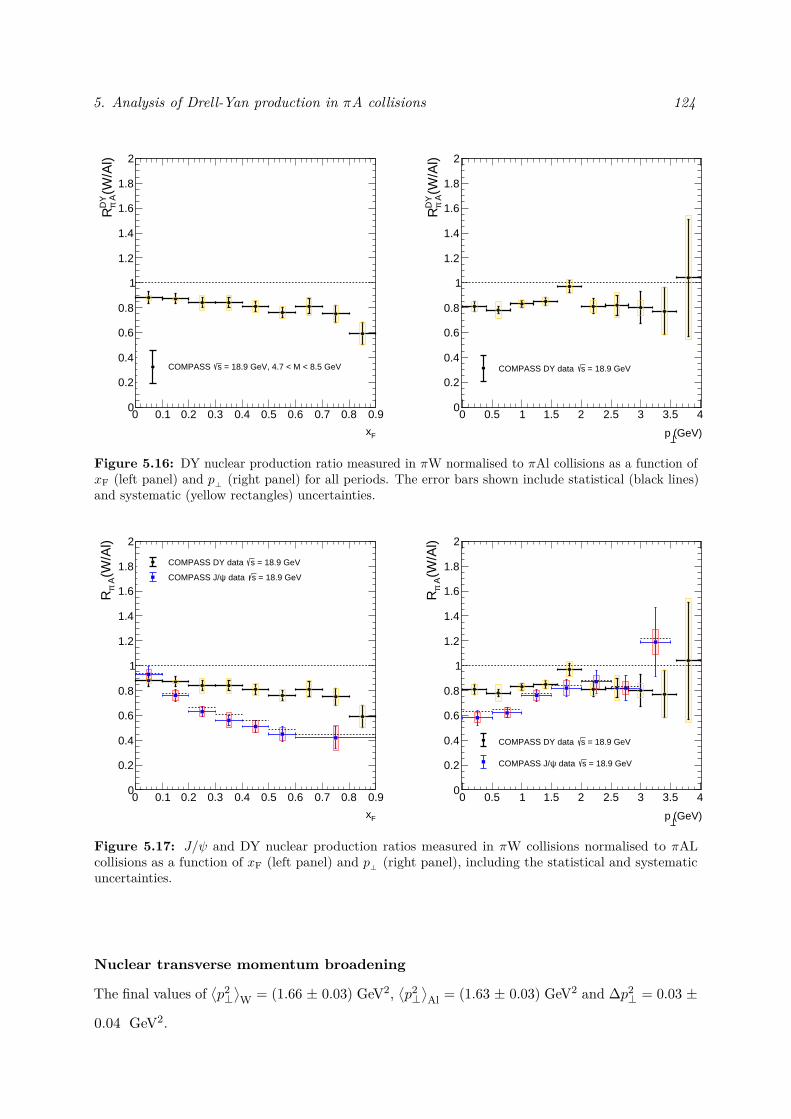
5. Analysis of Drell-Yan production in πA collisions 124
0 0.1 0.2 0.3 0.4 0.5 0.6 0.7 0.8 0.9
Fx
0
0.2
0.4
0.6
0.8
1
1.2
1.4
1.6
1.8
2
(W/A
l)D
Y AπR
= 18.9 GeV, 4.7 < M < 8.5 GeVsCOMPASS
0 0.5 1 1.5 2 2.5 3 3.5 4
(GeV)p
0
0.2
0.4
0.6
0.8
1
1.2
1.4
1.6
1.8
2
(W/A
l)D
Y AπR
= 18.9 GeVsCOMPASS DY data
Figure 5.16: DY nuclear production ratio measured in πW normalised to πAl collisions as a function ofxF (left panel) and p⊥ (right panel) for all periods. The error bars shown include statistical (black lines)and systematic (yellow rectangles) uncertainties.
0 0.1 0.2 0.3 0.4 0.5 0.6 0.7 0.8 0.9
Fx
0
0.2
0.4
0.6
0.8
1
1.2
1.4
1.6
1.8
2
(W/A
l) Aπ
R
= 18.9 GeVsCOMPASS DY data
= 18.9 GeVs data ψCOMPASS J/
0 0.5 1 1.5 2 2.5 3 3.5 4
(GeV)p
0
0.2
0.4
0.6
0.8
1
1.2
1.4
1.6
1.8
2
(W/A
l) Aπ
R
= 18.9 GeVsCOMPASS DY data
= 18.9 GeVs data ψCOMPASS J/
Figure 5.17: J/ψ and DY nuclear production ratios measured in πW collisions normalised to πALcollisions as a function of xF (left panel) and p⊥ (right panel), including the statistical and systematicuncertainties.
Nuclear transverse momentum broadening
The final values of⟨p2⊥⟩W = (1.66 ± 0.03) GeV2,
⟨p2⊥⟩Al = (1.63 ± 0.03) GeV2 and ∆p2
⊥ = 0.03 ±
0.04 GeV2.
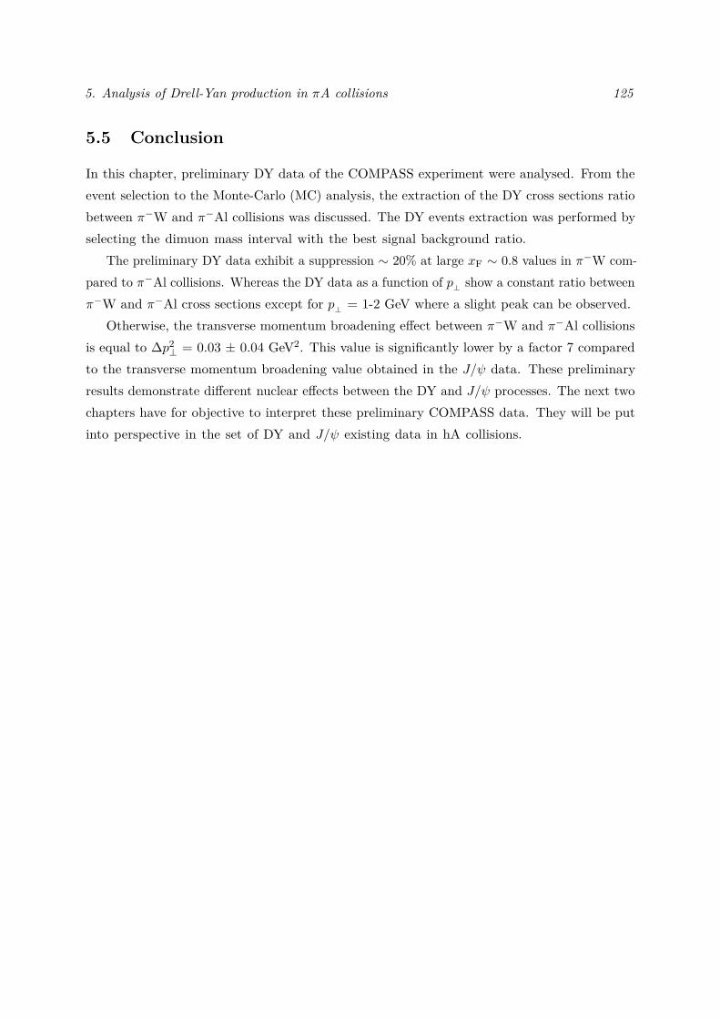
5. Analysis of Drell-Yan production in πA collisions 125
5.5 Conclusion
In this chapter, preliminary DY data of the COMPASS experiment were analysed. From theevent selection to the Monte-Carlo (MC) analysis, the extraction of the DY cross sections ratiobetween π−W and π−Al collisions was discussed. The DY events extraction was performed byselecting the dimuon mass interval with the best signal background ratio.
The preliminary DY data exhibit a suppression ∼ 20% at large xF ∼ 0.8 values in π−W com-pared to π−Al collisions. Whereas the DY data as a function of p⊥ show a constant ratio betweenπ−W and π−Al cross sections except for p⊥ = 1-2 GeV where a slight peak can be observed.
Otherwise, the transverse momentum broadening effect between π−W and π−Al collisionsis equal to ∆p2
⊥ = 0.03 ± 0.04 GeV2. This value is significantly lower by a factor 7 comparedto the transverse momentum broadening value obtained in the J/ψ data. These preliminaryresults demonstrate different nuclear effects between the DY and J/ψ processes. The next twochapters have for objective to interpret these preliminary COMPASS data. They will be putinto perspective in the set of DY and J/ψ existing data in hA collisions.
6Initial-state energy loss effects in the Drell-Yan process
Contents
6.1 Initial-state energy loss model . . . . . . . . . . . . . . . . . . . . . . . 1276.2 Uncertainties computation . . . . . . . . . . . . . . . . . . . . . . . . . 1286.3 DY Rapidity dependence . . . . . . . . . . . . . . . . . . . . . . . . . . 128
6.3.1 E906 experiment . . . . . . . . . . . . . . . . . . . . . . . . . . . . . . . 1286.3.2 E866 experiment . . . . . . . . . . . . . . . . . . . . . . . . . . . . . . . 1306.3.3 NA10 experiment . . . . . . . . . . . . . . . . . . . . . . . . . . . . . . . 1306.3.4 COMPASS experiment . . . . . . . . . . . . . . . . . . . . . . . . . . . . 1326.3.5 E615 experiment . . . . . . . . . . . . . . . . . . . . . . . . . . . . . . . 1346.3.6 Discussion about meson PDF at large x . . . . . . . . . . . . . . . . . . 136
6.4 x2 scaling in Drell-Yan production . . . . . . . . . . . . . . . . . . . . 1376.5 Conclusion . . . . . . . . . . . . . . . . . . . . . . . . . . . . . . . . . . 138
In this chapter, the radiative energy loss effect in the LPM regime will be investigated througha phenomenological analysis of Drell-Yan data in pA and πA fixed-target collisions. In theDY process, the quark propagating from the beam hadron through the nucleus is sensitive tothe initial-state energy loss as discussed in section 2.4. The goal of this chapter is to make aglobal analysis of the existing DY data by comparing them to an initial-state energy loss modelbased on the BDMPS formalism and with the latest EPPS16 nPDFs [78]. Until now, no DYdata in hA collisions could clearly demonstrate the presence of a radiative energy loss effect.E866/NuSea at FNAL performed high-statistics measurements of the DY process in pA collisonsat√s = 38.7 GeV in the large xF domain, 0 . xF . 0.9 [85, 124]. Their interpretation of
an observed large suppression as a function of xF in heavy nuclei remained elusive for a longtime. This suppression could be attributed to nPDF, i.e. anti-shadowing sea quarks at x2 .
0.1 as discussed in section 2.2, or to a presence of significant energy loss effect [144, 145, 146].Thanks to the global analysis of the DY data set in hA, including new data from the COMPASS
126
6. Initial-state energy loss effects in the Drell-Yan process 127
experiment [119], I will try to provide a consistent picture of cold nuclear effects at fixed-targetenergy. This chapter is based on an article published in Journal of High Energy Physics (JHEP)
prepared jointly with François Arleo and Stephane Platchkov [1].
6.1 Initial-state energy loss model
The effects of initial-state energy loss on the DY cross section in pA and πA collisions can be mod-elled as [147]
dσ(hA)dxF dM
=∑
i,j=q,q,g
∫ 1
0dx1
∫ 1
0dx2
∫ (1−x1)Eb
0dεPi(ε) fhi
(x1 + ε
Eb
)fAj (x2)
× dσijdxF dM
(x1x2s) , (6.1)
where Eb is the hadron beam energy in the rest frame of the nucleus, and Pi is the probabilitydistribution in the energy loss of the parton i [42]. The latter has been determined numericallyfrom a Poisson approximation [148, 149], using the LPM medium-induced gluon spectrumderived by BDMPS [106] as introduced in section 2.4.2. In the case of the DY process, theinitial-state energy loss of the incident parton is modelled by a shift of its fraction of momentumx1. Consequently, the beam PDF is not evaluated at x1 but at x1 + ∆x1, where ∆x1 =ε/Eb encodes the energy loss effect. In the high Eb energy limit, it implies ∆x1 → 0, i.e.the initial-state energy loss is suppressed.
The DY cross section in pA and πA is calculated at NLO using the DYNNLO Monte Carloprogram [150, 43]. The transport coefficient expression q(x,Q2) in Eq. (6.2) is approximatedusing the gluon distribution parametrisation in the nucleus at small x value as q(x) ∝ xG(x) ∝x−α, where α = 0.3 suggested by fits to HERA data [151].1 The transport coefficient isparametrized as (see appendix of [4]),
q(x) ≡ q0
(10−2
x
)0.3
; x = min(xA, x2) ; xA ≡1
2mpL, (6.2)
with mp ≡ 1 GeV, is the proton mass. The medium length is L = (3/4)R where R = r0A1/3, the
nuclear radius in a hard sphere nuclear density approximation with r0 = (4πρ/3)−1/3 = 1.12 fmand ρ is the nuclear matter density [3]. At x2 . xA, the transport coefficient q(x) is consideredas frozen as its Q2 energy scale dependence at low scales qL . 1GeV2.2 The only free parameterof the model is the transport coefficient q0 evaluated at x = 10−2. It was extracted from J/ψ
data within the FCEL approach, q0 = 0.07-0.09 GeV2/fm [152].1The scale at which xG(x) should be evaluated is semi-hard Q2 ∼ qL ∼ 1 GeV2.2The condition is satisfied in low beam energy, see [2].
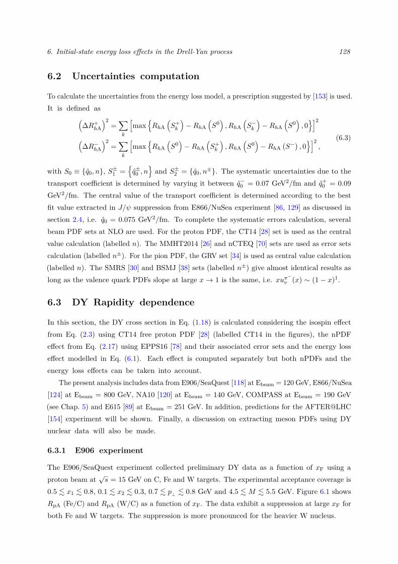
6. Initial-state energy loss effects in the Drell-Yan process 128
6.2 Uncertainties computation
To calculate the uncertainties from the energy loss model, a prescription suggested by [153] is used.It is defined as(
∆R+hA
)2=∑k
[max
{RhA
(S+k
)−RhA
(S0), RhA
(S−k
)−RhA
(S0), 0}]2
(∆R−hA
)2=∑k
[max
{RhA
(S0)−RhA
(S+k
), RhA
(S0)−RhA
(S−), 0}]2
,(6.3)
with S0 ≡ {q0, n}, S±1 ={q±0 , n
}and S±2 = {q0, n
±}. The systematic uncertainties due to thetransport coefficient is determined by varying it between q−0 = 0.07 GeV2/fm and q+
0 = 0.09GeV2/fm. The central value of the transport coefficient is determined according to the bestfit value extracted in J/ψ suppression from E866/NuSea experiment [86, 129] as discussed insection 2.4, i.e. q0 = 0.075 GeV2/fm. To complete the systematic errors calculation, severalbeam PDF sets at NLO are used. For the proton PDF, the CT14 [28] set is used as the centralvalue calculation (labelled n). The MMHT2014 [26] and nCTEQ [70] sets are used as error setscalculation (labelled n±). For the pion PDF, the GRV set [34] is used as central value calculation(labelled n). The SMRS [30] and BSMJ [38] sets (labelled n±) give almost identical results aslong as the valence quark PDFs slope at large x→ 1 is the same, i.e. xuπ−v (x) ∼ (1− x)1.
6.3 DY Rapidity dependence
In this section, the DY cross section in Eq. (1.18) is calculated considering the isospin effectfrom Eq. (2.3) using CT14 free proton PDF [28] (labelled CT14 in the figures), the nPDFeffect from Eq. (2.17) using EPPS16 [78] and their associated error sets and the energy losseffect modelled in Eq. (6.1). Each effect is computed separately but both nPDFs and theenergy loss effects can be taken into account.
The present analysis includes data from E906/SeaQuest [118] at Ebeam = 120 GeV, E866/NuSea[124] at Ebeam = 800 GeV, NA10 [120] at Ebeam = 140 GeV, COMPASS at Ebeam = 190 GeV(see Chap. 5) and E615 [89] at Ebeam = 251 GeV. In addition, predictions for the AFTER@LHC[154] experiment will be shown. Finally, a discussion on extracting meson PDFs using DYnuclear data will also be made.
6.3.1 E906 experiment
The E906/SeaQuest experiment collected preliminary DY data as a function of xF using aproton beam at
√s = 15 GeV on C, Fe and W targets. The experimental acceptance coverage is
0.5 . x1 . 0.8, 0.1 . x2 . 0.3, 0.7 . p⊥ . 0.8 GeV and 4.5 .M . 5.5 GeV. Figure 6.1 showsRpA (Fe/C) and RpA (W/C) as a function of xF. The data exhibit a suppression at large xF forboth Fe and W targets. The suppression is more pronounced for the heavier W nucleus.
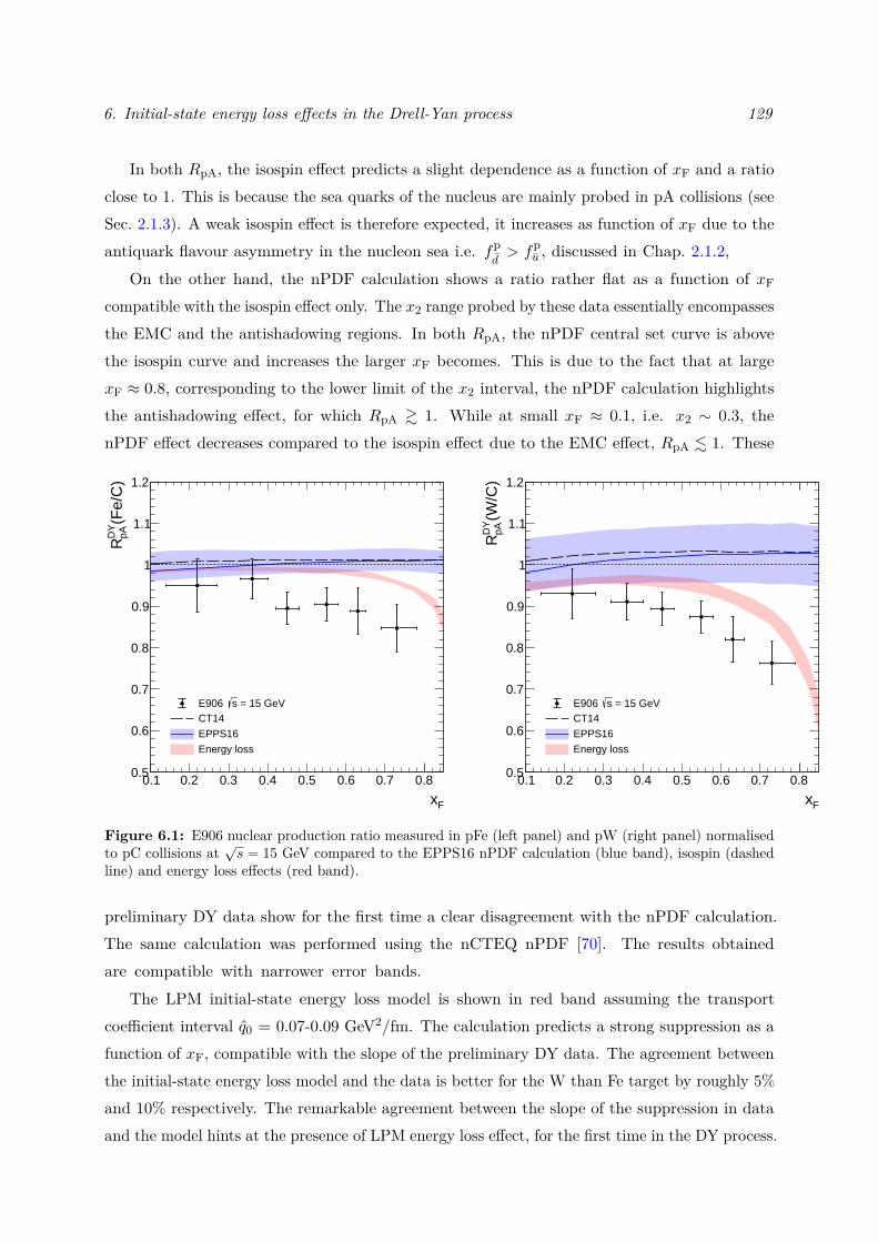
6. Initial-state energy loss effects in the Drell-Yan process 129
In both RpA, the isospin effect predicts a slight dependence as a function of xF and a ratioclose to 1. This is because the sea quarks of the nucleus are mainly probed in pA collisions (seeSec. 2.1.3). A weak isospin effect is therefore expected, it increases as function of xF due to theantiquark flavour asymmetry in the nucleon sea i.e. fp
d> fpu , discussed in Chap. 2.1.2,
On the other hand, the nPDF calculation shows a ratio rather flat as a function of xFcompatible with the isospin effect only. The x2 range probed by these data essentially encompassesthe EMC and the antishadowing regions. In both RpA, the nPDF central set curve is abovethe isospin curve and increases the larger xF becomes. This is due to the fact that at largexF ≈ 0.8, corresponding to the lower limit of the x2 interval, the nPDF calculation highlightsthe antishadowing effect, for which RpA & 1. While at small xF ≈ 0.1, i.e. x2 ∼ 0.3, thenPDF effect decreases compared to the isospin effect due to the EMC effect, RpA . 1. These
0.1 0.2 0.3 0.4 0.5 0.6 0.7 0.8
Fx
0.5
0.6
0.7
0.8
0.9
1
1.1
1.2
(Fe/
C)
pADY
R
= 15 GeVsE906 CT14
EPPS16
Energy loss
0.1 0.2 0.3 0.4 0.5 0.6 0.7 0.8
Fx
0.5
0.6
0.7
0.8
0.9
1
1.1
1.2(W
/C)
pADY
R
= 15 GeVsE906 CT14
EPPS16
Energy loss
Figure 6.1: E906 nuclear production ratio measured in pFe (left panel) and pW (right panel) normalisedto pC collisions at
√s = 15 GeV compared to the EPPS16 nPDF calculation (blue band), isospin (dashed
line) and energy loss effects (red band).
preliminary DY data show for the first time a clear disagreement with the nPDF calculation.The same calculation was performed using the nCTEQ nPDF [70]. The results obtainedare compatible with narrower error bands.
The LPM initial-state energy loss model is shown in red band assuming the transportcoefficient interval q0 = 0.07-0.09 GeV2/fm. The calculation predicts a strong suppression as afunction of xF, compatible with the slope of the preliminary DY data. The agreement betweenthe initial-state energy loss model and the data is better for the W than Fe target by roughly 5%and 10% respectively. The remarkable agreement between the slope of the suppression in dataand the model hints at the presence of LPM energy loss effect, for the first time in the DY process.
6. Initial-state energy loss effects in the Drell-Yan process 130
The relative disagreement of the normalisation could be explained by three reasons: (i) aslight contribution of the anti-shadowing effect could reduce the normalisation of RpA, (ii) alack of the antiquark flavour asymmetry effect in the proton, (iii) a slightly higher transportcoefficient would improve the agreement with data. These three reasons together might explain apart of the observed disagreement. Finally, a last observation can be made about the differencein agreement between the energy loss model and the data in the Fe and W targets. The L-dependence of the energy loss model does not seem to reproduce correctly the data. Nonetheless,the final DY data from E906 experiment are not still available. An additional contributionof the FCEL energy loss from Eq. (2.39), expected at NLO in the qq → γ?g process, canplay a role in suppression at large xF.
6.3.2 E866 experiment
The E866/NuSea experiment collected DY data on a wide range in xF, 0.1 . xF . 0.9 usinga proton beam at
√s = 38.7 GeV on Be, Fe and W targets [85, 124]. The integrated mass
range is 4 < M < 8 GeV, with an additional kinematic cut 0.02 . x2 . 0.10. These dataprobe a x2 range dominated by the shadowing effect, i.e. RpA . 1. The comparison betweencalculations and data is shown in Fig. 6.2.
The agreement between the data and the nPDF calculation is satisfactory for the two ratios3.The nPDF effect follow the same trend as the data. The higher xF values are related to smallerx2 ∼ 0.02 where the shadowing effect contributes.
On the other hand, the LPM initial-state energy loss model shows a weaker suppressionas a function of xF compared to the kinematics of E906/SeaQuest, 〈ε〉LPM/Eb → 0 in thehigh Eb beam energy limit. Consequently, this effect is negligible for both ratios except atlarge xF & 0.8 for the heavier W nucleus. At this beam energy, and above, the initial-stateenergy loss effect is suppressed. Therefore, the DY data in pA collisions seem relevant to beincluded in the global nPDF fit analyses. Recently [155], new DY data have been collectedin pA collisions as a function of y from the CMS experiment at
√s = 8.16 TeV in 15 < M
< 60 GeV and -3 < y < 2. As expected, the data do not provide evidence of suppressionwhose origin would be due to a LPM energy loss effect.
6.3.3 NA10 experiment
The NA10 experiment collected DY data on two nuclear W and D targets at√s = 16.2
GeV. The experimental acceptance coverage is 4.35 < M < 15 GeV excluding the Υ peakregion 8.5 < M < 11 GeV.
3However, these data are used in the global fit of EPPS16 as discussed in Sec. 2.2.1
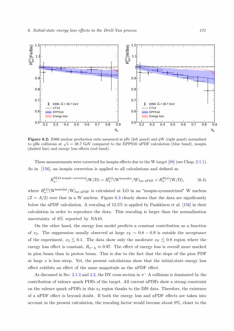
6. Initial-state energy loss effects in the Drell-Yan process 131
0.2 0.3 0.4 0.5 0.6 0.7 0.8 0.9
Fx
0.5
0.6
0.7
0.8
0.9
1
1.1
1.2
(Fe/
Be)
pADY
R
= 38.7 GeVsE866 CT14
EPPS16
Energy loss
0.2 0.3 0.4 0.5 0.6 0.7 0.8 0.9
Fx
0.5
0.6
0.7
0.8
0.9
1
1.1
1.2
(W/B
e)pAD
YR
= 38.7 GeVsE866 CT14
EPPS16
Energy loss
Figure 6.2: E866 nuclear production ratio measured in pFe (left panel) and pW (right panel) normalisedto pBe collisions at
√s = 38.7 GeV compared to the EPPS16 nPDF calculation (blue band), isospin
(dashed line) and energy loss effects (red band).
These measurements were corrected for isospin effects due to the W target [88] (see Chap. 2.1.1).As in [156], an isospin correction is applied to all calculations and defined as
RNLO-isospin correctedπ− (W/D) = RLO
π− (Wisoscalar/W)no nPDF ×RNLOπ− (W/D), (6.4)
where RLOπ− (Wisoscalar/W)no nPDF is calculated at LO in an "isospin-symmetrized" W nucleus
(Z = A/2) over that in a W nucleus. Figure 6.3 clearly shows that the data are significantlybelow the nPDF calculation. A rescaling of 12.5% is applied by Paakkinen et al. [156] in theircalculation in order to reproduce the data. This rescaling is larger than the normalizationuncertainty of 6% reported by NA10.
On the other hand, the energy loss model predicts a constant contribution as a functionof x2. The suppression usually observed at large xF ∼ 0.8 − 0.9 is outside the acceptanceof the experiment, x2 . 0.1. The data show only the moderate xF . 0.8 region where theenergy loss effect is constant, Rπ−A ≈ 0.97. The effect of energy loss is overall more markedin pion beam than in proton beam. This is due to the fact that the slope of the pion PDFat large x is less steep. Yet, the present calculations show that the initial-state energy losseffect exhibits an effect of the same magnitude as the nPDF effect.
As discussed in Sec. 2.1.3 and 2.2, the DY cross section in π− A collisions is dominated by thecontribution of valence quark PDFs of the target. All current nPDFs show a strong constrainton the valence quark nPDFs in this x2 region thanks to the DIS data. Therefore, the existenceof a nPDF effect is beyond doubt. If both the energy loss and nPDF effects are taken intoaccount in the present calculation, the rescaling factor would become about 9%, closer to the
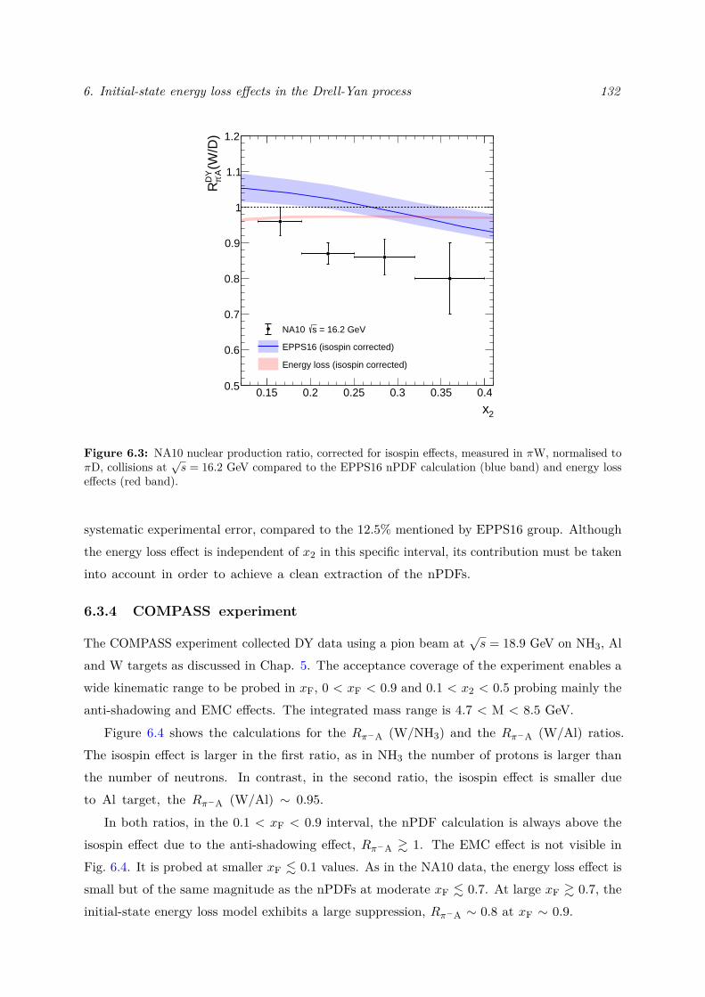
6. Initial-state energy loss effects in the Drell-Yan process 132
0.15 0.2 0.25 0.3 0.35 0.4
2x
0.5
0.6
0.7
0.8
0.9
1
1.1
1.2
(W/D
)A- πDY
R
= 16.2 GeVsNA10
EPPS16 (isospin corrected)
Energy loss (isospin corrected)
Figure 6.3: NA10 nuclear production ratio, corrected for isospin effects, measured in πW, normalised toπD, collisions at
√s = 16.2 GeV compared to the EPPS16 nPDF calculation (blue band) and energy loss
effects (red band).
systematic experimental error, compared to the 12.5% mentioned by EPPS16 group. Althoughthe energy loss effect is independent of x2 in this specific interval, its contribution must be takeninto account in order to achieve a clean extraction of the nPDFs.
6.3.4 COMPASS experiment
The COMPASS experiment collected DY data using a pion beam at√s = 18.9 GeV on NH3, Al
and W targets as discussed in Chap. 5. The acceptance coverage of the experiment enables awide kinematic range to be probed in xF, 0 < xF < 0.9 and 0.1 < x2 < 0.5 probing mainly theanti-shadowing and EMC effects. The integrated mass range is 4.7 < M < 8.5 GeV.
Figure 6.4 shows the calculations for the Rπ−A (W/NH3) and the Rπ−A (W/Al) ratios.The isospin effect is larger in the first ratio, as in NH3 the number of protons is larger thanthe number of neutrons. In contrast, in the second ratio, the isospin effect is smaller dueto Al target, the Rπ−A (W/Al) ∼ 0.95.
In both ratios, in the 0.1 < xF < 0.9 interval, the nPDF calculation is always above theisospin effect due to the anti-shadowing effect, Rπ−A & 1. The EMC effect is not visible inFig. 6.4. It is probed at smaller xF . 0.1 values. As in the NA10 data, the energy loss effect issmall but of the same magnitude as the nPDFs at moderate xF . 0.7. At large xF & 0.7, theinitial-state energy loss model exhibits a large suppression, Rπ−A ∼ 0.8 at xF ∼ 0.9.
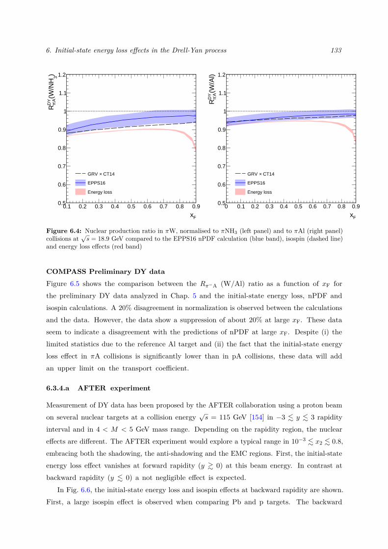
6. Initial-state energy loss effects in the Drell-Yan process 133
0.1 0.2 0.3 0.4 0.5 0.6 0.7 0.8 0.9
Fx
0.5
0.6
0.7
0.8
0.9
1
1.1
1.2) 3(W
/NH
A- πDY
R
CT14×GRV
EPPS16
Energy loss
0 0.1 0.2 0.3 0.4 0.5 0.6 0.7 0.8 0.9
Fx
0.5
0.6
0.7
0.8
0.9
1
1.1
1.2
(W/A
l)A- πDY
R
CT14×GRV
EPPS16
Energy loss
Figure 6.4: Nuclear production ratio in πW, normalised to πNH3 (left panel) and to πAl (right panel)collisions at
√s = 18.9 GeV compared to the EPPS16 nPDF calculation (blue band), isospin (dashed line)
and energy loss effects (red band)
COMPASS Preliminary DY dataFigure 6.5 shows the comparison between the Rπ−A (W/Al) ratio as a function of xF forthe preliminary DY data analyzed in Chap. 5 and the initial-state energy loss, nPDF andisospin calculations. A 20% disagreement in normalization is observed between the calculationsand the data. However, the data show a suppression of about 20% at large xF. These dataseem to indicate a disagreement with the predictions of nPDF at large xF. Despite (i) thelimited statistics due to the reference Al target and (ii) the fact that the initial-state energyloss effect in πA collisions is significantly lower than in pA collisions, these data will addan upper limit on the transport coefficient.
6.3.4.a AFTER experiment
Measurement of DY data has been proposed by the AFTER collaboration using a proton beamon several nuclear targets at a collision energy
√s = 115 GeV [154] in −3 . y . 3 rapidity
interval and in 4 < M < 5 GeV mass range. Depending on the rapidity region, the nucleareffects are different. The AFTER experiment would explore a typical range in 10−3 . x2 . 0.8,embracing both the shadowing, the anti-shadowing and the EMC regions. First, the initial-stateenergy loss effect vanishes at forward rapidity (y & 0) at this beam energy. In contrast atbackward rapidity (y . 0) a not negligible effect is expected.
In Fig. 6.6, the initial-state energy loss and isospin effects at backward rapidity are shown.First, a large isospin effect is observed when comparing Pb and p targets. The backward
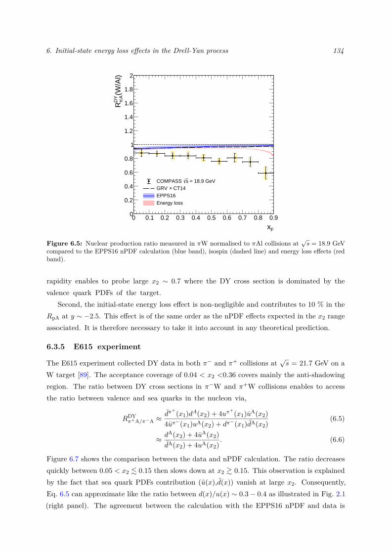
6. Initial-state energy loss effects in the Drell-Yan process 134
0 0.1 0.2 0.3 0.4 0.5 0.6 0.7 0.8 0.9
Fx
0
0.2
0.4
0.6
0.8
1
1.2
1.4
1.6
1.8
2
(W/A
l)A- πDY
R
= 18.9 GeVsCOMPASS CT14×GRV
EPPS16
Energy loss
Figure 6.5: Nuclear production ratio measured in πW normalised to πAl collisions at√s = 18.9 GeV
compared to the EPPS16 nPDF calculation (blue band), isospin (dashed line) and energy loss effects (redband).
rapidity enables to probe large x2 ∼ 0.7 where the DY cross section is dominated by thevalence quark PDFs of the target.
Second, the initial-state energy loss effect is non-negligible and contributes to 10 % in theRpA at y ∼ −2.5. This effect is of the same order as the nPDF effects expected in the x2 rangeassociated. It is therefore necessary to take it into account in any theoretical prediction.
6.3.5 E615 experiment
The E615 experiment collected DY data in both π− and π+ collisions at√s = 21.7 GeV on a
W target [89]. The acceptance coverage of 0.04 < x2 <0.36 covers mainly the anti-shadowingregion. The ratio between DY cross sections in π−W and π+W collisions enables to accessthe ratio between valence and sea quarks in the nucleon via,
RDYπ+A/π−A ≈
dπ+(x1)dA(x2) + 4uπ+(x1)uA(x2)
4uπ−(x1)uA(x2) + dπ−(x1)dA(x2)(6.5)
≈ dA(x2) + 4uA(x2)dA(x2) + 4uA(x2)
. (6.6)
Figure 6.7 shows the comparison between the data and nPDF calculation. The ratio decreasesquickly between 0.05 < x2 . 0.15 then slows down at x2 & 0.15. This observation is explainedby the fact that sea quark PDFs contribution (u(x),d(x)) vanish at large x2. Consequently,Eq. 6.5 can approximate like the ratio between d(x)/u(x) ∼ 0.3− 0.4 as illustrated in Fig. 2.1(right panel). The agreement between the calculation with the EPPS16 nPDF and data is
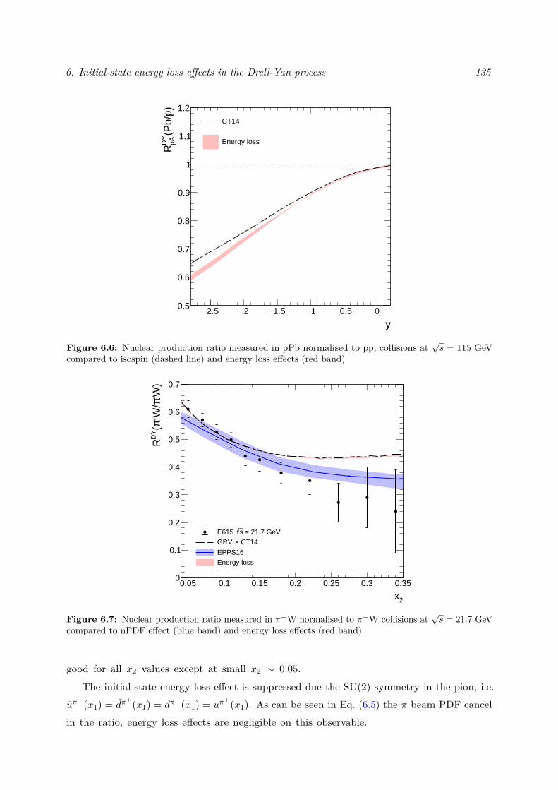
6. Initial-state energy loss effects in the Drell-Yan process 135
2.5− 2− 1.5− 1− 0.5− 0
y
0.5
0.6
0.7
0.8
0.9
1
1.1
1.2
(Pb/
p)pAD
YR
CT14
Energy loss
Figure 6.6: Nuclear production ratio measured in pPb normalised to pp, collisions at√s = 115 GeV
compared to isospin (dashed line) and energy loss effects (red band)
0.05 0.1 0.15 0.2 0.25 0.3 0.35
2x
0
0.1
0.2
0.3
0.4
0.5
0.6
0.7
W)
- πW
/+ π(
DY
R
= 21.7 GeVsE615 CT14×GRV
EPPS16Energy loss
Figure 6.7: Nuclear production ratio measured in π+W normalised to π−W collisions at√s = 21.7 GeV
compared to nPDF effect (blue band) and energy loss effects (red band).
good for all x2 values except at small x2 ∼ 0.05.The initial-state energy loss effect is suppressed due the SU(2) symmetry in the pion, i.e.
uπ−(x1) = dπ
+(x1) = dπ−(x1) = uπ
+(x1). As can be seen in Eq. (6.5) the π beam PDF cancelin the ratio, energy loss effects are negligible on this observable.
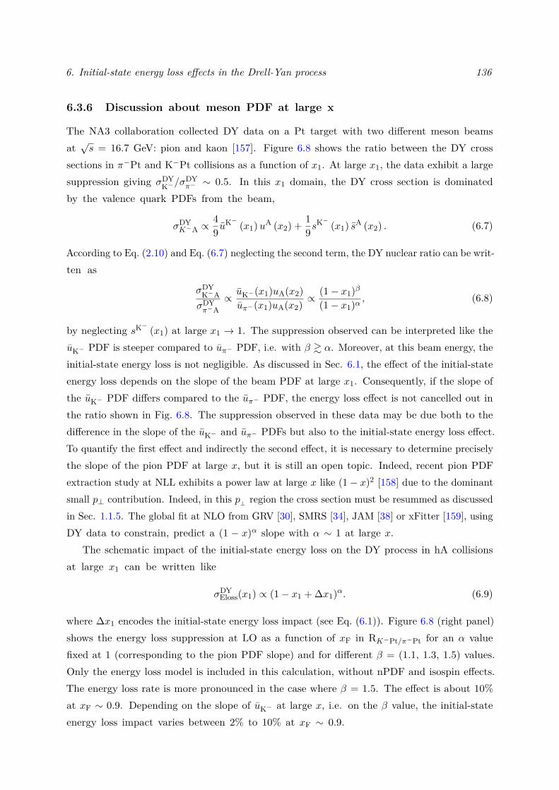
6. Initial-state energy loss effects in the Drell-Yan process 136
6.3.6 Discussion about meson PDF at large x
The NA3 collaboration collected DY data on a Pt target with two different meson beamsat√s = 16.7 GeV: pion and kaon [157]. Figure 6.8 shows the ratio between the DY cross
sections in π−Pt and K−Pt collisions as a function of x1. At large x1, the data exhibit a largesuppression giving σDYK−/σ
DYπ− ∼ 0.5. In this x1 domain, the DY cross section is dominated
by the valence quark PDFs from the beam,
σDYK−A ∝
49 u
K− (x1)uA (x2) + 19s
K− (x1) sA (x2) . (6.7)
According to Eq. (2.10) and Eq. (6.7) neglecting the second term, the DY nuclear ratio can be writ-ten as
σDYK−AσDYπ−A
∝ uK−(x1)uA(x2)uπ−(x1)uA(x2) ∝
(1− x1)β(1− x1)α , (6.8)
by neglecting sK− (x1) at large x1 → 1. The suppression observed can be interpreted like theuK− PDF is steeper compared to uπ− PDF, i.e. with β & α. Moreover, at this beam energy, theinitial-state energy loss is not negligible. As discussed in Sec. 6.1, the effect of the initial-stateenergy loss depends on the slope of the beam PDF at large x1. Consequently, if the slope ofthe uK− PDF differs compared to the uπ− PDF, the energy loss effect is not cancelled out inthe ratio shown in Fig. 6.8. The suppression observed in these data may be due both to thedifference in the slope of the uK− and uπ− PDFs but also to the initial-state energy loss effect.To quantify the first effect and indirectly the second effect, it is necessary to determine preciselythe slope of the pion PDF at large x, but it is still an open topic. Indeed, recent pion PDFextraction study at NLL exhibits a power law at large x like (1− x)2 [158] due to the dominantsmall p⊥ contribution. Indeed, in this p⊥ region the cross section must be resummed as discussedin Sec. 1.1.5. The global fit at NLO from GRV [30], SMRS [34], JAM [38] or xFitter [159], usingDY data to constrain, predict a (1 − x)α slope with α ∼ 1 at large x.
The schematic impact of the initial-state energy loss on the DY process in hA collisionsat large x1 can be written like
σDYEloss(x1) ∝ (1− x1 + ∆x1)α. (6.9)
where ∆x1 encodes the initial-state energy loss impact (see Eq. (6.1)). Figure 6.8 (right panel)shows the energy loss suppression at LO as a function of xF in RK−Pt/π−Pt for an α valuefixed at 1 (corresponding to the pion PDF slope) and for different β = (1.1, 1.3, 1.5) values.Only the energy loss model is included in this calculation, without nPDF and isospin effects.The energy loss rate is more pronounced in the case where β = 1.5. The effect is about 10%at xF ∼ 0.9. Depending on the slope of uK− at large x, i.e. on the β value, the initial-stateenergy loss impact varies between 2% to 10% at xF ∼ 0.9.
6. Initial-state energy loss effects in the Drell-Yan process 137
0 0.1 0.2 0.3 0.4 0.5 0.6 0.7 0.8 0.9
Fx
0.9
0.92
0.94
0.96
0.98
1
1.02
1.04
1.06 Pt
πK
Pt/
R
= 1.1β = 1, α = 1.3β = 1, α = 1.5β = 1, α
Figure 6.8: DY nuclear production ratio measured in K−Pt normalised to π−Pt collisions at√s = 16.7
GeV from NA3 experiment [157] (left panel) and the impact of α and β values on the initial-state energyloss model calculation at LO using Pt nucleus at
√s = 16.7 GeV (right panel).
Consequently, the suppression observed in Fig. 6.8 need to be interpreted by taking intoaccount the initial-state energy loss. In particular, if the slope of uK− is more pronouncedat large x1 compared to uπ− . A cleaner slope extraction will be more safe in light targetbut in this case, the statistics will be weaker.
6.4 x2 scaling in Drell-Yan production
In the previous section, we showed that the initial-state energy loss plays an important role in theinterpretation of data at low beam energy, typically at Ebeam < 1 TeV. Preliminary data fromE906/SeaQuest show for the first time a clear disagreement with the nPDF calculation. Otherwise,the nPDF calculation exhibits a good agreement with DY data from E866/NuSea. One of thestrong hypotheses of the nPDF formalism consists in considering that the QCD factorizationis verified at all energies and therefore a proper extraction of the nPDFs is possible. Thefactorised expression for the DY cross section can be written independently of the center-of-massenergy of the collision. At forward rapidity, we have
dσ(pA)dxF dM
' fpq (xF)×
∑j=q,q,g
∫dx2 f
Aj (x2) dσqj
dxF dM(xFx2s)
' fpq (xF)×
∑j=q,q,g
fAj (x2) dσqj
dxF dM(M2)
(6.10)
by considering at forward rapidity region, xF ∼ x1 � x2 and x2 ≈ s/ (xFs). The DY crosssection approximation in Eq. (6.10) depends exclusively on the dimuon invariant mass M .
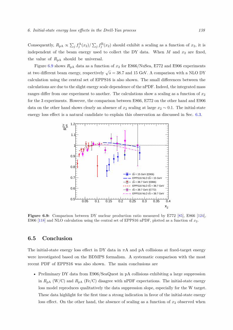
6. Initial-state energy loss effects in the Drell-Yan process 138
Consequently, RpA ∝∑j f
Aj (x2)/∑j f
Bj (x2) should exhibit a scaling as a function of x2, it is
independent of the beam energy used to collect the DY data. When M and x2 are fixed,the value of RpA should be universal.
Figure 6.9 shows RpA data as a function of x2 for E866/NuSea, E772 and E906 experimentsat two different beam energy, respectively
√s = 38.7 and 15 GeV. A comparison with a NLO DY
calculation using the central set of EPPS16 is also shown. The small differences between thecalculations are due to the slight energy scale dependence of the nPDF. Indeed, the integrated massranges differ from one experiment to another. The calculations show a scaling as a function of x2
for the 3 experiments. However, the comparison between E866, E772 on the other hand and E906data on the other hand shows clearly an absence of x2 scaling at large x2 ∼ 0.1. The initial-stateenergy loss effect is a natural candidate to explain this observation as discussed in Sec. 6.3.
0.05 0.1 0.15 0.2 0.25 0.3 0.35 0.4
2x
0.5
0.6
0.7
0.8
0.9
1
1.1
1.2
pADY
R
= 15 GeV (E906)s
= 15 GeV sEPPS16 NLO
= 38.7 GeV (E866)s
= 38.7 GeV sEPPS16 NLO
= 38.7 GeV (E772)s
= 38.7 GeVsEPPS16 NLO
Figure 6.9: Comparison between DY nuclear production ratio measured by E772 [85], E866 [124],E906 [118] and NLO calculation using the central set of EPPS16 nPDF, plotted as a function of x2.
6.5 Conclusion
The initial-state energy loss effect in DY data in πA and pA collisions at fixed-target energywere investigated based on the BDMPS formalism. A systematic comparison with the mostrecent PDF of EPPS16 was also shown. The main conclusions are
• Preliminary DY data from E906/SeaQuest in pA collisions exhibiting a large suppressionin RpA (W/C) and RpA (Fe/C) disagree with nPDF expectations. The initial-state energyloss model reproduces qualitatively the data suppression slope, especially for the W target.These data highlight for the first time a strong indication in favor of the initial-state energyloss effect. On the other hand, the absence of scaling as a function of x2 observed when
6. Initial-state energy loss effects in the Drell-Yan process 139
comparing the E866, E772 and E906 data also indicates that an effect, other than thenPDF, is at work;
• The DY data from E866/NuSea show that at a beam energy of 800 GeV, the initial energyloss effect becomes negligible, 〈ε〉LPM/E → 0. Except at very large xF ∼ 0.8-0.9, a regionin which it is necessary to take this effect into account. In general, these data are relevantto extract nPDFs in a clean way;
• The DY data in πA are less suitable for easily demonstrating the initial-state energy loss.Indeed, due to the fact that the slope of the pion PDF at large x is less steep than that ofthe proton, the energy loss effect in these collisions is less pronounced. Apart from thispoint, the DY data from the NA10 experiment show that it was necessary to take intoaccount the energy loss effect in the interpretation of the data. This effect has a magnitudesimilar to that of the nPDF contribution. The preliminary DY data from the COMPASSexperiment exhibit a suppression at large xF & 0.8 whose amplitude is compatible (for thesuppression slope) with the initial-state energy loss effect. However, a difference of 20% inthe normalization persists between the calculations and the preliminary data.
• The AFTER collaboration projects to collect DY data in a range at high enough rapidityto be able to constrain EMC, anti-shadowing and shadowing effects. The energy loss modelpredicts in the most backward rapidity region an effect of around 10%. The magnitude ofthe effect is comparable to the expected nPDF effect in this region. It is therefore necessaryto take this effect into account in order to be able to perform a clean and relevant nPDFextraction;
• The PDF extraction of mesons at large x is performed mainly using the DY nuclear data onheavy nucleus for better statistics. However, the initial-state energy loss plays a significantrole that must be taken into account.
7Transverse momentum broadening effect in world data
Contents
7.1 Model . . . . . . . . . . . . . . . . . . . . . . . . . . . . . . . . . . . . . 1417.1.1 Broadening definition . . . . . . . . . . . . . . . . . . . . . . . . . . . . 1417.1.2 Coherence length . . . . . . . . . . . . . . . . . . . . . . . . . . . . . . . 1427.1.3 Hard processes . . . . . . . . . . . . . . . . . . . . . . . . . . . . . . . . 142
7.2 Extraction of the nuclear broadening from data . . . . . . . . . . . . 1437.2.1 Data . . . . . . . . . . . . . . . . . . . . . . . . . . . . . . . . . . . . . . 1437.2.2 Method extraction . . . . . . . . . . . . . . . . . . . . . . . . . . . . . . 1437.2.3 Uncertainty of the broadening calculation . . . . . . . . . . . . . . . . . 145
7.3 Extraction of the transport coefficient q0 . . . . . . . . . . . . . . . . 1467.3.1 Global fit . . . . . . . . . . . . . . . . . . . . . . . . . . . . . . . . . . . 1467.3.2 Nuclear broadening from the COMPASS experiment . . . . . . . . . . . 148
7.4 nPDF and radiative energy loss effects . . . . . . . . . . . . . . . . . 1497.5 Relation between the broadening and the gluon distribution . . . . 1517.6 RpA as a function of p⊥ in the Drell-Yan process . . . . . . . . . . . 152
7.6.1 Model . . . . . . . . . . . . . . . . . . . . . . . . . . . . . . . . . . . . . 1527.6.2 E866/NuSea experiment . . . . . . . . . . . . . . . . . . . . . . . . . . . 1537.6.3 PHENIX experiment . . . . . . . . . . . . . . . . . . . . . . . . . . . . . 1547.6.4 COMPASS experiment . . . . . . . . . . . . . . . . . . . . . . . . . . . . 156
7.7 Conclusion . . . . . . . . . . . . . . . . . . . . . . . . . . . . . . . . . . 157
When a parton enters in a QCD medium, it interacts via multiple scattering inducing
radiative energy loss and broadening effects. The first effect was investigated in Chap. 6. The
main goal of this chapter is to analyse the nuclear broadening using available Drell-Yan (DY)
and quarkonium data in pA and πA collisions. The simple observable in order to study the
nuclear broadening effect value in hA collisions reads
∆p2⊥ =
⟨p2⊥
⟩hA−⟨p2⊥
⟩hp. (7.1)
140
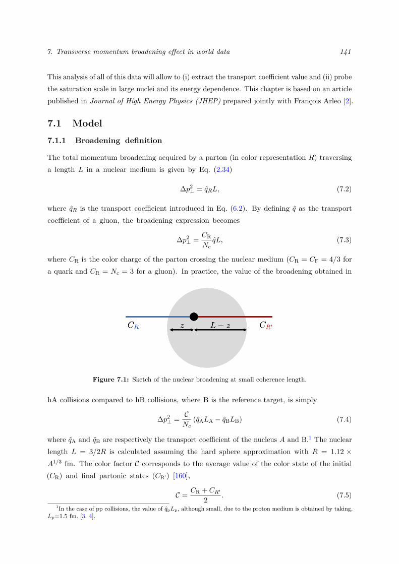
7. Transverse momentum broadening effect in world data 141
This analysis of all of this data will allow to (i) extract the transport coefficient value and (ii) probethe saturation scale in large nuclei and its energy dependence. This chapter is based on an articlepublished in Journal of High Energy Physics (JHEP) prepared jointly with François Arleo [2].
7.1 Model
7.1.1 Broadening definition
The total momentum broadening acquired by a parton (in color representation R) traversinga length L in a nuclear medium is given by Eq. (2.34)
∆p2⊥ = qRL, (7.2)
where qR is the transport coefficient introduced in Eq. (6.2). By defining q as the transportcoefficient of a gluon, the broadening expression becomes
∆p2⊥ = CR
NcqL, (7.3)
where CR is the color charge of the parton crossing the nuclear medium (CR = CF = 4/3 fora quark and CR = Nc = 3 for a gluon). In practice, the value of the broadening obtained in
Figure 7.1: Sketch of the nuclear broadening at small coherence length.
hA collisions compared to hB collisions, where B is the reference target, is simply
∆p2⊥ = C
Nc(qALA − qBLB) (7.4)
where qA and qB are respectively the transport coefficient of the nucleus A and B.1 The nuclearlength L = 3/2R is calculated assuming the hard sphere approximation with R = 1.12 ×A1/3 fm. The color factor C corresponds to the average value of the color state of the initial(CR) and final partonic states (CR’) [160],
C = CR + CR′
2 . (7.5)1In the case of pp collisions, the value of qpLp, although small, due to the proton medium is obtained by taking,
Lp=1.5 fm. [3, 4].
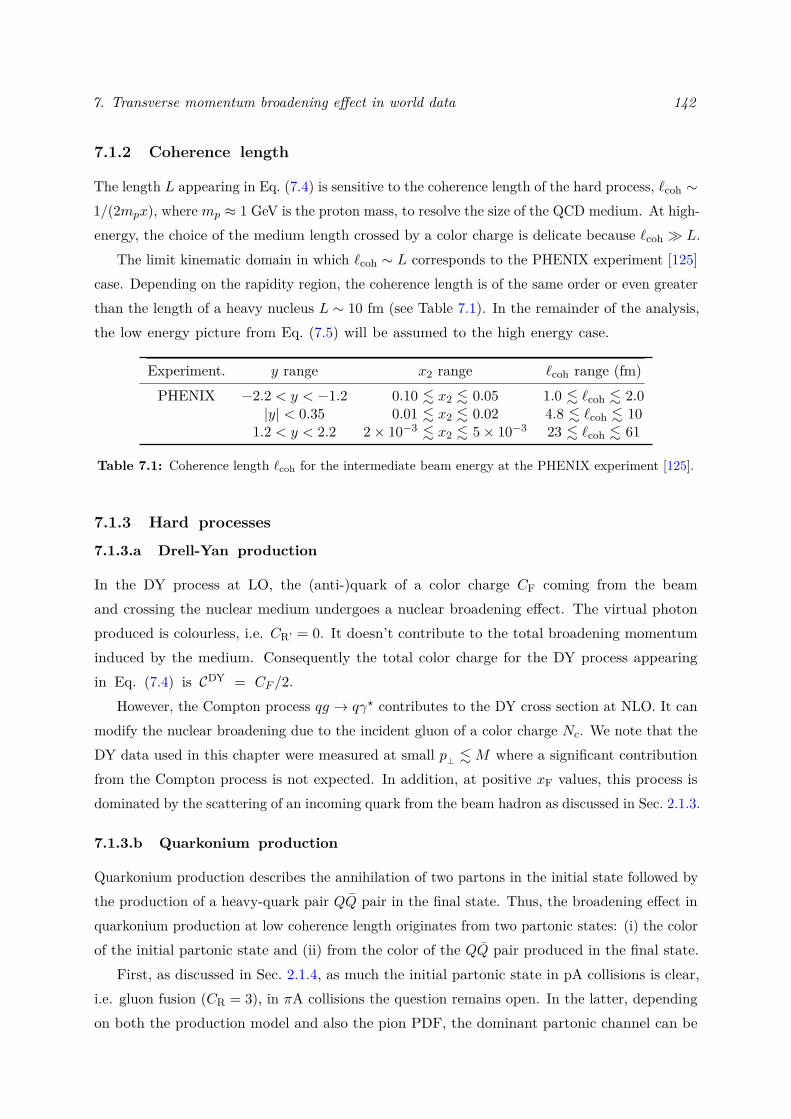
7. Transverse momentum broadening effect in world data 142
7.1.2 Coherence length
The length L appearing in Eq. (7.4) is sensitive to the coherence length of the hard process, `coh ∼1/(2mpx), where mp ≈ 1 GeV is the proton mass, to resolve the size of the QCD medium. At high-energy, the choice of the medium length crossed by a color charge is delicate because `coh � L.
The limit kinematic domain in which `coh ∼ L corresponds to the PHENIX experiment [125]case. Depending on the rapidity region, the coherence length is of the same order or even greaterthan the length of a heavy nucleus L ∼ 10 fm (see Table 7.1). In the remainder of the analysis,the low energy picture from Eq. (7.5) will be assumed to the high energy case.
Experiment. y range x2 range `coh range (fm)PHENIX −2.2 < y < −1.2 0.10 . x2 . 0.05 1.0 . `coh . 2.0
|y| < 0.35 0.01 . x2 . 0.02 4.8 . `coh . 101.2 < y < 2.2 2× 10⁻³ . x2 . 5× 10⁻³ 23 . `coh . 61
Table 7.1: Coherence length `coh for the intermediate beam energy at the PHENIX experiment [125].
7.1.3 Hard processes
7.1.3.a Drell-Yan production
In the DY process at LO, the (anti-)quark of a color charge CF coming from the beamand crossing the nuclear medium undergoes a nuclear broadening effect. The virtual photonproduced is colourless, i.e. CR’ = 0. It doesn’t contribute to the total broadening momentuminduced by the medium. Consequently the total color charge for the DY process appearingin Eq. (7.4) is CDY = CF /2.
However, the Compton process qg → qγ? contributes to the DY cross section at NLO. It canmodify the nuclear broadening due to the incident gluon of a color charge Nc. We note that theDY data used in this chapter were measured at small p⊥ .M where a significant contributionfrom the Compton process is not expected. In addition, at positive xF values, this process isdominated by the scattering of an incoming quark from the beam hadron as discussed in Sec. 2.1.3.
7.1.3.b Quarkonium production
Quarkonium production describes the annihilation of two partons in the initial state followed bythe production of a heavy-quark pair QQ pair in the final state. Thus, the broadening effect inquarkonium production at low coherence length originates from two partonic states: (i) the colorof the initial partonic state and (ii) from the color of the QQ pair produced in the final state.
First, as discussed in Sec. 2.1.4, as much the initial partonic state in pA collisions is clear,i.e. gluon fusion (CR = 3), in πA collisions the question remains open. In the latter, dependingon both the production model and also the pion PDF, the dominant partonic channel can be
7. Transverse momentum broadening effect in world data 143
gg either or qq. In this analysis and according to the Fig. 2.3, the qq channel is considered asdominant in the quarkonium production cross section in πA collisions (CR = 4/3).
Secondly, in the final state, the QQ pair can be produced in a singlet (CR’ = 0) or octet(CR’ = 3) color state depending on the production model. In the CEM or the NRQCD, theQQ pairis essentially produced in an octet color state. Consequently, the QQ pair must neutralize its colorbefore hadronizing2, i.e. `8 � `QQ, where `had and `QQ are respectively the hadronisation andcoherence lengths. Whilst in the CSM model, the QQ is already produced in a singlet color state,i.e. `1 ∼ `QQ. In this study, we assume that the QQ pair is produced mainly in a color octet stateduring its propagation throughout the nucleus, but the singlet picture will be investigated too.
Table 7.2 summarises the color factors used for the DY and quarkonium in octet andsinglet production in πA and pA collisions.
Process Collision C
DY πA/ pA CF /2Quarkonium πA (CF +Nc)/2Quarkonium pA Nc
Quarkonium (singlet) πA/ pA Nc/2
Table 7.2: Color factors used for the DY and quarkonium in octet and singlet production in πA and pAcollisions.
7.2 Extraction of the nuclear broadening from data
7.2.1 Data
The present analysis includes world quarkonium data from fixed-target (NA3, NA10 and E772)to collider (PHENIX, ALICE and LHCb) energies for different rapidity domains and projectiles(π and p hadron beams). In addition, DY data from NA10 and E772 are included in thisanalysis. The forward data at RHIC (1.2 < y < 2.2) and at LHC (2 < y < 4 for LHCbexperiment) probe smallest x2 values, x2 ≈ 3 × 10−3 and x2 ≈ 2 × 10⁻⁵, respectively. Thesedata investigate the x-dependence of the transport coefficient in Eq. (6.2). A factor of 400 in√s is observed between the data from SPS to LHC energies.
7.2.2 Method extraction
By definition, the average transverse momentum squared in Eq. (7.1) is defined as
⟨p2⊥
⟩=(∫ ∞
0dp⊥p2
⊥dσdp⊥
)/
(∫ ∞0
dp⊥dσdp⊥
). (7.6)
2For example in the CEM model at LO, the QQ pair produced in color octet state neutralizes its color byemitting a gluon before being hadronized, QQ→ g + J/ψ.
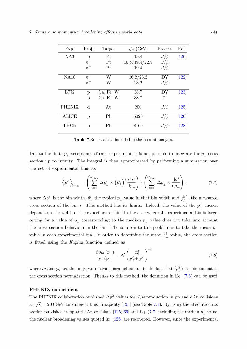
7. Transverse momentum broadening effect in world data 144
Exp. Proj. Target√s (GeV) Process Ref.
NA3 p Pt 19.4 J/ψ [120]π− Pt 16.8/19.4/22.9 J/ψπ+ Pt 19.4 J/ψ
NA10 π− W 16.2/23.2 DY [122]π− W 23.2 J/ψ
E772 p Ca, Fe, W 38.7 DY [123]p Ca, Fe, W 38.7 Υ
PHENIX d Au 200 J/ψ [125]
ALICE p Pb 5020 J/ψ [126]
LHCb p Pb 8160 J/ψ [128]
Table 7.3: Data sets included in the present analysis.
Due to the finite p⊥ acceptance of each experiment, it is not possible to integrate the p⊥ crosssection up to infinity. The integral is then approximated by performing a summation overthe set of experimental bins as
⟨p2⊥
⟩bins
=
Nbins∑i=1
∆pi⊥×(pi⊥
)2 dσidp⊥
/Nbins∑
i=1∆pi⊥× dσi
dp⊥
, (7.7)
where ∆pi⊥is the bin width, pi⊥ the typical p⊥ value in that bin width and dσi
dp⊥ , the measuredcross section of the bin i. This method has its limits. Indeed, the value of the pi⊥ chosendepends on the width of the experimental bin. In the case where the experimental bin is large,opting for a value of p⊥ corresponding to the median p⊥ value does not take into accountthe cross section behaviour in the bin. The solution to this problem is to take the mean p⊥
value in each experimental bin. In order to determine the mean pi⊥ value, the cross sectionis fitted using the Kaplan function defined as
dσfit (p⊥)p⊥dp⊥
= N(
p20
p20 + p2
⊥
)m(7.8)
where m and p0 are the only two relevant parameters due to the fact that⟨p2⊥⟩is independent of
the cross section normalisation. Thanks to this method, the definition in Eq. (7.6) can be used.
PHENIX experimentThe PHENIX collaboration published ∆p2
⊥values for J/ψ production in pp and dAu collisions
at√s = 200 GeV for different bins in rapidity [125] (see Table 7.1). By using the absolute cross
section published in pp and dAu collisions [125, 66] and Eq. (7.7) including the median p⊥ value,the nuclear broadening values quoted in [125] are recovered. However, since the experimental
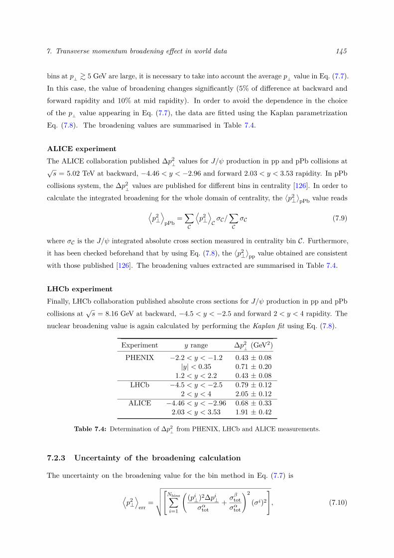
7. Transverse momentum broadening effect in world data 145
bins at p⊥ & 5 GeV are large, it is necessary to take into account the average p⊥ value in Eq. (7.7).In this case, the value of broadening changes significantly (5% of difference at backward andforward rapidity and 10% at mid rapidity). In order to avoid the dependence in the choiceof the p⊥ value appearing in Eq. (7.7), the data are fitted using the Kaplan parametrizationEq. (7.8). The broadening values are summarised in Table 7.4.
ALICE experimentThe ALICE collaboration published ∆p2
⊥values for J/ψ production in pp and pPb collisions at
√s = 5.02 TeV at backward, −4.46 < y < −2.96 and forward 2.03 < y < 3.53 rapidity. In pPb
collisions system, the ∆p2⊥values are published for different bins in centrality [126]. In order to
calculate the integrated broadening for the whole domain of centrality, the⟨p2⊥⟩
pPb value reads⟨p2⊥
⟩pPb
=∑C
⟨p2⊥
⟩CσC/
∑CσC (7.9)
where σC is the J/ψ integrated absolute cross section measured in centrality bin C. Furthermore,it has been checked beforehand that by using Eq. (7.8), the
⟨p2⊥⟩
pp value obtained are consistentwith those published [126]. The broadening values extracted are summarised in Table 7.4.
LHCb experimentFinally, LHCb collaboration published absolute cross sections for J/ψ production in pp and pPbcollisions at
√s = 8.16 GeV at backward, −4.5 < y < −2.5 and forward 2 < y < 4 rapidity. The
nuclear broadening value is again calculated by performing the Kaplan fit using Eq. (7.8).
Experiment y range ∆p2⊥(GeV2)
PHENIX −2.2 < y < −1.2 0.43 ± 0.08|y| < 0.35 0.71 ± 0.20
1.2 < y < 2.2 0.43 ± 0.08LHCb −4.5 < y < −2.5 0.79 ± 0.12
2 < y < 4 2.05 ± 0.12ALICE −4.46 < y < −2.96 0.68 ± 0.33
2.03 < y < 3.53 1.91 ± 0.42
Table 7.4: Determination of ∆p2⊥from PHENIX, LHCb and ALICE measurements.
7.2.3 Uncertainty of the broadening calculation
The uncertainty on the broadening value for the bin method in Eq. (7.7) is
⟨p2⊥
⟩err
=
√√√√√Nbins∑i=1
((pi⊥)2∆pi⊥
σαtot+ σβtotσαtot
)2
(σi)2
, (7.10)
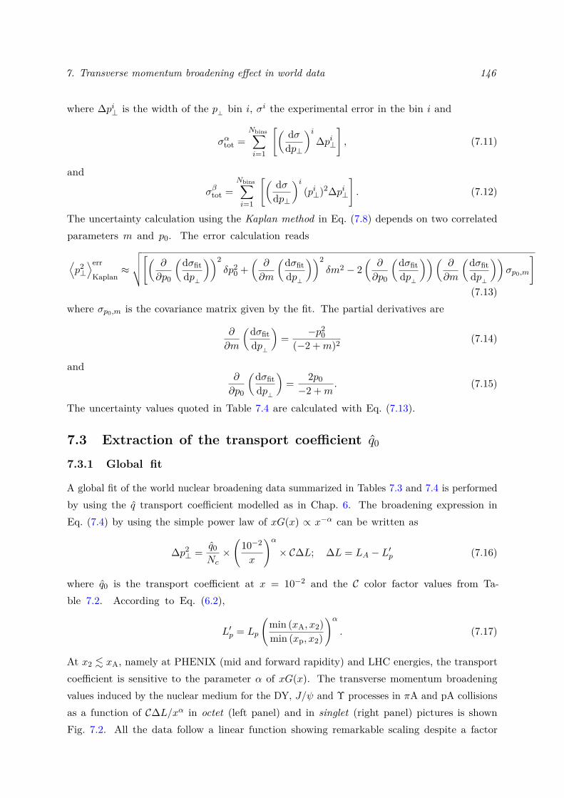
7. Transverse momentum broadening effect in world data 146
where ∆pi⊥ is the width of the p⊥ bin i, σi the experimental error in the bin i and
σαtot =Nbins∑i=1
[( dσdp⊥
)i∆pi⊥
], (7.11)
and
σβtot =Nbins∑i=1
[( dσdp⊥
)i(pi⊥)2∆pi⊥
]. (7.12)
The uncertainty calculation using the Kaplan method in Eq. (7.8) depends on two correlatedparameters m and p0. The error calculation reads
⟨p2⊥
⟩errKaplan
≈
√√√√[( ∂
∂p0
(dσfitdp⊥
))2δp2
0 +(∂
∂m
(dσfitdp⊥
))2δm2 − 2
(∂
∂p0
(dσfitdp⊥
))(∂
∂m
(dσfitdp⊥
))σp0,m
](7.13)
where σp0,m is the covariance matrix given by the fit. The partial derivatives are
∂
∂m
(dσfitdp⊥
)= −p2
0(−2 +m)2 (7.14)
and∂
∂p0
(dσfitdp⊥
)= 2p0−2 +m
. (7.15)
The uncertainty values quoted in Table 7.4 are calculated with Eq. (7.13).
7.3 Extraction of the transport coefficient q0
7.3.1 Global fit
A global fit of the world nuclear broadening data summarized in Tables 7.3 and 7.4 is performedby using the q transport coefficient modelled as in Chap. 6. The broadening expression inEq. (7.4) by using the simple power law of xG(x) ∝ x−α can be written as
∆p2⊥ = q0
Nc×(
10−2
x
)α× C∆L; ∆L = LA − L′p (7.16)
where q0 is the transport coefficient at x = 10−2 and the C color factor values from Ta-ble 7.2. According to Eq. (6.2),
L′p = Lp
(min (xA, x2)min (xp, x2)
)α. (7.17)
At x2 . xA, namely at PHENIX (mid and forward rapidity) and LHC energies, the transportcoefficient is sensitive to the parameter α of xG(x). The transverse momentum broadeningvalues induced by the nuclear medium for the DY, J/ψ and Υ processes in πA and pA collisionsas a function of C∆L/xα in octet (left panel) and in singlet (right panel) pictures is shownFig. 7.2. All the data follow a linear function showing remarkable scaling despite a factor
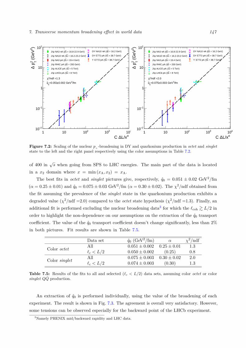
7. Transverse momentum broadening effect in world data 147
1 10 210 310 410αL/x∆C
2−10
1−10
1
10
210)2 (
GeV
2 T p∆
/fm20.002 GeV±=0.0510
q
/ndf =1.32χ
= 16.2 GeV)sA (πDY NA10
= 38.7 GeV)sDY E772 pA (
= 38.7 GeV)s E772 pA (Υ
= 16.8-22.9 GeV)sA (π NA3 ψJ/
= 16.2-23.2 GeV)sA (π NA10 ψJ/
= 19.4 GeV)s NA3 pA (ψJ/
= 200 GeV)s RHIC pA (ψJ/
= 5 TeV)s ALICE pA (ψJ/
= 8 TeV)s LHCb pA (ψJ/
1 10 210 310 410αL/x∆C
2−10
1−10
1
10
210)2 (
GeV
2 T p∆
/fm20.003 GeV±=0.0750
q
/ndf =2.02χ
= 16.2 GeV)sA (πDY NA10
= 38.7 GeV)sDY E772 pA (
= 38.7 GeV)s E772 pA (Υ
= 16.8-22.9 GeV)sA (π NA3 ψJ/
= 16.2-23.2 GeV)sA (π NA10 ψJ/
= 19.4 GeV)s NA3 pA (ψJ/
= 200 GeV)s RHIC pA (ψJ/
= 5 TeV)s ALICE pA (ψJ/
= 8 TeV)s LHCb pA (ψJ/
Figure 7.2: Scaling of the nuclear p⊥ -broadening in DY and quarkonium production in octet and singletstate to the left and the right panel respectively using the color assumptions in Table 7.2.
of 400 in√s when going from SPS to LHC energies. The main part of the data is located
in a x2 domain where x = min (xA, x2) = xA.The best fits in octet and singlet pictures give, respectively, q0 = 0.051 ± 0.02 GeV2/fm
(α = 0.25± 0.01) and q0 = 0.075± 0.03 GeV2/fm (α = 0.30± 0.02). The χ2/ndf obtained fromthe fit assuming the prevalence of the singlet state in the quarkonium production exhibits adegraded value (χ2/ndf =2.0) compared to the octet state hypothesis (χ2/ndf =1.3). Finally, anadditional fit is performed excluding the nuclear broadening data3 for which the `coh & L/2 inorder to highlight the non-dependence on our assumptions on the extraction of the q0 transportcoefficient. The value of the q0 transport coefficient doesn’t change significantly, less than 2%in both pictures. Fit results are shown in Table 7.5.
Data set q0 (GeV2/fm) α χ2/ndf
Color octet All 0.051± 0.002 0.25± 0.01 1.3`c < L/2 0.050± 0.002 (0.25) 0.8
Color singlet All 0.075± 0.003 0.30± 0.02 2.0`c < L/2 0.074± 0.003 (0.30) 1.3
Table 7.5: Results of the fits to all and selected (`c < L/2) data sets, assuming color octet or colorsinglet QQ production.
An extraction of q0 is performed individually, using the value of the broadening of eachexperiment. The result is shown in Fig. 7.3. The agreement is overall very satisfactory. However,some tensions can be observed especially for the backward point of the LHCb experiment.
3Namely PHENIX mid/backward rapidity and LHC data.
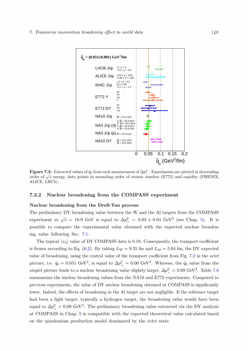
7. Transverse momentum broadening effect in world data 148
/fm)2 (GeV0
q
NA10 DY = 23.2 GeVs = 16.2 GeVs
(p)ψNA3 J/ = 19.4 GeVs
)π (ψNA3 J/ = 22.9 GeVs -π = 19.4 GeVs +π
= 19.4 GeVs -π = 16.8 GeVs -π
ψNA10 J/ = 23.2 GeVs
E772 DYWFeCa
ΥE772 WFeCaC
ψRHIC J/1.2 < y < 2.2|y| < 0.35-2.2 < y < -1.2
ψALICE J/ 2.03 < y < 3.53-4.46 < y < -2.96
ψLHCB J/ 2 < y < 4-4.5 < y < -2.5
/fm20.001) GeV± = (0.0510
q
0 0.05 0.1 0.15 0.2
Figure 7.3: Extracted values of q0 from each measurement of ∆p2⊥. Experiments are plotted in descending
order of√s energy, data points in ascending order of atomic number (E772) and rapidity (PHENIX,
ALICE, LHCb).
7.3.2 Nuclear broadening from the COMPASS experiment
Nuclear broadening from the Drell-Yan processThe preliminary DY broadening value between the W and the Al targets from the COMPASSexperiment at
√s = 18.9 GeV is equal to ∆p2
⊥ = 0.03 ± 0.04 GeV2 (see Chap. 5). It ispossible to compare the experimental value obtained with the expected nuclear broaden-ing value following Sec. 7.1.
The typical 〈x2〉 value of DY COMPASS data is 0.19. Consequently, the transport coefficientis frozen according to Eq. (6.2). By taking LW = 9.55 fm and LAl = 5.04 fm, the DY expectedvalue of broadening, using the central value of the transport coefficient from Fig. 7.2 in the octetpicture, i.e. q0 = 0.051 GeV2, is equal to ∆p2
⊥ = 0.06 GeV2. Whereas, the q0 value from thesinglet picture leads to a nuclear broadening value slightly larger, ∆p2
⊥ = 0.09 GeV2. Table 7.6summarizes the nuclear broadening values from the NA10 and E772 experiments. Compared toprevious experiments, the value of DY nuclear broadening obtained at COMPASS is significantlylower. Indeed, the effects of broadening in the Al target are not negligible. If the reference targethad been a light target, typically a hydrogen target, the broadening value would have beenequal to ∆p2
⊥ = 0.09 GeV2. The preliminary broadening value extracted via the DY analysisat COMPASS in Chap. 5 is compatible with the expected theoretical value calculated basedon the quarkonium production model dominated by the octet state.
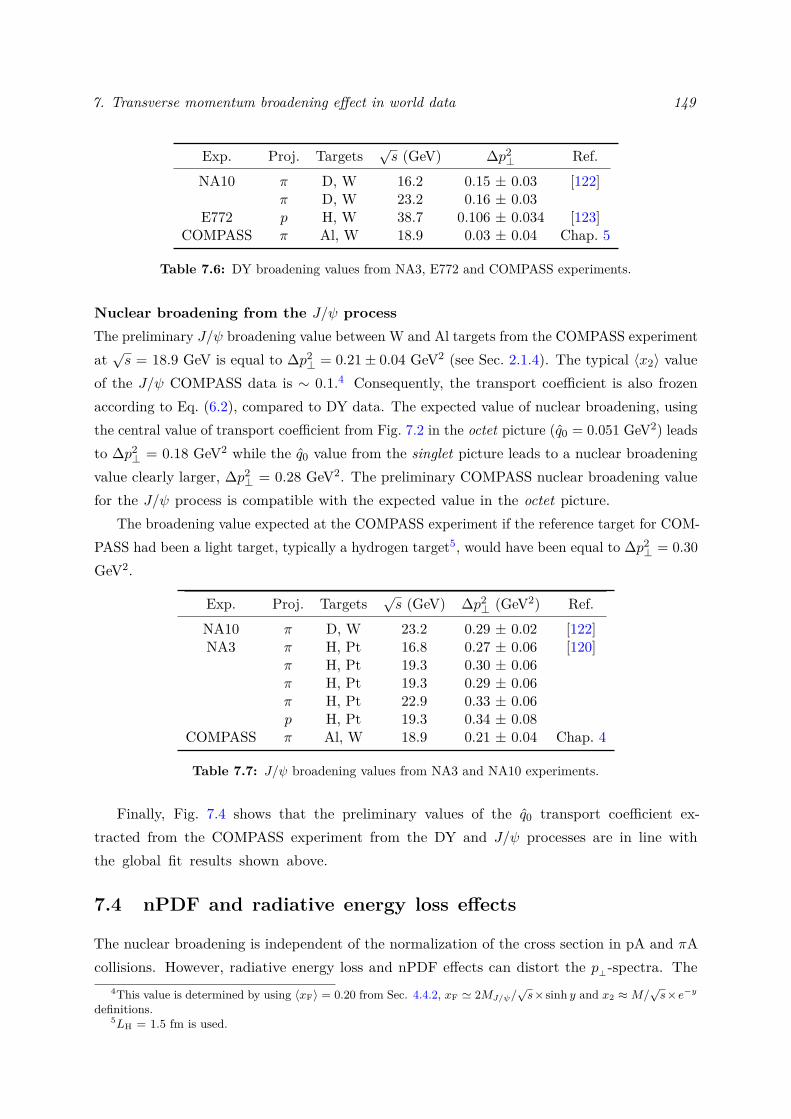
7. Transverse momentum broadening effect in world data 149
Exp. Proj. Targets√s (GeV) ∆p2
⊥ Ref.NA10 π D, W 16.2 0.15 ± 0.03 [122]
π D, W 23.2 0.16 ± 0.03E772 p H, W 38.7 0.106 ± 0.034 [123]
COMPASS π Al, W 18.9 0.03 ± 0.04 Chap. 5
Table 7.6: DY broadening values from NA3, E772 and COMPASS experiments.
Nuclear broadening from the J/ψ processThe preliminary J/ψ broadening value between W and Al targets from the COMPASS experimentat√s = 18.9 GeV is equal to ∆p2
⊥ = 0.21± 0.04 GeV2 (see Sec. 2.1.4). The typical 〈x2〉 valueof the J/ψ COMPASS data is ∼ 0.1.4 Consequently, the transport coefficient is also frozenaccording to Eq. (6.2), compared to DY data. The expected value of nuclear broadening, usingthe central value of transport coefficient from Fig. 7.2 in the octet picture (q0 = 0.051 GeV2) leadsto ∆p2
⊥ = 0.18 GeV2 while the q0 value from the singlet picture leads to a nuclear broadeningvalue clearly larger, ∆p2
⊥ = 0.28 GeV2. The preliminary COMPASS nuclear broadening valuefor the J/ψ process is compatible with the expected value in the octet picture.
The broadening value expected at the COMPASS experiment if the reference target for COM-PASS had been a light target, typically a hydrogen target5, would have been equal to ∆p2
⊥ = 0.30GeV2.
Exp. Proj. Targets√s (GeV) ∆p2
⊥ (GeV2) Ref.NA10 π D, W 23.2 0.29 ± 0.02 [122]NA3 π H, Pt 16.8 0.27 ± 0.06 [120]
π H, Pt 19.3 0.30 ± 0.06π H, Pt 19.3 0.29 ± 0.06π H, Pt 22.9 0.33 ± 0.06p H, Pt 19.3 0.34 ± 0.08
COMPASS π Al, W 18.9 0.21 ± 0.04 Chap. 4
Table 7.7: J/ψ broadening values from NA3 and NA10 experiments.
Finally, Fig. 7.4 shows that the preliminary values of the q0 transport coefficient ex-tracted from the COMPASS experiment from the DY and J/ψ processes are in line withthe global fit results shown above.
7.4 nPDF and radiative energy loss effects
The nuclear broadening is independent of the normalization of the cross section in pA and πAcollisions. However, radiative energy loss and nPDF effects can distort the p⊥-spectra. The
4This value is determined by using 〈xF〉 = 0.20 from Sec. 4.4.2, xF ' 2MJ/ψ/√s× sinh y and x2 ≈M/
√s×e−y
definitions.5LH = 1.5 fm is used.
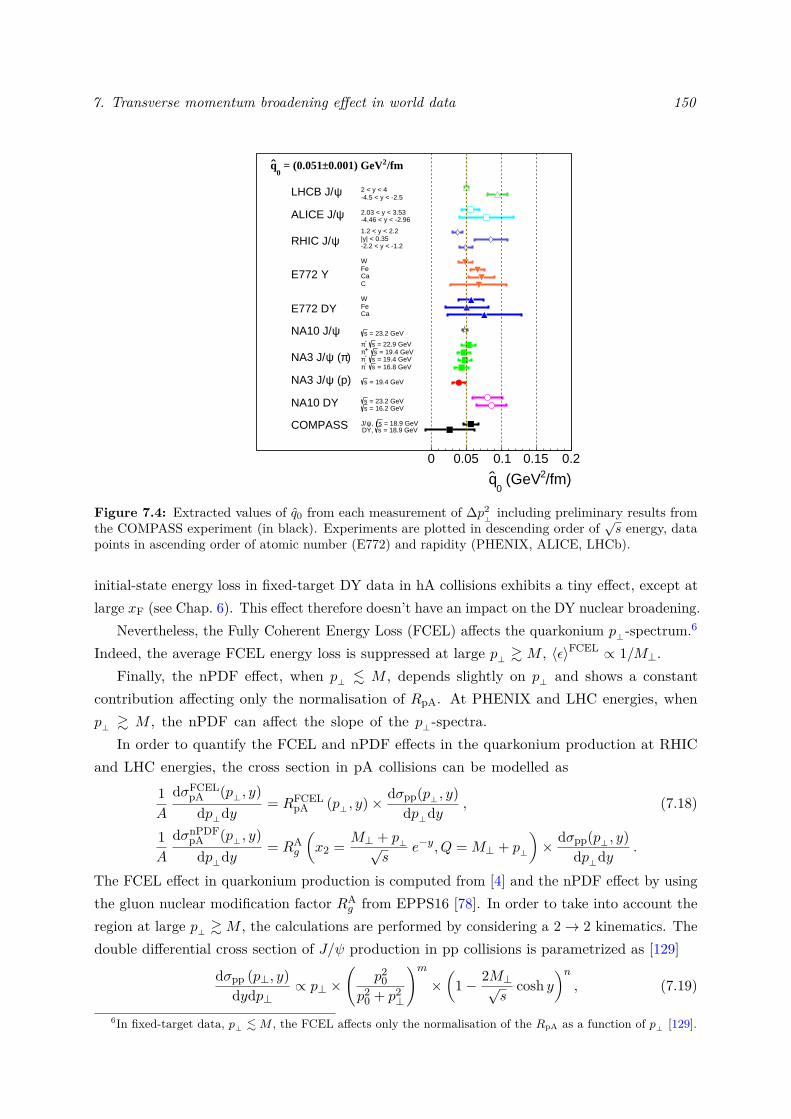
7. Transverse momentum broadening effect in world data 150
/fm)2 (GeV0
q
COMPASS = 18.9 GeVs, ψJ/ = 18.9 GeVsDY,
NA10 DY = 23.2 GeVs = 16.2 GeVs
(p)ψNA3 J/ = 19.4 GeVs
)π (ψNA3 J/ = 22.9 GeVs -π = 19.4 GeVs +π
= 19.4 GeVs -π = 16.8 GeVs -π
ψNA10 J/ = 23.2 GeVs
E772 DYWFeCa
ΥE772 WFeCaC
ψRHIC J/1.2 < y < 2.2|y| < 0.35-2.2 < y < -1.2
ψALICE J/ 2.03 < y < 3.53-4.46 < y < -2.96
ψLHCB J/ 2 < y < 4-4.5 < y < -2.5
/fm20.001) GeV± = (0.0510
q
0 0.05 0.1 0.15 0.2
Figure 7.4: Extracted values of q0 from each measurement of ∆p2⊥including preliminary results from
the COMPASS experiment (in black). Experiments are plotted in descending order of√s energy, data
points in ascending order of atomic number (E772) and rapidity (PHENIX, ALICE, LHCb).
initial-state energy loss in fixed-target DY data in hA collisions exhibits a tiny effect, except atlarge xF (see Chap. 6). This effect therefore doesn’t have an impact on the DY nuclear broadening.
Nevertheless, the Fully Coherent Energy Loss (FCEL) affects the quarkonium p⊥-spectrum.6
Indeed, the average FCEL energy loss is suppressed at large p⊥ & M , 〈ε〉FCEL ∝ 1/M⊥.Finally, the nPDF effect, when p⊥ . M , depends slightly on p⊥ and shows a constant
contribution affecting only the normalisation of RpA. At PHENIX and LHC energies, whenp⊥ & M , the nPDF can affect the slope of the p⊥-spectra.
In order to quantify the FCEL and nPDF effects in the quarkonium production at RHICand LHC energies, the cross section in pA collisions can be modelled as
1A
dσFCELpA (p⊥ , y)dp⊥dy
= RFCELpA (p⊥ , y)× dσpp(p⊥ , y)
dp⊥dy, (7.18)
1A
dσnPDFpA (p⊥ , y)dp⊥dy
= RAg
(x2 = M⊥ + p⊥√
se−y, Q = M⊥ + p⊥
)× dσpp(p⊥ , y)
dp⊥dy.
The FCEL effect in quarkonium production is computed from [4] and the nPDF effect by usingthe gluon nuclear modification factor RA
g from EPPS16 [78]. In order to take into account theregion at large p⊥ &M , the calculations are performed by considering a 2→ 2 kinematics. Thedouble differential cross section of J/ψ production in pp collisions is parametrized as [129]
dσpp (p⊥, y)dydp⊥
∝ p⊥ ×(
p20
p20 + p2
⊥
)m×(
1− 2M⊥√s
cosh y)n
, (7.19)
6In fixed-target data, p⊥ .M , the FCEL affects only the normalisation of the RpA as a function of p⊥ [129].
7. Transverse momentum broadening effect in world data 151
where the values of N , n, m and p0 parameters were extracted from the LHC data in [129].Figure 7.5 shows the FCEL and the EPPS16 nPDF effects at backward (left panel) and forward(right panel) rapidities at LHCb energy (
√s = 8160 GeV). The FCEL calculation, in both
rapidity ranges, exibits a constant RpA for p⊥ & 5 GeV. For p⊥ . M , RpA shows a smalldepletion, more accentuated at forward compared to backward rapidity. The nPDF calculationalso shows a RpA . 1 increasing as a function of p⊥ (x2) due to the shadowing effect at forwardrapidity. At backward rapidity, the RpA slightly increases and decreases around 1 as a functionof p⊥ mainly due to the anti-shadowing and EMC regions.7
The impact of these effects on the broadening calculation using Eq. (7.18) in PHENIX andLHC data is summarized in Table 7.8. Although the FCEL and nPDF effects (with a large
Experiment System y range ∆p2⊥
∣∣FCEL (GeV2) ∆p2
⊥
∣∣nPDF (GeV2)
PHENIX dAu −2.2 < y < −1.2 0.1 [-0.2 ; 0]dAu |y| < 0.35 0.1 [0.1 ; 0.4]dAu 1.2 < y < 2.2 0.1 [0.1 ; 0.4]
LHCb pPb −4.5 < y < −2.5 0.2 [0.1 ; 0.6]pPb 2 < y < 4 [0.5 ; 0.6] [0.1 ; 0.7]
Table 7.8: Calculation of ∆p2⊥
∣∣FCEL and ∆p2
⊥
∣∣nPDF at RHIC and LHC.
uncertainty) may impact the nuclear broadening value of the J/ψ process, the results show aweak effect. This shows that nuclear broadening is the dominant effect in the data. Furthermore,a strong correlation coefficient (0.7) for each EPPS16 error set in the broadening calculationinterval is observed between backward and forward rapidity at LHC. A better constraint ofnPDFs in one of these two ranges in rapidity will impact them in the same way.
7.5 Relation between the broadening and the gluon distribution
The transport coefficient q is directly related to the gluon distribution xG(x) of the nucleonin Eq. (6.2). It is therefore possible to use recent PDFs of the proton in order to test therelationship between q and xG(x) and also their scale dependence. From Eq. (7.4) andEq. (6.2), the broadening reads
∆p2⊥ ∝ Cαs
(Q2) [xG
(x,Q2
)LA − x′G
(x′, Q2
)Lp]≡ Cαs∆(xGL). (7.20)
The scale Q2 appearing in Eq. (7.20) should be of the order of magnitude of ∆p2⊥. At low-
scales8, ∆p2⊥. 1 GeV2, Q2 is frozen at the input scale9 of the proton PDF, according to Q2 =
min(Q2
0, λ∆p2⊥). Figure 7.6 shows the fit of nuclear broadening data in the octet picture using the
7By considering p⊥ =0 GeV and 〈y〉=-3.5, x2 ∼ 0.1 and at p⊥ =20 GeV, x2 ∼ 0.8. This p⊥ region embracingboth antishadowing effect mainly at small p⊥ and EMC effect at large p⊥ .
8All the data used are in this regime, except the LHC data at forward rapidity.9Typically, Q2
0 = 1− 2 GeV2.
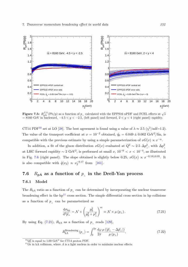
7. Transverse momentum broadening effect in world data 152
0 2 4 6 8 10 12 14 16 18 20
(GeV)p
0
0.2
0.4
0.6
0.8
1
1.2
1.4
1.6
1.8
2
(Pb/
p)pA
R
= 8160 GeV, -4.5 < y < -2.5s
EPPS16 nPDF central set
EPPS16 nPDF error sets
/fm (<y> = -3.5)2 = 0.05 GeV0
qFCEL
0 2 4 6 8 10 12 14 16 18 20
(GeV)p
0
0.2
0.4
0.6
0.8
1
1.2
1.4
1.6
1.8
2
(Pb/
p)pA
R
= 8160 GeV, 2 < y < 4s
EPPS16 nPDF central set
EPPS16 nPDF error sets
/fm (<y> = 3)2 = 0.05 GeV0
qFCEL
Figure 7.5: RJ/ψpA (Pb/p) as a function of p⊥ calculated with the EPPS16 nPDF and FCEL effects at√s
= 8160 GeV in backward, −4.5 < y < −2.5, (left panel) and forward, 2 < y < 4 (right panel) rapidity.
CT14 PDF10 set at LO [28]. The best agreement is found using a value of λ ≈ 2.5 (χ2/ndf=1.2).The value of the transport coefficient at x = 10−2 obtained, q0 = 0.049 ± 0.002 GeV2/fm, iscompatible with the previous estimate by using a simple parameterization of xG(x) ∝ x−α.
In addition, a fit of the gluon distribution xG(x) evaluated at Q2 ∼ 2.5 ∆p2⊥, with ∆p2
⊥
at LHC forward rapidity ∼ 2 GeV2, is performed at small x, 10−6 < x < 10−4, as illustratedin Fig. 7.6 (right panel). The slope obtained is slightly below 0.25, xG(x) ∝ x−0.18±0.05. Itis also compatible with q(x2) ∝ x−0.17
2 from [161].
7.6 RpA as a function of p⊥ in the Drell-Yan process
7.6.1 Model
The RhA ratio as a function of p⊥ can be determined by incorporating the nuclear transversebroadening effect in the hp11 cross section. The simple differential cross section in hp collisionsas a function of p⊥ can be parameterized as
dσhpd2~p⊥
= N ×(
p20
p20 + p2
⊥
)m≡ N × µ (p⊥) . (7.21)
By using Eq. (7.21), RhA as a function of p⊥ reads [129],
RBroadeninghA (p⊥) =
∫ 2π
0
dϕ2π
µ (|~p⊥ −∆~p⊥|)µ (p⊥) , (7.22)
10Q20 is equal to 1.69 GeV2 for CT14 proton PDF.
11Or in hA collisions, where A is a light nucleus in order to minimise nuclear effects
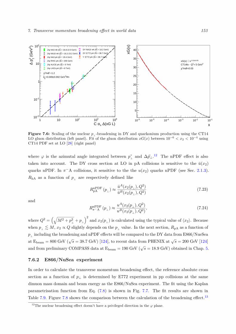
7. Transverse momentum broadening effect in world data 153
1 10 210 310 410(xG L)∆ sαC
2−10
1−10
1
10
210)2 (
GeV
2 T p∆
/fm20.002 GeV±=0.0490
q
/ndf =1.22χ
= 16.2 GeV)sA (πDY NA10
= 38.7 GeV)sDY E772 pA (
= 38.7 GeV)s E772 pA (Υ
= 16.8-22.9 GeV)sA (π NA3 ψJ/
= 16.2-23.2 GeV)sA (π NA10 ψJ/
= 19.4 GeV)s NA3 pA (ψJ/
= 200 GeV)s RHIC pA (ψJ/
= 5 TeV)s ALICE pA (ψJ/
= 8 TeV)s LHCb pA (ψJ/
6−10 5−10 4−10 3−10 2−10 1−10
x
5
10
15
20
25
30
35
40
xG(x
)
2= 5 GeV2CT14lo - Q
0.05±-0.18 x∝xG(x)
/ndf=0.032χ
Figure 7.6: Scaling of the nuclear p⊥-broadening in DY and quarkonium production using the CT14LO gluon distribution (left panel). Fit of the gluon distribution xG(x) between 10−6 < x2 < 10−4 usingCT14 PDF set at LO [28] (right panel)
where ϕ is the azimutal angle integrated between ~p⊥ and ∆~p⊥.12 The nPDF effect is alsotaken into account. The DY cross section at LO in pA collisions is sensitive to the u(x2)quarks nPDF. In π−A collisions, it sensitive to the the u(x2) quarks nPDF (see Sec. 2.1.3).RhA as a function of p⊥ are respectively defined like
RnPDFpA (p⊥) ≈ uA(x2(p⊥), Q2)
uB(x2(p⊥), Q2)(7.23)
andRnPDFπ−A (p⊥) ≈ uA(x2(p⊥), Q2)
uB(x2(p⊥), Q2) ,(7.24)
where Q2 =(√
M2 + p2⊥
+ p⊥
)2and x2(p⊥) is calculated using the typical value of 〈x2〉. Because
when p⊥ .M , x2 ∝ Q slightly depends on the p⊥ value. In the next section, RpA as a function ofp⊥ including the broadening and nPDF effects will be compared to the DY data from E866/NueSeaat Ebeam = 800 GeV (
√s = 38.7 GeV) [124], to recent data from PHENIX at
√s = 200 GeV [124]
and from preliminary COMPASS data at Ebeam = 190 GeV (√s = 18.9 GeV) obtained in Chap. 5.
7.6.2 E866/NuSea experiment
In order to calculate the transverse momentum broadening effect, the reference absolute crosssection as a function of p⊥ is determined by E772 experiment in pp collisions at the samedimuon mass domain and beam energy as the E866/NuSea experiment. The fit using the Kaplanparametrisation function from Eq. (7.8) is shown in Fig. 7.7. The fit results are shown inTable 7.9. Figure 7.8 shows the comparison between the calculation of the broadening effect.13
12The nuclear broadening effect doesn’t have a privileged direction in the ϕ plane.
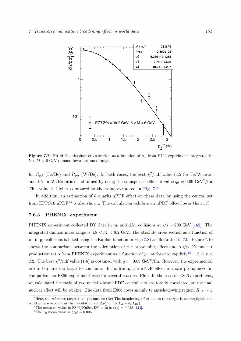
7. Transverse momentum broadening effect in world data 154
0 0.5 1 1.5 2 2.5 3 (GeV)p
1-10
1
(pb)
2/d
psd
/ ndf 2c 36.8 / 9Prob 05- 2.862ep0 0.1355± 6.289 p1 0.682± 3.74 p2 3.297± 10.21
= 38.7 GeV, 5 < M < 6 GeVsE866 772
Figure 7.7: Fit of the absolute cross section as a function of p⊥ from E722 experiment integrated in5 < M < 6 GeV dimuon invariant mass range.
for RpA (Fe/Be) and RpA (W/Be). In both cases, the best χ2/ndf value (1.2 for Fe/W ratioand 1.5 for W/Be ratio) is obtained by using the transport coefficient value q0 = 0.09 GeV2/fm.This value is higher compared to the value extracted in Fig. 7.2.
In addition, an estimation of u quarks nPDF effect on these data by using the central setfrom EPPS16 nPDF14 is also shown. The calculation exhibits an nPDF effect lower than 5%.
7.6.3 PHENIX experiment
PHENIX experiment collected DY data in pp and dAu collisions at√s = 200 GeV [162]. The
integrated dimuon mass range is 4.8 < M < 8.2 GeV. The absolute cross section as a function ofp⊥ in pp collisions is fitted using the Kaplan function in Eq. (7.8) as illustrated in 7.9. Figure 7.10shows the comparison between the calculation of the broadening effect and Au/p DY nuclearproduction ratio from PHENIX experiment as a function of p⊥ at forward rapditiy15, 1.2 < y <2.2. The best χ2/ndf value (1.6) is obtained with q0 = 0.09 GeV2/fm. However, the experimentalerrors bar are too large to conclude. In addition, the nPDF effect is more pronounced incomparison to E866 experiment case for several reasons. First, in the case of E866 experiment,we calculated the ratio of two nuclei whose nPDF central sets are totally correlated, so the finalnuclear effect will be weaker. The data from E866 cover mainly te antishadowing region, RpA ∼ 1.
13Here, the reference target is a light nucleus (Be) The broadening effect due to this target is not negligible andis taken into account in the calculation via ∆p2
⊥ ∝ (qA LA − qB LBe).14The mean x2 value in E866/NuSea DY data is 〈x2〉 = 0.038 [124].15The x2 mean value is 〈x2〉 = 0.005.
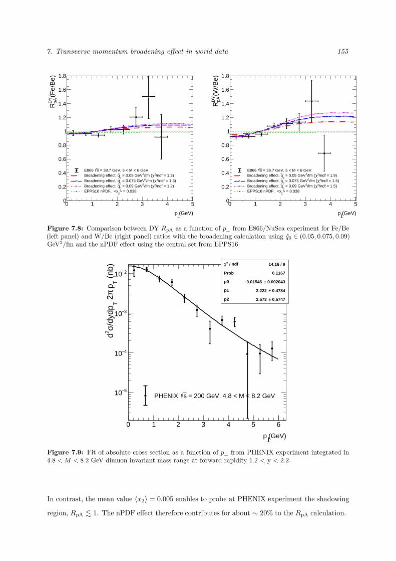
7. Transverse momentum broadening effect in world data 155
0 1 2 3 4 5
(GeV)p
0
0.2
0.4
0.6
0.8
1
1.2
1.4
1.6
1.8
(Fe/
Be)
DY
pAR
= 38.7 GeV, 5 < M < 6 GeVsE866 /ndf = 1.3)2χ/fm (2 = 0.05 GeV
0qBroadening effect,
/ndf = 1.3)2χ/fm (2 = 0.075 GeV0
qBroadening effect, /ndf = 1.2)2χ/fm (2 = 0.09 GeV
0qBroadening effect, > = 0.038
2EPPS16 nPDF, <x
0 1 2 3 4 5
(GeV)p
0
0.2
0.4
0.6
0.8
1
1.2
1.4
1.6
1.8
(W/B
e)D
YpA
R
= 38.7 GeV, 5 < M < 6 GeVsE866 /ndf = 1.9)2χ/fm (2 = 0.05 GeV
0qBroadening effect,
/ndf = 1.5)2χ/fm (2 = 0.075 GeV0
qBroadening effect, /ndf = 1.5)2χ/fm (2 = 0.09 GeV
0qBroadening effect, > = 0.038
2EPPS16 nPDF, <x
Figure 7.8: Comparison between DY RpA as a function of p⊥ from E866/NuSea experiment for Fe/Be(left panel) and W/Be (right panel) ratios with the broadening calculation using q0 ∈ (0.05, 0.075, 0.09)GeV2/fm and the nPDF effect using the central set from EPPS16.
0 1 2 3 4 5 6
(GeV)p
5−10
4−10
3−10
2−10 (nb
)T
pπ 2
T/d
ydp
σ2 d
/ ndf 2χ 14.16 / 9
Prob 0.1167
p0 0.002043± 0.01546
p1 0.4784± 2.222
p2 0.5747± 2.573
= 200 GeV, 4.8 < M < 8.2 GeVsPHENIX
Figure 7.9: Fit of absolute cross section as a function of p⊥ from PHENIX experiment integrated in4.8 < M < 8.2 GeV dimuon invariant mass range at forward rapidity 1.2 < y < 2.2.
In contrast, the mean value 〈x2〉 = 0.005 enables to probe at PHENIX experiment the shadowing
region, RpA . 1. The nPDF effect therefore contributes for about ∼ 20% to the RpA calculation.
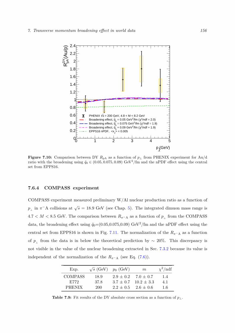
7. Transverse momentum broadening effect in world data 156
0 1 2 3 4 5
(GeV)p
0
0.2
0.4
0.6
0.8
1
1.2
1.4
1.6
1.8
2
2.2
2.4
(Au/
p)D
YpA
R
= 200 GeV, 4.8 < M < 8.2 GeVsPHENIX /ndf = 2.0)2χ/fm (2 = 0.05 GeV
0qBroadening effect,
/ndf = 1.9)2χ/fm (2 = 0.075 GeV0
qBroadening effect, /ndf = 1.9)2χ/fm (2 = 0.09 GeV
0qBroadening effect, > = 0.005
2EPPS16 nPDF, <x
Figure 7.10: Comparison between DY RpA as a function of p⊥ from PHENIX experiment for Au/dratio with the broadening using q0 ∈ (0.05, 0.075, 0.09) GeV2/fm and the nPDF effect using the centralset from EPPS16.
7.6.4 COMPASS experiment
COMPASS experiment measured preliminary W/Al nuclear production ratio as a function of
p⊥ in π−A collisions at√s = 18.9 GeV (see Chap. 5). The integrated dimuon mass range is
4.7 < M < 8.5 GeV. The comparison between Rπ−A as a function of p⊥ from the COMPASS
data, the broadening effect using q0=(0.05,0.075,0.09) GeV2/fm and the nPDF effect using the
central set from EPPS16 is shown in Fig. 7.11. The normalization of the Rπ−A as a function
of p⊥ from the data is in below the theoretical prediction by ∼ 20%. This discrepancy is
not visible in the value of the nuclear broadening extracted in Sec. 7.3.2 because its value is
independent of the normalization of the Rπ−A (see Eq. (7.6)).
Exp.√s (GeV) p0 (GeV) m χ2/ndf
COMPASS 18.9 2.9 ± 0.2 7.0 ± 0.7 1.4E772 37.8 3.7 ± 0.7 10.2 ± 3.3 4.1
PHENIX 200 2.2 ± 0.5 2.6 ± 0.6 1.6
Table 7.9: Fit results of the DY absolute cross section as a function of p⊥.
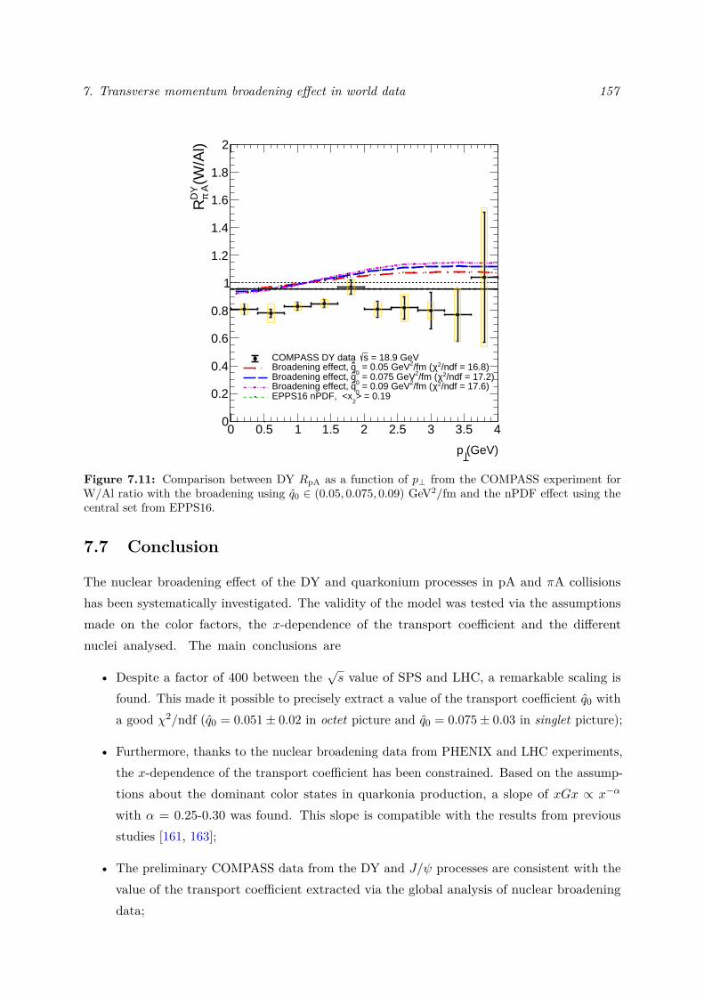
7. Transverse momentum broadening effect in world data 157
0 0.5 1 1.5 2 2.5 3 3.5 4
(GeV)p
0
0.2
0.4
0.6
0.8
1
1.2
1.4
1.6
1.8
2
(W/A
l)D
Y AπR
= 18.9 GeVsCOMPASS DY data /ndf = 16.8)2χ/fm (2 = 0.05 GeV
0qBroadening effect,
/ndf = 17.2)2χ/fm (2 = 0.075 GeV0
qBroadening effect, /ndf = 17.6)2χ/fm (2 = 0.09 GeV
0qBroadening effect, > = 0.19
2EPPS16 nPDF, <x
Figure 7.11: Comparison between DY RpA as a function of p⊥ from the COMPASS experiment forW/Al ratio with the broadening using q0 ∈ (0.05, 0.075, 0.09) GeV2/fm and the nPDF effect using thecentral set from EPPS16.
7.7 Conclusion
The nuclear broadening effect of the DY and quarkonium processes in pA and πA collisionshas been systematically investigated. The validity of the model was tested via the assumptionsmade on the color factors, the x-dependence of the transport coefficient and the differentnuclei analysed. The main conclusions are
• Despite a factor of 400 between the√s value of SPS and LHC, a remarkable scaling is
found. This made it possible to precisely extract a value of the transport coefficient q0 witha good χ2/ndf (q0 = 0.051± 0.02 in octet picture and q0 = 0.075± 0.03 in singlet picture);
• Furthermore, thanks to the nuclear broadening data from PHENIX and LHC experiments,the x-dependence of the transport coefficient has been constrained. Based on the assump-tions about the dominant color states in quarkonia production, a slope of xGx ∝ x−α
with α = 0.25-0.30 was found. This slope is compatible with the results from previousstudies [161, 163];
• The preliminary COMPASS data from the DY and J/ψ processes are consistent with thevalue of the transport coefficient extracted via the global analysis of nuclear broadeningdata;
7. Transverse momentum broadening effect in world data 158
• The p⊥ dependence of RhA has also been investigated. A compatibility was found betweenthe broadening calculation using q0=(0.05,0.075,0.09) GeV2/fm transport coefficient intervaland the DY data at E866, PHENIX and COMPASS experiments. A weak nPDF effect isobserved as a function of p⊥ at E866 and COMPASS experiments. A more pronouncedeffect is shown at PHENIX experiment due to the strong shadowing effect at x2 ∼ 0.005.
8Conclusion
Thirty years after the last data collected in πA published by the NA10 experiment, preliminarydata from the 2018 run as a function of xF and p⊥ of the Drell-Yan (DY) and J/ψ processesfrom the COMPASS experiment on two nuclear targets, W and Al, were analyzed. From thesignal extraction to the evaluation of cross sections, including Monte Carlo simulations, eachstep of the experimental analysis have been presented. Using a multidimensional analysis andsimulating each physical process participating in the dimuon mass spectrum, the evolution of theJ/ψ number as a function of xF and p⊥ was quantified in π−W and π−Al collisions.
These preliminary J/ψ data, collected in a large amount, highlight a strong suppressionof the cross section in both p⊥ and xF variables in the π−W collisions compared to the π−Alcollisions. A contrario, preliminary DY data show less suppression. RDY
π−A(W/Al) ratio exhibitsa slight depletion at large xF and a Cronin peak at p⊥ = 1-2 GeV. Due to large experimentalerrors, the latter is compatible with ∆p2
⊥=0. In both analyzes, the calculation of the value of
the nuclear transverse momentum broadening shows a compatibility with previous experiments,∆p2⊥(J/ψ) = 0.21 ± 0.04 GeV2 and ∆p2
⊥(DY) = 0.03 ± 0.04 GeV2.The cold nuclear matter effects in the DY and quarkonium productions as a function of
the rapidity and transverse momentum from fixed-target to collider energies was investigated.In two phenomenological studies Refs. [1] and [2], the first one is a study of the initial-state energy loss effects in DY data from fixed target experiments. For the first time, thepreliminary data from the Fermilab E906/SeaQuest experiment demonstrate, without ambiguity,an energy loss effect in pA collisions in DY data.
Finally, the second one is a study of the nuclear transverse momentum dependence in theDY and quarkonium production highlights a unique effect present at all collisions energies:nuclear broadening. A precise extraction of the transport coefficient has been performed
159
8. Conclusion 160
using color and octet quarkonium production assumption. The latter is compatible withthe previous radiative energy loss studies.
The interpretation of nuclear data in hA collisions is limited by the size of the uncertainties innPDF effect. The measurement of Deep Inelastic scattering (DIS) data proposed by the Electron-Ion-Collider (EIC) collaboration should add constrains on the nPDF allowing to considerablyreduce their error bands [93, 94]. Future DY data at low beam energy (Ebeam . 100 GeV)can bring constraints on the transport coefficient. Indeed, at these energies, the initial-stateenergy loss effect dominates the ratio of nuclear DY cross sections as a function of xF. Usinga proton beam versus a pion beam leads to a stronger effects.
Bibliography
[1] F. Arleo, C.-J. Naïm and S. Platchkov, Initial-state energy loss in cold QCD matter andthe Drell-Yan process, JHEP 01 (2019) 129 [1810.05120].
[2] F. Arleo and C.-J. Naïm, Nuclear p⊥-broadening of Drell-Yan and quarkonium productionfrom SPS to LHC, JHEP 07 (2020) 220 [2004.07188].
[3] F. Arleo and S. Peigne, J/ψ suppression in p-A collisions from parton energy loss in coldQCD matter, Phys. Rev. Lett. 109 (2012) 122301 [1204.4609].
[4] F. Arleo and S. Peigné, Heavy-quarkonium suppression in pA collisions from parton energyloss in cold QCD matter, JHEP 03 (2013) 122 [1212.0434].
[5] J. H. Christenson, G. S. Hicks, L. M. Lederman, P. J. Limon, B. G. Pope et al.,Observation of massive muon pairs in hadron collisions, Phys. Rev. Lett. 25 (1970) 1523.
[6] J. H. Christenson, G. S. Hicks, L. M. Lederman, P. J. Limon, B. G. Pope et al.,Observation of muon pairs in high-energy hadron collisions, Phys. Rev. D 8 (1973) 2016.
[7] S. D. Drell and T.-M. Yan, Massive Lepton Pair Production in Hadron-Hadron Collisionsat High-Energies, Phys. Rev. Lett. 25 (1970) 316.
[8] F. Ravndal, Feynman and the quark model, Int. J. Mod. Phys. A 8 (1993) 4369.
[9] E598 collaboration, J. Aubert et al., Experimental Observation of a Heavy Particle J ,Phys. Rev. Lett. 33 (1974) 1404.
[10] SLAC-SP-017 collaboration, J. Augustin et al., Discovery of a Narrow Resonance ine+e− Annihilation, Phys. Rev. Lett. 33 (1974) 1406.
[11] J. D. Bjorken, ed., In Conclusion: A Collection of Summary Talks in High Energy Physics.2003.
[12] S. Ting, The Discovery of the J Particle: A Personal Recollection, Rev. Mod. Phys. 49(1977) 235.
[13] G. Abrams et al., The Discovery of a Second Narrow Resonance in e+ e- Annihilation,Phys. Rev. Lett. 33 (1974) 1453.
161
Bibliography 162
[14] J. D. Bjorken, CURRENT ALGEBRA AT SMALL DISTANCES, Conf. Proc. C670717(1967) 55.
[15] H. D. Politzer, Reliable Perturbative Results for Strong Interactions?, Phys. Rev. Lett. 30(1973) 1346.
[16] D. J. Gross and F. Wilczek, Ultraviolet Behavior of Nonabelian Gauge Theories, Phys.Rev. Lett. 30 (1973) 1343.
[17] H1 collaboration, F. Aaron et al., Inclusive Deep Inelastic Scattering at High Q2 withLongitudinally Polarised Lepton Beams at HERA, JHEP 09 (2012) 061 [1206.7007].
[18] CTEQ collaboration, R. Brock et al., Handbook of perturbative QCD: Version 1.0, Rev.Mod. Phys. 67 (1995) 157.
[19] L. N. Lipatov, The parton model and perturbation theory, Sov. J. Nucl. Phys. 20 (1975) 94.
[20] V. N. Gribov and L. N. Lipatov, Deep inelastic e p scattering in perturbation theory, Sov.J. Nucl. Phys. 15 (1972) 438.
[21] S. Catani and M. Grazzini, Collinear factorization and splitting functions fornext-to-next-to-leading order QCD calculations, Phys. Lett. B446 (1999) 143[hep-ph/9810389].
[22] S. Moch, J. A. M. Vermaseren and A. Vogt, The three-loop splitting functions in QCD:The non-singlet case, Nucl. Phys. B688 (2004) 101 [hep-ph/0403192].
[23] A. Vogt, S. Moch and J. A. M. Vermaseren, The three-loop splitting functions in QCD:The singlet case, Nucl. Phys. B691 (2004) 129 [hep-ph/0404111].
[24] G. Altarelli and G. Parisi, Asymptotic Freedom in Parton Language, Nucl. Phys. B 126(1977) 298.
[25] R. Field, Applications of Perturbative QCD, vol. 77. 1989.
[26] L. A. Harland-Lang, A. D. Martin, P. Motylinski and R. S. Thorne, Parton distributionsin the LHC era: MMHT 2014 PDFs, Eur. Phys. J. C75 (2015) 204 [1412.3989].
[27] D. Stump et al., Inclusive jet production, parton distributions, and the search for newphysics, JHEP 10 (2003) 046 [hep-ph/0303013].
[28] S. Dulat, T.-J. Hou, J. Gao, M. Guzzi, J. Huston et al., New parton distribution functionsfrom a global analysis of quantum chromodynamics, Phys. Rev. D93 (2016) 033006[1506.07443].
Bibliography 163
[29] NNPDF collaboration, R. D. Ball et al., Parton distributions from high-precision colliderdata, Eur. Phys. J. C 77 (2017) 663 [1706.00428].
[30] P. Sutton, A. D. Martin, R. Roberts and W. Stirling, Parton distributions for the pionextracted from Drell-Yan and prompt photon experiments, Phys. Rev. D 45 (1992) 2349.
[31] NA10 collaboration, B. Betev et al., Differential Cross-section of High Mass Muon PairsProduced by a 194-GeV/cπ− Beam on a Tungsten Target, Z. Phys. C28 (1985) 9.
[32] J. S. Conway et al., Experimental Study of Muon Pairs Produced by 252-GeV Pions onTungsten, Phys. Rev. D39 (1989) 92.
[33] WA70 collaboration, E. Bonvin et al., DOUBLE PROMPT PHOTON PRODUCTIONAT HIGH TRANSVERSE MOMENTUM BY pi- ON PROTONS AT 280-GeV/c, Z. Phys.C41 (1989) 591.
[34] M. Glück, E. Reya and A. Vogt, Pionic parton distributions, Z. Phys. C53 (1992) 651.
[35] M. Gluck, E. Reya and I. Schienbein, Pionic parton distributions revisited, Eur. Phys. J. C10 (1999) 313 [hep-ph/9903288].
[36] ZEUS collaboration, S. Chekanov et al., Leading neutron production in e+ p collisions atHERA, Nucl. Phys. B637 (2002) 3 [hep-ex/0205076].
[37] H1 collaboration, F. D. Aaron et al., Measurement of Leading Neutron Production inDeep-Inelastic Scattering at HERA, Eur. Phys. J. C68 (2010) 381 [1001.0532].
[38] P. C. Barry, N. Sato, W. Melnitchouk and C.-R. Ji, First Monte Carlo Global QCDAnalysis of Pion Parton Distributions, Phys. Rev. Lett. 121 (2018) 152001 [1804.01965].
[39] I. R. Kenyon, The Drell-Yan Process, Rept. Prog. Phys. 45 (1982) 1261.
[40] Y. L. Dokshitzer, V. A. Khoze, A. H. Mueller and S. Troian, Basics of perturbative QCD.1991.
[41] R. Ellis, W. Stirling and B. Webber, QCD and collider physics, vol. 8. CambridgeUniversity Press, 2, 2011.
[42] R. Baier, Y. L. Dokshitzer, A. H. Mueller and D. Schiff, Quenching of hadron spectra inmedia, JHEP 09 (2001) 033 [hep-ph/0106347].
[43] S. Catani, L. Cieri, G. Ferrera, D. de Florian and M. Grazzini, Vector boson production athadron colliders: a fully exclusive QCD calculation at NNLO, Phys. Rev. Lett. 103 (2009)082001 [0903.2120].
Bibliography 164
[44] PHENIX collaboration, C. Aidala et al., Measurements of µµ pairs from open heavyflavor and Drell-Yan in p+ p collisions at
√s = 200 GeV, Phys. Rev. D 99 (2019) 072003
[1805.02448].
[45] S. Gavin et al., Production of the Drell-Yan pairs in high-energy nucleon- nucleoncollisions, Int. J. Mod. Phys. A10 (1995) 2961 [hep-ph/9502372].
[46] Y. L. Dokshitzer, D. Diakonov and S. I. Troian, Hard Processes in QuantumChromodynamics, Phys. Rept. 58 (1980) 269.
[47] J. C. Collins, D. E. Soper and G. F. Sterman, Transverse Momentum Distribution inDrell-Yan Pair and W and Z Boson Production, Nucl. Phys. B250 (1985) 199.
[48] S. Catani, D. de Florian, G. Ferrera and M. Grazzini, Vector boson production at hadroncolliders: transverse-momentum resummation and leptonic decay, JHEP 12 (2015) 047[1507.06937].
[49] M. Kramer, Charmonium production at high-energy colliders, Pramana 51 (1998) 145.
[50] R. Vogt, The xF dependence of ψ and Drell-Yan production, Phys. Rev. C61 (2000)035203 [hep-ph/9907317].
[51] Y.-Q. Ma and R. Vogt, Quarkonium Production in an Improved Color Evaporation Model,Phys. Rev. D94 (2016) 114029 [1609.06042].
[52] C.-H. Chang, Hadronic production of J/ψ associated with a gluon, Nucl. Phys. B172(1980) 425.
[53] J. Lansberg, J/ψ production at sqrt(s)=1.96 and 7 TeV: Color-Singlet Model, NNLO* andpolarisation, J. Phys. G 38 (2011) 124110 [1107.0292].
[54] G. T. Bodwin, E. Braaten and G. P. Lepage, Rigorous QCD analysis of inclusiveannihilation and production of heavy quarkonium, Phys. Rev. D51 (1995) 1125[hep-ph/9407339].
[55] W. Buchmuller and S. H. H. Tye, Quarkonia and Quantum Chromodynamics, Phys. Rev.D24 (1981) 132.
[56] E. J. Eichten and C. Quigg, Quarkonium wave functions at the origin: an update,1904.11542.
[57] CDF collaboration, F. Abe et al., J/ψ and ψ(2S) production in pp collisions at√s = 1.8
TeV, Phys. Rev. Lett. 79 (1997) 572.
Bibliography 165
[58] P. Nason et al., Bottom production, in 1999 CERN Workshop on standard model physics(and more) at the LHC, CERN, Geneva, Switzerland, 25-26 May: Proceedings,pp. 231–304, 1999, hep-ph/0003142.
[59] F. Maltoni et al., Analysis of charmonium production at fixed-target experiments in theNRQCD approach, Phys. Lett. B638 (2006) 202 [hep-ph/0601203].
[60] NuSea collaboration, J. Webb et al., Absolute Drell-Yan dimuon cross-sections in 800GeV / c pp and pd collisions, hep-ex/0302019.
[61] CMS collaboration, A. M. Sirunyan et al., Measurement of the differential Drell-Yan crosssection in proton-proton collisions at
√s = 13 TeV, JHEP 12 (2019) 059 [1812.10529].
[62] ATLAS collaboration, G. Aad et al., Measurement of the Z/γ∗ boson transversemomentum distribution in pp collisions at
√s = 7 TeV with the ATLAS detector, JHEP
09 (2014) 145 [1406.3660].
[63] CMS collaboration, V. Khachatryan et al., Measurement of the transverse momentumspectra of weak vector bosons produced in proton-proton collisions at
√s = 8 TeV, JHEP
02 (2017) 096 [1606.05864].
[64] PHENIX collaboration, U. Acharya et al., J/ψ and ψ(2S) production at forward rapidityin p+p collisions at
√s = 510 GeV, Phys. Rev. D 101 (2020) 052006 [1912.13424].
[65] PHENIX collaboration, S. Adler et al., J/ψ production from proton proton collisions at√s = 200-GeV, Phys. Rev. Lett. 92 (2004) 051802 [hep-ex/0307019].
[66] PHENIX collaboration, A. Adare et al., Ground and excited charmonium stateproduction in p+ p collisions at
√s = 200 GeV, Phys. Rev. D 85 (2012) 092004
[1105.1966].
[67] LHCb collaboration, R. Aaij et al., Measurement of J/ψ production in pp collisions at√s = 7 TeV, Eur. Phys. J. C 71 (2011) 1645 [1103.0423].
[68] LHCb collaboration, R. Aaij et al., Production of J/psi and Upsilon mesons in ppcollisions at sqrt(s) = 8 TeV, JHEP 06 (2013) 064 [1304.6977].
[69] NuSea collaboration, E. Hawker et al., Measurement of the light anti-quark flavorasymmetry in the nucleon sea, Phys. Rev. Lett. 80 (1998) 3715 [hep-ex/9803011].
[70] K. Kovarik et al., nCTEQ15 - Global analysis of nuclear parton distributions withuncertainties in the CTEQ framework, Phys. Rev. D93 (2016) 085037 [1509.00792].
Bibliography 166
[71] SeaQuest collaboration, C. Aidala et al., The SeaQuest Spectrometer at Fermilab, Nucl.Instrum. Meth. A 930 (2019) 49 [1706.09990].
[72] B. P. Dannowitz, Nuclear Dependence of Proton-Induced Drell-Yan Dimuon Production at120 GeV at Seaquest, Ph.D. thesis, Illinois U., Urbana, 2016. 10.2172/1294515.
[73] NuSea collaboration, L. Zhu et al., Measurement of Υ Production for p+ p and p+ d
Interactions at 800 GeV/c, Phys. Rev. Lett. 100 (2008) 062301 [0710.2344].
[74] A. Martin, W. Stirling, R. Thorne and G. Watt, Parton distributions for the LHC, Eur.Phys. J. C63 (2009) 189 [0901.0002].
[75] European Muon collaboration, J. J. Aubert et al., The ratio of the nucleon structurefunctions F2n for iron and deuterium, Phys. Lett. B123 (1983) 275.
[76] CLAS collaboration, B. Schmookler et al., Modified structure of protons and neutrons incorrelated pairs, Nature 566 (2019) 354.
[77] D. de Florian, R. Sassot, P. Zurita and M. Stratmann, Global Analysis of Nuclear PartonDistributions, Phys. Rev. D85 (2012) 074028 [1112.6324].
[78] K. J. Eskola, P. Paakkinen, H. Paukkunen and C. A. Salgado, EPPS16: Nuclear partondistributions with LHC data, Eur. Phys. J. C77 (2017) 163 [1612.05741].
[79] PHENIX collaboration, S. S. Adler et al., Centrality dependence of pi0 and etaproduction at large transverse momentum in √sNN =200 GeV dAu collisions, Phys. Rev.Lett. 98 (2007) 172302 [nucl-ex/0610036].
[80] STAR collaboration, B. I. Abelev et al., Inclusive π0, η, and direct photon production athigh transverse momentum in p+ p and d+Au collisions at √sNN = 200 GeV, Phys. Rev.C81 (2010) 064904 [0912.3838].
[81] CMS collaboration, V. Khachatryan et al., Study of W boson production in pPb collisionsat √sNN = 5.02 TeV, Phys. Lett. B750 (2015) 565 [1503.05825].
[82] CMS collaboration, V. Khachatryan et al., Study of Z boson production in pPb collisionsat √sNN = 5.02 TeV, Phys. Lett. B759 (2016) 36 [1512.06461].
[83] ATLAS collaboration, G. Aad et al., Z boson production in p+Pb collisions at√sNN = 5.02 TeV measured with the ATLAS detector, Phys. Rev. C92 (2015) 044915
[1507.06232].
[84] CMS collaboration, S. Chatrchyan et al., Studies of dijet transverse momentum balanceand pseudorapidity distributions in pPb collisions at √sNN = 5.02 TeV, Eur. Phys. J. C74(2014) 2951 [1401.4433].
Bibliography 167
[85] E772 collaboration, D. M. Alde et al., Nuclear dependence of dimuon production at800 GeV in the E772 experiment, Phys. Rev. Lett. 64 (1990) 2479.
[86] E866 collaboration, M. J. Leitch et al., Measurement of differences between J/ψ and ψ′
suppression in pA collisions, Phys. Rev. Lett. 84 (2000) 3256 [nucl-ex/9909007].
[87] NA3 collaboration, J. Badier et al., Test of nuclear effects in hadronic dimuon production,Phys. Lett. B104 (1981) 335.
[88] NA10 collaboration, P. Bordalo et al., Nuclear Effects on the Nucleon Structure Functionsin Hadronic High Mass Dimuon Production, Phys. Lett. B193 (1987) 368.
[89] J. Heinrich et al., Measurement of the Ratio of Sea to Valence Quarks in the Nucleon,Phys. Rev. Lett. 63 (1989) 356.
[90] K. J. Eskola, H. Paukkunen and C. A. Salgado, EPS09 - a New Generation of NLO andLO Nuclear Parton Distribution Functions, JHEP 04 (2009) 065 [0902.4154].
[91] K. J. Eskola, I. Helenius, P. Paakkinen and H. Paukkunen, A QCD analysis of LHCbD-meson data in p+Pb collisions, 1906.02512.
[92] R. Sassot, M. Stratmann and P. Zurita, Fragmentations Functions in Nuclear Media, Phys.Rev. D 81 (2010) 054001 [0912.1311].
[93] A. Deshpande, R. Milner, R. Venugopalan and W. Vogelsang, Study of the fundamentalstructure of matter with an electron-ion collider, Ann. Rev. Nucl. Part. Sci. 55 (2005) 165[hep-ph/0506148].
[94] A. Accardi et al., Electron Ion Collider: The Next QCD Frontier, Eur. Phys. J. A52(2016) 268 [1212.1701].
[95] F. Karsch and H. Satz, The Spectral analysis of strongly interacting matter, Z. Phys. C51(1991) 209.
[96] H. Satz, Colour deconfinement and quarkonium binding, J. Phys. G32 (2006) R25[hep-ph/0512217].
[97] T. Matsui and H. Satz, J/ψ suppression by Quark–Gluon plasma formation, Phys. Lett.B178 (1986) 416.
[98] A. Capella, J. A. Casado, C. Pajares, A. V. Ramallo and J. Tran Thanh Van, Nucleareffects in J/ψ suppression, Phys. Lett. B206 (1988) 354.
[99] F. Arleo and V.-N. Tram, A systematic study of J/ψ suppression in cold nuclear matter,Eur. Phys. J. C55 (2008) 449 [hep-ph/0612043].
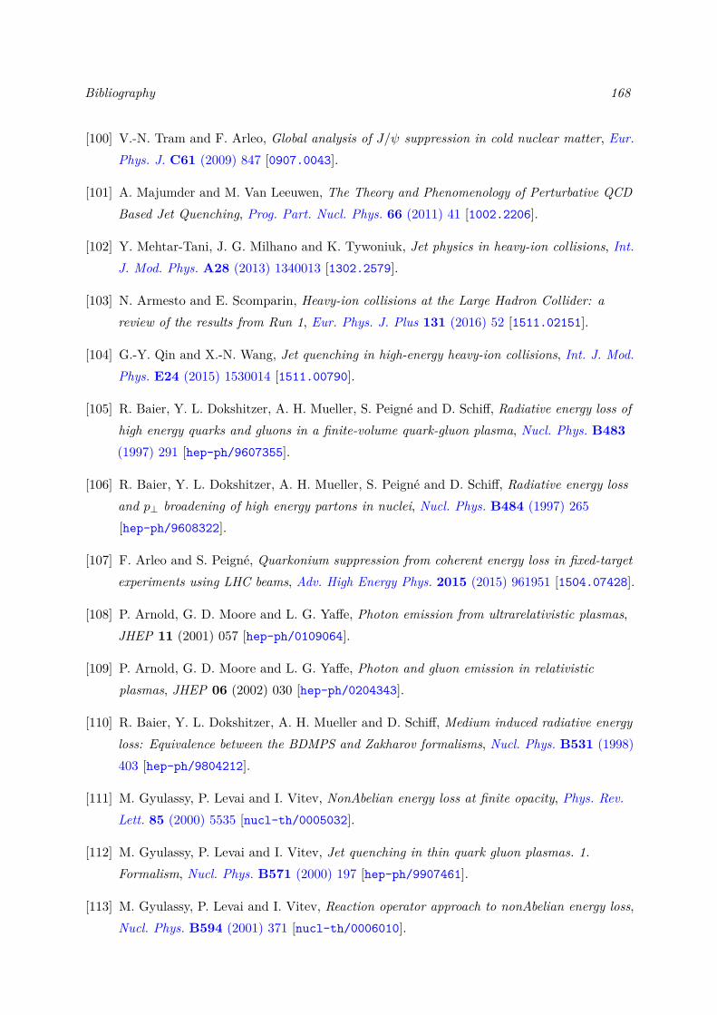
Bibliography 168
[100] V.-N. Tram and F. Arleo, Global analysis of J/ψ suppression in cold nuclear matter, Eur.Phys. J. C61 (2009) 847 [0907.0043].
[101] A. Majumder and M. Van Leeuwen, The Theory and Phenomenology of Perturbative QCDBased Jet Quenching, Prog. Part. Nucl. Phys. 66 (2011) 41 [1002.2206].
[102] Y. Mehtar-Tani, J. G. Milhano and K. Tywoniuk, Jet physics in heavy-ion collisions, Int.J. Mod. Phys. A28 (2013) 1340013 [1302.2579].
[103] N. Armesto and E. Scomparin, Heavy-ion collisions at the Large Hadron Collider: areview of the results from Run 1, Eur. Phys. J. Plus 131 (2016) 52 [1511.02151].
[104] G.-Y. Qin and X.-N. Wang, Jet quenching in high-energy heavy-ion collisions, Int. J. Mod.Phys. E24 (2015) 1530014 [1511.00790].
[105] R. Baier, Y. L. Dokshitzer, A. H. Mueller, S. Peigné and D. Schiff, Radiative energy loss ofhigh energy quarks and gluons in a finite-volume quark-gluon plasma, Nucl. Phys. B483(1997) 291 [hep-ph/9607355].
[106] R. Baier, Y. L. Dokshitzer, A. H. Mueller, S. Peigné and D. Schiff, Radiative energy lossand p⊥ broadening of high energy partons in nuclei, Nucl. Phys. B484 (1997) 265[hep-ph/9608322].
[107] F. Arleo and S. Peigné, Quarkonium suppression from coherent energy loss in fixed-targetexperiments using LHC beams, Adv. High Energy Phys. 2015 (2015) 961951 [1504.07428].
[108] P. Arnold, G. D. Moore and L. G. Yaffe, Photon emission from ultrarelativistic plasmas,JHEP 11 (2001) 057 [hep-ph/0109064].
[109] P. Arnold, G. D. Moore and L. G. Yaffe, Photon and gluon emission in relativisticplasmas, JHEP 06 (2002) 030 [hep-ph/0204343].
[110] R. Baier, Y. L. Dokshitzer, A. H. Mueller and D. Schiff, Medium induced radiative energyloss: Equivalence between the BDMPS and Zakharov formalisms, Nucl. Phys. B531 (1998)403 [hep-ph/9804212].
[111] M. Gyulassy, P. Levai and I. Vitev, NonAbelian energy loss at finite opacity, Phys. Rev.Lett. 85 (2000) 5535 [nucl-th/0005032].
[112] M. Gyulassy, P. Levai and I. Vitev, Jet quenching in thin quark gluon plasmas. 1.Formalism, Nucl. Phys. B571 (2000) 197 [hep-ph/9907461].
[113] M. Gyulassy, P. Levai and I. Vitev, Reaction operator approach to nonAbelian energy loss,Nucl. Phys. B594 (2001) 371 [nucl-th/0006010].
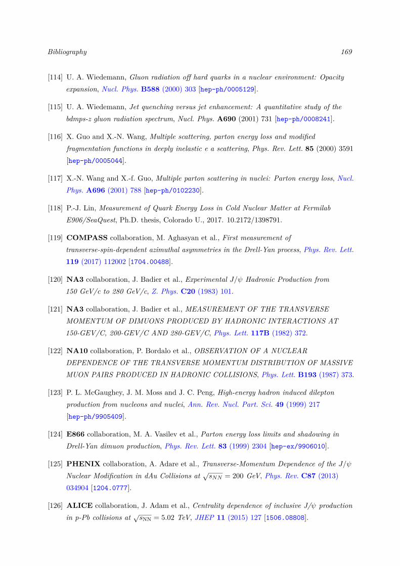
Bibliography 169
[114] U. A. Wiedemann, Gluon radiation off hard quarks in a nuclear environment: Opacityexpansion, Nucl. Phys. B588 (2000) 303 [hep-ph/0005129].
[115] U. A. Wiedemann, Jet quenching versus jet enhancement: A quantitative study of thebdmps-z gluon radiation spectrum, Nucl. Phys. A690 (2001) 731 [hep-ph/0008241].
[116] X. Guo and X.-N. Wang, Multiple scattering, parton energy loss and modifiedfragmentation functions in deeply inelastic e a scattering, Phys. Rev. Lett. 85 (2000) 3591[hep-ph/0005044].
[117] X.-N. Wang and X.-f. Guo, Multiple parton scattering in nuclei: Parton energy loss, Nucl.Phys. A696 (2001) 788 [hep-ph/0102230].
[118] P.-J. Lin, Measurement of Quark Energy Loss in Cold Nuclear Matter at FermilabE906/SeaQuest, Ph.D. thesis, Colorado U., 2017. 10.2172/1398791.
[119] COMPASS collaboration, M. Aghasyan et al., First measurement oftransverse-spin-dependent azimuthal asymmetries in the Drell-Yan process, Phys. Rev. Lett.119 (2017) 112002 [1704.00488].
[120] NA3 collaboration, J. Badier et al., Experimental J/ψ Hadronic Production from150 GeV/c to 280 GeV/c, Z. Phys. C20 (1983) 101.
[121] NA3 collaboration, J. Badier et al., MEASUREMENT OF THE TRANSVERSEMOMENTUM OF DIMUONS PRODUCED BY HADRONIC INTERACTIONS AT150-GEV/C, 200-GEV/C AND 280-GEV/C, Phys. Lett. 117B (1982) 372.
[122] NA10 collaboration, P. Bordalo et al., OBSERVATION OF A NUCLEARDEPENDENCE OF THE TRANSVERSE MOMENTUM DISTRIBUTION OF MASSIVEMUON PAIRS PRODUCED IN HADRONIC COLLISIONS, Phys. Lett. B193 (1987) 373.
[123] P. L. McGaughey, J. M. Moss and J. C. Peng, High-energy hadron induced dileptonproduction from nucleons and nuclei, Ann. Rev. Nucl. Part. Sci. 49 (1999) 217[hep-ph/9905409].
[124] E866 collaboration, M. A. Vasilev et al., Parton energy loss limits and shadowing inDrell-Yan dimuon production, Phys. Rev. Lett. 83 (1999) 2304 [hep-ex/9906010].
[125] PHENIX collaboration, A. Adare et al., Transverse-Momentum Dependence of the J/ψNuclear Modification in dAu Collisions at √sNN = 200 GeV, Phys. Rev. C87 (2013)034904 [1204.0777].
[126] ALICE collaboration, J. Adam et al., Centrality dependence of inclusive J/ψ productionin p-Pb collisions at √sNN = 5.02 TeV, JHEP 11 (2015) 127 [1506.08808].
Bibliography 170
[127] ALICE collaboration, M. Tarhini, Charmonium production in Pb–Pb and p–Pb collisionsat forward rapidity measured with ALICE, Nucl. Phys. A 967 (2017) 588.
[128] LHCb collaboration, R. Aaij et al., Prompt and nonprompt J/ψ production and nuclearmodification in pPb collisions at √sNN = 8.16 TeV, Phys. Lett. B 774 (2017) 159[1706.07122].
[129] F. Arleo, R. Kolevatov, S. Peigné and M. Rustamova, Centrality and p⊥ dependence ofJ/ψ suppression in proton-nucleus collisions from parton energy loss, JHEP 05 (2013) 155[1304.0901].
[130] NA58 Collaboration collaboration, G. Baum, J. Kyynäräinen and A. Tripet,COMPASS: a proposal for a common muon and proton apparatus for structure andspectroscopy, Tech. Rep. CERN-SPSLC-96-14. SPSLC-P-297, CERN, Geneva, 1996.
[131] G. Baum, J. Kyynäräinen and A. Tripet, COMPASS: Common Muon and ProtonApparatus for Structure and Spectroscopy; Add. 1, Tech. Rep. CERN-SPSLC-96-30.SPSLC-P-297-Add-1, CERN, Geneva, 1996.
[132] COMPASS collaboration, F. Gautheron et al., COMPASS-II Proposal, .
[133] H. W. Atherton, C. Bovet, N. T. Doble, L. Piemontese, A. Placci et al., Precisemeasurements of particle production by 400 GeV/c protons on beryllium targets, CERNYellow Reports: Monographs. CERN, Geneva, 1980, 10.5170/CERN-1980-007.
[134] COMPASS collaboration, P. Abbon et al., The COMPASS experiment at CERN, Nucl.Instrum. Meth. A 577 (2007) 455 [hep-ex/0703049].
[135] R. Longo, Measurement of spin effects in the Drell-Yan process at the COMPASSexperiment, Ph.D. thesis, Turin U., 2018.
[136] Particle Data Group collaboration, M. Tanabashi et al., Review of Particle Physics,Phys. Rev. D 98 (2018) 030001.
[137] P. Lösel and R. Müller, Design and construction of large size micromegas chambers for theupgrade of the ATLAS muon spectrometer, .
[138] F. Thibaud et al., Performance of large pixelised Micromegas detectors in the COMPASSenvironment, JINST 9 (2014) C02005.
[139] J. Marroncle, La grande chambre à dérive DC4, Saclay (2008) .
[140] Experimental determination of the townsend coefficient for argon-co2 gas mixtures at highfields, .
Bibliography 171
[141] G. Braun et al., F1: An Eight channel time to digital converter chip for high rateexperiments, in 5th Workshop on Electronics for the LHC Experiments (LEB 99),pp. 383–387, 9, 1999, hep-ex/9911009.
[142] T. Sjostrand, S. Mrenna and P. Z. Skands, A Brief Introduction to PYTHIA 8.1, Comput.Phys. Commun. 178 (2008) 852 [0710.3820].
[143] A. Ito et al., Measurement of the Continuum of Dimuons Produced in High-Energy Proton- Nucleus Collisions, Phys. Rev. D 23 (1981) 604.
[144] M. B. Johnson, B. Z. Kopeliovich, I. K. Potashnikova, P. L. McGaughey, J. M. Moss et al.,Energy loss versus shadowing in the Drell-Yan reaction on nuclei, Phys. Rev. C65 (2002)025203 [hep-ph/0105195].
[145] R. Neufeld, I. Vitev and B.-W. Zhang, A possible determination of the quark radiationlength in cold nuclear matter, Phys.Lett. B704 (2011) 590 [1010.3708].
[146] L.-H. Song and L.-W. Yan, Constraining the transport coefficient in cold nuclear matterwith the Drell-Yan process, Phys. Rev. C96 (2017) 045203.
[147] F. Arleo, Constraints on quark energy loss from Drell-Yan data, Phys. Lett. B532 (2002)231 [hep-ph/0201066].
[148] F. Arleo, Tomography of cold and hot QCD matter: Tools and diagnosis, JHEP 11 (2002)044 [hep-ph/0210104].
[149] C. A. Salgado and U. A. Wiedemann, Calculating quenching weights, Phys. Rev. D68(2003) 014008 [hep-ph/0302184].
[150] S. Catani and M. Grazzini, An NNLO subtraction formalism in hadron collisions and itsapplication to Higgs boson production at the LHC, Phys. Rev. Lett. 98 (2007) 222002[hep-ph/0703012].
[151] K. J. Golec-Biernat and M. Wüsthoff, Saturation effects in deep inelastic scattering at lowQ2 and its implications on diffraction, Phys. Rev. D59 (1998) 014017 [hep-ph/9807513].
[152] F. Arleo and S. Peigné, Quarkonium suppression in heavy-ion collisions from coherentenergy loss in cold nuclear matter, JHEP 10 (2014) 73 [1407.5054].
[153] J. Pumplin, D. Stump, R. Brock, D. Casey, J. Huston et al., Uncertainties of predictionsfrom parton distribution functions. 2. The Hessian method, Phys. Rev. D 65 (2001) 014013[hep-ph/0101032].
Bibliography 172
[154] C. Hadjidakis et al., Physics opportunities with a fixed target experiment at the LHC(AFTER@LHC), PoS PSTP2017 (2018) 035.
[155] CMS Collaboration collaboration, Differential measurements of the Drell–Yan processin the muon channel in pPb collisions at √sNN = 8.16 TeV, Tech. Rep.CMS-PAS-HIN-18-003, CERN, Geneva, 2020.
[156] P. Paakkinen, K. J. Eskola and H. Paukkunen, Applicability of pion nucleus Drell-Yandata in global analysis of nuclear parton distribution functions, Phys. Lett. B768 (2017) 7[1609.07262].
[157] Saclay-CERN-College de France-Ecole Poly-Orsay collaboration, J. Badier et al.,Measurement of the K−/π− Structure Function Ratio Using the Drell-Yan Process, Phys.Lett. B 93 (1980) 354.
[158] M. Aicher, A. Schafer and W. Vogelsang, Soft-gluon resummation and the valence partondistribution function of the pion, Phys. Rev. Lett. 105 (2010) 252003 [1009.2481].
[159] I. Novikov et al., Parton Distribution Functions of the Charged Pion Within The xFitterFramework, 2002.02902.
[160] F. Cougoulic and S. Peigné, Nuclear p⊥-broadening of an energetic parton pair,1712.01953.
[161] P. Ru, Z.-B. Kang, E. Wang, H. Xing and B.-W. Zhang, A global extraction of the jettransport coefficient in cold nuclear matter, 1907.11808.
[162] Y. H. Leung, PHENIX measurements of charm, bottom, and Drell-Yan via dimuons inp+p and p+Au collisions at √sNN = 200 GeV, PoS HardProbes2018 (2019) 160.
[163] K. J. Golec-Biernat and M. Wusthoff, Saturation in diffractive deep inelastic scattering,Phys. Rev. D60 (1999) 114023 [hep-ph/9903358].
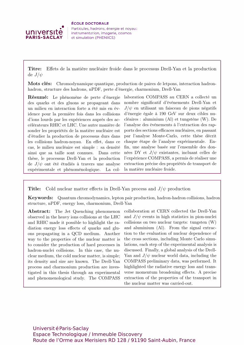
Titre: Effets de la matière nucléaire froide dans le processus Drell-Yan et la productionde J/
Mots clés: Chromodynamique quantique, production de paires de letpons, interaction hadron-hadron, structure des hadrons, nPDF, perte d’énergie, charmonium, Drell-Yan
Résumé: Le phénomène de perte d’énergiedes quarks et des gluons se propageant dansun milieu en interaction forte a été mis en év-idence pour la première fois dans les collisionsd’ions lourds par les expériences auprès des ac-célérateurs RHIC et LHC. Une autre manière desonder les propriétés de la matière nucléaire estd’étudier la production de processus durs dansles collisions hadron-noyau. En effet, dans cecas, le milieu nucléaire est simple : sa densitéainsi que sa taille sont connues. Dans cettethèse, le processus Drell-Yan et la productionde J/ ont été étudiés à travers une analyseexpérimentale et phénoménologique. La col-
laboration COMPASS au CERN a collecté unnombre significatif d’événements Drell-Yan etJ/ en utilisant un faisceau de pions négatifsd’énergie égale à 190 GeV sur deux cibles nu-cléaires : aluminium (Al) et tungstène (W). Del’analyse des événements à l’extraction des rap-ports des sections efficaces nucléaires, en passantpar l’analyse Monte-Carlo, cette thèse décritchaque étape de l’analyse expérimentale. En-fin, une analyse basée sur l’ensemble des don-nées DY et J/ existantes, incluant celles del’expérience COMPASS, a permis de réaliser uneextraction précise des propriétés de transport dela matière nucléaire froide.
Title: Cold nuclear matter effects in Drell-Yan process and J/ production
Keywords: Quantum chromodynamics, lepton pair production, hadron-hadron collisions, hadronstructure, nPDF, energy loss, charmonium, Drell-Yan
Abstract: The Jet Quenching phenomenonobserved in the heavy ions collisions at the LHCand RHIC made it possible to highlight the ra-diation energy loss effects of quarks and glu-ons propagating in a QCD medium. Anotherway to the properties of the nuclear matter isto consider the production of hard processes inhadron-nuclei collisions. In this case, the nu-clear medium, the cold nuclear matter, is simple;its density and size are known. The Drell-Yanprocess and charmonium production are inves-tigated in this thesis through an experimentaland phenomenological study. The COMPASS
collaboration at CERN collected the Drell-Yanand J/ events in high statistics in pion-nucleicollisions on two nuclear targets: tungsten (W)and aluminium (Al). From the signal extrac-tion to the evaluation of nuclear dependence ofthe cross sections, including Monte Carlo simu-lations, each step of the experimental analysis isdiscussed. Finally, a global analysis of the Drell-Yan and J/ nuclear world data, including theCOMPASS preliminary data, was performed. Ithighlighted the radiative energy loss and trans-verse momentum broadening effects. A preciseextraction of the properties of the transport inthe nuclear matter was carried-out.
Université Paris-SaclayEspace Technologique / Immeuble DiscoveryRoute de l’Orme aux Merisiers RD 128 / 91190 Saint-Aubin, France