cold-air pool dynamics observed by a sodar-rass in the new zealand alps
TRANSCRIPT
ISARS Auckland, New Zealand Jan., 2014
Marwan Katurji
COLD-AIR POOL DYNAMICS OBSERVED BY A SODAR-RASS SYSTEM IN THE NEW
ZEALAND SOUTHERN ALPS
Authors and Participants:
Marwan Katurji Bob Noonan Tobias Schulmann Peyman Zawar-Reza Andrew Sturman
Centre for Atmospheric Research University of Canterbury, Christchurch New Zealand
ISARS Auckland, New Zealand Jan., 2014
Marwan Katurji
Research Objective
Establish a climatology of intermontane atmospheric boundary layers (BL) in order to understand the dynamic coupling and decoupling of the intermontane BL with extra-mountain disturbances
Implications
For regional to basin scale downscaling of climate models that don't properly resolve intermontane BLs, especially for stable BLs.
Establishing relationships between wind shear and air temperature profiles (threshold analysis).
ISARS Auckland, New Zealand Jan., 2014
Marwan Katurji
Methods
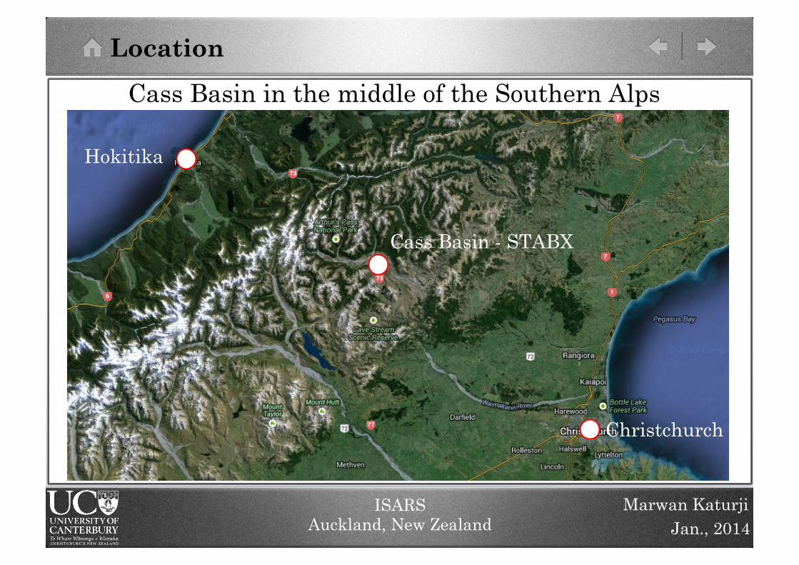
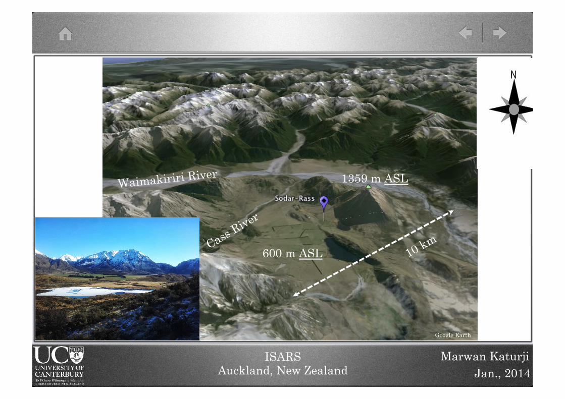
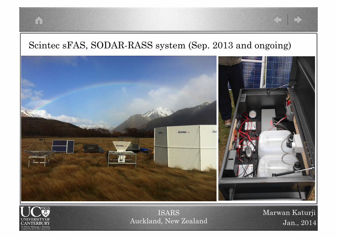
Setup of a SODAR-RASS system in the heart of an elevated basin within New Zealand’s Southern Alps
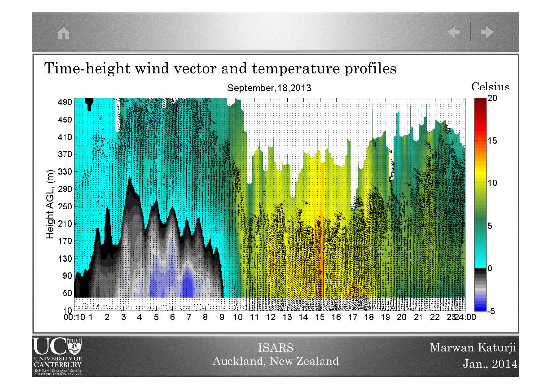
Measure wind velocity and air temperature at 10 minute intervals and at 5 m vertical resolution up to an effective height of ~ 400m
Establish a ridge-top weather station to measure regional weather variations
Test the applicability of an artificial neural network algorithm, known as Self Organized Maps (SOM), to analyze large datasets produced from the long term deployment of the SODAR-RASS system
This talk’s content (preliminary results)
1. Provide a summary from September 2013 observations
2. Introduce SOM results (pattern recognition and clustering)
3. Verify SOM results with regard to mean diurnal variation
4. Explore night-time profiles
5. Future research
ISARS Auckland, New Zealand Jan., 2014
Marwan Katurji
ISARS Auckland, New Zealand Jan., 2014
Marwan Katurji
Hokitika
Christchurch
Cass Basin - STABX
Cass Basin in the middle of the Southern Alps
Location
ISARS Auckland, New Zealand Jan., 2014
Marwan Katurji
Google Earth
Waimakiriri River
600 m ASL
1359 m ASL
ISARS Auckland, New Zealand Jan., 2014
Marwan Katurji
Scintec sFAS, SODAR-RASS system (Sep. 2013 and ongoing)
ISARS Auckland, New Zealand Jan., 2014
Marwan Katurji
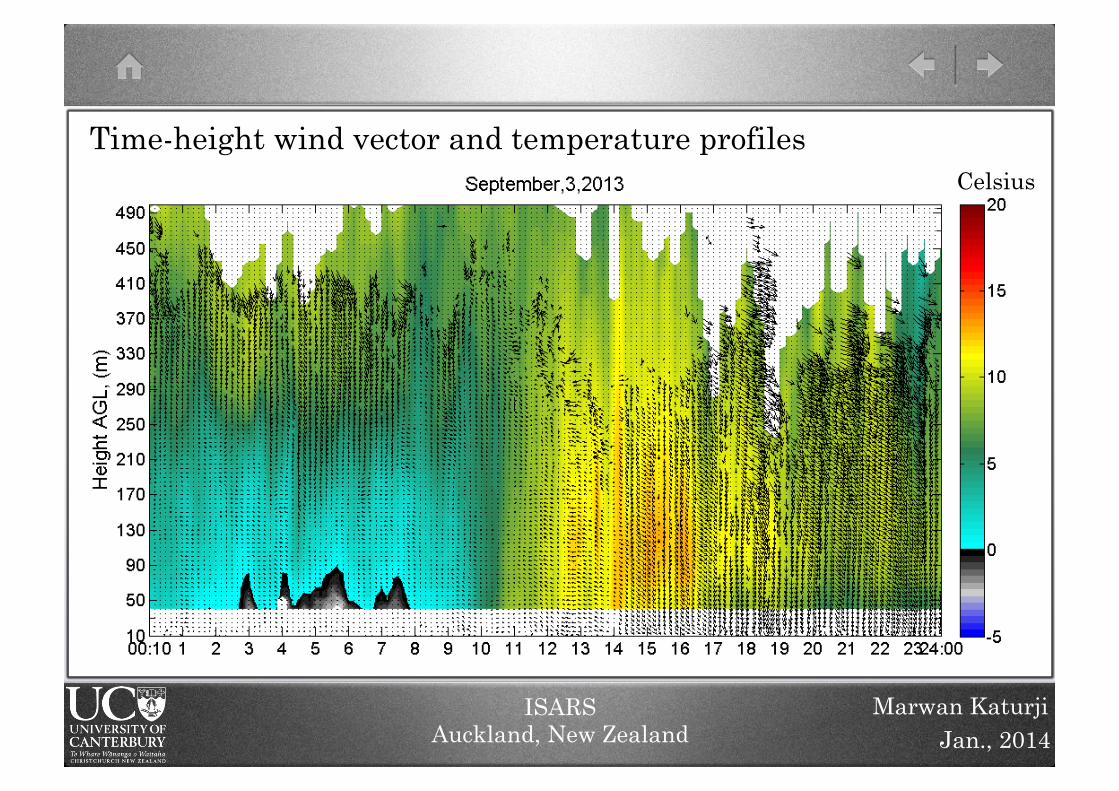
Time-height wind vector and temperature profiles Celsius
ISARS Auckland, New Zealand Jan., 2014
Marwan Katurji
Time-height wind vector and temperature profiles Celsius
276 277 278 279 280 281 282 283 284 2850
50
100
150
200
250
300
350
400
450
500
Potential Temperature (Kelvin)
Hei
ght,
AGL
(m)
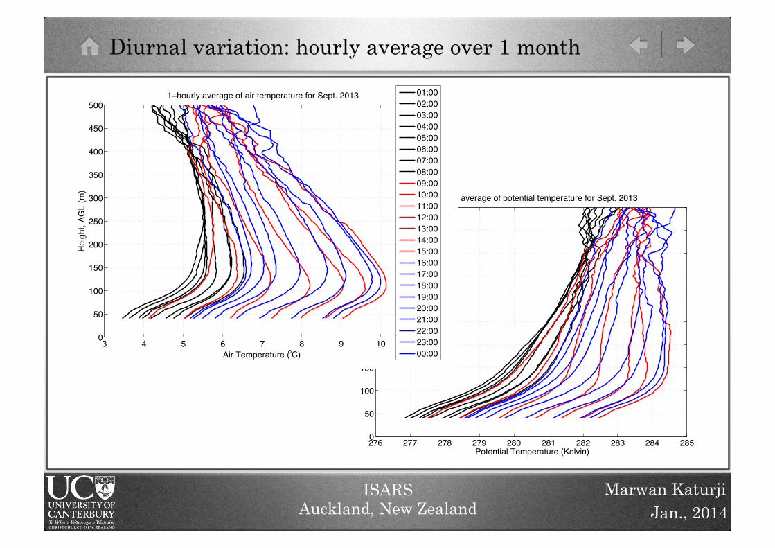
1−hourly average of potential temperature for Sept. 2013
ISARS Auckland, New Zealand Jan., 2014
Marwan Katurji
3 4 5 6 7 8 9 10 110
50
100
150
200
250
300
350
400
450
500
Air Temperature (oC)
Hei
ght,
AGL
(m)
1−hourly average of air temperature for Sept. 2013
01:0002:0003:0004:0005:0006:0007:0008:0009:0010:0011:0012:0013:0014:0015:0016:0017:0018:0019:0020:0021:0022:0023:0000:00
Diurnal variation: hourly average over 1 month
ISARS Auckland, New Zealand Jan., 2014
Marwan Katurji
−10 −5 0 5 10
100
200
300
400
500
−10 −5 0 5 10
100
200
300
400
500
−10 −5 0 5 10
100
200
300
400
500
−10 −5 0 5 10
100
200
300
400
500
−10 −5 0 5 10
100
200
300
400
500
−10 −5 0 5 10
100
200
300
400
500
−10 −5 0 5 10
100
200
300
400
500
−10 −5 0 5 10
100
200
300
400
500
−10 −5 0 5 10
100
200
300
400
500
−10 −5 0 5 10
100
200
300
400
500
−10 −5 0 5 10
100
200
300
400
500
−10 −5 0 5 10
100
200
300
400
500jj
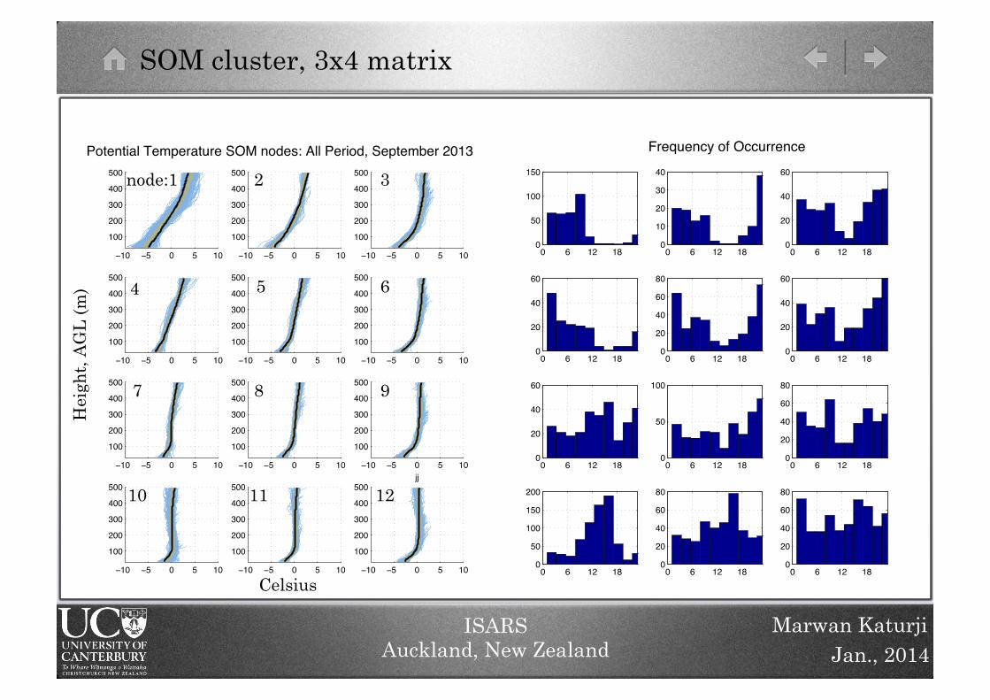
Potential Temperature SOM nodes: All Period, September 2013
SOM cluster, 3x4 matrix
Celsius
Hei
ght,
AG
L (
m)
0 6 12 180
50
100
150
0 6 12 180
10
20
30
40
0 6 12 180
20
40
60
0 6 12 180
20
40
60
0 6 12 180
20
40
60
80
0 6 12 180
20
40
60
0 6 12 180
20
40
60
0 6 12 180
50
100
0 6 12 180
20
40
60
80
0 6 12 180
50
100
150
200
0 6 12 180
20
40
60
80
0 6 12 180
20
40
60
80
Frequency of Occurrence
node:1 2 3
5 4 6
7 8 9
10 11 12
ISARS Auckland, New Zealand Jan., 2014
Marwan Katurji
−10 −5 0 5 10
100
200
300
400
500
−10 −5 0 5 10
100
200
300
400
500
−10 −5 0 5 10
100
200
300
400
500
−10 −5 0 5 10
100
200
300
400
500
−10 −5 0 5 10
100
200
300
400
500
−10 −5 0 5 10
100
200
300
400
500
−10 −5 0 5 10
100
200
300
400
500
−10 −5 0 5 10
100
200
300
400
500
−10 −5 0 5 10
100
200
300
400
500
−10 −5 0 5 10
100
200
300
400
500
−10 −5 0 5 10
100
200
300
400
500
−10 −5 0 5 10
100
200
300
400
500jj
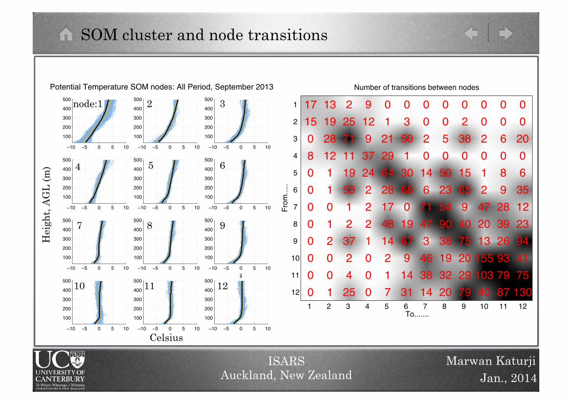
Potential Temperature SOM nodes: All Period, September 2013
17150800000000
1319281211012001
2257111195312372425
912937242221000
0121296428174814217
0350130660196791431
002014671473463814
00505023549038193220
02380156594075202979
00201247201315510340
006089283926937987
002006351223944175130
Number of transitions between nodes
To.......
From
.....
1 2 3 4 5 6 7 8 9 10 11 12
1
2
3
4
5
6
7
8
9
10
11
12
SOM cluster and node transitions H
eigh
t, A
GL
(m
)
Celsius
node:1 2 3
5 4 6
7 8 9
10 11 12
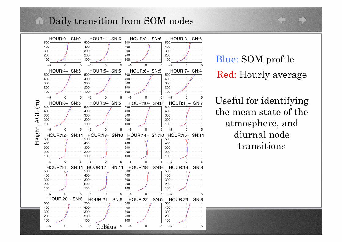
Daily transition from SOM nodes
−5 0 5100200300400500
HOUR:0− SN:9
−5 0 5100200300400500
HOUR:1− SN:6
−5 0 5100200300400500
HOUR:2− SN:6
−5 0 5100200300400500
HOUR:3− SN:6
−5 0 5100200300400500
HOUR:4− SN:5
−5 0 5100200300400500
HOUR:5− SN:5
−5 0 5100200300400500
HOUR:6− SN:5
−5 0 5100200300400500
HOUR:7− SN:4
−5 0 5100200300400500
HOUR:8− SN:5
−5 0 5100200300400500
HOUR:9− SN:5
−5 0 5100200300400500
HOUR:10− SN:8
−5 0 5100200300400500
HOUR:11− SN:7
−5 0 5100200300400500
HOUR:12− SN:11
−5 0 5100200300400500
HOUR:13− SN10
−5 0 5100200300400500
HOUR:14− SN:10
−5 0 5100200300400500
HOUR:15− SN:11
−5 0 5100200300400500
HOUR:16− SN:11
−5 0 5100200300400500
HOUR:17− SN:11
−5 0 5100200300400500
HOUR:18− SN:9
−5 0 5100200300400500
HOUR:19− SN:8
−5 0 5100200300400500
HOUR:20− SN:6
−5 0 5100200300400500
HOUR:21− SN:6
−5 0 5100200300400500
HOUR:22− SN:5
−5 0 5100200300400500
HOUR:23− SN:8
Blue: SOM profile
Red: Hourly average
Useful for identifying the mean state of the
atmosphere, and diurnal node transitions
Celsius
Hei
ght,
AG
L (
m)
ISARS Auckland, New Zealand Jan., 2014
Marwan Katurji
0 10 20 30
100
200
300
400
500
0 10 20 30
100
200
300
400
500
0 10 20 30
100
200
300
400
500
0 10 20 30
100
200
300
400
500
0 10 20 30
100
200
300
400
500
0 10 20 30
100
200
300
400
500
0 10 20 30
100
200
300
400
500
0 10 20 30
100
200
300
400
500
0 10 20 30
100
200
300
400
500
0 10 20 30
100
200
300
400
500
0 10 20 30
100
200
300
400
500
0 10 20 30
100
200
300
400
500
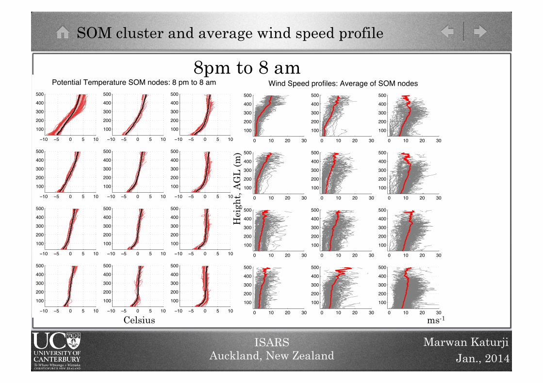
Wind Speed profiles: Average of SOM nodes
−10 −5 0 5 10
100
200
300
400
500
−10 −5 0 5 10
100
200
300
400
500
−10 −5 0 5 10
100
200
300
400
500
−10 −5 0 5 10
100
200
300
400
500
−10 −5 0 5 10
100
200
300
400
500
−10 −5 0 5 10
100
200
300
400
500
−10 −5 0 5 10
100
200
300
400
500
−10 −5 0 5 10
100
200
300
400
500
−10 −5 0 5 10
100
200
300
400
500
−10 −5 0 5 10
100
200
300
400
500
−10 −5 0 5 10
100
200
300
400
500
−10 −5 0 5 10
100
200
300
400
500
Potential Temperature SOM nodes: 8 pm to 8 am
SOM cluster and average wind speed profile
8pm to 8 am
Hei
ght,
AG
L (
m)
Celsius ms-1
ISARS Auckland, New Zealand Jan., 2014
Marwan Katurji
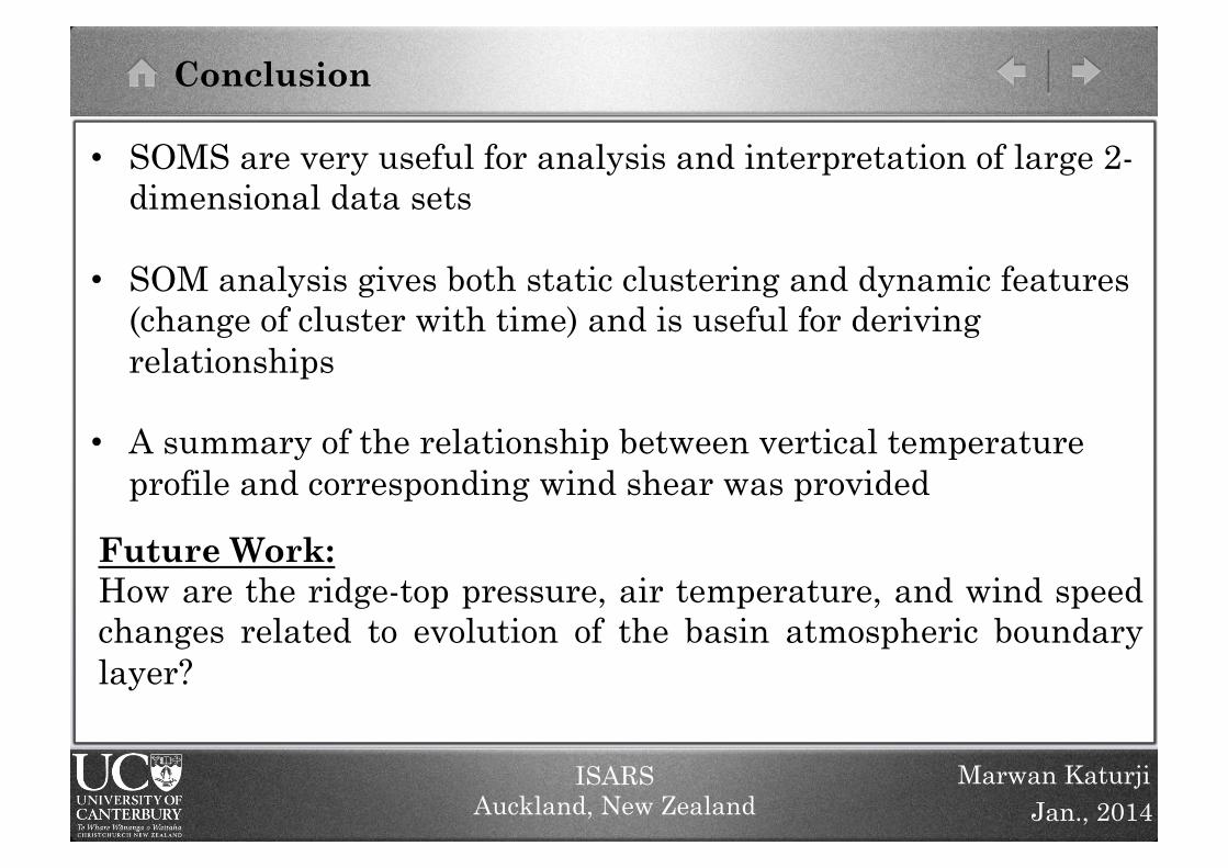
Conclusion
• SOMS are very useful for analysis and interpretation of large 2-dimensional data sets
• SOM analysis gives both static clustering and dynamic features (change of cluster with time) and is useful for deriving relationships
• A summary of the relationship between vertical temperature profile and corresponding wind shear was provided
Future Work: How are the ridge-top pressure, air temperature, and wind speed changes related to evolution of the basin atmospheric boundary layer?
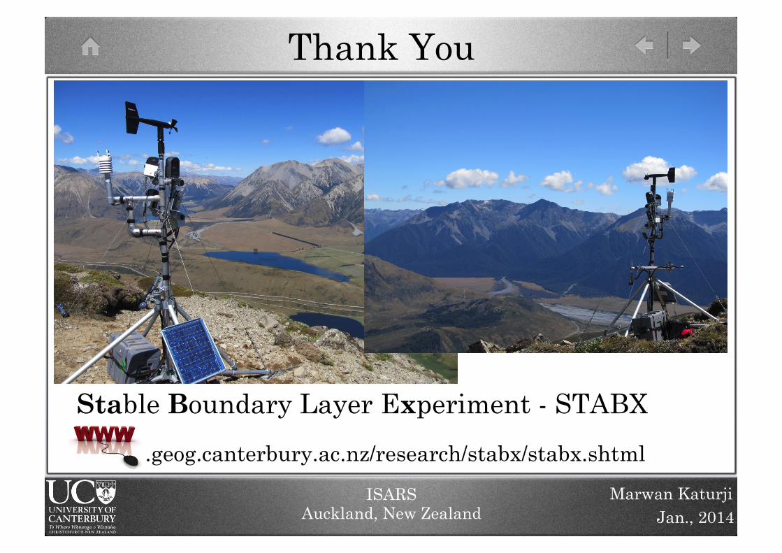
Thank You
ISARS Auckland, New Zealand Jan., 2014
Marwan Katurji
.geog.canterbury.ac.nz/research/stabx/stabx.shtml
Stable Boundary Layer Experiment - STABX