co depletion in the gould belt clouds

Mon. Not. R. Astron. Soc. 422, 968–980 (2012) doi:10.1111/j.1365-2966.2012.20643.x

CO depletion in the Gould Belt clouds

H. Christie,1� S. Viti,1 J. Yates,1 J. Hatchell,2 G. A. Fuller,3 A. Duarte-Cabral,4,5

S. Sadavoy,6 J. V. Buckle,7,8 S. Graves,7,8 J. Roberts,9 D. Nutter,10 C. Davis,11

G. J. White,12,13 M. Hogerheijde,14 D. Ward-Thompson,10 H. Butner,15 J. Richer7,8

and J. Di Francesco16

1Department of Physics and Astronomy, UCL, Gower Street, London WC1E 6BT2School of Physics, University of Exeter, Stocker Road, Exeter EX4 4QL3Jodrell Bank Centre for Astrophysics, School of Physics and Astronomy, University of Manchester, Oxford Road, Manchester M13 9PL4Univ. Bordeaux, LAB, UMR 5804, F-33270 Floriac, France5CNRS, LAB, UMR 5804, F-33270 Floriac, France6Department of Physics and Astronomy, University of Victoria, PO Box 355, STN CSC, Victoria, BC V8W 3P6, Canada7Astrophysics Group, Cavandish Laboratory, JJ Thomson Avenue, Cambridge CB3 0HE8Kavli Institute for Cosmology, c/o Institute of Astronomy, University of Cambridge, Madingley Road, Cambridge CB3 0HA9Instituto Nacional de Technica Aeroespacial, 28830 San Fernando de Henares, Spain10School of Physics and Astronomy, Cardiff University, Queen’s Buildings, The Parade, Cardiff CF24 3AA11Joint Astronomy Centre, 660 North A’ohoku Place, University Park, Hilo, HI 96720, USA12Department of Physics and Astronomy, The Open University, Milton Keynes MK7 6AA13The Rutherford Appleton Laboratory, Space Science and Technology Division, Didcot OX11 0NL14Leiden Observatory, Leiden University, PO Box 9513, 2300 RA Leiden, the Netherlands15Department of Physics and Astronomy, James Madison University, Harrisonburg, VA 22807, USA16National Research Council of Canada, Herzberg Institute of Astrophysics, Department of Physics and Astronomy, University of Victoria, Victoria, BC V9E2E7, Canada

Accepted 2012 January 27. Received 2012 January 26; in original form 2011 November 18

ABSTRACTWe present a statistical comparison of CO depletion in a set of local molecular clouds within theGould Belt using Sub-millimetre Common User Bolometer Array (SCUBA) and HeterodyneArray Receiver Programme (HARP) data. This is the most wide-ranging study of depletion thusfar within the Gould Belt. We estimate CO column densities assuming local thermodynamicequilibrium and, for a selection of sources, using the radiative transfer code RADEX in order tocompare the two column density estimation methods. High levels of depletion are seen in thecentres of several dust cores in all the clouds. We find that in the gas surrounding protostars,levels of depletion are somewhat lower than for starless cores with the exception of a fewhighly depleted protostellar cores in Serpens and NGC 2024. There is a tentative correlationbetween core mass and core depletion, particularly in Taurus and Serpens. Taurus has, onaverage, the highest levels of depletion. Ophiuchus has low average levels of depletion whichcould perhaps be related to the anomalous dust grain size distribution observed in this cloud.High levels of depletion are often seen around the edges of regions of optical emission (Orion)or in more evolved or less dynamic regions such as the bowl of L1495 in Taurus and thenorth-western region of Serpens.

Key words: molecular data – stars: abundances – stars: formation – ISM: abundances.

1 IN T RO D U C T I O N

In dense, cold, star-forming cores, molecules in the gas phase freeze-out on to dust grains, forming icy mantles on grain surfaces. Theextent to which this freeze-out (or depletion) occurs for a par-ticular molecule depends on a complicated chemistry that varies

�E-mail: [email protected]

non-linearly with time and physical environment. The strong de-pendence of depletion on the age and make-up of a core could makeit a useful probe of core history.

Depletion is difficult to quantify observationally. It is commonto use gas phase emission from molecules such as CO to infer thefraction of the species that is in the solid phase. This requires acomparison of gas phase molecular line emission with continuumemission from dust. Several assumptions are made about the stateof the emitting gas and dust, and the possible destruction of the

C© 2012 The AuthorsMonthly Notices of the Royal Astronomical Society C© 2012 RAS

CO depletion in the Gould Belt clouds 969

molecule by other means is often ignored. This method has beensuccessful, and studies show significant depletion in star formingcores (see Caselli et al. 1999; Bacmann et al. 2002; Redman et al.2002; Savva et al. 2003; Thomas & Fuller 2008; Duarte-Cabral et al.2010).

In addition to studies of the gas phase, one can directly observemolecules in the solid state using e.g. the absorption of IR emissionfrom background sources (see reviews by van Dishoeck 2004; Oberget al. 2011).

Several authors have attempted to model cores including freeze-out reactions to replicate observed line strengths and profiles. Thesemodels require accurate depletion and desorption rate estimatesfrom laboratory experiments that are very difficult to make. Des-orption can occur as a result of several processes including directimpact of cosmic rays which cause local heating of the grain surface,leading to the desorption of species in the mantle. Cosmic rays willalso ionize or excite molecules as they pass through the dense gasin a molecular core. UV photons are produced as a result of theseexcitations and these, in turn, can impart energy to the grain sur-face by dissociation of molecules in the mantle (particularly water).The formation of hydrogen molecules on grains will also cause localheating of the surface. The relative importance of these as desorptionmechanisms in the dark cloud environment is discussed in Robertset al. (2007). It is worth noting that, despite recent experiments(Oberg et al. 2009; Munoz Caro et al. 2010), rates of non-thermaldesorption as a function of density and mantle composition, requiredfor chemical codes, have not yet been accurately determined. Evenwith these uncertainties, modelling provides strong arguments fordepletion of molecules in dense cores. In many cases where multi-ple observations of different species are available, it is impossible toreproduce observationally derived abundances and ratios betweenabundances without substantial freeze-out, suggesting that this is animportant contributor to the chemistry of star-forming regions (e.g.Taylor & Williams 1996; Aikawa et al. 2001; Viti et al. 2003).

To study how the depletion of CO relates to environment, onerequires line data from the CO isotopologues as well as continuumdata from dust, from a variety of sources. The James Clerk MaxwellTelescope (JCMT) Gould Belt Survey (GBS; Ward-Thompson et al.2007) can provide these data. The Gould Belt is a system of kine-matically related stars and gas, mainly within 500 pc, highlightedby O- and B-type stars and containing numerous interesting andwell-studied molecular clouds, all with very different properties.The GBS, making use of Sub-millimetre Common User BolometerArray-2 (SCUBA-2) (dust continuum emission), POL-2 and Het-erodyne Array Receiver Programme (HARP) (spectral line emissionfor three isotopologues of CO) on the JCMT, aims to achieve consis-tent and detailed sets of data for many star-forming regions withinthe Gould Belt (see Buckle et al. 2010, 2011; Davis et al. 2010;Graves et al. 2010; White et al., in preparation, for the survey firstlook papers). This survey will help to build a better picture of starformation and how it is linked to environment. In this paper we usethe early GBS spectral data from HARP together with cataloguesof dust cores collated by Sadavoy et al. (2010) from SCUBA dustemission maps to study depletion in five GBS regions, representinga range of physical conditions: NGC 2024 and NGC 2071 in Orion,L1495 in Taurus, the Ophiuchus main cloud core (L1688), and theSerpens main cluster. We compare the depletions using a consistentmethodology that allows meaningful comparisons between theseregions to be made. We discuss how depletion factors are calcu-lated, compare local thermodynamic equilibrium (LTE) methodswith the use of RADEX and discuss how depletion varies in a regionand between regions.

2 DATA

The HARP instrument at the JCMT in Hawaii (see Buckle et al.2009, for more details of HARP) was used to map regions in Orion,Taurus, Serpens and Ophiuchus as part of the JCMT Gould BeltLegacy Survey. Table 1 lists the sizes of and distance to each cloudas well as the centre, area and sensitivity of each respective map. Inconjunction with Auto-Correlation Spectral Imaging System (AC-SIS), spectra were obtained for the 12CO J = (3 → 2) line at 345.796GHz at high and low resolution. HARP used wide-band imaging (upto 1.9 GHz bandwidth) in single sideband mode to cover both theJ = (3 → 2) transitions of 13CO and C18O at 330.588 and 329.331GHz, respectively. Narrow-band imaging results in higher resolu-tion spectra with channels of up to 31 kHz. 12CO maps generallycover physically larger areas. The data have a spectral resolutionof 0.05 km s−1 or 0.85 km s−1 for the high- and low-resolution se-tups, respectively. We use only the smaller sections of maps forwhich spectra from all three isotopologues are available and use thehigh-resolution images of 12CO.

HARP has 16 receivers, separated by 30 arcsec in the focal plane,resulting in a footprint of around 2 arcmin projected on the sky. Thebeam width of the JCMT is ∼14 arcsec full width at half-maximum(FWHM) at the frequencies of the CO lines. For a fully sampledmap, telescope scans were made in the raster position-switched ob-serving mode where the telescope scans along the direction parallelto the edges of the map, taking spectra separated by 7.3 arcsec. Thisis done first in one direction and then again in the perpendiculardirection for better coverage (the basket weave technique). Pixelsthus represent regions on the sky that are around 7 arcsec apart (seeBuckle et al. 2010, for more detail). Noise levels vary from map tomap depending on weather conditions at the time of data acquisitionand total hours dedicated to each observation. We used the currentbest reductions for each cloud. The resulting maps were not re-duced entirely similarly but the differences in reduction techniquesfor the separate regions (type of binning used, etc.) have a minoreffect on the results. Detailed information on the maps and theirreductions can be found in the GBS first look papers (referenced inSection 1).

We use results from dust emission data produced using SCUBA,also at the JCMT, as part of the SCUBA Legacy Catalogue (DiFrancesco et al. 2008). SCUBA is comprised of two hexagonalarrays of detectors, a long-wave array with 37 pixels and a shortwave array with 91 pixels. The relevant data are maps of 850-µmemission taken using the long-wave array and smoothed with a 1σ

Gaussian (see Di Francesco et al. 2008, for details), resulting in aspatial resolution for each Scuba Legacy Catalogue (SLC) map of22.9 arcsec at 850 µm.

3 A D E P L E T I O N FAC TO R F O R T H E D U S TC O R E S – LT E A NA LY S I S

Our sample of dust cores is taken directly from the catalogue pro-duced by Sadavoy et al. (2010) using the SCUBA 850-µm dustemission maps mentioned above. These authors used the clumpidentification algorithm ‘CLUMPFIND’ (Williams, de Geus & Blitz1994) to pick out localized regions of strong emission. CLUMPFIND

first identifies closed contours at the highest level of emission inthe map as peaks, then contours in flux down to a minimum levelthat is specified by the user. The area inside the minimum con-tour, and including a peak, is defined as the clump and integratedemission as well as peak values are outputted. We compared peakfluxes at the centre of each core from the Sadavoy et al. catalogue

C© 2012 The Authors, MNRAS 422, 968–980Monthly Notices of the Royal Astronomical Society C© 2012 RAS

970 H. Christie et al.

Table 1. Details of the observations.

Region Distance (pc) Isotopologue Map centre (J2000) Map area rms noise(arcsec2) (K)a

Serpens 260 12CO 18h30m 260 0.121◦14′

13CO 18h30m 77 0.241◦13′

C18O 18h30m 77 0.251◦13′

Taurus 140 12CO 4h18m 264/120(se)b 0.10/0.13(se)4h20m(se)28◦22′27◦11′(se)

13CO as 12CO 450/378(se) 0.15/0.24(se)C18O as 12CO 450/378(se) 0.18/0.29(se)

Ophiuchus 125 12CO 16h28m 900 0.49−24◦33′

13CO as 12CO 256 0.18C18O as 12CO 256 0.16

NGC 2024 415 12CO 05h42m 243 0.11−01◦54′

13CO as 12CO as 12CO 0.18C18O as 12CO as 12CO 0.14

NGC 2071 415 12CO 05h47m 292 0.2100◦20′

13CO as 12CO as 12CO 0.10C18O as 12CO as 12CO 0.13

aRms noise values in 0.1 km s−1 channels.bThe letters ‘se’ refer to the south-eastern region of Taurus L1495.

with our CO data at the same position. We refer to the identifiedregions as ‘cores’ since their sizes are generally less than 0.1 pc andthey contain typically a few solar masses of material. A typical star-less core has a density of around 105 cm−3 and temperature 10 K (DiFrancesco et al. 2007). Since CO freezes out below ∼20 K (15–17 K;Nakagawa 1980), and the amount of freeze-out should directly scalewith the density of the surrounding material (Rawlings et al. 1992),the high densities and low temperatures observed in the centres ofthese cores are expected to result in significant depletion of CO onto dust grains. Hence, we derive hydrogen column densities fromboth the dust and C18O data and use the ratio between the two asa measure of depletion in the core centres. To this end, C18O ispreferred to either 13CO or 12CO because it is more optically thin,and thus more representative of the whole column of gas, than eitherof the other two isotopologues. To derive a column density fromthe dust emission, we assume that emission from dust arises froman opacity modulated blackbody curve at a temperature of 10 K forthe starless cores and 20 K for those coincident with a young stellarobject (YSO) candidate identified by Spitzer (i.e. the protostellarcores). We discuss the implications of assuming fixed dust temper-atures for the cores in Section 6. To infer the total column densityof the dust from the emission at 850 µm, we use

Fν =∫

�

Bν(T , ν)κνNH2μmpd� (1)

where Fν is the peak flux per beam at frequency ν, Bν is the black-body function at the same frequency and temperature T , κν is thedust emissivity per unit mass of gas and dust at the same frequency,NH2 is the column density of molecular hydrogen, μ is the meanmolecular mass, mp is the mass of a proton and � is the beam size ofthe relevant telescope. We assume a dust emissivity of 1.97 cm2 g−1

(Ossenkopf & Henning 1994), assuming grains in a gas volumedensity of 106 cm−3 with thin ice mantles. The same paper quotes avalue for the dust emissivity with a thick ice mantle of 1.47 cm2 g−1.This represents a small error compared to, for example, temperatureestimates, so we do not consider the change in optical propertiesof the grains due to the growth of icy mantles to be a dominanteffect. The equation above assumes an emitting area larger than thebeam size of the relevant telescope. The beam size of the JCMTis generally smaller than CLUMPFIND derived diameters for the dustcores, so we do not consider beam dilution effects to be a problemand assume a beam filling factor of 1 in all cases.

The hydrogen column densities from the C18O maps were firstderived assuming LTE and optically thin emission. Critical densi-ties of the CO lines (some 104 cm−3) are generally lower than thetypical core density of around 106 cm−3, so material should be ther-malized. Buckle et al. (2010) calculated optical depths for the threeCO isotopologue lines in Orion B and showed that the C18O line isoptically thin across the whole of the imaged region, so our assump-tion of low optical depth in the C18O lines is likely to be valid evenin the denser dust cores (in Section 6 we consider the implicationsof optical depth effects on our depletion results). Accordingly, theBoltzmann and Planck equations give

N (C18O) = (5.21 × 1012) × Tex(12CO) × ∫Tmbdv

e−31.6/Tex(12CO), (2)

where N(C18O) is the column density of C18O (cm−2), Tex(12CO) isthe excitation temperature of the line (from the 12CO line profile),and Tmb is the main beam temperature.

We then assumed a N(C18O)/N(H2) ratio of 1.7 × 10−7 (Frerking,Langer & Wilson 1982) to convert from C18O to hydrogen columndensity. We discuss the implications of this assumption in Section 6.



We used the peak temperature of the 12CO line to estimate thegas kinetic temperature, and hence the line excitation temperaturein LTE, using

Tex(12CO) = 16.59K

ln(1 + 16.6Tmax(12CO)+0.036

), (3)

again following from the Boltzmann and Planck equations describ-ing LTE, assuming an optically thick line. Tmax is the peak tem-perature of the 12CO line at the centre of the dust core. We adopta main beam efficiency of 0.63 (Buckle et al. 2009). More detailon the derivation of equation (3) can be found in Pineda, Caselli &Goodman (2008). The 0.036 term results from the removal of thecosmic microwave background at 2.7 K.

The use of equation (3) requires that the 12CO line be opticallythick and not self-absorbed at its peak. In the case of the 12CO maps,lines are often self-absorbed and so cannot be used to estimate anaccurate gas temperature in all cases. If we assume the 13CO line tobe optically thick, it can be used in place of the 12CO line, in a mod-ified form of equation (3), to estimate the excitation temperature incores where the latter is obviously self-absorbed. We used the 13COline to estimate the temperature if the 13CO line peak was higherthan the 12CO in the line centre, otherwise the 12CO line was con-sidered to be sufficiently accurate. The 13CO lines, however, werealso self-absorbed. In these cases, we used the peak line temperature(i.e. the height of the peaks at the line edge rather than at the centre)as the best possible first estimate of the gas temperature and notethat these will probably be slightly underestimated in several cases.

It is difficult, looking at the profiles of the three lines together,to disentangle the effects of self-absorption from the possibility ofthere being several CO condensations lying along the line of sight.The position of the C18O peak can help, but again in many casesit does not peak at the frequency where the 13CO and 12CO linesdip, which would definitely point to self-absorption in the latter twoisotopologues. Of the 186 cores, in total roughly 60 per cent havea clear double peak in the 12CO line. For 70 per cent of these, theC18O line peaks in the dip of the 12CO line. The rest of the profiles(making up roughly 20 per cent of the total) are more complicatedwith the C18O line peaking nearer in frequency to one of the 12COline peaks or itself showing a double profile. For consistency, weadopted the approach detailed above, using the 12CO and 13CO tofind a kinetic temperature, even when self-absorbed. In Section 6 wediscuss the implications of using 12CO and 13CO, which probablytrace hotter gas than the dust, to derive excitation temperatures forthe central regions of the cores.

The integrated intensity of the C18O emission was found by fittinga Gaussian profile to the line using DIPSO (part of the STARLINK

software package; Warren-Smith & Wallace 1993). In cases wherethe C18O exhibited two or more peaks, the separate peaks wereconsidered to be due to distinct cores along the line of sight and weincluded emission from all lines in the sum. In doing this, we assumethat emission from dust derives from all cores along the line of sightand we find an average measure of the depletion factor. Such coreswill not, in reality, contain equal amounts of dust, but since it is notpossible to disentangle the dust emission from different cores alongthe line of sight we are unable to estimate the level of depletionin individual cores. Using the hydrogen column density calculatedfrom the dust data and the hydrogen column density calculated fromthe C18O, we derived a depletion factor, Fdep, given by

Fdep = N (H2)dust

N (H2)CO, (4)

where N(H2)dust and N(H2)CO are the hydrogen column densitiescalculated from the dust and the C18O, respectively.

The more CO is depleted on to dust grains, the lower the hydro-gen column density derived from the CO gas phase emission andhence the higher the value of Fdep. In Section 6, we discuss theuncertainties in the derived depletion factors.

4 R E S U LT S O F T H E LT E A NA LY S I S

Figs 1–3 show depletion factors versus dust column density for allfive regions and Figs 4–6 show depletion factors versus positionwithin each cloud. Average starless and protostellar depletion fac-tors are listed in Table 2. The results will be discussed in detail foreach source. We present a more general analysis in Section 5.

4.1 Serpens

The Serpens main cluster, a region of the Serpens molecular cloudparticularly rich in star formation, has been extensively studiedand shown to contain a population of Class 0/I sources (e.g. seeDavis et al. 1999) as well as an apparently older one containingmore evolved Class II/III sources (Harvey et al. 2007). Kaas et al.(2004) suggested that the region underwent a burst of star formationroughly 2 Myr ago followed by a later one around 105 yr ago. Themain cluster is complex, made up of two distinct subclusters, thenorth-west (NW) and south-east (SE). These two regions are joinedby dusty, finger-like structures or filaments. The NW is more quies-cent and cooler, whereas the SE is more filamentary, more turbulent

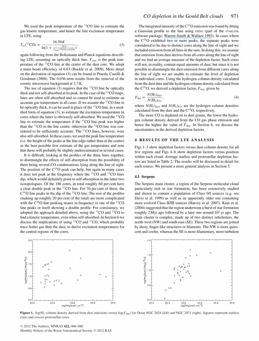
Figure 1. log(H2 column density derived from dust emission) versus log(Fdep) for Orion NGC 2024 (left) and NGC 2071 (right). Squares represent starlesscores and crosses protostellar cores.


https://www.researchgate.net/publication/241356083_Astronomical_Data_Analysis_Software_and_Systems_III?el=1_x_8&enrichId=rgreq-ae3246f3-f274-4b31-8c43-92f8f14a2a02&enrichSource=Y292ZXJQYWdlOzIyNDk1NDE1NTtBUzo5OTUzNzczMzU1NDE5M0AxNDAwNzQzMDUzNjA5


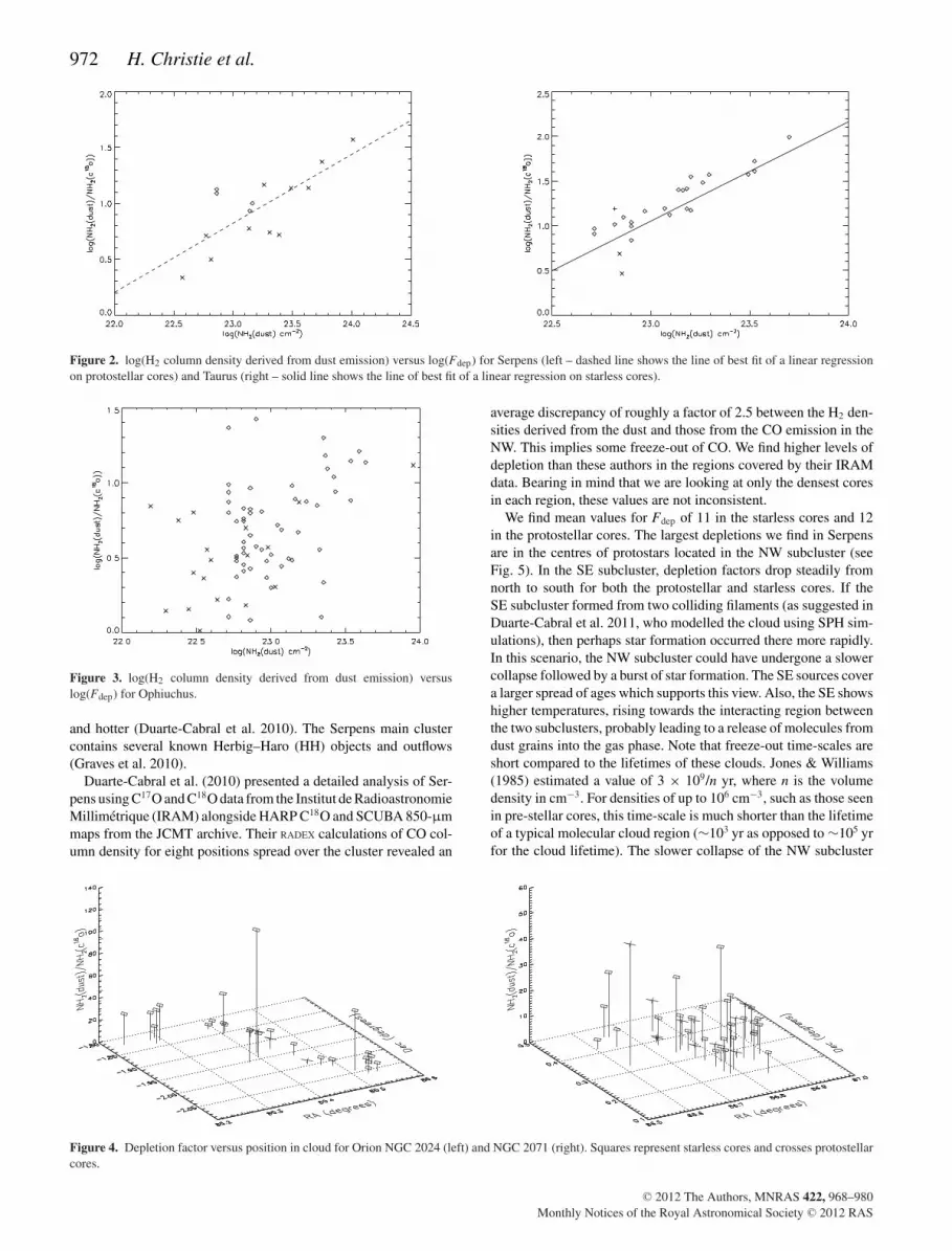
Figure 2. log(H2 column density derived from dust emission) versus log(Fdep) for Serpens (left – dashed line shows the line of best fit of a linear regressionon protostellar cores) and Taurus (right – solid line shows the line of best fit of a linear regression on starless cores).

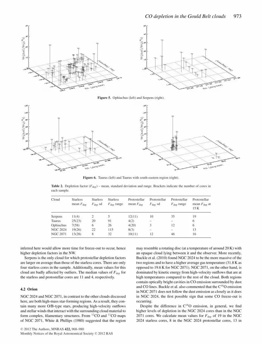
Figure 3. log(H2 column density derived from dust emission) versuslog(Fdep) for Ophiuchus.

and hotter (Duarte-Cabral et al. 2010). The Serpens main clustercontains several known Herbig–Haro (HH) objects and outflows(Graves et al. 2010).

Duarte-Cabral et al. (2010) presented a detailed analysis of Ser-pens using C17O and C18O data from the Institut de RadioastronomieMillimetrique (IRAM) alongside HARP C18O and SCUBA 850-µmmaps from the JCMT archive. Their RADEX calculations of CO col-umn density for eight positions spread over the cluster revealed an

average discrepancy of roughly a factor of 2.5 between the H2 den-sities derived from the dust and those from the CO emission in theNW. This implies some freeze-out of CO. We find higher levels ofdepletion than these authors in the regions covered by their IRAMdata. Bearing in mind that we are looking at only the densest coresin each region, these values are not inconsistent.

We find mean values for Fdep of 11 in the starless cores and 12in the protostellar cores. The largest depletions we find in Serpensare in the centres of protostars located in the NW subcluster (seeFig. 5). In the SE subcluster, depletion factors drop steadily fromnorth to south for both the protostellar and starless cores. If theSE subcluster formed from two colliding filaments (as suggested inDuarte-Cabral et al. 2011, who modelled the cloud using SPH sim-ulations), then perhaps star formation occurred there more rapidly.In this scenario, the NW subcluster could have undergone a slowercollapse followed by a burst of star formation. The SE sources covera larger spread of ages which supports this view. Also, the SE showshigher temperatures, rising towards the interacting region betweenthe two subclusters, probably leading to a release of molecules fromdust grains into the gas phase. Note that freeze-out time-scales areshort compared to the lifetimes of these clouds. Jones & Williams(1985) estimated a value of 3 × 109/n yr, where n is the volumedensity in cm−3. For densities of up to 106 cm−3, such as those seenin pre-stellar cores, this time-scale is much shorter than the lifetimeof a typical molecular cloud region (∼103 yr as opposed to ∼105 yrfor the cloud lifetime). The slower collapse of the NW subcluster

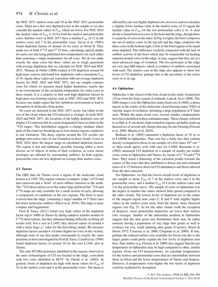
Figure 4. Depletion factor versus position in cloud for Orion NGC 2024 (left) and NGC 2071 (right). Squares represent starless cores and crosses protostellarcores.



Figure 5. Ophiuchus (left) and Serpens (right).

Figure 6. Taurus (left) and Taurus with south-eastern region (right).

Table 2. Depletion factor (Fdep) – mean, standard deviation and range. Brackets indicate the number of cores ineach sample.

Cloud Starless Starless Starless Protostellar Protostellar Protostellar Protostellarmean Fdep Fdep sd Fdep range mean Fdep Fdep sd Fdep range mean Fdep at

15 K

Serpens 11(4) 2 5 12(11) 10 35 19Taurus 25(23) 20 91 4(2) – – 6Ophiuchus 7(58) 6 26 4(20) 3 12 6NGC 2024 19(26) 22 115 8(3) – – 13NGC 2071 13(28) 8 32 10(11) 12 46 16

inferred here would allow more time for freeze-out to occur, hencehigher depletion factors in the NW.

Serpens is the only cloud for which protostellar depletion factorsare larger on average than those of the starless cores. There are onlyfour starless cores in the sample. Additionally, mean values for thiscloud are badly affected by outliers. The median values of Fdep forthe starless and protostellar cores are 11 and 4, respectively.

4.2 Orion

NGC 2024 and NGC 2071, in contrast to the other clouds discussedhere, are both high-mass star-forming regions. As a result, they con-tain many more O/B-type stars, producing high-velocity outflowsand stellar winds that interact with the surrounding cloud material toform complex, filamentary structures. From 12CO and 13CO mapsof NGC 2071, White & Phillips (1980) suggested that the region

may resemble a rotating disc (at a temperature of around 20 K) withan opaque cloud lying between it and the observer. More recently,Buckle et al. (2010) found NGC 2024 to be the more massive of thetwo regions and to have a higher average gas temperature (31.8 K asopposed to 19.6 K for NGC 2071). NGC 2071, on the other hand, isdominated by kinetic energy from high-velocity outflows that are athigh temperatures compared to the rest of the cloud. Both regionscontain optically bright cavities in CO emission surrounded by dustand CO lines. Buckle et al. also commented that the C18O emissionin NGC 2071 does not follow the dust emission as closely as it doesin NGC 2024, the first possible sign that some CO freeze-out isoccurring.

Despite the difference in C18O emission, in general, we findhigher levels of depletion in the NGC 2024 cores than in the NGC2071 cores. We calculate mean values for Fdep of 19 in the NGC2024 starless cores, 8 in the NGC 2024 protostellar cores, 13 in



the NGC 2071 starless cores and 10 in the NGC 2071 protostellarcores. There are a few very depleted cores in the sample so we alsoconsider the median values of Fdep which are lower. For NGC 2024the median value of Fdep is 10 for both the starless and protostellarcores. Starless cores in NGC 2071 have a median Fdep of 12 in thestarless cores and 7 in the protostellar cores. Savva et al. (2003)found depletion factors of around 10 for cores in Orion B. Theymade use of both C18O and C17O lines, calculating optical depthsfor each core and using published dust temperatures for each ratherthan assuming a single temperature for all cores. We do not studyexactly the same cores but these values are in rough agreementwith average depletions that we calculate for NGC 2024 and NGC2071. Thomas & Fuller (2008) looked at CO depletion around 84high-mass sources and found low depletions with a maximum Fdep

of 10. Again, these values are consistent with our average depletionfactors for NGC 2024 and NGC 2071, but our sample containscores for which we measure much higher depletions, maybe dueto an overestimate of the excitation temperature for some cores inthese clouds. It is a surprise to find such high depletion factors inhigh-mass star-forming regions such as NGC 2024 and NGC 2071because one might expect the hot, turbulent environment to lead todesorption of molecules from grains.

No cores are detected in the NGC 2071 cavity, but rather in therest of the cloud where the CO emission is stronger. In both NGC2024 and NGC 2071, the locations of the highly depleted cores alldisplay CO emission but in a more fragmented form (evident in the12CO maps). This distribution suggests a clumpy medium whereparts of the cloud are breaking up to form denser regions conduciveto star formation. The dusty regions around the CO cavities areperhaps also active sites of star formation in these clouds. Cores inNGC 2024 show the largest range in calculated depletion factors.The region is hot and turbulent, possibly housing either a morediverse set of objects in terms of their evolution, or cores whoseenvelopes are affected by surrounding outflows. In both regions,protostellar cores are less depleted on average than starless cores.

4.3 Taurus

The GBS data for Taurus cover a region of the molecular cloudknown as L1495. This region contains a compact ‘ridge’ of CO anddust emission and a ‘bowl’ of more diffuse emission in the north.The 12CO observations cover the entire ridge and bowl but 13CO andC18O maps are only available for a small section of each, allowinga comparison of conditions in the two regions. The bowl is moreevolved than the ridge, containing a larger number of T Tauri starsbut fewer molecular outflows (Davis et al. 2010). The ridge is morecompact and fragmented.

Ford & Yancy (2011) found very high values of the depletionfactor (up to 1000) in Taurus by fitting radiative transfer models toC18O observations, but they admitted finding difficulty in fitting allresults well. For a core in L1495, they derived values of around 4with a fairly large χ2 value for the best-fitting model. We measuredepletion factors around 4–10 times higher for cores in the vicinity,although none of our dust peaks corresponds to exactly the samepositions as those investigated by Ford & Yancy. Caselli et al. (1999)found depletion factors of around 10 for the core L1544, also inTaurus.

The only SCUBA protostars identified in the regions observed inthe rarer isotopologues of CO are located in the ridge, coincidentwith two cores identified in HCO+ by Onishi et al. (2002). Ingeneral, levels of depletion are high with mean values for Fdep of25 in the starless cores and 4 in the protostellar cores. The mean is

affected by one very highly depleted core, however, and we calculatea slightly lower median value in the starless cores of 15 (again themedian value of Fdep for the two protostellar cores is 4). A cleardivide is found between cores in the bowl and the ridge, though thereis a paucity of cores in the latter. In Fig. 6 (right), the bowl comprisesthe set of starless cores in the top left and the ridge comprises thethree cores in the bottom right. Cores in the bowl appear to be muchmore depleted. This difference could be connected with the lack ofoutflow activity in the bowl which may be responsible for heatingmaterial around cores in the ridge, or may suggest that they are at amore advanced stage of evolution. The two protostars in the ridgeare very near HH objects, which is evidence of outflows associatedwith each. The starless core in the ridge also appears to show lowlevels of CO depletion, perhaps due to the proximity of the activecores or to its age.

4.4 Ophiuchus

Ophiuchus is the closest of the four clouds in this study, located just125 pc from the Solar system (Lombardi, Lada & Alves 2008). TheGBS images cover the Ophiuchus main cloud core (L1688), a denseregion in the centre of the molecular cloud housing many YSOs atvarying stages of evolution, including a large population of T Tauristars. Within the main cloud core, several smaller condensationshave been identified in dust continuum maps. These clumps, referredto as Oph A–F, are dense, high extinction regions, probably made upthemselves of several sub-clumps that may be star-forming (Friesenet al. 2009; Maruta et al. 2010).

Redman et al. (2002) measured a depletion factor of 10 or soin L1689B in Ophiuchus. That core has a fairly low dust columndensity (compared to those in our sample) of a few times 1022 cm−2

so their result agrees well with ours for L1688. Bacmann et al.(2002) measured CO depletion in a sample of nearby pre-stellarcores, some in Ophiuchus and Taurus, by means of C17O and C18Olines. They noted a flattening of the emission profile towards thecentres of the cores that they attributed to freeze-out and estimatedratios of 4–15 between observed CO abundances and those inferredfrom the dust emission.

For Ophiuchus, we find the lowest overall levels of depletion inour sample (a mean Fdep of 7 in the starless cores and 4 in theprotostellar cores, and a median Fdep of 4 in the starless cores and3 in the protostellar cores). The sample of cores in Ophiuchus wasthe largest in number but values showed little spread compared tothe other clouds. The lowest levels of depletion are in the centreof the imaged region near cores C, E and F with slightly highervalues in the starless cores away from the denser, more obscuredregions (see Fig. 5). As for the other clouds (with the exceptionof Serpens), mean protostellar depletions are lower than starlesscore averages. Studies of the interstellar medium in Ophiuchussuggest that the dust grain size distribution there may be ratherunusual, having a population of very large dust grains as well asevidence for very small spinning dust grains (Carrasco, Strom &Strom 1972; Casassus et al. 2008; Chapman et al. 2009). If true,perhaps the reduced surface area available for freeze-out due to thelarger grains could partly explain the low levels of depletion seenhere. Past studies (e.g. Friesen et al. 2009) also suggest that the gastemperature in Ophiuchus may be high compared to other, similarregions. From our CO measurements, we calculate temperaturesfor the starless and protostellar cores that are intermediate betweenthose in Orion and the lower temperatures of Taurus and Serpens.However, if temperatures were higher the low levels of depletioncould be explained by desorption.



5 G LOBA L A NA LY SIS O F D EPLETION DATA

5.1 Comparison of sources and previous results

We see a large range in Fdep from unity (no depletion) up to 112in NGC 2024. Table 2 lists average values of Fdep for both theprotostellar and starless cores in all five regions. Overall, levels ofCO depletion are highest in Taurus and NGC 2024 and lowest inOphiuchus. The fact that we see the largest levels of depletion inTaurus and NGC 2024, the two most contrasting clouds in terms oftheir physical conditions (one being cool and fairly quiescent andthe other hot and turbulent), is interesting. Core samples for bothclouds are made up mainly of starless cores and for both there isa large spread in derived depletion factors. In Orion, the depletionfactors in cores track much less well the core dust column densities.The majority of the cores are not very depleted, with a couple ofvery highly depleted cores affecting the mean.

The highest values of Fdep that we find are large compared tomost past studies of which we are aware. We cover, however, manymore sources in our study and the average depletion factors wefind are in fair agreement with previously derived values. Table 3compares values from the literature with ours for the same clouds.Even taking into account errors, which in most cases will cause usto overestimate the depletion factor (see Section 6), this possibilitycannot completely explain the extremely high depletions found insome cores. The JCMT beam for both the line and continuum dataat the wavelengths we use is small so we are looking at the verycentres of the cores, where one would expect to see higher depletionfactors, rather than an average over a larger region. There are onlya few very highly depleted cores (around 6 with an Fdep higher than40). All but one of these are classified as starless and are probablyolder, more evolved cores for which molecules have had more timeto deplete.

5.2 Density versus depletion correlation

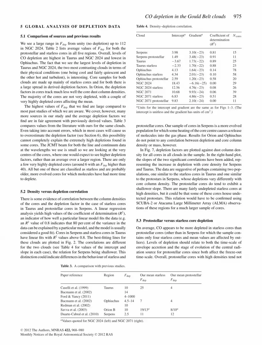
There is some evidence of correlation between the column densitiesof the cores and the depletion factor in the case of starless coresin Taurus and protostellar cores in Serpens. A linear regressionanalysis yields high values of the coefficient of determination (R2),an indicator of how well a particular linear model fits the data (e.g.an R2 value of 0.8 indicates that 80 per cent of the variance in thedata can be explained by a particular model, and the model is usuallyconsidered a good fit). Cores in Serpens and starless cores in Taurushave linear fits with R2 values above 0.8. The best-fitting lines forthese clouds are plotted in Fig. 2. The correlations are differentfor the two clouds (see Table 4 for values of the intercept andslope in each case), the relation for Serpens being shallower. Thisdistinction could indicate differences in the behaviour of starless and

Table 4. Density–depletion correlation.

Cloud Intercepta Gradienta Coefficient of N cores

determination(R2)

Serpens 3.98 3.10(−23) 0.81 15Serpens protostellar 1.49 3.48(−23) 0.91 11Taurus −3.67 1.73(−22) 0.89 25Taurus starless −2.33 1.70(−22) 0.88 23Ophiuchus 4.13 1.64(−23) 0.14 78Ophiuchus starless 4.34 2.01(−23) 0.10 58Ophiuchus protostellar 2.59 1.20(−23) 0.58 20NGC 2024 18.43 −6.16(−25) 0.00 29NGC 2024 starless 12.56 4.76(−23) 0.08 26NGC 2071 10.68 9.93(−24) 0.06 39NGC 2071 starless 6.83 4.86(−23) 0.51 28NGC 2071 protostellar 9.83 2.10(−24) 0.00 11

aUnits for the intercept and gradient are the same as for Figs 1–3. (Theintercept is unitless and the gradient has units of cm3.)

protostellar cores. Our sample of cores in Serpens is a more evolvedpopulation for which some heating of the core centre causes a releaseof molecules into the gas phase. Results for Orion and Ophiuchusdo not point to any correlation between depletion and core columndensity or mass, however.

In Fig. 7, depletion factors are plotted against dust column den-sity for all cores in all clouds in the sample. In the right-hand plot,the slopes of the two significant correlations have been added, rep-resenting the increase in depletion with core density for Serpensand Taurus. The data are suggestive of perhaps containing two pop-ulations, one similar to the starless cores in Taurus and one similarto the protostars in Serpens, whose depletions vary differently withcore column density. The protostellar cores do tend to exhibit ashallower slope. There are many fairly undepleted starless cores athigh densities, but it could be that some of these cores house unde-tected protostars. This relation would have to be confirmed usingSCUBA-2 or Atacama Large Millimeter Array (ALMA) observa-tions of these regions for a much larger sample of cores.

5.3 Protostellar versus starless core depletion

On average, CO appears to be more depleted in starless cores thanprotostellar cores (other than in Serpens for which the sample con-tains only four starless cores and mean values are affected by out-liers). Levels of depletion should relate to both the time-scale ofenvelope accretion and the stage of evolution of the central radi-ation source for protostellar cores since both affect the freeze-outtime-scale. Overall, protostellar cores with high densities tend not

Table 3. A comparison with previous studies.

Paper reference Region Fdep Our mean starless Our mean protostellarFdep Fdep

Caselli et al. (1999) Taurus 10 25 4Bacmann et al. (2002) 14Ford & Yancy (2011) 4–1000Bacmann et al. (2002) Ophiuchus 4.5–14 7 4Redman et al. (2002) 10Savva et al. (2003) Orion B 10 19/13a 8/10a

Duarte-Cabral et al. (2010) Serpens 2.5 11 12

aValues quoted for NGC 2024 (left) and NGC 2071 (right).



Figure 7. Fdep versus dust column density for all clouds. Trends are plotted for Serpens (dotted line) and Taurus (solid line).

to be very depleted in comparison with dense starless cores in thesame cloud. Jørgenson, Schoier & van Dishoeck (2005) looked atdepletion profiles across 16 protostellar cores and found that thesize of the depletion zone grew with envelope mass in the earlystages of evolution and then shrink as the central star began to heatthe inner regions. Perhaps we see here that higher mass protostarsare in a more advanced stage of evolution where a substantial enve-lope has been formed (hence the higher dust column densities) andthe central star has begun to evaporate material from the grains inthe centre. It would be useful to model in more detail a selectionof cores from each cloud to get a handle on ages, density structuresand a more accurate measure of depletion. It should be noted that,in crowded environments, the infrared observations towards severalcores may be misinterpreted or contaminated by the infrared emis-sion from nearby, more evolved YSOs or from a brighter, diffuseinfrared background. Therefore, very faint protostellar emission,such as from Very Low Luminosity Objects (VeLLOs; Pineda et al.2011), in these regions may be misclassified.

6 U N C E RTA I N T I E S IN TH E LTE D E R I V E DD E P L E T I O N FAC TO R

The calculation of column densities via LTE does of course havedrawbacks. The temperatures used to derive hydrogen column den-sities from CO are uncertain since they are roughly calculated, more

than one rotational transition of a given molecule not being avail-able. The CO temperatures are derived from the 12CO and 13COprofiles which may well arise in hotter regions of the cloud, beingself-absorbed in the core centre. In such a case, the use of these lineswould result in an artificially high C18O temperature and low abun-dance being derived, leading to overestimates of the CO depletion.Furthermore, the exponential factor including Tex in equation (2)for calculating CO column density rises rapidly below about 20 K,so the difference between assuming a temperature of 20 and 10 Kleads to a factor of around 2.5 difference in the derived depletionfactor.

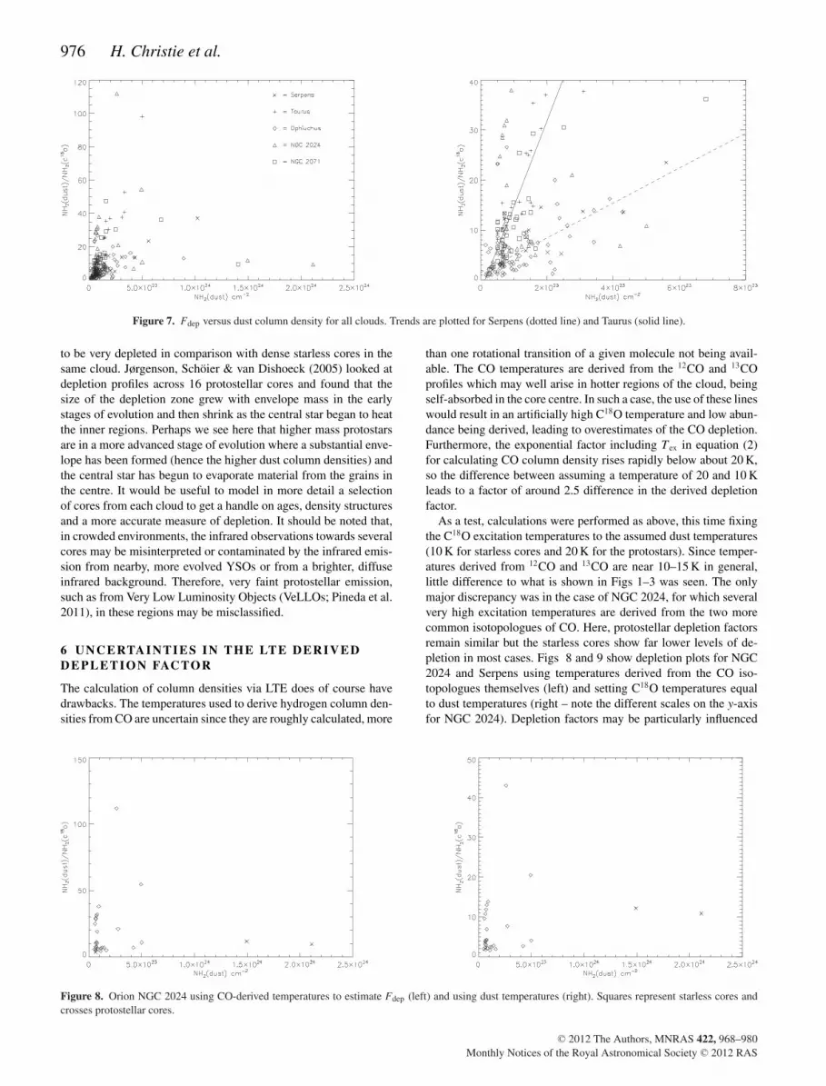
As a test, calculations were performed as above, this time fixingthe C18O excitation temperatures to the assumed dust temperatures(10 K for starless cores and 20 K for the protostars). Since temper-atures derived from 12CO and 13CO are near 10–15 K in general,little difference to what is shown in Figs 1–3 was seen. The onlymajor discrepancy was in the case of NGC 2024, for which severalvery high excitation temperatures are derived from the two morecommon isotopologues of CO. Here, protostellar depletion factorsremain similar but the starless cores show far lower levels of de-pletion in most cases. Figs 8 and 9 show depletion plots for NGC2024 and Serpens using temperatures derived from the CO iso-topologues themselves (left) and setting C18O temperatures equalto dust temperatures (right – note the different scales on the y-axisfor NGC 2024). Depletion factors may be particularly influenced

Figure 8. Orion NGC 2024 using CO-derived temperatures to estimate Fdep (left) and using dust temperatures (right). Squares represent starless cores andcrosses protostellar cores.



Figure 9. Serpens using CO-derived temperatures to estimate Fdep (left) and using dust temperatures (right).

by the temperature estimation in this cloud since the isotopologuesused to calculate temperatures will trace the hotter surrounding re-gions (due to higher optical depth in the denser regions) which maybe more diverse physically, or contrast more with the dense corecentres, than for the other regions due to the filamentary structureand outflow activity.

A major cause of error in our results may be the assumption ofoptically thin C18O in the core centres. Higher optical depth in thatline could lead to an underestimate of the CO gas phase abundanceand hence an overestimate of the depletion. We estimated C18Oopacities very roughly using fig. 12 from Curtis, Richer & Buckle(2010) showing the variation of the C18O opacity with the ratio ofthe 13CO to C18O line peaks for X(13CO)/X(C18O) equal to 7.3(Wilson & Rood 1994). Using the ratios of the peak 13CO and C18Otemperatures at the dust peaks, we estimated C18O opacities for thecores. Values were primarily very low and greater than 1 in only 25of the 370 cores in our sample. Correcting equation (2) using ourderived value of the optical depth made very little difference to theresultant plots. Note, however, that the same method is used for allcores in all clouds, so that while derived individual values of Fdep

may suffer from these uncertainties a comparison between regionsshould still be possible.

The beam size of the JCMT (14 arcsec for the CO maps) isgenerally smaller than CLUMPFIND-derived diameters for the dustcores, so we do not consider beam dilution effects to be a problemand assume a beam filling factor of 1 in all cases.

The calculation of molecular hydrogen column densityfrom C18O emission requires the assumption of a constantN(C18O)/N(H2) ratio. Published values vary by a factor of ∼7from 0.7 × 10−7 (Tafalla & Santiago 2004) to 4.8 × 10−7 (Leeet al. 2003). We adopt the value quoted in Frerking et al. (1982) andnote that this choice may influence our calculated depletion factorsdifferently in different regions.

In our dust column density calculations, we assume fixed dusttemperatures of 10 K for the starless cores and 20 K for the proto-stars. Using the higher temperature for the protostellar cores resultsin lower densities being derived from the dust and so lower values ofthe depletion factor for these cores. For the protostellar cores, therewill likely be some local heating of the dust near to the core centres,so we adopt 20 K. Modelling work in the past has suggested thatdust temperatures for Class 0 and Class I sources may be closer to15 K than the 20 K assumed here (Shirley, Evans & Rawlings 2002;Young et al. 2003), though with fairly significant spreads in derivedtemperatures (4.8 K for the former and 8 K for the latter). In addi-

tion, Larsson et al. (2000) studied the spectral energy distributionsof five submillimetre sources in Serpens and derived dust temper-atures of around 30 K for those sources. Given these differences, itis somewhat unrealistic to define a single dust temperature for thecores. As a test, we re-calculated depletion factors assuming a dusttemperature for all the cores of 15 K. In this instance, protostellarcore depletion factors rise by a factor of only 1.6 compared to thosecalculated assuming 20 K, so this is probably not a major effectcompared to other assumptions we make.

Depletion factors may be underestimated due to the larger beamsize of the telescope at 850 µm relative to that of the spectral line data(22.9 and 14 arcsec, respectively). The SCUBA beam will samplea larger area around the dust cores so that the flux will be slightlydiluted compared to the CO maps which sample the more centralregions of the cores. Although both beams are smaller than the corediameters (from CLUMPFIND), our assumption of an even distributionof material across the cores will not be accurate.

The 850-µm fluxes and the C18O peak line temperatures alsohave associated uncertainties due to the underlying noise in the data(30 mJy for the SCUBA data, see Table 1 for the CO rms noisevalues). We estimate the error on the calculated depletion factorfor a typical starless core in Serpens and derive an error of ±1.47on a depletion factor of 10. This is likely to be similar for othercores (less for those with brighter emission) and is not significantcompared to some of the uncertainties mentioned above.

The 12CO J = (3 → 2) line falls within the SCUBA 850-µmband so we investigated the possible effect of contamination ofthe dust emission. Recent work suggests that the highest levelsof contamination occur in molecular outflow regions rather thanin quiescent cores. In these cases, the CO flux contribution canreach around 0.40 Jy beam−1 (in grade 2 weather for one of theoutflows of NGC 2071) and is estimated to be much lower for theregions studied here, at most 25 per cent of the total peak flux andusually much less. This would result in a reduction in NH2 dust of25 per cent with an equivalent decrease in the resulting depletionfactor. This is, however, a worst-case scenario and errors resultingfrom contamination will probably be far lower in most cases (EmilyDrabek, private communication).

7 E VA L UAT I N G D E P L E T I O N FAC TO R SUSI NG RADEX

We used RADEX (van der Tak et al. 2007), a radiative transfer code ap-proximating a large velocity gradient (LVG) approach, to calculate


https://www.researchgate.net/publication/23616524_The_relationship_between_carbon_monoxide_abundance_and_visual_extinction_in_interstellar_clouds?el=1_x_8&enrichId=rgreq-ae3246f3-f274-4b31-8c43-92f8f14a2a02&enrichSource=Y292ZXJQYWdlOzIyNDk1NDE1NTtBUzo5OTUzNzczMzU1NDE5M0AxNDAwNzQzMDUzNjA5


CO column densities and derive alternative depletion factors. RADEX

and LTE are both approximations. In LTE, the Boltzmann equa-tion accurately describes the level populations for any molecule,with the excitation temperature of all lines equal to the gas kinetictemperature. RADEX, on the other hand, takes into account both col-lisions and the local radiation field. It does not, however, includeany external radiation field. Using both methods should allow us toprobe the range of conditions in the clouds. White, Casali & Eiroa(1995) compared C18O column densities in the Serpens molec-ular cloud calculated using LTE and LVG methods. They foundthat, particularly for cooler, dense material, LTE methods tended tounderestimate column densities compared to LVG calculations byfactors of around 4–8 at 10 K.

To solve the level populations, RADEX uses the escape probabilitymethod to describe the effect of the radiation field. RADEX allows forthe use of several different geometries which affect the escape prob-ability calculations. Here we used a homogeneous sphere havingtested other geometries and found the choice made little differenceto the results. For the RADEX calculations, two grids of models wererun, one for the 13CO data and one for the C18O data. For both,the column density of the molecule and the gas kinetic temperaturewere left as free parameters. The dust density was fixed using the850-µm emission exactly as for the LTE calculations and convertedto a volume density using the CLUMPFIND derived core sizes. Wemeasured line widths from the HARP 13CO and C18O spectra at thepeak of the dust emission. We then assumed a canonical ratio of 7.3

Table 5. LTE and RADEX results – Taurse refers to the south-eastern region of L1495 (the ridge). Brackets indicate powers of 10.

Core RA (J2000) Dec. (J2000) Rad Density of Column Tex Fdep Tkin Fdep Reduced(pc) gasa density of (LTE) (LTE) (RADEX) (RADEX) χ2

(cm−3) gas (cm−3)

Oph p3 16h26m10s4 −24◦20′ ′56′ 0.027 4.0(5) 6.74(22) 35 K 2 37 K 1 8.69Oph p4 ↑∗ 16h26m27s6 −24◦23′ ′57′ 0.054 2.7(6) 8.93(23) 29 K 13 28 K 0 267.88Oph p10 16h27m00s5 −24◦26′ ′38′ 0.017 1.7(5) 1.76(22) 23 K 1 28 K 1 2.07Oph p13 16h27m07s2 −24◦38′ ′08′ 0.023 2.3(5) 3.32(22) 18 K 1 14 K 1 2.09Oph s18 16h26m36s3 −24◦17′ ′56′ 0.026 6.2(5) 1.00(23) 27 K 3 22 K 2 5.51Oph s42 16h27m58s6 −24◦33′ ′43′ 0.033 1.0(6) 2.24(23) 17 K 20 12 K 14 0.09Oph s53 16h27m05s0 −24◦39′ ′14′ 0.029 1.3(6) 2.24(23) 18 K 2 10 K 3 0.43

Taurse p1 04h19m42s3 27◦13′ ′37′ 0.024 4.8(5) 7.15(22) 12 K 3 8 K 2 0.07Taurse p2 04h19m58s4 27◦10′ ′00′ 0.026 4.3(5) 6.95(22) 12 K 5 12 K 4 0.17Taurse s1 04h19m50s8 27◦11′ ′30′ 0.019 5.6(5) 6.56(22) 9 K 8 10 K 16 0.04Taur s9 04h18m33s6 28◦26′ ′53′ 0.008 2.5(6) 1.24(23) 10 K 13 10 K 7 0.25Taur s18 ∗ 04h18m38s7 28◦21′ ′30′ 0.009 5.6(6) 3.11(23) 11 K 38 8 K 4 0.02Taur s21 ∗ 04h18m41s0 28◦22′ ′00′ 0.006 9.1(6) 3.35(23) 11 K 16 8 K 9 0.80Taur s22 ∗ 04h18m42s4 28◦21′ ′30′ 0.006 1.8(6) 6.56(22) 11 K 15 8 K 2 0.21Taur s24 ↑∗ 04h18m43s7 28◦23′ ′24′ 0.012 4.5(6) 3.35(23) 11 K 53 7 K 1 1.38

Serp p2 18h29m49s8 01◦16′ ′39′ 0.055 3.0(6) 1.02(24) 21 K 37 13 K 14 0.06Serp p3 18h29m51s4 01◦16′ ′33′ 0.038 7.8(5) 1.82(23) 20 K 15 14 K 9 0.46Serp p8 18h30m00s2 01◦10′ ′21′ 0.037 2.9(5) 6.53(22) 13 K 3 10 K 1 0.45Serp p9 18h30m00s2 01◦11′ ′39′ 0.053 6.2(5) 2.02(23) 17 K 6 14 K 5 1.42Serp p11 18h30m01s8 01◦15′ ′09′ 0.035 2.7(5) 5.91(22) 19 K 5 26 K 6 0.19Serp s2 18h30m02s6 01◦09′ ′03′ 0.028 8.4(5) 1.45(23) 11 K 10 11 K 5 0.87Serp s3 18h30m05s0 01◦15′ ′15′ 0.022 5.4(5) 7.25(22) 18 K 13 64 K 10 11.38Serp s4 18h30m13s4 01◦16′ ′15′ 0.032 3.7(5) 7.25(22) 15 K 12 31 K 15 0.03

NGC 2024 p1 td 05h41m43s0 −01◦54′ ′20′ 0.168 6.9(4) 7.15(22) 59 K 12 64 K 0 28.44NGC 2024 p2 td 05h41m44s6 −01◦55′ ′38′ 0.233 5.7(4) 8.18(22) 71 K 10 80 K 0 147.78NGC 2024 p3 t 05h41m49s4 −01◦59′ ′38′ 0.084 4.0(4) 2.05(22) 22 K 4 24 K 1 14.21NGC 2024 s29 05h41m33s4 −01◦49′ ′50′ 0.044 4.0(5) 1.10(23) 24 K 4 80 K 3 17.57NGC 2024 s31 t 05h41m36s2 −01◦56′ ′32′ 0.120 3.7(5) 2.76(23) 36 K 21 80 K 7 697.60NGC 2024 s39 05h42m03s1 −02◦04′ ′21′ 0.064 2.0(5) 7.94(22) 20 K 10 35 K 11 0.19NGC 2024 s40 05h42m05s9 −02◦03′ ′33′ 0.067 1.6(5) 6.56(22) 16 K 10 72 K 7 32.57NGC 2024 s47 05h41m36s6 −01◦49′ ′26′ 0.056 4.8(5) 1.66(23) 43 K 5 80 K 3 69.31NGC 2024 s53 05h42m02s7 −02◦02′ ′33′ 0.104 7.7(5) 4.93(23) 25 K 54 24 K 46 0.55

NGC 2071 p3 05h46m55s0 00◦23′ ′26′ 0.055 1.0(5) 3.52(22) 21 K 3 14 K 1 1.15NGC 2071 p10 t 05h47m20s2 00◦16′ ′02′ 0.053 9.6(4) 2.80(22) 25 K 2 28 K 2 5.23NGC 2071 p12 05h47m37s0 00◦20′ ′02′ 0.087 1.7(5) 8.91(22) 15 K 13 17 K 13 0.24NGC 2071 s3 05h46m36s2 00◦27′ ′32′ 0.052 2.5(5) 7.94(22) 16 K 12 13 K 7 0.30NGC 2071 s17 t 05h47m12s6 00◦15′ ′38′ 0.048 2.7(5) 7.94(22) 28 K 4 33 K 4 16.14NGC 2071 s23 05h47m31s4 00◦16′ ′26′ 0.040 2.1(5) 5.18(22) 20 K 12 35 K 13 0.04

aValues inferred from observations of the dust emission using the method outlined in Section 3.∗Many equally good fits were achieved so there was no unique model fit to the data.↑The C18O peak for the line is higher than the 13CO peak.tThe 13CO line peak is higher than the 12CO peak (and hence is more likely to be optically thick or self-absorbed).tdThe 13CO profile is double peaked.



between the 13CO and the C18O abundances (Wilson & Rood 1994).The best-fitting output to the observed line intensities of both 13COand C18O was selected by minimizing the value of the reduced χ2

parameter given by

(I18obs − I18mod)2

(�I18obs)2+ (I13obs − I13mod)2

(�I13obs)2, (5)

where Iobs and Imod are the observed and modelled peak line intensi-ties. This method assumes that 13CO and C18O are tracing the samegas though this may not be the case.

7.1 LTE versus RADEX

Both the RADEX and LTE results are shown in Table 5 as wellas some properties of the cores from the Sadavoy et al. (2010)catalogue. We did not analyse all cores with RADEX but chosea few to get some idea of how different the results from RADEX

and LTE would be and how effectively RADEX could be used withthe data available to evaluate depletion factors. We selected coresfrom a variety of positions within the cloud, and with varyingproperties.

Table 5 lists an identifier for each core, its position, the (CLUMPFIND

defined) radius, dust density, dust column density, temperature de-rived from the 12CO lines in LTE, depletion derived in LTE, gaskinetic temperature from RADEX and the depletion factor calculatedwith RADEX. The final column lists the reduced χ2 value, intended togive an idea of how well the best-fitting model and observed valuesagree in each case. We consider values of this parameter below 2 toindicate a good fit (with the gas kinetic temperature and the 13COand C18O column densities as free parameters). Note again that adepletion factor of 1 indicates no depletion.

In Table 5, there are three cores for which values of Fdep are equalto 0 as calculated by RADEX indicating that the column density ofhydrogen calculated using the dust emission was a lot lower thanthat calculated using the gas phase CO emission. In these cases,the RADEX kinetic temperature was higher than 25 K. If correct, itis likely that the CO in these cases emanates from warmer regionsoutside of the dense cores. The χ2 values for these cores were alsoall high.

In most cases, RADEX and the LTE approximation yielded sim-ilar values for the depletion factor and gas kinetic temperature.There appears, however, to be a tendency towards lower depletion

estimates when using RADEX rather than LTE. Several cores, par-ticularly those in Taurus and NGC 2024, were very difficult to fitusing RADEX (either never finding a good fit, indicated by the highvalues for the fit parameter in Table 5, or else finding equally goodfits for several input combinations, marked by an asterisk in thetable). Other than six cores, four of which are in NGC 2024, kinetictemperatures derived via the two methods agree to within 4–5 K onaverage. We note that the maximum depletion factor we calculatefor the cores in Serpens is similar to that found by Duarte-Cabralet al. (2010).

Fig. 10 shows LTE versus RADEX derived depletion factors. Theleft-hand plot includes the full sample of fitted cores (with starlesscores as squares and protostellar cores as crosses). The right-handplot shows only those for which we could find a fairly good uniquefit with RADEX (χ2 less than 2). Looking at the right-hand plot, itdoes appear that for several cores (two in particular) LTE methodsoverestimate CO depletion (or underestimate column densities).The two cores for which this effect is most prominent are the twodensest cores in the sample. If LTE line intensities reach a maximumfor a given column density, and if the population is sub-thermal, ahigher column density of CO is required to reach the same lineintensities. Where LTE depletions are high may be a result of highoptical depth in the C18O line, resulting in an underestimate of COgas column density in the LTE approximation. On the other hand,using the 13CO line in the RADEX models may lead to problems dueto self-absorption in that line.

Cores with very different depletion factors derived from the twomethods did tend to display double-peaked 13CO line profiles orhave higher intensities in the C18O line than the 13CO, both indi-cations of self-absorption. We also use core sizes from the codeCLUMPFIND to calculate dust volume densities to input into RADEX,which may introduce further uncertainty. The fact that we haveonly one transition for each isotopologue of CO is likely the maincause of error when using RADEX to estimate column densities. Itis encouraging that temperatures, depletions and general trendsagree to some extent in those cores for which we could achievea good fit (a median discrepancy of 2 in the depletion factor and4 K in the temperature). To use this code to find depletion fac-tors for all cores and properly compare regions, we would needa good and unique fit for all cores. It would be preferable to ob-tain data with several transitions for C18O rather than using twoisotopologues.

Figure 10. RADEX versus LTE depletion factors. Left: all cores fitted with RADEX (starless cores are squares, protostellar cores are crosses). Right: only coreswith a good (χ2 less than 2), unique RADEX fit.



8 SU M M A RY

We have used the C18O and dust emission in dense cores within fivelocal star-forming regions, experimenting with both LTE and non-LTE methods, to compare statistically large-scale depletion factors.We find the following.

(i) Within each cloud, the highest levels of depletion are found inthe longer lived regions (Serpens and Taurus) or fragmented regionsaround the edges of CO cavities (Orion).

(ii) Cores in Ophiuchus (L1688) are the least depleted overall.This behaviour could be connected to the anomalous grain sizedistribution inferred from observations of this cloud.

(iii) There is a strong correlation between core density and de-pletion in both Serpens and Taurus.

(iv) Starless cores are, on average, more depleted than protostel-lar cores (an overall mean depletion factor of 13 rather than 7) andprotostars may show a different trend with core density to the star-less cores. This could be due to the evaporation of material fromdust grains after heating by nearby sources.

We note that while our study suffers from uncertainties due totemperature estimations and the assumption of LTE, these are of-ten systematic and should not affect comparison of depletion factorsamong the different clouds. These factors do, however, affect the de-pletion factors derived for individual cores. Multiline observationsof C18O as well as other isotopologues should help to constrainbetter the CO column densities and temperatures and achieve moreaccurate measures of the depletion factors.

AC K N OW L E D G M E N T S

We would like to thank the referee for very helpful comments andcareful reading, and the Gould Belt Survey team.

R E F E R E N C E S

Aikawa Y., Ohashi N., Inutsuka S., Herbst E., Takakuwa S., 2001, ApJ, 552,639

Bacmann A., Lefloch B., Ceccarelli C., Castets A., Steinacker J., LoinardL., 2002, ApJ, 389, 6

Buckle J. V. et al., 2009, MNRAS, 399, 1026Buckle J. V. et al., 2010, MNRAS, 401, 204Buckle J. V. et al., 2011, MNRAS, in press (doi:10.1111/j.1365-

2966.2012.20628.x)Carrasco L., Strom S. E., Strom K. M., 1972, ApJ, 182, 95Casassus S. et al., 2008, MNRAS, 391, 1075Caselli P., Walmsley C. M., Tafalla M., Dore L., Myers P. C., 1999, ApJ,

523, 165Chapman N. L., Mundy L. G., Lai S.-P., Evans N., 2009, ApJ, 690, 496Curtis E. I., Richer J. S., Buckle J. V., 2010, MNRAS, 401, 455Davis C. F., Matthews H. E., Ray T. P., Dent W. R. F., Richer J. S., 1999,

MNRAS, 309, 141Davis C. J. et al., 2010, MNRAS, 405, 759Di Francesco J., Evans N. J., II, Caselli P., Myers P. C., Shirley Y., Aikawa

Y., Tafalla M., 2007, in Reipurth B., Jewitt D., Keil K., eds, Protostarsand Planets V. Univ. Arizona Press, Tucson, p. 17

Di Francesco J., Johnstone D., Kirk H. M., MacKenzie T., Ledwosinska E.,2008, ApJS, 175, 277

Duarte-Cabral A., Fuller G. A., Peretto N., Hatchell J., Ladd E. F., BuckleJ., Richer J., Graves S. F., 2010, A&A, 519, 27

Duarte-Cabral A., Dobbs C. L., Peretto N., Fuller G. A., 2011, A&A, 528,50

Frerking M. A., Langer W. D., Wilson R. W., 1982, ApJ, 262, 590Friesen R. K., Di Francesco J., Shirley Y. L., Myers P. C., 2009, ApJ, 697,

1457Graves S. F. et al., 2010, MNRAS, 409, 141Harvey P. M., Merın B., Huard T. L., Rebull L. M., Chapman N., Evans

N. J., II, Myers P. C., 2007, ApJ, 663, 1149Jones A. P., Williams D. A., 1985, MNRAS, 217, 413Jørgenson J. K., Schoier F. L., van Dishoeck E. F., 2005, A&A, 435, 177Kaas A. A. et al., 2004, A&A, 421, 623Larsson B. et al., 2000, A&A, 363, 253Lombardi M., Lada C. J., Alves J., 2008, A&A, 480, 785Maruta H., Nakamura F., Nishi R., Ikeda N., Kitamura Y., 2010, ApJ, 714,

680Munoz Caro G. M., Jimenez-Escobar A., Martın-Gago J. A., Rogero C.,

Atienza C., Puertas S., Sobrado J. M., Torres-Redondo J., 2010, A&A,522, 108

Nakagawa N., 1980, in Andrew B. H., ed., Proc. IAU Symp. 87, InterstellarMolecules. Reidel, Dordrecht, p. 365

Oberg K. I., Garrod R. T., van Dishoeck E. F., Linnartz H., 2009, A&A, 504,891

Oberg K. I., Boogert A. C. A., Pontoppidean K. M., van den Broek S., vanDishoeck E. F., Bottinelli S., Blake G. A., Evans N. J., II, 2011, ApJ,740, 1090

Onishi T., Mizuno A., Kawamura A., Tachihara K., Fukui Y., 2002, ApJ,575, 950

Ossenkopf V., Henning T., 1994, A&A, 291, 943Pineda J. E., Caselli P., Goodman A. A., 2008, ApJ, 679, 481Pineda J. E. et al., 2011, ApJ, 743, 201Rawlings J. M. C., Hartquist T. W., Menten K. M., Williams D. A., 1992,

MNRAS, 255, 471Redman M. P., Rawlings J. M. C., Nutter D. J., Ward-Thompson D., Williams

D. A., 2002, MNRAS, 337, 17Roberts J. F., Rawlings J., Viti S., Williams D. A., 2007, MNRAS, 382, 733Sadavoy S. I. et al., 2010, ApJ, 710, 1247Savva D., Little L. T., Phillips R. R., Gibb A. G., 2003, MNRAS, 343, 259Shirley Y. L., Evans N. J., Rawlings J. M. C., 2002, ApJ, 575, 337Taylor S. D., Williams D. A., 1996, MNRAS, 282, 1343Thomas H. S., Fuller G. A., 2008, A&A, 479, 751van der Tak F. F. S., Black J. H., Schoier F. L., Jansen D. J., van Dishoeck

E. F., 2007, A&A, 468, 627van Dishoeck E. F., 2004, ARA&A, 42, 119Viti S., Girart J. M., Garrod R., Williams D. A., Estalella R., 2003, A&A,

399, 187Ward-Thompson D. et al., 2007, PASP, 119, 855Warren-Smith R. F., Wallace P. T., 1993, in Hanisch R. J., Brissenden

R. J. V., Barnes J., eds, ASP Conf. Ser. Vol. 52, Astronomical DataAnalysis Software and Systems II. Astron. Soc. Pac., San Francisco,p. 229

White G. J., Phillips J. P., 1980, MNRAS, 194, 947White G. J., Casali M. M., Eiroa C., 1995, A&A, 298, 594Williams J. P., de Geus E. J., Blitz L., 1994, ApJ, 428, 693Wilson T. L., Rood R., 1994, A&A, 32, 191Young C. H., Shirley Y. L., Evans N. J., Rawlings J. M. C., 2003, ApJ, 145,

111

This paper has been typeset from a TEX/LATEX file prepared by the author.


https://www.researchgate.net/publication/23616524_The_relationship_between_carbon_monoxide_abundance_and_visual_extinction_in_interstellar_clouds?el=1_x_8&enrichId=rgreq-ae3246f3-f274-4b31-8c43-92f8f14a2a02&enrichSource=Y292ZXJQYWdlOzIyNDk1NDE1NTtBUzo5OTUzNzczMzU1NDE5M0AxNDAwNzQzMDUzNjA5





co depletion in the gould belt clouds

Documents