BJP

S - A

ccepte

d Manusc

ript

Closed Form Expressions for Moments of a Class of

Beta Generalized Distributions

Gauss M. CordeiroDepartamento de Estatıstica e Informatica,Universidade Federal Rural of Pernambuco,

52171-900, Recife, PE, Brazile-mail:gausscordeiro@uol.com.br

Saralees NadarajahSchool of Mathematics, University of Manchester,

Manchester M13 9PL, UKe-mail:saralees.nadarajah@manchester.ac.uk

Abstract

For the first time, we derive explicit closed form expressions for moments ofsome beta generalized distributions including the beta gamma, beta normal, betabeta, beta Student t and beta F distributions. These expressions are given asinfinite weighted sums of well-known special functions for which numerical routinesfor computation are available.Keywords: Beta beta distribution, Beta F distribution, Beta gamma distribution,Beta normal distribution, Beta Student t distribution, Generalized Kampe de Ferietfunction, Lauricellla function of type A

1 Introduction

Generalized distributions have been widely studied in statistics and numerous authorshave developed various classes of these distributions. Eugene et al. (2002) first proposeda general class of distributions for a random variable defined from the logit of the betarandom variable by employing two parameters whose role is to introduce skewness and tovary tail weights. In this paper, we derive explicit closed form expressions for the momentsof this class of distributions. The expressions take the form of infinite sums of well-knownspecial functions which are very simple to be implemented in practice for several betageneralized distributions. In fact, we derive closed form expressions for the moments ofthe beta gamma, beta normal, beta beta, beta Student t and beta F distributions. Thereason that we choose these special distributions (gamma, normal, beta, Student t andF ) is because they are perhaps the most popular distributions in statistics and variousapplied areas and they possess finite moments to ensure existence of the moments of theassociated beta generalized distributions. Similar results could in principle be derived forother beta generalized distributions. These closed form expressions can be used to obtainthe same for functions of moments, for example, moment generating function, cumulantgenerating function, characteristic function, factorial and central moments, etc.

1

BJP

S - A

ccepte

d Manusc

ript

The calculations in this article involve some special functions, including the well-known

incomplete gamma function defined by

γ(α, x) =

∫ x

0

wα−1e−wdw, α > 0,

the error function erf(.) defined by

erf(x) =2√π

∫ x

0

exp(−t2)dt,

the beta function (Γ(·) is the gamma function) given by

B(a, b) =

∫ ∞

0

wa−1(1− w)b−1dw =Γ(a)Γ(b)

Γ(a + b),

the incomplete beta function ratio, i.e. the cumulative distribution function (cdf) of thebeta distribution with parameters a and b, defined by

Ix(a, b) =1

B(a, b)

∫ x

0

wa−1(1− w)b−1dw,

the confluent hypergeometric function defined by

1F1(a; b; z) =∞∑i=0

(a)izi

(b)ii!,

where (a)i is the ascending factorial defined by (with the convention that (a)0 = 1)

(a)i = a(a + 1) · · · (a + i− 1),

the Gaussian hypergeometric function defined by

2F1(a, b; c; z) =∞∑i=0

(a)i(b)izi

(c)ii!,

the Lauricella function of type A (Exton, 1978; Aarts, 2000) defined by

F(n)A (a; b1, . . . , bn; c1, . . . , cn; x1, . . . , xn)∞∑

m1=0

· · ·∞∑

mn=0

(a)m1+···+mn (b1)m1· · · (bn)mn

(c1)m1· · · (cn)mn

xm11 · · ·xmn

n

m1! · · ·mn!, (1)

and the generalized Kampe de Feriet function (Exton, 1978; Mathai, 1993; Aarts, 2000;Chaudhry and Zubair, 2002) defined by

FA:BC:D ((a) : (b1); . . . , (bn); (c) : (d1); . . . , (dn); x1, . . . , xn)

=∞∑

m1=0

· · ·∞∑

mn=0

((a))m1+···+mn ((b1))m1· · · ((bn))mn

((c))m1+···+mn ((d1))m1· · · ((dn))mn

xm11 · · · xmn

n

m1! · · ·mn!, (2)

where a = (a1, a2, . . . , aA), bi = (bi,1, bi,2, . . . , bi,B) for i = 1, 2, . . . , n, c = (c1, c2, . . . , cC),di = (di,1, di,2, . . . , di,D) for i = 1, 2, . . . , n, and

((f))k = ((f1, f2, . . . , fp))k = (f1)k(f2)k · · · (fp)k

2

BJP

S - A

ccepte

d Manusc

ript

denotes the product of ascending factorials. Numerical routines for the direct computationof functions (1) and (2) are available, see Exton (1978) and Mathematica (Trott, 2006).

The rest of the paper is organized as follows. Section 2 defines the class of beta gene-ralized distributions. Section 3 gives general expansions for calculating the moments ofbeta generalized distribution as infinite weighted sums of probability weighted moments(PWMs) of the parent distribution. Closed form expressions for moments of the betagamma and beta normal distributions are given in Sections 4 and 5, respectively. InSections 6, 7 and 8 we give closed form expressions for moments of the beta beta, betaStudent t and beta F distributions, respectively. Section 9 provides some numerical cal-culations for these moments. Section 10 ends with some conclusions.

2 The Class of Beta Generalized Distributions

Let G be the cumulative distribution function (cdf) of a random variable. The functionF (x) given by

F (x) = IG(x)(a, b) =1

B(a, b)

∫ G(x)

0

ωa−1(1− ω)b−1dω, (3)

defines the cdf of the class of beta G distributions, where a > 0 and b > 0 are twoadditional parameters whose role is to introduce skewness and to vary tail weights, andIG(x)(a, b) is the incomplete beta function ratio evaluated at G(x). Application of X =G−1(V ) to V following the beta B(a, b) distribution yields X with cdf (3). Several authorsintroduced and studied particular members of this class of distributions over the last years,mainly after the works of Eugene et al. (2002) and Jones (2004a).

The beta normal (BN) distribution introduced by Eugene et al. (2002) is obtained bytaking G(x) to be the cdf of the normal distribution. This distribution can be unimodaland bimodal. Some expressions for the moments of the BN distribution were derived byGupta and Nadarajah (2004a). Nadarajah and Kotz (2004) introduced the beta Gumbeldistribution by taking G(x) to be the cdf of the Gumbel distribution and provided closedform expressions for the moments and discussed the asymptotic distribution of the ex-treme order statistics and the maximum likelihood estimation procedure. Nadarajah andGupta (2004) proposed the beta Frechet distribution by taking G(x) to be the Frechetdistribution, derived the analytical shapes of the density and hazard rate functions andcalculated the asymptotic distribution of the extreme order statistics. Nadarajah andKotz (2006) obtained the moment generating function, the first four cumulants and theasymptotic distribution of the extreme order statistics for the beta exponential distribu-tion and examined maximum likelihood estimation of its parameters.

The probability density function (pdf) corresponding to (3) has a very simple form

f(x) =g(x)

B(a, b)G(x)a−1{1−G(x)}b−1, (4)

where g(x) = dG(x)/dx is the density of the baseline distribution. The density f(x) willbe most tractable when both functions G(x) and g(x) = dG(x)/dx have simple analyticexpressions. Except for some special choices for G(x) in equation (3), it would appearthat the density (4) will be difficult to deal with in generality. If g(x) is a symmetricdistribution around zero, then f(x) will also be a symmetric distribution when a = b.

3

BJP

S - A

ccepte

d Manusc

ript

3 General Formulae for the Moments

For b > 0 real non-integer, we have the power series

{1−G(x)}b−1 =∞∑i=0

(−1)i

(b− 1

i

)G(x)i,

where the binomial coefficient is defined for any real b. From the above expansion andequation (4), we can express the density of the beta G as

f(x) = g(x)∞∑i=0

wiG(x)a+i−1, (5)

where

wi = wi(a, b) =(−1)i

(b−1

i

)

B(a, b).

If b is an integer, the index i in the previous sum stops at b − 1. If a is an integer,equation (5) gives the pdf of the beta G as an infinite power series expansion of cdf’s ofG. Otherwise, if a is real non-integer, we can expand G(x)a+i−1 as follows

G(x)a+i−1 = [1− {1−G(x)}]a+i−1 =∞∑

j=0

(−1)j

(a + i− 1

j

){1−G(x)}j

and then

G(x)a+i−1 =∞∑

j=0

j∑r=0

(−1)j+r

(a + i− 1

j

)(j

r

)G(x)r.

Hence, we can write from equation (4)

f(x) = g(x)∞∑

i,j=0

j∑r=0

wi,j,rG(x)r, (6)

where the coefficients

wi,j,r = wi,j,r(a, b) =(−1)i+j+r

(a+i−1

j

)(b−1

i

)(jr

)

B(a, b)

are constants. Expansion (6), which holds for any real non-integer a, gives the pdf of thebeta G as an infinite power series expansion of cdf’s of G. If b is an integer, the indexi in equation (6) stops at b − 1. Equations (5) and (6) are used to derive closed formexpressions for the moments of the beta gamma, beta normal, beta beta, beta Student tand beta F distributions valid for a integer and a real non-integer, respectively. We have

∞∑i=0

wi = 1 and∞∑

i,j=0

j∑r=0

wi,j,r = 1.

From now on we assume X following the pdf of any parent G distribution and Y thepdf of the beta G distribution. The sth moment of Y can be expressed in terms of the(s, r)th PWM of X, say τs,r = E{XsG(X)r}. For a integer, we obtain

µ′s =∞∑

r=0

wrτs,r+a−1, (7)

4

BJP

S - A

ccepte

d Manusc

ript

whereas for a real non-integer we have

µ′s =∞∑

i,j=0

j∑r=0

wi,j,rτs,r. (8)

Equations (7) and (8) are of very simple forms and constitute the main results of thissection. Hence, we can calculate the moments of the beta G distribution in terms ofinfinite weighted sums of PWMs of G.

4 Moments of the Beta Gamma

A random variable X has a gamma G(α, β) distribution with parameters α > 0 and β > 0if its cdf is

G(x) =γ(α, βx)

Γ(α), x > 0.

For s > 0, we have E(Xs) = Γ(s + α)/Γ(βsα). A random variable Y has a beta gammaBG(a, b, α, β) distribution if its pdf is

f(x) =βαxα−1e−βx

B(a, b)Γ(α)a+b−1γ(α, βx)a−1 {Γ(α)− γ(α, βx)}b−1 , x > 0.

Some properties of the beta gamma distribution are discussed in Kong et al. (2007). Weobtain τs,r using the series expansion for the incomplete gamma function. We have

G(x) =(βx)α

Γ(α)

∞∑m=0

(−βx)m

(α + m)m!,

and then

τs,r =βα

Γ(α)

∫ ∞

0

xs+α−1 exp(−βx)

{(βx)α

Γ(α)

∞∑m=0

(−βx)m

(α + m)m!

}r

dx

=β−s

Γ(α)r+1

∫ ∞

0

us+α−1 exp(−u)

{uα

∞∑m=0

(−u)m

(α + m)m!

}r

du.

The last integral can be obtained from equations (24) and (25) of Nadarajah (2008) as

τs,r =β−sα−rΓ(s + α(r + 1))

Γ(α)r+1F

(r)A (s+α(r+1); α, . . . , α; α+1, . . . , α+1;−1, . . . ,−1). (9)

Hence, the moments of the beta gamma distribution can be written as infinite weightedsums of the Lauricella functions of type A from equations (7) and (9) for a integer andfrom (8) and (9) for a real non-integer, respectively.

5 Moments of the Beta Normal

The BN distribution, introduced by Eugene et al. (2002), is obtained by taking G(x) tobe the cdf of the normal distribution in equation (3). The density of the BN(a, b, µ, σ2)distribution is given by

f(x) =σ−1

B(a, b)φ

(x− µ

σ

){Φ

(x− µ

σ

)}a−1 {1− Φ

(x− µ

σ

)}b−1

, (10)

5

BJP

S - A

ccepte

d Manusc

ript

−6 −4 −2 0 2 4 6

0.0

0.1

0.2

0.3

0.4

x

f(x)

a=1, b=1a=0.8, b=2a=5, b=0.1

−6 −4 −2 0 2 4 6

0.00

0.02

0.04

0.06

0.08

0.10

x

f(x)

a=0.05, b=0.15a=0.1, b=0.05a=0.1, b=0.1

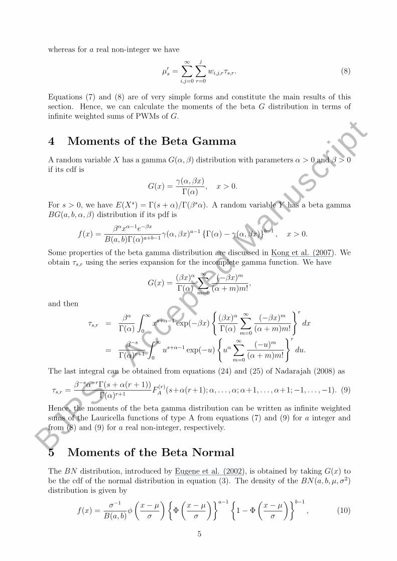
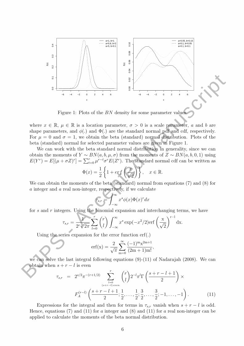
Figure 1: Plots of the BN density for some parameter values.

where x ∈ R, µ ∈ R is a location parameter, σ > 0 is a scale parameter, a and b areshape parameters, and φ(.) and Φ(.) are the standard normal pdf and cdf, respectively.For µ = 0 and σ = 1, we obtain the beta (standard) normal distribution. Plots of thebeta (standard) normal for selected parameter values are given in Figure 1.

We can work with the beta standard normal distribution in generality, since we canobtain the moments of Y ∼ BN(a, b, µ, σ) from the moments of Z ∼ BN(a, b, 0, 1) usingE(Y r) = E[(µ + σZ)r] =

∑rt=0 µr−tσrE(Zr). The standard normal cdf can be written as

Φ(x) =1

2

{1 + erf

(x√2

)}, x ∈ R.

We can obtain the moments of the beta (standard) normal from equations (7) and (8) fora integer and a real non-integer, respectively, if we calculate

τs,r =

∫ ∞

−∞xsφ(x)Φ(x)rdx

for s and r integers. Using the binomial expansion and interchanging terms, we have

τs,r =1

2r√

2π

r∑

l=0

(r

l

) ∫ ∞

−∞xs exp(−x2/2)erf

(x√2

)r−l

dx.

Using the series expansion for the error function erf(.)

erf(x) =2√π

∞∑m=0

(−1)mx2m+1

(2m + 1)m!,

we can solve the last integral following equations (9)-(11) of Nadarajah (2008). We canobtain when s + r − l is even

τs,r = 2s/2π−(r+1/2)

r∑l=0

(s+r−l) even

(r

l

)2−lπlΓ

(s + r − l + 1

2

)×

F(r−l)A

(s + r − l + 1

2;1

2, . . . ,

1

2;3

2, . . . ,

3

2;−1, . . . ,−1

). (11)

Expressions for the integral and then for terms in τs,r vanish when s + r − l is odd.Hence, equations (7) and (11) for a integer and (8) and (11) for a real non-integer can beapplied to calculate the moments of the beta normal distribution.

6

BJP

S - A

ccepte

d Manusc

ript

6 Moments of the Beta Beta

The beta distribution is the most flexible family of distributions. It has relationships withseveral of the well-known univariate distributions. Beta distributions are very versatileand a variety of uncertainties can be usefully modeled by them. Many of the finiterange distributions encountered in practice can be easily transformed into the standardbeta distribution. In reliability and life testing experiments, many times the data aremodeled by finite range distributions, see, for example, Barlow and Proschan (1975). Inrecent years, beta distributions have been used in modeling distributions of hydrologicvariables. Many generalizations of the beta distribution involving algebraic, exponentialand hypergeometric functions have been proposed in the literature; see the book of Guptaand Nadarajah (2004b) for detailed accounts.

The pdf and cdf of the beta B(α, β) distribution with parameters α > 0 and β > 0 aresimply g(x) = xα−1(1−x)β−1/B(α, β) and G(x) = Ix(α, β) = B(α, β)−1

∫ x

0tα−1(1−t)β−1dt

for 0 < x < 1. In this section, an enlargement of the beta family of distributions on (0, 1)is presented. We introduce, for the first time, the so-called four parameter beta betaBB(a, b, α, β) distribution with density (for 0 < x < 1) given by

f(x) =xα−1(1− x)β−1

B(α, β)B(a, b)Ix(α, β)a−1 {1− Ix(α, β)}b−1 . (12)

The PWM of the B(α, β) distribution is

τs,r =1

B(α, β)

∫ 1

0

xs+α−1(1− x)β−1Ix(α, β)rdx.

Using the incomplete beta function expansion for β real non-integer

Ix(α, β) =xα

B(α, β)

∞∑m=0

(1− β)mxm

(α + m)m!,

and the fact (f)k = Γ(f + k)/Γ(f), the last integral can be obtained from the algebraicdevelopments made by Nadarajah (2008, Section 5) which convert the function I(k, l)defined in equation (28) to the expression (30) of his paper written in terms of the gen-eralized Kampe de Feriet function. Hence, we obtain

τs,r = α−rB(α, β)−(r+1)B(β, s + α(r + 1))×F 1:2

1:1

((s + α(r + 1)) : (1− β, α); . . . ; (1− β, α) :

(β + s + α(r + 1)) : (α + 1); . . . ; (α + 1); 1, . . . , 1). (13)

The moments of the beta beta distribution follow immediately as infinite sums of thegeneralized Kampe de Feriet functions from equations (7) and (13) for a integer and from(8) and (13) for a real non-integer.

7 Moments of the Beta Student t

The Student t distribution is the second most popular continuous distribution in statistics,second only to the normal distribution. The density of the Student tν distribution withν > 0 degrees of freedom is (for −∞ < x < ∞)

g(x) =1√

νB(1/2, ν/2)

(1 +

x2

ν

)−(ν+1)/2

.

7

BJP

S - A

ccepte

d Manusc

ript

For any real x, the cdf of the Student tν distribution is simply G(x) = Iy(1/2, ν/2), wherey = (x +

√x2 + ν)/(2

√x2 + ν). The density of the beta Student BS(a, b, ν) distribution

with parameters ν, a and b is then given by (for any x)

f(x) =

(1 + x2

ν

)−(ν+1)/2

√νB(a, b)B(1/2, ν/2)

{Ix+√

x2+ν

2√

x2+ν

(1/2, ν/2)}a−1{1− Ix+√

x2+ν

2√

x2+ν

(1/2, ν/2)}b−1. (14)

The beta Student is then symmetric around zero only when a = b.Since the pdf of the Student tν distribution is symmetric around zero, the (s, r)th

PWM of the Student tν distribution can be expressed as

τs,r =

∫ ∞

0

xsG(x)rg(x)dx + (−1)s

∫ ∞

0

xs {1−G(x)}r g(x)dx.

For k, n and m positive integers, we now define

A(k, n, m) =

∫ ∞

0

xkG(x)m−1 {1−G(x)}n−m g(x)dx

and rewrite τs,r as

τs,r = A(s, r + 1, r + 1) + (−1)sA(s, r + 1, 1).

For x ≥ 0, we have G(x) = 12+ 1

2Ix2/(ν+x2)(1/2, ν/2). Following Nadarajah (2007), setting

y = x2/(ν + x2) and using the incomplete beta function expansion and the fact (f)k =Γ(f + k)/Γ(f), we calculate the integral A(k, n,m) in terms of the generalized Kampe deFeriet function. Then, from equation (7) of his paper we can obtain A(s, r +1, r +1) andA(s, r + 1, 1). Combining these expressions, we reach the formula

τs,r =νs/2

2r+1

r∑p=0

p even

(r

p

)2p+1B−1−p(1/2, ν/2)B

(ν − s

2,s + p + 1

2

)

×F 1:21:1

((s + p + 1

2

):

(1− ν

2,1

2

); . . . ;

(1− ν

2,1

2

);

(ν + p + 1

2

):

(3

2

); . . . ;

(3

2

); 1, . . . , 1

). (15)

Hence, the moments of the beta Student t distribution can be written as infinite weightedsums of the generalized Kampe de Feriet functions from equations (7) and (15) for ainteger and from (8) and (15) for a real non-integer.

8 Moments of the Beta F

The F distribution arises frequently as the null distribution of a test statistic, especiallyin likelihood ratio tests, perhaps most notably in the analysis of variance. Consider theF (2α, 2β) distribution with degrees of freedom 2α and 2β and pdf and cdf for x > 0,α > 0 and β > 0 given by

g(x) =ααxα−1

βαB(α, β)(1 + αx/β)α+β(16)

8

BJP

S - A

ccepte

d Manusc

ript

0 2 4 6 8 10

0.0

0.1

0.2

0.3

0.4

0.5

x

f(x)

a=1, b=1a=10, b=2a=0.5, b=2a=20, b=4.5

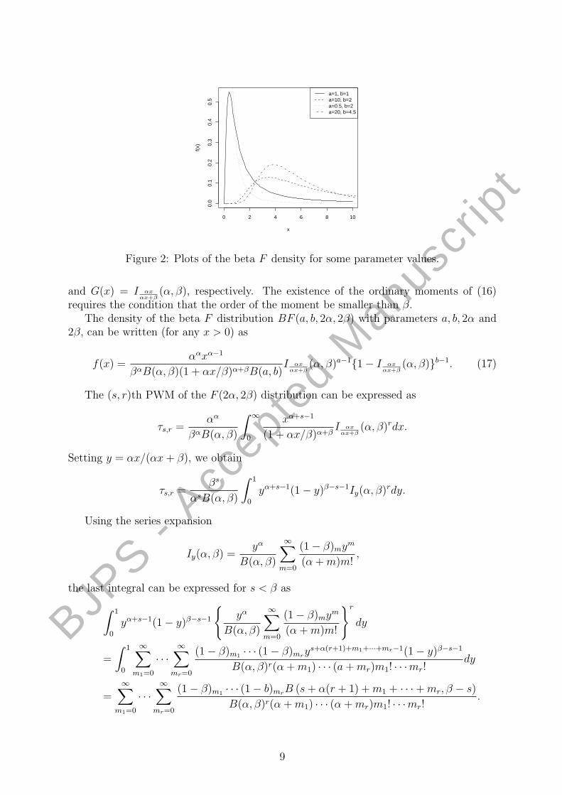
Figure 2: Plots of the beta F density for some parameter values.

and G(x) = I αxαx+β

(α, β), respectively. The existence of the ordinary moments of (16)requires the condition that the order of the moment be smaller than β.

The density of the beta F distribution BF (a, b, 2α, 2β) with parameters a, b, 2α and2β, can be written (for any x > 0) as

f(x) =ααxα−1

βαB(α, β)(1 + αx/β)α+βB(a, b)I αx

αx+β(α, β)a−1{1− I αx

αx+β(α, β)}b−1. (17)

The (s, r)th PWM of the F (2α, 2β) distribution can be expressed as

τs,r =αα

βαB(α, β)

∫ ∞

0

xα+s−1

(1 + αx/β)α+βI αx

αx+β(α, β)rdx.

Setting y = αx/(αx + β), we obtain

τs,r =βs

αsB(α, β)

∫ 1

0

yα+s−1(1− y)β−s−1Iy(α, β)rdy.

Using the series expansion

Iy(α, β) =yα

B(α, β)

∞∑m=0

(1− β)mym

(α + m)m!,

the last integral can be expressed for s < β as

∫ 1

0

yα+s−1(1− y)β−s−1

{yα

B(α, β)

∞∑m=0

(1− β)mym

(α + m)m!

}r

dy

=

∫ 1

0

∞∑m1=0

· · ·∞∑

mr=0

(1− β)m1 · · · (1− β)mrys+α(r+1)+m1+···+mr−1(1− y)β−s−1

B(α, β)r(α + m1) · · · (a + mr)m1! · · ·mr!dy

=∞∑

m1=0

· · ·∞∑

mr=0

(1− β)m1 · · · (1− b)mrB (s + α(r + 1) + m1 + · · ·+ mr, β − s)

B(α, β)r(α + m1) · · · (α + mr)m1! · · ·mr!.

9

BJP

S - A

ccepte

d Manusc

ript

Using (f)k = Γ(f+k)/Γ(f) and the definition of the generalized Kampe de Feriet functionin equation (2), we can write τs,r (for s < b) as

τs,r =βs

αs+rB(α, β)r+1B (β − s, s + α(r + 1))×

F 1:21:1

((s + α(r + 1)) : (1− β, α); . . . ; (1− β, α);

(β + α(r + 1)) : (α + 1); . . . ; (α + 1); 1, . . . , 1). (18)

It is easy to verify that that this expression exists for s < β. Hence, the moments of thebeta F distribution can be written as infinite weighted sums of the generalized Kampede Feriet functions from equations (7) and (18) for a integer and from (8) and (18) for areal non-integer.

9 Numerical Applications

In this section we provide numerical values for the moments of some beta generalizeddistributions. We compute Lauricella function of type A using the formula (Erdelyi,1936, page 696, equation (1))

F(n)A [α, β1, . . . , βn; γ1, . . . , γn; x1, . . . , xn] =

1

Γ (α)

∫ ∞

0

tα−1 exp(−t) 1F1 (β1; γ1; x1t) · · · 1F1 (βn; γn; xnt) dt (19)

and the Generalized Kampe de Feriet function using the equation (2.1.5.15) given inExton (1978)

F 1:21:1 ((a) : (c1, d1); . . . ; (cn, dn); (c) : (a + b); (f1); . . . ; (dn); s1, . . . , sn)

=1

B(a, b)

∫ 1

0

xa−1(1− x)b−12F1 (c1, d1; f1; s1x) · · · 2F1 (cn, dn; fn; snx) dx. (20)

Establishing in-built routines for these special functions can be used to compute themoments. This can be more efficient than computing the moments by writing say somecodes in SAS or R. It can also be more accurate computationally to use these in-builtroutines. Other representations for moments (for example, integral representations) canbe prone to rounding off errors among others. In fact, we compare the numerical momentsobtained using these special functions in Mathematica scripts with those calculated fromsome Maple codes for direct integration of the density functions in 350 selected choicesof parameters for the beta generalized distributions discussed in this section. The scriptswere written and tested on Maple version 10, and Mathematica version 5.0.0.0, to obtainnumerical moments of the beta generalized distributions. For rare selections of parameters(6.86%), Maple fails to calculate numerical values for the moments while Mathematicasucceeds in almost all cases tested (it fails in only 2.29% of cases). Comparing the nu-merical values obtained with Maple and Mathematica we found that, in almost all cases,the results agree using both softwares.

The moments of five beta generalized distributions were computed using our infiniteweighted sums of Lauricella and Generalized Kampe de Feriet functions by evaluatingthese functions from equations (19) and (20), respectively. For selected parameter valuesa = 1.5 and b = 2.5, Table 1 gives some numerical values for the ordinary moments (µ′r, r =

10

BJP

S - A

ccepte

d Manusc

ript

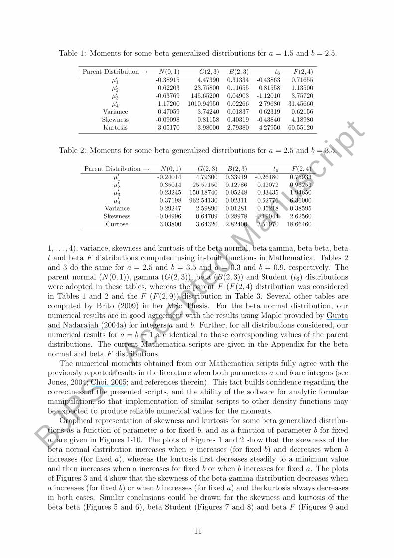
Table 1: Moments for some beta generalized distributions for a = 1.5 and b = 2.5.

Parent Distribution → N(0, 1) G(2, 3) B(2, 3) t6 F (2, 4)µ′1 -0.38915 4.47390 0.31334 -0.43863 0.71655µ′2 0.62203 23.75800 0.11655 0.81558 1.13500µ′3 -0.63769 145.65200 0.04903 -1.12010 3.75720µ′4 1.17200 1010.94950 0.02266 2.79680 31.45660

Variance 0.47059 3.74240 0.01837 0.62319 0.62156Skewness -0.09098 0.81158 0.40319 -0.43840 4.18980Kurtosis 3.05170 3.98000 2.79380 4.27950 60.55120

Table 2: Moments for some beta generalized distributions for a = 2.5 and b = 3.5.

Parent Distribution → N(0, 1) G(2, 3) B(2, 3) t6 F (2, 4)µ′1 -0.24014 4.79300 0.33919 -0.26180 0.75933µ′2 0.35014 25.57150 0.12786 0.42072 0.96253µ′3 -0.23245 150.18740 0.05248 -0.33435 1.94650µ′4 0.37198 962.54130 0.02311 0.62776 6.36000

Variance 0.29247 2.59890 0.01281 0.35218 0.38595Skewness -0.04996 0.64709 0.28978 -0.19044 2.62560Curtose 3.03800 3.64320 2.82400 3.51970 18.66460

1, . . . , 4), variance, skewness and kurtosis of the beta normal, beta gamma, beta beta, betat and beta F distributions computed using in-built functions in Mathematica. Tables 2and 3 do the same for a = 2.5 and b = 3.5 and a = 0.3 and b = 0.9, respectively. Theparent normal (N(0, 1)), gamma (G(2, 3)), beta (B(2, 3)) and Student (t6) distributionswere adopted in these tables, whereas the parent F (F (2, 4) distribution was consideredin Tables 1 and 2 and the F (F (2, 9)) distribution in Table 3. Several other tables arecomputed by Brito (2009) in her MSc Thesis. For the beta normal distribution, ournumerical results are in good agreement with the results using Maple provided by Guptaand Nadarajah (2004a) for integers a and b. Further, for all distributions considered, ournumerical results for a = b = 1 are identical to those corresponding values of the parentdistributions. The current Mathematica scripts are given in the Appendix for the betanormal and beta F distributions.

The numerical moments obtained from our Mathematica scripts fully agree with thepreviously reported results in the literature when both parameters a and b are integers (seeJones, 2004; Choi, 2005; and references therein). This fact builds confidence regarding thecorrectness of the presented scripts, and the ability of the software for analytic formulaemanipulation, so that implementation of similar scripts to other density functions maybe expected to produce reliable numerical values for the moments.

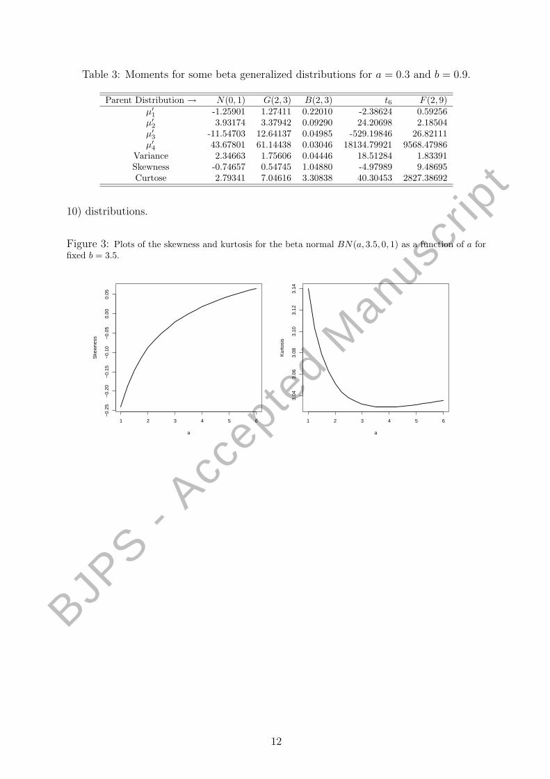
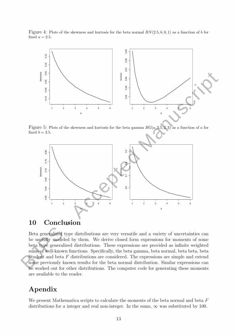
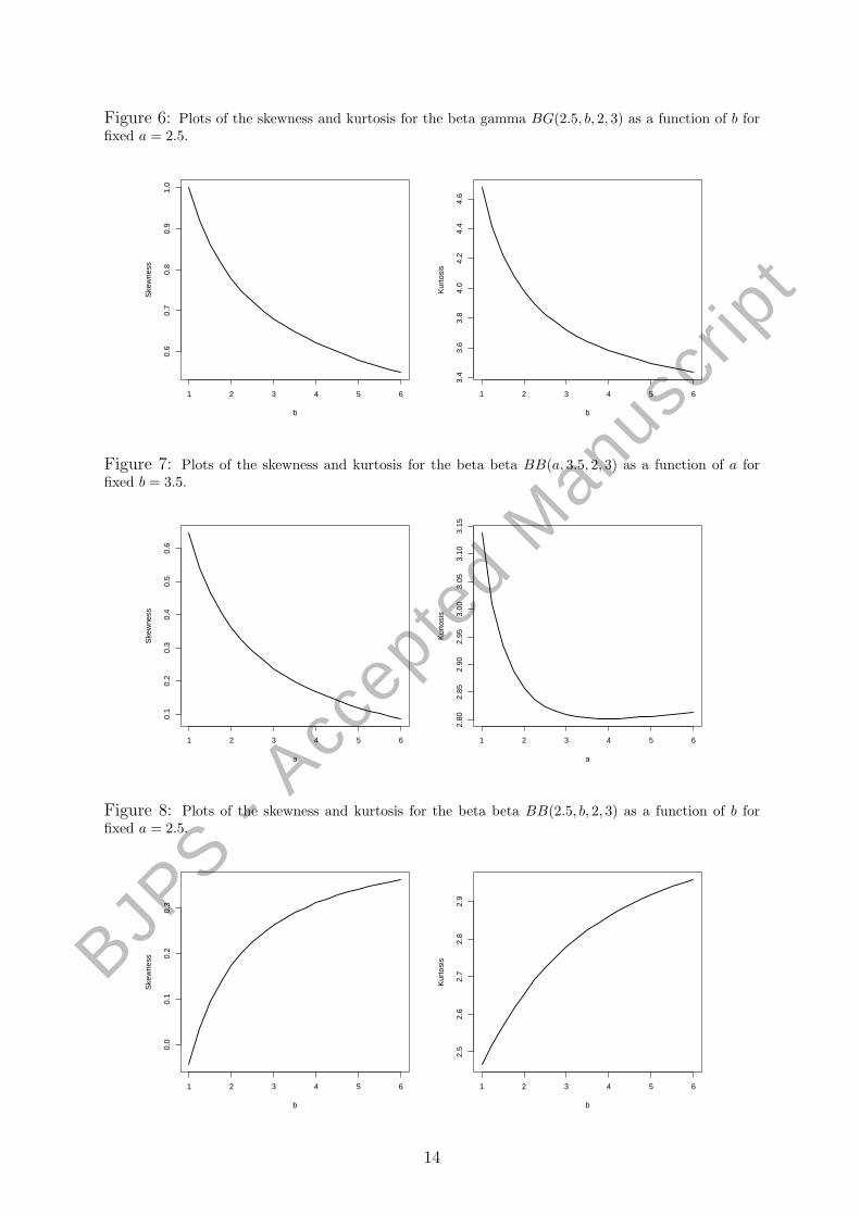
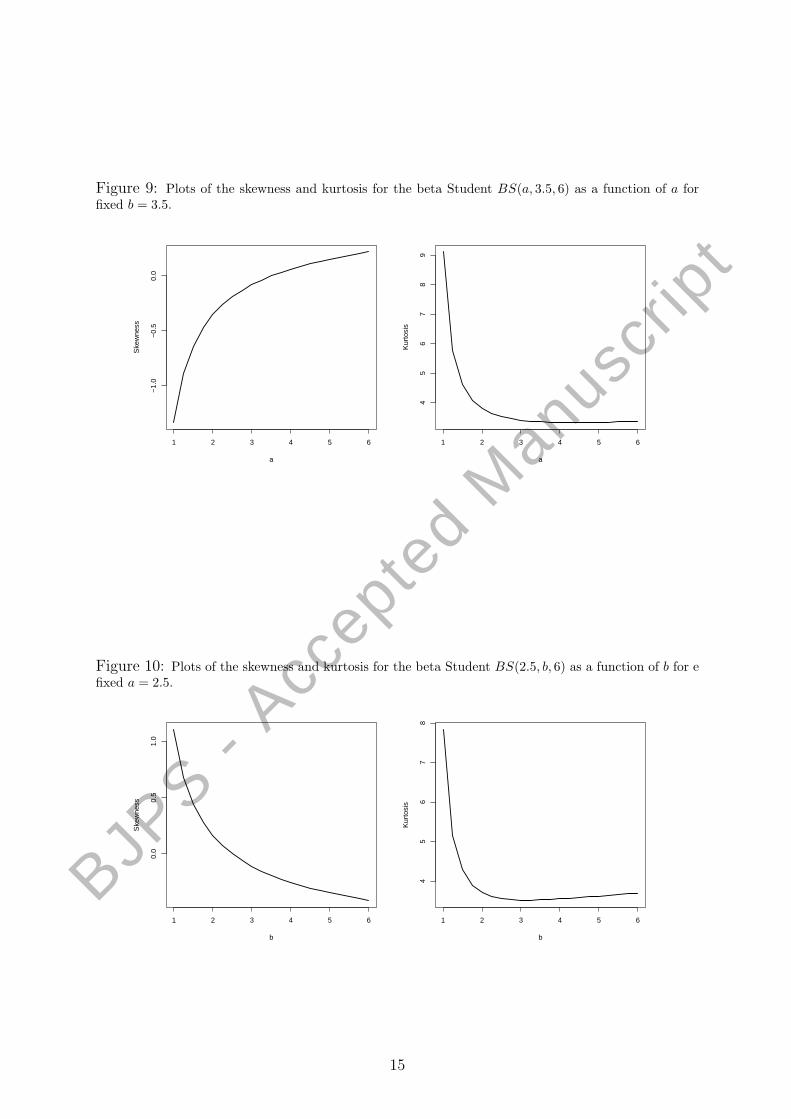
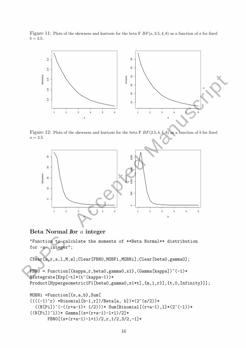
Graphical representation of skewness and kurtosis for some beta generalized distribu-tions as a function of parameter a for fixed b, and as a function of parameter b for fixeda, are given in Figures 1-10. The plots of Figures 1 and 2 show that the skewness of thebeta normal distribution increases when a increases (for fixed b) and decreases when bincreases (for fixed a), whereas the kurtosis first decreases steadily to a minimum valueand then increases when a increases for fixed b or when b increases for fixed a. The plotsof Figures 3 and 4 show that the skewness of the beta gamma distribution decreases whena increases (for fixed b) or when b increases (for fixed a) and the kurtosis always decreasesin both cases. Similar conclusions could be drawn for the skewness and kurtosis of thebeta beta (Figures 5 and 6), beta Student (Figures 7 and 8) and beta F (Figures 9 and

11

BJP

S - A

ccepte

d Manusc

ript

Table 3: Moments for some beta generalized distributions for a = 0.3 and b = 0.9.

Parent Distribution → N(0, 1) G(2, 3) B(2, 3) t6 F (2, 9)µ′1 -1.25901 1.27411 0.22010 -2.38624 0.59256µ′2 3.93174 3.37942 0.09290 24.20698 2.18504µ′3 -11.54703 12.64137 0.04985 -529.19846 26.82111µ′4 43.67801 61.14438 0.03046 18134.79921 9568.47986

Variance 2.34663 1.75606 0.04446 18.51284 1.83391Skewness -0.74657 0.54745 1.04880 -4.97989 9.48695Curtose 2.79341 7.04616 3.30838 40.30453 2827.38692

10) distributions.

Figure 3: Plots of the skewness and kurtosis for the beta normal BN(a, 3.5, 0, 1) as a function of a forfixed b = 3.5.

1 2 3 4 5 6

−0.

25−

0.20

−0.

15−

0.10

−0.

050.

000.

05

a

Ske

wne

ss

1 2 3 4 5 6

3.04

3.06

3.08

3.10

3.12

3.14

a

Kur

tosi

s

12

BJP

S - A

ccepte

d Manusc

ript

Figure 4: Plots of the skewness and kurtosis for the beta normal BN(2.5, b, 0, 1) as a function of b forfixed a = 2.5.

1 2 3 4 5 6

−0.

10−

0.05

0.00

0.05

0.10

0.15

b

Ske

wne

ss

1 2 3 4 5 6

3.04

3.05

3.06

3.07

3.08

3.09

b

Kur

tosi

s

Figure 5: Plots of the skewness and kurtosis for the beta gamma BG(a, 3.5, 2, 3) as a function of a forfixed b = 3.5.

1 2 3 4 5 6

0.55

0.60

0.65

0.70

0.75

0.80

a

Ske

wne

ss

1 2 3 4 5 6

3.6

3.7

3.8

3.9

a

Kur

tosi

s

10 Conclusion

Beta generalized type distributions are very versatile and a variety of uncertainties canbe usefully modeled by them. We derive closed form expressions for moments of somebeta type generalized distributions. These expressions are provided as infinite weightedsums of well-known functions. Specifically, the beta gamma, beta normal, beta beta, betaStudent and beta F distributions are considered. The expressions are simple and extendsome previously known results for the beta normal distribution. Similar expressions canbe worked out for other distributions. The computer code for generating these momentsare available to the reader.

Apendix

We present Mathematica scripts to calculate the moments of the beta normal and beta Fdistributions for a integer and real non-integer. In the sums, ∞ was substituted by 100.

13

BJP

S - A

ccepte

d Manusc

ript

Figure 6: Plots of the skewness and kurtosis for the beta gamma BG(2.5, b, 2, 3) as a function of b forfixed a = 2.5.

1 2 3 4 5 6

0.6

0.7

0.8

0.9

1.0

b

Ske

wne

ss

1 2 3 4 5 6

3.4

3.6

3.8

4.0

4.2

4.4

4.6

b

Kur

tosi

s

Figure 7: Plots of the skewness and kurtosis for the beta beta BB(a, 3.5, 2, 3) as a function of a forfixed b = 3.5.

1 2 3 4 5 6

0.1

0.2

0.3

0.4

0.5

0.6

a

Ske

wne

ss

1 2 3 4 5 6

2.80

2.85

2.90

2.95

3.00

3.05

3.10

3.15

a

Kur

tosi

s

Figure 8: Plots of the skewness and kurtosis for the beta beta BB(2.5, b, 2, 3) as a function of b forfixed a = 2.5.

1 2 3 4 5 6

0.0

0.1

0.2

0.3

b

Ske

wne

ss

1 2 3 4 5 6

2.5

2.6

2.7

2.8

2.9

b

Kur

tosi

s

14

BJP

S - A

ccepte

d Manusc

ript

Figure 9: Plots of the skewness and kurtosis for the beta Student BS(a, 3.5, 6) as a function of a forfixed b = 3.5.

1 2 3 4 5 6

−1.

0−

0.5

0.0

a

Ske

wne

ss

1 2 3 4 5 6

45

67

89

a

Kur

tosi

s

Figure 10: Plots of the skewness and kurtosis for the beta Student BS(2.5, b, 6) as a function of b for efixed a = 2.5.

1 2 3 4 5 6

0.0

0.5

1.0

b

Ske

wne

ss

1 2 3 4 5 6

45

67

8

b

Kur

tosi

s

15

BJP

S - A

ccepte

d Manusc

ript

Figure 11: Plots of the skewness and kurtosis for the beta F BF (a, 3.5, 4, 8) as a function of a for fixedb = 3.5.

1 2 3 4 5 6

2.4

2.6

2.8

3.0

3.2

a

Ske

wne

ss

1 2 3 4 5 6

1618

2022

2426

a

Kur

tosi

s

Figure 12: Plots of the skewness and kurtosis for the beta F BF (2.5, b, 4, 8) as a function of b for fixeda = 2.5.

1 2 3 4 5 6

510

1520

25

b

Ske

wne

ss

1 2 3 4 5 6

050

010

0015

0020

00

b

Kur

tosi

s

Beta Normal for a integer

"Function to calculate the moments of **Beta Normal** distribution

for -a- integer";

Clear[a,r,s,l,M,w];Clear[FBN0,MOBFi,MOBNi];Clear[beta0,gamma0];

FBN0 = Function[{kappa,r,beta0,gamma0,x1},(Gamma[kappa])^(-1)*

NIntegrate[Exp[-t]*(t^(kappa-1))*

Product[Hypergeometric1F1[beta0,gamma0,x1*t],{m,1,r}],{t,0,Infinity}]];

MOBNi =Function[{s,a,b},Sum[

((((-1)^r) *Binomial[b-1,r])/Beta[a, b])*(2^(s/2))*

((N[Pi])^(-((r+a-1)+ 1/2)))* Sum[Binomial[(r+a-1),l]*(2^(-l))*

((N[Pi])^l))* Gamma[(s+(r+a-1)-l+1)/2]*

FBN0[(s+(r+a-1)-l+1)/2,r,1/2,3/2,-1]*

16

BJP

S - A

ccepte

d Manusc

ript

If[IntegerPart[(s+(r+a-1)-l)/2]==(s+(r+a-1)-l)/2,1,0],

{l,0,(r+a-1)}],{r,0,100}]];

Beta Normal for a real non integer

"Function to calculate the moments of ** Beta Normal ** distribution

for -a- non-integer";

Clear[a,r,s,l,M,w,kappa];Clear[FBN0,FBF1,FBN1,MOBFni,MOBNni];

Clear[beta1,gamma1];

FBN1 = Function[{kappa,r,beta1,gamma1,x1},(Gamma[kappa])^(-1)*

NIntegrate[Exp[-t]*t^(kappa-1)*

Product[Hypergeometric1F1[beta1,gamma1,x1*t],{m,1,r}],{t,0,Infinity}]];

MOBNni = Function[{s,a,b},Sum[

Sum[Sum[((((-1)^(i+j+r))*Binomial[a+i-1,j]*Binomial[b-1,i]*

Binomial[j,r])/Beta[a,b])*(2^(s/2))*((N[Pi])^(-(r+1/2)))*

Sum[Binomial[r,l]*(2^(-l))*((N[Pi])^l)* Gamma[(s+r-l+1)/2]*

FBN1[(s+r-l+1)/2,r,1/2,3/2,-1]*

If[IntegerPart[(s+r-l)/2] == (s+r-l)/2,1,0],{l 0,r}],

{r,0,j}],{j,0,100}],{i,0,100}]];

Beta F for a integer

Clear[FBN0,FBF0];Clear[alpha0];Clear[beta0];Clear[s];Clear[a];Clear[b];

"Function to calculate the moments of **Beta F** distribution for

-a- integer";

FBF0 = Function[{z,w,r,alpha0,beta0,x},

((Beta[z,(w-z)])^(-1))*

NIntegrate[(t^(z-1))*((1-t)^(w-z-1))*

Product[Hypergeometric2F1[1-beta0,alpha0,alpha0+1,x*t],{m,1,r}],

{t,0,1}]];

MOBFi = Function[{s,a,b,alpha0,beta0},

If[s<beta0,Sum[(((-1)^r)*Binomial[b-1,r])/Beta[a,b])*

((beta0)^s)*Beta[beta0-s,s+ alpha0*(r + a)]*

N[FBF0[(s+alpha0*(r+a)),(beta0+alpha0*(r+a)),(r+a-1),alpha0,

beta0,1]])/(((alpha0)^(s+(r+a-1)))*(Beta[alpha0,beta0]^(r + a))),

{r,0,100}],"**Verify if s < beta!**"]];

17

BJP

S - A

ccepte

d Manusc

ript

Beta F for a real non-integer

"Function to calculate the moments of **Beta F** distribution for

-a- non-integer";

Clear[FBF1,MOBFi,MOBFni];Clear[alpha1];Clear[beta1];Clear[a];Clear[b];

FBF1 = Function[{z,w,r,alpha1,beta1,x1},(Beta[z,(w-z)]^(-1))*

NIntegrate[(t^(z-1))*((1-t)^(w-z-1))*

Product[Hypergeometric2F1[1-beta1,alpha1,alpha1+1,x1*t],{m,1,r}],

{t,0,1}]];

MOBFni = Function[{s,a,b,alpha1,beta1},

If[s < beta1,

Sum[Sum[Sum[((((-1)^(i+j+r))*Binomial[a+i-1,j]*Binomial[b-1,i]*

Binomial[j,r])/Beta[a,b])*((beta1)^s/(((alpha1)^(s+r))*

(Beta[alpha1,beta1]^(r+1))))*Beta[beta1-s,s+alpha1*(r+1)]*

N[FBF1[(s+alpha1*(r+1)),(beta1+alpha1*(r+1)),r,alpha1,beta1,1]],

{r,0,j}],{j,0,100}],{i,0,100}], "** Verify if s < beta! **"]];

Acknowledgments

Financial support from CNPq and CAPES is gratefully acknowledged. We thank threereferees and the editor for comments which improved the paper. We also thank to Mrs.Rejane Brito, Miss Alice Lemos and Dr. Claudio Cristino for helping with some numericalcomputation.

References

[1] Aarts, R. M., 2000. Lauricella functions. From MathWorld, A Wolfram Web Re-source, created by Eric W. Weisstein.(http://mathwomathworld.wolfram.com/LauricellaFunctions.html).

[2] Barlow, R. E. and Proschan, F., 1975. Statistical Theory of Reliability. Holt, Rinehartand Winston, New York.

[3] Brito, R., 2009. Estudo de expansoes assintoticas, avaliacao numerica de momentosdas distribuicoes beta generalizadas, aplicacoes em modelos de regressao e analise dis-criminante. Dissertacao de Mestrado no Programa de Pos-Graduacao em Biometriae Estatıstica Aplicada da Universidade Federal Rural de Pernambuco, Recife, Brazil.

[4] Chaudhry, M. A. and Zubair, S. M., 2002. On a Class of Incomplete Gamma Func-tions with Applications. Chapman and Hall, Boca Raton, Florida.

[5] Choi, J., 2005. Letter to the Editor. Commun. Statist. - Theory and Methods, 34,997–998.

[6] Erdelyi, A., 1936. Uber einige bestimmte Integrale, in denen die WhittakerschenMk,m–Funktionen auftreten. Mathematische Zeitschrift, 40, 693–702.

18

BJP

S - A

ccepte

d Manusc

ript

[7] Eugene, N., Lee, C. and Famoye, F., 2002. Beta-normal distribution and its applica-

tions. Commun. Statist. - Theory and Methods, 31, 497–512.

[8] Exton, H., 1978. Handbook of Hypergeometric Integrals: Theory, Applications, Tables,Computer Programs. Halsted Press, New York.

[9] Gupta, A. K. and Nadarajah, S., 2004a. On the moments of the beta normal distri-bution. Commun. Statist. - Theory and Methods, 33, 1–13.

[10] Gupta, A. K. and Nadarajah, S., 2004b. The Handbook of the Beta Distributions andIts Applications. Marcel Dekker, New York.

[11] Jones, M. C., 2004a. Families of distributions arising from distributions of orderstatistics. Test, 13, 1–43.

[12] Jones, M. C., 2004b. Letter to the Editor “The moments of beta-normal distributionwith integer parameters are the moments of order statistics from normal distribu-tions”. Communications in Statistics- Theory and Methods, 33, 2869–2870.

[13] Kong, L., Lee, C. and Sepanski, J. H., 2007. On the properties of beta gammadistributions. J. Modern Applied Statistical Methods, 6, 173–187.

[14] Mathai, A. M., 1993. Hypergeometric Functions of Several Matrix Arguments: APreliminary Report. Centre for Mathematical Sciences, Trivandrum.

[15] Nadarajah, S., 2007. Explicit expressions for moments of t order statistics. C. R.Acad. Sci. Paris, Ser. I, 345, 523–526.

[16] Nadarajah, S., 2008. Explicit expressions for moments of order statistics. Statisticsand Probability Letters, 78, 196–205.

[17] Nadarajah, S. and Gupta, A. K., 2004. The beta Frechet distribution. Far EastJournal of Theoretical Statistics, 14, 15–24.

[18] Nadarajah, S. and Kotz, S., 2004. The beta Gumbel distribution. Math. Probab.Eng., 10, 323–332.

[19] Nadarajah, S. and Kotz, S., 2006. The beta exponential distribution. Reliability En-gineering and System Safety, 91, 689–697.

[20] Trott, M., 2006. The Mathematica Guidebook for Symbolics. With 1 DVD–ROM(Windows, Macintosh and UNIX). Springer, New York.

19