arX

iv:2

001.

0184

7v1

[cs

.IT

] 7

Jan

202

0

On Bounds and Closed Form Expressions for

Capacities of Discrete Memoryless Channels with

Invertible Positive Matrices

Thuan Nguyen

School of Electrical and

Computer Engineering

Oregon State University

Corvallis, OR, 97331

Email: nguyeth9@oregonstate.edu

Thinh Nguyen

School of Electrical and

Computer Engineering

Oregon State University

Corvallis, 97331

Email: thinhq@eecs.oregonstate.edu

Abstract—While capacities of discrete memoryless channels arewell studied, it is still not possible to obtain a closed form expres-sion for the capacity of an arbitrary discrete memoryless channel.This paper describes an elementary technique based on Karush-Kuhn-Tucker (KKT) conditions to obtain (1) a good upper boundof a discrete memoryless channel having an invertible positivechannel matrix and (2) a closed form expression for the capacityif the channel matrix satisfies certain conditions related to itssingular value and its Gershgorin’s disk.

Index Terms—Wireless Communication, Convex Optimization,Channel Capacity, Mutual Information.

I. INTRODUCTION

Discrete memoryless channels (DMC) play a critical role

in the early development of information theory and its ap-

plications. DMCs are especially useful for studying many

well-known modulation/demodulation schemes (e.g., PSK and

QAM ) in which the continuous inputs and outputs of a

channel are quantized into discrete symbols. Thus, there exists

a rich literature on the capacities of DMCs [1], [2], [3], [4],

[5], [6], [7]. In particular, capacities of many well-known

channels such as (weakly) symmetric channels can be written

in elementary formulas [1]. However, it is often not possible

to express the capacity of an arbitrary DMC in a closed form

expression [1]. Recently, several papers have been able to

obtain closed form expressions for a small class of DMCs

with small alphabets. For example, Martin et al. established

closed form expression for a general binary channel [8]. Liang

showed that the capacity of channels with two inputs and three

outputs can be expressed as an infinite series [9]. Paul Cotae

et al. found the capacity of two input and two output channels

in term of the eigenvalues of the channel matrices [10]. On the

other hand, the problem of finding the capacity of a discrete

memoryless channel can be formulated as a convex optimiza-

tion problem [11], [12]. Thus, efficient algorithmic solutions

exist. There is also others algorithms such as Arimoto-Blahut

algorithm [2], [3] which can be accelerated in [13], [14], [15].

In [16], [17], another iterative method which can yield both

upper and lower bounds for the channel capacity.

That said, it is still beneficial to find the channel capacity

in closed form expression for a number of reasons. These

include (1) formulas can often provide a good intuition about

the relationship between the capacity and different channel

parameters, (2) formulas offer a faster way to determine the

capacity than that of algorithms, and (3) formulas are useful

for analytical derivations where closed form expression of the

capacity is needed in the intermediate steps. To that end, our

paper describes an elementary technique based on the theory

of convex optimization, to find closed form expressions for

(1) a new upper bound on capacities of discrete memoryless

channels with positive invertible channel matrix and (2) the

optimality conditions of the channel matrix such that the upper

bound is precisely the capacity. In particular, the optimality

conditions establish a relationship between the singular value

and the Gershgorin’s disk of the channel matrix.

II. PRELIMINARIES

A. Convex Optimization and KKT Conditions

A DMC is characterized by a random variable X ∈{x1, x2, . . . , xm} for the inputs, a random variable Y ∈{y1, y2, . . . , yn} for the outputs, and a channel matrix A ∈R

m×n. In this paper, we consider DMCs with equal number

of inputs and outputs n, thus A ∈ Rn×n. The matrix entry

Aij represents the conditional probability that given xi is

transmitted, yj is received. Let p = (p1, p2, . . . , pn)T be the

input probability mass vector (pmf) of X , where pi denotes

the probability of xi to be transmitted, then the pmf of Yis q = (q1, q2, . . . , qn)

T = AT p. The mutual information

between X and Y is:

I(X ;Y ) = H(Y )−H(Y |X), (1)

where

H(Y ) = −

n∑

j=1

qj log qj (2)

H(Y |X) = −

n∑

i=1

n∑

j=1

piAij logAij . (3)

The mutual information function can be written as:

I(X ;Y ) = −

n∑

j=1

(AT p)j log (AT p)j +

n∑

i=1

n∑

j=1

piAij logAij ,

(4)

where (AT p)j denotes the jth component of the vector q =(AT p). The capacity C associated with a channel matrix Ais the theoretical maximum rate at which information can be

transmitted over the channel without the error [5], [18], [19].

It is obtained using the optimal pmf p∗ such that I(X ;Y )is maximized. For a given channel matrix A, I(X ;Y ) is a

concave function of p [1]. Therefore, maximizing I(X ;Y ) is

equivalent to minimizing −I(X ;Y ), and finding the capacity

can be cast as the following convex problem:

Minimize:n∑

j=1

(AT p)j log (AT p)j −

n∑

i=1

n∑

j=1

piAij logAij .

Subject to:{

p � 0

1T p = 1.

The optimal p∗ can be found efficiently using various

algorithms such as gradient methods [20], but in a few cases,

p∗ can be found directly using the Karush-Kuhn-Tucker (KKT)

conditions [20]. To explain the KKT conditions, we first state

the canonical convex optimization problem below:

Problem P1: Minimize: f(x)Subject to:

{

gi(x) ≤ 0, i = 1, 2, . . . n,

hj(x) = 0, j = 1, 2, . . . ,m,

where f(x), gi(x) are convex functions and hj(x) is a linear

function.

Define the Lagrangian function as:

L(x, λ, ν) = f(x) +

n∑

i=1

λigi(x) +

m∑

j=1

νjhj(x), (5)

then the KKT conditions [20] states that, the optimal point

x∗ must satisfy:

gi(x∗) ≤ 0,

hj(x∗) = 0,

dL(x,λ,ν)dx |x=x∗,λ=λ∗,ν=ν∗ = 0,

λ∗i gi(x

∗) = 0,

λ∗i ≥ 0.

(6)

for i = 1, 2, . . . , n, j = 1, 2, . . . ,m.

B. Elementary Linear Algebra Results

Definition 1. Let A ∈ Rn×n be an invertible channel matrix

and H(Ai) = −∑n

k=1 Aik logAik be the entropy of ith row,

define

Kj = −

n∑

i=1

A−1ji

n∑

k=1

Aik logAik =

n∑

i=1

A−1ji H(Ai),

where A−1ji denotes the entry (j, i) of the inverse matrix A−1.

Kmax = maxj Kj and Kmin = minj Kj are called the max-

imum and minimum inverse row entropies of A, respectively.

Definition 2. Let A ∈ Rn×n be a square matrix. The

Gershgorin radius of ith row of A [21] is defined as:

Ri(A) =

n∑

j 6=i

|Aij |. (7)

The Gershgorin ratio of ith row of A is defined as:

ci(A) =Aii

Ri(A), (8)

and the minimum Gershgorin ratio of A is defined as:

cmin(A) = mini

Aii

Ri(A). (9)

We note that since the channel matrix is a stochastic matrix,

therefore

cmin(A) = mini

Aii

Ri(A)= min

i

Aii

1−Aii. (10)

Definition 3. Let A ∈ Rn×n be a square matrix.

(a) A is called a positive matrix if Aij > 0 for ∀ i, j.

(b) A is called a strictly diagonally dominant positive matrix

[22] if A is a positive matrix and

Aii >∑

j 6=i

Aij , ∀i, j. (11)

Lemma 1. Let A ∈ Rn×n be a strictly diagonally dominant

positive channel matrix then (a) it is invertible; (b) the

eigenvalues of A−1 are 1λi

∀ i where λi are eigenvalues of

A, (c) A−1ii > 0 and the largest absolute element in the ith

column of A−1 is A−1ii , i.e., A−1

ii ≥ |A−1ji | for ∀ j.

Proof. The proof is shown in Appendix A.

Lemma 2. Let A ∈ Rn×n be a strictly diagonally dominant

positive matrix, then:

ci(A−T ) ≥

cmin(A) − 1

(n− 1), ∀i. (12)

Moreover, for any rows k and l,

|A−1ki |+ |A−1

li | ≤ A−1ii

cmin(A)

cmin(A)− 1, ∀i. (13)

Proof. The proof is shown in Appendix B.

Lemma 3. Let A ∈ Rn×n be a strictly diagonally dominant

positive matrix, then:

maxi,j

A−1ij ≤

1

σmin(A), (14)

where maxi,j A−1ij is the largest entry in A−1 and σmin(A) is

the minimum singular value of A.

Proof. The proof is shown in Appendix C.

Lemma 4. Let A ∈ Rn×n be an invertible channel matrix,

then

A−11 = 1,

i.e., the sum of any row of A−1 equals to 1. Furthermore, for

any probability mass vector x, sum of the vector y = A−Txequal to 1.

Proof. The proof is shown in Appendix D.

III. MAIN RESULTS

Our first main result is an upper bound on the capacity

of discrete memoryless channels having invertible positive

channel matrices.

Proposition 1 (Main Result 1). Let A ∈ Rn×n be an

invertible positive channel matrix and

q∗j =2−Kj

∑ni=1 2

−Ki, (15)

p∗ = A−T q∗, (16)

then the capacity C associated with the channel matrix A is

upper bounded by:

C ≤ −

n∑

j=1

q∗j log q∗j +

n∑

i=1

n∑

j=1

p∗iAij logAij . (17)

Proof. Let q be the pmf of the output Y , then q = A−T p.

Thus,

I(X ;Y ) = H(Y )−H(Y |X) (18)

= −

n∑

j=1

qj log qj +

n∑

i

(A−T q)i

n∑

k

Aik logAik.

We construct the Lagrangian in (5) using −I(X ;Y ) as the

objective function and optimization variable qj :

L(qj, λj , νj) = −I(X ;Y )−n∑

j=1

qjλj + ν(n∑

j=1

qj − 1), (19)

where the constraints g(x) and h(x) in problem P1 are

translated into −qj ≤ 0 and∑n

j=1 qj = 1, respectively.

Using the KKT conditions in (6), the optimal points q∗j , λ∗j ,

ν∗ for all j, must satisfy:

q∗j ≥ 0, (20)n∑

j=1

q∗j = 1, (21)

ν∗ − λ∗j −

dI(X ;Y )

dq∗j= 0, (22)

λ∗j ≥ 0, (23)

λ∗j q

∗j = 0. (24)

Since 0 ≤ pi ≤ 1 and∑n

i=1 pi = 1, there exists at least

one pi > 0 . Since Aij > 0 ∀i, j, we have:

q∗j =

n∑

i=1

p∗iAij > 0, ∀j. (25)

Based on (24) and (25), we must have λ∗j = 0, ∀j. Therefore,

all five KKT conditions (20-24) are reduced to the following

two conditions:n∑

j=1

q∗j = 1, (26)

ν∗ −dI(X ;Y )

dq∗j= 0. (27)

Next,

dI(X ;Y )

dqj=

n∑

i=1

A−1ji

n∑

k=1

Aik logAik − (1 + log qj)

= −Kj − (1 + log qj). (28)

Using (27) and (28), we have:

q∗j = 2−Kj−ν∗−1. (29)

Plugging (29) to (26), we have:

n∑

j=1

2−Kj−ν∗−1 = 1,

ν∗ = log

n∑

j=1

2−Kj−1.

From (29),

q∗j = 2−Kj−ν∗−1 =2−Kj

2ν∗+1=

2−Kj

∑nj=1 2

−Kj, ∀j. (30)

If q∗ is such that p∗ = A−T q∗ � 0 and (A−T q∗)T1 =∑n

i p∗i = 1, then p∗ is a valid p.m.f and Proposition 1

will hold with equality by the KKT conditions. However

these two constraints might not hold in general. On the other

hand, maximizing I(X ;Y ) in terms of q and ignoring these

constraints is equivalent to enlarging the feasible region, will

necessarily yield a value that is at least equal to the capacity

C. Thus, by plugging q∗ into (18), we obtain the proof for the

upper bound.

Next, we present some sufficient conditions on the channel

matrix A such that its capacity can be written in closed

form expression. We note that the channel capacity closed

form expression is also discovered in [4] and [6] using the

input distribution variables. However in both [4] and [6], the

sufficient conditions for closed form expression are not fully

characterized.

Proposition 2 (Main Result 2). Let A ∈ Rn×n be a strictly

diagonally dominant positive matrix, if ∀i,

ci(A−T ) ≥ (n− 1)2Kmax−Kmin , (31)

then the capacity of channel matrix A admits a closed form

expression which is exactly the upper bound in Proposition 1.

Proof. Based on the discussion of the KKT conditions, it is

sufficient to show that if p∗ = A−T q∗ � 0 and∑n

i p∗i =

(A−T q∗)T1 = 1 then C has a closed form expression. The

condition (A−T q∗)T1 = 1 is always true as shown in Lemma

4 in the Appendix D. Thus, we only need to show that if

ci(A−T ) ≥ 2Kmax−Kmin , then p∗ = A−T q∗ � 0.

Let q∗min = minj q∗j and q∗max = maxj q

∗j , we have:

p∗i =∑

j

q∗jA−1ji

= q∗i A−1ii +

∑

j 6=i

q∗jA−1ji

≥ q∗minA−1ii − (

∑

j 6=i

q∗j )(∑

j 6=i

|A−1ji |) (32)

≥ q∗minA−1ii − (n− 1)q∗max(

∑

j 6=i

|A−1ji |), (33)

with (32) due to A−1ii > 0 which follows by Lemma 1-c, (33)

is due to q∗max ≥ q∗j ∀ j. Now if we want p∗i ≥ 0, ∀ i, from

(33), it is sufficient to require that, ∀i,

ci(A−T ) =

A−1ii

∑

j 6=i |A−1ji |

≥(n− 1)q∗max

q∗min

= (n− 1)

2−Kmin

∑nj=1 2

−Kj

2−Kmax

∑nj=1 2

−Kj

(34)

= (n− 1)2Kmax−Kmin ,

with (34) due to (30) and q∗max, q∗min are corresponding to

Kmin, Kmax, respectively. Thus, Proposition 2 is proven.

We are now ready to state and prove the third main result

that characterizes the sufficient conditions on a channel matrix

so that the upper bound in Proposition 1 is precisely the

capacity.

Proposition 3 (Main Result 3). Let A ∈ Rn×n be a strictly

diagonally dominant positive channel matrix and Hmax(A) be

the maximum row entropy of A. The capacity C is the upper

bound in Proposition 1 i.e., hold with equality if

V

√

cmin(A)− 1

(n− 1)2≥ 2

nHmax(A)σmin(A) , (35)

where σmin(A) is the minimum singular value of channel

matrix A, and

V =cmin(A)

cmin(A) − 1. (36)

Proof. From (12) in Lemma 2 and Proposition 2, if we can

show that

cmin(A)− 1

(n− 1)≥ (n− 1)2Kmax−Kmin , (37)

then Proposition 3 is proven. Suppose that Kmax and Kmin areobtained at rows j = L and j = S, respectively. We note thatfrom (30), qmax = maxj qj and qmin = minj qj correspond

to Kmin and Kmax, respectively. Thus, from the Definition 1,we have:

Kmax−Kmin =

n∑

i=1

A−1Li H(Ai)−

n∑

i=1

A−1Si H(Ai)

≤ |

n∑

i=1

A−1Li H(Ai)|+ |

n∑

i=1

A−1Si H(Ai)| (38)

≤ |n∑

i=1

A−1Li ||H(Ai)|+ |

n∑

i=1

A−1Si ||H(Ai)|(39)

≤ Hmax(A)n∑

i=1

(|A−1Li |+ |A−1

Si |) (40)

≤ Hmax(A)n∑

i=1

A−1ii

cmin(A)

cmin(A)− 1(41)

≤ nHmax(A)(maxi,j

A−1ij )

cmin(A)

cmin(A)− 1(42)

≤nHmax(A)V

σmin(A), (43)

where (38) due to the property of absolute value function,

(39) due to Schwarz inequality, (40) due to Hmax(A) is the

maximum row entropy of A, (41) due to (13), (42) due to

maxi,j A−1ij is the largest entry in A−1 and (43) is due to

Lemma 3. Thus,

(n− 1)2nHmax(A)V

σmin(A) ≥ (n− 1)2Kmax−Kmin. (44)

From (37) and (44), if

cmin(A)− 1

(n− 1)≥ (n− 1)2

nHmax(A)Vσmin(A) , (45)

then the capacity C is the upper bound in Proposition 1. (45)

is equivalent to (35). Thus Proposition 3 is proven.

An easy to use version of Proposition 3 is stated in Corollary

1.

Corollary 1. The capacity C is the upper bound in Proposi-

tion 1 ifcmin(A)− 1

(n− 1)2≥ 2

2n log nσmin(A) . (46)

Proof. Similar to Proposition 3,

Kmax−Kmin =n∑

i=1

A−1Li H(Ai)−

n∑

i=1

A−1Si H(Ai)

≤ |n∑

i=1

A−1Li H(Ai)|+ |

n∑

i=1

A−1Si H(Ai)| (47)

≤ |n∑

i=1

A−1Li ||H(Ai)|+ |

n∑

i=1

A−1Si ||H(Ai)|(48)

≤ Hmax(A)n∑

i=1

(|A−1Li |+ |A−1

Si |) (49)

≤ Hmax(A)n(2maxi,j

A−1ij ) (50)

≤2n log n

σmin(A), (51)

with (47), (48), (49) are similar to (38), (39), (40), re-

spectively. (50) is due to maxi,j A−1ij is the largest entry in

A−1, (51) due to Hmax(A) ≤ logn and Lemma 3. Thus, by

changingnHmax(A)V

σmin(A) in (45) by2n lognσmin(A) , the Corollary 1 is

proven.

A direct result of Proposition 3 without using singular value

is shown in Corollary 2.

Corollary 2. The capacity C is the upper bound in Proposi-

tion 1 if

V

√

cmin(A)− 1

(n− 1)2≥ 2

nH∗max(A)

σ∗ , (52)

where,

V =cmin(A)

cmin(A) − 1, (53)

σ∗ =cmin(A)− n/2

cmin(A) + 1, (54)

H∗max(A) = log(cmin(A)+1)+

log(n− 1)− cmin(A) log cmin(A)

cmin(A) + 1.

(55)

Proof. We will construct the lower bound for σmin(A) and the

upper bound for Hmax(A). From Lemma 5 in Appendix E

σmin(A) ≥cmin(A)− n/2

cmin(A) + 1= σ∗, (56)

and

Hmax(A) ≤ log(cmin(A)+1)+log(n− 1)−cmin(A) log cmin(A)

cmin(A) + 1

= H∗max(A). (57)

Therefore

nHmax(A)V

σmin(A)≤

nH∗max(A)

σ∗. (58)

Thus, by changingnHmax(A)σmin(A) in (35) by

nH∗

max(A)σ∗

, the

Corollary 2 is proven.

We note that, when cmin(A) is relatively larger than the

size of matrix n, the lower bound of σmin(A) goes to 1. We

also note that (52) can be checked efficiency without requiring

both Hmax(A) and σmin(A) at the expense of a looser upper

bound as compare to (35).

IV. EXAMPLES AND NUMERICAL RESULTS

A. Example 1: Reliable Channels

We illustrate the optimality conditions in Proposition 3using a reliable channel having the channel matrix:

A =

0.95 0.01 0.040.03 0.95 0.020.02 0.02 0.96

.

Here, n = 3, σmin(A) = 0.92424, σ∗ = 0.875 andHmax(A) = 0.33494, H∗

max(A) = 0.3364. From Definition2, cmin(A) = 19. The closed form channel capacity can bereadily computed by Proposition 1 since the channel matrix

satisfies both conditions in Proposition 3 and Corollary 2. Theoptimal input and output probability mass vectors are:

qT =

[

0.33087 0.32806 0.34107]

,

pT =

[

0.33067 0.33480 0.33453]

,

respectively and the capacity is 1.2715.

In general, for a good channel with n inputs and n outputs

whose symbol error probabilities are small, then it is likely

that the channel matrix will satisfy the optimality conditions

in Proposition 1. This is because the diagonal entries Aii

(probability of receiving correct the ith symbol) tend to be

larger than the sum of other entries in its row (probability of

errors), satisfying the property of diagonally dominant matrix.

B. Example 2: Cooperative Relay-MISO Channels

In this example, we investigate the channel capacity for a

class of channels named Relay-MISO (Relay - Multiple Input

Single Output). Relay-MISO channel [23] can be constructed

by the combination of a relay channel [24] [25] and a Multiple

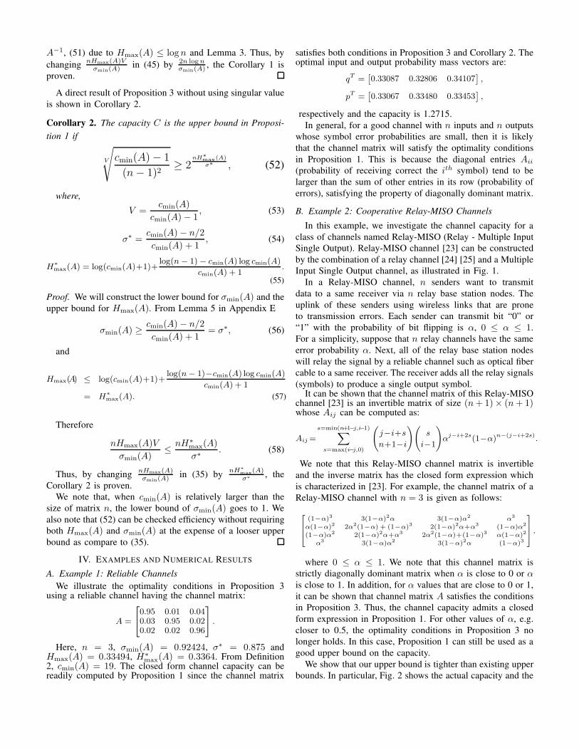
Input Single Output channel, as illustrated in Fig. 1.

In a Relay-MISO channel, n senders want to transmit

data to a same receiver via n relay base station nodes. The

uplink of these senders using wireless links that are prone

to transmission errors. Each sender can transmit bit “0” or

“1” with the probability of bit flipping is α, 0 ≤ α ≤ 1.

For a simplicity, suppose that n relay channels have the same

error probability α. Next, all of the relay base station nodes

will relay the signal by a reliable channel such as optical fiber

cable to a same receiver. The receiver adds all the relay signals

(symbols) to produce a single output symbol.It can be shown that the channel matrix of this Relay-MISO

channel [23] is an invertible matrix of size (n+ 1)× (n+ 1)whose Aij can be computed as:

Aij=

s=min(n+1−j,i−1)∑

s=max(i−j,0)

(

j−i+s

n+1−i

)(

s

i−1

)

αj−i+2s(1−α)n−(j−i+2s)

.

We note that this Relay-MISO channel matrix is invertible

and the inverse matrix has the closed form expression which

is characterized in [23]. For example, the channel matrix of a

Relay-MISO channel with n = 3 is given as follows:

(1−α)3 3(1−α)2α 3(1−α)α2 α3

α(1−α)2 2α2(1−α) + (1−α)3 2(1−α)2α+α3 (1−α)α2

(1−α)α2 2(1−α)2α+α3 2α2(1−α)+(1−α)3 α(1−α)2

α3 3(1−α)α2 3(1−α)2α (1−α)3

,

where 0 ≤ α ≤ 1. We note that this channel matrix is

strictly diagonally dominant matrix when α is close to 0 or αis close to 1. In addition, for α values that are close to 0 or 1,

it can be shown that channel matrix A satisfies the conditions

in Proposition 3. Thus, the channel capacity admits a closed

form expression in Proposition 1. For other values of α, e.g.

closer to 0.5, the optimality conditions in Proposition 3 no

longer holds. In this case, Proposition 1 can still be used as a

good upper bound on the capacity.

We show that our upper bound is tighter than existing upper

bounds. In particular, Fig. 2 shows the actual capacity and the

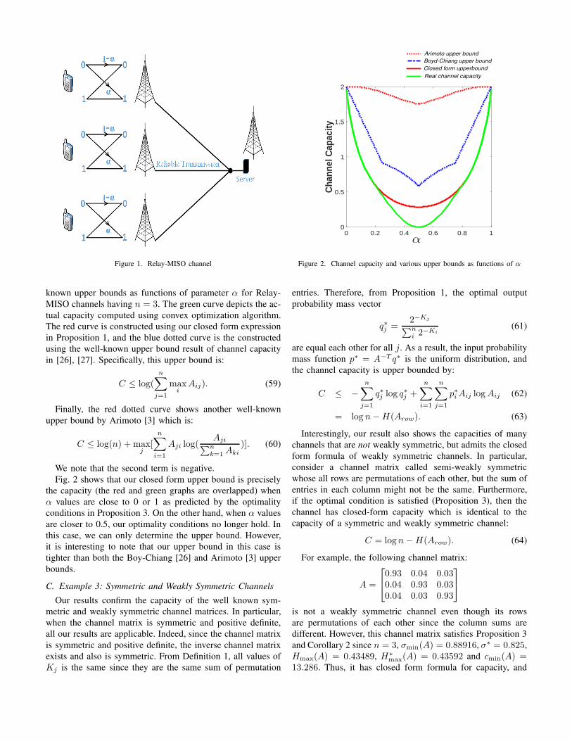
Figure 1. Relay-MISO channel

known upper bounds as functions of parameter α for Relay-

MISO channels having n = 3. The green curve depicts the ac-

tual capacity computed using convex optimization algorithm.

The red curve is constructed using our closed form expression

in Proposition 1, and the blue dotted curve is the constructed

using the well-known upper bound result of channel capacity

in [26], [27]. Specifically, this upper bound is:

C ≤ log(

n∑

j=1

maxi

Aij). (59)

Finally, the red dotted curve shows another well-known

upper bound by Arimoto [3] which is:

C ≤ log(n) + maxj

[

n∑

i=1

Aji log(Aji

∑nk=1 Aki

)]. (60)

We note that the second term is negative.

Fig. 2 shows that our closed form upper bound is precisely

the capacity (the red and green graphs are overlapped) when

α values are close to 0 or 1 as predicted by the optimality

conditions in Proposition 3. On the other hand, when α values

are closer to 0.5, our optimality conditions no longer hold. In

this case, we can only determine the upper bound. However,

it is interesting to note that our upper bound in this case is

tighter than both the Boy-Chiang [26] and Arimoto [3] upper

bounds.

C. Example 3: Symmetric and Weakly Symmetric Channels

Our results confirm the capacity of the well known sym-

metric and weakly symmetric channel matrices. In particular,

when the channel matrix is symmetric and positive definite,

all our results are applicable. Indeed, since the channel matrix

is symmetric and positive definite, the inverse channel matrix

exists and also is symmetric. From Definition 1, all values of

Kj is the same since they are the same sum of permutation

α0 0.2 0.4 0.6 0.8 1

Cha

nnel

Cap

acity

0

0.5

1

1.5

2

Boyd-Chiang upper bound

Arimoto upper bound

Closed form upperbound

Real channel capacity

Figure 2. Channel capacity and various upper bounds as functions of α

entries. Therefore, from Proposition 1, the optimal output

probability mass vector

q∗j =2−Kj

∑ni 2

−Ki(61)

are equal each other for all j. As a result, the input probability

mass function p∗ = A−T q∗ is the uniform distribution, and

the channel capacity is upper bounded by:

C ≤ −

n∑

j=1

q∗j log q∗j +

n∑

i=1

n∑

j=1

p∗iAij logAij (62)

= log n−H(Arow). (63)

Interestingly, our result also shows the capacities of many

channels that are not weakly symmetric, but admits the closed

form formula of weakly symmetric channels. In particular,

consider a channel matrix called semi-weakly symmetric

whose all rows are permutations of each other, but the sum of

entries in each column might not be the same. Furthermore,

if the optimal condition is satisfied (Proposition 3), then the

channel has closed-form capacity which is identical to the

capacity of a symmetric and weakly symmetric channel:

C = logn−H(Arow). (64)

For example, the following channel matrix:

A =

0.93 0.04 0.030.04 0.93 0.030.04 0.03 0.93

is not a weakly symmetric channel even though its rows

are permutations of each other since the column sums are

different. However, this channel matrix satisfies Proposition 3

and Corollary 2 since n = 3, σmin(A) = 0.88916, σ∗ = 0.825,

Hmax(A) = 0.43489, H∗max(A) = 0.43592 and cmin(A) =

13.286. Thus, it has closed form formula for capacity, and

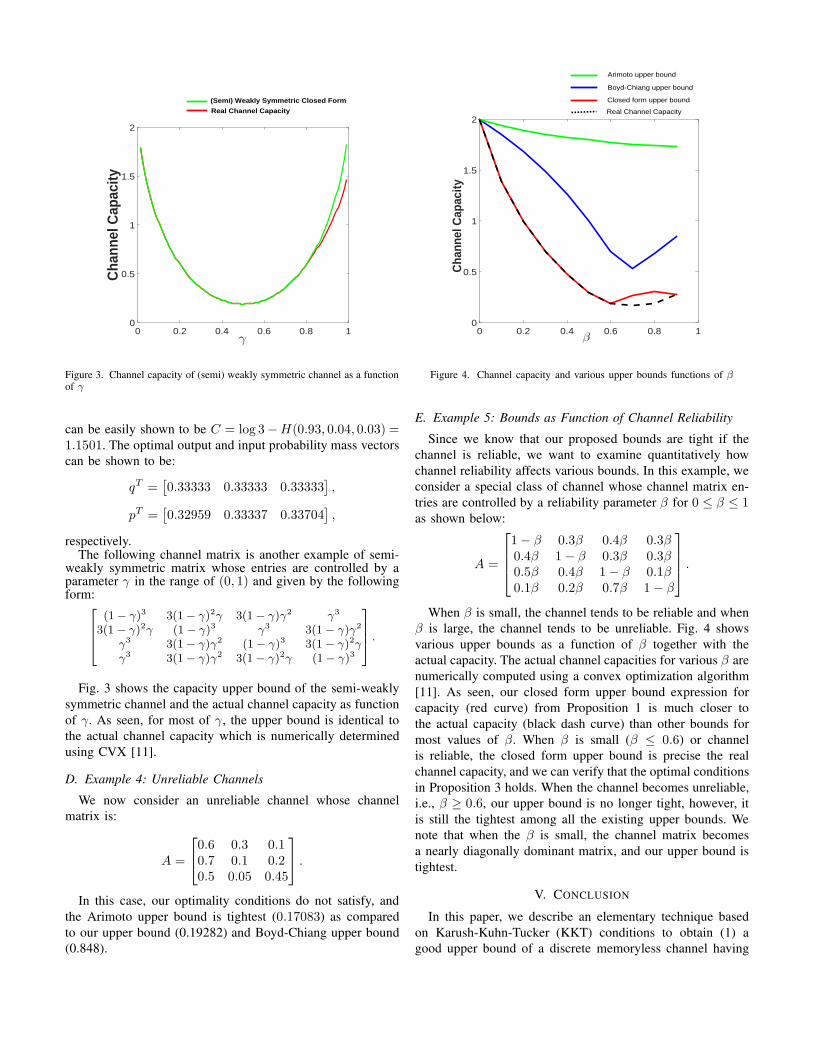
γ0 0.2 0.4 0.6 0.8 1

Cha

nnel

Cap

acity

0

0.5

1

1.5

2

(Semi) Weakly Symmetric Closed Form

Real Channel Capacity

Figure 3. Channel capacity of (semi) weakly symmetric channel as a functionof γ

can be easily shown to be C = log 3−H(0.93, 0.04, 0.03) =1.1501. The optimal output and input probability mass vectors

can be shown to be:

qT =[

0.33333 0.33333 0.33333]

,

pT =[

0.32959 0.33337 0.33704]

,

respectively.The following channel matrix is another example of semi-

weakly symmetric matrix whose entries are controlled by aparameter γ in the range of (0, 1) and given by the followingform:

(1− γ)3 3(1− γ)2γ 3(1− γ)γ2 γ3

3(1− γ)2γ (1− γ)3 γ3 3(1− γ)γ2

γ3 3(1− γ)γ2 (1− γ)3 3(1− γ)2γγ3 3(1− γ)γ2 3(1− γ)2γ (1− γ)3

.

Fig. 3 shows the capacity upper bound of the semi-weakly

symmetric channel and the actual channel capacity as function

of γ. As seen, for most of γ, the upper bound is identical to

the actual channel capacity which is numerically determined

using CVX [11].

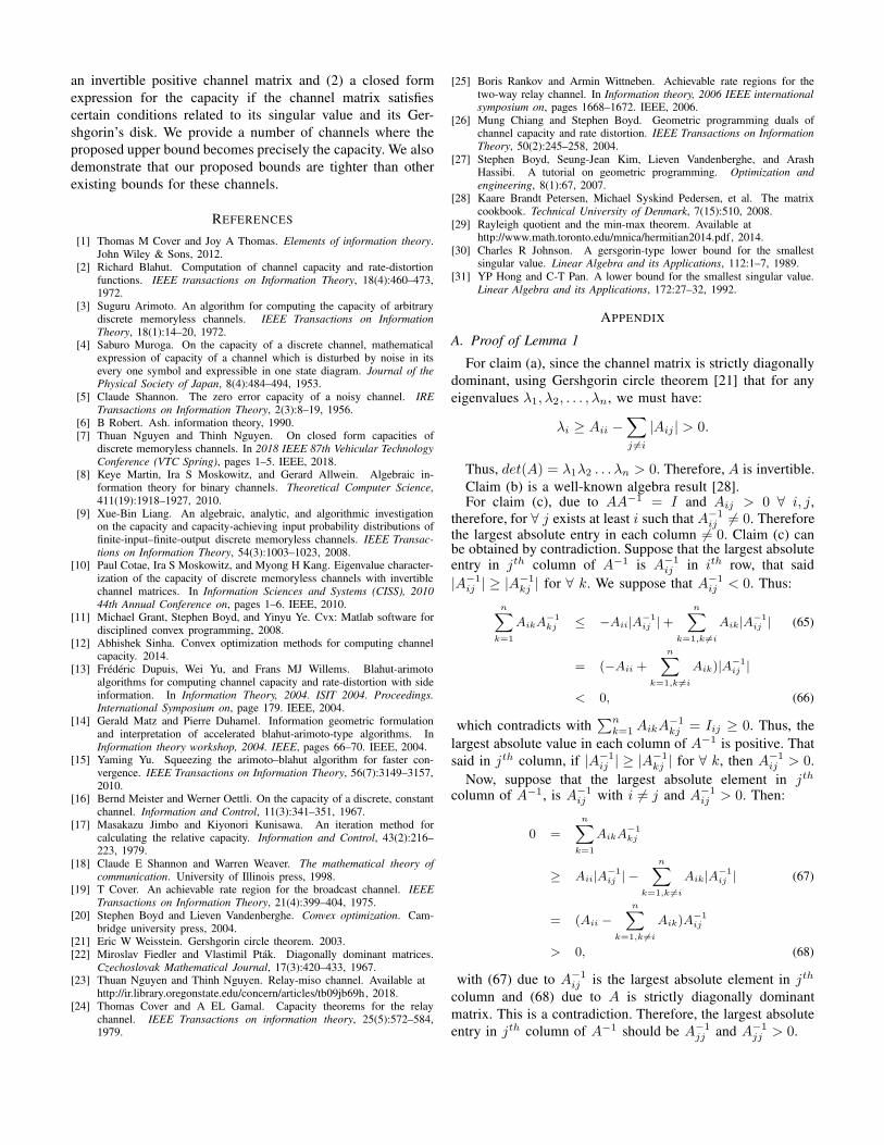
D. Example 4: Unreliable Channels

We now consider an unreliable channel whose channel

matrix is:

A =

0.6 0.3 0.10.7 0.1 0.20.5 0.05 0.45

.

In this case, our optimality conditions do not satisfy, and

the Arimoto upper bound is tightest (0.17083) as compared

to our upper bound (0.19282) and Boyd-Chiang upper bound

(0.848).

β0 0.2 0.4 0.6 0.8 1

Cha

nnel

Cap

acity

0

0.5

1

1.5

2

Arimoto upper bound

Boyd-Chiang upper bound

Closed form upper bound

Real Channel Capacity

Figure 4. Channel capacity and various upper bounds functions of β

E. Example 5: Bounds as Function of Channel Reliability

Since we know that our proposed bounds are tight if the

channel is reliable, we want to examine quantitatively how

channel reliability affects various bounds. In this example, we

consider a special class of channel whose channel matrix en-

tries are controlled by a reliability parameter β for 0 ≤ β ≤ 1as shown below:

A =

1− β 0.3β 0.4β 0.3β0.4β 1− β 0.3β 0.3β0.5β 0.4β 1− β 0.1β0.1β 0.2β 0.7β 1− β

.

When β is small, the channel tends to be reliable and when

β is large, the channel tends to be unreliable. Fig. 4 shows

various upper bounds as a function of β together with the

actual capacity. The actual channel capacities for various β are

numerically computed using a convex optimization algorithm

[11]. As seen, our closed form upper bound expression for

capacity (red curve) from Proposition 1 is much closer to

the actual capacity (black dash curve) than other bounds for

most values of β. When β is small (β ≤ 0.6) or channel

is reliable, the closed form upper bound is precise the real

channel capacity, and we can verify that the optimal conditions

in Proposition 3 holds. When the channel becomes unreliable,

i.e., β ≥ 0.6, our upper bound is no longer tight, however, it

is still the tightest among all the existing upper bounds. We

note that when the β is small, the channel matrix becomes

a nearly diagonally dominant matrix, and our upper bound is

tightest.

V. CONCLUSION

In this paper, we describe an elementary technique based

on Karush-Kuhn-Tucker (KKT) conditions to obtain (1) a

good upper bound of a discrete memoryless channel having

an invertible positive channel matrix and (2) a closed form

expression for the capacity if the channel matrix satisfies

certain conditions related to its singular value and its Ger-

shgorin’s disk. We provide a number of channels where the

proposed upper bound becomes precisely the capacity. We also

demonstrate that our proposed bounds are tighter than other

existing bounds for these channels.

REFERENCES

[1] Thomas M Cover and Joy A Thomas. Elements of information theory.John Wiley & Sons, 2012.

[2] Richard Blahut. Computation of channel capacity and rate-distortionfunctions. IEEE transactions on Information Theory, 18(4):460–473,1972.

[3] Suguru Arimoto. An algorithm for computing the capacity of arbitrarydiscrete memoryless channels. IEEE Transactions on Information

Theory, 18(1):14–20, 1972.[4] Saburo Muroga. On the capacity of a discrete channel, mathematical

expression of capacity of a channel which is disturbed by noise in itsevery one symbol and expressible in one state diagram. Journal of thePhysical Society of Japan, 8(4):484–494, 1953.

[5] Claude Shannon. The zero error capacity of a noisy channel. IRE

Transactions on Information Theory, 2(3):8–19, 1956.[6] B Robert. Ash. information theory, 1990.[7] Thuan Nguyen and Thinh Nguyen. On closed form capacities of

discrete memoryless channels. In 2018 IEEE 87th Vehicular Technology

Conference (VTC Spring), pages 1–5. IEEE, 2018.[8] Keye Martin, Ira S Moskowitz, and Gerard Allwein. Algebraic in-

formation theory for binary channels. Theoretical Computer Science,411(19):1918–1927, 2010.

[9] Xue-Bin Liang. An algebraic, analytic, and algorithmic investigationon the capacity and capacity-achieving input probability distributions offinite-input–finite-output discrete memoryless channels. IEEE Transac-

tions on Information Theory, 54(3):1003–1023, 2008.[10] Paul Cotae, Ira S Moskowitz, and Myong H Kang. Eigenvalue character-

ization of the capacity of discrete memoryless channels with invertiblechannel matrices. In Information Sciences and Systems (CISS), 2010

44th Annual Conference on, pages 1–6. IEEE, 2010.[11] Michael Grant, Stephen Boyd, and Yinyu Ye. Cvx: Matlab software for

disciplined convex programming, 2008.[12] Abhishek Sinha. Convex optimization methods for computing channel

capacity. 2014.[13] Frederic Dupuis, Wei Yu, and Frans MJ Willems. Blahut-arimoto

algorithms for computing channel capacity and rate-distortion with sideinformation. In Information Theory, 2004. ISIT 2004. Proceedings.International Symposium on, page 179. IEEE, 2004.

[14] Gerald Matz and Pierre Duhamel. Information geometric formulationand interpretation of accelerated blahut-arimoto-type algorithms. InInformation theory workshop, 2004. IEEE, pages 66–70. IEEE, 2004.

[15] Yaming Yu. Squeezing the arimoto–blahut algorithm for faster con-vergence. IEEE Transactions on Information Theory, 56(7):3149–3157,2010.

[16] Bernd Meister and Werner Oettli. On the capacity of a discrete, constantchannel. Information and Control, 11(3):341–351, 1967.

[17] Masakazu Jimbo and Kiyonori Kunisawa. An iteration method forcalculating the relative capacity. Information and Control, 43(2):216–223, 1979.

[18] Claude E Shannon and Warren Weaver. The mathematical theory of

communication. University of Illinois press, 1998.[19] T Cover. An achievable rate region for the broadcast channel. IEEE

Transactions on Information Theory, 21(4):399–404, 1975.[20] Stephen Boyd and Lieven Vandenberghe. Convex optimization. Cam-

bridge university press, 2004.[21] Eric W Weisstein. Gershgorin circle theorem. 2003.[22] Miroslav Fiedler and Vlastimil Ptak. Diagonally dominant matrices.

Czechoslovak Mathematical Journal, 17(3):420–433, 1967.[23] Thuan Nguyen and Thinh Nguyen. Relay-miso channel. Available at

http://ir.library.oregonstate.edu/concern/articles/tb09jb69h, 2018.[24] Thomas Cover and A EL Gamal. Capacity theorems for the relay

channel. IEEE Transactions on information theory, 25(5):572–584,1979.

[25] Boris Rankov and Armin Wittneben. Achievable rate regions for thetwo-way relay channel. In Information theory, 2006 IEEE internationalsymposium on, pages 1668–1672. IEEE, 2006.

[26] Mung Chiang and Stephen Boyd. Geometric programming duals ofchannel capacity and rate distortion. IEEE Transactions on Information

Theory, 50(2):245–258, 2004.

[27] Stephen Boyd, Seung-Jean Kim, Lieven Vandenberghe, and ArashHassibi. A tutorial on geometric programming. Optimization and

engineering, 8(1):67, 2007.[28] Kaare Brandt Petersen, Michael Syskind Pedersen, et al. The matrix

cookbook. Technical University of Denmark, 7(15):510, 2008.

[29] Rayleigh quotient and the min-max theorem. Available athttp://www.math.toronto.edu/mnica/hermitian2014.pdf, 2014.

[30] Charles R Johnson. A gersgorin-type lower bound for the smallestsingular value. Linear Algebra and its Applications, 112:1–7, 1989.

[31] YP Hong and C-T Pan. A lower bound for the smallest singular value.Linear Algebra and its Applications, 172:27–32, 1992.

APPENDIX

A. Proof of Lemma 1

For claim (a), since the channel matrix is strictly diagonally

dominant, using Gershgorin circle theorem [21] that for any

eigenvalues λ1, λ2, . . . , λn, we must have:

λi ≥ Aii −∑

j 6=i

|Aij | > 0.

Thus, det(A) = λ1λ2 . . . λn > 0. Therefore, A is invertible.

Claim (b) is a well-known algebra result [28].For claim (c), due to AA−1 = I and Aij > 0 ∀ i, j,

therefore, for ∀ j exists at least i such that A−1ij 6= 0. Therefore

the largest absolute entry in each column 6= 0. Claim (c) canbe obtained by contradiction. Suppose that the largest absoluteentry in jth column of A−1 is A−1

ij in ith row, that said

|A−1ij | ≥ |A−1

kj | for ∀ k. We suppose that A−1ij < 0. Thus:

n∑

k=1

AikA−1kj ≤ −Aii|A

−1ij |+

n∑

k=1,k 6=i

Aik|A−1ij | (65)

= (−Aii +n∑

k=1,k 6=i

Aik)|A−1ij |

< 0, (66)

which contradicts with∑n

k=1 AikA−1kj = Iij ≥ 0. Thus, the

largest absolute value in each column of A−1 is positive. That

said in jth column, if |A−1ij | ≥ |A−1

kj | for ∀ k, then A−1ij > 0.

Now, suppose that the largest absolute element in jth

column of A−1, is A−1ij with i 6= j and A−1

ij > 0. Then:

0 =

n∑

k=1

AikA−1kj

≥ Aii|A−1ij | −

n∑

k=1,k 6=i

Aik|A−1ij | (67)

= (Aii −n∑

k=1,k 6=i

Aik)A−1ij

> 0, (68)

with (67) due to A−1ij is the largest absolute element in jth

column and (68) due to A is strictly diagonally dominant

matrix. This is a contradiction. Therefore, the largest absolute

entry in jth column of A−1 should be A−1jj and A−1

jj > 0.

B. Proof of Lemma 2

First, let’s show that the second largest absolute value ineach column of A−1 is a negative entry by contradictionmethod. Suppose that the second largest absolute value in jth

column of A−1 is positive and in kth row (k 6= j), A−1kj ≥ 0.

Consider,

0 =n∑

i=1

AkiA−1ij

≥ AkjA−1jj +AkkA

−1kj − |

n∑

i=1,i6=k;i6=j

AkiA−1ij | (69)

≥ AkjA−1jj +AkkA

−1kj −

n∑

i=1,i6=k;i6=j

|AkiA−1ij | (70)

≥ AkjA−1jj +AkkA

−1kj −

n∑

i=1,i6=k;i6=j

Aki|A−1ij | (71)

≥ AkjA−1jj +AkkA

−1kj −

n∑

i=1,i6=k;i6=j

Aki|A−1kj | (72)

= AkjA−1jj +A

−1kj (Akk −

n∑

i=1,i6=k;i6=j

Aki) (73)

> 0, (74)

with (69) due to the fact that C ≥ −|C| for ∀ C, (70) dueto the triangle inequality, (71) due to Aki is positive, (72) dueto A−1

kj is the second largest absolute value in jth column of

A−1, (73) due to the assumption that A−1kj ≥ 0 and (74) due

to (11) such that Akk ≥∑n

i=1,i6=k Aki ≥∑n

i=1,i6=k;i6=j Aki.

Thus, the second largest absolute value in column of A−1 isnegative (A−1

kj < 0). Due to Lemma 1 part c, A−1jj is the largest

absolute value entry and A−1jj > 0. Similarly,

0 =

n∑

i=1

AkiA−1ij

≤ AkjA−1jj + AkkA

−1kj + |

n∑

i=1,i6=k;i6=j

AkiA−1ij | (75)

≤ AkjA−1jj + AkkA

−1kj +

n∑

i=1,i6=k;i6=j

|AkiA−1ij | (76)

≤ AkjA−1jj + AkkA

−1kj +

n∑

i=1,i6=k;i6=j

Aki|A−1ij | (77)

≤ AkjA−1jj − Akk|A

−1kj |+

n∑

i=1,i6=k;i6=j

Aki|A−1kj | (78)

with (75) due to the fact that C ≤ |C| for ∀ C, (76) due tothe triangle inequality, (77) due to Aki ≥ 0, ∀ i and (78) dueto A−1

kj < 0 and A−1kj is the second largest absolute value in

jth column. Hence,

AkjA−1jj ≥ Akk|A

−1kj | −

n∑

i=1,i6=k;i6=j

Aki|A−1kj |

A−1jj ≥

|A−1kj |(Akk −

∑ni=1,i6=k;i6=j Aki)

Akj

A−1jj ≥ |A−1

kj |

Akk −Akk

cmin(A)Akk

cmin(A)

(79)

A−1jj ≥ |A−1

kj |[cmin(A)− 1], (80)

for ∀ j, with (79) due to Definition 2 and (9) such thatAkk

cmin(A)≥

∑ni=1,i6=k Aki ≥

∑ni=1,i6=k,i6=j Aki. Thus, we

have:

cj(A−T ) =

A−1jj

∑

k 6=j |A−1kj |

≥cmin(A)− 1

n− 1. (81)

Thus, (12) is proven.Next, we note that from (80)

A−1jj

cmin(A)− 1≥ |A−1

kj |, (82)

for ∀ k. Moreover, from Lemma 1, A−1jj ≥ 0 and is the largest

entry in jth row. Thus, for an arbitrary L and S,

|A−1Lj |+ |A−1

Sj | ≤ A−1jj +

A−1jj

cmin(A)− 1

= A−1jj

cmin(A)

cmin(A)− 1, (83)

for ∀ j. Thus, (13) is proven.

C. Proof of Lemma 3

Consider the matrix B = A−1A−T , B is symmetric, all its

eigenvalues are real and satisfy the Rayleigh quotient [29]. Let

λmaxB be the maximum eigenvalue of B then from [29]

R(B, x) =x∗Bx

x∗x≤ λmax

B . (84)

Consider the unit vector e = [0, . . . , 1, . . . , 0]T with entry

“1” is in the ith column. Let x = e in (84), we have:

Bii ≤ λmaxB . (85)

Thus,

λmaxB ≥ Bii

=

n∑

j=1

A−1ij A−1

ij

≥ (A−1ii )

2. (86)

Now since B is a symmetric matrix λmaxB = σmax(B)

[28]. However, from [28], σmax(B) = σmax(A−1A−T ) =

σ2maxA

−1 and σmaxA−1 =

1

σmin(A). Thus:

1

σmin(A)≥ A−1

ii . (87)

From Lemma 1-c, the largest entry in A−1 must be a

diagonal element, thus

maxi,j

A−1ij ≤

1

σmin(A).

D. Proof of Lemma 4

For the first claim, since A is a stochastic matrix,

A1 = 1.

Left multiply both sides by A−1 results in 1 = A−11. For the

second claim, left multiplying y = A−Tx by 1T , we have:

1T y = 1TA−Tx = xTA−11 = xT 1 = 1,

where we use A−11 = 1 in the previous claim.

Thus, we have∑n

i p∗i = 1 since from (30), q∗ is a

probability mass vector.

E. Proof of Corollary 2

Lemma 5. Lower bound of σmin(A) and upper bound of

Hmax(A) are σ∗ and H∗max(A), respectively

σmin(A) ≥ σ∗ =cmin(A) − n/2

cmin(A) + 1, (88)

and

Hmax(A) ≤ H∗max(A), (89)

where

H∗max(A)=log(cmin(A)+1)+

log(n−1)−cmin(A) log cmin(A)

cmin(A) + 1.

(90)

Proof. Due to the channel matrix is a strictly diagonally

dominant positive matrix. Thus, we have

Akk ≥cmin(A)

cmin(A) + 1, (91)

Rk(A) = 1−Akk ≤ 1−cmin(A)

cmin(A) + 1=

1

cmin(A) + 1, (92)

Ck(A) =

j=n∑

j=1,j 6=k

Ajk ≤

j=n∑

j=1,j 6=k

Rj(A) ≤n− 1

cmin(A) + 1,

(93)

for ∀ k with (91) due to (10), (92) due to (91), (93) due to

the fact that ∀ j 6= k, Ajk ≤∑

j 6=k Ajk = Rj(A) and each

Rj(A) ≤1

cmin(A) + 1which is proven in (91). Now, we are

ready to establish the upper bound of Hmax(A) and the lower

bound of σmin(A), respectively.

• Suppose that Hmax(A) achieves at kth row, then

Hmax(A) = −(n∑

i=1

Aki logAki)

= −(Akk logAkk +n∑

i=1,i6=k

Aki logAki)

= −Akk logAkk

− (1−Akk)

n∑

i=1,i6=k

Aki

1−Akk(log

Aki

1−Akk+log(1−Akk))

= −Akk logAkk

− (1− Akk)n∑

i=1,i6=k

Aki

1− Akklog

Aki

1− Akk

− (1− Akk) log(1− Akk)

≤ −Akk logAkk + (1− Akk) log(n− 1)

− (1− Akk) log(1− Akk) (94)

= −(Akk logAkk + (1− Akk) log(1− Akk

n− 1))

≤ −(cmin(A)

cmin(A) + 1log

cmin(A)

cmin(A) + 1

+ (1−cmin(A)

cmin(A) + 1) log

1−cmin(A)

cmin(A) + 1

n− 1) (95)

= log(cmin(A)+1)+log(n−1)−cmin(A) log cmin(A)

cmin(A) + 1,

with (94) is due to −∑n

i=1,i6=k

Aki

1−Akklog

Aki

1−Akkis the

entropy of n−1 elements which is bounded by log(n−1). For

(95), first we show that f(x) = −(x log x+(1−x) log(1 − x

n− 1))

is monotonically decreasing function forx

1− x≥ n − 1.

Indeed,

d(f(x))

d(x)= log x− log(1− x)− log(n− 1)

= −(logx

1− x− log(n− 1)).

Thus, ifx

1− x≥ n− 1 then

d(f(x))

d(x)≤ 0. However, from

(91),

Akk

1−Akk≥

cmin(A)

cmin(A) + 1

1−cmin(A)

cmin(A) + 1

= cmin(A). (96)

From (52)

cmin(A) ≥ 1+(n−1)22nH∗

max(A)

σ∗ ≥ 1+(n−1)2 > n−1, (97)

due tonH∗

max(A)σ∗

≥ 0 and n ≥ 2. Thus,Akk

1−Akk> n − 1.

From (96) and (97), f(x) is decreasing function and (95) is

constructed by plugging the lower bound of Akk in (91).

• Secondly, the lower bound of σmin(A) can be found in

[30] (Theorem 3)

σmin(A) ≥ min1≤k≤n

|Akk| −1

2(Rk(A) + Ck(A)), (98)

or in [31] (Theorem 0)

σmin(A)≥ min1≤k≤n

1

2({4|Akk|

2+(Rk(A)−Ck(A))2}1/2−[Rk(A)+Ck(A)]),

(99)

with Rk(A) =∑j=n

j=1,j 6=k |Akj | and Ck(A) =∑j=n

j=1,j 6=k |Ajk|, respectively. Thus, if we use the lower bound

established in (99),

σmin(A) ≥1

2({4[

cmin(A)

cmin(A) + 1]2}1/2

− [1

cmin(A) + 1+

n− 1

cmin(A) + 1]) (100)

=cmin(A)− n/2

cmin(A) + 1= σ∗,

with (100) due to (91), (92), (93) and the fact that {Rk(A)−Ck(A)}

2 ≥ 0.

A similar lower bound can be constructed using (98)

σmin(A) ≥cmin(A)

cmin(A) + 1

−1

2(

1

cmin(A) + 1+

n− 1

cmin(A) + 1) (101)

=cmin(A)− n/2

cmin(A) + 1= σ∗,

with (101) due to (91), (92) and (93). As seen, both our

approaches yield a same lower bound of σmin(A). However,

(99) is tighter than (98) due to {Rk(A)− Ck(A)}2.