choice and demand - su lms

Choice and Demand PARTTWO

Chapter 3Preferences and Utility

Chapter 4Utility Maximization and Choice

Chapter 5Income and Substitution Effects

Chapter 6Demand Relationships among Goods

In Part 2 we will investigate the economic theory of choice. One goal of this examination is to develop thenotion of demand in a formal way so that it can be used in later sections of the text when we turn to thestudy of markets. A more general goal of this part is to illustrate the approach economists use for explaininghow individuals make choices in a wide variety of contexts.

Part 2 begins with a description of the way economists model individual preferences, which are usually referredto by the formal term utility. Chapter 3 shows how economists are able to conceptualize utility in a mathematicalway. This permits an examination of the various exchanges that individuals are willing to make voluntarily.

The utility concept is used in Chapter 4 to illustrate the theory of choice. The fundamental hypothesis ofthe chapter is that people faced with limited incomes will make economic choices in such a way as toachieve as much utility as possible. Chapter 4 uses mathematical and intuitive analyses to indicate theinsights that this hypothesis provides about economic behavior.

Chapters 5 and 6 use the model of utility maximization to investigate how individuals will respond tochanges in their circumstances. Chapter 5 is primarily concerned with responses to changes in the price of acommodity, an analysis that leads directly to the demand curve concept. Chapter 6 applies this type ofanalysis to developing an understanding of demand relationships among different goods.

87

This page intentionally left blank

CHAPTERTHREE Preferences and Utility

In this chapter we look at the way in which economists characterize individuals’ prefer-ences. We begin with a fairly abstract discussion of the ‘‘preference relation,’’ but quicklyturn to the economists’ primary tool for studying individual choices—the utility function.We look at some general characteristics of that function and a few simple examples ofspecific utility functions we will encounter throughout this book.

Axioms of Rational ChoiceOne way to begin an analysis of individuals’ choices is to state a basic set of postulates, oraxioms, that characterize ‘‘rational’’ behavior. These begin with the concept of ‘‘prefer-ence’’: An individual who reports that ‘‘A is preferred to B’’ is taken to mean that allthings considered, he or she feels better off under situation A than under situation B. Thepreference relation is assumed to have three basic properties as follows.

I. Completeness. If A and B are any two situations, the individual can always specifyexactly one of the following three possibilities:1. ‘‘A is preferred to B,’’2. ‘‘B is preferred to A,’’ or3. ‘‘A and B are equally attractive.’’

Consequently, people are assumed not to be paralyzed by indecision: They com-pletely understand and can always make up their minds about the desirability of anytwo alternatives. The assumption also rules out the possibility that an individual canreport both that A is preferred to B and that B is preferred to A.

II. Transitivity. If an individual reports that ‘‘A is preferred to B’’ and ‘‘B is preferred toC,’’ then he or she must also report that ‘‘A is preferred to C.’’

This assumption states that the individual’s choices are internally consistent. Suchan assumption can be subjected to empirical study. Generally, such studies concludethat a person’s choices are indeed transitive, but this conclusion must be modified incases where the individual may not fully understand the consequences of the choiceshe or she is making. Because, for the most part, we will assume choices are fullyinformed (but see the discussion of uncertainty in Chapter 7 and elsewhere), the tran-sitivity property seems to be an appropriate assumption to make about preferences.

III. Continuity. If an individual reports ‘‘A is preferred to B,’’ then situations suitably‘‘close to’’ A must also be preferred to B.

This rather technical assumption is required if we wish to analyze individuals’responses to relatively small changes in income and prices. The purpose of theassumption is to rule out certain kinds of discontinuous, knife-edge preferences thatpose problems for a mathematical development of the theory of choice. Assuming

89

continuity does not seem to risk missing types of economic behavior that are impor-tant in the real world (but see Problem 3.14 for some counterexamples).

UtilityGiven the assumptions of completeness, transitivity, and continuity, it is possible to showformally that people are able to rank all possible situations from the least desirable to themost.1 Following the terminology introduced by the nineteenth-century political theoristJeremy Bentham, economists call this ranking utility.2 We also will follow Bentham bysaying that more desirable situations offer more utility than do less desirable ones. Thatis, if a person prefers situation A to situation B, we would say that the utility assigned tooption A, denoted by U(A), exceeds the utility assigned to B, U(B).

Nonuniqueness of utility measuresWe might even attach numbers to these utility rankings; however, these numbers will notbe unique. Any set of numbers we arbitrarily assign that accurately reflects the originalpreference ordering will imply the same set of choices. It makes no difference whether wesay that U(A) ! 5 and U(B) ! 4, or that U(A) ! 1,000,000 and U(B) ! 0.5. In both casesthe numbers imply that A is preferred to B. In technical terms, our notion of utility isdefined only up to an order-preserving (‘‘monotonic’’) transformation.3 Any set of num-bers that accurately reflects a person’s preference ordering will do. Consequently, it makesno sense to ask ‘‘how much more is A preferred than B?’’ because that question has nounique answer. Surveys that ask people to rank their ‘‘happiness’’ on a scale of 1 to 10could just as well use a scale of 7 to 1,000,000. We can only hope that a person whoreports he or she is a ‘‘6’’ on the scale one day and a ‘‘7’’ on the next day is indeed happieron the second day. Therefore, utility rankings are like the ordinal rankings of restaurantsor movies using one, two, three, or four stars. They simply record the relative desirabilityof commodity bundles.

This lack of uniqueness in the assignment of utility numbers also implies that it is notpossible to compare utilities of different people. If one person reports that a steak dinnerprovides a utility of ‘‘5’’ and another person reports that the same dinner offers a utilityof ‘‘100,’’ we cannot say which individual values the dinner more because they could beusing different scales. Similarly, we have no way of measuring whether a move from sit-uation A to situation B provides more utility to one person or another. Nonetheless, aswe will see, economists can say quite a bit about utility rankings by examining what peo-ple voluntarily choose to do.

The ceteris paribus assumptionBecause utility refers to overall satisfaction, such a measure clearly is affected by a variety offactors. A person’s utility is affected not only by his or her consumption of physical com-modities but also by psychological attitudes, peer group pressures, personal experiences, andthe general cultural environment. Although economists do have a general interest in exam-ining such influences, a narrowing of focus is usually necessary. Consequently, a common

1These properties and their connection to representation of preferences by a utility function are discussed in detail in AndreuMas-Colell, Michael D. Whinston, and Jerry R. Green, Microeconomic Theory (New York: Oxford University Press, 1995).2J. Bentham, Introduction to the Principles of Morals and Legislation (London: Hafner, 1848).3We can denote this idea mathematically by saying that any numerical utility ranking (U ) can be transformed into another setof numbers by the function F providing that F(U ) is order preserving. This can be ensured if F 0(U ) > 0. For example, thetransformation F(U ) ! U2 is order preserving as is the transformation F(U ) ! ln U. At some places in the text and problemswe will find it convenient to make such transformations to make a particular utility ranking easier to analyze.

90 Part 2: Choice and Demand

practice is to devote attention exclusively to choices among quantifiable options (e.g., therelative quantities of food and shelter bought, the number of hours worked per week, or thevotes among specific taxing formulas) while holding constant the other things that affectbehavior. This ceteris paribus (‘‘other things being equal’’) assumption is invoked in alleconomic analyses of utility-maximizing choices so as to make the analysis of choicesmanageable within a simplified setting.

Utility from consumption of goodsAs an important example of the ceteris paribus assumption, consider an individual’sproblem of choosing, at a single point in time, among n consumption goods x1, x2, …, xn.We shall assume that the individual’s ranking of these goods can be represented by a util-ity function of the form

utility ! U x1, x2, . . . , xn; other things" #, (3:1)

where the x’s refer to the quantities of the goods that might be chosen and the ‘‘otherthings’’ notation is used as a reminder that many aspects of individual welfare are beingheld constant in the analysis.

Often it is easier to write Equation 3.1 as

utility ! U x1, x2, . . . , xn" # (3:2)

Or, if only two goods are being considered, as

utility ! U x, y" #, (3:20)

where it is clear that everything is being held constant (i.e., outside the frame of analysis)except the goods actually referred to in the utility function. It would be tedious to remindyou at each step what is being held constant in the analysis, but it should be rememberedthat some form of the ceteris paribus assumption will always be in effect.

Arguments of utility functionsThe utility function notation is used to indicate how an individual ranks the particulararguments of the function being considered. In the most common case, the utility func-tion (Equation 3.2) will be used to represent how an individual ranks certain bundles ofgoods that might be purchased at one point in time. On occasion we will use other argu-ments in the utility function, and it is best to clear up certain conventions at the outset.For example, it may be useful to talk about the utility an individual receives from realwealth (W). Therefore, we shall use the notation

utility ! U"W#: (3:3)

Unless the individual is a rather peculiar, Scrooge-type person, wealth in its own rightgives no direct utility. Rather, it is only when wealth is spent on consumption goods thatany utility results. For this reason, Equation 3.3 will be taken to mean that the utility fromwealth is in fact derived by spending that wealth in such a way as to yield as much utilityas possible.

Two other arguments of utility functions will be used in later chapters. In Chapter 16we will be concerned with the individual’s labor–leisure choice and will therefore have toconsider the presence of leisure in the utility function. A function of the form

utility ! U"c, h# (3:4)

will be used. Here, c represents consumption and h represents hours of nonwork time(i.e., leisure) during a particular period.

Chapter 3: Preferences and Utility 91

In Chapter 17 we will be interested in the individual’s consumption decisions in differ-ent periods. In that chapter we will use a utility function of the form

utility ! U"c1, c2#, (3:5)

where c1 is consumption in this period and c2 is consumption in the next period. Bychanging the arguments of the utility function, therefore, we will be able to focus on spe-cific aspects of an individual’s choices in a variety of simplified settings.

In summary, we start our examination of individual behavior with the followingdefinition.

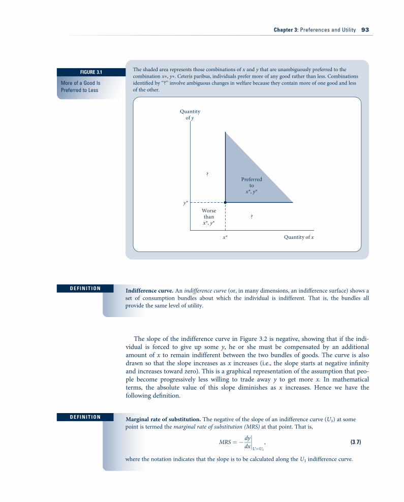
Economic goodsIn this representation the variables are taken to be ‘‘goods’’; that is, whatever economicquantities they represent, we assume that more of any particular xi during some period ispreferred to less. We assume this is true of every good, be it a simple consumption itemsuch as a hot dog or a complex aggregate such as wealth or leisure. We have pictured thisconvention for a two-good utility function in Figure 3.1. There, all consumption bundlesin the shaded area are preferred to the bundle x$, y$ because any bundle in the shaded areaprovides more of at least one of the goods. By our definition of ‘‘goods,’’ bundles of goodsin the shaded area are ranked higher than x$, y$. Similarly, bundles in the area marked‘‘worse’’ are clearly inferior to x$, y$ because they contain less of at least one of the goodsand no more of the other. Bundles in the two areas indicated by question marks are diffi-cult to compare with x$, y$ because they contain more of one of the goods and less of theother. Movements into these areas involve trade-offs between the two goods.

Trades and SubstitutionMost economic activity involves voluntary trading between individuals. When someonebuys, say, a loaf of bread, he or she is voluntarily giving up one thing (money) for some-thing else (bread) that is of greater value to that individual. To examine this kind of vol-untary transaction, we need to develop a formal apparatus for illustrating trades in theutility function context. We first motivate our discussion with a graphical presentationand then turn to some more formal mathematics.

Indifference curves and the marginal rate of substitutionVoluntary trades can best be studied using the graphical device of an indifference curve.In Figure 3.2, the curve U1 represents all the alternative combinations of x and y forwhich an individual is equally well off (remember again that all other arguments of theutility function are held constant). This person is equally happy consuming, for example,either the combination of goods x1, y1 or the combination x2, y2. This curve representingall the consumption bundles that the individual ranks equally is called an indifferencecurve.

D E F I N I T I O N Utility. Individuals’ preferences are assumed to be represented by a utility function of the form

U x1, x2, . . . , xn" #, (3:6)

where x1, x2, …, xn are the quantities of each of n goods that might be consumed in a period. Thisfunction is unique only up to an order-preserving transformation.


The slope of the indifference curve in Figure 3.2 is negative, showing that if the indi-vidual is forced to give up some y, he or she must be compensated by an additionalamount of x to remain indifferent between the two bundles of goods. The curve is alsodrawn so that the slope increases as x increases (i.e., the slope starts at negative infinityand increases toward zero). This is a graphical representation of the assumption that peo-ple become progressively less willing to trade away y to get more x. In mathematicalterms, the absolute value of this slope diminishes as x increases. Hence we have thefollowing definition.

The shaded area represents those combinations of x and y that are unambiguously preferred to thecombination x$, y$. Ceteris paribus, individuals prefer more of any good rather than less. Combinationsidentified by ‘‘?’’ involve ambiguous changes in welfare because they contain more of one good and lessof the other.

Quantity of x

Quantityof y

?

?

Preferredto

x*, y*

Worsethanx*, y*

y*

x*

D E F I N I T I O N Indifference curve. An indifference curve (or, in many dimensions, an indifference surface) shows aset of consumption bundles about which the individual is indifferent. That is, the bundles allprovide the same level of utility.

D E F I N I T I O N Marginal rate of substitution. The negative of the slope of an indifference curve (U1) at somepoint is termed the marginal rate of substitution (MRS) at that point. That is,

MRS ! % dydx

!!!!U!U1

, (3:7)

where the notation indicates that the slope is to be calculated along the U1 indifference curve.

FIGURE 3.1

More of a Good IsPreferred to Less


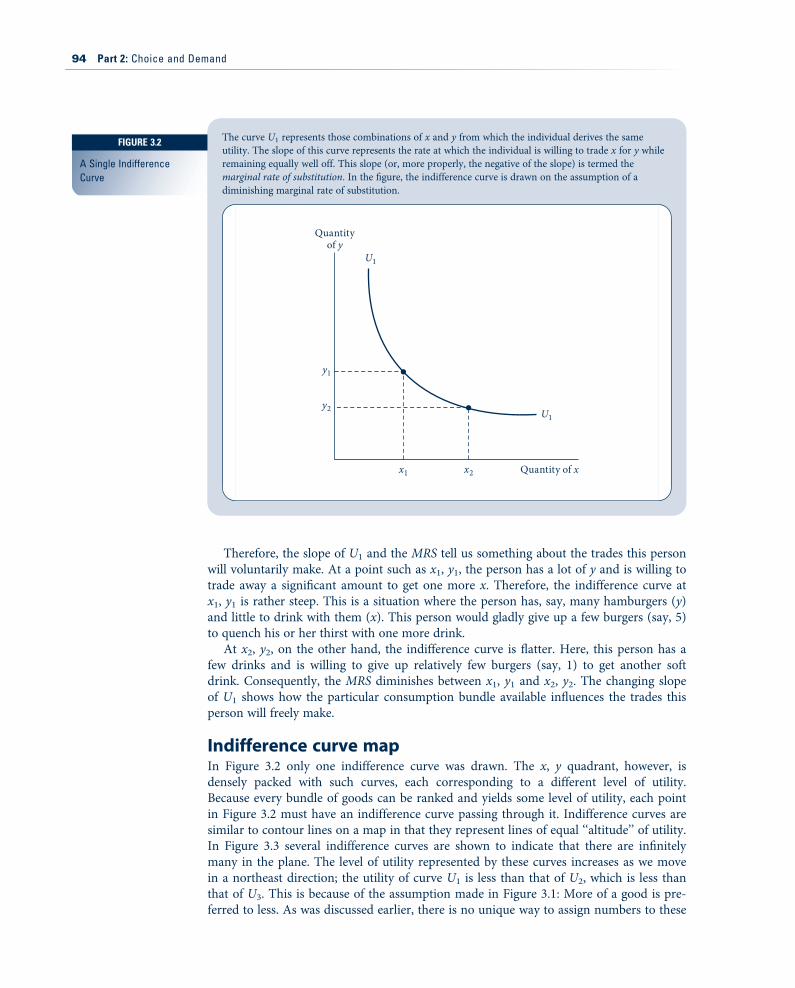
Therefore, the slope of U1 and the MRS tell us something about the trades this personwill voluntarily make. At a point such as x1, y1, the person has a lot of y and is willing totrade away a significant amount to get one more x. Therefore, the indifference curve atx1, y1 is rather steep. This is a situation where the person has, say, many hamburgers (y)and little to drink with them (x). This person would gladly give up a few burgers (say, 5)to quench his or her thirst with one more drink.

At x2, y2, on the other hand, the indifference curve is flatter. Here, this person has afew drinks and is willing to give up relatively few burgers (say, 1) to get another softdrink. Consequently, the MRS diminishes between x1, y1 and x2, y2. The changing slopeof U1 shows how the particular consumption bundle available influences the trades thisperson will freely make.

Indifference curve mapIn Figure 3.2 only one indifference curve was drawn. The x, y quadrant, however, isdensely packed with such curves, each corresponding to a different level of utility.Because every bundle of goods can be ranked and yields some level of utility, each pointin Figure 3.2 must have an indifference curve passing through it. Indifference curves aresimilar to contour lines on a map in that they represent lines of equal ‘‘altitude’’ of utility.In Figure 3.3 several indifference curves are shown to indicate that there are infinitelymany in the plane. The level of utility represented by these curves increases as we movein a northeast direction; the utility of curve U1 is less than that of U2, which is less thanthat of U3. This is because of the assumption made in Figure 3.1: More of a good is pre-ferred to less. As was discussed earlier, there is no unique way to assign numbers to these

The curve U1 represents those combinations of x and y from which the individual derives the sameutility. The slope of this curve represents the rate at which the individual is willing to trade x for y whileremaining equally well off. This slope (or, more properly, the negative of the slope) is termed themarginal rate of substitution. In the figure, the indifference curve is drawn on the assumption of adiminishing marginal rate of substitution.

Quantity of x

Quantityof y

x2x1

y1

U1

U1y2

FIGURE 3.2

A Single IndifferenceCurve


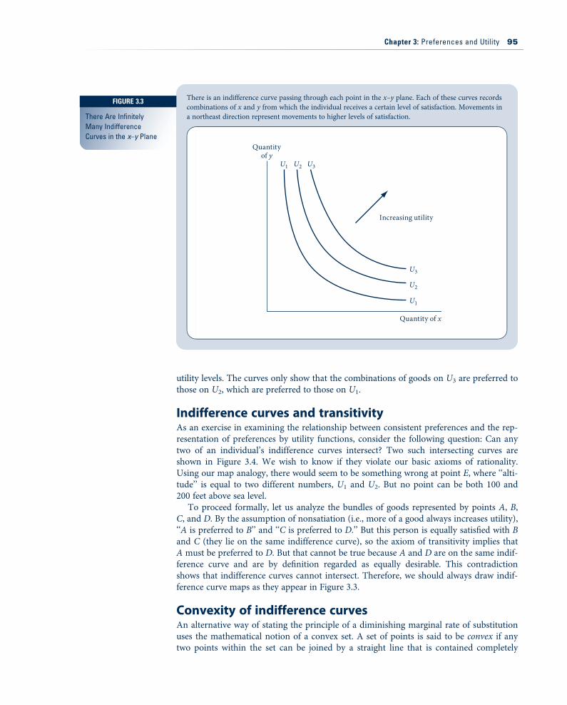
utility levels. The curves only show that the combinations of goods on U3 are preferred tothose on U2, which are preferred to those on U1.

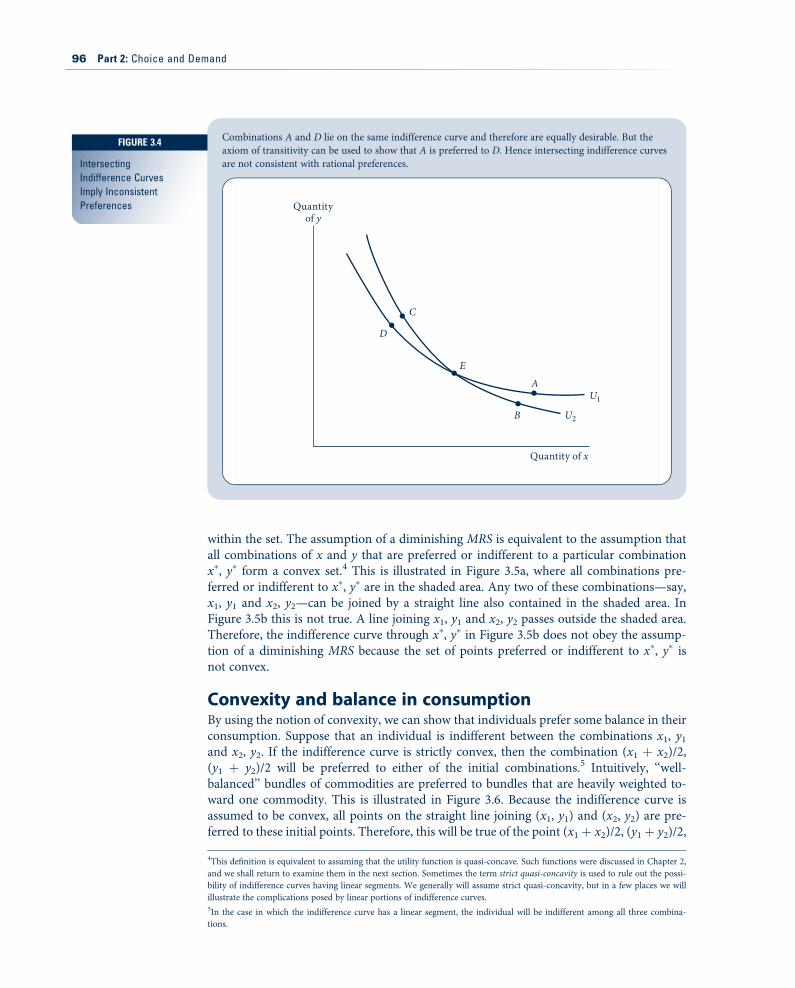
Indifference curves and transitivityAs an exercise in examining the relationship between consistent preferences and the rep-resentation of preferences by utility functions, consider the following question: Can anytwo of an individual’s indifference curves intersect? Two such intersecting curves areshown in Figure 3.4. We wish to know if they violate our basic axioms of rationality.Using our map analogy, there would seem to be something wrong at point E, where ‘‘alti-tude’’ is equal to two different numbers, U1 and U2. But no point can be both 100 and200 feet above sea level.

To proceed formally, let us analyze the bundles of goods represented by points A, B,C, and D. By the assumption of nonsatiation (i.e., more of a good always increases utility),‘‘A is preferred to B’’ and ‘‘C is preferred to D.’’ But this person is equally satisfied with Band C (they lie on the same indifference curve), so the axiom of transitivity implies thatA must be preferred to D. But that cannot be true because A and D are on the same indif-ference curve and are by definition regarded as equally desirable. This contradictionshows that indifference curves cannot intersect. Therefore, we should always draw indif-ference curve maps as they appear in Figure 3.3.

Convexity of indifference curvesAn alternative way of stating the principle of a diminishing marginal rate of substitutionuses the mathematical notion of a convex set. A set of points is said to be convex if anytwo points within the set can be joined by a straight line that is contained completely

There is an indifference curve passing through each point in the x–y plane. Each of these curves recordscombinations of x and y from which the individual receives a certain level of satisfaction. Movements ina northeast direction represent movements to higher levels of satisfaction.

Quantity of x

Quantityof y

Increasing utility

U1

U1

U2

U3

U2 U3

FIGURE 3.3

There Are InfinitelyMany IndifferenceCurves in the x–y Plane


within the set. The assumption of a diminishing MRS is equivalent to the assumption thatall combinations of x and y that are preferred or indifferent to a particular combinationx$, y$ form a convex set.4 This is illustrated in Figure 3.5a, where all combinations pre-ferred or indifferent to x$, y$ are in the shaded area. Any two of these combinations—say,x1, y1 and x2, y2—can be joined by a straight line also contained in the shaded area. InFigure 3.5b this is not true. A line joining x1, y1 and x2, y2 passes outside the shaded area.Therefore, the indifference curve through x$, y$ in Figure 3.5b does not obey the assump-tion of a diminishing MRS because the set of points preferred or indifferent to x$, y$ isnot convex.

Convexity and balance in consumptionBy using the notion of convexity, we can show that individuals prefer some balance in theirconsumption. Suppose that an individual is indifferent between the combinations x1, y1and x2, y2. If the indifference curve is strictly convex, then the combination (x1 & x2)/2,(y1 & y2)/2 will be preferred to either of the initial combinations.5 Intuitively, ‘‘well-balanced’’ bundles of commodities are preferred to bundles that are heavily weighted to-ward one commodity. This is illustrated in Figure 3.6. Because the indifference curve isassumed to be convex, all points on the straight line joining (x1, y1) and (x2, y2) are pre-ferred to these initial points. Therefore, this will be true of the point (x1& x2)/2, (y1& y2)/2,

Combinations A and D lie on the same indifference curve and therefore are equally desirable. But theaxiom of transitivity can be used to show that A is preferred to D. Hence intersecting indifference curvesare not consistent with rational preferences.

Quantity of x

Quantityof y

D

C

EA

B U2

U1

4This definition is equivalent to assuming that the utility function is quasi-concave. Such functions were discussed in Chapter 2,and we shall return to examine them in the next section. Sometimes the term strict quasi-concavity is used to rule out the possi-bility of indifference curves having linear segments. We generally will assume strict quasi-concavity, but in a few places we willillustrate the complications posed by linear portions of indifference curves.5In the case in which the indifference curve has a linear segment, the individual will be indifferent among all three combina-tions.

FIGURE 3.4

IntersectingIndifference CurvesImply InconsistentPreferences


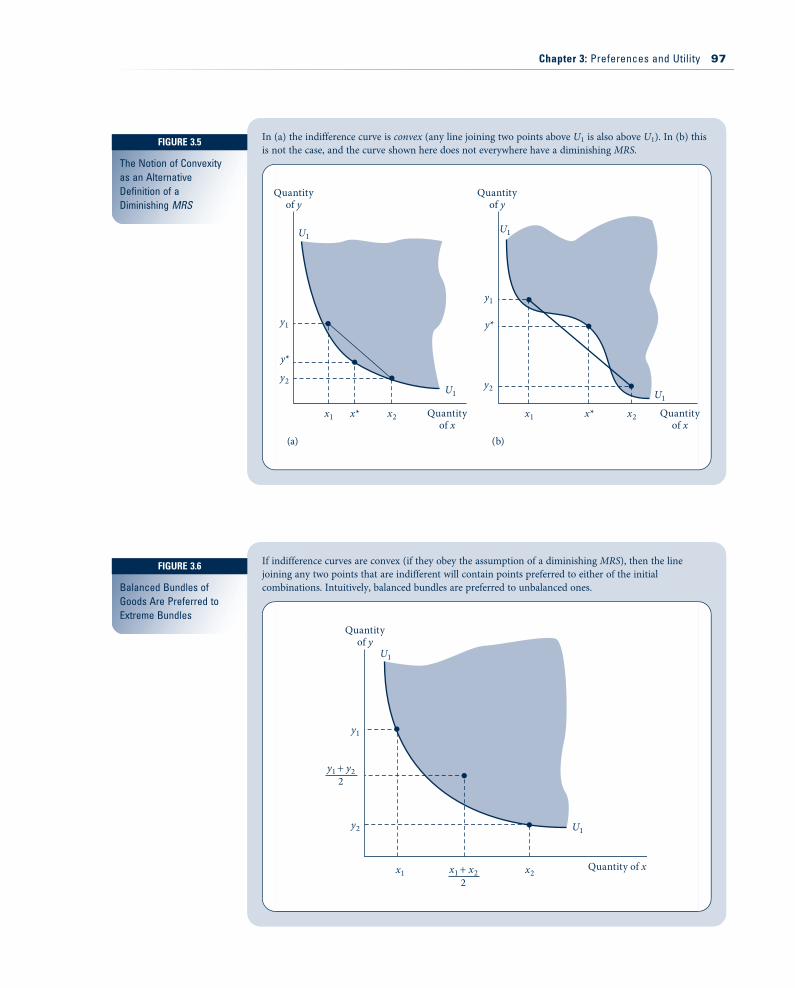
In (a) the indifference curve is convex (any line joining two points above U1 is also above U1). In (b) thisis not the case, and the curve shown here does not everywhere have a diminishing MRS.

Quantityof x

Quantityof x

Quantityof y

Quantityof y

(b)(a)

U1U1

U1 U1

y1

y2 y2

x1 x1 x2x*x2x*

y*

y1

y*

If indifference curves are convex (if they obey the assumption of a diminishing MRS), then the linejoining any two points that are indifferent will contain points preferred to either of the initialcombinations. Intuitively, balanced bundles are preferred to unbalanced ones.

Quantity of x

Quantityof y

2x1 + x2

2y1 + y2

U1

U1

y1

x1 x2

y2

FIGURE 3.5

The Notion of Convexityas an AlternativeDefinition of aDiminishing MRS

FIGURE 3.6

Balanced Bundles ofGoods Are Preferred toExtreme Bundles


which lies at the midpoint of such a line. Indeed, any proportional combination of the twoindifferent bundles of goods will be preferred to the initial bundles because it will representa more balanced combination. Thus, strict convexity is equivalent to the assumption of adiminishing MRS. Both assumptions rule out the possibility of an indifference curve beingstraight over any portion of its length.

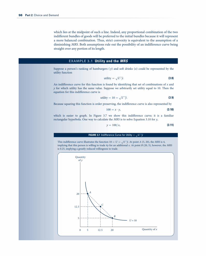
EXAMPLE 3.1 Utility and the MRS

Suppose a person’s ranking of hamburgers ( y) and soft drinks (x) could be represented by theutility function

utility ! """"""""x ' yp

: (3:8)

An indifference curve for this function is found by identifying that set of combinations of x andy for which utility has the same value. Suppose we arbitrarily set utility equal to 10. Then theequation for this indifference curve is

utility ! 10 ! """"""""x ' yp

: (3:9)

Because squaring this function is order preserving, the indifference curve is also represented by

100 ! x ' y, (3:10)

which is easier to graph. In Figure 3.7 we show this indifference curve; it is a familiarrectangular hyperbola. One way to calculate the MRS is to solve Equation 3.10 for y,

y ! 100=x, (3:11)

FIGURE 3.73Indifference Curve for Utility ! """""""""x ' yp

This indifference curve illustrates the function 10 ! U ! """"""""x ' yp

. At point A (5, 20), the MRS is 4,implying that this person is willing to trade 4y for an additional x. At point B (20, 5), however, the MRSis 0.25, implying a greatly reduced willingness to trade.

Quantity of x

Quantityof y

20

12.5

5

200 5 12.5

A

C

BU = 10


The Mathematics of IndifferenceCurvesA mathematical derivation of the indifference curve concept provides additional insightsabout the nature of preferences. In this section we look at a two-good example that tiesdirectly to the graphical treatment provided previously. Later in the chapter we look atthe many-good case, but conclude that this more complicated case adds only a few addi-tional insights.

The marginal rate of substitutionSuppose an individual receives utility from consuming two goods whose quantities aregiven by x and y. This person’s ranking of bundles of these goods can be represented by autility function of the form U x, y" #. Those combinations of the two goods that yield aspecific level of utility, say k, are represented by solutions to the implicit equationU x, y" # ! k. In Chapter 2 (see Equation 2.23) we showed that the trade-offs implied bysuch an equation are given by:

dydxjU x, y" # ! k ! %

Ux

Uy: (3:16)

That is, the rate at which x can be traded for y is given by the negative of the ratio of the‘‘marginal utility’’ of good x to that of good y. Assuming additional amounts of bothgoods provide added utility, this trade-off rate will be negative, implying that increases inthe quantity of good x must be met by decreases in the quantity of good y to keep utility

And then use the definition (Equation 3.7):

MRS ! %dy=dx along U1" # ! 100=x2: (3:12)

Clearly this MRS decreases as x increases. At a point such as A on the indifference curve with alot of hamburgers (say, x ! 5, y ! 20), the slope is steep so the MRS is high:

MRS at "5, 20# ! 100=x2 ! 100=25 ! 4: (3:13)

Here the person is willing to give up 4 hamburgers to get 1 more soft drink. On the other hand,at B where there are relatively few hamburgers (here x ! 20, y ! 5), the slope is flat and theMRS is low:

MRS at "20, 5# ! 100=x2 ! 100=400 ! 0:25: (3:14)

Now he or she will only give up one quarter of a hamburger for another soft drink. Notice alsohow convexity of the indifference curve U1 is illustrated by this numerical example. Point C ismidway between points A and B; at C this person has 12.5 hamburgers and 12.5 soft drinks.Here utility is given by

utility ! """"""""x ' yp !

""""""""""""""12:5" #2

q! 12:5, (3:15)

which clearly exceeds the utility along U1 (which was assumed to be 10).

QUERY: From our derivation here, it appears that the MRS depends only on the quantity of xconsumed. Why is this misleading? How does the quantity of y implicitly enter into Equations3.13 and 3.14?


constant. Earlier we defined the marginal rate of substitution as the negative (or absolutevalue) of this trade-off, so now we have:

MRS ! % dydxjU x, y" #! k !

Ux

Uy: (3:17)

This derivation helps in understanding why the MRS does not depend specifically onhow utility is measured. Because the MRS is a ratio of two utility measures, the units‘‘drop out’’ in the computation. For example, suppose good x represents food and that wehave chosen a utility function for which an extra unit of food yields 6 extra units of utility(sometimes these units are called utils). Suppose also that y represents clothing and withthis utility function each extra unit of clothing provides 2 extra units of utility. In thiscase it is clear that this person is willing to give up 3 units of clothing (thereby losing 6utils) in exchange for 1 extra unit of food (thereby gaining 6 utils):

MRS ! % dydx! Ux

Uy! 6 utils per unit x

2 utils per unit y! 3 units y per unit x: (3:18)

Notice that the utility measure used here (utils) drops out in making this computationand what remains is purely in terms of the units of the two goods. This shows that theMRS will be unchanged no matter what specific utility ranking is used.6

Convexity of Indifference CurvesIn Chapter 1 we described how economists were able to resolve the water–diamond par-adox by proposing that the price of water is low because one more gallon provides rela-tively little in terms of increased utility. Water is (for the most part) plentiful; therefore,its marginal utility is low. Of course, in a desert, water would be scarce and its marginalutility (and price) could be high. Thus, one might conclude that the marginal utilityassociated with water consumption decreases as more water is consumed—in formalterms, the second (partial) derivative of the utility function (i.e., Uxx ! @ 2U=@x2) shouldbe negative.

Intuitively it seems that this commonsense idea should also explain why indifferencecurves are convex. The fact that people are increasingly less willing to part with good yto get more x (while holding utility constant) seems to refer to the samephenomenon—that people do not want too much of any one good. Unfortunately, theprecise connection between diminishing marginal utility and a diminishing MRS iscomplex, even in the two-good case. As we showed in Chapter 2, a function will (bydefinition) have convex indifference curves, providing it is quasi-concave. But the condi-tions required for quasi-concavity are messy, and the assumption of diminishing mar-ginal utility (i.e., negative second-order partial derivatives) will not ensure that theyhold.7 Still, as we shall see, there are good reasons for assuming that utility functions(and many other functions used in microeconomics) are quasi-concave; thus, we willnot be too concerned with situations in which they are not.

6More formally, let F U x, y" #( ) be any monotonic transformation of the utility function with F0"U# > 0. With this new utility

ranking the MRS is given by:

MRS ! @F=@x@F=@y

! F0"U#:Ux

F0"U#:Uy! Ux

Uy;

which is the same as the MRS for the original utility function.7Specifically, for the function U"x, y# to be quasi-concave the following condition must hold (see Equation 2.114):

UxxU2x % 2UxyUxUy & UyyU2

y < 0:

The assumptions that Uxx , Uyy < 0 will not ensure this. One must also be concerned with the sign of the cross partial derivative Uxy .


EXAMPLE 3.2 Showing Convexity of Indifference Curves

Calculation of the MRS for specific utility functions is frequently a good shortcut for showingconvexity of indifference curves. In particular, the process can be much simpler than applyingthe definition of quasi-concavity, although it is more difficult to generalize to more than twogoods. Here we look at how Equation 3.17 can be used for three different utility functions (formore practice, see Problem 3.1).

1. U"x, y# ! """"""""x ' yp

.This example just repeats the case illustrated in Example 3.1. One shortcut to applyingEquation 3.17 that can simplify the algebra is to take the logarithm of this utility function.Because taking logs is order preserving, this will not alter the MRS to be calculated.Thus, let

U$ x, y" # ! ln U x, y" #( ) ! 0:5 ln x & 0:5 ln y: (3:19)

Applying Equation 3.17 yields

MRS ! @U$=@x

@U$=@y! 0:5=x

0:5=y! y

x, (3:20)

which seems to be a much simpler approach than we used previously.8 Clearly this MRS isdiminishing as x increases and y decreases. Therefore, the indifference curves are convex.

2. U(x, y) ! x & xy & y.In this case there is no advantage to transforming this utility function. Applying Equation3.17 yields

MRS ! @U=@x@U=@y

! 1& y1& x

: (3:21)

Again, this ratio clearly decreases as x increases and y decreases; thus, the indifferencecurves for this function are convex.

3. U"x, y# !"""""""""""""""x2 & y2

p

For this example it is easier to use the transformation

U$ x, y" # ! U x, y" #( )2 ! x2 & y2: (3:22)

Because this is the equation for a quarter-circle, we should begin to suspect that there mightbe some problems with the indifference curves for this utility function. These suspicions areconfirmed by again applying the definition of the MRS to yield

MRS ! @U$=@x

@U$@y! 2x

2y! x

y: (3:23)

For this function, it is clear that, as x increases and y decreases, theMRS increases! Hence theindifference curves are concave, not convex, and this is clearly not a quasi-concave function.

QUERY: Does a doubling of x and y change the MRS in each of these three examples? That is,does the MRS depend only on the ratio of x to y, not on the absolute scale of purchases? (Seealso Example 3.3.)

8In Example 3.1 we looked at the U ! 10 indifference curve. Thus, for that curve, y ! 100/x, and the MRS in Equation 3.20would be MRS ! 100/x2 as calculated before.


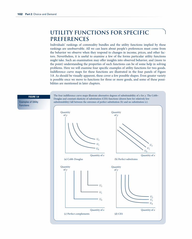
Utility Functions for SpecificPreferencesIndividuals’ rankings of commodity bundles and the utility functions implied by theserankings are unobservable. All we can learn about people’s preferences must come fromthe behavior we observe when they respond to changes in income, prices, and other fac-tors. Nevertheless, it is useful to examine a few of the forms particular utility functionsmight take. Such an examination may offer insights into observed behavior, and (more tothe point) understanding the properties of such functions can be of some help in solvingproblems. Here we will examine four specific examples of utility functions for two goods.Indifference curve maps for these functions are illustrated in the four panels of Figure3.8. As should be visually apparent, these cover a few possible shapes. Even greater varietyis possible once we move to functions for three or more goods, and some of these possi-bilities are mentioned in later chapters.

The four indifference curve maps illustrate alternative degrees of substitutability of x for y. The Cobb–Douglas and constant elasticity of substitution (CES) functions (drawn here for relatively lowsubstitutability) fall between the extremes of perfect substitution (b) and no substitution (c).

Quantity of x(a) Cobb-Douglas

Quantityof y

Quantityof y

Quantityof y

Quantityof y

Quantity of x(b) Perfect substitutes

Quantity of x(c) Perfect complements

Quantity of x(d) CES

U2

U2

U2

U2

U1

U0 U1U0

U1

U1U0 U0

FIGURE 3.8

Examples of UtilityFunctions


Cobb–Douglas utilityFigure 3.8a shows the familiar shape of an indifference curve. One commonly used utilityfunction that generates such curves has the form

utility ! U x, y" # ! xayb, (3:24)

where a and b are positive constants.In Examples 3.1 and 3.2, we studied a particular case of this function for which a ! b !

0.5. The more general case presented in Equation 3.24 is termed a Cobb–Douglas utilityfunction, after two researchers who used such a function for their detailed study of produc-tion relationships in the U.S. economy (see Chapter 9). In general, the relative sizes of aand b indicate the relative importance of the two goods to this individual. Because utility isunique only up to a monotonic transformation, it is often convenient to normalize theseparameters so that a & b ! 1. In this case, utility would be given by

U x, y" # ! xd y1%d (3:25)

where d ! a= a& b" #, 1% d ! b= a& b" #:

Perfect substitutesThe linear indifference curves in Figure 3.8b are generated by a utility function of theform

utility ! U x, y" # ! ax & by, (3:26)

where, again, a and b are positive constants. That the indifference curves for this functionare straight lines should be readily apparent: Any particular level curve can be calculatedby setting U(x, y) equal to a constant that specifies a straight line. The linear nature ofthese indifference curves gave rise to the term perfect substitutes to describe the impliedrelationship between x and y. Because the MRS is constant (and equal to a/b) along theentire indifference curve, our previous notions of a diminishing MRS do not apply in thiscase. A person with these preferences would be willing to give up the same amount of yto get one more x no matter how much x was being consumed. Such a situation mightdescribe the relationship between different brands of what is essentially the same product.For example, many people (including the author) do not care where they buy gasoline. Agallon of gas is a gallon of gas despite the best efforts of the Exxon and Shell advertisingdepartments to convince me otherwise. Given this fact, I am always willing to give up 10gallons of Exxon in exchange for 10 gallons of Shell because it does not matter to mewhich I use or where I got my last tankful. Indeed, as we will see in the next chapter, oneimplication of such a relationship is that I will buy all my gas from the least expensiveseller. Because I do not experience a diminishing MRS of Exxon for Shell, I have noreason to seek a balance among the gasoline types I use.

Perfect complementsA situation directly opposite to the case of perfect substitutes is illustrated by theL-shaped indifference curves in Figure 3.8c. These preferences would apply to goods that‘‘go together’’—coffee and cream, peanut butter and jelly, and cream cheese and lox arefamiliar examples. The indifference curves shown in Figure 3.8c imply that these pairs ofgoods will be used in the fixed proportional relationship represented by the vertices ofthe curves. A person who prefers 1 ounce of cream with 8 ounces of coffee will want 2ounces of cream with 16 ounces of coffee. Extra coffee without cream is of no value tothis person, just as extra cream would be of no value without coffee. Only by choosingthe goods together can utility be increased.


These concepts can be formalized by examining the mathematical form of the utilityfunction that generates these L-shaped indifference curves:

utility ! U x, y" # ! min ax, by" #: (3:27)

Here a and b are positive parameters, and the operator ‘‘min’’ means that utility is givenby the smaller of the two terms in the parentheses. In the coffee–cream example, if we letounces of coffee be represented by x and ounces of cream by y, utility would be given by

utility ! U x, y" # ! min x, 8y" #: (3:28)

Now 8 ounces of coffee and 1 ounce of cream provide 8 units of utility. But 16 ounces ofcoffee and 1 ounce of cream still provide only 8 units of utility because min(16, 8) ! 8.The extra coffee without cream is of no value, as shown by the horizontal section of theindifference curves for movement away from a vertex; utility does not increase when onlyx increases (with y constant). Only if coffee and cream are both doubled (to 16 and 2,respectively) will utility increase to 16.

More generally, neither of the two goods specified in the utility function given byEquation 3.27 will be consumed in superfluous amounts if ax ! by. In this case, the ratioof the quantity of good x consumed to that of good y will be a constant given by

yx! a

b: (3:29)

Consumption will occur at the vertices of the indifference curves shown in Figure 3.8c.

CES utilityThe three specific utility functions illustrated thus far are special cases of the more generalCES function, which takes the form

utility ! U x, y" # ! xd

d& yd

d, (3:30)

where d * 1, d 6! 0, and

utility ! U x, y" # ! ln x & ln y (3:31)

when d ! 0. It is obvious that the case of perfect substitutes corresponds to the limitingcase, d ! 1, in Equation 3.30 and that the Cobb–Douglas9 case corresponds to d ! 0 inEquation 3.31. Less obvious is that the case of fixed proportions corresponds to d ! %1in Equation 3.30, but that result can also be shown using a limits argument.

The use of the term elasticity of substitution for this function derives from the notionthat the possibilities illustrated in Figure 3.8 correspond to various values for the substitu-tion parameter, s, which for this function is given by s ! 1/(1 % d). For perfect substi-tutes, then s !1, and the fixed proportions case has s ! 0.10 Because the CES functionallows us to explore all these cases, and many cases in between, it will prove useful forillustrating the degree of substitutability present in various economic relationships.

The specific shape of the CES function illustrated in Figure 3.8a is for the cased ! %1. That is,

utility ! %x%1 % y%1 ! % 1x% 1

y: (3:32)

9The CES function could easily be generalized to allow for differing weights to be attached to the two goods. Because the mainuse of the function is to examine substitution questions, we usually will not make that generalization. In some of the applica-tions of the CES function, we will also omit the denominators of the function because these constitute only a scale factor whend is positive. For negative values of d, however, the denominator is needed to ensure that marginal utility is positive.10The elasticity of substitution concept is discussed in more detail in connection with production functions in Chapter 9.


For this situation, s ! 1/(1 % d) ! 1/2, and, as the graph shows, these sharply curvedindifference curves apparently fall between the Cobb–Douglas and fixed proportion cases.The negative signs in this utility function may seem strange, but the marginal utilities ofboth x and y are positive and diminishing, as would be expected. This explains why dmust appear in the denominators in Equation 3.30. In the particular case of Equation3.32, utility increases from %1 (when x ! y ! 0) toward 0 as x and y increase. This isan odd utility scale, perhaps, but perfectly acceptable and often useful.

EXAMPLE 3.3 Homothetic Preferences

All the utility functions described in Figure 3.8 are homothetic (see Chapter 2). That is,the marginal rate of substitution for these functions depends only on the ratio of the amounts ofthe two goods, not on the total quantities of the goods. This fact is obvious for the case of theperfect substitutes (when the MRS is the same at every point) and the case of perfectcomplements (where the MRS is infinite for y/x > a/b, undefined when y/x ! a/b, and zerowhen y/x < a/b). For the general Cobb–Douglas function, the MRS can be found as

MRS ! @U=@x@U=@y

! axa%1yb

bxayb%1 !ab' yx, (3:33)

which clearly depends only on the ratio y/x. Showing that the CES function is also homothetic isleft as an exercise (see Problem 3.12).

The importance of homothetic functions is that one indifference curve is much like another.Slopes of the curves depend only on the ratio y/x, not on how far the curve is from the origin.Indifference curves for higher utility are simple copies of those for lower utility. Hence we canstudy the behavior of an individual who has homothetic preferences by looking only at oneindifference curve or at a few nearby curves without fearing that our results would changedramatically at different levels of utility.

QUERY: How might you define homothetic functions geometrically? What would the locus ofall points with a particular MRS look like on an individual’s indifference curve map?

EXAMPLE 3.4 Nonhomothetic Preferences

Although all the indifference curve maps in Figure 3.8 exhibit homothetic preferences, this neednot always be true. Consider the quasi-linear utility function

utility ! U x, y" # ! x & ln y: (3:34)

For this function, good y exhibits diminishing marginal utility, but good x does not. The MRScan be computed as

MRS ! @U=@x@U=@y

! 11=y! y' (3:35)

The MRS diminishes as the chosen quantity of y decreases, but it is independent of the quantityof x consumed. Because x has a constant marginal utility, a person’s willingness to give up y toget one more unit of x depends only on how much y he or she has. Contrary to the homotheticcase, a doubling of both x and y doubles the MRS rather than leaving it unchanged.

QUERY: What does the indifference curve map for the utility function in Equation 3.34 looklike? Why might this approximate a situation where y is a specific good and x representseverything else?


The Many-Good CaseAll the concepts we have studied thus far for the case of two goods can be generalized tosituations where utility is a function of arbitrarily many goods. In this section, we willbriefly explore those generalizations. Although this examination will not add much towhat we have already shown, considering peoples’ preferences for many goods can be im-portant in applied economics, as we will see in later chapters.

If utility is a function of n goods of the form U x1, x2, . . . , xn" #, then the equation

U x1, x2, . . . , xn" # ! k (3:36)

defines an indifference surface in n dimensions. This surface shows all those combina-tions of the n goods that yield the same level of utility. Although it is probably impossibleto picture what such a surface would look like, we will continue to assume that it is con-vex. That is, balanced bundles of goods will be preferred to unbalanced ones. Hence theutility function, even in many dimensions, will be assumed to be quasi-concave.

The MRS with many goodsWe can study the trades that a person might voluntarily make between any two of thesegoods (say, x1 and x2) by again using the implicit function theorem:

MRS ! % dx2dx1

U x1, x2, ..., xn" # ! k !Ux1 x1, x2, . . . , xn" #Ux2 x1, x2, . . . , xn" #

:

!!!! (3:37)

The notation here makes the important point that an individual’s willingness to trade x1for x2 will depend not only on the quantities of these two goods but also on the quantitiesof all the other goods. An individual’s willingness to trade food for clothing will dependnot only on the quantities of food and clothing he or she has but also on how much‘‘shelter’’ he or she has. In general it would be expected that changes in the quantities ofany of these other goods would affect the trade-off represented by Equation 3.37. It is thispossibility that can sometimes make it difficult to generalize the findings of simple two-good models to the many-good case. One must be careful to specify what is beingassumed about the quantities of the other goods. In later chapters we will occasionallylook at such complexities. However, for the most part, the two-good model will be goodenough for developing intuition about economic relationships.

SUMMARY

In this chapter we have described the way in which econo-mists formalize individuals’ preferences about the goodsthey choose. We drew several conclusions about such prefer-ences that will play a central role in our analysis of thetheory of choice in the following chapters:

• If individuals obey certain basic behavioral postulatesin their preferences among goods, they will be able torank all commodity bundles, and that ranking can berepresented by a utility function. In making choices,individuals will behave as though they were maximiz-ing this function.

• Utility functions for two goods can be illustrated by anindifference curve map. Each indifference curve con-tour on this map shows all the commodity bundles thatyield a given level of utility.

• The negative of the slope of an indifference curve isdefined as the marginal rate of substitution (MRS). Thisshows the rate at which an individual would willingly giveup an amount of one good (y) if he or she were compen-sated by receiving one more unit of another good (x).

• The assumption that the MRS decreases as x is substi-tuted for y in consumption is consistent with the notionthat individuals prefer some balance in their consump-tion choices. If theMRS is always decreasing, individualswill have strictly convex indifference curves. That is,their utility function will be strictly quasi-concave.

• A few simple functional forms can capture importantdifferences in individuals’ preferences for two (or more)goods. Here we examined the Cobb–Douglas function, thelinear function (perfect substitutes), the fixed proportions


function (perfect complements), and the CES function(which includes the other three as special cases).

• It is a simple matter mathematically to generalize fromtwo-good examples to many goods. And, as we shall

see, studying peoples’ choices among many goods canyield many insights. But the mathematics of manygoods is not especially intuitive; therefore, we will pri-marily rely on two-good cases to build such intuition.

PROBLEMS

3.1Graph a typical indifference curve for the following utility functions, and determine whether they have convex indifferencecurves (i.e., whether the MRS declines as x increases).

a. U(x, y) ! 3x & y.

b. U x, y" # ! """"""""x ' yp

.

c. U x, y" # !"""xp& y.

d. U x, y" # !"""""""""""""""x2 % y2

p.

e. U x, y" # ! xyx & y

.

3.2In footnote 7 we showed that for a utility function for two goods to have a strictly diminishing MRS (i.e., to be strictly quasi-concave), the following condition must hold:

UxxU2x % 2UxyUxUy & UyyU2

y < 0

Use this condition to check the convexity of the indifference curves for each of the utility functions in Problem 3.1. Describe theprecise relationship between diminishing marginal utility and quasi-concavity for each case.

3.3Consider the following utility functions:

a. U(x, y) ! xy.b. U(x, y) ! x2y2.c. U(x, y) ! ln x & ln y.

Show that each of these has a diminishing MRS but that they exhibit constant, increasing, and decreasing marginal utility,respectively. What do you conclude?

3.4As we saw in Figure 3.5, one way to show convexity of indifference curves is to show that, for any two points (x1, y1) and

(x2, y2) on an indifference curve that promises U ! k, the utility associated with the pointx1 & x2

2;y1 & y2

2

# $is at least as

great as k. Use this approach to discuss the convexity of the indifference curves for the following three functions. Be sure to

graph your results.

a. U(x, y) ! min(x, y).b. U(x, y) ! max(x, y).c. U(x, y) ! x & y.

3.5The Phillie Phanatic (PP) always eats his ballpark franks in a special way; he uses a foot-long hot dog together with preciselyhalf a bun, 1 ounce of mustard, and 2 ounces of pickle relish. His utility is a function only of these four items, and any extraamount of a single item without the other constituents is worthless.


a. What form does PP’s utility function for these four goods have?b. How might we simplify matters by considering PP’s utility to be a function of only one good? What is that good?c. Suppose foot-long hot dogs cost $1.00 each, buns cost $0.50 each, mustard costs $0.05 per ounce, and pickle relish costs

$0.15 per ounce. How much does the good defined in part (b) cost?d. If the price of foot-long hot dogs increases by 50 percent (to $1.50 each), what is the percentage increase in the price of the

good?e. How would a 50 percent increase in the price of a bun affect the price of the good? Why is your answer different from

part (d)?f. If the government wanted to raise $1.00 by taxing the goods that PP buys, how should it spread this tax over the four goods

so as to minimize the utility cost to PP?

3.6Many advertising slogans seem to be asserting something about people’s preferences. How would you capture the followingslogans with a mathematical utility function?

a. Promise margarine is just as good as butter.b. Things go better with Coke.c. You can’t eat just one Pringle’s potato chip.d. Krispy Kreme glazed doughnuts are just better than Dunkin’ Donuts.e. Miller Brewing advises us to drink (beer) ‘‘responsibly.’’ [What would ‘‘irresponsible’’ drinking be?]

3.7a. A consumer is willing to trade 3 units of x for 1 unit of y when she has 6 units of x and 5 units of y. She is also willing

to trade in 6 units of x for 2 units of y when she has 12 units of x and 3 units of y. She is indifferent between bundle(6, 5) and bundle (12, 3). What is the utility function for goods x and y? Hint: What is the shape of the indifferencecurve?

b. A consumer is willing to trade 4 units of x for 1 unit of y when she is consuming bundle (8, 1). She is also willing to tradein 1 unit of x for 2 units of y when she is consuming bundle (4, 4). She is indifferent between these two bundles. Assumingthat the utility function is Cobb–Douglas of the form U(x, y) ! xayb, where a and b are positive constants, what is theutility function for this consumer?

c. Was there a redundancy of information in part (b)? If yes, how much is the minimum amount of information required inthat question to derive the utility function?

3.8Find utility functions given each of the following indifference curves [defined by U (Æ) ! k]:

a. z ! k1=d

xa=dyb=d.

b. y ! 0:5"""""""""""""""""""""""""""""x2 % 4 x2 % k" #

p% 0:5x.

c. z !"""""""""""""""""""""""""""""""""y4 % 4x x2y % k" #

p

2x% y2

2x.

Analytical Problems

3.9 Initial endowmentsSuppose that a person has initial amounts of the two goods that provide utility to him or her. These initial amounts are givenby x and y.

a. Graph these initial amounts on this person’s indifference curve map.b. If this person can trade x for y (or vice versa) with other people, what kinds of trades would he or she voluntarily make?

What kinds would not be made? How do these trades relate to this person’s MRS at the point x, y" #?c. Suppose this person is relatively happy with the initial amounts in his or her possession and will only consider trades that

increase utility by at least amount k. How would you illustrate this on the indifference curve map?


3.10 Cobb–Douglas utilityExample 3.3 shows that the MRS for the Cobb–Douglas function

U x, y" # ! xayb

is given by

MRS ! ab

yx

# $:

a. Does this result depend on whether a & b ! 1? Does this sum have any relevance to the theory of choice?b. For commodity bundles for which y ! x, how does the MRS depend on the values of a and b? Develop an intuitive expla-

nation of why, if a > b, MRS > 1. Illustrate your argument with a graph.c. Suppose an individual obtains utility only from amounts of x and y that exceed minimal subsistence levels given by x0, y0.

In this case,

U x, y" # ! x % x0" #a y % y0" #b

Is this function homothetic? (For a further discussion, see the Extensions to Chapter 4.)

3.11 Independent marginal utilitiesTwo goods have independent marginal utilities if

@ 2U@y@x

! @ 2U@x@y

! 0:

Show that if we assume diminishing marginal utility for each good, then any utility function with independent marginalutilities will have a diminishing MRS. Provide an example to show that the converse of this statement is not true.

3.12 CES utilitya. Show that the CES function

axd

d& b

yd

d

is homothetic. How does the MRS depend on the ratio y/x?b. Show that your results from part (a) agree with our discussion of the cases d ! 1 (perfect substitutes) and d ! 0 (Cobb–

Douglas).c. Show that the MRS is strictly diminishing for all values of d < 1.d. Show that if x ! y, the MRS for this function depends only on the relative sizes of a and b.e. Calculate the MRS for this function when y/x ! 0.9 and y/x ! 1.1 for the two cases d ! 0.5 and d ! %1. What do you con-

clude about the extent to which the MRS changes in the vicinity of x ! y? How would you interpret this geometrically?

3.13 The quasi-linear functionConsider the function U(x, y) ! x & ln y. This is a function that is used relatively frequently in economic modeling as it hassome useful properties.

a. Find the MRS of the function. Now, interpret the result.b. Confirm that the function is quasi-concave.c. Find the equation for an indifference curve for this function.d. Compare the marginal utility of x and y. How do you interpret these functions? How might consumers choose between x

and y as they try to increase their utility by, for example, consuming more when their income increases? (We will look atthis ‘‘income effect’’ in detail in the Chapter 5 problems.)

e. Considering how the utility changes as the quantities of the two goods increase, describe some situations where this func-tion might be useful.


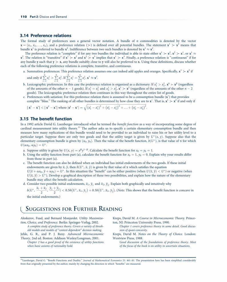
3.14 Preference relationsThe formal study of preferences uses a general vector notation. A bundle of n commodities is denoted by the vectorx ! x1, x2, . . . , xn" #, and a preference relation (C) is defined over all potential bundles. The statement x1 C x2 means thatbundle x1 is preferred to bundle x2. Indifference between two such bundles is denoted by x1 + x2.

The preference relation is ‘‘complete’’ if for any two bundles the individual is able to state either x1 C x2, x2 C x1, or x1 +x2. The relation is ‘‘transitive’’ if x1 C x2 and x2 C x3 implies that x1 C x3. Finally, a preference relation is ‘‘continuous’’ if forany bundle y such that y C x, any bundle suitably close to y will also be preferred to x. Using these definitions, discuss whethereach of the following preference relations is complete, transitive, and continuous.

a. Summation preferences: This preference relation assumes one can indeed add apples and oranges. Specifically, x1 C x2 if

and only ifPn

i!1x1i >

Pn

i!1x2i . If

Pn

i!1x1i !

Pn

i!1x2i , x

1 + x2.

b. Lexicographic preferences: In this case the preference relation is organized as a dictionary: If x11 > x21, x1 , x2 (regardless

of the amounts of the other n % 1 goods). If x11 ! x21 and x12 > x22, x1 C x2 (regardless of the amounts of the other n % 2

goods). The lexicographic preference relation then continues in this way throughout the entire list of goods.c. Preferences with satiation: For this preference relation there is assumed to be a consumption bundle (x$) that provides

complete ‘‘bliss.’’ The ranking of all other bundles is determined by how close they are to x$. That is, x1 C x2 if and only if

| x1 % x$| < | x2 % x$| where jxi % x$j !""""""""""""""""""""""""""""""""""""""""""""""""""""""""""""""""""""""""""""""""""""xi1 % x$1" #2 & xi2 % x$x

% &2 & . . .& xin % x$n% &2q

.

3.15 The benefit functionIn a 1992 article David G. Luenberger introduced what he termed the benefit function as a way of incorporating some degree ofcardinal measurement into utility theory.11 The author asks us to specify a certain elementary consumption bundle and thenmeasure how many replications of this bundle would need to be provided to an individual to raise his or her utility level to aparticular target. Suppose there are only two goods and that the utility target is given by U$ x, y" #: Suppose also that theelementary consumption bundle is given by x0, y0" #. Then the value of the benefit function, b U$" #, is that value of a for whichU ax0, ay0" # ! U$.

a. Suppose utility is given by U x, y" # ! xby1%b. Calculate the benefit function for x0 ! y0 ! 1.b. Using the utility function from part (a), calculate the benefit function for x0 ! 1, y0 ! 0. Explain why your results differ

from those in part (a).c. The benefit function can also be defined when an individual has initial endowments of the two goods. If these initial

endowments are given by x, y, then b U$, x, y" # is given by that value of a which satisfies the equationU x & ax0, y & ay0" # ! U$. In this situation the ‘‘benefit’’ can be either positive (when U x, y" # < U$) or negative (whenU x, y" # > U$). Develop a graphical description of these two possibilities, and explain how the nature of the elementarybundle may affect the benefit calculation.

d. Consider two possible initial endowments, x1, y1 and x2, y2. Explain both graphically and intuitively why

b"U$, x1 & x22

,y1 & y2

2# < 0:5b U$, x1, y1

% && 0:5b U$, x2, y2

% &. (Note: This shows that the benefit function is concave in

the initial endowments.)

SUGGESTIONS FOR FURTHER READING

Aleskerov, Fuad, and Bernard Monjardet. Utility Maximiza-tion, Choice, and Preference. Berlin: Springer-Verlag, 2002.

A complete study of preference theory. Covers a variety of thresh-old models and models of ‘‘context-dependent’’ decision making.

Jehle, G. R., and P. J. Reny. Advanced MicroeconomicTheory, 2nd ed. Boston: Addison Wesley/Longman, 2001.

Chapter 2 has a good proof of the existence of utility functionswhen basic axioms of rationality hold.

Kreps, David M. A Course in Microeconomic Theory. Prince-ton, NJ: Princeton University Press, 1990.

Chapter 1 covers preference theory in some detail. Good discus-sion of quasi-concavity.

Kreps, David M. Notes on the Theory of Choice. London:Westview Press, 1988.

Good discussion of the foundations of preference theory. Mostof the focus of the book is on utility in uncertain situations.

11Luenberger, David G. ‘‘Benefit Functions and Duality.’’ Journal of Mathematical Economics 21: 461–81. The presentation here has been simplified considerablyfrom that originally presented by the author, mainly by changing the direction in which ‘‘benefits’’ are measured.


Mas-Colell, Andrea, Michael D. Whinston, and Jerry R.Green. Microeconomic Theory. New York: Oxford UniversityPress, 1995.

Chapters 2 and 3 provide a detailed development of preferencerelations and their representation by utility functions.

Stigler, G. ‘‘The Development of Utility Theory.’’ Journal ofPolitical Economy 59, pts. 1–2 (August/October 1950): 307–27,373–96.

A lucid and complete survey of the history of utility theory. Hasmany interesting insights and asides.


EXTENSIONS SPECIAL PREFERENCES

The utility function concept is a general one that can beadapted to a large number of special circumstances. Discoveryof ingenious functional forms that reflect the essential aspectsof some problem can provide a number of insights that wouldnot be readily apparent with a more literary approach. Herewe look at four aspects of preferences that economists havetried to model: (1) threshold effects, (2) quality, (3) habits andaddiction, and (4) second-party preferences. In Chapters 7and 17, we illustrate a number of additional ways of capturingaspects of preferences.

E3.1 Threshold effectsThe model of utility that we developed in this chapter impliesan individual will always prefer commodity bundle A to bun-dle B, provided U(A) > U(B). There may be events that willcause people to shift quickly from consuming bundle A toconsuming B. In many cases, however, such a lightning-quickresponse seems unlikely. People may in fact be ‘‘set in theirways’’ and may require a rather large change in circumstancesto change what they do. For example, individuals may nothave especially strong opinions about what precise brand oftoothpaste they choose and may stick with what they knowdespite a proliferation of new (and perhaps better) brands.Similarly, people may stick with an old favorite TV show eventhough it has declined in quality. One way to capture suchbehavior is to assume individuals make decisions as thoughthey faced thresholds of preference. In such a situation, com-modity bundle A might be chosen over B only when

U"A# > U"B# & ‹!; (i)

where ! is the threshold that must be overcome. With thisspecification, indifference curves then may be rather thick andeven fuzzy, rather than the distinct contour lines shown inthis chapter. Threshold models of this type are used exten-sively in marketing. The theory behind such models is pre-sented in detail in Aleskerov and Monjardet (2002). There,the authors consider a number of ways of specifying thethreshold so that it might depend on the characteristics of thebundles being considered or on other contextual variables.

Alternative fuelsVedenov, Duffield, and Wetzstein (2006) use the thresholdidea to examine the conditions under which individuals willshift from gasoline to other fuels (primarily ethanol) for

powering their cars. The authors point out that the main dis-advantage of using gasoline in recent years has been the exces-sive price volatility of the product relative to other fuels. Theyconclude that switching to ethanol blends is efficient (espe-cially during periods of increased gasoline price volatility),provided that the blends do not decrease fuel efficiency.

E3.2 QualityBecause many consumption items differ widely in quality,economists have an interest in incorporating such differencesinto models of choice. One approach is simply to regard itemsof different quality as totally separate goods that are relativelyclose substitutes. But this approach can be unwieldy becauseof the large number of goods involved. An alternativeapproach focuses on quality as a direct item of choice. Utilitymight in this case be reflected by

utility ! U q, Q" #, (ii)

where q is the quantity consumed and Q is the quality of thatconsumption. Although this approach permits some examina-tion of quality–quantity trade-offs, it encounters difficultywhen the quantity consumed of a commodity (e.g., wine) con-sists of a variety of qualities. Quality might then be defined asan average (see Theil,1 1952), but that approach may not beappropriate when the quality of new goods is changing rapidly(e.g., as in the case of personal computers). A more generalapproach (originally suggested by Lancaster, 1971) focuses ona well-defined set of attributes of goods and assumes thatthose attributes provide utility. If a good q provides two suchattributes, a1 and a2, then utility might be written as

utility ! U q, a1"q#, a2"q#( ), (iii)

and utility improvements might arise either because this indi-vidual chooses a larger quantity of the good or because a givenquantity yields a higher level of valuable attributes.

Personal computersThis is the practice followed by economists who studydemand in such rapidly changing industries as personal com-puters. In this case it would clearly be incorrect to focus onlyon the quantity of personal computers purchased each year

1Theil also suggests measuring quality by looking at correlations betweenchanges in consumption and the income elasticities of various goods.

because new machines are much better than old ones (and,presumably, provide more utility). For example, Berndt,Griliches, and Rappaport (1995) find that personal computerquality has been increasing about 30 percent per year over arelatively long period, primarily because of improved attri-butes such as faster processors or better hard drives. A personwho spends, say, $2,000 for a personal computer today buysmuch more utility than did a similar consumer 5 years ago.

E3.3 Habits and addictionBecause consumption occurs over time, there is the possibilitythat decisions made in one period will affect utility in laterperiods. Habits are formed when individuals discover theyenjoy using a commodity in one period and this increasestheir consumption in subsequent periods. An extreme case isaddiction (be it to drugs, cigarettes, or Marx Brothers movies),where past consumption significantly increases the utility ofpresent consumption. One way to portray these ideas mathe-matically is to assume that utility in period t depends on con-sumption in period t and the total of all previousconsumption of the habit-forming good (say, X):

utility ! Ut xt , yt , st" #, (iv)

where

st !X1

i!1xt%i:

In empirical applications, however, data on all past levels ofconsumption usually do not exist. Therefore, it is common tomodel habits using only data on current consumption (xt)and on consumption in the previous period (xt%1). A commonway to proceed is to assume that utility is given by

utility ! Ut x$t , yt% &

, (v)

where x$t is some simple function of xt and xt%1, such asx$t ! xt % xt%1 or x$t ! xt=xt%1. Such functions imply that,ceteris paribus, the higher xt%1, the more xt will be chosen inthe current period.

Modeling habitsThese approaches to modeling habits have been applied to awide variety of topics. Stigler and Becker (1977) use suchmodels to explain why people develop a ‘‘taste’’ for going tooperas or playing golf. Becker, Grossman, and Murphy (1994)adapt the models to studying cigarette smoking and otheraddictive behavior. They show that reductions in smokingearly in life can have large effects on eventual cigarette con-sumption because of the dynamics in individuals’ utility func-tions. Whether addictive behavior is ‘‘rational’’ has beenextensively studied by economists. For example, Gruber andKoszegi (2001) show that smoking can be approached as arational, although time-inconsistent,2 choice.

E3.4 Second-party preferencesIndividuals clearly care about the well-being of other individu-als. Phenomena such as making charitable contributions ormaking bequests to children cannot be understood withoutrecognizing the interdependence that exists among people.Second-party preferences can be incorporated into the utilityfunction of person i, say, by

utility ! Ui xi, yi, Uj% &

, (vi)

where Uj is the utility of someone else.If @Ui /@Uj > 0 then this person will engage in altruistic

behavior, whereas if @Ui /@Uj < 0 then he or she will demon-strate the malevolent behavior associated with envy. The usualcase of @Ui /@Uj ! 0 is then simply a middle ground betweenthese alternative preference types. Gary Becker has been a pio-neer in the study of these possibilities and has written on a va-riety of topics, including the general theory of socialinteractions (1976) and the importance of altruism in thetheory of the family (1981).

Evolutionary biology and geneticsBiologists have suggested a particular form for the utility func-tion in Equation vi, drawn from the theory of genetics. In thiscase

utility ! Ui xi, yi" # &X

j

rjUj, (vii)

where rj measures closeness of the genetic relationshipbetween person i and person j. For parents and children, forexample, rj ! 0.5, whereas for cousins rj ! 0.125. Bergstrom(1996) describes a few of the conclusions about evolutionarybehavior that biologists have drawn from this particular func-tional form.

ReferencesAleskerov, Fuad, and Bernard Monjardet. Utility Maximiza-

tion, Choice, and Preference. Berlin: Springer-Verlag,2002.

Becker, Gary S. The Economic Approach to Human Behavior.Chicago: University of Chicago Press, 1976.

____. A Treatise on the Family. Cambridge, MA: HarvardUniversity Press, 1981.

Becker, Gary S., Michael Grossman, and Kevin M. Murphy.‘‘An Empirical Analysis of Cigarette Addiction.’’ Ameri-can Economic Review (June 1994): 396–418.

Bergstrom, Theodore C. ‘‘Economics in a Family Way.’’ Jour-nal of Economic Literature (December 1996): 1903–34.

Berndt, Ernst R., Zvi Griliches, and Neal J. Rappaport. ‘‘Econ-ometric Estimates of Price Indexes for Personal Com-puters in the 1990s.’’ Journal of Econometrics (July 1995):243–68.

Gruber, Jonathan, and Botond Koszegi. ‘‘Is Addiction‘Rational’? Theory and Evidence.’’ Quarterly Journal ofEconomics (November 2001): 1261–303.

2For more on time inconsistency, see Chapter 17.


Lancaster, Kelvin J. Consumer Demand: A New Approach.New York: Columbia University Press, 1971.

Stigler, George J., and Gary S. Becker. ‘‘De Gustibus Non EstDisputandum.’’ American Economic Review (March1977): 76–90.

Theil, Henri. ‘‘Qualities, Prices, and Budget Enquiries.’’ Reviewof Economic Studies (April 1952): 129–47.

Vedenov, Dmitry V., James A. Duffield, and Michael E. Wetz-stein. ‘‘Entry of Alternative Fuels in a Volatile U.S. Gaso-line Market.’’ Journal of Agricultural and ResourceEconomics (April 2006): 1–13.


choice and demand - su lms

Documents