children’s numeracy skills
TRANSCRIPT

The Longitudinal Study of Australian Children
The Longitudinal Study of Australian Children
Annual statistical report 2011
Australian Institute of Family Studies

© Commonwealth of Australia 2012
With the exception of AIFS branding, the Commonwealth Coat of Arms, content provided by third parties, and any material protected by a trademark, all textual material presented in this publication is provided under a Creative Commons Attribution 3.0 Australia licence (CC BY 3.0) <creativecommons.org/licenses/by/3.0/au>. You may copy, distribute and build upon this work for commercial and non-commercial purposes; however, you must attribute the Commonwealth of Australia as the copyright holder of the work. Content that is copyrighted by a third party is subject to the licensing arrangements of the original owner.
The Australian Institute of Family Studies is committed to the creation and dissemination of research-based information on family functioning and wellbeing. Views expressed in its publications are those of individual authors and may not reflect those of the Australian Institute of Family Studies.
Growing Up in Australia: The Longitudinal Study of Australian Children is conducted in partnership between the Australian Government Department of Families, Housing, Community Services and Indigenous Affairs (FaHCSIA), the Australian Institute of Family Studies (AIFS) and the Australian Bureau of Statistics (ABS), with advice provided by a consortium of leading researchers from research institutions and universities throughout Australia.
Australian Institute of Family Studies. (2012). The Longitudinal Study of Australian Children Annual Statistical Report 2011.
ISSN 1839-5767 (Print) ISSN 1839-5775 (Online)
Edited by Brigit Maguire and Ben Edwards
Copyedited and typeset by Lan Wang
Printed by Vega Press

LSAC Annual Statistical Report 2011 | iii
Contents
Foreword ix
Acknowledgements xi
Glossary of LSAC terms xiii
1. Introduction 11.1 About the study 21.2 Analyses presented in this report 31.3 Subpopulation groups 51.4 Key points to be noted 61.5 Further reading 61.6 References 6
2. Parental mental health 7Ben Edwards and Brigit Maguire, Australian Institute of Family Studies
2.1 Measuring psychological distress 72.2 Parents’ psychological distress 82.3 Chronicity of parental psychological distress 92.4 Prevalence of mothers’ psychological distress in couple families and lone-mother families 92.5 Jobless households and parental psychological distress 112.6 Relationship between parenting behaviours and parental psychological distress 132.7 Summary 162.8 Further reading 162.9 References 16
3. Fathers’ involvement in children’s personal care activities 19Jennifer Baxter, Australian Institute of Family Studies
3.1 Overall levels of involvement in personal care activities 203.2 Fathers’ characteristics and involvement in personal care 213.3 Fathers’ involvement in personal care and the co-parental relationship 273.4 Fathers’ involvement in personal care and parenting 283.5 Summary 293.6 Further reading 313.7 References 31
4. Families with a child with disability: Joblessness, financial hardship and social support 33Brigit Maguire, Australian Institute of Family Studies
4.1 Families with a child with disability 354.2 Families with a child with disability and experience of joblessness and financial hardship 354.3 Families with a child with disability and access to social support 384.4 Summary 404.5 Further reading 414.6 References 41
5. Turned on, tuned in or dropped out? Young children’s use of television and transmission of social advantage 43Michael Bittman, University of New England Mark Sipthorp, Australian Institute of Family Studies
5.1 Young children’s use of television 455.2 Children’s television viewing and family socio-economic position 46

iv | Australian Institute of Family Studies
5.3 Time spent reading and family socio-economic position 475.4 Parental concerns about television viewing, and mediation practices 485.5 Supervision of children’s use of television and family socio-economic position 495.6 Summary 545.7 Further reading 545.8 References 54
6. Access to preschool education in the year before full-time school 57Brigit Maguire and Alan Hayes, Australian Institute of Family Studies
6.1 Children’s attendance at education/care programs 586.2 Subgroup comparisons 606.3 Summary 656.4 Further reading 656.5 References 65
7. Housing characteristics and changes across waves 67Brigit Maguire, Ben Edwards and Carol Soloff, Australian Institute of Family Studies
7.1 Housing mobility 687.2 Housing tenure 697.3 Housing overcrowding 717.4 Mobility, tenure and overcrowding 737.5 Summary 767.6 Further reading 767.7 References 76
8. Children’s numeracy skills 79Galina Daraganova, Australian Institute of Family Studies John Ainley, Australian Council of Educational Research
8.1 Measuring numeracy in LSAC 808.2 Teachers’ ratings of numeracy 828.3 NAPLAN Numeracy test Year 3 results 858.4 Analysis by socio-demographic characteristics 858.5 Summary 888.6 Further reading 888.7 References 89
9. Children’s body mass index: Cohort, age and socio-economic influences 91Melissa Wake, Centre for Community Child Health, Royal Children’s Hospital; Murdoch Children’s Research Institute; and Department of Pediatrics, University of Melbourne Brigit Maguire, Australian Institute of Family Studies
9.1 Definitions and methods 929.2 Prevalence of underweight, overweight and obesity in Waves 1–3 939.3 Correlations of BMI between time points (waves) 949.4 Stability and change in BMI categories between time points (waves) 959.5 Persistence of overweight/obesity, by family socio-economic position and neighbourhood
disadvantage 979.6 Summary 989.7 Further reading 999.8 References 99

LSAC Annual Statistical Report 2011 | v
List of figuresFigure 2.1 Parents with moderate/high psychological distress, two-parent families,
B and K cohorts, Waves 1–3 10Figure 2.2 Mothers with moderate/high psychological distress, two-parent and lone-mother
families, B and K cohorts, Waves 1–3 10Figure 2.3 Mothers with moderate/high psychological distress, by whether family is jobless,
B and K cohorts, Waves 1–3 11Figure 2.4 Fathers with moderate/high psychological distress, by whether family is jobless, B and
K cohorts, Waves 1–3 12Figure 2.5 Lone mothers with moderate/high psychological distress, by whether family is jobless,
B and K cohorts, Waves 1–3 12Figure 2.6 Mothers with higher hostile/irritable parenting, by mothers’ levels of psychological
distress, B and K cohorts, Waves 1–3 14Figure 2.7 Fathers with higher hostile/irritable parenting, by fathers’ levels of psychological
distress, B and K cohorts, Waves 1–3 14Figure 2.8 Mothers with lower parental warmth, by mothers’ levels of psychological distress,
B and K cohorts, Waves 1–3 15Figure 2.9 Fathers with lower parental warmth, by fathers’ levels of psychological distress, B and
K cohorts, Waves 1–3 15Figure 3.1 Fathers’ involvement in getting children dressed/ready for the day, by fathers’ working
hours, B cohort Waves 2 and 3 and K cohort Wave 2 23Figure 3.2 Fathers’ involvement in getting children ready for bed, by fathers’ working hours,
B cohort Waves 2 and 3 and K cohort Wave 2 24Figure 3.3 Fathers’ involvement in getting children dressed/ready for the day, by mothers’
working hours, B cohort Waves 2 and 3 and K cohort Wave 2 25Figure 3.4 Fathers’ involvement in getting children ready for bed, by mothers’ working hours,
B cohort Waves 2 and 3 and K cohort Wave 2 25Figure 3.5 Fathers’ involvement in selected children’s personal care activities, by whether father
has non-resident children, B cohort Wave 3 26Figure 3.6 Fathers’ involvement in selected children’s personal care activities, by child gender,
B cohort Waves 2 and 3, K cohort Wave 2 27Figure 3.7 Fathers’ involvement in children’s personal care, by mothers’ ratings of fathers as a
resource or support, B cohort Wave 3 28Figure 3.8 Fathers’ involvement in personal care by fathers’ level of warm parenting style,
B cohort Wave 3 29Figure 5.1 Study child’s hours of television viewing, weekdays and weekends, B cohort Waves 1–3 46Figure 5.2 Study child’s hours of television viewing, weekdays and weekends, K cohort Waves 1–3 46Figure 5.3 Study child’s hours of television viewing, weekdays, by family socio-economic position,
B cohort Waves 2–3 and K cohort Wave 3 47Figure 5.4 Study child’s hours of being read to, weekdays and weekends, by family
socio-economic position, B cohort Wave 2 48Figure 5.5 Study child’s hours of reading, weekdays and weekends, by family socio-economic
position, K cohort Wave 3 48Figure 5.6 Parental concerns about study child’s television viewing, by family socio-economic
position, B and K cohorts, Wave 3.5 49Figure 5.7 Parents’ enforcement of rules about study child’s television viewing, by family
socio-economic position, B and K cohorts, Wave 3.5 50Figure 5.8 Study child’s independent use of television, by family socio-economic position,
B cohort Wave 2.5 51Figure 8.1 Percentage of children who developed particular numeracy skills, by teachers’ ratings,
K cohort Wave 1 82Figure 8.2 Percentage of children who achieved each level of competency of the ARS Numeracy
Skills sub-scale for 6–7 year olds, K cohort Wave 2 83

vi | Australian Institute of Family Studies
Figure 8.3 Percentage of children who achieved each level of competency of the ARS Numeracy Skills sub-scale for 8–9 year olds, K cohort Wave 3 84
Figure 9.1 Correlation between BMI, B cohort Wave 2 vs Wave 3 94Figure 9.2 Correlation between BMI, K cohort Waves 1 vs 2, Waves 2 vs 3 and Waves 1 vs 3 95

LSAC Annual Statistical Report 2011 | vii
List of tablesTable 1.1 Number of children, B and K cohorts, Waves 1–3.5 2Table 1.2 Response rates, B and K cohorts, Waves 1–3.5 4Table 1.3 Subpopulation groups used in comparisons throughout the report, B and K cohorts,
Waves 1–3 5Table 2.1 Level of psychological distress, mothers and fathers, B and K cohorts, Waves 1–3 8Table 2.2 Persistence of psychological distress across waves, mothers and fathers,
B and K cohorts, Waves 1–3 9Table 3.1 Frequency of parents’ involvement in personal care activities in the past month,
fathers and mothers, B cohort Waves 2 and 3, and K cohort Wave 2 21Table 3.2 Summary of associations between parental and child characteristics and fathers’
personal care involvement, B cohort Waves 2 and 3 and K cohort Wave 2 22Table 4.1 Study children and siblings with disability, B and K cohorts, Waves 1–3 35Table 4.2 Waves at which at least one child in family had a disability, B and K cohorts, Waves 1–3 35Table 4.3 Experience of joblessness in families with and without a child with disability, B and K
cohorts, Wave 3 36Table 4.4 Family type in families with and without a child with disability, B and K cohorts, Wave 3 36Table 4.5 Experience of multiple financial hardships in families with and without a child with
disability, B and K cohorts, Wave 3 37Table 4.6 Experience of specific financial hardships in families with and without a child with
disability, B and K cohorts, Wave 3 38Table 4.7 Mothers’ and fathers’ access to social support, by whether family includes a child with
disability, B and K cohorts, Wave 3 39Table 4.8 How often mothers/fathers needed help or support but couldn’t get it, by whether
family includes a child with disability, B and K cohorts, Wave 3 40Table 5.1 Rules about television viewing, by family socio-economic position, B and K cohorts,
Wave 3.5 49Table 5.2 Parent and child television co-viewing, by family socio-economic position, B cohort
Wave 2.5 and K cohort Wave 3.5 50Table 5.3 Frequency with which child turned television on by themselves, by frequency of
parental television co-viewing, B cohort Wave 2.5 52Table 5.4 Frequency with which child changed channel with remote, by frequency of parental
television co-viewing, B cohort Wave 2.5 52Table 5.5 Frequency with which television was on when no one was watching, by family
socio-economic position, B cohort Wave 2.5 and K cohort Wave 3.5 53Table 5.6 Frequency with which television was on at mealtimes, by family socio-economic
position, B cohort Wave 2.5 and K cohort Wave 3.5 53Table 6.1 Sample of children in first year of full-time school, K cohort Wave 2 and B cohort Wave 4 59Table 6.2 Attendance at education/care program, comparison groups, K cohort Wave 1 and
B cohort Wave 3 60Table 6.3 Number of days and mean number of hours per week attendance, by program group,
K cohort Wave 1 and B cohort Wave 3 61Table 6.4 Attendance at education/care program, by family socio-economic position, K cohort
Wave 1 and B cohort Wave 3 61Table 6.5 Attendance at education/care program, by mother’s work hours, K cohort Wave 1 and
B cohort Wave 3 62Table 6.6 Attendance at education/care program, by main language spoken at home by child, K
cohort Wave 1 and B cohort Wave 3 63Table 6.7 Attendance at education/care program, by whether child is of Aboriginal or Torres
Strait Islander background, K cohort Wave 1 and B cohort Wave 3 63Table 6.8 Attendance at education/care program, by family type, K cohort Wave 1 and B cohort
Wave 3 64

Table 6.9 Attendance at education/care program, by whether family was jobless, K cohort Wave 1 and B cohort Wave 3 64
Table 7.1 Housing mobility, B and K cohorts, Waves 1–3 68Table 7.2 Type of house move, B and K cohorts, Waves 1–3 68Table 7.3 Types of housing tenure, B and K cohorts, Waves 1–3 69Table 7.4 Change in housing tenure type, B cohort, Wave 1 to Wave 3 70Table 7.5 Change in housing tenure, K cohort, Wave 1 to Wave 3 70Table 7.6 Housing overcrowding, B and K cohorts, Waves 1–3 71Table 7.7 Housing overcrowding and dwelling type, B and K cohorts, Waves 1–3 72Table 7.8 Number of waves living in overcrowded house, B and K cohorts, Waves 1–3 72Table 7.9 Other relatives and non-relatives in children’s households, by whether house
overcrowded, B and K cohorts, Waves 1–3 73Table 7.10 Change in housing tenure after moving, B cohort, Wave 1 to Wave 2 74Table 7.11 Change in housing tenure after moving, B cohort, Wave 2 to Wave 3 75Table 7.12 Change in housing overcrowding after moving, B cohort, Wave 1 to Wave 2 75Table 7.13 Change in housing overcrowding after moving, B cohort, Wave 2 to Wave 3 75Table 8.1 Numeracy assessments, K cohort Waves 1–3 80Table 8.2 Teachers’ ratings scale, K cohort Wave 1 80Table 8.3 Academic Rating Scale, Numeracy Skills sub-scale at 6–7 years, K cohort Wave 2 81Table 8.4 Academic Rating Scale, Numeracy Skills sub-scale at 8–9 years, K cohort Wave 3 81Table 8.5 Performance against the National Minimum Standards (NMS) for numeracy, NAPLAN,
K cohort Wave 3, 2008–09 85Table 8.6 Mean numeracy scores, by subpopulation groups, K cohort Waves 1–3 86Table 9.1 BMI categories and mean BMI z-scores, B cohort Waves 2–3 and K cohort Waves 1–3 93Table 9.2 Movement between BMI categories, B cohort Waves 2–3 95Table 9.3 Movement between BMI categories, K cohort Waves 1–2 96Table 9.4 Movement between BMI categories, K cohort Waves 1, 2 and 3 96Table 9.5 Number of waves overweight/obese or obese, B cohort Waves 2–3 and K cohort
Waves 1–3 97Table 9.6 Number of waves overweight/obese or obese, by family socio-economic position and
neighbourhood disadvantage, B cohort Waves 2–3 98Table 9.7 Number of waves overweight/obese or obese, by family socio-economic position and
neighbourhood disadvantage, K cohort Waves 1–3 99

Chapter 1:
LSAC Annual Statistical Report 2011 | ix
I am pleased to introduce the second of the Annual Statistical Report series for Growing Up in Australia: The Longitudinal Study of Australian Children (LSAC). This report builds on the 2010 report to further explore the multiple facets of children’s lives that influence their wellbeing.
In doing so, the report provides a foundation for further research that can inform government policies and programs to support the wellbeing of children and their families.
This report uses longitudinal data from children aged 0–10 years to investigate changes in children’s experiences and development over time. This provides insight into experiences of prolonged disadvantage and critical points of transition in children’s lives. Aspects of children’s family environments and experiences are also examined in parts of the report, including their parents’ mental health, their fathers’ involvement in their personal care activities, characteristics of their families’ housing arrangements, and experiences of families with a child with disability. Other sections of the report investigate aspects of children’s development, including numeracy skills, body mass index, exposure to television and other media, and access to preschool in the year before children start school. Some chapters also examine these variations in children’s development and experiences by different socio-demographic characteristics.
In covering such a range of topics, this report will provide policy-makers, researchers, practitioners and others with a valuable introduction to the wealth of information collected by the study.
Alan HayesDirectorAustralian Institute of Family Studies
Foreword


Chapter 1:
LSAC Annual Statistical Report 2011 | xi
The Australian Institute of Family Studies thanks the Australian Government Department of Families, Housing, Community Services and Indigenous Affairs (FaHCSIA) for funding this report, and the FaHCSIA LSAC Team for their contributions.
We are also grateful to the following reviewers for their comments on earlier versions of specific chapters:
■ Rebecca Giallo, Parenting Research Centre;
■ Lyn Craig, Social Policy Research Centre, University of New South Wales;
■ Matthew Gray, Centre for Aboriginal Economic Policy Research, Australian National University;
■ Margaret Cupitt, Australian Communications and Media Authority;
■ Alison Elliott, Faculty of Education and Social Work, University of Sydney;
■ Matthew Taylor, National Centre for Social and Economic Modelling, University of Canberra;
■ Sven Silburn, Centre for Child Development and Education, Menzies School of Health Research;
■ Sue Thomson, Australian Council for Educational Research;
■ Michael Sawyer, Children, Youth and Women’s Health Service, University of Adelaide; and
■ Mary Hawkins, Royal Children’s Hospital, University of Melbourne.
We would also like to thank our colleagues in the LSAC team at AIFS:
■ Daryl Higgins, Project Executive Director
■ Ben Edwards, Executive Manager Longitudinal Studies
■ Jacqui Harvey, Design Manager
■ Galina Daraganova, Research Fellow/Analyst
■ Mark Sipthorp, Data Manager
■ Jennifer Renda, Senior Research Officer
■ Brigit Maguire, Senior Research Officer
■ Monica Dickson, Project Officer
For more information about the study, see <www.aifs.gov.au/growingup>.
This report uses unit record data from Growing Up in Australia: The Longitudinal Study of Australian Children. The study is conducted in a partnership between FaHCSIA, the Australian Institute of Family Studies (AIFS) and the Australian Bureau of Statistics (ABS). The findings and views reported here are those of the individual authors and should not be attributed to FaHCSIA, AIFS or the ABS.
Acknowledgements


Chapter 1:
LSAC Annual Statistical Report 2011 | xiii
Glossary of LSAC terms
B cohort The younger group (“baby” cohort) of study children.
■ aged 0–1 in Wave 1 (2004)
■ aged 2–3 in Wave 2 (2006)
■ aged 4–5 in Wave 3 (2008)
K cohort The older group (“kindergarten” cohort) of study children.
■ aged 4–5 in Wave 1 (2004)
■ aged 6–7 in Wave 2 (2006)
■ aged 8–9 in Wave 3 (2008)
LSAC Growing Up in Australia: The Longitudinal Study of Australian Children. A nationally representative longitudinal study of child development that commenced in 2004. Data is collected from study children, and their parents, carers and teachers, and through linkage with other national datasets.
Parent 1 The child’s primary parent, defined as the child’s primary caregiver, or the parent who knows the child best. In the majority of cases, this is the child’s biological mother, but can also be the father or another guardian.
Parent 2 The child’s second parent, usually the partner of the primary parent. In most cases, this is the child’s biological father, but can also be the mother, another partner of the primary parent, or another guardian.
Study child (or child)
The sampling unit for LSAC is the study child, so “child” refers to the child selected for inclusion in the study. Data collected and reported relate to this child.
Wave Periods of data collection:
■ Wave 1 in 2004 (B cohort were 0–1 years, K cohort were 4–5 years)
■ Wave 1.5 in 2005 (B cohort were 1–2 years, K cohort were 5–6 years)
■ Wave 2 in 2006 (B cohort were 2–3 years, K cohort were 6–7 years)
■ Wave 2.5 in 2007 (B cohort were 3–4 years, K cohort were 7 –8 years)
■ Wave 3 in 2008 (B cohort were 4–5 years, K cohort were 8–9 years)
■ Wave 3.5 in 2009 (B cohort were 5–6 years, K cohort were 9–10 years)

Chapter 1: Introduction
LSAC Annual Statistical Report 2011 | 1
G rowing Up in Australia: The Longitudinal Study of Australian Children (LSAC) is Australia’s first nationally representative longitudinal study of child development. The purpose of the study is to provide data that enable a comprehensive understanding of children’s
development within Australia’s current social, economic and cultural environment (Department of Families, Housing, Community Services and Indigenous Affairs [FaHCSIA], 2009). The longitudinal nature of the study enables researchers to examine the dynamics of change as children develop, and to go beyond the static pictures provided by cross-sectional statistics. The study thereby gives policy-makers and researchers access to quality data about children’s development in the current Australian environment.
The study was initiated and is funded by the Australian Government Department of Families, Housing, Community Services and Indigenous Affairs, and is conducted in partnership with the Australian Institute of Family Studies (AIFS) and the Australian Bureau of Statistics (ABS). A consortium of leading researchers and experts from universities and research agencies provide advice to the study.
This is the second volume in the LSAC Annual Statistical Report series. The purpose of these reports is to provide an overview of the data from the study and thereby describe aspects of Australian children’s lives and development. The reports also make use of the longitudinal nature of LSAC data to describe the dynamics of change as children develop, and how their families and lives change as they grow older.
1Introduction
This report is structured around five themes (covering the two broad domains of children’s environments and children’s development), with chapters as follows:
1. Introduction
Families
2. Parental mental health
3. Fathers’ involvement in children’s personal care activities
4. Families with a child with disability: Joblessness, financial hardship and social support
5. Turned on, tuned in or dropped out? Young children’s use of television and transmission of social advantage
Education
6. Access to preschool education in the year before full-time school
Housing, neighbourhood and community
7. Housing characteristics and changes across waves
Cognitive development and learning
8. Children’s numeracy skills
Physical development and health
9. Children’s body mass index: Cohort, age and socio-economic influences

2 | Australian Institute of Family Studies
Each chapter in the report concludes with a list of “further reading” for those interested in other work that has used LSAC data to explore particular topics.
The first section of this introductory chapter provides a brief overview of LSAC, the second describes the analytical approaches used throughout the main chapters of the report, and the third section introduces subgroups that are used in some of the main chapters.
1.1 About the studyStudy designThe LSAC study has an accelerated cross-sequential design, with two cohorts of children:
■ the B (“baby”) cohort, who were aged 0–1 years at the beginning of the study (born between March 2003 and February 2004); and
■ the K (“kindergarten”) cohort, who were aged 4–5 years at the beginning of the study (born from March 1999 to February 2000).
The first wave of data collection was in 2004, with subsequent main waves every two years. In 2005, 2007 and 2009 respondents were also sent a between-waves mail survey. Table 1.1 summarises the ages and sample sizes for the two cohorts across the first three waves of the study.
Table 1.1 Number of children, B and K cohorts, Waves 1–3.5
Wave 1 (2004)
Wave 1.5 (2005)
Wave 2 (2006)
Wave 2.5 (2007)
Wave 3 (2008)
Wave 3.5 (2009)
B cohort 0–1 years 1–2 years 2–3 years 3–4 years 4–5 years 5–6 years
5,107 3,573 4,606 3,246 4,386 3,012
K cohort 4–5 years 5–6 years 6–7 years 7–8 years 8–9 years 9–10 years
4,983 3,594 4,464 3,252 4,332 2,972
This design means that from the third wave of the study, the children’s ages overlap; that is, children were aged 4–5 years in the first wave for the K cohort and in the third wave for the B cohort. Thus, by covering the first three waves of the study, this report includes data on children between the ages of 0 and 10 years.
Respondents and collection methodsOne feature of LSAC is its use of multiple respondents. This provides a rich picture of children’s lives and development, as responses can be compared between different respondents (e.g., parents and teachers) to provide an insight into children’s behaviour in different contexts. The use of multiple respondents also helps to reduce the effects of respondent bias. In the first three waves of the study, data were collected from:
■ parents of the study child:
– the primary parent (not necessarily a biological parent) (Parent 1)—defined as the parent who knows most about the child;1
– the secondary parent (not necessarily a biological parent) (Parent 2)—defined as another person in the household with a parental relationship to the child, or the partner of the primary carer; and
– a parent living elsewhere (PLE)—a parent who lives apart from the child but who has contact with the child (if applicable);
■ the study child;
■ carers/teachers (depending on the child’s age); and
■ interviewer observations.
1 For separated families with shared care, the interviewer worked with the family to identify who the child’s primary parent was for the purposes of data collection.

Chapter 1: Introduction
LSAC Annual Statistical Report 2011 | 3
In the first three waves of the study, the primary respondent was the child’s primary parent. In the majority of cases, this was the child’s biological mother, but may also have been someone else who knew the most about the child.
A variety of data collection methods have been used in the study, including:
■ face-to-face interviews;
– on paper; and
– by computer-assisted interview (CAI);
■ self-complete questionnaires:
– during interview:
– leave-behind; and
– mail-out;
■ physical measurements of the child, including height, weight, girth, body fat and blood pressure;
■ direct assessments of the child’s vocabulary and cognition;
■ time use diaries;
■ computer-assisted telephone interviews (CATI); and
■ linked administrative data (e.g., Medicare).
The interviews and questionnaires include validated scales appropriate to the children’s ages.
Sampling and survey designThe sampling unit for LSAC is the study child. The sampling frame for the study was the Medicare Australia (formerly Health Insurance Commission) enrolments database, which is the most comprehensive database of Australia’s population, particularly of young children. In 2004, approximately 18,800 children (aged 0–1 or 4–5 years) were sampled from this database, using a two-stage clustered design. In the first stage, 311 postcodes were randomly selected (very remote postcodes were excluded due to the high cost of collecting data from these areas). In the second stage, children were randomly selected within each postcode, with the two cohorts being sampled from the same postcodes. A process of stratification was used to ensure that the numbers of children selected were roughly proportionate to the total numbers of children within each state/territory, and within the capital city statistical districts and the rest of each state. The method of postcode selection took into account the number of children in the postcode; hence, all the potential participants in the study Australia-wide had an approximately equal chance of selection (about one in 25).2
Response ratesThe 18,800 families selected were then invited to participate in the study. Of these, 54% of families agreed to take part in the study (57% of B cohort families and 50% of K cohort families). About 35% of families refused to participate (33% of B cohort families and 38% of K cohort families), and 11% of families could not be contacted (e.g., because the address was out-of-date, or only a post office box address was provided) (10% of B cohort families and 12% of K cohort families).
This resulted in a nationally representative sample of 5,107 0–1 year olds and 4,983 4–5 year olds who were Australian citizens or permanent residents. Table 1.2 (on page 4) presents the response rates for each of the three main waves, and each of the three between-wave surveys.3
1.2 Analyses presented in this reportThis report includes data from the first three waves and between-waves surveys of the study. Analyses for the two cohorts (B and K) are presented separately throughout this report.
2 See Soloff, Lawrence, and Johnstone (2005) for more information about the study design.
3 The sample sizes reported in analyses using more than one wave may be lower than those shown in Table 1.2 because they would include only those responding to all waves. (Note that some of the families responding in Wave 3 did not respond in Wave 2.)

4 | Australian Institute of Family Studies
Table 1.2 Response rates, B and K cohorts, Waves 1–3.5
Wave 1 Wave 1.5 Wave 2 Wave 2.5 Wave 3 Wave 3.5
B cohort
Number of responses 5,107 3,573 4,606 3,246 4,386 3,012
Response rate of Wave 1 100.0% 70.0% 90.2% 63.6% 85.9% 59.0%
Response rate of available sample a – 70.6% 91.2% 66.8% 88.2% 63.1%
K cohort
Number of responses 4,983 3,594 4,464 3,252 4,332 2,972
Response rate of Wave 1 100.0% 72.1% 89.6% 65.3% 86.9% 59.6%
Response rate of available sample a – 72.8% 90.9% 69.0% 89.7% 64.0%
Total
Number of responses 10,090 7,167 9,070 6,498 8,718 5,984
Response rate of Wave 1 100.0% 71.0% 89.9% 64.4% 86.4% 59.3%
Response rate of available sample a – 71.7% 91.1% 67.9% 89.0% 63.6%
Note: a The available sample excludes those families who opted out of the study between waves. For the between-waves surveys, the available sample is the number of between-waves surveys that were mailed out.
Given the breadth and depth of topics included in the study, chapters in this report do not necessarily use data from all three waves and/or cohorts. For example, under the Education theme in the Annual Statistical Report 2010, we focused on the first two waves of the study, looking at family child care arrangements, while in the current (2011) report, the chapter in the same theme uses data from Wave 1 of the K cohort and Wave 3 of the B cohort to explore which children attended a preschool program in the year before full-time school (Chapter 6).
Three general approaches are taken to the analyses in this report:
■ comparisons between certain subpopulation groups (summarised in Table 1.3 on page 5) on the various aspects of children’s environments and development—for example, comparison of television-watching behaviours for children from different socio-economic backgrounds;
■ examination of trends across waves (as children get older)—for example, examination of how the prevalence of overweight/obesity varies for children of different ages, and the persistence of overweight/obesity across waves; and
■ comparisons between the B and K cohorts at the same age (where appropriate)––for example, investigation of differences in prevalence of overweight/obesity between the two cohorts at age 4–5 years.4
Weighting and survey analysisSample weights (for the study children) have been produced for the study dataset in order to reduce the effect of bias in sample selection and participant non-response (Misson & Sipthorp, 2007; Sipthorp & Misson, 2009; Soloff et al., 2005; Soloff, Lawrence, Misson, & Johnstone, 2006). This gives greater weight to population groups that are under-represented in the sample, and less weight to groups that are over-represented in the sample. Weighting therefore ensures that the study sample more accurately represents the sampled population.
These sample weights are used in analyses presented throughout this report. Cross-sectional or longitudinal weights are used when examining data from more than one wave. Analyses were conducted using Stata® svy (survey) commands, which take into account the clusters and strata used in the study design when producing measures of the reliability of estimates.
4 In making comparisons between the two cohorts at the same age, it is important to consider the differences between them, particularly because the B cohort has the potential to be affected by more non-random attrition between waves. See the LSAC Data User Guide (AIFS, 2011).

Chapter 1: Introduction
LSAC Annual Statistical Report 2011 | 5
1.3 Subpopulation groupsIn some chapters in this report, comparisons are made between different subpopulation groups on the various aspects of children’s environments and development that are explored using the data from LSAC. For example, Chapter 6 investigates differences in access to preschool education in the year before full-time school for children from different subgroups. The subpopulations used in the comparisons are those identified as priority groups for policy interventions or those that are expected (based on previous research) to differ in terms of their experiences or outcomes. These subgroups were introduced in detail in the Annual Statistical Report 2010, and are summarised in Table 1.3.
Table 1.3 Subpopulation groups used in comparisons throughout the report, B and K cohorts, Waves 1–3
Categories
B cohort K cohort
0–1 years 2–3 years 4–5 years 4–5 years 6–7 years 8–9 years
% %
Child gender
Boys 51.2 51.1 51.0 51.2 51.3 51.3
Girls 48.8 48.9 49.1 48.8 48.7 48.7
No. of observations 5,107 4,606 4,386 4,983 4,464 4,331
Main language spoken at home by child
English 87.2 87.9 87.0 86.0 85.2 86.1
Not English 12.8 12.1 13.0 14.0 14.8 13.9
No. of observations 5,104 4,603 4,384 4,983 4,464 4,331
Family type a
Two-parent family 89.5 87.0 86.0 85.6 83.9 84.0
Lone-mother family 10.5 13.0 14.0 14.4 16.1 16.0
No. of observations 5,104 4,593 4,375 4,946 4,426 4,288
Number of siblings in the household b
None 39.1 19.9 11.4 11.5 9.6 8.6
One 36.4 47.3 46.3 47.5 43.9 42.5
Two 16.4 22.5 28.7 26.8 30.2 30.7
Three or more 8.1 10.3 13.6 14.2 16.3 18.2
No. of observations 5,107 4,606 4,386 4,983 4,464 4,331
Family socio-economic position (SEP) c
Lowest 25% 28.6 31.2 31.5 28.6 30.3 31.5
Middle 50% 48.9 47.9 47.8 50.0 48.8 48.8
Highest 25% 22.5 20.9 20.7 21.4 20.9 19.7
No. of observations 5,092 4,602 4,382 4,965 4,458 4,327
Notes: a Two-parent families are those in which the child lives with two parents in their primary household. This includes children living with biological and/or non-biological parents, children living with same-sex couple parents, and children living in other two-parent family types (e.g., with their mother and their grandmother). Lone-mother families are those in which the child lives with one female parent only (who is not necessarily the child’s biological mother). Where children had shared parenting arrangements, the family type was defined according to the child’s primary household, as identified by the study family. There were very few lone-father families (less than 1% for each cohort), so these were excluded from analyses comparing different family types.b Siblings include biological, adopted, foster, step- and half-siblings. Children may also have siblings who do not live in their household, but these siblings are not included here.c The measure of SEP, developed by Blakemore, Strazdins, and Gibbings (2009), uses information about combined annual family income, educational attainment of parents and parents’ occupational status to summarise the social and economic resources available to families. The standardised SEP scores have been divided into groups as shown in the table.
Percentages may not total exactly 100.0% due to rounding.

6 | Australian Institute of Family Studies
1.4 Key points to be notedMost of the information was collected from the children’s primary and secondary parents (Parent 1 and Parent 2 respectively). The majority of primary parents were mothers (i.e., at all waves, more than 96% of the Parent 1 group were women) and the majority of secondary parents were fathers. In some chapters, data collected from the Parent 1 group are reported for mothers only, and data from the Parent 2 group are reported for fathers only.
Some chapters compare responses to particular questions across waves. In some cases, these questions were collected using different methods in different waves (e.g., by interview in one wave and by self-complete questionnaire in another).
Unless specifically noted, all references to the child’s “household” or “family” are to those of their primary parent (Parent 1), and do not include any other household or family they may have with a parent living elsewhere. Similarly, unless specified in the chapter, any reference to “parents” is to Parent 1 and Parent 2, not to parents living elsewhere.
1.5 Further readingAustralian Institute of Family Studies. (2011). Longitudinal Study of Australian Children: Data user guide. Melbourne: AIFS.
Gray, M., & Smart, D. (2008). Growing Up in Australia: The Longitudinal Study of Australian Children is now walking and talking. Family Matters, 79, 5–13.
Gray, M., & Smart, D. (2009). Growing Up in Australia: The Longitudinal Study of Australian Children: A valuable new data source for economists. Australian Economic Review, 42(3), 367–376.
Sanson, A. (2003). Growing Up in Australia: The first 12 months of a landmark study. Family Matters, 64, 40–47.
Sanson, A., Nicholson, J., Ungerer, J., Zubrick, S. R., & Wilson, K. (2002). Introducing the Longitudinal Study of Australian Children (Discussion Paper No. 1). Melbourne: Australian Institute of Family Studies.
Soloff, C., Sanson, A., Millward, C., & Consortium Advisory Group. (2003). Proposed study design and Wave 1 data collection (Discussion Paper No. 2). Melbourne: Australian Institute of Family Studies.
1.6 ReferencesAustralian Institute of Family Studies. (2011). Longitudinal Study of Australian Children: Data user guide. Melbourne: AIFS.
Blakemore, T., Strazdins, L., & Gibbings, J. (2009). Measuring family socioeconomic position. Australian Social Policy, 8, 121-168.
Misson, S., & Sipthorp, M. (2007). Wave 2 weighting and non-response (Technical Paper No. 5). Melbourne: Australian Institute of Family Studies.
Sipthorp, M., & Misson, S. (2009). Wave 3 weighting and non-response (Technical Paper No. 6). Melbourne: Australian Institute of Family Studies.
Soloff, C., Lawrence, D., & Johnstone, R. (2005). LSAC sample design (Technical Paper No. 1). Melbourne: Australian Institute of Family Studies.
Soloff, C., Lawrence, D., Misson, S., & Johnstone, R. (2006). Wave 1 weighting and non-response. Melbourne: Australian Institute of Family Studies.

Chapter 2: Parental mental health
LSAC Annual Statistical Report 2011 | 7
2Ben Edwards and Brigit MaguireAustralian Institute of Family Studies
Parental mental health
In addition to being a study of children, Growing Up in Australia: The Longitudinal Study of Australian Children (LSAC) also collects extensive information about parents’ lives, including information about their mental health. The World Health Organization (2008) has estimated
that unipolar depression is the third leading cause of burden of disease worldwide and that among women of childbearing age (15–44 years), poor mental health is the leading cause. In Australia, mental health is a national health priority. Estimates from the 2007 National Survey of Mental Health and Wellbeing (Australian Bureau of Statistics [ABS], 2007) suggest that mental health problems in the population affected 3.2 million people in the 12 months prior to the survey. The highest prevalence from this survey was at 16–24 years (26%), followed by the prime child rearing years of 25–34 years (25%) and 35–44 years (23%).
Mental health problems of mothers in particular have been widely documented to be associated with adverse outcomes in children, including conduct problems and hyperactivity, depression, anxiety and medical problems (Beardslee, Versage, & Gladstone, 1998; Gunlicks & Weissman, 2008; Kramer et al., 1998). Less is known about the influence of fathers’ mental health on children’s outcomes (see Kane & Garber, 2004, for a review). A consistent explanation for the link between parental mental health and children’s poor development is that mental health problems affect a person’s ability to parent effectively and be responsive to their child’s needs, and may be associated with more irritable and angry parenting and lower parental warmth (Kane & Garber, 2004; Lovejoy, Grazcyk, O’Hare, & Neuman, 2000; Wilson & Durbin, 2010).
This chapter uses data from LSAC to document the extent of mental health problems (as indicated by moderate to high levels of psychological distress) of mothers and fathers of children in Australia. It presents information about the prevalence of psychological distress in Australian parents in the four weeks prior to the LSAC interview. The chronicity of these problems––the extent to which moderate/high levels of psychological distress persist––is also explored. As LSAC is one of the few nationally representative longitudinal studies that collects information about fathers’ mental health, the extent to which both mothers and fathers in couple families experience psychological distress is also described. The mental health problems of lone mothers and parents living in jobless households are also documented. Finally, the extent to which parents with moderate/high levels of psychological distress show poorer parenting behaviours is explored.
2.1 Measuring psychological distressParental psychological distress is used as an indicator of risk for mental health problems. Psychological distress is measured in LSAC using the Kessler 6 (K6) scale, which comprises six items and has been widely used and validated in many epidemiological studies (e.g., Furukawa, Kessler, Slade, & Andrews, 2003). Parents who score highly on this measure are at risk of a serious mental illness (other than substance use disorder). People with a wide range of mental disorders also typically experience high levels of distress as well as specific symptoms. The rationale behind the scale is to focus on non-specific distress rather than specific symptomatology. The K6 questions ask the respondent to reflect on the previous four weeks and report on how often they felt:
■ nervous; ■ hopeless; ■ restless or fidgety;

8 | Australian Institute of Family Studies
■ so depressed that nothing could cheer them up;
■ that everything was an effort; and/or
■ worthless.
Scores from the K6 are rescaled to a range between 0 and 24, and these are categorised into three groups (Hilton et al., 2008):
■ 0–7: low psychological distress (mental disorder unlikely);
■ 8–12: moderate psychological distress (mental disorder possible); and
■ 13–24: high psychological distress (mental disorder very likely).
This chapter focuses primarily on mothers and fathers with moderate/high levels of psychological distress (i.e., the two highest scoring groups). It is important to recognise that the K6 screens for the risk of serious mental illness and is not a diagnostic measure; all conclusions from the chapter should keep this limitation in mind.
Estimates of the incidence of psychological distress in this chapter are likely to be lower than estimates of mental health problems from the 2007 National Survey of Mental Health and Wellbeing (ABS, 2007) because in LSAC parents are reporting on a much shorter time period (four weeks, compared to 12 months). Moreover, the measures of mental health problems used in the two studies were also different.1
2.2 Parents’ psychological distressFor mothers in LSAC, rates of moderate/high psychological distress were highest at Wave 1, when their children were younger, a finding that is consistent with other research (e.g., Skipstein, Janson, Stoolmiller, & Mathiesen, 2010). Table 2.1 shows that for the B cohort, 13% of mothers of children in their first year of life (Wave 1) had moderate/high levels of psychological distress, compared to 11% in Waves 2 and 3. For the K cohort, 17% of mothers had moderate/high levels of psychological distress when their children were 4–5 years old (Wave 1), as did 12% in Wave 2 and 14% in Wave 3.
Fathers were less likely to show moderate/high levels of psychological distress, compared to mothers. Table 2.1 shows that for the B cohort, 10% of fathers of 0–1 year olds (Wave 1) had moderate/high levels of psychological distress, as did 9% in Wave 2 and 10% in Wave 3. For the K cohort, 11% of fathers of 4–5 year olds (Wave 1) had moderate/high levels of psychological distress, as did 10% in Wave 2 and 12% in Wave 3.
Table 2.1 Level of psychological distress, mothers and fathers, B and K cohorts, Waves 1–3
B cohort K cohort
HighMod-erate
Low Total No. of obser-
vations
HighMod-erate
Low Total No. of obser-
vations% %
Mothers
Wave 1 2.8 10.1 87.1 100.0 4,307 4.0 13.3 82.7 100.0 4,164
Wave 2 2.6 7.9 89.5 100.0 4,469 2.8 9.3 87.9 100.0 4,287
Wave 3 2.8 8.2 89.0 100.0 3,800 3.4 10.4 86.2 100.0 3,736
Fathers
Wave 1 1.9 7.9 90.2 100.0 3,494 2.3 9.1 88.7 100.0 3,287
Wave 2 1.6 7.0 91.4 100.0 3,137 2.3 7.8 90.0 100.0 2,980
Wave 3 2.1 7.8 90.1 100.0 2,754 1.8 9.7 88.5 100.0 2,715
Note: Percentages may not total exactly 100% due to rounding.
It is not surprising that fathers reported less psychological distress than mothers. The most commonly occurring mental health disorders in the population are affective disorders such as
1 The 2007 Survey of Mental Health and Wellbeing was designed to focus on mental health issues and, as such, used a more detailed measure—the Composite International Diagnostic Interview (Robins et al., 1988)—to determine whether an individual had a specific mental health diagnosis.

Chapter 2: Parental mental health
LSAC Annual Statistical Report 2011 | 9
depression and anxiety, and the incidence of these disorders in the population is higher for females than males (ABS, 2007). The indication of differences in levels of psychological distress between the two cohorts for mothers and fathers may be due to the different ages of the children in the two cohorts, or to the fact that families in the B cohort tend to be slightly more socio-economically advantaged than those in the K cohort (see Australian Institute of Family Studies [AIFS], 2010) and, as we shall see later, psychological distress tends to be over-represented in the more disadvantaged groups in the community.
2.3 Chronicity of parental psychological distressIn general, chronic, ongoing mental health problems are likely to be far more detrimental to children’s development than problems that are able to be treated effectively by counselling, medication and other mental health services and are therefore only transitory in nature (ABS, 2007). LSAC is able to provide some insight into the extent to which parental psychological distress persists over the years.2 Table 2.2 shows that for mothers who participated in all three waves of LSAC, 21% in the B cohort and 26% in the K cohort had moderate/high psychological distress in at least one wave. Eight per cent of B cohort mothers experienced moderate/high levels of psychological distress in at least two waves, and 11% of K cohort mothers did so. Eighteen per cent of fathers in the B cohort experienced moderate/high levels of psychological distress in at least one wave, and 20% of K cohort fathers did so.
Table 2.2 Persistence of psychological distress across waves, mothers and fathers, B and K cohorts, Waves 1–3
Moderate/high psychological distress
B cohort K cohort
Mothers Fathers Mothers Fathers
% %
Never 79.0 82.4 74.3 79.7
One wave 13.0 11.5 15.2 12.4
Two waves 6.2 4.3 7.0 5.7
Three waves 1.7 1.8 3.5 2.2
Total 100.0 100.0 100.0 100.0
No. of observations 3,258 2,054 3,161 1,996
Notes: Figures in the table are percentages with population survey weights that account for sample attrition and are weighted to the general population of mothers or fathers of 0–1 year olds in 2004 (B cohort) and 4–5 year olds in 2004 (K cohort). Only information from mothers or fathers present at all three waves are included in this table. Percentages may not total exactly 100% due to rounding.
While there were substantial numbers of parents in the LSAC population who had experienced moderate/high levels of psychological distress in at least one wave, far fewer had had persistent psychological distress across the three biennial waves.
2.4 Prevalence of mothers’ psychological distress in couple families and lone-mother families
In this section, we explore the levels of psychological distress of mothers in couple families and lone-mother families. Although there are some lone fathers who are their children’s primary parents in LSAC, this sub-group is too small to provide reliable estimates (fewer than 5% at all waves for both cohorts).
For children living in families where there are two parental figures present, the experience of having one parent with moderate/high levels of psychological distress may be ameliorated by the presence of the other parent who does not have these issues. In some families, both parents may have moderate/high levels of psychological distress; however, the data from LSAC suggest that this
2 It is important to acknowledge that LSAC data are collected every two years and so do not show parents’ levels of psychological distress in between waves.

10 | Australian Institute of Family Studies
circumstance rarely occurs (see Figure 2.1). Only 1–3% of children in either cohort were living in a household at any one of the three waves where both parents had moderate/high levels of psychological distress.
While the co-occurrence of psychological distress in both parents only affects a small percentage of the population of Australian children, at all waves and for both cohorts, around one in five children had at least one parent in the household with moderate/high levels of psychological distress. For the B cohort, 15–19% of children lived with at least one parent with psychological distress, whereas for the K cohort, it was even greater, with 17–22% living with at least one parent with moderate/high levels of psychological distress.
Lone mothers had much higher levels of psychological distress than mothers from couple families (Figure 2.2). For the B cohort, 23–25% of lone mothers had moderate/high levels of psychological distress at any one of the three waves, compared to 9–12% of mothers in couple families. For the
96 7
117 8
8
78
8
89
2
12
3
22
0
5
10
15
20
25
Wave 1 Wave 2 Wave 3 Wave 1 Wave 2 Wave 3B cohort K cohort
Perc
enta
ge w
ith m
oder
ate/
high
psyc
holo
gica
l dis
tres
s
Mother only Father only Both mother and father
Figure 2.1 Parents with moderate/high psychological distress, two-parent families, B and K cohorts, Waves 1–3
12 9 915
10 12
2523 23
3026
30
0
5
10
15
20
25
30
35
40
Wave 1 Wave 2 Wave 3 Wave 1 Wave 2 Wave 3
B cohort K cohort
Perc
enta
ge w
ith m
oder
ate/
high
psyc
holo
gica
l dis
tres
s
Mothers in two-parent families Mothers in lone-mother families
Note: Confidence intervals are shown by the “I” bars at the top of each column. Where confidence intervals for the groups being compared do not overlap, this indicates that the values are significantly different.
Figure 2.2 Mothers with moderate/high psychological distress, two-parent and lone-mother families, B and K cohorts, Waves 1–3

Chapter 2: Parental mental health
LSAC Annual Statistical Report 2011 | 11
K cohort, the rates of psychological distress for lone mothers were even higher: 26–30% at any one of the three waves had a moderate/high level of psychological distress, while for couple mothers it was 10–15%. While the percentage of lone mothers with psychological distress may seem very high, these estimates are similar to findings from the 2007 Survey of Mental Health and Wellbeing, where the proportion of lone parents (with children) who reported having mental health problems in the previous 12 months was estimated to be just over 34% (ABS, 2007).3
2.5 Jobless households and parental psychological distressIn June 2010, there were 580,000 children under the age of 15 living in a jobless family in Australia, the fourth highest rate within the Organisation for Economic Co-operation and Development (OECD) (Australian Social Inclusion Board, 2011). During the recent global financial crisis, the percentage of children living in jobless families increased from 13% in 2008 to 15% in 2009; however, this had fallen to 14% in June 2010 (Australian Social Inclusion Board, 2011). There is a substantial literature on the link between losing a job and having mental health problems (see Gray, Edwards, Hayes, & Baxter, 2009, for a review), and this is particularly the case when other adult members of the household are not employed (Clark, 2003; Mendolia, 2009).
Consistent with this research, the evidence from LSAC suggests that the prevalence of moderate/high levels of psychological distress in parents who live in jobless households is at least twice that of the rest of the parent population. Jobless families are defined here as two-parent families in which neither parent is employed, or lone-parent families in which the parent is not employed. Figure 2.3 shows that the percentage of mothers in jobless families with moderate/high levels of psychological distress is between 22% and 25% for all waves in the B cohort, compared to 9–11% in households where at least one adult in the household has a job. Similar findings are evident for the K cohort mothers, with 29–39% of mothers in jobless families having moderate/high levels of psychological distress for all waves, compared to 11–15% of mothers not living in a jobless household. Figure 2.4 (on page 12) shows a similar pattern for fathers in the B cohort: 19–26% of fathers had moderate/high levels of psychological distress when in a jobless household at all waves, compared to 8–9% not living in a jobless household. In the K cohort, 22–25% of fathers had moderate/high levels of psychological distress when living in a jobless household, compared to 10–11% of fathers not living in a jobless household.
11 9 1015
11 13
25 22 25
3529
39
0
5
10
15
20
25
30
35
40
45
50
Wave 1 Wave 2 Wave 3 Wave 1 Wave 2 Wave 3B cohort K cohort
Perc
enta
ge w
ith m
oder
ate/
high
psyc
holo
gica
l dis
tres
s
Not jobless family Jobless family
Note: Jobless families are defined here as two-parent families in which neither parent is employed, or lone-parent families in which the parent is not employed. Confidence intervals are shown by the “I” bars at the top of each column. Where confidence intervals for the groups being compared do not overlap, this indicates that the values are significantly different.
Figure 2.3 Mothers with moderate/high psychological distress, by whether family is jobless, B and K cohorts, Waves 1–3
3 The survey found that 252,000 lone parents (34%)—compared to 1 million parents in couple families (19%)—reported having mental health problems.

12 | Australian Institute of Family Studies
Because joblessness is more common in lone-parent families (Gray & Baxter, 2011), we also investigated the relationship between joblessness and psychological distress within the subpopulation of lone-mother families.4 Figure 2.5 shows that lone mothers in the K cohort who were jobless had higher levels of psychological distress than those who were employed; however, this was not the case for jobless lone mothers in the B cohort.
9 8 9 11 10 1119 23 26 23 22 25
0
5
10
15
20
25
30
35
40
45
50
Wave 1 Wave 2 Wave 3 Wave 1 Wave 2 Wave 3B cohort K cohort
Perc
enta
ge w
ith m
oder
ate/
high
psyc
holo
gica
l dis
tres
s
Not jobless family Jobless family
Note: Jobless families are defined here as two-parent families in which neither parent is employed, or lone-parent families in which the parent is not employed. Confidence intervals are shown by the “I” bars at the top of each column. Where confidence intervals for the groups being compared do not overlap, this indicates that the values are significantly different.
Figure 2.4 Fathers with moderate/high psychological distress, by whether family is jobless, B and K cohorts, Waves 1–3
2723 26
3932
41
1822 21 19 20 23
0
5
10
15
20
25
30
35
40
45
50
55
Wave 1 Wave 2 Wave 3 Wave 1 Wave 2 Wave 3B cohort K cohort
Perc
enta
ge w
ith m
oder
ate/
high
psyc
holo
gica
l dis
tres
s
Not jobless family Jobless family
Note: Jobless lone-mother families are those in which the mother is not employed. Confidence intervals are shown by the “I” bars at the top of each column. Where confidence intervals for the groups being compared do not overlap, this indicates that the values are significantly different.
Figure 2.5 Lone mothers with moderate/high psychological distress, by whether family is jobless, B and K cohorts, Waves 1–3
4 There are too few lone father families in LSAC to investigate these families separately.

Chapter 2: Parental mental health
LSAC Annual Statistical Report 2011 | 13
Whether the association between joblessness and parental psychological distress reflects the extent to which unemployment is “scarring” (Arulampalam, 2001; Arulampalam, Gregg, & Gregory, 2001) or that parents with psychological distress find it difficult to maintain employment is important, but beyond the scope of this chapter to disentangle. Further, longitudinal analyses would need to be conducted to address this question. However, despite the limitations of the current analyses, the evidence presented suggests that children living in jobless households are at greater risk of their parents having mental health problems. Policies that are successful in addressing household joblessness are likely to have “flow-on” effects, such as improvements in children’s development. It is important to note that there is some research that suggests that poor job quality (e.g., low pay, long hours, unskilled work, long commuting times) is associated with poorer mental health, so the type of job held may also be important (Cooklin, Canterford, Strazdins, & Nicholson, 2010).
2.6 Relationship between parenting behaviours and parental psychological distress
Mental health problems have been found to be associated with less responsive, less warm, more irritable and more angry parenting, which is in turn associated with poorer child outcomes (Bromfield, Lamont, Parker, & Horsfall, 2010). Numerous quantitative summaries of studies (meta-analyses) investigating the association between parenting and mental health have shown that having mental health problems can be related to poorer parenting behaviours (Kane & Garber, 2004; Lovejoy, et al., 2000; Wilson & Durbin, 2010). In particular, studies of mothers suggest that depressed mothers are more likely to criticise, have more conflict, and are angrier and more irritable with their children.
In keeping with findings from previous research, in this section we define and explain the parenting measures that have been used to measure hostile/irritable parenting and parental warmth, and then examine the extent to which having moderate/high levels of psychological distress is associated with higher levels of hostile/irritable parenting and lower levels of parental warmth.
Hostile/irritable parenting and parental warmthHostile/irritable parenting was measured using two different scales for the two cohorts. For the B cohort, hostile/irritable parenting was evaluated by asking parents about the extent to which they engaged in irritable and angry behaviours such as: “I have raised my voice with or shouted at this child” and “I have been angry with this child”. Parents responded to these by indicating on a ten-point scale that they had used these behaviours “not at all” to “all the time”. For the K cohort, hostile/irritable parenting was evaluated by asking parents about the extent to which they engaged in behaviours such as: “Of all the times you talk to this child about his/her behaviour, how often is this disapproval?” and “How often do you feel you are having problems managing this child in general?” Parents responded to these questions by indicating on a five-point scale that they used these behaviours “never/almost never” to “all the time”. Scores on these items were summed, and those in the upper quintile (the highest fifth of scores) were classified as having higher hostility. Parents generally did not report much hostile/irritable parenting, hence this classification indicates relatively higher, but not very high, levels of hostility.
Parental warmth was measured by asking parents how often they displayed warm affectionate behaviour towards their child; for example: “How often do you enjoy doing things with this child?” and “How often do you express affection by hugging, kissing and holding this child?” Parents were asked to rate on a five-point scale the extent to which warmth was displayed, ranging from “never/almost never” to “always/almost always”. Scores were then summed, and those falling into the lowest quintile (fifth) were classified as indicating lower warmth. It should be noted that parents generally gave positive answers to these questions (usually in the “often” or “always/almost always” range), and hence a position in the lowest quintile does not indicate that the parents had very low warmth; rather that their scores were lower than the remainder of the sample.
Psychological distress and parenting behavioursIn general, we found that parents with moderate/high levels of psychological distress were more likely to demonstrate higher levels of hostile/irritable parenting and lower levels of parental warmth.

14 | Australian Institute of Family Studies
This is most evident when considering higher levels of hostile/irritable parenting. Figure 2.6 shows that at least one in three mothers with moderate/high levels of psychological distress reported higher hostile/irritable parenting (33–41% over the three waves and for both cohorts), compared to 17–19% of mothers with low levels of psychological distress. The “gap” was very large, at between 15 and 23 percentage points. Similar results were found for fathers (Figure 2.7). About one in three fathers (31–41%) with moderate/high levels of psychological distress reported higher hostile/irritable parenting, compared to fewer than one in five (18–19%) of those with low levels of psychological distress. The gap was also very large between the two groups, at between 12 and 23 percentage points.
18 18 19 17 18 18
33
4136 37
41 39
0
5
10
15
20
25
30
35
40
45
50
Wave 1 Wave 2 Wave 3 Wave 1 Wave 2 Wave 3B cohort K cohort
Perc
enta
ge w
ith h
ighe
r hos
tile/
irrita
ble
pare
ntin
g Low psychological distress Moderate/high psychological distress
Note: Confidence intervals are shown by the “I” bars at the top of each column. Where confidence intervals for the groups being compared do not overlap, this indicates that the values are significantly different.
Figure 2.6 Mothers with higher hostile/irritable parenting, by mothers’ levels of psychological distress, B and K cohorts, Waves 1–3
18 19 19 19 19 18
36 38 3531
3641
0
5
10
15
20
25
30
35
40
45
50
Wave 1 Wave 2 Wave 3 Wave 1 Wave 2 Wave 3B cohort K cohort
Perc
enta
ge w
ith h
ighe
r hos
tile/
irrita
ble
pare
ntin
g
Low psychological distress Moderate/high psychological distress
Note: Confidence intervals are shown by the “I” bars at the top of each column. Where confidence intervals for the groups being compared do not overlap, this indicates that the values are significantly different.
Figure 2.7 Fathers with higher hostile/irritable parenting, by fathers’ levels of psychological distress, B and K cohorts, Waves 1–3

Chapter 2: Parental mental health
LSAC Annual Statistical Report 2011 | 15
The differences in levels of psychological distress in the percentage of parents who reported lower parental warmth were not as pronounced, but were still evident. One in four mothers (24–31%) with moderate/high levels of psychological distress had lower parenting warmth, while this was the case for one in five mothers (19–20%) with low levels of psychological distress (Figure 2.8). For fathers, almost the same pattern was evident (Figure 2.9).
These differences were more pronounced for mothers than fathers. For example, Figure 2.8 shows that over the three waves, for both cohorts, the percentage of mothers who reported lower parental warmth was between 5 and 12 percentage points higher when they had moderate/high levels of psychological distress than when they had low levels. For fathers who reported lower parental warmth (Figure 2.9), this difference between the levels of distress was between 4 and 9 percentage points.
20 19 19 19 19 19
2731
2427 27 27
0
5
10
15
20
25
30
35
40
Wave 1 Wave 2 Wave 3 Wave 1 Wave 2 Wave 3B cohort K cohort
Perc
enta
ge w
ith lo
wer
par
enta
l war
mth
Low psychological distress Moderate/high psychological distress
Note: Confidence intervals are shown by the “I” bars at the top of each column. Where confidence intervals for the groups being compared do not overlap, this indicates that the values are significantly different.
Figure 2.8 Mothers with lower parental warmth, by mothers’ levels of psychological distress, B and K cohorts, Waves 1–3
19 19 19 20 20 1925 26 28 26 24
28
0
5
10
15
20
25
30
35
40
Wave 1 Wave 2 Wave 3 Wave 1 Wave 2 Wave 3B cohort K cohort
Perc
enta
ge w
ith lo
wer
par
enta
l war
mth
Low psychological distress Moderate/high psychological distress
Note: Confidence intervals are shown by the “I” bars at the top of each column. Where confidence intervals for the groups being compared do not overlap, this indicates that the values are significantly different.
Figure 2.9 Fathers with lower parental warmth, by fathers’ levels of psychological distress, B and K cohorts, Waves 1–3

16 | Australian Institute of Family Studies
2.7 SummaryA significant minority of parents of young children in Australia is at risk of mental health problems. Between 11% and 13% of mothers of preschool children (B cohort) had moderate/high levels of psychological distress at each of the three waves of data collection, while the incidence was a little lower for the fathers (9–10%). For parents of children in primary school (K cohort), 12–17% of mothers and 10–12% of fathers had moderate/high levels of psychological distress.
Although only up to 4% of children had parents who experienced moderate/high levels of psychological distress at all three waves, there was a substantial number of parents experiencing moderate/high levels of psychological distress in at least one wave (18–26%).
The co-occurrence of psychological distress in both parents of children living in a couple family was rare (1–3%), but having at least one parent with moderate/high levels of psychological distress at each wave was common (one in five).
It was even more common for children living in lone-mother households to be exposed to moderate/high parental psychological distress—at least one in four lone mothers experienced distress, which was about double the rate for coupled mothers.
Mothers and fathers living in jobless households had about twice the rate of moderate/high levels of psychological distress than parents who were not living in jobless households.
Parental psychological distress is associated with poorer parenting. Hostile/irritable parenting in particular was reported at much higher rates by mothers (33–41%) and fathers (31–41%) who reported moderate/high levels of psychological distress, compared to those with low levels of psychological distress (mothers: 17–19%, fathers: 18–19%). Both mothers and fathers with moderate/high levels of psychological distress were also more likely to show lower parental warmth, compared to those without mental health problems.
This chapter has used LSAC data to document the prevalence, chronicity and concordance of parental psychological distress as an indicator of the risk of mothers and fathers of Australian children having mental health problems. Future work will be able to make further use of LSAC data—particularly with the longitudinal nature of the study, and the information collected about children’s households, experiences and development—to further elucidate the prevalence of mental health problems in parents of older children, and to investigate the effect of parental mental health problems on children’s development.
2.8 Further readingCooklin, A. R., Canterford, L., Strazdins, L., & Nicholson, J. M. (2010). Employment conditions and maternal postpartum mental health: Results from the Longitudinal Study of Australian Children. Archives of Women’s Mental Health, 14(3), 217–225.
Emerson, E., & Llewellyn, G. (2008). The mental health of Australian mothers and fathers of young children at risk of disability. Australian and New Zealand Journal of Public Health, 32(1), 53–59.
Martin, J., Hiscock, H., Hardy, P., Davey, B., & Wake, M. (2007). Adverse associations of infant and child sleep problems and parent health: An Australian population study. Pediatrics, 119(5), 947–955.
Qu, L., Soriano, G., & Weston, R. (2006). Starting early, starting late: The health and wellbeing of mother and child. Family Matters, 74, 4–11.
Wake, M., Sanson, A., Berthelsen, D., Hardy, P., Misson, S., Smith, K., & Ungerer, J. (2008). How well are Australian infants and children aged 4 to 5 doing? (Social Policy Research Paper No. 36). Canberra: Department of Families, Housing, Community Services and Indigenous Affairs.
Yamauchi, C. (2010). Parental investment in children: Differential pathways of parental education and mental health. The Economic Record, 86(273), 210–226.
2.9 ReferencesArulampalam, W. (2001). Is unemployment really scarring? Effects of unemployment experiences on wages. The Economic Journal, 111(November), F585–F606.
Arulampalam, W., Gregg, P., & Gregory, M. (2001). Unemployment scarring. The Economic Journal, 111(November), (F577–F584).
Australian Bureau of Statistics. (2007). National Survey of Mental Health and Wellbeing: Summary of results. Canberra: ABS.

Chapter 2: Parental mental health
LSAC Annual Statistical Report 2011 | 17
Australian Institute of Family Studies. (2010). Longitudinal Study of Australian Children data user guide. Melbourne: AIFS.
Australian Social Inclusion Board. (2011). Addressing barriers for jobless families. Canberra: Department of Prime Minister and Cabinet.
Beardslee, W. R., Versage, E. M., & Gladstone, T. R. G. (1998). Children of affectively ill parents: A review of the past 10 years. Journal of the American Academy of Child and Adolescent Psychiatry, 37, 1134–1141.
Bromfield, L., Lamont, A., Parker, R., & Horsfall, B. (2010). Issues for the safety and wellbeing of children in families with multiple and complex problems (Issues Paper No. 33). Melbourne: National Child Protection Clearinghouse.
Clark, A. (2003). Unemployment as a social norm: Psychological evidence from panel data. Journal of Labor Economics, 21, 323–351.
Cooklin, A. R., Canterford, L., Strazdins, L., & Nicholson, J. M. (2010). Employment conditions and maternal postpartum mental health: Results from the Longitudinal Study of Australian Children. Archives of Women’s Mental Health, 14(3), 217–225.
Furukawa, T. A., Kessler, R. C., Slade, T., & Andrews, G. (2003). The performance of the K6 and K10 screening scales for psychological distress in the Australian National Survey of Mental Health and Well-Being. Psychological Medicine, 33, 357–362.
Gray, M., & Baxter, J. (2011). Parents and the labour market. In Australian Institute of Family Studies. (Ed.), The Longitudinal Study of Australian Children annual statistical report 2010. Melbourne: AIFS.
Gray, M., Edwards, B., Hayes, A., & Baxter, J. (2009). The impacts of recessions on families. Family Matters, 83, 7–14.
Gunlicks, M. L., & Weissman, M. M. (2008). Change in child psychopathology with improvement in parental depression: A systematic review. Journal of the American Academy of Child and Adolescent Psychiatry, 47, 379–389.
Hilton, M. F., Whiteford, H. A., Sheridan, J. S., Cleary, C. M., Chant, D. C., Wang, P. S., et al. (2008). The prevalence of psychological distress in employees and associated occupational risk factors. Journal of Occupational and Environmental Medicine, 50, 746–757.
Kane, P., & Garber, J. (2004). The relations among depression in fathers, children’s psychopathology, and father-child conflict: A meta-analysis. Clinical Psychology Review, 24, 339–360.
Kramer, R. A., Warner, V., Olfson, M., Ebanks, C. M., Chaput, F., & Weissman, M. M. (1998). General medical problems among the offspring of depressed parents: A 10-year follow-up. Journal of the American Academy of Child and Adolescent Psychiatry, 37, 602–611.
Lovejoy, M. C., Grazcyk, P. A., O’Hare, E., & Neuman, G. (2000). Maternal depression and parenting behaviour. Clinical Psychology Review, 20, 561–592.
Mendolia, S. (2009). The impact of job loss on family mental health. Unpublished manuscript, School of Economics, University of New South Wales, Sydney.
Robins, L. N., Wing, J., Wittchen, H. U., Helzer, J. E., Babor, T. F., Burke, J., et al. (1988). The Composite International Diagnostic Interview: An epidemiologic instrument suitable for use in conjunction with different diagnostic systems and in different cultures. Archives of General Psychiatry, 45, 1069–1077.
Skipstein, A., Janson, H., Stoolmiller, M., & Mathiesen, K. S. (2010). Trajectories of maternal symptoms of anxiety and depression: A 13-year longitudinal study of a population-based sample. BMC Public Health, 10, 589. doi:10.1186/1471-2458-10-589
Wilson, S., & Durbin, C. E. (2010). Effects of paternal depression on fathers’ parenting behaviors: A meta-analytic review. Clinical Psychology Review, 30, 167–180.
World Health Organization. (2008). The global burden of disease: 2004 update. Geneva: WHO.


Chapter 3: Fathers’ involvement in children’s personal care activities
LSAC Annual Statistical Report 2011 | 19
Jennifer BaxterAustralian Institute of Family Studies
The roles that fathers play in Australian families are multifaceted, with many fathers being the main income earners, but also being involved in the day-to-day activities of raising children (Baxter & Smart, 2010). While, on average, fathers spend less time than mothers
with children and are less involved in tasks associated with the care of children, they nevertheless often have some level of engagement in these activities. This chapter uses data from Growing Up in Australia: The Longitudinal Study of Australian Children (LSAC) to take a closer look at the degree to which fathers are involved with their children’s personal care activities and provide insights into this aspect of father involvement.
Previous analyses of fathers’ participation in child care tasks have shown that fathers typically spend less time with children than do mothers (Craig & Mullan, 2010), and also the nature of child care time for fathers and mothers tends to be quite different (Craig, 2006). In particular, mothers usually do more of the tasks associated with the care of children, while fathers’ time with children is more likely to involve playing or talking with children. Differences between mothers and fathers in the time they spend in child care tasks are not surprising given their differences in engagement in paid work, with mothers often working part-time hours or remaining out of paid work while their children are very young. Fathers, on the other hand, are usually in full-time employment when they have young children (Baxter, Gray, Alexander, Strazdins, & Bittman, 2007). This results in mothers and fathers often spending very different amounts of time with children in total, and also means that fathers spend a relatively small amount of time alone with children (Baxter & Smart, 2010; Craig, 2006; Wilson & Prior, 2010). This is likely to have implications for parents’ involvement in particular child care tasks.
An important factor to consider when examining the involvement by fathers (or mothers) in child care tasks concerns the age of the children (Wang & Bianchi, 2009). In examining what types of child care tasks are done by parents, it is important to take into account that children’s needs for assistance with personal care will vary considerably as they grow, such that once they are school-aged, fairly minimal assistance by parents may be required. As such, as children grow, parents’ time spent in child care may shift from task-oriented personal care to other tasks, such as helping children with homework or driving them to activities. In this chapter, the elements of child care examined include fathers’ involvement in tasks such as helping children bathe and shower, helping them get ready for bed, and helping them get dressed in the morning. Differences in involvement according to the age of children are examined throughout the analyses.
These analyses extend some of the earlier work by Baxter and Smart (2010), who examined how fathers in couple families with young children contribute to family life. This chapter focuses on illustrating how fathers’ involvement in personal care activities varies across fathers and families with different characteristics, and across children’s age groups. Biological and step-fathers are included in the analyses. The analyses also explore how fathers’ involvement in children’s personal care is linked with other measures of family wellbeing. This includes looking at mothers’ reports of one aspect of the co-parental relationship—how much of a resource or support fathers are to mothers in raising children—and also at the degree of fathers’ parental warmth. It is expected that relationships between these measures will be found, as involvement in personal care activities by fathers is likely to provide opportunities to develop relationships with children. Further, sharing in tasks that are a central part of raising children is expected to be related to the quality of the co-parental relationship (Van Egeren & Hawkins, 2004).
3Fathers’ involvement in children’s personal care activities
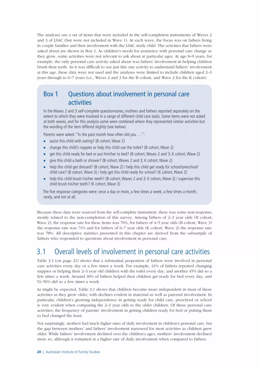
20 | Australian Institute of Family Studies
The analyses use a set of items that were included in the self-completion instruments of Waves 2 and 3 of LSAC (but were not included in Wave 1). At each wave, the focus was on fathers living in couple families and their involvement with the LSAC study child. The activities that fathers were asked about are shown in Box 1. As children’s needs for assistance with personal care change as they grow, some activities were not relevant to ask about at particular ages. At age 8–9 years, for example, the only personal care activity asked about was fathers’ involvement in helping children brush their teeth. As it was difficult to use just this one activity to understand fathers’ involvement at this age, these data were not used and the analyses were limited to include children aged 2–3 years through to 6–7 years (i.e., Waves 2 and 3 for the B cohort, and Wave 2 for the K cohort).
Box 1 Questions about involvement in personal care activities
In the Waves 2 and 3 self-complete questionnaires, mothers and fathers reported separately on the extent to which they were involved in a range of different child care tasks. Some items were not asked at both waves, and for this analysis some were combined where they represented similar activities but the wording of the item differed slightly (see below).
Parents were asked: “In the past month how often did you …”: ■ assist this child with eating? (B cohort, Wave 2) ■ change this child’s nappies or help this child use the toilet? (B cohort, Wave 2) ■ get this child ready for bed or put him/her to bed? (B cohort, Waves 2 and 3; K cohort, Wave 2) ■ give this child a bath or shower? (B cohort, Waves 2 and 3; K cohort, Wave 2) ■ help this child get dressed? (B cohort, Wave 2) / help this child get ready for school/preschool/
child care? (B cohort, Wave 3) / help get this child ready for school? (K cohort, Wave 2) ■ help this child brush his/her teeth? (B cohort, Waves 2 and 3; K cohort, Wave 2) / supervise this
child brush his/her teeth? (K cohort, Wave 3)
The five response categories were: once a day or more, a few times a week, a few times a month, rarely, and not at all.
Because these data were sourced from the self-complete instrument, there was some non-response, mostly related to the non-completion of this survey. Among fathers of 2–3 year olds (B cohort, Wave 2), the response rate for these items was 76%, for fathers of 4–5 year olds (B cohort, Wave 3) the response rate was 71% and for fathers of 6–7 year olds (K cohort, Wave 2) the response rate was 78%. All descriptive statistics presented in this chapter are derived from the subsample of fathers who responded to questions about involvement in personal care.
3.1 Overall levels of involvement in personal care activitiesTable 3.1 (on page 21) shows that a substantial proportion of fathers were involved in personal care activities every day or a few times a week. For example, 41% of fathers reported changing nappies or helping their 2–3 year old children with the toilet every day, and another 45% did so a few times a week. Around 30% of fathers helped their children get ready for bed every day, and 51–56% did so a few times a week.
As might be expected, Table 3.1 shows that children become more independent in most of these activities as they grow older, with declines evident in maternal as well as paternal involvement. In particular, children’s growing independence in getting ready for child care, preschool or school is very evident when comparing the 2–3 year olds to the older children. Of these personal care activities, the frequency of parents’ involvement in getting children ready for bed or putting them to bed changed the least.
Not surprisingly, mothers had much higher rates of daily involvement in children’s personal care, but the gap between mothers’ and fathers’ involvement narrowed for most activities as children grew older. While fathers’ involvement declined over the children’s ages, mothers’ involvement declined more so, although it remained at a higher rate of daily involvement when compared to fathers.

Chapter 3: Fathers’ involvement in children’s personal care activities
LSAC Annual Statistical Report 2011 | 21
Table 3.1 Frequency of parents’ involvement in personal care activities in the past month, fathers and mothers, B cohort Waves 2 and 3, and K cohort Wave 2
Fathers’ frequency of involvement Mothers’ daily
involve-ment
Once a day or more
A few times a week
A few times a month
Rarely or not at all
Total
% %
Assist child with eating
2–3 years 31.1 41.9 11.7 15.4 100.0 55.1
Change child’s nappies/help use toilet
2–3 years 40.9 44.7 7.4 6.9 100.0 88.8
Help child get dressed/ready for day
2–3 years 29.4 54.7 11.5 4.5 100.0 89.7
4–5 years 13.7 31.2 17.8 37.3 100.0 47.2
6–7 years 17.5 29.6 17.7 35.2 100.0 48.2
Get child ready for bed/put child to bed
2–3 years 27.6 55.9 10.7 5.8 100.0 79.2
4–5 years 30.9 52.2 10.7 6.2 100.0 72.0
6–7 years 28.2 50.7 11.6 9.5 100.0 62.2
Give child a bath or shower
2–3 years 18.8 55.7 15.6 10.0 100.0 64.4
4–5 years 17.0 51.4 18.1 13.5 100.0 61.2
6–7 years 11.4 44.2 18.0 26.2 100.0 40.4
Help/supervise child brushing teeth
2–3 years 21.1 46.5 14.9 17.4 100.0 69.8
4–5 years 20.3 46.2 15.1 18.4 100.0 59.0
6–7 years 13.1 36.0 15.3 35.7 100.0 32.7
Note: For fathers, sample sizes were 3,090 at 2–3 years, 2,732 at 4–5 years, and 2,904 at 6–7 years. For mothers, sample sizes were 3,198 at 2–3 years, 3,829 at 4–5 years, and 3,015 at 6–7 years. Numbers varied slightly on specific items due to small amounts of item non-response. Percentages may not total exactly 100.0% due to rounding.
Source: Baxter & Smart (2010), Table 11
3.2 Fathers’ characteristics and involvement in personal care
This section turns to the question of which fathers are more involved in their children’s personal care, and whether factors related to this involvement are apparent across the different types of personal care, and across children’s age groups. These analyses are informed by previous analyses in Baxter and Smart (2010) and by the vast international literature on fathering (e.g., Belsky, 1984; Lamb, 1997; Lamb, Pleck, Charnov, & Levine, 1987; Pleck, 1997).
Specifically, this section examines how father involvement varies with fathers’ usual paid work hours (not employed, and working 1–34 hours, 35–44 hours, 45–54 hours, or 55 hours or more per week); mothers’ usual paid work hours (not employed, and working 1–34 hours, or 35 hours or more per week); parents’ marital status (married or cohabiting); fathers having children living elsewhere; and the sex of the child.1
These analyses explore fathers’ responses regarding involvement in personal care by each of these variables. All these associations are examined by the age of the child. To assess whether
1 Other variables included in the multivariate analyses by Baxter and Smart (2010), but not examined here, were: mothers’ and fathers’ level of educational attainment, child’s health, child temperament, numbers of older and younger siblings, parent-reported financial wellbeing and happiness of the relationship, fathers’ age and relationship to child (biological or step-), fathers’ mental health, fathers’ main language spoken at home and fathers’ Indigenous status.
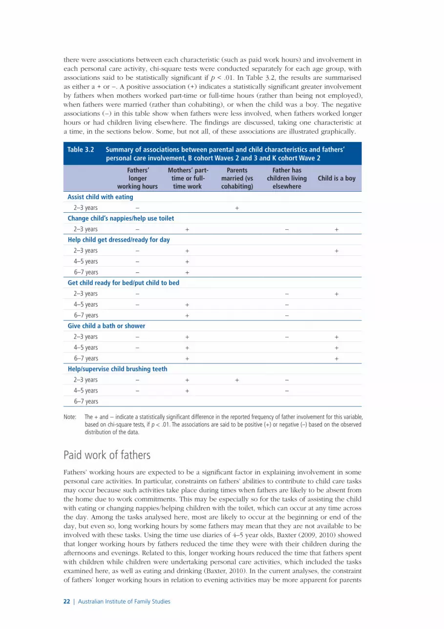
22 | Australian Institute of Family Studies
there were associations between each characteristic (such as paid work hours) and involvement in each personal care activity, chi-square tests were conducted separately for each age group, with associations said to be statistically significant if p < .01. In Table 3.2, the results are summarised as either a + or −. A positive association (+) indicates a statistically significant greater involvement by fathers when mothers worked part-time or full-time hours (rather than being not employed), when fathers were married (rather than cohabiting), or when the child was a boy. The negative associations (−) in this table show when fathers were less involved, when fathers worked longer hours or had children living elsewhere. The findings are discussed, taking one characteristic at a time, in the sections below. Some, but not all, of these associations are illustrated graphically.
Table 3.2 Summary of associations between parental and child characteristics and fathers’ personal care involvement, B cohort Waves 2 and 3 and K cohort Wave 2
Fathers’ longer
working hours
Mothers’ part-time or full-time work
Parents married (vs cohab iting)
Father has children living
elsewhereChild is a boy
Assist child with eating
2–3 years − +
Change child’s nappies/help use toilet
2–3 years − + − +
Help child get dressed/ready for day
2–3 years − + +
4–5 years − +
6–7 years − +
Get child ready for bed/put child to bed
2–3 years − − +
4–5 years − + −
6–7 years + −
Give child a bath or shower
2–3 years − + − +
4–5 years − + +
6–7 years + +
Help/supervise child brushing teeth
2–3 years − + + −
4–5 years − + −
6–7 years
Note: The + and − indicate a statistically significant difference in the reported frequency of father involvement for this variable, based on chi-square tests, if p < .01. The associations are said to be positive (+) or negative (–) based on the observed distribution of the data.
Paid work of fathersFathers’ working hours are expected to be a significant factor in explaining involvement in some personal care activities. In particular, constraints on fathers’ abilities to contribute to child care tasks may occur because such activities take place during times when fathers are likely to be absent from the home due to work commitments. This may be especially so for the tasks of assisting the child with eating or changing nappies/helping children with the toilet, which can occur at any time across the day. Among the tasks analysed here, most are likely to occur at the beginning or end of the day, but even so, long working hours by some fathers may mean that they are not available to be involved with these tasks. Using the time use diaries of 4–5 year olds, Baxter (2009, 2010) showed that longer working hours by fathers reduced the time they were with their children during the afternoons and evenings. Related to this, longer working hours reduced the time that fathers spent with children while children were undertaking personal care activities, which included the tasks examined here, as well as eating and drinking (Baxter, 2010). In the current analyses, the constraint of fathers’ longer working hours in relation to evening activities may be more apparent for parents
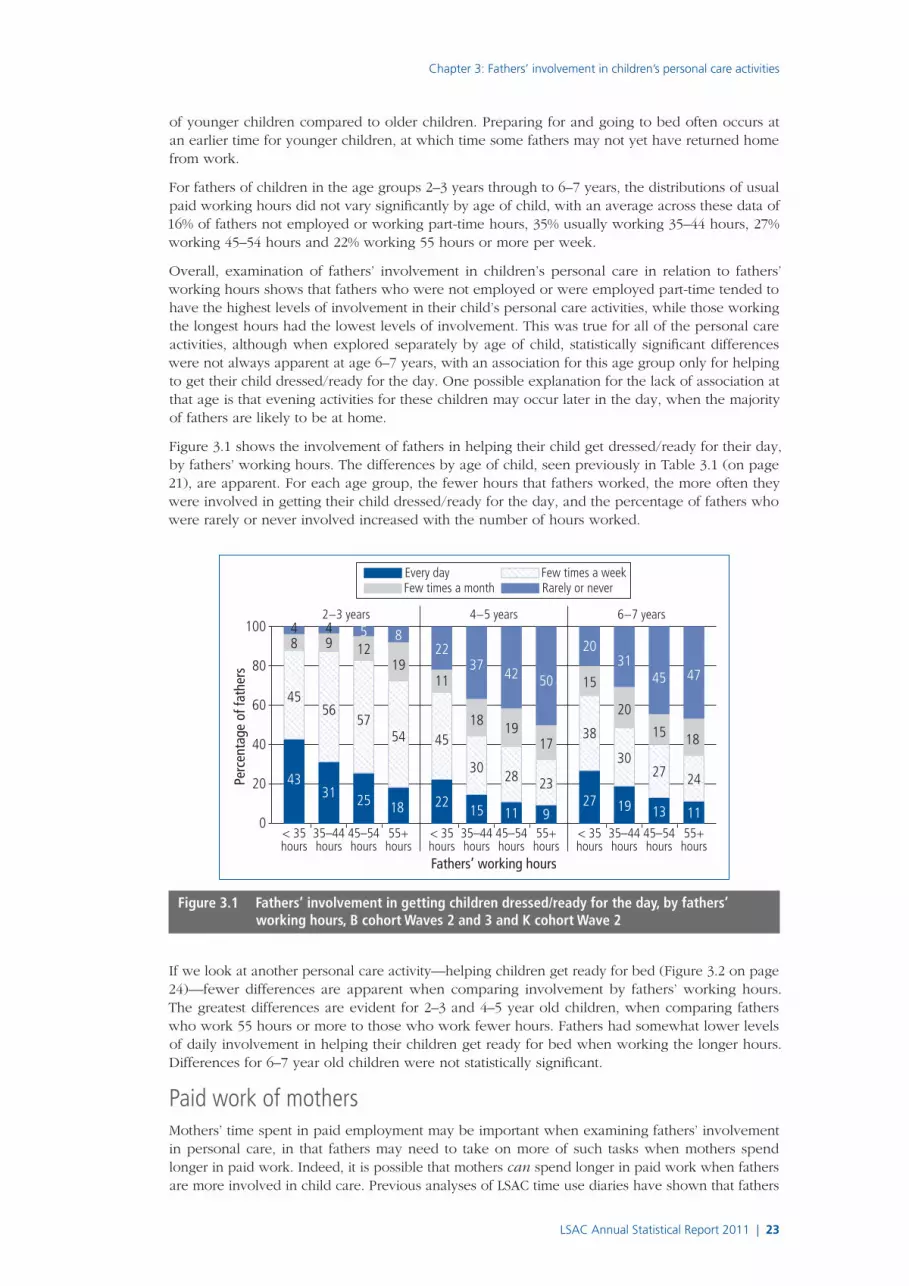
Chapter 3: Fathers’ involvement in children’s personal care activities
LSAC Annual Statistical Report 2011 | 23
of younger children compared to older children. Preparing for and going to bed often occurs at an earlier time for younger children, at which time some fathers may not yet have returned home from work.
For fathers of children in the age groups 2–3 years through to 6–7 years, the distributions of usual paid working hours did not vary significantly by age of child, with an average across these data of 16% of fathers not employed or working part-time hours, 35% usually working 35–44 hours, 27% working 45–54 hours and 22% working 55 hours or more per week.
Overall, examination of fathers’ involvement in children’s personal care in relation to fathers’ working hours shows that fathers who were not employed or were employed part-time tended to have the highest levels of involvement in their child’s personal care activities, while those working the longest hours had the lowest levels of involvement. This was true for all of the personal care activities, although when explored separately by age of child, statistically significant differences were not always apparent at age 6–7 years, with an association for this age group only for helping to get their child dressed/ready for the day. One possible explanation for the lack of association at that age is that evening activities for these children may occur later in the day, when the majority of fathers are likely to be at home.
Figure 3.1 shows the involvement of fathers in helping their child get dressed/ready for their day, by fathers’ working hours. The differences by age of child, seen previously in Table 3.1 (on page 21), are apparent. For each age group, the fewer hours that fathers worked, the more often they were involved in getting their child dressed/ready for the day, and the percentage of fathers who were rarely or never involved increased with the number of hours worked.
43
45
84
31
56
94
25
57
125
18
54
19
8
22
45
11
22
15
30
18
37
11
28
19
42
9
23
17
50
27
38
15
20
19
30
20
31
13
27
15
45
11
24
18
47
0
20
40
60
80
100
Perc
enta
ge o
f fat
hers
< 35hours
35–44hours
45–54hours
55+hours
< 35hours
35–44hours
45–54hours
55+hours
< 35hours
35–44hours
45–54hours
55+hours
Every day Few times a weekFew times a month Rarely or never
4−5 years 6−7 years2−3 years
Fathers’ working hours
Figure 3.1 Fathers’ involvement in getting children dressed/ready for the day, by fathers’ working hours, B cohort Waves 2 and 3 and K cohort Wave 2
If we look at another personal care activity—helping children get ready for bed (Figure 3.2 on page 24)—fewer differences are apparent when comparing involvement by fathers’ working hours. The greatest differences are evident for 2–3 and 4–5 year old children, when comparing fathers who work 55 hours or more to those who work fewer hours. Fathers had somewhat lower levels of daily involvement in helping their children get ready for bed when working the longer hours. Differences for 6–7 year old children were not statistically significant.
Paid work of mothersMothers’ time spent in paid employment may be important when examining fathers’ involvement in personal care, in that fathers may need to take on more of such tasks when mothers spend longer in paid work. Indeed, it is possible that mothers can spend longer in paid work when fathers are more involved in child care. Previous analyses of LSAC time use diaries have shown that fathers

24 | Australian Institute of Family Studies
spend more time with children when mothers are in paid work, especially full-time work, after taking into account fathers’ own working hours and other characteristics (Baxter, 2009; Baxter & Smart, 2010). Also, Baxter (2010) showed that fathers of 4–5 year olds are more involved in children’s personal care activities (including eating and drinking) when mothers work full-time hours, compared to when mothers are not employed.
While it is unclear whether associations between mothers’ working hours and father involvement varied by age of children, it is worth noting that mothers’ working hours themselves varied by age of children, as mothers were more likely to be out of employment and less likely to be employed full-time when they had 2–3 year olds (49% not employed, 40% employed part-time and 11% full-time), compared to when they had 4–5 year old children (42% not employed, 44% employed part-time and 14% full-time) or 6–7 year old children (39% not employed, 44% employed part-time and 18% full-time).
As summarised in Table 3.2 (on page 22), when mothers were in part-time or full-time paid work, fathers tended to report more frequent involvement in children’s personal care activities, relative to when mothers were not in employment. Statistically significant associations were apparent for most activities at most ages. These analyses sometimes showed that fathers’ involvement was particularly high when mothers worked full-time hours, but not when mothers worked part-time hours. This, for example, was the case for analyses of giving their child a bath or shower at ages 2–3 years and 4–5 years.
Figure 3.3 (on page 25) shows that fathers were most likely to help children get ready for the day if mothers worked full-time hours. Fathers had higher rates of daily involvement in this activity in these families, compared to families in which mothers were not employed or worked part-time hours. This was particularly apparent for the 4–5 year old children.
Variation in fathers’ involvement in getting children ready for bed in relation to mothers’ working hours, was statistically significant at ages 4–5 and 6–7 years. However, as Figure 3.4 (on page 25) shows, the differences were quite small. Statistically significant differences were also apparent for helping children with their bath or shower, and helping them brush their teeth and, for 2–3 year olds, changing nappies/helping children with the toilet. In these cases, fathers were more involved when mothers worked full-time hours. The other personal care activity for 2–3 year olds—helping them eat—did not vary with mothers’ work hours.
Every day Few times a weekFew times a month Rarely or never
34
50
88
31
54
106
27
58
105
17
58
16
8
34
48
126
35
48
107
29
54
116
21
56
14
9
27
49
12
12
29
51
11
9
30
49
10
11
24
49
15
12
0
20
40
60
80
100
< 35hours
35–44hours
45–54hours
55+hours
Perc
enta
ge o
f fat
hers
< 35hours
35–44hours
45–54hours
55+hours
< 35hours
35–44hours
45–54hours
55+hours
4−5 years 6−7 years2−3 years
Fathers’ working hours
Figure 3.2 Fathers’ involvement in getting children ready for bed, by fathers’ working hours, B cohort Waves 2 and 3 and K cohort Wave 2
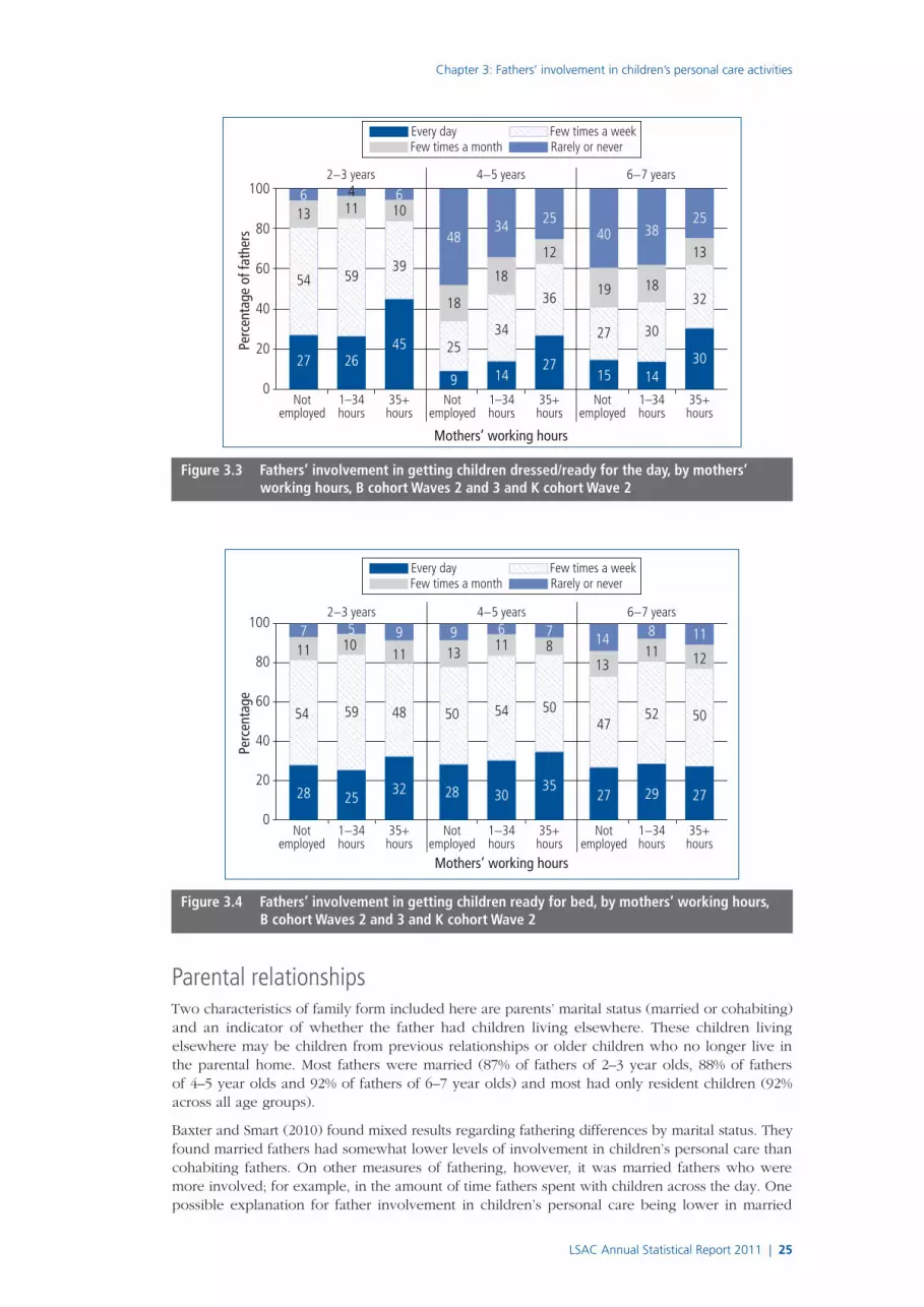
Chapter 3: Fathers’ involvement in children’s personal care activities
LSAC Annual Statistical Report 2011 | 25
Every day Few times a weekFew times a month Rarely or never
27
54
136
26
59
11
45
39
106
9
25
18
48
14
34
18
34
27
36
12
25
15
27
19
40
14
30
18
38
30
32
13
25
0
20
40
60
80
4100
Perc
enta
ge o
f fat
hers
4−5 years 6−7 years
Notemployed
1–34hours
35+hours
Notemployed
1–34hours
35+hours
Notemployed
1–34hours
35+hours
2−3 years
Mothers’ working hours
Figure 3.3 Fathers’ involvement in getting children dressed/ready for the day, by mothers’ working hours, B cohort Waves 2 and 3 and K cohort Wave 2
Every day Few times a weekFew times a month Rarely or never
28
50
139
30
54
116
35
50
87
27
47
13
14
29
52
118
27
50
12
11
4−5 years 6−7 years
28
54
117
25
59
105
32
48
11
9
0
20
40
60
80
100
Notemployed
1−34hours
35+hours
Notemployed
1−34hours
35+hours
Notemployed
1−34hours
35+hours
2−3 years
Perc
enta
ge
Mothers’ working hours
Figure 3.4 Fathers’ involvement in getting children ready for bed, by mothers’ working hours, B cohort Waves 2 and 3 and K cohort Wave 2
Parental relationshipsTwo characteristics of family form included here are parents’ marital status (married or cohabiting) and an indicator of whether the father had children living elsewhere. These children living elsewhere may be children from previous relationships or older children who no longer live in the parental home. Most fathers were married (87% of fathers of 2–3 year olds, 88% of fathers of 4–5 year olds and 92% of fathers of 6–7 year olds) and most had only resident children (92% across all age groups).
Baxter and Smart (2010) found mixed results regarding fathering differences by marital status. They found married fathers had somewhat lower levels of involvement in children’s personal care than cohabiting fathers. On other measures of fathering, however, it was married fathers who were more involved; for example, in the amount of time fathers spent with children across the day. One possible explanation for father involvement in children’s personal care being lower in married

26 | Australian Institute of Family Studies
couple families is that being married may indicate a more traditional approach to parenting when compared to cohabiting relationships, meaning that in married couples, mothers may take primary responsibility for child care tasks.
As shown in Table 3.2 (on page 22), when explored separately by age, statistically significant variation by marital status was rarely observed. Where it was observed, the differences related to married fathers being more frequently involved in assisting 2–3 year olds with eating, nappies/toilet and brushing teeth, and in getting 4–5 year olds ready for bed.
Having children living elsewhere was expected to diminish fathers’ time for involvement with resident children’s personal care, as the fathers’ time might sometimes be directed to non-resident children. Baxter and Smart’s (2010) analyses showed that this characteristic was quite often associated with lower levels of father involvement.
The summary in Table 3.2 (on page 22) shows that fathers with children living elsewhere were less likely to help their LSAC child with the typically evening activities of getting them ready for bed, helping with brushing teeth, or having a bath or shower. Differences between fathers with and without non-resident children are shown for a range of activities for 4–5 year old children in Figure 3.5.
Every day Few times a weekFew times a month Rarely or never
14311738
112516
49
020406080
100
Getting child dressed/ready for day
17
50
1815
14
44
2220
Helping with bathingor showering
31
52
116
21
49
1614
020406080
100
Perc
enta
ge o
f fat
hers
Getting childready for bed
21
45
1519
10381438
Helping/supervisingbrushing teeth
Residentchildren only
Non-residentchildren
Residentchildren only
Non-residentchildren
Figure 3.5 Fathers’ involvement in selected children’s personal care activities, by whether father has non-resident children, B cohort Wave 3
The other way in which parental relationships are commonly examined is by comparing biological fathers to step-fathers. In the multivariate analyses presented by Baxter and Smart (2010), biological fathers had higher levels of involvement in getting children ready for bed and helping with brushing teeth, or having a bath or shower. They did not differ significantly in their involvement in other personal care activities. There were too few step-fathers in the sample, however, to explore these relationships separately at different ages of children.
Boys and girlsAs well as age, the other child characteristic examined here is the gender of the child. It was expected that when differences between involvement in care of children varied by gender, it would show fathers being more involved with boys than with girls (see, for example, Marsiglio, 1991; Wood & Repetti, 2004). However, the extent to which such differences would be apparent among the younger children was not clear, especially given that gender differences in father involvement are not always apparent (see, for example, Bronte-Tinkew, Scott, Horowitz, & Lilja, 2009; Laflamme, Pomerleau, & Malcuit, 2002). It seems plausible that gender differences might emerge as children grow and children themselves favour the involvement of one parent over the other in personal care tasks, or parents feel that such tasks might be better overseen by the parent of the same gender.

Chapter 3: Fathers’ involvement in children’s personal care activities
LSAC Annual Statistical Report 2011 | 27
As shown in Table 3.2 (on page 22), there was some evidence of fathers being more involved in personal care activities for sons rather than daughters. However, the evidence of there being different associations with child gender across ages of children was quite mixed, with no evidence of overall greater involvement by fathers with sons as children grew older. The larger gender differences were apparent for the more personal of the activities: changing nappies/helping with the toilet and helping children with bathing or showering. These data are shown in Figure 3.6. At age 6–7 years it is especially apparent that fathers were more likely to be regularly (every day or a few times a week) involved in helping their boys with bathing or showering than they were with helping their girls.
4435
21 16 19 14 13 9
4248
5455 50
50 4639
7 9 16 16 1918 18
18
7 9 9 13 12 19 2234
0
20
40
60
80
100
Boy Girl Boy Girl Boy Girl Boy Girl2–3 years 2–3 years 4–5 years 6–7 years
Perc
enta
ge o
f fat
hers
Change nappies/help with toilet Help with bathing or showering
Every day Few times a week Few times a month Rarely or never
Figure 3.6 Fathers’ involvement in selected children’s personal care activities, by child gender, B cohort Waves 2 and 3, K cohort Wave 2
Variability in fathers’ involvementThe above analyses have highlighted some of the differences in fathers’ involvement in personal care activities. However, it is worth noting that despite these differences, the characteristics included here did not always explain a great deal of the variation in fathers’ personal care involvement. That is, while statistically significant differences were apparent, this did not always mean very low or very high levels of involvement in one group relative to another. For example, looking at fathers’ working hours, even among those working the longest hours, there remained sizable proportions who reported being frequently involved with activities such as getting children ready for the day. At the other end of the spectrum, fathers who were not in full-time jobs were much more likely than other fathers to have regular involvement in this activity, but nevertheless, some of these fathers were rarely or never involved. In the data on fathers’ involvement in the personal care of boys versus girls, while there are some clear differences, still the vast majority of fathers were involved at least a few times a week with their daughters’ personal care.
3.3 Fathers’ involvement in personal care and the co-parental relationship
Fathers’ involvement in their children’s personal care, and thus sharing these tasks with the mother, could be seen to be one way in which fathers contribute to the co-parental relationship. In this section, the LSAC data for 4–5 year old children (B cohort, Wave 3) are used to test this, by looking for associations between the personal care involvement items and mothers’ reports of fathers being a resource or support in raising their children. The restriction to this one age group is because this was the only time at which there was a question capturing views about co-parenting as well as questions about personal care involvement.

28 | Australian Institute of Family Studies
Of the sample in which fathers’ personal care involvement data were available, 47% of mothers said that fathers were always a resource or support, 37% said fathers were often a resource or support and 14% said they were sometimes a resource or support. Only 3% gave responses of “rarely” or “never”, and these are combined with “sometimes” in the analyses below.2
Figure 3.7 shows that fathers who were rated higher by their partner in terms of how often they were a resource or support in raising children more often had frequent involvement in children’s personal care activities. For example, among those fathers who were reported by mothers to be less often a resource of support, 28% helped get their child dressed or ready for the day at least a few times a week, 51% helped with bathing or showering at least a few times a week, and 67% helped get their child ready for bed at least a few times a week. These figures were considerably higher, at 52%, 74% and 86% respectively, for fathers who were rated as always being a resource or support.
Every day Few times a week Few times a month Rarely or never
7
21
18
53
12
29
19
41
17
35
16
33
20
40
60
80
100
Perc
enta
ge o
f fat
hers
How often father is a resource/support to mother
11
40
22
28
14
51
20
16
21
53
16
10
18
49
18
15
25
57
108
37
49
104
Getting child dressed/ready for day
Helping with bathingor showering
Getting childready for bed
0Less
than oftenOften Always Less
than oftenOften Always Less
than oftenOften Always
Figure 3.7 Fathers’ involvement in children’s personal care, by mothers’ ratings of fathers as a resource or support, B cohort Wave 3
However, it is interesting to note that involvement in personal care does not always guarantee a high rating of being a resource or support; just as infrequent involvement does not always guarantee a low rating. Clearly, providing input to children’s personal care is just one dimension of the co-parental relationship.
3.4 Fathers’ involvement in personal care and parentingFor fathers, being involved in the personal care of children may provide opportunities to develop a close relationship, or it may follow from fathers having a close relationship with their child. While these analyses do not set out to ascertain whether either of these pathways are more dominant, the data allow us to examine whether fathers who are more involved in children’s personal care tend to have a parenting style that is more “warm”. This warm parenting style is the average of responses regarding how often fathers do the following:
■ express affection by hugging, kissing and holding this child;
■ hug or hold this child for no particular reason;
■ tell this child how happy he/she makes you;
■ have warm, close times together with this child;
2 Parents were also asked to rate themselves in terms of how often they were a resource or support to their partner. Interestingly, overall the distribution based on fathers’ self-reports is similar to that of mothers’ reports about fathers. Of the fathers, 40% said they were always a resource or support, 41% said they were often a resource or support, 17% said they were sometimes a support and 3% said they were rarely or never a resource or support.
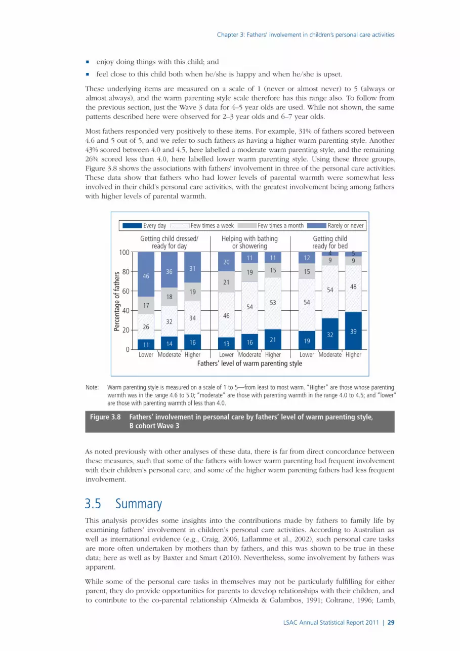
Chapter 3: Fathers’ involvement in children’s personal care activities
LSAC Annual Statistical Report 2011 | 29
■ enjoy doing things with this child; and
■ feel close to this child both when he/she is happy and when he/she is upset.
These underlying items are measured on a scale of 1 (never or almost never) to 5 (always or almost always), and the warm parenting style scale therefore has this range also. To follow from the previous section, just the Wave 3 data for 4–5 year olds are used. While not shown, the same patterns described here were observed for 2–3 year olds and 6–7 year olds.
Most fathers responded very positively to these items. For example, 31% of fathers scored between 4.6 and 5 out of 5, and we refer to such fathers as having a higher warm parenting style. Another 43% scored between 4.0 and 4.5, here labelled a moderate warm parenting style, and the remaining 26% scored less than 4.0, here labelled lower warm parenting style. Using these three groups, Figure 3.8 shows the associations with fathers’ involvement in three of the personal care activities. These data show that fathers who had lower levels of parental warmth were somewhat less involved in their child’s personal care activities, with the greatest involvement being among fathers with higher levels of parental warmth.
Every day Few times a week Few times a month Rarely or never
11
26
17
46
14
32
18
36
16
34
19
31
0
20
40
60
80
100
Perc
enta
ge o
f fat
hers
Fathers’ level of warm parenting style
Getting child dressed/ready for day
13
46
21
20
16
54
19
11
21
53
15
11
Helping with bathingor showering
19
54
15
12
32
54
94
39
48
95
Getting childready for bed
Lower Moderate Higher Lower Moderate Higher Lower Moderate Higher
Note: Warm parenting style is measured on a scale of 1 to 5—from least to most warm. “Higher” are those whose parenting warmth was in the range 4.6 to 5.0; “moderate” are those with parenting warmth in the range 4.0 to 4.5; and “lower” are those with parenting warmth of less than 4.0.
Figure 3.8 Fathers’ involvement in personal care by fathers’ level of warm parenting style, B cohort Wave 3
As noted previously with other analyses of these data, there is far from direct concordance between these measures, such that some of the fathers with lower warm parenting had frequent involvement with their children’s personal care, and some of the higher warm parenting fathers had less frequent involvement.
3.5 SummaryThis analysis provides some insights into the contributions made by fathers to family life by examining fathers’ involvement in children’s personal care activities. According to Australian as well as international evidence (e.g., Craig, 2006; Laflamme et al., 2002), such personal care tasks are more often undertaken by mothers than by fathers, and this was shown to be true in these data; here as well as by Baxter and Smart (2010). Nevertheless, some involvement by fathers was apparent.
While some of the personal care tasks in themselves may not be particularly fulfilling for either parent, they do provide opportunities for parents to develop relationships with their children, and to contribute to the co-parental relationship (Almeida & Galambos, 1991; Coltrane, 1996; Lamb,

30 | Australian Institute of Family Studies
1997). Also, fathers’ involvement in their children’s personal care activities may reflect their interest in spending time with children and their desire to have an active parenting role. Certainly these data have shown that there is an association between involvement in personal care activities and warm parenting, as well as in mothers’ perceptions of fathers as being a resource and support. In these analyses, we could not ascertain whether fathers’ involvement in children’s personal care came about because of a different attitude or motivation toward children and parenting, but it is likely that this is to some extent true.
These analyses showed that certain factors were associated with different levels of involvement by fathers in children’s personal care. In particular, fathers’ paid working hours was an important factor, with lower levels of involvement found among those working longer hours. This was less apparent for the 4–5 year old children, for whom involvement by fathers (and mothers) across the range of activities had declined relative to younger children. These analyses also showed that when mothers worked longer hours, fathers tended to be more involved in personal care activities. Differences between married and cohabiting fathers were small and usually not statistically significant. On the other hand, lower levels of involvement were often found for fathers who had non-resident children. Fathers were found to be more involved with the care of boys than girls, especially for the more personal activities, although differences were not all statistically significant.
An important point is that factors beyond those analysed here are likely to contribute to different levels of involvement by fathers. In fact this may, in some respects, come back to the degree to which fathers wish to be involved as parents—their level of motivation (Lamb, 1997; Lamb et al., 1987). For example, even among fathers who work long hours, there will be fathers who frequently help with the care of children; and in families with mothers who are not employed, there will be full-time employed fathers who like to share the care of children on weekends, or in the morning or evenings.
This paper has examined just one way in which fathers can contribute to the upbringing of children, and as such does not present a comprehensive picture of fathering. Nevertheless, the analyses allow us to see that involvement in children’s personal care is connected to other aspects of fathering (parenting style and co-parenting) and that it does vary with some characteristics of fathers and families.
Gaining greater insights into the ways in which fathers contribute to family life, and of factors that are associated with lesser or greater involvement by fathers, can be used to inform the development of policies that may affect families’ decisions about the sharing of child care tasks. While government policy and fathering are most often discussed in relation to separated families, there are areas in which policy can also be relevant to fathering in intact families. Most often, this is discussed in relation to issues of work and family. For example, as we have seen here, there are different patterns of father involvement according to parental employment patterns, and thus the nature of the labour market and related workplace policies may make a difference to the ways in which fathers can participate in various child care tasks. Policies concerning leave for fathers or concerning access to family-friendly work arrangements are particularly relevant here.
We have seen here that the majority of fathers in the LSAC study:
■ have some involvement with their child’s personal care;
■ are reported to be supportive partners; and
■ exhibit warm parenting behaviours.
While a small proportion, there are some fathers who portray a less positive picture, and this is a reminder that some fathers may face certain barriers to being involved as a parent. For these fathers, there may be opportunities for policies and programs to encourage and support involvement in family life. This may include, for example, helping to overcome potential barriers, such as those that can arise through relationship conflict and mental health difficulties.3
This study of fathers’ involvement in children’s personal care provides some insights that have not previously been explored in relation to how fathers participate in raising their children. With LSAC being a longitudinal study, it will be interesting to see how fathers’ involvement in these activities relates to patterns of fathering at later ages as children grow older.
3 For examples of such programs, see <www.aifs.gov.au/cafca/topics/issue/issue.html#parenting>.

Chapter 3: Fathers’ involvement in children’s personal care activities
LSAC Annual Statistical Report 2011 | 31
3.6 Further readingBaxter, J. A. (2007). When dad works long hours: How work hours are associated with fathering 4–5-year-old children. Family Matters, 77, 60–69.
Baxter, J. A. (2010). An exploration of the timing and nature of parental time with 4–5 year olds using Australian children’s time use data (Research Paper No. 45). Melbourne: Australian Institute of Family Studies.
Baxter, J. A., Gray, M., Alexander, M., Strazdins, L., & Bittman, M. (2007). Mothers and fathers with young children: Paid employment, caring and wellbeing (Social Policy Research Paper No. 30). Canberra: Department of Families, Housing, Community Services and Indigenous Affairs.
Baxter, J. A., & Hayes, A. (2007). How four year olds spend their day: Insights into the caring contexts of young children. Family Matters, 76, 34–43.
Baxter, J. A., & Smart, D. (2010). Fathering in Australia among couple families with young children (Occasional Paper No. 37). Canberra: Department of Families, Housing, Community Services and Indigenous Affairs.
Hosking, A., Whitehouse, G., & Baxter, J. (2010). Duration of leave and resident fathers’ involvement in infant care in Australia. Journal of Marriage and Family, 72, 15.
3.7 ReferencesAlmeida, D. M., & Galambos, N. L. (1991). Examining father involvement and the quality of father–adolescent relations. Journal of Research on Adolescence, 1(2), 155–172.
Baxter, J. A. (2009). Parental time with children: Do job characteristics make a difference? (AIFS Research Paper No. 44). Melbourne: Australian Institute of Family Studies.
Baxter, J. A. (2010). An exploration of the timing and nature of parental time with 4–5 year olds using Australian children’s time use data (Research Paper No. 45). Melbourne: Australian Institute of Family Studies.
Baxter, J. A., Gray, M., Alexander, M., Strazdins, L., & Bittman, M. (2007). Mothers and fathers with young children: Paid employment, caring and wellbeing (Social Policy Research Paper No. 30). Canberra: Department of Families, Community Services and Indigenous Affairs.
Baxter, J. A., & Smart, D. (2010). Fathering in Australia among couple families with young children (Occasional Paper No. 37). Canberra: Department of Families, Housing, Community Services and Indigenous Affairs.
Belsky, J. (1984). The determinants of parenting: A process model. Child Development, 55(1), 83–96.
Bronte-Tinkew, J., Scott, M. E., Horowitz, A., & Lilja, E. (2009). Pregnancy intentions during the transition to parenthood and links to coparenting for first-time fathers of infants. Parenting, 9(1), 1–35.
Coltrane, S. (1996). Family man. New York: Oxford University Press
Craig, L. (2006). Does father care mean fathers share? A comparison of how mothers and fathers in intact families spend time with children. Gender and Society, 20(2), 259–281.
Craig, L., & Mullan, K. (2010). Parenthood, gender and work family time in the United States, Australia, Italy, France, and Denmark. Journal of Marriage and Family, 72(5), 1344–1361.
Laflamme, D., Pomerleau , A., & Malcuit , G. (2002). A comparison of fathers’ and mothers’ involvement in child care and stimulation behaviors during free-play with their infants at 9 and 15 months. Sex roles, 47(11), 507–518.
Lamb, M. E. (1997). Fathers and child development: An introductory overview and guide. In The role of the father in child development (3rd ed., pp. 1–18). New York: Wiley.
Lamb, M. E., Pleck, J., Charnov, E., & Levine, J. (1987). A biosocial perspective on paternal behavior and involvement. In J. B. Lancaster, J. Altmann, A. S. Rossi, & L. R. Sherrod (Eds.), Parenting across the life span: Biosocial dimensions (pp. 111–141). New York: Aldine de Gruyter.
Marsiglio, W. (1991). Paternal engagement activities with minor children. Journal of Marriage and Family, 53(4), 973–986.
Pleck, J. (1997). Paternal involvement: Levels, sources and consequences. In M. E. Lamb (Ed.), The role of the father in child development (3rd ed., pp. 66–103). New York: Wiley.
Van Egeren, L. A., & Hawkins, D. P. (2004). Coming to terms with coparenting: Implications of definition and measurement. Journal of Adult Development, 11(3), 165–178.
Wang, R., & Bianchi, S. M. (2009). ATUS fathers’ involvement in child care. Social Indicators Research, 93(1), 141–145.
Wilson, K. R., & Prior, M. R. (2010). Father involvement: The importance of paternal solo care. Early Child Development and Care, 180(10), 1391–1405.
Wood, J. J., & Repetti, R. L. (2004). What gets dad involved? A longitudinal study of change in parental child caregiving involvement. Journal of Family Psychology, 18(1), 237–249.


Chapter 4: Families with a child with disability
LSAC Annual Statistical Report 2011 | 33
Brigit MaguireAustralian Institute of Family Studies
Supporting children with disability and their carers and families is an important priority for the Australian Government. The recent commitment to establishing a National Disability Insurance Scheme (Macklin, Gillard, & McLucas, 2011), and the appointment of a new Minister for
Disability Reform (Macklin, 2011) signals a changing policy environment in relation to providing support for people with disability, their carers and their families. A National Disability Insurance Scheme would support people with disability and allow them to exercise choice and control in their lives and thereby achieve their best in life (McLucas, 2011). While a National Disability Insurance Scheme focuses on providing support to individuals with disability, this support will have important flow-on effects for their families.
Within this context, this chapter provides information about the experiences of families with children with disability. While all families, including those with a child with disability, have a wide range of strengths and capabilities, there is broad recognition that families with a child with disability may experience barriers to full participation in society. On a population level, people with disability experience a range of social disadvantages, including lower participation in education and employment, reduced economic resources, greater financial stress, and fewer opportunities for participation in society (Australian Institute of Health and Welfare [AIHW], 2009; Edwards & Higgins, 2009; Saunders, 2006). When parents are carers of children with disability they also experience barriers to employment and social participation (Australian Bureau of Statistics [ABS], 2009a; Edwards & Gray, 2009; Edwards, Higgins, Gray, Zmijewski, & Kingston, 2008; House of Representatives Standing Committee on Family Housing Community and Youth, 2009), and these disadvantages can then flow on to those children and other children in the family (Emerson & Llewellyn, 2008).
In order to address the barriers that people with disability and their families face, it is essential to understand the nature of these experiences. This chapter therefore focuses on families’ experiences of joblessness, financial hardship and accessing social support. This is in recognition that these families may experience not only financial barriers, but also restrictions in accessing different types of social support, including emotional and practical support. The Longitudinal Study of Australian Children (LSAC) collects extensive information, covering a range of topics, about all members of the study child’s household, which provides a unique opportunity to explore the broad experiences of families with a child with disability and to directly compare them with families without a child with disability.
This chapter uses data from the B and K cohorts at Waves 2 and 3 to address the following questions:
■ How many LSAC study children and siblings had a disability that restricted their everyday activities? How many families had a child with disability at multiple time points?
■ Did families with a child with disability experience higher rates of joblessness or a greater number of financial hardships than families without a child with disability?
■ Did parents with a child with disability have access to the same level of social support as parents without a child with disability? Did they feel that they were able to get the help/support they needed as often as parents without a child with disability?
There are two commonly used measures of disability in the Australian population, used by both the Australian Bureau of Statistics and the Australian Institute of Health and Welfare. The first measure
4Families with a child with disabilityJoblessness, financial hardship and social support

34 | Australian Institute of Family Studies
defines people with disability as being those with a condition that has lasted or is expected to last at least six months and who experience limitations or restrictions in their performance of an activity or on their participation in society (ABS, 2003, 2009b; AIHW, 2009). The second measure is a subset of the first measure and defines people who experience a severe or profound core activity limitation as being those who sometimes or always need help with mobility, self-care or communication (AIHW, 2009).
Because LSAC is a study of the general population of children and their families, and not a survey of those with disability in particular, the first of these measures (from ABS, 2003) has been used to collect data in LSAC, and is used throughout this chapter. It is possible that the LSAC sample under-represents children with a severe or profound core activity limitation, because this level of disability may have restricted their family’s participation in the study.
The questions about disability used in this chapter are taken from the LSAC Household Form, a component of the interview that contains questions asked about every member of the study child’s household. Study children and their siblings were defined as having a disability if the respondent (usually the primary parent) answered “yes” to both of the following two questions in relation to the study child/sibling:1
1. Does [person] have any medical conditions or disabilities that have lasted, or are likely to last, for six months or more?
a. Sight problems (not corrected by glasses or contact lenses)
b. Hearing problems (where communication is restricted, or an aid to assist with or substitute for hearing is used)
c. Speech problems
d. Blackouts, fits or loss of consciousness
e. Difficulty learning or understanding things
f. Limited use of arms or fingers
g. Difficulty gripping things
h. Limited use of legs or feet
i. Any condition that restricts physical activity or physical work
j. Any disfigurement or deformity
2. Still thinking of conditions lasting six months or more, is [person] restricted in everyday activities because of any of the following?
a. Shortness of breath or breathing difficulty
b. Chronic or recurring pain
c. A nervous or emotional condition (requiring treatment)
d. Any mental illness for which help or supervision is required long-term
e. Long-term effects as a result of a head injury, stroke or other brain damage
f. Any other long-term condition, such as arthritis, asthma, heart disease, Alzheimer’s, dementia, etc.
g. Any other long-term disease or condition that requires treatment or medication
All references to a “child with disability” in the remainder of this chapter are to those who meet both of these criteria. Readers should note that some children were reported as not having a disability but as being restricted in their everyday activities, and vice versa; these children were not defined as having a disability for the purposes of this chapter.
The most important caveat to note when reading this chapter is that it groups a very wide range of disabilities together, including those that may have different effects on carers and families, and those that have different financial implications. While such a grouping is appropriate for a general study of child development, such as LSAC, further insight into the caring and financial implications of having children with particular disabilities is better provided by other research that relates to specific types of disabilities.
1 Note that there were slight wording differences between Waves 2 and 3 in the lists of conditions for both of these questions (which were presented to respondents on a prompt card); however, these differences were not expected to lead to any substantial variations in results for the two waves.

Chapter 4: Families with a child with disability
LSAC Annual Statistical Report 2011 | 35
4.1 Families with a child with disabilityTable 4.1 shows the percentages of LSAC families with at least one child with disability who was restricted in their everyday activities. The table shows that between 3% and 5% of LSAC families included at least one child with disability, with the higher percentages being in the K cohort, particularly at age 6–7 years. Because there are more siblings than study children in the sample (i.e., there is only one study child for each family, but potentially multiple siblings per family), families are slightly more likely to have a sibling with disability compared to the study children themselves. For the B cohort, percentages of children with disability remained consistent between Waves 2 and 3 (at 3%), whereas for the K cohort, percentages decreased slightly between the two waves (from 5% to 3%). This may reflect a peak in the percentages of children with disability in the early school years, which has been observed in other data sources (e.g., AIHW, 2009).
Table 4.1 Study children and siblings with disability, B and K cohorts, Waves 1–3
Age of B cohort study child Age of K cohort study child
2–3 years 4–5 years 6–7 years 8–9 years
% %
Study child has a disability and is restricted in everyday activities
0.9 1.3 2.1 1.6
At least one sibling has a disability and is restricted in everyday activities
2.0 1.8 2.9 2.0
Total number of families with at least one child with disability who is restricted in everyday activities
2.9 3.0 4.6 3.3
No. of observations 4,606 4,253 4,464 4,196
Table 4.2, which includes only those families who responded at both Wave 2 and Wave 3, shows the number of waves at which at least one child in the family was reported to have a disability and to be restricted in everyday activities. K cohort families were more likely to have a child with disability at one wave (5%) or two waves (2%) compared to the B cohort (4% one wave and 1% two waves). The relatively low percentage of families with a child with disability at multiple waves suggests that in the LSAC sample, many disabilities (or at least the restrictions arising from them) may to some extent have been transitory.
Table 4.2 Waves at which at least one child in family had a disability, B and K cohorts, Waves 1–3
B cohort K cohort
%
Neither Wave 2 nor Wave 3 95.0 93.6
One wave (either Wave 2 or Wave 3) 4.2 4.7
Both Wave 2 and Wave 3 0.9 1.7
Totals 100.0 100.0
No. of observations 4,253 4,196
Note: Only includes families who responded at both Waves 2 and 3. Percentages may not total exactly 100.0% due to rounding.
4.2 Families with a child with disability and experience of joblessness and financial hardship
This section investigates the experiences of families with a child with disability (whether the study child or a sibling) in relation to joblessness and financial hardship.
JoblessnessJoblessness affects a family’s financial wellbeing and ability to purchase any specialised equipment, medication or services a child with disability may need, as well as having broader effects on the family and children (Reference Group on Welfare Reform, 2000). In this chapter, a two-parent

36 | Australian Institute of Family Studies
family is defined as jobless if neither parent was employed, and a lone-parent family is defined as jobless if the lone parent was not employed.2
Table 4.3 shows the association between whether a family had a child with disability and whether the family was jobless. The table shows that in both cohorts, families with a child with disability were more likely to be jobless. In the B cohort (when the study child was 4–5 years old), this difference was not statistically significant. In the K cohort (when the study child was 8–9 years old), the difference was statistically significant.
Table 4.3 Experience of joblessness in families with and without a child with disability, B and K cohorts, Wave 3
B cohort (study child 4–5 years old) K cohort (study child 8–9 years old)
Family includes child with disability
Family does not include child
with disability
Family includes child with disability
Family does not include child
with disability
% %
Jobless 13.9 10.6 18.3 8.0
At least one job 86.1 89.4 81.7 92.0
Totals 100.0 100.0 100.0 100.0
No. of observations 124 4,127 144 4,051
Note: B cohort: χ2 (1, n = 4,251) = 1.4, p = .43; K cohort: χ2 (1, n = 4,195) = 18.7, p < .01.
Previous analysis using LSAC data has shown that lone-parent families are much more likely to be jobless compared to two-parent families (see Gray & Baxter, 2011). The numbers of families with a child with disability in the LSAC sample are too small to support a separate investigation for lone-parent and two-parent families of the relationship between joblessness and whether the family includes a child with disability. However, Table 4.4 shows that for both cohorts, there was no statistically significant relationship between whether the family was a lone-mother or two-parent family and whether the family included a child with disability; that is, the two groups of families with and without a child with disability comprised similar proportions of lone-mother families and two-parent families. This suggests that the higher rates of joblessness in families with a child with disability are not necessarily because of a greater number of lone-mother families in that group.
Table 4.4 Family type in families with and without a child with disability, B and K cohorts, Wave 3
B cohort (study child 4–5 years old) K cohort (study child 8–9 years old)
Family includes child with disability
Family does not include child
with disability
Family includes child with disability
Family does not include child
with disability
% %
Lone-mother family 18.6 13.4 18.8 15.3
Two-parent family 81.4 86.6 81.2 84.7
Totals 100.0 100.0 100.0 100.0
No. of observations 124 4,118 143 4,012
Note: There were very few lone-father families (less than 1% for each cohort), so these were excluded from analyses comparing different family types. B cohort: χ2 (1, n = 4,242) = 2.8, p = .15; K cohort: χ2 (1, n = 4,155) = 1.2, p = .33.
2 See Chapter 1 for information about how lone-parent families are defined.

Chapter 4: Families with a child with disability
LSAC Annual Statistical Report 2011 | 37
Financial hardship
Each study respondent (the study child’s primary parent) was asked a series of questions (based on Bray, 2001) to measure the family’s experience of financial hardship:
In the last 12 months, have any of these happened to you/any members of the household because you/any of you were short of money:
1. Could not pay gas, electricity or telephone bills on time
2. Could not pay the mortgage or rent payments on time
3. Went without meals
4. Were unable to heat or cool your home
5. Pawned or sold something because you needed cash
6. Sought assistance from a welfare or community organisation
A greater number of hardships experienced indicates greater financial difficulty, such that a family who has experienced two of these will most likely be in greater difficulty than a family who experiences just one. Table 4.5 shows the differences between families with/without a child with disability in terms of the number of financial hardships they experienced. The table shows similar (statistically significant) results for the two cohorts, with families with a child with disability being more likely to experience at least one financial hardship (37% compared to 19–21% of families without a child with disability) and more likely to experience a greater number of financial difficulties.
Table 4.5 Experience of multiple financial hardships in families with and without a child with disability, B and K cohorts, Wave 3
B cohort (study child 4–5 years old) K cohort (study child 8–9 years old)
Family includes child with disability
Family does not include child
with disability
Family includes child with disability
Family does not include child
with disability
% %
No hardships 63.3 79.1 63.2 80.8
One hardship 22.1 13.1 18.6 10.8
Two hardships 8.9 5.4 11.5 5.8
Three or more hardships 5.8 2.4 6.7 2.6
Totals 100.0 100.0 100.0 100.0
No. of observations 124 4,111 143 4,042
Note: B cohort: χ2 (3, n = 4,235) = 19.4, p < .01; K cohort: χ2 (3, n = 4,185) = 28.1, p < .01. Percentages may not total exactly 100.0% due to rounding.
Table 4.6 (on page 38) provides more detail about the specific financial hardships that families experienced. The table shows that B cohort families with a child with disability were statistically more likely to report being unable to pay bills on time, going without meals, and being unable to heat or cool their home, compared to families without a child with disability. For example, 29% of families with a child with disability reported being unable to pay their gas, electricity or telephone bills on time at least once in the previous 12 months, compared to 17% of families without a child with disability. Out of the six financial hardship categories, K cohort families with a child with disability were statistically more likely to report being unable to pay bills and being unable to pay the mortgage or rent payments, compared to families without a child with disability.

38 | Australian Institute of Family Studies
4.3 Families with a child with disability and access to social support
This section of the chapter looks at whether parents with/without a child with disability have different levels of access to social support. As a measure of social support, both parents were asked a series of questions based on the Social Support Survey (Ware & Sherbourne, 1992), which are summarised into four measures:
People sometimes look to others for companionship, assistance, or other types of support. How often are each of the following kinds of support available to you if you need it?
1. Emotional/informational support:
� Someone you can count on to listen to you when you need to talk
� Someone to confide in or talk to about yourself or your problems
� Someone to share your most private worries and fears with
� Someone to turn to for suggestions about how to deal with a personal problem
2. Tangible support:
� Someone to help you if you were confined to bed
� Someone to take you to the doctor if you needed it
� Someone to prepare your meals if you were unable to do it yourself
� Someone to help with daily chores if you were sick
Table 4.6 Experience of specific financial hardships in families with and without a child with disability, B and K cohorts, Wave 3
B cohort (study child 4–5 years old)
K cohort (study child 8–9 years old)
Family includes child with disability
Family does not include child
with disability
Family includes child with disability
Family does not include child
with disability
% %
Could not pay gas, electricity or telephone bills on time
28.8 16.9 * 29.3 15.7 *
Could not pay the mortgage or rent payments on time
11.5 6.9 15.7 6.9 *
Went without meals 5.5 1.6 * 4.8 1.7
Were unable to heat or cool your home
4.0 0.7 * 2.7 1.4
Pawned or sold something because you needed cash
Sought assistance from
1.4 3.1 6.3 2.4
a welfare or community organisation
7.4 3.1 7.9 3.3
No. of observations 124 4,111 143 4,042
Note: * Statistically significant difference between families with/without a child with disability. Could not pay gas, electricity or telephone bills on time: B cohort: χ2 (1, n = 4,235) = 12.2, p < .01; K cohort: χ2 (1, n = 4,185) = 18.3, p < .01. Could not pay the mortgage or rent payments on time: B cohort: χ2 (1, n = 4,235) = 3.9, p = .05; K cohort: χ2 (1, n = 4,185) = 15.6, p < .01. Went without meals: B cohort: χ2 (1, n = 4,235) = 11.2, p < .01; K cohort: χ2 (1, n = 4,185) = 6.8, p = .01. Were unable to heat or cool your home: B cohort: χ2 (1, n = 4,235) = 15.9, p < .01; K cohort: χ2 (1, n = 4,185) = 1.42, p = .25. Pawned or sold something because you needed cash: B cohort: χ2 (1, n = 4,235) = 1.3, p = .23; K cohort:χ2 (1, n = 4,185) = 8.0, p = .01. Sought assistance from a welfare or community organisation: B cohort: χ2 (1, n = 4,235) = 7.4, p = .01; K cohort: χ2 (1, n = 4,185) = 8.6, p = .02.

Chapter 4: Families with a child with disability
LSAC Annual Statistical Report 2011 | 39
3. Affectionate support:
� Someone who shows you love and affection
� Someone to love and make you feel wanted
� Someone who hugs you
4. Positive social interaction:
� Someone to have a good time with
� Someone to get together with for relaxation
� Someone to do something enjoyable with
Response options: 1 = None of the time, 2 = A little of the time, 3 = Some of the time, 4 = Most of the time, 5 = All of the time.
The items making up each of these four measures were averaged, giving an overall score for each measure, such that higher scores reflected a greater level of social support. A measure of “total social support” was also generated from the average of all items across the four measures. Table 4.7 shows that there was a statistically significant difference between mothers with a child with disability and mothers without a child with disability in the K cohort, with mothers with a child with disability reporting significantly lower levels of access to emotional/informational support, tangible support, positive social interaction and total social support. There were no significant differences between the two groups for B cohort mothers or B and K cohort fathers.
Table 4.7 Mothers’ and fathers’ access to social support, by whether family includes a child with disability, B and K cohorts, Wave 3
Mothers Fathers
Family includes child with disability
Family does not include child with disability
Family includes child with disability
Family does not include child with disability
Mean score (n) Mean score (n)
B cohort (study child 4–5 years old)
Emotional/informational support 3.85 (104) 3.89 (3,697) 3.53 (72) 3.65 (2,664)
Tangible support 3.59 (103) 3.76 (3,694) 4.24 (72) 4.22 (2,660)
Affectionate support 4.18 (104) 4.21 (3,692) 4.26 (72) 4.27 (2,655)
Positive social interaction 3.94 (104) 4.07 (2,693) 4.15 (72) 4.16 (2,657)
Total social support 3.86 (104) 3.96 (3,697) 4.02 (73) 4.05 (2,666)
K cohort (study child 8–9 years old)
Emotional/informational support 3.42 (122) 3.90 * (3,595) 3.47 (85) 3.56 (2,608)
Tangible support 3.31 (122) 3.79 * (3,591) 4.08 (85) 4.12 (2,605)
Affectionate support 3.91 (122) 4.19 (3,588) 4.09 (85) 4.15 (2,601)
Positive social interaction 3.69 (122) 4.05 * (3,591) 4.02 (85) 4.09 (2,598)
Total social support 3.55 (122) 3.95 * (3,596) 3.89 (85) 3.96 (2,610)
Note: * Statistically significant difference between families with/without a child with disability. B cohort mothers: t(271): Emotional/informational support = 0.32, p = .75; Tangible support = 1.48, p = .14; Affectionate support = 0.27, p = .79; Positive social interaction = 1.07, p = .29; Total social support = 0.98, p = .33. B cohort fathers: t(270): Emotional/informational support = 0.89, p = .37; Tangible support = –0.16, p = .87; Affectionate support = 0.07, p = .95; Positive social interaction = 0.12, p = .91; Total social support = 0.77, p = .30. K cohort mothers: t(270): Emotional/informational support = 3.98, p < .01; Tangible support = 3.69, p < .01; Affectionate support = 2.40, p = .02; Positive social interaction = 3.01, p < .01; Total social support = 3.90, p < .01. K cohort fathers: t(269): Emotional/informational support = 0.57, p = .57; Tangible support = 0.31, p = .76; Affectionate support = 0.39, p = .70; Positive social interaction = 0.53, p = .60; Total social support = 0.54, p = .59.

40 | Australian Institute of Family Studies
Parents were also asked how often they felt that they needed help/support from someone but were unable to get it. Table 4.8 shows how mothers and fathers with and without a child with disability responded to this question. The table shows a similar pattern for both mothers and fathers for both cohorts. Mothers with a child with disability were more likely to say they were unable to get the help/support they needed “very often” or “often” (B cohort: 24%, K cohort: 25%) compared to mothers without a child with disability (B cohort: 11%, K cohort: 12%). This difference was statistically significant for both cohorts.
Table 4.8 How often mothers/fathers needed help or support but couldn’t get it, by whether family includes a child with disability, B and K cohorts, Wave 3
Needed help or support but couldn’t get it
Mothers Fathers
Family includes child with disability
Family does not include child
with disability
Family includes child with disability
Family does not include child
with disability
% %
B cohort (study child 4–5 years old)
Very often 7.4 2.6 0.0 2.1
Often 16.3 8.7 10.7 6.1
Sometimes 52.0 52.8 41.4 41.7
Never 24.3 35.9 47.9 50.1
Total 100.0 100.0 100.0 100.0
No. of observations 90 3,130 71 2,623
K cohort (study child 8–9 years old)
Very often 9.9 3.1 7.5 2.1
Often 14.8 9.0 7.6 6.3
Sometimes 59.3 49.8 46.3 41.8
Never 16.0 38.1 38.7 49.8
Total 100.0 100.0 100.0 100.0
No. of observations 95 2,843 84 2,540
Note: Questions about support needed were in the two parents’ leave-behind questionnaires, so the sample size is lower than for questions in the main interview. B cohort: Mothers: χ2 (3, n = 3,220) = 17.1, p < .01; Fathers: χ2 (3, n = 2,694) = 3.8, p = .36. K cohort: Mothers: χ2 (3, n = 2,938) = 28.2, p < .01; Fathers: χ2 (3, n = 2,624) = 12.4, p = .01. Percentages may not total exactly 100.0% due to rounding.
The difference between fathers with and without a child with disability was not statistically significant in either cohort, though fathers of a child with disability were slightly more likely to say they were unable to get the support they needed. Fathers in general were less likely than mothers to say that they were unable to get the support they needed. In the B cohort, 11% of fathers of a child with disability said they couldn’t get the support they needed “very often” or “often”, compared to 24% of mothers of a child with disability and, similarly, 8% of fathers in the B cohort without a child with disability said they couldn’t get the support they needed “very often” or “often”, compared to 11% of mothers with a child with disability.
4.4 SummaryThis chapter has explored a number of areas in which families with a child with disability may experience barriers to full participation in society. While there are a relatively low number of families with a child with disability participating in LSAC (ranging from 3% to 5% between Waves 2 and 3), this chapter has provided some insight into differences between families with/without a child with disability.
Families with a child with disability were more likely to be jobless, though this difference was significant only for the older cohort. There were similar proportions of lone-mother families within the groups of families with and without a child with disability, which suggests that the higher rates of joblessness in families with a child with disability were not necessarily because of a greater number of lone-mother families in that group.

Chapter 4: Families with a child with disability
LSAC Annual Statistical Report 2011 | 41
Similarly, families with a child with disability were more likely to experience financial hardships. Families in the younger cohort with a child with disability were more likely to report (at least once in the previous 12 months) being unable to pay bills on time, going without meals, and being unable to heat or cool their home, compared to families without a child with disability. Families in the older cohort with a child with disability were more likely to report being unable to pay bills and being unable to pay the mortgage or rent payments.
Mothers in the older cohort with a child with disability reported significantly lower levels of access to emotional/information support, tangible support and positive social interaction, compared to mothers without a child with disability. For fathers in the older cohort and both mothers and fathers in the younger cohort, there was no statistically significant difference between mothers and fathers with or without a child with disability in the level of social support they had access to—including emotional/informational support, tangible support, affectionate support, and positive social interaction.
Despite there being few differences in access to support, both mothers and fathers of a child with disability were more likely to report being unable to access help/support when they felt they needed it. These results suggest that families with a child with disability do not necessarily have access to less support than other families, but that they may need more support than parents who do not have a child with disability.
This chapter has therefore provided broad contextual information about the experiences of Australian families with a child with disability in direct comparison to families without a child with disability. The results suggest that while financial support is important for families with a child with disability, additional social support may also be needed, including emotional support and tangible support, or just being able to access help when needed. Further research specific to particular disabilities is needed to elucidate the particular financial and social barriers experienced by families of children with specific disabilities.
4.5 Further readingEmerson, E., & Einfeld, S. (2010). Emotional and behavioural difficulties in young children with and without developmental delay: A bi-national perspective. Journal of Child Psychology and Psychiatry, 51(5), 583–593.
Emerson, E., & Llewellyn, G. (2008). The mental health of Australian mothers and fathers of young children at risk of disability. Australian and New Zealand Journal of Public Health, 31(1), 53–59.
4.6 ReferencesAustralian Bureau of Statistics. (2003). Disability, ageing and carers: Summary of findings (Cat. No. 4430.0). Canberra: ABS.
Australian Bureau of Statistics. (2009a, September). Carers and employment. In Australian Bureau of Statistics, Australian social trends (Cat No. 4102.0). Canberra: ABS.
Australian Bureau of Statistics. (2009b). Disability, ageing and carers, Australia: Summary of findings (Cat. No. 4430.0). Canberra: ABS.
Australian Institute of Health and Welfare. (2009). Australia’s welfare 2009. Canberra: AIHW.
Bray, R. J. (2001). Hardship in Australia: An analysis of financial stress indicators in the 1998–99 Australian Bureau of Statistics Household Expenditure Survey (Occasional Paper No. 4). Canberra: Department of Family and Community Services.
Edwards, B., & Gray, M. (2009). Determinants of the labour force status of female carers. Australian Journal of Labour Economics, 12, 5–21.
Edwards, B., & Higgins, D. J. (2009). Is caring a health hazard? The mental health and vitality of carers of a person with a disability in Australia. Medical Journal of Australia, 190(7), S61–S65.
Edwards, B., Higgins, D. J., Gray, M., Zmijewski, N., & Kingston, M. (2008). The nature and impact of caring for family members with a disability in Australia (Research Report No. 16). Melbourne: Australian Institute of Family Studies.
Emerson, E., & Llewellyn, G. (2008). The mental health of Australian mothers and fathers of young children at risk of disability. Australian and New Zealand Journal of Public Health, 32(1), 53–59.
Gray, M., & Baxter, J. (2011). Parents and the labour market. In Australian Institute of Family Studies, The Longitudinal Study of Australian Children Annual statistical report 2010. Melbourne: AIFS.
House of Representatives Standing Committee on Family Housing Community and Youth. (2009). Who cares …? Report on the Inquiry Into Better Support for Carers. Canberra: Parliament of the Commonwealth of Australia.
Macklin, J. (2011, 12 December). Putting disability reform at the centre of government (Media Release). Retrieved from <www.jennymacklin.fahcsia.gov.au/mediareleases/2011/Pages/jm_m_disabreform_12december2011.aspx>.

42 | Australian Institute of Family Studies
Macklin, J., Gillard, J., & McLucas, J. (2011, 19 August). COAG delivers key step for National Disability Insurance Scheme (Media Release). Retrieved from <www.jennymacklin.fahcsia.gov.au/mediareleases/2011/Pages/coag_delivers_key_nat_disability_insurance_scheme_19082011.aspx>.
McLucas, J. (2011, 9 December). Forging ahead towards a National Disability Insurance Scheme (Media Release 9). Retrieved from <www.janmclucas.fahcsia.gov.au/mediareleases/2011/Pages/forging_ahead_ndis.aspx>.
Reference Group on Welfare Reform. (2000). Participation support for a more equitable society. Canberra: Department of Family and Community Services.
Saunders, P. (2006). The costs of disability and the incidence of poverty (Social Policy Research Centre Discussion Paper No. 147). Sydney: Social Policy Research Centre, University of New South Wales.
Ware, J. E., & Sherbourne, D. D. (1992). The MOS 36 (R)-Item Short Form Health Survey (SF-36):I: Conceptual framework and item selection. Medical Care, 30(6), 473–483.

Chapter 5: Turned on, tuned in or dropped out?
LSAC Annual Statistical Report 2011 | 43
5Michael BittmanUniversity of New England
Mark SipthorpAustralian Institute of Family Studies
There has been, and is, much talk about how children today have been born into a world of new, digital media. In contrast to their parents—who have been described as “digital immigrants” because they have had to assimilate to the newly developed electronic
environment—these children have been described as “digital natives”. They have never known a world before digital technology. However, despite this breathless talk, it is not until children are well into their teens that their engagement with this new media rivals the time devoted to the older medium—television (Australian Communications and Media Authority, 2009). Nor is it clear that the era of broadcast television has come to an end (Hartley, 2004) and that television is metaphorically “dead”.
At least one television set is found in 99% of Australian households, and nearly half (48%) of all private dwellings not only have two or more televisions, but all these sets are on standby and ready to use. Access to a DVD player or recorder is also very high, with this device found in 88% of Australian homes (Australian Bureau of Statistics [ABS], 2008a). Australian adults spend, on average, about 2 hours and 46 minutes per day watching television as a main activity or have it running in the background while they do something else (ABS, 2008b; authors’ own calculations). Consequently, television is likely to be an integral part of most Australian children’s experiences of growing up.
Since television has, in most countries, been in private homes for more than half a century, there is now a substantial body of research on how its use affects children. In general, society (especially public health authorities) views the prospect of children spending excessive time in front of a television screen with some anxiety. The research literature on the harms of television far outweighs the literature on its benefits (Millwood, Hargrave, & Livingstone, 2006; Pecora, Murray, & Wartella, 2007; Rutherford & Bittman, 2007). Children’s consumption of television has been linked in the research literature with concerns about obesity, sleep disruption, delayed language acquisition, poor school performance, aggression, and commercialisation of children.
Some of the literature on the effects of television on young children is primarily concerned with the content in television programs. For example, in the literature on aggression and fright, researchers have argued that violent and traumatic content disturbs children’s socio-emotional development. Young children’s inability to distinguish between screen action and real life means that threatening or traumatic visual content may lead to fear, fright and nightmares (Cantor, 2001). However, if adults are watching as well and/or respond to the child’s distress, the research suggests they can effectively comfort young children and forestall any long-term effects of fright (Cantor, 2001).
Televised drama and movies often involve depictions of violence, and news programs report on violent happenings in the world. Experiments have shown that exposure to violent content increases the likelihood of aggressive behaviour by children in the short term. Because the depiction of aggression is often associated with heroism and does not always show pain and suffering, it is argued that long-term exposure to these violent stimuli desensitises children to the suffering of others and promotes resorting to aggression as the first response in any situation (Bjorkqvist, 1985;
Turned on, tuned in or dropped out?Young children’s use of television and transmission of social advantage

44 | Australian Institute of Family Studies
Christakis & Zimmerman, 2007). Some authors argue that having parents co-view this content with their children—particularly if they discuss the depictions viewed—plays a vital role in counteracting the “effects” it might otherwise have (Christakis & Zimmerman, 2009).
Children’s programming can be surrounded by advertisements for merchandised products related to the program. Those concerned about the commercialisation of children argue that very young children, who often cannot differentiate advertisements from program material, are thus “groomed” for a life of consumerism in the future (Chakroff, 2007). Marketing to children is an explicit strategy for building brand loyalty. According to Schor (2004), by 18 months of age, US babies can recognise logos, and by 2 years, they ask for products by brand name. During their nursery school years, children will request an average of 25 products a day, and by the time they enter primary school, the average child can identify 200 logos. Children between the ages of 6 and 12 years spend more time shopping than on reading, attending youth groups, playing outdoors or household conversation. Not only has US children’s direct spending mushroomed over the last 15 years (to an estimated US$30 billion), but it also has another US$600 billion of influence over parental purchases (Schor, 2004).
In contrast, the literature on the benefits of television focuses on the educational value of some programs (e.g., Sesame Street) in increasing vocabulary, literacy and numeracy. Once again, the context created by parents seems more important than the information transmitted by the device. Experiments have shown that children do not learn language by being exposed to television alone; it is only when exposure is accompanied by interaction with adults that learning occurs (Saxton, 2010).
Despite these studies, the bulk of the literature ignores program content and concentrates on children’s raw exposure time to television. Since it is difficult to design surveys that log the content of programs watched and it is much simpler to gather information about the time spent watching, it is hard to avoid the impression that this emphasis on how long children watch television rather than what they watch is an attempt to make a virtue out of a necessity. Bearing in mind this proviso, it has been commonly argued that, because there can be no more than 24 hours in a day, the time devoted to television steals time away from more healthy pursuits. Some have reasoned, for instance, that television is associated with doing less moderate-to-vigorous physical activity (Brown, Bittman, & Nicholson, 2007). Similarly, time spent in consuming television has been shown to be associated with less time spent reading, smaller vocabulary and poorer school performance (Brown et al., 2007). Watching excessive amounts of television at the wrong hours of the day, particularly where there is a television in the child’s bedroom, has been shown to be associated with shorter and poorer quality sleep (Owens et al., 1999).
Based on its interpretation of this research, the American Academy of Pediatrics (2010) advised parents that in the first two years of a child’s life, they:
need positive interaction with other children and adults … especially … when learning to talk and play … The American Academy of Pediatrics strongly discourages television viewing for children ages two years old or younger, and encourages interactive play … For older children, the Academy advises no more than one to two hours per day of educational, nonviolent programs, which should be supervised by parents or other responsible adults in the home. (para. 1–3)
However, other commentators are far more temperate in moving from the research findings to providing advice to parents. Most of the research findings indicate associations—for example, more television viewing is associated with less time spent reading (Rutherford & Bittman, 2007)—but these kinds of findings should not be mistaken for showing causation, as causation in either direction is plausible. Does the child who finds reading more difficult devote less time to reading and, therefore, has more time for television? Similarly, such “reverse causation” can be argued in relation to obesity—obese children may exercise less because they find it unpleasant, and therefore have more time for television. Also, the “discovery” that what parents do mediates or moderates the likely “effects” of media on their child’s health, educational and socio-emotional developmental outcomes is relatively new. Many of the “findings” in the literature pre-date this discovery and do not adjust for the countervailing effects of having parents present in the context of media use (Hancox, Milne, & Poulton, 2005).

Chapter 5: Turned on, tuned in or dropped out?
LSAC Annual Statistical Report 2011 | 45
5.1 Young children’s use of televisionSo what are Australian children’s typical patterns of daily exposure to television? How does this change as they mature? Does television viewing displace reading? What do their parents do about children’s television consumption? Are any of these behaviours associated with social advantage or disadvantage?
Growing Up in Australia: The Longitudinal Study of Australian Children (LSAC) has an accurate method for estimating children’s time spent watching television programs, including material stored on DVDs. Parents completed a time use diary that recorded their child’s activities on a designated day(s). This method has been validated against instruments that log people’s time and has been shown to be much superior to simply asking parents to estimate the time their children spend watching television (Vandewater & Lee, 2009). The study also asks questions about parents’ concerns about their child’s use of television and how they attempt to manage it (see also LSAC, 2011).
This chapter uses data from the time use diaries collected for a weekday and a weekend day in Waves 1–3 for both the B and K cohorts. Extra information, especially about parental practices surrounding the child’s use of television, is drawn from two between-waves mail-out surveys (at Waves 2.5 and 3.5). Since the time use diaries relied on parents mailing back their completed diaries, the response rate for these was lower than for other data collection methods used in the study (such as face-to-face interviews). There has been a decline in overall response rates for both the main and between-waves data collections over time (see Chapter 1). For the main waves, the response rates have been higher and did not decline much between Waves 2 and 3 (91% to 89%, or 2.1 percentage points, both cohorts combined). However, the between-waves response rate was substantially lower in Wave 1.5 (73%), and declined by about four percentage points between each subsequent between-wave survey—to 69% and 64% in Waves 2.5 and 3.5 respectively. What is important to note, however, is that the effect of this differential non-response on estimates produced from the between-waves surveys has generally been fairly small, meaning that one can still produce reliable estimates from these surveys. Nevertheless, the reader should bear in mind that the statistics reported in this chapter may be subject to more response bias than those reported in other chapters in this report.
As shown in Figures 5.1 and 5.2 (on page 46), the time children spent watching television varied according to whether it was a weekday or a weekend day, especially beyond the age of 6 years. Figure 5.1 shows the amount of time B cohort children spent watching television at each of the first three main waves. Australian children aged 0–1 years spend little time watching television. On any given day, regardless of the day of the week, fewer than 50% watched any television and only a quarter watched for longer than an hour. Two years later, only about a third of the B cohort children watched for less than an hour a day, another third for 1–2 hours per day, and the final third watched for more than the recommended 2 hours per day. By age 4–5 years, the weekday pattern remained unchanged but the pattern of weekend viewing had tipped towards longer exposure times, with fewer than one quarter watching for less than an hour and 45% watching for 2 hours or more.
Figure 5.2 shows how much time K cohort children spent watching television at each of the first three main waves. At 6–9 years old (Waves 2 and 3), television viewing was typically a weekend activity. During the week, around 40% of children watched less than one hour per day, including 18% who watched no television at all. At the other extreme, between a quarter and a third watched television for 2 hours or more a day. For this age group, the most frequent duration of television viewing on a weekday was 1–2 hours, a pattern followed by about one-third of the children.
In contrast, on weekend days, the majority of children aged 6–9 years watched television for more than 2 hours per day, and between a quarter and a third watched for 3 hours or more (Figure 5.2). Only one in ten watched no television on the weekend, a similarly small proportion watched less than one hour a day, and between a quarter and a third watched 1–2 hours a day on the weekend. Children aged 8–9 years were the most likely (32%) to watch television for more than 3 hours on a weekend day.

46 | Australian Institute of Family Studies
5.2 Children’s television viewing and family socio-economic position
At critical ages for child development (0–3 years), especially for the acquisition of language (Saxton, 2010), there appears to be a social gradient to children’s television viewing. Figure 5.3 shows how time spent watching television varied by a child’s family socio-economic position (SEP); that is, it exhibited a social gradient. The figure shows that the more disadvantaged the child’s background, the more likely it was that they would watch television for more than 2 hours per day and the less likely that they would watch no television on a given day. By age 4–5, regardless of the cohort being followed, the major difference was that the proportion of children from more disadvantaged backgrounds (lowest 25% SEP) watching more than 3 hours per day was more than double that of children from advantaged backgrounds (highest 25% SEP). School-aged children (K cohort aged
53
21
16
6 4
53
21
16
64
11
21
35
19
15 1318
35
21
1413
20
34
1815
11 12
32
2421
0
10
20
30
40
50
60
Doesn’twatch
< 1hour
1–2hours
2–3hours
3+hours
Doesn’twatch
< 1hour
1–2hours
2–3hours
3+hours
Weekday Weekend
Perc
enta
ge
Wave 1 Wave 2 Wave 3
Figure 5.1 Study child’s hours of television viewing, weekdays and weekends, B cohort Waves 1–3
1014
31
23 23
9 11
2924
28
18
23
34
15
11 11 10
30
25 25
18 19
33
1614
10 8
26 25
32
0
10
20
30
40
50
60
Perc
enta
ge
Wave 1 Wave 2 Wave 3
Doesn’twatch
< 1hour
1–2hours
2–3hours
3+hours
Doesn’twatch
< 1hour
1–2hours
2–3hours
3+hours
Weekday Weekend
Figure 5.2 Study child’s hours of television viewing, weekdays and weekends, K cohort Waves 1–3

Chapter 5: Turned on, tuned in or dropped out?
LSAC Annual Statistical Report 2011 | 47
8–9 years) exhibited a much more attenuated social gradient in their television viewing, although compared to the lowest 25%, the most advantaged group was still about half as likely to watch television for 3 or more hours a day and more likely to use it for less than one hour or not at all.
9
15
35
2023
11
17
32
1922
1416
31
20 20
10
22
35
20
13 12
20
35
19
15 15
20
35
16
1313
25
35
17
10
19
24
34
15
9
27
19
31
1311
0
10
20
30
40
2–3 years 4–5 years 8–9 years
Perc
enta
ge
Doesn’twatch
< 1hour
1–2hours
2–3hours
3+hours
Doesn’twatch
< 1hour
1–2hours
2–3hours
3+hours
Doesn’twatch
< 1hour
1–2hours
2–3hours
3+hours
Lowest 25% SEP Middle 50% SEP Highest 25% SEP
Note: This figure includes three selected age groups for a comparison across the early–mid-childhood years.
Figure 5.3 Study child’s hours of television viewing, weekdays, by family socio-economic position, B cohort Waves 2–3 and K cohort Wave 3
5.3 Time spent reading and family socio-economic positionIn Waves 1, 2 and 3, parents completed a diary of the child’s activities on a designated day, including a record of how much time the child spent reading something from a book or being read to. Researchers have proposed that the reason that “excessive” television watching should be avoided is that it displaces more desirable uses of time, such as time spent learning to read (see, for instance, Hancox et al., 2005).
Figures 5.4 and 5.5 show how time spent being read to or reading varied by family socio-economic position for two selected age groups. Figure 5.4, for the B cohort at Wave 2 (aged 2–3 years), shows an obvious social gradient in this activity—the higher the family’s socio-economic position, the higher the chances that the child would be read a story and, moreover, the more likely it was that when stories were read, the activity would last for a longer time. Specialists in the study of how children acquire language talk about a “vocabulary spurt”. This occurs around the ages of 2–6 years, when the rate of adding new words to their vocabulary jumps from 50 words at early stages to 10,000 words or more at the end of the “spurt” (Saxton, 2010). Figure 5.4 shows that among the most disadvantaged families, on a given weekday or a weekend day, 41–47% of children were not read to at all, compared with only 15–22% of children in the most advantaged families. While a quarter of the children with the most advantaged backgrounds were read to for more than an hour on any given day of the week, only 16% of children from the most disadvantaged backgrounds were read to for this length of time. The 50% of families that fall in middle of the distribution by socio-economic position exhibited patterns of reading to the study child almost perfectly equidistant between the lowest and highest groups. When the data that generated Figure 5.4 are used to calculate the average (mean) time spent reading to children, the time spent reading to children in the third year of life was slightly lower on average than children reading or being read to at later ages.
School-aged children (K cohort Wave 3, aged 8–9 years) exhibited similar patterns of reading print media as for the B cohort Wave 2 children, but the differences in time spent reading for an hour or more by socio-economic status were more attenuated among the older children, as shown in Figure 5.5. This evidence suggests that one way in which parents with higher educational

48 | Australian Institute of Family Studies
attainments transmit social advantage to their children is by emphasising the acquisition of print literacy over television viewing.
47
37
13
2 1
41 41
16
2 1
35
45
17
31
26
49
21
31
22
53
21
30
15
55
25
410
10
20
30
40
50
60Pe
rcen
tage
Lowest 25% SEP Middle 50% SEP Highest 25% SEP
Notread to
< 1hour
1–2hours
2–3hours
3+hours
Notread to
< 1hour
1–2hours
2–3hours
3+hours
Weekday Weekend
Figure 5.4 Study child’s hours of being read to, weekdays and weekends, by family socio-economic position, B cohort Wave 2
46
35
15
31
54
28
12
3 3
38 39
18
41
54
26
15
3 2
27
41
24
62
38
31
22
7
2
10
20
30
40
50
60
Perc
enta
ge
Lowest 25% SEP Middle 50% SEP Highest 25% SEP
Noreading
< 1hour
1–2hours
2–3hours
3+hours
Noreading
< 1hour
1–2hours
2–3hours
3+hours
Weekday Weekend
Figure 5.5 Study child’s hours of reading, weekdays and weekends, by family socio-economic position, K cohort Wave 3
5.4 Parental concerns about television viewing, and mediation practices
This section examines parental concerns about their child’s television viewing, and how this varies by the family’s socio-economic position. As shown in Figure 5.6 (on page 49), despite the social gradient evident in relation to supervising a child’s access to television, discussed later in this chapter, B cohort parents at Wave 3.5 (children aged 5–6 years) showed similar levels of concern about their child’s television viewing, regardless of their socio-economic status. Most parents (87–88%) had no concerns about their child’s television and DVD watching. Only one parent in ten

Chapter 5: Turned on, tuned in or dropped out?
LSAC Annual Statistical Report 2011 | 49
admitted to being even fairly concerned about their child’s television viewing and the proportion declaring they were very concerned was negligible (1–3%).
Figure 5.6 also shows the level of concern that K cohort parents at Wave 3.5 (children aged 9–10 years) had about their child’s television watching. Here, approximately two in ten parents expressed some level of concern. This increased concern is curious given that children at this age spent less time using televisions and DVDs on weekdays than 5–6 year olds (as illustrated in Figure 5.2 on page 46), so perhaps this concern is about weekend behaviour or the growing time demands of homework for 9–10 year olds.
87
103
78
17
5
88
11
2
83
14
3
87
12
1
81
16
30
10
20
30
40
50
60
70
80
90
100
Notconcerned
Fairlyconcerned
Veryconcerned
Notconcerned
Fairlyconcerned
Veryconcerned
5–6 years 9–10 years
Perc
enta
ge
Lowest 25% SEP Middle 50% SEP Highest 25% SEP
Figure 5.6 Parental concerns about study child’s television viewing, by family socio-economic position, B and K cohorts, Wave 3.5
5.5 Supervision of children’s use of television and family socio-economic position
Parents were asked to report whether they had rules about which television programs their child could watch and how much, and when their child could watch television or DVDs. Table 5.1 demonstrates that regardless of socio-economic status, the overwhelming majority of parents claimed to have rules governing their children’s television watching. The consensus (94–98%) on the presence of family rules about program content is strong and enduring. There is slightly weaker consensus (about 71–81%) reporting that the family had rules governing the quantity of television the child could watch, and 83–94% of parents claimed they had rules about when a child could watch television. There was only a mild variation by socio-economic status.
Table 5.1 Rules about television viewing, by family socio-economic position, B and K cohorts, Wave 3.5
Family has rules about …
B cohort (5–6 years) K cohort (9–10 years)
Lowest 25% SEP
Middle 50% SEP
Highest 25% SEP
Lowest 25% SEP
Middle 50% SEP
Highest 25% SEP
% %
programs that can be watched 93.9 97.2 98.4 93.5 97.8 98.0
quantity of television viewing 73.3 77.4 79.8 70.6 76.9 81.4
when child can watch television 82.5 91.1 93.9 84.1 90.8 92.7
No. of observations 539 1,503 866 567 1,449 854

50 | Australian Institute of Family Studies
While parents agreed that they had rules about their child’s television watching, they also admitted to there being some inconsistency in the application of these rules, and once again this did not vary greatly by socio-economic status. Figure 5.7 shows that only about 40% of parents of 5–6 year olds claimed that they enforced the rules all of the time, and only about 35% of parents of 9–10 year olds made a similar claim. Around 50% of the parents of children in both cohorts said they enforced the rules most of the time, and a small proportion (3–10%) said they enforced the rules about half of the time or less.
43
49
71 1
34
56
72 1
42
54
40 1
36
56
6
1 1
42
55
30 0
35
57
61 00
10
20
30
40
50
60
All thetime
Most ofthe time
Abouthalf the
time
Lessthan halfthe time
Never All thetime
Most ofthe time
Abouthalf the
time
Lessthan halfthe time
Never
5–6 years 9–10 years
Perc
enta
ge
Lowest 25% SEP Middle 50% SEP Highest 25% SEP
Figure 5.7 Parents’ enforcement of rules about study child’s television viewing, by family socio-economic position, B and K cohorts, Wave 3.5
LSAC also asks respondents about certain parental practices in relation to their children’s television viewing. One such practice is co-viewing; that is, parents watching television programs with their children. This practice has been shown to be powerful in reassuring children who are frightened by actions or events displayed on the screen (Cantor, 2001). Co-viewing also has a significant positive effect on the child’s acquisition of language. Experiments have shown that simply placing unaccompanied children in front of a television set does not improve their vocabulary (Saxton, 2010). However, children interacting with their parents while watching television not only improves their vocabulary but also helps them to distinguish between fantasy, dramatic representation, and reality, and to distinguish program material from advertising (Pecora et al., 2007). It is interesting to note that disadvantaged groups were more likely to engage in this beneficial practice than more advantaged groups when their children were aged 3–4 years and 9–10 years, as shown in Table 5.2.
Table 5.2 Parent and child television co-viewing, by family socio-economic position, B cohort Wave 2.5 and K cohort Wave 3.5
Parental co-viewing
B cohort (3–4 years) K cohort (9–10 years)
Lowest 25% SEP
Middle 50% SEP
Highest 25% SEP
Lowest 25% SEP
Middle 50% SEP
Highest 25% SEP
% %
All the time 7.9 2.2 4.0 7.2 2.3 2.6
Most of the time 41.6 34.2 26.5 44.2 39.4 34.4
About half of the time 34.5 39.3 36.2 31.1 38.5 37.4
Less than half of the time/Never 16.0 24.3 33.4 17.4 19.8 25.7
Total 100.0 100.0 100.0 100.0 100.0 100.0
No. of observations 553 1,521 870 580 1,462 864
Note: Percentages may not total exactly 100.0% due to rounding.

Chapter 5: Turned on, tuned in or dropped out?
LSAC Annual Statistical Report 2011 | 51
However, parents’ answers to other questions about the family’s management of the child’s television watching indicate that there may be lower levels of supervision than generally claimed about the existence and enforcement of rules, especially at the critical age of 3–4 years.
Parents of children aged 3–4 years were asked how often the child turned on the television set by themselves. According to their parents’ reports, 37% of children from the least advantaged families turned on the television by themselves often, a further 29% sometimes, 18% only rarely, and the remaining 17% never. Proportions were roughly reversed among children from the most advantaged families; only 16% often turned on the set by themselves, 25% sometimes did, another 25% did so rarely, and 34% never did. Children from the large subgroup of families in the middle of distribution of socio-economic status fell neatly in between these extremes, as shown in Figure 5.8.
There is also an apparent, though less pronounced, social gradient in answers about the study child’s control over changing channels with the remote control. This was most evident in the finding that more than half (52%) of 3–4 year olds from the most advantaged families never used the remote control to change channels, compared to fewer than a third (32%) of those from the least advantaged families. At the other extreme, only 11% of children from the highest socio-economic group often changed channels using the remote, compared to nearly a quarter of the children (23%) from families in the lowest socio-economic group. Once again, the proportion of children from families in the middle distribution of socio-economic advantage who never or often used the remote to select programs was intermediate and equidistant from those of the subgroups at the extremes of the distribution. There was no clear patterning by socio-economic advantage for the categories of children who sometimes or rarely used the remote to change channels, as shown in Figure 5.8.
37
29
18 17
23 23 21
3228 29
19
24
1720 21
42
16
25 25
34
11
1620
52
0
10
20
30
40
50
60
Often Sometimes Rarely Never Often Sometimes Rarely Never
Child turns on TV by themselves Child changes channel with remote
Perc
enta
ge
Lowest 25% SEP Middle 50% SEP Highest 25% SEP
Figure 5.8 Study child’s independent use of television, by family socio-economic position, B cohort Wave 2.5
Of course, encouraging children to self-regulate according to a set of family rules is a genuine step that parents can take as part of normal child development. Children’s independent use of the television at age 3–4 years is not in itself undesirable. So this information about practices needs to be interpreted with some caution. More information about what happens as a result of the child’s independent use of the television is needed before we can determine whether the child has internalised parental norms about use of the television. For example, if the child voluntarily watches recommended programming or uses the remote control to limit the time spent watching television, then the child’s use of the television is not harmful. If, on the other hand, parents are not monitoring program content or the quantity of television use, then there are no effective parental norms guiding behaviour.
A proportion of the 3–4 year old study children’s use of television is unsupervised. We can obtain a picture of how this looks by considering how the child’s independent use of the television

52 | Australian Institute of Family Studies
varies with the frequency with which parents watch television with their child (Tables 5.3 and 5.4). If, for example, parents say they always co-view, then the child’s use of the remote is effectively supervised play with the remote device, regardless of how frequently the child uses the remote. If the parents claim that they often watch television with the child, then even if the child uses the remote often (or less frequently), this is also likely to be supervised play. However, if the parents claim that they sometimes co-view, but the child uses the remote often, then logic suggests that some portion of the child’s use of the television remote is unsupervised.
In Table 5.3, the shaded cells indicate where the child was likely to have turned on the television by themselves unsupervised. Using the same reasoning in Table 5.4, the shaded cells show where the parents’ answers indicated that the child used the remote control unsupervised. It is worth noting that the absolute numbers of children in these “most likely unsupervised” cells was a small proportion of all the 3–4 year old children in the B cohort with data for these items—439 cases out of a possible 3,143 (14%) turned on the television by themselves, and 254 cases out of a possible 3,136 (8%) changed channels using the remote (not shown in tables).
Table 5.3 Frequency with which child turned television on by themselves, by frequency of parental television co-viewing, B cohort Wave 2.5
Turned TV on by themselves
Parental co-viewing
OftenSome-times
Rarely Never Total No. of obser-
vations%
Always 38.5 22.4 15.1 24.0 100.0 124
Often 33.5 25.4 18.2 22.9 100.0 1,175
Sometimes 22.1 a 30.6 22.4 24.9 100.0 1,589
Rarely 19.5 a 26.4 a 21.9 32.2 100.0 218
Never 8.4 a 11.6 a 5.7 a 74.3 100.0 37
Notes: a The shaded area indicates where the frequency with which the child turned the television on by themselves is greater than the frequency of parental co-viewing, suggesting the child turned the television on by themselves unsupervised.
Table 5.4 Frequency with which child changed channel with remote, by frequency of parental television co-viewing, B cohort Wave 2.5
Changed channel with remote
Parental co-viewing
OftenSome-times
Rarely Never Total No. of obser-
vations%
Always 26.0 21.4 12.6 40.0 100.0 123
Often 21.1 20.3 20.5 38.2 100.0 1,174
Sometimes 13.9 a 20.1 22.8 43.1 100.0 1,583
Rarely 9.4 a 13.5 a 18.7 58.5 100.0 217
Never 7.9 a 2.2 a 5.1 a 84.9 100.0 39
Notes: a The shaded area indicates where the frequency with which the child used the television remote by themselves is greater than frequency of parental co-viewing, suggesting unsupervised use of the television remote. Percentages may not total exactly 100.0% due to rounding.
The family practice of having the television running even when no one is watching may be considered to be an indicator of whether or not the family is implementing rules about television use––both in terms of content and quantity. Table 5.5 (on page 53) shows that a small proportion of families with 3–4 year olds and 9–10 year olds reported that the television was “always” on, even when no one was watching. A substantial proportion (one-quarter to a half, depending on socio-economic status) reported that the set was “often” or “sometimes” running even when no one was watching. Among the remaining families, the television was “rarely” or “never” on when no one was watching. The proportion of families who had the television on “rarely” or “never” when no one was watching increased with the age of the child. Socio-economic status affected how likely it was that the television would be running while there was no one viewing. This was most evident in households with a child aged 9–10 years, in which a high proportion (75%) of socio-economically
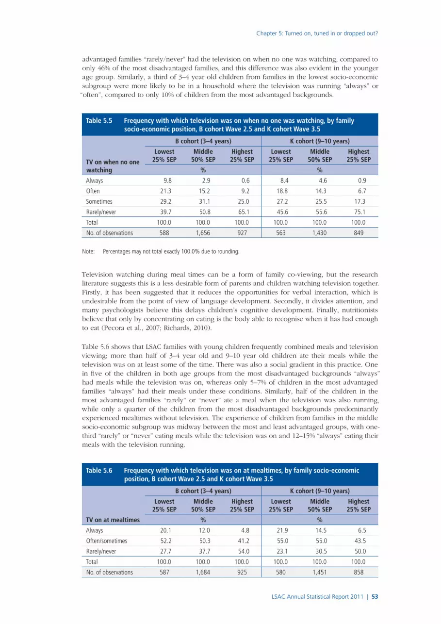
Chapter 5: Turned on, tuned in or dropped out?
LSAC Annual Statistical Report 2011 | 53
advantaged families “rarely/never” had the television on when no one was watching, compared to only 46% of the most disadvantaged families, and this difference was also evident in the younger age group. Similarly, a third of 3–4 year old children from families in the lowest socio-economic subgroup were more likely to be in a household where the television was running “always” or “often”, compared to only 10% of children from the most advantaged backgrounds.
Table 5.5 Frequency with which television was on when no one was watching, by family socio-economic position, B cohort Wave 2.5 and K cohort Wave 3.5
TV on when no one watching
B cohort (3–4 years) K cohort (9–10 years)
Lowest 25% SEP
Middle 50% SEP
Highest 25% SEP
Lowest 25% SEP
Middle 50% SEP
Highest 25% SEP
% %
Always 9.8 2.9 0.6 8.4 4.6 0.9
Often 21.3 15.2 9.2 18.8 14.3 6.7
Sometimes 29.2 31.1 25.0 27.2 25.5 17.3
Rarely/never 39.7 50.8 65.1 45.6 55.6 75.1
Total 100.0 100.0 100.0 100.0 100.0 100.0
No. of observations 588 1,656 927 563 1,430 849
Note: Percentages may not total exactly 100.0% due to rounding.
Television watching during meal times can be a form of family co-viewing, but the research literature suggests this is a less desirable form of parents and children watching television together. Firstly, it has been suggested that it reduces the opportunities for verbal interaction, which is undesirable from the point of view of language development. Secondly, it divides attention, and many psychologists believe this delays children’s cognitive development. Finally, nutritionists believe that only by concentrating on eating is the body able to recognise when it has had enough to eat (Pecora et al., 2007; Richards, 2010).
Table 5.6 shows that LSAC families with young children frequently combined meals and television viewing; more than half of 3–4 year old and 9–10 year old children ate their meals while the television was on at least some of the time. There was also a social gradient in this practice. One in five of the children in both age groups from the most disadvantaged backgrounds “always” had meals while the television was on, whereas only 5–7% of children in the most advantaged families “always” had their meals under these conditions. Similarly, half of the children in the most advantaged families “rarely” or “never” ate a meal when the television was also running, while only a quarter of the children from the most disadvantaged backgrounds predominantly experienced mealtimes without television. The experience of children from families in the middle socio-economic subgroup was midway between the most and least advantaged groups, with one-third “rarely” or “never” eating meals while the television was on and 12–15% “always” eating their meals with the television running.
Table 5.6 Frequency with which television was on at mealtimes, by family socio-economic position, B cohort Wave 2.5 and K cohort Wave 3.5
TV on at mealtimes
B cohort (3–4 years) K cohort (9–10 years)
Lowest 25% SEP
Middle 50% SEP
Highest 25% SEP
Lowest 25% SEP
Middle 50% SEP
Highest 25% SEP
% %
Always 20.1 12.0 4.8 21.9 14.5 6.5
Often/sometimes 52.2 50.3 41.2 55.0 55.0 43.5
Rarely/never 27.7 37.7 54.0 23.1 30.5 50.0
Total 100.0 100.0 100.0 100.0 100.0 100.0
No. of observations 587 1,684 925 580 1,451 858

54 | Australian Institute of Family Studies
5.6 SummaryTo paraphrase Mark Twain, reports of the demise of broadcast television (Hartley, 2004) are greatly exaggerated. This older medium is currently the dominant form of media used by young children in Australia. Children’s television watching is low in the first year of life, but by age 2–3 years, television occupies a significant proportion of the child’s time, a proportion that remains fairly constant thereafter. A substantial proportion of children above the age of 2 years spend more than the American Academy of Pediatrics’ (2010) recommended limit of 2 hours per day watching television, especially on weekends.
Lower hours of children’s television watching and higher hours spent using print media (either being read to or reading for themselves) are associated with increases in socio-economic advantage. Since competency with print media is important for school achievement, this may be one of the mechanisms through which social advantage is transmitted across generations.
Practically all parents, regardless of socio-economic position, claimed to have rules about television watching, governing suitable program material, when the television could be watched and for how long. However, the data suggest that many of these rules were applied inconsistently. In some households, the television was often running when no one was watching, or meals were consumed while it was on. Similarly, the child may have turned on the television or changed channels using the remote, at least in some instances, without parental supervision. The context for children’s use of television varied by the families’ socio-economic position, with less consistent supervision being evident among the more disadvantaged families. This was offset to some extent, however, because families from the lowest socio-economic backgrounds engaged more frequently in watching television with their children. In previous research, co-viewing with adults has been shown to reduce children’s trauma and fright, and improve cognition, vocabulary and media literacy.
Early studies of new media––games consoles, computers, the Internet and mobile phones––assumed that the effect of these digital technologies would be very similar to those of the older medium of television. Although there have been some findings that suggest that an increase in time spent by children in front of “screens” is a contributor to the growing problem of obesity/overweight among children (Hardy, Dobbins, Denney-Wilson, Okely, & Booth, 2009), there are unexpected findings that suggest new media affect children’s development in different ways than television, especially in their educational, social and emotional development (Bittman, Rutherford, Brown, & Unsworth, 2010).
5.7 Further readingAustralian Communications and Media Authority. (2009). Use of electronic media and communications: Early childhood to teenage years. Canberra: ACMA.
Brown, J. E., Nicholson, J. M., Broom, D. H., & Bittman, M. (2010). Television viewing by school-age children: Associations with physical activity, snack food consumption and unhealthy weight. Social Indicators Research, 101, 221–225.
Rutherford, L., Bittman, M., & Biron, D. (2010). Young children and the media: A discussion paper. Melbourne: Australian Research Alliance for Children and Youth (ARACY).
5.8 ReferencesAmerican Academy of Pediatrics. (2010). Where we stand: TV viewing time. Elk Grove Village, IL: American Academy of Pediatrics. Retrieved from <www.healthychildren.org/English/family-life/Media/pages/Where-We-Stand-TV-Viewing-Time.aspx>.
Australian Bureau of Statistics. (2008a). Environmental issues: Energy use and conservation (Cat. No. 4602.0.55.001). Canberra: ABS.
Australia Bureau of Statistics. (2008b). Microdata: Time use survey. Basic CURF, Australia 2006 (Cat. No. 4152.0.55.001). Canberra: ABS.
Australian Communications and Media Authority. (2009). Use of electronic media and communication: Early childhood to teenage years. Canberra: ACMA.
Bittman, M., Rutherford, L., Brown, J. E., & Unsworth, L. (2010, 18–20 November). Digital natives? New and old media and children’s outcomes. Paper presented at the Current Issues and Prospects of Time-Use Study in East and West conference, Seoul National University, Seoul, Korea.
Bjorkqvist, K. (1985). Violent films, anxiety and aggression. Helsinki: Finnish Society of Sciences and Letters.

Chapter 5: Turned on, tuned in or dropped out?
LSAC Annual Statistical Report 2011 | 55
Brown, J., Bittman, M., & Nicholson, J. (2007). Time or money: The impact or parental employment on time that 4 to 5 year olds spend in language building activities. Australian Journal of Labour Economics, 10(3), 149–166.
Cantor, J. (2001). The media and children’s fears, anxieties and perceptions of danger. In D. Singer & J. Singer (Eds.), Handbook of children and the media (pp. 207–221). Thousand Oaks, CA: Sage.
Chakroff, J. (2007). Parental mediation of advertising and consumer communication: The effectiveness of parental intervention on young children’s materialistic attitudes. Unpublished doctoral dissertation, Ohio State University, Columbus, Ohio. Retrieved from <www.ohiolink.edu/etd/send-pdf.cgi/ChakroffJenniferLeigh.pdf?acc_num=osu1190001119>.
Christakis, D., & Zimmerman, F. (2007). Violent television during pre-school is associated with anti-social behaviour during school age. Pediatrics, 120(5), 993–999.
Christakis, D., & Zimmerman, F. J. (2009). Young children and the media: Limitations of current knowledge and future directions for research. American Behavioral Scientist, 52(8), 1177–1185.
Hancox, R. J., Milne, B. J., & Poulton, R. (2005). Association of television viewing during childhood with poor educational achievement. Archives of Pediatrics and Adolescent Medicine, 159, 614–618.
Hardy, L. L., Dobbins, T. A., Denney-Wilson, E., Okely, A. D., & Booth, M. L. (2009). Sedentariness, small-screen recreation, and fitness in youth. The American Journal of Preventive Medicine, 36(2), 120–125.
Hartley, J. (2004). From republic of letters to television republic? Citizen readers in the era of broadcast television. In L. Spigel & J. Olsson (Eds.), Television after TV: Essays on a medium in transition (pp. 386–417). Durham, NC: Duke University Press.
Longitudinal Study of Australian Children. (2011). Growing Up in Australia: The Longitudinal Study of Australian Children 2009–10 Annual Report. Canberra: FaHCSIA.
Millwood Hargrave, A., & Livingstone, S. (2006). Harm and offence in media content: A review of the evidence. Bristol: Intellect Books.
Owens, J., Maxim, R., McGuinn, M., Nobile, C., Msall, M., & Alario, A. (1999). Television-viewing habits and sleep disturbance in school children. Pediatrics, 104(3), e27.
Pecora, M., Murray, J. P., & Wartella, E. (Eds.). (2007). Children and television: Fifty fears of research. Mahwah, NJ: Lawrence Erlbaum.
Richards, J. E. (2010). The development of attention to simple and complex visual stimuli in infants: Behavioral and psychophysiological measures. Developmental Review, 30, 203–219.
Rutherford, L., & Bittman, M. (2007). Review of research literature. In Australian Communications and Media Authority, Media and communication in Australian families 2007: Report of the Media and Society Research Project (pp. 203–356). Melbourne: ACMA.
Saxton, M. (2010). Child language: Acquisition and development. London: Sage.
Schor, J. (2004). Born to buy: The commercialized child and the new consumer culture. New York: Schribner.
Vandewater, E., & Lee, S. (2009). Measuring children’s media use in the digital age: Issues and challenges. American Behavioral Scientist, 52, 1152.


Chapter 6: Access to preschool education in the year before full-time school
LSAC Annual Statistical Report 2011 | 57
Brigit Maguire and Alan HayesAustralian Institute of Family Studies
The importance of the years children spend prior to school is now well recognised (Hayes, 2007). A good beginning to life bears dividends for development, health and wellbeing, both throughout childhood and across life (Keating & Hertzman, 1999), and many of the effects
of disadvantage can be ameliorated through high-quality early childhood interventions.
Australia, like many other countries, has made early childhood development, education and care an area of particular national policy priority. Early childhood education and care (ECEC) has emerged as an area of policy priority internationally, driven by growing recognition of the benefits that flow from investments in the early years (Organisation for Economic Co-operation and Development [OECD], 2001, 2006), and supported by a wealth of evidence, across a range of disciplines (Meisels & Shonkoff, 2000). The benefits are broad in scope and include: advancing the development, health and wellbeing of children; supporting workforce participation and equality of opportunity for parents; addressing poverty, disadvantage and social exclusion; arresting the intergenerational transmission of inequality; and facilitating social and economic mobility (OECD, 2006).
Starting Strong II (OECD, 2006), a review of studies of ECEC in twenty OECD countries, divides ECEC into two broad approaches. The first approach includes studies in France and the OECD English-speaking countries that focus on school readiness (highlighting cognitive development and the acquisition of the capabilities, orientations and skills required to make a successful transition to school). The second includes studies of ECEC programs that emphasise a broader set of skills for life, reflecting a social pedagogy approach, as represented by the Nordic and Central European countries.
Early childhood education and care in Australia has tended to be characterised by a patchwork of provisions, regulatory regimes and policy contexts that reflect the divide between care and education (Elliott, 2006). The background to the patchwork stems from the emergence in the late nineteenth century of, on the one hand, the kindergarten movement, with its focus on early learning and preparation for school and, on the other, day nurseries, with their charitable and welfare focus on providing quality care (Press & Hayes, 2000).
These divergent paths have resulted in very different systems for managing and regulating the provision of ECEC services. When one adds the complex tapestry of the public, private, not-for-profit, charitable, church and community players, the patchwork becomes even more complex. The divide is further reinforced in many jurisdictions by vesting government responsibility for the policy, administration and regulation of preschools and child care in the separate portfolios of education and community services, respectively.
Preschools and early learning centres have remained the province of educators, with a higher proportion of qualified teachers and a clearer focus on curriculum and pedagogy than typically found in child care. Increasingly, the mix of public and private provision has become more complex, with many private schools establishing early learning centres that provide preschool programs, often with extended hours. In contrast, public and community preschools typically provide preschool programs within set hours and within school terms, which creates its own set of issues, given that an increasing number of families have both parents in paid employment.
As such, preschool provision is itself a patchwork, varying widely across the states and territories in the extent of provision and equity of access. The Australian Government has recently committed to
6Access to preschool education in the year before full-time school

58 | Australian Institute of Family Studies
providing, by 2013, universal access to preschool in the year before full-time school (Department of Education, Employment and Workplace Relations [DEEWR], 2011a). While the responsibility for delivering these programs remains with the individual states and territories, this program is expected to introduce some consistency in access to preschool education across the jurisdictions.
The partnership between families and ECEC providers seems a common ingredient in the success of initiatives to support and nurture development in early life, and beyond. Research from the US National Institute of Child Health and Human Development (NICHD Early Child Care Research Network, 2003) and from the UK’s Effective Provision of Pre-School Education (EPPE) Project (Sammons et al., 2002, 2003) demonstrates that high-quality child care and preschool education can have very positive effects on children’s language and cognitive development during the early years. In both studies, however, parent and family characteristics were stronger determinants of children’s outcomes than the early childhood programs per se. Family and community, working in combination, powerfully determine outcomes in ways that are greater than either working alone.
The salience of quality has been evident in the emphasis on regulation and accreditation of early childhood education and care. From 1 January 2012, Australia is implementing a new National Quality Framework for Early Childhood Education and Care, which covers day care providers (both long day care and family day care), preschool and out-of-school-hours care programs. The framework aims to introduce national legislation, quality standards and quality assessment processes to raise and continually improve education and care services. Under the framework, care providers are required to meet certain minimum standards, such as in staff-to-child ratios and staff qualifications (DEEWR, 2011b).
Results from Growing Up in Australia: The Longitudinal Study of Australian Children (LSAC) are beginning to illustrate the connection between families’ experiences of socioeconomic disadvantage and outcomes for children. The study provides large-scale national data on the experiences and outcomes of Australian children from infancy onwards, which contribute to the evidence base for ECEC policy and practice in this country.
This chapter uses data from 4–5 year olds in LSAC to examine rates of access to preschool education in the year before full-time school, and how these vary for families from different socio-demographic backgrounds. The socio-demographic groups examined in this chapter (introduced in Chapter 1) are:
■ family socio-economic position (SEP; lowest 25%, middle 50%, highest 25%);
■ mother’s work hours (not working, part-time, full-time);
■ whether the child mainly speaks English or another language at home;
■ whether the child is of Aboriginal or Torres Strait Islander origin;
■ family type (two-parent family, lone-mother family); and
■ whether the family is jobless.
Data from the K cohort at Wave 1 and the B cohort at Wave 3 are used. In making comparisons between the two cohorts, it is important to consider the differences between them, particularly because the B cohort sample has been affected by non-random attrition between waves.1
This chapter builds on the information provided by previous analyses (Harrison, Ungerer, Smith, Zubrick, & Wise, 2009), which used Wave 1 data for both cohorts to investigate a range of questions related to child care and early education. This chapter introduces recent data from the B cohort, and focuses specifically on access to preschool education in the year before full-time school and how this varies by family socio-demographic characteristics.
6.1 Children’s attendance at education/care programsChildren were selected for inclusion in the analyses in this chapter if they were in their first year of school when they were 5–6 years old. Eligibility was determined using a series of questions asked of children’s parents (usually their mothers), which provided details about the child’s main education/care arrangement, as well as any secondary arrangements.
1 See the LSAC Data User Guide (Australian Institute of Family Studies, 2011) for more information about between-waves attrition.

Chapter 6: Access to preschool education in the year before full-time school
LSAC Annual Statistical Report 2011 | 59
For the K cohort, information from Wave 2 was used to identify the program that children were attending in 2005 (when they were 5–6 years old). K cohort children were included in the sample if they were in “kindergarten/reception/preparatory” in 2005 and lived in any state/territory other than Queensland. K cohort children who lived in Queensland were excluded from the sample because Queensland did not have a pre–Year 1 program in 2005, so it was not expected that 5–6 year olds in that state would be in their first year of full-time school.
For the B cohort, data from Wave 4 were used to determine what program children were attending in 2009 (when they were 5–6 years old). B cohort children from all states/territories were included in the sample if they were attending a pre–Year 1 program in 2009. Children from Queensland were included in the B cohort sample because Queensland introduced an optional pre–Year 1 program (“preparatory”) in schools in 2007 (Department of Education and Training, 2008).
Table 6.1 shows the numbers of children who were retained in the sample for analyses in this chapter. The top section of the table shows the numbers of K cohort children who were in kindergarten/reception/preparatory (depending on the state/territory they lived in) in 2005, when they were 5–6 years old, and those who were excluded from the sample. The table shows that 2,661 children were in scope for the analyses. The following children were excluded:
■ 950 children who lived in Queensland in 2004 or 2005;
■ 547 children who were already in Year 1 or Year 2, or in an ungraded or “other” (unidentifiable) program in 2005;
■ 180 children whose program information was missing in 2005; and
■ 126 children who were already in full-time school when they were 4–5 years old (suggesting that they repeated the first year of school when they were 5–6 years old).
The second section of the table shows the numbers of B cohort children who were in pre–Year 1 in 2009, when they were 5–6 years old. The table shows that 3,211 children were included in the analyses and 896 cases were excluded.
Table 6.1 Sample of children in first year of full-time school, K cohort Wave 2 and B cohort Wave 4
No. of observations
K cohort (2005)
Retained sample 2,661
Excluded sample
Lived in Queensland Year 1 950
Year 1 526
Year 2/ungraded/other a 21
Missing 180
In full-time school at 4–5 years 126
Total 4,464
B cohort (2009)
Retained sample 3,211
Excluded sample
Year 1 724
Year 2/ungraded/not in school at 5–6 years a 77
Missing 17
In full-time school at 4–5 years 70
Other program 8
Total 4,107
Note: a These three groups were combined because of small cell sizes in each.
Table 6.2 (on page 60) shows the programs that children attended in the year before they began full-time school. These are combined into four comparison groups to be used to examine differences in access to preschool education for different socio-demographic groups. Because the focus of these analyses is on access to preschool education, these data show only the main
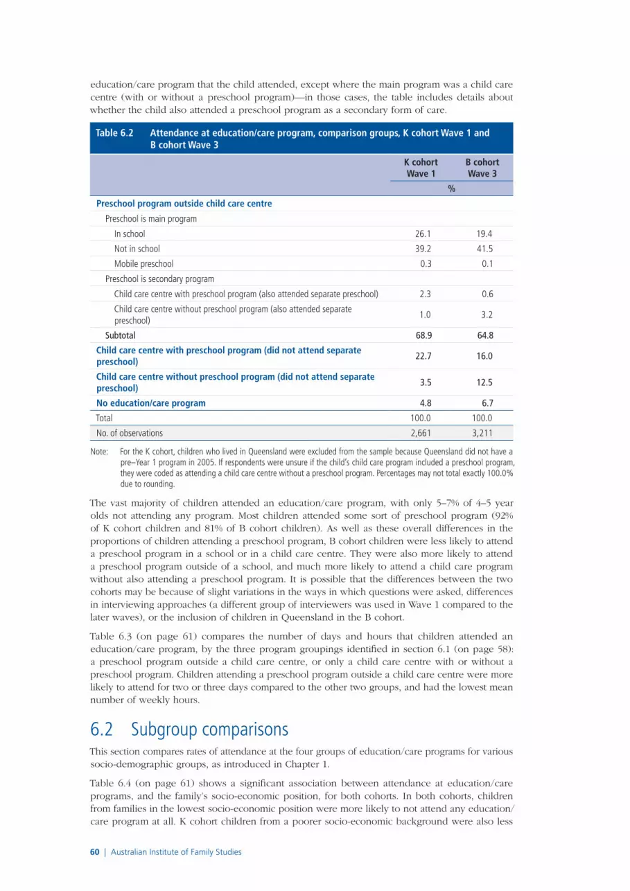
60 | Australian Institute of Family Studies
education/care program that the child attended, except where the main program was a child care centre (with or without a preschool program)—in those cases, the table includes details about whether the child also attended a preschool program as a secondary form of care.
Table 6.2 Attendance at education/care program, comparison groups, K cohort Wave 1 and B cohort Wave 3
K cohort Wave 1
B cohort Wave 3
%
Preschool program outside child care centre
Preschool is main program
In school 26.1 19.4
Not in school 39.2 41.5
Mobile preschool 0.3 0.1
Preschool is secondary program
Child care centre with preschool program (also attended separate preschool) 2.3 0.6
Child care centre without preschool program (also attended separate preschool)
1.0 3.2
Subtotal 68.9 64.8
Child care centre with preschool program (did not attend separate preschool)
22.7 16.0
Child care centre without preschool program (did not attend separate preschool)
3.5 12.5
No education/care program 4.8 6.7
Total 100.0 100.0
No. of observations 2,661 3,211
Note: For the K cohort, children who lived in Queensland were excluded from the sample because Queensland did not have a pre–Year 1 program in 2005. If respondents were unsure if the child’s child care program included a preschool program, they were coded as attending a child care centre without a preschool program. Percentages may not total exactly 100.0% due to rounding.
The vast majority of children attended an education/care program, with only 5–7% of 4–5 year olds not attending any program. Most children attended some sort of preschool program (92% of K cohort children and 81% of B cohort children). As well as these overall differences in the proportions of children attending a preschool program, B cohort children were less likely to attend a preschool program in a school or in a child care centre. They were also more likely to attend a preschool program outside of a school, and much more likely to attend a child care program without also attending a preschool program. It is possible that the differences between the two cohorts may be because of slight variations in the ways in which questions were asked, differences in interviewing approaches (a different group of interviewers was used in Wave 1 compared to the later waves), or the inclusion of children in Queensland in the B cohort.
Table 6.3 (on page 61) compares the number of days and hours that children attended an education/care program, by the three program groupings identified in section 6.1 (on page 58): a preschool program outside a child care centre, or only a child care centre with or without a preschool program. Children attending a preschool program outside a child care centre were more likely to attend for two or three days compared to the other two groups, and had the lowest mean number of weekly hours.
6.2 Subgroup comparisonsThis section compares rates of attendance at the four groups of education/care programs for various socio-demographic groups, as introduced in Chapter 1.
Table 6.4 (on page 61) shows a significant association between attendance at education/care programs, and the family’s socio-economic position, for both cohorts. In both cohorts, children from families in the lowest socio-economic position were more likely to not attend any education/care program at all. K cohort children from a poorer socio-economic background were also less

Chapter 6: Access to preschool education in the year before full-time school
LSAC Annual Statistical Report 2011 | 61
likely to attend a child care centre with a preschool program. There were only small differences between the SEP categories of K cohort children attending a preschool program outside of a child care centre and those at a child care centre without a preschool program. B cohort children from a lower socio-economic background were less likely to attend a preschool program outside of a child care centre, but did not differ largely from the other SEP categories in the percentages attending a child care centre, with or without a preschool program.
Table 6.3 Number of days and mean number of hours per week attendance, by program group, K cohort Wave 1 and B cohort Wave 3
Number of days attending per week
K cohort Wave 1 B cohort Wave 3
Preschool outside
child care centre
Child care centre with
preschool
Child care centre
without preschool
Preschool outside
child care centre
Child care centre with
preschool
Child care centre
without preschool
% %
One 4.2 7.9 6.3 3.6 7.6 7.8
Two 34.1 33.8 31.9 42.4 41.0 32.1
Three 39.6 33.2 29.9 40.5 27.5 31.5
Four 17.2 9.7 10.3 8.4 11.9 12.5
Five 4.8 15.4 21.5 4.6 11.8 16.0
Six 0.1 0.0 0.0 0.0 0.0 0.0
Irregular 0.0 0.0 0.0 0.4 0.2 0.1
Total 100.0 100.0 100.0 100.0 100.0 100.0
No. of observations 1,889 574 92 2,151 482 397
Mean Mean
Mean no. of hours attending per week
12.7 21.4 22.6 13.2 20.1 22.7
Note: Percentages may not total exactly 100.0% due to rounding.
Table 6.4 Attendance at education/care program, by family socio-economic position, K cohort Wave 1 and B cohort Wave 3
Lowest 25% SEP Middle 50% SEP Highest 25% SEP
%
K cohort Wave 1
Preschool program outside child care centre 66.2 71.1 67.3
Child care centre with preschool program (did not attend separate preschool)
20.5 21.6 27.4
Child care centre without preschool program (did not attend separate preschool)
3.3 3.8 3.3
No education/care program 10.0 3.5 2.1
Total 100.0 100.0 100.0
No. of observations 549 1,353 753
B cohort Wave 3
Preschool program outside child care centre 60.2 64.6 71.5
Child care centre with preschool program (did not attend separate preschool)
14.6 17.5 14.5
Child care centre without preschool program (did not attend separate preschool)
12.4 12.6 12.2
No education/care program 12.8 5.3 1.8
Total 100.0 100.0 100.0
No. of observations 732 1,637 840
Notes: K cohort: χ2 (6, n = 2,655) = 62.2, p < .01; B cohort: χ2 (6, n = 3,209) = 93.8, p < .01. Percentages may not total exactly 100.0% due to rounding.

62 | Australian Institute of Family Studies
Similar patterns were seen for the two cohorts in the relationship between mothers’ work hours and attendance at different education/care programs, with significant associations for both cohorts (Table 6.5). Children whose mothers worked 35 or more hours each week were more likely than the other children to attend a child care centre with or without a preschool program. These children had the lowest rates of attendance at preschools outside of child care centres. Children whose mothers were not working2 were more likely than the others to attend a preschool outside of a child care centre, but were also more likely not to attend any education/care program at all. Children whose mothers worked less than 35 hours per week had rates of attendance at preschools outside of child care centres that were almost as high as those of mothers who were not working. These children were also the least likely not to attend any education/care program at all.
Table 6.5 Attendance at education/care program, by mother’s work hours, K cohort Wave 1 and B cohort Wave 3
Mother not working
Mother working < 35 hours a
week
Mother working 35+ hours a
week%
K cohort Wave 1
Preschool program outside child care centre 72.3 69.9 52.2
Child care centre with preschool program (did not attend separate preschool)
17.6 24.3 39.3
Child care without preschool program (did not attend separate preschool)
3.1 3.5 4.2
No education/care program 7.0 2.2 4.2
Total 100.0 100.0 100.0
No. of observations 1,177 1,093 318
B cohort Wave 3
Preschool program outside child care centre 69.0 66.8 45.8
Child care centre with preschool program (did not attend separate preschool)
13.1 16.2 24.4
Child care without preschool program (did not attend separate preschool)
8.1 13.2 23.8
No education/care program 9.9 3.7 6.0
Total 100.0 100.0 100.0
No. of observations 1,291 1,442 415
Notes: K cohort: χ2 (6, n = 2,588) = 96.0, p < .01; B cohort: χ2 (6, n = 3,148) = 158.7, p < .01. Percentages may not total exactly 100.0% due to rounding.
Attendance at different education/care programs varied significantly by whether the child mainly spoke English or another language at home, for the K cohort only (Table 6.6 on page 63). Children who mostly spoke a language other than English at home were more likely not to attend any education/care program at all, and less likely to attend preschools outside of child care centres. However, they were more likely to attend a child care centre with a preschool program (and a child care centre without a preschool program in the K cohort).
Table 6.7 (on page 63) shows that children who identified as Aboriginal or Torres Strait Islanders were generally more likely to not be in any education/care program at all. There was a significant association between whether the child was Indigenous or not and their attendance at preschool and other programs, for the B cohort only. For the B cohort, Indigenous children were less likely to attend preschools outside child care centres, and more likely to attend a child care centre with or without a preschool program.
There was a significant relationship between attendance at education/care programs and the types of family in which children were living, for both cohorts (Table 6.8 on page 64). (See Chapter 1
2 The category of mothers “not working” includes mothers who were on long-term leave, unemployed or not in the labour force.
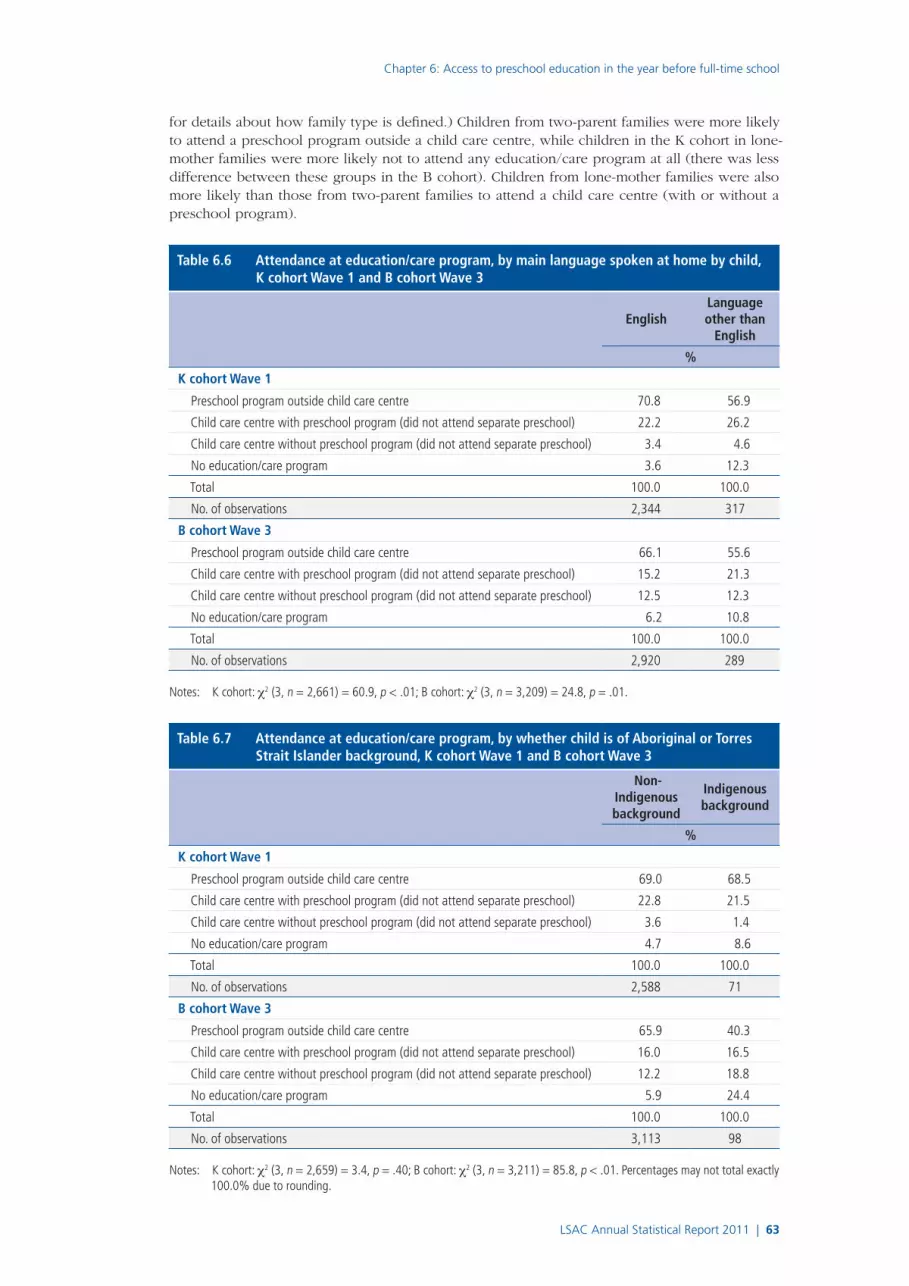
Chapter 6: Access to preschool education in the year before full-time school
LSAC Annual Statistical Report 2011 | 63
for details about how family type is defined.) Children from two-parent families were more likely to attend a preschool program outside a child care centre, while children in the K cohort in lone-mother families were more likely not to attend any education/care program at all (there was less difference between these groups in the B cohort). Children from lone-mother families were also more likely than those from two-parent families to attend a child care centre (with or without a preschool program).
Table 6.6 Attendance at education/care program, by main language spoken at home by child, K cohort Wave 1 and B cohort Wave 3
EnglishLanguage other than
English
%
K cohort Wave 1
Preschool program outside child care centre 70.8 56.9
Child care centre with preschool program (did not attend separate preschool) 22.2 26.2
Child care centre without preschool program (did not attend separate preschool) 3.4 4.6
No education/care program 3.6 12.3
Total 100.0 100.0
No. of observations 2,344 317
B cohort Wave 3
Preschool program outside child care centre 66.1 55.6
Child care centre with preschool program (did not attend separate preschool) 15.2 21.3
Child care centre without preschool program (did not attend separate preschool) 12.5 12.3
No education/care program 6.2 10.8
Total 100.0 100.0
No. of observations 2,920 289
Notes: K cohort: χ2 (3, n = 2,661) = 60.9, p < .01; B cohort: χ2 (3, n = 3,209) = 24.8, p = .01.
Table 6.7 Attendance at education/care program, by whether child is of Aboriginal or Torres Strait Islander background, K cohort Wave 1 and B cohort Wave 3
Non-Indigenous background
Indigenous background
%
K cohort Wave 1
Preschool program outside child care centre 69.0 68.5
Child care centre with preschool program (did not attend separate preschool) 22.8 21.5
Child care centre without preschool program (did not attend separate preschool) 3.6 1.4
No education/care program 4.7 8.6
Total 100.0 100.0
No. of observations 2,588 71
B cohort Wave 3
Preschool program outside child care centre 65.9 40.3
Child care centre with preschool program (did not attend separate preschool) 16.0 16.5
Child care centre without preschool program (did not attend separate preschool) 12.2 18.8
No education/care program 5.9 24.4
Total 100.0 100.0
No. of observations 3,113 98
Notes: K cohort: χ2 (3, n = 2,659) = 3.4, p = .40; B cohort: χ2 (3, n = 3,211) = 85.8, p < .01. Percentages may not total exactly 100.0% due to rounding.
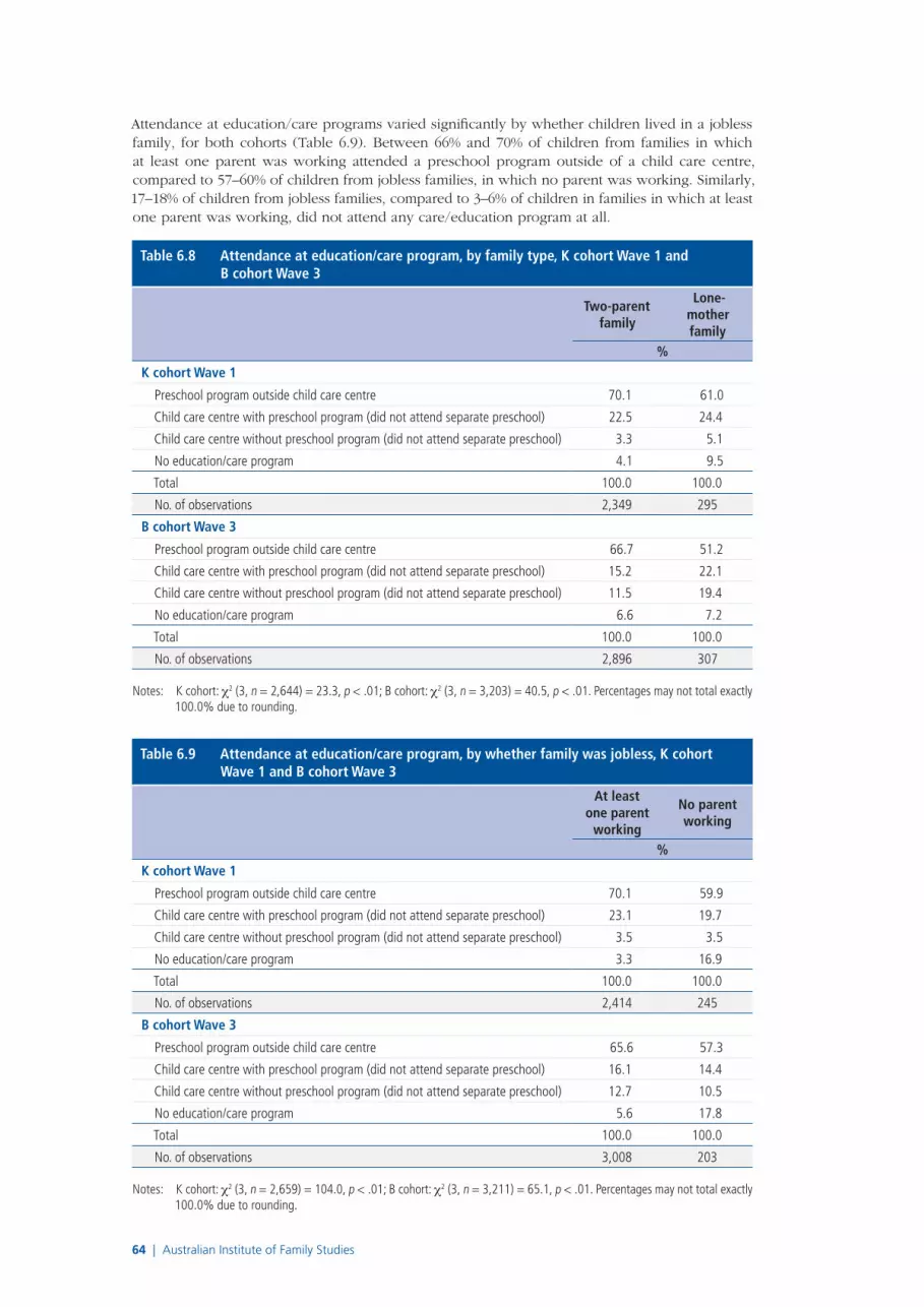
64 | Australian Institute of Family Studies
Attendance at education/care programs varied significantly by whether children lived in a jobless family, for both cohorts (Table 6.9). Between 66% and 70% of children from families in which at least one parent was working attended a preschool program outside of a child care centre, compared to 57–60% of children from jobless families, in which no parent was working. Similarly, 17–18% of children from jobless families, compared to 3–6% of children in families in which at least one parent was working, did not attend any care/education program at all.
Table 6.8 Attendance at education/care program, by family type, K cohort Wave 1 and B cohort Wave 3
Two-parent family
Lone-mother family
%
K cohort Wave 1
Preschool program outside child care centre 70.1 61.0
Child care centre with preschool program (did not attend separate preschool) 22.5 24.4
Child care centre without preschool program (did not attend separate preschool) 3.3 5.1
No education/care program 4.1 9.5
Total 100.0 100.0
No. of observations 2,349 295
B cohort Wave 3
Preschool program outside child care centre 66.7 51.2
Child care centre with preschool program (did not attend separate preschool) 15.2 22.1
Child care centre without preschool program (did not attend separate preschool) 11.5 19.4
No education/care program 6.6 7.2
Total 100.0 100.0
No. of observations 2,896 307
Notes: K cohort: χ2 (3, n = 2,644) = 23.3, p < .01; B cohort: χ2 (3, n = 3,203) = 40.5, p < .01. Percentages may not total exactly 100.0% due to rounding.
Table 6.9 Attendance at education/care program, by whether family was jobless, K cohort Wave 1 and B cohort Wave 3
At least one parent
working
No parent working
%
K cohort Wave 1
Preschool program outside child care centre 70.1 59.9
Child care centre with preschool program (did not attend separate preschool) 23.1 19.7
Child care centre without preschool program (did not attend separate preschool) 3.5 3.5
No education/care program 3.3 16.9
Total 100.0 100.0
No. of observations 2,414 245
B cohort Wave 3
Preschool program outside child care centre 65.6 57.3
Child care centre with preschool program (did not attend separate preschool) 16.1 14.4
Child care centre without preschool program (did not attend separate preschool) 12.7 10.5
No education/care program 5.6 17.8
Total 100.0 100.0
No. of observations 3,008 203
Notes: K cohort: χ2 (3, n = 2,659) = 104.0, p < .01; B cohort: χ2 (3, n = 3,211) = 65.1, p < .01. Percentages may not total exactly 100.0% due to rounding.

Chapter 6: Access to preschool education in the year before full-time school
LSAC Annual Statistical Report 2011 | 65
6.3 SummaryThe analyses provided in this chapter show the high level of involvement of 4–5 year olds in early childhood education and care, especially preschool programs. Only 5–7% of children were not attending some form of early childhood education and care program.
Clear differences emerged when the data were analysed by family socio-economic position. Children from more disadvantaged families were more likely not to attend any education/care program at all. Levels of attendance were also related to maternal work, with the children of mothers who were either not working or working less than 35 hours each week being more likely than others to attend preschool programs outside of child care centres. Children of mothers who worked 35 or more hours each week were more likely than the others to attend a child care centre, with or without a preschool program.
Family characteristics were also related to access to education/care programs. Children were less likely to attend a preschool program outside a child care centre if they spoke a language other than English at home (significant for K cohort only), or if they were of Aboriginal or Torres Strait Islander background (B cohort only). Children from two-parent families were also more likely to attend preschool outside of a child care setting than those from lone-mother households, who were more likely to be attending child care with or without a preschool element.
The longitudinal information available in LSAC will be able to facilitate further research to investigate the relationship between ECEC and children’s outcomes, and differences in the quality of ECEC services. Collectively, the results have clear implications for policy and practice, in providing an indication of the socio-demographic groups who may have limited access to preschool education programs in the year before full-time school. While they demonstrate a high level of attendance in ECEC, they also show that there remains a clear divide between those enrolled in preschool and those who attend child care, with or without an associated preschool program. Those who are most disadvantaged remain the least likely to be attending any form of ECEC at 4–5 years of age.
6.4 Further readingAustralian Institute of Health and Welfare. (2009). A picture of Australia’s children 2009. Canberra: AIHW.
Harrison, L., & Ungerer, L. (2005). What can the Longitudinal Study of Australian Children tell us about infants’ and 4 to 5 year olds’ experiences of early childhood education and care? Family Matters, 72, 26–35.
Harrison, L., Ungerer, J., Smith, J., Zubrick, S., & Wise, S. (2010). Child care and early education in Australia: The Longitudinal Study of Australian Children (Social Policy Research Paper No. 40). Canberra: Department of Families, Housing, Community Services and Indigenous Affairs.
6.5 ReferencesAustralian Institute of Family Studies. (2011). Longitudinal Study of Australian Children Data User Guide. Melbourne: AIFS.
Department of Education and Training. (2008). About Prep. Brisbane: DET. Retrieved from <education.qld.gov.au/strategic/advice/earlychildhood/aboutprep.html>.
Department of Education, Employment and Workplace Relations. (2011a). Early childhood education: Universal access. Canberra: DEEWR. Retrieved from <www.deewr.gov.au/EarlyChildhood/Policy_Agenda/ECUA/Pages/home.aspx>.
Department of Education, Employment and Workplace Relations. (2011b). National Quality Framework for Early Childhood Education & Care. Canberra: DEEWR. Retrieved from <www.deewr.gov.au/earlychildhood/policy_agenda/quality/pages/home.aspx>.
Elliott, A. (2006). Early childhood education: Pathways to quality and equity for all children (Australian Education Review). Camberwell, Vic.: ACER Press.
Harrison, L. J., Ungerer, J. A., Smith, G. J., Zubrick, S. R., & Wise, S. (2009). Child care and early education in Australia: The Longitudinal Study of Australian Children (Social Policy Research Paper No. 40). Canberra: Department of Families, Housing, Community Services and Indigenous Affairs.
Hayes, A. (2007). Why early in life is not enough: Timing and sustainability in prevention and early intervention. In A. France & R. Homel (Eds.), Pathways and crime prevention: Theory, policy and practice (pp. 202–225). Uffculme, UK: Willan Publishing.
Keating, D. P., & Hertzman, C. (1999). Modernity’s paradox. In D. P. Keating & C. Hertzman (Eds.), Developmental health and the wealth of nations: Social, biological and educational dynamics (pp. 1–18). New York: The Guildford Press.

66 | Australian Institute of Family Studies
Meisels, S. J., & Shonkoff, J. P. (2000). Early intervention: A continuing evolution. In J. P. Shonkoff & S. J. Meisels (Eds.), Handbook of early childhood intervention (2nd Ed.; pp. 3–31). Cambridge: Cambridge University Press.
National Institute of Child Health and Human Development Early Child Care Research Network. (2003). Families matter: Even for kids in child care. Journal of Developmental and Behavioral Pediatrics, 24, 58–62.
Organisation for Economic Co-operation and Development. (2001). Starting strong: Early childhood education and care. Paris: OECD.
Organisation for Economic Co-operation and Development. (2006). Starting strong II: Early childhood education and care. Paris: OECD.
Press, F., & Hayes, A. (2000). OECD thematic review of early childhood education and care policy: Australian background report. Canberra: AGPS.
Sammons, P., Sylva, K., Melhuish, E., Siraj-Blatchford, I., Taggart, B., & Elliott, K. (2002). Measuring the impact of pre-school in children’s cognitive progress over the preschool period (Technical Paper No. 8a). London: Institute of Education, University of London.
Sammons, P., Sylva, K., Melhuish, E., Siraj-Blatchford, I., Taggart, B., & Elliot, K. (2003). Measuring the impact of pre-school in children’s social behavioural development over the preschool period (Technical Paper No. 8b). London: Institute of Education, University of London.

Chapter 7: Housing characteristics and changes across waves
LSAC Annual Statistical Report 2011 | 67
Brigit Maguire, Ben Edwards and Carol SoloffAustralian Institute of Family Studies
The characteristics of children’s homes and family living arrangements, being a large part of their physical and social environment, have important influences on their development and wellbeing (Bronfenbrenner & Morris, 2006). A recent scoping study (Dockery et al.,
2010) identified Growing Up in Australia: The Longitudinal Study of Australian Children (LSAC) as a useful source of data for analysing housing and child developmental outcomes. This chapter describes three aspects of housing that are expected to be important for children’s outcomes: housing mobility, tenure and overcrowding (Dockery et al., 2010).
In a review of residential mobility in childhood, Jelleyman and Spencer (2008) found that population residential mobility varies internationally. The Australian population is among the most mobile, with higher rates demonstrated for children aged 1–4 years, and declining until adolescence (Bell & Hugo, 2000). The authors reported that higher rates of residential mobility are associated with poverty, housing tenure, unemployment, family disruption, and single-parenting. In terms of the relationship between mobility and child developmental outcomes, studies in the United States have found associations between residential mobility and dropping out of school (Astone & McLanahan, 1994), repeating a school grade, or being suspended or expelled (Simpson & Fowler, 1994; Wood, Halfon, Scarlata, Newacheck, & Nessim, 1993).
Australian families have a wide range of housing arrangements, and therefore great variation in their security of tenure.1 When people have secure housing tenure, they are likely to have a greater sense of autonomy, certainty and sense of control, which reduces levels of stress and increases family stability. Security of housing tenure has been found to affect the mental health of parents. It also influences family stability, including children attending a fewer number of schools and having better educational performance and rates of school completion (Australian Housing and Urban Research Institute [AHURI], 2006). Both family stability and parental mental health can have a significant effect on children’s development.
Overcrowded conditions have been well documented to have negative effects on children and families. Overcrowding has been associated with higher levels of stress in parents and children, higher rates of infectious diseases, poorer parenting, and increased family conflict (Evans, 2006). It is also a risk factor for child neglect and abuse (Council of Australian Governments [COAG], 2009). When there is overcrowding in a household, children are more likely to withdraw and less likely to explore and play, which then has implications for their learning. In fact, overcrowding has been associated with poorer cognitive development in children, including having lower IQs (Evans, 2006).
This chapter capitalises on the longitudinal nature of LSAC by using Waves 1 to 3 for the B and K cohorts to explore changes in (and persistence of) these three housing characteristics across waves, as children grow older. The first section of the chapter focuses on variations in mobility, and examines whether children move within their local area or further. The second focuses on housing tenure, and how this changes across Waves 1 to 3 for each of the cohorts. The third uses a measure of overcrowding to investigate how many children experience overcrowding at one or multiple waves of LSAC, and also examines how overcrowding varies by different dwelling types. The final section of the chapter explores the relationships between mobility and housing tenure, and mobility and overcrowding, for the younger B cohort only.
1 Assessment of the level of security of housing tenure is a complex issue; however, for the purposes of this chapter, insecure housing tenure is associated with renting rather than purchasing or owning a home.
7Housing characteristics and changes across waves

68 | Australian Institute of Family Studies
7.1 Housing mobilityTable 7.1 shows how often children in LSAC had moved house since birth. Looking first at the percentages of children who had never moved, this shows a large decline among B cohort children across the first two waves, from 84% of 0–1 year olds to 57% of 2–3 year olds (a drop of 27 percentage points). There is less change between waves for the other age groups (5–13 percentage points), which suggests that children are most likely to experience moving house in the first two to three years of their lives.
Table 7.1 Housing mobility, B and K cohorts, Waves 1–3
B cohort K cohort
0–1 year 2–3 years 4–5 years 4–5 years 6–7 years 8–9 years
% %
Never moved 84.2 56.5 43.6 39.7 32.2 27.1
Moved once since birth 13.7 28.4 28.1 29.5 27.8 25.9
Moved twice since birth 2.1 10.0 15.8 30.8 25.4 23.3
Moved three times since birth – a 3.7 7.2 – a 11.6 14.2
Moved four or more times since birth
– a 1.4 5.4 – a 3.0 9.4
Total 100.0 100.0 100.0 100.0 100.0 100.0
No. of observations 4,250 4,250 4,250 4,192 4,192 4,192
Notes: Cases were only included if data were available at all waves. a In Wave 1, the maximum number of moves since birth was recorded as “two or more”, which means that the total number of moves for this wave will be underestimated, particularly for the K cohort. Percentages may not total exactly 100.0% due to rounding.
By the time they were 4–5 years old, more than half of the children had moved house at least once. When children were 8–9 years, only one quarter had never moved house, one quarter had moved once, one quarter had moved twice, and the final quarter had moved three or more times since they were born. A small proportion of children in the most recent wave for both cohorts (5% of 4–5 year olds, B cohort, and 9% of 8–9 year olds) had moved four or more times since birth.
Table 7.2 shows the types of moves that families make, in terms of whether they moved within their local area, or further away. The data shown relate to the family’s most recent move, and the table shows a similar pattern for the two cohorts at both Wave 2 and Wave 3. Just under half of all families who moved between waves moved within the same town or suburb, and an additional third of families moved slightly further away, but still within the same area or region. Between 11% and 13% of families who moved did so to somewhere out of their area or region, but still within the same state, and a smaller percentage (8–9%) moved further away still—interstate or from overseas.2
Table 7.2 Type of house move, B and K cohorts, Waves 1–3
B cohort K cohort
Moved between Waves 1 & 2
Moved between Waves 2 & 3
Moved between Waves 1 & 2
Moved between Waves 2 & 3
% %
Within town or suburb 45.0 45.2 47.9 47.5
Within area or region 36.1 33.9 32.8 30.1
Within state 10.8 12.6 11.0 13.1
Interstate 7.7 7.3 8.0 8.1
From overseas a 0.4 1.0 0.3 1.2
Total 100.0 100.0 100.0 100.0
No. of observations 1,622 1,381 1,213 1,048
Note: Cases were only included if data were available for both waves under consideration (Waves 1 and 2, or Waves 2 and 3). a A small number of study families lived in Australia in Wave 1, lived overseas in Wave 2, and lived back in Australia in Wave 3.
2 A small number of study families lived in Australia in Wave 1, lived overseas in Wave 2, and lived back in Australia in Wave 3.

Chapter 7: Housing characteristics and changes across waves
LSAC Annual Statistical Report 2011 | 69
7.2 Housing tenureAt each wave, the child’s primary parent was asked to provide details about the family’s current housing tenure arrangements. While these questions were asked slightly differently at each of the three waves, they have been summarised into the five categories shown in Table 7.3. The first category, “owner without a mortgage”, includes those families in which the respondent (or the child’s secondary parent living in the household) owned their house outright. The second category, “owner with a mortgage”, includes those families in which the child’s primary and/or secondary parent was currently paying off a mortgage on the house. The third category, “renter—private landlord”, includes families who paid rent through a real estate agent or to someone (not a relative) who did not live in the home. The fourth category, “renter—public housing”, includes families who paid rent to a state or territory housing authority. The final category includes “other tenure types”, such as paying rent to someone else in the same dwelling (such as in a boarder arrangement), a relative or friend, an employer, a community/cooperative housing group, a caravan park, an unspecified landlord or the government; purchasing a house under a rent/buy scheme; living in a property under a life tenure scheme; or living in a property rent-free. Changes in tenure between waves do not necessarily mean that a family has moved house, as they may change their tenure arrangement within the same property (e.g., moving from having a mortgage to owning the property outright). Conversely, mobility doesn’t necessarily reflect a change in tenure as families may move between two properties with the same tenure arrangement.
Table 7.3 Types of housing tenure, B and K cohorts, Waves 1–3
B cohort K cohort0–1 year 2–3 years 4–5 years 4–5 years 6–7 years 8–9 years
% %
Owner without mortgage 7.4 8.8 10.5 11.2 11.6 12.7
Owner with mortgage 59.7 59.0 57.2 60.7 61.1 58.9
Renter—private landlord 19.2 18.8 19.3 16.7 15.4 16.4
Renter—public housing 2.4 3.9 4.4 2.6 4.5 5.0
Other tenure type a 11.4 9.5 8.4 8.9 7.4 7.0
Total 100.0 100.0 100.0 100.0 100.0 100.0
No. of observations 4,241 4,241 4,241 4,190 4,190 4,190
Notes: Cases were only included if the data were available at all waves. a The “other” category includes: renting from a person in the same dwelling, relatives or friends, employer, community/cooperative housing group, caravan park, unspecified landlord or the government; purchasing the dwelling under a rent/buy scheme; living in a dwelling under a life tenure scheme; or living in a dwelling rent-free (all of these categories had small sample sizes). Percentages may not total exactly 100.0% due to rounding.
Table 7.3 shows changes in housing tenure across waves, as the children grow older. Around 60% of families at all waves had a mortgage on the property they lived in, and this was the most common tenure type. There was a slight reduction across the three waves for both cohorts in the percentages who had a mortgage (from 60% in Wave 1 to 57% in Wave 3 for the B cohort, and from 61% to 59% for the K cohort), and a corresponding increase in the percentages who owned their house outright (from 7% to 11% in the B cohort, and from 11% to 13% in the K cohort). The second most common tenure type was renting from a private landlord (15–19%), and this remained stable across the waves, at 19% for B cohort families, and between 15% and 17% for K cohort families. There was a slight increase in the percentage of families who were renting public housing; from 2% to 4% of B cohort families and from 3% to 5% of K cohort families. The percentages of families with other tenure types declined slightly across the three waves, from 11% to 8% of B cohort families and from 9% to 7% of K cohort families.
While the percentages of children in some of the tenure types show some variation across waves, others show only slight changes. Nevertheless, these trends between waves conceal the fact that many individual children experienced a change in housing tenure during this time. The next two tables look at how individual children’s housing arrangements changed between Waves 1 and 3 of the study. Overall, 26% of B cohort children and 23% of K cohort children experienced a change in tenure between Waves 1 and 3.

70 | Australian Institute of Family Studies
Table 7.4 shows the change in housing tenure experienced by individual B cohort children at Wave 1 (when they were 0–1 years) and at Wave 3 (when they were 4–5 years).3 The shaded cells on the diagonal of the table indicate those who remained in the same housing tenure category at both waves. The table shows that the group that experienced the greatest consistency at both waves was that of the families who owned or were purchasing their home. Ninety per cent of those who owned or were purchasing their home when the study child was 0–1 years were still in this group four years later. However, 8% of these had moved into private rental. Those families who were in public housing also showed low levels of movement out of this type of tenure, with 64% of those families who were in this group when the child was 0–1 years old remaining in this situation. However, 12% had moved into private rental, and 10% were purchasing or owned their own home. After those in the “other” category, private rentals were the most unstable tenure type, as just over half of the families who were renting privately when the study child was 0–1 year old were still doing so when the child was 4–5 years, a third owned or were purchasing their home, and 4% were renting public housing.
Table 7.5 shows the change in housing tenure experienced by individual K cohort children between Wave 1 (when they were 4–5 years) and Wave 3 (when they were 8–9 years). The shaded cells on the diagonal of the table indicate those who remained in the same housing tenure category between waves. These families show similar patterns of movement between categories to those seen for
3 Note that families may have changed tenure type more than once between waves.
Table 7.4 Change in housing tenure type, B cohort, Wave 1 to Wave 3
Wave 3 (4–5 years)
Wave 1 (0–1 years)
Owner/purchaser
Renter—private landlord
Renter—public
housing
Other tenure type b
Total No. of obser-vations
%Owner/purchaser 89.6 a 7.5 0.0 2.9 100.0 2,909
Renter—private landlord
32.4 52.5 a 4.0 11.2 100.0 768
Renter—public housing
9.7 12.1 63.9 a 14.3 100.0 83
Other tenure type b 33.5 24.0 12.1 30.4 a 100.0 482
Total 67.8 19.3 4.4 8.5 100.0 4,242
Notes: Cases were only included if data were available in both Waves 1 and 3. a The percentages in these cells indicate families who remained in the same housing tenure category at both Waves 1 and 3. b The “other” category includes: renting from a person in the same dwelling, relatives or friends, employer, community/cooperative housing group, caravan park, unspecified landlord or the government; purchasing the dwelling under a rent/buy scheme; living in a dwelling under a life tenure scheme; or living in a dwelling rent-free, all of which had small sample sizes. Percentages may not total exactly 100.0% due to rounding.
Table 7.5 Change in housing tenure, K cohort, Wave 1 to Wave 3
Wave 3 (8–9 years)
Wave 1 (4–5 years)
Owner/purchaser
Renter—private landlord
Renter—public
housing
Other tenure type *
Total No. of obser-vations
%Owner/purchaser 90.7 a 6.7 0.1 2.5 100.0 3,055
Renter—private landlord
33.8 52.3 a 3.8 10.1 100.0 673
Renter—public housing
8.7 11.1 75.5 a 4.7 100.0 93
Other tenure type b 30.5 17.4 18.9 33.2 a 100.0 369
Total 71.7 16.3 5.0 7.0 100.0 4,190
Notes: Only families who were present in both Waves 1 and 3 are included. a The percentages in these cells indicate families who remained in the same housing tenure category at both Waves 1 and 3. b The “other” category includes: renting from a person in the same dwelling, relatives or friends, employer, community/cooperative housing group, caravan park, unspecified landlord or the government; purchasing the dwelling under a rent/buy scheme; living in a dwelling under a life tenure scheme; or living in a dwelling rent-free (all of these categories had small sample sizes).

Chapter 7: Housing characteristics and changes across waves
LSAC Annual Statistical Report 2011 | 71
B cohort families, with the least change occurring for those who owned or were purchasing their home at Wave 1, and the most change for those in the “other” category. Families who were originally living in public housing showed less movement than B cohort families, however, with 76% of families who were living in public housing when their study child was 4–5 years old remaining in this type of housing, 11% moving into private rental, and 9% owning or purchasing their home.
7.3 Housing overcrowdingThe Canadian National Occupancy Standard (Australian Bureau of Statistics [ABS], 2007; Dockery et al., 2010) is an indicator of housing overcrowding that is often used in Australia and internationally. A house is defined as being overcrowded if it does not meet the following criteria:
■ there are no more than two persons in each bedroom;
■ children under 5 years old of the same or different gender may share a bedroom;
■ children between 5 and 18 years may share a bedroom with other children between 0 and 18 years only if they are of the same gender; and
■ single adults aged 18 years or older, and parents and couples, have a separate bedroom (ABS, 2007; Dockery et al., 2010).
These criteria were applied to the LSAC data to create an indicator of overcrowding. However, the data collected in LSAC do not include all the information needed for the precise derivation of this indicator, so a number of additional assumptions were made:
■ a boarder or housemate who is unrelated to the study child is defined as having a partner only if they are identified as being a partner of the child’s primary or secondary parent;
■ siblings of the study child do not have partners;
■ if two people are the uncle/aunt of the study child, they are defined as a couple if one of them is a sibling of a parent of the study child, and the other is defined as an “other relative/in-law”, unless the “other relative” is the sibling of the child’s other parent;
■ nieces/nephews of the child’s parent, or cousins of the study child, do not have partners; and
■ if the house has five or more bedrooms in Wave 1, the household is not overcrowded (the Wave 1 response options only specified 1, 2, 3, 4, or 5 or more bedrooms).
The percentages of families meeting this derived measure of overcrowding are shown in Table 7.6. The table shows that between 6% and 10% of families lived in overcrowded homes at any one wave for both cohorts. There was a slight increase in this percentage over time for both cohorts, from 6% of 0–1 year olds to 8% of 4–5 year olds in the B cohort, and from 7% of 4–5 year olds to 10% of 8–9 year olds in the K cohort. This increase may in part be due to changes in the overcrowding criteria for children older than 5 years (as children of different genders may share a bedroom when they are younger than 5 years, but should have separate bedrooms once they are 5 years and older).
Table 7.6 Housing overcrowding, B and K cohorts, Waves 1–3
B cohort K cohort
0–1 year 2–3 years 4–5 years 4–5 years 6–7 years 8–9 years
% %
Housing overcrowding 6.1 6.8 7.9 7.0 8.3 9.8
No. of observations 4,248 4,248 4,248 4,191 4,191 4,191
Notes: Cases were only included if data were available at all waves. Indicator of overcrowding developed to meet the criteria for the Canadian National Occupancy Standard (ABS, 2007; Dockery et al., 2010), with slight modifications for LSAC data.
Table 7.7 (on page 72) shows how overcrowding is experienced by families living in different types of dwellings. Information about dwelling type was obtained from observations made by the interviewers when they visited the study families. Some categories of dwelling types were reported infrequently—“caravan/cabin”, “house or flat attached to shop etc.”, and “farm”—so these have been combined into the “other” category.
The table shows that a “separate house” was the most common dwelling type for both cohorts at all waves. However, overcrowding was most likely to be experienced by families living in a flat/
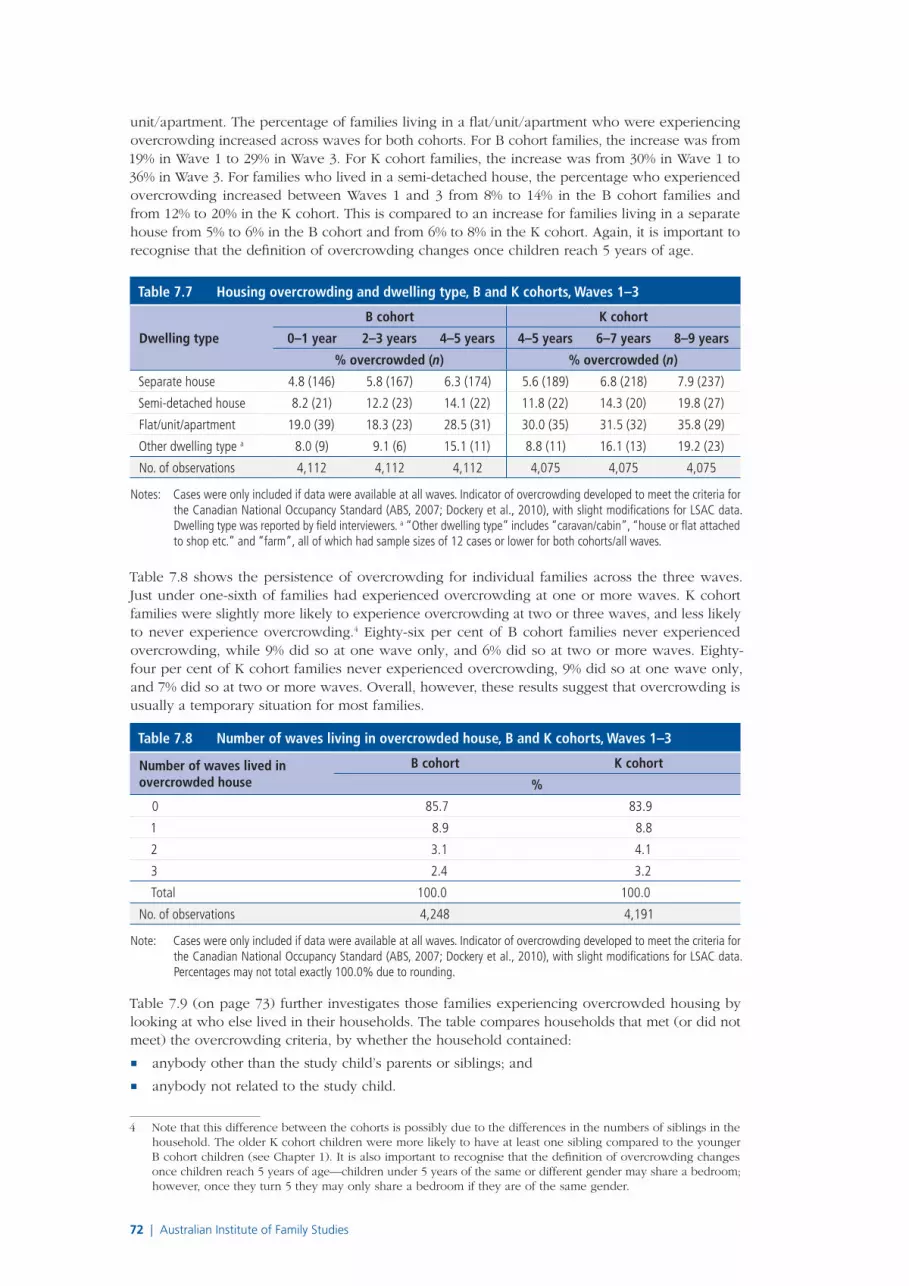
72 | Australian Institute of Family Studies
unit/apartment. The percentage of families living in a flat/unit/apartment who were experiencing overcrowding increased across waves for both cohorts. For B cohort families, the increase was from 19% in Wave 1 to 29% in Wave 3. For K cohort families, the increase was from 30% in Wave 1 to 36% in Wave 3. For families who lived in a semi-detached house, the percentage who experienced overcrowding increased between Waves 1 and 3 from 8% to 14% in the B cohort families and from 12% to 20% in the K cohort. This is compared to an increase for families living in a separate house from 5% to 6% in the B cohort and from 6% to 8% in the K cohort. Again, it is important to recognise that the definition of overcrowding changes once children reach 5 years of age.
Table 7.7 Housing overcrowding and dwelling type, B and K cohorts, Waves 1–3
Dwelling type
B cohort K cohort
0–1 year 2–3 years 4–5 years 4–5 years 6–7 years 8–9 years
% overcrowded (n) % overcrowded (n)
Separate house 4.8 (146) 5.8 (167) 6.3 (174) 5.6 (189) 6.8 (218) 7.9 (237)
Semi-detached house 8.2 (21) 12.2 (23) 14.1 (22) 11.8 (22) 14.3 (20) 19.8 (27)
Flat/unit/apartment 19.0 (39) 18.3 (23) 28.5 (31) 30.0 (35) 31.5 (32) 35.8 (29)
Other dwelling type a 8.0 (9) 9.1 (6) 15.1 (11) 8.8 (11) 16.1 (13) 19.2 (23)
No. of observations 4,112 4,112 4,112 4,075 4,075 4,075
Notes: Cases were only included if data were available at all waves. Indicator of overcrowding developed to meet the criteria for the Canadian National Occupancy Standard (ABS, 2007; Dockery et al., 2010), with slight modifications for LSAC data. Dwelling type was reported by field interviewers. a “Other dwelling type” includes “caravan/cabin”, “house or flat attached to shop etc.” and “farm”, all of which had sample sizes of 12 cases or lower for both cohorts/all waves.
Table 7.8 shows the persistence of overcrowding for individual families across the three waves. Just under one-sixth of families had experienced overcrowding at one or more waves. K cohort families were slightly more likely to experience overcrowding at two or three waves, and less likely to never experience overcrowding.4 Eighty-six per cent of B cohort families never experienced overcrowding, while 9% did so at one wave only, and 6% did so at two or more waves. Eighty-four per cent of K cohort families never experienced overcrowding, 9% did so at one wave only, and 7% did so at two or more waves. Overall, however, these results suggest that overcrowding is usually a temporary situation for most families.
Table 7.8 Number of waves living in overcrowded house, B and K cohorts, Waves 1–3
Number of waves lived in overcrowded house
B cohort K cohort
%
0 85.7 83.9
1 8.9 8.8
2 3.1 4.1
3 2.4 3.2
Total 100.0 100.0
No. of observations 4,248 4,191
Note: Cases were only included if data were available at all waves. Indicator of overcrowding developed to meet the criteria for the Canadian National Occupancy Standard (ABS, 2007; Dockery et al., 2010), with slight modifications for LSAC data. Percentages may not total exactly 100.0% due to rounding.
Table 7.9 (on page 73) further investigates those families experiencing overcrowded housing by looking at who else lived in their households. The table compares households that met (or did not meet) the overcrowding criteria, by whether the household contained:
■ anybody other than the study child’s parents or siblings; and
■ anybody not related to the study child.
4 Note that this difference between the cohorts is possibly due to the differences in the numbers of siblings in the household. The older K cohort children were more likely to have at least one sibling compared to the younger B cohort children (see Chapter 1). It is also important to recognise that the definition of overcrowding changes once children reach 5 years of age—children under 5 years of the same or different gender may share a bedroom; however, once they turn 5 they may only share a bedroom if they are of the same gender.

Chapter 7: Housing characteristics and changes across waves
LSAC Annual Statistical Report 2011 | 73
Table 7.9 Other relatives and non-relatives in children’s households, by whether house overcrowded, B and K cohorts, Waves 1–3
B cohort K cohort
0–1 year
2–3 years
4–5 years
4–5 years
6–7 years
8–9 years
% %
House overcrowded
Lives with one or more people who are not a parent/sibling of the study child
45.2 46.7 39.1 26.9 31.2 32.8
Lives with one or more people who are not related to the study child
6.6 4.9 5.8 3.5 5.6 6.8
No. of observations 227 229 253 274 303 335
House not overcrowded
Lives with one or more people who are not a parent/sibling of the study child
6.6 6.8 6.3 5.5 7.4 6.6
Lives with one or more people who are not related to the study child
1.4 1.7 1.9 1.5 3.1 3.6
No. of observations 4,021 4,019 3,995 3,917 3,888 3,856
Notes: Cases were only included if data were available at all waves. Indicator of overcrowding developed to meet the criteria for the Canadian National Occupancy Standard (ABS, 2007; Dockery et al., 2010), with slight modifications for LSAC data.
By comparing these two groups, we can get a sense of whether children lived with extended family members or with people who were not related to them. For example, the table shows that 45% of 0–1 year olds living in an overcrowded house lived with people who were not a parent or sibling, but only 7% lived with someone who was not related to them, suggesting that 38% lived with extended family members.
The table shows fairly similar patterns for the two cohorts across the three waves, although K cohort children who lived in an overcrowded house were less likely to live with one or more people who were not their parents/siblings. Between 27% and 47% of children experiencing overcrowding lived with someone who was not their parent/sibling, compared to between 6% and 7% of children living in a house that was not overcrowded. Between 4% and 7% of children living in an overcrowded house lived with someone not related to them, compared to between 1% and 4% of children not in an overcrowded home. In interpreting these results, it is important to note the small numbers of families living in overcrowded housing in comparison to those families not living in overcrowded housing.
7.4 Mobility, tenure and overcrowdingThis final section investigates the relationships between mobility and housing tenure, and mobility and overcrowding, and focuses on the younger group of children (the B cohort) because of the relatively high levels of mobility experienced by this group. The first two tables, Table 7.10 (on page 74) and Table 7.11 (on page 75), show changes in housing tenure after moving house between waves.5 The shaded cells on the diagonal of each table indicate those who remained in the same category between waves.
Table 7.10 shows the housing tenure in Wave 1 and Wave 2 after moving house between those two waves. Among those families who moved, the largest groups were those who initially lived in a house on which they had a mortgage, followed by those in private rentals. A large percentage (63%) of families who owned their house outright in Wave 1 moved into a new house with a mortgage, suggesting that some families may upgrade their houses when their children are young. Twenty-three per cent of Wave 1 outright owners moved to a new house that they also owned outright, and 6% moved into a rental property.
5 Note that families may have moved more than once within the two years between waves.
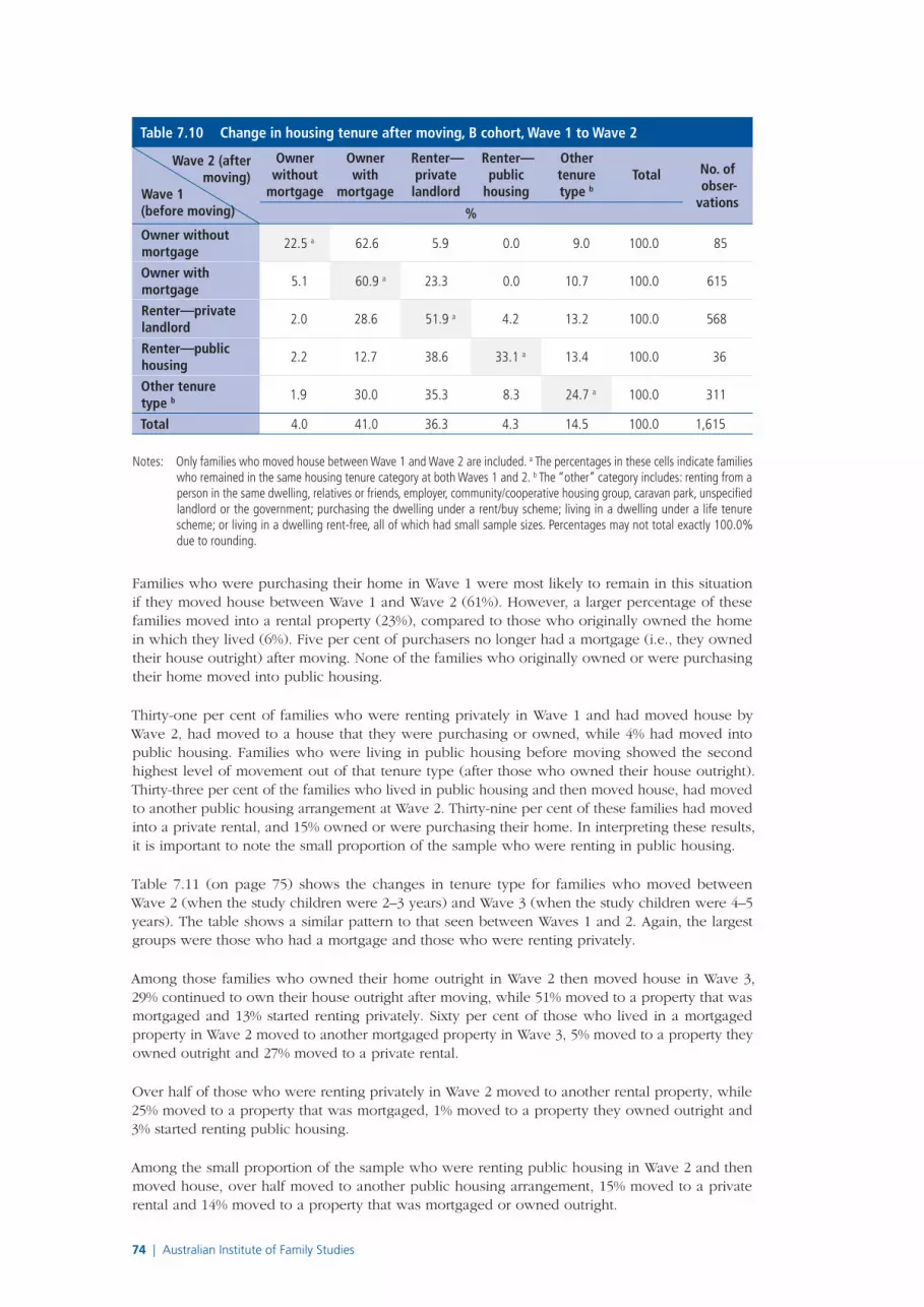
74 | Australian Institute of Family Studies
Table 7.10 Change in housing tenure after moving, B cohort, Wave 1 to Wave 2
Wave 2 (after moving)
Wave 1 (before moving)
Owner without
mort gage
Owner with
mort gage
Renter—private
landlord
Renter—public
housing
Other tenure type b
Total No. of obser-
vations%
Owner without mortgage
22.5 a 62.6 5.9 0.0 9.0 100.0 85
Owner with mortgage
5.1 60.9 a 23.3 0.0 10.7 100.0 615
Renter—private landlord
2.0 28.6 51.9 a 4.2 13.2 100.0 568
Renter—public housing
2.2 12.7 38.6 33.1 a 13.4 100.0 36
Other tenure type b 1.9 30.0 35.3 8.3 24.7 a 100.0 311
Total 4.0 41.0 36.3 4.3 14.5 100.0 1,615
Notes: Only families who moved house between Wave 1 and Wave 2 are included. a The percentages in these cells indicate families who remained in the same housing tenure category at both Waves 1 and 2. b The “other” category includes: renting from a person in the same dwelling, relatives or friends, employer, community/cooperative housing group, caravan park, unspecified landlord or the government; purchasing the dwelling under a rent/buy scheme; living in a dwelling under a life tenure scheme; or living in a dwelling rent-free, all of which had small sample sizes. Percentages may not total exactly 100.0% due to rounding.
Families who were purchasing their home in Wave 1 were most likely to remain in this situation if they moved house between Wave 1 and Wave 2 (61%). However, a larger percentage of these families moved into a rental property (23%), compared to those who originally owned the home in which they lived (6%). Five per cent of purchasers no longer had a mortgage (i.e., they owned their house outright) after moving. None of the families who originally owned or were purchasing their home moved into public housing.
Thirty-one per cent of families who were renting privately in Wave 1 and had moved house by Wave 2, had moved to a house that they were purchasing or owned, while 4% had moved into public housing. Families who were living in public housing before moving showed the second highest level of movement out of that tenure type (after those who owned their house outright). Thirty-three per cent of the families who lived in public housing and then moved house, had moved to another public housing arrangement at Wave 2. Thirty-nine per cent of these families had moved into a private rental, and 15% owned or were purchasing their home. In interpreting these results, it is important to note the small proportion of the sample who were renting in public housing.
Table 7.11 (on page 75) shows the changes in tenure type for families who moved between Wave 2 (when the study children were 2–3 years) and Wave 3 (when the study children were 4–5 years). The table shows a similar pattern to that seen between Waves 1 and 2. Again, the largest groups were those who had a mortgage and those who were renting privately.
Among those families who owned their home outright in Wave 2 then moved house in Wave 3, 29% continued to own their house outright after moving, while 51% moved to a property that was mortgaged and 13% started renting privately. Sixty per cent of those who lived in a mortgaged property in Wave 2 moved to another mortgaged property in Wave 3, 5% moved to a property they owned outright and 27% moved to a private rental.
Over half of those who were renting privately in Wave 2 moved to another rental property, while 25% moved to a property that was mortgaged, 1% moved to a property they owned outright and 3% started renting public housing.
Among the small proportion of the sample who were renting public housing in Wave 2 and then moved house, over half moved to another public housing arrangement, 15% moved to a private rental and 14% moved to a property that was mortgaged or owned outright.

Chapter 7: Housing characteristics and changes across waves
LSAC Annual Statistical Report 2011 | 75
Table 7.11 Change in housing tenure after moving, B cohort, Wave 2 to Wave 3
Wave 3 (after moving)
Wave 2 (before moving)
Owner without
mort gage
Owner with
mort gage
Renter—private
landlord
Renter—public
housing
Other tenure type b
Total No. of obser-
vations%
Owner without mortgage
28.6 a 50.5 12.7 0.0 8.1 100.0 85
Owner with mortgage
5.0 59.8 a 27.1 0.0 8.0 100.0 512
Renter—private landlord
1.3 25.4 56.0 a 3.0 14.3 100.0 432
Renter—public housing
3.8 10.2 14.5 56.0 a 15.5 100.0 35
Other tenure type b 3.1 37.2 27.4 3.4 28.9 a 100.0 229
Total 4.6 40.4 36.4 4.2 14.4 100.0 1,293
Notes: Only families who moved house between Wave 2 and Wave 3 are included. a The percentages in these cells indicate families who remained in the same housing tenure category at both Waves 2 and 3. b The “other” category includes: renting from a person in the same dwelling, relatives or friends, employer, community/cooperative housing group, caravan park, unspecified landlord or the government; purchasing the dwelling under a rent/buy scheme; living in a dwelling under a life tenure scheme; or living in a dwelling rent-free, all of which had small sample sizes. Percentages may not total exactly 100.0% due to rounding.
The final two tables in this chapter explore changes in experiences of overcrowding after moving house, again with a focus on the B cohort. Table 7.12 shows changes and persistence of overcrowding for families who moved between when their study child was 0–1 years (Wave 1) and 2–3 years (Wave 2). The shaded cells on the diagonal of the table indicate those who remained in the same category between waves. The table shows that two-thirds of families who lived in an overcrowded house in Wave 1 and then moved, moved into a house where they did not experience overcrowding. However, one-third moved into a house that was also overcrowded.
Table 7.12 Change in housing overcrowding after moving, B cohort, Wave 1 to Wave 2
Wave 2 (after moving)
Wave 1 (before moving)
OvercrowdingNo
overcrowdingTotal
No. of observations
%
Overcrowding 32.1 a 67.9 100.0 126
No overcrowding 6.1 93.9 a 100.0 1,494
Total 8.4 91.6 100.0 1,620
Notes: Only families who moved house between Wave 1 and Wave 2 are included. a The percentages in these cells indicate families who remained in the same overcrowding category at both Waves 1 and 2.
Table 7.13 shows a similar pattern for the children who moved house between when they were 2–3 years (Wave 2) and when they were 4–5 years (Wave 3). Seventy-six per cent of children who lived in an overcrowded hours moved to one that was not, and 24% also lived in an overcrowded house after moving.
Table 7.13 Change in housing overcrowding after moving, B cohort, Wave 2 to Wave 3
Wave 3 (after moving)
Wave 2 (before moving)
OvercrowdingNo
overcrowdingTotal
No. of observations
%
Overcrowding 23.6 a 76.4 100.0 87
No overcrowding 7.2 92.8 a 100.0 1,206
Total 8.7 91.3 100.0 1,293
Notes: Only families who moved house between Wave 2 and Wave 3 are included. a The percentages in these cells indicate families who remained in the same overcrowding category at both Waves 2 and 3.
76 | Australian Institute of Family Studies
7.5 SummaryThis chapter has made use of two aspects of the LSAC data—its longitudinal nature and the information collected about the people with whom children live. The chapter has examined housing mobility, tenure and overcrowding as three aspects of children’s housing that are thought to have important influences on their development (Dockery et al., 2010).
The analyses show that LSAC children have experienced high levels of housing mobility, with approximately three-quarters of children moving house at least once before they turned 10. Children were most likely to move house when they were young, but the majority of moves were within the same local area. For many children, housing mobility also led to changes in their housing tenure and levels of overcrowding (mostly to less crowding).
More than half of the families owned or were purchasing their own home, and the percentage that did so increased as the children became older. This group of families had the greatest consistency of tenure between waves, as most families remained in this tenure category even after moving house between waves. A reasonable proportion of families who owned their own house outright when their children were babies acquired a mortgage when they moved into a new house.
Using the Canadian National Occupancy Standard (ABS, 2007; Dockery et al., 2010), this chapter has shown that fewer than 10% of children younger than 10 years lived in an overcrowded house. The majority of families who experienced overcrowding did so at only one wave. Similarly, families who lived in an overcrowded house were less likely to do so after moving. Children in overcrowded homes were more likely to be living with extended family members compared to those not experiencing overcrowding.
Further research is needed to better understand the housing characteristics of the families who fall into the “other tenure type” category in this chapter. Although there is a relatively small number of families in this situation, because of the nature of these housing arrangements (including paying rent to someone else in the house, a friend or a relative), it is likely that many of these families experience high levels of overcrowding and mobility, particularly when living in shared housing arrangements (e.g., sharing with relatives), which is common after family separation (AIHW, 2007).
Future analysis using LSAC data will be able to examine the relationships between housing characteristics and children’s outcomes in Australia, and thereby help to reduce the dearth of information in this area.
7.6 Further readingDockery, A. M., Kendall, G., Li, J., Mahendran, A., Ong, R., & Strazdins, L. (2010). Housing and children’s development and wellbeing: A scoping study (AHURI Final Report No. 149). Melbourne: Australian Housing and Urban Research Institute.
7.7 ReferencesAstone, N. M., & McLanahan, S. S. (1994). Family structure, residential mobility, and school dropout: A research note. Demography, 31, 575–583.
Australian Bureau of Statistics. (2007). Housing occupancy and costs, Australia 2005–2006 (Cat. No. 4130.0.55.001). Canberra: ABS.
Australian Housing and Urban Research Institute. (2006). How does security of tenure impact on public housing tenants? (AHURI Research and Policy Bulletin No. 78). Melbourne: AHURI.
Australian Institute of Health and Welfare. (2007). Homeless people in SAAP: Supported Accommodation Assistance Program National Data Collection Agency annual report (Cat. No. HOU 156). Canberra: AIHW.
Bell, M. & Hugo, G. (2000). Internal migration in Australia 1991–1996: Overview and the overseas-born. Canberra: Department of Immigration and Multicultural Affairs.
Bronfenbrenner, U., & Morris, P. A. (2006). The bioecological model of human development. In W. Damon & R. M. Lerner (Eds.), Handbook of child psychology (Vol. 1, pp. 793–828). New York: John Wiley & Sons.
Council of Australian Governments. (2009). Protecting children is everyone’s business: National Framework for Protecting Australia’s Children 2009–2020. Canberra: COAG.
Dockery, A. M., Kendall, G., Li, J., Mahendran, A., Ong, R., & Strazdins, L. (2010). Housing and children’s development and wellbeing: A scoping study (AHURI Final Report No. 149). Melbourne: Australian Housing and Urban Research Institute.
Evans, G. W. (2006). Child development and the physical environment. Annual Review of Psychology, 57, 423–451.
Chapter 7: Housing characteristics and changes across waves
LSAC Annual Statistical Report 2011 | 77
Jelleyman, T., & Spencer, N. (2008). Residential mobility in childhood and health outcomes: A systematic review. Journal of Epidemiology and Community Health, 62, 584–592.
Simpson, G. A., & Fowler, M. G. (1994). Geographic mobility and children’s emotional/behavioral adjustment and school functioning. Pediatrics, 93(2), 303–309.
Wood, D., Halfon, N., Scarlata, D., Newacheck, P., & Nessim, S. (1993). Impact of family relocation on children’s growth, development, school function, and behavior. Journal of the American Medical Association, 270(1), 1334–1338.

78 | Australian Institute of Family Studies

Chapter 8: Children’s numeracy skills
LSAC Annual Statistical Report 2011 | 79
Galina DaraganovaAustralian Institute of Family Studies
John AinleyAustralian Council of Educational Research
Numeracy, and the capacity to be numerate, is the ability to reason with numbers and to effectively apply mathematical concepts in everyday life (Ministerial Council for Education Early Childhood Development and Youth Affairs [MCEECDYA], 2008). A number of studies
have suggested that early numeracy is grounded in number competence (such as recognising the value of quantities and grasping the principles of counting) (Jordan, Kaplan, Rameni, & Locuniak, 2009), informal number sense (e.g., understanding terms such as “more”, “less”, “bigger” and “smaller”; knowing that numbers in a counting sequence refer to specific quantities and that higher numbers reflect greater quantities) (Griffin, 2004), and more general factors sometimes characterised as “working memory” (Raghubar, Barnes, & Hecht, 2010). Reid (2008) showed that an early informal understanding of quantitative relationships provides the basis for developing formal mathematical knowledge.
Thomson, Rowe, Underwood, and Peck (2005) followed the development of numeracy in a sample of Australian children from preschool to the first year of school. Their study highlighted children’s diverse preschool experiences and showed that there was a wide range in early numeracy achievement across the sites that were examined.
But numeracy is more than just numbers and measurements. Research has shown that young people’s numeracy skills are a vital foundation for their subsequent achievements through school and into further education, training and work (e.g., Aubrey, Godfrey, & Dahl, 2006; Doig & de Lemos, 2000; Stevenson & Stigler, 1992; Young-Loveridge, Peters, & Carr, 1997). Therefore, one of the major objectives in educational policy is to provide children with strong numeracy skills through the years of schooling.
To enrich the understanding of the factors that lead to better educational outcomes, a number of national and international assessment surveys take place worldwide. These include the Organisation for Economic Co-operation and Development (OECD) Programme for International Student Assessment (PISA), the Trends in International Mathematics and Science Studies (TIMSS), and the Australian National Assessment Program—Literacy and Numeracy (NAPLAN) (Australian Curriculum Assessment and Reporting Authority [ACARA], 2010b). Recent results from the OECD PISA reveal that, while 15-year-old Australian students are still performing well above the OECD average (OECD, 2010), their results in numeracy have declined significantly over recent years. Significant gaps in achievement are also observed between students from different socio-economic backgrounds.
This chapter uses data from the K cohort of Growing Up in Australia: The Longitudinal Study of Australian Children (LSAC) to examine the numeracy skills demonstrated by children at different ages, and whether levels of numeracy skills vary for children from different socio-demographic backgrounds. The socio-demographic groups examined in this chapter are categorised by:
■ child gender;
■ socio-economic characteristics:
– family socio-economic position (SEP)—lowest 25%, middle 50%, highest 25%; and
8Children’s numeracy skills

80 | Australian Institute of Family Studies
– mother’s working hours—not working (including those unemployed, on maternity leave, and not in the labour force), working less than 35 hours per week, or working 35 hours or more per week; and
■ family characteristics:
– family type—two-parent family, lone-mother family; and
– number of siblings in the household—no siblings, one or two siblings, three or more siblings.
See Chapter 1 for details about these groups.
8.1 Measuring numeracy in LSACIn LSAC, information on the child’s numeracy skills is obtained from two different sources:
■ teachers’ ratings; and
■ NAPLAN results.
A list of numeracy measures used in Waves 1–3 is presented in Table 8.1.
Table 8.1 Numeracy assessments, K cohort Waves 1–3
Time pointAverage age (SD = 3 months)
InstrumentRespondent/informant
No. of obser-vations a
Wave 1, 2004 4 years, 9 months Teachers’ ratings Teacher b 3,176
Wave 2, 2006 6 years, 10 monthsTeachers’ ratings: Academic Rating Scale, Numeracy Skills sub-scale, 6–7 years
Teacher b 3,505
Wave 3, 2008 8 years, 10 monthsTeachers’ ratings: Academic Rating Scale, Numeracy Skills sub-scale, 8–9 years
Teacher b 3,533
2008/09 8 years, 7 months NAPLAN: Numeracy test, Year 3 c Study child 2,514
Notes: a The number of observations is determined by availability of the data. b Teachers’ ratings were provided by the teacher who had primary responsibility for the planning and delivery of the group program in which the study child participated. c K cohort children sat the Year 3 NAPLAN Numeracy test in 2008 or 2009, depending on the year of their enrolment. Those children (n = 770) who sat the Year 5 NAPLAN Numeracy test in 2009 are not included in this chapter.
Teachers’ ratingsTeachers’ ratings were collected using the LSAC teacher questionnaire, in which teachers were asked to judge the proficiency of the child’s numeracy skills in relation to other children the same age. The items in the teachers’ ratings covered different areas of numeracy, such as number, measurement and space, and differed across waves to reflect different levels of difficulty.
In Wave 1, teachers were asked to rate the child’s numeracy skills compared to other children of a similar age, using a yes/no scale of five items (see Table 8.2 for a list of items). The total numeracy score was calculated as the number of yes responses; the higher the score, the more numeracy skills a child had acquired.
Table 8.2 Teachers’ ratings scale, K cohort Wave 1
Item Abbreviation
1 Able to sort and classify objects by shape or colour Sort and classify
2 Able to count the number of a few objects accurately Count objects
3 Able to count to 20 Count to 20
4 Able to recognise numbers Recognise numbers
5 Able to do simple addition with concrete materials Simple addition
In Waves 2 and 3, teachers’ ratings of the children’s numeracy skills were obtained using the Numeracy Skills sub-scale of the Academic Rating Scale (ARS) for 6–7 year olds and 8–9 year olds, respectively. These scales were adapted for use in Australian schools by Rothman (2009). Tables 8.3 and 8.4 (on page 81) present the scale items used for different ages. Teachers were asked to rate a child’s proficiency on each item using a five-point ordinal scale (1 = not yet, 2 = beginning, 3 = in progress, 4 = intermediate, 5 = proficient). The overall measure of numeracy achievement was
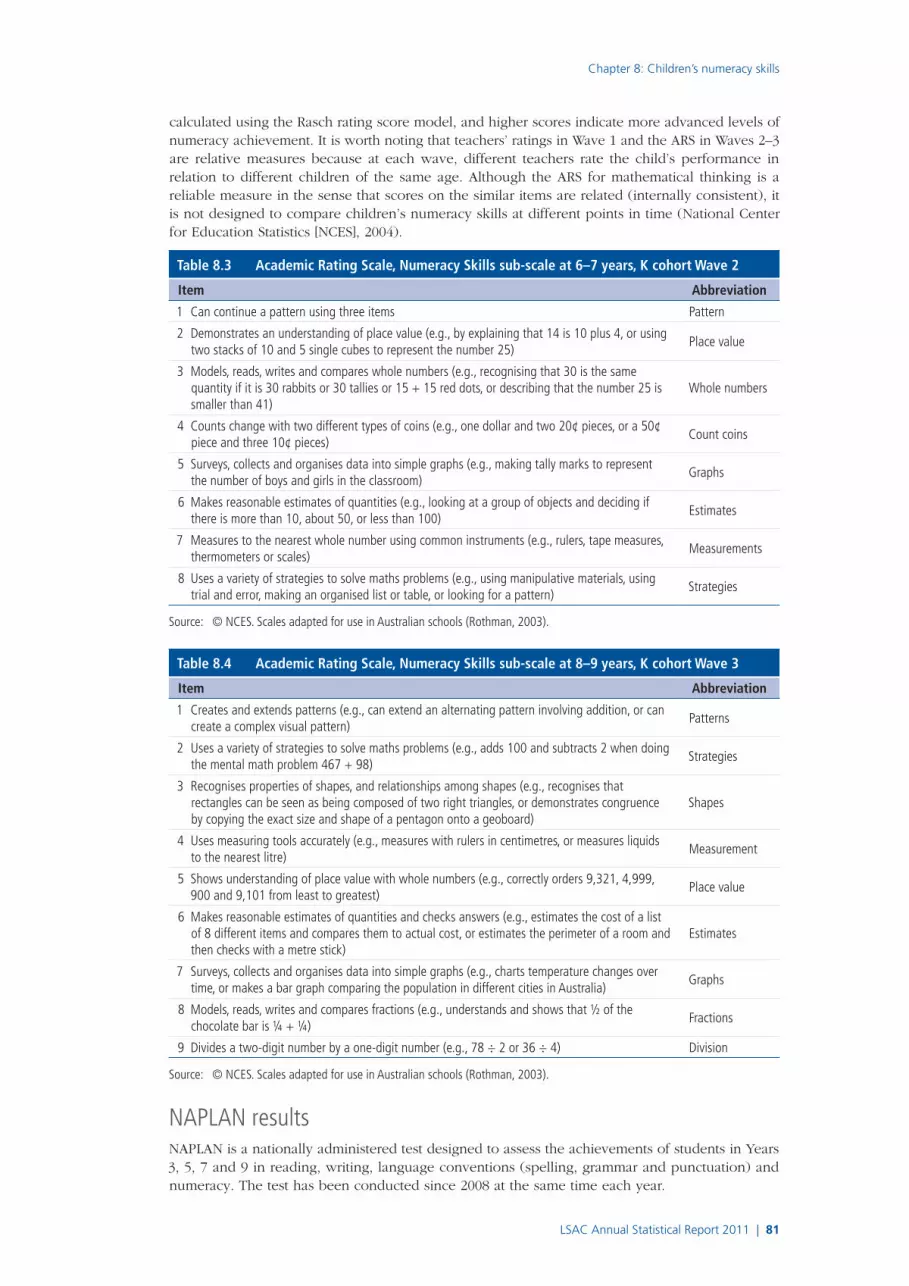
Chapter 8: Children’s numeracy skills
LSAC Annual Statistical Report 2011 | 81
calculated using the Rasch rating score model, and higher scores indicate more advanced levels of numeracy achievement. It is worth noting that teachers’ ratings in Wave 1 and the ARS in Waves 2–3 are relative measures because at each wave, different teachers rate the child’s performance in relation to different children of the same age. Although the ARS for mathematical thinking is a reliable measure in the sense that scores on the similar items are related (internally consistent), it is not designed to compare children’s numeracy skills at different points in time (National Center for Education Statistics [NCES], 2004).
Table 8.3 Academic Rating Scale, Numeracy Skills sub-scale at 6–7 years, K cohort Wave 2
Item Abbreviation
1 Can continue a pattern using three items Pattern
2 Demonstrates an understanding of place value (e.g., by explaining that 14 is 10 plus 4, or using two stacks of 10 and 5 single cubes to represent the number 25)
Place value
3 Models, reads, writes and compares whole numbers (e.g., recognising that 30 is the same quantity if it is 30 rabbits or 30 tallies or 15 + 15 red dots, or describing that the number 25 is smaller than 41)
Whole numbers
4 Counts change with two different types of coins (e.g., one dollar and two 20¢ pieces, or a 50¢ piece and three 10¢ pieces)
Count coins
5 Surveys, collects and organises data into simple graphs (e.g., making tally marks to represent the number of boys and girls in the classroom)
Graphs
6 Makes reasonable estimates of quantities (e.g., looking at a group of objects and deciding if there is more than 10, about 50, or less than 100)
Estimates
7 Measures to the nearest whole number using common instruments (e.g., rulers, tape measures, thermometers or scales)
Measurements
8 Uses a variety of strategies to solve maths problems (e.g., using manipulative materials, using trial and error, making an organised list or table, or looking for a pattern)
Strategies
Source: © NCES. Scales adapted for use in Australian schools (Rothman, 2003).
Table 8.4 Academic Rating Scale, Numeracy Skills sub-scale at 8–9 years, K cohort Wave 3
Item Abbreviation
1 Creates and extends patterns (e.g., can extend an alternating pattern involving addition, or can create a complex visual pattern)
Patterns
2 Uses a variety of strategies to solve maths problems (e.g., adds 100 and subtracts 2 when doing the mental math problem 467 + 98)
Strategies
3 Recognises properties of shapes, and relationships among shapes (e.g., recognises that rectangles can be seen as being composed of two right triangles, or demonstrates congruence by copying the exact size and shape of a pentagon onto a geoboard)
Shapes
4 Uses measuring tools accurately (e.g., measures with rulers in centimetres, or measures liquids to the nearest litre)
Measurement
5 Shows understanding of place value with whole numbers (e.g., correctly orders 9,321, 4,999, 900 and 9,101 from least to greatest)
Place value
6 Makes reasonable estimates of quantities and checks answers (e.g., estimates the cost of a list of 8 different items and compares them to actual cost, or estimates the perimeter of a room and then checks with a metre stick)
Estimates
7 Surveys, collects and organises data into simple graphs (e.g., charts temperature changes over time, or makes a bar graph comparing the population in different cities in Australia)
Graphs
8 Models, reads, writes and compares fractions (e.g., understands and shows that ½ of the chocolate bar is ¼ + ¼)
Fractions
9 Divides a two-digit number by a one-digit number (e.g., 78 ÷ 2 or 36 ÷ 4) Division
Source: © NCES. Scales adapted for use in Australian schools (Rothman, 2003).
NAPLAN resultsNAPLAN is a nationally administered test designed to assess the achievements of students in Years 3, 5, 7 and 9 in reading, writing, language conventions (spelling, grammar and punctuation) and numeracy. The test has been conducted since 2008 at the same time each year.

82 | Australian Institute of Family Studies
The NAPLAN Numeracy test measures the achievement of students in five broad areas of numeracy—number; algebra, function and pattern; measurement, chance and data; space; and working mathematically—as defined by the Statements of Learning for Mathematics (MCEECDYA, 2008). The test contains multiple-choice items and constructed response items. The Numeracy Skills sub-scale has scaled scores that are grouped into 10 bands. Bands correspond to the complexity of skills being assessed; that is, test items are more complex in higher bands. Band 2 refers to the National Minimum Standards (NMS) for children in Year 3. Year 3 children who score in Band 1 are performing below the NMS, and Year 3 children who score in Band 3 and above demonstrate academic performance above the NMS for Year 3.
In this chapter, we use only the results from the Year 3 NAPLAN Numeracy test, which took place in 2008 and in 2009.
8.2 Teachers’ ratings of numeracyNumeracy in kindergarten years (4–5 years old)Figure 8.1 shows the proportion of children who had developed particular numeracy skills (able) and who had not (not able). About 95% of children in the K cohort at Wave 1 (whose average age was 4 years and 9 months) could sort and classify objects by shape and colour as well as count the number of a few objects accurately. Seventy-two per cent of children were able to recognise numbers and 62% of children were able to count to 20. Thirty-four per cent of children were able to do simple addition with concrete materials.
66
28
38
6
4
34
72
62
94
96
0 10 20 30 40 50 60 70 80 90 100
Sort and classify
Count objects
Count to 20
Recognise numbers
Simple addition
Not able Able
Percentage of children
Figure 8.1 Percentage of children who developed particular numeracy skills, by teachers’ ratings, K cohort Wave 1
Numeracy in early primary years (6–7 years old)Figure 8.2 (on page 83) shows the proportion of children at different levels of proficiency on each item of the Numeracy Skills sub-scale of the Academic Rating Scale for 6–7 year olds. The degree to which the children had acquired the competencies is reflected by different categories. Children who did not demonstrate the skill are represented by the “not yet” category. The “beginning” category represents the proportion of children who were just beginning to demonstrate the skill. The proportion of children who demonstrated the skill with some regularity is represented by the third category, “in progress”. The “intermediate” category represents the proportion of children who demonstrated the skill with average competence. The last category, “proficient”, represents children who demonstrated the skill competently and consistently.

Chapter 8: Children’s numeracy skills
LSAC Annual Statistical Report 2011 | 83
The average age of the K cohort children at Wave 2 was 6 years and 10 months. Most of these were able to continue a pattern using three items; that is, 93% of these children achieved a proficient (52%), intermediate (28%) or in progress (13%) level of competency. Six per cent of the children were just beginning to demonstrate the skill and only 1% of them were not yet able to continue a pattern.
More than 80% of the children were able to understand place value. Of these, 31% of children were able to understand place value competently and consistently and 50% were able to apply this skill with average competence (intermediate = 29%) or regularly (in progress = 21%). Around one-fifth either used it very rarely (12%) or had not yet developed this skill (7%) .
Most of the children were able to manipulate whole numbers, with every third child being proficient (34%) and every second child applying this skill either with average competence (intermediate = 29%) or regularly (in progress = 20%). One in six of the children either were just beginning to apply this skill (11%) or did not demonstrate this skill (6%).
About 80% of the children were able to make reasonable estimates of quantities and represent data using graphs, with 20% of them being able to do it proficiently and about 60% being able to do it at intermediate or in-progress levels. Fifteen per cent of children tried to make reasonable estimates (beginning ) and 16% of children attempted to use graphs (beginning). Only 3–6% of the children had not yet developed these skills.
About 70% of children were able to use strategies to solve mathematical problems, count change using different coins and make measurements, with about 13% of them being proficient and 54–59% achieving either at intermediate or in-progress levels. Out of the whole sample, 16% of children could not calculate change, 14% were not able to use measurement instruments and 8% did not use different strategies to solve mathematical problems.
Overall, around 50% of children were achieving at intermediate or in-progress levels on all the skill items, with the variation in proportions mainly observed at the extreme ends of achievement.
7
6
16
5
6
14
8
6
12
11
17
16
15
19
20
28
29
29
24
33
34
27
30
52
31
34
13
20
20
12
13
13
21
20
30
25
25
28
29
0 10 20 30 40 50 60 70 80 90 100
Pattern
Place value
Whole numbers
Count coins
Graphs
Estimates
Measurements
Strategies
Not yet Beginning In progress Intermediate Proficient
Percentage of children
1
Notes: Percentages may not total exactly 100% due to rounding.
Figure 8.2 Percentage of children who achieved each level of competency of the ARS Numeracy Skills sub-scale for 6–7 year olds, K cohort Wave 2
Numeracy in middle primary years (8–9 years old)Figure 8.3 (on page 84) shows the different levels of proficiency achieved on each item of the Numeracy Skills sub-scale of the ARS for 8–9 year olds. As above, the degree to which the children had acquired the competencies is reflected by different categories, ranging from not yet to proficient.
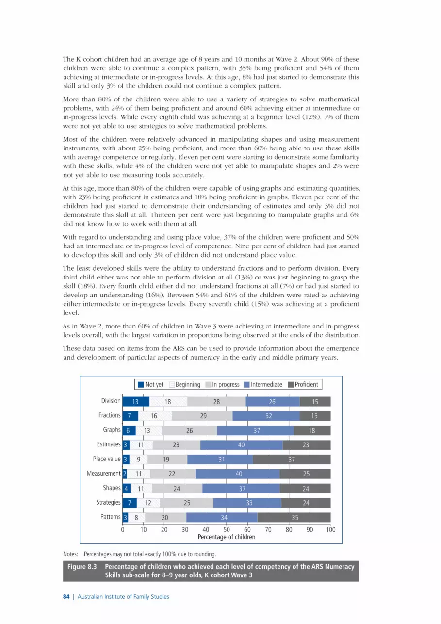
84 | Australian Institute of Family Studies
The K cohort children had an average age of 8 years and 10 months at Wave 2. About 90% of these children were able to continue a complex pattern, with 35% being proficient and 54% of them achieving at intermediate or in-progress levels. At this age, 8% had just started to demonstrate this skill and only 3% of the children could not continue a complex pattern.
More than 80% of the children were able to use a variety of strategies to solve mathematical problems, with 24% of them being proficient and around 60% achieving either at intermediate or in-progress levels. While every eighth child was achieving at a beginner level (12%), 7% of them were not yet able to use strategies to solve mathematical problems.
Most of the children were relatively advanced in manipulating shapes and using measurement instruments, with about 25% being proficient, and more than 60% being able to use these skills with average competence or regularly. Eleven per cent were starting to demonstrate some familiarity with these skills, while 4% of the children were not yet able to manipulate shapes and 2% were not yet able to use measuring tools accurately.
At this age, more than 80% of the children were capable of using graphs and estimating quantities, with 23% being proficient in estimates and 18% being proficient in graphs. Eleven per cent of the children had just started to demonstrate their understanding of estimates and only 3% did not demonstrate this skill at all. Thirteen per cent were just beginning to manipulate graphs and 6% did not know how to work with them at all.
With regard to understanding and using place value, 37% of the children were proficient and 50% had an intermediate or in-progress level of competence. Nine per cent of children had just started to develop this skill and only 3% of children did not understand place value.
The least developed skills were the ability to understand fractions and to perform division. Every third child either was not able to perform division at all (13%) or was just beginning to grasp the skill (18%). Every fourth child either did not understand fractions at all (7%) or had just started to develop an understanding (16%). Between 54% and 61% of the children were rated as achieving either intermediate or in-progress levels. Every seventh child (15%) was achieving at a proficient level.
As in Wave 2, more than 60% of children in Wave 3 were achieving at intermediate and in-progress levels overall, with the largest variation in proportions being observed at the ends of the distribution.
These data based on items from the ARS can be used to provide information about the emergence and development of particular aspects of numeracy in the early and middle primary years.
3
7
4
2
3
7
13
8
12
11
11
9
16
18
20
25
24
22
19
29
28
34
33
37
40
31
32
26
35
24
24
25
37
15
15
Patterns
Strategies
Shapes
Measurement
Place value
6 13 26 37 18Graphs
3 11 23 40 23Estimates
Fractions
Division
Not yet Beginning In progress Intermediate Proficient
0 10 20 30 40 50 60 70 80 90 100Percentage of children
Notes: Percentages may not total exactly 100% due to rounding.
Figure 8.3 Percentage of children who achieved each level of competency of the ARS Numeracy Skills sub-scale for 8–9 year olds, K cohort Wave 3

Chapter 8: Children’s numeracy skills
LSAC Annual Statistical Report 2011 | 85
8.3 NAPLAN Numeracy test Year 3 resultsTable 8.5 shows NAPLAN Numeracy test results for children in the K cohort who sat Year 3 NAPLAN tests in 2008 or 2009. There were 2,381 children who sat the NAPLAN test in 2008 and 142 children who sat the test in 2009—a total of 2,523 children. The children’s average age was 8 years and 7 months.
Ninety per cent of these children performed above the National Minimum Standards (Band 3 and above). Only 2% of children performed below the NMS (Band 1) and 8% of children performed at the NMS (Band 2). The average mean score was within Band 5. Nine out of the 2,523 children were exempted from the test.
Table 8.5 Performance against the National Minimum Standards (NMS) for numeracy, NAPLAN, K cohort Wave 3, 2008–09
Below NMS (%)
At NMS (%)
Above NMS (%) Exempt (%)
Total no. of
children
Mean test score (SD)
Band 1 Band 2 Band 3 Band 4 Band 5 Band 6+
1.9(n = 48)
7.6(n = 192)
17.0(n = 429)
25.9(n = 654)
25.4(n = 640)
21.8(n = 551)
0.4(n = 9)
2,523427.0 (2.7)(n = 2,514)
As described by ACARA (2010b), a student assessed to be meeting the NMS at Year 3 (Band 2) would be expected to be able to: double a whole number to solve a simple problem, recognise a two-dimensional shape within a pattern of different shapes, visually compare the area of similar shapes, and locate a position of an object on a simple plan. A student assessed to be just above the NMS (Band 3) would be expected to be able to: use repeated addition or simple multiplication to solve simple problems, interpret a timetable and locate information, select the most likely outcome in a simple chance event, recognise geometric properties of two-dimensional shapes, and use a grid to identify a symmetrical drawing. The largest proportion of students had performances located in Bands 4 and 5. A student assessed to be in Band 4 would be expected to be able to: use addition and subtraction of two-digit numbers to solve problems, continue number patterns, recognise and use simple fractions to solve problems, identify a prism displayed in an everyday context, estimate the volume of liquid in a familiar container, and visualise a three-dimensional model from a different perspective. A student assessed to be in Band 5 would be expected to be able to: apply a small range of strategies to solve problems, match a digital time to a given analogue time, identify a quarter-turn rotation of a two-dimensional shape, interpret directions to identify a location on a simple map, and interpret a number line to find the number halfway between two three-digit numbers.
8.4 Analysis by socio-demographic characteristicsThis section examines the relationships between children’s levels of proficiency in numeracy and key demographic and family characteristics, using subpopulation groups characterised by:
■ child gender;
■ socio-economic characteristics:
– family socio-economic position—lowest 25%, middle 50%, highest 25%; and
– mother’s working hours—not working (including those unemployed, on maternity leave, and not in the labour force), working less than 35 hours per week, or working 35 hours or more per week; and
■ family characteristics:
– family type—two-parent family, lone mother family; and
– number of siblings in the household—no siblings, one or two siblings, three or more siblings.
These descriptors were chosen as factors that were likely to be associated with numeracy outcomes for children (Battle & Lewis, 2002; Casey, Nuttall, & Pezaris, 2001; Downey, 1995; Fennema, Sowder, & Carpenter, 1999; Goldberg & Prause, 2010; Horwood & Ferguson, 1999; Matthews, Ponitz, & Morrison, 2009; Pong, Dronkers, & Hampden-Thompson, 2003; Shavit & Pierce, 1991). Another
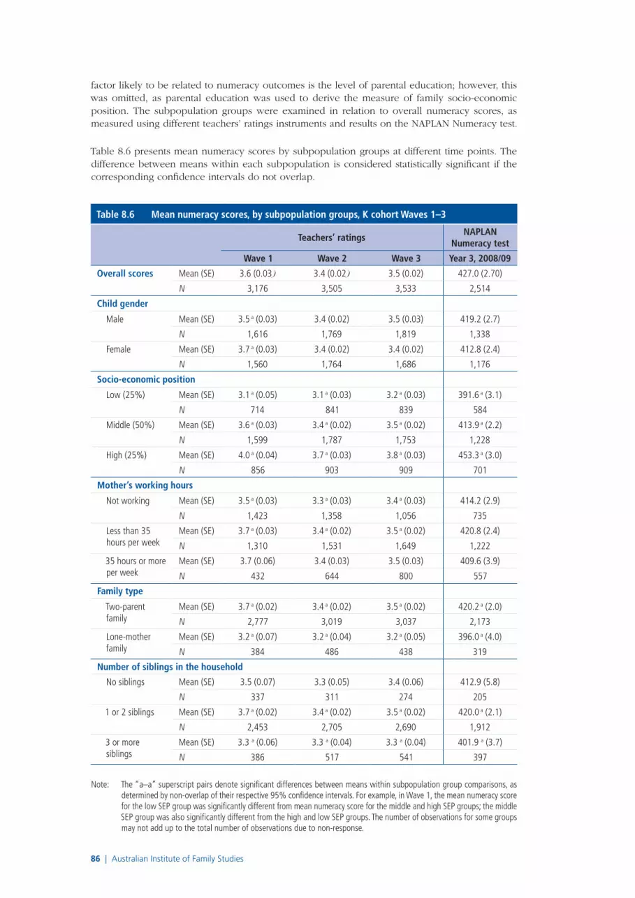
86 | Australian Institute of Family Studies
factor likely to be related to numeracy outcomes is the level of parental education; however, this was omitted, as parental education was used to derive the measure of family socio-economic position. The subpopulation groups were examined in relation to overall numeracy scores, as measured using different teachers’ ratings instruments and results on the NAPLAN Numeracy test.
Table 8.6 presents mean numeracy scores by subpopulation groups at different time points. The difference between means within each subpopulation is considered statistically significant if the corresponding confidence intervals do not overlap.
Table 8.6 Mean numeracy scores, by subpopulation groups, K cohort Waves 1–3
Teachers’ ratingsNAPLAN
Numeracy test
Wave 1 Wave 2 Wave 3 Year 3, 2008/09
Overall scores Mean (SE) 3.6 (0.03) 3.4 (0.02) 3.5 (0.02) 427.0 (2.70)
N 3,176 3,505 3,533 2,514
Child gender
Male Mean (SE) 3.5 a (0.03) 3.4 (0.02) 3.5 (0.03) 419.2 (2.7)
N 1,616 1,769 1,819 1,338
Female Mean (SE) 3.7 a (0.03) 3.4 (0.02) 3.4 (0.02) 412.8 (2.4)
N 1,560 1,764 1,686 1,176
Socio-economic position
Low (25%) Mean (SE) 3.1 a (0.05) 3.1 a (0.03) 3.2 a (0.03) 391.6 a (3.1)
N 714 841 839 584
Middle (50%) Mean (SE) 3.6 a (0.03) 3.4 a (0.02) 3.5 a (0.02) 413.9 a (2.2)
N 1,599 1,787 1,753 1,228
High (25%) Mean (SE) 4.0 a (0.04) 3.7 a (0.03) 3.8 a (0.03) 453.3 a (3.0)
N 856 903 909 701
Mother’s working hours
Not working Mean (SE) 3.5 a (0.03) 3.3 a (0.03) 3.4 a (0.03) 414.2 (2.9)
N 1,423 1,358 1,056 735
Less than 35 hours per week
Mean (SE) 3.7 a (0.03) 3.4 a (0.02) 3.5 a (0.02) 420.8 (2.4)
N 1,310 1,531 1,649 1,222
35 hours or more per week
Mean (SE) 3.7 (0.06) 3.4 (0.03) 3.5 (0.03) 409.6 (3.9)
N 432 644 800 557
Family type
Two-parent family
Mean (SE) 3.7 a (0.02) 3.4 a (0.02) 3.5 a (0.02) 420.2 a (2.0)
N 2,777 3,019 3,037 2,173
Lone-mother family
Mean (SE) 3.2 a (0.07) 3.2 a (0.04) 3.2 a (0.05) 396.0 a (4.0)
N 384 486 438 319
Number of siblings in the household
No siblings Mean (SE) 3.5 (0.07) 3.3 (0.05) 3.4 (0.06) 412.9 (5.8)
N 337 311 274 205
1 or 2 siblings Mean (SE) 3.7 a (0.02) 3.4 a (0.02) 3.5 a (0.02) 420.0 a (2.1)
N 2,453 2,705 2,690 1,912
3 or more siblings
Mean (SE) 3.3 a (0.06) 3.3 a (0.04) 3.3 a (0.04) 401.9 a (3.7)
N 386 517 541 397
Note: The “a–a” superscript pairs denote significant differences between means within subpopulation group comparisons, as determined by non-overlap of their respective 95% confidence intervals. For example, in Wave 1, the mean numeracy score for the low SEP group was significantly different from mean numeracy score for the middle and high SEP groups; the middle SEP group was also significantly different from the high and low SEP groups. The number of observations for some groups may not add up to the total number of observations due to non-response.

Chapter 8: Children’s numeracy skills
LSAC Annual Statistical Report 2011 | 87
Child genderAmong K cohort children at Wave 1, girls tended to have more developed numeracy skills than boys (and this difference was significant). As the children grew older, boys had slightly higher numeracy scores than girls; however, these differences were not statistically significant.
Socio-economic characteristicsThere were significant differences in numeracy achievement according to family socio-economic position. Children from families with a lower socio-economic position had significantly lower scores than children from higher socio-economic backgrounds. This difference remained statistically significant at different ages and across different numeracy measures.
Children’s progress in numeracy was also associated with their mother’s working hours. According to teachers’ ratings, children with mothers working either less than 35 hours or 35 or more hours per week scored higher than children with non-working mothers. But the difference in scores was statistically significant only between children whose mothers worked 0 hours and who worked less than 35 hours per week. These differences were consistent at all three time points. In contrast, analyses of the NAPLAN test results did not reveal any significant differences in numeracy achievement according to mother’s working hours.
Family characteristicsA relationship between other family characteristics and numeracy achievement was also evident. Compared to children from two-parent families, children from lone-mother families had significantly lower numeracy scores for every numeracy measure at all ages.
The number of siblings in the household was also associated with level of numeracy achievement. While there was no statistically significant difference in numeracy progress between children with or without siblings, children with three or more siblings had significantly lower numeracy scores compared with children who had only one or two siblings. This relationship was consistent for every numeracy measure. It is important to note that these associations could reflect other correlated influences, such as that of lower socio-economic position (Downey, 1995; Shavit & Pierce, 1991). Multivariate analyses, which go beyond the scope of this chapter, would be required to explore these possibilities.
In addition to these results, it was found that children’s language background (English- or non–English speaking) was not associated with their level of numeracy achievement (data not shown). It was also found that while the children of mothers under 25 years old received lower teachers’ ratings compared with the children of older mothers, these differences disappeared after controlling for family socio-economic characteristics (data not shown).
Sub-group analyses in perspectiveThe results of the sub-group analyses for child gender do not reveal significant numeracy differences between boys and girls. National results reported for NAPLAN show a similar-sized difference of five scale points (the standard deviation is approximately 72 points) in favour of males for Year 3 students (ACARA, 2010a). Results for Year 4 students in the TIMSS show a similar difference of six scale points (the standard deviation is approximately 100 scale points) between boys and girls in Australia—a difference that is not statistically significant (Thomson, Wernert, Underwood, & Nicholas, 2008). The results for Year 4 in TIMSS indicate inter-country differences in the mathematics achievement of boys and girls, with boys scoring higher than girls in countries such as the United States, Sweden and Germany, but girls scoring higher than boys in countries such as Singapore and the Russian Federation. NAPLAN Numeracy test scores show wider numeracy gaps between boys and girls in Australia, with gaps of 10 to 12 scale points in Years 5, 7 and 9 in favour of boys (ACARA, 2010a). Similarly, TIMSS results for mathematics in Year 8 show a statistically significant gap of 15 points in favour of boys. However, this difference in favour of boys is not evident in all, or even a majority, of the TIMSS countries (Thomson, et al., 2008).
Associations with socio-economic position (or socio-economic status) appear to be broadly similar to those derived from these other studies, though it is not possible to compare these relationships directly because the measures are not equivalent. In NAPLAN, the Year 3 numeracy scores for

88 | Australian Institute of Family Studies
children whose parents were senior managers and professionals were 55 points higher (on a metric where the standard deviation was 72 points) than those for children whose parents were in unskilled manual, office and sales occupations. Children who had at least one parent who was a university graduate had scores 73 points higher than those whose parents had attained Year 11 or less at school (ACARA, 2010a). TIMSS does not report differences by parental occupation or education for Year 4 children, but it does report differences according to the estimated number of books in the home. In Australia, Year 4 students from homes with more than 100 books had substantially higher average mathematics scores (a difference of 59 scale points) than those from homes with 25 or fewer books (Thomson, et al., 2008). This relationship was true for Australian Year 4 students, as well as, on average, across the participating countries. The TIMSS results for Year 8 students showed an even stronger relationship between mathematics scores and the number of books in the home, with the corresponding difference being around 80 points. In addition, those Year 8 data showed a gap of 74 points between Australian children who had a parent who was a university graduate and children whose parents had not completed upper secondary education (on a scale with a standard deviation of approximately 100 points) (Thomson et al., 2008). Similar associations between measures of socio-economic background and mathematical literacy (a somewhat different concept to numeracy) are evident in results from the OECD PISA (Thomson, De Bortoli, Nicholas, Hillman, & Buckley, 2010).
8.5 SummaryThis chapter has provided an overview of the LSAC children’s achievements in numeracy at different ages, as assessed by teachers’ ratings and the children’s performance on the NAPLAN Numeracy test. Overall, children had well-developed numeracy skills. At 4–5 years, most children were able to recognise numbers, count objects and count to 20, and classify and sort objects. At this age, one in three children were not able to do simple addition. At 6–7 years old, more than 70% of children were able to continue a pattern, understand place value, manipulate whole numbers, use graphs, make reasonable estimates, and use different mathematical strategies. The least developed skills at this age were calculating change using different types of coins and measuring to the whole number using common instruments. At 8–9 years, most children were able to create and extend a pattern using multiple rules, manipulate different shapes, use measurement tools accurately, check their answers, and organise data into graphs. At this age, the most difficult skills to develop were manipulation with fractions and division.
The level of proficiency varied according to socio-economic position and family characteristics. Children from lower socio-economic backgrounds tended to perform at a lower level compared to those from higher socio-economic backgrounds. Children living in lone-mother families or families with three or more siblings had lower numeracy scores, on average, than did children who were living with two parents or who had one or two siblings, respectively. It is worth noting that patterns of differences in NAPLAN results were consistent with teachers’ ratings in terms of differences between groups.
While the analysis presented in this chapter is descriptive, the results provide support for intergenerational mobility policies, which aim to improve the opportunities for children from disadvantaged backgrounds. The results also emphasise the importance of undertaking further research on the relationships between children’s backgrounds and their development, using both teachers’ ratings of their attainment of aspects of numeracy and measures of numeracy based on the standardised assessments contained in NAPLAN.
8.6 Further readingHarrison, L. J., McLeod, S., Berthelsen, D., & Walker, S. (2009). Literacy, numeracy, and learning in school-aged children identified as having a speech and language impairment in early childhood. International Journal of Speech-Language Pathology, 11(5), 392–403.
Smart, D., Sanson, A., Baxter, J., Edwards, B., & Hayes, A. (2008). Home-to-school transitions for financially disadvantaged children. Sydney: The Smith Family.

Chapter 8: Children’s numeracy skills
LSAC Annual Statistical Report 2011 | 89
8.7 ReferencesAubrey, C., Godfrey, R., & Dahl, S. (2006). Early mathematics development and later achievement: Further evidence. Mathematics Education Research Journal, 18(1), 27–46.
Australian Curriculum Assessment and Reporting Authority. (2010a). NAPLAN achievement in reading, writing, language conventions and numeracy: National report for 2010. Sydney: ACARA.
Australian Curriculum Assessment and Reporting Authority. (2010b). National Assessment Program—Literacy and Numeracy. Melbourne: ACARA.
Battle, J., & Lewis, M. (2002). The increasing significance of class: The relative effects of race and socioeconomic status on academic achievement. Journal of Poverty, 6(2), 21–35.
Casey, M. B., Nuttall, R. L., & Pezaris, E. (2001). Spatial-mechanical reasoning skills versus mathematics self-confidence as mediators of gender differences on mathematics subtests using cross-natioanl gender-based items. Journal for Reseach in Mathematics Education, 32, 28–57.
Doig, B., & de Lemos, M. (2000). I can do maths. Melbourne: Australian Council for Educational Research.
Downey, D. B. (1995). When bigger is not better: Family size, parental resources, and children’s educational performance. American Sociological Review, 60(5), 746–761.
Fennema, E., Sowder, J., & Carpenter, T. P. (1999). Creating classrooms that promote understanding. In E. Fennema & T. Romberg (Eds.), Mathematics classrooms that promote understanding (pp. 185–200). Mahwah, NJ: Lawrence Erlbaum Associates.
Goldberg, W., & Prause, J. (2010). Maternal work early in the lives of children and its distal associations with achievement and behavior problems: A meta-analysis. Psychological Bulletin, 136(6), 915–942.
Griffin, S. (2004). Building number sense with Number Worlds: A mathematics program for young children. Early Childhood Research Quarterly, 19(1), 173–180.
Horwood, L. J., & Fergusson, D. M. (1999). A longitudinal study of maternal labour force participation and child academic achievement. Journal of Child Psychology and Psychiatry, 40(7), 1013–1024.
Jordan, N., Kaplan, D., Rameni, C., & Locuniak, M. (2009). Early math matters: Kindergarten number competence and later mathematics outcomes. Developmental Psychology, 45(3), 850–867.
Matthews, J., Ponitz, C., Morrison, F. (2009). Early gender differences in self-regulation and academic achievement. Journal of Educational Psychology, 101(3), 689–704.
Ministerial Council for Education Early Childhood Development and Youth Affairs. (2008). Statements of Learning for Mathematics. Melbourne: MCEECDYA.
National Center for Education Statistics. (2004). User’s manual for the ECLS-K third grade public-use data file and electronic code book (NCES 2004–001). Washington, DC: US Department of Education, Institute of Education Sciences.
Organisation for Economic Co-operation and Development. (2010). PISA 2009 results: What students know and can do. Student performance in reading, mathematics and science: Vol. 1. Paris: OECD.
Pong, S.-L., Dronkers, J., & Hampden-Thompson, G. (2003). Family policies and children’s school achievement in single- versus two-parent families. Journal of Marriage and Family, 65, 681–699.
Raghubar, K., Barnes, M., & Hecht, S. (2010). Working memory and mathematics: A review of developmental, individual difference, and cognitive approaches. Learning and Individual Differences, 20, 110–122.
Reid, K. (2008). Preschool children’s informal understanding of discrete and continuous quantity concepts. (Unpublished doctoral dissertation). University of Melbourne, Melbourne.
Rothman, S. (2003). An Australian version of the Adaptive PPVT-III for use in research (Unpublished paper). Melbourne: Australian Council for Educational Research.
Rothman, S. (2009). The development and use of educational measures in the Longitudinal Study of Australian Children. Paper presented at the 2nd LSAC Research Conference, Melbourne.
Shavit, Y., & Pierce, J. L. (1991). Sibship size and educational attainment in nuclear and extended families: Arabs and Jews in Israel. American Sociological Review, 56(3), 321–330.
Stevenson, H., & Stigler, J. (1992). The learning gap: Why our schools are failing and what we can learn from Japanese and Chinese education. New York: Summit Books.
Thomson, S., De Bortoli, L., Nicholas, M., Hillman, K., & Buckley, S. (2010). Challenges for Australian education: Results from PISA 2009. Melbourne: Australian Council for Educational Research.
Thomson, S., Rowe, K., Underwood, C., & Peck, R. (2005). Numeracy in the early years. Melbourne: Australian Council for Educational Research.
Thomson, S., Wernert, N., Underwood, C., & Nicholas, M. (2008). TIMSS 07: Taking a closer look at mathematics and science in Australia. Melbourne: Australian Council for Educational Research.
Young-Loveridge, J., Peters, S., & Carr, M. (1997). Enhancing the mathematics of four-year-olds: An overview of the EMI-4S study. Journal of Australian Research in Early Childhood Education, 2, 82–93.


Chapter 9: Children’s body mass index
LSAC Annual Statistical Report 2011 | 91
Melissa WakeCentre for Community Child Health, Royal Children’s Hospital; Murdoch Children’s Research Institute; and Department of Pediatrics, University of Melbourne
Brigit MaguireAustralian Institute of Family Studies
Australian and international policy-makers recognise the childhood obesity epidemic (Wang & Lobstein, 2006) to be one of the most serious threats to the future health of the population and the viability of the health care system (Ludwig, 2007). Among its many adverse
associations, having a high childhood body mass index (BMI) increases both cardiovascular risk in children (Andersen et al., 2008) and cardiovascular events in these children when they reach adulthood (Baker, Olsen, & Sorensen, 2007).
After a precipitous 20-year rise in childhood obesity since about 1985 (Norton, Dollman, Martin, & Harten, 2006), there is some evidence that its prevalence may now be stabilising (Ogden, Carroll, Curtin, Lamb, & Flegal, 2010; Ogden, Carroll, & Flegal, 2008), though there are as yet few reports that the prevalence has actually begun to fall (Nichols et al., 2011). Thus, around 6%, or a quarter of a million, 2–16 year old Australians are currently estimated to be obese (Australian Bureau of Statistics [ABS], 2010), with many more overweight (CSIRO Preventative Health National Research Flagship & University of South Australia, 2008). However, most Australian information about trends in childhood obesity comes from cross-sectional rather than longitudinal studies, precluding a life-course viewpoint of when and how obesity develops.
Australian governments have responded with initiatives aiming to increase physical activity and improve nutrition in preschool and school-aged children (e.g., Walking School Buses, Active After School, Kids Go for Your Life) and the development of clinical guidelines for primary care surveillance and lifestyle counselling of children and adolescents (e.g., National Health and Medical Research Council [NHMRC], 2003). Central to the efforts of the new Australian National Preventive Health Agency (ANPHA, 2011) is the promotion of a healthy lifestyle and good nutrition, and the reduction of the incidence of obesity among Australians.
It has long been recognised that there is an inverse relationship between socio-economic status and overweight/obesity in adult women (Sobal & Stunkard, 1989), and lower ranked occupations and lower education are linked to greater weight gain in both men and women (Ball & Crawford, 2004). However, most studies have been cross-sectional, with prospective studies of children being particularly limited. Thus, as late as the turn of this millennium, the relationship between socio-economic status and weight was not consistently demonstrated for children in Australia (Booth et al., 2001) or other countries (NHMRC, 2003). Socio-economic gradients have emerged more recently—for example, in 5–10 year old English children between 1974 and 2003 (Reilly et al., 2005)—with overweight/obesity in children from low-income families being responsible for much of the continuing acceleration of prevalence between 1997 and 2003. Cross-sectional associations have now been reported for the 4–5 year olds in the first wave of Growing Up in Australia: The Longitudinal Study of Australian Children (LSAC) (Wake, Hardy, Canterford, Sawyer, & Carlin, 2007), but longitudinal associations have yet to be examined.
Release of the third wave of LSAC makes available repeated measures of height and weight for two large, nationally representative cohorts of children born four years apart and aged between 2 and 9 years. This provides a unique opportunity to investigate, at a national level, how body
9Children’s body mass indexCohort, age and socio-economic influences

92 | Australian Institute of Family Studies
mass index tracks across the preschool and early school years, and how these temporal patterns may vary according to socio-economic characteristics.
Thus, this chapter uses data from the B cohort at Waves 2 and 3, and the K cohort at all three waves. Weighted data are used throughout the chapter, unless otherwise specified. The following questions are addressed:
■ What is the prevalence of underweight, normal weight, overweight and obesity in children at each of the three waves?
■ How strongly does BMI correlate between time points (waves) in each cohort?
■ What proportions of children remain in the same BMI category, or move up or down BMI categories, between waves?
■ How many children are consistently overweight/obese or obese across all waves?
■ How do family socio-economic position and neighbourhood disadvantage influence the persistence of overweight and obesity?
9.1 Definitions and methodsHeight and weight measurementsAt each wave, trained interviewers measured the children’s weight in light clothing to the nearest 50 g using glass bathroom scales. Height was measured twice, without shoes, to the nearest 0.1 cm using a portable rigid stadiometer. The average of the two height measurements was used in the analyses; where the two differed by more than 0.5 cm, a third measurement was taken and the average of the two closest was used.
Body mass indexBMI is calculated as weight/height squared and expressed as kg/m2. Child population surveys typically use BMI as an indicator of adiposity1 because these measurements are feasible for large-scale, community-based studies. BMI could not be calculated for the B cohort at Wave 1, because measuring the length of infants poses technical challenges.
BMI statusThe children were classified as being overweight or obese according to the International Obesity Taskforce (IOTF) age- and sex-specific BMI cutpoints (Cole, Bellizzi, Flegal, & Dietz, 2000), and as underweight using the Cole cutpoints derived using comparable methods (Cole, Flegal, Nicholls, & Jackson, 2007). All other children were classified as being of normal weight.
BMI z-scoreTo facilitate analysis, the children’s raw BMI were transformed using the 2000 US Centers for Disease Control (CDC) growth reference data (Kuczmarksi et al., 2002) so that they had a mean of zero and a standard deviation of 1 in the populations from which they were derived (not strictly speaking z-scores, but usually referred to as such). A z-score below 0 implies the child is below the average for the reference population, and a z-score above 0 implies they are above the average.
Socio-economic positionSocio-economic position (SEP), as introduced in Chapter 1, was categorised into quartiles and grouped into the 25% most disadvantaged, the middle 50%, and the 25% most advantaged.
Neighbourhood disadvantageSocio-Economic Indexes for Areas (SEIFA) values are standardised scores by geographic area compiled from Census data to numerically summarise the social and economic conditions of Australia (national mean 1,000, standard deviation (SD) 100; higher values represent greater advantage). At each wave, the family’s SEIFA Disadvantage Index was recorded for the most recent
1 “Adiposity” refers to the proportion of a person’s body that is made up of fat.

Chapter 9: Children’s body mass index
LSAC Annual Statistical Report 2011 | 93
postcode of residence (ABS, 2008). SEIFA scores were categorised by quartile into the 25% most disadvantaged, the middle 50%, and the 25% most advantaged, using cutpoints from the distribution of national SEIFA scores.
9.2 Prevalence of underweight, overweight and obesity in Waves 1–3
As can be seen from Table 9.1, LSAC is a rich source of BMI data, with measurements available for virtually every child at every wave. The large sample size and high retention lends confidence to the interpretation of longitudinal and secular trends.
Table 9.1 BMI categories and mean BMI z-scores, B cohort Waves 2–3 and K cohort Waves 1–3
Age YearNo. of obser-
vations
Under-weight
Normal weight
Over-weight
Obese BMI z-score
% MeanStandard
error
2–3 years 2006 4,522 5.3 71.3 18.6 4.8 0.53 0.02
4–5 years (B cohort)
2008 4,196 6.6 69.8 17.6 6.0 0.54 0.02
4–5 years (K cohort)
2004 4,934 5.2 74.2 15.1 5.5 0.55 0.02
6–7 years 2006 4,423 5.1 75.2 13.8 5.9 0.39 0.02
8–9 years 2008 4,289 5.5 69.5 17.9 7.1 0.40 0.02
On examining the continuous BMI z-score values, it is immediately obvious that the mean z-score range of 0.39 to 0.55 is well above the mean of 0.0 that, by definition, characterised the original normative population. For the CDC reference BMI data, this comprised children in the US Midwest in the 1960s to 1970s before the onset of the obesity epidemic (Kuczmarksi et al., 2002). These relatively high mean BMI z-score values have been a feature of modern populations since at least the mid-1990s (Lazarus, Wake, Hesketh, & Waters, 2000), indicating that not only has the prevalence of overweight and obesity increased, but that the BMI of the “average” child is now about half a standard deviation higher than 40 years ago.
Table 9.1 also shows that, in both cohorts, the percentage of children in the “normal” BMI category fell to below 70% by Wave 3. In the K cohort, this was due almost solely to a rising prevalence of overweight/obese children (a 21% increase, from 21% at age 4–5 years to 25% at 8–9 years), while the prevalence of underweight remained relatively constant between 5% and 6%. Of particular concern was the sharp longitudinal rise in overweight/obesity in middle childhood for the K cohort from 20% at Wave 2 to 25% at Wave 3—a 27% increase in just two years.
Notwithstanding the socio-demographic differences between the two cohorts (see LSAC Data User Guide [AIFS, 2011]), also concerning is that the prevalence of overweight/obesity at age 4–5 years was 15% more for the B cohort at Wave 3 (24%) than the K cohort at Wave 1 (21%). This contrasts with recent Victorian data suggesting a fall in overweight/obesity between 1999 and 2007 for Victorian 3.5-year-olds (Nichols et al., 2011).
More surprisingly, changes in the B cohort were more prominent at the opposite end of the spectrum. While overweight/obesity rose within the cohort by less than one percentage point between Waves 2 and 3, underweight increased by 24% (from 5% at age 2–3 years to 7% at age 4–5 years). Similarly, comparing the two cohorts at age 4–5 years, the prevalence of underweight was 27% higher in the B cohort (7%) than the K cohort (5%) at the same age. Given the small absolute numbers, the short period of follow-up (since BMI was not available at Wave 1) and lack of adjustment for potential confounders, these figures must be interpreted with caution. Nonetheless, this apparent rise in underweight is supported by recent cross-sectional surveys internationally. For example, studies from Spain (Martinez-Vizcaino et al., 2009), Norway (Bjornelv, Lydersen, Mykletun, & Holmen, 2007) and Western Australia (Martin et al., 2008) have all identified trends over time to more underweight in 9–17 year olds, in parallel with rising or stable overweight/obesity, resulting in a net reduction of children and adolescents in the normal weight category.

94 | Australian Institute of Family Studies
9.3 Correlations of BMI between time points (waves)
Figure 9.1 shows a scatterplot of BMI in the B cohort at age 2–3 years (Wave 2) plotted against their
BMI at age 4–5 years (Wave 3). Each dot in the scatterplot represents a single child. Dots along the
diagonal represent children with BMI that were similar in both waves. Dots that are further above
the diagonal represent children whose BMI increased from Wave 2 to Wave 3, while dots that are
further below the diagonal represent children whose BMI decreased from Wave 2 to Wave 3. There
is a strong positive linear relationship between children’s BMI at Wave 2 and Wave 3 (rho = 0.63,
p < .001), with 40% of variance between BMI in common.
10
15
20
25
30
BMI a
t Wav
e 3
(4–5
yea
rs)
10 15 20 25 30BMI at Wave 2 (2–3 years)
Note: Scatterplot shows unweighted data.
Figure 9.1 Correlation between BMI, B cohort Wave 2 vs Wave 3
Figure 9.2 (on page 95) similarly shows three BMI scatterplots that summarise the relationships
between BMI for the K cohort at ages 4–5, 6–7 and 8–9 years. Compared to the modest tracking2
displayed by the younger age group, K cohort BMI track increasingly strongly as the children
progress through the primary school years (80% correlation from Wave 1 to Wave 2, 87% from
Wave 2 to Wave 3, and 73% from Wave 1 to Wave 3). Nonetheless, a substantial minority still shows
evidence of divergent trajectories over this time.
Taken together, it can be seen that BMI track ever more strongly from the ages of 2 to 9 years in
these two large, population-based cohorts. The immediate policy implication is that, with obesity
becoming more entrenched and therefore possibly less reversible by the middle school years,
early and effective prevention and intervention is essential throughout the preschool and school
transition years.
2 “Tracking” refers to the stability of children’s BMI across waves. Figures 9.1 and 9.2 show that as children get older, the scatterplots of their BMI between waves becomes increasingly clustered and linear across the diagonal of the graph. This means that as they get older, their BMI is less likely to change between waves; that is, it tracks more strongly.

Chapter 9: Children’s body mass index
LSAC Annual Statistical Report 2011 | 95
Wave 1(4–5 years)
Wave 2(6–7 years)
Wave 3(8–9 years)
10 20 30
10
20
30
10 20 3010
20
30
BMI BMI
BMI
BMI
Note: Scatterplots show unweighted data.
Figure 9.2 Correlation between BMI, K cohort Waves 1 vs 2, Waves 2 vs 3 and Waves 1 vs 3
9.4 Stability and change in BMI categories between time points (waves)
Table 9.2 summarises movement between BMI categories for the B cohort between Waves 2 and 3. The shaded cells on the diagonal of the table indicate those children who remained in the same category between waves. Overall, nearly three-quarters (74%) of children remained in the same underweight, normal weight, or overweight/obese category, while 26% moved either up (13%) or down (13%) in category. Only 0.2% of children moved up or down by two categories, that is, from underweight to overweight/obese or vice versa.
Table 9.2 Movement between BMI categories, B cohort Waves 2–3
Wave 3 (4–5 years)
Wave 2 (2–3 years)
Underweight Normal weightOverweight/
obeseTotals
% %
Underweight 2.2 a 3.0 0.1 5.4
Normal weight 4.3 58.0 a 9.4 71.6
Overweight/obese 0.1 8.7 14.2 a 23.0
Totals (n = 4,126) 6.6 69.7 23.7 100.0
Note: a The percentages in these cells indicate those children who remained in the same BMI category from Waves 2 to 3. Percentages may not total exactly 100.0% due to rounding.
Similarly, Table 9.3 (on page 96) summarises movement between BMI categories for the K cohort between Waves 1 and 2. The shaded cells on the diagonal of the table indicate those children who remained in the same category between waves. As would be expected from the stronger BMI correlations reported in section 9.3 (on page 94), the great majority (83%) of children remained in the same BMI category, with only 17% moving either up (8%) or down (9%) in category. Unlike the toddler age group, marked changes in BMI category did not occur in this age group; no child moved two categories; that is, from underweight to overweight/obese or vice versa.
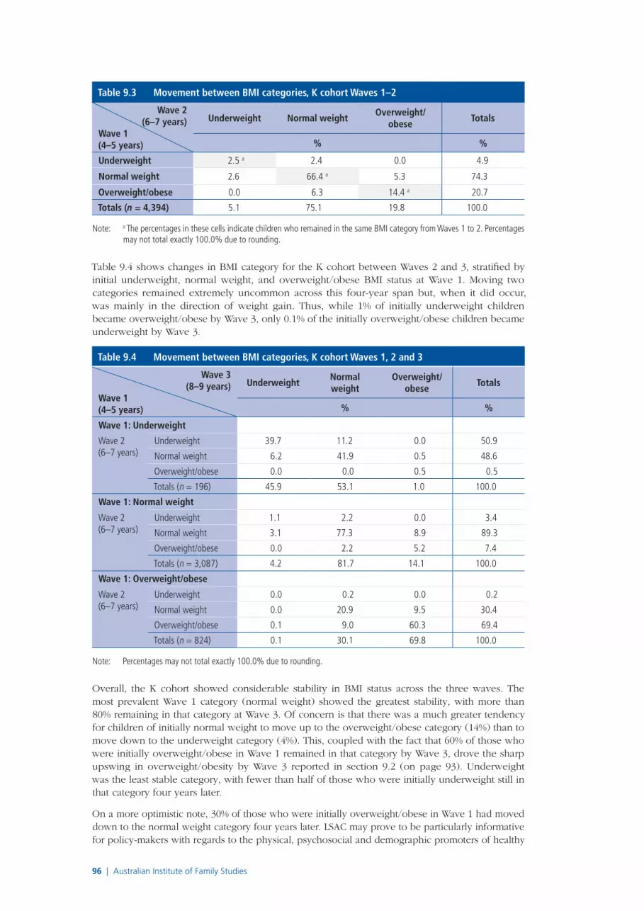
96 | Australian Institute of Family Studies
Table 9.3 Movement between BMI categories, K cohort Waves 1–2
Wave 2 (6–7 years)
Wave 1 (4–5 years)
Underweight Normal weightOverweight/
obeseTotals
% %
Underweight 2.5 a 2.4 0.0 4.9
Normal weight 2.6 66.4 a 5.3 74.3
Overweight/obese 0.0 6.3 14.4 a 20.7
Totals (n = 4,394) 5.1 75.1 19.8 100.0
Note: a The percentages in these cells indicate children who remained in the same BMI category from Waves 1 to 2. Percentages may not total exactly 100.0% due to rounding.
Table 9.4 shows changes in BMI category for the K cohort between Waves 2 and 3, stratified by initial underweight, normal weight, and overweight/obese BMI status at Wave 1. Moving two categories remained extremely uncommon across this four-year span but, when it did occur, was mainly in the direction of weight gain. Thus, while 1% of initially underweight children became overweight/obese by Wave 3, only 0.1% of the initially overweight/obese children became underweight by Wave 3.
Table 9.4 Movement between BMI categories, K cohort Waves 1, 2 and 3
Wave 3 (8–9 years)
Wave 1 (4–5 years)
UnderweightNormal weight
Overweight/obese
Totals
% %
Wave 1: Underweight
Wave 2 (6–7 years)
Underweight 39.7 11.2 0.0 50.9
Normal weight 6.2 41.9 0.5 48.6
Overweight/obese 0.0 0.0 0.5 0.5
Totals (n = 196) 45.9 53.1 1.0 100.0
Wave 1: Normal weight
Wave 2 (6–7 years)
Underweight 1.1 2.2 0.0 3.4
Normal weight 3.1 77.3 8.9 89.3
Overweight/obese 0.0 2.2 5.2 7.4
Totals (n = 3,087) 4.2 81.7 14.1 100.0
Wave 1: Overweight/obese
Wave 2 (6–7 years)
Underweight 0.0 0.2 0.0 0.2
Normal weight 0.0 20.9 9.5 30.4
Overweight/obese 0.1 9.0 60.3 69.4
Totals (n = 824) 0.1 30.1 69.8 100.0
Note: Percentages may not total exactly 100.0% due to rounding.
Overall, the K cohort showed considerable stability in BMI status across the three waves. The most prevalent Wave 1 category (normal weight) showed the greatest stability, with more than 80% remaining in that category at Wave 3. Of concern is that there was a much greater tendency for children of initially normal weight to move up to the overweight/obese category (14%) than to move down to the underweight category (4%). This, coupled with the fact that 60% of those who were initially overweight/obese in Wave 1 remained in that category by Wave 3, drove the sharp upswing in overweight/obesity by Wave 3 reported in section 9.2 (on page 93). Underweight was the least stable category, with fewer than half of those who were initially underweight still in that category four years later.
On a more optimistic note, 30% of those who were initially overweight/obese in Wave 1 had moved down to the normal weight category four years later. LSAC may prove to be particularly informative for policy-makers with regards to the physical, psychosocial and demographic promoters of healthy

Chapter 9: Children’s body mass index
LSAC Annual Statistical Report 2011 | 97
weight in today’s environment, by following these promoters in the relatively large group of children who lose excess adiposity over time.
9.5 Persistence of overweight/obesity, by family socio-economic position and neighbourhood disadvantage
It is clear from the above that, despite the relatively strong tracking of BMI throughout childhood, individual children have widely varying trajectories, sometimes characterised by dramatic upward and downward shifts in relative BMI over time. The top panel of Table 9.5 shows the proportions of children who were never overweight/obese, and the proportions who were overweight/obese at one, two or (for K cohort children) all three waves. The lower panel of the table shows the proportions of children who were obese at zero, one, two or three waves. While overweight/obesity was commonly persistent (14% of the B cohort at both waves, and 12% of K cohort children at all three waves), persistent obesity affected only small numbers (2% of the B cohort at both waves, and 3% of the K cohort children at all three waves).
Table 9.5 Number of waves overweight/obese or obese, B cohort Waves 2–3 and K cohort Waves 1–3
B cohort (Waves 2–3) K cohort (Waves 1–3)
%
Number of waves overweight/obese0 67.5 67.31 18.4 12.62 14.2 7.73 – 12.3Total 100.0 100.0
No. of observations 4,126 4,107
Number of waves obese0 91.5 90.61 6.3 4.02 2.2 2.23 – 3.2Total 100.0 100.0
No. of observations 4,126 4,107
Note: Cases were only included if data were available at all waves.
Whether these small numbers with persistent obesity go on to suffer the burden of disease remains to be established. While obese individuals are known to experience greater cardiovascular, metabolic, musculoskeletal and other morbidities, an important question for policy-makers is whether and how this is related to lifetime exposure to obesity, as opposed to its immediate effects. Several published longitudinal studies suggest that resolution of childhood obesity reverses subsequent morbidity back to the levels of those who were never obese (Juonala et al., 2011; Viner & Cole, 2005; Wake et al., 2010). However, these conclusions were all limited by measuring obesity at only two time points (at exposure and outcome). It is likely that prolonged obesity may result in subsequent major physical and psychosocial morbidities and costs. LSAC, using its repeated biennial measurement of childhood BMI to determine lifetime obesity exposure and timing, will be well placed to address these issues as the children grow older.
Earlier cross-sectional analyses of Wave 1 LSAC data have already confirmed a substantial socio-economic gradient in obesity rates at the age of 4–5 years, with children in the lowest quintile of social disadvantage being 47% more likely to be in a heavier BMI category compared to those in the highest quintile (Wake et al., 2007).
Table 9.6 (on page 98) shows B cohort associations between socio-demographic markers (analysed separately by socio-economic position and by neighbourhood disadvantage, both measured at Wave 2) and the number of waves at which children were overweight/obese and obese. For both groupings and both markers, there were clear trends for those with the most

98 | Australian Institute of Family Studies
persistent overweight/obesity to cluster in the lowest 25% group. These associations were seen for individual SEP and neighbourhood disadvantage, and for persistent obesity and persistent overweight/obesity combined. Thus, 4% of children in the lowest quartile of SEP, but only 0.4% of those in the highest quartile, were obese at both waves (p < .001). Similarly, though less strikingly, 5% of children in the lowest quartile of neighbourhood disadvantage, but only 2% of those in the highest quartile, were obese at both waves (p < .01).
Table 9.6 Number of waves overweight/obese or obese, by family socio-economic position and neighbourhood disadvantage, B cohort Waves 2–3
Family socio-economic position Neighbourhood disadvantage
Lowest 25%
Middle 50%
Highest 25%
Most disadvan-
taged 25%
Middle 50%
Most advan taged
25%% %
Number of waves overweight/obese0 65.7 67.5 69.8 66.8 66.8 69.31 17.3 18.8 18.3 16.0 18.7 18.52 17.0 13.7 11.3 17.2 14.5 12.2Total 100.0 100.0 100.0 100.0 100.0 100.0No. of observations
941 2,114 1,069 400 2,571 1,155
Number of waves obese0 89.3 91.5 94.8 87.0 91.5 93.51 6.9 6.6 4.8 8.2 6.5 5.02 3.9 2.0 0.4 4.7 2.1 1.5Total 100.0 100.0 100.0 100.0 100.0 100.0No. of observations
941 2,114 1,069 400 2,571 1,155
Notes: Neighbourhood disadvantage categorised by SEIFA scores. SEP and SEIFA were measured at Wave 2. Overweight/obese: SEP: χ2 (4, n = 4,124) = 14.8, p = .02; SEIFA: χ2 (4, n = 4,126) = 8.4, p = .2. Obese: SEP: χ2 (4, n = 4,124) = 35.0, p < .001; SEIFA: χ2 (4, n = 4,126) = 23.1, p < .01.
In much the same way, Table 9.7 (on page 99) shows K cohort associations across the three waves. Gradients in this older group were even more striking. Thus, three-quarters of the children in the highest SEP quartile, but less than 60% of those in the lowest quartile, were not overweight at all three time points.
For both groupings and both markers, there were again clear trends for those with the most persistent overweight/obesity to cluster in the lowest 25% group. These gradients were even stronger when only persistent obesity was considered. Thus, 7% of children in the lowest quartile of SEP, but only 3% of those in the highest quartile, were obese at two or more waves (p < .001). Similarly, 8% of children in the lowest quartile of neighbourhood disadvantage, but only 4% of those in the highest quartile, were obese at two or more waves (p < .01).
9.6 SummaryThis chapter has made use of the rich BMI data available in LSAC to investigate how children’s BMI track across the preschool and early school years, and how patterns of change vary for children from different socio-economic backgrounds. The analysis shows a general decline in the percentages of children in the normal weight category, both across waves and between the two cohorts. The population levels of overweight/obesity also increased sharply in the middle childhood years.
At both the population and individual level, there was more between-waves variation in BMI for younger children compared to older children. While the majority of children were in the normal weight category at all waves, a large percentage of those who were overweight/obese remained in that category between waves. Approximately a third of the children who were overweight/obese when they were 4–5 years were in the normal weight category when they were 8–9 years. Unfortunately, this was more than offset by the greater absolute numbers of children moving up
Table 9.7 Number of waves overweight/obese or obese, by family socio-economic position and neighbourhood disadvantage, K cohort Waves 1–3
Family socio-economic position Neighbourhood disadvantage
Lowest 25%
Middle 50%
Highest 25%
Most disadvan-taged 25%
Middle 50%
Most advan taged
25%% %
Number of waves overweight/obese0 58.6 68.8 75.1 62.6 67.3 70.21 15.6 11.7 11.3 11.7 12.7 13.02 10.2 7.5 5.0 9.8 8.2 5.43 15.7 12.1 8.7 15.9 11.9 11.4Total 100.0 100.0 100.0 100.0 100.0 100.0No. of observations
864 2,122 1,114 568 2,403 1,136
Number of waves obese0 86.8 91.1 94.3 87.3 90.2 93.31 6.0 3.5 2.9 4.7 4.3 3.12 2.7 2.6 0.7 2.6 2.6 1.13 4.5 2.7 2.1 5.5 2.9 2.5Total 100.0 100.0 100.0 100.0 100.0 100.0No. of observations
864 2,122 1,114 568 2,403 1,136
Notes: Neighbourhood disadvantage categorised by SEIFA scores. SEP and SEIFA were measured at Wave 1. Overweight/obese: SEP: χ2 (6, n = 4,100) = 69.1, p < .001; SEIFA: χ2 (6, n = 4,107) = 22.7, p < .01. Obese: SEP: χ2 (6, n = 4,100) = 40.8, p < .001; SEIFA: χ2 (6, n = 4,107) = 25.9, p < .1.

Chapter 9: Children’s body mass index
LSAC Annual Statistical Report 2011 | 99
from the normal weight category into the overweight or obese categories. However, with such a wide range of outcomes, LSAC is well placed to examine predictors of both worsening BMI and resolving overweight. Underweight was the least stable category, with most of these children moving into the normal weight category between waves. Persistent overweight/obesity clustered in the most disadvantaged 25% of children on measures of family socio-economic position and neighbourhood disadvantage, with the patterns being stronger for obesity.
These findings support a focus on early and effective prevention and intervention throughout the preschool years and transitions into school. This is particularly important for children experiencing either family-level or neighbourhood-level disadvantage. Future waves and analyses of LSAC data will be able to provide insight into the effects of persistent overweight/obesity on ongoing physical and psychosocial outcomes, as well as tracking changes in BMI through later childhood and adolescence.
9.7 Further readingWake, M., Hardy, P., Canterford, L., Sawyer, M., & Carlin, J. B. (2007). Overweight, obesity and girth of Australian pre-schoolers: Prevalence and socio-economic correlates. International Journal of Obesity, 31, 1044–1051.
Wake, M., Hardy, P., Sawyer, M., & Carlin, J. (2008). Comorbidities of overweight/obesity in Australian pre-schoolers: A cross-sectional population study. Archives of Disease in Childhood, 93(6), 502–507.
Wake, M., Nicholson, J. M., Hardy, P., & Smith, K. (2007). Preschooler obesity and parenting styles of mothers and fathers: Australian national population study. Pediatrics, 120, e1520–e1527.
9.8 ReferencesAndersen, L. B., Sardinha, L. B., Froberg, K., Riddoch, C. J., Page, A. S., & Anderssen, S. A. (2008). Fitness, fatness and clustering of cardiovascular risk factors in children from Denmark, Estonia and Portugal: The European Youth Heart Study. International Journal of Pediatric Obesity, 3(Suppl. 1), 58–66.
Australian Bureau of Statistics. (2008). Socio-Economic Indexes for Areas (SEIFA): Technical Paper 2006 (Cat. No. 2039.0.55.001). Canberra: ABS.
Australian Bureau of Statistics. (2010). Population by age and sex, Australian States and Territories, Jun 2010 (Cat. No. 3201.0). Canberra: ABS. Retrieved from <www.abs.gov.au/ausstats/[email protected]/mf/3201.0>.
persistent overweight/obesity to cluster in the lowest 25% group. These associations were seen for individual SEP and neighbourhood disadvantage, and for persistent obesity and persistent overweight/obesity combined. Thus, 4% of children in the lowest quartile of SEP, but only 0.4% of those in the highest quartile, were obese at both waves (p < .001). Similarly, though less strikingly, 5% of children in the lowest quartile of neighbourhood disadvantage, but only 2% of those in the highest quartile, were obese at both waves (p < .01).
Table 9.6 Number of waves overweight/obese or obese, by family socio-economic position and neighbourhood disadvantage, B cohort Waves 2–3
Family socio-economic position Neighbourhood disadvantage
Lowest 25%
Middle 50%
Highest 25%
Most disadvan-
taged 25%
Middle 50%
Most advan taged
25%% %
Number of waves overweight/obese0 65.7 67.5 69.8 66.8 66.8 69.31 17.3 18.8 18.3 16.0 18.7 18.52 17.0 13.7 11.3 17.2 14.5 12.2Total 100.0 100.0 100.0 100.0 100.0 100.0No. of observations
941 2,114 1,069 400 2,571 1,155
Number of waves obese0 89.3 91.5 94.8 87.0 91.5 93.51 6.9 6.6 4.8 8.2 6.5 5.02 3.9 2.0 0.4 4.7 2.1 1.5Total 100.0 100.0 100.0 100.0 100.0 100.0No. of observations
941 2,114 1,069 400 2,571 1,155
Notes: Neighbourhood disadvantage categorised by SEIFA scores. SEP and SEIFA were measured at Wave 2. Overweight/obese: SEP: χ2 (4, n = 4,124) = 14.8, p = .02; SEIFA: χ2 (4, n = 4,126) = 8.4, p = .2. Obese: SEP: χ2 (4, n = 4,124) = 35.0, p < .001; SEIFA: χ2 (4, n = 4,126) = 23.1, p < .01.
In much the same way, Table 9.7 (on page 99) shows K cohort associations across the three waves. Gradients in this older group were even more striking. Thus, three-quarters of the children in the highest SEP quartile, but less than 60% of those in the lowest quartile, were not overweight at all three time points.
For both groupings and both markers, there were again clear trends for those with the most persistent overweight/obesity to cluster in the lowest 25% group. These gradients were even stronger when only persistent obesity was considered. Thus, 7% of children in the lowest quartile of SEP, but only 3% of those in the highest quartile, were obese at two or more waves (p < .001). Similarly, 8% of children in the lowest quartile of neighbourhood disadvantage, but only 4% of those in the highest quartile, were obese at two or more waves (p < .01).
9.6 SummaryThis chapter has made use of the rich BMI data available in LSAC to investigate how children’s BMI track across the preschool and early school years, and how patterns of change vary for children from different socio-economic backgrounds. The analysis shows a general decline in the percentages of children in the normal weight category, both across waves and between the two cohorts. The population levels of overweight/obesity also increased sharply in the middle childhood years.
At both the population and individual level, there was more between-waves variation in BMI for younger children compared to older children. While the majority of children were in the normal weight category at all waves, a large percentage of those who were overweight/obese remained in that category between waves. Approximately a third of the children who were overweight/obese when they were 4–5 years were in the normal weight category when they were 8–9 years. Unfortunately, this was more than offset by the greater absolute numbers of children moving up
Table 9.7 Number of waves overweight/obese or obese, by family socio-economic position and neighbourhood disadvantage, K cohort Waves 1–3
Family socio-economic position Neighbourhood disadvantage
Lowest 25%
Middle 50%
Highest 25%
Most disadvan-taged 25%
Middle 50%
Most advan taged
25%% %
Number of waves overweight/obese0 58.6 68.8 75.1 62.6 67.3 70.21 15.6 11.7 11.3 11.7 12.7 13.02 10.2 7.5 5.0 9.8 8.2 5.43 15.7 12.1 8.7 15.9 11.9 11.4Total 100.0 100.0 100.0 100.0 100.0 100.0No. of observations
864 2,122 1,114 568 2,403 1,136
Number of waves obese0 86.8 91.1 94.3 87.3 90.2 93.31 6.0 3.5 2.9 4.7 4.3 3.12 2.7 2.6 0.7 2.6 2.6 1.13 4.5 2.7 2.1 5.5 2.9 2.5Total 100.0 100.0 100.0 100.0 100.0 100.0No. of observations
864 2,122 1,114 568 2,403 1,136
Notes: Neighbourhood disadvantage categorised by SEIFA scores. SEP and SEIFA were measured at Wave 1. Overweight/obese: SEP: χ2 (6, n = 4,100) = 69.1, p < .001; SEIFA: χ2 (6, n = 4,107) = 22.7, p < .01. Obese: SEP: χ2 (6, n = 4,100) = 40.8, p < .001; SEIFA: χ2 (6, n = 4,107) = 25.9, p < .1.

100 | Australian Institute of Family Studies
Australian Institute of Family Studies. (2011). Longitudinal Study of Australian Children: Data user guide. Melbourne: AIFS.
Australian National Preventive Health Agency. (2011). Frequently asked questions. Canberra: ANPHA. Retrieved from <www.anpha.gov.au/internet/anpha/publishing.nsf/Content/faqs>.
Baker, J. L., Olsen, L. W., & Sorensen, T. (2007). Childhood body-mass index and the risk of coronary heart disease in adulthood. The New England Journal of Medicine, 357(23), 2329–2337.
Ball, K., & Crawford, D. (2004). Socio-economic status and weight change in adults: A review. Social Science & Medicine, 60, 1987–2010.
Bjørnelv, S., Lydersen, S., Mykletun, A., & Holmen, T. L. (2007). Changes in BMI-distribution from 1966–69 to 1995–97 in adolescents: The Young-HUNT study, Norway. BMC Public Health, 7, 279.
Booth, M. L., Wake, M., Armstrong, T., Chey, T., Hesketh, K., & Mathur, S. (2001). The epidemiology of overweight and obesity among Australian children and adolescents, 1995–1997. Australian and New Zealand Journal of Public Health, 25, 162–169.
Cole, T. J., Bellizzi, M. C., Flegal, K. M., & Dietz, W. H. (2000). Establishing a standard definition for child overweight and obesity worldwide: International survey. British Medical Journal, 320, 1240–1243.
Cole, T. J., Flegal, K. M., Nicholls, D., & Jackson, A. A. (2007). Body mass index cut offs to define thinness in children and adolescents: International survey. British Medical Journal, 335(7612), 194.
CSIRO Preventative Health National Research Flagship & University of South Australia. (2008). 2007 Australian National Children’s Nutrition and Physical Activity Survey: Main findings. Canberra: Department of Health and Ageing, Department of Agriculture, Fisheries and Forestry and Australian Food and Grocery Council.
Juonala, M., Magnussen, C. G., Berenson, G. S., Venn, A., Burns, T. L., Sabin, M. A. et al. (2011). Childhood adiposity, adult adiposity and cardiovascular risk factors. New England Journal of Medicine, 365(20), 1876–1885.
Kuczmarksi, R. J., Ogden, C. L., Guo, S. S., Grummer-Strawn, L. M., Flegal, K. M., Mei, Z. et al. (2002). 2000 CDC growth charts for the United States: Methods and development. Vital and Health Statistics: Series 11. Data From the National Health Survey, 246, 1–190.
Lazarus, R., Wake, M., Hesketh, K., & Waters, E. (2000). Change in body mass index in Australian primary school children, 1985–1997. International Journal of Obesity, 24(6), 679–684.
Ludwig, D. S. (2007). Childhood obesity: The shape of things to come. The New England Journal of Medicine, 357(23), 2325–2327.
Martin, K., Rosenberg, M., Miller, M., French, S., McCormack, G., Bull, F., et al. (2008). Move and munch final report: Trends in physical activity, nutrition and body size in Western Australian children and adolescents. The Child and Adolescent Physical Activity and Nutrition Survey (CAPANS) 2008. Leederville, WA: Physical Activity Taskforce Secretariat, WA Department of Sport and Recreation.
Martinez-Vizcaino, V., Sánchez López, M., Moya Martínez, P., Solera Martinez, M., Notario Pacheco, B., Salcedo Aguilar, F., & Rodríguez-Artalejo, F. (2009). Trends in excess weight and thinness among Spanish schoolchildren in the period 1992–2004: the Cuenca study. Public Health Nutrition, 12(7), 1015–1018.
National Health and Medical Research Council. (2003). Clinical practice guidelines for the management of overweight and obesity in children and adolescents. Canberra: NHMRC. Retrieved from <www.health.gov.au/internet/main/publishing.nsf/Content/893169B10DD846FCCA256F190003BADA/$File/children.pdf>.
Nichols, M. S., de Silva-Sanigorski, A. M., Cleary, J. E., Goldfield, S. R., Colahan, A., & Swinburn, B. A. (2011). Decreasing trends in overweight and obesity among an Australian population of preschool children. International Journal of Obesity, 35, 916–924.
Norton, K., Dollman, J., Martin, M., & Harten, N. (2006). Descriptive epidemiology of childhood overweight and obesity in Australia: 1901–2003. International Journal of Pediatric Obesity, 1, 232–238.
Ogden, C. L., Carroll, M. D., Curtin, L. R., Lamb, M. M., & Flegal, K. M. (2010). Prevalence of high body mass index in US children and adolescents, 2007–2008. Journal of the American Medical Association, 303(3), 242–249.
Ogden, C. L., Carroll, M. D., & Flegal, K. M. (2008). High body mass index for age among US children and adolescents, 2003–2006. Journal of the American Medical Association, 299(20), 2401–2405.
Reilly, J. J., Armstrong, J., Dorosty, A. R., Emmett, P. M., Ness, A., & Rogers, I. et al. (2005). Early life risk factors for obesity in childhood: Cohort study. British Medical Journal, 330, 1357–1359.
Sobal, J., & Stunkard, A. J. (1989). Socio-economic status and obesity: A review of the literature. Psychological Bulletin, 105, 260–275.
Viner, R. M., & Cole, T. J. (2005). Adult socio-economic, educational, social, and psychological outcomes of childhood obesity: National birth cohort study. British Medical Journal, 330(7504), 1354–1357.
Wake, M., Canterford, L., Patton, G. C., Hesketh, K., Hardy, P., Williams, J., et al. (2010). Comorbidities of overweight/obesity experienced in adolescence: Longitudinal study. Archives of Disease in Childhood, 95(3), 162–168.
Wake, M., Hardy, P., Canterford, L., Sawyer, M., & Carlin, J. B. (2007). Overweight, obesity and girth of Australian preschoolers: Prevalence and socio-economic correlates. International Journal of Obesity, 31(7), 1044–1051.
Wang, Y., & Lobstein, T. (2006). Worldwide trends in childhood overweight and obesity. International Journal of Pediatric Obesity, 1(1), 11–25.