chapter 2 - noaa chemical sciences laboratory

2 O3 N93Li9

CHAPTER 2

Ozone and Temperature Trends

Authors: R. Stolarski

V. Fioletov L. Bishop S. Godin R.D. Bojkov V. Kirchhoff M.-L. Chanin J. Zawodny

C.S. Zerefos

Additional Contributors: W. Chu M.P. McCormick J. DeLuisi P. Newman A. Hansson M. Prendez J.. Kerr J. Staehelin E. Lysenko B. Subbaraya

Chapter 2

Ozone and Temperature Trends

Contents

SCIENTIFICSUMMARY....................................................................................................2.1

2.1 INTRODUCTION..........................................................................................................2.3

2.2 INSTRUMENTS ............................................................................................................2.3

2.2.1 Dobson.............................................................................................................2.3 2.2.2 Filter Ozonometers..........................................................................................2.3 2.2.3 TOMS..............................................................................................................2.3 2.2.4 Ozonesondes....................................................................................................2.3 2.2.5 Umkehr............................................................................................................2.4 2.2.6 SAGE...............................................................................................................2.4

2.3 OBSERVED TRENDS...................................................................................................2.4

2.3.1 Factors Contributing to Ozone and Temperature Variability...........................2.4 2.3.1.1 Solar Cycle ....................................................................................... 2.4 2.3.1.2 Energetic Particles............................................................................2.4 2.3.1.3 Quasi-Biennial Oscillation...............................................................2.4 2.3.1.4 El Niño-Southern Oscillation ..........................................................2.5

2.3.1.5 Atmospheric Nuclear Tests ..............................................................2.5 2.3.1.6 Volcanic Eruptions ...........................................................................2.5

2.3.2 Antarctic Trends .............................................................................................. 2.5 2.3.3 Global Trends in Total Ozone..........................................................................2.10

2.3.3.1 Ground Station Trends ......................................................................2.10 2.3.3.2 Comparison of Ground Station and Satellite Data...........................2.15 2.3.3.3 Trends from Satellite Data ...............................................................2.18

2.3.4 Trends in the Ozone Profile ............................................................................. 2.24 2.3.4.1 Ozonesondes.....................................................................................2.24 2.3.4.2 SAGE ...............................................................................................2.25 2.3.4.3 Umkehr.............................................................................................2.25 2.3.4.4 Comparison of Profile Trends..........................................................2.28

2.3.5 Temperature.....................................................................................................2.28

2.4 SUMMARY....................................................................................................................2.29

REFERENCES......................................................................................................................2.30

OZONE AND TEMPERATURE TRENDS

SCIENTIFIC SUMMARY

Observational Record: Since the 1989 assessment, the observational record includes an additional 2.5 years of Dobson, Stratospheric Aerosol and Gas Experiment (SAGE) and Total Ozone Mapping Spectrometer (TOMS) data and a complete re-analysis of 29 ground-based M83/M1 24 stations in the former Soviet Union. This is complemented by a major new advance in the observational record of an internally-calibrated TOMS data set that is now independent of ground-based observations. Trend analyses of SAGE data have been extended to the lower stratosphere and the Umkehr data have been reanalyzed.

Antarctic Ozone: The Antarctic ozone hole in 1991 was as deep and as extensive in area as those of 1987, 1989, and 1990. The low value of total ozone measured in 1991 was 110 Dobson Units, a decrease of 60 per-cent compared with ozone levels prior to the mid-1970s. The previously noted quasi-biennial modulation of the severity of the ozone hole did not occur during the last 3 years. The area of the ozone hole was similar for these 4 years.

Trends In Total Ozone: Ground-based (Dobson and M831M1 24) and satellite (TOMS) observations of total column ozone through March 1991 were analyzed, allowing for the influence of solar cycle and quasi-biennial oscillation (see table). They show that:

• The northern mid-latitude winter and summer decreases during the 1980s were larger than the average trend since 1970 by about 2 percent per decade. A significant longitudinal variance of the trend since 1979 is observed.

• For the first time there are statistically significant decreases in all seasons in both the Northern and Southern Hemispheres at mid- and high-latitudes during the 1980s; the northern mid-latitude long-term trends (1970 to 1991), while smaller, are also statistically significant in all seasons.

• There has been no statistically significant decrease in tropical latitudes from 25°N to 25°S.

Trends In the Vertical Distribution of Ozone: Balloonsonde, ground-based Umkehr, and satellite SAGE observations show that: • Ozone is decreasing in the lower stratosphere, i.e., below 25 km, at about 10 percent per decade, consis-

tent with the observed decrease in column ozone. • Changes in the observed vertical distribution of ozone in the upper stratosphere near 40 km are qualita-

tively consistent with theoretical predictions, but are smaller in magnitude. • Measurements indicate that ozone levels in the troposphere, over the few existing ozone sounding sta-

tions at northern mid-latitudes, have increased about 10 percent per decade over the past two decades.

Trends in Stratospheric Temperature: The temperature record indicates a small cooling (about 0.3 CC per decade) of the lower stratosphere in the sense of that expected from the observed change in the stratospheric concentration of ozone.

Total ozone trends in percent per decade with 95 percent confidence limits TOMS: 1979-1991 Ground-based: 26°N-64°N

45'S Equator 45°N 1979-1991 1970-1991 Dec-Mar -5.2 ± 1.5 +0.3 ± 4.5 -5.6 ± 3.5 -4.7 ± 0.9 -2.7 ± 0.7 May-Aug -6.2 ± 3.0 +0.1 ± 5.2 -2.9 ± 2.1 -3.3 ± 1.2 -1.3 ± 0.4 Sep-Nov -4.4 ± 3.2 +0.3 ± 5.0 -1.7 ± 1.9 -1.2 ± 1.6 -1.2 ± 0.6

2.1

271 INTRODUCTION-

This chapter is an update of the extensive reviews of the state of knowledge of measured ozone trends published in the Report of the International Ozone Trends Panel.-, l988VMO199Oa)-and.the -ScientificAssessmenr'f Stratospheric Ozone: 1989 (-WMOr1-990b). The chapter contains a review of progress since these reports, including updating of the ozone records, in most cases through March 1991. Also included are some new, unpublished reanalyses of these records including a complete reevaluation of 29 stations located in the former Soviet Union. The major new advance in knowledge of the measured ozone trend is the existence of independently cali-brated satellite data records from the Total Ozone Mapping Spectrometer (TOMS) and Stratospheric Aerosol and Gas Experiment (SAGE) instruments. These confirm many of the findings, originally derived from the Dobson record, concerning northern mid-latitude changes in ozone. We now have results from several instruments, whereas the previously reported changes were dependent on the calibration of a single instrument. This chapter will compare the ozone records from many different instruments to determine whether or not they provide a consistent picture of the ozone change that has occurred in the atmosphere. The chapter also briefly considers the problem of stratospheric temperature change. As in previous reports, this problem received significantly less attention and the report is not nearly as complete. This area needs more attention in the future.

2.2 INSTRUMENTS

2.2.1 Dobson

The Ozone Trends Panel (WMO, 1990a) used data from Dobson stations that had been provisional -ly revised by R.D. Bojkov using monthly mean cor-rections (Bojkov etal., 1990).

Since then, a number of the Dobson stations have revised their entire data records making daily correc-tions based on detailed calibration records. These include Belsk, Hradec Kralove, Ahmedabad, and the four Japanese stations: Sapporo, Tateno, Kagoshima, and Naha. Several other stations have been provi-sionally revised on a monthly basis by the station. For the rest, this report continues to use Bojkov's pro-


visional revisions. All data have been updated through March 1991.

2.2.2 Filter Ozonometers

The filter ozonometer (M83) was developed in the mid-1950s. In its initial configuration, the instru-ment had significant systematic errors. In the early 1970s, the instrument was modified and improved light filters were used. Since 1973, this modified instrument has been used in the former Soviet Union portion of ozone monitoring stations. Since 1986, the M83 has been replaced by the M124, which is a mod-ified design but uses the same light filters. The data before 1973 should not be used for the analysis of trends because of large systematic errors. One cause of the instrument problems was the frequent replace-ment of instruments with new ones about every 2 years. Prior to carrying out the trend analysis report-ed here, the data from this network were revised by careful checking of calibration records.

2.2.3 TOMS

TOMS was launched on Nimbus-7 in October 1978 and is still working in 1991. The main problem with maintaining a long-term ozone record with TOMS is the degradation of the diffuser plate used to make the solar observation for determination of albedo. Early evaluations of the ozone data from TOMS (Fleig et al., 1986) included a correction for diffuser plate darkening. This correction yielded a TOMS data set that tracked the corresponding Dobson measure-ments until about 1982 or 1983. After that the TOMS, and the companion solar backscatter ultravi-olet spectrometer, began to drift downward with respect to Dobson measurements (WMO, 1990a). A new method has been derived to improve the correc-tion to the diffuser plate (Herman, et al., 1991). The entire data set has been reprocessed (called Version 6) and is estimated to be precise to ± 1.3 percent (2(y) at the end of 1989 relative to the beginning of the record.

2.2.4 Ozonesondes

The previous assessment (WMO, 1990b) ana-lyzed the records from a network of nine ozonesonde stations. This study has not been updated for this

2.3

PREc€D'NG PAGE BLANK NOT FILMED


report. The record from Payerne has recently been reanalyzed by Staehelin and Schmid (1991) to correct for changes in the time of day of launch. This reana-lyzed record has been used to illustrate some of the features of the observed profile of ozone loss.

2.2.5 Umkelir

The Umkehr technique for measuring the profile of ozone concentration has been in use since its dis-covery by Götz (1931). In the last assessment report, trends from the records of 10 stations covering the period 1977 to 1987 were analyzed. Mateer and DeLuisi (1991) have devised an improved Umkehr retrieval algorithm. This algorithm is an optimal sta-tistical or maximum likelihood retrieval and uses improved a priori profiles and the Paur and Bass (1985) ozone absorption coefficients and their tem-perature dependence.

2.2.6 SAGE

The SAGE I and SAGE II instruments measure the vertical profile of ozone at sunrise and sunset (McCormick et al., 1989). The SAGE I data set extends over the period from February 1979 through November 1981 and has not been revised since the previous assessment. SAGE II continues to return data since beginning operation in October 1984. The last 6I2 years of SAGE II ozone data through mid-1991 are presented here. The SAGE measurement technique is insensitive to drift in instrumental cali-bration; however, there may be systematic differences between SAGE I and SAGE II. The potential sys-tematic differences are less than 2 percent between 25 and 45 km, increasing to approximately 6 percent at 20 km. The largest change from previous assess-ments is that the SAGE I and SAGE II ozone profiles below 25 km have now been extensively intercom-pared with ozonesondes and the trend estimates can be calculated down to 17 km altitude.

2.3 OBSERVED TRENDS

when estimating trends. The following subsections briefly describe those influences thought to be signif-icant.

2.3.1.1 Solar Cycle

The 11-year solar cycle has an influence on stratospheric ozone amounts. Both theoretical calcu-lations and observations (Stolarski et al., 1990) show a 1 to 2 percent peak-to-peak variation in total ozone (WMO, 1990a, Chapter 7). In the upper stratosphere, where theory says most of the variability should occur, the only long-term ozone record is from Umkehr measurements. This record shows a 2 per-cent peak to peak variation at 40 km rising to 5 per-cent at 45 km (Reinsel et al., 1989). Details of the analysis of the solar cycle effect have little effect on the deduction of ozone trends from the 35-year Dobson records, but they can be important to deduc-tion of trends from the much shorter 11- to 12-year TOMS and SAGE records. The influence of the 11-year solar cycle effect on temperatures was reviewed by von Cossart and Taubenheim (1987) and Chanin et al. (1987). Kokin et al. (1990) gave a 3-5 K ampli-tude in the upper mesosphere and about 1.5 K in the upper stratosphere.

2.3.1.2 Energetic Particles

Another phenomenon related to the solar cycle that has produced observed effects on atmospheric ozone concerns high-energy protons (Zerefos and Crutzen, 1975; Heath et al., 1977; Solomon and Crutzen, 1981; McPeters and Jackman, 1985). These solar proton events (SPEs) are sporadic, and events with a large impact on ozone are rare. Particularly large events were those of August 1972. It has been suggested that the late 1989 events were partially responsible for the low total ozone seen in the north polar region in the spring of 1990 (Reid etal., 1991), and enhancements of NO2 and decreases in ozone were observed by SAGE during this period (Zawodny and McCormick, personal communica-tion).

2.3.1 Factors Contributing to Ozone and Temperature Variability

Several natural influences contribute to ozone and temperature variability and must be considered

2.3.1.3 Quasi-Biennial Oscillation

There is a clear quasi-biennial oscillation (QBO) signal in total ozone data at the equator, with magni-

2.4


tude of about 4 to 5 percent peak to peak (Bojkov, 1987; WMO, 1990a; Hilsenrath and Schlesinger, 1981). As a function of altitude, the ozone profile changes due to the QBO are much larger (Bojkov, 1987; Zawodny and McCormick, 1991). Two separate equatorial peak QBO amplitudes are found at 24 km (20 percent peak to peak) and 34 km (15 percent peak to peak). Although these variations are large, they largely cancel out in the total ozone column.

2.3.1.4 El Niño—Southern Oscillation

A relationship of total ozone to El Niflo-Southern Oscillation (ENSO) has also been suggest-ed. The tropical Dobson data show 3 to 4 percent variations which correlate with the Southern Oscillation Index (SOD (Zerefos et al., 1991a,b). The SOl shows a major ENSO event in 1982-1983 that has been suggested to be partly responsible for the negative ozone deviations at high latitudes in the Northern Hemisphere (Bojkov, 1987a).

2.3.1.5 Atmospheric Nuclear Tests

Chemical models predict that the atmospheric nuclear test series of the late 1950s and early 1960s may have had an observable effect on the baseline amount of ozone measured by the Dobson instru-ments during the 1960s.

2.3.1.6 Volcanic Eruptions

Finally, explosive volcanic eruptions are a spo-radic and unpredictable potential perturbation of ozone or cause interference with ozone measure-ments. There have been several major eruptions and a number of minor eruptions during the period of the ozone data record. The eruption of Gunung Agung in 1963 is near the beginning of most of the ground-based ozone records. The only major eruption during the period of most of the ozone data records was El ChichOn in Mexico in 1982. El ChichOn has had at most a 2 percent effect on measured total ozone (Chandra and Stolarski, 1991). Indications from recent measurements of the volcanic eruptions of Mt. Pinatubo are that it may have injected two to three times more material than El ChichOn. The current analysis does not include any ozone measurements during or after the June 1991 eruption of Mt.

Pinatubo. The aerosol increase in the lower strato-sphere from large volcanic eruptions has also pro-duced a large (4K) temperature rise (Labitzke et al., 1983; Michelangeli etal., 1989).

2.3.2 Antarctic Trends

The springtime Antarctic ozone hole has been observed since the late 1970s (Farman, ci al., 1985; Chubachi, 1985). Measurements by ground-based instruments, balloonsondes, and satellites have shown that the depletion occurs mainly during September with the ozone concentration in the lower strato-sphere between about 14 and 22 km declining to nearly zero concentrations by early October.

The Antarctic ozone holes of 1989 and 1990 were both characterized by low total ozone values over much of the south polar region (Stolarski, et al., 1990; Newman et al., 1991). The depth and extent of the hole in each of these years were comparable to the large 1987 ozone hole discussed in WMO (1990b). In 1990, the hole lasted a particularly long time, through December (Newman etal., 1991). The vortex appeared to have been weakened by wave events in August, but it persisted because very little wave activity was propagated upward from the tropo-sphere. Figure 2-1 shows the TOMS daily minimum total ozone (for a 20 latitude by 5° longitude bin) measured in the south polar region from August through November (updated from Newman et al., 1991, by Schoeberl, personal communication). The shaded area in Figure 2-1 indicates the range of mini-mum values for all years from 1979 through 1990. Also indicated are the minima for 1979, 1987, 1988, 1989, and 1990. The 1991 data, shown as dots, show a decline through early October that is similar to the previous deep ozone hole years 1987, 1989, and 1990. A minimum value of 110 Dobson units (DU), slightly lower than in previous years, was reached in early October 1991. This was the preliminary num-ber available in October from real time processing. The final number from the regular processing system was 108 DU (Krueger, personal communication). The recovery through the middle of November 1991 has closely followed that of 1989. The quasi-biennial modulation of the depth of the ozone hole that has been previously noted (Garcia and Solomon, 1987; Lait etal., 1987) is not evident in the data for the last 3 years.

2.5


I AM

A II II

N\N\N\\''\ VP "i r nr

1ITU1 \NN NNN\\NN\ \ >\\N'\Nt !i 3J' h'LJ!\\\'N\ \\\\\ ''I

I kNN\\N\ \\ \\\\\\\ • ... ''I

• 1987 . • 1953 - - - - I •

• N 1989 .._._._

- 1990

- 1991••••• I I I

Aug 1 Sep 1 Oct 1 Nov 1 Dec 1 Month

Figure 2-1 TOMS daily minimum total ozone measured south of 30S from August through November. The individual years 1979, 1987, 1988, 1989, 1990, and 1991 are shown. The shaded area indicates the range of daily minima for all years from 1979 through 1990 (Schoeberl, personal communication, 1991).

300

250

U)

C

200

150

100

The September decrease in Antarctic ozone has been clearly shown to be a lower stratospheric phe-nomenon (mainly between 14 and 22 km altitude) with nearly all of the ozone being removed in cold years with deep ozone holes (Hofmann et al., 1987; Gardiner, 1988; Komhyr et al., 1988). This was again the case in 1989 and 1990 (Deshler etal., 1990; Deshler and Hofmann, 1991). The lower stratospher-ic ozone decrease detected by balloon ozonesondes has been confirmed by measurements from SAGE (McCormick and Larsen, 1986, 1988), from lidar (Browell etal., 1988), and from in Situ measurements on aircraft (Proffitt et al., 1989).

The Antarctic ozone hole is occurring during the spring when sunlight reaches the vortex while it is

still intact. There is a strong correlation of low total ozone amounts with low temperatures in the lower stratosphere. An example is shown in Figure 2-2 for the data over the Japanese station Syowa. The cold years are dynamically less active with a more stable vortex, which results in a stronger and more persis-tent ozone depletion. During the period when the vortex is warming (September through December), there appears to be a significant negative temperature trend if only the cold years are considered. The warmer years are dynamically active, with conse-quent variability that overwhelms any possible trend (Newman et al., 1990; Randel, 1988).

For the recent 4 years with deep ozone holes (1987, 1989-1991), the area covered by the ozone

2.6

15

-II

a) I-a)

.0 a U)

E a) I C I-a)

-C 4-,

0 (I) 9-0 Co

FD I-

10

5


400

375

350

Q) 300 C 0

c 275

250 0

'• 225

200

175

I I

Syowa station +

+ + ++ + +

+ + +

+++

+

+ + +

++ j

—80 —75 —70 —65 —60 Temperature (°C)

Figure 2-2 Correlation of October monthly mean 100-hPa temperatures and total ozone amounts measured above Syowa, Antarctica.

Area Enclosed by 200 DU Contour

- 1987

1988

- - 1989

1990

- 1991

25.5 Co

a, 4-, a) E 0

2.7

C 0

J Aug Sep Oct Nov Dec Month

Figure 2-3 The area of the south polar region with total ozone amount less than 200 DU as measured by TOMS on a daily basis for each of the last 5 years.

rIr7 •4'

2.7


350

330

S a

310

0

-4-I 290 0 I-

270

250

Integrated Southern Hemisphere Total Ozone - I

(

1987

1990 - 1991

J F MA M J JASO N 0

Month

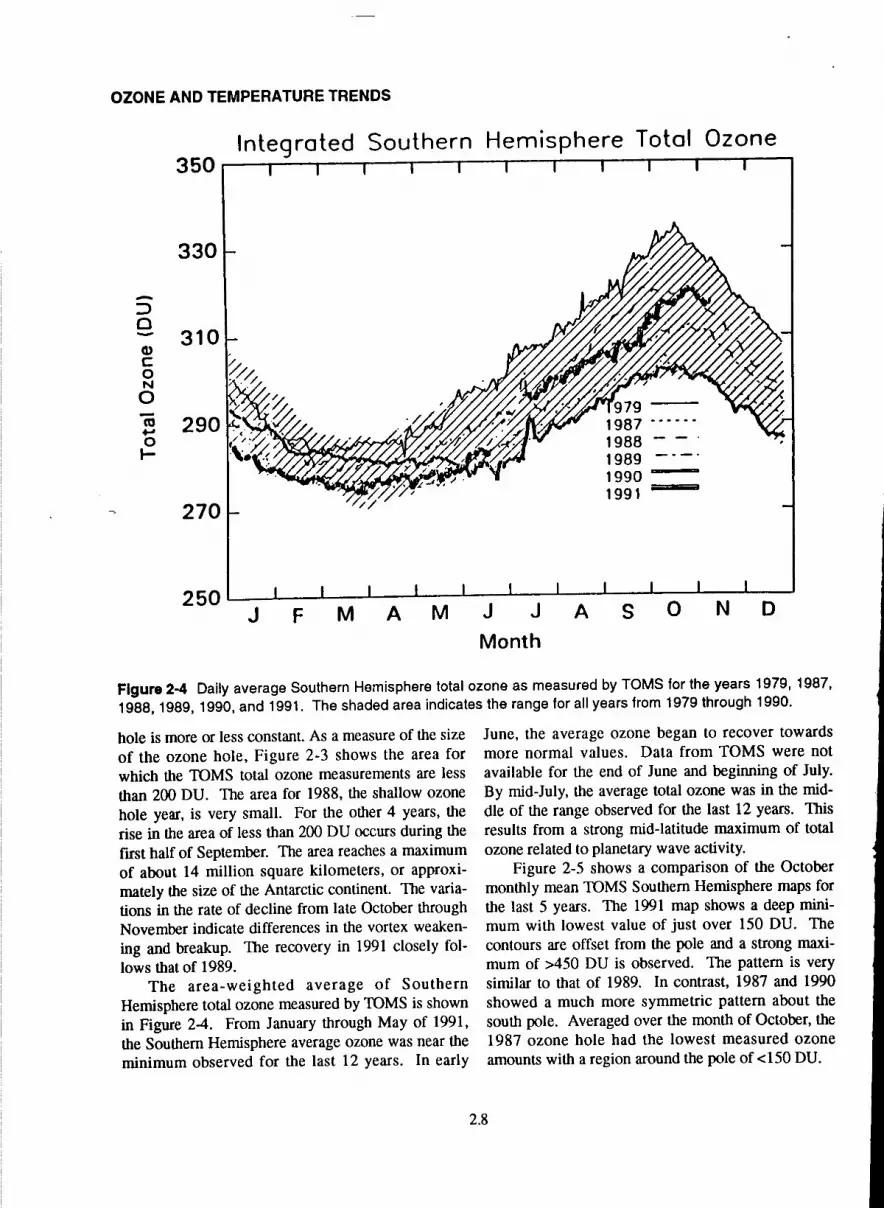
Figure 2-4 Daily average Southern Hemisphere total ozone as measured by TOMS for the years 1979, 1987, 1988, 1989, 1990, and 1991. The shaded area indicates the range for all years from 1979 through 1990.

hole is more or less constant. As a measure of the size of the ozone hole, Figure 2-3 shows the area for which the TOMS total ozone measurements are less than 200 DU. The area for 1988, the shallow ozone hole year, is very small. For the other 4 years, the rise in the area of less than 200 DU occurs during the first half of September. The area reaches a maximum of about 14 million square kilometers, or approxi-mately the size of the Antarctic continent. The varia-tions in the rate of decline from late October through November indicate differences in the vortex weaken-ing and breakup. The recovery in 1991 closely fol-lows that of 1989.

The area-weighted average of Southern Hemisphere total ozone measured by TOMS is shown in Figure 24. From January through May of 1991, the Southern Hemisphere average ozone was near the minimum observed for the last 12 years. In early

June, the average ozone began to recover towards more normal values. Data from TOMS were not available for the end of June and beginning of July. By mid-July, the average total ozone was in the mid-dle of the range observed for the last 12 years. This results from a strong mid-latitude maximum of total ozone related to planetary wave activity.

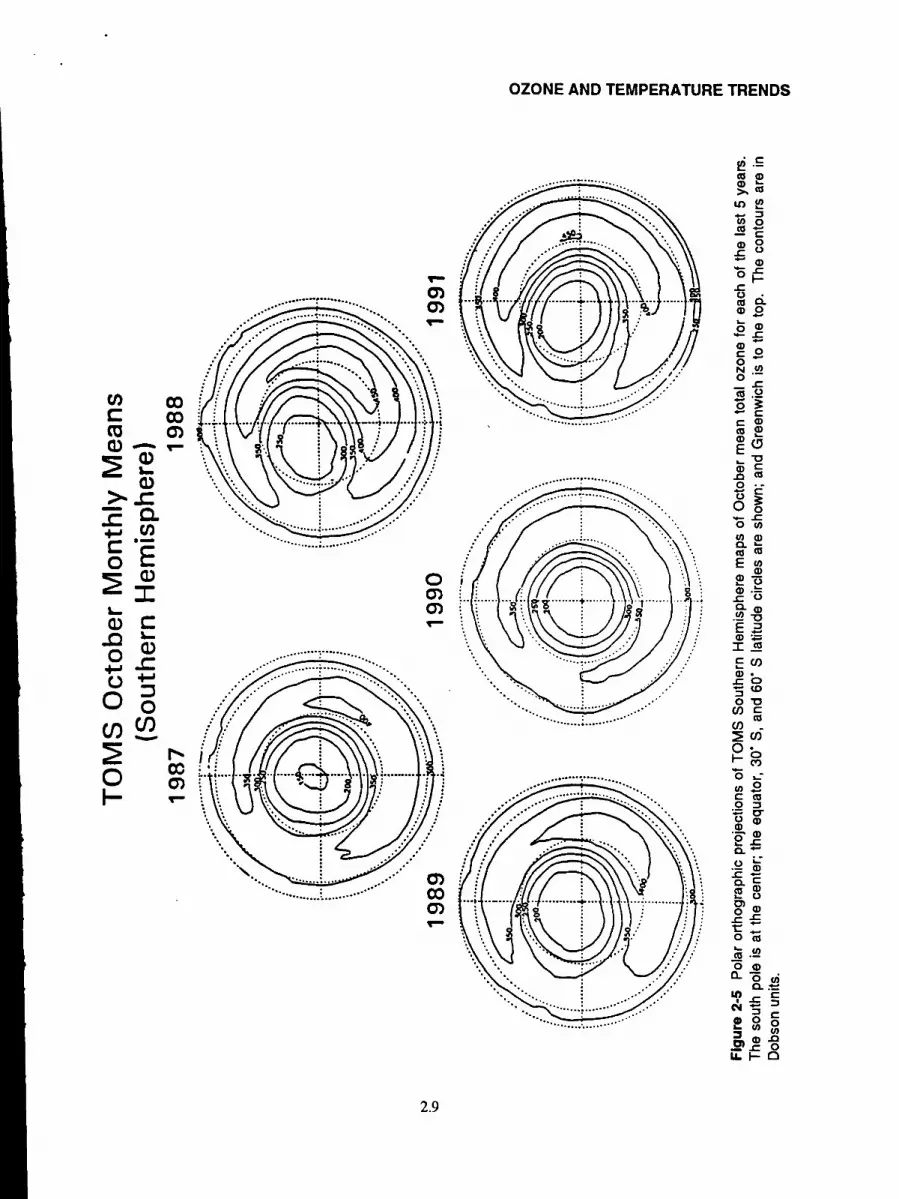
Figure 2-5 shows a comparison of the October monthly mean TOMS Southern Hemisphere maps for the last 5 years. The 1991 map shows a deep mini-mum with lowest value of just over 150 DU. The contours are offset from the pole and a strong maxi-mum of >450 DU is observed. The pattern is very similar to that of 1989. In contrast, 1987 and 1990 showed a much more symmetric pattern about the south pole. Averaged over the month of October, the 1987 ozone hole had the lowest measured ozone amounts with a region around the pole of <150 DU.

2.8

C/)

co CD

co C)

G) a)

>c:

0

C)

0 CD

I

0

N

O OD C,

F—

C) co C)

C) .............

0 (n C) 1

2.9

rt


t ca,

Co

Lo

Coo

a,0 C.)

—w

-C C.) ca 0.

0 N . 0

co a,0

- Ca

C)0

OCo

ca ca E

a, . _C C)

° a, .! -o

a,

C(/)

a,. -Co

CD

o v

co (I) -

c/) 0•0 0.: 0.2 0

cr

0.

CD o

tm

.2 -C-

0a, cc

0

c.1C 000

Cou)

2co


2.3.3 Global Trends in Total Ozone

2.3.3.1 Ground Station Trends

As in the previous reports (WMO 1986; WMO, 1990a,b), the trend analysis of ozone series uses a statistical model that fits terms for seasonal variation in mean ozone, seasonal variation in ozone trends, and the effects of the QBO, solar cycles, atmospheric nuclear tests (where appropriate), and autocorrelated noise (see, e.g., Reinsel et al., 1987; Bojkov et al., 1990). In some cases, simplified versions of the full model were fit. For the longer Dobson series, the trend fitted for each month was a "hockey stick," with a level baseline prior to December 1969 and a linear trend after 1970. For series that began after 1970, the trend is a simple linear monthly trend.

The Ozone Trends Panel Report (WMO, 1990a) analyzed the available Dobson data through the end of 1986. An update through October of 1988 was given in the 1989 WMO—UNEP assessment report (WMO, 1990b). Dobson data are now available through March of 1991. The earlier reports used pub-lished data, some of which had been "provisionally revised" by R.D. Bojkov in an attempt to remove the effect of some obvious changes due to calibrations. Since that time a number of stations have reevaluated their data and calibrations and have issued what could be called "officially reevaluated" data sets. The last column and footnotes in Table 2-1 indicate the data source used for each station. Also available now are reevaluated data from 29 stations using the M83/M124 filter instruments in the former Soviet Union (Bojkov and Fioletov, 1991). During the sec-ond half of the 1980s, Brewer spectrophotometers replaced Dobson instruments at some stations with long ozone records (Canada); continuity of ozone records at these stations used in the present assess-ment was achieved by reporting simulated Dobson data to the World Ozone Data Center based on a 3-year overlap study of the instruments.

Two different forms of analysis have been per-formed on the ground-based data. The standard anal-ysis performs a trend analysis as described previously at each ground-based station. The results of these analyses are reported as Table 2-1, which gives trend results for the seasons December—March (Northern Hemisphere winter), May—August (Northern Hemi-sphere summer), September—November (Northern

Hemisphere fall), and a year-round trend that is the average trend over all months of the year. As a con-tinuation of this form of analysis, individual station trends can be appropriately averaged over regions to yield regional trends as reported in Table 2-2 for North America, Europe, and the Far East.

A second form of analysis forms a composite ozone series for a region, or a latitude belt, by a com-bination of the individual ozone series at the stations within that region or latitude belt. The primary advantage of this approach is the ability to include data from stations with records too short to analyze with the normal trend analysis, or which stopped tak-ing data before the beginning of the trend period, in order to stabilize the regional or belt average. In the case of the filter (M83/M124) data, the ozone records are so variable that regional averages supply consid-erable stabilization. The method of producing these series was to average the deseasonalized series together, and then to add back in an average seasonal component in order to calculate percentage trends. A problem with this construction is that series with data starting after the beginning of the trend period (usual-ly taken to be 1970) are adjusted to have monthly means of zero, and this has the effect of muting any negative trend in the composite series when a late starting series is averaged in with the rest. Other methods of seasonal adjustment have been investigat-ed, but no completely satisfactory technique has been found. Trends from the zonal series appear to be sen-sitive to the method of composition of the aggregate series, and these will be used for illustration and sen-sitivity studies only. However, trends obtained from the composite filter series are not very sensitive to the method of construction, since the individual series have a common time span.

Table 2-1 shows the results of the individual sta-tion analysis, and the trends for the mid-latitude northen stations are plotted versus latitude in Figure 2-6. The trends are negative in all seasons, and year-round, at nearly all stations. There is also a clear gra-dient with latitude for the bulk of the stations, with more northerly stations exhibiting the largest negative trends. The two most northerly stations, Reykjavik and Lerwick, break the pattern, with positive trends in the winter, and positive or nearly zero trends in the summer. This may reflect difficulty in very low sun measurements or be an indication of longitudinal

2.10


Table 2-1 Long-term trends derived from ground-based total ozone data for individual stations. These estimates were derived from the Allied statistical model using data from January 1958 through March 1991 where possible, with a linear trend fit to the period 1970-1991.

LatYear Round

Trend SEDec-Mar

Trend SEMay-Aug

Trend SESep-Nov

Trend SE Codes North America:

Churchill 59 N -3.4 .5 -4.3 .8 -3.2 .6 -2.4 .8 2 Edmonton 54 N -1.4 .4 -2.6 .8 -0.7 .6 -0.4 .7 2 Goose Bay 53 N -1.3 .4 -1.4 .8 -1.5 .5 0.1 .6 2 Caribou 47 N -2.2 .4 -3.7 .8 -1.2 .4 -1.1 .6 2 Bismarck 47 N -2.4 .4 -3.5 .7 -2.0 .5 -1.0 .6 2 Toronto 44N -1.5 .4 -3.1 .8 -1.3 .4 0.1 .7 2 Boulder 40 N -2.7 .4 -3.1 .8 -2.6 .4 -1.8 .6 2 Wallops Is. 38N -1.5 .6 -2.9 1.2 -0.8 .7 -1.3 .8 2 Nashville 36N -2.1 .4 -3.3 .8 -2.0 .4 -1.6 .6 2 Tallahasse 30N -2.0 .5 -3.5 .9 -1.5 .5 -1.7 .6 3

Europe: Reykjavik MN -0.3 .7 .2 1.4 -0.7 .6 -0.2 1.1 3 Lerwick 60N -0.1 .7 .9 1.5 -1.0 .6 .7 1.1 1,2 St. Petersburg 60 N -3.1 .5 -4.5 1.1 -1.8 .6 -2.5 .8 2 Beisk 52N -2.2 .5 -3.8 1.0 -1.0 .6 -1.6 .8 1 Bracknell 51 N -3.4 .5 -43 1.0 -3.1 .6 -2.3 .9 1,2 Hradec Kralove SON -1.8 .5 -4.0 .9 -0.3 .5 -0.7 .7 1 Uccle 51 N -2.9 .6 -2.5 1.3 -2.7 .7 -3.4 1.1 3 Hohenpeissenberg 48 N -2.3 .5 -3.1 1.0 -1.7 .5 -1.2 .8 1,2 Arosa 47 N -2.4 .4 -3.4 .8 -1.8 .4 -1.8 .6 2 Vigna di Valle 42 N -0.8 .4 -2.3 .9 .4 .5 -0.2 .5 2 CagliarilElmas 39N -0.4 .5 -1.8 1.0 .7 .6 -0.1 .8 2

Far East: Nagaevo** 60N -3.4 1.0 -2.5 1.9 -4.6 1.2 -0.8 2.0 1,2 Petropavlosk** 53 N -2.4 .8 -2.0 1.4 -1.8 1.6 -3.0 1.1 1,2 Sahalin** 47 N -2.0 .8 -2.7 1.4 -0.9 1.2 -2.4 1.1 1,2 Sapporo 43 N -1.3 .5 -2.4 .8 -1.1 .6 -0.2 .6 1 Tateno 36N -0.9 .4 -2.1 .8 -0.6 .4 0.3 .5 1 Kagoshima 32N .4 .5 -0.4 .8 .7 .5 1.0 .6 1 Naha 26N -0.3 .7 -0.8 1.2 -0.1 .8 -0.3 .9 1

Low Latitude: Quetta 30N -0.2 .6 -0.1 .9 .2 .6 -0.4 .7 2 Cairo 30N -0.0 .8 -0.5 1.7 -0.4 .9 1.0 .8 2 Ahmedabad 23 N .4 .5 -0.7 .8 1.0 .7 1.3 .6 1 Mauna Loa 20N -0.2 .5 -0.8 .8 .3 .5 -0.4 .5 2 Mexico City 19N L6 1.3 1.7 2.3 0.7 1.7 2.1 .8 3 Huancayo 12S -0.5 .2 -0.7 .3 -0.6 .3 -0.2 .3 2 Samoa 14S -1.2 1.0 -1.8 .9 1.8 1.5 .4 1.4 2

Southern Hemisphere: Aspendale 38S -2.6 .4 -3.1 .4 -2.5 .6 -2.3 .6 1,2 Hobart 43S -2.2 .4 -1.6 .6 -3.4 .6 -1.2 .7 2 Invercargill 46S -3.5 .5 -3.8 .7. -3.8 .8 -2.7 .9 1 MacQuarie Is. 54S -0.1 .8 1.0 1.0 -1.2 1.1 .1 1.3 3

*Codes: 1 = Reevaluated by the operating agency, 2 = Provisionally reevaluated (R. Bojkov) 3 = Needs further reevaluation

M-83 Station - -

2.11


Table 2-2 Regional and zonal long-term ozone trends trends derived from ground-based total ozone data. These estimates were derived from the Allied statistical model using data from January 1958 through March 1991 where possible (January 1973-March 1991 for the filler series), with a linear trend fit over the period 1970-1991.

Year Round Dec-Mar May-Aug Sep-Nov Trend SE Trend SE Trend SE Trend SE

Dobson Regional Trends':

North America -2.1 .3 -3.2 .4 -1.7 .4 -1.1 .3 Europe -1.8 .3 -2.9 .4 -1.2 .3 -1.2 .3 Far East -1.2 .4 -1.8 .5 -0.9 .5 -0.4 .4 260_640 N combined -1.8 .2 -2.7 .3 -1.3 .2 -1.0 .2

Filter (M-83/124) Regional Trends2:

Central Asia -1.4 .6 -2.1 1.1 -0.7 .8 -1.8 .7 Eastern Siberia -2.1 .6 -2.2 1.2 -1.0 .7 -2.2 .6 European Region -3.2 .6 -4.1 1.2 -2.5 .7 -2.1 .5 Western Siberia -1.6 .6 -1.9 1.3 -1.0 .6 -1.6 .7 Average filter -2.1 3* -2.6 .6 -1.3 4** -1.9 •3*

Combined Regional3 : -1.8 .3 -2.7 .4 -1.3 .2 -1.2 .3

Zonal Bands4: 530....40 N -1.6 .4 -2.1 .7 -1.2 .4 -0.9 .3 40°-52°N -1.6 .3 -2.8 .7 -1.0 .3 -0.7 .3 30°-39°N -0.7 .4 -1.3 .6 -0.4 .4 -0.2 .3

Notes:1. The Dobson regional trends, and the corresponding 26°-64 0 N average, are obtained as weighted

averages of the trends at each station from Table 2-1. The weights and standard errors take into account the different series lengths and precision at each station.

2. The U.S.S.R. regional trends and the zonal band trends are calculated by applying the standard trend analysis model to average total ozone series for each region or zone, computed from the individual ozone deviations from monthly means at each station.

3. The combined regional trends include the former Soviet Union (average filter) as a fourth region to be combined with the Dobson regional trends.

4. The zonal band series include the former U.S.S.R. stations, and also a number of Dobson stations additional to those in Table 2-1, whose records are too short to be of use in direct trend analyses. The zonal band results are included here for completeness, but the trend values are sensitive to the exact method of construction of the series (see text).

Includes 3 Dobson stations **Estimated standard error, not calculated

2.12


Mexico

Lerwic

tReykja

Ouetta/Kagosh

A Cario

Maa Ahda Naha

I 0

(5

Goose

CagliaAVigna Tateno

Petrop

Sappor A Uccle Nagaev Wallop Sahali

Ednt

Bod e Hohenp roront

Nashvi Bismar—(—Arosa

Tattah A A Belsk Caribo

Hradec - Dec Mar

I Church Brackn

I I ISt Pet

I 10 20 30 40 50 60 70

Latitude in ON 2

1

0

Jo

-3 I-

-4

-510 20 30 40 50 60 70

Latitude in ON

Figure 2-6a Individual station long-term trends, by season, for 39 Northern Hemisphere stations, versus sta-tion latitude. The estimates were derived from the standard seasonal model using data from 1958 through 1969 as a baseline, and monthly linear trends over the period 1970 through March 1991.

2.13

Ahmeda Mexico Kagosh Caglia

Quetta Vigna Ma

Naha Hradec Carto A Edmont

- Tater,o Sappor SahaIi Aeykja Wallop Belsk 'L

/Caribo Lerwic A Toront A i..Goose

TaIIah Arosa AA Hohenp - Petrop St Pet

Nashvi Bisrnar

Boulde Uccle

Brackn Church

May-Aug

I I I INagaev


1

cc

-1

C,

E -3 I-

-4

I

A Kagosir Carlo A

'Lérwic

ATto A .9°..........................

C A—SapporA A A

Mauna Naha Quetta Vigna A Edmont

H radec A Bisrnar— Nagaev

A WallopLfL. Hohenp

Caribo A A A

Nashvi A A Betsk a a T h Boulde Arosa

A A ChurchA Brackn SahaU A

St Pet A

Petrop A

Uccle

20 30 40 50 60 Latitude in °N

A Mexico

WE

A Atcagosh

AhmedaCro ...C .

Mauna A Quetta A A Naha (aoIia Rey

A ATateno Vigna

A Sappor Goose A A Edmont

Wallop Toront A A A Sahali—A Hradec

Tallah Caribo ABelok Nashvj Bismar— A Petrop

Hohenp A Arosa

Boulde A Uccle A St Pet

A Church—iA--Nagaev Brackn

Year Roundi

- 10 20 30 40 50 60 70 Latitude in °N

Figure 2-6b Individual station long-term trends, by season, for 39 Northern Hemisphere stations, versus sta-tion latitude. The estimates were derived from the standard seasonal model using data from 1958 through 1969 as a baseline, and monthly linear trends over the period 1970 through March 1991.

2.14

IL 0 0

.C

I-

-4


variation in trends, which is discussed below in con-junction with the TOMS data analysis.

Average trends in North America, Europe, and the Far East have been calculated using a variance components model described in Reinsel el al. (1981), which takes into account the precision of the trend estimate at each station (primarily length of record and natural variability) and variablility of the station trends inside a region. These average trends are pre-sented in Table 2-2 as the 26°-64N combined Dobson trend. This average trend is –2.7 percent per decade in the winter, –1.3 percent per decade in the summer, and –1.0 percent per decade in the fall. All three of these results are statistically significant.

This represents a significant new finding versus the last assessment (WMO, 1990b) and the results of Bojkov et al. (1990). Significant winter trends were also found in those studies (as well as in the Ozone Trends Panel report, WMO, 1990a), and the current winter trends are slightly more negative than found then. The summer trends found in the last assessment were much smaller and not statistically significant (fall trends were not given). Bojkov et al. (1990) found a (barely) significant summer trend, but the fall trend was nearly zero. The current trends are much larger and statistically significant in all three seasons.

For visualizing the results for these three regions, Figure 2-7 shows composite series for North America, Europe, and the Far East with a strong sta-tistical smoother drawn through the data. (These composite series were constructed slightly differently from those described above—they have solar, QBO, and nuclear testing effects subtracted as well as the seasonal effect, before averaging the series.) The trends are evident in all three regions, and an appar-ent increase in slope after 1980 is quite noticeable in North America and Europe. This increase in the trend in the 1980s is discussed again later when the TOMS data are considered.

Composite series (the second method described previously) were constructed for the filter (M831M124) data for four major regions of the for-mer Soviet Union where the characteristics of the ozone regime have shown some distinguishable dif-ferences (Bojkov and Fioletov, 1991). The results of fitting trends to these regional series are also given in Table 2-2. The results are very similar to the Dobson regional results, with significant negative trends in every season.

Given the close match of the Dobson and filter results, it makes sense to combine these estimates, although they derive from different types of analy-ses. If we consider the former Soviet Union as a fourth region, we can compute an omnibus mid-lat-itude Northern Hemisphere trend, which is given in Table 2-2 as "Combined Regional Trends." The trend estimates from this combination are –2.7 per-cent per decade in the winter, –1.3 percent per decade in the summer, and –1.2 percent per decade in the fall. All of these are statistically very signifi-cant. These combined regional results probably represent the best estimates of the overall mid-lati-tude Northern Hemisphere seasonal trends.

The latitude belt composite series were anal-ysed with the full standard statistical model, and the trend results are reported in Table 2-2. The trend results are similar to, but slightly less nega-tive than, the average of trends calculated at indi-vidual stations from the Dobson network. Figure 2-8 shows the 40°-52 N zonal trends by month, calculated from a simpler statistical model and with a slightly different construction, both with and without the M83/M124 filter data, by month of the year. The results are seen to be essentially identical regardless of whether or not the filter data are included. The belt trends are reported here primari-ly for comparison with previous assessments (WMO, 1990a,b).

2.3.3.2 Comparison of Ground Station and Satellite Data

While the trends reported above are based on a 33-year record from 1958 to 1991, the satellite record is only a little over 12 years in length. This raises the question of interpreting the 12-year trends in the con-text of the longer Dobson record. Fioletov (1989, updated 1991) has examined this question by utiliz-ing the zonal series (40°-52N and 53'-64'N) described above and calculated a sliding 11-year trend starting with the first 11 years of the data set, i.e., from 1958 through 1968. The results are shown on Figure 2-9 for the annual average, winter, and summer trends at 40°-52° and 53°-64'N. The most recent 11-year trends are more negative than in the past, although substantial negative winter trends occurred in the 11-year periods ending in the range 1975-1980.

2.15

C 0

1960 1965 1970 1975 1980 1985 199

1960 1965 1970 1975 1980 1985 1990

YEAR

C 0


10

5

C 2°

-10

-15North America

Figure 2-7 Regional average ozone series versus time. The series were calculated by taking seasonal, solar, OBO, and nuclear components at each station as determined from the full standard model (including trends) and subtracting these components (but not the trend component) from the ozone series at each station. The resulting series with seasonal, solar, etc., components removed, were averaged over all stations in the respec-tive regions. The thick line is a strong statistical smoother (a 4-year moving robust regression) intended to bring out the slowly changing features in the data.

2.16

OZONE AND TEMPERATURE TRENDS e

40 52 N 00000 All data zz* Dobson only

).

9

a a SS a

a aS a

-1J A b U ND J F MA M J

Month

Figure 2-8 Ozone trends versus month obtained using the full statistical model on the 40-52' N latitude band series with and without the inclusion of the filter ozonometer data (Fioletov, personal communication, 1991).

8

_-Co

cD

..Summer

.2- 0

-2 ------ - -- ----- Annual...—- - -

CD.4- -------

Winter -•• S....

-----

-8-

1960-1970 1965-1975 1970-1980 1975-1985 1980-1990

11-Year Period

Figure 2-9 Sliding 11-year trend determined from Dobson series for the latitude band 40-52 N. The series was deseasonalized and had the 11-year solar cycle removed before fitting of the trends. Each point on the graph was obtained by fitting a linear 11-year trend through the given time period, i.e., 1960 through 1970 or 1980 through 1990 (Fioletov, personal communication, 1991).

U) D Cu C.) CD

a) 0 4-C

a)

2.17


A significant new data set is the internally recali-brated TOMS global total ozone, called Version 6. The previous TOMS data set, Version 5, also was internally calibrated, but the method broke down with increasing length of the data record, and TOMS was found to drift significantly with respect to the ground-based Dobson network. The drift was as much as 5

percent by 1987, leading to use of TOMS data in the Ozone Trends Panel Report in only "normalized to Dobson" mode. The TOMS Version 6 data have been compared to the World Primary Standard Dobson Instrument (#83) when TOMS passes over that instru-ment during its calibration each summer at Mauna Loa (McPeters and Komhyr, 1991). These compar-isons show agreement over the time period 1979 to 1990 to within the stated error bars. Comparison of TOMS with an aggregate of stations is reported later in this chapter, indicating that TOMS has drifted downward relative to those stations by 0.5 to 1 per-cent per decade, which is within the quoted error bar.

Table 2-3 shows a comparison of the trend derived from TOMS over a number of Dobson sta-tions along with the trend from the Dobson data for the same time period (November 1978 to March 1991). The Dobson trends over this time period show more variability, as would be expected, and average less in magnitude than the TOMS trends over the same stations; —3.5 versus —4.6 percent per decade in December—March, and —3.0 versus —3.5 percent per decade in May—August. Comparison of the Dobson trends over the TOMS time period with the Dobson trends in Table 2-1 from 1970 through 1991, shows the recent short-term trends to be consistently more negative for the nonequatorial stations (poleward of 25' north or south): 30 out of 34 stations are more negative in both seasons.

Figure 2-10 compares the time series of devia-tions from the seasonal average for TOMS with that for the Dobson instruments averaged over the latitude band, 40°-52°N. An important point to note is the shortness of the TOMS record compared with the Dobson; therefore, firm conclusions regarding total ozone trends rely on both records. The TOMS record provides global coverage while the Dobson provides a long record and frequent calibration checks. The two series exhibit almost identical features over their common timespan. The trends are nearly the same, as seen in Table 2-3, and the maxima and minima are highly correlated. In most cases, the TOMS record

The TOMS data were analyzed by Stolarski et al. (1991) for trends over the period November 1978 to May 1990. They found no ozone trend near the equa-tor, and an increasing trend towards high latitudes in both hemispheres. The Northern Hemisphere midlat-itude trend is the most important new result from this study. An update of those results through March of 1991 is shown in Figure 2-11. Trends have been shown only to within about 10' of the terminator because of possible high solar zenith angle problems with TOMS (see e.g., Pommereau et al., 1989; Lefèvre and Cariolle, 1991a,b). The figure shows the trend as a function of latitude and season obtained from a statistical model including a fit to the 11-year solar cycle, the quasi-biennial oscillation, and a linear trend. The results are similar to those obtained by Stolarski et al. (1991) showing a winter to early spring maximum in the trend at northern mid-lati-tudes, although the trend through March of 1991 is smaller than that through May of 1990. The winter-time peak rate of ozone decrease near 40°N is slightly greater than 6 percent per decade in Figure 2-11 as compared to a value of greater than 8 percent per decade in Stolarski et al. (1991).

Because of the global coverage of the TOMS data, it can also be used to map the latitudinal and longitudinal structure of the ozone change. Figure 2-12 shows a global map of the average trend, obtained from the TOMS data through March of 1991, for the season comprising the months from December through March (Northern Hemisphere winter and Southern Hemisphere summer). Superimposed are the trend results obtained from the Dobson stations listed in Table 2-1 analyzed over the same time peri-od as TOMS. The TOMS results show strong longi-tudinal variations at high northern latitudes, which are also seen in the ground-based data. The longitu-dinal variations at 60°N are marginally statistically significant, but there is no obvious way to determine whether or not they indicate a longitudinal variation in the cause of the trend.

Figure 2-13 shows the equivalent global map of the TOMS trends with superimposed Dobson trends

has somewhat less pronounced maxima and minima. This is particularly evident in the winter of 1982-1983.

2.3.3.3 Trends from Satellite Data

2.18


Table 2-3 A comparison of TOMS ozone trends with short-term trends (over the same data peri-od, November 1978-March 1991) derived from ground-based total ozone data for individual sta-tions. The TOMS trends given in the table are calculated for the 5 0 latitude by 100 longitude block con-taining the station.

Lat

December-March Ground TOMS

Trend SE Trend SE

May-August Ground TOMS

Trend SE Trend SE North America

Churchill 58 N -5.4 2.3 -2.3 2.1 -6.7 1.5 -6.4 1.5 Edmonton 53 N -5.5 2.1 -5.5 2.2 -7.5 1.0 -5.2 1.2 Goose Bay 53N 2.1 2.6 -1.1 2.4 -5.1 1.4 -4.3 1.3 Caribou 47N -4.7 2.4 -3.5 2.6 -3.4 1.1 -4.3 1.2 Bismarck 46N -4.4 1.9 -4.6 1.8 -5.1 1.4 -5.2 1.3 Toronto 43 N -4.3 2.0 -6.6 2.4 -2.8 1.1 -3.1 0.9 Boulder 40N -2.4 2.0 -4.4 1.9 -2.5 1.2 -3.6 1.2 Wallops Island 38N -6.8 1.8 -7.4 2.1 -1.9 1.6 -2.6 1.0 Nashville 36N -7.3 1.9 -6.8 2.1 -2.0 1.2 -1.8 0.9 Tallahassee 30N -5.8 2.8 -6.3 1.9 -2.8 2.0 -1.7 0.9 Average: -4.5 -4.8 -4.0 -3.8

Europe - Reykjavik 64N -0.0 5.6 -0.8 4.1 -4.8 1.3 -4.5 1.4 Lerwick 60N 1.3 14 -2.9 3.6 -5.6 1.9 -5.7 1.5 St. Petersburg 60N -4.6 2.7 -5.8 2.6 -4.0 1.6 -4.7 1.4 Belsk 52N -5.4 2.8 -5.9 2.9 -5.3 1.3 -4.1 1.6 Bracknell 51 N -3.8 2.5 -4.4 2.7 -5.9 1.3 -5.0 1.4 Uccle SON -4.4 2.7 -6.3 2.6 -4.3 1.3 -4.7 1.3 Hradec Kralove SON -5.0 2.6 -6.6 2.6 -3.5 1.1 -4.4 1.4 Hohenpeissenberg 47N -3.8 2.9 -69 2.7 -2.4 1.1 -3.7 1.2 Arosa 46N -5.9 2.5 -6.1 2.7 -2.8 1.3 -4.4 1.4 Vigna di Valle 42N -6.0 2.8 -6.3 2.5 -4.4 1.3 -3.4 1.1 Cagliari/Elmas 39N -3.8 3.4 -4.4 2.5 -0.8 2.3 -2.7 1.2 Average -3.8 -5.1 -4.0 -.4.3

Far East Nagaevo 60N -4.3 2.5 -4.4 2.1 -3.0 2.0 -3.9 1.5 Petropavlovsk 53N -5.2 2.1 -6.8 1.7 -1.8 2.7 -3.8 1.5 Sahalin 47N -4.2 1.5 -7.6 1.5 -1.1 1.7 -4.3 1.5 Sapporo 43 N -3.7 2.1 -68 2.1 -4.0 1.6 -3.9 1.7 Tateno 36N -3.3 2.3 -6.2 2.2 -2.2 1.2 -3.3 1.2 Kagoshima 31 N -2.9 1.9 -5.0 2.0 -1.5 1.1 -2.6 1.1 Naha 26N -3.2 1.8 -3.5 1.6 -1.3 1.1 -2.2 1.0 Average -3.8 -5.8 -2.1 -3.4

Low Latitudes Quetta 30N -3.0 2.6 -4.8 2.4 -0.9 1.5 -2.6 1.3 Cairo 30N -1.6 2.5 -3.2 2.2 -1.2 1.2 -3.0 1.0 Ahmedabad 23 N -0.3 2.4 -2.3 1.6 -2.3 1.5 -0.9 1.0 Mauna Lea 19N 1.0 2.3 -1.8 2.1 2.0 1.4 0.3 1.0 Mexico City 19N 3.8 4.8 -1.8 1.8 3.7 4.0 0.1 1.1 Huancayo 12 S 1.2 0.6 0.1 0.6 -0.5 0.8 -03 0.9 Samoa 14S -0.4 1.1 -1.1 1.1 0.5 2.0 -1.1 1.5 Average -+0.1 -2.1 +0.2 -1.1

Southern Hemisphere Aspendale 38 S -4.6 1.0 -3.2 0.9 -2.9 1.4 -3.0 1.7 Hobart 42 S -5.5 1.3 -3.7 1.0 -5.5 1.6 -48 1.7 Invercargill 46 S -7.1 1.4 -5.0 1.0 -6.1 1.7 -6.6 1.9 MacQuarie Island 54 S -6.1 2.1 -5.9 1.1 -4.5 2.8 -5.8 2.1 Average -5.8 -45 -4.8 -5.0 Average all stations -3.5 -4.6 - -3.0 -3.5

2.19

TOMS

S — C W e (i) 0

U) C

> ci) 0 C/)


10.0

C a) e5° Q

U) C 0

C0.0 > G)

C 0 Co

o r -10

1955 1960 1965 1970 1975 1980 1985 1990 1995

Year

Figure 2-10 A comparison of TOMS and Dobson data for northern middle latitudes. The TOMS series is deseasonalized mean ozone over 40'-52' N. The Dobson series is the composite series constructed from deseasonalized ozone for stations in the latitude range 40-52' N. The data plotted are a 1-year moving mean, which smooths high-frequency variations, but broadens and decreases the amplitude of large excur-sions such as that of the winter of 1982-1983.

TOMS Trend in Percent/Decade

80N

60 N

40N

20 N

t Equ -J

20

40

60

80

I I I I *

-/4

-. -4

)--- 8----

---'i 30 20'

I I I I I I I Jan Feb Mar Apr May Jun Jul Aug Sep Oct Nov Dec

Month

Figure 2-11 Trend obtained from TOMS total ozone data as a function of latitude and season. Data included extends from November 1978 through March 1991. Unshaded area indicates where trends are statistically significant at the 2a level (Bloomfield, personal communication, 1991).

2.20


Dec-Mar Ozone Trends (%ldecade)

60 N

50 N

4014

30 N

20 N

iON

a) =

As

20S

30S

40S

50S

60S

Kago 21

a Tr

on

al Is T

Tal 5

Cairo Quetta

Na

Ahmmed 2

Mauna Loa waft C41

1.20a

spendale

Ho

180 120W 60W 0 60E 120E 180

Longitude

Figure 2-12 Contours of constant TOMS average trend for December through March over the period November 1978—March 1991, versus latitude and longitude. Superimposed are the corresponding short-term (also November 1978—March 1991) ground-based trends. The numerical value of the ground-based trend is centered as nearly as possible over the station's location. All trends in percent per decade.

2.21


May-Aug Ozone Trends (%ldecade)

'B

Lsiinwa /

.BOB&Sk -5.3/

Boti

Toron

W Is 1.9

ÔT

Mau" WADO Cii

//'\ / \ / (K I //

/

1 i I I I I I 111 11111 I I I I I

180 120W 60W 0 60E 120E 180

Longitude

Figure 2-13 Contours of constant TOMS average trend for May through August over the period November 1978—March 1991, versus latitude and longitude. Superimposed are the corresponding short-term (also November 1978—March 1991) ground-based trends. The numerical value of the ground-based trend is cen-tered as nearly as possible over the station's location. All trends in percent per decade.

60 N

50 N

40 N

30 N

20 N

iON

0

los

20S

30S

40S

50S

60S

2.22

-2

ci) Co 0 ci) 0 ci) 0. 4-C ci) 0

a) a. 0C

-o C ci) —

-4

-6

-8

-10


y-v -

-12

,• -, X

, x

/V/V/ ./ / X IV X

V -V/X' I- X

\\ "X-X - V

VXV

V

V.-V-V,

V Dec-Mar

x May-Aug

• Sep-Nov

-14

-60 -40 -20 0 20 40 60

Latitude (negative numbers are South)

Figure 2-14 TOMS trends in zonal mean ozone versus latitude, by season. The data period is November 1978 through March 1991.

at each station for the season May—August (Southern Hemisphere winter and Northern Hemisphere sum-mer). Longitudinal variations are seen in both hemi-spheres, but are not as pronounced as those in the December—March northern high latitudes.

The zonal mean seasonal trends obtained from TOMS are shown in Figure 2-14 as a function of lati-tude. The three seasons shown all have near-zero trends around the equator. The December—March trend reaches just about —6 percent per decade at high southern latitudes (summer) and nearly —6 per-cent per decade at northern middle latitudes (winter). The northern winter negative trend maximizes at about 40°N and then decreases poleward as the longi-

tudinal variations increase. The May—August (sum-mer) trend in the Northern Hemisphere increases steadily as latitude increases until it is actually larger than the winter trend at 60°N. This steady increase with latitude is consistent with the summer trend found for the Dobson stations over the longer time period 1970-1991, as shown in Figure 2-6. The September—November (fall) trend is smaller in the Northern Hemisphere than the summer or winter trends except near 60°N. In the Southern Hemisphere, the September—November trend is for spring and the large trends (-14 percent per decade) are indicative of the region near the Antarctic ozone hole.

2.23


2.3.4 Trends in the Ozone Profile

2.3.4.1 Ozonesondes

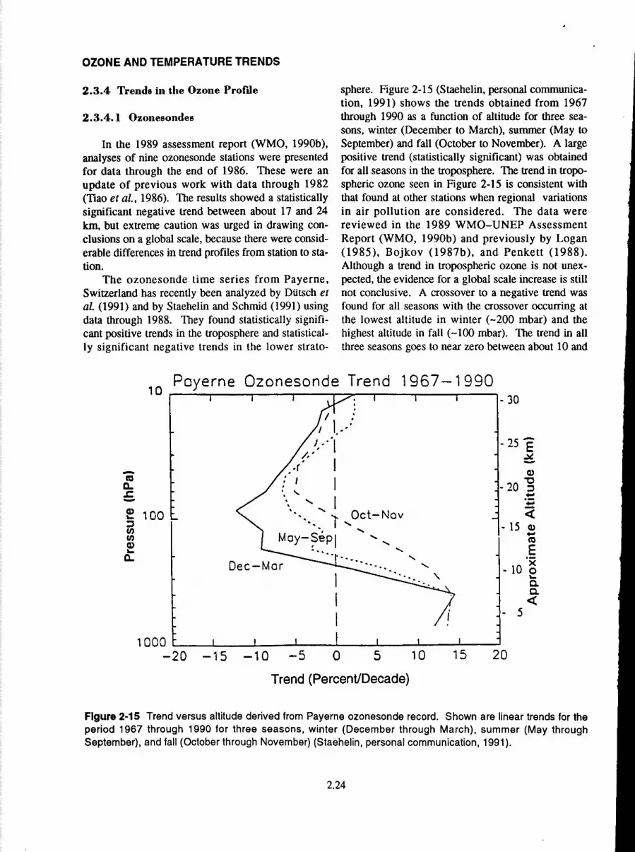
In the 1989 assessment report (WMO, 1990b), analyses of nine ozonesonde stations were presented for data through the end of 1986. These were an update of previous work with data through 1982 (Tiao et al., 1986). The results showed a statistically significant negative trend between about 17 and 24 km, but extreme caution was urged in drawing con-clusions on a global scale, because there were consid-erable differences in trend profiles from station to sta-tion.

The ozonesonde time series from Payerne, Switzerland has recently been analyzed by Diitsch et al. (1991) and by Staehelin and Schmid (1991) using data through 1988. They found statistically signifi-cant positive trends in the troposphere and statistical-ly significant negative trends in the lower strato-

sphere. Figure 2-15 (Staehelin, personal communica-tion, 1991) shows the trends obtained from 1967 through 1990 as a function of altitude for three sea-sons, winter (December to March), summer (May to September) and fall (October to November). A large positive trend (statistically significant) was obtained for all seasons in the troposphere. The trend in tropo-spheric ozone seen in Figure 2-15 is consistent with that found at other stations when regional variations in air pollution are considered. The data were reviewed in the 1989 WMO—UNEP Assessment Report (WMO, 1990b) and previously by Logan (1985), Bojkov (1987b), and Penkett (1988). Although a trend in tropospheric ozone is not unex-pected, the evidence for a global scale increase is still not conclusive. A crossover to a negative trend was found for all seasons with the crossover occurring at the lowest altitude in winter (-200 mbar) and the highest altitude in fall (-100 mbar). The trend in all three seasons goes to near zero between about 10 and

10 Payerne Ozonesonde Trend 1967-1990

a a) 0

a) loo U, (I) a)

CL

1000

30

25

a) 20

15 a) a)

E X

10 0 0. 0.

.5

I I -

/ I..••-

• \ -,I • Oct—Nov

May-Sp1 .

Dec-Mar ..•....

I I I j-

-20 -15 -10 -5 0 5 10 15 20

Trend (Percent/Decade)

Figure 2-15 Trend versus altitude derived from Payerne ozonesonde record. Shown are linear trends for the period 1967 through 1990 for three seasons, winter (December through March), summer (May through September), and fall (October through November) (Staehelin, personal communication, 1991).

2.24


20 mbar. Since the total ozone column from each ozonesonde profile is normalized to Dobson column measurements, the integrated effect of the sonde trend profile is necessarily quantitatively consistent with the Dobson trends.

The change in the altitude profile of ozone is graphically illustrated in Figure 2-16 (Staehelin, per-sonal communication, 1991), which shows the profile obtained from the Payerne ozonesondes averaged over three different 2-year time periods. The time periods, 1969-70, 1979-80, and 1989-90 were cho-sen to be near the maxima of three consecutive solar cycles. Two-year time periods were chosen to remove seasonal variations and to approximately remove the effects of the quasi-biennial oscillation. The profiles in Figure 2-16 clearly show that lower ozone concentrations are measured throughout the ozone peak region in the lower stratosphere during 1989-90.

2.3.4.2 SAGE

The Ozone Trends Panel Report showed ozone changes as a function of altitude above 25 km obtained by differencing 3 years of SAGE II data from the more than 2 years of SAGE I data. Since that report, the SAGE I and SAGE II ozone profiles below 25 km have been validated (Veiga and Chu, 1991) and trends down to 17 km altitude can be eval-uated. Additionally, there are now more than 6 years of SAGE II data which, when combined with SAGE I data, can be used to give an independent determina-tion of the altitude profile of ozone change.

Figure 2-17 is a latitude-altitude plot of the annual average trends deduced from the combined SAGE I/SAGE II data set (McCormick etal., 1992). Ozone trends deduced from SAGE in the middle stratosphere (25-35 km) are small and not signifi-cantly different from zero. Above 35 km, the trends are generally negative. The maximum decrease is found near 42 km at 20°S latitude and changes in the Southern Hemisphere are larger than those in the Northern Hemisphere. The latitudinal dependence and magnitude of the upper stratospheric trends is at variance with model predictions (see Figure 2-18). In the lower stratosphere, strong negative trends are seen with a weak latitude dependence. The strongest lower stratospheric trends appear near about 25° in each hemisphere.

1989/90—\ \ 25 E

I • a)

1979/8020

a) 4-.

1969/70 15 E 0 0. 0.

10

50 100 150

Ozone Concentration (nbar)

Figure 2-16 Average ozone concentration versus alti-tude measured over Payerne for three 2-year periods, 1969-1970, 1979-1980, and 1989-1990. Periods were chosen to be approximately during solar maxi-mum and 2 years was used to remove most of any QBO effect (Staehelin, personal communication, 1991).

2.3.4.3 Umkelir

The Umkehr record was analyzed in the Ozone Trends Panel Report and in the 1989 WMO—UNEP assessment. Data from 10 statinn were e1ii,tpcI frr

the time period 1977-1987 using two different assumptions concerning data immediately after El ChichOn. One assumption was to delete the data for 2 years after the eruption and the other was to include a statistical term in the analysis with the shape of the lidar optical thickness. These procedures led to simi-lar results: a decrease in Levels 7 and 8 (-35-45 kin), which is statistically significant, or nearly so, at the two a level. The Umkehr records have now been updated through 1990 and analyzed by DeLuisi (per-sonal communication).

10

20

0 . 50

a) I.-0

LOO CD

200

/

500

1000

2.25

C

-o

0 C 0 0 C :3

Lo

It,

Cl) C)

c

Lo (N

0 U)

C:

LP) C:

'3) -c C: 0 :3 D

'3)

CL) 0

:3

'3)

0

a) :3 0 N 0 ci)

-C

0

(1)

C a)

E ci)

:3 (1) cci ()

E

w

w

0

(I)

c'J C 0)

0)

0

a)

e)

t-. 0

0 F-

I. -o

LL c


C 0) 0)

0)

0)

Cl) V C C) h.. I-0 N 0

CL

0 L.. C)

(n 0 j w C.,

C/)

I-

V C

w >i 0 0 0 i- - - C.1 C)

G) . 0 0 . . . . • a a a a

0 It) 0 It) 0 U) 0 C") C') 04 ci

(w) en,y

2.26

U 0 <

I'

( I -D \'

Y1 I7 I 7'\Ii

I1

\ I 1:1'

C 0

a) -o 0

I I

0 LCJ 0 iC) 0 ifl 0 L(J 0 Lt) If) ,4- - r) N) (N (Ni —

(w)j) aPn:TlIV


C %4O

C). C) CC)

OQ C) '—C

0 0 tf)

r

U)

cu 0 ci

u1

ci) CL

C ci)

I-

0 1

U)QU) cc

0

Ca, o U) a, C o2 0 o . - 0

a,

Li

C.)

0)

< a,—C/)

>C a, 0)

Ua, E

c" C o a, —CC

EDo

L)LC) WI

U) N EZ

Z LO

M U) U) E C

-.

co

U 0

I > OC

C 0

a, a, C5 (D — 0.> U) E cc °C0 o cC

a, co a,

co c1

I- W W v

IL. Cl) Cl)

2.27

55 50 45 40 35 30 25 20 16

10 5 0

—1.5

I I __ I

— 1 —0.5 0 0.5 1

I-

a,


2.3.4.4 Comparison of Profile Trends

To facilitate a direct comparison with SAGE, the Umkehr record has been analyzed from 1979 through 1990. The resulting trend and error bars are shown in Figure 2-18 along with the SAGE trends. Following WMO (1990a,b), only the Umkehr results in Layers 4 through 8 are shown. The trend profiles from Umkehr and SAGE agree to within their uncer-tainties and show a maximum decrease of _1/2 percent per year in Layers 7 and 8 (35-45 km), which is approximately half of the change predicted by mod-els. No significant trend is observed in the 25-30-km region. SAGE and Umkehr independently confirm the large negative trends in the lower stratosphere (below 25 km) seen in the ozonesonde data.

2.3.5 Temperature

Ozone and temperature generally correlate posi-tively in the lower stratosphere and negatively in the upper stratosphere, but the respective responses to various forcings may complicate this relationship. Temperature is subject to frequent fluctuations whether of external (solar, volcanic) or internal origin

(planetary and gravity waves, QBO, etc.). This tem-perature variability may result in fluctuations in either total ozone or in ozone concentration. Conversely ozone changes, such as those reported in this chapter, will affect the absorption rate of ultravi-olet and infrared radiation and can lead to tempera-ture changes in response. It is important to compare trends in the temperature with those observed in ozone concentration.

Even though the number of measurements is very large, the search for temperature trends has received far less attention. The previous assessment report (WMO, 1990b) concluded that there was some evi-dence of a generally negative trend in the lower stratosphere, with large spatial variability. The upper-limit zonal-average trend was given as —0.6 to —0.8 K per decade between the 100 and 10 hPa levels, respectively. Recently, Labitzke and van Loon (1991), who had earlier indicated a cooling of 0.4 K per decade at 20 and 24 km in October—November between 20° and 50° N, have cast some doubts about their results from radiosondes due to the high vari-ability observed, mostly in winter.

Two studies of trends deduced from radiosondes have been performed since the last assessment

Trend (Degrees/Decade) Figure 2-19 Rawinsonde temperature trend estimates in . per decade as a function of altitude. Horizontal bars represent 95 percent confidence limits of estimated trends (Miller etal., 1991).

2.28


80

70

I I

E60

95R confidence a,

50

40

30-15 -10 -5 0 5 10

Trend (K/Decade) Figure 2-20 Temperature trend versus altitude for 6-month summer season from April through September obtained by lidar measurements above Observatoire de Haute Provence in southern France. Data period was from 1979 through 1990 (Hauchecorne etal., 1991).

(Miller et al., 1991; and Oort and Liu, 1991). Both use the data set already used by Angell (1988); i.e., 62 stations extending from 80°N to 80°S. Miller et al. (1991) deduced a warming of the order of 0.3° per decade between the surface and 5 km (500 mb) and a maximum cooling of 0.4° per decade between 16 km (100 mb) and 20 km (50 mb) as shown in Figure 2-19. Oort and Liu (1991) treated the two hemispheres and deduced a trend of —0.38° per decade in the Northern Hemisphere compared to —0.43° per decade in the Southern Hemisphere.

These recent analyses support a global cooling of the lower stratosphere of between 0.3 K and 0.5 K per decade. Significantly more work needs to be done on temperature trends but it appears that a rela-tively conservative conclusion can be reached that there has been a global mean cooling of the lower stratosphere of about 0.3 K per decade over the last 2 to 3 decades.

Other recent results concerning the upper strato-sphere and mesosphere (Kokin et al., 1990; Aikin et al., 1991; Hauchecorne et al., 1991) have been obtained. Figure 2-20, from Hauchecorne et al. (1991), illustrates the results obtained in summer by

lidar at 44°N, 61°E. Whereas a clear cooling of 4 K per decade associated with CO 2 increase is observed in the mesosphere, the —1 K per decade seen between 35 and 50 km is below the significance level. The same type of result is observed from four rocket sites by Kokin et al. (1991). In those two cases the quite significant response to the 11-year solar forcing has been taken into account and extracted independently. Aikin el al. (1991) examined satellite data using the synthesized Stratospheric Sounding Unit (SSU) chan-nel 47x centered near 0.5 hPa or 55 km and they con-firmed that the mesospheric cooling of Figure 2-20 was global scale. The comparison with models at 40 km, which indicates between 1 and 2 K per decade, due half to the 03 depletion and half to the CO2 increase, is within the error bars of the observations, but the cooling observed above 50 km is much larger than expected from models.

2.4 SUMMARY

The Antarctic ozone hole of 1989 was deep and long-lasting, demonstrating that 1987 was not unique. The 1990 ozone hole was also quite deep, similar to

2.29


both 1987 and 1989. It lasted through December, the latest disappearance yet of the springtime ozone hole. The 1991 ozone hole was again deep and long-last-ing, very similar to 1989. Thus, four of the last five years have had deep long-lasting ozone holes. The previously noted quasi-biennial modulation of the severity of the ozone hole did not occur during the last 3 years. The area of the ozone hole has remained constant for the years 1987, 1989, 1990, and 1991.

For the first time statistically significant decreas-es in total ozone are being observed in all seasons in both the Northern and Southern Hemispheres at mid-dle and high latitudes. Southern mid-latitude total ozone trends from the TOMS data are statistically significant in all seasons south of about 25S. This is consistent with the analyses from the few existing Dobson stations with long records. The northern mid-latitude winter decrease found by the Ozone Trends Panel has continued and is now somewhat larger than previously reported, extending into the spring and summer. The majority of Dobson stations now show a statistically significant summer trend since 1970. The Dobson measurements have now been confirmed by independent measurement systems, i.e., TOMS and SAGE. The TOMS negative trends are about 1 percent more negative than those from the Dobson instruments at the same latitude. There is longitudi-nal structure to the trends derived from TOMS for northern mid-latitudes. The longitudinal structure in the Dobson data is less clear, but reasonably consis-tent with that from TOMS. No statistically signifi-cant decreases are seen in tropical latitudes, from 25°Sto25° N.

SAGE and ozonesonde measurements have demonstrated that the northern middle latitude trends are occurring in the lower stratosphere. The negative trend in the lower stratosphere, below 25 km, is about 10 percent per decade, consistent with the observed decrease in column ozone. The measured upper stratospheric trend from both SAGE and Umkehr have a shape with altitude that is similar to model predictions, but the magnitude is somewhat smaller than that of the models. Tropospheric ozone increas-es of 10 percent per decade over the last 2 decades are seen over the few existing ozone sounding sta-tions at northern middle latitudes.

The temperature record and understanding of changes in temperature are not in nearly as good

shape as the ozone record. The existing record indi-cates a small cooling (about 0.3 K per decade) of the lower stratosphere in the sense of that expected from the observed change in the stratospheric concentra-tion of ozone.

REFERENCES:

Aikin, A.C., M.L. Chanin, J. Nash, and D.J. Kendig, Temperature trends in the lower mesosphere, Geophys. Res. Len., 18,416-419,1991.

Angell, J.K. Variations in trends in tropospheric and stratospheric global temperatures, 1958-87, J. Climate, 12, 1296-1313, 1988.

Bojkov, R.D., The 1983 and 1985 anomalies in ozone distribution in perspective, Mon. Wea. Rev., 115, 2187-2201,1987a.

Bojkov, R.D., Ozone changes at the surface and in the free troposphere, in Tropospheric Ozone: Proceedings of the NATO Workshop, ed. by I.S.A. Isaksen, pp. 83-96, D. Reidel, Boston, 1987b.

Bojkov, R.D., L. Bishop, W.J. Hill, G.C. Reinsel, and G.C. Tiao, A statistical trend analysis of revised Dobson total ozone data over the Northern Hemisphere, J. Geophys. Res., 95, 9785-9807, 1990.

Bojkov, R.D., and V.E. Fioletov, The ozone changes over mid-latitude Eurasia based on re-evaluated filter ozonometer data, J. Geophys. Res., submit-ted, 1991.

Browell, EX, L.R. Poole, M.P. McCormick, S. Ismail, C.F. Butler, S.A. Kooi, M.M. Szedlmayer, R.L. Jones, A. Krueger, and A.F. Tuck, Large-scale variations in ozone and polar stratospheric clouds measured with airborne lidar during formation of the 1987 ozone hole over Antarctica, Polar Ozone Workshop, NASA Ref. Pubi. 10014,61-(A, 1988.

Chandra, S., and R.S. Stolarski, Recent trends in strato-spheric total ozone: implications of dynamical and El ChichOn perturbations, Geophys. Res. Lett., 18, 2277-2280,1991.

Chanin, M.L., N. Smires, and A. Hauchecome, Long-term variation of the temperature of the middle atmosphere at mid-latitude: dynamical and radia-tive causes, J. Geophys. Res., 92, 10933-10941, 1987.

Chubachi, S., A special ozone observation at Syowa Station, Antarctica from February 1982 to

2.30


January 1983, in Atmospheric Ozone, Ed. by C. S. Zerefos and A.M. Ghazi, Reidel, Dordrecht, 285-289,1985.

Deshler, T., and D.J. Hofmann, Ozone profiles at McMurdo Station, Antarctica, the Austral spring of 1990, Geophys. Res. Lett., 18, 657-660, 1991.

Deshler, T., D.J. Hofmann, J.V. Hereford, and C. B. Sutter, Ozone and temperature profiles over McMurdo Station, Antarctica, in the spring of 1989, Geophys. Res. Lett., 17, 151-154,1990.

Dtitsch, H.U., J. Bader, and J. Staehelin, Separation of solar effects on ozone from anthropogenically produced trends, J. Geomagnetism and Geoelectriciiy, in press, 1991.

Farman, J.C., B.G. Gardiner, and J.D. Shanklin, Large losses of total ozone in Antarctica reveal seasonal CIO,,/NO,, interaction, Nature, 315, 207-210,1985.

Fioletov, V.E., Total ozone content variations on vari-ous temporal scales, Proceedings of the 28th Liege International Astrophysical Colloquium, Liege, Belgium, 1989 (updated 1991).

Fleig, A.J., P.K. Bhartia, C.G. Wellemeyer, and D.S. Silberstein, Seven years of total ozone from the TOMS instrument-a report on data quality, Geophys. Res. Lett., 13, 1355-1358, 1986.

Garcia, R.R., and S. Solomon, A possible relationship between interannual variability in Antarctic ozone and the quasi-biennial oscillation, Geophys. Res. Lett., 14, 848-851, 1987.

Gardiner, B .G., Comparative morphology of the ver-tical ozone profile in the Antarctic spring, Geophys. Res. Len., 15, 901-904,1988.

GOtz, EW.P., Zum Strahlungsklima des Spitzbergen Sommers, Gerlands Beitrage zur Geophys., 31, 119-154,1931.

Hauchecorne, A., M.L. Chanin, and P. Keckhut, Climatology and trends of the middle atmo-spheric temperature (33-87 km) as seen by Rayleigh lidar over the south of France, J. Geophys:Res., 96, 15297-15309, 1991.

Heath, D.F., A.J. Krueger, and P.J. Crutzen, Solar proton event: influence on stratospheric ozone, Science, 197, 886-888, 1977.

Herman, J.R., R. Hudson, R. McPeters, R. Stolarski, Z. Ahmad, X.-Y. Gu, S. Taylor, and C. Wellemeyer, A new self-calibration method applied to TOMS/SBUV backscattered ultravio-

let data to determine long-term global ozone change, J. Geophys. Res., 96, 7531-7545, 1991.

Hilsenrath, E., and B.M. Schlesinger, Total ozone seasonal and interannual variations derived from the 7-year Nimbus-4 BUV data set, J. Geophys. Res., 86, 12087-12096,1981.

Hofmann, D.J., J.W. Harder, J.M. Rosen, J.V. Hereford, and J.R. Carpenter, Ozone profile measurements at McMurdo Station, Antarctica during the spring of 1987, J. Geophys. Res., 94, 16527-16536,1989.

Jager, H., and K. Wege, Stratospheric ozone depletion at northern midlatitudes after major volcanic eruptions, J. Atmos. Chem., 10, 273-20,1990.

Kokin, G.A., Ye. V. Lysenko, and S.Kh. Rozenfeld, Temperature changes in the stratosphere and mesosphere in 1964-1988 based on rocket sounding data, lzvestiya, Atmospheric and Oceanic Physics, 26, 518, 1990.

Komhyr, W.D., R.D. Grass, and R.K. Leonard, Total ozone, ozone vertical distribution, and strato-spheric temperatures at South Pole, Antarctica, in 1986 and 1987, J. Geophys. Res., 94, 11429-11436,1988.

Labitzke, K., B. Naujokat, and M.P. McCormick, Temperature effects on the stratosphere of the April 4, 1982, eruption of El ChichOn, Mexico, Geophys. Res. Len., 10, 24-26,1983.

Labitzke, K., and H. van Loon, Some complications in determining trends in the stratosphere, Adv. Space Res., 11,(3)21-(3)30, 1991.

Lait, L.R., M.R. Schoeberl, and P.A. Newman, Quasi-biennial modulation of Antarctic ozone, J. Geophys. Res., 94, 11559-11571, 1989.

Lapworth, A., Report of a re-evaluation of total ozone data from the UK Dobson network for the last decade, UK Meteorological Office Manuscript, 1991.

Lefèvre, F,. and D. Cariolle, Total ozone measure-ments and stratospheric cloud detection during the AASE and the TECHNOPS Arctic balloon campaign, Geop/zys. Res. Len., 18, 33-36, 1991a.

Lefèvre, F., D. Cariolle, S. Muller, and F. Karcher, Total ozone from TOVS/H1R52 infrared radi-ances during the formation of the 1987 "ozone hole", J. Geophys. Res., 96, 12893-12911, 1991b.

2.31


Logan, J.A., Tropospheric ozone: seasonal behavior, trends, and anthropogenic influence, J. Geophys. Res., 90,10463-10482,1985.

Mateer, C.L., and J.J. DeLuisi, A new Umkehr inver-sion algorithm, Manuscript, 1991.

McCormick, M.P., and J.C. Larsen, Antarctic spring-time measurements of ozone, nitrogen dioxide, and aerosol extinction by SAM II, SAGE, and SAGE II, Geophys. Res. Lett., 13, 1280-1283, 1986.

McCormick, M.P., and J.C. Larsen, Antarctic mea-surements of ozone by SAGE II in the spring of 1985, 1986, and 1987, Geophys. Res. Lett., 15, 907-910,1988.

McCormick, M.P., J.M. Zawodny, R.E. Veiga, J.C. Larsen, and P. H. Wang, An overview of SAGE I and II ozone measurements, Planet. Space Sci., 37,1567-1586,1989.

McCormick, M.P., R.E. Veiga, and W.P. Chu, Stratospheric ozone profile and total ozone trends derived from the SAGE I and SAGE II data, Geophys. Res. Lett., 19, 269-272,1992.

McPeters, R.D., and C.H. Jackman, The response of ozone to solar proton events during solar cycle 21: the observations, J. Geophys. Res., 90, 7945-7954,1985.

McPeters, R.D., and W.D. Komhyr, Long-term changes in TOMS relative to World Primary Standard Dobson Spectrometer 83, J. Geophys. Res. 96, 2987-2993,1991.

Michelangeli, DX, M. Allen, and Y.L. Yung, El ChichOn volcanic aerosols: impact of radiative, thermal, and chemical perturbations, J. Geophys. Res., 94, 18429-18444, 1989.

Miller, A.J., R.M. Nagatani, G.C. Tiao, X.F. Niu, G.C. Reinsel, D. Wuebbles, and K. Grant, Comparisons of observed ozone and temperature trends, submitted to Geophys. Res. Lea., 1991.

Newman, P.A., M.R. Schoeberl, and L.R. Lait, Comparison of the Southern Hemisphere springs of 1988 and 1987, Proceedings of the NATO Advanced Research Workshop on Dynamics, Transport and Photochemistry in the Middle Atmosphere of the Southern Hemisphere, San Francisco, CA, USA, April 15-17, 1989, Kluwer Academic Publishers, Dordrecht, The Netherlands, 1990.

Newman, P., R. Stolarski, M. Schoeberl, R. McPeters, and A. Krueger, The 1990 Antarctic ozone hole

as observed by TOMS, Geophys. Res. Lett., 18, 661-664,1991.

Oort, A.H., and H. Liu, Upper air temperature trends over the globe, 1958-1989, J. Climate, submit-ted, 1991.

Paur, R.J., and A.M. Bass, The ultraviolet cross-sec-tions of ozone: II. Results and temperature dependence, in Atmospheric Ozone, Ed. by C.S. Zerefos and A.M. Ghazi, Reidel, Dordrecht, 611-616,1985.

Penkett, S.A., Indications and causes of ozone increases in the troposphere, in The Changing Atmosphere, edited by F.S. Rowland and I.S.A. Isaksen pp. 91-103, Wiley-Interscience, New York, 1988.

Pommereau, J.P., F. Goutail, H. LeTexier, and T.S. Jorgensen, Stratospheric ozone and nitrogen dioxide monitoring at southern and northern polar latitudes, Proc. of the 28th International Astrophysical Colloquium, Liege, Belgium, 1989.

Proffitt, M.H., M.J. Steinkamp, J.A. Powell, R.J. McLaughlin, O.A. Mills, A.L. Schmeltekopf, T L. Thompson, A.F. Tuck, T. Tyler, R.H. Winkler, and K.R. Chan, In-situ ozone measurements within the 1987 Antarctic ozone hole from a high altitude ER-2 aircraft, J. Geophys. Res., 94, 16547-16556,1989.

Randel, W.J., The anomalous circulation in the Southern Hemisphere stratosphere during spring 1987, Geophys. Res. Lett., 15, 911-914, 1988.

Reid, G.C., S. Solomon, and R.R. Garcia, Response of the middle atmosphere to the solar proton events of August—December, 1989, Geophys. Res. Lett., 18, 1019-1022,1991.

Reinsel, G.C., G.C. Tiao, A.J. Miller, D.J. Wuebbles, P.S. Connell, C.L. Mateer, and J.J. DeLuisi, Statistical analysis of total ozone and strato-spheric Umkehr data for trends and solar cycle relationship, J. Geophys. Res., 92, 2201-2209, 1987.

Reinsel, G., G.C. Tiao, M.N. Wang, R. Lewis, and D. Nychka, Statistical analysis of stratospheric ozone for the detections of trends, Atmos. Envir., 15, 1569-1577,1981.

Reinsel, G.C., G.C. Yiao, J.J. DeLuisi, S. Basu, and K. Carreise, trend analysis of aerosol-corrected Umkehr ozone profile data through 1987, J. Geophys. Res., 94,16373-16386,1989.

2.32


Solomon, S., and P.J. Crutzen, Analysis of the August 1972 solar proton event including chlorine chemistry, J. Geophys. Res., 86, 1140-1146, 1981.

Staehelin, J., and W. Schmid, Trend analysis of tropo-spheric ozone concentrations utilizing the 20-year data set of ozone balloon soundings over Payerne (Switzerland), Atmos. Envir., 25a, 1739-1749,1991.

Stolarski, R.S., M.R. Schoebert, P.A. Newman, R.D. McPeters, and A.J. Krueger, The 1989 Antarctic ozone hole as observed by TOMS, Geophys. Res. Lett., 17, 1267-1270, 1990.

Stolarski, R.S., P. Bloomfield, R.D. McPeters, and J. R. Herman, Total ozone trends deduced from Nimbus-7 TOMS data, Geophys. Res. Lett., 18, 1015-1018,1991.

Tiao, G.C., G.C. Reinsel, J.H. Frederick, G.M. Allenby, C.L. Mateer, A.J. Miller, and J.J. DeLuisi, A sta-tistical trend analysis of ozonesonde data, J. Geophys. Res., 91, 13121-13136, 1986.

Veiga, R.E., and W.P. Chu, Validation of SAGE I and SAGE II ozone in the lower stratosphere, EOS Trans. of the AGU, 72, 68, 1991.

von Cossart, G., and J. Taubenheim, Solar cycle and long-period variations of mesospheric tempera-tures, J. Atmos. Terr Phys., 49, 303-307, 1987.

WMO, Report of the International Ozone Trends Panel: 1988, World Meteorological Organization

Global Ozone and Monitoring Network Report #18, WMO, Washington, DC, 1990a.

WMO, International Ozone Assessment: 1989, World Meterological Organization Global Ozone and Monitoring Network Report #20, WMO, Washington, DC, 1990b.

Zawodny, J.M., and M.P. McCormick, Stratospheric aerosol and gas experiment II measurements of the quasi-biennial oscillations in ozone and nitrogen dioxide, J. Geophys. Res., 96, 9371-9378,1991.

Zerefos, C.S., and P.J. Crutzen, Stratospheric thick-ness variations over the Northern Hemisphere and their possible relation to solar activity, J. Geophys. Res., 80, 5041-5043, 1975.

Zerefos, C.S., A.F. Bais, L.C. Ziomas, and R.D. Bojkov, On the relative importance of QBO and ENSO in the revised Dobson total ozone records, J. Geophys. Res., submitted, 1991a.

Zerefos, C.S., A.F. Bais, K. Ziomas, and R.D. Bojkov, Total ozone forcing from El Nifio events, Paper presented at the XV IUGG General Assembly, Vienna, Austria., 1991b.

2.33

chapter 2 - noaa chemical sciences laboratory

Documents