chaotic systems in complex phase space

PRAMANA c© Indian Academy of Sciences Vol. 73, No. 3— journal of September 2009

physics pp. 453–470

Chaotic systems in complex phase space

CARL M BENDER1,∗, JOSHUA FEINBERG2, DANIEL W HOOK3

and DAVID J WEIR3

1Department of Physics, Washington University, St. Louis, MO 63130, USA2Department of Physics, University of Haifa at Oranim, Tivon 36006,Israel and Department of Physics, Technion, Haifa 32000, Israel3Blackett Laboratory, Imperial College London, London SW7 2AZ, UK∗Corresponding authorE-mail: [email protected]; [email protected]; [email protected];[email protected]

Abstract. This paper examines numerically the complex classical trajectories of thekicked rotor and the double pendulum. Both of these systems exhibit a transition tochaos, and this feature is studied in complex phase space. Additionally, it is shown thatthe short-time and long-time behaviours of these two PT -symmetric dynamical models incomplex phase space exhibit strong qualitative similarities.

Keywords. PT symmetry; approach to chaos; kicked rotor; standard map; double pen-dulum.

PACS Nos 05.45.-a; 05.45.Pq; 11.30.Er; 02.30.Hq

1. Introduction

The past decade has seen intense activity in the field of PT quantum mechanics[1,2]. A PT -symmetric Hamiltonian is said to have an unbroken PT symmetry if itseigenfunctions are PT symmetric. A Hamiltonian having an unbroken PT symme-try is physically relevant because its eigenvalues are real and it generates unitarytime evolution. Such a Hamiltonian defines a conventional quantum-mechanicaltheory even though it may not be Dirac Hermitian. (A linear operator is DiracHermitian if it remains invariant under the combined operations of matrix trans-position and complex conjugation.) One can regard such non-Hermitian quantum-mechanical systems as being complex extensions of conventional quantum systems.

Interesting features of PT quantum mechanics have motivated many recent stud-ies of PT classical mechanics. In particular, solutions to Hamilton’s equations havebeen examined for various systems whose Hamiltonians are PT symmetric. Forsuch systems the classical trajectories are typically complex [3–16]. These trajecto-ries can lie in many-sheeted Riemann surfaces and often have elaborate topologicalstructure. When the PT symmetry of the quantum Hamiltonian is not broken, the

453

Carl M Bender et al

real-energy trajectories of the corresponding classical Hamiltonian are found to beclosed and periodic [8,13].

The purpose of this paper is to explore a new aspect of complex classical me-chanics, namely, the complex extension of chaotic behaviour. Specifically, we studytwo classical systems: the kicked rotor and the double pendulum. The kicked rotoris a paradigm for studying the dynamics of chaotic systems described by time-dependent Hamiltonians [17–19]. The planar double pendulum is also a dynamicalmodel whose classical motion is known to be chaotic [20]. The Hamiltonians forboth of these dynamical systems are PT symmetric so long as the parameters Kin the Hamiltonian for the kicked rotor (4) and g in the Hamiltonian for the doublependulum (10) are real. We use a variety of computational tools in order to derivethe numerical results presented. The C programming language was used to imple-ment a fully symplectic three-stage Gauss–Legendre Runge–Kutta method for thesimulation of the double pendulum, and standard functionality in Mathematica 6was used in the study of the kicked rotor.

This paper is organized as follows: In §2 we define the kicked rotor and mentionbriefly the transition associated with the disappearance of KAM trajectories. In §3we describe the planar double pendulum and describe the analogous transition thatoccurs for this dynamical system. We also reproduce the numerical work of Heylconcerning flip times. This work reveals fractal-like structure in the plane of initialconditions [21]. Then, in §§4 and 5 we study the short- and long-time behavioursof the kicked rotor and the double pendulum in the complex domain, whereinpart of our objective is to identify indicators for the transition to chaos. We alsodemonstrate that these two very different dynamical systems exhibit remarkablysimilar features. Section 6 contains some concluding remarks.

2. Kicked rotor

The Hamiltonian for the kicked rotor is [17–19]

H =p2

2I+ K cos θ

∞∑n=−∞

δ(t− nT ), (1)

where I is the moment of inertia of the rotor, p is its angular momentum and θ is theangular coordinate. As the rotor turns, it is subjected to a periodic impulse, which isapplied at times t = 0, ±T, ±2T, . . . . The magnitude of the impulse is proportionalto K, a constant having dimensions of angular momentum. This Hamiltonian isPT symmetric because it is symmetric separately under the operation of angularreflection P, where P: θ → 2π − θ and P: p → −p, and the operation of timereversal T , where T : t → −t, T : p → −p, and T leaves θ invariant. (Note thatangular reflection P is not the same as spacial reflection, which maps θ → π − θ.)

Hamilton’s equations of motion derived from (1) are

dθ

dt=

p

Iand

dp

dt= K sin θ

∞∑n=0

δ(t− nT ). (2)

454 Pramana – J. Phys., Vol. 73, No. 3, September 2009


These equations imply that the angular momentum p changes discontinuously ateach kick, but remains constant between kicks. As a result, the angle θ changeslinearly with time t between kicks and is continuous at each kick.

It is customary to denote pn = p(nT + 0+) and θn = θ(nT + 0+). Thus, pn isthe angular momentum and θn is the angle variable immediately after the nth kick.These variables satisfy the discretized version of (2):

θn+1 = θn +T

Ipn and pn+1 = pn + K sin θn+1. (3)

It is conventional to replace pn and K by the dimensionless quantities TI pn → pn

and TI K → K, in terms of which we rewrite (3) in dimensionless form as

θn+1 = θn + pn and pn+1 = pn + K sin θn+1. (4)

This system of difference equations, which depends on a single dimensionless realparameter K, is known as the standard map. It is straightforward to show that thestandard map is area-preserving in p− θ phase space. The angular variable θn maybe taken modulo 2π. It then follows from the first equation in (4) that pn may alsobe taken modulo 2π. Thus, (4) maps the two-dimensional torus onto itself.

The behaviour of the standard map (4) has been studied extensively[17–19,22–26]. For small K the motion in phase space is bounded and chaoticin some regions. As K increases, KAM trajectories disappear. At the critical valueKc = 0.9716 . . . only the KAM trajectories with golden-mean winding number andwith inverse golden-mean winding number remain, and the motion in phase spaceis still confined. For K > Kc the last bounding trajectory is destroyed and globaldiffusion in phase space ensues. The critical behaviour near Kc has been studiedintensively [23,26].

Figure 1 illustrates the transition from subcritical to supercritical K for thekicked rotor. In this figure we display four sets of superpositions of phase planes,each consisting of 11 randomly chosen initial conditions θ0, p0. For each set of initialconditions we allow the time variable n to range from 1 to several thousand. Thevalues of K for these four plots are 0.40, 0.97, 2.0 and 4.0.

In this paper we continue the classical dynamics described by the standard map(4) into complex phase space [26a]. Our objective here is to generalize (4) into com-plex phase space and thereby gain a better understanding of the critical behaviournear Kc. To accomplish this we are motivated to extend the analysis of refs [3–16]to time-dependent systems. Thus, we treat pn, θn and sometimes K as complexvariables, which we separate into real and imaginary parts as

pn = rn + isn, θn = αn + iβn, K = L + iM. (5)

Substituting (5) in (4), we obtain the complexified standard map

αn+1 = αn + rn, βn+1 = βn + sn,

rn+1 = rn + L sin αn+1 cosh βn+1 −M cosαn+1 sinhβn+1,

sn+1 = sn + L cosαn+1 sinhβn+1 + M sin αn+1 cosh βn+1. (6)

In §§4 and 5 we display and discuss the results of our numerical studies of (6).

Pramana – J. Phys., Vol. 73, No. 3, September 2009 455

Carl M Bender et al

Figure 1. Four phase-plane views of the kicked rotor. In each of the figureswe display the superposition of the discrete phase-plane trajectories θn, pn for11 randomly chosen initial conditions. The time variable n ranges from 1 toseveral thousand. The values of K for the four plots are 0.40, 0.97, 2.0 and4.0. The KAM surfaces separate Poincare islands. As K increases, the KAMsurfaces gradually disappear and the trajectories diffuse into the phase plane.

Figure 2. Configuration of the double pendulum. The double pendulumconsists of two massless rods, each having a massive bob at the end. Thesecond rod hangs from the end of the first rod. The two rods swing in a planeand are acted on by a homogeneous gravitational field of strength g.

3. Double pendulum

As shown in figure 2, a planar double pendulum consists of a massless rod of length`1 with a bob of mass m1 at the lower end from which hangs a second massless rod



of length `2 with a second bob of mass m2. This compound pendulum swings in ahomogeneous gravitational field g, and its motion is constrained to a plane.

In this paper we take both bobs to have unit mass and both rods to have unitlength. The coordinates of the bobs in terms of the angles from the vertical are

x1 = sin θ1, y1 = − cos θ1,

x2 = sin θ1 + sin θ2, y2 = − cos θ1 − cos θ2. (7)

Therefore, the potential and kinetic energies of the double pendulum are

V = −g cos θ2 − 2g cos θ1 and T = θ21 + 1

2 θ22 + θ1θ2 cos(θ1 − θ2). (8)

From these one can form the Lagrangian L = T − V , and then construct theHamiltonian for the system by a Legendre transform. We obtain

H =p21 + 2p2

2 − 2p1p2 cos(θ1 − θ2)2

[sin2(θ1 − θ2) + 1

] − g cos θ2 − 2g cos θ1. (9)

This Hamiltonian is PT symmetric because it is symmetric separately under angu-lar reflection P, where P: θ1,2 → 2π− θ1,2 and P: p1,2 → −p1,2, and time reversalT , where T : t → −t, T : p1,2 → −p1,2, and T leaves θ1,2 invariant.

Hamilton’s equations are then

p1 = −∂H

∂θ1= −2g sin θ1 − p1p2 sin(θ1 − θ2)

sin2(θ1 − θ2) + 1

+[p2

1 + 2p22 − 2p1p2 cos(θ1 − θ2)] sin[2(θ1 − θ2)]

2[sin2(θ1 − θ2) + 1]2,

θ1 =∂H

∂p1=

p1 − p2 cos(θ1 − θ2)sin2(θ1 − θ2) + 1

,

p2 = −∂H

∂θ2= −g sin θ2 +

p1p2 sin(θ1 − θ2)sin2(θ1 − θ2) + 1

− [p21 + 2p2

2 − 2p1p2 cos(θ1 − θ2)] sin[2(θ1 − θ2)]2[sin2(θ1 − θ2) + 1]2

,

θ2 =∂H

∂p2=

2p2 − p1 cos(θ1 − θ2)sin2(θ1 − θ2) + 1

. (10)

Note that this system conserves energy, unlike the kicked rotor whose Hamiltonian(1) is time-dependent.

A beautiful and convincing numerical demonstration that the motion of the dou-ble pendulum is complicated and elaborate was given by Heyl [21]. In his workHeyl calculates for a given initial condition the time required for either pendulumto exhibit a flip; that is, for either θ1 or θ2 to exceed the value π. This calculationis then performed for the limited set of initial conditions for which p1(0) = 0 andp2(0) = 0, and the initial values of θ1 and θ2 both range from 0 to 2π. Each pixelin the initial θ1, θ2 plane is then coloured according to the length of the flip time.

We have applied Heyl’s approach to the double pendulum in (10) and have useda Gauss–Legendre Runge–Kutta method, which is known to be fully symplectic


Carl M Bender et al

Figure 3. Flip times for initial conditions −π ≤ θ1(0) ≤ π, −π ≤ θ2(0) ≤ π,p1(0) = 0 and p2(0) = 0. By a flip we mean that the angular position of eitherbob exceeds π. This figure contains a 600 × 600 grid of pixels. The colourof each pixel characterizes the behaviour of the double pendulum that arisesfrom the initial condition [θ1(0), θ2(0)]. If neither pendulum flips within 100time units, then the pixel is black (the convex-lens-shaped region in the centreof the figure). If one of the pendula flips in a short time, the pixel is coloureddark gray. Longer flip times are indicated by lighter shades of gray. Thefractal-like structure throughout the diagram reveals the nontrivial dynamicsof the double pendulum. Because of parity symmetry this figure is symmetricunder the combined reflections θ1,2 → −θ1,2. Note that different pixels areassociated with different energies and that there is an elliptical region at thecentre of the figure in which flips are forbidden by energy considerations.

[31,32]. The results of this calculation are given in figure 3. This figure is com-posed of a 600× 600 grid of pixels, where each pixel represents the initial condition[θ1(0), θ2(0)]. If neither pendulum flips within 100 time units, then the pixel is as-signed the colour black (the convex-lens-shaped region in the centre of the figure).If either pendulum flips in a short time, the pixel is coloured dark gray, with longerflip times being indicated by lighter shades of gray. Notice the fractal-like structurethroughout the diagram. The appearance of this complicated structure demon-strates that even though the double pendulum has only two degrees of freedom, itexhibits rich and nontrivial dynamics.

In analogy with the kicked rotor, there is a transition in the behaviour of thedouble pendulum in which KAM surfaces disappear as a dimensionless parameterincreases beyond a critical value. This parameter, which measures the strength ofthe gravitational field relative to the total energy, is defined as [20] γ ≡ m1g`1/E.The transition occurs near γ = 0.1 and ref. [20] shows that at the transition thelast surviving KAM surface is the one with winding number being equal to thegolden mean. In figure 4 we plot the Poincare sections generated from 25 randomlychosen initial conditions for four different values of γ. The plot displays points inthe θ1, p1 plane when θ2 = 0 and simultaneously p2 > 0. A KAM surface is visiblewhen γ = 0.05, which is below the critical value. At γ = 0.1, which is near thecritical value, the KAM surface disappears. For the other two values of γ, whichare significantly greater than the critical value, the distribution of points in the plot



Figure 4. Poincare plots for the double pendulum for four values of γ. Belowthe critical value, which is near γ = 0.1, the final KAM surface can still beseen in the second plot, but this surface evaporates as γ increases past thecritical value and the points in the plot spread. This plot is analogous to thatin figure 1 for the kicked rotor.

becomes diffuse in a manner analogous to the behaviour displayed in figure 1 forthe kicked rotor in the K > Kc regime.

4. Short-time behaviour

Having reviewed some properties of the kicked rotor and the double pendulum, weproceed to examine the behaviour of the solutions to the kicked rotor and doublependulum equations of motion in the complex domain. To do so, we do not changethe form of the equations of motion, but rather we take complex initial conditionsand in some cases we allow the parameter K in (4) for the kicked rotor and theparameter g in (10) for the double pendulum to take on complex values.

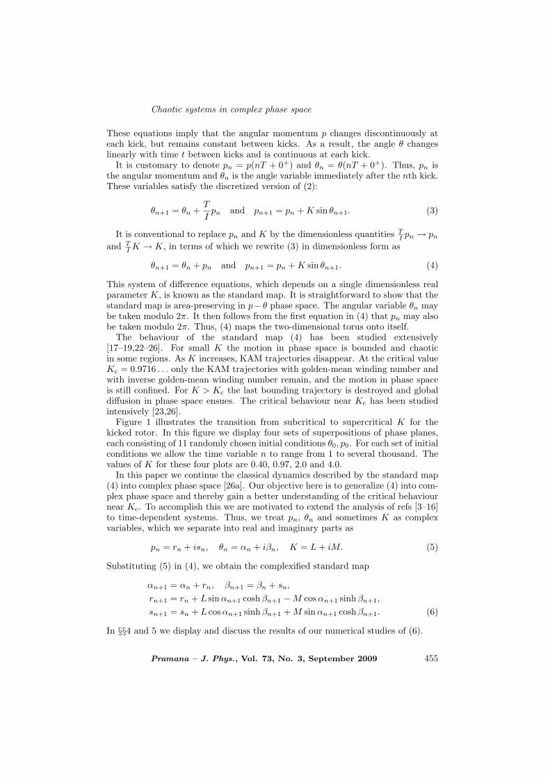
In this section we investigate the behaviour of these dynamical systems for shorttimes; that is, for up to 1000 time steps. For the kicked rotor, let us see whathappens if we take the initial momentum to be real, p0 = 0, but take the initialangle to have a small imaginary component, θ0 = 1 + 0.0001i. In figure 5 we plotthe points θn in the complex-θ plane for n = 0, 1, 2, . . . , 1000 for a range of realvalues of K around the critical point Kc = 0.9716 . . . . While it is difficult to see thesubtle change from subcritical to supercritical behaviour in real plots like those infigure 1, a qualitative change in the complex behaviour is quite evident in figure 5[33]. Below Kc the points tend to occupy a two-dimensional region in the complexplane with some fine structure in it, but as K increases above Kc, the points tendto coalesce along well-separated one-dimensional curves.


Carl M Bender et al

Figure 5. Behaviour of the solution to the kicked rotor in the complex-θplane for a range of real values of K near Kc = 0.9716 . . . . We take as aninitial condition p0 = 0 and θ0 = 1 + 0.0001i and allow the system to evolvefor n = 1000 time steps. For each value of n we plot the complex value of θn

as a point in the complex-θ plane. The plot corresponding to the critical valueis highlighted. Note that there is a qualitative change in the nature of thesecomplex plots as K passes through its critical value. Specifically, the pointsmaking up the plot become less uniform and more stratified. These changesin behaviour are easier to observe than those in figure 1.

In analogy with figure 5, we plot in figure 6 a trajectory for the double pendulumin the Re θ1, Im p2 plane as a function of t for 0 ≤ t ≤ 224. We take two values of γ,one subcritical and one supercritical, and use the slightly complex initial conditionsθ1 = 3.1, θ2 = 3.1 + 0.0001i, p1 = 1.283 and p2 = 1.283 in which the numbers arechosen at random. When γ is above the critical value the trajectory appears tobe confined to distinct narrow bands, somewhat similar to the stratified structuresthat occur for K > Kc in figure 5 for the kicked rotor. However, when γ is belowthe critical value, the trajectory spreads and is similar to the more diffuse behaviourin figure 5 when K < Kc. It would be interesting to understand this stratificationanalytically and also to understand its relation to KAM theory.

A more dramatic way to observe the transition from the subcritical to the super-critical regions of the kicked rotor is to construct plots like that in figure 3 for thedouble pendulum. We take p0 = 0 and take a range of complex initial values forθ0: −π ≤ Re θ0 ≤ π and −π ≤ Im θ0 ≤ π. For each initial condition we allow thekicked rotor to evolve up to a maximum of 400 time steps and determine the time



Figure 6. Trajectory for the double pendulum resulting from the slightlycomplex initial conditions θ1 = 3, θ2 = 3 + 0.0001i, p1 = p2 = 2. Theparameter γ is varied by changing the values of g and l1 and fixing m1 = E = 1.This plot displays the trajectory in the Re θ1, Im p2 plane as a function of tfor 0 ≤ t ≤ 1000. The trajectory is confined to narrow bands when γ is abovethe critical value and is more diffuse when it is below the critical value. Inthis sense, this is similar to figure 5 for the kicked rotor.

step at which the real part of pn becomes infinite, if it does become infinite. (Here,by infinite we mean that the numerical value of Re pn exceeds 10308, the largestnumber that may be represented in double precision arithmetic.) We then performthis calculation for each pixel on a 628×628 grid representing the complex-θ0 plane.We assign a colour to each pixel corresponding to the time at which pn becomesinfinite: White indicates that pn does not become infinite within 400 time steps,and darker shades indicate that pn becomes infinite after shorter times.

In figure 7 we display the results of this calculation for K = 0.01, 0.1, 0.2 and0.6, and in figure 8 we display the results for this calculation for K = 0.9, 1.1, 2.0and 5.0. Note that all these figures exhibit a complicated dendritic and fractal-likestructure. A number of qualitative changes occur as K increases past its criticalvalue. One obvious change is that the dendritic landscape becomes smoother andmore rounded as K increases. A less obvious change is that the regions in whichRe pn does not diverge for n ≤ 400 become connected when K exceeds Kc.


Carl M Bender et al

Figure 7. Behaviour of the solution to the kicked rotor in the complex-θplane for four real values of K and a range of complex initial conditions:p0 = 0, 0 ≤ Re θ0 ≤ 2π and 0 ≤ Im θ0 ≤ 2π. We allow the system toevolve for at most n = 400 time steps. We assign a colour to each value ofθ0 according to the time at which Re pn becomes infinite (if it does so). Thegraph of initial values of θ clearly has fractal structure. Distinctive changesoccur in the nature of these complex plots as K increases.

Instead of constraining K to be real, we can, of course, take K to be complex.In figure 9 we take K = 0.6i. Note that the fractal structure in figures 7 and 8 ispreserved, but it is distorted and loses its left–right symmetry.

Rather than requiring that K passes its critical value on the real-K axis, it ispossible to go from a subcritical real value to a supercritical real value via a pathin the complex-K plane, as in figure 10. The pictures making up this figure areconstructed from values of K that lie on a semicircle of radius 0.6 and are centred atthe critical value Kc = 0.9716 . . . . In these figures we observe fractal structures likethose in figures 7–9, but they are slightly distorted. However, there is a significantdifference in that there is mottling (replacement of large patches of solid shading bya speckled pattern) in the graphs where K is complex; this mottling is absent whenK is pure real or pure imaginary. (Note that when K is complex, PT symmetry isbroken if the T operator is antilinear, that is, it changes the sign of i [33a].

We have performed a related study for the double pendulum: We allow g tobe complex and repeat the numerical analysis of the short-time behaviour that weused to produce figure 3. We find that as the imaginary part of g increases, thefractal-like structure that we see in figure 3 gradually moves outward towards thecorners of the figure. Correspondingly, the boundaries between different coloured



Figure 8. Same as in figure 7 with four higher values of K. There are manyqualitative changes that occur as K increases. For example, the dendriticlandscape that occurs for smaller values of K becomes smoother and morerounded as K increases. A subtle but important change is that the whiteregions, the regions in which Re pn does not diverge for n ≤ 400, becomeconnected when K exceeds Kc.

Figure 9. Same as in figures 7 and 8 except that K = 0.6i. Observe thatwhile many features of the fractal structure in figures 7 and 8 are preserved,they are distorted and the left-right symmetry is destroyed.


Carl M Bender et al

Figure 10. Same as in figure 7 except that the pictures making up this figureare constructed from values of K lying on a semicircle of radius 0.6 and cen-tred at the critical value Kc = 0.9716 . . . . In these figures we observe fractalstructures similar to those in figures 7–9, but slightly distorted. An impor-tant difference between this figure and figures 7–9 is that there is mottling(speckling) in those graphs where K is complex.

regions become smoother. To demonstrate this effect, we choose four differentcomplex values, g = 0.1+0.005i, 0.1+0.01i, 0.1+0.1i, 0.1i, and plot the results infigure 11.

5. Long-time behaviour

In this section we study the long-time behaviour of the kicked rotor and the doublependulum in complex phase space and we find that they share many qualitativefeatures in this regime as well. By long-time we mean roughly 104 to 105 time stepsor time units rather than the 103 time steps taken in §4. We find that the solutionsto the dynamical equations for these systems exhibit characteristic behaviours atdifferent time scales. On a long-time scale, which is determined by the imaginarypart of the initial value of an angle, the solutions tend to ring; that is, the envelope ofthe solution grows and decays to zero with gradually changing periods. On a short-time scale the solution exhibits a distinct and clearly identifiable rapid oscillation,as we can see in figure 12.

We use the language of multiple-scale perturbation theory here [34] to describethis oscillatory behaviour. However, for both the kicked rotor and the double



Figure 11. Short-time behaviour of the double pendulum with complexg. Same as figure 3 but with g = 0.1 + 0.005i, 0.1 + 0.01i, 0.1 + 0.1i, 0.1i.As Im g increases, the fractal-like structure seen in figure 3 moves outwardand towards the corners, and boundaries between differently coloured regionsbecome smooth. Unlike figure 3, there are no energetically-forbidden-flipregions because there exist complex pathways from any pixel to a flippedconfiguration.

pendulum the unperturbed equations are not linear, and thus the usual techniquesof multiple-scale perturbation theory cannot be applied directly in these cases.

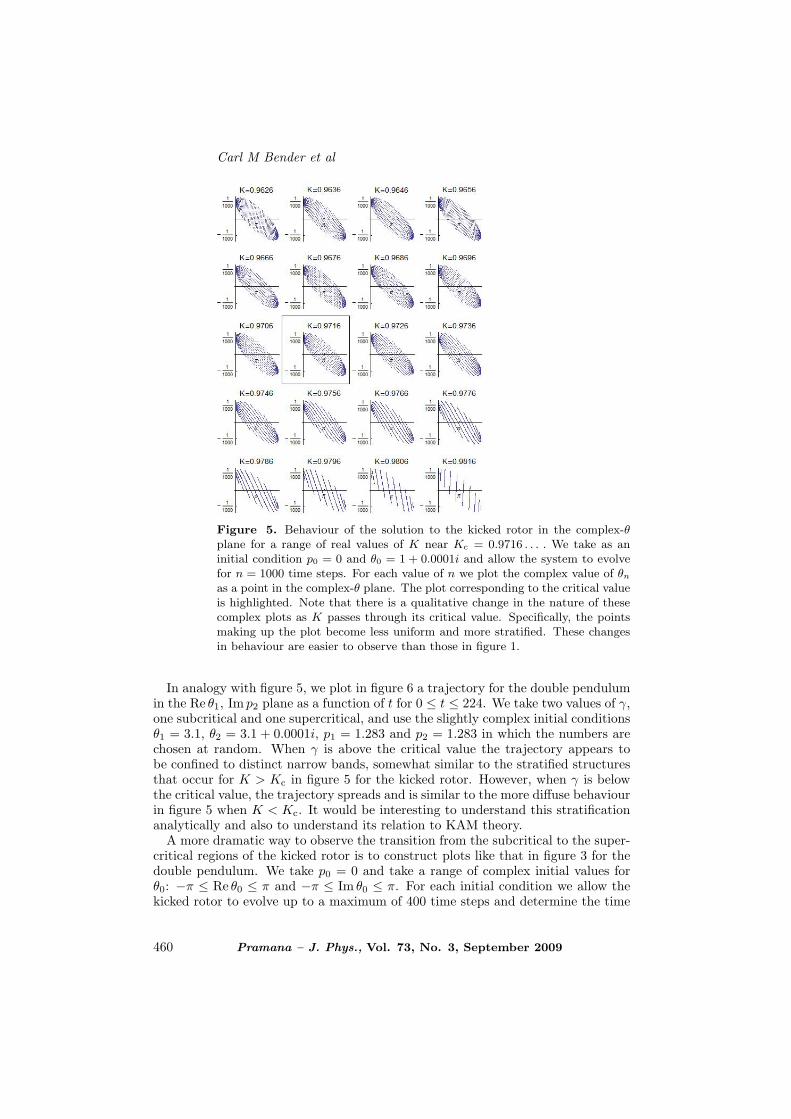
Let us first examine the kicked rotor. As an initial condition we choose p0 = 0and θ0 = 1 + iε. In figure 12 we take K = 0.6 and ε = 10−5 and we plot Re θn,Im θn, Re pn and Im pn for 0 ≤ n <∼ 260 000. Note that while Re θn and Re pn

oscillate within almost constant boundaries, Im θn and Im pn appear to ring witha period of order 1/ε. To verify this dependence on ε we take ε = 10−4, which isten times larger, and we do not change the other initial conditions or the value ofK. The result for Im θn is given in figure 13, where we see that the period of theringing is roughly ten times shorter than the period in figure 12. In both of thesefigures the ringing eventually comes to an abrupt end, at which point the iterationdiverges and the amplitude of oscillation becomes infinite; this happens after about21

2 rings in figure 12 and after about 11 rings in figure 13.While the inverse of the imaginary part of θ0 appears to set the scale of the

ringing period, we have found that the length of the ringing period is also sensitiveto the value of K. In figure 14 we plot Im pn for four values of K: 0.5, 0.53, 0.55and 1.0. For each of these values of K we plot Im pn until it diverges. The initialconditions for each graph in figure 14 are the same as those in figure 12.

The double pendulum exhibits a long-time ringing behaviour that almost exactlyparallels that of the kicked rotor. We plot the long-time behaviour of Im θ1 forg = 1 and initial conditions p1(0) = p2(0) = 0, θ1(0) = 1 and θ2(0) = 10−4i infigure 15 and for θ2(0) = 2×10−4i in figure 16. Note that, like the kicked rotor, the


Carl M Bender et al

Figure 12. Long-time behaviour of the kicked rotor with initial conditionsp0 = 0 and θ0 = 1 + 10−5i and K = 0.6. While the real parts of pn and θn

oscillate between almost constant boundaries, the imaginary parts of pn and θn

exhibit a synchronized ringing behaviour whose period is of order 1/ (Im θ0). Inaddition to the long-time ringing there is a short-time oscillation that becomesmost pronounced when the amplitude of the ringing is at a maximum. Afterabout 2 1

2rings the solution abruptly diverges and ceases to exist.

long-time scale ringing periods are determined by the imaginary part of the initialvalue of an angle; here, the period is proportional to 1/ [Im θ2(0)].

6. Concluding remarks

Apart from making the obvious remark that the two nonlinear systems studied inthis paper exhibit very similar short-time and long-time dynamical behaviours, thiswork indicates that studying the dynamics of classical chaotic systems in complexphase space may help us to understand the onset of chaos. For example, for the



Figure 13. Same as in figure 12 except that the imaginary part of θ0 is tentimes smaller: θ0 = 1 + 10−4i and only the imaginary part of θn is displayed.In this figure the period of the ringing is ten times shorter and there are about11 rings before the solution destabilizes and ceases to exist.

Figure 14. Long-time behaviour of Im pn for the kicked rotor for four differ-ent values of K. The initial conditions are the same as in figure 12. Observethat the period of ringing is quite sensitive to the value of K.

case of the kicked rotor, we observe in figure 5 a change in the complex behaviouras K increases past Kc. Of course, the results reported here are empirical, but theyclearly underscore the need for a deeper analytical understanding of these models.For example, an important unanswered question is, what is the analog of the KAMtheorem in complex phase space?

Finally, we remark that the kicked rotor is one of the rare time-dependent systemswhose quantum dynamics may be studied in detail. Indeed, the kicked rotor is aparadigm for studying quantum chaos. It might be useful to explore the PT -deformed analog of the work of Fishman et al and Jain [19] because (i) this wouldbe a nontrivial extension of PT quantum mechanics to time-dependent systemsand (ii) it may help to define and understand PT -symmetric quantum chaos.


Carl M Bender et al

Figure 15. Long-time behaviour of the double pendulum with g = 1. Theinitial conditions used for this plot are p1(0) = p2(0) = 0, θ1(0) = 1 andθ2(0) = 10−4i. Like the kicked rotor, the imaginary part of an angle exhibits aringing behaviour whose characteristic period is of order 1/Im θ2(0). The plotterminates when the solution to the equations of motion abruptly diverges.Like the kicked rotor, there is also a short-time oscillation, but unlike thekicked rotor, the positive and negative peaks are out of phase with one another.

Figure 16. Same as figure 15 but with θ2(0) = 2×10−4i. Note that doublingthe imaginary part of θ2(0) has the effect of roughly halving the ringing period.

Acknowledgements

We thank S Fishman and F Leyvraz for discussions and I Guarnery for bringingref. [27] to our attention. CMB is supported by the U.S. Department of Energy.JF thanks the KITP at UC Santa Barbara for its hospitality while this paper wascompleted. His research at the KITP was supported in part by the National Sci-ence Foundation under Grant No. PHY05-51164. DWH is supported by SymplecticLtd. DJW thanks the Imperial College High Performance Computing Service, URL:http: // www.imperial.ac.uk / ict/services / teachingandresearchservices/highperfor-mancecomputing.

References

[1] C M Bender, Contemp. Phys. 46, 277 (2005); Rep. Prog. Phys. 70, 947 (2007)[2] P Dorey, C Dunning and R Tateo, J. Phys. A: Math. Gen. 40, R205 (2007)[3] C M Bender, S Boettcher and P N Meisinger, J. Math. Phys. 40, 2201 (1999)



[4] A Nanayakkara, Czech. J. Phys. 54, 101 (2004); J. Phys. A: Math. Gen. 37, 4321(2004)

[5] C M Bender, J-H Chen, D W Darg and K A Milton, J. Phys. A: Math. Gen. 39,4219 (2006)

[6] C M Bender and D W Darg, J. Math. Phys. 48, 042703 (2007)[7] C M Bender, D D Holm and D W Hook, J. Phys. A: Math. Theor. 40, F81 (2007)[8] C M Bender, D D Holm and D W Hook, J. Phys. A: Math. Theor. 40, F793 (2007)[9] C M Bender, D C Brody, J-H Chen and E Furlan, J. Phys. A: Math. Theor. 40, F153

(2007)[10] A Fring, J. Phys. A: Math. Theor. 40, 4215 (2007)[11] C M Bender and J Feinberg, J. Phys. A: Math. Theor. 41, 244004 (2008)[12] C M Bender and D W Hook, J. Phys. A: Math. Theor. 41, 244005 (2008)[13] C M Bender, D C Brody and D W Hook, J. Phys. A: Math. Theor. 41, 352003 (2008)

T Arpornthip and C M Bender, Pramana – J. Phys. 73, 259 (2009)[14] A V Smilga, J. Phys. A: Math. Theor. 41, 244026 (2008)[15] A V Smilga, J. Phys. A: Math. Theor. 42, 095301 (2009)[16] S Ghosh and S K Modak, Phys. Lett. A373, 1212 (2009)[17] E Ott, Chaos in dynamical systems (Cambridge University Press, Cambridge, 2002),

2nd ed.[18] M Tabor, Chaos and integrability in nonlinear dynamics: An introduction (Wiley-

Interscience, New York, 1989)[19] S Fishman, Quantum Localization in Quantum Chaos, Proc. of the International

School of Physics “Enrico Fermi”, Varenna, July 1991 (North-Holland, New York,1993)S R Jain, Phys. Rev. Lett. 70, 3553 (1993)S Fishman, Quantum Localization in Quantum Dynamics of Simple Systems, Proc.of the 44th Scottish Universities Summer School in Physics, Stirling, August 1994,edited by G L Oppo, S M Barnett, E Riis and M Wilkinson (SUSSP Publicationsand Institute of Physics, Bristol, 1996)S Fishman, D R Grempel and R E Prange, Phys. Rev. Lett. 49, 509 (1982)D R Grempel, R E Prange and S Fishman, Phys. Rev. A29, 1639 (1984)

[20] P H Richter and H-J Scholz, Chaos in classical mechanics: The double pendulum instochastic phenomena and chaotic behaviour in complex systems edited by P Schuster(Springer-Verlag, Berlin, 1984)

[21] J S Heyl, http://tabitha.phas.ubc.ca/wiki/index.php/Double pendulum (2007)[22] A J Lichtenberg and M A Lieberman, Regular and stochastic motion (Springer-Verlag,

New York, 1983)[23] D Ben-Simon and L P Kadanoff, Physica D13, 82 (1984)

R S MacKay, J D Meiss and I C Percival, Phys. Rev. Lett. 52, 697 (1984); PhysicaD13, 55 (1984)I Dana and S Fishman, Physica D17, 63 (1985)

[24] B V Chirikov, Phys. Rep. 52, 263 (1979)[25] D L Shepelyansky, Physica D8, 208 (1983)[26] J M Greene, J. Math. Phys. 20, 1183 (1981)[26a] The idea to study chaotic systems in complex phase space was introduced in ref. [27].

The motivation in these papers was to study the effects of classical chaos on semiclas-sical tunnelling. In the instanton calculus one must deal with a complex configurationspace. Additional complex studies are found in refs [28–30]

[27] A Ishikawa, A Tanaka and A Shudo, J. Phys. A: Math. Theor. 40, F397 (2007)T Onishi, A Shudo, K S Ikeda and K Takahashi, Phys. Rev. E68, 056211 (2003)


Carl M Bender et al

A Shudo, Y Ishii and K S Ikeda, J. Phys. A: Math. Gen. 35, L31 (2002)T Onishi, A Shudo, K S Ikeda and K Takahashi, Phys. Rev. E64, 025201 (2001)

[28] J M Greene and I C Percival, Physica D3, 540 (1982)I C Percival, Physica D6, 67 (1982)

[29] A Berretti and L Chierchaia, Nonlinearity 3, 39 (1990)A Berretti and S Marmi, Phys. Rev. Lett. 68, 1443 (1992)S Marmi, J. Phys. A23, 3447 (1990)

[30] V F Lazutkin and C Simo, Int. J. Bifurcation Chaos Appl. Sci. Eng. 2, 253 (1997)[31] R I McLachlan and P Atela, Nonlinearity 5, 541 (1992)[32] B Leimkuhler and S Reich, Simulating Hamiltonian dynamics (Cambridge University

Press, Cambridge, 2004)[33] These qualitative changes in behaviour were mentioned briefly in talks given by

C M Bender and D W Hook at the Workshop on Pseudo-Hermitian Hamiltoniansin Quantum Physics VI, held in London, July 2007.

[33a] When K and g become imaginary the system becomes invariant under combinedPT reflection. However, now P is the spatial reflection, P: θ → θ + π, so that bothcos θ and sin θ, and thus the Cartesian coordinates, change sign. The sign of the an-gular momentum now remains unchanged under parity reflection. This explains thesymmetry of the plots when K and g are pure imaginary (see figure 9 and the lower-right plot in figure 11 respectively). This change of symmetry of the system as itscouplings vary in complex parameter space is not unusual. For example, at a genericpoint in coupling space for the three-dimensional anisotropic harmonic oscillator, theonly symmetry is parity. However, when any two couplings coincide and are differentfrom the third, the reflection symmetry is enhanced and becomes a continuous sym-metry, namely, an O(2) symmetry around the third axis. (There remains parity-timereflection symmetry in the third direction.) When all three couplings coincide, thesymmetry is enhanced further and becomes a full O(3) symmetry

[34] C M Bender and S A Orszag, Advanced mathematical methods for scientists andengineers (McGraw Hill, New York, 1978)


chaotic systems in complex phase space

Documents