cfd study of a diesel engine operating in dual
TRANSCRIPT

UNIVERSITÀ DEGLI STUDI DI NAPOLI FEDERICO II
SCUOLA POLITECNICA E DELLE SCIENZE DI BASE
Department of Industrial Engineering
DOCTORAL THESIS
CFD STUDY OF A DIESEL ENGINE
OPERATING IN DUAL FUEL MODE
Tutor Ph.D. Candidate
Prof. Maria Cristina Cameretti Roberta De Robbio
Prof. Raffaele Tuccillo
Ph.D. School Coordinator
Prof. Michele Grassi
XXXII CYCLE
2
Index
Introduction ...................................................................................................... 4
Abbreviations ................................................................................................... 7
Chapter 1 – DUAL FUEL .............................................................................. 10
1.1 Diesel Engine............................................................................................ 10
1.2 Dual Fuel Systems .................................................................................... 21
1.3 Fuels ......................................................................................................... 24
1.3.1 Diesel oil ............................................................................................ 24
1.3.2 Natural gas ......................................................................................... 26
1.4 State of the art ........................................................................................... 27
Chapter 2 – MODELLING ............................................................................. 39
2.1 Fluid Dynamics ........................................................................................ 39
2.1.1 Numerical analysis ............................................................................. 42
2.1.2 Discretization ..................................................................................... 43
2.1.3 Meshing .............................................................................................. 45
2.1.4 Solution methods................................................................................ 47
2.1.5 Errors .................................................................................................. 48
2.2 Turbulence ................................................................................................ 48
2.3 Turbulence models ................................................................................... 51
2.4 Combustion models .................................................................................. 53
2.4.1 Finite rate – Eddy dissipation model ................................................. 54
2.4.2 Non-premixed combustion models .................................................... 56
2.4.2.1 Mixture fraction theory ................................................................. 57
2.4.2.2 Laminar flamelet model ................................................................ 60
2.4.3 Premixed combustion models ............................................................ 64
2.5 Flame Models: G-equation ....................................................................... 71
2.6 Liquid Jet Atomisation and Breakup models ........................................... 73
2.6.1 TAB Model ........................................................................................ 74
2.6.2 WAVE Model .................................................................................... 75
2.6.3 KHRT Model ..................................................................................... 76
2.7 Combustion features and problems .......................................................... 77
Chapter 3 – PRELIMINARY EXPERIENCE ............................................... 81
3.1 Micro gas turbine ...................................................................................... 81
3.2 Dual Fuel diesel engines ........................................................................... 96
Chapter 4 – LIGHT DUTY ENGINE .......................................................... 121
4.1 Methodology........................................................................................... 121
4.2 One-dimensional Model ......................................................................... 122
4.3 Three-dimensional Model ...................................................................... 125

3
4.4 Test Cases ............................................................................................... 127
4.5 Full Diesel Results .................................................................................. 129
4.6 Dual Fuel Results ................................................................................... 135
Chapter 5 – OPTICALLY ACCESSIBLE ENGINE ................................... 147
5.1 Experimental results ............................................................................... 147
5.2 Methodology........................................................................................... 155
5.3 Case study ............................................................................................... 162
5.4 Two-step mechanism results .................................................................. 164
5.5 Li and Williams mechanism results ....................................................... 178
5.5.1 Case RP = 15% ................................................................................ 178
5.5.2 Case RP = 22% ................................................................................ 182
5.5.3 Comparison RP =10, 15, 22%.......................................................... 189
5.5.4 Comparison of Autoignition model vs 2-step model ....................... 192
5.5.5 Comparison RP = 80% vs RP = 22% .............................................. 194
Chapter 6 – HEAVY DUTY ENGINE ........................................................ 201
6.1 Experimental Setup ................................................................................ 201
6.2 Experimental Results .............................................................................. 206
6.3 CFD Methodology .................................................................................. 209
6.4 CFD results ............................................................................................. 215
6.4.1 Medium Load: Li and Williams model ............................................ 215
6.4.2 High Load: Li and Williams model ................................................. 217
6.4.3 High Load vs Medium load: Li and Williams ................................. 219
6.4.4 High Load: Ra and Reitz model ....................................................... 220
6.4.5 Li and Williams vs Ra and Reitz model .......................................... 223
Chapter 7 – DEFINITE IMPROVEMENTS TO THE RESEARCH ENGINE
SIMULATION .......................................................................................... 227
7.1 Geometry ................................................................................................ 227
7.2 Crevices .................................................................................................. 229
7.3 Autoignition induced flame propagation ................................................ 232
7.4 Results .................................................................................................... 234
Conclusions .................................................................................................. 242
Acknowledgments ........................................................................................ 245
References .................................................................................................... 246
Appendix ...................................................................................................... 256
4
Introduction
In the last years climate change has become an emergency that united
countries of the world to make agreements to reduce pollutant emissions. the
Kyoto Protocol and the Paris Agreement dictated the purposes to limit the
global warming, respectively for the periods 2013 – 2020 and up to 2030 [1].
In the European Union the targets were transposed into the Climate and
Energy package 2020 that plans the achievement of 20% share of renewables
in energy consumption, an improvement of 20% in energy efficiency and a
20% reduction in greenhouse emissions by the 2020 with respect to the 1990.
While the targets of the Paris Agreement are defined in the Clean Energy
package with an increase of share of renewable energy of 27%, an increase of
27% for the energy efficiency and a 40% reduction of greenhouse emission
by 2030 compared again to the levels of 1990.
In this context, the diesel engine, whose combustion is characterised by high
emissions of particulate matter and nitric oxides, is likely to disappear from
the future automotive market. However, the high performances of this well
established engine may still represent a resource in terms of power, efficiency
and reliability. In this regard, a possible solution is to readapt the engine to
operate in Dual Fuel mode. As the name suggests, by supplying the engine
with a second fuel, such as natural gas, it is possible to combine the above
mentioned advantages of the diesel engine with the advantages of a gaseous
fuel like natural gas, achieving a good compromise between the necessity to
guarantee high performances and the necessity to use low carbon fuels with
lower impact on the environment.
In order to assess the benefits and limits of this technology, it is necessary a
deep investigation of the phenomena that characterise the combustion
development that results further complicated, due to the interaction of two
5
burning fuels. As a matter of fact, they present different features and, above
all, they burn in different ways: diesel vapour in a diffusive flame while
natural gas in a premixed flame.
To this purpose, Computational Fluid Dynamics is the most powerful tool
allowing investigation of the different processes that take place inside the
cylinder such as turbulence, fuel atomisation and chemical kinetics. Clearly,
major difficulties are encountered in the choice of a combustion model
suitable for both fuels. In this regard, kinetics plays a key role in the
description of the oxidation process. Much work must be done to implement
a reaction scheme that includes both fuels and that allows to predict the
interaction of the two fuels.
Based on the outcomes of an activity carried out by some researchers of
University of Naples “Federico II”, this thesis aimed at a progressive
improvement of the methodology and more detailed kinetic mechanism were
utilised to better comprehend the actual combustion mechanism and
pollutants formation. Starting from a simplified kinetics scheme for diesel oil
and natural gas oxidation, firstly a new mechanism including 9 reactions was
introduced for the ignition of methane (considered as the main component of
natural gas), in this way it was possible to release from empirical correlations
for the ignition of at least one of the two fuels. Finally, this model was
compared with a more detailed scheme consisting of 100 species and 432
reactions.
Further criticalities arise from the wide operating range of the engine,
especially for automotive applications. To overcome the typical problem
related to the computational cost of the CFD based approach, the utilisation
of different tools such as a one-dimensional model demonstrated to be
helpful for extending the numerical investigations to multiple cases

6
characterised by either different load levels or changes in the fuel injection
settings.
In this framework the experimental activity represented an effective tool for
the validation of the numerical outcomes, since experimental data provided
important information on the behaviour of three distinct diesel engines, say: a
light-duty common rail engine, an optically accessible research engine and a
heavy-duty engine. The main point to be highlighted is that the study of three
engines with different characteristics allowed a wide investigation on
different operating conditions.

7
Abbreviations
0D Zero-Dimensional
1D One-Dimensional
3D Three-Dimensional
ATDC After Top Dead Centre
BMEP Brake Mean Effective Pressure
BTDC Before Top Dead Centre
CAD Crank Angle Degrees
CE Chemical Equilibrium
CFD Computational Fluid Dynamics
CI Compression Ignition
CNG Compressed Natural Gas
DAQ Data Acquisition
DES Detached Eddy Simulation
DF Dual Fuel
DI Direct Injection
DNS Direct Numerical Simulation
DOC Diesel Oxidation Catalyst
DPF Diesel Particulate Filter
ECU Electronic Control Unit
8
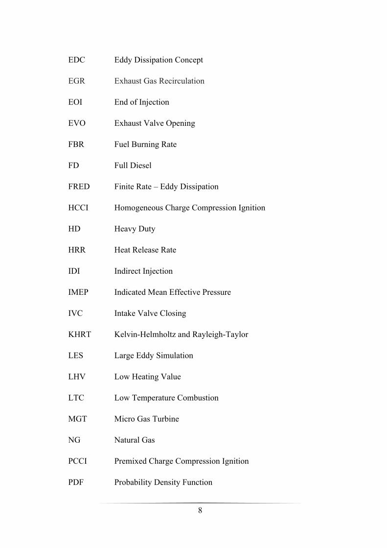
EDC Eddy Dissipation Concept
EGR Exhaust Gas Recirculation
EOI End of Injection
EVO Exhaust Valve Opening
FBR Fuel Burning Rate
FD Full Diesel
FRED Finite Rate – Eddy Dissipation
HCCI Homogeneous Charge Compression Ignition
HD Heavy Duty
HRR Heat Release Rate
IDI Indirect Injection
IMEP Indicated Mean Effective Pressure
IVC Intake Valve Closing
KHRT Kelvin-Helmholtz and Rayleigh-Taylor
LES Large Eddy Simulation
LHV Low Heating Value
LTC Low Temperature Combustion
MGT Micro Gas Turbine
NG Natural Gas
PCCI Premixed Charge Compression Ignition
PDF Probability Density Function
9
PFI Port Fuel Injection
PID Proportional Integral Derivative
PM Particulate Matter
PN Particulate Number
PPC Partially Premixed Combustion
PRF Primary Reference Fuel
RANS Reynolds Averaged Navier-Stokes
RCCI Reactivity Controlled Compression Ignition
RNG Renormalization Group
RP Premixed Ratio
RSM Reynolds Stress Model
SCR Selective Catalytic Reduction
SI Spark Ignition
SLF Steady Laminar Flamelet
SOC Start of Combustion
SOI Start of Injection
SOP Start of Pilot
TDC Top Dead Centre
THC Total Unburned Hydrocarbons
UHC Unburned Hydrocarbons
VVA Variable Valve Actuation
10
Chapter 1
DUAL FUEL
In this section, a summary of the main characteristics of the Diesel
engine and its evolution in the years is illustrated, explaining the
motivations and the advantages that could lead the introduction of the
Dual Fuel system in the current European automotive scenario.
1.1 Diesel Engine
The invention of the Diesel engine is dated back to 1892 when Rudolf Diesel
published an essay describing a thermodynamic cycle where combustion
occurred with an isothermal compression [2]. The idea was to introduce the
finely atomised fuel into air taken at a temperature above the igniting-point of
the fuel, which ignites on introduction. In order to exceed the temperature of
combustion, air must be tightly compressed. However, the compression
required must be at a level that an engine operating following this cycle could
never perform any usable work. Then in 1893 Diesel adopted the constant
pressure cycle. In his 1895 patent application it is simply stated that
compression must be sufficient to trigger ignition. Also, the degree of
compression is lower than that needed for isothermal ignition.
With the efforts of Diesel and the resources of M.A.N. in Augsburg
combined, after five years (1897) a practical engine was finally developed
[3]. His concept permitted a doubling of efficiency due to much greater
expansion ratios without detonation or knock. The first diesel engine was a
four-stroke single-cylinder engine with a bore and stroke respectively of 250
mm and 400 mm, with a final compression of 32 bar, rated 14 kW at 150 rpm
with a specific fuel consumption of 324 g/kWh resulting in an effective
11
efficiency of 26.2% [4]. Since then, engine developments have continued to
contribute to the steadily widening internal combustion engines markets.
The Diesel engine presents some advantages with respect to the Otto engine;
the most important are reported below [5]:
1. Higher overall efficiency, to allow the self-ignition of diesel oil, the diesel
engine usually operates with lean air/fuel ratio of 18 to 70 (or F/A=0.014 to
0.056) and with compression ratios doubled (12 to 24) compared to the Otto
engine ones (8 to 12).
2. Higher flexibility, the efficiency decreases slower when the load decreases,
indeed the load level is controlled by the air/fuel ratio, so when it is necessary
to reduce the power produced it is possible to simply reduce the amount of
fuel injected in the cylinder without pressure drops due to the throttle valve.
Also, the pumping work requirements are low.
3. Use of low value fuels, their production in refinery requires lower energy
consumption. This aspect combined with the previous one allows a more
efficient and cost-effective management of the engine.
On the other hand, the diesel engine presents a higher weight-power ratio.
The higher compression ratios and consequently the higher pressure reached,
highlighted in point 1, demands to the various components to be stronger and
more rigid to withstand the mechanical and thermal stresses. These stresses
are represented by the noise and vibrations caused by the harshness of
combustion which develops in this kind of engine. Indeed, in this engine,
combustion is not characterised by the propagation of a flame front through
the combustion chamber but, as already stated, by the auto-ignition of a fuel,
that after a small ignition delay burns rapidly. Moreover, the use of heavier
materials, not only increases the weight of the engine but also, enhances the
inertia of the moving components preventing them to reach high engine

12
speeds, thus lower power is obtained, and this contributes to further reduce
the weight-power ratio.
It follows that the diesel engine is more suitable for medium-high power
applications where the weight and the size are secondary to operating costs,
such as on road industrial transports, agricultural vehicles, earth moving
machines, rail and marine propulsion, as well as fixed installations for
electrical power generation. However, the previously mentioned operating
flexibility at different load levels allowed the adoption of diesel engines also
for applications at lower power such as heavy-duty diesel engines which
generally include lorries and buses and passenger cars which usually operate
at partial load.
Therefore, the diesel engine has an extremely wide range of utilisation and it
can be used both in a 2-stroke and 4-stroke cycles. Of course, depending on
the application and the power needed a certain configuration is preferred.
Usually large size engines operate on the 2-stroke cycle in contrast to the
small- and medium-size diesels.
As reported in Table 1.1, the different types of engines can be categorised on
the base of their size; as already stated dimensions and thus weight of the
engine influence every other characteristic or operating condition, so it
results that a large size engine produces high power but performs at low
speed. In this regard, the compression-ignition combustion is an unsteady,
heterogeneous, three-dimensional process and the details of this process
depend on the characteristics of many factors such as the fuel, the injection-
system and design of the combustion chamber. All these factors influence
and manage combustion development; a correct combination of them can
promote an efficient combustion (complete oxidation and low emissions) in
the entire operating range.

13
Tab. 1.1: Characteristics of common diesel engines [3, 4].
Size Large Medium Small
Cycle 2-stroke 4-stroke 4-stroke
Bore [mm] 150 – 1,000 200 – 650 60 – 120
Stroke/Bore 1.2 – 3.5 0.9 – 1.3 0.9 – 1.1
Max speed [rpm] 60 – 120 300 – 800 1,000 – 5,000
Compression
ratio 12 – 15 15 – 22 22 – 24
Power [kW] 5,000 per cylinder 150 – 20,000 5 – 400
Injection pressure Very high Medium High/Low
Chamber Quiescent Bowl-in-piston
Deep bowl-in-
piston/
Pre-chamber
Firstly, the injection timing is used to control combustion timing. Actually,
before the fuel starts to burn a delay period occurs, it is necessary to keep this
delay short to hold the maximum cylinder gas pressure below the maximum
the engine can tolerate. The measure of the ease of ignition of a specific fuel
is indicated by its cetane number which must be above a certain value in a
typical diesel environment.
Secondly, the injection pressure level must be properly chosen with the aim
to provide a sufficient velocity to the fuel jet, so that it is efficiently atomised,
that it can cross the combustion chamber in the time available and that it can
fully utilise the air charge. When the necessary injection pressure cannot be
achieved due to technological limits or to high costs of the injection system,
in order to meet the requirements of an efficient combustion, the lack of
sufficient pressure can be compensated by a right design of the combustion
chamber shape, able to generate a certain level of air motion which promotes

14
a good vaporisation and mixing of the charge. In fact, the major problem is to
achieve sufficiently rapid mixing between the injected fuel and the air in the
appropriate crank angle interval close to the top dead centre but this crank
angle interval varies with the engine speed and then with the engine size. For
this reason, as reported in Table 1.1 the largest size engines usually present a
quiescent combustion chamber (Figure 1.1.a), which means that the chamber
is not designed with the particular aim to generate high turbulence, but the
injection pressure must increase to allow the fuel to reach every part of the
chamber due to the increased dimensions of the cylinder.
Fig. 1.1: Diesel engine combustion chamber, (a) quiescent chamber,
(b) and (c) bowl-in-piston chamber [3].
On the other side, as engine size decreases, less fuel jet penetration is
necessary while more vigorous air motion is necessary, and it can be obtained
with the aid of more complex geometry of the combustion chamber (Figures
1.1.b and c). Also, swirl motion can be enhanced by enhancing the
compression ratio, which has higher values for small size engines (Table 1.1).
15
Over the years, different changes have been made to improve the diesel
engine performances in efficiency, power, and degree of emission control. In
1905 the first turbochargers are manufactured by Büchi. Turbocharging and
supercharging consist in compress the inlet air with the use of an exhaust-
driven-turbine-compressor combination and a mechanically driven pump
respectively. Turbocharging and supercharging increase the air mass flow per
unit displaced volume, then more fuel can be injected and burned, and more
power can be delivered while avoiding excessive black smoke in the exhaust.
The brake mean effective pressure (BMEP) can increase from 700 – 900 kPa
to 1,000 – 1,200 kPa. These methods are mainly used in larger engine, to
reduce engine size and weight for a given power output, so to reduce the
weight to power ratio. In this way, for the same dimensions the 2-stroke cycle
is competitive with the 4-stroke one because only air is lost in the cylinder
scavenging process.
An important change is the indirect injection (IDI), introduced in the 1909 on
engines that need a vigorous charge motion, such as small high-speed ones
used in automobiles; it is the division of the combustion chamber into two
parts: the main chamber and the auxiliary pre-chamber. During the
compression stroke air is forced to enter in the auxiliary chamber from the
main one above the piston through a set of orifices, the connecting passage
between the two chamber is properly shaped so that the flow gains high
turbulence within the auxiliary chamber. Usually, fuel is injected into the pre-
chamber so the pressure of the injector can be lower than the one required by
direct injection systems (DI). In the pre-chamber combustion starts and the
consequent pressure rise forces the fluid to mix back with the air into the
main chamber.
The evolution of diesel engine is closely linked to the development of the
injection system with the assistance of electronical devices which ensure a
better control on pressure, timing and quantity of fuel. The basic

16
configuration consists of an injection pump, delivery pipes and fuel injector
nozzles. The earlier injection pumps were crankshaft driven via a series of
gears and chains.
In the Unit injector the injector nozzle and the high-pressure injection pump
are combined in a compact assembly installed directly in the cylinder head.
An individual pump is assigned to each cylinder where an electric valve
ensures an accurate timing of injection. This configuration eliminates the
need for high-pressure pipes and their associated failures but at the same time
allows much higher injection pressure (up to 2,200 bar) then, ideal
combination of air-fuel mixture, high efficiency, low consumption and
emissions against high power.
Nowadays the better performances are attained by the utilisation of the
common-rail injection system (Figure 1.2) where fuel at high pressure (up to
2,500 bar) is stored in a distribution pipe (rail) common to all injectors. The
first prototype was implemented on a low-speed 2-stroke crosshead engine in
the 1979 but the first mass-produced common rail diesel engine for passenger
car is dated 1997 (Fiat 1.9 JTD). The purpose of the pressure pump is to
maintain a target pressure in the rail which is constant and not affected by
fluctuations caused by the nozzle opening. Injection is controlled by solenoid
or piezoelectric valves, governed by an electronic control unit (ECU), due to
their precision they make possible fine electronic control over timing and fuel
quantity and allow pressure to maintain a constant value from the start till the
end of the injection, equal to the pressure in the rail. This permits to provide
an efficient atomisation of the fuel and then a decreasing of emissions.
Moreover, advanced common-rail systems can perform multiple injections
per stroke. By injecting a small amount of fuel before the real injection it is
possible to reduce the explosiveness of compressed ignition combustion, so
to reduce vibrations and noise.

17
Fig. 1.2: Common rail injection system scheme [6].
In the latest decades the main improvements made on the diesel engine
include technologies and devices that aim to reduce emissions, by operating
an after-treatment of the exhaust gases. They can also be used as silencers to
reduce noise. The first device, introduced in 1980 on non-road machines and
in 1985 on automobiles [7], is the Diesel Particulate Filter (DPF). The
oxidation of CO and unburned hydrocarbon can be achieved with the
utilisation of the Diesel Oxidation Catalyst (DOC). For the reduction of NOx
emissions the Lean NOx trap was introduced in 2008 on passenger cars with
the VW 2.0 TDI engine by Volkswagen, and, in 2006 Daimler-Chrysler
launched the first series-production passenger car engine with the Selective
Catalytic Reduction (SCR) exhaust gas after-treatment, the Mercedes-Benz
OM 642. The development of these devices is extremely important since
greater attention must be put on the pollutants problem. In this regard, the
European Union established the acceptable limits for exhaust emissions of
new vehicles sold in the member states. These limitations, as reported in
Tables 1.2 to 1.4 for the different categories of diesel engines, due to the

18
escalating greenhouse gas and pollutants emergency of the recent years, are
becoming constantly more stringent. Compliance is determined by running
the engine at a standardized test cycle. It is worth-noting that starting from
2009 (directive Euro V) also the number of particles of soot has been
regulated.
Tab. 1.2: UE emission standards for light commercial vehicles with a
reference mass ≤ 1305 kg (in g/km and particles/km for PN) [8].
Engine Pollutant Euro 1
(1992)
Euro 2
(1996)
Euro 3
(2000)
Euro 4
(2005)
Euro 5
(2009)
Euro 6
(2014)
Diesel
Engine
CO 2.72 1.00 0.64 0.50 0.50 0.50
HC - - - - - -
NOx - - 0.50 0.25 0.18 0.08
HC +
NOx 0.97 0.70 0.56 0.30 0.23 0.17
PM 0.14 0.08 0.05 0.025 0.005 0.0045
PN - - - - 6.0 e11 6.0 e11
Tab. 1.3: UE emission standards for light commercial vehicles with a
reference mass ≥ 1305 kg and ≤ 3500 kg (in g/km and particles/km for PN)
[8].
Engine Pollutant Euro 1
(1994)
Euro 2
(1999)
Euro 3
(2002)
Euro 4
(2006)
Euro 5
(2012)
Euro 6
(2016)
Diesel
Engine
CO 6.9 1.5 0.95 0.74 0.74 0.74
HC - - - - - -
NOx - - 0.78 0.39 0.28 0.125
HC +
NOx 1.7 1.2 0.86 0.46 0.35 0.215
PM 0.25 0.17 0.10 0.06 0.005 0.0045
PN - - - - 6.0 e11 6.0 e11
19
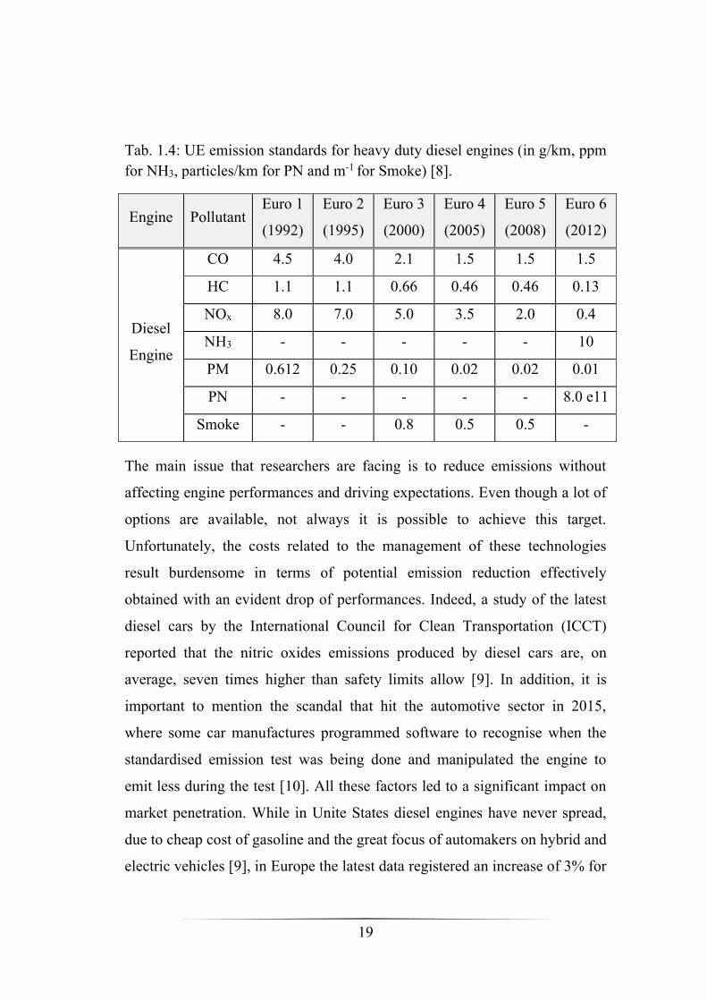
Tab. 1.4: UE emission standards for heavy duty diesel engines (in g/km, ppm
for NH3, particles/km for PN and m-1 for Smoke) [8].
Engine Pollutant Euro 1
(1992)
Euro 2
(1995)
Euro 3
(2000)
Euro 4
(2005)
Euro 5
(2008)
Euro 6
(2012)
Diesel
Engine
CO 4.5 4.0 2.1 1.5 1.5 1.5
HC 1.1 1.1 0.66 0.46 0.46 0.13
NOx 8.0 7.0 5.0 3.5 2.0 0.4
NH3 - - - - - 10
PM 0.612 0.25 0.10 0.02 0.02 0.01
PN - - - - - 8.0 e11
Smoke - - 0.8 0.5 0.5 -
The main issue that researchers are facing is to reduce emissions without
affecting engine performances and driving expectations. Even though a lot of
options are available, not always it is possible to achieve this target.
Unfortunately, the costs related to the management of these technologies
result burdensome in terms of potential emission reduction effectively
obtained with an evident drop of performances. Indeed, a study of the latest
diesel cars by the International Council for Clean Transportation (ICCT)
reported that the nitric oxides emissions produced by diesel cars are, on
average, seven times higher than safety limits allow [9]. In addition, it is
important to mention the scandal that hit the automotive sector in 2015,
where some car manufactures programmed software to recognise when the
standardised emission test was being done and manipulated the engine to
emit less during the test [10]. All these factors led to a significant impact on
market penetration. While in Unite States diesel engines have never spread,
due to cheap cost of gasoline and the great focus of automakers on hybrid and
electric vehicles [9], in Europe the latest data registered an increase of 3% for
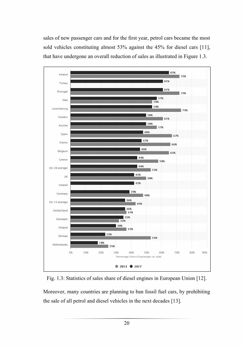
20
sales of new passenger cars and for the first year, petrol cars became the most
sold vehicles constituting almost 53% against the 45% for diesel cars [11],
that have undergone an overall reduction of sales as illustrated in Figure 1.3.
Fig. 1.3: Statistics of sales share of diesel engines in European Union [12].
Moreover, many countries are planning to ban fossil fuel cars, by prohibiting
the sale of all petrol and diesel vehicles in the next decades [13].

21
Despite of all these issues a great part of cars in Europe are still sold and
equipped with Diesel engines so they will not disappear soon from the
transport scenario. Also, after over a century of development, new strategies
have still a little potential for further improvements. In particular, low
temperature combustion (LTC) strategies such as Homogeneous Charge
Compression Ignition (HCCI), Premixed Charge Compression Ignition
(PCCI) and Reactivity Controlled Compression Ignition (RCCI) produce near
zero oxides of nitrogen and particulate matter emissions since in all the LTC
strategies the fuel-air mixture is premixed and they exhibit a characteristic
low temperature heat release followed by main heat release without any
diffusion phase combustion [14]. Furthermore, much work is being done on
the use of alternative fuels like biodiesel (vegetable oils), synthetic diesel
made from shale oil and coal, or fuels used as diesel supplement fractions
such as natural gas, methanol and ethanol (methyl and ethyl alcohols).
1.2 Dual Fuel Systems
In this context, the introduction of a Dual Fuel (DF) system represents a
possible solution to some typical problems that are still unsolved for the
conventional diesel engines, with particular reference to its environmental
impact. Indeed, Dual Fuel system results from the need to readapt a well-
established technology like internal combustion engine, in a period
characterised by new requirements of emission dictated by more and more
stringent regulations. In addition, the depletion and the consequent rising cost
of petroleum pushed the scientific research in the direction of more eco-
friendly and available fuels. Also, the main challenge is to keep the same
performances (efficiency, durability, reliability and specific power output) of
a standard engine. Actually, it is important to highlight that both compression
and spark ignition engines can operate in Dual Fuel mode with different
configurations depending on the fuels used and their way of introduction
inside the cylinder (DI or IDI).

22
Fig. 1.4: Dual Fuel scheme [15].
However, in this thesis, a diesel engine supplied with natural gas (NG) as
primary fuel is studied while other solutions are illustrated in section 1.4. In
particular, as shown in Figure 1.4, natural gas is premixed with air inside the
intake manifold, then at the end of compression stroke a little amount of
diesel oil is injected to ignite the mixture causing multiple flame fronts that
propagate through the combustion chamber. In this sense, the Dual Fuel
technology could be considered as a particular application of PCCI concept,
above mentioned.
In this case, only slight modifications can be implemented on existing
engines, a high level of thermal efficiency can be still ensured, since NG,
thanks to its high resistance to knock, can easily withstand the typical high
compression ratio of this kind of engine.
Also, natural gas represents a good solution to all the problem previously
described: it is available worldwide, it is expected to remain less expensive
than gasoline and its use leads to different benefits in terms of emissions.

23
Indeed, its combustion is relatively clean since it is a mixture of different
species whose major component is methane (almost 95% of mass fraction),
that has the lowest carbon/hydrogen ratio among hydrocarbons, thus for the
same amount of burned fuel less CO2 is produced.
Moreover, as it is known, there are three mechanism of NOx formation:
thermal, prompt and fuel. In engines, NOx are mainly produced by the
thermal mechanism. In Dual Fuel, being NG port fuel injected, a lean
premixed charge is formed, and lower temperatures are achieved because
combustion occurs at an equivalent ratio far from stoichiometric value
(φ<<1), as shown in Figure 1.5.
Fig. 1.5: Equivalence ratio – Flame temperature [16].
In the last years, great attention has been paid on the effect of particulate
matter, especially in the cities, where, often, a stop of traffic is imposed to
cars equipped with diesel engines. Also, in this regard Dual Fuel technology
can represent a viable solution since only the reduced amount of diesel oil
necessary to ignite the mixture, is injected to start the combustion of the main
fuel that is a gas, and then, does not produce PM at the exhaust. Usually

24
Selective Catalytic Reduction and Diesel Particulate Filter are used to reduce
PM and NOx but these methods are based on the use of precious and
expensive metals, while in this case, by only increasing NG energy
contribution, it is possible to obtain the same effect.
On the other hand, the main drawback of DF combustion is the high level of
carbon monoxide and unburned hydrocarbons emitted in the exhaust. As a
matter of fact, the NG/air mixture is lean and it becomes leaner with the load
decrease, it can happen that equivalence ratio falls outside the flammability
limits so to prevent the achievement of an efficient flame propagation,
especially at part load. This could imply a performances’ decrease with
respect to the original configuration.
In this sense, an appropriate optimization of the engine operating parameters
is needed, by deepening the complex combustion phenomenon of two fuels.
1.3 Fuels
As already stated, one of the characteristics of a certain Dual Fuel
configuration is the couple of fuels used. Of course, different combinations
provide different results in terms of performances, emissions and above all
different combustion developments. In the next paragraphs, the features of
the main fuels utilised for the DF technology are illustrated.
1.3.1 Diesel oil
In order to ensure a correct start of combustion (SOC) in diesel engines, the
fuel must present suited characteristics of atomisation, vaporisation and
autoignition. The most common type of diesel oil derives from the distillation
of petroleum, but it is important to highlight that other sources such as
biomass, animal fat and coal liquefaction are increasingly being exploited.
Petrodiesel (or fossil diesel) is composed of about 75% saturated
hydrocarbons (paraffins including n-, iso- and cycloparaffins), and 25%

25
aromatic hydrocarbons (naphthalenes and alkylbenzenes). The average
chemical formula ranges from C10H20 to C15H28 [17].
Tab. 1.5: Diesel oil and Gasoline properties [4, 17].
Fuel Diesel oil Gasoline
Distillation range [°C] 200 – 350 30 – 200
Carbon atoms per molecule 9 to 25 4 to 11
LHV [MJ/kg] 43.1 43.2
Density @ 15 °C [kg/m3] 840 720
Volumetric energy density [MJ/l] 35.86 32.18
Viscosity [cSt] 2.0 – 5.35 0.37 – 0.44
Flash Point [°C] 52 – 96 < 21
CO2 emission [g/MJ] 73.25 73.38
In Table 1.3 the characteristics of diesel oil and gasoline are reported.
Gasoline includes hydrocarbons of the lighter fraction of the petroleum
distillation. Indeed, the temperature range is lower and less carbon atoms per
molecule are contained. Components at higher boiling point, burn less easily,
this is the reason why diesel engines typically produce smoke at the exhaust.
The Lower Heating Value (LHV) is almost the same, but the higher diesel
density implies a higher volumetric energy density and consequently a lower
fuel consumption. Also, a high fuel viscosity prevents the correct flow inside
the injection system and a good level of atomisation which influence all the
jet formation and distribution process. Both fuels should have low sulphur
content in order to avoid corrosion due to the formation of sulphuric acid.
In diesel engine the main issue is the fuel autoignition. It defines the start and
development of combustion and consequently the performance and emission
output. In order to achieve a good control on these parameters it is necessary
to have a short ignition delay when sprayed into hot compressed air. The
ignition delay is cause by physical and chemical factors. Physical delay is

26
due to the actual time necessary for two parcels (fuel and oxidiser) to meet
and react. The chemical delay is a property of the fuel and depends on the
readiness to the self-ignition and it is measured by the cetane number. A
higher cetane number indicates a short ignition delay. European (EN 590
standard) road diesel has a minimum cetane number of 51 [17]. However, the
cetane number for standard diesel ranges between 47 and 60 [4].
1.3.2 Natural gas
Natural Gas is a gas mixture consisting primarily of hydrocarbons (alkanes)
such as methane, ethane, propane, butane and pentanes. It may present, also,
little amount of hydrogen sulphide, carbon dioxide, water vapor and
sometimes helium and nitrogen [18]. In Table 1.4 a typical composition of
Natural is reported.
Tab. 1.6: Typical composition of Natural Gas [19].
Component Formula Volume [%]
Methane CH4 > 85
Ethane C2H6 3 – 8
Propane C3H8 1 – 2
Butane C4H10 < 1
Pentane C5H12 < 1
Carbon dioxide CO2 1 – 2
Hydrogen sulphide H2S < 1
Nitrogen N2 1 – 5
Helium He < 0.5
As it is possible to notice, the main constituent of NG is methane, for this
reason, usually, it is possible to consider only this component to describe the
properties of the whole mixture and use the two terms indifferently. Methane
is widely used in residential, commercial and industrial heating, industrial

27
feedstock, power generation and vehicle transportation. In this last field, the
use of a gaseous fuel can bring significant advantages since it can easily mix
with air to form a homogeneous charge. In this way the adiabatic flame
temperature reaches lower value with important benefits in terms of NOx
emissions. Also, methane is characterised by a high resistance to knock
(octane number of 120 – 130) that allows its utilisation in engines with high
compression ratio such as diesel engine in Dual Fuel mode. In this regard, the
interest on the utilisation of this fuel is given by the high stability of the
molecule structure that prevents the autoignition of the fuel before the pilot
injection. Gasoline and diesel vehicle can be easily converted to run on
natural gas with slight modifications to the original engine. However, an
engine properly designed to operate with this specific fuel can provide better
performance outputs. Methane has a Lower Heating Value of 49,8 MJ/kg,
higher than both gasoline and diesel oil (Table 1.2) and the highest
stoichiometric ratio among the hydrocarbons (αst = 17.24). On the other hand,
the introduction of a gaseous fuel reduces the maximum engine power
achievable with respect to the same engine supplied with gasoline (10%),
since it reduces the filling coefficient. Moreover, the gaseous nature of this
fuel penalises the storage and transportation by vehicle. Indeed, critical
temperature of methane is -83 °C, then tanks suitable to withstand pressures
of 200 – 250 bar, are required, with a quadruple enhancement of size [4].
1.4 State of the art
In the last years several researchers have been interested into the Dual Fuel
technology, analysing the behaviour of the combustion in different operating
conditions, and also studying different configurations and solutions in order
to overcome the limits that affect its operation. In particular, the development
of models and correlations between the fuel properties, operating parameters
and emissions can be beneficial for the optimization of the process. The
models used for the simulations include 0D, 1D, multi-zone and 3D

28
approaches. The 0D and 1D models are mainly used for the prediction of
performances and emissions based on empirical models [20, 21] and they can
be useful to provide the boundary conditions for the multidimensional
simulations or even experiments [22]. However, a good description of the
phenomena and prediction of emissions is achieved by models that study in
detail the evolution of the combustion throughout the cylinder. Although,
multi-zone models have shown reasonable results [23], it is clear that the best
information can be retrieved from 3D CFD [24]. In literature computational
fluid dynamics is widely exploited in combination with experimental
activities for the investigation of the Dual Fuel combustion. Indeed, Akbarian
et at. [25] compared emissions and performances in full diesel and dual fuel
mode. After finishing the experimental tests in full diesel mode, the engine
was converted with few modifications to dual mode. The experimental tests
were carried out under different loads (10, 25, 50, 75, and 100%) and
different pilot to gaseous fuel ratios (30, 40 and 50%). Results showed that at
constant engine speed, dual fuel mode has lower CO2, NOx and PM under all
load conditions and port gaseous fuel ratio when compared to full diesel
mode. At full load, the dual fuel engine has relatively lower CO emission and
higher HC emission while the specific energy consumption is similar to that
for the diesel engine. The CFD simulations were performed on a mesh that
does not present valves and allows only closed cycles. 13 species are
included in the 10 kinetic reactions and 6 equilibrium equation were
employed. Numerical results showed good agreement with the experimental
ones. Finally, the authors suggested a pilot fuel ratio of 30% in full load and
to raise it to 50% in half load operation.
Huang et al. [26] studied the effects of multiple injection on the combustion
at low load condition in order to improve the thermal efficiency and reduce
emissions. Results showed that, when the first diesel injection timing is
advanced, the indicated thermal efficiency and nitrogen oxide emissions
29
increase first and then decrease, while the maximum pressure rise rate,
carbon monoxide and methane emissions reduce initially and then increase,
attaining a relatively high indicated thermal efficiency. Indeed, the proportion
of premixed combustion of the first injected diesel and the duration of flame
propagation of natural gas has considerable influence on methane emissions.
The kinetic mechanism involves 45 components and 142 reactions where
diesel and natural gas are, respectively represented by n-heptane and
methane. The computation efforts were reduced thanks to the symmetry of
the combustion chamber, since the injector has eight equally spaced nozzle
orifices, a 45° sector mesh was generated to simulate one spray plume. In
their research Shu et al. [27] demonstrated that the peak cylinder pressure
increases as the spray angle increases from 60° to 140°, but it slightly
decreases by the further increase of the spray angle to 160°. Generally,
combustion duration decreases with the spray angle. Also, the NOx emissions
ascend when spray angle increases. On the other hand, the unburned methane
is almost unchangeable while the CO emissions keep at lower level for all
spray angles. The Reynolds Averaged Navier-Stokes (RANS) approach was
used for the turbulence modelling and a modified rapid distortion
renormalization group (RNG) k-ε turbulence model. The SAGE model was
used to simulate the combustion process of the NG-diesel dual fuel engine,
the chemical kinetics mechanism of which consists of 76 species and 464
reactions. The Kelvin-Helmholtz and Rayleigh-Taylor (KHRT) model was
chosen to simulate the break-up of diesel fuel. Once again, since eight nozzle
holes are distributed symmetrically, the cylinder model was simplified as a
45° fan-shaped area where the single fuel spray is located in the centre. In
[28] the authors implemented a new simulation model with the aim to
understand the mechanisms behind soot formation in diesel-CNG
combustion. The soot evolution was investigated under different natural gas
substitution ratios with single and split fuel injection and integrated with a
reduced heptane/methane polycyclic aromatic hydrocarbons mechanism.

30
They affirmed that, as the CNG substitution ratio increases the equivalence
ratio distribution becomes more homogenous and the ignition delay gets
extended while the combustion duration gets shorter both with single and
split injection. A slight increase of pressure is observed when the split
injection is used. Indeed, split injection changes fuel distribution and
vaporisation. Consequently, the prolonged ignition delay in higher CNG
substitution ratios provides more time to fuel and air for the mixing, which
reduces drastically soot mass formation. Papagiannakis et al. [29] studied the
effects of different air oxygen enrichment degree (addition of oxygen in the
intake air) on dual fuel combustion. In particular, it can accelerate the
burning rate and reduce the ignition delay, in this way the specific energy
consumption and CO emissions decrease too, without impairing the soot and
NO emissions. Ghazal et al. [30] proposed to use a turbocharger to enhance
fuel saving. Since methane has high octane number, it can well withstand the
high compression ratios of the diesel engines. However, to avoid knock
occurrence Sremec et al. [31] suggested not exceeding a compression ratio of
16 for turbocharged intake condition but this limit rises to 18 for ambient
intake condition.
As already mentioned, NG can be directly introduced in the combustion
chamber. In [32] the authors analysed direct and indirect CNG injection
methods influence on combustion process and heat transfer. Direct injection
provides advantages in terms of thermal efficiency and a higher degree of
fuel consumption while through indirect injection a homogeneous mixture is
produced in the combustion chamber and a reduction of soot formation is
obtained, especially in poor combustion areas. Moreover, they affirmed that a
proper direct injection can be more efficient than indirect injection in terms
of engine economy (higher cycle efficiency) and can reduce emissions of
harmful substances. Indeed, as demonstrated by Zoldak et al. [33] direct
injection of natural gas creates a stratification of this fuel portion and avoids

31
excessive premixing, which tempers the rate of pressure rate. They studied
several azimuthal angles between NG and diesel fuel nozzles, diesel pilot
injection timing and quantity splits. The results indicated that the direct
injection of natural gas can successfully control the rate of pressure rise while
improving the NOx, HC and soot emissions to meet the targets for engines
equipped with modern aftertreatment systems. Also, the optimization of the
piston bowl geometry is required to ensure a good combustion efficiency.
The direct injection of NG needs the design and the testing of new injectors.
In this regard paper [34] presented the tests results of the prototype design of
hydraulically assisted injector that is designed for gas supply into diesel
engines.
Stettler et al. [35] evaluated the emissions reduction obtained with the
oxidation catalyst. They compared energy consumption, greenhouse gas and
noxious emissions for five after-market dual fuel configurations of two heavy
goods vehicles were compared relative to their full diesel baseline values
over transient and steady state testing. Over a transient cycle, CO2 emissions
are reduced by up 9% while methane emissions due to incomplete
combustion are 50 – 127% higher; results showed that the oxidation catalyst
can reduce emissions by at most 15%.
Since the presence of the gaseous fuel affects considerably the features and
the development of the combustion, one of the main goals of research is the
modelling of the interaction between the two fuels. Mousavi et al. [36]
investigated and compared some important combustion’s characteristics at
part load and full load. Ignition delay and combustion duration time at part
load are longer due to insufficient methane concentration which could not be
burned completed because of lower combustion speed. A significant amount
of the unburned methane usually remains in the most remote areas from
diesel fuel injector such as the piston bowl. The slow progress of combustion
process at part load, leads the heat release to be drawn more toward the
32
expansion stroke which causes incomplete combustion, and consequently
high amounts of UHC and CO are emitted. Also, at part load, low
temperature gas surrounds diesel spray and interferes with a rapid liquid
droplet evaporation. The KIVA-3V was used to simulate the closed part of
the cycle with tetradecane (C14H30) and methane (CH4) as representatives of
diesel and natural gas fuels, respectively. A mechanism consisting of three
reactions describes the combustion, one for diesel vapour and two for the
methane. Also, six equilibrium reactions and the extended Zel’dovich NO
formation complete the chemical model. Finally, they suggested increasing
the amount of diesel fuel, with the assumption of constant input energy, to
overcome the part load disadvantages, since diffusion flame penetration is
increased. Hence, very lean methane/air mixture could be ignited suitably and
propagated quickly due to size enlargement of diesel combustion region.
Talekar et al. [37] affirmed that traces of gaseous fuel can affect ignition
delay, temperature of auto-ignition process, duration of first-stage ignition
and laminar burning velocity. This influence is dependent on the diesel
substitution ratio, as this ratio increases beyond 95%, authors have found that
traditional auto ignition models, which are created for diesel-like fuels, do
not predict major combustion phases. Below this threshold value the first
stage of dual fuel combustion, which is the auto-ignition, is assumed not
affected by the presence of another fuel species and standard models can be
applied without any change. Indeed, the main focus of their simulation is the
creation of a unified modelling approach for Dual Fuel combustion. The G-
equation flame propagation model and LES turbulent model are used
combined with a detailed chemistry: the LLNL of n-heptane and the
GRIMECH 3.0 for methane oxidation. The intermediate chemical mechanism
obtained consists of 181 species and 1,714 reactions, which is still
computationally expensive to run 3D combustion simulations, hence a further
reduction was obtained by considering only the strongest reaction paths, this
is the path flux analysis (PFA). Their new overall combustion model proved
33
to effectively predict most extreme dual fuel combustion mode including
three major intertwined processes of slow kernel development, flame
propagation and end-gas ignition. In this way substitution up to 98-99% can
be achieved. Barro et al. [38] focused on the evaluation of the phases in
which the combustion is split: the auto-ignition phase and the premixed flame
propagation phase. The distribution of fuel burnt in the auto-ignition phase
and in the premixed flame propagation is provided by the trapped natural gas
within the spray volume. In order to investigate the effects of the dilution
heat capacity and fuel chemistry impact during the ignition delay period of
the NG-diesel dual fuel engine on dual fuel engine ignition process, Li et al.
[39] replaced methane with two artificial species representing the unique
features of methane: one for the examination of diluting impact due to
decreased O2 concentration and the other for the evaluation of the heat
capacity impact. Also, the contributions of the key radicals such as OH, HO2
and H to chemical reactions are analysed. The addition of NG retards the start
of combustion and elongates the ignition delay at low and medium load
conditions. It was believed that the elongated ignition delay was due only to
the displacement of a portion of intake air by NG, which decreases the
concentration of O2 in cylinder. Nevertheless, the introduction of CH4 to
intake air also increases the heat capacity of the air-fuel mixture formed. The
fuel chemistry coupled was a reduced primary reference fuel (PRF)
mechanism consisting of 45 species and 142 reactions. The simulation started
from the intake valve closing (IVC) with the assumed homogeneous mixture
of methane, air, and residue gas and completed at exhaust valve opening
(EVO).
As matter of fact, the choice of the model has a fundamental role in the CFD
analysis. Nowadays several well-established models have been implemented
and, depending on the operating conditions certain models can be more
suitable than others to describe the processes inside the combustion chamber.

34
Kusaka et al. [40] performed numerical studies using a multi-dimensional
model combined with detailed chemical kinetics, including 43 species and
173 elementary reactions. Instead, in [41] the combustion mechanism for
natural gas/diesel oil mixture includes 81 species and 421 reactions. In paper
[42] methane and n-heptane were used as representative of natural gas and
diesel fuels in a chemical kinetics mechanism which consists of 42 species
and 57 reactions for prediction of n-heptane oxidation with the addition of a
series of major methane oxidation pathways. Huang et al. [43] developed a
reduced n-heptane-n-butylbenzene-NG-polycyclic aromatic hydrocarbon
(PAH) mechanism with 746 reactions and 143 species. Therefore, to model
diesel fuel a mixture of n-heptane and n-butylbenzene was used while to
model NG, a mixture of methane, ethane and propane was used. Combustion
process was simulated by combining the mentioned mechanism with the
SAGE combustion model. The renormalized group (RNG) k-ε model, the
turbulence model was used to simulate the turbulence characteristics. The
spray atomisation and droplet breakup processes were predicted by the
Kelvin-Helmholtz and Rayleigh-Taylor (KHRT) models, respectively. Kahila
et al. [44] performed large-eddy simulations (LES) together with a finite-rate
chemistry model of two diesel surrogate (n-dodecane) mechanisms consisting
respectively of 54 species and 269 reactions, and 96 species and 993
reactions. It is stated that dual fuel ignition can be separated into three stages:
the first is the ignition due to low temperature chemistry which results
delayed with both mechanisms by the methane presence in the ambient; the
second is the ignition at the spray tips; the last is represented by the full
oxidation of available CH4 and premixed flame. Chemical decomposition of
n-dodecane produces heat, intermediate species and radicals, enabling a faster
ignition compared to homogeneous ignition of pure methane-air mixtures. On
the other hand, the ambient methane influences the early decomposition of n-
dodecane mainly by consuming OH radical and forming methyl radicals
which activate other inhibiting reactions. Therefore, ambient methane
35
influences the low- and high-temperature chemistry throughout the ignition
process. Both first- and second-stage ignition processes are inhibited
compared to the single-fuel reference case. The high-temperature ignition
process begins near the most reactive mixture fraction conditions. The role of
low-temperature reactions is of particular importance for initiation of the
production of intermediate species and heat, required in methane oxidation
and both applied mechanisms yield qualitatively the same features in the DF
configuration. The primary breakup is considered by sampling computational
parcels from the Rosin- Rammler size distribution while the secondary break-
up is modelled by the KHRT model. Also, laminar 1D igniting counter-flow
flamelet computations resemble the LES results, indicating their applicability
to understand the DF ignition process.
However, it is clear that the simple replacement of diesel fuel with natural
gas does not allow to optimize the performance of the engine due to the high
THC emissions particularly at lower loads. Increasing the injection timing of
pilot diesel fuel helps to reduce THC but causes an increase of the nitrogen
oxides. Therefore, more complex combustion strategies should be realized to
meet vehicles emission standards. In paper [45], the benefits obtainable
through the activation of the low combustion temperatures were evaluated.
LTC can be activated by means of very early diesel injection timings and
with the maximum by natural gas share tolerable for stable combustion. The
experimental activity was also focused to analyse the particle emissions. The
activation of LTC showed the potential to simultaneously reduce both THC
and NOx emissions as well as ensuring ultra-low particle emissions. Hence,
LTC should be considered as a key-strategy to make DF engines compliant
with the limits imposed for the vehicles approval.
Dual fuel configurations can be implemented also on Spark Ignition engines.
This is the case illustrated in [46] where gasoline is injected in the intake
manifold, while the CNG is injected in the combustion chamber, in order to
36
have a charge stratification without the impingement of liquid fuels on the
piston and cylinder walls.
Moreover, it is important to mention that the natural gas is not the only fuel
used for diesel substitution. Indeed, Vipavanich eta al. [47] investigated a
different configuration such as the port fuel injection of gasoline to form a
premixed charge prior to induction into the combustion chamber and ignition
by the main diesel fuel. In this way an enhancement of the engine thermal
efficiency over the diesel baseline combustion was attained. However, the
real purpose of Dual Fuel strategy is to utilise renewable and clean fuels.
Zang et al. [48] compared the ignition characteristics of natural gas and
methanol in a Dual Fuel mode in a diesel engine. Results show that both
methane and methanol retard the ignition of diesel vapour, but this effect is
more significant when methanol is used. Hydroxyl radical is an important
ignition promoter, during dehydrogenation process of methanol, the
production of OH is possible only through the decomposition of H2O2, which
is stable at lower temperature; then the reaction activity of methanol is
decreased, compared to natural gas.
Zhao et al. [49, 50, 51, 52] deeply studied the effects of ethanol burning in a
Heavy Duty diesel engine. They demonstrated that the characteristics of
ethanol such as high knock resistance and high latent heat of vaporisation,
increase the reactivity gradient. However, ethanol-diesel dual-fuel
combustion suffers from poor engine efficiency at low load due to
incomplete combustion. Several ethanol energy fractions were explored in
conjunction with the effect of different diesel injection strategies, and internal
and external EGR on combustion, emissions, and efficiency. For the best
emissions case, NOx and soot emissions were reduced by 65% and 29%,
respectively.
Another important strategy is the utilisation of hydrogen and methane blends
or syngas in a compression ignition engine. Karagoz et al. [53] injected a gas

37
with a composition of 30% of H2 and 70% of CH4. Different energy inputs
from the gas were tested (0, 15, 40 and 75% of the total fuel energy content)
in full load conditions. Both NOx and soot emissions are taken under control
with 15% and 40% energy content rates in the gas fuel compared to the
diesel-only condition. Although an increase is observed in CO and THC
emissions with gas fuel addition compared to the diesel only condition, an
improvement is considered compared to the results obtained for only methane
fuel usage with diesel fuel. Moreover, in the 75% energy content case,
combustion assumes features typical of a gasoline engine. In addition to the
tri-fuel configuration Alrazen et al. [54] investigate a dual fuel mode when
only H2 is injected as gaseous fuel. Although a significant CO2 reduction is
achieved, the emissions of nitric oxides drastically increase and, it is
important to take in account that the addition of CNG in hydrogen is
necessary to produce a smoother combustion of hydrogen, and to ensure a
safe operation of the engine and mechanical durability. In [55] a chemical
kinetics and CFD analysis was performed to evaluate the combustion of
syngas derived from biomass and coke-oven solid feedstock in a micro-pilot
ignited supercharged dual-fuel engine under lean conditions. The syngas
mixture consists of H2, CO, CO2, CH4 and N2. Results show that the NOx
formation is driven mostly by hydrogen while CH4, have also important
effects on combustion parameters such as laminar flame speed and ignition
delay. Finally, in [56], also part of diesel oil is constituted by a renewable
liquid fuel such as n-butanol. The authors demonstrated that the higher
evaporation latent heat of n-butanol combined with the better homogeneity
obtained due to natural gas can be beneficial for the reduction of NOx
emissions.
In this framework, experimental and numerical studies on dual fuel engine
are addressed by the authors in [57, 58, 59] who discussed the effects of
different fuel ratios (natural gas/diesel), up to 90%, on the performances and

38
emission levels of a light duty diesel engine. In papers [60, 61], the same
authors tested two different load levels (50 and 100 Nm) with different
injection timings which influence the combustion development of the mixture
natural gas/air. The results of these studies are better illustrated and discussed
in Chapter 3.
39
Chapter 2
MODELLING
In this chapter, an overview of the main principles of the computational fluid
dynamics was provided, pointing out the models utilised in this thesis.
2.1 Fluid Dynamics
The study of the fluids (liquids, gases and plasmas) and their interactions
with surfaces is suggested by the necessity to foresee the flow of a fluid in a
lot of applications of engineering, physical sciences and even arts [62].
Examples of these applications include: the interaction of fluid with the
blades of a turbine, the mass flow through pipelines, the air flow around a
wing and consequently the forces and moments on the aircraft, the prediction
of the weather, some of its principles are even used in traffic engineering,
where traffic is seen as a continuous fluid, and the modelling of a wide
variety of natural phenomena in video games.
The discipline that makes possible to understand and analyse the
development of the motion of the fluids is the Fluid Dynamics.
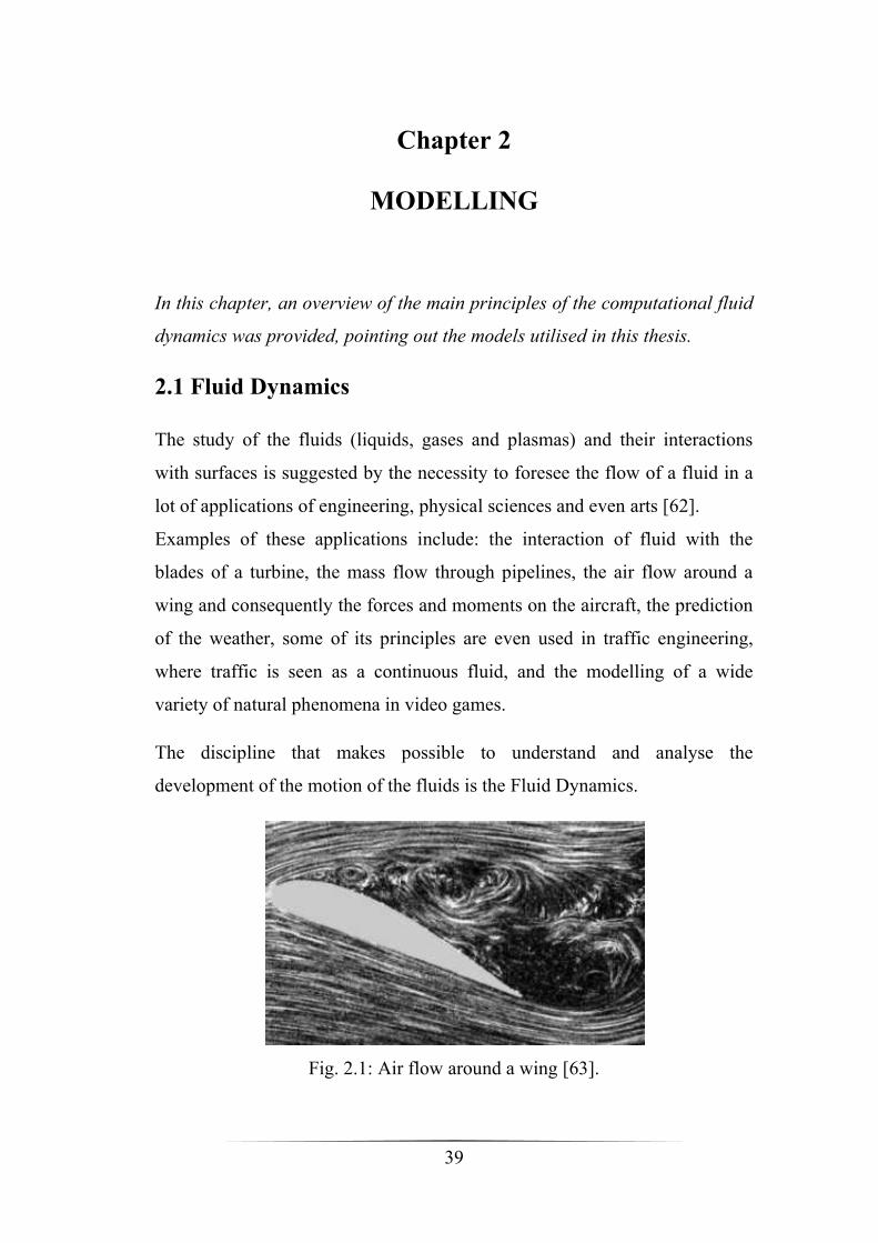
Fig. 2.1: Air flow around a wing [63].

40
The solution of a fluid dynamics problem is obtained by writing a complex
system of differential equations, which describe the motion of a fluid from
the macroscopic point of view.
The fundamental axioms of fluid dynamics are the conservation laws [64],
which in their most general form can be written as follow:
▪ Conservation of mass:
𝜕𝜌
𝜕𝑡+𝜕(𝜌𝑢)
𝜕𝑥+𝜕(𝜌𝑣)
𝜕𝑦+𝜕(𝜌𝑤)
𝜕𝑧=𝜕𝜌𝑠𝜕𝑡
Where 𝜌 is fluid density and 𝑢, 𝑣 and 𝑤 represent flow velocity vector
components 𝐯 = (𝑢, 𝑣, 𝑤). The source 𝜕𝜌𝑠
𝜕𝑡 is the mass added to the
continuous phase from a dispersed second phase (e.g., due to vaporisation
of liquid droplet).
▪ Conservation of momentum (Navier-Stokes equations):
𝜕(𝜌𝑢)
𝜕𝑡+𝜕(𝜌𝑢2)
𝜕𝑥+𝜕(𝜌𝑢𝑣)
𝜕𝑦+𝜕(𝜌𝑢𝑤)
𝜕𝑧
= −𝜕𝑝
𝜕𝑥+𝜕(𝜎𝑥)
𝜕𝑥+𝜕(𝜏𝑦𝑥)
𝜕𝑦+𝜕(𝜏𝑧𝑥)
𝜕𝑧+ 𝜌𝑓𝑥 + (𝑭𝑠)𝑥
𝜕(𝜌𝑣)
𝜕𝑡+𝜕(𝜌𝑣𝑢)
𝜕𝑥+𝜕(𝜌𝑣2)
𝜕𝑦+𝜕(𝜌𝑣𝑤)
𝜕𝑧
= −𝜕𝑝
𝜕𝑦+𝜕(𝜏𝑥𝑦)
𝜕𝑥+𝜕(𝜎𝑦)
𝜕𝑦+𝜕(𝜏𝑧𝑦)
𝜕𝑧+ 𝜌𝑓𝑦 + (𝑭𝑠)𝑦
𝜕(𝜌𝑤)
𝜕𝑡+𝜕(𝜌𝑤𝑢)
𝜕𝑥+𝜕(𝜌𝑤𝑣)
𝜕𝑦+𝜕(𝜌𝑤2)
𝜕𝑧
= −𝜕𝑝
𝜕𝑧+𝜕(𝜏𝑥𝑧)
𝜕𝑥+𝜕(𝜏𝑦𝑧)
𝜕𝑦+𝜕(𝜎𝑧)
𝜕𝑧+ 𝜌𝑓𝑧 + (𝑭𝑠)𝑧

41
Where 𝑝 is the static pressure, 𝜌𝑓𝑖 is the gravitational body force, 𝐹𝑠 is
the external body forces and 𝜎𝑖 and 𝜏𝑖𝑗 are the terms of the stress
tensor.
𝜏 = (
𝜎𝑥 𝜏𝑥𝑦 𝜏𝑥𝑧𝜏𝑦𝑥 𝜎𝑦 𝜏𝑦𝑧𝜏𝑧𝑥 𝜏𝑧𝑦 𝜎𝑧
)
= 𝜇 ∙
(
2 ∙𝜕𝑢
𝜕𝑥(𝜕𝑢
𝜕𝑦+𝜕𝑣
𝜕𝑥) (
𝜕𝑤
𝜕𝑥+𝜕𝑢
𝜕𝑧)
(𝜕𝑢
𝜕𝑦+𝜕𝑣
𝜕𝑥) 2 ∙
𝜕𝑣
𝜕𝑦(𝜕𝑤
𝜕𝑦+𝜕𝑣
𝜕𝑧)
(𝜕𝑤
𝜕𝑥+𝜕𝑢
𝜕𝑧) (
𝜕𝑤
𝜕𝑦+𝜕𝑣
𝜕𝑧) 2 ∙
𝜕𝑤
𝜕𝑧 )
Where 𝜇 is the dynamic viscosity.
▪ Conservation of energy:
𝜕𝜌𝐸
𝜕𝑡+𝜕[(𝜌𝐸 + 𝑝)𝑢]
𝜕𝑥+𝜕[(𝜌𝐸 + 𝑝)𝑣]
𝜕𝑦+𝜕[(𝜌𝐸 + 𝑝)𝑤]
𝜕𝑧
= ∇(−(𝜆𝑐 ∙ ∇𝑇) −∑ℎ𝑗 ∙ 𝐉𝑗𝑗
+ (𝛕𝑖𝑗𝐯)) + 𝑆ℎ
The left hand represents the local variation and transport in the total
energy including the work done on or by the system via pressure, so 𝐸
is total energy, −∇(𝜆𝑐 ∙ ∇𝑇) is diffusive heat flow through system’s
boundaries, −∇∑ ℎ𝑗 ∙ 𝐉𝑗𝑗 is the internal source of energy (e.g.
radiation), ∇(𝛕𝑖𝑗𝐯) total energy variation due to dissipative forces and
𝑆ℎ is the work done on or by the system due to mass force.
This is a non-linear set of partial differential equations which can be
analytically solved only for laminar flows and simpler geometries such
spheres or flat plates, but in practical cases the flow very often is turbulent
and the geometries are more complicated. For these reasons, in the last
42
decades, the numerical analysis has been widely spread; it is, indeed, a
different approach to the resolution of mathematical problems, enabled by the
development of the electronic calculators which allow to do longer and more
complex calculations in short time. In particular, the solution of fluid
dynamics problems using electronic machines is called Computational Fluid
Dynamics (CFD).
The use of CFD to simulate a great part of phenomena related to fluid
mechanics as flow, heat and mass transfer and chemical reactions, clearly,
implies great economical and practical advantages:
▪ conceptual studied of new design in reduced time;
▪ redesign;
▪ product development;
▪ preliminary analysis of system in conditions hardly replicable;
▪ assessment of quantities difficult to measure directly;
▪ troubleshooting.
For example, it is possible to know how a machine will respond before
performing a test and thus to avoid conditions that can take damage, or
simply to understand how the product’s performances are affected by this
flows and the changes of arrangement which caused them.
Several commercial software solves fluid dynamics equations, in this thesis
FLUENT, KIVA and FORTE are used. Each of them can be specialised in a
particular application, like KIVA and FORTE that are used for internal
combustion engines simulations.
2.1.1 Numerical analysis
The aim of numerical analysis is not to seek exact answers but it wants to
attain results which can properly approximate the real solutions through the
study of algorithms; as consequence, the presence of errors must be taken

43
into account, maintaining them within reasonable bounds to give a good
representation of the analysed phenomena [65].
Usually the solution is reached through the same basic procedure:
1. The geometry of the problem is defined.
2. The volume occupied by the fluid is divided into discrete cells (mesh).
3. The equations that represent the physical modelling are defined.
4. Boundary conditions are determined. This means that the behaviour
and the properties of the fluid must be specified at the limits of the
domain. For transient cases there must be also an initial condition.
5. Equations are solved.
6. A postprocessor is used for the analysis and visualization of the
results.
2.1.2 Discretization
Through a discretization process a continuous problem is replaced by a
discrete one whose results approximate the solution of the continuous
problem. This is done by dividing the domain into a series of volumes of
infinitesimal dimensions so to generate a calculation grid, the so-called mesh,
and for each volume, by writing conservation laws.
Fig. 2.2: Generic mesh [66].
44
The assumption behind this process is that all the points belonging to a
certain volume are characterised by the same value of pressure, temperature
and density, this is an acceptable approximation given the extremely small
size. In this way conservation laws can be seen as a simple system of
algebraic equations and no longer as partial differential equations, because
the generic derivative is now a finite difference:
𝑑𝑢𝑖𝑑𝑥
=𝑢𝑖+1 − 𝑢𝑖∆𝑥
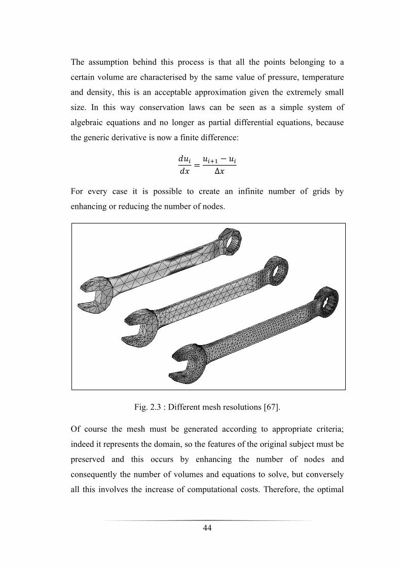
For every case it is possible to create an infinite number of grids by
enhancing or reducing the number of nodes.
Fig. 2.3 : Different mesh resolutions [67].
Of course the mesh must be generated according to appropriate criteria;
indeed it represents the domain, so the features of the original subject must be
preserved and this occurs by enhancing the number of nodes and
consequently the number of volumes and equations to solve, but conversely
all this involves the increase of computational costs. Therefore, the optimal

45
choice is dictated by economic needs, available time, degree of accuracy
required and power of electronic machines.
The most common discretization methods are:
▪ Finite volume method: this is the standard approach used in the
greatest part of commercial CFD codes, it is characterised by high
solution speed, high Reynolds number turbulent flow and it is
particularly effective in combustion problems.
▪ Finite element method (FEM): this is mainly used in structural
analysis but is also used in fluid dynamics where the Reynolds
number are of the order of ten thousands.
▪ Finite difference method: it is used only in specialized codes with
complex geometries.
Aside from these, there are other methods as the spectral element method, the
boundary element method and the high-resolution discretization schemes.
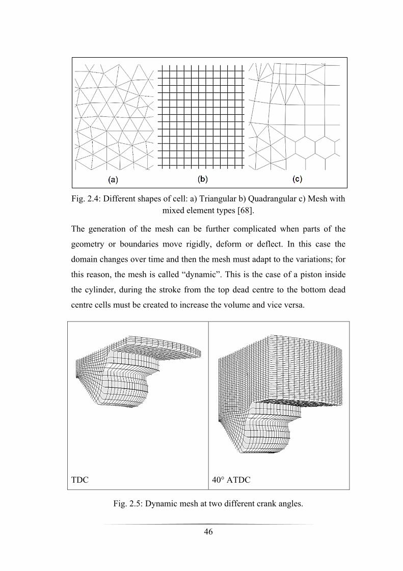
2.1.3 Meshing
There are numerous ways to generate a mesh (e.g. starting from the surfaces
or from the interior solid) and several types of meshes characterised by a
different shape of cells. The most common grids are triangular and
quadrangular (Figures 2.4.a and b), or respectively tetrahedral and hexahedral
in a three-dimensional environment: usually the second type is preferred
because with the same number of nodes, a better accuracy can be provided,
despite triangular cells can better follow the border of the domain. However,
it is possible to mix different shapes of cell in the same grid exploiting the
features of each type (Figure 2.4.c).
46
Fig. 2.4: Different shapes of cell: a) Triangular b) Quadrangular c) Mesh with
mixed element types [68].
The generation of the mesh can be further complicated when parts of the
geometry or boundaries move rigidly, deform or deflect. In this case the
domain changes over time and then the mesh must adapt to the variations; for
this reason, the mesh is called “dynamic”. This is the case of a piston inside
the cylinder, during the stroke from the top dead centre to the bottom dead
centre cells must be created to increase the volume and vice versa.
TDC
40° ATDC
Fig. 2.5: Dynamic mesh at two different crank angles.

47
Also, the generic conservative equations must be modified to take into
account the movement of the mesh:
𝑑
𝑑𝑡∫𝜌𝜙𝑑𝑉𝑉
+∫ 𝜌𝜙(𝒖 − 𝒖𝒈) ∙ 𝑑𝐴𝜕𝑉
= ∫ Γ∇𝜙 ∙ 𝑑𝐴𝜕𝑉
+∫𝑆𝜙𝑑𝑉𝑉
Where 𝒖 is the velocity of the fluid, 𝒖𝒈 is the velocity of the mesh and ∂V
represents the boundary of the control volume V.
2.1.4 Solution methods
The solution of the equations can be accomplished with direct or iterative
methods.
Direct methods solve all the equations directly and reach the solution in a
finite number of steps. These methods would give the precise answer if they
were performed in infinite precision arithmetic. Examples include Gaussian
elimination, the QR factorization method for solving system of linear
equations, and the simpler method of linear programming.
In contrast, iterative methods start from an initial guess and iteratively give
successive approximations that converge to the exact solution only at the
limit, that is after an endless number of steps, but in practice the calculation is
interrupted after is reached the desired degree of accuracy. So even using
infinite precision arithmetic these methods would not reach the true solution
but there always will be residuals. Among these methods there are Newton’s
method, the bisection method and Jacobi iteration.
Furthermore, some methods are direct in principle but are usually used as
iterative ones because the number of steps needed to obtain the exact solution
is so large that an approximation can be well accepted; GMRES and the
conjugate method are examples.
48
Usually, in CFD and numerical analysis simulations iterative methods are
commonly used to solve the equations for steady or transient state.
2.1.5 Errors
Both direct and iterative methods are affected by errors:
▪ Round off errors: arise because it is impossible to represent all real
numbers exactly in reality or on a machine with finite memory.
▪ Truncation errors: are committed when an iterative method is
terminated or a mathematical procedure is approximated, and the
approximated solution differs from the exact solution.
▪ Discretization errors: these are intrinsic to numerical approaches,
the solution of the discrete problem does not coincide with the
solution of the continuous problem.
Once an error is generated, it will generally propagate through the
calculation, so due to their presence it is important to introduce the notion of
numerical stability. An algorithm is called numerically stable if an error,
whatever its cause is, does not increase during the calculation. When this
condition is fulfilled the problem is well-conditioned, meaning that if the
problem data change by a small amount, the solution changes by only a small
amount too. On the contrary when any small error in the data grows to be a
large error, the problem is ill-conditioned. Both the original problem and the
algorithm used can be well-conditioned and/or ill-conditioned and any
combination is possible.
2.2 Turbulence
As already stated in practice cases fluid flows are very often turbulent.
In laminar flows kinetic energy is dissipated because of the action of
molecular viscosity and the fluid streamlines do not mix laterally. On the
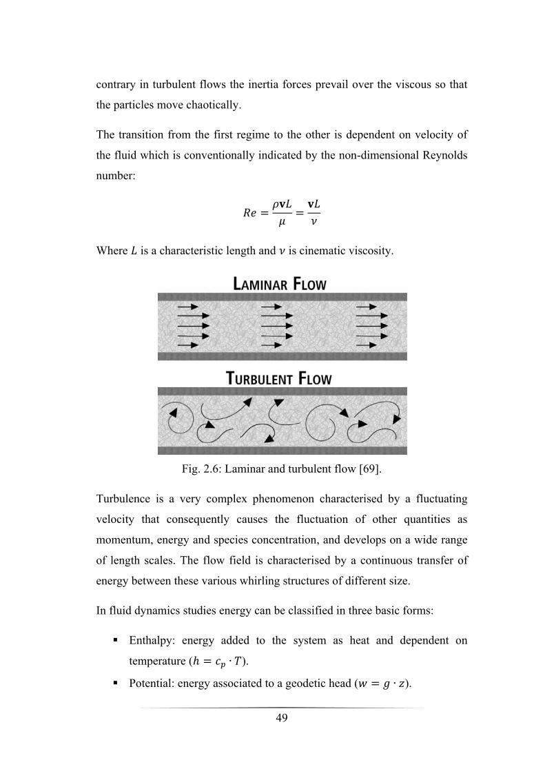
49
contrary in turbulent flows the inertia forces prevail over the viscous so that
the particles move chaotically.
The transition from the first regime to the other is dependent on velocity of
the fluid which is conventionally indicated by the non-dimensional Reynolds
number:
𝑅𝑒 =𝜌𝐯𝐿
𝜇=𝐯𝐿
𝜈
Where 𝐿 is a characteristic length and 𝜈 is cinematic viscosity.
Fig. 2.6: Laminar and turbulent flow [69].
Turbulence is a very complex phenomenon characterised by a fluctuating
velocity that consequently causes the fluctuation of other quantities as
momentum, energy and species concentration, and develops on a wide range
of length scales. The flow field is characterised by a continuous transfer of
energy between these various whirling structures of different size.
In fluid dynamics studies energy can be classified in three basic forms:
▪ Enthalpy: energy added to the system as heat and dependent on
temperature (ℎ = 𝑐𝑝 ∙ 𝑇).
▪ Potential: energy associated to a geodetic head (𝑤 = 𝑔 ∙ 𝑧).
50
▪ Kinetic: energy manifesting in the speed of particles of the fluid
(𝑘 =1
2∙ 𝐯2).
In combustion phenomena that are the object of this work, kinetic energy is
widely predominant while the other two can be considered negligible.
All the modelling is based on the idea formulated by Richardson, that all
kinetic energy 𝑘 entering the system owned by larger vortices is transferred
to the ones of gradually decreasing size and at least dissipated as heat in the
smaller eddies where the viscous forces prevail on inertial forces. The
dissipation term is given by the derivative of kinetic energy with respect to
time: 휀 =𝜕𝑘
𝜕𝑡 . For this reason, this theory is called “energy cascade
mechanism” of turbulent flow.
Under general conditions it is not possible to quantify the dimensions of the
smaller length scales and the entity of dissipation. An important solution was
given by Kolmogorov, who in 1941 published his theory applicable to fluids
with high Reynolds number.
The first hypothesis is represented by considering turbulence as homogenous
and isotropic, this means that the components of velocity along the three
directions have the same value (𝑢 = 𝑣 = 𝑤) and kinetic energy can be
written as follow:
𝑘 =1
2∙ (𝑢2̅̅ ̅ + 𝑣2̅̅ ̅ + 𝑤2̅̅ ̅̅ ) =
1
2∙ (𝑢2̅̅ ̅ + 𝑢2̅̅ ̅ + 𝑢2̅̅ ̅) =
3
2∙ (𝑢2̅̅ ̅)
The second hypothesis is that all characteristics of smaller length scales of all
turbulent flows are universal and are determined by viscosity 𝜈 and
dissipation 휀. By combining these two parameters, it is possible to define
quantitatively a characteristic length called “Kolmogorov scale”, time and
velocity:

51
▪ 𝜂 = (𝜈3
𝜖)14⁄
▪ 𝑡𝜂 = (𝜈)12⁄
=𝜂2
𝜈
▪ 𝑢𝜂 = (𝜈 ∙ 𝜂)14⁄
Given the stationarity of the process, which implies that the energy dissipated
is the same entering the system, it is possible to identify also for larger eddies
a characteristic length 𝐿𝐼, time 𝑡𝑡 and velocity 𝑢′, but unlike the previous
case, as the phenomena are governed by inertial parameters, cinematic
viscosity is not utilised. In fact for macrovortices 𝐿𝐼, called “integral scale”,
is known and is given by the dimensions of the larger scales which are
delimitated by the geometry at issue; velocity is easily measurable knowing
the mass flows and the surfaces of passage; the time is given by the ratio of
length and velocity and is called “turnover time”; finally it is also possible to
express the dissipation energy as 휀 =𝑢′3
𝐿𝐼.
Thus, comparing the characteristics of the various length scales, it is possible
to understand the flow field and to select the best suited solution model to the
problem.
2.3 Turbulence models
Since resolving all the instantaneous exact governing equations is
computationally impossible due to the excessive expenses, in such cases the
primary approach is for example to bypass this obstacle creating models
capable of time-averaging, ensemble-averaging or manipulating the equations
by removing smaller scales so that they may be easily solved.
However the modified equations are the result of analytical and experimental
studies in which it is necessary to introduce new variables which require new
equations and constants to close the problem, so the turbulence models are
52
needed to determine and approximate also these unsolved phenomena, by
assigning a certain value to these terms.
However, there is not a universal model best suited to describe all classes of
problems. The choice is made considering different factors as computing
resources, the established practice for a certain class of problem, the level of
accuracy required, the amount of time available and of course the physics of
the flow. Beside computational costs depend on the range of scales modelled,
the wider is this range the higher are the costs.
Below are briefly shown the main models used in CFD:
Direct numerical simulation (DNS) is not a real model as the equations are
numerically solved in all time and spatial scales; this means that it is the most
accurate but also the most expensive process.
The Reynolds-averaged Navier-Stokes (RANS) equations are the time-
averaged equations that describe the motion of fluid flows; the basic concept
behind this model is that the solution variables are decomposed in a mean
and a fluctuating component:
𝜙𝑖 = �̅�𝑖 + 𝜙𝑖′
Where �̅�𝑖′ = 0
This approach introduces a new term which represents the effect of
turbulence, it is called “Reynolds stresses” and other correlations are required
in order to close the problem. For this reason, RANS models can be divided
into two groups:
▪ The Boussinesq hypothesis uses few algebraic equations to
determine turbulent viscosity 𝜇𝑡, turbulent kinetic energy 𝑘 and
turbulent dissipation 휀. Among these there are the Spalart-Allmaras
model, the 𝑘-휀 models and the 𝑘-𝜔 models.

53
▪ Reynolds stress model (RSM) attempts to actually solve transport
equations for each of the terms in the Reynolds stress tensor, this
implies the addition of equations that increase further CPU effort.
Large eddy simulation (LES) solves only larger eddies which are strongly
influenced by the geometry of the domain, the Kolmogorov scales, are
previously numerically filtered and then properly modelled. Resolving larger
eddies allows to utilise a coarser mesh and broader time-steps size, this
means to reduce computational costs which fall between DNS and RANS
approaches.
Detached eddy simulation (DES) is a hybrid formulation which combines
RANS and LES models, the domain is divided into two zones: the region
located near the boundary layer, where the turbulent length scale is less than
the maximum grid dimension, is solved with RANS; while to the core region
where the turbulent length scales exceed the grid dimension is assigned the
LES mode solution, thereby a sub-grid scale formulation is required only in
this zone and the cost of the computation is considerably cut down. However,
the RANS/LES switch complicates the generation of the mesh because a
single smooth velocity field must be provided across the two regions.
Other turbulence models which will be only mentioned are: coherent vortex
simulation, vortex method, vorticity confinement method and linear eddy
model.
2.4 Combustion models
Combustion models describe all chemical and physical reactions which
derive from combustion. Clearly these phenomena are extremely complex as
interaction between particles must be simulated considering turbulence’s
effects.
54
The starting consideration concerns the fuel and oxidizer streams entering the
reaction zone, if they are separated the combustion is called non-premixed (or
diffusion), otherwise if they are mixed, before burning, the combustion is
defined as premixed.
The first approach aims to model the mixing and the transport of each
chemical species by solving conservation equations that represent
convection, diffusion and sources, so for the ith component:
𝜕(𝜌𝑌𝑖)
𝜕𝑡+ ∇ ∙ (𝜌𝐯𝑌𝑖) = −∇ ∙ 𝐉𝑖 + 𝑅𝑖
𝑌 is mass fraction, 𝐉 is the diffusion flux and 𝑅 is the rate of production.
Actually, all mass fractions must sum to unity, if there are N chemical
species in the system, N-1 equations will be solved and the last component’s
mass fraction is obtained as 1 minus the sum of the N-1 solved mass
fractions. Usually the Nth species is the one with the largest mass fraction
thereby numerical errors are reduced.
The diffusion flux is generated by gradients of concentration and temperature
and is given by Fick’s law:
𝐉𝑖 = −(𝜌𝐷𝑚,𝑖 +𝜇𝑡𝑆𝑐𝑡) ∇𝑌𝑖 − 𝐷𝑇,𝑖
∇𝑇
𝑇
𝐷𝑚,𝑖 is the mass diffusion coefficient, 𝜇𝑡is the turbulent viscosity, 𝑆𝑐𝑡 is the
Schmidt number and 𝐷𝑇,𝑖 is thermal diffusion coefficient.
Several models were formulated to describe the source term. The most
important are the finite-rate and the eddy-dissipation model.
2.4.1 Finite rate – Eddy dissipation model
The finite-rate model ignores the effect of turbulence and determines the
reactions rate by the Arrhenius kinetic expression:

55
𝑅𝑘 = 𝑅𝑓 − 𝑅𝑏 = 𝑘𝑓∏[𝐶𝑗]𝑎𝑗
𝑁
𝑗=1
− 𝑘𝑏∏[𝐶𝑗]𝑏𝑗
𝑁
𝑗=1
𝐶𝑗 is the molar concentration, 𝑎𝑗 and 𝑏𝑗 are stoichiometric coefficient, 𝑘𝑓 and
𝑘𝑏 are the forward and backward rate constants which are obtained using
Arrhenius’ expression:
𝑘 = 𝐴𝑇𝑥exp (−𝐸𝑎𝑅𝑇)
𝐴 is the pre-exponential factor, 𝑥 is temperature exponent, 𝐸𝑎 is the
activation energy and 𝑅 is universal gas constant.
On the contrary the eddy-dissipation model, formulated by Magnussen and
Hjertager [70], neglects the kinetic rate and considers the problem linked
only to fluid dynamics which means that is mixing-limited; this is possible
when the fuel burns rapidly or at least when reactions are quicker than
mixing phenomena. In this case reactions rate of all species are calculated
and the one that limits the process, that is the smallest, is chosen:
𝑅𝑡 = 𝐶휀
𝑘∙ min(𝑌𝑅 , 𝑌𝑃)
𝐶 is a factor proportional to turbulent combustion, 𝑌𝑅 and 𝑌𝑃 are mass
fractions of reactants and products, 𝑘 is the turbulent kinetic energy and 휀 is
turbulent energy dissipation. The ratio 𝑘 is called “characteristic mixing time”
and indicates that the chemical reaction rate is governed by the large-eddy
time scales and the combustion extinguishes if there is not turbulence, thus
clearly this model is not suited to describe laminar flames. Moreover, an
ignition source is not required which is acceptable for diffusion flames but in
premixed flames the reactants will burn as soon as they enter the
computational domain.
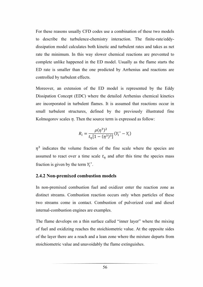
56
For these reasons usually CFD codes use a combination of these two models
to describe the turbulence-chemistry interaction. The finite-rate/eddy-
dissipation model calculates both kinetic and turbulent rates and takes as net
rate the minimum. In this way slower chemical reactions are prevented to
complete unlike happened in the ED model. Usually as the flame starts the
ED rate is smaller than the one predicted by Arrhenius and reactions are
controlled by turbulent effects.
Moreover, an extension of the ED model is represented by the Eddy
Dissipation Concept (EDC) where the detailed Arrhenius chemical kinetics
are incorporated in turbulent flames. It is assumed that reactions occur in
small turbulent structures, defined by the previously illustrated fine
Kolmogorov scales 𝜂. Then the source term is expressed as follow:
𝑅𝑖 =𝜌(𝜂3)2
𝑡𝜂[1 − (𝜂3)3]
(𝑌𝑖∗ − 𝑌𝑖)
𝜂3 indicates the volume fraction of the fine scale where the species are
assumed to react over a time scale 𝑡𝜂 and after this time the species mass
fraction is given by the term 𝑌𝑖∗.
2.4.2 Non-premixed combustion models
In non-premixed combustion fuel and oxidizer enter the reaction zone as
distinct streams. Combustion reaction occurs only when particles of these
two streams come in contact. Combustion of pulverized coal and diesel
internal-combustion engines are examples.
The flame develops on a thin surface called “inner layer” where the mixing
of fuel and oxidizing reaches the stoichiometric value. At the opposite sides
of the layer there are a reach and a lean zone where the mixture departs from
stoichiometric value and unavoidably the flame extinguishes.

57
For this reason, it is noticeable the strong dependence of non-premixed
flames on convection and diffusion caused by turbulence, which allows a
more intimate mixing between reactants. This phase requires larger time than
the time necessary for combustion, thus the problem can be reduced to a
single variable able to represent the trend of mixing and independent of the
chemical: this parameter is called mixture fraction.
Once mixed, the chemistry can be modelled as being in chemical equilibrium
with the Equilibrium model, being near chemical equilibrium with Steady
Laminar Flamelet or significantly far from chemical equilibrium with the
Unsteady Laminar Flamelet model.
2.4.2.1 Mixture fraction theory
The mixture fraction is the mass fraction originated from the fuel stream, that
is the local mass fraction of burned and unburned fuel elements (C, H, etc.) in
all species (CO2, H2O, O2, etc.). The greatest advantage of this approach is
that atomic elements are conserved in chemical reactions, thus the mixture
fraction is a conserved scalar quantity, in this way the solution involves only
transport equations for one or two conserved scalars and source terms are
equal to zero. Equation for individual species are not solved. Instead, species
concentrations are derived from the predicted mixture fraction fields. At
least, to save computational time, the thermochemistry calculations are pre-
processed and then stored in a look-up table.
Moreover, interaction of turbulence and chemistry is accounted for with an
assumed-shape Probability Density Function (PDF).
The mixture can be written in term of atomic mass fraction as:
𝑓 =𝑍𝑖 − 𝑍𝑖,𝑜𝑥
𝑍𝑖,𝑓𝑢𝑒𝑙 − 𝑍𝑖,𝑜𝑥

58
𝑍𝑖 is the elemental mass fraction for element 𝑖, the subscript 𝑜𝑥 is for the
oxidizer and the subscript 𝑓𝑢𝑒𝑙 denotes the value for the fuel both at stream
inlet. The sum of all mixture fractions in the system is always equal to 1.
Under the hypothesis of equal diffusivities, which is problematic for laminar
flows but acceptable for turbulent flows because convection overwhelms
molecular diffusion, the species equations can be reduced to a single equation
for the mixture fraction. The Favre mean (density-averaged) mixture fraction
equation is:
𝜕
𝜕𝑡(𝜌𝑓)̅ + ∇ ∙ (𝜌𝐯𝑓)̅ = ∇ ∙ (
𝜇𝑡𝜎𝑡∇𝑓)̅
At this point in condition of chemical equilibrium, all thermochemical scalar
𝜙 (species, density and temperature) are uniquely related to the mixture
fractions.
𝜙𝑖 = 𝜙𝑖(𝑓)
To give a closure to the problem it is necessary to solve another conservation
equation for mixture fraction variance which describe turbulence-chemistry
interaction:
𝜕
𝜕𝑡(𝜌𝑓′2̅̅ ̅̅ ) + ∇ ∙ (𝜌𝐯𝑓′2̅̅ ̅̅ ) = ∇ ∙ (
𝜇𝑡𝜎𝑡∇𝑓′2̅̅ ̅̅ ) + 𝐶𝑔𝜇𝑡(∇𝑓)̅
2− 𝐶𝑑𝜌
휀
𝑘𝑓′2̅̅ ̅̅
Where 𝑓′ = 𝑓 − 𝑓,̅ 𝜎𝑡, 𝐶𝑔 and 𝐶𝑑 are constants.
Actually, due to the unpredictability of this parameter, in numerical analysis
the solution of this equation is reached imposing a Probability Density
Function (PDF). The PDF is the fraction of time that the fluid spends in the
vicinity of the state 𝑓.
In fact, the fluctuating value of 𝑓 spends some time in a range denoted as Δ𝑓.
The function 𝑝(𝑓) represents the frequency with which 𝑓 is found in such
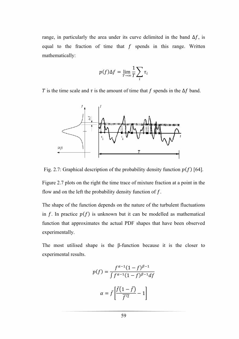
59
range, in particularly the area under its curve delimited in the band Δ𝑓, is
equal to the fraction of time that 𝑓 spends in this range. Written
mathematically:
𝑝(𝑓)Δ𝑓 = lim𝑇→∞
1
𝑇∑𝜏𝑖𝑖
𝑇 is the time scale and 𝜏 is the amount of time that 𝑓 spends in the Δ𝑓 band.
Fig. 2.7: Graphical description of the probability density function 𝑝(𝑓) [64].
Figure 2.7 plots on the right the time trace of mixture fraction at a point in the
flow and on the left the probability density function of 𝑓.
The shape of the function depends on the nature of the turbulent fluctuations
in 𝑓. In practice 𝑝(𝑓) is unknown but it can be modelled as mathematical
function that approximates the actual PDF shapes that have been observed
experimentally.
The most utilised shape is the β-function because it is the closer to
experimental results.
𝑝(𝑓) =𝑓𝛼−1(1 − 𝑓)𝛽−1
∫𝑓𝛼−1(1 − 𝑓)𝛽−1𝑑𝑓
𝛼 = 𝑓̅ [𝑓(̅1 − 𝑓)̅
𝑓′2̅̅ ̅̅− 1]
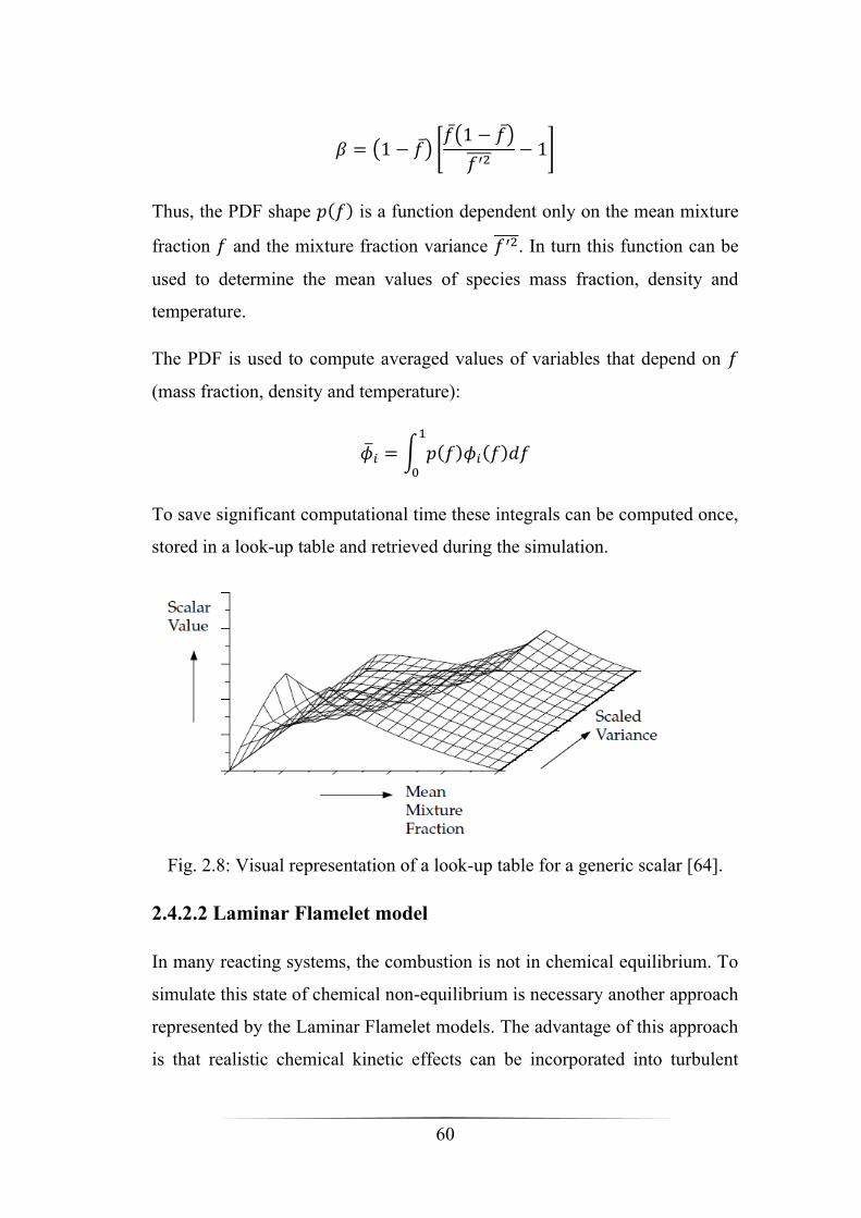
60
𝛽 = (1 − 𝑓)̅ [𝑓(̅1 − 𝑓)̅
𝑓′2̅̅ ̅̅− 1]
Thus, the PDF shape 𝑝(𝑓) is a function dependent only on the mean mixture
fraction 𝑓 and the mixture fraction variance 𝑓′2̅̅ ̅̅ . In turn this function can be
used to determine the mean values of species mass fraction, density and
temperature.
The PDF is used to compute averaged values of variables that depend on 𝑓
(mass fraction, density and temperature):
�̅�𝑖 = ∫ 𝑝(𝑓)𝜙𝑖(𝑓)𝑑𝑓1
0
To save significant computational time these integrals can be computed once,
stored in a look-up table and retrieved during the simulation.
Fig. 2.8: Visual representation of a look-up table for a generic scalar [64].
2.4.2.2 Laminar Flamelet model
In many reacting systems, the combustion is not in chemical equilibrium. To
simulate this state of chemical non-equilibrium is necessary another approach
represented by the Laminar Flamelet models. The advantage of this approach
is that realistic chemical kinetic effects can be incorporated into turbulent

61
flames. In fact, the chemistry is pre-processed and tabulated, offering huge
computational savings.
Moreover it is possible to distinguish the Steady Flamelet model to describe
the phenomena of diffusion flame stretched by turbulence with a relatively
fast chemistry and the Unsteady Laminar Flamelet model to follow the slow-
forming product species that are far from chemical equilibrium, this last is
the case of gaseous pollutants (NOx and low-temperature CO oxidation).
The basic concept of this theory is that the turbulent flame is seen as an
ensemble of thin, laminar, locally one-dimensional flamelet located within
the turbulent flow field.
In particularly the individual flamelet is an independent thin reactive-
diffusive layer whose structure is the same of a simple laminar flame which
configuration is easy to perform by experiments or to calculate.
The location of the flamelet is identified through statistical PDF methods; in
fact as the distribution of mixture fraction is known, for example using a β-
function, it is possible to situate the layer where 𝑓 reach the stoichiometric
value.
After defining the stoichiometric surface on which reactions take place, the
next step is to describe the combustion itself. Usually to represent a flamelet,
it is used a common laminar diffusion flame type in a turbulent counterflow.
The geometry is very simple and consists of opposed fuel and oxidizer jets.
As the distance between the jets is decreased and/or the velocity of the jets is
increased, the flame is strained and increasingly departs from chemical
equilibrium until it is eventually extinguished.
This flame is easy to perform experimentally so that mass fraction and
temperature fields can be measured. Otherwise due to simplicity of this
configuration it is possible to calculate these parameters because the
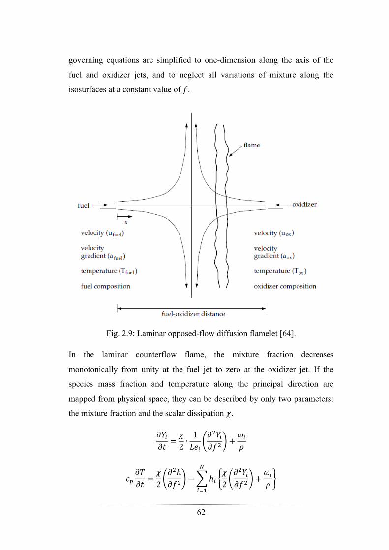
62
governing equations are simplified to one-dimension along the axis of the
fuel and oxidizer jets, and to neglect all variations of mixture along the
isosurfaces at a constant value of 𝑓.
Fig. 2.9: Laminar opposed-flow diffusion flamelet [64].
In the laminar counterflow flame, the mixture fraction decreases
monotonically from unity at the fuel jet to zero at the oxidizer jet. If the
species mass fraction and temperature along the principal direction are
mapped from physical space, they can be described by only two parameters:
the mixture fraction and the scalar dissipation 𝜒.
𝜕𝑌𝑖𝜕𝑡=𝜒
2∙1
𝐿𝑒𝑖(𝜕2𝑌𝑖𝜕𝑓2
) +𝜔𝑖𝜌
𝑐𝑝𝜕𝑇
𝜕𝑡=𝜒
2(𝜕2ℎ
𝜕𝑓2) −∑ℎ𝑖 {
𝜒
2(𝜕2𝑌𝑖𝜕𝑓2
) +𝜔𝑖𝜌}
𝑁
𝑖=1
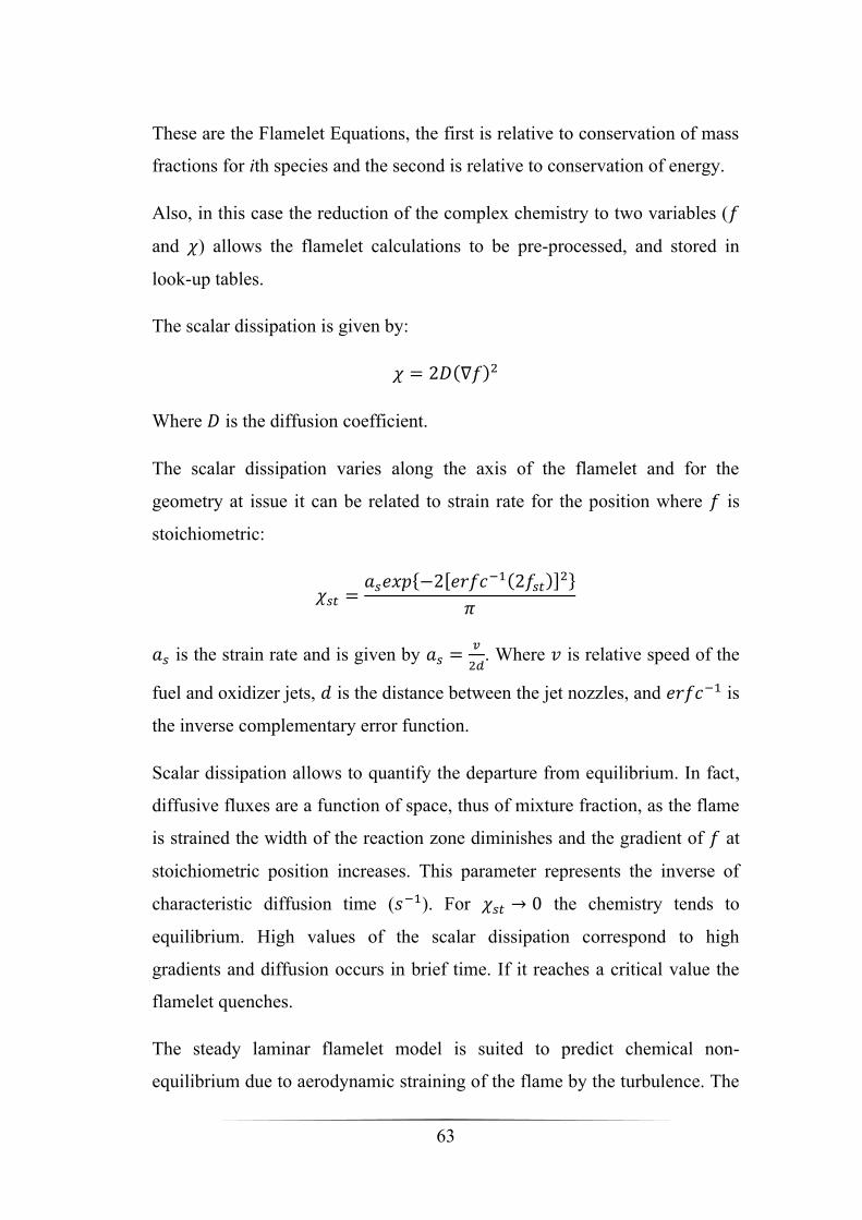
63
These are the Flamelet Equations, the first is relative to conservation of mass
fractions for ith species and the second is relative to conservation of energy.
Also, in this case the reduction of the complex chemistry to two variables (𝑓
and 𝜒) allows the flamelet calculations to be pre-processed, and stored in
look-up tables.
The scalar dissipation is given by:
𝜒 = 2𝐷(∇𝑓)2
Where 𝐷 is the diffusion coefficient.
The scalar dissipation varies along the axis of the flamelet and for the
geometry at issue it can be related to strain rate for the position where 𝑓 is
stoichiometric:
𝜒𝑠𝑡 =𝑎𝑠𝑒𝑥𝑝{−2[𝑒𝑟𝑓𝑐
−1(2𝑓𝑠𝑡)]2}
𝜋
𝑎𝑠 is the strain rate and is given by 𝑎𝑠 =𝑣
2𝑑. Where 𝑣 is relative speed of the
fuel and oxidizer jets, 𝑑 is the distance between the jet nozzles, and 𝑒𝑟𝑓𝑐−1 is
the inverse complementary error function.
Scalar dissipation allows to quantify the departure from equilibrium. In fact,
diffusive fluxes are a function of space, thus of mixture fraction, as the flame
is strained the width of the reaction zone diminishes and the gradient of 𝑓 at
stoichiometric position increases. This parameter represents the inverse of
characteristic diffusion time (𝑠−1). For 𝜒𝑠𝑡 → 0 the chemistry tends to
equilibrium. High values of the scalar dissipation correspond to high
gradients and diffusion occurs in brief time. If it reaches a critical value the
flamelet quenches.
The steady laminar flamelet model is suited to predict chemical non-
equilibrium due to aerodynamic straining of the flame by the turbulence. The
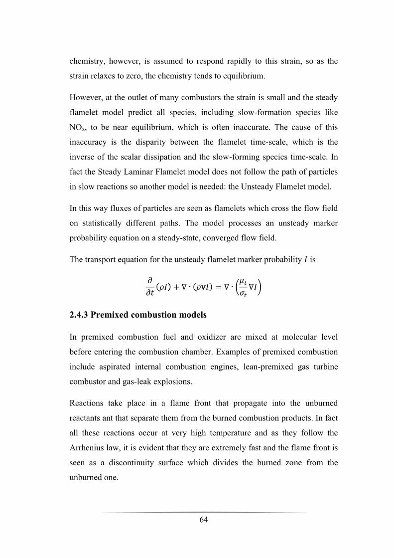
64
chemistry, however, is assumed to respond rapidly to this strain, so as the
strain relaxes to zero, the chemistry tends to equilibrium.
However, at the outlet of many combustors the strain is small and the steady
flamelet model predict all species, including slow-formation species like
NOx, to be near equilibrium, which is often inaccurate. The cause of this
inaccuracy is the disparity between the flamelet time-scale, which is the
inverse of the scalar dissipation and the slow-forming species time-scale. In
fact the Steady Laminar Flamelet model does not follow the path of particles
in slow reactions so another model is needed: the Unsteady Flamelet model.
In this way fluxes of particles are seen as flamelets which cross the flow field
on statistically different paths. The model processes an unsteady marker
probability equation on a steady-state, converged flow field.
The transport equation for the unsteady flamelet marker probability 𝐼 is
𝜕
𝜕𝑡(𝜌𝐼) + ∇ ∙ (𝜌𝐯𝐼) = ∇ ∙ (
𝜇𝑡𝜎𝑡∇𝐼)
2.4.3 Premixed combustion models
In premixed combustion fuel and oxidizer are mixed at molecular level
before entering the combustion chamber. Examples of premixed combustion
include aspirated internal combustion engines, lean-premixed gas turbine
combustor and gas-leak explosions.
Reactions take place in a flame front that propagate into the unburned
reactants ant that separate them from the burned combustion products. In fact
all these reactions occur at very high temperature and as they follow the
Arrhenius law, it is evident that they are extremely fast and the flame front is
seen as a discontinuity surface which divides the burned zone from the
unburned one.

65
The thin flame is stretched and contorted by turbulence and this makes really
difficult to model this type of combustion.
For subsonic flows, the overall rate of propagation of the turbulent flame
(𝑑𝑚𝑏
𝑑𝑡) is determined by both the laminar flame speed 𝑆𝐿 [m/s] and the
turbulent eddies.
The laminar flame speed refers to a combustion in absence of motion or a
laminar motion at very low speed and is determined by the kinetic scheme
and the burning rate of the species. Thus, it represents the synthesis of all the
detailed chemical kinetics and molecular diffusion processes.
𝑑𝑚𝑏𝑑𝑡
= 𝜌𝑢𝐴𝐿𝑆𝐿
The flame front has a certain thickness indicated with 𝛿𝐿[m] and it is linked
to laminar speed by the following relation:
𝛿𝐿 =𝜈
𝑆𝐿
It is also possible to define a characteristic time:
𝑡𝑐 =𝛿𝐿𝑆𝐿
This is the time that a particle spends to cross the flam front that is a chemical
reaction time.
To capture the laminar flame speed and the flame thickness that is of order of
millimetres or smaller, the internal flame structure would need to be resolved,
but the resolution required is usually unaffordable.
For this reason the best solution is the obtained by the experimentation: air
and fuel enter in a transparent tube at a given speed, by reacting a flame front

66
will be visible through the tube, if the flame front is steady, the entering
reagents speed will represent 𝑆𝐿.
Fig. 2.10: Laminar flame speed for two different hydrocarbons [71].
The laminar flame speed is a function of the equivalent ratio 𝜑 and in
particular it reaches a maximum near stoichiometric mixture.
Moreover 𝑆𝐿 depends on the fuel, temperature and pressure:
𝑆𝐿0 = 0.2632 − 0.8472(𝜑 − 1.13)2
Beside 𝑆𝐿0 is the flame speed at ambient temperature and atmospheric
pressure. For different operating condition:
𝑆𝐿 = 𝑆𝐿0 (𝑇
𝑇0)𝛼𝑠
(𝑝
𝑝0)𝛽𝑠
(1 − 𝑐𝑥𝑟𝛿𝑠)
• 𝛼𝑠 = 2.18 − 0.8(𝜑 − 1)
• 𝛽𝑠 = −0.16 + 0.22(𝜑 − 1)
• 𝑐 = 2.1
• 𝛿𝑠 = 0.77
• 𝑥𝑟 is the percentage of inert in unburned mixture

67
Moreover, the flame considered in the tube is planar, which means that it an
“unstreached flame”. Actually, the flame propagates spherically and a
“stretch” effect must be taken to account.
𝑘 =1
𝐴𝐿
𝑑𝐴𝐿𝑑𝑡
=2
𝑟
𝑑𝑟
𝑑𝑡
With 𝐴𝐿, it is denoted the laminar area over the time.
In some cases the stretch coefficient 𝑘 tends to enhance the laminar speed but
in other cases it can have the opposite effect. This is determined by another
parameter which is characterised experimentally and is called Markstein
length 𝐿𝑀.
𝑆𝐿,𝑠 = 𝑆𝐿,𝑢 − 𝑘𝐿𝑀
The other phenomenon that influences the propagation is the turbulence, its
effect is to wrinkle the propagating laminar flame sheet increasing the area
and in turn effective flame speed. The large eddies wrinkle and corrugate the
front, while the eddies smaller than the flame thickness may penetrate it and
modify the laminar structure.
To understand the influence of turbulence in the combustion, it is necessary
to compare the scales of length, velocity and time of the two phenomena.
This is how the Borghi diagram works, basing on the ratio of these quantities,
identifies different zones which correspond to different combustion regimes.
As shown in Figure 2.11 the various zones are delimited by non-dimensional
parameters. Apart from the Reynolds number, the most important are the
Damköhler number and the Karlovitz number; the first compares the
characteristic time of macrovortices and combustion, the second compares
the characteristic time of combustion and microvortices.
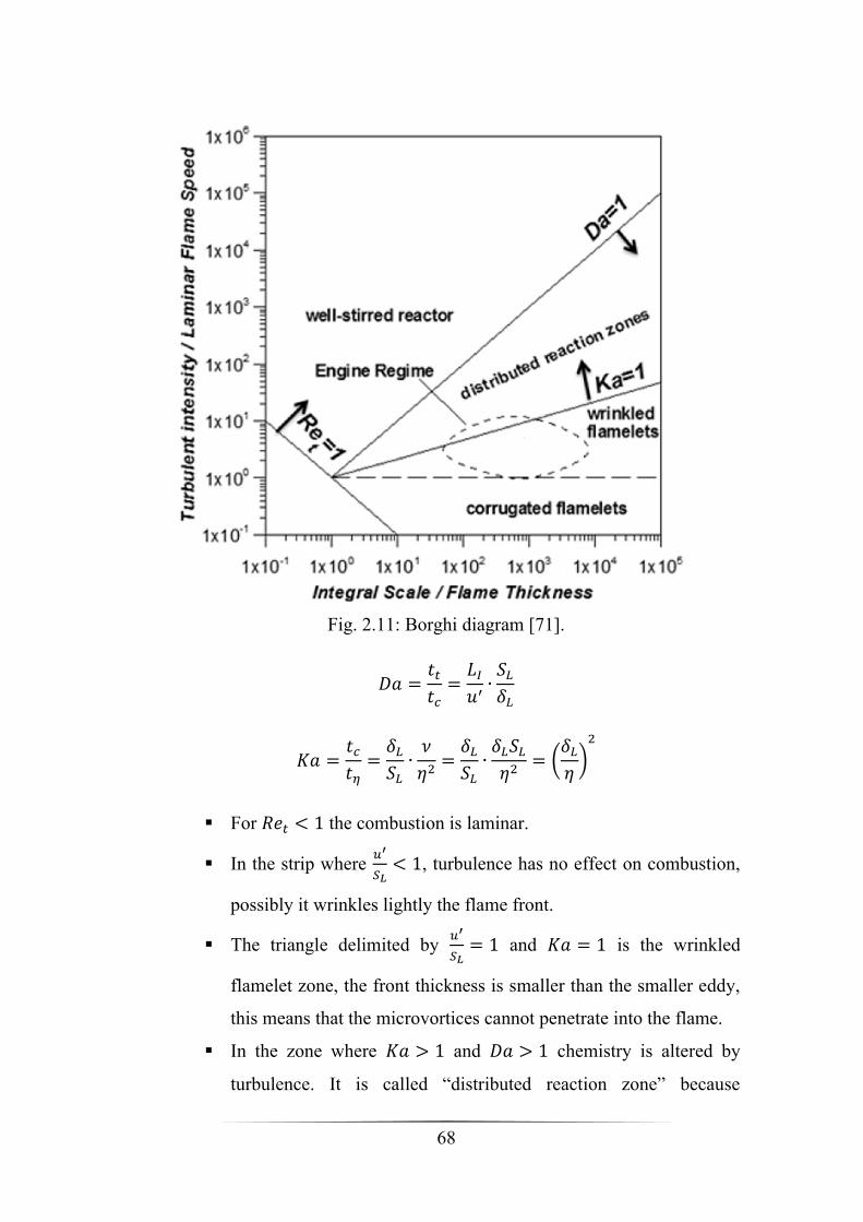
68
Fig. 2.11: Borghi diagram [71].
𝐷𝑎 =𝑡𝑡𝑡𝑐=𝐿𝐼𝑢′∙𝑆𝐿𝛿𝐿
𝐾𝑎 =𝑡𝑐𝑡𝜂=𝛿𝐿𝑆𝐿∙𝜈
𝜂2=𝛿𝐿𝑆𝐿∙𝛿𝐿𝑆𝐿𝜂2
= (𝛿𝐿𝜂)2
▪ For 𝑅𝑒𝑡 < 1 the combustion is laminar.
▪ In the strip where 𝑢′
𝑆𝐿< 1, turbulence has no effect on combustion,
possibly it wrinkles lightly the flame front.
▪ The triangle delimited by 𝑢′
𝑆𝐿= 1 and 𝐾𝑎 = 1 is the wrinkled
flamelet zone, the front thickness is smaller than the smaller eddy,
this means that the microvortices cannot penetrate into the flame.
▪ In the zone where 𝐾𝑎 > 1 and 𝐷𝑎 > 1 chemistry is altered by
turbulence. It is called “distributed reaction zone” because

69
microvortices can enter into the reaction zone and macrovortices
can break the flame front generating separated combustion zones.
▪ For 𝐷𝑎 < 1 larger eddy enters the flame which disappears, this
implies a homogeneous reactor and the combustion occurs
diffusely throughout the volume without a real propagation
mechanism.
To take account of all that combustion speed is written in a different way:
(𝑑𝑚𝑏𝑑𝑡)𝑇= 𝜌𝑢𝐴𝑇𝑆𝐿 = 𝜌𝑢𝐴𝐿𝑆𝑇
Due to difficulties to assess the turbulent flame speed, combustion is seen as
a turbulent flame front which propagates locally at laminar speed.
At least the term 𝐴𝑇 is evaluated with the assistance of an important tool
which is fractal geometry.
Fig. 2.12: Example of fractal geometry [71].
Fractal geometry allows to calculate the reaction area’s increase 𝐴𝑇 due to
turbulence compared to the average value of 𝐴𝐿.

70
𝐴𝑇 = (𝐴𝑇𝐴𝐿)𝐴𝐿
However an important premixed combustion model implemented in CFD
codes is based on Zimont’s work, applicable when 𝐾𝑎 < 1, it involves the
solution of a transport equation for reaction progress variable and the closure
equation is based on the definition of turbulent flame speed.
𝜕
𝜕𝑡(𝜌𝑐) + ∇ ∙ (𝜌𝑣𝑐) = ∇ ∙ (
𝜇𝑡𝑆𝑐𝑡∇𝑐) + 𝜌𝑆𝑐
𝑐 is the mean reaction progress variable and 𝑆𝑐is the reaction progress source
term [s-1].
The progress variable is defined as a normalized sum of the product species:
𝑐 =∑ 𝑌𝑖𝑛𝑖=1
∑ 𝑌𝑖,𝑒𝑞𝑛𝑖=1
Where 𝑛 is the number of products, 𝑌𝑖 is the mass fraction of ith product
species and 𝑌𝑖,𝑒𝑞 is the equilibrium mass fraction of ith product species.
Then:
• 𝑐 = 0 for unburned mixture
• 𝑐 = 1 for burned mixture
The mean reaction rate is given by:
𝜌𝑆𝑐 = 𝜌𝑢𝑆𝑇|∇𝑐|
The Zimont turbulent flame speed closure is computed using the following
correlation:
𝑆𝑇 = 𝐵𝑢′ (𝜏𝑡𝜏𝑐)1 4⁄
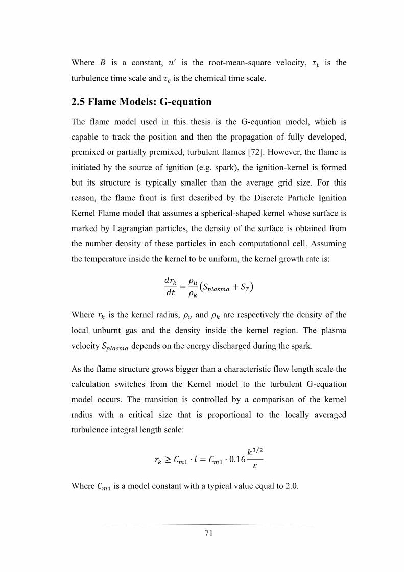
71
Where 𝐵 is a constant, 𝑢′ is the root-mean-square velocity, 𝜏𝑡 is the
turbulence time scale and 𝜏𝑐 is the chemical time scale.
2.5 Flame Models: G-equation
The flame model used in this thesis is the G-equation model, which is
capable to track the position and then the propagation of fully developed,
premixed or partially premixed, turbulent flames [72]. However, the flame is
initiated by the source of ignition (e.g. spark), the ignition-kernel is formed
but its structure is typically smaller than the average grid size. For this
reason, the flame front is first described by the Discrete Particle Ignition
Kernel Flame model that assumes a spherical-shaped kernel whose surface is
marked by Lagrangian particles, the density of the surface is obtained from
the number density of these particles in each computational cell. Assuming
the temperature inside the kernel to be uniform, the kernel growth rate is:
𝑑𝑟𝑘𝑑𝑡=𝜌𝑢𝜌𝑘(𝑆𝑝𝑙𝑎𝑠𝑚𝑎 + 𝑆𝑇)
Where 𝑟𝑘 is the kernel radius, 𝜌𝑢 and 𝜌𝑘 are respectively the density of the
local unburnt gas and the density inside the kernel region. The plasma
velocity 𝑆𝑝𝑙𝑎𝑠𝑚𝑎 depends on the energy discharged during the spark.
As the flame structure grows bigger than a characteristic flow length scale the
calculation switches from the Kernel model to the turbulent G-equation
model occurs. The transition is controlled by a comparison of the kernel
radius with a critical size that is proportional to the locally averaged
turbulence integral length scale:
𝑟𝑘 ≥ 𝐶𝑚1 ∙ 𝑙 = 𝐶𝑚1 ∙ 0.16𝑘3 2⁄
휀
Where 𝐶𝑚1 is a model constant with a typical value equal to 2.0.

72
The flame propagation can be also induced by the autoignition kinetics. In
this case a temperature criterion is used: computational cells with
temperatures greater than the critical temperature become ignition sites.
The G-equation model consists of the Favre-averaged mean equation and its
variance.
𝜕�̃�
𝜕𝑡+ (�̃� − 𝒖𝒗𝒆𝒓𝒕𝒆𝒙) ∙ ∇�̃� =
�̅�𝑢�̅�𝑏𝑆𝑇0|∇�̃�| − 𝐷𝑇�̃�|∇�̃�|
𝜕𝐺′′2̃
𝜕𝑡+ �̃� ∙ ∇𝐺′′2̃ = ∇∥ ∙ (
�̅�𝑢�̅�𝑏𝐷𝑇∇∥𝐺
′′2̃) + 2𝐷𝑇(∇�̃�)2− 𝑐𝑠
휀̃
�̃�𝐺′′2̃
Where ∇∥ denotes the tangential gradient operator, 𝒖 is the fluid velocity,
𝒖𝒗𝒆𝒓𝒕𝒆𝒙 is the velocity of the moving vertex, 𝜌𝑢 and 𝜌𝑏 are respectively, the
average densities of the unburned and burned mixtures, 𝐷𝑇 is the turbulent
diffusivity, 𝜅 is the Favre mean flame front curvature and 𝑐𝑠 is a model
constant.
The prediction of the turbulent burning velocity is obtained by the scaling of
laminar flame speed; indeed, it is an intrinsic property of a premixed fuel/air
for a given unburned temperature, pressure, and composition (species mass
fractions). It is possible to specify the laminar flame speed via a simple
“power law formulation”:
𝑆𝐿0 = 𝑆𝐿,𝑟𝑒𝑓
0 (𝑇𝑢𝑇𝑢,𝑟𝑒𝑓
)
𝛼
(𝑝
𝑝𝑟𝑒𝑓)
𝛽
𝐹𝑑𝑖𝑙
Where the subscript 𝑟𝑒𝑓 means the reference condition (typically at 298 K
and 1 atm) and the subscript 0 is referred to a planar and unstretched flame.
𝐹𝑑𝑖𝑙 takes in account the diluent effect. The exponents 𝛼 and 𝛽 describe the
temperature and pressure dependencies.

73
The reference flame speed can be calculated using two formulas. The first
one is defined by Metghalchi [73]:
𝑆𝐿,𝑟𝑒𝑓0 = 𝐵𝑚 + 𝐵𝜙(𝜙 − 𝜙𝑚)
2
However, for very lean or very rich mixture can give negative flame speeds,
on the contrary the second one by Gülder [74] has always not negative
solution:
𝑆𝐿,𝑟𝑒𝑓0 = 𝜔𝜙𝜂𝑒𝑥𝑝(−𝜉(𝜙 − 𝜎)2)
The coefficients 𝐵𝑚, 𝐵𝜙, 𝜙𝑚 and 𝜔, 𝜂, 𝜉 and 𝜎 respectively in the
Metghalchi and Gülder correlations depend on the selected fuel.
This model provides a complete description of a premixed turbulent flame-
front propagation together with the Reynolds-averaged Navier-Stokes
equations.
2.6 Liquid Jet Atomisation and Breakup models
In order to increase the surface/volume ratio of the fuel, it is necessary to
disrupt the liquid jet introduced in the combustion chamber. Actually, the
injection phase is extremely complex since it is characterised by a series of
different phenomena such as atomisation, vaporisation and distribution of
parcels, that contribute to a more efficient heat exchange between fuel and air
with a consequent faster vaporisation, then a shorter ignition delay and a
reduction of pollution. For instance, it is important to prevent the combustion
of big drops still at liquid state, since they are the main cause of smoke in the
exhaust gas.
A fundamental parameter used to compare the forces that promote and
oppose to the droplets break-up is the Weber number:
𝑊𝑒 =𝜌𝑔𝑢𝑟
2𝐷
𝜎

74
Indeed, the numerator represents the aerodynamic forces that tend to disrupt
the liquid jet while the denominator presents the surface tension as stabilising
force. The break-up of the droplet occurs as soon as a critical value of the
Weber number is reached.
In this paragraph well-established models used for the simulation of spray
evolution and its interaction with air, are illustrated [75].
2.6.1 TAB Model
The model presented in [76] is based on the Taylor’s analogy of the droplet
distortion to an oscillating spring-mass system:
𝑚�̈� = 𝐹 − 𝑘𝑥 − 𝑑�̇�
The external force acting on the mass, the restoring force of the spring and
the damping force are respectively analogous to the gas aerodynamic force,
the liquid surface tension force and the liquid force, as show in the following:
𝐹
𝑚= 𝐶𝐹
𝜌𝑔𝑢2
𝜌𝑙𝑟;
𝑘
𝑚= 𝐶𝑘
𝜎
𝜌𝑙𝑟3;
𝑑
𝑚= 𝐶𝑑
𝜇𝑙
𝜌𝑙𝑟2
�̈� =𝐶𝐹𝐶𝑏
𝜌𝑔
𝜌𝑙
𝑢2
𝑟2−𝐶𝑑𝜎
𝜌𝑙𝑟3𝑥 −
𝐶𝑘𝜇𝑙𝜌𝑙𝑟
2�̇�
The damping time is expressed as:
1
𝑡𝑑=𝐶𝑑2
𝜇𝑙𝜌𝑙𝑟
2
The function becomes:
𝑥(𝑡) =𝐶𝐹𝐶𝑘𝐶𝑏
𝑊𝑒 + 𝑒(−𝑡 𝑡𝑑⁄
)[(𝑥0 −
𝐶𝐹𝐶𝑘𝐶𝑏
𝑊𝑒) cos𝜔𝑡 +1
𝜔(�̇�0 +
𝑥0 −𝐶𝐹𝐶𝑘𝐶𝑏
𝑊𝑒
𝑡𝑑)sin𝜔𝑡]
𝐶𝐹, 𝐶𝑘 and 𝐶𝑏 are dimensionless constants, determined by comparing
experimental and theoretical results. For example, in shock tube experiments
75
the critical Weber number for break-up was found to be 𝑊𝑒𝑐𝑟𝑖𝑡 ≅ 6, 𝑡𝑑 ≅ ∞
and 𝑥0 = �̇�0 = 0, then:
𝑥(𝑡) =𝐶𝐹𝐶𝑘𝐶𝑏
𝑊𝑒(1 − cos𝜔𝑡)
The model predict break-up only if 𝑥 > 1, which occurs if:
2𝐶𝐹𝐶𝑘𝐶𝑏
𝑊𝑒 > 1
Hence, the model gives the experimental result for:
𝐶𝑘𝐶𝑏𝐶𝐹
= 2𝑊𝑒𝑐𝑟𝑖𝑡 = 12
2.6.2 WAVE Model
The Wave model assumes that aerodynamic forces provoke unstable wave on
the surfaces of the jet [77]. The liquid jet is injected in the shape of blobs
with an initial radius 𝑎 then broken into smaller droplets of radius 𝑟
following the law of variation:
𝑑𝑎
𝑑𝑡= −(𝑎 − 𝑟)/𝜏
𝑟 = 𝐵0Λ
Where 𝜏 is the break-up time:
𝜏 =3.72𝐵1𝑎
ΛΩ
Λ is the wavelength of the most unstable wave disturbance and Ω is the
maximum wave growth rate:
Λ = 9.02𝑟(1 + 0.45𝑍0.5)(1 + 0.4𝑇0.7)
(1 + 0.87𝑊𝑒1.67)0.6
76
Ω =(0.34 + 0.38𝑊𝑒1.5)
(1 + 𝑍)(1 + 1.4𝑇0.6)√
𝜎
(𝜌𝑙𝑟3)
𝑍 is the Ohnesorge number: 𝑍 =√𝑊𝑒
𝑅𝑒
𝑇 is the Taylor number: 𝑇 = 𝑍 ∙ 𝑊𝑒0.5
Usually a calibration of the two constants 𝐵0 and 𝐵1 is necessary for the
fitting of the numerical results with experimental ones. In literature a value of
𝐵0 = 0.61 is most common [78, 79], while for 𝐵1 a range from 1.7 to 30 is
acceptable [80].
2.6.3 KHRT Model
The Kelvin-Helmholtz (KH) model is based on the Wave model [78] and is
used to predict the initial break-up of the intact liquid core or the injected
blobs. The Rayleigh-Taylor (RT) model is used combined with the KH model
to describe the secondary break-up of the droplets. The RT model predicts
the development of the instabilities on the surface of droplet that grow until a
characteristic time is reached and the break-up happens.
The droplet acceleration and the break-up time are:
𝑎 =3
8𝐶𝐷
𝜌𝑔𝑢𝑟2
𝜌𝑙𝑟; 𝜏𝑅𝑇 =
𝐶𝜏
𝐾𝑅𝑇
Usually it assumed 𝐶𝜏 = 1. Also:
Λ𝑅𝑇 = 2𝜋 𝐶𝑅𝑇 𝐾𝑅𝑇⁄
Ω𝑅𝑇 = √2
3√3𝜎
|𝑔𝑡(𝜌𝑙 − 𝜌𝑔)|3 2⁄
𝜌𝑙 + 𝜌𝑔
𝐶𝐷, 𝐶𝑅𝑇 and 𝐾𝑅𝑇 are constants.
The new droplet radius is:
𝑟𝑐 = 𝜋𝐶𝑅𝑇 𝐾𝑅𝑇⁄

77
2.7 Combustion features and problems
In the previous paragraphs different models were outlined for the different
combustion regimes. If focusing on the Dual Fuel configuration studied in
this thesis, the primary fuel is natural gas that is introduced into the intake
manifold with air in order to mix perfectly and to obtain the conditions for a
premixed combustion while the little amount of diesel oil injected as source
of ignition burns in the same way as any other diesel engine such as in a
diffusive, non-premixed flame.
For each of the two distinct types of combustion, the process is extremely
complex, characterised by different phenomena that can even influence each
other. Experimental activity provides useful validation tests for numerical
investigation. By observing the different phenomena, it is possible to
formulate important correlations that reproduce in the best way the real
behaviour of all the elements involved in this process. In particular, these
correlations are used in the numerical analysis that allows a deep
investigation of each issue relating and unrelating from the others, and that,
in turn, can be useful to experimental tests to identify the most interesting
cases. Clearly, the more the models are detailed, the more the costs in terms
of computational efforts are expensive.
Premixed combustion develops following a mechanism of flame propagation
from any identified ignition point. Diffusive combustion is basically
turbulence - controlled, since it is reasonable to assume that, as already said,
the reaction takes place as soon as the reactants reach the correct autoignition
conditions. Furthermore, direct injection in a diesel engine requires proper
models for the prediction of jet distribution and vaporisation to be added to
the set of equations for the CFD problem solution. For these reasons, it is
easy to understand that DF simulations are characterised by a higher degree
of complexity, since models for each of the above mentioned phenomena and

78
for the two fuels must be implemented and used in the code with a
consequent increase of computational efforts. Also, the various phenomena
can have a different impact depending on the operating conditions. As a
matter of fact, great attention must be paid to the natural gas processes, since
it usually burns in lean mixtures with air when employed in dual fuel
applications. Therefore, a flame front cannot be always generated and
propagated correctly throughout the combustion chamber. Consequently, the
model that theoretically is the most suitable for conventional natural gas
combustions, could be practice inadequate for the description of this
particular process. Furthermore, the diesel vapour burning modifies the
methane – air premixed ratio, because it subtracts a fraction of oxygen
necessary to the combustion development of NG. However, the inability to
sustain the flame front propagation is compensated by the wide spreading of
diesel oil that allows the mixture ignition to occur in many points of the
combustion chamber. Of course, this implies the need of a correct prediction
of the ignition of both fuel, which can be described through empirical
correlations or detailed sets of chemical reactions. In the first case, after a
certain delay evaluated by correlations, fuel starts to burn as soon as the
autoignition conditions are reached; this mechanism is suitable for the diesel
oil ignition. Using detailed kinetic schemes implies that “low temperature
reactions” are firstly activated, so describing the early ignition phases. The
fastest oxidation reactions develop only once the activation temperature is
reached
Based on the above considerations, the main challenge for a exhaustive
numerical model of dual fuel combustion is the choice of the kinetic scheme
and the related oxidation mechanism. In literature a lot of mechanism can be
found for the two distinct fuels. but it is not possible to simply merge them
together; indeed, the presence of one fuel can likely influence the reaction
development of the other one. It may be possible that one fuel is present in
79
the kinetic scheme of the other one as an intermediate species. Nevertheless,
this does not ensure a proper modelling of the combustion development of
the secondary fuel.
Moreover, every commonly used fuel (diesel oil, gasoline, natural gas…)
consists of a mixture of species but generally, when the composition is not
specified, a surrogate of a single compound is used. In addition, a great
number of intermediate species is involved in the long chain of reactions.
With the aim to keep the time of calculations acceptable, usually reduced
kinetic schemes are implemented in the codes by merging more reactions in a
limited number of steps, and modifying the constants of the model in order to
meet the timing of the whole process. Sometimes, this practice is due to the
computational limits of the solver that is not capable to deal with more
reactions at once.
It is important to highlight that another limit can be imposed by the code used
to perform calculations. Although a model that is capable to simulate the dual
fuel combustion may exist, it is not sure that is available among the
commercial solver options.
Finally, another important issue that affects the difficulty of the calculations
regards the dimensions and features of the mesh grid. Depending on the
number and the shape of the cells, the code resolves the equations for each
cell and with a certain degree of accuracy. Furthermore, the numerical study
of reciprocating engines is also complicated by the necessity of a dynamic
mesh. Indeed, the volume variation and the valve opening period dictated by
the cyclic operation of this type of engine requires a continuous change of the
domain geometry and consequently the mesh grid. For these reasons,
alongside the study of dual fuel diesel engines supplied with NG, parallel
investigations were carried out by the author of this thesis on systems which
work under steady conditions, such as the micro gas turbines, as reported in

80
section 3.1. In fact, air and fuel continuously flow inside the combustion
chamber within a stationary domain, so that no dynamic mesh is needed.
Therefore, all the computational efforts can be addressed to the utilisation of
more detailed kinetics schemes and combustion models.

81
Chapter 3
PRELIMINARY EXPERIENCE
In the present chapter the parallel studies led by the author on micro gas
turbines and the previous experiences of the researchers of the University of
Naples on the computational fluid dynamics and on the combustion kinetic of
Dual Fuel technology that framed this thesis are illustrated.
3.1 Micro gas turbine
Micro gas turbines (MGT) are gas turbines with power rating ranging from a
few kW and 100 kW. The adjective “micro” is due to the total redesign of the
machines’ architecture with respect to standard gas turbines as a consequence
of the downsizing. Indeed, the rotating parts present radial flows, a
centrifugal compressor and a centripetal turbine (turbocharger) while the
combustor usually has a reverse flow annular configuration in order to reduce
the dimensions of the whole implant. This last component is the object of the
investigation.
As already said, the steady operating conditions of this type of system allow
to focus on the testing of more complex kinetic schemes, fuel compositions
and combustion models. Therefore, in the present paragraph the study carried
out on a combustor of a micro gas turbines with a nominal power output of
30 kW is illustrated.
The reference case was simulated with the natural gas, the study of the 30kW
gas turbines was focused on the utilisation of hydrogen enriched NG, that
seems an appealing solution to DF problems due to its positive stabilising
effect on lean natural gas flame despite the well-known risk of flashback [81,
82, 83, 84].
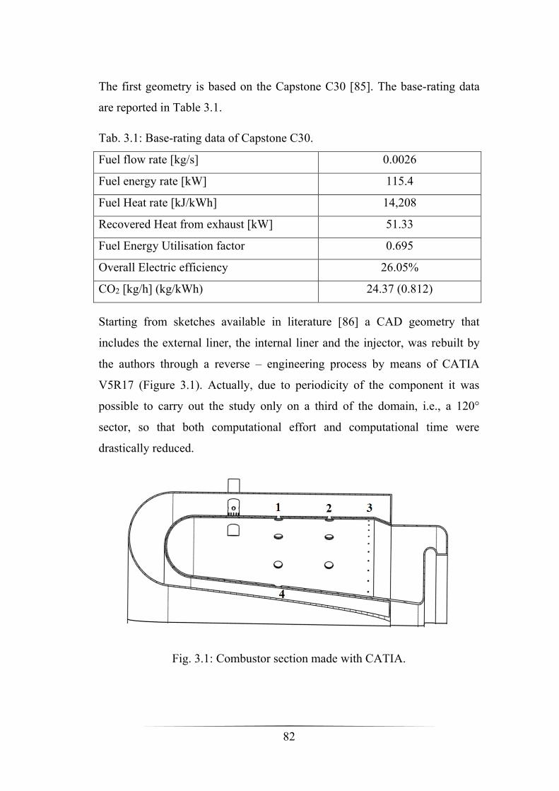
82
The first geometry is based on the Capstone C30 [85]. The base-rating data
are reported in Table 3.1.
Tab. 3.1: Base-rating data of Capstone C30.
Fuel flow rate [kg/s] 0.0026
Fuel energy rate [kW] 115.4
Fuel Heat rate [kJ/kWh] 14,208
Recovered Heat from exhaust [kW] 51.33
Fuel Energy Utilisation factor 0.695
Overall Electric efficiency 26.05%
CO2 [kg/h] (kg/kWh) 24.37 (0.812)
Starting from sketches available in literature [86] a CAD geometry that
includes the external liner, the internal liner and the injector, was rebuilt by
the authors through a reverse – engineering process by means of CATIA
V5R17 (Figure 3.1). Actually, due to periodicity of the component it was
possible to carry out the study only on a third of the domain, i.e., a 120°
sector, so that both computational effort and computational time were
drastically reduced.
Fig. 3.1: Combustor section made with CATIA.
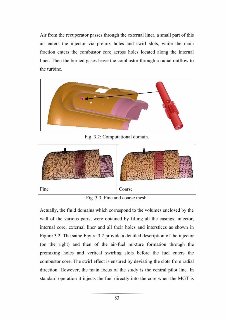
83
Air from the recuperator passes through the external liner, a small part of this
air enters the injector via premix holes and swirl slots, while the main
fraction enters the combustor core across holes located along the internal
liner. Then the burned gases leave the combustor through a radial outflow to
the turbine.
Fig. 3.2: Computational domain.
Fine
Coarse
Fig. 3.3: Fine and coarse mesh.
Actually, the fluid domains which correspond to the volumes enclosed by the
wall of the various parts, were obtained by filling all the casings: injector,
internal core, external liner and all their holes and interstices as shown in
Figure 3.2. The same Figure 3.2 provide a detailed description of the injector
(on the right) and then of the air-fuel mixture formation through the
premixing holes and vertical swirling slots before the fuel enters the
combustor core. The swirl effect is ensured by deviating the slots from radial
direction. However, the main focus of the study is the central pilot line. In
standard operation it injects the fuel directly into the core when the MGT is

84
operating at part loads, usually below 70%, but the authors’ proposal is to
exploit it to be an alternate option for hydrogen injection.
Moreover, two meshes, whose data are reported in Table 3.2, were created to
operate a sensitivity analysis (Figure 3.3).
Tab. 3.2: Details of the computational meshes.
Domain Pilot Premix Liner Core
Fine 1,350 33,000 130,000 240,000
Coarse 800 24,000 55,000 44,000
As demonstrated in paper [82] the coarse grid was considered as able to
provide a fair approximation of more refined results with a reduced
computational effort.
Regarding to the chemical kinetics, the authors have selected the methane
three-step oxidation mechanism by Novosselov and Malte [87]. Such a
scheme is completed, as well known, by a 5-equation set for the thermal and
prompt NO formation (Table 3.3).
The scheme reported in Table 3.4 describes the oxidation mechanism of the
other hydrocarbons present in Natural Gas (NG).
In addition, all the test cases involving hydrogen contents have been
simulated with the Jachimowski reduced scheme [88]. Such a scheme
includes the Zel’dovich reactions [89] in order to describe the oxidation
process of hydrogen together with a correct model of the nitrogen chemistry
in combustion (Table 3.5).
The CFD analysis was performed with the ANSYS-FLUENT solver where
all the reaction schemes in Tables 3.3, 3.4 and 3.5 were implemented, and the
EDC based method was adopted.
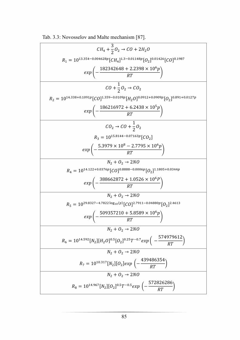
85
Tab. 3.3: Novosselov and Malte mechanism [87].
𝐶𝐻4 +3
2𝑂2 → 𝐶𝑂 + 2𝐻2𝑂
𝑅1 = 1013.354−0.004628𝑝[𝐶𝐻4]
1.3−0.01148𝑝[𝑂2]0.01426[𝐶𝑂]0.1987
𝑒𝑥𝑝 (−182342648 + 2.2398 × 10⁶𝑝
𝑅𝑇)
𝐶𝑂 +1
2𝑂2 → 𝐶𝑂2
𝑅2 = 1014.338+0.1091𝑝[𝐶𝑂]1.359−0.0109𝑝[𝐻2𝑂]
0.0912+0.0909𝑝[𝑂2]0.891+0.0127𝑝
𝑒𝑥𝑝 (−186216972 + 6.2438 × 10⁵𝑝
𝑅𝑇)
𝐶𝑂2 → 𝐶𝑂 +1
2𝑂2
𝑅3 = 1015.8144−0.07163𝑝[𝐶𝑂2]
𝑒𝑥𝑝 (−5.3979 × 10⁸ − 2.7795 × 10⁶𝑝
𝑅𝑇)
𝑁2 + 𝑂2 → 2𝑁𝑂
𝑅4 = 1014.122+0.0376𝑝[𝐶𝑂]0.8888−0.0006𝑝[𝑂2]
1.1805+0.0344𝑝
𝑒𝑥𝑝 (−388662872 + 1.0526 × 10⁶𝑃
𝑅𝑇)
𝑁2 + 𝑂2 → 2𝑁𝑂
𝑅5 = 1029.8327−4.7822 log10(𝑝)[𝐶𝑂]2.7911−0.04880𝑝[𝑂2]
2.4613
𝑒𝑥𝑝 (−509357210 + 5.8589 × 10⁶𝑝
𝑅𝑇)
𝑁2 + 𝑂2 → 2𝑁𝑂
𝑅6 = 1014.592[𝑁2][𝐻2𝑂]
0.5[𝑂2]0.25𝑇−0.7𝑒𝑥𝑝 ( −
574979612
𝑅𝑇)
𝑁2 + 𝑂2 → 2𝑁𝑂
𝑅7 = 1010.317[𝑁2][𝑂2]𝑒𝑥𝑝 (−
439486354
𝑅𝑇)
𝑁2 + 𝑂2 → 2𝑁𝑂
𝑅8 = 1014.967[𝑁2][𝑂2]
0.5𝑇−0.5𝑒𝑥𝑝 (−572826286
𝑅𝑇)
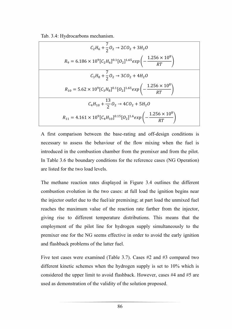
86
Tab. 3.4: Hydrocarbons mechanism.
𝐶2𝐻6 +7
2𝑂2 → 2𝐶𝑂2 + 3𝐻2𝑂
𝑅9 = 6.186 × 10⁹[𝐶2𝐻6]
0.1[𝑂2]1.65𝑒𝑥𝑝 (−
1.256 × 10⁸
𝑅𝑇)
𝐶3𝐻8 +7
2𝑂2 → 3𝐶𝑂2 + 4𝐻2𝑂
𝑅10 = 5.62 × 10⁹[𝐶3𝐻8]
0.1[𝑂2]1.65𝑒𝑥𝑝 (−
1.256 × 10⁸
𝑅𝑇)
𝐶4𝐻10 +13
2𝑂2 → 4𝐶𝑂2 + 5𝐻2𝑂
𝑅11 = 4.161 × 10⁹[𝐶4𝐻10]
0.15[𝑂2]1.6𝑒𝑥𝑝 (−
1.256 × 10⁸
𝑅𝑇)
A first comparison between the base-rating and off-design conditions is
necessary to assess the behaviour of the flow mixing when the fuel is
introduced in the combustion chamber from the premixer and from the pilot.
In Table 3.6 the boundary conditions for the reference cases (NG Operation)
are listed for the two load levels.
The methane reaction rates displayed in Figure 3.4 outlines the different
combustion evolution in the two cases: at full load the ignition begins near
the injector outlet due to the fuel/air premixing; at part load the unmixed fuel
reaches the maximum value of the reaction rate farther from the injector,
giving rise to different temperature distributions. This means that the
employment of the pilot line for hydrogen supply simultaneously to the
premixer one for the NG seems effective in order to avoid the early ignition
and flashback problems of the latter fuel.
Five test cases were examined (Table 3.7). Cases #2 and #3 compared two
different kinetic schemes when the hydrogen supply is set to 10% which is
considered the upper limit to avoid flashback. However, cases #4 and #5 are
used as demonstration of the validity of the solution proposed.

87
Tab. 3.5: Jachimowski and Zeldovich mechanisms.
𝐻 + 𝑂𝐻 +𝑀 = 𝐻2𝑂 +𝑀
𝑅1 = 2.21 × 10¹⁶[𝐻][𝑂𝐻] 𝑇−2
𝐻 + 𝐻 +𝑀 = 𝐻2 +𝑀
𝑅2 = 7.3 × 10¹¹[𝐻][𝐻] 𝑇−1
𝐻2 +𝑂2 = 𝑂𝐻 + 𝑂𝐻
𝑅3 = 1.7 × 10¹⁰[𝐻2][𝑂2]𝑒𝑥𝑝 (−
2.0083 × 10⁸
𝑅𝑇)
𝐻 + 𝑂2 = 𝑂𝐻 + 𝑂
𝑅4 = 1.2 × 10¹⁴[𝐻][𝑂2]𝑇
−0.91𝑒𝑥𝑝 (−6.9086 × 10⁷
𝑅𝑇)
𝑂𝐻 + 𝐻2 = 𝐻2𝑂 + 𝐻
𝑅5 = 2.2 × 10¹⁰[𝑂𝐻][𝐻2]𝑒𝑥𝑝 (−
2.1548 × 10⁷
𝑅𝑇)
𝑂 +𝐻2 = 𝑂𝐻 + 𝐻
𝑅6 = 50.6[𝑂][𝐻2]𝑇2.67𝑒𝑥𝑝 (−
2.6317 × 10⁷
𝑅𝑇)
𝑂𝐻 + 𝑂𝐻 = 𝐻2𝑂 + 𝑂
𝑅7 = 6.3 × 10⁹[𝑂𝐻][𝑂𝐻]𝑒𝑥𝑝 (−
4560560
𝑅𝑇)
𝑁 + 𝑁 +𝑀 = 𝑁2 +𝑀
𝑅8 = 2.8 × 10¹¹[𝑁][𝑁]𝑇−0.8
𝑂 + 𝑂 +𝑀 = 𝑂2 +𝑀
𝑅9 = 1.1 × 10¹¹[𝑂][𝑂]𝑇−1
𝑁 + 𝑂2 = 𝑁𝑂 + 𝑂
𝑅10 = 6400000 × [𝑁][𝑂2]𝑇1𝑒𝑥𝑝 (−
2.6359 × 10⁷
𝑅𝑇)
𝑁 + 𝑁𝑂 = 𝑁2 + 𝑂
𝑅11 = 1.6 × 10¹⁰[𝑁][𝑁𝑂]
𝑁 + 𝑂𝐻 = 𝑁𝑂 + 𝐻
𝑅12 = 6.3 × 10⁸[𝑁][𝑂𝐻]𝑇0.5

88
Tab. 3.6 Boundary condition data for the combustion simulation
Base Rating 70% Load
Combustor Inlet Temperature (K) 870 883
Combustor Outlet Pressure (bar) 3.20 2.62
Fuel mass flow rate (kg/s) 0.00292 0.00183
Oxidant mass flow rate (kg/s) 0.306 0.270
Overall equivalence ratio 0.143 0.102
Base – Rating
Rate of reaction
[kg/(m3s)]
70% Load
Fig. 3.4 Comparison of methane reaction rates at base-rating and part-load.
Tab. 3.7: Test cases
Case #1 Base – Rating, Natural Gas from premixer
Case #2 90% NG from premixer – 10% H2 from pilot
(Nitric Oxides from Novosellov and Malte scheme)
Case #3 90% NG from premixer – 10% H2 from pilot
(Nitric Oxides from Jachimowski scheme)
Case #4 75% NG from premixer – 25% H2 from pilot
(Nitric Oxides from Jachimowski scheme)
Case #5 75% NG– 25% H2 mixture from premixer
(Nitric Oxides from Jachimowski scheme)
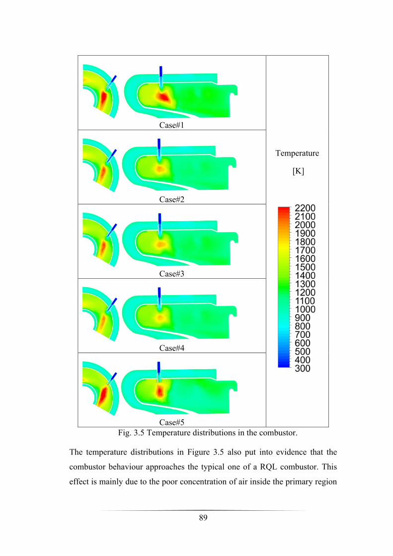
89
Case#1
Temperature
[K]
Case#2
Case#3
Case#4
Case#5
Fig. 3.5 Temperature distributions in the combustor.
The temperature distributions in Figure 3.5 also put into evidence that the
combustor behaviour approaches the typical one of a RQL combustor. This
effect is mainly due to the poor concentration of air inside the primary region

90
of the core. The air flow delivery from the secondary and dilution holes
produces a typical quick mixing with the combustion products with a
consequent steep decrease in temperature. The combustion completion takes
place, therefore, under lean conditions and the nitric oxide formation is
strongly decelerated.
Tab. 3.8 Volume averaged and outlet properties from CFD.
Case Tmax
[K]
Tout
[K] NO
[ppm]
CO
[ppm]
Burned CH4
[%]
Burned H2
[%]
#1 2567 1206 5.07 462 99.86 --
#2 2274 1159 3.82 841 99.60 99.99
#3 2296 1178 5.38 1153 99.80 99.99
#4 2140 1178 5.88 836 99.63 99.87
#5 2717 1153 8.01 728 99.79 99.99
From the results in Table 3.8, it is noted that in all the cases the value of the
NO calculated are close to that provided by the manufacturer, meaning that
the kinetic mechanisms can well describe the chemistry of the process. In
cases #2 and #3, with the 10% of H2 from pilot, the maximum temperature
and, consequently, the NO values decrease. On the other hand, despite the
lower peak of temperature in the primary zone in case #4 presents higher
values of NO amount since hydrogen has the higher flame temperature.
Furthermore, case #5 highlight the highest temperature levels and NO
emissions due to the intake of hydrogen in the premixing duct which leads to
an unusual combustion. Such a phenomenon is highlighted in the Figure 3.6
where a comparison between the H2 reaction rate distributions in a larger
picture of the injector plane is shown. In the case #5, as expected, the ignition
starts in the premixing line. Therefore, the proposed supply solution appears
to be effective for the combined use of hydrogen and natural gas in order to
avoid a pre-ignition inside the premixing line and gives the possibility of
reaching higher H2/NG ratios. Moreover, the results in Table 3.8 put into
evidence that a nearly complete oxidation of both methane and hydrogen.

91
Nevertheless, the same Table 3.8 indicates that non-negligible amounts of
carbon monoxide are produced by the several combustion regimes. Such
amounts are generally increased in all cases with hydrogen, so that a slight
decrease in combustion efficiency should be taken into account.
H2 from pilot
H2 from premixer
Rate of reaction
[kg/(m3s)]
Fig. 3.6 Comparison between the reaction rate of H2 when injected from the
pilot or the premixer.
Tab. 3.9 Maximum reaction rates.
Case CH4 oxidation rate [kg/(m3s)] H2 oxidation rate [kg/(m3s)]
#2 5.82 28.49
#3 12.77 27.92
#4 14.28 23.46
#5 30.77 38.13
Finally, in Table 3.9 the reaction rates for CH4 and H2 are compared. As it is
possible to notice, in all cases the maximum reaction rate for hydrogen is
higher than the rate for methane. Also, Figure 3.7 evidences that the zones of
higher methane consumption are located in correspondence of the zone of
higher reaction rates of hydrogen. This means that hydrogen represents a sort
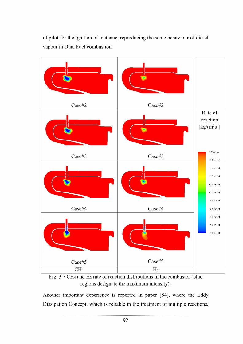
92
of pilot for the ignition of methane, reproducing the same behaviour of diesel
vapour in Dual Fuel combustion.
Case#2
Case#2
Rate of
reaction
[kg/(m3s)]
Case#3
Case#3
Case#4
Case#4
Case#5
Case#5
CH4 H2
Fig. 3.7 CH4 and H2 rate of reaction distributions in the combustor (blue
regions designate the maximum intensity).
Another important experience is reported in paper [84], where the Eddy
Dissipation Concept, which is reliable in the treatment of multiple reactions,

93
is compared with flamelet-PDF based approach. The mixture fraction theory,
as widely illustrated in Chapter 2, can be applied to non-premixed and
partially premixed flames where a strong dependence on convection and
diffusion caused by turbulence is observed. Once mixed, the chemistry can
be modelled as being in chemical equilibrium (CE), near chemical
equilibrium with the Steady Laminar Flamelet (SLF) or far from it with the
Unsteady Laminar Flamelet model. The kinetic mechanisms of Novosselov
and Jachimowski (Tables 3.3, 3.4 and 3.5) are used, respectively for the
hydrocarbons oxidation, and for the complex hydrogen kinetics. In order to
evaluate the quality of the results, the reference case was also simulated with
the well-established GRIMECH mechanisms consisting of 53 species and
325 reactions, since it includes detailed kinetics for both hydrocarbons and
hydrogen.
In Table 3.10 the test cases with the relative model and configuration are
listed, the simulations were performed in accordance with the same boundary
conditions reported in Table 3.6 for the full load.
Tab. 3.10: Test cases.
Case Model Fuel
#4 EDC NG
#5 EDC (GRIMECH) NG
#6 SLF NG
#7 CE NG
#8 SLF 75%NG + 25%H2 Premixed
#9 CE 75%NG + 25%H2 Separated fuel streams
It is important to highlight that the use of the CE model was necessary
because it is the only model in ANSYS-FLUENT that allows two distinct
fuel streams, with two different compositions to be set. Actually, before

94
utilising hydrogen, first attempts with these models have been carried out by
suppling the MGT combustor with natural gas only.
Tab. 3.11: Volume averaged and outlet properties from CFD.
Case Tmax
[K]
Tout
[K]
NO
[ppm]
CO
[ppm]
Burned CH4
[%]
Burned H2
[%]
#4 2567 1206 5.07 462 99.88 --
#5 2458.6 1263 38 1602 99.88 --
#6 2475.8 1116 417 9.3e-2 77.62 --
#7 2504.6 1093.7 163 7.6e-10 70.47 --
#8 2543 1086 276 0.63 68.79 62.79
#9 2540 1129.8 607 1.36 83.31 83.31
From Table 3.11 it is possible to see that in cases with EDC model
combustion is highly efficient and NOx emissions comply with the
manufacturer’s data. Even if the cases with the PPC models present lower
temperature at outlet, a higher value of NOx has been calculated; however,
CO concentrations are near to zero but in the two cases with hydrogen, CH4
is not able to oxide completely maybe due to the presence of hydrogen itself.
Figure 3.8 shows the temperature’s levels; case #4 presents higher values
while case #5 is characterised by a wider zone at high temperature. It is
important to notice that cases #6 and #7, both employing the pdf tables but
with either the flamelet or the chemical equilibrium approach, do not present
differences. For this reason, it is possible to try a comparison between two
modes of injecting H2 in the combustor. The only PPC model that allows
utilisation of two different fuel streams is the CE, so in case #8 25% of
hydrogen is mixed with the NG in the premix line, while in case #9 he same
amount of hydrogen is injected separately from the pilot line.
This time, the early hydrogen ignition occurs in both cases #8 and #9. In the
former as already proven in [82] this behaviour was expected, while for case
#9 it can be explained by two different reasons: the first one is related to the
CE model, apparently even without the high reactivity of hydrogen, natural
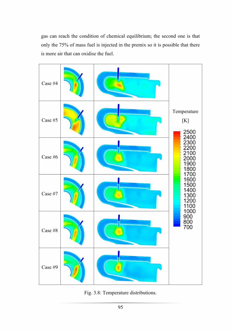
95
gas can reach the condition of chemical equilibrium; the second one is that
only the 75% of mass fuel is injected in the premix so it is possible that there
is more air that can oxidise the fuel.
Case #4
Temperature
[K]
Case #5
Case #6
Case #7
Case #8
Case #9
Fig. 3.8: Temperature distributions.

96
3.2 Dual Fuel diesel engines
Previous to the studies directly involving the Ph. D candidate, the Dual Fuel
technology has represented the object of investigation of a research group in
the University of Naples “Federico II”. In the last decade, it has collected a
series of results that represent the basis for this thesis. To better understand
the evolution of the work carried out by the author, an overview of the
previous findings is reported in this section.
The first studies [57, 58, 59] were focused on the evaluation of the CFD
potential to predict the main features of combustion and pollutant formation
of a common rail diesel engine supplied with natural gas and diesel oil, under
different conditions induced by different choices of the operating parameters
and fuel ratio. Indeed, the calculations were compared with experimental data
obtained on a light duty direct injection diesel engine at steady state test
bench whose characteristics are outlined in Table 3.12:
Tab. 3.12: Characteristics of the engine used in the experimental activity.
Engine 1.9 Multijet
Type 4 stroke CI
Number of cylinders 4
Valves/cylinder 2
Bore [mm] 82
Stroke [mm] 90.4
Cylinder volume displacement [cm3] 480
Maximum power [kW] 88
Maximum torque [Nm] 255 @ 2,000 rpm
Compression ratio 18:1
The experimental activity was carried out at Istituto Motori (CNR) on a
diesel engine fuelled by either diesel oil (full diesel operation, FD) or natural
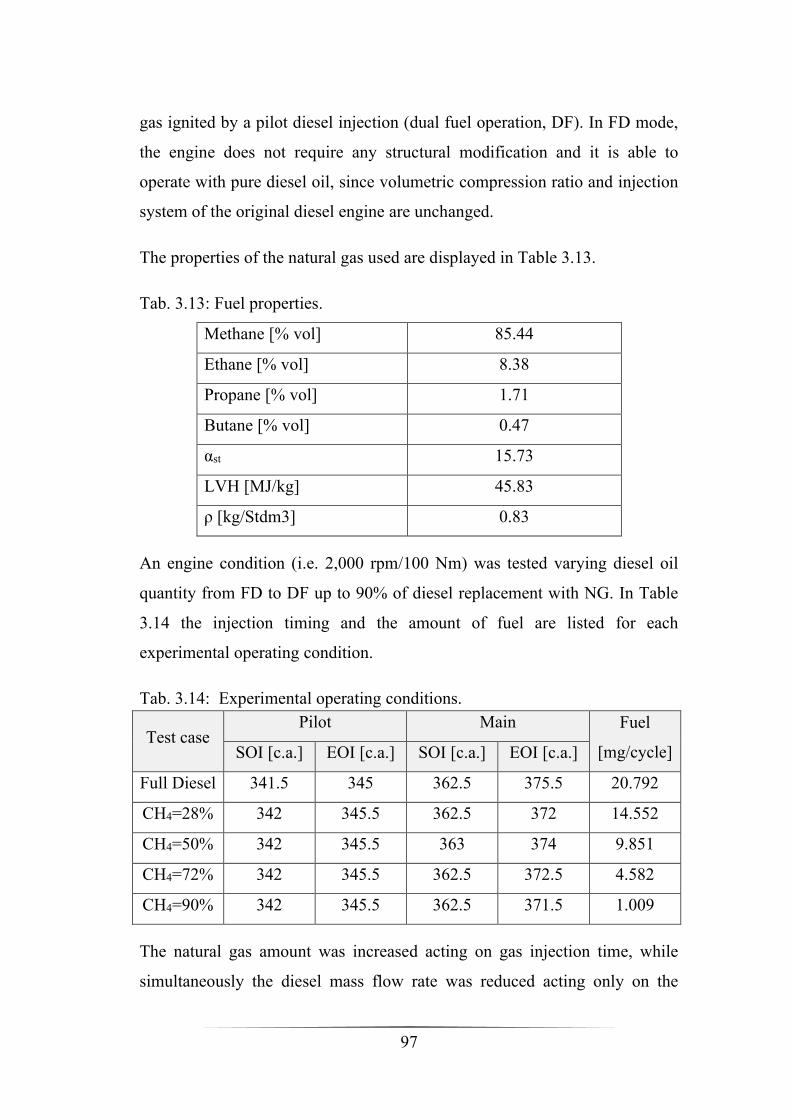
97
gas ignited by a pilot diesel injection (dual fuel operation, DF). In FD mode,
the engine does not require any structural modification and it is able to
operate with pure diesel oil, since volumetric compression ratio and injection
system of the original diesel engine are unchanged.
The properties of the natural gas used are displayed in Table 3.13.
Tab. 3.13: Fuel properties.
Methane [% vol] 85.44
Ethane [% vol] 8.38
Propane [% vol] 1.71
Butane [% vol] 0.47
αst 15.73
LVH [MJ/kg] 45.83
ρ [kg/Stdm3] 0.83
An engine condition (i.e. 2,000 rpm/100 Nm) was tested varying diesel oil
quantity from FD to DF up to 90% of diesel replacement with NG. In Table
3.14 the injection timing and the amount of fuel are listed for each
experimental operating condition.
Tab. 3.14: Experimental operating conditions.
Test case Pilot Main Fuel
[mg/cycle] SOI [c.a.] EOI [c.a.] SOI [c.a.] EOI [c.a.]
Full Diesel 341.5 345 362.5 375.5 20.792
CH4=28% 342 345.5 362.5 372 14.552
CH4=50% 342 345.5 363 374 9.851
CH4=72% 342 345.5 362.5 372.5 4.582
CH4=90% 342 345.5 362.5 371.5 1.009
The natural gas amount was increased acting on gas injection time, while
simultaneously the diesel mass flow rate was reduced acting only on the

98
injection pressure, leaving the injection advance and the pilot and the main
duration unchanged with respect to the FD mode. In this way, the liquid fuel
injection conditions have been the same in FD and DF operation, since the
test points have been set at the same injection advance both in FD and DF
mode.
Fig. 3.9: Experimental Rate of Heat Releases by varying the NG ratio.
In Figure 3.9 the rate of heat release is plotted for a better understanding of
combustion development by varying natural gas ratio. These operating
conditions are characterised by high THC emissions and low efficiency. On
the other hand, at high power output the combustion conditions achieve a
relevant improvement but, since there is at least one ignition start point for
each diesel injector hole, the combustion speed can become so high as to
induce knocking, despite of the high methane octane number (130). This
behaviour causes difficulties for an effective control of the DF combustion.
In the CH4 = 90% case the start of natural gas ignition is anticipated with a
sudden slope causing a formation of NOx certainly greater (Figure 3.10)
while the CO contents decrease (Figure 3.11).

99
The experimental activity was used as a validating tool for the evaluation of
the numerical calculations’ potential. It should be highlighted that the
authors’ approach to the study of the dual fuel diesel engine, in this first
phase, was different from the classical numerical-experimental matching.
Indeed, according with the experimental tests, some numerical results
obtained in similar operating conditions were analysed although some key
aspects differ considerably.
Fig. 3.10: Experimental mass fraction of NO.
Fig. 3.11: Experimental mass fraction of CO.

100
Since, a mesh grid of the actual engine geometry was not available, the
calculations were carried out on a different geometry which, as reported in
Table 3.15, has almost the same cylinder displacement but different
volumetric pressure ratio and external duct shape. In addition, the cylinder
considered for the CFD is a four-valve one, while the engine at the test bed
has only two valves per cylinder.
Tab. 3.15: Characteristics of the engine used in the numerical activity.
Engine 3.0 Multijet
Type 4 stroke CI
Number of cylinders 6
Valves/cylinder 4
Bore [mm] 84
Stroke [mm] 90
Cylinder volume displacement [cm3] 499
Compression ratio 16:1
The cylinder and duct structured dynamic mesh (Figure 3.12) was obtained
by using the ANSYS-ICEM CFD meshing tool. The multi-block structured
Cartesian grid was set up as a result of the mesh generation consistent with
the valve geometry. The grid size independence was reached with a mesh of
104,000 cells, the cylinder and bowl volume discretization being of nearly
58,000 and 5000 cells respectively. It is worth-noting that such a reduced
mesh size produced, however, a fair convergence of the results if compared
with those obtained with more refined grids, also due to the well-known
robustness of the KIVA3-V solver: this allowed the development of multiple
numerical cases in a reasonable computational time.
In order to examine the dual fuel combustion process in-cylinder and to
explore, as stated above, the potential, especially in terms of emissions, of
this new technology the CFD solver KIVA-3V was adopted.
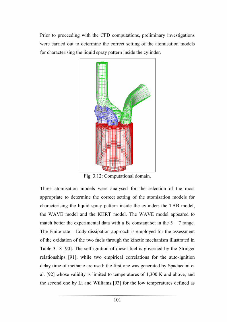
101
Prior to proceeding with the CFD computations, preliminary investigations
were carried out to determine the correct setting of the atomisation models
for characterising the liquid spray pattern inside the cylinder.
Fig. 3.12: Computational domain.
Three atomisation models were analysed for the selection of the most
appropriate to determine the correct setting of the atomisation models for
characterising the liquid spray pattern inside the cylinder: the TAB model,
the WAVE model and the KHRT model. The WAVE model appeared to
match better the experimental data with a B1 constant set in the 5 – 7 range.
The Finite rate – Eddy dissipation approach is employed for the assessment
of the oxidation of the two fuels through the kinetic mechanism illustrated in
Table 3.18 [90]. The self-ignition of diesel fuel is governed by the Stringer
relationships [91]; while two empirical correlations for the auto-ignition
delay time of methane are used: the first one was generated by Spadaccini et
al. [92] whose validity is limited to temperatures of 1,300 K and above, and
the second one by Li and Williams [93] for the low temperatures defined as

102
less than 1,300 K. The combustion simulation is completed by a system of
chemical kinetic equations for the mechanism of thermal nitric oxide
formation [89]. However, the computation of the ignition delay is activated
by starting from an auto-ignition threshold that was set at 1,100K.
Tab. 3.16: Kinetic mechanism [90].
1. 𝐶12𝐻26 + 37 2⁄ 𝑂2 → 12𝐶𝑂2 + 13𝐻2𝑂
𝑅𝑓1 = 3.0 × 10¹¹[𝐶12𝐻26]
0.25[𝑂2]1.5𝑒𝑥𝑝 (−
15,780
𝑇)
𝑅𝑏1 = 0
2. 𝐶𝐻4 + 3 2⁄ 𝑂2 → 𝐶𝑂 + 2𝐻2𝑂
𝑅𝑓2 = 1015.220[𝐶𝐻4]
1.460[𝑂2]0.5217𝑒𝑥𝑝 (−
20,643
𝑇)
𝑅𝑏2 = 0
3. 𝐶𝑂 + 1 2⁄ 𝑂2 → 𝐶𝑂2
𝑅𝑓3 = 1014.902[𝐶𝑂]1.6904[𝑂2]
1.570𝑒𝑥𝑝 (−11,613
𝑇)
𝑅𝑏3 = 1014.349[𝐶𝑂2]
1.0𝑒𝑥𝑝 (−62,281
𝑇)
Unlike the experimental tests, where the diesel oil injection consists of a pilot
and a main injection, in the numerical simulations only a main injection was
set for both FD and DF cases. Moreover, the fuel injection timing was
determined in order to produce, in all cases, the auto-ignition at
approximately the same crank angle.
The results of the CFD computations reported in Table 3.17, show that all
cases are characterised by almost the same level of indicated mean effective
pressure (IMEP) with a slight decrease for increasing NG rates and a
consequent decay in thermal efficiency.

103
Tab. 3.17: Numerical results.
CH4
[%]
IMEP
[bar]
Tout at EVO
[K]
CO2 at EVO
[%]
CO2 Index
[kg/kWh]
0 6.77 1093 10.14 0.750
28 6.49 1022 9.95 0.765
50 6.77 1036 9.27 0.686
72 6.61 1275 8.28 0.625
90 6.03 1243 7.95 0.658
On the opposite, the enhancement of the outlet temperature implies a
different response of the turbocharging system when the engine is operating
in dual fuel mode. Most important is the reduction of CO2 content and CO2
index when increasing the CH4 rate which demonstrate the effective benefit
attainable from the dual fuel concept adoption.
The pressure cycles, displayed in Figure 3.13, refer to the most significant
cases. It is possible to notice that, by increasing the methane rate, the shape
of the pressure cycles and the peak pressure positions and levels change, due
to a different combustion development. The distributions in a bowl
meridional section in Figure 3.14 also confirm that the methane combustion
in the 90% case induces higher temperature peaks in proximity of TDC with
respect to the 50% case because of a sudden growing to a full combustion
immediately after the pilot injection start.
The Figure 3.15 shows the NO distribution at the same crank angle and the
highest concentration is present in the 90% case, as expected.
The comparison of numerical and experimental results outlined in Figure
3.16, evidences that a good agreement can be found in terms of in-cylinder
pressures. The enhanced peaks at the highest values of methane (or NG)
contents confirms that an optimization of the injection timing is necessary to
ensure a regular combustion development.
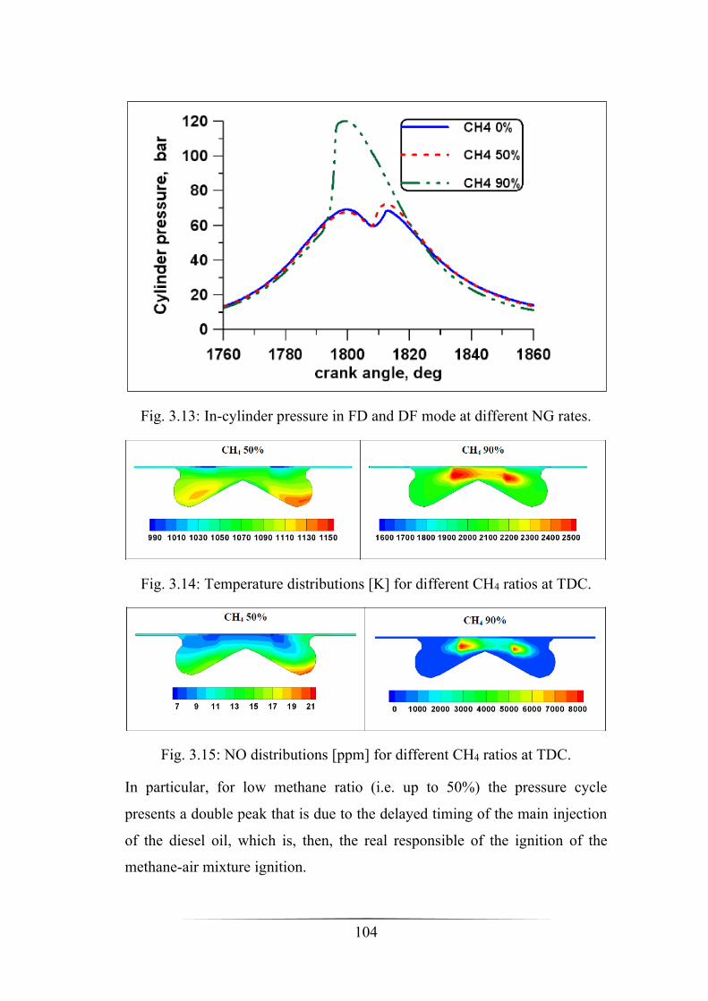
104
Fig. 3.13: In-cylinder pressure in FD and DF mode at different NG rates.
Fig. 3.14: Temperature distributions [K] for different CH4 ratios at TDC.
Fig. 3.15: NO distributions [ppm] for different CH4 ratios at TDC.
In particular, for low methane ratio (i.e. up to 50%) the pressure cycle
presents a double peak that is due to the delayed timing of the main injection
of the diesel oil, which is, then, the real responsible of the ignition of the
methane-air mixture ignition.

105
Fig. 3.16: Comparison of pressure cycles at different CH4 rates.

106
On the contrary, at CH4 = 90%, it is evident that the mixture ignition occurs
after the pilot injection but before the main injection and in advance with
respect to the TDC. This explains the single peak and the steeper pressure
rise that can even lead to knock.
Fig. 3.17: Comparison of experimental and numerical NO and CO2 fractions.
Finally, by examining the CO2 and NO levels in Figure 3.17, the
experimental and numerical levels trends show a reasonable accordance in
terms of variation of these species with the NG contents. Both numerical and
experimental results suggest an increase of NO for the higher rations of CH4,

107
while a slight decrease in the CO2 fraction is obtained because of the
diminished H/C ratio in the fuel blend. It is worth-noting that the typical
trade-off between these noxious species can be observed up to nearly 40 –
50% of methane rate. Beyond such limits, a simultaneous reduction in both
pollutants occurs as a consequence of the increased air/fuel ratios together
with the variations in the injection setup of the diesel fuel, like previously
discussed. NG rate at 70 – 90% levels lead to conditions close to knocking
and to a relevant increase of nitric oxides.
Such results point out that the CFD based activity is able to predict the engine
response to different rates of natural gas independently of the actual engine
geometry. However, in papers [60, 61] the authors discussed the results of a
numerical study on a domain that precisely reproduces the geometry of the
actual engine whose characteristics are listed in Table 3.14. In particular,
based on a new set of experimental tests the effect of different injection
timings on performance and pollutant fractions were analysed. Two data sets
were originated, one in FD and the other one in the DF operation with the
same boundary conditions (i.e. air mass flow rate, injection advance etc.) for
two different loads (50 and 100 Nm) at 2,000 rpm. In each test case the only
difference between FD and DF mode is the decreased amount of diesel fuel,
achieved by a reduction of the main injection duration, and compensated by
the injection of the gaseous fuel in the intake manifold to keep the same
engine torque. For each engine operating condition, several diesel injection
timings were tested. In particular, they were modified from extremely
advanced to largely delayed injections, with respect to the optimal value
adopted in full diesel condition. In the investigated test cases, the amount of
diesel oil was fixed at a minimum value (less than 20%), at given load and
speed, by varying the injection timing (Table 3.18). As a consequence, the
natural gas amount was automatically regulated and its measured value was
kept almost constant, i.e. nearly the 80% of the total fuel at 100 Nm and

108
about 75% at 50 Nm. The composition of the natural gas used during the
experimental activity is the same as already reported in Table 3.13.
Tab. 3.18: Testing operating conditions.
Test case Start of Pilot
BTDC
Pilot duration
[CAD]
Main duration
[CAD]
Rail Pressure
[bar]
FD
100 Nm
17
23
27
32
3.0
3.0
3.0
3.0
8.0
8.7
8.0
8.7
810
793
775
795
FD
50 Nm
15
20
26
29
3.2
3.0
3.6
3.9
8.0
8.1
8.0
7.5
591
568
565
565
DF
100 Nm
80% NG
17
23
27
33
3.0
3.0
3.0
3.0
5.0
4.6
4.1
4.0
815
810
809
809
DF
50 Nm
75 % NG
16
22
27
31
4.0
3.6
3.1
3.7
5.1
5.5
5.0
4.7
626
626
625
624
In Figure 3.18 the trend of the measured emissions in FD and DF are
compared. In Figure 3.18 the experimental NO trends show a reduced
amount of the NO emissions in the dual fuel mode operations, compared with
the full diesel one, especially at part load operation. Also, the values decrease
for lower injection advances due to a milder combustion. The CO and HC
emissions (Figures 3.18.b and c), as expected, present an opposite trend with
respect to the NO one, and the values in the dual fuel mode at 50 Nm are
higher due to a not complete combustion. Moreover, in Figure 3.18.c the
emission of HC in full diesel are not reported because they are considered
negligible if compared with the levels of the dual fuel cases for all injection
advances.

109
a)
b)
c)
Fig. 3.18: Comparison of experimental a) NO, b) CO and c) HC in FD and
DF mode for the two load level.

110
Tab. 3.19 Engine efficiency and CO2 emissions.
Test case Start of Pilot
BTDC
CO2
[%]
Brake
Efficiency
EICO2
[g/kWh]
FD
100 Nm
17
23
27
32
6.0
6.1
6.0
6.2
34.3
37.3
37.3
36.8
484.8
465.6
464.7
480.3
FD
50 Nm
15
20
26
29
3.9
3.8
3.8
3.8
28.7
30.7
31.8
31.7
571.1
519.2
515.0
518.0
DF
100 Nm
80% NG
17
23
27
33
5.0
5.0
5.2
5.4
33.8
33.8
34.7
35.3
376.1
374.7
375.0
383.2
DF
50 Nm
75 % NG
16
22
27
31
3.4
3.3
3.3
3.4
21.2
21.9
22.8
27.7
462.0
454.1
482.1
431.9
The incomplete combustion typical of DF operation induces a general
decrease in the engine efficiency, especially at 50 Nm, as illustrated in Table
3.19. However, despite the efficiency reduction, not only the CO2 contents in
the exhausts but also the CO2 emission index decreases in the case of dual
fuel mode for both loads, so confirming the validity of this fuel supply
system. Generally, the delayed cases present a smooth combustion but with a
not really complete oxidation and then a lower combustion effectiveness that
affects the engine efficiency. On the other hand, an advanced diesel injection
improves the mixing between diesel oil and NG/air mixture in the
combustion chamber, allowing a better mixture homogeneity and therefore a
more efficient combustion development also with very lean mixtures. In
Figure 3.19 the experimental pressure cycles for the most advanced injection
timing are displayed for the two loads both in full diesel and dual fuel mode.

111
Fig. 3.19 Comparison of pressure cycles for FD and DF operation.
In accordance with the experimental test cases, 3D simulations were
performed by using the CFD ANSYS-FLUENT code. Once achieved a
satisfactory confidence level of the numerical activities, the aim of the
computational calculations was to search an optimized strategy to reduce
emissions and to avoid undesirable phenomena.
Fig. 3.20: Computational domain and unstructured mesh.

112
As already anticipated, the computational domain reproduces the geometry of
the actual engine (Figure 3.20). It includes the inlet and exhaust ducts and
open valve period. The cylinder and duct block-unstructured mesh was
obtained by means of the ANSYS meshing tool. The cylinder mesh size is of
about 600,000 cells at BDC and of 300,000 calls at TDC, while the bowl one
is of 84,000 cells.
The boundary conditions require the assignment of the inlet pressure and
temperature data and of the exhaust pressure. Such data were derived from
the experimental measurements at the intake and the exhaust manifolds. The
turbulent flow motion through the external ducts and inside the cylinder is
approached by a realizable k-ε, two-equation, model, while the diesel oil
atomisation is described by the Wave model. The Hardenberg & Hase
correlation was used to reproduce the combustion delay for the diesel fuel.
The combustion model relies on the Finite Rate – Eddy Dissipation scheme
with four reactions: the first three for the methane oxidation [87] and the last
one for the diesel oil oxidation as listed in Table 3.20:
Tab. 3.20: Kinetic mechanism.
1. 𝐶𝐻4 + 3 2⁄ 𝑂2 → 𝐶𝑂 + 2𝐻2𝑂
𝑅1 = 1013.354−0.004628𝑝[𝐶𝐻4]
1.3−0.01148𝑝[𝑂2]0.01426[𝐶𝑂]0.1987𝑒−
21932+269.4𝑝𝑇
2. 𝐶𝑂 + 1 2⁄ 𝑂2 → 𝐶𝑂2
𝑅2 = 1014.338−0.1091𝑝[𝐶𝑂]1.359−0.0109𝑝[𝐻2𝑂]
0.0912+0.0909𝑝[𝑂2]0.891+0.0127𝑝𝑒−
21398+71.1𝑝𝑇
3. 𝐶𝑂2 → 𝐶𝑂 + 1 2⁄ 𝑂2
𝑅3 = 1015.8114+0.07163𝑝[𝐶𝑂2]𝑒
−649258−334.31𝑝
𝑇
4. 𝐶10𝐻22 + 31 2⁄ 𝑂2 → 10𝐶𝑂2 + 11𝐻2𝑂
𝑅4 = 2.587 × 10⁹[𝐶10𝐻22]
0.25[𝑂2]1.5𝑒−
15106𝑇
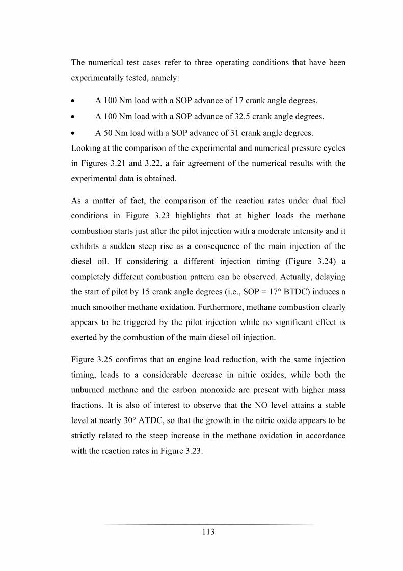
113
The numerical test cases refer to three operating conditions that have been
experimentally tested, namely:
• A 100 Nm load with a SOP advance of 17 crank angle degrees.
• A 100 Nm load with a SOP advance of 32.5 crank angle degrees.
• A 50 Nm load with a SOP advance of 31 crank angle degrees.
Looking at the comparison of the experimental and numerical pressure cycles
in Figures 3.21 and 3.22, a fair agreement of the numerical results with the
experimental data is obtained.
As a matter of fact, the comparison of the reaction rates under dual fuel
conditions in Figure 3.23 highlights that at higher loads the methane
combustion starts just after the pilot injection with a moderate intensity and it
exhibits a sudden steep rise as a consequence of the main injection of the
diesel oil. If considering a different injection timing (Figure 3.24) a
completely different combustion pattern can be observed. Actually, delaying
the start of pilot by 15 crank angle degrees (i.e., SOP = 17° BTDC) induces a
much smoother methane oxidation. Furthermore, methane combustion clearly
appears to be triggered by the pilot injection while no significant effect is
exerted by the combustion of the main diesel oil injection.
Figure 3.25 confirms that an engine load reduction, with the same injection
timing, leads to a considerable decrease in nitric oxides, while both the
unburned methane and the carbon monoxide are present with higher mass
fractions. It is also of interest to observe that the NO level attains a stable
level at nearly 30° ATDC, so that the growth in the nitric oxide appears to be
strictly related to the steep increase in the methane oxidation in accordance
with the reaction rates in Figure 3.23.
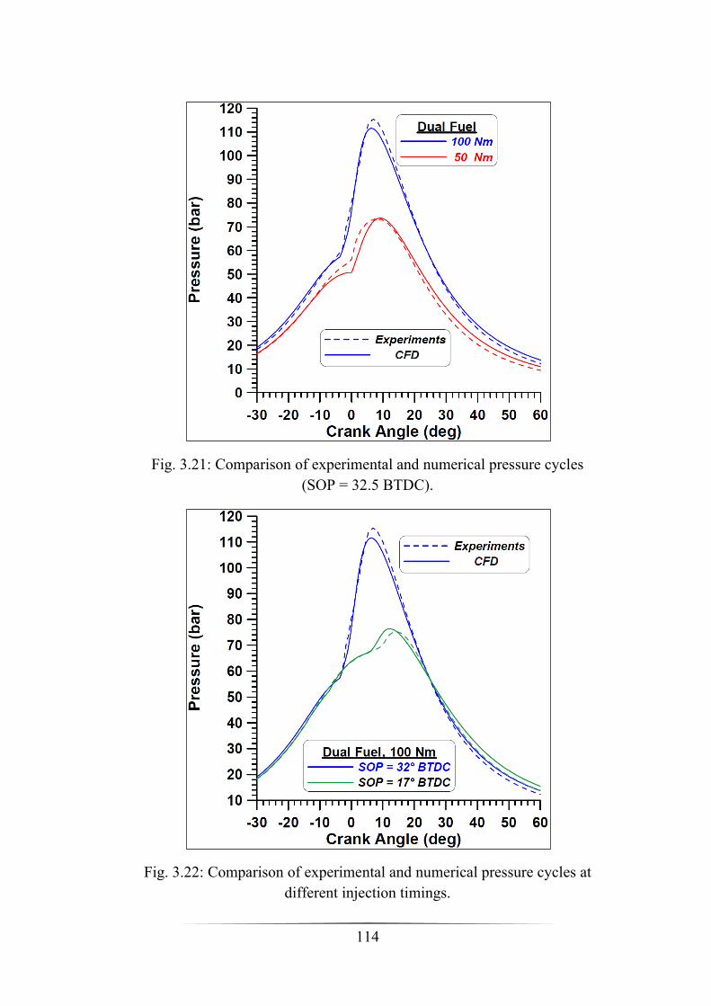
114
Fig. 3.21: Comparison of experimental and numerical pressure cycles
(SOP = 32.5 BTDC).
Fig. 3.22: Comparison of experimental and numerical pressure cycles at
different injection timings.
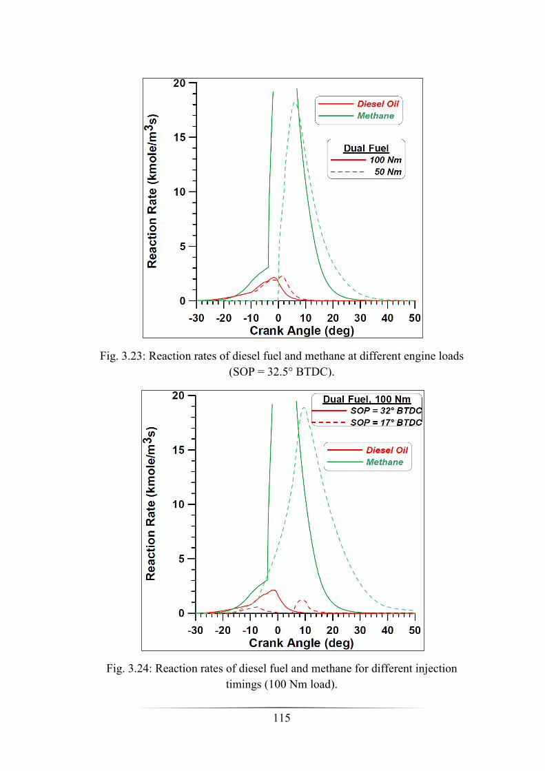
115
Fig. 3.23: Reaction rates of diesel fuel and methane at different engine loads
(SOP = 32.5° BTDC).
Fig. 3.24: Reaction rates of diesel fuel and methane for different injection
timings (100 Nm load).

116
Fig. 3.25: Pollutant formation and methane consumption at different engine
loads (SOP = 32.5°-31° BTDC).
Fig. 3.26: Pollutant formation and methane consumption for different
injection timings (100 Nm load).

117
Figure 3.26 highlights that advancing the start of injection (SOI) a more
efficient combustion is achieved with lower values of products of incomplete
combustion such as CH4 and CO. This is due to the higher pressure (Figure
3.22) and consequently, higher temperature reached. On the other hand, this
implies a greater formation of nitric oxides.
Moreover, when shifting from full diesel to dual fuel mode, the increases in
unburned methane and carbon monoxide emissions, appear to be not so
relevant in the case of a large injection advance (of nearly 32°) but they attain
unacceptable levels if operating the engine with a lower injection advance, of
17° BTDC.
TDC
Temperature [K]
100 Nm
10°ATDC
20°ATDC
Fig. 3.27: In-cylinder temperature distributions at 100 Nm load, Dual Fuel
(SOP = 32.5° BTDC).
Actually, at 100 Nm load with advanced SOP, a quite uniform temperature
distribution is observed after 10°ATDC. This can be intended as a
consequence of the steep combustion development that was observed in

118
Figure 3.23. On the contrary, at 50 Nm the temperature pattern is more
irregular, probably due to the major difficulties in the flame front propagation
throughout the methane-air mixture.
TDC
Temperature [K]
50 Nm
10°ATDC
20°ATDC
Fig. 3.28: In-cylinder temperature distributions at 50 Nm load, Dual Fuel
(SOP = 31° BTDC).
TDC
Methane
100 Nm
10°ATDC
Fig. 3.29: In-cylinder distributions of methane mass fraction at 100 Nm load,
Dual Fuel (SOP = 32.5 BTDC).

119
Figure 3.29 evidences that, at the higher load, the fuel consumption is almost
completed at 10° ATDC and the unburned methane contents are practically
negligible, as already shown in Figure 3.25.
TDC
Methane
50 Nm
10°ATDC
20°ATDC
Fig. 3.30: In-cylinder distributions of methane mass fraction at 50 Nm load,
Dual Fuel (SOP = 32.5 BTDC).
Figure 3.30 confirms that by reducing the engine load, a slower consumption
of methane is achieved at 10 crank angle degrees, because of the lower
reaction rate already outlined in Figure 3.23. Finally, retarding the start of
pilot injection (i.e., 17° BTDC), the difficulties in the methane combustion
development appear to be more evident. Indeed, in Figure 3.31 it is clearly
shown that in the squish zone of the chamber non-negligible methane
contents are still detected and this explains the increased levels of unburned
species displayed in the previous Figure 3.26.

120
TDC
Methane
100 Nm
10°ATDC
20°ATDC
Fig. 3.31: In-cylinder distributions of methane mass fraction at 100 Nm load,
dual fuel (SOP = 17 BTDC).
121
Chapter 4
LIGHT DUTY ENGINE
Based on the experimental activity illustrated in the previous chapter [60,
61], in this section an integrated numerical methodology between a one-
dimensional and a three-dimensional code is developed with the aim to
predict the behaviour of a light duty engine by varying injection advance in
full diesel and dual fuel modes [94].
4.1 Methodology
The phenomena that occur in the cylinder are very complex and strongly
depend on the boundary conditions imposed at the cylinder control system.
Usually, the reduced experimental test cases available do not allow an overall
view of the engine behaviour in the different operating conditions, therefore
by combining the results of one-dimensional and three-dimensional models,
it is possible to carry out correlations in order to extend the range of
functioning.
In particular, starting from experimental test cases carried out at a test bench
at Istituto Motori and reported in the previous chapter [60, 61] in Table 3.18,
a proper calibration of numerical models has been implemented in order to
reach a quite good fitting between experimental and numerical results. Then,
the results obtained from 3D simulations provide to the 1D model the
information necessary to build correlations between parameters that
characterise the development of combustion (start, duration and heat release
peak position) on an extended range. In this way, in turn, once the most
interesting cases are identified, the same correlations provide the boundary
conditions to CFD simulations to deeper investigate the in-cylinder processes
such as the in-cylinder fuel vapour, temperature, burning rate distributions.

122
The reason behind this procedure is due to the advantages of one-dimensional
codes that allow to perform fast calculations and to simulate the whole
engine, not only the combustion inside the cylinder but including the
turbocharger, the intake and exhaust systems and other control devices. On
the other hand, the 3D calculation requires several consecutive cycles to
achieve convergence and therefore long computational times. However, only
the CFD analysis allows to better understand the mechanisms which govern
the combustion phenomenon inside the cylinder.
The calculations have been referred to a light duty direct injection
diesel engine whose specifications are reported in Table 3.15. The reason of
the use of a different geometry from the one used in the experimental activity
was due to the necessity to study an engine with features compliant with
more modern engines.
4.2 One-dimensional Model
The solution of the commercial code is based on one-dimensional fluid
dynamics for the ducts and zero-dimensional in-cylinder calculation. Detailed
modelling of individual components is included to specify the phenomena in
the singular components. In this way the software can recreate the behaviour
of the whole engine. The first step is to give general information of the
engine as engine type (SI or CI) number of strokes, number of cylinders and
valve and of course the dimensions of the cylinder (Table 4.1, the same as
Table 3.15). The building of the engine is made by adding the various
components and linking each other on a canvas (Figure 4.1). Some objects
are designed and utilised for a specific purpose such as the cylinder and the
turbocharger, while other objects like the air filter and the muffler can be
obtained by the combination of pipes and junctions.
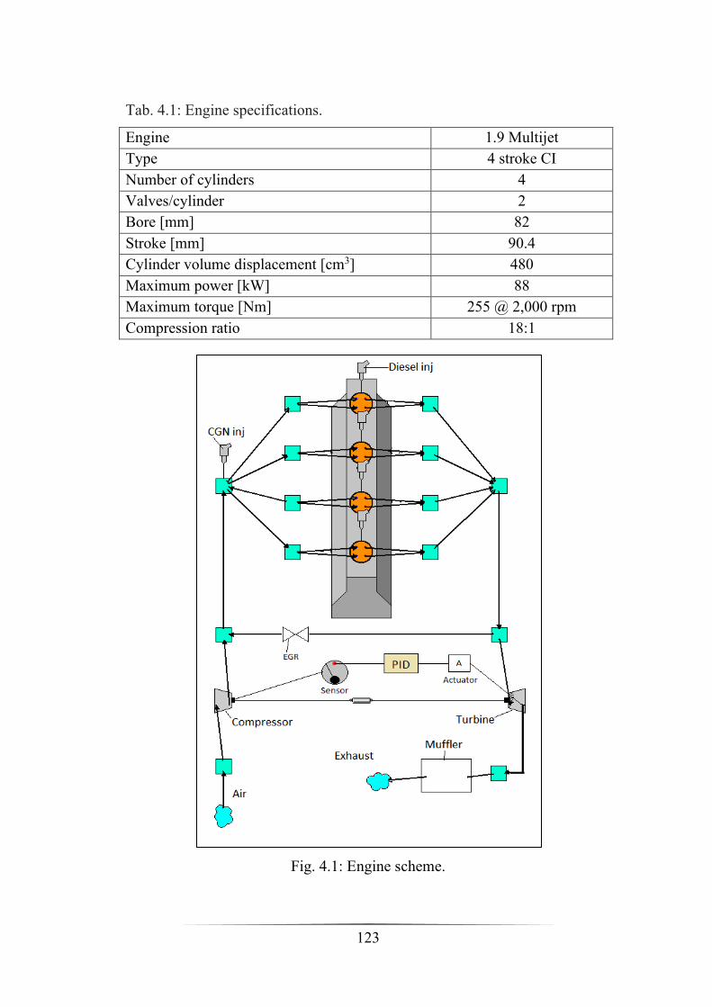
123
Tab. 4.1: Engine specifications.
Engine 1.9 Multijet
Type 4 stroke CI
Number of cylinders 4
Valves/cylinder 2
Bore [mm] 82
Stroke [mm] 90.4
Cylinder volume displacement [cm3] 480
Maximum power [kW] 88
Maximum torque [Nm] 255 @ 2,000 rpm
Compression ratio 18:1
Fig. 4.1: Engine scheme.

124
The engine is a turbocharged four cylinders, four strokes and four valves per
cylinder, there is also an EGR valve which in this study is kept constantly
closed. Also, a PID controlled is put on the vane opening of the Variable
Geometry Turbine in order to obtain a fixed boost pressure while a sensor is
linked to the compressor exit as feedback of the pressure ratio. The NG
injector is located before the different intake pipes that lead to each cylinder
since it constantly injects a certain amount of gas (expressed in kg/h).
Instead, a diesel injector is dedicated for each cylinder since diesel oil is
directly in the chamber, the nozzle injects a fixed mass (mg) each cycle and
the law of injection is composed of a pilot and a main.
The Annand model is set to describe the heat transfer between the colder
cylinder walls and the hot gas:
𝑄 = ℎ𝑐𝐴(𝑇𝑔 − 𝑇𝑤)
The first term represents the heat exchanged by convection, 𝐴 is the surface
of heat exchange, 𝑇𝑔 and 𝑇𝑤 are respectively the temperature of the hot gas
and cold walls, the focus of this correlation is the coefficient ℎ𝑐 that is related
to the engine parameters:
𝑁𝑢 = (ℎ𝑐𝑏
𝑘) = 𝑎 (
𝜌𝑆�̅�𝑏
𝜇)
𝑑
Where 𝑁𝑢 is the Nusselt number, 𝑏 is the bore, 𝑘 is thermal conductivity, 𝑎
is a constant in a range between 0.35 and 0.7, 𝜌 is the density of the gas, 𝑆�̅� is
mean piston speed, 𝜇 is the dynamic viscosity and 𝑑 is constant equal to 0.7.
For the combustion model the multi-Component Wiebe function is used to
describe the process. It is a composition of different single Wiebe function,
each of them estimates the mass fraction burned. The single Wiebe function
is expressed as:
𝑥𝑏 = {1 − 𝑒𝑥𝑝 [−𝑎 (𝜃 − 𝜃0∆𝜃
)𝑚+1
]}

125
𝑎 is a constant related to the combustion duration ∆𝜃, and 𝑚 is the form
factor. The function indicates that the mass fraction burned profile grow from
zero (𝜃0) and tends to one, and the difference between the crank angles of the
start and the end of the combustion is the duration of the combustion.
In the full diesel mode two Wiebe curves have to be defines, the first for the
pilot and the second for the main while in dual fuel mode a third curve is
added for the NG combustion. For the three (or two) combustions the fitting
for the Wiebe correlation is made by assigning the three crank angles at
which three determined percentage in mass are burned, in particular the three
percentages are 0.5%, 50% and 98% that identify respectively the start, the
peak and the end of the burning law.
The released heat is obtained from the instantaneous burned mass fraction via
the following correlation:
𝑑𝑄𝑆𝑆𝑑𝜃
Δ𝜃 = 𝑚𝑏𝑘𝑖𝑑𝑥𝑏𝑑𝜃
Δ𝜃
For the data fitting of the Wiebe functions the three crank angles that identify
the law of fuel burning are obtained from CFD results.
4.3 Three-dimensional Model
CFD simulations have been referred to a light duty direct injection diesel
engine, whose geometry and mesh are reported in Figure 4.2. The cylinder
and bowl discretization is of 535,000 and 46,000 cells, respectively.
The computational domain includes the intake and exhaust ducts and
the valve profiles, in order to evaluate the mass exchange processes
The computational simulations were performed mean the three-dimensional
ANSYS-FLUENT code. Combustion is modelled with the Finite rate – Eddy
Dissipation model and a kinetic mechanism made of four reactions (Table
4.2).

126
Fig. 4.2: Mesh of the cylinder, intake and exhaust ducts.
Tab. 4.2: Kinetic mechanism [87].
1. 𝐶𝐻4 + 3 2⁄ 𝑂2 → 𝐶𝑂 + 2𝐻2𝑂
𝑅1 = 1013.354−0.004628𝑝[𝐶𝐻4]
1.3−0.01148𝑝[𝑂2]0.01426[𝐶𝑂]0.1987𝑒−
21932+269.4𝑝𝑇
2. 𝐶𝑂 + 1 2⁄ 𝑂2 → 𝐶𝑂2
𝑅2 = 1014.338−0.1091𝑝[𝐶𝑂]1.359−0.0109𝑝[𝐻2𝑂]
0.0912+0.0909𝑝[𝑂2]0.891+0.0127𝑝𝑒−
21398+71.1𝑝𝑇
3. 𝐶𝑂2 → 𝐶𝑂 + 1 2⁄ 𝑂2
𝑅3 = 1015.8114+0.07163𝑝[𝐶𝑂2]𝑒
−649258−334.31𝑝
𝑇
4. 𝐶10𝐻22 + 31 2⁄ 𝑂2 → 10𝐶𝑂2 + 11𝐻2𝑂
𝑅4 = 2.587 × 10⁹[𝐶10𝐻22]
0.25[𝑂2]1.5𝑒−
15106𝑇
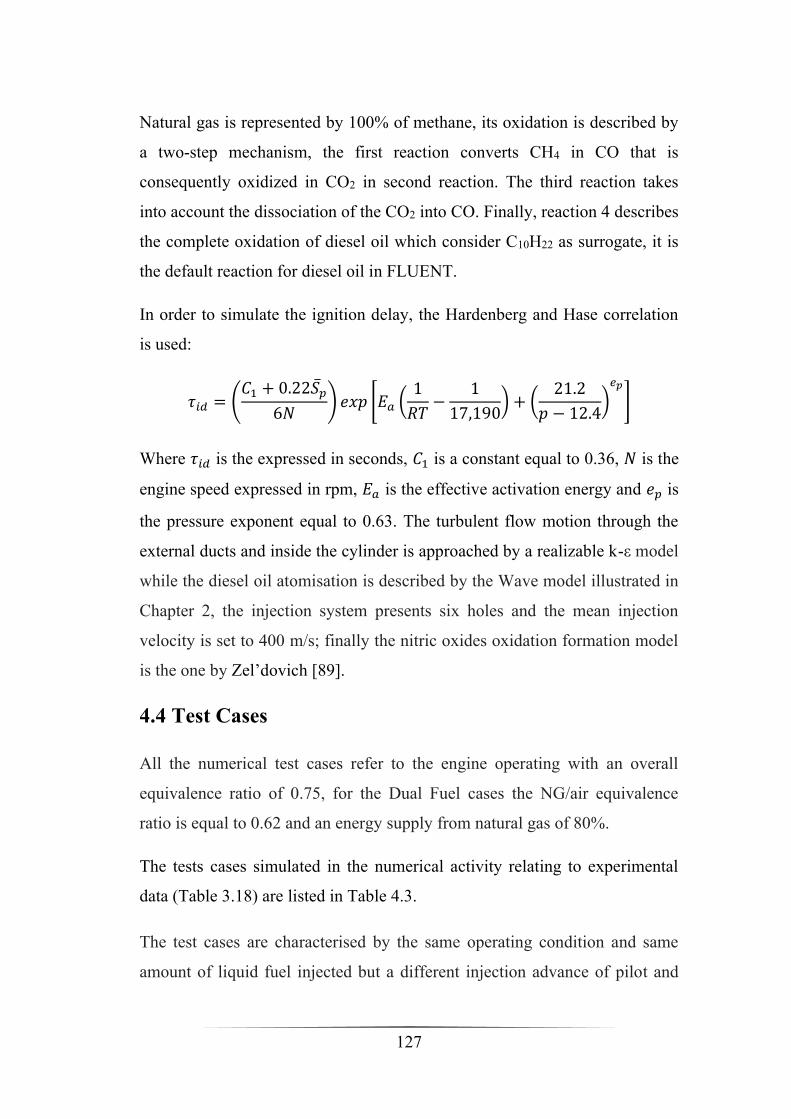
127
Natural gas is represented by 100% of methane, its oxidation is described by
a two-step mechanism, the first reaction converts CH4 in CO that is
consequently oxidized in CO2 in second reaction. The third reaction takes
into account the dissociation of the CO2 into CO. Finally, reaction 4 describes
the complete oxidation of diesel oil which consider C10H22 as surrogate, it is
the default reaction for diesel oil in FLUENT.
In order to simulate the ignition delay, the Hardenberg and Hase correlation
is used:
𝜏𝑖𝑑 = (𝐶1 + 0.22𝑆�̅�
6𝑁) 𝑒𝑥𝑝 [𝐸𝑎 (
1
𝑅𝑇−
1
17,190) + (
21.2
𝑝 − 12.4)𝑒𝑝
]
Where 𝜏𝑖𝑑 is the expressed in seconds, 𝐶1 is a constant equal to 0.36, 𝑁 is the
engine speed expressed in rpm, 𝐸𝑎 is the effective activation energy and 𝑒𝑝 is
the pressure exponent equal to 0.63. The turbulent flow motion through the
external ducts and inside the cylinder is approached by a realizable k-ε model
while the diesel oil atomisation is described by the Wave model illustrated in
Chapter 2, the injection system presents six holes and the mean injection
velocity is set to 400 m/s; finally the nitric oxides oxidation formation model
is the one by Zel’dovich [89].
4.4 Test Cases
All the numerical test cases refer to the engine operating with an overall
equivalence ratio of 0.75, for the Dual Fuel cases the NG/air equivalence
ratio is equal to 0.62 and an energy supply from natural gas of 80%.
The tests cases simulated in the numerical activity relating to experimental
data (Table 3.18) are listed in Table 4.3.
The test cases are characterised by the same operating condition and same
amount of liquid fuel injected but a different injection advance of pilot and

128
main jets and a fixed dwell angle, i.e. the angular shift between pilot and
main injection starts.
It is important to highlight that the start of injection can provoke significant
effects on the combustion development and the emission production.
Tab. 4.3: Test cases.
FULL DIESEL Pilot Injection Main Injection
Injected Mass 1 mg 20.7 mg
Test Cases Start Duration Start Duration
Case 1 8° BTDC 3° 14° ATDC 8°
Case 2 12° BTDC 3° 10° ATDC 8°
Case 3 17° BTDC 3° 5° ATDC 8°
Case 4 22° BTDC 3° TCD 8°
Case 5 27° BTDC 3° 5° BTDC 8°
Case 6 32° BTDC 3° 10° BTDC 8°
DUAL FUEL Pilot Injection Main Injection
Injected Mass 1 mg 2.8 mg
Test Cases Start Duration Start Duration
Case 7 12° BTDC 3° 5° ATDC 5°
Case 8 17° BTDC 3° TDC 5°
Case 9 27° BTDC 3° 10° BTDC 5°
For the full diesel simulations four cases (1, 2, 4 and 6) have been used for
the construction of the correlations which should be able to predict the
development of the combustion. Then cases 3 and 5 are used as a proof of
validation of these correlations. Instead, for the dual fuel mode cases the
correlations are found for the three cases performed (7, 8 and 9).

129
4.5 Full Diesel Results
As already said full diesel cases 1, 2, 4 and 6 were performed with the three-
dimensional code, the results in terms of fuel oxidation rate (Figure 4.3) are
used to calibrate the one-dimensional model. In particular, for the pilot and
main injections respectively the start, the peak position and the end of
combustion obtained from CFD calculations are assigned in the Wiebe
function. Figure 4.4 shows the calibration of the fuel burning rates of the
CFD and 1D calculations for the case 2 (SOP -12°): the combustion timing
corresponds in both models. A first validation is made through a comparison
of pressure curves which confirm that the 1D dimensional model can
reproduce the 3D results (Figures 4.5 to 4.8). Based on these outcomes, three
correlations for pilot and three correlations for the main injection (start, peak
and end of combustion) have been obtained by using second order
polynomial curves, as shown in Figures 4.9 and 4.10.
At this point, cases 3 and 5 have been performed by the two codes but the
start, the peak and the end of combustion for the 1D model are provided by
the correlations previously obtained. Figures 4.11 and 4.12 demonstrate that
the use of these correlations allows to simulate new cases by varying the
injection timing in the 1D with greatly reduced computational time and to
provide the boundary conditions to realise a CFD calculation for the
estimation of emissions and engine performances.
In Figure 4.13 the temperature distributions at 20° ATDC are reported for
three cases (2, 3 and 5). Of course the combustion development is completely
different: for the case 2 the first flame nuclei are detected near fuel jets; in
case 3 the combustion is in the middle of the process, high temperatures, due
to ignition, are more distributed in the chamber; in case 5 the combustion is
at the final stage.
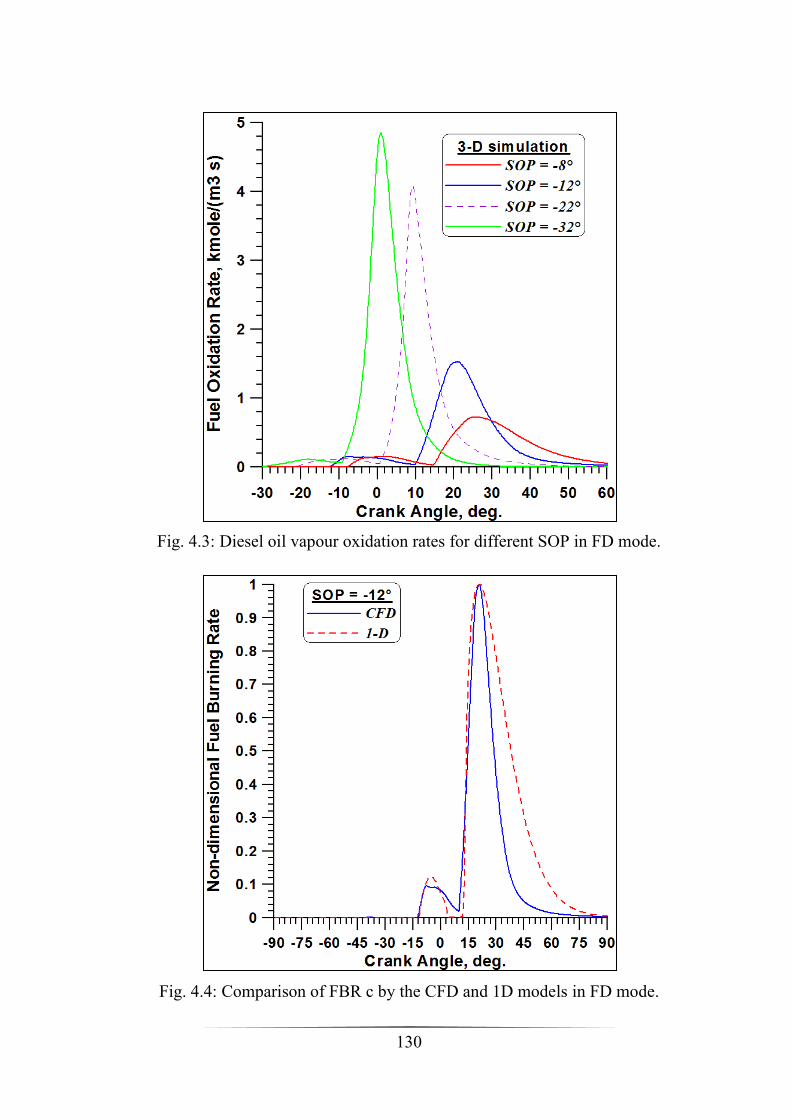
130
Fig. 4.3: Diesel oil vapour oxidation rates for different SOP in FD mode.
Fig. 4.4: Comparison of FBR c by the CFD and 1D models in FD mode.

131
Fig. 4.5: In-cylinder pressure by the CFD and 1D models (SOP=8° BTDC) in
FD mode.
Fig. 4.6: In-cylinder pressure by the CFD and 1D models (SOP=12° BTDC)
in FD mode.

132
Fig. 4.7: In-cylinder pressure by the CFD and 1D models (SOP=22° BTDC)
in FD mode.
Fig. 4.8: In-cylinder pressure by the CFD and 1D models (SOP=32° BTDC)
in FD mode.
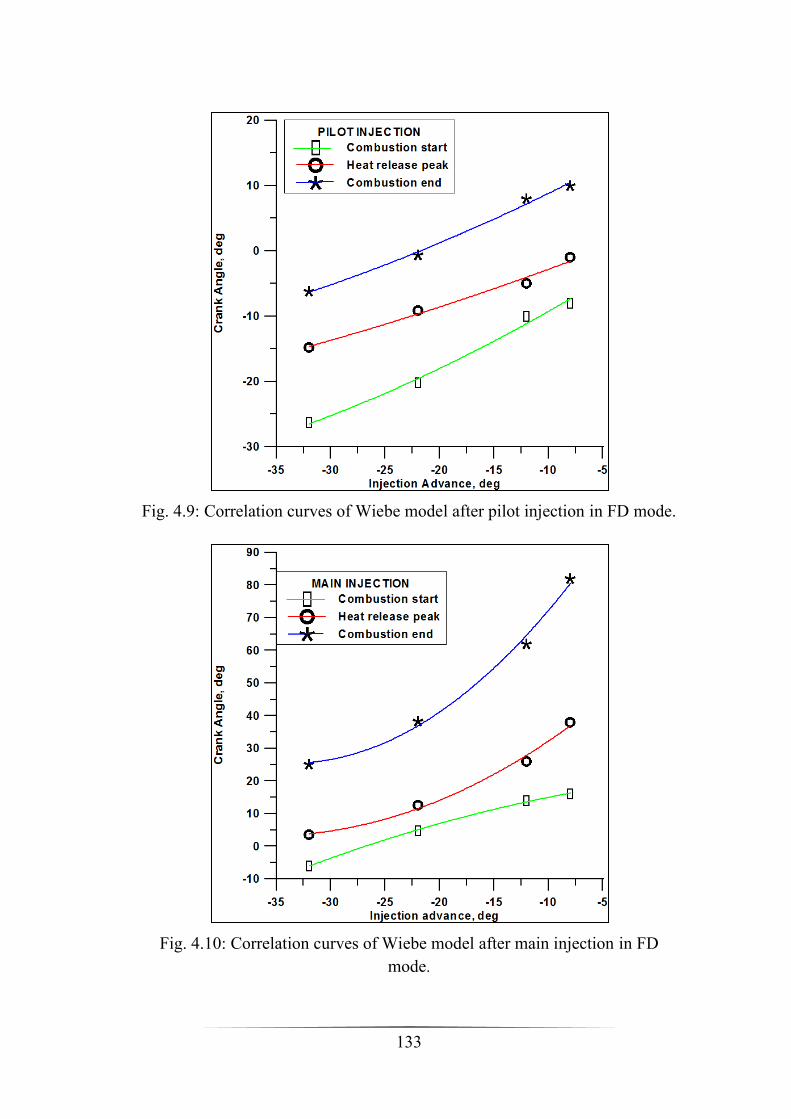
133
Fig. 4.9: Correlation curves of Wiebe model after pilot injection in FD mode.
Fig. 4.10: Correlation curves of Wiebe model after main injection in FD
mode.
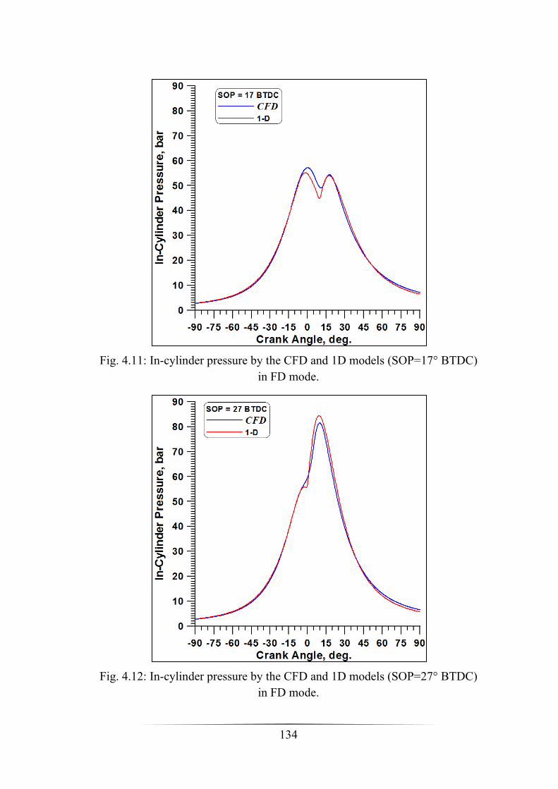
134
Fig. 4.11: In-cylinder pressure by the CFD and 1D models (SOP=17° BTDC)
in FD mode.
Fig. 4.12: In-cylinder pressure by the CFD and 1D models (SOP=27° BTDC)
in FD mode.

135
S.O.P. = 12° BTDC
Temperature
[K]
S.O.P. = 17° BTDC
S.O.P. = 27° BTDC
Fig. 4.13: Temperature distributions for different injection timings at 20°
ATDC.
4.6 Dual Fuel Results
As shown in Table 4.2 for dual fuel cases only three starts of injection have
been selected, i.e. cases 2, 3 and 5. However, the only difference is the
reduced duration of the main injection in order to reduce the liquid fuel
amount since about of 80% of energy is now provided by the natural gas
introduced in the inlet manifold.

136
Fig. 4.14: Comparison of fuel oxidation rates for FD and DF operation.
Fig. 4.15: Fuel mass fractions of diesel oil and NG in DF mode.
137
The role of the pilot and main injection of the diesel fuel is the ignition of the
natural gas/air mixture and the activation of multiple flame fronts that
accelerate the natural gas oxidation. This is confirmed by Figure 4.14, The
higher and anticipated peak of curve for NG is due to a fast ignition of gas
mixture after the pilot injection.
Actually, the most relevant increase in the slope of the methane oxidation
rate can be detected after the ignition of the diesel fuel from the pilot
injection. Also, the main diesel oil ignition appears to be helpful exclusively
to accelerate the combustion of methane as stated before. Moreover, Figure
4.15 confirms that the deep decrease in methane mass fraction occurs at
nearly 7° BTDC, so 10° later than the start of pilot injection. Finally, it is
important to notice that the pressure curve in dual fuel mode is more similar
to the trend of a spark ignition than a diesel engine (Figure 4.16).
Following the same procedure used for the full diesel operation, the three
cases were firstly simulated with CFD code. Figure 4.17 illustrated the three
methane oxidation rates while in Figure 4.18 the calibration of the fuel
burning rates of 1D model Wiebe functions for pilot, main and methane
combustion starting from the 3D results is reported. In Figures 4.19 to 4.20
the comparison between the 3D and 1D pressure curves demonstrate that the
one-dimensional model is again capable to fairly reproduce the CFD results.
Also, as expected, the pressure peak increases with the SOP value.
In order build the Wiebe correlations, the same method used for full diesel
cases is used, second order polynomial curves are used for the fitting of the
combustion parameters as illustrated in Figure 4.22.

138
Fig. 4.16: Comparison of in-cylinder pressure by CFD for FD and DF.
Fig. 4.17: CFD methane oxidation rates for different injection advances.

139
Fig. 4.18: Calibration of fuel burning rates computed by the CFD and 1D
model for SOP=17° BTDC in DF mode.
Fig. 4.19: In-cylinder pressure by the CFD and 1D models (SOP=12° BTDC)
in DF mode.
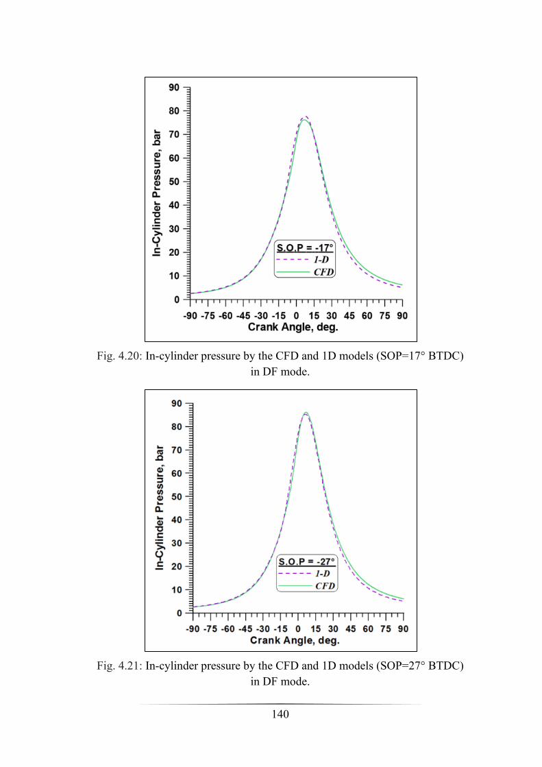
140
Fig. 4.20: In-cylinder pressure by the CFD and 1D models (SOP=17° BTDC)
in DF mode.
Fig. 4.21: In-cylinder pressure by the CFD and 1D models (SOP=27° BTDC)
in DF mode.
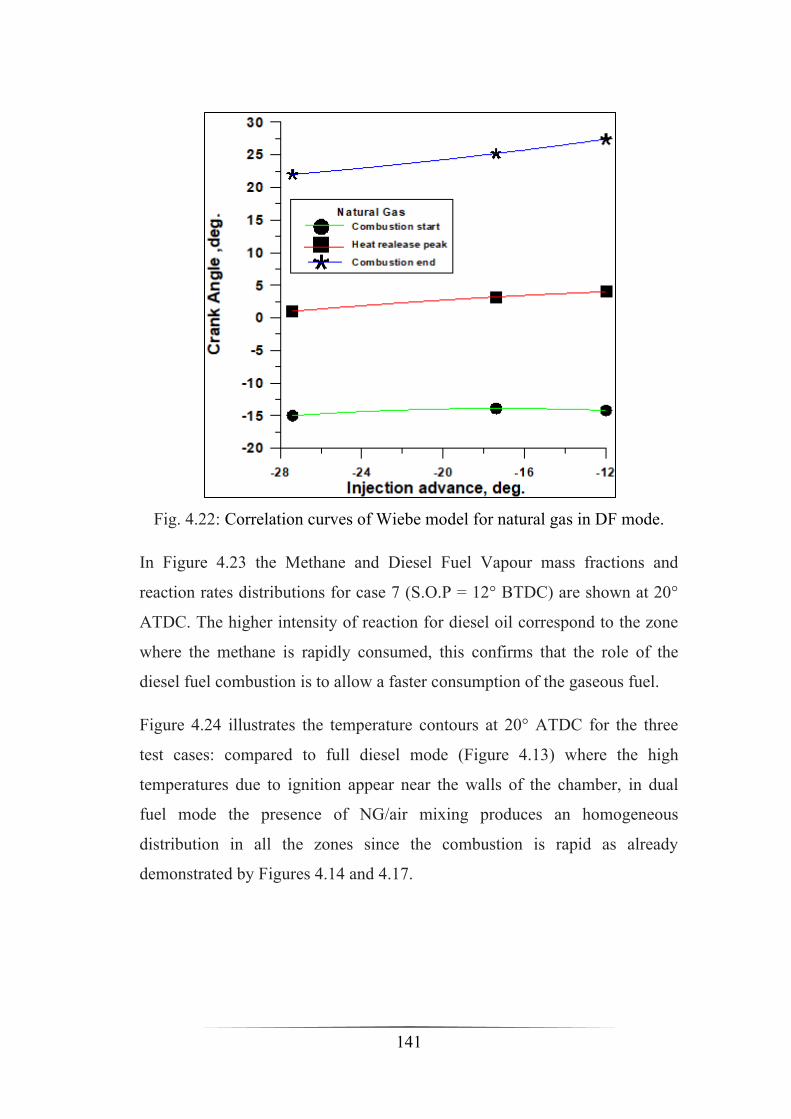
141
Fig. 4.22: Correlation curves of Wiebe model for natural gas in DF mode.
In Figure 4.23 the Methane and Diesel Fuel Vapour mass fractions and
reaction rates distributions for case 7 (S.O.P = 12° BTDC) are shown at 20°
ATDC. The higher intensity of reaction for diesel oil correspond to the zone
where the methane is rapidly consumed, this confirms that the role of the
diesel fuel combustion is to allow a faster consumption of the gaseous fuel.
Figure 4.24 illustrates the temperature contours at 20° ATDC for the three
test cases: compared to full diesel mode (Figure 4.13) where the high
temperatures due to ignition appear near the walls of the chamber, in dual
fuel mode the presence of NG/air mixing produces an homogeneous
distribution in all the zones since the combustion is rapid as already
demonstrated by Figures 4.14 and 4.17.

142
Methane
Diesel Vapour
Diesel Fuel Oxidation Rate [kmol/(m3s)]
Fig. 4.23: Methane, diesel fuel vapour mass fractions and reaction rates
distributions (SOP=12° BTDC) at 20° ATDC in DF mode.

143
S.O.P. = 12° BTDC
Temperature
[K]
S.O.P. = 17° BTDC
S.O.P. = 27° BTDC
Fig. 4.24: Temperature distributions for different injection timings at 20°
ATDC in DF mode.
Figures 4.25 and 4.26 report the NO and CO emissions. The low nitric oxides
emissions in case 7 confirm the results of the fuel burning rate trend in Figure
4.17 where the less anticipated injection implied a lower peak of combustion.
It is important to highlight that the correlations calculated for the one-
dimensional models allow the prediction of the engine performances in a
wide and continuous range of operating conditions.

144
Case 7, S.O.P. = 12° BTDC
NO
Case 8, S.O.P. = 17° BTDC
Case 9, S.O.P. = 27° BTDC
Fig. 4.25: NO mass fraction distributions for different injection timings at 20°
ATDC in DF mode.
Figure 4.27 shows a comparison between the trends of the indicated mean
effective pressures for the examined cases in full diesel and dual fuel mode,
in FD mode the IMEP decreases significantly with a reduction of the
injection advance while in DF mode, despite the slight increase it can be
considered almost constant. For this reason, in dual fuel mode a right choice
of SOP can be suggested as a function of the only reduction of the pollutants.
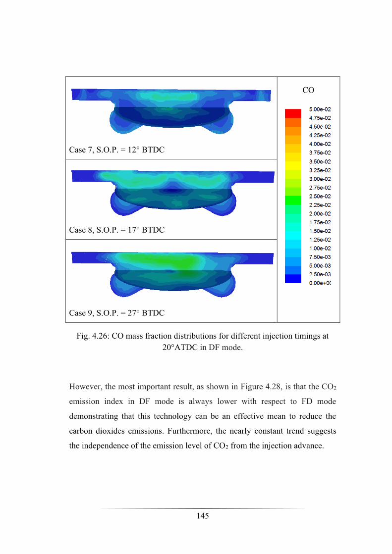
145
Case 7, S.O.P. = 12° BTDC
CO
Case 8, S.O.P. = 17° BTDC
Case 9, S.O.P. = 27° BTDC
Fig. 4.26: CO mass fraction distributions for different injection timings at
20°ATDC in DF mode.
However, the most important result, as shown in Figure 4.28, is that the CO2
emission index in DF mode is always lower with respect to FD mode
demonstrating that this technology can be an effective mean to reduce the
carbon dioxides emissions. Furthermore, the nearly constant trend suggests
the independence of the emission level of CO2 from the injection advance.

146
Fig. 4.27: IMEP calculated by 1D model for FD and DF modes.
Fig. 4.28: CO2 emissions calculated by 1D model for FD and DF modes.

147
Chapter 5
OPTICALLY ACCESSIBLE ENGINE
In this chapter simulations and results based on the experimental activity
carried out at Istituto Motori on an optically accessible single cylinder
research engine [95] and published in papers [96, 97] are illustrated. It is
necessary to highlight that the aim of this research is different from the
previous chapter, the object of the investigation is a research engine that
allows to directly observe the phenomena that occur inside the cylinder,
therefore the attention is mainly focused on the fundamental features of the
combustion rather than on engine performance. In this specific case, the
different test cases are not characterised by a diesel substitution but by
increased methane addition. The purpose is to analyse the effect of the
methane presence on the combustion, rather than the variations in
combustion development for a given fuel energy input. As a matter of fact, the
data set includes some information on in-cylinder distributions (i.e. OH) that
can represent a significant test case for the CFD analysis.
5.1 Experimental results
The aim of the experimental campaign was to visualise the combustion
development in terms of species concentration, especially for OH radical that
is considered to be a significant signal of the combustion rate intensity and
location. In the current paragraph an overview of the experimental setup and
results is given in order to better understand the methodology used and
results obtained from the numerical calculations.

148
In order to make the research engine under consideration optically accessible,
a modification of the combustion bowl was necessary. In particular, the lower
part was substituted with a quartz window, as shown in Figures 5.1 and 5.2.
Fig. 5.1: Optical single cylinder engine experimental setup.
Fig. 5.2: Modified geometry of the combustion chamber.
The engine is equipped with a Common Rail injection system of a the four-
cylinder standard engine. The engine specifications are reported in Table 5.1.
Tab. 5.1: Engine specifications.
Engine type 4-stroke, single cylinder, 4 valves
Bore [mm] 85
Stroke [mm] 92
Cylinder vol. displ. [cm3] 522
Combustion bowl volume [cm3] 19.7
Vol. compression ratio 16.5:1

149
The investigation of the spatial distribution and temporal evolution of the
UV-VIS emission light of the typical combustion species was made though
spectroscopic measurements recorded with an ICCD camera. Data were
detected with the spectrograph placed at two central working wavelengths:
350 and 500 nm. In particular, the OH spatial distribution was investigated by
means of a band pass filter at 310 nm wavelength [98]. The exposure time of
images and spectra detected was of 55 µs, that at engine speed of 1500 rpm,
corresponds to 0.5° deg. More details and specifications can be found in [95].
Tab. 5.2: Injection systems specifications
Diesel Injection system Common rail
Number of holes 7
Cone angle of fuel jet axis 148°
Hole diameter [mm] 0.141
Methane Injection system PFI
Number of holes 1
Maximum injection pressure [bar] 5
Tab. 5.3: Engine operating conditions.
Engine speed [rpm] 1500 1500 1500 1500 1500 1500 1500
Methane flow rate
[mg/str] 0.0 0.1 0.86 1.32 1.57 1.88 2.14
Diesel SOI -3 -3 -3 -3 -3 -3 -3
Diesel inj. duration [µs] 450 450 450 450 450 450 450
Diesel flow rate [mg/str] 8.9 8.9 8.9 8.9 8.9 8.9 8.9
Pin [bar] 1.27 1.27 1.27 1.27 1.27 1.27 1.27
Tin [°C] 52 50 50 50 50 49 49
Tout [°C] 72 77 80 95 107 115 128
Air flow rate [kg/s] 35.4 34.8 34.6 34.4 34.2 33.7 33.4
Premixed ratio 0 1 10 15 17 20 22

150
In Table 5.2 the injection systems specifications are reported. Since the
methane is port fuel injected to mix with air into the intake manifold, the
injection pressure can be low.
The engine operating conditions and thus experimental test cases are listed in
Table 5.3.
The different test cases are characterised by the same engine speed and same
amount of diesel fuel, which means start and duration of injection, while the
amount of methane is increased to vary the premixed ratio (RP) value that
indicates the percentage ratio of energy input due to methane and is
expressed as follows.
𝑅𝑃 =(𝑚𝑝𝐿𝐻𝑉𝑝)
(𝑚𝑝𝐿𝐻𝑉𝑝 +𝑚𝑑𝐿𝐻𝑉𝑑)× 100
Where 𝑚𝑝 and 𝑚𝑑 are the mass flow rate of premixed fuel (methane) and
directly injected fuel (diesel), respectively, 𝐿𝐻𝑉𝑝 and 𝐿𝐻𝑉𝑑 their lower
heating values. Therefore, the RP is equal to zero in full diesel and greater
than zero in dual fuel mode. The experimental purpose was to investigate the
diesel combustion and emissions when only a poor amount of methane was
added to air in order to identify regions where the combustion is not efficient.
However, it is important to highlight that the premixed ratio of the examined
test cases is significantly low and far from the usual load levels for a diesel
engine, but it is important to take into account that the presence of a quartz
window imposes limits on the amount of fuel that can burn inside the
chamber.
In Figure 5.3 the in-cylinder pressures are displayed for only three test cases:
RP = 0, 15 and 22%, since these three test cases have been used for the
numerical simulations.
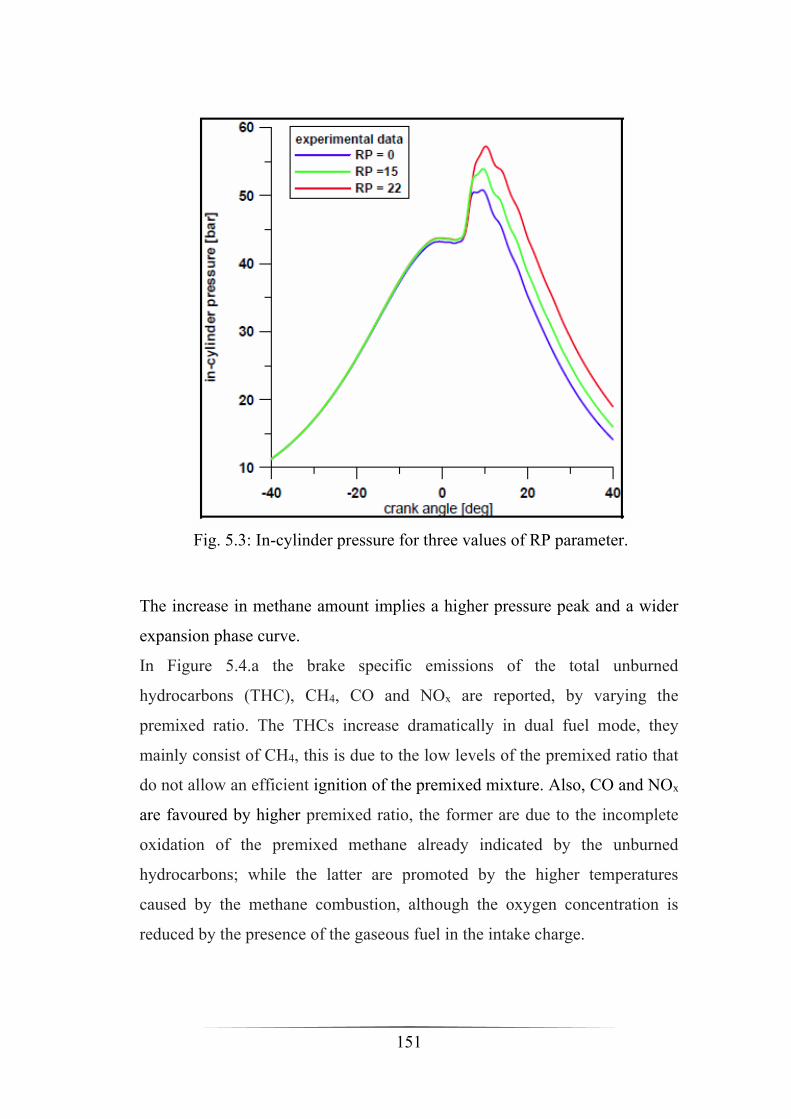
151
Fig. 5.3: In-cylinder pressure for three values of RP parameter.
The increase in methane amount implies a higher pressure peak and a wider
expansion phase curve.
In Figure 5.4.a the brake specific emissions of the total unburned
hydrocarbons (THC), CH4, CO and NOx are reported, by varying the
premixed ratio. The THCs increase dramatically in dual fuel mode, they
mainly consist of CH4, this is due to the low levels of the premixed ratio that
do not allow an efficient ignition of the premixed mixture. Also, CO and NOx
are favoured by higher premixed ratio, the former are due to the incomplete
oxidation of the premixed methane already indicated by the unburned
hydrocarbons; while the latter are promoted by the higher temperatures
caused by the methane combustion, although the oxygen concentration is
reduced by the presence of the gaseous fuel in the intake charge.
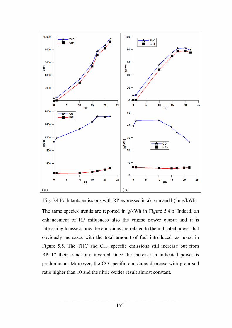
152
(a)
(b)
Fig. 5.4 Pollutants emissions with RP expressed in a) ppm and b) in g/kWh.
The same species trends are reported in g/kWh in Figure 5.4.b. Indeed, an
enhancement of RP influences also the engine power output and it is
interesting to assess how the emissions are related to the indicated power that
obviously increases with the total amount of fuel introduced, as noted in
Figure 5.5. The THC and CH4 specific emissions still increase but from
RP=17 their trends are inverted since the increase in indicated power is
predominant. Moreover, the CO specific emissions decrease with premixed
ratio higher than 10 and the nitric oxides result almost constant.

153
Fig. 5.5: Indicated power versus premixed ratio.
Fig. 5.6: CO2 emission index versus premixed ratio.
Finally, the CO2 emission index decreases, due to the combined effect of the
reduced carbon ratio in the fuel and the power increase.
Confirming that dual fuel strategy can effectively reduce the emissions of this
greenhouse gas.
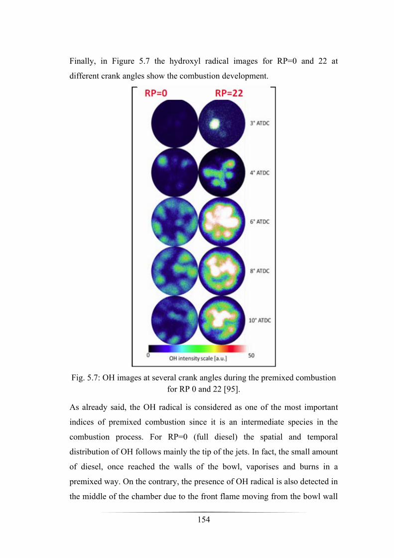
154
Finally, in Figure 5.7 the hydroxyl radical images for RP=0 and 22 at
different crank angles show the combustion development.
Fig. 5.7: OH images at several crank angles during the premixed combustion
for RP 0 and 22 [95].
As already said, the OH radical is considered as one of the most important
indices of premixed combustion since it is an intermediate species in the
combustion process. For RP=0 (full diesel) the spatial and temporal
distribution of OH follows mainly the tip of the jets. In fact, the small amount
of diesel, once reached the walls of the bowl, vaporises and burns in a
premixed way. On the contrary, the presence of OH radical is also detected in
the middle of the chamber due to the front flame moving from the bowl wall

155
towards the centre in a methane/air charge. Therefore, in dual fuel
combustion reactions occur with a more homogenous distribution in the
whole bowl with respect to diesel mode.
5.2 Methodology
As said above, the available experimental tests were carried out on a
research, optically accessible cylinder that required relevant changes in the
bowl geometry. Due to the lack of a mesh grid that reproduced the real
geometry, the CFD analysis presented in this chapter aimed to reproduce the
same tests in an in-cylinder domain with the same baseline geometrical
features but with a bowl shape more consistent with those usually adopted for
automotive application, proving the transferability of the experimental results
to real diesel engines and providing more detailed information on the dual
fuel combustion. However, in Chapter 7 a further improvement was made
with the reproduction of the exact bowl geometry and with the deep
investigation of the crevices issue that considerably affects this research
engine.
The CFD calculations were performed with the KIVA-3V solver on the
computational domain in Figure 5.8. The meshed domain was obtained by
using the ANSYS-ICEM meshing tool and it consists of 104,000 cells
(approximately 58,000 cells for the cylinder and 5,000 cells for the bowl),
including the external ducts and the valve lift laws.
The model utilised to describe the combustion process is the Finite Rate –
Eddy Dissipation approach. This model seems to be the most suitable to
describe the combustion development because as previously highlighted
these test cases are characterised by an extremely low equivalence ratio that
fall outside the flammability limits of methane, so preventing the propagation
of a flame front.
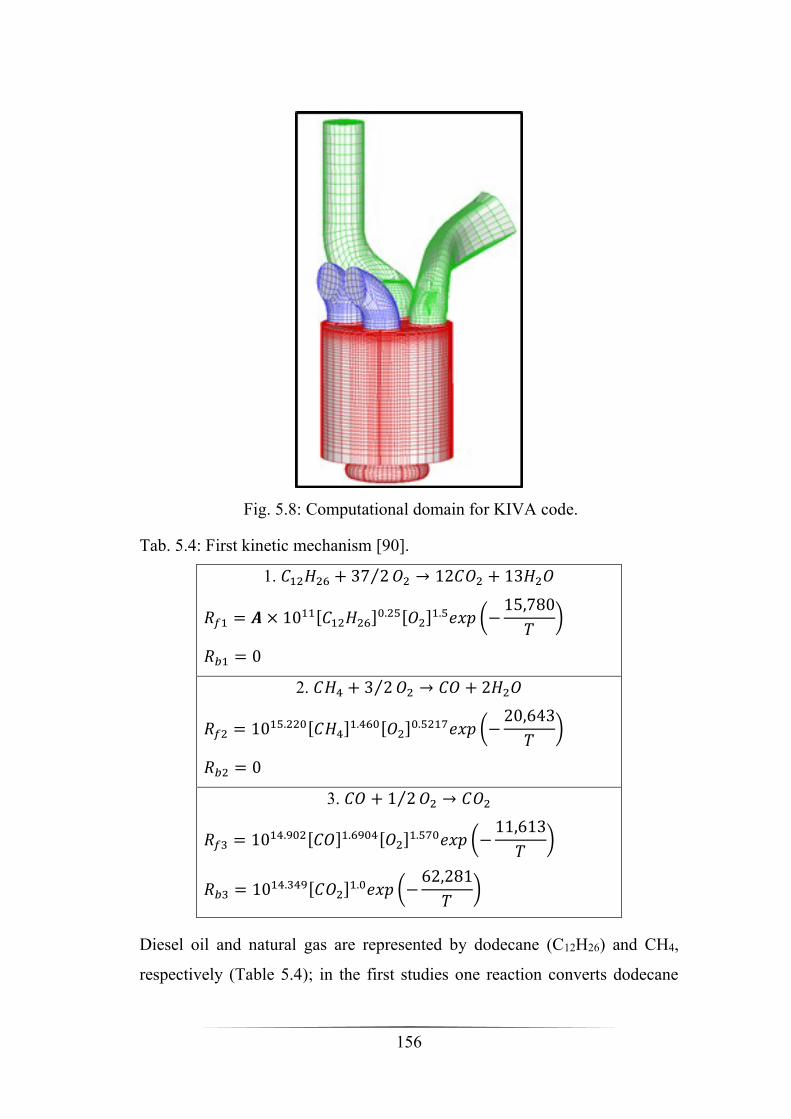
156
Fig. 5.8: Computational domain for KIVA code.
Tab. 5.4: First kinetic mechanism [90].
1. 𝐶12𝐻26 + 37 2⁄ 𝑂2 → 12𝐶𝑂2 + 13𝐻2𝑂
𝑅𝑓1 = 𝑨 × 1011[𝐶12𝐻26]
0.25[𝑂2]1.5𝑒𝑥𝑝 (−
15,780
𝑇)
𝑅𝑏1 = 0
2. 𝐶𝐻4 + 3 2⁄ 𝑂2 → 𝐶𝑂 + 2𝐻2𝑂
𝑅𝑓2 = 1015.220[𝐶𝐻4]
1.460[𝑂2]0.5217𝑒𝑥𝑝 (−
20,643
𝑇)
𝑅𝑏2 = 0
3. 𝐶𝑂 + 1 2⁄ 𝑂2 → 𝐶𝑂2
𝑅𝑓3 = 1014.902[𝐶𝑂]1.6904[𝑂2]
1.570𝑒𝑥𝑝 (−11,613
𝑇)
𝑅𝑏3 = 1014.349[𝐶𝑂2]
1.0𝑒𝑥𝑝 (−62,281
𝑇)
Diesel oil and natural gas are represented by dodecane (C12H26) and CH4,
respectively (Table 5.4); in the first studies one reaction converts dodecane
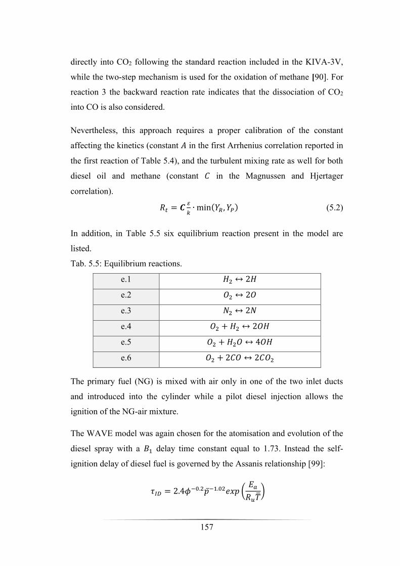
157
directly into CO2 following the standard reaction included in the KIVA-3V,
while the two-step mechanism is used for the oxidation of methane [90]. For
reaction 3 the backward reaction rate indicates that the dissociation of CO2
into CO is also considered.
Nevertheless, this approach requires a proper calibration of the constant
affecting the kinetics (constant 𝐴 in the first Arrhenius correlation reported in
the first reaction of Table 5.4), and the turbulent mixing rate as well for both
diesel oil and methane (constant 𝐶 in the Magnussen and Hjertager
correlation).
𝑅𝑡 = 𝑪 𝑘∙ min(𝑌𝑅 , 𝑌𝑃) (5.2)
In addition, in Table 5.5 six equilibrium reaction present in the model are
listed.
Tab. 5.5: Equilibrium reactions.
e.1 𝐻2 ↔ 2𝐻
e.2 𝑂2 ↔ 2𝑂
e.3 𝑁2 ↔ 2𝑁
e.4 𝑂2 + 𝐻2 ↔ 2𝑂𝐻
e.5 𝑂2 + 𝐻2𝑂 ↔ 4𝑂𝐻
e.6 𝑂2 + 2𝐶𝑂 ↔ 2𝐶𝑂2
The primary fuel (NG) is mixed with air only in one of the two inlet ducts
and introduced into the cylinder while a pilot diesel injection allows the
ignition of the NG-air mixture.
The WAVE model was again chosen for the atomisation and evolution of the
diesel spray with a 𝐵1 delay time constant equal to 1.73. Instead the self-
ignition delay of diesel fuel is governed by the Assanis relationship [99]:
𝜏𝐼𝐷 = 2.4𝜙−0.2�̅�−1.02𝑒𝑥𝑝 (
𝐸𝑎
𝑅𝑢�̅�)
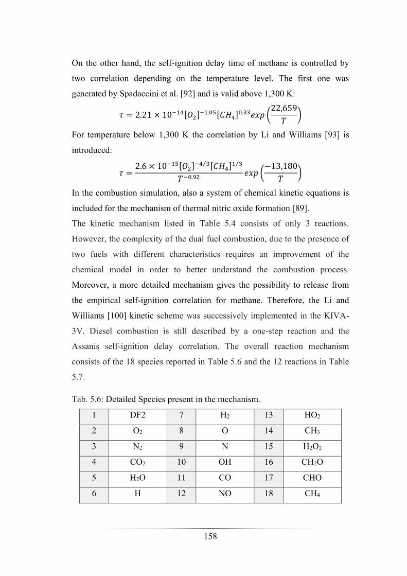
158
On the other hand, the self-ignition delay time of methane is controlled by
two correlation depending on the temperature level. The first one was
generated by Spadaccini et al. [92] and is valid above 1,300 K:
𝜏 = 2.21 × 10⁻¹⁴[𝑂2]−1.05[𝐶𝐻4]
0.33𝑒𝑥𝑝 (22,659
𝑇)
For temperature below 1,300 K the correlation by Li and Williams [93] is
introduced:
𝜏 =2.6 × 10⁻¹⁵[𝑂2]
−4 3⁄ [𝐶𝐻4]1 3⁄
𝑇−0.92𝑒𝑥𝑝 (
−13,180
𝑇)
In the combustion simulation, also a system of chemical kinetic equations is
included for the mechanism of thermal nitric oxide formation [89].
The kinetic mechanism listed in Table 5.4 consists of only 3 reactions.
However, the complexity of the dual fuel combustion, due to the presence of
two fuels with different characteristics requires an improvement of the
chemical model in order to better understand the combustion process.
Moreover, a more detailed mechanism gives the possibility to release from
the empirical self-ignition correlation for methane. Therefore, the Li and
Williams [100] kinetic scheme was successively implemented in the KIVA-
3V. Diesel combustion is still described by a one-step reaction and the
Assanis self-ignition delay correlation. The overall reaction mechanism
consists of the 18 species reported in Table 5.6 and the 12 reactions in Table
5.7.
Tab. 5.6: Detailed Species present in the mechanism.
1 DF2 7 H2 13 HO2
2 O2 8 O 14 CH3
3 N2 9 N 15 H2O2
4 CO2 10 OH 16 CH2O
5 H2O 11 CO 17 CHO
6 H 12 NO 18 CH4
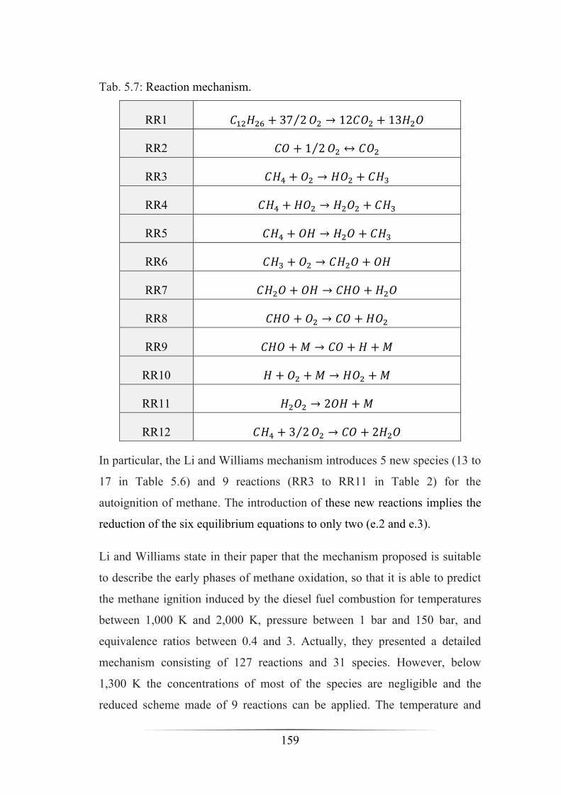
159
Tab. 5.7: Reaction mechanism.
RR1 𝐶12𝐻26 + 37 2⁄ 𝑂2 → 12𝐶𝑂2 + 13𝐻2𝑂
RR2 𝐶𝑂 + 1 2⁄ 𝑂2 ↔ 𝐶𝑂2
RR3 𝐶𝐻4 + 𝑂2 → 𝐻𝑂2 + 𝐶𝐻3
RR4 𝐶𝐻4 + 𝐻𝑂2 → 𝐻2𝑂2 + 𝐶𝐻3
RR5 𝐶𝐻4 + 𝑂𝐻 → 𝐻2𝑂 + 𝐶𝐻3
RR6 𝐶𝐻3 + 𝑂2 → 𝐶𝐻2𝑂 + 𝑂𝐻
RR7 𝐶𝐻2𝑂 + 𝑂𝐻 → 𝐶𝐻𝑂 + 𝐻2𝑂
RR8 𝐶𝐻𝑂 + 𝑂2 → 𝐶𝑂 + 𝐻𝑂2
RR9 𝐶𝐻𝑂 +𝑀 → 𝐶𝑂 + 𝐻 +𝑀
RR10 𝐻 + 𝑂2 +𝑀 → 𝐻𝑂2 +𝑀
RR11 𝐻2𝑂2 → 2𝑂𝐻 +𝑀
RR12 𝐶𝐻4 + 3 2⁄ 𝑂2 → 𝐶𝑂 + 2𝐻2𝑂
In particular, the Li and Williams mechanism introduces 5 new species (13 to
17 in Table 5.6) and 9 reactions (RR3 to RR11 in Table 2) for the
autoignition of methane. The introduction of these new reactions implies the
reduction of the six equilibrium equations to only two (e.2 and e.3).
Li and Williams state in their paper that the mechanism proposed is suitable
to describe the early phases of methane oxidation, so that it is able to predict
the methane ignition induced by the diesel fuel combustion for temperatures
between 1,000 K and 2,000 K, pressure between 1 bar and 150 bar, and
equivalence ratios between 0.4 and 3. Actually, they presented a detailed
mechanism consisting of 127 reactions and 31 species. However, below
1,300 K the concentrations of most of the species are negligible and the
reduced scheme made of 9 reactions can be applied. The temperature and

160
pressure ranges of this mechanism are consistent with those typical of a high
compression ratio. On the contrary, the methane-air equivalence ratio can be
lower at reduced engine loads. However, higher local equivalence ratios are
expected because of the oxygen consumption that derives from the earlier
diesel fuel combustion.
In Table 5.7 reaction 12, which represents the oxidation of methane to carbon
monoxide, is still present but it is activated when the cell temperature is
above 1,300 K. While the oxidation is completed by reaction 2 that refers to
the association and dissociation of CO2 in CO. The thermal NOx prediction is
still described by the Zel’dovich mechanism.
Fig. 5.9: Temperature calculated by Li and Williams in [100].

161
Preliminarily, Li and Williams calculated the temperature trend for a mixture
at 1,136 K, 100 bar and an equivalence ratio of 0.4 (Figure 5.9), then the
reaction scheme was tested in CHEMKIN using a closed homogenous reactor
under the same condition showing a good agreement with their results
(Figure 5.10).
Fig. 5.10: CHEMKIN results.
Combustion is again simulated with the Finite rate – Eddy dissipation model
for the same reasons previously mentioned but, since methane is premixed
with air, for reactions from 3 to 12, only the kinetic rate is considered. In
Table 5.8 the values of constants in the Arrhenius correlation for each
reaction are listed.
Finally, the atomisation model used is still the WAVE model, after a proper
calibration the values of 𝐵0 = 0.61 and 𝐵1 = 7 are set for the two model
constants.

162
Tab. 5.8: Values of A, n and Ta [100].
Reaction A [mol, cm3, s] N [-] Ta [K]
RR1 8.00 x 10+11 0.0 15,780
RR2 7.9899 x 10+14 0.0 11,613
RR3 3.980 x 10+10 0.0 28,626
RR4 9.04 x 10+09 0.0 12,401
RR5 1.60 x 10+04 1.83 1,395
RR6 3.30 x 10+08 0.0 4,498
RR7 3.90 x 10+07 0.89 204.5
RR8 3.00 x 10+09 0.0 0.0
RR9 1.86 x 10+09 -1.0 8,552
RR10 6.76 x 10+16 -1.4 0.0
RR11 1.20 x 10+14 0.0 22,901
RR12 1.6596 x 10+15 0.0 20,643
5.3 Case study
From the experimental test case only three RP values were chosen to be
reproduced with the two-step mechanism for methane, i.e. RP = 0, 15 and 22.
Instead, for the implementation of the Li and Williams kinetic mechanism the
RP =10, 15 and 22 were chosen. In addition, an arbitrary fourth case with a
premixed ratio closer to that of a real engine (RP=80%) has been added and
performed only numerically. The first three cases aimed to analyse the dual
fuel combustion, but the role of the diesel oil is clearly predominant. On the
other hand, in the RP=80% case the amount of methane allows the
methane/air ratio to fall inside the flammability limits and different
combustion behaviour is expected.

163
Tab. 5.9 Operating conditions in the computational cases
RP [%] 0 10 15 22 80
Thermal Power (fuel LHV) [kW] 4.78 5.32 5.6 6.125 23.53
IMEP [bar] 1.4 1.8 2.3 3.75 13.16
Trapped Air Mass [mg/cycle] 786 769 764 742 673
Injected diesel oil [mg/cycle] 8.9 8.9 8.9 8.9 8.9
Trapped Methane Mass [mg/cycle] 0 0.86 1.32 2.14 30
Methane mass fraction 0 0.00112 0.00172 0.00287 0.03885
Air/Fuel Ratio 88.39 78.78 74.80 67.23 19.08
Fuel/Air Equivalence Ratio 0.164 0.187 0.199 0.24 0.871
Methane/Air Equivalence Ratio 0 0.0193 0.0298 0.0497 0.6968
For all cases with RP up to 22%, the fuel thermal power and the indicated
mean effective pressure levels listed in Table 5.9 are considerably lower than
those atypical of mean or full loads. The same Table displays the values of
air and fuel masses considered in each calculation. The boundary conditions
such as pressure and temperature at the inflow of the duct and the injection
timing are derived by experimental test reported in Table 5.3. According to
the experimental procedure, the injection timing is fixed, the single injection
starts at 3.3° BTDC and has a duration of 4.5 crank angle degrees, that means
that the amount of diesel oil injected is the same for all the cases. Hence, the
additional energy supply is provided exclusively by methane.
In order to achieve an adequate level of periodic convergence each case was
performed for multiple engine cycles. Figure 5.11 shows the in-cylinder
pressure by KIVA-3V solver for three subsequent cycles. The first cycle
differs significantly from the other and cannot be considered reliable. After at
least three cycles the calculation provide what is considered as the final
solution. Therefore, all the results discussed in the following refer to the third
computed cycle.

164
Fig. 5.11: Example of convergence history of the computed in-cylinder
pressure to the periodic regime.
5.4 Two-step mechanism results
In this section, the results obtained with the two-step mechanism for methane
oxidation are illustrated. Since the scheme consists of few reactions, the
reliability of the ignition delay correlations employed for diesel vapour and
methane influences the quality of the results. The turbulence-chemistry
interaction is governed by the 𝐶 constant in equation (5.2) for the reactant
mixing rate. A proper calibration of this parameter was necessary for the
prediction of both diesel oil and methane combustion development (Table
5.10).
Tab. 5.10: Constants of calibration.
RP 0% 15% 22%
𝐴 36 24 12
𝐶𝑑𝑖𝑒𝑠𝑒𝑙 6 9 27
𝐶𝑚𝑒𝑡ℎ𝑎𝑛𝑒 - 108 108

165
Firstly, the evolution of the multiphase is illustrated in Figure 5.12. The
liquid fuel particles progressively decrease and disappear and in turn the
corresponding region is filled with vaporised fuel.
TDC
5° ATDC
Fig. 5.12 Particle jets and diesel vapor mass fraction (%) contours (RP=22).
In Figures from 5.13 to 5.15 the comparison of numerical and experimental
in-cylinder mean pressure is illustrated for the three test cases considered. As
it can be observed, the typical features such as start of pressure rise, rise and
peak appear to be correctly detected. In Figure 5.16, also the numerical
temperature trend (for case RP=22) reproduce properly the experimental one.

166
Fig. 5.13: In cylinder pressure for RP=0.
Fig. 5.14: In cylinder pressure for RP =15.
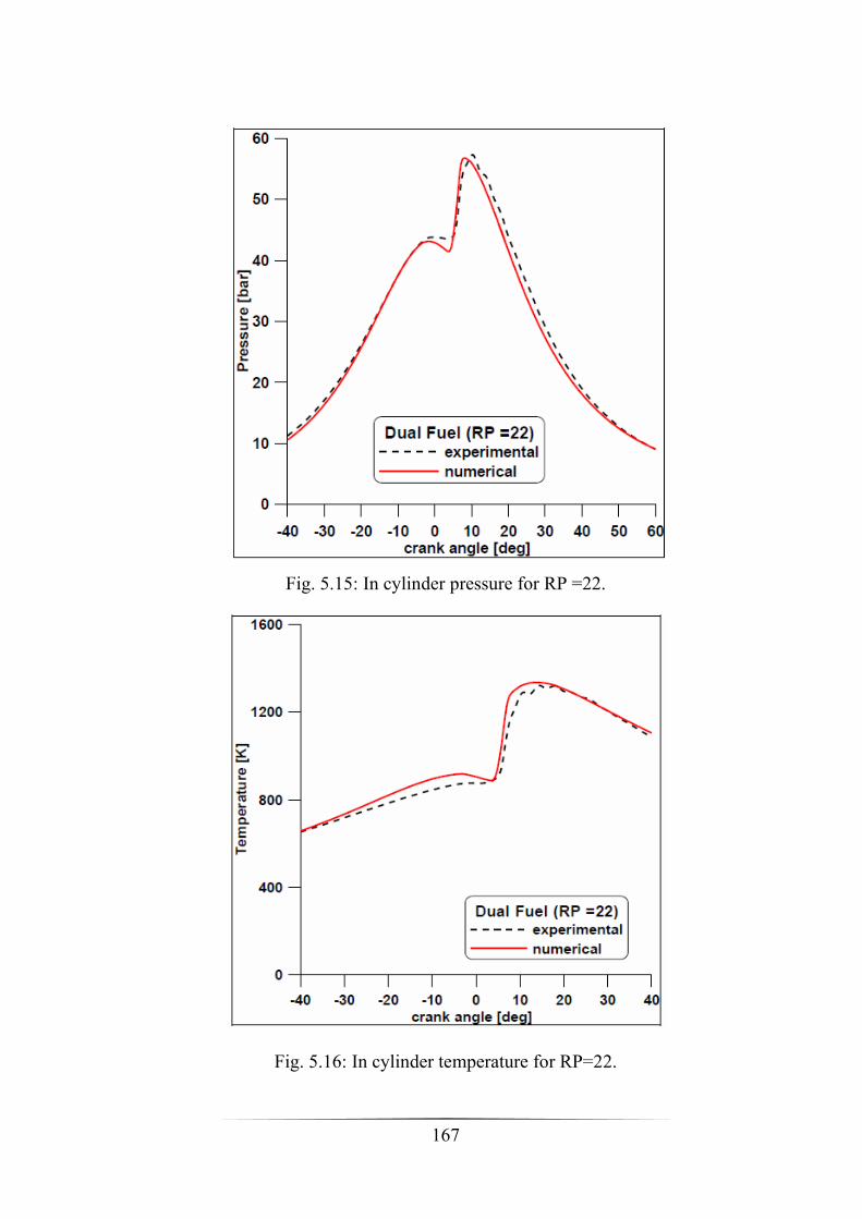
167
Fig. 5.15: In cylinder pressure for RP =22.
Fig. 5.16: In cylinder temperature for RP=22.
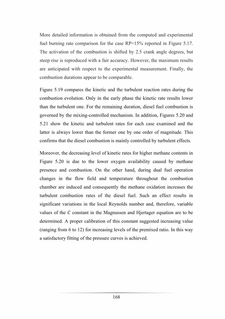
168
More detailed information is obtained from the computed and experimental
fuel burning rate comparison for the case RP=15% reported in Figure 5.17.
The activation of the combustion is shifted by 2.5 crank angle degrees, but
steep rise is reproduced with a fair accuracy. However, the maximum results
are anticipated with respect to the experimental measurement. Finally, the
combustion durations appear to be comparable.
Figure 5.19 compares the kinetic and the turbulent reaction rates during the
combustion evolution. Only in the early phase the kinetic rate results lower
than the turbulent one. For the remaining duration, diesel fuel combustion is
governed by the mixing-controlled mechanism. In addition, Figures 5.20 and
5.21 show the kinetic and turbulent rates for each case examined and the
latter is always lower than the former one by one order of magnitude. This
confirms that the diesel combustion is mainly controlled by turbulent effects.
Moreover, the decreasing level of kinetic rates for higher methane contents in
Figure 5.20 is due to the lower oxygen availability caused by methane
presence and combustion. On the other hand, during dual fuel operation
changes in the flow field and temperature throughout the combustion
chamber are induced and consequently the methane oxidation increases the
turbulent combustion rates of the diesel fuel. Such an effect results in
significant variations in the local Reynolds number and, therefore, variable
values of the 𝐶 constant in the Magnussen and Hjertager equation are to be
determined. A proper calibration of this constant suggested increasing value
(ranging from 6 to 12) for increasing levels of the premixed ratio. In this way
a satisfactory fitting of the pressure curves is achieved.
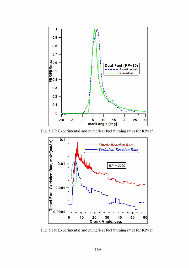
169
Fig. 5.17: Experimental and numerical fuel burning rates for RP=15.
Fig. 5.18: Experimental and numerical fuel burning rates for RP=15.
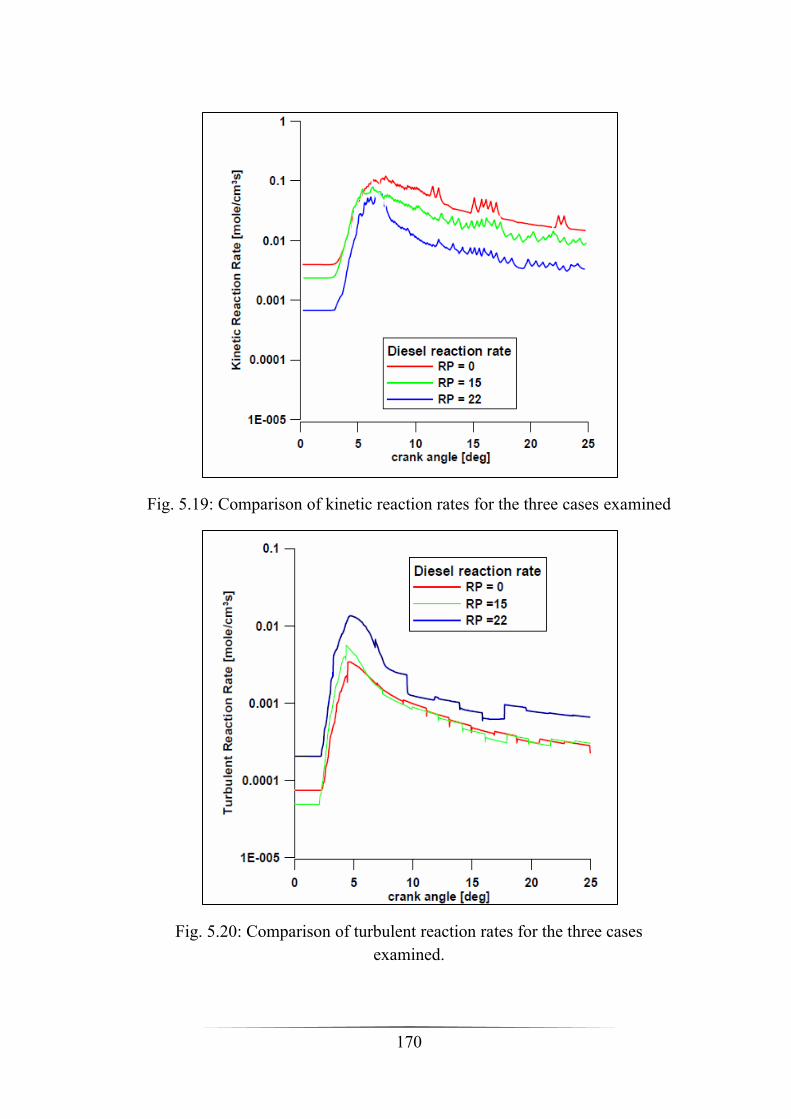
170
Fig. 5.19: Comparison of kinetic reaction rates for the three cases examined
Fig. 5.20: Comparison of turbulent reaction rates for the three cases
examined.

171
Fig. 5.21: FBR trend for the full diesel and dual fuel (RP=22) case.
In Figure 5.21 the total FBR trends are illustrated for full diesel and dual fuel
(RP=22) cases. As expected, the addition of methane in the intake manifold
varies the physical and transport properties of the introduced mixture such as
the partial pressure of oxygen, retarding the pre-ignition reaction activity and
hence enhancing the duration of the delay. Moreover, diesel vapour burns in
a shorter time, while the dual fuel combustion presents a longer duration and
a smoother behaviour. However, it should be taken into account that also the
heat exchange properties can be affected by the presence of methane in the
mixture.
For RP=22, the fuel burned fraction and the FBR of natural gas and diesel oil
are shown in Figures 5.22 and 5.23 respectively. Differently from diesel
vapour, methane does not complete the combustion. As previously
highlighted, the equivalence ratio of methane is outside the flammability
limits of this fuels, then a not efficient flame propagation is expected for
these test cases. This result is in agreement with the unburned species in the
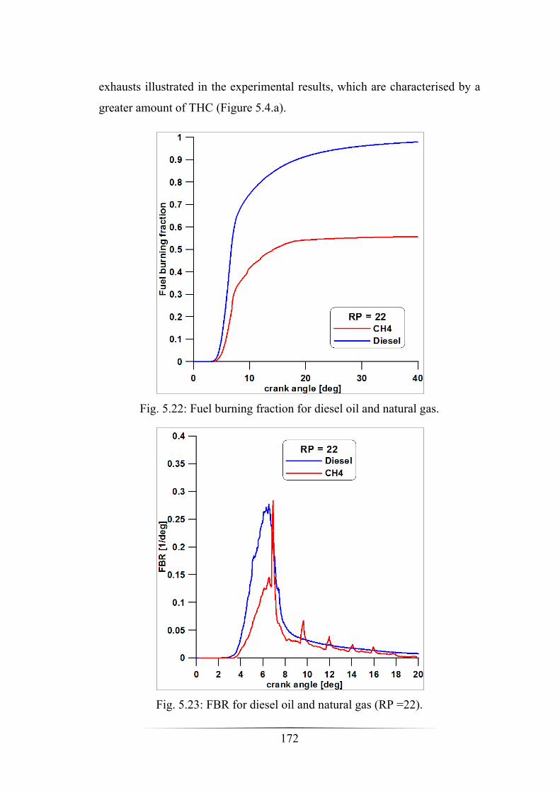
172
exhausts illustrated in the experimental results, which are characterised by a
greater amount of THC (Figure 5.4.a).
Fig. 5.22: Fuel burning fraction for diesel oil and natural gas.
Fig. 5.23: FBR for diesel oil and natural gas (RP =22).
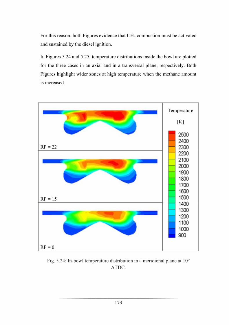
173
For this reason, both Figures evidence that CH4 combustion must be activated
and sustained by the diesel ignition.
In Figures 5.24 and 5.25, temperature distributions inside the bowl are plotted
for the three cases in an axial and in a transversal plane, respectively. Both
Figures highlight wider zones at high temperature when the methane amount
is increased.
RP = 22
Temperature
[K]
RP = 15
RP = 0
Fig. 5.24: In-bowl temperature distribution in a meridional plane at 10°
ATDC.
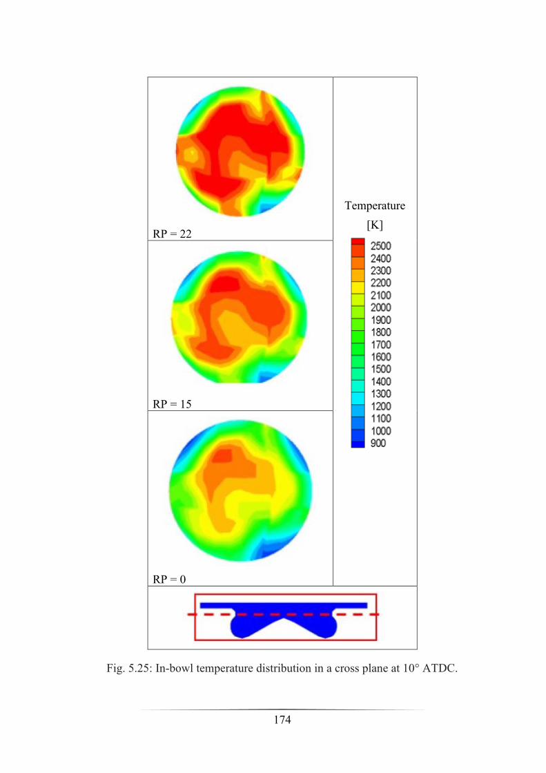
174
RP = 22
Temperature
[K]
RP = 15
RP = 0
Fig. 5.25: In-bowl temperature distribution in a cross plane at 10° ATDC.

175
RP = 22
OH
RP = 15
RP = 0
Fig. 5.26. In-bowl OH distribution in meridional plane at 10° ATDC.
The OH distributions reported in Figures 5.26 and 5.27 are coherent with the
temperature contours. Indeed, the high oxidation rate intensity detected by
the OH production implies the corresponding region at high temperature.
In Figure 5.28 a qualitative comparison between the numerical and
experimental distribution for case RP=22 demonstrates that the CFD
simulations have proven to be capable to reproduce the real phenomena that
occur inside the cylinder.
Finally, Figure 5.29 shows the NO fraction levels in the exhaust for the three
numerical and experimental cases highlighting a good agreement between the
trends since both detected an increase of nitric oxides with the increase of the
NG amount. Nevertheless, numerical computations tend to overestimate the
emissions of this pollutant.

176
RP = 22
OH
RP = 15
RP = 0
Fig. 5.27: In-bowl OH distribution in a cross plane at 10° ATDC
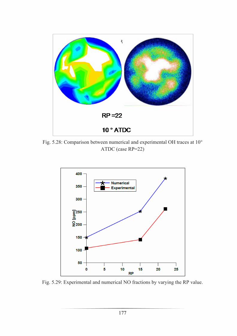
177
Fig. 5.28: Comparison between numerical and experimental OH traces at 10°
ATDC (case RP=22)
Fig. 5.29: Experimental and numerical NO fractions by varying the RP value.
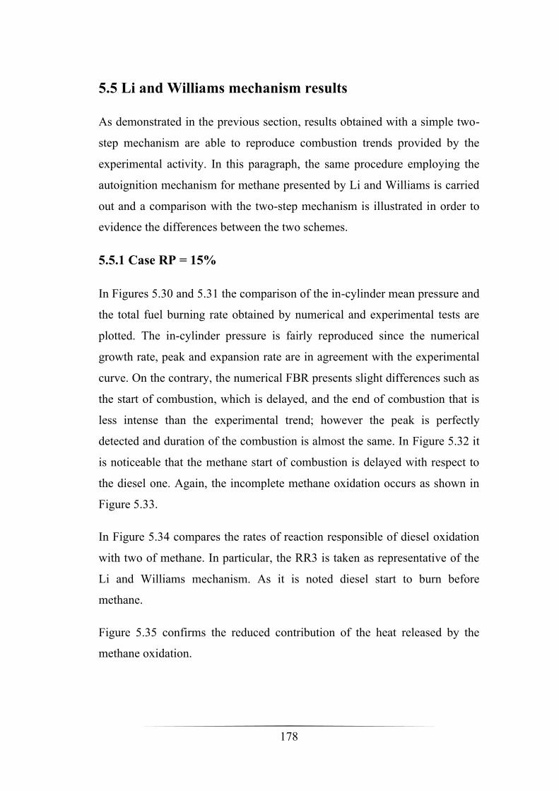
178
5.5 Li and Williams mechanism results
As demonstrated in the previous section, results obtained with a simple two-
step mechanism are able to reproduce combustion trends provided by the
experimental activity. In this paragraph, the same procedure employing the
autoignition mechanism for methane presented by Li and Williams is carried
out and a comparison with the two-step mechanism is illustrated in order to
evidence the differences between the two schemes.
5.5.1 Case RP = 15%
In Figures 5.30 and 5.31 the comparison of the in-cylinder mean pressure and
the total fuel burning rate obtained by numerical and experimental tests are
plotted. The in-cylinder pressure is fairly reproduced since the numerical
growth rate, peak and expansion rate are in agreement with the experimental
curve. On the contrary, the numerical FBR presents slight differences such as
the start of combustion, which is delayed, and the end of combustion that is
less intense than the experimental trend; however the peak is perfectly
detected and duration of the combustion is almost the same. In Figure 5.32 it
is noticeable that the methane start of combustion is delayed with respect to
the diesel one. Again, the incomplete methane oxidation occurs as shown in
Figure 5.33.
In Figure 5.34 compares the rates of reaction responsible of diesel oxidation
with two of methane. In particular, the RR3 is taken as representative of the
Li and Williams mechanism. As it is noted diesel start to burn before
methane.
Figure 5.35 confirms the reduced contribution of the heat released by the
methane oxidation.
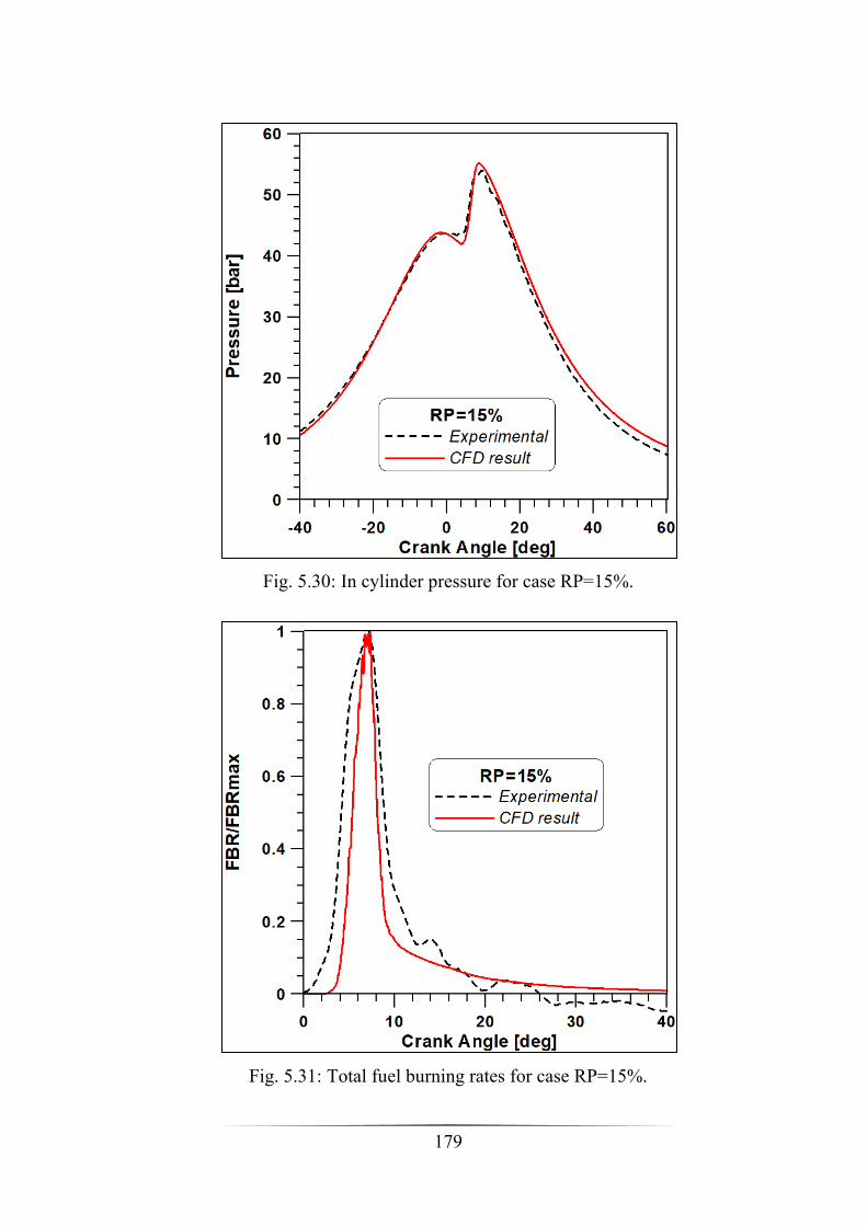
179
Fig. 5.30: In cylinder pressure for case RP=15%.
Fig. 5.31: Total fuel burning rates for case RP=15%.
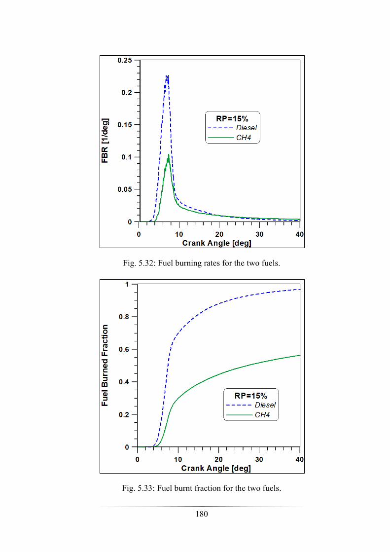
180
Fig. 5.32: Fuel burning rates for the two fuels.
Fig. 5.33: Fuel burnt fraction for the two fuels.
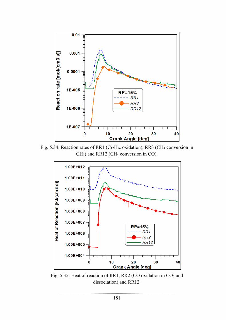
181
Fig. 5.34: Reaction rates of RR1 (C12H26 oxidation), RR3 (CH4 conversion in
CH3) and RR12 (CH4 conversion in CO).
Fig. 5.35: Heat of reaction of RR1, RR2 (CO oxidation in CO2 and
dissociation) and RR12.

182
5.5.2 Case RP = 22%
The in-cylinder pressure obtained from numerical simulations in good
agreement with the experimental one (Figure 5.36). In particular, a perfect
accordance is noted for the pressure increasing timing and the growth rate,
but the peak position is slightly anticipated, and this induces a lower pressure
during the expansion phase.
The comparison between the numerical and experimental volume averaged
temperatures (Figure 5.37) is necessary to assess the reliability of the CFD
simulations. Indeed, the mesh used slight differs from the geometry of the
real engine tested on the bench. However, since the temperature trends
present a good agreement, it is possible to affirm that the energy levels
obtained are the same.
Temperature appears to be widely stratified during all the combustion
process.
Fig. 5.36: In cylinder pressure for case RP =22%.
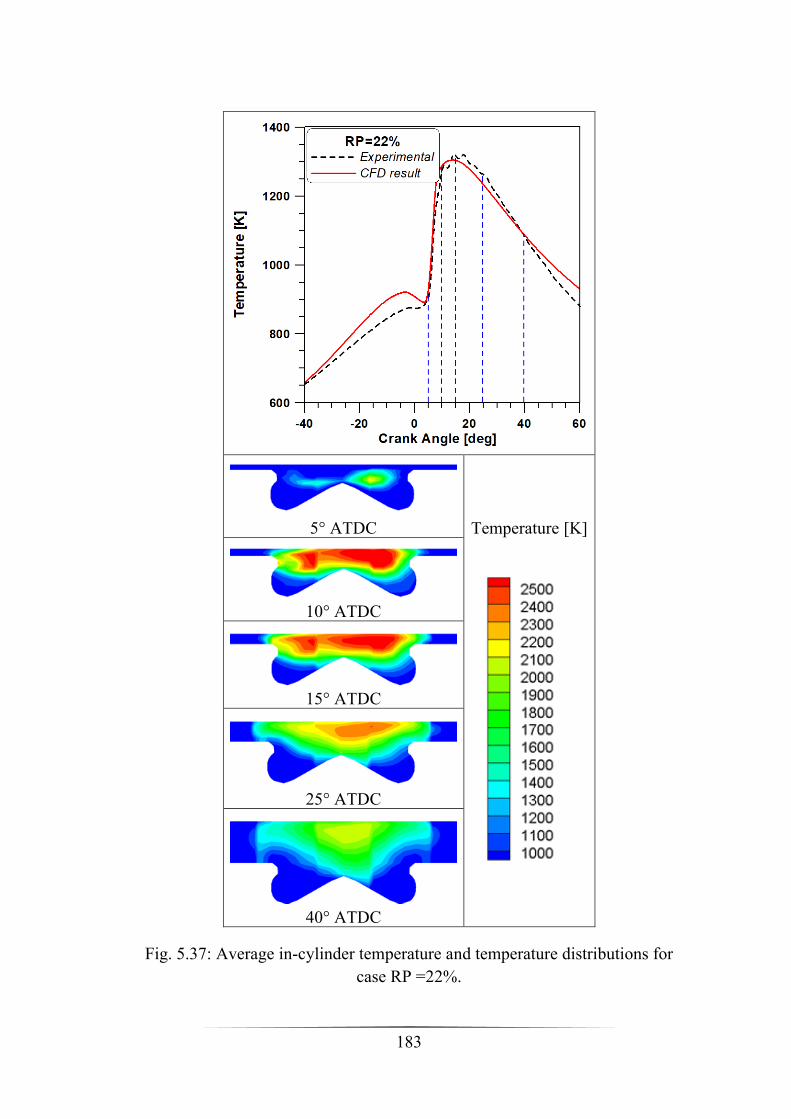
183
5° ATDC Temperature [K]
10° ATDC
15° ATDC
25° ATDC
40° ATDC
Fig. 5.37: Average in-cylinder temperature and temperature distributions for
case RP =22%.

184
Moreover, Figure 5.37 match the in-cylinder mean temperature with the
distribution of the same variable in an axial section at different crank angles.
At 5° ATDC temperature begins to increase since the first flame cores are
ignited. At 10° and 15° ATDC the peak of temperature is reached and wide
zones at high temperature are clearly detected. It is important to highlight that
in these zones the greater nitric oxides production is expected.
Fig. 5.38: Comparison of experimental and numerical total fuel burning rates.
Figure 5.38 shows differences with respect to the combustion development of
methane in the RP=15 case: although the start is again delayed, the peak, is
slightly anticipated and the duration is shorter.
In Figure 5.39 the FBR of the two different fuels is reported. Of course, a
predominant activity is shown by diesel oil since the reduced amount of
ethane injected.
Figure 5.40 evidences, once again the incomplete oxidation of methane
which represents the major drawback of this technology.

185
Fig. 5.39: diesel and methane fuel burning rates.
Fig. 5.40: Fuel burning fraction for the two fuels.

186
Figures 5.41 and 5.42 plot the role of several reactions of the combustion
mechanism. Like before, the RR1 describes the diesel vapour combustion,
RR12 the complete methane oxidation and RR2 and RR3 are reported as
representative of the Li and Williams scheme. The activation of all methane
reactions is always delayed with respect to diesel oxidation. Therefore, this
mechanism confirms that methane is ignited by diesel oil combustion.
Moreover, as an example of the importance of the ignition process, the
activation of the RR3 reaction, which occurs at a temperatures below 1300 K
and converts methane into an intermediate species, is anticipated with respect
to the start of the RR12 reaction, which involves the final methane oxidation.
Figure 5.42 points out that the main contribution to overall combustion heat
release is provided by the first reaction, i.e., the one involving diesel fuel.
Indeed, the thermal power peak of reactions RR3 and RR12 is lower by 1 or
2 orders of magnitude compared with the one from diesel vapour oxidation.
Figure 5.43 displays the evolution of the main and some intermediate species
considered in the mechanism. Again, it is demonstrated that the diesel
consumption occurs before the decrease in methane contents. Also, the
validity of the mechanism is proven by the earlier formation of the
intermediate species at lower temperature before the activation of the main
methane reaction. The same Figure plots the sequential methane consumption
inside the cylinder that reach its maximum rate between 5° and 10° ATDC, as
confirmed by the CH4 trend. After this period, it is noted that methane still
present in the squish zone completes the oxidation process while a significant
amount of unburned hydrocarbons remains trapped inside the combustion
bowl at the later crank angles. It is obvious that the poor methane / air
equivalence ratio is not adequate to allow the flame front to reach these
zones.

187
Fig. 5.41: Reaction rates of RR1 (C12H26 oxidation), RR3 (CH4 conversion
in CH3) and RR12 (CH4 conversion in CO).
Fig. 5.42: Heat of reaction of RR1, RR2 (CO oxidation in CO2 and
dissociation) and RR12.

188
5° ATDC
CH4 [ppm]
10° ATDC
20° ATDC
40° ATDC
Fig. 5.43: Species evolution and methane distributions at different crank
angles.
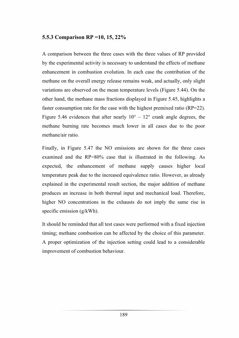
189
5.5.3 Comparison RP =10, 15, 22%
A comparison between the three cases with the three values of RP provided
by the experimental activity is necessary to understand the effects of methane
enhancement in combustion evolution. In each case the contribution of the
methane on the overall energy release remains weak, and actually, only slight
variations are observed on the mean temperature levels (Figure 5.44). On the
other hand, the methane mass fractions displayed in Figure 5.45, highlights a
faster consumption rate for the case with the highest premixed ratio (RP=22).
Figure 5.46 evidences that after nearly 10° – 12° crank angle degrees, the
methane burning rate becomes much lower in all cases due to the poor
methane/air ratio.
Finally, in Figure 5.47 the NO emissions are shown for the three cases
examined and the RP=80% case that is illustrated in the following. As
expected, the enhancement of methane supply causes higher local
temperature peak due to the increased equivalence ratio. However, as already
explained in the experimental result section, the major addition of methane
produces an increase in both thermal input and mechanical load. Therefore,
higher NO concentrations in the exhausts do not imply the same rise in
specific emission (g/kWh).
It should be reminded that all test cases were performed with a fixed injection
timing; methane combustion can be affected by the choice of this parameter.
A proper optimization of the injection setting could lead to a considerable
improvement of combustion behaviour.

190
Fig. 5.44: Average in-cylinder temperatures for RP=10, 15 and 22%.
Fig. 5.45: Comparison of methane mass fractions for RP=10, 15 and 22%.

191
Fig. 5.46: Comparison of methane reaction rates for RP=10, 15 and 22%.
Fig. 5.47 Comparison of NO emissions for RP=10,15 and 22%.

192
5.5.4 Comparison of Autoignition model vs 2-step model
The comparison between the results obtained with the employment of the Li
and Williams model and the tow-step mechanism is necessary to asses if an
improvement has been achieved for the combustion description. Figure 5.48
does not evidence significant differences in the reproduction of the pressure
curve. Recalling Figure 5.38, the FBR peak obtained with the Li and
Williams model results anticipated with respect to the experimental one,
Figure 5.49 displays an even more anticipated peak for the two-step
mechanism and consequently an earlier end of combustion. An important
feature highlighted by Figure 5.50 is a smoother methane consumption with
the autoignition model that appears to be more realistic, since the low
methane-air ratio causes a slow ignition of the premixed charge.
Fig. 5.48: In cylinder pressure for case RP=22%.
193
Fig. 5.49: Comparison of total fuel burning rates by different models.
Fig. 5.50: Comparison of total fuel burning rates by different models.

194
5.5.5 Comparison RP = 80% vs RP = 22%
A great enhancement of methane amount causes an evident increase of
pressure and temperature peaks as shown in Figures 5.51 and 5.52. This
explains the higher emissions of NO for the RP=80% as already illustrated in
Figure 5.47. Differently from the other cases, with an energy input from
methane of 80% the mixture falls between the flammability limits of methane
and a more efficient combustion is achieved. However, a divergence of
pressure and temperature is detected nearly 40° BTDC, this can be due to
earlier activation of some reactions in the autoignition mechanism favoured
by the higher equivalence ratio. Combustion development is considerably
different from the cases previously discussed. Firstly, the over FBR (Figure
5.53) of RP=80% evidences an anticipated start of combustion and longer
duration than in the RP=22% case. Figure 5.54 demonstrates that the longer
duration is caused by the CH4 contents. Moreover Figure 5.55 shows that in
this case methane burns almost completely at the expense of diesel oil. This
can be explained by Figure 5.56 that reports the oxygen consumption. As it is
possible to see, oxygen concentration decreases more rapidly in the RP=80%
case since the more intense methane oxidation subtracts oxygen to diesel
vapour combustion.
Figures 5.57 and 5.58 show that RR12 is predominant with respect to RR1. In
particular, even the rate of a reaction in the autoignition mechanism (RR3)
results higher than the one of the diesel oxidation.

195
Fig. 5.51: In cylinder pressure for case RP =22 and 80%.
Fig. 5.52: In cylinder temperatures for cases RP=22 and 80%.

196
Fig. 5.53: Comparison of total fuel burning rates for cases RP=22 and 80%.
Fig. 5.54: Comparison of diesel and methane fuel burning rates for RP=80%.

197
Fig. 5.55: Fuel burning fractions for the two fuels for RP=80%.
Fig. 5.56: Comparison of oxygen mass fractions for cases RP =22 and 80%.

198
Fig. 5.57: Reaction rates of RR1 (C12H26 oxidation), RR2 (CO oxidation in
CO2 and dissociation) and RR12 (CH4 conversion in CO)for RP=80%.
Fig. 5.58: Reaction rates of RR1, RR3 (CH4 conversion in CH3) and RR12
for RP=80%.

199
Fig. 5.59: Reaction rate distributions of RR3 and RR12 for RP=80%.
In Figure 5.59 the reaction rates of two reactions involving methane are
compared. RR3 and RR12 are activated below and above 1300 K,
respectively, the former is taken as representative of the autoignition
mechanism and convert CH4 in CH3 that is an intermediate species, the latter
converts CH4 in CO. For this reason, the sequential plot of the RR12 reaction
rate recalls a flame front propagation through the combustion chamber. As
noted at 15° ATDC the end-wall regions of the bowl are already reached by
the methane combustion progress in according to Figure 5.55. A real
200
interaction between the RR3 and RR12 reactions can be only detected in the
earliest ignition phases (i.e., within the interval 3°BTDC – 3° ATDC).
Starting from 5° crank angles ATDC, the RR3 reaction presents a more
evident scattering with respect to the RR12 progress. Actually, the flame
front related to the main methane oxidation seems to proceed in an ordinate
way, while the dispersion of the RR3 reaction is probably related to the
existence of local zones with lower temperature levels.
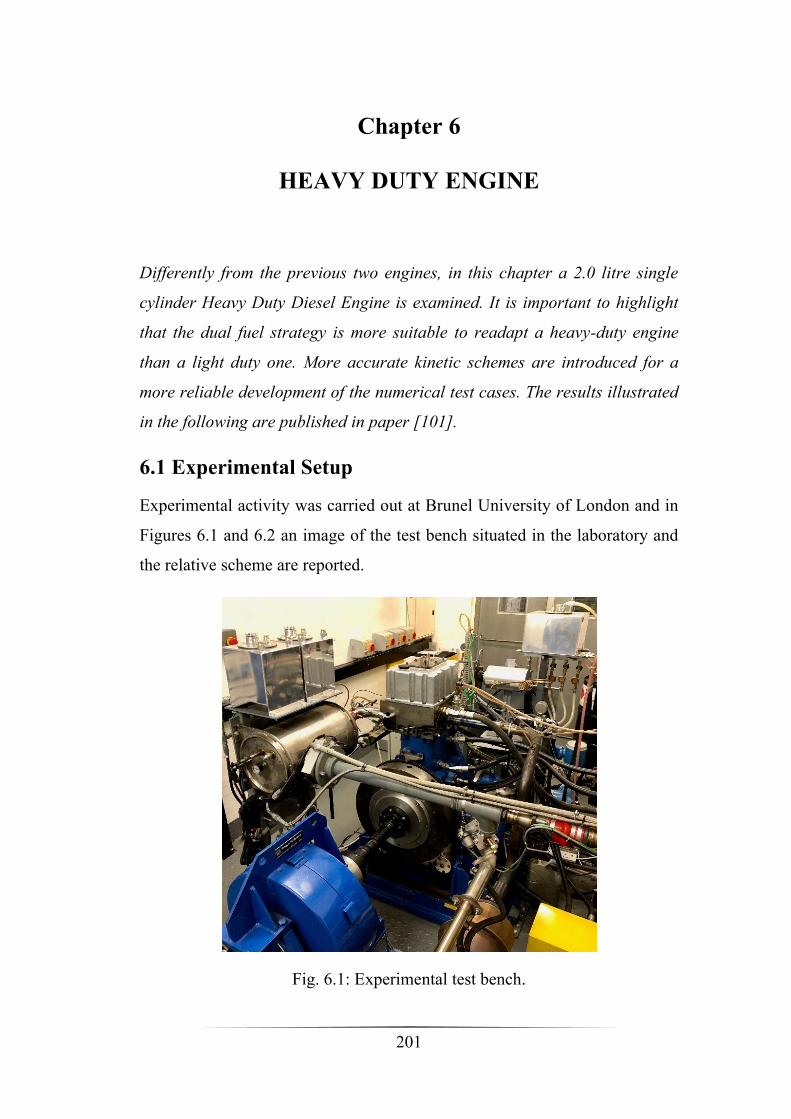
201
Chapter 6
HEAVY DUTY ENGINE
Differently from the previous two engines, in this chapter a 2.0 litre single
cylinder Heavy Duty Diesel Engine is examined. It is important to highlight
that the dual fuel strategy is more suitable to readapt a heavy-duty engine
than a light duty one. More accurate kinetic schemes are introduced for a
more reliable development of the numerical test cases. The results illustrated
in the following are published in paper [101].
6.1 Experimental Setup
Experimental activity was carried out at Brunel University of London and in
Figures 6.1 and 6.2 an image of the test bench situated in the laboratory and
the relative scheme are reported.
Fig. 6.1: Experimental test bench.
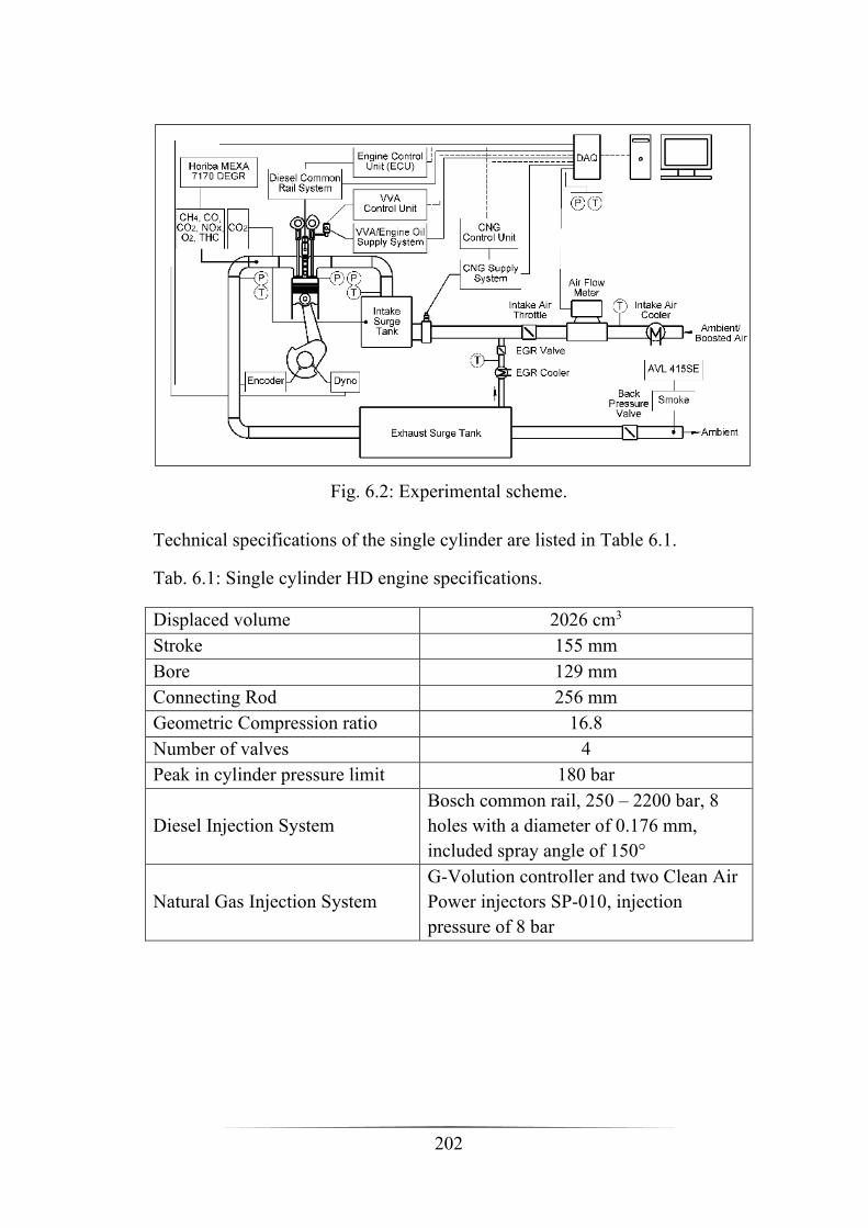
202
Fig. 6.2: Experimental scheme.
Technical specifications of the single cylinder are listed in Table 6.1.
Tab. 6.1: Single cylinder HD engine specifications.
Displaced volume 2026 cm3
Stroke 155 mm
Bore 129 mm
Connecting Rod 256 mm
Geometric Compression ratio 16.8
Number of valves 4
Peak in cylinder pressure limit 180 bar
Diesel Injection System
Bosch common rail, 250 – 2200 bar, 8
holes with a diameter of 0.176 mm,
included spray angle of 150°
Natural Gas Injection System
G-Volution controller and two Clean Air
Power injectors SP-010, injection
pressure of 8 bar
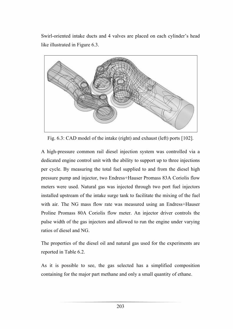
203
Swirl-oriented intake ducts and 4 valves are placed on each cylinder’s head
like illustrated in Figure 6.3.
Fig. 6.3: CAD model of the intake (right) and exhaust (left) ports [102].
A high-pressure common rail diesel injection system was controlled via a
dedicated engine control unit with the ability to support up to three injections
per cycle. By measuring the total fuel supplied to and from the diesel high
pressure pump and injector, two Endress+Hauser Promass 83A Coriolis flow
meters were used. Natural gas was injected through two port fuel injectors
installed upstream of the intake surge tank to facilitate the mixing of the fuel
with air. The NG mass flow rate was measured using an Endress+Hauser
Proline Promass 80A Coriolis flow meter. An injector driver controls the
pulse width of the gas injectors and allowed to run the engine under varying
ratios of diesel and NG.
The properties of the diesel oil and natural gas used for the experiments are
reported in Table 6.2.
As it is possible to see, the gas selected has a simplified composition
containing for the major part methane and only a small quantity of ethane.
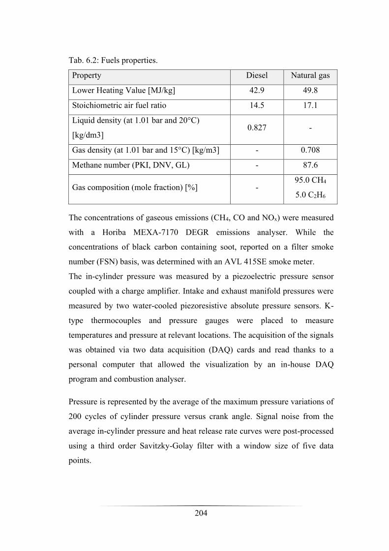
204
Tab. 6.2: Fuels properties.
Property Diesel Natural gas
Lower Heating Value [MJ/kg] 42.9 49.8
Stoichiometric air fuel ratio 14.5 17.1
Liquid density (at 1.01 bar and 20°C)
[kg/dm3] 0.827 -
Gas density (at 1.01 bar and 15°C) [kg/m3] - 0.708
Methane number (PKI, DNV, GL) - 87.6
Gas composition (mole fraction) [%] - 95.0 CH4
5.0 C2H6
The concentrations of gaseous emissions (CH4, CO and NOx) were measured
with a Horiba MEXA-7170 DEGR emissions analyser. While the
concentrations of black carbon containing soot, reported on a filter smoke
number (FSN) basis, was determined with an AVL 415SE smoke meter.
The in-cylinder pressure was measured by a piezoelectric pressure sensor
coupled with a charge amplifier. Intake and exhaust manifold pressures were
measured by two water-cooled piezoresistive absolute pressure sensors. K-
type thermocouples and pressure gauges were placed to measure
temperatures and pressure at relevant locations. The acquisition of the signals
was obtained via two data acquisition (DAQ) cards and read thanks to a
personal computer that allowed the visualization by an in-house DAQ
program and combustion analyser.
Pressure is represented by the average of the maximum pressure variations of
200 cycles of cylinder pressure versus crank angle. Signal noise from the
average in-cylinder pressure and heat release rate curves were post-processed
using a third order Savitzky-Golay filter with a window size of five data
points.

205
The tests cases and the relative experimental engine conditions are listed in
Table 6.3.
Tab. 6.3. Testing conditions for the different engine operating modes.
Load Low Medium High
Engine load (IMEP) [bar] 6 12 18
Percentage of full engine load [%] 25 50 75
Engine speed [rpm] 1200 1200 1200
Diesel Injected Mass [g/cycle] 0.0156 0.0274 0.0421
Diesel Injection pressure [bar] 1000 1300 1600
Diesel Start of injection [CAD] -5.951 -1.523 6.477
Duration of Diesel injection [deg] 4.77 5.03 5.02
Natural Gas Energy fraction (NG%) 80±1 80±1 80±1
Natural Gas Equivalence ratio [-] 0.375 0.444 0.521
Intake manifold air temperature [°C] 41 42 44
Intake manifold air pressure [bar] 1.25 1.90 2.60
Exhaust manifold pressure [bar] 1.35 2.0 2.7
Exhaust gas recirculation (EGR) 0% 0% 0%
Three different load levels (25%, 50% and 75% of full engine load) were
investigated, for a fixed engine speed of 1,200 rpm and a fixed NG energy
fraction (80%), defined as the ratio of the energy content of the NG to the
total fuel energy supplied. Differently from the research engine studied in the
previous chapter, the load levels considered are near to the typical ones of a
real engine. These cases were determined after the optimisation of the diesel
start of injection, considering as upper bound for calibration a maximum
pressure rise rate of 20 bar/CAD. Therefore, the start of injection is retarded
with the load increase. Also, the valve opening period is varied by variable
valve actuation system. Although the engine is equipped with an EGR
system, like shown in Figure 6.2), the testing activity does not include this
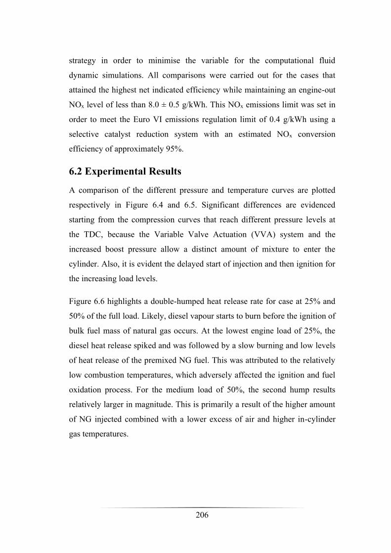
206
strategy in order to minimise the variable for the computational fluid
dynamic simulations. All comparisons were carried out for the cases that
attained the highest net indicated efficiency while maintaining an engine-out
NOx level of less than 8.0 ± 0.5 g/kWh. This NOx emissions limit was set in
order to meet the Euro VI emissions regulation limit of 0.4 g/kWh using a
selective catalyst reduction system with an estimated NOx conversion
efficiency of approximately 95%.
6.2 Experimental Results
A comparison of the different pressure and temperature curves are plotted
respectively in Figure 6.4 and 6.5. Significant differences are evidenced
starting from the compression curves that reach different pressure levels at
the TDC, because the Variable Valve Actuation (VVA) system and the
increased boost pressure allow a distinct amount of mixture to enter the
cylinder. Also, it is evident the delayed start of injection and then ignition for
the increasing load levels.
Figure 6.6 highlights a double-humped heat release rate for case at 25% and
50% of the full load. Likely, diesel vapour starts to burn before the ignition of
bulk fuel mass of natural gas occurs. At the lowest engine load of 25%, the
diesel heat release spiked and was followed by a slow burning and low levels
of heat release of the premixed NG fuel. This was attributed to the relatively
low combustion temperatures, which adversely affected the ignition and fuel
oxidation process. For the medium load of 50%, the second hump results
relatively larger in magnitude. This is primarily a result of the higher amount
of NG injected combined with a lower excess of air and higher in-cylinder
gas temperatures.
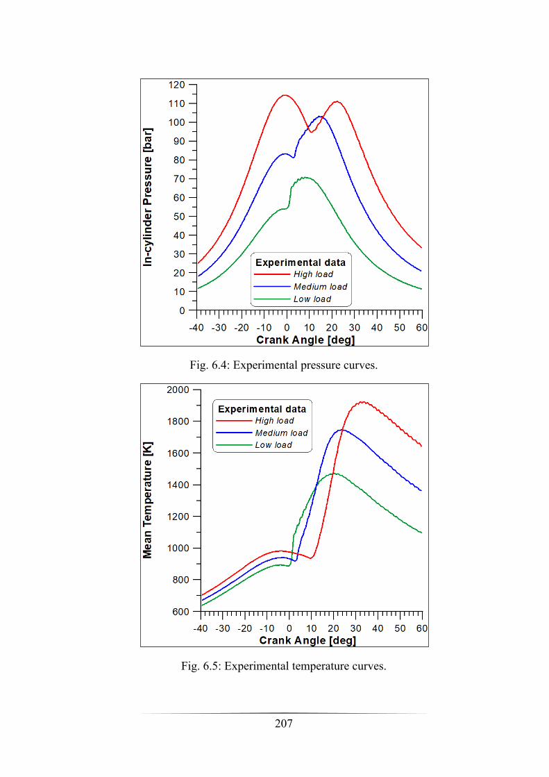
207
Fig. 6.4: Experimental pressure curves.
Fig. 6.5: Experimental temperature curves.
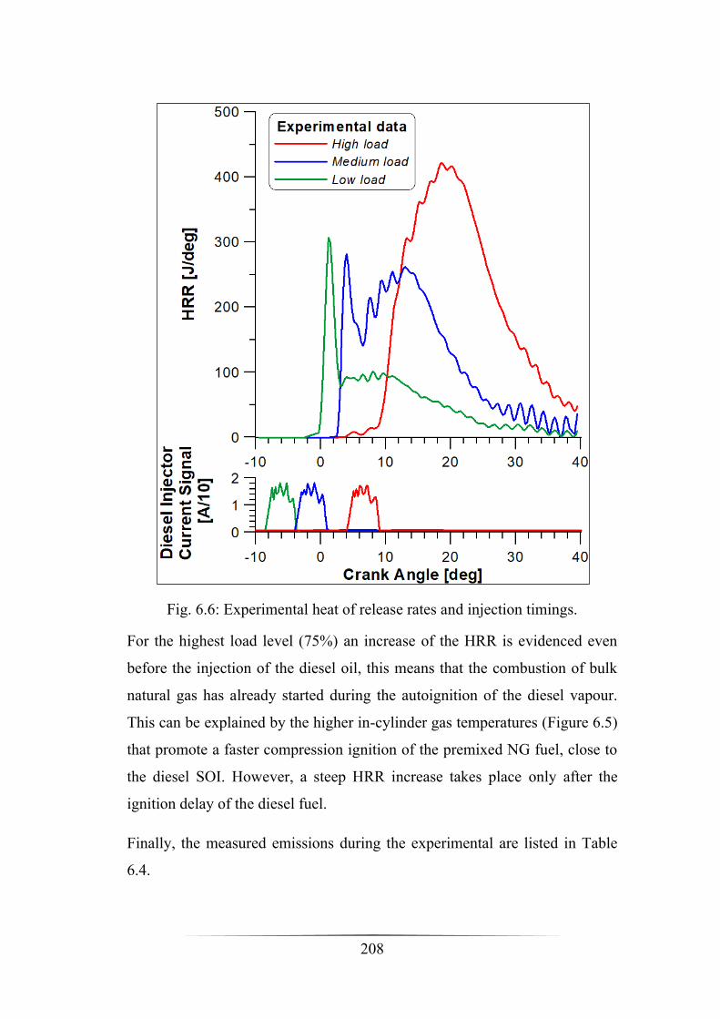
208
Fig. 6.6: Experimental heat of release rates and injection timings.
For the highest load level (75%) an increase of the HRR is evidenced even
before the injection of the diesel oil, this means that the combustion of bulk
natural gas has already started during the autoignition of the diesel vapour.
This can be explained by the higher in-cylinder gas temperatures (Figure 6.5)
that promote a faster compression ignition of the premixed NG fuel, close to
the diesel SOI. However, a steep HRR increase takes place only after the
ignition delay of the diesel fuel.
Finally, the measured emissions during the experimental are listed in Table
6.4.

209
Tab. 6.4: Experimental Emissions
[ppm] Low Load Medium Load High Load
CH4 7483 3009 1011
UHC 7448 3035 1062
CO 2159 1258 628
6.3 CFD Methodology
In the previous chapter a more detailed scheme for the autoignition of
methane, assumed as the only component of natural gas, was implemented,
while the diesel oxidation was represented by a one-step reaction mechanism.
Now, a new kinetic mechanism is introduced for the n-dodecane, still used as
diesel oil surrogate, consisting of 100 species and 432 reactions introduced
by Ra and Reitz in [103], and compared with the previous one. Although a
simpler mechanism is preferable for the computational time reduction, the
kinetic mechanism complication is also dictated by the necessity of a further
knowledge of the various phenomena which characterise the combustion
process. Based on the experimental activity, firstly a calibration, and
secondly a validation of the kinetic mechanism has been made for cases at
50% (medium) and 75% (high) of the load performed with the 3D code
ANSYS-FORTE.
Starting from a drawing of the stepped-lip piston bowl, displayed in Figure
6.7 [102], the profile of the combustion chamber was designed (Figure 6.8).
The mesh was created with the K3PREPW tool, included in the KIVA-3V
workbench, which is able to generate mesh grids that can be read by the
ANSYS-FORTE solver. The K3PREPW is a software specialised in the
creation of grids for internal combustion engine. However, only the

210
combustion chamber and the cylinder can be reproduced, allowing only the
simulation of closed cycles from the intake valve closing to the exhaust valve
opening. The not perfect assessment of the mass exchange inside the cylinder
due to the absence of the valves and their opening period, is compensated by
a significant reduction of computational efforts. Moreover, due to the
circumferential periodicity the computational domain was limited to only a
45° sector and a further calculation time reduction is achieved (Figure 6.9).
The final mesh consists of about 38,000 nodes.
Fig. 6.7: Drawing of the piston cross-section [102].

211
Fig. 6.8: Combustion bowl profile.
Fig. 6.9: 45° sector mesh.

212
The computational methodology founds on the integrated use of two solvers:
KIVA-3V and ANSYS-FORTE. The first one is used only for the flow
solution during the intake process on a similar geometry with open valve
periods, in order to establish proper levels of turbulence and swirled flow
parameters by making use of standard k-ε equations. More specifically, this
solver provides the values of Turbulent Kinetic Energy and Turbulent Length
Scale that are required by FORTE as turbulence initial conditions. This
second solver is exploited for its advanced features in terms of complex
kinetic mechanisms, turbulence-chemistry interaction and droplet breakup
modelling.
In Table 6.5 the boundary condition for the CFD simulation are listed. The
initial conditions are set at 40° BTDC. Indeed, as already said, the engine is
equipped with a VVA system that varies the IVC and this crank angle was
chosen for all the case.
Tab. 6.5. Simulation initial conditions at 40° BTDC.
Load Medium High
Diesel Start of injection [CAD] -1.523 6.477
Duration of Diesel injection [deg] 5.03 5.02
Diesel Injected Mass [g/cycle] 0.0274 0.0421
Natural Gas mass fraction (NG%) 2.51 2.93
Pressure [bar] 17.7 24.21
Temperature [K] 667 699
Turbulent Kinetic Energy [cm2/s] 1.0×10⁵ 1.0×10⁵
Turbulent Length Scale [cm] 0.422 0.422
The Droplet breakup computation in FORTE is carried out by the combined
Kelvin Helmoltz – Rayleigh Taylor approach.

213
Recalling Table 6.3, it is possible to observe that even at 75% load operation,
the natural gas – air equivalence ratio is close to the lower flammable limit.
For this reason, the effects of the turbulent flame propagation can be
neglected and, once again it seems to be more appropriate to base the
combustion process for both fuels on the turbulence – chemistry interaction.
The first kinetic mechanism is the same used in the previous chapter (Tables
5.6 and 5.7) consisting of the one-step reaction for the oxidation of n-
dodecane and the 9-reaction mechanism presented by Li and Williams. Also,
in these simulations, NG composition is assumed to be made of 100%
methane contents, due to simplified composition of the gaseous fuel used
during the experimental tests (Table 6.2).
Tab. 6.6: Detailed Species present in the mechanism.
1 DF2 7 H2 13 HO2
2 O2 8 O 14 CH3
3 N2 9 N 15 H2O2
4 CO2 10 OH 16 CH2O
5 H2O 11 CO 17 CHO
6 H 12 NO 18 CH4
Differently from the previous chapters, the Zel’dovich mechanism for nitric
oxides formation was not implemented in ANSYS-FORTE. Therefore, four
species, i.e. N2, O, N and NO, that are reported in Table 6.6 and that are not
present in the kinetic scheme in Table 6.7, are, actually not used. For this
reason, for these CFD simulations, the estimation of NOx emissions is not
included.
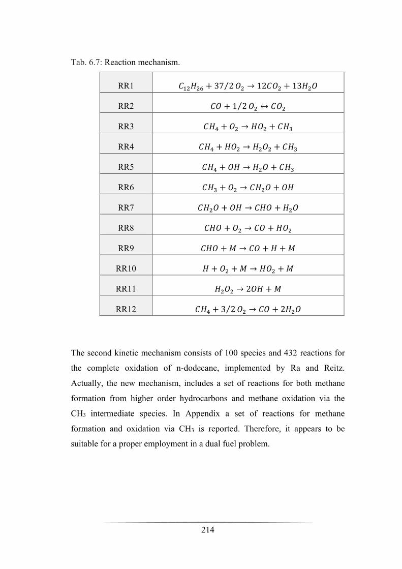
214
Tab. 6.7: Reaction mechanism.
RR1 𝐶12𝐻26 + 37 2⁄ 𝑂2 → 12𝐶𝑂2 + 13𝐻2𝑂
RR2 𝐶𝑂 + 1 2⁄ 𝑂2 ↔ 𝐶𝑂2
RR3 𝐶𝐻4 + 𝑂2 → 𝐻𝑂2 + 𝐶𝐻3
RR4 𝐶𝐻4 + 𝐻𝑂2 → 𝐻2𝑂2 + 𝐶𝐻3
RR5 𝐶𝐻4 + 𝑂𝐻 → 𝐻2𝑂 + 𝐶𝐻3
RR6 𝐶𝐻3 + 𝑂2 → 𝐶𝐻2𝑂 + 𝑂𝐻
RR7 𝐶𝐻2𝑂 + 𝑂𝐻 → 𝐶𝐻𝑂 + 𝐻2𝑂
RR8 𝐶𝐻𝑂 + 𝑂2 → 𝐶𝑂 + 𝐻𝑂2
RR9 𝐶𝐻𝑂 +𝑀 → 𝐶𝑂 + 𝐻 +𝑀
RR10 𝐻 + 𝑂2 +𝑀 → 𝐻𝑂2 +𝑀
RR11 𝐻2𝑂2 → 2𝑂𝐻 +𝑀
RR12 𝐶𝐻4 + 3 2⁄ 𝑂2 → 𝐶𝑂 + 2𝐻2𝑂
The second kinetic mechanism consists of 100 species and 432 reactions for
the complete oxidation of n-dodecane, implemented by Ra and Reitz.
Actually, the new mechanism, includes a set of reactions for both methane
formation from higher order hydrocarbons and methane oxidation via the
CH3 intermediate species. In Appendix a set of reactions for methane
formation and oxidation via CH3 is reported. Therefore, it appears to be
suitable for a proper employment in a dual fuel problem.
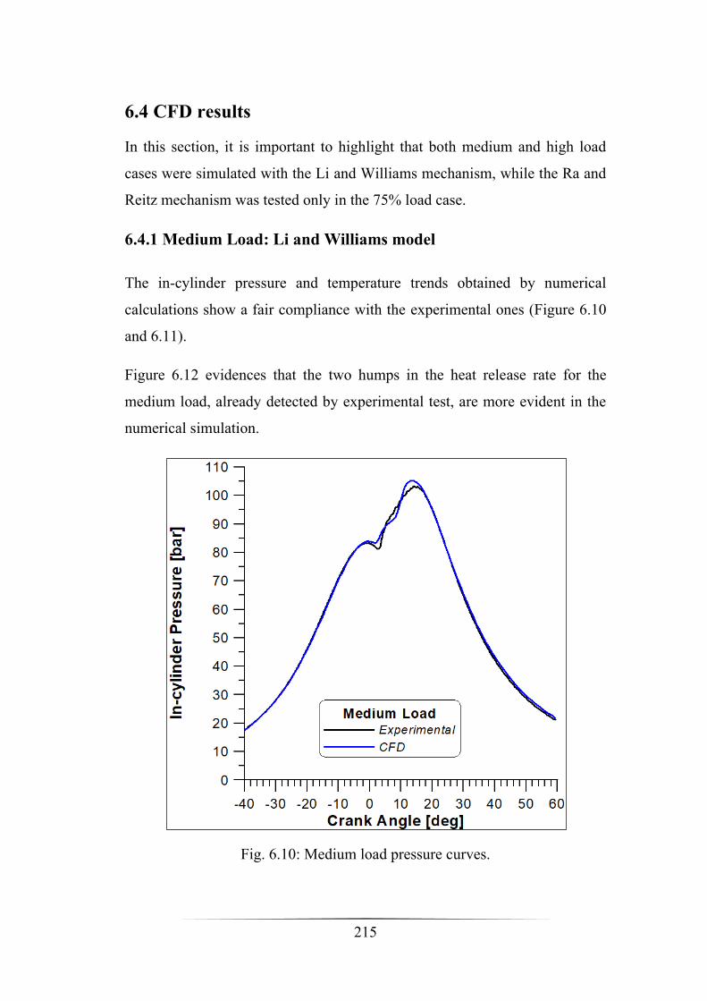
215
6.4 CFD results
In this section, it is important to highlight that both medium and high load
cases were simulated with the Li and Williams mechanism, while the Ra and
Reitz mechanism was tested only in the 75% load case.
6.4.1 Medium Load: Li and Williams model
The in-cylinder pressure and temperature trends obtained by numerical
calculations show a fair compliance with the experimental ones (Figure 6.10
and 6.11).
Figure 6.12 evidences that the two humps in the heat release rate for the
medium load, already detected by experimental test, are more evident in the
numerical simulation.
Fig. 6.10: Medium load pressure curves.
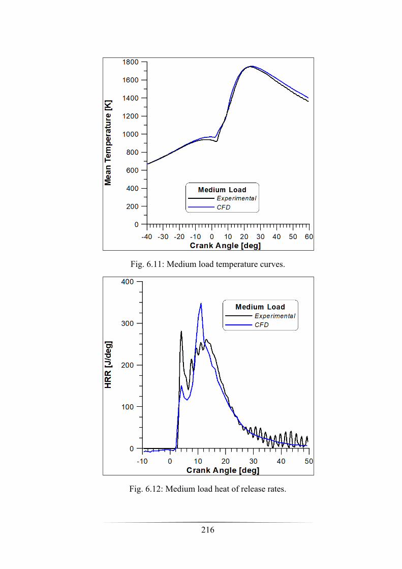
216
Fig. 6.11: Medium load temperature curves.
Fig. 6.12: Medium load heat of release rates.

217
An important result obtained from the same Figure is that experimental and
numerical starts of combustion match perfectly. However, the two peaks, that
highlight two distinct burning rates for diesel fuel and natural gas, are
correctly detected in timing but their magnitude show opposite trends.
Indeed, differently from the experimental tests, the first one is lower with
respect to the second one and this implies a different increase to the
maximum of pressure. Nevertheless, the final part of combustion is fairly
reproduced.
6.4.2 High Load: Li and Williams model
The numerical pressure trend, displayed in Figure 6.13, differs from the
experimental one only in the rise to the peak. In particular, a second lower
hump is observed before the peak pressure. This is due to the fact that the Li
and Williams model concerns only the methane autoignition, while the diesel
vapour is converted directly in CO2 though a single-step reaction. It appears
that the two combustion processes are independent from each other.
Therefore, the first hump is caused by the direct oxidation of n-dodecane and
the second hump is the effect of the methane oxidation. Also, in Figure 6.14
the mean temperature does not present a straight rise to the peak, in
accordance with the pressure trend. The validation of these considerations is
provided by Figure 6.15, since the first peak in the heat release is comparable
with the second one showing a different behaviour from the one previously
observed in the medium load case. However, the experimental HRR, as
explained in the experimental results section, is characterises by a single
hump trend. Although, the numerical start of combustion is not perfectly
detected, the estimation of combustion duration can be considered
acceptable.
Finally, a perfect agreement of the expansion phase is shown in all Figures.
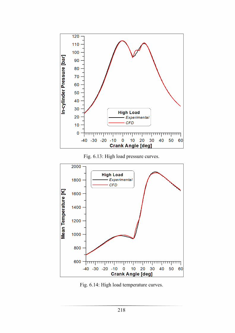
218
Fig. 6.13: High load pressure curves.
Fig. 6.14: High load temperature curves.
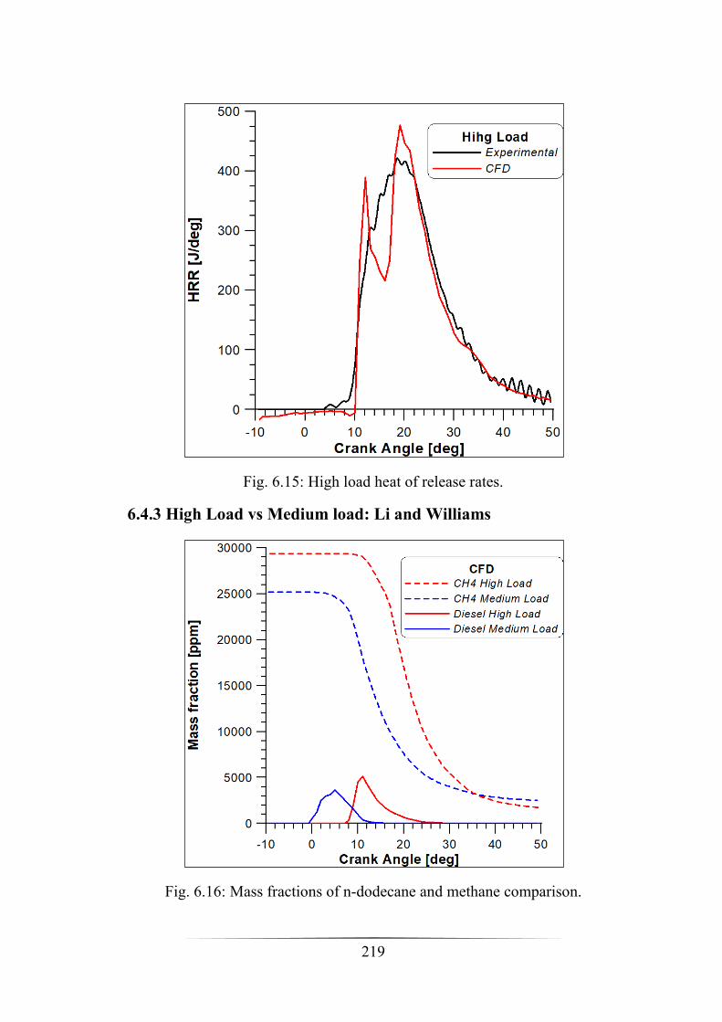
219
Fig. 6.15: High load heat of release rates.
6.4.3 High Load vs Medium load: Li and Williams
Fig. 6.16: Mass fractions of n-dodecane and methane comparison.
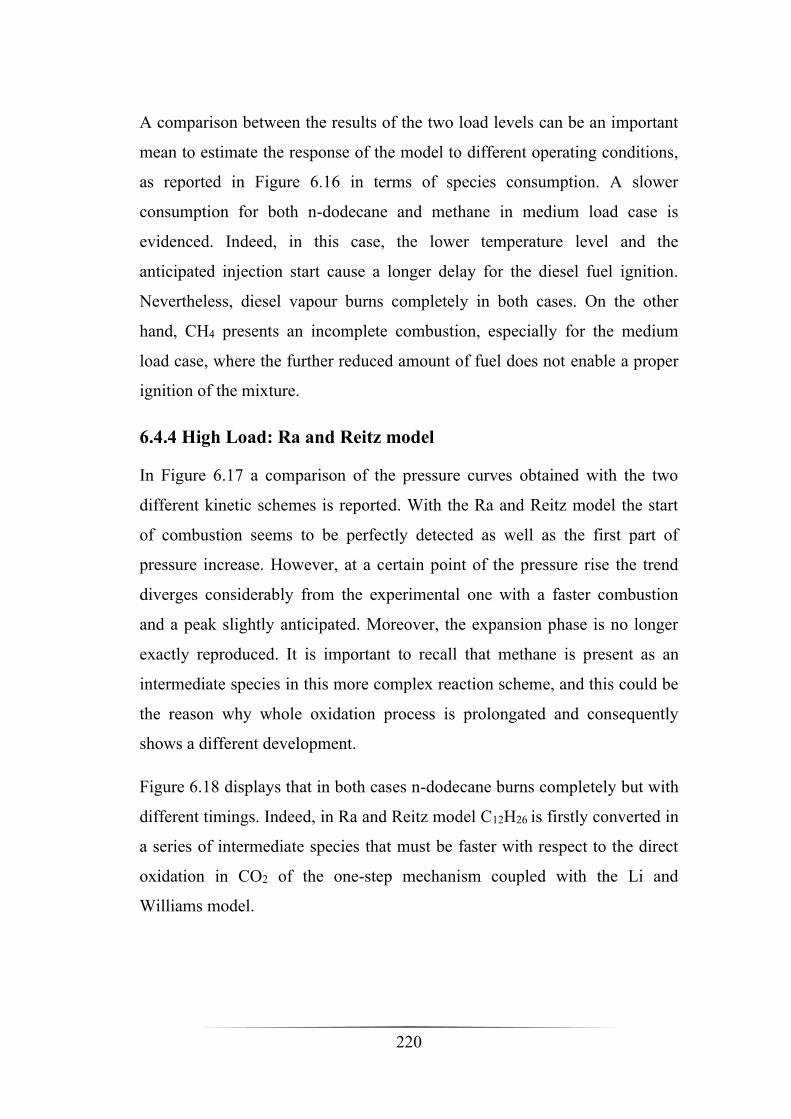
220
A comparison between the results of the two load levels can be an important
mean to estimate the response of the model to different operating conditions,
as reported in Figure 6.16 in terms of species consumption. A slower
consumption for both n-dodecane and methane in medium load case is
evidenced. Indeed, in this case, the lower temperature level and the
anticipated injection start cause a longer delay for the diesel fuel ignition.
Nevertheless, diesel vapour burns completely in both cases. On the other
hand, CH4 presents an incomplete combustion, especially for the medium
load case, where the further reduced amount of fuel does not enable a proper
ignition of the mixture.
6.4.4 High Load: Ra and Reitz model
In Figure 6.17 a comparison of the pressure curves obtained with the two
different kinetic schemes is reported. With the Ra and Reitz model the start
of combustion seems to be perfectly detected as well as the first part of
pressure increase. However, at a certain point of the pressure rise the trend
diverges considerably from the experimental one with a faster combustion
and a peak slightly anticipated. Moreover, the expansion phase is no longer
exactly reproduced. It is important to recall that methane is present as an
intermediate species in this more complex reaction scheme, and this could be
the reason why whole oxidation process is prolongated and consequently
shows a different development.
Figure 6.18 displays that in both cases n-dodecane burns completely but with
different timings. Indeed, in Ra and Reitz model C12H26 is firstly converted in
a series of intermediate species that must be faster with respect to the direct
oxidation in CO2 of the one-step mechanism coupled with the Li and
Williams model.
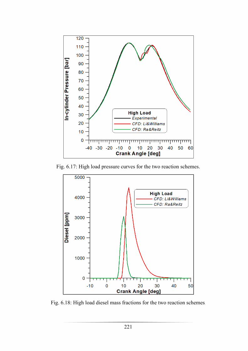
221
Fig. 6.17: High load pressure curves for the two reaction schemes.
Fig. 6.18: High load diesel mass fractions for the two reaction schemes.

222
Fig. 6.19: High load methane mass fractions for the two reaction schemes.
Fig. 6.20: High load CO mass fractions for the two reaction schemes.

223
Fig. 6.21: High load UHC mass fractions for the two reaction schemes.
Methane consumption in Figure 6.19 highlights that with the Ra and Reitz
model a faster and almost completed oxidation is achieved, explaining the
anticipated peak in the pressure curve (Figure 6.17). Figure 6.20 confirms the
complete oxidation of CH4 since almost no unburned hydrocarbon are
produced at the exhaust, being in contrast with the experimental
measurements. Finally, Figure 6.21 points out a more efficient CO oxidation
provided by the Ra and Reitz model.
6.4.5 Li and Williams vs Ra and Reitz model
In this last section an overall overview and a comparison of the experimental
and numerical results are reported for a more comprehensive descriptions of
the outcomes of the CFD analysis.
As evidenced in Table 6.8, Li and Williams kinetic model allows a correct
prediction of methane combustion, while as already stated, the Ra and Reitz
CH4 and UHC results are in contrast with the well-known dual fuel
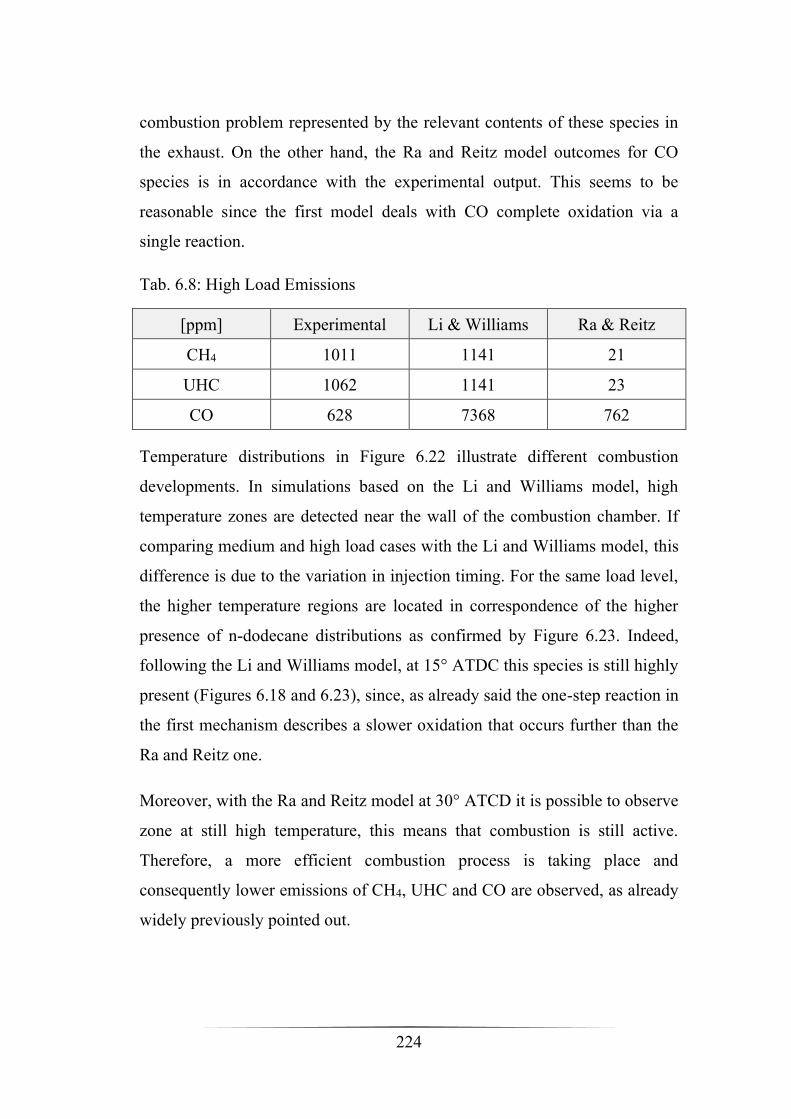
224
combustion problem represented by the relevant contents of these species in
the exhaust. On the other hand, the Ra and Reitz model outcomes for CO
species is in accordance with the experimental output. This seems to be
reasonable since the first model deals with CO complete oxidation via a
single reaction.
Tab. 6.8: High Load Emissions
[ppm] Experimental Li & Williams Ra & Reitz
CH4 1011 1141 21
UHC 1062 1141 23
CO 628 7368 762
Temperature distributions in Figure 6.22 illustrate different combustion
developments. In simulations based on the Li and Williams model, high
temperature zones are detected near the wall of the combustion chamber. If
comparing medium and high load cases with the Li and Williams model, this
difference is due to the variation in injection timing. For the same load level,
the higher temperature regions are located in correspondence of the higher
presence of n-dodecane distributions as confirmed by Figure 6.23. Indeed,
following the Li and Williams model, at 15° ATDC this species is still highly
present (Figures 6.18 and 6.23), since, as already said the one-step reaction in
the first mechanism describes a slower oxidation that occurs further than the
Ra and Reitz one.
Moreover, with the Ra and Reitz model at 30° ATCD it is possible to observe
zone at still high temperature, this means that combustion is still active.
Therefore, a more efficient combustion process is taking place and
consequently lower emissions of CH4, UHC and CO are observed, as already
widely previously pointed out.
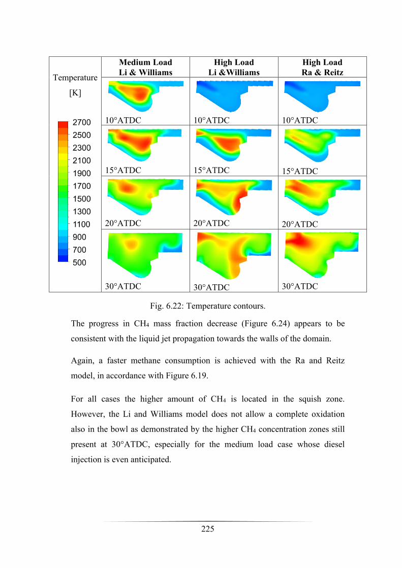
225
Temperature
[K]
Medium Load
Li & Williams
High Load
Li &Williams
High Load
Ra & Reitz
10°ATDC
10°ATDC
10°ATDC
15°ATDC 15°ATDC 15°ATDC
20°ATDC 20°ATDC 20°ATDC
30°ATDC 30°ATDC 30°ATDC
Fig. 6.22: Temperature contours.
The progress in CH4 mass fraction decrease (Figure 6.24) appears to be
consistent with the liquid jet propagation towards the walls of the domain.
Again, a faster methane consumption is achieved with the Ra and Reitz
model, in accordance with Figure 6.19.
For all cases the higher amount of CH4 is located in the squish zone.
However, the Li and Williams model does not allow a complete oxidation
also in the bowl as demonstrated by the higher CH4 concentration zones still
present at 30°ATDC, especially for the medium load case whose diesel
injection is even anticipated.
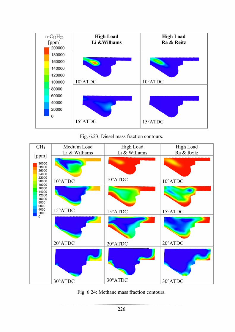
226
n-C12H26
[ppm]
High Load
Li &Williams
High Load
Ra & Reitz
10°ATDC
10°ATDC
15°ATDC
15°ATDC
Fig. 6.23: Diesel mass fraction contours.
CH4
[ppm]
Medium Load
Li & Williams
High Load
Li & Williams
High Load
Ra & Reitz
10°ATDC
10°ATDC
10°ATDC
15°ATDC 15°ATDC 15°ATDC
20°ATDC 20°ATDC 20°ATDC
30°ATDC 30°ATDC 30°ATDC
Fig. 6.24: Methane mass fraction contours.
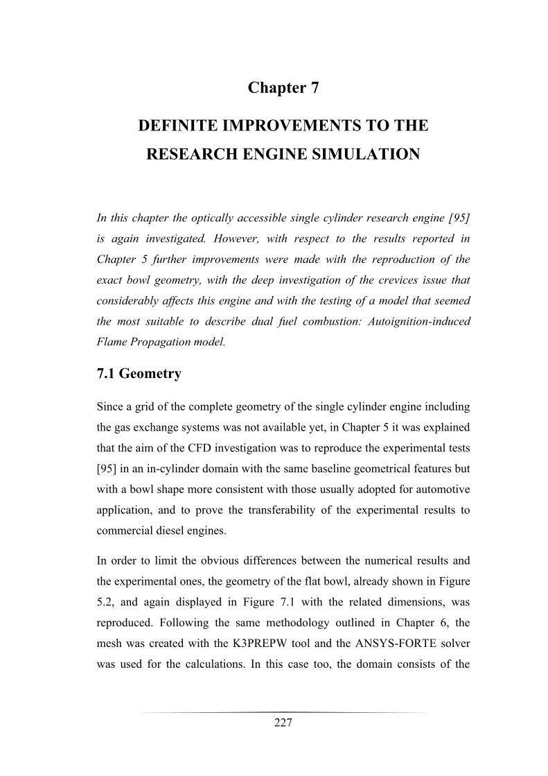
227
Chapter 7
DEFINITE IMPROVEMENTS TO THE
RESEARCH ENGINE SIMULATION
In this chapter the optically accessible single cylinder research engine [95]
is again investigated. However, with respect to the results reported in
Chapter 5 further improvements were made with the reproduction of the
exact bowl geometry, with the deep investigation of the crevices issue that
considerably affects this engine and with the testing of a model that seemed
the most suitable to describe dual fuel combustion: Autoignition-induced
Flame Propagation model.
7.1 Geometry
Since a grid of the complete geometry of the single cylinder engine including
the gas exchange systems was not available yet, in Chapter 5 it was explained
that the aim of the CFD investigation was to reproduce the experimental tests
[95] in an in-cylinder domain with the same baseline geometrical features but
with a bowl shape more consistent with those usually adopted for automotive
application, and to prove the transferability of the experimental results to
commercial diesel engines.
In order to limit the obvious differences between the numerical results and
the experimental ones, the geometry of the flat bowl, already shown in Figure
5.2, and again displayed in Figure 7.1 with the related dimensions, was
reproduced. Following the same methodology outlined in Chapter 6, the
mesh was created with the K3PREPW tool and the ANSYS-FORTE solver
was used for the calculations. In this case too, the domain consists of the

228
combustion chamber and the cylinder, so allowing only the simulation of
closed periods.
Fig. 7.1: Modified geometry of the combustion chamber.
Fig. 7.2: Modified geometry of the combustion chamber.

229
The diesel injector has 7 holes (Table 5.2) periodically distributed
approximately every 51.43° along the circumferential direction. Therefore, a
sector with the same opening angle, having the jet radial direction as bisector,
was considered for the computational domain. The final mesh displayed in
Figure 7.2, consists of 64,166 nodes and 63,808 cells.
7.2 Crevices
The optically accessible research engine is affected by significant mass
losses. Indeed, the adherence of the piston to the cylinder walls cannot be
ensured with the use of lubricating oil that would prevent the visibility in the
combustion chamber, but it is provided with particular rings, that allows the
mass of the methane-air mixture to flow into the crevices region during the
compression stroke and to return to the combustion chamber during the
expansion phase. This phenomenon influences the estimation of the actual
compression ratio. Indeed, in Table 5.1 it is reported a value of the geometric
compression ratio equal to 16.5, but in the practice the pressure curve
demonstrates that a lower effective value is reached during the end of the
compression stroke. Therefore, in the simulations carried out in Chapter 5,
the geometric compression ratio of the open valves mesh grid was calibrated
in order to follow the pressure curve during the compression phase. However,
this methodology cannot take into account the variations of equivalence ratio
that is consequent to the mass loss. For this reason, in the present chapter a
crevice model is added to the calculation set-up. In this way, it is possible to
evaluate the behaviour of the combustion development when a part of the
mass escapes and returns in the cylinder. Moreover, this model allows a
better evaluation of the amount of mass involved in this process.
The crevice model, used by the FORTE solver, was implemented by
Namazian and Heywood [104].

230
Fig. 7.3: Schematic diagram of the crevice volumes and planes used in the
model [72].
In Figure 7.3 the diagram of the volumes and planes considered for the
equations setting is reported. It is assumed that the flow in the crevice region
1 is a fully-developed laminar flow and the pressure is uniform and equal to
the cylinder pressure. Also, regions 2, 3 and 4 each have a uniform pressure
and the temperature is assumed to be equal to the wall temperature. The
continuity equations for the region 2, 3 and 4 can be written as follow:
𝑚𝑜2𝑝𝑜2
𝑑𝑝2𝑑𝑡
= �̇�12 − �̇�23
𝑚𝑜3𝑝𝑜3
𝑑𝑝3𝑑𝑡
= �̇�13 + �̇�23 − �̇�34 − �̇�35
𝑚𝑜4𝑝𝑜4
𝑑𝑝4𝑑𝑡
= �̇�34 − �̇�45

231
The subscript “o” refers to a reference condition, 𝑚 is the mass, 𝑝 is the
pressure, 𝑡 is the time and the double subscript designates the flow from the
first to the second numbered region.
The mass flow rate through the ring gap is calculated by the orifice flow
equation:
�̇� = 𝐶𝑑𝐴𝑔𝜌𝑐𝜂
Where 𝐶𝑑 is the discharge coefficient (0.6 – 0.86), 𝐴𝑔 is the cross-sectional
area available to the flow, 𝜌 is the density, 𝑐 is the speed of sound and 𝜂 is
the compressibility factor defined as:
𝜂𝑖 = √2
𝛾 − 1[(𝑝𝑖+1𝑝𝑖)
2𝛾− (𝑝𝑖+1𝑝𝑖)
𝛾+1𝛾]
Where 𝛾 is the ratio of specific heats and the subscript “i” on the pressure
terms denoted the region where the properties are calculated, with acceptable
values running from 1 to 4.
In order to calculate the mass flow rate through the rings, the FORTE code
requires some geometrical parameters as listed in Table 7.1. The values
reported in the second column are obtained through a calibration process
because the actual ones were unknown. In paper [104] Namazian and
Heywood tested their model on an engine with similar characteristics as those
under investigation; hence, starting from the values reported in their work a
progressive adjustment of the parameters was operated until the numerical
compression curve reproduced the one measured during the experimental
activity.

232
Tab. 7.1: Crevice model input parameter.
Engine Bore [mm] 85.0
Gas Temperature Inside Crevice [K] 600
Height of the crevice region between the top of the crevice and
the first compression ring [cm] 3.0
Crevice Thickness between the Piston edge and the Cylinder
Liner [mm] 0.64
Cross-sectional flow Gap Area – first ring [cm2] 0.021
Cross-sectional flow Gap Area – second ring [cm2] 0.021
Volume Behind Top Ring [cm3] 0.2457
Volume Between Ring 1 and 2 [cm3] 0.2548
Volume Behind Second Ring [cm3] 0.2457
First Ring Thickness [cm] 0.1
Second Ring Thickness [cm] 0.1
First Ring lateral Width [cm] 0.1
Second Ring lateral Width [cm] 0.1
Mass of the First Ring [g] 10.0
Mass of the Second Ring [g] 10.0
Bottom Clearance – First Ring [mm] 0.025
Bottom Clearance – Second Ring [mm] 0.025
Top Clearance – First Ring [mm] 0.025
Top Clearance – Second Ring [mm] 0.025
7.3 Autoignition induced flame propagation
In previous calculations the Finite rate – Eddy Dissipation model seemed to
be the most suitable for the combustion development description; indeed, due
to poor equivalence ratio of the operating conditions, it was not possible to
obtain a proper flame propagation. However, in this Chapter the RP = 22%
case was tested with the autoignition induced flame propagation model
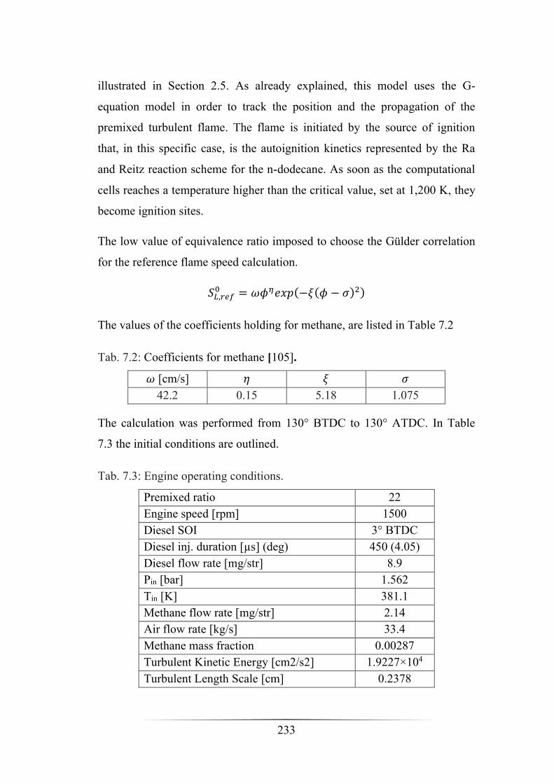
233
illustrated in Section 2.5. As already explained, this model uses the G-
equation model in order to track the position and the propagation of the
premixed turbulent flame. The flame is initiated by the source of ignition
that, in this specific case, is the autoignition kinetics represented by the Ra
and Reitz reaction scheme for the n-dodecane. As soon as the computational
cells reaches a temperature higher than the critical value, set at 1,200 K, they
become ignition sites.
The low value of equivalence ratio imposed to choose the Gülder correlation
for the reference flame speed calculation.
𝑆𝐿,𝑟𝑒𝑓0 = 𝜔𝜙𝜂𝑒𝑥𝑝(−𝜉(𝜙 − 𝜎)2)
The values of the coefficients holding for methane, are listed in Table 7.2
Tab. 7.2: Coefficients for methane [105].
𝜔 [cm/s] 𝜂 𝜉 𝜎
42.2 0.15 5.18 1.075
The calculation was performed from 130° BTDC to 130° ATDC. In Table
7.3 the initial conditions are outlined.
Tab. 7.3: Engine operating conditions.
Premixed ratio 22
Engine speed [rpm] 1500
Diesel SOI 3° BTDC
Diesel inj. duration [µs] (deg) 450 (4.05)
Diesel flow rate [mg/str] 8.9
Pin [bar] 1.562
Tin [K] 381.1
Methane flow rate [mg/str] 2.14
Air flow rate [kg/s] 33.4
Methane mass fraction 0.00287
Turbulent Kinetic Energy [cm2/s2] 1.9227×10⁴
Turbulent Length Scale [cm] 0.2378
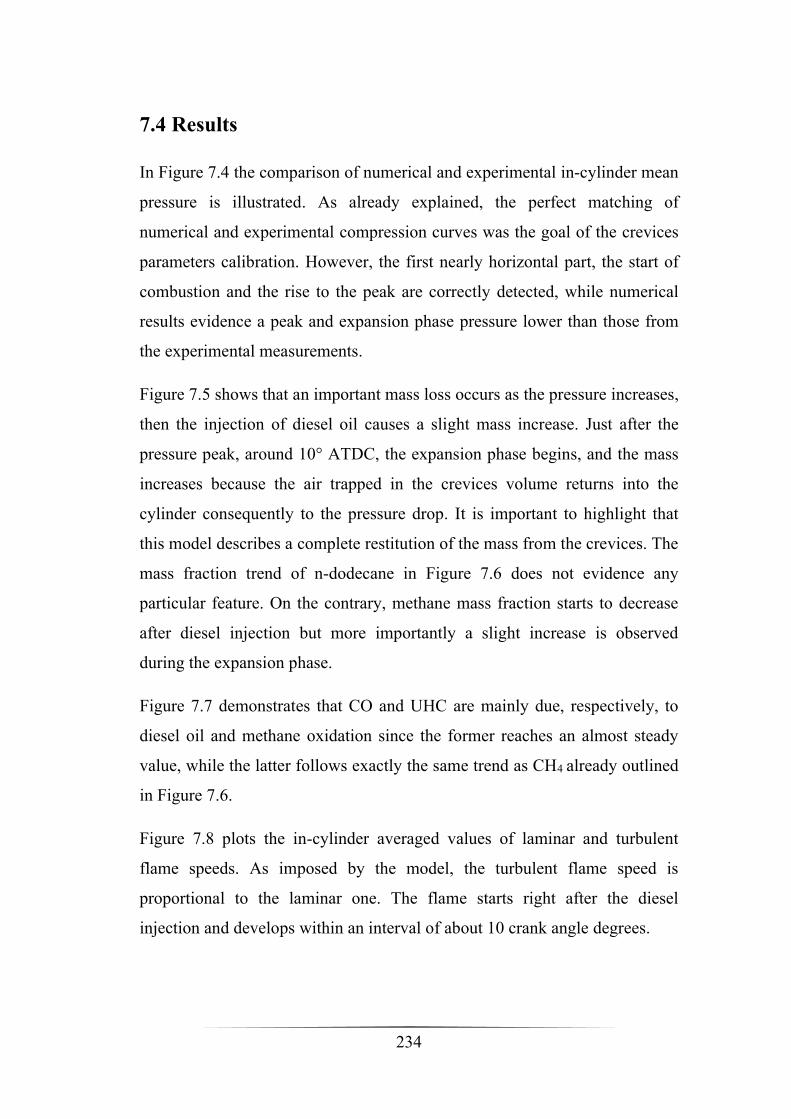
234
7.4 Results
In Figure 7.4 the comparison of numerical and experimental in-cylinder mean
pressure is illustrated. As already explained, the perfect matching of
numerical and experimental compression curves was the goal of the crevices
parameters calibration. However, the first nearly horizontal part, the start of
combustion and the rise to the peak are correctly detected, while numerical
results evidence a peak and expansion phase pressure lower than those from
the experimental measurements.
Figure 7.5 shows that an important mass loss occurs as the pressure increases,
then the injection of diesel oil causes a slight mass increase. Just after the
pressure peak, around 10° ATDC, the expansion phase begins, and the mass
increases because the air trapped in the crevices volume returns into the
cylinder consequently to the pressure drop. It is important to highlight that
this model describes a complete restitution of the mass from the crevices. The
mass fraction trend of n-dodecane in Figure 7.6 does not evidence any
particular feature. On the contrary, methane mass fraction starts to decrease
after diesel injection but more importantly a slight increase is observed
during the expansion phase.
Figure 7.7 demonstrates that CO and UHC are mainly due, respectively, to
diesel oil and methane oxidation since the former reaches an almost steady
value, while the latter follows exactly the same trend as CH4 already outlined
in Figure 7.6.
Figure 7.8 plots the in-cylinder averaged values of laminar and turbulent
flame speeds. As imposed by the model, the turbulent flame speed is
proportional to the laminar one. The flame starts right after the diesel
injection and develops within an interval of about 10 crank angle degrees.

235
Fig. 7.4: In cylinder pressure for RP=22.
Fig. 7.5: In cylinder mass.

236
Fig. 7.6: Mass fractions of methane and n-dodecane.
Fig. 7.7: Mass fractions of unburned hydrocarbons and carbon monoxide.
-10 0 10 20 30 40 50 60 70 80
Crank Angle [deg]
0
2000
4000
6000
8000
10000
12000
14000
Mass f
racti
on
[p
pm
]
RP=22%CH4
Diesel
-10 0 10 20 30 40 50 60 70 80
Crank Angle [deg]
0
2000
4000
6000
8000
10000
Mass f
racti
on
[p
pm
]
RP=22%UHC
CO

237
Fig. 7.8: Laminar and Turbulent flame speeds.
Figure 7.9 displays the temperature distributions at different crank angle
degrees in a meridional plane passing through the jet radial direction. Just
after TDC, higher temperatures are detected near the jet tips, recalling that in
this test case the amount of methane energy supply is only of 22%, it seems
reasonable that combustion start is mainly due to diesel vapour oxidation.
However, a sort of front flame is able to quickly propagate after 5° ATDC
(Figures 7.10 and 7.11). After this crank angle, higher concentration of
methane remains in the furthest zone from the jets, especially in the squish
zone, since during the expansion phase methane is released by the crevices
(Figure 7.12).
0 5 10 15 20
Crank Angle [deg]
0
100
200
300
400
500
600
700
800
Fla
me S
peed
[cm
/s]
RP=22%Laminar
Turbulent
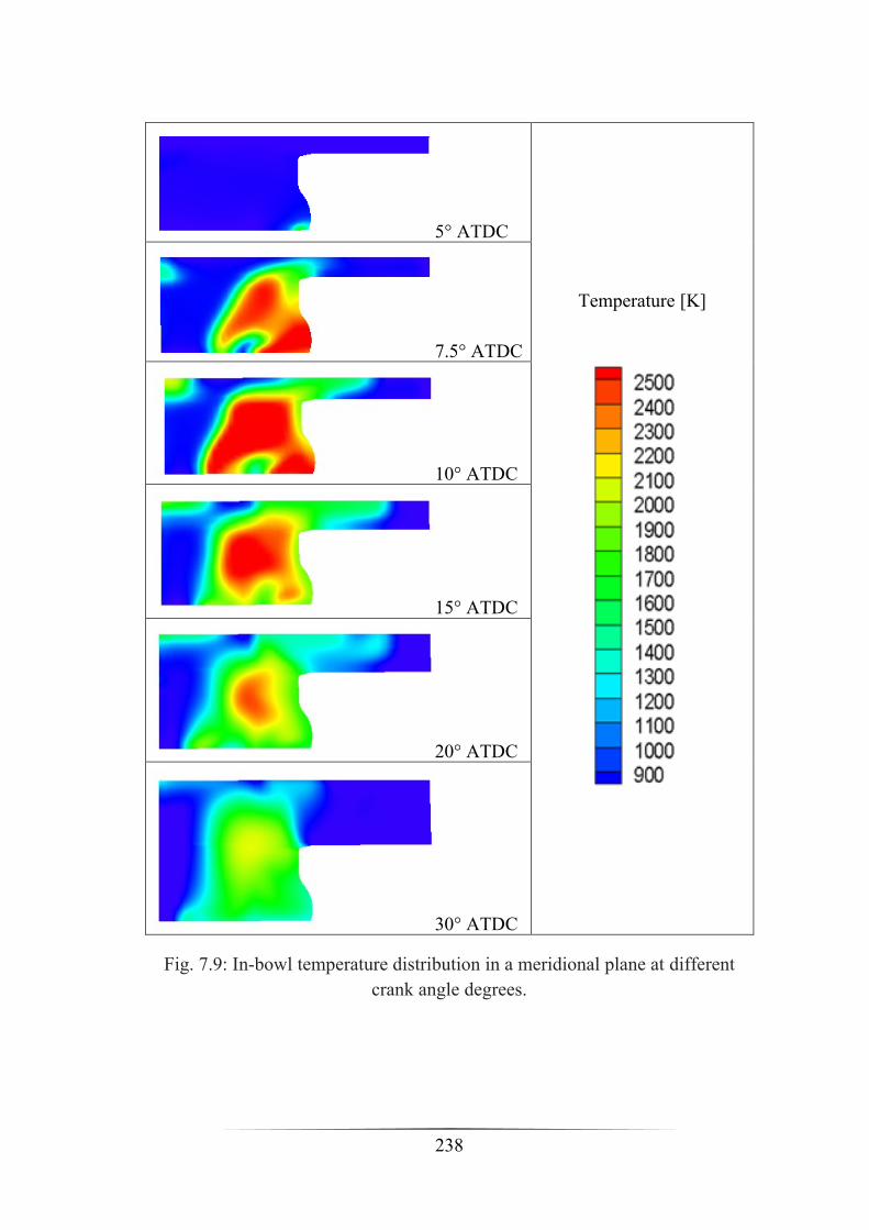
238
5° ATDC
Temperature [K]
7.5° ATDC
10° ATDC
15° ATDC
20° ATDC
30° ATDC
Fig. 7.9: In-bowl temperature distribution in a meridional plane at different
crank angle degrees.
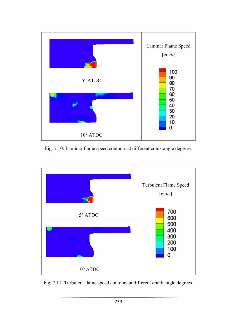
239
5° ATDC
Laminar Flame Speed
[cm/s]
10° ATDC
Fig. 7.10: Laminar flame speed contours at different crank angle degrees.
5° ATDC
Turbulent Flame Speed
[cm/s]
10° ATDC
Fig. 7.11: Turbulent flame speed contours at different crank angle degrees.
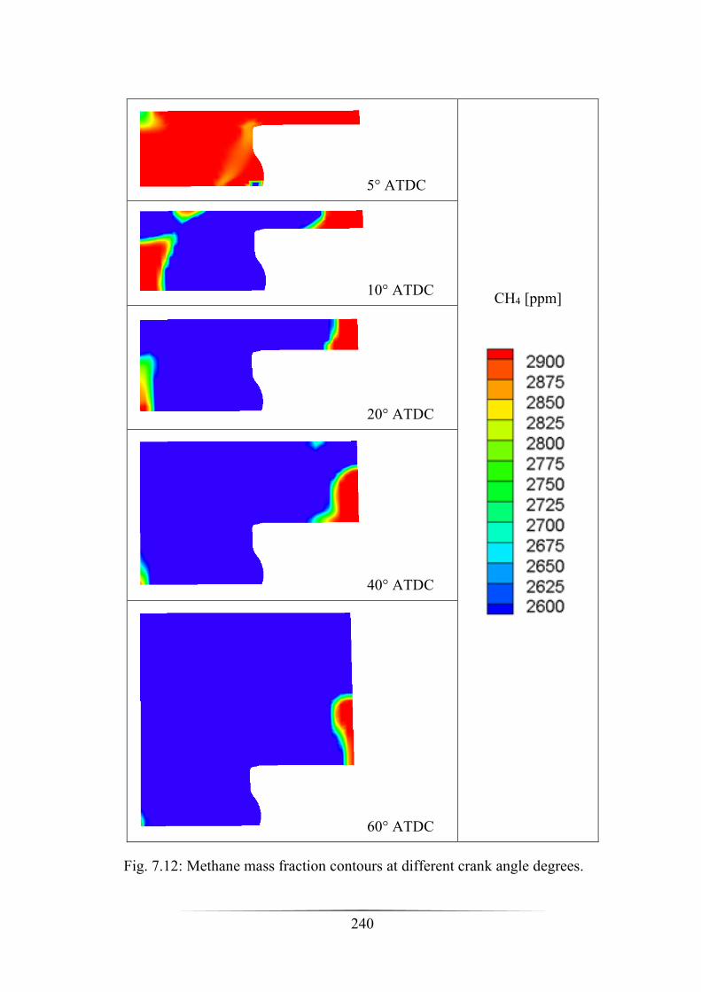
240
5° ATDC
CH4 [ppm]
10° ATDC
20° ATDC
40° ATDC
60° ATDC
Fig. 7.12: Methane mass fraction contours at different crank angle degrees.

241
In conclusion, this final numerical set up provides a more comprehensive
overview of the real phenomena affecting the dual fuel combustion in the
research engine:
- The effect of the mass flow through the devices is correctly detected,
in terms of actual in-cylinder mass trapped and, consequently, of
effective fuel/air ratio in the early phases of the combustion processes.
- Taking into account for crevices flow also allows identification of the
unburned methane location, which is mainly bounded in the squish
region.
- The G-equation mechanism for flame activation puts into evidence
that a sort of flame propagation takes place within a limited range of
crank angles; after that, a quick flame extinguishment is observed,
probably due to the very poor methane-air equivalence ratio. The latter
gives an additional reason for the relevant amount of unburned species
in this particular test case.

242
Conclusions
A CFD study of Dual Fuel combustion in a diesel engine was presented in
this thesis. The aim was to investigate the main phenomena that characterise
the combustion development, evidencing the criticalities that arise from the
addition of a second fuel that introduced new issues to face in the description
of the overall oxidation problem.
Due to the availability of experimental data used as an important validation
tool in a wide range of operating conditions, it was possible to implement and
test reliable computational models. In particular a progressive improvement
of the methodology and more detailed kinetic mechanism were utilised to
better comprehend the actual combustion mechanism and pollutants
formation.
Firstly, an integrated numerical methodology between a one-dimensional and
a three-dimensional code is developed for the prediction of the behaviour of a
light duty common rail diesel engine, by varying injection advance in full
diesel and dual fuel modes. In this phase, the aim was to build three
correlations for pilot and three correlations for the main injection (start, peak
and end of combustion) in order to extend the range of functioning and then,
to provide the boundary conditions for the cases not experimentally tested to
numerical simulations.
3D calculations were performed with ANSYS-FLUENT solver and the
kinetic mechanism consisting of only one reaction for the diesel vapour
oxidation and three reactions for the methane oxidation. A comparison
between the trends of the IMEP for the examined cases in full diesel and dual
fuel mode, evidences that in FD mode the IMEP decreases significantly with
a reduction of the injection advance, while in DF mode it can be considered

243
almost constant. For this reason, in dual fuel mode a right choice of SOP can
be suggested as a function of the only reduction of the pollutants. However,
the most important result, is that the CO2 emission index in DF mode is
always lower with respect to FD mode confirming that this technology can be
an effective mean to reduce the carbon dioxides emissions
Secondly, based on the experimental activity carried out on an optically
accessible single cylinder research engine, it was possible to visualise the
phenomena that occur inside the cylinder, focusing the attention on the
fundamental features of the combustion. Indeed, the experimental tests were
characterised by an increasing addition of methane and a constant amount of
diesel oil. In this way it was possible to analyse the effects of the methane
presence on the combustion. The KIVA-3V code was used for the numerical
simulations, where the Li and Williams scheme for the autoignition of
methane was implemented and compared with the previously cited kinetic
mechanism. Results showed a fair compliance with experimental
measurement, especially for OH distributions; since this radical represents an
important signal of the combustion rate intensity and location, CFD
simulations have proven to be capable to reproduce the real phenomena that
occur inside the cylinder. Moreover, another important achievement is
attained by the good agreement between the trends of numerical and
experimental NO fraction levels in the exhaust, although a slight
overestimation for the former with respect to the latter.
Finally, a further improvement was obtained during the study of the heavy
duty diesel engine, whose actual geometry was reproduced with the
K3PREPW mesh tool. In this phase, the Li and Williams model was
compared with the far more detailed kinetic mechanism presented by Ra and
Reitz. Results, obtained with the ANSYS-FORTE code, evidence that the Li
and Williams kinetic model allows a correct prediction of methane
combustion, while the Ra and Reitz CH4 and UHC results are in contrast with

244
the well-known dual fuel combustion problem represented by the relevant
contents of these species in the exhaust. On the other hand, the Ra and Reitz
model outcomes for CO species is in accordance with the experimental
output.
In conclusion, it is possible to affirm that results showed a good agreement
with experimental data, highlighting important features that characterise Dual
Fuel combustion. However, much work has still to be done in order to predict
the whole behaviour of the system as the latest outcomes outlined that both
models evidenced limits in the assessment of pollutant emissions. Moreover,
a mechanism for nitric oxides formation should be re-introduced. In this
sense, the completion of this study is currently addressed to the setup of a
more comprehensive mechanism based on the combined use of the Ra and
Reitz and Grimech 3.0 schemes, in order to obtain the best prediction of the
behaviour of both fuels. At the same time, this approach could lead to a
proper evaluation of NOx formation.
In each section of this study, it was affirmed that the equivalence ratio of
natural gas was lower than the flammability limits and, consequently, the
choice of the combustion model favoured the turbulence-chemistry
interaction. Nevertheless, in the final part of this thesis, the use of a G-
equation based model allowed identification of multiple flame nucleations
from which a sort of flame propagation takes place.
Once reached a comprehensive assessment of all dual fuel based phenomena,
future works should be oriented at utilise more eco-friendly fuels such as
syngas or biogas.

245
Acknowledgments
The simulations presented in this thesis have been achieved thanks to a
licensed version of the software ANSYS-FLUENT, FORTE and CHEMKIN.
246
References
[1] http://www.isprambiente.gov.it/ files2018/ area-stampa/ comunicati-
stampa/ graficiemissioni.pdf
[2] https://en.wikipedia.org/wiki/Diesel_engine
[3] Heywood John B. – Internal Combustion Engine Fundamentals
[4] Migliaccio, M., Della Volpe, R., 1995, Motori a combustione interna per
autotrazione.
[5] Ferrari, G., Motori a combustione Interna, Il Capitello
[6] https://en.wikipedia.org/wiki/Common_rail
[7] https://en.wikipedia.org/wiki/Diesel_particulate_filter
[8] https://en.wikipedia.org/wiki/European_emission_standards
[9] https://www.theguardian.com/cities/2017/apr/13/death-of-diesel-wonder-
fuel-new-asbestos
[10] https://en.wikipedia.org/wiki/Diesel_emissions_scandal
[11] https://www.eea.europa.eu/highlights/no-improvements-on-average-co2
[12] https://www.statista.com/statistics/425324/eu-car-sales-share-of-diesel-
engines-by- country/
[13] https://www.roadtraffic-technology.com/features/european-countries-
banning-fossil-fuel-cars/
[14] Murugesa Pandian, M., Anand, K., “Comparison of different low
temperature combustion strategies in a light duty air cooled diesel engine”,
Applied Thermal Engineering 142, 2018, 380-390,
https://doi.org/10.1016/j.applthermaleng.2018.07.047.
[15] https://www.cummins.com/engines/drilling/dual-fuel-engines-drilling
[16] Lozza, G., 2006, Turbine a Gas e Cicli Combinati, Bologna, ed. Progetto
Leonardo.
[17] https://en.wikipedia.org/wiki/Diesel_fuel

247
[18] https://en.wikipedia.org/wiki/Natural_gas
[19] https://www.slideshare.net/ahmedshoman792/natural-gas-dehydration
[20] Frerichs, J. and Eilts, P., “Development of a Physically/Chemically
Based Approach for 2-Stage Ignition Delay Calculation in Medium Speed
Dual-Fuel Engines,” SAE Technical Paper 2019-24-0068, 2019,
doi:10.4271/2019-24-0068.
[21] Ahmed, S.A., Zhou, S., Zhu, Y., Feng, Y., “Performance and Emission
Characteristics Analysis of Dual Fuel Compression Ignition Engine Using
Natural Gas and Diesel” International Journal of Thermodynamics (IJoT)
Vol. 21 (No. 1), pp. 16-25, 2018, doi: 10.5541/ijot.316300.
[22] Kozarac, D., Bozic, M., Vucetic, A., Krajnovic, J. et al., “Experimental
and Numerical Analysis of a Dual Fuel Operation of Turbocharged Engine at
Mid-High Load,” SAE Technical Paper 2019-24-0122, 2019,
doi:10.4271/2019-24-0122.
[23] Eder, L., Ban, M., Pirker, G., Vujanovic, M., Priesching, P., and
Wimmer, A., Development and Validation of 3D-CFD Injection and
Combustion Models for Dual Fuel Combustion in Diesel Ignited Large Gas
Engines, Energies 2018, 11, 643; doi: 10.3390/en1130643.
[24] Merts, M. and Verhelst, S., “Literature Review on Dual-Fuel
Combustion Modelling,” SAE Technical Paper 2019-24-0120, 2019,
doi:10.4271/2019-24-0120.
[25] Akbarian, E., Najafi, B., Jafari, M., Ardabili, S.F., Shamshirband, S.,
Chau, K., (2018) “Experimental and computational fluid dynamics-based
numerical simulation of using natural gas in a dual-fueled diesel engine”,
Engineering Applications of Computational Fluid Mechanics, 12:1, 517-534,
DOI:10.1080/19942060.2018.1472670.
[26] Huang, H., Zhu, Z., Chen, Y., Chen, Y., Lv, D., Zhu, J., Ouyang, T.,
“Experimental and numerical study of multiple injection effects on
combustion and emission characteristics of natural gas–diesel dual-fuel
engine”, Energy Conversion and Management 183 (2019) 84-96, doi:
10.1016/j.enconman.2018.12.110.
[27] Shu, J., Fu, J., Liu, J., Ma, Y., Wang, S., Deng, B., Zeng, D., “Effects of
injector spray angle on combustion and emissions characteristics of a natural
248
gas (NG)-diesel dual fuel engine based on CFD coupled with reduced
chemical kinetic model”, Applied Energy 233-234 (2019) 182-195, doi:
10.1016/j.apenergy.2018.10.040.
[28] Zhou, H., Li., X., Lee, C.F., “Investigation on soot emissions from
diesel-CNG dual-fuel”, International Journal of Hydrogen Energy,
https://doi.org/10.1016/j.ijhydene.2019.02.012.
[29] Papagiannakis, R.G, Rakopoulos, D.C., C.D., “Evaluation of the Air
Oxygen Enrichment Effects on Combustion and Emissions of Natural
Gas/Diesel Dual-Fuel Engines at Various Loads and Pilot Fuel Quantities”,
Energies 2018, 11, 3028; doi:10.3390/en11113028.
[30] Ghazal, O.H., “Air Pollution Reduction and Environment Protection
Using Methane Fuel for Turbocharged CI Engines”, Journal of Ecological
Engineering, Volume 19, Issue 5, September 2018, pages 52-58, doi:
10.12911/22998993/91276.
[31] Sremec, M., Taritaš, I., Sjerić, M., Kozarac, D., “Numerical
Investigation of Injection Timing Influence on Fuel Slip and Influence of
Compression Ratio on Knock Occurrence in Conventional Dual Fuel
Engine”, J. sustain. dev. energy water environ. syst., 5(4), pp 518-532, 2017,
doi: 10.13044/j.sdewes.d5.0163.
[32] Tulwin, T., and Sochaczewski, R., “The dual-fuel CFD combustion
model with direct and indirect CNG injection”, ITM Web Conferences 15,
07016 (2017) doi: 10.1051/itmconf/20171507016.
[33] Zoldak, P., Sobiesiak, A., Wickman, D., and Bergin, M., "Combustion
Simulation of Dual Fuel CNG Engine Using Direct Injection of Natural Gas
and Diesel," SAE Int. J. Engines 8(2):2015, doi:10.4271/2015-01-0851.
[34] Majczak, A., Baranski, G., Siadkowska, K., Sochaczewski, R., “cng
injector research for dual fuel engine”, Advances in Science and Technology
Research Journal, Volume 11, Iss. 1, 2017, pages 212-219, DOI:
10.12913/22998624/68458.
[35] Stettler, M.E.J., Midgley, W.J.B., Swanson, J.J., Cebon, D., Boies,
A.M., “Greenhouse Gas and Noxious Emissions from Dual Fuel Diesel and
Natural Gas Heavy Goods Vehicles”, Environ. Sci. Technol. 2016, 50, 2018-
2026.

249
[36] Mousavi, S.M., Saray, R.K., Poorghasemi, K., Maghbouli, “A numerical
investigation on combustion and emission characteristics of a dual fuel
engine at part load condition”, Fuel 166 (2016) 309-319, doi:
10.1016/j.fuel.2015.10.052.
[37] Talekar, A., Lai, M.-C., Tomita, E., Kawahara, N. et al., “Numerical
Investigation of Natural Gas-Diesel Dual Fuel Engine with End Gas
Ignition”, SAE Technical Paper 2018-01-0199, 2018, doi:10.4271/2018-01-
0199.
[38] Barro, C., Nani, C., Hutter, R., and Boulouchos, K., "Spray Model
Based Phenomenological Combustion Description and Experimental
Validation for a Dual Fuel Engine", SAE Technical Paper 2017-24-0098,
2017, doi:10.4271/2017-24-0098.
[39] Li, Y., Guo, H., and Li, H., "Evaluation of Kinetics Process in CFD
Model and Its Application in Ignition Process Analysis of a Natural Gas-
Diesel Dual Fuel Engine", SAE Technical Paper 2017-01-0554, 2017,
doi:10.4271/2017-01-0554.
[40] Kusaka, J., Tsuzuki, K., Daisho, Y., Saito, T., “A Numerical Study on
Combustion and Exhaust Gas Emissions Characteristics of a Dual Fuel
Natural Gas Engine Using a Multi-Dimensional Model Combined With
Detailed Kinetics” SAE Technical Paper 2002-01-1750.
[41] Cantore, G., Mattarelli, E., Rinaldini C.A. Savioli, T., Scrignoli, F.
“Numerical Optimization of the Injection Strategy on a Light Duty Diesel
Engine Operating in Dual Fuel (CNG/Diesel) Mode”, International Journal of
Heat and Technology, Vol. 37, No. 3, 2019, pp 682-688,
https://doi.org/10.18280/ijht.370303.
[42] Maghbouli, A., Saray, R.K., Shafee, S., Ghafouri, J., “Numerical study
of combustion and emission characteristics of dual-fuel engines using 3D-
CFD models coupled with chemical kinetics”, Fuel 106 (2013) 98-105, doi:
10.1016/j.fuel.2012.10.055.
[43] Huang, H., Lv, D., Zhu, J., Zhu, Z., Chen, Y., Pan, Y., Pan, M.,
“Development of a new reduced diesel/natural gas mechanism for dual-fuel
engine combustion and emission prediction”, Fuel 263 (2019) 30-42, doi:
10.1016/j.fuel.2018.08.161.
250
[44] Kahila, H., Wehrfritz, A., Kaario, O., Vourinen, V., “Large-Eddy
simulation of dual-fuel ignition: Diesel spray injection into a lean methane-
air mixture”, Combustion and Flame 199 (2019) 131-151, doi:
10.1016/j.combustflame.2018.10.014.
[45] De Simio, L., Gambino, M., and Iannaccone, S., "Effects of Low
Temperature Combustion on Particle and Gaseous Emission of a Dual Fuel
Light Duty Engine," SAE Technical Paper 2017-24-0081, 2017,
doi:10.4271/2017-24-0081.
[46] Catapano, F., Di Iorio, S., Sementa, P., and Vaglieco, B., "Particle
Formation and Emissions in an Optical Small Displacement SI Engine Dual
Fueled with CNG DI and Gasoline PFI," SAE Technical Paper 2017-24-
0092, 2017, doi:10.4271/2017- 24-0092.
[47] Vipavanich, C., Chuepeng, S., Skullog, S., “Heat release analysis and
thermal efficiency of a single cylinder diesel dual fuel engine with gasoline
port injection”, Case Studies in Thermal Engineering 12, 2018, 143-148,
https://doi.org/10.1016/j.csite.2018.04.011.
[48] Zang R., Yao C., Yin Z., et al. (2016). “Mechanistic Study of Ignition
Characteristics of Diesel/Methanol and Diesel/Methane. Dual Fuel Engine”.
Energy & Fuels, Volume 30, Issue 10, pag. 8630-8637.
[49] Pedrozo, V.B., May, I., Dalla Nora, M., Cairns, A., Zhao, H.,
“Experimental analysis of ethanol dual-fuel combustion in a heavy-duty
diesel engine: An optimisation at low load”, Applied Energy 165, 2016, 166-
182, http://dx.doi.org/10.1016/j.apenergy.2015.12.052.
[50] Pedrozo, V., May, I., and Zhao, H., "Characterization of Low Load
Ethanol Dual-Fuel Combustion using Single and Split Diesel Injections on a
Heavy-Duty Engine," SAE Technical Paper 2016-01-0778, 2016,
doi:10.4271/2016-01-0778.
[51] Pedrozo, V.B., May, I., Lanzanova, T.D.M., Zhao, H., “Potential of
internal EGR and throttled operation for low load extension of ethanol–diesel
dual-fuel reactivity controlled compression ignition combustion on a heavy-
duty engine”, Fuel 179, 2016, 391-405,
http://dx.doi.org/10.1016/j.fuel.2016.03.090.

251
[52] Pedrozo, V.B., May, I., Zhao, H., “Exploring the mid-load potential of
ethanol-diesel dual-fuel combustion with and without EGR”, Applied Energy
193, 2017, 263-275, http://dx.doi.org/10.1016/j.apenergy.2017.02.043.
[53] Karagoz, Y., Guler I., Sandalci T. et al. “Effects of hydrogen and
methane addition on combustion characteristics, emissions, and performance
of a CI engine”. International Journal of Hydrogen Energy, 2016, Volume 41,
Issue 2, pag. 1313-1325.
[54] Alrazen H.A.; Abu Talib A.R.; Ahmad K.A., “A two-component CFD
studies of the effects of H-2, CNG, and diesel blend on combustion
characteristics and emissions of a diesel engine”. International Journal of
Hydrogen Energy, 2016, Volume 41, Issue 24, pag. 10483-10495.
[55] Stylianidis, N., Azimov, U., Kawahara, N., and Tomita, E., "Chemical
Kinetics and Computational Fluid-Dynamics Analysis of H2/CO/CO2/CH4
Syngas Combustion and NOx Formation in a Micro-Pilot-Ignited
Supercharged Dual Fuel Engine," SAE Technical Paper 2017-24-0027, 2017,
doi:10.4271/2017-24-0027.
[56] Meng, X., Tian, H., Long, W., Zhou, Y., Bi, M., Tian, J, Lee, C.F.,
“Experimental study of using additive in the pilot fuel on the performance
and emission trade-offs in the diesel/CNG (methane emulated) dual-fuel
combustion mode”, Applied Thermal Engineering 157, 2019, 113718,
https://doi.org/10.1016/j.applthermaleng.2019.113718
[57] Abagnale, C., Cameretti, M.C., De Simio, L., Iannaccone, S., Tuccillo,
R., “Experimental and Numerical Study of a Diesel Engine Operating in Dual
Fuel Mode”, Proceeding 67° Congresso ATI 2012.
[58] Abagnale, C., Cameretti, M.C., De Simio, L., Gambino, M., Iannaccone,
S., Tuccillo, R., “Numerical simulation and experimental test of dual fuel
operated diesel engines”, Applied Thermal Engineering 65 (2014) 403-417,
doi: 10.1016/j.applthermaleng.2014.01.040.
[59] Abagnale, C., Cameretti, M.C., De Simio, L., Gambino, M., Iannaccone,
S., Tuccillo, R., “Combined numerical-experimental study of dual fuel diesel
engine”, Energy Procedia 45 (2014) 721-730, doi:
10.1016/j.egypro.2014.01.077.
[60] Abagnale, C., Cameretti, M., Ciaravola, U., Tuccillo, R. et al., "Dual
Fuel Diesel Engine at Variable Operating Conditions: A Numerical and
252
Experimental Study", SAE Technical Paper 2015-24-2411, 2015,
doi:10.4271/2015-24-2411.
[61] M.C. Cameretti, U. Ciaravola, R. Tuccillo, L. De Simio, S. Iannaccone,
“A numerical and experimental study of dualfuel diesel engine for different
injection timings”, Applied Thermal Engineering (2016), doi:
10.1016/j.applthermaleng.2015.12.071.
[62] https://en.wikipedia.org/wiki/Computational_fluid_dynamics
[63] http://sustainabilityworkshop.autodesk.com/products/metrics-and-
basics-fluid-flow
[64] Ansys Fluent, 2009, Theory Guide.
[65] https://en.wikipedia.org/wiki/Numerical_analysis
[66] ANSYS, “Introduction to ANSYS CFD Professional”.
[67] https://www.comsol.com/multiphysics/mesh-refinement
[68] http://sageography.myschoolstuff.co.za/wiki/grade-12-
caps/geomorphology/drainage-systems-in-south-africa/discharge-of-a-river/.
[69] https://user-images.githubusercontent.com/193367/38030812-f6c4f174-
3299-11e8-91ed-30684ceae715.png
[70] Magnussen, B.F. and Hjertager, B.H., 1977, On Mathematical Modeling
of Turbulent Combustion with Special Emphasis on Soot Formation, 16th.
Symposium on Combustion, The Combustion Institute, Pittsburgh.
[71] Course notes “Thermofluid-dynamics”, Bozza, F., University of Naples.
[72] Ansys Forte, 2016, Theory Manual.
[73] Metghalchi, M., Keck, J. C., “Burning Velocities of Methanol, Ethanol
and iso-Octane-Air Mixtures”, 19th Symposium (International) on
Combustion/ The Combustion Institute, p. 275, 1983.
[74] Gülder, O., ¨L. Correlations of laminar combustion data for alternative
S.I. engine fuels”, SAE paper 841000, 1984.
[75] Cameretti, M.C., and Tuccillo R., “Flowand Atomization Models for
C.R. Diesel Engine CFD Simulation,” Proceedings of ASME/IEEE 2007
Joint Rail Conference and Internal Combustion Engine Division Spring
253
Technical Conference. vol. ASME paper JRCICE2007-40068, p. 451-461,
ISBN: 0791837955, Pueblo, Colorado, USA, March 2007, doi:
10.1115/JRC/ICE2007-40068.
[76] O'Rourke P.J.,. Amsden, 1987, A.A, The TAB Method for Numerical
Calculation of Spray Droplet Break up, SAE paper 872089.
[77] Reitz R.D., Diwakar R., 1987, Structure of High-Pressure Fuel Sprays,
SAE paper 870598.
[78] Reitz R.D, 1987, Modelling Atomisation Processes in High-Pressure
Vaporising Sprays, Atomisation and Sprays Tech., vol.3, pp. 309-337.
[79] Patterson, M.A., Kong, S.C, Hampson, G.J, Reitz, R.D.,:1994,
"Modelling the Effect of Fuel Injection Characteristics on Diesel Engine Soot
and NOx Emissions", SAE paper 940523.
[80] Belardini, P., Bertoli, C., Cameretti, M.C., 1998, "Numerical Analysis
on the Influence of Jets Break-up Model Formulation on Diesel Engines
Combustion Computations", in ATOMIZATION AND SPRAYS, vol.8,
pp123-154, april 1998.
[81] Abagnale C., Cameretti M.C., De Robbio R., Tuccillo R, 2016, “CFD
Study of a MGT Combustor supplied with Syngas”, Energy Procedia, ed
Elsevier, doi: 10.1016/j.egypro.2016.11.118.
[82] Abagnale C., Cameretti M.C., De Robbio R., Tuccillo R, 2017,
“Thermal cycle and combustion analysis of a solar-assisted micro gas
turbine”, ENERGIES, vol. 10, ISSN: 1996-1073, doi: 10.3390/en10060773.
[83] Cameretti, M.C., De Robbio, R., Tuccillo, R., 2017, “CFD study of a
micro - Combustor under variable operating conditions” Proceedings of the
ASME Turbo Expo, 2017 DOI: 10.1115/GT2017-63661.
[84] De Robbio, R., 2017, “Innovative Combustion Analysis of a Micro-Gas
Turbine Burner Supplied with Hydrogen-Natural Gas Mixtures”. ENERGY
PROCEDIA, vol. 126, p.858-866, doi: 10.1016/j.egypro.2017.08.295.
[85] Capstone Turbine Corporation, 2009, Technical Reference, Capstone
MicroTurbine Fuel Requirements, Document No. 410002, California.
[86] Chen, J., Mitchell, M.G., Nourse, J.G., 2010, “Development of Ultra-
Low Emission Diesel Fuel-Fired Microturbine Engines for Vehicular Heavy
254
Duty Applications: Combustion Modifications”, Paper GT2010-23181,
ASME Turbo Expo, Glasgow, UK.
[87] Novosselov ,I. V., Malte, P. C., 2007, ”Development and Application of
an Eight-Step Global Mechanism for CFD and CRN Simulations of Lean-
Premixed Combustors”, ASME paper GT2007-27990.
[88] Jachimowski C. J., “An Analytical Study of Hydrogen-Air Reaction
Mechanism with Application to Scramjet Combustion”, NASA-TP-2791,
1988.
[89] Zel’dovich, Y.B., Sadovnikov, P.Y., Frank-Kamenetskik, D.A., 1947,
Oxidation of Nitrogen in Combustion, Academy of Science of SR, Institute
of Chemical Physics, Moscow- Leningrad.
[90] Nicol, G.D., Malte, P.C., Hamer, A.J, Roby, R.J., and Steele, R.C., 1998,
A Five-Step Global Methane Oxidation – NO Formation Mechanism for
Lean Premixed Gas Turbine Combustione, ASME paper 98-GT-185.
[91] Stringer, F.W., Clarke A., E., and Clarke, J.S., 1970, The Spontaneous
Ignition of Hydrocarbon Fuels in a Flowing System, proc. Instn Mech. Engrs,
vol. 184, pt. 3J, 1969-1970.
[92] Spadaccini, L.J. , and TeVelde, L.J., 1982, Autoignition Characteristics
of Aircraft Type Fuels, Comb. & Flame, 46:283-300.
[93] Li, S.C. and Williams, F.A, 2000, Reaction Mechanism for Methane
Ignition, ASME paper no. 2000-GT-145
[94] Cameretti, M.C., De Robbio, R., and Tuccillo, R., "Performance
Improvement and Emission Control of a Dual Fuel Operated Diesel Engine",
SAE Technical Paper 2017-24-0066, 2017, doi:10.4271/2017-24-0066.
[95] Magno, A., Mancaruso, E., and Vaglieco, B., "Combustion Analysis of
Dual Fuel Operation in Single Cylinder Research Engine Fuelled with
Methane and Diesel," SAE Technical Paper 2015-24-2461, 2015,
doi:10.4271/2015-24-2461.
[96] Mancaruso, E., Sequino, L., Vaglieco, B. M., Cameretti, M.C. et al.,
“CFD Analysis of the Combustion Process in Dual- Fuel Diesel Engine,”
SAE Technical Paper 2018-01-0257, 2018, doi:10.4271/2018-01-0257.

255
[97] Cameretti, M.C., De Robbio, R., and Tuccillo, R., “Ignition and
Combustion Modelling in a Dual Fuel Diesel Engine”. Accepted on the
Journal Propulsion and Power Research.
[98] Gaydon, A.G., “The Spectroscopy of Flames,” (London, Chapman and
Hall, 1957).
[99] Assanis, D.F., Filipi, Z.S., Fiveland, S.B., and Syrimis, M., “A
Predictive Ignition Delay Correlation Under Steady- State and Transient
Operation of a Direct Injection Diesel Engine,” ASME 125:450, 2003,
doi:10.1115/1.1563238.
[100] S.C. Li, F.A. Williams, Reaction Mechanism for Methane Ignition,
Journal of Engineering for Gas Turbines and Power, Vol. 124, pag. 471-480,
2002, doi: 10.1115/1.1377871.
[101] Cameretti, M.C., De Robbio, R., Tuccillo, R., Pedrozo, V. et al.,
Integrated CFD-Experimental Methodology for the Study of a Dual Fuel
Heavy Duty Diesel Engine,” SAE Technical Paper 2019-24-0093, 2019,
doi:10.4271/2019-24-0093.
[102] May, I., “An Experimental Investigation Of Lean-Burn Dual-Fuel
Combustion in a Heavy Duty Diesel Engine”, PhD Thesis.
[103] Wang, H., Ra, Y., Jia, M., and Reitz, R. D., “Development of a
Reduced N-Dodecane-PAH Mechanism and its Application for N-Dodecane
Soot Predictions,” Fuel 136:25-36, 2014, doi:10.1016/j.fuel.2014.07.028.
[104] Namazian, M., Heywood, J. B., “Flow in the Piston-Cylinder-Ring
Crevices of a Spark-Ignition Engine: Effect on the Hydrocarbon Emissions,
Efficiency and Power”.
[105] Amirante, R., Distaso, E., Tamburano, P., Reitz, R.D., “Laminar flame
speed correlations for methane, ethane, propane and their mixtures, and
natural gas and gasoline for spark-ignition engine simulations”, International
Journal of Engine Research 2017, Vol. 18(9) 951-970, DOI:
10.1177/1468087417720018.

256
Appendix
!===================================
ch3+h(+M)=ch4(+M) 2.14E15 -0.4 0.0E0
h2/2.0/
h2o/5.0/
co/2.0/
co2/3.0/
LOW/3.31E30 -4.0E0 2.10803E3/
TROE/0.0E0 1.0E-15 1.0E-15 4.0E1/
ch4+h=ch3+h2 1.727E4 3.0 8.22395E3
REV/6.61E2 3.0E0 7.74402E3/
ch4+oh=ch3+h2o 1.93E5 2.4 2.10612E3
REV/4.82E2 2.9E0 1.485994E4/
ch4+o=ch3+oh 2.13E6 2.21 6.47992E3
REV/3.557E4 2.21E0 3.91993E3/
ch3+ho2=ch4+o2 7.2E12 0.0 0.0E0
ch4+ho2=ch3+h2o2 3.42E11 0.0 1.928991E4
ch3+ho2=ch3o+oh 2.2E13 0.0 0.0E0
ch3+oh=ch2o+h2 2.25E13 0.0 4.29995E3
ch3+o=ch2o+h 8.0E13 0.0 0.0E0
ch3+o2=ch3o+o 1.995E18 -1.57 2.921009E4
ch2+h+M=ch3+M 2.107E11 1.0 -1.961998E4
REV/1.968E16 0.0E0 9.252008E4/
ch3+oh=ch2+h2o 3.0E6 2.0 2.5E3
ch3+o2=ch2o+oh 7.47E11 0.0 1.425E4
!----------------------------