cfd and piv investigation of uv reactor
TRANSCRIPT
C F D A N D PIV INVESTIGATION OF U V R E A C T O R
H Y D R O D Y N A M I C S
by
Angelo Sozzi
Chemiker F H , Zuercher Hochschule Winterthur, 2000
A T H E S I S S U B M I T T E D IN P A R T I A L F U L F I L L M E N T O F
T H E R E Q U I R E M E N T S F O R T H E D E G R E E O F
M A S T E R O F A P P L I E D S C I E N C E
in
The Faculty of Graduate Studies
(Chemical and Biological Engineering)
T H E U N I V E R S I T Y O F B R I T I S H C O L U M B I A
May 2005
© Angelo Sozzi, 2005
Abstract
The performance of ultraviolet (UV) reactors used for water treatment is greatly influenced by the reactor hydrodynamics, due to the non-homogeneity of the UV-radiation field. Yet, a present lack of rigorous quantitative understanding of the flow behavior in such reactor geometries is shown to limit the versatile and efficient optimization of UV reactors. In this research, the key characteristics of turbulent flow in annular UV-reactors and its influence on reactor performance were studied using particle image velocimetry (PIV) measurements and computational fluid dynamics (CFD) simulations.
Two conceptual reactor configurations, with inlets either concentric (L-shape) or normal (U-shape) to the reactor axis, were investigated experimentally. The time averaged velocity data revealed a strong dependency of the hydrodynamic profile to the inlet position. The frontal inlet of the L-shape reactor resulted in an expanding jet flow with high velocities close to the radiation source (UV-lamp) and areas of recirculation close to the inlet. The perpendicular inlet of the U-shape reactor brought about higher velocities along the outer reactor walls far from the central lamp.
Numerical simulations, using a commercial CFD software package, Fluent, were performed for the L- and U-shape reactor configurations. The influences of mesh structure and the Standard n-e, Realizable K-e, and Reynolds stress (RSM) turbulence models were evaluated. The results from the Realizable «-e and RSM models were in good agreement with the experimental findings. However, the Realizable K-e model provided the closest match under the given computational restraints.
UV disinfection models were developed by integrating UV-fluence rate and inactivation kinetics with the reactor hydrodynamics. Both, a particle tracking (Lagrangian) random walk model and a volumetric reaction rate based (Eulerian) model were implemented. The performance results of the two approaches were in good agreement with each other and with the experimental data from an industrial prototype reactor. The simulation results provided detailed information on the velocity profiles, reaction rates, and areas of possible short circuiting within the UV-reactor. It is expected that the application of the verified integrated CFD models will help to improve the design and optimization of UV-reactors.
ii
Table of Contents
Abstract 1 1
Table of Contents iii
List of Figures vi
List of Tables viii
List of Symbols ix
Acknowledgments xi
Chapter 1 Introduction, background and objectives 1 1.1 Literature review 3
1.1.1 Safe drinking water 3 1.1.2 Methods of water treatment and new approaches 4 1.1.3 UV-reactors 5 1.1.4 Particle image velocimetry (PIV) 6
1.1.4.1 A short history 6 1.1.5 CFD • 8 1.1.6 Turbulence modeling 9
1.1.6.1 Eddy viscosity concept 10 1.1.6.2 Standard K-e model 11 1.1.6.3 Realizable n-e model 12 1.1.6.4 Reynolds stress model (RSM) 13 1.1.6.5 Choosing a turbulence model 13 1.1.6.6 Summary 14
1.2 Research objectives 14 Bibliography 19
iii
Chapter 2 Experimental investigation of the flow field in annular UV reactors using PIV 20 2.1 Introduction 20 2.2 Experiments 23
2.2.1 Experimental setup 23 2.2.2 P I V measurement system 24 2.2.3 Experimental procedures 25
2.3 Results and discussions 26 2.3.1 L-shape reactor 26 2.3.2 U-shape reactor 30
2.4 Conclusion 33 2.5 Tables and figures 35
Bibliography 49
Chapter 3 CFD study of annular UV-reactor hydrodynamics 50 3.1 Introduction 50 3.2 C F D modeling 54 3.3 P I V experiments 55 3.4 Results and discussion 56
3.4.1 L-shape reactor 56 3.4.1.1 Influence of grid structure 56 3.4.1.2 Comparison of turbulence models 58
3.4.2 U-shape reactor 60 3.4.3 Conclusions 63
3.5 Tables and figures 65 Bibliography 81
Chapter 4 Integrated UV reactor model development 82 4.1 Introduction 82 4.2 Modeling setup 84
4.2.1 Flow model • 84 4.2.2 UV-fluence rate models 85
4.2.2.1 Infinite line source or radial model 85 4.2.2.2 Finite line source or multiple point source summa
tion (MPSS) model 86 4.2.3 Disinfection kinetics model 86 4.2.4 Integrated reactor performance model 87
4.3 Experimental work 88 4.4 Results and discussion 89
4.4.1 Fluence rate 89
iv
4.4.2 Lagrangian approach for simulating reactor performance . . 89 4.4.3 Eulerian approach for simulating reactor performance . . . . 90 4.4.4 Comparison of inactivation in two reactor geometries . . . . 90 4.4.5 UV-reactor model evaluation 92
4.5 Conclusions 93 4.6 Tables and figures 95
Bibliography 105
Chapter 5 Conclusions and recommendations 106 5.1 Conclusions 106 5.2 Recommendations 108
Appendix A Specifications of the experimental setup 110 A . 1 P I V setup 110
A . l . l P I V camera I l l A.1.2 Camera lens I l l A.1.3 Laser 112 A.1.4 Seeding 112 A.1.5 System hub 113 A.1.6 P I V table 114 A.1.7 Flu id and aquarium 114 A . 1.8 Refractive index matching 114
Appendix B Programs 117 B . l UV-radiat ion U D F s 117
B . l . l Radial model 118 B . l . 2 M P S S radiation model 120
B.2 Lagrangian disinfection model 123 B.3 Eulerian disinfection model 124 B.4 Fluent scheme file 125 B.5 Excel velocity data import macro 127
v
List of Figures
1.1 Schematic representation of scales in turbulent flow and their relationship to modeling approaches 9
2.1 Schematic of the experimental setup 36 2.2 L- and U-shape reactor geometries 37 2.3 Vectors of velocity magnitude from PIV measurements at the verti
cal centre-plane of the L-shape reactor 38 2.4 Contours of velocity magnitudes along the center-plane of the L-
shape rector, for volumetric inlet flows of 11, 8 and 4 GPM 39 2.5 Contour plots of axial velocity (U) for three inlet speeds at three
positions 40 2.6 Contours of velocity magnitude in the L-shape reactor where the
lamp tip is moved 41 2.7 Map of velocity magnitude vectors in the outlet region of both rector
shapes 42 2.8 Map of velocity magnitude vectors in the U-shape inlet plane, flap
ping flow phenomena 43 2.9 Nummercial representation of the lapping flow captured as instan
taneous (time dependent) vertical (V) velocity. 44 2.10 Vectors of velocity magnitude at the vertical center-plane of the
U-shape reactor 45 2.11 Contours of velocity magnitude at the vertical center-plane of the
U-shape reactor 46
3.1 Schematic diagram of L- and U-shape reactor geometries 66 3.2 Different mesh sizes and structures used for the L-shape reactor . . 67 3.3 Vectors of velocity magnitude in the L-shape reactor 68 3.4 PIV experimental vectors of velocity magnitude in the L-shape reactor. 69 3.5 Quantitative comparison of the (axial) z-velocity component ob
tained using three L-shape mesh structures 70
vi
3.6 Vectors of velocity magnitude in the L-shape reactor using the R S M turbulence model 71
3.7 Z-velocity from three turbulence models in the L-shape reactor. . . 72 3.8 Contours of velocity magnitude, center plane of the L-shape reactor,
a) Standard K-e, b) Realizable «-e, c) R S M , and d) P I V experimental values 73
3.9 Influence of unstructured mesh density in the U-shape inlet region. 74 3.10 Influence of structured mesh density in the U-shape inlet region. . . 75 3.11 P I V experimental vectors of velocity magnitude in the L-shape reactor. 76 3.12 Vectors of velocity magnitude on the center plane of the U-shape
reactor 77 3.13 Z-velocity comparison of three turbulence models to P I V results for
the U-shape reactor 78
4.1 L-shape, U-shape, and industrial prototype reactor geometries. . . . 96 4.2 Fluence rates for the radial and M P S S radiation models at the centre
of the lamp arc 97 4.3 Lagrangian particles tracks in an L-shape reactor colored by ab
sorbed Dose 98 4.4 Lagrangian dose distribution, L-shape, 25 G P M with M P S S radia
tion model 99 4.5 Contours of microorganism concentration and reaction rates in L -
shape geometry 100 4.6 Lagrangian dose distribution and Eulerian concentration distribu
tion for L - and U-shape reactor geometries 101 4.7 Log reduction in the L - and U-shape reactor geometries for different
flow rates 102 4.8 Eulerian and Lagrangian model results compared to experimental
data over a range of flow rates 103
A.1 P I V Setup 110 A.2 Camera parameter I l l A.3 Lens I l l A.4 Laser parameters 112 A.5 P S P particles 112 A!6 P I V hub 113 A.7 Hub system info 113 A.8 P I V table 114 A.9 P I V optical distortion images 116 A . 10 P I V optical distortion graph 116
B . l Boundary check for radial model 118
vi i

List of Tables
1.1 Oxidation potential of several oxidants in water 5
2.1 PIV system specifications 35
3.1 Comparison of K-E turbulence models and RSM-model 65
4.1 Dimensons for the L-shape, U-shape and industrial prototype (L-shape) reactor geometries 95
4.2 Log reduction results over a range of flow rates for the L-shape. . . 95
A.1 PIV camera specifications I l l A.2 PIV lens specifications I l l A.3 PIV laser specifications 112 A.4 Seeding specification 112 A.5 Hub specifications 113 A.6 Refractive indices 115
viii

List of Symbols
C Concentration of microorganisms, [mol/L]
C M Empirical coefficient, mixing length model, [-]
D Dose, [mJ/cm 2]
Dx Diameter of the inlet tube, [cm]
D 2 Diameter of the reactor body, [cm]
D3 Diameter of the quartz sleeve, [cm]
E Fluence rate, [mW/cm 2 ]
k Inactivation rate constant, [cm 2/mJ]
L i Lengt of inlet tube, [cm]
L 2 Lengt of reactor body, [cm]
L 3 Lengt of lamp arc, [cm]
lm Mix ing length, [m]
Zj Distance from lamp point to current point (MPSS) , [1
N Organism concentration, [PFU/mL]
N 0 Initial organism concentration, [PFU/mL]
n Number of points for M P S S model, [-]
P Germicidal lamp output (254 nm) per cm, [W/cm]
Q Flow rate, [m 3/s]
ix
r Radial distance from lamp, [cm]
TL Radius of lamp sleeve, [cm]
t Time, [s]
U Ax ia l velocity, [m/s]
V Radial velocity, [m/s]
z Ax ia l distance on lamp, [cm]
G r e e k le t ters
e Turbulent energy dissipation rate, [-]
K Turbulent kinetic energy, [-]
iit Turbulent viscosity,
fj, F lu id viscosity, [kg/m s]
aw Absorption coefficient of fluid, [cm - 1 ]
A b b r e v i a t i o n s
A d O x Advanced Oxidation
C F D Computational fluid dynamics
G P M US gallons per minute
L D V Laser Doppler velocimetry
M P S S Multiple point source summation
P D E s Partial differential equations
P I V Particle image velocimetry
R A N S Reynolds averaged Navier-Stokes
R S M Reynolds stress model
U V Ul t ra Violet (at 254 nm)
X
Acknowledgments
I would like to thank my supervisor Dr. Fariborz Taghipour, for offering me the opportunity to enter an interesting new field, without his patience, guidance and support this thesis would not exist.
Particular thanks goes to Siamak Elyasi for the animated discussions where many of the ideas and solutions were developed and Ramn Toor, whose cheerful disposition, comments and camaraderie made the office a better place to work.
I would also like to acknowledge the assistance of the staff of the Chemical and Biological Engineering Department at U B C . Thanks to the shop wil l follow at a more leisurely speed.
Furthermore, I would like to thank: Bojun Zhang, a summer student who's abili ty to generate structured meshes for almost any geometry saved me many hours, and An i t a Fischer, for her help in the often tedious process of data extraction.
Thanks also go to N S E R C for their important financial contribution.
A n d finally, I owe it all to my wife, Fan. She gave herself to this effort even more than I. After leaving China and settling in Switzerland, she was not only willing to continent hop again, but also learnt English in record time and found a great job to support our household. Without her devoted help and encouragement, this work would likely have never been completed.
x i
Chapter
Introduction, background and
objectives
Drinking water is one of the most widely used, yet under-appreciated natural re
sources in the modern world. The supply and distribution of safe, potable water has
been nominated as one of the top 5 engineering achievements of the 20th century,
contributing to the quality of life by virtually eliminating waterborne diseases (35).
However, the contamination of water resources by civilization ( e.g. hormones, pes
ticides, fuel products), chlorine resistant microorganisms (e.g. Cryptosporidium),
and mounting evidence that the use of chlorine for disinfection can result in poten
tially carcinogenic disinfection byproducts (DBPs) (2) have increased the demand
for alternative treatment methods. In particular, UV-based technologies have seen
rapid development and are being applied to both water disinfection and reduction
of low concentration contaminants. The use of UV-radiation for disinfection relies
on the inactivation of microorganisms through direct mutation of the D N A , while
the U V application for advanced oxidation processes (AOPs) involves exciting ox
idants such as hydrogen peroxide (H2O2) or ozone (O3) to form highly reactive
hydroxyl-radicals {'OH) to oxidize (toxic) contaminants. It has been shown that
the majority of contaminants present in water can be either destroyed completely
or reduced to more (bio-)degradable forms through oxidation (12).
The boost in UV-treatment development was initiated by a series of legislative
events-. The United States Environmental Protection Agency (US-EPA) adapted
the Safe Drinking Water Act in 1996 to include maximum allowable concentration
1
2
levels of D B P s in potable water (30). The same year the U S - E P A also revised
the guidelines for known chemical, physical and microbiological parameters and
extended the list of monitored toxic contaminants. Canada followed suit with their
own legislative changes while many European countries had already put similar
regulations into effect (28). In 1998, standards for water systems utilizing surface
water supplies were tightened, affecting over 140 million Americans. In the year
2000 the U S - E P A proposed tougher requirements for groundwater. The regulations
apply to more than 150,000 water systems in the US alone. In order to comply
with the updated Safe Drinking Water Act , an estimated $150 billion wil l be have
to be invested to ensure the continued provision of safe drinking water, with a
predicted $40 billion to be invested in new technologies (31).
This market stimulated the development of new or underdeveloped technologies
to meet the demand in water quality. In addition to traditional treatment methods
such as filtration, chlorination, and ozonation (22), the array of new methods
being developed include the use of U V radiation for primary disinfection and U V
advanced oxidation for the removal of toxic, recalcitrant contaminants. Other
methods under discussion are the addition of chloramines (less aggressive and
odorless) for the persistent disinfection in distribution systems, activated carbon
for the adsorption and/or biodegradation of organic contaminants, and the use of
membranes for the removal of heavy metals and organic contaminants (12). While
both U V disinfection and U V Advanced Oxidation Processes have been known for
over 20 years (9), the applications remained mainly of academic interest, due to the
high effectiveness and low costs of chlorination. But UV-based technologies fit the
new requirements for non D B P generating disinfection processes (UV-disinfection)
and show promise for the removal of low concentration recalcitrant contaminants
(UV-Advanced Oxidation).
A n early cost comparison from the year 1992 (18) showed a cost envelope for
UV-treatment processes of 1-10 US$ per thousand gallons, for the removal of or
ganic contaminants in the range of 0.1-1000 ppm. Later studies confirmed these
figures (11) placing UV-processes in the cost range of sustainable treatment alter
natives. Since expenses can vary widely depending on the type of contaminant to
be treated, Bolton et al. (3, 4) proposed a figure of merit for economic compar
isons, relating the total expenses incurred, to the electrical energy used per order
3
of magnitude in oxidative reduction ( E E / O ) for each 1 m 3 of treated fluid. Re
ports comparing treatment processes on this basis (23, 24) indicate that the high
energy consumption of UV-lamps account for a large portion of the running costs.
Further, it has been demonstrated that reactor hydrodynamics and lamp position
are crucial to optimize the yield of U V radiation and ensure quality (5). W i t h
U V power consumption as a main cost factor, over specification of the lamp power
output is not a viable option; yet guaranteed constant water quality is crucial for
health reasons and cannot be compromised. A n in-depth understanding of U V -
reactors based on validated models is therefore needed to ensure efficient reactor
designs.
Since the radiation field, defined as the fluence rate (E) and given by the spa
tial location and operating conditions of the lamp(s), is non-uniformly distributed
and reaction rates in UV-reactors are a function of both the local fluence rate
and concentration of contaminant (s), reactor performance is dependent on both
residence time and the hydrodynamic flow through the reactor geometry. Thus,
a general model that can be used to improve the UV-reactor design has to take
the actual flow field information inside the reactor into account. Computational
Flu id Dynamics ( C F D ) makes the development of such models possible by mathe
matically solving the momentum and mass conservation equations that govern the
flow inside a defined domain. Finally, reactor performance can be computed by
integrating hydrodynamics with radiation distribution and U V reaction kinetics
submodels.
1.1 Li terature review
1.1.1 Safe drinking water
Improper waste disposal, slack quality control, aging or missing distribution sys
tems, and other factors can lead to the contamination of drinking water supplies.
Headlines about the loss of human life connected to E. Coli and Cryptosporidium
paryum oocysts are reminders that clean water is very much a current issue. Less
tragic, but in many ways even more thought provoking, are reports of endocrine
disrupters such as estrogen (birth control hormone) found in water streams (32).
4
Endocrine disrupters have been linked to gender changes occurring in fish and
invertebrates and are under investigation. Indeed, over the last decade most coun
tries have introduced intensified legislative measures to monitor and remove con
taminants that present health risks and are known, or likely to occur, in public
drinking water supplies.
The widely publicized incidences of illness and even deaths occurring in the
US and Canada due to bacterial and parasite infections (Cryptosporidium in M i l
waukee, W i , U S A (1993) and E.Coli in Walkerton, Ontario, Canada (2000)) were
traced back to the contamination of drinking water. These high profile cases (29)
heightened the awareness in the public and scientific community to chlorine re
sistant microorganisms and have since led to changes and additions to the Safe
Drinking Water Ac t (USA) (30), with many other countries taking similar steps.
The new guidelines were introduced, in large part, to govern the development
and implementation of (new) drinking water treatment processes that achieve a fa
vorable balance between the risk of possible contamination, cost of ownership, and
possible negative treatment impacts such as the formation of disinfection byprod
ucts (DBPs) .
1.1.2 Methods of water treatment and new approaches
The use of UV-radiation for disinfection purposes is undisputed (13), but the newer
challenge of removing trace contaminants has yet to be dealt with. The fact that
biological treatment and conventional chemical oxidation have low removal rates
for many environmental contaminants (e.g. M T B E (36)), led to the development
of alternative methods in order to cost-effectively meet the new environmental
standards.
One such group of technologies is referred to as Advanced Oxidation Processes
(AOPs). They involve the generation of a powerful but non-selective transient ox
idation species, primarily the hydroxyl radical ('OH) which has one of the highest
thermodynamic oxidation potentials (Table 1.1). Hydroxyl radicals can be gener
ated in several ways, with photochemical processes showing great potential. The
production of'OH radicals, through irradiation of hydrogen peroxide (H1O2) with
U V , is of special interest, since these reactors are very similar to those used for
5
UV-disinfection, but with much higher fluence rates.
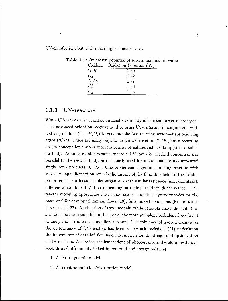
T a b l e 1.1: Oxidation potential of several oxidants in water Oxidant Oxidation Potential (eV) 'OH 2780 0 3 2.42 H202 1.77 CI 1.36 02 1.23
1.1.3 UV-reactors
While UV-radiation in disinfection reactors directly affects the target microorgan
isms, advanced oxidation reactors need to bring UV-radiation in conjunction with
a strong oxidant (e.g. H2O2) to generate the fast reacting intermediate oxidizing
agent ('OH). There are many ways to design UV-reactors (7, 15), but a recurring
design concept for simpler reactors consist of submerged UV-lamp(s) in a tubu
lar body. Annular reactor designs, where a U V lamp is installed concentric and
parallel to the reactor body, are currently used for many small to medium-sized
single lamp products (6, 25). One of the challenges in modeling reactors with
spatially dependt reaction rates is the impact of the fluid flow field on the reactor
performance. For instance microorganisms with similar residence times can absorb
different amounts of UV-dose, depending on their path through the reactor. U V -
reactor modeling approaches have made use of simplified hydrodynamics for the
cases of fully developed laminar flows (10), fully mixed conditions (8) and tanks
in series (19, 27). Application of these models, while valuable under the stated re
strictions, are questionable in the case of the more prevalent turbulent flows found
in many industrial continuous flow reactors. The influence of hydrodynamics on
the performance of UV-reactors has been widely acknowledged (21) underlining
the importance of detailed flow field information for the design and optimization
of UV-reactors. Analyzing the interactions of photo-reactors therefore involves at
least three (sub) models, linked by material and energy balances:
1. A hydrodynamic model
2. A radiation emission/distribution model
6
3. A kinetic model (disinfection or advanced oxidation)
each of which wil l be treated separately in what follows.
Due to the increasing power of computers, Computational F lu id Dynamics
(CFD) has become an efficient tool to simulate fluid flow behavior in complex
geometries. C F D is based on the numerical solution of partial differential equa
tions (PDEs), expressing the local balances of mass, momentum and energy, po
tentially coupled to the transport equations of the reacting species. However, such
P D E s could include phenomenological terms that should be adjusted to provide
the correct results. For example, turbulent stresses are computationally expensive
to calculate and several models have been developed, describing time-averaged
(simplified) results. The choice of an adequate approximation lies with the model
operator. Since the accuracy of C F D simulations is dependent on choices made
during the model setup, experimental validation by measuring flow characteristics
would be preferable.
1.1.4 Particle image velocimetry (PIV)
Particle Image Velocimetry (PIV) is currently one of the most advanced experimen
tal methods to visualize and measure flow characteristics. The general principle of
P I V is to illuminate tracer particles in the flow field of interest with a two dimen
sional sheet of laser light and acquire two images of the flow field with a known
time separation. The velocity field is determined from the distance traveled by the
tracer particles between the two images, divided by the known time interval.
1.1.4.1 A s h o r t h i s t o r y
The year 2004 marked the 20th anniversary of particle image velocimetry. P I V
has enjoyed a long and adventurous journey from the early roots beginning in
1977 when Laser Speckle Velocimetry (LSV) was demonstrated to measure flow
fields. In 1984, R . J Adrian (1) pointed out that the illumination of particles in a
fluid flow by a light sheet would almost never create a speckle pattern. The image
would rather show the tracks of individual particles, hence making particle image
velocimetry possible. The initial groundwork to modern P I V was then laid down
by Adrian (17), who described the expectation value of an auto-correlation function
7
for double-exposure continuous P I V images. Later the theory was generalized to
include exposures over multiple recordings (16).
To visualize and study the structure of turbulent flow, the particles must be
able to follow the flow, including small-scale local turbulence. This implies the use
of very small particles, a few tens of microns in diameter for liquids, which in turn
necessitates the use of high intensity illumination to compensate for the small light
scattering cross-section. Coupled with the short time exposures needed to prevent
blurring, the only viable solution was the use of high intensity pulsed lasers.
There still remained the problem of processing the obtained data. Initial meth
ods relied on the determination of two-dimensional correlations by analog optical
means. W i t h the advent of computers, enough computing power was available
to perform the two-dimensional Fourier transform needed for the auto-correlation
methods.
One of the most important changes in P I V was the move from photographic to
digital image recording. Westerweel's (33) proof of concept, showing that digital
P I V was as accurate as film P I V , did much to reduce initial concerns on the
much lower resolution of digital images. The fast evolution of digital cameras has
surpassed 1000x1000 pixel resolution and is currently approaching levels equivalent
to that of 35 mm films.
The second important change was the introduction of interline transfer cam
eras, as these cameras can record two images only microseconds apart. Thus many
problems associated with double-exposed (single) pictures could be addressed. The
need for image shifting was eliminated, since the direction of the flow was deter
mined automatically by the order of the images. Auto-correlation, known to be
superior to cross-correlation, was finally feasible with digital images and fast com
puters. Separate images allowed the resolution of movements smaller than a full
particle diameter, increasing the dynamic range, defined as
, maximum measurable velocity , . dynamic range = —— r ; : — : — (1.1)
minimum measurable velocity
by an order of magnitude, enough to resolve even turbulent flows. Presently,
the single camera, planar light sheet, cross-correlation P I V with a double-pulsed
Neodymium-doped Yt t r i um Aluminum Garnet (Nd :YAG) laser and 2kx2k cross
8
correlation camera is standardly used and sold commercially. These systems have
enough spatial resolution and dynamic range to resolve turbulent flow fields. But
the dynamic range of currently no more than 200:1 is still small enough to make
P I V experimental investigations exercises in optimization. P I V results have been
used to validate C F D simulations in the airplane and car industries for some time
now (34). Studies of turbulent flows in rectangular (14) and tubular channels (26),
have been published for dimensions and flow conditions similar to those used in
this study.
1.1.5 C F D
Computational fluid dynamics, C F D , solves the following conservation equations:
dxi
and momentum conservation:
= 0 (1.2)
dt U j dxj pdxi ^dxjdxj
that govern the flow. These equations are based on the assumption of Newtonian
fluids with constant medium properties . The computational domain is discretized
(or meshed) into a number of small cells (finite volumes). In the meshed compu
tational domain, the P D E s are approximated as a set of algebraic equations that
can be solved numerically. Meshing of the domain is crucial, can be very time con
suming, and needs a good initial understanding of the investigated volume. For
the finite volume method employed by many commercial C F D software packages,
such as Fluent, this consists of:
• Formal integration of the governing equations of fluid flow over all the (finite)
control volumes of the solution domain.
• Discretisation involving the substitution of a variety of finite-difference type
approximations for the terms in the integrated equation representing flow
processes such as convection, diffusion and sources. This converts the integral
equations into a system of algebraic equations.
9
• Solution of the algebraic equations by an iterative method.
1.1.6 Turbulence modeling
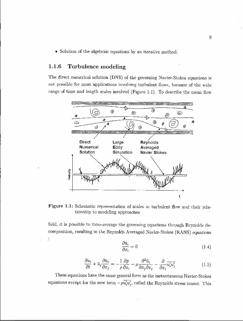
The direct numerical solution (DNS) of the governing Navier-Stokes equations is
not possible for most applications involving turbulent flows, because of the wide
range of time and length scales involved (Figure 1.1). To describe the mean flow
Direct Numerical Solution
7
Large Eddy Simulation
Reynolds Averaged Navier Stokes
Figure 1.1: Schematic representation of scales in turbulent flow and their relationship to modeling approaches
field, it is possible to time-average the governing equations through Reynolds de
composition, resulting in the Reynolds Averaged Navier-Stokes (RANS) equations
duj
dxi = 0 (1.4)
duj
dt
'Ui dui _ 1 dp d2
j dxj p dxi + ^ dxjdxj
d (1.5)
These equations have the same general form as the instantaneous Navier-Stokes
equations except for the new term -pv^, called the Reynolds stress tensor. This
10
term is usually negative and represents the effect of smaller scale motions on the
mean flow. It acts as an additional stress and dominates the transport processes
by several orders of magnitude over molecular transport. To close the R A N S
equations, individual Reynolds stress components can be solved throughout the
flow field. This is computationally expensive because the Reynolds stresses are
tensor quantities. Reynolds stress is a higher-order moment that has to be modeled
in terms of the knowns. This is referred to as the closure approximation, the
challenge of which lies in the representation of the unknown terms in a way that
mimics the real physics of the small turbulent length scales as close as possible.
1.1.6.1 E d d y v i s c o s i t y c o n c e p t
Boussinesq (1885) hypothesized a relationship between the Reynolds stressed and
mean velocity gradients of the flow by assuming isotropy of the stresses, i.e.,
where fit is the turbulent or eddy viscosity similar to the molecular viscosity, ex
cept that it is a flow property and depends on the local state of turbulence, K
is the turbulent kinetic energy per unit mass and the term The idea behind this
hypothesis is that momentum transfer in turbulent flows is dominated by the mix
ing caused by large eddies. Turbulent eddies are visualized as molecules, colliding
and exchanging momentum and thus, can be derived analogous to the molecular
transport of momentum as described by the kinetic theory of gases. This is quite
bold, since the mean free path between molecules is large compared to turbulent
eddies that can be assumed to be on the same order as the flow scales. Despite
these differences, models based on the Boussinesq hypothesis perform well in many
cases.
Prandtl (1925) proposed a mixing-length model for [it analogous to the kinetic
theory of gases where the turbulent viscosity can be related to the characteristic
velocity of turbulence V and a length scale of turbulence called the mixing length
(1.6)
\h oc VI •m (1.7)
11
Prandtl proposed this in the context of a turbulent shear layer with only one mean gradient du\/dx2- He suggested that the turbulent fluctuations can be expressed
as:
V = L dui
allowing the turbulent viscosity to be expressed as:
I dui I dxo
(1.8)
(1.9)
lm is usually specified, from experimental knowledge, as constant across the shear layer for most of the thin shear layers, and takes a different value in the boundary layers to account for the different layers. This is not a very suitable closure method since difficulties arise in determining the missing length for complicated flows. Mixing length models typically fail in predicting flow separations, because large eddies persist in the mean flow and cannot be modeled from local properties alone. This is a so-called zero equation model because no additional equations are needed for closure.
As an improvement to the above closure problem, transport equations are generally solved to specify the turbulent velocity and length scales involved. Depending on the number of additional equations solved, they are called one or two equation models. «-e models are two-equation models since they require the solution of both the turbulent velocity and the length scale.
1.1.6.2 S t a n d a r d « - e m o d e l
This family of models is widely used in turbulence simulations because of its general applicability. It is a two equation model, in which transport equations are solved for turbulent kinetic energy n, and instead of modeling the length scale itself they use the turbulent energy dissipation rate e where:
e = Kalb
m (1.10)
This approach is preferred by engineers since it does not require a secondary source and the simple gradient diffusion hypothesis is fairly accurate. In this model the
12
turbulent viscosity is related to K and e by the following equation:
Vt = pC^ (1.11)
where is an empirical coefficient. To close the equation, the local values of
K and e are obtained by solving their transport equations. These can be derived
from the Navier-Stokes equations of which a detailed description can be found in
"Lectures in Mathematical Modeling of Turbulence" (20). In essence the turbulent
diffusivity of K and e are related to the turbulent viscosity with additional empirical
constants, which are known as turbulent Prandtl numbers for K and e. The final
model contains 4 empirical parameters that have been determined experimentally
by Launder and Spalding (20).
The standard n-e model has some limitations and drawbacks since this is a
semi-empirical model. The equation for e is based on physical reasoning while the
model equation for K is derived mathematically. One of the problems encountered
is the fact that the equation does not ensure that turbulent normal stresses are
positive, which is contradictory to real physics.
1.1.6.3 R e a l i z a b l e K-e m o d e l
The realizable n-e model is an improvement over the standard model with certain
mathematical constraints on the Reynolds stresses, consistent with the physics of
turbulent flows. It has a new formulation for e that is derived from the exact equa
tion for the transport of the mean-square vorticity fluctuation. It outperforms the
standard n-e model for flows involving rotation, boundary layers under strong ad
verse pressure gradients, and recirculation. Even so, it pays to keep the underlying
assumptions of all n-e models in mind:
• Turbulence is assumed to be nearly isotropic
• The spectral distributions of turbulent quantities are assumed to be similar
• It is true only at high Reynolds numbers
These assumptions may not be valid for the flows encountered in practical envi
ronments. Also, all K-e based models tend to over-predict turbulence generation
13
in regions of high acceleration and deceleration where the isotropic assumption no
longer holds.
1.1.6.4 R e y n o l d s s t ress m o d e l ( R S M )
The one and two-equation models presented assume that the principal axes of
both the Reynolds stress tensor and the mean strain-rate tensor are coincident
everywhere in the flow. This Boussinesq approximation weakens in flows with
sudden changes in the mean strain rate, flows with strong curved surfaces, flows
with separation, and flows with three-dimensional features. A Reynolds stress
model, in theory, wil l circumvent the deficiencies of the Boussinesq approximation.
The individual Reynolds stresses are calculated directly using differential transport
equations and solution of the e equations provides the remaining turbulent scale to
obtain closure of the Reynolds-averaged momentum equation. This second-order
moment closure method offers an advantage over scalar eddy viscosity approaches
in that the transport equations possess several exact terms and, therefore, a closer
connection to the exact equations. Reynolds stress transport modeling also for
mally accounts for the effects of streamline curvature, and rapid changes in strain
rate more rigorously than one- and two-equation models. While possessing more
exact terms, the computational cost of the calculation is substantially greater,
as the approach requires solutions of seven additional transport equations. Also,
the model is not fully mechanistic and contains empirical constants (e.g., in the
pressure and dissipation terms). A tendency to require denser mesh, higher com
putational costs, and the fact that, in many cases, it does not perform better than
the two equation models have to be weighed against the stated advantages.
1.1.6.5 C h o o s i n g a t u r b u l e n c e m o d e l
No turbulence model is universally applicable to all conditions. Therefore, it is
important to chose an appropriate turbulence model for each application at hand,
be sure to understand the underlying assumptions, and if possible perform a model
validation.
Generally, any of the two equation n-e models are recommended as a starting
baseline model. Once unsteady vortex shedding is involved, the Realizable-K-
14
e version of the K-e model should be used. For more complex flows including
curved flows and rotating flows, the computationally more expensive Reynolds
Stress Model (RSM) might be considered. Due to the numeric stability of the
standard n-e model, it is often used as the starting point for subsequent changes
in turbulence model choice. It should also be noted that, for many industrial
solutions, the grid resolution might have a higher impact than the turbulence
model used.
1.1.6.6 S u m m a r y
C F D calculations are influenced by parameters such as mesh size and structure,
mathematical discretisation method used, and the choice of turbulence models.
Accordingly, calculations should be verified experimentally before integrating fur
ther components into the model.
1.2 Research objectives
The objectives of this thesis are to study the fluid flow of water in annular U V
reactors, both experimentally and through C F D simulations, with the aim of iden
tifying key parameters to achieve verified C F D flow field calculations. A two-
dimensional flow visualization technique, Particle Image Velocimetry (PIV), is used
to obtain the main hydrodynamic characteristics of the given flow configurations.
A U V reactor performance model is then established by integrating hydrodynamics
with radiation and reaction rate submodels. The objectives are achieved through
the following steps:
1. Identify typical annular reactor designs and establish plexiglas prototypes for
flow visualization.
2. Develop an experimentally substantiated understanding of the flow field in
side the UV-prototype reactors by means of particle image velocimetry (PIV).
3. Establish the computational hydrodynamics of UV-reactors through C F D
models and study the influence of model assumptions. Assess the validity of
the flow prediction through comparison with P I V results.
15
4. Adapt and integrate UV-radiation models for mesh-based C F D calculations.
5. Develop a general, particle based (Lagrangian) model, coupling UV-radiation
and reaction kinetics to reactor hydrodynamics to simulate overall U V dis
infection performance.
6. Develop a model based on volumetric reaction rates (Eulerian), that is ca
pable of handling more than single step reactions (applicable for advanced
oxidation).
7. Evaluate and compare integrated U V reactor performance models.
What follows are the three research chapters composing the main body of this
thesis. Objectives 1 and 2 are the focus of Chapter 2 with the title "Experimental
investigation of flow fields in annular UV-reactors using P I V " . Chapter 3 with the
title " C F D study of annular UV-reactor hydrodynamics" concentrates on Objec
tive 3. Finally Objectives 4 to 7 are addressed in Chapter 4, entitled "Integrated
U V reactor model development". Chapter 5 summarizes conclusions and recom
mendations.
Bibliography
[1] A D R I A N , R . J . Probability density of turbulence from multiple field Particle
Image Velocimetry. Fifth Symposium on Turbulent Shear Flows., Ithaca,
N Y , U S A , 1985, pp. 11-7. Compilation and indexing terms, Copyright 2004
Elsevier Engineering Information, Inc.
[2] A R B U C K L E , T . E . , H R U D E Y , S. E . , K R A S N E R , S. W . , N U C K O L S , J . R . ,
R I C H A R D S O N , S. D . , S I N G E R , P . , M E N D O L A , P . , D O D D S , L . , W E I S E L , C ,
A S H L E Y , D . L . , F R O E S E , K . L . , P E G R A M , R . A . , S C H U L T Z , I. R . , R E I F ,
J . , B A C H A N D , A . M . , B E N O I T , F . M . , L Y N B E R G , M . , P O O L E , C , A N D
W A L L E R , K . Assessing exposure in epidemiologic studies to disinfection by
products in drinking water: report from an international workshop. Environ
Health Perspect 110 Suppl 1 (Feb 2002), 53-60.
16
[3] B O L T O N , J . R . , B I R C H E R , K . G . , T U M A S , W . , A N D T O L M A N , C . A .
Figures-of-merit for the technical development and application of advanced
oxidation technologies for both electric- and solar-driven systems. Pure and
Applied Chemistry 73 (2001), 627-637.
[4] B O L T O N , J . R . , A N D BlRCHNER, K . G . Figures of merit for the technical
development and application of advanced oxidation processes. Journal of
Advanced Oxidation Technologies 1 (1996), 13-17.
[5] B O L T O N , J . R . , W R I G H T , H . , A N D R O K J E R , D . Using a mathematical
fluence rate model to estimate the sensor readings in a multi-lamp ultraviolet
reactor. Journal of Environmental Engineering and Science 4 (January 2005),
27-31. Supplement 1.
[6] B R A U N , A . , J A K O B , L . , A N D O L I V E R O S , E . Advanced oxidation processes
- concepts of reactor design. Journal of Water Supply: Research and
Technology-AQUA 42, 3 (1993), 166-173.
[7] C A S S A N O , A . E . , M A R T I N , C . A . , B R A N D I , R . J . , A N D A L F A N O , O . M .
Photoreactor analysis and design: Fundamentals and applications. Industrial
& Engineering Chemistry Research 34 (1995), 2155-201.
[8] C H A N G , P . B . L . , A N D Y O U N G , T . M . Kinetics of methyl tert-butyl ether
degradation and by-product formation during uv/hydrogen peroxide water
treatment. In Proceedings of the Air & Waste Management Association's
Annual Conference & Exhibition, 93rd, Salt Lake City, UT, United States,
June 18-22, 2000 (2000), pp. 7036-7055.
[9] C L A R K E , N . , A N D K N O W L E S , G . High-purity water using hydrogen peroxide
and uv radiation. Effluent & Water Treatment Journal 22 (1982), 335-8, 340-
1.
[10] E L K A N Z I , E . M . , A N D K H E N G , G . B . H2o2/uv degradation kinetics of
isoprene in aqueous solution. Journal of Hazardous Materials 73 (2000), 55-
62.
17
[11] E S P L U G A S , S. Economic aspects of integrated (chemical + biological)
processes for water treatment. Journal of Advanced Oxidation Technologies 2
(1997), 197-202.
[12] G O - G A T E , P . R . , A N D P A N D I T , A . B . A review of imperative technologies
for wastewater treatment, i i : Hybrid methods. Advances in Environmental
Research 8 (2004), 553-597.
[13] H A N Z O N , B . , A N D V I G I L I A , R . U V disinfection. Wastewater Technology
Showcase 2, 3 (1999), 24-28.
[14] I S L A M , M . S., H A G A , K . , K A M I N A G A , M . , H I N O , R . , A N D M O N D E , M .
Experimental analysis of turbulent flow structure in a fully developed rib
roughened rectangular channel with piv. Experiments in Fluids 33 (2002),
296-306.
[15] K A R P E L V E L L E I T N E R , N . , L E B R A S , E . , F O U C A U L T , E . , A N D B o u s -
G A R B I E S , J . - L . A new photochemical reactor design for the treatment of
absorbing solutions. Water Science and Technology 35 (1997), 215-222.
[16] K E A N E , A . , A N D A D R I A N , R . Particle-imaging techniques for experimental
fluid mechanics. Annual Review of Fluid Mechanics (1991).
[17] K E A N E , R . , A N D A D R I A N , R . Optimization of particle image velocimeters
part i double pulsed systems. Measurement and Technology 1, 11 (November
1990), 1202-1215.
[18] K I D M A N , R . , A N D T S U J I , K . Preliminary costs comparison of advanced
oxidation processes. Tech. rep., Los Alamos National Laboratory, 1992.
[19] L A B A S , M . D . , Z A L A Z A R , C . S., B R A N D I , R . J . , M A R T I N , C . A . , A N D
C A S S A N O , A . E . Scaling up of a photoreactor for formic acid degradation
employing hydrogen peroxide and uv radiation. Helvetica Chimica Acta 85
(2002), 82-95.
[20] L A U N D E R , B . E . , A N D S P A L D I N G , D . B . Lectures in mathematical modeling
of turbulence. Academic Press, London, 1972.
18
[21] L A W R Y S H Y N , Y . A . , A N D C A I R N S , B . U V disinfection of water: the need for
uv reactor validation. Water Science & Technology: Water Supply 3 (2003),
293-300.
[22] L E T T E R M A N , R . Water quality and treatment - A Handbook of community
water supplies (5th Edition). McGraw-Hi l l , 1999.
[23] M U E L L E R , J . P . , A N D J E K E L , M . Comparision of advanced oxidation
processes in flow-through pilot plants (parti). Water Science and Technol
ogy 44, 5 (2001), 303-309.
[24] M U E L L E R , J . P . , A N D J E K E L , M . Comparision of advanced oxidation
processes in flow-through pilot plants (partii). Water Science and Technology
44, 5 (2001), 311-315.
[25] O P P E N L A E N D E R , T . Photochemical purification of water and air. Wiley-
V C H , 2003.
[26] P R U V O S T , J . , L E G R A N D , J . , L E G E N T I L H O M M E , P . , A N D D O U B L I E Z , L .
Particle image velocimetry investigation of the flow-field of a 3d turbulent
annular swirling decaying flow induced by means of a tangential inlet. Exper
iments in Fluids 29 (2000), 291-301.
[27] P U M A , G . L . , A N D Y U E , P . L . Modeling and design of thin-film slurry
photocatalytic reactors for water purification. Chemical Engineering Science
58 (2003), 2269-2281.
[28] R A D C L I F F , R . International drinking water regulations:the developed world
sets the standards. On Tap Magazine Spring (2003).
[29] R I T T E R , L . , S O L O M O N , K . , S I B L E Y , P . , H A L L , K . , K E E N , P . , M A T T U ,
G . , A N D L I N T O N , B . Sources, pathways, and relative risks of contaminants
in surface water and groundwater: a perspective prepared for the walkerton
inquiry. Journal of Toxicology and Environmental Health, Part A 65 (2002),
1-142.
[30] U S E P A . Clean water act. U S - E P A , 1996.
http://www.epa.gov/safewater/sdwa/index.html.
19
[31] U S E P A . 1999 drinking water infrastructure needs survey, modeling the cost
of infrastructure. Tech. rep., U S - E P A , February 2001.
[32] V o s , J . G . , D Y B I N G , E . , G R E I M , H . A . , L A D E F O G E D , O . , L A M B R E , C . ,
T A R A Z O N A , J . V . , B R A N D T , I., A N D V E T H A A K , A . D . Health effects
of endocrine-disrupting chemicals on wildlife, with special reference to the
european situation. Critical Reviews in Toxicology 30 (2000), 71-133.
[33] W E S T E R W E E L , J . Digital particle image velocimetry: Theory and application.
P h D thesis, Universityof Delft, 1993.
[34] W u , H . L . , P E N G , X . F . , A N D C H E N , T . K . Influence of sleeve tube on
the flow and heat transfer behavior at a t-junction. International Journal of
Heat and Mass Transfer 46 (2003), 2637-2644.
[35] W U L F , W . A . Great achievements and grand challenges. The Bridge 30, 3&4 (2000), 6-11.
[36] Y E H , C . K . , A N D N O V A K , J . Anaerobic biodegradation of gasoline oxy
genates in soils. Water Environment Research 66, 5 (1994).
Chapter
Experimental investigation of the flow field in annular UV reactors using PIV
In this chapter, the experimental investigation of flow in different annular U V
reactors wil l be discussed. Starting with the underlying ideas of the experiment,
Particle Image Velocimetry (PIV) is introduced. Considering that P I V is a new
entrant in the field of fluid flow measurements, some topics concerning this method
are covered in more detail.
2.1 Introduct ion
Annular UV-reactors have become more popular over the last few years, mainly
due to the successful introduction of UV-photoreactors for water disinfection and
advanced oxidation processes (AOPs) for the removal of organic contaminants.
These reactors use U V radiation to either directly affect hazardous organisms for
water disinfection or to excite a strong oxidant such as H2O2 or O 3 to generate
highly reactive hydroxyl radicals in situ, which in turn oxidize (toxic) organic
substances. The design of photoreactors is largely' determined by the radiation
distribution field and thus, the placement of UV-lamp(s) as radiation sources. The
annular reactor, a cylinder with a concentric lamp parallel to the reactor body,
20
21
strikes a good balance between the lamp placement and reactor geometry for small
to medium single lamp systems and is the basic design for many current products
(2, 15).
Many annular reactor designs use a horizontal cylindrical body and variations
in the placement of the inlet and outlet tubes. The resulting typical reactor outlines
resemble the letters S, U and L and are the source of the descriptive names (Figure
2.1):
• U-shape: inlet and outlet are normal to the reactor axis, parallel and in the
same direction (e.g. top inlet and outlet)
• L-shape: inlet is parallel and co-centric to the reactor axis, the outlet is
normal to the reactor axis (e.g. front inlet, top outlet)
• S-shape: inlet and outlet are normal to the reactor axis, parallel and in
opposite directions (e.g. top inlet, bottom outlet). This is a variant of the
U-shape reactor.
The central lamp is commonly entered through an end cap and needs to be fixed
in place at the opposite end. For the L-shape reactor, a lamp support structure
(lamp holder) is required near the reactor entrance.
The design of reactors containing radiation fields to initiate the desired reac
tion is a relatively new area of research, but the numbers of recent publications
show an increasing interest. The main challenge of operating under non-uniform
concentration and radiation distributions is the highly non-uniform local rate of
reaction (3), resulting in a high impact of the fluid flow field on reactor perfor
mance. For example, a bacteria passing through a badly designed reactor may not
spend enough time in the volumes close to the radiation source and wil l most likely
not receive a high enough dose to be inactivated.
Simplified models have been established for modeling UV-reactor hydrodynam
ics using fully developed laminar flows (7), fully mixed conditions (4), or tanks in
series (12). While these models are valuable under the stated restrictions, their
application to the more prevalent non-uniform flows in industrial continuous flow
reactors is questionable. The link between hydrodynamics, radiation distribution
and the reaction rate greatly increases the complexity of the models simulating
22
UV-reactor performance. In particular, the influence of the flow field on the per
formance of UV-photoreactors has been widely acknowledged (13). This underlines
the importance of detailed flow-field information for performance analysis and de
sign optimization of UV-reactors.
There have been some effort's using Computational F lu id Dynamics (CFD) to
simulate the flow fields in UV-reactors (10, 11, 14); however, none of these studies
conducted experiments to evaluate the C F D modeling results. Using C F D , the
governing equations of mass and momentum conservation are solved iteratively
in a discretized representation of the computational domain. C F D results are
influenced by several parameters such as discretisation method, mesh structure
and the choice of turbulence models for the momentum conservation equations. As
a result, the C F D models need to be validated against reliable experiments. The
hydrodynamics of U V water treatment systems have been studied experimentally
to some degree. Schoenen et al. (17) demonstrated the effect of the reactor flow
field on the performance of water disinfection systems. Chiu et al. (5) used laser
Doppler velocimetry to experimentally obtain velocity information in a cross-flow
UV-reactor. Despite these limited studies, no detailed experimental information
covering a range of flow rates and reactor geometries is currently available for
UV-reactors.
Particle Image Velocimetry (PIV) is one of the most advanced experimental
methods available to visualize the main flow characteristics of a given configuration.
It provides a non-intrusive measurement of the instantaneous planar velocity field
over a global domain. As the name suggests, it records the position of small tracer
particles over time to extract the local fluid velocity. P I V requires four basic
components: an optically transparent test-section containing the seeded fluid, an
illuminating light source (laser), a recording device ( C C D camera) and a computer
algorithm to process (cross-correlate) the recorded images (1). P I V has been widely
used in the aviation and automobile industry and there have been some studies of
turbulent flows in rectangular (9) and tubular channels (16). P I V results have also
been used to evaluate C F D simulations (19). To the author's knowledge, no work
has been reported in the open literature on the study of flow-fields in photoreactors.
This work presents a study of the annular UV-reactor hydrodynamics and de
termines the time-averaged turbulent flow field using P I V in two (U- and L - shape)
23
full-scale Plexiglas reactor models. Flow structures in the inlet region of both reac
tors are described in detail for a range of flow rates. The influence of lamp position
and holder position for the L-shape reactor are determined. For the U-shape reac
tor, the time dependency of the flow at the inlet plane perpendicular to the axis
is demonstrated.
2.2 Exper iments
2.2.1 Experimental setup
Figure 2.1 shows a schematic of the experimental setup. A 100 L reservoir con
nected to a centrifugal pump was used to circulate distilled water through the
test section in a closed loop. The flow rate at the reactor inlet was measured and
adjusted by a flow-meter (Cole-Parmer, 5-25 G P M ) . Full scale Plexiglas models of
the complete configuration for U - and L-shape reactors, with internal components
including the quartz lamp-sleeve and lamp-holder were used for the P I V measure
ments. Both test sections (reactors) share major dimensions based on existing
industrial designs for an estimated throughput of 40 L / m i n (^ 10 G P M ) . The test
rig was designed as a modular system with a central tube internal diameter (ID)
of Di=8.89 cm (3.5 inches) and a reactor length of L=88.9 cm (35 inches). Both
end-caps were designed to be removable, facilitating the change of reactor config
urations. The inlet and outlet ports with an ID of D 2 =1.91 cm (0.75 inch) were
placed 2.54 cm (1 inch) from each respective end for the U-shape. The L-shape
inlet was centred on the front-plate (Figure 2.2).
A concentric quartz tube of outer diameter (OD) D 3 = 2 cm (0.788 inches) was
used to represent the UV-lamp sleeve with minimal optical interference on the laser
sheet. The sleeve entered the reactor volume through a Teflon seal (Swagelok) and
remained readily movable along the reactor axis. A cylindrical extrusion was used
to fix the opposite end of the UV-sleeve for the U-shape, while a three pronged
holder fixed the lamp sleeve concentric to the reactor tube for the L-shape reactor
(Figure 2.2). The holder, a concentric ring of 0.3 cm thickness and a length of 1.52
cm (0.6 inch) with three radial cylindrical struts of 0.5 cm (0.2 inch) diameter, was
slipped over the lamp with the struts centered at 18.5 cm (7.3 inches) from the
24
inlet. The holder's side-faces were minimized and the edges beveled to minimize
exposure to the flow. The mean flow rates varied between Q = 2 . 5 2 x l 0 - 4 m 3 / s ( « 4
G P M ) and Q = 6 . 9 4 x l 0 ~ 4 m 3 / s G P M ) . For the majority of the measurements
Q = 6 . 9 4 x l 0 - 4 m 3 / s , corresponding to a mean axial velocity of 0.11 m/s and a
Reynolds number Re=10,000, was examined.
The annular reactor's were placed within a Plexiglas tank (130 cmx30 cmx30
cm) filled with distilled water, to eliminate optical distortion caused by the reactors
curved external surface (see Appendix A for details). The whole experimental
apparatus was finally placed on an extruded aluminum structure, consisting of a
central table with two movable side planes and one movable top plane, all equipped
with X Y linear slides. This allowed the laser and the camera to be placed and
moved at a consistent 90 degree angle.
2.2.2 P I V measurement system
Table 2.1 gives an overview of the P I V system specifications (Flow-Map 2D, Dantec
Dynamics). The P I V illumination system consisted of a dual head N d : Y A G laser
(New Wave Research: Model SoloIII-15 Hz) emitting 10 ns pulses with maximal
energies of up to 50 mJ/pulse. The collinear frequency doubled beam (1064 nm to
532 nm) was spread into a sheet of 1-2 mm thickness through a set of cylindrical
lenses directly attached to the laser head. The particle images were recorded on
a high-resolution progressive scan interline C C D camera (Hamamatsu: HiSense
M k l l ) at a maximum rate of 5 Hz. The camera with a resolution of 1344x1024
pixels and a 12 bit dynamic range, was fitted with a 514 nm line filter to minimize
stray light. The camera and the laser were connected to a P I V hub with a frame
grabber and 1.0 G B R A M to buffer the image stream. The hub's programmable
synchronizer controlled the timing of the laser illumination and the camera image
acquisition. The hub connected to a P C , where the experimental sequence was
programmed and the resulting data stream was analyzed asynchronously (Figure
2.1).
25
2.2.3 Experimental procedures
For the P I V measurements, the time interval between two laser pulses was adjusted
between 600 and 1500 fis. Tests concerning the number of images needed to get
accurate time-averaged measurements were performed by taking a series of 1600
instantaneous velocity field measurements. Vector statistics of samples containing
the full set and subsets of 800, 400, 200 and 100 images were compared. It was
found that a sample size of about 200 images produce a stable time-averaged result.
A l l further measurements were therefore performed with 250 or more image pairs
for the best measurement accuracy. The amount of seeding (~50 mg/L) was
determined by allowing not less than 10 particles per interrogation window. Small
interrogation window sizes are desirable to resolve small turbulent flow structures,
but require a high number of particles and are more sensitive to high velocity
gradients. The influence of window size on the adaptive cross-correlation algorithm
was evaluated. It was found that a final window size of 16x16 pixels with 50%
overlap and two adaptation steps could be applied without loss of accuracy. A
measurement rate of 0.1 Hz was chosen to minimize the influence of longer term
fluctuations.
The accuracy of the velocity measurements was determined through statistical
analysis over the 250 instantaneous vector fields at several points. Small errors
(95% confidence interval) of less than 1% were determined for the high velocities
at the inlet. The relative errors were found to be less than 5% for the intermediate
flow rates at 10 cm from the reactor inlet, and around 17% for the low axial
flow speeds at 23 cm and beyond (Figures 2.5a-c). A t low flow rates, any gains
in accuracy from longer A t intervals were offset through the out-of-plane loss of
particles.
The configuration of the test sections allowed for a maximum possible number
of planes to be observed; however, parts of the reactor were blocked by obstacles
in the path of either the laser or camera. The planes of interest, parallel and
perpendicular to the main reactor flow, were specified for each reactor. The center
planes were accessible to both laser and camera, which allowed the capture of
the major flow characteristics in both test sections. The inlet region, with high
gradients of flow velocities and high impact in determining the overall flow, was
given the most attention. Viewable areas covered by one camera position were
26
determined by the C C D resolution and reactor height, resulting in oblong windows
of 11 x 8.9 cm.
2.3 Results and discussions
In the statistical description of turbulence, the total instantaneous velocity is de
composed into its time-averaged velocity component and a turbulent fluctuation
component. Using the large time resolved velocity data sets from P I V , it is pos
sible to investigate both components in any direction in a planar field. Single
instantaneous velocity fields show the characteristics of raw measurements, but
deliver little information for understanding the fundamental flow physics. The
mean (time-averaged) P I V velocity fields discussed here, trade off instantaneous
(temporal) information for the time-averaged flow distribution, in order to visualize
only the prevailing flow structures inside the reactor. The turbulent fluctuations
remain accessible as statistical measures of local interactions due to unsteady be
havior. Further information such as turbulent kinetic energies and vorticity which
could be calculated from the same set of flow field data wi l l not be discussed.
The two test section geometries are presented separately starting with the L-shape
reactor.
2.3.1 L-shape reactor
Figure 2.3a-b shows the composite time-averaged P I V measurements obtained from
4 camera positions within the L-shape reactor. The flow entered through a straight
concentric inlet tube from the right and passed to the left. The tube with an ^ = 4 5
allowed the flow to fully develop. The axisymmetric jet entering was subjected to
an expansion ratio of |^=4.6. The emerging flow structures along the reactor axis
could be categorized into three distinct zones of jet expansion, recirculation, and
redevelopment zones. The geometry with a sudden expansion created a central
expanding jet (jet expansion zone). Between the jet and the slower fluid, shear
layers with high velocity gradients formed and the expanding jet also introduced
adverse pressure gradients. In this area between jet and outer reactor walls, a
zone with recirculating fluid flow is formed (recirculation zone). The shear layer,
27
separating the expanding jet from the recirculation zone, grew by entraining the
surrounding slow moving fluid and finally merged with the outer boundaries (walls)
at the reattachment point. The reattachment point is defined as the point where
the shear layer touches the wall, splitting into fluid returning to the recirculation
area and fluid joining the bulk liquid flow. After interacting with the lamp holder
the flow finally evened out in the "redevelopment zone".
The contours of velocity magnitude (Figure 2.4) show the local velocity mag
nitudes formed by the sum of square roots of the mean velocity in both z-(U) and
r-(V) directions, parallel and perpendicular to the reactor axis (\JU2 4- V2) for
three flow rates. The white areas indicate velocities of more than 0.15 m/s in any
direction and areas of low velocities appear darker or black. The shear layer is a
distinct and nearly stationary region visible between the two opposing flows.
A t 2.5 cm (1 inch), the round jet impinges on the semi-spherical lamp tip with
little visible dispersion. The separating flow stays attached to the lamp surface
until the lamp holder lifts the flow from the lamp and increases the angle of the
shear layer, resulting in a reattachment for the reactor top at 20 cm (8.8 inch),
corresponding to 2 . 5 x D 2 in length from the inlet. In Figure 2.4, the reattachment
point is shown by the (dark) shear layer meeting the walls. Roughly extrapolating
the shear layer for a reattachment point without the holder, the point corresponds
to more than 3xD2 from the inlet. Even taking into account that a linear extrap-
, olation might not be true, the lamp seems to reduce the angle of the shear layer
growth rather than spreading the inlet jet.
Experimental results by various researchers, gathered by Forester and Evans
(8), show that the reattachment point for similar geometries with no obstructions
can be found around 2-3 x D 2 from the inlet. The lower than anticipated spreading
of the jet could be explained by the coanda effect, the tendency of a flow to follow
a (curved) surface. Devenport and Sutton (6) observed an opposite trend when
placing a blunt center-body downstream of the sudden expansion; the curvature of
the shear layer increased, resulting in an earlier reattachment point. This shows
the potential importance of the shape of the lamp tip on the flow field.
In the recirculation zone, returning flows are visible along the top and lower
walls with recirculation starting close to the reattachment points (Figure 2.3b). A t
a volumetric inflow of 11 G P M the counterstream flows reach maximal negative
28
velocities of -0.26 m/s corresponding to 0.11 x V ; n / e t . Although there have been
no systematic experimental investigations into the effect of expansion geometries
on the maximum back flow velocity, Forester and Evans (8) report values of 0.096
Viniet for a similar geometry without a central annulus. The recirculating flow feeds
into the expanding shear layer and loses velocity, resulting in a concentric zone of
low velocity along the reactor walls close to the entrance. The flow in the inlet
region matches the characteristics of a standard expanding jet without obstacles
in many respects. The central lamp seems to have little effect on the expanding
jet in the inlet region and recirculation zone.
In the region of the lamp holder, the flow patterns deviated from a standard
expanding jet. The axial velocity profile up to this point remained symmetric, as
can be seen in Figure 2.5a-b. The ridge between lamp-holder and lamp clearly
disturbed the flow attached to the lamp's face, and deflected the main flow away
from the center (Figure 2.5c). For the top part of the reactor, the shear layer
showed the deflection toward the walls as discussed. For the lower part, this
was not as evident, with the lower spoke of the lamp holder centered directly in
the measurement plane. The flow separated around the cylindrical spoke and a
closer analysis of the instantaneous velocity maps indicated that a periodic vortex
shedding typical for blunt body flows occurred. The low measurement frequency of
0.1 Hz did not allow a resolution of the shedding phenomenon. In the time-averaged
statistical solution, the alternating velocities perpendicular to the measurement
plane cancel each other out, resulting in an area of low axial velocity. This time
dependent behavior remained local and confined. The axial velocity profile in
Figure 2.3b shows the slower and less stable flow in the zone right after the lower
holder spoke and the faster flow between the top spokes. This pattern is thought
to be repeated three times over the circular cross-section, with the extremes (in
plane with spoke and between the spokes) visible here. In the redevelopment zone
after the reattachment point, the flow evens out and assumes turbulent plug flow
characteristics over the remaining length beyond 20 cm.
Predictable and stable flow patterns are important to ensure compliance with
minimal reactor performance levels over a range of volumetric flow rates. This
scalability is especially vi tal for mandated limits like the UV-disinfection rates for
drinking water. To study the effect of flow rate on the reactor hydrodynamics,
29
flow rates of Q = 6 . 9 4 x l ( r 4 m 3 / s (11 G P M ) , Q = 5 . 0 5 x l ( r 4 m 3 / s (8 G P M ) and
Q=2 .52x l0~ 4 m 3 /s(4 G P M ) respectively, corresponding to Reynolds numbers of
Re=10200, 7500 and 3700 in the main body of the reactor, were examined. Figure
2.5 shows axial velocity profiles at three positions downstream of the reactor inlet.
The axial velocity profile obtained at 1.3 cm (0.5 inch) from the reactor inlet,
was in good qualitative agreement with an expanding jet flow (18). A t 10 cm
(4 inch), the velocity of the recirculating flow for the lowest inlet speed drops
disproportionally. The contours of velocity magnitude show that the centers of
recirculation have moved while the central jet remains stable. A t 23 cm (9 inch)
the profiles show a similar behavior; the reduced flow speed changed the angle of
the shear layer above the lamp holder resulting in a broader axial profile. The
flow below the lamp shows changes in both the axial profile and the contours of
velocity magnitude. This might be caused by the change in flow speed influencing
the frequency of the vortex shedding after the spoke.
Figure 2.4 shows the contours of velocity magnitude for the three inlet rates.
The observations made above hold true and show that within the tested flow
regimes the flow structures remained stable, confirming that, over a broad range
of inlet velocities, changes of internal flow distribution occur, but the flow struc
tures scale predictably with the flow rates. The figures give a good qualitative
comparison of the overall similarity for the different flow speeds, indicating that
flow patterns stay predictable within the tested volumetric range.
To test the influence of changes in the internal reactor geometry on the flow
behavior, two additional measurements were performed (Figure 2.6). First, the
lamp and lamp holder were moved 2.54 cm (1 inch) away from the inlet, keeping
the position of the lamp holder fixed relative to the lamp. This is a change possible
with the little effort for any L-shape design, thus representing a likely modification.
The contours of velocity magnitude,in Figure 2.6b show an elongation of the inlet
jet and a less pronounced change of radial expansion just after impinging on the
moved lamp tip. The remaining flow structures were shifted by 2.54 cm as expected
and retained their shape. Without the lamp holder breaking the jet away from the
lamp, it could extend much further into the reactor domain. A n extended shear
layer would introduce more turbulent kinetic energy and thus mixing over the
length of the reactor. O n the other hand, a segregated flow with high velocities
30
and thus short residence times at the core might receive lower UV-dose, even
though it remains in the volume of high fluence rates.
In a second change of the internal geometry, the lamp holder was moved to
7.62 cm (3 inches) from the reactor inlet while the lamp tip remained at 2.54
cm (1 inch). The higher velocities close to the inlet reduced the lamp holder's
influence on the flow (Figure 2.6c). The deflection of the shear layer toward the
outer walls was not as pronounced and the resulting shallower reattachment angle
led to a less well defined reattachment point. Both reattachment and recirculation
points moved less than 1 cm closer to the inlet while reflux zones pronouncedly
changed their appearance. This change of reactor geometry had a much deeper
impact on the resulting flow structures and removed the axisymmetry in the inlet
region. The inlet jet retained much of its former shape despite the new obstacle.
The recirculation point in the lower reactor part remained almost unmoved, now
situated behind the lamp holder.
The axial velocity profiles at 38 cm (15 inch) or later were similar in all cases,
thus indicating that any disturbances from the inlet region have abated at one-
third of the distance along the reactor. No changes in the flow emerged, until the
outlet dictated flow structures became predominant close to the reactor outflow.
Figure 2.7 shows the P I V data for the final reactor section. The vectors of ve
locity magnitude for both the L - and U-shapes agree well and indicated that any
hydrodynamic influence from further upstream has abated.
The results indicate that the shape and position of the lamp and the lamp
holder can impact the flow distribution within the L - and U-shaped reactors. If
enhanced mixing is desirable, changing the position of geometry of the lamp tip
and the lamp holder offer the best starting points for improving flow mixing.
2.3.2 U-shape reactor
The second reactor examined was the U-shape, with all dimensions remaining fixed
except for the inlet position and removal of the lamp holder since it is not needed
in this design. The change of the inlet position resulted in a distinctly different
flow distribution. The inlet in U-shape reactors is known to strongly influence
reactor hydrodynamics, off-center inlets have been used to induce swirling flows
31
throughout the domain (16). For U V applications on the other hand, a uniformly
turbulent, well-mixed flow is sought. Swirling might lead to stable flow structures
remaining far from the energy source and thus receiving lower UV-dose.
From the top inlet, a round expanding jet entered the reactor, through a
straight tube with an ^=45 allowing for a fully-developed flow. The inlet po
sition was situated on the curved reactor surface, 3.8 cm (1.5 inch) from the inlet
wall and 85.1 cm (33.5 inches) from the outlet, resulting in asymmetric boundaries
of the jet expansion volume. The expanding jet impinged on the concentric lamp
surface and separated around it (Figure 2.8). The flow remained attached to the
round lamp surface, until the streams recombined below and detached. Figure 2.8
shows the plane perpendicular to the main reactor body, centered below the inlet
at 3.8 cm (1.5 inches). The view of the flow close to the lamp was blocked by the
hexagonal nut holding the lamp, but the flow detaching from the lamp is clearly
visible. The velocity vectors averaged from 800 P I V measurements taken over a
period of 2 h resulted in a symmetric inlet flow (Figure 2.8b). The average vector
of the detaching flow was centered but proved to be unstable and influenced by
several factors. Symmetrical results were only obtained after averaging P I V mea
surements taken over more than one hour. The vectors of velocity magnitude from
subsets of 100 P I V measurements (16 minutes) show the two main stable states of
the time dependent flow (Figure 2.8c-d). Repeated measurements confirmed the
flapping flow phenomenon occurred at a lower frequency than can be explained by
vortex shedding.
A point P I (Figure 2.8b) was defined in the recirculation area to determine
a possible pattern in the flapping flow. A plot of the V (vertical) velocity at P I
over 800 instantaneous measurements (Figure 2.9) shows that velocity changes of
more than 1.5 m/s occurred. The moving average over 10 instantaneous points,
revealed two plateau velocities where the flow remains stable correlating with the
(right/left) states in Figure 2.8c-d. No indication of a repeating pattern was found
in the reversal of flow directions as the flow velocity remained stable from 1 up to
18 minutes.
The results indicate that the instability originated at the jet impinging point
on the lamp. The geometry imposes an unstable equilibrium and the flow seeks
a lower potential. W i t h a fully symmetric geometry only a small perturbation
32
is needed to favor one side of the lamp over the other. Once the flow follows a
wall, it wi l l remain attached, according to the coanda effect. The flow leaving the
lamp with a directional bias finally impinges on the reactor walls and follows the
curvature back to the inlet. The biased returning flow thus reinforced the bias by
exerting pressure on the inlet jet and stabilized the flow structure. However, the
symmetrical reactor geometry limits this effect and the energy required to flip the
flow remains low. Vortex shedding after the lamp and turbulent flow vortices in the
inlet jet and wall flows occasionally overlap and exert enough force to flip the flow
from one side to the other. There might be further effects exerting an influence
on the fluctuating flow, such as a pulsing inlet flow (from pump irregularities), the
movement of boundary conditions, and in particular the movements of the lamp.
If the flow remains stable on one side for an extended period of time, a swirling
motion could build up along the reactor length. Measurements where the inlet
was deliberately offset by 2 mm horizontally, showed that the flow did indeed sta
bilize and remain on one side of the lamp, leading to a clockwise swirling motion
for an offset to the right (similar to the image in Figure 2.8b). While flow rever
sals still occurred for single measurements, there were no longer two stable states
discernible. This supports the notion that the flapping flow is a result of flow
instability where the inlet flow impinged on the central lamp surface.
Time-averaged results could still be made by extending the acquisition period
to compensate for the time dependence at the inlet. Figure 2.10 shows the compos
ite time-averaged results from P I V measurements at 4 camera positions along the
central plane. The qualitative analysis of these measurements shows that a ma
jority of the flow followed the lower wall in the main reactor direction. This might
lead to lowered reactor performance due to a high flow velocity (short residence
time) far from the radiation source.
Further investigation revealed that the flow field in this part of the reactor is
highly three dimensional. The inlet jet impinging on the lower reactor wall followed
its curvature upwards as seen in Figure 2.8 but also follows the main flow direction
along the reactor. Finally, these two diagonal wall flows meet at the top of the
reactor center-plane at about 20 cm, but the flapping inlet flow does not allow
this structure to fully stabilize. Yet, while not capturing all aspects of the reactor
hydrodynamics, the center plane gives the most accurate 2D representation of the
33
overall flow field.
The expanding jet at the inlet creates a low pressure gradient leading to two
recirculation regions in the top half of the reactor: a small zone behind the inlet
with a clearly defined recirculation point and a broader, less defined zone toward
the outlet with a center roughly 14 cm from the inlet. The contours of velocity
magnitude (Figure 2.11) show the recirculation zone as a dark area with little
stream-wise velocity close to the top wall. A t regions about 25 cm downstream
of the inlet, the streams that followed the outer walls recombine and continue
stream-wise; they are visible on the center plane as a confined zone of sudden high
velocity (white) close to the top. The fast flow along the lower wall extended to
roughly the same region at about 25 cm, where it detached and dissipated into
the main stream. Over the next 15 cm the flow distributed evenly and after about
5 x D 2 length, the flow in the U-shape reactor assumed an axial profile equivalent
to a turbulent plug flow (Figure 2.10).
The flow field at the outlet of the U-shape reactor is equivalent to that of the
L-shape reactor (Figure 2.7) and is driven by the velocity gradient of the out-flow
contraction. The S-shape reactor is expected to exhibit a similar flow field to that
of the U-shape throughout most of the reactor volume, with an outlet flow field in
the opposite direction.
2.4 Conclusion
The flow fields in two typical cylindrical annular UV-reactor configurations were
examined and the dependency of the hydrodynamics on the inlet position was
demonstrated. Using P I V , the instantaneous and time-averaged, flow properties
were studied for a number of flow conditions and over a range of changes in geom
etry.
As a measurement technique, P I V was effective in capturing large areas of ve
locity field information. The vectors of velocity arranged as axial profiles gave a
good qualitative impression of the overall flow field in these reactors. Examina
tion of the time-averaged velocity field revealed characteristic time-averaged flow
structures for both reactor configurations.
For the L-shape reactor, the flow patterns remain stable and thus predictable
34
over a range of flow rates and minor changes in internal geometry. The inlet
region exhibits a typical expanding jet behavior including flow recirculation and
zones of slow flow close to the inlet. The rate of expansion of the inlet jet was
influenced (reduced) by the central annulus and the coanda effect was proposed as
an explanation for this behavior. Time dependent flow structures (vortex shedding)
were observed around the lamp holder and it was shown that these remain localized.
For the U-shape reactor, the flow structures were found to be less stable. A
time dependent flapping flow perpendicular to the main reactor axis was observed
with no discernible pattern.
The results indicated that simple changes in reactor geometry, such as rearrang
ing the inlet position can significantly impact the local flow field and therefore the
expected UV-dose distribution and the reactor performance. The L-shape reactor
showed high velocity fields closer to the radiation source while the U-shape reactor
demonstrated higher velocities along the outer reactor walls far from the central
lamp. Therefore, the L-shape is expected to provide a more uniform dose distrib
ution and a better reactor performance. The detailed qualitative and quantitative
information on reactor hydrodynamics presented, could be used for the validation
of C F D flow predictions in annular reactors.
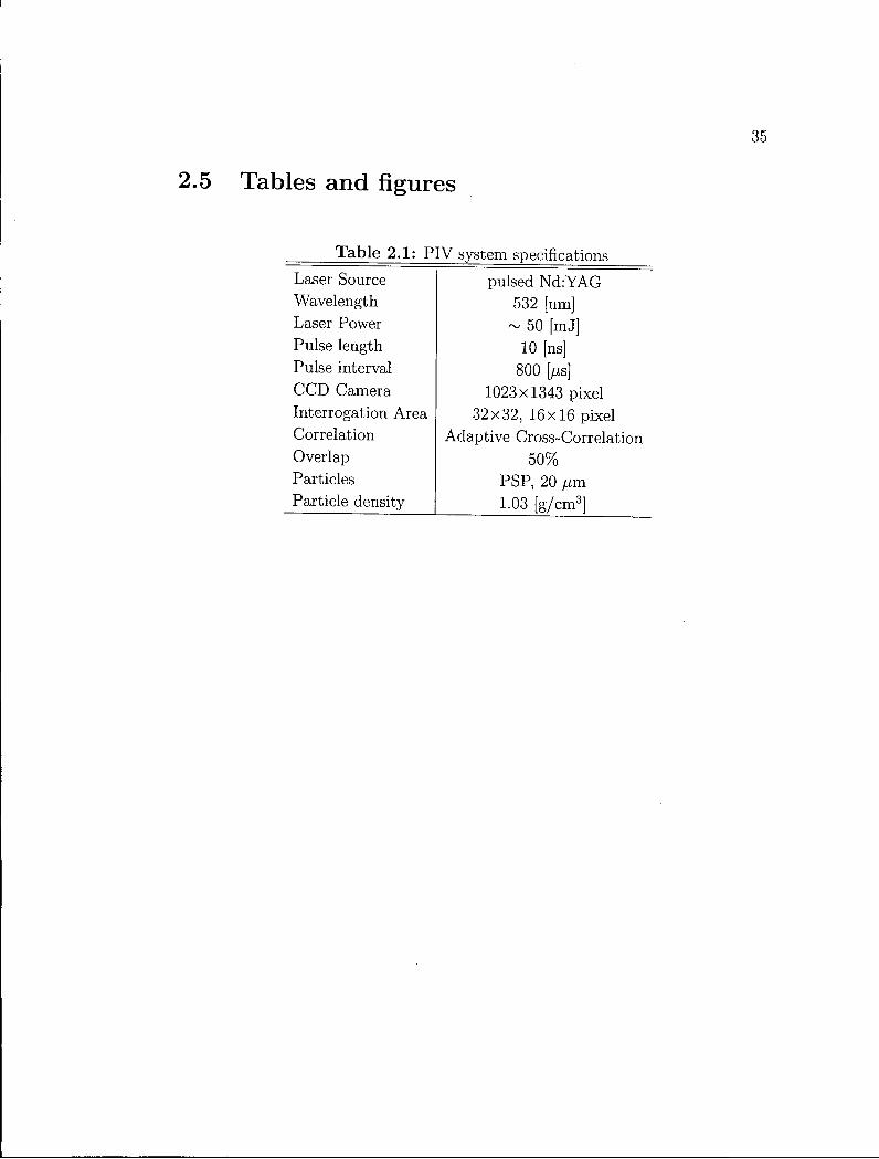
Tables and figures
T a b l e 2.1: P I V system specifications
Laser Source pulsed N d : Y A G Wavelength 532 [nm] Laser Power ~ 50 [mJ] Pulse length 10 [ns] Pulse interval 800 [fjs] C C D Camera 1023x1343 pixel Interrogation Area 32x32, 16x16 pixel Correlation Adaptive Cross-Correlation Overlap 50% Particles PSP, 20 yum Particle density 1.03 [g/cm3]
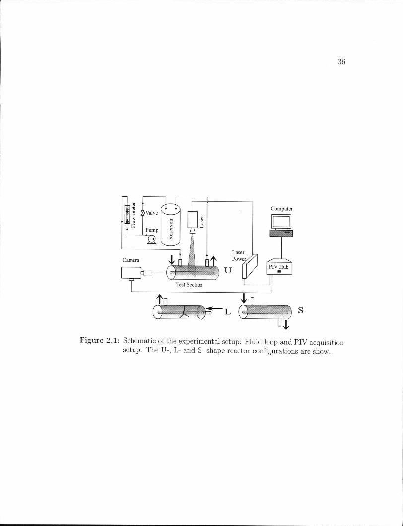
36
F i g u r e 2.1: Schematic of the experimental setup: Flu id loop and P I V acquisition setup. The U - , L - and S- shape reactor configurations are show.
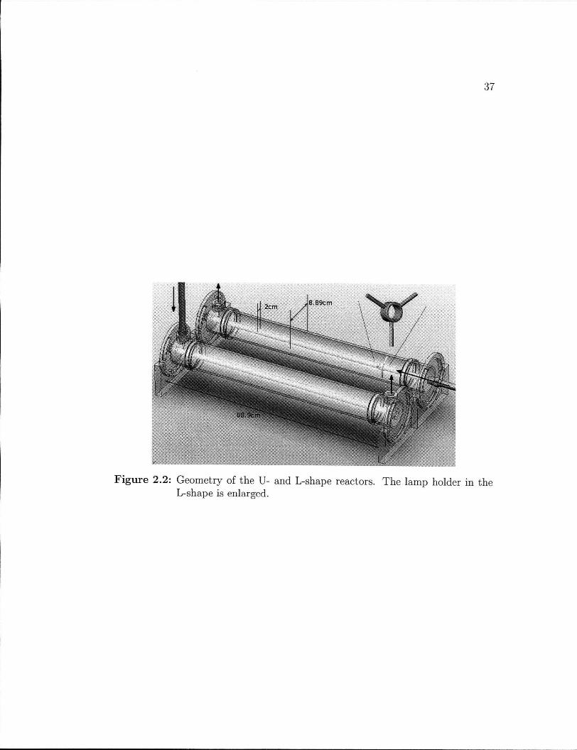
37
F i g u r e 2.2: Geometry of the U - and L-shape reactors. The lamp holder in the L-shape is enlarged.
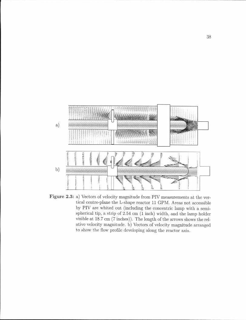
38
s S S s s 5 ? 5 S S
b) 1
F i g u r e 2.3: a) Vectors of velocity magnitude from P I V measurements at the vertical centre-plane the L-shape reactor 11 G P M . Areas not accessible by P I V are whited out (including the concentric lamp with a semi-spherical tip, a strip of 2.54 cm (1 inch) width, and the lamp holder visible at 18.7 cm (7 inches)). The length of the arrows shows the relative velocity magnitude, b) Vectors of velocity magnitude arranged to show the flow profile developing along the reactor axis.
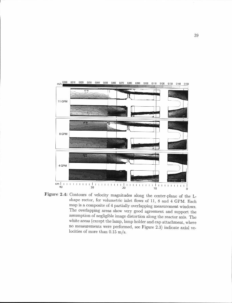
39
F i g u r e 2.4: Contours of velocity magnitudes along the center-plane of the re
shape rector, for volumetric inlet flows of 11, 8 and 4 G P M . Each map is a composite of 4 partially overlapping measurement windows. The overlapping areas show very good agreement and support the assumption of negligible image distortion along the reactor axis. The white areas (except the lamp, lamp holder and cap attachment, where no measurements were performed, see Figure 2.3) indicate axial velocities of more than 0.15 m/s.
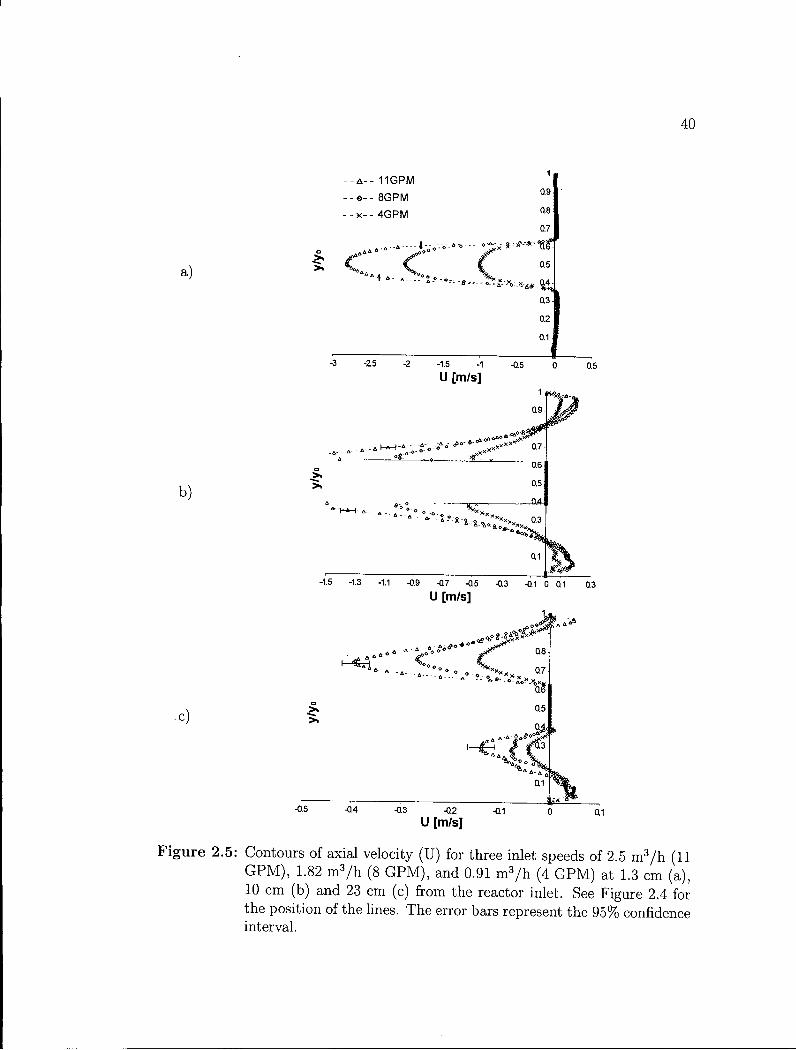
40
- - a - - 11GPM
- © - 8GPM
-x-4GPM 0.7
-2-5 -2 -1.5 -1 .05 0 0.5
U [m/s]
b)
-1.5 -1.3 -1.1 -0.9 -0.7 -Q5 -0.3 -0.1 0 Q1 Q3
U [m/s]
•c)
o Q5
Q1
, 1 •0.5 -0.4 -Q3 -0.2 -CI1 0 Q1
U [m/s]
F i g u r e 2.5: Contours of axial velocity (U) for three inlet speeds of 2.5 m 3 / h (11 G P M ) , 1.82 m 3 / h (8 G P M ) , and 0.91 m 3 / h (4 G P M ) at 1.3 cm (a), 10 cm (b) and 23 cm (c) from the reactor inlet. See Figure 2.4 for the position of the lines. The error bars represent the 95% confidence interval.
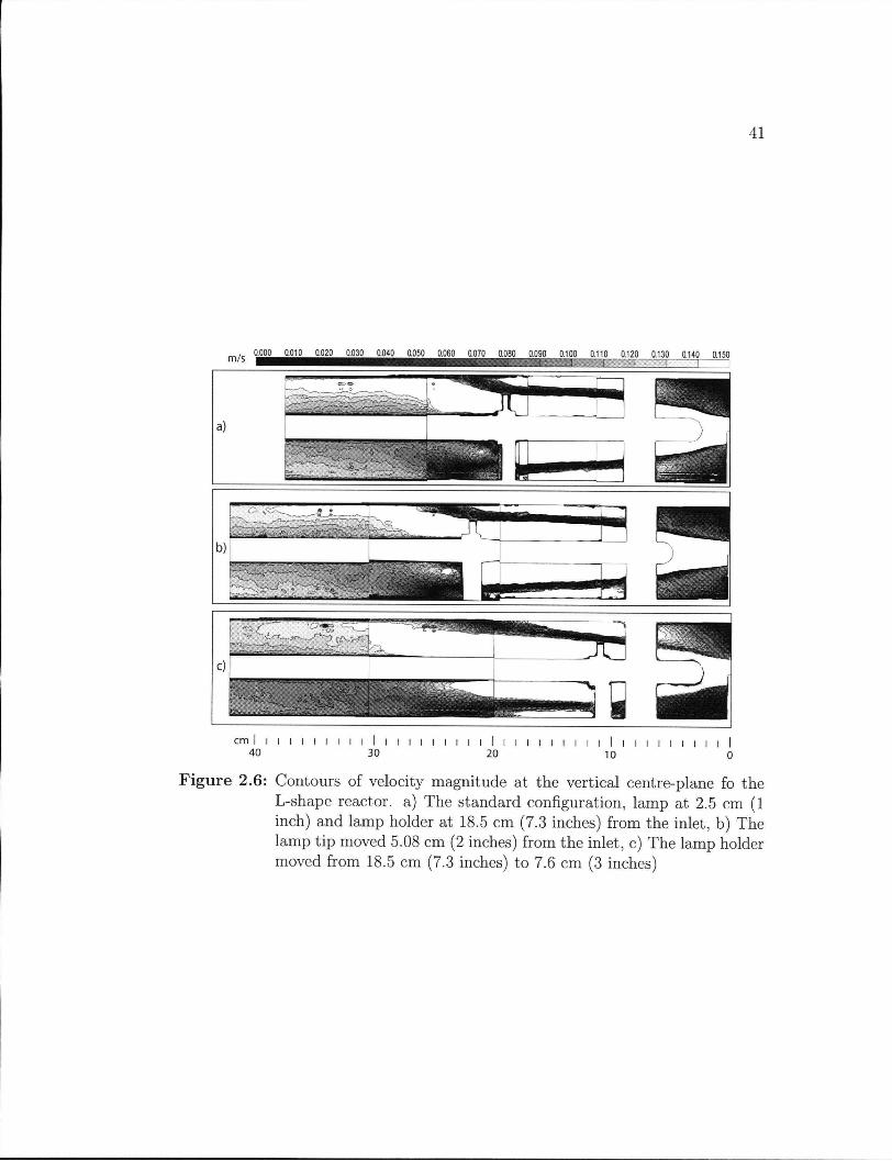
41
a) a) -
cm I i i i i i i i i i I i i 4 0 30
I I I I I I I I I I I I I I I I I I I I I I I I I I I I 20 10 0
F i g u r e 2.6: Contours of velocity magnitude at the vertical centre-plane fo the L-shape reactor, a) The standard configuration, lamp at 2.5 cm (1 inch) and lamp holder at 18.5 cm (7.3 inches) from the inlet, b) The lamp tip moved 5.08 cm (2 inches) from the inlet, c) The lamp holder moved from 18.5 cm (7.3 inches) to 7.6 cm (3 inches)
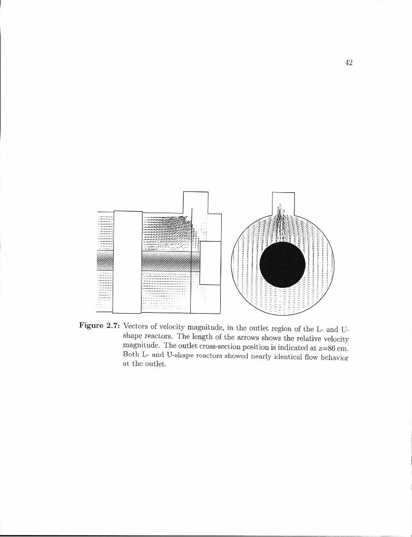
F i g u r e 2.7: Vectors of velocity magnitude, in the outlet region of the L - and U -shape reactors. The length of the arrows shows the relative velocity magnitude. The outlet cross-section position is indicated at z=86 cm. Both L - and U-shape reactors showed nearly identical flow behavior at the outlet.
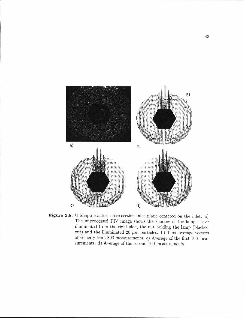
43
F i g u r e 2.8: U-Shape reactor, cross-section inlet plane centered on the inlet, a) The unprocessed P I V image shows the shadow of the lamp sleeve illuminated from the right side, the nut holding the lamp (blacked out) and the illuminated 20 pm particles, b) Time-average vectors of velocity from 800 measurements, c) Average of the first 100 measurements, d) Average of the second 100 measurements.
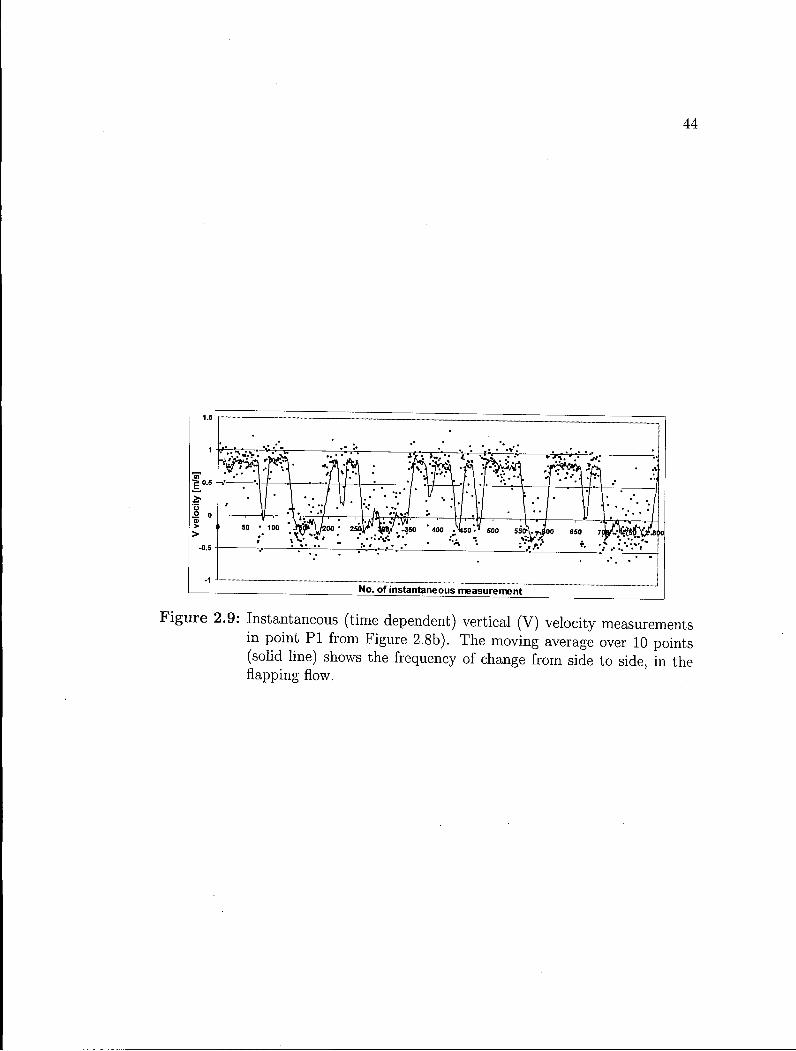
44
1.5
| No. of instantaneous measurement |
F i g u r e 2.9: Instantaneous (time dependent) vertical (V) velocity measurements in point P I from Figure 2.8b). The moving average over 10 points (solid line) shows the frequency of change from side to side, in the flapping flow.
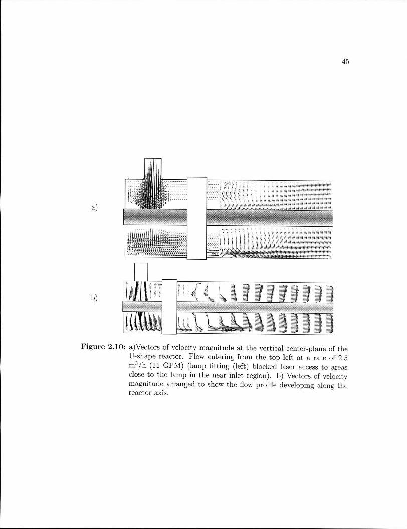
45
F i g u r e 2.10: a)Vectors of velocity magnitude at the vertical center-plane of the U-shape reactor. Flow entering from the top left at a rate of 2.5 m 3 / h (11 G P M ) (lamp fitting (left) blocked laser access to areas close to the lamp in the near inlet region), b) Vectors of velocity magnitude arranged to show the flow profile developing along the reactor axis.
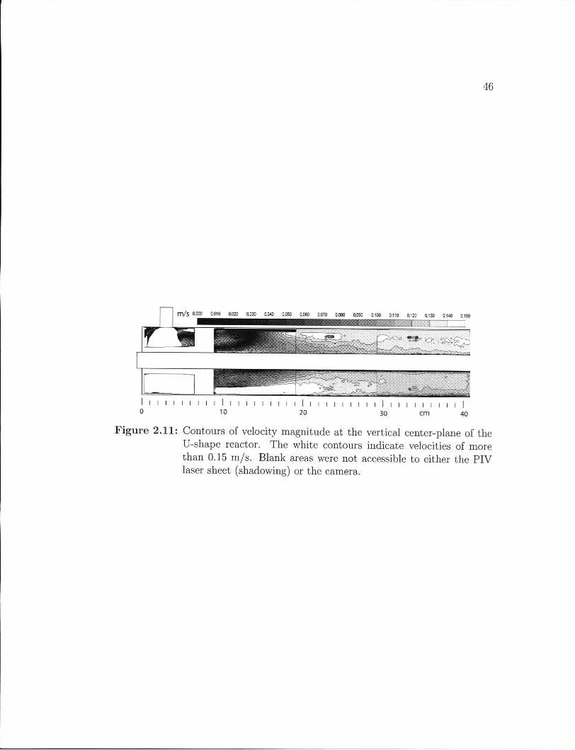
46
m/S 0000 0.010 0.020 0.030 0.040 0050 0.060 0.070 0.OBO 0.090 0.100 0.110 0.120 0.130 0.140 0.150
fir If
c c I I I I I I I I I I I I I I I I I I I
10 I I I I I I I I I I I I I I I I I I I I I
20 30 c m 40
ure 2.11: Contours of velocity magnitude at the vertical center-plane of the U-shape reactor. The white contours indicate velocities of more than 0.15 m/s. Blank areas were not accessible to either the P I V laser sheet (shadowing) or the camera.
47
Bib l iography
[1] A D R I A N , R . J . Twenty years of particle image velocimetry. In 12th Inter
national Symposium on Aplications of Laser Techniques to Fluid Mechanics,
Lisbon (July 2004).
[2] B R A U N , A . , J A K O B , L . , A N D O L I V E R O S , E . Advanced oxidation processes
- concepts of reactor design. Journal of Water Supply: Research and
Technology-AQUA 42, 3 (1993), 166-173.
[3] C A S S A N O , A . E . , M A R T I N , C . A . , B R A N D I , R . J . , A N D A L F A N O , O . M .
Photoreactor analysis and design: Fundamentals and applications. Industrial
& Engineering Chemistry Research 34 (1995), 2155-201.
[4] C H A N G , P . B . L . , A N D Y O U N G , T . M . Kinetics of methyl tert-butyl ether
degradation and by-product formation during uv/hydrogen peroxide water
treatment. In Proceedings of the Air & Waste Management Association's
Annual Conference & Exhibition, 93rd, Salt'Lake City, UT, United States,
June 18-22, 2000 (2000), pp. 7036-7055.
[5] C H I U , K . , L Y N , D . A . , A N D B L A T C H L E Y , E . R . Integrated uv disinfec
tion model based on particle tracking. Journal of Environmental Engineering
(1999), 7-16.
[6] D E V E N P O R T , W . J . , A N D S U T T O N , E . P . A n experimental study of two
flows through an axisymmetric sudden expansion. Experiments in Fluids 14,
6 (1993), 423-432.
[7] E L K A N Z I , E . M . , A N D K H E N G , G . B . H 2 o 2 / u v degradation kinetics of
isoprene in aqueous solution. Journal of Hazardous Materials 73 (2000), 55-
62.
[8] F O R E S T E R , S . E . , A N D E V A N S , G . M . Computational modelling study
of the hydrodynamics in a sudden expansion - tapered contraction reactor
geometry. Chemical Engineering Science 52, 21 (1997), 3773-3785.
[9] I S L A M , M . S . , H A G A , K . , K A M I N A G A , M . , H I N O , R . , A N D M O N D E , M .
Experimental analysis of turbulent flow structure in a fully developed rib
48
roughened rectangular channel with piv. Experiments in Fluids 33 (2002),
296-306.
[10] J A N E X , M . L . , S A V O Y E , P . , D O - Q U A N G , Z . , B L A T C H L E Y , E . , I., A N D
L A I N E , J . M . Impact of water quality and reactor hydrodynamics on waste
water disinfection by uv, use of cfd modeling for performance optimization.
Water Science and Technology 38 (1998), 71-78.
[11] K A M I M U R A , M . , F U R U K A W A , S . , A N D H I R O T S U J I , J . Development of a
simulator for ozone/uv reactor based on cfd analysis. Water science and
technology : a journal of the International Association on Water Pollution
Research 46 (2002), 13-19.
[12] L A B A S , M . D . , Z A L A Z A R , C . S . , B R A N D I , R . J . , M A R T I N , C . A . , A N D
C A S S A N O , A . E . Scaling up of a photoreactor for formic acid degradation
employing hydrogen peroxide and uv radiation. Helvetica Chimica Acta 85
(2002), 82-95.
[13] L A W R Y S H Y N , Y . A . , A N D C A I R N S , B . U v disinfection of water: the need for
uv reactor validation. Water Science & Technology: Water Supply 3 (2003),
293-300.
[14] L Y N , D . A . , C H I U , K . , A N D B L A T C H L E Y , E . R . , I. Numerical modeling of
flow and disinfection in uv disinfection channels. Journal of Environmental
Engineering (Reston, Virginia) 125 (1999), 17-26.
[15] O P P E N L A E N D E R , T . Photochemical purification of water and air. Wiley-
V C H , 2003.
[16] P R U V O S T , J . , L E G R A N D , J . , L E G E N T I L H O M M E , P . , A N D D O U B L I E Z , L .
Particle image velocimetry investigation of the flow-field of a 3d turbulent
annular swirling decaying flow induced by means of a tangential inlet. Exper
iments in Fluids 29 (2000), 291-301.
[17] S C H O E N E N , D . , K O L C H , A . , A N D G E B E L , J . Influence of geometrical pa
rameters in different irradiation vessels on uv disinfection rate. International
Journal of Hygiene and Environmental Medicine 194 , 3 (1993), 313-320.
49
[18] W E I S G R A B E R , T . H . , A N D L I E P M A N , D . Turbulent structure during tran
sition to self-similiarity in a round jet. Experiments in Fluids 24 (1998),
210-224.
[19] W u , H . L . , P E N G , X . F . , A N D C H E N , T . K . Influence of sleeve tube on
the flow and heat transfer behavior at a t-junction. International Journal of
Heat and Mass Transfer 46 (2003), 2637-2644.
Chapter
CFD study of annular UV-reactor
hydrodynamics
The following chapter covers the computational fluid dynamics (CFD) models cre
ated to study the hydrodynamic flow in annular reactors. The influence of mesh
density and choice of turbulence models is discussed. Finally, the C F D modeling
results are compared to P I V experimental data and conclusions on the validity of
the models are made.
3.1 Introduct ion
Water treatment processes using UV-technology have seen a rapid growth over
the last decade (12). The increasing public awareness of water as a resource, and
increasing regulations, have resulted in a compound annual growth rate of 11%
(1996-2001) for the North American UV-market, and a slightly higher rate was
estimated for the following years (16).
A successful fundamental simulation of UV-systems is the basis for several
applications: virtual prototyping, cost effective design optimization, and on-line
control and performance evaluation. U V reactor simulation can be achieved by
considering the rate of reaction linked to the non-homogeneous UV-fluence rate
through the local volumetric rate of energy absorption. This spatial dependency
makes a three-dimensional resolution of the reaction rate indispensable (9). Only
after computing the full hydrodynamic flow of the reactor does it become possible
50
51
to correctly model the reaction rate inside UV-reactors. The effect of the interac
tion between reactor hydrodynamics and local radiation intensity on the concen
tration distribution of contaminants in UV-advanced oxidation reactors (AdOx)
was shown by Pareek et al. (11). Schoenen et al. (19) demonstrated the influence
of the flow field and geometry on the performance of disinfection systems.
Realizing the importance of an integrated model, Romero et al. (18) set up
the fundamental balances needed to solve the mass, momentum, energy, radia
tion and chemical reaction rate equations for annular UV-reactors. Because of a
lack of computing power, they assumed axial symmetry and implemented a sim
plified set of equations for two-dimensional geometries, a method that was then
applied for subsequent studies of different geometries and reaction kinetics by Cas-
sano et al. (2). W i t h the increased performance of computational resources and
the development of simulation software, computational fluid dynamics (CFD) is
becoming an affordable engineering tool to simulate and optimize reactor designs.
The viability of C F D for the design and optimization of chemical reactors has been
demonstrated for a variety of systems (1, 11, 20). C F D has been applied to the
simulation of UV-reactors hydrodynamics (21). It has also been utilized to sim
ulate UV-reactor performance through the integration of reactor hydrodynamics,
radiation distribution and UV-reaction kinetics (9).
While C F D is becoming a mainstream modeling tool, anticipating the flow
characteristics and selecting the appropriate modeling technologies (boundary con
ditions, turbulence model, etc.) remain the responsibility of the user. As C F D is
based on the governing equations of mass and momentum conservation as well
as mathematical models with simplifying assumptions, there are many possible
sources for errors, and validation of the C F D results is vital for the effective use of
such a model. Advanced experimental methods such as laser Doppler velocimetry
(LDV) and particle image velocimetry (PIV) have been shown to give detailed
information on the turbulent flow field in stirred vessels (10, 15) and in tubular
channels (4, 6, 13).
C F D solves the governing equations of the flow mass and momentum conserva
tion in the discretized computational domain using a numerical (e.g. finite volume)
method. Different approaches can be taken for modeling turbulent flows. In the
Reynolds averaged Navier-Stokes (RANS) approach, instantaneous velocity com-
52
ponents are usually divided into their mean and fluctuating values (u = u + u').
The mass and momentum conservation in suffix notation are:
duj
dxi = 0 (3-1)
duj
dt '3dxj
dui uty) i,j = l,2,3(forx,y,z) (3.2)
where Ui is the instantaneous velocity, ul the mean velocity, and u\ the fluctuating
velocity component in the ith direction. The unknown terms —pu^u'j, called the
Reynolds stresses, represent the effect of small scale turbulence on the mean flow
and need to be closed by using one of the turbulence models.
Among the factors that may influence the C F D results are the discretisation
of the domain (structure and size of the cells), and the type of modeling approach
employed (turbulence model, etc). Gr id generation is often quoted as the most
important and most time consuming part of C F D analysis. The quality of the grid
has a direct influence on the quality of the analysis, regardless of the flow solver
used. Additionally, the solver will be more robust and efficient when using a well
constructed mesh. A quality grid, capable of representing the geometry, is the
basis for a reliable, accurate simulation. In general, both mesh quality and grid
independence of the solution need to be ensured (3).
When the flow is within the turbulent regime (typically the case in UV-reactors),
additional models are required to consider the effect of turbulent fluctuations on
the flow. For most engineering applications, only the mean effect of turbulent
quantities is important; therefore, the time-averaged flow properties are of inter
est. The R A N S equations are the established averaging approach for modeling
turbulence. Two classes of R A N S turbulence models are the n-e models and the
Reynolds stress model (RSM), each relying on a set of implied assumptions with
relative advantages and disadvantages. The «-e models use the Boussinesq hy
pothesis to relate the Reynolds stresses to the mean velocity gradient through the
turbulent kinetic energy K and the turbulent dissipation rate e. This implies locally
isotropic turbulent fluctuations and a local equilibrium of the production and dis
sipation terms. Primary shear stresses are predicted well wi th these two-equation
models, but secondary shear stresses and normal stresses are not.
53
The Standard n-e model is the simplest of the two-equation models. It is
robust, economic, and predicts a wide range of flows reasonably well. But the as
sumptions are only valid in fully turbulent flows; it cannot deal well with complex
three-dimensional flows, sudden changes in the mean strain rate, curved surfaces,
secondary motions and flow separation. It tends to over-predict turbulence gener
ation in areas where the mean flow is highly accelerated or decelerated (8).
The Realizable «-e model incorporates time scale realizability and an additional
source term in the epsilon equation for improved performance in flows involving
adverse pressure gradients (including separated flows). It also features a realiz
ability constraint on the predicted stress tensor. This avoids excessive levels of
turbulence generation in regions of large mean strain, such as occur in impinging
flows.
The R S M model uses the exact transport equations for Reynolds stresses, clos
ing the unknown correlations at this level (second-order closure model). It aban
dons the isotropic eddy-viscosity hypothesis and performs well for many complex
flows (e.g. highly swirling flows). The seven additional partial differential equa
tions (PDEs) and a tendency to require a finer mesh make it computationally more
expensive. Table 3.1 provides a brief summary of the advantages and disadvantages
of the K-e and Reynolds stress models.
Despite a number of studies on C F D modeling of UV-reactor hydrodynamics,
and the development of integrated C F D models for UV-reactor performance, to
the author's knowledge there have been no efforts reported in the open literature
to validate the C F D simulations with experimentally obtained flow field informa
tion. Also, little if any information can be found on the effect of computational
domain discretisation and turbulence models on the C F D results. The objective
of this work was to carry out a comprehensive C F D study of the turbulent flow
occurring in annular UV-reactors and to compare the results with experimental
measurements. The cylindrical UV-reactor with a concentric lamp parallel to the
reactor body, which represents the basic design for many current UV-reactors, was
investigated. The effect of grid number and structure on the C F D results in two
commonly used UV-reactor geometries, with an inlet parallel (L-shape) and normal
(U-shape) to the main reactor body, were studied. The influence of three differ
ent turbulence models was also assessed for both geometries. The results were
54
evaluated by comparison with experimental data obtained from Particle Image Velocimetry (PIV) .
3.2 CFD modeling
The two model UV-reactor geometries studied, the L-shape and U-shape shown
in Figure 3.1, are based on the existing industrial reactors as currently used. The
simulation results were compared to the experimental P I V results from Plexiglas
prototypes having the same dimensions. Both shapes shared the same main reac
tion tube diameter of 8.9 cm (3.5 inch), length of 88.9 cm (35 inch), with a central
UV-lamp of 2 cm (0.79 inch) in diameter. The inlet and outlet ports, with a diam
eter of 1.91 cm (0.75 inch), were placed 2.54 cm (1 inch) from each respective end
for the U-shape, while the L-shape inlet was centred on the front plate. The inlet
tube length with an = 45 was chosen to ensure that a fully developed flow was
established at the entrance of the reactor. A volumetric inlet rate of 6 .94xl0~ 4
m 3 / s (11 G P M ) , corresponding to a mean inlet velocity of 2.43 m/s, a mean axial
velocity in the reactor of 0.11 m/s, and a Reynolds number of 10,000 was set.
The commercial mesh generator G A M B I T was used to create the grid and the
tgrid tool was employed to merge separately meshed domains. The inlet and outlet
tubes were meshed with 5,000-8,000 structured (Cooper) cells in all cases. Both
structured and unstructured cells were employed to discretize the main reactor
domain (Figure 3.2). For the unstructured tetrahedral mesh, no subdomains were
needed. The size of cells was defined by cell-volume and refined manually if nec
essary. For the structured mesh, the domain was split into several subdomains
reducing the use of unstructured cells to the volume containing the lamp holder in
the L-shape reactor. For the U-shape, the inlet volume and lamp region with high
velocity gradients, round jet impingement, and flow separation required a higher
mesh resolution, while the lamp tip and the lamp holder needed more attention in
the case of the L-shape.
A commercial C F D software package, Fluent (V6.1.22), was used to solve the
conservation of mass and momentum equations for the described geometries. The
internal structures were reproduced as 3D volumes and a no-slip boundary condi
tion was imposed on the reactor walls. The operating fluid was defined as water
55
at 293 K . Velocity inlets, with a hydraulic diameter of 1.91 cm, 10% turbulent
intensity, and a uniform velocity distribution were defined and a fully-developed
flow (outflow) was applied at the exit. In all cases, the standard log law wall func
tions were employed. The segregated steady-state solver was used to iterate the
solutions, starting with a first order upwind discretisation scheme, and continuing
with the second order upwind scheme for the final converged solution. The SIM
P L E method was chosen for the pressure-velocity coupling. Convergence of the
numerical solution was ensured by monitoring the scaled residuals of continuity, x-
,y-,z- velocities, and the turbulence parameters to a criterion of less than 1 0 - 5 . In
addition, the velocity magnitude at two points defined in areas with high velocity
gradients were used as indicators.
The importance of correctly resolving the turbulent flow behavior for chemical
reactors has been stressed. The exact Navier-Stokes equations, are replaced by
Reynolds averaged equations generating the need for closure models to obtain
solutions. However, no turbulence model is universal and the choice is based
on considerations of domain geometry and the anticipated flow behavior. Three
turbulence models, the Standard «-e model, the Realizable K-e model, and the
Reynolds Stress Model (RSM) were selected, based on availability (most widely
used models) and usability (average time and computing power needed).
3.3 P I V experiments
The C F D flow simulations were validated using experimental P I V results. P I V is
a non-intrusive method of instantaneous flow field visualization. A sheet of laser
light flash-illuminates particles in the flow field and a digital camera captures the
two points in time. The resulting flow velocity extracted from this digital image
pair is an instantaneous snapshot of the flow in the area viewed.
The particle images were recorded using an 80C60 HiSense P I V camera con
nected to a FlowMap System Hub (Dantec Dynamics Inc.) for synchronization. A
NewWave Solo-15 laser system provided illumination of the particles. The seeding
(PSP, 20 ^ m diameter, 1.03 g/cm 3 ) was adjusted to 5 — 10 particles per interro
gation window. The image data were analyzed with a multi-pass adaptive cross-
correlation technique with interrogation windows of 32x32 pixels and an overlap of
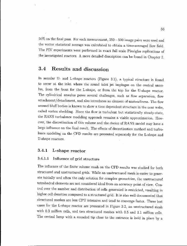
56
50% on the final pass. For each measurement, 250 - 500 image pairs were used and
the vector statistical average was calculated to obtain a time-averaged flow field.
The P I V experiments were performed in exact full scale Plexiglas replications of
the investigated reactors. A more detailed description can be found in Chapter 2.
3.4 Results and discussion
In annular U - and L-shape reactors (Figure 3.1), a typical structure is found
to occur at the inlet where the round inlet jet impinges on the central annu-
lus, from the front for the L-shape, or from the top for the U-shape reactor.
The cylindrical annulus poses several challenges, such as flow separation, flow
attachment/detachment, and also introduces an element of unsteadiness. The flow
around bluff bodies is known to show a time dependent structure in the near wake,
called vortex shedding. Since the flow is turbulent but statistically steady-state,
the R A N S turbulence modeling approach remains a viable approximation. How
ever, the discretisation of this volume and the choice of R A N S model may have a
large influence on the final result. The effects of discretisation method and turbu
lence modeling on the C F D results are presented separately for the L-shape and
U-shape reactors.
3.4.1 L-shape reactor
3.4.1.1 I n f l u e n c e o f g r i d s t r u c t u r e
The influence of the finite volume mesh on the C F D results was studied for both
structured and unstructured grids. While an unstructured mesh is easier to gener
ate initially and often the only solution for complex geometries, the unstructured
tetrahedral elements are not considered ideal from an accuracy point of view. Con
trol over the number and distribution of cells generated is restricted, resulting in
higher cell densities compared to a structured grid. It is also well documented that
structured meshes are less C P U intensive and tend to converge faster. Three test
cases for the L-shape reactor are presented in Figure 3.2, an unstructured mesh
with 0.3 million cells, and two structured meshes with 0.5 and 1.1 million cells.
The central lamp with a rounded tip close to the entrance is held in place by a
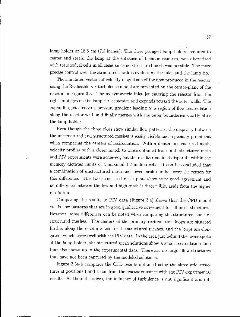
57
lamp holder at 18.6 cm (7.3 inches). The three pronged lamp holder, required to
center and retain the lamp at the entrance of L-shape reactors, was discretized
with tetrahedral cells in all cases since no structured mesh was possible. The more
precise control over the structured mesh is evident at the inlet and the lamp tip.
The simulated vectors of velocity magnitude of the flow produced in the reactor
using the Realizable n-e turbulence model are presented on the center-plane of the
reactor in Figure 3.3. The axisymmetric inlet jet entering the reactor from the
right impinges on the lamp tip, separates and expands toward the outer walls. The
expanding jet creates a pressure gradient leading to a region of flow recirculation
along the reactor wall, and finally merges with the outer boundaries shortly after
the lamp holder.
Even though the three plots show similar flow patterns, the disparity between
the unstructured and structured meshes is easily visible and especially prominent
when comparing the centers of recirculation. W i t h a denser unstructured mesh,
velocity profiles with a closer match to those obtained from both structured mesh
and P I V experiments were achieved, but the results remained disparate within the
memory dictated limits of a maximal 1.2 million cells. It can be concluded that
a combination of unstructured mesh and lower mesh number were the reason for
this difference. The two structured mesh plots show very good agreement and
no difference between the low and high mesh is discernible, aside from the higher
resolution.
Comparing the results to P I V data (Figure 3.4) shows that the C F D model
yields flow patterns that are in good qualitative agreement for all mesh structures.
However, some differences can be noted when comparing the structured and un
structured meshes. The centers of the primary recirculation loops are situated
further along the reactor z-axis for the structured meshes, and the loops are elon
gated, which agrees well with the P I V data. In the area just behind the lower spoke
of the lamp holder, the structured mesh solutions show a small recirculation loop
that also shows up in the experimental data. There are no major flow structures
that have not been captured by the modeled solutions.
Figure 3.5a-b compares the C F D results obtained using the three grid struc
tures at positions 1 and 15 cm from the reactor entrance with the P I V experimental
results. A t these distances, the influence of turbulence is not significant and dif-
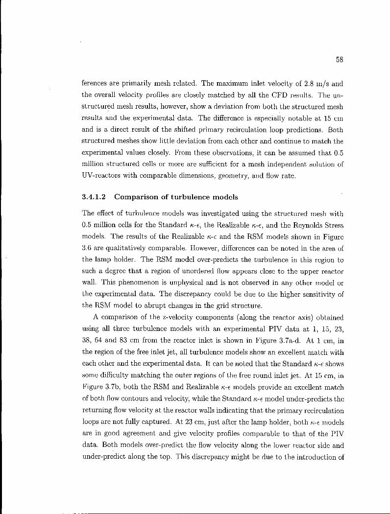
58
ferences are primarily mesh related. The maximum inlet velocity of 2.8 m/s and
the overall velocity profiles are closely matched by all the C F D results. The un
structured mesh results, however, show a deviation from both the structured mesh
results and the experimental data. The difference is especially notable at 15 cm
and is a direct result of the shifted primary recirculation loop predictions. Both
structured meshes show little deviation from each other and continue to match the
experimental values closely. From these observations, it can be assumed that 0.5
million structured cells or more are sufficient for a mesh independent solution of
UV-reactors with comparable dimensions, geometry, and flow rate.
3.4.1 .2 C o m p a r i s o n o f t u r b u l e n c e m o d e l s
The effect of turbulence models was investigated using the structured mesh with
0.5 million cells for the Standard K-e, the Realizable K-e , and the Reynolds Stress
models. The results of the Realizable n-e and the R S M models shown in Figure
3.6 are qualitatively comparable. However, differences can be noted in the area of
the lamp holder. The R S M model over-predicts the turbulence in this region to
such a degree that a region of unordered flow appears close to the upper reactor
wall. This phenomenon is unphysical and is not observed in any other model or
the experimental data. The discrepancy could be due to the higher sensitivity of
the R S M model to abrupt changes in the grid structure.
A comparison of the z-velocity components (along the reactor axis) obtained
using all three turbulence models with an experimental P I V data at 1, 15, 23,
38, 64 and 83 cm from the reactor inlet is shown in Figure 3.7a-d. At 1 cm, in
the region of the free inlet jet, all turbulence models show an excellent match with
each other and the experimental data. It can be noted that the Standard n-e shows
some difficulty matching the outer regions of the free round inlet jet. A t 15 cm, in
Figure 3.7b, both the R S M and Realizable n-e models provide an excellent match
of both flow contours and velocity, while the Standard n-e model under-predicts the
returning flow velocity at the reactor walls indicating that the primary recirculation
loops are not fully captured. At 23 cm, just after the lamp holder, both n-e models
are in good agreement and give velocity profiles comparable to that of the P I V
data. Both models over-predict the flow velocity along the lower reactor side and
under-predict along the top. This discrepancy might be due to the introduction of
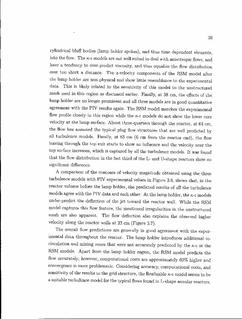
59
cylindrical bluff bodies (lamp holder spokes), and thus time dependent elements,
into the flow. The K-e models are not well suited to deal with anisotropic flows, and
have a tendency to over-predict viscosity, and thus equalize the flow distribution
over too short a distance. The z-velocity components of the R S M model after
the lamp holder are non-physical and show little resemblance to the experimental
data. This is likely related to the sensitivity of this model to the unstructured
mesh used in this region as discussed earlier. Finally, at 38 cm, the effects of the
lamp holder are no longer prominent and all three models are in good quantitative
agreement with the P I V results again. The R S M model matches the experimental
flow profile closely in this region while the K-e models do not show the lower core
velocity at the lamp surface. About three-quarters through the reactor, at 64 cm,
the flow has assumed the typical plug flow structures that are well predicted by
all turbulence models. Finally, at 83 cm (6 cm from the reactor end), the flow
leaving through the top exit starts to show an influence and the velocity near the
top surface increases, which is captured by all the turbulence models. It was found
that the flow distribution in the last third of the L - and U-shape reactors show no
significant difference.
A comparison of the contours of velocity magnitude obtained using the three
turbulence models with P I V experimental values in Figure 3.8, shows that, in the
reactor volume before the lamp holder, the predicted results of all the turbulence
models agree with the P I V data and each other. A t the lamp holder, the n-e models
under-predict the deflection of the jet toward the reactor wall. While the R S M
model captures this flow feature, the mentioned irregularities in the unstructured
mesh are also apparent. The flow deflection also explains the observed higher
velocity along the reactor walls at 23 cm (Figure 3.7).
The overall flow predictions are generally in good agreement with the exper
imental data throughout the reactor. The lamp holder introduces additional re
circulation and mixing zones that were not accurately predicted by the K-C or the
R S M models. Apart from the lamp holder region, the R S M model predicts the
flow accurately; however, computational costs are approximately 60% higher and
convergence is more problematic. Considering accuracy, computational costs, and
sensitivity of the results to the grid structure, the Realizable n-e model seems to be
a suitable turbulence model for the typical flows found in L-shape annular reactors.
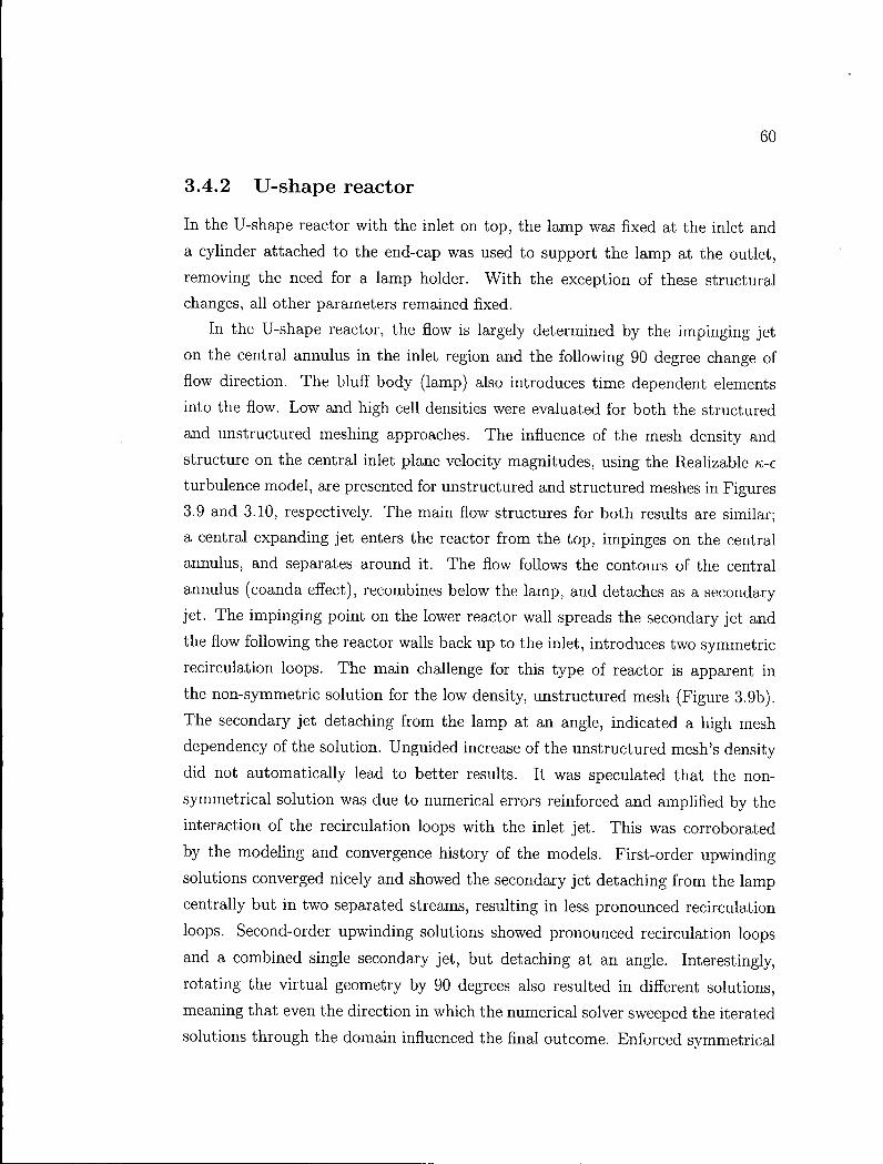
60
3.4.2 U-shape reactor
In the U-shape reactor with the inlet on top, the lamp was fixed at the inlet and
a cylinder attached to the end-cap was used to support the lamp at the outlet,
removing the need for a lamp holder. W i t h the exception of these structural
changes, all other parameters remained fixed.
In the U-shape reactor, the flow is largely determined by the impinging jet
on the central annulus in the inlet region and the following 90 degree change of
flow direction. The bluff body (lamp) also introduces time dependent elements
into the flow. Low and high cell densities were evaluated for both the structured
and unstructured meshing approaches. The influence of the mesh density and
structure on the central inlet plane velocity magnitudes, using the Realizable n-e
turbulence model, are presented for unstructured and structured meshes in Figures
3.9 and 3.10, respectively. The main flow structures for both results are similar;
a central expanding jet enters the reactor from the top, impinges on the central
annulus, and separates around it. The flow follows the contours of the central
annulus (coanda effect), recombines below the lamp, and detaches as a secondary
jet. The impinging point on the lower reactor wall spreads the secondary jet and
the flow following the reactor walls back up to the inlet, introduces two symmetric
recirculation loops. The main challenge for this type of reactor is apparent in
the non-symmetric solution for the low density, unstructured mesh (Figure 3.9b).
The secondary jet detaching from the lamp at an angle, indicated a high mesh
dependency of the solution. Unguided increase of the unstructured mesh's density
did not automatically lead to better results. It was speculated that the non
symmetrical solution was due to numerical errors reinforced and amplified by the
interaction of the recirculation loops with the inlet jet. This was corroborated
by the modeling and convergence history of the models. First-order upwinding
solutions converged nicely and showed the secondary jet detaching from the lamp
centrally but in two separated streams, resulting in less pronounced recirculation
loops. Second-order upwinding solutions showed pronounced recirculation loops
and a combined single secondary jet, but detaching at an angle. Interestingly,
rotating the virtual geometry by 90 degrees also resulted in different solutions,
meaning that even the direction in which the numerical solver sweeped the iterated
solutions through the domain influenced the final outcome. Enforced symmetrical
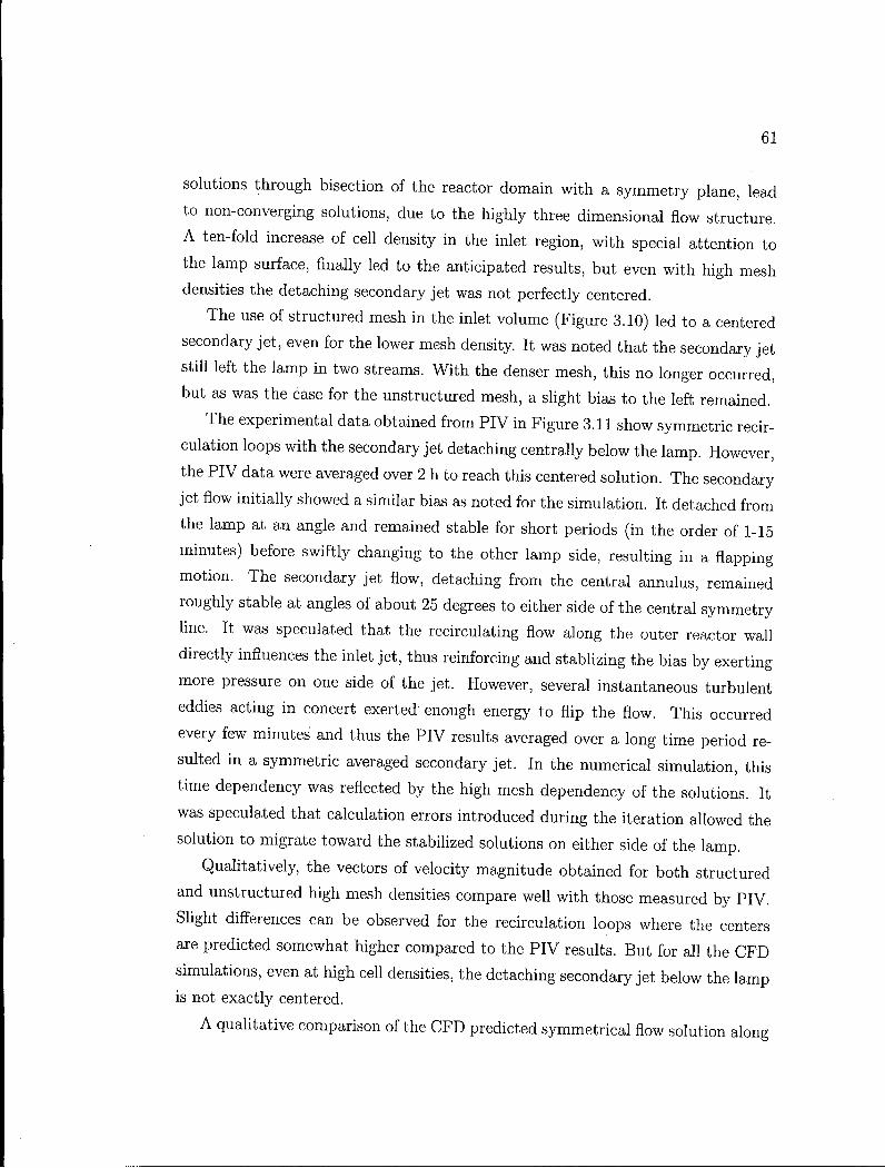
61
solutions through bisection of the reactor domain with a symmetry plane, lead
to non-converging solutions, due to the highly three dimensional flow structure.
A ten-fold increase of cell density in the inlet region, with special attention to
the lamp surface, finally led to the anticipated results, but even with high mesh
densities the detaching secondary jet was not perfectly centered.
The use of structured mesh in the inlet volume (Figure 3.10) led to a centered
secondary jet, even for the lower mesh density. It was noted that the secondary jet
still left the lamp in two streams. W i t h the denser mesh, this no longer occurred,
but as was the case for the unstructured mesh, a slight bias to the left remained.
The experimental data obtained from P I V in Figure 3.11 show symmetric recir
culation loops with the secondary jet detaching centrally below the lamp. However,
the P I V data were averaged over 2 h to reach this centered solution. The secondary
jet flow initially showed a similar bias as noted for the simulation. It detached from
the lamp at an angle and remained stable for short periods (in the order of 1-15
minutes) before swiftly changing to the other lamp side, resulting in a flapping
motion. The secondary jet flow, detaching from the central annulus, remained
roughly stable at angles of about 25 degrees to either side of the central symmetry
line. It was speculated that the recirculating flow along the outer reactor wall
directly influences the inlet jet, thus reinforcing and stablizing the bias by exerting
more pressure on one side of the jet. However, several instantaneous turbulent
eddies acting in concert exerted enough energy to flip the flow. This occurred
every few minutes and thus the P I V results averaged over a long time period re
sulted in a symmetric averaged secondary jet. In the numerical simulation, this
time dependency was reflected by the high mesh dependency of the solutions. It
was speculated that calculation errors introduced during the iteration allowed the
solution to migrate toward the stabilized solutions on either side of the lamp.
Qualitatively, the vectors of velocity magnitude obtained for both structured
and unstructured high mesh densities compare well with those measured by P IV .
Slight differences can be observed for the recirculation loops where the centers
are predicted somewhat higher compared to the P I V results. But for all the C F D
simulations, even at high cell densities, the detaching secondary jet below the lamp
is not exactly centered.
A qualitative comparison of the C F D predicted symmetrical flow solution along
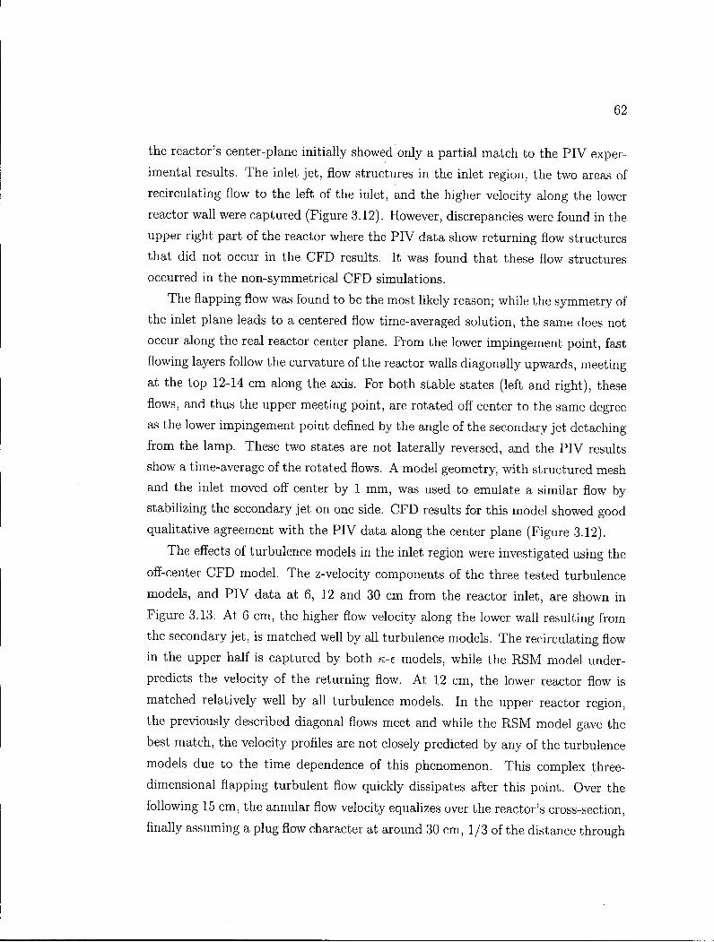
62
the reactor's center-plane initially showed only a partial match to the P I V exper
imental results. The inlet jet, flow structures in the inlet region, the two areas of
recirculating flow to the left of the inlet, and the higher velocity along the lower
reactor wall were captured (Figure 3.12). However, discrepancies were found in the
upper right part of the reactor where the P I V data show returning flow structures
that did not occur in the C F D results. It was found that these flow structures
occurred in the non-symmetrical C F D simulations.
The flapping flow was found to be the most likely reason; while the symmetry of
the inlet plane leads to a centered flow time-averaged solution, the same does not
occur along the real reactor center plane. From the lower impingement point, fast
flowing layers follow the curvature of the reactor walls diagonally upwards, meeting
at the top 12-14 cm along the axis. For both stable states (left and right), these
flows, and thus the upper meeting point, are rotated off center to the same degree
as the lower impingement point defined by the angle of the secondary jet detaching
from the lamp. These two states are not laterally reversed, and the P I V results
show a time-average of the rotated flows. A model geometry, with structured mesh
and the inlet moved off center by 1 mm, was used to emulate a similar flow by
stabilizing the secondary jet on one side. C F D results for this model showed good
qualitative agreement with the P I V data along the center plane (Figure 3.12).
The effects of turbulence models in the inlet region were investigated using the
off-center C F D model. The z-velocity components of the three tested turbulence
models, and P I V data at 6, 12 and 30 cm from the reactor inlet, are shown in
Figure 3.13. At 6 cm, the higher flow velocity along the lower wall resulting from
the secondary jet, is matched well by all turbulence models. The recirculating flow
in the upper half is captured by both K-e models, while the R S M model under-
predicts the velocity of the returning flow. At 12 cm, the lower reactor flow is
matched relatively well by all turbulence models. In the upper reactor region,
the previously described diagonal flows meet and while the R S M model gave the
best match, the velocity profiles are not closely predicted by any of the turbulence
models due to the time dependence of this phenomenon. This complex three-
dimensional flapping turbulent flow quickly dissipates after this point. Over the
following 15 cm, the annular flow velocity equalizes over the reactor's cross-section,
finally assuming a plug flow character at around 30 cm, 1/3 of the distance through
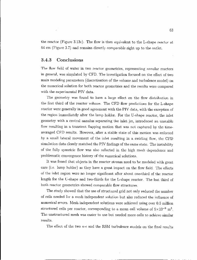
63
the reactor (Figure 3.13c). The flow is then equivalent to the L-shape reactor at
64 cm (Figure 3.7) and remains directly comparable right up to the outlet.
3.4.3 Conclusions
The flow field of water in two reactor geometries, representing annular reactors
in general, was simulated by C F D . The investigation focused on the effect of two
main modeling parameters (discretisation of the volume and turbulence model) on
the numerical solution for both reactor geometries and the results were compared
with the experimental P I V data.
The geometry was found to have a large effect on the flow distribution in
the first third of the reactor volume. The C F D flow predictions for the L-shape
reactor were generally in good agreement with the P I V data, with the exception of
the region immediately after the lamp holder. For the U-shape reactor, the inlet
geometry with a central annulus separating the inlet jet, introduced an unstable
flow resulting in a transient flapping motion that was not captured by the time-
averaged C F D results. However, after a stable state of this motion was enforced
by a small lateral movement of the inlet resulting in a swirling flow, the C F D
simulation data closely matched the P I V findings of the same state. The instability
of the fully symetric flow was also reflected in the high mesh dependence and
problematic convergence history of the numerical solutions.
It was found that objects in the reactor stream need to be modeled with great
care (i.e. lamp holder) as they have a great impact on the flow field. The effects
of the inlet region were no longer significant after about one-third of the reactor
length for the U-shape and two-thirds for the L-shape reactor. The last third of
both reactor geometries showed comparable flow structures.
The study showed that the use of structured grid not only reduced the number
of cells needed for a mesh independent solution but also reduced the influence of
numerical errors. Mesh independent solutions were achieved using over 0.5 million
structured cells per reactor, corresponding to a mean cell volume of 5 x l 0 ~ 9 m 3 .
The unstructured mesh was easier to use but needed more cells to achieve similar
results.
The effect of the two K-e and the R S M turbulence models on the final results
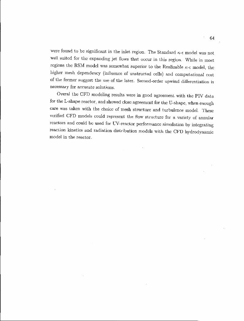
64
were found to be significant in the inlet region. The Standard n-t model was not
well suited for the expanding jet flows that occur in this region. While in most
regions the R S M model was somewhat superior to the Realizable n-e model, the
higher mesh dependency (influence of unstructed cells) and computational cost
of the former suggest the use of the later. Second-order upwind differentiation is
necessary for accurate solutions.
Overal the C F D modeling results were in good agreement with the P I V data
for the L-shape reactor, and showed close agreement for the U-shape, when enough
care was taken with the choice of mesh structure and turbulence model. These
verified C F D models could represent the flow structure for a variety of annular
reactors and could be used for UV-reactor performance simulation by integrating
reaction kinetics and radiation distribution models with the C F D hydrodynamic
model in the reactor.
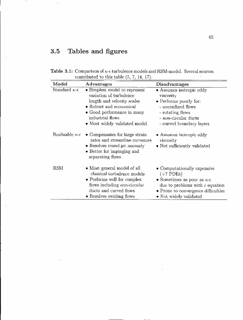
65
3.5 Tables and figures
Table 3.1: Comparison of n-t turbulence models and RSM-rnodel. Several sources contributed to this table (5, 7, 14, 17).
M o d e l Advan tages Disadvantages Standard n-e • Simplest model to represent • Assumes isotropic eddy
variation of turbulence viscosity length and velocity scales • Performs poorly for:
• Robust and economical - unconfined flows • Good performance in many - rotating flows
industrial flows - non-circular ducts • Most widely validated model - curved boundary layers
Realizable K-C • Compensates for large strain • Assumes isotropic eddy rates and streamline curvature viscosity
• Resolves round-jet anomaly • Not sufficiently validated • Better for impinging and
separating flows
R S M • Most general model of all • Computationally expensive classical turbulence models (+7 PDEs)
• Performs well for complex • Sometimes as poor as K-e flows including non-circular due to problems with e equation ducts and curved flows • Prone to convergence difficulties
• Resolves swirling flows • Not widely validated
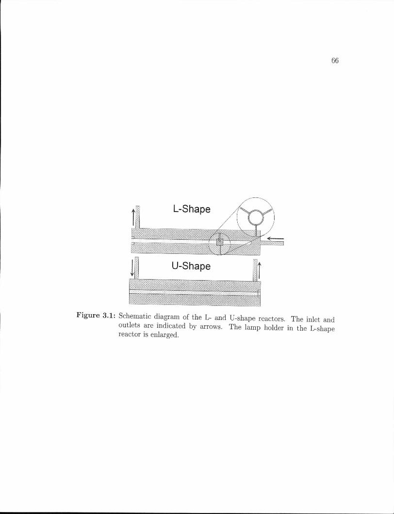
66
L-Shape
U-Shape
F i g u r e 3.1: Schematic diagram of the L- and U-shape reactors. The inlet and outlets are indicated by arrows. The lamp holder in the L-shape reactor is enlarged.
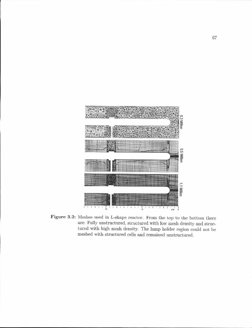
67
F i g u r e 3.2: Meshes used in L-shape reactor. From the top to the bottom there are: Fully unstructured, structured with low mesh density and structured with high mesh density. The lamp holder region could not be meshed with structured cells and remained unstructured.
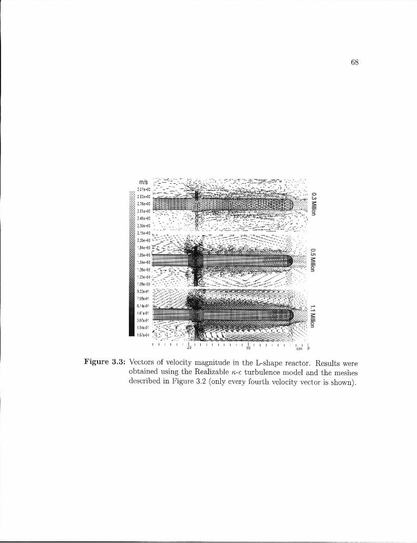
68
F i g u r e 3.3: Vectors of velocity magnitude in the L-shape reactor. Results were obtained using the Realizable n-e turbulence model and the meshes described in Figure 3.2 (only every fourth velocity vector is shown).
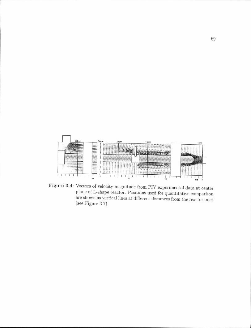
69
F i g u r e 3.4: Vectors of velocity magnitude from P I V experimental data at center plane of L-shape reactor. Positions used for quantitative comparison are shown as vertical lines at different distances from the reactor inlet (see Figure 3 . 7 ) .
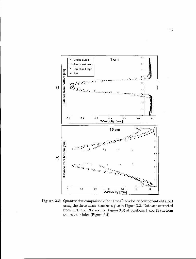
70
a)
E u •
E o c o .a E o k.
Q) O C
n
b
x Unstructured
Structured Low
° Structured High
• PIV
-1.4 -O.E
Z-Velocity [m/s] 0.1
b)
E u E o o
E o i_
« * -
0) o c (0 (0 b
15 cm
" it * *
K b " " ' " • •
X "V X . . ? , . « • • • •
-0.6 -0.4 -0.2
Z-Velocity [m/s]
Figure 3.5: Quantitative comparison of the (axial) z-velocity component obtained using the three mesh structures give in Figure 3.2. Data are extracted from C F D and P I V results (Figure 3.3) at positions 1 and 15 cm from the reactor inlet (Figure 3.4)
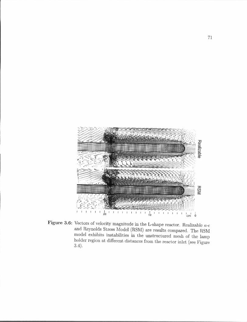
71
F i g u r e 3.6: Vectors of velocity magnitude in the L-shape reactor. Realizable K-e and Reynolds Stress Model (RSM) are results compared. The R S M model exhibits instabilities in the unstructured mesh of the lamp holder region at different distances from the reactor inlet (see Figure
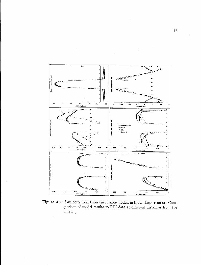
72
F i g u r e 3.7: Z-velocity from three turbulence models in the L-shape reactor. Comparison of model results to P I V data at different distances from the inlet.
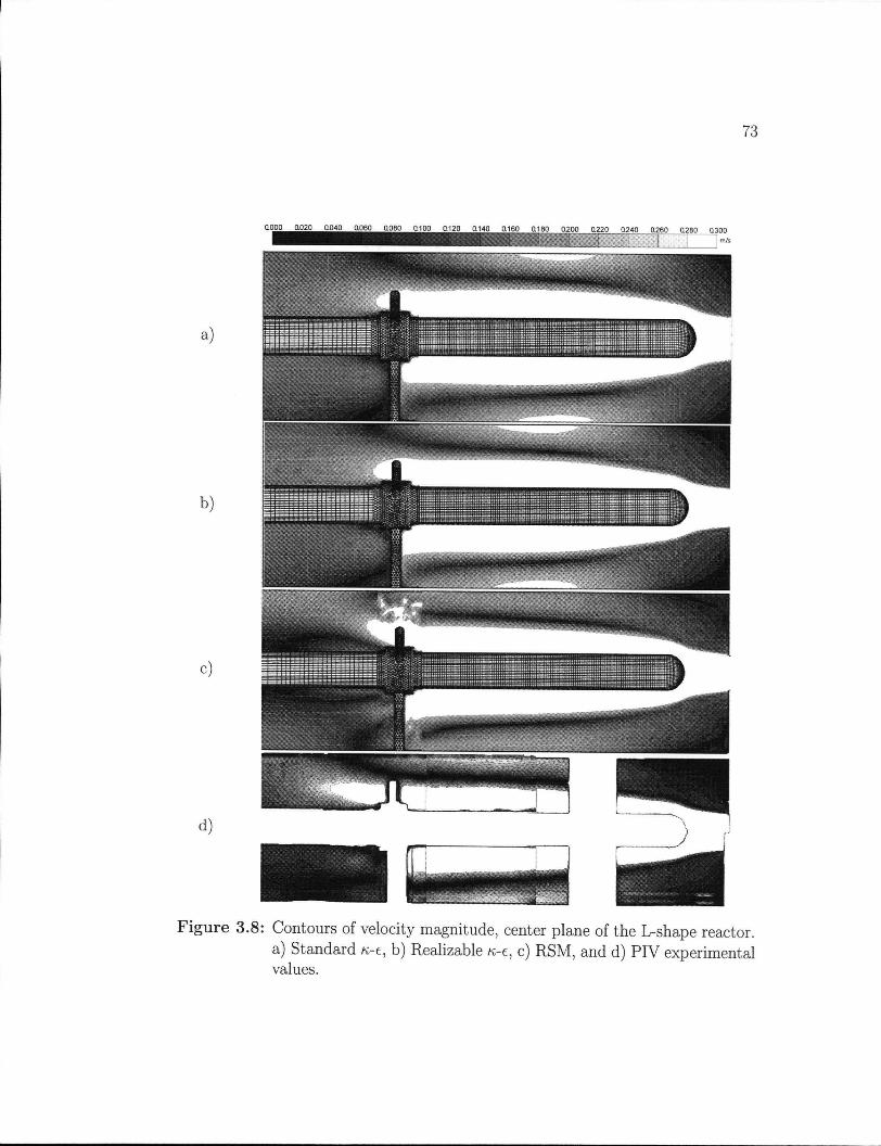
73
aooo 0.020 ao40 ao60 goao moo gi2o gi40 ai6o 018O 0200 a??o 0240 0260 Q280 a3O0 | | | [ | cn/i
a)
b)
c)
d)
F i g u r e 3.8: Contours of velocity magnitude, center plane of the L-shape reactor. a) Standard K-e, b) Realizable «-e, c) R S M , and d) P I V experimental values.
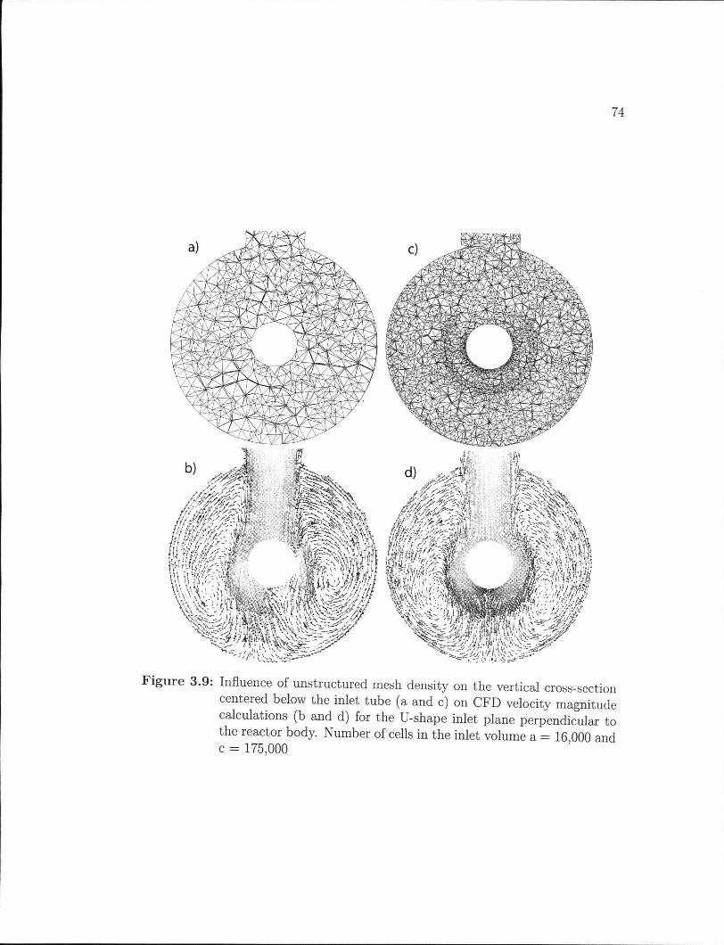
74
F i g u r e 3.9: Influence of unstructured mesh density on the vertical cross-section centered below the inlet tube (a and c) on C F D velocity magnitude calculations (b and d) for the U-shape inlet plane perpendicular to the reactor body. Number of cells in the inlet volume a = 16 000 and c = 175,000
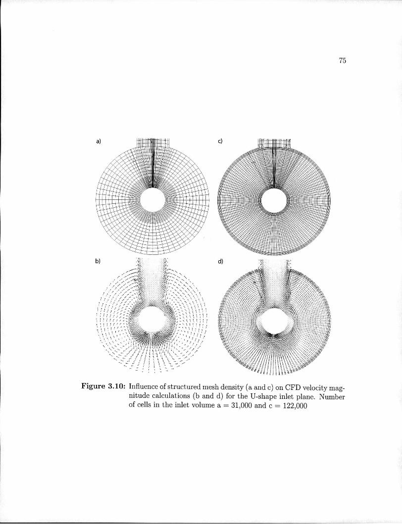
75
F i g u r e 3.10: Influence of structured mesh density (a and c) on C F D velocity magnitude calculations (b and d) for the U-shape inlet plane. Number of cells in the inlet volume a = 31,000 and c = 122,000
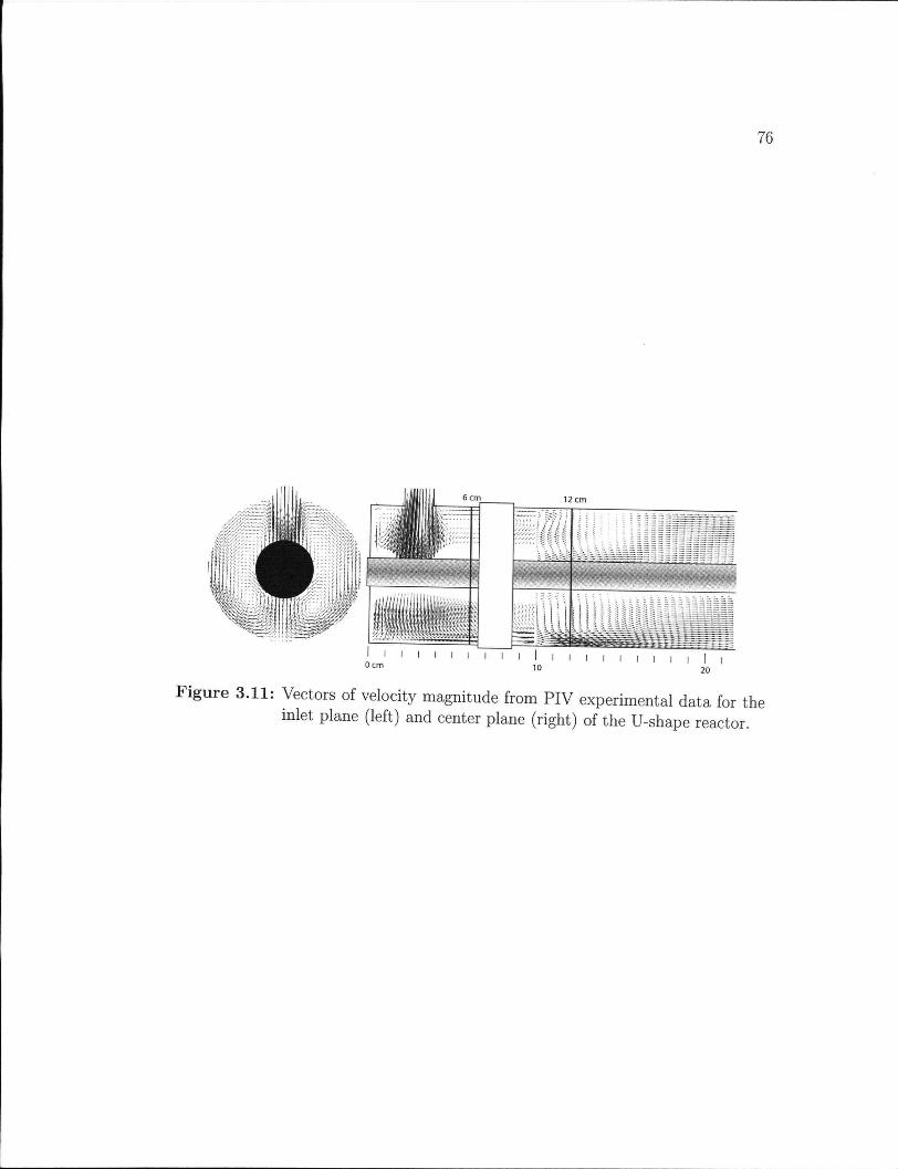
76
F i g u r e 3.11: Vectors of velocity magnitude from P I V experimental data for the inlet plane (left) and center plane (right) of the U-shape reactor.
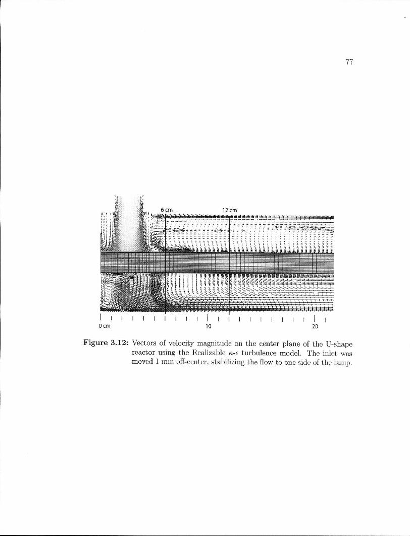
77
F i g u r e 3.12: Vectors of velocity magnitude on the center plane of the U-shape reactor using the Realizable n-e turbulence model. The inlet was moved 1 mm off-center, stabilizing the flow to one side of the lamp.
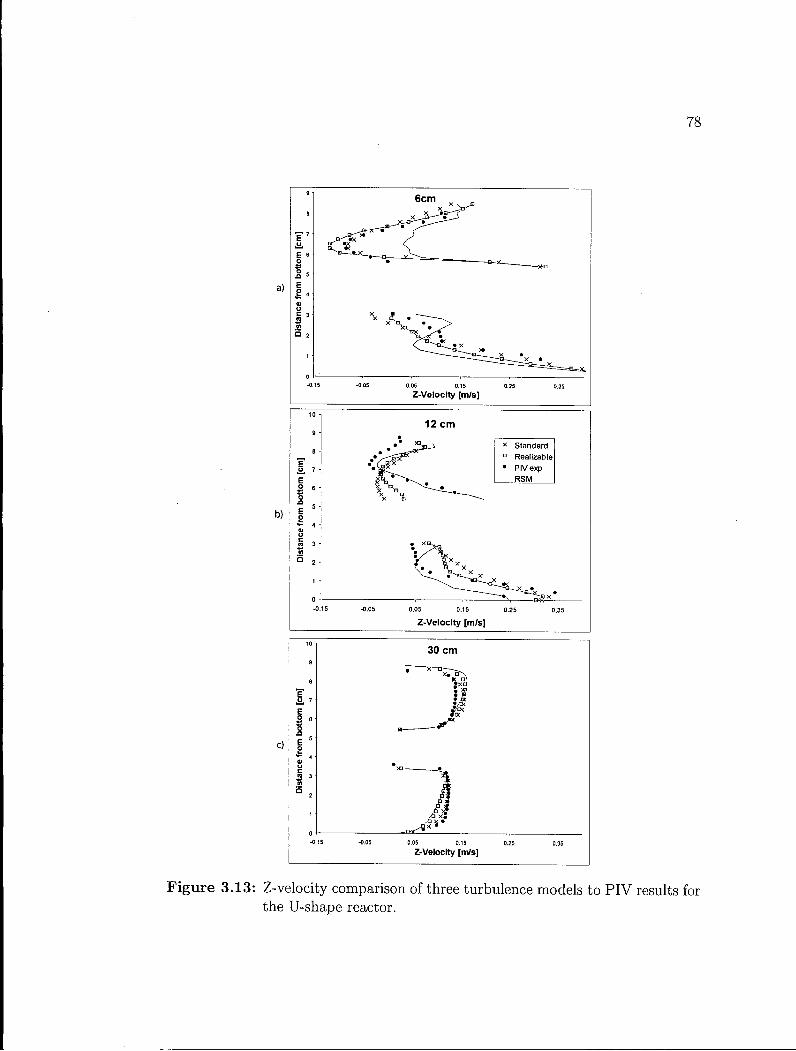
78
F i g u r e 3.13: Z-velocity comparison of three turbulence models to P I V results for the U-shape reactor.
79
Bib l iography
[1] B A R K E R , A . , H A I D A R I , A . H . , A N D M A R S H A L L , E . M . Design reactors via
cfd. CEP Magazine December ( 2001) , 3 0 - 3 9 .
[2] C A S S A N O , A . E . , M A R T I N , C . A . , B R A N D I , R . J . , A N D A L F A N O , O . M .
Photoreactor analysis and design: Fundamentals and applications. Industrial
& Engineering Chemistry Research 34 ( 1 9 9 5 ) , 2 1 5 5 - 2 0 1 .
[3] D O U G L A S , R . W . , C A R E Y , G . F . , W H I T E , D . R . , H A N S E N , G . A . ,
K A L L I N D E R I S , Y . , A N D W E A T H E R H I L , N . P . Current views on grid
generation: Summaries of a panel discussion. Numerical Heat Transfer
B:Fundamentals ( 2 0 0 2 ) .
[4] E S C U D I E R , M . P . , A N D S M I T H , S. Turbulent flow of newtonian and shear-
thinning liquids through a sudden axisymmetric expansion. Experiments in
Fluids 27 ( 1 9 9 9 ) , 4 2 7 - 4 3 4 .
[5] F L U E N T . Fluent user guide: Chapter 10. Modeling turbulence. Fluent, 2 0 0 3 .
[6] H u , H . , K O B A Y A S H I , T . , S A G A , T . , S E G A W A , S., A N D T A N I G U C H I , N .
Particle image velocimetry planar laser-induced fluoroscence measurements
on lobed jet mixing flows. Experiments in Fluids Suppl ( 2 0 0 0 ) , 1 4 1 - 1 5 7 .
[7] J A W , S. Y . , A N D C H E N , C . J . Present status of second order closure tur
bulence models, hoverview. Journal of Enineering Mechanics May ( 1998) ,
4 8 5 - 5 0 1 .
[8] J . O . H l N Z E . Turbulence. McGraw-Hi l l Publishing, 1975 .
[9] K A M I M U R A , M . , F U R U K A W A , S., A N D H I R O T S U J I , J . Development of a
simulator for ozone/uv reactor based on cfd analysis. Water science and
technology : a journal of the International Association on Water Pollution
Research 46 ( 2 0 0 2 ) , 1 3 - 1 9 .
[10] M E Y E R S , K . J . , W A R D , R . W . , A N D B A R K E R , A . A digital particle im
age velocimetry investigation of flow field instabilities of axial flow impellers.
Journal of Fluids Engineering 119 ( 1997) , 6 2 3 - 6 3 1 .
80
[11] P A R E E K , V . K . , Cox, S . J . , B R U N G S , M . P . , Y O U N G , B . , A N D A D E S I N A ,
A . A . Computational fluid dynamic (cfd) simulation of a pilot-scale annular
bunbble column photocatalytic reactor. Chemical Engineering Science 58
(2003), 859-865.
[12] P I R N I E , M . , L I N D E N , K . G . , A N D J A M E S P . M A L L E Y , J . Ultraviolet
disinfection guidance manual, draft epa 815-d-03-007. USEPA (2003).
[13] P R U V O S T , J . , L E G R A N D , J . , L E G E N T I L H O M M E , P . , A N D D O U B L I E Z , L .
Particle image velocimetry investigation of the flow-field of a 3d turbulent
annular swirling decaying flow induced by means of a tangential inlet. Exper
iments in Fluids 29 (2000), 291-301.
[14] R A N A D E , V . V . Computational flow modeling for chemical reaction engi
neering. Academic Press, 2002.
[15] R A N A D E , V . V . , P E R R A R D , M . , S A U Z E , N . L . , X U E R E B , C , A N D
B E R T R A N D , J . Trailing vortices of rushton turbines: P i v measurements and
cfd simulations with snapshot approach. Transactions in Chemical Engineer
ing 79A (2001), 3-12.
[16] R E S E A R C H , M . The us market for ultraviolet water treatment equipment.
MarketReaserach.com 2000 (1999), 2-5. MarketLooks.
[17] R O D I , W . Turbulence models and their application in hydraulics. I A H R , 1979.
[18] R O M E R O , R . L . , A L F A N O , O . M . , M A R C H E T T I , J . L . , A N D C A S S A N O ,
A . E . Modeling and parametric sensitivity of an annular photoreactor with
complex kinetics. Chemical Engineering Science 38 (1983), 1593-1605.
[19] S C H O E N E N , D . , K O L C H , A . , A N D G E B E L , J . Influence of geometrical pa
rameters in different irradiation vessels on uv disinfection rate. International
Journal of Hygiene and Environmental Medicine 194, 3 (1993), 313-320.
[20] U N L U T U R K , S . K . , H . A R A S T O O P O U R , A N D K O U T C H M A , T . Modeling of
uv dose distribution in a thin-film uv reactor for processingof apple cider.
Journal of Food Engineering 65, 1 (November 2004), 125-136.
81
[21] W R I G H T , N . G . , A N D H A R G R A V E S , D . M . The use of cfd in the evaluation
of uv treatment systems. Journal of Hydroinformatics ( 2 0 0 1 ) .
Chapter
Integrated UV reactor model
development
In this chapter, further development of the verified computational fluid dynamics
(CFD) model for the simulation of U V reactor performance is described. The
integration of UV-radiation models into Fluent is described in the first part. In
the second part, the integration of reaction kinetics into the C F D model is specified
and the integrated model is evaluated against the experimental results.
4.1 Introduct ion
Alternative water treatment methods have gained popularity, due to increasingly
stringent environmental regulations and concerns regarding chemical treatment
methods. UV-based technologies, especially, have seen a rapid growth over the last
decade (13). The use of UV-radiation for disinfection relies on the inactivation of
microorganisms through changes in the pathogens D N A (i.e. formation of thymine
dimers), rendering them unable to reproduce. U V application for advanced oxida
tion processes (AOPs) involves exciting a strong oxidant such as H2O2 or O3 to
generate highly reactive hydroxyl radicals to oxidize (toxic) organic substrates. In
both applications, the local rate of reaction is linked to the non-uniform radiation
distribution (UV-fluence rate). Reactor performance is thus strongly dependent
on hydrodynamic transport processes, influencing the spatial distribution of the
microorganisms or toxic substrates. The influence of the flow field and reactor
82
83
geometry on the performance of disinfection systems has been demonstrated by
Schoenen et al. (15) and Chiu et al. (4), while the effect of interactions between
reactor hydrodynamics and local radiation fluence on contaminants in A O P s was
shown by Pareek et al. (12).
In a UV-reactor, the fluid behavior defines the spatial concentration distribu
tion and flow of chemical agents or microorganisms through the reactor volume.
UV-lamp(s) supply the radiation driving the main reaction with fluence rate at
tenuated by distance and transmittance of the media. Finally, the reaction rate
is determined by the local UV-fluence rate, concentration of the species, and the
kinetic rate constants. Modeling photo-reactors therefore involves three submodels
for hydrodynamics, radiation fluence rate distribution, and UV-reaction kinetics
that are coupled by the material and energy balances.
The use of advanced numerical simulation tools, in particular computational
fluid dynamics ( C F D ) , to model the flow and transport in chemical engineering
processes has attracted much attention in recent years, e.g. (1, 12, 17). Integrated
C F D models have also been used to simulate photo-reactor performance, e.g. (4,
7, 9). A key advantage of simulating reactor performance by solving the governing
equations of the system is the virtual prototyping capability, allowing for a rapid
evaluation of design alternatives.
The objective of this work was to implement an integrated numerical model
using C F D coupled with a UV-radiation model and (volumetric) reaction rates to
evaluate UV-disinfection reactors. A commercial C F D code, Fluent 6.2, provided
the necessary code extensions to implement and execute the described submodels.
Annular UV-reactors with a concentric lamp parallel to the reactor axis, repre
senting a widely used design for UV-reactors, were investigated. Both, continuum
(Eulerian) and dispersed phase (Lagrangian) approaches to disinfection modeling
were implemented, combining a spatial UV-fluence rate model with first order ki
netics for disinfection. The effect of UV-radiation models on reactor performance
was studied by considering infinite line source and finite line source models. The
numerical disinfection efficiency (log reduction) for two reactor geometries, inlet
normal to the reactor axis (U-shape) and inlet parallel to the reactor axis (L-
shape), were compared for several flow rates. The log reduction for a commercially
available annular UV-reactor was then simulated based on the technical data and
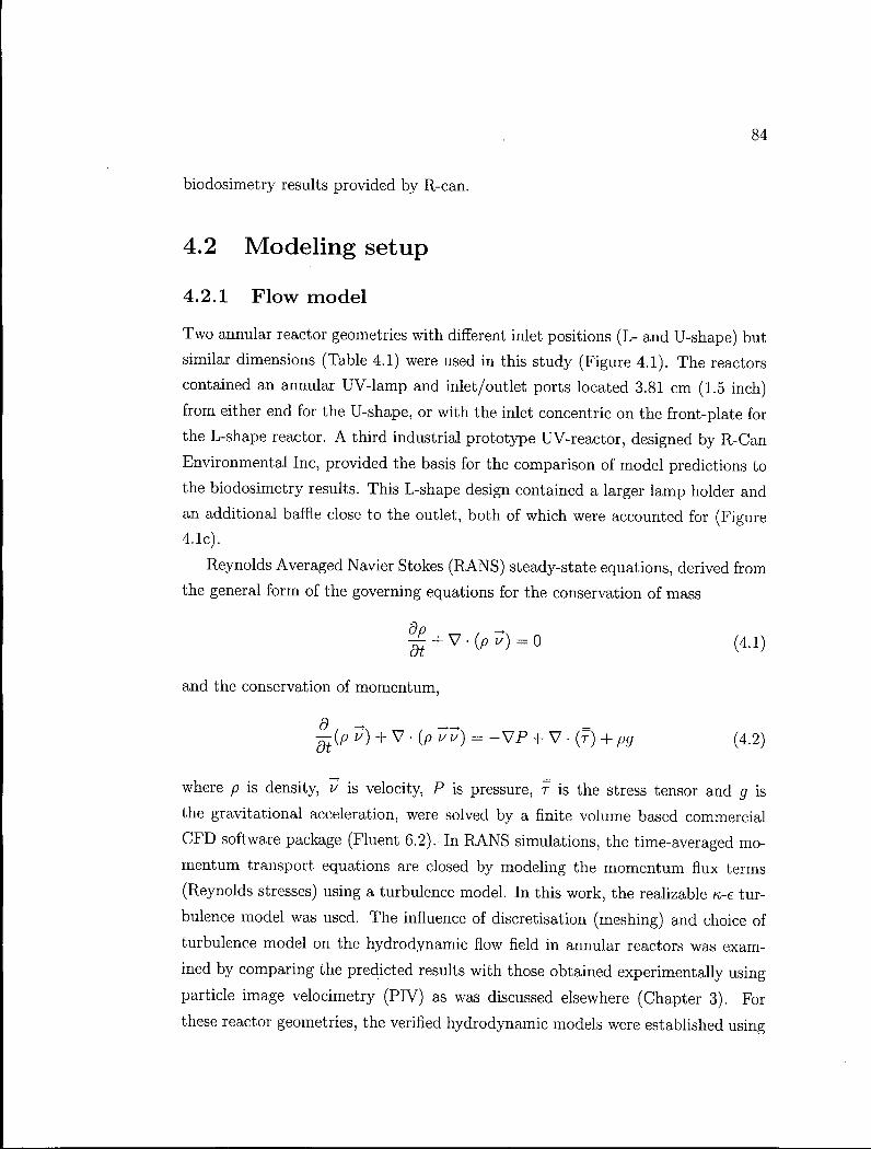
84
biodosimetry results provided by R-can.
4.2 Modeling setup
4.2.1 Flow model
Two annular reactor geometries with different inlet positions (L- and U-shape) but
similar dimensions (Table 4.1) were used in this study (Figure 4.1). The reactors
contained an annular UV-lamp and inlet/outlet ports located 3.81 cm (1.5 inch)
from either end for the U-shape, or with the inlet concentric on the front-plate for
the L-shape reactor. A third industrial prototype UV-reactor, designed by R-Can
Environmental Inc, provided the basis for the comparison of model predictions to
the biodosimetry results. This L-shape design contained a larger lamp holder and
an additional baffle close to the outlet, both of which were accounted for (Figure
4.1c).
Reynolds Averaged Navier Stokes (RANS) steady-state equations, derived from
the general form of the governing equations for the conservation of mass
^ + V - ( p ^ = 0 (4.1)
and the conservation of momentum,
— {Pv) + V-{pVv) = -VP + V-(7) + pg (4.2)
where p is density, u is velocity, P is pressure, T is the stress tensor and g is
the gravitational acceleration, were solved by a finite volume based commercial
C F D software package (Fluent 6.2). In R A N S simulations, the time-averaged mo
mentum transport equations are closed by modeling the momentum flux terms
(Reynolds stresses) using a turbulence model. In this work, the realizable «-e tur
bulence model was used. The influence of discretisation (meshing) and choice of
turbulence model on the hydrodynamic flow field in annular reactors was exam
ined by comparing the predicted results with those obtained experimentally using
particle image velocimetry (PIV) as was discussed elsewhere (Chapter 3). For
these reactor geometries, the verified hydrodynamic models were established using
85
a mix of structured and unstructured meshes (0.5-1 million cells). No-slip bound
ary conditions were set at the reactor walls and the UV-lamp. The inlet boundary
conditions were defined as a mass flow with the fluid properties of liquid water and
10% turbulent intensity over the diameter. A n inlet tube with an = 45 ensured
a fully developed flow entering the reactor. Numerical convergence was defined at
scaled residuals smaller than 1 x 10~ 5 for second order upwind solutions.
4.2.2 UV-fluence rate models
Assuming uniform optical properties of the fluid, the UV-fluence rate at any given
point can be described independent of the flow field, as a function of the distance
to the source, the optical transmissivity of the fluid, and the initial UV-output (2).
The assumption implies low concentrations of contaminants and little or no change
in the optical behavior of the reacting agent, which are appropriate for the case
of UV-disinfection. Monochromatic UV-fluence models of increasing complexity,
from one-dimensional radial to discrete ordinate (DO), have been proposed. L i u
et al. (8) showed that, in many situations, shadowing, reflection and refraction
effects have little influence on the final distribution. For the present study, two
UV-models describing the spatial distribution of fluence rate were implemented
in the reactor performance model to calculate the fluence rate at each point as a
function of its distance from the lamp and the UV-transmittance of the medium.
4.2.2.1 Infinite line source or radial model
This model assumes the lamp to be represented as a line source with radiation
emitted normal to the lamp axis. The fluence rate E, is related to the UV-lamp
radiant power per unit length and the radial distance, r [cm], from the lamp center
line (16). Simplified for an axisymmetric annular system, the local fluence rate,
E(r), is expressed as p
E(r) = ^exp{aw(r~rL)} (4.3)
where P is the total germicidal lamp output [mW], L is the axial lamp arc length
[cm], ri is the lamp sleeve radius [cm] and aw is the absorption coefficient of the
86
fluid [cm 1 ] . aw can be calculated from the transimissivity, T,by following equation
aw = ln{10)log(T) (4.4)
This model does not deal with refraction or reflection and cannot describe what
happens near the lamp ends, but is easy to implement and has been shown to
perform reasonably well for standard reactor sizes (8).
4.2.2.2 F i n i t e l i n e s o u r c e o r m u l t i p l e p o i n t s o u r c e s u m m a t i o n ( M P S S )
m o d e l
In this method the lamp is approximated as a series of point light sources emitting
radiation in all directions (2). The UV-fluence at each location in the domain is
estimated as the sum of energy received from each individual point source in the
system: -p r /.I
(4.5) i=l 1
-o-w(r - rL)-r
where z [cm] represents the axial distance and U the distance from the current
location [cm] to the point source number out of a total of n sources. Results
were found to be independent of the number of sources with n — 100 for the present
models. Fluence rate changes over the length of the lamp and diffuse radiation at
the lamp ends are predicted with this model, but it has been suggested that the
model overpredicts fluence rates close to the lamp surface (8).
4.2.3 Disinfection kinetics model
MS2 bacteriophage biodosimetry is the method of choice for log inactivation stud
ies of UV-disinfections systems and a standardized protocol is available from the
U S - E P A Environmental Technology Verification ( E T V ) program. MS2 is non
pathogenic to human, has a relatively high UV-resistance and, being a single
stranded R N A virus, its dose response for UV-inactivation can be described by
conventional first order Chick-Watson kinetics:
N = N0e~' (4.6)
87
where No represents the initial organism concentration (plaque forming units per
ml)[PFU/ml] and N the organism concentration after UV-exposure [PFU/ml] , k
is the inactivation rate constant [cm 2/mJ], E is the UV-fluence rate [mW/cm 2 ] ,
and t is the exposure time [s]. Dose (sometimes referred to as fluence) is defined as
the UV-fluence rate multiplied by the time, i.e. D = E x t [mJ/cm 2 ]. In general
usage, the SI units are exchanged for the equivalent but more manageable units
shown here (3).
Dose response curves are measured under tightly controlled conditions using
a collimated beam of U V to eliminate the influence of hydrodynamics and non
uniform fluence rates, and are recorded as the log inactivation (logjf-) per unit
dose. The rate constant k in Equation 4.6 can be obtained from the slope of y^^y
plotted against dose D. Each culture of MS2 macrophages has to be calibrated
separately, but an inactivation constant of k = 0.1 c m 2 / m J has been reported by
several sources (10, 11, 14).
4.2.4 Integrated reactor performance model
For disinfection reactions in continuous reactors, the path a microorganism takes
is key to the amount of UV-radiation (dose) it absorbs. The position of microor
ganisms in the reactor can be tracked in the Eulerian or Lagrangian reference
frames. In the Lagrangian framework, after obtaining the velocity field by solving
the transport equations, single organisms are treated as discrete particles where
the trajectory is predicted by integrating the force balance on the particle. Ran
dom effects of turbulence on the particle are accounted for by the Discrete Random
Walk (DRW), or "eddy lifetime" model, where the interaction of a particle with
a succession of discrete stylized fluid phase turbulent eddies is simulated (6). The
particle trajectories are computed based on a steady continuous-phase flow field.
A statistically significant number of particles (representing microorganisms) is re
leased at the reactor inlet (No) and the dose is integrated along the path of each
particle, multiplying the average local fluence rate (E) by the time step A t . For
each dose interval i, the number of remaining vital particles (microorganisms) iV,
is calculated by:
Ni = on x N0e-kDi (4.7)
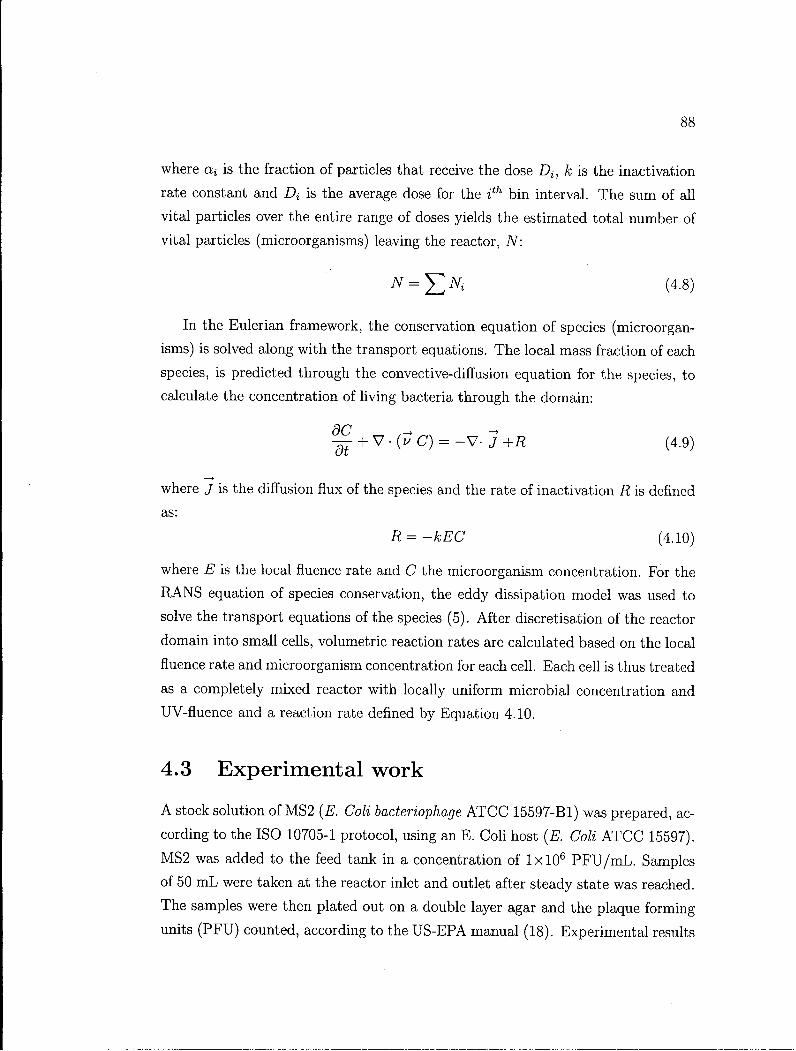
88
where ctj is the fraction of particles that receive the dose D j , k is the inactivation
rate constant and Di is the average dose for the ith bin interval. The sum of all
vital particles over the entire range of doses yields the estimated total number of
vital particles (microorganisms) leaving the reactor, TV:
N = y £ / N i (4.8)
In the Eulerian framework, the conservation equation of species (microorgan
isms) is solved along with the transport equations. The local mass fraction of each
species, is predicted through the convective-diffusion equation for the species, to
calculate the concentration of living bacteria through the domain:
— + V - ( i / C ) = - V - J+R (4.9)
where J is the diffusion flux of the species and the rate of inactivation R is defined
as:
R = -kEC (4.10)
where E is the local fluence rate and C the microorganism concentration. For the
R A N S equation of species conservation, the eddy dissipation model was used to
solve the transport equations of the species (5). After discretisation of the reactor
domain into small cells, volumetric reaction rates are calculated based on the local
fluence rate and microorganism concentration for each cell. Each cell is thus treated
as a completely mixed reactor with locally uniform microbial concentration and
UV-fluence and a reaction rate defined by Equation 4.10.
4.3 E x p e r i m e n t a l work
A stock solution of MS2 (E. Coli bacteriophage A T C C 15597-B1) was prepared, ac
cording to the ISO 10705-1 protocol, using an E . Col i host (E. Coli A T C C 15597).
MS2 was added to the feed tank in a concentration of l x l O 6 P F U / m L . Samples
of 50 m L were taken at the reactor inlet and outlet after steady state was reached.
The samples were then plated out on a double layer agar and the plaque forming
units (PFU) counted, according to the U S - E P A manual (18). Experimental results
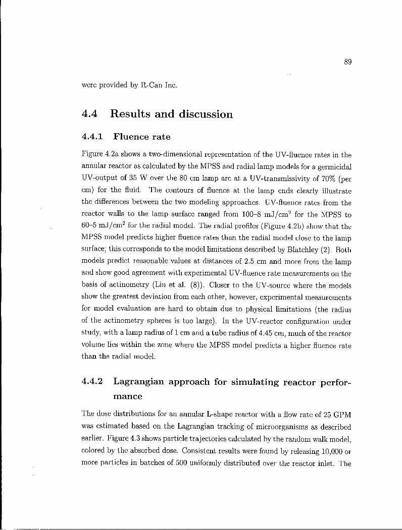
89
were provided by R-Can Inc.
4.4 Results and discussion
4.4.1 Fluence rate
Figure 4.2a shows a two-dimensional representation of the UV-fluence rates in the
annular reactor as calculated by the M P S S and radial lamp models for a germicidal
UV-output of 35 W over the 80 cm lamp arc at a UV-transmissivity of 70% (per
cm) for the fluid. The contours of fluence at the lamp ends clearly illustrate
the differences between the two modeling approaches. UV-fluence rates from the
reactor walls to the lamp surface ranged from 100-8 m J / c m 2 for the M P S S to
60-5 m J / c m 2 for the radial model. The radial profiles (Figure 4.2b) show that the
M P S S model predicts higher fluence rates than the radial model close to the lamp
surface; this corresponds to the model limitations described by Blatchley (2). Both
models predict reasonable values at distances of 2.5 cm and more from the lamp
and show good agreement with experimental UV-fluence rate measurements on the
basis of actinometry (Liu et al. (8)). Closer to the UV-source where the models
show the greatest deviation from each other, however, experimental measurements
for model evaluation are hard to obtain due to physical limitations (the radius
of the actinometry spheres is too large). In the UV-reactor configuration under
study, with a lamp radius of 1 cm and a tube radius of 4.45 cm, much of the reactor
volume lies within the zone where the M P S S model predicts a higher fluence rate
than the radial model.
4.4.2 Lagrangian approach for simulating reactor perfor
mance
The dose distributions for an annular L-shape reactor with a flow rate of 25 G P M
was estimated based on the Lagrangian tracking of microorganisms as described
earlier. Figure 4.3 shows particle trajectories calculated by the random walk model,
colored by the absorbed dose. Consistent results were found by releasing 10,000 or
more particles in batches of 500 uniformly distributed over the reactor inlet. The
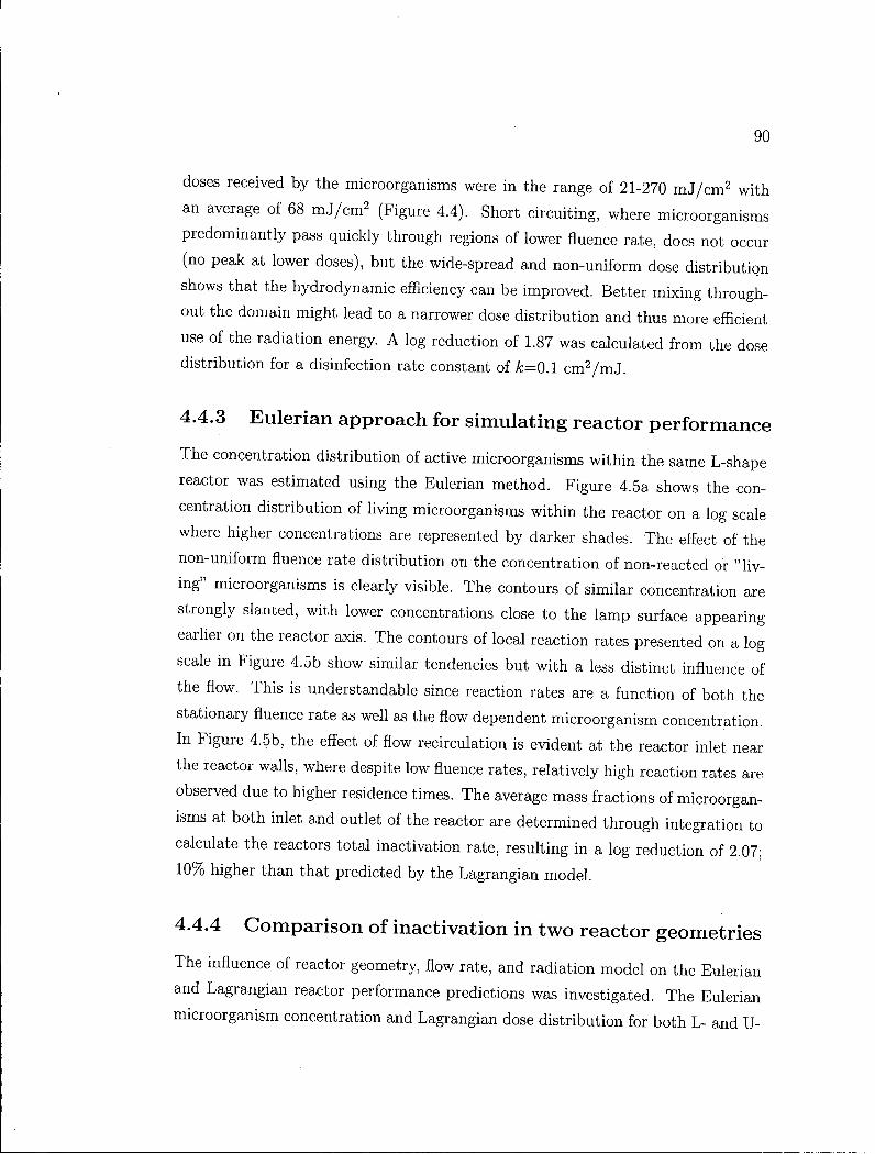
90
doses received by the microorganisms were in the range of 21-270 m J / c m 2 with
an average of 68 m J / c m 2 (Figure 4.4). Short circuiting, where microorganisms
predominantly pass quickly through regions of lower fluence rate, does not occur
(no peak at lower doses), but the wide-spread and non-uniform dose distribution
shows that the hydrodynamic efficiency can be improved. Better mixing through
out the domain might lead to a narrower dose distribution and thus more efficient
use of the radiation energy. A log reduction of 1.87 was calculated from the dose
distribution for a disinfection rate constant of A;=0.1 c m 2 / m J .
4.4.3 Eulerian approach for simulating reactor performance
The concentration distribution of active microorganisms within the same L-shape
reactor was estimated using the Eulerian method. Figure 4.5a shows the con
centration distribution of living microorganisms within the reactor on a log scale
where higher concentrations are represented by darker shades. The effect of the
non-uniform fluence rate distribution on the concentration of non-reacted or " l iv
ing" microorganisms is clearly visible. The contours of similar concentration are
strongly slanted, with lower concentrations close to the lamp surface appearing
earlier on the reactor axis. The contours of local reaction rates presented on a log
scale in Figure 4.5b show similar tendencies but with a less distinct influence of
the flow. This is understandable since reaction rates are a function of both the
stationary fluence rate as well as the flow dependent microorganism concentration.
In Figure 4.5b, the effect of flow recirculation is evident at the reactor inlet near
the reactor walls, where despite low fluence rates, relatively high reaction rates are
observed due to higher residence times. The average mass fractions of microorgan
isms at both inlet and outlet of the reactor are determined through integration to
calculate the reactors total inactivation rate, resulting in a log reduction of 2.07;
10% higher than that predicted by the Lagrangian model.
4.4.4 Comparison of inactivation in two reactor geometries
The influence of reactor geometry, flow rate, and radiation model on the Eulerian
and Lagrangian reactor performance predictions was investigated. The Eulerian
microorganism concentration and Lagrangian dose distribution for both L - and U -
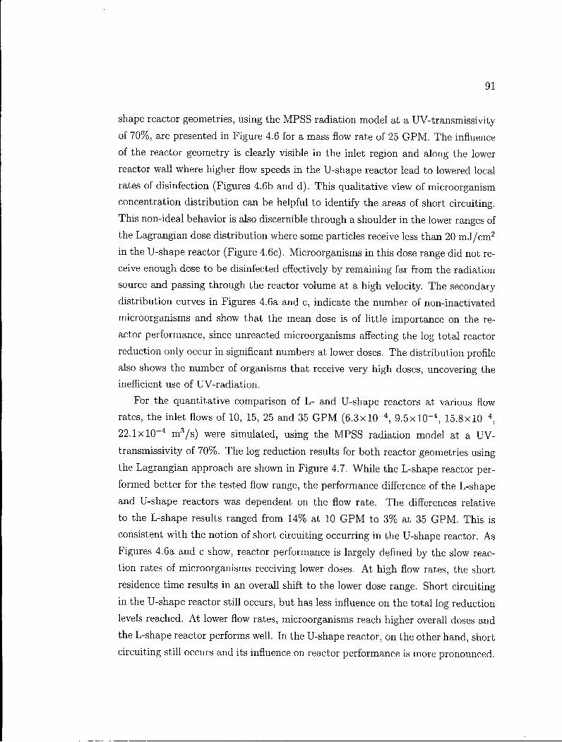
91
shape reactor geometries, using the M P S S radiation model at a UV-transmissivity
of 70%, are presented in Figure 4.6 for a mass flow rate of 25 G P M . The influence
of the reactor geometry is clearly visible in the inlet region and along the lower
reactor wall where higher flow speeds in the U-shape reactor lead to lowered local
rates of disinfection (Figures 4.6b and d). This qualitative view of microorganism
concentration distribution can be helpful to identify the areas of short circuiting.
This non-ideal behavior is also discernible through a shoulder in the lower ranges of
the Lagrangian dose distribution where some particles receive less than 20 m J / c m 2
in the U-shape reactor (Figure 4.6c). Microorganisms in this dose range did not re
ceive enough dose to be disinfected effectively by remaining far from the radiation
source and passing through the reactor volume at a high velocity. The secondary
distribution curves in Figures 4.6a and c, indicate the number of non-inactivated
microorganisms and show that the mean dose is of little importance on the re
actor performance, since unreacted microorganisms affecting the log total reactor
reduction only occur in significant numbers at lower doses. The distribution profile
also shows the number of organisms that receive very high doses, uncovering the
inefficient use of UV-radiation.
For the quantitative comparison of L - and U-shape reactors at various flow
rates, the inlet flows of 10, 15, 25 and 35 G P M (6.3 x l O " 4 , 9.5 x l O ' 4 , 15 .8x lO" 4 ,
22 .1x l0~ 4 m 3 / s ) were simulated, using the M P S S radiation model at a U V -
transmissivity of 70%. The log reduction results for both reactor geometries using
the Lagrangian approach are shown in Figure 4.7. While the L-shape reactor per
formed better for the tested flow range, the performance difference of the L-shape
and U-shape reactors was dependent on the flow rate. The differences relative
to the L-shape results ranged from 14% at 10 G P M to 3% at 35 G P M . This is
consistent with the notion of short circuiting occurring in the U-shape reactor. As
Figures 4.6a and c show, reactor performance is largely defined by the slow reac
tion rates of microorganisms receiving lower doses. A t high flow rates, the short
residence time results in an overall shift to the lower dose range. Short circuiting
in the U-shape reactor still occurs, but has less influence on the total log reduction
levels reached. A t lower flow rates, microorganisms reach higher overall doses and
the L-shape reactor performs well. In the U-shape reactor, on the other hand, short
circuiting still occurs and its influence on reactor performance is more pronounced.
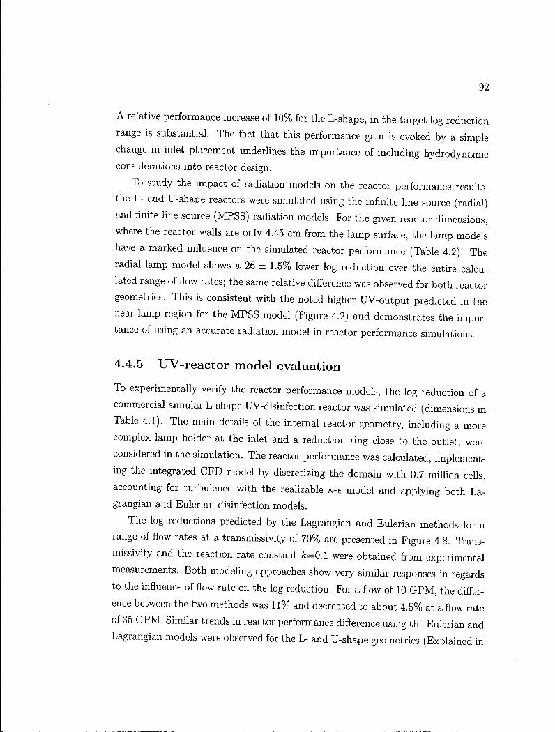
92
A relative performance increase of 10% for the L-shape, in the target log reduction
range is substantial. The fact that this performance gain is evoked by a simple
change in inlet placement underlines the importance of including hydrodynamic
considerations into reactor design.
To study the impact of radiation models on the reactor performance results,
the L - and U-shape reactors were simulated using the infinite line source (radial)
and finite line source (MPSS) radiation models. For the given reactor dimensions,
where the reactor walls are only 4.45 cm from the lamp surface, the lamp models
have a marked influence on the simulated reactor performance (Table 4.2). The
radial lamp model shows a 26 ± 1.5% lower log reduction over the entire calcu
lated range of flow rates; the same relative difference was observed for both reactor
geometries. This is consistent with the noted higher UV-output predicted in the
near lamp region for the M P S S model (Figure 4.2) and demonstrates the impor
tance of using an accurate radiation model in reactor performance simulations.
4.4.5 UV-reactor model evaluation
To experimentally verify the reactor performance models, the log reduction of a
commercial annular L-shape UV-disinfection reactor was simulated (dimensions in
Table 4.1). The main details of the internal reactor geometry, including a more
complex lamp holder at the inlet and a reduction ring close to the outlet, were
considered in the simulation. The reactor performance was calculated, implement
ing the integrated C F D model by discretizing the domain with 0.7 million cells,
accounting for turbulence with the realizable n-e model and applying both La
grangian and Eulerian disinfection models.
The log reductions predicted by the Lagrangian and Eulerian methods for a
range of flow rates at a transmissivity of 70% are presented in Figure 4.8. Trans-
rnissivity and the reaction rate constant k=0.1 were obtained from experimental
measurements. Both modeling approaches show very similar responses in regards
to the influence of flow rate on the log reduction. For a flow of 10 G P M , the differ
ence between the two methods was 11% and decreased to about 4.5% at a flow rate
of 35 G P M . Similar trends in reactor performance difference using the Eulerian and
Lagrangian models were observed for the L - and U-shape geometries (Explained in
93
section 4.4.4). The deviation between the Eulerian and Lagrangian methods has
not been examined in depth, but possible causes are the different approaches taken
by the two models, the numerical errors from the choice of the finite-rate reaction
model (eddy-dissipation model used), and the inclusion of turbulent diffusion in
the Eulerian model, that does not occur in the Lagrangian model. Both modeling
results show a good agreement with the biodosimetry measurements performed for
this reactor. Like most biological assays, biodosimetry has a considerable variance
and not enough experimental values were available for a detailed comparison of the
modeling approaches. However, the results indicate the possibility of modeling a
UV-reactors performance to a close degree, knowing the geometrical specifications
and operating conditions using either Lagrangian or Eulerian approaches.
4.5 Conclus ions
Disinfection models based on the Lagrangian and Eulerian methods were suc
cessfully implemented in a commercial C F D code and provided results in good
agreement with the experimental data over a range of flow rates. Though the
Lagrangian and Eulerian methods could be used interchangeably, the final log re
duction results deviated between 4-11 percent for the tested range of flow rates.
Both models can be used to gain complimentary information on the same reactor;
while the Lagrangian method provides estimates of the UV-dose distribution and
the particle tracks visualize flows patterns, the Eulerian approach shows the con
centration distribution and local reaction rates. The combined information can be
used to predict and monitor reactor performance levels and to enhance the reac
tor designs. A t a higher computational cost, the Eulerian model delivers a more
conclusive image of the local disinfection rates within the reactor volume. More im
portantly, this model can be extended to UV-based Advanced Oxidation Processes,
which involve additional volumetric reactions, by including further reaction steps.
The model parameters have a significant impact on the final simulation results.
In this study, the selection of finite line source or infinite line source radiation
model was found to influence the reactor performance results by about 26 %.
While costly and time consuming construction of intermediate prototypes can be
reduced through the use of UV-reactor simulations, complimentary experiments

94
remain necessary to verify reactor performance, for the final UV-reactor designs.
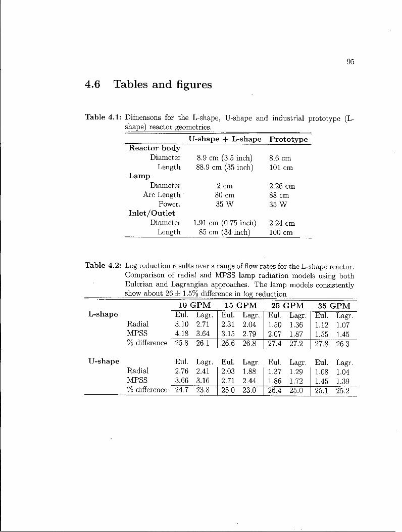
95
4.6 Tables and figures
T a b l e 4 .1: Dimensons for the L-shape, U-shape and industrial prototype (L-shape) reactor geometries.
U - s h a p e + L - s h a p e P r o t o t y p e R e a c t o r b o d y
Diameter 8.9 cm (3.5 inch) 8.6 cm Length 88.9 cm (35 inch) 101 cm
L a m p
Diameter 2 cm 2.26 cm Arc Length 80 cm 88 cm
Power. 35 W 35 W I n l e t / O u t l e t
Diameter 1.91 cm (0.75 inch) 2.24 cm Length 85 cm (34 inch) 100 cm
T a b l e 4.2: Log reduction results over a range of flow rates for the L-shape reactor. Comparison of radial and M P S S lamp radiation models using both Eulerian and Lagrangian approaches. The lamp models consistently show about 26 ± 1.5% difference in log reduction
10 G P M 15 G P M 25 G P M 35 G P M L - s h a p e Eu l . Lagr.
Radial 3.10 2.71 M P S S 4.18 3.64
Eul . Lagr. 2.31 2.04 3.15 2.79
Eu l . Lagr. 1.50 1.36 2.07 1.87
Eu l . Lagr. 1.12 1.07 1.55 1.45
% difference 25.8 26.1
U - s h a p e Eu l . Lagr. Radial 2.76 2.41 M P S S 3.66 3.16
26.6 26.8
Eul . Lagr. 2.03 1.88 2.71 2.44
27.4 27.2
Eu l . Lagr. 1.37 1.29 1.86 1.72
27.8 26.3
Eul . Lagr. 1.08 1.04 1.45 1.39
% difference 24.7 23.8 25.0 23.0 26.4 25.0 25.1 25.2
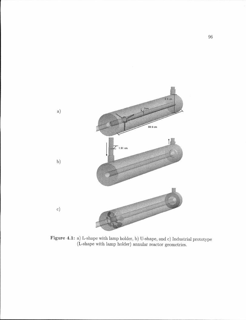
96
Figure 4.1: a) L-shape with lamp holder, b) U-shape, and c) Industrial prototype (L-shape with lamp holder) annular reactor geometries.
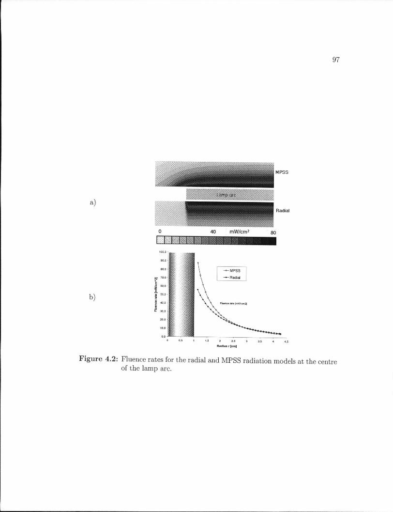
97
F i g u r e 4.2: Fluence rates for the radial and M P S S radiation models at the centre of the lamp arc.
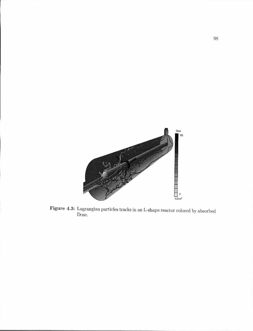
98
F i g u r e 4.3: Lagrangian particles tracks in an L-shape reactor colored by absorbed Dose.
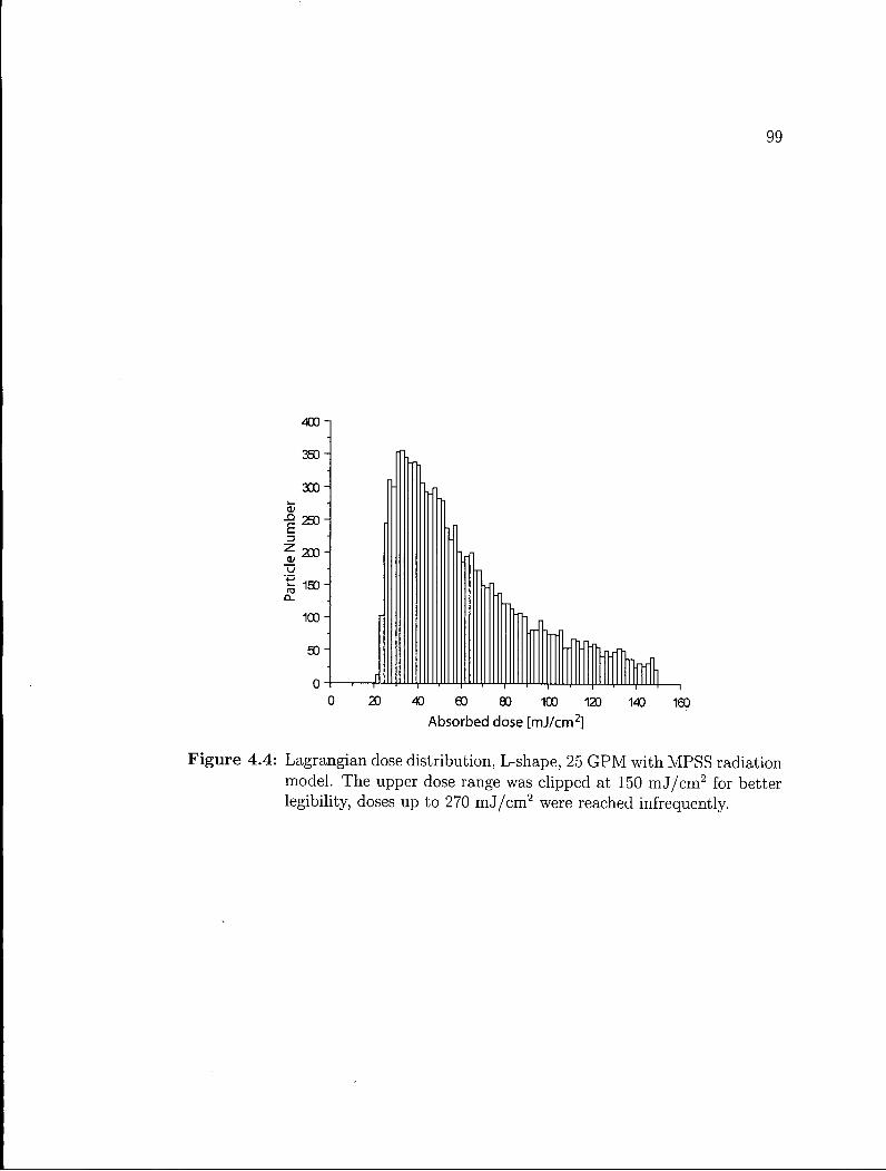
99
F i g u r e 4.4: Lagrangian dose distribution, L-shape, 25 G P M with M P S S radiation model. The upper dose range was clipped at 150 m J / c m 2 for better legibility, doses up to 270 m J / c m 2 were reached infrequently.
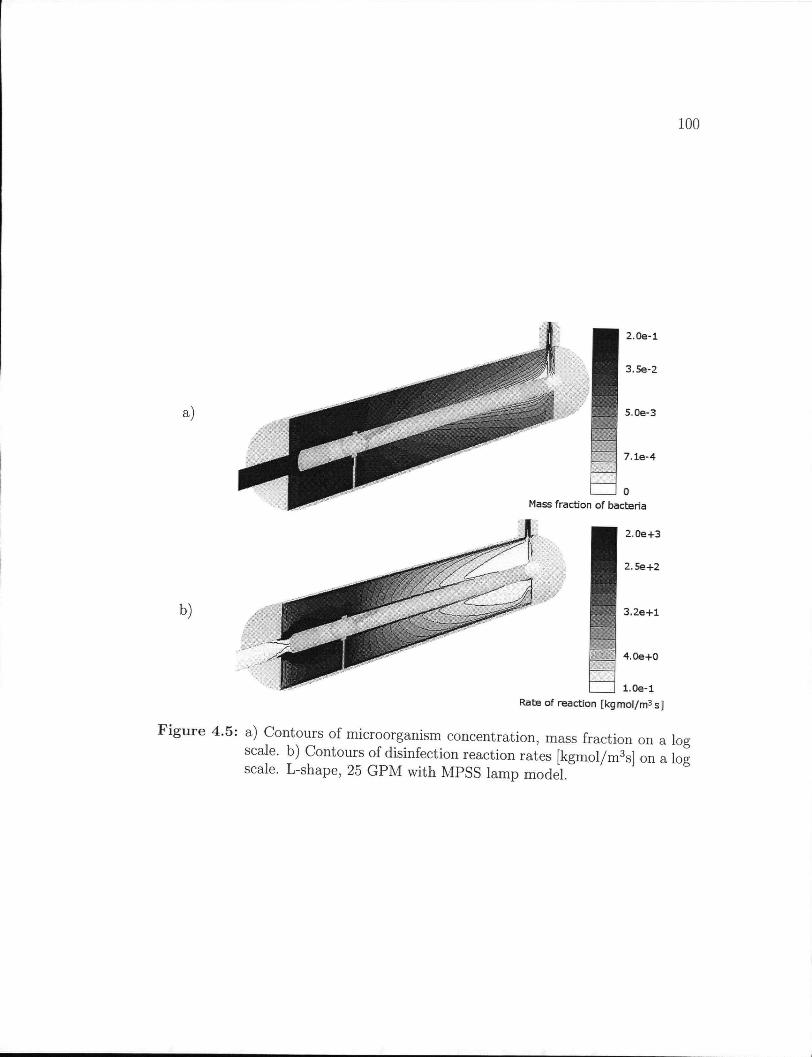
100
a)
2 . 0 e - l
3 . S e - 2
5 . 0 e - 3
7 . 1 e - 4
Mass fraction of bacteria
2 . 0 e + 3
2 . 5 e + 2
3 . 2 e + l
4 . 0 e + 0
1 . 0 e - l
R a t s o f r e a c t i o n [ k g m o l / m 3 s ]
F i g u r e 4.5: a) Contours of microorganism concentration, mass fraction on a log scale, b) Contours of disinfection reaction rates [kgmol/m 3s] on a log scale. L-shape, 25 G P M with M P S S lamp model.
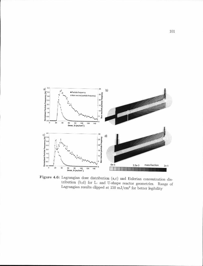
101
F i g u r e 4.6: Lagrangian dose distribution (a,c) and Eulerian concentration distribution (b,d) for L - and U-shape reactor geometries. Range of Lagrangian results clipped at 150 m J / c m 2 for better legibility
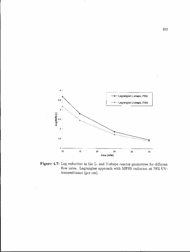
102
F i g u r e 4.7: Log reduction in the L- and U-shape reactor geometries for different flow rates. Lagrangian approach with M P S S radiation at 70% U V -transmittance (per cm).
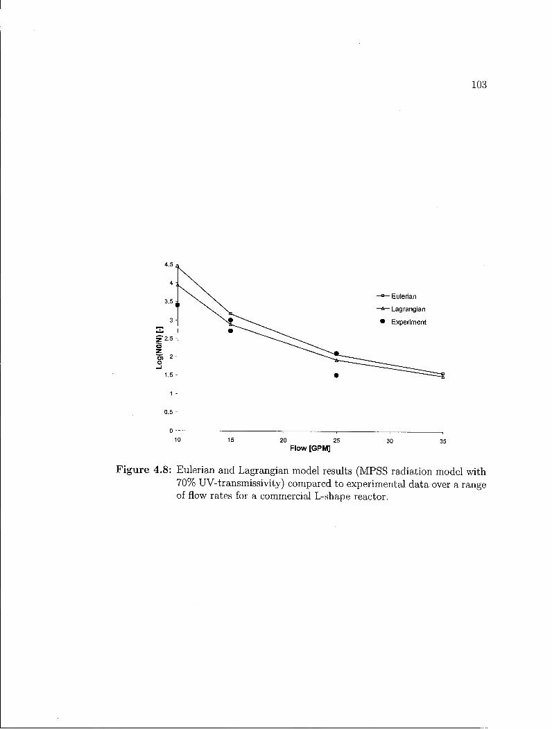
103
F i g u r e 4.8: Eulerian and Lagrangian model results (MPSS radiation model with 70% UV-transmissivity) compared to experimental data over a range of flow rates for a commercial L-shape reactor.
104
Bib l iography
[1] B A R K E R , A . , H A I D A R I , A . H . , A N D M A R S H A L L , E . M . Design reactors via
cfd. CEP Magazine December ( 2 0 0 1 ) , 3 0 - 3 9 .
[2] B L A T C H L E Y , E . R . Numerical modelling of uv intensity: Application to
collimated-beam reactors and continuous-flow systems. Water Research 31, 9
( 1 9 9 7 ) , 2 2 0 5 - 2 2 1 8 .
[3] B O L T O N , J . R . Calculation of ultraviolet fluence rate distributions in an
annular reactor: Significance of refraction and reflection. Water Research 34,
1 3 ( 2 0 0 0 ) , 3 3 1 5 - 3 3 2 4 .
[4] C H I U , K . , L Y N , D . A . , A N D B L A T C H L E Y , E . R . Integrated uv disinfec
tion model based on particle tracking. Journal of Environmental Engineering
(1999) , 7 - 1 6 .
[5] F L U E N T . Fluent user guide: Chapter 13. Modeling species transport and finite-
rate chemistry. Fluent.inc, 2004 .
[6] F L U E N T . Fluent user guide: Chapter 19. Discreete phase models. Fluent.inc, 2004 .
[7] K A M I M U R A , M . , F U R U K A W A , S., A N D H I R O T S U J I , J . Development of a
simulator for ozone/uv reactor based on cfd analysis. Water science and
technology : a journal of the International Association on Water Pollution
Research 46 ( 2 0 0 2 ) , 1 3 - 1 9 .
[8] L I U , D . , D U C O S T E , J . , J I N , S., A N D L I N D E N , K . Evaluation of alternative
fluence rate distribution models. Journal of Water Supply: Research and
Technology-AQUA 53.6 ( 2004) , 3 9 1 - 4 0 8 .
[9] L Y N , D . A . , C H I U , K . , A N D B L A T C H L E Y , E . R . , I. Numerical modeling of
flow and disinfection in uv disinfection channels. Journal of Environmental
Engineering (Reston, Virginia) 125 ( 1 9 9 9 ) , 1 7 - 2 6 .
105
[10] M O F I D I , A . A . , C O F F E Y , B . M . , G R E E N , J . F . , A N D C H O U , C . I. In
vestigation of ultraviolet light disinfection. Tech. rep., Metropolitan Water
District of Southern California, 2002.
[11] M U L K E Y , L . A . Etv joint verification statement, uv disinfection of sec
ondary effluent system by suntec inc. Tech. rep., US-Environmental Protec
tion Agency, Envronmental Technology Verifcation Programm, 2003.
[12] P A R E E K , V . K . , Cox, S. J . , B R U N G S , M . P . , Y O U N G , B . , A N D A D E S I N A ,
A . A . Computational fluid dynamic (cfd) simulation of a pilot-scale annular
bunbble column photocatalytic reactor. Chemical Engineering Science 58
(2003), 859-865.
[13] P I R N I E , M . , L I N D E N , K . G . , A N D J A M E S P . M A L L E Y , J . Ultraviolet
disinfection guidance manual, draft epa 815-d-03-007. USEPA (2003).
[14] S C H E I B L E , O . K . , A N D M C G R A T H , J . A . Generic verification protocol for
high-rate, wet-weather flow disinfection applications. Tech. rep., US Environ
mental Protection Agency, 2000.
[15] S C H O E N E N , D . , K O L C H , A . , A N D G E B E L , J . Influence of geometrical pa
rameters in different irradiation vessels on uv disinfection rate. International
Journal of Hygiene and Environmental Medicine 194, 3 (1993), 313-320.
[16] T A G H I P O U R , F . Ultraviolet and ionizing radiation for microorganism inacti
vation. Water Research 38, 18 (2004), 3940-3948.
[17] U N L U T U R K , S. K . , H . A R A S T O O P O U R , A N D K O U T C H M A , T . Modeling of
uv dose distribution in a thin-film uv reactor for processingof apple cider.
Journal of Food Engineering 65, 1 (November 2004), 125-136.
[18] U S - E P A . USEPA Manual of methods for virology EPA 600/4-84/013 (N16),
June 2001.
Chapter
Conclusions and recommendations
5.1 Conclus ions
A detailed evaluation of the hydrodynamic flow in annular UV-reactors was per
formed for two characteristic reactor configurations, with inlets either concentric
(L-shape) or normal (U-shape) to the main reactor axis. The flow structures on
the vertical center plane were experimentally investigated employing particle image
velocimetry (PIV) and numerically .simulated using a commercial computational
fluid dynamics (CFD) software package.
Time averaged P I V velocity field results revealed the prevailing characteristic
flow structures for both reactor configurations. The results confirmed that changes
in reactor geometry, both external (inlet position) and internal (lamp tip and
holder), have a significant impact on the flow distribution. The inlet region of
the L-shape reactor exhibited a typical and stable expanding jet behavior with
zones of low velocity flow and flow recirculation. In the U-shape reactor, the flow
separation around the central annulus introduced an unsteady flapping motion
and the 90 degree change in directions resulted in a sustained asymmetric velocity
profile with higher velocities along the lower wall, far from the central lamp. It
was also shown that small lateral displacements or tilting of the inlet tube were
sufficient to induce a swirling flow throughout the reactor domain. This instability
was also reflected in the high mesh dependence and problematic convergence of
the numerical solutions.
The reactor configuration was found to have a dominant effect on the highly
106
107
three-dimensional flow distribution in the inlet region. These effects attenuated
and were no longer significant after approximately one-third of the U-shape and
two-thirds of the L-shape reactor length. In the final third, the axial velocity
profiles of both reactors were governed by the position of the outlet, and since this
was the same for the two cases, the results cloesly matched one another
C F D simulations of the reactors used in the experiments were conducted and
the mean velocity predictions were generally in a good agreement with the exper
imental values. Mesh independent solutions were achieved at mean cell volumes
of 5 x l 0 ~ 9 m 3 (0.5-1 million cells per reactor) when using structured cells. Of the
three tested turbulence models, the Realizable n-e model showed the best overall
agreement with the experimental data and was consequently employed for further
investigations. The Standard n-e turbulence model did not perform well in regions
with high velocity gradients such as in the inlet jet. The R S M model showed
very good agreement with P I V data, except in regions with unstructured mesh
and with time dependent flow phenomena (e.g. downstream of the lamp-holder).
High computational costs and mesh dependency problems made the use or R S M
unfavorable under the given technical constraints.
Disinfection performance of an industrial UV-reactor was successfully simulated
by integrating UV-fluence rate and inactivation kinetics with the C F D hydrody-
namic flow predictions, using MS2 bacteriophages as a model organism. While
the Lagrangian random walk model provided the statistical dose distribution and
particle tracks to visualize flow patterns, the Eulerian model, using a combination
of species transport and volumetric reaction modeling, showed the concentration
distribution and local inactivation rates.
MS2 inactivation results predicted by the two integrated approaches were found
to be in good agreement with each other, yielding deviations of 4-11% for the tested
range of flow rates (10-35 G P M ) . Results matched the biodosimetry findings well,
considering that errors of 20% or more are standardly encountered for biological
assays. The results were highly influenced by the choice of radiation model (ra
dial or M P S S ) , where a consistent difference of about 26% was found. For the
current situation, the M P S S model showed an overall better fit, but not enough
experimental data were available for a conclusive judgment.
108
Reactor performance levels under identical simulation conditions were 5-14%
lower for the U-shape configuration, when compared to the L-shape. The poorer
performance of the former suggests that some short circuiting takes place, confirm
ing the observed differences of the flow profiles. While numerical models provide
detailed information on the velocity profiles, reaction rates, and areas of possible
short circuiting within UV-reactors, complimentary experiments remain necessary
to validate the accuracy of the results.
5.2 Recommendat ions
From the current study, it was not clear to what extent the final performance
results were affected by each model component. A detailed parametric study of
the influence of hydrodynamic flow, UV-radiation, and reaction kinetics would help
to determine the emphasis of future model development.
Verification of C F D results based on one-dimensional quantitative and two-
dimensional qualitative comparisons of the velocity data was successful. However,
a quantitative comparison of the full two-dimensional flow field information would
make much better use of the available velocity magnitude information from P I V .
Such a detailed comparison would likely be a powerful tool to determine problem
atic areas with high deviations while also providing a more rigorous validation.
The Eulerian disinfection model predictions could be validated by P L I F (planar
laser induced fluorescence) measurements. P L I F provides quantitative, instant
concentration field data, giving access to the characterization of concentration
fluctuations and mixing features in liquids. The setup is closely related to P I V
and additional data could be gathered with the same equipment. This would
allow the quality of the species transport based kinetic model to be assessed.
While the Realizable n-e turbulence model predicted the experimental velocity
profiles reasonably well, the initial results from the R S M model were also very
promising, considering the computational restrictions. Higher mesh densities in the
area of the lamp holder should be explored to determine if the observed deviations
can be eliminated. The R S M model may well prove to be the most versatile
turbulence modeling approach.
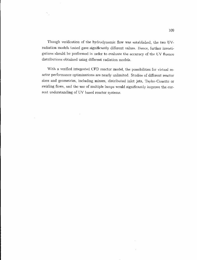
109
Though verification of the hydrodynamic flow was established, the two U V -
radiation models tested gave significantly different values. Hence, further investi
gations should be performed in order to evaluate the accuracy of the U V fluence
distributions obtained using different radiation models.
W i t h a verified integrated C F D reactor model, the possibilities for virtual re
actor performance optimizations are nearly unlimited. Studies of different reactor
sizes and geometries, including mixers, distributed inlet jets, Taylor-Couette or
swirling flows, and the use of multiple lamps would significantly improve the cur
rent understanding of U V based reactor systems.
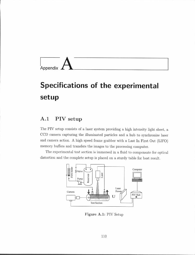
Appendix A Specifications of the experimental setup
A . 1 P I V setup
The P I V setup consists of a laser system providing a high intensity light sheet, a
C C D camera capturing the illuminated particles and a hub to synchronize laser
and camera action. A high speed frame grabber with a Last In First Out (LIFO)
memory buffers and transfers the images to the processing computer.
The experimental test section is immersed in a fluid to compensate for optical
distortion and the complete setup is placed on a sturdy table for best result.
f l
I $ Valve
Pump c
I
Computer
Camera y — c r t
Test Section
F i g u r e A .1: P I V Setup
110
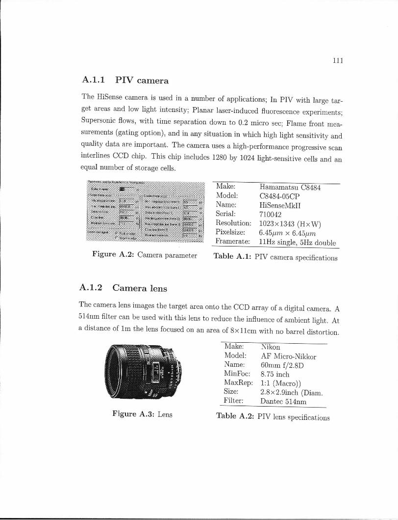
I l l
A . l . l P I V camera
The HiSense camera is used in a number of applications; In P I V with large tar
get areas and low light intensity; Planar laser-induced fluorescence experiments;
Supersonic flows, with time separation down to 0.2 micro sec; Flame front mea
surements (gating option), and in any situation in which high light sensitivity and
quality data are important. The camera uses a high-performance progressive scan
interlines C C D chip. This chip includes 1280 by 1024 light-sensitive cells and an
equal number of storage cells.
Par.ame.tefs user! la Asynchronous framing mode:.; •
Delay to open: :: | | | JQE u:
:"Single-frame mciris ' :-nhMrfiamr ,. ~H,.
M,n.,r , t t gM,„r , l ,„ 1 K |ia5 J \ Miry integration timeframe] ]: . -j;4"-H ' us
" Max.;integi,s!ion time (frame 1.]: j4,5 : : ^ |
i Delay to cose .:• .. [152.0 ;ns|: • Delay to close [frame; tj: • ' \QM': ' ':. us j
Close time;;' J88496.0: p$X Mm.-integration timeframe i). J8849b.Q-'• (is j Maximum flame rate:. j l T ? ~ Hz Max. integrationtiftie 1 2] : r 16.0 n ; , |
Frame start signal: (~ p , , , , -Close timeframe 2j: :. : j.3843B,0: ^ ;
Make: Hamamatsu C8484 Model: C8484-05CP Name: HiSenseMkll Serial: 710042 Resolution: 1023 x 1343 (H x W) Pixelsize: 6.45//r?7 x 6.45/rm. Framerate: 11Hz single, 5Hz double
F i g u r e A .2: Camera parameter Tab le A .1: P I V camera specifications
A . 1 . 2 Camera lens
The camera lens images the target area onto the C C D array of a digital camera. A
514nm filter can be used with this lens to reduce the influence of ambient light. At
a distance of l m the lens focused on an area of 8 x l l c m with no barrel distortion.
Make: Nikon Model: A F Micro-Nikkor Name: 60mm f/2.8D MinFoc: 8.75 inch MaxRep: 1:1 (Macro)) Size: 2.8x2.9inch (Diam. Filter: Dantec 514nm
F i g u r e A . 3 : Lens Tab le A .2: P I V lens specifications
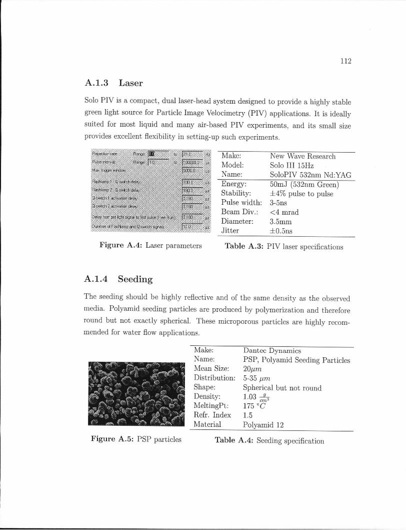
112
A.1 .3 Laser
Solo P I V is a compact, dual laser-head system designed to provide a highly stable
green light source for Particle Image Velocimetry (PIV) applications. It is ideally
suited for most liquid and many air-based P I V experiments, and its small size
provides excellent flexibility in setting-up such experiments.
Repetition rate:
Pulse interval:
Max. trigger window:
Range:
Range: 1.0
21.0
Flashlamp 1 - Q-switch delay:
Flashlamp 2 • Q-switch delay:
Q-switch 1 activation delay:
Q-switch 2 activation delay:
Delay from prelighl signal to first pulse (Free Run]:
Duration of Flashlamp and Q-switch signals:
100000.0
5000.0
(190.0
|190.0
[0 180
I01B0
10.0
Hz
us
(IS
us
US
US
US
us
us
Make: New Wave Research Model: Solo III 15Hz Name: SoloPIV 532nm N d : Y A G Energy: Stability: Pulse width: Beam Div.: Diameter: Jitter
50mJ (532nm Green) ± 4 % pulse to pulse 3-5ns <4 mrad 3.5mm ±0.5ns
F i g u r e A.4: Laser parameters Tab le A.3: P I V laser specifications
A . 1.4 Seeding
The seeding should be highly reflective and of the same density as the observed
media. Polyamid seeding particles are produced by polymerization and therefore
round but not exactly spherical. These microporous particles are highly recom
mended for water flow applications.
Make: Dantec Dynamics Name: PSP, Polyamid Seeding Particles Mean Size: 20/im Distribution: 5-35 pim Shape: Spherical but not round Density: 1.03 •£* MeltingPt: 175 °C Refr. Index 1.5 Material Polyamid 12
F i g u r e A.5: P S P particles Tab le A.4: Seeding specification
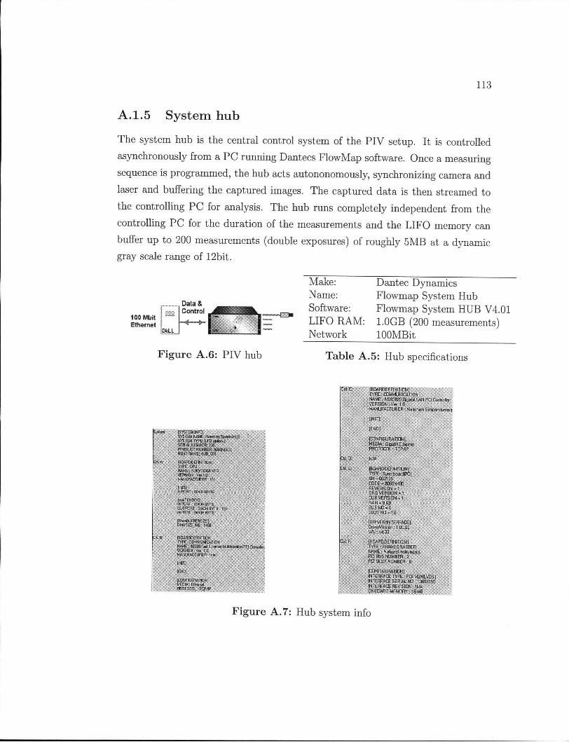
113
A . 1.5 System hub
The system hub is the central control system of the P I V setup. It is controlled
asynchronously from a P C running Dantecs FlowMap software. Once a measuring
sequence is programmed, the hub acts autononomously, synchronizing camera and
laser and buffering the captured images. The captured data is then streamed to
the controlling P C for analysis. The hub runs completely independent from the
controlling P C for the duration of the measurements and the L I F O memory can
buffer up to 200 measurements (double exposures) of roughly 5 M B at a dynamic
gray scale range of 12bit.
Data & Con t ro l
F i g u r e A . 6 : P I V hub
Make: Dantec Dynamics Name: Flowmap System Hub Software: Flowmap System H U B V4.01 L I F O R A M : 1.0GB (200 measurements) Network 100MBit
Tab le A.5: Hub specifications
HOST NAME: HUBJXR IBOJVTDOEFIMIHONI
136 908ONO631
HNiri
(EN01
(CONFIGURATION) MEOW: Elton* PROTOCOL: TCP/IP
Ctrl D:
CKI E:
|80.ARDDEFiNt!10?f) TYPE : COMMUNICATION NAME : NSG363D Gipabil LAN Prj CoAolfer VERSION : Vet. 1.0
: vJ^NUFACTURER :N^riansm S:Fneontludols
UNIT]
[ENDS
[CONFIGURATION] MEOIA: GeaB Efeeiret Pa0T0C0L:TCP;tP
WA
BQARDDEFINIIlQNf TYPE : Sine baeidpCIJ 5N-OCXM35 CQDE-SEON-tOO REVERSION . 1
BUS N O - 0 SIDING =18.
[DRIVER INTERFACE] DwerVeision: TOOiOO V A / : v « 3
IBMFIDDEFINmr jN ] TYPE : FRAWEGRA8BER N A M E : N^aH^lriii/wnetilt PCI BUS NUMBER : 2 PCI SLOT NUMBER : 8
[CON FIGURATION] INTERFACE T Y P E : P C M INTERFACE SERIAL NO : 13B371S0
, . i REVIS ION: N/A ONBOARD MEMOWrlSMB
F i g u r e A . 7 : Hub system info
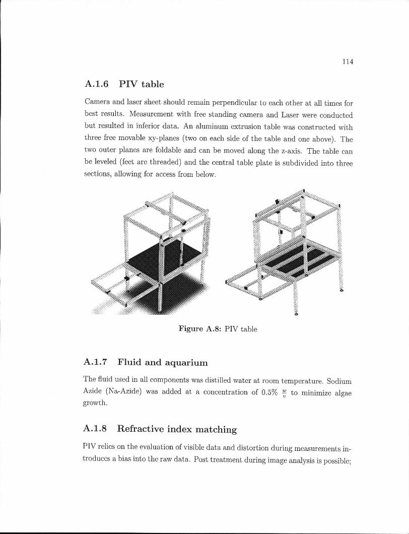
114
A . 1.6 P I V table
Camera and laser sheet should remain perpendicular to each other at all times for
best results. Measurement with free standing camera and Laser were conducted
but resulted in inferior data. A n aluminum extrusion table was constructed with
three free movable xy-planes (two on each side of the table and one above). The
two outer planes are foldable and can be moved along the z-axis. The table can
be leveled (feet are threaded) and the central table plate is subdivided into three
sections, allowing for access from below.
F i g u r e A . 8 : P I V table
A . 1.7 Fluid and aquarium
The fluid used in all components was distilled water at room temperature. Sodium
Azide (Na-Azide) was added at a concentration of 0.5% ^ to minimize algae
growth.
A.1.8 Refractive index matching
P I V relies on the evaluation of visible data and distortion during measurements in
troduces a bias into the raw data. Post treatment during image analysis is possible;
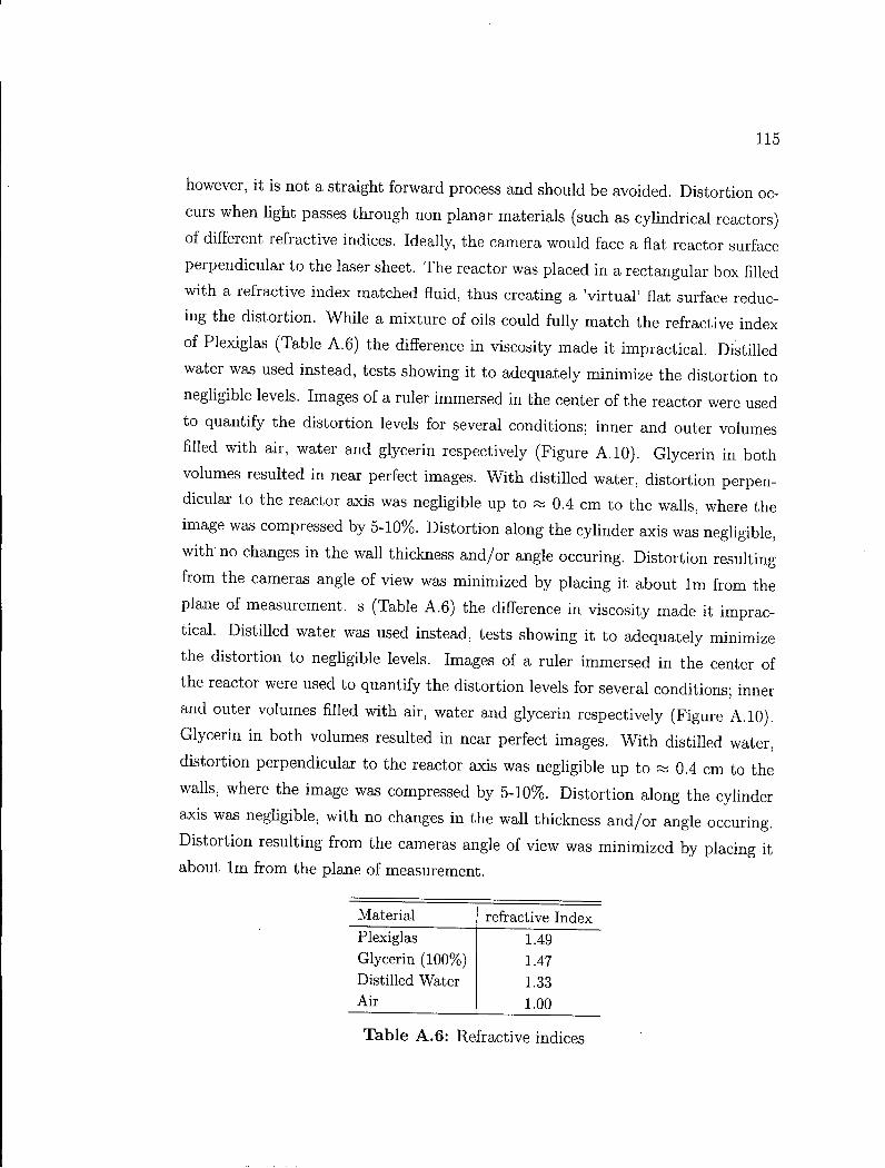
115
however, it is not a straight forward process and should be avoided. Distortion oc
curs when light passes through non planar materials (such as cylindrical reactors)
of different refractive indices. Ideally, the camera would face a flat reactor surface
perpendicular to the laser sheet. The reactor was placed in a rectangular box filled
with a refractive index matched fluid, thus creating a 'virtual ' flat surface reduc
ing the distortion. While a mixture of oils could fully match the refractive index
of Plexiglas (Table A.6) the difference in viscosity made it impractical. Distilled
water was used instead, tests showing it to adequately minimize the distortion to
negligible levels. Images of a ruler immersed in the center of the reactor were used
to quantify the distortion levels for several conditions; inner and outer volumes
filled with air, water and glycerin respectively (Figure A . 10). Glycerin in both
volumes resulted in near perfect images. W i t h distilled water, distortion perpen
dicular to the reactor axis was negligible up to ~ 0.4 cm to the walls, where the
image was compressed by 5-10%. Distortion along the cylinder axis was negligible,
with no changes in the wall thickness and/or angle occuring. Distortion resulting
from the cameras angle of view was minimized by placing it about l m from the
plane of measurement, s (Table A.6) the difference in viscosity made it imprac
tical. Distilled water was used instead, tests showing it to adequately minimize
the distortion to negligible levels. Images of a ruler immersed in the center of
the reactor were used to quantify the distortion levels for several conditions; inner
and outer volumes filled with air, water and glycerin respectively (Figure A . 10).
Glycerin in both volumes resulted in near perfect images. W i t h distilled water,
distortion perpendicular to the reactor axis was negligible up to ~ 0.4 cm to the
walls, where the image was compressed by 5-10%. Distortion along the cylinder
axis was negligible, with no changes in the wall thickness and/or angle occuring.
Distortion resulting from the cameras angle of view was minimized by placing it
about l m from the plane of measurement.
Material refractive Index
Plexiglas 1.49 Glycerin (100%) 1.47 Distilled Water 1.33 A i r 1.00
Tab le A . 6 : Refractive indices
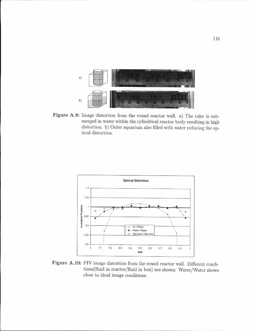
116
a)
b)
i
1 cq
F i g u r e A . 9 : Image distortion from the round reactor wall, a) The ruler is submerged in water within the cylindrical reactor body resulting in high distortion, b) Outer aquarium also filled with water reducing the optical distortion.
O p t i c a l D i s t o r t i o n
•o 0.95 •
O \ ' O
\
•-+-- A i r /Water
- • — W a t e r / W a t e r
o Glycerine/Gfyceri ns
01 0 2 0 3 0 4 0.5
d/dO
0 6 0.7
F i g u r e A . 10: P I V image distortion from the round reactor wall. Different conditions (fluid in reactor/fluid in box) are shown: Water/Water shows close to ideal image conditions.
Appendix B Programs
The following listing are the programs and macros written to extend the capabilities of Fluent as needed for the thesis objectives or to simplify the handling of large amounts of data.
B. l UV-radiation UDFs
The UV-radiation models were written and implemented in the C programming
language and linked to Fluent as user defined functions (UDFs) . The two following
files represent the radial and the M P S S radiation models used. While both UDFs
can be run as an interpreted programs, a user defined memory ( U D M ) space has to
be allocated beforehand. (Define - User Defined - Memory ==> set to 1). Fluent
has a bug that does not allocate the U D M space immediately, plotting the contours
of the U D M wi l l solve this.
Both radiation models were designed to handle multiple lamps. Each lamp is
defined by the x,y,z coordinates of its start and endpoints that are hard coded
within the U D F . The units used are cm and the program wil l automatically con
verts all values to the proper SI units. There is no security checks to verify if lamp
coordinates are within the reactor space. For the case of multiple lamps, the local
fluence rates are accumulated within each cell.
Shadowing effects have not been included and radiation calculations rely solely
on the distance information of each cell centroid. Therefore, radiation calculations
do not stop at the boundaries and care has to be taken with reactor shapes that
117
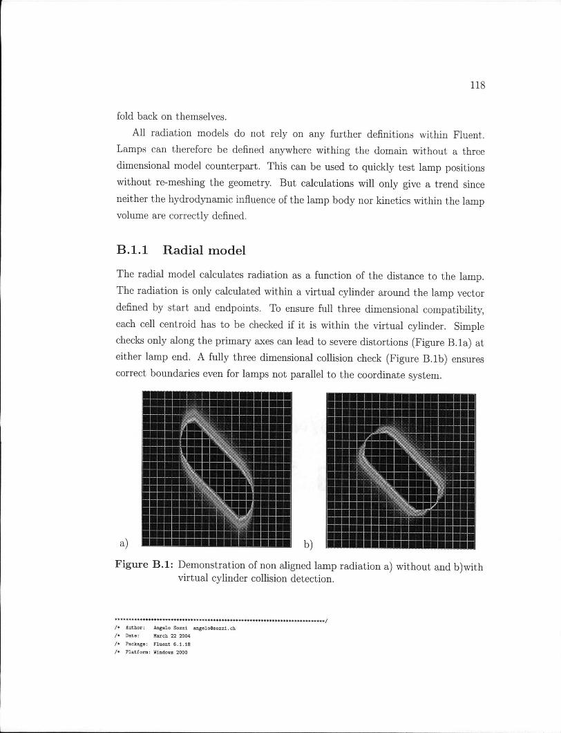
118
fold back on themselves.
A l l radiation models do not rely on any further definitions within Fluent.
Lamps can therefore be defined anywhere withing the domain without a three
dimensional model counterpart. This can be used to quickly test lamp positions
without re-meshing the geometry. But calculations wil l only give a trend since
neither the hydrodynamic influence of the lamp body nor kinetics within the lamp
volume are correctly defined.
B . l . l R a d i a l model
The radial model calculates radiation as a function of the distance to the lamp.
The radiation is only calculated within a virtual cylinder around the lamp vector
defined by start and endpoints. To ensure full three dimensional compatibility,
each cell centroid has to be checked if it is within the virtual cylinder. Simple
checks only along the primary axes can lead to severe distortions (Figure B. la ) at
either lamp end. A fully three dimensional collision check (Figure B . lb ) ensures
correct boundaries even for lamps not parallel to the coordinate system.
I B B B B B ^ M B B B B B B B B B B B
!S88fiBk '"SS5SSSSS llllk " M l
" ~ " • • • • I k M l
a)
J i n M B B B B U B L - . . • • • • • • S i . M l » • BBSSk^ssss:::
• • • I k ' W i l l
b)
"Hi M B T H L M l IBk BI • M B B B H "
. _ k M l IV ' M B H L
JBBI
F i g u r e B . l : Demonstration of non aligned lamp radiation a) without and b)with virtual cylinder collision detection.
**************************
/* Author: Angelo Sozzi angelofl.sozzi.ch /* Date: March 22 2004 /* Package: Fluent 6.1.18 /* Platform: Windows 2000
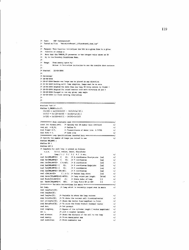
/+ Type: UDF <interpreted /* Tested on F i l e "March/oldRoundl_l/fixedtest5_chem.cas" /* /* Purpose: This function i n i t i a l i z e s the UDS in a given Zone to a given /* function of radius r. /* Note that the THREAD_ID parameter is the integer value shown as ID /* by in the Boundary Conditions Menu. / •
/* Usage: Free memory space by: /* Solver -> I n i t i a l i z e I n i t i a l i z e to see the results show contours /* /* Started: 23-03-2004 /* /* Revisions: /* 25-08-2004 /* 09-07-2004 Remake now lamps can be placed in any direction /* 21-05-2004 Working multi lamp adaption, lamps must be on axis /* 19-05-2004 Adapted for more than one lamp 2D Array errorB in Fluent ! /* 26-03-2004 Adapted for round reactor with main direction of pos Y /* 23-03-2004 Changed to use any given lamp angle /* 22-03-2004 (i) Fi r s t working compilation /* /*
#include "udf.h" ffdeflne V_CROSS(a,b,r)\
« r H 0 ] - Ca)[l]*Cb)C2] - (b)[l]»(a>[2],\ (r)[l] - (a)[2]*(b)[0] - (b) [2]*(a) [0] ,\ <r>[2] - Ca)[0]*(b)[l] - (b)[0].(a)[l]>
/*********** Some constants used **************+**+**************************/ const int thread_id=2; /* Specify the ID number here (2=fluid) */ real p i i - M_PI; /* Define Pi */ real Trans- 0.7; /* Transmittance of Water 1/cm 0.7=70'/, */ real Alfa • 1; /* Alfa 1/cm */ /*+********* Lamp Specifications inserted here *************#****************/ /* Specify the number of lamps you intend to use */ tfdefine NRLAMPS 1 ffdefine ON 1 ftdefine OFF 0 /* lampdata for each lamp is passed as follows:
x,y,z, X,Y,Z, radius, Izero, Slevelndex /* Lamp / 1 / 2 / 3 / 4/ 5 etc. */ real Xst[NRLAMPS]= { 0>; /* X coordinates Startpoints [cm] */ real Yst[NRLAMPS]- { 0>; /* Y coordinates [cm] */ real Zst[NRLAMPS]- { 4.45}; /* Z coordinates [cm] */ real Xnd[NRLAMPS]» { 0}; /* X coordinates Endpoints [cm] */ real Ynd[NRLAMPS]- { 0}; /* Y coordinates [cm] */ real Znd[NRLAMPS]» {84.45}; /* Z coordinates [cm] */ real r[NRLAMPS]= < 1.0 }; /* RadiuB lamp sieve [cm] */ real Izero[NRLAMPS]»<0.4375}; /* Lamp output per length [W/cm] */ real SLndx[NRLAMPS]-< 1}; /* Sieve index of lamp [-] */ int OnDff[NRLAMPS]-{ ON}; /* Lamp State ON or OFF [-] */ /***«•*«**** Variable declarations for macro *********•******************»***/ int lamp; /* Lamp which i s currently looped over in macro */ real lampStart[3]; real lampEnd[3]; real lampVec[3]; /* Variable to store the lamp vectors */ real PointVec[3]; /* To store the current c e l l (location)vector */ real ptlampVec[3]; /* Store the vector from LampStart to Point */ real KreuzProd[3]; /* To store the Cross Product (normal) vector +/ real dot; /* Dot product */ real lengthsq; /*' Square of the cylinder length ( vector magnitude) •/ int i ; /* just a counter variable */ real distanz; /* store the distance of the c e l l to the lamp */ real sumtop; /* Store denominator sum */ real sumbottom; /* Store nominator sum */
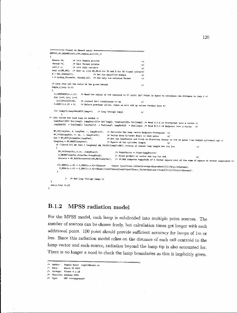
120
/•****•****• Fluent on demand macro *****************************************/ DEFINE_ON_DEMAND(lnit_UDS_radius_multiVl_l) { Domain *d; /* Init Domain pointer */ Thread * t ; /* Init Thread pointer */ c e l l _ t c; /* Init Cell variable */ real xc[ND_ND]; /* Init xc with ND_ND=2 for 2D and 3 for 3D Fluent solver*/ d » Get_Domain(l); /* Get the specified domain */ t - Lookup_Thread(d, thread_id); /* Use only the selected Thread */
/* Loop over a l l the c e l l s i n the given thread */ begin_c_loop (c,t) {
C_CENTROID(xc,c,t); /* Read the values of the centroid in SI units [m] ! Point in space to calculate the distance to lamp 1 */ for (i-0;' i<3; i++)
xc[i]»xc[i]*100; /* convert Cell coordinates to cm */ C_UDHI(c,t,0) = 0; /* Delete previous values, since we w i l l add up values further down */
for (lamp=0;lamp<NRLAMPS;lamp++) /* loop through lamps */ i
/* calc values for each lamp as needed */
lampStart [0]« Xst [lamp]; lampStart [1]«- YstClamp]; lampStart [2] - Zst[lamp]; /* Read X,Y,Z 0 f Startpoint into a vector */ lampEnd[0] - Xnd[lamp]; lampEnd[l) - YndElampJ; lampEnd[2] - Znd[lamp]; /* Read X,Y,Z of Endpoint into a vector */
NV_VV(lampVec, », lampEnd, -, lampStart); /* Calculate the lamp vector Endpoint-Startpoint */ NV_VV(ptlampVec, =, xc, -, lampStart); /* Vector from Cylinder Start to test point */ dot - NV_DOT(ptlampVec,lampVec); /* Dot the lampVector and Point to StartLamp Vector to see i f point l i e s behind cylinderd cap */ lengthsq - NV_MAG2(larapVec); /* Square of the cylinder length */
i f ((dot>0.0f) Wt (dot < lengthsq) ftft (OnOff[lamp]—ON)) /*check i f inside lamp length 0-x 1-y 2»z +/
NV_VV(PolntVec,-,xc,~,lampStart); /* PointVector = Point-lampStart*/ V_CROSS(lampVec,PointVec,KreuzProd); /* Cross product of vector see top for def. +/ distanz - NV_MAG(KreuzProd)/NV_MAG(lampVec); /* NV_HAG computes magnitude of a vector square root of the aumm of square of vector components
//C_UDMI(c,t,0) - C_UDMI(c,t,0)+(Sleeve* Izero* (pow(Trans,(Alfa*(distanz-SleeveRad)))))/(2*pii*distanz); C.UDMI(c,t,0) - C_UDMI(c,t,0) + CSLndx [lamp]+Izero[lamp]*(pow(Trans,(Alfa*(distanz-r[lamp])))))/(2*pii*distanz);
} /* End loop through lamps */ }
end_c_loop (c,t) }
B.1.2 M P S S radiation model
For the M P S S model, each lamp is subdivided into multiple point sources. The
number of sources can be chosen freely, but calculation times get longer with each
additional point. 100 point should provide sufficient accuracy for lamps of l m or
less. Since this radiation model relies on the distance of each cell centroid to the
lamp vector and each source, radiation beyond the lamp tip is also accounted for.
There is no longer a need to check the lamp boundaries as this is implicitly given.
/***************************************************************************/ /* Author: Angelo Sozzi angeloGsozzi.ch /* Date: March 22 2004 /* Package: Fluent 6.1.18 /+ Platform: Windows 2000 /* Type: UDF <interpreted>
/* Tested on F i l e "C:/CFD/Cube_test/20/" /* /* Purpose: This function i n i t i a l i z e s the UDS in a given Zone to a given /* function of radius r. /* Note that the THREAD_ID parameter is the integer value shown as ID /* by i n the Boundary Conditions Menu. /* /* Usage: Free memory space by: /* In the Solver -> I n i t i a l i z e Intiallze to see the results show contours /* /* Started: 23-03-2004 /* /* Revisions: /*13-12-2004 Modified to eliminate divide by zero inf error ( i f distanz>r loop) /* 23-09-2004 This i s the PSS Model now /* 09-07-2004 Remeake now lamps can be placed in any direction /* 21-05-2004 Working multilamp adaption, lamps must be on axis /* 19-05-2004 Adapted for more than one lamp 2D Array errors i n FluBnt ? /* 26-03-2004 Adapted for round reactor with main direction of pos Y /* 23-03-2004 Changed to use any given lamp angle /* 22-03-2004 (i) Fir s t working compilation /* /*
#include "udf.h" tfdefine V_CRDSS(a,b,r)\
C(r)[0] - < a ) [ l X b)[2] - ( b)[l ] * ( a)[2],\ (r)[13 - (a)[2]*Cb)[0] - Cb)[2]*(a)[0].\ Cr)E2] - Ca)[0]*(b)[l] - Cb)[0]*(a)[l])
/******»**** Some constants used ************************************+*******/ const int thread_id=2; /* Specify the ID number here (2=fluid) */ real p i i = M_PI; /* Define Pi */ real Trans- 0.7; /* Transmittance of Water 1/cra 0.7=70*/. */ real Alfa =1; /* Alfa 1/cm */ real NrPts- 100; /* Number of points that the lamp w i l l be discretized to /*********** Lamp Specifications inserted here ****************************/ #define NRLAMPS 1 #define ON 1 #define OFF 0 /* Specify the number of lamps you intend to use */ /* lampdata for each lamp is passed i n rows as follows:
start x,y,z, end X,Y,Z, radius, Izero, Slevelndex
/* Lamp { 1 . 2 , 3 , 4 , 5 etc.} »/ real Xst[NRLAMPS]- 0> /* X coordinates Startpoints [cm] »/ real Yat[NRLAMPS]- < 0} /* Y coordinated " [cm] »/ real Zst[NRLAMPS]- •C 4.45} /* Z coordinates " [cm] »/ real Xnd[NRLAMPS]- { 0} /* X coordinates Endpoints [cm] */ real Ynd[NRLAMPS]- i 0} /* Y coordinates " [cm] «/ real Znd[NRLAMPS]= < 84.45} /* Z coordinates " [cm] «/ real r[NRLAMPS]- { 1.0} /* Radius lamp sieve [cm] •/ real Izero[NRLAMPS] -{0.4375} /* Lamp output per LampLength [W/cm »/ real SLndx[NRLAMPS] -i 1} /* Sieve index of lamp [-] •/ int OnOff[NRLAMPS] -{ ON} /* Lamp State ON or OFF [-] »/
/*********** Variable declarations for macro ********»***********•*****+*/ int lamp; /* Lamp which is currently looped over i n macro */ real lampStart[3]; real lampEnd[3]; real lampVec[3]; /* Variable to store the lamp vectors */ real PointVec[3]; /* To store the current c e l l (location)vector */ real ptlampVec[3]; /* Store the vector from LampStart to Point */ real KreuzProd[3]; /* To store the Cross Product (normal) vector */ real lampPt[3]; /* Store the coordinats of a point on the lamp */ real lampUnit[3]; /* Store the lamp unit vector */ real addVector[3]; /* Vector to be added to Start for point pos +/ real PtPtVector [3]; /* The Point to Point Vector +/
122
real abstand; /* Distance from Point on Lamp to Cell »/ real I f u l l ; /» UV lamp Power output of the whole lamp [W] »/ real dot; / • Dot product •/ real LampLength; /* Lamp cylinder LampLength (magnitude) •/ real parameter; / • Lamp Unit raultiplicator variable */ real larada; /« as above but i n the lamp loop */ real k; /* The Absorbtion coefficient [1/cm] »/ int i ; /* just a counter variable »/ int points; /* counter to go through points */ real distanz; /» store the distance of the c e l l to the lamp •/ real sumtop; /» Store denominator summ »/ real sumbottom; /* Store nominator summ •/ real summup; /* summ of values from each point */ int flag-O; /*********** Fluent on demand macro **************************************/
DEFINE_0N_DEMAND(init_UDS_radius„multiV3_l) { Domain *d; /* Ini t Domain pointer */ Thread * t ; /* Init Thread pointer */ c e l l _ t c; /* Init Call variable */ real xc[ND_ND]; /+ Init xc with ND_ND=2 for 2D and 3 for 3D Fluent solver */ d - Get_Domain(l); /* Get the specified domain */ t - Lookup_Thread(d, thread_id); /* Use only the selected Thread */ k • -log(10)*loglO(Trans); /+ Calculate k from T */
/* Loop over a l l the c e l l s in the given thread */ begin_c_loop (c,t) {
C_CENTROID(xe,c,t); /* Read the values of the centroid in SI units [m] ! Point in space to calculate the distance to lamp 1 use */ for (i=0; i<3; i++)
xc[i]=xc[i]*100; /* convert Cell coordinates to cm */ C_UDMl(c,t,0) - 0; /* Delete previous values, since we w i l l add up values further down */
for (lamp-0;lamp<NRLAMPS;lamp++) /• loop through lamps */ {
/* calc values for each lamp as needed */ lampStart[0]- Xst[lamp]; lampStart[1]• Yst[lamp]; lampStart[2]• Zst[lamp]; /* Read X.Y.Z of Startpoint into a vector */ lampEndtO] - Xnd[lamp]; lampEnd[l] - Ynd[lamp]; lampEnd[2] - ZndClamp]; /* Read X.Y.Z of Endpoint into a vector */
NV_VV(larapVec, -, lampEnd, -, lampStart); /* Calculate the lamp vector Endpoint-Startpoint */ NV_VV(ptlampVec, «, xc, -, lampStart); /* Vector from Lamp Cylinder Start to test point +/ LampLength = NV_MAG(lampVec); /* Lamp cylinder LampLength */ I f u l l - IzeroUamp] *LampLength; /* Calculate the f u l l lamp output in [W] from the Output per lentgh [W/cm] */ V_CROSS(lampVec,ptlampVec,KreuzProd); /* Cross product of vector see top for def. */ distanz - HV_MAG(KreuzProd)/LampLength; /* HV_KAG computes magnitude of a vector square root of the summ of square of vector components lampUnit[0]-lampVec[0]/LampLength; lampUnit[l]=lampVec[1]/LampLength; lampUnit[2]-lampVec[2]/LampLength; /* Calculate the Lamp Unit vector */
parameter « LampLength/NrPts; /* LamUnit multiplicator */ imup » 0; /» In i t i a l i z e the summup for each lamp */
i f (distanz> r[lamp])< for (points«0;points<NrPts;points++) /* Loop through discretized points on lamp */
lamda - parameter*point S; /* Calculate the Parameter to multiply the LampUnit Vector by */ addVector[0]-lamPUnit[0]*lamda; addVector[1]-lampUnit[1]*lamda; addVector[2]-lampUnit[2]*lamda; /* Multiply */ KV.VVdampPt, -, lampStart, +, addVector); /* Finally Calculate the X,Y,Z of the point on the Lamp */ NV_VV(PtPtVector, xc, -, lampPt); /* Vector from C e l l to point on Lamp abstand » NV_MAG(PtPtVector); /* Distance from Point to CellCentre
summup = summup+((Ifull/NrPts)/(4*pii*abstand*abstand)+exp(-k*(distanz-r[lamp]))); } /* End loop through points on lamp »/ C_UDMI(c,t,0) » C_UDMI(c,t,0)+summup; } /*End the i f statement*/
} /* End loop through lamps */ > /* End loop through Cells in Thread */ end_c_loop (c,t)
> /* End On Demand Macro */
123
B.2 Lagrangian disinfection model
The Lagrangian model relies heavily on the Fluent discrete phase model ( D P M )
environment. The D P M environment has to be set up as described in the manual
for particle tracking, before employing the Lagrangian model. A n additional user
variable and the UV-radiation model are also needed. The dose-setup function
redefines the D P M user scalar name. The absorbed-dose function has to be hooked
to the D P M - U D F environment and calculates the dose absorbed along the path of
each particle. The dose-output function finally redefines the Report-DPM-Sample-
output menu to output the absorbed dose values into an external file.
*************** /* Author: Angelo Sozzi angeloGsozzi.ch /* Date: April 07 2004 /* Package: Fluent 6.1.18 /* Platform: Windows 2000 /* Type: UDF <interpreted> /* Tested on F i l e "March/oldRoundl_l/fixedtestS^chem.cae" /« /* Purpose: This function Integrates the Dose of a particle injected by /* Particle tracking. See 4-150 UDF manual. /* /« /• /* Usage: Interpret, and hook the UDF to Init. Open a UDS. /* In the Solve -> I n i t i a l i z e Intialize to see the results show contours /* /« Started: 23-03-2004 /• /* Revisions: /* 12-03-2005 Removed deactivation calc /* 04-06-2004 (i) F i r s t working compilation /» /*************************
ftinclude "udf.h"
static real dose_0;
DEFINE_ON_DEMAND(dose_setup) {
/* i f memory for the particle variable t i t l e s has not been allocated yet. do i t now •/
i f (NULLP(user_particle_vars)) {
Init_User_Particle_Vars(); }
/* Set the name and label*/ strcpy(uaer_particle_vars[0].name, "absorbed-dose"); strcpy(user_particle_vars[0].label, "Absorbed Dose");
124
/* Update the user scalar variables */
DEFINE_DPM_SCALAR_uTDATE(absorhed_dose, c e l l , thread, i n i t i a l i z e , p) <
i f ( i n i t i a l i z e ) /* i f this i s a new particle */ {
/+ this i s the i n i t i a l i z a t i o n c a l l , set: p->user[0] contains the Dose index, i n i t i a l i z e to 0. dose_0 contains the dose at the start of a time step*/ p->user[0] » 0. ;
dose_0 - 0.; /* be sure to have dose i n UDMI[0] in W/cm"2 */ > else {
p->user[0] +» P_DT(p) * C.UDMI(cell.thread,0)*1000; // in mJ/cnT2 /* Add dose in this time step to dose history. */ /* P_DT(p) is the time of the last timestep in [s]. */
}
/* Set the output formating of the "report-discrete phase-sample" comand */ DEFINE_DPH_QUTPUT(dose_output, header, fp, p, thread, plane) {
char name[100];
fp»fopen("dpm_output.dpm","a");
i f (header) i
i f (NNULLP(thread)) fprintf (fp, " C/,s */,d)\n" ,thread->head->dpm_summary ,sort_f ile_name,2) ;
else fprintf (fp," (*/.s 7,d)\n" ,plane->sort_f ile_name,2) ; fprintf (fp, " ('/.10s 5,10s 7,s)\n" , "time" , "absorbed-dose" , "name") ;
}
else {
sprintf (name, "'As: "/,d" ,p~>injection->narae,p->part_id) ; fprintf (fp,"(('/,15.6g '/.10.6g) */.s)\n", p->state.time, p->user[0] , name);
}
fclose(fp);
B.3 Eulerian disinfection model
The Eulerian disinfection model requires the user to define a reaction in Fluent by
enabling the species transport model. Two materials, one for dead and one living
bacteria, with the properties of water are then generated. Finally a single step reac-k
tion is defined with the following stoichiometry: ILivemicroorg. —> l D e a r i m i c r o o r s .
The reaction has to be named " inactivation", since the U D F wi l l access a function
with this name and calculate the appropriate volumetric reaction rate based on the
local UV-fluence (i.e. k = f{UVfiuence). It is important to have all used material
in the proper sequence (1) Life Microorg. (2) Dead Microorg. (3) Water (bulk
material).
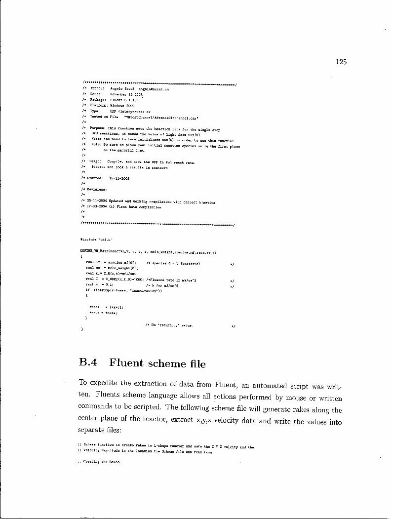
125
/***^****************************^ /* Author: Angelo Sozzi angeloGsozzi.ch /* Date: November 15 2003 /* Package: Fluent 6.1.18 /* Platform: Windows 2000 /* Type: UDF <interpreted> or /* Tested on F i l e "VRtestchannel/Advancedl/channel.cas" /* /* Purpose: This function sets the Reaction rate for the single step /* UVU reactions, i t takes the value of light from UDM[0] /* Note: You need to have i n i t i a l i z e d UDH[0] in order to use this function. /* Note: Be sure to place your i n i t i a l reaction species on i n the f i r s t place /* on the material l i s t . /* /* Usage: Compile, and hook the UDF to Vol react rate. /* Iterate and look a results i n contours /• /» Started: 15-11-2003 /• /* Revisions: /* /• 25-11-2004 Updated and working compilation v i t h correct kinetics /+ 17-03-2004 Ci) F i r s t beta compilation /• /* /****»**+»***********+*****•*******+•****************•*******+•*************/
((include "udf.h"
DEFIN£_VR_RATE(ReactV3_2, c, t, r, mole_weight,species.mf.rate,rr_t) {
real mfl = species_mf [0]; /+ species 0 • b (bacteria) re a l mwl ™ mole_weightCO]; real cl» C_R(c,t)*mf1/mwl; real I - C_UDMI(c,t,0)*1000; AFluence rate i n mW/cm-2 real k • 0.1; /* k for mJ/cm"2 i f (!strcmp(r->name, "inactivation")) {
•rate = I*k*cl; * r r _ t » *rate;
}
/* No "return..;" value.
B . 4 F luent scheme file
To expedite the extraction of data from Fluent, an automated script was writ
ten. Fluents scheme language allows all actions performed by mouse or written
commands to be scripted. The following scheme file wi l l generate rakes along the
center plane of the reactor, extract x,y,z velocity data and write the values into
separate files:
;; Scheme function to create rakes in L-shape reactor and safe the X,Y,Z velcity and the Velocity Magnitude in the location the Scheme f i l e was read from
Creating the Rakes
(ti-menu-load-string "surface/rake-surface aaRake-z-0.5 0 1.74 0.5 0 -1.74 0.5 100")
(do ((z 1.0 (+ z 1.0))) ((> z 6.0)) (ti-menu-load-string (format #f "surface/rake-surface aaRake-z-0~f 0 1.74 "4.If 0 -1.74 "4.If 100" z z z))
) (do ((z 6.9 (+ z 0.1))) ((> z 7.7))
(ti-menu-load-string (format #f "surface/rake-surface aaRake-z-0~3.If 0 1.74 "4.If 0 -1.74 "4.If 100" z z z))
) (do ((z 8.0 (+ z 1.0))) ((> z 9.0))
(ti-menu-load-atring (format fff "surface/rake-surface aaRake-z-0~f 0 1.74 "4.If 0 -1.74 "4.If 100" z z z))
) (do ((z 10.0 (+ z 5.0))) ((> z 30.0))
(ti-menu-load-string (format #f "surface/rake-surface aaRake-z-~f 0 1.74 "4.If 0 -1.74 "4.If 100" z z z))
)
;; Saving X-velocity values
(ti-menu-load-string "plot/plot yes Rake-z-0.5-x-velocity.xy no no no x-velocity yes 0 1 0 aarake-z-0.5 ()")
(do (<z 1.0 (+ z 1.0))) ((> z 6.0)) (ti-menu-load-string
(format #f "plot/plot yes Rake-z-0"f-x-velocity.xy no no no x-velocity yes 0 10 aarake-z-0"f ()" z z)) )
(do ((z 6.9 (+ z 0.1))) ((> z 7.7)) (ti-menu-load-string
(format Sf "plot/plot yes Rake-z-0"3.if-x-velocity.xy no no no x-velocity yes 0 10 aarake-z-0~3.If ()" z z))
) (do ((z 8.0 (+ z 1.0))) ((> z 9.0))
(t i-menu-1oad-s t r ing
(format ftf "plot/plot yes Rake-z-0~f-x-velocity.xy no no no x-velocity yes 0 1 0 aarake-z-0"f ()" z z))
(do (<z 10.0 (+ z 5.0))) ((> z 30.0)) (ti-menu-load-string
(format ftf "plot/plot yes Rake-z-~f-x-velocity.xy no no no x-velocity yes 0 1 0 aarake-z-~f ()" z z)) )
;; Saving Y-Velocity values (ti-menu-load-string "plot/plot yes Rake-z-0.5-y-velocity.xy no no no y-velocity yes 0 1 0 aarake-z-0.5 ()")
(do ((z 1.0 (+ z 1.0))) ((> z 6.0)) (ti-menu-load-string
(format #f "plot/plot yes Rake-z-0"f-y-velocity.xy no no no y-velocity yes 0 1 0 aaraka-z-0~f ( ) " z z)) ) (do ((z 6.9 (+ z 0.1))) ((> z 7.7))
(ti-menu-load-string
(format #f "plot/plot yes Rake-z-0~3.if-y-velocity.xy no no no y-valocity yes 0 1 0 aarake-z-0"3.If ( ) " z z)) )
(do ((z 8.0 (+ z 1.0))) ((> z 9.0)) (ti-menu-load-string
(format #f "plot/plot yes Rake-z-0~f-y-velocity.xy no no no y-velocity yes 0 1 0 aarake-z-0~f ( ) " z z))
) (do ((z 10.0 (+ z 5.0))) ((> z 30.0))
(ti-menu-load-string
(format ftf "plot/plot yes Rake-z-~f-y-velocity.xy no no no y-velocity yes 0 1 0 aarake-z-"f ( ) " z z)) )
127
;; Saving Z-Velocity values (ti-menu-load-string "plot/plot yes Rake-z-0.5-z-velocity.xy no no no z-velocity yes 0 1 0 aarake-z-0.5 ()")
(do ((z 1.0 (+ z 1.0))) ((> z 6.0)) (ti-menu-load-string (format flf "plot/plot yes Rake-z-0"f-z-velocity.xy no no no z-velocity yes 0 1 0 aarake-z-0"f ()" z z))
)
(do ((z 6.9 (• z 0.1))) ((> z 7.7)) (ti-menu-load-string (format «f "plot/plot yes Rake-z-0"3.lf-z-velocity.xy no no no z-velocity yes 0 1 0 aarake-z-0"3.If ()" z z))
)
(do ((z 8.0 (+ z 1.0))) ((> z 9.0)) (ti-menu-load-string (format #f "plot/plot yes Rake-z-0"f-z-velocity.xy no no no z-velocity yes 0 10 aarake-z-0"f ()" z z))
) (do ((z 10.0 (+ z 5.0))) ((> z 30.0))
(ti-menu-load-string (format (tf "plot/plot yes Rake-z-"f-z-velocity.xy no no no z-velocity yes 0 1 0 aarake-z-"f ()" z z))
)
;; Saving Velocity-Magnitude values (ti-menu-load-string "plot/plot yes Rake-z-0.5-velocity-magnitude.xy no no no velocity-magnitude yes 0 1 0 aarake-z-0.5 ()")
(do ((z 1.0 (+ z 1.0))) ((> z 6.0)) (ti-menu-load-string (format #f "plot/plot yes Rake-z-0"f-velocity-magnitude.xy no no no velocity-magnitude yes 0 10 aarake-z-0"f ()" z z))
)
(do ((z 6.9 (+ z 0.1))) ((> z 7.7)) (ti-menu-load-string (format Sf "plot/plot yes Rake-z-0'3.If-velocity-magnitude.xy no no no velocity-magnitude yes 0 1 0 aarake-z-0~3.If ()" z z))
)
(do ((z 8.0 (+ z 1.0))) ((> z 9.0)) (ti-menu-load-string (format *f "plot/plot yes Rake-z-0"f-veloclty-magnitude.xy no no no velocity-magnitude yes 0 1 0 aarake-z-0"f ()" z z))
)
(do ((z 10.0 (+ z 5.0))) ((> z 30.0)) (ti-menu-load-string (format #f "plot/plot yes Rake-z-"f-velocity-magnltude.xy no no no velocity-magnitude yes 0 1 0 aarake-z-"f ()" z z))
)
B.5 E x c e l velocity data import macro
In order to import the files written by the Fluent scheme file, an excel macro was
created. When pointed to the folder containing the scheme exported data, it wi l l
import the velocity data. Only the z-velocity import is shown, other data can be
imported by changing the filename in the program. Two additional macros are
used to properly align the data and to prune the multiple x axis values.
Sub import_z()
' import.z Macro
* Macro recorded 8/3/2004 by Angelo
' Keyboard Shortcut: Ctrl+Shift+E ' Make sure you are i n the sheet you want to imort the data into before starting!
Dim i . Max As Integer Dim name, pfad Dim colOffset, rowOffset colOffset - 2 1 Nr of Columns to offset the import from rowOffset =3 ' Nr of Rows to offsett the import from
Max - 23 ' The maximum number of f i l e s to read In (don't try more than you have
For i - 1 To Max name - WorksheetaC'filename").Cells(i, 1).Value ' This is where the filenumberlng is stored (rake z-position) '-z-velocity '-y-velocity '-x-velocity '-velocity-magnitude pfad • "TEXT;C:\extract\Rake-z-" + name + "-z-velocity.xy" ' The path where the f i l e s are situated With ActiveSheet.queryTables.Add(Connection:«pfad, Destination:-ActiveSheet.Cells(l + rowOffset, i * 2 - 1 + colOffset))
.name - "Rake-z-0" + LTrim(Str$(i)) + "-x-velocity.xy"
.FieldNames " True
.RowNumbers « False
.FillAdjacentFormulas - False
.PreserveFormatting • True
.RefreshOnFileDpen - False
.RefreshStyle <-> xlInsertDeleteCells
.SavePassword = False
.SaveData - True
.AdjustColumnWidth = True
.RefreshPeriod - 0
.TextFilePromptOnRefresh « False
.TextFilePlatform - 437
.TextFileStartRow = 5
.TextFileParseType - xlDelimited
.TextFileTextQualifier - xlTextQuallfierDoubleQuote
.TextFileConsecutiveDellmiter » False
.TextFileTabDelimlter - True
.TextFileSemicolonDelimiter • False
.TextFileCommaDelimiter • False
.TextFileSpaceDelimiter • False
.TextFilaColumnDataTypes - Array(l) -TextFilaTrailingMinusNumbera • True .Refresh Backgroundrjuery:°False
End With Next i
End Sub
Sub cut^pasteQ
cut_paste Macro Macro recorded 8/3/2004 by Angelo
This Macro makes sure that the missing points from the y-rakes in the reactor are lined up properly It compares the x values of the f i r s t row ( f u l l 100 points) to the x values of the later rows and i f i t finds a mismatch i t cuts the cells from those two rows aad shifts them down to the point where the x values match up again
Dim j , i , first_row, second_row As Integer Dim x i , x2, row_test, xfix, lastusedRow, laBtusedColumn, ExcelLastCell Dim colOffset, rowOffset
colOffset =2 ' Nr of Columns to offset the import from rowOffset - 3 ' Nr of Rows to offsett the import from
ExcelLastCell * ActiveSheet.Cells.SpecialCells(xlLastCell) 'lastusedColumn - ActiveSheet.Cells(row0ffset + 1, 150).End(xlLeft).Column 'Find the last used c e l l i n the row lastusedColumn -» ActiveSheet.UsedRange.Columns.Count ' Only works for sheets with no other data but Hey i t works
For j • colOffset + 1 To lastusedColumn / 2 ' loop through columns with data row_test = 0 xfix - -1000000
lastusedRow - ActiveSheet.Cells(150, j).End(xlUp).Row 'Find the last used c e l l i n the row
If ActiveSheet.Cells(lastusedRow, j).Value = " ) " Then ActiveSheet.Cells(lastusedRow, j).ClearContents lastusedRow = lastusedRow - 1
End If
For i «= rowOffset + 1 To lastusedRow xl = ActiveSheet.Cells(i, colDffset + 1) 'Cells(Rows,Columns) = Range(Al) If ActiveSheet.Cells(i, 1 + 2 * j).Value <> " ) " Then x2 - ActiveSheet.Cells(i, 1 + 2 * j).Value ' If x2 - Empty Then Stop If Abs(xl - x2) / Abs(xl) > 0.1 And row^test = 0 Then
first.row - i row_test = 1 xfix «= x2
End If If Abs(xflx - xl) / Abs(xl) < 0.0001 Then
second_row = i ' Stop
End If Next i 'Stop If row_test <> 0 Then
ActiveSheet.Range(Cells(first_row, 1 + 2 * j ) , Cells(100, 2 + 2 * j)).Select Selection.Cut ActiveSheet.Cells(second_row, 1 + 2 * j).Select ActiveSheet.Paste
End If ' Stop
Next j
End Sub Sub Delete_Every_Dther_Column() Dim y, i , xRng, xCounter, offset
' Dimension variables. y - True 1 Change this to True i f you want to delete rows 1, 3, 5, and so on. i = 1 Set xRng - Selection ' Loop once for every row i n the selection. For xCounter = 1 To xRng.Columns.Count
' If Y is True, then... If y - True Then
' ...delete an entire row of ce l l s . xRng.Cells(i).EntireColumn.Delete
' Otherwise... Else
' ...increment I by one so ue can cycle through range. 1 - i + 1
End If
' If Y is True, make i t False; i f Y is False, make i t True, y = Not y
Next xCounter End Sub