categorical data analysis and interpretation - emory university
TRANSCRIPT

Fellows Introduction to Research Training
Categorical Data Analysis and Interpretation
Scott Gillespie, MS, MSPHAssociate Director
Pediatrics Biostatistics CoreEmory University + CHOA
October 29, 2021
2
Definition
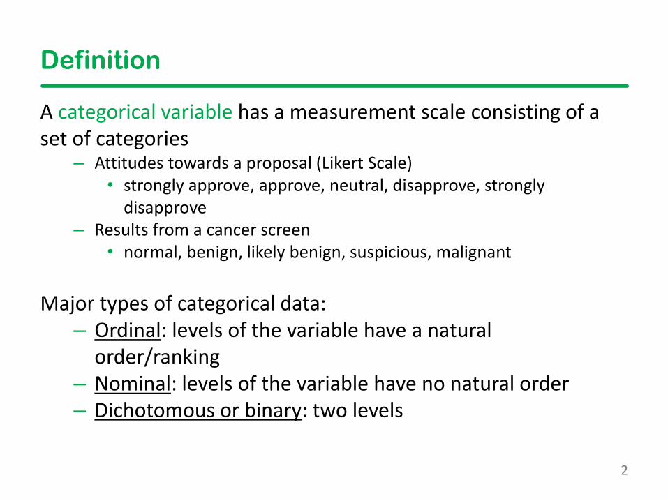
A categorical variable has a measurement scale consisting of a set of categories
– Attitudes towards a proposal (Likert Scale)• strongly approve, approve, neutral, disapprove, strongly
disapprove – Results from a cancer screen
• normal, benign, likely benign, suspicious, malignant
Major types of categorical data:– Ordinal: levels of the variable have a natural
order/ranking– Nominal: levels of the variable have no natural order– Dichotomous or binary: two levels
3
Example
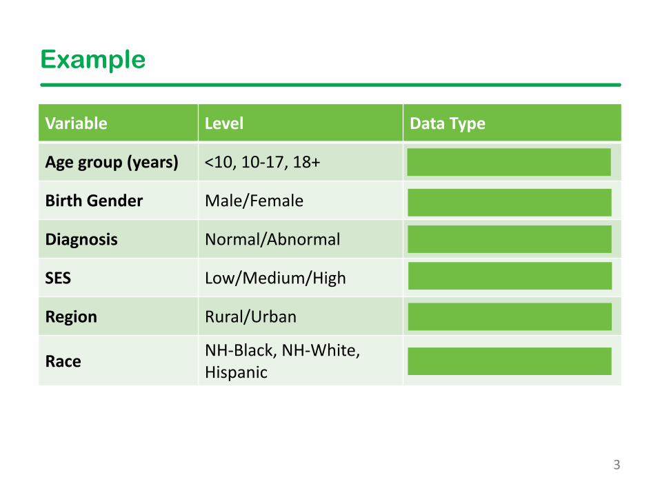
Variable Level Data Type
Age group (years) <10, 10-17, 18+ Ordinal
Birth Gender Male/Female Dichotomous and Nominal
Diagnosis Normal/Abnormal Dichotomous and Nominal
SES Low/Medium/High Ordinal
Region Rural/Urban Dichotomous and Nominal
Race NH-Black, NH-White, Hispanic Nominal
4
Exploring Associations
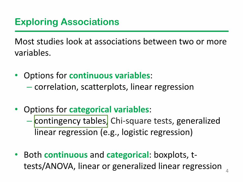
Most studies look at associations between two or more variables.
• Options for continuous variables: – correlation, scatterplots, linear regression
• Options for categorical variables: – contingency tables, Chi-square tests, generalized
linear regression (e.g., logistic regression)
• Both continuous and categorical: boxplots, t-tests/ANOVA, linear or generalized linear regression
5
Contingency Tables
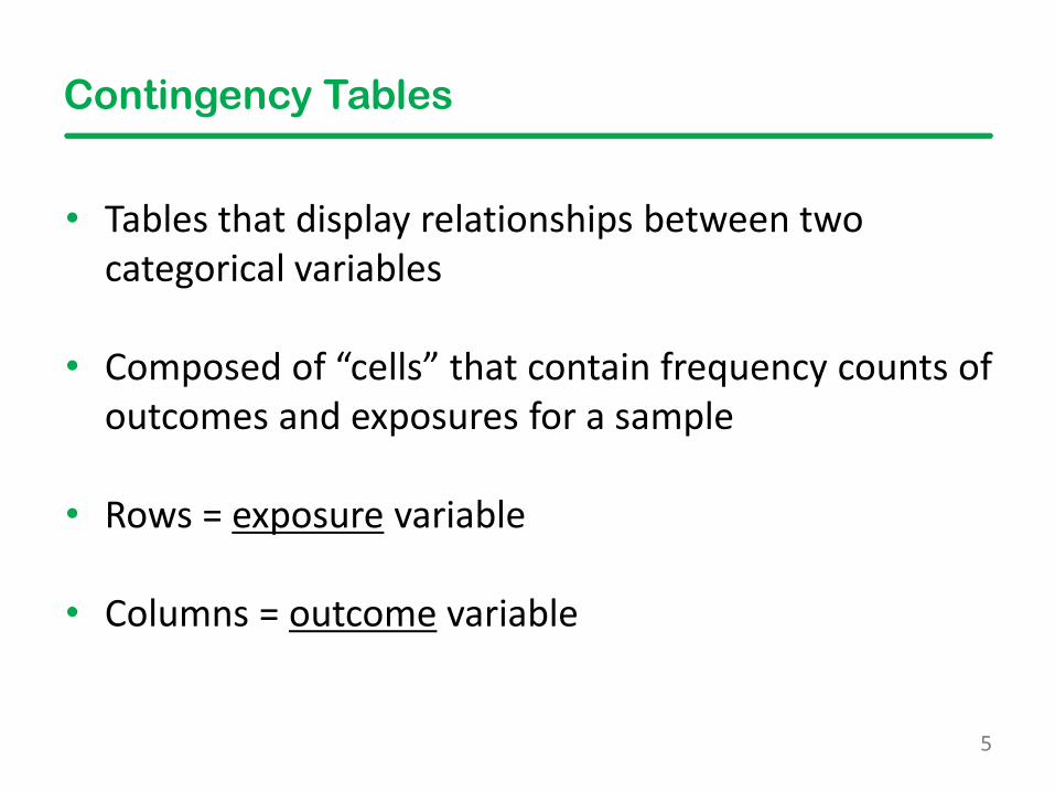
• Tables that display relationships between two categorical variables
• Composed of “cells” that contain frequency counts of outcomes and exposures for a sample
• Rows = exposure variable
• Columns = outcome variable
6
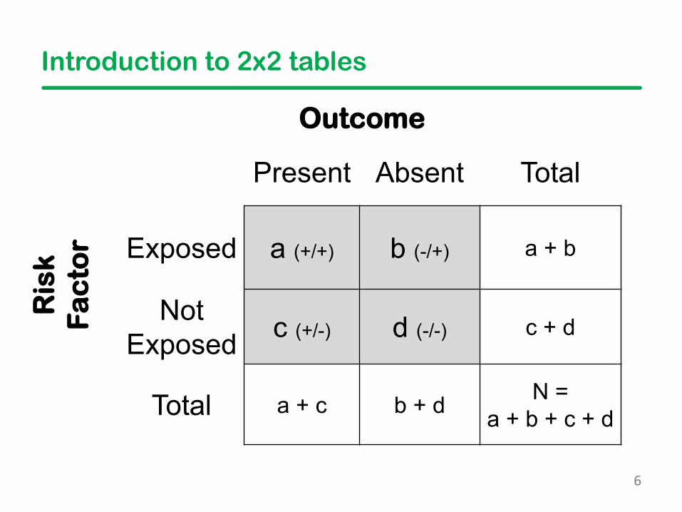
Introduction to 2x2 tables
Outcome
Present Absent Total
Ris
kF
ac
tor Exposed a (+/+) b (-/+) a + b
Not Exposed c (+/-) d (-/-) c + d
Total a + c b + d N = a + b + c + d
7
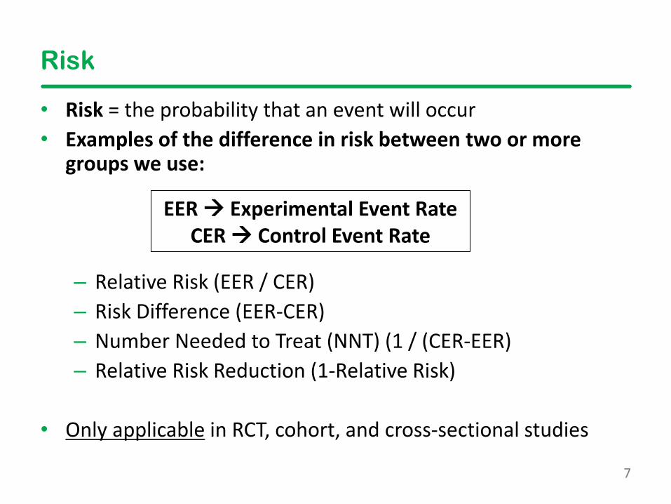
Risk
• Risk = the probability that an event will occur• Examples of the difference in risk between two or more
groups we use:
– Relative Risk (EER / CER)– Risk Difference (EER-CER)– Number Needed to Treat (NNT) (1 / (CER-EER)– Relative Risk Reduction (1-Relative Risk)
• Only applicable in RCT, cohort, and cross-sectional studies
EER Experimental Event RateCER Control Event Rate
8
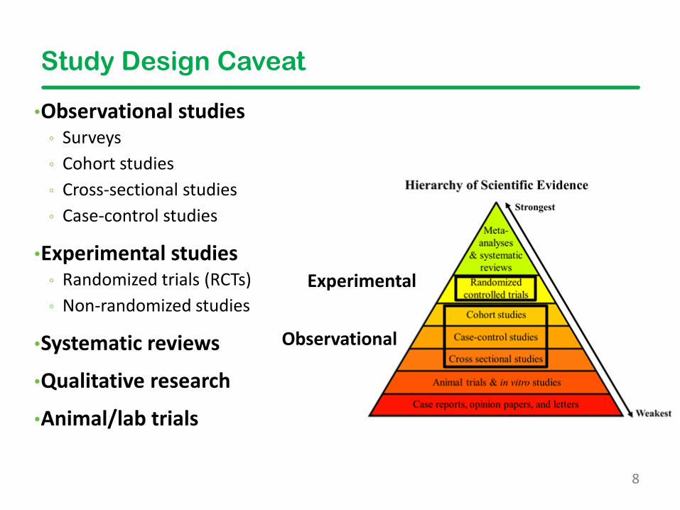
Study Design Caveat
•Observational studies ◦ Surveys ◦ Cohort studies ◦ Cross-sectional studies ◦ Case-control studies
•Experimental studies ◦ Randomized trials (RCTs) ◦ Non-randomized studies
•Systematic reviews
•Qualitative research
•Animal/lab trials
Experimental
Observational
9
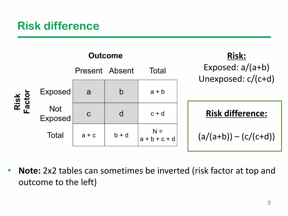
Risk difference
• Note: 2x2 tables can sometimes be inverted (risk factor at top and outcome to the left)
Risk:Exposed: a/(a+b)
Unexposed: c/(c+d)
Risk difference:
(a/(a+b)) – (c/(c+d))
10
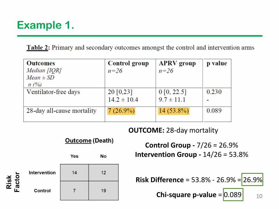
Example 1.
OUTCOME: 28-day mortality
Risk Difference = 53.8% - 26.9% = 26.9%
Chi-square p-value = 0.089
Control Group - 7/26 = 26.9%Intervention Group - 14/26 = 53.8%
11
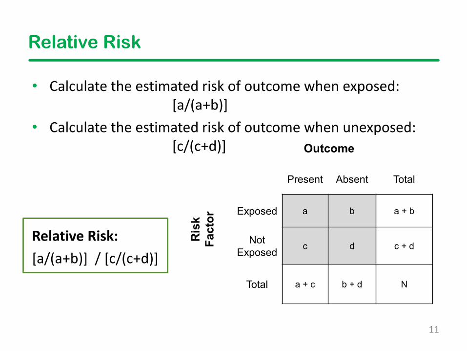
Relative Risk
• Calculate the estimated risk of outcome when exposed: [a/(a+b)]
• Calculate the estimated risk of outcome when unexposed: [c/(c+d)]
Relative Risk:[a/(a+b)] / [c/(c+d)]
Outcome
Present Absent TotalR
isk
Fact
orExposed a b a + b
NotExposed c d c + d
Total a + c b + d N
12
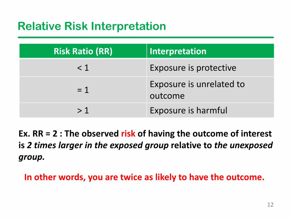
Relative Risk Interpretation
Risk Ratio (RR) Interpretation
< 1 Exposure is protective
= 1 Exposure is unrelated to outcome
> 1 Exposure is harmful
Ex. RR = 2 : The observed risk of having the outcome of interest is 2 times larger in the exposed group relative to the unexposed group.
In other words, you are twice as likely to have the outcome.
13
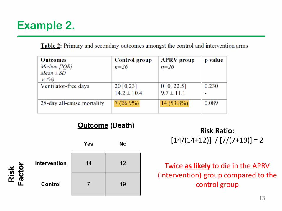
Example 2.
Outcome (Death)
Yes No
Ris
kFa
ctor Intervention 14 12
Control 7 19
Risk Ratio:[14/(14+12)] / [7/(7+19)] = 2
Twice as likely to die in the APRV (intervention) group compared to the
control group

14
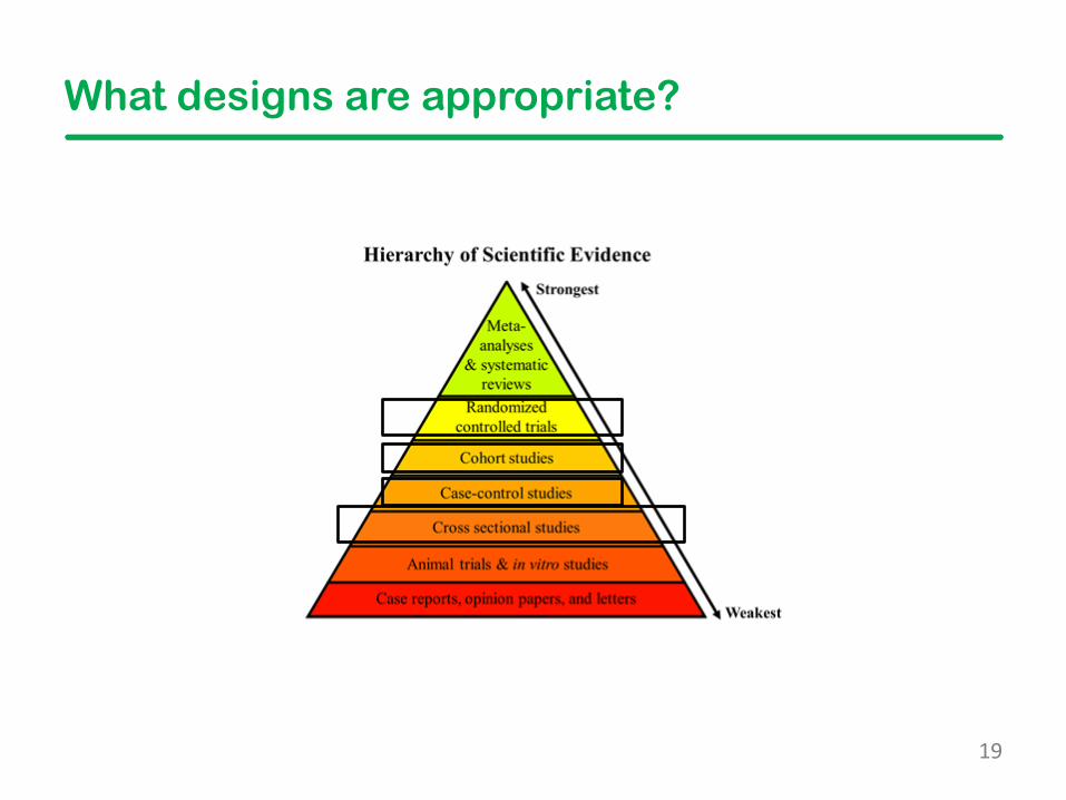
What designs are appropriate?
15
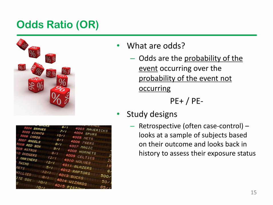
• What are odds?– Odds are the probability of the
event occurring over the probability of the event not occurring
PE+ / PE-• Study designs
– Retrospective (often case-control) –looks at a sample of subjects based on their outcome and looks back in history to assess their exposure status
Odds Ratio (OR)
16
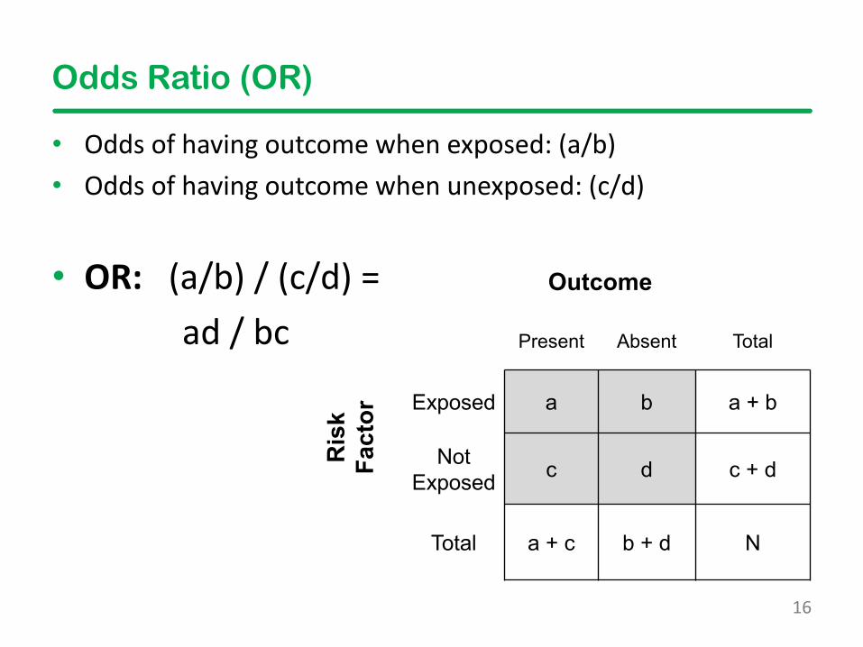
Odds Ratio (OR)
• Odds of having outcome when exposed: (a/b)• Odds of having outcome when unexposed: (c/d)
• OR: (a/b) / (c/d) = ad / bc
Outcome
Present Absent TotalR
isk
Fact
or Exposed a b a + b
Not Exposed c d c + d
Total a + c b + d N
17
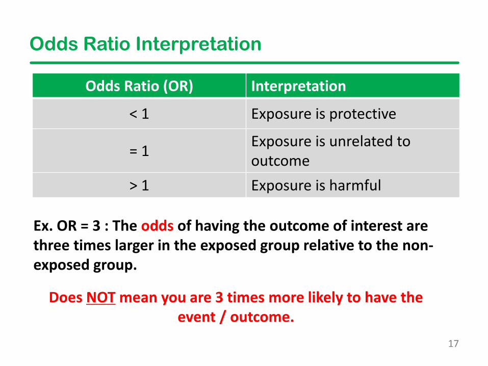
Odds Ratio Interpretation
Odds Ratio (OR) Interpretation
< 1 Exposure is protective
= 1 Exposure is unrelated to outcome
> 1 Exposure is harmful
Does NOT mean you are 3 times more likely to have the event / outcome.
Ex. OR = 3 : The odds of having the outcome of interest are three times larger in the exposed group relative to the non-exposed group.
18
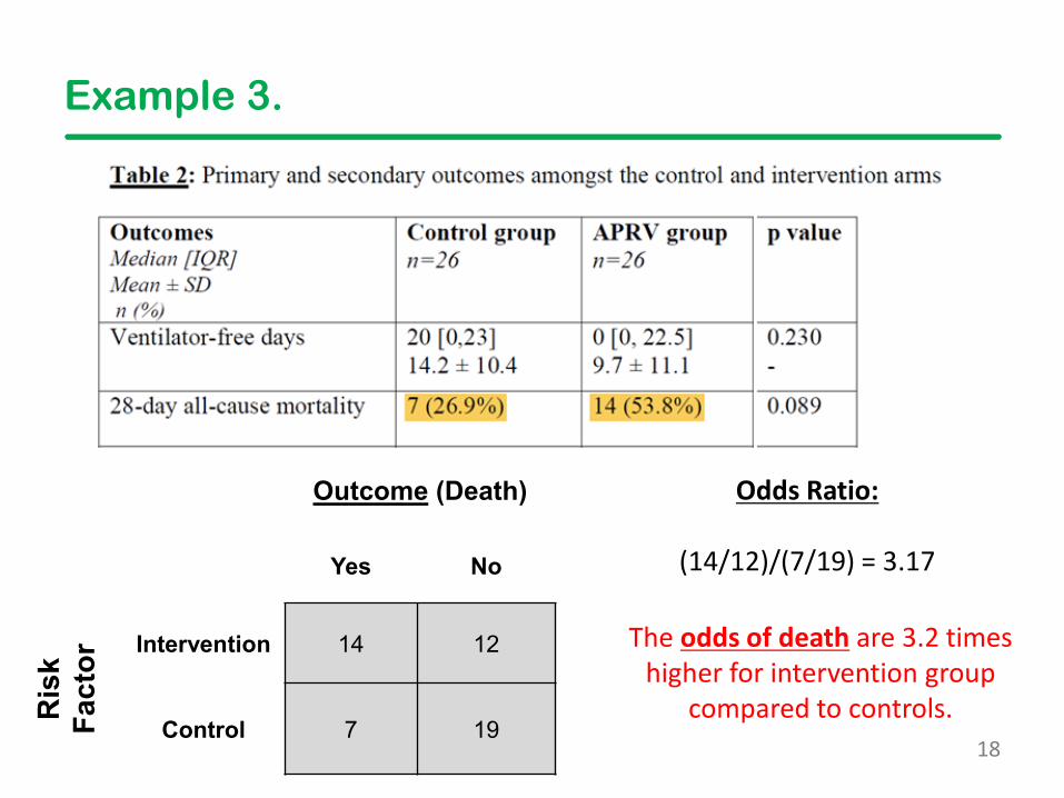
Example 3.
Outcome (Death)
Yes No
Ris
kFa
ctor Intervention 14 12
Control 7 19
Odds Ratio:
(14/12)/(7/19) = 3.17
The odds of death are 3.2 times higher for intervention group
compared to controls.
19
What designs are appropriate?
20
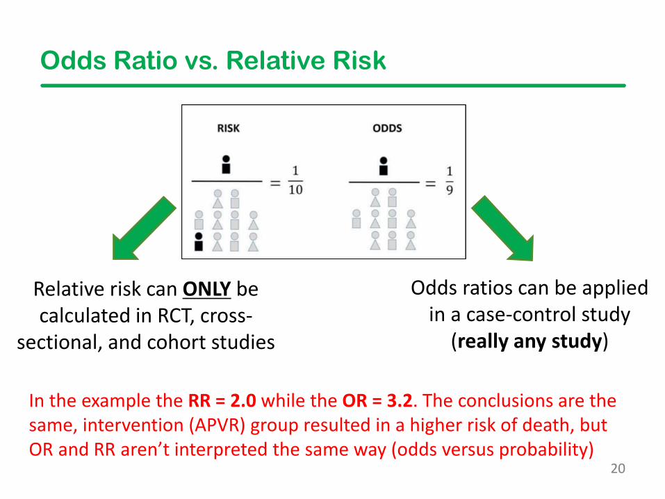
Odds Ratio vs. Relative Risk
Relative risk can ONLY be calculated in RCT, cross-
sectional, and cohort studies
Odds ratios can be applied in a case-control study
(really any study)
In the example the RR = 2.0 while the OR = 3.2. The conclusions are the same, intervention (APVR) group resulted in a higher risk of death, but OR and RR aren’t interpreted the same way (odds versus probability)
21
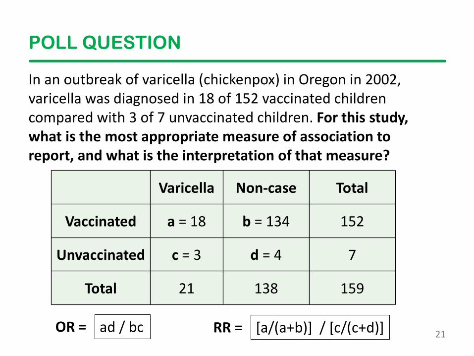
POLL QUESTION
In an outbreak of varicella (chickenpox) in Oregon in 2002, varicella was diagnosed in 18 of 152 vaccinated children compared with 3 of 7 unvaccinated children. For this study, what is the most appropriate measure of association to report, and what is the interpretation of that measure?
Varicella Non-case Total
Vaccinated a = 18 b = 134 152
Unvaccinated c = 3 d = 4 7
Total 21 138 159
ad / bc [a/(a+b)] / [c/(c+d)] OR = RR =
22
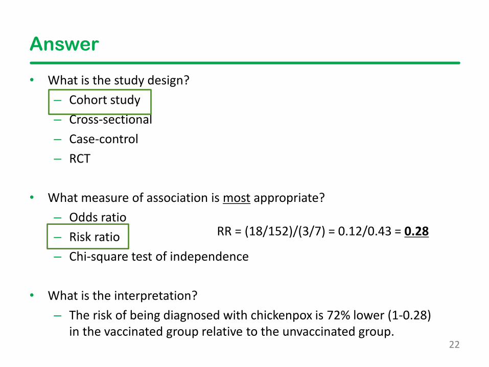
Answer
• What is the study design?– Cohort study– Cross-sectional– Case-control– RCT
• What measure of association is most appropriate?– Odds ratio– Risk ratio– Chi-square test of independence
• What is the interpretation? – The risk of being diagnosed with chickenpox is 72% lower (1-0.28)
in the vaccinated group relative to the unvaccinated group.
RR = (18/152)/(3/7) = 0.12/0.43 = 0.28
23
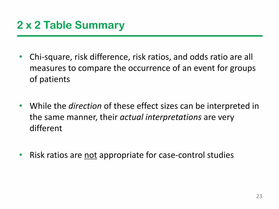
2 x 2 Table Summary
• Chi-square, risk difference, risk ratios, and odds ratio are all measures to compare the occurrence of an event for groups of patients
• While the direction of these effect sizes can be interpreted in the same manner, their actual interpretations are very different
• Risk ratios are not appropriate for case-control studies
24
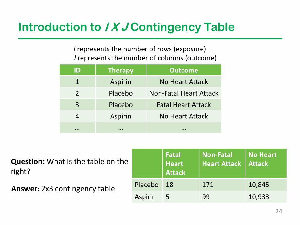
Introduction to I X J Contingency Table
Fatal Heart Attack
Non-Fatal Heart Attack
No Heart Attack
Placebo 18 171 10,845
Aspirin 5 99 10,933
Question: What is the table on the right?
ID Therapy Outcome1 Aspirin No Heart Attack2 Placebo Non-Fatal Heart Attack3 Placebo Fatal Heart Attack4 Aspirin No Heart Attack… … …
I represents the number of rows (exposure)J represents the number of columns (outcome)
Answer: 2x3 contingency table
25
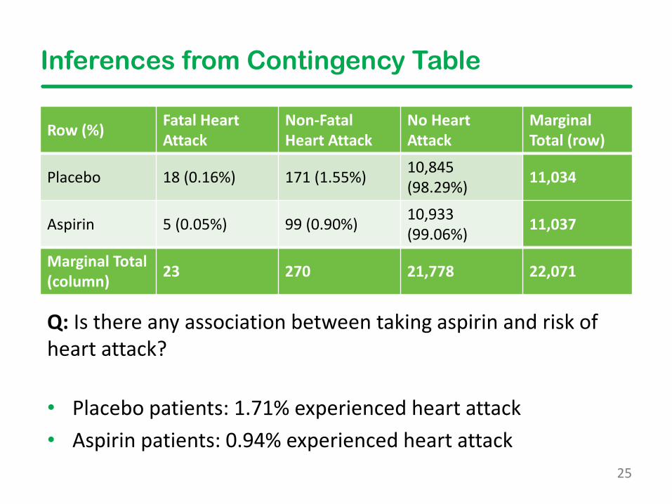
Inferences from Contingency Table
Row (%) Fatal Heart Attack
Non-Fatal Heart Attack
No Heart Attack
Marginal Total (row)
Placebo 18 (0.16%) 171 (1.55%) 10,845 (98.29%) 11,034
Aspirin 5 (0.05%) 99 (0.90%) 10,933 (99.06%) 11,037
Marginal Total (column) 23 270 21,778 22,071
Q: Is there any association between taking aspirin and risk of heart attack?
• Placebo patients: 1.71% experienced heart attack• Aspirin patients: 0.94% experienced heart attack
26
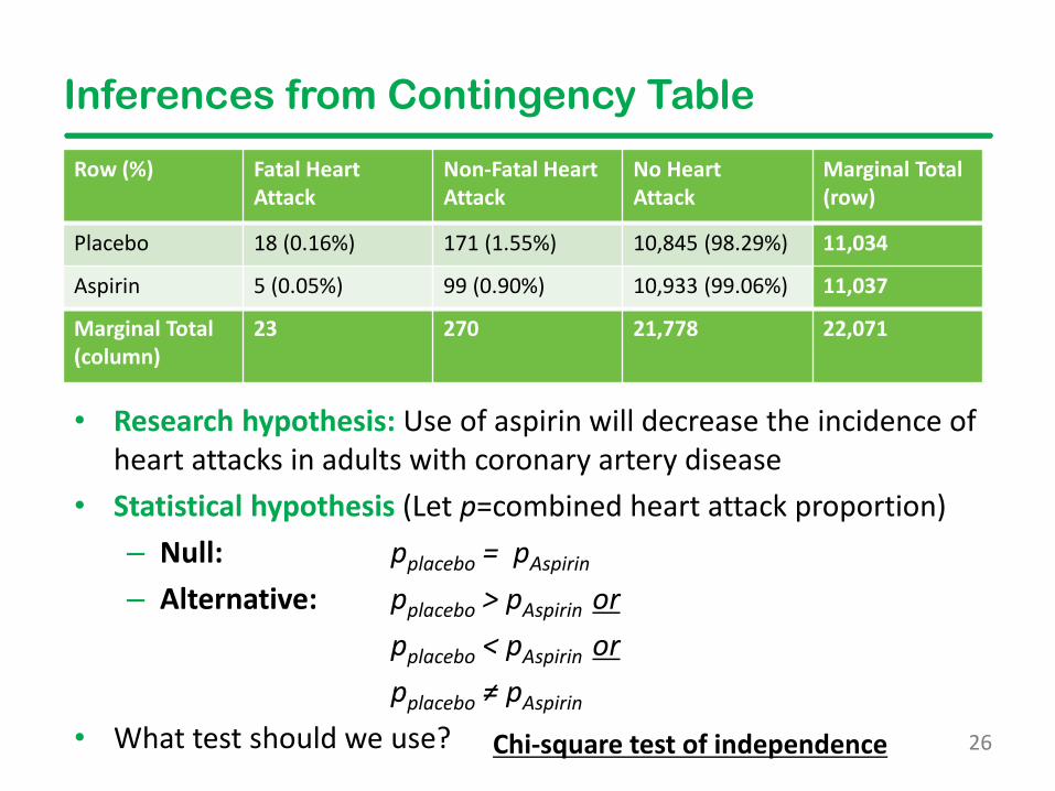
Inferences from Contingency Table
Row (%) Fatal Heart Attack
Non-Fatal Heart Attack
No Heart Attack
Marginal Total (row)
Placebo 18 (0.16%) 171 (1.55%) 10,845 (98.29%) 11,034
Aspirin 5 (0.05%) 99 (0.90%) 10,933 (99.06%) 11,037
Marginal Total (column)
23 270 21,778 22,071
• Research hypothesis: Use of aspirin will decrease the incidence of heart attacks in adults with coronary artery disease
• Statistical hypothesis (Let p=combined heart attack proportion)– Null: pplacebo = pAspirin
– Alternative: pplacebo > pAspirin orpplacebo < pAspirin orpplacebo ≠ pAspirin
• What test should we use? Chi-square test of independence
27
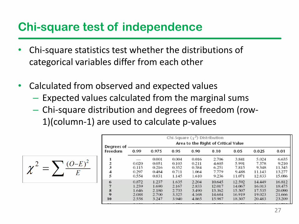
Chi-square test of independence
• Chi-square statistics test whether the distributions of categorical variables differ from each other
• Calculated from observed and expected values – Expected values calculated from the marginal sums– Chi-square distribution and degrees of freedom (row-
1)(column-1) are used to calculate p-values
28
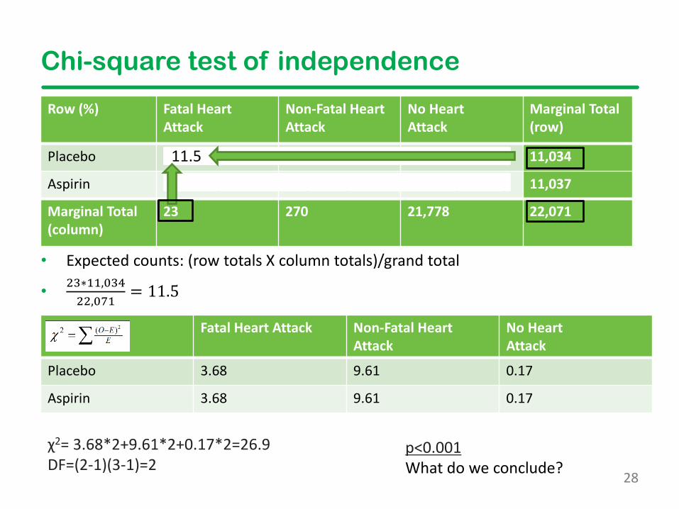
Chi-square test of independence
• Expected counts: (row totals X column totals)/grand total
• 23∗11,03422,071
= 11.5
p<0.001What do we conclude?
Row (%) Fatal Heart Attack
Non-Fatal Heart Attack
No Heart Attack
Marginal Total (row)
Placebo 18 (0.16%) 171 (1.55%) 10,845 (98.29%) 11,034
Aspirin 5 (0.05%) 99 (0.90%) 10,933 (99.06%) 11,037
Marginal Total (column)
23 270 21,778 22,071
χ2= 3.68*2+9.61*2+0.17*2=26.9 DF=(2-1)(3-1)=2
11.5
Fatal Heart Attack Non-Fatal Heart Attack
No Heart Attack
Placebo 3.68 9.61 0.17
Aspirin 3.68 9.61 0.17
29
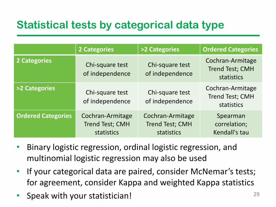
Statistical tests by categorical data type
2 Categories >2 Categories Ordered Categories
2 Categories Chi-square test of independence
Chi-square test of independence
Cochran-Armitage Trend Test; CMH
statistics
>2 Categories Chi-square test of independence
Chi-square test of independence
Cochran-Armitage Trend Test; CMH
statistics
Ordered Categories Cochran-Armitage Trend Test; CMH
statistics
Cochran-Armitage Trend Test; CMH
statistics
Spearman correlation;
Kendall's tau
• Binary logistic regression, ordinal logistic regression, and multinomial logistic regression may also be used
• If your categorical data are paired, consider McNemar’s tests; for agreement, consider Kappa and weighted Kappa statistics
• Speak with your statistician!
Fellows Introduction to Research Training
Categorical Data Analysis and Interpretation
Scott Gillespie, MS, MSPHAssociate Director
Pediatrics Biostatistics CoreEmory University + CHOA
October 29, 2021