catching killers uea dec 2012
TRANSCRIPT
Catching Killers: Geographic Profiling from criminology to ecology
Mark StevensonSchool of Biological and Chemical
Sciences, Queen Mary, University of London

AcknowledgementsTexas State•Kim RossmoQueen Mary•Bob Verity•Steve Le ComberAin Shams University, Cairo•Ali Hassan
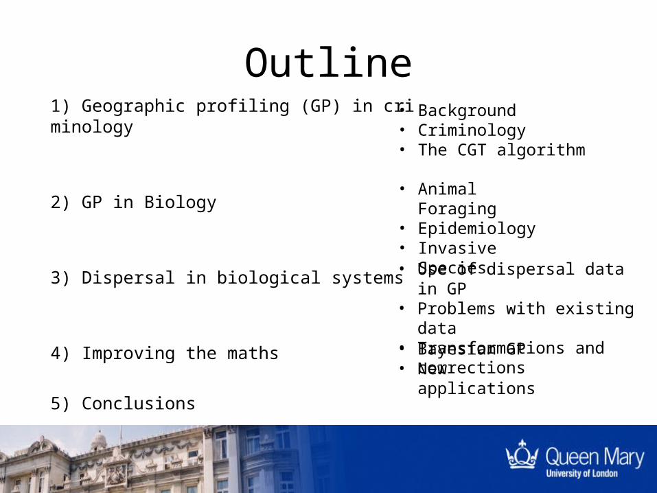
Outline1) Geographic profiling (GP) in criminology
2) GP in Biology
3) Dispersal in biological systems
4) Improving the maths
5) Conclusions
• Background• Criminology• The CGT algorithm
• Animal Foraging
• Epidemiology• Invasive
Species
• Bayesian GP• New
applications
• Use of dispersal data in GP
• Problems with existing data
• Transformations and corrections
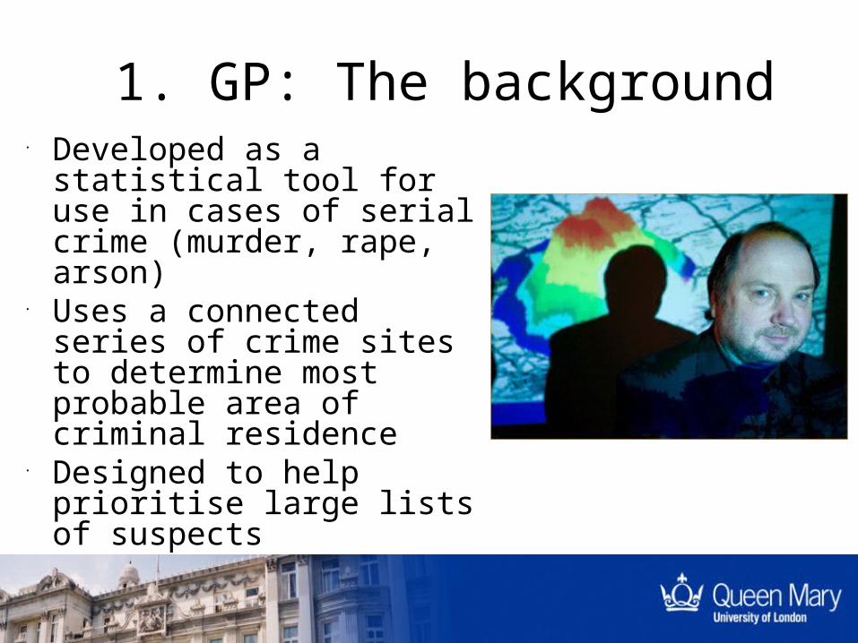
1. GP: The background• Developed as a statistical tool for use in cases of serial crime (murder, rape, arson)
• Uses a connected series of crime sites to determine most probable area of criminal residence
• Designed to help prioritise large lists of suspects
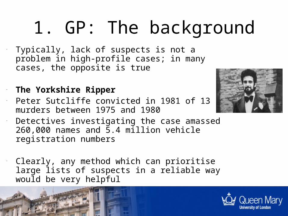
• Typically, lack of suspects is not a problem in high-profile cases; in many cases, the opposite is true
• The Yorkshire Ripper• Peter Sutcliffe convicted in 1981 of 13 murders between 1975 and 1980
• Detectives investigating the case amassed 260,000 names and 5.4 million vehicle registration numbers
• Clearly, any method which can prioritise large lists of suspects in a reliable way would be very helpful
1. GP: The background

1. GP: Criminology• Grew from the field of environmental criminology.
• This field was formalised by Brantingham and Brantingham in the 80’s
• They were interested in the activity space and awareness space of criminals to predict how they would act.
• Kim was their PhD student• He turned the problem around and used the location of the offences to predict the home location of the offender.

1. GP: The Criminal Geographic Targeting
algorithm•So Kim came up with this:
Where
and
Key parameters are B, f and g
These two functions describe a switch which locates the buffer zone of diameter B
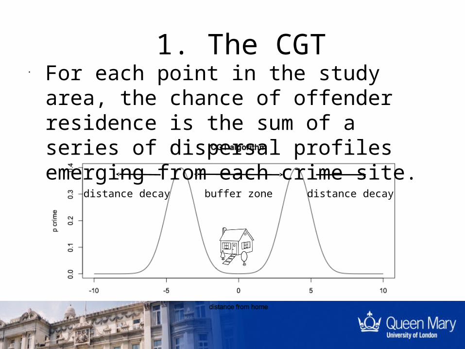
1. The CGT• For each point in the study area, the chance of offender residence is the sum of a series of dispersal profiles emerging from each crime site.
buffer zonedistance decay distance decay
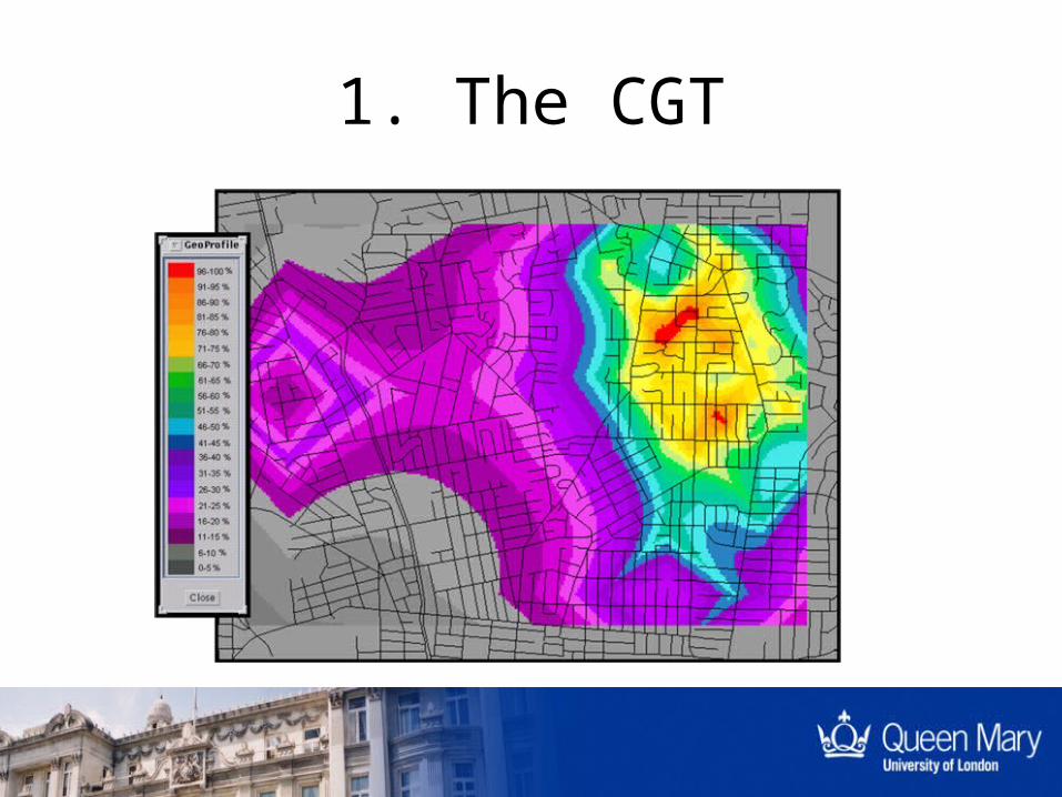
1. The CGT
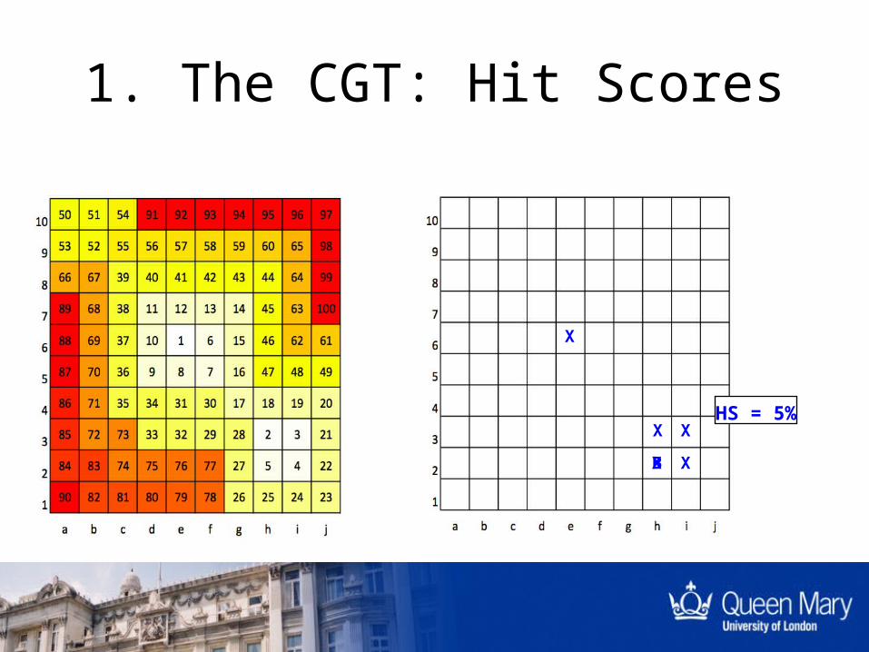
X
X
X XXB
HS = 5%
1. The CGT: Hit Scores
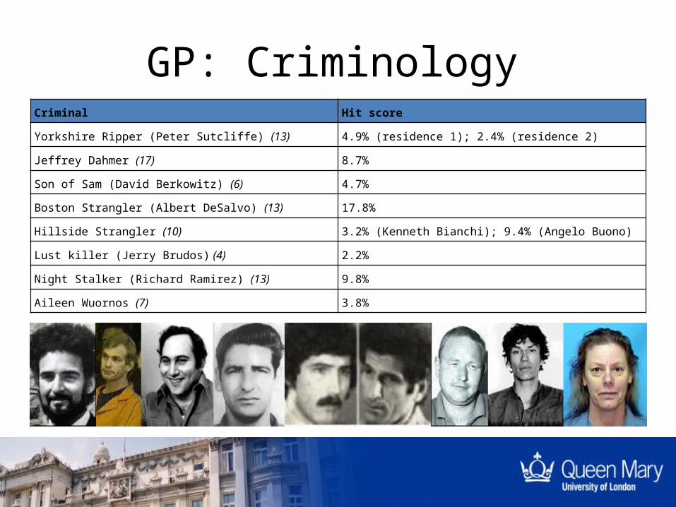
GP: CriminologyCriminal Hit score
Yorkshire Ripper (Peter Sutcliffe) (13) 4.9% (residence 1); 2.4% (residence 2)
Jeffrey Dahmer (17) 8.7%
Son of Sam (David Berkowitz) (6) 4.7%
Boston Strangler (Albert DeSalvo) (13) 17.8%
Hillside Strangler (10) 3.2% (Kenneth Bianchi); 9.4% (Angelo Buono)
Lust killer (Jerry Brudos) (4) 2.2%
Night Stalker (Richard Ramirez) (13) 9.8%
Aileen Wuornos (7) 3.8%
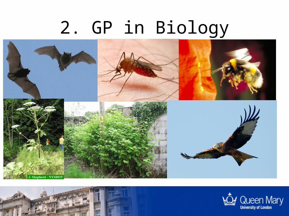
2. GP in Biology
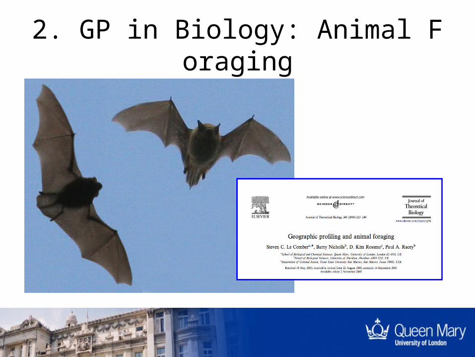
2. GP in Biology: Animal Foraging
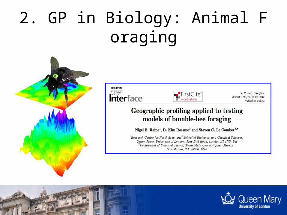
2. GP in Biology: Animal Foraging
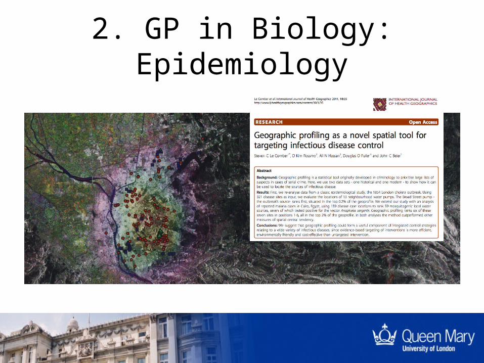
2. GP in Biology: Epidemiology
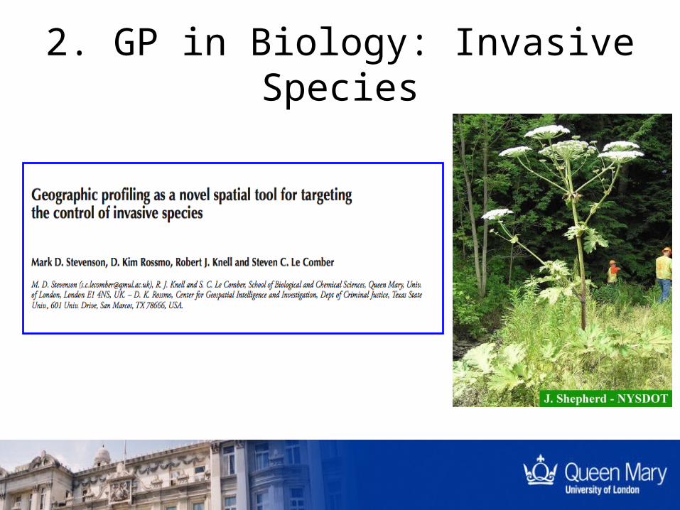
2. GP in Biology: Invasive Species

2. GP in Biology: Invasive Species
• Invasive species cause enormous damage to crops, pastures and forests around the world, with an estimated cost of $29 billion dollars annually
• Invasive species are now viewed as the second most important driver of world biodiversity loss behind habitat destruction and have been identified as a significant component of global change
• Identifying source populations of invasive species in the early stages of an invasion can be used to target control efforts more efficiently and more effectively
2. GP in Biology: Invasive Species
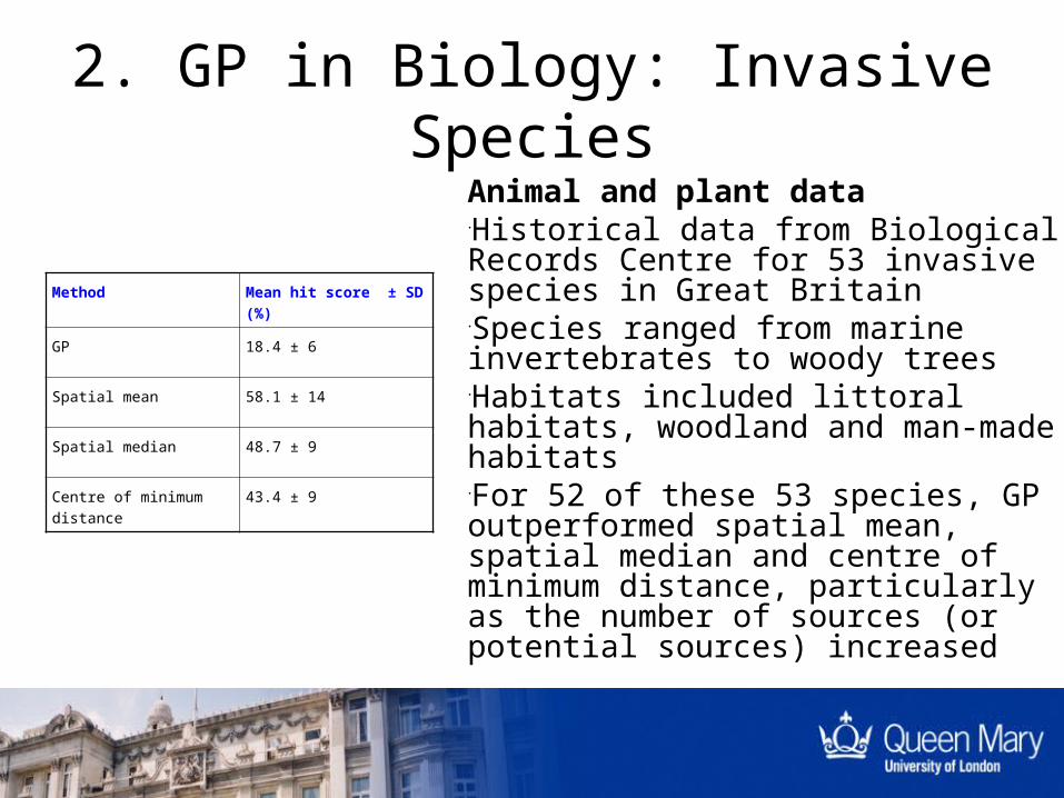
Animal and plant data•Historical data from Biological Records Centre for 53 invasive species in Great Britain•Species ranged from marine invertebrates to woody trees•Habitats included littoral habitats, woodland and man-made habitats•For 52 of these 53 species, GP outperformed spatial mean, spatial median and centre of minimum distance, particularly as the number of sources (or potential sources) increased
Method Mean hit score ± SD (%)
GP 18.4 ± 6
Spatial mean 58.1 ± 14
Spatial median 48.7 ± 9
Centre of minimum distance
43.4 ± 9
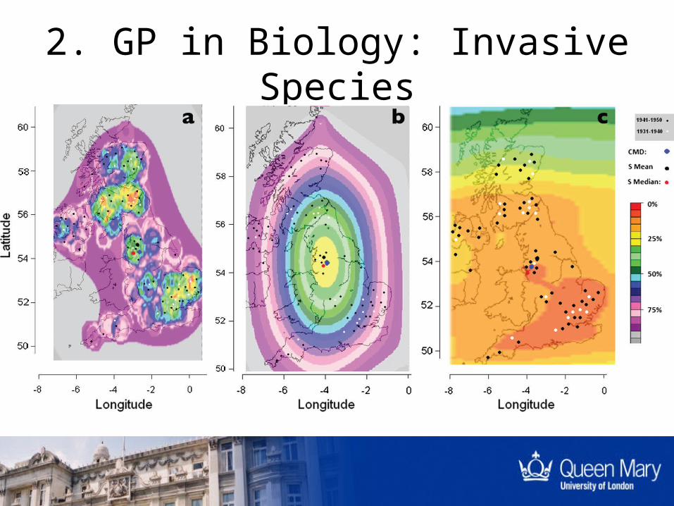
2. GP in Biology: Invasive Species
2. GP in Biology: Invasive Species
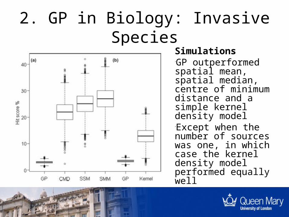
Simulations•GP outperformed spatial mean, spatial median, centre of minimum distance and a simple kernel density model•Except when the number of sources was one, in which case the kernel density model performed equally well
3. Dispersal in Biological systems
•So how do I use GP for my particular species?•Need just point pattern data•And some form of dispersal distribution•Fortunately, there are lots available!•Dispersal is an active research area•Many papers publish histograms of dispersal distance
3. Dispersal in Biological systems
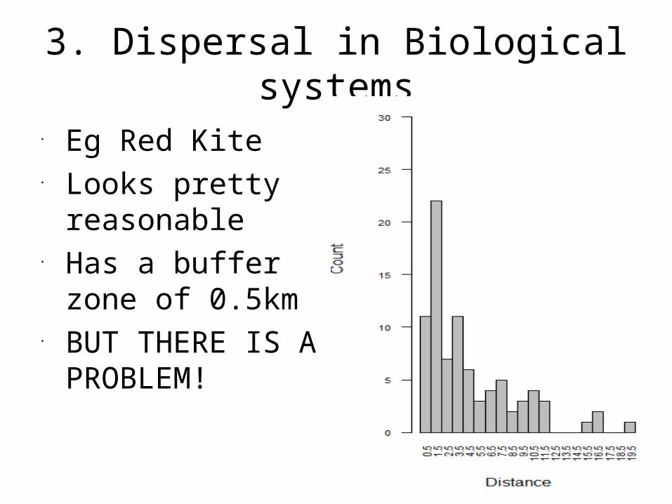
• Eg Red Kite• Looks pretty reasonable
• Has a buffer zone of 0.5km
• BUT THERE IS A PROBLEM!
3. Dispersal in Biological systems
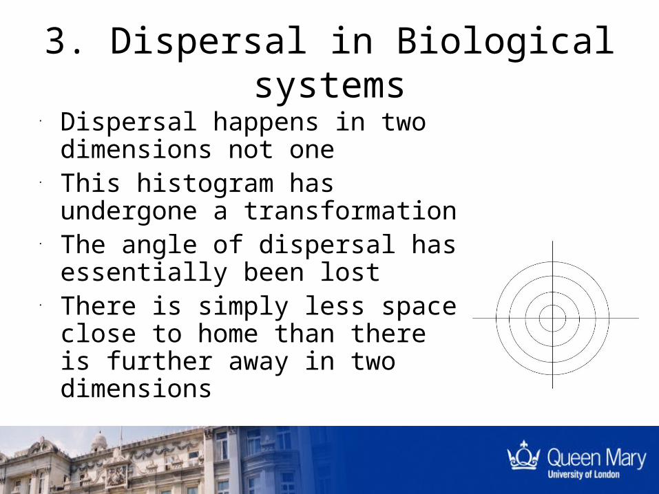
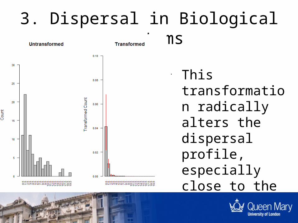
• Dispersal happens in two dimensions not one
• This histogram has undergone a transformation
• The angle of dispersal has essentially been lost
• There is simply less space close to home than there is further away in two dimensions
3. Dispersal in Biological systems
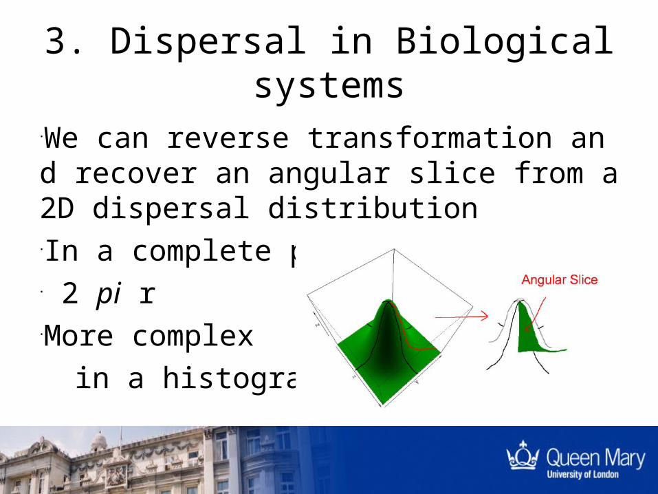
•We can reverse transformation and recover an angular slice from a 2D dispersal distribution•In a complete pdf it is easy• 2 pi r•More complex in a histogram
3. Dispersal in Biological systems
• This transformation radically alters the dispersal profile, especially close to the source.
3. Dispersal in Biological systems
• This error is very prevalant in the literature
• Reviewing it at the moment but 50 papers already and growing
• Don’t use 1D histograms to represent 2D dispersal
• Use the transformation!

4. Improving the maths of GP
•The mathematics of GP has – understandably – been driven by the need for practical solutions to the problems encountered by law enforcement agenciesThe CGT •Doesn’t describe a true probability surface•Equation should use a product rather than a sum•Is the buffer zone real? However, it is highly effective…why???
4. Improving the maths of GP
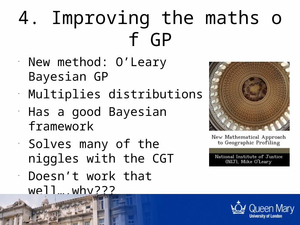
• New method: O’Leary Bayesian GP
• Multiplies distributions• Has a good Bayesian framework
• Solves many of the niggles with the CGT
• Doesn’t work that well….why???

4. Improving the maths of GP
• The results for differing number of sources from the Ecography paper led us in a new direction.
• Dealing with the possibility of multiple sources became an important issue to differentiate model performance.
• All boils down to this summation vs multiplication
4. Improving the maths of GP
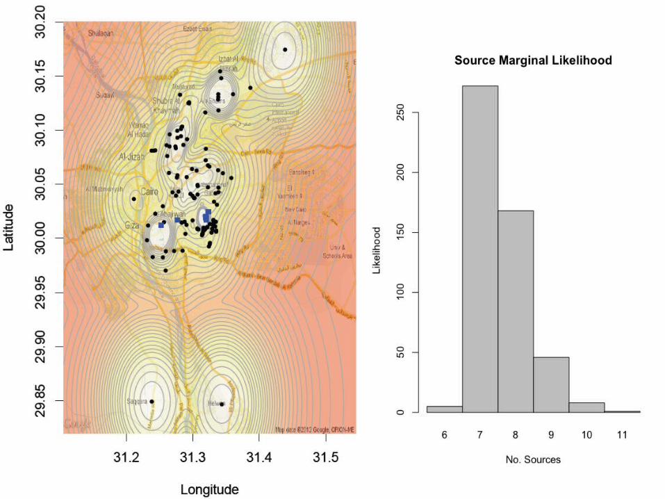
The Dirichlet Process model was born!•Addresses the issue of multiple sources within a well-defined Bayesian framework•Dirichlet Process assigns crimes to sources (does not require the number of groups to be specified in advance)•Uses a concentration parameter, alpha, to describe the process of cluster formation*(for the technically minded, we place a diffuse hyperprior over alpha, favouring model flexibility over statistical power)
4. Improving the maths of GP
How the model works1.Calculates the probability of the data for a given set of sources, as in the O’Leary model2.Uses Bayes’ Rule to invert the problem, calculating the probability of the source locations, given the data3.Integrates over all possible groupings…

4. Improving the maths of GP
• but there are lots of possible groupings
• B100 is47585391276764833658790768841387207826363669686825611466616334637559114497892442622672724044217756306953557882560751
• or 10115. For comparison, there are approximately15747724136275002577605653961181555468044717914527116709366231425076185631031296or 1080 protons in the universe (Eddington’s number)
4. Improving the maths of GP
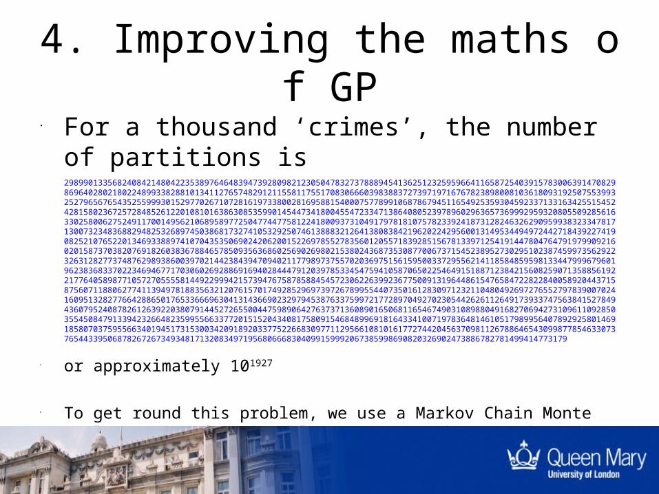
• For a thousand ‘crimes’, the number of partitions is29899013356824084214804223538976464839473928098212305047832737888945413625123259596641165872540391578300639147082986964028021802248993382881013411276574829121155811755170830666039838837273971971676782389800810361809319250755399325279656765435255999301529770267107281619733800281695881540007577899106878679451165492535930459233713316342551545242815802367257284852612201081016386308535990145447341800455472334713864080523978960296365736999295932080550928561633025800627524911700149562106895897725047744775812241800937310491797818107578233924187312824632629095993832334781713007323483688294825326897450386817327410532925074613888321264138083842196202242956001314953449497244271843922741908252107652201346933889741070435350690242062001522697855278356012055718392851567813397125419144780476479197990921602015873703820769182603836788465785093563686025690269802153802436873530877006737154523895273029510238745997356292232631282773748762989386003970214423843947094021177989737557020369751561595003372955621411858485959813344799967960196238368337022346946771703060269288691694028444791203978533454759410587065022546491518871238421560825907135885619221776405898771057270555581449229994215739476758785884545723062263992367750091319644861547658472282284005892044371587560711880627741139497818835632120761570174928529697397267899554407350161283097123211048049269727655279783900702416095132827766428865017653366696304131436690232979453876337599721772897049270230544262611264917393374756384152784943607952408782612639220380791445272655004475989064276373713608901650681165467490310898804916827069427310961109285035545084791339423266482359955663377201515204340817580915468489969181643341007197836481461051798995640789292580146918580703759556634019451731530034209189203377522668309771129566108101617727442045637098112678864654309987785463307376544339506878267267349348171320834971956806668304099159992067385998690820326902473886782781499414773179
• or approximately 101927
• To get round this problem, we use a Markov Chain Monte Carlo routine for Dirichlet Processes that is adapted from Neal (2000)
4. Improving the maths of GP
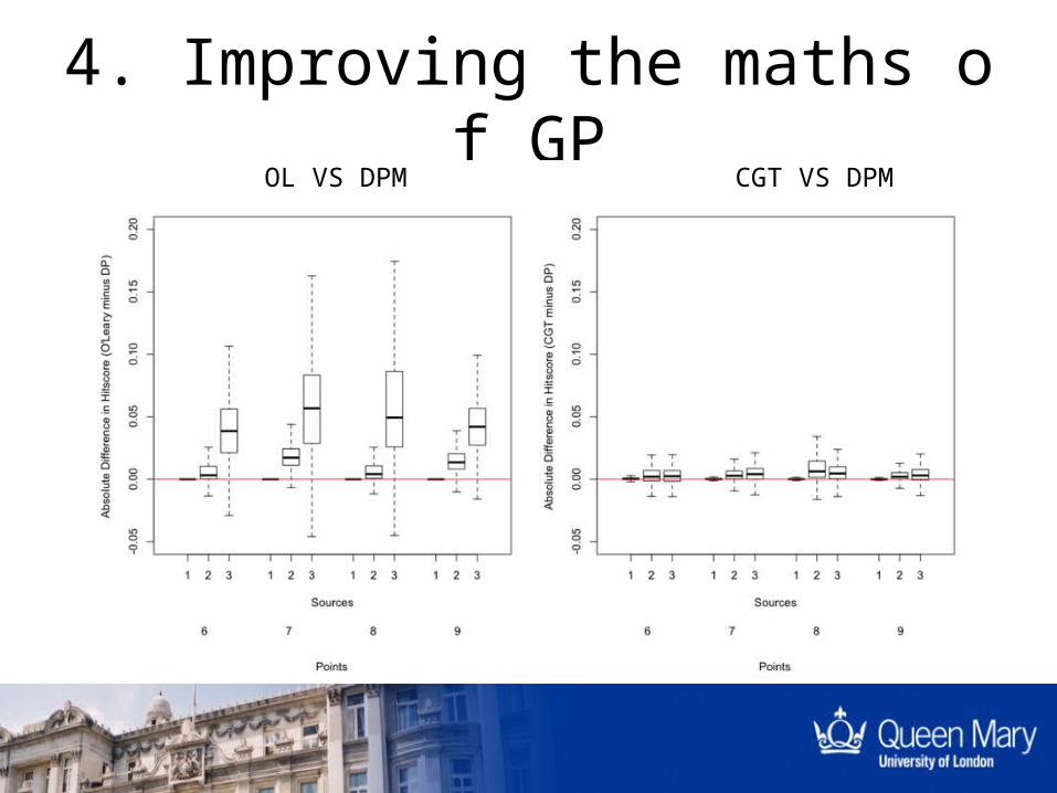
OL VS DPM CGT VS DPM
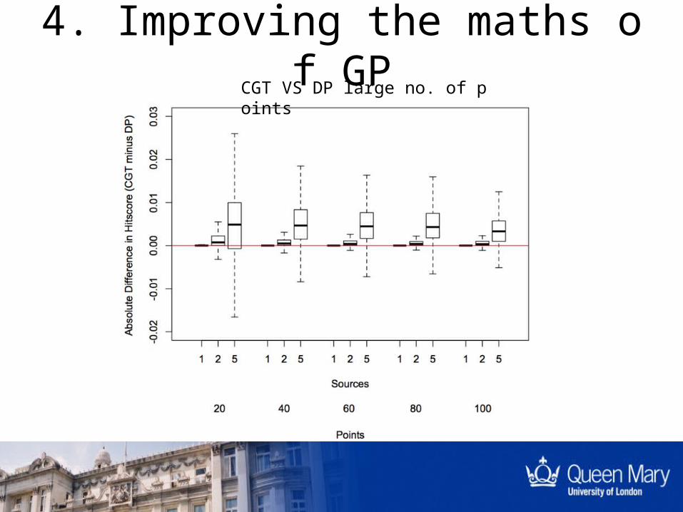
4. Improving the maths of GPCGT VS DP large no. of p
oints

4. Improving the maths of GP
• Now we have a model that is both theoretically sound and performs well!
• So let’s test it out…
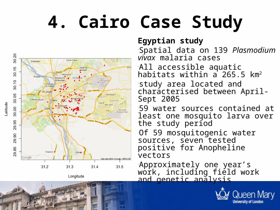
4. Cairo Case StudyEgyptian study•Spatial data on 139 Plasmodium vivax malaria cases•All accessible aquatic habitats within a 265.5 km2
•study area located and characterised between April-Sept 2005•59 water sources contained at least one mosquito larva over the study period•Of 59 mosquitogenic water sources, seven tested positive for Anopheline vectors •Approximately one year’s work, including field work and genetic analysis
4. Cairo Case study•Run all three approaches and see which one does the best•O’Learys simple Bayesian•Rossmos CGT•Our DPM model
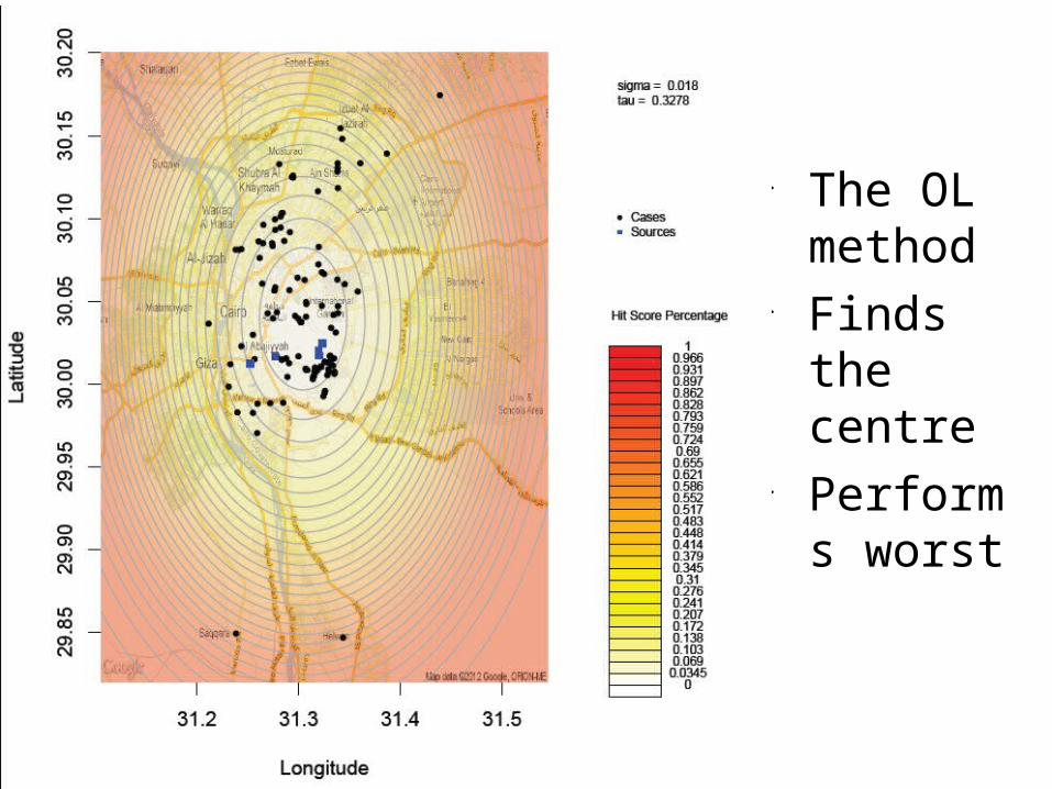
• The OL method
• Finds the centre
• Performs worst
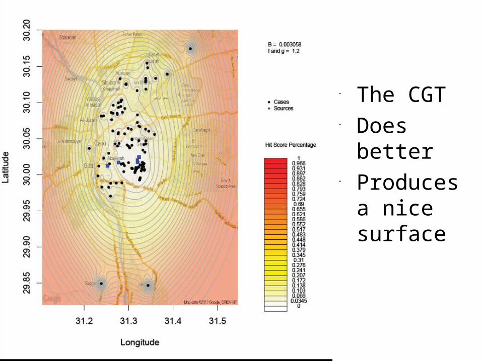
• The CGT• Does better
• Produces a nice surface
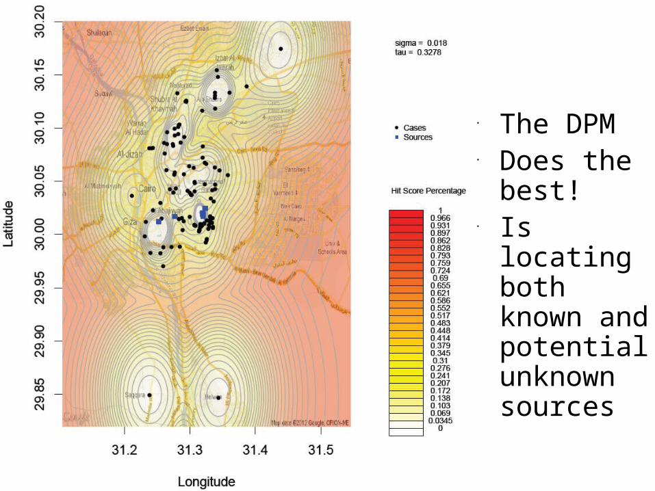
• The DPM• Does the best!
• Is locating both known and potential unknown sources
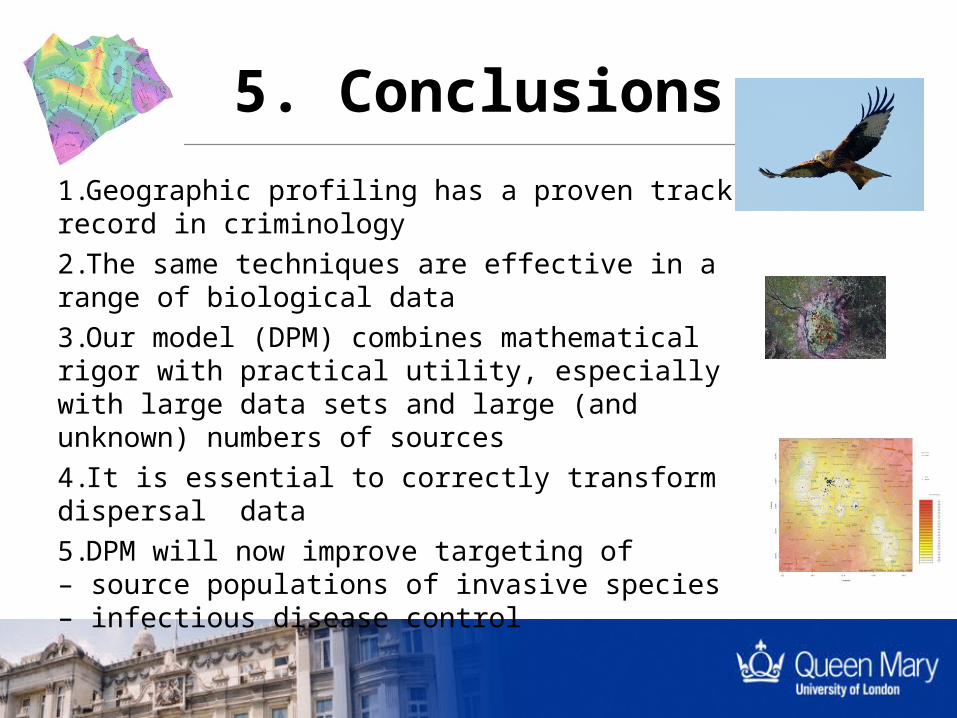
5. Conclusions1.Geographic profiling has a proven track record in criminology2.The same techniques are effective in a range of biological data3.Our model (DPM) combines mathematical rigor with practical utility, especially with large data sets and large (and unknown) numbers of sources4.It is essential to correctly transform dispersal data5.DPM will now improve targeting of– source populations of invasive species– infectious disease control