capm and fama and french

Estimation of Expected Return:

The Fama and French Three-Factor Model

Vs.

The Chen, Novy-Marx and Zhang Three-

Factor Model

Authors:

David Kilsgård

Filip Wittorf

Master thesis in finance

Spring 2011

Supervisor: Göran Andersson

Contact: [email protected], [email protected]

Department of Business Administration at Lund University

Abstract

The study examines the adequacy of the measurement of the cross-section of expected stock

returns on the London Stock Exchange of the recent three-factor model introduced by Chen,

Novy-Marx and Zhang against that of the Fama and French three-factor model. The former

model use factors in addition to the market factor based on profitability and investment while

the latter model use factors based on size and book-to-market equity. The models are tested

together with the CAPM on a number of anomalies based trading strategies. It is found that

the three-factor models consistently outperforms the CAPM and that the model by Chen,

Novy-Marx and Zhang in general is not able to outperform the Fama and French three-factor

model during the time period tested on the London Stock Exchange.

Keywords: Fama and French Three-Factor Model, CAPM, Asset pricing, Anomalies, Cost of

Equity, Chen, Novy-Marx and Zhang.

Acknowledgements

We thank our supervisor Göran Andersson for his valuable advices in the writing process.

Table of Content

Introduction ............................................................................................................................................. 1

1.1 Background .................................................................................................................................... 1

1.2 Problem discussion ........................................................................................................................ 4

1.3 Purpose .......................................................................................................................................... 5

1.4 Limitations ..................................................................................................................................... 5

1.5 Outline ........................................................................................................................................... 6

1.6 Definitions ..................................................................................................................................... 6

Theoretical Background .......................................................................................................................... 7

2.1 Cost of Equity ................................................................................................................................ 7

2.2 The Capital Asset Pricing Model (CAPM) ....................................................................................... 7

2.3 The Fama French Three-Factor Model (FF3) ................................................................................. 9

2.4 The Chen, Novy-Marx and Zhang Three-Factor Model (CNMZ) .................................................. 10

2.5 Explanatory variables (FF3) ......................................................................................................... 12

2.5.1 SMB....................................................................................................................................... 13

2.5.2 HML ...................................................................................................................................... 13

2.5.3 Rm-Rf .................................................................................................................................... 14

2.6 Explanatory variables (CNMZ) ..................................................................................................... 14

2.6.1 INV ........................................................................................................................................ 16

2.6.2 ROE ....................................................................................................................................... 17

2.6.3 MKT....................................................................................................................................... 17

2.7 Dependent variables ................................................................................................................... 17

2.7.1 Dependent variables (FF3) ................................................................................................... 17

2.7.2 The risk-free interest rate ..................................................................................................... 18

2.7.3 Dependent variables (CNMZ) .............................................................................................. 18

2.7.4 The risk-free interest rate ..................................................................................................... 19

2.8 Previous research ........................................................................................................................ 19

Method .................................................................................................................................................. 21

3.1 Selection ...................................................................................................................................... 21

3.1.1 Time period .......................................................................................................................... 22

3.1.2 Data ...................................................................................................................................... 22

3.1.3 Sample .................................................................................................................................. 23

3.2 Portfolios’ construction FF3 ........................................................................................................ 23

3.3 Portfolios’ construction CNMZ .................................................................................................... 24

3.4 Explanatory variables .................................................................................................................. 25

3.4.1 MKT....................................................................................................................................... 25

3.4.2 SMB....................................................................................................................................... 25

3.4.3 HML ...................................................................................................................................... 26

3.4.4 INV ........................................................................................................................................ 27

3.4.5 ROE ....................................................................................................................................... 28

3.5 Dependent variables (FF3) .......................................................................................................... 28

3.6 Dependent variables (CNMZ) ..................................................................................................... 30

3.7 The risk-free interest rate............................................................................................................ 30

3.8 Test Portfolios.............................................................................................................................. 30

3.8.1 Calendar-time Factor Regressions ........................................................................................ 30

3.8.2 Earnings Surprises ................................................................................................................ 31

3.8.3 Net Stock Issues .................................................................................................................... 32

3.8.4 Asset Growth ........................................................................................................................ 32

3.8.5 Book-to-Market Equity ......................................................................................................... 33

3.8.6 Industries .............................................................................................................................. 33

Analysis and Results .............................................................................................................................. 34

4.1 Explanatory variables .................................................................................................................. 34

4.1.1 Descriptive statistics ............................................................................................................. 34

4.1.2 SMB and HML ....................................................................................................................... 34

4.1.3 INV and ROE ......................................................................................................................... 35

4.2 Results of the regressions for the FF3 ......................................................................................... 37


4.3 Results of the regressions for the CNMZ ..................................................................................... 39


4.4 Results for the regressions including all three models ............................................................... 40

4.4.1 Earnings Surprises ................................................................................................................ 40

4.4.2 Net Stock Issues .................................................................................................................... 42

4.4.3 Asset Growth ........................................................................................................................ 43

4.4.4 Book-to-Market Equity ......................................................................................................... 45

4.4.5 Industries .............................................................................................................................. 47

4.5 Validity and reliability ...................................................................................................................... 48

4.5.1 Multicollinearity ................................................................................................................... 48

4.5.2 Homoscedasticity and heteroscedasticity ............................................................................ 48

4.5.3 Database reliability ............................................................................................................... 49

Conclusion ............................................................................................................................................. 50

5.1 Conclusions .................................................................................................................................. 50

5.2 Future research ........................................................................................................................... 53

References ............................................................................................................................................. 54

Articles ............................................................................................................................................... 54

Books ................................................................................................................................................. 57

Internet sources ................................................................................................................................ 57

Databases .......................................................................................................................................... 57

Laws ................................................................................................................................................... 58

Appendix ................................................................................................................................................ 59

List of figures and tables

Figure 1: FTSE UK Index Series Family Tree ................................................................................................................ 6

Figure 2: Sorting by size ..................................................................................................................................................... 12

Figure 3: Sorting by BE/ME .............................................................................................................................................. 12

Figure 4: Sorting on size and BE/ME into six portfolios ...................................................................................... 13

Figure 5 Sorting on I/A ....................................................................................................................................................... 15

Figure 6: Sorting by ROE .................................................................................................................................................... 15


Figure 8: Sorting on I/A, ROE, and Size into 27 portfolios .................................................................................. 16

Figure 7: The 25 dependent portfolios ........................................................................................................................ 18

Figure 8: Portfolios triple sorted on INV, ROE and size ....................................................................................... 24


Figure 10: Sorting by BE/ME............................................................................................................................................ 26

Figure 11: Sorting on size and BE/ME ......................................................................................................................... 27

Figure 12: Sorting on I/A ................................................................................................................................................... 27

Figure 13: Sorting on ROE ................................................................................................................................................. 28

Figure 14: 4x4 matrix of the 16 dependent portfolios .......................................................................................... 29

Table 1: FF3 explanatory variables data, .................................................................................................................... 35

Table 2: CNMZ explanatory variables data, ............................................................................................................... 36

Table 3: FF3 16 portfolios regression data ................................................................................................................ 37

Table 4: CNMZ 27 portfolios regression data ........................................................................................................... 39

Table 5: FF3 explanatory variables correlation data ............................................................................................. 48

Table 6: CNMZ explanatory variables correlation data ........................................................................................ 48

Table 7: SMB values .............................................................................................................................................................. 59

Table 8: Descripitive statistics of INV and ROE........................................................................................................ 60

Table 9: Descripitive statistics of SMB and HML ..................................................................................................... 61

Table 10: Earnings Surprises ........................................................................................................................................... 62

Table 11: Net Stock Issues and Asset Growth ........................................................................................................... 63

Table 12: Book-to-market equity ................................................................................................................................... 64

Table 13: Book-to-market equity R2 values ............................................................................................................... 65

Table 14: Ten Industry Portfolios .................................................................................................................................. 66

Table 15: Industry sectors of the Ten Industry Portfolios .................................................................................. 67

Table 16: GQ tests on Earnings Surprises, Net Stock Issues and Asset Growth ........................................ 68

Table 17: GQ tests on Ten Industry Portfolios and Book-to-Market Equity ............................................... 69

Table 18: Companies included in the sample ........................................................................................................... 70

1

Chapter 1

Introduction

This first chapter introduces the background of the dissertation. In addition, the chapter

contains the problem discussion and purpose of the thesis. Furthermore, it describes the

limitations of the study, the outline of the thesis as well as the definitions of specific terms.

1.1 Background

Estimating expected stock returns and calculating the cost of equity lies at the heart of several

financial and economic decisions, ranging from estimating expected returns for asset

allocation and evaluate mutual fund performance to decisions regarding capital budgeting and

stock valuation.1 Making the correct decisions will greatly impact the future value of a

company or the future performance of a portfolio of assets. Therefore, over the years several

different models have been created to estimate, as accurately as possible, these variables in

order to facilitate the complex decision making process for managers and investors alike.

One of the earlier models called the Capital Asset Pricing Model (hereafter CAPM) was

developed in the 1960s, individually by Jack Treynor2, William Sharpe3, John Lintner4 and

Jan Mossin5.

�� = �� + �� − ��

The equation is explained in the theory section

However, the model has since then been the focus of a great deal of criticism, among the

earliest were Roll in 19776, Ross in 19767 and Roll and Ross in 19808. In 1977 Roll9 stated,

which has come to be known as Roll’s critique, that it is not possible to test the CAPM; a

statement based on two main points regarding the market portfolio. The first point is that the

1 Chen, Novy-Marx & Zhang (2011)

2 Treynor (1961) (1962)

3 Sharpe (1964)

4 Lintner (1965)

5 Mossin (1966)

6 Roll (1977)

7 Ross (1976)

8 Roll & Ross (1980)

9 Roll (1977)

2

CAPM’s validity is comparable to the market, with respect to all investment opportunities,

being mean-variance efficient, or in other words the assumption that the CAPM equation

holds is equal to the market portfolio being mean-variance efficient. The second point is that

the true market portfolio is unknown since the true market portfolio would need to include all

available traded and non-traded assets e.g. commodities, human capital, real estate, basically

everything with any sort of value. Hence, the model is not testable unless the market

portfolio’s true composition is known, in other words all investment opportunities (assets) are

observable and included in the market portfolio.

A year earlier Ross10 published a solution to Roll’s critique, called the arbitrage pricing theory

(APT). The benefits of the APT are that it holds in disequilibrium and not only in equilibrium

situations and it allows for more than one explanatory factor. Furthermore, there is no

obligation, unlike in CAPM, for the market portfolio to be mean-variance efficient and

therefore the market portfolio is of little consequence for the APT.11 In 1980 Roll and Ross12

published a research paper in which they empirically tested the APT. Based on the result of

past empirical work, which had concluded that there might exists several factors in the

processes of generating asset returns, they investigated whether those factors exist and if they

are associated with a risk premium. With their basic test on expected returns on equities

traded on the New York and American Exchanges, the authors identified that definitely three,

possibly four, factors are present and carry a risk premium or a price as the authors refer to

it13. The presence of more than just one factor casts doubt on the CAPM’s ability to explain

asset returns, being a one factor model, as well as the validity of its results.

Furthermore in 1995, Jagannathan and McGrattan argued that a large portion of the required

rate of return that the investors have on a company cannot be explained by the CAPM14. In

addition to Roll, Bartholdy and Peare also argue that since the world market portfolio is not

observable it is not even possible to estimate the CAPM15. In addition, Friend and Blume

argued that the CAPM estimates the cost of equity for low-beta stocks too low, and the

estimates for high-beta stocks are too high; a result from empirical work which states that the

10

Ross (1976) 11

Ross (1976) 12

Roll & Ross (1980) 13

Roll & Ross (1980) 14

Jagannathan & McGrattan (1995) 15

Bartholdy & Peare (2005)

3

relation between average return and beta is flatter than predicted by the model16. According to

Jagannathan and McGrattan the poor empirical record of the model17 might be the result of

too many simplifying assumptions, hence theoretical failings of the model18. Further, Banz

stated that there is a size effect on returns because low market-value stocks earned a higher

return than was predicted by the CAPM19. In the early part of the 90’s Eugene Fama and

Kenneth French, who are among the loudest critics of the CAPM, argued that the market beta

alone is not enough to explain expected returns20 Fama and French found that small stocks

and value stocks, stocks with high book-to-market equity ratios (BE/ME), have high average

returns compared to big stocks and growth stocks, stocks with low book-to-market equity

ratios, that are not being captured by their market beta’s21.

In a response to the limitations of the CAPM, Fama and French presented their model in 1993

called the Fama French Three Factor-Model (hereafter called FF3). The model included two

additional explanatory variables, beside the explanatory variable of the overall market factor

of the CAPM, the two factors relate to firm size and book-to-market value of equity22.

�� − �� = �� − �� + �� + ��

� ��


By expanding the CAPM with these two additional factors the model´s level of explanation

increased considerably23.

However, as with the CAPM the FF3 has been the target of criticism from for instance

Lakonishok, Shleifer and Vishny and Haugen who argue that due to systematic overreaction

by investors to corporate news; the subsequent unrealistic predictions of possible future high

or low growth, and the size and book to-market equity effects are due to the overreaction

rather than compensation for risk bearing. The overreaction will lead to underpricing of value

stocks and overpricing of growth stocks.24 Furthermore, Berk states that companies with small

market capitalization will due to mispricing or economic risk by construction earn higher

16

Friend & Blume (1970) 17

Fama & French (2004) 18

Jagannathan & McGrattan (1995) 19

Banz (1981) 20





Lakonishok, Shleifer & Vishny (1994) Haugen (1995)

4

mean returns.25 In addition, in a study by Ferson and Harvey the authors find that the FF3 fails

to explain conditional expected returns26 and Griffin and Lemmon find that the explanatory

power of BE/ME is more consistent with mispricing explanations and is inconsistent with a

distress risk interpretation27.

In 2011 Chen, Novy-Marx and Zhang published an alternative three-factor model (hereafter

CNMZ) in a response to past research showing that the FF3 cannot explain several capital

market anomalies28. The model has two variables in addition to the CAPM market variable;

one variable based on investment and one variable based on profitability. The authors argue

that this model adds explanatory power superior to that of the FF329.

�� − �� = �� + ��

� �� !"� + #$%� ��&��


1.2 Problem discussion

The CAPM have been found unable to explain asset pricing anomalies. As has been described

previously there has been much literature written on the limitations of the CAPM, further

examples of this include DeBondt and Thaler, Rosenberg, Reid and Lanstein, Fama and

French, Lakonishok, Shleifer and Vishny, and Jegadeesh and Titman. DeBondt and Thaler30

state that returns show covariance with P/E and prior returns; recent losers outperform

winners, and the authors notice abnormal returns in January each year, the well-known

phenomenon “January effects”. Rosenberg, Reid and Lanstein31 detected abnormal returns

using two strategies based on book-to-market and investing in prior losers. Fama and French32

33 show that stocks with low book-to-market, value stocks, outperforms stocks with high

book-to-market, growth stocks, and that the returns of smaller companies outperform the

returns of larger companies. Lakonishok, Shleifer and Vishny34 have found that average

returns show covariance with earnings-to-price and cash flow-to-price. Jegadeesh and

Titman35 demonstrate that recent winners, on average, keep earning higher returns.

25

Berk (1995) 26

Ferson & Harvey (1999) 27

Griffin & Lemmon (2001) 28

Chen, Novy-Marx & Zhang (2011) 29


DeBondt, & Thaler (1985) 31

Rosenberg, Reid & Lanstein (1985) 32



Lakonishok, Shleifer & Vishny (1994) 35

Jegadeesh, Narasin & Titman (1993)

5

Considering the findings of this literature it is clear that there exists a wide range of anomalies

on the market which makes it desirable to find a model that is able to explain as much as

possible of the mentioned asset pricing anomalies, in order to get a correct estimation of the

cost of equity. Given the arguments of superiority over the FF3 and the positive empirical

results supporting these arguments in Chen, Novy-Marx and Zhang36 may the CNMZ be the

answer?

1.3 Purpose

The purpose of this thesis is to find out if the Chen, Novy-Marx and Zhang Three-Factor

Model is valid and if it manages to outperform the Fama and French Three-Factor Model.

1.4 Limitations

We limit our research to a market outside the US stock markets since we want to test the

adequacy of the measurement of the cross-section of expected stock returns on a market

different than the one researched in Chen, Novy-Marx and Zhang. This is done in order to see

if the CNMZ model is valid on and outperforms the FF3 on other markets as well. The market

we study is the London Stock Exchange and more specifically the FTSE All Share Index,

since it represents 98-99% of the UK’s market capitalization and is “considered to be the best

performance measure of the overall London equity market” and “regular index reviews are

conducted to ensure that a continuous and accurate representation of the market is

maintained”37. It will therefore reduce the risk of data errors. In order to conform to the FF3

and CNMZ, financial companies and companies with negative book value of equity are

excluded from the sample. Financial companies include insurance and real estate companies

and are the companies with SIC-codes 6000-6799. In addition our time period is limited to

approximately 9 years, July 2002 to March 2011. The reason for this limitation is the

accessibility to accurate and reliable quarterly data from Datastream.

36


FTSE All-Share Index Fact Sheet p.1

6

Figure 1: FTSE UK Index Series Family Tree. Source: FTSE All-Share Index Fact Sheet

1.5 Outline

The dissertation has the following outline.

Chapter 2

This chapter explains the theory of the different models used in the study. The procedure of

obtaining the variables and constructing and testing the models in the original articles are

presented. Furthermore, it also briefly reviews some previous research in asset pricing.

Chapter 3

The method of how the study is conducted is presented in this chapter, from the selection and

data collection to the obtainment of the models´ variables, the construction of the different

portfolios and finally description of the different tests conducted in the study.

Chapter 4

In this chapter the results of the study are presented and analysed as well as the validity and

reliability of the study.

Chapter 5

The conclusion of the study and suggestions for future research are presented in this chapter.

1.6 Definitions

Book value of equity is the book value of equity minus minority interest.

Financial companies are companies with the SIC-codes 6000-6799.

Growth stocks are stocks with low book-to-market equity.

Value stocks are stocks with high book-to-market equity.

7

Chapter 2

Theoretical Background

In this chapter the theories of the different models used in the study are presented as well as

how both their dependent- and explanatory variables are created and estimated. In addition,

the chapter also briefly presents some of the previous researches that are similar to this study.

2.1 Cost of Equity

The cost of equity is the expected return that shareholders of a firm demand38. The required

return is a premium for holding a risky asset and the return is demanded to be superior to the

return obtained by investing in the risk free asset39.

2.2 The Capital Asset Pricing Model (CAPM)

Since the models of main interest in this study are the FF3 and the CNMZ only a brief

description of the CAPM will be given below, for more detailed description see for instance

Copeland, Weston, and Shastri40. Markowitz showed that an investor optimally should hold a

portfolio with the highest expected return given a certain level of variance, a mean-variance

efficient portfolio41. The CAPM builds on to this and showed that the market portfolio, which

is the value-weighted portfolio of all existing assets in the world, can be a mean-variance

efficient portfolio42. Some assumptions are necessary for this to be the case43:

• Investors are risk averse

• Investors have homogenous expectations

• There is a risk-free asset in which investors can borrow or lend without any limit

• There exists a fixed quantity of assets and all assets are marketable

• All investors share the same information and markets are frictionless

• Market imperfections such as taxes are absent

38

Ogden, Jen & O’Connor (2003) 39

Ogden, Jen & O’Connor (2003) 40

Copeland, Weston, & Shastri (2005) 41

Markowitz (1959) 42


Copeland, Weston, & Shastri (2005)

8

With the CAPM came a measure to quantify and price risk where an asset´s quantity of risk is

measured by its covariance with the market divided by the variance of the market, its beta,

and the market price of risk is measured by the risk premium44, see equations below:

Quantity of risk, beta

= '&"��, ��)�

�Eq. 1�

where

'&"��, �� = The covariance of the independent variables �� and ��

�� = Return on asset .

�� = Return on the market

)� = The standard deviation of the market

Market price of risk, risk premium

/�� − ��0 �Eq. 2�

where,

�� = The expected return on the market

�� = The risk-free interest rate

To measure the expected excess return of an asset the risk-free rate is added and the whole

CAPM equation looks as seen below

�� = �� + �/�� − ��0 �Eq. 3�

where,

�� = The expected return on asset i


�� − �� = The expected excess return of the market

�� = The coefficient or the beta of the independent variable �� − ��

Actual returns are obtained by excluding the expectation symbol �� from the equation and

including the intercept, time subscripts, and a white noise error term ε:

��3 − ��3 = 4 + �� 3 − ��3� + 5�3 �Eq. 4�

44

Copeland, Weston, & Shastri (2005)

9

2.3 The Fama French Three-Factor Model (FF3)

By expanding the traditional CAPM with two more variables, size (ME) and book-to-market

equity (BE/ME), Fama and French discovered that the two variables significantly increased

the model’s level of explanation and help explain much of the average stock returns45. The

authors state that this is because those variables account for the underlying risk of stocks46,

the two variables are represented by two portfolios named small minus big (SMB) and high

minus low (HML). The size factor is the market equity (ME) of the company and is defined as

the price of the company’s stock multiplied with the number of outstanding shares at the end

of June of year t47. The book-to-market equity (BE/ME) factor is derived by dividing the

company’s book value of equity (BE) at the end of December year t-1, with its market value

of equity (ME) at the end of December year t-148. The three explanatory variables of the FF3;

Rm-Rf, SMB and HML, are risk factors that according to the authors catch the non-

diversifiable variance of stocks49. Fama and French use a sample including all stocks on the

New York Stock Exchange (NYSE), and the American Stock Exchange (AMEX) from July

1963-December 1991 and also from 1972 and forward all NASDAQ stocks, financial

companies and companies with negative book equity are excluded from the sample50. The

FF3 equation is expressed like the following:

�� − �� = �� − �� + �� + ��

� �� Eq. 5�

where,



�� − �� = The expected excess return of the market

�� = The expected return of the size factor

�� = The expected return on the BE/ME factor,

�� , �� and ��

� = The coefficients or the betas of the three independent variables

�� − ��, �� and ��. The three different betas are estimated by running time series

regressions.

45






Fama & French (1993)

10



��3 − ��3 = 4 + �� 3 − ��3� + �� 3 + ��

� ��8 + 5�3 �Eq. 6�

2.4 The Chen, Novy-Marx and Zhang Three-Factor Model (CNMZ)

The CNMZ model expands the CAPM with two additional factors based on investment and

profitability51. The first additional factor is called INV and builds on the returns of a portfolio

including companies with low investments less the returns of a portfolio including companies

with high investment, low-minus-high INV. The second additional factor is called ROE and

builds on the returns of a portfolio including companies with high return-on-equity less the

returns of a portfolio including companies with low return-on-equity, high-minus-low ROE.

The authors argue that the INV variable has a similar role as the Fama and French value factor

HML52 in the way that firms with low book-to-market equity, that is a high stock price

compared to the book equity, have more growth opportunities than their high book-to-market

counterparts and thereby invests more and due to this earn lower expected returns53. The INV

variable do a good job in explaining the variance of returns with origin in the net stock issues

anomaly found by Fama and French54 and the asset growth anomaly found by Cooper Gulen,

and Schill55, the explanation to this is that firms with high net stock issues and high asset

growth invest more and due to this earn lower expected returns than their low net stock issues

and low asset growth counterparts56. The authors write that the profitability variable, the

ROE, explain the variance of returns since shocks to profitability are positively related to

contemporary shocks to returns, this finding the authors argue adds explanatory power that is

not present in the FF357. The ROE variable is found to do good job in explaining the variance

of the returns with portfolios formed on the earnings surprises anomaly found by Foster,

Olsen, and Shevlin58, the idiosyncratic volatility anomaly found by Ang, Hodrick, Xing, and

51

Chen, Novy-Marx, & Zhang (2011) 52




Cooper, Gulen, & Schill (2008) 56



Foster, Olsen & Shevlin (1984)

11

Zhang59, on failure probability found by Campbell, Hilscher, and Szilagyi60, and on Ohlson´s

O-score found by Ohlson61.

Chen, Novy-Marx and Zhang62 follow Fama and French63 and use the same indices for their

sample; all stocks from the NYSE, the AMEX, and the NASDAQ. Chen, Novy-Marx and

Zhang64 collect the data for these indices, the Fama and French factors SMB and HML, and

the risk-free rate from Kenneth French´s homepage65.The sample has a time period of January

1972-December 2010 and financial companies and companies with negative book value of

equity are excluded66. AMEX changed name to NYSE AMEX after NYSE Euronext acquired

AMEX in 200867.

�� − �� = �� + ��

� �� !"� + #$%� ��&�� Eq. 7�

where



�� = The expected excess return of the market

�� !"� = The expected return of the investment factor

��&�� = The expected return on the productivity factor

�� , ��

� , and #$%� are the coefficients or the betas of the three independent variables

��, !" and �&�. The three different betas are estimated by running time series

regressions.



��3 − ��3 = 4 + �� 3 + ��

� !"3 + #$%� �&�3 + 5�3 �Eq. 8�

59

Ang, Hodrick, Xing, & Zhang (2006) 60

Campbell, Hilscher, & Szilagyi(2008) 61

Ohlson (1980) 62




http://mba.tuck.dartmouth.edu/pages/faculty/ken.french/index.html 66


http://corporate.nyx.com/en/who-we-are/history/new-york

12

2.5 Explanatory variables (FF3)

Firstly, in order to derive the SMB variable and HML variable the NYSE stocks of the sample

are ranked on size. The NYSE median size is used to divide all stocks of the NYSE, AMEX,

and NASDAQ into two size groups, small and big (S and B), as illustrated in figure 2.

Figure 2: Sorting by size, where ● is a company in the small group.

Secondly, the companies are further divided into three book-to-market groups; low (L),

medium (M) and high (H), where the lowest 30% of the shares are part of the low group, the

middle 40% are part of the medium group and the highest 30% are part of the high group68, as

can be seen in figure 3.

Figure 3: Sorting by BE/ME, where ● is a company in the medium group.

Because of previous results, indicating that BE/ME has a higher level of explanatory power

for the average return of stocks than size has69, there are three BE/ME groups and only two

size groups. All stocks will be present in one book-to-market group and in one size group, as

illustrated in figure 4.

68



13

Figure 4: Sorting on size and BE/ME into six portfolios, where ● is the same company as in figure 2 and 3,

and is here shown to be present in one size portfolio and in one BE/ME portfolio.

The monthly excess returns are calculated from July year t to June year t+1. The returns are

calculated from July year t in order to ascertain that the information regarding the book value

of equity for year t-1 is available to the market70.

Thirdly, as can be seen in figure 4, six portfolios are constructed; Small/Low (S/L),

Small/Medium (S/M), Small/High (S/H), Big/Low (B/L), Big/Medium (B/M) and Big/High

(B/H)71. The explanatory variables SMB and HML are derived from these six portfolios72.

2.5.1 SMB

The size risk is represented by the SMB portfolio, which is the difference each month

between the average return for the three small portfolios (S/L, S/M, S/H) and the average

return for the three big portfolios (B/L, B/M, B/H)73.

�� = ��<==�>? + ��<==�@A�B� + ��<==��CD�3 − ��C�>? + ��C�@A�B� + ��C��CD�

3 �Eq. 9�

2.5.2 HML

The BE/ME risk is represented by the HML portfolio which is the difference each month

between the average return for the two high BE/ME portfolios (S/H, B/H) and the average

70





14

return of the two low BE/ME portfolios (S/L, B/L)74. Notice that the two medium portfolios

S/M and B/M are not included in the HML portfolio since Fama and French concludes that

the HML variable operates best when defined this way75.

�� = ��<==��CD + ��C��CD�2 − ��<==�>? + ��C�>?�

2 �Eq. 10�

2.5.3 Rm-Rf

Fama and French use all companies on the NYSE, and the AMEX from 1963-1991 and also

all NASDAQ stocks from 1972-1991 as a proxy for the market portfolio, financial companies

are excluded and companies with negative book-to-market equity that were excluded from the

sample are here included76. The market factor is the value-weighted excess return of these

stocks which is obtained by taking the value-weighted return less the return of the risk-free

rate77.

2.6 Explanatory variables (CNMZ)

Firstly, in order to construct the INV variable and ROE variable, the investment-to-asset

factor (I/A) has to be derived. The I/A factor is defined as the annual change in gross

property, plant, and equipment (PP&E) plus the annual change in inventories (INVT) divided

by the lagged book value of assets (TA).78

G = ∆II&�3 + ∆ !"�3

�G3KL �Eq. 11�

The changes in PP&E capture the capital investments in fixed assets, for instance machines

and buildings and the changes in inventories capture investments in current assets such as raw

materials and finished goods. Secondly, the ROE factor is derived by dividing the quarterly

net profit (NP) with one-quarter-lagged book equity (BE). The book-equity is defined as the

shareholders equity plus balance sheet deferred taxes and investment tax credit less the book

value of the preferred stock.79

�&��<M3>N = !I3��3KL

�Eq. 12�

74






Chen, Novy-Marx & Zhang (2011)

15

Thirdly, a third factor is obtained which is the size factor. Size is measured by multiplying the

number of outstanding shares with the stock price.

Fourthly, the stocks are independently ranked and triple sorted on the I/A factor, the ROE

factor, and on size. The companies are in June each year sorted on their I/A factor into three

groups, low 30%, medium 40% and high 30%, as illustrated in figure 5.

Figure 5 Sorting on I/A where ● is a company in the low group

Independently the ROE factor is obtained monthly where the firms are sorted each month

according to their latest announced quarterly earnings. The companies are sorted on their

ROE factor into terciles, see figure 6, with the same division as in the I/A.

Figure 6: Sorting by ROE, where ● is a company in the low group.

The firms are independently ranked each month on size following Fama and French by taking

the NYSE median to sort the stocks from NYSE, AMEX and NASDAQ into terciles,

illustrated in figure 7, again using the same weights as the I/A factor.


16

Fifthly by taking intersections of the three I/A groups, the three ROE groups and the three size

groups 27 portfolios are created each month, see figure 8. Lastly, the explanatory variables

INV and ROE are derived from these 27 portfolios.80

Figure 8: Sorting on I/A, ROE, and Size into 27 portfolios, where ● represents a company in with low ROE, low

I/A and small size. This company is thereby placed in the Linv, Lroe, Ssize portfolio.

2.6.1 INV

The INV variable, low- minus-high INV, is derived by the difference each month between the average

return of the nine low I/A portfolios and the average return of the nine high I/A portfolios.81

!"= ��OP �N>@ �Q�R@ + ��OP �N>@ �Q�R@ + ��OP �N>@ �Q�R@ + ��OP �N>@ �Q�R@

+ ��OP �N>@ �Q�R@ + ��OP �N>@ �Q�R@ + ��OP �N>@ �Q�R@ + ��OP �N>@ �Q�R@ + ��OP �N>@ �Q�R@ � 9S

− ��OP �N>@ �Q�R@ + ��OP �N>@ �Q�R@ + ��OP �N>@ �Q�R@ + ��OP �N>@ �Q�R@

+ ��OP �N>@ �Q�R@ + ��OP �N>@ �Q�R@ + ��OP �N>@ �Q�R@ + ��OP �N>@ �Q�R@ + ��OP �N>@ �Q�R@ � 9S �Eq. 13�

80



17

2.6.2 ROE

The ROE variable, high-minus-low ROE, is derived by taking the difference each month

between the average return of the nine high ROE portfolios and the nine low ROE

portfolios82.

�&�= ��N>@ ��OP �Q�R@ + ��N>@ ��OP �Q�R@ + ��N>@ ��OP �Q�R@ + ��N>@ ��OP �Q�R@

+ ��N>@ ��OP �Q�R@ + ��N>@ ��OP �Q�R@ + ��N>@ ��OP �Q�R@ + ��N>@ ��OP �Q�R@ + ��N>@ ��OP �Q�R@ � 9S

− ��N>@ ��OP �Q�R@ + ��N>@ ��OP �Q�R@ + ��N>@ ��OP �Q�R@ + ��N>@ ��OP �Q�R@

+ ��N>@ ��OP �Q�R@ + ��N>@ ��OP �Q�R@ + ��N>@ ��OP �Q�R@ + ��N>@ ��OP �Q�R@ + ��N>@ ��OP �Q�R@ � 9S �Eq. 14�

2.6.3 MKT

Chen, Novy-Marx, and Zhang83 collect the data for the MKT variable from Kenneth French´s

homepage84 where the MKT variable is built up of all the stocks on the NYSE, AMEX and

NASDAQ, excluding financial companies and including companies with negative book value

of equity. The value-weighted return of these stocks is taken and the return on the risk-free

rate is subtracted to obtain the value-weighted excess return.

2.7 Dependent variables

2.7.1 Dependent variables (FF3)

In the same manner as the six size-BE/ME portfolios were constructed, 25 portfolios are

formed in June each year t by size and BE/ME and their excess return is used as dependent

variables in the time-series regressions85, see figure 7. Size is measured at the end of June

year t and BE/ME is measured in December year t-186. The 25 portfolios are formed by a 5 by

5 matrix of five size groups and five BE/ME groups, see figure 6, the excess returns of the 25

portfolios from July of year t to June year t+1 acts as the dependent variables87. Regressions

are run for each one of the 25 portfolios and like the explanatory variables, any given stock of

the portfolios of the explained variables will be present in one size group and one BE/ME

group.

82



http://mba.tuck.dartmouth.edu/pages/faculty/ken.french/ 85




18

Figure 7: The 25 dependent portfolios, each square represent a portfolio.

The ● is a stock in the portfolio with the smallest size and lowest BE/ME.

2.7.2 The risk-free interest rate

Fama and French use the one-month US Treasury bill as the risk-free rate88.

2.7.3 Dependent variables (CNMZ)

The dependent variables used in the article by Chen, Novy-Marx and Zhang to test the CNMZ

consist of nine different portfolio sorts89. Portfolios are sorted on:

• Short-Term Prior Returns

• Earnings Surprises

• Idiosyncratic Volatility

• Distress

• Net Stock Issues

• Asset Growth

• Book-to-Market Equity

88



19

• Industries, CAPM Betas, and Market Equity

• Hansen-Jagannathan Distance

For a description of the background of these test portfolios see the previous research section

below.

2.7.4 The risk-free interest rate

Chen, Novy-Marx and Zhang90 follow Fama and French91 and use the one-month US

Treasury bill as the risk-free rate which is collected from Kenneth French´s homepage92.

2.8 Previous research

Short-Term Prior Returns builds on the so called momentum effect from an article by

Jegadeesh and Titman93. In the momentum effect it can be seen that past winners on the stock

market from last year continue to outperform last year´s losers one year ahead. Earnings

Surprises builds on Standardized Unexpected Earnings from an article by Foster, Olsen and

Shevlin94. The so called post-announcement earnings drift is researched and it is found that

the more positive the unexpected announced are earnings the more positive are the abnormal

returns following the earnings announcement, this goes the opposite way for negative

unexpected announced earnings. Idiosyncratic Volatility is based on an article by Ang,

Hodrick, Xing, and Zhang95. It is found that stock with high idiosyncratic volatility relative to

the FF3 have abnormally low average returns. Distress builds on failure probability and

Ohlson´s O-score96 from an article by Campbell, Hilscher, and Szilagyi97. The article presents

a measure to predict company defaults. Net Stock Issues builds on an article by Fama and

French98. The results show that high net stock issues is associated with lower average returns

while low net stock issues is associated with higher average returns. Asset Growth builds on

an article by Cooper, Gulen, and Schill99. It is found that firms with low asset growth have

higher average returns than their counterparts with high asset growth which obtains

significant negative returns in the empirical test performed. Book-to-Market Equity is based

90



http://mba.tuck.dartmouth.edu/pages/faculty/ken.french/ 93

Jegadeesh & Titman (1993) 94

Foster, Olsen & Shevlin (1984) 95

Ang, Hodrick, Xing, & Zhang (2006) 96

Ohlson (1980) 97

Campbell, Hilscher, & Szilagyi(2008) 98


Cooper, Gulen, & Schill (2008)

20

on the FF3 by Fama and French100. In Fama and French it is found that small stocks and value

stocks tend to outperform big stocks and growth stocks. The creation of the dependent

variables in the FF3 can be seen just above in section 2.5. Industries, CAPM Betas, and

Market Equity are based on an article by Lewellen, Nagel, and Shanken101. Tests are

performed on the FF3 factors size and book-to-market on portfolios based on these factors

and on industries. It is concluded that asset pricing models should not be evaluated on their

performance in explaining average returns with the origin in these FF3 factors. Hansen-

Jagannathan Distance is based on an article by Hansen and Jagannathan102. In this article a

method is developed in which one can compare different asset pricing models against each

other.

100


Lewellen, Nagel, & Shanken (2008) 102

Hansen & Jagannathan (1997)

21

Chapter 3

Method

Firstly, this chapter explains the selection process of determining which companies are to be

included in the study. Secondly, it explains the time period of our study and how the data for

the study has been gathered. Thirdly it presents the number of companies included in our

sample as well as how the variables needed for the regression analysis have been created.

3.1 Selection

We conduct our study outside the US stock markets since we want to test the adequacy of the

measurement of the cross-section of expected stock returns on a market different than the one

researched in Chen, Novy-Marx and Zhang. This limitation is made in order to see if the

CNMZ model is valid on and outperforms the FF3 on other markets as well. The study is

therefore conducted on The London Stock Exchange on the FTSE All Share Index. Our

choice of this particular stock market outside of the US stock market is made because we

deemed it to be interesting to test the model on one of the world´s major financial centres. The

choice of the FTSE All Share Index as can be seen in section 1.4 is made since that the index

is seen as the best measure of the general performance of the London Stock Exchange103.

Furthermore since London is one of the world´s major financial centres the FTSE All Share

Index is a highly liquid index which allows us to avoid the risk of mispricing caused by non-

trading. Non-trading occurs when we obtain the return of an asset that trades less frequently

than other assets, if we for instance take the return of the last end day of the month, while the

last quoted asset price of the less frequently traded asset is from another date, this give an

inaccurate monthly return for this asset since news may have arrived that would have had an

impact of the stock price of the asset if it had been traded after the arrival of the news.104

Companies with negative book equity are not included in the tests. Financial firms with SIC-

codes 6000-6799 are excluded from the sample in accordance with the Fama and French105

and Chen, Novy-Marx, and Zhang106 articles. Financial companies are excluded since “the

high leverage that is normal for these firms probably does not have the same meaning as for

103

FTSE All-Share Index Fact Sheet 104

Campbell, Lo & MacKinlay (1997) 105



22

nonfinancial firms, where high leverage more likely indicates distress”.107 From our sample

on the London Stock Exchange we are excluding the following sectors: ‘Banks’, ‘Equity

Investment Instruments’, ‘Financial Services’, ‘Life Insurance’, ‘Non-equity Investment

Instruments’, ‘Nonlife Insurance’, ‘Real Estate Investment & Services’, and ‘Real Estate

Investment Trusts’. The reason for these exclusions is to make sure that our study complies

with the studies of Fama and French and Chen, Novy-Marx and Zhang.

3.1.1 Time period

The time period in which the models are tested is July 2002 – March 2011, this gives a total

of 105 months. The time period is limited to the accessibility of quarterly data from the

database Datastream.

3.1.2 Data

Data is collected from the database Datastream. The FTSE All Share index includes as of

March 2011 a total of 626 companies. Excluding financial companies reduces the number of

companies with 257 and gives a sample of 369 companies. Applying this sample to the time

period of 105 months gives a total of 38745 company months. Further exclusion of companies

with negative book equity excludes 1722 company months. The final sample thereby consists

of 37023 observed company months. Annual data with the following data types in Datastream

is collected;

• WC02999 which stands for Total Assets,

• WC03501 which stands for Common Equity (Key Item),

• WC02501 which stands for Property, Plant and Equipment – Net (Key Item),

• WC02101 which stands for Inventories – Total (Key Item),

• NOSH which stands for Number of Shares,

• MV which stands for Market Value.

Quarterly data is collected using the following data types;

• DWNP which stands for Net Profit (Income),

• DWSE which stands for Common / Shareholder´s Equity,

• NOSH which stands for Number of Shares.

107

Fama & French p.429 (1992)

23

Monthly data with the following data types is collected;

• MV which stands for Market Value,

• P which stands for Price (Adjusted - Default).

We are aware of the risks of using secondary data from a database in the data collection; there

may be errors in the data. However we have conducted an evaluation of the accounting data

from Datastream, see section 4.5.3. Fama and French and Chen, Novy-Marx and Zhang use

The Center for Research in Security Prices (CRSP) to collect prices and Compustat to collect

accounting information. We understand that there may be differences in the data reported in

CRSP, Compustat and Datastream. Calculations are made in Excel.

3.1.3 Sample

The sample consists of 369 companies on the FTSE All Share Index. The full sample applied

on the time period July 2002 – March 2011, 105 months, consists of 37023 company months.

3.2 Portfolios’ construction FF3

In June each year, t, the companies in our sample are sorted on both size and BE/ME. Size is

measured as the market value of equity in June, t, and BE/ME is book value of equity divided

by the market value of equity in December, t-1. For instance, the portfolios of 2009 are

formed by taking the market value of equity, ME, in June 2009 and the end of year book

value of equity, BE, of 2008 which is divided by the market value of equity of December

2008. Next, the returns are taken from the end of July 2009 to the end of June 2010 hence the

returns of the portfolios of 2009 extend from July 2009 to June 2010. Following Fama and

French108 we use the same time period, the end of July year t to the end of June year t+1, to

measure the portfolio returns and the end of June each year to measure the market value of

equity and to construct the portfolios. This specific time period also ensures that the market

has access to the accounting data before the returns are measured. As for the example above

in the first few months of 2009 it cannot be expected that the market have access to the

specific accounting data due to the fact that it might not yet have been published. However,

by the end of June the information should be available to the market through for instance

company’s annual reports. We regard that the UK Company Act 2006 states that the annual

report for public companies should be completed no later than six months after the financial

year109. Consequently companies, of which the financial year follows the calendar year, have

108


Companies Act 2006

24

to complete their reports before the end of June. Each year six portfolios are created and used

for the construction of the FF3 three explanatory variables RM-RF, SMB and HML. In

addition sixteen portfolios are created to be used as the dependent variables.

3.3 Portfolios’ construction CNMZ

Each year in June the stocks of our sample from the FTSE All Share Index are ranked on their

I/A and sorted into terciles with the weights 30/40/30. The same argument goes here as above

that the market does not have access to the information of the annual accounting data before it

has been published; therefore the portfolio formation on investment is done in June six

months after the end of the financial year for companies following the calendar year.

Independently each month the stocks of our sample are ranked on their ROE and sorted into

terciles with the same weights as the I/A terciles. The stocks are sorted on their ROE as the

quarterly accounting data is available to the market, see further description in 3.4.5.

Independently of the other sorts the companies of our sample are ranked at the end of every

month on their size and sorted into terciles with the same weights as the I/A and ROE terciles.

Size is measured as the number of outstanding stocks multiplied with the stock price at the

end of the month. The stocks are then triple sorted every month on I/A, ROE, and size into 27

portfolios, see figure 8. The 27 portfolios are then used to create the explanatory variables

INV and ROE, see further explanation below in of the creation of these variables in sections

3.4.4, and 3.4.5, respectively. The creation of the dependent variables of the CNMZ can be

seen in section 3.8.

Figure 8: Portfolios triple sorted on INV, ROE and size. Each rectangle and every color shade is a portfolio.

25

3.4 Explanatory variables

3.4.1 MKT

The market factor of all models equals the value-weighted portfolio of all existing individual

assets in the world110. Our proxy for the market portfolio is the value-weighted MSCI World-

index. We have chosen this index in order to obtain a proxy as close as possible to the true

market portfolio. We have further chosen to measure the betas of our sample of the UK stocks

against this world index rather than a UK index to avoid measuring the betas against an index

with industry weights different to that of the market portfolio. 111 Because, doing that would

lead to an incorrect measurement of the market-wide systematic risk112. Monthly value-

weighted returns from July 2002 to March 2011 have been collected from Datastream using

the data type P, which is an adjusted price. The Datastream adjusted price includes

adjustments for capital actions, for example stock splits. The returns are taken at the last

trading day of each month. The returns are exchanged from US Dollars to British Pounds

using Datastream. The risk-free rate is subtracted from the MSCI-World index value-

weighted return in order to obtain the value-weighted excess return from the index in

accordance with Fama and French113 and Chen, Novy-Marx and Zhang articles114,

respectively.

3.4.2 SMB

In accordance with Fama and French each company included in our sample is ranked based

on the size of their market value of equity (ME) in order to create the explanatory variable

SMB. The companies are divided by the median into two groups; Small and Big.


110


Koller, Goedhart, & Wessels (2005) 112

Koller, Goedhart, & Wessels (2005) 113

Fama & French (1993) Chen, Novy-Marx, & Zhang (2011) 114

Chen, Novy-Marx, & Zhang (2011)

26

The SMB variable is derived by subtracting the average return each month for the three big

portfolios from the average return each month for the three small portfolios, see equation 9 on

page 13.

3.4.3 HML

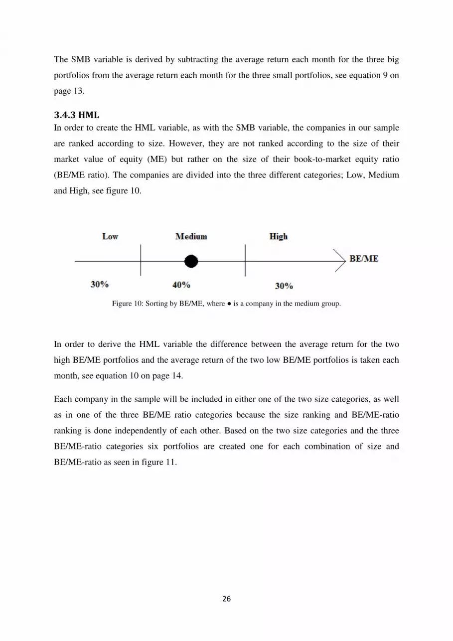
In order to create the HML variable, as with the SMB variable, the companies in our sample

are ranked according to size. However, they are not ranked according to the size of their

market value of equity (ME) but rather on the size of their book-to-market equity ratio

(BE/ME ratio). The companies are divided into the three different categories; Low, Medium

and High, see figure 10.

Figure 10: Sorting by BE/ME, where ● is a company in the medium group.

In order to derive the HML variable the difference between the average return for the two

high BE/ME portfolios and the average return of the two low BE/ME portfolios is taken each

month, see equation 10 on page 14.

Each company in the sample will be included in either one of the two size categories, as well

as in one of the three BE/ME ratio categories because the size ranking and BE/ME-ratio

ranking is done independently of each other. Based on the two size categories and the three

BE/ME-ratio categories six portfolios are created one for each combination of size and

BE/ME-ratio as seen in figure 11.

27

Figure 11: Sorting on size and BE/ME, where ● is the same company as in figure 2 and 3,

and is here shown to be present in one size portfolio and in one BE/ME portfolio.

3.4.4 INV

In order to derive the INV variable, low-minus-high INV, the I/A factor firstly has to be

estimated for each of the companies in our sample. This is accomplished by dividing the

property, plant, and equipment (PP&E) and the annual change in inventories (INVT) with the

lagged book value of assets (TA)115, see equation 11 on page 14.

Each month, in June, the stocks in our sample from the FTSE All Share Index are based on

their value of the I/A factor sorted into three groups, low, medium and high, on a yearly basis,

as illustrated in figure 12.

Figure 12: Sorting on I/A, where ● is a company in the low I/A group.

115


28

In order to estimate the INV variable the difference between the average return of the nine low I/A

portfolios and the average return of the nine high I/A portfolios is taken each month, see equation 13

on page 16.

3.4.5 ROE

Return on equity, high-minus-low ROE, is measured following Chen, Novy-Marx and Zhang

as quarterly earnings divided by one quarter lagged book equity116. This gives the ROE factor

that is used to rank and sort the companies which in turn will give the ROE variable used in

the regressions. Datastream data types DWNP and DWSE are used to obtain quarterly

earnings and book equity, respectively. Independently of the I/A sort the companies of our

sample from the FTSE All Share Index are ranked each month on ROE according to their

latest announced quarterly earnings, as illustrated in figure 13. For example if the fourth

quarter year t-1 quarterly earnings are announced in March year t then these earnings are

divided by the third quarter year t-1 book equity to rank companies according to ROE in

April. The same companies will then stay in the same groups until the next quarterly earnings

are announced.

Figure 13: Sorting on ROE, where ● is a company in the low ROE group.

Each month the nine high ROE portfolios minus the nine low ROE portfolios create the ROE

variable, see equation 14 on page 17, which is used in the regressions with the CNMZ.

3.5 Dependent variables (FF3)

Since our sample consists of fewer companies than in Fama and French’s study we only use

the excess returns of 16 portfolios, instead of 25 portfolios used by Fama and French, as

dependent variables in the time-series regressions. By using fewer portfolios the risk of

obtaining portfolios that only contain one or even zero companies is avoided. These 16

portfolios are constructed with the same method used to construct the six size-BE/ME

portfolios. The portfolios are formed in June each year, t, by size, which is measured in the

116


29

end of June year, t, and BE/ME, which is measured in the end of December year, t-1. Each

year the monthly returns are measured from the end of July year, t, to June year, t+1, and in

June, t+1, the portfolios are rebalanced. Four size groups and four BE/ME groups are created

and the 16 portfolios are formed by a 4x4 matrix consisting of these two categories, as can be

seen in figure 14.

Figure 14: 4x4 matrix of the 16 dependent portfolios, where the ● is a company in the Small/Low portfolio.

The four size groups are Small, 2, 3 and Big and the four BE/ME groups are Low, 2, 3 and

High. The stocks are distributed into four groups of equal size hence each group contain 25%

of the stocks. For example 25% of the stocks will be in the size group Small, 25% will be in

the size group 2 and so forth. Regarding the explanatory variables any given stock of the

portfolios of the explained variables will be present in both one size group and one BE/ME

group. From the beginning of July of year, t, to the end of June year, t+1, for the years 2002-

2010, the excess returns of the 16 portfolios are the dependent variables.

By running Ordinary Least Squares (OLS) time series regressions the betas of the three

explanatory variables is estimated. 16 regressions are run for the whole time period of 2002-

2010.

30

3.6 Dependent variables (CNMZ)

The dependent variables in the CNMZ are the portfolios that can be seen in section 3.8. As

seen in section 2.7.3 the article by Chen, Novy-Marx and Zhang117 use nine portfolios to test

the CNMZ. We are performing five of these tests as well as one that is not conducted by

Chen, Novy-Marx and Zhang118.

3.7 The risk-free interest rate

Our proxy for the risk-free interest rate is the UK Treasury bill with a one month term to

maturity obtained from Datastream. The Datastream name of the interest rate is UK Treasury

Bill Tender - Middle Rate. We have chosen this rate since treasuries issued by the UK

government are as close to a risk-free rate as one can come. These treasuries would be one of

the first choices for the risk-free rate of the investor in UK stocks due to the fact that it is in

the same currency as the stocks and the investor thereby avoids any risk of losing money on

currency fluctuations of the British Pound. The choice of using one-month term to maturity is

in order to comply with the Fama and French119 and Chen, Novy-Marx, and Zhang120 articles.

Since the interest rate is expressed on a yearly basis we used the following model to obtain the

monthly rate of interest:

T� = �1 + T�U�V L

LWX − 1 �Eq. 15�

Where T� equals the monthly rate of interest and T�U is the yearly rate of interest.

3.8 Test Portfolios

3.8.1 Calendar-time Factor Regressions

Following Chen, Novy-Marx and Zhang121 as well as Fama and French122 we use factor

regressions to test the CNMZ:

��3 − ��3 = 4 + �� 3 + ��

� !"3 + #$%� �&�3 + 5�3 �Eq. 8�

where if the model performs sufficient enough the α should be statistically insignificant from

zero. Furthermore, due to the simplistic nature of the portfolio approach and following Chen,

117






Fama & French (1993,1996)

31

Novy-Marx and Zhang123, we test the CNMZ by using several different test portfolios that

have been constructed on a wide range of variables.

The first test is time-series regressions where there has been no change to the construction of

the portfolios. The 27 portfolios are formed by taking the intersections of the I/A factor, the

ROE factor and the size factor. The monthly excess returns from each of the 27 portfolios are

used as dependent variables in the regressions.

3.8.2 Earnings Surprises

Earnings surprises are measured as Standardized Unexpected Earnings (SUE) following an

article by Foster, Olsen, and Shevlin124. SUE is calculated by taking the change in a

company’s most recent quarterly earnings per share from its earnings per share four quarters

ago divided by the standard deviation of this change in quarterly earnings over the antecedent

eight quarters. Since quarterly data is necessary from eight months prior to the measurement

of SUE the time period of our SUE observations is measured from January 2005-March 2011,

a period of 75 months. The quarterly earnings are collected by using the Datastream data type

DWNP and the number of shares outstanding in the quarter antecedent to the earnings quarter

are collected with the data type NOSH. The earnings are then divided by the number of shares

to get the earnings per share. The stocks from our sample from the FTSE All Share Index are

ranked and sorted into deciles at the beginning of each month according their latest past SUE.

The stocks are sorted into deciles with decile one containing the stocks with the lowest SUE

and decile ten containing the stocks with the highest SUE. Following the CNMZ article we

only report the results of deciles one (Low), five, ten (High) and High minus Low (H-L) to

save space.125 For each portfolio monthly value-weighted returns are taken at the end of each

month and each portfolio is rebalanced in the beginning of every month according to its latest

past SUE. In this way the February and March portfolios include the same companies as the

January portfolio since these months are all part of quarter one and share the same latest past

SUE. For this quarter one portfolio the monthly returns are taken from January to March and

afterwards in April the quarter two portfolio is formed. The value weighted returns of each

portfolio month are regressed on the returns from the CAPM, FF3, and CNMZ portfolios.

123


Foster, Olsen & Shevlin (1984) 125


32

3.8.3 Net Stock Issues

Net stock issues are measured following a Fama and French126 article. Net stock issues are

calculated as the change in the natural log of outstanding shares as of yearend t-1 and

outstanding shares as of yearend t-2. The Datastream data type NOSH is used to collect the

yearend outstanding shares. Each year t in June the sample from the FTSE All Share Index is

sorted into deciles based on net stock issues for the yearend of t-1. Following Chen, Novy-

Marx, and Zhang127 the firms with negative net stock issues are sorted into decile one and the

firms with zero net stock issues are sorted into decile two. The firms with positive net stock

issues are then sorted into the rest of the eight deciles. Following the CNMZ article we only

report the results of deciles one (Low), five, ten (High) and High minus Low (H-L) to save

space128. Monthly value weighted returns are taken at the end of each month for all deciles

from July year t to June year t+1. The portfolios are then rebalanced in June year t+1. In this

way the deciles contains the same companies from July to June and are then rebalanced. The

value weighted returns of each portfolio month are regressed on the returns from the CAPM,

FF3, and CNMZ portfolios.

3.8.4 Asset Growth

Following an article by Cooper, Gulen, and Schill129 asset growth is measured as total assets

at the end of the year t-1 less total assets at the end of the year t-2 divided by total assets at the

end of the year t-2. The Datastream data type WC02999 is used to obtain the total assets of

each company in the sample. In each June year t the shares of the sample from the FTSE All

Share Index are ranked and sorted into deciles according to their asset growth. Decile one

contain the stocks with the lowest asset growth and decile ten contain the stocks with the

highest asset growth. Following the CNMZ article we only report the results of deciles one

(Low), five, ten (High) and High minus Low (H-L) to save space130.Monthly value weighted

are taken at the end of each month for all deciles from July year t to June year t+1 and the

portfolios are then rebalanced in June year t+1. In this way the deciles contains the same

companies from July to June and are then rebalanced. The value weighted returns of each

portfolio month are regressed on the returns from the CAPM, FF3, and CNMZ portfolios.

126




Cooper, Gulen & Schill (2008) 130


33

3.8.5 Book-to-Market Equity

The test is conducted by instead of taking the monthly excess returns from each of the 27

portfolios, the excess returns from the 16 size and book-to-market portfolios, the FF3

portfolios, are instead used as dependent variables in the factor regressions. The results of the

CNMZ are then compared against the results of the FF3 and CAPM as in accordance with

Chen, Novy-Marx, and Zhang131.

3.8.6 Industries

We follow Chen, Novy-Marx, and Zhang132 and divide companies into ten industry portfolios

where the division of different industries into the ten portfolios can be found on Kenneth

French´s homepage133. For the different industry sectors of the FTSE All Share Index

included in the ten industry portfolios, see table 15. Tests are performed on ten industry

portfolios from our sample from the FTSE All Share Index with the returns of every portfolio

regressed on the CAPM, FF3, and CNMZ.

131



http://mba.tuck.dartmouth.edu/pages/faculty/ken.french/index.html

34

Chapter 4

Analysis and Results

In this chapter the results of the study are analysed and discussed, as well as the validity of the

results. In order to make it easier to comprehend, we have chosen to integrate the analysis part

and the results part as opposed to presenting each part separately.

4.1 Explanatory variables

4.1.1 Descriptive statistics

In tables 8, and 9, respectively descriptive statistics of the explanatory variables can be seen.

Our INV variable obtains a positive average monthly return of 0.02% while the ROE variable

obtains a negative average monthly return of -0.15%. These results are different from Chen,

Novy-Marx, and Zhang where both variables obtain large positive monthly returns. Our SMB

variable obtains a negative average monthly return of -0.70%. The only variable with a large

positive average monthly return is the value stock variable HML which obtains a positive

average monthly return of 1.73%. The market factor is not good at explaining the average

returns of any of the other independent variables measured by adjusted R² values. SMB and

HML are better at explaining the average returns of the ROE variable with an adjusted R² of

52%. INV and ROE can explain 32% of the variance of the returns of the SMB variable.

4.1.2 SMB and HML

The explanatory variables in the FF3 regression, SMB, HML and MKT, have been estimated

on a monthly basis. A total of 105 values for each variable have been derived. In table 1

below, the average of the explanatory variables are presented. It is worth noticing that the

SMB variable obtains a negative value, which means that on average during the period small

size companies, small-cap, tend to achieve a lower return than large size companies, large-

cap. This result contradicts the Fama and French theory which states that small-cap stocks

tend to outperform large-cap stocks134, or in other words small companies will on average

yield a higher return than large companies. When examining the data for the SMB variable,

see table 7, it is evident that during 2009 and 2010 small-caps performed worse than large-

134


35

caps. Because, in the 2009 portfolio all SMB values are negative and in the 2010 portfolio

two thirds of the values are negative.

One possible explanation for this could be that following a period where the market has

experienced a sharp decline, as it did in 2008, investors will prefer to invest in larger

companies. The reason being that they are, as will be discussed later in this chapter, less risky

than smaller companies

However, the HML variable obtains a positive value which means that stocks with a high

BE/ME ratio, called value stocks, outperforms stocks with a low BE/ME ratio, known as

growth stocks. This result is perfectly in-line with the Fama and French theory that value

stocks should outperform growth stocks135.

% Rm - Rf SMB HML

Average 0,1439 % – 0,7008 % 1,7314 %

Number of

observations

105 105 105

Table 1: FF3 explanatory variables data, Number of observations and average values for the explanatory variables in the regression

��3 − ��3 = 4 + �� 3 − ��3� + ��

� ��3 + �� + 5�3 �Eq. 6�

4.1.3 INV and ROE

The explanatory variables in the CNMZ regression, INV, ROE and MKT, have just like the

explanatory variables in the FF3 been estimated on a monthly basis, giving a total of 105

observations. The average value of the explanatory variables is presented in table 2. The INV

variable obtains a positive value, which means that in our sample companies in the low

investment ratio portfolios have achieved higher average returns that the companies in the

high investment ratio portfolios. According to Liu, Whited, and Zhang136 when companies are

faced with high cost of capital they are more likely to reduce their investments, because they

have less projects with a positive net present value (NPV) to invest in. Low investments, in

relation to the asset base, should therefore indicate a potential for high future average returns.

However, the ROE variable has obtained a negative value, which means that during our time

period companies have been less profitable, especially the companies in the high profitability

135


Liu, Whited & Zhang (2009)

36

ratio portfolios. This indicates a potential for lower returns because, quite intuitively,

companies that are expected to be relatively less profitable will most likely deliver lower

returns and vice versa.

These results differ from those of the Chen, Novy-Marx and Zhang study which obtained

positive values for both variables. One possible explanation for this could be the fact that our

time period is significantly shorter than that of the Chen, Novy-Marx and Zhang study.

Furthermore, much of our time period have experienced several highly negative economic

events, such as the aftermath of the dot-com bubble, the financial crisis of 2008/2009 which

lead to a global economic downturn, the collapse of Iceland’s financial system and the

sovereign debt crisis of several European countries. These events have, for instance, had the

effect of reducing companies’ sales which leads to lower profitability levels.

% Rm - Rf INV ROE

Average 0,1439 % 0,0246 % – 0,1549 %

Number of

observations

105 105 105

Table 2: CNMZ explanatory variables data, Number of observations and average values for the explanatory variables in the regression

��3 − ��3 = 4 + �� 3 + ��

� !"3 + #$%� �&�3 + 5�3 �Eq. 8�

37

4.2 Results of the regressions for the FF3


A regression analysis for the FF3 has been conducted for each of the sixteen dependent

portfolios in compliance with the model:

��3 − ��3 = 4 + �� 3 − ��3� + �� 3 + ��

� �� + 5�3 �Eq. 6�

In table 3 the intercept and its related p-values, the coefficients for the explanatory variables

as well as the value of the adjusted r-squared are presented for the period of 2002 - 2011.

Table 3: FF3 16 portfolios regression data, Intercept and p-values, coefficients, adjusted R² according to the

model

��3 − ��3 = 4 + �� 3 − ��3� + ��

� ��3 + �� + 5�3 �Eq. 6�

The results of table 3, shows that for four of the portfolios, 2_L, 2_2, 2_H and B_2, the α is

positively significant at the 5 % level. This means that the model underestimates the returns

for those four portfolios, had the intercept instead been negatively significant, the model

would then have overestimated the return of the portfolios. When the α value is not

significantly different from zero the model neither overestimates or underestimates the return

of the portfolio. What is worth noticing is that three out of those four portfolios are in the

second lowest size group, which might indicate that the FF3 have problem correctly

estimating companies of that size, at least in our study.

38

We use the adjusted R² to measure the level of explanation, because adjusted R² takes the loss

of degrees of freedom related to adding extra variables into consideration137. It is therefore a

more accurate measure of the goodness of fit than the unadjusted R². The value of the

adjusted R² for the FF3 regressions ranges between 55% and 82%.

Furthermore, the results of table 3 show that the beta values for portfolios that contain larger

sized companies are smaller than the beta values for portfolios containing smaller sized

companies. This illustrates that larger size firms are less risky than smaller sized firms and

will therefore on average yield a lower return than small companies, since the higher the risk

the higher the return must be for people to be willing to invest; this is in consistence with the

mean-variance theory of Markowitz138. This result coincides with the Fama and French theory

that states that small-cap stocks tend to outperform large-cap stocks139.

137

Brooks (2008) 138

Markowitz (1959) 139


39

4.3 Results of the regressions for the CNMZ


Regression analyses for the CNMZ have been conducted for each of the 27 dependent

portfolios in compliance with the model:

��3 − ��3 = 4 + �� 3 + ��

� !"3 + #$%� �&�3 + 5�3 �Eq. 8�

The intercept and its related p-values, the coefficients for the explanatory variables as well as

the value of the adjusted r-squared for the period of 2002 - 2011 is presented in table 4.

Table 4: CNMZ 27 portfolios regression data, Intercept and p-values, coefficients, adjusted R² according to the

model

��3 − ��3 = 4 + �� 3 + ��

� !"3 + #$%� �&�3 + 5�3 �Eq. 8�

40

Table 4 shows that the CNMZ underestimates the returns of 11 portfolios since the α is

positively significant at the 5 % level for these portfolios. Surprisingly of these 11 portfolios,

4 are in the low investment group, which is about 44% of the total portfolios in that group. In

addition, 5 of the 11 portfolios are in the high investment category, about 56% of the total

amount of portfolios in that category. This indicates that in our study the CNMZ seems to

have difficulties correctly estimating the returns of portfolios containing either companies

with a low investment ratio or companies with a high investment ratio.

The value of the adjusted R² for the CNMZ regressions range from between as low as 1.3% to

77%. An explanation to why the adjusted R² values for the CNMZ, compared to the FF3, gets

as low as 1.3% could be that the CNMZ regressions contain more dependent portfolios than

the FF3 regressions, 27 compared to 16. Therefore, each CNMZ portfolio contains on average

fewer companies than the FF3 portfolios, which might have a negative impact on its adjusted

R² values. Especially for the portfolios that might contain fewer companies, due to our limited

sample and time period, than the other portfolios, for instance the Hinv/Lroe/Bsize portfolio

which only obtains a adjusted R² value of 1.3%.

4.4 Results for the regressions including all three models

4.4.1 Earnings Surprises

Table 10 shows that the high SUE decile earns an average monthly return of 0.013% while the

low SUE decile earns an average monthly return of 0.07%. This means that firms with high

earnings surprises earn higher average returns than firms with low earnings surprises. Our

high-minus low SUE decile earns obtains a CAPM alpha of 0.007, (t=1.20), a Fama and

French alpha of 0.011, (t=2.11), and a CNMZ alpha of 0.005 (t=1.08). The CNMZ thereby

has the lowest alpha of the three models and can thereby do a good job in comparison with the

other models in explaining the post-earnings announcement drift of the high-minus-low

portfolio. However the difference of the alphas is small; 0.06. The high-minus-low decile has

a ROE beta of 0.71, where a positive beta means that a portfolio has higher return on equity.

This gives the intuitive result that firms that have experienced positive earnings surprises have

higher average returns than their counterparts that have experienced negative earnings

surprises. The high-minus-low decile CNMZ market beta equals -0.21 and the INV beta

equals -0.67, where a negative INV beta means that a portfolio invest more. The negative

INV beta thereby implies that firms with positive earnings surprises invest more than their

counterparts with negative earnings surprises. Furthermore since the positive earnings

41

surprises firms earn higher average returns this finding implies that the market may have

looked positively on the investments of these firms resulting in higher average returns of these

stocks. The CNMZ model obtains the highest mean absolute error of its alphas; 0.08

compared to 0.07 for the CAPM and the FF3. This means that the CNMZ is doing slightly

worse in explaining the post-announcement earnings drift when looking at all portfolios.

Again the difference is small; 0.01. All models are rejected by the Gibbons, Ross, and

Shanken test - the GRS test.140 This finding means that the null hypothesis that all alpha

values are equal to zero is rejected and therefore none of the models perfectly explains the

anomaly. Looking at the adjusted R² values the results shows a pattern that the FF3

consistently obtains the highest adjusted R² for every portfolio, the CNMZ consistently come

in the middle and the CAPM consistently obtains the lowest adjusted R². The finding is most

obvious in the low decile, where the FF3 obtains an adjusted R² of 73% while the second best

model in this decile, the CNMZ reaches 55%. Thus this result implies that the FF3 is good at

explaining the variance of the returns of this decile. Looking at all deciles the CAPM obtains

adjusted R² of 11% to 39%, the CNMZ 35% to 55%, and the FF3 41% to 73%. The adjusted

R² measure suggests that the FF3 overall is the most adequate model in explaining the

variance of the returns of the post-announcement earnings drift.

In Chen, Novy-Marx, and Zhang the high decile earns a return of 0.77% and the low decile

earns an average return of 0.41%. This is in line with our results and the findings of Foster,

Olsen and Shevlin141 where companies with high earnings surprises earn higher average

returns than their counterparts with low earnings surprises. The high-minus low SUE decile

obtains a CAPM alpha of 0.40, (t=3.27), a Fama and French alpha of 0.46, (t=3.55), and a

CNMZ alpha of 0.12 (t=0.91). The CNMZ obtains the lowest alpha which is the same result

we reach, though the difference of the alphas of Chen, Novy-Marx and Zhang are much

larger. The ROE beta is 0.35 while the CAPM beta and the FF3 beta are -0.03, and -0.01,

respectively. The positive ROE beta is in line with our results while the CAPM and FF3 betas

of Chen, Novy-Marx, and Zhang are much smaller than our CAPM and FF3 betas. The

negative INV beta we obtain means that the firms with positive earnings surprises, which

were found to earn higher average returns, are investing more than their counterparts. This

result is contrary to the finding of Chen, Novy-Marx, and Zhang that firms that earn higher

average returns invest less than their counterparts. In Chen, Novy-Marz, and Zhang the mean

140

Gibbons, Ross, & Shanken (1989) 141

Foster, Olsen & Shevlin (1984)

42

absolute error is found to be 0.16% of the CAPM, 0.17% of the FF3, and 0.10% of the

CNMZ; that is the CNMZ obtains the smallest mean absolute error of the models. We obtain

the opposite result since the CNMZ mean absolute error is the largest in our results. In Chen,

Novy-Marx, and Zhang the CAPM and the FF3 are rejected by the GRS test but the CNMZ is

not rejected.

The difference in the results can be because a number of reasons. The time period in Chen,

Novy-Marx, and Zhang is longer with 468 months of data while we have 105 months of data.

The Chen, Novy-Marx, and Zhang sample using data from Kenneth French´s homepage142

contains 1837 firms as of December 2010 while our sample contains 369 firms as of the same

date. The Chen, Novy-Marx, and Zhang sample and our sample are also from different

markets; the USA and the UK, respectively. As discussed earlier there are also many financial

downturns during our time period.

4.4.2 Net Stock Issues

In table 11 panel A it can be seen that firms with high net stock issues earn higher average

returns than firms with low net stock issues; 1.02% versus 0.62% per month. The high-minus-

low portfolio obtains a CAPM alpha of 0.003 (t=0.93), a FF3 alpha of 0.003 (t=0.83), and a

CNMZ alpha of 0.003 (t=0.82); all models have the same alpha of this decile. The mean

absolute errors of the alphas are 0.06 for the CAPM, 0.05 of the FF3, and 0.06 of the CNMZ.

The FF3 thereby has slightly lower errors of its alphas, however the difference is only 0.01.

Since all models obtain the same alpha and roughly the same mean average error they do an

equally good job in explaining the variance of the returns controlling for net stock issues. The

high-minus-low decile has a factor loading on the INV of -0.27 (t=-1.72). The high decile has

an INV beta of -0.42 while the low decile has a beta of -0.15. This implies that companies

with high net stock issues invest more than companies with low net stock issues. Furthermore

since the companies with higher net stock issues on average obtains 0.4% higher average

returns per month than their low net stock issues counterparts this could mean that the

investments of the high net stock issues firms have had a positive impact on the stock price

and the average returns. The high-minus-low decile has a factor loading on the ROE of -0.41

(t=-3.41), the high decile -1.08 and the low decile -0.61. This would suggest that the high

decile earn lower average returns since a lower ROE beta implies lower profitability.

However the high decile earns higher average returns during our time period. One reason for

this could be that the firms with high net stock issues in our sample have managed to create

142


43

value with the funds obtained from the stock issues. The investments made with the funds

seem to have been made in projects with net present value exceeding zero which has had a

positive impact on the stock price. The lower profitability measured by return on equity would

be a direct effect of the increase in the number of stocks which leads to lower earnings in

pounds per stock.

An evaluation of the adjusted R² values gives the same result as in section 4.4.1 where the

FF3 obtains the highest adjusted R² values, the CNMZ takes the second place and the CAPM

obtains the lowest adjusted R² values. The CAPM obtains adjusted R² of 15% to 59%, the

CNMZ 23% to 68%, and the CNMZ 25% to 79%. The CNMZ adjusted R² comes close to the

FF3 corresponding value of portfolio five, implying that both of the models are good at

explaining the variance of the returns of the middle portfolio. The CNMZ is also close to the

adjusted R² of FF3 on the high-minus-low decile, however the explanatory power of this

decile judged by the adjusted R² measure is not impressive for any of them.

In Chen, Novy-Marx and Zhang and in Fama and French143 firms with high net stock issues

earn lower average returns than firms with low net stock issues, contrary to our results. In

Chen, Novy-Marx and Zhang the corresponding results are obtained; a high-minus low

portfolio CAPM alpha of -0.64 (t=-4.40), a FF3 alpha of -0.63 (t=-4.42), and a CNMZ alpha

of -0.26 (t=-1.79). Consequently the CNMZ alpha is the lowest with some margin while our

high-minus-low alphas all are equal. In both, the Chen, Novy-Marx and Zhang study and in

our study all models are rejected by the GRS test, which implies that the alphas are not equal

to zero. The results from the CNMZ article are: high-minus-low decile has a factor loading on

the INV of -0.24 (t=-3.65). Here our results and the results from Chen, Novy-Marx and Zhang

article are quite similar; it is found that high net stock issues firms invest more than low net

stock issues firms. In Chen, Novy-Marx and Zhang the high decile has a ROE factor loading

of -0.24 and the low decile has a ROE factor loading of 0.12, consequently the high decile has

a lower factor loading on ROE than the low decile.

4.4.3 Asset Growth

As can be seen in table 11 panel B high asset growth firms earns higher average returns than

low asset growth firms; 1.02% versus 0.96% per month. This is the opposite of the results

from the CNMZ article where high asset growth firms earns lower average returns than low

asset growth firms; 0.20% versus 0.99% per month. Our high-minus-low decile obtains a

143


44

CAPM alpha of 0.000 (t=0.11), a FF3 alpha of 0.002 (t=0.39), and a CNMZ alpha of -0.002

(t=-0.54). The CNMZ article has the corresponding alphas: CAPM alpha of -0.87 (t=-4.26), a

FF3 alpha of -0.45 (t=-2.53), and a CNMZ alpha of -0.52 (t=-2.80). The FF3 outperforms the

CNMZ in explaining the variance of the returns controlling for asset growth in the Chen,

Novy-Marx and Zhang. In Chen, Novy-Marx and Zhang the CAPM alpha mean absolute error

is 0.22%, FF3 alpha of 0.14%, and a CNMZ alpha of 0.15%, thus not large differences

between the models. Our corresponding results are a CAPM mean absolute error of its alpha

of 0.007, and FF3 and CNMZ obtains slightly lower mean absolute errors of their alphas of

0.005, this implies that the FF3 and the CNMZ explains the variance of the returns due to the

asset growth anomaly slightly better than the CAPM. The high-minus-low decile in Chen,

Novy-Marx and Zhang has a factor loading on the INV of -1.17 and a ROE factor loading of

0.23 (t=2.37). We have corresponding results of the high-minus-low decile: a factor loading

on the INV of -0.72 (t=4.16) which means that companies with high asset growth invest more

than companies with low asset growth, and a ROE factor loading of 0.23 (t=1.59), these are

quite similar results. The result of a positive factor loading on the ROE for the high-minus-

low decile means that companies with high asset growth is more profitable than companies

with low asset growth. The negative high-minus-low INV beta implies for both our study and

the Chen, Novy-Marx and Zhang study that firms with high asset growth invest more heavily

than their counterparts with low asset growth. In both studies all models get rejected by the

GRS test. The adjusted R² values of the asset growth deciles gives similar results as in 4.4.1,

and 4.4.2, respectively, with one exception; the CNMZ obtains the highest adjusted R²

explanatory power for the high-minus-low decile. In the high-minus-low decile the CAPM,

and the FF3 have adjusted R² value close to zero which means that they cannot be trusted to

explain the variance of the returns of this portfolio, judging by the adjusted R² measure. The

CNMZ obtains an adjusted R² of 22% for this portfolio which is not much either, but better

than zero. In the low decile the FF3 and the CNMZ obtain the same adjusted R² which means

that they are equally good at explaining the variance of the returns of this decile. Overall the

CAPM obtains adjusted R² of -0.03% to 44%, the CNMZ 22% to 69%, and the FF3 -1% to

72%.

Our results show that companies with high asset growth have higher average returns than

companies with low asset growth, which is the opposite of Chen, Novy-Marx and Zhang and

also of Cooper, Gulen, and Schill144 who find that high asset growth firms have lower average

144

Cooper, Gulen, & Schill (2008)

45

returns than low asset growth firms. Companies with high asset growth are more profitable

and thus invest more145 and since they invest more they should have lower average returns146.

However, since our results show them to actually have higher average returns, a possible

explanation is that they have made sound investments for instance, investments with a

positive net present value (NPV), investments that have had value creating synergies like

economies of scale and scope and so forth, such investments would be well received by the

market and result in higher returns.

4.4.4 Book-to-Market Equity

Table 12 shows factor regression on the FF3 16 size and book-to-market portfolios. The

results in table 6, panel A, show that value stocks earn higher average returns compared to

growth stocks. Because, the average high-minus-low returns is approximately 0.6% per month

(t = 0.62) in the smallest size quintile and about 0.5% (t = 0.65) in the largest size quintile.

The small-stock value-minus-growth quintile has a CAPM alpha of 0.006% (t = 0.85)

although low it is still larger than the FF3 alpha of – 0.005% (t = – 0.36). The big-stock value-

minus-growth quintile has a CAPM alpha of 0.005% (t = 1.42) and the FF3 obtains an alpha

of only 0.003% (t = 0.77).

The results from panel A coincides very well with those of Chen, Novy-Marx and Zhang,

their results also show that value stocks on average earn higher returns than growth stocks,

this also corresponds with the Fama and French theory that small-cap stocks tend to

outperform large-cap stocks.147 Furthermore, Chen, Novy-Marx and Zhang’s results also

achieve a consistently higher alpha value for the CAPM compared to the FF3, which shows

that the FF3, as expected, outperforms the CAPM.

Panel B shows that the small-stock value-minus-growth alpha for the CNMZ has a positive

value of 0.005% (t = 1.08) which is the opposite of the negative alpha value obtained by the

FF3 of – 0.005% (t = – 0.36). However, it is only a difference of 0.01 between the two results.

In addition, the CNMZ does a good job in capturing the small-growth anomaly since its alpha

value is only 0.003% compared to the FF3 alpha value of 0.008%. Furthermore, for the big-

stock value-minus-growth quintile the CNMZ obtains only a slightly higher alpha of 0.005%

compared to the FF3 alpha of 0.003%. In addition, the CNMZ also obtains a slightly higher

145




46

alpha of 0.009% compared to the FF3 alpha of 0.003% for the small-value portfolio, but it

perfectly match the FF3 alpha of 0.003% for the big-growth portfolio. The FF3 does however

outperform the CNMZ when it comes to the mean absolute error (m.a.e) metric, 0.0034%

compared to 0.0057% for the CNMZ and 0.0065% for the CAPM.

Our results from panel B match Chen, Novy-Marx and Zhang’s results very well and even

surpass them on some points. For instance, regarding the small-value portfolio where they

experienced a large difference between their model and the FF3 but our results show only a

slight difference.

Panel B also shows that value stocks have higher INV factor loadings compared to growth

stocks, since the value stocks have less negative loadings than growth stocks. The loading

spread range from approximately 0.12 to 0.55. This result is equivalent to that of Chen, Novy-

Marx and Zhang’s. Growth firms that have high valuation ratios have more growth

opportunities and thus invest more compared to companies that have low valuation ratios.

Regarding the ROE factor loadings, panel B shows that both value stocks and growth stocks

obtain negative values and the loading spreads range from approximately – 0.14 to – 0.07.

This result differs from the Chen, Novy-Marx and Zhang study since they only obtain a

negative value for the high-minus-low portfolio in the largest size quintile. The negative ROE

factor loadings are because the value stocks obtain higher negative loadings than growth

stocks. The reason that all the portfolios have negative factor loadings is because, as

explained in 4.1.3, our time period have experienced several economic crisis which have lead

to lower profitability for both value stocks and growth stocks. However, the crises have had a

larger negative effect on the profitability of value stocks than growth stocks. All three models

are rejected by the GRS test, which is the same result as in the Chen, Novy-Marx and Zhang

study.

In table 13, the adjusted R2 values for each portfolio for the three different models are

presented. The results show that the CAPM obtains the lowest R2 values of 15% to 74%

however; its R2 values do match those of the FF3 for the portfolios containing the biggest

sized companies. Overall the FF3 obtains the highest R2 values ranging from 55% in the

small-stock growth quintile to 82 % in the small-stock value quintile. Hence, the FF3 does a

good job estimating small sized value stocks. In addition, the CNMZ obtains values ranging

47

from 32% for the small-stock growth quintile to 76% for the portfolio with the biggest size

and average book-to-market equity companies. The CNMZ match the FF3 well when it comes

to the portfolios containing the average sized companies. Furthermore, the CNMZ

outperforms both the CAPM and the FF3 when it comes to the portfolios that consist of the

biggest sized companies, by obtaining higher R2 values for each of the portfolios in the

biggest size quintile. Hence, the CNMZ does a better job estimating big sized stocks than the

FF3.

4.4.5 Industries

In table 14 it can be seen that all of the models are rejected by the GRS test. In Chen, Novy-

Marx and Zhang the only model that is not rejected by the GRS test is the CAPM. In our

study the CAPM obtains the highest mean absolute error of its alphas, followed by the

CNMZ, and the FF3 obtains the lowest mean absolute error of its alphas. However the

differences are not large. In Chen, Novy-Marx and Zhang the corresponding results are

CAPM mean absolute error 0.15%, FF3 and CNMZ 0.19%, not large differences either. One

more time the FF3 consequently obtains the highest adjusted R². The CNMZ obtains slightly

lower R² values while the CAPM obtain the lowest R² values. The CAPM obtains adjusted R²

of 29% to 61%, the CNMZ 28% to 72%, and the FF3 26% to 78%. The CNMZ is good at

explaining the variance of the returns of the Manuf and HiTec sectors, with adjusted R² high

and close to those of the FF3.

48

4.5 Validity and reliability

4.5.1 Multicollinearity

A factor that might affect our results is multicollinearity, because if our variables are highly

correlated, small changes in the data might lead to erratic changes in the coefficient estimates.

The results of the test for multicollinearity are presented in tables 5 and 6. Although there

seem to be some small level of negative correlation between SMB and HML in the FF3 and

between INV and ROE in the CNMZ, but since none of the correlations exceed neither 0.5

nor – 0.5 we conclude that multicollinearity should not cause a problem in our study.

FF3 Rm-Rf SMB HML

Rm-Rf 1,000

SMB – 0,060 1,000

HML 0,354 – 0,471 1,000

Table 5: FF3 explanatory variables correlation data, Correlation between the explanatory variables in the

regression

��3 − ��3 = 4 + �� 3 − ��3� + ��

� ��3 + �� + 5�3 �Eq. 6�

CNMZ Rm-Rf INV ROE

Rm-Rf 1,000

INV 0,240 1,000

ROE – 0,348 – 0,466 1,000

Table 6: CNMZ explanatory variables correlation data, Correlation between the explanatory variables in the regression

��3 − ��3 = 4 + �� 3 + ��

� !"3 + #$%� �&�3 + 5�3 �Eq. 8�

4.5.2 Homoscedasticity and heteroscedasticity

An underlying assumption for regression analysis is that the variance of the error is constant

across observations, in other words there exist homoscedasticity148. Assuming a distribution

of data is homoscedastic when in actuality it is heteroscedastic will result in an overestimation

of the goodness of fit, in our case the adjusted R² values. If we have heteroskedasticity instead

of homoscedasticity it will not affect the coefficients of the variables, but instead it will have

an effect on the standard errors of the coefficients. Therefore, in order for us to comment on

the significance of the variables, we need to test for occurrence of homoscedasticity or

148

Brooks (2008)

49

heteroscedasticity. In order to test for presence of heteroscedasticity we have conducted a

Goldfeld-Quandt test, see tables 16 and 17, respectively. The null hypothesis of the test is that

there is homoscedasticity and consequently a rejection by the GQ test implies that

heteroscedasticity is present. The results show that heteroscedasticity is generally present in

the same deciles across models. The FF3 could not be rejected on slightly fewer occasions

than the CAPM and the CNMZ.

4.5.3 Database reliability

In order to see if the data we collected from the database Datastream is accurate we have

conducted an evaluation of the accounting data by looking at the annual reports from the

homepages of 33 companies, one company randomly selected from each industry sector seen

in table 15. This evaluation sample of 33 companies equals 9% of the total number of

companies in our sample. The evaluation gave satisfactory results as it was found that the

accounting data obtained from Datastream coincided with the data of the annual reports from

the companies´ homepages.

50

Chapter 5

Conclusion

In this chapter the conclusions of our study are presented as well as suggestions of future

research topics.

5.1 Conclusions

The CMNZ is found to produce inferior results, compared to the FF3, when regressions are

made using the monthly excess returns from its own 27 portfolios as the dependent variables.

This is evident since the model produces several α values that are positively significant at the

5 % level, which means that the model underestimates the returns for several portfolios,

especially those containing either companies with a low investment ratio or companies with a

high investment ratio. Although the FF3 also obtains α values that are positively significant at

the 5 % level, the percentage of portfolios are far less than for the CNMZ and a measure of

whether or not it performed sufficiently enough was that the α values should be statistically

insignificant from zero.

Furthermore, the CNMZ obtains lower adjusted R² values, ranging from 1.3% to 77%,

compared to the FF3 which obtains adjusted R² values between 55% and 82%. As previously

stated one explanation to why the adjusted R² values for the CNMZ are much lower than the

FF3 values could be that the CNMZ regressions contain more dependent portfolios than the

FF3 regressions. Hence each CNMZ portfolio will on average contain fewer companies than

the FF3 portfolios which might have a negative impact on its adjusted R² values. Therefore,

further studies containing more companies, thereby increasing both the number of companies

in each CNMZ portfolio and the total number of FF3 portfolios, need to be conducted.

However, in the book-to-market equity test instead of taking the monthly excess returns from

the 27 CNMZ portfolios, the excess returns from the 16 FF3 portfolios are used as dependent

variables in the regressions. This improves the CNMZ results. The findings from this test

show that the CNMZ performance is, on average, nearly equivalent to the performance of the

FF3, since the α values of the CNMZ are close to those of the FF3. The α values are at times

higher than those of the FF3, but only slightly, and at times the CNMZ obtains α values that

51

are lower than the FF3, for example in the small-growth quintile. Which means that the

CNMZ does a better job in capturing the small-growth anomaly than the FF3, and since it

obtains the same α value as the FF3 for, for instance, the big-growth portfolio it does an equal

job in capturing the big-growth anomaly. The results from the book-to-market equity test even

at some points surpass those of Chen, Novy-Marx and Zhang for instance regarding the small-

value portfolio. Where their results show a large difference between the models our results

only show a slight difference.

In addition, the adjusted R² values for the CNMZ significantly improve when both models are

regressed on the same dependent variables, ranging from 32% to 76%. Although, on average

the FF3 obtains higher adjusted R2 values the CNMZ outperforms it regarding portfolios that

consist of the biggest sized companies obtaining higher R2 values for each of the portfolios in

the biggest size quintile. Hence, the CNMZ better explains the excess returns for big sized

stocks than the FF3.

With the earnings surprises test it is found that all three models do a good job in explaining

both the average return and the variance of the returns when controlling for earnings surprises.

Hence, all three models explain the post-earnings announcement drift. In the Chen, Novy-

Marx and Zhang study the authors judge the CNMZ to be the better model to explain the post-

earnings announcement drift. However, with our results such a judgment is not possible since

none of the models is clearly superior to the other models. Although, the FF3 seems to be the

better model, though not superior, since it obtains the lowest α values for most portfolios as

well as the highest adjusted R2 values for each portfolio. It is also found that companies with

higher average returns invest more than firms with lower average returns.

One possible explanation for why the CNMZ is not deemed the best model to explain post-

earnings announcement drift could be that the time period is shorter for our study and it

contains fewer companies compared to the Chen, Novy-Marx and Zhang study.

In the net stock issues test it is found that our results are the opposite of those in the Chen,

Novy-Marx and Zhang study since in our study firms with high net stock issues earn higher

average returns than firms with low net stock issues. Chen, Novy-Marx and Zhang find that

firms with high net stock issues earn lower average returns than firms with low net stock

issues. Since all models obtain the same alpha and roughly the same mean average error all

three models do an equally good job in explaining the variance of the returns when controlling

for net stock issues. However, regarding the high-minus-low decile the factor loading on the

52

INV obtains a negative value, as did the Chen, Novy-Marx and Zhang study. This suggests

that high net issues firms invest more than low net issues firms, and that high net issues firms

are somewhat less profitable than low net issues firms. Putting together the findings that the

high net stock issues firms investment more and also earn higher average returns would imply

that there is a tendency that the market reacts positively to investments which gives higher

average returns of the stocks that invest more. The findings of the earnings surprises

portfolios go in the same direction. These findings are contrary to the results of Chen, Novy-

Marx, and Zhang where higher investments are found to lead to lower average returns.

In addition, our results for the asset growth test are also found to be the opposite of those in

the Chen, Novy-Marx and Zhang study, since in our study high asset growth firms earn higher

average returns than low asset growth firms. In Chen, Novy-Marx and Zhang’s study the

CNMZ underperforms the FF3 in explaining the variance of the returns when controlling for

asset growth, this is also the case in our study but not by as much as in their study. In our

study the CNMZ obtains more equivalent values compared to those of the FF3, the only

difference is for the high-minus-low decile. Again it is found that the portfolios that invest

more earn higher average returns. These findings may be solely present in our sample and in

our time period, i.e. the same sample on another time period may give another result and the

other way around.

The results of the industries test also finds that the FF3 on average outperforms the CNMZ

since the FF3 obtains, on average, both the lowest α values and the highest adjusted R2 values.

However, the CNMZ does obtain the highest adjusted R2 value and lowest α value for the

Energy industry, the highest adjusted R2 value and equal α value for both the Telecom

industry and Utilities industry.

Chen, Novy-Marx and Zhang’s final conclusion is that their model at a minimum “seems a

parsimonious description of the cross-section of expected stock returns. As such it might be

useful in many applications that require expected return estimates, such as evaluating mutual

fund performance, measuring abnormal returns in event studies, estimating expected returns

for asset allocation, and calculating costs of equity for capital budgeting and stock

valuation”.149

149

Chen, Novy-Marx & Zhang p.18 (2011)

53

Based on our study, our final conclusion is that the CNMZ model might be used as a

complement to the FF3 but not as a substitute since the FF3, on average, delivers superior

results compared to those of the CNMZ. However, the INV variable and ROE variable deliver

useful information about companies performance, regarding their investment ratios and

profitability ratios, and thereby their expected future returns. Together with the information

provided by the FF3; the CNMZ can prove to be, for instance, a useful complementary tool

for investors when evaluating possible investments.

5.2 Future research

For future studies it might be interesting to conduct the different tests that were not conducted

in our study, Idiosyncratic Volatility, Distress and Hansen-Jagannathan Distance.

Furthermore, for future studies a longer time period can be used to see how it will affect the

outcomes of the CNMZ compared to the FF3; will the results of the CNMZ improve or

diminish? In addition, future studies can be performed on different markets, for instance the

Japanese market, the German market, the French market or the Russian market. It can also be

interesting to conduct studies on two or more markets simultaneously to for instance see how

the CNMZ performs on developing markets compared to more mature markets. It might also

be interesting to add a fourth variable to the CNMZ in order to see whether or not it improves

the performance of the model.

54

References

Articles

Ang, A., Hodrick, R.J., Xing, Y. and, Zhang X. (2006), “The Cross-Section of Volatility and

Expected Returns”. Journal of Finance, Vol. 61, No.1, pp. 259-299.

Banz, R.W. (1981), “The Relationship Between Return and Market Value of Common

Stocks”. Journal of Financial Economics, Vol. 9, No. 1, pp. 3-18.

Bartholdy, J., and Peare, P. (2005), “Estimation of expected return: CAPM vs. Fama and French”. International Review of Financial Analysis, Vol. 14, No. 4, pp. 407–427. Berk, J. B., (1995). “A Critique of Size Related Anomalies”. Review of Financial Studies,

Vol. 8, No. 2, pp. 275-286.

Chen, L., Novy-Marx, R., and Zhang, L. (2011), “An alternative three-factor model”.

Working Paper available at http://papers.ssrn.com/sol3/papers.cfm?abstract_id=1418117.

Cooper, M.J., Huseyin, G., and Schill, M.J. (2008), “Asset growth and the cross-section of

stock returns”, Journal of Finance, Vol. 63, No.4, pp. 1609-1652.

DeBondt, Werner F.M., and Richard Thaler (1985), “Does the stock market overreact?”.

Journal of Finance, Vol. 40, No. 3, pp. 793-805.

Fama, E. and French, K., (1992), “The cross-section of expected stock returns”. Journal of

Finance, Vol. 47, No. 2 pp. 427-465.

Fama, E. and French, K., (1993), “Common risk factors in the returns on stocks and bonds”.


Fama, E. and French, K., (1996), “Multifactor explanation of asset pricing anomalies”. Journal of Finance, Vol. 51, No. 1 pp. 55-84.

Fama, E. and French, K. (2004), “The Capital Asset Pricing Model: Theory and Evidence”.

Journal of Economic Perspectives, Vol. 18, No. 3, pp. 25-47.

55

Fama, E. and French, K. (2008), “Dissecting anomalies”, Journal of Finance, Vol. 63, No.4, pp. 1653–1678.

Ferson, W. E., and C. R. Harvey, (1999), “Conditioning Variables and the Cross-Section of

Stock Returns”. Journal of Finance, Vol. 54, No. 4, pp. 1325-1360.

Friend, I. and Blume, M. (1970), “Measurement of Portfolio Performance Under

Uncertainty”. American Economic Review, Vol. 60, No 4, pp. 561-575.

Foster, G., Olsen, C., and Shevlin, T. (1984), “Earnings releases, anomalies, and the behavior

of security returns”. The Accounting Review, Vol. 59, No.4, pp. 574-603.

Gibbons, M., Ross, S. and Shanken, J. (1989), “A test of the efficiency of a given portfolio”. Econometrica, Vol. 57, No. 5, pp. 1121–1152.

Griffin, J. M., and M. Lemmon, 2001, “Does Book-to-Market Equity Proxy for Distress Risk

or Mispricing?” working paper, Arizona State University.

Hansen, P.H., and Jagannathan, R., (1997), “Assesing Specification Errors in Stochastic

Discount Factor Models”, Journal of Finance, Vol. 52, No. 2, pp. 557-590.

Jagannathan, R. and McGrattan, E. (1995), “The CAPM Debate”. Federal Reserve Bank of

Minneapolis Quarterly Review, Vol. 19, No. 4, pp. 2-17.

Jegadeesh, Narasin and Sheridan Titman (1993), “Returns to buying winners and selling

losers: Implications for stock market efficiency”. Journal of Finance, Vol. 48, No.1, pp. 65-

91.

Lakonishok, Shleifer and Vishny (1994), “Contrarian investment, extrapolation and risk”.


Lewellen, J., Nagel, S., and Shanken, J. (2010), “A skeptical appraisal of asset pricing tests”,

Journal of Financial Economic, Vol. 96, No.1, pp. 175-194.

56

Lintner, J. (1965), “The Valuation of Risk Assets and the Selection of Risky Investments in

Stock Portfolios and Capital Budgets”. The Review of Economics and Statistics, Vol. 47, No.

1, pp. 13-37.

Liu, L., Whited, T., and Zhang, L. (2009), “Investment-Based Expected Stock Returns”.

Journal of Political Economy, Vol. 117, No. 6, pp. 1105-1139.

Mossin, J. (1966), “Equilibrium in a Capital Asset Market”. Econometrica, Vol. 34, No. 4, pp.

768-783.

Ohlson, J.A. (1980), “Financial ratios and the probabilistic prediction of bankruptcy”. Journal

of Accounting Research, Vol. 18, No. 1, pp.109-131.

Roll, R. (1977), “A critique of the asset pricing theory's tests Part I: On past and potential

testability of the theory”. Journal of Financial Economics, Vol. 4, No. 2, pp. 129-176.

Ross, S. (1976), “The arbitrage theory of capital asset pricing”. Journal of Economic Theory,

Vol. 13, No. 3, pp. 341-360.

Roll, R and Ross, S. (1980), “An Empirical Investigation of the Arbitrage Pricing Theory”.


Rosenberg, B., Reid, K., and Lanstein R. (1985), “Persuasive evidence of market

inefficiency”. Journal of Portfolio Management, Vol. 11, No. 3, pp. 9-16.

Sharpe, W.F. (1964), “Capital Asset Prices: A Theory of Market Equilibrium under

Conditions of Risk”. Journal of Finance, Vol. 19, No. 3, pp. 425-442.

Treynor, J.L. (1961). “Market Value, Time and Risk”. Unpublished manuscript dated

8/8/1961, No. 95-209.

Treynor, J.L. (1962). “Toward a Theory of Market Value of Risky Assets”. Unpublished

manuscript. Subsequently published as Chapter 2 of Korajczyk (1999).

57

Books

Brooks, C. (2008), Introductory Econometrics for Finance, 2nd Edition, Cambridge:

Cambridge University Press.

Campbell, J., Lo, A. and MacKinlay, A. (1997), The Econometrics of Financial Markets,

Princeton, New Jersey: Princeton University Press.

Copeland, T.E., Weston, J.F, and Shastri, K (2005), Finacial Theory and Corporate Policy,

4th Edition: International Edition, Upper Saddle River, New Jersey: Pearson Education.

Koller, T., Goedthart, M., and Wessels, D. (2005), Measuring and Managing the Value of

Companies, 4th Edition, Hoboken, New Jersey: John Wiley and Sons.

Haugen, R., 1995, The New Finance: The Case Against Efficient Markets, Englewood Cliffs, New Jersey: Prentice Hall. Markowitz, H. (1959), Portfolio Selection: Efficient Diversification of Investments, New York: John Wiley and Sons.

Ogden, P., Jen, F.C. and O´Connor, P.F. (2003), Advanced Corporate Finance, Upper Saddle

River, New Jersey: Pearson Education.

Internet sources

London Stock Exchange [2011-04-01]

www.londonstockexchange.com

FTSE All-Share Index Fact Sheet [2011-07-02]:

http://www.ftse.com/Indices/UK_Indices/Downloads/FTSE_All-Share_Index_Factsheet.pdf

Kenneth French´s homepage [2011-04-15]


NYSE Euronext [2011-06-27]

http://corporate.nyx.com/en/who-we-are/history/new-york

Databases

Datastream

58

Laws

The United Kingdom of Great Britain and Northern Ireland Companies Act 2006 Part 15 — Accounts and reports Chapter 10 — Filing of accounts and reports Duty to file accounts and report

442 Period allowed for filing account http://www.legislation.gov.uk/ukpga/2006/46/pdfs/ukpga_20060046_en.pdf

59

Appendix

Table 7: SMB values

SMB values for each early portfolio (July 2002-March 2011, 105 months)

60

Table 8: Descripitive statistics of INV and ROE

Descriptive statistics of the INV factor and the ROE factor (July 2002-March 2011, 105 months)

61

Table 9: Descripitive statistics of SMB and HML

Descriptive statistics of the SMB factor and the INV factor (July 2002-March 2011, 105 months)

62

Table 10: Earnings Surprises

Calendar times factor regressions for monthly percent excess returns of the SUE deciles (January 2005-March 2011, 75 months)

63

Table 11: Net Stock Issues and Asset Growth

Calendar time factor regressions for monthly percent excess returns of the Net Stock Issues deciles and the Asset Growth deciles (July 2002-March 2011,

105 months)

64

Table 12: Book-to-market equity

Calendar time factor regressions for monthly percent excess returns of 16 size and book-to-market equity portfolios (July 2002-March 2011, 105 months)

65

Table 13: Book-to-market equity R2 values

R2 values for CAPM, FF3 and CNMZ based on calendar time factor regressions for monthly percent excess returns of 16 size and book-to-

market equity portfolios (July 2002-March 2011, 105 months)

66

Table 14: Ten Industry Portfolios

Calendar time factor regressions for monthly percent excess returns of Ten Industry Portfolios (July 2002-March 2011, 105 months)

67

Table 15: Industry sectors of the Ten Industry Portfolios

The different industry sectors of the FTSE All Share Index included in the Ten Industry Portfolios. Financial companies with SIC-codes 6000-6799 are excluded

from the sample. The division of industries included in the Ten Industry Portfolios can be found on Kenneth French´s homepage150

.

150


68

Table 16: GQ tests on Earnings Surprises, Net Stock Issues and Asset Growth

Goldfeld-Quandt test for detection of heteroscedasticity. The null hypothesis of the test is that there is homoscedasticity.

69

Table 17: GQ tests on Ten Industry Portfolios and Book-to-Market Equity

Goldfeld-Quandt test for detection of heteroscedasticity. The null hypothesis of the test is that there is homoscedasticity.

70

Table 18: Companies included in the sample

Companies included in the sample from the London Stock Exchange FTSE All Share Index.

Financial companies with SIC-codes 6000-6799 are excluded from the sample.

A-L

71

L-Y

capm and fama and french

Documents