Environmental Science & Policy 7 (2004) 221–233

Capital vintage and climate change policies: the caseof US pulp and paper

Brynhildur Davidsdottira, Matthias Ruthb,∗a Center for Energy and Environmental Studies and the Department of Geography, Boston University,

675 Commonwealth Avenue, Boston, MA 02215, USAb School of Public Affairs, Environmental Policy Program, University of Maryland, 3139 Van Munching Hall,

College Park, MD 20742, USA

Abstract

The climate change policy debate and ensuing discussions about industrial energy use and carbon emissions have highlighted the needto: (a) aggregate engineering information to a level relevant for economic policy analysis while maintaining sufficient detail so that resultsare meaningful for industry decision makers, (b) properly represent an industry’s capital vintage structure to better understand inertiaassociated with changes in aggregate industrial emissions profiles, and (c) identify policy instruments that leverage an industry’s potentialfor technological change such that carbon emissions can be noticeably reduced. This paper presents an econometric analysis of energy useand emissions profiles of the US Pulp and Paper Industry and uses the resulting set of equations to specify a dynamic model for the analysisof select climate change policies. Scenarios of cost of carbon, energy tax, and investment-led policies indicate that a combination of costof carbon and investment-led policies can achieve the desired result of rapidly improving overall efficiency of the industry and promotingchanges in fuel mix, which together can result in drastic reductions of carbon emissions.© 2004 Elsevier Ltd. All rights reserved.

Keywords:Pulp and paper industry; Climate change policy; Industrial energy efficiency; Technology policy; Engineering–economic analysis; Capital vintage;Dynamic modeling

1. Introduction

The climate change policy debate and ensuing discus-sions about industrial energy use and carbon emissions havehighlighted the need to address in economic models sev-eral issues that have previously been relegated to the side-lines. First, there remain many non-reconciled differences inmethodologies and findings from top–down and bottom–upapproaches (OECD, 1998; Jacobsen, 1998). Top–down ap-proaches are strong in capturing interrelationships betweendifferent sectors of the economy, typically assuming au-tonomous rates of technological change. Impacts of climatechange policies are measured in terms of changes in GDPand often indicate potentially significant economic lossesranging between 1 and 2% of the GDP, given the assumedrates of technological change (Weyant, 1999). In contrast,bottom–up approaches provide detailed representations oftechnology features and associated abilities for technologychange (OECD, 1998) but frequently suffer from an inabilityto link industry-specific changes to overall economic activ-

∗ Corresponding author. Tel.:+1-301-405-6075; fax:+1-301-403-4675.E-mail address:mruth1@umd.edu (M. Ruth).

ity. The bottom–up models assume that the economy is op-erating within the production possibilities frontier and thusfeasible cost-efficient options exist to reduce energy use andcarbon emissions. Consequently, results are typically fairlyoptimistic about the cost of efficiency improvements and car-bon emissions reductions (Sutherland, 2000), which resultsin the expectation that we can reduce carbon emissions pos-sibly at a profit. Incompatibilities between bottom–up andtop–down studies have led to a call by more than 100 lead-ing international industry experts for less aggregated ana-lytical economic modeling that can support environmentalpolicy and investment decisions, and increased presence ofengineering–economic perspectives in data collection andmodeling efforts (Dowd and Newman, 1999).

Second, a growing number of industry-specific economicanalyses place emphasis on the role that the age structure(vintage structure) of the capital stock or capital vintageplays for firms’ input choice, rate of technology change, andenvironmental performance. Theoretical work dating back toLeontief (1947), Fisher (1965)andDiewert (1980)exploresconditions under which an aggregate capital stock can bedefined and the relevance that relative efficiencies of capitalof different vintage classes have for that definition (Doms,

1462-9011/$ – see front matter © 2004 Elsevier Ltd. All rights reserved.doi:10.1016/j.envsci.2004.02.007

222 B. Davidsdottir, M. Ruth / Environmental Science & Policy 7 (2004) 221–233

1996). In this context, empirical work on specific industries,such as the pulp and paper industry explores the ability of theindustry to adjust operations in light of environmental regu-lations (Ruth et al., 2004; Gray and Shadbegian, 1998). Suchadjustment is directly linked to capital vintage as shown byGray and Shadbegian (1998)who demonstrate that it is un-economical and difficult for paper mills which are old andcapital intensive to change their production processes in or-der to achieve higher efficiency or to meet environmentalregulations.

Capital vintage effects have also been associated withtechnology and institutional lock-in (Arthur, 1994; Unruh,2000). The incremental development of a firm’s knowledgebase over time produces standard operating procedures thatare seen as a barrier to the adoption of new technologies.In addition, since capital investments are generally financedfrom a firm’s own cash flow, internal investments generallyare geared towards strengthening existing production pro-cesses and products. Thus, as the firm grows older it be-comes less inclined to update its technologies and as a resultclosely follows a specific technology trajectory. Thus, ini-tial technology choices may gradually rigidify and lock inpotentially inefficient processes.

The role of industrial capital vintage structure in influ-encing future investment choice and effectiveness of climatechange policies has led to calls for more detailed represen-tations of capital vintage structures in general equilibriumand integrated assessment models alike (Jacobi and Wing,1999; Sands et al., 1999).

Third, the focus on individual industries has led to callsfor maximum leverage of industry-specific potentials for ef-ficiency improvement and emissions reductions (Koomeyet al., 1998; Ruth et al., 2000a, b). Identification of thosepotentials must be tied to economic analyses that simul-taneously represent industry-specific technology with suffi-cient detail to identify leverage points and at an aggregateenough level to connect to economy-wide representations ofthe industrial system. Choosing the “right” level of aggrega-tion can also significantly facilitate dialog about industrialchange between economists and policy makers on the onehand, and decision makers in industry on the other hand.

It is in this context that the present study assesses changesin energy use and carbon emissions profiles of the US Pulpand Paper Industry. The study distinguishes between changesin demand for and production of paper and paperboard,changes in the capital vintage structure of the industry andaccompanying changes in demand for seven different fuels.Econometric time series analyses are used to specify thesechanges through time and a dynamic engineering-economicmodel is developed for sensitivity analysis of the resultingsystem of equations and for analysis of likely impacts of al-ternative climate change policies on energy use and carbonemissions profiles.

The following section presents a brief overview of the USPulp and Paper Industry and the system boundaries under-lying this study.Section 3addresses data sources and the

econometric component of this study.Section 4presents thestructure and results of scenario analyses. The paper closeswith a discussion of the results and their implications.

2. Industry overview

Based on energy use per dollar value of shipments, theUS Pulp and Paper Industry (Standard Industry Classifica-tion (SIC) 26) ranks as the second most energy-intensiveindustry group in the manufacturing sector (EIA, 1997),following petroleum and coal products (Standard IndustryClassification (SIC) 29). Energy intensity of pulp and paperproduction in the US is greater than that of pulp and paperproducers in many other countries (Farla et al., 1997). In1994, the US Pulp and Paper Industry accounted for 2.96%of total US energy consumption or 2.6 billion BTUs1, con-tributing approximately 9% to total manufacturing carbondioxide emissions (Martin et al., 2000).

For at least the last 20 years, changes in aggregate aver-age energy efficiency in US pulp and paper production havebeen incremental. Key drivers behind efficiency improve-ments are advancements in housekeeping practices, such asbetter insulation, and a shift to recycled fibers, which havesubstantially lower total energy cost than virgin fibers (Ruthand Harrington, 1997). Efficiency improvements have alsooccurred through investment in new more efficient capital,but due to low turnover rates of the capital stock such in-vestments only gradually improve efficiency. The industryalso has reduced its carbon intensity by improving its energyefficiency and by switching away from carbon intensive fu-els, such as residual fuel oil, and towards natural gas. Sinceself-generated fuels are considered carbon neutral, a switchto self-generated energy has reduced the carbon intensity ofthe industry as well. Currently over 56% of the industry’senergy use is self-generated.

A continued increase in energy efficiency requires instal-lation of new, more efficient capital and the simultaneous re-tirement of older, less efficient capital. However, the indus-try is the most capital-intensive manufacturing industry inthe United States (Slinn, 1992). Extremely high capital costsand the high cost associated with temporary shut-downs forcapital upgrades have greatly hampered the rate of capi-tal turnover. The slow rate of capital turnover manifests it-self in the slow incremental rate of technological changein the industry and is a leading reason for the gradual ef-ficiency improvement of the aggregate capital stock. Timeseries analysis of capital turnover, fuel choice and efficien-cies can shed light on the extent to which market dynamicsfor the industry’s products and changes in fuel prices affectthe industry’s energy use and carbon emissions profiles. Ex-ploring trajectories of the resulting set of systems equationsunder different technology and policy assumptions can il-lustrate the effectiveness of different policy interventions.

1 1 BTU = 0.01055 MJ.

B. Davidsdottir, M. Ruth / Environmental Science & Policy 7 (2004) 221–233 223

Paper and

Paperboard

Production

PulpingEnergy

Recovery

Wood

Preparation

Pulping

Liquor

Wood

Waste

Pulpwood

Virgin

Wood

Pulp

Paper and

Paperboard

Wastepaper

Purchased

Energy

Heat, Steam

Electricity

Carbon

Carbon

Carbon

Carbon

Wastepaper

Fig. 1. System boundaries and industry components.

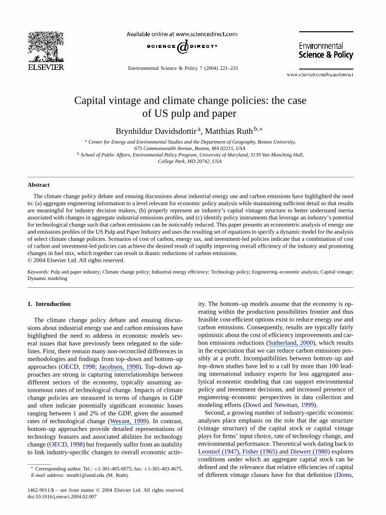
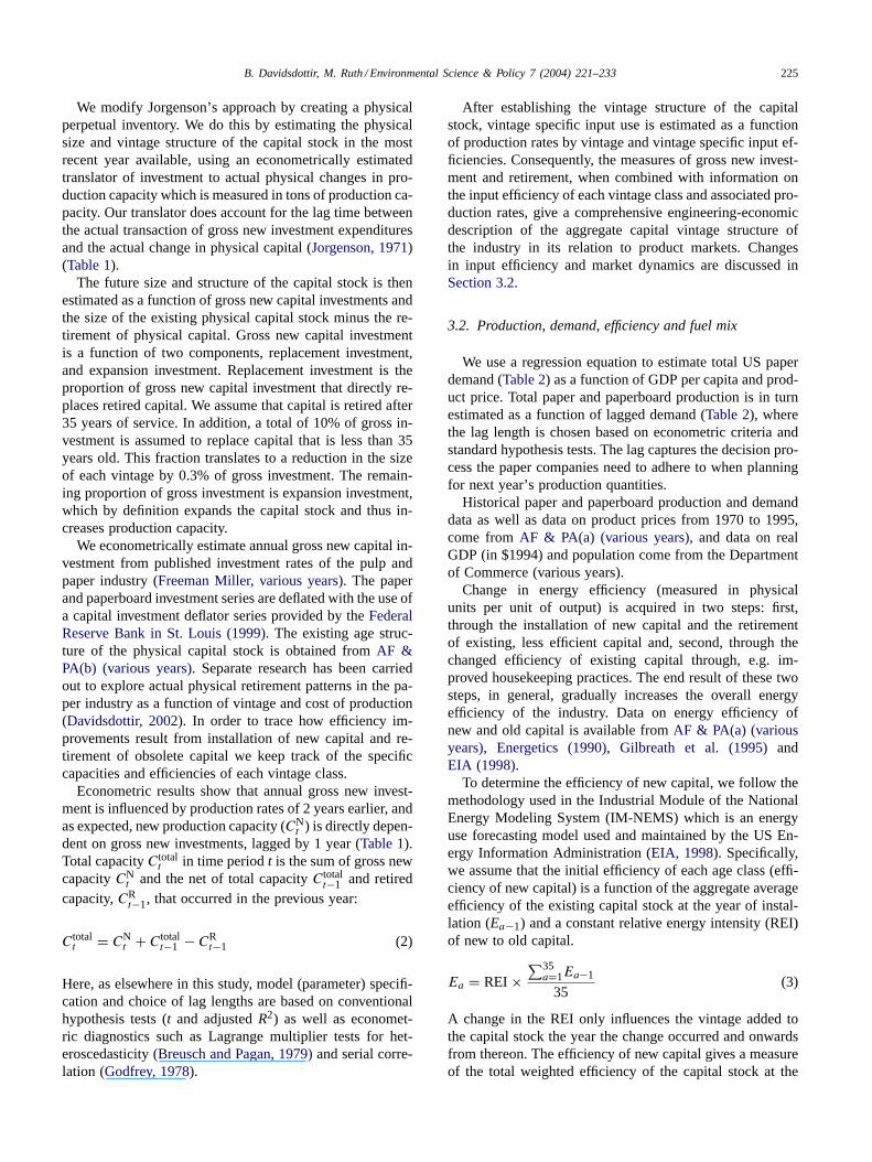
For the purposes of this study, we calculate demand forand supply of output from the industry, and we trace energyinputs as they enter the industry from the rest of the economyboth self-generated and purchased (Fig. 1). Thus, the modelcontains sufficient process-specific detail to be a meaningfulrepresentation of policy and investment decision making, ashas already been demonstrated in the use of earlier versionsof the model in dialog between industry and policy leaders(cf. Ruth et al., 2000c). Our study, further contributes to re-search on the dynamics of industrial energy use and emis-sions by providing an application of capital vintage analy-sis, which has received little attention in industry specificclimate change policy analysis and in industrial ecology ingeneral.

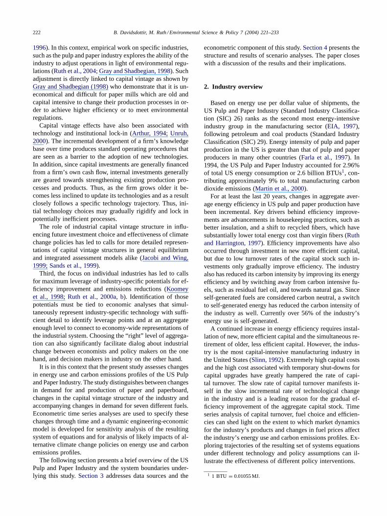
Table 1Regression results for investment and capacity (t-statistics in parenthesis)

Dependant variables

Regressors Functional formand lags

Demand (1000short tons)

New investment(logn $1000)

New capacity(1000 short tons)

Production (1000short tons)

Constant 566608.14 (15.54) 12.18 (26.13) 1210.69 (6.25) −3498.36 (−17.57)GDP/population ($1994) 3.37 (6.64)Indexed product price (1982=100) t−1 −379.47 (−3.38)Demand (1000 short tons) t−1 0.971 (14.63)New investment ($1000) t−1 0.00038 (5.63)Production (1000 short tons) t−2 0.00003 (5.58)Adjusted Ra2 0.92 0.92 0.60 0.95LM χ2b 1.487 (0.779) 2.370 (0.503) 3.484 (0.332) 2.375 (0.498)LM χ2(1)b 0.664 (0.553) 1.522 (0.099) 1.302 (0.132) 0.803 (0.777)

a Lagrange multiplier estimate of serial correlation (Breusch and Pagan, 1979), significance level in parenthesis.b Lagrange multiplier estimate of heteroscedasticity (Godfrey, 1978), significance level in parenthesis.

3. Empirical analysis

3.1. Capital vintage and production capacity

To model changes in the age distribution and size of thecapital stock, we apply a modified version of the perpetualinventory methods pioneered byJorgenson (1968, 1996).The end-of period capital stock at timet is typically esti-mated as a function of gross new capital investments (It),existing capital stock (Kt−1) in the previous year (t−1) andrate of replacement (µ), where all variables are measured inmonetary units:

Kt = It + (1 − µ) × Kt−1 (1)

224B

.D

avid

sdo

ttir,M

.R

uth

/Enviro

nm

en

tal

Scie

nce

&P

olicy

7(2

00

4)

22

1–

23

3

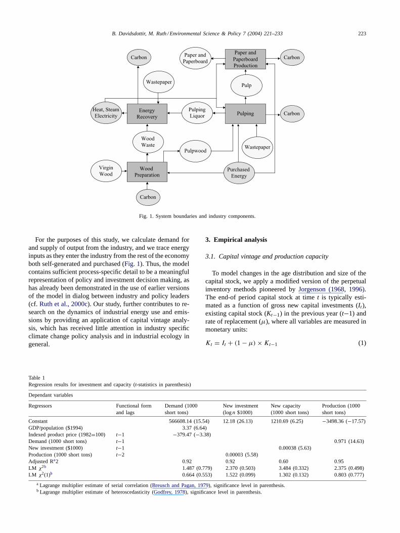
Table 2Regression results for industrial energy use module (t-statistics in parentheses)

Dependent variables

Regressors Functional form and lags Energy efficiency(logn), MillionBTU/tons)

Natural gas(billion BTU)

Coal (log)(billion BTU)

Residual fuel oil(billion BTU)

Electricity (billionBTU)

Self-generated energy(logn) (billion BTU)

Distillate fuel oil (%of total energy use)

Constant 4.115 (42.386) −4554312.680 (−4.644) 13.690 (72.179) 3177127.123 (7.202) −1655197.175 (−33.767) 6.061 (8.614) 0.046 (2.734)Cumulative production index Logn −0.161 (−5.841)Cumulative paper production Logn −201155.338 (−6.29069)Total paper production (1000 tons) Logn 452685.329 (4.996) −0.00000405 (−2.238) 167456.253 (34.975) 0.703 (10.886) −0.003 (−2.297)Coal price/electricity price (t−2) −4.262 (−12.019)

(t−4) −0.943 (−3.218)Residual fuel oil price

($ per million BTU)Logn (t−2) −134765.520 (−7.7281)

Average energy pricea

($ per million BTU)(t−3) 0.028 (5.664)

Primary energy price (PEP)b Logn (t-3) −0.033 (−2.995)($ per million BTU)Coal price/natural gas price (t) 88774.988 (3.105)Electricity price/PEP (t) −8961.999 (−5.943)

(t−1) −7664.524 (−4.751)Distillate fuel oil price

($ per million BTU)(t) −0.002 (−8.496)

LM χ2c 0.656 (0.883) 0.976 (0.913) 4.959 (0.292) 2.113 (0.549) 2.373 (0.667) 2.234 (0.525) 2.375 (0.498)

LMχ2(1)d 1.450 (0.228) 0.564 (0.453) 0.586 (0.444) 1.709 (0.191) 1.704 (0.192) 0.403 (0.526) 0.419 (0.517)

Adjusted R2 0.954 0.754 0.959 0.932 0.988 0.986 0.939

a Average energy price is a non-weigthted average of all fuel prices.b Primary energy price is a non-weighted average of primary energy prices.c Lagrange multiplier estimate of heteroscedasticity (Godfrey, 1978), significance level in parenthesis.d Lagrange multiplier estimate of serial correlation (Breusch and Pagan, 1979), significance level in parenthesis.

B. Davidsdottir, M. Ruth / Environmental Science & Policy 7 (2004) 221–233 225

We modify Jorgenson’s approach by creating a physicalperpetual inventory. We do this by estimating the physicalsize and vintage structure of the capital stock in the mostrecent year available, using an econometrically estimatedtranslator of investment to actual physical changes in pro-duction capacity which is measured in tons of production ca-pacity. Our translator does account for the lag time betweenthe actual transaction of gross new investment expendituresand the actual change in physical capital (Jorgenson, 1971)(Table 1).

The future size and structure of the capital stock is thenestimated as a function of gross new capital investments andthe size of the existing physical capital stock minus the re-tirement of physical capital. Gross new capital investmentis a function of two components, replacement investment,and expansion investment. Replacement investment is theproportion of gross new capital investment that directly re-places retired capital. We assume that capital is retired after35 years of service. In addition, a total of 10% of gross in-vestment is assumed to replace capital that is less than 35years old. This fraction translates to a reduction in the sizeof each vintage by 0.3% of gross investment. The remain-ing proportion of gross investment is expansion investment,which by definition expands the capital stock and thus in-creases production capacity.

We econometrically estimate annual gross new capital in-vestment from published investment rates of the pulp andpaper industry (Freeman Miller, various years). The paperand paperboard investment series are deflated with the use ofa capital investment deflator series provided by theFederalReserve Bank in St. Louis (1999). The existing age struc-ture of the physical capital stock is obtained fromAF &PA(b) (various years). Separate research has been carriedout to explore actual physical retirement patterns in the pa-per industry as a function of vintage and cost of production(Davidsdottir, 2002). In order to trace how efficiency im-provements result from installation of new capital and re-tirement of obsolete capital we keep track of the specificcapacities and efficiencies of each vintage class.

Econometric results show that annual gross new invest-ment is influenced by production rates of 2 years earlier, andas expected, new production capacity (CN

t ) is directly depen-dent on gross new investments, lagged by 1 year (Table 1).Total capacityCtotal

t in time periodt is the sum of gross newcapacityCN

t and the net of total capacityCtotalt−1 and retired

capacity,CRt−1, that occurred in the previous year:

Ctotalt = CN

t + Ctotalt−1 − CR

t−1 (2)

Here, as elsewhere in this study, model (parameter) specifi-cation and choice of lag lengths are based on conventionalhypothesis tests (t and adjustedR2) as well as economet-ric diagnostics such as Lagrange multiplier tests for het-eroscedasticity (Breusch and Pagan, 1979)and serial corre-lation (Godfrey, 1978).

After establishing the vintage structure of the capitalstock, vintage specific input use is estimated as a functionof production rates by vintage and vintage specific input ef-ficiencies. Consequently, the measures of gross new invest-ment and retirement, when combined with information onthe input efficiency of each vintage class and associated pro-duction rates, give a comprehensive engineering-economicdescription of the aggregate capital vintage structure ofthe industry in its relation to product markets. Changesin input efficiency and market dynamics are discussed inSection 3.2.

3.2. Production, demand, efficiency and fuel mix

We use a regression equation to estimate total US paperdemand (Table 2) as a function of GDP per capita and prod-uct price. Total paper and paperboard production is in turnestimated as a function of lagged demand (Table 2), wherethe lag length is chosen based on econometric criteria andstandard hypothesis tests. The lag captures the decision pro-cess the paper companies need to adhere to when planningfor next year’s production quantities.

Historical paper and paperboard production and demanddata as well as data on product prices from 1970 to 1995,come fromAF & PA(a) (various years), and data on realGDP (in $1994) and population come from the Departmentof Commerce (various years).

Change in energy efficiency (measured in physicalunits per unit of output) is acquired in two steps: first,through the installation of new capital and the retirementof existing, less efficient capital and, second, through thechanged efficiency of existing capital through, e.g. im-proved housekeeping practices. The end result of these twosteps, in general, gradually increases the overall energyefficiency of the industry. Data on energy efficiency ofnew and old capital is available fromAF & PA(a) (variousyears), Energetics (1990), Gilbreath et al. (1995)andEIA (1998).

To determine the efficiency of new capital, we follow themethodology used in the Industrial Module of the NationalEnergy Modeling System (IM-NEMS) which is an energyuse forecasting model used and maintained by the US En-ergy Information Administration (EIA, 1998). Specifically,we assume that the initial efficiency of each age class (effi-ciency of new capital) is a function of the aggregate averageefficiency of the existing capital stock at the year of instal-lation (Ea−1) and a constant relative energy intensity (REI)of new to old capital.

Ea = REI ×∑35

a=1Ea−1

35(3)

A change in the REI only influences the vintage added tothe capital stock the year the change occurred and onwardsfrom thereon. The efficiency of new capital gives a measureof the total weighted efficiency of the capital stock at the

226 B. Davidsdottir, M. Ruth / Environmental Science & Policy 7 (2004) 221–233

time of installation of each vintage (WENt ) weighted by each

vintage share of total production (qta/QtS).

WENt =

35∑a=1

Ea ×(

qta

QtS

)(4)

WhereQtS is the total production per year,Ea is the energyefficiency of new capital, anda is the age class or vintage.

To determine changes in energy efficiency of existing cap-ital we estimate learning curves that relate weighted averageenergy efficiencies of the capital stock (WEO

t ) to cumulativeproduction (Xt) and lagged energy prices (Pt−n). Cumula-tive production is used as an indicator of experience (Yelle,1979; Ruth, 1993). Lagged energy prices are used to capturethe delayed impacts that market signals have on housekeep-ing practices (Table 2).

WEOt = f(Xt, Pt−n) (5)

We assume that the rate of change in the energy efficiencyof the existing capital stock is uniform across vintages. Thatis, the efficiency of 10-year-old capital changes as fast as theefficiency of 20-year-old capital. This assumption is madeout of lack of data for capturing the actual rate of changeby vintage. Theoretical studies have shown that generallythe rate increases slowly up to vintages of 5–7 years of ageand then declines after that (Mulder et al., 2001). Separateresearch has been carried out to explore specifically learningcurves for already installed capital or “existing” capital inthe industry (Davidsdottir, 2002). Over time, the efficiencyof the existing capital stock changes as a function of age andinput prices and thus the two impacts on aggregate weightedefficiency are combined using the following equations:

diff t = ((WEOt−1 − WEO

t )/WEOt−1) − ((WEN

t−1

− WENt )/WEN

t−1) (6)

WEt = (1 − diff t) × WENt (7)

Where difft is the difference in the rate of change betweenchanges in the total capital stock, both due to the investmentin new capital and changes due to, e.g. improved housekeep-ing practices((WEO

t−1−WEOt )/WEO

t−1), and changes in theefficiency of the total capital stock only due to the investmentin new, more efficient capital((WEN

t−1 − WENt )/WEN

t−1).WEt is the total weighted average energy efficiency of thecapital stock, and includes changes in the efficiency of bothnew and existing capital.

Following Chern and Just (1980)we use seemingly un-related regressions (Zellner, 1962) to determine the frac-tional share of each fuel used in the industry. The use of aseemingly unrelated regression system enables us to explic-itly take into account the potential for fuel substitution. Theshare of each fuel (Ee

t ) of type e (e = 1 . . . 7) in yeart isa function of relative and absolute fuel prices in lagged andsimultaneous form (Pe

t andt−x) and of production levels (Qt).Again, lagged responses capture the inertia in the system,

where the industry cannot always instantly switch from onefuel to another. Contracts with fuel companies are made 6months to a year in advance and some changes require mod-ifications in boilers. Regression results are listed inTable 2.Historical fuel prices, on which these results are based, havebeen obtained fromEIA (various years). Data on total en-ergy use is fromAF & PA(b) (various years).

The opportunity cost of chemicals and wastes forself-generation are assumed negligible because of hightransport cost of the chemicals and wastes. In contrast, theopportunity cost of the capital for self-generation is notzero. Unfortunately, little information is available to reliablyquantify capital cost of self-generation on an industry-widebasis, and we assume that the price of self-generated en-ergy is zero. As a result of this assumption, we are likely tooverestimate the rate of expansion of self-generation.

4. Scenario analysis

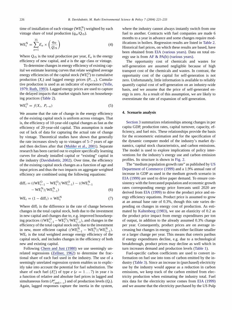
Section 3summarizes relationships among changes in percapita GDP, production rates, capital turnover, capacity, ef-ficiency, and fuel mix. These relationships provide the basisfor the econometric estimation and for the specification ofthe dynamic computer model of the industry’s market dy-namics, capital stock characteristics, and carbon emissions.The model is used to explore implications of policy inter-ventions for the industry’s energy use and carbon emissionprofiles. Its structure is shown inFig. 2.

The “medium population growth rate” as published byUSDepartment of Commerce (1999)and a 1.9% annual rate ofincrease in GDP as used in the medium growth scenario inEIA (1999)are used to drive paper demand. To ensure con-sistency with the forecasted population and economic growthrates corresponding energy price forecasts until 2020 arederived fromEIA (1999) to drive the product price and en-ergy efficiency equations. Product price is assumed to growat an annual base rate of 0.3%, though this rate varies de-pending on changes in energy cost of production. As esti-mated byKaltenberg (1983), we use an elasticity of 0.2 asthe product price impact from energy expenditures per tonof output, in addition to the already assumed 0.3% changeper year. Consequently, product prices are on average in-creasing but changes in energy costs either facilitate smalleror a larger change per year. This means that ceteris paribusif energy expenditures decline, e.g. due to a technologicalbreakthrough, product prices may decline as well which inturn increases demand and production levels (Table 1).

Fuel-specific carbon coefficients are used to convert in-formation on fuel use into tons of carbon emitted by the in-dustry (Table 3). Since an increase in (purchased) electricityuse by the industry would appear as a reduction in carbonemissions, we keep track of the carbon emitted from elec-tricity production when estimating the industry total. Fuelmix data for the electricity sector comes fromEIA (1999)and we assume that the electricity purchased by the US Pulp

B. Davidsdottir, M. Ruth / Environmental Science & Policy 7 (2004) 221–233 227

GDPProduct

prices

Demand

ProductionCapacity

investment

Capital

turnover

Capacity

utilization

Energy

prices

Carbon

coefficients

Energy

efficiency

Capacity

retirement

Energy

prices

Total energy

use

Carbon

emissionsExogenous

Variables

Endogenous

Variables

Capacity

Population

Legend:

Fig. 2. Model structure.

and Paper Industry is generated at the US average fuel mixin electricity production.

We run the simulation model with historic time seriesdata for GDP, population and energy prices. The equationspresented inTables 1 and 2were those for which econo-metric test criteria were satisfied and for which historic sys-tem performance was best mimicked. For example, giventhe model’s specification, the mean square error of simu-lated versus actual energy use by fuel type is less than 2%.Varying the estimated parameters (inTables 1 and 2) withintheir respective confidence intervals changes the actual nu-merical results but the observed trends and our qualitativeconclusions about the effects of alternative policies remainunaffected. Also, the actual numerical results of the modelare of course sensitive to the exogenous parameters, such asGDP growth rates and energy prices (see regression resultsin Tables 1 and 2). However, the price and GDP forecaststhat are used in the model are both derived from NEMS sce-narios to achieve consistency. Varying the rate of change inthose exogenous parameters will modify the trends seen inthe base scenario (e.g. an increase in GDP growth results inan increase in paper demand and thus higher growth rates),yet such a change will not change the qualitative conclusionsabout the various policies.

Table 3Carbon content of fuels (Source:EIA, 1994)

Fuel type Metric tons of carbon per billionBTU (1994 value)

Coal 25.61Coal (electricity generation) 25.71Natural gas 14.47Residual fuel oil 21.49Oil (electricity generation) 19.95Liquid petroleum gas 17.02Distillate fuel oil 19.95

20302020201020001990198019701960

0,00e+0

1,00e+6

2,00e+6

3,00e+6

4,00e+6

Year

En

erg

y U

se b

y S

ou

rce (

bil

lio

n B

TU

'S)

Total energy use

Purchased

Selfgenerated

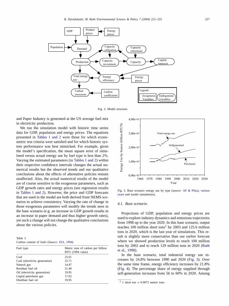
Fig. 3. Base scenario energy use by type (source:AF & PA(a), variousyearsand model simulations).

4.1. Base scenario

Projections of GDP, population and energy prices areused to explore industry dynamics and emissions trajectoriesfrom 1998 up to the year 2020. In this base scenario, outputreaches 100 million short tons2 by 2003 and 125.6 milliontons in 2020, which is the last year of simulations. This re-sult is slightly more conservative than our earlier forecastwhere we showed production levels to reach 100 milliontons by 2002 and to reach 129 million tons in 2020 (Ruthet al., 1998).

In the base scenario, total industrial energy use in-creases by 24.8% between 1990 and 2020 (Fig. 3). Overthe same time frame, energy efficiency increases by 21.8%(Fig. 4). The percentage share of energy supplied throughself-generation increases from 56 to 60% in 2020. Among

2 1 short ton= 0.9072 metric tons.

228 B. Davidsdottir, M. Ruth / Environmental Science & Policy 7 (2004) 221–233

20302020201020001990198019701960

0,0

0,1

0,2

0,3

0,4

0,5

0,6

Year

Fra

cti

on

al

share

of

each

fu

el

Selfgenerated

Residual fuel oil

Coal

Electricity

Natural Gas

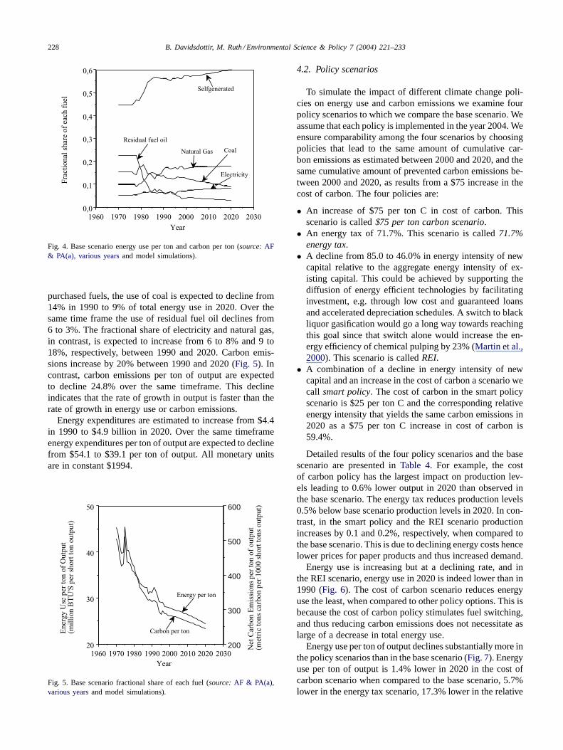
Fig. 4. Base scenario energy use per ton and carbon per ton (source:AF& PA(a), various yearsand model simulations).

purchased fuels, the use of coal is expected to decline from14% in 1990 to 9% of total energy use in 2020. Over thesame time frame the use of residual fuel oil declines from6 to 3%. The fractional share of electricity and natural gas,in contrast, is expected to increase from 6 to 8% and 9 to18%, respectively, between 1990 and 2020. Carbon emis-sions increase by 20% between 1990 and 2020 (Fig. 5). Incontrast, carbon emissions per ton of output are expectedto decline 24.8% over the same timeframe. This declineindicates that the rate of growth in output is faster than therate of growth in energy use or carbon emissions.

Energy expenditures are estimated to increase from $4.4in 1990 to $4.9 billion in 2020. Over the same timeframeenergy expenditures per ton of output are expected to declinefrom $54.1 to $39.1 per ton of output. All monetary unitsare in constant $1994.

20302020201020001990198019701960

20

30

40

50

200

300

400

500

600

Year

En

erg

y U

se p

er

ton

of

Ou

tpu

t (m

illi

on

BT

U'S

per

sho

rt t

on

ou

tpu

t)

Net

Carb

on

Em

issi

on

s p

er

ton

of

ou

tpu

t(m

etr

ic t

on

s carb

on

per

10

00

sh

ort

to

ns

ou

tpu

t)

Energy per ton

Carbon per ton

Fig. 5. Base scenario fractional share of each fuel (source:AF & PA(a),various yearsand model simulations).

4.2. Policy scenarios

To simulate the impact of different climate change poli-cies on energy use and carbon emissions we examine fourpolicy scenarios to which we compare the base scenario. Weassume that each policy is implemented in the year 2004. Weensure comparability among the four scenarios by choosingpolicies that lead to the same amount of cumulative car-bon emissions as estimated between 2000 and 2020, and thesame cumulative amount of prevented carbon emissions be-tween 2000 and 2020, as results from a $75 increase in thecost of carbon. The four policies are:

• An increase of $75 per ton C in cost of carbon. Thisscenario is called$75 per ton carbon scenario.

• An energy tax of 71.7%. This scenario is called71.7%energy tax.

• A decline from 85.0 to 46.0% in energy intensity of newcapital relative to the aggregate energy intensity of ex-isting capital. This could be achieved by supporting thediffusion of energy efficient technologies by facilitatinginvestment, e.g. through low cost and guaranteed loansand accelerated depreciation schedules. A switch to blackliquor gasification would go a long way towards reachingthis goal since that switch alone would increase the en-ergy efficiency of chemical pulping by 23% (Martin et al.,2000). This scenario is calledREI.

• A combination of a decline in energy intensity of newcapital and an increase in the cost of carbon a scenario wecall smart policy. The cost of carbon in the smart policyscenario is $25 per ton C and the corresponding relativeenergy intensity that yields the same carbon emissions in2020 as a $75 per ton C increase in cost of carbon is59.4%.

Detailed results of the four policy scenarios and the basescenario are presented inTable 4. For example, the costof carbon policy has the largest impact on production lev-els leading to 0.6% lower output in 2020 than observed inthe base scenario. The energy tax reduces production levels0.5% below base scenario production levels in 2020. In con-trast, in the smart policy and the REI scenario productionincreases by 0.1 and 0.2%, respectively, when compared tothe base scenario. This is due to declining energy costs hencelower prices for paper products and thus increased demand.

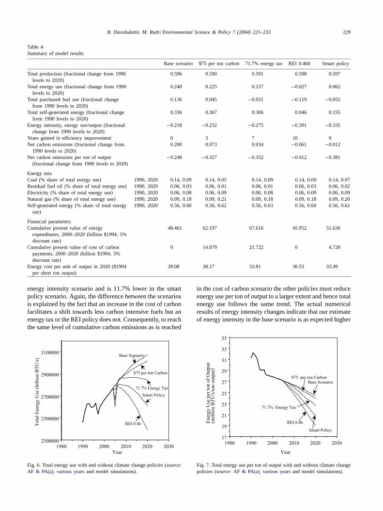
Energy use is increasing but at a declining rate, and inthe REI scenario, energy use in 2020 is indeed lower than in1990 (Fig. 6). The cost of carbon scenario reduces energyuse the least, when compared to other policy options. This isbecause the cost of carbon policy stimulates fuel switching,and thus reducing carbon emissions does not necessitate aslarge of a decrease in total energy use.

Energy use per ton of output declines substantially more inthe policy scenarios than in the base scenario (Fig. 7). Energyuse per ton of output is 1.4% lower in 2020 in the cost ofcarbon scenario when compared to the base scenario, 5.7%lower in the energy tax scenario, 17.3% lower in the relative

B. Davidsdottir, M. Ruth / Environmental Science & Policy 7 (2004) 221–233 229

Table 4Summary of model results

Base scenario $75 per ton carbon 71.7% energy tax REI 0.460 Smart policy

Total production (fractional change from 1990levels to 2020)

0.596 0.590 0.591 0.598 0.597

Total energy use (fractional change from 1990levels to 2020)

0.248 0.225 0.157 −0.027 0.062

Total purchased fuel use (fractional changefrom 1990 levels to 2020)

0.136 0.045 −0.031 −0.119 −0.055

Total self-generated energy (fractional changefrom 1990 levels to 2020)

0.336 0.367 0.306 0.046 0.155

Energy intensity, energy use/output (fractionalchange from 1990 levels to 2020)

−0.218 −0.232 −0.275 −0.391 −0.335

Years gained in efficiency improvement 0 3 7 10 9Net carbon emissions (fractional change from

1990 levels to 2020)0.200 0.073 0.034 −0.061 −0.012

Net carbon emissions per ton of output(fractional change from 1990 levels to 2020)

−0.248 −0.327 −0.352 −0.412 −0.381

Energy mixCoal (% share of total energy use) 1990, 2020 0.14, 0.09 0.14, 0.05 0.14, 0.09 0.14, 0.09 0.14, 0.07Residual fuel oil (% share of total energy use) 1990, 2020 0.06, 0.03 0.06, 0.01 0.06, 0.01 0.06, 0.03 0.06, 0.02Electricity (% share of total energy use) 1990, 2020 0.06, 0.08 0.06, 0.09 0.06, 0.08 0.06, 0.09 0.06, 0.09Natural gas (% share of total energy use) 1990, 2020 0.09, 0.18 0.09, 0.21 0.09, 0.18 0.09, 0.18 0.09, 0.20Self-generated energy (% share of total energy

use)1990, 2020 0.56, 0.60 0.56, 0.62 0.56, 0.63 0.56, 0.60 0.56, 0.61

Financial parametersCumulative present value of energy

expenditures, 2000–2020 (billion $1994, 5%discount rate)

48.461 62.197 67.616 45.952 51.636

Cumulative present value of cost of carbonpayments, 2000–2020 (billion $1994, 5%discount rate)

0 14.079 21.722 0 4.720

Energy cost per unit of output in 2020 ($1994per short ton output)

39.08 38.17 33.81 30.53 33.49

energy intensity scenario and is 11.7% lower in the smartpolicy scenario. Again, the difference between the scenariosis explained by the fact that an increase in the cost of carbonfacilitates a shift towards less carbon intensive fuels but anenergy tax or the REI policy does not. Consequently, to reachthe same level of cumulative carbon emissions as is reached

203020202010200019901980

2300000

2500000

2700000

2900000

3100000

Year

To

tal

En

erg

y U

se (

bil

lio

n B

TU

's)

Base Scenario

$75 per ton Carbon

71.7% Energy Tax

REI 0.46

Smart Policy

Fig. 6. Total energy use with and without climate change policies (source:AF & PA(a), various yearsand model simulations).

in the cost of carbon scenario the other policies must reduceenergy use per ton of output to a larger extent and hence totalenergy use follows the same trend. The actual numericalresults of energy intensity changes indicate that our estimateof energy intensity in the base scenario is as expected higher

203020202010200019901980

17

19

21

23

25

27

29

31

33

35

Year

Energ

y U

se p

er

ton o

f O

utp

ut

(mil

lion B

TU

's/t

on o

utp

ut)

$75 per ton Carbon

Base Scenario

71.7% Energy Tax

Smart Policy

REI 0.46

Fig. 7. Total energy use per ton of output with and without climate changepolicies (source:AF & PA(a), various yearsand model simulations).

230 B. Davidsdottir, M. Ruth / Environmental Science & Policy 7 (2004) 221–233

203020202010200019901980

1,30e+6

1,40e+6

1,50e+6

1,60e+6

1,70e+6

1,80e+6

1,90e+6

Year

Self

genera

ted E

nerg

y U

se(B

illi

on

BT

U's

)

Base Scenario

$75 per ton Carbon

71.7% Energy Tax

REI 0.46

Smart Policy

Fig. 8. Self-generated energy use with and without climate change policies(source:AF & PA(a), various yearsand model simulations).

than in business as usual scenarios of bottom up studies(e.g.Energetics, 1990). Also, the results in the smart policyscenario and the REI scenario, or approximately 20 and 19million BTU’s per ton of output, respectively, are slightlyhigher than a penetration of 100% advanced technologieswhich result in an aggregate intensity of approximately 18million BTU’s per ton of output (Energetics, 1990).

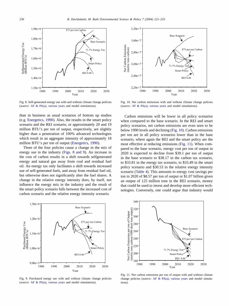
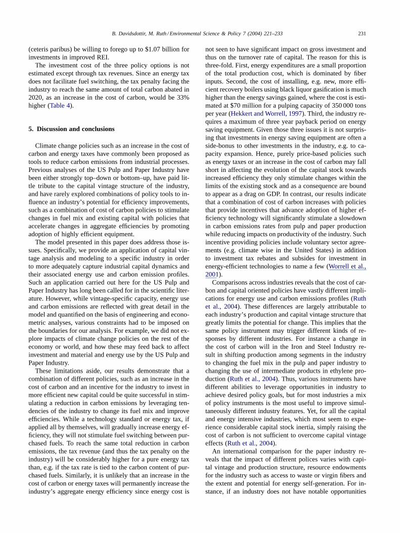
Three of the four policies cause a change in the mix ofenergy use in the industry (Figs. 8 and 9). An increase inthe cost of carbon results in a shift towards selfgeneratedenergy and natural gas away from coal and residual fueloil. An energy tax only facilitates a shift towards increaseduse of self-generated fuels, and away from residual fuel oil,but otherwise does not significantly alter the fuel shares. Achange in the relative energy intensity does, by itself, notinfluence the energy mix in the industry and the result ofthe smart policy scenario falls between the increased cost ofcarbon scenario and the relative energy intensity scenario.

203020202010200019901980

9,00e+5

1,00e+6

1,10e+6

1,20e+6

1,30e+6

Year

Pu

rch

ase

d E

nerg

y U

se(B

illi

on

BT

U's

)

Base Scenario

Smart Policy

REI 0.46

71.7% Energy Tax

$75 per ton Carbon

Fig. 9. Purchased energy use with and without climate change policies(source:AF & PA(a), various yearsand model simulations).

203020202010200019901980

2,20e+7

2,40e+7

2,60e+7

2,80e+7

3,00e+7

3,20e+7

Year

Net

Carb

on

Em

issi

on

s(m

etr

ic t

ons

carb

on)

Base Scenario

$75 per ton Carbon

71.7% Energy Tax

Smart Policy

REI 0.46

Fig. 10. Net carbon emissions with and without climate change policies(source:AF & PA(a), various yearsand model simulations).

Carbon emissions will be lower in all policy scenarioswhen compared to the base scenario. In the REI and smartpolicy scenarios, net carbon emissions are even seen to bebelow 1990 levels and declining (Fig. 10). Carbon emissionsper ton are in all policy scenarios lower than in the basescenario, where again the REI and the smart policy are themost effective at reducing emissions (Fig. 11). When com-pared to the base scenario, energy cost per ton of output in2020 is expected to decline from $39.1 per ton of outputin the base scenario to $38.17 in the carbon tax scenario,to $33.81 in the energy tax scenario, to $33.49 in the smartpolicy scenario and $30.53 in the relative energy intensityscenario (Table 4). This amounts to energy cost savings perton in 2020 of $8.57 per ton of output or $1.07 billion givenan output of 125 million tons in the REI scenario, moneythat could be used to invest and develop more efficient tech-nologies. Conversely, one could argue that industry would

203020202010200019901980

180

200

220

240

260

280

300

320

340

Year

Net

Carb

on

Em

issi

on

s p

er

ton

of

Ou

tpu

t(m

etr

ic t

on

s carb

on

/10

00

sh

ort

to

ns

ou

tpu

t)

Base Scenario

$75 per ton Carbon

71.7% Energy Tax

REI 0.46

Smart Policy

Fig. 11. Net carbon emissions per ton of output with and without climatechange policies (source:AF & PA(a), various yearsand model simula-tions).

B. Davidsdottir, M. Ruth / Environmental Science & Policy 7 (2004) 221–233 231

(ceteris paribus) be willing to forego up to $1.07 billion forinvestments in improved REI.

The investment cost of the three policy options is notestimated except through tax revenues. Since an energy taxdoes not facilitate fuel switching, the tax penalty facing theindustry to reach the same amount of total carbon abated in2020, as an increase in the cost of carbon, would be 33%higher (Table 4).

5. Discussion and conclusions

Climate change policies such as an increase in the cost ofcarbon and energy taxes have commonly been proposed astools to reduce carbon emissions from industrial processes.Previous analyses of the US Pulp and Paper Industry havebeen either strongly top–down or bottom–up, have paid lit-tle tribute to the capital vintage structure of the industry,and have rarely explored combinations of policy tools to in-fluence an industry’s potential for efficiency improvements,such as a combination of cost of carbon policies to stimulatechanges in fuel mix and existing capital with policies thataccelerate changes in aggregate efficiencies by promotingadoption of highly efficient equipment.

The model presented in this paper does address those is-sues. Specifically, we provide an application of capital vin-tage analysis and modeling to a specific industry in orderto more adequately capture industrial capital dynamics andtheir associated energy use and carbon emission profiles.Such an application carried out here for the US Pulp andPaper Industry has long been called for in the scientific liter-ature. However, while vintage-specific capacity, energy useand carbon emissions are reflected with great detail in themodel and quantified on the basis of engineering and econo-metric analyses, various constraints had to be imposed onthe boundaries for our analysis. For example, we did not ex-plore impacts of climate change policies on the rest of theeconomy or world, and how these may feed back to affectinvestment and material and energy use by the US Pulp andPaper Industry.

These limitations aside, our results demonstrate that acombination of different policies, such as an increase in thecost of carbon and an incentive for the industry to invest inmore efficient new capital could be quite successful in stim-ulating a reduction in carbon emissions by leveraging ten-dencies of the industry to change its fuel mix and improveefficiencies. While a technology standard or energy tax, ifapplied all by themselves, will gradually increase energy ef-ficiency, they will not stimulate fuel switching between pur-chased fuels. To reach the same total reduction in carbonemissions, the tax revenue (and thus the tax penalty on theindustry) will be considerably higher for a pure energy taxthan, e.g. if the tax rate is tied to the carbon content of pur-chased fuels. Similarly, it is unlikely that an increase in thecost of carbon or energy taxes will permanently increase theindustry’s aggregate energy efficiency since energy cost is

not seen to have significant impact on gross investment andthus on the turnover rate of capital. The reason for this isthree-fold. First, energy expenditures are a small proportionof the total production cost, which is dominated by fiberinputs. Second, the cost of installing, e.g. new, more effi-cient recovery boilers using black liquor gasification is muchhigher than the energy savings gained, where the cost is esti-mated at $70 million for a pulping capacity of 350 000 tonsper year (Hekkert and Worrell, 1997). Third, the industry re-quires a maximum of three year payback period on energysaving equipment. Given those three issues it is not surpris-ing that investments in energy saving equipment are often aside-bonus to other investments in the industry, e.g. to ca-pacity expansion. Hence, purely price-based policies suchas energy taxes or an increase in the cost of carbon may fallshort in affecting the evolution of the capital stock towardsincreased efficiency they only stimulate changes within thelimits of the existing stock and as a consequence are boundto appear as a drag on GDP. In contrast, our results indicatethat a combination of cost of carbon increases with policiesthat provide incentives that advance adoption of higher ef-ficiency technology will significantly stimulate a slowdownin carbon emissions rates from pulp and paper productionwhile reducing impacts on productivity of the industry. Suchincentive providing policies include voluntary sector agree-ments (e.g. climate wise in the United States) in additionto investment tax rebates and subsides for investment inenergy-efficient technologies to name a few (Worrell et al.,2001).

Comparisons across industries reveals that the cost of car-bon and capital oriented policies have vastly different impli-cations for energy use and carbon emissions profiles (Ruthet al., 2004). These differences are largely attributable toeach industry’s production and capital vintage structure thatgreatly limits the potential for change. This implies that thesame policy instrument may trigger different kinds of re-sponses by different industries. For instance a change inthe cost of carbon will in the Iron and Steel Industry re-sult in shifting production among segments in the industryto changing the fuel mix in the pulp and paper industry tochanging the use of intermediate products in ethylene pro-duction (Ruth et al., 2004). Thus, various instruments havedifferent abilities to leverage opportunities in industry toachieve desired policy goals, but for most industries a mixof policy instruments is the most useful to improve simul-taneously different industry features. Yet, for all the capitaland energy intensive industries, which most seem to expe-rience considerable capital stock inertia, simply raising thecost of carbon is not sufficient to overcome capital vintageeffects (Ruth et al., 2004).

An international comparison for the paper industry re-veals that the impact of different polices varies with capi-tal vintage and production structure, resource endowmentsfor the industry such as access to waste or virgin fibers andthe extent and potential for energy self-generation. For in-stance, if an industry does not have notable opportunities

232 B. Davidsdottir, M. Ruth / Environmental Science & Policy 7 (2004) 221–233

for energy self-generation an increase in energy prices as aresult of increased cost of carbon or energy taxes, is likelyto reduce production levels and increase energy efficiencymore than if the industry was able to shift over to increasedself-generation. However, regardless of location, resourceavailability and production structure, an increase in the rateof capital turnover is the most important factor in perma-nently changing carbon emission profiles and energy effi-ciency in the pulp and paper industry (see for, e.g.Nystromand Cornland, 2003).

Acknowledgements

This paper was made possible by financial support fromUS EPA under Grant Number X 826822-01-0, and benefitedsignificantly from extensive discussions with members of theAmerican Forest and Paper Association and US Departmentof Energy and valuable feedback from three anonymous ref-erees. However, the results presented here not necessarilyrepresent their views, and responsibility for any errors solelyresides with the authors.

References

AF & PA(a), various years. Statistics of Paper Paperboard andWoodpulp. The American Forest and Paper Association, Washington,DC.

AF&PA(b), various years. Paper, Paperboard and Woodpulp FiberConsumption. The American Forest and Paper Association,Washington, DC.

Arthur, B.W., 1994. Increasing Returns and Path Dependence in theEconomy. The University of Michigan Press, Ann Arbor, MI.

Breusch, T., Pagan, A., 1979. A simple test for heteroscedasticity andrandom coefficient variation. Econometrica 47, 1287–1294.

Chern, W.S., Just, R.E., 1980. A generalized model of fuel choices withapplication to the paper industry. Energy Sys. Pol. 4 (4), 273–294.

Davidsdottir, B., 2002, A vintage analysis of regional energy and fiber use.Technological Change and Greenhouse Gas Emissions in the US PaperIndustry. PhD Dissertation, Department of Geography and the Centerfor Energy and Environmental Studies, Boston University, Boston, MA.

Diewert, E., 1980. Aggregation problems in the measurement of capital.In Usher, D. (Ed.), The Measurement of Capital. University of ChicagoPress, Chicago, IL, pp. 433–528.

Doms, M.E., 1996. Estimating capital efficiency schedules withinproduction functions. Econ. Inquiry 34, 78–92.

Dowd, J., Newman, J., 1999. Challenges and Opportunities for AdvancingEngineering–Economic Policy Analysis: Highlights of the IEAInternational Workshop on Technologies to Reduce Greenhouse GasEmissions, 5–7 May, Washington, DC. International Energy Agency,Paris.

EIA. various years. Annual Energy Review. Department of Energy/EnergyInformation Administration, Washington, DC.

EIA, 1994. Emissions of Greenhouse Gases in the United States1987–1992. DOE/EIA-0573, Washington DC.

EIA, 1997. Manufacturing Energy Consumption Survey, 1994. Departmentof Energy/Energy Information Administration, Washington, DC.

EIA, 1998. Industrial Sector Demand Module of the NationalEnergy Modeling System. Office of Integrated Analysis andForecasting. Department of Energy/Energy Information Administration,Washington, DC.

EIA, 1999. Annual Energy Outlook. Department of Energy/EnergyInformation Administration, Washington, DC.

Energetics, 1990. Industrial Technologies: Industry Profiles. Energetics,Columbia.

Farla, J., Blok, K., Schipper, L., 1997. Energy efficiency developmentsin the pulp and paper industry. Energy Pol. 25, 745–758.

Freeman Miller, various years. Pulp and Paper. San Francisco, CA.Federal Reserve Bank in St. Louis, 1999. Gross Private Domestic

Investment: Chain-type Price Index.http://www.stls.frb.org/fred/data/gdp/gpdictpi.accessed:9/15/99.

Fisher, F., 1965. Embodied technical change and the existence of anaggregate capital stock. Rev. Econ. Study 32, 263–288.

Gilbreath, K.R., Gupta, A., Larson, E., Nilsson, L., 1995. Backgroundpaper in energy efficiency and the pulp and paper industry, Preparedfor the ACEEE 1995 Summer Study on Energy Efficiency in Industry.Grand Island, NY, 1–4 August 1995.

Godfrey, L.G., 1978. Testing against general autoregressive and movingaverage error models when the regressors include lagged dependentvariables. Econometrica 46, 1293–1302.

Gray, W.B., Shadbegian, R.J., 1998. Environmental regulation, investmenttiming, and technology choice. J. Ind. Econ. 46, 235–256.

Hekkert, M.P., Worrell, E., 1997. Technology Characterization for NaturalOrganic Materials, Input data for Western European MARKAL, UtrechtUniversity, The Netherlands.

Jacobi, H.D., Wing, I.S., 1999. Adjustment time, capital malleability andpolicy cost. Energy J. (Special issue), 73–92.

Jacobsen, H.K., 1998. Integrating the bottom–up and top–down approachto energy–economy modeling: the case of Denmark. Energy Econ.20 (4), 443–461.

Jorgenson, D.W., 1968. Optimal capital accumulation and investmentbehavior. J. Political Econ. 76 (3), 1123–1151.

Jorgenson, D.W., 1971. Econometric studies of investment behavior: areview. J. Econ. Lit. 9 (4), 1111–1147.

Jorgenson, D.W., 1996. Investment. MIT Press, Cambridge.Kaltenberg, M.C., 1983, Differential Regional Growth in US Pulp, Paper

and Paperboard Production: an Econometric Analysis with Projections.Ph.D. Thesis, University of Wisconsin, Madison, WI.

Koomey, J.G., Koomey, R., Richey, C., LAitner, S., Markel, R.J., Marnay,C., 1998. Technology and Greenhouse Gas Emissions: an IntegratedScenario Analysis Using the LBNL-NEMS Model. LBL-42054/EPA430-R-98-021, Lawrence Berkeley National Laboratory, Berkeley, CA.

Leontief, W., 1947. Introduction to a theory of internal structure offunctional relationships. Econometrica 15, 361–373.

Martin, N., Angliani, N., Einstein, D., Khrushch, M., Worrell, E.,Price, L.K., 2000. Opportunities to Improve Energy Efficiency andReduce Greenhouse Gas Emissions in the US Pulp and PaperIndustry. Lawrence Berkeley National Laboratory, EnvironmentalEnergy Technology Division, Report Number LBNL-46141. July 2000,Berkeley, CA.

Mulder, P., deGrot, H.L.F.L., Hofkes, M.W., 2001, Explaining the EnergyEfficiency Paradox: a Vintage Model With Returns to Diversity andLearning-by Using, Vrije University, Amsterdam, The Netherlands.

Nystrom, I., Cornland, D.W., 2003. Strategic choices: Swedish climateintervention policies and the forest industry’s role in reducing CO2

emissions. Energy Pol. 31, 937–950.OECD, 1998, Mapping the Energy Future, Energy Modeling and Climate

Change Policy. OECD/IEA, France.Ruth, M., 1993. Integrating Economics, Ecology and Thermodynamics.

Kluwer Academic Publishers, Dordrecht, The Netherlands.Ruth, M., Harrington, T., 1997. Dynamics of material and energy use in

US pulp and paper manufacturing. Ind. Ecol. 1, 147–168.Ruth, M., Davidsdottir, B., Amato, A., Tanizaki, J., 1998. Impacts of

Energy And Carbon Taxes On Energy Intensive Industries. ReportPrepared for the US-EPA.

Ruth, M., Davidsdottir, B., Laitner, S., 2000a. Impacts of energy andcarbon taxes on the US Pulp and Paper Industry. Energy Pol. 28,259–270.

B. Davidsdottir, M. Ruth / Environmental Science & Policy 7 (2004) 221–233 233

Ruth, M., Amato, A., Davidsdottir, B., 2000b. Impacts of market-basedclimate change policy on the US Iron and Steel Industry. EnergySources 22 (3), 269–280.

Ruth, M., Davisdottir, B., Laitner, S., 2000c. Using climate change policiesto promote efficiency in the US Pulp and Paper Industry. TAPPI J.Washington, DC, 2000.

Ruth, M., Davidsdottir, B., Amato, A., 2004. Dynamic industrial systemsanalysis for policy assessment. In van den Bergh, J., Janssen M. (Eds.),The Economics Of Industrial Ecology, Edward Elgar Publishers, UK,in press.

Sands, R.D., Edmonds, J.A., MacCracken, C.N., 1999. SGM 2000: ModelDescription and Theory, Draft, Pacific Northwest National Laboratory.

Slinn, R.J., 1992. The paper industry and capital. TAPPI J. Washington,DC, 1992.

Sutherland, R.J., 2000. No cost efforts to reduce carbon emissions in theUS: an economic perspective. Energy J. 21 (3), 89–112.

Unruh, G.C., 2000. Understanding carbon lock-in. Energy Pol. 28, 817–830.

US Department of Commerce, 1999. various years. Statistical Abstracts ofthe United States. US Department of Commerce/Bureau of the Census,Washington, DC.

Weyant, J., 1999. The Costs of the Kyoto Protocol: a multi-modelevaluation. Energy J. (Special issue).

Worrell, E., Price, L., Ruth, M., 2001. Policy modeling for energyefficiency improvements in US industry. Ann. Rev. Energy Environ.26, 117–143.

Yelle, L.E., 1979. The learning curve: historical survey and comprehensivesurvey. Decision Sci. 10, 302–334.

Zellner, A., 1962. An efficient method of estimating seemingly unrelatedregressions and tests for aggregation bias. J. Am. Stat. Assoc. 57,348–368.

Dr. Brynhildur Davidsdottir is the book review editor for the journalEcological Economicsand teaches at Boston University. She holds degreesin biology, international relations and resource and environmental man-agement in addition to a Ph.D. in energy and environmental analysis. Inher research Dr. Davidsdottir combines her multidisciplinary backgroundto analyze relationships between economic, social and environmental sys-tems. Current research projects include the development of energy sustain-ability indicators, dynamic modeling of social and environmental systemsgoverned as common property resources, dynamic modeling of industrialsystems and the development of Carbon Emissions Economic EfficiencyIndicators for the United States.

Dr. Matthias Ruth is Professor and Director of the Environmental PolicyProgram at the School of Public Affairs at the University of Maryland.His research focuses on modeling of natural resource use, industrial andinfrastructural system analysis and environmental economics and policy.His theoretical work draws on concepts from engineering, economics andecology while his applied research utilizes methods of dynamic modelingas well as adaptive and anticipatory management. Professor Ruth haspublished six books and over 80 papers and book chapters in the scientificliterature. He collaborates extensively with scientists and policy makersin the USA, Canada, Europe, Asia, and Africa.