Capital Allocation in Insurance: EconomicCapital and the Allocation of the Default

Option Value∗

Michael SherrisFaculty of Commerce and Economics,University of New South Wales,Sydney, NSW, Australia, 2052email: m.sherris@unsw.edu.au

andJohn van der Hoek

Department of Applied Mathematics,University of Adelaide,

Adelaide, S.A. Australia, 5005email: jvanderh@maths.adelaide.edu.au

September 7, 2004

AbstractThe determination and allocation of economic capital is important for

pricing, risk management and related insurer financial decision making.This paper considers the allocation of economic capital to lines of businessin insurance. We show how to derive closed form results for the completemarkets, arbitrage-free allocation of the insurer default option value, orinsolvency exchange option, to lines of business for an insurer balancesheet. We assume that individual lines of business and the surplus ratioare joint log-normal although the method we adopt allows other assump-tions. The allocation of the default option value is required for fair pricingin the multi-line insurer. We discuss and illustrate other methods of capi-tal allocation, including Myers-Read, and give numerical examples for thecapital allocation of the default option value based on explicit payoffs byline.

JEL Classification: G22, G13, G32Keywords: capital allocation, insurance, default option value

∗This research supported by Australian Research Council Discovery Grant DP0345036and financial support from the UNSW Actuarial Foundation of The Institute of Actuaries ofAustralia. We thank Wina Wahyudi for excellent research assistance. An earlier version waspresented at the 39th Actuarial Research Conference, Iowa, August 2004, and submitted tothe 14th International AFIR Colloquium, Boston, November 2004.

1

IntroductionCapital allocation in insurance is a topic of great interest to both practitionersand academics. Butsic (1999) [2], Meyers (2003) [7], Myers and Read (2001)[10], Merton and Perold (1993) [8], Panjer (2001) [11], Phillips, Cummins andAllen (1998) [12], Valdez and Chernih (2003), Venter (2004) [16], Zanjani (2002)[17] and Zeppetella (2002) [18] are amongst an increasing number of authorsaddressing the issue of capital allocation in insurance.Venter (2004) [16] gives a comprehensive review and discussion of approaches

for allocating capital to lines of business including a discussion of the Myersand Read (2001) [10] approach based on Butsic (1999) [2]. Cummins (2000) [3]provides an overview of capital allocation in insurance including the methodsof allocating capital proposed by Merton and Perold (1993) [8] and Myers andRead (2001) [10]. An often stated benefit of the Myers and Read (2001) [10]approach is that all capital is allocated whereas the Merton and Perold (1993) [8]approach leaves some capital unallocated. Myers and Read (2001) [10] identifythe importance of the insurer default option in determining capital allocation.They show how a marginal default option value can be used to determine thecapital required to maintain a specified insurer default option value to liabilityratio for small changes in lines of business. These marginal default values arethen used to allocate insurer capital.Cummins (2000) [3] states (page 24)

Because the amounts of capital allocated to each line of busi-ness differ substantially between the M-R and M-P methods, thetwo methods will not yield the same pricing and project decisionswhen used with a method that employs by-line capital allocations.Consequently, it is important to determine which method is correct.

Cummins (2000) [3] also states in the final sentence of his conclusion

Finally, the winning firms in the twenty-first century will be theones that successfully implement capital allocation and other finan-cial decision-making techniques. Such firms will make better pricing,underwriting and entry/exit decisions and create value for sharehold-ers.

Mildenhall (2002) [9] shows that the Myers and Read (2001) [10] method willonly allocate the default option value in practice so that the values "add-up"for insurance loss distributions by line of business that are homogeneous. Thisis important since capital allocation is often used in practice for determiningthe amount of capital required as lines of business are grown or exited.Phillips, Cummins and Allen (1998) [12] argue that it is not appropriate

to allocate capital to lines of business. Gründl and Schmeiser (2003) [4] makethe case that there is no need to allocate capital for the purposes of pricinginsurance contracts and determining surplus requirements.

2

Sherris (2004) [14] discusses capital allocation in a complete markets andfrictionless model. He shows how economic capital of the total insurer balancesheet can be allocated by line of business. He gives results for the allocation ofthe default option value allowing explicitly for the share of the asset shortfallfor each line of business in the event of insolvency. His approach fully allocatesthe total insurer default option value to lines of business regardless of the lossdistribution provided arbitrage-free values can be determined. Allocation oftotal insurer capital requires an allocation of assets as well as the default optionvalue. Sherris (2004) [14] shows there is no unique or optimal way to allocate theassets to lines of business without additional criteria. These allocations differfrom the Myers and Read (2001) [10] allocations and we explain the reason forthe differences.The allocation of the insurer level default option value has economic signifi-

cance since this determines the fair price of insurance by line. Fair prices of linesof business reflect the risk of the liability as well as the allocation of the defaultoption value to the line of business. Thus the allocation of the default optionvalue by line of business is critical to fair pricing in the multi-line insurer. Forpricing it is necessary to allocate the default option value to lines of business inorder for insurance prices to include the impact of insolvency on claims. We dothis explicitly based on the insurer balance sheet and the explicit by-line payoffsallowing for insolvency.In this paper we derive closed form expressions for the default option value

by line of business under the assumption that lines of business and the ratio ofassets to liabilities are joint log-normal. The approach used can be generalised toother distributions for lines of business. We review the Myers and Read (2001)[10] results and other approaches to capital allocation in insurance and explainwhy they differ from the explicit pay-off approach that we use. Our approachevaluates the default option value by line of business directly. Total insurerdefault option value is the sum of the by-line values since these values are shownto "add-up" by definition. The Myers and Read (2001) [10] approach is basedon the total insurer default option value and (partial derivatives) sensitivities tosmall changes in lines of business are used to allocate capital. These sensitivitiesgive the infinitesimal increases in capital required in the static insurer balancesheet for an infinitesimal increase in the liability value of a line of business inorder for the default value per unit of total insurer liability to remain unchanged.They should not be used as capital allocations for the current insurer balancesheet. We also derive expressions for these partial derivatives for our defaultoption values. Our total insurer balance sheet default option value and partialderivatives are similar to those of Myers and Read (2001) [10], differing onlybecause of the different distributional assumptions we use for lines of businessand the ratio of assets to liabilities.A major difference between our approach and other approaches is that we

explicitly determine the value of the default option by line of business basedon the payoffs to line of business in insolvency. We also recognise that there isno unique allocation of assets to line of business without additional criteria andhence no unique capital allocation in a model with complete markets and no

3

market frictions. We illustrate the results with numerical examples.

1 Allocation of Economic Capital and the In-surer Balance Sheet

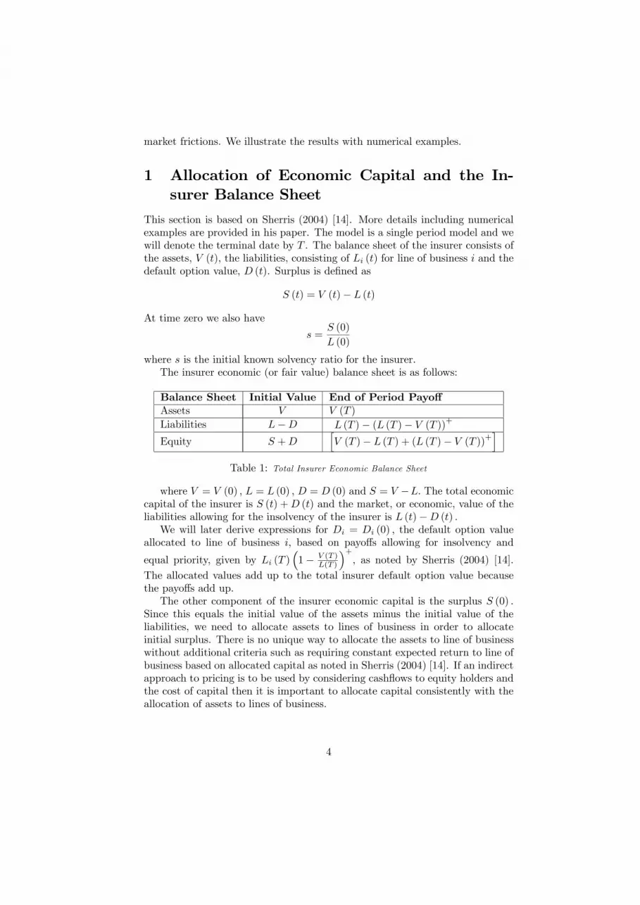
This section is based on Sherris (2004) [14]. More details including numericalexamples are provided in his paper. The model is a single period model and wewill denote the terminal date by T . The balance sheet of the insurer consists ofthe assets, V (t), the liabilities, consisting of Li (t) for line of business i and thedefault option value, D (t). Surplus is defined as

S (t) = V (t)− L (t)

At time zero we also have

s =S (0)

L (0)

where s is the initial known solvency ratio for the insurer.The insurer economic (or fair value) balance sheet is as follows:

Balance Sheet Initial Value End of Period PayoffAssets V V (T )

Liabilities L−D L (T )− (L (T )− V (T ))+

Equity S +DhV (T )− L (T ) + (L (T )− V (T ))

+i

Table 1: Total Insurer Economic Balance Sheet

where V = V (0) , L = L (0) , D = D (0) and S = V −L. The total economiccapital of the insurer is S (t) +D (t) and the market, or economic, value of theliabilities allowing for the insolvency of the insurer is L (t)−D (t) .We will later derive expressions for Di = Di (0) , the default option value

allocated to line of business i, based on payoffs allowing for insolvency and

equal priority, given by Li (T )³1− V (T )

L(T )

´+, as noted by Sherris (2004) [14].

The allocated values add up to the total insurer default option value becausethe payoffs add up.The other component of the insurer economic capital is the surplus S (0) .

Since this equals the initial value of the assets minus the initial value of theliabilities, we need to allocate assets to lines of business in order to allocateinitial surplus. There is no unique way to allocate the assets to line of businesswithout additional criteria such as requiring constant expected return to line ofbusiness based on allocated capital as noted in Sherris (2004) [14]. If an indirectapproach to pricing is to be used by considering cashflows to equity holders andthe cost of capital then it is important to allocate capital consistently with theallocation of assets to lines of business.

4

We can determine the solvency ratio for each line of business based on anarbitrary allocation of assets to line of business. This will be denoted by

esi = SiLi=

Vi − LiLi

where Vi is the value of the assets allocated to line of business i at time 0 andwe use esi to differentiate this from the si in Myers and Read (2001) [10] whichis defined as a partial derivative. The difference between these two definitionswill be covered in more detail later in this paper.The values of the payoff to each line of business in the event of insolvency

determines the internal balance sheet for line of business i:

Balance Sheet Initial Value End of Period PayoffAssets Vi Vi (T )

Liabilities Li −Di Li (T )− Li (T )³1− V (T )

L(T )

´+Equity Si +Di

∙Vi (T )− Li (T ) + Li (T )

³1− V (T )

L(T )

´+¸Table 2: Internal Balance Sheet for Line of Business i

The by-line allocation of the default option value is not arbitrary and shouldequal the value of the loss in the claims payable to the line of business in theevent of insolvency. The total surplus is allocated to lines of business so thatS =

PMi=1 Si with

S =MXi=1

esiLiso that if xi , Li

L then

es = MXi=1

xiesiwhere

PMi=1 xi = 1. The allocation of Si is arbitrary unless other criteria are

specified. For instance, if allocated capital is to be used for pricing purposes,then it needs to be allocated consistent with the assumption made about ex-pected cost of capital by line and the allocation of assets to line of business.To differentiate our allocations of the default option value from the sensitiv-

ities in Myers and Read (2001) [10] we define

edi = Di

Li

so that

D =MXi=1

ediLi5

The allocation of the default option value and the surplus is such that the lineof business allocations add to the total economic capital with

S +D =MXi=1

³esi + edi´LiThe allocation of capital to lines of business is an internal allocation that hasno direct economic implications for the solvency of the insurer. It is the totalinsurer level of capital that determines the future likelihood of insolvency of theinsurer - how it is allocated to lines of business has no direct bearing on thesolvency of the insurer. The economic impact of insolvency is determined by theinsurer default option value. The allocation of the insurer default option valueto line of business is important since it is included in the fair price of insuranceby line of business. This by-line price is an entity specific price since it adjuststhe market price of an insurance risk, assuming no default by the insurer, forthe default cost of the insurance entity.In Phillips, Cummins and Allen (1998) [12] and in Sherris (2003) [13], the

assumption is made that the insurer default option value can be allocated tolines of business in proportion to the liability values for pricing purposes so that

Di =LiLD for all i

which implies that edi = d for all i

In order for Myers and Read (2001) [10] to use their sensitivities for capitalallocation they also assume that these sensitivities must be the same for alllines of business. However, as shown in Sherris (2003) [13], such an allocationis not the fair (arbitrage-free) allocation of the insurer default option value byline of business. The Myers and Read (2001) [10] sensitivities are not capitalallocations for the current balance sheet. The Myers and Read (2001) [10]sensitivities “add up”, but there is an infinite number of capital allocations byline that will also “add up”. None of these has economic significance exceptthat based on the actual pay-offs by-line in the event of insolvency as given inthis paper.

2 The Insurer Default Option Value and Allo-cation to Line of Business

For a given insurer balance sheet, Sherris (2004) [14] shows how the insurerdefault option value can be allocated to lines of business and that this can bedone uniquely by line of business. The liability payoffs by line of business inthe event of insolvency can be explicitly determined allowing for the ranking ofdifferent lines of business, which for an insurer is normally an equal priority ofpolicyholders with claims outstanding at the date of insolvency. He also shows

6

that default option values by line of business do not depend on the surplusallocation to line of business as the results of Myers and Read (2001) [10] wouldsuggest. He shows that, in a complete and frictionless market model, thereis no unique allocation of surplus without imposing additional criteria such asrequiring each line of business to have an equal expected return on capital oran equal solvency ratio.We derive closed form expressions for the default option value and the allo-

cation of this value by line of business. Our assumptions are different to thoseof Myers and Read (2001) [10] and the approach provides a more flexible andgeneral method of determining the insurer default option value as well as itsallocation to lines of business. We will formally determine the default optionvalue and the allocation of the default option and surplus to line of business.We will then relate our results to the assumptions and results of Myers andRead (2001) [10].Denote the value of the liabilities of line i = 1, . . . ,M at time t by Li (t) for

0 ≤ t ≤ T where T is the end of period. Assume that the risk-neutral dynamicsof Li (t) are

dLi (t) = µiLi (t) dt+ σiLi (t) dBi (t) for i = 1, . . . ,M (1)

and that the amount Li (T ) is the claim amount paid at time T , so thatclaims for each line have a log-normal distribution at time T . Bi (t) ; i =1, . . . ,M, are Brownian motions under the risk-neutral dynamics. We also as-sume dBi (t) dBj (t) = ρijdt. If Li can be replicated by traded assets and thereare no claim payments made other than at the end of the period then µi = r,the risk free rate. The total liabilities are given by

L (t) ,MXi=1

Li (t)

These values for the liabilities assume claims are paid in full and ignore theeffect of insolvency of the insurer on claim payments. The insurance policies arecontingent claims on the value of the liabilities with payoff that depends on theinsurer solvency.The value of the assets of the insurer at time t are denoted by V (t) for

0 ≤ t ≤ T . We assume that the ratio of assets to liabilities

Λ (t) , V (t)

L (t)(2)

follows geometric Brownian motion with risk neutral dynamics given by

dΛ (t) = µΛΛ (t) dt+ σΛΛ (t) dBΛ (t) (3)

with

Λ (0) =V (0)

L (0)= (1 + s)

7

where s is the solvency ratio at time 0. BΛ (t) is a Brownian motion under therisk-neutral dynamics. Note that the initial balance sheet values of the totalassets and liabilities are V (0) and L (0) respectively. We assume that we knowthe parameters µΛ and σΛ for the dynamics of the ratio of assets to liabilitiesand that these are not approximated from the dynamics of the individual assetsand liabilities. Later in this paper, to be consistent with the Myers and Read(2001) [10] results, we will need to derive approximate expressions for theseparameters in terms of the dynamics of the individual assets and liabilities.Myers and Read (2001) [10] assume that both L and V are log-normal in

order to apply the Margrabe (1978) [6] exchange option formula. In our as-sumptions, the ratio of assets to liabilities, Λ (t) is assumed to be log-normal.We know that if L and V are portfolios of individual assets and lines of busi-ness respectively, each with log-normal dynamics, then the portfolio can notbe log-normal unless the portfolio is dynamically rebalanced to ensure constantweights. In the Myers and Read (2001) [10] model the proportions of the linesof business are assumed fixed at the start of the period and not continuouslyrebalanced.In our approach it is possible to consider a wider range of processes for the

individual lines of business for which it will be reasonable to assume that theratio of assets to liabilities, Λ (t) , is approximately log-normal. If assets areselected at the start of the period to closely match the liabilities then the ratioof assets to liabilities at the end of the period should be well approximated witha log-normal distribution. These assumptions in practice need to be assessedagainst empirical data.The payoff for the insurer default option at the end of the period is

[L (T )− V (T )]+ (4)

We assume that all lines of business rank equally in the event of default,so that policyholders who have claims due and payable in line of business iwill be entitled to a share Li(T )

L(T ) of the assets of the company, where the total

outstanding claim amount is L (T ) =PM

i=1 Li (T ) . Sherris (2004) [14] showsthat the end-of-period payoff to line of business i is well defined based on thisequal priority and given by

Li(T )L(T ) V (T ) if L (T ) > V (T ) (or V (T )

L(T ) ≤ 1)

Li (T ) if L (T ) ≤ V (T ) (or V (T )L(T ) > 1)

(5)

This is the normal situation for policyholders of insurers. They rank equally foroutstanding claim payments in the event of default of the insurer.The value of the exchange option allocated to line of business i is denoted by

Di (t) . This is given by the value of the pay-off to the line of business allowing

8

for the payoffs in the event of insurer default. Assuming no-arbitrage, this is

Di (t) = EQ

"e−r(T−t)Li (T )

∙1− V (T )

L (T )

¸+|Ft

#= EQ

he−r(T−t)Li (T ) [1− Λ (T )]+ |Ft

i(6)

where (Ft) is the filtration defined by the Brownian motions BΛ (t) , Bi (t) ;i = 1, . . . ,M, and Q indicates that the expectation is under the risk neutraldynamics.The total company level insolvency exchange option for the insurer is

D (t) = EQhe−r(T−t) [L (T )− V (T )]+ |Ft

i=

MXi=1

EQ

"e−r(T−t)Li (T )

∙1− V (T )

L (T )

¸+|Ft

#

=MXi=1

EQhe−r(T−t)Li (T ) [1− Λ (T )]+ |Ft

iThe value of the insolvency exchange option allocated to each line of business“adds up” to the total insurer value since the total insurer insolvency payoff isthe sum of the amounts allocated to line of business using the equal priority foroutstanding claims given in (5).Since we assume individual lines of business are log-normal and the ratio of

assets to liabilities is log-normal we can derive the value of the default optionvalue for each line of business in closed form. The value of the insurer totaldefault option is then derived as the sum of the default option values for eachline of business. This is an important feature of our approach. We derive closedform expressions for by-line values based on payoffs and, since the pay-offs sumto the total insurer pay-off, our total insurer default option value is the sum ofthe by-line values.The insurer default option value for line of business i can be derived using a

change of numeraire from the risk free bank account to Li (t) and correspondingchange of measure. First note that under the risk neutral measure Q

Li (T ) = Li (0) eµiTZi (T )

where

Zi (T ) = exp

∙σiB

i (T )− 12σ2iT

¸Define Qi on FT by

dQi

dQ|FT = Zi (T ) (7)

and note thatEQ [Zi (T ) |Ft] = Zi (t) 0 ≤ t ≤ T

9

Now, by Bayes Theorem,

EQi

he−r(T−t) (1− Λ (T ))+ |Ft

i=

EQhe−r(T−t)Zi (T ) (1− Λ (T ))+ |Ft

iEQ [Zi (T ) |Ft]

so that

Di (t) = EQhe−r(T−t)Li (T ) [1− Λ (T )]+ |Ft

i= EQi

he−r(T−t) (1− Λ (T ))+ |Ft

iZi (t)Li (0) e

µiT

= Li (t) eµi(T−t)EQi

he−r(T−t) (1− Λ (T ))+ |Ft

i(8)

We can make the change of numeraire involved in the above more explicitby noting that the default option value for line of business i can be written as

Di (t)

Li (t) e(r−µi)t=

ert

Li (t) e(r−µi)tEQ

he−rTLi (T ) [1− Λ (T )]+ |Ft

i=

ert

Li (t) e(r−µi)tEQ

"Li (T ) e

(r−µi)T

erTLi (T ) [1− Λ (T )]+

Li (T ) e(r−µi)T|Ft

#

= EQ

"Zi (T )

Zi (t)

Li (T ) [1− Λ (T )]+

Li (T ) e(r−µi)T|Ft

#

where Zi (t) = 1Li(0)

Li(t)e(r−µi)t

ert . Using the Radon-Nikodym density process asbefore given by

dQi

dQ|FT = Zi (T )

where Zi (t) is a non-negative Q-martingale with initial value Zi (0) = 1, underthe changed probability measure we have

Di (t)

Li (t) e(r−µi)t= EQi

"Li (T ) [1− Λ (T )]+

Li (T ) e(r−µi)T|Ft

#or

Di (t) = Li (t) eµi(T−t)EQi

he−r(T−t) (1− Λ (T ))+ |Ft

ias derived in Equation (8) .Note that BΛ (t) , Bj (t) ; j = 1, . . . ,M, are Brownian motions under Q. We

can show that eBΛ (t) = BΛ (t)−ρiΛσit and eBj (t) = Bj (t)−ρijσit are Brownianmotions under Qi. Details are given in Appendix A for completeness.In order to derive a closed form for the value of the insurer default option

for line of business i consider

M (t) = EQhe−r(T−t) [1− Λ (T )]+ |Ft

i10

This is the value at time t of a European put option on an underlying assetpaying a continuous dividend at rate r − µΛ with current price Λ (t) , exercisedate T , and strike price 1. By assumption Λ (T ) has a log-normal distribution.Using the classical Black-Scholes result we have the closed form

M (t) = e−r(T−t)N (−d2t)− Λ (t) e−(r−µΛ)(T−t)N (−d1t) (9)

where

d1t =lnΛ (t) +

¡µΛ +

12σ

2Λ

¢(T − t)

σΛp(T − t)

(10)

and

d2t =lnΛ (t) +

¡µΛ − 1

2σ2Λ

¢(T − t)

σΛp(T − t)

= d1t − σΛp(T − t) (11)

The default option value for line of business i is then given by

Di (t) = Li (t) eµi(T−t)EQi

he−r(T−t) (1− Λ (T ))+ |Ft

i= Li (t) e

µi(T−t)M i (t) (12)

where M i (t) is evaluated with the same formula as for M (t) but with µΛreplaced by µiΛ = µΛ + ρiΛσiσΛ where

dBi (t) dBΛ (t) = ρiΛdt

This follows since

dΛ (t) = µΛΛ (t) dt+ σΛΛ (t)³d eBΛ (t) + ρiΛσidt

´= (µΛ + ρiΛσiσΛ)Λ (t) dt+ σΛΛ (t) d eBΛ (t)

The (instantaneous) correlation between each line of business and the asset toliability ratio is required to evaluate the default option value for line of businessi. Later in this paper we will consider evaluating this default option value usingour approach to compare with the results from Myers and Read (2001) [10].The total insurer default option value is then given by

D (t) = EQhe−r(T−t) [L (T )− V (T )]

+ |Fti

=MXi=1

Di (t) =MXi=1

Li (t) eµi(T−t)M i (t)

Note that if Li = Li (0) , Di = Di (0) and D = D (0) then

M i (0) = e−rTN (−d2i)− Λ (0) e−(r−(µΛ+ρiΛσiσΛ))TN (−d1i) (13)

where

d1i =lnΛ (0) +

¡µΛ + ρiΛσiσΛ +

12σ

2Λ

¢T

σΛ√T

(14)

11

and

d2i =lnΛ (0) +

¡µΛ + ρiΛσiσΛ − 1

2σ2Λ

¢T

σΛ√T

= d1i − σΛ√T (15)

We then have

∂D

∂Li=

∂³PM

i=1Di

´∂Li

=∂³PM

i=1 LieµiTM i (0)

´∂Li

=Di

Li+

MXj=1

LjeµjT

∂M j (0)

∂Li

= edi + MXj=1

Lj∂ edj∂Li

In Myers and Read (2001) [10] di is defined as a sensitivity ∂D∂Li. We have

defined our edi based on the the explicit payoffs for each line of business. As wewill show later in a numerical example these results differ. However our ∂D

∂Liis

equivalent to the Myers and Read (2001) [10] di and this is not the allocationof the default option value by line of business. A derivation of an expression for∂D∂Li

for the assumptions we have used for the arbitrage-free, complete marketsdefault option value by line is given in Appendix B.For the total insurer balance sheet

d =D

L=1

L

MXi=1

LieµiTM i (0)

=MXi=1

xi ediNow consider the insurer surplus. By definition

S (t) = EQhe−r(T−t) [V (T )− L (T )] |Ft

iNote that even if S (t) ≤ 0 for t < T, the insurer is not regarded as insolvent. Itis only at the end of the period, t = T , that solvency is assessed in this model.If we assume that a fraction αi of all of the assets is apportioned to line of

12

business i withPM

i=1 αi = 1, we then have

S (t) = EQ

"e−r(T−t)

MXi=1

[αiV (T )− Li (T )] |Ft

#

= EQ

"e−r(T−t)

MXi=1

αiV (T ) |Ft

#−EQ

"e−r(T−t)

MXi=1

Li (T ) |Ft

#

=MXi=1

hαie

(µA−r)(T−t)V (t)− e(µi−r)(T−t)Li (t)i

If the assets and liabilities pay no intermediate cash flows then this becomes

S =MXi=1

(αiV − Li) =MXi=1

Si

We also have esi = αi(1 + s)L

Li− 1

These allocations are not sensitivities and are not unique. Additional criteriaare required to determine the αi uniquely.

3 Myers and Read RevisitedButsic (1999) [2] and Myers and Read (2001) [10] determine an allocation ofthe default option value by considering marginal changes to the total defaultinsurer option value for changes in the initial value of each line of business.We will only consider the case of their log-normal assumptions although bothnormal and log-normal results are given in Myers and Read (2001) [10]. Theygive formulae for the case where the aggregate losses and the asset values areassumed joint log-normal. Similar results are given in Butsic (1999) [2].They derive the default option value per unit of initial liability value, D

L ,under the joint log-normal assumption as

d = f (s, σ) = N {z}− (1 + s)N {z − σ}

where

z =− ln (1 + s)

σ+1

2σ

σ =qσ2L + σ2V − 2σLV

xi =LiL

σ2L =MXi=1

xixjρijσiσj

13

and

σLV =MXi=1

xiρiV σiσV

Correlations between log losses for lines of business i and j are denoted byρij and correlations between log asset values and log losses in a single line aredenoted by ρiV . For the Myers and Read (2001) [10] assumptions it is importantto note that the value of the default option for the insurer depends only on thesurplus ratio s and the volatility of the surplus ratio. The default value will notchange if an insurer makes changes to its business mix, its assets or its capitalstructure as long as the surplus ratio and its volatility are maintained.Under the joint log-normal assumptions, Myers and Read (2001) [10] define

the marginal default value as

di =∂D

∂Li

and derive the result that

di = d+

µ∂d

∂s

¶(si − s) +

µ∂d

∂σ

¶µ1

σ

£¡σiL − σ2L

¢¤− (σiV − σLV )

¶(16)

They then consider what happens when the insurer expands or contracts busi-ness in a single line. They consider two assumptions. One is that the companymaintains a constant surplus to liability ratio for every line so that

si =∂S

∂Li= s for all i

and obtain marginal default values of

di = d+

µ∂d

∂σ

¶µ1

σ

£¡σiL − σ2L

¢¤− (σiV − σLV )

¶for this case. They state that since this implies a different allocation of defaultrisk to each line of business, this does not make sense since if the companydefaults on one policy then it defaults on all policies.They state that surplus should be allocated to lines of business, using si

i = 1, 2, . . . ,M , to equalize marginal default values so that

di =∂D

∂Li= d for all i

and the surplus allocation is given by

si = s−µ∂d

∂s

¶−1µ∂d

∂σ

¶µ1

σ

£¡σiL − σ2L

¢¤− (σiV − σLV )

¶(17)

This gives the capital allocation proposed by Myers and Read (2001) [10] wheretotal capital equals surplus plus the default option value. Note that if di = dfor all i and surplus is allocated as proposed by Myers and Read (2001) [10],

14

then Di =LiL D and the allocation of the default option value is in proportion to

the value of the liabilities by line of business. The motivation for this selection

of si is that since ∂∂Li

¡DL

¢= 1

L

h∂D∂Li− D

L

i, selecting si so that ∂D

∂Li= D

L for

all i ensures ∂∂Li

¡DL

¢= 0. This is for (infinitesimal) incremental changes in a

line of business assuming all other things equal and for a static balance sheet.A constant di is required to maintain the current balance sheet default valueper unit of total liabilities D

L and the Myers and Read (2001) [10] si gives theincremental capital required from shareholders for small changes in a single linei, all other things equal, but these are not capital allocations for the currentbalance sheet.For their log-normal case, they use the assumption that the total assets and

the total liabilities are log-normal to derive a closed form for the total insurerdefault option value. The capital allocation to line of business i will be

(si + di)Li

with total capital ofMXi=1

(si + di)Li = (s+ d)L

The results of Sherris (2004) [14] give the allocation of the insurer defaultoption to line of business based on payoffs in the event of insolvency. We havederived a closed form for the insurer default option values based on the as-sumption that each line of business is log-normal and the ratio of the assetsto liabilities is log-normal. In order to compare our results with the assump-tions for the log-normal case in Myers and Read (2001) [10] we need to deriveapproximations to the parameters for dΛ (t).Consider the derivation of the parameters used in Myers and Read (2001)

[10] for the total liabilities. In our case we assume individual lines of business arelog-normal, but not the total of the liabilities. If we consider the total liabilitiesthen we can write

dL (t) =MXi=1

dLi (t)

=MXi=1

µiLi (t) dt+ σiLi (t) dBi (t)

= L (t)

"MXi=1

xitµidt+ xitσidBi (t)

#where

xit =Li (t)

L (t)or

dL

L=

ÃMXi=1

xitµi

!dt+

MXi=1

xitσidBi (t)

15

We can immediately see that unless we rebalance the proportion of each lineof business in the insurer liabilities the xit =

Li(t)L(t) will not be constant. ThusÃ

MXi=1

xitµi

!and

MXi=1

xitσi will not be constant and will depend on Li (t) and

L (t). In order for the total liability to be log-normal these drifts and diffusionsneed to be deterministic.In order to value the insurer default option, Myers and Read (2001) [10]

implicitly assume that the aggregate losses have risk neutral dynamics (log-normal)

dL

L= rdt+ σLdB

L (t)

and the assets are also log-normal with risk neutral dynamics

dV

V= rdt+ σV dB

V (t)

with instantaneous correlation given by dBL (t) dBV (t) = ρLV dt. Myers andRead (2001) [10] equate the moments of the aggregate losses to the moments ofthe sum of the individual losses. If we make the assumption that

xit = xi0 ,Li (0)

L (0)

for all t thendL

L=

"rdt+

MXi=1

xiσidBi (t)

#This gives expressions for the variance of the aggregate losses in terms of theindividual losses as follows

σ2L =MXi=1

MXj=1

xixjρijσiσj (18)

For Myers and Read (2001) [10]

dΛ (t) = d

µV (t)

L (t)

¶=

dV (t)

L (t)− V (t)

L (t)2 dL (t)−

1

L (t)2 dV (t) dL (t) +

V (t)

L (t)3 dL (t)

2

= Λ (t)

∙ ¡σ2L − σLσV ρLV

¢dt

+σV dBV (t)− σLdB

L (t)

¸(19)

so thatµΛ = σ2L − σLσV ρLV (20)

andσ2Λ = σ2V + σ2L − 2σLσV ρLV (21)

16

We can evaluate ρLV using the Myers and Read (2001) [10] assumptions bynoting that

σLdBL (t) =

MXi=1

xiσidBi (t)

so that

σV σLdBL (t) dBV (t) =

MXi=1

xiσidBi (t) dBV (t)

=MXi=1

xiσiσV ρiV dt

hence

σLσV ρLV =MXi=1

xiσiσV ρiV (22)

We derived a closed form for the default option value for line of business i inequation (8) . If we assume that t = 0, T = 1 and µi = r, as in Myers and Read(2001) [10] then

Di = LierM i (0)

where M i (0) is evaluated with the same formula as for M (t) in equation (9)with µΛ replaced by µ

iΛ = µΛ + ρiΛσiσΛ and T = 1 with

dBi (t) dBΛ (t) = ρiΛdt

HenceM i (0) = e−rN (−d2i)− Λ (0) e−(r−(µΛ+ρiΛσiσΛ))N (−d1i) (23)

where

d1i =lnΛ (0) +

¡µΛ + ρiΛσiσΛ +

12σ

2Λ

¢σΛ

(24)

and

d2i =lnΛ (0) +

¡µΛ + ρiΛσiσΛ − 1

2σ2Λ

¢σΛ

= d1i − σΛ (25)

This then gives

Di = LiN (−d2i)− LiΛ (0) e(µΛ+ρiΛσiσΛ)N (−d1i)

and edi = Di

Li= N (−d2i)− Λ (0) e(µΛ+ρiΛσiσΛ)N (−d1i)

We can derive an expression for µiΛ as follows.

σiσΛdBi (t) dBΛ (t) = σidB

i (t)£σV dB

V (t)− σLdBL (t)

¤= [σiσV ρiV − σiσLρiL] dt

17

and hence

µiΛ = µΛ + ρiΛσiσΛ

= σ2L − σLσV ρLV + σiσV ρiV − σiσLρiL (26)

The default option value as a function of L1, L2, . . . , LM , V is homogeneousof degree 1 so that

D =MXi=1

µ∂D

∂Li

¶Li +

µ∂D

∂V

¶V

and, since L =MXi=1

Li we also have that

D =

µ∂D

∂L

¶L+

µ∂D

∂V

¶V

This means that µ∂D

∂L

¶L =

MXi=1

µ∂D

∂Li

¶Li

Note that, as demonstrated in the numerical examples below, di = ∂D∂Li

6= edi =Di

Liwhere Di is the by line allocation of the default option value based on equal

priority of line of business in the event of insolvency in this paper.Under our assumptions the total value of the default option under the Myers

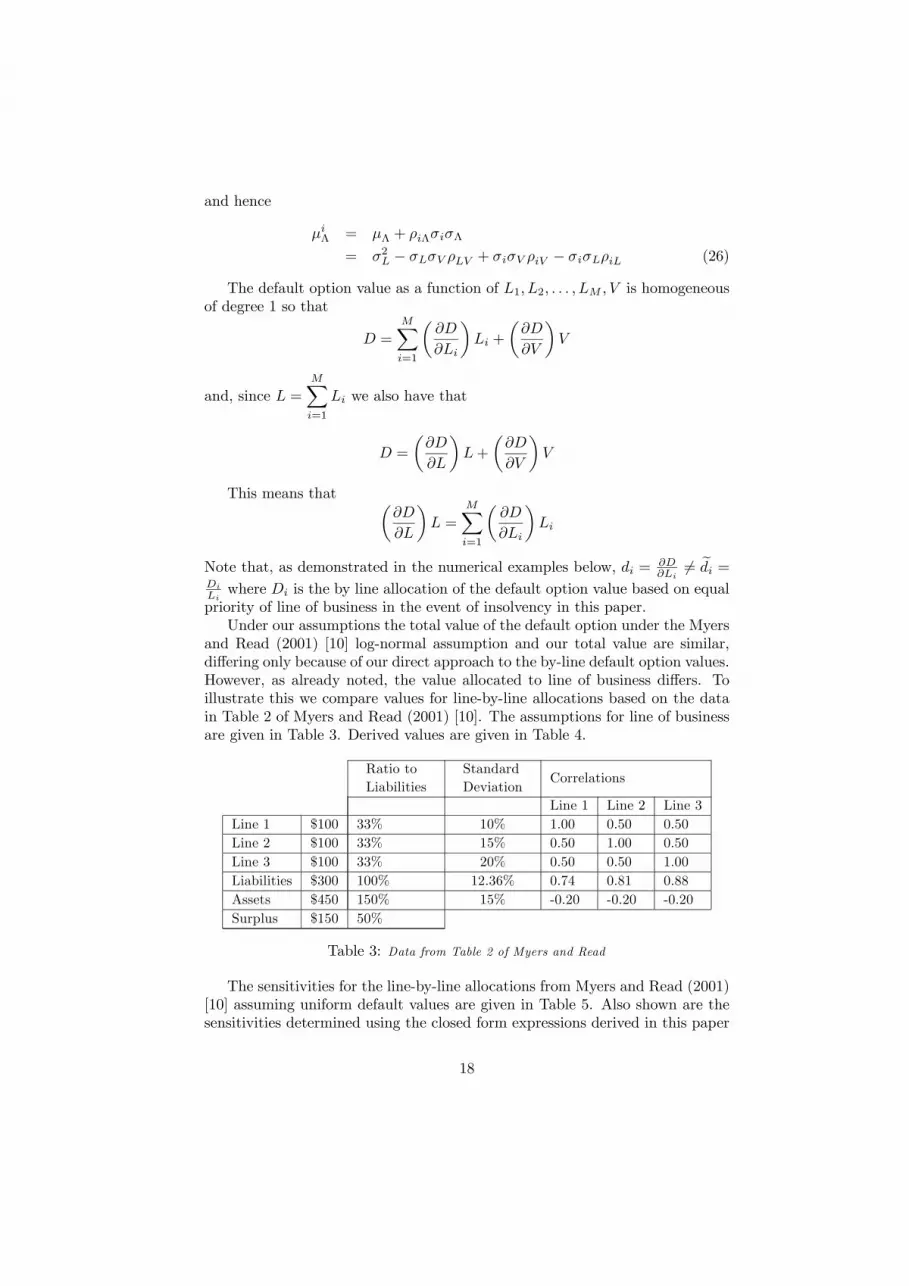
and Read (2001) [10] log-normal assumption and our total value are similar,differing only because of our direct approach to the by-line default option values.However, as already noted, the value allocated to line of business differs. Toillustrate this we compare values for line-by-line allocations based on the datain Table 2 of Myers and Read (2001) [10]. The assumptions for line of businessare given in Table 3. Derived values are given in Table 4.

Ratio toLiabilities

StandardDeviation

Correlations

Line 1 Line 2 Line 3Line 1 $100 33% 10% 1.00 0.50 0.50Line 2 $100 33% 15% 0.50 1.00 0.50Line 3 $100 33% 20% 0.50 0.50 1.00Liabilities $300 100% 12.36% 0.74 0.81 0.88Assets $450 150% 15% -0.20 -0.20 -0.20Surplus $150 50%

Table 3: Data from Table 2 of Myers and Read

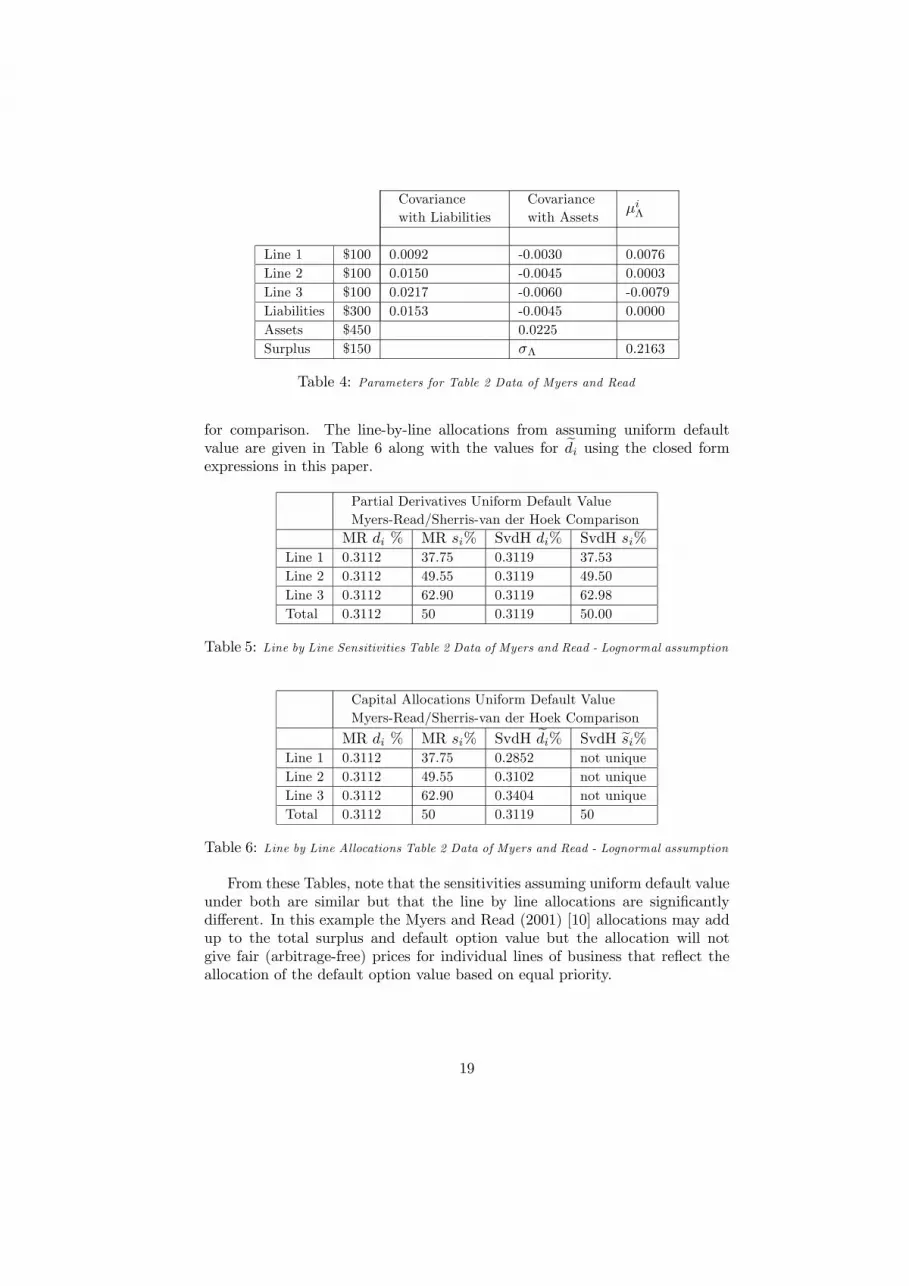
The sensitivities for the line-by-line allocations from Myers and Read (2001)[10] assuming uniform default values are given in Table 5. Also shown are thesensitivities determined using the closed form expressions derived in this paper

18

Covariancewith Liabilities

Covariancewith Assets

µiΛ

Line 1 $100 0.0092 -0.0030 0.0076Line 2 $100 0.0150 -0.0045 0.0003Line 3 $100 0.0217 -0.0060 -0.0079Liabilities $300 0.0153 -0.0045 0.0000Assets $450 0.0225Surplus $150 σΛ 0.2163

Table 4: Parameters for Table 2 Data of Myers and Read

for comparison. The line-by-line allocations from assuming uniform defaultvalue are given in Table 6 along with the values for edi using the closed formexpressions in this paper.

Partial Derivatives Uniform Default ValueMyers-Read/Sherris-van der Hoek ComparisonMR di % MR si% SvdH di% SvdH si%

Line 1 0.3112 37.75 0.3119 37.53Line 2 0.3112 49.55 0.3119 49.50Line 3 0.3112 62.90 0.3119 62.98Total 0.3112 50 0.3119 50.00

Table 5: Line by Line Sensitivities Table 2 Data of Myers and Read - Lognormal assumption

Capital Allocations Uniform Default ValueMyers-Read/Sherris-van der Hoek Comparison

MR di % MR si% SvdH edi% SvdH esi%Line 1 0.3112 37.75 0.2852 not uniqueLine 2 0.3112 49.55 0.3102 not uniqueLine 3 0.3112 62.90 0.3404 not uniqueTotal 0.3112 50 0.3119 50

Table 6: Line by Line Allocations Table 2 Data of Myers and Read - Lognormal assumption

From these Tables, note that the sensitivities assuming uniform default valueunder both are similar but that the line by line allocations are significantlydifferent. In this example the Myers and Read (2001) [10] allocations may addup to the total surplus and default option value but the allocation will notgive fair (arbitrage-free) prices for individual lines of business that reflect theallocation of the default option value based on equal priority.

19

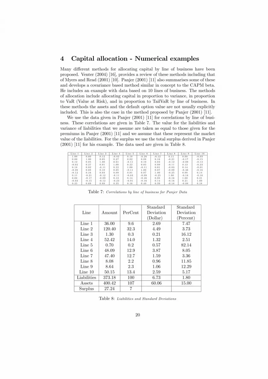
4 Capital allocation - Numerical examplesMany different methods for allocating capital by line of business have beenproposed. Venter (2004) [16], provides a review of these methods including thatof Myers and Read (2001) [10]. Panjer (2001) [11] also summarises some of theseand develops a covariance based method similar in concept to the CAPM beta.He includes an example with data based on 10 lines of business. The methodsof allocation include allocating capital in proportion to variance, in proportionto VaR (Value at Risk), and in proportion to TailVaR by line of business. Inthese methods the assets and the default option value are not usually explicitlyincluded. This is also the case in the method proposed by Panjer (2001) [11].We use the data given in Panjer (2001) [11] for correlations by line of busi-

ness. These correlations are given in Table 7. The value for the liabilities andvariance of liabilities that we assume are taken as equal to those given for thepremiums in Panjer (2001) [11] and we assume that these represent the marketvalue of the liabilities. For the surplus we use the total surplus derived in Panjer(2001) [11] for his example. The data used are given in Table 8.

L in e 1 L in e 2 L in e 3 L in e 4 L in e 5 L in e 6 L in e 7 L in e 8 L in e 9 L in e 1 01 .0 0 0 .0 0 0 .1 2 -0 .0 2 0 .1 8 -0 .2 6 -0 .1 2 0 .1 1 0 .0 8 -0 .0 30 .0 0 1 .0 0 0 .0 5 0 .2 7 0 .0 2 0 .0 8 0 .1 6 -0 .2 1 - 0 .1 7 -0 .1 50 .1 2 0 .0 5 1 .0 0 0 .0 1 -0 .1 1 0 .1 0 0 .0 3 -0 .1 2 - 0 .0 9 -0 .1 2-0 .0 2 0 .2 7 0 .0 1 1 .0 0 0 .2 2 0 .0 5 0 .0 9 -0 .1 1 0 .1 3 -0 .2 30 .1 8 0 .0 2 -0 .1 1 0 .2 2 1 .0 0 -0 .1 1 0 .0 1 -0 .0 3 0 .1 4 -0 .0 1-0 .2 6 0 .0 8 0 .1 0 0 .0 5 -0 .1 1 1 .0 0 0 .0 7 -0 .0 9 - 0 .4 6 -0 .1 6-0 .1 2 0 .1 6 0 .0 3 0 .0 9 0 .0 1 0 .0 7 1 .0 0 -0 .2 5 0 .0 8 0 .1 40 .1 1 - 0 .2 1 -0 .1 2 -0 .1 1 -0 .0 3 -0 .0 9 -0 .2 5 1 .0 0 - 0 .1 6 -0 .1 60 .0 8 - 0 .1 7 -0 .0 9 0 .1 3 0 .1 4 -0 .4 6 0 .0 8 -0 .1 6 1 .0 0 0 .2 1-0 .0 3 - 0 .1 5 -0 .1 2 -0 .2 3 -0 .0 1 -0 .1 6 0 .1 4 -0 .1 6 0 .2 1 1 .0 00 .2 5 0 .6 9 0 .0 9 0 .3 5 0 .1 6 0 .4 0 0 .3 9 -0 .1 8 - 0 .0 8 0 .1 8

Table 7: Correlations by line of business for Panjer Data

Line Amount PerCentStandardDeviation(Dollar)

StandardDeviation(Percent)

Line 1 36.00 9.6 2.69 7.47Line 2 120.40 32.3 4.49 3.73Line 3 1.30 0.3 0.21 16.12Line 4 52.42 14.0 1.32 2.51Line 5 0.70 0.2 0.57 82.14Line 6 48.09 12.9 3.87 8.05Line 7 47.40 12.7 1.59 3.36Line 8 8.08 2.2 0.96 11.85Line 9 8.64 2.3 1.06 12.29Line 10 50.15 13.4 2.59 5.17Liabilities 373.18 100 6.73 1.80Assets 400.42 107 60.06 15.00Surplus 27.24 7

Table 8: Liabilities and Standard Deviations

20

Capital Allocation Normal Distribution

-10.00%

0.00%

10.00%

20.00%

30.00%

40.00%

50.00%

beta var tailvar sd

Risk Measure

%

Line 1Line 2Line 3Line 4Line 5Line 6Line 7Line 8Line 9Line 10

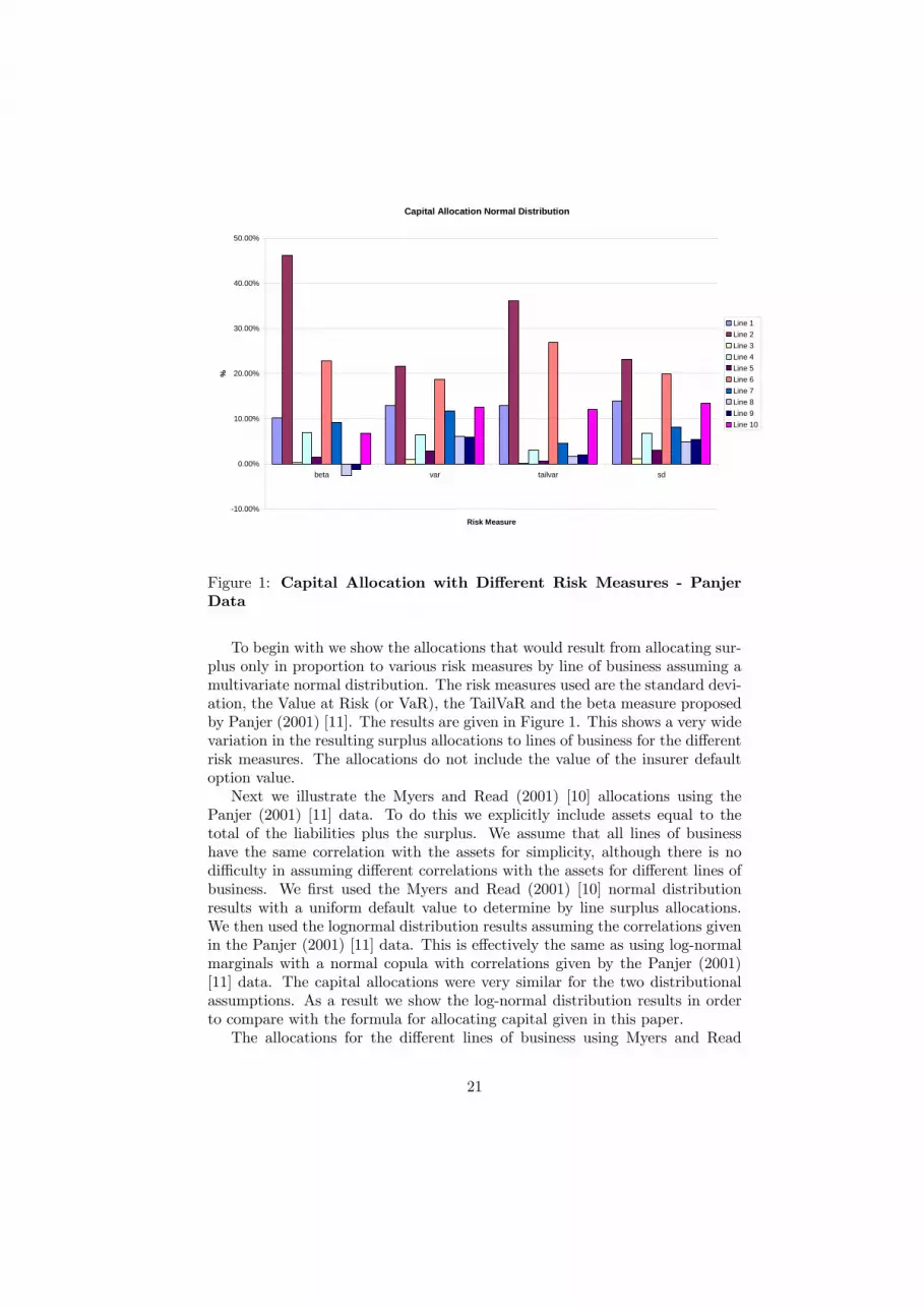
Figure 1: Capital Allocation with Different Risk Measures - PanjerData

To begin with we show the allocations that would result from allocating sur-plus only in proportion to various risk measures by line of business assuming amultivariate normal distribution. The risk measures used are the standard devi-ation, the Value at Risk (or VaR), the TailVaR and the beta measure proposedby Panjer (2001) [11]. The results are given in Figure 1. This shows a very widevariation in the resulting surplus allocations to lines of business for the differentrisk measures. The allocations do not include the value of the insurer defaultoption value.Next we illustrate the Myers and Read (2001) [10] allocations using the

Panjer (2001) [11] data. To do this we explicitly include assets equal to thetotal of the liabilities plus the surplus. We assume that all lines of businesshave the same correlation with the assets for simplicity, although there is nodifficulty in assuming different correlations with the assets for different lines ofbusiness. We first used the Myers and Read (2001) [10] normal distributionresults with a uniform default value to determine by line surplus allocations.We then used the lognormal distribution results assuming the correlations givenin the Panjer (2001) [11] data. This is effectively the same as using log-normalmarginals with a normal copula with correlations given by the Panjer (2001)[11] data. The capital allocations were very similar for the two distributionalassumptions. As a result we show the log-normal distribution results in orderto compare with the formula for allocating capital given in this paper.The allocations for the different lines of business using Myers and Read

21

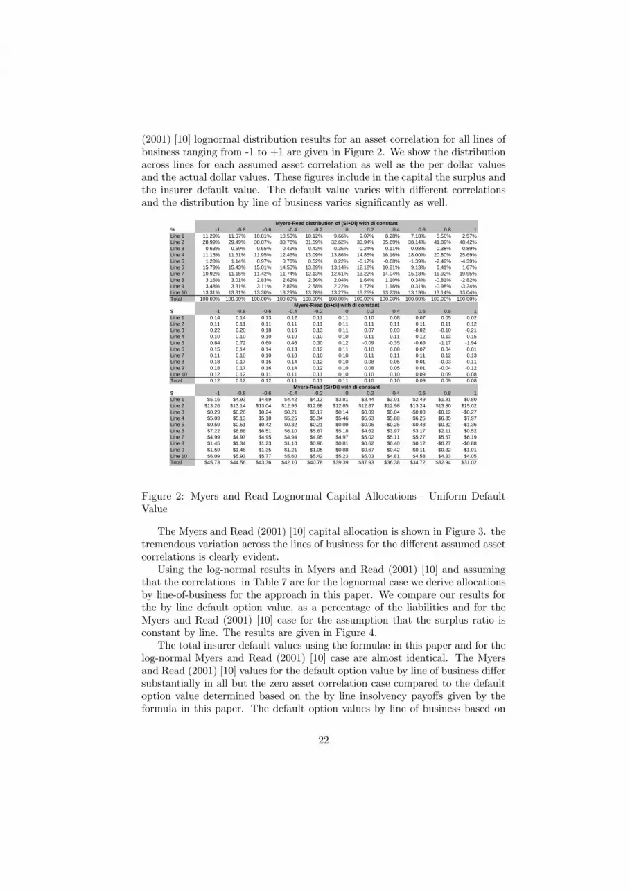
(2001) [10] lognormal distribution results for an asset correlation for all lines ofbusiness ranging from -1 to +1 are given in Figure 2. We show the distributionacross lines for each assumed asset correlation as well as the per dollar valuesand the actual dollar values. These figures include in the capital the surplus andthe insurer default value. The default value varies with different correlationsand the distribution by line of business varies significantly as well.

Myers-Read distribution of (Si+Di) with di constant% -1 -0.8 -0.6 -0.4 -0.2 0 0.2 0.4 0.6 0.8 1Line 1 11.29% 11.07% 10.81% 10.50% 10.12% 9.66% 9.07% 8.28% 7.18% 5.50% 2.57%Line 2 28.99% 29.49% 30.07% 30.76% 31.59% 32.62% 33.94% 35.69% 38.14% 41.89% 48.42%Line 3 0.63% 0.59% 0.55% 0.49% 0.43% 0.35% 0.24% 0.11% -0.08% -0.38% -0.89%Line 4 11.13% 11.51% 11.95% 12.46% 13.09% 13.86% 14.85% 16.16% 18.00% 20.80% 25.69%Line 5 1.28% 1.14% 0.97% 0.76% 0.52% 0.22% -0.17% -0.68% -1.39% -2.49% -4.39%Line 6 15.79% 15.43% 15.01% 14.50% 13.89% 13.14% 12.18% 10.91% 9.13% 6.41% 1.67%Line 7 10.92% 11.15% 11.42% 11.74% 12.13% 12.61% 13.22% 14.04% 15.18% 16.92% 19.95%Line 8 3.16% 3.01% 2.83% 2.62% 2.36% 2.04% 1.64% 1.10% 0.34% -0.81% -2.82%Line 9 3.48% 3.31% 3.11% 2.87% 2.58% 2.22% 1.77% 1.16% 0.31% -0.98% -3.24%Line 10 13.31% 13.31% 13.30% 13.29% 13.28% 13.27% 13.25% 13.23% 13.19% 13.14% 13.04%Total 100.00% 100.00% 100.00% 100.00% 100.00% 100.00% 100.00% 100.00% 100.00% 100.00% 100.00%

Myers-Read (si+di) with di constant$ -1 -0.8 -0.6 -0.4 -0.2 0 0.2 0.4 0.6 0.8 1Line 1 0.14 0.14 0.13 0.12 0.11 0.11 0.10 0.08 0.07 0.05 0.02Line 2 0.11 0.11 0.11 0.11 0.11 0.11 0.11 0.11 0.11 0.11 0.12Line 3 0.22 0.20 0.18 0.16 0.13 0.11 0.07 0.03 -0.02 -0.10 -0.21Line 4 0.10 0.10 0.10 0.10 0.10 0.10 0.11 0.11 0.12 0.13 0.15Line 5 0.84 0.72 0.60 0.46 0.30 0.12 -0.09 -0.35 -0.69 -1.17 -1.94Line 6 0.15 0.14 0.14 0.13 0.12 0.11 0.10 0.08 0.07 0.04 0.01Line 7 0.11 0.10 0.10 0.10 0.10 0.10 0.11 0.11 0.11 0.12 0.13Line 8 0.18 0.17 0.15 0.14 0.12 0.10 0.08 0.05 0.01 -0.03 -0.11Line 9 0.18 0.17 0.16 0.14 0.12 0.10 0.08 0.05 0.01 -0.04 -0.12Line 10 0.12 0.12 0.11 0.11 0.11 0.10 0.10 0.10 0.09 0.09 0.08Total 0.12 0.12 0.12 0.11 0.11 0.11 0.10 0.10 0.09 0.09 0.08

Myers-Read (Si+Di) with di constant$ -1 -0.8 -0.6 -0.4 -0.2 0 0.2 0.4 0.6 0.8 1Line 1 $5.16 $4.93 $4.69 $4.42 $4.13 $3.81 $3.44 $3.01 $2.49 $1.81 $0.80Line 2 $13.26 $13.14 $13.04 $12.95 $12.88 $12.85 $12.87 $12.98 $13.24 $13.80 $15.02Line 3 $0.29 $0.26 $0.24 $0.21 $0.17 $0.14 $0.09 $0.04 -$0.03 -$0.12 -$0.27Line 4 $5.09 $5.13 $5.18 $5.25 $5.34 $5.46 $5.63 $5.88 $6.25 $6.85 $7.97Line 5 $0.59 $0.51 $0.42 $0.32 $0.21 $0.09 -$0.06 -$0.25 -$0.48 -$0.82 -$1.36Line 6 $7.22 $6.88 $6.51 $6.10 $5.67 $5.18 $4.62 $3.97 $3.17 $2.11 $0.52Line 7 $4.99 $4.97 $4.95 $4.94 $4.95 $4.97 $5.02 $5.11 $5.27 $5.57 $6.19Line 8 $1.45 $1.34 $1.23 $1.10 $0.96 $0.81 $0.62 $0.40 $0.12 -$0.27 -$0.88Line 9 $1.59 $1.48 $1.35 $1.21 $1.05 $0.88 $0.67 $0.42 $0.11 -$0.32 -$1.01Line 10 $6.09 $5.93 $5.77 $5.60 $5.42 $5.23 $5.03 $4.81 $4.58 $4.33 $4.05Total $45.73 $44.56 $43.36 $42.10 $40.78 $39.39 $37.93 $36.38 $34.72 $32.94 $31.02

Figure 2: Myers and Read Lognormal Capital Allocations - Uniform DefaultValue

The Myers and Read (2001) [10] capital allocation is shown in Figure 3. thetremendous variation across the lines of business for the different assumed assetcorrelations is clearly evident.Using the log-normal results in Myers and Read (2001) [10] and assuming

that the correlations in Table 7 are for the lognormal case we derive allocationsby line-of-business for the approach in this paper. We compare our results forthe by line default option value, as a percentage of the liabilities and for theMyers and Read (2001) [10] case for the assumption that the surplus ratio isconstant by line. The results are given in Figure 4.The total insurer default values using the formulae in this paper and for the

log-normal Myers and Read (2001) [10] case are almost identical. The Myersand Read (2001) [10] values for the default option value by line of business differsubstantially in all but the zero asset correlation case compared to the defaultoption value determined based on the by line insolvency payoffs given by theformula in this paper. The default option values by line of business based on

22

Myers-Read (si + di) with di constant

-200.00%

-150.00%

-100.00%

-50.00%

0.00%

50.00%

100.00%

-1 -0.8 -0.6 -0.4 -0.2 0 0.2 0.4 0.6 0.8 1

Correlation with Assets

Perc

enta

ge

Line 1Line 2Line 3Line 4Line 5Line 6Line 7Line 8Line 9Line 10

Figure 3: Myers-Read Allocations - Panjer data assuming Log-normaldistributions

Myers-Read di, Constant si$ -1 -0.8 -0.6 -0.4 -0.2 0 0.2 0.4 0.6 0.8 1Line 1 5.63% 5.21% 4.76% 4.29% 3.79% 3.26% 2.69% 2.08% 1.40% 0.66% -0.16%Line 2 4.55% 4.31% 4.07% 3.82% 3.56% 3.29% 3.01% 2.73% 2.43% 2.13% 1.81%Line 3 8.17% 7.31% 6.40% 5.42% 4.38% 3.24% 2.00% 0.63% -0.92% -2.68% -4.65%Line 4 4.13% 3.95% 3.77% 3.59% 3.40% 3.22% 3.03% 2.85% 2.67% 2.50% 2.34%Line 5 28.08% 23.92% 19.48% 14.69% 9.48% 3.77% -2.57% -9.70% -17.84% -27.26% -38.00%Line 6 5.85% 5.40% 4.92% 4.42% 3.89% 3.32% 2.71% 2.05% 1.32% 0.51% -0.38%Line 7 4.40% 4.18% 3.95% 3.72% 3.48% 3.23% 2.98% 2.73% 2.46% 2.20% 1.92%Line 8 6.78% 6.13% 5.44% 4.71% 3.93% 3.08% 2.16% 1.15% 0.02% -1.25% -2.67%Line 9 6.95% 6.28% 5.57% 4.82% 4.01% 3.14% 2.19% 1.14% -0.03% -1.35% -2.83%Line 10 4.92% 4.61% 4.28% 3.94% 3.59% 3.22% 2.82% 2.41% 1.96% 1.48% 0.96%Total 4.95% 4.64% 4.32% 3.98% 3.63% 3.26% 2.87% 2.45% 2.01% 1.53% 1.01%

Sherris di$ -1 -0.8 -0.6 -0.4 -0.2 0 0.2 0.4 0.6 0.8 1Line 1 5.07% 4.74% 4.39% 4.03% 3.65% 3.26% 2.84% 2.41% 1.95% 1.46% 0.94%Line 2 4.88% 4.59% 4.28% 3.96% 3.62% 3.26% 2.88% 2.48% 2.05% 1.57% 1.06%Line 3 5.54% 5.10% 4.66% 4.20% 3.73% 3.25% 2.76% 2.26% 1.75% 1.23% 0.71%Line 4 4.81% 4.53% 4.23% 3.92% 3.60% 3.25% 2.88% 2.49% 2.07% 1.60% 1.09%Line 5 10.14% 8.64% 7.19% 5.80% 4.51% 3.32% 2.28% 1.40% 0.72% 0.27% 0.05%Line 6 5.11% 4.77% 4.41% 4.05% 3.66% 3.26% 2.85% 2.41% 1.94% 1.45% 0.93%Line 7 4.86% 4.56% 4.26% 3.94% 3.61% 3.25% 2.88% 2.48% 2.05% 1.58% 1.07%Line 8 5.28% 4.90% 4.50% 4.09% 3.67% 3.23% 2.78% 2.32% 1.83% 1.33% 0.81%Line 9 5.32% 4.92% 4.52% 4.11% 3.68% 3.24% 2.79% 2.31% 1.82% 1.32% 0.80%Line 10 4.95% 4.64% 4.31% 3.97% 3.62% 3.25% 2.86% 2.45% 2.00% 1.52% 1.01%Total 4.96% 4.64% 4.32% 3.98% 3.63% 3.26% 2.87% 2.45% 2.01% 1.53% 1.02%

Figure 4: Myers and Read and Sherris Default Option Allocations - Lognormalassumption

23

Sherris di

0.00%

2.00%

4.00%

6.00%

8.00%

10.00%

12.00%

-1 -0.8 -0.6 -0.4 -0.2 0 0.2 0.4 0.6 0.8 1

Correlation

Perc

anta

ge

Line 1Line 2Line 3Line 4Line 5Line 6Line 7Line 8Line 9Line 10Total

Figure 5: Sherris Default Option Values

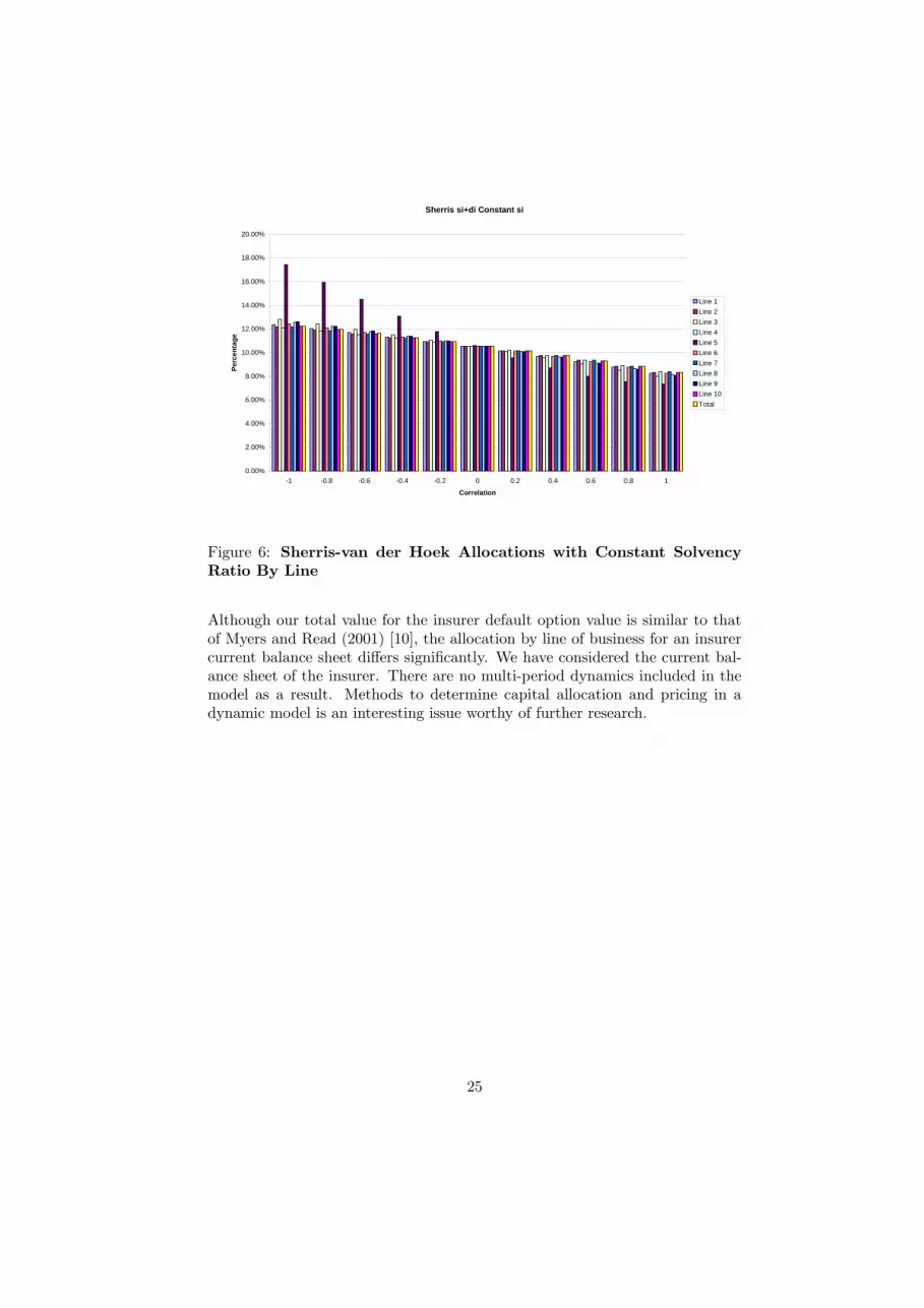
Sherris (2004) [14] and the formula in this paper are shown in Figure 5. InFigure 6 we show the allocation of capital assuming a constant by-line surplusratio and including the default option value for differing correlations betweenassets and lines of business using the results in this paper.Given the differences in allocations for these different methods we urge cau-

tion to those using by-line allocations for insurer financial decision making.From the results it is important to reflect the correlation of the liabilities withthe assets in any capital allocation and it is also important to determine thefair allocation of the default option based on assumed payoffs in the event ofinsolvency by line of business if these are to be used for pricing in the multi-lineinsurer.

5 ConclusionWe have developed expressions for the allocation of the insurer default optionvalue by line of business that reflects the actual by-line payoff in the eventof insolvency. We have used the assumption of log-normal lines of businessand a log-normal ratio of asset to liabilities to derive closed form results andillustrated these with examples from Myers and Read (2001) [10] and data fromPanjer (2001) [11]. The approach we have used will give fair default optionvalues for lines of business that can be used in pricing for the multiline insurer.We have shown how the results of applying different methods of allocation

can give significantly different results so that the approach used is important.

24

Sherris si+di Constant si

0.00%

2.00%

4.00%

6.00%

8.00%

10.00%

12.00%

14.00%

16.00%

18.00%

20.00%

-1 -0.8 -0.6 -0.4 -0.2 0 0.2 0.4 0.6 0.8 1

Correlation

Perc

enta

ge

Line 1Line 2Line 3Line 4Line 5Line 6Line 7Line 8Line 9Line 10Total

Figure 6: Sherris-van der Hoek Allocations with Constant SolvencyRatio By Line

Although our total value for the insurer default option value is similar to thatof Myers and Read (2001) [10], the allocation by line of business for an insurercurrent balance sheet differs significantly. We have considered the current bal-ance sheet of the insurer. There are no multi-period dynamics included in themodel as a result. Methods to determine capital allocation and pricing in adynamic model is an interesting issue worthy of further research.

25

6 Appendix A - Change of MeasureLemma 1 If Bj (t) 0 ≤ t ≤ T is a Brownian motion under Q then

eBj (t) = Bj (t)− ρijσit

is Brownian motion under Qi.

Proof. LetBj (t) be Brownian motion underQ and eBj (t) ≡ Bj (t)−R t0ϕij (u) du

be Brownian motion under Qi. We need to derive ϕij (t) for 0 ≤ t ≤ T. Wehave

EQi

h eBj (t) |Fsi= EQ

hZi (t) eBj (t) |Fs

it > s

Now

Li (t) = Li (0) exp

∙µµi −

1

2σ2i

¶t+ σiB

i (t)

¸so

Zi (t) =1

Li (0)

Li (t) e(r−µi)t

ert

= exp

∙−12σ2i t+ σiB

i (t)

¸and

dZi (t) = Zi (t)σidBi (t)

It follows that

d³Zi (t) eBj (t)

´= Zi (t) d eBj (t) + eBj (t) dZi (t) + d eBj (t) dZi (t)

= Zi (t) dBj (t)− Zi (t)ϕ

ij (t) dt+ eBj (t) dZi (t) + d eBj (t) dZi (t)

= Zi (t) dBj (t) +

£Zi (t) ρijσi − Zi (t)ϕ

ij (t)¤dt+ eBj (t) dZi (t)

hence

Zi (t) eBj (t) =

"Zi (s) eBj (s) +

R ts

h eBj (u) dZi (u) + Zi (u) dBj (u)

i+R tsZi (u)

£ρijσi − ϕij (u)

¤du

#

and

EQhZi (t) eBj (t) |Fs

i= Zi (s) eBj (s) +EQ

∙Z t

s

Zi (u)£ρijσi − ϕij (u)

¤du|Fs

¸We also have

EQi

h³ eBj (t)2 − t´|Fsi= EQ

hZi (t)

³ eBj (t)2 − t´|Fsi

26

and

d³Zi (t)

³ eBj (t)2 − t´´

=

⎡⎣ 2Zi (t) eBj (t)hd eBj (t)− ϕij (t) dt

i+³ eBj (t)

2 − t´dZi (t) + 2 eBj (t) d eBj (t)Zi (t)σidB

i (t)

⎤⎦=

"2Zi (t) eBj (t) d eBj (t) +

³ eBj (t)2 − t

´dZi (t)

+2Zi (t) eBj (t)£σiρij − ϕij (t)

¤dt

#so

EQhZi (t)

³ eBj (t)2 − t´|Fsi

= Zi (s)³ eBj (s)2 − s

´+EQ

∙Z t

s

2Zi (u) eBj (u)£σiρij − ϕij (u)

¤du|Fs

¸Therefore we have that

ϕij (t) = σiρij j = 1, 2, . . . ,M,Λ

since in this caseEQi

h eBj (t) |Fsi= eBj (s)

EQi

h³ eBj (t)2 − t

´|Fsi=³ eBj (s)

2 − s´

and from Levy’s Theorem (1948), subject to some technical conditions, eBj (t)is Brownian motion under Qi (see for example Karatzas and Shreve (1988) [5]pages 156-157).Under the change of measure Qi

dLj (t) = µjLj (t) dt+ σjLj (t) dBj (t)

= µjLj (t) dt+ σjLj (t)hd eBj (t) + σiρijdt

i=

¡µj + σiσjρij

¢Lj (t) dt+ σjLj (t) d eBj (t) j = 1, . . . ,M (27)

and

dΛ (t) = µΛΛ (t) dt+ σΛΛ (t) dBΛ (t)

= µΛΛ (t) dt+ σΛΛ (t)hd eBΛ (t) + σiρiΛdt

i= (µΛ + σiσΛρiΛ)Λ (t) dt+ σΛΛ (t) d eBΛ (t) (28)

27

7 Appendix B - Default Option Value Sensitiv-ity for Line of Business

Assume that µi = r, so that there are no intermediate cash flows on the liabili-ties, for all i and T = 1. We then have

Di = LierM i (0)

= Li

hN (−d2i)− Λ (0) eµ

iΛN (−d1i)

i= Li

hN (−d2i)− (1 + s) eµ

iΛN (−d1i)

i= Li edi (29)

where

d1i =ln (1 + s) +

¡µiΛ +

12σ

2Λ

¢σΛ

d2i = d1i − σΛ

µiΛ = µΛ + ρiΛσiσΛ

and

D =MXi=1

Di

The Myers and Read (2001) [10] sensitivity for our default option value is thengiven by

di =∂D

∂Li

= edi + MXj=1

Lj∂ edj∂Li

= edi + MXj=1

Lj∂ edj∂s

∂s

∂Li+

MXj=1

Lj∂ edj∂σΛ

∂σΛ∂Li

+MXj=1

Lj∂ edj∂µjΛ

∂µjΛ∂Li

(30)

since edj is a function of s, σΛ and µjΛ.Note that

N 0 (−d2j) = (1 + s) eµjΛN 0 (−d1j)

so that∂ edj∂s

= −eµjΛN 0 (−d1j)

Now∂s

∂Li=1

L(si − s) (31)

28

where

si =∂V

∂Li− 1

is the additional marginal capital subscribed per unit of liability for line i. Forthe current balance sheet, the surplus ratio s is given by

V = (1 + s)L

Hence∂V

∂Li= L

∂s

∂Li+ (1 + s)

from which (31) follows.We also have

∂ edj∂σΛ

= N 0 (−d2j)

and

∂σΛ∂Li

=1

σΛL

£−¡σ2L − σLσV ρLV + σiσV ρiV − σiσLρiL

¢¤= − µiΛ

σΛL

Now∂ edj∂µjΛ

= − (1 + s) eµjΛN 0 (−d1j)

and

∂µjΛ∂Li

=∂

∂Li

£σ2L − σLσV ρLV + σjσV ρjV − σjσLρjL

¤=

∂

∂Li

£σ2L − σLσV ρLV

¤− 1

L

£σiσjρij − σjσLρjL

¤Since

σ2L =MXi=1

MXj=1

xixjρijσiσj

and∂xj∂Li

=1

L[δji − xj ]

whereδji = 1 if j = i and 0 if j 6= i

we have

∂σ2L∂Li

= 2MXi=1

MXj=1

xjρijσiσj1

L[δji − xi] =

2

L

£σiσLρiL − σ2L

¤Also

σLσV ρLV = σLV =MXi=1

xiσiσV ρiV

29

so∂σLV∂Li

=MXi=1

σiσV ρiV1

L[δji − xi] =

1

L[σiσV ρiV − σLV ]

and

∂µjΛ∂Li

=1

L

£2¡σiσLρiL − σ2L

¢− (σiσV ρiV − σLV )−

¡σiσjρij − σjσLρjL

¢¤Putting this all together we have an expression for the sensitivity of our defaultoption value for a marginal change in a single line of business

∂D

∂Li

= edi + MXj=1

Lj

³−eµ

jΛN 0 (−d1j)

´µ 1L(si − s)

¶

+MXj=1

LjN0 (−d2j)

µ− µiΛσΛL

¶(32)

−MXj=1

LjL

³(1 + s) eµ

jΛN 0 (−d1j)

´⎛⎝⎡⎣ 2¡σiσLρiL − σ2L

¢− (σiσV ρiV − σLV )−¡σiσjρij − σjσLρjL

¢⎤⎦⎞⎠

Note that this is a function of the marginal additional capital required perunit of liability for a marginal change in line of business, si, all other thingsequal. These sensitivities can be determined so that the insurer level defaultoption value per unit of liability does not change for a marginal change in a lineof business and so that the sensitivity of the total insurer default option valuefor each line of business is equal. We would then solve for the required si bysetting ∂D

∂Li= di = d = D

L based on the current insurer balance sheet values ofD and L, exactly as in Myers and Read (2001) [10].

30

References[1] Butsic, R. P, 1994, Solvency Measurement for Property-Liability Risk

Based Capital Applications, Journal of Risk and Insurance, Vol 61, 4, 656-690.

[2] Butsic, R. P., 1999, Capital Allocation for Property-Liability Insurers: ACatastrophe Reinsurance Application, Casualty Actuarial Society Forum,Spring, 1-70.

[3] Cummins, J. David , Allocation of Capital in the Insurance Industry, RiskManagement and Insurance Review, Spring 2000, Vol 3, 1, 7-28.

[4] Gründl, H. and H. Schmeiser, 2003, "Capital Allocation for InsuranceCompanies — What Good is it?" Working Paper, Humboldt-Universitätzu Berlin, School of Business and Economics, September 2003, Schmeiser).http://www.wiwi.hu-berlin.de/vers/german/pers/papers/ap03.pdf

[5] Karatzas, I. and S. E. Shreve, 1988, Brownian Motion and Stochastic Cal-culus, Springer-Verlag.

[6] Margrabe, W., 1978, The Value of an Option to Exchange One Asset forAnother, Journal of Finance, 33, 1, 177-186.

[7] Meyers, G., 2003, The Economics of Capital Allocation,paper presented to the Bowles Symposium April 2003(http://www.casact.org/coneduc/specsem/sp2003/papers/)

[8] Merton, R. C. and A. F. Perold, 1993, Theory of Risk Capital in FinancialFirms, Journal of Applied Corporate Finance, 6, 16-32.

[9] Mildenhall, S. J., 2004, A Note on the Myers and Read Capital AllocationFormula, North American Actuarial Journal, Vol 8, No 2, 32-44. (earlierversions available from http://www.mynl.com/pptp/)

[10] Myers, S. C. and J. A Read Jr., 2001, Capital Allocation for InsuranceCompanies, Journal of Risk and Insurance, Vol. 68, No. 4,545-580.

[11] Panjer, H. H., 2001, Measurement of Risk, Solvency Require-ments and Allocation of Capital within Financial Conglomerates,Society of Actuaries, IntraCompany Capital Allocation Papers,http://www.soa.org/research/intracompany.html.

[12] Phillips, R. D., J. D. Cummins and F. Allen, 1998, Financial Pricing ofInsurance in the Multiple-Line Insurance Company, Journal of Risk andInsurance, Vol. 65, No. 4, 597-636.

[13] Sherris, M., 2003, Equilibrium Insurance Pricing, Market Value of Liabil-ities and Optimal Capitalization, Proceedings of the 13th AFIR Interna-tional Colloquium, Maastricht, Netherlands, Vol 1, 195-220 and UNSWActuarial Studies Working Paper, http://www.actuary.unsw.edu.au/.

31

[14] Sherris, M., 2004, Solvency, Capital Allocation and Fair Rateof Return in Insurance, UNSW Actuarial Studies Working Paper,http://www.actuary.unsw.edu.au/.

[15] Valdez, E. A. and A. Chernih, 2003, Wang’s Capital Allocation Formulafor Elliptically-Contoured Distributions, Insurance: Mathematics & Eco-nomics, Volume 33, Issue 3, 517-532.

[16] Venter, G. G., 2004, Capital Allocation Survey with Commentary, NorthAmerican Actuarial Journal, Vol 8, No 2, 96-107.

[17] Zanjani, G. 2002, Pricing and capital allocation in catastrophe insurance,Journal of Financial Economics, 65, 283-305.

[18] Zeppetella, T., 2002, Allocation of Required Capital by Line of Busi-ness, Society of Actuaries, IntraCompany Capital Allocation Papers,http://www.soa.org/research/intracompany.html

32