cande-1980 : box culverts and soil models - rosa p
TRANSCRIPT
FE562. K3no.r iWA-RD-80-172
Report No. FHWA/RD-80/172
IANDE-1980: BOX CULVERTS AND SOIL MODELS
May 1981
Final Report
*Mm o*
Document is available to the public throughthe National Technical Information Service,
Springfield, Virginia 22161
Prepared for
FEDERAL HIGHWAY ADMINISTRATION
Offices of Research & Development
Structures and Applied Mechanics Division
Washington, D.C. 20590
FOREWORD
This report presents the results of a study designed to extend the
capability of the FHWA "CANDE" (Culvert Analysis and Design) computerprogram to include the capability for the automated finite elementanalysis for the structural design of precast reinforced concrete boxculvert installations. The study also resulted in a new reinforcedconcrete model with loading through ultimate, unloading and redistributionof stresses due to cracking, as well as a new soil model (the so-calledDuncan model). Included in the report is a User Manual Supplement andthree (3) solved sample problems. Overlay instructions permit theprogram to be executed more efficiently and with less computer corestorage requirements. This report will be of primary interest tosupervisors, engineers, and consultants responsible for the design ofculverts.
This report is being distributed under FHWA Bulletin with sufficientcopies of the report to provide one copy to each regional office, onecopy to each division, and one copy to each State highway department.Direct distribution is being made to the division offices.
"Charles F. Scheffey"j
x Director, Office of Research/ Federal Highway Administration
NOTICE
This document is disseminated under the sponsorship of the Department of
Transportation in the interest of information exchange. The UnitedStates Government assumes no liability for its contents or use thereof.
The contents of this report reflect the views of the authors, who areresponsible for the facts and the accuracy of the data presented herein.The contents do not necessarily reflect the official views or policy of
the Department of Transportation.
This report does not constitute a standard, specification, or regulation,
The United States Government does not endorse products or manufacturers.Trademarks or manufacturers' names appear herein only because they are
considered essential to the object of this document.
Technical Report Documentation Page
1. Report No.
FHWA/RD-80/172
2. Government Accession No. 3. Recipient's Catalog No.
4. Title and Subtitle
CANDE-1980: Box Culverts and Soil Models
5. Report Date
May 19816. Performing Organization Code
7. Author's)
Katona, M.G, Vittes, P.P., Lee, C.H., and Ho, H.T.
8. Performing Organization Report No.
9. Performing Organization Name and Address
University of Notre DameNotre Dame, Indiana 46556
10. Work Unit No. (TRAIS)
3513-24111. Contract or Gront No.
D0T-FH-1 1-9408
12. Sponsoring Agency Name and Address
Offices of Research and DevelopmentFederal Highway AdministrationU.S. Department of TransportationWashington, D.C. 20590
13. Type of Report and Period Covered
Final ReportNovember 1978-October 1980
DEPARTMENTTRANSPORTATION
\$}Y Spc isoring Agency Code
15. Supplementary Notes
George W. Ring, Contract Manager, HRS-14JAN11198Z
\—LiDHAnV
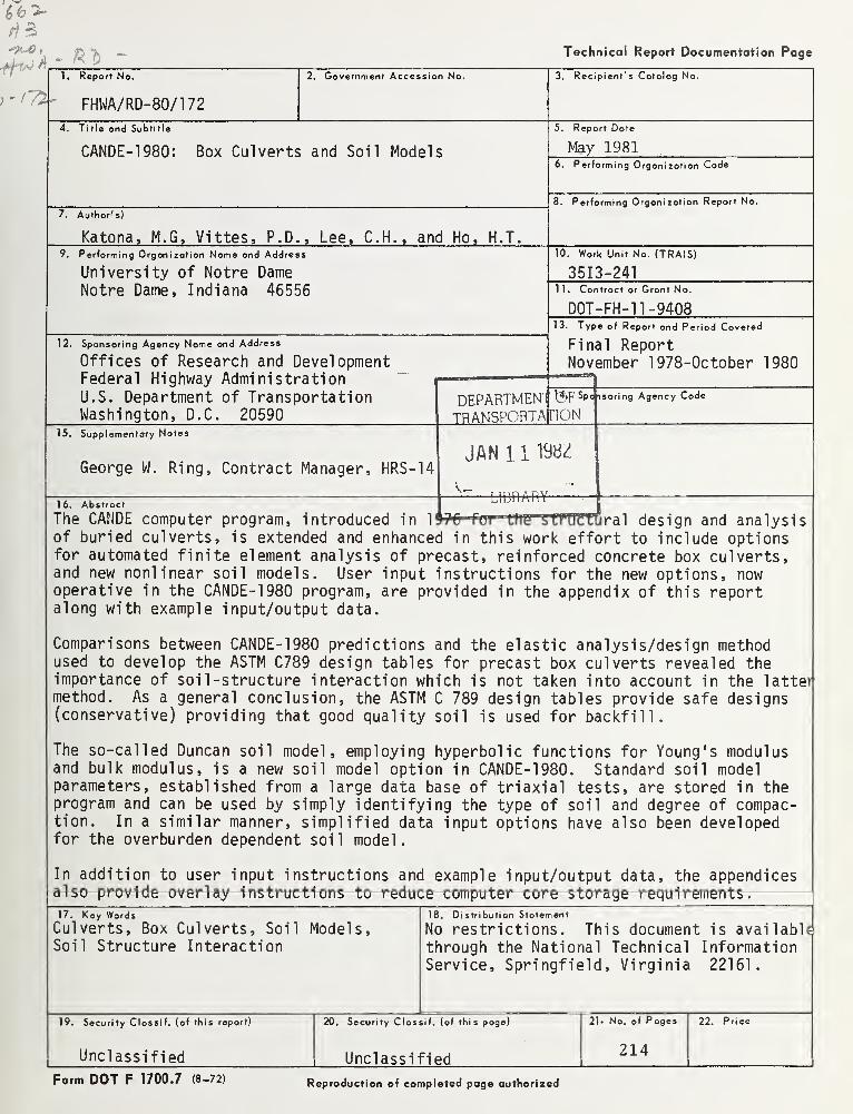
16. Abstract
The CANDE computer program, introduced in 1 970 Fur lilt! iJTTUctijral design and analysisof buried culverts, is extended and enhanced in this work effort to include optionsfor automated finite element analysis of precast, reinforced concrete box culverts,and new nonlinear soil models. User input instructions for the new options, nowoperative in the CANDE-1980 program, are provided in the appendix of this reportalong with example input/output data.
Comparisons between CANDE-1980 predictions and the elastic analysis/design methodused to develop the ASTM C789 design tables for precast box culverts revealed theimportance of soil -structure interaction which is not taken into account in the lattermethod. As a general conclusion, the ASTM C 789 design tables provide safe designs(conservative) providing that good quality soil is used for backfill.
The so-called Duncan soil model, employing hyperbolic functions for Young's modulusand bulk modulus, is a new soil model option in CANDE-1980. Standard soil modelparameters, established from a large data base of triaxial tests, are stored in theprogram and can be used by simply identifying the type of soil and degree of compac-tion. In a similar manner, simplified data input options have also been developedfor the overburden dependent soil model.
In addition to user input instructions and example input/output data, the appendicesalso provide overlay instructions to reduce computer core storage requirements.
17. Key Words
Culverts, Box Culverts, Soil Models,Soil Structure Interaction
18. Distribution Statement
No restrictions. This document is availablethrough the National Technical InformationService, Springfield, Virginia 22161.
19. Security Classif. (of this report)
Unclassified
20. Security Classif. (of this page)
Unclassified
21. No. of Pages
214
22. Price
Form DOT F 1700.7 (8-72) Reproduction of completed page authorized

ACKNOWLEDGMENTS
Representatives of industry, state highway departments, universities
and research groups have been very helpful in providing information and
constructive comments for this research effort. A special thank you is
extended to Dr. James M. Duncan of the University of California for
providing data and details of his soil model, and to Dr. Frank J. Heger
of Simpson Gumpertz and Heger Inc. who, along with representatives of
the American Concrete Pipe Association, supplied experimental data for
out-of-ground tests. Mr. Robert Thacker provided consultation on over-
laying the CANDE program on the IBM computers and programming the metric
version of CANDE-1980.

TABLE OF CONTENTS
page
CHAPTER 1 - INTRODUCTION 1
1.1 Background 1
1.2 Objectives 2
1.3 Scope and Approach 2
CHAPTER 2 - REVIEW OF PRECAST BOX CULVERTS 4
2.1 Background 4
2.2 Development and rational of ASTM precastbox culvert standards 5
CHAPTER 3 - REINFORCED CONCRETE MODEL 10
3.1 Objective 10
3.2 Assumptions, limitations and approach 10
3.3 Basic formulation for beam-rod element 12
3.4 Finite element interpolations 16
3.5 Stress-strain relationships 19
3.6 Section properties 23
3.7 Incremental solution strategy 24
3.8 Measures of reinforced concrete performance 26
3.9 Standard parameters for concrete and reinforcement .... 29
CHAPTER 4 - EVALUATION OF REINFORCED CONCRETE MODEL FORCIRCULAR PIPE LOADED IN THREE-EDGE BEARING 31
4.1 Preliminary investigations 31
4.2 Experimental tests 33
4.3 Analytical model and comparison of results 37
CHAPTER 5 - EVALUATION OF REINFORCED CONCRETE MODEL FORBOX CULVERTS LOADED IN FOUR-EDGE BEARING 49
5.1 Experimental tests 49
5.2 CANDE model 535.3 Comparison of models with experiments 53
53CHAPTER 6 - DEVELOPMENT OF LEVEL 2 BOX MESH 62
6.1 Parameters to define the models 626.2 Assumptions and limitations 67
CHAPTER 7 - EVALUATION OF CANDE BOX-SOIL SYSTEM 71
7.1 Sensitivity of soil parameters 71
7.2 Comparison with test data - 79
in
TABLE OF CONTENTS (Continued)
Page
CHAPTER 8 - EVALUATION OF ASTM C789 DESIGN TABLES WITH CANDE 85
8.1 Box section studies for dead load 85
8.2 Box section studies with live loads Ill
CHAPTER 9 - SOIL MODELS 115
9.1 Duncan model representation of elastic parameters 1179.2 CANDE solution strategy for Duncan model 1219.3 Standard hyperbolic parameters 125
CHAPTER 10 - SUMMARY AND CONCLUSIONS 132
APPENDICES
A - Details of reinforced concrete model 134
B - CANDE-1980; User Manual Supplement 147C - Sample of input data and output 177D - System overlay 202
REFERENCES 208
IV
CHAPTER 1
INTRODUCTION
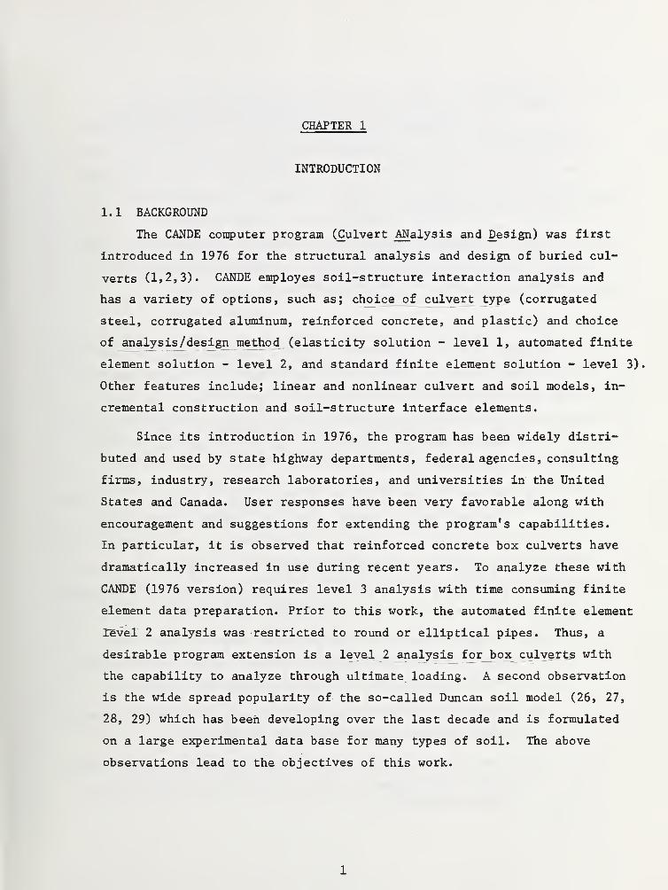
1.1 BACKGROUND
The CANDE computer program (Culvert ANalysis and Design) was first
introduced in 1976 for the structural analysis and design of buried cul-
verts (1,2,3). CANDE employes soil-structure interaction analysis and
has a variety of options, such as; choice of culvert type (corrugated
steel, corrugated aluminum, reinforced concrete, and plastic) and choice
of analysis /design method (elasticity solution - level 1, automated finite
element solution - level 2, and standard finite element solution - level 3)
Other features include; linear and nonlinear culvert and soil models, in-
cremental construction and soil-structure interface elements.
Since its introduction in 1976, the program has been widely distri-
buted and used by state highway departments, federal agencies, consulting
firms, industry, research laboratories, and universities in the United
States and Canada. User responses have been very favorable along with
encouragement and suggestions for extending the program's capabilities.
In particular, it is observed that reinforced concrete box culverts have
dramatically increased in use during recent years. To analyze these with
CANDE (1976 version) requires level 3 analysis with time consuming finite
element data preparation. Prior to this work, the automated finite element
level 2 analysis was restricted to round or elliptical pipes. Thus, a
desirable program extension is a level 2 analysis for box culverts with
the capability to analyze through ultimate loading. A second observation
is the wide spread popularity of the so-called Duncan soil model (26, 27,
28, 29) which has been developing over the last decade and is formulated
on a large experimental data base for many types of soil. The above
observations lead to the objectives of this work.
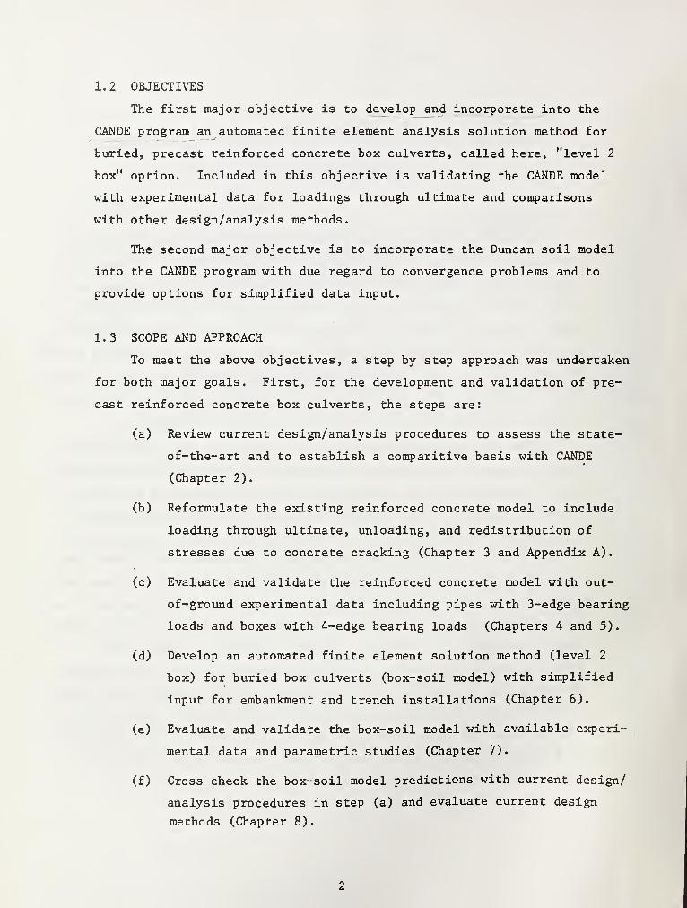
1.2 OBJECTIVES
The first major objective is to develop and incorporate into the
CANDE program an automated finite element analysis solution method for
buried, precast reinforced concrete box culverts, called here, "level 2
box" option. Included in this objective is validating the CANDE model
with experimental data for loadings through ultimate and comparisons
with other design/analysis methods.
The second major objective is to incorporate the Duncan soil model
into the CANDE program with due regard to convergence problems and to
provide options for simplified data input.
1.3 SCOPE AND APPROACH
To meet the above objectives, a step by step approach was undertaken
for both major goals. First, for the development and validation of pre-
cast reinforced concrete box culverts, the steps are:
(a) Review current design/analysis procedures to assess the state-
of-the-art and to establish a comparitive basis with CANDE
(Chapter 2).
(b) Reformulate the existing reinforced concrete model to include
loading through ultimate, unloading, and redistribution of
stresses due to concrete cracking (Chapter 3 and Appendix A).
(c) Evaluate and validate the reinforced concrete model with out-
of-ground experimental data including pipes with 3-edge bearing
loads and boxes with 4-edge bearing loads (Chapters 4 and 5).
(d) Develop an automated finite element solution method (level 2
box) for buried box culverts (box-soil model) with simplified
input for embankment and trench installations (Chapter 6).
(e) Evaluate and validate the box-soil model with available experi-
mental data and parametric studies (Chapter 7).
(f) Cross check the box-soil model predictions with current design/
analysis procedures in step (a) and evaluate current design
methods (Chapter 8).
Next, for the objective of incorporating the Duncan soil model and
simplifying soil model input, the steps are (Chapter 9):
(a) Evaluate the Duncan soil model to verify reasonable behavior
in confined compression and triaxial loading.
(b) Investigate iterative solution strategies to enhance convergence
and incorporate the model into CANDE program.
(c) Establish standard model parameters dependent on soil type and
degree of compaction for the simplified data input option.
Also, simplify data input for the existing overburden dependent
soil model.
All program modifications noted above have been incorporated into
CANDE, hereafter called CANDE-1980 to distinguish it from the 1976 version.
Appendix B provides input instructions to exercise the new options contained
in CANDE-1980. These instructions are a supplement to the 1976 CANDE User
Manual (2) and only need to be referred to if the new options are desired.
In other words, the 1976 user manual is compatible with the CANDE-1980
program. Appendix C illustrates input-output data for some of the new
options and Appendix D provides system overlay instructions to reduce
core storage.
The CANDE-1980 program discussed herein is based on the English
system of units. A companion program in metric units has been developed
and is also available from FHWA.
CHAPTER 2
REVIEW OF PRECAST BOX CULVERTS
In this chapter a brief review on the development of precast rein-
forced concrete box culverts is presented along with a discussion of
current design procedures. The intent is to acquaint the reader with
precast box culverts, terminology and design concepts and to "set the
stage" for the CANDE methodology presented in later chapters. For
brevity, "reinforced concrete box culverts" will be referred to as "box
culverts".
2.1 BACKGROUND
Precast box culverts, as opposed to cast-in-place box culverts, are
relatively recent additions in culvert technology, coming into popular
use within the last decade. For many years, cast-in-place box culverts
have been used in installations with special requirements or by design
preference. However, cast-in-place culverts have inherent disadvantages;
high labor costs associated with cast-in-place construction, lengthy
periods of traffic disruption, and minimal quality control often compensated
for by conservative designs. Alternatively, plant-produced box culverts,
manufactured under strict quality control and installed by rapid cut-and-
fill procedures, can offset these disadvantages particularly if the box
dimensions, reinforcement, ect., are standardized for manufacture.
With the above motivation, the Virginia Department of Highways
and the American Concrete Pipe Association (ACPA) , with financial support
from the Wire Reinforcement Institute, initiated a cooperative program,
early in 1971, to develop manufacturing specifications and standard
designs for precast box culverts. These specifications were to be
adaptable as a national standard under the auspices of the American
Society of Testing Materials (ASTM) and the American Association of State
Highway and Transportation Officials (AASHTO) . To this end, ACPA contracted
the consulting firm of Simpson, Gumpertz and Heger Inc. (SGH) to develop
a computerized design program for precast box culverts in cooperation
with ASTM committee C-13.
Ultimately, this effort culminated in the ASTM C789 and AASHTO M259
specifications on Precast Reinforced Concrete Box Sections for Culverts,
Storm Drains and Sewers first published in 1974. These specifications were
limited to box culverts with a minimum of two feet (0.61 m) of earth cover.
Further developmental work by SGH resulted in the additional specifications
ASTM C850 and AASHTO M273 published in 1976 for precast box culvert in-
stallations with less than two feet of earth cover. The above ASTM and
AASHTO specifications are essentially the same except for a few details
which are apparently now resolved. For purposes of this study, the
ASTM specifications will be used as reference. Design methods for pre-
cast box culverts, other than those embodied in ASTM or AASHTO specifi-
cations, will not be reviewed here since they are not standardized nor
have they gained national acceptance. Recently, ACPA published a sur-
vey (Concrete Pipe News, June 1980) showing that usage of precast box
culverts, designed by ASTM specifications, has increased dramatically
within the last year. . . the number of projects and linear footage
installed in 1979 is almost equal to the total for the previous five years!
2.2 DEVELOPMENT AND RATIONALE OF ASTM PRECAST BOX CULVERT STANDARDS
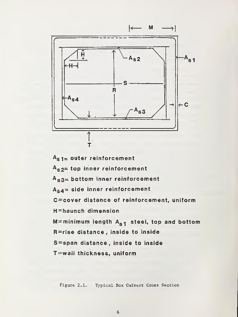
The SGH computerized design program (12) is the basis of the
design rationale in the ASTM C789 design tables. A typical box cross-
section is shown in Figure 2.1 along with nomenclature. The SGH design/
analysis approach includes the following steps; (a) load distributions
are assumed around the culvert in an attempt to simulate dead earth loads
and live loads, (b) moment, shear, and thrust distributions are determined
by standard matrix methods using elastic, uncracked concrete section pro-
perties, (c) in the design mode, steel areas are determined by an ulti-
mate strength theory for bending and thrust, where ultimate moments and
thrusts are obtained from step (b) multiplied by a load factor, (d) crack-
width (0.01 inch allowable) is checked using a semi-empirical formula
M ^1
f^
1
/\T 14> -vAt2 \
-»
<-M
R
:-As4
1 _,
k
s1
<-C
t.T
As i= outer reinforcement
AS 2= top inner reinforcement
A S3= bottom inner reinforcement
AS4= side inner reinforcement
C = cover distance of reinforcement, uniform
H=haunch dimension
M=minimum length As1 steei, top and bottom
R=rise distance , inside to inside
S = span distance, inside to inside
T=wall thickness, uniform
Figure 2.1. Typical Box Culvert Cross Section
controlled by steel stress at service loads, (e) ultimate shear stress
( 2 /P~ ) is checked against the nominal shear stress obtained in step (b)
multipled by a load factor.
For the standard box sizes shown in Table 2.1, the SGH design program
was used to generate the ASTM C789 design tables wherein steel reinforce-
ment requirements are specified as a function of design earth cover be-
ginning with a two foot minimum.
In a similar manner, ASTM C850 design tables were generated for earth
covers less than two feet. Here, the SGH design procedure was modified
to include requirements for longitudinal steel design due to concentrated
live loads (see ASTM Symposium STP 630).
Although the SGH design/analysis program has not been validated
with experimental data from buried box culverts, fairly good correlation
with out-of-ground experimental tests has been reported (13). More will
be said about these experiments in Chapter 5.
Experimental data for instrumented, buried box culverts is extremely
limited. As of this writing, only two state highway departments (Kentucky
and Illinois) are known to have undertaken experimental programs for in-
strumenting (settlement, soil pressure, and strain gages) buried box
culvert installations. Other states have made visual inspection reports
on the performance of buried box installations, but this data has marginal
value for validating design/analysis procedures. Data from the Kentucky
Department of Transportation was made available for this study and is
used to evaluate the CANDE program in Chapter 7.
In summary, the ASTM design tables for buried, precast box culverts,
which are based on the SGH design/analysis program, have not been pre-
viously validated with experimental data from buried installations. Nor
have the tables been cross-checked with analytical procedures, such as
CANDE, employing soil-structure interaction and the nonlinear nature of
reinforced concrete. With this goal in mind, a step by step approach is
presented in the following chapters. First, the theory of CANDE 's non-
linear, reinforced concrete model is developed. Second, the model is
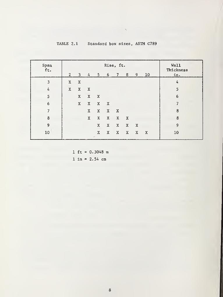
TABLE 2.1 Standard box sizes, ASTM C789
Spanft.
2 3 4 5
Rise, ft.
6 7 8 9 10
WallThickness
in.
3 X X 4
4 X X X 5
5 X X X 6
6 X X X X 7
7 X X X X 8
8 X X XXX 8
9 X XXX X 9
10 X XXX X X 10
1 ft = 0.3048 m
1 in = 2.54 cm
validated with experimental data for out-of-ground conditions. Third,
the reinforced concrete model is combined with soil system models and
compared with experimental data from a buried installation. Last, the
CANDE model is used to evaluate the ASTM design tables.
CHAPTER 3
REINFORCED CONCRETE MODEL
3.1 OBJECTIVE
A reinforced concrete, beam-rod member, whether it be part of a
culvert or any other structural system, poses a difficult analysis
problem due to the nonlinear material behavior of concrete in com-
pression, cracking of concrete in tension, yielding of reinforcement
steel, and the composite interaction of concrete and reinforcement.
Matters are further complicated when the internal loading is not
proportional, i.e., when the internal moment, shear and thrust at
a particular cross section change in different proportions (including
load reversals) during the loading history. Such is the case for
buried culverts during the installation process.
In this chapter, the development of a reinforced concrete beam-
rod element is developed in the context of a finite element formulation
for CANDE-1980. This model is more general than the model in CANDE-1976
and includes; incremental loading through ultimate, unloading, and
redistribution of stresses due to cracking.
The following presentation provides an overview of the model
development emphasizing assumptions and limitations. Details of the
numerical solution strategy are presented in Appendix A. Evaluation
of the model with experimental data and other theories is presented
in subsequent chapters.
3.2 ASSUMPTIONS, LIMITATIONS, AND APPROACH
Listed below are the fundamental assumptions for the reinforced
concrete beam-rod element.
10
I
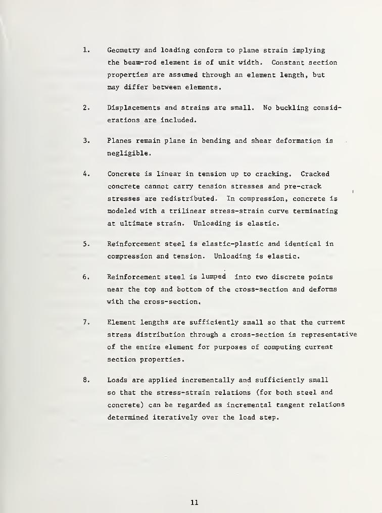
1. Geometry and loading conform to plane strain implying
the beam-rod element is of unit width. Constant section
properties are assumed through an element length, but
may differ between elements.
2. Displacements and strains are small. No buckling consid-
erations are included.
3. Planes remain plane in bending and shear deformation is
negligible.
4. Concrete is linear in tension up to cracking. Cracked
concrete cannot carry tension stresses and pre-crack
stresses are redistributed. In compression, concrete is
modeled with a trilinear stress-strain curve terminating
at ultimate strain. Unloading is elastic.
5. Reinforcement steel is elastic-plastic and identical in
compression and tension. Unloading is elastic.
6. Reinforcement steel is lumped into two discrete points
near the top and bottom of the cross-section and deforms
with the cross-section,
7. Element lengths are sufficiently small so that the current
stress distribution through a cross-section is representative
of the entire element for purposes of computing current
section properties.
8. Loads are applied incrementally and sufficiently small
so that the stress-strain relations (for both steel and
concrete) can be regarded as incremental tangent relations
determined iteratively over the load step.
11
In overall perspective, the developmental steps begin with an
incremental statement of virtual work wherein the beam-rod assumptions
are introduced along with standard finite element interpolation func-
tions for axial and bending deflections. This results in a tangent
element stiffness matrix and incremental load vector that can be
assembled into a global set of system equations with unknown nodal
degrees of freedom, and solved by standard techniques (1). However,
the global matrix contains estimates of the bending and axial stiff-
ness for each beam-rod element (as well as estimates for soil stiff-
ness if nonlinear soil models are part of the system). Thus, each
load step is repetitively solved (iterated), and the results are used
to improve the stiffness estimates until convergence is achieved.
Prior to the first loading increment, the beam-rod element is
assumed stress free and uncracked so initial stiffnesses correspond
to an uncracked, elastic, transformed reinforced concrete cross-
section. Upon applying the first load increment, the first tentative
solution may indicate that some elements should have had reduced
stiffnesses due to cracking or yielding of the section. Using the
strain distribution at the beginning and end of the load step, new
stiffness estimates are obtained and the process is iterated to con-
vergence. Each subsequent load step is treated in a similar fashion
where a history of maximum stress and strain is maintained for pur-
poses of identifying unloading conditions.
The above assumptions and general approach are outlined in the
following development,
3,3 BASIC FORMULATION FOR BEAM-ROD ELEMENT
In this section we consider an incremental virtual work statement
for a unit width, beam-rod element with body forces given by:
6AV = 5AU - 6AW (3,1)
with 5AU = / / SeAa dxdy = internal virtual work incrementx y
12
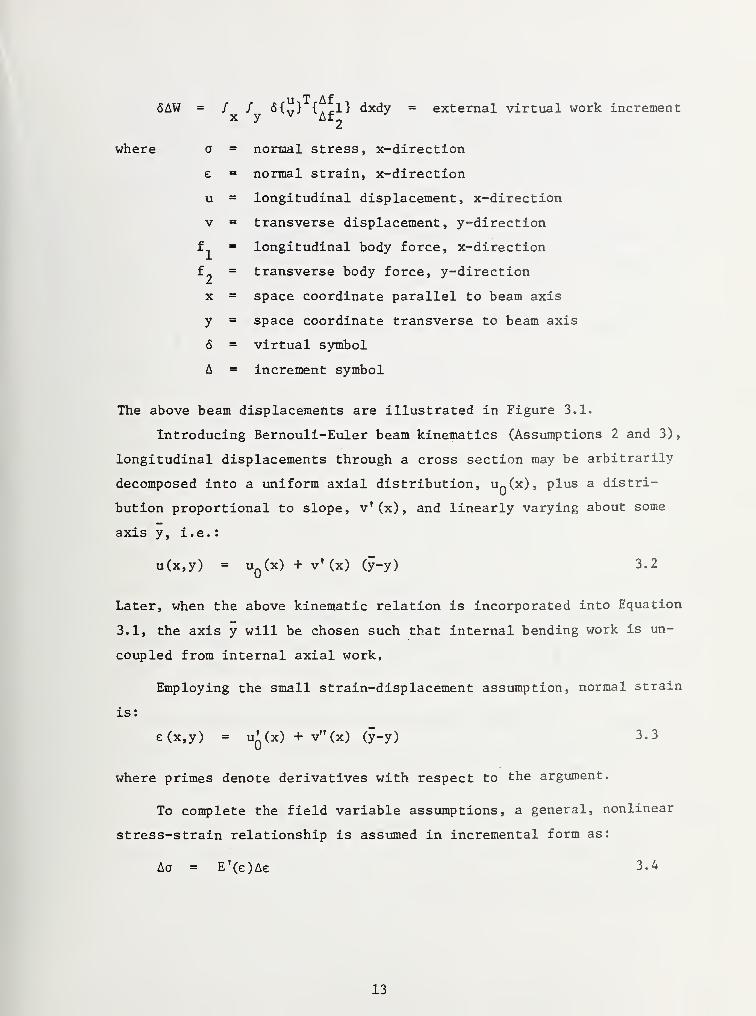
SAW = f f 6{. 7 } { , -1} dxdy = external virtual work incrementx y v Af„
where a = normal stress, x-direction
e = normal strain, x-direction
u = longitudinal displacement, x-direction
v = transverse displacement, y-direction
f. = longitudinal body force, x-direction
f_ = transverse body force, y-direction
x = space coordinate parallel to beam axis
y = space coordinate transverse to beam axis
6 = virtual symbol
A = increment symbol
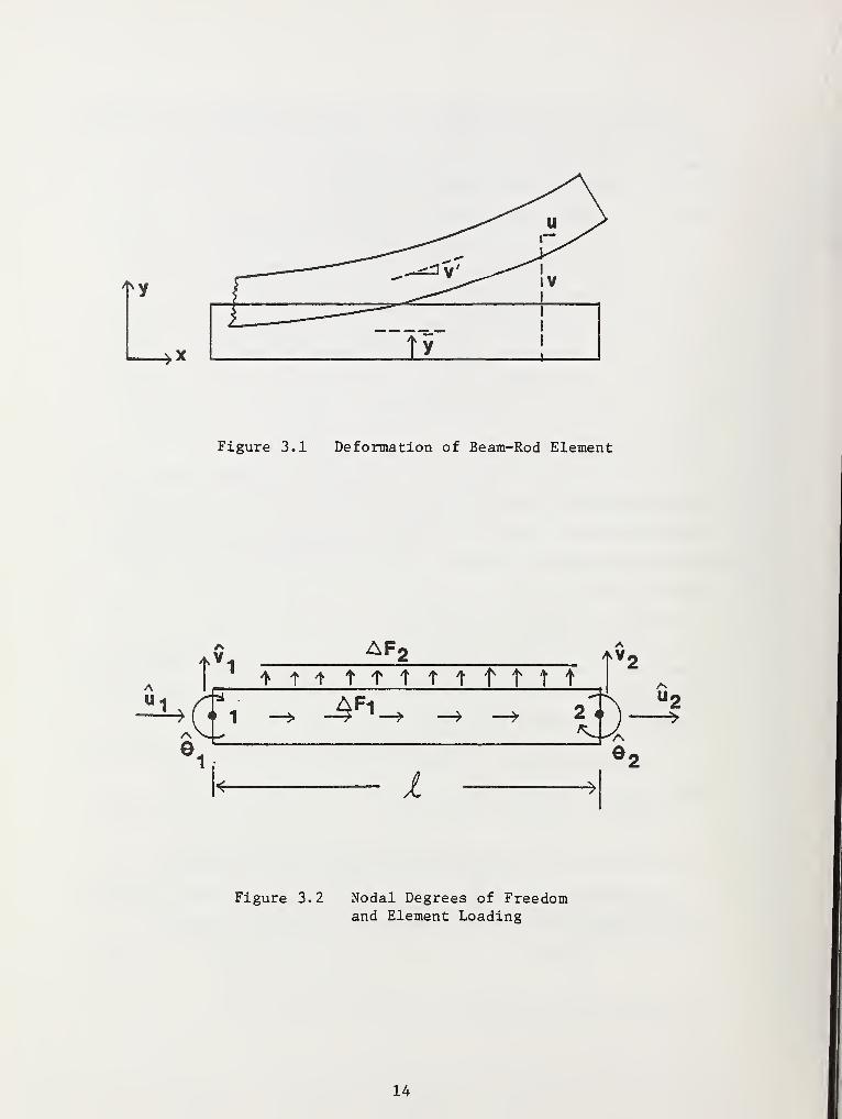
The above beam displacements are illustrated in Figure 3.1.
Introducing Bernouli-Euler beam kinematics (Assumptions 2 and 3),
longitudinal displacements through a cross section may be arbitrarily
decomposed into a uniform axial distribution, u (x), plus a distri-
bution proportional to slope, v'(x), and linearly varying about some
axis y, i.e.
:
u(x,y) = uQ(x) + v f
(x) (y-y) 3.2
Later, when the above kinematic relation is incorporated into Equation
3,1, the axis y will be chosen such that internal bending work is un-
coupled from internal axial work,
Employing the small strain-displacement assumption, normal strain
is:
e(x,y) = u^(x) + v"(x) (5-y) 3.3
where primes denote derivatives with respect to the argument.
To complete the field variable assumptions, a general, nonlinear
stress-strain relationship is assumed in incremental form as:
Aa = E'(e)Ae 3,4
13
4*
Figure 3.1 Deformation of Beam-Rod Element
AF-
A t1 MHt t f t f t t t
Ui /^R~ AF1
A
i>r«i £>-*e
i
Figure 3.2 Nodal Degrees of Freedomand Element Loading
14
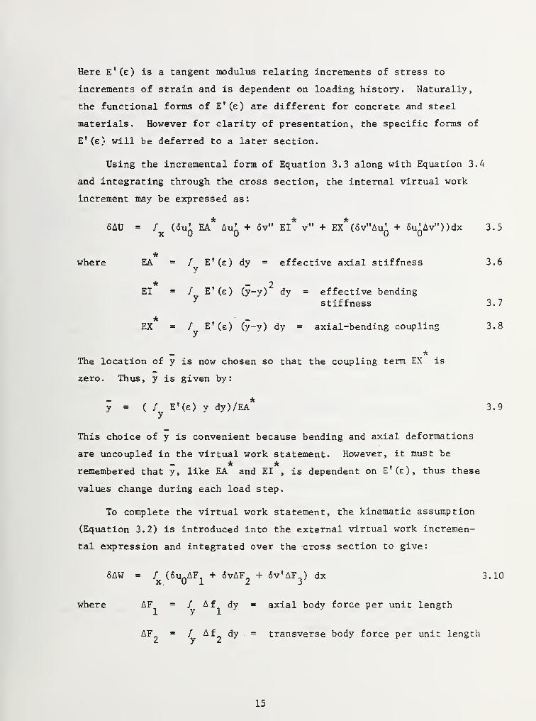
Here Ef (e) is a tangent modulus relating increments of stress to
increments of strain and is dependent on loading history. Naturally,
the functional forms of E'(e) are different for concrete and steel
materials. However for clarity of presentation, the specific forms of
E'(e) will be deferred to a later section.
Using the incremental form of Equation 3.3 along with Equation 3.4
and integrating through the cross section, the internal virtual work
increment may be expressed as:
5AU = / (6ui EA* Aul + 6vM EI* v" + EX*(5v"Au: + 6ulAv"))dx 3.5x
*where EA = / E' (e) dy = effective axial stiffness 3.6
y
* _ 2EI = / E'(e) (y-y) dy = effective bending
y stiffness 3.7
*EX = / E'(e) (y-y) dy = axial-bending coupling 3.8
_ *The location of y is now chosen so that the coupling term EX is
zero. Thus, y is given by:
y = ( / E»(e) y dy)/EA* 3.9
This choice of y is convenient because bending and axial deformations
are uncoupled in the virtual work statement. However, it must be
remembered that y, like EA and EI , is dependent on E'(e), thus these
values change during each load step.
To complete the virtual work statement, the kinematic assumption
(Equation 3.2) is introduced into the external virtual work incremen-
tal expression and integrated over the cross section to give:
6AW = / ( 6u AFl+ 6vAF
2+ <Sv?AF
3) dx 3 ' 10
where AF = / Af, dy = axial body force per unit length1 y 1
AF„ = J" Af dy = transverse bodv force per unit length2 y 2
J f
15
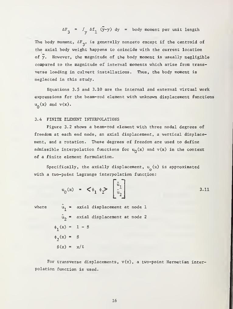
AF = / Af (y-y) dy = body moment per unit lengthj y x
The body moment, AF , is generally nonzero except if the centroid of
the axial body weight happens to coincide with the current location
of y. However, the magnitude of the body moment is usually negligible
compared to the magnitude of internal moments which arise from trans-
verse loading in culvert installations. Thus, the body moment is
neglected in this study.
Equations 3.5 and 3.10 are the internal and external virtual work
expressions for the beam-rod element with unknown displacement functions
u (x) and v(x).
3.4 FINITE ELEMENT INTERPOLATIONS
Figure 3.2 shows a beam-rod element with three nodal degrees of
freedom at each end node, an axial displacement, a vertical displace-
ment, and a rotation. These degrees of freedom are used to define
admissible interpolation functions for un (x) and v(x) in the context
of a finite element formulation.
Specifically, the axially displacement, u (x) is approximated
with a two-point Lagrange interpolation function:
* D]uQ(x) = O, cj) > 3.11
where u, = axial displacement at node 1
u~ = axial displacement at node 2
(J>
1(x) =1-6
4>
2(x) = 3
B(X) = x/£
For transverse displacements, v(x), a two-point Hermetian inter-
polation function is used.
16
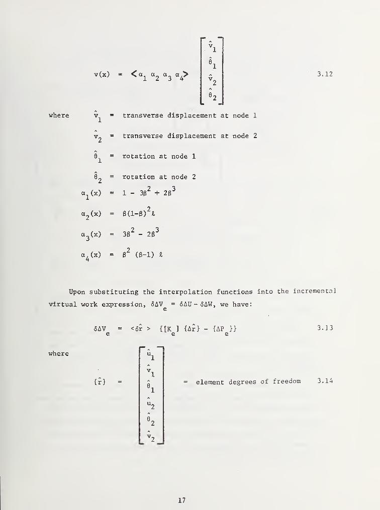
v(x) = <al
a2
a3
a? v.3.12
where v = transverse displacement at node 1
v„ = transverse displacement at node 2
6.. = rotation at node 1
6„ = rotation at node 2
a1(x)
2 31 - 33 + 23
a2(x)
a3(x)
= 3(1-3) I
2 333 - 23
a4(x) = 3 (3-D I
Upon substituting the interpolation functions into the Incremental
virtual work expression, 6AV = 5AU-6AW, we have:e
6AV = <6r > {[K ] {Ar} - {AP }}e e e
3.13
where
{r}
~*A*
ul
*
v1J_
A
61
/v
U2
*
92
/v
_v2
= element degrees of freedom 3.14
17
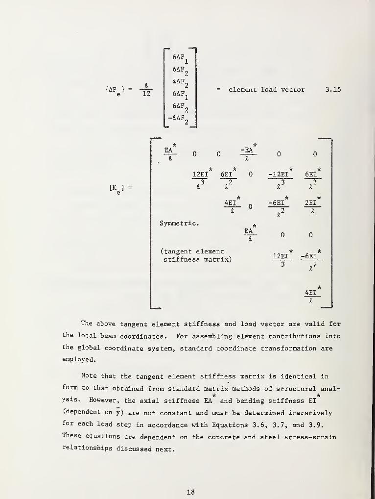
{AP } = -jVe 12
6AF]
6AF,
JIAF,i
6AF]
6AF,
-£AF,
= element load vector 3.15
[K ]=
e
* *EA n n -EA
\J
£
k12EI 6EI
*3
*2
*
«.
c. *EA
Symmetric.
(tangent elementstiffness matrix)
-12EI
-6EI
6EI
2EI
* *12EI -6EI
4EI
The above tangent element stiffness and load vector are valid for
the local beam coordinates. For assembling element contributions into
the global coordinate system, standard coordinate transformation are
employed.
Note that the tangent element stiffness matrix is identical in
form to that obtained from standard matrix methods of structural anal-
ysis. However, the axial stiffness EA and bending stiffness EI
(dependent on y) are not constant and must be determined iteratively
for each load step in accordance with Equations 3.6, 3.7, and 3.9.
These equations are dependent on the concrete and steel stress-strain
relationships discussed next.
18
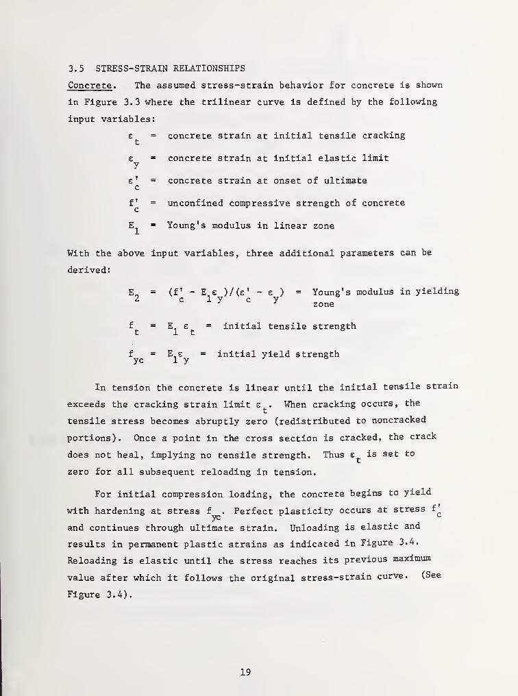
3.5 STRESS-STRAIN RELATIONSHIPS
Concrete . The assumed stress-strain behavior for concrete is shown
in Figure 3.3 where the trilinear curve is defined by the following
input variables:
e = concrete strain at initial tensile cracking
e = concrete strain at initial elastic limity
e' = concrete strain at onset of ultimatec
f ' = unconfined compressive strength of concrete
E = Young's modulus in linear zone
With the above input variables, three additional parameters can be
derived:
E n = (f - E e )/(e' - e ) = Young's modulus in yielding2 c 1 y c yJ zone
£' - E, e = initial tensile strengthtitf = E,e = initial yield strengthyc 1 y
J b
In tension the concrete is linear until the initial tensile strain
exceeds the cracking strain limit e . When cracking occurs, the
tensile stress becomes abruptly zero (redistributed to noncracked
portions). Once a point in the cross section is cracked, the crack
does not heal, implying no tensile strength. Thus e is set to
zero for all subsequent reloading in tension.
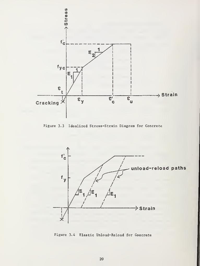
For initial compression loading, the concrete begins to yield
with hardening at stress f . Perfect plasticity occurs at stress f^
and continues through ultimate strain. Unloading is elastic and
results in permanent plastic strains as indicated in Figure 3.4.
Reloading is elastic until the stress reaches its previous maximum
value after which it follows the original stress-strain curve. (See
Figure 3.4).
19
CO
(0
Cracking
> Strain
Figure 3.3 Idealized Stress-Strain Diagram for Concrete
unload-reload paths
i/-iE
i A/ /
// -^Strain
Figure 3.4 Elastic Unload-Reload for Concrete
20
With the above understanding, the tangent modulus relationship
for concrete confined in a plane is expressed as:
E'(e) = E (1 - a(e)) 3.17c c
2where E = E / (1 - v )
c 1 c
with E = elastic, confined plane modulus of concrete
v Poisson's ratio of concrete (constant)c
a(e) = dimensionless function of stress-strain history
The dimensionless function a(e) ranges in value from 0.0 (elastic
response) to 1.0 (perfectly-plastic response), representing the non-
linear effect of concrete. The actual value of a(e) to be used for
any given load increment is dependent on; known values of stress and
strain at the beginning of the step, known history parameters for
cracking and yielding, and unknown values of stress and strain at the
end of the step (iteration). Appendix A provides the details for
determining a(e) for all loading histories.
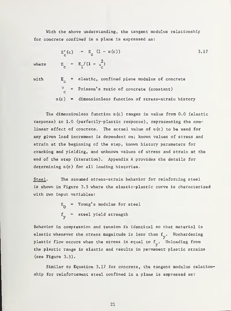
Steel . The assumed stress-strain behavior for reinforcing steel
is shown in Figure 3.5 where the elastic-plastic curve is characterized
with two input variables:
En= Young's modulus for steel
f = steel yield strength
Behavior in compression and tension is identical so that material is
elastic whenever the stress magnitude is less than f . Nonhardening
plastic flow occurs when the stress is equal to f , Unloading from
the plastic range is elastic and results in permanent plastic strains
(see Figure 3,5).
Similar to Equation 3,17 for concrete, the tangent modulus relation-
ship for reinforcement steel confined in a plane is expressed as:
21
(0
©
CO
fy-~
s
s
-fy
-^Strain
Figure 3.5 Idealized Stress-Strain Diagramfor Reinforcing Steel
Xunit I
width 7'
Figure 3.6 Reinforced Concrete Cross Section
22
E' (e) = E (1 - a(e)) 3.18s s
2where E = EJ (1 - v )
s s
with E = elastic, confined plane modulus of steels
v = Poisson's ratio of steel (constant)s
a(e) dimensionless function of stress-strain history
As in the case of concrete, the function a(e) for steel ranges in
value from 0,0 (elastic) to 1.0 (perfectly plastic) depending on
stress-strain history and stress values at the beginning and end of
each load step (see Appendix A).
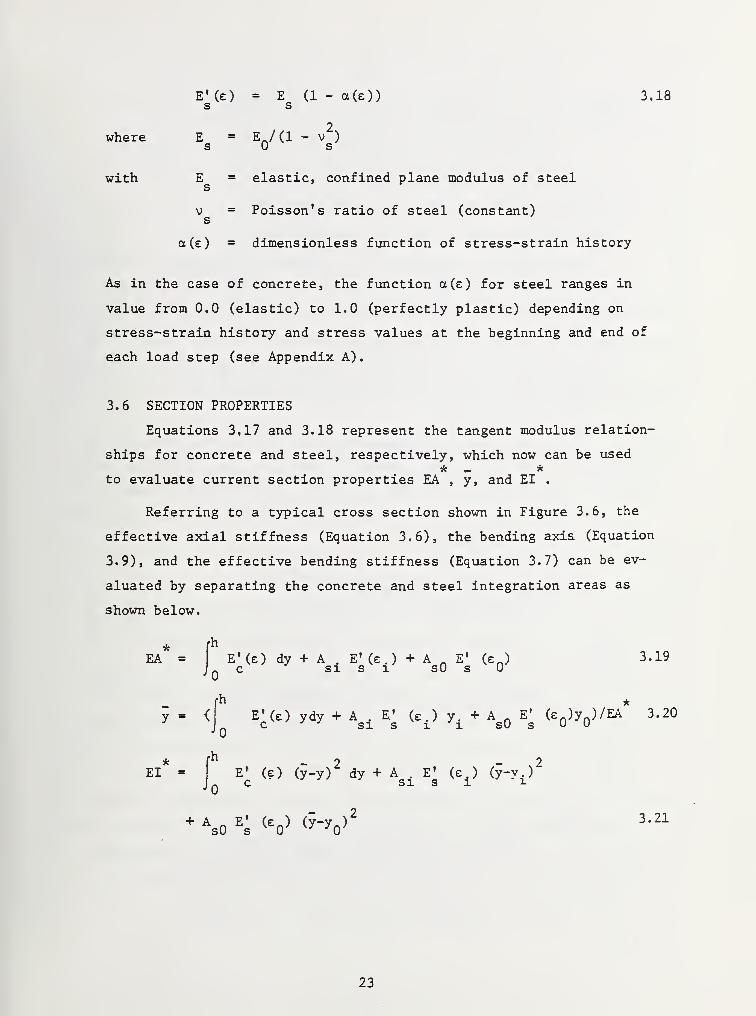
3.6 SECTION PROPERTIES
Equations 3,17 and 3.18 represent the tangent modulus relation-
ships for concrete and steel, respectively, which now can be used
to evaluate current section properties EA , y, and EI ,
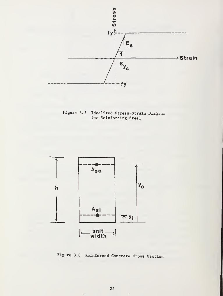
Referring to a typical cross section shown in Figure 3.6, the
effective axial stiffness (Equation 3.6), the bending axis (Equation
3.9), and the effective bending stiffness (Equation 3.7) can be ev-
aluated by separating the concrete and steel integration areas as
shown below.
* AEA = E'(e) dy + A . E» (e . ) + A _ E» (e A )
3.19c si s i sO s
y = <[ E»(£ ) ydy + A . E' (e.) y. + A . E' (e )y )/EA* 3.20J
jc
v ' J si s iJx sO s
EI =rh
2 _.,.,- ,2E* (?) (y-y) dy + A . E' (e . ) (y-y.)c si si i
+ aso
e;
<io>
(?-yo)2 3 - 21
23
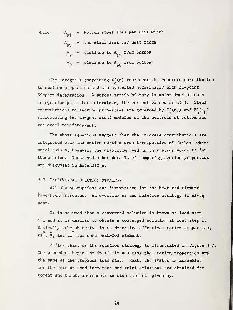
where A .= bottom steel area per unit width
. si
A - = top steel area per unit widthsO
y. = distance to A . from bottomy i sx
y^ = distance to A _ from bottomJ sO
The integrals containing E'(e) represent the concrete contributionc
to section properties and are evaluated numerically with 11-point
Simpson integration, A stress-strain history is maintained at each
integration point for determining the current values of a(e). Steel
contributions to section properties are governed by E' (e ) and E'(e )S X s u
representing the tangent steel modulus at the centroid of bottom and
top steel reinforcement.
The above equations suggest that the concrete contributions are
integrated over the entire section area irrespective of "holes" where
steel exists, however, the algorithm used in this study accounts for
these holes. These and other details of computing section properties
are discussed in Appendix A,
3.7 INCREMENTAL SOLUTION STRATEGY
All the assumptions and derivations for the beam-rod element
have been presented. An overview of the solution strategy is given
next.
It is assumed that a converged solution is known at load step
i-1 and it is desired to obtain a converged solution at load step i.
Basically, the objective is to determine effective section properties,* - *
EI , y, and EI for each beam-rod element.
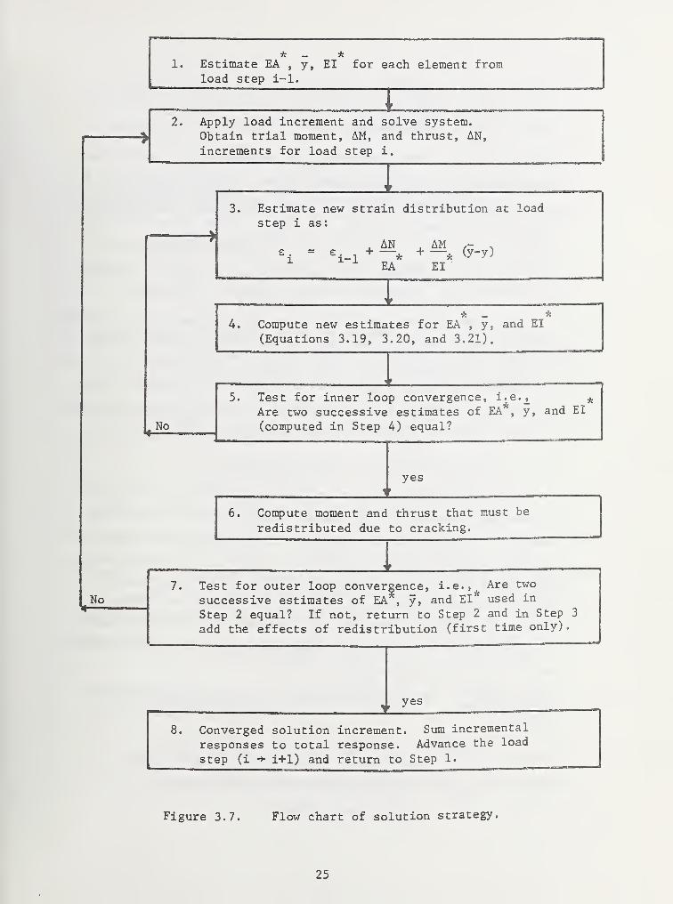
A flow chart of the solution strategy is illustrated in Figure. 3. 7.
The procedure begins by initially assuming the section properties are
the same as the previous load step. Next, the system is assembled
for the current load increment and trial solutions are obtained for
moment and thrust increments in each element, given by:
24
* AEstimate EA
, y, EI for each element fromload step i-1.
Apply load increment and solve system.Obtain trial moment, AM, and thrust, AN,
increments for load step i.
3. Estimate new strain distribution at load
step i as:
AN= e-i+ —
*
l-l *EA
+ —* (y-y)
EI
No
No
5.
* _4. Compute new estimates for EA
, y, and EI
(Equations 3.19, 3.20, and 3.21).
Test for inner loop convergence, i...e._,,
Are two successive estimates of EA, y, and EI
(computed in Step 4) equal?
yes
6. Compute moment and thrust that must be
redistributed due to cracking.
Test for outer loop convergence, i.e., Are two
successive estimates of EA , y, and EI used in
Step 2 equal? If not, return to Step 2 and in Step 3
add the effects of redistribution (first time only).
yes
8. Converged solution increment. Sum incremental
responses to total response. Advance the load
step (i -> i+1) and return to Step 1.
Figure 3.7. Flow chart of solution strategy.
25
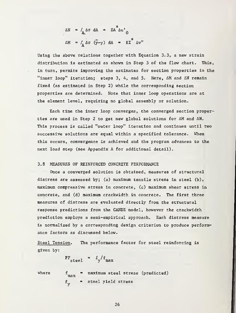
AN = /. Aa dA = EA Au'A.
AM - f Aa (y-y) dA - EI Av"A
Using the above relations together with Equation 3.3, a new strain
distribution is estimated as shown in Step 3 of the flow chart. This,
in turn, permits improving the estimates for section properties in the
"inner loop" iteration; steps 3, 4, and 5. Here, AM and AN remain
fixed (as estimated in Step 2) while the corresponding section
properties are determined. Note that inner loop operations are at
the element level, requiring no global assembly or solution.
Each time the inner loop converges, the converged section proper-
ties are used in Step 2 to get new global solutions for AM and AN.
This process is called "outer loop" iteration and continues until two
successive solutions are equal within a specified tolerance. When
this occurs, convergence is achieved and the program advances to the
next load step (see Appendix A for additional detail),
3.8 MEASURES OF REINFORCED CONCRETE PERFORMANCE
Once a converged solution is obtained, measures of structural
distress are assessed by; (a) maximum tensile stress in steel (b),
maximum compressive stress in concrete, (c) maximum shear stress in
concrete, and (d) maximum crackwidth in concrete. The first three
measures of distress are evaluated directly from the structural
response predictions from the CANDE model, however the crackwidth
prediction employs a semi-empirical approach. Each distress measure
is normalized by a corresponding design criterion to produce perform-
ance factors as discussed below.
Steel Tension . The performance factor for steel reinforcing is
given by:
PF , = f /fsteel y max
where f = maximum steel stress (predicted)max r
f = steel yield stressy
26
For properly designed structures, this performance factor should be
in the range of 1,5 to 2,0, When the steel begins to yield, the
performance factor becomes 1,0 and remains .there through ultimate
loading.
Concrete Compression . For the outer concrete fibers experiencing
compressive stress from thrust and bending, the performance factor is:
PF = V/ocomp . c max
where a = maximum compressive stress (predicted)
f* = compressive strength of concretec
Proper designs should have this performance factor in the range 1.6 to
2.5, The performance factor remains at 1.0 when the concrete becomes
perfectly plastic and remains there through ultimate loading.
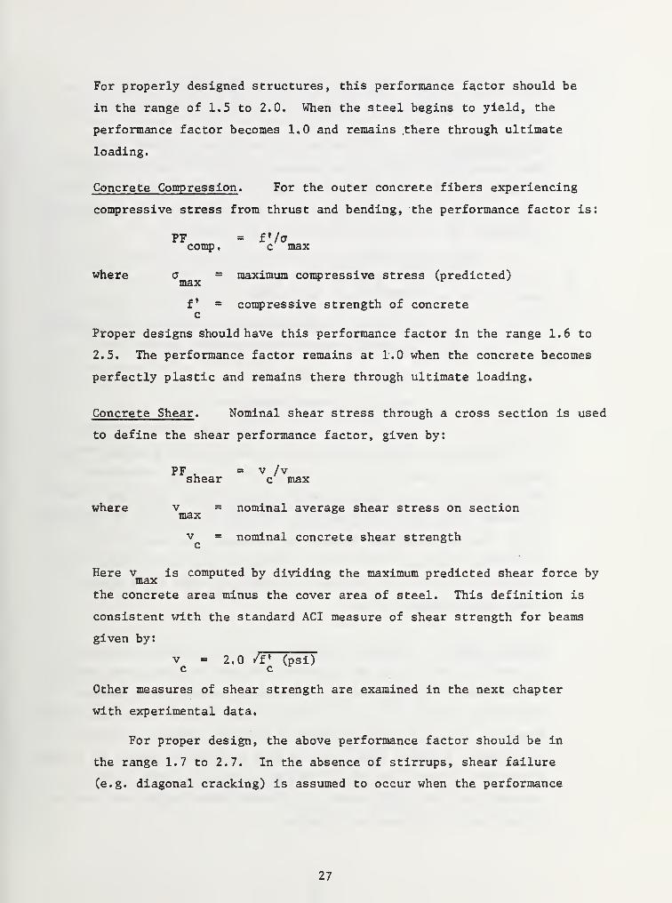
Concrete Shear . Nominal shear stress through a cross section is used
to define the shear performance factor, given by:
PF .o v /v
shear c max
where v = nominal average shear stress on sectionmax °
v = nominal concrete shear strengthc
Here v is computed by dividing the maximum predicted shear force by
the concrete area minus the cover area of steel. This definition is
consistent with the standard ACI measure of shear strength for beams
given by:
v - 2.0 TV (psi)c c
Other measures of shear strength are examined in the next chapter
with experimental data,
For proper design, the above performance factor should be in
the range 1.7 to 2.7. In the absence of stirrups, shear failure
(e.g. diagonal cracking) is assumed to occur when the performance
27
factor value is 1.0. Note that the CANDE model does not incorporate
diagonal cracking into the stress-strain law, only flexural cracking.
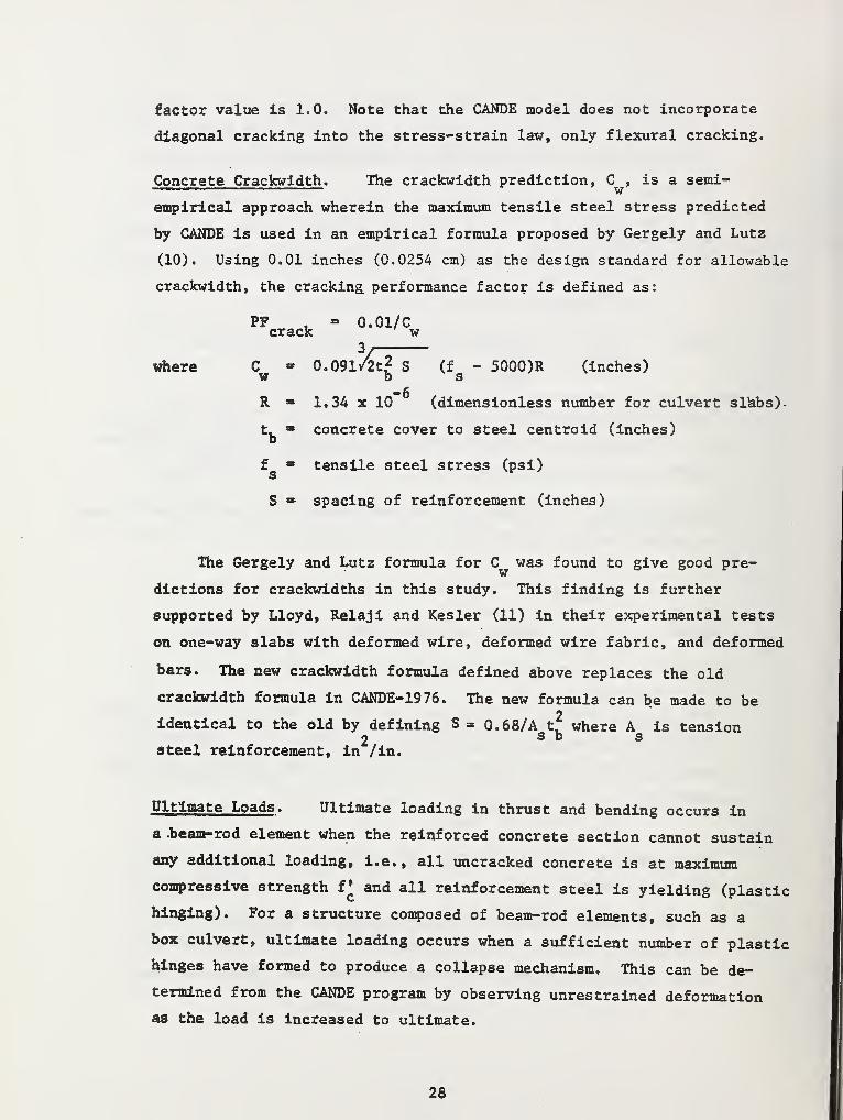
Concrete Crackwidth . The crackwidth prediction, C , is a semi-
empirical approach wherein the maximum tensile steel stress predicted
by CANDE is used in an empirical formula proposed by Gergely and Lutz
(10). Using 0.01 inches (0.0254 cm) as the design standard for allowable
crackwidth, the cracking, performance factor is defined as:
PP , » 0.01/Ccrack w
3
/£?where C - Q.091/2t* S (f - 5000)R (inches)W D S
R 1,34 x 10 (dimensionless number for culvert slabs).
t. concrete cover to steel centroid (inches)D
f tensile steel stress (psi)
S spacing of reinforcement (inches)
The Gergely and Lutz formula for C was found to give good pre-w
dictions for crackwidths in this study. This finding is further
supported by Lloyd, Relaji and Kesler (11) in their experimental tests
on one-way slabs with deformed wire, deformed wire fabric, and deformed
bars. The new crackwidth formula defined above replaces the old
crackwidth formula in CANDE-19 76. The new formula can be made to be2
identical to the old by defining S = 0.68/A t^ where A is tension2 sos
steel reinforcement, in /in.
Ultimate Loads . Ultimate loading in thrust and bending occurs in
a .beam-rod element when the reinforced concrete section cannot sustain
any additional loading, i.e., all uncracked concrete is at maximum
compressive strength f ' and all reinforcement steel is yielding (plastic
hinging). For a structure composed of beam-rod elements, such as a
box culvert, ultimate loading occurs when a sufficient number of plastic
hinges have formed to produce a collapse mechanism. This can be de-
termined from the CANDE program by observing unrestrained deformation
as the load is increased to ultimate.
28
Ultimate loading in shear is assumed to occur when the performance
factor for shear in any beam-rod element becomes 1,0. If a structure
fails in shear prior to flexural-thrust failures, the CANDE model is
still capable of carrying load up to flexural-thrust failure because
diagonal cracking is not included in the model development. Thus for
loads exceeding concrete shear failure, it must be presumed that suf-
ficient shear reinforcement (stirrups) is available.
3.9 STANDARD PARAMETERS FOR CONCRETE AND REINFORCEMENT
Based on investigations presented in subsequent chapters, a set
of standard parameter values for concrete is given in Table 3,1 (see
also Figure 3.3). Except for compressive strength f and cracking
strain e , the parameters are assigned unique values, some of which
are dependent on f*.'
For subsequent analytical studies, the concrete will be
characterized by specifying f and £ . The remaining parametersc t
are assigned the standard values shown in Table 3.1 unless stated
otherwise.
Standard parameters for reinforcement steel are shown in Table 3.2
wherein the yield stress in considered as the primary variable.
29
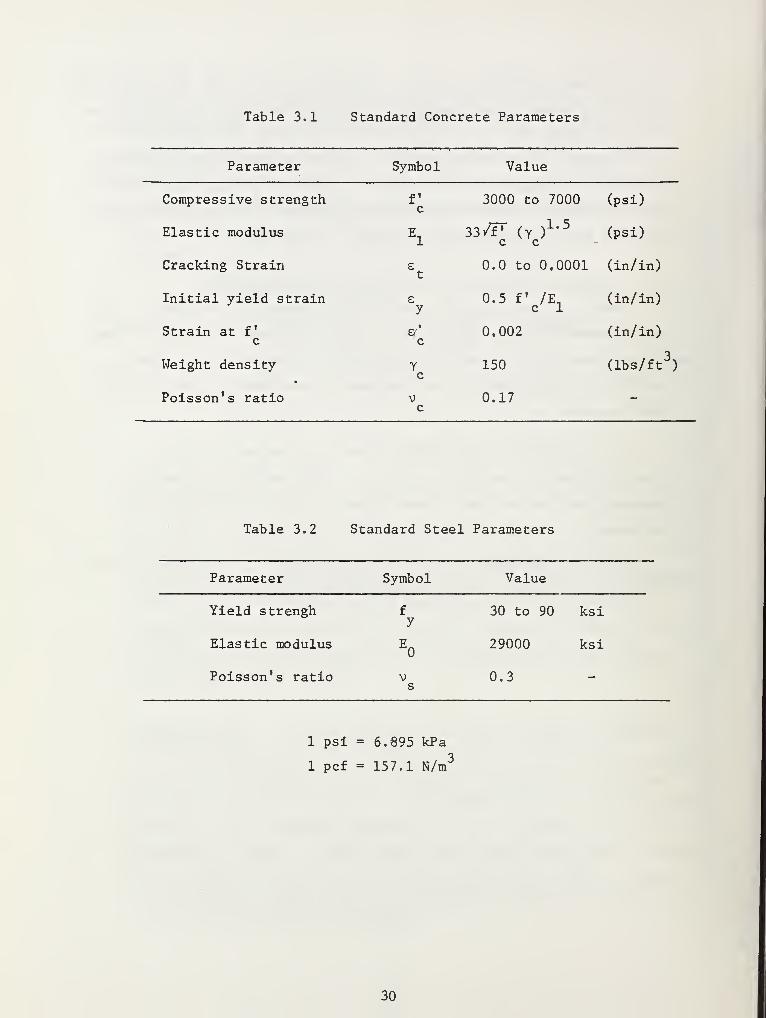
Table 3.1 Standard Concrete Parameters
Parameter Symbol Value
Compressive strength
Elastic modulus
Cracking Strain
Initial yield strain
Strain at fc
Weight density
Poisson's ratio
fc
3000 to 7000 (psi)
33/F (y )1,5
(psi)c c
0,0 to 0,0001 (in/in)
0.5 f /E,c 1
(in/ in)
0,002 (in/in)
150 (lbs/ft3)
0.17 _
Table 3.2 Standard Steel Parameters
Parameter Symbol Value
Yield strengh
Elastic modulus
Poisson's ratio
30 to 90 ksi
29000 ksi
0.3 _
1 psi = 6.895 kPa
1 pcf = 157.1 N/m~
30
CHAPTER 4
EVALUATION OF REINFORCED CONCRETE MODEL
FOR CIRCULAR PIPE LOADED IN THREE-EDGE BEARING
In this chapter the validity of the reinforced concrete model
(presented in the previous chapter) is examined by comparing results
with experimental data for circular pipe tested out-of-ground in three
edge bearing, i.e., the so-called D-load test (ASTM C497-65T), The
objective is to determine if the model can reasonably predict load-
deflection histories, the load at which 0.01 inch (0.254 cm) crackwidths
occur, and ultimate load.
4.1 PRELIMINARY INVESTIGATIONS
Prior to comparing the model performance with circular pipe test
data, a preliminary study was undertaken for staticrlly determinate,
reinforced concrete beams with transverse loading and combined trans-
verse with axial loading. The purpose of this preliminary study was
to investigate the sensitivity of modeling parameters and to compare
the model predictions with published experimental beam data (8,9) and
conventional ultimate strength theories (4,5). Major findings from
the preliminary study are listed below, additional detail is reported
in Reference (6)
.
1. For all the beams studied, including both single and double
reinforcement, the predicted ultimate moment capacity for
transverse loading agreed within 1% to those computed in
accordance with ACI 318-77.
2. Predicted load-deflection curves through ultimate were in
close agreement with experimental data (8) obtained from
two point loading of simply supported, rectangular beams
with approximately 1.7% tension steel reinforcement.
31
3. In the presence of axial thrust loads, the predicted ultimate
moment capacity was in good agreement with experimental data
(9), wherein the ultimate moment capacity initially is in-
creased as the axial thrust increased up to the balance
point on the ultimate moment-thrust interaction diagram.
Thereafter, the moment capacity steadily decreased to zero
as thrust was increased to ultimate.
4. As expected, the predictions for ultimate thrust-moment
capacity were not influenced by the model input parameters
e , e , and e' which describe the concrete stress-straint y c
curve up to compressive strength. Only the strength para-
meters for concrete and steel (f ' and f ) influenced ultimatec y
capacity. However, the load-deflection path to ultimate is
influenced by e , e , and e1 and the initial elastic moduliJ
t' y* c
values for steel and concrete,
5. The concrete cracking strain parameter e was found to have
a significant effect on the load-deformation curves for
lightly reinforced beams (typical for culvert cross-sections).
As the parameter e decreases over a practical range (0.0001
to 0.0) the effective stiffness decreases resulting in
greater deformations for the same load.
6. The compressive concrete strain parameters, e , and e', also
influence the shape of the load-deformation curves, but to
a lesser extent than e . As e is decreased over the ranget y
0.0008 to 0.0003 the deformations slightly increase. Con-
versely, as e' is decreased over the range 0.0025 to 0.0015c
deformations decrease.
These preliminary studies demonstrated that the reinforced concrete
model was working properly and provided insights for modeling and
interpreting results for the circular pipes in three-edge bearing dis-
cussed next.
32
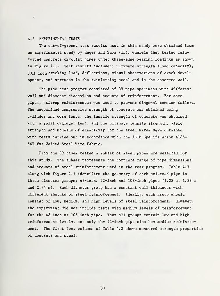
4.2 EXPERIMENTAL TESTS
The out-of-ground test results used in this study were obtained from
an experimental study by Heger and Saba (15), wherein they tested rein-
forced concrete circular pipes under three-edge bearing loadings as shown
in Figure 4.1. Test results included; ultimate strength (load capacity),
0.01 inch cracking l:>ad, deflections, visual observations of crack devel-
opment, and stresses; in the reinforcing steel and in the concrete wall.
The pipe test program consisted of 39 pipe specimens with different
wall and diameter dimensions and amounts of reinforcement. For some
pipes, stirrup reinforcement was used to prevent diagonal tension failure.
The unconfined compressive strength of concrete was obtained using
cylinder and core tests, the tensile strength of concrete was obtained
with a split cylinder test, and the ultimate tensile strength, yield
strength and modulus of elasticity for the steel wires were obtained
with tests carried out in accordance with the ASTM Specification A185-
56T for Welded Steel Wire Fabric.
From the 39 pipes tested a subset of seven pipes are selected for
this study. The subset represents the complete range of pipe dimensions
and amounts of steel reiinforcement used in the test program. Table 4.1
along with Figure 4.1 identifies the geometry of each selected pipe in
three diameter groups; 48-inch, 72-inch and 108-inch pipes (1.22 m, 1.83 m
and 2.74 m) . Each dianeter group has a constant wall thickness with
different amounts of steel reinforcement. Ideally, each group should
consist of low, medium, and high levels of steel reinforcement. However,
the experiment did not include tests with medium levels of reinforcement
for the 43-inch or 108-inch pipe. Thus all groups contain low and high
reinforcement levels, but only the 72-inch pipe also has medium reinforce-
ment. The first four columns of Table 4.2 shows measured strength properties
of concrete and steel.
33
Load P
!
Oi
//
~1\\
P/2t fP/2
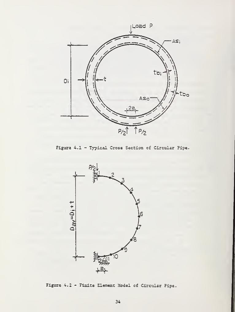
Figure 4.1 - Typical Cross Section of Circular Pipe.
QI!
>IT3
Q
Figure 4.2 - Finite Element Model of Circular Pise,
34

TABLE 4.1 - Geometric Characteristics of the Analyzed
Pipes to Compare Test and CANDE Results
Pipes Di ti Asi Aso tbi tbo a
(in) (in) (in2/in) (in 2 /in) (in) (in) (in)
J 48 5 .01683(L) . 01233 (L) 1.10 1.09 2
K 48 5 .02708(H) .01992(H) 1.13 1.11 2
B 72 7 . 03142 (L) . 02342 (L) 1.14 1.12 3
*G 72 7 . 05158 (M) . 03692 (M) 1.18 1.15 3
D 72 7 .07292(H) .05158(H) 1.21 1.18 3
*Q 108 9 .05158(L) . 04000 (L) 1.18 1.16 4.5
p 108 9 .10317(H) .07383(H) 1.18 1.15 4.5
They have stirrup reinforcement
1 in = 2.54 cm
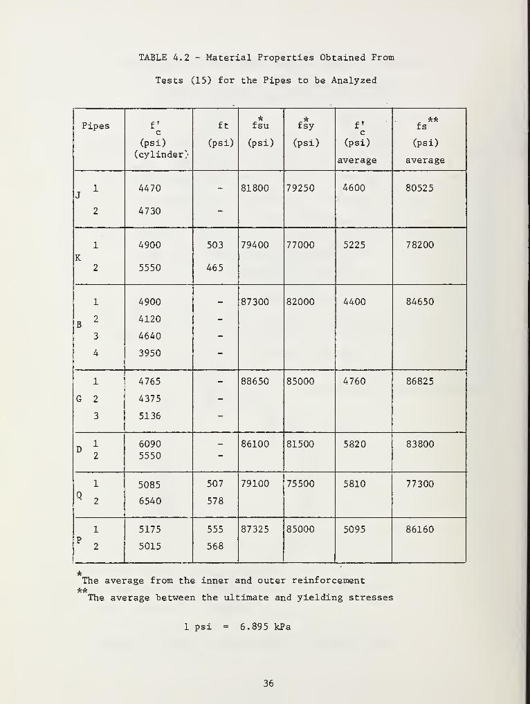
TABLE 4.2 - Material Properties Obtained From
Tests (15) for the Pipes to be Analyzed
Pipes fc
ft*
fsu fsy Vc
k*fs
(psi) (psi) (psi) (psi) (psi) (psi)
(cylinder)average average
1J
4470 - 81800 79250 4600 80525
2 4730 -
1 4900 503 79400 77000 5225 78200
K2 5550 465
1 4900 - 87300 82000 4400 84650
B2 4120 -
3 4640 -
4 3950 -
1 4765 - 88650 85000 4760 86825
G 2 4375 -
3 5136 -
' \
6090 — 86100 81500 5820 838005550 —
1 5085 507 79100 75500 5810 77300
Q2 6540 578
1 5175 555 87325 85000 5095 86160P
2 5015 568
The average from the inner and outer reinforcement**
The average between the ultimate and yielding stresses
1 psi = 6.895 kPa
36
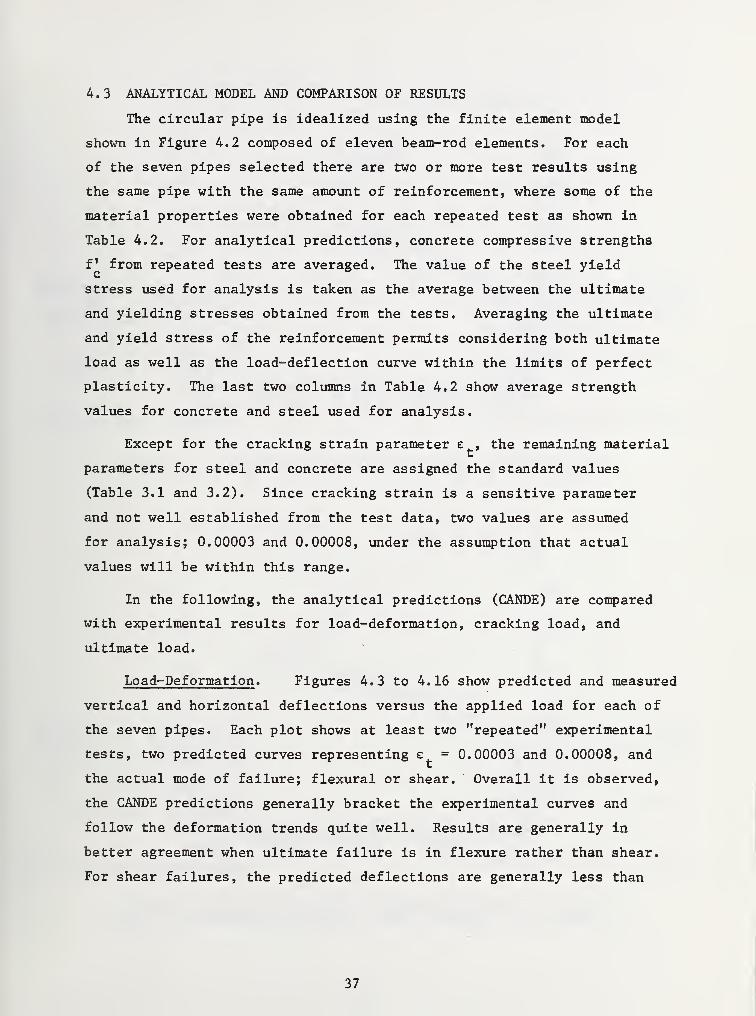
4.3 ANALYTICAL MODEL AND COMPARISON OF RESULTS
The circular pipe is idealized using the finite element model
shown in Figure 4.2 composed of eleven beam-rod elements. For each
of the seven pipes selected there are two or more test results using
the same pipe with the same amount of reinforcement, where some of the
material properties were obtained for each repeated test as shown in
Table 4.2. For analytical predictions, concrete compressive strengths
f from repeated tests are averaged. The value of the steel yield
stress used for analysis is taken as the average between the ultimate
and yielding stresses obtained from the tests. Averaging the ultimate
and yield stress of the reinforcement permits considering both ultimate
load as well as the load-deflection curve within the limits of perfect
plasticity. The last two columns in Table 4.2 show average strength
values for concrete and steel used for analysis.
Except for the cracking strain parameter e , the remaining material
parameters for steel and concrete are assigned the standard values
(Table 3.1 and 3.2). Since cracking strain is a sensitive parameter
and not well established from the test data, two values are assumed
for analysis; 0.00003 and 0.00008, under the assumption that actual
values will be within this range.
In the following, the analytical predictions (CANDE) are compared
with experimental results for load-deformation, cracking load, and
ultimate load.
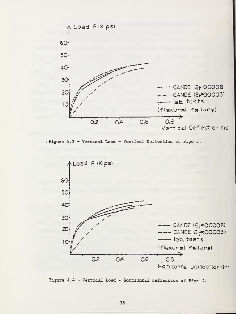
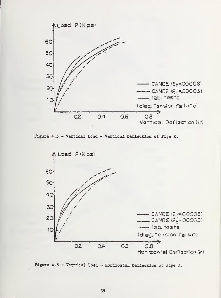
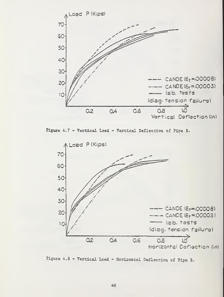
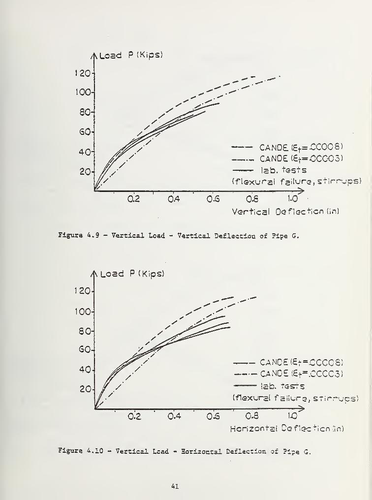
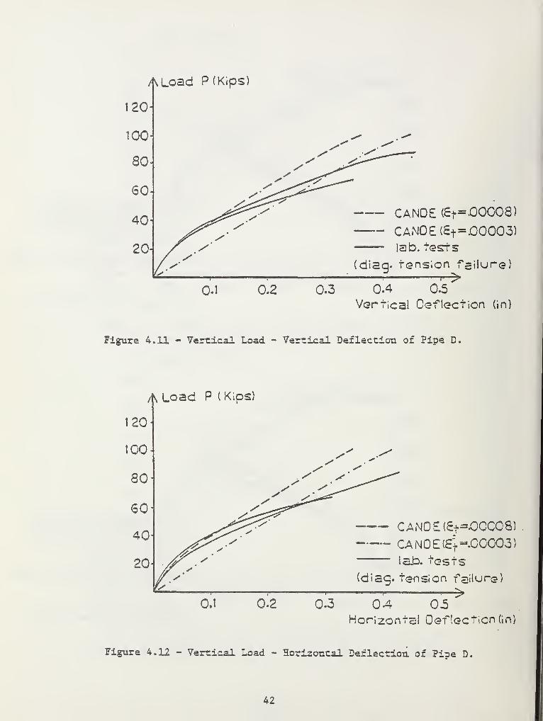
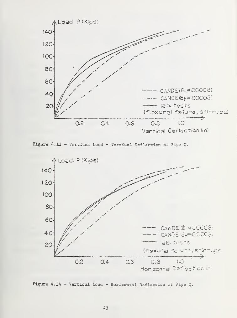
Load-Deformation . Figures 4.3 to 4.16 show predicted and measured
vertical and horizontal deflections versus the applied load for each of
the seven pipes. Each plot shows at least two "repeated" experimental
tests, two predicted curves representing e = 0.00003 and 0.00008, and
the actual mode of failure; flexural or shear. Overall it is observed,
the CANDE predictions generally bracket the experimental curves and
follow the deformation trends quite well. Results are generally in
better agreement when ultimate failure is in flexure rather than shear.
For shear failures, the predicted deflections are generally less than
37
A Load P (Kips)
GO-
CANOE (5^.00008)
• CANOE (Et=;00003)
sb. tests
(flexural failure)
0.8
Vertical Oeflection (in)
Figure 4.3 - Vertical Load - Vertical Deflection of Pipe J.
A Load P (Kips)
CANOE (£ t=.0000S)
CANOE (8t=.00003)
lab, tests
^——
^
0.2
(ftexural failure)
0.4 0.S 0.8
Horizontal Deflection (in)
Figure 4.4 - Vertical Load - Horizontal Deflection of Pipe J.
38
A Load P(Kips)
02 QA 0.6
CANOE (6f».C0008)
CANOE (E t-00003)
. lab. tests
(diag. tension failure)
0-8
Vortical Oeflection (in)
Figure 4.5 - Vertical Load - Vertical Deflection of Pipe K.
A Load P (Kips)
60-
50-
40'
30
20
10
CANOE (6 t=.CCC08)CANOE (S+-.00C03
)
lab. tests
(diag. tension failure)
OjSm
OSHorizontal Deflection (in)
Figure 4.6 - Vertical Load - Horizontal Deflection of Pipe Z.
39
a Load P (Kips)
0.2
CAN0£(6t = «00OO8)
CAN0E(8t=.0O0O3)ab. tests
(diag- tension failure)
o,4 as as 10
Vertical Deflection (in)
Figure 4,7 - Vertical Load - Vertical Deflection of Pipe B.
A Load P (Kips
- CANOE (5t=.00C03)- CANOE (6t =.00003)
ib. tests(diag. tension failure)
0.8 1.0
Horizontal Deflection (in)
Figure 4.8 - Vertical Load - Horizontal Deflection of Pise 3.
40
A Load P (Kips
0.2n r-
0.4
CAN0E(£t=-C'COOS)
CAN0£(£t=OCC0o)lab. tests
(flexural failure, stirrups:
QJS 0-S 1-0
Vertical (Deflection (in:
Figure 4.9 - Vertical Load - Vertical Deflection of Pipe G.
A Load P (Kios)
CANOE (Sr-CCC0S)CANOE (8t
= CCCCo)
lab. tests
(flexurai failure, STirrucs)
o.a o.4 o.s o-Q io"
Horizontal Ce flection (in]
Figure 4.10 - Vertical Lead - Horizontal Deflection of Pipe G.
41
A Load P(Kips)
120-
— CANDE (£t=-00008)— CANOE (Et=.00003)
ab. tests
(diag. tension failure)
0.1 0.2 0.3 0.4 0.5
Vertical Oeflection (in)
Figure 4.11 - Vertical Load - Vertical Deflection of Pipe D.
A Load P ( Kips)
0.1 0.2 0.3
CANOE (6f=00008)
CA NO E(8"t =.00003)
lab. tests
(diac;. tension failure)
OA 05Horizontal Oeflection (in)
Figure 4.12 - Vertical Load - Horizontal Deflection of Pipe D.
42
A Load P (Kips)
140-
120-
CANOE (£ t=.OOCCS)
CANDE(£t=-00003)
ab. tests(flexural failure, stirrups)—
>
i-o
Vertical Deflection (in)
Figure 4.13 - Vertical Load - Vertical Deflection of Pipe Q.
^ Load- P (Kips)
140
CANOE (£f=CCCCS)CANOE S-^CCCCc)
ab. Tesrs
(flexural failure, stirrucs;
0.S 0.8 1.0
Horizcntal C2fec~.cn [in!
Figure 4.14 - Vertical Load - Horizontal Deflection of ?ioe Q.
43
160
140
120
100
80
SO
40
20
A Load P (Kips)
CANO£(Et=.00008)
CANOE (6t=O0003)lab. tests
0.2 04
(diacj. tension failure)—>0.6 0.8
Vertical Oeflection (in)
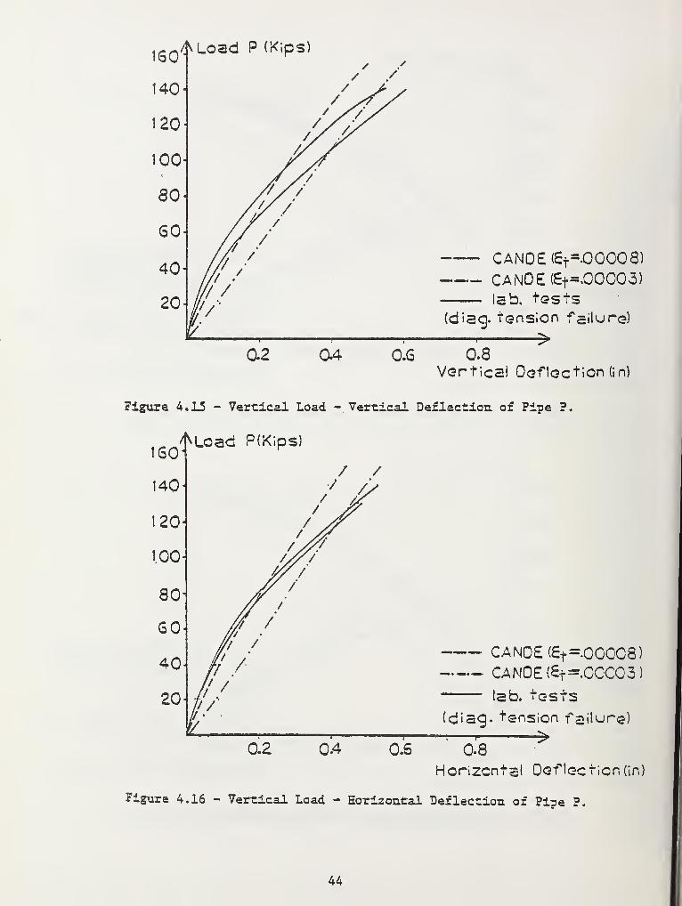
Figure 4.15 - Vertical Load -Vertical Deflection, of Pipe P.
<^Load P(Kips)
0.2 0.4
CANOE (£t--000C8)CANOE (Ef=0CC03)
lab. tests
(diag. tension failure)—i : ' >0.6 0-8
Horizontal Oeflection (in)
Figure 4.16 - Vertical Load - Horizontal Deflection of Pipe P.
44
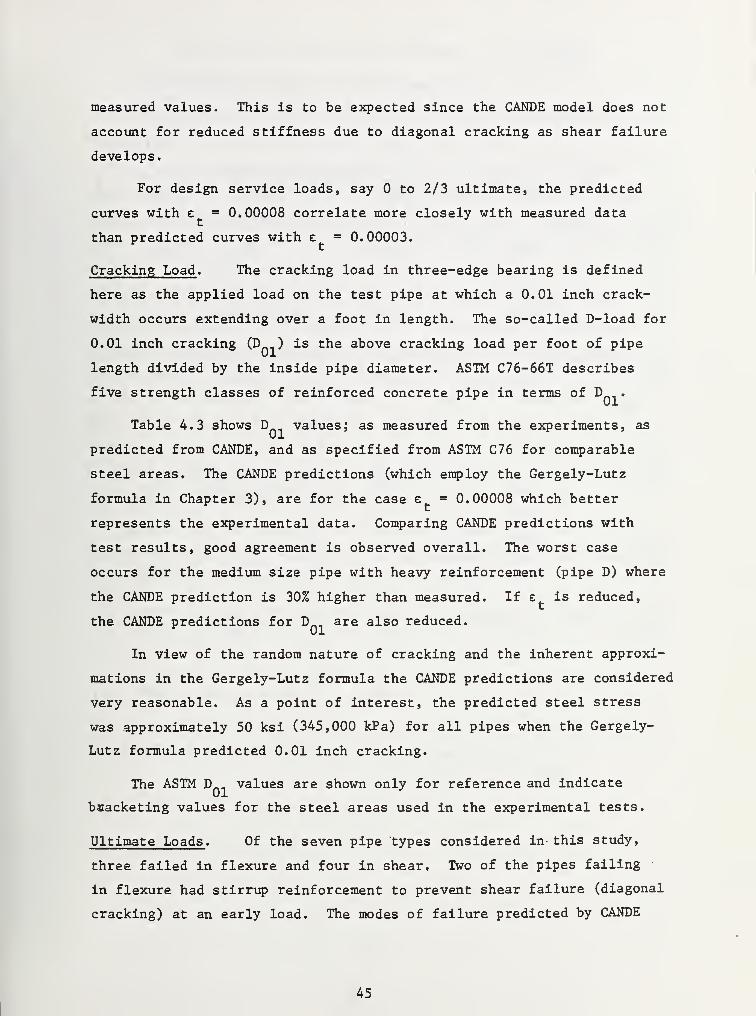
measured values. This is to be expected since the CANDE model does not
account for reduced stiffness due to diagonal cracking as shear failure
develops.
For design service loads, say to 2/3 ultimate, the predicted
curves with e = 0,00008 correlate more closely with measured data
than predicted curves with e = 0.00003.
Cracking Load . The cracking load in three-edge bearing is defined
here as the applied load on the test pipe at which a 0.01 inch crack-
width occurs extending over a foot in length. The so-called D-load for
0.01 inch cracking (Dm ) is the above cracking load per foot of pipe
length divided by the inside pipe diameter. ASTM C76-66T describes
five strength classes of reinforced concrete pipe in terms of D .
Table 4.3 shows D values; as measured from the experiments, as
predicted from CANDE, and as specified from ASTM C76 for comparable
steel areas. The CANDE predictions (which employ the Gergely-Lutz
formula in Chapter 3), are for the case e = 0.00008 which better
represents the experimental data. Comparing CANDE predictions with
test results, good agreement is observed overall. The worst case
occurs for the medium size pipe with heavy reinforcement (pipe D) where
the CANDE prediction is 30% higher than measured. If e is reduced,
the CANDE predictions for D are also reduced.
In view of the random nature of cracking and the inherent approxi-
mations in the Gergely-Lutz formula the CANDE predictions are considered
very reasonable. As a point of interest, the predicted steel stress
was approximately 50 ksi (345,000 kPa) for all pipes when the Gergely-
Lutz formula predicted 0.01 inch cracking.
The ASTM D_. values are shown only for reference and indicate
bracketing values for the steel areas used in the experimental tests.
Ultimate Loads . Of the seven pipe types considered in- this study,
three failed in flexure and four in shear. Two of the pipes failing
in flexure had stirrup reinforcement to prevent shear failure (diagonal
cracking) at an early load. The modes of failure predicted by CANDE
45
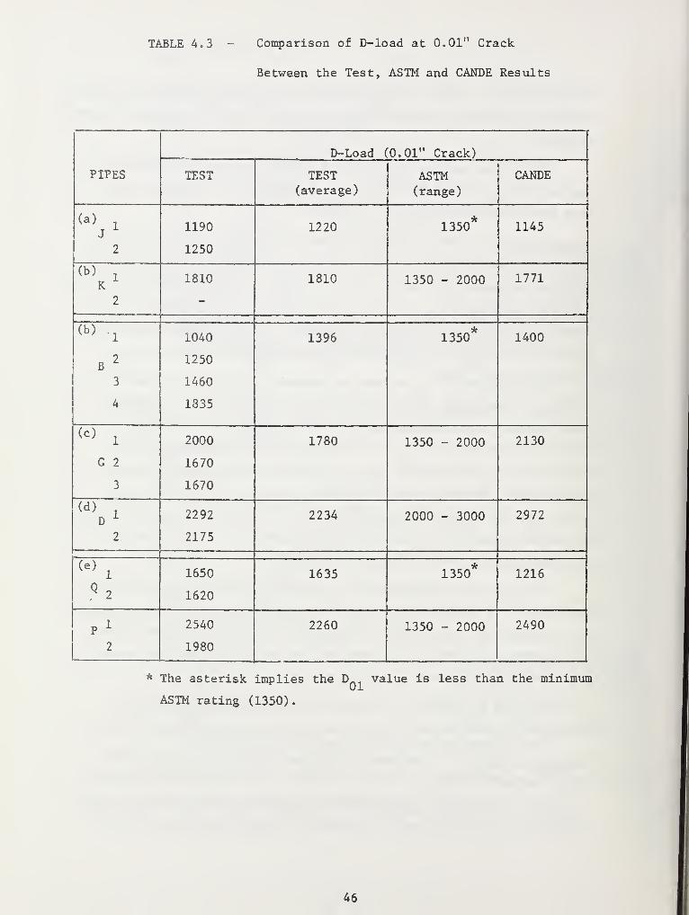
TABLE 4.3 - Comparison of D-load at 0.01" Crack
Between the Test, ASTM and CANDE Results
PIPES
D-Load (0.01" Crack)
TEST TEST(average)
ASTM(range)
CANDE
(a)
J
2
1190
1250
1220 1350* 1145
(b) .
K1
2
1810 1810 1350 - 2000 1771
(b)x
B2
3
4
1040
1250
1460
1835
1396 1350* 1400
(c)x
G 2
3
2000
1670
1670
1780 1350 - 2000 2130
(d)
Di
2
2292
2175
2234 2000 - 3000 2972
(e)
Q2
1650
1620
1635 1350* 1216
Pl
2
2540
1980
2260 1350 - 2000 2490
* The asterisk implies the D value is less than the minimum
ASTM rating (1350).
46
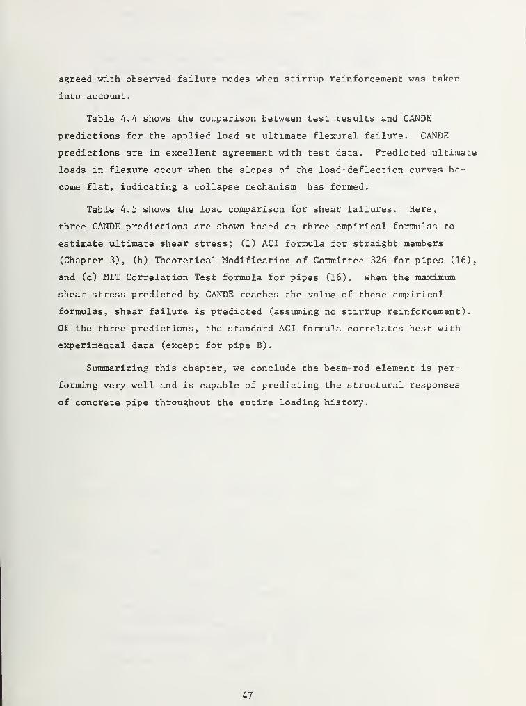
agreed with observed failure modes when stirrup reinforcement was taken
into account.
Table 4.4 shows the comparison between test results and CANDE
predictions for the applied load at ultimate flexural failure. CANDE
predictions are in excellent agreement with test data. Predicted ultimate
loads in flexure occur when the slopes of the load-deflection curves be-
come flat, indicating a collapse mechanism has formed.
Table 4.5 shows the load comparison for shear failures. Here,
three CANDE predictions are shown based on three empirical formulas to
estimate ultimate shear stress; (1) ACI formula for straight members
(Chapter 3), (b) Theoretical Modification of Committee 326 for pipes (16),
and (c) MIT Correlation Test formula for pipes (16), When the maximum
shear stress predicted by CANDE reaches the value of these empirical
formulas, shear failure is predicted (assuming no stirrup reinforcement).
Of the three predictions, the standard ACI formula correlates best with
experimental data (except for pipe B).
Summarizing this chapter, we conclude the beam-rod element is per-
forming very well and is capable of predicting the structural responses
of concrete pipe throughout the entire loading history.
47
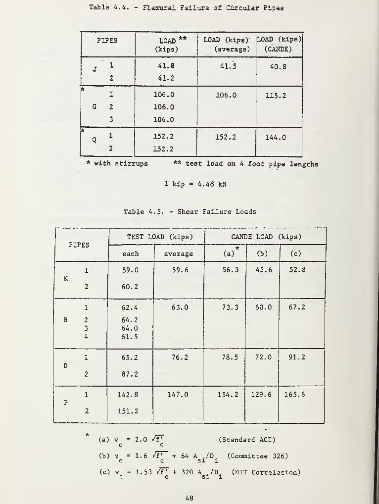
Table 4.4. - Flexural Failure of Circular Pipes
PIPES LOAD**
(kips)
LOAD (kips)
(average)
LOAD (kips)
(CANDE)~
Jl
2
41.6
41.2
41.5 40.8
1
G 2
3
106.0
106.0
106.0
106.0 115.2
k
QX
2
152.2
152.2
152.2 144.0
* with stirrups ** test load on 4 foot pipe lengths
1 kip = 4.48 kN
Table 4.5. - Shear Failure Loads
PIPESTEST LOAD (kips) CANDE LOAD (kips)
each average*
(a) (b) (c)
1
K2
59.0
60.2
59.6 56.3 45.6 52.8
1
B 2
3
4
62.4
64.264.061.5
63.0 73.3 60.0 67.2
D
2
65.2
87.2
76.2 78.5 72.0 91.2
1
P
2
142.8
151.2
147.0 154.2 129.6 165.6
(a) v = 2.0 TVc
(Standard ACI)
(b) V = 1.6 TV + 64 A ,/D. (Committee 326)c c si 1
(c) v - 1.53 JV + 320 A ./D. (MIT Correlation)C C SI 1
48
CHAPTER 5
EVALUATION OF REINFORCED CONCRETE MODEL FOR
BOX CULVERTS LOADED IN FOUR-EDGE BEARING
• Like the previous chapter, this -chapter continues to examine the
validity of CANDE's reinforced concrete, beam-rod element. Here, we
compare CANDE results with experimental data for box culverts tested in
four-edge bearing. The results to be compared include the load for
0.01 inch cracking and ultimate load. The experimental data did not
include load-deformation histories, consequently these cannot be com-
pared. For reference, the comparisons also include the SGH analytical
predictions (12) based on an elastic analysis discussed in Chapter 2.
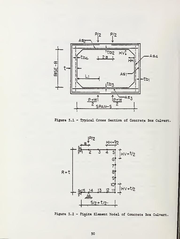
5.1 EXPERIMENTAL TEST
The experimental results used for the comparison belong to a test
program (13,14) where out-of-ground reinforced concrete box culverts
with welded wire fabric were loaded up to failure. The loading was
applied as shown in Figure 5,1 using a 4-edge bearing testing apparatus.
The material properties of concrete were determined using cylinder tests
and core tests for each kind of box, and the mechanical properties of
the reinforcement were determined by tensile tests (19). Three span
sizes of box were tested, small, medium and large with three levels of
reinforcement in each size, low, medium and high. Thus, nine types of
boxes were tested with two repeated tests per box type.
Tables 5.1 and 5.2 together with Figure 5.1 show the measured
geometries and material strengths for each test box where repeated boxes
are labelled A and B. Note that the core tests for f ' are generallyc
higher than cylinder tests for f and the ultimate steel stress is 10 to
20% higher than initial yield stress.
The test program was performed to verify the SGH analysis/design
method (12) which in turn was used to develop the ASTM standard designs
for reinforced concrete box culverts (21),
49
i
uCSL
t-
P/2 P/2
1tb2 HVt
LiASf
1*3
IK
t \
•AS4
--tbi
t fp-rAs3P+W2 2
Figure 5.1 - Typical Cross Section of Concrete Bos Culvert.
u a „
•f—ff2 HH+^
R+t
• • •rt 2 3 4 5
6
7t
8*
| Thv+s
9*
*d5 .14
J77777
>Vz
10" -t
13 12 it lHV+t£
1, S/? + t/2~t^ 1
Figure 5.2 - Finite Element Model of Concrete Box Culvert.
50
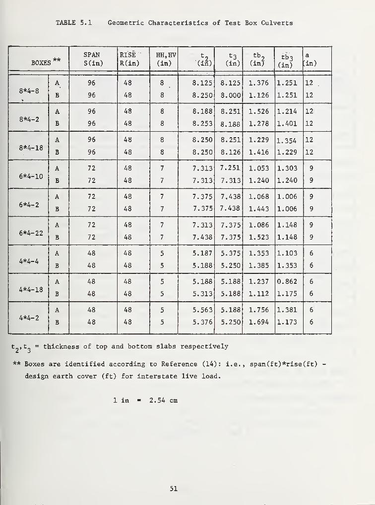
TABLE 5.1 Geometric Characteristics of Test Box Culverts
*•*BOXES
SPANS(in)
RISER(in)
HH,HV(in) (in)
t3
(in)
tb
(in?tt>3
(in)
a
:in)
8*4-8A
B
96
96
48
48
8
8
8.125
8.250
8.125
8.000
1.376
1.126
1.251
1.251
12
12
8*4-2A
B
96
96
48
48
8
8
8.188
8.253
8.251
8.188
1.526
1.278
1.214
1.401
12
12
8*4-18A
B
96
96
48
48
8
8
8.250
8.250
8.251
8.126
1.229
1.416
1.354
1.229
12
12
6*4-10A
B
72
72
48
48
7
7
7.313
7.313
7.251
7.313
1.053
1.240
1.303
1.240
9
9
6*4-2A
B
72
72
48
48
7
7
7.375
7.375
7.438
7.438
1.068
1.443
1.006
1.006
9
9
6*4-22A
B
72
72
48
48
7
7
7.313
7.438
7.375
7.375
1.086
1.523
1.148
1.148
9
9
4*4-4A
B
48
48
48
48
5
5
5.187
5.188
5.375
5.250
1.353
1.385
1.103
1.353
6
6
4*4-18A
B
48
48
48
48
5
5
5.188
5.313
5.188
5.188
1.237
1.112
0.862
1.175
6
6
4*4-2A
B
48
48
48
48
5
5
5.563
5.376
5.188
5.250
1.756
1.694
1.381
1.173
6
6
t 9> t_ = thickness of top and bottom slabs respectively
** Boxes are identified according to Reference (14): i.e., span(ft)*rise(ft)
design earth cover (ft) for interstate live load.
1 in = 2.54 cm
51
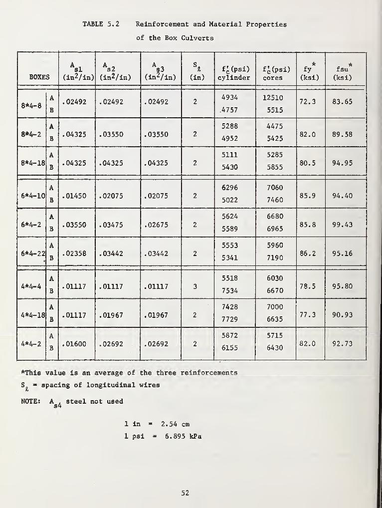
TABLE 5.2 Reinforcement and Material Properties
of the Box Culverts
BOXESsi
(in2/in)
As2
(in2/in)s3
(in2/in) (in)
fc (psi)
cylinderf c (psi)
cores
*fy
(ksi)
fsu
(ksi)
8*4-8A
B
.02492 .02492 .02492 24934
4757
12510
551572.3 83.65
8*4-2A
B.04325 .03550 .03550 2
5288
4952
4475
542582.0 89.58
8*4-18A
B.04325 .04325 .04325 2
5111
5430
5285
585580.5 94.95
6*4-10A
B.01450 .02075 .02075 2
6296
5022
7060
746085.9 94.40
6*4-2A
B.03550 .03475 .02675 2
5624
5589
6680
696585.8 99.43
6*4-22A
B.02358 .03442 .03442 2
5553
5341
5960
719086.2 95.16
4*4-4A
B.01117 .01117 .01117 3
5518
7534
6030
667078.5 95.80
4*4-18A
B.01117 .01967 .01967 2
7428
7729
7000
663577.3 90.93
4*4-2A
B.01600 .02692 .02692 2
5872
6155
5715
643082.0 92.73
*This value is an average of the three reinforcements
S = spacing of longitudinal wires
NOTE: A . steel not useds4
1 in = 2.54 cm
1 psi = 6.895 kPa
52
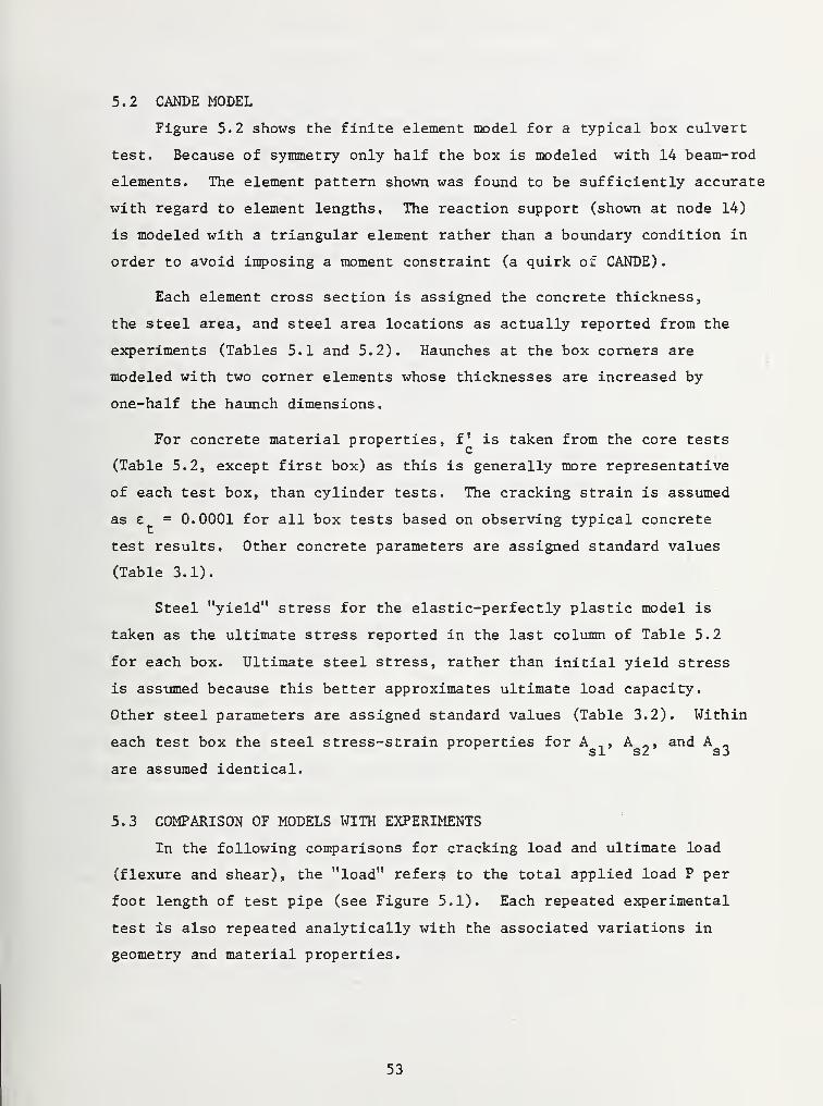
5.2 CANDE MODEL
Figure 5.2 shows the finite element model for a typical box culvert
test. Because of symmetry only half the box is modeled with 14 beam-rod
elements. The element pattern shown was found to be sufficiently accurate
with regard to element lengths. The reaction support (shown at node 14)
is modeled with a triangular element rather than a boundary condition in
order to avoid imposing a moment constraint (a quirk of CANDE)
.
Each element cross section is assigned the concrete thickness,
the steel area, and steel area locations as actually reported from the
experiments (Tables 5.1 and 5.2). Haunches at the box corners are
modeled with two corner elements whose thicknesses are increased by
one-half the haunch dimensions.
For concrete material properties, f* is taken from the core tests
(Table 5.2, except first box) as this is generally more representative
of each test box, than cylinder tests. The cracking strain is assumed
as e = 0.0001 for all box tests based on observing typical concrete
test results. Other concrete parameters are assigned standard values
(Table 3.1).
Steel "yield" stress for the elastic-perfectly plastic model is
taken as the ultimate stress reported in the last column of Table 5.2
for each box. Ultimate steel stress, rather than initial yield stress
is assumed because this better approximates ultimate load capacity.
Other steel parameters are assigned standard values (Table 3.2). Within
each test box the steel stress-strain properties for A ,, A _, and A „si sZ sj
are assumed identical.
5.3 COMPARISON OF MODELS WITH EXPERIMENTS
In the following comparisons for cracking load and ultimate load
(flexure and shear), the "load" refers to the total applied load P per
foot length of test pipe (see Figure 5.1). Each repeated experimental
test is also repeated analytically with the associated variations in
geometry and material properties.
53
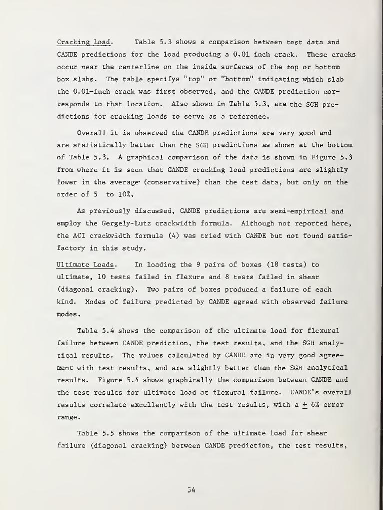
Cracking Load . Table 5.3 shows a comparison between test data and
CANDE predictions for the load producing a 0.01 inch crack. These cracks
occur near the centerline on the inside surfaces of the top or bottom
box slabs. The table specifys "top" or "bottom" indicating which slab
the 0.01-inch crack was first observed, and the CANDE prediction cor-
responds to that location. Also shown in Table 5.3, are the SGH pre-
dictions for cracking loads to serve as a reference.
Overall it is observed the CANDE predictions are very good and
are statistically better than the SGH predictions as shown at the bottom
of Table 5.3, A graphical comparison of the data is shown in Figure 5.3
from where it is seen that CANDE cracking load predictions are slightly
lower in the average* (conservative) than the test data, but only on the
order of 5 to 10%,
As previously discussed, CANDE predictions are semi-empirical and
employ the Gergely-Lutz crackwidth formula. Although not reported here,
the ACI crackwidth formula (4) was tried with CANDE but not found satis-
factory in this study.
Ultimate Loads . In loading the 9 pairs of boxes (18 tests) to
ultimate, 10 tests failed in flexure and 8 tests failed in shear
(diagonal cracking). Two pairs of boxes produced a failure of each
kind. Modes of failure predicted by CANDE agreed with observed failure
modes
.
Table 5.4 shows the comparison of the ultimate load for flexural
failure between CANDE prediction, the test results, and the SGH analy-
tical results. The values calculated by CANDE are in very good agree-
ment with test results, and are slightly better than the SGH analytical
results. Figure 5.4 shows graphically the comparison between CANDE and
the test results for ultimate load at flexural failure. CANDE' s overall
results correlate excellently with the test results, with a + 6% error
range.
Table 5.5 shows the comparison of the ultimate load for shear
failure (diagonal cracking) between CANDE prediction, the test results,
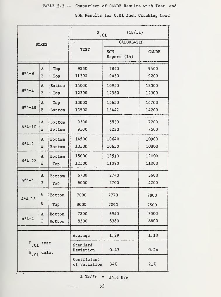
TABLE 5.3 — Comparison of CANDE Results with Test and
SGH Results for 0.01 inch Cracking Load
p. 01
(lb/f t)
BOXES
TEST
CALCULATED
SGHReport (14)
CANDE
8*4-8A
B
Top
Top
9250
11300
7840
9430
9400
9200
8*4-2A
B
Bottom
Top
14000
12300
10950
12360
12300
12300
8*4-18A
B
Top
Bottom
13000
13500
15650
13442
14700
14200
6*4-10A
B
Bottom
Bottom
9500
9500
5830
6220
7200
7500
6*4-2A
B
Bottom
Bottom
14500
10500
10640
10650
10900
10800
6*4-22A
B
Bottom
Top
15000
12500
12510
11090
12000
11000
4*4-4A
B
Bottom
Top
6700
6000
2740
2700
3600
4200
4*4-18A
B
Bottom
Top
7000
8000
7770
7090
7800
7500
4*4-2A
B
Bottom
Bottom
7800
8500
6940
8380
7500
8600
p.oi
test
Average 1.29 1.10
StandardDeviation 0.43 0.24
P m calc.. Ul
Coefficientof Variation 34% 21%
1 lb/ft = 14.6 N/m
55
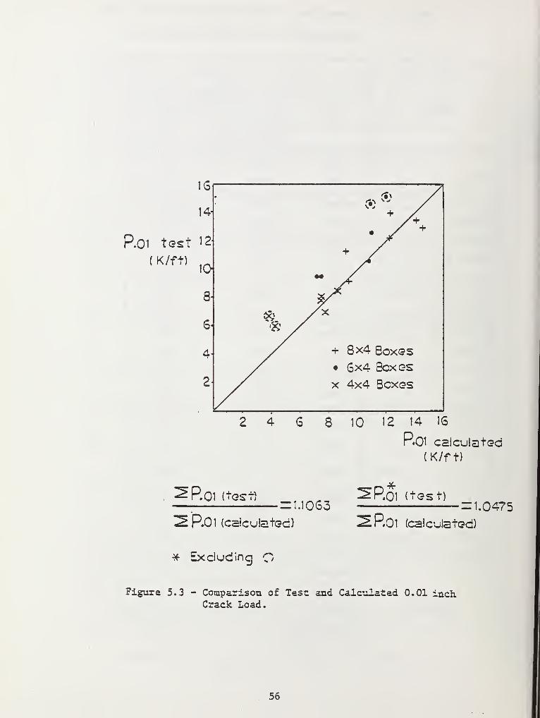
16
14
P.01 test 12
( K/ft)
+ 8x4 Boxes• 6x4 Boxes
x 4x4 Boxes
8 10 12 14 16
P.01 calculated
(K/ft)
P.01 (test)= 1.1063
P.01 (calculated)
Roi (test)
P.01 (calculated)
= 1.0475
* Excluding O
Figure 5.3 - Comparison of Test and Calculated 0.01 inchCrack Load.
56
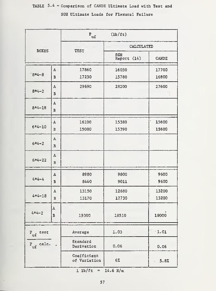
TABLE 5.4 - Comparison of CANDE Ultimate Load with Test and
SGH Ultimate Loads for Flexural Failure
BOXES
uf(lb/ft)
TESTCALCULATED
SGHReport (14) CANDE
' 8*4-8A
B
17860
17230
16050
15780
17700
16800
8*4-2A
B
29690 28200 27600
8*4-18A
B
6*4-10A
B
16100
15000
15380
15390
15600
15600
6*4-2A
B
6*4-22A
B
4*4-4A
B
8980
8440
9800
9011
9600
9600
4*4-18A
B
13150
13170
12680
12730
13200
13200
4*4-2A
B 19300 18510 18000
P _ testuf
•
Average 1.03 1,01
StandardDerivation 0.06 0.06
P calc.uf
Coefficientof Variation 6% . 5.8%
1 lb/ft 14.6 N/m
57
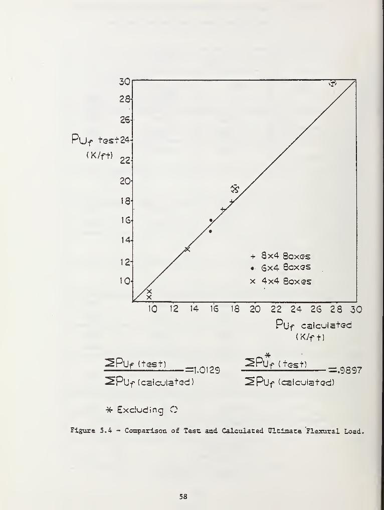
30
+ 8x4 Boxes•• 6x4 Soxes
x 4x4 Boxes
10 12 14 16 18 20 22 24 26 28 30
Pllf calculated
(K/f t)
^PUf (test)
2PUf (calculated)
1.0129:P0f (test:
=.9897
'PUf (calculated)
4fr Excluding
Figure 5.4 - Comparison of Test and Calculated Ultimata Flexural Load.
58
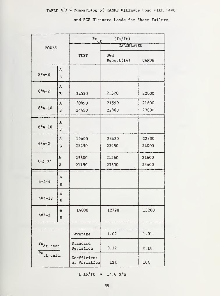
TABLE 5.5 - Comparison of CANDE Ultimate Load with Test
and SGH Ultimate Loads for Shear Failure
Pudt
(lb/ft)
BOXES
TEST
CALCULATED
SGHReport (14) CANDE
8*4-8A
B
8*4-2A
B 22520 21520 22000
8*4-18A
B
20890
24490
21590
22860
21600
23000
6*4-10A
B
6*4-2A
B
19400
25250
23420
23950
22800
24000
6*4-22A
B
25'680
21150
21260
23530
21600
23400
4*4-4A
B
4*4-18A
B
4*4-2A
B
14080 12790 13200
Pu,dt test
Average 1.02 1.01
StandardDeviation 0.12 0.10
p.
,
dt calc.Coefficientof Variation 12% 10%
1 lb/ft = 14.6 N/m
59
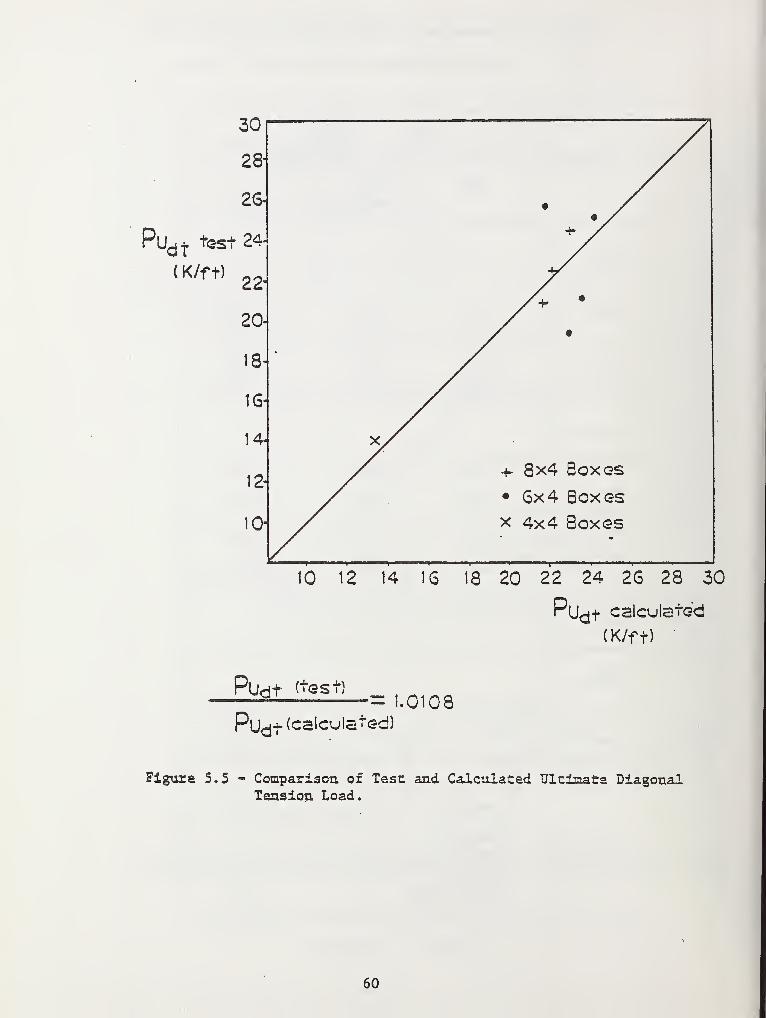
30
28-
26-
Pudt test 24-+» /
(K/ft)22.
20-
18-
16-
14- x/
12--h 8x4 Boxes• 6x4 Boxgs
10- x 4x4 Boxes
10 12 8 20 22 24 26 28 30
PlU+ calculated'dt
(K/ff)
Pbdt ^est)
Pu^t (calculated)
•= 1.0108
Figure 5.5 - Comparison of Test and Calculated Ultimate DiagonalTension Load.
60
and the SGH analytical results. The values obtained from CANDE are
assuming that the maximum shear stress resisted by the concrete is
2.0 / f f. Once again the values obtained from CANDE are very close to
c
the test results and are a better prediction than the analytical results
of SGH. The test results are compared graphically with CANDE results
in Figure 5.5, from where we can observe that the amount of error from
CANDE is in the range of + 10%, a very good correlation for practical
purposes.
The performance of the beam-rod element used in the CANDE program
to model reinforced concrete box culverts has been shown to perform
very well in out-of-ground loading. Subsequent studies will consider
the box culvert buried, subjected to soil loads as well as live loads.
The empirical formulas for crack prediction and shear resistance used
in CANDE will be the same ones used in this chapter, where their per-
formance was found satisfactory.
61
CHAPTER 6
DEVELOPMENT OF LEVEL 2 BOX MESH
The reinforced concrete box culvert model is now considered for
its actual function as a conduit buried in soil. Accordingly, both the
soil and the box form the structural system, hereafter called box-soil
structure. The soil plays a dual role; on the beneficial side it adds
substantial stiffness to the box-soil structures, on the detrimental
side it transits gravity and applied loads to the box during the in-
stallation process.
To determine loads acting on the box requires a complete model of
the box-soil structure simulating the entire installation process. In
this chapter a general finite element model of the box-soil structure
is presented with the intent of developing an automated finite element
mesh subroutine suitable for simulating the vast majority of box-soil
installations encountered in practice. This is called the level 2 box
option of CANDE.
To develop an automated finite element mesh requires some limiting
assumptions and specifications of a variety of parameters describing
the box-soil system. Overall assumptions are symmetry about the ver-
tical centerline and plane strain geometry and loading. Adjustable
system parameters include; box dimensions (span and rise), soil boundary
dimensions (width from centerline, depth below box, and height of cover
above box), soil zones (in situ soil, fill soil, and bedding soil) and
installation type (embankment or trench). These parameters along with
the question of mesh refinement are discussed in the following.
6.1 PARAMETERS TO DEFINE THE MODELS
The depth and width of the entire soil zone are specified in
terms of the particular box dimensions being analyzed. The box culvert
62
is idealized with beam elements located along the middle line of the
walls, so the nominal box span used in our model is equal to the inside
span of the box plus its thickness. Likewise for the nominal rise of
the box. Defining Rl as half the nominal span and R2 as half the
nominal rise, as shown in Figure 6.1, the soil depth below the box is
set at 3R2, and the soil width is set at 4R1 from the box sides. These
soil boundaries are adjudged to be outside the zone of soil-structure
interaction based on previous studies (1).
The height of cover (see Figure 6.1) is an input parameter denoting
the final fill height above the box. However, the height of the mesh
over the top of the box is limited to 3R2 or the specified height of
soil cover, whichever is less. For cover heights greater than 3R2
equivalent loading is used as discussed subsequently.
Other geometry parameters that need to be defined are the trench
depth and trench width as shown in Figure 6.1. If the mesh model is
intended to represent an embankment installation, the trench width is
4R1 so that only fill soil exists on the sides and in situ soil is
leveled with bottom of the box.
The material zones are in situ soil, bedding and fill soil, where
each zone can be assigned the same or different soil mechanical pro-
perties. In addition to Rl and R2, the box culvert geometry is defined
with the side, bottom and top slabs thicknesses, and haunch dimensions
as shown in Figure 6.2. The amount of steel reinforcement around the
box is defined by steel areas A , A , A and A along with a common
cover thickness as shown in Figure 6.3.
So far only the parameters of the box-soil systems and the general
dimensions have been discussed, nothing has been said about the finite
element mesh itself or the sequence of loading. The example shown in
Figure 6.4 will be used to explain the mesh arrangement. All the di-
mensions and height of soil cover are shown. A trench configuration
is used with three zones of soil for the system. The values of Rl and
R2 give the overall size of the mesh as previously discussed (see
63
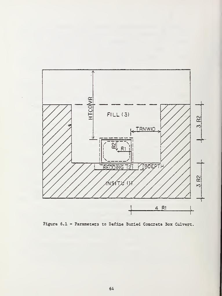
A
CMcr
00
4 R1
Figure 6.1 - Parameters to Define Buried Concrete Box Culvert.
64
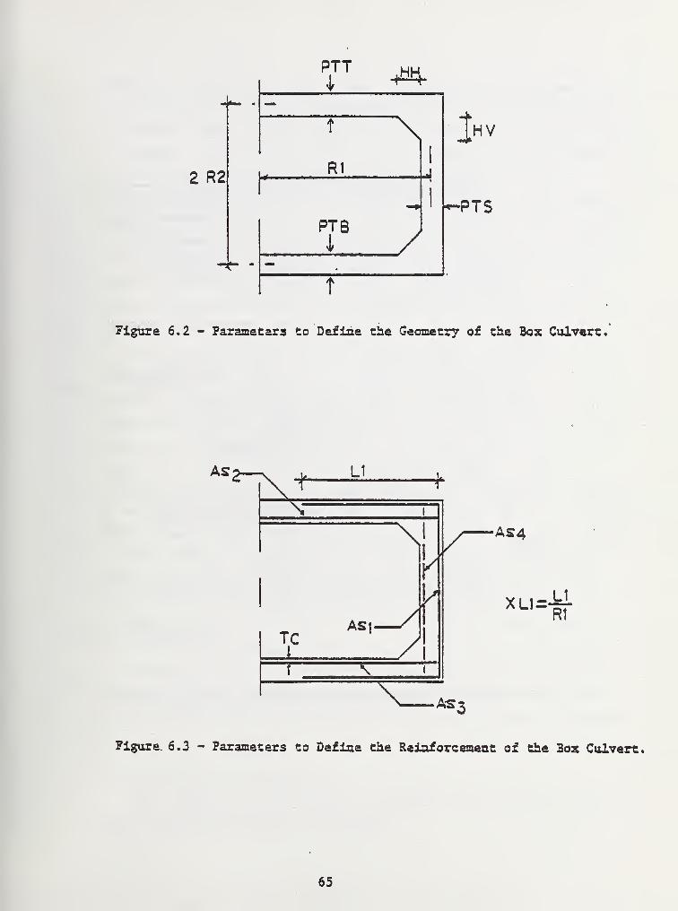
Z R2
i-
-* ' *-PTS
Figure 6.2 - Parameters to Define the Geometry of the Bos Culvert,
AS4
XL1--kLXU"R1
Figure. 6.3 - Parameters to Define the Reinforcement of the Box Culvert.
65
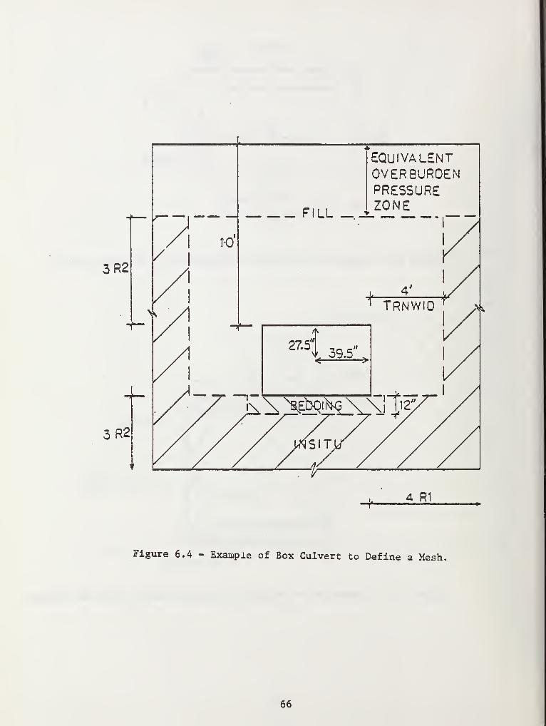
3R2
3R2
4 R1
Figure 6.4 - Example of Box Culvert to Define a Mesh.
66
Figure 6.1). The finite element mesh configuration for the example is
shown in Figure 6.5, where by symmetry only half of the box-soil system
is modeled. The same figure shows the soil elements and the nodal points
of the mesh. The number of layers of soil elements on top of the box
can decrease if the height cover of soil is less than 3R2, but will
never be less than two rows. The soil elements near the box are smaller,
so that a more refined mesh around the box can provide a better behavior
of the box-soil model where the stress gradients are known to be highest.
The soil elements are four node, nonconforming quadrilaterals with ex-
cellent performance characteristics (1). The coordinates of the nodes
are all related to Rl and R2 and, if desired, can be changed using the
extended level 2 option (see Appendix B).
The loading sequence, called incremental construction (1,2), simu-
lates the actual installation process of placing soil layers in a series
of lifts. Figure 6.6 shows the construction increment numbers of element
groups entering sequentially into the system. The initial system (first
construction increment) includes all in situ soil, bedding, and the box
loaded with its own body weight. Subsequent increments, numbers 2
through 9, are gravity loaded layers of fill soil. For specified heights
of soil cover less than 3R2, the mesh over the top of the box is assigned
proportionally less soil layers. If the height of soil cover is greater
than 3R2, the load due to the soil over 3R2 is applied as equivalent
overburden pressure increments. This load sequence is applied after
the ninth soil layer using n-9 additional load increments, where n is
the total number of construction increments specified in the input.
The box-soil mesh described here is generated automatically using
the CANBOX subroutine to generate all the necessary data required to
define the finite element mesh of the system. CANBOX subroutine para-
meters, options and mesh size are discussed with more detail in Appendix
B.
6.2 ASSUMPTIONS AND LIMITATIONS
When using this automatic mesh generation, there are some assump-
tions involved that should be remembered.
67
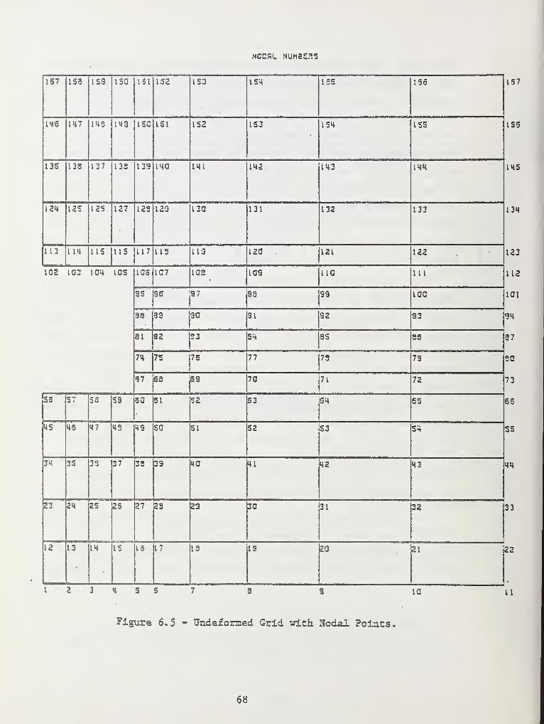
MOCfiL MUM3£?.S
137
146
1S3
147
159 150 I SI 152
143 143 ISC iSl
153
152
154
153
ISS
1S4
155
ISS
135 135 137 133
124 1 25
113 114
125
113
139
127 123
140
129
141 142
130 131
115
102 103 104 105
So 57 S3 39
4S 46 47
117
108
113 113 120
107 103 109
gs 95
98 39
81 32
74
67
50
43 43
97 93
90 91
75 75
S4
77
63r
51 52
70
SO SI S2
143
132
121
110
99
92
35
73
71
S4
53
,44
133
122
111
100
93
36
79
72
S4
34 35 35 37 33 39 40 41 42 43
23 24 25
12
27 23 23
13 14 IS 15 17
30
13 13
12 3 4 3 5
31
20
32
21
10 11
Figure 6,5 - Underormed Grid with Nodal Points.
68
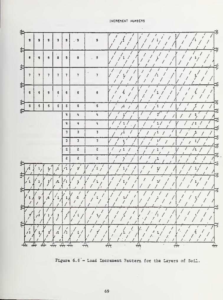
INCREMENT NUneERS
cfc
*
£-
/ / / / / / / / A / / ''
' / /7 //i
/ / /
/ /i / '
//
/ // /
r / // /
;
// / /
// V /
/ A
f 7/ < r—
/ / / // y / / / / /
/ / / /
/
/
' / > / /3
77// / /
/ /
/t /T" 1"
/'*
/ /l/ /'/ /!// / / /
• / / /
/ /t// / /
I7X7 'i '/ '/ / /
/
/ /'/
" / >' /
/ - i/ ' V / /i / /
/ / / ,
' / tx 7 /I/ /' / /' /," / a / * !/ /
;
3/ /
77^
//77177771777
/ / /
/ / i /r / / /
/
/ 7 1' / /
/^/*- /
r- d / / // /
/ / / / / 1
'7
/I
' 77 /1 ' 77777 77p?
/
1
*
*
/
r //
/1
/
/ // /t
/ / / V/ /
/ / // /
/
/ / V // A
/
/
/
/ /I
v/
T
/
^ / /
z1 L'U i/f A <
A ' , / /
V '
t
/>v;
/ / / A
y // ,
/ /
/ / //
-///// /
/L / ; /
//arv
/
$L
/
/
/
V J A/
/
/ /
/
/ / /.
/ /
/i /
/ /7 / /
/ / / / /
T-T-T-)
/ / / /
t/
/ / 7
47 -7T"rrr
/l
/I
/•/ / / // / /
Y / /
/ / /
/ / / /1/ / : / /
"7T
/• / / / /
/ / / / /
^T 7T/ / / /
Figure 6.6 - Load Increment: Pattern for the Layers of Soil.
69
a) To simplify the mesh, we are assuming symmetry about the
vertical axis so only half of the box-soil system is analyzed. This
assumption implies that only symmetric loading can be applied to the
box when using concentrated loads on top of the mesh. For most of
the cases a symmetric loading arrangement satisfies the loading cond-
ditions
.
b) Three different zones of soil can be specified within the
soil mesh; fill soil, bedding soil, and in situ soil.
c) When a trench condition is specified, the in situ soil
forming the trench extrados goes all the way up to the top of the
mesh, whereas for the embankment condition, the in situ soil remains
at the level of the bottom slab of the box culvert.
d) For the concrete box culvert, the thickness of the wall is
constant along a particular side but may vary between sides. However,
the concrete cover of the reinforcement is the same for all sides.
Many of the above assumptions can be removed by use of extended
level 2 option (see Appendix B ) which allows selective modification
of the automated mesh discussed above. Virtually all limitations can
be removed by use of level 3 option wherein the user defines his own
mesh (1,2).
70
CHAPTER 7
EVALUATION OF CANDE BOX-SOIL SYSTEM
In the previous chapters the reinforced concrete beam-rod element
was evaluated with experimental data for out-of-ground structures from
which we concluded that the beam-rod element itself performs satisfact-
orily. In this chapter we examine the performance of the reinforced
concrete model as a buried box culvert, where the soil-box structure
is modeled with the level 2 box finite element idealization described in
the previous chapter. Using this structural system the loads acting on
the box are not prespecified, but rather are determined from the finite
element solution of the box-soil system. Thus, the performance of the
box culvert model depends, in part, on the responses of the soil system.
To evaluate the CANDE box-soil model we first consider a parameter
sensitivity study to assess the influence of soil stiffness and installation
type on the structural behavior of a typical box culvert. Secondly, we
compare the CANDE predictions with full scale field test data (24), pro-
viding a direct validation of the box-soil model.
7.1 SENSITIVITY OF SOIL PARAMETERS
In this section the influence of soil parameters on the structural
performance of a particular box section is examined. Soil parameters
considered include; elastic properties and type of installation (trench
or embankment).
The particular box section (hereafter called standard box) used to
examine sensitivity of the soil parameters was obtained from the ASTM
Standards (21) for box sections under earth dead load conditions. An
intermediate size box with medium reinforcement was chosen to be repre-
sentative for this study. Specifically, the standard box has 8 feet (2.4 m)
71
span, 6 feet (1.8 m) rise and 8 inches (20.3 cm) wall thicknesses (8*6-8)
with a specified design earth cover of 10 feet (3.05 m) . The material
properties for the standard box culvert are:
fc
and
TC
S„
= 5000 psi(3A500 kPa)
= 0.0001
= 65000 psi(448000 kPa)
= 150 pcf(23.5 kN/m3)
= 4286.8 ksi(29550 MPa)
= 0.017
= 29000 ksi(200000 MPa)
= 0.30
1.25 inch(3.18 cm)
2.0 inch(5.08 cm)
(unconfined compressive stress of concrete)
(maximum tensile strain of concrete)
(yield stress of reinforcement)
(unit weight of concrete)
(concrete Young's modulus)
(concrete Poisson's ratio)
(steel Young's modulus)
(steel Poisson's ratio)
(concrete cover)
(spacing longitudinal reinforcement)
The characteristics of the 8*6-8 box cross section are shown in
Table 7.1, where the nomenclature is referred to the typical cross section
shown in Figure 7.1.
For the purposes of this study, elastic soil properties are assumed
in a range covering stiff, medium and soft soils, where their parameters
are Young's modulus and Poisson's ratio. Table 7.2 summarizes the pro-
perties of the in situ, bedding and fill soil for the soft, medium and
stiff soil model. The fill soil weight density is assumed 120 pcf (18.8
kN/m-*) for all types so that only stiffness is varied. Bedding and
in situ soil zones are not assigned a weight density since they form the
initial configuration.
Installation type . For the first study the influence of installation
type on the standard box is considered for a trench condition versus
72
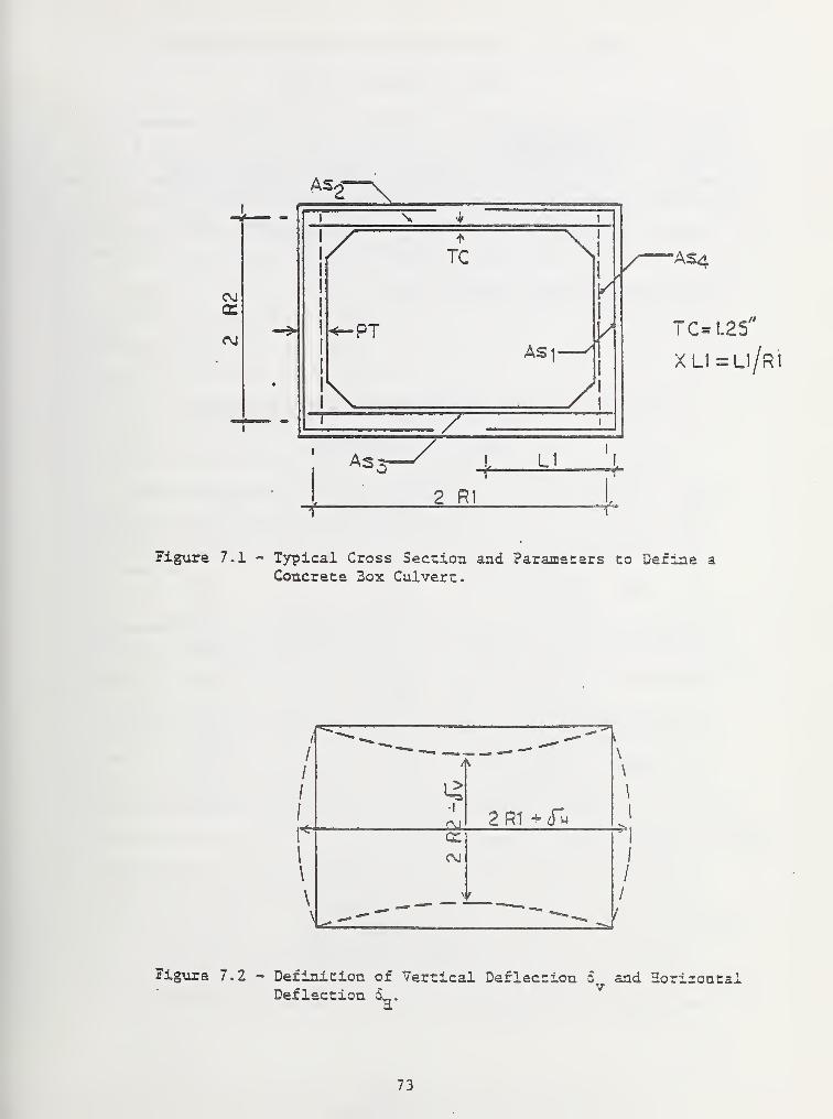
CM<r
CM
Figure 7.1 - Typical Cross Section and Parameters co Define aConcrete Box Culvert.
Figure 7.2 - Definition of Vertical Deflection o and HorizontalDeflection 5,
v
a*
73
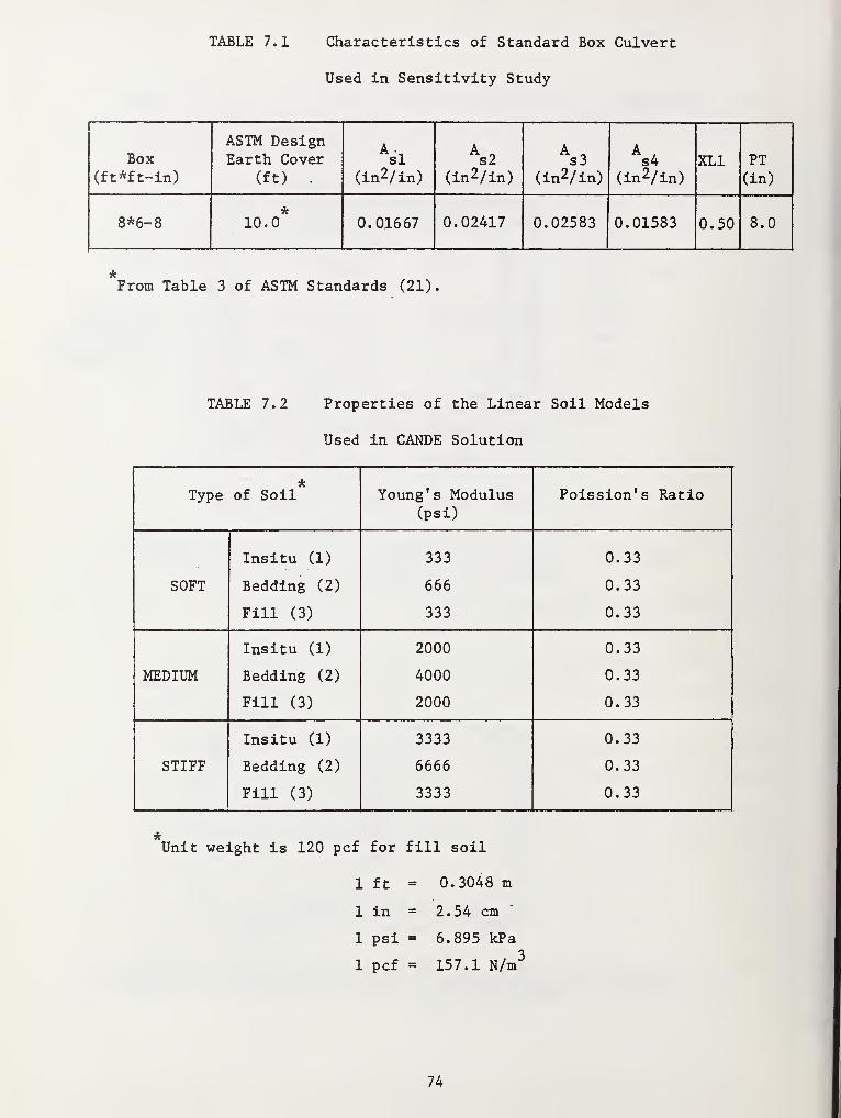
TABLE 7.1 Characteristics of Standard Box Culvert
Used in Sensitivity Study
Box(ft*ft-in)
ASTM DesignEarth Cover
(ft) .
si(in2/in)
s2(in 2/in)
s3(in2/in)
AAs4
(in 2/in)XL1 PT
(in)
8*6-8 10.0 0.01667 0.02417 0.02583 0.01583 0.50 8.0
From Table 3 of ASTM Standards (21).
TABLE 7.2 Properties of the Linear Soil Models
Used in CANDE Solution
Type*
of Soil Young ' s Modulus(psi)
Poission's Ratio
Insitu (1) 333 0.33
SOFT Bedding (2) 666 0.33
Fill (3) 333 0.33
Insitu (1) 2000 0.33
MEDIUM Bedding (2) 4000 0.33
Fill (3) 2000 0.33
Insitu (1) 3333 0.33
STIFF Bedding (2) 6666 0.33
Fill (3) 3333 0.33
Unit weight is 120 pcf for fill soil
1 ft = 0.3048 m
1 in = 2.54 cm
1 psi = 6.895 kPa
1 pcf = 157.1 N/m"
74
an embankment condition. The trench width beyond the box sides is taken
as 2.0 feet (0.61 m) (narrow trench) and soil properties for both instal-
lation types are assigned medium stiffness values (see Table 7.2). In
both cases, the box was loaded up to 28 feet (8.53 m) of soil cover above
the box. Figure 7.2 shows the definition of vertical and horizontal
relative displacements used in subsequent discussions.
Figure 7.3 shows the fill height versus vertical displacement history
of the box, from where it's observed that the embankment configuration
produces slightly greater vertical deflections in the box. Figure 7.4
shows the bending moment diagrams and shear force diagrams in the box
at 28 feet of soil cover for both installation types. The embankment
condition gives greater bending moments and shear forces acting in the
box, which conforms to the greater deflections previously observed.
From this comparison it was concluded that the embankment condition
produces slightly greater loading conditions on the box so that in all
subsequent studies presented herein only the embankment condition will
be considered.
Soil Stiffness . The effect of elastic soil stiffness is investigated
using the same standard box (8*6-8) with an embankment soil configuration,
where the properties of the soil are varied to idealize a soft, medium
and stiff soil as defined in Table 7.2. With these values a range of
variation is covered so the effect of each can be observed. Figure 7.5
shows the load versus vertical deflection history of the box for the
three classes of soil stiffness, where the box is loaded up to failure
for each case. The failures for the box culverts are defined by exceeding
ultimate shear capacity (V ) or by the formation of plastic hinge mechanisms
from excessive moments and thrust (M ) . In this study shear failure
occurs before plastic hinging in the standard box (8*6-8) for all the
three types of soil. Failure occurs first for the soft condition, whereas
for the medium and stiff soil conditions failure occurs at a greater
height of soil cover. Note that when ultimate bending failure (M ) occurs,
the deflections do not show a flat slope (increase without bounds) as
75
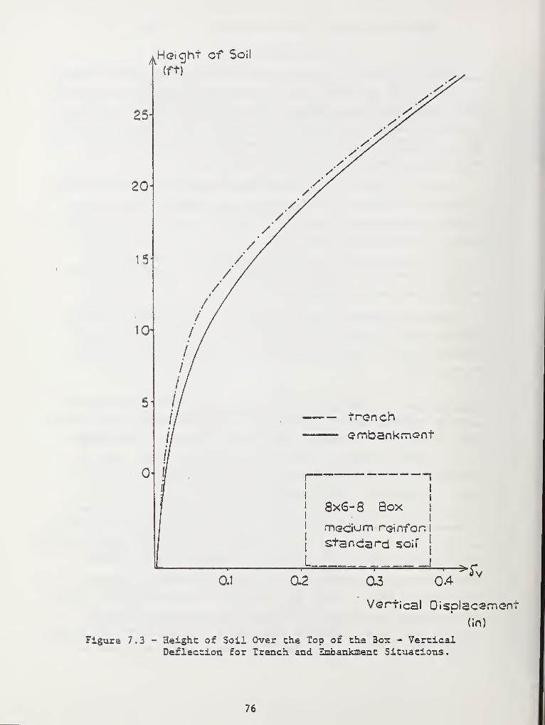
.Height of Soi
(ft)
25-
20-
15
to
5— Troncn— embankment
8x6-8 Box
medium reinfor.
standard soif
0.1 02 03 0.4**fv
Vertical Oisplacemen
(in)
Figure 7.3 - Height of Soil Over the Top of the Box - VerticalDeflection for Trench and Embankment Situations.
76
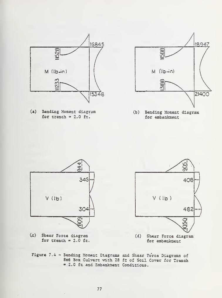
(a) Bending Moment diagramfor trench 2.0 ft.
(b) Bending Moment diagramfor embankment
Cc) Shear Force diagramfor trench 3 2.0 ft.
(d) Shear Force diagramfor embankment
Figure 7.4 - Bending Moment Diagrams and Shear Fo'rce Diagrams of8x6 Box Culvert with 28 ft of Soil Cover for Trench* 2.0 ft and. Embankment Conditions.
77
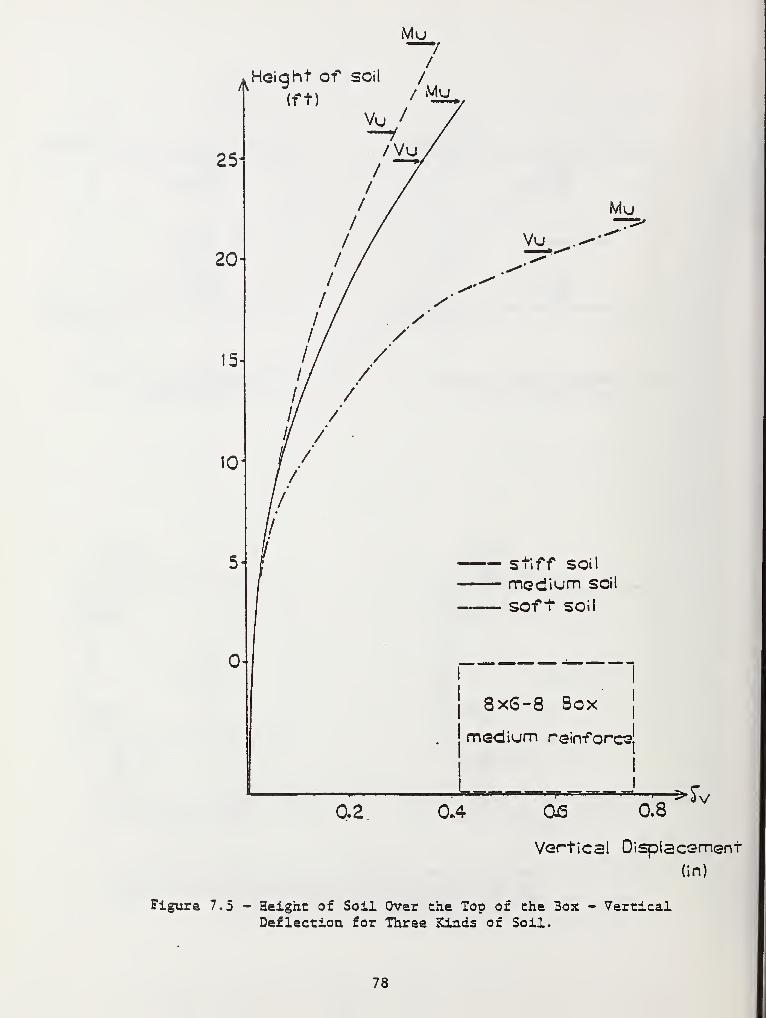
Mu
/
A Heiqht of soil /
* (ft) /***,Vu /
25-
20
Mu
Vu
Stiff SOil
medium soil
soft soil
8x6-8 Sox
medium reinforce:
L—0.2 0.4 05 0.8
»fv
Vertical Displacement
(in)
Figure 7.5 - Height of Soil Over Che Top of che Box - VerticalDeflection for Three Kinds of Soil.
78
they did in previous studies with out-of-ground culverts with applied
loads. This is because the soil stiffness is now controlling deflections
at ultimate. Accordingly, the slope of the deflection curves at ultimate
is in near proportion to soil stiffness. From Figure 7.5 it is evident
that the soft soil condition is restricted to smaller cover heights to
reach ultimate than the stiffer soils. Thus, the medium and stiff soil
conditions are more favorable for the box behavior.
Figure 7.6 shows the bending moment diagrams for the box at bending
failure (presuming stirrups) for the three types of soil conditions. It
is observed that even when the failure occurs at different heights of
soil cover, the maximum moments are similar as would be expected for
ultimate moments. From this comparison it is evident that the type of
soil is an important factor for analysis and design of a box culvert.
7.2 COMPARISON WITH TEST DATA
To validate the box-soil model, CANDE results are compared with test
data from a full scale field installation. Test data on buried box
culverts is very limited. However, recent research reports from the
Department of Transportation, Lexington, Kentucky (23,24,25) have supplied
some test data. From these reports, data was obtained for a box culvert
in Clark County, Kentucky, designed as an embankment with a yielding
foundation within a bedrock formation (24). Instrumentation on the box
included normal pressure gages and a few strain gages on reinforcement
steel which were reported not to function properly, thus only normal
pressure comparisons are used for this study. The box is identified
as Station 123+95 in the report (24) and its cross section as modeled
by CANDE is shown in Figure 7.7 along with reinforcement areas.
The level 2 box embankment condition is used for the model with
three zones of soil that are assumed linear with the properties shown
in Table 7.3. The in situ soil is bedrock so a large value is assumed
for its modulus of elasticity. Table 7.4 shows the material properties
used in CANDE to model the box culvert. The concrete and steel strengths
used in CANDE were obtained from data presented in a report (25) and the
79
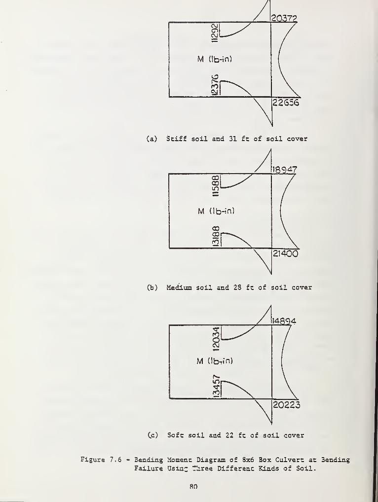
(a) Stiff soil and 31 ft of soil cover
A189*7CD y /CO ^^ /iO—
'
I
M db-in)
CO
\X
21400
(b) Medium soil and 28 ft of soil cover
(c) Soft soil and 22 ft of soil cover
Figure 7.6 - 3ending Momenc Diagram of 8x6 Box Culvert at 3endingFailure Usinc Three Different Kinds of Soil.
80
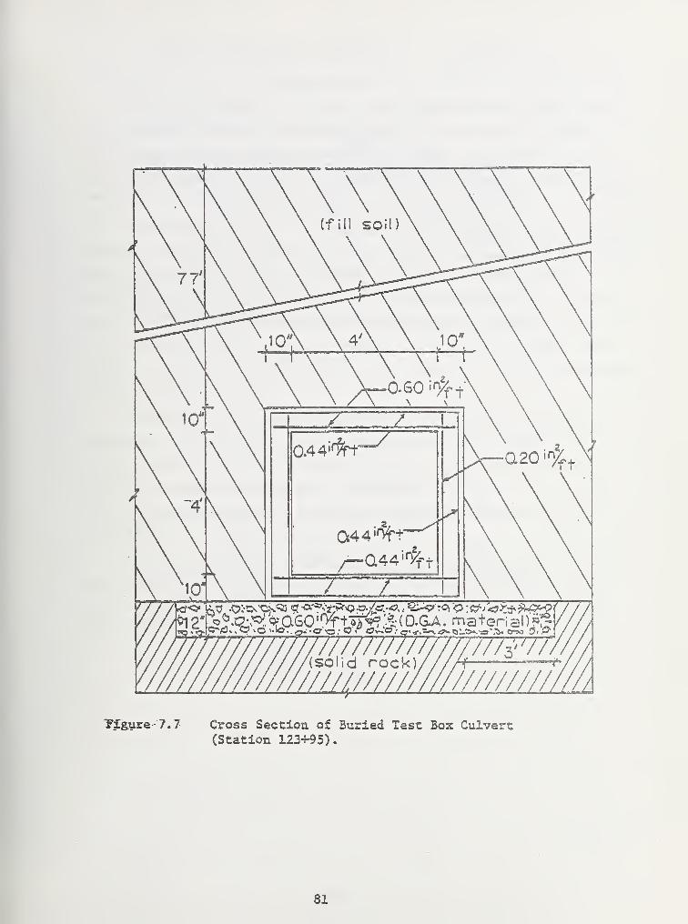
z77777777777777777T77/
(solid rock)////f *
y////////M»Tfgure-7.7 Cross Section of Buried Test Box Culvert
(Station 123+95).
81
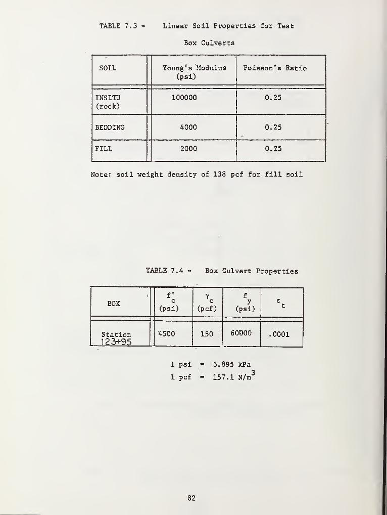
TABLE 7.3 - Linear Soil Properties for Test
Box Culverts
SOIL Young's Modulus(psi)
Poisson's Ratio
INSITU(rock)
100000 0.25
BEDDING 4000 0.25
FILL 2000 0.25
Note: soil weight density of 138 pcf for fill soil
TABLE 7.4 - Box Culvert Properties
BOXfc
(psi)
Yc
(pcf)
fy
(psi)
et
Station123+95
4500 150 60O00 .0001
1 psi - 6.895 kPa
1 pcf = 157.1 N/nf
82
other properties are assigned standard values (Tables 3.1 and 3.2).
The box is loaded up to 77 feet (23.5 m) of soil cover using small
load increments thereby obtaining a history of the box-soil system
performance. However, the only information that can be used for com-
parison is the pressure distribution on the box which was experimentally
measured at two heights of fill soil, 21.6 feet (6.58 m) and 77 feet (23.5 m)
.
To measure the pressure around the box, eight Carlson earth pressure
cells were installed, two on each side of the box. Figure 7.8 shows the
CANDE pressure distribution around the box at the two fill heights of
soil, along with the measured test data. CANDE predictions of the pres-
sure is very close to the measured value for the top and bottom slabs.
The measured pressure on the sidewalls is different for the right wall
and the left wall, and CANDE prediction is closer to the values measured
for the right wall.
From CANDE, some interesting observations are, when loaded up to
the maximum 77 feet (23.5 m) of soil cover, the bottom corner steel
started to yield for the last load increment. Also, the 0.01 inch
(0*0254 cm) crack first developed with 60 feet (18.3 m) of soil cover.
These observations suggest an economical design was achieved with no
conservatism.
After this last study it can be said that the reinforced concrete
beam element to model the box culverts and the box-soil system appear,
to give reasonably good predictions of the behavior and performance of
buried box culverts.
83
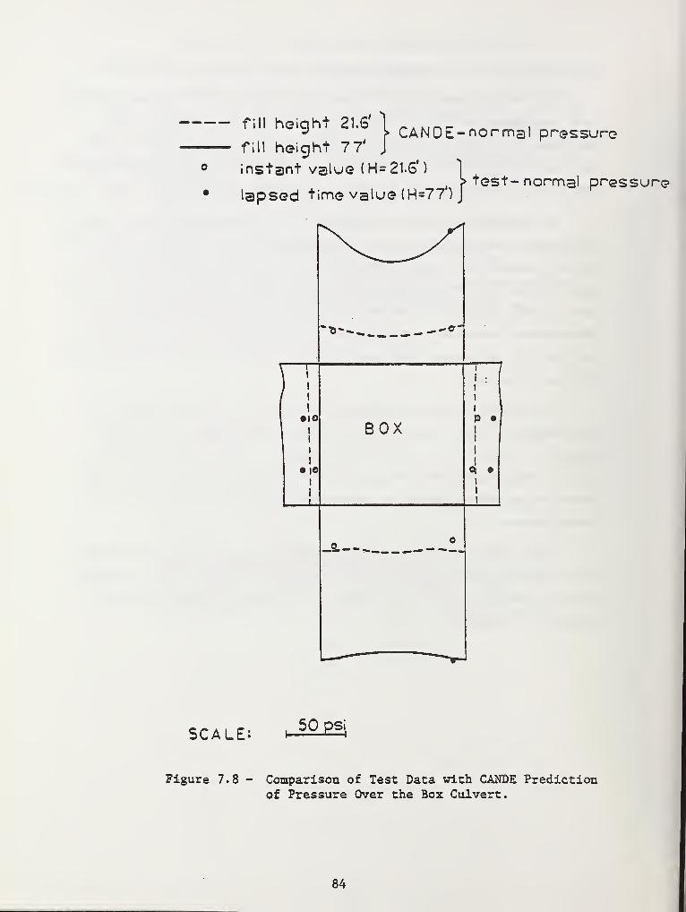
fill heiqht 21.6' 1 ^ AKin r «~ ,J > CANOE- normal pressurefill height 77' J
instant value (H= 21.6')
, > test- normal pressurelapsed time value (H=77)
J
SCALE: 50 psi
Figure 7.8 - Comparison of Test Data with CANDE Predictionof Pressure Over the Box Culvert.
84
CHAPTER 8
EVALUATION OF ASTM C-789 DESIGN TABLES WITH CANDE
In the previous chapter, CANDE' s reinforced concrete beam-rod
element has been developed and compared with experimental data for both
in ground and out-of-ground culverts. Overall, very good correlation
was observed for all aspects of structural performance, including;
load-deformation curves, cracking loads, ultimate loads, and soil pres-
sures, thereby lending a measure of confidence and validity to the
CANDE model.
In this chapter the objective is to cross-evaluate CANDE with ASTM-
C789 design tables for buried box culverts (21). As discussed in Chapter
2, the ASTM design tables are based on an elastic method of standard
analysis together with the ultimate method of reinforced concrete design
(12) . However, the magnitude and distribution of loads acting on the
box are assumed, as opposed to determining loads with soil-structure
interaction models like CANDE. In Chapter 5 it was shown that CANDE'
predictions for out-of-ground box culverts loaded in bearing correlated
very closely with the analytical predictions subsequently used to develop
the ASTM design tables (14). Thus for buried boxes, it may be presumed
that comparisons between CANDE and ASTM design tables will be influenced
primarily by the modeling of soil and soil-structure interaction as op-
posed to the modeling of the box.
The comparisons reported herein are divided into two main sections;
(1) dead loading due to soil weight only (ASTM C789, Table 3), and (2)
dead loading due to soil weight plus HS20 live loading conditions (ASTM
C789, Table 1).
8.1 BOX SECTION STUDIES FOR DEAD LOAD
Table 3 of ASTM C789 lists the design earth cover (allowable fill
height) for each standard box size as a function of- the steel reinforce-
85
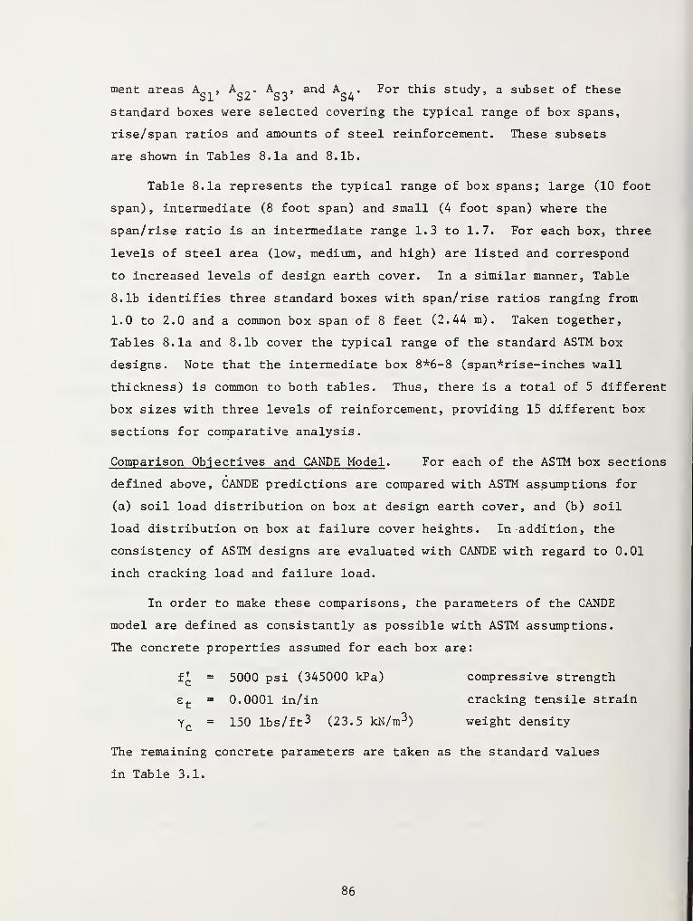
ment areas A ., ^c?* ^cV anc* ^qa' ^or this study, a subset of these
standard boxes were selected covering the typical range of box spans,
rise/span ratios and amounts of steel reinforcement. These subsets
are shown in Tables 8.1a and 8.1b.
Table 8.1a represents the typical range of box spans; large (10 foot
span) , intermediate (8 foot span) and small (4 foot span) where the
span/rise ratio is an intermediate range 1.3 to 1.7. For each box, three
levels of steel area (low, medium, and high) are listed and correspond
to increased levels of design earth cover. In a similar manner, Table
8.1b identifies three standard boxes with span/rise ratios ranging from
1.0 to 2.0 and a common box span of 8 feet (2.44 m) . Taken together,
Tables 8.1a and 8.1b cover the typical range of the standard ASTM box
designs. Note that the intermediate box 8*6-8 (span*rise-inches wall
thickness) is common to both tables. Thus, there is a total of 5 different
box sizes with three levels of reinforcement, providing 15 different box
sections for comparative analysis.
Comparison Objectives and CANDE Model . For each of the ASTM box sections
defined above, CANDE predictions are compared with ASTM assumptions for
(a) soil load distribution on box at design earth cover, and (b) soil
load distribution on box at failure cover heights. In addition, the
consistency of ASTM designs are evaluated with CANDE with regard to 0.01
inch cracking load and failure load.
In order to make these comparisons, the parameters of the CANDE
model are defined as consistantly as possible with ASTM assumptions.
The concrete properties assumed for each box are:
f£ = 5000 psi (345000 kPa) compressive strength
e t= 0.0001 in/in cracking tensile strain
Yc= 150 lbs/ft 3 (23.5 kN/m3 ) weight density
The remaining concrete parameters are taken as the standard values
in Table 3.1.
86
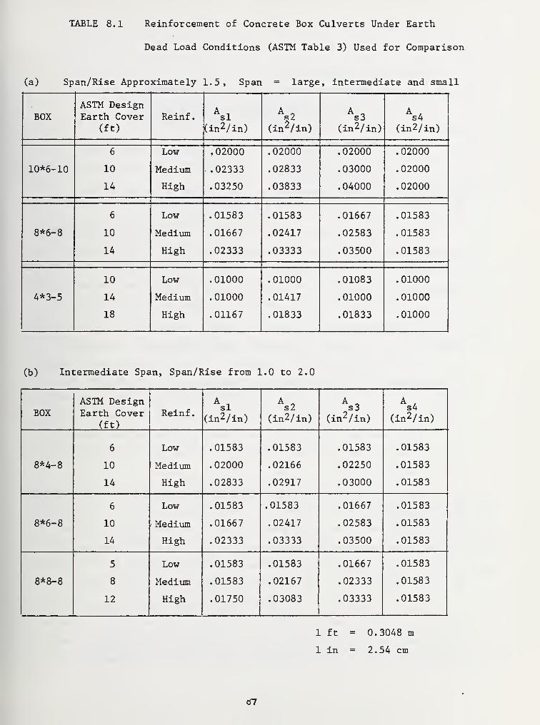
TABLE 8.1 Reinforcement of Concrete Box Culverts Under Earth
Dead Load Conditions (ASTM Table 3) Used for Comparison
(a) Span/Rise Approximately 1.5, Span = large, intermediate and small
BOXASTM DesignEarth Cover
(ft)
Reinf
.
si(in2/in)
s2(in2/in)
AQs3
(in2/in)
A/s4
(in2/in)
6 Low .02000 .02000 .02000 .02000
10*6-10 10 Medium .02333 .02833 .03000 .02000
14 High .03250 .03833 .04000 .02000
6 Low .01583 .01583 .01667 .01583
8*6-8 10 Medium .01667 .02417 .02583 .01583
14 High .02333 .03333 .03500 .01583
10 Low .01000 .01000 .01083 .01000
4*3-5 14 Medium . 01000 .01417 .01000 . 01000
18 High .01167 .01833 .01833 .01000
(b) Intermediate Span, Span/Rise from 1.0 to 2.0
BOXASTM DesignEarth Cover
(ft)
Reinf.
Aisi
(in2 /in)
As2
(in2/in)
AOs3
(in2 /in)
A/s4
(in2/in)
8*4-8
6
10
14
Low
Medium
High
.01583
.02000
.02833
.01583
.02166
.02917
.01583
.02250
.03000
.01583
.01583
.01583
8*6-8
6
10
14
Low
: Medium
High
.01583
.01667
.02333
.01583
.02417
.03333
.01667
.02583
.03500
.01583
.01583
.01583
8*8-8
5
8
12
Low
Medium
High
.01583
.01583
.01750
.01583
.02167
.03083
.01667
.02333
.03333
.01583
.01583
.01583
1 ft = 0.3048 m
1 in = 2.54 cm
07
and
Assumed steel properties are:
fy
= 65000 psi (448000 kPa) yield stress
Es = 29000 ksi (200000 MPa) Young's modulus
Tc= 1.25 in (3.18 cm) concrete cover to steel center
S^ = 2.00 in (5.08 cm) longitudinal spacing for crack prediction
An example of the CANDE input parameters for 8x6 box is given in
Appendix C.
Since the ASTM approach does not consider soil stiffness, the CANDE
solutions use two soil conditions, soft and stiff, for the analysis of each
box, thereby bracketing the practical range of soil stiffness. Soil moduli
values for soft and stiff conditions are given in previous chapter in Table3
7.2. For both conditions, soil density is taken as 120 pcf (18.8 kN/m ).
All CANDE solutions are obtained using the new level 2 box generation
scheme for an embankment installation. Nine construction increments of
soil are used to-bring the soil height up to the ASTM design cover height
to facilitate the comparison of loading distributions assumed by ASTM with
those predicted by CANDE. Thereafter, additional soil layers are added
until flexural failure is observed. During this loading sequence, the
cover height causing initial 0.01 inch cracking is determined along with
the cover height causing shear failure, providing shear failure occurs
before flexural failure.
Load Distribution Comparisons at Design Cover Height . The ASTM assumed
load pattern due' to soil pressure and box weight are shown in Figure 8.1.
Vertical soil pressures are assumed uniform and proportional to cover
height. Lateral pressures are assumed to vary linearly, dependent on
the coefficient of lateral earth pressure generally assumed to be 0.5.
No shear traction on the box sides is assumed in the ASTM pattern.
Figure 8.2 illustrates, the nature of a typical load distribution
predicted by CANDE resulting from soil loading and box weight. Vertical
soil pressures are not uniform, lower in the middle where bending defor-
mation is greatest. Lateral pressure along the box increases with depth
88
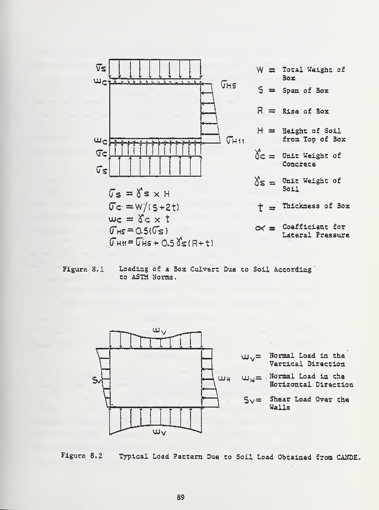
Fs
ujc{ :l t
<Jc
C"s
t > ;'
Z y ; t, :, i. j, y I i. Z—
f—s r - rm2 ,i 4
'
+ ** T 7 '<
*-* H-
Ghs
R1 G"wn
(7s = X* s x H
Oc=W/(S+2t)aic = !fcx t
(Tms = 0.5(Cs)
(Thu^Ghs* 0.5 3s(R+t)
W = Total Weight ofBox
S =• Span of Box
R = Rise of Box
H = Height of Soilfrom. Top of Box
Oc = Unit Weight ofConcrete
#S = IJnit WeiSat ofSoil
+ s Thickness of Box
0< = Coefficient forLateral Pressure
Figure 8.1 Loading of a Box Culvert Due to Soil Accordingto ASTM Norms.
UJvy=
OJH UJ w=
Sv=
Normal Load in theVertical Direction
Normal Load in theHorizontal Direction
Shear Load Over theWalls
Figure 8.2 Typical Load Pattern Due co Soil Load Obtained from CANDE.
89
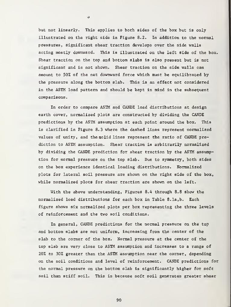
but not linearly. This applies to both sides of the box but is only
illustrated on the right side in Figure 8.2. In addition to the normal
pressures, significant shear traction develops over the side walls
acting mostly downward. This is illustrated on the left side of the box.
Shear traction on the top and bottom slabs is also present but is not
significant and is not shown. Shear traction on the side walls can
amount to 50% of the net downward force which must be equilibrated by
the pressure along the bottom slab. This is an effect not considered
in the ASTM load pattern and should be kept in mind in the subsequent
comparisons.
In order to compare ASTM and CANDE load distributions at design
earth cover, normalized plots are constructed by dividing the CANDE
predictions by the ASTM assumption at each point around the box. This
is clarified in Figure 8.3 where the dashed lines represent normalized
values of unity, and the solid lines represent the ratio of CANDE pre-
diction to ASTM assumption. Shear traction is arbitrarily normalized
by dividing the CANDE prediction for shear traction by the ASTM assump-
tion for normal pressure on the top slab. Due to symmetry, both sides
on the box experience identical loading distributions. Normalized
plots for lateral soil pressure are shown on the right side of the box,
while normalized plots for shear traction are shown on the left.
With the above understanding, Figures 8.4 through 8.8 show the
normalized load distributions for each box in Table 8.1a,b. Each
figure shows six normalized plots per box representing the three levels
of reinforcement and the two soil conditions.
In general, CANDE predictions for the normal pressure on the top
and bottom slabs are not uniform, increasing from the center of the
slab to the corner of the box. Normal pressure at the center of the
top slab are very close to ASTM assumption and increases to a range of
20% to 30% greater than the ASTM assumption near the corner, depending
on the soil conditions and level of reinforcement. CANDE predictions for
the normal pressure on the bottom slab is significantly higher for soft
soil than stiff soil. This is because soft soil generates greater shear
90
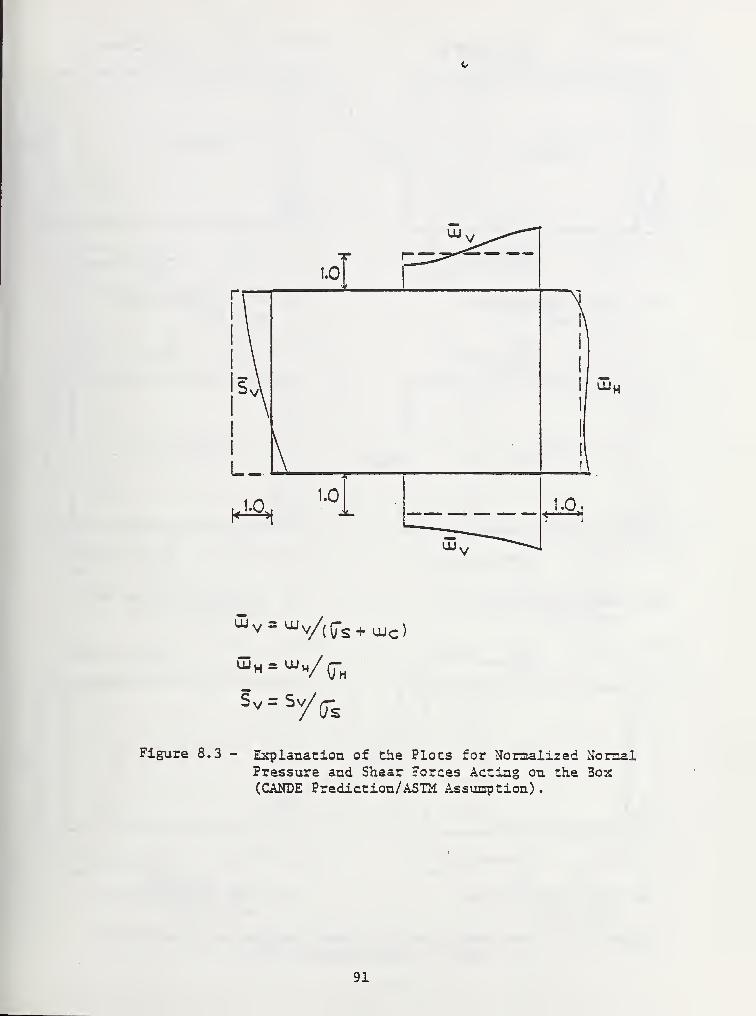
^
Olw =V= ^v/ffs+UJc)
Figure 8.3 - Explanation of the Plots for Normalized NormalPressure and Shear Forces Acting on the 3ox(CANDE Prediction/ASTM Assumption)
.
91
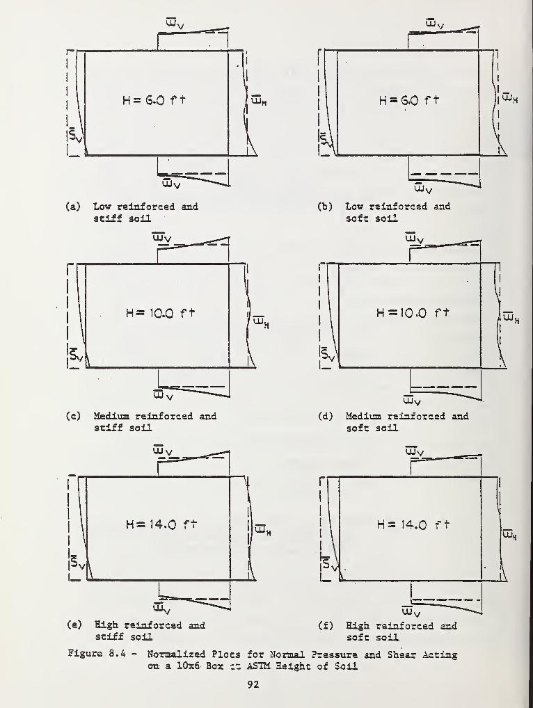
(a) Low reinforced and
stiff soil
UJV
UJV
(b) Low reinforced andsoft soil
(c) Medium reinforced andstiff soil
UJV(d) Medium reinforced and
soft soil
UJ V
Hs 14.0 f"
(e) High reinforced andstiff soil
vu,
UJy
(f) High reinforced andsoft soil
Figure 8.4 - Normalized Plots for Normal Pressure and Shear Actingon a 10x6 Box iZ ASTM Height of Soil
92
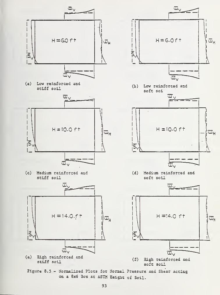
(a) Low reinforced andstiff soil
(c) Medium reinforced andstiff soil
(e) High reinforced andstiff soil
Ulu
I UJ,
(b) Low reinforced andsoft soi
-PH
(d) Medium reinforced andsoft soil
(f) High reinforced andsoft soil
Figure 8.5 - Normalized Plots for Normal Pressure and Shear Actingou a 8x6 Box ac ASTM Height of Soil.
93
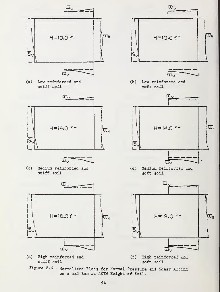
UJH
(a) Low reinforced andstiff soil
UJ V(b) Low reinforced and
soft soil
UJv UJV
(c) Medium reinforced andstiff soil
(d) Medium reinforced andsoft soil
UJV
(f) High reinforced andsoft soil
(e) High reinforced andstiff soil
Figure 8.6 - Normalized Plots for Normal Pressure and Shear Actingon a 4x3 Box at ASTM Height of Soil.
94
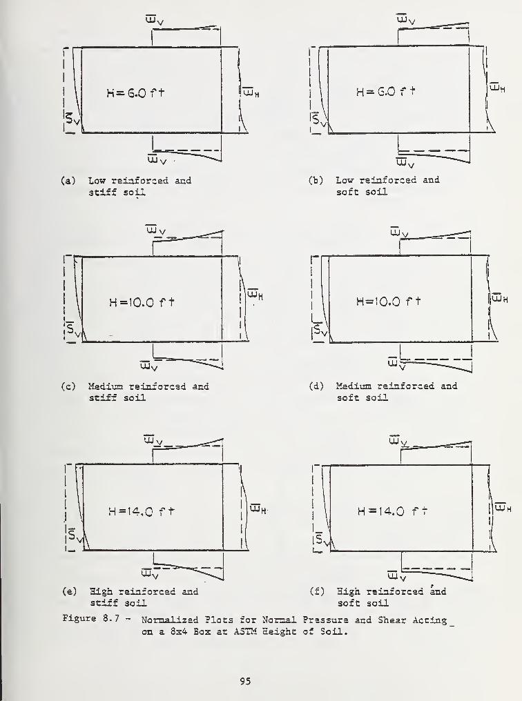
(a) Low reinforced andstiff soil
UJ H
I
i
H=6.0 ft Ivjl
\ {
1-"v "**
(d) Lov reinforced and
soft soil
UJ V
(c) Medium reinforced andstiff soil
UJh
(d) Medium reinforced andsoft soil
UJ V UJy_
(e) High reinforced andstiff soil
ujh
oj v(f) High reinforced and
soft soil
Figure 8.7 - Normalized Plots for Normal Pressure and Shear Actingon a 8x4 Box at ASTM Height of Soil.
|UJh
95
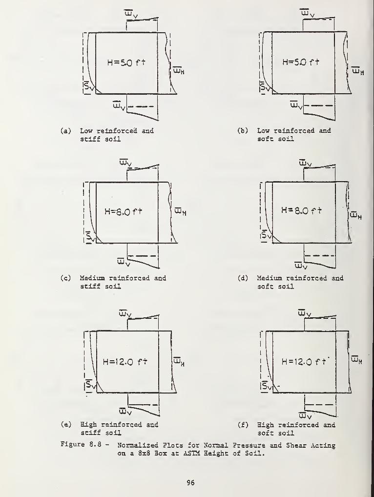
(a) Low reinforced andstiff soil
(b) Low reinforced andsoft soil
ujv UJv
(c) Medium reinforced andstiff soil
(d) Medium reinforced andsoft soil
UJV UJv
(e) High reinforced andstiff soil
UJv(f) High reinforced and
soft soil
Figure 8.8 - Normalized Plocs for Normal Pressure and Shear Actingon a 8x8 Box at ASTM Height of Soil.
96
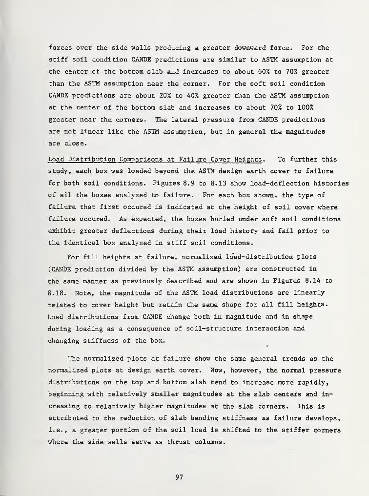
forces over the side walls producing a greater downward force. For the
stiff soil condition CANDE predictions are similar to ASTM assumption at
the center of the bottom slab and increases to about 60% to 70% greater
than the ASTM assumption near the corner. For the soft soil condition
CANDE predictions are about 20% to 40% greater than the ASTM assumption
at the center of the bottom slab and increases to about 70% to 100%
greater near the corners. The lateral pressure from CANDE predictions
are not linear like the ASTM assumption, but in general the magnitudes
are close.
Load Distribution Comparisons at Failure Cover Heights . To further this
study, each box was loaded beyond the ASTM design earth cover to failure
for both soil conditions. Figures 8.9 to 8.13 show load-deflection histories
of all the boxes analyzed to failure. For each box shown, the type of
failure that first occured is indicated at the height of soil cover where
failure occured. As expected, the boxes buried under soft soil conditions
exhibit greater deflections during their load history and fail prior to
the identical box analyzed in stiff soil conditions.
For fill heights at failure, normalized load-distribution plots
(CANDE prediction divided by the ASTM assumption) are constructed in
the same manner as previously described and are shown in Figures 8.14 to
8.18. Note, the magnitude of the ASTM load distributions are linearly
related to cover height but retain the same shape for all fill heights.
Load distributions from CANDE change both in magnitude and in shape
during loading as a consequence of soil-structure interaction and
changing stiffness of the box.
The normalized plots at failure show the same general trends as the
normalized plots at design earth cover. Now, however, the normal pressure
distributions on the top and bottom slab tend to increase more rapidly,
beginning with relatively smaller magnitudes at the slab centers and in-
creasing to relatively higher magnitudes at the slab corners. This is
attributed to the reduction of slab bending stiffness as failure develops,
i.e., a greater portion of the soil load is shifted to the stiffer corners
where the side walls serve as thrust columns.
97
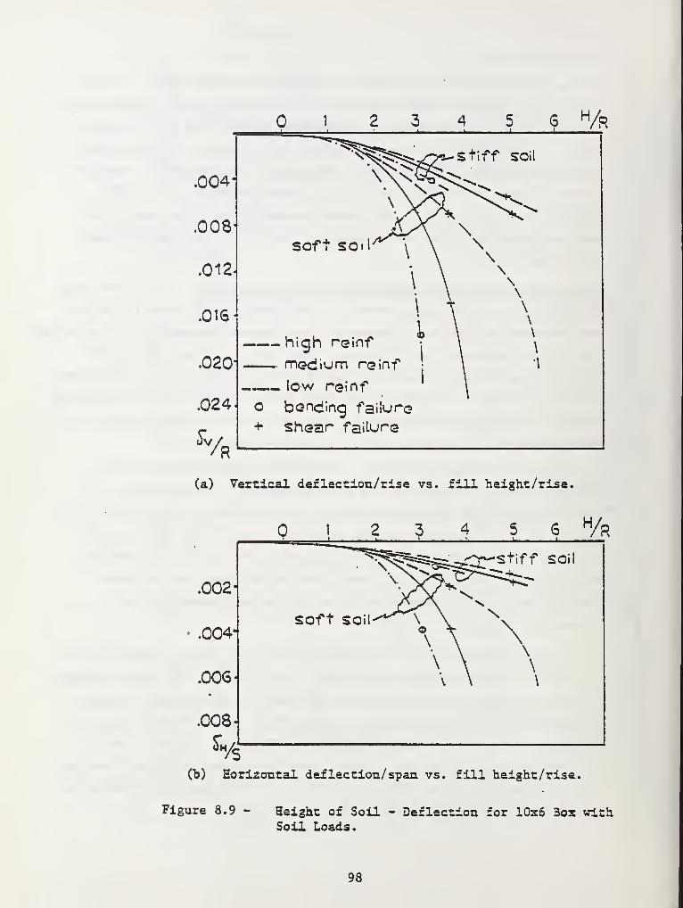
.0041
.008
.012
.016
.020
.024
&
soft SO
i
'/r
o+
high reinf
medium reinf
low reinf
bonding failure
shear failure
(a) Vertical deflection/rise vs. fill height /rise.
.002
.0041
.006
.008-1
Sh
1 2 31
i ~5 6
H/r
iff soil
SOft SOil
'/s
(b) Horizontal deflection/ span vs. fill height/rise.
Figure 8.9 - Height of Soil - Deflection for 10x6 Box withSoil Loads.
98
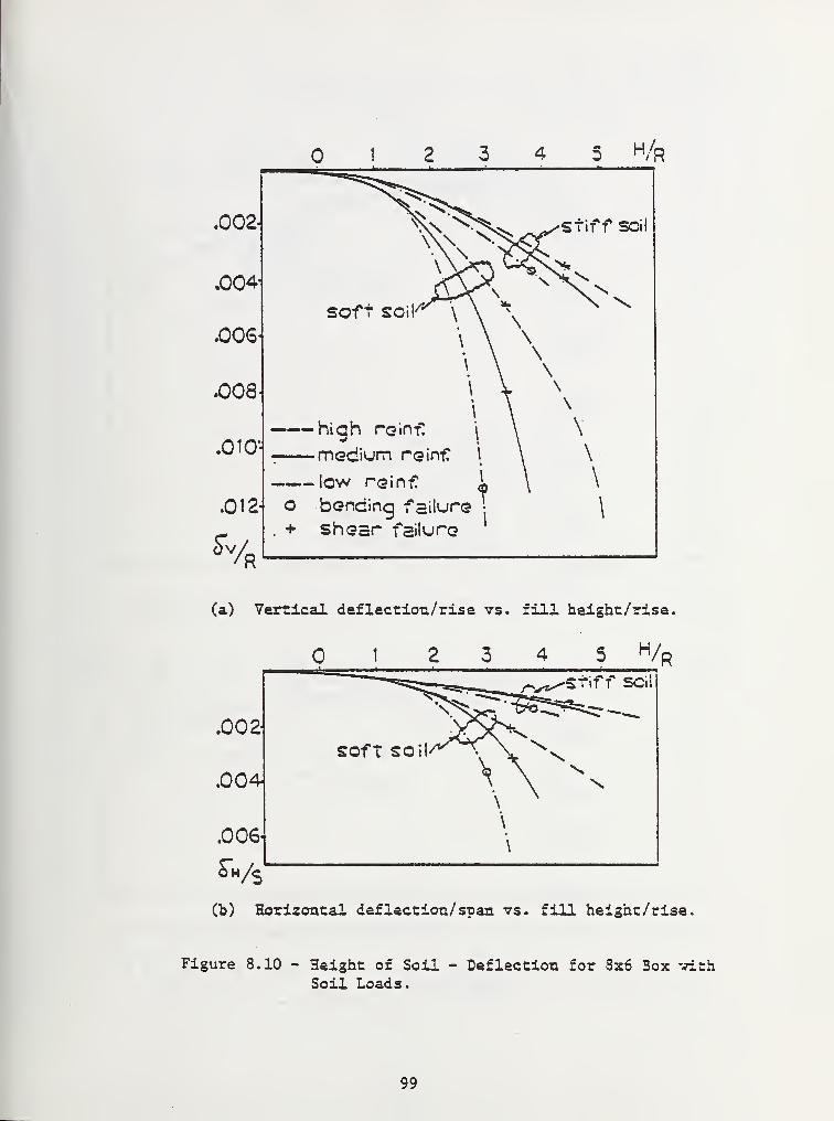
3 4 5 H/R
.002-1
,004
.006
.008
.010-
.012-
H
Stiff SCi
SOft SOi
high re inf.
medium reinf
low reinfo bending failure
. + shear failure
(a) Vertical deflection/rise vs. fill height /rise.
5 HA
.002
.oo4^
.006
Ws
stiff so
soft so
(b) Horizontal deflection/ span vs. fill height/rise.
Figure 8.10 - Height of Soil - Deflection for 3x6 3ox withSoil Loads.
99
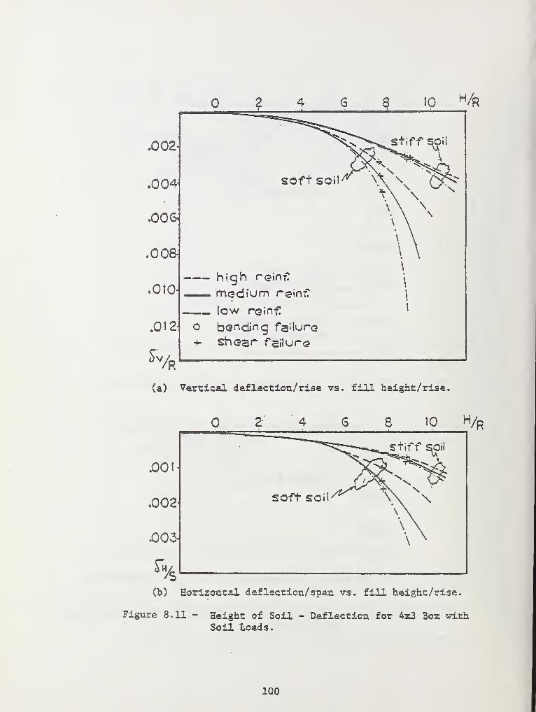
8 10 H/R
SOft SOil
S^^stiff SOii
\ \
\ \\ \
high reinfI
medium reinf 1
low reinf i
bonding failure
+ shoar failure
.002-
.004-
.00G
.008-
.010-
.012
Sv/R
(a) Vertical deflection/rise vs. fill height/rise-
.001
.002
£03-1
ft4/s
Stiff SOil
10 H/R
soft so
(b) Horizontal deflection/ span vs.. fill height/rise.
Figure 8.11 - Height of Soil - Deflection for 4x3 Box withSoil Loads.
100
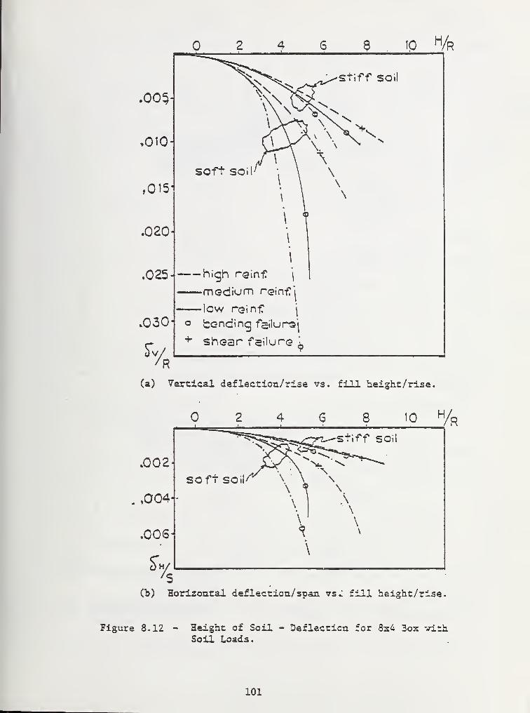
10 h/r
.030-
high rsinf\
modium rsinfj
low roinf?\
o bonding failursj
+ shoar failure9
(a) Vertical deflection/rise vs. fill height/rise.
.002-
,004-
.006-
r.%
Stiff SOi
10 H/R
soft so
(h) Horizontal deflection/spaa vs.: fill height/rise.
Figure 8.12 - Height of Soil - Deflection for 8x4 Box withSoil Loads.
101
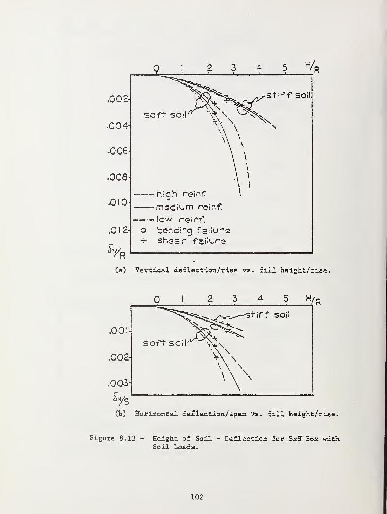
2 3 h/p
.002
.004
.006
.008
.010
.012
, ~^-g^' ' L"
SOft SOil^ \\ \
V\
\
"\
I
i 1
i ' ii
^rStif f SOil
high reinf
medium reinf.
low reinf.
o bonding failure+• shear failure
(a) Vertical deflection/rise vs. fill height/rise,
1 2 3 4 5 H/R
soft soi
stiff soil
.001
.002-
.003-
fys(h) Horizontal deflection/span vs. fill height/rise.
Figure 8.13 - Height of Soil - Deflection for 8x8" Box withSoil Loads.
102
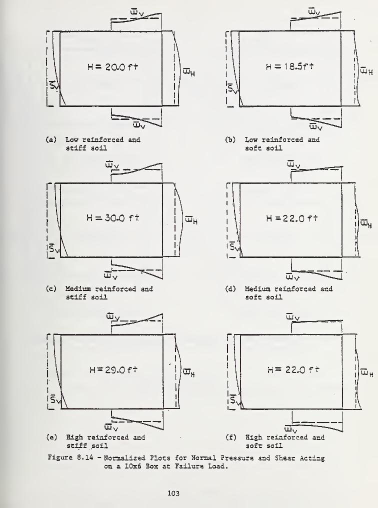
UJv
UJV
(a) Low reinforced andstiff soil
ULly
(b) Low reinforced andsoft soil
(c) Medium reinforced andstiff soil
UJv/
(d) Medium reinforced andsoft soil
(e) High reinforced andstiff soil
(f ) High reinforced andsoft soil
Figure 8.14 - Normalized Plots for Normal Pressure and Shear Actingon a 10x6 Box at Failure Load.
103

(a) Low reinforced andstiff soil
(c) Medium reinforced andstiff soil
(b) Low reinforced andsoft soil
UJy
(d) Medium reinforced andsoft soil
Note: The 8x6 box with high reinforcement has plots similar to the mediumreinforced, where the failure is due to shear.
Figure 8.15 - Normalized Plots for Normal Pressure and Shear Actingon a 8x6 Box at Failure Load.
104
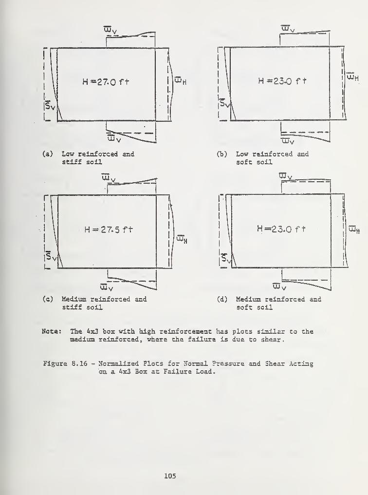
(a) Low reinforced andstiff soil
(c) Medium reinforced andstiff soil
(b) Low reinforced andsoft soil
(d) Medium reinforced andsoft soil
Note: The 4x3 box with high reinforcement has plots similar Co themedium reinforced, where the failure is due to shear.
Figure 8.16 - Normalized Plots for Normal Pressure and Shear Actingon a 4x3 Box at Failure Load.
105
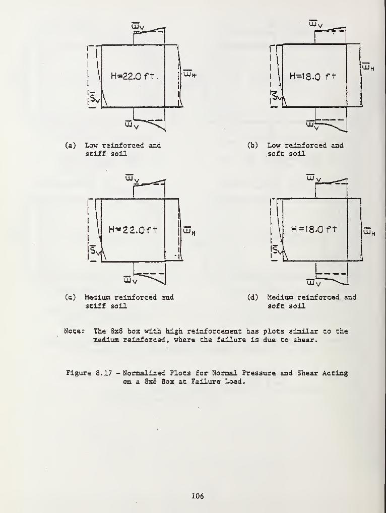
UJV uu v
rri\
|\ H=22.0 ft
.
1
1
jSv1
1
1
3/^(a) Low reinforced and
stlff soil
UJh-uj h
(b) Low reinforced andsoft soil
(c) Medium reinforced andstiff soil
UJ V
(d) Medium reinforced, andsoft soil
Noter The 8x8 box with high reinforcement has plots similar to themedium reinforced, where the failure is due to shear.
Figure 8.17 -Normalized Plots for Normal Pressure and Shear Actingon a 8x8 Box at Failure Load.
106

(a) Low reinforced andstiff soil
(b) Low reinforced andsoft soil
(c) Medium reinforced andstiff soil
(d) Most reinforced andsoft soil
(e) High reinforced andstiff soil
Ol v(f ) High reinforced and
soft soil
Figure 8.18 - Normalized Plots for Normal Pressure and Shear Actingon a 8x4 Box at Failure Load.
107
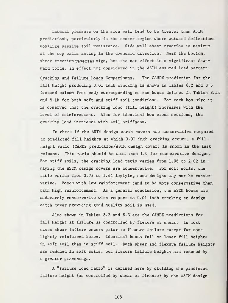
Lateral pressure on the side wall tend to be greater than ASTM
predictions, particularly in the center region where outward deflections
mobilize passive soil resistance. Side wall shear traction is maximum
at the top walls acting in the downward direction. Near the bottom,
shear traction reverses sign, but the net effect is a significant down-
ward force, an effect not considered in the ASTM assumed load pattern.
Cracking and Failure Loads Comparisons . The CANDE prediction for the
fill height producing 0.01 inch cracking is shown in Tables 8.2 and 8.3
(second column from end) corresponding to the boxes defined in Tables 8.1a
and 8.1b for both soft and stiff soil conditions. For each box size it
is observed that the cracking load (fill height) increases with the
level of reinforcement. Also for identical box cross sections, the
cracking load increases with soil stiffness.
To check if the ASTM design earth covers are conservative compared
to predicted fill heights at which 0.01 inch cracking occurs, a fill-
height ratio (CANDE prediction/ASTM design cover) is shown in the last
columns. This ratio should be more than 1.0 for conservative designs.
For stiff soils, the cracking load ratio varies from 1.06 to 2.02 im-
plying the ASTM design covers are conservative. For soft soils, the
ratio varies from 0.75 to 1.44 implying some designs may not be conser-
vative. Boxes with low reinforcement tend to be more conservative than
with high reinforcement. As a general conclusion, the ASTM boxes are
moderately conservative with respect to 0.01 inch cracking at design
earth cover providing good quality soil is used.
Also shown in Tables 8.2 and 8.3 are the CANDE predictions for
fill height at failure as controlled by flexure or shear. In most
cases shear failure occurs prior to flexure failure except for some
lightly reinforced boxes. Identical boxes fail at lower fill heights
in soft soil than in stiff soil. Both shear and flexure failure heights
are reduced in soft soils, but flexure failure heights are reduced by
a greater precentage.
A "failure load ratio" is defined here by dividing the predicted
failure height (as controlled by shear or flexure) by the ASTM design
108
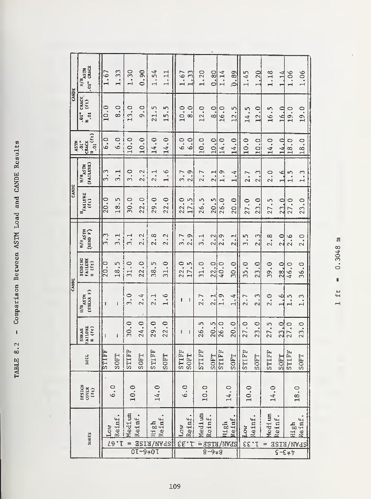
3CO
<rf
WP
3CO
CO
O
s0)
CD
•u
01
PQ
3.o(0
•H
CO
§*
Oo
CN
00
wrJ
M
< Ur^ CO o o st rH P- CO o o st Ol m o 00 SJ vO vOvO CO CO t7i m iH vO CO CM 00 rH CO st CM rH r- o O
uZ wo
iH iH rH O iH rH r-\ r-l rH O H .O rH r-\ rH r- rH <-{
§ a'
O o O O m m o o o o o m m o m c o o-< o O 00 CO CT> rH m o oo CM 00 v£> CM st CN so vo CTv cr>
°.s' iH iH CN rH rH rH rH rH rH T-i rH H rH rH
P -H O -H
O o O O o o o o O O o o O o O O o o«s< o vO vO O O st st vO vO o o st st o o st st 00 00
U X H iH rH rH rH rH rH rH rH rH rH r-i rH rH
siV) 3< J CO rH O CN rH vO r-^ <7\ r* t-h <Ti st r~H CO O vC m COI M
a5
-«. < CO CO CO CN CN rH CO CM CN CM rH rH CM CN CM r- rH rH
uu OS
3- o m O O O O o m m m o o o O m o o o< ~ o 00 O CN 0\ CN cm r-^ vO O vO O r^ CO r^ cn r-» COz CN H CO CN CN CN CN rH CN CN CN CN CN CM CM CM CM CM
EC3n CO i-\ rH CN 00 CM r>» cr\ rH CN ON r-i m CO 00 o VO Oz z
CO CO CO CN CN CN CO CM CO CM CN CM co CM CM CN CM CM= &O wi-i 3 u o m O O m O o m o o O O o o o o O OO J <*•
S3~ O oo r-t CN 00 rH cn r->. r-\ CN O O m co <y> co] vO vO
ua
03 lb Z CN rH CO CM CO CO CM t-{ CO CM St CO CO CM CO CM st CO
£* O st t-4 vO r». rH <J\ st r*> CO O VO m CO
1 l CO CM CN rH CM CM rH rH CM CN CM H rH t-t
— !rtZ o"
O O O O m m O O o O m o o oE<1 ^» • • • •
< 3 «-J _1 ^<
O st ON CM1 1 vO o vO O r» CO r>. co r-~ CO
1 ICO CN CN CN CM CM CM CM CM CN CM CM CM CN
CO < ZEh
fa fa fa fa fa fa fa fa fa_i fa H fa H fa H fa h fa H fa H fa H fa Eh fa HH fa H fa M fa M fa H Pn M fa H fa M fa i—
i
favo H O H O H O H O H O H O H O H O H o
CO CO CO CO CO CO CO CO CO CO CO CO CO CO CO CO CO CO
g*~ O O o o o o o o oH-t U «J • • • • • • • s .
w O^ vO o st vO o st o st 00a u iH rH rH r-\ rH rH <-{
g . . g • E •
«4-4 § MH 4-1 <4H 3 iw IW 4-1 3 Mh 4H3 •H 3 rC 3 ^ 3 •H C 43 C C •H C xi 3
5 •H T3 -H 00 -H S «H T3 -H 00 -H 5 •H T3 iH Ml •Ho CJ (U CD •H <U O 0) (U (U •H CU o CU QJ 0) •H <D
uXa9
hJ Crf 2 erf pc erf r4 Crf S erf X Crf J crf 5^ Cri 32 crf
£9"T = asiH/NVdS ett -ffSTH/KVaS ££ •I = aSIH/NVdSOT-9¥01 8-9*8 S-£*V
00stOCO
109

COi->
H3CO
aWO
sCO
cd
o
co<ccu
CD
CD
«coCO
•HMCO
to
en
oo
w
*8 O CO o m <r <}- r^ en o o -* CT CN <r CTi oo en mm n m H vO O vO en CN 00 rH 0C O <r \o o en r-«
Z3
"" orH rH rH rH iH H rH rH rH O rH C CN rH rH rH rH O
S£O O O m o m o o O O O ir rH CN m vO o o
o CT» oo m rH CO < O 00 CN 00 VO CN o r*- en 00 vo ejviH iH CN rH rH rH H r- H rH rH
w
3°. 2 °.u =
O o O O O O o o © o o c O O o o o ovO vO o O -tf < vO vO o o ^ <t m m oo co CN CN
rH rH rH rH rH H rH r- rH rH
El r^ CO 00 iH CN vO r-. ejv. r*. rH C7\ -J <r o oo en oo mVI =< -1X — en CO CN CN CN rH cn cn CN CN rH r- <r en CN CN rH rH^- <z u.
as.
^
< w
3C O o O O O O o m m m o c o o o o o o< <- CN o oo !-H rH en cn r^ so o vO C CN oo CN oo CN CO
= CN CN CN CN en cn CN rH CN CN CN CN CN rH CN rH CN rH
V.< a
r»» en 00 rH ej\ cr\ r-^ o> rH CN Cf\ r— r^ o <!• Ov r^ en= z— act
cn en CN CN CN rH en cn en cn CN CN «^- <a- en CN CN CN
z =e ^— 3 «J o O o O o o o m O O o c m o O O o oa _ •—
z — «->
M < CN o 00 rH o vo cn r-» rH CN o c en o r~- en CN f*
a
x b. S CM CN CO CN sT CN CN rH en cn <3- f" CN CN CN CN en cn
2
v. << u 1 1
•1
CN vO• •
1 1
P^ rH <T\ <3 »tf vO oo en oo in
s * en CN rH CN CN rH r- >d- en CN CN rH rH
O o o m m O O O O O O o o0£ as u< a «- <r rH en vO o vO O CN oo CN oo CN 00
•7 < a1 1 en
1 en cn1 1 CN CN CN CN CN rH CN rH CN rH
fa Ifa fa fa fa fa fa fa fa_i fa H fa H fa H fa H fa H fa E-i fa H fa H fa H
1—
1
fa M fa M fa M fa H fa H fa M fa M fa H fay. H O H O H O H O H O H O H O H O H O
CO CO CO CO co to CO CO CO CO CO CO CO CO in CO CO CO
z•J OS ».
o o o o o o o o OH JI 11 • • • • * • men > w. vO o >cr vO o o- m oo CNa 3 rH rf rH rH rH
g . e • R<u 3 M-l <u UH 3 >H 4-1 "4-1 3 IH ,3 iw
1* C -H C rC C 5 C •H fi X c fr c •H C 60 3O •H 1 T3 •H GO -H O «H 73 -H 00 «H o •H T3 •H •H 'Hi-l CD | CD 0) •H CD r4 (U CU CU •H CU rJ 0) (1) CU S CU
x04 \ 2 Pi! 33 OS OS * Qi rc cd cr! SJ a! rv!
0*3 = asia/NVds ee* I=3SIS/NVdS *I = 3S T'5i/NVdS8-V*8 8-9^'8 8--8*<?
110
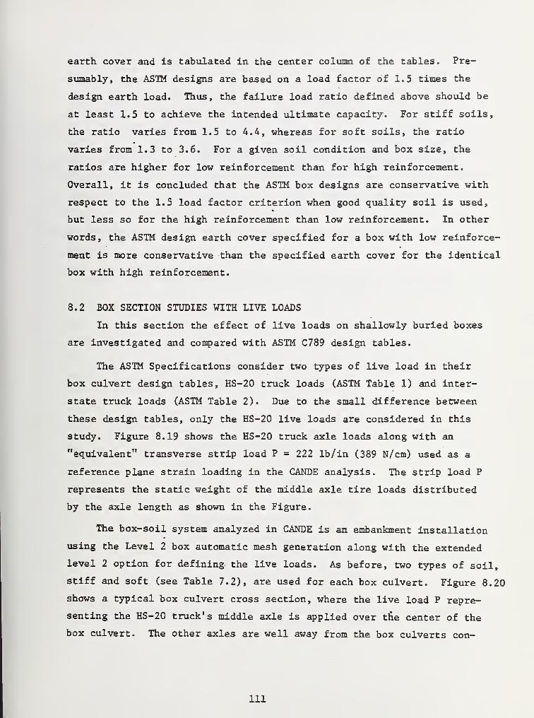
earth cover and is tabulated in the center column of the tables. Pre-
sumably, the ASTM designs are based on a load factor of 1.5 times the
design earth load. Thus, the failure load ratio defined above should be
at least 1.5 to achieve the intended ultimate capacity. For stiff soils,
the ratio varies from 1.5 to 4.4, whereas for soft soils, the ratio
varies from 1.3 to 3.6. For a given soil condition and box size, the
ratios are higher for low reinforcement than for high reinforcement.
Overall, it is concluded that the ASTM box designs are conservative with
respect to the 1.5 load factor criterion when good quality soil is used,
but less so for the high reinforcement than low reinforcement. In other
words, the ASTM design earth cover specified for a box with low reinforce-
ment is more conservative than the specified earth cover for the identical
box with high reinforcement.
8.2 BOX SECTION STUDIES WITH LIVE LOADS
In this section the effect of live loads on shallowly buried boxes
are investigated and compared with ASTM C789 design tables.
The ASTM Specifications consider two types of live load in their
box culvert design tables, HS-20 truck loads (ASTM Table 1) and inter-
state truck loads (ASTM Table 2). Due to the small difference between
these design tables, only the HS-20 live loads are considered in this
study. Figure 8.19 shows the HS-20 truck axle loads along with an
"equivalent" transverse strip load P = 222 lb/in (389 N/cm) used as a
reference plane strain loading in the CANDE analysis. The strip load P
represents the static weight of the middle axle tire loads distributed
by the axle length as shown in the Figure.
The box-soil system analyzed in CANDE is an embankment installation
using the Level 2 box automatic mesh generation along with the extended
level 2 option for defining the live loads. As before, two types of soil,
stiff and soft (see Table 7.2), are used for each box culvert. Figure 8.20
shows a typical box culvert cross section, where the live load P repre-
senting the HS-20 truck's middle axle is applied over tne center of the
box culvert. The other axles are well away from the box culverts con-
Ill
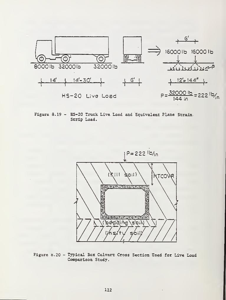
B8000 lb 320001b 320001b
f-^4/ f r\*14=30 f^f
HS-20 Live Load
f-^-4\,
5 ISOOOIb 160001b
I 1
-kiuhudjSl*^
p= 32000 lb =222 i b/144 in
«n
Figure 8.19 - HS-20 Truck Live Load and Equivalent Plane StrainStrip Load.
P=222 1 b/in
(/ns/t-
4-
Figure a. 20 - Typical Box Culvert Cross Section Used for Live LoadComparison Study.
112
sidered herein and have negligible influence on the box deformations.
To study the effect of live load at shallow soil cover, a set of
five boxes representing a range of sizes and span/rise ratios were
selected from ASTM Table 1. Each of these boxes has as a minimum
allowable fill height of 2.0 feet (0.61 m) to disperse the concentrated
live load. Table 8.4 lists these boxes and the ASTM steel reinforcement
areas specified for the common minimum soil cover. For the CANDE analysis
each box was incrementally loaded with soil layers up to 2.0 feet
cover height. Next, the live load P was applied and then incrementally
increased to a value P* at which a 0.01 inch crack occurred in the box
culvert. This was repeated for each of the five boxes using stiff and
soft soil conditions.
By forming the load ratio P*/P, the ASTM designs can be evaluated
on the basis of 0.01 inch cracking design criterion. Table 8.5 shows
the results of this study. Note that the load ratios are high but
fairly uniform, ranging from 4.0 to 4.7 including both soil conditions.
Thus, it is concluded that ASTM designs at 2.0 ft cover heights tend to
be overly conservative even if impact loads are added to the HS-20
loading (ASTM recommends impact loads up to 20%)
.
Studies similar to the above indicated that the influence of live
loads is negligible compared to dead loads for fill heights greater
than eight feet.
113
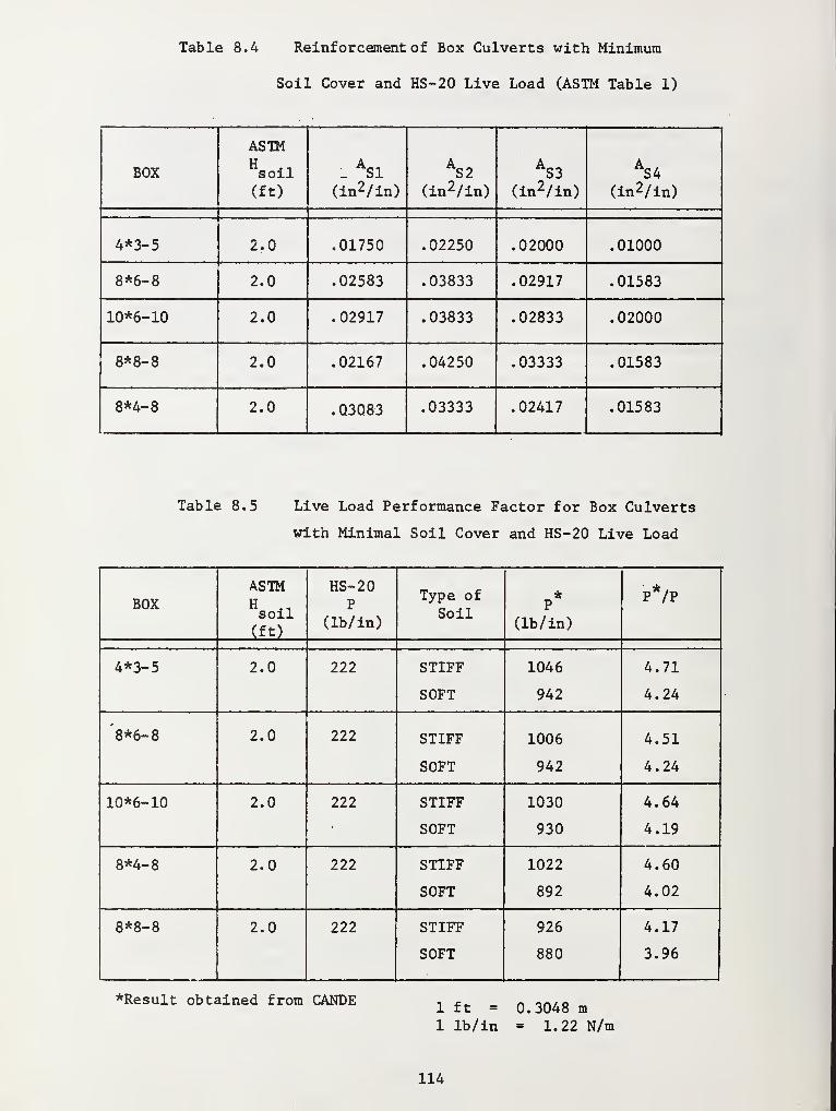
Table 8.4 Reinforcement of Box Culverts with Minimum
Soil Cover and HS-20 Live Load (ASTM Table 1)
BOX
ASTMHsoil(ft)
.Asi
(in2/in)
AS2
(in 2/in)
AS3
(in2/in)
AS4
(in2/in)
4*3-5 2.0 .01750 .02250 .02000 .01000
8*6-8 2.0 .02583 .03833 .02917 .01583
10*6-10 2.0 .02917 .03833 .02833 .02000
8*8-8 2.0 .02167 .04250 .03333 .01583
8*4-8 2.0 .Q3Q83 .03333 .02417 .01583
Table 8.5 Live Load Performance Factor for Box Culverts
with Minimal Soil Cover and HS-20 Live Load
BOXASTMHsoil(ft)
HS-20P
(lb/ in)
Type of
Soil
*P
(lb/in)
P*/P
4*3-5 2.0 222 STIFF
SOFT
1046
942
4.71
4.24
'8*6-8 2.0 222 STIFF
SOFT
1006
942
4.51
4.24
10*6-10 2.0 222 STIFF
SOFT
1030
930
4.64
4.19
8*4-8 2.0 222 STIFF
SOFT
1022
892
4.60
4.02
8*8-8 2.0 222 STIFF
SOFT
926
880
4.17
3.96
*Result obtained from CANDE1 ft = 0.3048 m1 lb/in = 1.22 N/m
114
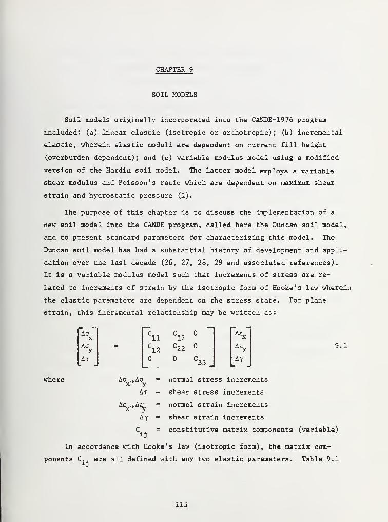
CHAPTER 9
SOIL MODELS
Soil models originally incorporated into the CANDE-1976 program
included: (a) linear elastic (isotropic or orthotropic) ; (b) incremental
elastic, wherein elastic moduli are dependent on current fill height
(overburden dependent); and (c) variable modulus model using a modified
version of the Hardin soil model. The latter model employs a variable
shear modulus and Poisson's ratio which are dependent on maximum shear
strain and hydrostatic pressure (1).
The purpose of this chapter is to discuss the implementation of a
new soil model into the CANDE program, called here the Duncan soil model,
and to present standard parameters for characterizing this model. The
Duncan soil model has had a substantial history of development and appli-
cation over the last decade (26, 27, 28, 29 and associated references).
It is a variable modulus model such that increments of stress are re-
lated to increments of strain by the isotropic form of Hooke's law wherein
the elastic paremeters are dependent on the stress state. For plane
strain, this incremental relationship may be written as:
Aax
Aay
At
11
12
C12 °
Aex
c22 Aey
o c„ ay
9.1
where Aa .,Aa normal stress incrementsx y
At = shear stress increments
Ae .,Ae- = normal strain increments
x yAy shear strain increments
C constitutive matrix components (variable)
In accordance with Hooke's law (isotropic form), the matrix com-
ponents C . . are all defined with any two elastic parameters. Table 9.1
115
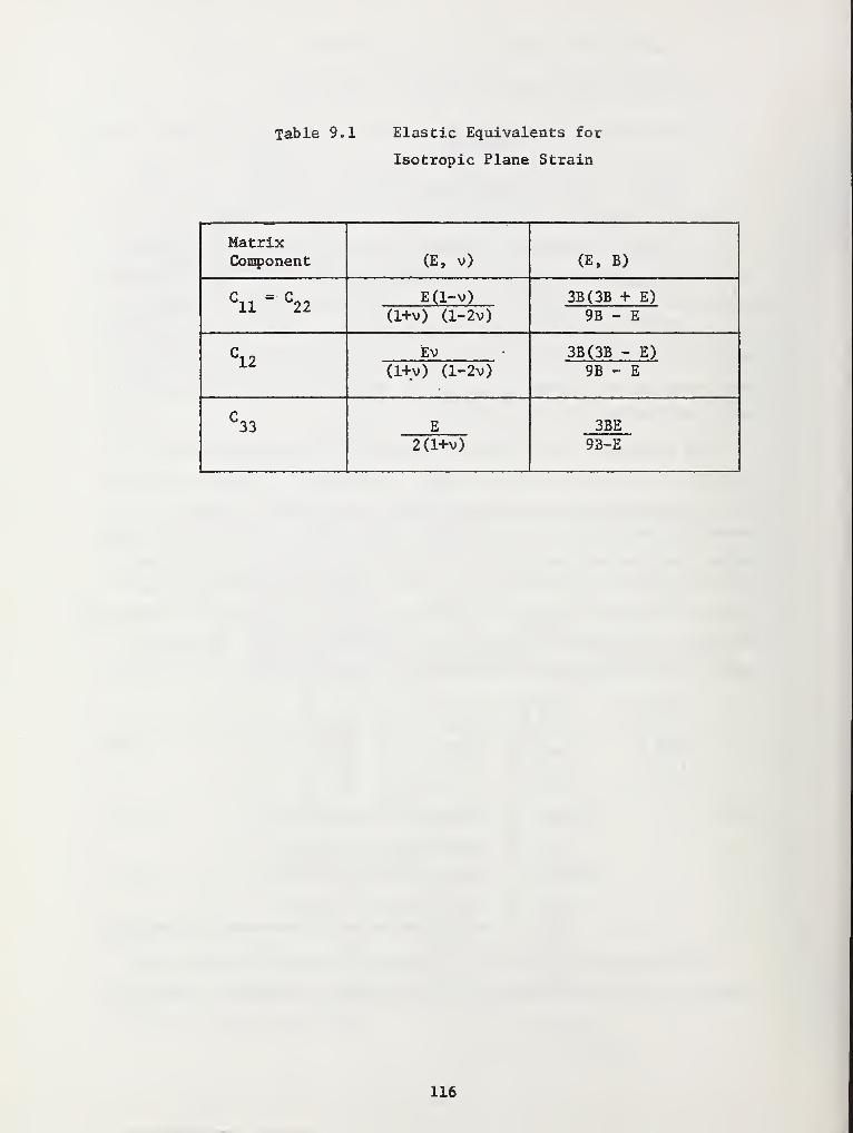
Table 9.1 Elastic Equivalents for
Isotropic Plane Strain
MatrixComponent (E, v) (E, B)
Cll - C
22E(l-v) 3B(3B + E)
9B - E(1+v) (l-2v)
C12
Ev 3B(3B - E)
9B - E(1+v) (l-2v)
C33 E 3BE
93-E2 (1+v)
116
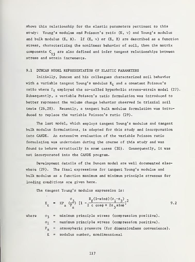
shows this relationship for the elastic parameters pertinent to this
study: Young's modulus and Poisson's ratio (E, v) and Young's modulus
and bulk modulus (E, B) . If (E, v) or (E, B) are described as a function
stress, characterizing the nonlinear behavior of soil, then the matrix
components C.. are also defined and infer tangent relationships between
stress and strain increments.
9.1 DUNCAN MODEL REPRESENTATION OF ELASTIC PARAMETERS
Initially, Duncan and his colleagues characterized soil behavior
with a variable tangent Young's modulus Et and a constant Poisson's
ratio where Fj- employed the so-called hyperbolic stress-strain model (27)
Subsequently, a variable Poisson's ratio formulation was introduced to
better represent the volume change behavior observed in triaxial soil
tests (26,28). Recently, a tangent bulk modulus formulation was intro-
duced to replace the variable Poisson's ratio (29).
The last model, which employs tangent Young's modulus and tangent
bulk modulus formulations, is adopted for this study and incorporation
into CANDE. An extensive evaluation of the variable Poisson ratio
formulation was undertaken during the course of this study and was
found to behave erratically in some cases (30). Consequently, it was
not incorporated into the CANDE program.
Development details of the Duncan model are well documented else-
where (29). The final expressions for tangent Young's modulus and
bulk modulus as a function maximum and minimum principle stresses for
loading conditions are given here.
'The tangent Young's modulus expression is:
a R (l-sin<f>)(a -a )
E = KP (^) [1 - — — -X
. J 9.2t a P 2 c cos<}> + 2a sxn<{>
3. -Jwhere a-j = minimum principle stress (compression positive),
o"! = maximum principle stress (compression positive).
Pa= atmospheric pressure (for dimensionless convenience)
.
K = modulus number, nondimensional
117
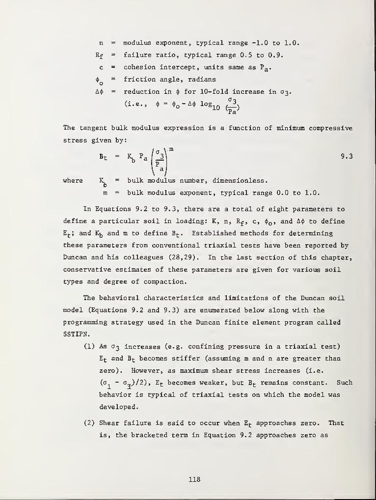
n = modulus exponent, typical range -1.0 to 1.0.
Rf = failure ratio, typical range 0.5 to 0.9.
c = cohesion intercept, units same as Pa .
<j>= friction angle, radians
A<J>= reduction in
<J>for 10-fold increase in 03.
(i.e., 4 -<j) -A(J» log ,_Axu
^Pa'
The tangent bulk modulus expression is a function of minimum compressive
stress given by:
9.3
where K_ = bulk modulus number, dimensionless.
m = bulk modulus exponent, typical range 0.0 to 1.0.
In Equations 9.2 to 9.3, there are a total of eight parameters to
define a particular soil in loading: K, n, Rf, c, <£ , and A<J) to define
Et ; and K^ and m to define Bt . Established methods for determining
these parameters from conventional triaxial tests have been reported by
Duncan and his colleagues (28,29). In the last section of this chapter,
conservative estimates of these parameters are given for various soil
types and degree of compaction.
The behavioral characteristics and limitations of the Duncan soil
model (Equations 9.2 and 9.3) are enumerated below along with the
programming strategy used in the Duncan finite element program called
SSTIPN.
(1) As 03 increases (e.g. confining pressure in a triaxial test)
E t and Bt becomes stiffer (assuming m and n are greater than
zero). However, as maximum shear stress increases (i.e.
(a. - cO/2), Et becomes weaker, but B«- remains constant. Such1 £ u
behavior is typical of triaxial tests on which the model was
developed.
(2) Shear failure is said to occur when Et approaches zero. That
is, the bracketed term in Equation 9.2 approaches zero as
118
a - a increases. If a significant portion of the soil mass
fails in shear, the results may no longer be reliable because
the model is not applicable for soil instability. To avoid
numerical problems, the SSTIPN algorithm arbitrarily limits
the minimum value of the bracketed term in Equation 9.2 to
1 - .95 Rf. Thus, Et does not actually become zero in shear
failure.
(3) Tension failure is said to occur when a 3 becomes tensile. In
such cases the soil stiffness breaks down and cannot carry load.
To cope with this problem, the SSTIPN algorithm computes a small
value for bulk modulus from Equation 9.3 by specifying a /P = 0.13 Si
whenever 03 is tensile. For the second elastic parameter,
Poisson's ratio is arbitrarily assigned the value 0.495 and
Equation 9.2 is ignored. This results in equivalent Young's
modulus whose value is approximately 3% of the bulk modulus.
(4) In addition to the special treatment for shear and tension
failures, the SSTIPN algorithm sets limits on Bt as predicted
from Equation 9.3 dependent on the value of Et from Equation 9.2.
Specifically, Bt = Et/3.0, if Bt is less than this value, and,
Bt = 34.0 Et , if Bt is greater than this value. These limits
correspond to maintaining the equivalent Poisson's ratio within
the range 0.0 to 0.495.
(5) For each load step (e.g. construction increment), the SSTIPN
algorithm utilizes two iterations to determine B^ and Et as
defined above. For the first iteration, the stresses existing
in the element at the end of the previous load step are used
to estimate Bt and Et to obtain approximate stress increments.
The second iteration repeats this solution wherein Bt and Et
are now determined by adding one-half of the stress increments
determined in the first iteration to the previous stress state.
Upon completion of the second iteration, the stresses are accumu-
lated and printed out, and the next load step is considered. No
convergence check is made.
119
(6) When an element first enters the system, the "existing" stress
state used to determine Btand E
fcfor the first iteration is
determined in a special manner depending on whether the element
is part of the initial system (e.g. pre-existing foundation) or
part of a new construction increment. For the case of elements
belonging to the initial system, existing stresses are defined
by the user (input), or if the foundation is composed of hori-
zontal rows, initial stresses can be automatically approximated
by overburden pressure and a lateral coefficient.
Elements belonging to a new construction increment do not
have an existing stress state prior to entering the system.
However in order to evaluate Et and Bt for the first iteration,
the SSTIPN algorithm estimates initial stresses based on element
height, soil density, assumed Poisson's ratio, and humped surface
angle.
(7) According to published reports (28,29), "unloading" of the
Duncan soil model is accomplished by replacing the tangent
Young's modulus function (Equation 9.2) with an unloading
expression; Eu = K Pa , 3vn, where 1^ is an unloading modulus(p )
number whose value is greater than K.
Although this is relatively easy to program, there are
serious theoretical objections to this description of unloading.
Presumably, the criterion for unloading (i.e. switching from
Et to Eu ) is by observing a decrease in maximum shear stress
irrespective of 03. Such a criterion may be sufficient for
load paths where 03 is constant (e.g. triaxial test), however
for more general load paths, serious violations of the contin-
uity principle can occur, i.e., two arbitrarily close load
paths should not result in dramatically different stress-strain
responses.
For this reason, the unloading function is not incorporated
into the CANDE program. Further research on unloading is war-
ranted.
120
9.2 CANDE SOLUTION STRATEGY FOR DUNCAN MODEL
The CANDE algorithm for the Duncan soil model is contained in a
new subroutine called DUNCAN. Here the representation of Et and Bt
(Equations 9.2 and 9.3), shear failure, and tension failure are treated
in a similar fashion to the SSTIPN algorithm discussed in the previous
section. However, there are some significant differences in the CANDE
solution strategy with regard to (a) number of iterations, (b) averaging
Et and Bt over a load step, and (c) treatment of elements entering the
system for the first time. These differences are discussed below.
Iterations . As previously explained, the SSTIPN algorithm uses two
iterations per load step for all loading schedules. Preliminary studies
during this research indicated that using just two iterations can lead
to serious error in predicting E and B even when load increments are
relatively small (e.g. one layer of elements per construction increment).
To deal with this problem, the CANDE algorithm allows the maximum
number of iterations to be specified by the user. During the iteration
process, the current estimate of Et for each element is compared percen-
tage-wise with the previous estimate of Et . *If two succeeding estimates
of Et converge within a specified error tolerance for all elements, the
iteration process is terminated and algorithm advances to the next load
step. Should convergence not be achieved after the specified maximum
number of iterations, a warning message is printed out prior to advancing
to the next load step.
Note, the convergence check is only considered for Et , not Bt .
However, it may be presumed that Bt converges more rapidly than Et
since the former is only a function 03, whereas the latter is a more
sensitive function dependent on a-~ and 03.
Averaging Et and Bt . Equations 9.2 and 9.3 are tangent moduli expressions
for Et and Bt for a particular principle stress state a-^ and 03. As a
load increment is applied, the stress state changes, inferring changes in
Et and Bt. In order to adequately represent the effects of these changes
in Equation 9.1, E and B should represent "average" values over the
load step. This, of course, is the purpose of iteration.
121
One way of obtaining average values is to evaluate Et and Bt based
on the average stress state during the load step as is done in the SSTIPN
algorithm. Alternatively, one may average Et at the beginning of the
load step with E^- at the end of the load step. Likewise for Bt . Speci-
fically, this may be written as:
Eavg
" a-r^'+rtj 9.4
Bavg " (1-r >B
lH' rB
29 - 5
where E , B = E , B at start-of-load-step (known)
E?
, B = E , B at end-of-load-step (iteratively determined)
r = averaging ratio, (generally r = 1/2)
For reasons to be subsequently discussed, the CANDE algorithm employs
the averaging scheme given by Equations 9.4 and 9.5. Comparison studies
between the stress averaging scheme and the moduli averaging scheme were
found to give nearly identical results for r = 1/2.
The averaging ratio r is treated as a material input parameter in
the CANDE program. Generally r = 1/2, however for pre-existing soil
zones, r = 1 permits proper calculation of pre-existing stresses as dis-
cussed next.
Entering Elements . Soil elements enter the structural system in one of
two categories. The first category apply s to pre-existing or in-situ
soil elements in which an initial stress state exists but is unknown.
Elements entering in this category are part of the initial configuration
and belong to the first construction increment.
The second category applys to fill soil elements, i.e., soil layers
added to the system in a predefined construction schedule. Here, the
initial stress state is non-existant prior to entry into the system.
Both categories present special starting problems for the iteration
procedures because the initial stress state is unknown or undefined.
If pre-existing soil zones are to be characterized by the Duncan
soil model, the 'initial stress state can be determined iteratively by
122
assuming the pre-existing soil zone is a construction increment loaded
with its own body weight (and, if desired, a consolidation pressure).
Here the averaging ratio should be set to 1.0, so that, Ea and Ba
are equal to the end-of-load-step values E£ and B2, respectively, and
correspond to the existing stress state. Beginning-of-load-step values
E-l and B^ are initially set to 0.0 when an element enters the system.
However when r = 1, they have no influence on the averaging process.
After the first construction increment is complete, the program auto-
matically sets the value of r to 1/2, so that, all subsequent moduli
calculations represent load step averages.
Elements entering the system in the second category have no initial
stiffness prior to loading so that Ej_ - B]_ = 0. Accordingly, using
r = 1/2 gives average moduli values equal to one-half of the end-of-load-
step values, E and B .
To start the iteration process for entering elements of either
category, some guess must be made for E2 and B2 in order to construct
the first trial stiffness matrix. This is achieved by arbitrarily de-
fining "dummy" principle stresses from which initial estimates of E2
and B2 are calculated. The dummy principle stresses have no effect on
the final values of E2 and B2» however they do influence the number of
iterations for convergence. Once an element has entered the system, the
initial guess for E2 arid B2 for all subsequent load steps are equated
to the last calculated values, thus dummy stresses are not required.
Cande Algorithm . Figure 9.1 is a flow chart of the CANDE algorithm
illustrating the solution strategy previously described. Some of the
limit bounds are defined differently than in the SSTIPN algorithm. For
example, the maximum equivalent Poisson ratio, vmax , is set at 0.48
rather than 0.495 in order to avoid unreasonably high values of C in
Equation 9.1. Also, the shear failure factor (1-D) is assigned a lower
limit of 0.05, rather than 1-0.95 Rf in order to provide a greater re-
duction of stiffness in shear failure.
123
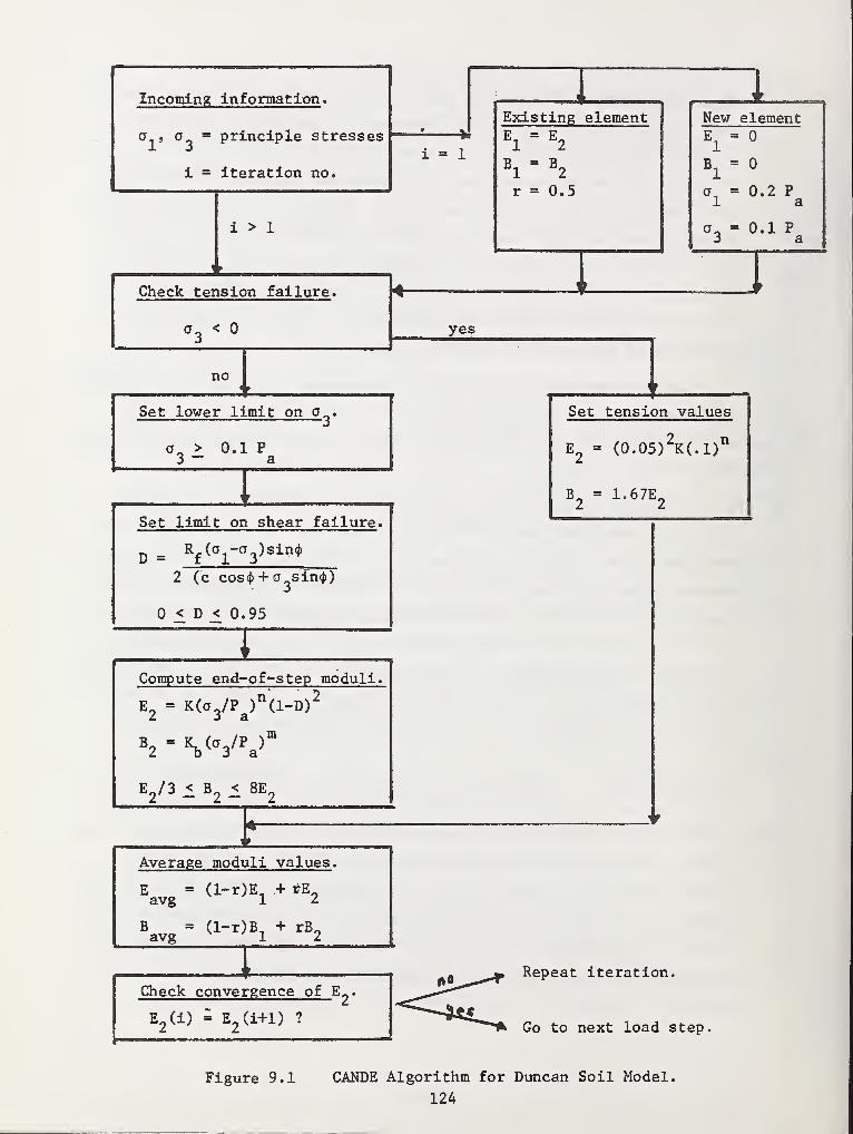
Incoming information,
a , a - principle stresses
i = iteration no.
i '/
Existing element New elementE =
Bi = °
a, = 0.2 P1 a
E1= E
2
B1= B
2
r = 0.5
i = 1
i > 1
>
a3= 0.1 P
a
.._ „. } 1
Check tension failure.
a3
<
t w I
yes
i
no< * )
Set lower limit on a . Set tension values
a > 0.1 P3 - a
E2
= (0.05)2K(.l)
n
B2
= 1.67E* f
Set limit on shear failure.
D = Rf
(a1"a
3) sin<J
)
2 (c cos<j) + a sin<j>)
< D <_ 0.95
' t
Compute end-of'-step moduli.
E, = K(a./P )n(l-D)
2
i j a.
B2 =VW
E2/3 £ B
2< 8E
2
' f
<k
1 *
Average moduli values.
E = (l-r)E. + rE.avg 1 2
B = (l-r)Bn+ rB„
avg 1 2
.... . _ .. 1*
fl ^-y RePeat iteration.
Check convergence of E„.
E2(i) = E
2(i+1) ? "^-si*c
A Go to next loac [ step.
Figure 9.1 CANDE Algorithm for Duncan Soil Model.
124
Two additional features of the CANDE algorithm not shown in Figure 9.1
are; (1) an under relaxation scheme to improve the rate of convergence
for E2, and (2) a constant Poisson ratio option which replaces the tangent
bulk modulus formulation.
The under relaxation scheme comes into play after the second iteration
wherein each estimate of E£ is a weighted average of the current estimate
and the previous estimate. This feature takes advantage of the observation
that E2 generally converges in an oscillatory manner.
When the constant Poisson ratio option is exercised, all references
to the bulk modulus formulation are bypassed. Otherwise, the algorithm
is essentially the same.
9.3 STANDARD HYPERBOLIC PARAMETERS
Whenever possible, the hyperbolic parameters characterizing the
Duncan soil model should be determined directly from triaxial tests
using established curve-fitting procedures (28,29). In many instances,
however, triaxial data may be unavailable, and so, it is convenient to
establish "standard" parameter values for various types of soil and
degrees of compaction. Table 9.2 (abstracted from Reference 29) provides
parameter values for four soil classifications, each with three levels
of compaction. These "standard" values are conservative in the sense
that they are typical of lower values of strength and moduli observed
from numerous triaxial tests for each soil type. An independent study (30)
to establish standard parameters for Et utilizing the same data base is
in good agreement with Table 9.2.
For convenience, the hyperbolic parameters in Table 9.2 are stored
in CANDE and may be used by simply identifying soil type and level of
compaction.
The behavior of the Duncan soil model for simulated uniaxial strain
and triaxial loading tests is shown in Figures 9.2 through 9.5 for the
standard parameters in Table 9.2. Specifically, Figure 9.2a shows axial
stress vs. axial strain in confined compression for three compaction
levels of coarse aggregates. The slope of these curves is the tangent
125
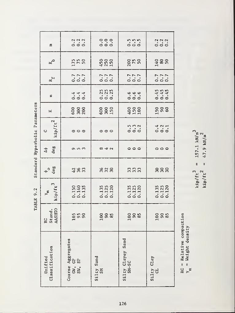
CO5-i
CD
4-1
CD
6CO
5-i
CO
Pi
OX>5-i
0)
a
T35-1
CO
§4-1
CO
CM
w
B
CN CN CM...o o o
o o o• • •
o o om m mdod
CM CM CM• • •
o o o
*f°m m or*» r^ mH
o o om m m<r cm iH
o m oo r>» mCM
o o o<t co mrH
14-1
Pi
r— r~^ r^
CD CD or— r^* r—
~
d o dr>. f*. r»
• • •
o o or» r>« r-.
odd
csr -a- -d-
• • •
o o o
m m mCN CM CM
• • •
o o ovO vO vO...o o o
m m m-si- < -a-
odd
wo o oo o oVO CO CM
o o oo o mvO CO rH
o o oo m o•vT rH rH
o o om o> \oH
CN4-1
<4-l
•Ho o o o o o
m co cn
odd•J- CM rH
• •
O O O
-e-M
< 3ci in co co «<r cm o o o o o o
o M CM vO CO<f CO en
^O CN OCO CO CO
CO CO COCO CO CO
o o oCO CO CO
CO4-1
e £•HJ*
0.150 0.140 0.135 0.135 0.125 0.120 0.135 0.125 0.120 0.135 0.125 0.120
RC
Stand.AASHTO
m m oO Q\ o\iH
o o mO C\ COo o mO CJ\ 00rH
o o mo o\ COrH
Unified
Classification
Coarse
Aggregates
GW,
GP
SW,
SP
Silty
Sand
SM
Silty
Clayey
Sand
SM-SC
Silty
Clay
CL
CO6 CM
rsS32
rH <T
II II
CO CM4-1 4J4-1 <4-(
a a,•H -H
co•H4-1
CJ
(0 >>
8-4-1
•Ho CO
CJ c<D
CD T3>•H 4-1
4-1 ,fl
CO 00rH •HCD CD
pej rs
II ii
CJ 6PS >-
126
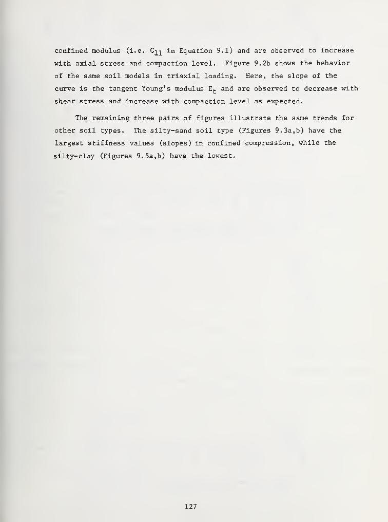
confined modulus (i.e. C-q in Equation 9.1) and are observed to increase
with axial stress and compaction level. Figure 9.2b shows the behavior
of the same soil models in triaxial loading. Here, the slope of the
curve is the tangent Young's modulus Et and are observed to decrease with
shear stress and increase with compaction level as expected.
The remaining three pairs of figures illustrate the same trends for
other soil types. The silty-sand soil type (Figures 9.3a,b) have the
largest stiffness values (slopes) in confined compression, while the
silty-clay (Figures 9.5a,b) have the lowest.
127
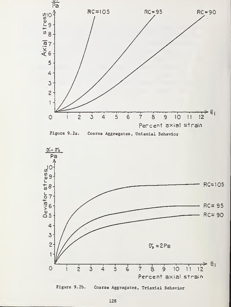
RC = 90
Figure 9.2a.
8 9 10
Percent axial strain
Coarse Aggregates, Uniaxial Behavior
12
tf-ft
- RC=105
5 6 7 8 9 10 11 12
Percent axial strain
Figure 9.2b. Coarse Aggregates, Triaxial Behavior
128
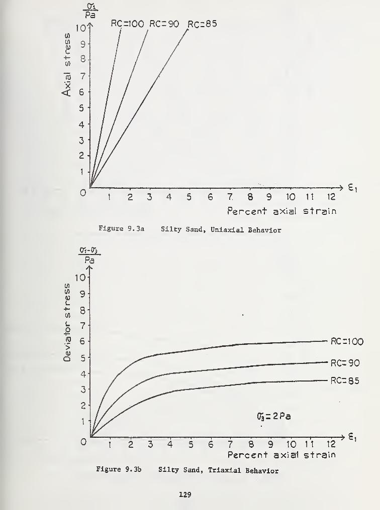
PaRCzlOO RC=90 RCi85
£4-(/)
x<
» £7 8 9 10 11 12
Percent axial strain
Figure 9.3a Silty Sand, Uniaxial Behavior
gj-ft
7 8 9 10 11 12
Percent axial strain
Figure 9.3b Silty Sand, Triaxial Behavior
129
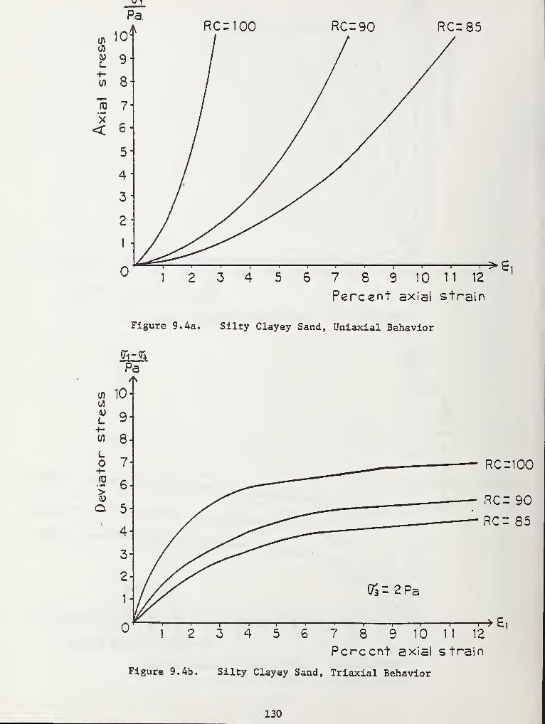
RC=90 RC=85
7 8 9 10 11 12
Percent axial strain
Figure 9.4a. Silty Clayey Sand, Uniaxial Behavior
<fl 10
RC-100
Figure 9.4b,
7 8 9 10
Percent axial strain
Silty Clayey Sand, Triaxial Behavior
130
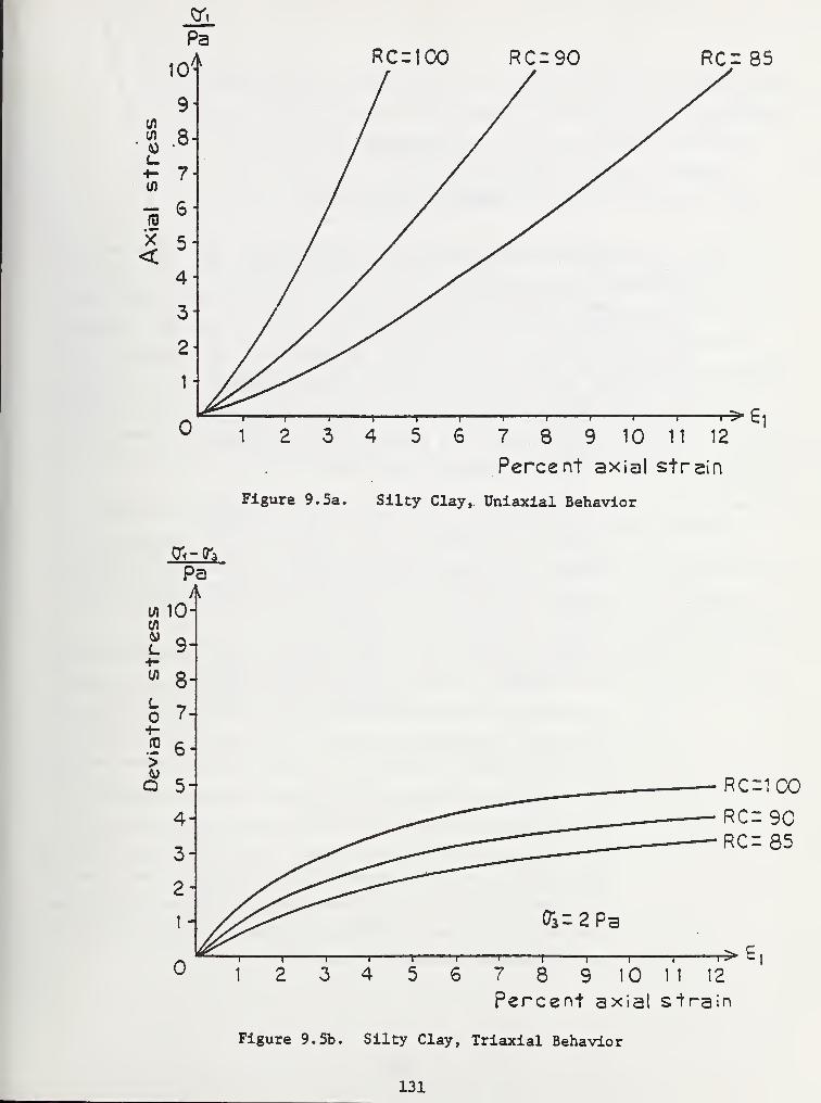
RC= 85
>6i
Percent axial strain
Figure 9.5a. Silty Clay, Uniaxial Behavior
o;-(r3
Percent axial strain
Figure 9.5b. Silty Clay, Triaxial Behavior
131
CHAPTER 10
SUMMARY AND CONCLUSIONS
This report presented a step by step development for the structural
analysis of buried, precast reinforced concrete box culverts using the
finite element method to model the soil-box system. Model predictions
were validated with measured data from both in-ground and out-of-ground
experimental tests. A user oriented soil-box model with automated finite
element mesh generation is operational in the CANDE-1980 computer program
and is referred to as "level 2 box" option. Also operational in CANDE-1980
is the Duncan soil model with simplified input options for standard types
of soil. Specific findings and conclusions from this work are listed below,
1. Load-deformation curve predictions for reinforced concrete
culverts are sensitive to the cracking strain parameter e .
However at ultimate flexural capacity, the maximum stresses of
concrete f and steel fy are the controlling parameters with
regard to the reinforced concrete model.
2. CANDE predictions are in good agreement with experimental data
from reinforced concrete pipes in three-edge bearing. Better
correlation for load-deformation curves was observed for pipes
failing by flexure than by shear. Predicted ultimate loads,
whether in shear or flexure, are within 10% of measured values.
3. The measured cracking load and ultimate load for reinforced
concrete box culverts tested in four-edge bearing show good
correlation with CANDE predictions. Predicted cracking loads
averaged 10% lower and ultimate loads averaged 1% lower than
experimental results. Predictions from the SGH design/analysis
approach are similar to CANDE predictions but showed slightly
more deviation from experimental data.
132
A. Measured soil pressures from a full scale burled box installation
are in good agreement with CANDE predictions at both intermediate
and final burial depths. Vertical soil pressures on top and
bottom slabs were in very close agreement, whereas measured
lateral pressures on the sides at full burial depth were some-
what lower than predicted.
5. Assumed soil load distributions on buried boxes used in the
development of ASTM C789 design tables were compared with pre-
dicted soil load distributions determined from CANDE resulting
in the following observations. (a) Vertical soil pressure on
the top and bottom slabs are not uniform as assumed but increases
monitonically from the centerline to the corners. (b) Shear
traction on the sidewalls produces a significant downward force
that must be equilibrated by an upward pressure on the bottom slab.
(c) Soil stiffness is an important parameter for determining soil
load distributions and magnitudes. The latter two effects are not
presently taken into account in the ASTM loading assumptions.
6. Based on CANDE predictions, the design earth covers specified in
ASTM C789 design tables are generally conservative providing
good quality backfill soil is assumed. However, specified earth
covers for boxes with high levels of reinforcement tend to be
less conservative than specified earth covers for boxes with low
levels of reinforcement.
133
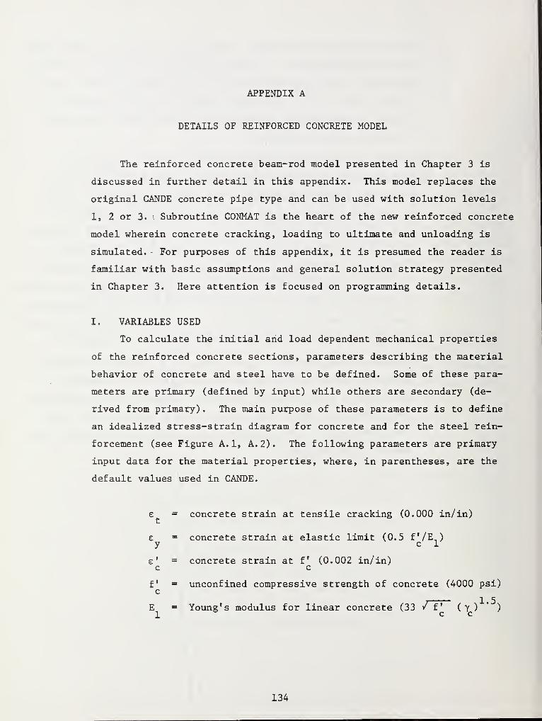
APPENDIX A
DETAILS OF REINFORCED CONCRETE MODEL
The reinforced concrete beam-rod model presented in Chapter 3 is
discussed in further detail in this appendix. This model replaces the
original CANDE concrete pipe type and can be used with solution levels
1, 2 or 3. ; Subroutine CONMAT is the heart of the new reinforced concrete
model wherein concrete cracking, loading to ultimate and unloading is
simulated. - For purposes of this appendix, it is presumed the reader is
familiar with basic assumptions and general solution strategy presented
in Chapter 3. Here attention is focused on programming details.
I. VARIABLES USED
To calculate the initial and load dependent mechanical properties
of the reinforced concrete sections, parameters describing the material
behavior of concrete and steel have to be defined. Some of these para-
meters are primary (defined by input) while others are secondary (de-
rived from primary) . The main purpose of these parameters is to define
an idealized stress-strain diagram for concrete and for the steel rein-
forcement (see Figure A. 1, A. 2) . The following parameters are primary
input data for the material properties, where, in parentheses, are the
default values used in CANDE.
e = concrete strain at tensile cracking (0.000 in/in)
e = concrete strain at elastic limit (0.5 f'/E,
)
y c 1
e' = concrete strain at f (0.002 in/in)c c
f = unconfined compressive strength of concrete (4000 psi)c
E = Young's modulus for linear concrete (33 vf 1 (y) "
)
1 c c
134
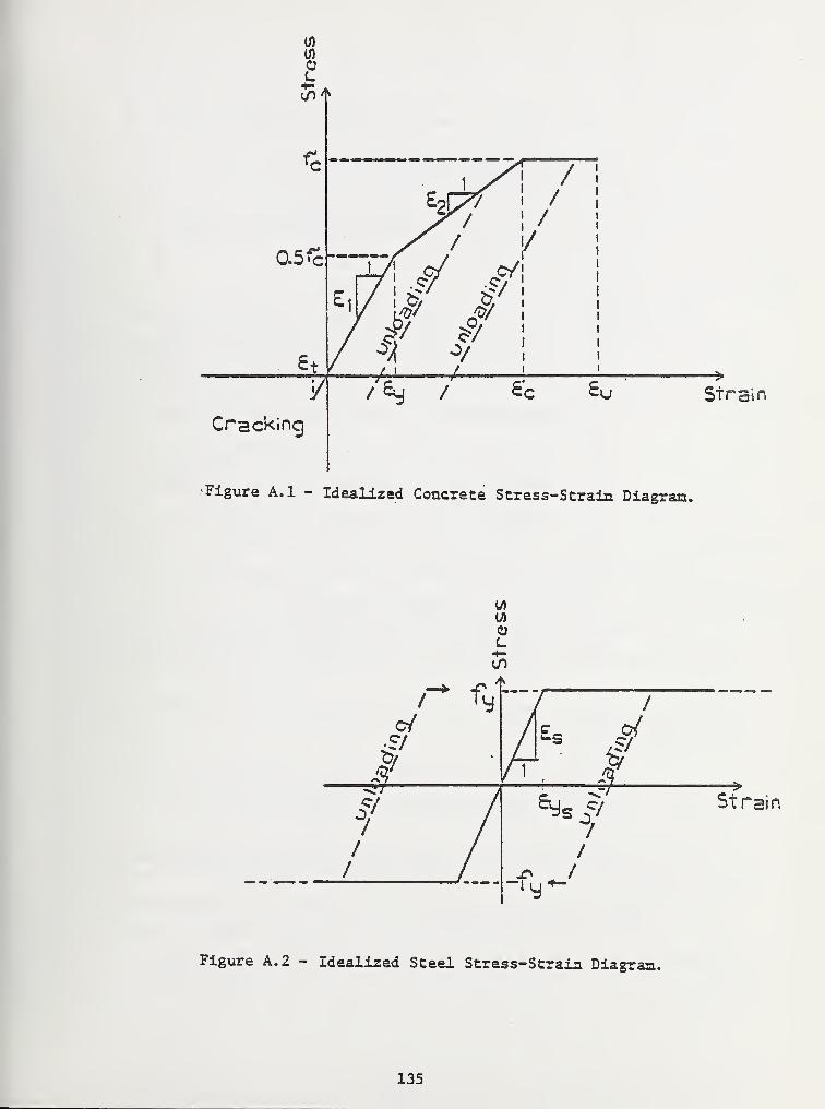
Strain
Cracking
Figure A.l - Idealized Concrete Stress-Strain Diagram.
00
0/% /
5/
f/
/
7/
#Strain
Figure A. 2 - Idealized Steel Stress-Strain Diagram.
135
v = Poisson's ratio for concrete (0.17)c
Y = unit weight of concrete (150 pcf)c
f = yield stress of steel (40000 psi)
E = Young's modulus of steel (29 x 10 psi)o
v = Poisson's ratio of steel (0.30)s
The following are secondary parameters derived from primary data:
2E = confined elastic modulus of concrete (E /(1-v )c 1 c
v = shear strength of concrete (2/ f ' psi)c c
f = maximum tensile stress of concrete (e x E )
f = concrete stress at elastic limit (e x E.,
)
yc y 1
2E = confined elastic modulus of steel (E /(1-v )s osn = concrete-to-steel modulus ratio (E /E )
c s
In addition, the analysis mode requires (see Figure A. 4):
h = wall thickness of concrete (in)
As. = area of inner reinforcement per unit length of pipe
(in /in)2
As^ = area of outer reinforcement per unit length of pipe
(in /in)2
c. = concrete cover on inner reinforcement (1.25 in)
c = concrete cover on outer reinforcement (1.25 in)o
Using these parameters the initial uncracked section properties are
defined as:
Effective axial stiffness:
EA* = E (h + (n-1) As. + (n-1) As )C X o
136
Neutral axis of bending:
2
_ (7- + As.(n-l)c. + As (n-l)(h-c ))y = E 2 x 1 o o
c_
EA
Effective bending stiffness:
3
EI* = E [yr + (£ - y)2h + (n-1) (As.(c.-y)
2+ A (h-c-y) 2
]c LI I 11 so o
The above section properties EA , y and EI are for the uncracked
cross section of 1 inch width with no loading. Now that the initial
stiffnesses of the beam-rod sections are defined, the beam-rod elements
are ready to be analyzed for the first load increment.
II. PROCEDURE TO CALCULATE THE SECTION PROPERTIES
Using the initial section properties above, the structural system
is solved for the first load increment resulting in trial solutions for
thrust and moment increments within each element. Due to the non-linearity
of the materials, the initially assumed section properties are modified
and another trial solution is obtained. This iterative solution technique,
which considers the average stress state during the increment to find
effective section properties, is repeated until convergence within the
load step is achieved.
CONMAT subroutine evaluates EA, y, and EI for each element until
all elements converge as the system advances from load step i-1 to load
step i. The procedure used for each load step is as follows:
a) For each element an increment of moment and thrust is obtained
from the general solution process. If a section initially cracks or
extends its crack, the stresses in the newly cracked region are zero,
thus, the pre-existing stresses prior to cracking must be redistributed.
This redistribution can be achieved with corrections to the thrust and
moment increment (called here thrust and moment redistribution). In
our approach this correction is made after the inner loop convergences,
so that, initially, moment and thrust redistribution is zero (see step h
137
for redistribution).
* _ *b) Assuming the section properties EA , y, and EI from the con-
verged solution at load increment i-1 and using the increment of moment
and thrust, a linear strain distribution for the section is calculated
(see Figure A. 3).
, AN , AM ,-• '
ei
= ei-i
+ m* +ei* (y"y)
where
e .
1= strain distribution from converged solution at load
increment i-1
AN = increment of thrust + (thrust redistribution, last
iteration)
AM = increment of moment + (moment redistribution, last
iteration)
y = spatial coordinate from section bottom.
This linear strain distribution e. is the first tentative solution1
of the iterative procedure.
For computational convenience, the section stiffness properties of
EA and EI (defined in Chapter 3) are divided by the confined-elastic* *
concrete modulus E , so that we may define A and I as:c
it *A = EA /E* * c
I = EI /Ec
Or more explicity, to obtain section properties the following integrals
must be evaluated (see Figure A. 4):
A = FE(y) dy + WSI (n-1) A +(WSO)(n-l) AgQ
' o
rh
o
FE(y) y dy + WSI (n-1) y . A . + WSO (n-1) y fcAJ ' J * ti si to so
A
I* = FE(y)(y-y)2dy + WSI(n-l) (y^-y)^. + WSO (n-1 ) (y^-?)^
138
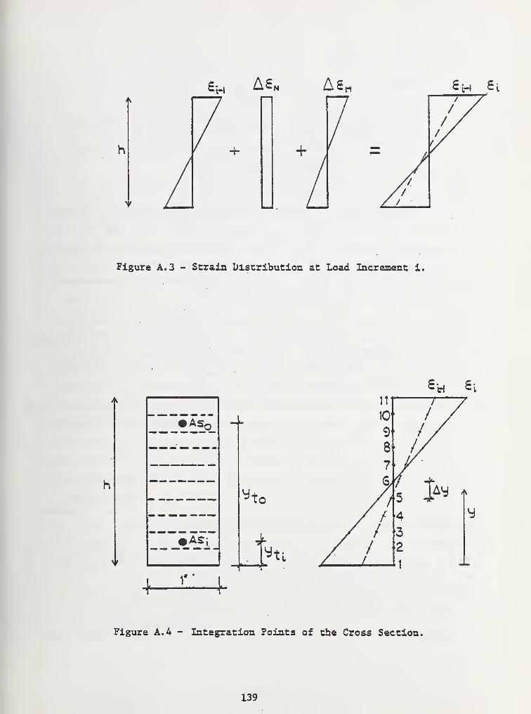
s-h A£ n n 6rl Si
+
Figure A. 3 - Strain Distribution at Load Increment i.
•AS,
»AS;
«t,
yti
4—X^4
Figure A. 4 - Integration Points of the Cross Section.
139
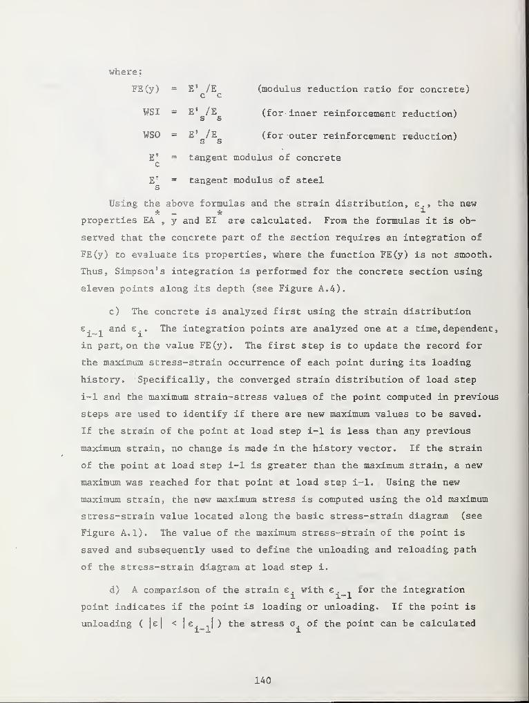
where:
FE(y) = E" /E (modulus reduction ratio for concrete)c c
WSI = E' /E (for inner reinforcement reduction)
WSO - E' /E (for -outer reinforcement reduction)s s
E' - tangent modulus of concretec
E' = tangent modulus of steels
Using the above formulas and the strain distribution, e . , the new
properties EA , y and EI are calculated. From the formulas it is ob-
served that the concrete part of the section requires an integration of
FE(y) to evaluate its properties, where the function FE(y) is not smooth.
Thus, Simpson's integration is performed for the concrete section using
eleven points along its depth (see Figure A. 4).
c) The concrete is analyzed first using the strain distribution
e . _ and £.. The integration points are analyzed one at a time, dependent,
in part, on the value FE(y). The first step is to update the record for
the maximum stress-strain occurrence of each point during its loading
history. Specifically, the converged strain distribution of load step
i-1 and the maximum strain-stress values of the point computed in previous
steps are used to identify if there are new maximum values to be saved.
If the strain of the point at load step i-1 is less than any previous
maximum strain, no change is made in the history vector. If the strain
of the point at load step i-1 is greater than the maximum strain, a new
maximum was reached for that point at load step i-1. Using the new
maximum strain, the new maximum stress is computed using the old maximum
stress-strain value located along the basic stress-strain diagram (see
Figure A.l). The value of the maximum stress-strain of the point is
saved and subsequently used to define the unloading and reloading path
of the stress-strain diagram at load step i.
d) A comparison of the strain e . with e .
1for the integration
point indicates if the point is loading or unloading. If the point is
unloading ( |e| <|e J ) the stress a of the point can be calculated
140
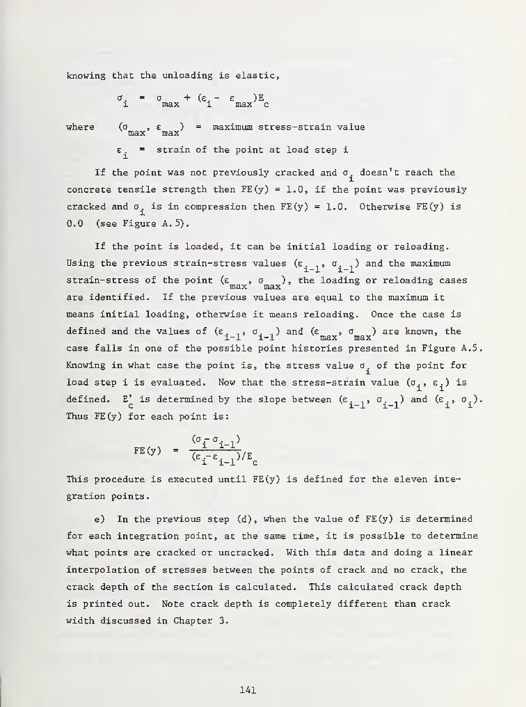
knowing that the unloading is elastic,
a . = o + (e. - e )E1 max 1 max c
where (a , e ) = maximum stress-strain valuemax max
e . = strain of the point at load step i
If the point was not previously cracked and a. doesn't reach the
concrete tensile strength then FE(y) = 1.0, if the point was previously
cracked and a. is in compression then FE(y) = 1.0. Otherwise FE(y) is
0.0 (see Figure A. 5).
If the point is loaded, it can be initial loading or reloading.
Using the previous strain-stress values (e . , a. ) and the maximum
strain-stress of the point (e , a ) , the loading or reloading casesmax max
are identified. If the previous values are equal to the maximum it
means initial loading, otherwise it means reloading. Once the case is
defined and the values of (e . ,, a. ,) and (e , a ) are known, thex-1 l-l max max
case falls in one of the possible point histories presented in Figure A. 5.
Knowing in what case the point is, the stress value a. of the point for
load step i is evaluated. Now that the stress-strain value (a., e.) is11defined. E' is determined by the slope between (e . n , a. .) and (e . , a.).
c l-i 1-1 1 1
Thus FE(y) for each point is:
1 1-1 c
This procedure is executed until FE(y) is defined for the eleven inte-
gration points.
e) In the previous step (d), when the value of FE(y) is determined
for each integration point, at the same time, it is possible to determine
what points are cracked or uncracked. With this data and doing a linear
interpolation of stresses between the points of crack and no crack, the
crack depth of the section is calculated. This calculated crack depth
is printed out. Note crack depth is completely different than crack
width discussed in Chapter 3.
141
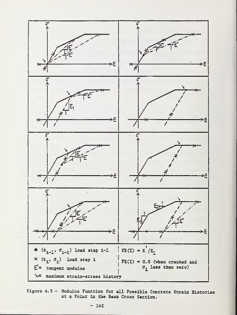
7 >S
* (e^* cr^) load step i-1 | FE(I)
X ^Ci* °i^
load step i FE(I)Ei Is tangent modulus i
\= maximum strain-stress history
E (Z^
0.0 (vhen cracked anda. less than zero)
Figure A. 5 - Modulus Function for all Possible Concrete Strain Historiesat a Point in the Beam Cross Section.
- 142
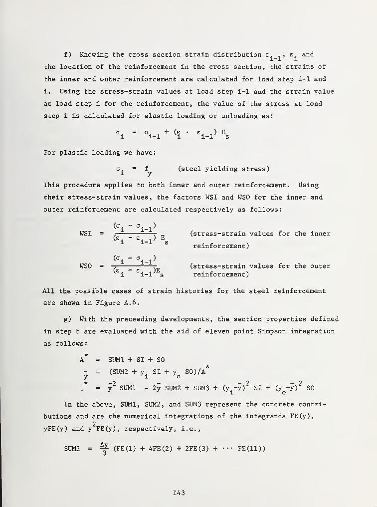
f) Knowing the cross section strain distribution £•_-]» e - an^
the location of the reinforcement in the cross section, the strains of
the inner and outer reinforcement are calculated for load step i-1 and
i. Using the stress-strain values at load step i-1 and the strain value
at load step i for the reinforcement, the value of the stress at load
step i is calculated for elastic loading or unloading as:
o . = a . - + (e - e . ) Ei l-l 1 i-I s
For plastic loading we have:
a. = f (steel yielding stress)
This procedure applies to both inner and outer reinforcement. Using
their stress-strain values, the factors WSI and WSO for the inner and
outer reinforcement are calculated respectively as follows
:
(ai
~ ai-l }
WSI = , r (stress-strain values for the inner<e
i" E
i-1>Es
reinforcement
)
(°i " ?i-l )
WSO = —(
r (stress-strain values for the outeri i-l s reinforcement)
All the possible cases of strain histories for the steel reinforcement
are shown in Figure A. 6.
g) With the preceeding developments, the section properties defined
in step b are evaluated with the aid of eleven point Simpson integration
as follows:
A = SUM1 + SI + SO
- = (SUM2 + y. SI + y SO)/Ay xoi* = y
2sumi - 2y sum2 + SUM3 + (y^-y)
2si + (y
Q-y) SO
In the above, SUMI, SUM2, and SUM3 represent the concrete contri-
butions and are the numerical integrations of the integrands FE(y),2
yFE(y) and y FE(y), respectively, i.e.,
SUMI - 4? (FE(1) + 4FE(2) + 2FE(3) + ••• FE(ll))
143
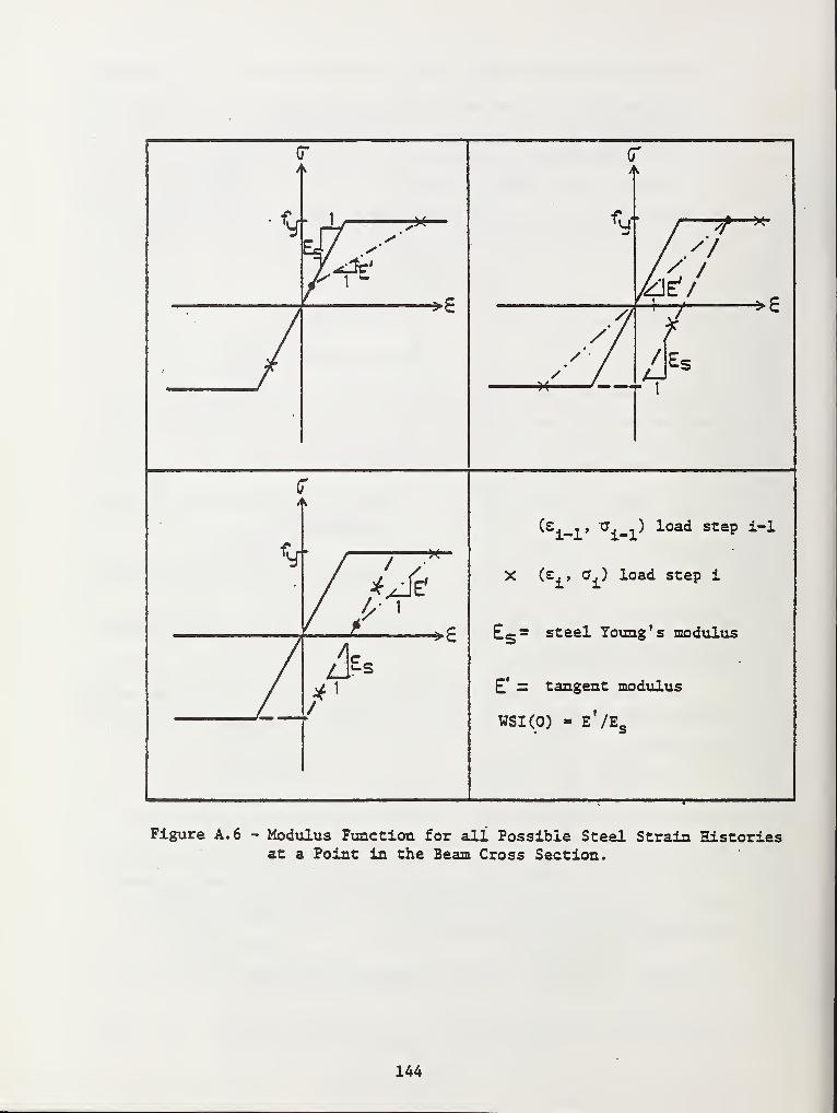
(£. ,, "O^i) l°a<i step i-1
X (Sj, <7.) load step i
Ee= steel Young's modulus
E* = tangent modulus
wsi(o) - eVe_
Figure A. 6 - Modulus Function for all Possible Steel Strain Historiesat a Point in the Beam Cross Section.
144
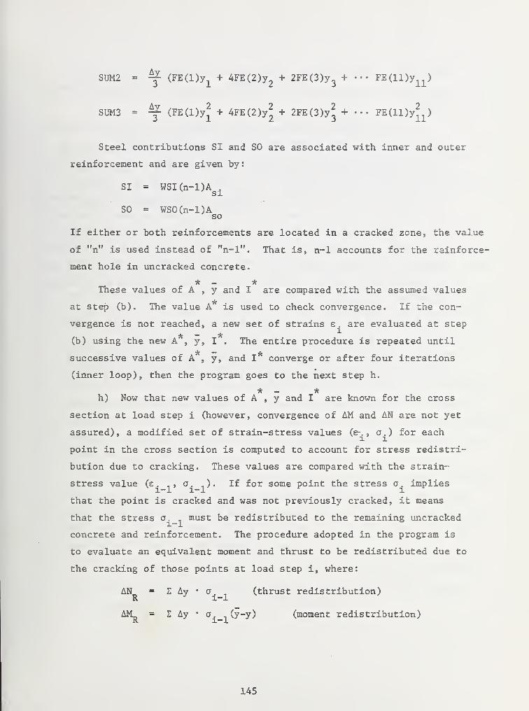
SUM2 = 4^ (FE(l)y + 4FE(2)y2+ 2FE(3)y
3+ ••• FE(ll)y )
SUM3 = 4f (FE(l)y? + 4FE(2)yJ + 2FE(3)y^ + ••• FE(ll)y^)
Steel contributions SI and SO are associated with inner and outer
reinforcement and are given by:
SI = WSI(n-l)A .
si
SO = WSO(n-l)Aso
If either or both reinforcements are located in a cracked zone, the value
of "n" is used instead of "n-1". That is, n-1 accounts for the reinforce-
ment hole in uncracked concrete.
* _ *These values of A , y and I are compared with the assumed values
at step (b). The value A is used to check convergence. If the con-
vergence is not reached, a new set of strains e. are evaluated at step
(b) using the new A , y, I . The entire procedure is repeated until•A* mm J-
successive values of A , y, and I converge or after four iterations
(inner loop), then the program goes to the next step h.
h) Now that new values of A , y and I are known for the cross
section at load step i (however, convergence of AM and AN are not yet
assured), a modified set of strain-stress values (e-. , a.) for each
point in the cross section is computed to account for stress redistri-
bution due to cracking. These values are compared with the strain-
stress value (e. ,, a. ,). If for some point the stress a. impliesl-l l-l i
that the point is cracked and was not previously cracked, it means
that the stress a. must be redistributed to the remaining uncracked
concrete and reinforcement. The procedure adopted in the program is
to evaluate an equivalent moment and thrust to be redistributed due to
the cracking of those points at load step i, where:
AN = Z Ay • a (thrust redistribution)
AM^ = Z Ay * o (y-y) (moment redistribution)
145
After the moment and thrust redistribution is complete the program is
ready to go to step (a) and do the same procedure for the next element
(node)
.
i) All elements of the reinforced concrete structure are analyzed4c
—4c
and the values of A , y, I , ANR and AM are calculated for each one.
4c~
If the values of A and y obtained for every element converge with the
ones obtained in the previous iteration and AN , AM are zero for allR R
the nodes, the trial solution has converged. Otherwise, the system is
* °" 4c
solved again using the values of A , y and I from the last iteration.
This is called "inner loop" iteration. Once the inner loop converges,
the section properties, EA , y, EI , are used to get another solution to
the entire soil-structure system. This gives new values for AM and AN
to repeat the inner loop. Successive solutions for AM and AN is called
outer loop iteration.
Outer loop iteration is repeated until a convergence is reached
between successive solutions for AM and AN. If convergence is not
reached after six trial response solutions, the program assumes the
last one as an approximate solution and advances to next load step.
146
APPENDIX B
CANDE-1980: USER MANUAL SUPPLEMENT
The following user's guide is a supplement to the 1976 "CANDE USER
MANUAL" (2). This supplement provides input instructions for the new
options on reinforced concrete box culverts and Duncan soil model described
in the main body of this report.
The original 1976 manual is still the principal reference source and
may be used without reference to this supplement if the new options are
not desired. Taken together, the original and new options form the program
called CANDE-1980. Input instructions for CANDE-1980 follows the same
pattern as the original program, composed of three main sections (A,B, and
C) as shown in Figure B.l, where new options are marked with an asterisk.
Section A is the master control input (card 1A) and is unchanged from
the original program. Section B (cards IB to 3B) includes a new input
option for modeling reinforced "concrete box" culverts in addition to
the original pipe types. The "concrete box" culvert type is only operative
in the analysis mode and cannot be used with solution level 1. Section C
(card sets C and D) includes the new "level 2 box" finite element generation
scheme discussed in Chapter 6 along with the new Duncan soil model option
presented in Chapter 9.
The supplemental input instructions to be given here provide a complete
set of data input for the subset of options shown in Figure B.2. Thus,
these instructions are self contained for "level 2 box" solutions with any
soil model. For extended level 2 and level 3 options, however, the 1976
user manual must also be used where noted.
Formatted input instructions for Sections A, B, and C are presented
in order, followed by explanatory comments and illustrations. Example
input-output data is given in the next appendix.
147
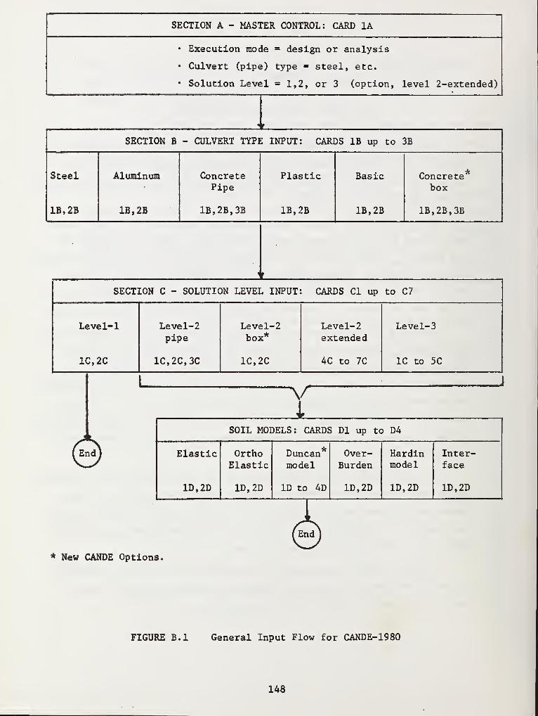
SECTION A - MASTER CONTROL: CARD 1A
• Execution mode = design or analysis
• Culvert (pipe) type steel, etc.
• Solution Level = 1,2, or 3 (option, level 2-extended)
SECTION B - CULVERT TYPE INPUT: CARDS IB up to 3B
Steel
1B,2B
Aluminum
1B,2B
ConcretePipe
1B,2B,3B
Plastic
1B,2B
Basic
1B,2B
Concretebox
1B,2B,3B
SECTION C - SOLUTION LEVEL INPUT: CARDS CI up to C7
Level-1
1C,2C
Level-
2
pipe
1C,2C,3C
Level-2box*
1C,2C
Level-2extended
4C to 7C
Level-3
1C to 5C
"V
(End)
iSOIL MODELS: CARDS Dl up to D4
Elastic
ID, 2D
OrthoElastic
ID, 2D
itDuncanmodel
ID to 4D
Over-Burden
ID, 2D
Hardinmodel
ID, 2D
Inter-face
ID, 2D
* New CANDE Options.
FIGURE B.l General Input Flow for CANDE-1980
148
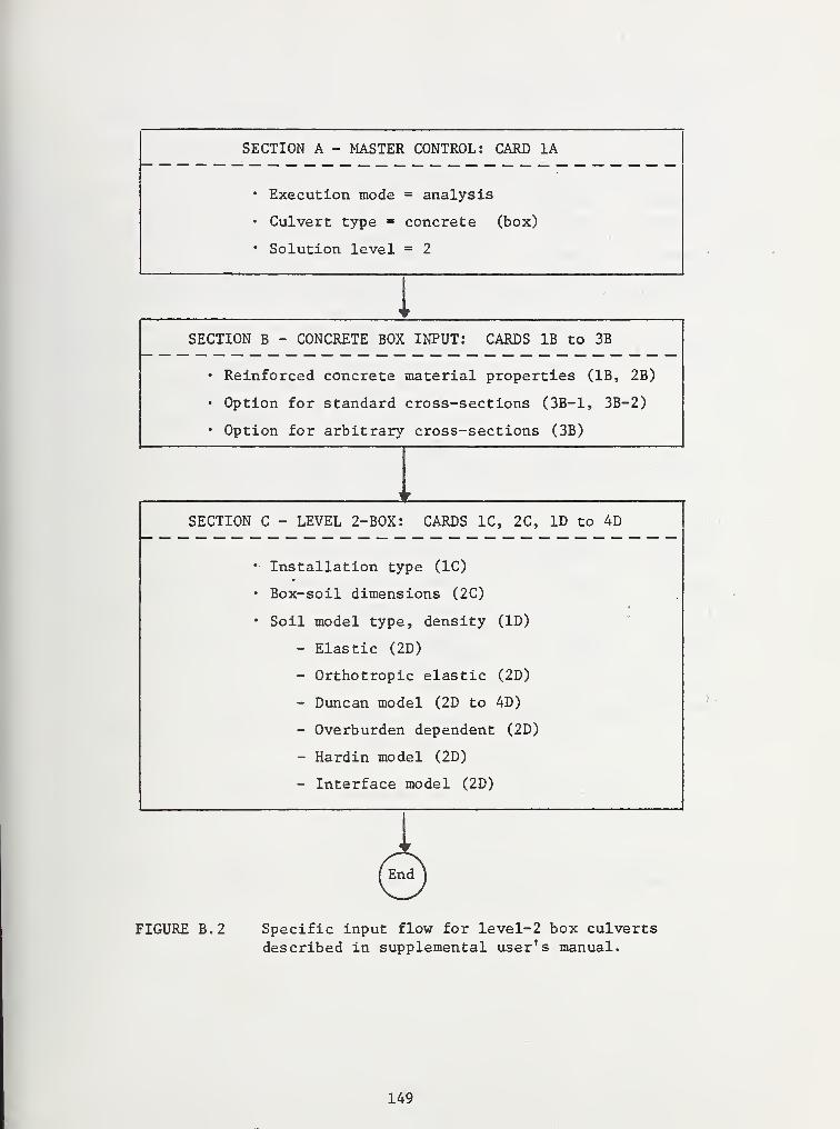
SECTION A - MASTER CONTROL: CARD 1A
• Execution mode = analysis
• Culvert type = concrete (box)
• Solution level = 2
SECTION B - CONCRETE BOX INPUT: CARDS IB to 3B
• Reinforced concrete material properties (IB, 2B)
• Option for standard cross-sections (3B-1, 3B-2)
• Option for arbitrary cross-sections (3B)
SECTION C - LEVEL 2-BOX: CARDS 1C, 2C, ID to 4D
• Installation type (1C)
• Box-soil dimensions (2C)
• Soil model type, density (ID)
- Elastic (2D)
- Orthotropic elastic (2D)
- Duncan model (2D to 4D)
- Overburden dependent (2D)
- Hardin model (2D)
- Interface model (2D)
FIGURE B.2 Specific input flow for level-2 box culverts
described in supplemental user's manual.
149
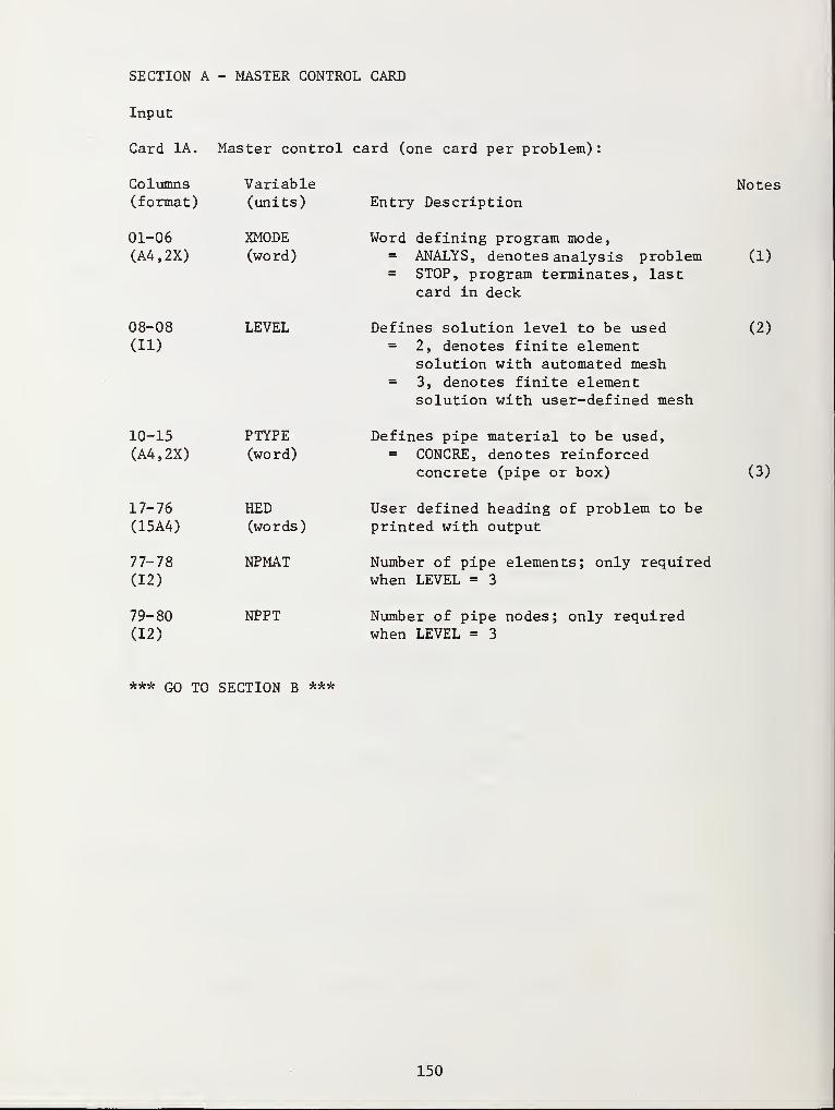
SECTION A - MASTER CONTROL CARD
Input
Card 1A. Master control card (one card per problem)
:
Columns(format)
01-06(A4,2X)
08-08
(ID
Variable(units)
XMODE(word)
LEVEL
Entry Description
Word defining program mode,= ANALYS, denotes analysis problem= STOP, program terminates, last
card in deck
Defines solution level to be used= 2, denotes finite element
solution with automated mesh= 3, denotes finite element
solution with user-defined mesh
Notes
(1)
(2)
10-15 PTYPE(A4,2X) (word)
17-76 HED(15A4) (words)
77-78 NPMAT(12)
79-80 NPPT
(12)
Defines pipe material to be used,= CONCRE, denotes reinforced
concrete (pipe or box)
User defined heading of problem to beprinted with output
Number of pipe elements; only requiredwhen LEVEL = 3
Number of pipe nodes; only requiredwhen LEVEL = 3
(3)
*** GO TO SECTION B ***
150
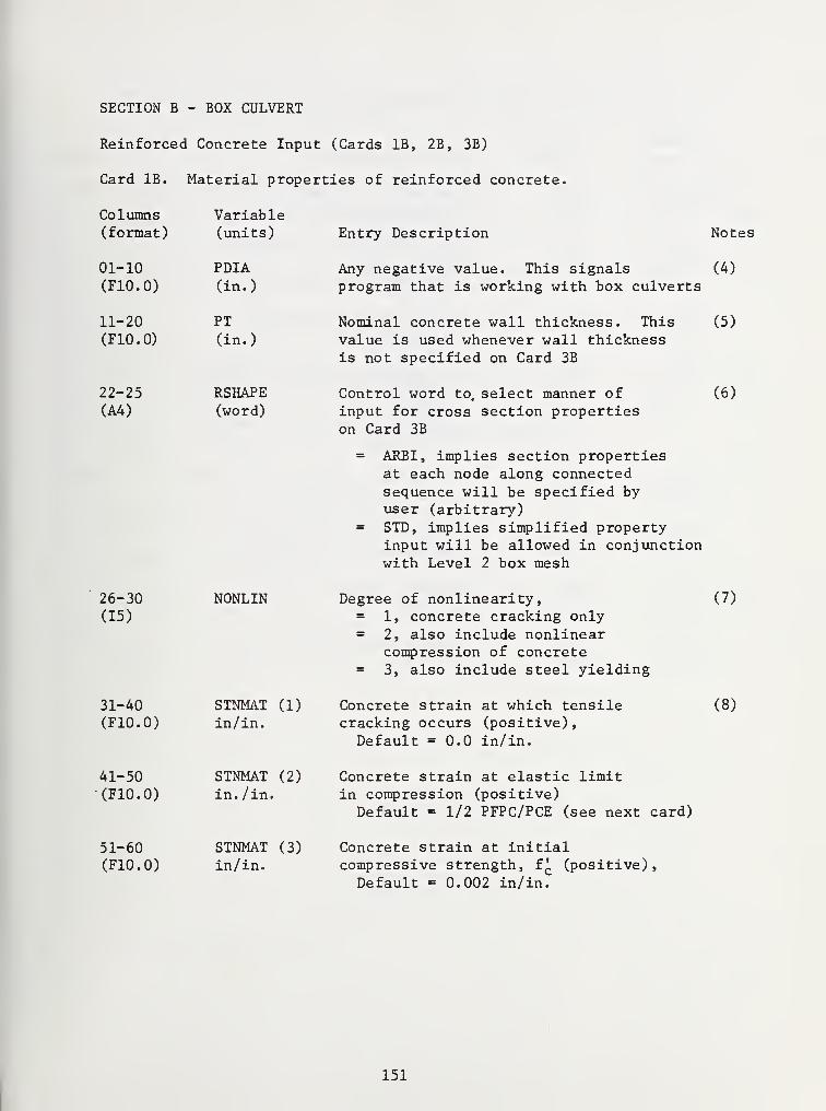
SECTION B - BOX CULVERT
Reinforced Concrete Input (Cards IB, 2B, 3B)
Card IB. Material properties of reinforced concrete.
Columns Variable(format) (units)
01-10 PDIA(F10.0) (in.)
11-20 PT(F10.0) (in.)
22-25 RSHAPE(A4) (word)
Entry Description Notes
26-30
(15)
NONLIN
31-40 STNMAT (1)
(F10.0) in/in.
41-50 STNMAT (2)
(F10.0) in. /in.
51-60 STNMAT (3)
(F10.0) in/in.
Any negative value. This signals (4)
program that is working with box culverts
Nominal concrete wall thickness. This (5)
value is used whenever wall thicknessis not specified on Card 3B
Control word to. select manner of (6)
input for cross section propertieson Card 3B
= ARBI, implies section propertiesat each node along connectedsequence will be specified byuser (arbitrary)
= STD, implies simplified propertyinput will be allowed in conjunctionwith Level 2 box mesh
Degree of nonlinearity
,
(7)
1, concrete cracking only= 2, also include nonlinear
compression of concrete= 3, also include steel yielding
Concrete strain at which tensile (8)
cracking occurs (positive),Default =0.0 in/in.
Concrete strain at elastic limitin compression (positive)Default = 1/2 PFPC/PCE (see next card)
Concrete strain at initialcompressive strength, f^, (positive),
Default = 0.002 in/in.
151
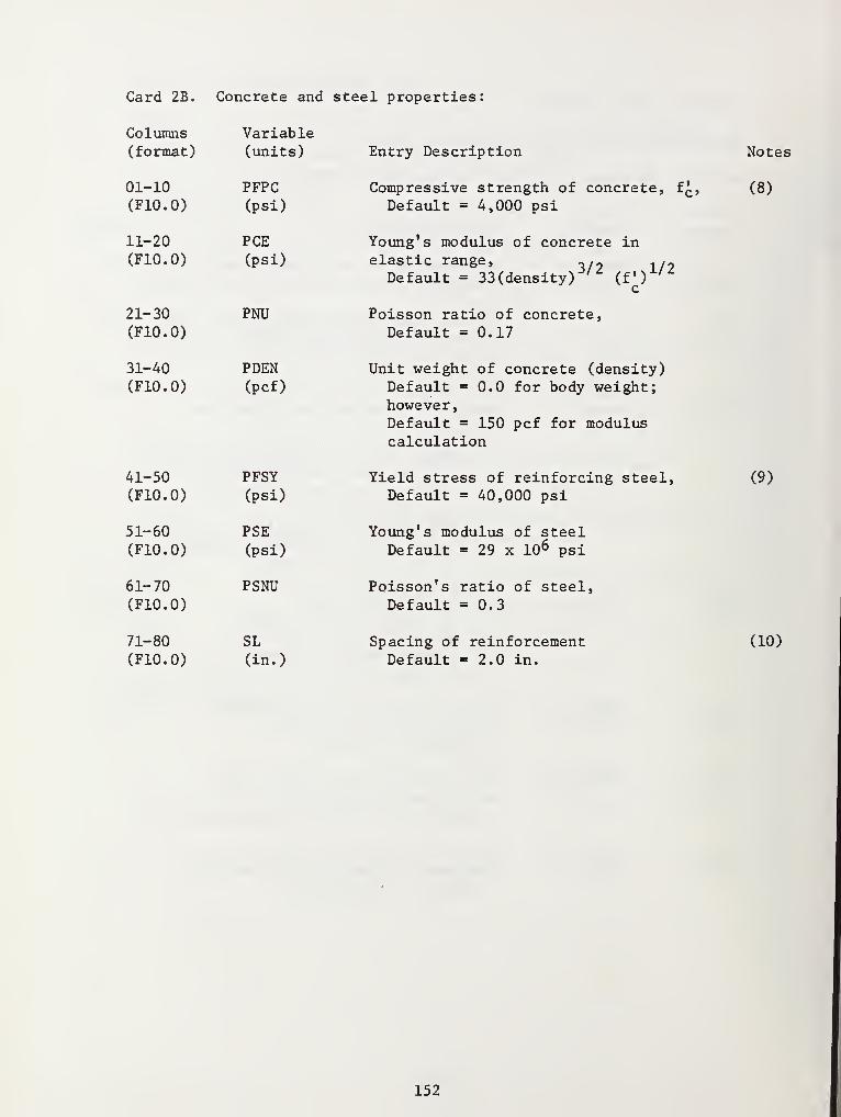
Card 2B. Concrete and
Columns Variable(format) (units)
01-10 PFPC(F10.0) (psi)
11-20 PCE(F10.0) (psi)
21-30 PNU(F10.0)
31-40 PDEN(F10.0) (pcf)
41-50 PFSY(F10.0) (psi)
51-60 PSE(F10.0) (psi)
61-70 PSNU(F10.0)
71-80 SL(F10.0) (in.)
steel properties:
Entry Description
Compressive strength of concrete, f£,
Default - 4,000 psi
Young's modulus of concrete inelastic range, ~.~ . ,
?Default = 33 (density) ' (f) '
c
Poisson ratio of concrete,Default = 0.17
Unit weight of concrete (density)Default = 0.0 for body weight;however,Default = 150 pcf for moduluscalculation
Yield stress of reinforcing steel,Default = 40,000 psi
Young's modulus of steelDefault = 29 x 106 psi
Poisson' s ratio of steel,Default =0.3
Spacing of reinforcementDefault = 2.0 in.
Notes
(8)
(9)
(10)
152
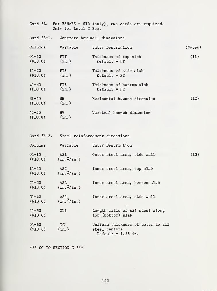
Card 3B. For RSHAPE = STD (only), two cards are required.Only for Level 2 Box.
Card 3B-1. Concrete Box-wall dimensions
Columns Variable Entry Description
01-10 PTT Thickness of top slab(F10.0) (in.) Default = PT
11-20 PTS Thickness of side slab(F10.0) (in.) Default = PT
21-30 PTB Thickness of bottom slab(F10.0) (in.) Default - PT
31-40 HH Horizontal haunch dimens(F10.0) (in.)
41-50 HV Vertical haunch dimensio(FIO.O) (in.)
(Notes)
(11)
(12)
Card 3B-2. Steel rei
Columns Variable
01-10(F10.0)
AS1(in.2/in.)
11-20(F10.0)
AS 2
(in.2/in.)
21-30
(F10.0)
AS 3
(in.2/in.)
31-40(F10.0)
AS4(in. 2/in.
)
41-50(F10.0)
XL1
51-60(F10.0)
TC(in.)
Entry Description
Outer steel area, side wall
Inner steel area, top slab
Inner steel area, bottom slab
Inner steel area, side wall
Length ratio of AS1 steel alongtop (bottom) slab
Uniform thickness of cover to allsteel centers
Default = 1.25 in.
(13)
*** GO TO SECTION C ***
153
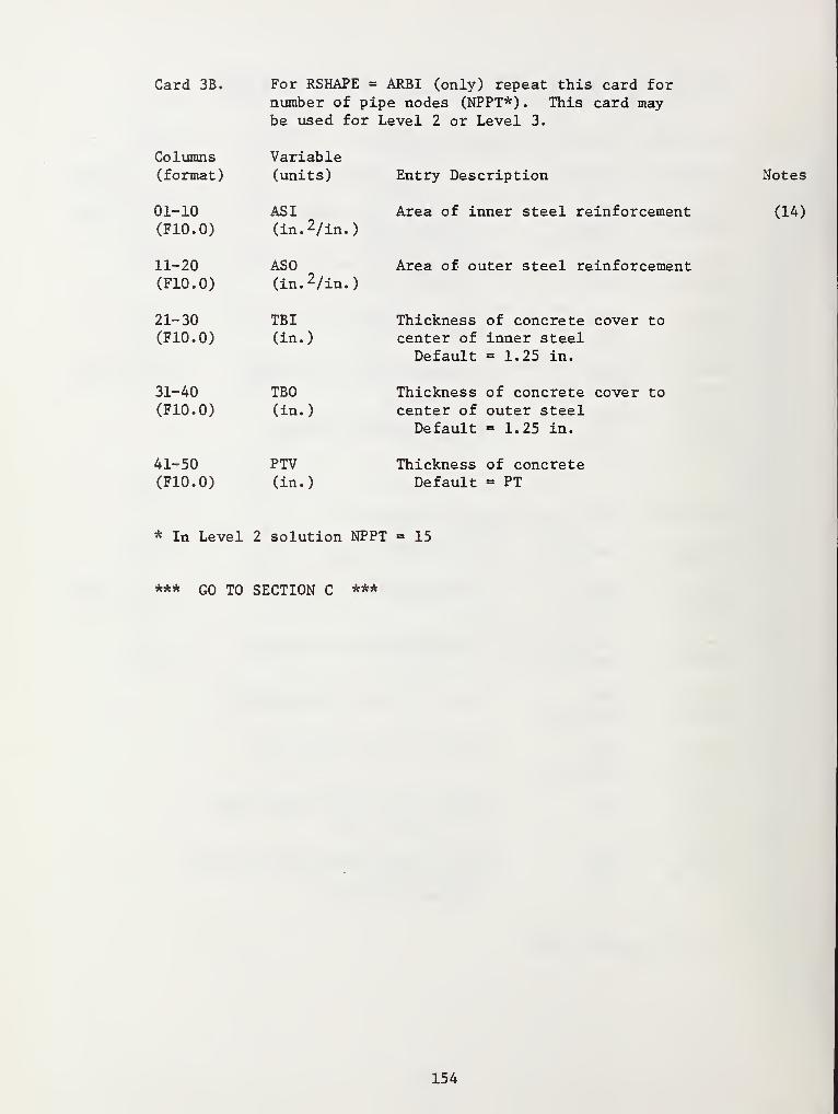
Card 3B. For RSHAPE = ARBI (only) repeat this card fornumber of pipe nodes (NPPT*) . This card maybe used for Level 2 or Level 3.
Entry Description Notes
Area of inner steel reinforcement (14)
Area of outer steel reinforcement
Thickness of concrete cover to
center of inner steelDefault = 1.25 in.
Thickness of concrete cover to
center of outer steelDefault = 1.25 in.
Thickness of concreteDefault = PT
* In Level 2 solution NPPT = 15
*** GO TO SECTION C ***
Columns(format)
Variable(units)
01-10(F10.0)
AS I
(in.2/in.
)
11-20(F10.0)
ASO(in. 2/in.
)
21-30(F10.0)
TBI(in.)
31-40(F10.0)
TBO(in.)
41-50(F10.0)
PTV(in.)
154
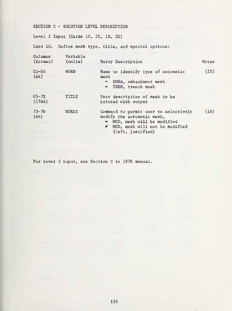
Columns Variable(format) (units)
01-04 WORD(A4)
SECTION C - SOLUTION LEVEL DESCRIPTION
Level 2 Input (Cards 1C, 2C, ID, 2D)
Card 1C. Define mesh type, title, and special options:
Entry Description
Name to identify type of automaticmesh
= EMBA, embankment mesh- TREN, trench mesh
User description of mesh to beprinted with output
Command to permit user to selectivelymodify the automatic mesh,
= MOD, mesh will be modified^ MOD, mesh will not be modified
(left, justified)
05-72(17A4)
73-76
(A4)
TITLE
W0RD1
Notes
(15)
(16)
For level 3 input, see Section C in 1976 manual.
155
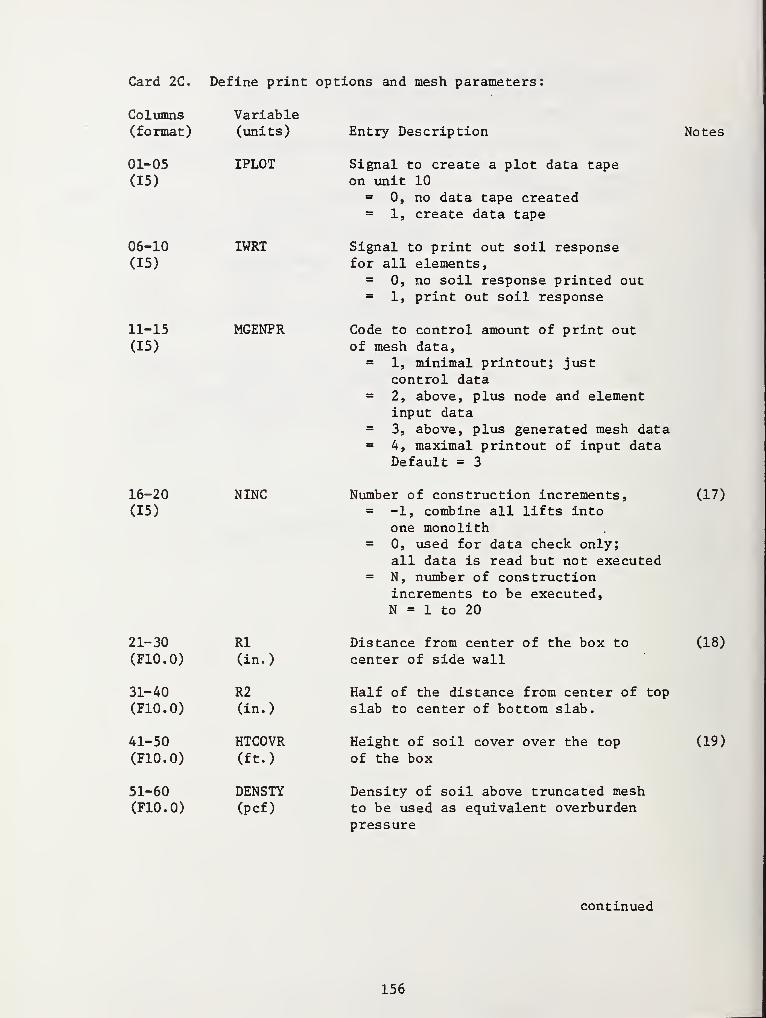
Card 2C. Define print options and mesh parameters:
Columns(format)
01-05
(15)
06-10
(15)
11-15
(15)
16-20
(15)
Variable(units)
IPLOT
IWRT
MGENPR
NINC
21-30 Rl(F10.0) (in.)
31-40 R2(F10.0) (in.)
41-50 HTCOVR(F10.0) (ft.)
51-60 DENSTY(F10.0) (pcf)
Entry Description Notes
Signal to create a plot data tapeon unit 10
= 0, no data tape created= 1, create data tape
Signal to print out soil responsefor all elements,
= 0, no soil response printed out= 1, print out soil response
Code to control amount of print outof mesh data,
= 1, minimal printout; justcontrol data
= 2, above, plus node and elementinput data
= 3, above, plus generated mesh data= 4, maximal printout of input data
Default = 3
Number of construction increments, (17)= -1, combine all lifts into
one monolith= 0, used for data check only;
all data is read but not executed= N, number of construction
increments to be executed,N = 1 to 20
Distance from center of the box to (18)
center of side wall
Half of the distance from center of top
slab to center of bottom slab.
Height of soil cover over the top (19)
of the box
Density of soil above truncated meshto be used as equivalent overburdenpressure
continued
156
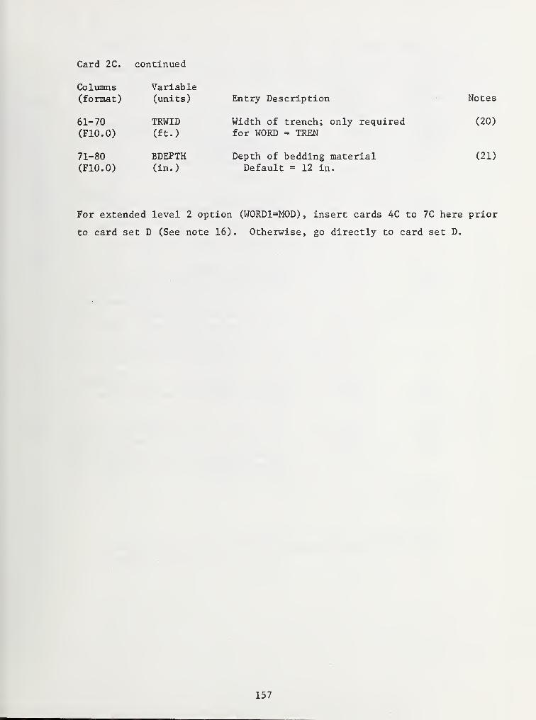
Card 2C. continued
Columns Variable(format) (units)
61-70 TRWID(F10.0) (ft.)
71-80 BDEPTH(F10.0) (in.)
Entry Description
Width of trench; only requiredfor WORD = TREN
Depth of bedding materialDefault = 12 in.
Notes
(20)
(21)
For extended level 2 option (W0RD1=M0D) , insert cards 4C to 7C here prior
to card set D (See note 16). Otherwise, go directly to card set D.
157
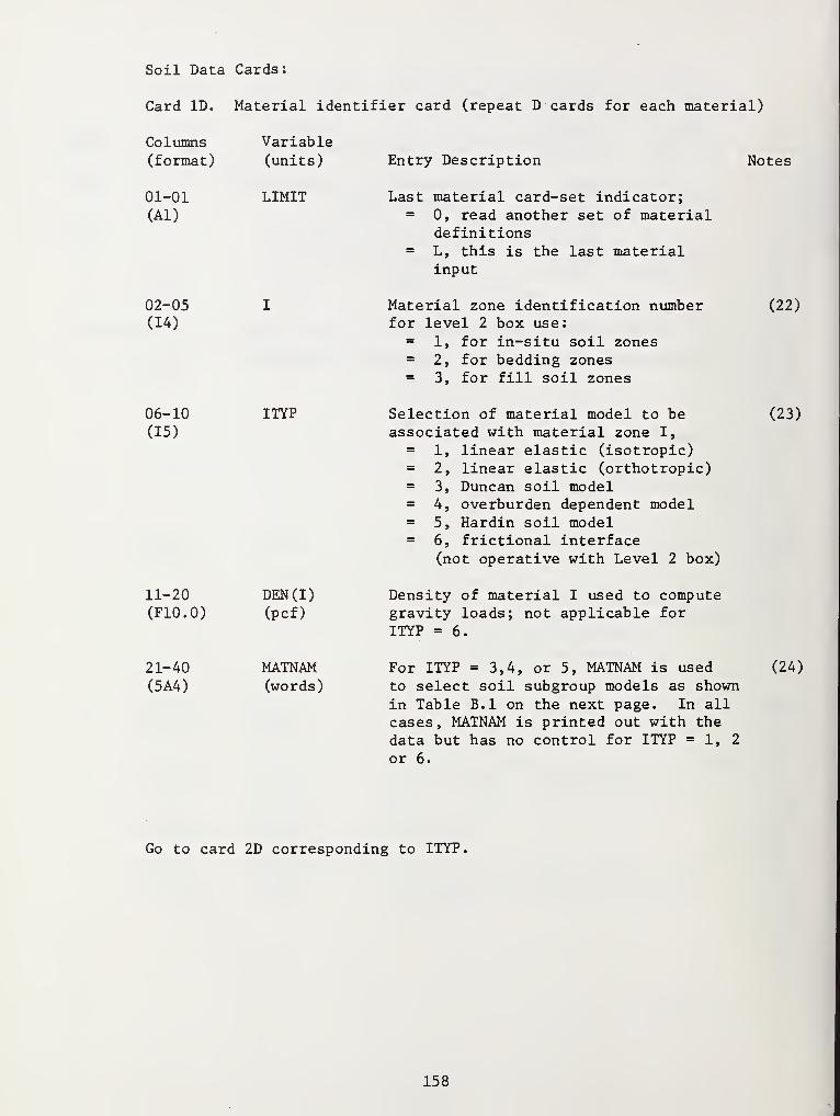
Soil Data Cards:
Card ID. Material identifier card (repeat D cards for each material)
Columns(format)
01-01(Al)
02-05
(14)
06-10
(15)
11-20(F10.0)
21-40(5A4)
Variable(units)
LIMIT
ITYP
DEN (I)
(pcf)
MATNAM(words)
Entry Description Notes
Last material card-set indicator;= 0, read another set of material
definitions= L, this is the last material
input
Material zone identification number (22)
for level 2 box use:= 1, for in-situ soil zones= 2, for bedding zones= 3, for fill soil zones
Selection of material model to be (23)
associated with material zone I,
= 1, linear elastic (isotropic)= 2, linear elastic (orthotropic)= 3, Duncan soil model= 4, overburden dependent model= 5, Hardin soil model= 6, frictional interface
(not operative with Level 2 box)
Density of material I used to computegravity loads; not applicable for
ITYP = 6.
For ITYP = 3,4, or 5, MATNAM is used (24)
to select soil subgroup models as shown
in Table B.l on the next page. In allcases, MATNAM is printed out with the
data but has no control for ITYP = 1, 2
or 6.
Go to card 2D corresponding to ITYP.
158
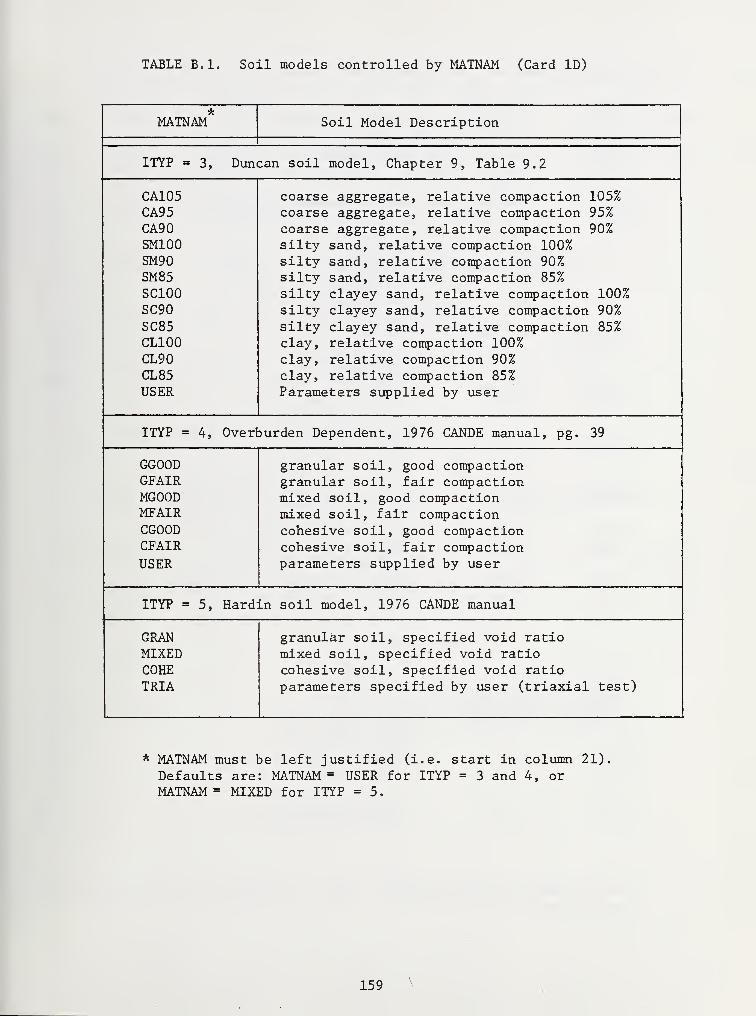
TABLE B.l. Soil models controlled by MATNAM (Card ID)
MATNAM Soil Model Description
ITYP = 3, Duncan soil model, Chapter 9, Table 9.2
CA105CA95CA90SM100SM90SM85SC100SC90SC85CL100CL90CL85USER
coarse aggregate, relative compaction 105%coarse aggregate, relative compaction 95%coarse aggregate, relative compaction 90%silty sand, relative compaction 100%silty sand, relative compaction 90%silty sand, relative compaction 85%silty clayey sand, relative compaction 100%silty clayey sand, relative compaction 90%silty clayey sand, relative compaction 85%clay, relative compaction 100%clay, relative compaction 90%clay, relative compaction 85%Parameters supplied by user
ITYP = 4, Overburden Dependent, 1976 CANDE manual, pg. 39
GGOODGFAIRMGOODMFAIRCGOODCFAIR
USER
granular soil, good compactiongranular soil, fair compactionmixed soil, good compactionmixed soil, fair compactioncohesive soil, good compactioncohesive soil, fair compactionparameters supplied by user
ITYP = 5, Hardin soil model, 1976 CANDE manual
GRANMIXEDCOHETRIA
granular soil, specified void ratio
mixed soil, specified void ratiocohesive soil, specified void ratioparameters specified by user (triaxial test)
* MATNAM must be left justified (i.e. start in column 21)
Defaults are: MATNAM = USER for ITYP = 3 and 4, orMATNAM = MIXED for ITYP = 5.
159
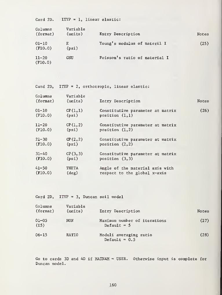
Card 2D. ITYP = 1, linear elastic-
Columns(format)
01-10(F10.0)
11-20(F10.0)
Variable(units)
E
(psi)
GNU
Entry Description
Young's modulus of materil I
Poisson's ratio of material I
Notes
(25)
Card 2D, ITYP = 2, orthotropic, linear elastic:
Columns Variable(format) (units) Entry Description
01-10 CP(1,1) Constitutive parameter at matrix(F10.0) (psi) position (1,1)
11-20 CP(1,2) Constitutive parameter at matrix(F10.0) (psi) position (1,2)
21-30 CP(2,2) Constitutive parameter at matrix(F10.0) (psi) position (2,2)
31-40 CP(3,3) Constitutive parameter at matrix(F10.0) (psi) position (3,3)
41-50 THETA Angle of the material axis with(F10.0) (deg) respect to the global x-axis
Notes
(26)
Card 2D, ITYP = 3, Duncan soil model
Columns(format)
01-05
(15)
06-15
Variable(units)
NON
RATIO
Entry Description
Maximum number of iterationsDefault = 5
Moduli averaging ratioDefault =0.5
Notes
(27)
(28)
Go to cards 3D and 4D if MATNAM = USER. Otherwise input is complete forDuncan model.
160
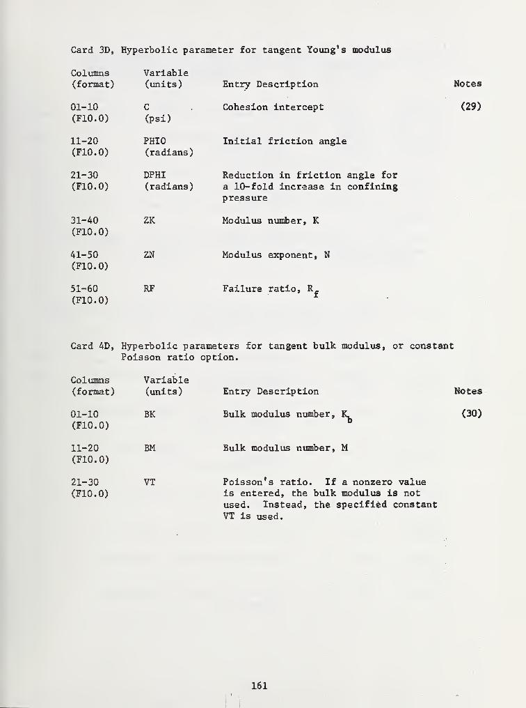
Card 3D, Hyperbolic parameter for tangent Young's modulus
Columns Variable(format) (units)
01-10 C
(F10.0) (psi)
11-20 PHIO(F10.0) (radians)
21-30 DPHI(F10.0) (radians)
31-40 ZK(F10.0)
41-50 ZN(F10.0)
51-60 RF(F10.0)
Entry Description Notes
Cohesion intercept (29)
Initial friction angle
Reduction in friction angle for
a 10-fold increase in confiningpressure
Modulus number, K
Modulus exponent, N
Failure ratio, R_
Card 4D, Hyperbolic parameters for tangent bulk modulus, or constantPoisson ratio option.
Entry Description Notes
Bulk modulus number, K, (30)
Bulk modulus number, M
Poisson 1s ratio. If a nonzero value
is entered, the bulk modulus is notused. Instead, the specified constantVT is used.
Columns Variable(format) (units)
01-10 BK(F10.0)
11-20 BM(F10.0)
21-30 VT(F10.0)
161i
i
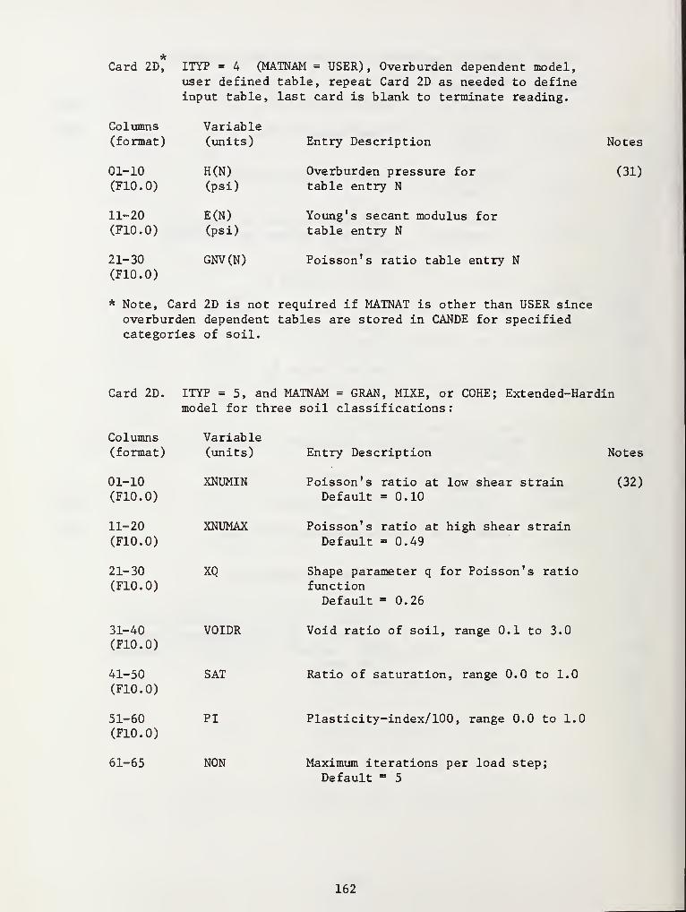
Card 2D, ITYP = 4 (MATNAM = USER), Overburden dependent model,user defined table, repeat Card 2D as needed to defineinput table, last card is blank to terminate reading.
Columns Variable(format) (units)
01-10 H(N)(F10.0) (psi)
11-20 E(N)(F10.0) (psi)
21-30 GNV(N)(F10.0)
Entry Description
Overburden pressure fortable entry N
Young's secant modulus fortable entry N
Poisson's ratio table entry N
Notes
(31)
* Note, Card 2D is not required if MATNAT is other than USER sinceoverburden dependent tables are stored in CANDE for specifiedcategories of soil.
ITYP =5, and MATNAM = GRAN, MIXE, or COHE; Extended-HardinCard 2D. ITYP = 5, a
model for t
Columns Variable(format) (units)
01-10 XNUMIN(F10.0)
11-20 XNUMAX(F10.0)
21-30 XQ(F10.0)
31-40 V0IDR(F10.0)
41-50 SAT(F10.0)
51-60 PI(F10.0)
Entry Description
Poisson's ratio at low shear strainDefault =0.10
Poisson's ratio at high shear strainDefault =0.49
Shape parameter q for Poisson's ratiofunctionDefault =0.26
Void ratio of soil, range 0.1 to 3.0
Ratio of saturation, range 0.0 to 1.0
Plasticity-index/ 100, range 0.0 to 1.0
Notes
(32)
61-65 NON Maximum iterations per load step;
Default = 5
162
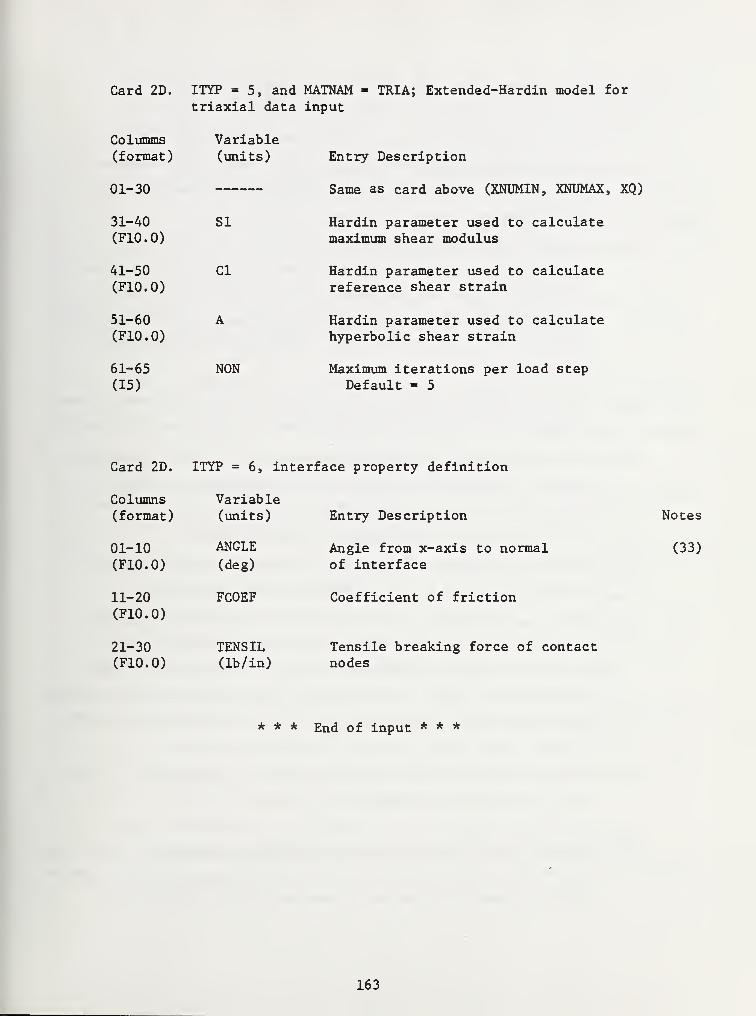
Card 2D. ITYP 5, and MATNAM = TRIA; Extended-Hardin model fortriaxial data input
Entry Description
Same as card above (XNUMIN, XNUMAX, XQ)
Hardin parameter used to calculatemaximum shear modulus
Hardin parameter used to calculatereference shear strain
Hardin parameter used to calculatehyperbolic shear strain
Maximum iterations per load stepDefault = 5
Columms Variable(format) (units)
01-30
31-40 SI(F10.0)
41-50 CI
(F10.0)
51-60 A(F10.0)
61-65 NON(15)
Card 2D. ITYP = 6, interface property definition
Columns Variabl(format) (units)
01-10 ANGLE
(F10.0) (deg)
11-20 FC0EF(F10.0)
21-30 TENSIL(F10.0) (lb/in)
Entry Description Notes
Angle from x-axis to normal (33)
of interface
Coefficient of friction
Tensile breaking force of contactnodes
* * * End of input * * *
163
COMMENTARY NOTES
(1) Each problem begins with the command ANALYSIS. The DESIGN option
is not available for box culverts. The program will continue to
execute problem data sets back-to-back until the command STOP is
encountered.
(2) Setting LEVEL=2 signals the program that the automatic mesh
generation feature will be used. "Level 2 box" is distinguished
from "Level 2 pipe" by a subsequent instruction in Section B.
Setting LEVEL=3 allows description of arbitrary reinforced concrete
structures and loading conditions. LEVEL=1 is not operable for
box cuJ verts.
(3) By setting PTYPE = CONCRE, the reinforced concrete beam-rod element
is used to model the culvert (for other pipe types see 1976 manual).
(4) Setting PDIA = -1.0 signals the program that Section B input data
is for a concrete box as opposed to a concrete pipe. Also, if
LEVEL = 2, it subsequently signals the program to read Section C
input for "level 2 box" instead of "level 2 pipe".
(5) Defining the default concrete wall thickness, PT, is simply for
convenience in limiting input data on subsequent cards.
(6) RSHAPE controls the two options for defining section properties
around the box. Setting RSHAPE = STD allows simplified input
for standard ASTM box sections and can only be used with LEVEL = 2.
Setting RSHAPE = ARBI allows the user to arbitrarily define section
properties at each node around the box and may be used with LEVEL =
2 or 3.
(7) Generally set NONLIN = 3 for all problems. Other options are pri-
marily for behavior studies.
(8) Figure B.3 illustrates the concrete material parameters representing
the concrete stress-strain behavior. Generally, the default options
provide reasonable parameter values except for cracking strain
164
STNMAT(l) and compressive strength PFPC which are conservative.
Cracking strain values up to 0.0001 were used for box culverts
studied in this report.
(9) Figure B.4 illustrates the reinforcement material parameters
representing the steel stress-strain behavior. Default options
provide reasonable parameter values except for steel yield stress
which is conservative. Standard ASTM box section reinforcement
assumes 65,000 psi yield strength.
(10) The spacing parameter is used only for crackwidth predictions in
the Gergely-Lutz formula (see Chapter 3). The default value was
used in this study.
(11) For the RSHAPE = STD option, refer to Figure B.5 for illustration
of standard box section parameters. If the top, side and bottom
slabs are the same thickness, these input variables can be skipped
and the default value PT, input on Card IB, will be used.
(12) Haunch dimensions are used by CANDE to increase the wall thickness
at corner nodes by a simple averaging process and are shown on
the printed output. Generally, HH = HV = PT.
(13) Steel placement is illustrated in Figure B.5 and corresponds to
standard ASTM box designs. All reinforcement steel areas are to
be defined per inch of length in the longitudinal direction. Con-
crete cover to all steel centers is specified with the parameters
TC. If variable TC values are desired use RSHAPE = ARBI.
(14) For the RSHAPE = ARBI option, refer to Figure B.6 for illustration
of parameters. In the level 2 option, the section properties are
defined individually at the 15 points (nodes) shown in the figure.
For level 3 solutions, the section properties are defined at the
culvert nodes (NPPT) established by the user.
(15) The embankment and trench configurations are illustrated in
Figure B. 7 and B.8. Each is composed of three soil zones; in situ,
bedding, and fill.
165
(16) By setting W0RD1 = MOD, the level 2 mesh can be selectively
modified by using the extended level 2 option. Modifications
include; defining new soil zones and shapes and specifying live
loads. When this option is exercised, additional data cards C4 to
C7 are inserted after card C2. Card C3 does exist for level 2
box input. Input instructions for cards C4 to C7 are in the 1976
user manual and the finite element mesh topology for level 2 box
is shown in Figure B.ll to B.14.
(17) Construction increments for the trench and embankment installations
are shown in Figures B.9 and B.10. In both cases, the first con-
struction increment contains the box culvert and in situ soil.
Increments 2,3,4 are each composed of two rows of elements uni-
formly spaced along the sides of the box. Increments 5 to 9 are
composed of one element row, increment 5 is 1/3 R2 thick, and
increments 6 to 9 are 2/3 R2 thick. For deep fill heights, sub-
sequent increments are formed with equivalent overburden pressure
(see note 19). The special case of NINC = -1 combines all incre-
ments into one (not recommended).
(18) Rl and R2 define the box size and control the overall dimensions
of the mesh as shown in Figure B.ll.
(19) HTCOVR is the distance from the middle of the top slab to the
final soil surface. If HTCOVR is specified greater than 3R2,
the mesh top boundary is truncated at the 3R2 level, and the
remaining soil load is applied as equivalent increments of over-
burden pressure (i.e. DENSTY * (HTCOVR - 3R2)/(NINC - 9)). If
HTCOVR is specified less than 3R2, the horizontal mesh line
closest to HTCOVR is moved to the specified height, but with the
condition that at least two layers of soil exist over the top
of the box.
(20) TRNWID defines the trench width from the middle of the box sidewall
to the in situ soil as shown in Figure B.7. The vertical mesh
line (Figure B.ll) closest to the specified position is moved to
this position to form the trench wall boundary. Minimum value
166
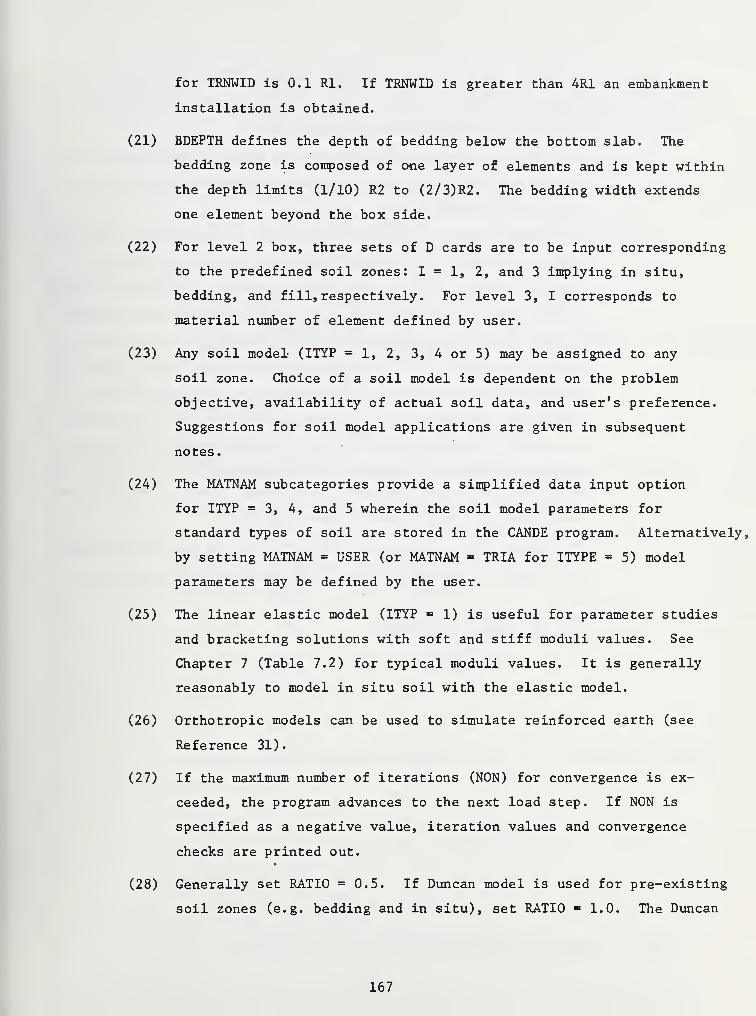
for TRNWID is 0.1 Rl. If TRNWID is greater than 4R1 an embankment
installation is obtained.
(21) BDEPTH defines the depth of bedding below the bottom slab. The
bedding zone is composed of one layer of elements and is kept within
the depth limits (1/10) R2 to (2/3)R2. The bedding width extends
one element beyond the box side.
(22) For level 2 box, three sets of D cards are to be input corresponding
to the predefined soil zones: I = 1, 2, and 3 implying in situ,
bedding, and fill, respectively. For level 3, I corresponds to
material number of element defined by user.
(23) Any soil model (ITYP = 1, 2, 3, 4 or 5) may be assigned to any
soil zone. Choice of a soil model is dependent on the problem
objective, availability of actual soil data, and user's preference.
Suggestions for soil model applications are given in subsequent
notes.
(24) The MATNAM subcategories provide a simplified data input option
for ITYP = 3, 4, and 5 wherein the soil model parameters for
standard types of soil are stored in the CANDE program. Alternatively,
by setting MATNAM = USER (or MATNAM = TRIA for ITYPE = 5) model
parameters may be defined by the user.
(25) The linear elastic model (ITYP = 1) is useful for parameter studies
and bracketing solutions with soft and stiff moduli values. See
Chapter 7 (Table 7.2) for typical moduli values. It is generally
reasonably to model in situ soil with the elastic model.
(26) Orthotropic models can be used to simulate reinforced earth (see
Reference 31).
(27) If the maximum number of iterations (NON) for convergence is ex-
ceeded, the program advances to the next load step. If NON is
specified as a negative value, iteration values and convergence
checks are printed out.
(28) Generally set RATIO = 0.5. If Duncan model is used for pre-existing
soil zones (e.g. bedding and in situ), set RATIO = 1.0. The Duncan
167
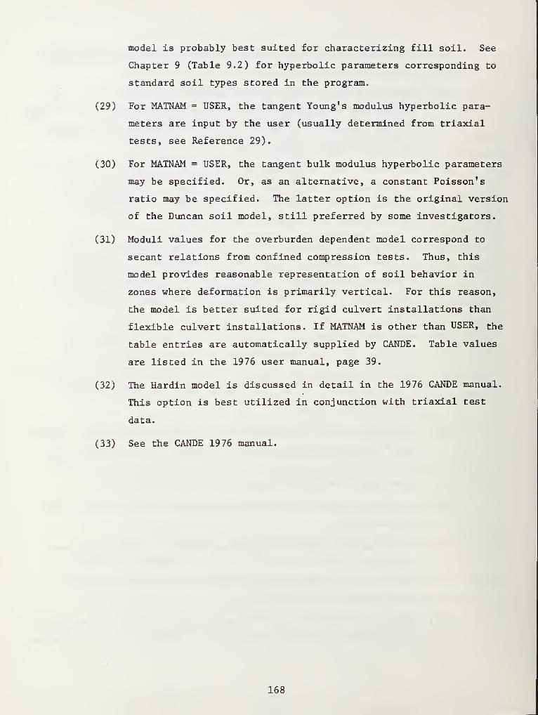
model is probably best suited for characterizing fill soil. See
Chapter 9 (Table 9.2) for hyperbolic parameters corresponding to
standard soil types stored in the program.
(29) For MATNAM = USER, the tangent Young's modulus hyperbolic para-
meters are input by the user (usually determined from triaxial
tests, see Reference 29).
(30) For MATNAM = USER, the tangent bulk modulus hyperbolic parameters
may be specified. Or, as an alternative, a constant Poisson's
ratio may be specified. The latter option is the original version
of the Duncan soil model, still preferred by some investigators.
(31) Moduli values for the overburden dependent model correspond to
secant relations from confined compression tests. Thus, this
model provides reasonable representation of soil behavior in
zones where deformation is primarily vertical. For this reason,
the model is better suited for rigid culvert installations than
flexible culvert installations. If MATNAM is other than USER, the
table entries are automatically supplied by CANDE. Table values
are listed in the 1976 user manual, page 39.
(32) The Hardin model is discussed in detail in the 1976 CANDE manual.
This option is best utilized in conjunction with triaxial test
data.
(33) See the CANDE 1976 manual.
168
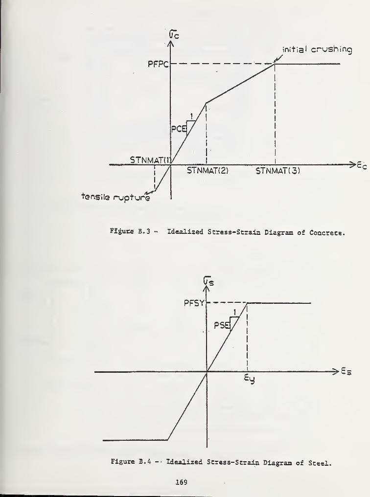
nitia' crushing
tensile njpture
Flgufie B.3 - Idealized Stress-Strain Diagram of Concrete.
f«
PFSY
->S S
Figure B.4 -- Idealized Stress-Strain Diagram of Steel.
169
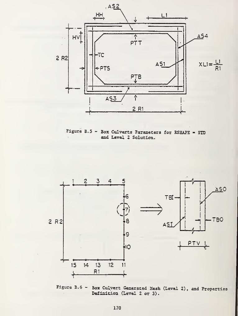
AS2
HH
2 R2
Hvt
AS3 / t
L 2_£1
LI
\/— tPTT \,
.
- r-TC
<-PTSAS1_^"
\_ PTB /r
AS4
XL1 = JJ.
R1
Figure B.5 - Box Culverts Parameters for RSHAPE - STDand Level 2 Solution.
2 R2
2 3 4 59 •
(
\
+6
7)
.8
15 14 13 12 11
R1 L
TBI
A/
Asiy
kK
aso
'BO
PTV
+
Figure B.6 - Box Culvert Generated Mesh (Level 2), and PropertiesDefinition (Level 2 or 3)
.
170
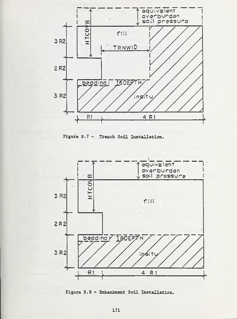
equivalentoverburdensoil pressure
3R2
2R2
3R2
Figure B.7 - Trench Soil Installation.
3R2
2R2
/
fequivalentoverburden
^ soil pressure
3R2
Figure B.8 - Embankment Soil Installation.
171
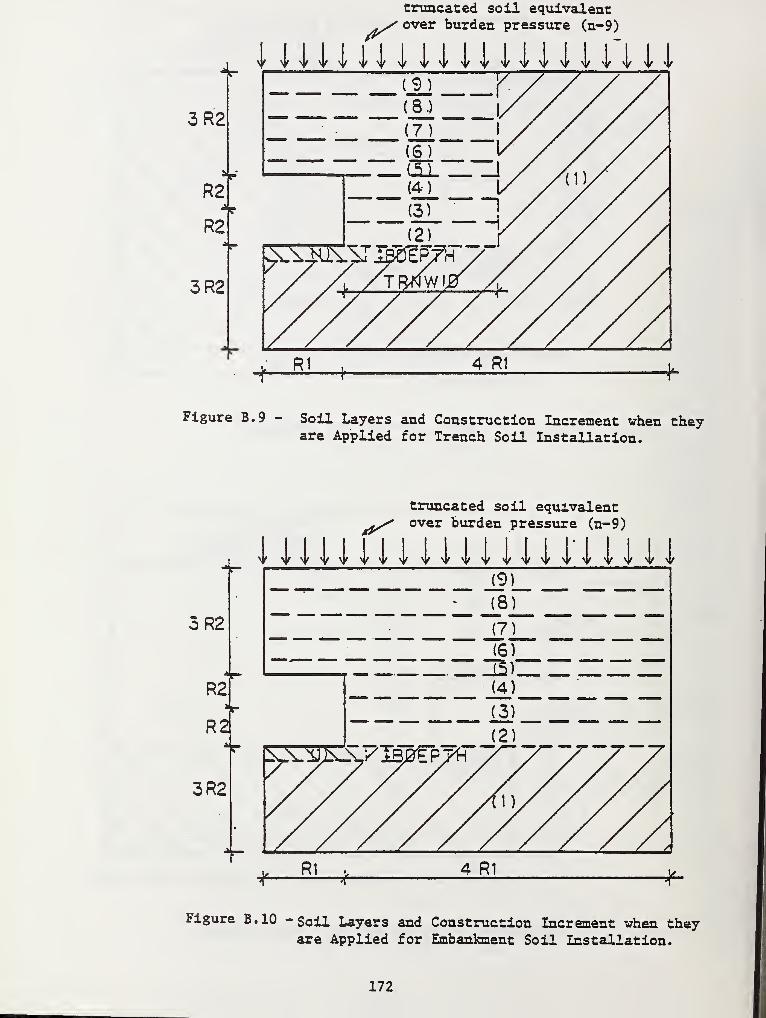
3R2
R2
R2
3R2
truncated soil equivalentjS over burden pressure (n-9)
V y V
Figure B.9 - Soil Layers and Construction Increment when theyare Applied for Trench Soil Installation.
truncated soil equivalent
^x" over burden pressure (n-9)
3R2
R2
R2I
3R2
Figure B.10 -Soil Layers and Construction Increment when theyare Applied for Embankment Soil Installation.
172
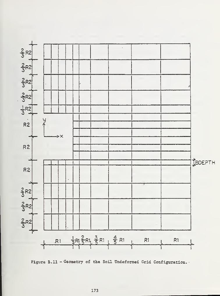
|R2
fR2
•|R2
•§R2
R2
R2
R2
|R2
§R2
¥2
'
^
A
X
>
I<̂BOEPT,1-
+*' jsigkigLL-i^ R1
fP'|,?"'p"' | ™1
R1
f
Figure B.ll -Geometry of the Soil Undeformed Grid Configuration.
173
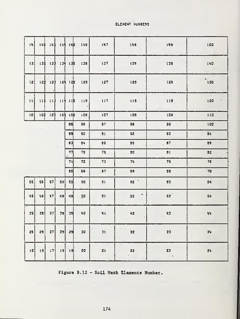
ELEMENT NUMBERS
14 14, i m: 1 14 1 14 5 146 147 143 149 150
13 n; ! 13: I 13'1 13 5 13S 137 133 139 140
12 12; ! 12: 1 12'1 12 5 125 127 123 129 ~130
11 ti, 1 n. i 11 1 11 5 115 117 113 119 120
10 loi 10: 1 10 1 10 5 iOS 107 103 109 no
95 96 97 99 39 100
89 90 91 92 93 94
53 94 9S 35 57 99
77 73 79 90 91 92
71 72 73 74 75 7S
SS 56 57 59 59 70
55 56 57 S3 59 SO 51 52'
S3 54
US >45 47 49 49 50 SI 52 * S3 54
35 35 37 39 33 40 41 42 43 44
25 25 27 23 29 30 31 32 33 34
IS 15 17 19 19 20 21 22 23 24
Figure B.12 - Soil Mesh Elements Number.
174
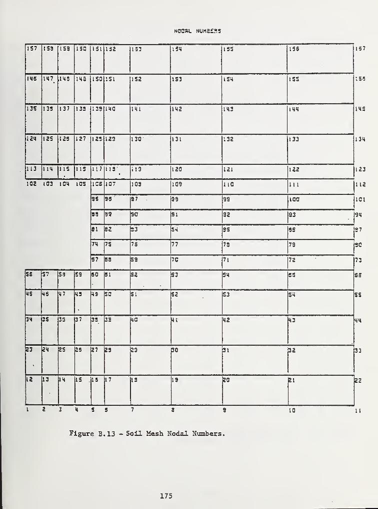
NOCfiL NUM2ESS
157 133 153 150 151 132 153 1S4 153 136
145 u7.
,14 3 143 ISO 1S1 152 153 iSU 155
1 35 135 137 133 133 140 141 142 143 i44
«24 125 125 127 123 123 130 131 132 133
113 ill 115 115 117 113 113 120 121 122
102 103 1 C4 105 1CS 107 103 103 no 111
35 35 37 S3 33 100
33 39 30 31 32 33
81 32 23 Sm 35 35
71 175 75 77 73 73
57 S3 S3 70 71 72
55 57 53 55 SO 61 52 53.
54 55
4S h5 47 43 49 SO Si S2 S3 5n
34 35 33 37 33 33 40 41' 42 43
23 24 25 25 27 23 23 30 31 32
12 13 14 15 IS 17 13 13 20 21
1 2 3 4 S 5 10 11
Figure B.13 - Soil Mesh Nodal Numbers.
175
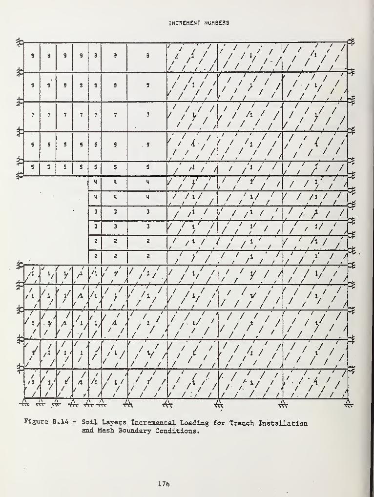
INCflEn£NT NUtt££R5
f*' / i < t
////-A/ / ,; / /
/ /'/ /
t t f *(&
/ /t / ' / / 1/ /
// / / // / / /
/ y / k /// /
^77?/ / / /
f*
y / 'i / /
/ / / //
z ' -/ i' sv ; / * >
TTi 7 I—7-7 iXi// ; /
/ / /
/
/ / / , I / / /
/ /I /
PT77/
/ /' / /I/ A / / ,/
z7^^7///•'/ 7 F7"~v
/ /l/ I7TJZZZZZZ7
^77/
r r
> /TP~7
/ / / / 1/ / / /
**
/
/iv 7 7
/* n/
/ / /
' / y / / ' /V // / /
/
/A
/
/ /
/ A /
/ // L
v'/V'1 /
t tit/ / / /
/ / / /' / A
?7—7—7—TrP
V ' '—L
/ A
V/
/
/
A7
/•/
/
/
/ //
7 /T
' /•
/ A
// /1 r
/
d-/
/
' /
/1/ 1 /j
//
/
1 <
//
/
' / ' / /
/ V / / /- /< / / / /« /
/ T/
/ / / / /
/i
// 7
//
/:
/J—i /I
//•m m* rr^ -^r -nT-TTT tn
' / 1
' // / /
/ /
7 /
/ / /
' / ./ /
r 7 A//// /
/ // / / / /
/ . / / / /
A w A ^Figure B»1A - Soil Layers Incremental Loading for Trench Installation
and Mesh Boundary Conditions.
17b
APPENDIX C
SAMPLE OF INPUT DATA AND OUTPUT
The three sample problems presented here cover the three solution
levels available when analyzing a reinforced concrete box culvert, that
is: level 2 box, extended level 2, and level 3. The three samples cor-
respond to box culverts analyzed during the process of this work.
Table D.l gives a brief description of the box type, solution level,
installation type, and some special comments of the sample problems.
Each problem is presented in the following format: (1) a listing of all
the input cards, and (2) selected CANDE output for the box responses.
The soil responses are not presented.
177
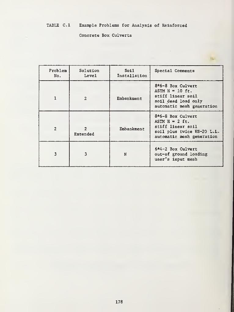
TABLE C.l Example Problems for Analysis of Reinforced
Concrete Box Culverts
ProblemNo.
SolutionLevel
SoilInstallation
Special Comments
1 2 Embankment
8*6-8 Box CulvertASTM H = 10 ft.
stiff linear soilsoil dead load onlyautomatic mesh generation
2 2
ExtendedEmbankment
8*6-8 Box CulvertASTM H = 2 ft.
stiff linear soilsoil plus twice HS-20 L.L.automatic mesh generation
3 3 N
6*4-2 Box Culvertout-of ground loadinguser's input mesh
178
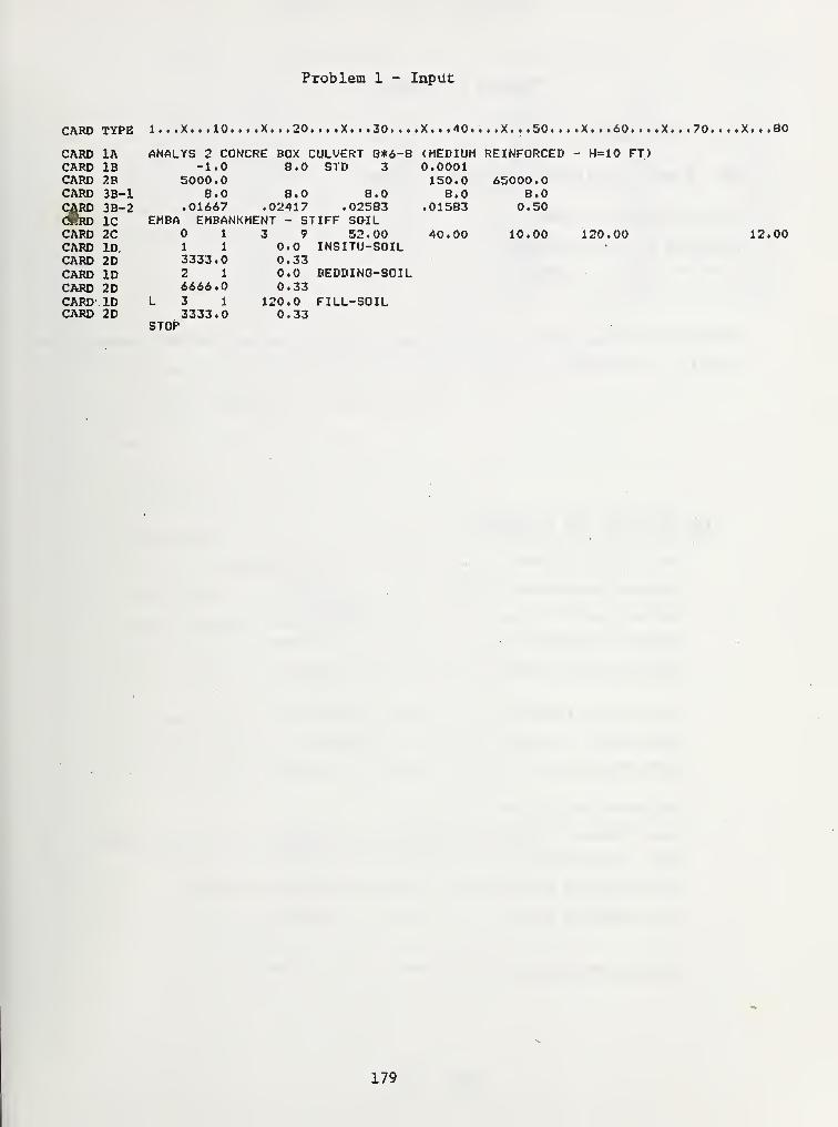
Problem 1 - Input
CARD TYPE 1...X...10....X...20....X...30....X...40....X...50....X...60....X...70....X...80
CARD 1ACARD IBCARD 2BCARD 3B-1CARD 3B-2
CARD 2CCARD ID,CARD 2DCARD IDCARD 2DCARD IDCARD 2D
150.0 65000.0B.O 8.0
.01583 0.50
ANALYS 2 CONCRE BOX CULVERT 8*6-8 (MEDIUM REINFORCED - H=10 FT)-1.0 8.0 STD 3 0.0001
5000.08.0 8.0 8.0
.01667 .02417 .02583EMBA EMBANKMENT - STIFF SQ-IL
1 3 9 52.000.0 INSITU-SOIL0.330.0 BEDDING-SOIL0.33
120.0 FILL-SOIL0.33
STOP
1 1
3333.02 1
6666.03 1
3333.0
40.00 10.00 120.00 12.00
179
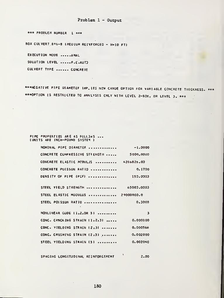
Problem 1 - Output
*** PROBLEM NUMBER 1 *«*
BOX CULVERT. 8*6-8 J MEDIUM REINFORCED - M«10 FT)
EXECUTION MOUE ANAL
SOLUTION LEVEL F.C.AUTD
CULVERT TYPE CONCRETE
•NEGATIVE PIPE UIAMETEF IMP. IES NEW CANOE OPTION FOR VARIABLE CONCRETE THICKNESS. ***
••OPTION IS RESTRICTED TO ANALYSIS CNLY WITH LEVEL 2-BOX, OR LEVEL 3. ***
PIPE PROPERTIES ARE AS FULL3WS ...(UNITS ARE INCH-POUNO SYSTEM )
NOMINAL PIPE DIAMETER -1.0000
CONCRETE COMPRESSIVE STRENGTH 5000.0000
CONCRETE ELASTIC MODULJS 4266826.00
CONCRETE PUISSON RATIO 0.1700
DENSITY OF PIPE IPCF) 150.0003
STEEL YIELD STRENGTH 65003.0000
STEEL ELASTIC MODULUS 29000000.0
STEEL POISSON RATIO 0.3000
NONLINEAR CUOE (1,2, OR 3 1 3
CONC. CROCKING STRAIN ( 1.2,3) 0.000100
CONC. YIELDING STRAIN (2,3) 0.000566
CONC. CRUSHING STRAIN (2,3) 0.002000
STEEL YIELDING STRAIN (3) 0.002040
SPACING LONGITUDINAL REINFORCEMENT 2.00
180
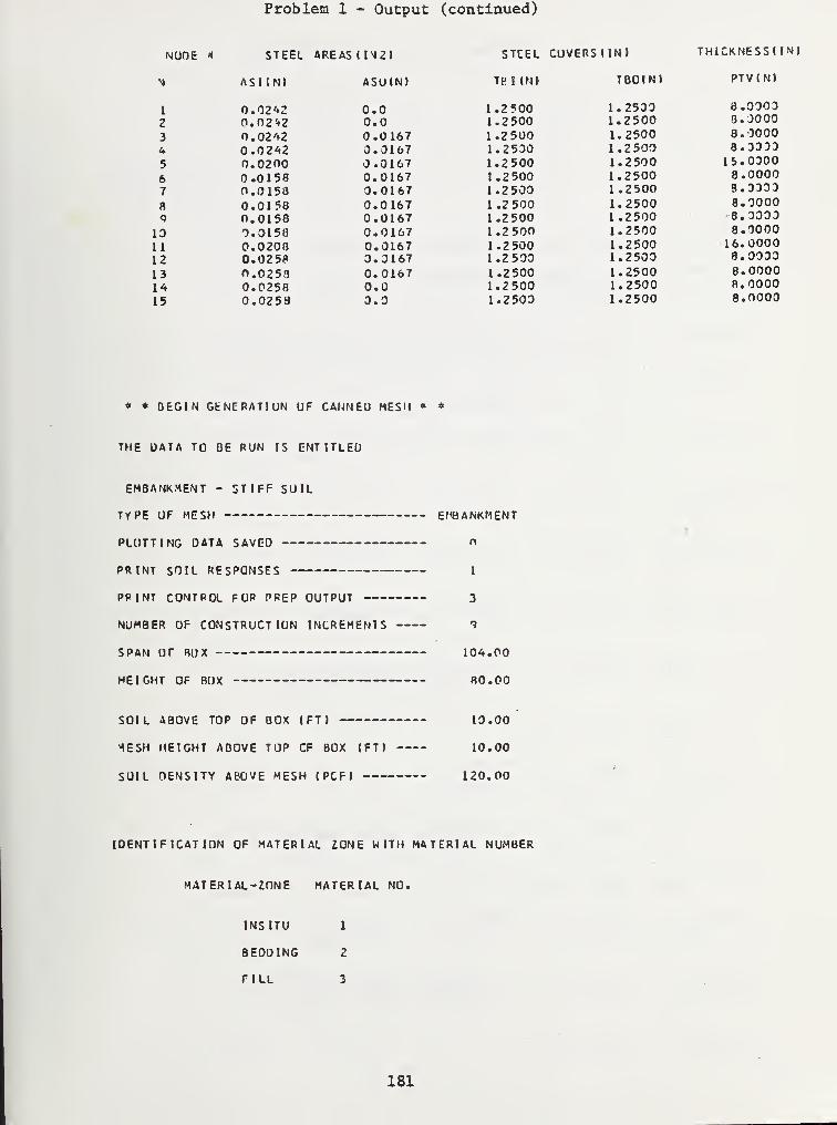
Problem 1 - Output (continued)
NODE * STEEL AREAS (IN2) STCEL CUVERSUN) TH1CKNESSUN)
V ASI(N) ASO(N) THI inj TBOIN) PTV(N)
1 0.0242 0.0 1.2500 1.2500 8.03032 0.02*2 0.0 1.2500 1.2500 3.3000
3 0.0242 0.0167 1.2500 1.2500 8.00004 0.0242 0.0167 1.2 500 1.2500 8.3333
5 0.0200 0.0167 1.2500 1.2500 15.0300
6 0.0158 0.0167 1.2 500 1.2500 8.00007 n.0150 0.0167 1.2500 1.2500 3.3333
a 0.0158 0.0167 1.2 500 1.2500 8.3000<> 0.0158 0.0167 1.2 500 1.2500 8.3033
13 0.0158 0.0167 1.2 500 1.2500 8.0000
11 0.0208 0.0167 1.2 500 1.2500 16.000012 0.0258 0.0167 1.2 500 1.2500 8.0033
13 O.0258 0.0167 1.2 500 1.2500 8.000014 0.0258 0.0 1.2500 1.2500 fl.0000
15 0.0253 0.0 1.2500 1.2500 8.0000
* * BEGIN GENERATION UF CANNED MESH * *
THE DATA TO BE RUN IS ENTITLED
EMBANKMENT - STIFF SOIL
TYPE UF MESH EMBANKMENT
PLOTTING DATA SAVED
PRINT SOIL RESPONSES 1
PRINT CONTROL FOR PREP OUTPUT 3
NUMBER OF CONSTRUCTION INCREMENTS <J
SPAN Or BOX 104.00
HEIGHT OF BOX 80.00
SOIL ABOVE TOP OF BOX (FT) 10.00
*1ESH HEIGHT ABOVE TOP CF BOX IFT) 10.00
SOIL DENSITY ABOVE MESH (PCF) 120.00
IDENTIFICATION OF MATERIAL ZONE WITH MATERIAL NUMBER
MATERIAL-ZONE MATERIAL NO.
INS ITU 1
BEDDING 2
FILL 3
181
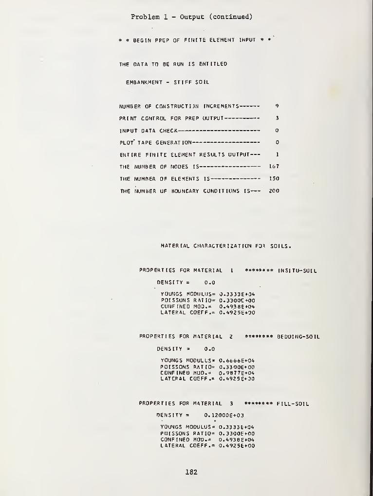
Problem 1 - Output (continued)
* * BEGIN PREP OF FINITE ELEMENT INPUT * *
THE DATA TO BE RUN IS ENTITLED
EMBANKMENT - STIFF SOIL
NUMBER OF CONSTRUCT UN INCREMENTS 9
PRINT CONTROL FOR PREP OUTPUT 3
INPUT DATA CHECK
PLOT* TAPE GENERATION
ENTIRE FINITE ELEMENT RESULTS UUTPUT 1
THE NUMBER OF NODES IS 167
THE NUMBER OF ELEMENTS IS 150
THE NUMBER UF BOUNCARY CUNDITIUNS IS 200
MATERIAL CHARACTERIZATION F3* SOILS.
PROPERTIES FOR MATERIAL I ******** INSITU-SUIL
DENSITY = 0.0
YOUNGS MODULUS" 0.3333E+0*POISSUNS RATIO= 0.3300C+00CONFINED MOD.= 0.4938E+0^LATERAL COEFF.= 0.<t925fc+00
PROPERTIES FOR MATERIAL 2 ******** OEUOING-SOIL
DENSITY = 0.0
YOUNGS MODULUS* 0.6666E+04POISSONS RAT 10= 0.3300E+00CUNFINEU MUD.= 0.9877E+04LATCRAL CUEFF.= O.^925E+0O
PROPERTIES FOR MATERIAL 3 ******** FILL-SOIL
DENSITY = 0.12000E+03•
YOUMGS MODULUS* 0.3333E+0*POISSONS RATION 0.3300E+00CONFINED MOD.= 0.4938E+04LATERAL COEFF.= 0.4925E+00
182
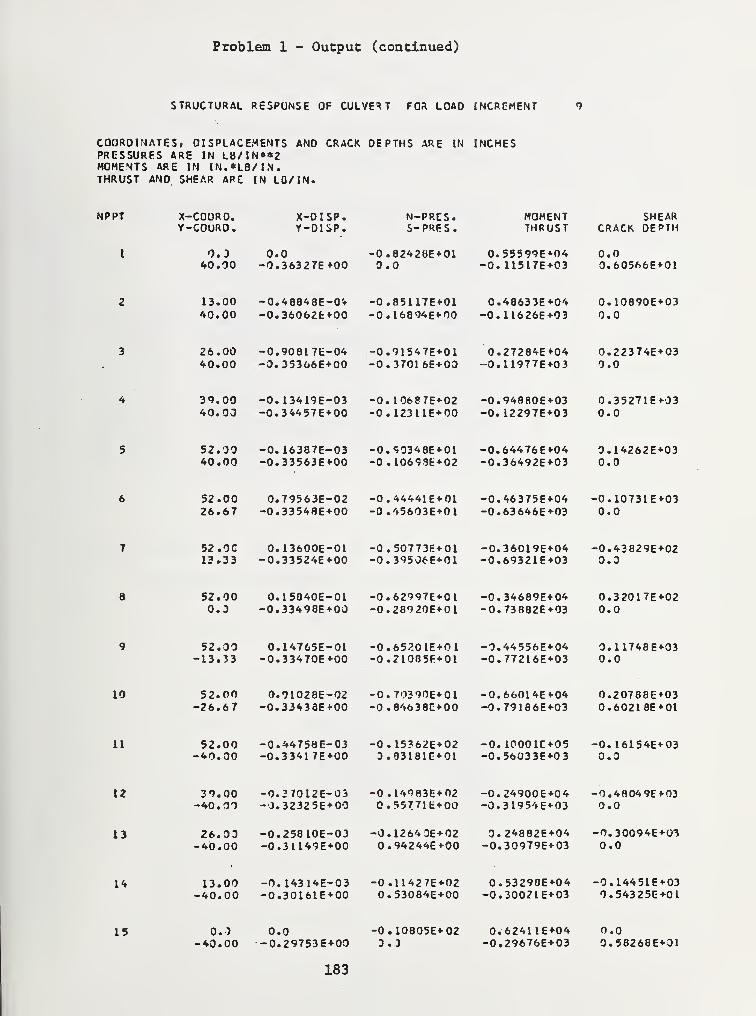
Problem 1 - Output (continued)
STRUCTURAL RESPONSE OF CULVERT FOR LOAD INCREMENT
COORDINATES. DISPLACEMENTS AND CRACK DEPTHS ARE IN INCHESPRESSURES ARE IN LB/IN**2MOMENTS ARE IN IN.*LB/IN.THRUST AND SHEAR ARE IN LO/IN.
NPPT
10
11
X-COORD.Y-COURD.
X-OISP.Y-OISP.
N-PRES.S-PRES.
MOMENTTHRUST
SHEARCRACK DEPTH
0.040.00
0.0-O.36327E+00
-0.82420E+010.0
0.55599E*04-0.11517E+03
0.00.60566E+01
13.0040.00
-0.48848E-04-0.36062fcf00
-0.85117E+01-0.16894E+00
0.48633E+04-0.11626E+03
0. 10890E+030.0
26.0040.00
-0.9081 7E-04-0.35366E+00
-0.91547E+01-0.37016E+00
0.27284E*04-0.11977E+03
0.22374E+030.0
39.0040.00
-0.13419E-03-0.34457E+00
-0.10687E+02-0.123UE+00
-0.948B0E+03-0. 12297E+03
0.35271E*330.0
52.0040.00
-0.16387E-03-0.33563E+00
-0.S0348E+01-0 . 10693E + 02
-0.64476E+04-0.36492E+03
0.14262E+030.0
52.0026.67
0.79563E-02-0.33548E+00
-0.44441E+01-0.45603E+01
-0.46375E+04-0.63 646E+03
-0.10731E+030.0
52. OC13.33
0.13600E-01-0.33524E+00
-0.50773E+01-0. 39506 E+Ol
-0.36019E«-04-0.69321E+03
-0.43829E+020.0
52.000.0
0.15840E-01-0.33498E+00
-0.62997E+01-0.28920E+01
-0.34689E+04-0.73882E+03
0.32017E+020.0
52.00-13.33
0.14765E-01-0.33470E+00
-0.65201E+OI-0.21085F+01
-0.44556E+04-0.77216E+03
0.11748E+030.0
52.00-26.67
0.91028E-02-0.33438E*00
-0. 70390E+01-0.84638E+00
-0.66014E*04-0.79186E+03
0.20788E«-030.60218E + 01
52.00-40.00
-0. 44758 E-03-0.3341 7E+00
-0. 15362E + 020.33181E+01
-0. 10001E+05-0.56033E+03
-0. 16154E4-030.0
t2 39.00 -0.27012E-03 -0.14983E + 02 -0.24900E+04 -0.4804 9E«-03•40.00 ~0.32325E*03 0.5577lt*00 -0.31954E*03 0.0
13 26.03 -0.25810E-03 -0.12640E+02 0.24882E+04 -0.30094E+0340.00 -0.31149E+00 0.94244E»00 -0.30979E+03 0.0
14 13.00 -0.14314E-03 -0.11427E+02 0.53298E+04 -0.14451E+0340.00 -0.30161E*00 0.53084E+00 -0.30021E+03 0.54325E+01
15 0.0 0.0 -0.10805E+02 0.624L1E+04 0.0•40.00 -0.29753E+00 3.0 -0.29676E+03 0.58268E+01
183
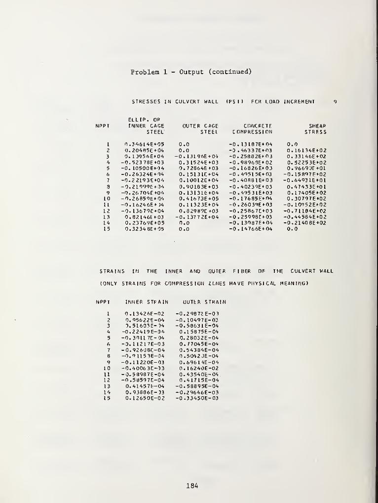
Problem 1 - Output (continued)
STRESSES IN CULVERT WALL (PS I ) FCR LOAD INCREMENT
ELLIP. OPPT INNER CAGE OUTER CAGE CONCRETE SHEAR
STEEL STEEL COMPRESSION STRESS
1 O.34614E+05 0.0 -0. 13187E+04 0.02 0.20485E+04 0.0 -0 .46337E+03 0. 16134E+023 0. 13956E+04 -0.13196E+04 -0.25882E+03 0.33146E+024 -0.52378E+03 0.31524E+03 -0.9B963E+02 0.52253E*-025 -0. 10500E+04 0.72864E+03 -0. 16826E*03 0.96693E«-016 -0.26324E+04 0. 15131E+04 -0. 49515E+03 -0. 15897E*027 -0.22193E+04 0.10012E+04 -0.40881E+03 -0.6493lE*0l9 -0.21999E+04 0.90183E+03 -0.40239E+03 0.47433E+019 -0.26 704E+04 0.13131E+04 -0 .49531E+03 0.17405E+0210 -0.26859E+04 0.41673E+05 -0. 17685E*r»4 0.30797E+0211 -0.16246E+ K 0. 11323E+04 -0.26039E+03 -0. 10952E+0212 -0. 13679C+04 0.82989E +03 -0.25867E+03 -0.71184E+0213 0.82146E+03 -0. 13772E+04 -0.25998E+03 -0.44584E*02I* 0.23769E+05 0.0 -0. 13087E+04 -0.21408E+0215 0.3234 8E+05 0.0 -0. 14766E* 04 0.0
STRAINS IN THE INNER ANU OUTER FIBER OF THE CULVERT WALL
(ONLY STRAINS FOR COMPRESSION ZLNES HAVE PHYSICAL MEANING)
NPPT INNER STRAIN OUTER STRAIN
I 0.13426E-02 -0.29872 E-032 0.95622E-04 -0. 10497E-033 1. 5 1 603 E- 14 -0.58631E-044 -0.22419E-34 0.15875E-C45 -0.3811 7E-04 0.28032E-046 -0. 11217E-03 0.77045E-047 -0.92608E-04 0.54384E-048 -0.9H53E-04 0.5042 JE-049 -0.1122 0E-03 0.69614E-0't
10 -0.'»0063E-D3 0.16240E-0211 -0.58987E-04 0.43540E-04.12 -0.58597E-04 0.41715E-0413 0.41457E-04 -0.58895E-0414 0.93886E-D3 -0.29646E-0315 0.12650E-02 -0.33450E-03
184
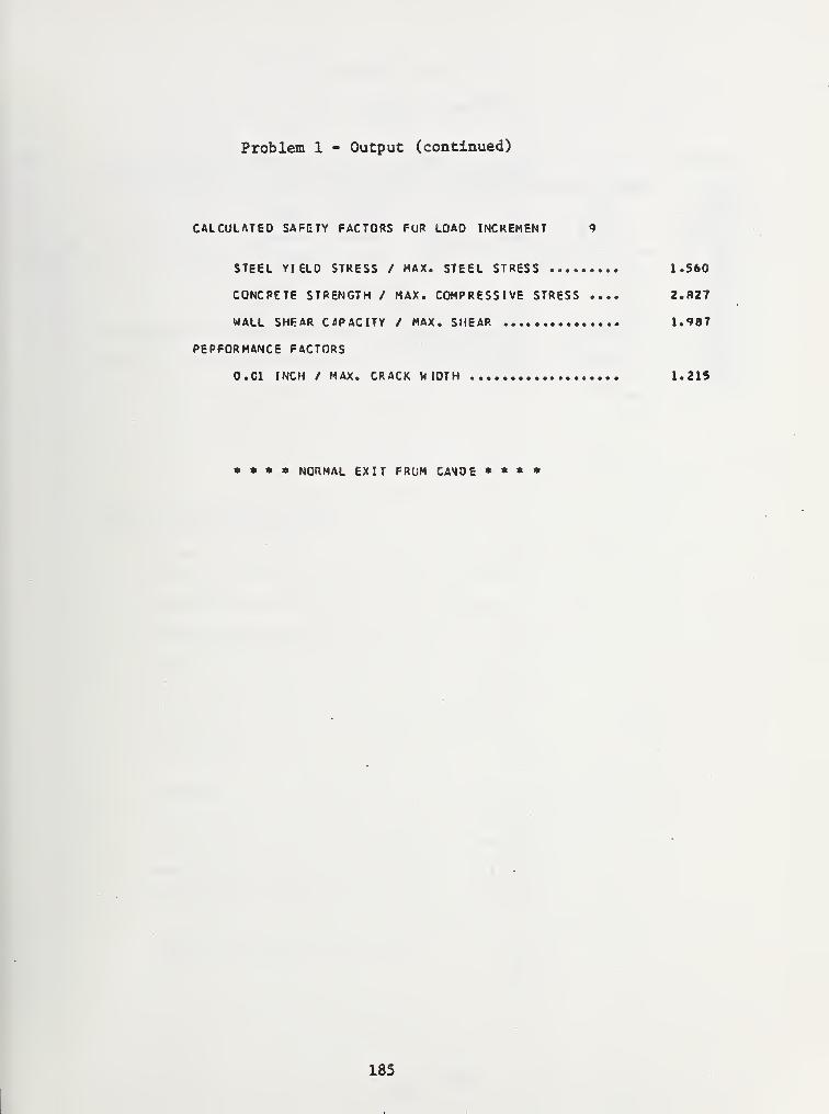
Problem 1 - Output (continued)
CALCULATED SAFETY FACTORS FUR LOAD INCREMENT 9
STEEL YIELD STRESS / MAX. STEEL STRESS 1.560
CONCRETE STRENGTH / MAX. COMPRESSIVE STRESS .... 2.827
WALL SHEAR CAPACITY / MAX. SHEAR 1.987
PERFORMANCE FACTORS
0.C1 INCH / MAX. CRACK WIDTH 1.215
+ * * * NORMAL EXIT FRUM CANDE * * * *
185
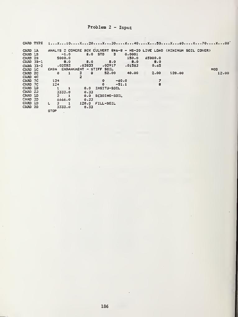
Problem 2 - Input
CARD TYPE 1
CARD 1A ANALYS 2 CONCRE BOX CULVERT 3*6-3 - HS-20 LIVE LOAD (MINIMUMCARD IB -1.0 8.0 STD 3 0.0001CARD 223 5000.0 150.0 6500CARD 3B-1 8.0 8.0 8.0 8.0 8.0CARD 33-2 .02583 .03833 .02917 .01583 0.65CARD 1C EMBA EMBANKMENT - STIFF SOILCARD 2C 1 3 8 52.00 40.00 2.00 120.00CARD 4C 2CARD 7C 124 -60 .0 7CARD 7C 124 -51 .1 8CARD ID 1 1 0.0 INSITU-SOILCARD 2D 3333.0 0.33CARD ID 2 1 0.0 BEDDING-SOILCARD 2D 6666.0 0.33CARD ID L 3 1 120.0 FILL-SOILCARD 2D 3333.0 0.33
.70....X...80
MOD12.00
STOP
186
,
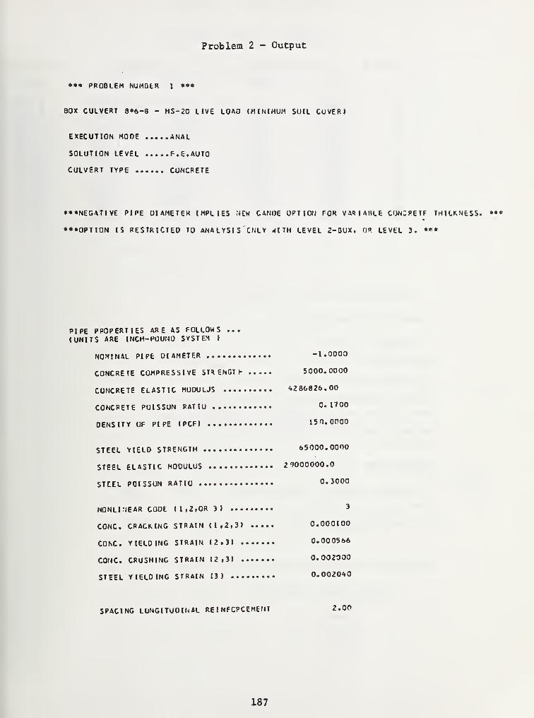
Problem 2 - Output
• •• PROBLEM NUMBER 1 **
BOX CULVERT 8»6-8 - HS-20 LIVE LOAD (MINIMUM SUIL CUVERI
EXECUTION MODE ANAL
SOLUTION LEVEL F.E.AUTO
CULVERT TYPE CUNCRETE
••NEGATIVE PIPE OIAMETER IMPLIES NCW CANOE OPTION FOR VARIABLE CONCRETE THICKNESS. *•*
••OPTION IS RESTRICTED TO ANALYSIS CNLY WITH LEVEL 2-BUX, OR LEVEL 3. ***
PIPE PROPERTIES ARE AS FOLLOWS ...
(UNITS ARE INCH-POUND SYSTEM »
NOMINAL PIPE OIAMETER -I. OOOO
CONCRETE COMPRESSIVE STRENGTH 5000.0000
CONCRETE ELASTIC MUDULJS 4286826. 00
CONCRETE PUISSUN RATIU 0. WOO
DENSITY OF PIPE (PCF) 150.0000
STEEL YIELO STRENGTH 65000.0000
STEEL ELASTIC MODULUS 29000000.0
STEEL POISSUN RATIO 0.3000
NONLINEAR COOE (1,2,OR 3) 3
CONC. CRACKING STRAIN (1,2,3) 0.000100
CONC. YIELDING STRAIN (2,31 0.000566
CONC. CRUSHING STRAIN 12,3) 0.002000
STEEL YIELOING STRAIN (3) 0.002040
SPACING LONGITUDINAL RE I NFCPCEMENT 2.00
187
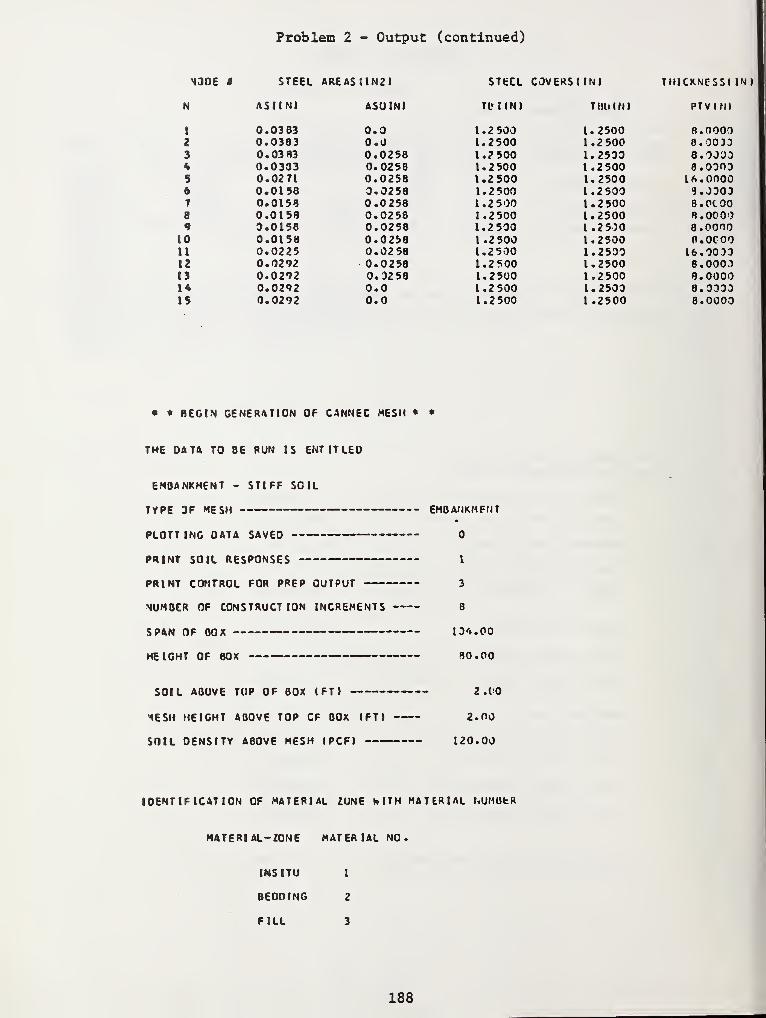
Problem 2 - Output (continued)
13DE * STEEL AREASUN2) STEEL COVERSUNI THICKNESS!
N ASIIN) ASO(N) TL> I ( N
)
TMMN.I PTV(N)
1 0.0383 0.0 1.2500 1.2500 8.00002 0.0383 0.0 1.2500 1.2500 8.00 33
3 0.03 A3 0.0258 1.2 500 1.2503 8.03334 0.0333 0.0258 1.2 500 1.2500 8.03035 0.0271 0.0258 1.2500 1.2500 1ft. 00006 0.0158 0.0258 1.2500 1.2500 9.33037 0.0158 0.0258 1.2 500 1.2 500 8.0C008 0.0158 0.0258 1.2500 1.2500 8.00009 0.0158 0.0258 1.2500 1.2 500 8.0000
10 0.0158 0.0258 1.2 500 1.2500 fl.OCOO11 0.0225 0.0258 t.2 500 1.2500 16.003312 0.0292 0.0258 1.2500 1.2500 8.000313 0.0292 0.3258 1.2 500 1.2 500 8.000014 0.0292 0.0 1.2500 1.2503 8.033315 0.0292 0.0 1.2500 1.2500 8.0000
• * BEGIN GENERATION OF CANNEC MESH * *
THE DATA TO BE RUN IS ENTITLED
EMBANKMENT - STIFF SOIL
TYPE 3F MESH EMBANKMENT
PLOTT ING DATA SAVED
PRINT SOIL RESPONSES I
PRINT CONTROL FOR PREP OUTPUT 3
NUMBER OF CONSTRUCTION INCREMENTS 8
SPAN OF BOX 134.00
HEIGHT OF BOX 80.00
SOIL ABOVE TOP OF BOX (FT) 2.(0
^ESH HEIGHT ABOVE TOP CF BOX (FT) 2.00
SOIL DENSITY ABOVE MESH IPCF1 120.00
IDENTIFICATION OF MATERIAL ZONE WITH MATERIAL NUMBER
MATERIAL-ZONE MATERIAL NO.
INS ITU 1
BEDDING 2
FILL 3
188
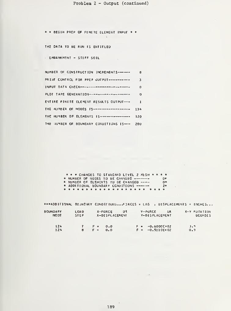
Problem 2 - Output (continued)
* * BEGIN PREP OF FINITE ELEMENT INPUT * *
THE DATA TO BE RUN IS ENTITLED
EMBANKMENT - STIFF SOIL
NUMBER OF CONSTRUCTION INCREMENTS
PRIMT CONTRCL FOR PPEP OUTPUT 3
INPUT DATA CHECK
PLOT TAPE GENERATION
ENTIRE FINITE ELEMENT RESULTS OUTPUT I
THE NJMEER OF NOOES 13 13*
THE NUMBER OF ELEMENTS IS 120
THE MUMBER OF BOUNCARY CONDITIONS IS 200
* * * CHANGES TO STANCARO LcVEL 2 MfcSH * * * *
* NUMBER OF NOOES TO BE CHANGED 0** NUMBER OF ELEMENTS TU BE CHANGED 0** ADDITIONAL BOUNOARY CGNUITIONS 2******************** **•*
•ADDITIONAL BOJNCARY COND IT IONS . . .P 3 R CES = LHS t DISPLACEMENTS = INCHES..
BOUNOARY LOAD X-FORCE 0* Y-FORCE OR X-Y PU TAT I UNNOOE STEP X-OISPLACEMENI Y-DISPLACEMENT UEGFEES
12* 7 F a 0.0 F = -0.6000C*02 ).">
12* 8 F » 0.0 F = -0.5U0E+02 0.0
189
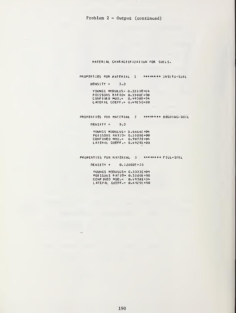
Problem 2 - Output (continued)
MATERIAL CHARACTER IZAT 1UN FOR SUILS.
PROPERTIES FOR MATERIAL 1 *«»*** INSITU-SLUL
DENSITY = 0.0
YOUNGS MO0ULUS= 0.3333EKKPOISSONS RAT 10= 0.3300C*00CONFINED MOl).= 0.4938E*04LATERAL COEFF.= U.4925E+00
PROPERTIES FOR MATERIAL 2 ***» BELUING-S01L
DENSITY = 0.0
YOUNCS MODULUS" 0.6666E*04POISSONS RATIO= 0.3300E*00CONF INEO MOO." 0.9877E+04LATERAL COEFF.= 0.49251*00
PROPERTIES FOR MATERIAL 3 **••* TILL-SOIL
DENSITY = 0. 12U00E*33
YOUNGS MODULUS" 0.3333CKKPOISSONS PATIO= 0.3300E*00CONF INED MOO." 0.4938E*04LATERAL COEFF." 0.<t925l*00
190
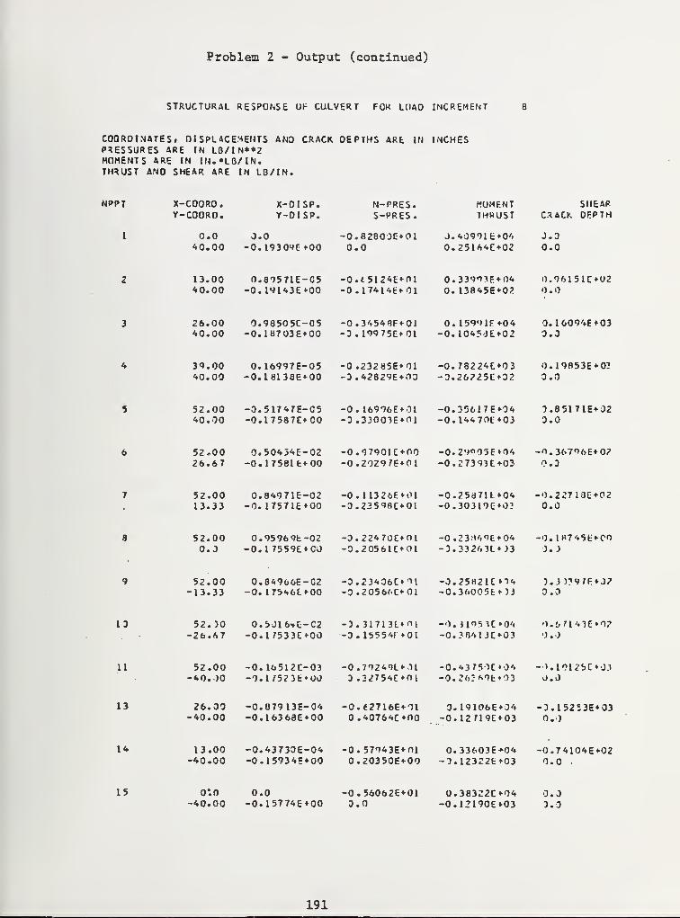
Problem 2 - Output (continued)
STRUCTURAL RESPONSE Of CULVERT FOR LOAD INCREMENT 8
COORDINATES. 01 SPLACEMENTS AND CRACK DEPTHS ARE IN INCHESPRESSURES ARE IN LB/IN**2MOMENTS ARE IN IN.*LB/IN.THRUST ANO SHEAR ARE IN LD/IN.
NPPT X-COORO. X-OISP. N-PRES. MUMENT SHEARY-COORO. Y-DISP. S-PRES. THRUST CRACK DEPTH
1 0.0 0.0 -0.82803C*0l J. 40991 fc *0'. J.
3
40.00 -0.1930<JE*00 0.0 0.25164E*02 0.0
2 13.00 0.89571E-G5 -0 .
I
5124E* 01 0.33993E+04 0.96151C*0240.00 -0.19143E*00 -0.17414E*01 0. 13845E*02 0.0
13
11
13
14
15
26.00 0.98505C-G5 -0.34548E*0l 0. 159«HE *04 0. 1609'»E*0340.00 -0. 18703E*00 -3.1<>975E*01 -0. 104?JE*02 0.3
3<».00 0.16997E-05 -0.23285E*0l -0.78224E+03 0.19853E + 03
40.00 -0.1«138E*00 -3.42829E*r»0 -3.26?25C*32 3.0
52.00 -0.51747E-05 -0. 16996E*01 -0.35617EO4 0.85171E*3240.00 -0.17587E*00 -3 ,33O03E*Ol -0.144 70L: *03 3.0
52.00 0.50454C-02 -0.9 7901C*00 -0.29°05E*0't -O.36796E+0226.67 -0.17581 fc*00 -0.20297E*01 -0.27393E+03 0.3
52.00 0.84971E-02 -0. 113 26E*01 -0.258711*04 -0.22713C*0213.33 -0. 17571E+00 -3.23598C+01 -0.30319E+02 0.0
52.00 0.95969E-02 -0.22470E*Ol -0.2 3*4OE*04 -0. 18745E*C00.0 -0.1 7559E*CJ -0.20561O01 -3.33263L03 0. J
52.00 0.84966E-02 -0.23406C* r>l -0.25H21E H4 3.3 )?V/F*J?13.33 -0. 17546E*00 -0.2056^C*Ol -0.36005EO3 0.0
52.50 0.531 64C-C2 -3. 317131*11 -o. »i95it*04 O.67l4in»0726.67 -0.17533E*00 -0. 155541: Ol -0.3 0413C*03 0.0
52.00 -0.16512C-03 -0.792 491* 11 -0.<.3 75">C»0'» -1.101250*0340.00 -O.I /523E*00 3 .2275'.C»ni -0.26?fc9t*93 0.0
26.00 -0.079 13E-04 -0.627I6E*Ol 3.19106E*04 -3.15253E+0340.00 -0.I6368E*00 0.^.0764E*no -0.12 H9L'*03 0.0
13.00 -0.43730E-04 -0.57943E+O1 0.33603E+04 -0.74104E*02•40.00 -0.15934E+00 0.20350E*00 -0.123Z2E*03 0.0 ,
O'.O 0.0 -0.56062E+01 0.383Z2C*04 0.3•40.00 -0.15774E*00 3.0 -0.12190E*03 3.3
191
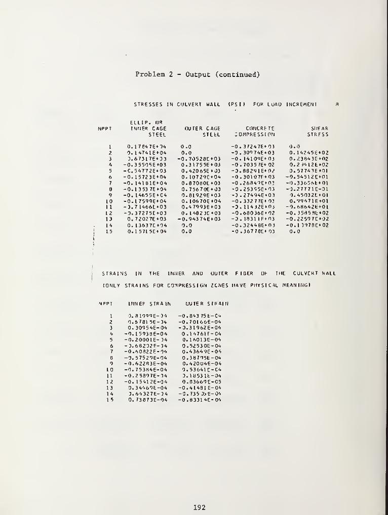
Problem 2 - Output (continued)
STRESSES IN CULVERT WALL (PS I ) FOR LUAO INCREMENT
NPPT
1
2
3
'
5
6
7
8
9
101112131*15
ELL1P. ORINNER CAGE
STEEL
0.17e47E*040. I 474 1E*043.67317E03
-0.35505E*03-C.54772E+03-0.15723E + 04-0. 14181E*04-0.1353 7E04-0. 14655E+C4-0.17599E+04-3.71466E*03-0.37275E+030.72027E*030. 13637E040.15715E*04
OUTER CAGESTLbL
0.00.0-O.7O528C*030.31755E*030.42065E »030. 10729C+040.870BOE+030.75670E + 030.81929E*030.10670E+040.47993E«-030.1482 3E*03-0.943 74£*030.00.0
CONCRETE;OMPRESSION
0. 37247E+03•0. 30974E + 030. 14109E*030.70357E* 02-3.8829lE*02-0.30107F>03-0.26849E*03-0.2 53 <;5E»-O3
O .27494E*03-0.33277E* 03-3. U432E*0j-0.68036E*02-3. 1831 IF*03-0.32448E*OJ-0 .36778E* 03
SMEARSTRESS
0.00. 14245E+020.23843E*020.2 Wl2fc*020.57743E*0I-0.54512E«-01-0.3365fcb»01-J.27771G-010.450321*010.99471F.»0l-0.68642E+01-0. 35853L«-02-0.22597C»02-0.1 197BC»020.0
STRAINS IN THE INNER AND OUTER FIBER OF THE CULVERT WALL
(ONLY STRAINS FOR COMPRESSION ZCNES HAVE PHYSICAL MEANING)
NPPT INNER STRAIN OUTER STRAIN
I 0.8 t9<J9E-0 4 -0.843 75E-C42 0.6781 5E-34 -0.70166E-043 0. 30954E-04 -0.31962E-044 -0.15938E-04 0.14761T-C45 -0.20001E-34 0. 16013E-046 -3.68232E-34 0.52530E-047 -0.60822E-04 0.43649C-048 -0.57529E-04 0.38795E--049 -O.A2283E-04 0.420U4E-04
10 -0.75384E-04 0.53641C--C411 -0.25897E-14 3. 10531b-0412 -0. 15412E-04 0.83669E--C513 0.34469E-04 -0.41481 E-0414 3.64327E-34 -0. 73535 E-•04
15 0.73873E-04 -0.83314E-04
192
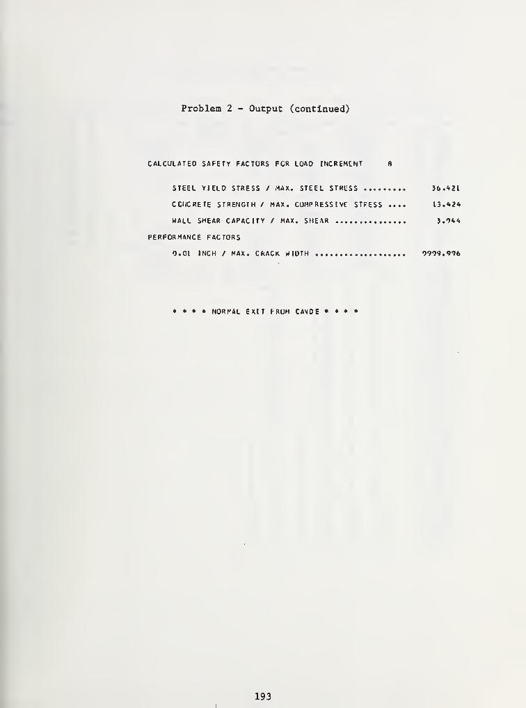
Problem 2 - Output (continued)
CALCULATED SAFETY FACTORS FOR LOAD INCREMtNT ft
STEEL YIELO STRESS / MAX. STEEL STRESS 36.*21
CCNCRETE STRENGTH / MAX. COMPRESSIVE STFESS .... 13. *24
WALL SHEAR CAPACITY / MAX. SHEAR 3.9**
PERFORMANCE FACTORS
0.01 INCH / MAX. CRACK WIDTH 9909.996
* • * * NORMAL EXIT FROM CA>iDE * • * *
193
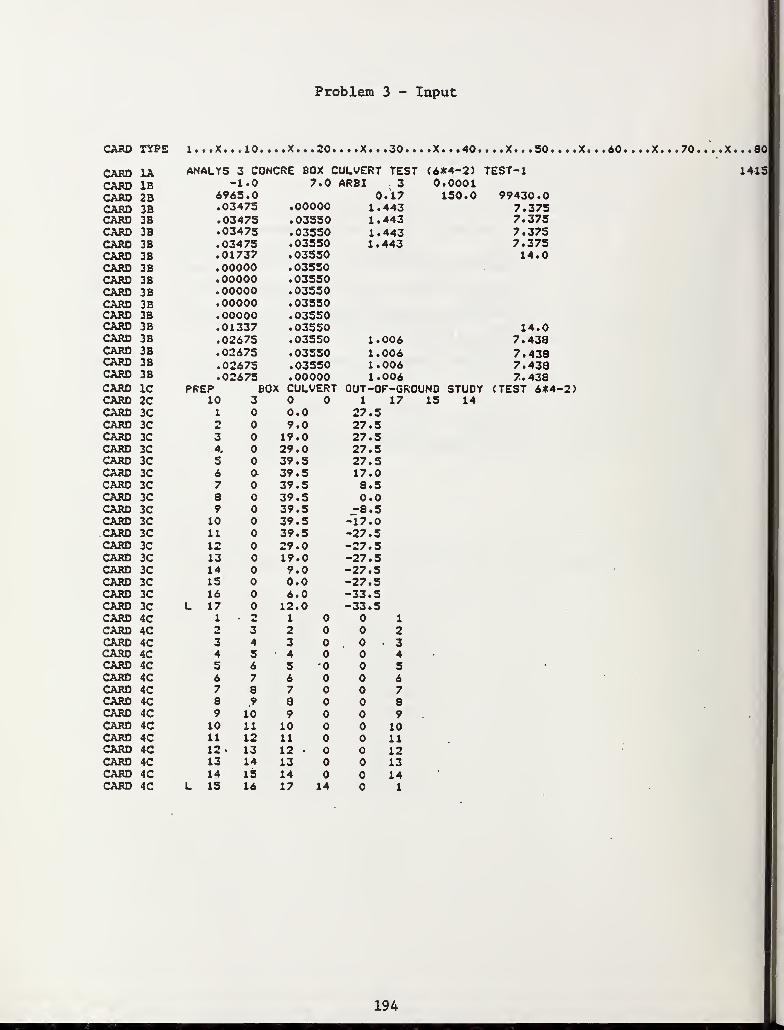
Problem 3 - Input
CARD TYPE
CARD 1A ANALYS 3 CONCRE BOX CULVERT TEST (6*4-2) TEST-1CARD IB -1.0 7 .0 ARBZ 3 0.0001CARD 2B 6965.0 .17 150.0 99430.0CARD 3B .03475 .00000 1.'443 7.375CARD 3B .03475 .03550 1.'443 7.375CARD 3B .03475 .03550 1. 443 7.375CARD 3B .03475 .03550 1.443 7.375CARD 3B .01737 .03550 14.0CARD 3B .00000 .03550CARD 3B .00000 .03550CARD 3B .00000 .03550CARD 3B .00000 .03550CARD 3B .00000 .03550CARD 3B .01337 .03550 14.0CARD 3B .o:2675 .03550 1.006 7.438CARD 3B .02675 .03550 1.006 7.438CARD 3B .0.2675 .03550 1.006 7.438CARD 3B .0.2675 .00000 1.006 7.438CARD 1C PREP BOX CULVERT OUT-OF-GROUND STUDY (TEST 6*-
CARD 2C 10 3 1 17 IS 14CARD 3C 1 0.0 27.5CARD 3C 9.0 27.5CARD 3C 3 19.0 27.5CARD 3C 4. 29.0 27.5CARD 3C 5 39.5 27.5CARD 3C 6 a 39.5 17.0CARD 3C 7 39.5 8.5CARD 3C 8 39.5 0.0CARD 3C 9 39.5 -8.5CARD 3C 10 39.5 -17.0CARD 3C 11 39.5 -27.5CARD 3C 12 29.0 -27.5CARD 3C 13 19.0 -27.5CARD 3C 14 9.0 -27.5CARD 3C 15 0.0 -27.5CARD 3C 16 6.0 -33.5CARD 3C L 17 12.0 -33.5CARD 4C 1 2 1 1
CARD 4C 2 3 2 2CARD 4C 3 4 3 . o 3CARD 4C 4 5 4 4CARD 4C 5 6 5 5CARD 4C 6 7 6 6CARD 4C 7 8 7 7CARD 4C 8 .9 8 8CARD 4C 9 10 9 9CARD 4C 10 11 10 10CARD 4C 11 12 11 11CARD 4C 12- 13 12 • 12CARD 4C 13 14 13 13CARD 4C 14 15 14 14CARD 4C L IS 16 17 14 1
.60....X...70....X...80
1415
194
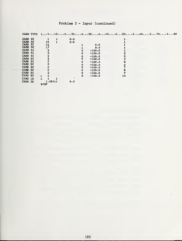
Problem 3 - Input (continued)
CARD TYPE 1.. .X...10....X...20....X...30....X...40. ...X...50....X...60.. ..X...70....X...80
CARD 5C 11 0.0 1
CARD SC IS 1 0.0 1CARD 5C 16 1 0.0 1CARD 5C 17 1 0.0 1CARD SC 2 -100.0 1CARD SC 2 -100.0 2CARD SC 2 -100.0 3
0.00.0
1 0.01 0.0
-100.0-100.0-100.0-100.0-100.0-100.0-100.0-100.0-100.0-100.0
CARD SC 2 -100.0 4CARD SC 2 -100.0 3CARD SC 2 -100.0 6CARD 5C 2 -100.0 7CARD SC 2 -100.0 8CARD SC 2 -100.0 9CARD SC L 2 -100.0 10CARD ID L 1 1 '
CARD 2D 1.0E+11 0.0STOP
195
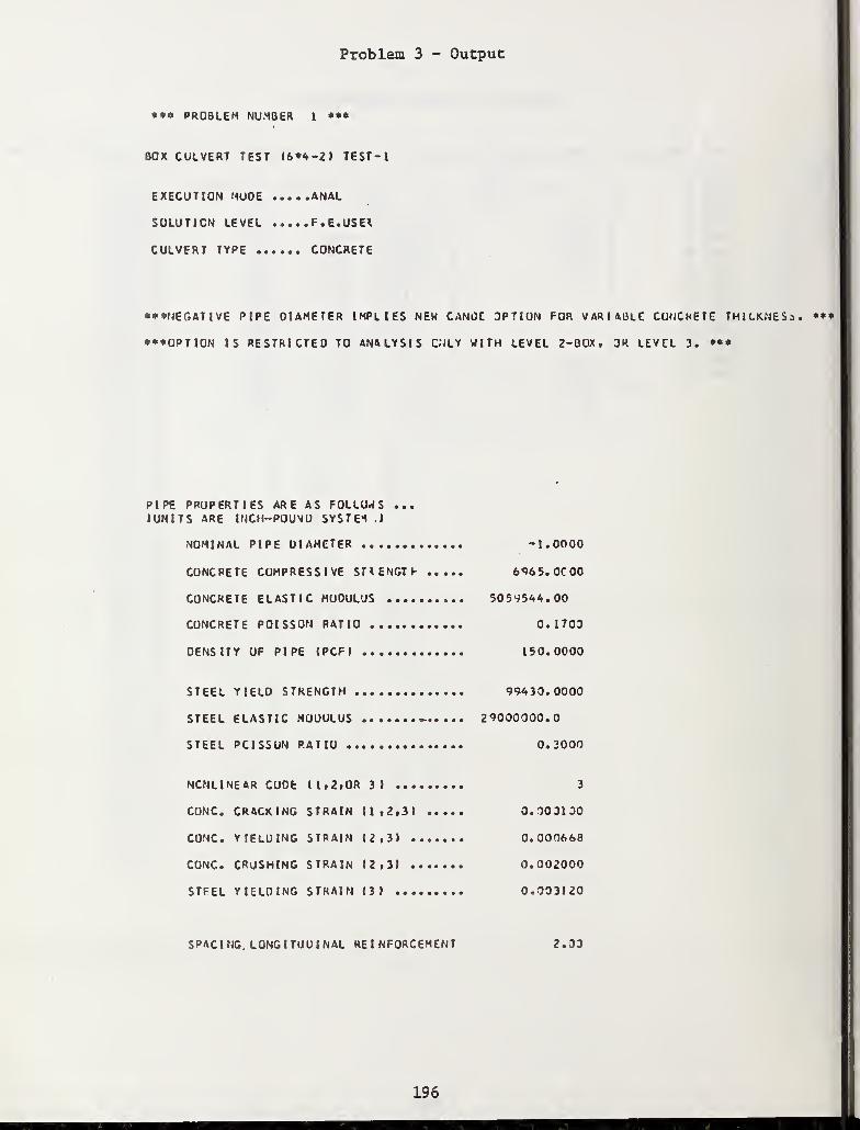
Problem 3 - Output
• PROBLEM NUMBER i *•*
BOX CULVERT TEST «6**-2J TEST-l
EXECUTION MUOE ANAL
SOLUTION LEVEL F.E.USE*
CULVERT TYPE CONCRETE
NEGATIVE PIPE DIAMETER IMPLIES NEW CANOC OPTION FOR VARIABLE CONCRETE THlCKNESi. *•OPTION IS RESTRICTED TO ANALYSIS CNLV WITH LEVEL 2-BOX, OR LEVCL 3.
PIPE PROPERTIES ARE AS FOLLOWS ...(UNITS ARE INCH-POUND SYSTEM ,)
NOMINAL PIPE DIAMETER -I. OOOO
CONCRETE COMPRESSIVE SMENGTh 6965. OCOO
CONCRETE ELASTIC MUOULUS 505*5*4.00
CONCRETE POISSON RATIO 0.1700
DENSITY OF PIPE (PCF) 150.0000
STEEL YIELD STRENGTH 99A30. 0000
STEEL ELASTIC MODULUS ^ 29000000.0
STEEL PCiSSUN RATIO 0.3000
NCNLINEAR CODE (1,2, OR 3) 3
CONC. CRACKING STRAIN (1,2.3) 0.000130
CONC. YIELDING STRAIN (2,31 0.000668
CONC. CRUSHING STRAIN (2,3) 0.002000
STFEL YIELOING STRAIN (3) 0.003120
SPACING. LONGITUDINAL RE I NFORCEMENT 2.00
196
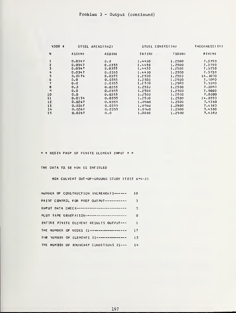
Problem 3 - Output (continued)
njoe * STEEL AREASIIN2) STEEL COVERS! IN) THICKNESS! IN »
N ASIfNI ASO(N) TBI IN) TDCXN) PTV(N)
I 0.0347 0.0 1.4430 1.2500 7.37502 0.0347 0.0355 1.4430 1.2500 7.37503 0.0347 0.0355 1.4430 1.2500 7.37504 0.0347 0.0355 1.44J0 1.2500 7.37505 0.0174 0.0355 1.2 500 I. 2503 14. JO-JO
6 0.0 0.0355 1.2 500 1.2500 7. 10037 0.0 0.0355 1.2 500 1.2500 7.00009 0.0 0.0355 1.2500 1.2500 7.0000n 0.0 0.0355 1.2500 1.2500 7.0000
10 0.0 0.0355 1.2500 1.2500 7.000011 0.0134 0.0355 1.2500 1.2500 14.000312 0.0267 0.0355 I .0060 1.2500 7.438013 0.0267 0.0355 1.0060 1.2500 7.438014 0.3267 0.0355 1.0 ObO 1.2500 7.438015 0.0267 0.0 1.0060 1.2500 7.4380
* * 8EGIN PREP OF FINITE ELEMENT INPUT * *
THE OATA TO. OE RUN IS ENTITLED
BOX CULVERT CUT-UF-GRUUNU STUOY I TEST 6*4-2)
NUMBER OF CONSTRUCTION INCREMENTS 10
PRINT CONTROL FOR PREP OUTPUT 3
INPUT OATA CHECK
PLUT TAPE GENEFATION
ENTIRE FINITE ELEMENT RESULTS OUTPUT— -1
THE NUMBER OF NOOES IS 17
THE NUMBER OF ELEMENTS IS 15
THE NUMBER OF BOUNCARY CUNDITIUNS IS 14
197
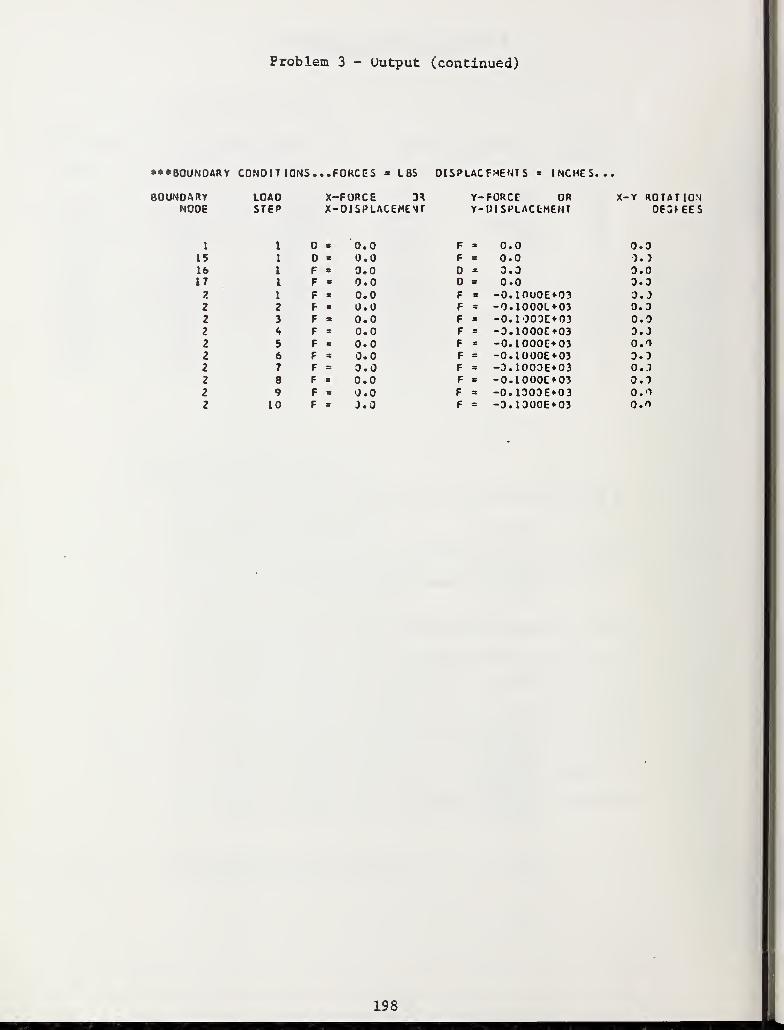
Problem 3 - Output (continued)
••BOUNDARY CONDI T IONS .. .FORCES * LBS DISPLACEMENT S » INCHES...
8OUN0ARYNODE
1
15
1617
2
2
2
2
2
2
2
2
2
2
LOAO X-FORCE 0* Y- FORCE ORSTEP X-OISPLACEMEMT Y- OlSPLACtMENT
I D » 0.0 F 3 0.01 » 0.0 F S 0.01 F « 0.0 S 0.01 F • 0.0 = 0.0I F » 0.0 F = -O.lOuOE«-032 F » 0.0 F a -0.1000L+033 F * 0.0 F s -0.1000C+034 F » 0.0 F a -O.IOOOE*035 F » 0.0 F -0.1000C*036 F = 0.0 F = -O.IOOOE*037 F 0.0 F a -0.1000E+038 F » 0.0 F = -0.1000C*039 F a 0.0 F 3 -0.1000E+0310 F * J.O F 3 -0.1000E*03
X-Y ROTATIONOE^EES
0.00.)0.00.0O.J0.00.00.00.00.50.00.10.1O.rt
198
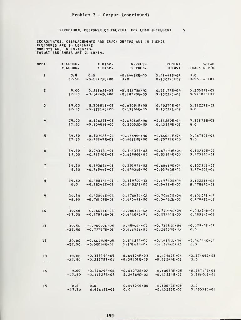
Problem 3 - Output (continued)
STRUCTURAL RESPONSE UF CULVERT FOR LOAO INCREMENT 5
COORDINATES t DISPLACEMENTS AND CRACK DEPTHS ARE IN INCHESPRESSURES ARE IN LB/IN**2MOMENTS ARE IN IN.*LB/IN.TH<US7 AND SHEAR ARE IN LB/IN.
NPPT X-COORD. X-OISP. N-PRFS. MOMENT SHEARY-COORO. r-DISP. S-PRES. THRUST C«ACK DEPTH
1 0.0 0.0 -0.6441CE*<>0 0.91441C*04 0.027.50 -0.15773E*00 3.0 0.l3239E«-02 0. 56336E«-0l
2 9.00 0.21162E-05 -3.«3278E»02 0.9ll7flE«-0* 0.25597E*0327.50 -3.l4942t*00 -3.18370E-05 3.13239E*02 3.57301EOI
3 19.00 0.50681E-05 -0.65051F*00 0.4027OEKK 0.51229EO327.50 -0.12B14E*00 0.17166E-05 0.13239E*02 0.0
4 29.00 0.83627E-05 -3.62088C*00 - J. 1 1200E*0« 0.51872E*0327.50 -0.10406E+00 0.26052C-05 0.13239E*02 0.0
5 39.50 0.10792E-G4 -0.46690t*00 -0.66008E*04 3.2675<>C»0327.50 -0.78849E-01 -0 .461
1
8E*00 -0.25778E*03 0.0
6 39.50 0.24313E-01 0.34437E-02 -0.67'»93E*0<» 0.12265E*0217.00 -0.78740E-01 -3.63980E»03 -0.53184E*03 0.47313COI
7 39.50 0.39382E-01 0.29297E-02 -0.6B619E»04 0. 1 32 36C 028.50 -0.785*6E-0l -0.64936E»no -0.53763EO3 0. 474J5E/01
8 39.50 0.45814E-01 3.51970O03 -3.69743E*r>'. 0.13221FO20.0 -0.78341E-01 -0.6452?E*00 -0. 5'.3 1 4E *03 0.47867CO1
9 39.50 0.4200JE-01 0.378071-02 -0. 7006 7 E »0<. 0.13231T»02-8.50 -0.7bl09E-01 -0 . 6<.568E»00 -0. 5<.P62t »02 0. «. 7<)<,2C 01
10 39.50 0.26661E-01 -0.7863VE-O2 -0. 71 90 9L *04 0.1322'»E*02-17.00 -0.77876fc-0l -0 .64 LOH^ J -0 . 55'.'. I E 03 J.'.OOl '»C *0 1
11 39.50 -0.9O*92L-O5 . 45"06F *00 -0.73 3801*0'. -0. ? 75 sor »03
-27.50 -0.77757C-01 -3.45692t*0J -0. 205
3
5C»03 n.o
12 29.00 -0.A619JE-05 0.6M27r«-O3 - 3 . 1 '. I 3 I L V» - 3. r><W S'.OO «
-27.50 -0.5006HE-01 3.ni67l-<^. -0. 1 3246C »-)2 J.O
11 19.00 -0.33335C-05 0.64524E*00 0.<»2963E *0<» -0. 57<.06CO3-27.50 -0.235756-01 -0.39101E-05 -0. 132*<SE»02 0.0
14 9.00 -0.57829E-06 -0.61072E+02 0.10070E*05 -0. 287 liC*03-27.50 -0.11727E-07 3.24769E-02 -0. 13234E02 . 586 06E Ol
15 0.0 0.0 0.64529E*00 0.100'»3E*05 3.0-27.50 0.92615E-02 0.0 -0. 13222C*02 0.505?U*Ol
199
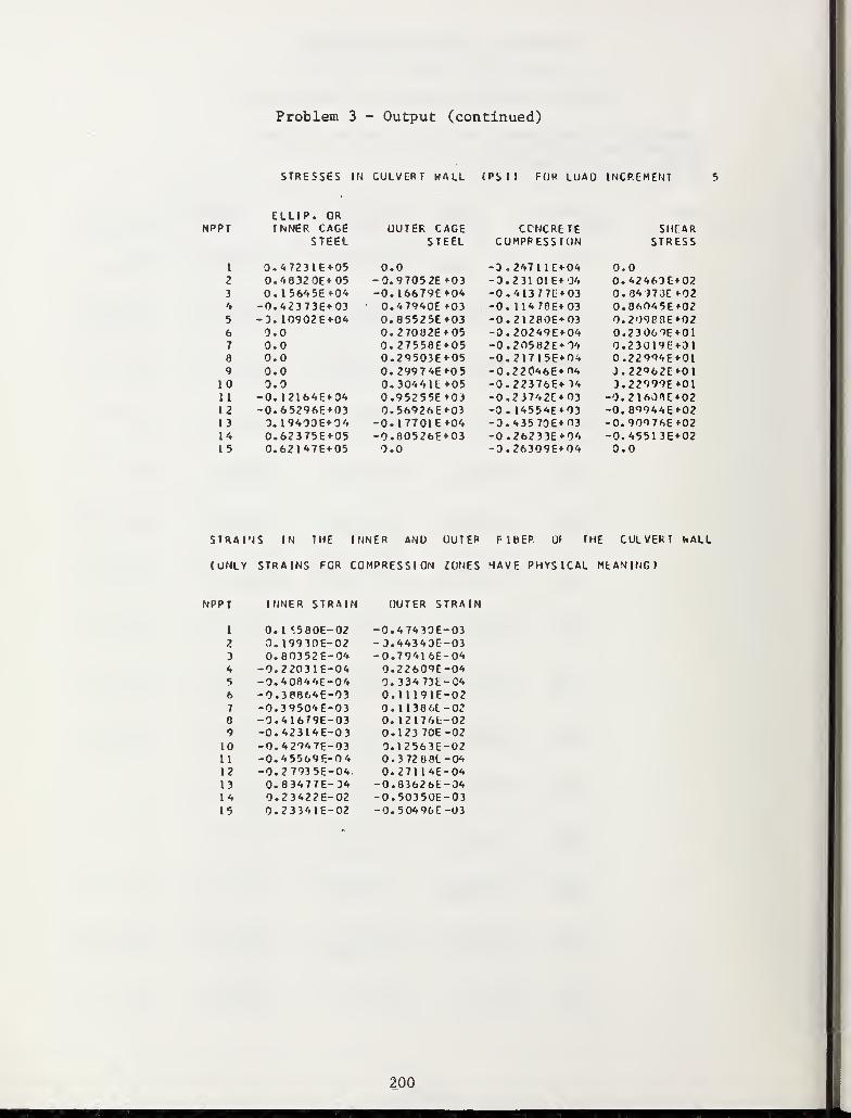
Problem 3 - Output (continued)
STRESSES IN CULVERT HALL (PS I) FOR LUAD INCREMENT
NPPT
I
2
3
4
5
6
7
8
9
10111213141 5
ELLIP. ORINNER CAGE
STEEL
0.47231E+050.4832 0E*050. 15645E*04-0.42373E*03-3. 10902E+040.00.00.00.00.0-0.12164E+04-0.65296E+030. 19400EO40.62375EO50.62147E*05
OUTER CAGESTEEL
0.00.97052E*03-0.16679E*040.47940E*030.85525E*030.27082E«-050.27558E*050.29503E*050.29974E+050.30441E*050.95255E »030.56926E+03-0.1 7701 E*04-0.80526E«-033.0
CONCRETECOMPRESSION
3. 247 11C + 04-3.2 31 01 E* 34
-0.41377E*03-0. H470f>03-0.21280E+03-0.20249E*04-0.20582EO'.-0.21715E+0*-0.22046E*n<,-0.22376EO40.23742E+03-0. 14554E+033.43570E*O3-0.26233E*04-0.26309E*04
SMEARSTRESS
0.00.42460E+020.84 )73C*020.86045E*020.209C8E*020.2306 9E*0l0.23019L: *010.2299'»E+013.22<'62E*013.22999E«-0t-0.21608E*02-0. 89944E*020.90976E*02-0.45513E*020.0
STRAINS IN THE INNER AND OUTER FIBER Of THE CULVERT WALL
(ONLY STRAINS FOR COMPRESSION ZONES HAVE PHYSICAL MtANING)
NPPT INNER STRAIN OUTER STRAIN
1 0.1 <580E-02 -0.47430E--032 0. 19930E-02 -3.44340E -03
3 0.80352E-04 -0.79416E--044 -0.22031E-04 0.22609E -04
5 -0.40844E-04 0.334 73E--C46 -0.38864E-03 0.11191E--027 -0.39504E-03 0.1138 6E--02
8 -0.41679E-03 0. 12176L--029 -0.42314E-03 0.12370E -02
10 -0.42947E-03 3.12563E--0211 -0.45569E-04 0.3 72B8L -04
12 -0.27935E-04 0.27114E--0413 0.83477E-34 -0.83626E--0414 0.23422E-02 -0.50350E--0315 0.23341E-02 -0.50496E -03
200
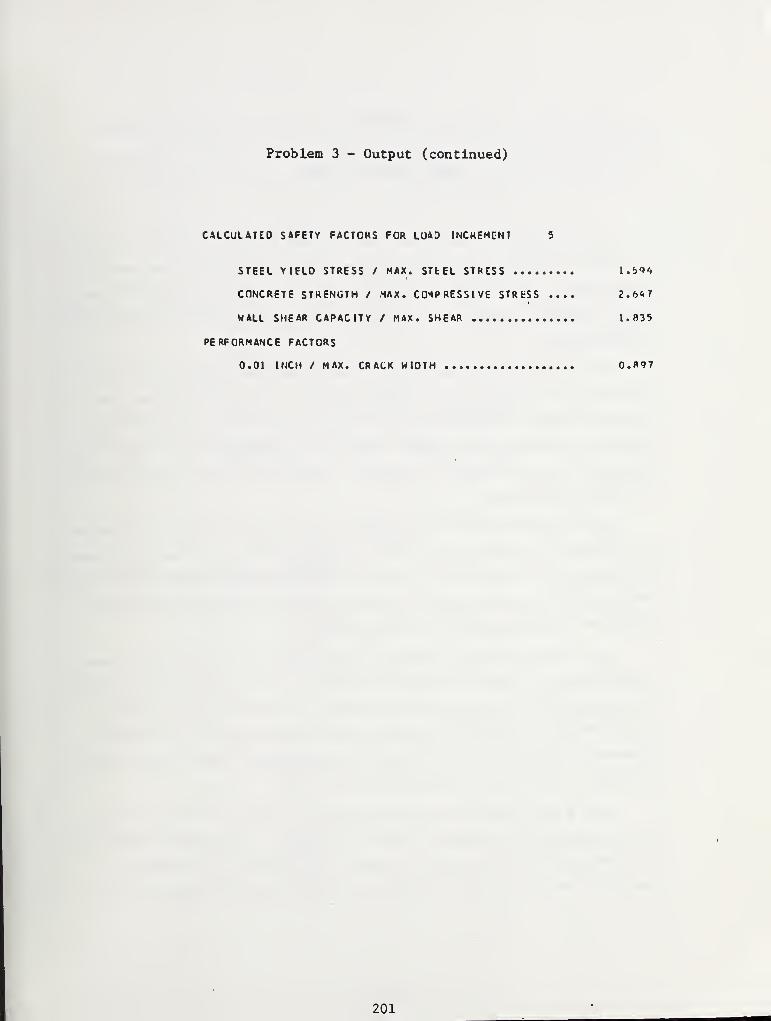
Problem 3 - Output (continued)
CALCULATED SAFETY FACTORS FOR LOAD INCREMENT 5
STEEL YIELD STRESS / MAX. STEEL STRCSS 1.59'*
CONCRETE STRENGTH / MAX. COMPRESSIVE STRESS .... 2.647
HALL SHEAR CAPACITY / MAX. SHEAR 1 . 835
PERFORMANCE FACTORS
0.01 INCH / MAX. CRACK WIDTH 0.897
201
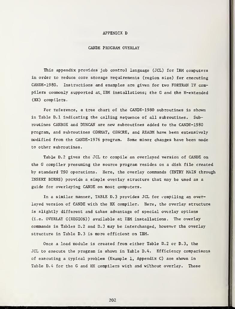
APPENDIX D
CANDE PROGRAM OVERLAY
This appendix provides job control language (JCL) for IBM computers
in order to reduce core storage requirements (region size) for executing
CANDE-1980. Instructions and examples are given for two FORTRAN IV com-
pilers commonly supported at. IBM installations; the G and the H-extended
(HX) compilers.
For reference, a tree chart of the CANDE-1980 subroutines is shown
in Table D.l indicating the calling sequence of all subroutines. Sub-
routines CANBOX and DUNCAN are new subroutines added to the CANDE-1980
program, and subroutines CONMAT, CONCRE, and READM have been extensively
modified from the CANDE-1976 program. Some minor changes have been made
to other subroutines.
Table D.2 gives the JCL to compile an overlayed version of CANDE on
the G compiler presuming the source program resides on a disk file created
by standard TSO operations. Here, the overlay commands (ENTRY MAIN through
INSERT BURNS) provide a simple overlay structure that may be used as a
guide for overlaying CANDE on most computers.
In a similar manner, TABLE D.3 provides JCL for compiling an over-
layed version of CANDE with the HX compiler. Here, the overlay structure
is slightly different and takes advantage of special overlay options
(i.e. OVERLAY C (REGION)) available at IBM installations. The overlay
commands in Tables D.2 and D.3 may be interchanged, however the overlay
structure in Table D.3 is more efficient on IBM.
Once a load module is created from either Table D.2 or D.3, the
JCL to execute the program is shown in Table D.4. Efficiency comparisons
of executing a typical problem (Example 1, Appendix C) are shown in
Table D.4 for the G and HX compilers with and without overlay. These
202
examples were executed on the IBM 370/168 computer at the University of
Notre Dame. It is observed that HX compiler with overlay provided the
most efficient results in terms of core storage, execution time, and
total cost.
203
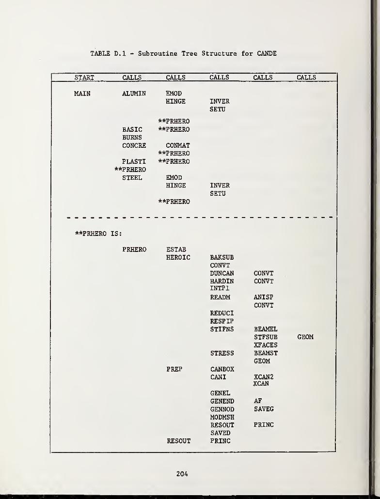
TABLE D.l - Subroutine Tree Structure for CANDE
START CALLS CALLS CALLS CALLS CALLS
MAIN ALUMIN
BASICBURNSCONCRE
EMODHINGE
**PRHERO**PRHERO
CONMAT
INVERSETU
**PRHEROPLASTI **PRHERO
**PRHEROSTEEL EMOD
HINGE
**PRHERO
INVERSETU
**PRHERO IS:
PRHERO ESTABHEROIC
PREP
RESOUT
BAKSUBCONVTDUNCANHARDININTPl
READM
REDUCIRESPIPSTIFNS
STRESS
CANBOXCANI
GENELGENENDGENNODMODMSHRESOUTSAVEDPRINC
CONVTCONVT
ANISPCONVT
BEAMELSTFSUBXFACESBEAMSTGEOM
XCAN2XCAN
AFSAVEG
PRINC
GEOM
J
204
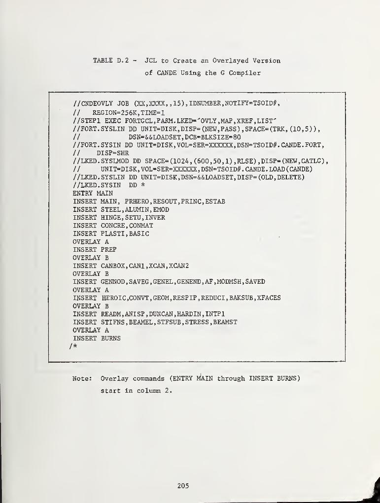
TABLE D.2 - JCL to Create an Overlayed Version
of CANDE Using the G Compiler
//CNDEOVLY JOB (XX,XXXX, , 15) , IDNUMBER,NOTIFY=TSOID#,
// REGION=256K,TIME=l//STEP1 EXEC FORTGCL,PARM.LKED='OVLY,MAP,XREF,LIST'//FORT.SYSLIN DD UNIT=DISK,DISP=(NEW,PASS ) ,SPACE=(TRK, (10,5) )
,
// DSN=&&LOADSET,DCB=BLKSIZE=80//FORT.SYSIN DD UNIT=DISK,VOL=SER=XXXXXX,DSN=TSOID#. CANDE. FORT,
// DISP=SHR//LKED.SYSLMOD DD SPACE= (1024, (600,50,1) ,RLSE) ,DISP= (NEW, CATLG)
,
// UNIT=DISK,VOL=SER=XXXXXX,DSN=TSOID#. CANDE. LOAD(CANDE)//LKED.SYSLIN DD UNIT=DISK,DSN=&&LOADSET,DISP= (OLD, DELETE)//LKED.SYSIN DD *
ENTRY MAININSERT MAIN, PRHERO,RESOUT,PRINC,ESTABINSERT STEEL, ALUMIN,EMODINSERT HINGE, SETU,INVERINSERT C0NCRE,C0NMATINSERT PLASTI, BASICOVERLAY AINSERT PREPOVERLAY B
INSERT CANB0X,CAN1,XCAN,XCAN2OVERLAY B
INSERT GENNOD , SAVEG , GENEL , GENEND , AF , MODMSH , SAVEDOVERLAY AINSERT HEROIC ,CONVT , GEOM, RESPIP , REDUCI , BAKSUB ,XFACESOVERLAY B
INSERT READM,ANISP, DUNCAN, HARDIN, INTP1INSERT STIFNS , BEAMEL , STFSUB , STRESS , BEAMSTOVERLAY AINSERT BURNS
/*
Note: Overlay commands (ENTRY MAIN through INSERT BURNS)
start in column 2.
205 J
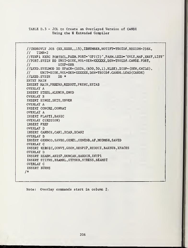
TABLE D.3 - JCL to Create an Overlayed Version of CANDEUsing the H Extended Compiler
//CNDEOVLY JOB (XX,XXXX, ,15) ,IDNUMBER,NOTIFY=TSOID#,REGION=256K,
// TIME=2//STEP1 EXEC F0RTXCL,PARM.F0RT='0PT(2)%PARM.LKED='0VLY,MAP,XREF,LIST'//FORT.SYSIN DD UNIT-DISK, VOL-SER-XXXXXX,DSN-TSOID#. CANDE. FORT,
// DISP=SHR//LKED.SYSLMOD DD SPACE= (1024, (600,50,1) ,RLSE) ,DISP= (NEW, CATLG)
,
// UNIT=DISK,VOL=SER=XXXXXX,DSN=TSOID#. CANDE. LOAD(CANDE)//LKED.SYSIN DD *
ENTRY MAININSERT MAIN,PRHERO,RESOUT,PRINC,ESTABOVERLAY AINSERT STEEL,ALUMIN,EMODOVERLAY B
INSERT HINGE, SETU,INVEROVERLAY AINSERT CONCRE,CONMATOVERLAY AINSERT PLASTI, BASICOVERLAY C (REGION)INSERT PREPOVERLAY DINSERT CANB0X,CAN1,XCAN,XCAN2OVERLAY DINSERT GENNOD, SAVEG , GENEL , GENEND , AF ,MODMSH , SAVEDOVERLAY C
INSERT HEROI C , CONVT , GEOM , RESP IP , REDUCI , BAKSUB , XFACESOVERLAY DINSERT READM,ANISP, DUNCAN, HARDIN, INTP1INSERT STIFNS , BEAMEL , STFSUB , STRESS , BEAMSTOVERLAY C
INSERT BURNS/*
Note: Overlay commands start in column 2.
206
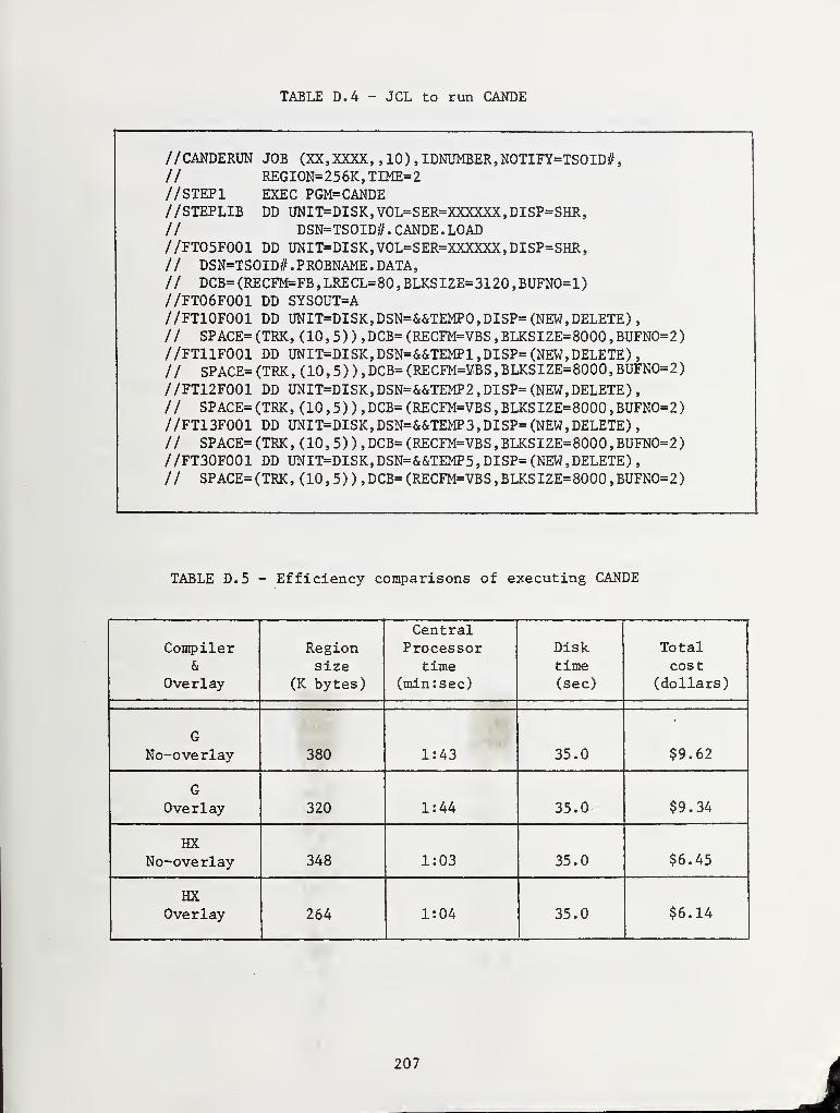
TABLE D.4 - JCL to run CANDE
//CANDERUN JOB (XX,XXXX, ,10) ,IDNUMBER,NOTIFY=TSOID#,// REGION=256K,TIME=2//STEP1 EXEC PGM=CANDE//STEPLIB DD UNIT=DISK,VOL=SER=XXXXXX,DISP=SHR,// DSN-TS0ID#. CANDE. LOAD//FTO5F001 DD UNIT=DISK,VOL=SER=XXXXXX,DISP=SHR,// DSN=TSOID#.PROBNAME.DATA,// DCB=(RECFM=FB,LRECL=80,BLKSIZE=3120,BUFNO=1)//FT06F001 DD SYSOUT=A//FT10F001 DD UNIT=DISK,DSN=&&TEMPO,DISP= (NEW, DELETE),// SPACE=(TRK, (10,5)) ,DCB=(RECFM=VBS,BLKSIZE=8000,BUFNO=2)//FT11F001 DD UNIT=DISK,DSN=&&TEMP1,DISP= (NEW, DELETE),// SPACE=(TRK,(10,5)),DCB=(RECFM=¥BS,BLKSIZE=8000,BUFNO=2)//FT12F001 DD UNIT=DISK,DSN=&&TEMP2,DISP= (NEW, DELETE)
,
// SPACE=(TRK, (10,5)),DCB=(RECFM=VBS,BLKSIZE=8000,BUFNO=2)//FT13F001 DD UNIT=DISK,DSN=&&TEMP3,DISP= (NEW, DELETE)
,
// SPACE=(TRK, (10,5)),DCB=(RECFM=VBS,BLKSIZE=8000,BUFNO=2)//FT30F001 DD UNIT=DISK,DSN=&&TEMP5,DISP= (NEW, DELETE)
,
// SPACE=(TRK, (10,5)),DCB=(RECFM=VBS,BLKSIZE=8000,BUFNO=2)
TABLE D.5 - Efficiency comparisons of executing CANDE
Compiler&
Overlay
Regionsize
(K bytes)
CentralProcessor
time(min:sec)
Disktime(sec)
Totalcost
(dollars)
G
No-overlay 380 1:43 35.0 $9.62
GOverlay 320 1:44 35.0^ $9.34
HXNo-overlay 348 1:03 35.0 $6.45
HXOverlay 264 1:04 35.0 $6.14
207 J
REFERENCES
1. Katona, M.G., et al., "CANDE - A Modern Approach for the StructuralDesign and Analysis of Buried Culverts," Report No. FHWA-RD-77-5,Federal Highway Administration, Washington, D.C., October 1976.
2. Katona, M.G. and Smith, J.M., "CANDE User Manual," Report No. FHWA-RD-77-6, Federal Highway Administration, Washington, D.C., October1976.
3. Katona, M.G. and Smith, J.M., "CANDE System Manual," Report No.
FHWA-RD-77-7, Federal Highway Administration, Washington, D.C.,
October 1976.
4. Building Code Requirements for Reinforced Concrete, American ConcreteInstitute, ACI 318-77, 1977, Detroit.
5. Commentary on Building Code Requirements for Reinforced Concrete,American Concrete Institute, ACI 318-77, 1977, Detroit.
6. Vittes, Pedro D., "Finite Element Analysis of Reinforced ConcreteBox Culvert," Master's Thesis, Dept. of Civil Eng. , Univ. of NotreDame, May, 1980.
7. Wang, C.K. and Salmon, D.G., Reinforced Concrete Design , IntextEducational Publishers, Second Edition.
8. Sozen, M.A. and Gamble, W.L., "Strength and -Cracking Characteristicsof Beams with #14 and #18 Bars Spliced with Mechanical Splices,"American Concrete Institute Journal, Detroit, December 1969, pp.949-956.
9. Berwanger, C. , "Effect of Axial Load on the Moment-Curvature Relation-ships of Reinforced Concrete Member," SP-50-11, American ConcreteInstitute, Detroit 1975, pp. 263-288.
10. Gergely, P. and Lutz, L.A. , "Maximum Crack Width in Reinforced Con-crete Flexural Members," SP-20, American Concrete Institute, Detroit1968, pp. 87-117.
11. Lloyd, J. P., Rejali, H.M. and Kesler, C.E., "Crack Control in One-Way Slabs Reinforced with Deformed Welded Wire Fabric," AmericanConcrete Institute Journal, Detroit, May 1969, pp. 366-376.
12. LaTona, R.W. and Heger, F. J. , "Computerized Design of Precast Rein-forced Concrete Box Culverts," Highway Research Record, Number 443,
pp. 40-51.
13. Boring, M.R., Heger, F.J. and Bealey, M. , "Test Programs for EvaluatingDesign Method and Standard Designs for Precast Concrete Box Culvertswith Welded Wire Fabric Reinforcing," Transportation Research Record518, pp. 49-63.
208
3-4 • Simpson Gumpertz and Heger Inc., "Report of Test Programs for
Evaluation of Design Method and Standard Designs for PrecastConcrete Box Culverts with Welded Wire Fabric Reinforcing,"submitted to American Concrete Pipe Association, July 1973.
15. Heger, F.J. and Saba, B.K., "The Structural Behavior of PrecastConcrete Pipe Reinforced with Welded Wire Fabric," ProgressReport No. 2, Project No. 1-7734, Cambridge, Massachusetts, July1961.
16. Heger, F.J., "A Theory for the Structural Behavior of ReinforcedConcrete Pipe," Thesis submitted to the Department of Civil Engi-neering, Massachusetts Institute of Technology, January 1962.
17. Heger, F.J., "Structural Behavior of Circular Reinforced ConcretePipe-Development of Theory," Journal of the American ConcreteInstitute, November 1963, pp. 1567-1613.
18. American Society for Testing Materials, "Standard Specification forReinforced Concrete Culvert, Storm Drain, and Sewer Pipe," (ASTMDesignation C76-70), 1970.
19. Breton, J.M. , "Precast Box Culvert Project - Fabric Materials Test,"Report to Frank Smith - Gifford Hill Pipe Company, April 1973.
20. American Society for Testing Materials, "Standard Specificationsfor Welded Wire Fabric for Concrete Reinforcement," (ASTM Desig-nations A185-73), 1973.
21. American Society for Testing Materials, "Standard Specificationfor Precast Reinforced Concrete Box Sections for Culverts, StormDrains, and Sewers," (ASTM Designation C789-76), 1976.
22. American Association of State Highway and Transportation Officials,"Interim Specification for Precast Reinforced Concrete Box Sectionsfor Culverts, Storm Drains and Sewers," (AASHTO Designation: M 259-
761), 1976.
23. Girdler, H.F. , "Loads on Box Culverts Under High Embankments,"Research Report 386, Department of Transportation, Division ofResearch, Lexington, Kentucky, April 1974.
24. Russ, R.L. , "Loads on Box Culverts under High Embankments: PositiveProjection, without Imperfect Trench," Research Report 431, Depart-ment of Transportation, Division of Research, Lexington, Kentucky,August 1975.
25. Allen, D.L., and Russ, R.L. , "Loads on Box Culverts under HighEmbankments: Analysis and Design Considerations," Research Report491, Department. of Transportation, Division of Research, Lexington,Kentucky, January 1978.
209 J
26. Kulhawy, F.H., J.M. Duncan, and H.B. Seed, "Finite Element Analysisof Stresses and Movements in Embankments during Construction," U.S.
Army Eng. Waterways Experiment Station, Contract Report 569-8,
Vicksburg, Miss., 1969.
27. Duncan, J.M. , and C.Y. Chang, "Nonlinear Analysis of Stress andStrain in Soils, Journal of Soil Mechanics and Foundations Div.
,
ASCE, vol. 96, No. SM5, Sept. 1970, pp. 1629-1653.
28. Wong, Kai S. and J.M. Duncan, "Hyperbolic Stress-Strain Parametersfor Nonlinear Finite Element Analysis of Stresses and Movements inSoil Masses," Report No. TE-74-3, University of California, Berkeley,July 1974.
29. Duncan, J.M. , et . al. , "Strength, Stress-Strain and Bulk ModulusParameters for Finite Element Analyses of Stresses and Movements in
Soil Masses, Report No. UCB/GT/ 78-02 to National Science Foundatidn,April 1978.
30. Lee, Chee-Hai, "Evaluation of Duncan's Hyperbolic Soil Model,"Master's Thesis, University of Notre Dame, May, 1979.
31. Katona, M.G., £t. al . , "Structural Evaluation of New Concepts for
Long-Span Culverts and Culvert Installations," FHWA Report No. RD-
79-115, Washington, D.C. , December, 1979.
o ,1
> mCNa — om -J IV)
i f\J •—
'
>o OoCOo D.. -
«U.S. GOVERNMENT PRINTING OFFICE:
FEDERALLY COORDINATED PROGRAM (FCP) OF HIGHWAYRESEARCH AND DEVELOPMENT
The Offices of Research and Development (R&D) of
the Federal Highway Administration (FHWA) are
responsible for a broad program of staff and contract
research and development and a Federal-aid
program, conducted by or through the State highway
transportation agencies, that includes the Highway
Planning and Research (HP&R) program and the
National Cooperative Highway Research Program
(NCHRP) managed by the Transportation Research
Board. The FCP is a carefully selected group of proj-
ects that uses research and development resources to
obtain timely solutions to urgent national highway
engineering problems.*
The diagonal double stripe on the cover of this report
represents a highway and is color-coded to identify
the FCP category that the report falls under. A red
stripe is used for category 1, dark blue for category 2,
light blue for category 3, brown for category 4, gray
for category 5, green for categories 6 and 7, and an
orange stripe identifies category 0.
FCP Category Descriptions
1. Improved Highway Design and Operation
for Safety
Safety R&D addresses problems associated with
the responsibilities of the FHWA under the
Highway Safety Act and includes investigation of
appropriate design standards, roadside hardware,
signing, and physical and scientific data for the
formulation of improved safety regulations.
2. Reduction of Traffic Congestion, and
Improved Operational Efficiency
Traffic R&D is concerned with increasing the
operational efficiency of existing highways by
advancing technology, by improving designs for
existing as well as new facilities, and by balancing
the demand-capacity relationship through traffic
management techniques such as bus and carpool
preferential treatment, motorist information, and
rerouting of traffic.
3. Environmental Considerations in Highway
Design, Location, Construction, and Opera-
tion
Environmental R&D is directed toward identify-
ing and evaluating highway elements that affect
• The complete seven-volume official statement of the FCP is available from
the National Technical Information Service, Springfield, Va. 22161. Single
copies of the introductory volume are available without charge from Program
Analysis (HRD-3), Offices of Research and Development, Federal Highway
Administration, Washington, D.C. 20590.
the quality of the human environment. The goals
are reduction of adverse highway and traffic
impacts, and protection and enhancement of the
environment.
4. Improved Materials Utilization andDurability
Materials R&D is concerned with expanding the
knowledge and technology of materials properties,
using available natural materials, improving struc-
tural foundation materials, recycling highway
materials, converting industrial wastes into useful
highway products, developing extender or
substitute materials for those in short supply, and
developing more rapid and reliable testing
procedures. The goals are lower highway con-
struction costs and extended maintenance-free
operation.
5. Improved Design to Reduce Costs, Extend
Life Expectancy, and Insure Structural
Safety
Structural R&D is concerned with furthering the
latest technological advances in structural and
hydraulic designs, fabrication processes, and
construction techniques to provide safe, efficient
highways at reasonable costs.
6. Improved Technology for HighwayConstruction
This category is concerned with the research,
development, and implementation of highway
construction technology to increase productivity,
reduce energy consumption, conserve dwindling
resources, and reduce costs while improving the
quality and methods of construction.
7. Improved Technology for HighwayMaintenance
This category addresses problems in preserving
the Nation's highways and includes activities in
physical maintenance, traffic services, manage-
ment, and equipment. The goal is to maximize
operational efficiency and safety to the traveling
public while conserving resources.
0. Other New Studies
This category, not included in the seven-volume
official statement of the FCP, is concerned with
HP&R and NCHRP studies not specifically related
to FCP projects. These studies involve R&Dsupport of other FHWA program office research.

DOT LIBRARY
DDDSb