calculating vibrational spectra with sum of product basis functions without storing full-dimensional...

Calculating vibrational spectra with sum of product basis functions without storing full-dimensional vectors or matricesArnaud Leclerc and Tucker Carrington

Citation: The Journal of Chemical Physics 140, 174111 (2014); doi: 10.1063/1.4871981 View online: http://dx.doi.org/10.1063/1.4871981 View Table of Contents: http://scitation.aip.org/content/aip/journal/jcp/140/17?ver=pdfcov Published by the AIP Publishing Articles you may be interested in Combination of perturbative and variational methods for calculating molecular spectra: Calculation of the = 3 – 5CH stretch overtone spectrum of CHF 3 J. Chem. Phys. 124, 114307 (2006); 10.1063/1.2178297 Finite basis representations with nondirect product basis functions having structure similar to that of sphericalharmonics J. Chem. Phys. 124, 014110 (2006); 10.1063/1.2141947 Full-dimensional quantum calculations of vibrational spectra of six-atom molecules. I. Theory and numericalresults J. Chem. Phys. 120, 2270 (2004); 10.1063/1.1636456 A contracted basis-Lanczos calculation of vibrational levels of methane: Solving the Schrödinger equation in ninedimensions J. Chem. Phys. 119, 101 (2003); 10.1063/1.1574016 Exploiting both C 3v symmetry and sparsity in vibrational calculations for methanelike molecules J. Chem. Phys. 119, 90 (2003); 10.1063/1.1573193

This article is copyrighted as indicated in the article. Reuse of AIP content is subject to the terms at: http://scitation.aip.org/termsconditions. Downloaded to IP:

178.83.85.98 On: Wed, 07 May 2014 02:44:03

THE JOURNAL OF CHEMICAL PHYSICS 140, 174111 (2014)

Calculating vibrational spectra with sum of product basis functions withoutstoring full-dimensional vectors or matrices

Arnaud Leclerc1,2,a) and Tucker Carrington1,b)

1Chemistry Department, Queen’s University, Kingston, Ontario K7L 3N6, Canada2Université de Lorraine, UMR CNRS 7565 SRSMC, Théorie-Modélisation-Simulation, 1 boulevard Arago,57070 Metz, France

(Received 25 February 2014; accepted 9 April 2014; published online 6 May 2014)

We propose an iterative method for computing vibrational spectra that significantly reduces thememory cost of calculations. It uses a direct product primitive basis, but does not require storing vec-tors with as many components as there are product basis functions. Wavefunctions are representedin a basis each of whose functions is a sum of products (SOP) and the factorizable structure of theHamiltonian is exploited. If the factors of the SOP basis functions are properly chosen, wavefunc-tions are linear combinations of a small number of SOP basis functions. The SOP basis functionsare generated using a shifted block power method. The factors are refined with a rank reductionalgorithm to cap the number of terms in a SOP basis function. The ideas are tested on a 20-D modelHamiltonian and a realistic CH3CN (12 dimensional) potential. For the 20-D problem, to use a stan-dard direct product iterative approach one would need to store vectors with about 1020 componentsand would hence require about 8 × 1011 GB. With the approach of this paper only 1 GB of memory isnecessary. Results for CH3CN agree well with those of a previous calculation on the same potential.© 2014 AIP Publishing LLC. [http://dx.doi.org/10.1063/1.4871981]

I. INTRODUCTION

The most general and systematic way of solving thetime-independent Schrödinger equation to compute vibra-tional bound states, and hence a vibrational spectrum, requirescomputing eigenvalues of a basis representation of the Hamil-tonian operator. When standard methods of “direct” linearalgebra are used to diagonalize the Hamiltonian matrix thememory cost of the calculation scales as N2, where N is thesize of the matrix and the number of basis functions. Diago-nalization can be avoided by using an iterative eigensolver tocompute the eigenvalues of interest. The Lanczos1, 2 and filterdiagonalization methods3–6 are popular iterative options. Iter-ative approaches require only the evaluation of matrix-vectorproducts. If it is not possible to do matrix-vector productswithout keeping the Hamiltonian matrix in memory then thememory cost of iterative methods also scales as N2. Fortu-nately, one can often exploit either structure of the basis (andthe Hamiltonian operator) or sparsity of the Hamiltonian ma-trix to evaluate matrix-vector products without storing (andsometimes without computing elements of) the Hamiltonianmatrix.7–9 In both cases, the memory cost of a product basisiterative calculation scales as N = nD, where n is a represen-tative number of basis functions for a single coordinate andD is the number of dimensions, which is the size of a vector(at least two vectors must be retained in memory). Exploitingthe structure of a product basis also makes it possible to eval-uate matrix-vector products efficiently (at a cost that scales,regardless of the complexity of the potential, as nD+1).8–18

a)Electronic mail: [email protected])Electronic mail: [email protected]

The combination of iterative algorithms and product ba-sis sets reduces the memory cost to nD, which is obviouslymuch less than n2D, required to store the Hamiltonian ma-trix in the product basis. However, even nD is very largeif D > 6. If D = 12 and n = 10 then for a single vec-tor one needs ∼8000 GB of memory. This is a manifesta-tion of the “curse of dimensionality.” To further reduce thememory cost one option is to use a better basis. It is nothard to devise a better basis, what is tricky is finding a ba-sis that has enough structure to make it possible to efficientlyevaluate matrix-vector products. If matrix-vector productsare not evaluated efficiently, reducing the number of basisfunctions required to represent the wavefunctions of inter-est can (significantly) increase the CPU cost of the calcu-lation. There are four popular ways of reducing basis size.First, prune a standard product basis by retaining only someof the functions.19–27 Second, use contracted basis functionsobtained by solving reduced-dimension eigenproblems.28–35

Third, optimize 1D functions with the multi-configurationtime dependent Hartree method (MCTDH).36, 37 Fourth, usebasis functions localized in the classically allowed region ofphase space.38–41 Some pruned bases are compatible with ef-ficient matrix-vector products, for both problems with sim-ple potentials (requiring no quadrature)42 and with generalpotentials (for which quadrature is necessary).17, 43–45 Sev-eral ideas have been proposed for evaluating matrix-vectorproducts with contracted bases.46–49 Because MCTDH usesa direct product basis it is straightforward to evaluate matrix-vector products at a cost that scales as nD+1 (with n the num-ber of single-particle functions). To date no one has attemptedto use iterative methods in conjunction with phase spacelocalized bases.

0021-9606/2014/140(17)/174111/13/$30.00 © 2014 AIP Publishing LLC140, 174111-1


178.83.85.98 On: Wed, 07 May 2014 02:44:03

174111-2 A. Leclerc and T. Carrington J. Chem. Phys. 140, 174111 (2014)

In this paper we propose an iterative method, for com-puting spectra, that significantly reduces the memory cost ofcalculations. We use a direct product basis (although the ideaswould also work with a pruned basis). To represent a wave-function, all previous product-basis iterative methods store nD

coefficients. Our new approach is motivated by the realizationthat, in some cases, the nD coefficients, used to represent afunction, can be computed from a much smaller set of num-bers. For example, a product of functions of a single variable,φ1(q1)φ2(q2). . . φD(qD), can be represented as

n∑i1=1

f(1)i1

θ1i1

(q1)n∑

i2=1

f(2)i2

θ2i2

(q2) · · ·n∑

iD=1

f(D)iD

θDiD

(qD)

and it is only necessary to store Dn numbers. Obviously, for areal problem the wavefunction is not a product of functions ofa single variable, but it should be possible to represent manywavefunctions as sums of products of functions of a singlevariable. If, for one wavefunction, R terms are required, onemust store RDn numbers. This may be much less than nD.When n = 10 and D = 12, RDn < nD if R < 8 × 109. Formany molecules it is surely possible to find a sum of products(SOP) representation of wavefunctions with a value of R smallenough that it is worth exploiting the SOP structure to reducethe memory cost.

We develop a method using SOP basis functions to findeigenpairs of a SOP operator in Sec. II. The memory costscales as nRD, which is the memory required to store one SOPbasis function, where R is the required number of terms in aSOP basis function. The key idea is to use basis functions thatare sums of products of optimized factors. Basis functions aredetermined, from matrix-vector products evaluated by doing1-D operations, by applying the Hamiltonian to other SOPfunctions. The number of terms in the basis functions is con-trolled by a reduction procedure. The reduction is a crucialpart of the method we propose.

In Sec. III, the method is tested on multidimensionalcoupled oscillator models with D as large as 20. The lowesttransitions of acetonitrile, CH3CN, (a 12-D problem) are com-puted and compared with results of Avila and Carrington50 inSec. IV.

II. SUM OF PRODUCTS EIGENSOLVER

A. SOP basis functions and CP format representation

Our goal is to calculate eigenstates of a Hamiltonianoperator by representing it in an efficient SOP basis. We de-fine a primitive product basis using 1-D functions θ

j

ij(qj ) with

ij = 1, . . . , nj for each coordinate qj. The primitive basis isunusably large. A SOP basis function, �k(q1, . . . , qD), can beexpanded in the primitive basis as

�k(q1, . . . , qD) �n1∑

i1=1

. . .

nD∑iD=1

Fi1i2...iD

D∏j=1

θj

ij(qj ). (1)

For SOP basis functions,

Fi1i2...iD =R∑

�=1

D∏j=1

f(�,j )ij

, (2)

where f (�, j) is a one-dimensional vector associated with the�th term and coordinate j, and there is no need to work ex-plicitly with Fi1i2...iD , which is a D-dimensional tensor withnD components. For example, if D = 2, a SOP basis functionwith two terms has the form

c1(q1)g1(q2) + c2(q1)g2(q2)

=∑i1

f(1,1)i1

θ1i1

(q1)∑i2

f(1,2)i2

θ2i2

(q2)

+∑i1

f(2,1)i1

θ1i1

(q1)∑i2

f(2,2)i2

θ2i2

(q2)

=2∑

�=1

∑i1

∑i2

f(�,1)i1

f(�,2)i2

θ1i1

(q1)θ2i2

(q2). (3)

Fi1i2...iD = ∑R�=1

∏Dj=1 f

(�,j )ij

represents the function in the

primitive∏D

j=1 θj

ij(qj ) basis. This SOP format for multi-

dimensional functions is known as the canonical polyadic(CP) decomposition for tensors in the applied mathemat-ics literature51–53 (also called parallel factor decompositionor separated representation). Truncating the sum at a givenrank R gives a reduced rank approximation for F. TheCP format has been successfully applied to the calculationof many-body electronic integrals and wavefunctions.54–59

Because the factors in the terms are not chosen froma pre-determined set, our basis functions are in the CPformat.

There are other reduced (compressed) tensor formatswhich could be used to compactly represent Fi1i2...iD . Themost familiar compression of this type, for a 2-D prob-lem, is the singular value decomposition. For D > 2, dif-ferent decompositions exist.60 In the Tucker format,60–62

Fi1i2...iD = ∑L1�1=1 . . .

∑LD

�D=1 K�1�2...�D

∏Dj=1 a

(j )ij �j

, where K iscalled the core tensor and Lj < nj ∀j = 1. . . D andthe a(j) are nj × Lj matrices. This format is equivalentto the one used by MCTDH.36 The Hierarchical Tuckerformat63–65 (of which the tensor train format66 is a par-ticular case) is a compromise between the Tucker formatand the CP format. It was first introduced by developers ofMCTDH.67

In this article we propose a procedure for making SOPbasis functions in the form of Eq. (2). How do we make the ba-sis functions? We shall begin with a function having one term(i.e., with rank 1) that is obtained from Fi1i2...iD = ∏D

j=1 f(1,j )ij

with some random f(1,j )ij

and obtain basis functions (see Sub-section II B) by applying the Hamiltonian operator. Through-out this paper we shall assume that the Hamiltonian is also asum of products,

H (q1, . . . , qD) =T∑

k=1

D∏j=1

hkj (qj ), (4)

where hkj is a one-dimensional operator acting in a Hilbertspace associated with coordinate qj. Kinetic energy operators(KEOs) almost always have this form. If the potential is notin SOP form it can be massaged into SOP form by using,for example, potfit,36, 37 multigrid potfit,68 or neural networkmethods.69–72


178.83.85.98 On: Wed, 07 May 2014 02:44:03


B. Shifted power method

In this subsection we explain how SOP basis functionsare made by applying the Hamiltonian. In the

∏Dj=1 θ

j

ij(qj )

basis the SOP basis functions are represented by the Fi1i2...iD

coefficients in Eq. (2). We use the power method, the sim-plest iterative method,73, 74 to determine the f

(�,j )ij

. Let F(0)

be a random start vector of the form of Eq. (2) and VEmax bethe eigenvector associated with the eigenvalue, Emax, whoseabsolute value is largest. Throughout this paper we shall as-sume that the minimum potential energy is zero and thereforethat all eigenvalues of H, the finite matrix representing theHamiltonian in the primitive

∏Dj=1 θ

j

ij(qj ) basis, are positive.

In this case, Emax is simply the largest eigenvalue. Assuming(F(0))T VEmax �= 0,

limNpow→∞

HNpow F(0) → VEmax . (5)

When Npow is large, F(Npow) = HNpow F(0) approaches the eigen-vector of H with the largest eigenvalue. If the Hamiltonian is aSOP (Eq. (4)) then F(Npow) has the form of Eq. (2). The conver-gence of the power method is known to be slow and to dependon gaps between eigenvalues close to Emax and Emax.73, 74 Theerror is approximately proportional to (Esl/Emax)Npow , whereEsl is the second largest eigenvalue.

We could use the F(Npow) sequence to compute the largesteigenvalue of H. Each F(Npow) has the form of Eq. (2) andhence its storage requires little memory. However, we do notwant the largest eigenvalue and we wish to compute more thanone eigenvalue. From a reasonable estimate of Emax one canobtain the smallest eigenvalue of H, from the linearly shiftedoperator

H̃ = H − σ1, σ = Emax. (6)

When several eigenstates are desired, one uses a block methodwhich begins with a set of B random start vectors. Alter-nating successive applications of H̃ with a modified Gram-Schmidt orthogonalization, we obtain a set of vectors, each ofthe form of Eq. (2), which converges to the eigenvectors as-sociated with the lowest eigenvalues of H. These are SOP ba-sis vectors. Orthogonalization requires adding vectors whichis done by concatenation. This increases the rank. It is notnecessary to orthogonalize after every application of H̃, in-stead the orthogonalization can be done only after each set ofNortho matrix-vector products. The convergence of the shiftedblock method is somewhat less slow than the convergenceof the simple power method and now depends on the gapsbetween the B smallest eigenvalues and the (B + 1)th small-est eigenvalue of H. Gaps between the B smallest eigenval-ues play no role. Degeneracies, within the block, cause noproblems. Rather than shifting with Emax, it is better to shiftwith a value slightly larger than the average of Emax and the(B + 1)th eigenvalue of H.75 In practice we use

σopt = Emax + E>

2, (7)

where E> is an upper bound for the (B + 1)th eigenvalue of H.The desired eigenvalues of H correspond to the largest eigen-values of H̃. The algorithm can be first applied to H with σ

= 0 and B = 1 to calculate Emax. E> is obtained by running

a few iterations of the algorithm with σ = Emax and a blocksize B + 1. The algorithm also works with the non-optimalshift σ = Emax.

The vectors obtained by successively applying (H̃)to a set of B start vectors and orthogonalizing will, ifNpow is large enough, approach the matrix of eigenvectorsV = (V1 . . . VB). We denote these vectors

F = (F

(Npow)1 . . . F

(Npow)B

). (8)

F can also be used as a basis for representing H, to ob-tain more accurate eigenvalues and eigenvectors. F is ourSOP basis. Even if Npow is not large enough to ensure thatF is a set of eigenvectors, the subspace spanned by theF set may be sufficient to obtain good approximations forthe smallest eigenpairs by projecting into the space, i.e., bycomputing eigenpairs of the generalized eigenvalue prob-lem, H(F )U = SUE, where H(F ) = FT HF and S = FT F .A simple eigenvalue problem would be sufficient to obtainthe eigenvectors if the F basis set were always perfectlyorthogonal. However residual non-orthogonality is present,due to a reduction (compression) step that must be introducedinto the algorithm (see Sec. II C). This explains why a gen-eralized eigenvalue problem is used. S is computed by doingone-dimensional operations53 (F and F′ being two vectors ofthe F set),

FT F′ =R∑

�=1

R′∑�′=1

D∏j=1

(f (�,j ))T f ′(�′,j ) (9)

with (f (�,j ))T f ′(�′,j ) = ∑nj

ij =1 f(�,j )ij

f′(�′,j )ij

. H(F ) matrix ele-ments are computed similarly, from 1-D operations (Eq. (11)of Sec. II C followed by a scalar product using an approachsimilar to that of Eq. (9)). It is advantageous to restart, ev-ery Ndiag iterations, with approximate eigenvectors of H thatare columns of FU. In our programs Ndiag can be equal to ora multiple of Northo (see Secs. III and IV). The approximateeigenvectors used to re-start are sums of B different F

(Npow)k

vectors and are obtained by concatenating, which increasesthe rank to BR if every F

(Npow)k has rank R.

In this section, we specify the SOP basis functions. Thusfar it appears that they are obtained from the vectors ofEq. (8). This, however, is not practical. Applying H to a vec-tor (and even re-starting and orthogonalizing) increases therank of the vectors (the number of products in the sum) andcauses the memory cost to explode. In Subsection II C weoutline how to obviate this problem by reducing the rankof the SOP basis functions. The combination of an iterativealgorithm for making a SOP basis and rank reduction willonly work if the basis vectors generated by the iterative al-gorithm converge to low-rank vectors. If they do, reducingthe rank of the vectors will cause little error. If they do not,and even if eigenvectors are low-rank and linear combina-tions of basis vectors generated by the iterative algorithm,reducing the rank of the vectors will cause significant error.We expect eigenvectors of H to be low rank and thereforeexpect it to be possible to reduce the rank of vectors gen-erated by the shifted power method, which approach eigen-vectors. The slow convergence of the power method is thus


178.83.85.98 On: Wed, 07 May 2014 02:44:03


compensated by the advantage of being able to work with lowrank vectors.

C. H application and rank reduction

The key step in the block power method is the applicationof H to a vector F to obtain a new vector F′. With T terms inH, the rank of F′ is a factor of T larger than the rank of F. Allvectors are represented as

Fi1i2...iD =R∑

�=1

s�

D∏j=1

f̃(�,j )ij

withnj∑ij

∣∣f̃ (�,j )ij

∣∣2 = 1,

(10)where, for each term (�) and each coordinate (j), f̃

(�,j )ij

is anormalized 1-D vector, s� is a normalization coefficient, andnj is the number of basis functions for coordinate j. Using nor-malized 1-D vectors allows us to order the different terms inthe expansion. This is useful for identifying dominant termsin the sum. H can be applied to F by evaluating 1-D matrix-vector products with matrix representations of 1-D opera-tors hkj in the θ

j

ijbasis, i.e., (hkj )ij ,i ′j = 〈θj

ij|hkj |θj

i ′j〉, and 1-D

vectors f̃(�,j )ij

,

(F′)i ′1i ′2···i ′D = (HF)i ′1...i ′D

=∑

i1,i2,···,iD

T∑k=1

D∏j ′=1

(hkj ′)i ′j ′ ij ′

R∑�=1

D∏j=1

s�f̃(�,j )ij

=T∑

k=1

R∑�=1

D∏j=1

∑ij

(hkj )i ′j ij s�f̃(�,j )ij

. (11)

Applying H to F, with R terms, yields a vector with RTterms. Owing to the fact that everything is done with1-D matrix-vector products, generating the vector F′ isinexpensive.

If the rank were not reduced after each matrix-vectorproduct, the rank of a vector obtained by applying H P timesto a start vector with R0 terms would be TPR0. If T and/or Pis large, one would need more, and not less, memory to storethe vector than would be required to store nD components.Table I shows, for n = 10, the maximum value of P for whichless memory is needed to store a vector obtained by applyingH P times to a start vector with rank one (R0 = 1). This tableclearly reveals that rank reduction is imperative.

What algorithm is used to reduce the rank and byhow much is the rank reduced? To reduce the rank, we

TABLE I. Maximum number of products H F before losing the memoryadvantage of the CP format if H has T terms, in D dimensions.

T\D 3 6 12 20 30

15 2 5 10 17 2530 2 4 8 13 20100 1 3 6 10 15200 1 2 5 8 13400 1 2 4 7 11

replace

F oldi1i2...iD

=Rold∑�=1

olds�

D∏j=1

oldf̃(�,j )ij

=⇒ F newi1i2...iD

=Rnew∑�=1

news�

D∏j=1

newf̃(�,j )ij

, (12)

where Rnew < Rold and choose newf̃(�,j )ij

to minimize ‖Fnew

− Fold ‖. Making this replacement changes a vector generatedby the power method, but because energy levels are computedby projecting into the space spanned by F , numerically exactresults can still be obtained. If Rnew ∼ Rold, ‖Fnew − Fold ‖ issmall but the memory cost is large. One might choose Rnew,for each reduction, so that ‖Fnew − Fold ‖ is less than somethreshold. Instead, we use the same Rnew for all reductionsand choose a value small enough that the memory cost ismuch less than the cost of storing nD components but largeenough that good results are obtained from a relatively smallvalue of Npow. Rank reduction is motivated by the realizationthat when the Hamiltonian is separable, i.e., H(q1, . . . , qD)= h1(q1) + h2(q2) + . . . + hD(qD), the wavefunctions areall of rank one and when coupling is not huge the rank ofwavefunctions is small (it is important to understand that therank of a wavefunction is not the same as the number of∏D

j=1 θj

ij(qj ) basis functions which contribute to it). In gen-

eral, the stronger the coupling, the larger the required value ofRnew. Note that wavefunctions are represented as linear com-binations of basis functions with rank Rnew and may thereforehave rank larger than Rnew.

We use an alternating least squares (ALSs) algorithm de-scribed in Ref. 53 to determine the newf̃

(�,j )ij

by minimizing

‖Fnew − Fold ‖. The reduction algorithm needs start values fornewf̃

(�,j )ij

. We use the Rnew terms in Fold with the largest s�

coefficients. Another possibility is to use random start vec-tors. For all l values newf̃

(�,j )ij

factors are varied, for a single j

= k, keeping all the other factors f̃(�,j )ij

∀j �= k fixed (andthen the vectors are normalized by changing s�). For eachcoordinate we solve

∂ ‖Fnew − Fold ‖∂newf̃

(�,k)ik

= 0 ∀�, ∀ik. (13)

For a single coordinate k, this requires solving linear systemswith an (Rnew × Rnew) matrix whose elements are

B(�̂, �̃) =D∏

j = 1j �= k

(new f̃ (�̂,j ))T new f̃ (�̃,j ) (14)

and with nk different right-hand-sides, the ikth of which is

dik (�̂) =Rold∑�=1

oldsloldf̃

(�,k)ik

D∏j = 1j �= k

(old f̃ (�,j ))T new f̃ (�̂,j ). (15)


178.83.85.98 On: Wed, 07 May 2014 02:44:03


newf̃(�̃,j )ij

is obtained by solving,∑�̃

B(�̂, �̃)newf̃(�̃,j )ij

= dij (�̂). (16)

Ill-conditioning is avoided with a penalty term as de-scribed in Ref. 53. Repeating this for all D coordinatesconstitutes one ALS iteration, with a computational cost of

O(D

(R3

new + n(R2

new + RnewRold)))

, (17)

where n is a representative value of nj. O(DnR2new) is the cost

of making the B matrices (B matrices for successive coordi-nates are made by updating53), O(DnRnewRold) is the cost ofcomputing the right-hand-sides, and O(DR3

new) is the cost ofsolving the linear systems.

One could iterate the ALS algorithm until ‖Fnew − Fold ‖is less than some pre-determined threshold. Instead, we fix thenumber of ALS iterations, NALS, on the basis of preliminarytests. We do this because computing ‖Fnew − Fold ‖ is costlyas it requires the calculation of many scalar products with vec-tors of rank (Rnew + Rold), which scales as O((Rnew + Rold)2).If Fnew determined by fixing the number of ALS iterationsis not a good approximation to Fold then we alter the vectorobtained from the block power method more than we wouldlike, however, this changes only a basis vector and does notpreclude computing accurate energy levels. More effective ormore efficient reduction algorithms exist, such as the Newtonmethod of Refs. 51 and 76 and the conjugate gradient methodof Ref. 77, but we have not tried to use them.

D. Combination of block power method withrank reduction: Reduced rank block powermethod (RRBPM)

Three operations in the block power method cause therank of the basis vectors to increase and must therefore befollowed by rank reduction. As already discussed, applyingH to a vector increases its rank by a factor of T. Orthogo-nalization requires adding vectors and the rank of the sumof two vectors is the sum of their ranks. After solving thegeneralized eigenvalue problem, the basis vectors are updatedby replacing them with linear combinations (the coefficientsbeing elements of the eigenvector matrix) of basis vectors;this also increases the rank. Orthogonalization and updat-ing increase the rank by much less than applying H, nev-ertheless if they are not followed by a rank reduction therank of the basis vectors will steadily increase during thecalculation.

The algorithm we use is:

1. Define B random rank-one initial vectors Fb with ele-ments

∏Dj=1 f

(1,j )b,ij

for b = 1, . . . , B, ij = 1, . . . , nj.2. Orthogonalize the Fb set with a modified Gram-Schmidt

procedure adapted to the SOP structure.3. First reduction step: if B > r, reduce the rank of the or-

thogonalized Fb to r using ALS.4. Iterate:

(a) Apply Fb ← (H − σ1)Fb ∀b = 1, . . . , B.(b) Main reduction step: reduce all the Fb to rank r using

ALS.

(c) Every Northo iterations:i. Orthogonalize the {Fb} set using a SOP-adapted

modified Gram-Schmidt procedure.ii. Reduce the rank of all the Fb to r using ALS.

(d) Every Ndiag iterations (multiple of Northo):i. Compute H(F )

bb′ = FTb HFb′ and Sbb′ = FT

b Fb′ .ii. Solve the generalized eigenvalue problem

H(F )U = SUE where E is the diagonal matrix ofeigenvalues and U is the matrix of eigenvectors.

iii. Update the vectors Fnewb′ = ∑B

b=1 Ubb′Fb.iv. Fb ← reduction of Fnew

b to rank r using ALS, ∀b= 1, . . . , B.

At step 2 and step 4(c)i, we orthogonalize with a Gram-Schmidt procedure adapted to exploit the SOP structure ofthe vectors. This requires computing scalar products of 1-Df̃ (1,j )b vectors and adding Fb vectors. At step 4(d)ii we also

add vectors. Adding vectors is done by concatenation.The program that implements the algorithm is not fully

optimized, but we have parallelized some of its steps.Step 4(a) is embarrassingly parallel because (H − σ1) can beapplied to each vector separately. In all the orthogonalizationsteps, there are two nested loops on indices b and b′:

for b = 1 to B

Fb ← Fb/‖Fb‖for b′ = b + 1 to B

Fb′ ← Fb′ − (FTb Fb′ )Fb

endend

The internal loop over b′ is parallelized. The reduction ofsteps 3, 4(b), 4(c)ii, and 4(d)iv is also done in parallel.

After step 2, the maximum rank of a basis vector is B.The first reduction step 3 is only done if B > r. After theapplication of (H − σ1), every basis vector has rank Tr (orTB during the first passage if B < r), which is reduced to rin step 4(b). After the orthogonalization step 4(c)i, as wellas after the diagonalization step 4(d)ii the rank is Br, but isimmediately reduced to r.

The memory cost is the memory required to store thelargest rank vectors. If T > B, then the largest rank vectors arethose obtained after application of (H − σ1) and they haverank of Tr. If B > T, then the largest rank vectors are thoseobtained after the orthogonalization and they have rank of Br.Therefore, the memory cost scales as

O(nDBT r) if T > B,(18)

O(nDB2r) if T < B.

The CPU cost is dominated by the reduction steps (scalingsare given in Sec. II C). The cost of one matrix vector productscales as O(T RDn2) (see Eq. (11)).

III. BILINEARLY COUPLED HARMONIC OSCILLATORS

We first test the reduced rank block power method bycomputing eigenvalues of a simple Hamiltonian for which


178.83.85.98 On: Wed, 07 May 2014 02:44:03


exact energy levels are known,

H (q1, . . . , qD) =D∑

j=1

ωj

2

(p2

j + q2j

) +D∑

i, j = 1i > j

αij qiqj (19)

with pj = −ı ∂∂qj

. The product basis∏D

j=1 θj

ij(qj ) is made

from nj harmonic oscillator basis functions for each coordi-

nate, i.e., eigenfunctions of ωj

2

(p2

j + q2j

). The exact levels of

H, obtained by transforming to normal coordinates are

Em1,m2,···,mD=

D∑j=1

νj

(1

2+ mj

), with mj = 0, 1, · · · .

(20)The normal mode frequencies ν j are square roots of the eigen-values of the matrix A whose elements are Aii = ω2

i andAij = αij

√ωi

√ωj . Despite the simplicity of the Hamilto-

nian, it is a good test of the RRBPM. Our goal is to determinewhether it is possible to obtain accurate levels when the cou-pling is large enough to significantly shift levels. Is it possibleto compute accurate levels with a value of r small enoughthe memory cost of the RRBPM is significantly less than thememory cost of a method that requires storing all nD compo-nents of vectors? Does the ALS procedure for rank reductionwork well in these conditions?

A. 6-D coupled oscillators

We arbitrarily choose the coefficients of Eq. (19),

ωj =√

j/2, j = 1, . . . , 6. (21)

For simplicity, the same value αij = 0.1 is given to all the cou-pling constants. The coefficient of a quadratic coupling termis about 14% of the smallest ωj. The coupling shifts the fre-quencies of transitions 0 → 9 and 0 → 39 by about 2%. Forrealistic transitions around 3000 cm−1, this would correspondto a shift of 60 cm−1; the coupling is therefore significant. En-ergies computed with the parameters of Table II are reportedin Table III. For a given choice of the Hamiltonian parametersand the basis size parameters (nj), one expects the accuracy tobe limited by the values of r, NALS, B, and the maximum valueof Npow. Increasing any of these will increase the accuracy.Regardless of the values of r and NALS, accurate energies canbe obtained by increasing B. The r, NALS, B, and Max(Npow)values in Table II were determined by testing various values,but many sets of parameter values work well. For the bilin-early coupled Hamiltonian, the largest eigenvalue of H couldbe estimated from the largest diagonal matrix element, butwe compute it with the power method (no shift, block sizeof one). We choose a shift close to the largest eigenvalue.This shift is not the optimal value given in Eq. (7). Decreas-ing the shift, as explained in Sec. II B, slightly accelerates theconvergence. For 3000 iterations the calculation requires ap-proximately 6 min on a computer with 2 Quad-Core AMD2.7 GHz processors, using all of the processing cores.

Two versions of the algorithm are tested, with andwithout updating eigenvectors (item 4d in the algorithm ofSec. II D). When there is no updating during the iterations,

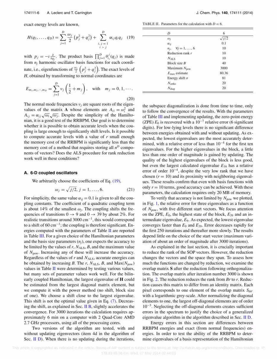
TABLE II. Parameters for the calculation with D = 6.

D 6ωj

√j/2

αij 0.1nj, ∀j = 1, . . . , 6 10Reduction rank r 10NALS 10Block size B 40Maximum Npow 3000Emax estimate 80.36Energy shift σ 81Northo 20Ndiag 20

the subspace diagonalization is done from time to time, onlyto follow the convergence of the results. With the parametersof Table III and implementing updating, the zero-point energy(ZPE) E0 is recovered with a 10−7 relative error (6 significantdigits). For low-lying levels there is no significant differencebetween energies obtained with and without updating. As ex-pected, the lowest eigenvalues are the most accurately deter-mined, with a relative error of less than 10−4 for the first teneigenvalues. For the higher eigenvalues in the block, a littleless than one order of magnitude is gained by updating. Thequality of the highest eigenvalues of the block is less good,but even the largest calculated eigenvalue E39 has a relativeerror of order 10−4, despite the very low rank that we havechosen (r = 10) and its proximity with neighboring eigenval-ues. These results confirm that even with basis functions withonly r = 10 terms, good accuracy can be achieved. With theseparameters, the calculation requires only 20 MB of memory.

To verify that accuracy is not limited by Npow we plotted,in Fig. 1, the relative error for three eigenvalues as a functionof Npow, with five different start vectors. We focus attentionon the ZPE, E0, the highest state of the block, E39 and an in-termediate eigenvalue, E9. As expected, the lowest eigenvalueconverges faster than E9 and E39. Error decreases rapidly forthe first 250 iterations and thereafter more slowly. The resultsdepend little on the choice of the start vector (maximum vari-ation of about an order of magnitude after 3000 iterations).

As explained in the last section, it is crucially importantto reduce the rank of the SOP vectors. However, the reductionchanges the vectors and the space they span. To assess howmuch the functions are changed by reduction, we examine theoverlap matrix S after the reduction following orthogonaliza-tion. The overlap matrix after iteration number 3000 is shownin Fig. 2. The reduction reduces the rank from Br to r. Reduc-tion causes this matrix to differ from an identity matrix. Eachpixel corresponds to one element of the overlap matrix Sbb′

with a logarithmic grey-scale. After normalizing the diagonalelements to one, the largest off-diagonal elements are of order10−3. Neglecting the off-diagonal elements creates sufficienterrors in the spectrum to justify the choice of a generalizedeigenvalue algorithm in the algorithm described in Sec. II D.

Energy errors in this section are differences betweenRRBPM energies and exact (from normal frequencies) en-ergies. In order to test the ability of the RRBPM to deter-mine eigenvalues of a basis representation of the Hamiltonian


178.83.85.98 On: Wed, 07 May 2014 02:44:03


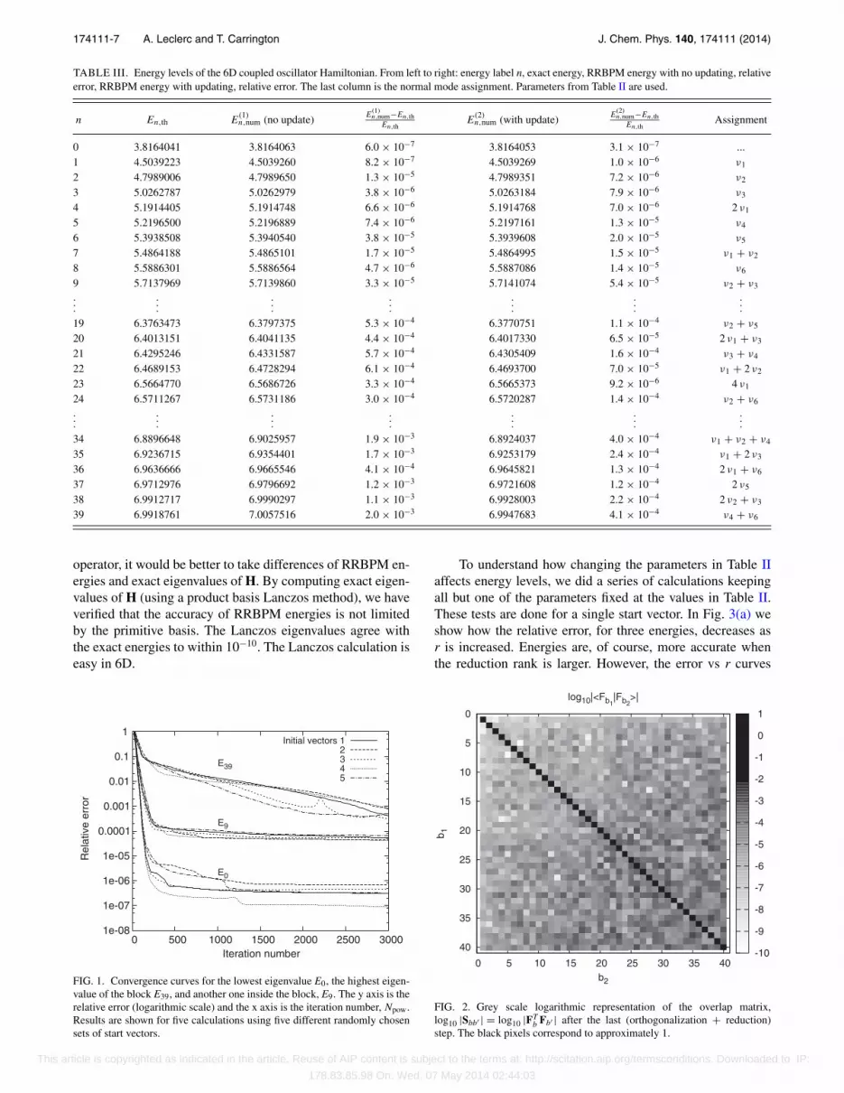
TABLE III. Energy levels of the 6D coupled oscillator Hamiltonian. From left to right: energy label n, exact energy, RRBPM energy with no updating, relativeerror, RRBPM energy with updating, relative error. The last column is the normal mode assignment. Parameters from Table II are used.

n En,th E(1)n,num (no update) E

(1)n,num−En,th

En,thE

(2)n,num (with update) E

(2)n,num−En,th

En,thAssignment

0 3.8164041 3.8164063 6.0 × 10−7 3.8164053 3.1 × 10−7 ...1 4.5039223 4.5039260 8.2 × 10−7 4.5039269 1.0 × 10−6 ν1

2 4.7989006 4.7989650 1.3 × 10−5 4.7989351 7.2 × 10−6 ν2

3 5.0262787 5.0262979 3.8 × 10−6 5.0263184 7.9 × 10−6 ν3

4 5.1914405 5.1914748 6.6 × 10−6 5.1914768 7.0 × 10−6 2 ν1

5 5.2196500 5.2196889 7.4 × 10−6 5.2197161 1.3 × 10−5 ν4

6 5.3938508 5.3940540 3.8 × 10−5 5.3939608 2.0 × 10−5 ν5

7 5.4864188 5.4865101 1.7 × 10−5 5.4864995 1.5 × 10−5 ν1 + ν2

8 5.5886301 5.5886564 4.7 × 10−6 5.5887086 1.4 × 10−5 ν6

9 5.7137969 5.7139860 3.3 × 10−5 5.7141074 5.4 × 10−5 ν2 + ν3

......

......

......

...19 6.3763473 6.3797375 5.3 × 10−4 6.3770751 1.1 × 10−4 ν2 + ν5

20 6.4013151 6.4041135 4.4 × 10−4 6.4017330 6.5 × 10−5 2 ν1 + ν3

21 6.4295246 6.4331587 5.7 × 10−4 6.4305409 1.6 × 10−4 ν3 + ν4

22 6.4689153 6.4728294 6.1 × 10−4 6.4693700 7.0 × 10−5 ν1 + 2 ν2

23 6.5664770 6.5686726 3.3 × 10−4 6.5665373 9.2 × 10−6 4 ν1

24 6.5711267 6.5731186 3.0 × 10−4 6.5720287 1.4 × 10−4 ν2 + ν6

......

......

......

...34 6.8896648 6.9025957 1.9 × 10−3 6.8924037 4.0 × 10−4 ν1 + ν2 + ν4

35 6.9236715 6.9354401 1.7 × 10−3 6.9253179 2.4 × 10−4 ν1 + 2 ν3

36 6.9636666 6.9665546 4.1 × 10−4 6.9645821 1.3 × 10−4 2 ν1 + ν6

37 6.9712976 6.9796692 1.2 × 10−3 6.9721608 1.2 × 10−4 2 ν5

38 6.9912717 6.9990297 1.1 × 10−3 6.9928003 2.2 × 10−4 2 ν2 + ν3

39 6.9918761 7.0057516 2.0 × 10−3 6.9947683 4.1 × 10−4 ν4 + ν6

operator, it would be better to take differences of RRBPM en-ergies and exact eigenvalues of H. By computing exact eigen-values of H (using a product basis Lanczos method), we haveverified that the accuracy of RRBPM energies is not limitedby the primitive basis. The Lanczos eigenvalues agree withthe exact energies to within 10−10. The Lanczos calculation iseasy in 6D.

1e-08

1e-07

1e-06

1e-05

0.0001

0.001

0.01

0.1

1

0 500 1000 1500 2000 2500 3000

Rel

ativ

e er

ror

Iteration number

E0

E9

E39

Initial vectors 12345

FIG. 1. Convergence curves for the lowest eigenvalue E0, the highest eigen-value of the block E39, and another one inside the block, E9. The y axis is therelative error (logarithmic scale) and the x axis is the iteration number, Npow.Results are shown for five calculations using five different randomly chosensets of start vectors.

To understand how changing the parameters in Table IIaffects energy levels, we did a series of calculations keepingall but one of the parameters fixed at the values in Table II.These tests are done for a single start vector. In Fig. 3(a) weshow how the relative error, for three energies, decreases asr is increased. Energies are, of course, more accurate whenthe reduction rank is larger. However, the error vs r curves

0

5

10

15

20

25

30

35

40

0 5 10 15 20 25 30 35 40

b 1

b2

log10|<Fb1|Fb2

>|

-10

-9

-8

-7

-6

-5

-4

-3

-2

-1

0

1

FIG. 2. Grey scale logarithmic representation of the overlap matrix,log10 |Sbb′ | = log10 |FT

b Fb′ | after the last (orthogonalization + reduction)step. The black pixels correspond to approximately 1.


178.83.85.98 On: Wed, 07 May 2014 02:44:03


1e-09

1e-08

1e-07

1e-06

1e-05

0.0001

0.001

0.01

0.1

1

0 5 10 15 20 25 30

Rel

ativ

e er

ror

Reduction rank

E0

E9

E39

1e-08

1e-07

1e-06

1e-05

0.0001

0.001

0.01

0.1

1

10 100 1000

Rel

ativ

e er

ror

Orthog.+diag. step

E0

E9

E39

(a) (b)

1e-10

1e-09

1e-08

1e-07

1e-06

1e-05

0.0001

0.001

0.01

0.1

1

0.5 0.2 0.1 0.05 0.02 0.01

Rel

ativ

e er

ror

Coupling terms amplitude

E0

E9

E39

(c)

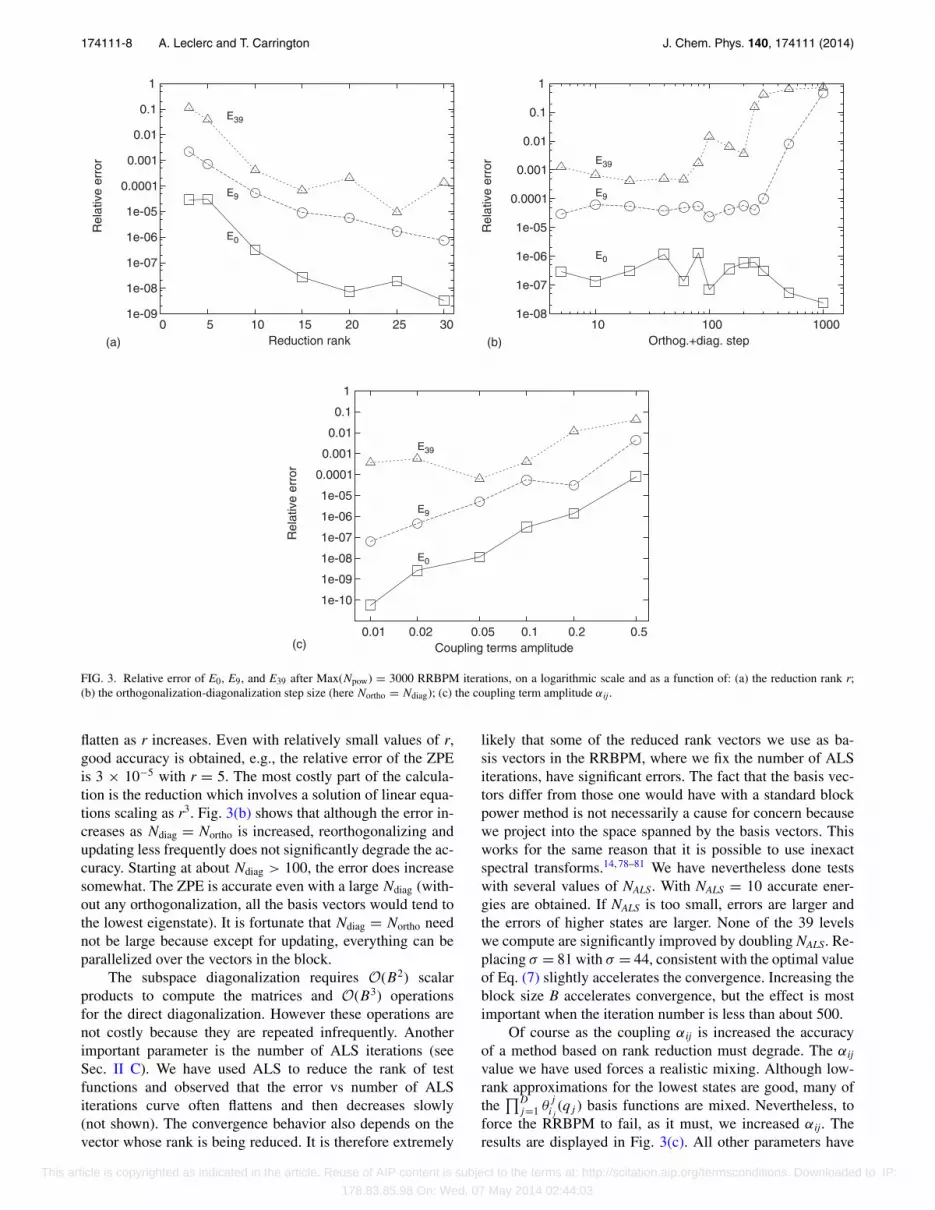
FIG. 3. Relative error of E0, E9, and E39 after Max(Npow) = 3000 RRBPM iterations, on a logarithmic scale and as a function of: (a) the reduction rank r;(b) the orthogonalization-diagonalization step size (here Northo = Ndiag); (c) the coupling term amplitude αij.

flatten as r increases. Even with relatively small values of r,good accuracy is obtained, e.g., the relative error of the ZPEis 3 × 10−5 with r = 5. The most costly part of the calcula-tion is the reduction which involves a solution of linear equa-tions scaling as r3. Fig. 3(b) shows that although the error in-creases as Ndiag = Northo is increased, reorthogonalizing andupdating less frequently does not significantly degrade the ac-curacy. Starting at about Ndiag > 100, the error does increasesomewhat. The ZPE is accurate even with a large Ndiag (with-out any orthogonalization, all the basis vectors would tend tothe lowest eigenstate). It is fortunate that Ndiag = Northo neednot be large because except for updating, everything can beparallelized over the vectors in the block.

The subspace diagonalization requires O(B2) scalarproducts to compute the matrices and O(B3) operationsfor the direct diagonalization. However these operations arenot costly because they are repeated infrequently. Anotherimportant parameter is the number of ALS iterations (seeSec. II C). We have used ALS to reduce the rank of testfunctions and observed that the error vs number of ALSiterations curve often flattens and then decreases slowly(not shown). The convergence behavior also depends on thevector whose rank is being reduced. It is therefore extremely

likely that some of the reduced rank vectors we use as ba-sis vectors in the RRBPM, where we fix the number of ALSiterations, have significant errors. The fact that the basis vec-tors differ from those one would have with a standard blockpower method is not necessarily a cause for concern becausewe project into the space spanned by the basis vectors. Thisworks for the same reason that it is possible to use inexactspectral transforms.14, 78–81 We have nevertheless done testswith several values of NALS. With NALS = 10 accurate ener-gies are obtained. If NALS is too small, errors are larger andthe errors of higher states are larger. None of the 39 levelswe compute are significantly improved by doubling NALS. Re-placing σ = 81 with σ = 44, consistent with the optimal valueof Eq. (7) slightly accelerates the convergence. Increasing theblock size B accelerates convergence, but the effect is mostimportant when the iteration number is less than about 500.

Of course as the coupling αij is increased the accuracyof a method based on rank reduction must degrade. The αij

value we have used forces a realistic mixing. Although low-rank approximations for the lowest states are good, many ofthe

∏Dj=1 θ

j

ij(qj ) basis functions are mixed. Nevertheless, to

force the RRBPM to fail, as it must, we increased αij. Theresults are displayed in Fig. 3(c). All other parameters have


178.83.85.98 On: Wed, 07 May 2014 02:44:03


the values in Table II except the energy shift which has beenadapted for each run because the spectral range changes. Asexpected, increasing the coupling increases the error. Whenαij is larger than 0.1 better accuracy can be obtained by in-creasing r.

B. 20-D coupled oscillators

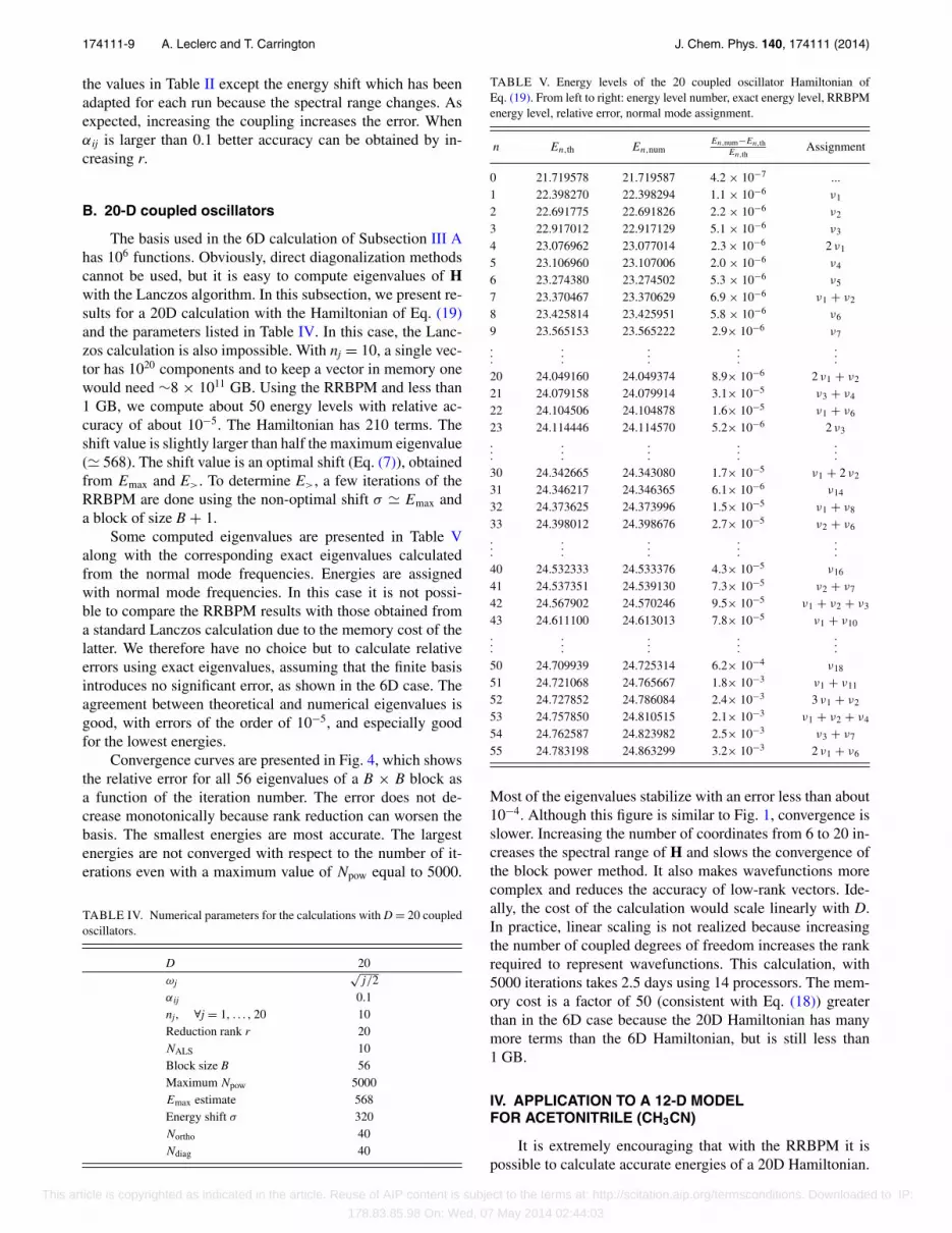
The basis used in the 6D calculation of Subsection III Ahas 106 functions. Obviously, direct diagonalization methodscannot be used, but it is easy to compute eigenvalues of Hwith the Lanczos algorithm. In this subsection, we present re-sults for a 20D calculation with the Hamiltonian of Eq. (19)and the parameters listed in Table IV. In this case, the Lanc-zos calculation is also impossible. With nj = 10, a single vec-tor has 1020 components and to keep a vector in memory onewould need ∼8 × 1011 GB. Using the RRBPM and less than1 GB, we compute about 50 energy levels with relative ac-curacy of about 10−5. The Hamiltonian has 210 terms. Theshift value is slightly larger than half the maximum eigenvalue(� 568). The shift value is an optimal shift (Eq. (7)), obtainedfrom Emax and E>. To determine E>, a few iterations of theRRBPM are done using the non-optimal shift σ � Emax anda block of size B + 1.

Some computed eigenvalues are presented in Table Valong with the corresponding exact eigenvalues calculatedfrom the normal mode frequencies. Energies are assignedwith normal mode frequencies. In this case it is not possi-ble to compare the RRBPM results with those obtained froma standard Lanczos calculation due to the memory cost of thelatter. We therefore have no choice but to calculate relativeerrors using exact eigenvalues, assuming that the finite basisintroduces no significant error, as shown in the 6D case. Theagreement between theoretical and numerical eigenvalues isgood, with errors of the order of 10−5, and especially goodfor the lowest energies.

Convergence curves are presented in Fig. 4, which showsthe relative error for all 56 eigenvalues of a B × B block asa function of the iteration number. The error does not de-crease monotonically because rank reduction can worsen thebasis. The smallest energies are most accurate. The largestenergies are not converged with respect to the number of it-erations even with a maximum value of Npow equal to 5000.

TABLE IV. Numerical parameters for the calculations with D = 20 coupledoscillators.

D 20ωj

√j/2

αij 0.1nj, ∀j = 1, . . . , 20 10Reduction rank r 20NALS 10Block size B 56Maximum Npow 5000Emax estimate 568Energy shift σ 320Northo 40Ndiag 40

TABLE V. Energy levels of the 20 coupled oscillator Hamiltonian ofEq. (19). From left to right: energy level number, exact energy level, RRBPMenergy level, relative error, normal mode assignment.

n En,th En,numEn,num−En,th

En,thAssignment

0 21.719578 21.719587 4.2 × 10−7 ...1 22.398270 22.398294 1.1 × 10−6 ν1

2 22.691775 22.691826 2.2 × 10−6 ν2

3 22.917012 22.917129 5.1 × 10−6 ν3

4 23.076962 23.077014 2.3 × 10−6 2 ν1

5 23.106960 23.107006 2.0 × 10−6 ν4

6 23.274380 23.274502 5.3 × 10−6 ν5

7 23.370467 23.370629 6.9 × 10−6 ν1 + ν2

8 23.425814 23.425951 5.8 × 10−6 ν6

9 23.565153 23.565222 2.9× 10−6 ν7

......

......

...20 24.049160 24.049374 8.9× 10−6 2 ν1 + ν2

21 24.079158 24.079914 3.1× 10−5 ν3 + ν4

22 24.104506 24.104878 1.6× 10−5 ν1 + ν6

23 24.114446 24.114570 5.2× 10−6 2 ν3

......

......

...30 24.342665 24.343080 1.7× 10−5 ν1 + 2 ν2

31 24.346217 24.346365 6.1× 10−6 ν14

32 24.373625 24.373996 1.5× 10−5 ν1 + ν8

33 24.398012 24.398676 2.7× 10−5 ν2 + ν6

......

......

...40 24.532333 24.533376 4.3× 10−5 ν16

41 24.537351 24.539130 7.3× 10−5 ν2 + ν7

42 24.567902 24.570246 9.5× 10−5 ν1 + ν2 + ν3

43 24.611100 24.613013 7.8× 10−5 ν1 + ν10

......

......

...50 24.709939 24.725314 6.2× 10−4 ν18

51 24.721068 24.765667 1.8× 10−3 ν1 + ν11

52 24.727852 24.786084 2.4× 10−3 3 ν1 + ν2

53 24.757850 24.810515 2.1× 10−3 ν1 + ν2 + ν4

54 24.762587 24.823982 2.5× 10−3 ν3 + ν7

55 24.783198 24.863299 3.2× 10−3 2 ν1 + ν6

Most of the eigenvalues stabilize with an error less than about10−4. Although this figure is similar to Fig. 1, convergence isslower. Increasing the number of coordinates from 6 to 20 in-creases the spectral range of H and slows the convergence ofthe block power method. It also makes wavefunctions morecomplex and reduces the accuracy of low-rank vectors. Ide-ally, the cost of the calculation would scale linearly with D.In practice, linear scaling is not realized because increasingthe number of coupled degrees of freedom increases the rankrequired to represent wavefunctions. This calculation, with5000 iterations takes 2.5 days using 14 processors. The mem-ory cost is a factor of 50 (consistent with Eq. (18)) greaterthan in the 6D case because the 20D Hamiltonian has manymore terms than the 6D Hamiltonian, but is still less than1 GB.

IV. APPLICATION TO A 12-D MODELFOR ACETONITRILE (CH3CN)

It is extremely encouraging that with the RRBPM it ispossible to calculate accurate energies of a 20D Hamiltonian.


178.83.85.98 On: Wed, 07 May 2014 02:44:03


1e-07

1e-06

1e-05

1e-04

0.001

0.01

0.1

1

0 500 1000 1500 2000 2500 3000 3500 4000 4500 5000

Rel

ativ

e er

ror

Iteration number

FIG. 4. Convergence curves of the energy levels of the 20-D coupled oscil-lator Hamiltonian. Parameters of Table IV are used. The y-axis is the relativeerror on a logarithmic scale and the x-axis is the iteration number Npow.

The Hamiltonian of Sec. III is chosen to facilitate testing thenumerical approach. Does the RRBPM also work well for arealistic Hamiltonian? One might worry that rank reductionwill make it impossible to compute accurate energies for aHamiltonian with a large number of coupling terms with re-alistic magnitudes. In this section we confirm that it workswell when applied to a 12D Hamiltonian in normal coordi-nates with a quartic potential. The potential is for acetonitrileCH3CN.

The normal coordinates are labelled qk with k = 1, 2,. . . 12. qk, k = 5, 6, . . . are two-fold degenerate (they corre-spond to q5. . . q8 of Ref. 82). We use the J = 0 normal coordi-nate KEO, but omit the π − π cross terms and the potential-like term,83

K = −1

2

∑k

ωk

∂2

∂q2k

. (22)

We use the quartic potential of Ref. 50 which isinferred from Ref. 82. Reference 82 gives force constantscalculated with a hybrid coupled cluster/density functionaltheory method. They also report vibrational levels computedfrom subspaces determined with second order perturbationtheory. The potential is

V (q1, . . . , q12) = 1

2

12∑i=1

ωiq2i + 1

6

12∑i=1

12∑j=1

12∑k=1

φ(3)ijkqiqjqk

+ 1

24

12∑i=1

12∑j=1

12∑k=1

12∑�=1

φ(4)ijk�qiqjqkq�. (23)

According to Ref. 82, constants smaller than 6 cm−1 werenot reported. The force constants must satisfy symmetry rela-tions given by Henry and Amat,84, 85 but usually expressed interms of the Nielsen k constants86 that correspond to the φ in

Eq. (23). All of the (937) non-zero φ constants can be deter-mined from (358) constants that Henry and Amat denote k0,k1, and k2. Reference 82 reports 132 φ. Some of the miss-ing φ are less than 6 cm−1, some of the missing φ are notsmall and can be determined from those reported, some of themissing φ are not small and cannot be determined from thosereported. Avila et al. assume that the force constants reportedin Ref. 82 are the φ that correspond to the k0 force constants(the corresponding φ are derivatives of the potential with re-spect to the x components of the doubly degenerate normalcoordinates) and, because they do not have values for them,put the k1 and k2 force constants equal to zero. The result-ing potential is invariant with respect to the C3v operations.There are 299 (108 cubic and 191 quartic) coupling terms inthe potential. Poirier and Halverson87 infer a different poten-tial from the force constants published in Ref. 82. Most en-ergy levels on their potential differ from their counterparts onthe potential of Ref. 50 by less than 1 cm−1. Either potentialcould be used to test the RRBPM, but we choose the potentialof Ref. 50.

To make the∏D

j=1 θj

ij(qj ) basis we use the harmonic os-

cillator basis functions that are eigenfunctions of the quadraticpart of the Hamiltonian. The harmonic frequencies are82 (incm−1) ω1 = 3065, ω2 = 2297, ω3 = 1413, ω4 = 920, ω5

= ω6 = 3149, ω7 = ω8 = 1487, ω9 = ω10 = 1061, ω11 = ω12

= 361.The RRBPM is used with the parameters of Table VI to

compute the smallest 70 energies of CH3CN. More energylevels could be obtained by using a larger block (B) or bycombining the RRBPM with the preconditioned inexact spec-tral transform method.78, 79 Increasing B would obviously in-crease the memory cost of the calculation, but with B = 70the memory cost is less than 1 GB. In the direct product ba-sis, storing only one vector would take 1113 GB. We have notincorporated symmetry adaptation and degenerate levels arecalculated together. We use the same nj as in Ref. 50 (but nopruning). The nj take into account the harmonic frequenciesωj and some strong coupling terms.

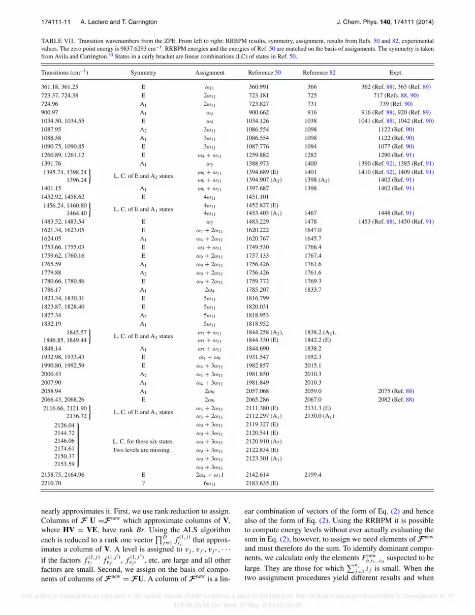
The lowest energy levels are given in Table VII wherethey are compared to previous theoretical results. We havedetermined vibrational assignments in two ways. Note that inSec. III each level was assigned the label of an exact wave-function but that in this section we assign, in the more usualsense, each level to the

∏Dj=1 θ

j

ij(qj ) basis function that most

TABLE VI. Parameters for the CH3CN calculations.

D 12nj, j = {1, 3, 4, 5, 6, 9, 10} 9nj, j = {2, 7, 8} 7nj, j = {11, 12} 27Reduction rank r 20NALS 10Block size B 70Maximum Npow 6000Emax estimate 311419Energy shift σ 170000Ndiag 20


178.83.85.98 On: Wed, 07 May 2014 02:44:03


TABLE VII. Transition wavenumbers from the ZPE. From left to right: RRBPM results, symmetry, assignment, results from Refs. 50 and 82, experimentalvalues. The zero point energy is 9837.6293 cm−1. RRBPM energies and the energies of Ref. 50 are matched on the basis of assignments. The symmetry is takenfrom Avila and Carrington.50 States in a curly bracket are linear combinations (LC) of states in Ref. 50.

Transitions (cm−1) Symmetry Assignment Reference 50 Reference 82 Expt.

361.18, 361.25 E ω11 360.991 366 362 (Ref. 88), 365 (Ref. 89)723.37, 724.38 E 2ω11 723.181 725 717 (Refs. 88, 90)724.96 A1 2ω11 723.827 731 739 (Ref. 90)900.97 A1 ω4 900.662 916 916 (Ref. 88), 920 (Ref. 89)1034.50, 1034.55 E ω9 1034.126 1038 1041 (Ref. 88), 1042 (Ref. 90)1087.95 A2 3ω11 1086.554 1098 1122 (Ref. 90)1088.58 A1 3ω11 1086.554 1098 1122 (Ref. 90)1090.75, 1090.85 E 3ω11 1087.776 1094 1077 (Ref. 90)1260.89, 1261.12 E ω4 + ω11 1259.882 1282 1290 (Ref. 91)1391.76 A1 ω3 1388.973 1400 1390 (Ref. 92), 1385 (Ref. 91)

ω9 + ω11 1394.689 (E) 1401 1410 (Ref. 92), 1409 (Ref. 91)L. C. of E and A2 states

ω9 + ω11 1394.907 (A2) 1398 (A2) 1402 (Ref. 91)1395.74, 1398.24

1396.24

}1401.15 A1 ω9 + ω11 1397.687 1398 1402 (Ref. 91)1452.92, 1458.62 E 4ω11 1451.101

4ω11 1452.827 (E)L. C. of E and A1 states

4ω11 1453.403 (A1) 1467 1448 (Ref. 91)1456.24, 1460.80

1464.40

}1483.52, 1483.54 E ω7 1483.229 1478 1453 (Ref. 88), 1450 (Ref. 91)1621.34, 1623.05 E ω4 + 2ω11 1620.222 1647.01624.05 A1 ω4 + 2ω11 1620.767 1645.71753.66, 1755.03 E ω3 + ω11 1749.530 1766.41759.62, 1760.16 E ω9 + 2ω11 1757.133 1767.41765.59 A1 ω9 + 2ω11 1756.426 1761.61779.88 A2 ω9 + 2ω11 1756.426 1761.61780.66, 1780.86 E ω9 + 2ω11 1759.772 1769.31786.17 A1 2ω4 1785.207 1833.71823.34, 1830.31 E 5ω11 1816.7991823.87, 1828.40 E 5ω11 1820.0311827.34 A2 5ω11 1818.9531832.19 A1 5ω11 1818.952

ω7 + ω11 1844.258 (A2), 1838.2 (A2),L. C. of E and A2 states

ω7 + ω11 1844.330 (E) 1842.2 (E)1845.57

1846.85, 1849.44

}1848.14 A1 ω7 + ω11 1844.690 1838.21932.98, 1933.43 E ω4 + ω9 1931.547 1952.31990.80, 1992.59 E ω4 + 3ω11 1982.857 2015.12000.43 A2 ω4 + 3ω11 1981.850 2010.32007.90 A1 ω4 + 3ω11 1981.849 2010.32058.94 A1 2ω9 2057.068 2059.0 2075 (Ref. 88)2066.43, 2068.26 E 2ω9 2065.286 2067.0 2082 (Ref. 88)

ω3 + 2ω11 2111.380 (E) 2131.3 (E)L. C. of E and A1 states

ω3 + 2ω11 2112.297 (A1) 2130.0 (A1)2116.66, 2121.90

2136.72

}ω9 + 3ω11 2119.327 (E)ω9 + 3ω11 2120.541 (E)

L. C. for these six states. ω9 + 3ω11 2120.910 (A2)Two levels are missing. ω9 + 3ω11 2122.834 (E)

ω9 + 3ω11 2123.301 (A1)ω9 + 3ω11

2126.042144.722146.062174.612150.372153.59

⎫⎪⎪⎪⎪⎪⎪⎬⎪⎪⎪⎪⎪⎪⎭

2158.75, 2164.96 E 2ω4 + ω11 2142.614 2199.42210.70 ? 6ω11 2183.635 (E)

nearly approximates it. First, we use rank reduction to assign.Columns of F U =Fnew which approximate columns of V,where HV = VE, have rank Br. Using the ALS algorithmeach is reduced to a rank one vector

∏Dj=1 f

(1,j )ij

that approx-imates a column of V. A level is assigned to vj , vj ′ , vj ′′ , · · ·if the factors f

(1,j )vj

f(1,j ′)vj ′ , f

(1,j ′′)vj ′′ , etc. are large and all other

factors are small. Second, we assign on the basis of compo-nents of columns of Fnew = FU. A column of Fnew is a lin-

ear combination of vectors of the form of Eq. (2) and hencealso of the form of Eq. (2). Using the RRBPM it is possibleto compute energy levels without ever actually evaluating thesum in Eq. (2), however, to assign we need elements of Fnew

and must therefore do the sum. To identify dominant compo-nents, we calculate only the elements F new

b,i1...iDsuspected to be

large. They are those for which∑nj

j=1 ij is small. When thetwo assignment procedures yield different results and when


178.83.85.98 On: Wed, 07 May 2014 02:44:03


no assignment can be deduced from the first we use thesecond.

Owing to the fact that we use the same basis and samepotential as Ref. 50, differences between our energies andthose of Ref. 50 are a measure of the accuracy of the RRBPM.The energies of Ref. 50 are obtained using a method that re-quires about an order of magnitude more memory, but whichdoes not require a simple force-field type potential. Experi-mental values are also listed in the last column. The RRBPMenergies are close to those of Ref. 50. The lowest RRBPMlevels in Table VII differ from the numbers in Ref. 50 bya few cm−1. The higher levels differ more. The levels withthe largest errors are: 1779.88, 1780.66 and 2000.43, 2007.90and the seven highest eigenvalues of the block. The high-est eigenvalues could be improved by using a larger B. It isnot surprising that eigenvalues at the edge of the block havelarger errors. Other large errors could be reduced by increas-ing r. Some of the eigenvectors corresponding to eigenvaluesnear the top of the block are nearly linear combinations ofthe eigenvectors of different symmetries computed with theSmolyak quadrature method of Ref. 50. We have not yet im-plemented a symmetry-adapted rank reduction and thereforethe rank reduction breaks the symmetry. In some cases, whenlevels are close together, the RRBPM energies and those ofRef. 50 are not close enough to match them unambiguously.When this problem occurs we match levels using their assign-ments, i.e., using the corresponding eigenvectors. Differencesbetween the energies of Ref. 50 and experiment are due tothe potential. Differences between the energies of Ref. 50 andthose obtained with the RRBPM are due to the low-rank ap-proximations and could be reduced by increasing r, B, themaximum Npow and NALS.

V. CONCLUSION

The use of iterative algorithms has opened the door toroutine calculation of (ro-)vibrational spectra of moleculeswith as many as four or five atoms.5, 8–11, 18, 93, 94 The sameideas can be used, with an adiabatic approximation, forvan der Waals complexes with 6 or fewer inter-molecularcoordinates.16, 95 Although iterative methods obviate the needto store the Hamiltonian matrix (or even to calculate its ma-trix elements), application of these ideas to larger moleculesis impeded by the size of the vectors that must be stored inmemory. Calculations are only “routine” if a product basis isused. With a product basis, the size of a vector scales as nD.For a J = 0 calculation, D = 12 for a molecule with 6 atoms;storing a vector with 1012 elements requires 8000 GB. Oneway to deal with this impasse is use a contracted basis. An-other is to prune a product basis set. In this article we suggesta third approach, based on exploiting the SOP form of theHamiltonian. At present it can only be applied to SOP Hamil-tonians. That is a limitation, but for many molecules with 6 ormore atoms for which one wishes to compute a spectrum ei-ther the only available potential energy surfaces (PESs) are inSOP form or the PES can be brought into SOP form withoutmaking a significant approximation. MCTDH is usually usedwith a SOP PES, there are however other options.96, 97

The principal idea of the RRBPM of this paper is the re-alization that whereas one needs nD numbers to represent ageneral function in a product basis, a function that is a SOPcan be represented with far fewer numbers. The simplest ex-ample is a product of D factors for which one only requiresnD numbers, much less than nD. If the factors of the termsin a SOP representation of a wavefunction are chosen care-fully, it should be possible to represent it with a relativelysmall number of terms. In this article, we show that it is pos-sible to obtain accurate energy levels for a 6-D model prob-lem with r = 10, for a 20-D model problem with r = 20 andfor CH3CN (12-D) with 299 coupling terms with r = 20. Thismakes it possible to reduce the memory cost of calculations bymany orders of magnitude. For the 20-D problem the memorycost is about 1 GB. The RRBPM uses a shifted block powermethod to make SOP basis functions. Applying the Hamilto-nian to a vector necessarily increases the number of terms inthe SOP. If this increase were not checked the memory costof the method would become large. We restrict the numberof terms by using a rank reduction idea.53 A somewhat sim-ilar power method idea has been used in Ref. 98. At eachstage of the procedure we exploit the SOP structure, e.g., toorthogonalize, to evaluate matrix-vector products etc.

The ideas introduced in this paper can be refined in sev-eral ways. Rather than using the block power method to gen-erate SOP functions one could use a better iterative approach.One option is a Davidson algorithm,99 another is a precon-ditioned inexact spectral transform (PIST) method.78, 80, 81 APIST version would also make it possible to target high-lyinglevels. Reducing the number of required iterations would re-duce the cost of the calculations. Any iterative method whosebasis vectors are close enough to the desired eigenvectors toenable rank reduction will be suitable. A symmetry-adaptedrank reduction method will obviate symmetry mixing of verynearly degenerate levels. The ALS reduction algorithm isnot the most efficient nor the most robust reduction algo-rithm in the literature. It could be replaced, for example,with a conjugate gradient-based algorithm.77 The general ap-proach is promising because its memory cost is low. It mightbe possible to use similar ideas with the Floquet formalismto solve the time-dependent Schrödinger equation to studya molecule in a strong external electromagnetic field.100 Insuch approaches memory cost is a serious problem becausethe time-dependent Schrödinger equation is solved in an ex-tended Hilbert space containing functions that depend on atime coordinate.101, 102 We have shown that the method can beused to solve the time-independent Schrödinger equation fora molecule with 6 atoms using less than 1 GB. Clearly, it willbe possible to compute spectra for much larger molecules.

ACKNOWLEDGMENTS

We thank Gustavo Avila for his help. Calculationshave been executed on computers of the Utinam Insti-tute at the Université de Franche-Comté, supported by theRégion de Franche-Comté and Institut des Sciences del’Univers (INSU) and on computers purchased with a grantfor the Canada Foundation for Innovation. This research wasfunded by the Natural Sciences and Engineering Research


178.83.85.98 On: Wed, 07 May 2014 02:44:03


Council of Canada. We thank James Brown for doing the 6-Ddirect-product Lanczos calculation.

1C. Lanczos, J. Res. Natl. Bur. Stand. 45, 255 (1950).2J. K. Cullum and R. A. Willoughby, Lanczos Algorithms for Large Sym-metric Eigenvalue Computations: Vol. I: Theory (SIAM Classics in Ap-plied Mathematics, 2002).

3D. Neuhauser, J. Chem. Phys. 93, 2611 (1990).4V. A. Mandelshtam and H. S. Taylor, J. Chem. Phys. 106, 5085 (1997).5R. Chen and H. Guo, J. Chem. Phys. 111, 464 (1999).6S.-W. Huang and T. Carrington, Chem. Phys. Lett. 312, 311 (1999).7H. Koeppel, W. Domcke, and L. S. Cederbaum, Adv. Chem. Phys. 57, 59(1984).

8M. Bramley and T. Carrington, J. Chem. Phys. 99, 8519 (1993).9M. Bramley, J. Tromp, T. Carrington, and G. Corey, J. Chem. Phys. 100,6175 (1994).

10C. Leforestier, L. Braly, K. Liu, M. Elrod, and R. Saykally, J. Chem. Phys.106, 8527 (1997).

11F. L. Quere and C. Leforestier, J. Chem. Phys. 94, 1118 (1991).12N. P. P. Sarkar and T. Carrington, J. Chem. Phys. 110, 10269 (1999).13G. M. R. Chen and H. Guo, J. Chem. Phys. 114, 4763 (2001).14J. C. Tremblay and T. Carrington, J. Chem. Phys. 125, 094311 (2006).15G. M. R. Chen and H. Guo, Chem. Phys. Lett. 320, 567 (2000).16R. Dawes, X.-G. Wang, A. W. Jasper, and T. Carrington, J. Chem. Phys.

133, 134304 (2010).17G. Avila and T. Carrington, J. Chem. Phys. 135, 064101 (2011).18J. C. Light and T. Carrington, Adv. Chem. Phys. 114, 263 (2000).19S. Carter, J. M. Bowman, and N. C. Handy, Theor. Chim. Acta 100, 191

(1998).20D. M. Benoit, J. Chem. Phys. 120, 562 (2004).21P. Meier, M. Neff, and G. Rauhut, J. Chem. Theory Comput. 7, 148 (2011).22R. Dawes and T. Carrington, J. Chem. Phys. 122, 134101 (2005).23R. Dawes and T. Carrington, J. Chem. Phys. 124, 054102 (2006).24S. Carter and N. C. Handy, Comput. Phys. Rep. 5, 115 (1986).25D. T. Colbert and W. H. Miller, J. Chem. Phys. 96, 1982 (1992).26H.-G. Yu, J. Chem. Phys. 117, 2030 (2002).27C. Iung, C. Leforestier, and R. E. Wyatt, J. Chem. Phys. 98, 6722 (1993).28Z. Bacic and J. C. Light, Annu. Rev. Phys. Chem. 40, 469 (1989).29J. R. Henderson and J. Tennyson, Chem. Phys. Lett. 173, 133 (1990).30M. Mladenovic, Spectrochim. Acta, Part A 58, 795 (2002).31D. Luckhaus, J. Chem. Phys. 113, 1329 (2000).32J. M. Bowman and B. Gazdy, J. Chem. Phys. 94, 454 (1991).33S. Carter and N. C. Handy, Comput. Phys. Commun. 51, 49 (1988).34M. J. Bramley and N. C. Handy, J. Chem. Phys. 98, 1378 (1993).35S. Carter and N. C. Handy, Mol. Phys. 100, 681 (2002).36Multidimensional Quantum Dynamics: MCTDH Theory and Applications,

edited by H.-D.Meyer, F. Gatti, and G. A. Worth (Wiley-VCH, Weinheim,2009).

37M. H. Beck, A. Jaeckle, G. A. Worth, and H.-D. Meyer, Phys. Rep. 324, 1(2000).

38M. J. Davis and E. J. Heller, J. Chem. Phys. 71, 3383 (1979).39B. Poirier, J. Theor. Comput. Chem. 2, 65 (2003).40T. Halverson and B. Poirier, J. Chem. Phys. 137, 224101 (2012).41A. Shimshovitz and D. J. Tannor, Phys. Rev. Lett. 109, 070402 (2012).42X.-G. Wang and T. Carrington, J. Phys. Chem. A 105, 2575 (2001).43G. Avila and T. Carrington, J. Chem. Phys. 131, 174103 (2009).44G. Avila and T. Carrington, J. Chem. Phys. 137, 174108 (2012).45D. Lauvergnat and A. Nauts, Spectrochim. Acta, Part A 119, 18 (2014).46M. Bramley and T. Carrington, J. Chem. Phys. 101, 8494 (1994).47X.-G. Wang and T. Carrington, J. Chem. Phys. 117, 6923 (2002).48R. A. Friesner, J. A. Bentley, M. Menou, and C. Leforestier, J. Chem.

Phys. 99, 324 (1993).49A. Viel and C. Leforestier, J. Chem. Phys. 112, 1212 (2000).50G. Avila and T. Carrington, J. Chem. Phys. 134, 054126 (2011).51T. Zhang and G. H. Golub, SIAM J. Matrix Anal. Appl. 23, 534 (2001).52G. Beylkin and M. J. Mohlenkamp, PNAS 99, 10246 (2002).53G. Beylkin and M. J. Mohlenkamp, SIAM J. Sci. Comput. 26, 2133

(2005).

54U. Benedikt, A. A. Auer, M. Espig, and W. Hackbusch, J. Chem. Phys.134, 054118 (2011).

55F. A. Bischoff and E. F. Valeev, J. Chem. Phys. 134, 104104 (2011).56F. A. Bischoff, R. J. Harrison, and E. F. Valeev, J. Chem. Phys. 137,

104103 (2012).57E. G. Hohenstein, R. M. Parrish, and T. J. Martinez, J. Chem. Phys. 137,

044103 (2012).58R. M. Parrish, E. G. Hohenstein, T. J. Martinez, and C. D. Sherrill, J.

Chem. Phys. 137, 224106 (2012).59E. G. Hohenstein, R. M. Parrish, C. D. Sherrill, and T. J. Martinez, J.

Chem. Phys. 137, 221101 (2012).60T. G. Kolda and B. W. Bader, SIAM Rev. 51, 455 (2009).61F. L. Hitchcock, J. Math. Phys. 6, 164 (1927).62L. R. Tucker, Psychometrika 31, 279 (1966).63W. Hackbusch and S. Kühn, J. Fourier Anal. Appl. 15, 706 (2009).64L. Grasedyck, SIAM J. Matrix Anal. Appl. 31, 2029 (2010).65D. Kressner and C. Tobler, Comput. Methods Appl. Math. 11, 363 (2011).66I. V. Oseledets, SIAM J. Sci. Comput. 33, 2295 (2011).67H. Wang and M. Thoss, J. Chem. Phys. 119, 1289 (2003).68D. Pelaez and H.-D. Meyer, J. Chem. Phys. 138, 014108 (2013).69S. Manzhos and T. Carrington, J. Chem. Phys. 125, 194105 (2006).70S. Manzhos and T. Carrington, J. Chem. Phys. 127, 014103 (2007).71S. Manzhos and T. Carrington, J. Chem. Phys. 129, 224104 (2008).72J. C. M. S. E. Pradhan, J.-L. Carreon-Macedo, and A. Brown, J. Phys.

Chem. A 117, 6925 (2013).73G. Strang, Introduction to Applied Mathematics (Wellesley Cambridge

Press, Wellesley, Massachusetts, 1986).74Y. Saad, Numerical Methods for Large Eigenvalue Problems, 2nd ed.

(SIAM Classics in Applied Mathematics, 2011).75B. N. Parlett, The Symmetric Eigenvalue Problem (Prentice Hall, Engle-

wood Cliffs, NJ, 1980), Chap. 4 (republished by SIAM, Philadelphia,1998).

76S. R. Chinnamsetty, M. Espig, B. N. Khoromskij, and W. Hackbusch, J.Chem. Phys. 127, 084110 (2007).

77M. Espig, W. Hackbusch, T. Rohwedder, and R. Schneider, Numer. Math.122, 469 (2012).

78S.-W. Huang and T. Carrington, Jr., J. Chem. Phys. 112, 8765 (2000).79B. Poirier and T. Carrington, Jr., J. Chem. Phys. 114, 9254 (2001).80B. Poirier and T. Carrington, Jr., J. Chem. Phys. 116, 1215 (2002).81W. Bian and B. Poirier, J. Theor. Comput. Chem. 2, 583 (2003).82D. Begue, P. Carbonnière, and C. Pouchan, J. Phys. Chem. A 109, 4611

(2005).83J. K. G. Watson, Mol. Phys. 15, 479 (1968).84L. Henry and G. Amat, J. Mol. Spectrosc. 5, 319 (1961).85L. Henry and G. Amat, J. Mol. Spectrosc. 15, 168 (1965).86H. H. Nielsen, Rev. Mod. Phys. 23, 90 (1951).87B. Poirier and T. Halverson, private communication (November 2013).88I. Nagawa and T. Shimanouchi, Spectrochim. Acta 18, 513 (1962).89M. Koivusaari, V. M. Horneman, and R. Anttila, J. Mol. Spectrosc. 152,

377 (1992).90A. Tolonen, M. Koivusaari, R. Paso, J. Schroderus, S. Alanko, and

R. Anttila, J. Mol. Spectrosc. 160, 554 (1993).91R. Paso, R. Anttila, and M. Koivusaari, J. Mol. Spectrosc. 165, 470 (1994).92J. Duncan, D. McKean, F. Tullini, G. Nivellini, and J. P. Pea, J. Mol. Spec-

trosc. 69, 123 (1978).93B. T. S. Edit Matyus, G. Czako, and A. G. Csaszar, J. Chem. Phys. 127,

084102 (2007).94H.-G. Yu and J. T. Muckerman, J. Mol. Spectrosc. 214, 11 (2002).95X.-G. Wang, T. Carrington, J. Tang, and A. R. W. McKellar, J. Chem.

Phys. 123, 034301 (2005).96U. Manthe, J. Chem. Phys. 105, 6989 (1996).97F. Huarte-Larraaga and U. Manthe, J. Chem. Phys. 113, 5115 (2000).98H. Nakatsuji, Acc. Chem. Res. 45, 1480 (2012).99E. Davidson, J. Comput. Phys. 17, 87 (1975).

100S.-I. Chu and D. A. Telnov, Phys. Rep. 390, 1 (2004).101A. Leclerc, S. Guérin, G. Jolicard, and J. P. Killingbeck, Phys. Rev. A 83,

032113 (2011).102A. Leclerc, G. Jolicard, D. Viennot, and J. P. Killingbeck, J. Chem. Phys.

136, 014106 (2012).


178.83.85.98 On: Wed, 07 May 2014 02:44:03

calculating vibrational spectra with sum of product basis functions without storing full-dimensional...

Documents