building embankments of fly/bottom ash mixtures - rosa p

Joint

Transportation

Research

Program

FBW A/IN/JTRP-97 /1

Final Report

BUILDING HIGHWAY EMBANKMENTS OF FLY/BOTTOM ASH MIXTURES

Ahmed M. K. Karim C. W. Lovell Rodrigo Salgado

September 1997

Indiana

Department

of Trans portation

Purdue

Univers ity

FINAL REPORT

BUILDING IDGHW AY EMBANKMENTS OF FLY/BOTTOM ASH :MIXTURES

FHW NIN/JTRP-97/1

by

Ahmed M. K. Karim Research Assistant

C.W. Lovell and Rodrigo Salgado Research Engineers

Purdue University School of Civil Engineering

Joint Transportation Research Program

Project No.: C-36-50S File No.: 6-19-18

Prepared in Cooperation with the Indiana Department of Transportation and

the U.S. Department of Transportation Federal Highway Administration

The contents of this report reflect the views of the authors who are responsible for the facts and the accuracy of the data presented herein. The contents do not necessarily reflect the official views of or the Federal Highway Administration and the Indiana Department of Transportation. This report does not constitute a standard, a specification, or a regulation.

Purdue University West Lafayette, Indiana 47907

September 11, 1997

ACKNOWLEDGMENT

The authors wish to acknowledge the help provided by Athar Khan, Dr. Tommy E. Nantung, David Ward, and Mir Zaheer of INDOT. Special thanks are extended to Tom Cofer of NIPSCO and Bob Balinger of PSI for their help during the extraction of the samples. The financial support by Indiana Department of Transportation, Northern Indiana Public Service Company (NIPSCO), Public Service Indiana (PSI) and, Purdue University is gratefully acknowledged.

TECHNICAL REPORT STANDARD TITLE PAGE

I. ReportNo. 2. Government Accession No. J. Recipient's Catlllog No.

FHW A/IN/JTRP-97 /l

4. Title and Subtitle 5. Report Date

Building Highway Embankments ofFly/Bottom Ash September 11, 1997

6. Performing Organization Code

7. Author(s) 8. Performing Organization Report No. Ahmed M.K. Karin; C. W. Lovell; and Rodrigo Salgado

FHW A/IN/JTRP-97 /l

9. Performing Organization Name and Address 10. Work Unit No. Joint Transportation Research Program 1284 Civil Engineering Building Purdue University II. Contract or Grant No.

West Lafavette Indiana 47907-1284 SPR-2115

12. Sponsoring Agency Name and Address 13. Type or Report and Period Covered

Indiana Department of Transportation Final Report State Office Building 100 North Senate Avenue Indianapolis, IN 46204 14. Sponsoring Agency Code

15. Supplementary Notes

Prepared in cooperation with the Indiana Department of Transportation and Federal Highway Administration.

16. Abstract

This research investigates the engineering properties of mixtures of bottom ash and Class F fly ash relevant to their utilization in highway embankment construction. The research included ash samples from two major power plants in Indiana that disposed of their ash differently. The first power plant disposes of the bottom ash and fly ash separately and hence explicit mixtures were synthetically formed and tested. The second power plant disposes of the bottom and fly ash together in a common location and hence they become mixed, forming implicit mixtures. The implicit mixtures were processed using a wet method, the Shallow Slurry Deposition Method, to produce homogeneous samples for the research. Characterization of the ash included grain size analysis, specific gravity, maximum and minimum density, in addition to microscopic investigation. The investigation of compaction behavior of a range of explicit and implicit mixtures was conducted at the standard energy effort. The effects of changing the mixture composition on the maximum dry unit weight and optimum moisture content were established. In order to study the effect of changing the moisture content on penetration resistance, surface penetration tests were performed on the compacted samples. Beyond the optimum moisture content, the penetration resistance of the samples drops significantly, which suggests that the compaction can better be conducted dry of optimum. To control the compaction appropriately, the degree of compaction of a sample must be determined using a compaction curve for a mixture of similar gradation.

Consolidated drained triaxial tests were performed on a range of explicit and implicit mixtures at three levels of confining pressures. For each mixture tested, two groups of samples were prepared, one at a relative compaction (R¾) of90% and the other at 95%. The results indicate that the drained shear strength depends on the mixture composition, the degree of compaction, and the confining pressure. Adequate shear strength and volumetric behavior was observed for the samples compacted at 95%. It was concluded that the shear strength of the ash mixtures is comparable to the shear strength of sandy soils

Discussion and recommendations regarding the stability of slopes of ash mixtures is included. Using the critical state angles is more feasible in the slope stability analysis in the case of embankments of implicit mixtures due to mixture variability.

17. Key Words 18. Distribution Statement

Bottom ash, fly ash, waste materials, highway materials, highway No restrictions. This document is available to the public through the embankments, compaction, triaxial tests, shear strength. National Technical Information Service, Springfield, VA 22161

19. Security Classif. (of this report) 20. Security Classif. (of this page) 21. No. of Pages 22. Price 249

Unclassified

Fonn DOT F 1700. 7 (8-69)

Digitized by the Internet Archive in 2011 with funding from

LYRASIS members and Sloan Foundation; Indiana Department of Transportation

http://www.archive.org/details/buildinghighwayeOOkari

ill

TABLE OF CONTENTS

Page LIST OF TABLES . . . . . . . . . . . . . . . . . . . . . . . . . . . . . . . . . . . . . . Vil

LIST OF FIGURES . . . . . . . . . . . . . . . . . . . . . . . . . . . . . . . . . . . . . viii

LIST OF SYMBOLS AND ABBREVIATIONS ........... .......... xv

11\'.iPLEMENTATION REPORT .................... ......... xvii

CHAPTER 1 INTRODUCTION . . . . . . . . . . . . . . . . . . . . . . . . . . . . . . . 1

1.1 Problem Statement . . . . . . . . . . . . . . . . . . . . . . . . . . . . . . . . l 1.2 Scope of this Study . . . . . . . . . . . . . . . . . . . . . . . . . . . . . . . . 3 1.3 Research Approach ................................ 3 1.4 Outline of this Report . . . . . . . . . . . . . . . . . . . . . . . . . . . . . . . 4

CHAPTER 2 COAL ASH GENERATION, DISPOSAL, CHARACTERISTICS, AND UTII..IZA TION . . . . . . . . . . . . . . . . . . . . . . . . . . . . . 6

2.1 Coal Ash Generation and Composition . . . . . . . . . . . . . . . . . . . . . 6 2.1.1 Coal Ash Generation in the United States and Indiana . . . . . . 6 2.1.2 Fly Ash Generation and Composition . . . . . . . . . . . . . . . . 8 2.1.3 Bottom Ash And Boiler Slag Generation and Composition . . 10

2.2 Coal Ash Disposal Practices in Indiana . . . . . . . . . . . . . . . . . . . 12 2.3 Engineering Properties of Coal Ash . . . . . . . . . . . . . . . . . . . . . 18

2.3.1 Physical Characteristics: . . . . . . . . . . . . . . . . . . . . . . . 18 2.3.1.lAppearance ......................... 18 2.3.1.2 Specific Gravity . . . . . . . . . . . . . . . . . . . . . . 20 2.3.1.3 Grain Size Distribution .................. 21

2.3.2 Mechanical Characteristics . . . . . . . . . . . . . . . . . . . . . 24 2.3.2.1 Soundness . . . . . . . . . . . . . . . . . . . . . . . . . . 24 2.3.2.2 Hardness and Toughness . . . . . . . . . . . . . . . . . 25 2.3.2.3 Compaction . . . . . . . . . . . . . . . . . . . . . . . . 25 2.3.2.4 Hydraulic Conductivity . . . . . . . . . . . . . . . . . . 37 2.3.2.5 Compressibility . . . . . . . . . . . . . . . . . . . . . . 38

IV

Page 2.3.2.6 Shear Strength . . . . . . . . . . . . . . . . . . . . . . . 39

2.4 Coal Ash Utilization In Embankment Construction ......... . .. 49 2.4.1 Overview of Current Practices of Coal Ash Utilizations

in Highway Construction . . . . . . . . . . . . . . . . . . . . . . 50 2.4.2 Environmental Concerns for Coal Ash Utilization in

Embankments . . . . . . . . . . . . . . . . . . . . . . . . . . . . 51 2.4.2.1 Dusting ......................... .. 51 2.4.2.2 External and internal Erosion . . . . . . . . . . . . . . 53 2.4.2.3 Leaching . . . . . . . . . . . . . . . . . . . . . . . . . . 53

2.4.3 Considerations For Coal Ash Utilization In Embankment Construction . . . . . . . . . . . . . . . . . . . . . . . . . 56 2.4.3.1 Design Considerations . . . . . . . . . . . . . 56 2.4.3.2 Construction Considerations . . . . . . . . . . 58

2.4.4 Field Performance of Coal Ash in Embankments ....... 59 2.4.4.1 East Street Valley Expressway,

Pennsylvania . . . . . . . . . . . . . . . . . . . . 59 2.4.4.2 U.S. 12 Demonstration Project,

Lake County, Indiana . . . . . . . . . . . . . . 62 2.4.4.3 I-495 and Edgemoor Road Interchange,

Wilmington, Delaware. . . . . . . . . . . . . . . 63

CHAPTER 3 EXPERIMENTAL APPARATUS AND PROCEDURES . . . . . . . 70

3 .1. Ash Sampling and Initial Processing . . . . . . . . . . . . . . . . . . . . . 70 3.1.1 Samples Sources . . . . . . . . . . . . . . . . . . . . . . . . . . . 70 3.1.2 Ash Generation and Disposal Procedures in Sampling Sources 70 3.1.3 Sampling Procedures ......................... 71

3.1.3.1 Sampling From Schahfer Power Plant ....... . . 71 3.1.3.2 Sampling From Gibson Power Plant ........ . . 74

3.2 Ash Characterization and Mixture Developments ............. 74 3.2. lOverview . . . . . . . . . . . . . . . . . . . . . . . . . . . . . . . . 74 3.2.2 Initial Processing, Grain Size Analysis, and Mixture Composition 75

3.2.2.1 Samples from Schahfer Power Plant . . . . . . . . . . 75 3.2.2.2 Samples from Gibson Power Plant . . . . . . . . . . . 76

3.2.3 Visual and Microscopic Examination ............... 80 3.2.4 Specific Gravity . . . . . . . . . . . . . . . . . . . . . . . . . . . . 80

3.3 Compaction of Ash Mixtures . . . . . . . . . . . . . . . . . . . . . . . . . 81 3 .4 Minimum and Maximum Density . . . . . . . . . . . . . . . . . . . . . . . 83 3.5 CID Triaxial Tests . . . . . . . . . . . . . . . . . . . . . . . . . . . . . . . . 83

3.5.1 Overview . . . . . . . . . . . . . . . . . . . . . . . . . . . . . . . . 83 3.5.2 Equipment . . . . . . . . . . . . . . . . . . . . . . . . . . . . . . . 84

V

Page 3.5.3 Test Procedure ............................ 87

CHAPTER 4 CHARACTERIZATION AND COMPACTION OF COAL ASH MIXTURES ................................ .. 92

4 .1 Overview . . . . . . . . . . . . . . . . . . . . . . . . . . . . . . . . . . . . . 92

4.2 Grain Size Analysis and Specific Gravity . . . . . . . . . . . . . . . . . . . . 92 4.2.1 Samples from Schahfer Power Plant . . . . . . . . . . . . . . . . . 92 4.2.2 Samples From Gibson Power Plant . . . . . . . . . . . . . . . . . 93 4.2.3 Discussion . . . . . . . . . . . . . . . . . . . . . . . . . . . . . . . 93

4.3 Visual and Microscopic Characterization . . . . . . . . . . . . . . . . . . . 100 4.3 .1 Results . . . . . . . . . . . . . . . . . . . . . . . . . . . . . . . . 100 4.3.2 Discussion . . . . . . . . . . . . . . . . . . . . . . . . . . . . . . . 102

4 .4 Compaction and Penetration . . . . . . . . . . . . . . . . . . . . . . . . . 113 4.4.1 Compaction Tests . . . . . . . . . . . . . . . . . . . . . . . . . . 113

4.4.1.lBehaviorofBottomAsh ................. 114

4.4.1.2 Behavior of the mixtures . . . . . . . . . . . . . . . . . 114 4.4.2 Penetration tests . . . . . . . . . . . . . . . . . . . . . . . . . . . 118 4.4.3 Discussion . . . . . . . . . . . . . . . . . . . . . . . . . . . . . . . 118

4.5 Maximum and Minimum Density . . . . . . . . . . . . . . . . . . . . . . . 124

4.5.1 Test Results . . . . . . . . . . . . . . . . . . . . . . . . . . . . . . 124

4. 5 .2 Discussion . . . . . . . . . . . . . . . . . . . . . . . . . . . . . . . 124 4.6 Summary . . . . . . . . . . . . . . . . . . . . . . . . . . . . . . . . . . . . . 126

CHAPTER 5 SHEAR STRENGTH AND VOLUMETRIC BEHAVIOR OF COAL ASH MIXTURES . . . . . . . . . . . . . . . . . . . . . . . . . . . . . 128

5.1 Overview . . . . . . . . . . . . . . . . . . . . . . . . . . . . . . . . . . . . 128 5. 2 Compressibility . . . . . . . . . . . . . . . . . . . . . . . . . . . . . . . . . 129

5.2.1 Test Results . . . . . . . . . . . . . . . . . . . . . . . . . . . . . 129 5.2.2 Discussion . . . . . . . . . . . . . . . . . . . . . . . . . . . . . . 130

5.3 Shear Behavior . . . . . . . . . . . . . . . . . . . . . . . . . . . . . . . . . 134 5.3.1 Introduction . . . . . . . . . . . . . . . . . . . . . . . . . . . . . 134 5.3.2 Behavior of Explicit Mixtures . . . . . . . . . . . . . . . . . . 138

5.3.2.1 Test Results ........................ 138 5.3.2.2 Discussion . . . . . . . . . . . . . . . . . . . . . . . . 138

a- Explicit Mixtures Compacted at R=95% 138 b- Explicit Mixtures Compacted at R=90% 150

5.3.3 Behavior of Implicit mixtures . . . . . . . . . . . . . . . . . . 152

5 .3.3.1 Test Results . ... . .. . ... . ..... . ..... . 5.3.3.2 Discussion ....................... .

a- Implicit Mixtures Compacted at R=95% b- Implicit Mixtures Compacted at R=90%

5.3.4 Effects of Fly Ash Content on Peak Angle </>' = ... . . . . 5.3.5 Effects of Fly Ash Content on Critical Angle</>' crit •• • ••

5.3.6 Dilation of Ash Mixtures .................... . 5 .4 Summary and Conclusions

CHAPTER 6 APPLICATIONS FOR HIGHWAY EMBANKMENTS

VI

Page

152 152 152 163 164 177 178 179

186

6.1 Overview . . . . . . . . . . . . . . . . . . . . . . . . . . . . . . . . . . . . 186 6.2 Materials Sources and Scopes . . . . . . . . . . . . . . . . . . . . . . . . 186 6.3 Embankments of Coal Ash Mixtures . . . . . . . . . . . . . . . . . . . . 187 6.4 Ash Characterization and processing . . . . . . . . . . . . . . . . . . . . 190 6.5 Compaction of Ash Mixtures . . . . . . . . . . . . . . . . . . . . . . . . 191 6.6 Shear Strength and Volumetric Behavior . . . . . . . . . . . . . . . . . 194 6. 7 Applications to Slope Stability . . . . . . . . . . . . . . . . . . . . . . . . 195 6.8 Utilization Practices Versus Disposal Practices . . . . . . . . . . . . . . 198

CHAPTER 7 CONCLUSIONS AND RECOMMENDATIONS FOR FUTURE RESEARCH . . . . . . . . . . . . . . . . . . . . . . . . . . 200

7 .1 Conclusions . . . . . . . . . . . . . . . . . . . . . . . . . . . . . . . . . . . 200 7 .2 Recommendations . . . . . . . . . . . . . . . . . . . . . . . . . . . . . . . 203

LIST OF REFERENCES . . . . . . . . . . . . . . . . . . . . . . . . . . . . . . . . . 205

APPENDIX: INDOT Special Provisions for Embankments Constructed of Coal Combustion By-Products . . . . . . . . . . . . . . . . . . . . . . . . . . 213

First Project: US 12/ over Kennedy Ave. . . . . . . . . . . . . . . 214 Second Project: I-465/5eii Street, Marion County, Indianapolis . . 219 Third Project: US 50, Knox County . . . . . . . . . . . . . . . . . . 225

Vil

LIST OF TABLES

Table Page 2.1 Coal Combustion By-Products (CCBPs) Quantities and Types Generated

by Power Plants in the State of Indiana. . . . . . . . . . . . . . . . . . . . . . . 9

2.2 Chemical Composition and Pozzolanic Activity Index of Sieved Fly Ash ........................................ . 11

2.3 Coal Combustion By-Products (CCBPs) Quantities and Types Generated in the United States . . . . . . . . . . . . . . . . . . . . . . . . . . . . . . . . . . 14

2.4 The Methods and Rates of Coal Ash Disposal in the State of Indiana . . . . 15

2.5 Specific Gravity of Bottom Ash Samples from Indiana Power Plants .... 22

2.6 Results of Soundness and Freeze-Thaw Tests on Bottom Ash ......... 26

2. 7 Results of Direct Shear Tests on Loose Bottom Ashes . . . . . . . . . . . . . 46

2.8 Results of Direct Shear Tests on Selected Indiana Bottom Ashes ....... 47

2.9 Utilizations of Coal Combustion By-Products in Highway Applications ... 52

2.10 Indiana Administrative Code Restricted Waste Site Type Criteria . . . . . . 55

3.1 Composition of Explicit Mixtures for Compaction (From Schahfer Plant) . 82

3.2 Composition of Implicit Mixtures for Compaction (From Gibson Plant) 82

3.3 CID Tri.axial Compression Tests on Explicit Mixtures (From Schahfer Plant) . . . . . . . . . . . . . . . . . . . . . . . . . . . . . . . . 89

3.4 CID Triaxial Compression Tests on Implicit Mixtures (From Gibson Plant) 90

4.1 Maximum and Minimum Density Tests on Explicit Mixtures (From Schahfer Plant) . . . . . . . . . . . . . . . . . . . . . . . . . . . . . . . 125

Vll1

LIST OF FIGURES

Figure Page

2.1 Trends of Coal Consumption by the Electric Utilities in the United States (1949-1993) . . . . . . . . . . . . . . . . . . . . . . . . . . . . . . . . . . . . . . . 7

2.2 Scanning Electron Microscopic Photos of Class F Fly Ash: (a) Passing No. 400 Sieve (b) Retained on No. 200 Sieve . . . . . . 19

2.3 Typical Particle Size Distribution Ranges for Coal Ash ............ 23

2.4 Typical Moisture-density Curves for A Compacted Cohesive Soil 29

2.5 Typical Compaction Curves for Western Pennsylvania Bituminous Fly Ashes . . . . . . . . . . . . . . . . . . . . . . . . . . . . . . . . . . . . . . . . 30

2.6 Typical Compaction Curves for Western United States Lignite and Subbituminous Fly Ash . . . . . . . . . . . . . . . . . . . . . . . . . . . . . . . 31

2. 7 Typical Moisture-density Relationship for Cohesionless Soils . . . . . . . . . 32

2.8 Moisture-density Curve for Bottom Ash from Gibson Power Plant, Indiana . . . . . . . . . . . . . . . . . . . . . . . . . . . . . . . . . . . . . . . . . 33

2.9 Field Methods for Determining the Soil Unit Weight ............. 36

2 .10 One-dimensional Compression of Bottom Ash and Sand . . . . . . . . . . . . 40

2.11 One-dimensional Compression of Indiana Bottom Ashes and a Medium Sand . . . . . . . . . . . . . . . . . . . . . . . . . . . . . . . . . . . . . 41

2.12 Constrained Modulus vs. Vertical Stress Curves for Indiana Bottom Ashes and a Medium Sand . . . . . . . . . . . . . . . . . . . . . . . . . . . . 42

2.13 Consolidation Test Data on Delmarva Stockpiled Class F Fly Ash Utilized in the Delaware Demonstration Project ................ 43

IX

Figure Page 2.14 Triaxial Test Results for Pulverized Bottom Ash Samples . . . . . . . . . . . 48

2.15 Typical Section in East Street Valley Expressway Embankment, Pennsylvania . . . . . . . . . . . . . . . . . . . . . . . . . . . . . . . . . . . . . 61

2.16 Smooth Wheel Roller Compacting Schahfer Bottom Ash in 1-12 Kennedy Intersection Embankment , Indiana ............... 64

2.17 Encasement of Bottom Ash With Till at the Vicinity of Concrete Members in 1-12 Kennedy Intersection Embankment, Indiana ....... 65

2.18 Typical Fly Ash Embankment Section in the 1-495 and Edgemoor Road Interchange, Delaware . . . . . . . . . . . . . . . . . . . . . . . . . . . . . . . . 68

2.19 Determination of Maximum Dry Density Value from One-point Standard Compaction test in the 1-495 and Edgemoor Road Interchange, Delaware . . . . . . . . . . . . . . . . . . . . . . . . . . . . . . . . . . . . . . . . 69

3 .1 Large Bottom Ash Particles Near the Discharge Point (Schahfer Power Plant) . . . . . . . . . . . . . . . . . . . . . . . . . . . . . . . . . . . . . . . . . . 72

3.2 Fine Bottom Ash Particles on the Surface of the Shallow Streams Between the Disposal Pond and the Discharge Point (Schahfer Power Plailt) . . . . . . . . . . . . . . . . . . . . . . . . . . . . . . . . . . . . . . . . . . 73

3.3 Hydrometer Tests for Grain Size Analysis of Fly Ash ............. 77

3.4 Mixing Equipment Used in Preparing Samples of Ash Mixtures for Compaction and Triaxial Testing. . . . . . . . . . . . . . . . . . . . . . . . . . 78

3.5 Flakes of Dried Homogeneous Ash Mixtures Prepared Using the Shallow Slurry Deposition Method From Gibson Power Plant. . . . . . . . . . . . . . 79

3.6 Triaxial Testing System Including MTS Soil Testing System, the Plumbing/Pressure Control Panel, and Vacuum/CO2 Percolation Panel ... 86

4.1 Grain Size Analysis of the Schahfer Plant Bottom Ash Samples . . . . . . . 94

4.2 Grain Size Analysis of the Schahfer Plant Class F Fly Ash Samples .... 95

X

Figure Page 4.3 Grain Size Analysis of the Schahfer Plant Class F Fly Ash and Bottom

Ash Explicit Mixtures . . . . . . . . . . . . . . . . . . . . . . . . . . . . . . . . 96

4.4 Grain Size Analysis of the Gibson Plant Initial Surface Samples of Class F Fly Ash and Bottom Ash Implicit Mixtures . . . . . . . . . . . . . . . . . . . 97

4.5 Grain Size Analysis of Ash Mixtures From the Gibson Plant, Location 4, (Shallow Slurry Deposition Method) ................ 98

4.6 Grain Size Analysis of the Gibson Plant Bottom Ash and Class F Fy Ash Implicit Mixtures . . . . . . . . . . . . . . . . . . . . . . . . . . . . . . . . . . . 99

4. 7 SEM Micrograph of Class F Fly Ash Particles from the Schahfer Plant: (a) Magnification x900 (b) Magnification xl400 . . . . . . . . . . . . . . 103

4.8 SEM Micrograph of Class F Fly Ash Particles from the Gibson Plant: (a)Magnification x900 (b)Magnification x1500 . . . . . . . . . . . . . . . 104

4.9 SEM Micrograph of Fine Bottom Ash Particles ( <0.075 mm) from the Schahfer Plant: (a)Magnification x250 (b )Magnification x400 . . . . . . . 105

4.10 LM Micrograph of Bottom Ash Particles (Schahfer Plant): (a) Retained on Sieve# 8 (Magnification xlO) (b)Retained on Sieve# 16 (Magnification x30) (c)Retained on Sieve# 30 (Magnification x25) ( d)Retained on Sieve # 50 (Magnification x30) . . . . . . . . . . . . . . . 106

4.11 LM Micrograph of Bottom Ash from the Gibson Plant: (Magnification x30) Passing Sieve # 30 and Retained on Sieve # 50 . . . . . . . . . . . . . . . 108

4.12 LM Micrograph of Ash Mixtures from the Gibson Plant With F2=22% : (a)A Single Bottom Ash Particle Covered With Fly Ash (Magnification x30) (b)Several Particles (Magnification xlO) . . . . . . . . . . . . . . . . . . . . 109

4.13 SEM Micrograph of Fines Contained in Fly/Bottom Ash Implicit Mixtures from the Gibson Plant, Location 1 (F2=22%) (a) Magnification x900 (b) Magnification x1500 . . . . . . . . . . . . . . . . . . . . . . . . . . . . . . 110

4.14 SEM Micrograph of Fines Contained in Fly/Bottom Ash Implicit Mixtures from the Gibson Plant, Location 4 (F2=74%): (a)Magnification x900 (b )Magnification x 1400 . . . . . . . . . . . . . . . . . . . . . . . . . . . . . . 111

XI

Figure Page 4.15 LM Micrograph of Ottawa Sand Passing US Sieve #30 and Retained on

Sieve# 50 (Magnification x 30) . . . . . . . . . . . . . . . . . . . . . . . . . 112

4.16 Compaction Curves of Bottom Ash and Class F Fly Ash Explicit Mixtures of the Schahfer Plant: (a)F1 = 0.0, 10, 25%, (b)F1 = 25, 50, 75, 100% . 115

4.17 Compaction Curves of Bottom Ash and Class F Fly Ash Explicit Mixtures F2= 22, 53, 48, 74 % . . . . . . . . . . . . . . . . . . . . . . . . . . . . . . . 117

4.18 Penetration Curves of Compacted Explicit Mixtures from Schahfer Bottom Ash and Class F fly ash {F1= 25%, 50%, 100%) ......... 120

4.19 Penetration Curves of Compacted Implicit Mixtures from Gibson Bottom Ash and Class F fly ash {F2= 22%, 53%, 48%, 74%) . . . . . . . . . . . 121

4.20 Surface Penetration of a Sample Compacted on the Dry Side of Optimum Moisture Content (General Bearing Capacity Failure due to a Stiff BehaviorJ22

4.21 Surface Penetration of a Sample Compacted on the Wet Side of Optimum Moisture Content (Punching Shear Failure Due to Soft Behavior) . . . . . 123

5.1 Isotropic Consolidation of Implicit Mixtures Compacted at R=95%, Consolidation Pressure of 200 kPa, and Fines Contents F2= 22%, 74% [(1/dv/v) vs. Time)] . . • . . . . . . . . . . . . . . • . . . . . . . . . . . . . . 131

5.2 Isotropic Consolidation of Implicit Mixtures With Fines Content F2=74%, Consolidation Pressure of 200 kPa, and Compacted at R=95%, 90% [(1/dv/v) vs. Time)] . . . . . . . . . . . . . . . . . . . . . . . . . . . . . . . . 132

5.3 Isotropic Consolidation for Implicit Mixtures . . . . . . . . . . . . . . . . . 133

5.4 Triaxial Samples (a)Intact Sample Mounted on MTS Soil Mechanics Test System (b) Failed Sample (Failure on a Plane) (c) Failed Sample (Bulging Failure) . . . . . . . . . . . . . . . . . . . . . . . . . . . . . . . . . . 135

5.5 CID Triaxial Tests on Bottom Ash (F1 =0.0), Compacted at R= 95% (a)Deviatoric Stress vs. Axial Strain (b)Volumetric Strain vs. Axial Strain (c)Effective Stress Path (d)Mobilized Angle of Shearing Resistance vs. Axial strain . . . . . . . . . . . . . . . . . . . . . . . . . . . . . . . . . . . 140

Xll

Figure Page 5.6 CID Triaxial Tests on Explicit Mixtures (F1 = 25%)Compacted at R= 95%

(a)Deviatoric Stress vs. Axial Strain (b)Volumetric Strain vs. Axial Strain (c)Effective Stress Path (d)Mobilized Angle of Shearing Resistance vs. Axial Strain . . . . . . . . . . . . . . . . . . . . . . . . . . . . . . . . . . . . . 142

5. 7 CID Triaxial Tests on Explicit Mixtures (F 1 = 50 % )Compacted at R = 95 % (a)Deviatoric Stress vs. Axial Strain (b)Volumetric Strain vs. Axial Strain ( c )Effective Stress Path ( d)Mobilized Angle of Shearing Resistance vs. Axial Strain . . . . . . . . . . . . . . . . . . . . . . . . . . . . . . . . . . . . . 144

5.8 CID Triaxial Tests on Explicit Mixtures (F1= 75%)Compacted at R= 95% (a)Deviatoric Stress vs. Axial Strain (b)Volumetric Strain vs. Axial Strain ( c )Effective Stress Path ( d)Mobilized Angle of Shearing Resistance vs. Axial Strain . . . . . . . . . . . . . . . . . . . . . . . . . . . . . . . . . . . . . 146

5.9 CID Triaxial Tests on Explicit Mixtures (F1 = 100%)Compacted at R= 95% (a)Deviatoric Stress vs. Axial Strain (b)Volumetric Strain vs. Axial Strain (c)Effective Stress Path (d)Mobilized Angle of Shearing Resistance vs. Axial Strain . . . . . . . . . . . . . . . . . . . . . . . . . . . . . . . . . . . . . 14 8

5.10 CID Triaxial Tests on Bottom Ash (F1= 0.0%)Compacted at R= 90% (a)Deviatoric Stress vs. Axial Strain (b)Volumetric Strain vs. Axial Strain (c)Effective Stress Path (d)Mobilized Angle of Shearing Resistance vs. Axial Strain . . . . . . . . . . . . . . . . . . . . . . . . . . . . . . . . . . . . . 153

5.11 CID Triaxial Tests on Explicit Mixtures (F1= 25%)Compacted at R= 90% (a)Deviatoric Stress vs. Axial Strain (b)Volumetric Strain vs. Axial Strain (c)Effective Stress Path (d)Mobilized Angle of Shearing Resistance vs. Axial Strain . . . . . . . . . . . . . . . . . . . . . . . . . . . . . . . . . . . . . 15 5

5.12 CID Triaxial Tests on Explicit Mixtures (F1= 50%)Compacted at R= 90% (a)Deviatoric Stress vs. Axial Strain (b)Volumetric Strain vs. Axial Strain (c)Effective Stress Path (d)Mobilized Angle of Shearing Resistance vs. Axial Strain . . . . . . . . . . . . . . . . . . . . . . . . . . . . . . . . . . . . . 157

5.13 CID Triaxial Tests on Explicit Mixtures (F1= 75%)Compacted at R= 90% (a)Deviatoric Stress vs. Axial Strain (b)Volumetric Strain vs. Axial Strain (c)Effective Stress Path (d)Mobilized Angle of Shearing Resistance vs. Axial Strain . . . . . . . . . . . . . . . . . . . . . . . . . . . . . . . . . . . . . 159

Xlll

Figure Page 5.14 CID Triaxial Tests on Explicit Mixtures (F1= 100%)Compacted at R= 90%

(a)Deviatoric Stress vs. Axial Strain (b)Volumetric Strain vs. Axial Strain (c)Effective Stress Path (d)Mobilized Angle of Shearing Resistance vs.

Axial Strain . . . . . . . . . . . . . . . . . . . . . . . . . . . . . . . . . . . . . 161

5.15 CID Triaxial Tests on Implicit Mixtures (F1= 22%)Compacted at R= 95% (a)Deviatoric Stress vs. Axial Strain (b)Volumetric Strain vs. Axial Strain (c)Effective Stress Path (d)Mobilized Angle of Shearing Resistance vs. Axial Strain . . . . . . . . . . . . . . . . . . . . . . . . . . . . . . . . . . . . . 165

5 .16 CID Triaxial Tests on Implicit Mixtures (F 1 = 53 % )Compacted at R = 95 % (a)Deviatoric Stress vs. Axial Strain (b)Volumetric Strain vs. Axial Strain (c)Effective Stress Path (d)Mobilized Angle of Shearing Resistance vs. Axial Strain . . . . . . . . . . . . . . . . . . . . . . . . . . . . . . . . . . . . . 167





5.21 Effects of Fly Ash Content (F1 %) and the Confining Pressure on the Peak Angle of Shearing Resistance</,' max for Explicit Mixtures (a)R= 95% (b)R= 90% . . . . . . . . . . . . . . . . . . . . . . . . . . . . . . 180

XlV

Figure ~ 5.22 Effects of Fines Content (F2%) and the Confining Pressure on the

Peak Angle of Shearing Resistance¢' max for Implicit Mixtures (a)R= 95% (b)R= 90% . . . . . . . . . . . . . . . . . . . . . . . . . . . . . . 181

5.23 Effects of Fly Ash Content (F1%) (or Fines Content, F2 %) and the Confining Pressure on the Critical Angle of Shearing Resistance¢' crit (a)for Explicit Mixtures (b)for Implicit Mixtures . . . . . . . . . . . . . . . 182

5.24 Measured vs. Predicted (¢'max - </>'crit) from Bolton's Correlation . . . . . 183

6.1 Cross Section of 56th Street-West CCBP Embankment, Indianapolis 189

6.2 Effect of Strength Angle and Slope Angle on the Factor of Safety of an Infinite Slope of Cohesionless Material . . . . . . . . . . . . . . . . . 197

ASCE ASTM C

c' CCBP cm DEM DOT EIA ENR EP EPA EPRI FHWA FGD IAC m. INDOT kN kPa LM LOI m N NIPSCO No. PaDER PaDOT pcf PSI psi R SPT SEM TCLP u USDOE USIFCAU

LIST OF ABBREVIATIONS AND SYMBOLS

American Society of Civil Engineers. American Society for Testing and Materials Total strength intercept Effective strength intercept Coal Combustion By-Product Centimeters Department of Environmental Management Department of Transportation Energy Information Administration Engineering News Record Extraction Procedure Environmental Protection Agency Electric Power Research Institute Federal Highway Administration Flue Gas Desulf erization Indiana Administrative Code Inch Indiana Department of Transportation Kilo Newton Kilo Pascal = 1000 Newton per square meter Light Microscope Loss on ignition meter Newton Northern Indiana Public Service Company Number Pennsylvania Department of Environmental Resources Pennsylvania Department of Transportation Pounds per cubic foot Public Services Indiana Pounds per square inch Relative compaction Standard Penetration Test Scanning Electron Microscope Toxicity Characteristics Leaching Procedure pore pressure at a point United States Department of Energy University of Southern Indiana Forum for Coal Ash Utilization

xv

XVI

VPM Vibration per minute u' 1 Major principal stress u' 1 Axial stress in the triaxia1 test u' 3 Effective radial stress in the triax.ial test u' 3 Minor effective principal stress </:,' Effective angle of shearing resistance ' crit Critical angle of shearing resistance. cf>' max Peak angle of shearing resistance. e Strain e. Axial Strain Gv Volumetric Strain

IMPLEMENTATION REPORT

This research is focused on the characterization of coal ash mixtures and

investigation of their behavior in compaction and shear strength. Two types of coal ash

mixtures were investigated in this research: explicit mixtures synthesized by mixing

bottom ash (from a pond) with dry class F fly ash (from silos) at specific proportions and

implicit mixtures (co-ponded ash) sampled directly from disposal sites. The utiliz.ation

of the ash mixtures in highway embankment construction may provide a feasible

alternative to their disposal. The success of this process depends on the mutual

collaboration between the generators of coal ash and the INDOT.

The following recommendations are made available to INDOT to commence

implementing the present research. The recommendations can also be useful to other

applications that include compacted coal ash mixtures.

The interested coal ash producers can be invited to participate in a unified

characterization process (developed by INDOT) composed of two parts:

A- The first part includes an environmental study for initial qualification of the

existing ash mixtures in a power plant which may be potentialy used in highway

embankment construction.

B- The second part includes the geotechnical charactemation of the ash properties

including grain size analysis, development of compaction curves and stress strain

relationships for the range of mixtures existing in disposal sites.

CHAPTER 1

INTRODUCTION

1. 1 Problem Statement

Embankment construction consumes large quantities of natural soils as structural

fill. On the other hand, large quantities of coal ash are generated annually by the electric

utility plants, which is a source of significant concern. Coal burning power plants in the

United States produce, annually, over 75 million tons of coal combustion-by products

(CCBP's), mostly fly ash and bottom ash (Srivastava and Collins 1989). The disposal of

these huge amounts of waste presents a significant problem that faces the electric utility

companies and the society in general. Recycling the coal ash by using it in large volume

projects, such as highway embankments construction, represents one of the most

promising alternatives to coal ash disposal.

Success of projects that made utilization of single types of coal ash has previously

been demonstrated showing financial savings to both the highway agencies and the utility

plants (Srivastava and Collins 1989; Brendel and Glogowski 1989; GAI and USIFCAU

1993). Unfortunately, most of the coal ash quantities generated in the state of Indiana are

disposed in ponds in the form of mixtures, to minimize disposal costs. Accordingly, the

coal ash mixtures have properties that depend upon the ash mixture composition. The

complex behavior of the ash mixtures in compaction and shear strength need to be

investigated. As the change in this behavior, due to changing ash mixture proportions,

becomes understood, recommendations about the utilization of coal ash mixtures can then

be developed.

More than 66 % of the generated coal ash in the state of Indiana becomes disposed

in mixtures (GAi and USIFCAU 1993). The ash types that are mostly disposed in this

fashion are Class F fly ash and bottom ash. Until recently, the Indiana Department of

2

Transportation (INDOT) specifications of coal ash utilization, in highway construction,

excluded the utilization of co-mingled ash from disposal ponds. The current special

provisions allow only mixtures with fly ash content up to 35 % • The major concerns are

due to the control of their compaction and the shear strength of these mixtures. Huang

(1990) also reported that the behavior of a bottom ash/fly ash mixtures is dependent upon

the mixture proportion. The engineering properties of separated single types of ash were

previously investigated (Huang 1990; Diamond 1985; Seals et al. 1972 ; DiGioia et al.

1986). Development of a standard guide for the use of coal combustion fly ash in

structural fill was initiated (Brendel 1993). However, very limited laboratory and even

less field data are available about the effects of mixture composition on the compaction

and shear strength.

Embankment construction demands large quantities of materials as structural fill.

The materials used as a structural fill must have adequate properties that survive as long

as the embankment exists. Natural soils are commonly used for such a purpose.

Meanwhile, the disposal of the large amounts of coal ash inflicts significant costs on the

utility companies. These costs are normally transferred to the consumers. If large

quantities of the coal ash can find utilization such as structural fills in embankments, the

disposal problem can be reduced. Natural soils can thus be saved for more valuable uses.

However, adequate compaction and stress-strain behavior needs to be demonstrated by

the ash mixtures before they can be used as structural fill.

Adequate shear strength and low compressibility of the compacted material during

service are among the most important factors required in a material used in highway

embankment construction. Class F fly ash and bottom ash are cohesionless materials. The

shear strength of these materials is mainly derived from the material composition, the

state of compaction and the confining stresses. The hydraulic conductivity of these

materials is normally similar to natural cohesionless soils, of similar gradations. Thus,

they compress almost immediately under vertical loads. The control of compaction and

the shear strength are the major concerns for design and construction. A well controlled

experimental program is thus needed to investigate the behavior of the mixture.

3

1.2 Scope of this Study

The scope of this study is to investigate the compaction and shear strength

behavior of coal ash mixtures to demonstrate their suitability for use in embankment

construction. Environmental, physical and chemical investigations have previously been

done for Indiana fly and bottom ashes (Diamond 1985; Huang 1990; Ke 1990). Both

implicit and explicit mixtures of Class F fly ash and bottom ash are targeted for

investigation in this research. These ash types were found most relevant for this research.

The bottom ash and Class F fly ash are highly under-utilized and mostly disposed. Their

relatively low market value makes them highly competitive to natural soils especially in

large fill-volume projects.

The use of ash mixtures in the construction of highway embankments is a

significant alternatives to disposal. Moreover, at the plants where the ash is disposed

separately, it is useful to investigate if the mixtures can provide an enhanced engineering

performance superior to a single ash type.

1.3 Research Ap_proach

The objectives of this research are to study the compaction and shear strength

behavior of fly/bottom ash mixtures as materials for embankment construction. To

accomplish these objectives, a laboratory experimental program was designed and

performed using coal ash from two power plants that disposed the ash differently. Two

types of mixtures were implemented in this study: explicit mixtures were formed from

mixing synthetically composed bottom ash with class F fly ash from power plant A, and

implicit mixtures consisted of processed samples from power plant B.

Initial surface samples followed by large, deeper samples, were extracted at the

two power plants aiming at an appropriate representation of the range of mixtures at the

disposal sites. Visual examination was performed using the naked eye, a light

microscope and a scanning electron microscope to study the shape and surface of the ash

particles. Earlier studies on these plants' ashes included chemical analysis, X-ray

diffraction, soundness, degradation, permeability, and CBR (Diamond 1985; Huang

1990; Ke 1990; Bhat and Lovell 1996). In this study the characterization tests included

4

determination of grain size distribution, and specific gravity tests. It also included

microscopic examinations using low magnifications and high magnification (scanning

electron microscopy SEM) microscopy.

The ash was processed to form samples from the mixtures. Synthetic mixtures

were then constructed, mixed, moistened, and compacted. E.a.ch mixture had a

characteristic compaction curve. A family of compaction curves was generated from the

compaction curves of the mixtures. The mixtures were tested in consolidated drained

(CID) triaxial compression tests at two compaction levels to investigate their

characteristics in compressibility and shear strength. The testing program provided

information about the change in behavior with respect to changes in the fly-bottom ash

proportions. The results are discussed and explained with consideration to the utilization

of the material in embankment construction. The results can be useful for assessing the

effects of utilization of a range of ash mixtures and the impacts on the control of

compaction.

1.4 Outline of this Thesis

Chapter 2 furnishes background about the coal ash generation, types (Class F fly

ash, Class C fly ash, bottom ash, and boiler slag), composition, disposal, and utilization.

An overview of the engineering properties of the ash with consideration to their relevance

to embankment construction is presented. The different concerns regarding the coal ash

utilization in embankments are also discussed including the environmental, economic

concerns and the performance concerns. Special considerations in design and construction

are discussed. Some examples from previous experiences in ash utilizations are included.

Chapter 3 explains the experimental program followed in this study. Sampling

procedures are outlined. Ash processing for the development of ash mixture samples is

explained. The characterization tests including grain size distribution, microscopic

examination, and specific gravity tests are described. The procedures implemented for

the compaction of the samples, the construction of compaction curves, and the laboratory

penetration tests are summarized. The equipment and procedures utilized in the triaxial

tests are also explained in chapter 3.

5

Chapter 4 summarizes the results of the compaction of different ash mixtures.

Discussion of the effects on the compacted dry density, due to changing the mixture

composition and the compaction moisture content, is included. The effects of changes in

the moisture content on the penetration resistance are discussed.

Chapter 5 summarizes the results of the shear tests using the triaxial procedures.

The axial stress and volumetric strain versus axial strain are presented for the explicit and

implicit ash mixtures. The effects of mixture compositions on the peak and critical angles

of shearing resistance are explained. The volumetric behavior during consolidation and

shear are discussed.

Chapter 6 presents the application of the results of this research to embankment

construction and design. Considerations related to the use of ash mixtures in embankment

construction are addressed. Chapter 6 also includes a discussion of the stability of slopes

and embankment performance. It also includes an examination of the impact of the

current disposal practices on the large volume utilizations and address the needs for

improving theses practices.

Chapter 7 recapitulates the conclusions of this research and summarizes the

recommendations for future research.

CHAPTER 2

COAL ASH GENERATION, DISPOSAL,

CHARACTERISTICS, AND UTILIZATION

2.1 Coal Ash Generation and Composition

2. 1. 1 Coal Ash Generation in the United States and Indiana

6

Coal combustion produces fly ash (Class C and Class F), bottom ash, boiler slag

(Black Beauty), and flu gas desulferization materials (FGD or scrubber sludge) as by

products. Coal is one of the major fuels for electricity production. According to the

United States Department of Energy records, about 800 million tons of coal are burned

annually in electric utility plants in the United States (EIA 1994b). F.ach type of coal

contains non-combustible materials that represent the main composition of the ash.

Approximately, 10% of the coal burned turns into ash. Some lignite coal contains 30%

of its composition as non-combustible matters (Huang 1990). Over the past four decades,

trends of coal consumption by electric utilities has shown no decrease as illustrated in

Figure 2.1 (EIA 1994a). The increasing demand for electric power has led to a

continuous increase in the coal use. Availability of coal sources in the United States

plays a major role in these trends. The recent developments in increasing coal burning

efficiency has not led to an actual reduction in the coal quantities burned, while the

advances in air pollution control technologies have increased the waste generation by the

utility companies.

More than 98 % of the total electric power developed in Indiana was generated

using coal as a fuel. Ranked fourth after Ohio, Texas and Pennsylvania, Indiana has

generated 95,746 million kilowatt-hours from coal fueled electric utilities in 1992 (EIA

1994c). Accordingly, Indiana is one of the major coal ash generators in the United

States.

By Soclor, 1949-1903

900·

~ 075· f.

J 450· C .2 !3 :; 225-

O· 1995 1950 1955 1960 1965 1970 1975 1980 1990

Figure 2.1 Trends of Coal Consumption by the Electric Utilities in the United States (1949-1993) . (EIA 1994a)

.....:i

8

A recent study of ash generation and utilization in Indiana indicates that more than six

million tons of coal combustion by products (CCBP) are generated annually. Table 2.1

displays the CCBP's annual production in Indiana by plant. The numbers were based on

quantities reported by utilities as a response to a questionnaire. They indicate that huge

amounts of by-products are generated. Out of the total quantity of CCBP's, more than

four million tons of fly ash (Class C and Class F) and bottom ash were generated. Most

of the coal ash in Indiana is treated as a waste. Utilization of the ash reduces the disposal

problem significantly. Huge quantities of ash are accumulated over time at disposal sites.

Recent studies have shown alternative possibilities for utilization of ash in highway

embankment construction.

2.1.2 Fly Ash Generation and Composition

Fly ash is generated as one of the by-products of coal combustion. It consists of

fine-grained, light-weight material that has grain sizes ranging between fine silt and fine

sand. The fly ash particles are carried off in the hot gas stream due to their very small

particle sizes and relatively large surface area. The fly ash particles are then collected

by the air pollution control equipment. Fly ash grains are composed of the

noncombustible mineral matters in the coal plus the carbon that remains unburned after

combustion. They are mainly composed of oxides of silicon, aluminum, iron, and

calcium (EPA 1988). Other minor ratios of potassium oxide (K20), sodium oxide

(Na20), magnesium oxide (MgO), titanium oxide (TiQ), phosphorous pentoxide (ij Q ),

and sulfur trioxide (S03) may also exist in the grain composition. These compounds of

oxides may interchangeably be existing in the ash in the form of sulfates, and/or silicates.

Small quantities of phosphates and trace elements may also exist in the formation of the

fly ash grains. Features of the trace elements existing in the coal ash are discussed in

further detail in Section 2.4.2.

Two types of fly ash may be generated, namely class C and class F fly ashes.

Class C fly ash results from burning subbituminous or lignite coals, while burning

bituminous or anthracite coals generates class F fly ash. Class F fly ash has pozzolanic

properties.

9

Table 2.1 Coal Combustion By-Products (CCBP' s) Quantities and Types Generated by Power Plants in !he state of Indiana. . . . . . (GAi and USIFCAU 1993) (NT = Nol Tested) (CCBP types""' according to 329 lndian.1 Adminis1n11ve Code)

Class C Fly Ash Class F Fly Ash Bonom Ash Boiler Slag FGDMaterial Total CCBPs Plant Quantity Type Quantity Typo Quantity Typo Quantity Typo Quantity Typo Quantity

tons/yr. tons/yr. tons/yr. tons/yr. tons/yr. tooslyr. Vinoenne& Diwicl B"""1 8,200 I 19,000 4 27,200 Rockport 331,000 I 142.000 3 473,000 Gibson 640,000 2 153,000 3 226,000 2 1,019,00 Pet=burg 301,400 NT 75,400 3 456,800 3 833,600 Edwarsport 7,900 2 1,900 2 9,800 R.atta 50,000 3,4 12,000 4 62,000 Merom 280.000 3 30.000 3,4 360,000 3,4 670,000 Brown 88,000 2.3 22,000 180,000 3 290,000 CUlley 88.000 2,3 22,000 110,000 Warriclc 200,000 2,3 50,000 3 250,000 laspor 12,000 4 12.000 O.E. Plastic. 27,850 3 10,120 3 37,970 Total 331,000 1,691,350 530,420 19.000 1,222,000 3,794,570

Crawfordsville District Cayuga 223,000 2 56,000 3 279,000 Wabash 120.000 3 30,000 4 150,000 Total 343,000 06,000 429,000

LaPorte District Sclwifer 10,900 NT 163,000 NT 127,800 NT 309,100 NT 610,800 MitebeU 75,400 NT 17,400 NT 92,800 Baily 41,000 NT 86,800 NT 127,800 Michigan City 33,000 NT 77,100 NT 110,100 St>te Line 20,000 3 1,200 3 9,300 4 30,500 Total 106,300 237,000 310,300 9,300 309,100 972,000

Seycamour District Tannen Creek 69,000 NT 10,000 NT 46,000 4 125,000 G.Uagber 76,000 2 20,000 3 96,00 Clifty Creek 194,000 3 240,890 4 434,890 Total 339,000 30,000 286,890 655,890

Greenfield District Pritchard 17,200 NT 4,300 NT 21,500 Pe,ry 27,920 NT 6,900 NT 34,900 Stout 75,000 NT 18,700 NT 93,700 Noblesville 4,100 3 1,000 4 5,100 Whitewater 19,500 2 4,875 2 24,375 Total 143,720 35,855 179,575

Total 437,300 2,754,070 992,575 315,190 1,531,900 6,031,035

10

The name "pozzolan" is derived from terminology used by the Romans' to describe a

volcanic ash deposit at Pozzuoli (Ingles and Metcalf 1972). The pozzolans are "siliceous

or siliceous and alwninous materials which in themselves possess little or no cementitious

value but will, in finely divided fonn and in the presence of moisture, chemically react

with calciwn hydroxide at ordinary temperatures to fonn compounds possessing

cementitious properties" (ASTM C 618-91). Mineralogical analysis reveals that the

chemical constituents of the ash exist in crystalline form or as a glass. Crystals of quartz,

magnetite, and hematite may exist in the fly ash. The typical glass content in fly ash

ranges between 66 and 88% (DiGioia and Brendel 1992). Carbon content in the ash is

usually measured by weight loss on ignition (LOI). A high carbon content may inhibit

pozzolanic reactions. An efficient power plant may have values of LOI as low as 3 % .

Class F fly ash is a pozzolanic material which needs adding both lime and water

to develop cementitious reactions. Sheu et al. (1990) reported data from testing Class F

fly ash generated using bituminous coal from the USA, Australia, and South Africa.

Table 2.2 displays the chemical composition of the fly as. The results show that chemical

composition was very slightly affected by the grain size. The loss on ignition (LOI) was

noticeably higher for the coarse fly ash retained on sieve no.200. They reported that the

pozzolanic activity increases as the grain size decreases.

Due to the presence of lime Class C fly ash has cementitious properties in

addition to its pozzolanic properties Accordingly, chemical reactions develop in the

presence of water and lead to the formation of chemical components at hydration similar

to those developed by the hydration of portland cement.

2.1.3 Bottom Ash And Boiler Slag Generation and Composition

Bottom ash is composed, similar to the fly ash, from the noncombustible portion

of the coal plus some carbon from the residual unburned coal (Huang 1990). Whereas

smaller ash grains go up the stack with the flu gases in the form of fly ash, the larger

grains are accumulated on the heat absorbing surfaces of the furnace. Gradually, excess

amounts of the larger grains fall into hoppers or conveyors at the bottom of the furnace.

Table 2.2

Items

11

Chemical Composition and Pazzolanic Activity Index of Sieved Fly Ash (Sheu et al. 1990)

Original Fly Ash Fly Ash Fly Ash Fly Ash fly ash Retained Passing Passing Passing

200 mesh 200 mesh 300 mesh 400 mesh

Chemical Composition

Ignition Loss 7.01 20.0 6.24 5.24 3.00 (%)

Si02 (%) 47.33 44.3 47.65 48.14 48.76

~03 (%) 24.88 16.77 23.35 25.77 28.78

Fez03 (%) 7.14 6.99 7.91 8.26 6.84

CaO (%) 8.21 7.99 9.44 8.25 7.75

MgO (%) 1.45 1.25 1.56 1.47 1.24

:KiO + Nap(%) 1.21 0.60 1.26 0.99 1.14

Ti02 (%) 1.34 0.50 1.01 1.40 0.63

S03 (%) 0.46 0.81 0.38 0.45 1.35

12

The ash particles are either solid or partially molten. As the particles cool down in dry

conditions, they form bottom ash particles. If the furnace temperature is high enough,

the bottom ash is in a molten state, either partially or totally. As the molten ash is

collected and quenched into water it forms glassy type particles that are called boiler

slag. The bottom ash is usually passed through a crusher after generation to reduce the

particle sizes before entering the disposal system.

The most common types of furnaces are the pulverized coal furnaces, the cyclone

furnaces, and the stoker furnaces in the United States. Pulverized-roal furnaces with dry

bottom or wet bottom are the most widely used types. A dry bottom normally generates

bottom ash since the ash leaves the boiler in a solid state. If the ash leaves the boiler in

a molten state, the boiler has a wet bottom. Cyclone furnaces reach very high

temperatures exceeding l 65D°C (3()()(J>F) which is high enough for the ash to be collected

in a completely molten condition. The cyclone furnaces are wet bottom furnaces,

normally generating 70 to 85% of the total ash as boiler slag. Only 15 to 30% of the

ash flow through the top of the boiler with the flu gases as fly ash.

Stoker-Fired furnaces usually produce coarser bottom ash grains than those

produced by pulverized-roal furnaces or cyclone furnaces. The ratios of ash types

generated from the Stoker furnaces vary based on their type. Some of the bottom ash

generated by Stoker-fired furnaces are of lower quality than others. Fragile popcorn like

bottom ash may be generated by some types of stoker boilers (Huang 1990).

2. 2 Coal Ash Dis_posal Practices in Indiana

The disposal of immense amounts of coal ash is a serious problem that faces

electric utility plants, and society in general. The costs associated with ash disposal are

also high. In the 1980's, the estimated costs for ash disposal in the USA ranged from

$375 million to $740 million (ENR 1980). These numbers have increased in the 1990's.

The rates of consumption of coal ash are still far behind the rates of generation. Table

2.3 displays the United States coal combustion by-products (CCBP's) production and

consumption. The greater portion of the ash produced is largely disposed. The US

Environmental Protection Agency (EPA) has delegated the management of CCBP's

13

disposal and utilization to the state's environmental departments. In general the states

departments of environmental management (OEM's) manage CCBP's disposal under

EPA' s solid waste disposal regulations, Subtitle D of the Resource Conservation and

Recovery Act (RCRA) (EPA 1990).

Most of the bottom ash and Class F fly ash are disposed, mainly because of their

low market value and the lack of large volume utilization practices. About 3 million tons

of ash are disposed annually in Indiana [ the flue gas desulferiz.ation (FGD) materials are

not included in these numbers]. Table 2.4 summarizes the current CCBP disposal rates

and methods in Indiana.

Coal ash is disposed using either a dry method or a wet method. Using the dry

method, the ash is stored dry in silos or in large piles then loaded into trucks and

transported to a disposal site, a landfill, where it is finally placed. The ash is then

compacted to reduce its permeability. To minimize the potential for outflow of leachates,

encasement of the ash is required to minimize infiltration of rain inside the fill and to

impede the outflow. A system of a hydraulic barrier, and a leachate collection system are

normally used for this purpose. The hydraulic barrier is either made of a low

permeability soil layer or a synthetic membrane. The leachate collection system can be

made of soil filter or synthetic filters. Combinations of these barriers and filters may

also be used to minimize any leachate transport out of the fill. This method of disposal

is usually used by power plants located in urban areas where the availability of land is

limited. The cost associated with the dry method is somewhat higher than that of the wet

method.

Most of the ash disposal in Indiana is performed using the wet method. As shown

in Table 2.4, this is how the majority of the ash is disposed. Using the wet method, the

ash is mixed with large quantities of water to form a slurry. The slurry is conveyed

hydraulically through pipelines to disposal ponds. Some power plants may have a special

disposal pond for each type of ash. Other power plants may convey the different types

of ash through separate pipelines but dispose them all in a single location where they

become mingled.

Table 2.3 Coal Combustion By-Products (CCBPs) Quantities and Types Generated in the United States (in Tons) (GAI and USIFCAU 1993)

CCBP Type

Fly Ash

Bottom Ash

Boiler Slag

FGD Material

Produced

48,931,722

13,705,653

5,234,316

18,932,688

Consumed

12,420,163

5,360,104

3,252,220

215,852

Percent

25.4%

39.1 %

62.1 %

1.1%

14

Table 2.4 The Methods and Rates of Coal Ash Disposal in The State of Indiana. (GAI and USIFCAU 1993)

Plant Bottom Ponded Landfilled Landfilled Ashb Ashe Ashd Boiler Slag

Vincennes District

Breed 0 0 8,200 0

Rockport 121,000 0 130,000 0

Gibson 0 643,000 0 0

Petersburg 0 164,800c 0 0

Edwardsport 0 9,800 0 0

Ratts 12,000 50,000 0 0

Merom 0 0 0 0

Brown 0 110,oooc 0 0

Culley 0 110,oooc 0 0

Warrick 0 250,000 0 0

Jasper 12,000 0 0 0

G. E. Plastics 0 0 38,oooc 0

Total 145,000 1,337,600 176,200 0

Crawfordsville District

Cayuga 0 279,000 0 0

Wabash 0 150,000 0 0

Total 0 429,000 0 0

Laporte District

Schahfer 127,800 0 0 0

Mitchell 0 0 0 0

Bailly 0 0 0 0

Michigan City 26,000 0 0 0

State line 0 0 9,200 0

Total 153,800 0 9,200 0

15

Contintued, Table 2.4

Seymour District

Tanners Creek 10,000 69,000 0 0

Gallagher 0 96,000 0 0

Clifty Creek 0 0 194,000 149,000

Total 10,000 165,000 194,000 149,000

Greenfield District

Pritchard 0 21,500 0 0

Perry 0 0 34,900 0

Stout 0 93,700 0 0

Noblesville 0 5,100 0 0

Whitewater 0 0 24,400C 0

Total 0 120,300 59,300C 0

Total 308,800 2,051,900 438,700 149,000

aDoes not include FGD material, by-products co-disposed with FGD material, or by-products disposed of in a Type I landfill.

bBottom ash ponded or landfilled separately from fly ash. cFly ash ponded alone or co-ponded fly ash and bottom ash. dFly ash landfilled seperately or with bottom ash. eAssumed co-disposal of fly ash and bottom ash.

16

17

Gradually, the disposal ponds are filled with ash deposits and less space for disposal

becomes available. The displaced water is normally flowed to a cooling pond.

As a pond becomes filled with ash, it is usually closed using a cover of soil and

vegetation while the disposal is directed to another pond site. This method of disposal

consumes large tracts of land that can otherwise be used more efficiently. This problem

can be minimized if the ash utilization rates were high enough to consume the ash as it

accumulates.

Developing new methods for disposal and improving the current disposal practices

may provide some potential for decreasing the disposal problem. In Canada, Ontario

Hydro owned and operated the large Natiocoke facility and developed a management plan

for its ash disposal facility. The coal ash was initially disposed in a large pond.

Accumulations of ash developed a very mildly sloped fan shaped delta around the

disposal outlets. The ash deposit was too soft for machinery to operate on its surface. An

alternative to direct deposit in the pond was developed. The disposal pipes were directed

to discharge the ash slurry in settling cells that were routinely dredged. The dredged ash

was piled on top of the soft deposite.d ash in the main pond. The ash was piled in mounds

that reached 10 m (30 ft) high. Problems such as stability of slopes founded on loose ash,

use of ash for building water retaining dikes, construction vehicles mobility on loose

lagoon ash, dust control, seepage, winter operation, and design of long term ash storage

mounds, had to be dealt with. These problems were solved successfully using a

combination of engineering practices and field experience (Chan and Cragg 1987).

Nevertheless, high piling of the ash only increases the capacity of a disposal site rather

than solving the disposal problem. Solutions that aim at increasing the capacity of

disposal sites offer a short term solution to disposal problems. Gibson power plant,

Indiana, constructed a third disposal site after filling one completely and nearly filled the

second site. Unless sufficient ash consumption takes place, any disposal site may

eventually run out of space. If the ash continues to be disposed at the current rates, more

costs will be inflicted on the power-generation process, which are then, transferred to the

end consumer.

2.3 Engineering Properties of Coal Ash

2.3.1 Physical Characteristics

2. 3 .1.1 A:wearance

18

The appearance of the ash materials differs based upon the type. Fly ash is a

powder like material. Fly ash particles are barely visible to the naked eye. Under

magnification, fly ash particles appear to be mostly spherical in shape (Diamond 1985).

Some of the particles are broken and some are hollow. Most of the particles with

diameters below 0.005 mm appear to be spherical. Figures 2.2 (a,b) display micrographs

of fine and coarse Class F fly ash particles (Sheu et al. 1990). The coarser fly ash

particles appear to include some non-spherical particles. The color of fly ash ranges

between gray to greenish gray depending upon the chemical composition of the ash

particles. Diamond (1985) reported that some fly ash particles are actually colorless and

some have very dark color. The color of the fly ash aggregate is the result of the

combined effect of the various colored and colorless individual particles rather than a

single color of all particles. Dry fly ash is hard to handle. It can be disturbed easily

forming dust. Moistened fly ash develops apparent cohesion similar to silty soils. As the

moisture content increases the fly ash color becomes darker. If the moisture content

increases sufficiently fly ash forms a dark slurry.

Bottom ash particles are coarser than the fly ash particles. The particles are

angular with colors ranging from gray to black, their surfaces are rough porous and dull

(Huang 1990). Angularity promotes interlocking and roughness resists inter-particle

sliding.

Boiler slag (wet bottom ash) grains are hard, shiny, black, angular to sub-angular

particles. Coarser particles are more porous. Some particles may be rounded or rod

shaped (Huang 1990). Slags from lignite and sub-bituminous coals tend to be more

vesicular than slags of the eastern bituminous coal (Huang 1990).

If the boiler slag is developed with bottom ash it may contain easily breakable

large particles. At some power plants (e.g. Gibson Plant and Schahfer Plant, Indiana)

the bottom ash and boiler slag are run through a crusher to reduce their aggregate size.

~I '

(a) Passing no.400 Sieve.

(b) Retained no.200 Sieve.

Figure 2.2 Scanning Electron Microscopic Photos of Class F Fly Ash: (a) Passing No.400 Sieve, (b) Retained on No. 200 Sieve. (Sheu et al. 1990)

19

20

They are then flushed with water and driven through the disposal pipes. As a result of

the crushing process, the particle shapes become more angular.

2.3. 1.2 Specific Gravity

The specific gravity of ash is affected by the chemistry and structure of the

individual particles. The iron content in ash particles increases the specific gravity. For

particles with similar chemical composition, the particles with solid structures tend to

have greater specific gravities than the particles with hollow and porous structures

(Huang 1990).

Fly ash particles normally have specific gravities that range between 2.1 to 2.9.

(Diamond 1985 ; GAI and USIFCAU 1993). The upper values in the range of specific

gravities is usually observed when iron is present in the coal. Lignite coal, typically high

in iron, generates Class C fly ash with relatively high specific gravity, ranging from 2.5

to 2.9. Sub-bituminous coal burning develops Class C fly ash with specific gravities

ranging from 2.1 to 2.6. The specific gravity of Class F fly ash formed from burning of

bituminous coal ranges between 2.3 and 2.6. Diamond (1985) used four different

methods to determine the specific gravity of each one of 14 fly ashes of different Classes.

All of the methods were based on pycnometery. Liquid pycnometric fluids, kerosene and

mercury, were used in two methods. The other two methods involved measurements in

nitrogen gas and helium gas (Diamond 1985). The inconsistency between the results of

the four methods was referred in part to the difficulty of voluntary fluid entrance into the

tiny inner voids of the fly ash. This is still an area of research on its own and most of

the methods used in that study are not common in most laboratories. More data are

needed to evaluate the results from the different methods.

The bottom ash particles tend to have specific gravity values that are less than

natural granular soils. Like the fly ash, bottom ash's specific gravity increases as the iron

content in the coal increases. Normally, the specific gravity of bottom ash particles

ranges between 2.0 and 2.6. Fragile popcorn bottom ash particles may have a specific

gravity value as low as 1.6 (Anderson et al. 1976). Boiler slag is more likely to have

specific gravities, higher than bottom ash, ranging from 2.6 to 2.9 with an average of

21

2.75. Table 2.5 displays the specific gravity of bottom ash sampled from Indiana power

plants using three different procedures. It can be easily noticed that the specific gravities

determined using the gas pycnometer were somewhat higher than the liquid pycnometer.

It was reported that, similar to the fly ash condition, gas molecules penetrated through

the very tiny voids and filled the more unaccessible to reach voids of bottom ash.

2.3.1,3 Grain Size Distribution

The typical ranges of grain size distribution for fly ash, bottom ash, and boiler

slag are displayed in Figure 2.3 (GAI and USIFCAU 1993). The sizes of the particles

range from the coarse gravel size to the coarse clay size particles.

The fly ash particle size ranges between 0.6 mm (No. 40 sieve) to 0.001 mm.

This range spans the mes of fine sands, silt, and coarse clay particles. Fly ash grain size

analysis is typically carried out either using some type of deposition method that

implements Stoke's law of viscosity or using sieves with very fine meshes. In the

deposition methods, the diameter of sedimenting particles are found at elapsing time

intervals. The idea is that coarser size particles will be deposited faster than the srnaller

in- size particles. This method assumes that the sedimenting particles are spherical in

shape, which is a reasonable approximation in the case of fly ash. Very fine meshes can

also be used for grain size analysis of fly ash. Sheu et al. (1990) reported that most of

the Class F fly ash, investigated, passed through No.400 sieve (0.0325 mm). Only less

than 6% were retained on no. 200 sieve (0.075 mm).

Crushed bottom ash is a well graded material. The particle size range typically

falls between 25.4 mm (1 inch) to 0.075 mm (sieve #.200). The fines content ranges

between 0 % and 10 % but those fines are in general nonplastic. Boiler slag grain size

distribution is more uniform. The majority of the particles fall in sizes ranging between

10 mm and 0.6 mm (No. 30). Some oversize particles may exist. The ASTM standards

(D 422-90), for particle size analysis, are typically used.

Table 2.5

Ash Source

Schahfer Unit 14 Unit 17

Mitchell Gibson Gallagher Wabash Brown Culley Richmond Perry Stout

Specific Gravity of Bottom Ash Samples From Indiana Power Plants (Huang 1990)

ASTM C 1282

2.81 2.47 2.35 2.50 3.05 2.45 2.70 3.20 2.79 1.84 3.43

ASTM D 854b

2.82 2.57 2.44 2.55 3.07 2.56 2.74 3.21 2.90 2.12 3.46

Gas Pycnometer

2.83 2.61 2.57 2.74 3.10 2.56 2.75 3.19 2.89 2.32 3.50

a

b

Standard test method for specific gravity and absorption of fine aggregate. Standard test method for specific gravity of soils.

22

100

90

80

70 ... :,:

~ w GO • ,.. ... "" 50 w

~ u.

.... 40 "" w u "" u, ...

JO

20

I 0

0

SIEVE ANALYSIS ClUR SQUARE

OPENINOS U.S. STAHOARO SERIES

J" 3/0" #4 HIO #20 #40 I

1J;21V11U

f"-;~··· •. I f _,._!_.. •

~!lki)f

I 00 I 0 I, 0 O. I ~- 0 I 0,001

COBBLES

PARTICLE OIAMETCR IH MM

I COARSE I r1Hc coARscl M£OIUM ] --;.;;;--- ---- I;: ORAVH I S!lfO I SILT AHO CLAY ~

Figure 2.3 Typical Particle Size Distribution Ranges for Coal Ash . (McLaren and Digioia 1987), (Huang 1990), (USIFCA and GAi 1993) .

BOTTOM ASH

BOILER SLAG

FLY ASH

N w

2.3.2 Mechanical Characteristics

2.3.2.1 Soundness

24

The soundness of a material provides a measure to the material ' s resistance to

disintegrate because of environmental effects. Cycles of freezing and thawing, wetting

and drying, heating and cooling can lead to the weathering of a material. The action of

aggressive water can also lead to weathering. The particles of fly ash are too small to be

affected by freezing and thawing. The action of the expansive forces from freezing water

in pores can be simulated in the laboratory. Bottom ash or boiler slag aggregates of

known size can be immersed in sodium sulphate or magnesium sulphate solutions. The

particles are then dried in an oven and then re-immersed in the sulphate solution (ASTM

C 88-83). The salt precipitates in the permeable pore spaces upon drying in the oven.

The rehydration of the salt upon re-immersion in the sulphate solution induces internal

expansive forces that can fracture the particles.

The loss in weight of the aggregates retained originally on a certain sieve size

indicates a measure of the soundness. The weight loss of bottom ash by this procedure

was reported as ranging between 2- 30% (Huang 1990). The range for boiler slag was

higher. Thermal stresses due to sudden cooling can lead to the formation of internal

fracture planes. Smaller ash particles may contain less fracture planes than the larger

ones. Boiler slag grains are affected more by the phenomenon of thermal fracturing than

bottom ash. Moreover, bottom ash particles contain larger pores than boiler slag

particles, which facilitates the drainage of the sulphate solution before it crystallizes in

the oven. Therefore, this test alon~ may not best discriminate for bottom ash quality.

More information is needed to judge on bottom ash soundness. Ke (1990) investigated

the durability of Indiana bottom ashes using the Sodium Sulfate Soundness test. Table 2.6

displays the weighted losses based on ASTM C 8-83. The fragile popcorn-like bottom

ash particles from Perry had undergone exceptionally high weight losses of 8.12 % . The

loss range for the typical bottom ashes from Schahfer and Gibson had a range between

2.84 and 1.25%. Freeze and thaw tests following AASHTO T-103 were also conducted

on 4 bottom ashes (Ke 1990). The weighted loss after 50 cycles of freezing and thawing

in totally immersed conditions are also displayed on Table 2.6. The popcorn-like particles

25

from Perry were highest in weighted loss. Bottom ashes from Schahfer and Gibson were

nearly similar in weighted loss.

2.3.2.2 Hardness and Toughness

Hardness is a measure of the material resistance to abrasion and toughness is a

measure of the material resistance to fracture under impact. The measurement of coarse

aggregate resistance to degradation by abrasion and impact using the Los Angeles

machine is standardized (ASTM C 535-81). Aggregates of known size are placed with

steel balls in a rotating steel drum. The drum contains an inner shelf that raises the steel

balls and the aggregates then drops them repeatedly as the drum rotates. At the end of

the test the aggregates are sieved and weighed to measure the degradation due to abrasion

and impact as percent loss. The percent weight loss of the initial sizes ranged between

27 and 53% for bottom ash and between 24 and 47% for boiler slag. Bottom ash

particles degradation by this test was found to be mainly due to particle fracturing rather

than surface wearing by abrasion (Huang 1990). Due to the porous nature of the bottom

ash particles they are affected by this test more than the boiler slag particles. The percent

loss also increases as the aggregate size increases, since coarser aggregates are more

porous. This test provides indication of the possibility of particle crushing under the

compaction equipment. The less the weight loss is, the better the quality of the ash.

2.3.2.3 Compaction

a- Compaction of Coal Ash

Compaction has long been recognized as an effective technique to stabilize soils.

Compaction is normally applied to bring the soil particles to a denser and more stable

arrangement. Accordingly, the shear strength of the soil is increased and the soil

compressibility and permeability are decreased. This is normally achieved by the

expulsion of air from the soil system and rearrangement of the solid particles, using

vibration, impact, kneading, or pressure. Soil has long been compacted in highway

Table 2.6 Results of Soundness and Freeze-Thaw Tests on Bottom Ash (Ke 1990)

Ash Source

Perry K Gibson Schahfer

Unit 14 Unit 17

Soundness Testsa Weighted Lossc ( % )

8.12 2.84

1.25 2.53

a Following ASTM C 88 or AASHTO T 104. b Following AASHTO T 103. c After 5 cycles of immersion and oven-drying.

Freeze-Thaw Testsb Weighted Lossd ( % )

7.66 3.38

2.26 3.55

d After 50 cycles of freezing and and thawing in a totally immersed condition.

26

27

embankments using different types of rollers, with or without vibrations. Normally the

fill is placed in loose lifts at a certain moisture content, then passed on by a suitable

roller as many times as required for the achievement of a certain minimum density. The

compaction level can be typically specified in terms of the relative compaction R % ,

where,

R = "Yd / "Yc1max 2.1

')' d = dry unit weight

"Yc1max= maximum dry unit weight based on a standard laboratory method (e.g. ASTM

D 698-91).

The compaction of natural soils have been studied extensively in the past (e.g.,

Proctor 1933; Lambe 1958; Joslin 1959; Foster 1962; Hodek and Lovell 1980; Hilf

1991). Fly ash, follows similar trends in compaction to those of low plasticity cohesive

soils. Dry ash can be very difficult to compact. The addition of moisture to dry ash can

generally assist the compaction procedure. An increasing moisture content during

compaction leads to an increasing dry unit weight until a maximum unit weight is

reached at a moisture content called the optimum moisture content. If more water is

added, beyond the optimum, the soil dry unit weight drops. Moisture contents less than

the optimum moisture content are called dry of optimum. Moisture contents greater than

the optimum moisture content are called wet of optimum. The relationship between the

compaction moisture content and the compacted dry unit weight of a cohesive soil is

displayed in Figure 2.4. Increases in the compaction energy reduce the required moisture

for obtaining the same dry unit weight. Conformal curves that have an apex at lower

moisture contents result from higher compaction energies. Figure 2.5 display typical

compaction curves for bituminous fly ashes. Figure 2.6 display the compaction curves

of subbituminous and lignite fly ashes.

Although the microstructure and hydration mechanisms of a cohesive soil are

totally different from that of a fly ash, the shapes of the compaction moisture-density

curves are relatively similar. The compaction moisture significantly affects the compacted

clay fabric. Class F fly ash particles are non-plastic. The effects of water during the

compaction of a fly ash are more related to lubrication than hydration. Moisture

28

facilitates handling of the fly ash. Dry fly ash is difficult to handle. It can easily be

disturbed, causing dusting. Conditioning the fly ash is an essential step before

compaction. The compacted dry unit weight of the fly ash is sensitive to small changes

in the compaction moisture contents. In other words, the compacted dry unit weight may

change rapidly over a narrow range of moisture. The compacted unit weights are

typically smaller than those of most soils.

The bottom ash response in compaction is mostly similar to that of cohesionless

soils. Cohesionless soils display a different behavior in compaction from that of cohesive

soils. If a dry cohesionless soil is compacted using a certain compaction energy, it will

reach a certain dry unit weight. Unlike what is observed for cohesive soils, the gradual

addition of water leads initially to reduction in the compacted dry unit weight of

cohesionless soils (Foster, 1962). As more water is added, the unit weight starts to

increase gradually with increasing the water content until all the voids are saturated with

water (Figure 2.7). If more water is added after the saturation point, the dry unit weight

will gradually decrease again. The reduction of dry unit weight at low moisture contents

is called "bulling". Capillary tension develops, leading to the development of an apparent

cohesion between the particles. The apparent cohesion resists the rearrangement of the

particles during compaction. Increasing the water content gradually reduces capillary

tension. Thus, the bulking vanishes and the soil reaches the maximum response to

compaction and highest unit weight is achieved. Consequently, no further increase in dry

unit weight is achieved by increasing the moisture content. Compaction of bottom ash

and boiler slag tends to follow the trends experienced in compacting cohesionless soils.

Nevertheless, due to the complex pore structure of bottom ash aggregates, irregular

response to compaction may be produced (Huang 1990). Figures 2.8 display the

compaction curve for a bottom ash from Gibson power plant. The bulking effects on the

dry unit weights obtained at low moisture content range can be easily noticed. Flushing

bottom ash in the field just before compaction was considered as an effective solution to

avoid bulking (Huang 1990). However, special considerations have to be applied if a

day liner system exist below the bottom ash fill.

2000

1900

1800

,.... 1700 ,,, E

' ~ ~ '-'

>,-...,:, I 600

. >..... ~ 1500 1.1.l 0

>-er: o 1400

1300

Sr:80%

'-Sr:70%

~oo~---_._ __ --1-__ ---1, ___ .l,.,_ __ ...... _

E 16 20 24 28 32 WATER CONTENT .w (%)

Figure 2.4 Typical Moisture-density Curves for A Compacted Cohesive Soil. (Nwabouki 1984)

29

C? E ... = .:,;

> I-en z w C

> C: C

2000

1800

1600

1400

1200

1000 0

I I -~

~

~ --

I -~

~ -"

120

110

C? -... 100 ,a

> 1-

90 en z w C

> 80 l5

~ I I -~ 70

5 10 15 20 25 30 35 40

WATER CONTENT ( PERCENT )

Figure 2.5 Typical Compaction Curves for Western Pennsylvania Bituminous Fly Ashes. (DiGioia et al. 1986)

30

120 LEGEND

I . CO S1.:c,,o i t um 1no .1 s

2. WY Suoo i t um1nous

3. WA $uo,o I tum I nous 115 ~- UT Su0io itum1nous

5. N. 0. L 1gn 1te

6 . TX Lignite 7. N. 0. Lign i te

110

100 .... '-'>

c..

>- 95 .... en :z .... C

>-C: 90 C

75 1------1---------------------1------1

70 .._ ___ .__ ________________ ___. ___ __.. ___ __.

0 10 15 20 25 30

MOISTURE CONTENT ( PERCENT )

Figure 2.6 Typical Compaction Curves for Western United States Lignite and Subbituminous Fly Ash. (DiGioia et al. 1986)

31

-C

Air dry

Complete saturation

Water contnt -----

Figure 2 . 7 Typical Moisture-density Relationship for Cohesionless Soils. (Foster 1962)

32

104

Gibson

Oo .........

0 - 100 u c..

'-" >, 0 ~

Cl'l C: CD

0 0 0 0 >, 96 ... 0 0

92...------,----.------------------~ 0 5 10 15 20 25 30

Water Content (%)

Figure 2. 8 Moisture-density Curve for Bottom Ash from Gibson Power Plant, Indiana. (Huang 1990)

33

34

b- Control of Field Compaction

The control of the compaction procedures in the field is necessary for achieving

a targeted level of performance from a compacted fill. One of three methods may be

adopted for writing the compaction specifications (Lovell 1991): a) End Results, b)

Procedure Specification, and c) A Combination of (a) and (b). Method (a) specifies the

minimum unit weight that may be achieved from the field compaction in terms of a

percentage of a standard laboratory maximum unit weight using a standardized

compaction effort. It also specifies a range of moisture contents to be used for achieving

the targeted unit weight from the compaction. Method (b) includes a detailed specification

of the field compaction process. The loose lift thickness, the compactor type and weight,

the number of passes, the vibration frequency, and the rating of compaction may be

specified. Method (c) would include both the compaction details and the end results. This

third method provides more control over the compaction process; nevertheless, for

successful compaction, it requires more experience on behalf of the specification writer.

Many test methods have been developed to assist the compaction quality control

in the field. Detailed discussions of these methods and their limitations were reported by

Johnson and Sallberg (1960), Holtz and Kovacs (1981), and DiGioia et al. (1986). The

control of compaction in the field is typically achieved by testing the compacted fill for

dry unit weight and moisture determination. The simplest methods for the determination

of the unit weight in the field involve sample extraction. Yet, these methods are,

somewhat, time consuming. The most popular methods in this category are the sand cone

method (ASTM D 1556-90), the rubber balloon method (ASTM D 2167-84), and the oil

(or water) replacement method (ASTM D 5030) (Figure, 2.9). In these methods, a

volume of soil is removed for moist weight determination, and replaced by a measurable

volume of another material. These methods have long been and still are utilized for the

control of compaction. However, due to concerns about the time consumed in drying the

retrieved soil in conventional ovens, techniques for soil drying, such as pan frying and

microwave oven are utilized.

Another method that utilizes chemical reactions for water content determination

is the Speedy method. It uses reactions of carbide with the water content to produce

35

acetylene gas. The gas pressure, which is proportional to the moisture content, is

measured on a calibrated gauge and correlated to the moisture content. Correlations

between this indirect method and the conventional oven is usually necessary for obtaining

good results (Holtz and Kovacs 1981).

The nuclear density gauge, is another quick method that is used almost routinely

at the present time in moderate and large size projects. It involves emitting a small dose

of gamma rays that penetrate the compacted lift and become scattered due to collision

with the soil particles. The amount of scatter is correlated to the total unit weight of the

material. The collision of neutrons with the hydrogen atoms in the water leads to their

scatter and provide means to determine the water content (ASTM D 3017-88; Holtz and

Kovacs 1981). One limitation of this method is that the chemical composition of the

sample may drastically affect the measurements. There is no universal correlation that

fits all soils. E.ach type of soil or fill has to have a material specific correlation for direct

unit weight determination. Unless reliable calibration and correlations are performed for

the nuclear density gauge, some difficulty with the accuracy of the method can be

experienced in practice. Sand cone with conventional oven drying is usually used as a

reference method for calibration and correlation.

A new method using the technique of time domain reflectometry (TDR) was

recently developed (Siddiqui and Dmevich 1995) for measuring the in-place density and

moisture content of soils. The method can be used for the field as well as the laboratory.

In the laboratory, the soil is compacted in a cylindrical metal mold with a base made of

a nonconductive material (wood or delrin). A coaxial transmission line is inserted in the

soil and the dielectric constant is measured. As the weight of soil in the mold is

measured and the total unit weight defined, the moisture content of the soil is determined

by the use of a known relationship.

Check val

Glass jar with 20-30 Ottawa (or similar) sand

Valve

(a) Sand cone

Balloon (partially pushed into excavated hole)

(c) Oil (or water) method

Figure 2.9 Field Methods for Determining the Soil Unit Weight. (Holtz and Kovacs 1981)

36

37

The dry unit weight and compaction moisture contents are not objectives

themselves but rather indications of a performance level to be expected. For example,

Lin and Lovell (1983) reported that the compaction moisture content affects the amount

and direction (expansion or compression) of deformation of a compacted cohesive soil

upon wetting. Compaction dry of optimum leads to more expansion upon saturation at

small loads and larger compressions at large loads. Compaction wet of optimum reduces

or eliminates the swelling potential at small loads and leads to larger compressibility at

small and intermediate loads. The shear strength of soils compacted wet of optimum tend

to be less than that of soils compacted dry of optimum. The study of the behavior of

compacted ash mixtures can provide information about how the shear strength changes

due to changes in compaction water content. This can provide guidelines on how

stringent the specifications of compaction should be in terms of water content ranges.

One of the methods that are often used in estimating the objective water content

and dry densities in the field is the one-point method. The method was originally adopted

for use in Ohio and Wyoming (Johnson and Sallberg 1960). A group of typical

compaction moisture-unit weight curves were developed. Performing only one

compaction test on a soil and plotting the result on the group of curves allow the

prediction of the maximum unit weight and the optimum moisture. The method assumes

that soils having the same maximum unit weight have similar moisture-unit weight

curves. The method further assumes that curves for higher weight materials have their

maximum unit weight occurring at lower optimum moisture contents and that the slope

of the compaction curves are relatively similar. The accuracy of the method can be

enhanced as the "one point" is located near the optimum. It was reported that the method

was used successfully in the past in determining the targeted density for field compaction

of a Class F fly ash (Srivastava and Collins 1989).

2.3.2.4 Hydraulic Conductivity

The hydraulic conductivity of a soil expresses the ability of a fluid, mostly water

in this context, to be conducted through its interconnected voids system. The hydraulic

conductivity is influenced by the solid void system in general. It is affected by the

38

connectivity, the number, the sizes, the tortuosity of voids in soil. Those are commonly

related to the particle sizes, the gradation, the relative unit weight, and the particle

shapes and texture. The hydraulic conductivity of compacted bottom ash ranges from 1

x 10·1 cm/fJeC to 5 x 1<>3 cm/fJeC (Huang 1990). The hydraulic conductivity of compacted

fly ash is significantly lower than the bottom ash. For compacted fly ash normal range

is between 1 x lcr' cm/sec to 1 x 1~ cm/sec (GAI and USIFCAU 1993). Wayne et

al. (1991) conducted a series of hydraulic conductivity tests on Class F fly ash. They

concluded that a hydraulic conductivity of 3.2 x 10-s cm/fJeC could be reached for samples

compacted at 90% of standard Proctor effort. This range is similar to the range of

hydraulic conductivity of silts reported by Das (1985).

2.3.2.5 Compressibility

The compressibility of a material indicates its behavior in deformation under static

vertical loads. Due to their low hydraulic conductivity, saturated cohesive soils tend to

take a long time to reach final deformations under vertical loads. Granular free draining

materials deform almost instantly under loads. Bottom ash with low fines content can be

considered as a free draining material. In this case settlements are instantaneous. Fly ash

is less permeable than bottom ash, but, it is more permeable than compacted cohesive

soils. Accordingly, settlements are likely to take place fully during construction.

At relatively low and intermediate stress levels, initial deformations of bottom ash

may involve particle reorientation and distortion. Compressibility of bottom ash and

boiler slag at intermediate stress levels may be comparable to compressibility of granular

materials of similar gradations and relative densities at similar stress levels (Huang 1990;

Seals et al. 1972). Seals et al. (1972) reported the results of testing bottom ash samples

in one dimensional compression at two levels of relative Density. The responses of

bottom ash in both loose and dense states are displayed (Figure 2.10). At high stress

levels, particle crushing incr~ and can have pronounced effects on the compressibility

behavior of the ash. The critical level of particle crushing depends upon the particle

size, angularity, strength of individual particles, and the grain size distribution (Lambe

and Whitman 1979). Huang (1990) reported similar trends for the compressibility of

39

bottom ashes from Indiana power plants. Figure 2.11 displays the results of one

dimensional compression tests on bottom ashes and a medium sand. Figure 2.12 Displays

the constrained modulus versus the vertical stresses. Particle crushing is responsible for

the observed lower values of constrained modulus for bottom ash compared to those of

the medium sand.

The behavior of Class F fly ash in compressibility is comparable in general to that

of cohesive soils. However, since the hydraulic conductivity of the compacted fly ash is

greater than that of a compacted plastic soil, fly ash is hence expected to deform in

considerably higher rates than cohesive soils. McLaren and DiGioia (1987) reported

values of the compression index of fly ash, Cc . The average value presented for Cc is

equal to 0.13, with a standard deviation of 0.088 and a coefficient of variation of 67 .1 % .

Figure 2.13 displays the stress versus the void ratio of a stockpiled fly ash (Srivastava

and Collins 1989). Fly ash can undergo large deformations if it is not well compacted.

The compressibility behavior of ash mixtures is more complex than that of a

single ash type. It depends upon the fine ash content in the mixture, the state of

compaction, the load level and the strength of the aggregates. Very little information is

published on ash mixture compressibility. However, most of the settlements are expected

to be completed during the construction period.

2.3.2.6 Shear Strength

The evaluation of the shear strength of compacted ash is essential for the

appropriate design of embankments. Bottom ash and boiler slag are basically cohesionless

materials. Dry fly ash is a powder-like material. As it becomes wet, it develops apparent

cohesion as a result of capillary tension. This type of cohesion vanishes upon saturation.

Class F fly ash requires the addition of lime and water to produce permanent cementing.

The shear strength of soils is typically expressed in terms of the effective strength

parameters c', q,'; where, q,' is the effective angle of shearing resistance and c' is the

... z: ... 2 u QC ... D,.

I

z:

C ] QC ,-. .,,

4

5 0 1

SOURCE

IIAIIMU

MITCNELL

IIEDIUII SANO UNIFOIII

2 3 4 5 STllSS KC/Cll 2

VOID RATIO RELATIVE DENSITY

08.62 78.9

eo.n 29.1

t::.0.64 64.2

.&0.84 16. 7

•0.65

Figure 2.10 One-dimensional Compression of Bottom Ash and Sand. (Seals et al. 1972)

40

Vertical stress, psi

1 10 100 1000 0.0 I

I

f ~

f . Q) -1.0 ~ ~ aj

..c C)

Q)

8 -2.0 Schahfer 14 .... 0--0 ,,., ,.......

Schahfer 17 0 •--• > A--A Gibson •-· Sand

-3.0 .. 'I

Figure 2.11 One-dimensional Compression of Indiana Bottom Ashes and a Medium Sand. (Huang 1990)

41

42

0 Gibson

• Gallagher

6. Schahfer 14

... Medium sand

18 · ' '

·-UJ 15 I...---!Zl ..... ,.., - 12 ~

""O 0 s 9

"O Q)

c:: ...... 6 (0

~ ~

rz:l c:: 3 0 u

o! j

0 30 60 90 120 150 180

Vertical stress, psi

Figure 2.12 Constrained Modulus Vs. Vertical Stress Curves for Indiana Bottom Ashes and a Medium Sand. (Huang 1990)

0

~ 0::

0 -0 >

1.40

I. 35

I 30

I I I I I I I I I I I I I I I I I I I 1-H--H I I 1----1 -1- 1---++-1-H

J I· I I· IJJ_LJJ~ldJ LLI±J l-4-H-1-H- ,~ -~-++1--j---11---1~

l---+--+-l--t--l-H---l--t--1-l-l-+-l-H----+---1-¼-+-I-I--l-1--H-+1-- --1--1- 1- t-l-l-l+l--- 1---I--I-I-I-I~ -•-

LI ~

I ' ' ' ' ' ' I.J.: I I I I H-l-,-----1--1- l --l-l - H -H-- - -l 1- 1- -1-1-'~-

-- m=n ll I I I 111 I -l-l- l-1--1-H - f---l-l-+--l-l~-1 I I I I I I I 11 I '-I_

1.25 : f?flI H-l--- -t--- - 1-l- l-t--• ---

I. 20 -

1.15 -•---

-1---1--1-1-H I I 11 I I-H-l~--- l--l--l--H-+-l--l--l---1-l-l-l--<-•-

~ 1-1411~Bil~■II!;:; ~

1.10 li.

I I I I I I II II I I I I II I H - - 1- ---'--'~H--H--l I I I I +--t-H-~

1.05 I I I I I I 11 I 1-H-1--H+t ttH+l---f---l-1---1-14-1--1-l

0.90

1.00 = ~ _ -=:::: =~~:•~~~ ~ -- ~--= t~~~I - -~ . ~ ~ ~ ~~-= _

0 .95 : === - - ,=,= =·=·= ==-=--.==---J-t-1---,~.=" =~ =---•-;;;;-=·=~ = = = ~ -- ~ - ~~ = = = J :t:::::::1::::1===t=:1~~t-=t-~1~1+,-=======t====l===f-=~1==,._,_ _ ___ ,_ -- , --- -- -•-- -H----1----1-

--1--1---1-l--1-l-l~------l--1-·-l-l--l-t--

10 100 1000 10000 100 000

LOG STRESS ( P. S. F.)

Figure 2.13 Consolidation Test Data on Delmarva Stockpiled Class F Fly Ash Utilized in the Delaware Demonstration Project. (Srivastava and Collins 1989)

~ w

44

effective cohesion. The evaluation of the shearing strength parameters is important for

the assessment of the stability of slopes, the bearing capacity of foundations, and the

lateral pressure of backfill against retaining structures.

The mechanisms that contribute to granular soil deformations are the distortion

and crushing of individual particles, and the relative movements between the individual

particles due to rolling and sliding at all stress levels. Failure of granular soils occur due

to the formation of a sliding surface where particles start moving over one another.

Resistance to failure is developed due to surface friction and particle interlocking.

Particle crushing can occur at different stress levels. It was reported (Lambe and

Whitman 1979) that particle crushing starts at small stresses, however their effects

become more significant when some critical stress is reached. This stress is low for the

large, angular, and weak particles. Loose uniform soils usually reach crushing faster than

dense well graded soils of the same mineral composition. For well graded quartz, it was

reported that a good fit for Mohr's failure envelope as a straight line may be obtained

at stresses up to 1000 kPa (172 psi). For calcareous sand, a good fit may only be

obtained for stresses up to 500 kPa (71 psi). The reason for lower values in the case of

calcareous sand is the occurrence of considerable particle crushing that results in the

reduction of the angle of shearing resistance. This leads to a curvature of the failure

envelope (Lambe and Whitman 1979).

An analogy may be drawn between the behavior of natural soils and the behavior

of coal ash in shear strength. Bottom ash and boiler slag can be investigated in view of

granular cohesionless soils. In general, the shearing resistance of a cohesionless soil is

affected by the relative unit weight, the void ratio, the confining stresses, the sample

size, the test type, and the rate of strain. It is also affected by the grain size distribution,

the strength of the individual particles, the siz.e, the shape, and the surface texture of soil

particles as well (Lambe and Whitman 1979; Rodriguez et al. 1988). Since denser

packing can be more easily achieved in well graded, rather than uniformly graded soils,

ct,' is higher for well graded soils. A generally similar behavior was reported for bottom

ash and boiler slag (Huang 1990).

45

The addition of small percentage of fines (fly ash) leads to increasing dry unit

weight and the strength in terms of CBR test results. However, the maximum strength

was achieved at fines content lower than that for maximum unit weight. Hard granular

particles do not crush at low stresses, the angle of shearing resistance does not decrease

until reaching relatively high stresses. Bottom ash particles may be more fragile than

natural sands, hence¢' may start decreasing at lower stresses. Angularity of particles

provide more interlocking, and hence greater ¢' for angular particles than rounded.

Bottom ash and boiler slag particles are generally angular to subangular. Nevertheless,

angularity increases the amount of crushing at low stress levels, because high stress

concentrations can take place.

Large particles need more effort to overcome the interlocking than small particles

in natural sands. This indicates greater shear strength for sands that contain larger size

particles. However, this must be viewed carefully when investigating bottom ash and

boiler slag because larger particles of bottom ash are more porous and may undergo

particle crushing at lower confining stresses than the smaller particles. Table 2. 7 displays

the angle of shearing resistance, obtained by direct shear tests, for samples of bottom

ash, boiler slag, and sand (Seals et al. 1972; Lambe and Whitman 1979; Sowers and

Sowers 1951). The angle of shearing resistance for bottom ash typically ranged from 32°

to 44° and for boiler slag from 37° to 46° (GAI and USIFCAU 1993; McLaren and

DiGioia 1987). Huang (1990) reported a slightly wider range of¢' also from direct shear

tests (Table 2.8). Srivastava and Collins (1989) reported a value for ¢' of 34.5° from

triaxial tests on pulverized bottom ash. The value of¢' for pulverized bottom ash was

greater than that for natural sands of the same size (Figure 2.14).

The angle of shearing resistance for compacted Class F fly ash was reported to

have a range from 25° to 40' (GAI and USIFCAU 1993). McLaren and DiGioia (1987)

reported an average value for Class F fly ash of 34° with standard deviation of 33 and

coefficient of variation 9.8%. In a comparison between shear strengths of sand and fly

ash, Parylak (1992) reported the tendency of having more curvature in Mohr's envelopes

for fly ash than for sand. The fly ash utilized in that study contained more than 85 % by

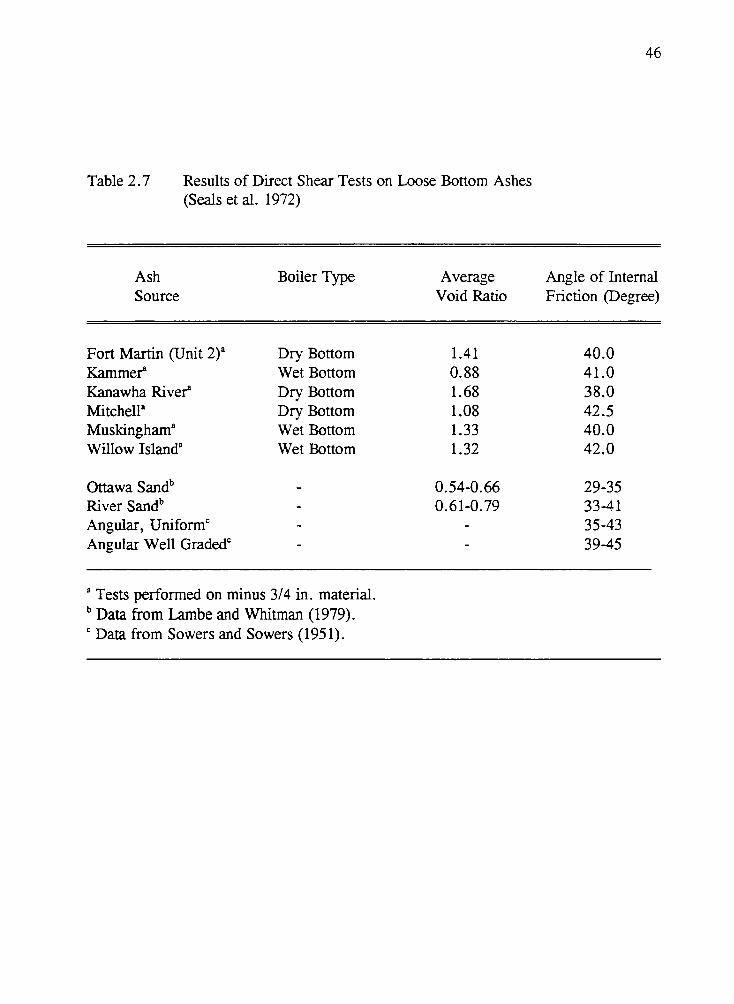
Table 2.7 Results of Direct Shear Tests on Loose Bottom Ashes (Seals et al. 1972)

Ash Source

Fort Martin (Unit 2)2

Kammer Kanawha River Mitchella Muskingham2

Willow Island2

Ottawa Sandb River Sandb Angular, Uniformc Angular Well Graded0

Boiler Type

Dry Bottom Wet Bottom Dry Bottom Dry Bottom Wet Bottom Wet Bottom

a Tests performed on minus 3/4 in. material. b Data from Lambe and Whitman (1979). 0 Data from Sowers and Sowers (1951).

Average Void Ratio

1.41 0.88 1.68 1.08 1.33 1.32

0.54-0.66 0.61-0. 79

46

Angle of Internal Friction (Degree)

40.0 41.0 38.0 42.5 40.0 42.0

29-35 33-41 35-43 39-45

Table 2.8

Material Source

Schahfer Unit 14a Unit 17

Gibson Gallagher Perry

Results of Direct Shear Tests on Selected Indiana Bottom Ashes (Huang 1990)

Loose Dense Strength Values of Strength Values of Intercept ' Intercept cf>' (psi) (deg) (psi) (deg)

0.48 35.1 1.49 46.3 0.14 39.2 3.12 47.7 0.20 44.8 1.66 55.0 0.49 41.3 2.00 51.6 0.49 41.5 3.00 50.6

a Boiler slag (wet bottom ash)

47

60-

50-(/)

n.: (/)

40-(/) w 0:: 30 -I-U)

0:: <{ 20-w I (/)

10

0

BA¢•345°

~/

---~ " ~ '-

" " \ \ \

I I I I I I I I I 40 50 60 70 80 90 100 110 120

NORMAL STRESS P.S. I.

BA- DELMARVA BOTTOM ASH SP SAND - TYPE F BORROW

Figure 2.14 Triaxial Test Results for Pulverized Bottom Ash Samples. (Srivastava and Collins 1989)

BA

SP SAND

~ 00

49

weight in the sand size, which is not common for fly ashes. Wayne et al. (1991) tested

Class F fly ash to evaluate its utilization as a structural fill in a highway embankment.

The triaxial tests were conducted to investigate the ash behavior in shearing. One of their

main concerns was the strength for long term conditions. They used consolidated-drained

triaxial tests on saturated samples to simulate this behavior under saturated conditions.

They also performed slow drained tests on as compacted partially saturated samples. The

idea was to inves~gate the long term response of the unsaturated fill. The strain rate was

adjusted (0.0001 in/min.) to ensure a drained response for theses samples, but no suction

measurements were made.

A comparison between the triaxial tests and shear box tests for testing coal ash

was recently reported by Clarke et al. (1993). They recommend the use of triaxia1 tests

since they are more controllable. The saturation process in the shear box tests may

remain partial and the results may be affected by the suction. In the triaxial tests,

drainage is controllable and the failure surface is not predetermined (Bishop and Henkel

1962). On the other hand, triaxial tests are more time consuming and have limitations

also that need to be considered.

2,4 Coal Ash Utilization In Embankment Construction

The construction of highway embankments requires substantial amounts of fill

materials. Soils, being the common source for such fill, are usually transported from

nearby borrow areas. Coal ash can be viewed as one of the viable alternatives for soils.

It can offer several advantages over many soils and rocks. Coal ash has a lower unit

weight than most soils. This property can be useful, especially when the compressibility

of the foundations is a source of concern. Relatively high shear strength can be obtained

if the coal ash is compacted appropriately. High shear strength allows for steeper slopes

and higher embankments. The ease of moisture control, especially in the case of dry fly

ash, simplifies the quality control of the compaction and encourages the utilization of coal

ash in construction. The availability of the coal ash, in locations where natural soil

sources may be scarce, makes their utilization beneficial in places such as the highly

developed urban areas. If costs of coal ash are kept low, compared to most natural soils,

50

the feasibility of using coal ash is enhanced. It also encourages the interested parties

(industry, governmental agencies, consultants, universities) to investigate thoroughly this

alternative.

There are, however, some limitations associated with the use of coal ash. These

limitations can be addressed by appropriate measures and precautions. The limitations

are mainly because of economic related concerns, mechanical performance concerns, and

environment related concerns. The economic concerns include costs due to special

design and construction considerations, and the additional training required for the design

and construction teams. The costs associated with the additional training required for the

construction and quality control teams are actually reduced every time a new project is

finished. The costs of the special design and construction considerations can be covered

if the costs of coal ash remain at low levels.

The performance concerns are related to the mechanical behavior of the coal ash.

Single types of ash were utifued successfully in several demonstration projects. Examples

of these projects are presented later in this section. Utiliz.ation of coal ash mixtures is still

restricted due to uncertainties associated with their mechanical performance and the

control of their compaction. The topic of this study is the investigation of the compaction

and shear strength of compacted mixtures of coal ash. Detailed examination and

discussions of these behaviors are included in the successive chapters.

The utiliz.ation of coal ash can lead to conserving natural soils near urban areas

and reduce the costs associated with ash disposal. Rather than conserving natural soils,

using coal ashes types ill and N (Indiana Administrative Code, 329 IAC 2-9-3)can be

environmentally safe. Strict limitations have been placed upon the proportion of trace

elements contained in their leachates. The environmental concerns are discussed further

in the following section.

2.4.1 Overview of Current Practices of Coal Ash Utiliz.ation in Highway Construction

The accumulation of huge amounts of coal ash in landfills and disposal ponds

encouraged many agencies to become involved in finding alternatives to coal ash

disposal. The characteristics of coal ash differ based upon type. Fly ashes are very fine

51

materials that have light unit weight. Class F fly ash has pozzolanic properties that need

the addition of lime and water to start cementing reactions. It is generated in large

quantities and can be successfully used as fill. Class C fly ash has self cementitious

properties that allow its use as an additive in cement mixtures or as a cement substitute.

Bottom ash has stable composition that favors its use as an aggregate substitute or as a

:fill. Boiler slag currently has a better market than bottom ash. Table 2.9 summarizes the

current uses of coal ash in highway construction.

2.4.2 Environmental Concerns for Coal Ash Utilization in Embankments

The utilization of coal ash in embankment construction has increased during the

last decade. The main environmental concerns are dusting, erosion, and leaching. Coal

ash has been treated as a waste material for a long time. The practices for the coal ash

disposal were directed to minimize the disposal cost rather than to improve the quality

of the coal ash as a construction material. The nature of the coal, the burning process,

and the disposal process all affect the ash composition and its quality and hence the

impacts on the environment. All these factors motivated research to investigate these

impacts. This is a very active area of research on its own.

2.4.2.1 Dusting

Dusting is generated if dry ash fines are disturbed. The fly ash particles are very

small. They mainly fall in a size range similar to silts and coarse clays. The dry fly ash

particles have no cohesive forces between themselves, and hence are very easily

disturbed forming dust. Many measures are commonly taken for the fly ash handling and

utilization in construction to minirniz.e the dusting problems. The dry fly ash is routinely

transported using pneumatic tankers similar to those used for transporting bulk portland

cement from manufacturer's silos to concrete mixing stations. Special equipments are

usually used for the ash placement and moistening. Conditioning the ash using water

normally reduces the dusting problem (DiGioia et al. 1986). To store the fly ash in

stockpiles, it has to be kept moist (approved anti dusting materials or water may be used)

or have some type of stable cover on top of it. The containment of the ash under soil

Table 2.9

52

Utilizations of Coal Combustion By-Products In Highway Applications (USDOC 1988)

Uses of Fly Ashes * Raw material in Portland Cement

* * * * * * * *

Replacement for cement in concrete Cement replacement in precast concrete products Ingredient in aerated concrete Mineral filler in asphaltic concrete Stabilization of highway subgrades Raw material in the manufacture of lightweight aggregates Material for structural fill Material for flowable fill or backfill

* Ingredient in grouting * Stablized fly ash base course without aggregate * Stablized fly ash-aggregate base course

Uses of Bottom Ash * Aggregate in ashphalt * Ingredient in bituminous stablized base for highways * Aggregate in Portland cement stablized bases for highways * Snow and ice abrasive * Structural fill * Unstabilized road base

Uses of Boiler Slag

* * * *

Snow and ice abrasive Road base aggregate Ingredient in anti-skid bituminous wearing course Sand blasting grit

Note: FGD materials are presently not widely used in highway construction.

53

cover and the use of surface vegetation eliminate the dusting problem. The problem of

dusting must be considered if ash mixtures are used.

2.4.2.2 External and Internal Erosion

Excluding Class C fly ash, coal ash may be generally considered as

cohesionless materials. The only forces that can resist particle movements are frictional

in nature. Erosion is a natural mass transporting phenomenon that is caused by wind or

water. Wind and rains can lead to serious erosion problems for exposed ash on

embankment sides. Cohesive soils with vegetation coverage are typically used to control

the surface erosion problem and provide an aesthetic view (DiGioia et al. 1986).

Appropriate encasement of the ash inside a system of base liner and a cover can

significantly minimize water infiltration and internal erosion of the ash. The system

consists of low hydraulic conductivity soils or synthetic materials plus filters. The

efficient compaction of ash mixtures can reduce their permeabilities and consequently the

internal infiltration.

2.4.2.3 Leaching

If water is infiltrated into the ash fill, leachates generated in the ash mass

may be transported to the surrounding environment including the soil and the ground

water. Major concerns are to be raised if the leachates contain deleterious substances at

concentrations that can have adverse effects on the environment.

The chemical composition of the ash is generally inert. It consists mainly of

oxides of silicon, aluminum, calcium, and iron. Minor proportions of compounds of

titanium, potassium, sulfur, and magnesium may also exist. Trace elements such as

compounds of barium, nickel, arsenic, silver, cadmium, lead, mercury, etc .. may also

be contained in the ash in very minimal proportions (GAi and USIFCAU 1993). The

Indiana Department of Transportation has restrictions on the use of coal ashes based on

the type of their leachates as defined by Indiana Administrative Code, 329 IAC 2-9-3.

Table 2.10 displays the criteria for defining the types of leachates based upon the levels

of concentrations of the substances included in these leachates ( the values included in

54

Table IO may be changed in the future, thus the current values in the original reference

must be consulted). Only the ashes classified as types m and N are used in highway

construction in Indiana. The utilization of type II is restricted (based upon the PH level)

and type I is not allowed due to the potential for finding hazardous levels of

concentrations in the leachates. Trace elements concentrations in the coal ash vary due

to both depositional and post depositional conditions of the coal, the combustion

procedure, ash type, technique for ash collection and transportation to disposal, the

duration of contact between the ash and the emitted gasses, and the disposal and post

disposal conditions. It is not simple to predict the concentrations of the trace elements

in the ash leachates. The chemical analysis of the parent coal is not alone sufficient.

Nevertheless, it is informative to perform it since it can reveal the noncombustible

substances existing in the coal.

Tests were developed to investigate the impacts of the leachates on the

environment (Jackson and Sorini 1987; USDOC 1988). The main objectives were to find

the concentrations of the deleterious elements in the leachates and to define if the ash is

hazardous or not. Solid wastes were classified under EPA's Resource conservation and

restoration Act, RCRA, regulations (EPA 1990). Under RCRA, a solid waste is to be

considered hazardous if it fails any of the criteria established for ignitability, corrosivity,

reactability, or toxicity (RCRA Subtitle C; EPA 1990). Coal ashes are not considered

ignitable. Types ill and N are considered neither corrosive nor reactive (USDOC 1988).

Ke (1990) suggested levels of resistivity, PH, soluble chloride content, and soluble

sulfates for non corrosive bottom ashes. According to these levels Huang and Lovell

(1993) reported, based upon laboratory tests, that 7 out of 11 Indiana bottom ashes,

tested in the laboratory, were found to be potentially corrosive. They recommended that

adequate protection must be provided to any metal structure placed within the vicinity

of a potentially corrosive ash. The main environmental concern is the level of

concentration of the deleterious substances in the ash leachate in comparison to the levels

indicated by the EPA regulations for toxicity. Tests such as the EP (Extraction

Procedure) test and the Toxicity Characteristic Leaching Procedure (TCLP) were

developed to determine the degree of hazard associated with leaching from waste disposal

Table 2.10 Indiana Administrative Code Restricted Waste Site Type Criteria Indiana Adminstrative Code, 329 IAC 2-9-3 (IAC 1993)

Parameter Concentrations (Milligram per Liter) Type IV Type ID

(1) Eor :earamete.rs !Ising the E:e Ioxidt}'. test: * Arsenic ~0.05 ~0.5 Barium ~1 ..:LlO Cadmium ~0.01 ~0.1 Chromium ~0.05 ~0.5 Lead ~0.05 ~0.5 Mercury ~0.002 ~0.2 Selenium ~0.01 ~0.1 Silver ~0.05 ~0.5

(2) Eor parameters using the LeaQhing MetbQd Iest: Barium ~1.0 ~10 Boron ..::;.2.0 ~20 Chlorides ~250 ~2,500 Copper ~0.25 ~2.5 Cyanide, Total ..::;.0.2 ~2.0 Flouride ..::;.1.4 ~14 Iron ~1.5 ~15 Manganese ~0.05 ~0.5 Nickle ~0.2 ~2.0 Phenols ~0.3 ~3.0 Sodium ..::;.250 ~2,500 Sulfate ~250 ~2,500 Sulfide, total ~l*** ~5.0 Total Dissolved Solids ..::;.500 ~5,000 Zinc ~2.5 ~25 pH (Standard Units) 6-9 5 - 10

*IDEM allows EP toxicity test or TCLP test. **Testing is not required.

Type II

~1.25 ~25 ~0.25 ~1.25 ~1.25 ~0.05 ~0.25 ~1.25

~25 ~50 ~6,250 ~6.25 ~5.0 ~35

** **

~5.0 ~7.5 ~6,250 ~6,250 ~12.5 ~12,500 ~62.5 4 - 11

Type I

<5.0 < 100 <1.0 <5.0 <5.0 <0.2 <1.0 <5.0

** ** ** ** ** ** ** ** ** ** ** ** ** ** ** **

***If detection limit problems exist, please consult the office of solid and Hazardous waste for guidance.

55

56

(Jackson and Sorini 1987). Leachates from coal ash rarely reach haz.ardous levels

(USDOC 1988). The utilization of coal ash mixtures has advantages over a single type

since hydraulic conductivity of the coal ash can be lowered to minimize the rate of

leachate generation. Meanwhile, the stability of the ash mixtures can be maintained. The

use of ponded ash may have an advantage over the freshly generated ash. The disposal

procedure includes flushing the samples with water. This may reduce the concentrations

of the elements attached on the surface of the ash particles.

Encasement of the coal ash embankments can minimize the infiltration of water

into and out from the ash. In addition to the encasement, a sitting criteria is normally

developed to provide a safety distance from the ash body (This criteria does not apply

to type IV ash) to water resources (surface or ground). Although this criteria is mainly

decided to protect the environment, the geotechnical aspects of the proposed site may

also dictate additional measures. Factors such as the hydraulic conductivity of the

surrounding soil in the site and the potential for having problems due to unfavorable soil

conditions must be considered.

2.4.3 Considerations For Coal Ash Utilization In Embankment Construction

A successful project is one in which the best use of the available resources is

made. It must serve the physical purposes of the project within the limitations imposed,

and to achieve the intended performance levels. Coal ashes, being no different than other

engineering materials, have their advantages and limitations. Successful design and

construction procedures would employ the material advantages and provide provisions

that would minimize or diminish· the limitations effects.

2.4.3.1 Design Considerations

In general the design plans have to satisfy the highway requirements, usually the

elevations and embankment top width. The requirements for safe environmental

performance must also be satisfied. All the site specific conditions including the

geological, hydrological, and topographical conditions have to be taken into consideration

in the design: The durability and soundness of the material have to be sufficient to stand

57

under the expected environmental and loading conditions as long as the structure exists.

Furthermore, the material has to be reasonably simple to utilize in construction. The

construction materials, being coal ashes in this case, must be compacted adequately.

The fill must sustain its own weight plus the loads imposed upon it without

excessive deformations within the possible site weather (environmental) and loading

conditions. The compressibility of the fill has to be acceptable. The slopes of the

embankment must be adequately stable. This particular consideration is directly related

to the appropriate assessment of the shear strength of the material. The shear strength of

the ash mixtures may possibly change with changes in the mixture proportions. The

stress-strain behavior may also change. Possible differential settlements may have to be

within acceptable levels. The embankment height in combination with the fill weight must

not impose excessive stresses on the foundation beyond the bearing capacity or beyond

acceptable compressibility limits. The unit weight of compacted coal ash mixtures are

lighter than most soils. This property can be used beneficially in the design. If

representative parameters are developed in the laboratory or by field testing, software

packages may be used for modeling the fill deformations and stability.

The detailed design must provide provisions for the drainage of surface water and

groundwater in addition to the control of capillary action is necessary to prevent ash

saturation. Ash saturation may lead to frost susceptibility or liquefaction problems in

addition to the environmental problems due to leaching (DiGioia 1994). The placement

criteria normally contain provisions to maintain adequate distances between the ash and

the drinking ground water (DiGioia et al. 1986). Appropriate encasement to minimize

migration of water in and out of the fill have to be considered in the design. Any

special provisions needed, for providing adequate protection of metals from corrosion and

adequate protection of concrete from sulphate attack, have to be included in the design.

Alternatives to metallic components such as fiber glass or PVC may be considered to

avoid corrosion. Use of stainless steel parts or providing protection using special coatings

may also be considered (Huang and Lovell 1993). It is also possible to use barriers of

compacted soils that have very low hydraulic conductivity or geosynthetics liners to

pr~vent the physical contact and the migration of leachates.

2.4.3.2 Construction Considerations

a- Site Preparation

58

The site preparation constitutes all the works required before the fill placement.

This includes diverting existing drainage, dewatering low areas, removal of trees and

brushes, removal of top soil, placement of drainage blankets and drains, and completion

of subsurface constructions.

b- Fill Transportation and Stockpiling

The coal ash has to be transported from utility plants to construction sites.

Covered dump trucks are usually used for transporting moistened coal ash to control

moisture loss and to avoid dusting. If dry fly ash is transported, special pneumatic

tankers similar to those used in transporting bulk portland cement are used to avoid

dusting. Huang (1990) expressed the feasible distances for coal utilization to be contained

by a circle with a ~dius that is a function of the transportation expenses as well as the

price for aggregate supply. Best value usually occurs if the ash borrow source is near to

the site. Stockpiling in the field is important. Sufficient quantities of ash has to be

stockpiled in the site to feed any surge needs in the construction process and to serve as

a contingency. The stockpiled materials have to be covered or watered to prevent

dusting.

c- Fill Placement and Compaction

Detailed specifications for placement and compaction of fly ash were reported

(DiGioia et al. 1986; Brendel et al. 1988; DiGioia 1994). The coal ash is usually placed

in loose lifts in the range of 20 to 30 cm (8 to 12 inch) thick using a dozer. A vibratory

roller may be used to compact the lifts. Pad-foot and smooth-drum vibratory rollers were

used successfully to compact fly ash efficiently (Digioia 1994). Vibration frequencies in

the order of 1800 to 2000 cycles/min were reported (DiGioia, 1994; Brendel and

Glogowski 1989). Smooth-drum vibratory roller was used efficiently for the compaction

of Schahfer bottom ash in the 1-12/Kennedy project. The surface of the ash must be

protected from dusting.

59

d- Performance monitoring

Concerns about the performance or for purposes of demonstration may lead to the

installation of instrumentation to monitor performance. The structural performance may

be monitored using vertical and horizontal inclinometer, settlement plates,

extensiometers, and piezometers. Inspection wells can be installed for monitoring the

ground water table conditions. Periodic collection and analysis of leachate samples may

be performed for environmental purposes.

2.4.4 Field Performance of Coal Ash in Embankments

2.4.4.1 East Street Valley Expressway, Pennsylvania

As part of the continuous effort to promote the use of coal combustion by

products (CCBP's) in highway construction, the Pennsylvania Department of

Transportation (PaDOT) and the Federal Highway Administration (FHW A) . agreed to use

Class F fly ash and Poz-0-Tec (mixture of lime, Class F fly ash, and FGD) in a large

embankment construction. The project was sponsored by Duquesene Light Company and

Electric Power Research Institute (EPRI) in cooperation with the Federal Highway

Administration (FHW A) and the Pennsylvania Department of Transportation (PaDOT).

Necessary review for environmental impacts were performed by the Pennsylvania

Department of Environmental Resources (PaDER). The East Street Valley Expressway

embankment was constructed, during 1987-1988, along a section of Interstate 1-279,

Pittsburgh, Pennsylvania. The embankment had an average width of 210 feet, an average

depth of 50 feet and an approximate length of 1490 feet. A total of 255,000 cubic yards

(approximately 353,000 tons) of CCBP's were utilized in the construction (Brendel and

Glogowski 1989; DiGioia 1994)

The laboratory and field investigations included both environmental and

geotechnical testing programs. The environmental testing, including the EP toxicity and

leachate testing, focused on the leachate composition and their impacts on the water

quality. The geotechnical investigations showed that the ground water was approximately

9 feet below the valley bottom. However, concerns were raised because the side slopes

of the valley were found to contain ground water as well. Adequate encasement of the

60

ash fill had to be implemente.d in the design. Figure 2.15 displays a typical cross section

for the embankment and the valley.

Class F fly ash was mainly retrieved from the disposal pond of Duquesne Light

Company's Cheswick Power Station. A small part was supplied from silos. The overly

wet fly ash from the pond was initially placed on top of a two feet thick layer of bottom

ash to drain the excess moisture by gravity. The saturated ash displayed surface

instability. Additional drying was achieved using rolling blades and aeration until the

moisture content of the fly ash became within the specified limits. The ash was then

transported to the construction site. The silo dry fly ash was moistened upon discharge

from the silos, loaded into trucks, and transported to the site. The placement of the

CCBP materials followed the typical PaDOT procedures specified for natural soil

placement (Brendel and Glogowski 1989). The material was dumped, spread in loose lifts

of 8 in., compacted using 4 to 6 passes from a 20 ton dual pad foot vibratory compactor

near a resonant frequency of 2000 VPM. The material was compacted to a minimum of

97% of maximum dry unit weight as determined by ASTM D 698, Method B. It was

noted that more passes were required to achieve the targeted unit weight when the

moisture content was significantly lower than the optimum moisture content. At the

optimum, four passes or less were adequate to achieve the required unit weight. At

excessively wet weather, loss of strength was experienced in the exposed layers. Drying

of these layers was necessary before the recompaction was performed.

The field unit weight was monitored using the nuclear density gauge. The Speedy

method, and the microwave oven were used along with the conventional oven for the

determination of moisture contents and the dry unit weight for parallel samples retrieved

using the sand cone method. The sand cone and the conventional oven method were used

to calibrate the other methods and develop correlations. The results of the compaction

tests were accumulated and used for the construction of a family of compaction curves

for the materials encountered. Subsequently, the one-point technique for compaction

control was applied. The embankment performance was monitored using settlement

.....

GEOTEXTILE

~

·CATCH BASIN 5

1(MIN. ) SOIL COVER

BELOW SUB-BASE

i---- --.12' NOMINAL WIDTH

~

SET BIi<!> PIPE DRAIN FILLED H AASHTO NO. 57 STONE (EVERY 3001

)

ASH

-2'- 8 11 UNDER DRAIN PROTECTIVE

COVER

-....._,c_~"- f:i"-:J- 9"-1211 AASHTO NO. 57 ""··-·-- -n-- - STONE

811 (j) PIPE DRAIN FILLED

WITH AASHTO NO. 57 STONE (EVERY 300')

2 - 611

~ PERFORATED SOR 23.5 ABS DRAIN PIPES(CONNECTED TO 84"1f> STORM SEWER)

PoOOT CLASS II, TYPE B, NEEDLE PUNCHED, NONWOVEN GEOTEXTILE

2° -8" UNOERORAIN PROTECTIVE SOIL COVER

Figure 2.15 Typical Section in East Street Valley Expressway Embankment, Pennsylvania. (Brendel and Glogowski 1989)

0\ ......

62

plates, horizontal slope indicators, and piezometers. Nearly all of the settlement of the

fly ash embankment occurred rapidly during the construction period. The predicted post

construction settlements of 3 in. overestimated the measured settlements. It was reported

that the actual field relative compaction approached 100 % and the prestress due to

compaction exceeded the embankment fill stresses, hence the settlements were

overestimated. The project demonstrated the success of using fly ash as structural fill

materials.

2.4A.2 U.S. 12 Demonstration Project, Lake County, Indiana

As orie of the major coal ash-producers in the United States, Indiana has found

it necessary to develop utilizations for coal combustion products to minimize their

disposal problem. One of the early experiences of Indiana Department of Transportation

(INDOI) on using coal ash in highway construction. is raising the bridge approach along

U.S. Route 12 (Columbus Drive) at the intersection with Kennedy avenue. The old

embankment on this highway needed to be raised using steep side slopes (2H: 1 V) due

limitations on the right of way (Davis et al. 1995). About twenty three thousand tons of

bottom ash were supplied from NIPSCO's Schahfer power plant to be placed in this

project. The leachate testing indicated that the ash was IAC waste Type m, having less

than 10 % of the hazardous waste concentrations defined in RCRA.

The ash was transported using open dump trucks. Loose lifts of 8 in thickness

were placed using a dozer and a grader. The bottom ash lifts were then compacted, using

a vibratory smooth wheel roller (Figure 2.16), to a final thickness of approximately 6 in.

The compacted dry units weight were not sensitive to the compaction moisture contents

except at very low moisture where bulking could occur. The bottom ash was thus flushed

with a fire hose as a method to provide adequate moisture for compaction and avoid

bulking. Compaction control in the field was conducted using a nuclear density gauge.

Comparatively, the moisture determination was conducted using the Speedy method, the

microwave oven and the conventional oven. All the methods were correlated to the

conventional oven method.

63

Provisions for metal corrosion and concrete sulfate attack were requested by

INDOT (Hoover and 2.andi 1993). Protective coatings and or, suitable fill materials were

used in the contact areas. Encasement of the coal ash was at the front and rear ends

where concrete elements are in contact with the fill. Three feet thick layer of silty clay

(till) was placed and compacted around the bottom ash. Figure 2.17 displays the

utilization of glacial till in the areas of contact with concrete elements. Encasement was

also provided on the north side between the bottom ash fill and the side slope. The north

side slope was constructed using coarse ballast aggregates to provide stability and build

a steeper slope. Vegetation coverage was placed on top of the one side slope originally

without soil coverage. The construction was completed in 1994.

2.4.4.3 I-495 and Edgemoor Road Interchange, Wilmington, Delaware.

This demonstration project was initiated as part of the Electric Power Research

Institute (EPRI) effort to promote the utilization of high volumes of coal ash instead of

disposal. The primary objective of this project was to construct and monitor the structural

and environmental behavior of a full-scale roadway embankment containing Class F fly

ash (Srivastava and Collins 1989). The project consisted of the construction of a new

above grade interchange connecting Interstate Route 495 with Edgemoor Road with all

the connected constructions including six new access ramps along with realignment,

reconstruction, and widening of several major access roads. Freshly generated, landfilled

or stockpiled Class F fly ashes, and pulverized bottom ash were utilized in construction

in this project. A typical cross section is displayed on Figure 2.18. The fly ash for the

embankment was provided from Delmarva Power and Light Company's Edgemoor

Station, Wilmington, and Atlantic Electric Company's Deepwater station in Penn's

Grove, New Jersey. The pulverized bottom ash was supplied by Delmarva.

The testing program included preliminary testing, control during construction, and

monitoring after construction. Prior to construction the laboratory testing focused on the

characterization and engineering behavior testing. The relatively fine grain sizes of the

64

Figure 2.16 Smooth Wheel Roller Compacting Schahfer Bottom Ash in I-12 Kennedy Intersection Embankment, Indiana .

65

Figure 2.17 Encasement of Bottom Ash With Till at the Vicinity of Concrete Members in I-12 Kennedy Intersection Embankment , Indiana.

66

bottom ash used in this project were attributed to a clinker grinder that the bottom ash

passed through before being disposed. Typical specific gravity values for the ashes used

in this project ranged between 2.03 to 2.3. The loss on ignition (LOI) ranged between

8.17% and 11.3%. Moisture density tests were performed in the laboratory using both

ASTM D-698 and ASTM D-1557. The optimum moisture content of the stockpiled ash

was reported to vary with changing the sampling location within the stockpile. The

permeabilities of the compacted fly ashes were found in the range between 104 and 10-5

cm/s. Compacted bottom ash samples were more permeable in the range of 10-3 cm/s,

although having relatively fine gradation.

One-dimensional compression tests on the compacted bottom ash samples

displayed smaller compression indices than fly ash samples. It 'Yas thus concluded that

the bottom ash would undergo significantly lower settlements than the fly ash. Triaxial

tests were performed according to ASTM D 3397. Angles of shearing resistance for the

fly ash were reported within the range of 17° To 18 which was considered to be

relatively low. Bottom ash samples displayed an angle of 34.5° which is comparable to

loose well-graded sand.

The principal considerations during construction were the control of moisture

content, and the control of compaction. The moisture was adjusted to avoid dusting and

facilitate the compaction. Too much moisture caused loss of strength and pumping while

too little moisture caused dusting and difficulty to achieve proper compaction. The field

densities were measured using a Troxler density gauge. The results based on back-scatter

measurements were found in agreement with those based on 8 inch probe penetration

(Srivastava and Collins 1989). The back-scatter technique was thus used for compaction

control during construction. The higher energy from the modified proctor density was

found to have minor difference from the densities achieved by the standard proctor.

Specifications for field com~on were established to achieve at least 95 % of maximum

unit weight, reached in the laboratory, based on standard proctor tests, ASTM D-698.

The moisture contents for the samples retrieved from the field compacted fill were

determined using the Speedy technique and the microwave oven. The nuclear density

gauge measurements were adjusted based upon the Speedy and the microwave results.

67

Corrections for the nuclear gauge measurements were necessary. The accumulated results

from the moisture-density tests were utilized to construct compaction curves.

Subsequently, the control of the compaction in the field was performed using one-point

method (Figure 2.19).

After construction monitoring demonstrated several significant results that helped

the overall judgment on the success of this project. Standard Penetration Tests (SPT)

were performed on the compacted fill to asses the bearing capacity of the fill. SPT values

ranged between 24 and 61 blows/foot were reported. Similarly, SPT's were conducted

on compacted granular fill. The results for both materials were found to be very similar.

Settlement monitoring have shown negligible long-term settlements. Most of the

settlements occurred during construction. Frost susceptibility testing were planned to be

completed after the end of construction on fly ash and granular fill materials for

comparison.

To monitor the environmental impacts of the ash fill four monitoring wells were

installed. Ground water monitoring was achieved by retrieving and analyzing water

samples from each well. It was concluded, based upon leaching tests and the analysis of

samples collected from the field, that the fly ash utilized for this project was

environmentally safe.

It was concluded that the compaction moisture was the key point for successful

placement and compaction of the fly ash (Srivastava and Collins 1989). The laboratory

moisture-density tests were used successfully to define the field placement moisture

contents. Compacted fly ash could support heavy construction equipments without

excessive rutting or damage. The dusting from poorly conditioned fly ash was found

comparable to dusting from natural soils. The bearing capacity characteristics from fly

ash in this project was reported to be comparable to those of well-graded sand and

gravel. Overall findings supported the use of fly ash as an embankment construction

material from the engineering and environmental points of view.

-1.D I

:x: " .c.

66 1

4' 24' 10' 241 4'

1 r-10" CONCRETE . j I I 3' 8

11

STONE BASE~::-----:: 18" TYPE A BORRON ~ TYPE F BORROW~' > ( SANDY SOIL)

~y /✓,"-. "-"-

COMPACTED FLY ASH FILL ( 12" LOOSE LIFTS)

--TYPE B BORROW MATERIAL (GRANULAR) 6

--c= ORIGINAL GRADE

EXCAVATE TO FIRM BOTTOM "-"-Y//,"-'\

Figure 2.18 Typical Fly Ash Ebankment Section in the 1-495 and Edgemoor Road Interchange, Delaware. (Srivastava and Collins 1989)

())_

/\ :c V

~-

0\ 00

90 -

05 -

80 -

r O 75 -I L ,,~i,uc_ I llflHAIHIVUI m :::0 / ✓ ~~"-·. !"-< 7 / 0-

-oo ~ rn "'lz -l (J) ~:; 70

-< _,_ ONE- POINT __ /DENS~

/ 0

65 -

60 -

/ I;:; /( '

PARALLEL~ MOISTURE - DENSITY CURVE

25 26

..., Q z

1-l

I~ -l I~

27 20

LABORATORY MOISTURE - DENSITY CURVES

29 30 31

MOISTURE CONTENT 32 33 34

Figure 2.19 Determination of Maximum Dry Density Value from One-point Standard Compaction Test in the I-495 and Edgemoor Road Interchange, Delaware. (Srivastava and Collins 1989)

35

(PERCENT)

$

70

CHAPTER 3

EXPERIMENTAL APPARATUS AND PROCEDURES

3, 1, Ash Sampling and Initial Processing

3.1.1 Samples Sources

Coal ash samples used in the present study were extracted from two power plants

in Indiana. The first power plant was the Schahfer power plant, located in Jasper county

and owned by the Northern Indiana Public Service Co. (NIPSCO). At the Schahfer plant,

the ash is disposed separately. The second power plant was the Gibson power plant,

located in Gibson county and owned by Public Service Indiana (PSI), is the largest

power plant in Indiana. Bottom ash and class F fly ash are co-disposed at the Gibson

power plant existing in the form of mixtures at disposal sites.

3.1.2 Ash Generation and Disposal Procedures in Sampling Sources

The Schahfer plant contains four power generating units (14, 15, 17, and 18).

Unit 14 has a cyclone furnace that generates boiler slag. The boiler slag is successfully

marketed. The other three units bum pulverized coal and generate bottom ash. The

bottom ash is mainly disposed, which motivated its inclusion in this research. It is

transported hydraulically and finally disposed on the margins of a disposal pond. Class

F fly ash was initially stored in silos in dry condition. The fly ash may be marketed,

used with lime to stabilize the flue gas desulferization (FGD) sludge, or disposed in a

landfill. The Class F fly ash generated by units 17 and 18 is mostly disposed in landfills.

This motivated its inclusion in this study.

The Gibson power plant contains pulverized coal burning units. Bottom ash and

Class F fly ash are generated from burning bituminous coal in Gibson Plant. The fly ash

71

is separated from the emitted hot gases using electrically charged precepitators, then

collected into hoppers. Two units were burning coals that had high sulfur content and

thus are devised with flue gas desulfem.ation (FGD) equipment. A minor fraction of the

Class F fly ash is collected from the hoppers, moistened, and used with lime to stabilize

the FGD sludge, locally on the plant site. However, the majority of the fly ash is slurried

using water jets then pumped through pipes to a discharge point close to a disposal pond.

The bottom ash is collected in a hopper, crushed, and pumped through pipes to be

discharged at the same location of the fly ash disposal. The fly ash and bottom ash thus

become mingled at the discharge location. The discharge location is connected to a

disposal pond by a 300-m long discharge channel. The ash mixtures flow along the

discharge channel to the disposal pond. A significant fraction of the ash settles along the

channel before the flow reaches the pond. A crane with a large bucket is used to dredge

the material from the channel.

3.1.3 Sampling Procedures

3.1.3.1 Sampling From Schahfer Power Plant

Sampling the bottom ash was performed in two stages. At first, six initial samples

(3-5 kg each) of bottom ash were extracted at the ground level. The samples were

collected from the disposal areas for units 15, 17, and 18 to provide guidance to the

collection of large samples. After performing grain size analysis on these samples, it was

concluded that small surface samples may not provide the best representation of the

bottom ash. It was also noticed that samples from discharge locations contain mostly

gravel size particles (Figure 3.1). Moreover, samples from the shallow streams formed

between the discharge locations and the disposal pond contain fine materials (Figure,

3.2). Hence, at the second sampling stage, two large ash samples (about 250 kg each)

were extracted from the margins of the disposal pond using a back-hoe. The bottom ash

samples were extracted from depths starting at the ground surface to approximately 2.5

m (8 feet) deep. Using this method of sampling typically rendered the samples in a

:..---·~-- ·- -"';;·;:,;.,..::...;;£:·

~ -- - ~~- '~\~ _;_~

Figure 3.1 Large Bottom Ash Particles Near the Discharge Point (Schahfer Power Plant).

72

73

Figure 3.2 Fine Bottom Ash Particles on the Surface of the Shallow Streams Between the Disposal Pond and the Discharge Point (Schahfer Power Plant).

74

disturbed condition. The samples were collected for grain size distribution testing and for

reconstituting laboratory testing samples. No natural soil was encountered among the

bottom ash samples retrieved. This indicated that the bottom ash depth extended beyond

the depths reached by the backhoe. The bottom ash samples were stored in 50-gallon

lined steel drums and transported to Purdue University. In addition to the bottom ash

samples, one large sample of Class F fly ash (approximately 250 kg) was extracted in

a dry condition from a storage silo. The fly ash was transported inside sealed 50-gallon,

lined metal drums to Purdue University.

3.1.3.2 Sampling From Gibson Power Plant

Similar to Schahfer, surface samples were collected from the disposal site of

Gibson power plant followed by the collection of large samples. To obtain representative

samples of the wide range of mixtures in Gibson Plant, large samples were collected

from four locations on the left bank of the discharge channel. The first sampling location

(location 1) was at the discharge point. This location was expected to contain a large

fraction of bottom ash content. The fourth sample was collected near the end of the

discharge channel (location 4) to provide mixtures of low bottom ash content. The other

two samples were collected from two intermediate locations (approximately 100m apart)

along the channel. The ash samples were then transported inside sealed 50-gallon, lined

metal drums to Purdue University.

3.2 Ash Characterization and Mixture Developments

3.2.1 Overview

The experimental program followed in this study aims at applying typical soil

testing procedures in the characterization and testing of the ash mixtures. Some simple

additional procedures were implemented as necessary to control fly ash dusting in the

laboratory. Two types of mixtures were sought to be examined in this research: explicit

mixtures formed from Schahfer plant ash and implicit mixtures formed from Gibson plant

ash. Explicit mixtures were formed by mixing a known quantity of fly ash with a known

75

quantity of bottom ash. Implicit mixtures were formed by processing the ash samples

from Gibson plant to produce homogeneous mixtures. The fines contents (% passing

#200) in the implicit mixtures were then determined (as an alternative to determining the

fly ash content).

3 .2.2 Initial Processing, Grain Size Analysis, and Mixture Composition

3 .2.2.1 Samples from Schahfer Power Plant

The dry Class F fly ash was mixed, then weighed and packed (3 kg) in double lined

plastic bag packages. The packages efficiently maintained the dry condition of the fly ash

and facilitated the handling. The packages were stored in dry conditions. Three hydrometer

tests following ASTM D 422-90 were performed on the fly ash (Figure 3.3). The moist

bottom ash was extracted out of the 50 gallon drums, placed in a 4' x 6' x 1' wood frame

lined with thick plastic sheets, and dried using hot halogen lamps. The dry bottom ash was

sieved following ASTM D 422-90. Sieves of the following opening sizes were used: 9.5

mm, 4.475 mm (#4), 2.25 mm (#8), 1.125 mm (#16), 0.5 mm (#30), 0.30 mm (#50), 0.15 mm

(#100), 0.075 mm (#200), and a pan. The weights of the retained ash were recorded. The

bottom ash fractions were stored inside double lined plastic bags to maintain their dry

condition. The grain size distribution of the bottom ash in each of the large samples was

determined.

To form an explicit mixture for compaction or triaxial testing, the bottom ash was

composed then mixed with fly ash. The bottom ash fraction in the mixture was formed

by composing the ash fractions to obtain a gradation similar to the average gradation of

the two large bottom ash samples (Section 3.1.3.1). A specific quantity of fly ash was

mixed with a predefined quantity of bottom ash to form an explicit mixture of known fly

ash content. The fly and bottom ash are mixed slowly by hand at first and then a specified

water quantity was sprayed gradually while the mixing was continued in a mortar mixer

(Figure 3.4). The moist samples were stored for 48 hours before any compaction or triaxial

tests. Precise control of the materials weights and moisture led to accurate control of the

moisture contents and dry densities.

76

Special respiratory equipment was used when necessary and forced air draft was used

to clean the laboratory air after operations. The laboratory was equipped with an air suction

system that passes the laboratory air through special filters before emitting it to the

atmosphere.

3.2.2.2 Samples from Gjbson Power Plant

The ash samples from Gibson power plant were collected in a moist condition. To

process the samples and form homogeneous mixtures, two methods were examined. The

first method included drying the mixtures, sieving them, then recombining the mixtures

explicitly. This method, despite its seeming simplicity, created a significant amount of

dusting in addition to the slowness of the process; thus, a second method needed to be

developed. The second method, the sallow slurry deposition method, is a wet method. It was

introduced, and examined, then implemented to reduce the large samples to smaller

homogeneous samples that maintain the sedimentation features. The second method is

succinctly summarized as follows: the mixtures are mixed mechanically to form a thick

homogenous slurry, the slurry is transported into a large shallow container (in which it is

allowed to dry) forming a "cake" (about 5 cm thick) . The dry cake is then divided into

manageable size "flakes" (15 cm x 15 cm, Figure 3.5) . The dry flakes are then utilized to

construct samples for compaction and triaxial tests. The method can be especially beneficial

for the mixtures that contain about 40% or more of fly ash content. To examine the method,

a total of 16 samples were extracted from 4 homogeneous slurry batches (four from each

batch) that were prepared from a single location. The results were reasonably successful and

the method, then implemented to prepare samples from the mixtures of moderate to high fly

ash contents. Samples from location 1 contained a large fraction of bottom ash and a

moisture content of 18% to 20%. A large sample was extracted ( about 100 kg), mixed

mechanically, then placed to dry in two large shallow trays. This sample did not form a

slurry when it was mixed and hence, thorough mixing and careful handling were needed to

avoid segregation. Samples from locations 2 and 3 contained higher fines contents (50% to

55%) and moisture contents, (25 to 30%). The ash formed a thick slurry as it was mixed. To

provide homogeneous samples from these locations, the homogeneous slurry was discharged

77

:,-, !' -.•:. ·~ ... y,, '

- ·

:;

Figure 3.3 Hydrometer Tests for Grain Size Analysis of Fly Ash.

Figure 3.4 Mixing Equipment Used in Preparing Samples of Ash Mixtures for Compaction and Triaxial Testing.

78

Figure 3.5 Flakes of Dried Homogeneous Ash Mixtures Prepared Using the Shallow Slurry Deposition Method From Gibson Power Plant.

79

80

in a shallow large container forming a large cake. Hot lamps were used to assist in drying

the slurry. To provide a sample that contained higher fines content, the particles larger than

# 16 were extracted from the slurry of location 4, by passing the slurry through a nest of

sieves (#4, #8, and #16). The slurry was then mixed, discharged, and dried, etc., following

a process similar to that of locations 2 and 3 samples. The dry "cake" from each sample was

divided into dry flakes of manageable sizes (approximately 15cmx:15cm). The ash flakes

were stored in dry conditions. To prepare a sample for compaction or triaxial testing, a dry

sample was placed in a mortar mixer and moisture was sprayed gradually during mixing in

a process similar to the process used for mixing the explicit mixtures. Mechanical sieving

following ASTM D 422 was used to determine the grain size distribution of the mixtures.

3.2.3 Visual and Microscopic Examination

The bottom ash and fly ash particles include a wide range of particle sizes. In

order to study the surface features and the shapes of ash particles and mixtures, the ash

was examined in three different ways: with the naked eye, a light microscope, and a

scanning electron microscope. Examination with the naked eye was used to identify the

shapes of the large ash particles (size #8 and larger), in addition to the apparent colors

and features of the smaller bottom ash particles. The light microscope (manufactured by

Nikon) was used to examine the particle shapes, color and surface features of smaller

bottom ash particles and large fly ash particles. It was also used to study the masking

effects that adding fly ash cause to the bottom ash surface features. The scanning electron

microscope (manufactured by Electro-Scan, Model. 2020) was utilized to examine the

shape and surface features of the fly ash particles. Using the light microscope, the

magnified images were captured on photomicrographs using a polaroid camera. Using

the electron scanning microscope, the images were captured on photomicrographs, in

addition to digitized files.

3.2.4 Specific Gravity

Specific gravity tests as described by ASTM D 854-92 were performed on the ash

samples. The method is based on liquid pycnometry (water was used in this study). The

81

weight of the solid particles is divided by the weight of water occupying the same volume

of the solids. This necessitates removal of air bubbles from the water and particle surface

pores. A vacuum pump (Duo-Seal Model No. 1405, manufactures by Sergent-Welch),

powered by a 1h Hp thermally protected A-C Motor (manufactured by General Electric),

was used for that purpose. The vacuum pump was capable of applying a partial vacuum

of 23 in. Hg to the contents of the pycnometer. At that level of vacuum the water boils

inside the pycnometer at room temperature when light shaking by hand is applied. A six

valve control panel was assembled in-house to allow testing several samples at the same

time. The tests were performed to determine the specific gravity of the Class F fly ash

and the composed bottom ash from Schahfer. The tests were also performed on the

Gibson processed mixtures of locations 1,2,3 and 4.

3.3 Compaction of Ash Mixtures

Compaction tests following ASTM D 698-91 were performed on six explicit

mixtures from Schahfer power plant and four implicit mixtures from Gibson power plant.

The explicit mixtures were composed as described in Section 3.2.2.1 The fly ash content

(FJ in each mixture is displayed in Table 3.1. The implicit mixtures were composed as

described in Section 3.2.2.2. The fines content (F:z) in each mixture is displayed in Table

3.2. The mixtures were moistened, then left undisturbed for 48 hours so that the moisture

content could equalize within the sample. The samples were then retrieved, hand mixed

and compacted according to ASTM D 698. The moisture-dry unit weight curves were

obtained for each mixture using, at least, five compaction tests.

Penetration tests were used to determine the appropriate range of moisture

contents for compaction. When several mixtures are compacted at a single moisture

content, their response to penetration will differ based on their relative compaction. If

the samples are too wet, they can be penetrated easily. This indicates a moisture range

that can lead to poor compaction. A hydraulically operated apparatus is the Acme

laboratory penetrometer (Model CT-426 manufactured by Soil Test), normally used for

testing concrete setting time (ASTM C 403-80). It is very similar in concept to the

82

Table 3 .1 Composition of Explicit Mixtures for Compaction ( From Schahfer Plant )

Explicit Mixture Fly Ash Content

F1%

CAI 0.0

CA2 10.0

CA3 25.0

CA4 50.0

CA5 75.0

CA6 100.

Table 3.2 Composition of Implicit Mixtures for Compaction ( From Gibson Plant)

Implicit Mixture Passing #200 Sampling Location

F¾ 2 From PlantB

CBI 22 Location I

CB2 53 Location 2

CB3 47 Location 3

CB4 75 Location 4

83

Proctor penetration set, but, it is more accurate, is simpler to operate, and has a higher

capacity gauge.

After a sample was compacted and the total weight of the moist sample plus the

mold was measured, the mold was placed on the base of the penetrometer. A needle was

then lowered to penetrate the sample a total distance of at least 1 in. (25.4 cm) at a rate

of 0.5 in. (13mm)/s. The penetration load was recorded. After penetration, the sample

was extracted out of the mold. Moisture content samples were obtained along the

unpenetrated portion of the sample. The load of penetration was then multiplied by the

reciprocal of the needle base area to determine the penetration pressure. Plots of

penetration pressure versus moisture content were generated.

3.4 Minimum And Maximum Density

The minimum and maximum density tests were performed on dry samples of

explicit mixtures with fly ash content of 25 % or less. The minimum density was

performed as described by ASTM D 4254-91 (Method B) standard procedures. The

maximum density was determined as described by ASTM D 4253-93 standard

procedures. A vertically vibrating table was used to increase the density of the dry

samples in a 4-in. diameter mold. To reduce the dusting due to vibrating the fly ash, the

assembly of the vibrating table, the sample and the surcharge weights were covered with

double-layered plastic envelopes. Time was allowed after each time the vibration stopped

for the disturbed fly ash particles to rest. The use of respiratory protection equipment

during the maximum and minimum density tests of dry ash samples was necessary. Based

on the minimum and maximum density values, the relative density of the mixtures can

be obtained.

3.5 CID Triaxial Tests

3.5.1 Overview

In order to study the behavior of compacted ash samples in shear, isotropically

consolidated, drained (CID) triaxial compression tests were conducted. In an explicit mixture

84

the objectives were to study the effects of changing the fly ash content and the compaction

level on the angle of shearing resistance and the volumetric behavior of the specimen in

drained shear. Similarly, in an implicit mixture, the effects of changing the fines content

needed to be investigated. The degree of stability of a slope in an embankment may depend

on the angle of shearing resistance of the compacted fill. Focus was placed on obtaining the

angle of shearing resistance, since Class F fly ash has negligible cementing properties and

hence the strength can be considered frictional and dilatational, rather than cohesive.

A total of 48 samples of ash mixtures were formed, compacted, saturated, and

consolidated following ASTM D 4767-88, then sheared under drained conditions. Two

levels of relative compaction (90 and 95%) were used per mixture. At each compaction

levei three tests were performed, each at a specific confining level. Two sample sizes were

used: for bottom ash and mixtures rich in bottom ash, IO cm x 20 cm (4in. x 8in.) samples

were used; for fly ash and mixtures rich in fly ash, 7 cm x 17 cm (2.8in. x 6.67in.) samples

were used. The composition, size, compaction ratio R, and confining pressure o3' of each

sample are given in Tables 3.3 and 3.4.

3.5.2 Equipment

The equipment used was the following: specimen preparation apparatus, testing

apparatus, and supplementary apparatus. The following preparing apparatus were used for

preparing a specimen: a mortar mixer (manufactured by Hobart), a flat top balance (Model

1-10 by Ohaus), a balance (Model 3600, manufactured by Mettler), a spray bottle, plastic

containers, a split mold plus a base, and a membrane expander. The testing apparatus

consisted of the following: MTS Soil Mechanics Test System, triaxial cells, a

pressure/plumbing control panei a vacuum control panel, and CO2 gas cylinders equipped

with pressure regulators (Figure 3.6). The supplementary apparatus consisted of: latex

membranes, a Nold water de-aerator, a vacuum pump (Sergent-Welch Duo-Seal Model

No. 1405), small leveling tooi straight edge, calipers.

The MTS Soil Mechanics Test System (Modified, Model-810) is controlled by a

458.2 MTS MicroConsole using a Testlink software. The software is run on a personal

85

computer (Dell, SX-386) connected to the MicroConsole via a 459.16 MTS Testlink

Connector Interface. This interface is also used for transferring the data, including the

axial displacement, the axial load, the cell pressure, and the pore pressure, to be

recorded automatically on the computer in a digitized form ( on an ASCII format data

file). The MicroConsole is equipped with a 458.13 AC controller for control and readout

of axial displacement (using an L VDT internally mounted on the MTS hydraulic actuator

Model 244.12). It is also equipped with three 458.11 DC controllers that were used in

this study for readout only of axial load (using an MTS load cell Model 661.19, max

load of 25 kN), cell pressure [using a pressure transducer Model Tffi/708-15-01

manufactured by Sensotec, maximum pressure of 300 psi (2100 kPa)] and pore pressure

[using a pressure transducer Model Tffi/708-15-02 manufactured by Sensotec, maximum

pressure of 300 psi, (2100 kPa)].

The triaxial test was performed using a strain-controlled mode. The axial

displacement was applied by the 244.12 hydraulic actuator that was mounted on an MTS

rigid loading frame. The hydraulic pressure is supplied to the hydraulic actuator from

a 510. lOB hydraulic pumping system. The 510. lOB hydraulic pumping system is capable

of pumping the hydraulic fluid (Mobil DTE 25 hydraulic Fluid) at a rate of 38.3 liter/min

and a maximum pressure of 3000 psi. The hydraulic system is equipped with a strong,

high efficiency, 25 hp hydraulic pump (Model JB0254DfA, manufactured by Sterling

Electric, Inc.). The movement and the load produced by the hydraulic actuator are

controlled by precision servo-hydraulic valves through a closed MTS loop. A maximum

load of 2500 kg (5.5 kips) can be generated from this system.

To percolate CO2 through the sample, a high pressure-low pressure regulator is used

to control the percolation pressure of CO2 before it enters the specimen. The CO2 tubing is

normally connected to the bottom platen. The top platten is usually connected to a regulated

vacuum line through the vacuum regulation panel. The vacuum regulation panel contains a

three way-valve, a vacuum regulator, a vacuum gauge, tubing and top and bottom platen

connections.

86

Figure 3.6 Triaxial Testing System Including MTS Soil Testing System, the Plumbing/ Pressure Control Panel, and Vacuum/CO2 Percolation Panel.

87

The pressure/plumbing control panel contains the pressure regulators that control

the cell pressure and the back pressure, in addition to pressure gages. It also contains the

plumbing system, including a saturation tank, a volume change burette, plumbing

control valves and the connecting tubings to the top and bottom plattens.

3.5.3 Test Procedure

Five explicit mixtures from Schahfer power plant and three implicit mixtures from

Gibson power plant were selected to be tested. Six samples were formed from each mixture

and divided into two groups. Each group contained three samples. The first group of samples

was compacted using moist tamping at a relative compaction R= 95%, and the second group,

atR=90%.

Each sample was compacted in a split mold in six layers inside a thin stretched

membrane. The sample was then mounted on the triaxial cell base, and the top platten was

mounted. A small vacuum was applied ( about 4 to 5 in. Hg) through the bottom platten

while the top platten valve was closed. The former was disassembled as the sample was

under the vacuum. A second membrane was typically added using a membrane expander and

then the cell chamber was assembled. After the cell pressure had been raised to 15 kPa, the

vacuum line was switched to be connected to the top platten and percolation of CO2 was

allowed through the bottom platten. The CO2 was typically percolated at an entrance

pressure ( measured at the bottom platten valve) of less than 2 psi for a period of 60 minutes.

The objective was the replacement of the majority of the air bubbles in the specimen's pores

by CO2 gas bubbles.

The CO2 line is then replaced by the bottom platten line (from the pressure control

panel). De-aired water was allowed to percolate very slowly under the partial vacuum plus

a small elevation head ( about 50 cm), until no more gas bubbles pass through the top platten.

The percolation is usually completed in 45 to 120 minutes. depending on the mixture

composition and the degree of compaction. The vacuum line is then disconnected from the

cell and replaced by the top platten water line (from the pressure control panel). The back

pressure is then increased simultaneously with the cell pressure to keep the effective

pressure on the sample at about 20 to 25 kPa. The pressures are increased very slowly in

88

about 30 to 60 minutes. A period of time is then allowed for the gas bubbles to dissolve in

the pressurized fluid, while the sample was allowed to absorb more de-aired water. The

fly/bottom ash mixtures of25 to 75% fly ash contents were typically difficult to saturate at

the maximum available back pressure supply level (500 kPa), using backpressure and

deaired water only. The use of CO2 percolation in addition to the use of de-aired water,

helped obtain B parameters in the range of 0.95 to 0.99 at the normal laboratory pressure

range.

The three samples in each group were consolidated to be sheared at effective

confining pressures ( a' 3) of 50, 100, and 200 kPa. After specimen saturation, the cell

pressure was increased until the required consolidation pressure is applied to the specimen.

Out of all the groups, only one group was tested at a' 3 = 50, 100, 150 kPa ( instead of 50,

100, and 200 kPa, due to some difficulty with pressure level in the laboratory). The time for

completing the consolidation was determined using two methods: the volume change versus

the square root of the time and the volume change versus the logarithm of time (ASTM D

2435-90). The effect of the fly ash content and the compaction level on the volume change

compressibility was examined.

Shearing oftriaxial specimens was conducted under strain-controlled conditions. The

rate of axial strain was determined such that the pore pressure build-up due to shear was

prevented. The deformation rate, deformation amount, and the data sampling rate were

entered interactively into the Testlink software display window, then the loading stage was

started, monitored and terminated automatically. Typically, specimen shearing was

completed in 4 to 8 hours. The pore pressure was typically monitored through one end of the

sample while the drainage was allowed through the other end. The volume change was

recorded manually versus the axial deformation. After the termination of each test, the total

sample was dried and the dry weight was used to check the accuracy of the targeted sample

dry unit weight. The samples were then stored temporarily until disposal. Each sample was

stored in a plastic bag, then tagged with the specimen name and date authorizing disposal.

The axial displacement, the axial load, and the volume change were recorded

automatically in a data file, as the test continued. The volume change was recorded manually

89

Table 3.3 CID Triaxial Compression on Explicit Mixtures (From Schahfer Plant )

Fly Ash Compaction Confining

Mixture Content, Ratio, Sample size Pressures cr3'

F1% R¾ m.x m. a, b, c (kPa)

TICAlH 0.0 95 4x8 50,100,200

TICA3H 25 95 4x8 50, 100,200

TICA4H 50 95 2.8 X 6.7 50,100,200

TICASH 75 95 2.8 X 6.7 50, 100,200

TICA6H 100 95 2.8 X 6.7 50,100,200

TICAlL 0.0 90 4x8 50,100,200

TXA3L 25 90 4x8 50, 100, 150

TICA4L 50 90 4x8 50,100,200

TICASL 75 90 2.8 X 6.7 50,100,200

TICA6L 100 90 2.8 X 6.7 50, 100, 200

90

Table 3.4 CID Triaxial Compression on Implicit Mixtures (From Gibson Plant)

Passing Compact. Confining Sampling

Mixture #200, Ratio, Sample size Pressures 0 3' Location

F2% R¾ In. X In. a, b, c (kPa)

TXBlH 22 95 4x8 50,100,200 Location I

TXB2H 53 95 4x8 50,100,200 Location 2

TXB4H 75 95 2.8 X 6.7 50,100,200 Location 4

TXBlL 22 90 4x8 50, 100,200 Location 1

TXB2L 53 90 4x8 50,100,200 Location 2

TXB4L 75 90 2.8 X 6.7 50,100,200 Location 4

91

and readings were entered manually into the data file. A spreadsheet was written to import

the data and perform the mathematical operations to detennine the axial strain ( eJ, the

volumetric strain ( e,..) and the deviatoric stress [ad= ( a' 1 - a' 3) , where a' 1 is the axial effective

stress and a\ is the radial effective stress], from the recorded data (Bishop and Henkel,

1962). The relationships between the deviatoric stress (aJ versus axial strain (Ea), and the

volumetric strain (e,..) versus axial strain(~) were generated. The effective stress path (q

versus p') curves were developed for all the tests. The mobilized angles of shearing resistance

were calculated and plotted versus the axial strain for each test. The peak angle of shearing

resistance at failure [ <f>' max= sin•1( a'i- o\1/( o'i + a\}] representing the maximum strength

and the critical angle <f>' crit representing the ultimate strength, were also calculated. The

effects of changing the mixtures composition (F1 ,F2 % ), the degree of compaction (R % ),

and the confining pressure ( o' 3) on the stress strain behavior were obtained.

92

CHAPTER4

CHARACTERIZATION AND COMP ACTION OF COAL ASH MIXTURES

4.1 Overview

This chapter includes results and discussion of the ash characterization and compaction. The

characterization tests include grain size analyses, visual and microscopic examination,

maximum and minimum densities, and specific gravity tests. This chapter also summarizes

the results of the compaction of the ash mixtures. It includes discussion of the effects of

changes in the mixture proportions and the compaction moisture contents on the compacted

dry density. Penetration tests on the compacted ash mixtures were performed. The effects

of changes in the moisture content on the penetration resistance are discussed.

4.2 Grain Size Analysis and Specific Gravity

4.2.1 Samples from Schahfer Power Plant

Initial surface samples of ponded bottom ash were retrieved from the Schahfer power

plant for visual characterization and grain size analysis. The grain size distributions of these

samples are displayed in Figure 4.1. Two large samples were subsequently collected. The

large samples were dried, then sieved (Section 3 .2.2.1) to separate the bottom ash into

:fractions based on their grain size. The results of the analysis of the two large samples were

used to define the gradation of the bottom ash used in the explicit mixtures. The resulting

bottom ash gradation is displayed as curve 2, Figure 4.1. The results show that the bottom

ash gradation is for most samples similar to a well graded sand. Gravel-size particles can be

found, however, in the vicinity of the discharge locations. Samples of fine gradation (fine sand

to silt sizes) were found in localized surface spots in the paths of the shallow streams on the

93

margins of the disposal pond. Hydrometer tests were conducted on three samples of Class F

fly ash from the Schahfer power plant, passing# 200 sieve (Section 3.2.2.1). The grain size

distribution of the fly ash is displayed in Fig. 4.2. Explicit mixtures were composed of the

class F fly ash and the bottom ash from Schahfer (fly ash contents included in Table 3.2). The

grain size distribution of the explicit mixtures is displayed in Fig. 4.3. The average specific

gravity values of the bottom ash and Class F fly ash samples were 2.58 and 2.41 respectively.

4.2.2 Samples From Gibson Power Plant

The grain size distnbution of the initial samples collected form several locations from Gibson

is displayed in Fig. 4.4. The initial sampling was followed by the collection oflarge samples

from four locations along the discharge channel (Section 3.1.3. 1). One implicit mixture was

formed from each one of the four sampling locations from Gibson Plant co-ponded bottom

ash and Class F fly ash. A mixture was formed by mixing and then drying a large sample

following the procedures described in Section 3.2.2.2. To verify the homogeneity of the

samples developed by the sluny deposition method, four samples were extracted from the dzy

"cake" of each one of four consecutive slurry batches from location 4 (a total of 16 samples).

The samples were sieved to determine their grain size distribution. The results are displayed

in Fig. 4.5. The grain size distnbution of the implicit mixtures from the different locations is

displayed in Fig. 4.6. The majority of the samples from Gibson Plant contained a percentage

offines that exceeded 35 %. The average specific gravity values of the implicit mixtures from

location 1,2, and 4 were 2.63, 2.56, and 2.44.

4.2.3 Discussion

The grain size distribution of the bottom ash varies based upon the location of

sampling. Small surface samples may not be representative of the actual gradation. The

samples tested indicate that the bottom ash, in general, has a gradation similar to well graded

sands. Large samples need to be processed to provide a correct representation. Oversized

particles are to be found near the discharge points. Oversized particles usually complicate the

compaction control. Fine particles (size of fine sand and coarse silts) found in localized spots

in paths of shallow streams should be avoided when choosing materials for embankments.

94

Schahfer Plant Bottom Ash GSD

-1 (Disch. Point)

2(8ottom Ash Mix) -3(Surface Sample)

4(Surface Sample) -S(Surface Sample) -7(US.12&Kenedy)

o L......:...--=-.:....:...:Lbli1::::::::::!!:::::~2...:..J-...;_..:.......i.....:...:....:....:..:.l._....:_..:._;_...:....:....:~ 0.01 0.1 10 100

Particle Size (mm)

Figure 4.1 Grain Size Analysis of the Schahfer Plant Bottom Ash Samples.

Schahfer Plant Fly Ash GSD of Fly/Bottom Ash Mixtures

0 [__ _ _f__l,___:____J_'._~:=::::::::===---"-----=----_'.___:_.:.....l..1....:...:L.__---=-----l.._.!.........'._f_i....'_.!....I 0.0001 0.001 0.01 0.1

Particle Size (mm)

Figure 4.2 Grain Size Analysis of the Schahfer Plant Class F Fly Ash Samples.

95

,._ Q) C: u: ';f?.

Schahfer Plant Explicit Ash Mixtures GSD of Fly/Bottom Ash Mixtures

10

Particle Size (mm)

100

96

1(8100-F0) -2(890-F10)

~

3 (875-F25) --4(850-FS0) -6(875-F25)

--a-

6(80-F100)

Figure 4.3 Grain Size Analysis of the Schahfer Plant Class F Fly Ash and Bottom Ash Explicit Mixtures.

... Q) C: ii: -;ft

Gibson Plant Fly/Bottom Ash GSD of Initial Samples

o LJ__U @~~::::::=Dl_J__j_l.J..i.Ll___.:l....J.....:.i..J.W 0.01 0.1 10 100

Particle Size (mm)

-Bot#1

Bot#2 -Active Pond (#16)

Active Pond(#17) -Active Pond (#7) -Active Pond (#14)

----Active Pond (#20)

97

Figure 4.4 Grain Size Analysis of the Gibson Plant Initial Surface Samples of Class F Fly Ash and Bottom Ash Implicit Mixtures.

.... Q) C

Gibson Plant Fly/Bottom Ash GSD Slurry Batches (Location 4)

90 1--------------'-'-'+--..---------1-------------.,__---=----........;

~ ~-_,_~--,....,-~-1----------·~--~~_,..,..,.~-----,~~~ ~

80 1----,-~--,..,-,.,+----'---'---'-· -'-'··---,--,-,-,...,...,...+---,---,-,.--,....,-........;

70 ~---------------------.,__---~ 0.01 .1 1 10 100

. . Particle Size (mm)

Batch 1 -Batch 2

Batch 3

Batch 4

98

Figure 4.5 Grain Size Analysis of Ash Mixtures From the Gibson Plant, Location 4 , (Shallow Slurry Deposition Method).

.... Q) C

Gibson Plant Implicit Ash Mixtures GSD of Fly/Bottom Ash Mixtures

~ ~------'--++-'---'--'--'-'-'----'--,--,-,---e-,-,..;--------,-~-----~

cf.

40e------'--'--"--'--'i-----'-...;.....;..~--'---'--'--'-'-'--'---------------'--l

20 -----~---·-· -· ·------~-----~ 0.01 0.1 10 100

. · Particle Size (mm)

99

-(1) Location 2

(2) Dischge Location -(3) Location 3

(4) Fly Ash Curve -(5) Location 4 Slurry

Figure 4.6 Grain Size Analysis of the Gibson Plant Bottom Ash and Class F Fly Ash Implicit Mixtures.

100

The grain size distribution of the implicit mixtures from Gibson display a wide range

of gradations. Similar to samples from the Schahfer Plant, small surface samples can

misrepresent the gradation. Surface samples are easily affected by environmental conditions.

Surface flow of precipitation can transport fines from high topographic locations, leaving

coarser gradations on the surface. However, if a deeper sample were to be extracted, greater

fines content may be found. Large samples should be extracted and a method to reduce them

should be used, for example, using the shallow slurry deposition method presented in Section

3 .2.2. Due to the natural deposition process, one normally expects that the larger particles

are deposited near the discharge point; meanwhile, gradually increasing fines content is

expected to be found in the mixtures as the distance from the discharge point increases. The

actual gradations at the site do not perfectly follow this idealization due to the variation in

discharge rates, variation in the production of ash types, environmental effects on the site, and

man-made transportation of the materials.

According to the results from samples tested in this research, while there was no direct

accurate relation that could be established between the radial distance from the discharge

point and the gradation of the ash, there were some observable trends. The sample from

location 2 (100m from the discharge point) contained about 5% more fines than the sample

from location 3 (200m from the discharge point). However, both samples were within a range

of 50%, ± 5% fines content. This suggests that improvements and innovations are needed, in

the disposal process, to further control the composition of the mixtures at the disposal

locations in the power plants. At present, the characterization and identification has to be

dealt with each time a borrow area is chosen as a source of material.

4.3 Visual and Microscopic Characterization

4.3.1 Results

Extensive visual and microscopic examinations were performed to examine the

particle shapes and swface features of fly and bottom ash particles. Samples of fly and bottom

ash were inspected in three different ways: with the naked eye, a light microscope (LM) and

101

a scanning electron microscope (SEM). For comparison, samples of Ottawa sand, passing #30

sieve (0.5 mm) and retained on #50 (0.3 mm) were examined under the light microscope.

The fly ash particles are spherical, powder-like particles. Some particles are hollow

and some particles are broken. Observed under the naked eye, their apparent color was tan

to grey, but under magnification the individual particles appeared to be black, tan, brown, or

colorless. Figures 4.7 (a,b) display SEM micrographs of Class F fly ash particles from

Schahfer. Figures 4.8 (a,b) display Class F fly ash particles from Gibson. A magnification of

:x30,000 was used to scan the surfaces of single particles of0.001 to 0.01mm diameter. The

surface of the particles appeared to be very smooth. The displayed micrographs also confirm

the surface smoothness for the larger particles. The Class F fly ash particles from Schahfer

were less smooth than those of Gibson, especially in the larger particle range ( > 0.03 mm).

The magnification factors utilized ranged between x900 and :x3550. The proportional scales

are displayed on the micrographs. The size range also appear to be consistent with the

hydrometer analysis provided earlier (Figure 4.2).

In general, a minor fraction of the bottom ash particles are finer than 0.075 mm (#200

U.S. sieve). Fine bottom ash particles, smaller than 0.075 mm (passing US sieve #200), were

also examined using the scanning electron microscope. The bottom ash particles in this size

range appeared to be of three types: fine fractions of shattered bottom ash particles, large

spherical fly ash-like particles, and conglomerates of bonded fly ash particles. The majority

of particles in this size range follows the first and second types [Figures 4. 9 (a), (b)]. The first

type can be easily identified by the irregular particle shape, and the gritty surface.

The majority of the bottom ash particles are significantly larger in size than 0.075 mm;

the visual inspection and the magnification using the light microscope were implemented for

their examination. Figures 4.10 (a,b,c, and d) display photomicrographs of bottom ash

particles (retained on# 8, 16, 30, 50), sampled from Schahfer power plant, using the light

microscope. The magnifications used were xl0, x20, and :x30. Figure 4.11 displays bottom

ash particles of 0.03 mm in size, from Gibson mixtures. These bottom ash particles were

extracted from a mixture from location 2 which had a fines content (F:z) = 53%, by sieving.

Some of the bottom ash particles had a trace of fly ash particles attached to their surfaces.

Other particles were entirely consisting of conglomerates of fly ash particles that were

102

attached together. These particles can be either weakly bonded or strongly cemented together.

The weakly bonded particles can be easily broken between the fingers.

:Mixtures from Gibson were visually and microscopically examined. Mixtures at F2=

22, 48, 53, and 74% fines content were examined under the light microscope to study the

composition of the particles and the effect of the fly ash particles on masking the surface

features of the bottom ash particles. Samples from the explicit mixtures at fly ash contents

(F1) of 10%, 25%, 50%, and 75% were also examined. Figures 4.12 (a,b) display particles

in an implicit mixture that had a 22% fines content. Figure 4.12 (a) displays a micrograph of

a 0.3 mm bottom ash particle covered with fly ash particles. Figure 4.12(b) displays several

particles of bottom ash nearly totally covered with fly ash particles. Figure 4 .13 ( a, b) display

SEM micro graphs of particles of ash mixtures from location 1 that passed sieve # 200. The

fly ash particles cover bottom ash particles. Some stick-shaped particles appeared in the

mixture (possibly some form of calcium composition). Figure 4.14 (a,b) contained a SEM

micrograph of a mixture from location 4 (F2= 48%), Gibson Power Plant. The fly ash particles

are covering all bottom ash particles. Agglomerated particles consisting of bonded fly ash

particles, either alone or combined with bottom ash particles were found in all size ranges.

Some of these particles are weakly bonded and could be broken easily between the fingers.

Other particles were strongly bonded and needed tapping with a mallet to break.

The shape and surface features of Ottawa sand particles, passing #30 (0.50 mm) and

retained on #50 (0.3 mm) were also examined. Figure 4.15 displays the sand particles at

magnification x30. These sand particles are typically rounded to sub-rounded and their surface

is less rough than the bottom ash.

4.3.2 Discussion

The shape, particle size range, and surface features of the bottom ash particles differ

from that of the fly ash particles. The bottom ash particles are irregular in shape. In general,

more than 90% of the bottom ash particles are greater in size than 0.075 mm. The particles

smaller than 0.075 mm were still greater than 0.03 mm. Even at the very fine range of bottom

ash particles, the spherical particles in these size ranges appeared to be a minor :fraction [ see,

for example, Figure 4.9(b)]. The surface of a typical bottom ash particle is rough and gritty.

103

(b) Figure 4. 7 SEM Micrograph of Class F Fly Ash Particles from the Schahfer Plant: (a) Magnification x900, (b) Magnification x1400.

(a)

(b) Figure 4.8 SEM Micrograph of Class F Fly Ash Particles from the Gibson Plant: (a)Magnification x900 (b)Magnification x1500.

104

(a)

(b) Figure 4.9 SEM Micrograph of Fine Bottom Ash Particles ( <0.075 mm) from the Schahfer Plant: (a)Magnification x250 (b)Magnification x400.

105

(a)

< ,... •

.4t,.' . (b)

... ..... .~, ,,, ~-..... . , " , t'•

~tfr-·~-.~~--

,..

106

Figure 4.10 LM Micrograph of Bottom Ash Particles (Schahfer Plant): (a) Retained on # 8 (Magnification xlO) (b)Retained on # 16 (Magnification x30) (c)Retained on# 30 (Magnification x25) (d)Retained on Sieve# 50 (Magnification x30), [Cont.]

107

(c)

(d) Figure 4.10 [Continued]

Figure 4.11 LM Micrograph of Bottom Ash from the Gibson Plant (Magnification x30)Passing Sieve # 30 and Retained on Sieve # 50.

108

(a)

(b)

~ ~ --,- ---- .,.

109

Figure 4.12 LM Micrograph of Ash Mixtures from the Gibson Plant With F2 =22% : (a) a Single Bottom Ash Particle Covered With Fly Ash (Magnification x30) (b) Several Particles (Magnification xlO)

110

(a)

(b) Figure 4.13 SEM Micrograph of Fines Contained in Fly/Bottom Ash Implicit Mixtures from the Gibson Plant, Location 1 {F2 =22%): (a) Magnification x900 (b) Magnification x1500.

111

(a)

(b) Figure 4.14 SEM Micrograph of Fines Contained in Fly/Bottom Ash Implicit Mixtures from the Gibson Plant, Location 4 (F2 =74%): ( a)Magnification x900 (b )Magnification x 1400.

112

Figure 4.15 LM Micrograph of Ottawa Sand Passing US Sieve #30 and Retained on Sieve# 50 (Magnification x30).

113

Conversely, the fly ash particles are smaller than 0.075, their shape is spherical, and

the particle surface is smooth to very smooth. The surfaces of the samples of fly ash from

Gibson had a very smooth surface, smoother than surfaces of Schahfer samples. At F 1~ 10%,

some of the bottom ash particles are fully covered with fly ash and some are partially

covered. At F1::::, 25%, the asperities of the bottom ash particles surfaces were covered with

the fly ash particles. The thickness of the fly ash layer attached to a bottom ash particle

increases as the fly ash content increase.

For the implicit mixtures from Gibson, except for the mixtures from location 1, fly ash

particles covered totally the surfaces of bottom ash particles. A percentage of particles

composed of agglomerates of bonded fly ash particles alone or combined with particles of

bottom ash was found in Gibson mixtures at all sizes. These particles were deposited in loose

conditions. Some of them are lightly cemented and some are strongly bonded; as they break

they tend to have a volume reduction. The weakly bonded particles may readily break

between the thumbs. These particles will be easily broken during compaction. The strongly

bonded ones needed tapping with a rubber mallet to break. The particles may break only at

elevated shear and volumetric stresses.

4.4 Compaction and Penetration

4.4.1 Compaction Tests

Six explicit mixtures and four implicit mixtures were prepared and tested in

compaction (Section 3.3). The fly ash content (F1) in the explicit mixtures and the percentage

passing #200 for the implicit mixtures (Fi) were displayed earlier (Table 3.1 and Table 3.2).

The compacted dry unit weight versus the moisture content curves of the explicit mixtures

(Schahfer Plant) are displayed in Figures 4.16 (a) and (b). Figure 4.16 (a) displays the

compaction curves of the mixtures containing F1= 0%, 10%, 25%. Figure 4.16 (b) displays

the compaction curves of the mixtures F1= 50%, 75%, and 100%, plus F1= 25% included for

comparison. The results of the compaction of implicit mixtures (Gibson Plant) are displayed

in Fig. 4 .17. The compacted dry unit weight versus moisture content curves of the implicit

mixtures of fines contents F2= 22, 53, 48, and 74% are displayed.

114

4.4.1.1 Behavior ofBottom Ash

At low moisture contents, part of the compaction effort is expended to overcome the

capillary tension between the particles. As the moisture content increases [Fig. 4.16(a)], the

effect of the capillary tension is decreased and the compacted dry unit weight increases until

a maximum dry unit weight y dmax is achieved at an optimum moisture content lt'pt . If the

moisture content is increased beyond the optimum point, free water flows out of the ash

during compaction. However, when the moisture is retained in the sample, by sealing the base

of the compaction mold, the density decreases because of positive pore pressure generation.

4.4.1.2 Behavior of the mixtures

The test results on the explicit mixtures show that as the fly ash content (F1 %)

increases from zero, the optimum moisture content w opt decreases, while the maximum dry

unit weighty dmax increases [Fig. 4.16 (a)]. Initially, in the absence of fly ash, the bottom ash

particles are in contact. At low fly ash content (F 1 = 0 to 10 % ), the fly ash acts as a lubricant,

assisting the sliding and rearrangement of the bottom ash into a dense arrangement at lower

moisture content and partially filling the inter-particle pores, hence y dmax increases. Bottom

ash particles are still in contact, but their rough surfaces are partially masked. When fly ash

content is increased to 25%, the fly ash particles further fill the inter-particle voids and assume

a dense arrangement, achieving a maximum y dmax· Bottom ash particles are either in contact,

or contain thin dense layers of fly ash in the middle. Higher fly ash contents separate the

bottom ash particles and y dmax gradually decreases, while w opt increases [Figure 4.16(b )]. At

some fly ash contents, all bottom ash particles can be separated, floating in a fly ash matrix.

The increase in w op1 is needed to release the capillary tension from the greater exposed surface

of the fly ash particles. There is an optimum fly ash content at which the densest mixture may

be developed. Although, for the explicit mixtures tested, a 25% fly ash content led to the

highest y dmax and the lowest w opt, this is not necessarily the optimum mixture.

Gibson implicit mixtures had fines content (F2 ) range of22% to 74%. As the fines

content (F2 %) increased, wop1 increased and y c1max decreased (Figure 4.17). This indicates that

the implicit mixtures from the Gibson plant, except for the sample from location 1, had fines

content greater than the optimum. The sample from location 1 had the highest y c1max and

Schahfer Plant Compaction Curves F1 = 0.0, 10, 25%

19 ,-----,-----,------------,----,------,

. . . . . .

18 ----------------:----------- -- ---:------- -------'----------------:---·-----..-... . . . . C")

E z ..:x:. . . :

: . : : . . :

i 17 --1-•················: ...... --r 1-:- --:-~ . . . .

§ 16 i : ; : i i ; :-- ---~---:----------------~ . . : : . . / \ ~ 0 : . : ~ : .

15 ----------------:----------------:---------·-----:--------------~-,---------------+--!-.---------: ----------------:---------------: j . ~

14 .___ ___ ___;_ ____ _;__ _ ____;._ _ ____,;_ __ .;.__ _ ___;_ _ __,

4 6 8 10 12 14 16 18 20 22

Water Content %

(a)

115

-(F0,B100)

(F10,B90) -(F25,B75)

Figure 4.16 Compaction Curves of Bottom Ash and Class F Fly Ash Explicit Mixtures of the Schahfer Plant: (a)F1 = 0.0, 10, 25% , (b)F1 = 25 , 50, 75, 100% .[Cont.]

Schahfer Plant Compaction Curves F1 = 25, 50, 75, 100%

19.-----------------------~

: : .

M 1s ··············-- i··-------·------ :------- -·-----1------------- ·--1--------· -:·---------------r--------------- 1----------------;·---------------

E ' ' .

I :: - --1 i J __ : ;_ ' . ' ~ i i :

C: ::> 15 ·-··---·-·------ :---------------- :- ---------·----- : -------·-· ------ ' ________________ ; ____________ __ __ :-------- ---- -----: ·--------------- :-------------··-

5 ,. _ __ . I_ l : . : . . ' : . : : 1 ~

13 ~----------------'----------' 4 6 8 10 12 14 16 18 20 22

Water Content %

(b)

Figure 4.16 [Continued]

116

---(F25,B75) -(FS0,B50) -(F75,B25)

(F100,B0)

Gibson Plant Compaction Curve F2 = 22, 53, 48, 7 4%

19 r------,---------,----~----------,

I :: ___ ~ - _j ______ i_ ---

:g, : . : . . Q) 16 .............................. :-······· · ... ·

~ 15 --- _, -- _j -- ' -----• . . ... ~ 0

14 .............................. 1························· ..... 1" ................. ... .

13 '------'-----'---------------5 10 15 20 25 30

Water Content %

Location 1

--Location 2 -Location 3

~

Location 4

117

Figure 4.17 Compaction Curves of Bottom Ash and Class F Fly Ash Explicit Mixtures F2= 22, 53,48, 74 %.

118

lowest w opt, and contained the lowest fines content. The grain size distribution, shows that

samples with this low fines content normally exist in the vicinity of a discharge point. It can

be expected also that as the gradation of the coarse particles become finer, a lesser amount

of fines becomes needed to fill the inter-particle voids and reach an optimum fines content.

4.4.2 Penetration tests

Penetration tests were performed on the implicit and explicit mixtures to determine

the effect of moisture content on the penetration pressure (Section 3.3). The tests were

performed on the compacted samples described by Section 4.5.1. The penetration pressure

versus the moisture content, for the explicit mixtures containing F1 = 25%, 50%, 100%, is

displayed in Figure 4.18. The penetration results of the implicit mixtures is displayed in Figure

4.19.

Three types of failure modes were observed as the penetration of the needle advanced.

The first type offailure was a general bearing failure (Figure 4.20). The second type of failure

is a punching failure, and it occurred on the excessively moist samples (Figure 4. 21). The

third type of failure was a punching failure combined with some signs of dilation and

cracking. This type occurred at or slightly above the optimum moisture content.

4. 4 .3 Discussion

The compaction of explicit mixtures of gradually increasing fly ash content display

two distinct behaviors. An increase in the dry unit weight and decrease in the optimum

moisture contents are observed as the fly ash content increases from zero to a certain fly ash

content, after which the dry unit weight decreases and the optimum moisture content

increases as the fly ash content increases further to 100%. Townsend (1972) reported similar

behavior for sand and silt mixtures. If only one mixture exists in the site, the choice of the

moisture range for compaction can be a simple process. The difficulty may arise when a fill

is composed of several mixtures and all are compacted at the same moisture range, using a

single energy level. Different responses will be achieved from the different mixtures. For

example a moisture range of 16 to 18% seems appropriate for compacting F 1 ~ 95% or F 1::::

5%, but is too wet for compacting most of the mixtures. Conversely, compacting at a

119

moisture range from 9 to 11 % seems to be reasonable for the mixtures where F1= 25% to

75%, but 9 to 11 % would be too dty for compacting the fly ash. Excessively dry compaction

can lead to reduction in y dmax , and perhaps dusting. Increasing the compaction effort may

increase the dty unit weight, but there are technical and economic limitations to increasing the

compaction effort. There is also a potential for over-compaction. Excessively wet compaction

can also lead to reduction of y c1max, in addition to the potential for softening and pumping.

Increasing the compaction effort does not improve the compaction in this case.

Penetration resistance can provide guidance for the upper level of the moisture range

to use in the compaction. The penetration tests indicate that moisture content ranges in excess

of the optimum moisture content may not be suitable for compaction of the mixtures. The

surface penetration is a form of bearing capacity failure. The bearing capacity increases as the

shear strength increases. Compacted mixtures are normally in a partially saturated condition.

Below the optimum moisture content, as the moisture content increases, the added

component of strength due to capillary tension is gradually reduced, while the dry unit weight

increases. As the moisture content increases beyond the optimum point, the reduction of the

dry unit weight in addition to the loss of capillary tension lead to the significant loss of the

resistance to penetration. When a compacted mixture becomes saturated, the added

component of strength due to capillary tension diminishes. The shearing resistance becomes

due to cohesionless strength, mainly derived from frictional and dilatational behaviors, as will

be discussed in the next chapter.

A range of 3 to 5% dry of optimum moisture content may be most appropriate for

compaction. Even for free-draining bottom ash, there is an expected level of moisture content

beyond which the moisture will flow through the ash pores. Unless effective drainage is

provided out of the fill, this excess water may remain within the fill. If a clay liner exists below

the ash, it may swell and possibly soften, if the ash lifts do not provide enough counter

pressure to prevent the swelling. This effect can be more important in the early stages of

construction.

Schahfer Plant Penetraion Curves F1 = 25, 50, 100%

300------------------------,

250 - . - - --:·······································1 -················

co 200 -------------- ------------------- - >-------------- -------------------:---------------- ----------- ---:.------------------------------------~ : ! ;; . l = ! 150 - --------:-- \- -··--···· - - -- --: - -

; 100 -----··!------1---------1- -········· ; ; ; j

0 '--------'--------'--------____; _____ __,

5 10 15 20 25 lnit. Water Content%

-(F25,B75)

(FSO,B50) -(F100,BO)

Figure 4.18 Penetration Curves of Compacted Explicit Mixtures from Schahfer Bottom Ash and Class F fly ash (F1= 25%, 50%, 100%).

120

C 0 ;: e! -Q) C Q) a..

Gibson Plant Penetration Curve F2 = 22, 53, 48, 7 4%

350---------------------~ 0 . .

300 ·· -·· ·· ·· ···· -i··· - ~· :••~·······••i :::~::] ::~:~

= o~--------------------~ 5 10 15 20 25 30

Water Content %

Location 1 ---Location 2

-e---

Location 3

Location 4

121

Figure 4.19 Penetration Curves of Compacted Implicit Mixtures from Gibson Bottom Ash and Class F fly ash (F2= 22%, 53%, 48%, 74%).

GIBSON MIXED FLY / BOTTOM ASH I3GCP2 - \VI C 12 %

GE"'ERAL B.C. FAIU.JRE

122

Figure 4.20 Surface Penetration of a Sample Compacted on the Dry Side of Optimum Moisture Content (General Bearing Capacity Failure due to a Stiff Behavior).

I3GCP4 - W / C 18 %

O V ER - :MOISTURE

123

Figure 4.21 Surface Penetration of a Sample Compacted on the Wet Side of Optimum Moisture Content (Punching Shear Failure Due to Soft Behavior).

124

4.5 Maximum and :Minimum Density

4.5.1 Test Results

The maximum and minimum density values were obtained for samples of explicit

mixtures ofF1 = 0%, 10%, and 25%. The experimental procedure is described in Section 3.4.

Table 4.1 displays the values of the maximum and minimum density for the mixtures tested.

The mixture with F1= 50% was also tested, but, significant dusting occurred during the

vibration and, hence, the results were not accurate. A comparison between the maximum

densities achieved by vibration and ASTM D 698 procedures, shows that the vibration

procedure provides practically similar dry unit weight at F1 = 25%. A similar behavior was

displayed by mixtures of sands and silts (Townsend 1972). A mixture of well graded sand

with fines content of 23% was compacted using vibration (in dry conditions) and using

ASTM D 698 (at optimum moisture content); the max dry unit weight provided by both

methods was essentially the same. It was stated that the maximum and minimum density

depend on the gradation and the percentage of fines. Normally one expects that more fines

can fill voids of a uniform sand than a well graded sand.

4.5.2 Discussion

Using the vibratory table, the maximum dry unit weight increases as the fly ash

content increases from zero. The fly ash particles gradually fill the inter-particle voids and

lead to a dry unit weight increase. A comparison between the maximum densities achieved

by vibration and ASTM D 698 procedures, shows that the vibration procedure provides

slightly higher dry unit weight at F 1 = 25%. At F 1 = 0 and 10%, the vibration provided higher

dry unit weights than ASTM D 698. The vibration becomes increasingly more effective as

the fly ash content decreased.

At high fly ash contents (50% and higher), the Vibration was not suitable for either dry

or saturated mixtures. Dry samples emitted dust and led to unreliable results due to the loss

of disturbed fines. Saturated samples of such fines content liquefy due to positive pore

pressure generation from the vibration. The maximum and minimum density values are

necessary to compute the relative density of a compacted granular material. The relative

Table 4.1 Maximum and :Minimum Density Tests on Explicit Mixtures

(From Schahfer Plant)

Fly Ash Max. Dry Density Min. Dry Density

Mixture Content (Vibration)

F % 1 (k:N/m3) (k:N/m3)

TXAl 0.0 16.38 13.01

TXA2 10 17.53 14.36

TXA3 25 18.40 15.17

TXA4 50 17.88 14.56

125

126

density can then be used as an alternative to the relative compaction for controlling the

compaction. As the fines content increase in a mixture, the accuracy of the procedures for

obtaining the maximum and minimum densities becomes questionable. Selig and Ladd (1972)

evaluated the relative density and its applications and discussed the method's limitations,

sources of error, and advantages of the method. They concluded that the relative density can

be a suitable method for control of granular materials compaction, however, they referred the

choice of using either the relative density or alternative method to the project engineer. They

emphasized the considerable care that needs to be practiced during the maximum and

minimum density determinations in addition to the field density measurements.

4.6 Summary

The gradation of bottom ash in disposal sites contained sizes that ranged mostly from

fine sand to fine gravel. The majority of the samples tested had a gradation similar to well

graded sands. The fly ash particle sizes range from fine sand to fine silt. The majority were

in the ranges of silt sizes. The bottom ash gradation depends on the method of disposal,

distance from disposal points, environmental aspects, and man-made changes. For implicit

mixtures that are co-ponded, the proportions of generation and the rates of discharge of the

different types also affect the gradation. For explicit mixtures, the fly ash to bottom ash ratios

can be specified. The mixtures are thus composed of the individual bottom ash and fly ash

particles. Implicit mixtures, however, consist of the individual fly ash and bottom ash particles

plus agglomerates of bonded particles of fly ash, either alone or combined with bottom ash

particles. The percent of particles smaller than 0.075 mm(# 200 US sieve) is used to describe

the amount of fines in the mixture.

Interaction between the different types of particles affect the behavior of the mixtures

in compaction and penetration. The maximum compacted dry unit weight increases gradually

until it reaches a maximum value as the fines content increase in the mixture from zero to an

optimum value. The increase in the maximum dry unit weight is associated with a decrease

in the optimum moisture content. As the fines content increases further in the mixtures, the

maximum dry unit weight decreases. The decrease in the maximum dry unit weight is

associated with an increase in the optimum moisture content of the mixtures. Implicit mixtures

127

with fines content greater than the optimum are expected to experience a decrease in the

maximum dry unit weight and an increase in the optimum moisture content. For a mixture,

the penetration resistance decreases significantly as the moisture content increases more than

the optimum. This indicates that compaction on the dry side of the optimum is more

appropriate. As the mixtures become excessively dry, however, dusting can occur and

compaction become increasingly difficult due to the effect of capillary tension between the

particles. In the field, the range should be detennined based on the range of existing mixtures

and the required level of compaction. Controlling the compaction using the relative density

can be less suitable as the fines content increase in the mixture. The testing method using

ASTM D 698 has two advantages: it can be used for testing mixtures with a wide range of

moisture contents and fines content, and it significantly minimizes or eliminates dusting. On

the other hand, the method however may not simulate the compaction method used in the site.

CHAPTERS

SHEAR STRENGTH AND VOLUMETRIC BERA VIOR

OF COAL ASH MIXTURES

S 1 Qvetview

128

In order to study the behavior of compacted mixtures of different proportions of

fly and bottom ash in shear strength, isotropically consolidated, drained (CID) triaxial

compression tests were conducted. This chapter presents the results and discussion of the

triaxial experimental program. The compressible behavior of the mixtures is examined.

The effects of changes in the mixtures composition and the confining pressure on the

volume change and the rate of consolidation are discussed. The results of the shear tests

using the triaxial procedures are extensively discussed and analyzed in the following

sequence: for each mixture at a relative compaction R, the deviatoric stress and volumetric

strain were plotted versus the axial strain at three levels of confining pressure a' 3• The

stress paths of the tests are displayed. The mobiliz.ed angle of shearing resistance is plotted

against the axial strain. A discussion and analysis of the behavior of each mixture follows.

To further focus and analyze the results, the peak angles for the different mixtures

were plotted against the fly ash content F 1 in the case of the explicit mixtures and against

the fines contents F2 in the case of the implicit mixtures. The plots were generated at a

relative compactions R= 90% and 95%. The volumetric behavior during shear is

discussed, including the compre~ve and dilative behavior of the mixtures. The use of the

Bolton's (1986) correlation for predicting the difference between the peak angles and the

critical state angles based upon the mean effective stress and the relative density is

attempted. Correlation parameters Q and Rare evaluated for the explicit mixtures that are

rich in bottom ash and the results are compared with those obtained for typical sands.

129

Although the subjects presented in this chapter were constructed with their

application to embankments as the primary objective, the results and discussions

introduced in this chapter can be extended to a wider range of stability and stress-strain

problems involving coal ash mixtures. The experimental program included selecting five

explicit mixtures from Schahferpowerplant (F1= 0, 25, 50, 75, 100%) and three implicit

mixtures from Gibson Power plant (F1 = 22, 53, 74%) to be tested. Six samples were

formed from each mixture and divided into two groups, three samples each. The first

group of samples was compacted at a relative compaction R = 95 % , and the second group,

at R=90%. Three levels of effective confining pressures were used per group (Section

3.5). The composition, size, compaction ratio R, and confining pressures o' 3 of each

sample were presented earlier (Tables 3.3 and 3.4).

5 2 Compressibility

5.2.1 Test Results

The samples for triaxial testing were compacted, then placed in the cell under an

initial effective confining pressure of 20 kPa. The samples were then saturated using back

pressure saturation while maintaining the effective confining pressure o' 3 at 20 kPa. They

were then consolidated using o' 3 as displayed in Tables 3.3 and 3.4. The volume change

(measured by the burette readings) due to consolidation was recorded against the time. The

change in volume (measured by the burette reading) was then plotted against the logarithm

of time to define the time and volume change at 100% consolidation. Figures 5.1 and 5.2

display change in volume [displayed in terms of (1-dv/v), where, vis the initial volume

before consolidation and dv is the change in volume] with respect to time for samples

TXBlHc (F2= 22%, R= 95%, o'3= 200 kPa), TXB4Hc (F2 = 74%, R= 95%, o\= 200

kPa) and TXB4Lc (F2= 74%, R= 90%, o\= 200 kPa). The time for 100% consolidation

was estimated from these plots to range approximately from 0.15 to 2 minutes. These

represent the range of times recorded for primary consolidation at the high stress level

(o'3= 200 k:Pa). The time for consolidation decreases as o\ decreases. Using the volume

130

change versus the square root of time gave practically the same results. The time for

consolidation increases with increasing fines content and decreases with increasing

compaction ratio R.

The volume change (dv) at the end of consolidation was also determined. As the

effective consolidation pressure increased on the samples, the volume change increased.

In order to demonstrate the effect of the compaction level on the compressibility of

mixtures containing similar fines content (F:J, the quantity (1-dv/v) at the end of

consolidation was plotted versus the effective confining pressure for implicit mixtures.

The mixtures were compacted to a relative compaction (R) of 95 % and 90%. Figure 5.3

[(a), (b), and (c)] displays the effect of Ron the volume change for implicit mixtures of

similar fines content (Fi). The volume change due to consolidation decreases as the relative

compaction R % increases. The dense compacted mixtures displayed a percentage volume

change ofless than 0.5%. The loose compacted mixtures of high fines contents (50% and

greater) display relatively higher volume changes than the mixtures of low fines content.

As the fines content decreases to 22 % , the volume change is relatively less.

5.2.2 Discussion

The compaction process changes the ash mixtures in ways that can be considered

similar to the effects of preconsolidation. The volume reduction in the case of compaction,

however, occurs in the volume of the air voids at a constant moisture content. The smaller

the compaction ratio (R%) is, the smaller the reduction in voids (air voids), and the greater

the volume change due to consolidation (as the sample becomes loaded after compaction),

especially at high consolidation pressures as the effect of prestress due to compaction

becomes exceeded. The implicit mixtures compacted at R= 90% displayed volumetric

strains Ev ranging from 0.7 % (for F2 = 22%) to 2.25% (for F2 = 74%) due to isotropic

consolidation pressure equal to 200 kPa.

As the relative compaction increases (R= 95%), the stiffness of the ash mixture

increases, the voids ratio decreases, and the volume change due to consolidation decreases,

as long as the consolidation pressure is less than the prestress due to compaction. The time

ISOTROPIC CONSOLIDATION TXBlHc & TXB4Hc (B 78%,F2 22%)&(B 26%,F2 74%)@(200kPa)

Figure 5 .1 Isotropic Consolidation of Implicit Mixtures Compacted at R = 95 % , Consolidation Pressure of 200 kPa, and Fines Contents F2= 22 % , 74% [(1/dv/v) vs. Time)].

131

,.-..

i "'O -'-'

1.005

1

0.995

0.

0.985

0.98

ISOTROPIC CONSOLIDATION TXB4Hc,TXB4Lc (B 26%, F2 74%) - (200kPa)

Time- Log scale (min)

Figure 5.2 Isotropic Consolidation of Implicit Mixtures With Fines Content F2 =74%, Consolidation Pressure of 200 kPa, and Compacted at R=95%, 90% [(1/dv/v) vs. Time)].

132

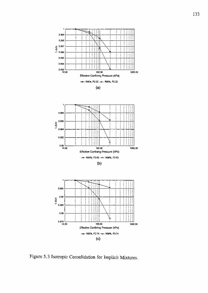
133

0.995 l------i-_;__;......;....:....;~+---i.,--i-~-~:-!"T!""T

.. 0.994 l------i-_;__;_--;....;....;,..;..;+-""T~~-::'::::1

... 0.993 L.-~--'--'--'-..;__;....;_;'--'-------'------:" 10.00 100.00 1000.00

Effective Confining Pressure (kPa)

...... R95%, F2-22 -e- R90%, F2-22

(a)

.. 0.998 1------i---:--'----:-~c.;-;+,:-----;---:---;--,:::1

<: 0.996 ...

~ ... 0.994 l---;--;.__;c-;.....;....;-;--;-+--'r--;---:---:-,,:77"1

... 0.992 l-----'---:----:----:-...;-;c.;-;+--'1--,---:---;-;-::':1

... o.~_Loo---'----'--'--'--=-...:....:1...;ooe.J.-oo----'---'-_;__;_ ...... -'----1000--:-' .oo


-- R95%, F2-53 -e- R90%, F2-53

(b)

.. 0.995 1---c..........;---;--l!!,_,;-;;..;-:-f---~----i-;---,~"h:1

<: 0.99 >

..

"i' ,- 0.985 l---...;___..;_...;....;.-;....;....;;..;.-1-',;----:----:---:--:---,-...,....,·'"'7·

.. 0.98 1----;,--....;--=-....;-..;....;;..;-:-f--""T-:---;---,:':o::1

. . . . 0.975 L.. __ ...:.,__.;_...;_...;_-'--'-----'-'-----------

moo 10000 1000m


...... R95%, F2-74 --e- R90%, F2-74

(c)

Figure 5.3 Isotropic Consolidation for Implicit Mixtures.

134

for consolidation also decreases as the strains become mostly elastic. Due to an isotropic

consolidation pressure of 200 kPa, s. was in the range from 0.4% (for F2 = 22 %) to 0.5%

(for F2 = 74%). The difference between the two ranges of Ev (at R= 90% and 95%)

illustrates the significance of changing the relative compaction level. A secondary

mechanism, due to the collapse of weakly bonded particles, may be considered. As the

relative compaction increases, most of the weakly bonded agglomerates of particles are

broken and do not contribute further to the volume changes that occur during the

consolidation.

As the fines content increases, the permeability of the mixtures decreases and the

time for volume change increases, at the same compaction level. The mixture stiffness

decreases as the fines content increases for mixtures compacted at the same relative

compaction (R). This leads to increasing the magnitude of the volumetric strain and the

time required to complete the volume change as the fines content increases.

S 3 Sbe.ar Behavior

5.3.1 Introduction

The samples were sheared in the triaxial apparatus under strain controlled drained

conditions. As a sample was deforming axially at a constant rate, the vertical load was

automatically measured and recorded simultaneously with the axial deformation. The

volume change due to the deviatoric stress was also monitored and recorded. The

deviatoric stress od= 0'1- a\ was calculated and plotted against the axial strain~. The

mobilized angles of shearing resistance, <p' m= sin-1 (o'i- a'3/o'i + o\) were calculated.

Figure 5.4(a) displays a 4 in. sample before shearing and the MTS testing system. As the

axial strain increases, the sample deforms gradually until failure occurs. Figures 5.4 (b)

and (c) display the two common failure patterns observed for the ash mixtures. Clearly

identifiable failure plane occurs for the dilatant stiff samples. The bulging pattern was

commonly observed for the contractive loose samples. Some samples displayed more

complex patterns, that is, a composition of those two patterns.

135

(a)

Figure 5.4 Triaxial Samples (a)Intact Sample Mounted on MTS Soil Mechanics Test System (b) Failed Sample (Failure on a Plane) (c) Failed Sample (Bulging Failure). [Continued]

136

I C

CrD TRl :\X! -\ L ("0\~ P~ESSiO:"--

srs,;.H:~R BOT'70\! r-:~Y AS!'":

(b)


137

(c)

Figure 5 .4 [Continued]

5 .3.2 Behavior of Explicit Mixtures

5 3 2 1 Test Results

138

Figures 5.5 (a) displays the deviatoric stress versus the axial strain of bottom ash

samples (F1= 0) compacted at R= 95% and tested at the effective confining pressure a\ levels (a=50 kPa, b= 100 kPa, c=200kPa). Similarly, Figure 5.5 (b) displays the

volumetric stress versus the axial strain. Figure 5.5 (c) displays the stress path (q-p')

diagram. Figure 5 .5 ( d) displays the mobilized angle of shearing resistance versus the axial

strain. Subsequently, the mixtures compacted at 95% are displayed in Figures 5.6, 5.7

5.8, and 5.9 for F 1= 25%, 50%, 75%, and 100%, respectively. Similarly, at R=90% and

F 1= 0.0, the results are displayed on Figure 5.10 (a, b, c, and d). The triaxial test results

of the explicit mixtures compacted at 90% for F 1 = 25, 50, 75, and 100%, are displayed

in Figures 5.11, 5.12, 5.13, and 5.14, respectively.

5 3 2 2 Discussion

a- Explicit Mixtures Compacted at R = 95 %

The bottom ash (F1 = 0.0) is a well graded granular material. The shearing

resistance of the bottom ash increases as the density increases. For the dense samples

(R=95%), the deviatoric stress increases to a peak, then drops with increasing the axial

strain. The increase in deviatoric stress is associated with a slight initial volumetric

contraction, followed by a gradually increasing rate of volume expansion (dilation). The

peak strength occurs when the ratio (dejdeJreaches a maximum value [Figures 5.5 (a,b)].

The post-peak reduction in deviatoric stress is associated with a decreased rate of dilation

until shear at a constant volume occurs at a critical state. Dilation is gradually decreased

as the confining pressure o' 3 increases. Since these tests are drained tests, the stress path

(q-p') diagram displays a straight line inclined at 45° from the horizontal [Figure 5.5 (c)].

The value of q increases gradually as p' increases until a maximum q is reached then p'

and q decrease until a critical state is observed. At a constant confining pressure o' 3, as the

axial strain increases from zero, the mobilized angle of shearing resistance increases to a

maximum (4>' max) then gradually decreases until it reaches a critical value (4>' cm) [Figure

139

5.5 (d)]. At the same level of axial strain, the mobilized angles of shearing resistance

decrease as the confining pressure increases.

As the fly ash content (F1) increases to 25% (TXA3H a,b,c), the samples display

a dilative behavior at the three levels of o' 3 [Figures 5. 6( a, b)]. The magnitudes of dilation

observed for the mixture where F1 = 25% in terms of the volumetric strain were less than

those observed for bottom ash (F1 = 0%). At this level of fly ash content, and relative

compaction (R = 95 % ) the fly ash particles are masking the bottom ash particles and filling

the inter-particle voids. However, denser arrangements are still possible. Thus the dilative

volumetric strain required for mobilizing the maximum deviatoric stress, becomes less than

the bottom ash alone. The maximum rate of dilation (dejdeJm.u and the maximum dilation

decrease as the confining pressure increases. The axial strains required for the mobilization

of the maximum deviatoric stress were practically the same as those observed in the case

of the bottom ash. Due to the reduction in strength after peak strength is reached, the stress

paths display a reduction in p' and q after reaching a peak value. At the same levels of

axial strain, the mobilized angle decreases as the confining pressure o' 3 increases [Figure

5.6 (d)].

As F 1 increases from 25% to 50% (TXA4H a,b,c), the peak deviatoric stresses

decrease significantly [Figure 5.7 (a)]. Only a slight post peak reduction is displayed by

the samples as the axial strains increase. The volumetric strain behavior becomes

contractive at all levels of confining stresses [Figure 5.7 (b)]. Although a very slight

tendency for dilation was displayed by the sample tested at o' 3 = 50 kPa. The contractive

behavior was greater as o' 3 was increased to 200 kPa. The m~onitude of q increases to a

maximum then decreases very slightly [Figure 5. 7 (c)]. At the same level of axial strain,

the mobilized angle decreases as the confining pressure o' 3 increases [Figure 5. 7 ( d)]. The

maximum shearing resistance was mobilized at an axial strain range of Ea between 0.5%

and 2% .

As F1 increases from 50% to 75% (TXA5H a,b,c) , the deviatoric stresses change

slightly and the sample response becomes stiffer [Figure 5.8 (a)]. The efficiency of

packing increases and a dilative behavior is observed at o' 3 = 50 kPa. Tendencies for

CID Triaxial, Fly/Bottom Ash Schahfer Plant Ash, (F1=0%, R=95%)

1000 ·,---------,-------,--------,-------,-----~

800 •..•.. ····················1····················· . . . i i

> 400 .. ., 0

200.

: i : :

i i i j

0 .... ----~------'----.....;....-----,-----~

0 5 10 15 Axial Strain %

1- (50 kPa) _ (100kPa) - (200kPa) 1


20 25

5 ·,--------,------,-------,------,-------,

4 ........................•..•. : ····························:·················=·····-· .L--. ..... ~ .... ~ ..... ~ ...... r. ..... =: ........................ . : :

l 3 . -----···----------u----- '. . . C 1 ! j in . .g 2 ....................•.

iii E .

j 1

; i i i 0 ..... ···············;···························-i-··························· 1···························· :---··························

-1 .1-. ____ .c....,._ ____ :-----------,--------,----------;

0 5 10 15 20 25 Axial Strain %

I- (50 kPa) - (100kPa) - (200kPa) I

140

(a)

(b)

Figure 5 _5 CID Triaxial Tests on Bottom Ash (F 1 =O. 0), Compacted at R = 95 % (a)Deviatoric Stress vs. Axial Strain (b)Volumetric Strain vs. Axial Strain (c)Effective Stress Path (d)Mobilized Angle of Shearing Resistance vs. Axial strain. [Continued]

500 ·---------------------------~

400 . ··················· : ..•.............•.. r-··················:-···················1················-·-i ·············-···· ···················

{300. ···················: ···················: ···················1···················: . .

C'" :

200. ··················· ' ··················· ' ········ ; i

100 · ···················/·······

0·"--~-L----.<.--------------------' 0 100 200 300 400 500

p· (kPa)

1- (50 kPa) __ (100kPa) __ (200kPa) 1


600 700

ro •~--------------------------~

g, 40 . ~ ., c, ,¥ 30 ·

: ; ; : . .

f················:····························:····························:···· . .

; : ; ;

: :

10. ····························r··························· '················-··········;-·····················- ···· 1·····················-·····

0 ---.-------,------------------------c 0 5 10 15 20 25

Axial Strain%

1- (50 kPa) _ (100kPa) __ (200kPa) 1

Figure 5.5 [continued]

141

(c)

(d)

CID Triaxial , Fly/Bottom Ash Schahfer Plant Ash, (F1 =25%, R=95%)

1000 ·~ - ---------------:----- -,

i !

800 ....... ····························, ··· ·························· ····'·································· ;··································

; 600 . ··································:···································:·································· :··································

i : i i > 400 .....•..........•.•.......••••••• : ••···· ····························'.································•·:••································ ~ : : :

! : j MEXICO

200. : .......... '. .. ............. ·········i··································

0 ---.------------------- --~


1- (50 kPa) _ (100kPa) _ (200kPa) I


20

1 ··~------------------ -----,

~~ ........... ~.·--······~·········~····················1···································

i 0.6 ■ ........ H•••----..;-----••••••:••••••••••••••••••• ••••••••• •••••••:•••••••••••••••••••••-••••••••••••

C:

~ 04 · ·········· · . . U) . . -~'- .

~ 0.2 · ........ ........................ : ................................ ...! ................................... : .................................. . ' .

0 ....... ·······················1···································:···································j···································

-0.2·'-. ------------------------0 5 10 15 20

Axial Strain %

I- (50 kf'a) - (100kPa) - (200kPa) I

142

(a)

(b)

Figure 5.6 CID Triaxial Tests on Explicit Mixtures (F1 = 25%)Compacted at R= 95 % (a)Deviatoric Stress vs. Axial Strain (b)Volumetric Strain vs. Axial Strain (c)Effective Stress Path (d)Mobilized Angle of Shearing Resistance vs. Axial Strain. [Continued]


500 ·~----------------------------~

400 · ··················· ; ··················· :···················· (················ -:············ ········:·················· · .................. .

300. ···················:···················: : : . :

' 1 : ! ~ : : 200 . ................... : ................... : .................. : .................. . ··················· : ................... ' .................. .

: : : : : : .

0·~----~---~--------------------~ 0 100 200 300 400 500

p' (kPa)

I- (SOkPa) - (100kPa) -- (200kPa) I


600 700

ro •-~----------------------------~

-g,40 .. :E-a, c;, ~ 30. "C a,

~ ~ 20. :::E

10 ·

- --- ----'----································-··--···-···-·-·······-·······

. : : : :

. . .

I I : :

•n••••••••••••••••••••n••••••••• • ••u•••••••••••• .. nn•••••• .. n••• : •••••••••••••••••••••••••••••H•••• : • • ••••••••••••••••••• .. •••••••••• •• •

0 --.---------------,---------------~

0 5 10 15 20 Axial Strain %

I- (SOkPa) -- (100kPa) -- (200kPa) I


143

(c)

(d)

CID Triaxial, Fly/Bottom Ash Schahfer Plant Ash, (F1 =50%, R=95%)

700 -,-------,-----,-----,-------,------:----,----,

soo ......... ....... , ................. , ....... - . '··· : : I

'"500 ................ .: ................. :················· i················· i ················ ! ·················l·················I················· ~ . . : : . ! ! -;;;400 · ........... :. · .: · : : · · · ·i·· · · u, . : : j :

~ 300 ·• ·············:·-··············· :·················i·················i·········· ; : 200. ..•.•.. , ......•.•••.•.• L. .. ··········· ' ................ '·················'·················:······ ......... l ............ .

. . 100

: i i ! i i i 0 ---.---'----'----,--------------~

0 2 4 6 8 10 12 Axial Strain %

I- (50 kPa) - (100kPa) - (200kPa) I


14 16

0---------,-----------,-----,-------,-----,

*::•=-~i~=--! __ 1

I __ i __ !-i-! :: •--~==-_!i-!== :: ! ===l :=1~:--_,. ----L L !- '- l ---! --,-- -

-1.6 ....... ---'----'-----,.------~--,------,--~

0 2 4 6 8 10 12 14 16 Axial Strain %

I- (50 kPa) - (100kPa) - (200kPa) I

144

(a)

(b)

Figure 5.7 CID Triaxial Tests on Explicit Mixtures (F1 = 50%)Compacted at R= 95% (a)Deviatoric Stress vs. Axial Strain (b)Volumetric Strain vs. Axial Strain (c)Effective Stress Path (d)Mobilized Angle of Shearing Resistance vs. Axial Strain. [Continued]


350 ·~-----------------------------~ . . .

:. --!-i-----l -i-- --:-------· i 200 i ; [ i i ,:r 150 . ·······················1······················· 1·········· .......... i .......... ··········-:·······················:·······················

100 · ·······················'·········· .

O·~.-----------~------------------~ 0 100 200 300 400

p' (kPa)

I- (SOkPa) -- (100kPa) - (200kPa) I


500 600

so -~-----------------------------~

40. - :

10

0

················:················· :·················1················· :··················:·················:··················1·················

0 2 4 6 8 10 12 14 16 Axial Strain %

I- (50 kPa) - (100kPa) - (200kPa) I

Figure 5 . 7 [Continued]

145

(c)

(d)


700 ·~--------------,-----,----,-----,

: ! 600· ········ · ··••i••···············1················· :················ 1···············r···············i'···············r···----········

OJ 500 ••.•• ···········i···· . . .....•.. ............ '·················: ................. :·················1,·················

i I . . . i : . -;;400 · ........ ·····,·················,-················ ,-················ r-················, ·················,·················,-················ 1,0 • : : : : : : ft! : : : : : :

1300 . . ··········+················i················ (···············; r ............... .! ................. : ................ . ~ : : : :

0 : : ; : : ' 200 . ....... ..... ; ................. ,...... .. ' . ' : ;

l l : . :

100. ················1·················1··········-·····1················ :················1·················1···············-1·················

0 ..,_ __ .;.,.._ __ '-------'----'--------'----'---...J

0 2 4 6 8 10 12 Axial Strain %

I-(50 kPa) - (100kPa) - (200kPa) I


14 16

0.4 ·,--:--~----r--~--7-.;;;;;;;;;;.;;;;;;;;;;;;;-~-~

: : : i ! : ;; 0 .. ··········--:·················(···············i·•··············i················ :·················1·················1·················

i-0•2 i i i ! [ ••••••••••• .. o•••••• . •••••••••••••••••

~ ! j j j I . . 0-0.4 . ·················:· ·············:-················t··--··········:·················:·················:·················:················· > ' ' ' : : : : . : : : :

-0.6 ................. ,: ................. : ................. : ················ : ............ : ............... ._: ............... ._: ................ .

I I I l t I i -0.S. ·················1·················1 ················1 ················1 ················1················ 1······· ..................... .

·1 ....... --------------------'-----'----' 0 2 4 6 8 10 12 14 16

Axial Strain %

1- (50 kPa) _ (100kPa) _ (200kPa) 1

146

(a)

(b)

Figure 5. 8 CID Triaxial Tests on Explicit Mixtures (F 1 = 75 % )Compacted at R = 95 % (a)Deviatoric Stress vs. Axial Strain (b)Volumetric Strain vs. Axial Strain (c)Effective Stress Path (d)Mobilized Angle of Shearing Resistance vs.Axial Strain. [Continued]


350 ·.------,------,-----------,------,-------,

300 . ·······················1······················· : ······················:·····················-·1·-·-·-····--·--··--·--• i•-··--·-·····--·-·-····

250 . ·-···········--·-······1-·-·--····-············:-······-···--·-·---··-·j··············---···---1----·-···· ···---·-·-·1-···-··-·-···-·········

'"°200· ··-··--···----······-·-;-···-----··············:······-··----·-·-----· :·····--··--·······---·;··········-··---·---···:·····-·-···-······-···· Q. : : : : . ~ : : : :

-;;: 150 - ··-···-·····-------·-·_i·--···----···········- ; --··---·· ··-·-----• : ••·--····· ·········--i----····---·-·--·--··-·:·····-··········-···· ·· i ~ = ! 1

100 - ··-··-···-----·--------:-------·· ·•--·---· '·•---·--··---·······--· ···--···-·······--···--'·-··---········-·-----·:-····-·-·-······-······

: i i o-~.----~----~--------------------~

0 100 200 300 400 p' (kPa)

I- (50 kPa) - (100kPa) -- (200kPa) I


500 600

50 -.-------------------------------~

40. ··--···: ---------------· ~ ·--·----·--·-- ··········-~············---·-·1 ······-----------

: : : . : : : : : . .

10 -

0

_; i----1--: _1 __ L_ __

0 2 4 6 8 10 12 14 16 Axial Strain %

1- (50 kPa) __ (100kPa) __ (200kPa) 1


147

(c)

(d)


700 ·---------------------,-----,

i i i i i '"500 ....... ···············: ······················:························1·······················:·······················:·······················

i 400 . .•.• ···•··· ·······i······················· :-······················ i ·····················-+······················i·······················

~300 • .......... ·······i····· ... : : i .... ··········I······················· 0 ; ;

200. ················•··: ....•.....•••••.••••••• , ..•.................... , •......................

100 · ••.................... : ...............•..•.... : ...................... : ..............•.... .... : .••.................... : ...................... .

: i ; : i 0 ..... ___ _.;_ ___ ....;.... ___ ....;.._ ___ --'--___ ..;...__ __ __.


I- (50 kPa) - (100kPa) - (200kPa) I


10 12

1·r----,-----,--------,-------,-----,-----,

······················1·······················;·······················:-······················

0.6 · ........... ·········· '·····················••:••····················· :······················••:••·····················'······················· ; j . [ .

~ 0,4 • •••••••• ••••••••••••• i•••• ••H••n•••••••••••l•••••••••••• •••••••••••i••••••••••••••• .. ••••••i••••u••••••• ••••••••••~•••••••••••••••••••••••

~ 0.2· ...... ···············l·······················l·······················l······················i·····················--1-······················ ;g O • • •·••· ··········-r··················· ··· j : : .... : ...................... .

-0.2 ....... ····- ·•······T ····················i······················· i························j ·······················:·······················

-0.4. ·······················:·····················••j••··········· ..... :························:·······················:·······················

-0.6·'---. -----'-----',------'------'---------'-'-------'

0 2 4 6 8 10 12 Axial Strain %

I- (50 kPa) - (100kPa) - (200kPa) I

148

(a)

(b)

Figure 5. 9 CID Triaxial Tests on Explicit Mixtures (F 1 = 100 % )Compacted at R = 95 % (a)Deviatoric Stress vs. Axial Strain (b)Volumetric Strain vs. Axial Strain (c)Effective Stress Path (d)Mobilized Angle of Shearing Resistance vs.Axial Strain.[Continued]


350 ·,--------------------------,------, . .

: · ---- _j __ - ·······i---- -1- -·-!- ---i----,.200 · ·······················:·······················: ······················: ······················ :·······················;···----i a.. : : : : .::.! : : : :

~l50 · ·······················i-····················· = ··· ····· ·········· 1·········· ··········r ·····················1·······················

100 · ·······················:·········· ........ . ····················••:••·····················:·······················:·······················

0

: : : l :

100 200 300 400 p' (kPa)

1- (50kPa) -- {100kPa) __ (200kPa) 1


500 600

W·,------------------------------~

,..,. g'40. ~

"' C)

~30. "C

"' ~ :g 20. ~

10 ·

: ; ; : . . t j

. . . . : : . . .

: ! : : ; . .

0-----------------------------------' 0 2 4 6 8 10 12

Axial Strain %

1- (50 kPa) __ (100kPa) __ (200kPa) 1


149

(c)

(d)

150

dilation are also observed for a' 3 = 100 and 200 kPa [Figure 5. 8 (b)] . The stress path

diagrams display increase in p' and q to peak values followed by a decrease until shearing

at a critical state takes place [Figure 5.8(c)]. The mobilized angles of shearing resistance

decrease as the effective confining pressure increases [Figure 5.8(d)]. The peak strengths

are mobilized at relatively small strains. The stresses also drop to their ultimate values at

relatively small strains (ea= 2 % ) .

As F1 increases to 100% (fXA6H a,b,c), the samples display a very slight change

in the deviatoric stresses reached. [Figure 5.9(a)]. The deviatoric stress increases to a

maximum then decreases until it reaches a constant value as the axial strain increases from

zero. There is also a slight increase in the dilative behavior. Dilation is observed for the

samples tested at a\= 50 and 100 kPa [Figure 5.9(b)]. A tendency for dilation is also

observed for a' 3 = 200 kPa. Accordingly, the magnitudes of q and p' increase to

maximum values then decrease [Figure 5.9(c)]. The mobilized angles of shearing

resistance increase gradually to a peak then decrease slightly as the axial strains increase

[Figure 5.9(d)]. As the effective confining pressure increases, the mobilized angles

decrease at the same axial strain level. It can be observed for F1 = 75 % and 100% that the

mobilized strength angles change slightly as the axial strains increase beyond 2 % .

b- Explicit Mixtures Compacted at R = 90 %

A significant decrease in shear strength occurs due to the reduction of the relative

compaction from 95% (TXAlH a,b,c) to 90% (TXAlL a,b,c). Although the bottom ash

samples (F1= 0) compacted at R=90% display a dilative behavior when tested at a'3 = 50

kPa and 100 kPa, the maximum deviatoric stresses are significantly less in comparison to

those achieved at R= 95% [Figures 5.10 (a,b)]. As the effective confining pressure

increases to o' 3= 200 kPa, (sample TXAll..c), the volumetric strains are contractive as the

axial strains increase from zero. The magnitudes of maximum volume increase for the

samples tested at a\= 50kPa and 100 kPa are approximately 50% of those observed at

R = 95 % . The reduction in the deviatoric stress and the angles of shearing resistance past

the peaks are more gradual than those compacted at R = 95 % . As displayed in the stress

151

path diagram, p' and q increase to peak values then decrease [Figures 5.10 (c)] . The

mobilized angle of shearing resistance decreases as the confining pressure increases. The

change in the mobilized angles is greater at small axial strains than that at larger strains

[Figures 5.10 (d)].

As F1 increases to 25% (TXAlL a,b,c) a significant change occurs in the strength

and volumetric behavior at this level of compaction (R=90%). The maximum deviatoric

stresses are reduced [Figures 5 .11 (a)], and the volumetric strains become contractive at

all three levels of confining pressure (a\= 50, 100, and 150 kPa). The magnitude of

compressive volumetric strains increase as a' 3 increases [Figures 5.11 (b)]. The values of

p' and q increase gradually to a maximum [Figure 5. ll(c)]. The mobilized angle of

shearing resistance increases gradually as the axial strains increase [Figure 5. ll(d)]. At

the same axial strain level, as the confining pressure increases the mobilized angle

decreases. The maximum shearing resistance angles are mobilized at higher strains as a' 3

increases.

As F1 further increases to 50%, the maximum deviatoric stresses continue to

decrease significantly [Figures 5 .12 (a)]. The volumetric strains remain contractive at the

three levels of confining pressure (a'3= 50, 100, and 200 kPa) [Figure 5.12(b)]. The

magnitude of compressive volumetric strains increase as a' 3 increases. The sample

TXA41b (a\= 100 kPa, F1= 50%) was slightly undercompacted. This explains why the

sample was almost as contractive as TXA4 Le ( a' 3 = 200 kPa, F1 = 50 % ) . The samples

display values of p' and q that increase gradually to a maximum [Figure 5.12(c)]. The

mobilized angle of shearing resistance increases gradually as the axial strains increase

[Figure 5.12(d)]. At the same axial strain level, as the confining pressure increases the

mobilized angle decreases. Axial strains of approximately 5 % are necessary to mobilize

maximum shearing resistance angles as low as 30° to 32° . The mobilized angles decrease I • as a 3 mcreases.

As F1 increases to 75% [I'XA5H (a, b, and c)] and 100% [TXA6H (a, b, and c)],

minor changes are observed in the maximum deviatoric stresses at this level of

compaction, [Figures 5.13 and 5.14]. Sample TXA4Lc (F1 =75%) was slightly over-

152

compacted and that led to stiffening the sample slightly and reduced the volumetric strains.

The volumetric strains remain contractive, however. At the same R and F1 values, a

sample compacted at R= 90% would become more contractive (greater Ev) than a sample

compacted at R value slightly greater than 90%. Since the sample at o' 3 = 100 kPa

displayed a gradual strain hardening behavior, the behavior at R= 90% and o'3 = 200 kPa

is expected to behave similarly. Accordingly, the peak strength angle at R= 90% can be

estimated to be approximately equal to the ultimate strength angle reached by a sample

compacted at R value slightly greater than 90%. The axial strain level required to mobilize

such an angle at o' 3 = 200 kPa is expected to be greater than the axial strain required to

mobilize the peak angle at o' 3 = 100 kPa. It is also notable that the maximum mobilized

angles were slightly different than those obtained at F 1 = 50%.

5.3.3 Behavior of Implicit Mixtures

5.3.3.1 Test Results

Figures 5.15 (a) displays the deviatoric stress versus the axial strain of the implicit

mixtures containing F2=22% {sampled from location 1, the discharge location) compacted

at R= 95% and tested at the effective confining pressure o\ levels (a=50 kPa, b=lOO

kPa., c=200kPa). Figure 5.15 (b) displays the volumetric stress versus the axial strain at

the tree levels of o\. Subsequently, Figure 5.15 (c) displays the stress path (q-p')

diagrams and Figure 5 .15 ( d) displays the mobilized angle of shearing resistance versus

the axial strain. Similarly, the test results of the mixtures compacted at 95 % and containing

F2 = 53% and 74% are displayed on Figures 5.16 and 5.17 respectively. Figures 5.18,

5.19, and 5.20 display the results for the samples compacted at R=90% and F2= 22, 53,

and 74% respectively.

5.3.3.2 Discussion

a- Implicit mixtures compacted at R = 95 %

Toe deviatoric stress versus axial stain curve of the implicit mixtures TXBlH a, b,

and c {F2 = 22 % ) displayed a typical dense granular material behavior similar to the


700 ·--- -------------------~

600 . ············· ····················1··································· j·································· i ··•························· r 500

· ······ ··························· (·······························r::::::::::::::::::::::::::::::::r::::::::::::::::::::::::::::::::: -;;;'400 •••••••. ·······················:--········ ···· ··· ,,, : ~ : iii 300 . . ······························ :·························•··•······: ········· ··························:··································· > ------ . .

~ 200 . ·················=···=····=···~···:···~····~···'.'.:'.···~···~····~···~···~···~···!"' .... ~ - - ----···-···-····l···~···-···························

';f!. C:

100 · : : : : :

0 ... ______ ....;..._ _ _ __________ ....;..._ _ ___ --J


1- (50 kPa) _ (100kPa} _ (200kPa) 1


20

3 ·,---------,---------,-------,-------,

2. ····································:··········· •••••••••-•••••=•••• .. • • •••• •• ••••••••••••••••••••••:-•••••••••••••• - •••••••••H•••• •

~ 1 ··················· iii .g ~ § 0

............... : __ _____ __ ___ ____ ________________ ____ · ......................... ........... : ................................... .

~

-1 . ............................... ··································:························· ···········:···································

-2· ...... - - --------------------~-0 5 10 15 20

Axial Strain%

I- (50 kPa) - (100kPa) - (200kPa) I

153

(a)

(b)

Figure 5.10 CID Triaxial Tests on Bottom Ash (F1 = 0.0%)Compacted at R= 90% (a)Deviatoric Stress vs. Axial Strain (b)Volumetric Strain vs. Axial Strain (c)Effective Stress Path (d)Mobilized Angle of Shearing Resistance vs.Axial Strain. [Continued]

350 -,----------------------------~ 300 - -----------------------1-----------------------!---------------- -- -- ---1-----------------------1---------------------- ;·----------------------

250 - -----------------------i-----------------------l----------------------1-----------------------i---------- __________ T _____________________ _

m' 200 • •••••••••••••••••••••••i••••••••••••••••••••••• i•••••••••••••••••••H•• 0 •••••••••••••••••••••• ; •••••••••••••••••••••Ui••••HOH••••••••••••••

Q. : : . : :

~,so- -----------------------:-----------------------:---------- ----------1---------- -----------:-----------------------1-----------------------

100 - -----------------------:---------- ---------. ----- -----------------'-----------------------'-----------------------:-----------------------

1 = l . i : : :

o-----------! __________ ! --------~ 0 100 200 300 400

p' (kPa)

I- (SOl<Pa) -- (100kPa) -- (200kPa) I


500 600

50 -,--------,--------,--------,-------,

10

0

0 5

: •• ••••••••••••••••••••••••n• ••nu•••••• .. •••••••••• •••••H•••••••••n•

' ' '

___________________________________ I ___________________________________ _

10 15 20 Axial Strain %

I- (SOkPa) - (100kPa) -- (200kPa) I


154

(c)

(d)


500 ·----------------------~

400. ···································:······················· ····:·····-···················· . :··········. ... .... .

~ , : l t300 • ••••••••••••••••••U•o •••HOOHOO iHOOHo••·•••••••••••• .. ••••••0 000 0: OH••••• .... ••••••••••••• ooo oooooOooooOoOOoooOooOoOo

"' "' e iii > 200 . ........ . ·········••··········· ·-·································· ··············· ..................... · .................................. . . . .

"' □ . . .

100. ~ ····························+·································· i···································1···································

0 .


1- (50 kPa) _ (100 kPa) _ (150 kPa) 1


20

0----------------------~

: : : : : :

-··-·-·-·:·····---··-·········· ····-···--·-···:·······················--···········

: : . . -- ----1 -- - r -··· .5 ...... -------------------------'


I- (50kPa) - (100kPa) - (150kPa) I

155

(a)

(b)

Figure 5. 11 CID Triaxial Tests on Explicit Mixtures (F 1 = 25 % )Compacted at R = 90 % (a)Deviatoric Stress vs. Axial Strain (b)Volumetric Strain vs. Axial Strain (c)Effective Stress Path (d)Mobilized Angle of Shearing Resistance vs. Axial Strain. [Continued]


250 ·,-------,-----,-----,------,-----.,.---- - - - --,

: :

{:. ··················· '___[ __ --.. J.-1. ___ i. --: .................. . C"' : : : :

100 · ···•·••••••••······ :··················•:············-·--·· :-•·--··--···-·----· :-•·-·--····-··--··-:·----·--·-----·---·:---·---·-·---···--·

I /------ - -i- :----'----o -----~---~--------------------~

50 100 150 200 250 300 p' (kPa)

I- (50 kPa) -- (100kPa) -- (150 kPa) I


350 400

~------------------------------~

0


I- (50 kPa) -- (100kPa) -- (150 kPa) I


156

(c)

(d)

CID Triaxial, Ry/Bottom Ash Schahfer Plant Ash, (F1 =50%, R=90%)

~ ·,-------,---,----,----,------,---,---~

: : 400 . ················-:·················:··········· ···· :-················ :················-:·················i••··············· :---··············

: ;

{300 -·----- ----------- :---·-·----------'.················· ~················ 1·················;····· ... ········-! _________________ ; ................ . f,/J : • • : : • :

r/l : : :

~ : ~ : . . . .,; 200 .............. ... ;........ . : . : : : ~ ~~: ___ : __ ~:_.....;· ___ : __ : __ :

······:··----[, -- 1· - - ! -- :·················i···········--o .... ----------------------------------'

C:

"§ ~

0 2 4 6 8 10 12 Axial Strain %

1- (50 kPa) _ (100kPa) _ (200kPa) 1

CID Triaxial, Ry/Bottom Ash Schahfer Plant Ash, (F1 =50%, R=90%)

14 16

0-----------------------~

···················:·················1 ................. i ................. :--............ .... :················· r ···············

: : : : .

~ 3 i ; -4. ·················(···············i··········-····· '··················. ·

. .

0 2 4 6 8 10 12 14 16 Axial Strain %

1- (50 kPa) _ (100kPa) _ (200kPa) 1

157

(a)

(b)

Figure 5 .12 CID Triaxial Tests on Explicit Mixtures (F 1 = 50 % )Compacted at R = 90 % (a)Deviatoric Stress vs. Axial Strain (b)Volumetric Strain vs. Axial Strain (c)Effective Stress Path (d)Mobilized Angle of Shearing Resistance vs. Axial Strain. [Continued]


250 ·,--------------,--------,-------,-------:--------,

/

I:. --- l····························i····························l·· ···········-

1

- -- --~ i ~

100 . ····························:··························· ...................••.•.... :····························1···························· : :

O·~.------~-----~-----------------' 0 100 200 300

p' (kPa)

I- (50 kPa) -- (100kPa) -- (200kPa) I


400 500

~ ·,---------,----...,.----.,------,-----,----.,-------~

····1················· ;················-:· ················ :··················'·················

i i i i i ~ .

0

············1---1····· --1- ;- --:--1 , ................ . 0 2 4 6 8 10 12 14 16

Axial Strain%

1- (50 kPa) -- (100kPa) __ (200kPa) 1


158

(c)

(d)


600 -~---------------------~

• • ••••••••••••••••••••• • • •• ••••••••-••• ••• ••••• ••••••• •••••••• ••••••••• • • o•• •••••••••• • H H• • ••••••••• •• •••

l 400 I • i ~ : . : r/l : : :

~ 300 - .. -···-·· .. ····················· ~------·····························; ................................... ; .............................. ___ _

ii5 : : ,,; . ~ 200 - - ------ . ------------------ ------ :-------------- -- ------ ---------- --- ; --- ------------ -------- -- ----------:---------------------------------- -

C:

100 - i i i

0 ..... -------'------------'---------'


1- (50 kPa) _ (100kPa) _ (200kPa) 1


20

0----------------------~

: : . . . . . . . .

"§ -1 5 - ------------------------ii5 -

~ 2. ----------------- ---------------i-------------·

-2.5 - ---------------------------------i-------------------------------- i ------------------

-3 -~. ---------------------~ 0 5 10 15 20

Axial Strain %

1- (50 kPa) _ (100kPa) _ (200kPa) 1

159

(a)

(b)

Figure 5.13 CID Triaxial Tests on Explicit Mixtures (F1= 75%)Compacted at R= 90% (a)Deviatoric Stress vs. Axial Strain (b)Volumetric Strain vs. Axial Strain (c)Effective Stress Path (d)Mobilized Angle of Shearing Resistance vs. Axial Strain. [Continued]


300 ·,---------,--------------,---------,---------,

250 · ····························'··························••:••··························'····························:············· ··•·········· i j j :

200 . ····························:··························••i••··························(·······················••i••··························

CQ • : : :

~150· ····························1····························1····························:············· ............. : ........................... .

,oo. -- -:---- =--i=~==~-1= ===1=:==:: O·~.-------------"------'----------------'

0 100 200 300 p' (kPa)

I- (50kPa) -- (100kPa) - (200kPa) I


400 500

50 ·~----------------------------~

,..,. Cl> .,

"C

•• • •••• .. ••••••••••••• :••••• •••• .. •••••••••••••••••• •••• ••:•••• ••••••••••••••• • 0.o.0000000.00

";30 . Cl l l l ~ : : : "C

i:. __ --f ----- -1---; ................................... . 0 ~.--------,----------,-------------------'


1-(50 kPa) __ (100kPa) __ (200kPa) 1


160

(c)

(d)

CID Triaxial , Fly/Bottom Ash Schahfer Plant Ash, (F1=100%, R=90%)

400 ·,----=-------,------:::::;::;:;=:::====,,_~==;'=-~-:----

'£ 300 . ···-·············· i ··· ··············· 1 :····················1····················;··················· ;···················

~ . .

J 200 · ····•······ 7··· : ············-····· l ··················+-················i··················· l ····-·-·········· I······-··········· > . : . . : c3

~

100 ·

0 ... ______________ .;__ ________ ___,

0 2 4 6 8 Axial Strain o/o

10

1- (50 kPa) - (100kPa) _ (200kPa) i


12 14

o~----------------------~

: i . i ; . .

••••••••••••HH•••••- -•.a•--•-••••••-•u

·2·····-·············-·-i-······ ··············1-· : :

-25 . ····-·········-··-··1······················ '·-·················-:-······-····--· i ........... . -3 •. ~. __________ _..,_ ___________ __,

0 2 4 6 8 10 12 Axial Strain %

1- (50 kPa) _ (100kPa) _ (200kPa) I

161

(a)

(b)

Figure 5 .14 CID Triaxial Tests on Explicit Mixtures (F 1 = 100 % )Compacted at R = 90 % (a)Deviatoric Stress vs. Axial Strain (b)Volumetric Strain vs. Axial Strain (c)Effective Stress Path (d)Mobilized Angle of Shearing Resistance vs. Axial Strain. [Continued]

CID Triaxial , Fly/Bottom Ash Schahfer Plant Ash, {F1=100%, R=90%)

200 -.----- --,-------,---------:--------,-----------,

,,, · - -- -1 -- 1········· - -·-r ·············· 1- -···· l"l:I : ;

!;, 100 - ----------------------------:-------------------------- . : .

~ I --------·······----· ...................... ;-·-------------------------·

o-~---------L-------'---------'---- - --------- ---' 0 100 200 300

p' {kPa)

I- (50 kPa) - (100kPa) -- (200kPa) I

CID Triaxial, Fly/Bottom Ash Schahfer Plant Ash, {F1=100%, R=90%)

400 500

50 -,-------------------------------,

0 .

0

-------'.-----·--············; ····-------------- --:---- .. ····•········· ;------·---···-------: .................... : ----------·--·······

; : •••• • ••••• • • •• •••• •• •• • • • •• • ••• •• •••••o• .. ••••o•u•

. .

-- ----- r -- i r----;- r--2 4 6 8

Axial Strain % 10

I- (50 kPa) -- (100kPa) -- (200kPa) I 12 14


162

(c)

(d)

163

behavior of the bottom ash discussed earlier in section 5.3 . 1.2. At all three levels of a' 3,

the deviatoric stresses increased to a peak value then decreased as the axial strains

increased from zero [Figure 5.15 (a)]. The volumetric strains displayed a dilative behavior

[Figure 5.15 (b)]. The maximum value of the ratio (deJdeJ is associated with the peak

deviatoric stresses. The stress path shows an increase of the values of p' and q to a peak,

then a decrease [Figure 5.15 (c)]. The mobilized friction angles display a stiff behavior as

the angles reach their peak values at small axial strains [Figure 5.15 (d)]. At an axial strain

level, the mobilized angles decrease as the confining stress o' 3 increases. The peak

strengths are mobilized at axial strains ranging between 1.5 to 2.0%.

As the fines content increases to F2 = 53 % , the maximum deviatoric stresses are

decreased; however, the deviatoric stresses versus the axial strains display a stiff behavior.

Peak stresses are reached at less than 1.8% axial strains, followed by a post peak reduction

until shearing at a critical state occurs [Figure 5.16 (a)]. The volumetric strains become

dilative only at a' 3 = 50 kPa, while a tendency to dilation remain visible on the other two

samples (a'3 = 100 and 200 kPa) [Figure 5.16 (b)]. The q-p' diagrams display an increase

to a peak followed by a decrease [Figure 5 .16 ( c)]. The strength angles reach their peak

values at an axial strain less than 2 % [Figure 5.16 (d)]. The mobilized angles decrease as

the confining stress increases.

As the fines contents increase to 74% (TXB4H a,b,c), the maximum deviatoric

stress further decreases [Figure 5.17 (a)]. The volumetric behavior become contractive,

however, the compressive volumetric strains ( e._,) are less than 1.2 % . The q-p' diagram

displays a peak, followed by a reduction in both p' and q [Figure 5 .17 ( d)]. The mobilized

angles of shearing resistance reach their peak values at an axial strain which is slightly less

than 2%.

b- Implicit mixtures compacted at R = 90 %

For the implicit mixture having F2= 22% (TXBlL a,b,c), as the compaction level

decreases to 90%, the maximum deviatoric stresses decrease significantly [Figure 5.18

(a)]. The deviatoric stresses reach their peak values at axial strains ranging between 1 %

164

(at o\ = 50 kpa) and 3% (at 9' = 200 kPa) . The volumetric strains become more

contractive especially as a\ = 200 kPa [Figure 5.18 (b)]. The q-p' diagram displays

increasing p' and q to a peak followed by a slight decrease [Figure 5 .18 ( c)]. The

mobilized strength angle reaches a peak value, at axial strains less than 2 % for a' 3 ..s;;,_ 100

kPa, then undergoes a slight drop [Figure 5.18(d)]. As the confining pressure increases

to a' 3 = 200 kPa the mobilized angle increases as the axial strains increase until a

maximum value is reached at about 2.4 % axial strains.

As the fines content increases to F2= 53% (TXB2L a,b,c), the peak deviatoric

stresses decrease [Figure 5 .19 (a)]. The volumetric strains become contractive and no

tendencies for dilation are observed at any of the three levels of o' 3 (50, 100, 200 kPa)

[Figure 5.19 (a)]. The values ofp' and q increase gradually to a peak value. Only at a'3= 50 kPa the values of q and p' decrease slightly after reaching the peak. [Figure 5.19 (c)].

The mobiliz.ed angles reach maximum at axial strains ..s;;,_ 6 % , except at o' 3 = 50 kPa the

stresses increase to a peak and then decrease. The peak deviatoric stresses are mobilized

at axial strains ranging from 1.5% (at o'3= 50 kPa) to 10% (o'3= 200 kPa).

As the fines content increases to 74% (TXB4L a,b,c) , the maximum deviatoric

stresses decrease [Figure 5.20 (a)]. The volumetric behavior become more contractive at

all three levels of o' 3 (50, 100, 200 kPa.). [Figure 5.20 (b)]. The values of p' and q

increase gradually to a maximum. [Figure 5.20 (c)]. Figure 5.20 (d) display the gradual

increase in the values of the mobilized angle of shearing resistance as the axial strains

increase. The peak deviatoric stresses are mobilized at axial strains ranging from 4% (at

o'3 = 50 kPa) to 11 % (o'3= 200 kPa).

5.3.4 Effects of Fly Ash Content on Peak Angle <!>'max

The peak angle ' max constitutes a measure of the maximum shearing resistance that

can be developed by a granular material. For dilative behavior, ' max occurs at the

maximum rate of dilation. Normally, the maximum rate of dilation develops at small

strains. On the other hand, in an ideal contractive behavior, ' max occurs at larger strains

and thus approaches ' crit as the volume decreases. The peak angle ' max depends upon the

CID Triaxial, Fly/Bottom Ash Gibson Plant Ash, (F2=22%, R=95%)

1000 ·r------,------,-------------

800 . .•......

: i i

1 600. ... ........ ! i ········1····························'······-···················

I!? i 400. . ········-···························! ···························'····························:···························

*

200 .......... -... ~ ... ~ .... ~ ... ~ ... ~.,.111!1 . ..... ___ ,;_ ___ ~ . .... ··························· ···························

□---------"------,-----_;_ ________ _j


I- (50 kPa) - (100kPa) - (200kPa) I


20 25

0.6 ·,-,.i;;;;;;;;;;;;;;;;;;;;;;;;;;;:::----,-----:-----,----,

- - -- ; ; -

-;; 0

----------· .. ···············1···························

j··························••:••············•·············

• •••••••••._ : ••• .. • .. •••••••••••••n••••• : •••••••-•• o••••••n••••••• ~~, .. -----: --: __ -0.4. ····························:····························:·············

-0.6 · ···························+··························_[.···························i······ ·············

-0.S ·c-. ----,------------------__J 0 5 10 15 20 25

Axial Strain %

I- (50 kPa) - (100kPa) - (200kPa) I

165

(a)

(b)

Figure 5 .15 CID Triaxial Tests on Implicit Mixtures (F1 = 22 % )Compacted at R = 95 % (a)Deviatoric Stress vs. Axial Strain (b)Volumetric Strain vs. Axial Strain (c)Effective Stress Path (d)Mobilized Angle of Shearing Resistance vs. Axial Strain. [Continued]


500 ··~ ----------------------------

i = · ··················· i···················j; __ : __ .......... ! ................... ! .................. . er : : :

200 •................... : ........•.......... : .................. . .................. :··················••;••·················:···················

. ····- . --- --·········i- i···················!··················· 0·~.--'-__..'--------"----'------"-----...;_----'-----J

0 100 200 300 400 500 p' (kPa)

I- (SOkPa) -- (100kPa) -- (200kPa) I


··································----

600 700

10 ·

------1 1 ---·---- -:···························r - -1-1---- -·- - ---

o -------"-------"'-------''----------------0 5 10 15

Axial Strain %

I- (SOkPa) - (100kPa) -- (200kPa) I


20 25

166

(c)

(d)


700 ··,-------------------------

: :

~· -- ·-:-- .f .............. '.i ! - _; ____ _ l i i i i i i

i400 i i i : i : ~ 300 ..... ············: ··· ··'····················:····················:····················:···················:-·················· a, : : :

Cl : : :

200 .. ···········•··. ················:··················· :····················:····················;···················'···················

,:~·.'----~!---~: ----': ___ ~i ___ :~: ----'i __ __, 0 2 4 6 8

Axial Strain % 10

1- (50 kPa) _ (100kPa) _ (200kPa) 1


12 14

0.4 ·,------------------------~

; : : ; :

,...,..,,--···;;,;;····::::·--·················

-0.8 .. ~. -----------------'---------' 0 2 4 6 8

Axial Strain % 10

1- (50 kPa) _ (100kPa) _ (200kPa) 1 12 14

167

(a)

(b)

Figure 5.16 CID Triaxial Tests on Implicit Mixtures (F1 = 53%)Compacted at R= 95% (a)Deviatoric Stress vs. Axial Strain (b)Volumetric Strain vs.Axial Strain (c)Effective Stress Path ( d)Mobilized Angle of Shearing Resistance vs. Axial Strain. [Continued]


350 -,-------------------------------~ ' . . '

: -- !- i --+- J ; -l200 : ; ; ; : ~ i I l f

• :: • : ~:~: : ' : i =-:::=::= =.~:~~ I i I

O·'--..-.--.c-------------j ____________ j ____ _.

0 100 200 300 400 p' (kPa)

1- (50kPa) _ (100kPa) __ (200kPa) 1


500 600

50 -,---------------------------------,

_::: I= T- ;--,=-= r: :r= 10 · : ; ; : ; ;

0 .. _~ ________ I ____ l _________ 1

______ · ___ __,

0 2 4 6 8 10 12 14 Axial Strain %

I- (50 kPa) -- (100kPa) -- (200kPa) I


168

(c)

(d)


600 ·-~-----------------------

i ~

~400

: i : l i : : 1300 . .•. ... . ······:·· . ·••••······

1················· ' ··•••·•••·•·•••• l ················ '.··············___:·················I·················

en : : :

8200 · · ···· · : ; : i : i 100 · ···············1---1··-·---1---1 -1-- -'- - 1·················

0 .... -----'------'------'-----'---_;_-----...;.._----'

0 2 4 6 8 10 12 Axial Strain %

I- (50 kPa) - (100kPa) - (200kPa) I


14 16

0....-------------------------0.2 ... --- _ _,.:...,. I . l : i :

: :

J-0.s · ·················'······ ·········· l················:+· 1 ~ ... ~ ... ~ ... ~ ... ::::-·=···=···:···~·· ~--..1..-·.····-···-···-···-···=··-····-··· 0 . .

> ~·: . - ___ !·············-i-' ················i- - i _: ____i __ -1.2 ··'--. _____ ....;._ __ _;_ __ _;__ __ ...;__ __ ..;__ __ .;..._ __

0 2 4 6 8 10 12 14 16 Axial Strain %

1- (50 kPa) _ (100kPa) _ (200kPa) 1

169

(a)

(b)

Figure 5 .17 CID Triaxial Tests on Implicit Mixtures (F 1 = 7 4 % )Compacted at R = 95 % (a)Deviatoric Stress vs. Axial Strain (b)Volumetric Strain vs. Axial Strain (c)Effective Stress Path (d)Mobilized Angle of Shearing Resistance vs. Axial Strain. [Continued]


300 ·.------ --,--------,--------,----- - --,--------, ~ I ! ! ! ! /

250 . ····························:····························:····························:···························· :··········7············ 1 I . l

200 . ····························1····························1···························• i••·························· ' ···························

m : : : ~ 150 · ····························'··························•·:••·········· ·••··········'.············· ··········································

-; : I : 100 · ·············-----·-----·-·-:·-----------

------··--··--------···--·-·-··----···---

0•·~.---'--....,.'------"--------------'---------' 0 100 200 300

p' (kPa)

I- (SOkPa) -- (100kPa) -- (200kPa) I


400 500

50 -,----,,---------,-----,----------,-------~

ri, a, .,, ';"30 -

°' C: c::( ..., ~20 · :l5 0 ::l:

10 ·

0

0

......................... :·· .. ············· :············ .. ·••;••···············;················•·:-----------------

: : : : : . : : . : .

; . i . i ' '

. '

- :11-- : ··············1- ---1 ' -2 4 6 8 10 12 14 16

Axial Strain %

1- (50 kPa) -- (100kPa) __ (200kPa) 1


170

(c)

(d)


600 ··~-----------------------

500 ................ : ................. , ......... _,,...~""""'-""""= = r.,::.;.~Y.'.Y.ll'.':".J.,r,,,,'. : : I I

1:• ~- r-;- -1···•••••••••••••:•••••••••••~••: I:~[ ~200 · · -······· ' ................. L ............... 1 ••••••....•.•..• : ••.•...••..••.•• '·················l··············...:·················

. .

100 ·

i I i . I i : 0 .... ------'----'----'-----'----...;__-----

0 2 4 6 8 10 12 Axial Strain %

1- (50 k?a) _ (100k?a) _ (200k?a) 1


14 16

0 '11:::...,,.._..-,----.,----------------:-------:--- -:-----,

: ! ! : ; C:

e .1s ·········-~-tii .

~ : : -2 . ···············--i-················1················· '··········· ... :················1················ i--...

~--I

-25 . ·················1·················1·················1················ 1················:·················j···············-i················· -3 ·· ~. ___________ ...;._ __ ...;__ __ ..;.___;;;__;__ __

0 2 4 6 8 10 12 14 16 Axial Strain %

1- (50 k?a) _ (100k?a) _ (200k?a) 1

171

(a)

(b)

Figure 5 . 18 CID Triaxial Tests on Implicit Mixtures (F1 = 22 % )Compacted at R = 90 % (a)Deviatoric Stress vs. Axial Strain (b)Volumetric Strain vs. Axial Strain (c)Effective Stress Path (d)Mobilized Angle of Shearing Resistance vs.Axial Strain. [Continued]


300 ·~----------------------- -----

~ . i i

: --i L- -i ~ ca : . : : !l50 · ····························1····························1············ ·············1············· ............. = ........................... .

100· ···························r·········· . .

0·-~.----------------"-------'-----------_, 0 100 200 300

p' (kPa)

1- {50kPa) -- {100kPa) _ (200kPa) 1


400 500

50 ·~----------------------------~

__ _1___ J L :---;- i- -L---10 · ················r·················1·················1·················1·················;······················································

0 .

0 2 4 6 8 10 12 14 16 Axial Strain%

1- {50kPa) -- (100kPa) _ (200kPa) 1


172

(c)

(d)


500 -,-------,---------,------,-,-------~

400 - -----------------------------·-----:·------------· --·----------·--i·---·-------·················-·····

m . , ; i300 · ··································1···································1···································1···································

in ,;200 ................. . --- l l i "' 0 . . .

: : :

100 ·

i r i o_._----~ - --- - -,---- ---,-------0 5 10 15

Axial Strain %

1- (50 kPa) _ (100kPa) _ (200kPa) 1


20

0------:---------,--------,---------,

----------·-················--·--·-------------------------·-········ 1························-··----·····

-3 . ·-·························-----···-:······--··-·-----·

-4 -.


1- (50 kPa) _ (100k?a) - (200k?a) 1 20

173

(a)

(b)

Figure 5 . 19 CID Triaxial Tests on Implicit Mixtures (F 1 = 53 % )Compacted at R = 90 % (a)Deviatoric Stress vs. Axial Strain (b)Volumetric Strain vs. Axial Strain (c)Effective Stress Path ( d)Mobilized Angle of Shearing Resistance vs. Axial Strain. [Continued]


250 ·~----------------------- --~

200 . ········ ······ ·············· '····························:····························'················· ·········· .·················· ·········· : :

; j '° 150 · ········· ···················:··························••:••··························'············ ··············:····························

Q. 6 C"' :

., 15:,

100 · ···························· ' ··························· . ·•···•···········•········ : ..•••...•.•••.•.•........... :••··························

: . : SO· - • - -1 _T ___ ,_ 0·~.-------''-----..._--------------~

0 100 200 300 p' (lcPa)

1- {50kPa) -- (100kPa) _ {200kPa) 1


400 500

~·--------------------------~

-i 20. -0

~ J5 0

~ 10

0


1- (50 kPa) - (100kPa) _ (200kPa) 1


174

(c)

(d)


500 ·~-- --------------------~

400 · ·················:···············••:••·· - ············i················

m . . . : . . :

t300· ·················:·· ·············:·················1·················1·················1·················1·················1·················

: . ; : ;

···-·1 -r l I 1---- 1---0 -"'. --~--~----'------'-----'----'----''------'

0 2 4 6 8 10 12 Axial Strain %

I- (50 kPa) -- (100kPa) - (200kPa) I


14 16

0-------------,---------------,

. ' . . ! , . --~:;: : : i:~:~~[=i-... -... -... -... -... -. .:•-... -... -... -... -... -. :~-~~ ': : : -3

· ················· :---···············1·················r········· ···-

~·'---"--------'----------------~ 0 2 4 6 8 10 12 14 16

Axial Strain %

1- (50 kPa) - (100kPa) _ (200kPa) 1

175

(a)

(b)

Figure 5.20 CID Triaxial Tests on Implicit Mixtures (F1 = 74%)Compacted at R= 90% (a)Deviatoric Stress vs. Axial Strain (b)Volumetric Strain vs. Axial Strain (c)Effective Stress Path (d)Mobilized Angle of Shearing Resistance vs. Axial Strain. [Continued]

250 ·.-----------,--------,---------,--------,--------,

2()() ~ : : -··························

i ,~ . ; --!-- -i ......................................... . C'" : :

,oo. -- -- 1----- .· -········1 --- -1·-······ -

0·~.--..._ __ -._ ___________________ _..;. _____ _,

0 100 200 300 p' (kPa)

1- (50 kPa) _ (100kPa) __ (200kPa) 1


400 500

35 ·.------:---~-~-~-c-~-~~ -~~-!6----:--.. ~.-........... -,--.. -....... --, ......... . ~25 • •• •••••u• ; : : ; ; :

! .:······--------·--!-----------·-·--· :-.-·---·-·-···--: ... _ ... _ ... _ ... -.: ...... _ ......... -i_···---······-···:·-··--·--········ <( • : • . : ! . il 1s - •·· .. --··---- '··-··--···---·-··'--····-····-···-·'-·-·-······-·····'·····-·······-···'······-·-··-··-·-'······-···--··--··'·-····---·····--· ~ . . : : : : :

1

''... ::1

: : i :=L••·········••i ·············••:!• :':i••··············· 0 4.--------'------------------------'

0 2 4 6 8 10 12 14 16 Axial Strain %

I- (SOkPa) -- (100kPa) -- (200kPa) I


176

(c)

(d)

177

state of compaction (R%), the confining pressure (o\), and the material composition (F1

or F2 %).

For the explicit mixtures, at a relative compaction R= 95%, ci>'max decreases

slightly (about 1 to 2 degree) as the fly ash content increases from F1 = 0% to 25 % for

the tests at o' 3 =50 and 100 k:Pa; while for o' 3 =200 k:Pa, q>' max increases slightly (about

1.5 deg.) [Figure 5.2l(a)]. As the fly ash increases to F 1= 50%, Q>~ decreases

significantly. As the fly ash increases further, q>' max changes only slightly. At relative

compaction (R) = 90%, ci>'max decreases rapidly between F1 = 0 and 50%, but changes

slightly as the fly ash increases further (F1 2.. 50%). This behavior is more strongly

observed at the higher confinement levels (o / = 100 to 200 k:Pa)[Figure 5.2l(b)].

For the implicit mixtures at a relative compaction (R) = 95 % , as the fines content

(F J increases from F2 = 22 % to 7 4 % , Q> 'max decreases. However, q> ~ decreases faster

between F2= 22% and 53% than between F2= 53% and 74%, especially at the higher o3'

values (100 kPa and 200 k:Pa) [Fig. 5.22(a)]. For R= 90%, ci>'max decreases rapidly

between F 2= 22% to 53%, but changes only slightly as F 2 increases further (F2 2.. 53%),

especially at the higher levels of confinement (o3' = 100 to 200 k:Pa) [Fig. 5.22(b)].

5.3.5 Effects of Fly ash Content on the Critical Angle q>' crit

The critical angle q>' crit provides a measure of the ultimate shearing resistance that

can be mobilized by the material. In case of an ideal dilative behavior, after reaching peak

strength, the strength decreases as the axial strain increases while the rate of dilation

decreases. The angle q>' crit is reached at large axial strains, as the material is sheared at

a constant volume. This is particularly important for the stiff samples, which reach a peak

strength and then loose a significant portion of the strength at fairly small axial strains.

For the dense explicit mixtures compacted at R= 95%, at a confining pressure

(o\), the critical angle q>' crit in the case of F1 = 25% is similar to that for F1 = 0% [(Fig.

5.23(a)]. Since the peak angle was also substantially unchanged between F1 = 0 and 25 % ,

it may be tentatively concluded that for F1 ~ 25% and R=95%, the mechanical behavior

of the mixture in the triaxial test is mostly determined by the bottom ash. The dilative

178

volumetric strain Ev , however, was greater for F1 = 0 than for Fi = 25% as discussed

earlier. As the fly ash increases to F 1= 50% , <t>'cnt decreases rapidly. As F 1 increases to

75%, <l>'crit continues to decrease, but then remains practically unchanged between F 1 =

75% and 100% [Figure 5.23(a)]. This was also observed in the case of the loose samples.

Hence, it can be concluded that at fly ash contents higher than 75 % , the shearing behavior

of the explicit mixtures is determined by the fly ash. It was also noticed that the changes

in critical strength angle between F 1 = 25 % and F1 = 50% are more significant than the

changes between F 1 = 50 % and F 1 = 75 % . For the implicit mixtures at R = 95 % , as the

fines content increases from F2 =22 % to F2 =53 % , ' crit decreases. Increasing F 2 to 74 %

leads to decreasing ' crit only slightly [Figure 5.23(b)].

5.3.6 Dilation of Ash Mixtures

The peak angle (' maJ may be considered as the summation of two angles: the

critical state angle ' crit plus an angle due to the soil dilation. Following Rowe's dilatancy

theory (Rowe 1962; De Josselin de Jong 1976), Bolton (1986) proposed that 0.8lJrmax can

adequately represent this added angle for a plane strain test (lJrmax is the peak angle of

dilation in a plane-strain test). In the case of triaxial testing, the peak angle of dilation can

only be characterized by the maximum value of the ratio (-dejde1). Additionally, <l>'crit

may be evaluated at large enough strains where shear occurs at a constant volume (Wood

1990). To estimate the peak secant angle of shearing (<l>'maJ, Bolton further presented a

correlation that calculates ' max as a function of the mean effective stress ( o' nJ, the relative

density (10 ), and the critical state angle (<l>'cnJ:

<f>'max -<f>'crn - 3 [Io(Q+lnpa-ln(lOOo'nJ-RiJ

where:

5.1

Q and RB are regression parameters [Bolton (1986) reported values of Q = IO and

RB = 1 for silica sands] and o' m = [(o' 1 + 2o' 3 )/3] at peak.

Pa = reference pressure that depends on the units of mo' a (p = lOOkPa = 1

kg/ cm2 = 1 tsf).

179

Equation (5.1) was used to predict (<P'max - <l>'crJ for the triaxial tests on mixtures of F1 =

0 [TXAlH(a, b, and c) and TXAlL(a and b)] and F1 = 25% [TXA3H(a, b, and c)],

where dilation was observed. At this range of mixtures (F1 = 0 to 25 % ) , the determination

of the maximum and minimum density values are more meaningful than for those

containing higher fines contents. The values of !0 for these specimens were 0.66

[TXAlH(a, b, and c)] , 0.43 [TXAlL(a,b)], and 0.75 [TXA3H(a,b,c)]. For these ash

mixtures, the value of Q = 10 was found to underestimate the peak value of ' max- A

value of RB =1 was combined with Q = 10.86 for F1 = 0.0 or Q= 10.05 for F1 = 25%,

provided reasonable estimates of ' max- ' crit (Figure 5.24) for the ash mixtures. This may

be an indication that the tendency for dilation in bottom ash is comparable to that of sands.

The bottom ash particles are highly angular in shape, and their surfaces are rough. These

two features of the bottom ash particles can lead to significant particle interlocking, hence

high dilatancy and strength.

5 4 Summary and Conclusions

Triaxial tests were performed on a range of explicit and implicit mixtures of bottom

ash and Class F fly ash to study their volumetric behavior and shear strength. The main

purpose is to provide guidelines and recommendations on their utilization in embankment

construction focusing on the control of their compaction. Five explicit mixtures from

Schahfer Power plant and three implicit mixtures from Gibson Power plant were tested to

provide a wide range of possible mixtures. Two groups were formed from each mixture.

One group was compacted at a relative compaction R = 95 % and the other at R =90 % .

Three levels of effective confining pressure were used per group. The volumetric changes

were monitored as the samples were consolidated under isotropic effective pressure. After

consolidation was completed, the samples were sheared under deviatoric stresses to

relatively large axial strains 12 % to 20 % . The majority of the samples displayed a shear

plane combined with bulging, in the case of dense samples or a general bulging failure in

the case of loose samples. Single-plane shear failures were more commonly displayed by

the stiff samples with fly ash contents 2- 50%.

180

ss ~-- - - ---------- -----------,

0 (

50◄~· i l.,, i O i ¥ 1 •

f ",, i ~ i : i · I ·•

40 ·······························:---·········· · ........ : : .. .... · · ·····t-······························

35 L------'------'--------'------- - - - ---0 20 40 60 80 100

Fly Ash Content %

(a)

50--------------------------, ctJ

45 . .. . .. : : i ··; ····························· ◄►

i :

l '°,, i D i i D i " I • : □

35 ·······························:····· · ·····················'······························· '······························ :••·····························

• 0

!:::.

!:::. 30

0 20 40 60 80 100

Fly Ash Content %

(b)

D 0'3 = 50kPa • 100 kPa • 150 kPa L::. 200 kPa

Figure 5.21 Effects of Fly Ash Content (F1 %) and the Confining Pressure on the Peak Angle of Shearing Resistance <t>' max for Explicit Mixtures (a)R = 95 % (b )R = 90 % .

181

52 ,--------------------------

: ..

0

- ·-·'· _ : ........................ i..... _ 1 ....................... ·r ....................... . I . l ~

46 •· e ···················;·························,························:························:·······················•:••······················

a, : : : D : is, 44 ---···•···········-·-···➔-··---·················•;-------------··········•;••···· ·· ················:----·-------------------:••······················ Q) : • :

; 42 ··v ···················i ·························: ························ i ····· • ··············· i ························:·······o ············ 40 i i : i i 8

38 ·························'························-'························-'·························;························i························

36 ...................... ..J ........................ J ........................ : ..... v ............... ! ........................ 1

....................... . : : : : . v

34'------'------'-------'-------=--------____J 20 30 40 50 60 70 80

Fines Content (pass.#200) %

(a)

46,-----.,-------,------------------44 .. 0. ................. : ························ : ........................ :·························' ·-·················- ·· : ·····- ··- ············

l i . . =

42 ························1························ 1························1·························:························•!••······················

- 40 ........................ · ............ ............ :••······················:························· ··························'························ g • : . ~ . . .

!_ 38 : .. : '. : :

~ 36 ........................ .: ........................ 1- ........................ L. .. D ............... : ......................... l ....................... . 34 ··v··················!······················: ····················••:••·······················:·························'········~············· . \ I : 32 ........................ : ........................ ' ........................ : ......................... : .................... - .. .' ....................... .

I I i • . 30 '------'-: ___ __..;_: ____ ':....· --"-"'---'---------=;:

8;:.._--1

20 30 40 50 60 70 80

Fines Content (pass. # 200) %

(b)

D o'3 =50kPa • 100kPa v 200kPa

Figure 5.22 Effects of Fines Content (F2 %) and the Confining Pressure on the Peak Angle of Shearing Resistance ¢'max for Implicit Mixtures (a)R= 95% (b)R= 90% .

182

46 r---------,------------------~

44D ·························1·····□··················+··························-;···························f .......................... . l I i .

l ~~: __ L~ _J : j__ _:I :U " -············I -!--v---!- ..... : __ -- ;.

: : : 32 ·····················•·····;···························L··························~···················v'····l·.························· : : . . ,, 30 '--------'-----'--------'---------_j

0 20 40 60 80 100

Fly Ash Content %

(a)

42 ,------,--------,----------------

: : 40 ··O················ '······················; ······················:······················ ;·····················-:······················

! i . . . .

i 38 ··:···············-i--····················-r······················:·····················t·····················r-·····················

l" . i i I D i ! □ 34 ······················ l······················:······················L····················l.·····················:· .................... . ; ; i . .

l ; I •

,, i l , . i i : 30 .__ ______________ :......_ __ --'-__ _

20 30 40 50 60 70 80

Fines Content (pass. #200) %

(b)

□ 0 1

3 = 50 kPa • 100 kPa 7 200kPa

Figure 5.23 Effects of Ply Ash Content (F1 %) (or Fines Content, F2 %) and the Confining Pressure on the Critical Angle of Shearing Resistance cp' crit (a)for Explicit Mixtures (b)for Implicit Mixtures.

10 ,---------------------,---------~

8 ·······························:······························· :·······························i·········································~ ··············

A 0 :

6 ·······························:······························· ·······························:··· 0 ····················,······························· : :

4 ............................... : ................... A ....................................... ' ............................... : .............................. .

2 . .. . . . . .. ·····:·······························.-··············-·········-···

0 =-----'-------'------''-------'----__J 0 2 4 6 8 10

I- Measured .A 100% Bot. 0=10.86 0 75% Bot. Q= 10.05 I

Figure 5.24 Measured vs. Predicted (q>' max - q>' crit) from Bolton's Correlation .

.. <

183

184

The following conclusions were made based on the results of the experimental

program:

1) At the same confining pressure and fly ash content, the volumetric strain due

to isotropic consolidation increases as the relative compaction decreases.

2) At the same fines content and relative compaction, the volumetric strain due to

isotropic consolidation increases as the consolidation pressure increases. The pre-stressing

effects of compaction can be considered similar to preconsolidation effects. At lower levels

of o' 3, the confining pressure can be below the prestress due to compaction. Hence, the

deformations are small and relatively rapid. As the confining (consolidation) pressure

increases, the deformations increase. At a certain confining level the prestress is surpassed.

The deformations become significantly greater as the confining pressure increases beyond

the prestress level. A secondary mechanism that increases the deformations is due to the

collapse of weakly bonded (agglomerated) particles.

3) The consolidation rate depends on the hydraulic conductivity of the mixtures.

As the fly ash content increases, the hydraulic conductivity decreases and the rate of

consolidation becomes slower. However, in the case of dense samples (R= 95%), the

samples mainly behave elastically and hence reach the end of consolidation very rapidly.

As the relative compaction decreases, the hydraulic conductivity may be greater, but, the

prestress pressure can be surpassed and hence large volume changes take place;

accordingly, more time is needed to complete the consolidation.

4) The bottom ash displayed an adequate shear strength behavior at the compaction

levels tested. The compaction of bottom ash can be easily achieved using vibration, so, it

is more beneficial to compact it at R 2.. 95 % .

5) The shear strength of the bottom ash and Class F fly ash mixtures depend on the

confining pressure, the mixture composition (F1 and F2 % ), and the compaction level

(relative compaction R%).

6) As granular materials, the ash mixtures have shear strengths that increase as the

effective confining pressure increases. However, at the same strain levels and relative

185

compaction, the mobilized angles of shearing resistance decrease as the confining pressure

increases.

7) The explicit and implicit ash mixtures compacted at 95% displayed adequate

behavior in shear and compressibility. The volumetric strain behavior during isotropic

consolidation displayed small volumetric strains in the order of 0.5 % at a' 3 = 200 kPa.

The volumetric strains during shear were either dilative or slightly contractive. The

contractive volumetric strains ( Ev) were in the order of O to O. 6 % . The strains increase as

the effective confining pressure increases and as the fly ash content increases.

8) At the same fly ash content and effective confining pressure a' 3, as the relative

compaction decreases to R = 90%, the maximum deviatoric stress and the maximum value

of q (the shear strength) decrease significantly. Meanwhile, the axial strains required for

achieving the maximum shear strength increase. As the fly ash content increases in the

mixtures, the axial strains required for maximum shear mobiliz.ation increase. The

volumetric behavior during shear becomes more compressible. As the content of weakly

cemented mixtures increase, the shear strength is decreased further and the volumetric

behavior during shear becomes more contractive, especially at the high confining pressures

(e.g. TXB4Lc, o'3 = 200 kPa, R= 90%, F2 = 74%).

186

CHAPTER 6

APPLICATIONS FOR HIGHWAY EMBANKMENTS

6, 1 Overview

This chapter merges the results of the experimental work included in this research

with the procedures for utiliz.ation of coal ash in highway embankment construction. The

state of Indiana ranks fourth in coal consumption for electricity generation. Coal

combustion produces waste materials that accumulate at a high rate every year. Bottom

ash and Class F fly ash are by far the most generated and most under-utilized coal

combustion by-products (CCBP's). Large portions of these materials are environmentally

safe when appropriate measures are taken in design and construction. Recycling these

materials through large volume utiliz.ations is the most viable alternative to their disposal.

This Chapter focuses, from the geotechnical point of view, on the application of

the results of this research to the current practices of building embankments using

mixtures of bottom ash and Class F fly ash. The economic, environmental, and

construction aspects were reviewed and discussed earlier in Chapter 2. The experimental

procedures utilized in this research were described in Chapter 3. The characterization

and compaction of ash mixtures were examined and discussed in Chapter 4. The

volumetric behavior and the shear strength of the mixtures were investigated and

discussed in Chapter 5. Critical discussions of the relevance of this experimental

research to building embankments of coal ash mixtures is presented in this Chapter. It

includes discussions of the construction and design procedures in light of the topics

presented in the earlier chapters.

187

6.2 Materials Sources and Scope

Bottom ash and Class F fly ash are typically collected from borrow areas in the

disposal sites of power plants or from storage silos (in the case of dry fly ash). A borrow

area is a location in a disposal site where the ash can be extracted. The type and the

quality of ash depends on the coal origin, the type of furnace, the procedure for

combustion, the collection techniques and the disposal procedures. These parameters are

not typically constant per power plant. Hence it is important to test and investigate the

chosen ash (for engineering and environmental properties) at each time a new borrow

area is designated. Since in a single borrow area, the ash mixtures may not be

homogeneous, the range of mixtures included in a borrow area need to be defined.

This research focuses on the use of environmentally safe coal ash mixtures that

are defined by RCRA as nonhazardous and are accepted by the Indiana Department of

Environmental Management and the Indiana Department of Transportation. Specifically,

these are nonhazardous mixtures of bottom ash and Class F fly ash classified as Types

IV and III, as defined by Indiana Administrative Code, 329 IAC 2-9-3 (Table 2.10).

Type Il of these materials may only be allowed if the pH value is between 5 and 10, and

if approved by the concerned departments.

6.3 Embankments of Coal Ash mixtures

Recycling the environmentally-safe coal ash mixtures in construction of highway

embankments can be beneficial. However, coal ash mixtures are considered a form of

industrial solid waste. The procedures and specifications followed in building the

embankments have to deal appropriately with the limitations imposed by the nature of

these materials. The coal ash embankments are typically built using techniques of

building normal soil embankments, plus techniques used in landfill construction.

The procedures for environmental protection must be compatible with the type of

coal ash used (Type IV, III, or II). The coal ash may be totally or partially encased

inside a system of a base liner and a cover. The liner and cover system are normally

constructed of a low hydraulic conductivity soil (compacted clay), impermeable

geosynthetics (geomembranes, e.g Koerner, 1990) or a combination of both types. These

188

hydraulic barriers can be combined with filters (made of soil or geosynthetics) if needed.

Drainage should be provided inside the encasement to avoid embankment saturation and

uncontrolled leachate migration.

Mitchell and Jaber (1990) discussed the factors controlling the long-term

properties of clay liners, both the desirable (from the engineering point of view) and the

required (from the regulatory agencies point of view). They concluded that most clay

soils are quite stable materials, since they are near their end point of degradation. The

compaction of these liners to a high density makes the hydraulic conductivity of these

materials very low. However, two sources may increase the hydraulic conductivity,

instability due to chemical interactions from leachates, and cracks due to deformations.

It is thus important to choose a medium plasticity clay liner that has a stable composition

against the expected leachates. The clay liner must produce low hydraulic conductivity

and high enough strength. The clay liners are recommended to be compacted wet of

optimum using a high energy. On the other hand, Koerner et. al. (1990) investigated the

long-term durability and aging of geomembranes. They discussed the different

degradation mechanisms for the geomembranes, concluding that research is still

advancing in this area.

Alleman et. al.(1996) investigated the environmental impacts of the coal ash

embankment on 56th street, across I-465W, Indianapolis, Indiana. The coal ash was

encased inside a system of a sloping base-compacted-clay liner and a clay liner cover (2ft

thick) (Figure 6.1). A one foot thick sand layer was placed above the base liner and

below the ash to collect any leachates. The environmental analysis included chemical

oxygen demand (COD), metal analyses (using inductively coupled plasma, ICP), and

Microtox™ bioassay tests. For further details refer to Alleman et al (1996).

Special instrumentation can be installed to monitor the performance of the

embankment, both environmentally and mechanically. Monitoring may take place during

and after construction. Wells are typically installed to monitor the migrations of leachates

from the coal ash to the surrounding soil (Larrimore et al. 1987). Settlement plates as

STA 21 +00

NOT TO SCALE

sidewalk

Coal Ash Fill

l' sand

Encasement Material

◄

/

N

56th Street

/ /

/ /

Existing Embnnkincnt

Leachate Collection Pipe

Figure 6.1 Cross Section of 56th Street-West, CCBP Embankments,Jndianapolis

(Alleman et al. 1996)

...... ~

190

well as vertical and horizontal inclinometers may be installed to monitor deformations

and movements in the embankment (Salgado 1996).

The following construction sequence may be applied. First, the site is prepared

for construction (leveling, cleaning trees and obstructions etc.); then, if needed, a base

liner is constructed. Alternatively, the base soil may be compacted if it can provide the

required hydraulic barrier, and if the risks from leachates are not significant. Filters may

be installed, if required, on top of the base to provide a drainage system for the leachate

collection. Loose lifts of coal ash are then placed and compacted one lift at a time. Lifts

of the encasement material are also compacted simultaneously with the lifts of the coal

ash. The complexity of the base liner (including drainage and single or double liner, etc.)

and the cover system are normally dependent on the type of ash (IV, m, or II) and the

site conditions.

6.4 Ash Characterization and Processing

The composition of the coal ash mixtures affects the compaction, shear and

volumetric behaviors. The microscopic study shows the effects of increasing the fly ash

on the fabric of the mixtures. Below the optimum fly ash content, the fly ash particles

gradually mask the surface of the bottom ash particles and fill the inter-particle voids.

As the fly ash content increases further, the fly ash fine particles gradually separate the

bottom ash particles. At a certain fly ash content, the bottom ash particles may no longer

be in contact and the behavior of the mixture becomes mainly controlled by the fly ash.

Hence, it is important to characterize the ash mixtures appropriately. For explicit

mixtures, the fly ash content in the mixture can be described directly. In the case of

implicit mixtures, the fines content (the percentage finer than 0.075 mm, sieve #200) is

proposed to be used. It provides a more direct technique for the characterization of the

mixtures. Moreover, it should be noted that, for implicit mixtures, weak aggregates may

be formed from agglomerates of smaller particles. These weak aggregates should be

broken such that the fines content and the gradation can be determined accurately.

The sample siz.e and location of sampling also affect samples gradations. Surface

samples are normally affected by environmental conditions (e.g. washing of fines due

191

to rainfall and surface runoff). Small surface samples may not accurately represent the

gradation in a location. To provide a better representation of the ash, large deeper

samples (80 kg or more ) can be obtained and then be reduced using the method of

quartering (ASTM D 421, D 422) or the shallow slurry deposition method (Section

3.2.2.2).

Implicit mixtures have to be excavated from a borrow area then transported and

stockpiled at the construction site. It is beneficial to plan these procedures such that

mixing of the ash is promoted and segregation is minimized. The moisture content may

be adjusted in the borrow location or on site. Excessively wet mixtures have to be disked

or plowed and aerated. Segregation should not result from the moisture adjustment

process. Excessively dry ash needs to be moistened.

Explicit mixtures may be mixed at the appropriate proportions using techniques

similar to those used in mixing concrete. Mixing may take place in the plant, during

transportation, or at the job site, depending on the feasibility of the mixing process. It

may be notable that the additional costs for the mixing must be justifiable. If the mixing

process takes place in the power plant, the mixed ash can normally be transported to the

site in dump trucks. The ash may be mixed during and after dumping for additional

homogeneity. This process and any others that assist in mixing the ash should be

implemented.

Stockpiling at the site must follow appropriate procedures such that the siting

criteria (Section 2.4.2) are not violated and the ash is stabilized (no dusting or surface

erosion occurs). The ash should also be protected from extreme weather conditions. If

a top thin layer of the ash becomes frozen, it may be broken and mixed with fresh

materials before using it in compaction. Thick deeply frozen ash may not be suitable for

use in compaction.

6.5 Compaction of Ash Mixtures

Compaction specification and control are essential for stabilizing the coal ash and

achieving the desired stability and performance levels in embankments. For a borrow

area, as the range of mixture compositions are defined, a "family" of compaction curves

192

can be developed as reference curves for this range of mixtures. The compaction curve

of a mixture depends on the mixture gradation. The family of compaction curves can be

used for determining the degree of compaction (the relative compaction R % ) for a

mixture with a certain gradation. It can also be used to define an allowable compaction

moisture range, and acceptable limits for the mixtures composition.

Limits can be defined on the composition of the mixtures. For example, a range

of bottom ash content can be specified (a minimum and a maximum) to facilitate the

compaction of the mixtures and achieve a minimum strength requirement. A compatible

moisture range must also be specified, such that, the mixtures included in this

composition range (bottom ash content to fly ash content range) can be compacted

adequately. If the moisture range is not suitable, or the range of mixtures is too wide,

excessively dry or excessively wet conditions may result. This point was also discussed

in Section (4.4.3). A minimum content, alone, of bottom ash can be specified, only, in

the case where a maximum bottom ash content is known and can still be compacted

adequately at the specified range of moisture.

For the coarse mixtures containing fines content, F2 (or fly ash content, f ), below the optimum fines content (or the optimum fly ash content), as the fines content

changes, the optimum moisture content wcipt and the maximum dry unit weight~

change rapidly. This indicates that if the range of mixtures included contain fines less

than the optimum fines content, then a narrow range of compaction moisture may be

used. If all the mixtures included have fines content greater than the optimum, the change

in wopt and 'Yc1max becomes more gradual as the fines content changes.

In compaction work, either end results or a procedure specification may be

applied. A combined procedure may also be applied. The compaction procedures can be

developed to maximize the strength. For coal ash mixtures, the composition of the ash

is not uniform. To decide on accepting or rejecting the work, the degree of compaction

of field compacted samples must be determined. The degree of compaction of the field

compacted sample of a certain gradation must be compared against a laboratory

compaction curve developed for samples of similar gradation. When a procedure

specification is applied, the compaction effort (lift thickness, equipment type, number of

193

passes, vibration, etc .. ) and the moisture range must be adjusted such that a minimum

degree of compaction (for example R = 95 % ) is achieved.

When writing the specifications for compaction, it is necessary to consider the

variability inherent in the testing procedures. Holtz (1972) presented a summary of a

study on the accuracy of controlling compaction using ASTM D-698. He concluded from

the study that in practice, a variation within a range of + 1.5 % resulted when a top

quality laboratory performed the compaction test using ASTM D-698-70. This range is

slightly higher than the current ranges in practice (e.g., ASTM D-698-91). However, it

indicates that variability due to testing is a factor. The variability due to field compaction

must also be considered. Very limited literature is available about the variability of field

compacted coal ash mixtures.

Alternatively, compaction control may be performed using the relative density

approach. This approach may only be used with mixtures of low fines content. In this

research, relative density was determined for mixtures with fly ash content up to 25 % .

Townsend (1972) investigated the effects of fines content on relative density of sands.

He cited a value of 12% fines as a generally considered bound placed by the U.S. Bureau

of Reclamation (USBR) and ASTM. In his investigation, however, he used fines contents

up to 23.1 %. The relative density approach is particularly useful because correlations can

be constructed between the relative density and measured properties of ash. This

technique was long used with granular soils (e.g. Bolton 1986, Al-Hussaini 1972). The

fines content in most implicit mixtures is greater than the suitable range for the relative

density approach. However, bottom ash and explicit mixtures with low fines content can

benefit from this approach. Very limited literature is available about the precision and

variability involved in the application of the relative density approach to coal ash

compaction control. Further research in this area can be beneficial.

For compacting coarse ash mixtures, composed mainly of bottom ash and very

low fines content ~ 5%), moisture should be adjusted such that the compaction is

achieved efficiently without using excessive moisture. These ash mixtures are normally

free-draining and have low ability to retain moisture. Coal ash embankments are typically

enclosed inside encasement of a system of a base liner and a cover to prevent leachate

194

migration. If excessive water is used, it will infiltrate though the ash and become trapped

by the liner, possibly, causing it to swell and soften.

6.6 Shear strength and Volumetric Behavior

In general, it is noted that the values of the angles of shearing resistance for the

dense ash mixtures are comparable to those for dense, well-graded sand and for dense

sand and gravel (e.g. Lambe and Whitman 1979). However, the shear strength (in tenns

of the peak angle of shearing resistance <l>'-J and the volumetric behavior (due to

consolidation or shearing) of the ash mixtures are affected by the degree of compaction,

the change in mixture composition, and the confining pressure.

The results of the laboratory testing indicate that adequate behavior was observed

for laboratory samples that have a degree of compaction (R) of 95% or greater. The

volumetric strains due to consolidation were not significant and the time to 100%

consolidation was relatively small. Based on settlement plate records, Brendel and

Glogowski (1989) reported that the settlements in the fly ash of the East Street Valley

Expressway embankment were completed during the construction period (Section

2.4.4.1). Alleman et al. (1996) also reported similar results for a recently completed

embankment of coal ash mixtures. This embankment was the first demonstration project

for building embankments of coal ash mixtures, in Indiana.

Furthermore, for the samples compacted at R = 95 % , the maximum deviatoric

stresses were achieved at low levels of axial strains. This indicates that only small strains

are required to mobilize the resistance. In other words, the material does not have to

experience large strains to mobilize the maximum resistance. For highway embankments,

this can be considered an advantage. However, in the case of dense samples of high fly

ash content, the strength also drops rapidly towards an ultimate strength as the strains

increase beyond the peak strength. The volumetric strains during shear were either

dilative (especially at low confining pressures, u' 3 =50 kPa) or slightly contractive

( especially at high confining pressure, u' 3 = 200 kPa). It was also observed that the

behavior of the dense samples with fly ash contents F1 (or fines content F 2 ) equal to or

less than 25 % were mainly determined by the bottom ash.

195

On the other hand, the samples compacted at R= 90% displayed a contractive

behavior. Only two samples of bottom ash, those tested at <1' 3 =50 kPa and 100 kPa,

displayed a slightly dilative behavior. Furthermore, the samples compacted at R=90%

displayed greater volumetric strains during consolidation and the time for consolidation

was relatively longer than the samples compacted at R=95 % . It was also noted that the

behavior was mainly determined by the fly ash for the loose samples at fly ash contents

F 1 ( or fines content F2) equal to or more than 50 % •

6. 7 Ap_plications To Slope Stability

The angles of shearing resistance are normally used to analyze the stability of side

slopes and the bearing capacity. The stability of slopes may be checked using one of the

methods based on limiting equilibrium. Duncan (1992) reported that the choice of the

particular method to use is not very critical, as long as the method satisfies the moment

and force equilibrium (e.g., Janbu, 1973; Morganstern and Price, 1965; Spencer 1967).

The choice of the parameters involved (4>', the dry unit weight, and problem geometry)

is more significant This following discussion aims at providing insight into the factors

involved.

The limiting equilibrium method is based on the following assumption: as the

strength of the material is reduced by a particular factor (F.S.), the whole slope is on the

point of failure. Unless the field compacted samples can be proven to display strength

behavior similar to the laboratory compacted samples, it may not be warranted to use

peak strengths derived from the laboratory tests in the design. Lowe (1969) also reported

that it is more logical to consider the strength at large strains rather than the peak

strength when using limiting equilibrium to analyze a slope.

The results provided in Chapter 5 are based on testing samples prepared using

moist tamping. The samples were prepared under "laboratory controlled" conditions.

And even in such case, variability may have occurred within the samples, since the

material is not made of uniform aggregates. Duncan (1992) added that unless the peak

strength can be mobilized over a wide range of strains, there is no guarantee that it will

be mobilized simultaneously along the full length of the slip surface. Furthermore, the

196

confining pressures will vary along the slip surface leading to reducing the strength

angle. In some locations, the stresses may be high enough to drive the material to

behave "loosely". Duncan concluded that using the residual stress is the only fully

reliable approach. In the field, the degree of compaction may possibly exceed that of the

laboratory. Furthermore, the use of vibration in the field may lead to a stiffer soil fabric.

However, the variability in the mixtures may lead to differences in the degree of

compaction of the mixtures. Reduced degree of compaction will result in softer

behaviors.

Advanced software packages, e.g. PCSTABL 5M; (Acheylios, 1988; Siegel et al.

1981; Boutrup and Lovell 1980) or similar, may be used to model the exact ash geometry

and properties including the encasement and foundation soil layers. The following

simplified analysis, however, is aimed at gaining insight into the factors involved.

Assuming failure were to occur in an infinite homogeneous slope of a dry cohesionless

ash mixture, the factor of safety can be calculated as,

F.S. = tan<t>' tan'3

6.1

where, </>' is the angle of shearing resistance and; [3 is the slope angle, and tan/3 = 1/h.

Figure 6.2 displays factors of safety versus¢' for h values ranging from 2 to 3.

If a factor of safety of 1.5 is to be required and the mixture is a loose fly ash rich

mixture (F1 = 75 % to 100%) with ¢' = 300 , then an " h" value of 2.6 (i.e. A slope of

2.6: 1) at least is required. On the other hand, if the mixture is a denser coarser mixture

and¢'= 38°, the slope may be steeper and h = 2 (i,e. a slope of 2:1). If a range of

mixtures were to be used, the slope angle should be designed such that the slope remains

stable at all conditions. The materials should be reliably compacted to a dense enough

state such that the shear strength is sufficient to satisfy the stability requirement (a

minimum F.S. is obtained). Otherwise, if the mixtures range is too wide and a targeted

strength angle may not be obtained, then the slope angles must be decreased, and an

alternative material or a retaining structure may be used. Limitations on the right of way

Cl)

LL

4.5

4

3.5

3

2.5

2

1.5

1

0.5 25

Phi' versus F.S "lnfinte Slope" F.S. = tan (Phi')/ tan (Beta)

30 35 40 45 50 Phi'

55 60

-G- (h=2) - (h=2.2) - (h=2.4) - (h=2.6) - (h=2.8) ~ (h=3)

Figure 6.2 Effect of Strength Angle and Slope Angle on the Factor of Safety of an Infinite Slope of Cohesionless Material

197

198

may dictate such conditions. The use of a mild slope may be inconceivable and an

alternative solution must be pursued.

The limit equilibrium method models the material behavior as a rigid perfectly

plastic behavior i.e. no consideration is made for the deformation. However, due to its

simplicity, it is widely used. The choice of the angle of shearing resistance must consider

the differences between the field conditions and the laboratory conditions. The field shear

strength can be different from the shear strength obtained in the laboratory. The

techniques for compaction are not similar, even though the relative compactions can be

the same. The States of stress on a soil element in the field may also be different from

the state of stress on a soil sample in the laboratory.

6.8 Utilization Practices Versus Disposal Practices

According to the results of this research, a mixture that is rich in bottom ash can

produce greater shear strength and smaller volumetric changes than a mixture that is rich

in fly ash, if both were compacted at the same R% (below 95%). However, if the

mixtures are compacted appropriately (R2.. 95 % ) adequate behaviors can be produced

from both bottom ash rich and fly ash rich mixtures. Limiting the use to bottom ash rich

mixtures only, can have significant impact on the potential for ash utilization. The typical

ash production ratio is 20 to 30% bottom ash and 80 to 70% fly ash. A significant

portion of the bottom ash settles closer to the discharging locations. The mixtures

existing near to a current or an old discharge location are typically rich in bottom ash.

Accordingly, the fly ash percentage becomes generally prevailing in the majority of co

mingled disposal sites.

A review of the current disposal practices is required. The problem that

complicates large volume utilizations is the lack of uniformity of the mixtures at disposal

sites. This makes the specifications of construction applicable only on a small window

of the existing material and necessitate writing specifications for each job individually.

Meanwhile, modifications in the disposal practices can further enhance the quality of the

disposed ash and significantly assist the utilization and recycling process. A multi-

199

disciplinary research is needed to provide alternatives to the current ash disposal

techniques.

Several improvements can be applied on the current disposal system. A record

containing the positions of discharging locations can be developed. The vicinities of these

points normally contain the coarsest mixtures. Geotechnical investigations can be

implemented to characterize designated borrow areas. Periodic characterization of the

disposal sites can be performed using procedures similar to the ones implemented in this

investigation. The data base developed can serve as ready records such that the

investigated borrow areas can become candidates for utilization in large volume highway

construction projects.

200

CHAPTER 7

CONCLUSIONS AND RECOMMENDATIONS FOR FUTURE RESEARCH

7 .1 Conclusions

The results of this research support the use of environmentally sound coal ash

mixtures in building highway embankments. Highway embankments of coal ash mixtures

can be beneficial if appropriate design and construction procedures are followed. The

material has to pass the appropriate environmental requirements before their use in

construction. As the environmental requirements are satisfied, the fly/bottom ash mixtures

can provide fill materials of comparable strengths to most granular soils while having the

advantage oflesser dry unit weights. Highway embankments can provide a final destination

for the ash, while using the coal ash can preserve natural soils that would otherwise be used

as embankment materials.

The major difficulty for utilizing coal ash mixtures is the heterogeneity of the

mixtures, a result of the current disposal practices. Characterization of the composition of

coal ash mixtures is important for the appropriate control of compaction. Small surface

samples may not represent the range of mixtures existing in a borrow area. To represent the

fine materials in a mixture, the fly ash content may be used in the case of explicit mixtures

while for the implicit mixtures the utilization of percent finer than 0.075mm provides a more

direct measure of the fines content.

The microscopic investigation shows that changing the fly ash content in the mixture

has a significant effect on the mixture behavior. As the fly ash content increases from zero

to approximately 25%, the fine fly ash particles gradually mask the rough bottom ash

particles surfaces and fill the voids between them. At high fly ash contents (greater than

201

50%) the bottom ash particles become separated and the mixture behavior is mostly

controlled by the fly ash.

Compaction provides an economic method for stabilizing the ash mixtures. The

compaction properties oflaboratory compacted samples (using ASTM D 698) depend on

the ash composition (fly ash content or fines content) and the compaction moisture content.

Below an optimum fly ash content, the maximum dry unit weight ( y ~ increases and the

optimum moisture content (w ~ decreases as the fly ash content increases. Conversely,

above the optimum ash content, adding fly ash decreases the maximum dry unit weight y c1max

and increases the optimum moisture content w opt·

The degree of compaction (the relative compaction, R¾) can be used effectively to

control the compaction of a wide range of coal ash mixtures. The dry unit weight of a

sample can be determined and the degree of compaction calculated using the compaction

curve of a material of similar composition and grain-size distribution. The compaction

moisture range and the compaction effort are adjusted so that the minimum value expected

for the degree of compaction reaches the target value ( e.g., at least 95% ).

To control compaction appropriately, a family of compaction curves needs to be

constructed for the range of existing mixtures in a power plant. To control field compaction,

the relative compaction needs to be checked against a compaction curve for a material with

grain-size distribution similar to the field-compacted fill. The compaction moisture range

and the compaction effort must be adjusted so that the minimum value expected for the

relative compaction (R) reaches the target value (e.g., at least 95%).

Increasing the degree of compaction leads to increasing the peak strength and

reducing the volumetric changes during consolidation and shearing. It also enhances the

behavior of the material under shear stresses leading to more dilation or tendency to dilation.

The peak angle of shearing resistance increases accordingly.

Using the degree of compaction of 95% in the laboratory provided adequate shear

strength angles and reduced the compressibility. The degree of compaction at 90% provided

202

lower peak shear strength and more compressible behavior during shear. It is hence

recommended to provide adequate compaction to reach a relative compaction of at least 95%

or greater.

The shear strength in terms of ' max or <1>:ro is a function of the ash mixture

composition, the degree of compaction R¾, and the confining pressure ot For slope

stability analysis, the design angle of shearing resistance ' needs to be chosen based upon

the minimum available angle provided by any of the mixtures within the fill.

In the case of explicit mixtures, the mixture proportion can be controlled to maximize

the strength of the fill and optimize ash disposal. The fly ash content in the mixture can be

chosen below the optimum fly ash content. The mixture may alternatively be designed to

maximize the fly ash disposal, and provide a lighter-weight fill, for example, as desirable if

the foundation soils are soft. In such a case it is advisable to include bottom ash contents of

25% or less, in order to produce a more uniform behavior of the mixture.

The composition of implicit mixtures in disposal sites is not uniform, but, the change

in texture is usually gradual, and the fines content is usually greater than optimum, except

near the vicinity of a discharge point. At the same relative compaction, as the mixtures

become rich in fines (F2 > 50%), the change in the strength angles ' becomes small.

In a dilatant behavior (dense material and moderate to low confinement), the

mobilized angle of shearing resistance increases to a peak value then decreases as the axial

strains increase from zero. The peak angle increases to a limit as the relative compaction

increases. Overcompaction and particle crushing limit the value of the peak angles that can

be achieved by increasing the degree of compaction.

At the same strain levels, the mobilized angles decrease as the confining pressure

increases and as the fines content increases. After reaching a peak, the strength of dense

mixtures that are rich in fines drops rapidly towards an ultimate value, as the axial strain

increases. For slope stability analysis, design strength angles need to be chosen such that it

203

can be achieved by the range of mixtures included in the slope and within the expected range

of deformations.

The compacted ash mixtures may exist in a state of partial saturation. The resulting

matric suction can lead to increasing the apparent strength, but it is not recommended to

apply this increase in the analysis, since its variability cannot be accurately predicted.

The current disposal practices of the coal ash need to be reviewed. New techniques

for coal ash disposal need to be developed. Special sedimentation techniques can be applied

to improve the homogeneity of the ash mixtures in disposal sites.

7.2 Recommendations

Data from field tests and embankment demonstration projects need to be combined

with results of this study to provide more insight into the problem. Correlations may be

developed between field compaction and laboratory compaction, as sufficient data are

accumulated.

Composition characterizations and families of compaction curves need to be

constructed for power plants that are interested in large volume utilization of mixtures.

New methods need to be developed for controlling and engineering the disposal

process of coal ash in the power plants need. The discharging and deposition process can

be designed aiming at more homogenous composition of the materials in the disposal

sites.

New quick methods for compaction control are needed. Methods such as index

tests (simple penetrometers) need to be investigated. Utiliz.ation of quick methods for

determining the moisture content and dry unit weight (e.g., time domain reflectometry)

can accelerate the results and need to be explored.

New techniques are needed for accelerating the soil drying and fines content

determination. For an appropriate control of the compaction of ash mixtures, the mixture

204

composition needs to be determined. The traditional techniques are time consuming. The

development of new techniques can accelerate construction.

Dynamic behavior of loose ash deposits in disposal ponds should be studied to

mitigate the hazards of ground shaking and failures of pond boundaries in power plants.

The ash mixtures are deposited in a loose to very loose condition, as hydraulic fill. The

moisture content and void ratio of these unstabilized materials are typically high. This

leads to significant instability as they become disturbed by deformation or vibration.

Numerical methods may be applied to model the stress strain behavior of

embankments of explicit mixtures. The explicit mixtures can be composed in a relatively

controlled- process. The stress strain behavior of the embankment and foundation soils

can then be modeled using numerical methods.

Approved anti dusting materials or water needs to be used where dusting is

anticipated during construction.

As a long term plan, based on progressively successful use of the fly/bottom ash

mixtures, improved disposal procedures can be developed and improved such that

controlled mixtures can be produced and utilized more reliably. In such conditions, the

power plants can benefit from long term contracts of coal ash utilization instead of the

current one-project basis. The INDOT specifications for construction can also be

simplified accordingly.

LIST OF REFERENCES

Notes:

ASCE AASHTO ASTM BIA ENR EPA EPRI FHWA IAC INDOT TRB TRR us USDOC USIFCAU

205

LIST OF REFERENCES

= American Society of Civil Engineers = American Association of State Highway and Transportation Officials = American Society for Testing and Materials = Energy Information Administration = Engineering News Record = Environmental Protection Agency = Electric Power Research Institute = Federal Highway Administration = Indiana Administrative Code = Indiana Department of Transportation = Transportation Research Board = Transportation Research Record = The United States = U S Department of Commerce = The University of Southern Indiana Forum for Coal Ash Utilization

-AASHTO (1986), "Standard Method of Test for Soundness of Aggregates by Use of Sodium Sulphate or Magnesium Sulfate," AASHTO Designation T 104-86, Washington, D.C.

- ASTM (1994) "Annual Book of ASTM Standards, Concrete and Mineral Aggregate" ASTM, Philadelphia, Pennsylvania.

- Achileos, Eftychios (1988), "User Guide For PCSTABL SM," Joint Highway Research Project, Informational Report, JHRP-88/19, 132 pp.

- Alleman, E. J., Fox, P. J., and De Battista, D., (1996),"Performance Evaluation of Highway Embankment Constructed Using Coal Ash," Report No. FHW NIN/JHRP-96/5, School of Civil Engineering, Purdue University, West Lafayette, Indiana, 64 pp.

- Al-Hussaini M. M. (1972), "Influence of Relative Density on the Strength and Deformation of of Sands Under Plane Strain Conditions," in Evaluation of Relative Density and its Role in Geotechnical Projects Involving Cohesionless Soils, Sym. Proceed. Ed. by Selig, E. T. and Ladd, R. S., 332-347 pp.

206

- Anderson, D. A. , Usmen, M., and Moulton, L. K., (1976), "Use of Power Plant Aggregate in Bituminous Construction," Transportation Research Record 595, pp. 18-24.

- Bhat, S. And Lovell, C.W. (1996), "Use of Coal Combustion Residues and Waste Foundry Sands in Flowable Fill," Report No. FHW A/IN/JHRP-96/2, School of Civil Engineering, Purdue University, West Lafayette, Indiana, 222 pp.

- Bishop, A. W., and Henkel, D. J. (1962), "The Measurement of Soil Properties in The Triaxial Test," Edward Arnold (Publishers), Ltd., London, 227 pp.

- Bolton M. D. (1986) "The strength and dilatancy of sands," Geotechnique, 36, No. 1 65-78

- Boutrup E., and Lovell C. W. (1980), "Search Technique in Slope Stability Analysis," Engineering Geology, 16(1), 51-61.

- Brendel G.F. (1993), "Development of an ASTM Standard on Coal Ash Structural Fills," Proceedings of the Tenth International Ash Use Symp., American Coal Ash Association, published by Electric Power Research Institute, Vol. 1, pp (17-1)-(17-5).

- Brendel G. F. and Glogowski, P. E. (1989), "Ash Utilization in Highways : Pennsylvania Demonstration Project," Interim Report, EPRI , GS-6431, Research Project 2422-19.

- Brendel, G. F., Glogowski, P. E., Kelly J. M., and Curry, A. M. (1988), "Fly Ash Construction Manual for Road and Site Applications, Volume 1: Specification Guidelines," Final Report, EPRI, CS-5981, Vol. 1, Research Project 2422-2, October.

- Chan, H. T. and Cragg, C. B. H. (1987) "Geotechnical Challenges Associated With Increasing the Storage Capacity of a Coal Ash Lagoon," Proceedings of the Eighth International Ash Utilization Symp., American Coal Association, Published by EPRI, Vol. 2.

- Clarke B. G., Yang, Y. and Coombs, R. (1993), "The Effect of time and Compaction on the Strength and Stiffness of Coal Ash," Proceedings of the Tenth International Ash Use Symposium, American Coal Association, Published by EPRI, Vol. 1.

- Das, B. M. (1985), "Principles of Geotechnical Engineering," PWS Publishers, Boston, MA.

207

- Davis, R. Jr., Khan, A., and Cofer T. (1995), "Use of Coal Combustion ByProducts, 11 Proceedings of 81st Annual Road School held at Purdue University, West Lafayette, IN, Feb., William B. McDermott, Editor, pp 52-74.

- De Josselin de Jong, G. (1976), "Rowe's stress-dilatancy relation based on friction," Geotechnique, London, England, 26(3), 527-534pp.

- Diamond, S. (1985), "Selection and Use of Fly Ash for Highway Concrete," Report No. FHW A/IN/JHRP-85/8, Final Report, School of Civil Engineering, Purdue University, West Lafayette, Indiana.

- DiGioia, A. M. (1994), "Ash Utilization in Embankment Construction," in Use of Coal Combustion By-Products In Highway Construction Workshop, Coordinated by: University of Southern Indiana Forum for Coal Ash Utilization (USIFCAU) in Cooperation with Indiana Department of Transportation (INDOT), Indianapolis, IN.

- DiGioia, A. M., McLaren, R. J., Burns, D. L., and Miller, D. E.(1986), "Fly Ash Design Manual For Road and Site Application, Vol. 1: Dry or Conditioned Placement," Manual Prepared for EPRI, CS-4419, Res. Proj. 2422-2, Interim Report, Feb.

- DiGioia and Brendel (1992), "Fly Ash Design Manual For Road and Site Application, Vol. 1: Dry or Conditioned Placement " Vol. 1, Manual Prepared for EPRI, TR-100472, Final Report.

- Duncan, J. M. (1992), "State-of-the-Art: Static Stability and Deformation Analysis," ASCE conference, Stability and Performance of Slopes and Embankments-IT, Edited by R. B. Seed and R. W. Boulanger, Geotechnical Special Publication No. 31.

- Energy Information Administration, EIA, (1994a), "Annual Energy Review 1993," U.S. Department of energy , Washington D.C. , July, 383 pp.

- Energy Information Administration, EIA, (1994b), "Costs and Quality of Fuels of Electric Utility Plants 1993, 11 U.S. Department of energy , Washington D.C. , July, 178 pp.

- Energy Information Administration, EIA, (1994c), "Electric Power Annual 1992," U.S. Department of energy , Washington D.C. , January, 183 pp.

- Engineering News Record, ENR, (1980), "Billions at Stake in Coal Waste Fight, 11

Vol. 204, No. 2, January 10.

208

- Environmental Protection Agency, EPA (1988), "Wastes From the Combustion of Coal by Electric Utility Power Plants," Report to Congress, U. S. Environmental Protection Agency, EPA/53-SW-88-002, February.

- Environmental Protection Agency, EPA, (1990), "RCRA Orientation Manual," U.S. Environmental Protection Agency, Washington, D.C.

- Foster, C. R. (1962), "Field Problems: Compaction,• in Foundation Engineering, Edited by Leonards, G. A. McGraw Hill BooK Co., Inc., New York.

- GAI Consultants, Inc. and USIFCAU (1993), "Use of Coal Combustion ByProducts in Highway Construction," Prepared for the General Assembly of Indiana and the Indiana Department of Transportation in response to House Enrolled Act 1056 and Senate Bill 209.

- Gary, D. H. and Lin, Y. K. (1972), "Engineering Properties of Compacted Fly Ash, 11 Journal of Soil Mechanics and Foundation Division, ASCE, 98(4), pp 361-380.

- Hilf, J. W. (1991), "Compacted Fill, 11 in Foundation Engineering Handbook, Edited by Fang, H. S., Van Nostrand Reinhold, New York.

- Hodek, R. J. and Lovell, C. W. (1980), "Soil Aggregates and Their Influence on Soil Compaction and Swelling,• Transportation Research Record 733, TRB, April, pp. 94-99.

-Holtz W. G. (1972), "The Relative Density Approach-Uses, Testing Requirements, Reliability, and Shortcomings," in Evaluation of Relative Density and its Role in Geotechnical Projects Involving Cohesionless Soils, Symp. Proceed. Ed. by Selig, E. T. and Ladd, R. S., ASTM, STP 523, pp 5-17.

- Holtz, R. D. and Kovacs, W. D. (1981), "An Introduction to Geotechnical Engineering,• Printce-Hall, Inc., Englewood Cilffs, New Jersey.

- Hoover, K. R. and Zandi, F. (1993), "Inter-department Communication to Mr. Anthony Uremovich, • Published in the proceedings of Use of Coal Combustion ByProducts In Highway Construction Workshop, Coordinated by: University of Southern Indiana Forum for Coal Ash Utilization (USIFCAU) in Cooperation with Indiana Department of Transportation (INDOT), Indianapolis, Indiana, January.

- Huang, W. H., (1990), "The Use of Bottom Ash In Highway Embankments, Subgrades, And Sub-bases,• Joint Highway Research Project, Final Report, FHWA/IN/JHRP-90/4, Purdue University, W. Lafayette, Indiana.

209

- Huang H. W. and Lovell, C. W. (1993), "Use of Bottom Ash and Slags in Highway Construction," Fourth International Symposium on the reclamation, Treatment, and Utilization of Coal Mining Wastes, Karakow, Poland, Sep., pp. 358-368.

- Indiana Administrative Code (1996 edition), Vol.7/14, Conway Greene Pub. Co., Cleveland, OH, 1996.

- Indiana Department of Transportation (1995), "Standard Specification," Indiana Department of Transportation.

- Ingles, 0. G. and Metcalf, J. B., (1972), "Soil Stabilization," Butterworths & Co., LTD., London, 374 pp.

- Janbu, Nilmar (1973), "Slope Stability computations," in Embankment Engineering, The Casagrande Volume, edited by Hirschfeld, R. C. And Poulos, S. J. by John Wiley and Sons.

- Jackson, L. P. and Sorini, S. (1987), "Evaluation of the Toxicity Characteristic Leaching Procedure (TCLP) on Utility Wastes," Final Report, August, CS- 5355, Electric Power Research Institute, Palo Alto, California.

- Johnson, A. W. and Sallberg, J. R.(1960), "Factors That Influence Field Compaction of Soils," Highway Research Board, Bulletin 272, Washington.

- Joslin, J. G.,(1959), "Ohio's Typical Moisture-Density Curves," American Society for Testing and Materials, STP No. 239, pp. 111-118.

- Ke, Te-Chih (1990), "The Physical Durability and Electrical Resistivity of Indiana Bottom Ash," Joint Highway Research Project, Final Report, FHW A/IN/JHRP-90/6, Purdue University, W. Lafayette, Indiana.

- Koerner, R. M. (1990), "Designing With Geosynthetics," 2nd Ed., Printce Hall. P625.

- Koerner, R. M., Halse, Y. H. And Lord, A. E. (1990), "Long-Term Durability and Aging of Geomembranes, in Waste Containment Systems: Construction Regulation, and Performance," Ed. Roudolph Bonaparte, Proceedings of a Symp., ASCE, Geotechnical Special Publication No. 26, pp 106-134.

- Lambe, T. W. (1958), "The Structure of Compacted Clay," Journal of the Soil Mechanics and Foundation Division, ASCE, SM2, 1654-1 to 1654-34.

210

- Lambe, T. W. and Whitman, R. V . (1979), "Soil Mechanics, SI Version," Wiley Eastern Limited, New Delhi, 553 pp.

- Larrimore, C. L., Pike C.W., Robnet, Q. L., and Pohland, F.G.(1987), "Use of Coal Ash in Highway Construction: Georgia Demonstration Project, EPRI, CS-5225, Project 2422-4, Interim Report, Palo Alto, CA.

- Lin, P. S. and Lovell, C. W. (1983) "Compressibility of Field Compacted Clay," TRR 897, Washington, D. C., May, pp 51-60.

- Lovell, C. W. (1991) "Waste Use and Disposal, Notes for CE 697E," Purdue University, W. Lafayette, Indiana.

- Lowe, John (1969) "Stability Analysis of Embankments, in Stability and Performance of Slopes and Embankments, Berkeley, CA, ASCE conference. pl-33.

- McLaren, R. J. and DiGioia, A. M., (1987) "The Typical Engineering Properties of Fly Ash," Geotechnical Practice for Waste Disposal '87, Proc. of a Specialty Conf., ASCE, Ann Arbor, Michigan, Geotechnical Special Publication No. 13, edited by: Edward Wood, ASCE, New York, pp. 683-697.

- Mitchell, J. K. and Jaber Makram (1990), "Factors Controlling the Long-Term Properties of Clay Liners, in Waste Containment Systems: Construction Regulation, and Performance", Ed. Roudolph Bonaparte, Proceedings of a Symp., ASCE, Geotechnical Special Publication No. 26, pp 84-106.

- Morgenstern M. E, and Price (1965), "The analysis of the stability of general slip surfaces", Geotechnique, 15 (1), 79-93.

- Nwabuokei, S. 0. (1984), "Compressibility and Shear Strength Characteristics of Impact Compacted Lacustrine Clays," Ph.D. Thesis, Purdue University, W. Lafayette, IN.

- Parylak, K.(1992), "Influence of Particle Structure on Properties of Fly Ash and Sand," in Grouting, Soil Improvement, and Geosynthetics, Proc. of Conf. Sponsored by ASCE, New Orleans, Louisiana, Feb. 25-28, Vol. 2, Geotech. Sp. Pub. no. 30, pp. 1031-1041.

- Proctor, R. R. (1933), "Fundamental Principles of Soil Compaction," Engineering News Record, ENR, Vol 111.

- Rodriguez, A. K., del Castillo, H., and Sowers, G. F. (1988), "Soil Mechanics in Highway Engineering," Trans. Tech. Publications, Clausthal-Zellerfeld, Germany.

211

- Rowe, P . W . (1962), "The Stress-Dilatancy Relation for Static Equilibrium of an Assembly of Particles in Contact," Proc. Of Roy. Soc. London, 500-527.

- Salgado, Rodrigo (1995), "In Situ Testing and Field Instrumentation," The Civil Engineering Handbook, W.F. Chen, Ed., Ch. 27, CRC Press, 921-944pp.

- Seals, R. K., Moulton, L. K., and Ruth, B. E. (1972),"Bottom ash: An Engineering Material," JSMFD, ASCE, Vol. 98, No. SM4, April, pp. 311-325.

- Sheu, T. C., Quo, L. W. and Kou, S. T.(1990), "Class F Fly Ash," Material Research Society Symposium Proceedings, Vol. 178, Material Research Society, pp. 159-166.

- Siddiqui, S.I. and Drnevich, V.P. (1995)," A New Method of Measuring Density and Moisture Content of Soil Using The Technique of Time Domain Reflectometry" Report No. FHW A/IN/JHRP-95/9, School of Civil Engineering, Purdue University, West Lafayette, Indiana, 271 pp.

- Siegel, R. A., Kovacs, W. D.,and Lovell C. W. (1981), "Random Surface Generation in Stability analysis" J. Of the Geotech. Engrg. Div. ASCE., 107(7), 966-1002 pp.

- Sowers, G. B. and Sowers, B. F. (1951), "Introductory Soil Mechanics and Foundations," Macmillan, New York.

- Sowers, G. F. (1979), "Introductory Soil Mechanics and Foundations: Geotechnical Engineering,"4th Edition, Macmillan, New York.

- Spencer, E (1967), "A Method of Analysis of the Stability of Embankments Assuming Parallel Slice Forces," Geotechnique, 17(1), pp 11-26.

- Srivastava, L. and Collins, R. J.(1989), "Ash Utilization in Highways: Delaware Demonstration Project," EPRI, GS-6481, Research Project 2422-3, Interim Report, Palo Alto, CA.

-Townsend, F. C. (1972), "Comparison of Vibrated Density and Standard Compaction Tests on Sands with Varying Amounts of Fines," Evaluation of Relative Density and its Role in Geotechnical Projects Involving Cohesionless Soils, Selig E.T., and Ladd R.S., Editors, ASTM, STP 523, 348-363pp.

- US Department of Commerce, USDOC (1988), "Overview on the Use and Storage of Coal Combustion Ash in the United States," U.S. Department of Commerce, Office of Energy, Washington, D.C., 24 pp.

212

- Wayne, M. H., Susavidge M. A., Hullings, D. E., Martin, J. P. and Cheng, S. C. (1991), "An Assessment of the Geotechnical Strength Characteristics of Fly Ash," Proc. of Ninth International Ash Utiliz.ation Symp., American Coal Assoc., Pub. by EPRI, vol. 3.

- Wood, D. M. (1990), "Soil Behaviour and Critical State Soil Mechanics," Cambridge University Press, New York.

Appendix INDOT Special Provisions For Embankments Constructed of

Coal Combustion By-Products

213

214

First Project: US 12/0ver Kennedy Ave.

Embankments Constructed of Bottom Ash Coal Combustion By-Products

DESCRIPTION. This work shall consist of using coal combustion by-products as borrow or B borrow material if such by-products are in accordance with Indiana Department of Environmental Management's and the Department's requirements as described herein. This material shall not be used as backfill for the reinforced earthwall.

MATERIALS. Coal combustion by-products include fly ash, bottom ash, or boiler slag produced by coal-fired electrical or steam generating units. Fly ash, bottom ash, and boiler slag shall be restricted to type IV and type 111. Such by-products may be type II if the pH is between 5 and IO as defined by 329 IAC 2-9-3. The following table shall be used to determine the type of coal combustion by-products. Type I by-products will not be permitted.

The material to be used shall be bottom ash. Such material shall be in accordance with 203.08 for borrow or 211 for B borrow. Bottom ash by-product type III shall be obtained from the R. M. Schahfer Power Plant in Jasper County. Sampling and testing data show that Schahfer ponded bottom ash is a type III by-product as defined by 329 IAC 2-9-3.

Figure I shown on the plans shows the S pond sampling locations at Schahfer Power Plant. Based on the test results, only materials near sampling locations S-3 and S-4 shall be used. Bottom ash may be supplied dry or in a moist condition in covered dump trucks.

INDIANA ADMINISTRATIVE CODE RESTRICTED WASTE SITE'TYPE CRITERIA

PARAMETER CONCENTRATIONS (milligrams !per liter)

(a) For Parameters Using the EP Toxicitv Test*

Arsenic Barium Cadmium Chromium Lead Mercury Selenium Silver

(b) For Parameters Using the Leaching Method Test

Barium Boron Chlorides Copper Cyanida, Total

Type IV

<0.05 <l <0.01 <0.05 <0.05 <0.002 <0.01 <0.05

<l <2 <250 <0.25 <0.2

Type I I I

<0.5 <1.25 <10 <25 <0.1 <0.25 <0.5 <1.25 <0.5 <1.25 <0.02 <0.05 <0.l <0.25 <0.5 <1.25

<10 <25 <20 <50 <2,500 <6,250 <2.5 <6.25 <2 <5

<5.0 <100 <1.0 <5.0 <5.0 <0.2 <l.0 <5.0

** ** **

** **

215

Flouride <1.4 <14 <35 ** Iron <1.15 <15 <** ** Manganese <0.05 <0.5 <** ** Nickel <0.2 <2 <5 ** Phenols <0.3 <3 <7.5 ** Sodium <250 <2,500 <6,250 ** Sulfate <250 <2,500 <6,250 ** Sulfide, Total <I*** <5 <12.5 ** Total Dissolved Solids .<500 <5,000 <12,500 ** Zinc <2.5 <25 <62.5 ** pH (Standard Units) 6-9 5 - 10 4-11 **

* ** ***

The Indiana Department of Environmental Management will pennit EP toxity test or TCLP test. Testing will not be required. If detection limit problems exist, the Indiana Department of Environmental Management's office of Solid and Hazardous Waste shall be consulted for guidance.

CONSTRUCTION REQUIREMENTS

ON-SITE STORAGE. Bottom ash may be stored in silos. pneumatic tank trucks. or bins, or stockpiled on site.

DUST CONTROL. Adequate measures shall be taken during construction to control dust. Spraying with water, limewater, bituminous sprays, or other sealing 'sprays will be considered to be acceptable methods for dust control.

SITING CRITERIA.Siting criteria ·will not apply to typeIV by-products as defined by 329 IAC-2-9-3. However, bottom ash type ill to be used to construct highway embankments or other structural fills shall not be placed as follows:

(a) Within 3 vertical feet (0.9 m) of the seasonal high water table, unless an adequate drainage system is provided to prohibit saturation of the coal combustion by-products. A zone of compacted soil may be placed at the base of the embankment or structural fill to achieve the required separation distance.

(b) Within 100 horizontal feet (30 m) ofa perennial stream, drainage channel, lake or reservoir, unless the embankment or structural fill is protected by a properly engineered diversion or structure that is approved by the Department.

(c) Within 300 horizontal feet (91 m) ofa well, spring, or other ground water source of potable water, unless it can be demonstrated and approved by lndiana Department of Environmental Management that no ground water degradation will occur.

(d) Within a wetland, floodplain, or other protected environmental resource area, unless appropriate approvals are obtained from the Federal. State, or local agency having jurisdiction.

(e) Within areas ofkarst topography or over mines. unless it is demonstrated that the integrity of the embankment will not be damaged by subsidence.

21 6

PLACEMENT AND COMPACTION. The placement and compaction of bottom ash by-product shall be performed in accordance with 203.23 except as follows:

(a) Bottom ash shall be compacted to at least 95 percent of the maximum dry density, at a moisture content between -3 to - 7 percentage points of optimum moisture content. Bottom ash shall not be placed at moisture content in excess of -3 percentage points of optimum moisture content.

(b) Moisture and density tests shall be perfonned so that the required density is achieved throughout the embankment. Frequency of testing shall be performed in accordance with the Department's Frequency Manual. The laboratory and field density detennination shall be made in accordance with 203.24.

PROTECTION OF MET AL AND CONCRETE APPURTENANCES. Type II coal combustion by-products may be corrosive to metal structures or may contribute to the deterioration of concrete by sulfate attack. For situations for which corrosive attack is a concern, the embedded materials shall be provided with cathodic protection, bitumen, polymer, or other protective coatings, or shall be provided with a substitute fill material in the contact areas, as appropriate. However, based on the test results, type ill bottom ash will not be.considered as corrosive to metal structures.

WEATHER RESTRICTION. Bottom ash may be placed during inclement weather conditions if placement procedures are adjusted to provide compaction and moisture control.

(a) A thin frozen layer ofless than 2 inches (50 mm) at the surface may be broken, blended in-place with fresh material, and recompacted. operations shall be suspended if this procedure is not effective, if water freezes during compaction, or if the temperature falls below 20 F ( -7 C) for 48 consecutive hours.

(b) If freezing temperatures continues for 48 hours, the affected layer of material shall be removed. Such material shall not be incorporated into the fill until thawing occurs. The material shall return to a moisture content of -3 to -7 percent, so that it may be compacted in accordance with 203.23.

(c) Compaction of bottom ash may proceed during wet weather if the required density is achieved.

COVER MATERIAL. Coal combustion by-products shall be covered or sealed with a minimum of 2 feet (0.6 m) of cohesive soil, finished pavement, or other structure. Cohesive soil (as described below) encasement shall be placed and compacted at the same time as the bottom ash lift. All cover materials shall be appropriately seeded and vegetated in accordance with 203.09.

The soil used for the encasement shall be "clay" or "silty" ("A-6" or "A-7-6") as classified under INDOT Standard Specification Section 902.1. This means that the soil particles must be more than 30% (by weight) smaller than 0.002 mm and less than 50% larger than .075 mm (by weight).

21 7

:tv1ETHOD OF :tv1EASURE:tv1ENT. Bottom ash embankment and encasement will be measured by the cubic yard (cubic meter).

BASIS OF PAYMENT. Bottom ash embankment will be paid for at the contract unit price per cubic yard ( cubic meter) placed and compacted. Encasement material will be paid for at the contract price per cubic yard ( cubic meter) furnished and compacted in place.

Payment will be made under:

Pay Item Pay Unit

Embankment, Bottom Ash ....................................................... Cubic Yard (Cubic Meter) Encasement Material ............................................................... Cubic Yard (Cubic Meter)

The bottom ash shall be supplied to the project site by the R. M. Schahfer Power Plant at no cost to the Contractor or the Department.

::> z:

L -

TO STA TIDN ·- ACCESS ROAD

PHOTO . ~2

BOTTOM ASH FROM UNIT 1"14

0 < 0 a:

w (.) (.)

<

a < 0 a:

"' "' w . (.)

EXP BOT

A

'OLD' l

S BOTTOM ASH_)

DISPOSAL BOTTOM ~ S

·AREA ASH FROM -!-+C==

· UNIT I" 1 7

SOT"TOM ASH FROM --1-+C:=

. ~NIT 1"18 STOCKPILES _Nq T SAMPLED DUE TO LARGE!CUANT1TY OF COAFiSE GR;A.INED .o RANGE-BROWN MATERIAL NOT REPRE·s EN TA TIVE.

BOTTCM ASH FFiOM · UNITS , s, 17 & ,·a

. FH.D TO_ ,. ,

s

-- 21. s

~ SKETCH OF WASTE DISPCS.4.L AREA ~WN. LOA CHKO. DAG ~l)lm~~• '"' L----w-1 T_H_s_A_~.1_f_~_~_NH_~_e_LR_o_g_:_:_~_~_~_~_1~_N_G_o_s o_T_!_~_~o_\_v_,._r_1 o_N_s __ ,1...J..J'_P_o_. _V_Jo ___ o_A_i_e_4~/__._'f __ 3 ,...,._ ... C:-....•- ..... _ .. ._.....,__ ___ ,~r-c--~-

!,ca...,,, ae. • i,,~,,.br,,,,;f\. Wo""'•O--M .. . ,a. ,t, .. ''>~

NORTHERN INDIANA PUBLIC SERVICE CO. HAI.I.MONO, IN.DIANA

SCALE: N.T.S,

OF.AWING ,.,,.u .... eER

93-114-A1 Fl.EV

FIGURE :.i . . . . --·--·-·-·-

219

Second Project: 1-465/56th Street, Marion County, Indianapolis

E!vIBANKMENTS CONSTRUCTED OF COAL CO!vIBUSTION BY-PRODUCTS

DESCRIPTION: This work shall consist of using coal combustion by-products (C.C.B.P.ls) as borrow or B borrow material if such by-products are in accordance with Indiana Department of Environmental Management's and the Departments requirements as described herein. This material shall not be used as backfill for the reinforced earthwall (if proposed).

MATERIALS: Coal combustion by-products include fly ash, bottom ash, or boiler slag produced by coal-fired electrical and/or steam generating units. Fly ash, bottom ash, and boiler slag shall be restricted to type IV and type lll. Such by-products may be type II if the pH is between 5 and 10 as defined by 329 IAC 2-9-3. The following table shall be used to detennine the type of the coal combustion by-products. Type I by-products shall not be pennitted.

The material to be used shall be a combination of fly ash and bottom ash. Such material shall be in accordance with 203.08 for borrow or 211 for B borrow. Coal combustion by-product type III shall be obtained from the E. W. Stout Generating Station in Indianapolis. Sampling and testing data show that Stout Ponded C.C.B.P.19 are a type III by-product as defined by 329 IAC 2-9-3.

Figure I as attached shows the sampling locations at Stout Generating Station. Based on the test results, only materials near sampling locations TP-1 and TP-2 shall be used. C.C.B.P. fill shall be taken from the upper 31 of the ash pond. Ash shall be supplied dry or in a moist condition on covered dump trucks.

INDIANA AD1\1INISTRATIVE CODE RESTRICTED WASTE SITE TYPE CRITERIA

PAR.Alv1ETER CONCENTRATIONS (milligrams per liter)

TypelV Type III Type II Type I

(1) For Parameters Using the EP Toxicity Test:*

Arsenic <0.05 <0.5 <1.25 <5.0 Barium <l <IO <25 <100 Cadmium <0.01 <0.1 <0.25 <1.0 Chromium <0.05 <0.5 <1.25 <5.0 Lead <0.05 <0.5 <1.25 <5.0 Mercury <0.002 <.02 <0.05 <0.02 Selenium <0.01 <0.1 <0.25 <1.0 Silver <0.05 <0.5 <1.25 <5.0

(2) For Parameters Using the Leaching Method Test:

Barium <I <10 <25 ** Boron <2 <20 <50 ** Chlorides <250 <2,500 <6,250 ** Copper <0.25 <2.5 <6.25 ** Cyanida, Total <0.2 <2 <5 **

220

Flouride <1.4 <14 <35 ** Iron <1.5 <15 <** ** Manganese <0.05 <0.50 <** ** Nickel <0.2 <2 <5 ** Phenols <0.3 <3 <7.5 ** Sodium <250 <2,500 <6,250 ** Sulfate <250 <20,500 <6,250 ** Sulfide, Total <]*** <5 <12.5 ** Total Dissolved Solids <500 <5,000 <12,500 ** Zinc <2.5 <25 <62.5 ** pH (Standard Units) 6-9 5 - 10 4-11 **

site.

* ** ***

The Indiana Department of Environmental Management will permit EP toxity test or TCLP test. Testing will not be required. If detection limit problems exist, the Indiana Department of Environmental Management's Office of Solid and Hazardous Waste shall be consulted for guidance.

CONSlRUCTION REQUIREMENTS

ON-SITE STORAGE. C.C.B.P.'S shall be stored in silos, pneumatic tank trucks, or bins, or stockpiled on

DUST CONlROL. Adequate measures shall be taken during construction to control dust. Spraying "ith water, limewater, bituminous sprays, or other sealing sprays mil be considered to be acceptable methods for dust control.

SITING CRITERIA. Siting criteria shall not apply to type IV by-products as defined by 329 IAC-2-9-3. However,.coal combustion by-products type III to be used to construct highway embankments or other structural fills shall not be placed as follows:

(a) Within 3 vertical feet (0.9 m) of the seasonal high water table, unless an adequate drainage system is provided to prohibit saturation of the coal combustion by-products. A zone of compacted soil shall be placed at the base of the embankment or structural fill to achieve the required separation distance.

(b) Within 100 horizontal feet (30 m) of a perennial stream, drainage channel, lake or reservoir, unless the embankment or structural fill is protected by a properly engineered diversion or structure that is approved by the Department.

(c) Within 300 horizontal feet (91 m) of a well, spring, or other ground water source of potable water, unless it can be demonstrated and approved by Indiana Department of Environmental Management that no ground water degradation will occur.

(d) Within a wetland, :floodplain, or other protected environmental resource area, unless appropriate approvals are obtained from the Federal, State, or local agency having jurisdiction.

(e) Within areas ofkarst topography or over mines, unless it is demonstrated that the integrity of the embankment will not be damaged by subsidence.

roller.

221

LOCATION. -C. C. B. P. ' s shall be placed from station 18+-00 TO station 28+-00 on the left side.

PLACEMENT AND COlvlPACTION. The placement and compaction of coal combustion by-product shall be performed in accordance with 203.23 except as follows:

Coal combustion By-Products (C.C.B.P.ls) shall be compacted using an approved vibratory steel wheel

The minimum total compactive effort for the vibratory steel wheel roller shall be 47,000 pounds. Total compactive effort is defined as that portion of the static weight acting upon the unsprung compaction drum added to the centrifugal force provided by that drum. If the manufacturer's charts do not list the static weight acting upon the compaction drum, the roller shall be satisfactorily weighed, the weight shall be added to the centrifugal force. and the roller rated in accordance with the Construction Industry Manufacturers Association (CIMA).

Unless otherwise approved in writing, each embankment lift shall receive a minimum of 3 passes with the static roller and a minimum of 2 additional passes. The additional passes shall be made with a static or a vibratory roller as directed by the Engineer. The material shall be bladed before using the vibratory or static roller. A pass shall be in accordance v.'ith 401.12. The rollers shall not exceed 3 miles per hour during these passes. The compaction or rolling shall start at the edges and progress towards the center of the embankment.

During compaction, the moisture content of the C.C.B.B.'s shall be maintained between IO% and 15%. Prior to compaction, the C.C.B.P. 's shall be placed in 8 inch (200 mm) loose lifts. No payment will be allowed for any water required for compaction. Nuclear gauges should not be used to measure moisture content unless a new calibration curve is made for C.C.B.P.ls.

Each lift of the encasement material shall be placed and compacted simultaneously \\1th a lift of C.C.B.P.'s. Encasement material shall be placed in accordance with Section 203.23 of the Standard Specifications.

C.C.B.P.18 shall contain a minimum of 60% bottom ash. The C.C.B.P.Is shall come from the area of TP-1 and TP-2, northeast of the power lines as shov.n in the included plan view of Ash Pond No. 1.

Surface drainage onto the site from offsite sources must be diverted to prevent excess water from entering the site during construction.

PROTECTION OF MET AL AND CONCRETE APPURTENANCES. Type II coal combustion by-products may be corrosive to metal structures or may contribute to the deterioration of concrete by sulfate attack. For situations for which corrosive attack is a concern. the embedded materials shall be provided v.'ith cathodic protection, bitumen, polymer, or other protective coatings, or shall be provided with a substitute fill material in the contact areas, as appropriate. However, based on the test results, type III C.C.B.P.'s will not be considered as corrosive to metal structures.

222

WEATHER RESTRICTION. C.C.B.P.'s may be placed during inclement weather conditions if placement procedures are adjusted to provide compaction and moisture control.

(a) A thin frozen layer of less than 2 inches (50 mm) at the surface may be broken, blended in-place with fresh material, and recompacted. Operations shall be suspended if this procedure is not effective, if water freezes during compaction, or if the temperature falls below 20 F (-7 C) for 48 consecutive hours.

(b) If freezing temperatures continues for 48 hours, the affected layer of material shall be removed. Such material shall not be incorporated into the fill until thawing occurs. The material shall return to a moisture content of 10 to 15 percent, so that it may be compacted in accordance with 203.23.

(c) Compaction of C.C.B.P.'s may proceed during wet weather if the required density is achieved.

COVER MATERIAL. Coal combustion by-products shall be covered or sealed with a minimum of 2 feet (0.6 m) of cohesive soil. C.C.B.P.'s should not be used within 2 feet (0.6 m) of the pavement section. Cohesive soil (as described below) encasement shall be placed and compacted at the same time as the bottom ash lift. All cover materials shall be appropriately seeded and vegetated in accordance with 203.09.

The soil used for the encasement shall be "clay" or "silty clay" ("A-6" or "A-7-6") as classified under INDOT Standard Specification section 903. This means that the soil particles must be more than 30% (by weight) smaller than 0.002 mm and less than 50% larger than .075 mm (by weight).

LEA CHA TE MONITORING. Leachates shall be monitored by installing a clay liner with a properly designed and approved leachate collection system under the part of the embankment that shall contain coal combustion by-products. To check background water quality sampling shall be done before placement of any coal combustion by-product. During embankment construction the sampling events shall be more frequent. After construction is complete. sampling shall be done on a quarterly basis at least five years to detect any leachate problems.

The leachate collection system shall be at least 50 ft. (15.33 m) long covering the entire width of the embankment or as specified on the plans.

METHOD OF MEASUREMENT. Bottom ash/fly ash embankment and encasement will be measured by the cubic yard ( cubic meter).

BASIS OF PAYMENT. C.C.B.P. embankments will be paid for at the contract unit price per cubic yard (cubic meter) placed and compacted. Encasement material will be paid for at the contract price per cubic yard (cubic motor) furnished and compacted in place.

223

Payment wili be made under:

Pay Item Pay Unit

Embankment., Bottom/Fly Ash ............... ........ ......... .. .. ... ..... .. . Cubic Yard (Cubic Meter) Encasement Material ............... .................................... .. ........ Cubic Yard (Cubic Meter) Leachate Collection System ................... .. ..... ..... ........ .... .. .. .... Lump Sum Leachate Monitoring .................................... ..... ........ ... ... ...... Lump Sum

The C.C.B.P.'s shall be supplied to the project site by the E. W. Stout Generating Station at no cost to the Contractor or the Department.

... ·. ·.

E- 1750 E-1500 E-1250 E-1000 E-750 E-500 ' ' ' ' -···· ·· · · ······ ·· ··· · ···· · ·· ····· ········ ···· ···· ·· ·· .. ·· · · ·········· · ····· ·· ·· ······ ····· N-750 . . . I

' .. ..... '. .... ·~6¢.~ . ;..:. : ~ . - . . .,5~ . _,,- .

'{I<- --- . : '<'-\'It.':, ; --- .

N-1000 ·

·~~j .

E-250 BASE UNE

224

W 250

UNIT j7 PRECIPITATOR

. ._,,~t. --- . . '!Ir>'.- . : ,,,,·

. c~ '- . 'ro:'c::--..

-1r._, 0 0

/

N- 1250

N-1500

---\

· ~ TP-6

~TP-7

~TP-5

... .. ~.'.'.:-~8········ ·····; ···· •• .. ~TP-3

\ . \ EXISTING ASH PONO .

\...... : ( . . .. .. . ....... _. ...... ...... .. ... . "' ... . . . . . .. . . :·····•·· · · ···· · :· ·

EXISTING: ASi-1 PONO · - . -.. _ • -.. . ._ · ·

- - -_ _ -::: -- -- -- .

TEST PIT PLAN ASH PONO No. 1

- -- -- ·- -- -- -- -- --

IPL E. W. STOUT GENERATING STATIOf\l IN OIANAPOLIS, INOIANA

I

I -, ·••· ·· . .

I

" " " ~ --- - -fl- ·_ - - ---- ~ 1 .- - -·-·-

/

~TP-1 / /

Project Number.

2 1 -07-94-0023 1 Scoie:

2

225

Third Project: US 50, Knox County

EMBANKMENTS CONSTRUCTED OF COAL COMBUSTION BY-PRODUCTS

DESCRIPTION: This work shall consist of using coal combustion by-products (C.C.B.P. ls) as borrow or 8 borrow material if such by-products are in accordance with Indiana Department of Environmental Management's and the Indiana Department of Transportation's requiremets as described herein. This material shall not be used as backfill for the reinforced earthwall (if proposed).

MATERIALS: Coal combustion by-products include fly ash, bottom ash, or boiler slag produced by coal-fired electrical and/or steam generating units. Fly ash, bottom ash, and boiler slag shall be restricted to type IV and type m. Such by-products may be type II if the pH is between 5 and 10 as defined by 329 IAC 2-9-3. The following table shall be used to determine the type of the coal combustion by-products. Type I by-products shall not be permitted.

The material to be used shall be a combination of f ly ash and bottom ash. such material shall be in accordance with 203.08 for borrow or 211 for B borrow. Coal combustion by-product type m shall be obtained from the E. Cinergy - Gibson Generating Station - Owensville, Indiana. Sampling and testing data show that Gibson co-mingled C. C. B. P. Is are a type I I by-product as defined by 329 IAC 2-9-3.

Sketch I as attached shows the sampling locations at Gibson Generating Station. Based on the test results, materials from South Ash Pond (location as shown in Sketch l) shall be used. Ash shall be supplied dry or in a moist condition on covered dump trucks.

INDIANA ADMINISTRATIVE CODE RESTRICTED WASTE SITE TYPE CRITERIA

PARAMETER CONCENTRATIONS (milligrams per liter),

(1) For Parameters Using the EP Toxicitv Test:*

Arsenic Barium Cadmium Chromium Lead Mercury Selenium Silver

Type I

<0.05 <l <0.01 <0.05 <0.05 <0.002 <0.01 <0.05

(2) For Parameters Using the Leaching Method Test:

Barium Boron Chlorides Copper Cyanida, Total

<l <2 <250 <0.25 <0.2

Type III Type II

<0.5 <l.25 <10 <25 <0.1 <0.25 <0.5 <1.25 <0.5 <1.25 <.02 <0.05 <0.1 <0.25 <0.5 <l.25

<10 <25 ** <20 <50 ** <2.500 <6,250 ** <2.5 <6.25 ** <2 <5 **

Type I

<5.0 <100 <1.0 <5.0 <5.0 <0.02 <1.0 <5.0

226

Flouride <1.4 <14 <35 ** Iron <l.5 <IS <** ** Manganese <O.OS <0.50 <** ** Nickel <0.2 <2 <5 ** Phenols <0.3 <3 <7.5 ** Sodium <250 <2,500 <6,250 ** Sulfate <250 <2,500 <6,250 ** Sulfide, Total <l*** <5 <12.5 ** Total Dissolved Solids <500 <5,000 <12,500 ** Zinc <2.5 <25 <62.5 ** pH (Standard Units) 6-9 S - 10 4 **

site.

* * *

The Indiana Department of Environmental Management ·will permit EP toxity test or TCLP test. Testing will not be required. If detection limit problems exist, the Indiana Department of Environmental Management's Office of Solid and Hazardous Waste shall be consulted for guidance.

CONSTRUCTION REQUIREMENTS

ON-SITE STORAGE. C.C.B.P.'s shall be stored in silos, pneumatic tank trucks, or bins, or stockpiled on

DUST CONTROL. Adequate measures shall be taken during construction to control dust. Spraying \\1th water, limewater, bituminous sprays, or other sealing sprays will be considered to be acceptable methods for dust control.

SITING CRITERIA. Siting criteria shall not apply to type IV by-products as defined by 329 IAC-2-9-3. However, coal combustion by-products type m to be used to construct highway embankments or other structural fills shall not be placed as follows:

(a) Within 3 vertical feet (0.9 m) of the seasonal high water table, unless an adequate drainage system is provided to prohibit saturation of the coal combustion by-products unless othernise specified by the Geotechnical Section of The Materials and Tests Di\ision.

(b) Within 100 horizontal feet (30 m) of a perennial stream, drainage channel, lake or reservoir, unless the embankment or structural fill is protected by a properly engineered diversion or structure that is approved by the Department.

(c) Within 300 horizontal feet (91 m) ofa well, spring, or other ground water source of potable water, unless it can be demonstrated and approved by Indiana Department of Environmental Management that no ground water degradation will occur.

(d) Within a wetland, floodplain, or other protected environmental resource area, unless appropriate approvals are obtained from the Federal, State, or local agency having jurisdiction.

(e) Within areas of karst topography or over mines, unless it is demonstrated that the integrity of the embankment will not be damaged by subsidence.

227

LOCATION. C.C.B.P.'s shall be placed from station 52l+o0 TO station 535+00.

PLACEMENT AND COMPACTION. The placement and compaction of coal combustion by-product shall be performed in accordance with 203.23 except as follows:

Coal combustion By-Products (C.C.B.P. 's) shall be compacted using an approved vibratory steel wheel roller.

The minimum total compactive effort for the vibratory steel wheel roller shall be 47,000 pounds (21338 Kg). Total compactive effort is defined as that portion of the static weight acting upon the unsprung compaction drum added to the centrifugal force provided by that drum. if the manufacturer's charts do not list the static weight acting upon the compaction cl.n.un, the roller shall be satisfactorily weighed, the weight shall be added to the centrifugal force, and the roller rated in accordance with the Construction Industry Manufacturers Association (CIMA).

Unless otherwise approved in writing, each embankment lift shall receive a minimum of 3 passes with the static roller and a minimum of 2 additional passes. The additional passes shall be made with a static or a vibratory roller as directed by the Engineer. The material shall be bladed before using the vibratory or static roller. A pass shall be in accordance with 401.12. The rollers shall not exceed 3 miles per hour during these passes. The compaction or rolling shall start at the edges and progress towards the center of the embankment.

During compaction, the moisture content of the C.C.B.P.Is shall be maintained between 5% and 9%. Prior to compaction, the C.C.B.P.'s shall be placed in 8 inch (200 mm) loose lifts. No payment will be allowed for any water required for compaction. Nuclear gauges should not be used to measure moisture content unless a new calibration curve is made for C.C.B.P.'s.

Each lift of the encasement material shall be placed and compacted simultaneously with a lift of C.C.B.P.'s. Encasement material shall be placed in accordance with Section 203.23 of the Standard Specifications (for encasement material placement see - sketch II & III).

C.C.B.P.'s shall contain a minimum of 65% bottom ash. The C.C.B.P.'s shall come from the area of South Ash Pond

Surface drainage onto the site from offsite sources must be diverted to prevent excess water from entering the site during construction.

French drains should be installed as shown on plans and be outletted at 1501 intervals.(see sketch II & Ill)

PROTECTION OF MET AL AND CONCRETE APPURTENANCES. Type II coal combustion by-products may be corrosive to metal structures or may contribute to the deterioration of concrete by sulfate attack. For situations for which corrosive attack is a concern, the embedded materials shall be provided with cathodic protection, bitumen, polymer, or other protective coatings, or shall be provided with a substitute fill material in the contact areas, as appropriate. However, based on the test results, type Ill C.C.B.P.'s will not be considered as corrosive to metal structures.

228

WEATHER RESTRICTION. C. C.B.P. 's may be placed during inclement weather conditions if placement procedures are adjusted to provide compaction and moisture control.

(a) A thin frozen layer of lose than 2 inches (50 mm) at the surface may be broken, blended in-place with fresh material, and recompacted. Operations shall be suspended if this procedure is not effective, if water freezes during compaction, or if the temperature falls below 20 F (-7 C) for 48 consecutive hours.

(b) If freezing temperatures continues for 48 hours, the affected layer of material shall be removed. Such material shall not be incorporated into the fill until thawing occurs. The material shall return to a moisture content of 5 to 9 percent, so that it may be compacted in accordance with 203.23.

(c) Compaction of C.C.B.P.'s may proceed during wet weather if the required density is achieved.

COVER MATERIAL. Coal combustion by-products shall be covered or sealed with a minimum of 2 feet (0.6 m) of cohesive soil. Cohesive soil (as described below) encasement shall be placed and compacted at the same time as the bottom ash lift. All cover materials shall be appropriately seeded and vegetated in accordance with 203.09.

The soil used for the encasement shall be "cohesive" (clay soils) which meet the requirements of" A-6" or "A-7-6" group of AASHTB 145.

LEACHATE MONITORING. The contractor should be aware that between approximate station 52l+o0 and approximate station 535+o0 several monitoring wells have been installed in the INDOT right of way outside the proposed limits of construction to assess groundwater quality. Wells have been placed on both side (south & north) side of U.S. 50. The wells are conspicuously marked and the contractor shall avoid any work in the area that could damage the wells.

METHOD OF MEASUREMENT. Bottom ash/fly ash embankment and encasement '\\ill be measured by the cubic yard ( cubic meter).

BASIS OF PAYMENT. C.C.B.P. embankments "ill be paid for at the contract unit price per cubic yard (cubic meter) placed and compacted. Encasement material '\\ill be paid for at the contract price per cubic yard (cubic meter)-furnished and compacted in place.

Payment '\\ill be made under:

Pay Item Pay Unit

Embankment, Bottom/Fly Ash ................................................. Cubic Yard (Cubic Meter) Encasement Material •.•.•...••....•.....•••..•..................•...........•••..•• Cubic Yard (Cubic Meter)

The C.C.B.P. 's shall be supplied to the project site by the Gibson Generating Station at no cost to the Contractor or the Department.

Notes: Prior to the award of the contract, the successful low bidder shall provide documentation to the

Department's Legal Section demonstrating that appropriate arrangements have been made between the Gibson Generating Station and the contractor to:

229

* secure approved CCBP's and delivery of the required amount/quality at a rate acceptable to the contractor at no cost to the contractor or Department

* Department

*

address the possible return of small quantities of unused CCBP at no cost to the contractor or

address possible union and subcontractor issues involved in the delivery/return of the CCBP

* If suitable CCBP cannot be acquired or a satisfactory agreement approved, the contractor shall be directed to substitute approved borrow in place of CCBP borrow. Payment shall be at the established contract unit price for borrow.

Special Notification: The Vincennes Construction Department will advise the following individuals of the time and place of the

preconstruction conference: Athar Khan (317-232-5280) of INDOT - Division of Materials and Tests, Richard Marsan of Cinergy Corporation (513-787-3446).

building embankments of fly/bottom ash mixtures - rosa p

Documents