bonded frp/steel deck-to-girder connections
TRANSCRIPT

Iv-Infra
Bonded FRP/steeldeck-to-girderconnectionsRenovation of movable bridgesJ.U. de Jong
Technische
UniversiteitDelft


BondedFRP/steel
deck-to-girderconnectionsRenovation of movable bridges
by
J.U. de Jong
to obtain the degree of Master of Scienceat the Delft University of Technology,
to be defended publicly on Friday December 14, 2018 at 11:30 AM.
Thesis committee: Prof. dr. ir. M. Veljković, TU DelftDr. M. Pavlović, TU Delfting. M. Zewald, Iv-InfraDr. S. Teixeira De Freitas, TU Delft
An electronic version of this thesis is available at http://repository.tudelft.nl/.
Iv-Infra


PrefaceThe work presented in this thesis focuses on stress analysis of adhesively bonded FRP/steel deck-to-girder connections and its strength performance. The project was carried out at the Faculty of CivilEngineering and Geosciences, Division of Structural Engineering, Steel and Composite Structures,Delft University of Technology.
In the first place, I would like to express my sincere gratitude to my university supervisor, Dr. MarkoPavlović for guiding and helping me throughout this thesis. I would like to express my appreciation toMerlijn Zewald, my company supervisor, for the time and energy, that he dedicated to reviewing myreport, and guidance throughout this thesis. I would like to show gratitude to my thesis committee, toProf. dr. Milan Veljković and Dr. Sofia Teixeira De Freitas for their professional guidance and criticalview, helping me to improve the quality of the work. I also owe gratitude to all of the employees of theSteel and Movable Structures department of Iv-Infra who were always open to my questions.
J.U. de JongDelft, December 2018
iii

SummaryMany movable bridges, built in the 1950’s and 1960’s, reach their end of service life or do not meetfuture traffic demands. Renovation of those bridge, if possible, is preferred over newly built from aneconomical point of view. Fibre-reinforced polymer (FRP) decks prove to be excellent for retrofittingbridge decks compared to traditional decks, mainly due to its high strength-to-weight ratio. Lightweightbridge decks are advantageous in movable bridges considering the savings on foundation, counter-weights and mechanical equipment, not to mention, reduced transportation costs, installation time andtraffic hindrance during execution.
Connecting FRP decks to the steel girders can either be done mechanically (bolts), chemically(bonded) or in a hybrid fashion. Adhesively bonded connections do not require drilling in the FRPdeck, thereby increasing its durability, have a more uniform stress distribution and fabrication costsare lower compared to bolted connections. Complex stress states and strength prediction of a bondedjoints are yet not fully understood, therefore rarely being applied in primary load bearing structures likebridges.
This thesis focuses on the stress analysis and strength prediction of adhesively bonded connectionbetween FRP decks and steel girders. An existing bridge, representative for renovation projects, isconsidered as case study. Its former bridge deck is replaced by a FRP deck and adhesively bondedto the steel girders. Structural analysis of the bridge deck performed with a global and local numericalmodel, focuses on the stress states in the bonded deck-to-girder connections. Traffic and thermalloads are the governing load cases, which show the largest stress concentrations. Peak stress levelsare obtained along the edges and ends of the bonded connection between the FRP deck and secondarygirders.
Comparison of results from the global and local model showed significant difference in stress levelsand was further investigated. Stress concentration factors are determined to relate the (peak) stressesfrom the global and local model for different adhesive thickness and elastic modulus. Stress resultsfrom the global model are tweaked with the stress concentration factors and compared with strengthvalues from literature. It can be concluded that bonded FRP/steel deck-to-girder connections are criticaldetails in movable bridges.
v

Contents
Summary v
1 Introduction 11.1 Project motivation . . . . . . . . . . . . . . . . . . . . . . . . . . . . . . . . . . . . . . . 11.2 Problem statement . . . . . . . . . . . . . . . . . . . . . . . . . . . . . . . . . . . . . . . 11.3 Aim and objectives . . . . . . . . . . . . . . . . . . . . . . . . . . . . . . . . . . . . . . . 21.4 Methodology . . . . . . . . . . . . . . . . . . . . . . . . . . . . . . . . . . . . . . . . . . 21.5 Limitations . . . . . . . . . . . . . . . . . . . . . . . . . . . . . . . . . . . . . . . . . . . 21.6 Outline . . . . . . . . . . . . . . . . . . . . . . . . . . . . . . . . . . . . . . . . . . . . . 2
2 State-of-the-art 32.1 Composite FRP/steel girders . . . . . . . . . . . . . . . . . . . . . . . . . . . . . . . . . 32.2 Adhesively bonded FRP/steel connections . . . . . . . . . . . . . . . . . . . . . . . . . . 4
2.2.1 Stress analysis . . . . . . . . . . . . . . . . . . . . . . . . . . . . . . . . . . . . . 42.2.2 Strength performance . . . . . . . . . . . . . . . . . . . . . . . . . . . . . . . . . 52.2.3 Thickness effect . . . . . . . . . . . . . . . . . . . . . . . . . . . . . . . . . . . . 62.2.4 Fatigue strength . . . . . . . . . . . . . . . . . . . . . . . . . . . . . . . . . . . . 62.2.5 Environmental effects . . . . . . . . . . . . . . . . . . . . . . . . . . . . . . . . . 72.2.6 Surface pretreatment . . . . . . . . . . . . . . . . . . . . . . . . . . . . . . . . . . 8
2.3 Summary . . . . . . . . . . . . . . . . . . . . . . . . . . . . . . . . . . . . . . . . . . . . 8
3 Case study 93.1 Background . . . . . . . . . . . . . . . . . . . . . . . . . . . . . . . . . . . . . . . . . . . 93.2 Structural design . . . . . . . . . . . . . . . . . . . . . . . . . . . . . . . . . . . . . . . . 93.3 Renovation project . . . . . . . . . . . . . . . . . . . . . . . . . . . . . . . . . . . . . . . 103.4 Design proposal . . . . . . . . . . . . . . . . . . . . . . . . . . . . . . . . . . . . . . . . 10
3.4.1 Deck type . . . . . . . . . . . . . . . . . . . . . . . . . . . . . . . . . . . . . . . . 103.4.2 Geometry . . . . . . . . . . . . . . . . . . . . . . . . . . . . . . . . . . . . . . . . 123.4.3 Stiffness properties . . . . . . . . . . . . . . . . . . . . . . . . . . . . . . . . . . . 123.4.4 Thermal properties . . . . . . . . . . . . . . . . . . . . . . . . . . . . . . . . . . . 133.4.5 Adhesive properties . . . . . . . . . . . . . . . . . . . . . . . . . . . . . . . . . . 13
3.5 Considered loads . . . . . . . . . . . . . . . . . . . . . . . . . . . . . . . . . . . . . . . . 133.5.1 Permanent loads . . . . . . . . . . . . . . . . . . . . . . . . . . . . . . . . . . . . 133.5.2 Traffic load model 1 . . . . . . . . . . . . . . . . . . . . . . . . . . . . . . . . . . 133.5.3 Load model 2 . . . . . . . . . . . . . . . . . . . . . . . . . . . . . . . . . . . . . . 143.5.4 Fatigue load model 4b . . . . . . . . . . . . . . . . . . . . . . . . . . . . . . . . . 143.5.5 Thermal loads . . . . . . . . . . . . . . . . . . . . . . . . . . . . . . . . . . . . . 15
3.6 Summary . . . . . . . . . . . . . . . . . . . . . . . . . . . . . . . . . . . . . . . . . . . . 16
4 Numerical models and methods 174.1 Global model . . . . . . . . . . . . . . . . . . . . . . . . . . . . . . . . . . . . . . . . . . 17
4.1.1 Boundary conditions . . . . . . . . . . . . . . . . . . . . . . . . . . . . . . . . . . 184.1.2 Element types . . . . . . . . . . . . . . . . . . . . . . . . . . . . . . . . . . . . . 184.1.3 Orthotropic stiffness GFRP . . . . . . . . . . . . . . . . . . . . . . . . . . . . . . 184.1.4 Deck-to-girder connections . . . . . . . . . . . . . . . . . . . . . . . . . . . . . . 184.1.5 Stress state bonded deck-to-girder connection . . . . . . . . . . . . . . . . . . . . 184.1.6 Limitations . . . . . . . . . . . . . . . . . . . . . . . . . . . . . . . . . . . . . . . 19
vii
viii Contents
4.2 Local model . . . . . . . . . . . . . . . . . . . . . . . . . . . . . . . . . . . . . . . . . . . 194.2.1 Dimensions . . . . . . . . . . . . . . . . . . . . . . . . . . . . . . . . . . . . . . . 194.2.2 Boundary conditions . . . . . . . . . . . . . . . . . . . . . . . . . . . . . . . . . . 194.2.3 Element types . . . . . . . . . . . . . . . . . . . . . . . . . . . . . . . . . . . . . 204.2.4 Modelling GFRP laminates. . . . . . . . . . . . . . . . . . . . . . . . . . . . . . . 214.2.5 Modelling adhesive layer . . . . . . . . . . . . . . . . . . . . . . . . . . . . . . . . 214.2.6 Stress state bonded deck-to-girder connection . . . . . . . . . . . . . . . . . . . . 21
4.3 Validation methods . . . . . . . . . . . . . . . . . . . . . . . . . . . . . . . . . . . . . . . 214.4 Summary . . . . . . . . . . . . . . . . . . . . . . . . . . . . . . . . . . . . . . . . . . . . 22
5 Structural analysis 235.1 Composite action . . . . . . . . . . . . . . . . . . . . . . . . . . . . . . . . . . . . . . . . 235.2 Bonded deck-to-girder connections . . . . . . . . . . . . . . . . . . . . . . . . . . . . . . 235.3 Permanent loads . . . . . . . . . . . . . . . . . . . . . . . . . . . . . . . . . . . . . . . . 24
5.3.1 Opening/closing . . . . . . . . . . . . . . . . . . . . . . . . . . . . . . . . . . . . 245.4 Traffic loads . . . . . . . . . . . . . . . . . . . . . . . . . . . . . . . . . . . . . . . . . . . 26
5.4.1 Global analysis . . . . . . . . . . . . . . . . . . . . . . . . . . . . . . . . . . . . . 265.4.2 Local analysis. . . . . . . . . . . . . . . . . . . . . . . . . . . . . . . . . . . . . . 275.4.3 Fatigue analysis . . . . . . . . . . . . . . . . . . . . . . . . . . . . . . . . . . . . 305.4.4 Effect of main girder . . . . . . . . . . . . . . . . . . . . . . . . . . . . . . . . . . 31
5.5 Thermal loads . . . . . . . . . . . . . . . . . . . . . . . . . . . . . . . . . . . . . . . . . 335.5.1 Global analysis . . . . . . . . . . . . . . . . . . . . . . . . . . . . . . . . . . . . . 345.5.2 Local analysis. . . . . . . . . . . . . . . . . . . . . . . . . . . . . . . . . . . . . . 345.5.3 Thermal cycles . . . . . . . . . . . . . . . . . . . . . . . . . . . . . . . . . . . . . 365.5.4 Effect of main girder . . . . . . . . . . . . . . . . . . . . . . . . . . . . . . . . . . 375.5.5 Deformation. . . . . . . . . . . . . . . . . . . . . . . . . . . . . . . . . . . . . . . 37
5.6 Conclusions. . . . . . . . . . . . . . . . . . . . . . . . . . . . . . . . . . . . . . . . . . . 38
6 Comparison of results 396.1 Deck-to-secondary girder . . . . . . . . . . . . . . . . . . . . . . . . . . . . . . . . . . . 396.2 Deck-to-main girder . . . . . . . . . . . . . . . . . . . . . . . . . . . . . . . . . . . . . . 416.3 Conclusions. . . . . . . . . . . . . . . . . . . . . . . . . . . . . . . . . . . . . . . . . . . 42
7 Parametric study 437.1 Shear stiffness . . . . . . . . . . . . . . . . . . . . . . . . . . . . . . . . . . . . . . . . . 437.2 Effect of adhesive thickness . . . . . . . . . . . . . . . . . . . . . . . . . . . . . . . . . . 437.3 Effect of adhesive elastic modulus. . . . . . . . . . . . . . . . . . . . . . . . . . . . . . . 447.4 Extreme cases . . . . . . . . . . . . . . . . . . . . . . . . . . . . . . . . . . . . . . . . . 457.5 Parametric relations . . . . . . . . . . . . . . . . . . . . . . . . . . . . . . . . . . . . . . 467.6 Stress concentration factors . . . . . . . . . . . . . . . . . . . . . . . . . . . . . . . . . . 477.7 Composite action . . . . . . . . . . . . . . . . . . . . . . . . . . . . . . . . . . . . . . . . 507.8 Conclusions. . . . . . . . . . . . . . . . . . . . . . . . . . . . . . . . . . . . . . . . . . . 51
8 Strength performance 538.1 Required strength . . . . . . . . . . . . . . . . . . . . . . . . . . . . . . . . . . . . . . . 538.2 Strength prediction . . . . . . . . . . . . . . . . . . . . . . . . . . . . . . . . . . . . . . . 548.3 Recommendation for experimental program . . . . . . . . . . . . . . . . . . . . . . . . . 558.4 Conclusions. . . . . . . . . . . . . . . . . . . . . . . . . . . . . . . . . . . . . . . . . . . 55
9 Conclusions and recommendations 579.1 Main conclusions . . . . . . . . . . . . . . . . . . . . . . . . . . . . . . . . . . . . . . . . 579.2 Recommendations . . . . . . . . . . . . . . . . . . . . . . . . . . . . . . . . . . . . . . . 58
A Figures 59
Bibliography 67
1Introduction
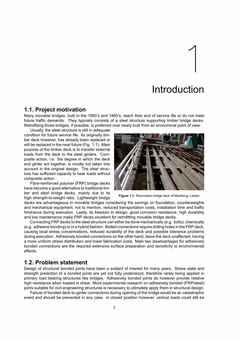
1.1. Project motivationMany movable bridges, built in the 1950’s and 1960’s, reach their end of service life or do not meetfuture traffic demands. They typically consists of a steel structure supporting timber bridge decks.Retrofitting those bridges, if possible, is preferred over newly built from an economical point of view.
Figure 1.1: Renovation bridge deck of Marebrug, Leiden
Usually, the steel structure is still in adequatecondition for future service life. Its originally tim-ber deck however, has already been replaced orwill be replaced in the near future (Fig. 1.1). Mainpurpose of the timber deck is to transfer externalloads from the deck to the steel girders. Com-posite action, i.e. the degree in which the deckand girder act together, is mostly not taken intoaccount in the original design. The steel struc-ture has sufficient capacity to bear loads withoutcomposite action.
Fibre-reinforced polymer (FRP) bridge deckshave become a good alternative to traditional tim-ber and steel bridge decks, mainly due to itshigh strength-to-weight ratio. Lightweight bridgedecks are advantageous in movable bridges considering the savings on foundation, counterweightsand mechanical equipment, not to mention, reduced transportation costs, installation time and traffichindrance during execution. Lastly, its freedom in design, good corrosion resistance, high durabilityand low maintenance make FRP decks excellent for retrofitting movable bridge decks.
Connecting FRP decks to the steel structure can either be donemechanically (e.g. bolts), chemically(e.g. adhesive bonding) or in a hybrid fashion. Bolted connections require drilling holes in the FRP deck,causing local stress concentrations, reduced durability of the deck and possible tolerance problemsduring execution. Adhesively bonded connections on the other hand, leave the deck unaffected, havinga more uniform stress distribution and lower fabrication costs. Main two disadvantages for adhesivelybonded connections are the required extensive surface preparation and sensitivity to environmentaleffects.
1.2. Problem statementDesign of structural bonded joints have been a subject of interest for many years. Stress state andstrength prediction of a bonded joints are yet not fully understood, therefore rarely being applied inprimary load bearing structures like bridges. Adhesively bonded joints do however provide relativehigh resistance when loaded in shear. More experimental research on adhesively bonded (FRP/steel)joints suitable for civil engineering structures is necessary to ultimately apply them in structural design.
Failure of bonded deck-to-girder connections during opening of the bridge would be an catastrophicevent and should be prevented in any case. In closed position however, vertical loads could still be
1

2 1. Introduction
transferred from the deck to the girders when the bonded connection has failed. Crack initiation in thebonded connection occurs when material strengths are exceeded in either the adhesive, adherend or atthe interface between the former two. Cyclic (traffic) loads lead to crack propagation, ultimately to failureof the entire connection. Crack initiation is most likely to occur at locations with stress concentrations.Insight in stress distributions and stress levels in bonded FRP/steel deck-to-girder connections aretherefore crucial for design.
1.3. Aim and objectivesThe overall aim of this thesis is to determine whether an adhesively bonded connection between FRPbridge decks and steel girders has appropriate strength performance for renovation of movable bridges.
With this aim, the following objectives and tasks are defined and covered in this thesis:
1. To review the state-of-the-art on stress analysis and strength performance of bonded (FRP/steel)connections.
2. To design a FRP deck and bonded connection suitable for renovation of a movable bridge.
3. To obtain a reliable method to determine the stress state in a bonded FRP/steel connection.
4. To identify governing load cases for movable FRP/steel bridges with bonded deck-to-girder con-nections.
5. To find critical locations, i.e. stress concentrations, in the bonded deck-to-girder connection.
6. To investigate the effects of different adhesive thickness and elastic modulus on the structuralbehaviour of bonded FRP/steel deck-to-girder connections.
7. To determine which reference levels of stress need to be used to compare the stresses from theanalysis, i.e. strength of the bonded connection.
8. To determine the utilisation ratio of the bonded FRP/steel deck-to-girder connection under gov-erning design loads.
1.4. MethodologyStress levels in the bonded FRP/steel deck-to-girder connections from structural analysis of a casestudy bridge are compared with strength values from literature.
1.5. LimitationsThe following limitations apply in this work:
• Linear static analysis in Finite Element Analysis (FEA) software packages.
• Stress based method for strength prediction of the bonded connections.
1.6. OutlineThis thesis starts with a literature review on themost recent developments regarding bonded (FRP/steel)joints. A case study of an existing movable bridge, used for stress analysis of the bonded FRP/steeldeck-to-girder connections, will be introduced in Chapter 3. Subsequently, Chapter 4 reviews the nu-merical models and methods considered to determine the stress states in the bonded deck-to-girderconnections. Chapter 5 presents the structural analysis results of the case study bridge. A compari-son is made between stress results from the numerical models in Chapter 6. Chapter 7 deals with theeffects of adhesive thickness and elastic modulus on the stress states in the bonded FRP/steel deck-to-girder connections. In Chapter 9, the main conclusions of this work are drawn and suggestions madefor future work.
2State-of-the-art
Many reviews have been made on the state-of-the-art on FRP decks and is therefore not included inthis work. The author recommends reading the state-of-the-art reviews on FRP decks by Csillag [5],Gürtler [8] and Schollmayer [14]. Parts of other work have been used to establish this chapter and isreferenced to.
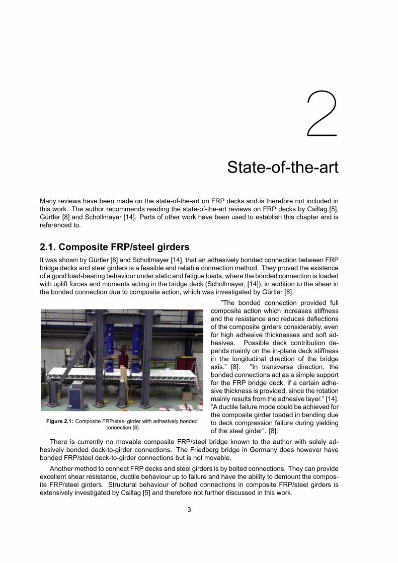
2.1. Composite FRP/steel girdersIt was shown by Gürtler [8] and Schollmayer [14], that an adhesively bonded connection between FRPbridge decks and steel girders is a feasible and reliable connection method. They proved the existenceof a good load-bearing behaviour under static and fatigue loads, where the bonded connection is loadedwith uplift forces and moments acting in the bridge deck (Schollmayer, [14]), in addition to the shear inthe bonded connection due to composite action, which was investigated by Gürtler [8].
Figure 2.1: Composite FRP/steel girder with adhesively bondedconnection [8]
”The bonded connection provided fullcomposite action which increases stiffnessand the resistance and reduces deflectionsof the composite girders considerably, evenfor high adhesive thicknesses and soft ad-hesives. Possible deck contribution de-pends mainly on the in-plane deck stiffnessin the longitudinal direction of the bridgeaxis.” [8]. ”In transverse direction, thebonded connections act as a simple supportfor the FRP bridge deck, if a certain adhe-sive thickness is provided, since the rotationmainly results from the adhesive layer.” [14].”A ductile failure mode could be achieved forthe composite girder loaded in bending dueto deck compression failure during yieldingof the steel girder”. [8].
There is currently no movable composite FRP/steel bridge known to the author with solely ad-hesively bonded deck-to-girder connections. The Friedberg bridge in Germany does however havebonded FRP/steel deck-to-girder connections but is not movable.
Another method to connect FRP decks and steel girders is by bolted connections. They can provideexcellent shear resistance, ductile behaviour up to failure and have the ability to demount the compos-ite FRP/steel girders. Structural behaviour of bolted connections in composite FRP/steel girders isextensively investigated by Csillag [5] and therefore not further discussed in this work.
3
4 2. State-of-the-art
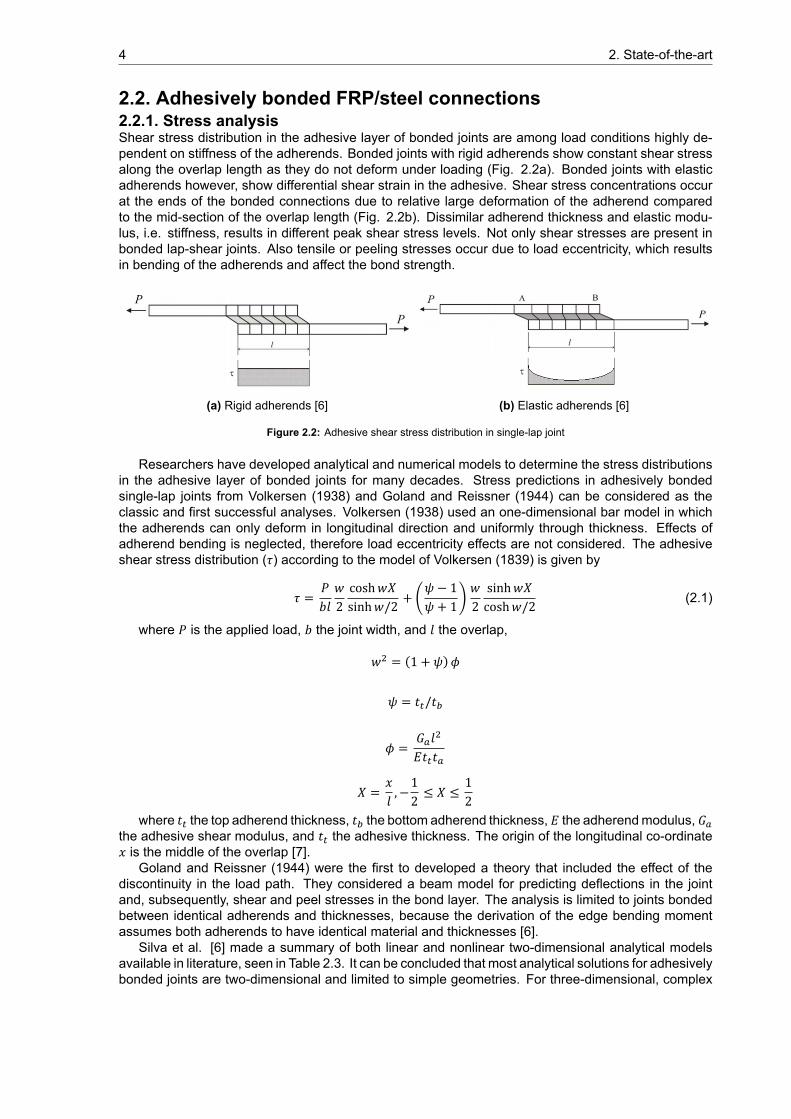
2.2. Adhesively bonded FRP/steel connections2.2.1. Stress analysisShear stress distribution in the adhesive layer of bonded joints are among load conditions highly de-pendent on stiffness of the adherends. Bonded joints with rigid adherends show constant shear stressalong the overlap length as they do not deform under loading (Fig. 2.2a). Bonded joints with elasticadherends however, show differential shear strain in the adhesive. Shear stress concentrations occurat the ends of the bonded connections due to relative large deformation of the adherend comparedto the mid-section of the overlap length (Fig. 2.2b). Dissimilar adherend thickness and elastic modu-lus, i.e. stiffness, results in different peak shear stress levels. Not only shear stresses are present inbonded lap-shear joints. Also tensile or peeling stresses occur due to load eccentricity, which resultsin bending of the adherends and affect the bond strength.
(a) Rigid adherends [6] (b) Elastic adherends [6]
Figure 2.2: Adhesive shear stress distribution in single-lap joint
Researchers have developed analytical and numerical models to determine the stress distributionsin the adhesive layer of bonded joints for many decades. Stress predictions in adhesively bondedsingle-lap joints from Volkersen (1938) and Goland and Reissner (1944) can be considered as theclassic and first successful analyses. Volkersen (1938) used an one-dimensional bar model in whichthe adherends can only deform in longitudinal direction and uniformly through thickness. Effects ofadherend bending is neglected, therefore load eccentricity effects are not considered. The adhesiveshear stress distribution (𝜏) according to the model of Volkersen (1839) is given by
𝜏 = 𝑃𝑏𝑙𝑤2cosh𝑤𝑋sinh𝑤/2 + (
𝜓 − 1𝜓 + 1)
𝑤2sinh𝑤𝑋cosh𝑤/2 (2.1)
where 𝑃 is the applied load, 𝑏 the joint width, and 𝑙 the overlap,
𝑤 = (1 + 𝜓)𝜙
𝜓 = 𝑡 /𝑡
𝜙 = 𝐺 𝑙𝐸𝑡 𝑡
𝑋 = 𝑥𝑙 , −
12 ≤ 𝑋 ≤
12
where 𝑡 the top adherend thickness, 𝑡 the bottom adherend thickness, 𝐸 the adherendmodulus, 𝐺the adhesive shear modulus, and 𝑡 the adhesive thickness. The origin of the longitudinal co-ordinate𝑥 is the middle of the overlap [7].
Goland and Reissner (1944) were the first to developed a theory that included the effect of thediscontinuity in the load path. They considered a beam model for predicting deflections in the jointand, subsequently, shear and peel stresses in the bond layer. The analysis is limited to joints bondedbetween identical adherends and thicknesses, because the derivation of the edge bending momentassumes both adherends to have identical material and thicknesses [6].
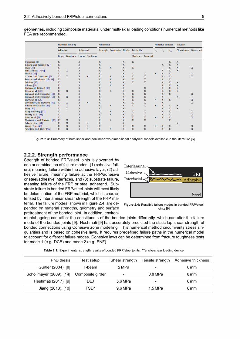
Silva et al. [6] made a summary of both linear and nonlinear two-dimensional analytical modelsavailable in literature, seen in Table 2.3. It can be concluded that most analytical solutions for adhesivelybonded joints are two-dimensional and limited to simple geometries. For three-dimensional, complex
2.2. Adhesively bonded FRP/steel connections 5
geometries, including composite materials, under multi-axial loading conditions numerical methods likeFEA are recommended.
Figure 2.3: Summary of both linear and nonlinear two-dimensional analytical models available in the literature [6]
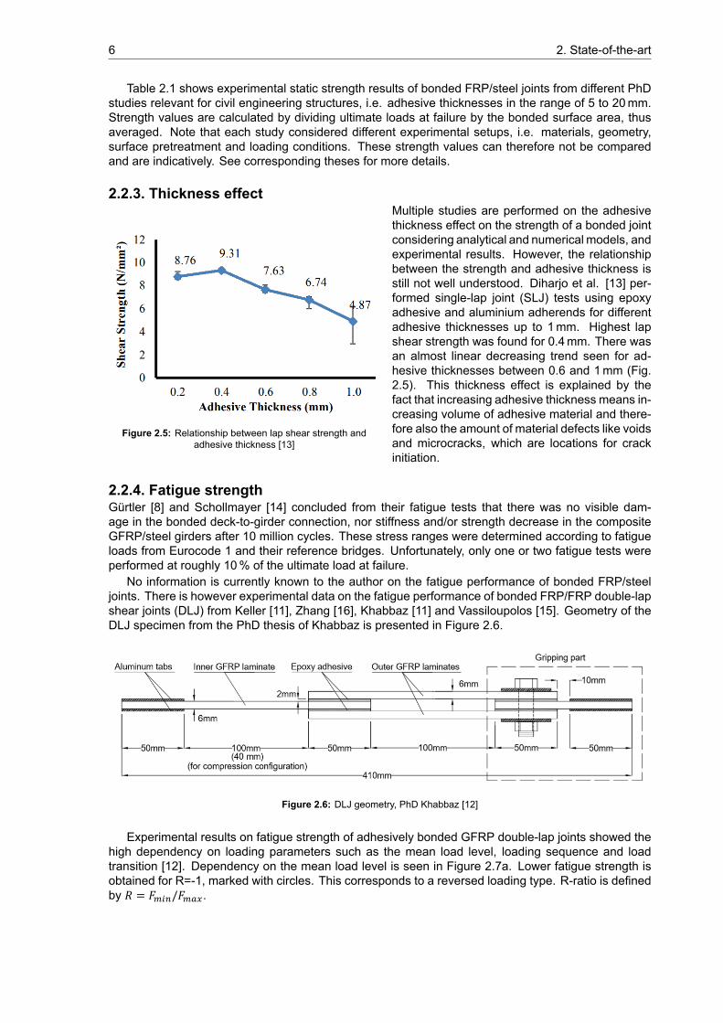
2.2.2. Strength performance
Figure 2.4: Possible failure modes in bonded FRP/steeljoints [9]
Strength of bonded FRP/steel joints is governed byone or combination of failure modes: (1) cohesive fail-ure, meaning failure within the adhesive layer, (2) ad-hesive failure, meaning failure at the FRP/adhesiveor steel/adhesive interfaces, and (3) substrate failure,meaning failure of the FRP or steel adherend. Sub-strate failure in bonded FRP/steel joints will most likelybe delamination of the FRP material, which is charac-terised by interlaminar shear strength of the FRP ma-terial. The failure modes, shown in Figure 2.4, are de-pended on material strengths, geometry and surfacepretreatment of the bonded joint. In addition, environ-mental ageing can affect the constituents of the bonded joints differently, which can alter the failuremode of the bonded joints [9]. Heshmati [9] has accurately predicted the static lap shear strength ofbonded connections using Cohesive zone modelling. This numerical method circumvents stress sin-gularities and is based on cohesive laws. It requires predefined failure paths in the numerical modelto account for different failure modes. Cohesive laws can be determined from fracture toughness testsfor mode 1 (e.g. DCB) and mode 2 (e.g. ENF).
Table 2.1: Experimental strength results of bonded FRP/steel joints. *Tensile-shear loading device.
PhD thesis Test setup Shear strength Tensile strength Adhesive thickness
Gürtler (2004), [8] T-beam 2MPa - 6mm
Schollmayer (2009), [14] Composite girder - 0.8MPa 8mm
Heshmati (2017), [9] DLJ 5.6MPa - 6mm
Jiang (2013), [10] TSD* 9.6MPa 1.5MPa 6mm
6 2. State-of-the-art
Table 2.1 shows experimental static strength results of bonded FRP/steel joints from different PhDstudies relevant for civil engineering structures, i.e. adhesive thicknesses in the range of 5 to 20mm.Strength values are calculated by dividing ultimate loads at failure by the bonded surface area, thusaveraged. Note that each study considered different experimental setups, i.e. materials, geometry,surface pretreatment and loading conditions. These strength values can therefore not be comparedand are indicatively. See corresponding theses for more details.
2.2.3. Thickness effect
Figure 2.5: Relationship between lap shear strength andadhesive thickness [13]
Multiple studies are performed on the adhesivethickness effect on the strength of a bonded jointconsidering analytical and numerical models, andexperimental results. However, the relationshipbetween the strength and adhesive thickness isstill not well understood. Diharjo et al. [13] per-formed single-lap joint (SLJ) tests using epoxyadhesive and aluminium adherends for differentadhesive thicknesses up to 1mm. Highest lapshear strength was found for 0.4mm. There wasan almost linear decreasing trend seen for ad-hesive thicknesses between 0.6 and 1mm (Fig.2.5). This thickness effect is explained by thefact that increasing adhesive thickness means in-creasing volume of adhesive material and there-fore also the amount of material defects like voidsand microcracks, which are locations for crackinitiation.
2.2.4. Fatigue strengthGürtler [8] and Schollmayer [14] concluded from their fatigue tests that there was no visible dam-age in the bonded deck-to-girder connection, nor stiffness and/or strength decrease in the compositeGFRP/steel girders after 10 million cycles. These stress ranges were determined according to fatigueloads from Eurocode 1 and their reference bridges. Unfortunately, only one or two fatigue tests wereperformed at roughly 10% of the ultimate load at failure.
No information is currently known to the author on the fatigue performance of bonded FRP/steeljoints. There is however experimental data on the fatigue performance of bonded FRP/FRP double-lapshear joints (DLJ) from Keller [11], Zhang [16], Khabbaz [11] and Vassiloupolos [15]. Geometry of theDLJ specimen from the PhD thesis of Khabbaz is presented in Figure 2.6.
Figure 2.6: DLJ geometry, PhD Khabbaz [12]
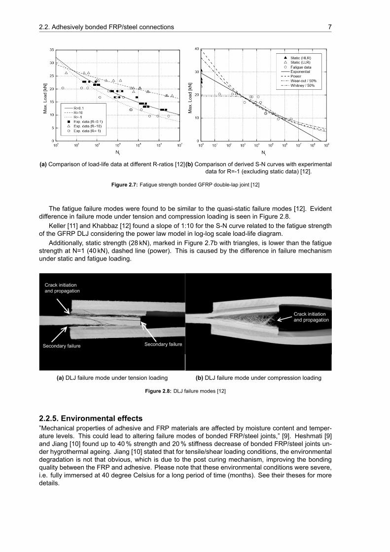
Experimental results on fatigue strength of adhesively bonded GFRP double-lap joints showed thehigh dependency on loading parameters such as the mean load level, loading sequence and loadtransition [12]. Dependency on the mean load level is seen in Figure 2.7a. Lower fatigue strength isobtained for R=-1, marked with circles. This corresponds to a reversed loading type. R-ratio is definedby 𝑅 = 𝐹 /𝐹 .
2.2. Adhesively bonded FRP/steel connections 7
(a) Comparison of load-life data at different R-ratios [12](b) Comparison of derived S-N curves with experimentaldata for R=-1 (excluding static data) [12].
Figure 2.7: Fatigue strength bonded GFRP double-lap joint [12]
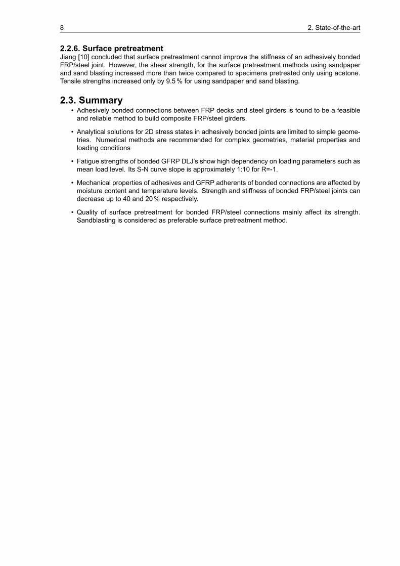
The fatigue failure modes were found to be similar to the quasi-static failure modes [12]. Evidentdifference in failure mode under tension and compression loading is seen in Figure 2.8.
Keller [11] and Khabbaz [12] found a slope of 1:10 for the S-N curve related to the fatigue strengthof the GFRP DLJ considering the power law model in log-log scale load-life diagram.
Additionally, static strength (28 kN), marked in Figure 2.7b with triangles, is lower than the fatiguestrength at N=1 (40 kN), dashed line (power). This is caused by the difference in failure mechanismunder static and fatigue loading.
(a) DLJ failure mode under tension loading (b) DLJ failure mode under compression loading
Figure 2.8: DLJ failure modes [12]
2.2.5. Environmental effects”Mechanical properties of adhesive and FRP materials are affected by moisture content and temper-ature levels. This could lead to altering failure modes of bonded FRP/steel joints,” [9]. Heshmati [9]and Jiang [10] found up to 40% strength and 20% stiffness decrease of bonded FRP/steel joints un-der hygrothermal ageing. Jiang [10] stated that for tensile/shear loading conditions, the environmentaldegradation is not that obvious, which is due to the post curing mechanism, improving the bondingquality between the FRP and adhesive. Please note that these environmental conditions were severe,i.e. fully immersed at 40 degree Celsius for a long period of time (months). See their theses for moredetails.
8 2. State-of-the-art
2.2.6. Surface pretreatmentJiang [10] concluded that surface pretreatment cannot improve the stiffness of an adhesively bondedFRP/steel joint. However, the shear strength, for the surface pretreatment methods using sandpaperand sand blasting increased more than twice compared to specimens pretreated only using acetone.Tensile strengths increased only by 9.5% for using sandpaper and sand blasting.
2.3. Summary• Adhesively bonded connections between FRP decks and steel girders is found to be a feasibleand reliable method to build composite FRP/steel girders.
• Analytical solutions for 2D stress states in adhesively bonded joints are limited to simple geome-tries. Numerical methods are recommended for complex geometries, material properties andloading conditions
• Fatigue strengths of bonded GFRP DLJ’s show high dependency on loading parameters such asmean load level. Its S-N curve slope is approximately 1:10 for R=-1.
• Mechanical properties of adhesives and GFRP adherents of bonded connections are affected bymoisture content and temperature levels. Strength and stiffness of bonded FRP/steel joints candecrease up to 40 and 20% respectively.
• Quality of surface pretreatment for bonded FRP/steel connections mainly affect its strength.Sandblasting is considered as preferable surface pretreatment method.
3Case study
This chapter introduces an actual renovation project of a movable bridge that is considered as casestudy in this thesis. It is assumed to be a representative movable bridge for future renovation projectsin which its current deck will be replaced by a GFRP deck and connected by a bonded connection tothe steel structure. Focus in this chapter will be on the bridge deck design and design loads consideredin this case study.
3.1. Background
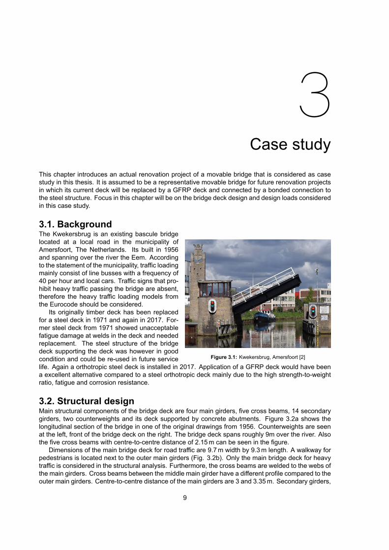
Figure 3.1: Kwekersbrug, Amersfoort [2]
The Kwekersbrug is an existing bascule bridgelocated at a local road in the municipality ofAmersfoort, The Netherlands. Its built in 1956and spanning over the river the Eem. Accordingto the statement of the municipality, traffic loadingmainly consist of line busses with a frequency of40 per hour and local cars. Traffic signs that pro-hibit heavy traffic passing the bridge are absent,therefore the heavy traffic loading models fromthe Eurocode should be considered.
Its originally timber deck has been replacedfor a steel deck in 1971 and again in 2017. For-mer steel deck from 1971 showed unacceptablefatigue damage at welds in the deck and neededreplacement. The steel structure of the bridgedeck supporting the deck was however in goodcondition and could be re-used in future servicelife. Again a orthotropic steel deck is installed in 2017. Application of a GFRP deck would have beena excellent alternative compared to a steel orthotropic deck mainly due to the high strength-to-weightratio, fatigue and corrosion resistance.
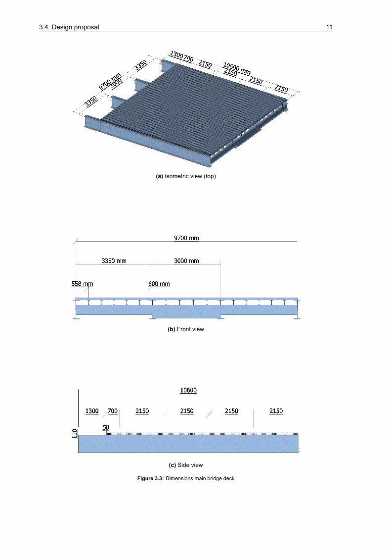
3.2. Structural designMain structural components of the bridge deck are four main girders, five cross beams, 14 secondarygirders, two counterweights and its deck supported by concrete abutments. Figure 3.2a shows thelongitudinal section of the bridge in one of the original drawings from 1956. Counterweights are seenat the left, front of the bridge deck on the right. The bridge deck spans roughly 9m over the river. Alsothe five cross beams with centre-to-centre distance of 2.15m can be seen in the figure.
Dimensions of the main bridge deck for road traffic are 9.7m width by 9.3m length. A walkway forpedestrians is located next to the outer main girders (Fig. 3.2b). Only the main bridge deck for heavytraffic is considered in the structural analysis. Furthermore, the cross beams are welded to the webs ofthe main girders. Cross beams between the middle main girder have a different profile compared to theouter main girders. Centre-to-centre distance of the main girders are 3 and 3.35m. Secondary girders,
9
10 3. Case study
INP220 profiles, are welded on top of the cross beams spanning in traffic direction. Top flanges of bothmain and secondary girders are in the same plane. The deck is connected to all those top flanges.Dimensions of the bridge deck considered for structural analysis is shown in Figure 3.3.
Table 3.1 contains the dimensions of the steel profiles in the bridge leaf. Where ℎ is the height,𝑡 the web thickness, 𝑏 the flange width and 𝑡 the flange thickness. All profiles are symmetricalI-sections.
(a) Longitudinal section (b) Cross-section
Figure 3.2: Technical drawings of the Kwekersbrug [ref?]
Table 3.1: Steel profiles
ℎ [mm] 𝑡 [mm] 𝑏 [mm] 𝑡 [mm]
Main girder 850 19 300 36Cross beams 420, 585 10 150 15
Secondary girder 220 8.1 98 12.2
3.3. Renovation projectThe following project requirements and boundary conditions are set for the renovation of the Kwekers-brug:
• Its original timber deck will be replaced by an FRP deck. Other structural components are inadequate condition for future service life.
• FRP deck is adhesively bonded onto the top flanges of the steel girders.
• Composite action between the FRP deck and girders is not required.
• Construction height of the deck needs to be equal tot the former bridge deck.
• Reference period of 30 years is considered for renovation.
3.4. Design proposalStarting point for the design of the FRP deck and adhesively bonded deck-to-girder connection is thatcomposite action between the deck and girders is not required. Stiffness of the FRP deck, adhesivethickness and elastic modulus can be designed to lower the stresses in the bonded connection as muchas possible, but still provide sufficient strength and stiffness. For preliminary design of FRP structuresit is recommended to satisfy the 1.2% tensile and 1.6% shear strain limit. The deck design proposalpresented in this section does satisfied these requirements.
3.4.1. Deck typeA vacuum infused panel with integrated webs made out of GFRP laminates is considered in for thedesign. Different types of loads on the deck require freedom in laminate design. CFRP laminates
3.4. Design proposal 11
X
YZ
(a) Isometric view (top)
X Y
Z
(b) Front view
XY
Z
(c) Side view
Figure 3.3: Dimensions main bridge deck
12 3. Case study
are not cost effective in a FRP deck with dimensions of 9m by 9m, therefore GFRP laminates areconsidered in the deck design as they also provide sufficient stiffness.
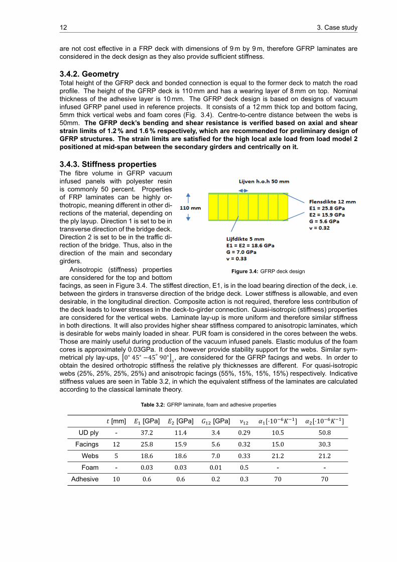
3.4.2. GeometryTotal height of the GFRP deck and bonded connection is equal to the former deck to match the roadprofile. The height of the GFRP deck is 110mm and has a wearing layer of 8mm on top. Nominalthickness of the adhesive layer is 10mm. The GFRP deck design is based on designs of vacuuminfused GFRP panel used in reference projects. It consists of a 12mm thick top and bottom facing,5mm thick vertical webs and foam cores (Fig. 3.4). Centre-to-centre distance between the webs is50mm. The GFRP deck’s bending and shear resistance is verified based on axial and shearstrain limits of 1.2% and 1.6% respectively, which are recommended for preliminary design ofGFRP structures. The strain limits are satisfied for the high local axle load from load model 2positioned at mid-span between the secondary girders and centrically on it.
3.4.3. Stiffness properties
Figure 3.4: GFRP deck design
The fibre volume in GFRP vacuuminfused panels with polyester resinis commonly 50 percent. Propertiesof FRP laminates can be highly or-thotropic, meaning different in other di-rections of the material, depending onthe ply layup. Direction 1 is set to be intransverse direction of the bridge deck.Direction 2 is set to be in the traffic di-rection of the bridge. Thus, also in thedirection of the main and secondarygirders.
Anisotropic (stiffness) propertiesare considered for the top and bottomfacings, as seen in Figure 3.4. The stiffest direction, E1, is in the load bearing direction of the deck, i.e.between the girders in transverse direction of the bridge deck. Lower stiffness is allowable, and evendesirable, in the longitudinal direction. Composite action is not required, therefore less contribution ofthe deck leads to lower stresses in the deck-to-girder connection. Quasi-isotropic (stiffness) propertiesare considered for the vertical webs. Laminate lay-up is more uniform and therefore similar stiffnessin both directions. It will also provides higher shear stiffness compared to anisotropic laminates, whichis desirable for webs mainly loaded in shear. PUR foam is considered in the cores between the webs.Those are mainly useful during production of the vacuum infused panels. Elastic modulus of the foamcores is approximately 0.03GPa. It does however provide stability support for the webs. Similar sym-metrical ply lay-ups, [0∘ 45∘ −45∘ 90∘] , are considered for the GFRP facings and webs. In order toobtain the desired orthotropic stiffness the relative ply thicknesses are different. For quasi-isotropicwebs (25%, 25%, 25%, 25%) and anisotropic facings (55%, 15%, 15%, 15%) respectively. Indicativestiffness values are seen in Table 3.2, in which the equivalent stiffness of the laminates are calculatedaccording to the classical laminate theory.
Table 3.2: GFRP laminate, foam and adhesive properties
𝑡 [mm] 𝐸 [GPa] 𝐸 [GPa] 𝐺 [GPa] 𝜈 𝛼 [⋅10 𝐾 ] 𝛼 [⋅10 𝐾 ]UD ply - 37.2 11.4 3.4 0.29 10.5 50.8Facings 12 25.8 15.9 5.6 0.32 15.0 30.3Webs 5 18.6 18.6 7.0 0.33 21.2 21.2Foam - 0.03 0.03 0.01 0.5 - -
Adhesive 10 0.6 0.6 0.2 0.3 70 70
3.5. Considered loads 13
3.4.4. Thermal propertiesComposite structures, i.e. consisting of different materials, can be sensitive to thermal loading. Re-straint structural components and differences in expansion cause internal stresses. Steel, glass fibres,resin, foam and adhesives have their own thermal properties. Most important thermal properties are (1)coefficient of thermal expansion, 𝛼, and (2) thermal conductivity, 𝜆. Coefficient of thermal expansion(CTE) is the amount of material change in dimension per temperature change. It is the magnitude ofstrain due to thermal expansion per degree Kelvin or Celsius in units of 𝐾 . The thermal conductivityis the rate of heat transfer through a material. The polymeric materials like polyester and acrylic havelarger CTE’s compared to glass fibres and steel. This is why unidirectional plies and also anisotropiclaminates have larger CTE in transverse direction compared to the fibre direction. Conservative CTE’sare considered and given in Table 3.2. Equivalent CTE’s of the laminates are calculated with classicallaminate theory. Thermal conductivity of steel is significantly larger compared to the GFRP laminates,foam and adhesive. This means that the heat transfer through steel is much faster and the GFRP deckacts as an insulator when exposed to (sun) radiation. Difference in thermal conductivity does affect thevertical temperature gradient over bridge deck height which is defined in the Eurocode.
3.4.5. Adhesive propertiesAn acrylic based adhesive is selected for this renovation project, mainly due to its high strength andlow elastic modulus. Besides, its large elongation at failure, i.e. ductile behaviour, is favourable inconnection when it comes to failure mechanisms of the structure. Also its high viscosity and long potlife make is easy to apply and suitable in bridges with large bonded surfaces and gaps. Table 3.3shows the lower limits of available material properties provided by the manufacturer of the adhesive.Coefficient of thermal expansion of the adhesive is assumed to be 70 ⋅ 10 𝐾 .
Table 3.3: Material properties of methacrylic SG230 HV, SciGrip [4]
Tensile strength 21 MPa
Tensile modulus 0.6 GPa
Shear strength 15 MPa
Maximum tensile elongation 100%
3.5. Considered loadsA selection of important permanent and variable loads for composite bridge decks are considered forstructural analysis according to the Eurocode and national annexes.
3.5.1. Permanent loadsPermanent loads consist of self-weight of the steel structure, counterweights, GFRP deck and wearinglayer. Density of steel is assumed to be 7850𝑘𝑔/𝑚 . Density of the laminates of the GFRP deck areassumed to be 1855𝑘𝑔/𝑚 considering a fibre volume of 50% in the unidirectional plies. The 8mmthick wearing layer has a weight of 0.2𝑘𝑁/𝑚 . Self-weight of the adhesive is neglected due to the lowvolume and density. Gravitation acceleration of 9.81𝑚/𝑠 is considered.
Requirement according to the Dutch norms (NEN6785) for movable bridges is a minimum result-ing support reaction at the front of the bridge deck, preventing opening of the bridge deck by wind.Counterweights are therefore slightly ’pushed’, which is accounted for in the model.
10.000 cycles of opening and closing per year is considered for this case study. Reference periodis 30 years.
3.5.2. Traffic load model 1Traffic load model 1 and 2 from the Eurocode are considered as static traffic loads, see EN 1991-2 for more details. Load model 1 consists of a set of tandems and an uniformly distributed load onthe corresponding notional lanes. The uniformly distributed load in the first notional is 9𝑘𝑁/𝑚 andthe axle loads of the corresponding tandem set are 300kN. Second lane respectively 2.5𝑘𝑁/𝑚 and
14 3. Case study
200kN. Dimensions of the tandem sets are shown in Figure 3.5a. Traffic load model 1 is recommendedto be used to analyse global effects.
According to NEN 6876, Dutch norm for assessment of existing structures in case of reconstruction,allows for notional lane layout which corresponds to the actual/current use of traffic lanes. That is twoin this case. Remaining width of the bridge deck is used for bicycles. As mentioned earlier, on eachside of the bridge deck a walkways for pedestrians is located. These are supported by steel cantileverbeams welded on the outer main girders. Since they are separated by curbs of height larger than200𝑚𝑚 no heavy traffic can be located there. This is also reason not to consider them for the analysisof the deck-to-girder connections. Since adding them has negligible effect on the stress state in thedeck-to-girder connections.
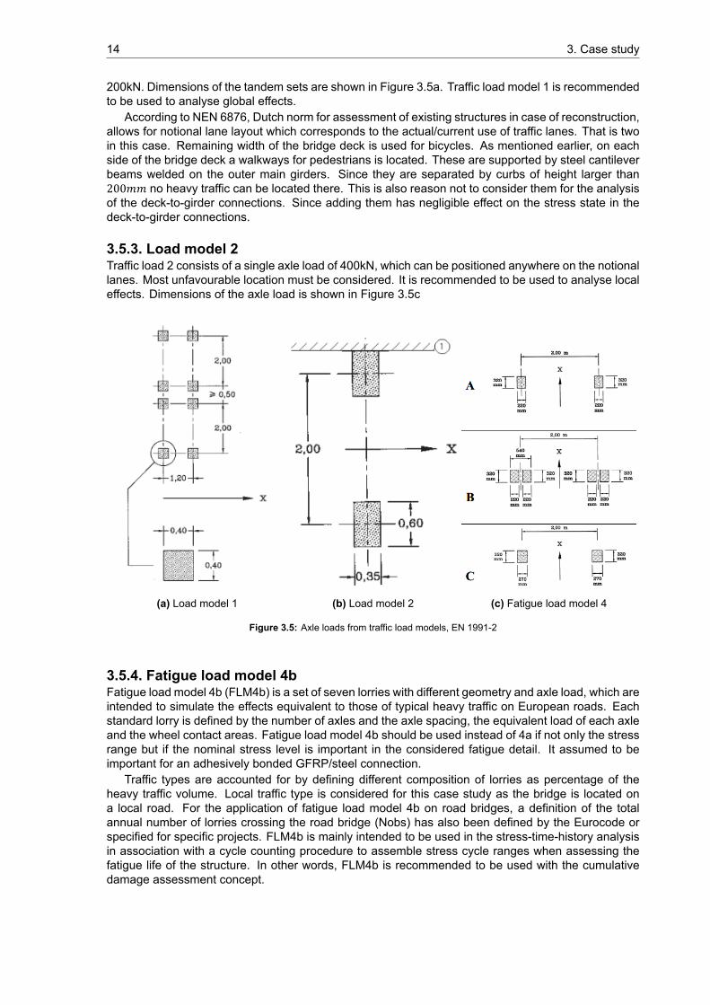
3.5.3. Load model 2Traffic load 2 consists of a single axle load of 400kN, which can be positioned anywhere on the notionallanes. Most unfavourable location must be considered. It is recommended to be used to analyse localeffects. Dimensions of the axle load is shown in Figure 3.5c
(a) Load model 1 (b) Load model 2 (c) Fatigue load model 4
Figure 3.5: Axle loads from traffic load models, EN 1991-2
3.5.4. Fatigue load model 4bFatigue load model 4b (FLM4b) is a set of seven lorries with different geometry and axle load, which areintended to simulate the effects equivalent to those of typical heavy traffic on European roads. Eachstandard lorry is defined by the number of axles and the axle spacing, the equivalent load of each axleand the wheel contact areas. Fatigue load model 4b should be used instead of 4a if not only the stressrange but if the nominal stress level is important in the considered fatigue detail. It assumed to beimportant for an adhesively bonded GFRP/steel connection.
Traffic types are accounted for by defining different composition of lorries as percentage of theheavy traffic volume. Local traffic type is considered for this case study as the bridge is located ona local road. For the application of fatigue load model 4b on road bridges, a definition of the totalannual number of lorries crossing the road bridge (Nobs) has also been defined by the Eurocode orspecified for specific projects. FLM4b is mainly intended to be used in the stress-time-history analysisin association with a cycle counting procedure to assemble stress cycle ranges when assessing thefatigue life of the structure. In other words, FLM4b is recommended to be used with the cumulativedamage assessment concept.

3.5. Considered loads 15
Figure 3.6: Fatigue load model 4b
3.5.5. Thermal loadsThermal loads according to EN 1991-1-5 are considered on the composite bridge deck. Bridge decksare grouped in (1) steel decks, (2) composite steel-concrete decks and (3) concrete decks. Unfortu-nately, there are no norms available for composite FRP/steel bridge decks. As the thermal conductivityand dimensions of a concrete deck is similar to a FRP deck, thermal loads are considered from group(2) steel-concrete bridge decks.
(a) Uniform temperature component (b) Vertical temperature gradient (c) Temperature differencecomponent
Figure 3.7: Thermal expansion load cases on the GFRP/steel bridge deck
Three thermal load cases are distinguished: (1) uniform temperature component, (2) vertical tem-perature gradient, and (3) temperature difference component. Both expansion and contraction shouldbe considered for each load case. Simultaneity of the former two load cases is accounted for with ana combination factor according to the Eurocode. Figure 3.7 shows the three thermal expansion loadcases. Height of the deck is indicated with ℎ. Reference temperature at time execution is 10 degreesCelsius. Only thermal expansion is considered for structural analysis as it governing over thermalcontraction in this case. Difference in CTE between the steel and GFRP times the 36 degrees for theuniform temperature component is gives larger relative expansion compared to the CTE of GFRP times15 degrees. The last thermal expansion load case, temperature difference component, is therefore notconsidered in structural analysis. No information is available on thermal cycles on bridge decks due todaily and seasonal variation. They are however deemed to be important for GFRP/steel bridge design.
16 3. Case study
3.6. SummaryA quick overview of this chapter is given below:
• The Kwekersbrug, an existing bascule bridge, is considered as representative movable bridgesuitable for replacing current deck for a GFRP deck using adhesively bonded deck-to-girder con-nections.
• Its bridge deck has a length of 9.3m and width of 9.7m. Main structural components of the bridgedeck are four steel main girders, cross beams, secondary girders and deck.
• Vacuum infused GFRP sandwich deck panels are considered in bridge deck design for retrofitting.It consists of top and bottom skins, vertical webs and foam cores. The GFRP deck is bonded tothe entire length and width of the top flanges of the main and secondary girders.
• A methyl methacrylic based adhesive layer of 10mm thick is considered in the bonded connectiondesign. Further mechanical properties: elastic modulus of 0.6GPa, tensile strength 21MPa,shear strength 15MPa and coefficient of thermal expansion of 70ppm per degree Celsius.
• Top and bottom skins of the GFRP sandwich deck are 12mm thick and have anisotropic stiffnessproperties. The 5mm thick vertical GFRP deck webs have quasi-isotropic stiffness properties.PUR foam cores in the deck have very low stiffness (0.03GPa) and weight, therefore excludedin numerical models.
• Thermal expansion coefficient of the deck skins are 30ppm. per degree Celsius in longitudinaldirection and 15ppm. per degree Celsius in transverse direction of the bridge deck. Conservativethermal properties of glass fibres and resin are considered.
• Permanent loads, traffic loading, thermal loading and loads during operation are considered foranalysis of the bonded deck-to-girder connection according to the Eurocode. Assumptions aremade for thermal loading on the GFRP/steel bridge deck, since currently no norms are availablefor GFRP/steel bridge decks.

4Numerical models and methods
Numerical models andmethods used for structural analysis of the case study bridge deck are presentedin this chapter.
4.1. Global modelOne numerical model is made for global analysis of the bridge deck in the finite element analysis(FEA) software package SCIA Engineer 17.1. This FEA software package is intended for engineeringpurposes. The global model consists of the entire bridge deck, including main structural components:steel main and secondary girders, cross beams and GFRP bridge deck, see Figure 4.1. Dimensionsand material properties are equal to the ones presented in Chapter 3. Counterweights are modelledas external bending moments acting at the main girder ends.
(a) Isometric view (b) Front view
(c) Top view (d) Side view
Figure 4.1: Global model
17
18 4. Numerical models and methods
4.1.1. Boundary conditionsThe trunnion bearings in the main girders are modelled as pinned supports at the ends of the fourmain girders. Translation in transverse direction is however unrestrained for three out of four supports(Fig. 4.2a). Front of the main girders are supported only vertically. The bridge deck is structurallyindeterminate due to the four supports in transverse direction.
4.1.2. Element typesThe steel structure is modelled in 1D beam elements, while the GFRP deck is modelled in 2D shellelements. The facings and webs of the GFRP deck are modelled separately with orthotropic stiffnessproperties in order to take the different laminate layups into account.
4.1.3. Orthotropic stiffness GFRPThe orthotropic stiffness properties are calculated using classical laminate theory. Elastic stiffnessproperties of the entire laminates are computed in the software tool, eLamX. This tool from the DresdenUniversity is based on the classical laminate theory. Output from the tool, ABD-matrix, is used as inputin SCIA Engineer for the GFRP deck and validated by hand and similar software tools. Since thelaminates are symmetric and balanced the 𝐵 part of the matrix has zero value entries. Also the 𝐴and 𝐴 are zero. 𝐷 and 𝐷 have non-zero values since the laminates are not full isotropic, meaningtorsion and bending coupling for the laminates.
4.1.4. Deck-to-girder connectionsThe deck-to-girder connections are modelled as a ’rib’, i.e. 1D beam elements (steel girders) are fixedto 2D shell element (bottom facing) and acts as a composite beam. It represents an infinite stiff bondedconnection with zero thickness. Eccentricities between the girders and cross beams are modelled bymaster-slave connections and ’dummy’ elements. These are infinitely stiff connections between twonodes without cross-sectional dimensions and weight.
4.1.5. Stress state bonded deck-to-girder connectionFEA software package SCIA Engineer does not compute interface stresses for the ’rib’ connection.Stress states in the deck-to-girder connections are therefore manually calculated post-process. Sincethe girders are modelled using beam elements only the longitudinal shear flow and distributed line loadcan be calculated. Stresses are obtained if these are divided by the width of the flange. The longitudinalshear stress can be calculated in either two ways:
1. Determine the in-plane membrane shear forces, 𝑛 force per unit length, in the bottom facingof the GFRP deck connected to the girders. The jump in shear force over the connected ’rib’corresponds to the longitudinal shear flow in the deck-to-girder connection. Longitudinal shearstress can be calculated dividing the shear flow by the width of the bonded connection, or in thiscase the full flange width:
𝜏 =Δ𝑛𝑏 (4.1)
2. The derivative of the normal force in the girder corresponds to the longitudinal shear flow in thedeck-to-girder connection based on equilibrium in the cross-section. Longitudinal shear stress isagain calculated dividing the shear flow over the bonded width:
𝜏 = 𝑑𝑁𝑑𝑥 ⋅ 𝑏 (4.2)
Similar approach for determining the normal stress in the connection:
1. Determine the out-of-plane shell shear forces, 𝑣 force per unit length, in the bottom facing ofthe GFRP deck connected to the girders. The jump in shear force over the connected ’rib’ corre-sponds to the distributed line load in the deck-to-girder connection. Normal stress can be calcu-lated dividing the line load by the width of the bonded connection:
𝜎 =Δ𝑣𝑏 (4.3)
4.2. Local model 19
2. Derivative of vertical shear force in the cross section is equal to the normal stress in the connec-tion:
𝜎 = 𝑑𝑉𝑑𝑥 ⋅ 𝑏 (4.4)
Both methods result in the same stress. Extracting internal forces from beam elements is howevermore convenient than internal forces from shell elements in SCIA. Stress states in the bonded deck-to-girder connections from the global model are calculated using the second method.
4.1.6. LimitationsBear in mind the following limitations of the global model:
1. The adhesive layer itself is not modelled. The bonded deck-to-girder connections are modelledby fixed connections. Thus, no slip occurs in the composite beams. In addition, stress statethrough thickness of the adhesive layer is not obtainable.
2. Due the use of 1D beam elements for the girders, stress states in transverse direction are notobtainable and uniform over width of the bonded connection. In addition, bending of the deckin transverse direction is not fully accurate as it supported by a line instead of a top flange withwidth.
3. A relative coarse mesh (50mm) is used, due to computational limits, corresponding with thecentre-to-centre distance of the webs of the deck. Local effects in longitudinal direction are there-fore not seen.
4. It is not possible to assign orthotropic coefficients of thermal expansion to materials in SCIA En-gineer. The governing CTE of the GFRP facings, which is in longitudinal direction, is consideredas both longitudinal and transverse direction of the laminate.
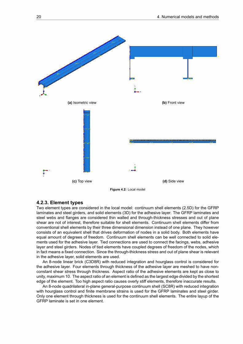
4.2. Local modelAn additional model is made to analyse the stress state in the connection between the deck and sec-ondary girder in more detail under traffic and thermal loads. Finite element analysis software packageAbaqus 6.14 is used for the local models. Purpose of the software is more research/educational orien-tated.
4.2.1. DimensionsThe local model consists of one and half secondary girder, adhesive layers and FRP deck. Adjacentsecondary girder is modelled to include vertical load distribution. The entire length (9.3m) is considered.Width of the deck is 1.5 times the c.t.c distance of the secondary girders, 900mm. The adhesivelayer thickness is 10mm. Width of the adhesive layer is equal to the width of the top flange of thesecondary girder, i.e. 98mm. Deck and girder can be considered as an continuous composite beamwith a cantilever end (Fig. 4.2). Dimensions and material properties are equal to the ones described inChapter 3.
4.2.2. Boundary conditionsSymmetry boundary condition is considered on the left side of the local model (Fig. 4.2b). This is al-lowed since the loads considered for this model are symmetrical with respect to the symmetry boundarycondition on the left side, i.e. level of the web of the girder. Meaning, restrained rotation around the lon-gitudinal axis, restrained rotation around the vertical(trough-thickness) axis, and restrained translationin transverse direction.
The secondary girders are supported by pinned supports at level of the cross beams, marked withthe yellow crosses in longitudinal direction (Fig. 4.2d). Width of the cross beams are taken into accountby applying the boundary conditions on the corresponding surface.
The right side of the model, the GFRP deck, is also restrained in rotation around the longitudinal andvertical axis. However, translation in transverse direction is unrestrained, allowing thermal expansionas it is in the bridge deck (Fig. 4.2b).
20 4. Numerical models and methods
(a) Isometric view (b) Front view
(c) Top view (d) Side view
Figure 4.2: Local model
4.2.3. Element typesTwo element types are considered in the local model: continuum shell elements (2.5D) for the GFRPlaminates and steel girders, and solid elements (3D) for the adhesive layer. The GFRP laminates andsteel webs and flanges are considered thin walled and through-thickness stresses and out of planeshear are not of interest, therefore suitable for shell elements. Continuum shell elements differ fromconventional shell elements by their three dimensional dimension instead of one plane. They howeverconsists of an equivalent shell that drives deformation of nodes in a solid body. Both elements haveequal amount of degrees of freedom. Continuum shell elements can be well connected to solid ele-ments used for the adhesive layer. Tied connections are used to connect the facings, webs, adhesivelayer and steel girders. Nodes of tied elements have coupled degrees of freedom of the nodes, whichin fact means a fixed connection. Since the through-thickness stress and out of plane shear is relevantin the adhesive layer, solid elements are used.
An 8-node linear brick (C3D8R) with reduced integration and hourglass control is considered forthe adhesive layer. Four elements through thickness of the adhesive layer are meshed to have non-constant shear stress through thickness. Aspect ratio of the adhesive elements are kept as close tounity, maximum 10. The aspect ratio of an element is defined as the largest edge divided by the shortestedge of the element. Too high aspect ratio causes overly stiff elements, therefore inaccurate results.
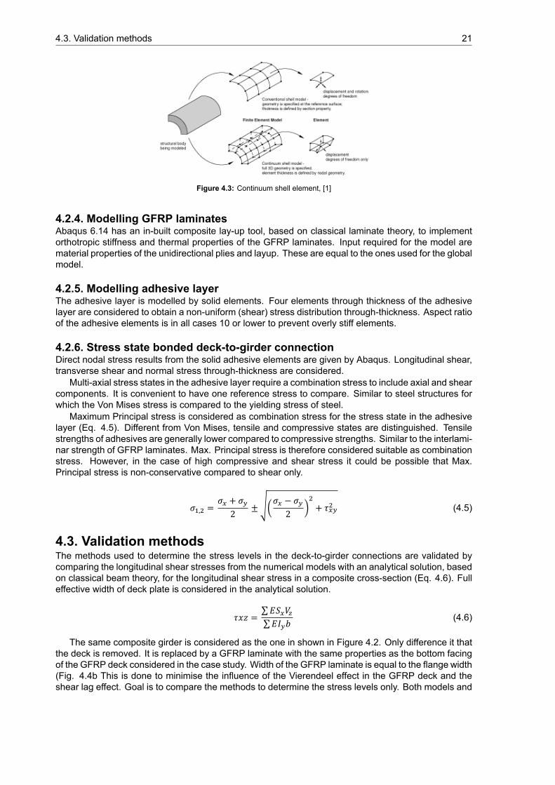
An 8-node quadrilateral in-plane general-purpose continuum shell (SC8R) with reduced integrationwith hourglass control and finite membrane strains is used for the GFRP laminates and steel girder.Only one element through thickness is used for the continuum shell elements. The entire layup of theGFRP laminate is set in one element.
4.3. Validation methods 21
Figure 4.3: Continuum shell element, [1]
4.2.4. Modelling GFRP laminatesAbaqus 6.14 has an in-built composite lay-up tool, based on classical laminate theory, to implementorthotropic stiffness and thermal properties of the GFRP laminates. Input required for the model arematerial properties of the unidirectional plies and layup. These are equal to the ones used for the globalmodel.
4.2.5. Modelling adhesive layerThe adhesive layer is modelled by solid elements. Four elements through thickness of the adhesivelayer are considered to obtain a non-uniform (shear) stress distribution through-thickness. Aspect ratioof the adhesive elements is in all cases 10 or lower to prevent overly stiff elements.
4.2.6. Stress state bonded deck-to-girder connectionDirect nodal stress results from the solid adhesive elements are given by Abaqus. Longitudinal shear,transverse shear and normal stress through-thickness are considered.
Multi-axial stress states in the adhesive layer require a combination stress to include axial and shearcomponents. It is convenient to have one reference stress to compare. Similar to steel structures forwhich the Von Mises stress is compared to the yielding stress of steel.
Maximum Principal stress is considered as combination stress for the stress state in the adhesivelayer (Eq. 4.5). Different from Von Mises, tensile and compressive states are distinguished. Tensilestrengths of adhesives are generally lower compared to compressive strengths. Similar to the interlami-nar strength of GFRP laminates. Max. Principal stress is therefore considered suitable as combinationstress. However, in the case of high compressive and shear stress it could be possible that Max.Principal stress is non-conservative compared to shear only.
𝜎 , =𝜎 + 𝜎2 ± √(
𝜎 − 𝜎2 ) + 𝜏 (4.5)
4.3. Validation methodsThe methods used to determine the stress levels in the deck-to-girder connections are validated bycomparing the longitudinal shear stresses from the numerical models with an analytical solution, basedon classical beam theory, for the longitudinal shear stress in a composite cross-section (Eq. 4.6). Fulleffective width of deck plate is considered in the analytical solution.
𝜏𝑥𝑧 =∑𝐸𝑆 𝑉∑𝐸𝐼 𝑏 (4.6)
The same composite girder is considered as the one in shown in Figure 4.2. Only difference it thatthe deck is removed. It is replaced by a GFRP laminate with the same properties as the bottom facingof the GFRP deck considered in the case study. Width of the GFRP laminate is equal to the flange width(Fig. 4.4b This is done to minimise the influence of the Vierendeel effect in the GFRP deck and theshear lag effect. Goal is to compare the methods to determine the stress levels only. Both models and
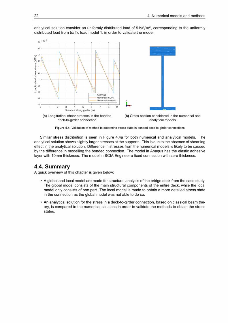
22 4. Numerical models and methods
analytical solution consider an uniformly distributed load of 9 𝑘𝑁/𝑚 , corresponding to the uniformlydistributed load from traffic load model 1, in order to validate the model.
0 1 2 3 4 5 6 7 8 9
Distance along girder (m)
-5
-4
-3
-2
-1
0
1
2
3
4
5
Lo
ng
itu
din
al sh
ea
r str
ess (
MP
a)
10-3
Analytical
Numerical (SCIA)
Numerical (Abaqus)
(a) Longitudinal shear stresses in the bondeddeck-to-girder connection
RP−1 RP−2 RP−3 RP−4 RP−5
X
Y
Z
(b) Cross-section considered in the numerical andanalytical models
Figure 4.4: Validation of method to determine stress state in bonded deck-to-girder connections
Similar stress distribution is seen in Figure 4.4a for both numerical and analytical models. Theanalytical solution shows slightly larger stresses at the supports. This is due to the absence of shear lageffect in the analytical solution. Difference in stresses from the numerical models is likely to be causedby the difference in modelling the bonded connection. The model in Abaqus has the elastic adhesivelayer with 10mm thickness. The model in SCIA Engineer a fixed connection with zero thickness.
4.4. SummaryA quick overview of this chapter is given below:
• A global and local model are made for structural analysis of the bridge deck from the case study.The global model consists of the main structural components of the entire deck, while the localmodel only consists of one part. The local model is made to obtain a more detailed stress statein the connection as the global model was not able to do so.
• An analytical solution for the stress in a deck-to-girder connection, based on classical beam the-ory, is compared to the numerical solutions in order to validate the methods to obtain the stressstates.
5Structural analysis
Results from the structural analysis of the case study bridge deck are presented in this chapter. Consid-ered loads and structural design are described in Chapter 3. Stress states in the bonded deck-to-girderconnections for global and local analysis are determined according to the methods and correspondingnumerical models described in Chapter 4.
5.1. Composite actionComposite structures consist of two or more different materials. They can act together as one unit ifthere are connected strongly enough. If this occurs, its called composite action. This concept is forexample deliberately used in composite concrete-steel girders. Goal is to design more slender andreduce deflections due to increased bending moment resistance. The concrete slab acts as compres-sive part in the composite cross section under sagging bending moments. Requirement is howeverthe presence of shear connectors between the steel girder and concrete slab to prevent slip betweenboth materials. The less slip, the more the concrete slab contributes to bending moment resistanceof the composite girder. This can be expressed in the degree of composite action, no slip means fullcomposite action. Contribution of the deck is however very much depending on stiffness of the deck.
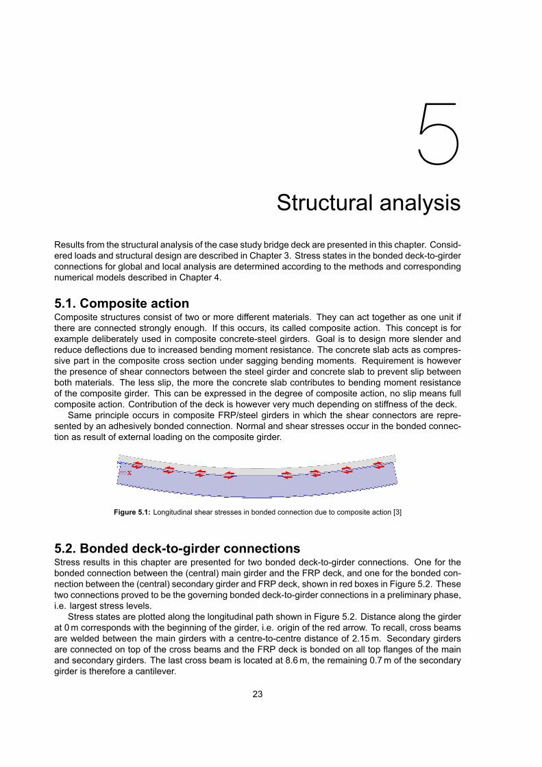
Same principle occurs in composite FRP/steel girders in which the shear connectors are repre-sented by an adhesively bonded connection. Normal and shear stresses occur in the bonded connec-tion as result of external loading on the composite girder.
Figure 5.1: Longitudinal shear stresses in bonded connection due to composite action [3]
5.2. Bonded deck-to-girder connectionsStress results in this chapter are presented for two bonded deck-to-girder connections. One for thebonded connection between the (central) main girder and the FRP deck, and one for the bonded con-nection between the (central) secondary girder and FRP deck, shown in red boxes in Figure 5.2. Thesetwo connections proved to be the governing bonded deck-to-girder connections in a preliminary phase,i.e. largest stress levels.
Stress states are plotted along the longitudinal path shown in Figure 5.2. Distance along the girderat 0m corresponds with the beginning of the girder, i.e. origin of the red arrow. To recall, cross beamsare welded between the main girders with a centre-to-centre distance of 2.15m. Secondary girdersare connected on top of the cross beams and the FRP deck is bonded on all top flanges of the mainand secondary girders. The last cross beam is located at 8.6m, the remaining 0.7m of the secondarygirder is therefore a cantilever.
23
24 5. Structural analysis
Figure 5.2: Considered deck-to-girder connections, front view (top). Longitudinal path along girders, side view (bottom)
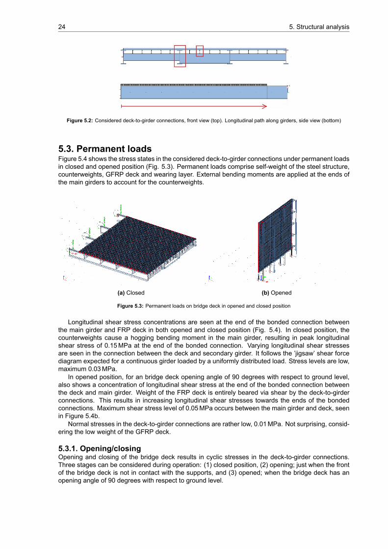
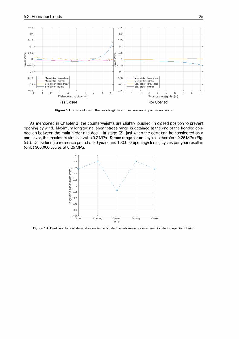
5.3. Permanent loadsFigure 5.4 shows the stress states in the considered deck-to-girder connections under permanent loadsin closed and opened position (Fig. 5.3). Permanent loads comprise self-weight of the steel structure,counterweights, GFRP deck and wearing layer. External bending moments are applied at the ends ofthe main girders to account for the counterweights.
(a) Closed (b) Opened
Figure 5.3: Permanent loads on bridge deck in opened and closed position
Longitudinal shear stress concentrations are seen at the end of the bonded connection betweenthe main girder and FRP deck in both opened and closed position (Fig. 5.4). In closed position, thecounterweights cause a hogging bending moment in the main girder, resulting in peak longitudinalshear stress of 0.15MPa at the end of the bonded connection. Varying longitudinal shear stressesare seen in the connection between the deck and secondary girder. It follows the ’jigsaw’ shear forcediagram expected for a continuous girder loaded by a uniformly distributed load. Stress levels are low,maximum 0.03MPa.
In opened position, for an bridge deck opening angle of 90 degrees with respect to ground level,also shows a concentration of longitudinal shear stress at the end of the bonded connection betweenthe deck and main girder. Weight of the FRP deck is entirely beared via shear by the deck-to-girderconnections. This results in increasing longitudinal shear stresses towards the ends of the bondedconnections. Maximum shear stress level of 0.05MPa occurs between the main girder and deck, seenin Figure 5.4b.
Normal stresses in the deck-to-girder connections are rather low, 0.01MPa. Not surprising, consid-ering the low weight of the GFRP deck.
5.3.1. Opening/closingOpening and closing of the bridge deck results in cyclic stresses in the deck-to-girder connections.Three stages can be considered during operation: (1) closed position, (2) opening; just when the frontof the bridge deck is not in contact with the supports, and (3) opened; when the bridge deck has anopening angle of 90 degrees with respect to ground level.
5.3. Permanent loads 25
0 1 2 3 4 5 6 7 8 9
Distance along girder (m)
-0.25
-0.2
-0.15
-0.1
-0.05
0
0.05
0.1
0.15
0.2
0.25S
tress (
MP
a)
Main girder - long. shear
Main girder - normal
Sec. girder - long. shear
Sec. girder - normal
(a) Closed
0 1 2 3 4 5 6 7 8 9
Distance along girder (m)
-0.25
-0.2
-0.15
-0.1
-0.05
0
0.05
0.1
0.15
0.2
0.25
Str
ess (
MP
a)
Main girder - long. shear
Main girder - normal
Sec. girder - long. shear
Sec. girder - normal
(b) Opened
Figure 5.4: Stress states in the deck-to-girder connections under permanent loads
As mentioned in Chapter 3, the counterweights are slightly ’pushed’ in closed position to preventopening by wind. Maximum longitudinal shear stress range is obtained at the end of the bonded con-nection between the main girder and deck. In stage (2), just when the deck can be considered as acantilever, the maximum stress level is 0.2MPa. Stress range for one cycle is therefore 0.25MPa (Fig.5.5). Considering a reference period of 30 years and 100.000 opening/closing cycles per year result in(only) 300.000 cycles at 0.25MPa.
Closed Opening Opened Closing Closed
Time
-0.25
-0.2
-0.15
-0.1
-0.05
0
0.05
0.1
0.15
0.2
0.25
Lo
ng
itu
din
al sh
ea
r str
ess (
MP
a)
Figure 5.5: Peak longitudinal shear stresses in the bonded deck-to-main girder connection during opening/closing
26 5. Structural analysis
5.4. Traffic loadsStress results in the bonded deck-to-girder connections due to traffic loads are presented in this section.Both static and fatigue traffic load models are considered, as mentioned in Chapter 3. Consideredstatic traffic load models are load model 1 (LM1) and 2 (LM2). Load model 1 consists of three tandemsystems and a uniformly distributed load. The actual traffic lane layout may be considered for renovationprojects according to the Dutch norm NEN 6786. Therefore only two tandem systems are consideredin the structural analysis. Load model 2 consists of a single axle load of 400 kN.
Fatigue load model 4b (FLM4b), according to the Dutch national annex NEN-EN 1991-2, is consid-ered for the fatigue analysis. It consists of a set of lorries with different axle loads and configuration asmentioned in Chapter 3. FLM4b should to be used for fatigue details in which not only stress range butalso nominal stress level is of importance. This is the case for bonded FRP joints, as shown in Chapter2.
Stress results presented in this section are divided in global and local analysis, corresponding tothe results from the global and local models respectively. Limitations of the global model, discussed inSection 4.1.6, made it necessary to develop an additional model to obtain a more detailed stress statein the adhesively bonded deck-to-girder connections.
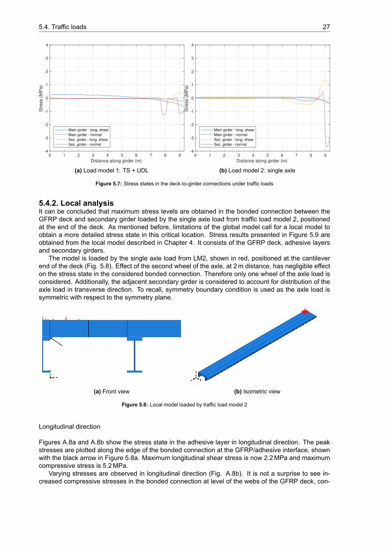
5.4.1. Global analysisFigure 5.6 shows the critical positions, i.e. largest stress levels, of the tandem systems from the trafficload models 1 and 2. This is for both cases at the end of the deck positioned on the cantilever partof the secondary girder. Stress states in the deck-to-girder connections are presented in Figure 5.7.Obviously, compressive stress concentrations are seen in the vicinity of axle loads. Also longitudinalshear stress peaks occur at this location, due to the internal shear forces in the composite FRP/steelgirders.
(a) Load model 1: tandem systems (b) Load model 2: single axle
Figure 5.6: Governing positions for the traffic load models on bridge deck
Maximum stresses occur in the bonded connection between the deck and secondary girders com-pared to main girders (Fig. 5.7). This is mainly due to the large difference in bending stiffness betweenthe main and secondary girders. Lower stresses are obtained in the bonded connection between thedeck and secondary girder for LM1 compared to LM2. This is mainly due to the difference in axle loadsfrom LM1 and LM2, 300 kN and 400 kN respectively.
Peak longitudinal shear stress is 1.4MPa at 8.95m distance along the girder for load model 2(Fig. 5.7b. Length of the wheel print is 0.35m, therefore maximum shear force occurs at this location.Maximum normal stress is 3.7MPa. A slight decrease in compressive stress is seen towards the endof the girder. Bending of the FRP deck in transverse direction causes peeling stresses at the end ofthe bonded connection.
5.4. Traffic loads 27
0 1 2 3 4 5 6 7 8 9
Distance along girder (m)
-4
-3
-2
-1
0
1
2
3
4S
tre
ss (
MP
a)
Main girder - long. shear
Main girder - normal
Sec. girder - long. shear
Sec. girder - normal
(a) Load model 1: TS + UDL
0 1 2 3 4 5 6 7 8 9
Distance along girder (m)
-4
-3
-2
-1
0
1
2
3
4
Str
ess (
MP
a)
Main girder - long. shear
Main girder - normal
Sec. girder - long. shear
Sec. girder - normal
(b) Load model 2: single axle
Figure 5.7: Stress states in the deck-to-girder connections under traffic loads
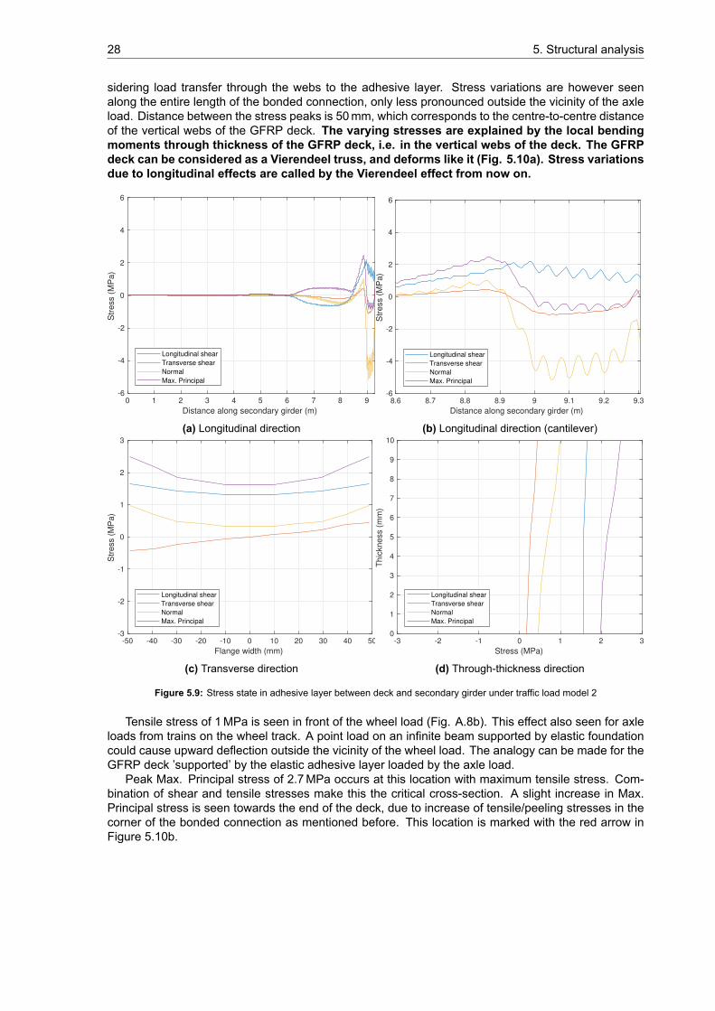
5.4.2. Local analysisIt can be concluded that maximum stress levels are obtained in the bonded connection between theGFRP deck and secondary girder loaded by the single axle load from traffic load model 2, positionedat the end of the deck. As mentioned before, limitations of the global model call for a local model toobtain a more detailed stress state in this critical location. Stress results presented in Figure 5.9 areobtained from the local model described in Chapter 4. It consists of the GFRP deck, adhesive layersand secondary girders.
The model is loaded by the single axle load from LM2, shown in red, positioned at the cantileverend of the deck (Fig. 5.8). Effect of the second wheel of the axle, at 2m distance, has negligible effecton the stress state in the considered bonded connection. Therefore only one wheel of the axle load isconsidered. Additionally, the adjacent secondary girder is considered to account for distribution of theaxle load in transverse direction. To recall, symmetry boundary condition is used as the axle load issymmetric with respect to the symmetry plane.
(a) Front view (b) Isometric view
Figure 5.8: Local model loaded by traffic load model 2
Longitudinal direction
Figures A.8a and A.8b show the stress state in the adhesive layer in longitudinal direction. The peakstresses are plotted along the edge of the bonded connection at the GFRP/adhesive interface, shownwith the black arrow in Figure 5.8a. Maximum longitudinal shear stress is now 2.2MPa and maximumcompressive stress is 5.2MPa.
Varying stresses are observed in longitudinal direction (Fig. A.8b). It is not a surprise to see in-creased compressive stresses in the bonded connection at level of the webs of the GFRP deck, con-
28 5. Structural analysis
sidering load transfer through the webs to the adhesive layer. Stress variations are however seenalong the entire length of the bonded connection, only less pronounced outside the vicinity of the axleload. Distance between the stress peaks is 50mm, which corresponds to the centre-to-centre distanceof the vertical webs of the GFRP deck. The varying stresses are explained by the local bendingmoments through thickness of the GFRP deck, i.e. in the vertical webs of the deck. The GFRPdeck can be considered as a Vierendeel truss, and deforms like it (Fig. 5.10a). Stress variationsdue to longitudinal effects are called by the Vierendeel effect from now on.
0 1 2 3 4 5 6 7 8 9
Distance along secondary girder (m)
-6
-4
-2
0
2
4
6
Str
ess (
MP
a)
Longitudinal shear
Transverse shear
Normal
Max. Principal
(a) Longitudinal direction
8.6 8.7 8.8 8.9 9 9.1 9.2 9.3
Distance along secondary girder (m)
-6
-4
-2
0
2
4
6
Str
ess (
MP
a)
Longitudinal shear
Transverse shear
Normal
Max. Principal
(b) Longitudinal direction (cantilever)
-50 -40 -30 -20 -10 0 10 20 30 40 50
Flange width (mm)
-3
-2
-1
0
1
2
3
Str
ess (
MP
a)
Longitudinal shear
Transverse shear
Normal
Max. Principal
(c) Transverse direction
-3 -2 -1 0 1 2 3
Stress (MPa)
0
1
2
3
4
5
6
7
8
9
10
Thic
kness (
mm
)
Longitudinal shear
Transverse shear
Normal
Max. Principal
(d) Through-thickness direction
Figure 5.9: Stress state in adhesive layer between deck and secondary girder under traffic load model 2
Tensile stress of 1MPa is seen in front of the wheel load (Fig. A.8b). This effect also seen for axleloads from trains on the wheel track. A point load on an infinite beam supported by elastic foundationcould cause upward deflection outside the vicinity of the wheel load. The analogy can be made for theGFRP deck ’supported’ by the elastic adhesive layer loaded by the axle load.
Peak Max. Principal stress of 2.7MPa occurs at this location with maximum tensile stress. Com-bination of shear and tensile stresses make this the critical cross-section. A slight increase in Max.Principal stress is seen towards the end of the deck, due to increase of tensile/peeling stresses in thecorner of the bonded connection as mentioned before. This location is marked with the red arrow inFigure 5.10b.
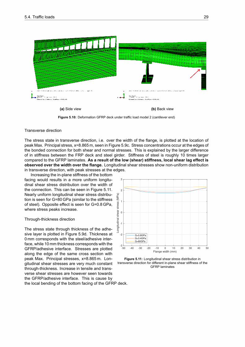
5.4. Traffic loads 29
(a) Side view (b) Back view
Figure 5.10: Deformation GFRP deck under traffic load model 2 (cantilever end)
Transverse direction
The stress state in transverse direction, i.e. over the width of the flange, is plotted at the location ofpeakMax. Principal stress, x=8.865m, seen in Figure 5.9c. Stress concentrations occur at the edges ofthe bonded connection for both shear and normal stresses. This is explained by the larger differenceof in stiffness between the FRP deck and steel girder. Stiffness of steel is roughly 10 times largercompared to the GFRP laminates. As a result of the low (shear) stiffness, local shear lag effect isobserved over the width over the flange. Longitudinal shear stresses show non-uniform distributionin transverse direction, with peak stresses at the edges.
-50 -40 -30 -20 -10 0 10 20 30 40 50
Flange width (mm)
-3
-2
-1
0
1
2
3
Longitudin
al shear
str
ess (
MP
a)
G=0.8GPa
G=3.4GPa
G=80GPa
Figure 5.11: Longitudinal shear stress distribution intransverse direction for different in-plane shear stiffness of the
GFRP laminates
Increasing the in-plane stiffness of the bottomfacing would results in a more uniform longitu-dinal shear stress distribution over the width ofthe connection. This can be seen in Figure 5.11.Nearly uniform longitudinal shear stress distribu-tion is seen for G=80GPa (similar to the stiffnessof steel). Opposite effect is seen for G=0.8GPa,where stress peaks increase.
Through-thickness direction
The stress state through thickness of the adhe-sive layer is plotted in Figure 5.9d. Thickness at0mm corresponds with the steel/adhesive inter-face, while 10mm thickness corresponds with theGFRP/adhesive interface. Stresses are plottedalong the edge of the same cross section withpeak Max. Principal stresses, x=8.865m. Lon-gitudinal shear stresses are very much constantthrough-thickness. Increase in tensile and trans-verse shear stresses are however seen towardsthe GFRP/adhesive interface. This is cause bythe local bending of the bottom facing of the GFRP deck.
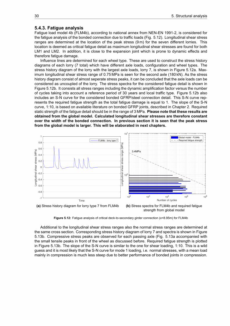
30 5. Structural analysis
5.4.3. Fatigue analysisFatigue load model 4b (FLM4b), according to national annex from NEN-EN 1991-2, is considered forthe fatigue analysis of the bonded connection due to traffic loads (Fig. 5.12). Longitudinal shear stressranges are determined at the location of the peak stress (9m) for the seven different lorries. Thislocation is deemed as critical fatigue detail as maximum longitudinal shear stresses are found for bothLM1 and LM2. In addition, it is close to the expansion joint which is prone to dynamic effects andtherefore fatigue damage.
Influence lines are determined for each wheel type. These are used to construct the stress historydiagrams of each lorry (7 total) which have different axle loads, configuration and wheel types. Thestress history diagram of the lorry with the largest axle loads, lorry 7, is shown in Figure 5.12a. Max-imum longitudinal shear stress range of 0.75MPa is seen for the second axle (180 kN). As the stresshistory diagram consist of almost seperate stress peaks, it can be concluded that the axle loads can beconsidered as uncoupled of the lorry. The stress spectra for the considered fatigue detail is shown inFigure 5.12b. It consists all stress ranges including the dynamic amplification factor versus the numberof cycles taking into account a reference period of 30 years and local traffic type. Figure 5.12b alsoincludes an S-N curve for the considered bonded GFRP/steel connection detail. This S-N curve rep-resents the required fatigue strength as the total fatigue damage is equal to 1. The slope of the S-Ncurve, 1:10, is based on available literature on bonded GFRP joints, described in Chapter 2. Requiredstatic strength of the fatigue detail should be in the range of 3MPa. Please note that these results areobtained from the global model. Calculated longitudinal shear stresses are therefore constantover the width of the bonded connection. In previous section it is seen that the peak stressfrom the global model is larger. This will be elaborated in next chapters.
Time-1
-0.8
-0.6
-0.4
-0.2
0
0.2
0.4
0.6
0.8
1
Lo
ng
itu
din
al sh
ea
r str
ess (
MP
a)
FLM4b - lorry type 7
(a) Stress history diagram for lorry type 7 from FLM4b
3.4MPa
100 102 104 106 108
Number of cycles
100
101
Longitudin
al shear
str
ess r
ange (
MP
a)
Global model - FLM4b
Required fatigue strength
(b) Stress spectra for FLM4b and required fatiguestrength from global model
Figure 5.12: Fatigue analysis of critical deck-to-secondary girder connection (x=8.95m) for FLM4b
Additional to the longitudinal shear stress ranges also the normal stress ranges are determined atthe same cross section. Corresponding stress history diagram of lorry 7 and spectra is shown in Figure5.13b. Compressive stress peaks are observed for each passing axle (Fig. 5.13a accompanied withthe small tensile peaks in front of the wheel as discussed before. Required fatigue strength is plottedin Figure 5.13b. The slope of the S-N curve is similar to the one for shear loading, 1:10. This is a wildguess and it is most likely that the S-N curve for mode 1 loading, i.e. normal stresses, with a mean loadmainly in compression is much less steep due to better performance of bonded joints in compression.
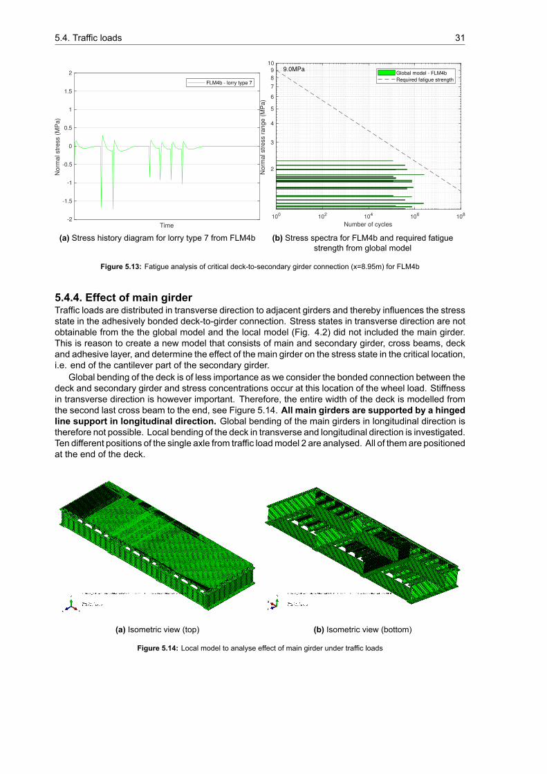
5.4. Traffic loads 31
Time-2
-1.5
-1
-0.5
0
0.5
1
1.5
2
No
rma
l str
ess (
MP
a)
FLM4b - lorry type 7
(a) Stress history diagram for lorry type 7 from FLM4b
9.0MPa
100 102 104 106 108
Number of cycles
2
3
4
5
6
7
8
9
10
No
rmal str
ess r
ang
e (
MP
a)
Global model - FLM4b
Required fatigue strength
(b) Stress spectra for FLM4b and required fatiguestrength from global model
Figure 5.13: Fatigue analysis of critical deck-to-secondary girder connection (x=8.95m) for FLM4b
5.4.4. Effect of main girderTraffic loads are distributed in transverse direction to adjacent girders and thereby influences the stressstate in the adhesively bonded deck-to-girder connection. Stress states in transverse direction are notobtainable from the the global model and the local model (Fig. 4.2) did not included the main girder.This is reason to create a new model that consists of main and secondary girder, cross beams, deckand adhesive layer, and determine the effect of the main girder on the stress state in the critical location,i.e. end of the cantilever part of the secondary girder.
Global bending of the deck is of less importance as we consider the bonded connection between thedeck and secondary girder and stress concentrations occur at this location of the wheel load. Stiffnessin transverse direction is however important. Therefore, the entire width of the deck is modelled fromthe second last cross beam to the end, see Figure 5.14. All main girders are supported by a hingedline support in longitudinal direction. Global bending of the main girders in longitudinal direction istherefore not possible. Local bending of the deck in transverse and longitudinal direction is investigated.Ten different positions of the single axle from traffic loadmodel 2 are analysed. All of them are positionedat the end of the deck.
(a) Isometric view (top) (b) Isometric view (bottom)
Figure 5.14: Local model to analyse effect of main girder under traffic loads
32 5. Structural analysis
Max. Principal stress
Governing position of the axle load from traffic load model 2, i.e. largest Max. Principal stresses, isthe one that was found by the global model, namely one wheel load is positioned centrically at thesecondary girder second from the main girder. The other wheel load of the axle is positioned in theother span between the main girders, see Figure 5.16a. Figure 5.16b shows the deformed model andcritical bonded connection. No significant difference is found in stress state between the local modelwith only deck and secondary girders and the one including main girders. See Figures 5.6b and A.6.
RP−1 RP−3 RP−4 RP−2
X
Y
Z
(a) Position axle load, back view (b) Deformed model, back view
Figure 5.15: Axle position for maximum Max. Principal stress
Peeling stresses
Peeling stresses in the corner of the extreme end of the bonded connection between the secondarygirder and deck adjacent to the main girder is maximum when the wheel load of the axle is positionedat mid-span (shown with the red arrow). The maximum peeling stress is 1.2MPa. It is expected toincrease for higher elastic modulus and lower thickness of the adhesive layer.
RP−1 RP−3 RP−4 RP−2
X
Y
Z
(a) Position axle load, back view (b) Deformed model, back view
Figure 5.16: Axle position for maximum peel stress
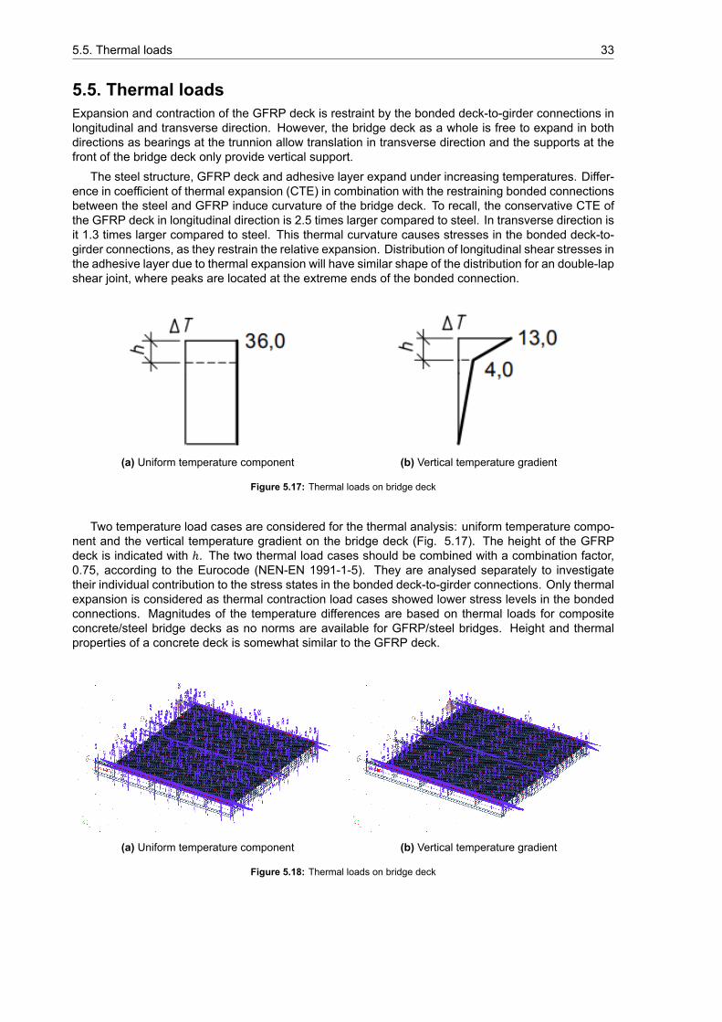
5.5. Thermal loads 33
5.5. Thermal loadsExpansion and contraction of the GFRP deck is restraint by the bonded deck-to-girder connections inlongitudinal and transverse direction. However, the bridge deck as a whole is free to expand in bothdirections as bearings at the trunnion allow translation in transverse direction and the supports at thefront of the bridge deck only provide vertical support.
The steel structure, GFRP deck and adhesive layer expand under increasing temperatures. Differ-ence in coefficient of thermal expansion (CTE) in combination with the restraining bonded connectionsbetween the steel and GFRP induce curvature of the bridge deck. To recall, the conservative CTE ofthe GFRP deck in longitudinal direction is 2.5 times larger compared to steel. In transverse direction isit 1.3 times larger compared to steel. This thermal curvature causes stresses in the bonded deck-to-girder connections, as they restrain the relative expansion. Distribution of longitudinal shear stresses inthe adhesive layer due to thermal expansion will have similar shape of the distribution for an double-lapshear joint, where peaks are located at the extreme ends of the bonded connection.
(a) Uniform temperature component (b) Vertical temperature gradient
Figure 5.17: Thermal loads on bridge deck
Two temperature load cases are considered for the thermal analysis: uniform temperature compo-nent and the vertical temperature gradient on the bridge deck (Fig. 5.17). The height of the GFRPdeck is indicated with ℎ. The two thermal load cases should be combined with a combination factor,0.75, according to the Eurocode (NEN-EN 1991-1-5). They are analysed separately to investigatetheir individual contribution to the stress states in the bonded deck-to-girder connections. Only thermalexpansion is considered as thermal contraction load cases showed lower stress levels in the bondedconnections. Magnitudes of the temperature differences are based on thermal loads for compositeconcrete/steel bridge decks as no norms are available for GFRP/steel bridges. Height and thermalproperties of a concrete deck is somewhat similar to the GFRP deck.
(a) Uniform temperature component (b) Vertical temperature gradient
Figure 5.18: Thermal loads on bridge deck
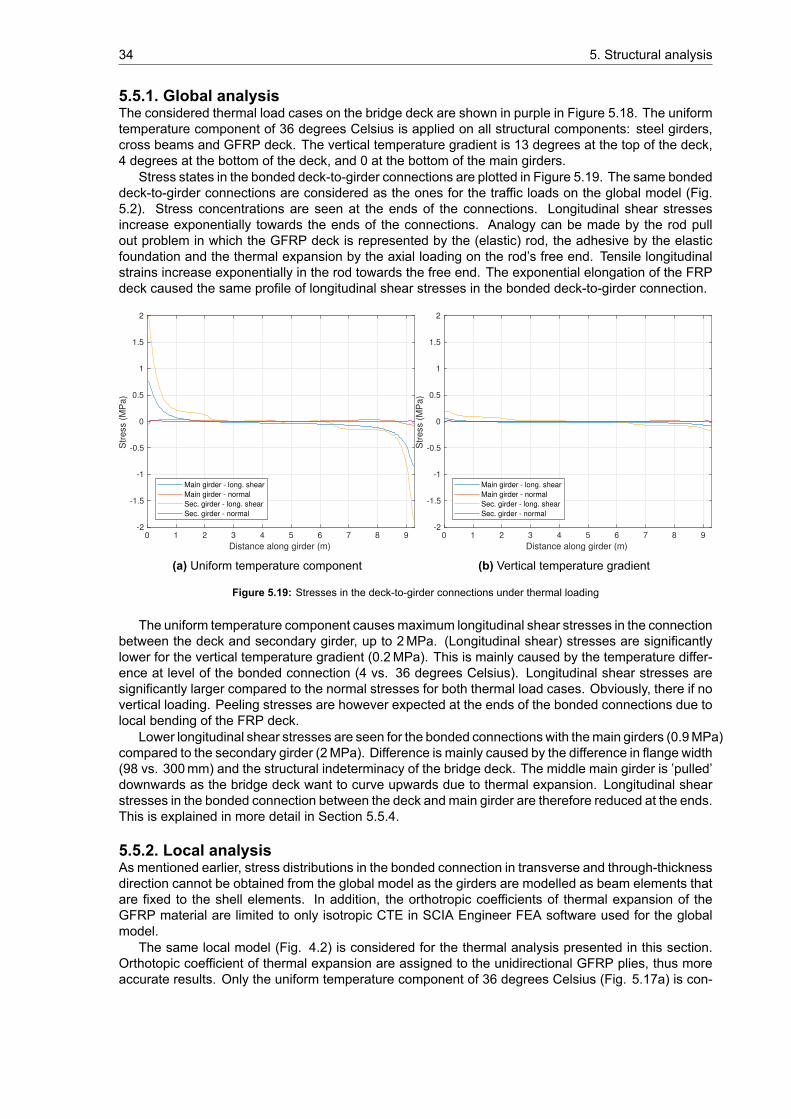
34 5. Structural analysis
5.5.1. Global analysisThe considered thermal load cases on the bridge deck are shown in purple in Figure 5.18. The uniformtemperature component of 36 degrees Celsius is applied on all structural components: steel girders,cross beams and GFRP deck. The vertical temperature gradient is 13 degrees at the top of the deck,4 degrees at the bottom of the deck, and 0 at the bottom of the main girders.
Stress states in the bonded deck-to-girder connections are plotted in Figure 5.19. The same bondeddeck-to-girder connections are considered as the ones for the traffic loads on the global model (Fig.5.2). Stress concentrations are seen at the ends of the connections. Longitudinal shear stressesincrease exponentially towards the ends of the connections. Analogy can be made by the rod pullout problem in which the GFRP deck is represented by the (elastic) rod, the adhesive by the elasticfoundation and the thermal expansion by the axial loading on the rod’s free end. Tensile longitudinalstrains increase exponentially in the rod towards the free end. The exponential elongation of the FRPdeck caused the same profile of longitudinal shear stresses in the bonded deck-to-girder connection.
0 1 2 3 4 5 6 7 8 9
Distance along girder (m)
-2
-1.5
-1
-0.5
0
0.5
1
1.5
2
Str
ess (
MP
a)
Main girder - long. shear
Main girder - normal
Sec. girder - long. shear
Sec. girder - normal
(a) Uniform temperature component
0 1 2 3 4 5 6 7 8 9
Distance along girder (m)
-2
-1.5
-1
-0.5
0
0.5
1
1.5
2
Str
ess (
MP
a)
Main girder - long. shear
Main girder - normal
Sec. girder - long. shear
Sec. girder - normal
(b) Vertical temperature gradient
Figure 5.19: Stresses in the deck-to-girder connections under thermal loading
The uniform temperature component causesmaximum longitudinal shear stresses in the connectionbetween the deck and secondary girder, up to 2MPa. (Longitudinal shear) stresses are significantlylower for the vertical temperature gradient (0.2MPa). This is mainly caused by the temperature differ-ence at level of the bonded connection (4 vs. 36 degrees Celsius). Longitudinal shear stresses aresignificantly larger compared to the normal stresses for both thermal load cases. Obviously, there if novertical loading. Peeling stresses are however expected at the ends of the bonded connections due tolocal bending of the FRP deck.
Lower longitudinal shear stresses are seen for the bonded connections with themain girders (0.9MPa)compared to the secondary girder (2MPa). Difference is mainly caused by the difference in flange width(98 vs. 300mm) and the structural indeterminacy of the bridge deck. The middle main girder is ’pulled’downwards as the bridge deck want to curve upwards due to thermal expansion. Longitudinal shearstresses in the bonded connection between the deck and main girder are therefore reduced at the ends.This is explained in more detail in Section 5.5.4.
5.5.2. Local analysisAs mentioned earlier, stress distributions in the bonded connection in transverse and through-thicknessdirection cannot be obtained from the global model as the girders are modelled as beam elements thatare fixed to the shell elements. In addition, the orthotropic coefficients of thermal expansion of theGFRP material are limited to only isotropic CTE in SCIA Engineer FEA software used for the globalmodel.
The same local model (Fig. 4.2) is considered for the thermal analysis presented in this section.Orthotopic coefficient of thermal expansion are assigned to the unidirectional GFRP plies, thus moreaccurate results. Only the uniform temperature component of 36 degrees Celsius (Fig. 5.17a) is con-
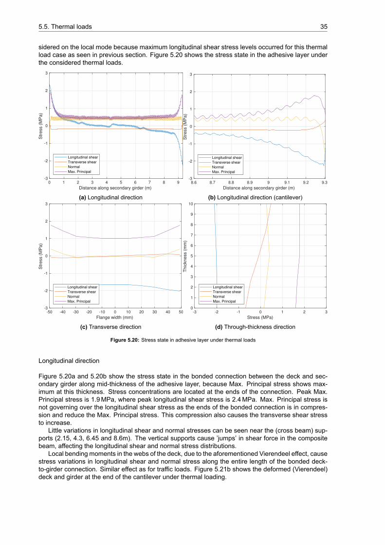
5.5. Thermal loads 35
sidered on the local mode because maximum longitudinal shear stress levels occurred for this thermalload case as seen in previous section. Figure 5.20 shows the stress state in the adhesive layer underthe considered thermal loads.
0 1 2 3 4 5 6 7 8 9
Distance along secondary girder (m)
-3
-2
-1
0
1
2
3
Str
ess (
MP
a)
Longitudinal shear
Transverse shear
Normal
Max. Principal
(a) Longitudinal direction
8.6 8.7 8.8 8.9 9 9.1 9.2 9.3
Distance along secondary girder (m)
-3
-2
-1
0
1
2
3
Str
ess (
MP
a)
Longitudinal shear
Transverse shear
Normal
Max. Principal
(b) Longitudinal direction (cantilever)
-50 -40 -30 -20 -10 0 10 20 30 40 50
Flange width (mm)
-3
-2
-1
0
1
2
3
Str
ess (
MP
a)
Longitudinal shear
Transverse shear
Normal
Max. Principal
(c) Transverse direction
-3 -2 -1 0 1 2 3
Stress (MPa)
0
1
2
3
4
5
6
7
8
9
10
Thic
kness (
mm
)
Longitudinal shear
Transverse shear
Normal
Max. Principal
(d) Through-thickness direction
Figure 5.20: Stress state in adhesive layer under thermal loads
Longitudinal direction
Figure 5.20a and 5.20b show the stress state in the bonded connection between the deck and sec-ondary girder along mid-thickness of the adhesive layer, because Max. Principal stress shows max-imum at this thickness. Stress concentrations are located at the ends of the connection. Peak Max.Principal stress is 1.9MPa, where peak longitudinal shear stress is 2.4MPa. Max. Principal stress isnot governing over the longitudinal shear stress as the ends of the bonded connection is in compres-sion and reduce the Max. Principal stress. This compression also causes the transverse shear stressto increase.
Little variations in longitudinal shear and normal stresses can be seen near the (cross beam) sup-ports (2.15, 4.3, 6.45 and 8.6m). The vertical supports cause ’jumps’ in shear force in the compositebeam, affecting the longitudinal shear and normal stress distributions.
Local bending moments in the webs of the deck, due to the aforementioned Vierendeel effect, causestress variations in longitudinal shear and normal stress along the entire length of the bonded deck-to-girder connection. Similar effect as for traffic loads. Figure 5.21b shows the deformed (Vierendeel)deck and girder at the end of the cantilever under thermal loading.
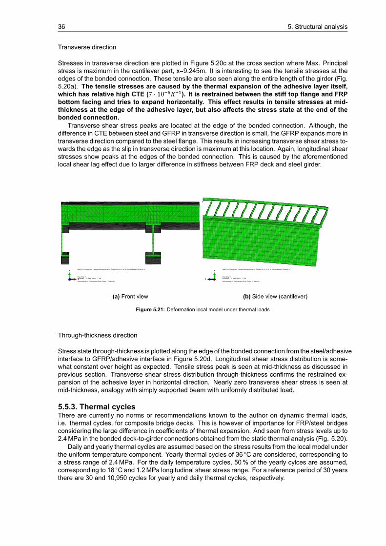
36 5. Structural analysis
Transverse direction
Stresses in transverse direction are plotted in Figure 5.20c at the cross section where Max. Principalstress is maximum in the cantilever part, x=9.245m. It is interesting to see the tensile stresses at theedges of the bonded connection. These tensile are also seen along the entire length of the girder (Fig.5.20a). The tensile stresses are caused by the thermal expansion of the adhesive layer itself,which has relative high CTE (7 ⋅ 10 𝐾 ). It is restrained between the stiff top flange and FRPbottom facing and tries to expand horizontally. This effect results in tensile stresses at mid-thickness at the edge of the adhesive layer, but also affects the stress state at the end of thebonded connection.
Transverse shear stress peaks are located at the edge of the bonded connection. Although, thedifference in CTE between steel and GFRP in transverse direction is small, the GFRP expands more intransverse direction compared to the steel flange. This results in increasing transverse shear stress to-wards the edge as the slip in transverse direction is maximum at this location. Again, longitudinal shearstresses show peaks at the edges of the bonded connection. This is caused by the aforementionedlocal shear lag effect due to larger difference in stiffness between FRP deck and steel girder.
Step: Step−1Increment 1: Step Time = 1.000
Deformed Var: U Deformation Scale Factor: +5.000e+01
ODB: TN−10−600.odb Abaqus/Standard 6.14−5 Tue Oct 23 14:17:25 W. Europe Daylight Time 2018
X
Y
Z
(a) Front view
Step: Step−1Increment 1: Step Time = 1.000
Deformed Var: U Deformation Scale Factor: +5.000e+01
ODB: TN−10−600.odb Abaqus/Standard 6.14−5 Tue Oct 23 14:17:25 W. Europe Daylight Time 2018
X
Y
Z
(b) Side view (cantilever)
Figure 5.21: Deformation local model under thermal loads
Through-thickness direction
Stress state through-thickness is plotted along the edge of the bonded connection from the steel/adhesiveinterface to GFRP/adhesive interface in Figure 5.20d. Longitudinal shear stress distribution is some-what constant over height as expected. Tensile stress peak is seen at mid-thickness as discussed inprevious section. Transverse shear stress distribution through-thickness confirms the restrained ex-pansion of the adhesive layer in horizontal direction. Nearly zero transverse shear stress is seen atmid-thickness, analogy with simply supported beam with uniformly distributed load.
5.5.3. Thermal cyclesThere are currently no norms or recommendations known to the author on dynamic thermal loads,i.e. thermal cycles, for composite bridge decks. This is however of importance for FRP/steel bridgesconsidering the large difference in coefficients of thermal expansion. And seen from stress levels up to2.4MPa in the bonded deck-to-girder connections obtained from the static thermal analysis (Fig. 5.20).
Daily and yearly thermal cycles are assumed based on the stress results from the local model underthe uniform temperature component. Yearly thermal cycles of 36 ∘C are considered, corresponding toa stress range of 2.4MPa. For the daily temperature cycles, 50% of the yearly cylces are assumed,corresponding to 18 ∘C and 1.2MPa longitudinal shear stress range. For a reference period of 30 yearsthere are 30 and 10,950 cycles for yearly and daily thermal cycles, respectively.
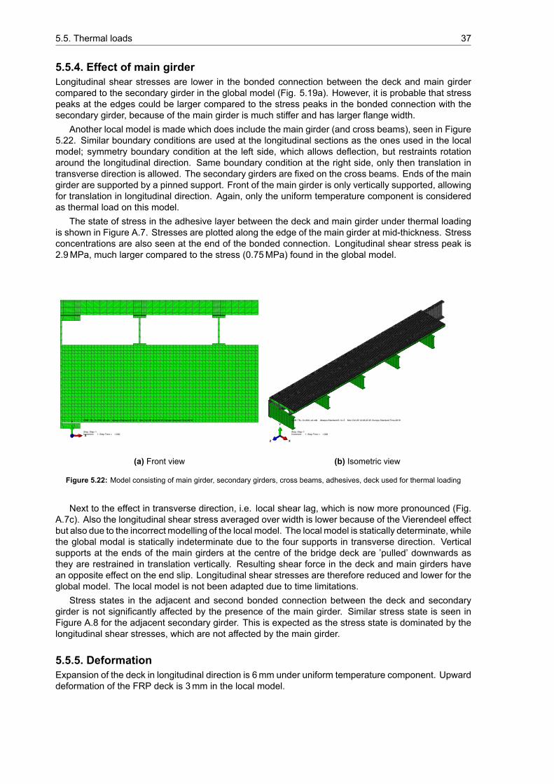
5.5. Thermal loads 37
5.5.4. Effect of main girderLongitudinal shear stresses are lower in the bonded connection between the deck and main girdercompared to the secondary girder in the global model (Fig. 5.19a). However, it is probable that stresspeaks at the edges could be larger compared to the stress peaks in the bonded connection with thesecondary girder, because of the main girder is much stiffer and has larger flange width.
Another local model is made which does include the main girder (and cross beams), seen in Figure5.22. Similar boundary conditions are used at the longitudinal sections as the ones used in the localmodel; symmetry boundary condition at the left side, which allows deflection, but restraints rotationaround the longitudinal direction. Same boundary condition at the right side, only then translation intransverse direction is allowed. The secondary girders are fixed on the cross beams. Ends of the maingirder are supported by a pinned support. Front of the main girder is only vertically supported, allowingfor translation in longitudinal direction. Again, only the uniform temperature component is consideredas thermal load on this model.
The state of stress in the adhesive layer between the deck and main girder under thermal loadingis shown in Figure A.7. Stresses are plotted along the edge of the main girder at mid-thickness. Stressconcentrations are also seen at the end of the bonded connection. Longitudinal shear stress peak is2.9MPa, much larger compared to the stress (0.75MPa) found in the global model.
Step: Step−1Increment 1: Step Time = 1.000
ODB: TN−10−600−v2.odb Abaqus/Standard 6.14−5 Mon Oct 29 12:03:23 W. Europe Standard Time 2018
X
Y
Z
(a) Front view
Step: Step−1Increment 1: Step Time = 1.000
ODB: TN−10−600−v2.odb Abaqus/Standard 6.14−5 Mon Oct 29 12:03:23 W. Europe Standard Time 2018
X
Y
Z
(b) Isometric view
Figure 5.22: Model consisting of main girder, secondary girders, cross beams, adhesives, deck used for thermal loading
Next to the effect in transverse direction, i.e. local shear lag, which is now more pronounced (Fig.A.7c). Also the longitudinal shear stress averaged over width is lower because of the Vierendeel effectbut also due to the incorrect modelling of the local model. The local model is statically determinate, whilethe global modal is statically indeterminate due to the four supports in transverse direction. Verticalsupports at the ends of the main girders at the centre of the bridge deck are ’pulled’ downwards asthey are restrained in translation vertically. Resulting shear force in the deck and main girders havean opposite effect on the end slip. Longitudinal shear stresses are therefore reduced and lower for theglobal model. The local model is not been adapted due to time limitations.
Stress states in the adjacent and second bonded connection between the deck and secondarygirder is not significantly affected by the presence of the main girder. Similar stress state is seen inFigure A.8 for the adjacent secondary girder. This is expected as the stress state is dominated by thelongitudinal shear stresses, which are not affected by the main girder.
5.5.5. DeformationExpansion of the deck in longitudinal direction is 6mm under uniform temperature component. Upwarddeformation of the FRP deck is 3mm in the local model.

38 5. Structural analysis
5.6. ConclusionsThe following conclusions can be drawn from this chapter:
• Maximum stresses occur in the bonded connection between the FRP deck and secondary girderat the cantilever end under thermal and traffic loads. Single axle load (400 kN) shows a longitu-dinal shear stress peak of 2.2MPa, while the uniform temperature component shows (36 ∘C) apeak of 2.4MPa.
• Stresses vary in longitudinal direction due to local bending moments in the webs of the FRP deck,caused by the Vierendeel effect.
• Longitudinal shear stresses in transverse direction show peaks at the edges of the bonded con-nection due to local shear lag effect. This is caused by the larger difference in stiffness of thedeck and girder.
• Effect of the main girder on the stress state in the critical bonded connection between the FRPdeck and secondary girder is negligible.
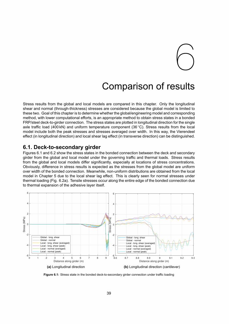
6Comparison of results
Stress results from the global and local models are compared in this chapter. Only the longitudinalshear and normal (through-thickness) stresses are considered because the global model is limited tothese two. Goal of this chapter is to determine whether the global/engineeringmodel and correspondingmethod, with lower computational efforts, is an appropriate method to obtain stress states in a bondedFRP/steel deck-to-girder connection. The stress states are plotted in longitudinal direction for the singleaxle traffic load (400 kN) and uniform temperature component (36 ∘C). Stress results from the localmodel include both the peak stresses and stresses averaged over width. In this way, the Vierendeeleffect (in longitudinal direction) and local shear lag effect (in transverse direction) can be distinguished.
6.1. Deck-to-secondary girderFigures 6.1 and 6.2 show the stress states in the bonded connection between the deck and secondarygirder from the global and local model under the governing traffic and thermal loads. Stress resultsfrom the global and local models differ significantly, especially at locations of stress concentrations.Obviously, difference in stress results is expected as the stresses from the global model are uniformover width of the bonded connection. Meanwhile, non-uniform distributions are obtained from the localmodel in Chapter 5 due to the local shear lag effect. This is clearly seen for normal stresses underthermal loading (Fig. 6.2a). Tensile stresses occur along the entire edge of the bonded connection dueto thermal expansion of the adhesive layer itself.
0 1 2 3 4 5 6 7 8 9
Distance along girder (m)
-6
-4
-2
0
2
4
6
Str
ess (
MP
a)
Global - long. shear
Global - normal
Local - long. shear (averaged)
Local - long. shear (peak)
Local - normal (averaged)
Local - normal (peak)
(a) Longitudinal direction
8.6 8.7 8.8 8.9 9 9.1 9.2 9.3
Distance along girder (m)
-6
-4
-2
0
2
4
6
Str
ess (
MP
a)
Global - long. shear
Global - normal
Local - long. shear (averaged)
Local - long. shear (peak)
Local - normal (averaged)
Local - normal (peak)
(b) Longitudinal direction (cantilever)
Figure 6.1: Stress state in the bonded deck-to-secondary girder connection under traffic loading
39
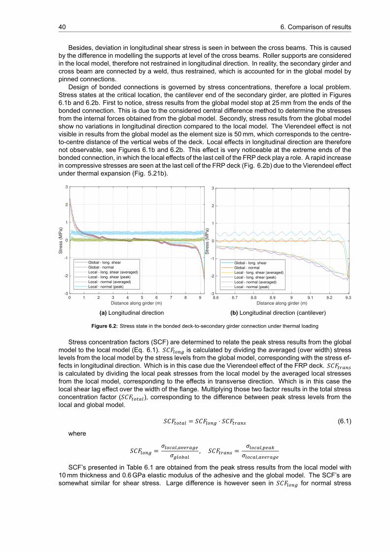
40 6. Comparison of results
Besides, deviation in longitudinal shear stress is seen in between the cross beams. This is causedby the difference in modelling the supports at level of the cross beams. Roller supports are consideredin the local model, therefore not restrained in longitudinal direction. In reality, the secondary girder andcross beam are connected by a weld, thus restrained, which is accounted for in the global model bypinned connections.
Design of bonded connections is governed by stress concentrations, therefore a local problem.Stress states at the critical location, the cantilever end of the secondary girder, are plotted in Figures6.1b and 6.2b. First to notice, stress results from the global model stop at 25mm from the ends of thebonded connection. This is due to the considered central difference method to determine the stressesfrom the internal forces obtained from the global model. Secondly, stress results from the global modelshow no variations in longitudinal direction compared to the local model. The Vierendeel effect is notvisible in results from the global model as the element size is 50mm, which corresponds to the centre-to-centre distance of the vertical webs of the deck. Local effects in longitudinal direction are thereforenot observable, see Figures 6.1b and 6.2b. This effect is very noticeable at the extreme ends of thebonded connection, in which the local effects of the last cell of the FRP deck play a role. A rapid increasein compressive stresses are seen at the last cell of the FRP deck (Fig. 6.2b) due to the Vierendeel effectunder thermal expansion (Fig. 5.21b).
0 1 2 3 4 5 6 7 8 9
Distance along girder (m)
-3
-2
-1
0
1
2
3
Str
ess (
MP
a)
Global - long. shear
Global - normal
Local - long. shear (averaged)
Local - long. shear (peak)
Local - normal (averaged)
Local - normal (peak)
(a) Longitudinal direction
8.6 8.7 8.8 8.9 9 9.1 9.2 9.3
Distance along girder (m)
-3
-2
-1
0
1
2
3
Str
ess (
MP
a)
Global - long. shear
Global - normal
Local - long. shear (averaged)
Local - long. shear (peak)
Local - normal (averaged)
Local - normal (peak)
(b) Longitudinal direction (cantilever)
Figure 6.2: Stress state in the bonded deck-to-secondary girder connection under thermal loading
Stress concentration factors (SCF) are determined to relate the peak stress results from the globalmodel to the local model (Eq. 6.1). 𝑆𝐶𝐹 is calculated by dividing the averaged (over width) stresslevels from the local model by the stress levels from the global model, corresponding with the stress ef-fects in longitudinal direction. Which is in this case due the Vierendeel effect of the FRP deck. 𝑆𝐶𝐹is calculated by dividing the local peak stresses from the local model by the averaged local stressesfrom the local model, corresponding to the effects in transverse direction. Which is in this case thelocal shear lag effect over the width of the flange. Multiplying those two factor results in the total stressconcentration factor (𝑆𝐶𝐹 ), corresponding to the difference between peak stress levels from thelocal and global model.
𝑆𝐶𝐹 = 𝑆𝐶𝐹 ⋅ 𝑆𝐶𝐹 (6.1)
where
𝑆𝐶𝐹 =𝜎 ,𝜎 , 𝑆𝐶𝐹 =
𝜎 ,𝜎 ,
SCF’s presented in Table 6.1 are obtained from the peak stress results from the local model with10mm thickness and 0.6GPa elastic modulus of the adhesive and the global model. The SCF’s aresomewhat similar for shear stress. Large difference is however seen in 𝑆𝐶𝐹 for normal stress
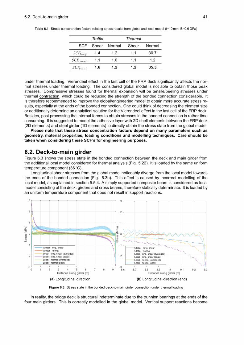
6.2. Deck-to-main girder 41
Table 6.1: Stress concentration factors relating stress results from global and local model (t=10mm, E=0.6GPa)
Traffic Thermal
SCF Shear Normal Shear Normal
𝑆𝐶𝐹 1.4 1.2 1.1 30.7
𝑆𝐶𝐹 1.1 1.0 1.1 1.2
𝑆𝐶𝐹 1.6 1.2 1.2 35.3
under thermal loading. Vierendeel effect in the last cell of the FRP deck significantly affects the nor-mal stresses under thermal loading. The considered global model is not able to obtain those peakstresses. Compressive stresses found for thermal expansion will be tensile/peeling stresses underthermal contraction, which could be reducing the strength of the bonded connection considerable. Itis therefore recommended to improve the global/engineering model to obtain more accurate stress re-sults, especially at the ends of the bonded connection. One could think of decreasing the element sizeor additionally determine an analytical solution for the Vierendeel effect in the last cell of the FRP deck.Besides, post processing the internal forces to obtain stresses in the bonded connection is rather timeconsuming. It is suggested to model the adhesive layer with 2D shell elements between the FRP deck(2D elements) and steel girder (1D elements) to directly obtain the stress state from the global model.
Please note that these stress concentration factors depend on many parameters such asgeometry, material properties, loading conditions and modelling techniques. Care should betaken when considering these SCF’s for engineering purposes.
6.2. Deck-to-main girderFigure 6.3 shows the stress state in the bonded connection between the deck and main girder fromthe additional local model considered for thermal analysis (Fig. 5.22). It is loaded by the same uniformtemperature component (36 ∘C).
Longitudinal shear stresses from the global model noticeably diverge from the local model towardsthe ends of the bonded connection (Fig. 6.3b). This effect is caused by incorrect modelling of thelocal model, as explained in section 5.5.4. A simply supported composite beam is considered as localmodel consisting of the deck, girders and cross beams, therefore statically determinate. It is loaded byan uniform temperature component that does not result in support reactions.
0 1 2 3 4 5 6 7 8 9
Distance along girder (m)
-3
-2
-1
0
1
2
3
Str
ess (
MP
a)
Global - long. shear
Global - normal
Local - long. shear (averaged)
Local - long. shear (peak)
Local - normal (averaged)
Local - normal (peak)
(a) Longitudinal direction
8.6 8.7 8.8 8.9 9 9.1 9.2 9.3
Distance along girder (m)
-3
-2
-1
0
1
2
3
Str
ess (
MP
a)
Global - long. shear
Global - normal
Local - long. shear (averaged)
Local - long. shear (peak)
Local - normal (averaged)
Local - normal (peak)
(b) Longitudinal direction (end)
Figure 6.3: Stress state in the bonded deck-to-main girder connection under thermal loading
In reality, the bridge deck is structural indeterminate due to the trunnion bearings at the ends of thefour main girders. This is correctly modelled in the global model. Vertical support reactions become
42 6. Comparison of results
non-zero due to upward curvature of the bridge deck in transverse direction under thermal expansion.Main girders in the centre of the bridge deck are ’pulled’ down, additional shear forces are induced inthe main girders. These shear forces have an opposite effect on the end slip of the deck andmain girdercompared to the thermal expansion of the GFRP deck relative to the steel girder. Result is reducedlongitudinal shear stresses near the end of the connection for the global model, which is seen in Figure6.3b. It should be noted that the CTE of the GFRP deck in transverse direction in the global model istwice as large as calculated, leading to non-conservative longitudinal shear stresses.
Apart from the difference in stress results between the global and local model, mentioned above,the local shear lag effect in transverse direction is more pronounced. The 𝑆𝐶𝐹 is 1.6 for the bondedconnection with the main girder, which is larger compared to the 1.1 found for the deck-to-secondarygirder connection (Table 6.1. It can be concluded that the stiffness of the girder which is bonded to thedeck has significantly effect on the stress distribution in transverse direction, 𝑆𝐶𝐹 .
6.3. ConclusionsThe following conclusions can be drawn from this chapter:
• Stress results from the global and local models differ significantly (up to 60% for shear stress),especially at locations of stress concentrations. Effects on local stress distributions in longitudinaland transverse direction are not obtainable in the considered global model.
• Stress concentration factors are determined to relate the stress results from the local and globalmodel; 𝑆𝐶𝐹 = 𝑆𝐶𝐹 ⋅𝑆𝐶𝐹 . Distinction is made between the longitudinal and transverseeffects, in this case Vierendeel and local shear lag effect. Total SCF for longitudinal shear stressis 1.6 for t=10mm and E=0.6GPa under traffic loading.
• Stress concentration factors depend on many parameters (modelling technique, material proper-ties, loading condition, etc.). Care should be taken when these SCF’s are considered for engi-neering purposes.
7Parametric study
Adhesive selection and geometry are important design choices for the bonded deck-to-girder connec-tions. Elastic modulus and thickness of the adhesive are the main parameters affecting the stiffnessof the bonded connection, therefore the local stress state in the adhesive layer and global behaviour,i.e. composite action. A parametric study is performed in this chapter varying adhesive thickness andelastic modulus in the local model loaded by the governing traffic and thermal loads. Goal is to deter-mine and discuss the effects of these two parameters. Additionally, stress concentration factors dueto longitudinal and transverse effects are determined as function of the two parameters investigated.Only longitudinal shear stress is considered since it is the predominant component in the Max. Prin-cipal stress states determined in Chapter 5 for both load cases. Besides, a fair comparison betweencombined stresses cannot be made. Many figures are made for this chapter. Figures relating to theresults from the thermal loading are therefore put in the appendix.
7.1. Shear stiffnessRelation between the shear stress, elastic modulus and thicknessof an isotropic adhesive element loaded in shear is given in Equa-tion 7.4. This equation is derived from the kinematic (Eq. 7.1),constitutive (Eq. 7.2) and material (Eq. 7.3) relations. It can beconcluded that the shear stress is proportional to the elastic mod-ulus and inversely proportional to the adhesive thickness. Samerelations hold for the bonded deck-to-girder connection, where 𝐺corresponds to its shear stiffness, 𝑡 to adhesive thickness, 𝜏 to av-erage lap shear stress and Δ𝑥 to the relative horizontal displace-ment between the bottom facing and top flange.
𝛾 = Δ𝑥𝑡 (7.1)
𝜏 = 𝐺𝛾 (7.2)
𝐺 = 𝐸2(1 + 𝜈) (7.3)
𝜏 = 𝐸2(1 + 𝜈)
Δ𝑥𝑡 (7.4)
7.2. Effect of adhesive thicknessFigures 7.1 and A.1 show the longitudinal shear stress distributions in the adhesive layer for four differ-ent adhesive thicknesses. As mentioned before, these stress results are from the local model (Fig. 4.2)under the single axle load (400 kN) and uniform temperature component (36 ∘C). Adhesive thicknessesfrom 5 to 20mm are assumed to be representative for (movable) bridges with bonded deck-to-girderconnections. In addition, 1mm thickness is considered as geometrical imperfections and toleranceproblems can be expected in real structures. The longitudinal shear stress distributions in the bondedconnections between deck and secondary girder are determined for 1, 5, 10 and 20mm adhesive thick-ness. Stresses in longitudinal direction, seen in Figures 7.1a and A.1a, are plotted along the edge ofthe secondary girder. Stresses in transverse direction, seen in Figures 7.1b and A.1b, are plotted atcross section with maximum longitudinal shear stress, i.e. x=8.99m and x=9.295m resp. for trafficand thermal loading. Note that the adhesive elastic modulus of 0.6GPa and other material propertiesremained the same.
43
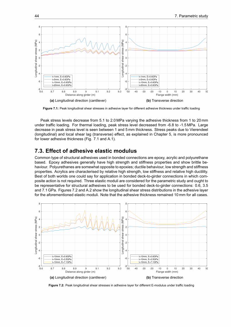
44 7. Parametric study
8.6 8.7 8.8 8.9 9 9.1 9.2 9.3
Distance along girder (m)
-8
-6
-4
-2
0
2
4
6
8
Longitudin
al shear
str
ess (
MP
a)
t=1mm, E=0.6GPa
t=5mm, E=0.6GPa
t=10mm, E=0.6GPa
t=20mm, E=0.6GPa
(a) Longitudinal direction (cantilever)
-50 -40 -30 -20 -10 0 10 20 30 40 50
Flange width (mm)
-8
-6
-4
-2
0
2
4
6
8
Longitudin
al shear
str
ess (
MP
a)
t=1mm, E=0.6GPa
t=5mm, E=0.6GPa
t=10mm, E=0.6GPa
t=20mm, E=0.6GPa
(b) Transverse direction
Figure 7.1: Peak longitudinal shear stresses in adhesive layer for different adhesive thickness under traffic loading
Peak stress levels decrease from 5.1 to 2.0MPa varying the adhesive thickness from 1 to 20mmunder traffic loading. For thermal loading, peak stress level decreased from -6.8 to -1.5MPa. Largedecrease in peak stress level is seen between 1 and 5mm thickness. Stress peaks due to Vierendeel(longitudinal) and local shear lag (transverse) effect, as explained in Chapter 5, is more pronouncedfor lower adhesive thickness (Fig. 7.1 and A.1).
7.3. Effect of adhesive elastic modulusCommon type of structural adhesives used in bonded connections are epoxy, acrylic and polyurethanebased. Epoxy adhesives generally have high strength and stiffness properties and show brittle be-haviour. Polyurethanes are somewhat opposite to epoxies; ductile behaviour, low strength and stiffnessproperties. Acrylics are characterised by relative high strength, low stiffness and relative high ductility.Best of both worlds one could say for application in bonded deck-to-girder connections in which com-posite action is not required. Three elastic moduli are considered for the parametric study and ought tobe representative for structural adhesives to be used for bonded deck-to-girder connections: 0.6, 3.5and 7.1GPa. Figures 7.2 and A.2 show the longitudinal shear stress distributions in the adhesive layerfor the aforementioned elastic moduli. Note that the adhesive thickness remained 10mm for all cases.
8.6 8.7 8.8 8.9 9 9.1 9.2 9.3
Distance along girder (m)
-8
-6
-4
-2
0
2
4
6
8
Longitudin
al shear
str
ess (
MP
a)
t=10mm, E=0.6GPa
t=10mm, E=3.5GPa
t=10mm, E=7.1GPa
(a) Longitudinal direction (cantilever)
-50 -40 -30 -20 -10 0 10 20 30 40 50
Flange width (mm)
-8
-6
-4
-2
0
2
4
6
8
Longitudin
al shear
str
ess (
MP
a)
t=10mm, E=0.6GPa
t=10mm, E=3.5GPa
t=10mm, E=7.1GPa
(b) Transverse direction
Figure 7.2: Peak longitudinal shear stresses in adhesive layer for different E-modulus under traffic loading

7.4. Extreme cases 45
Peak stress levels increase from 2.2 to 6.3MPa for increasing adhesive elastic modulus from 0.6to 7.1GPa under traffic loads, while for thermal loads an increase from -2.3 to -6.2MPa is obtained.Again, next to increase of total peak stresses, stress peaks due to longitudinal and transverse effectsbecome more pronounced as seen in Figures 7.1 and A.1.
7.4. Extreme casesTwo extreme cases, based on results from previous sections, are considered to determine the longi-tudinal shear stress distributions with the combined effect of adhesive thickness and elastic modulusresulting in the expected lowest and largest stress peak levels. The two extreme cases consists of(1) t=1mm and E=7.1GPa, and (2) t=20mm and E=0.6GPa. Figures 7.3 and 7.4 show the stressdistributions in longitudinal and transverse direction under respectively traffic and thermal loading.
8.6 8.7 8.8 8.9 9 9.1 9.2 9.3
Distance along girder (m)
-20
-15
-10
-5
0
5
10
15
20
Lo
ng
itu
din
al she
ar
str
ess (
MP
a)
t=1mm, E=7.1GPa
t=20mm, E=0.6GPa
(a) Longitudinal direction (cantilever)
-50 -40 -30 -20 -10 0 10 20 30 40 50
Flange width (mm)
-20
-15
-10
-5
0
5
10
15
20
Lo
ng
itu
din
al she
ar
str
ess (
MP
a)
t=1mm, E=7.1GPa
t=20mm, E=0.6GPa
(b) Transverse direction
Figure 7.3: Peak longitudinal shear stresses in adhesive layer for two extreme cases under traffic loading
As expected, significant increase is peak stress levels seen between the extreme cases. Stresspeak levels increase from 2 to 14MPa under traffic loading. An increase of -1.5 to -17MPa is seen forthermal loading. The local shear lag and Vierendeel effect is this time very noticeable (Fig. 7.3 and7.4).
8.6 8.7 8.8 8.9 9 9.1 9.2 9.3
Distance along girder (m)
-20
-15
-10
-5
0
5
10
15
20
Lo
ng
itu
din
al sh
ea
r str
ess (
MP
a)
t=1mm, E=7.1GPa
t=20mm, E=0.6GPa
(a) Longitudinal direction (cantilever)
-50 -40 -30 -20 -10 0 10 20 30 40 50
Flange width (mm)
-20
-15
-10
-5
0
5
10
15
20
Lo
ng
itu
din
al sh
ea
r str
ess (
MP
a)
t=1mm, E=7.1GPa
t=20mm, E=0.6GPa
(b) Transverse direction
Figure 7.4: Peak longitudinal shear stresses in adhesive layer for two extreme cases under thermal loading
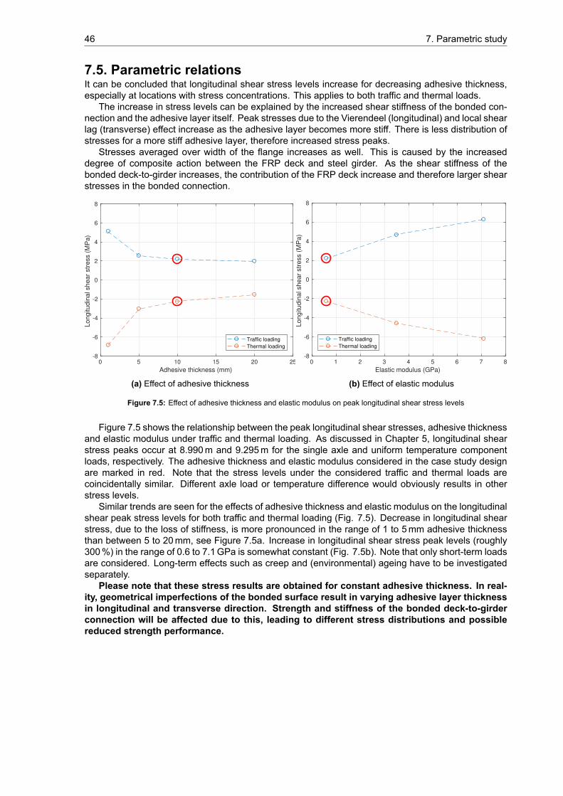
46 7. Parametric study
7.5. Parametric relationsIt can be concluded that longitudinal shear stress levels increase for decreasing adhesive thickness,especially at locations with stress concentrations. This applies to both traffic and thermal loads.
The increase in stress levels can be explained by the increased shear stiffness of the bonded con-nection and the adhesive layer itself. Peak stresses due to the Vierendeel (longitudinal) and local shearlag (transverse) effect increase as the adhesive layer becomes more stiff. There is less distribution ofstresses for a more stiff adhesive layer, therefore increased stress peaks.
Stresses averaged over width of the flange increases as well. This is caused by the increaseddegree of composite action between the FRP deck and steel girder. As the shear stiffness of thebonded deck-to-girder increases, the contribution of the FRP deck increase and therefore larger shearstresses in the bonded connection.
0 5 10 15 20 25
Adhesive thickness (mm)
-8
-6
-4
-2
0
2
4
6
8
Longitudin
al shear
str
ess (
MP
a)
Traffic loading
Thermal loading
(a) Effect of adhesive thickness
0 1 2 3 4 5 6 7 8
Elastic modulus (GPa)
-8
-6
-4
-2
0
2
4
6
8
Lo
ng
itu
din
al sh
ea
r str
ess (
MP
a)
Traffic loading
Thermal loading
(b) Effect of elastic modulus
Figure 7.5: Effect of adhesive thickness and elastic modulus on peak longitudinal shear stress levels
Figure 7.5 shows the relationship between the peak longitudinal shear stresses, adhesive thicknessand elastic modulus under traffic and thermal loading. As discussed in Chapter 5, longitudinal shearstress peaks occur at 8.990m and 9.295m for the single axle and uniform temperature componentloads, respectively. The adhesive thickness and elastic modulus considered in the case study designare marked in red. Note that the stress levels under the considered traffic and thermal loads arecoincidentally similar. Different axle load or temperature difference would obviously results in otherstress levels.
Similar trends are seen for the effects of adhesive thickness and elastic modulus on the longitudinalshear peak stress levels for both traffic and thermal loading (Fig. 7.5). Decrease in longitudinal shearstress, due to the loss of stiffness, is more pronounced in the range of 1 to 5mm adhesive thicknessthan between 5 to 20mm, see Figure 7.5a. Increase in longitudinal shear stress peak levels (roughly300%) in the range of 0.6 to 7.1GPa is somewhat constant (Fig. 7.5b). Note that only short-term loadsare considered. Long-term effects such as creep and (environmental) ageing have to be investigatedseparately.
Please note that these stress results are obtained for constant adhesive thickness. In real-ity, geometrical imperfections of the bonded surface result in varying adhesive layer thicknessin longitudinal and transverse direction. Strength and stiffness of the bonded deck-to-girderconnection will be affected due to this, leading to different stress distributions and possiblereduced strength performance.
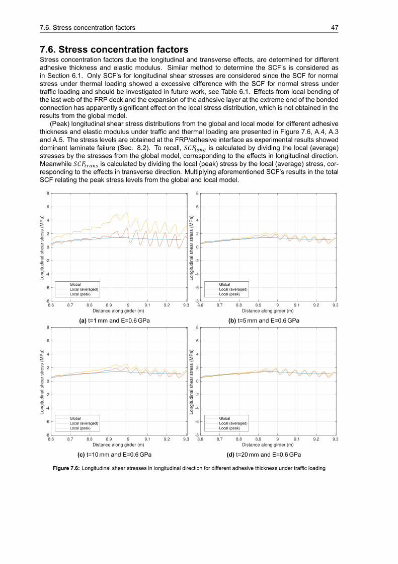
7.6. Stress concentration factors 47
7.6. Stress concentration factorsStress concentration factors due the longitudinal and transverse effects, are determined for differentadhesive thickness and elastic modulus. Similar method to determine the SCF’s is considered asin Section 6.1. Only SCF’s for longitudinal shear stresses are considered since the SCF for normalstress under thermal loading showed a excessive difference with the SCF for normal stress undertraffic loading and should be investigated in future work, see Table 6.1. Effects from local bending ofthe last web of the FRP deck and the expansion of the adhesive layer at the extreme end of the bondedconnection has apparently significant effect on the local stress distribution, which is not obtained in theresults from the global model.
(Peak) longitudinal shear stress distributions from the global and local model for different adhesivethickness and elastic modulus under traffic and thermal loading are presented in Figure 7.6, A.4, A.3and A.5. The stress levels are obtained at the FRP/adhesive interface as experimental results showeddominant laminate failure (Sec. 8.2). To recall, 𝑆𝐶𝐹 is calculated by dividing the local (average)stresses by the stresses from the global model, corresponding to the effects in longitudinal direction.Meanwhile 𝑆𝐶𝐹 is calculated by dividing the local (peak) stress by the local (average) stress, cor-responding to the effects in transverse direction. Multiplying aforementioned SCF’s results in the totalSCF relating the peak stress levels from the global and local model.
8.6 8.7 8.8 8.9 9 9.1 9.2 9.3
Distance along girder (m)
-8
-6
-4
-2
0
2
4
6
8
Longitudin
al shear
str
ess (
MP
a)
Global
Local (averaged)
Local (peak)
(a) t=1mm and E=0.6GPa
8.6 8.7 8.8 8.9 9 9.1 9.2 9.3
Distance along girder (m)
-8
-6
-4
-2
0
2
4
6
8Longitudin
al shear
str
ess (
MP
a)
Global
Local (averaged)
Local (peak)
(b) t=5mm and E=0.6GPa
8.6 8.7 8.8 8.9 9 9.1 9.2 9.3
Distance along girder (m)
-8
-6
-4
-2
0
2
4
6
8
Longitudin
al shear
str
ess (
MP
a)
Global
Local (averaged)
Local (peak)
(c) t=10mm and E=0.6GPa
8.6 8.7 8.8 8.9 9 9.1 9.2 9.3
Distance along girder (m)
-8
-6
-4
-2
0
2
4
6
8
Longitudin
al shear
str
ess (
MP
a)
Global
Local (averaged)
Local (peak)
(d) t=20mm and E=0.6GPa
Figure 7.6: Longitudinal shear stresses in longitudinal direction for different adhesive thickness under traffic loading
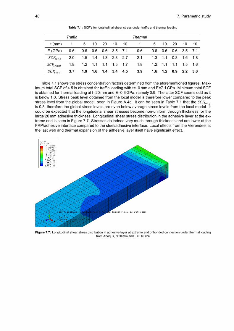
48 7. Parametric study
Table 7.1: SCF’s for longitudinal shear stress under traffic and thermal loading
Traffic Thermal
t (mm) 1 5 10 20 10 10 1 5 10 20 10 10
E (GPa) 0.6 0.6 0.6 0.6 3.5 7.1 0.6 0.6 0.6 0.6 3.5 7.1
𝑆𝐶𝐹 2.0 1.5 1.4 1.3 2.3 2.7 2.1 1.3 1.1 0.8 1.6 1.8
𝑆𝐶𝐹 1.8 1.2 1.1 1.1 1.5 1.7 1.8 1.2 1.1 1.1 1.5 1.6
𝑆𝐶𝐹 3.7 1.9 1.6 1.4 3.4 4.5 3.9 1.6 1.2 0.9 2.2 3.0
Table 7.1 shows the stress concentration factors determined from the aforementioned figures. Max-imum total SCF of 4.5 is obtained for traffic loading with t=10mm and E=7.1GPa. Minimum total SCFis obtained for thermal loading at t=20mm and E=0.6GPa, namely 0.9. The latter SCF seems odd as itis below 1.0. Stress peak level obtained from the local model is therefore lower compared to the peakstress level from the global model, seen in Figure A.4d. It can be seen in Table 7.1 that the 𝑆𝐶𝐹is 0.8, therefore the global stress levels are even below average stress levels from the local model. Itcould be expected that the longitudinal shear stresses become non-uniform through thickness for thelarge 20mm adhesive thickness. Longitudinal shear stress distribution in the adhesive layer at the ex-treme end is seen in Figure 7.7. Stresses do indeed vary much through-thickness and are lower at theFRP/adhesive interface compared to the steel/adhesive interface. Local effects from the Vierendeel atthe last web and thermal expansion of the adhesive layer itself have significant effect.
Figure 7.7: Longitudinal shear stress distribution in adhesive layer at extreme end of bonded connection under thermal loadingfrom Abaqus, t=20mm and E=0.6GPa
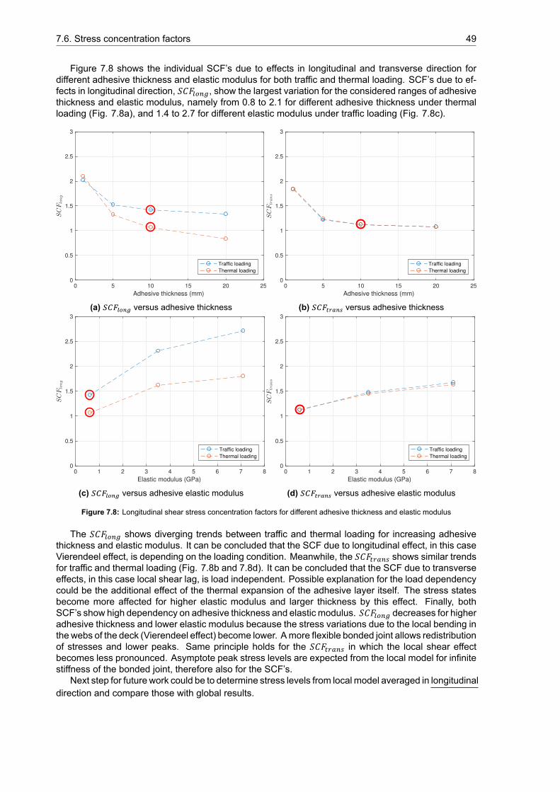
7.6. Stress concentration factors 49
Figure 7.8 shows the individual SCF’s due to effects in longitudinal and transverse direction fordifferent adhesive thickness and elastic modulus for both traffic and thermal loading. SCF’s due to ef-fects in longitudinal direction, 𝑆𝐶𝐹 , show the largest variation for the considered ranges of adhesivethickness and elastic modulus, namely from 0.8 to 2.1 for different adhesive thickness under thermalloading (Fig. 7.8a), and 1.4 to 2.7 for different elastic modulus under traffic loading (Fig. 7.8c).
0 5 10 15 20 25
Adhesive thickness (mm)
0
0.5
1
1.5
2
2.5
3
Traffic loading
Thermal loading
(a) versus adhesive thickness
0 5 10 15 20 25
Adhesive thickness (mm)
0
0.5
1
1.5
2
2.5
3
Traffic loading
Thermal loading
(b) versus adhesive thickness
0 1 2 3 4 5 6 7 8
Elastic modulus (GPa)
0
0.5
1
1.5
2
2.5
3
Traffic loading
Thermal loading
(c) versus adhesive elastic modulus
0 1 2 3 4 5 6 7 8
Elastic modulus (GPa)
0
0.5
1
1.5
2
2.5
3
Traffic loading
Thermal loading
(d) versus adhesive elastic modulus
Figure 7.8: Longitudinal shear stress concentration factors for different adhesive thickness and elastic modulus
The 𝑆𝐶𝐹 shows diverging trends between traffic and thermal loading for increasing adhesivethickness and elastic modulus. It can be concluded that the SCF due to longitudinal effect, in this caseVierendeel effect, is depending on the loading condition. Meanwhile, the 𝑆𝐶𝐹 shows similar trendsfor traffic and thermal loading (Fig. 7.8b and 7.8d). It can be concluded that the SCF due to transverseeffects, in this case local shear lag, is load independent. Possible explanation for the load dependencycould be the additional effect of the thermal expansion of the adhesive layer itself. The stress statesbecome more affected for higher elastic modulus and larger thickness by this effect. Finally, bothSCF’s show high dependency on adhesive thickness and elastic modulus. 𝑆𝐶𝐹 decreases for higheradhesive thickness and lower elastic modulus because the stress variations due to the local bending inthe webs of the deck (Vierendeel effect) become lower. Amore flexible bonded joint allows redistributionof stresses and lower peaks. Same principle holds for the 𝑆𝐶𝐹 in which the local shear effectbecomes less pronounced. Asymptote peak stress levels are expected from the local model for infinitestiffness of the bonded joint, therefore also for the SCF’s.
Next step for future work could be to determine stress levels from local model averaged in longitudinaldirection and compare those with global results.
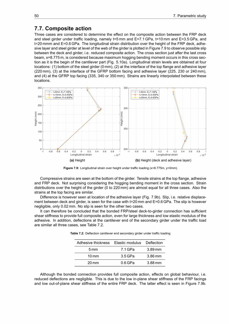
50 7. Parametric study
7.7. Composite actionThree cases are considered to determine the effect on the composite action between the FRP deckand steel girder under traffic loading, namely t=5mm and E=7.1GPa, t=10mm and E=3.5GPa, andt=20mmm and E=0.6GPa. The longitudinal strain distribution over the height of the FRP deck, adhe-sive layer and steel girder at level of the web of the girder is plotted in Figure 7.9 to observe possible slipbetween the deck and girder, i.e. reduced composite action. The cross section just after the last crossbeam, x=8.775m, is considered because maximum hogging bending moment occurs in this cross sec-tion as it is the begin of the cantilever part (Fig. 5.10a). Longitudinal strain levels are obtained at fourlocations: (1) bottom of the steel girder (0mm), (2) at the interface of the top flange and adhesive layer(220mm), (3) at the interface of the GFRP bottom facing and adhesive layer (225, 230 or 240mm),and (4) at the GFRP top facing (335, 340 or 350mm). Strains are linearly interpolated between theselocations.
-1 -0.8 -0.6 -0.4 -0.2 0 0.2 0.4 0.6 0.8 1
Longitudinal strain 10-3
0
50
100
150
200
250
300
350
He
igh
t (m
m)
t=5mm, E=7.1GPa
t=10mm, E=3.5GPa
t=20mm, E=0.6GPa
(a) Height
-1 -0.8 -0.6 -0.4 -0.2 0 0.2 0.4 0.6 0.8 1
Longitudinal strain 10-3
200
250
300
350
He
igh
t (m
m)
t=5mm, E=7.1GPa
t=10mm, E=3.5GPa
t=20mm, E=0.6GPa
(b) Height (deck and adhesive layer)
Figure 7.9: Longitudinal strain over height under traffic loading (x=8.775m, y=0mm)
Compressive strains are seen at the bottom of the girder. Tensile strains at the top flange, adhesiveand FRP deck. Not surprising considering the hogging bending moment in the cross section. Straindistributions over the height of the girder (0 to 220mm) are almost equal for all three cases. Also thestrains at the top facing are similar.
Difference is however seen at location of the adhesive layer (Fig. 7.9b). Slip, i.e. relative displace-ment between deck and girder, is seen for the case with t=20mm and E=0.6GPa. The slip is howevernegligible, only 0.02mm. No slip is seen for the other two cases.
It can therefore be concluded that the bonded FRP/steel deck-to-girder connection has sufficientshear stiffness to provide full composite action, even for large thickness and low elastic modulus of theadhesive. In addition, deflections at the cantilever end of the secondary girder under the traffic loadare similar all three cases, see Table 7.2.
Table 7.2: Deflection cantilever end secondary girder under traffic loading
Adhesive thickness Elastic modulus Deflection
5mm 7.1GPa 3.89mm
10mm 3.5GPa 3.86mm
20mm 0.6GPa 3.88mm
Although the bonded connection provides full composite action, effects on global behaviour, i.e.reduced deflections are negligible. This is due to the low in-plane shear stiffness of the FRP facingsand low out-of-plane shear stiffness of the entire FRP deck. The latter effect is seen in Figure 7.9b.
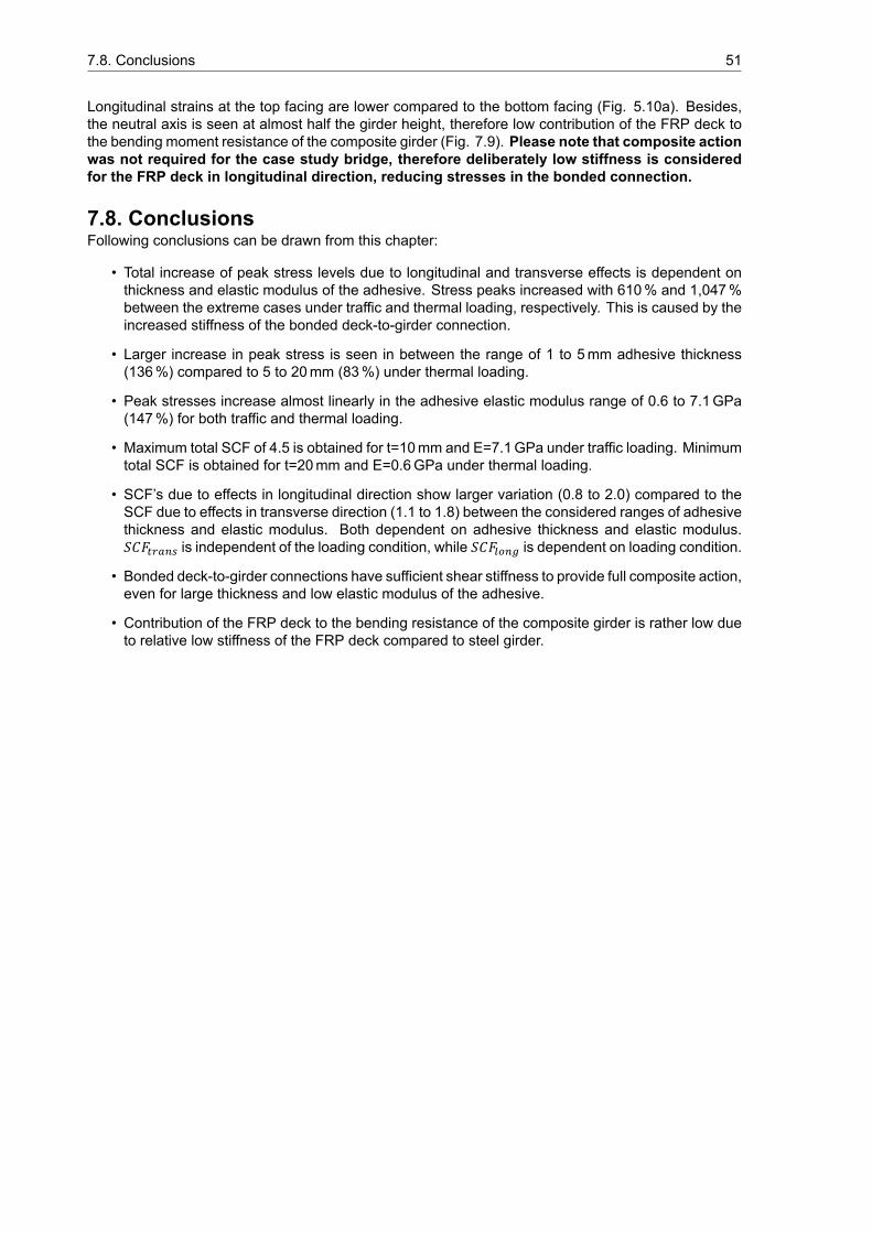
7.8. Conclusions 51
Longitudinal strains at the top facing are lower compared to the bottom facing (Fig. 5.10a). Besides,the neutral axis is seen at almost half the girder height, therefore low contribution of the FRP deck tothe bending moment resistance of the composite girder (Fig. 7.9). Please note that composite actionwas not required for the case study bridge, therefore deliberately low stiffness is consideredfor the FRP deck in longitudinal direction, reducing stresses in the bonded connection.
7.8. ConclusionsFollowing conclusions can be drawn from this chapter:
• Total increase of peak stress levels due to longitudinal and transverse effects is dependent onthickness and elastic modulus of the adhesive. Stress peaks increased with 610% and 1,047%between the extreme cases under traffic and thermal loading, respectively. This is caused by theincreased stiffness of the bonded deck-to-girder connection.
• Larger increase in peak stress is seen in between the range of 1 to 5mm adhesive thickness(136%) compared to 5 to 20mm (83%) under thermal loading.
• Peak stresses increase almost linearly in the adhesive elastic modulus range of 0.6 to 7.1GPa(147%) for both traffic and thermal loading.
• Maximum total SCF of 4.5 is obtained for t=10mm and E=7.1GPa under traffic loading. Minimumtotal SCF is obtained for t=20mm and E=0.6GPa under thermal loading.
• SCF’s due to effects in longitudinal direction show larger variation (0.8 to 2.0) compared to theSCF due to effects in transverse direction (1.1 to 1.8) between the considered ranges of adhesivethickness and elastic modulus. Both dependent on adhesive thickness and elastic modulus.𝑆𝐶𝐹 is independent of the loading condition, while 𝑆𝐶𝐹 is dependent on loading condition.
• Bonded deck-to-girder connections have sufficient shear stiffness to provide full composite action,even for large thickness and low elastic modulus of the adhesive.
• Contribution of the FRP deck to the bending resistance of the composite girder is rather low dueto relative low stiffness of the FRP deck compared to steel girder.

8Strength performance
8.1. Required strengthThe required (static) strength of the considered bonded GFRP/steel deck-to-girder connection is de-termined based on the stress results from the structural analysis in Chapter 5 and literature on fatiguestrength from Chapter 2.
5.4MPa
100 102 104 106 108
Number of cycles
100
101
Longitudin
al shear
str
ess r
ange (
MP
a)
Global model - FLM4b
Global model (*SCF) - FLM4b
Required fatigue strength
Figure 8.1: Fatigue shear stress ranges from global model under FLM4band required lap shear fatigue strength
Peak longitudinal shear stress levelof 2.2MPa is obtained in the bondedconnection between the FRP deck andsteel secondary girder under the singleaxle load (400 kN) from the local model(Fig. 5.6b). In addition, the stress con-centration factors obtained from thecomparison of stress results from theglobal and local model (Table 6.1)are used to tweak the fatigue shearstress ranges obtained from the globalmodel under FLM4b (Fig. 5.12). Thestress concentration factor for longitu-dinal shear stresses is 1.6 consider-ing the local model with adhesive thick-ness 10mmand 0.6GPa elastic modu-lus. The tweaked fatigue stresses arepresented in Figure 2.7. The verticalposition of the slope is set such that thetotal fatigue damage is equal to 1. Thefatigue damage is calculated accord-ing to Palmgren-Miner rule assuming aconstant slope of 1:10, obtained from the work of Keller [11] and Khabbaz [12].
Static strength is generally lower compared to the dynamic strength, i.e. fatigue strength at N=1,due to the difference in failure mechanism/mode. This is also in the experimental results from Khabbaz[12]. Static strength values seen in Figure 2.7b are lower compared to the extrapolated S-N curve(dashed line) according to the power model, namely 40 kN versus 28 kN static strength (marked in blacktriangles). This is roughly 70% of the static strength. If similar ratio between static and dynamicstrength is considered applied on the required fatigue lap shear strength shown in Figure 5.12b,the required static lap shear strength of the bonded GFRP/steel deck-to-girder connection is inthe range of 4 to 5MPa.
The assumed stress ranges due to the thermal cycles from Section 5.5.3 had negligible effect on therequired lap shear strength, namely 5.41MPa compared to 5.40MPa without thermal cycles. Requirefatigue normal strength, i.e. tension or compression, is not determined because there no data known tothe author on the possible S-N curve for fatigue performance of bonded GFRP joints in mode 1 loading.
53
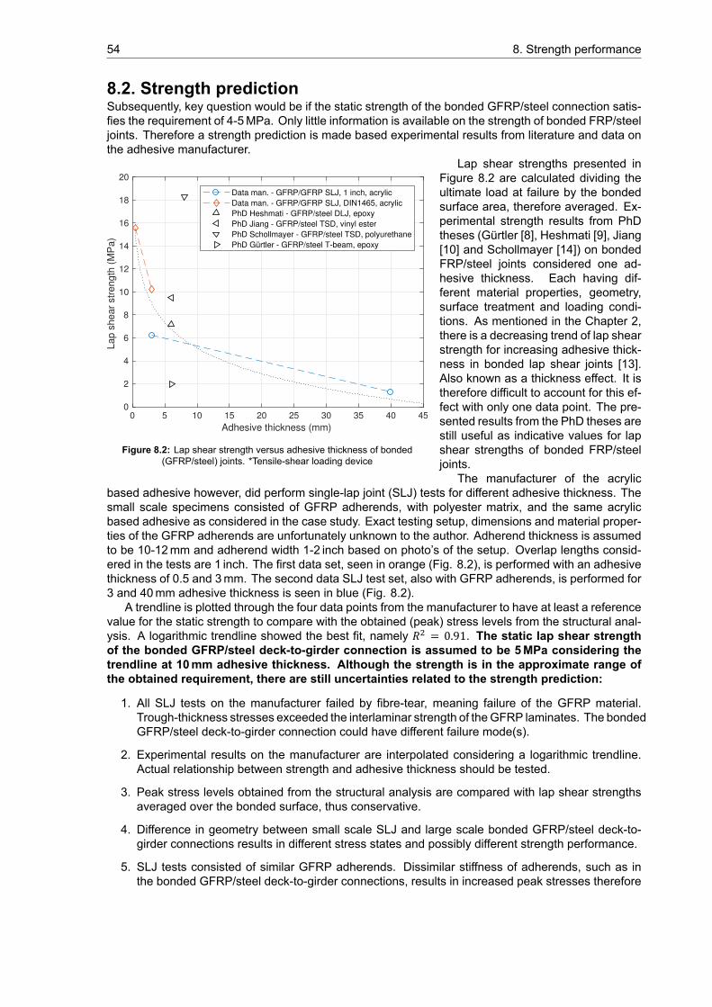
54 8. Strength performance
8.2. Strength predictionSubsequently, key question would be if the static strength of the bonded GFRP/steel connection satis-fies the requirement of 4-5MPa. Only little information is available on the strength of bonded FRP/steeljoints. Therefore a strength prediction is made based experimental results from literature and data onthe adhesive manufacturer.
0 5 10 15 20 25 30 35 40 45
Adhesive thickness (mm)
0
2
4
6
8
10
12
14
16
18
20
La
p s
he
ar
str
en
gth
(M
Pa
)
Data man. - GFRP/GFRP SLJ, 1 inch, acrylic
Data man. - GFRP/GFRP SLJ, DIN1465, acrylic
PhD Heshmati - GFRP/steel DLJ, epoxy
PhD Jiang - GFRP/steel TSD, vinyl ester
PhD Schollmayer - GFRP/steel TSD, polyurethane
PhD Gürtler - GFRP/steel T-beam, epoxy
Figure 8.2: Lap shear strength versus adhesive thickness of bonded(GFRP/steel) joints. *Tensile-shear loading device
Lap shear strengths presented inFigure 8.2 are calculated dividing theultimate load at failure by the bondedsurface area, therefore averaged. Ex-perimental strength results from PhDtheses (Gürtler [8], Heshmati [9], Jiang[10] and Schollmayer [14]) on bondedFRP/steel joints considered one ad-hesive thickness. Each having dif-ferent material properties, geometry,surface treatment and loading condi-tions. As mentioned in the Chapter 2,there is a decreasing trend of lap shearstrength for increasing adhesive thick-ness in bonded lap shear joints [13].Also known as a thickness effect. It istherefore difficult to account for this ef-fect with only one data point. The pre-sented results from the PhD theses arestill useful as indicative values for lapshear strengths of bonded FRP/steeljoints.
The manufacturer of the acrylicbased adhesive however, did perform single-lap joint (SLJ) tests for different adhesive thickness. Thesmall scale specimens consisted of GFRP adherends, with polyester matrix, and the same acrylicbased adhesive as considered in the case study. Exact testing setup, dimensions and material proper-ties of the GFRP adherends are unfortunately unknown to the author. Adherend thickness is assumedto be 10-12mm and adherend width 1-2 inch based on photo’s of the setup. Overlap lengths consid-ered in the tests are 1 inch. The first data set, seen in orange (Fig. 8.2), is performed with an adhesivethickness of 0.5 and 3mm. The second data SLJ test set, also with GFRP adherends, is performed for3 and 40mm adhesive thickness is seen in blue (Fig. 8.2).
A trendline is plotted through the four data points from the manufacturer to have at least a referencevalue for the static strength to compare with the obtained (peak) stress levels from the structural anal-ysis. A logarithmic trendline showed the best fit, namely 𝑅 = 0.91. The static lap shear strengthof the bonded GFRP/steel deck-to-girder connection is assumed to be 5MPa considering thetrendline at 10mm adhesive thickness. Although the strength is in the approximate range ofthe obtained requirement, there are still uncertainties related to the strength prediction:
1. All SLJ tests on the manufacturer failed by fibre-tear, meaning failure of the GFRP material.Trough-thickness stresses exceeded the interlaminar strength of theGFRP laminates. The bondedGFRP/steel deck-to-girder connection could have different failure mode(s).
2. Experimental results on the manufacturer are interpolated considering a logarithmic trendline.Actual relationship between strength and adhesive thickness should be tested.
3. Peak stress levels obtained from the structural analysis are compared with lap shear strengthsaveraged over the bonded surface, thus conservative.
4. Difference in geometry between small scale SLJ and large scale bonded GFRP/steel deck-to-girder connections results in different stress states and possibly different strength performance.
5. SLJ tests consisted of similar GFRP adherends. Dissimilar stiffness of adherends, such as inthe bonded GFRP/steel deck-to-girder connections, results in increased peak stresses therefore
8.3. Recommendation for experimental program 55
reducing strength performance.
6. Bonded deck-to-girder connections are multi-axially loaded, while the SLJ tests are uni-axiallyloaded. Complex stress states in the bonded FRP/steel deck-to-girder connection might showlower strength performance.
8.3. Recommendation for experimental programIdeally, one would determine the strength of the bonded FRP/steel deck-to-girder connection in a largescale test to obtain the most accurate results and determine coupled global and local behaviour. Theauthor suggest a more cost and time effective experimental program to determine the static and fatiguestrength of a bonded FRP/steel deck-to-girder connection.
It includes static and fatigue tests on a bonded FRP/steel double-lap joint (DLJ) for various adhe-sive thickness, in which the inner adherend is steel and the outer adherends from FRP material. DLJis considered because the stress state is somewhat similar to the one found in the deck-to-girder con-nection, i.e. dominant longitudinal shear stress. Single-lap joints (SLJ) show larger peeling stresseswhich reduce strength performance as explained in Chapter 2.
Material properties of the adhesive and adherends should be determined prior to the joint teststo obtain a detailed stress distribution in the bonded connection using FEA. This comprises elastic,strength and thermal properties. Emphasis should be put on the interlaminar (shear) strength of theFRP laminates as it is shown to be the governing parameter in the fatigue tests performed by themanufacturer.
Static strength tests of the DLJ should be performed for different under both tension and compres-sion loading to account for different failure modes. Khabbaz [12] observed similar failure modes forcorresponding fatigue loading, i.e. R-ratios. DLJ specimens with different overlap lengths would beneeded to determine the asymptote that would lead to experimentally determined static peak strength.ASTM D3528 could be considered as standard for DLJ tests.
When it comes to fatigue strength, the author suggest to perform fatigue tests on the same DLJat constant amplitude load ranges at 30, 50 and 70% of the static strength determined from the staticDLJ tests under various R-ratios, let’s say R=-1, R=0.1 and R=10. And again for various adhesivethickness. Similar test setup is recommended as Khabbaz has used [12] (Fig. 2.6) or same setup asmentioned above. In this way, the load-life or S-N diagram can be constructed and be used for fatigueanalysis depending on different adhesive thickness and R-ratio.
Lastly, it is recommended to experimentally determine the static and fatigue tensile strengths.Thereby the strength performance is covered for both mode 1 and mode 2 of the bonded connection.Ideally, mixed modes tests are performed considering the complex stress states in the deck-to-girderconnections. Tensile-shear loading devices as used by Schollmayer [14] and Jiang [10] can be con-sidered.
8.4. ConclusionsThe following conclusions can be drawn from this chapter:
• The required static lap shear strength of the bonded GFRP/steel deck-to-girder connection is inthe range of 4 to 5MPa based on the fatigue analysis performed on the global model includingthe derived SCF.
• The predicted static lap shear strength is 5MPa based on GFRP/GFRP SLJ tests with various ad-hesive thickness. Although the strength is in the approximate range of the obtained requirement,there are still uncertainties related to the laminate failure.
• Stresses from the local model should be determined at the FRP/adhesive interface, as failure otthe SLJ specimens was governed by laminate failure.

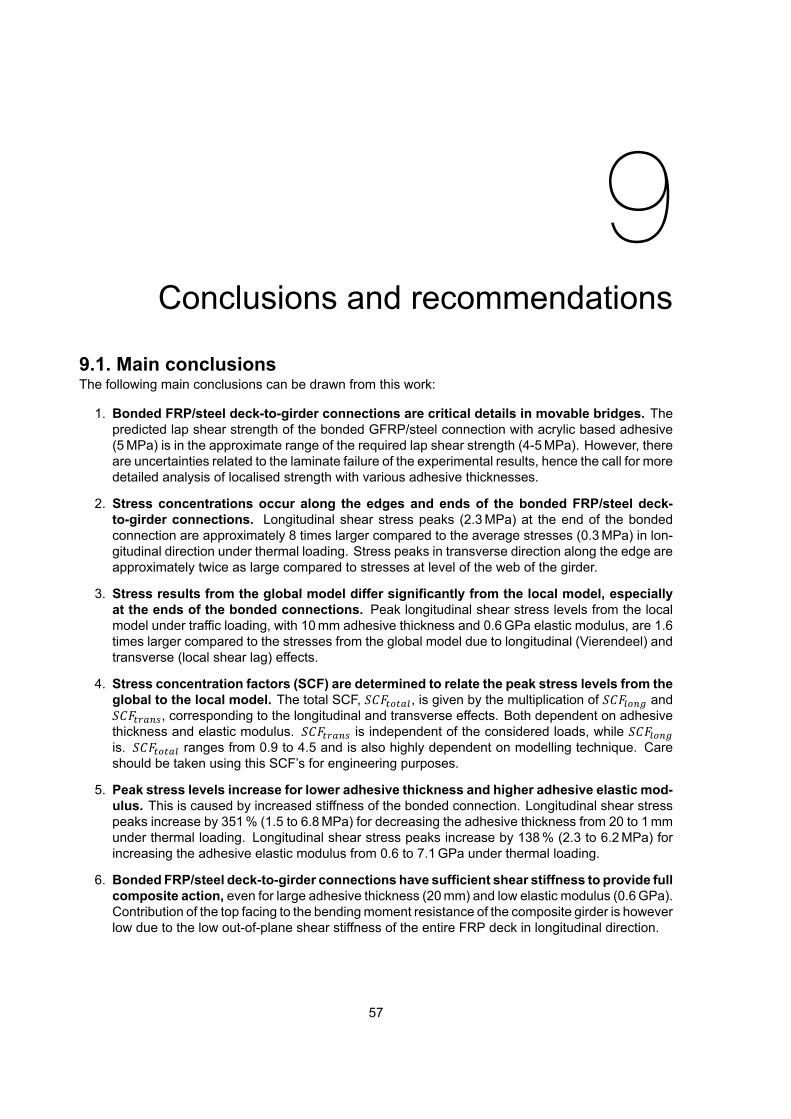
9Conclusions and recommendations
9.1. Main conclusionsThe following main conclusions can be drawn from this work:
1. Bonded FRP/steel deck-to-girder connections are critical details in movable bridges. Thepredicted lap shear strength of the bonded GFRP/steel connection with acrylic based adhesive(5MPa) is in the approximate range of the required lap shear strength (4-5MPa). However, thereare uncertainties related to the laminate failure of the experimental results, hence the call for moredetailed analysis of localised strength with various adhesive thicknesses.
2. Stress concentrations occur along the edges and ends of the bonded FRP/steel deck-to-girder connections. Longitudinal shear stress peaks (2.3MPa) at the end of the bondedconnection are approximately 8 times larger compared to the average stresses (0.3MPa) in lon-gitudinal direction under thermal loading. Stress peaks in transverse direction along the edge areapproximately twice as large compared to stresses at level of the web of the girder.
3. Stress results from the global model differ significantly from the local model, especiallyat the ends of the bonded connections. Peak longitudinal shear stress levels from the localmodel under traffic loading, with 10mm adhesive thickness and 0.6GPa elastic modulus, are 1.6times larger compared to the stresses from the global model due to longitudinal (Vierendeel) andtransverse (local shear lag) effects.
4. Stress concentration factors (SCF) are determined to relate the peak stress levels from theglobal to the local model. The total SCF, 𝑆𝐶𝐹 , is given by the multiplication of 𝑆𝐶𝐹 and𝑆𝐶𝐹 , corresponding to the longitudinal and transverse effects. Both dependent on adhesivethickness and elastic modulus. 𝑆𝐶𝐹 is independent of the considered loads, while 𝑆𝐶𝐹is. 𝑆𝐶𝐹 ranges from 0.9 to 4.5 and is also highly dependent on modelling technique. Careshould be taken using this SCF’s for engineering purposes.
5. Peak stress levels increase for lower adhesive thickness and higher adhesive elastic mod-ulus. This is caused by increased stiffness of the bonded connection. Longitudinal shear stresspeaks increase by 351% (1.5 to 6.8MPa) for decreasing the adhesive thickness from 20 to 1mmunder thermal loading. Longitudinal shear stress peaks increase by 138% (2.3 to 6.2MPa) forincreasing the adhesive elastic modulus from 0.6 to 7.1GPa under thermal loading.
6. Bonded FRP/steel deck-to-girder connections have sufficient shear stiffness to provide fullcomposite action, even for large adhesive thickness (20mm) and low elastic modulus (0.6GPa).Contribution of the top facing to the bendingmoment resistance of the composite girder is howeverlow due to the low out-of-plane shear stiffness of the entire FRP deck in longitudinal direction.
57

58 9. Conclusions and recommendations
9.2. RecommendationsFollowing aspects could be considered in future work:
• Improve modelling technique for global/engineering models to obtain a more detailed stress statein the bonded deck-to-girder connections, especially at the ends.
• Experimentally determine the static and fatigue strength of bonded FRP/steel joints under bothtensile and shear loading conditions with various adhesive thickness.
• Determine the effects of geometrical imperfections on strength and stiffness performance of ad-hesively bonded FRP/steel connections.
• Include short-term, long-term and environmental effects on strength performance of bonded FRP/steelconnections such as curing, ageing, creep, freeze-thaw cycles, temperature, moisture, etc.
• Determine recommendations/norms on thermal load cycles for composite FRP/steel bridges.
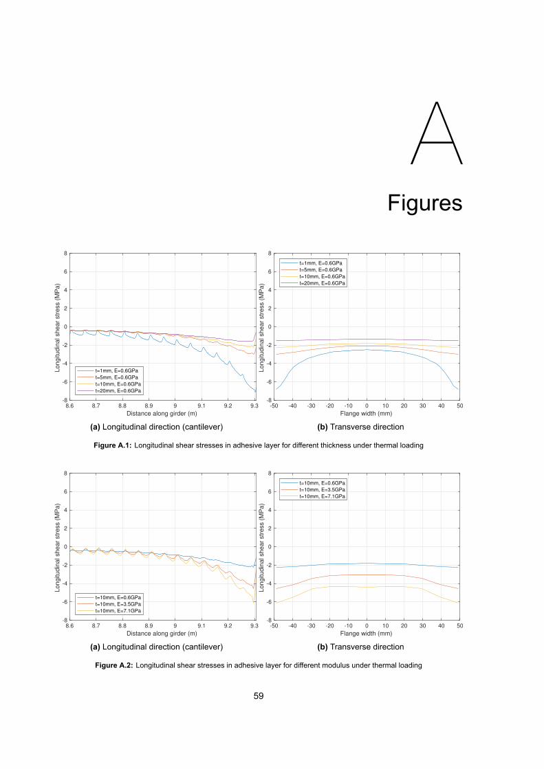
AFigures
8.6 8.7 8.8 8.9 9 9.1 9.2 9.3
Distance along girder (m)
-8
-6
-4
-2
0
2
4
6
8
Longitudin
al shear
str
ess (
MP
a)
t=1mm, E=0.6GPa
t=5mm, E=0.6GPa
t=10mm, E=0.6GPa
t=20mm, E=0.6GPa
(a) Longitudinal direction (cantilever)
-50 -40 -30 -20 -10 0 10 20 30 40 50
Flange width (mm)
-8
-6
-4
-2
0
2
4
6
8
Longitudin
al shear
str
ess (
MP
a)
t=1mm, E=0.6GPa
t=5mm, E=0.6GPa
t=10mm, E=0.6GPa
t=20mm, E=0.6GPa
(b) Transverse direction
Figure A.1: Longitudinal shear stresses in adhesive layer for different thickness under thermal loading
8.6 8.7 8.8 8.9 9 9.1 9.2 9.3
Distance along girder (m)
-8
-6
-4
-2
0
2
4
6
8
Longitudin
al shear
str
ess (
MP
a)
t=10mm, E=0.6GPa
t=10mm, E=3.5GPa
t=10mm, E=7.1GPa
(a) Longitudinal direction (cantilever)
-50 -40 -30 -20 -10 0 10 20 30 40 50
Flange width (mm)
-8
-6
-4
-2
0
2
4
6
8
Longitudin
al shear
str
ess (
MP
a)
t=10mm, E=0.6GPa
t=10mm, E=3.5GPa
t=10mm, E=7.1GPa
(b) Transverse direction
Figure A.2: Longitudinal shear stresses in adhesive layer for different modulus under thermal loading
59
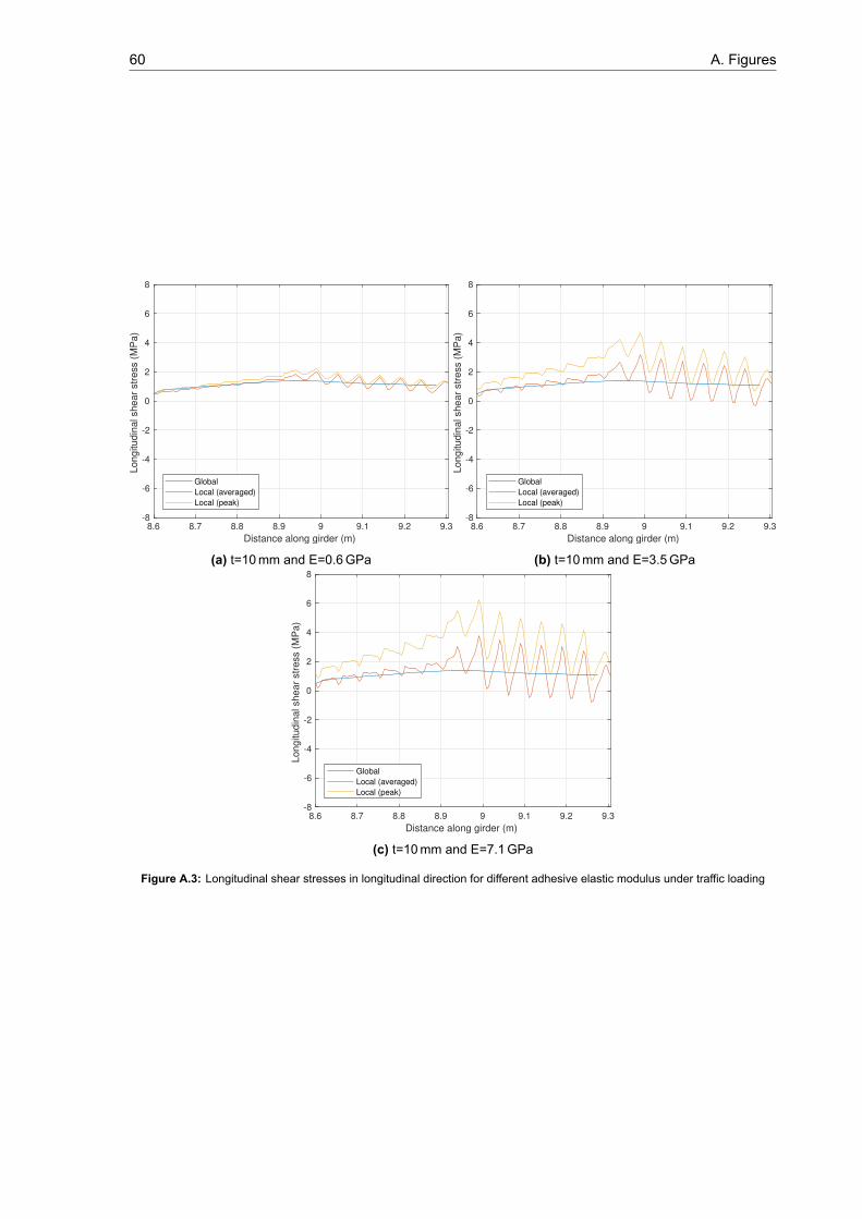
60 A. Figures
8.6 8.7 8.8 8.9 9 9.1 9.2 9.3
Distance along girder (m)
-8
-6
-4
-2
0
2
4
6
8
Longitudin
al shear
str
ess (
MP
a)
Global
Local (averaged)
Local (peak)
(a) t=10mm and E=0.6GPa
8.6 8.7 8.8 8.9 9 9.1 9.2 9.3
Distance along girder (m)
-8
-6
-4
-2
0
2
4
6
8
Longitudin
al shear
str
ess (
MP
a)
Global
Local (averaged)
Local (peak)
(b) t=10mm and E=3.5GPa
8.6 8.7 8.8 8.9 9 9.1 9.2 9.3
Distance along girder (m)
-8
-6
-4
-2
0
2
4
6
8
Longitudin
al shear
str
ess (
MP
a)
Global
Local (averaged)
Local (peak)
(c) t=10mm and E=7.1GPa
Figure A.3: Longitudinal shear stresses in longitudinal direction for different adhesive elastic modulus under traffic loading
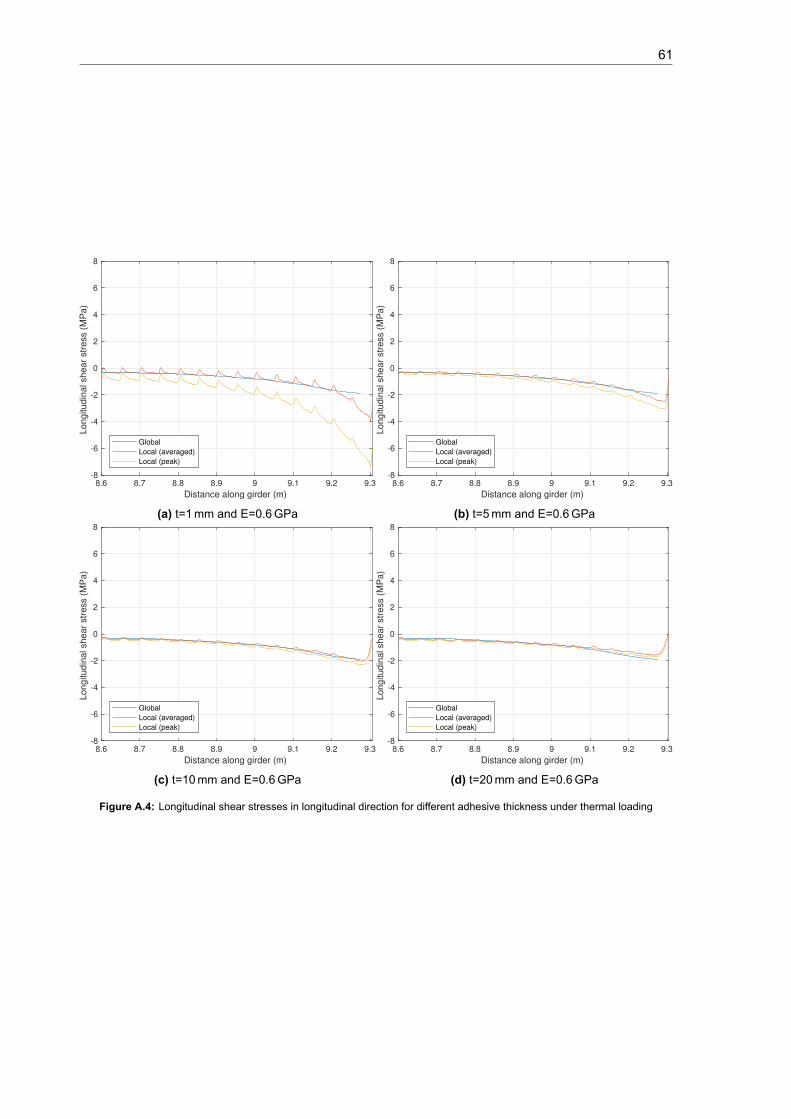
61
8.6 8.7 8.8 8.9 9 9.1 9.2 9.3
Distance along girder (m)
-8
-6
-4
-2
0
2
4
6
8
Longitudin
al shear
str
ess (
MP
a)
Global
Local (averaged)
Local (peak)
(a) t=1mm and E=0.6GPa
8.6 8.7 8.8 8.9 9 9.1 9.2 9.3
Distance along girder (m)
-8
-6
-4
-2
0
2
4
6
8
Longitudin
al shear
str
ess (
MP
a)
Global
Local (averaged)
Local (peak)
(b) t=5mm and E=0.6GPa
8.6 8.7 8.8 8.9 9 9.1 9.2 9.3
Distance along girder (m)
-8
-6
-4
-2
0
2
4
6
8
Longitudin
al shear
str
ess (
MP
a)
Global
Local (averaged)
Local (peak)
(c) t=10mm and E=0.6GPa
8.6 8.7 8.8 8.9 9 9.1 9.2 9.3
Distance along girder (m)
-8
-6
-4
-2
0
2
4
6
8
Longitudin
al shear
str
ess (
MP
a)
Global
Local (averaged)
Local (peak)
(d) t=20mm and E=0.6GPa
Figure A.4: Longitudinal shear stresses in longitudinal direction for different adhesive thickness under thermal loading
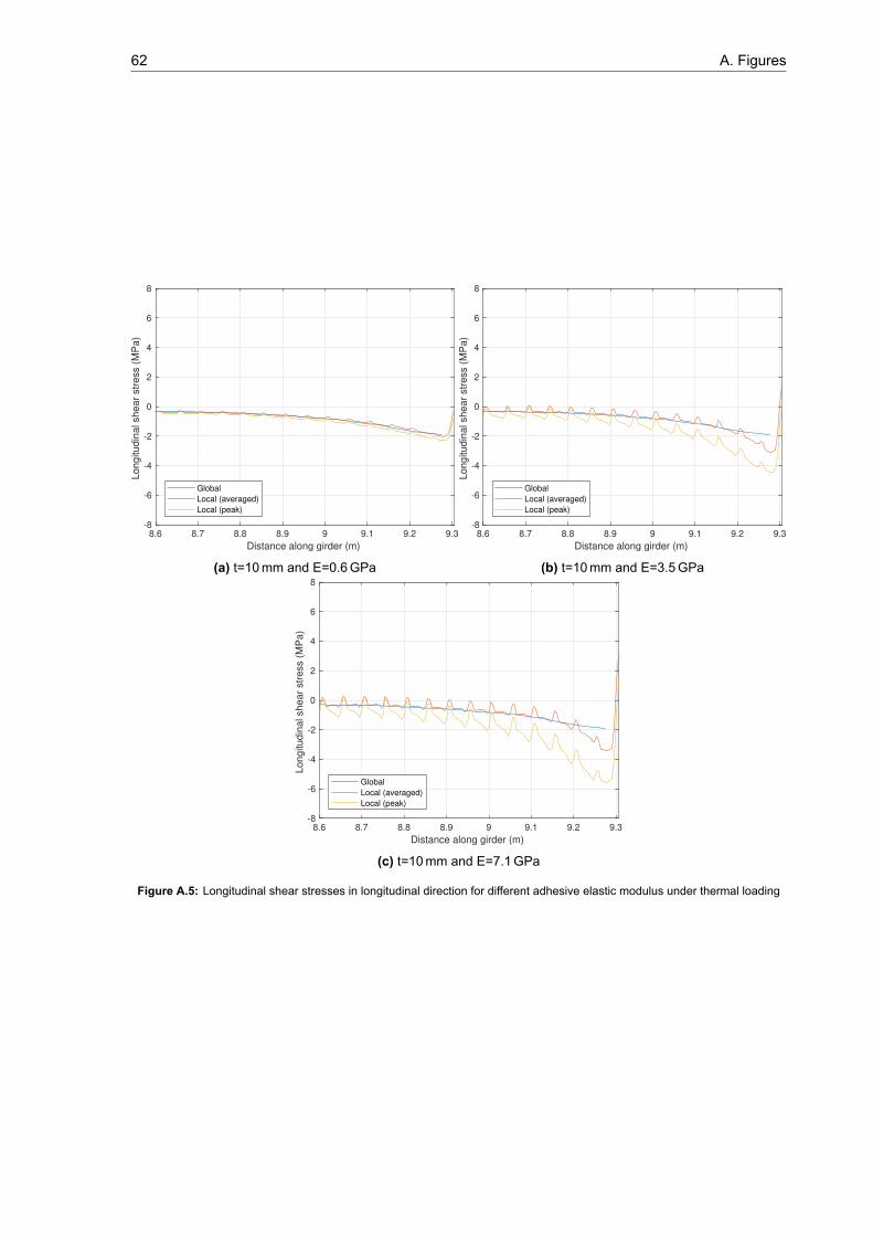
62 A. Figures
8.6 8.7 8.8 8.9 9 9.1 9.2 9.3
Distance along girder (m)
-8
-6
-4
-2
0
2
4
6
8
Longitudin
al shear
str
ess (
MP
a)
Global
Local (averaged)
Local (peak)
(a) t=10mm and E=0.6GPa
8.6 8.7 8.8 8.9 9 9.1 9.2 9.3
Distance along girder (m)
-8
-6
-4
-2
0
2
4
6
8
Longitudin
al shear
str
ess (
MP
a)
Global
Local (averaged)
Local (peak)
(b) t=10mm and E=3.5GPa
8.6 8.7 8.8 8.9 9 9.1 9.2 9.3
Distance along girder (m)
-8
-6
-4
-2
0
2
4
6
8
Longitudin
al shear
str
ess (
MP
a)
Global
Local (averaged)
Local (peak)
(c) t=10mm and E=7.1GPa
Figure A.5: Longitudinal shear stresses in longitudinal direction for different adhesive elastic modulus under thermal loading
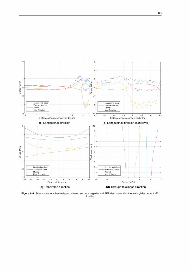
63
6.5 7 7.5 8 8.5 9
Distance along secondary girder (m)
-6
-4
-2
0
2
4
6
Str
ess (
MP
a)
Longitudinal shear
Transverse shear
Normal
Max. Principal
(a) Longitudinal direction
8.6 8.7 8.8 8.9 9 9.1 9.2 9.3
Distance along secondary girder (m)
-6
-4
-2
0
2
4
6
Str
ess (
MP
a)
Longitudinal shear
Transverse shear
Normal
Max. Principal
(b) Longitudinal direction (cantilever)
-50 -40 -30 -20 -10 0 10 20 30 40 50
Flange width (mm)
-3
-2
-1
0
1
2
3
Str
ess (
MP
a)
Longitudinal shear
Transverse shear
Normal
Max. Principal
(c) Transverse direction
-3 -2 -1 0 1 2 3
Stress (MPa)
0
1
2
3
4
5
6
7
8
9
10
Thic
kness (
mm
)
Longitudinal shear
Transverse shear
Normal
Max. Principal
(d) Through-thickness direction
Figure A.6: Stress state in adhesive layer between secondary girder and FRP deck second to the main girder under trafficloading
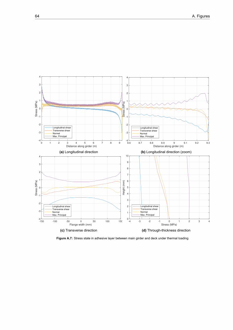
64 A. Figures
0 1 2 3 4 5 6 7 8 9
Distance along girder (m)
-4
-3
-2
-1
0
1
2
3
4
Str
ess (
MP
a)
Longitudinal shear
Transverse shear
Normal
Max. Principal
(a) Longitudinal direction
8.6 8.7 8.8 8.9 9 9.1 9.2 9.3
Distance along girder (m)
-4
-3
-2
-1
0
1
2
3
4
Str
ess (
MP
a)
Longitudinal shear
Transverse shear
Normal
Max. Principal
(b) Longitudinal direction (zoom)
-150 -100 -50 0 50 100 150
Flange width (mm)
-4
-3
-2
-1
0
1
2
3
4
Str
ess (
MP
a)
Longitudinal shear
Transverse shear
Normal
Max. Principal
(c) Transverse direction
-4 -3 -2 -1 0 1 2 3 4
Stress (MPa)
0
1
2
3
4
5
6
7
8
9
10
Heig
ht (m
m)
Longitudinal shear
Transverse shear
Normal
Max. Principal
(d) Through-thickness direction
Figure A.7: Stress state in adhesive layer between main girder and deck under thermal loading
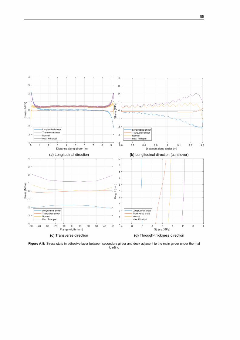
65
0 1 2 3 4 5 6 7 8 9
Distance along girder (m)
-4
-3
-2
-1
0
1
2
3
4
Str
ess (
MP
a)
Longitudinal shear
Transverse shear
Normal
Max. Principal
(a) Longitudinal direction
8.6 8.7 8.8 8.9 9 9.1 9.2 9.3
Distance along girder (m)
-4
-3
-2
-1
0
1
2
3
4
Str
ess (
MP
a)
Longitudinal shear
Transverse shear
Normal
Max. Principal
(b) Longitudinal direction (cantilever)
-50 -40 -30 -20 -10 0 10 20 30 40 50
Flange width (mm)
-4
-3
-2
-1
0
1
2
3
4
Str
ess (
MP
a)
Longitudinal shear
Transverse shear
Normal
Max. Principal
(c) Transverse direction
-4 -3 -2 -1 0 1 2 3 4
Stress (MPa)
0
1
2
3
4
5
6
7
8
9
10
Heig
ht (m
m)
Longitudinal shear
Transverse shear
Normal
Max. Principal
(d) Through-thickness direction
Figure A.8: Stress state in adhesive layer between secondary girder and deck adjacent to the main girder under thermalloading

Bibliography[1] Abaqus 6.14 documentation, 2014. URL http://ivt-abaqusdoc.ivt.ntnu.no:2080/v6.
14/books/usi/default.htm.
[2] Kwekersbrug, 2017. URL https://deskgram.org/p/1504987829817505663_1445028526.
[3] Scia engineer composite design steel-concrete composite structures, 2017. URL https://help.scia.net/download/17.0/en/CompositeDesign_enu.pdf.
[4] Scigrip technical datasheet sg230 hv methacrylate adhesive, 2017. URL https://scigrip.com/assets/tds/SG230HV-TDS-US-0417.pdf.
[5] F. Csillag. Demountable deck-to-girder connection of frp-steel hybrid bridges. Master’s thesis,Delft University of Technology, 2018.
[6] Lucas F.M. da Silva et al. Analytical models of adhesively bonded joints-part 1: Literature survey.International Journal of Adhesion Adhesives, 2008.
[7] Lucas F.M. da Silva et al. Analytical models of adhesively bonded joints-part 2: Comparativestudy. International Journal of Adhesion Adhesives, 2008.
[8] H.W. Gürtler. Composite Action of FRP Bridge Decks Adhesively Bonded to Steel Main Girder.PhD thesis, ÉCOLE POLYTECHNIQUE FÉDÉRALE DE LAUSANNE, December 2004.
[9] M. Heshmati. Durability and Long-term Performance of Adhesively Bonded FRP/steel Joints. PhDthesis, Chalmers University of Technology, 2017.
[10] X. Jiang. Mechanical Behaviour and Durability of FRP-to-steel Adhesively-bonded Joints. PhDthesis, Delft University of Technology, 2013.
[11] T. Keller and T. Tirelli. Fatigue behavior of adhesively connected pultruded gfrp profiles. CompositeStructures 65, 2004.
[12] R. Sarfaraz Khabbaz. Fatigue Life Prediction of Adhesively-Bonded Fiber-Reinforced PolymerStructural Joints under Spectrum Loading Patterns. PhD thesis, ÉCOLE POLYTECHNIQUEFÉDÉRALE DE LAUSANNE, December 2012.
[13] Roy Aries P. Tarigan Kuncoro Diharjo, Miftahul Anwar and Ahmad Rivai. Effect of Adhesive Thick-ness and Surface Treatment to Shear Strength on Single Lap Joint AL/CFRP Using Adhesive ofEpoxy/Al-fine-powder. PhD thesis, Sebelas Maret University, Indonesia, 2016.
[14] M. Schollmayer. Through-Thickness Performance of Adhesive Connections Between FRP BridgeDecks and Steel Main Girders. PhD thesis, ÉCOLE POLYTECHNIQUE FÉDÉRALE DE LAU-SANNE, February 2009.
[15] A.P. Vassilopoulos and T. Keller. Fatigue of Fiber-reinforced Composites. Springer, 2011.
[16] Y. Zhang. Fracture and Fatigue of Adhesively-Bonded Fiber-Reinforced Polymer Structural Joints.PhD thesis, ÉCOLE POLYTECHNIQUE FÉDÉRALE DE LAUSANNE, April 2010.
67