bioeconomic analysis of the shrimp trawl fishery in the tonkin gulf, vietnam
TRANSCRIPT
BIOECONOMIC ANALYSIS OF THE SHRIMP TRAWL FISHERY IN THE
TONKIN GULF, VIETNAM
NGUYEN VIET THANH
A THESIS SUBMITTED IN PARTIAL FULFILLMENT OF
THE REQUIREMENTS FOR THE DEGREE OF MASTER OF
SCIENCE OF THE UNIVERSITY OF TROMSO
MAY, 2006
DEPARTMENT OF ECONOMICS
THE NORWEGIAN COLLEGE OF FISHERY SCIENCE
UNIVERSITY OF TROMS∅
9037 TROMSO, NORWAY

ii
Cover picture:
The Fisheries Harbor in Hong Gai town, Halong Bay (Tonkin Gulf), Vietnam (Source: http://www.terragalleria.com/vietnam/vietnam.halong.html)
iii
Abstract
The objective of this study is to investigate the sustainability properties of the stock and
management of the shrimp trawl fishery in the Tonkin Gulf, Vietnam. Surplus production
models of Verhulst-Schaefer and Gompertz-Fox are applied to the shrimp trawl fishery,
which is a typical tropical fishery with the characteristic properties of small scale and
multi-species fisheries. There are two shrimp spawning seasons per year in the Gulf. This
implies that it is appropriate to divide the time scale into a half year in accordance with the
biological year of the stock. The surplus production models which are usually associated
with calendar year catch and effort data, in this study are applied for a half year time
interval data. Empirical data were collected from the enumerator project (ALRMV), which
was supported by DANIDA and carried out in Vietnam from 2000 to 2004. The catch and
effort data aggregated from the data of the project were monthly collected by the
questionnaire methodology in local fishing ports. Standard reference points with and
without discounting are analyzed and policy implications of the findings are indicated.
Entry tax and closing seasons may be reasonable regulations for the fishery in order to
achieve maximum economic and sustainable yield.
Key words: Bioeconomic analysis, shrimp trawl fishery, fisheries management, Vietnam

iv
Dedication
This work is dedicated to my parents and my wife who has been a great
supported in my endeavors. The most dedication is to my daughter, Thuy
Duong and my son, Phuc Lam who represent my future.
v
Acknowledgement
My appreciation goes to my supervisor, Associate professor Arne Eide who encouraged
me in choosing the subject, giving me guidance from the very beginning up to the end of
the thesis design.
I would like to thank Dr Dao Manh Son, director of the ALRMV project and especially Ms
Nguyen Thi Dieu Thuy, the officer of the ALRMV project who helped me a lot to collect
data during my field trip to Vietnam. Thanks to numerous of my friends in the Ministry of
Fisheries who assist me during the field trip.
I would also like to say Tusen takk to NORAD for funding my stay in Norway, thanks to
NFH for all the quality and effort you put in for the running of this International Master
course. To SEMUT, I give thanks to you for making things easy during my field trip home
financially.
I would like to express my deep gratitude to Dr Tran Thi Dung, Department of Science and
Technology; Dr Ngo Anh Tuan, Finance and Investment Department; Professor Nguyen
Chu Hoi, Institute of Economic and Planning who helped me to decide and catch the
opportunity of further education in Norway.
Thanks Dr Hung. NT, Mr. Dung. LD, Mr. Long. LK, Ms. Daisy, Vietnamese students and
IFM students in Troms¢ who gave me valuable comments on my thesis.
Nguyen Viet Thanh
May 2006, Troms¢, Norway
vi
Table of contents
Table of contents .................................................................................................................. vi
List of Figures ....................................................................................................................viii
List of tables ......................................................................................................................... ix
Abbreviation .......................................................................................................................... x
Introduction ........................................................................................................................... 1
Background information........................................................................................................ 3
1. Resource biology....................................................................................................... 3
2. The fishery................................................................................................................. 4
2.1. Fishing grounds and fishing seasons ................................................................. 4
2.2. Fishing fleet and fishing gears........................................................................... 5
2.3. The landing and the price .................................................................................. 5
2.4. Fishing communities ......................................................................................... 9
2.5. Management ...................................................................................................... 9
The basics of the model....................................................................................................... 11
1. Biological growth .................................................................................................... 12
1.1. General models................................................................................................ 12
1.2. Logistic growth model..................................................................................... 12
1.3. Gompertz growth model.................................................................................. 13
1.4. Comparison of the Logistic and Gompertz models:........................................ 13
2. The harvest function ................................................................................................ 14
2.1. General models................................................................................................ 14
2.2. Verhulst-Schaefer model ................................................................................. 15
2.3. Gompertz-Fox model ...................................................................................... 15
3. Economics ............................................................................................................... 15
4. Estimating the parameters ....................................................................................... 16
4.1. Verhulst-Schaefer model ................................................................................. 16
4.2. Gompertz-Fox model ...................................................................................... 17
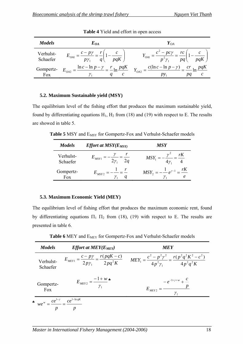
5. Reference points ...................................................................................................... 17
5.1. Open access yield (YOA).................................................................................. 17
5.2. Maximum Sustainable yield (MSY)................................................................ 18
5.3. Maximum Economic Yield (MEY)................................................................. 18
5.4. Optimal biomass, yield and effort ................................................................... 19
vii
Data ..................................................................................................................................... 20
1. Standardization........................................................................................................ 20
1.1. CPUE (for shrimps)......................................................................................... 20
1.2. Fishing effort ................................................................................................... 20
1.3. Catch................................................................................................................ 21
1.4. Price of shrimp ................................................................................................ 22
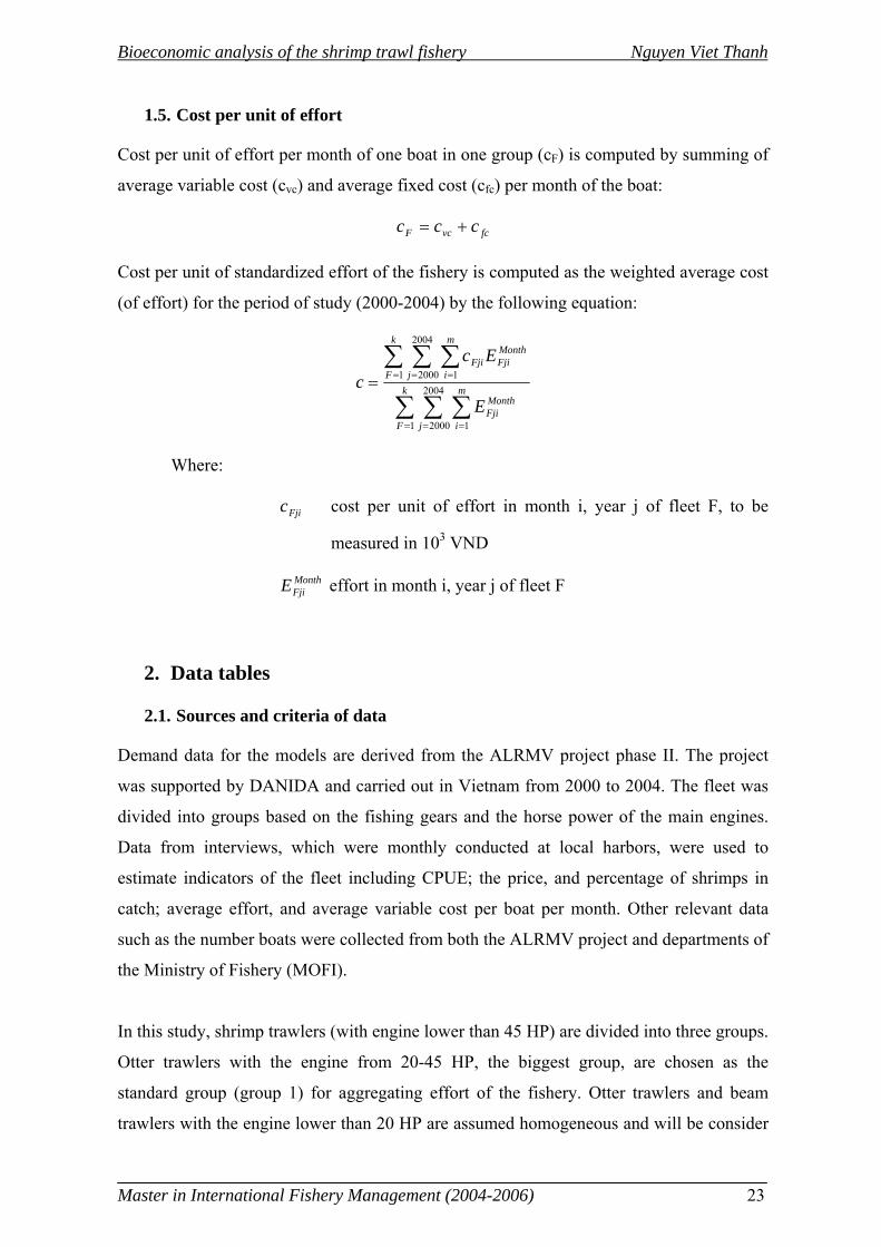
1.5. Cost per unit of effort ...................................................................................... 23
2. Data tables ............................................................................................................... 23
2.1. Sources and criteria of data ............................................................................. 23
2.2. Data tables ....................................................................................................... 24
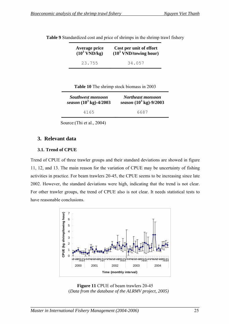
3. Relevant data ........................................................................................................... 25
3.1. Trend of CPUE................................................................................................ 25
3.2. Average mesh size........................................................................................... 26
Results ................................................................................................................................. 29
1. Parameters ............................................................................................................... 29
2. Results from models ................................................................................................ 30
3. The results under discounting.................................................................................. 33
4. Relevant results ....................................................................................................... 34
4.1 The trend of CPUE for different trawler groups ............................................. 34
4.2 The trend of mesh size in cod end of different trawler groups........................ 35
Discussion ........................................................................................................................... 36
1. Models ..................................................................................................................... 36
2. Reference points ...................................................................................................... 37
3. Management ............................................................................................................ 38
3.1 The present regulations.................................................................................... 38
3.2 Alternative regulations .................................................................................... 40
4 Future works............................................................................................................ 41
Conclusions ......................................................................................................................... 42
Reference............................................................................................................................. 44
Appendix 1: Tax policies to achieve reference points......................................................... 47
Appendix 2: Regression results ........................................................................................... 49
Appendix 3: The questionnaire which was used in the ALRMV project............................ 52
Appendix 4: Estimating indicators in the ALRMV project................................................. 54
Appendix 5: Data table from the ALRMV project.............................................................. 56
viii
List of Figures
Figure 1 Shrimp fishing grounds (penaeidae) in the Tonkin Gulf........................................ 4
Figure 2 The proportion of main fish groups in the landing of beam trawlers 20-45 HP..... 6
Figure 3 The proportion of main fish groups in the landing of beam trawlers <20 HP ........ 6
Figure 4 The proportion of main fish groups in the landing of OT 20-45 ............................ 7
Figure 5 The proportion of main fish groups in the landing of OT <20 ............................... 7
Figure 6 The landing price of main fish groups of BT 20-45 ............................................... 7
Figure 7 The landing price of main fish groups of BT <20 .................................................. 8
Figure 8 The landing price of main fish groups of OT 20-45 ............................................... 8
Figure 9 The landing price of main fish groups of OT <20 .................................................. 8
Figure 10 The Logistic (broken line) and Gompertz models .............................................. 13
Figure 11 CPUE of beam trawlers 20-45 ............................................................................ 25
Figure 12 CPUE of otter trawlers 20-45 ............................................................................. 26
Figure 13 CPUE of OT<20 (2000-2002) and BT<20 (2003-2004) .................................... 26
Figure 14 Mesh size in the codend of beam trawlers 20-45................................................ 27
Figure 15 Mesh size in the codend of beam trawlers <20HP.............................................. 27
Figure 16 Mesh size in the codend of otter trawlers 20-45 HP........................................... 28
Figure 17 Mesh size in the codend of otter trawlers <20 HP .............................................. 28
Figure 18 Catch versus effort .............................................................................................. 31
Figure 19 TR, TC versus effort ........................................................................................... 31
ix
List of tables
Table 1 Mean CPUE of the shrimp trawl surveys in the Tonkin Gulf .................................. 4
Table 2 Shrimp trawl fleet in 2003....................................................................................... 5
Table 3 The length of some species in the shrimp trawl surveys....................................... 10
Table 4 Yield and effort in open access .............................................................................. 18
Table 5 MSY and EMSY for Gompertz-Fox and Verhulst-Schaefer models........................ 18
Table 6 MEY and EMEY for Gompertz-Fox and Verhulst-Schaefer models ....................... 18
Table 7 Standardized catch, effort, CPUE of the fishery by half years............................... 24
Table 8 Average fixed costs for different trawler groups in 2001 ...................................... 24
Table 9 Standardized cost and price of shrimps in the shrimp trawl fishery ...................... 25
Table 10 The shrimp stock biomass in 2003....................................................................... 25
Table 11 Estimated coefficients using OLS method ........................................................... 29
Table 12 The catchability (q) in 2003 ................................................................................. 30
Table 13 Estimated r, K parameters .................................................................................... 30
Table 14 Catch Reference Points ........................................................................................ 32
Table 15 Effort Reference Points ........................................................................................ 32
Table 16 Tax policies to achieve MSY ............................................................................... 32
Table 17 Tax policies to achieve MEY ............................................................................... 32
Table 18 Optimal reference points ...................................................................................... 33
Table 19 Tax policies to achieve optimal reference points ................................................. 34
Table 20 Test for the trend of CPUE of shrimps in the fishery........................................... 35
Table 21 Test for the trend of mesh size in the fishery ....................................................... 35
Table 22 Types of fisheries regulations............................................................................... 40
Table 23 Proposal entry tax/boat/month.............................................................................. 40
Table 24 The proposal closed season for a half year to achieve selected reference points. 41
x
Abbreviation
ALMRV Assessment of Living Marine Resources in Vietnam
DANIDA Danish International Development Agency
IFEP Institute of Fisheries Economic and Planning
NADAREP National Directorate of Fisheries Resource Exploitation and Protection
RIMF Research Institute For Marine Fisheries
MOFI Ministry of Fishery Vietnam
CPUE Catch per unit of effort
HP Horse power
VND Vietnam Dong
BT 20-45 HP Beam trawlers with engine from 20 HP to 45 HP
OT 20-45 HP Otter trawlers with engine from 20 HP to 45 HP
BT <20 HP Beam trawlers with engine lower than 20 HP
OT <20 HP Otter trawlers with engine lower than 20 HP
MSY, EMSY Maximum sustainable yield, effort at MSY
MEY, EMEY Maximum economic yield, effort at MEY
YOA, EOA Open access yield, effort at YOA
Introduction The Tonkin Gulf is a semi-closed gulf in the Northwest of the South China Sea with total
area about 126,250 km2 (Vietnam’s sea water-the Western part: 67,203 km2 or 53.23%). It
is a shallow Gulf, the average depth around 38 m and maximum depth less than 100 m.
The Gulf is one of the most important fishing grounds in Vietnam’s sea water. It
contributes to around 16% of Vietnam’s marine resources, 30% of all fishing boats and
about 20% of annual total landings from marine fisheries (Chinh, 2005). The fisheries in
the Gulf are small scale, multi-species and multi-gears fisheries. In 2003, there were about
26,000 fishing boats using 25 different types of gears in the Gulf; 86% of these boats had
the engine lower than 45 HP (Chinh, 2005). There were 166 species of 74 different
families identified by bottom trawl surveys in the offshore water of the Gulf (Son, 2001).
Shrimps are the most important commercial species in Vietnam’s marine waters. In 2003,
shrimp landing contributed around 17 % in monetary value of the marine capture
fisheries (MOFI, 2006). There has been found 58 shrimp species, in the Western part of
Tonkin Gulf, mainly belong to the family of Penaeidae. Most shrimp species are
distributed along the coastal areas, spawning seasons are February-March (spring) and
June-July (autumn)_(Son, 2003). The shrimp trawl fishery in the Tonkin Gulf has a long
history of development. Before 1985, almost all fishing boats were otter trawls belonging
to stated-owned enterprises and used engines of higher than 200 HP. However, due to low
economic returns, they have been closed (Long, 2003). At present, shrimp trawl fleet are
small scale and under private ownership. In 1997, the fleet occupied about 18% of the total
fishing boats in the Gulf, the shrimp trawlers was about 9-13m in length, almost used
engines of 15-30 HP and operated in the waters within 30 m depth. The fishing trip was
around one or two days (Long, 2003). Shrimp landing was estimated around 11.445 tones,
occupying about 4.6 % of the total catch of the Gulf’s fisheries in 2003 (Chinh, 2005).
Some studies indicate that maximum sustainable yield (MSY) in the coastal areas of the
Tonkin Gulf was reached since 1994 and that fishing activities give low economic returns
due to overfishing (Long, 2001; Long, 2003). Catch per unit of effort (CPUE) globally
declined from 1.34 to 0.34 ton/HP/year between 1985 and 1997 (Son, 2003). In addition,
fisheries in the Gulf as well as other sea waters in Vietnam are argued still in the open
Bioeconomic analysis of the shrimp trawl fishery Nguyen Viet Thanh
Master in International Fishery Management (2004-2006) 2
access situation (FAO, 2005). It has been shown that it is difficult to achieve the
sustainable development of the fisheries and in the long run, the stocks may be in danger.
This is also valid in the shrimp fishery by trawl. The current fishing effort seems to be too
high for a sustainable exploitation even though no quantitative analysis has been carried
out so far.
The objective of this study is to investigate the sustainability properties of the stock and
management of the shrimp trawl fishery in the Tonkin Gulf by using bio-economic
analysis of historical data. The basis assumption is that the management objectives are to
sustain development and to maximize economic yield. The major questions that arise in
this case include:
(1) What is the sustainable harvest of selected reference points? Must the fishing effort
be reduces in order to reach the reference points?
(2) Is the current management regime efficient? If not what should be the alternative
regulations?
The hypothesis of the study is that, the catch by shrimp trawlers is expected too high to
meet the reference points MEY (Maximum Economic Yield) and MSY (Maximum
Sustainable Yield), and the shrimp catches have been declining over the studied period. It
is assumed that fishery regulations are inefficient and the actual situation is close to open
access.
In this study, standard surplus production models of Verhulst-Schaefer and Gompertz-Fox
are used to analyze the data derived from an enumerator program (ALRMV project) which
was supported by DANIDA and carried out in Vietnam from 2000-2004. The time series
cover a short time span, which may involve the “one way trip” problem since the full
development history of the fishery is not covered. Furthermore, simple models may not
describe the full dynamics of such a complicated system.
Chapter 2 brings the reader some background information on the shrimp trawl fishery in
the Tonkin Gulf. Chapter 3 presents the basics of the models used. Chapter 4 covers the
data set applied - the standardization of the data for the models. Chapter 5 shows the
results from the models and relevant results. The thesis results are summarized in the
discussion and conclusion parts, chapter 6 and chapter 7.
Bioeconomic analysis of the shrimp trawl fishery Nguyen Viet Thanh
Master in International Fishery Management (2004-2006) 3
Background information
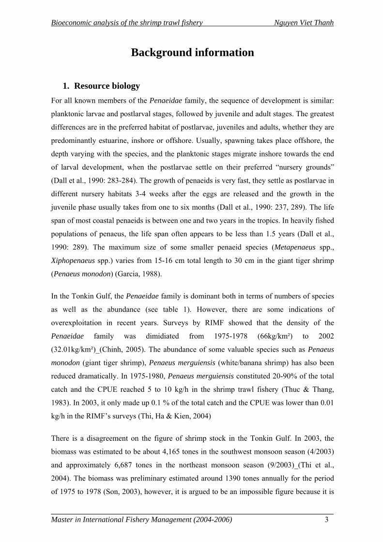
1. Resource biology For all known members of the Penaeidae family, the sequence of development is similar:
planktonic larvae and postlarval stages, followed by juvenile and adult stages. The greatest
differences are in the preferred habitat of postlarvae, juveniles and adults, whether they are
predominantly estuarine, inshore or offshore. Usually, spawning takes place offshore, the
depth varying with the species, and the planktonic stages migrate inshore towards the end
of larval development, when the postlarvae settle on their preferred “nursery grounds”
(Dall et al., 1990: 283-284). The growth of penaeids is very fast, they settle as postlarvae in
different nursery habitats 3-4 weeks after the eggs are released and the growth in the
juvenile phase usually takes from one to six months (Dall et al., 1990: 237, 289). The life
span of most coastal penaeids is between one and two years in the tropics. In heavily fished
populations of penaeus, the life span often appears to be less than 1.5 years (Dall et al.,
1990: 289). The maximum size of some smaller penaeid species (Metapenaeus spp.,
Xiphopenaeus spp.) varies from 15-16 cm total length to 30 cm in the giant tiger shrimp
(Penaeus monodon) (Garcia, 1988).
In the Tonkin Gulf, the Penaeidae family is dominant both in terms of numbers of species
as well as the abundance (see table 1). However, there are some indications of
overexploitation in recent years. Surveys by RIMF showed that the density of the
Penaeidae family was dimidiated from 1975-1978 (66kg/km²) to 2002
(32.01kg/km²)_(Chinh, 2005). The abundance of some valuable species such as Penaeus
monodon (giant tiger shrimp), Penaeus merguiensis (white/banana shrimp) has also been
reduced dramatically. In 1975-1980, Penaeus merguiensis constituted 20-90% of the total
catch and the CPUE reached 5 to 10 kg/h in the shrimp trawl fishery (Thuc & Thang,
1983). In 2003, it only made up 0.1 % of the total catch and the CPUE was lower than 0.01
kg/h in the RIMF’s surveys (Thi, Ha & Kien, 2004)
There is a disagreement on the figure of shrimp stock in the Tonkin Gulf. In 2003, the
biomass was estimated to be about 4,165 tones in the southwest monsoon season (4/2003)
and approximately 6,687 tones in the northeast monsoon season (9/2003)_(Thi et al.,
2004). The biomass was preliminary estimated around 1390 tones annually for the period
of 1975 to 1978 (Son, 2003), however, it is argued to be an impossible figure because it is
Bioeconomic analysis of the shrimp trawl fishery Nguyen Viet Thanh
Master in International Fishery Management (2004-2006) 4
about eight times lower than the shrimp landing in 2003 (Chinh, 2005). The disagreement
may be a consequence of different estimation methods.
Table 1 Mean CPUE of the shrimp trawl surveys in the Tonkin Gulf
CPUE (kg/h) Family
April, 2003 September, 2003
Penaeidae (18 species) 1.33 1.93
Scyllaridae (3 species) - 0.01
Solenoceridae(1 species) 0.06 0.35
Squillidae (6 species) 0.60 0.35
Total 1.99 2.64
Source: (Thi et al., 2004)
2. The fishery
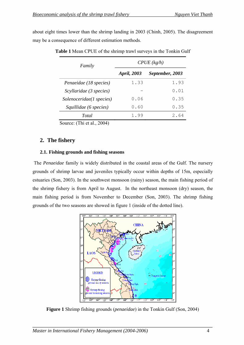
2.1. Fishing grounds and fishing seasons
The Penaeidae family is widely distributed in the coastal areas of the Gulf. The nursery
grounds of shrimp larvae and juveniles typically occur within depths of 15m, especially
estuaries (Son, 2003). In the southwest monsoon (rainy) season, the main fishing period of
the shrimp fishery is from April to August. In the northeast monsoon (dry) season, the
main fishing period is from November to December (Son, 2003). The shrimp fishing
grounds of the two seasons are showed in figure 1 (inside of the dotted line).
Figure 1 Shrimp fishing grounds (penaeidae) in the Tonkin Gulf (Son, 2004)
Bioeconomic analysis of the shrimp trawl fishery Nguyen Viet Thanh
Master in International Fishery Management (2004-2006) 5
2.2. Fishing fleet and fishing gears
Otter trawl and beam trawl are the two main gears used in the shrimp fishery. Both otter
and beam trawlers use the single boat, for horizontal opening trawls, the otter trawlers uses
otter-boards while the beam trawlers use sticks or pipes. Beam trawlers often have the
engine ranging from 22-90 HP, rarely up to 250 HP. A small boat tows 1 to 2 beam trawls,
but larger boats can tow up to 18 beam trawls (Long et al., 2002). The net mouth is
horizontally propped open by bamboo or steel pipes. Sometimes, the fishers use two skis
that are joined together with the lead and head rope for slipping along the seabed easily.
The fishing ground of beam trawlers are sandy-muddy bottom and shallow waters. Target
species are shrimp, crab and small demersal fish. The shrimp otter trawlers often use the
engine with less than 60 HP and operate within 30 m water depths (Long et al., 2002). The
otter boards are rectangular and flat, and are made of wood and iron. Iron tickler chains
(about 1.5-3.5 m) are used to round up the shrimp in the sand.
At present, there are few shrimp trawlers with larger engines than 45 HP in the Tonkin
Gulf (below 10%). In addition, the percentage of shrimp in catch of these is also low, for
example lower than 10% for the otter trawl fleet with engine 46-89 HP1. In this study, only
trawlers with engine size less than 45 HP is used (table 2).
Table 2 Shrimp trawl fleet in 2003
Groups Beam trawl Otter trawl Total
< 20 HP 203 1749 1952
20 HP to 45 HP 211 1808 2019
Total 414 3557 3971
Source: NADAREP, MOFI, 2005
2.3. The landing and the price
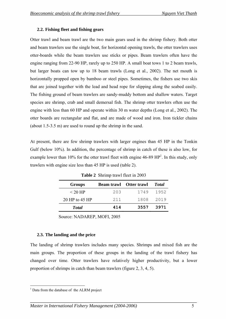
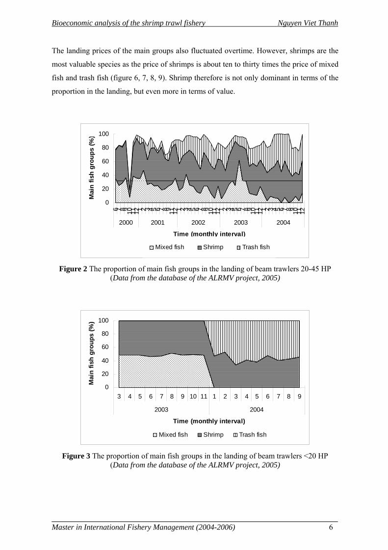
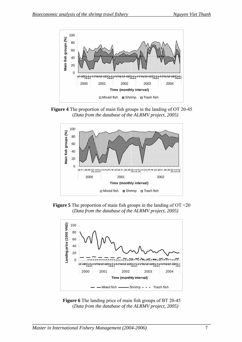
The landing of shrimp trawlers includes many species. Shrimps and mixed fish are the
main groups. The proportion of these groups in the landing of the trawl fishery has
changed over time. Otter trawlers have relatively higher productivity, but a lower
proportion of shrimps in catch than beam trawlers (figure 2, 3, 4, 5).
1 Data from the database of the ALRM project
Bioeconomic analysis of the shrimp trawl fishery Nguyen Viet Thanh
Master in International Fishery Management (2004-2006) 6
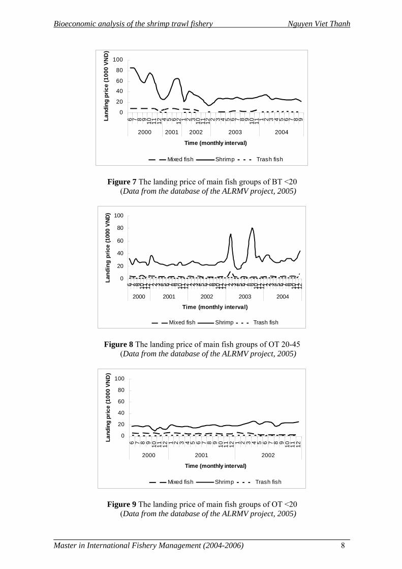
The landing prices of the main groups also fluctuated overtime. However, shrimps are the
most valuable species as the price of shrimps is about ten to thirty times the price of mixed
fish and trash fish (figure 6, 7, 8, 9). Shrimp therefore is not only dominant in terms of the
proportion in the landing, but even more in terms of value.
0
20
40
60
80
100
6 7 8 9 10 11 12 1 2 3 4 5 6 7 8 9 11 12 1 2 3 4 5 6 7 8 9 10 11 12 1 2 3 4 5 6 7 8 9 10 11 12 1 2 3 4 5 6 7 8 9 10 11 12
2000 2001 2002 2003 2004
Time (monthly interval)
Mai
n fis
h gr
oups
(%)
Mixed fish Shrimp Trash fish
Figure 2 The proportion of main fish groups in the landing of beam trawlers 20-45 HP
(Data from the database of the ALRMV project, 2005)
0
20
40
60
80
100
3 4 5 6 7 8 9 10 11 1 2 3 4 5 6 7 8 9
2003 2004
Time (monthly interval)
Mai
n fis
h gr
oups
(%)
Mixed fish Shrimp Trash fish
Figure 3 The proportion of main fish groups in the landing of beam trawlers <20 HP (Data from the database of the ALRMV project, 2005)
Bioeconomic analysis of the shrimp trawl fishery Nguyen Viet Thanh
Master in International Fishery Management (2004-2006) 7
0
20
40
60
80
100
6 7 8 9 10 11 12 1 2 3 4 5 6 7 8 9 10 11 12 1 2 3 4 5 6 7 8 9 10 11 12 1 2 3 4 5 6 7 8 9 10 11 12 1 2 3 4 5 6 7 8 9 10 11 12
2000 2001 2002 2003 2004
Time (monthly interval)
Mai
n fis
h gr
oups
(%)
Mixed fish Shrimp Trash fish
Figure 4 The proportion of main fish groups in the landing of OT 20-45 (Data from the database of the ALRMV project, 2005)
0
20
40
60
80
100
6 7 8 9 10 11 12 1 2 3 4 5 6 7 8 9 10 11 12 1 2 3 4 5 6 7 8 9 10 11 122000 2001 2002
Time (monthly interval)
Mai
n fis
h gr
oups
(%)
Mixed fish Shrimp Trash fish
Figure 5 The proportion of main fish groups in the landing of OT <20 (Data from the database of the ALRMV project, 2005)
0
20
40
60
80
100
6 7 8 9 10 11 12 1 2 3 4 5 6 7 8 9 10 11 12 1 2 3 4 5 6 7 8 9 10 11 12 1 2 3 4 5 6 7 8 9 10 11 12 1 2 3 4 5 6 7 8 9 10 11
2000 2001 2002 2003 2004
Time (monthly interval)
Land
ing
pric
e (1
000
VND
)
Mixed fish Shrimp Trash fish
Figure 6 The landing price of main fish groups of BT 20-45 (Data from the database of the ALRMV project, 2005)
Bioeconomic analysis of the shrimp trawl fishery Nguyen Viet Thanh
Master in International Fishery Management (2004-2006) 8
0
20
40
60
80
100
6 7 8 9 10 11 12 4 5 6 12 1 2 3 10 11 12 2 3 4 5 6 7 8 9 10 11 1 2 3 4 5 6 7 8 9
2000 2001 2002 2003 2004
Time (monthly interval)
Land
ing
pric
e (1
000
VND
)
Mixed fish Shrimp Trash fish
Figure 7 The landing price of main fish groups of BT <20 (Data from the database of the ALRMV project, 2005)
0
20
40
60
80
100
6 7 8 9 10 11 12 1 2 3 4 5 6 7 8 9 10 11 12 1 2 3 4 5 6 7 8 9 10 11 12 1 2 3 4 5 6 7 8 9 10 11 12 1 2 3 4 5 6 7 8 9 10 11 122000 2001 2002 2003 2004
Time (monthly interval)
Land
ing
pric
e (1
000
VND
)
Mixed fish Shrimp Trash fish
Figure 8 The landing price of main fish groups of OT 20-45 (Data from the database of the ALRMV project, 2005)
0
20
40
60
80
100
6 7 8 9 10 11 12 1 2 3 4 5 6 7 8 9 10 11 12 1 2 3 4 5 6 7 8 9 10 11 12
2000 2001 2002
Time (monthly interval)
Land
ing
pric
e (1
000
VND
)
Mixed fish Shrimp Trash fish
Figure 9 The landing price of main fish groups of OT <20 (Data from the database of the ALRMV project, 2005)
Bioeconomic analysis of the shrimp trawl fishery Nguyen Viet Thanh
Master in International Fishery Management (2004-2006) 9
Figure 6, 7 shows that beam trawler price on shrimp catch has been reduced by about one
third from 2000 to 2004. This implies that valuable shrimp species in catch of beam
trawlers may have been reduced significantly.
2.4. Fishing communities
In the coastal areas, fishers are often poor and have moved from the agricultural villages or
floating communities. Those who have fished from the rivers near sea have moved to fish
in the sea (Hersoug et al., 2002; Thong, 1998). In 1994, the amount of fishers in Tonkin
Gulf (Red rive delta) was around 46,254 persons living in 112 communities, of which 13
communes are set in town, district’s capital; 56 villages in the rivulet, port; 43 villages in
the beaches (Thong, 1998). These figures imply that fishing communities are very diverse
and complex, which may make the top down management system impossible to operate. In
practice, fishers often do not comply with national and provincial fisheries rules and
regulations, and, worse, they are often not aware of them. In part, the problem results from
many rules having been made as ad hoc decrees, some being contradiction to others
(Ruddle, 1998).
2.5. Management
The fisheries law was promulgated on 01 July 2004 and was apparently intended to serve
as the main instrument for national living aquatic resources management. However, a
highly detailed Circular issued on 28 April 2000 by the Vice-Minister of Fisheries,
provided instruments on many aspects of the fisheries management, including the shrimp
trawl fishery. These instruments include allowable concentrations of toxic substances in
waters inhabited by aquatic organisms, minimum permitted mesh sizes by gear type,
prohibited species, area closures during spawning seasons and minimum size regulation.
In fact, the Government of Vietnam is in the process of making the basic legal and
institutional changes necessary, in order to ensure a more market-oriented economy. As a
consequence, the legal framework governing fisheries still lacks coherence. The problems
of small scale and industrial fisheries management have hardly been touch-on, despite
recognizing an overfishing problems (Ruddle, 1998). In the shrimp trawl fishery, the
compliance of regulations is also questionable.
Bioeconomic analysis of the shrimp trawl fishery Nguyen Viet Thanh
Master in International Fishery Management (2004-2006) 10
The license regulation is opposed to an open access system, in which a limited number of
boats or boat owners are given licenses (King, 1995). In case of the shrimp trawl fishery
(also other marine fisheries in Vietnam), the regulation has been applied ineffectively.
Fishing licenses are imposed, but many fishermen appear to ignore them. Licenses are
granted on the basis of submitting a number of supporting documents such as vessel
inspection and registration papers. A small license fee, proportional to engine size is
levied. In this case, a license application generally leads to a license being issued and the
shrimp trawl fishery as well as other marine capture fisheries are, in fact, in the open
access situation (FAO, 2005).
The minimum legal length regulation is imposed but it seems to be inefficiently in the
shrimp trawl fishery. Table 3 shows some shrimp species (Metapenaeus intermedius,
Metapenaeus affinis) were caught with equal mean length in catch, around one third of the
minimum legal length. Other species (Penaeus merguiensis) which was abundant in 1980s
had almost disappeared according to surveys in 2003.
Table 3 The length of some species in the shrimp trawl surveys in comparison with the minimum legal length
The length in surveys (mm)
4/2003 9/2003 Species
The minimum
legal length (mm)
Mean length Variance Mean
length Variance
Metapenaeus intermedius 95 33.6 20-40 23.4 20-40 Metapenaeus affinis 95 - - 23.4 10-30 Penaeus merguiensis 110 - - - -
Source: (MOFI, 2006; Thi et al., 2004)
Bioeconomic analysis of the shrimp trawl fishery Nguyen Viet Thanh
Master in International Fishery Management (2004-2006) 11
The basics of the model
The shrimp trawl fishery is a typical tropical fishery with all characteristic properties of
small scale and multi-species tropical fisheries. In such cases, surplus production models
often have shown to be an appropriate analysis tool when catch and effort data are
available. This is supported by Hilborn & Walters:
“It is quite difficult to age many fishes, particularly tropical ones, and age-
structured analysis is often not practical in these fisheries. Moreover, in the
tropical fisheries, the catch consists of many species, and the catch data are
difficult if not impossible to collect by species. Management regulations are
also difficult to make species specific. In these cases, treating the entire catch
as a biomass dynamics pool may be more appropriate than trying to look at
single species dynamics” (Hilborn & Walters, 1992:298).
Garcia (1988: 237) also argues that surplus production models might be more appropriate
than other in shrimp fisheries because of short life span of species, which means that
equilibrium conditions are close to exist at any time within a biological year, which
starting with the main recruitment. With respect to the Tonkin Gulf, there are two shrimp
spawning seasons per year (February-March and June-July). This implies that it is
appropriate to divide the time scale into a half year in accordance with the biological year
of the stock. Surplus production models which are generally applicable to a calendar year
data, now, are applied for a half year time interval data in this study. It is assumed that the
stock will reach an equilibrium situation within a period of six months. The models use
steady state (equilibrium) conditions to formulate reference points and equilibrium
assumptions to estimate parameters.
In this chapter, surplus production models are presented in general forms and assumptions
will also be paid attention. Verhulst-Schaefer and Gompertz-Fox models are used and
parameters estimated from catch and effort data.

Bioeconomic analysis of the shrimp trawl fishery Nguyen Viet Thanh
Master in International Fishery Management (2004-2006) 12
1. Biological growth
1.1. General models
A general biological growth model of a fish stock in case of absence of harvesting and
other human interference can be expressed (Eide, 1989; Pella & Tomlinson, 1969):
mu sXrXdtdX
+= (1)
Where
X stock size to be measured in terms of biomass (cohorts are implicit);
r growth rate of the stock, a positive parameter, includes recruitment and
growth of individuals;
s mortality rate of the sock, a negative parameter, includes natural death of
individuals (from all causes other than capture by man);
m, u positive constants.
The growth equation of Pella and Tomlinson (1969) is defined by:
⎥⎥⎦
⎤
⎢⎢⎣
⎡⎟⎠⎞
⎜⎝⎛−=
−1
1m
KXrX
dtdX (2)
Where
K the environmental carrying capacity
r in this case is called the intrinsic growth rate
This is a simplified case of the general growth equation when u = 1 and s = -rK1-m.
1.2. Logistic growth model
The logistic growth model first proposed as a population model by P.F. Verhulst in 1838
)1(KXrX
dtdX
−= (3)
This is a special case of the Pella and Tomlinson equation when m = 2. The logistic growth
function is said to describe a process of feedback, or compensation, which controls the
growth of the population as its level increases. The logistic growth curve is symmetrical
Bioeconomic analysis of the shrimp trawl fishery Nguyen Viet Thanh
Master in International Fishery Management (2004-2006) 13
round its point of inflexion. This simple model has been used widely both from a
theoretical standpoint and as a convenient empirical curve (Richards, 1959).
1.3. Gompertz growth model
The Gompertz growth model proposed by Gompertz in 1825, is defined by:
⎟⎠⎞
⎜⎝⎛=
XKrX
dtdX
elog (4)
The Gompertz curve, which resembles the logistic curve in many features but is
asymmetrical (inflecting at X = K/e = 0.368 K), has also been used extensively in
population studies (Fox, 1970; Richards, 1959). The Gompertz model is a special case of
the Pella and Tomlinson equation when m →1.
1.4. Comparison of the Logistic and Gompertz models:
The Logistic and Gompertz models are graphed in the figure 10. For a given stock size at
time t = 0 and a given carrying capacity, the Gompertz model may expects a faster growth
of the stock size over time than the Logistic model.
5 10 15 20 25 30t
2
4
6
8
10
X
2 4 6 8 10X
0.1
0.2
0.3
0.4
0.5
dXêdt
Figure 10 The Logistic (broken line) and Gompertz models
K
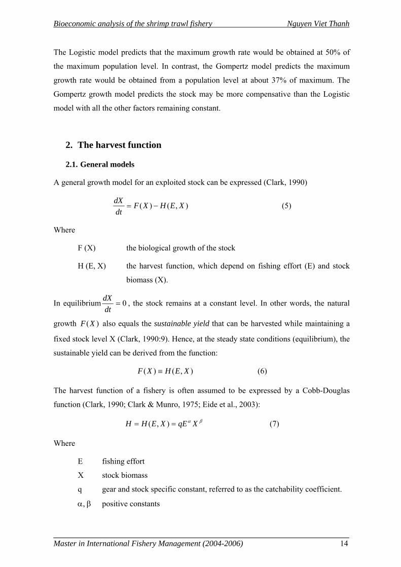
Bioeconomic analysis of the shrimp trawl fishery Nguyen Viet Thanh
Master in International Fishery Management (2004-2006) 14
The Logistic model predicts that the maximum growth rate would be obtained at 50% of
the maximum population level. In contrast, the Gompertz model predicts the maximum
growth rate would be obtained from a population level at about 37% of maximum. The
Gompertz growth model predicts the stock may be more compensative than the Logistic
model with all the other factors remaining constant.
2. The harvest function
2.1. General models
A general growth model for an exploited stock can be expressed (Clark, 1990)
),()( XEHXFdtdX
−= (5)
Where
F (X) the biological growth of the stock
H (E, X) the harvest function, which depend on fishing effort (E) and stock
biomass (X).
In equilibrium 0=dtdX , the stock remains at a constant level. In other words, the natural
growth )(XF also equals the sustainable yield that can be harvested while maintaining a
fixed stock level X (Clark, 1990:9). Hence, at the steady state conditions (equilibrium), the
sustainable yield can be derived from the function:
),()( XEHXF ≡ (6)
The harvest function of a fishery is often assumed to be expressed by a Cobb-Douglas
function (Clark, 1990; Clark & Munro, 1975; Eide et al., 2003):
βα XqEXEHH == ),( (7)
Where
E fishing effort
X stock biomass
q gear and stock specific constant, referred to as the catchability coefficient.
α, β positive constants
Bioeconomic analysis of the shrimp trawl fishery Nguyen Viet Thanh
Master in International Fishery Management (2004-2006) 15
In case α = β = 1, the harvest function simplifies to:
qEXXEH =),( (8)
Fishing effort (E) here is in this study aggregated from a number of different harvesting
activities and measured by towing hours. Similarly the biomass variable X consists of
number of harvested shrimp species (to be measured in kg).
2.2. Verhulst-Schaefer model
This model assume that the biological growth follows the Logistic growth function
rKqEKX
KXrXqEX −=⇔−= )1( (9)
The sustainable yield for a given level of effort:
22
1 )( ErKqqKEEH −= (10)
2.3. Gompertz-Fox model
This model assume that the biological growth follows the Gompertz growth function
rqEe
e
KXXKrXqEX =⇔⎟⎠⎞
⎜⎝⎛= log (11)
The sustainable yield for a given level of effort:
rqE
rqE qKEe
e
qKEEH−
==)(2 (12)
3. Economics
Total sustainable revenue (TR) and total cost (TC) of the fishery are defined (Clark, 1990;
Schaefer, 1954):
))(),(()( tXtEHptTR ∗= (13)
)()( tEctTC ∗= (14)
Bioeconomic analysis of the shrimp trawl fishery Nguyen Viet Thanh
Master in International Fishery Management (2004-2006) 16
Where
p constant price per unit of harvested biomass
c constant cost per unit of effort
The difference between total sustainable revenue TR and total cost TC is called the
sustainable economic rent provided by the fishery resource at each given level of effort E:
)())(),(()()()( tEctXtEHptTCtTRt ∗−∗=−=∏ (15)
The equation that maximize the present value (PV) of the fishery can be expressed
∫∞
=
− ∏=0
)(maxmaxt
t dttePV δ (16)
Subject to the constraint ),()( XEHXFdtdX
−=
The equation to solve for optimal biomass under discounting is (Clark, 1985; Clark, 1990;
Clark & Munro, 1975):
δ=−
−)()()(')('
XapXFXaXF (17)
Where:
δ Discounted rate
)(XF Growth rate of the stock
)(Xa Cost per unit of harvest
4. Estimating the parameters
4.1. Verhulst-Schaefer model
The model uses the Logistic growth function, the relationship between CPUE and effort is
linear as derived from the sustainable yield equation (10):
Bioeconomic analysis of the shrimp trawl fishery Nguyen Viet Thanh
Master in International Fishery Management (2004-2006) 17
2111
211
2
1
11
21
1
)(
;:
)(
EpEcpcEpH
EEHrKqqKwhere
ECPUEErKqqK
EEHCPUE
γγ
γγ
γγ
γγ
+−=−=Π
+=⇒
−==
+=⇔−==
(18)
4.2. Gompertz-Fox model
The model uses the Gompertz growth function, the relationship between Log (CPUE) and
effort is linear as derived from the sustainable yield equation (12):
)(
);(:
)()()(
1
1
22
2
1
122
2
cpeEcEpH
EeHrqqKLnwhere
EErqqKLnCPUELnqKe
EEHCPUE
E
E
rqE
−=−=Π
=⇒
−==
+=−=⇔==
+
+
−
γγ
γγ
γγ
γγ
(19)
5. Reference points
5.1. Open access yield (YOA)
In the open access situation, fishers will join in the fishery until marginal cost (MC) is
equal average revenue (AR). In this case, the open access stock biomass (XOA) is defined
by cost per unit effort, price and the catchability coefficient:
pqcXpqX
EHpcARMC OAOA =⇒=
∗=⇔= (20)
The yield and effort in the open access situation are shown in table 4
Bioeconomic analysis of the shrimp trawl fishery Nguyen Viet Thanh
Master in International Fishery Management (2004-2006) 18
Table 4 Yield and effort in open access
Models EOA YOA
Verhulst-Schaefer ⎟⎟
⎠
⎞⎜⎜⎝
⎛−=
−=
pqKc
qr
ppcEOA 11
1 γγ ⎟⎟
⎠
⎞⎜⎜⎝
⎛−=
−=
pqKc
pqrc
ppccYOA 1
12
2
1 γγ
Gompertz-Fox c
pqKqrpcEOA lnlnln
12 =
−−=
γγ
cpqK
pqcr
pypccYOA ln)ln(ln
12 =
−−=
γ
5.2. Maximum Sustainable yield (MSY)
The equilibrium level of the fishing effort that produces the maximum sustainable yield,
found by differentiating equations H1, H2 from (18) and (19) with respect to E. The results
are showed in table 5.
Table 5 MSY and EMSY for Gompertz-Fox and Verhulst-Schaefer models
Models Effort at MSY(EMSY) MSY
Verhulst-Schaefer q
rEMSY 22 11 =−=
γγ
44 1
2
1rKMSY =−=
γγ
Gompertz-Fox q
rEMSY =−=1
21γ
e
rKeMSY =−= −1
12
1 γ
γ
5.3. Maximum Economic Yield (MEY)
The equilibrium level of fishing effort that produces the maximum economic rent, found
by differentiating equations Π1 Π2 from (18), (19) with respect to E. The results are
presented in table 6.
Table 6 MEY and EMEY for Gompertz-Fox and Verhulst-Schaefer models
Models Effort at MEY(EMEY) MEY
Verhulst-Schaefer
KpqcpqKr
ppcEMEY 2
11 2
)(2
−=
−=
γγ
KqpcKqpr
ppcMEY 22
2222
12
222
1 4)(
4−
=−
=γγ
Gompertz-
Fox 12
1γ
wEMEY+−
= ♣
1
1
2 γ
γ
pce
E
w
MEY
+−=
++−
♣ p
cep
ceweqK
wln11 −−
==γ
Bioeconomic analysis of the shrimp trawl fishery Nguyen Viet Thanh
Master in International Fishery Management (2004-2006) 19
5.4. Optimal biomass, yield and effort
Optimal biomass can be determined in the Logistic model from equation (18)_(Clark,
1990; Clark & Munro, 1975):
⎟⎟⎟
⎠
⎞
⎜⎜⎜
⎝
⎛+⎟⎟
⎠
⎞⎜⎜⎝
⎛−++⎟⎟
⎠
⎞⎜⎜⎝
⎛−+=
pqKrc
rpqKc
rpqKcKX δδδ 811
4
2*
1 (21)
Optimal biomass for the Gompertz model can be determined (Clarke, Yoshimoto & Pooley, 1992):
011ln *2
*2
=⎟⎟⎠
⎞⎜⎜⎝
⎛−⎟
⎠⎞
⎜⎝⎛ +−⎟
⎟⎠
⎞⎜⎜⎝
⎛
pqXc
rXK δ (22)
Optimal yield (F[X1,2*]) and optimal effort (E1,2
*) can be determined by following
equation:
[ ]
*2,1
*2,1*
2,1 qXXF
E = (23)
Bioeconomic analysis of the shrimp trawl fishery Nguyen Viet Thanh
Master in International Fishery Management (2004-2006) 20
Data
1. Standardization
In order to apply the bioeconomic models on the shrimp trawl fishery, catch and effort of
different shrimp trawler groups need to be standardized. Standardized catch and effort are
computed based on the data derived from the ALRMV project (see appendix 5). The data
includes monthly indicators for difference shrimp trawler groups, average CPUE to be
measured in kg/towing hour; average effort to be measured in towing hours/boat; average
percentage of shrimp in catch; average price of shrimp to be measured in 103 VND;
average variable cost per towing hour to be measured in 103 VND. The questionnaire and
equations to estimate these indicators are shown in appendix 3 and 4.
1.1. CPUE (for shrimps)
Standardized CPUE of different trawler groups is calculated based on average CPUE and
average percentage of shrimp in catch2
FF psMeanCPUECPUE *=
Where:
FCPUE standardized CPUE of fleet F in a month, to be
measured in kg shrimp/towing hour
MeanCPUE average CPUE of fleet F in that month, to be
measured in kg (mixed fish)/towing hour;
Fps average percentage of shrimp in the catch of fleet F in that month;
1.2. Fishing effort
Efforts of the different trawler groups are standardized based on their relative fishing
powers. Which is defined, and can be measured as the ratio of the CPUE of the group to
2 These indicators are derived from appendix 5

Bioeconomic analysis of the shrimp trawl fishery Nguyen Viet Thanh
Master in International Fishery Management (2004-2006) 21
that of another group taken as a standard and fishing on the same density of fish on the
same type of ground (Beverton & Holt, 1993). In this way each group can be allotted a
power factor which is used to compute its standardized effort. The standardized effort of
the fishery is estimated by following steps:
1.2.1. Effort per month of fleet F is estimated
FFFmonthF pfneE **=
Where:
monthFE total effort per month of fleet F, to be measured in towing
hours
Fe average effort per month of one boat in fleet F, to be
measured in towing hours;
Fn number of boats in fleet F for the period of study;
S
FF CPUE
CPUEpf = power factor of fleet F to the standard fleet (S) in that month;
1.2.2. Effort per a half year of fleet F is estimated
6*1
m
EE
m
i
monthiF
HalfyearF
∑== (m ≤ 6) where m- number of months that fleet F were
observed in that half year
1.2.3. Total effort per a half year of the fishery is estimated
∑=
=k
F
HalfYearFEE
1 Where k- number of fleet (or boat groups)
1.3. Catch
Catch are then standardized based on some steps. First, the landing shrimp of each group is
estimated by multiplying the CPUE with average effort of one boat and the number of
boats in the group. Afterward, total landing shrimp of the fishery is computed by summing
the landing shrimp of different shrimp trawler groups. The standardized process of the
catch is described by following equations:
Bioeconomic analysis of the shrimp trawl fishery Nguyen Viet Thanh
Master in International Fishery Management (2004-2006) 22
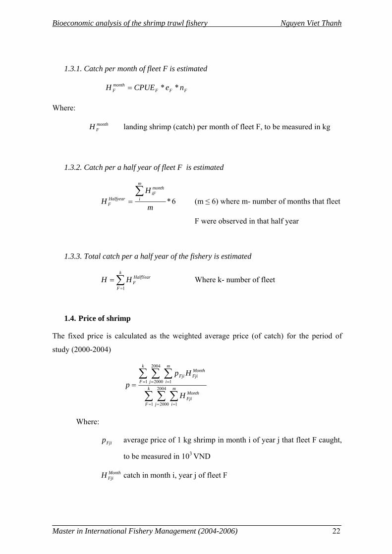
1.3.1. Catch per month of fleet F is estimated
FFFmonthF neCPUEH **=
Where:
monthFH landing shrimp (catch) per month of fleet F, to be measured in kg
1.3.2. Catch per a half year of fleet F is estimated
6*m
HH
m
i
monthiF
HalfyearF
∑= (m ≤ 6) where m- number of months that fleet
F were observed in that half year
1.3.3. Total catch per a half year of the fishery is estimated
∑=
=k
F
HalfYearFHH
1 Where k- number of fleet
1.4. Price of shrimp
The fixed price is calculated as the weighted average price (of catch) for the period of
study (2000-2004)
∑ ∑ ∑
∑ ∑ ∑
= = =
= = == k
F j
m
i
MonthFji
k
F j
m
i
MonthFjiFji
H
Hpp
1
2004
2000 1
1
2004
2000 1
Where:
Fjip average price of 1 kg shrimp in month i of year j that fleet F caught,
to be measured in 103 VND
MonthFjiH catch in month i, year j of fleet F
Bioeconomic analysis of the shrimp trawl fishery Nguyen Viet Thanh
Master in International Fishery Management (2004-2006) 23
1.5. Cost per unit of effort
Cost per unit of effort per month of one boat in one group (cF) is computed by summing of
average variable cost (cvc) and average fixed cost (cfc) per month of the boat:
fcvcF ccc +=
Cost per unit of standardized effort of the fishery is computed as the weighted average cost
(of effort) for the period of study (2000-2004) by the following equation:
∑ ∑ ∑
∑ ∑ ∑
= = =
= = == k
F j
m
i
MonthFji
k
F j
m
i
MonthFjiFji
E
Ecc
1
2004
2000 1
1
2004
2000 1
Where:
Fjic cost per unit of effort in month i, year j of fleet F, to be
measured in 103 VND
MonthFjiE effort in month i, year j of fleet F
2. Data tables
2.1. Sources and criteria of data
Demand data for the models are derived from the ALRMV project phase II. The project
was supported by DANIDA and carried out in Vietnam from 2000 to 2004. The fleet was
divided into groups based on the fishing gears and the horse power of the main engines.
Data from interviews, which were monthly conducted at local harbors, were used to
estimate indicators of the fleet including CPUE; the price, and percentage of shrimps in
catch; average effort, and average variable cost per boat per month. Other relevant data
such as the number boats were collected from both the ALRMV project and departments of
the Ministry of Fishery (MOFI).
In this study, shrimp trawlers (with engine lower than 45 HP) are divided into three groups.
Otter trawlers with the engine from 20-45 HP, the biggest group, are chosen as the
standard group (group 1) for aggregating effort of the fishery. Otter trawlers and beam
trawlers with the engine lower than 20 HP are assumed homogeneous and will be consider
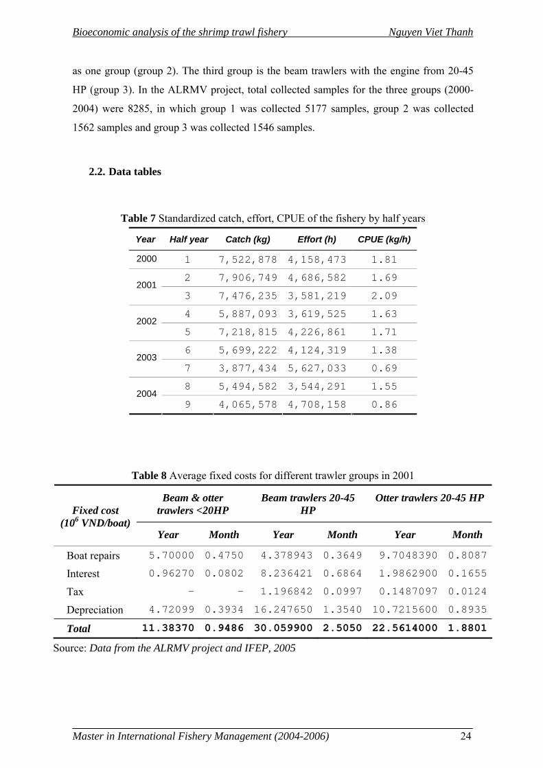
Bioeconomic analysis of the shrimp trawl fishery Nguyen Viet Thanh
Master in International Fishery Management (2004-2006) 24
as one group (group 2). The third group is the beam trawlers with the engine from 20-45
HP (group 3). In the ALRMV project, total collected samples for the three groups (2000-
2004) were 8285, in which group 1 was collected 5177 samples, group 2 was collected
1562 samples and group 3 was collected 1546 samples.
2.2. Data tables
Table 7 Standardized catch, effort, CPUE of the fishery by half years
Year Half year Catch (kg) Effort (h) CPUE (kg/h)
2000 1 7,522,878 4,158,473 1.81
2 7,906,749 4,686,582 1.69 2001
3 7,476,235 3,581,219 2.09
4 5,887,093 3,619,525 1.63 2002
5 7,218,815 4,226,861 1.71
6 5,699,222 4,124,319 1.38 2003
7 3,877,434 5,627,033 0.69
8 5,494,582 3,544,291 1.55 2004
9 4,065,578 4,708,158 0.86
Table 8 Average fixed costs for different trawler groups in 2001
Beam & otter trawlers <20HP
Beam trawlers 20-45 HP
Otter trawlers 20-45 HP
Fixed cost (106 VND/boat)
Year Month Year Month Year Month
Boat repairs 5.70000 0.4750 4.378943 0.3649 9.7048390 0.8087
Interest 0.96270 0.0802 8.236421 0.6864 1.9862900 0.1655
Tax - - 1.196842 0.0997 0.1487097 0.0124
Depreciation 4.72099 0.3934 16.247650 1.3540 10.7215600 0.8935
Total 11.38370 0.9486 30.059900 2.5050 22.5614000 1.8801
Source: Data from the ALRMV project and IFEP, 2005
Bioeconomic analysis of the shrimp trawl fishery Nguyen Viet Thanh
Master in International Fishery Management (2004-2006) 25
Table 9 Standardized cost and price of shrimps in the shrimp trawl fishery
Average price (103 VND/kg)
Cost per unit of effort (103 VND/towing hour)
23.755 34.057
Table 10 The shrimp stock biomass in 2003
Southwest monsoon season (103 kg)-4/2003
Northeast monsoon season (103 kg)-9/2003
4165 6687
Source:(Thi et al., 2004)
3. Relevant data
3.1. Trend of CPUE
Trend of CPUE of three trawler groups and their standard deviations are showed in figure
11, 12, and 13. The main reason for the variation of CPUE may be uncertainty of fishing
activities in practice. For beam trawlers 20-45, the CPUE seems to be increasing since late
2002. However, the standard deviations were high, indicating that the trend is not clear.
For other trawler groups, the trend of CPUE also is not clear. It needs statistical tests to
have reasonable conclusions.
0
1
2
3
4
5
6
7
6 7 8 9 10 11 12 1 2 3 4 5 6 7 8 9 11 12 1 2 3 4 5 6 7 8 9 10 11 12 1 2 3 4 5 6 7 8 9 10 11 12 1 2 3 4 5 6 7 8 9 10 11 12
2000 2001 2002 2003 2004
Time (monthly interval)
CPUE
(kg
shrim
p/to
win
g ho
ur)
Figure 11 CPUE of beam trawlers 20-45 (Data from the database of the ALRMV project, 2005)
Bioeconomic analysis of the shrimp trawl fishery Nguyen Viet Thanh
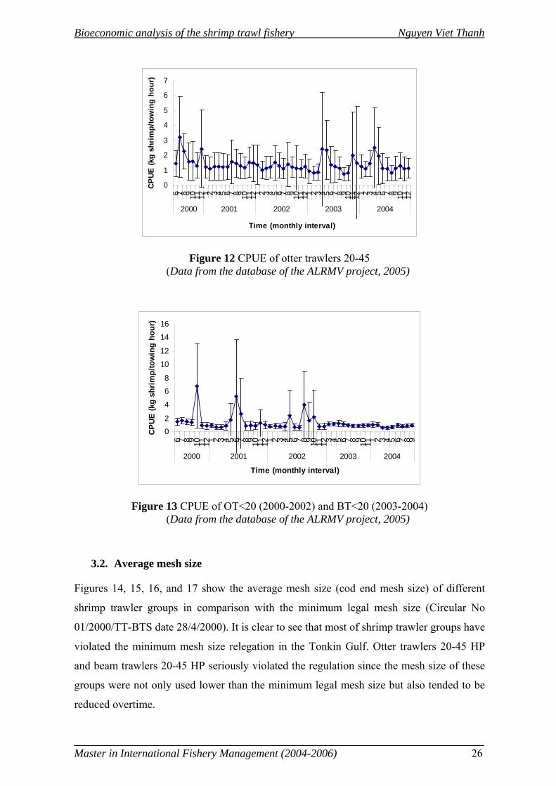
Master in International Fishery Management (2004-2006) 26
0
1
2
3
4
5
6
7
6 7 8 9 10 11 12 1 2 3 4 5 6 7 8 9 10 11 12 1 2 3 4 5 6 7 8 9 10 11 12 1 2 3 4 5 6 7 8 9 10 11 12 1 2 3 4 5 6 7 8 9 10 11 12
2000 2001 2002 2003 2004
Time (monthly interval)
CPUE
(kg
shrim
p/to
win
g ho
ur)
Figure 12 CPUE of otter trawlers 20-45 (Data from the database of the ALRMV project, 2005)
0
2
4
6
8
10
12
14
16
6 7 8 9 10 11 12 1 2 3 4 5 6 7 8 9 10 11 12 1 2 3 4 5 6 7 8 9 10 11 12 3 4 5 6 7 8 9 10 11 1 2 3 4 5 6 7 8 9
2000 2001 2002 2003 2004
Time (monthly interval)
CPU
E (k
g sh
rim
p/to
win
g ho
ur)
Figure 13 CPUE of OT<20 (2000-2002) and BT<20 (2003-2004) (Data from the database of the ALRMV project, 2005)
3.2. Average mesh size
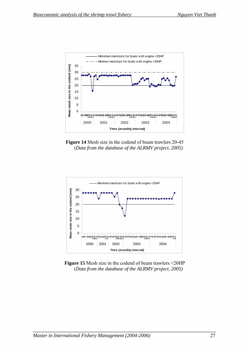
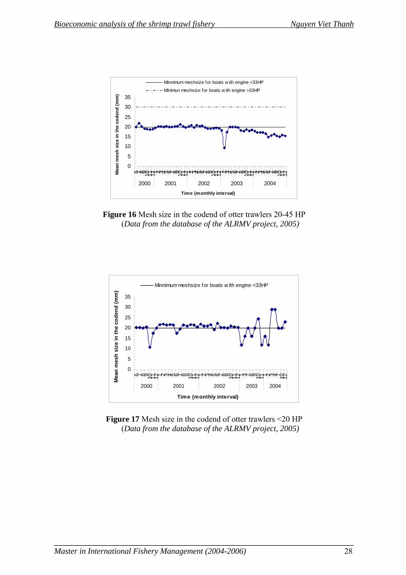
Figures 14, 15, 16, and 17 show the average mesh size (cod end mesh size) of different
shrimp trawler groups in comparison with the minimum legal mesh size (Circular No
01/2000/TT-BTS date 28/4/2000). It is clear to see that most of shrimp trawler groups have
violated the minimum mesh size relegation in the Tonkin Gulf. Otter trawlers 20-45 HP
and beam trawlers 20-45 HP seriously violated the regulation since the mesh size of these
groups were not only used lower than the minimum legal mesh size but also tended to be
reduced overtime.
Bioeconomic analysis of the shrimp trawl fishery Nguyen Viet Thanh
Master in International Fishery Management (2004-2006) 27
0
5
10
15
20
25
30
35
6 7 8 9 10 11 12 1 2 3 4 5 6 7 8 9 10 11 12 1 2 3 4 5 6 7 8 9 10 11 12 1 2 3 4 5 6 7 8 9 10 11 12 1 2 3 4 5 6 7 8 9 10 11 12
2000 2001 2002 2003 2004
Time (monthly interval)
Mea
n m
esh
size
in th
e co
dend
(mm
)
Minnimum meshsize for boats w ith engine <33HP
Minimun meshsize for boats w ith engine >33HP
Figure 14 Mesh size in the codend of beam trawlers 20-45 (Data from the database of the ALRMV project, 2005)
0
5
10
15
20
25
30
6 7 8 9 10 11 4 5 6 12 1 2 3 10 11 12 2 3 4 5 6 7 8 9 10 11 1 2 3 4 5 6 7 8 9 12
2000 2001 2002 2003 2004
Time (monthly interval)
Mea
n m
esh
size
in th
e co
dend
(mm
)
Minnimum meshsize for boats w ith engine <33HP
Figure 15 Mesh size in the codend of beam trawlers <20HP (Data from the database of the ALRMV project, 2005)
Bioeconomic analysis of the shrimp trawl fishery Nguyen Viet Thanh
Master in International Fishery Management (2004-2006) 28
0
5
10
15
20
25
30
35
6 7 8 9 10 11 12 1 2 3 4 5 6 7 8 9 10 11 12 1 2 3 4 5 6 7 8 9 10 11 12 1 2 3 4 5 6 7 8 9 10 11 12 1 2 3 4 5 6 7 8 9 10 11 12
2000 2001 2002 2003 2004
Time (monthly interval)
Mea
n m
esh
size
in th
e co
dend
(mm
)
Minnimum meshsize for boats w ith engine <33HP
Minimun meshsize for boats w ith engine >33HP
Figure 16 Mesh size in the codend of otter trawlers 20-45 HP (Data from the database of the ALRMV project, 2005)
0
5
10
15
20
25
30
35
6 7 8 9 10 11 12 1 2 3 4 5 6 7 8 9 10 11 12 1 2 3 4 5 6 7 8 9 10 11 12 1 3 7 8 9 10 11 1 2 3 4 7 10 12
2000 2001 2002 2003 2004
Time (monthly interval)
Mea
n m
esh
size
in th
e co
dend
(mm
)
Minnimum meshsize for boats w ith engine <33HP
Figure 17 Mesh size in the codend of otter trawlers <20 HP (Data from the database of the ALRMV project, 2005)
Bioeconomic analysis of the shrimp trawl fishery Nguyen Viet Thanh
Master in International Fishery Management (2004-2006) 29
Results
1. Parameters
The results of estimating coefficientsγ, γ1 from equations (18) and (19) are shown in
Table11. For both Verhulst-Schaefer and Gompertz-Fox models, the results indicated an
expected negative relationship between CPUE and effort, slope coefficient equal
-5.056*10-7 and -4.302*10-7 for Verhulst-Schaefer and Gompertz-Fox models respectively.
The P-values indicating that the slope coefficients are different from zero with a
significance level of 95%. The R2 values 0.581 and 0.635 indicate that about 60% percent
of CPUE variations are explained by Verhulst-Schaefer and Gompertz-Fox models
respectively, by the explanatory variable effort. The observed R2 values shows that the two
models give reasonable fit to the data, the Gompertz-Fox model was slightly better than the
Verhulst-Schaefer model.
Table 11 Estimated coefficients using OLS method
Verhulst-Schaefer model Gompertz-Fox model
Estimated coefficient
t-value Estimated coefficient
t-value
γ 3.640 5.212* 2.176 4.106*
γ1 -5.056x10⁻⁷ -3.114* -4.302x10⁻⁷ -3.491*
df 8 df 8 R2 0.581 R2 0.635 F 9.696 F 12.187
* Significant at the 5% level
Table 12, 13 shows predicted catchability (q), intrinsic growth rate (r) and the carrying
capacity (K) from the models for the fishery. The catchability was computed from the
estimated biomass, which were derived from independent surveys in 2003. Afterward,
intrinsic growth rate and the carrying capacity were calculated based on estimated
coefficients, which were derived from the two models (table 11). Verhulst-Schaefer model
predicted intrinsic growth rate almost three times that of the Gompertz-Fox model. In case
of the carrying capacity, it was vice versa for the two models.
Bioeconomic analysis of the shrimp trawl fishery Nguyen Viet Thanh
Master in International Fishery Management (2004-2006) 30
Table 12 The catchability (q) in 2003
Southwest monsoon season (10-7 hour-1)
Northeast monsoon season (10-7 hour-1)
The average catchability(10-7 hour-1)
3.31779 1.03047 2.17413
Table 13 Estimated r, K parameters
Models
Parameters Verhulst-Schaefer Gompertz-Fox
r 1.564950 0.505324
K 16.740900 40.528400
r = intrinsic growth in a half year-1 K = carrying capacity in 106 kg
2. Results from models
The graph of the equilibrium yields derived from the two models against effort are shown
in figure 18. The two models showed considerable differences in predicted reference points
(table 14). The Gompertz-Fox model (short broken line) showed that the MSY of the
shrimp fishery was 15% higher than that of the Verhulst-Schaefer model (long broken
line). If this comparison is extended to the effort level at MSY, it is shown that the
Gompertz-Fox model was 35 % lower than the one of the Verhulst-Schaefer model. While
estimated profits at MSY (p*MSY-c*EMSY) showed the Gompertz-Fox model with a
higher profit of 200% because of differences in predicted effort. The Gompertz-Fox model
predicted the stock was heavily exploited, while the Verhulst-Schaefer model predicted the
stock was fully exploited.
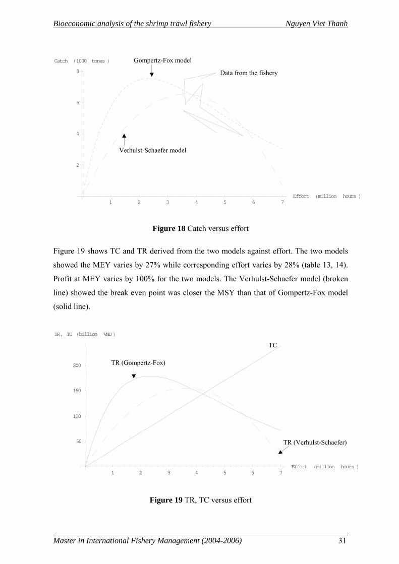
Bioeconomic analysis of the shrimp trawl fishery Nguyen Viet Thanh
Master in International Fishery Management (2004-2006) 31
1 2 3 4 5 6 7Effort Hmillion hours L
2
4
6
8
Catch H1000 tones L
Figure 18 Catch versus effort
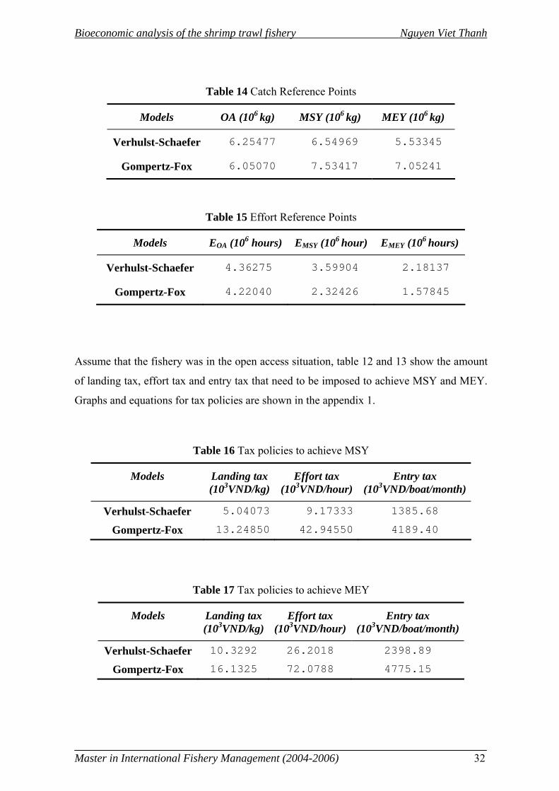
Figure 19 shows TC and TR derived from the two models against effort. The two models
showed the MEY varies by 27% while corresponding effort varies by 28% (table 13, 14).
Profit at MEY varies by 100% for the two models. The Verhulst-Schaefer model (broken
line) showed the break even point was closer the MSY than that of Gompertz-Fox model
(solid line).
1 2 3 4 5 6 7Effort Hmillion hours L
50
100
150
200
TR, TC Hbillion VNDL
Figure 19 TR, TC versus effort
TC
TR (Gompertz-Fox)
TR (Verhulst-Schaefer)
Data from the fishery
Gompertz-Fox model
Verhulst-Schaefer model
Bioeconomic analysis of the shrimp trawl fishery Nguyen Viet Thanh
Master in International Fishery Management (2004-2006) 32
Table 14 Catch Reference Points
Models OA (106 kg) MSY (106 kg) MEY (106 kg)
Verhulst-Schaefer 6.25477 6.54969 5.53345
Gompertz-Fox 6.05070 7.53417 7.05241
Table 15 Effort Reference Points
Models EOA (106 hours) EMSY (106 hour) EMEY (106 hours)
Verhulst-Schaefer 4.36275 3.59904 2.18137
Gompertz-Fox 4.22040 2.32426 1.57845
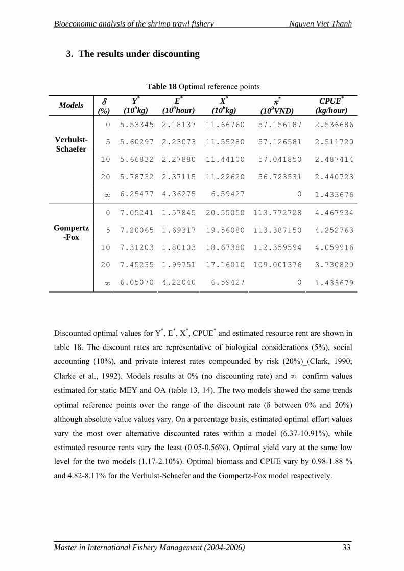
Assume that the fishery was in the open access situation, table 12 and 13 show the amount
of landing tax, effort tax and entry tax that need to be imposed to achieve MSY and MEY.
Graphs and equations for tax policies are shown in the appendix 1.
Table 16 Tax policies to achieve MSY
Models Landing tax (103VND/kg)
Effort tax (103VND/hour)
Entry tax (103VND/boat/month)
Verhulst-Schaefer 5.04073 9.17333 1385.68
Gompertz-Fox 13.24850 42.94550 4189.40
Table 17 Tax policies to achieve MEY
Models Landing tax (103VND/kg)
Effort tax (103VND/hour)
Entry tax (103VND/boat/month)
Verhulst-Schaefer 10.3292 26.2018 2398.89
Gompertz-Fox 16.1325 72.0788 4775.15
Bioeconomic analysis of the shrimp trawl fishery Nguyen Viet Thanh
Master in International Fishery Management (2004-2006) 33
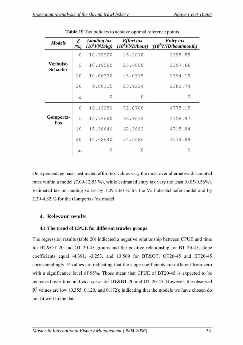
3. The results under discounting
Table 18 Optimal reference points
Models δ (%)
Y*
(106kg) E*
(106hour) X*
(106kg) π*
(109VND) CPUE*
(kg/hour)
0 5.53345 2.18137 11.66760 57.156187 2.536686
5 5.60297 2.23073 11.55280 57.126581 2.511720
10 5.66832 2.27880 11.44100 57.041850 2.487414
20 5.78732 2.37115 11.22620 56.723531 2.440723
Verhulst-Schaefer
∞ 6.25477 4.36275 6.59427 0 1.433676
0 7.05241 1.57845 20.55050 113.772728 4.467934
5 7.20065 1.69317 19.56080 113.387150 4.252763
10 7.31203 1.80103 18.67380 112.359594 4.059916
20 7.45235 1.99751 17.16010 109.001376 3.730820
Gompertz-Fox
∞ 6.05070 4.22040 6.59427 0 1.433679
Discounted optimal values for Y*, E*, X*, CPUE* and estimated resource rent are shown in
table 18. The discount rates are representative of biological considerations (5%), social
accounting (10%), and private interest rates compounded by risk (20%)_(Clark, 1990;
Clarke et al., 1992). Models results at 0% (no discounting rate) and ∞ confirm values
estimated for static MEY and OA (table 13, 14). The two models showed the same trends
optimal reference points over the range of the discount rate (δ between 0% and 20%)
although absolute value values vary. On a percentage basis, estimated optimal effort values
vary the most over alternative discounted rates within a model (6.37-10.91%), while
estimated resource rents vary the least (0.05-0.56%). Optimal yield vary at the same low
level for the two models (1.17-2.10%). Optimal biomass and CPUE vary by 0.98-1.88 %
and 4.82-8.11% for the Verhulst-Schaefer and the Gompertz-Fox model respectively.
Bioeconomic analysis of the shrimp trawl fishery Nguyen Viet Thanh
Master in International Fishery Management (2004-2006) 34
Table 19 Tax policies to achieve optimal reference points
Models δ (%)
Landing tax (103VND/kg)
Effort tax (103VND/hour)
Entry tax (103VND/boat/month)
0 10.32920 26.2018 2398.89
5 10.19580 25.6089 2397.66
10 10.06330 25.0315 2394.10
20 9.80135 23.9224 2380.74
Verhulst-Schaefer
∞ 0 0 0
0 16.13250 72.0788 4775.15
5 15.74680 66.9674 4758.97
10 15.36640 62.3863 4715.84
20 14.62640 54.5686 4574.89
Gompertz-Fox
∞ 0 0 0
On a percentage basis, estimated effort tax values vary the most over alternative discounted
rates within a model (7.09-12.53 %), while estimated entry tax vary the least (0.05-0.56%).
Estimated tax on landing varies by 1.29-2.60 % for the Verhulst-Schaefer model and by
2.39-4.82 % for the Gompertz-Fox model.
4. Relevant results
4.1 The trend of CPUE for different trawler groups
The regression results (table 20) indicated a negative relationship between CPUE and time
for BT&OT 20 and OT 20-45 groups and the positive relationship for BT 20-45, slope
coefficients equal -4.391, -3.253, and 13.569 for BT&OT, OT20-45 and BT20-45
correspondingly. P-values are indicating that the slope coefficients are different from zero
with a significance level of 95%. Those mean that CPUE of BT20-45 is expected to be
increased over time and vice versa for OT&BT 20 and OT 20-45. However, the observed
R2 values are low (0.355, 0.120, and 0.172); indicating that the models we have chosen do
not fit well to the data.
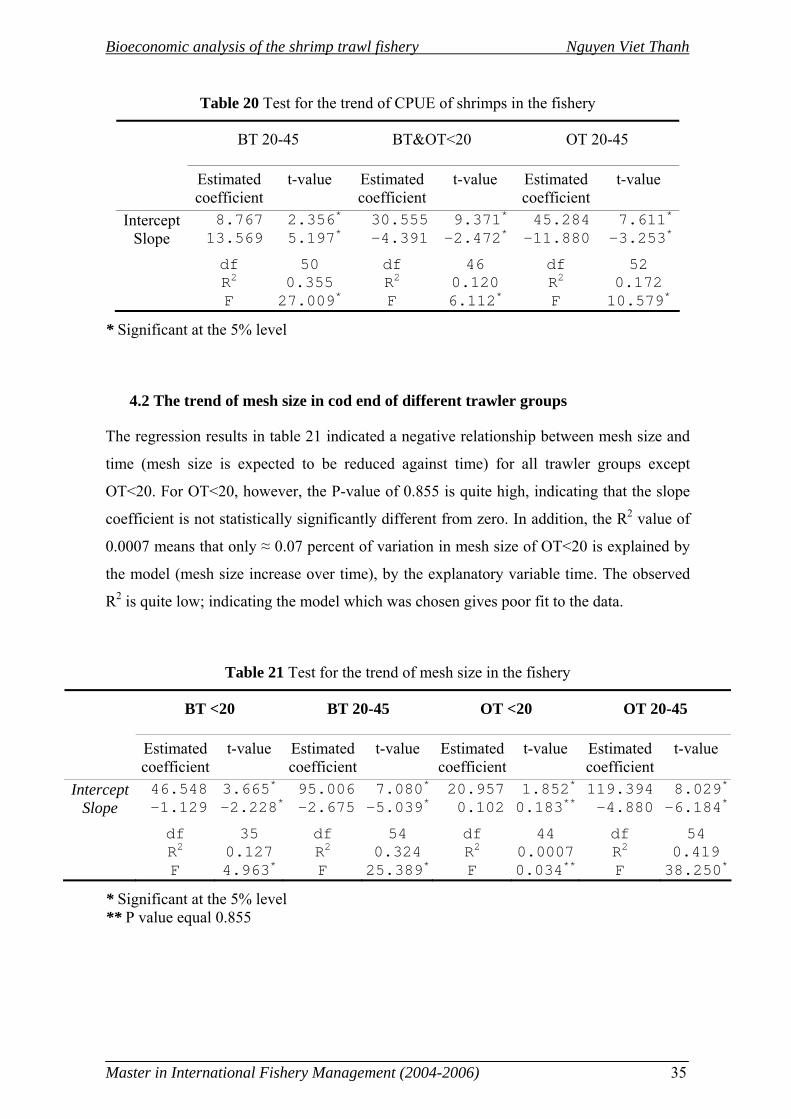
Bioeconomic analysis of the shrimp trawl fishery Nguyen Viet Thanh
Master in International Fishery Management (2004-2006) 35
Table 20 Test for the trend of CPUE of shrimps in the fishery
BT 20-45 BT&OT<20 OT 20-45
Estimated coefficient
t-value Estimated coefficient
t-value Estimated coefficient
t-value
Intercept 8.767 2.356* 30.555 9.371* 45.284 7.611*
Slope 13.569 5.197* -4.391 -2.472* -11.880 -3.253*
df 50 df 46 df 52 R2 0.355 R2 0.120 R2 0.172 F 27.009* F 6.112* F 10.579*
* Significant at the 5% level
4.2 The trend of mesh size in cod end of different trawler groups
The regression results in table 21 indicated a negative relationship between mesh size and
time (mesh size is expected to be reduced against time) for all trawler groups except
OT<20. For OT<20, however, the P-value of 0.855 is quite high, indicating that the slope
coefficient is not statistically significantly different from zero. In addition, the R2 value of
0.0007 means that only ≈ 0.07 percent of variation in mesh size of OT<20 is explained by
the model (mesh size increase over time), by the explanatory variable time. The observed
R2 is quite low; indicating the model which was chosen gives poor fit to the data.
Table 21 Test for the trend of mesh size in the fishery
BT <20 BT 20-45 OT <20 OT 20-45
Estimated coefficient
t-value Estimated coefficient
t-value Estimated coefficient
t-value Estimated coefficient
t-value
Intercept 46.548 3.665* 95.006 7.080* 20.957 1.852* 119.394 8.029*
Slope -1.129 -2.228* -2.675 -5.039* 0.102 0.183** -4.880 -6.184*
df 35 df 54 df 44 df 54 R2 0.127 R2 0.324 R2 0.0007 R2 0.419 F 4.963* F 25.389* F 0.034** F 38.250*
* Significant at the 5% level ** P value equal 0.855
Bioeconomic analysis of the shrimp trawl fishery Nguyen Viet Thanh
Master in International Fishery Management (2004-2006) 36
Discussion
1. Models
The two models, Verhulst-Schaefer and Gompertz-Fox, appeared to estimate valid
biological parameters and reasonable economic results for the shrimp trawl fishery in the
Tonkin Gulf. The two models also had statistically significant coefficients, which might
make their results to be acceptable. Theoretically, the Gompertz-Fox model may predict a
growth compensation as the stock is reduced than the corresponding compensation
described by the Verhulst-Schaefer model. Both models could be considered as special
cases of the Pella and Tomlinson model (when m→1 and m = 2). Furthermore, data ranges
of catch and effort were small (see figure 18) which may give poor background for
choosing a priority model.
In this study, the relevant results indicated that the fishery was in a situation of
overexploitation. Mesh size in the cod end of almost all trawler groups were significantly
decreased (except the OT<20 group), indicating a compensation of reduced landing of
shrimps overtime. The CPUE of OT 20-45, OT&BT<20 trawler groups had also decreased,
even though the CPUE of the BT 20-45 trawler group was increased. The landing shrimp
price and the mesh size in cod end of this trawler group had been reduced, implying that
less valuable species and juvenile shrimp had been caught. Long (2001; 2003) argues that
shrimp trawler fleet are shortened both in size and number due to overfishing problems.
Chinh (2005) shows that the density of penaeid stocks have been reduced by a half over the
last thirty years (1975-2002).
The fish stock being overexploited means that the shrimp biomass was below the biomass
level of MSY. The Verhulst-Schaefer model proposed the current multi species shrimp
biomass to be closer to the MSY level than the Gompertz-Fox model did. The Verhulst-
Schaefer model also predicted the intrinsic growth rate of the shrimp stock (per a half year)
three times higher than the Gompertz-Fox model predicted. In addition, the regression
results (table 11) showed slightly better fit for the Gompertz-Fox model than the Verhulst-
Schaefer model. However, the data which used for the two models was the short time
Bioeconomic analysis of the shrimp trawl fishery Nguyen Viet Thanh
Master in International Fishery Management (2004-2006) 37
series data. It implies that the results may not globally describe the development of the
fishery. The reference points derived from the models may be just local reference points. In
this study, a range of reference points, which derived from the two models are chosen in
order to take consideration of uncertainty in practice.
2. Reference points
The results from the two models showed the open access yield of the fishery was around
6,000 tones for a half year (12,000 tones per year). This yield is in accordance with the
official catch statistic, which was around 11,445 tones in 2003 (Chinh, 2005). The open
access yield figure may also be appropriate to the figure of the shrimp biomass, which was
estimated about 4,165 tones in the southwest monsoon season and approximately 6,687
tones in the northeast monsoon season (Thi et al., 2004). Since the penaeid shrimps, which
are short life span species, have high turn-over growth rate annually. It is quite common
for the shrimp population to have an annual growth which in biomass terms exceeds the
population size at some points during the year. Fox (1970) argues that commercial
exploitation of marine fish population is usually directed towards mature individuals and,
if spawning occurs during the year, survival of the population may be ensured – even at
100% annual fishing mortality. Other arguments could be derived from multispecies
considerations. The species composition probably has changed over time, typically towards
less valuable species. This could change the MSY value dynamically over time. The
possibility depletion of one species may be reduced by the increase of other species
(Guland & Rothschild, 1984).
The two models showed that the fishery was at least fully exploited both in terms of
maximizing yield and maximizing resource rent. The EMSY and EMEY of the fishery from
the Verhulst-Schaefer model were about 3.6 and 2.2 millions towing hours respectively.
The EMSY and EMEY of the fishery from the Gompertz-Fox model were around 2.3 and 1.6
millions towing hours correspondingly (table15). The effort of the fishery in 2004 (average
effort for a half year) was estimated around 4.1 millions towing hours (table 7), indicating
that the harvest of the shrimp stock was not sustainable regarding to the referent points.
The effort of the fishery should be strongly reduced to achieve optimal reference points.
The current effort of the fishery (2004) should be reduced roughly 12 % (Verhulst-
Bioeconomic analysis of the shrimp trawl fishery Nguyen Viet Thanh
Master in International Fishery Management (2004-2006) 38
Schaefer model) to 44 % (Gompert-Fox model) to archive the MSY and about 46 % to
61% to reach the MEY.
The data (figure 14-17) showed that for the otter trawler groups, the mesh size seem to
violate the minimum mesh size regulation more than what was the case in the beam trawler
groups. It means otter trawlers probably harvested smaller shrimps than beam trawlers did.
Furthermore, iron tickler chains of otter trawlers which were used to round up the shrimp
in the sand, may destroy critical habitats in coastal areas. For those reasons, it seems like
effort of otter trawlers, the dominant group in the shrimp trawl fishery, should first be
reduced in order to reach the reference points (MSY or MEY). The OT 20-45 was the
biggest group and the one violating the minimum mesh size regulation the most. The
CPUE and mesh size of the OT 20-45 also had been reduced over time, implying that the
effort of this group should strictly be controlled.
3. Management
3.1 The present regulations
Many regulations have been applied in the shrimp trawl fishery but the compliance of these
regulations is questionable. This aspect will be discussed through analyzing the efficiency
of some major regulations which have been applied for the shrimp trawl fishery both in
practical and theoretical aspects.
3.1.1 The minimum legal length regulation
The data showed that, the minimum legal length regulation seems to be violated in the
shrimp trawl fishery. Landing shrimps were quite small compared with the minimum legal
shrimp size. The difficulties in monitoring are substantial since the fishery is multi species
which may be managed appropriately by input regulations.
Minimum size regulation opens for discarding captured undersized individuals. Some
fisheries where catch is not harmed by catching method may exist, such as mollusks
gathered by hand or crustaceans caught by traps. In other fisheries, e.g. trawling, the
probabilities of fish surviving after discarding, are very small (King, 1995). The idea is to
change gears or fishing areas in such cases. Those imply that the minimum legal length
regulation has little application to the shrimp trawl fishery both in terms of theoretical and
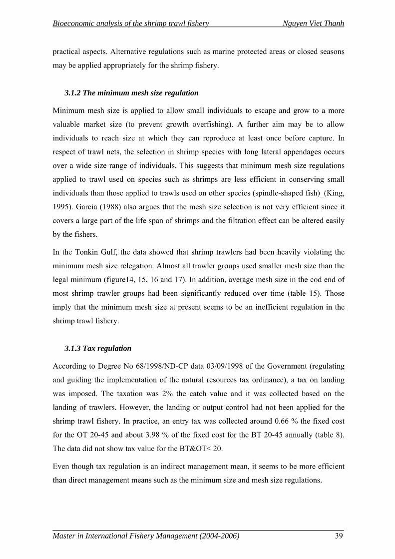
Bioeconomic analysis of the shrimp trawl fishery Nguyen Viet Thanh
Master in International Fishery Management (2004-2006) 39
practical aspects. Alternative regulations such as marine protected areas or closed seasons
may be applied appropriately for the shrimp fishery.
3.1.2 The minimum mesh size regulation
Minimum mesh size is applied to allow small individuals to escape and grow to a more
valuable market size (to prevent growth overfishing). A further aim may be to allow
individuals to reach size at which they can reproduce at least once before capture. In
respect of trawl nets, the selection in shrimp species with long lateral appendages occurs
over a wide size range of individuals. This suggests that minimum mesh size regulations
applied to trawl used on species such as shrimps are less efficient in conserving small
individuals than those applied to trawls used on other species (spindle-shaped fish)_(King,
1995). Garcia (1988) also argues that the mesh size selection is not very efficient since it
covers a large part of the life span of shrimps and the filtration effect can be altered easily
by the fishers.
In the Tonkin Gulf, the data showed that shrimp trawlers had been heavily violating the
minimum mesh size relegation. Almost all trawler groups used smaller mesh size than the
legal minimum (figure14, 15, 16 and 17). In addition, average mesh size in the cod end of
most shrimp trawler groups had been significantly reduced over time (table 15). Those
imply that the minimum mesh size at present seems to be an inefficient regulation in the
shrimp trawl fishery.
3.1.3 Tax regulation
According to Degree No 68/1998/ND-CP data 03/09/1998 of the Government (regulating
and guiding the implementation of the natural resources tax ordinance), a tax on landing
was imposed. The taxation was 2% the catch value and it was collected based on the
landing of trawlers. However, the landing or output control had not been applied for the
shrimp trawl fishery. In practice, an entry tax was collected around 0.66 % the fixed cost
for the OT 20-45 and about 3.98 % of the fixed cost for the BT 20-45 annually (table 8).
The data did not show tax value for the BT&OT< 20.
Even though tax regulation is an indirect management mean, it seems to be more efficient
than direct management means such as the minimum size and mesh size regulations.
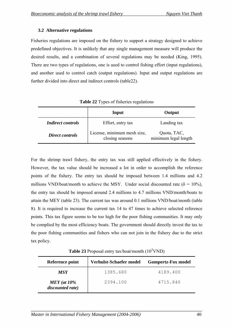
Bioeconomic analysis of the shrimp trawl fishery Nguyen Viet Thanh
Master in International Fishery Management (2004-2006) 40
3.2 Alternative regulations
Fisheries regulations are imposed on the fishery to support a strategy designed to achieve
predefined objectives. It is unlikely that any single management measure will produce the
desired results, and a combination of several regulations may be needed (King, 1995).
There are two types of regulations, one is used to control fishing effort (input regulations),
and another used to control catch (output regulations). Input and output regulations are
further divided into direct and indirect controls (table22).
Table 22 Types of fisheries regulations
Input Output
Indirect controls Effort, entry tax Landing tax
Direct controls License, minimum mesh size, closing seasons
Quota, TAC, minimum legal length
For the shrimp trawl fishery, the entry tax was still applied effectively in the fishery.
However, the tax value should be increased a lot in order to accomplish the reference
points of the fishery. The entry tax should be imposed between 1.4 millions and 4.2
millions VND/boat/month to achieve the MSY. Under social discounted rate (δ = 10%),
the entry tax should be imposed around 2.4 millions to 4.7 millions VND/month/boats to
attain the MEY (table 23). The current tax was around 0.1 millions VND/boat/month (table
8). It is required to increase the current tax 14 to 47 times to achieve selected reference
points. This tax figure seems to be too high for the poor fishing communities. It may only
be complied by the most efficiency boats. The government should directly invest the tax to
the poor fishing communities and fishers who can not join in the fishery due to the strict
tax policy.
Table 23 Proposal entry tax/boat/month (103VND)
Reference point Verhulst-Schaefer model Gompertz-Fox model
MSY 1385.680 4189.400
MEY (at 10% discounted rate)
2394.100 4715.840
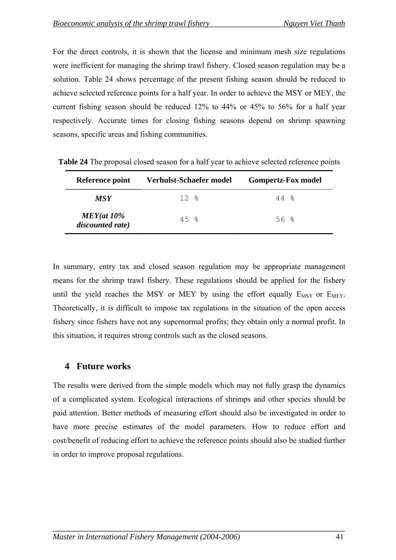
Bioeconomic analysis of the shrimp trawl fishery Nguyen Viet Thanh
Master in International Fishery Management (2004-2006) 41
For the direct controls, it is shown that the license and minimum mesh size regulations
were inefficient for managing the shrimp trawl fishery. Closed season regulation may be a
solution. Table 24 shows percentage of the present fishing season should be reduced to
achieve selected reference points for a half year. In order to achieve the MSY or MEY, the
current fishing season should be reduced 12% to 44% or 45% to 56% for a half year
respectively. Accurate times for closing fishing seasons depend on shrimp spawning
seasons, specific areas and fishing communities.
Table 24 The proposal closed season for a half year to achieve selected reference points
Reference point Verhulst-Schaefer model Gompertz-Fox model
MSY 12 % 44 %
MEY(at 10% discounted rate)
45 % 56 %
In summary, entry tax and closed season regulation may be appropriate management
means for the shrimp trawl fishery. These regulations should be applied for the fishery
until the yield reaches the MSY or MEY by using the effort equally EMSY or EMEY.
Theoretically, it is difficult to impose tax regulations in the situation of the open access
fishery since fishers have not any supernormal profits; they obtain only a normal profit. In
this situation, it requires strong controls such as the closed seasons.
4 Future works
The results were derived from the simple models which may not fully grasp the dynamics
of a complicated system. Ecological interactions of shrimps and other species should be
paid attention. Better methods of measuring effort should also be investigated in order to
have more precise estimates of the model parameters. How to reduce effort and
cost/benefit of reducing effort to achieve the reference points should also be studied further
in order to improve proposal regulations.
Bioeconomic analysis of the shrimp trawl fishery Nguyen Viet Thanh
Master in International Fishery Management (2004-2006) 42
Conclusions
In this study two surplus production models (Verhulst-Schaefer and Gompertz-Fox) have
been presented and parameterized when applying catch and effort data from a Vietnamese
shrimp fishery. The data is aggregated in time periods of half year in accordance with the
biological year of the shrimp stock in the Tonkin Gulf. Results derived from the models are
reasonable compared with the independent surveys and official statistics. The models
should be applied in a flexible way regarding the biological characteristics of the stock. On
the other hand, for the fast growing species with a high turn-over rate (short life span) in
tropical areas such as for these shrimps, using data from the enumerator program could be
an alternative method and may reduce the problems of inefficient statistic data.
The two models, Verhulst-Schaefer and Gompertz-Fox, appeared to estimate valid
biological parameters and reasonable economic results for the shrimp trawl fishery in the
Tonkin Gulf. The two models also have statistically significant coefficients, which may
make their results be acceptable. In addition, data ranges of catch and effort were small
which may give poor background for choosing a priority model. Besides, the data which
was used for the models is the short time series data. It implies that the results may not
globally describe the development of the fishery. The reference points derived from the
models may be just local reference points. A range of reference points, which derived from
the two models, are chosen in order to take consideration of uncertainty in practice.
The two models showed that the fishery was at least fully exploited both in terms of
maximizing yield and maximizing resource rent. The harvest of the shrimp stock was not
sustainable regarding to the referent points. The current effort of the fishery (2004) should
be reduced roughly 12 % to 44 % to archive the MSY and about 46 % to 61% to reach the
static MEY (at 0% discounted rate).
Minimum mesh size, legal length regulations may not appropriate for the shrimp trawl
fishery both from a theoretical and a practical point of view. Entry tax and closed season
may be preferable management means for the shrimp trawl fishery. The entry tax should be
imposed between 1.4 millions and 4.2 millions VND/month/boat to achieve the MSY.
Bioeconomic analysis of the shrimp trawl fishery Nguyen Viet Thanh
Master in International Fishery Management (2004-2006) 43
Under social discounted rate (δ = 10%), the entry tax should be imposed around 2.4
millions to 4.7 millions VND/month/boats to attain the MEY. The closed season regulation
should be imposed based on shrimp spawning seasons, specific areas and fishing
communities. The present fishing season should be reduced 12% to 44% (for a half year) to
achieve MSY and 45% to 56% (for a half year) to attain MEY under social discounted rate
(δ = 10%). Both entry tax and the closed season regulation should be applied for the
fishery until the yield reaches the MSY or MEY by using the effort equally EMSY or EMEY.
Theoretically, it is difficult to impose tax regulations in the situation of the open access
fishery since fishers have not any supernormal profits; they obtain only a normal profit. In
this situation, it requires strong controls such as the closed seasons.
Bioeconomic analysis of the shrimp trawl fishery Nguyen Viet Thanh
Master in International Fishery Management (2004-2006) 44
Reference
BEVERTON, R. J. H. & HOLT, S. J. (1993). On the dynamics of exploited fish populations. Chapman & Hall, London.
CHINH, N., VAN, LV., HUY, LQ., NINH, LV., DUONG, NQ., CUONG, NM., THANH, NQ.,. (2005). Quy hoach khai thac xa bo Vinh Bac Bo den nam 2010 (Offshore marine capture fisheries plan to 2010 for the Tonkin Gulf) (ed. N. Chinh). Institute of economics and planning, Hanoi.
CLARK, C. W. (1985). Bioeconomic modelling and fisheries management. John Wiley & Sons, Inc., New York.
CLARK, C. W. (1990). Mathematical bioeconomics: the optimal management of renewable resources, 2 edition. A Wiley-Interscience Publication, Canada.
CLARK, C. W. & MUNRO, G. R. (1975). The economic of fishing and modern capital theory: a simplified approach. Environmental economics and management 2, 92-106.
CLARKE, R. P., YOSHIMOTO, S. S. & POOLEY, S. G. (1992). A bioeconomic analysis of the Northwestern Hawaiian Islands Lobster fishery. Marine Resource Economics 7, 115-140.
DALL, W., HILL, B. J., ROTHLISBERY, P. C. & SHARPLES, D. J. (1990). The biology of the Penaeidae. In Advances in marine biology, vol. 27 (ed. J. H. S. Blaxter and A. J. Southward), pp. 487. Academic Press, London.
EIDE, A. (1989). Stock estimates for some fish stocks of the Barents Sea based on predation data and the population growth function of Pella and Tomlinson. The Norwegian College of Fishery Science, University of Tromso, Norway.
EIDE, A., SKJOLD, F., OLSEN, F. & FLAATEN, O. (2003). Harvest functions: The Norwegian bottom trawl cod fisheries. Marine Resource Economics 18.
FAO. (2005). Vietnam fisheries. In Country profile, vol. 2006.
FOX, W. W. (1970). An Exponential Surplus-Yield Model for Optimizing Exploited Fish Populations. Trans.Am. Fish. Soc. 99, 80-88.
GARCIA, S. (1988). Tropical penaeid prawns. In Fish population dynamics (ed. J.A.Gulland), pp. 422. John Wiley & Sons, London.
GULAND, J. A. & ROTHSCHILD, B. J. (1984). Penaeid shrimps - their biology and management. Fishing News Books Ltd, Surrey.
HERSOUG, B., FALK-PETERSEN, I.-B., HEEN, K. & REINERTSEN, H. (2002). Report from Fishery Education Mission to Vietnam.
HILBORN, R. & WALTERS, C. J. (1992). Quantitative Fisheries Stock Assessment: Choice, dynamics and uncertainty. Chapman and Hall, London.
Bioeconomic analysis of the shrimp trawl fishery Nguyen Viet Thanh
Master in International Fishery Management (2004-2006) 45
KING, M. (1995). Fisheries biology, assessment and management. Fishing News Books, London.
LONG, N. (2001). Status of offshore fishing technology in Vietnam. In Marine Fisheries Research, vol. II, pp. 347-348. Agriculture Publishing House, Vietnam.
LONG, N. (2003). A preliminary analysis on socioeconomic situation of coastal fishing communities in Vietnam. In Assessment, Management and Future Directions for Coastal Fisheries in Asian Countries (ed. L. G. G. Silvestre, I. Stobutzki, M. Ahmed, R.A. Valmonte-Santos, C. Luna, L. Lachica-Aliño, P. Munro, V. Christensen and D. Pauly), pp. 657-688. The World fish center and the Asian Development Bank (ADB), Malaysia.
LONG, N., KHANG, N. V., HAI, V. D. & CHOKESANGUAN, B. (2002). Fishing gear and methods in Southeast Asia: IV. Vietnam. Southeast Asia Fisheries Development Center.
MOFI. (2006). www.fistenet.gov.vn.
PELLA, J. J. & TOMLINSON, P. K. (1969). A general stock production model. Bull. IATTC 13, 421-496.
RICHARDS, F. J. (1959). A flexible growth function for empirical use. Experimental Botany 10, 290-300.
RUDDLE, K. (1998). Traditional community-based coastal marine fisheries management in Vietnam. Ocean and Coastal Management 40, 1-22.
SCHAEFER, M. B. (1954). Some considerations of population dynamics and economics in relation to the management of the commersial marine fisheries. Bull. IATTC 1, 26-56.
SON, D. M. (2001). Offshore fisheries resources in the Tonkin Gulf, Southeast region and the Center of Eastern Sea of Vietnam. In Marine Fisheries Research, vol. II (ed. B. D. Chung, D. M. Son and C. T. Vinh), pp. 137-164. Agriculture Publishing House, Haiphong.
SON, D. M. (2004). Country report for the fisheries component of the UNEP/GEF/SCS project. In Reversing environmental degradation trends in the South China Sea and Gulf of Thai Lan, pp. 55. Research Institute For Marine Fisheries, Hai Phong.
SON, D. M., AND THUOC, P.,. (2003). Management of Coastal Fisheries in Vietnam. In Assessment, Management and Future Directions for Coastal Fisheries in Asian Countries (ed. L. G. G. Silvestre, I. Stobutzki, M. Ahmed, R.A. Valmonte-Santos, C. Luna, L. Lachica-Aliño, P. Munro, V. Christensen and D. Pauly), pp. 1120. the WorldFish Center and the Asian Development Bank (ADB), Malaysia.
THI, D. V., HA, V. V. & KIEN, L. T. (2004). Technical report: status of the marine resource based on the trawl and gill net surveys in 2003, pp. 27. Research Institute For Marine Fisheries, Hai Phong.
Bioeconomic analysis of the shrimp trawl fishery Nguyen Viet Thanh
Master in International Fishery Management (2004-2006) 46
THONG, H. X. (1998). Traditional orgnization of fisheries communitites in Vietnam. In The ninth Biennial conference of the International Institute of fisheries economic and trade, vol. 1 (ed. A. Eide and T. Vassdal), pp. 286-292. the International Institute of fisheries economic and trade, Tromso, Norway.
THUC, V. N. & THANG, N. V. (1983). Biological cheracteristics of Penaeus Merguiensis in the western part of Tonkin Gulf, pp. 11. Reserch Institute For Marine Fisheries, Hai Phong.
THUY, N. T. D. (2005). Development of the sustainable fisheries indicators based on the data of enumerator program, pp. 16. ALRMV project, Hanoi.
Bioeconomic analysis of the shrimp trawl fishery Nguyen Viet Thanh
Master in International Fishery Management (2004-2006) 47
Appendix 1: Tax policies to achieve reference points
1. Landing tax: Assume that the fishery is in the open access situation. T is the landing tax that needs to be
created in order to achieve MEY (or MSY); T is defined by an equation:
(p - T)*MEY = c*EMEY
Hence: T = p – c*EMEY/MEY
2. Effort tax:
Assume that the fishery is in the open access situation. T is the effort tax that needs to be
created in order to achieve MEY (or MSY); T is defined by an equation:
p*MEY = (c + T)*EMEY
Hence: T = [(p*MEY)/EMEY] - c
Effort Tax
TR=p*H TC=c*E
Pi=TR-TC
TC'=(c+T)*E
Effort
TC, T
R
EMEY
p*MEY
Landing Tax
TR=p*H
TC=c*E
Pi=TR-TC
TR'=(p-T)*H
Effort
TC, T
R
EMEY
(p-T)*MEY
Bioeconomic analysis of the shrimp trawl fishery Nguyen Viet Thanh
Master in International Fishery Management (2004-2006) 48
3. Entry tax: Assume that the fishery is in the open access situation. T is the entry tax (for the whole
fishery) that needs to be created in order to achieve MEY (or MSY); T is defined by an
equation:
p*MEY = c*EMEY + T
Hence: T = p*MEY – c*EMEY
Entry Tax
TR=p*H TC=c*E
Pi=TR-TC
TC'=c*E+T
Effort
TC, T
R
EMEY
p*MEY
Bioeconomic analysis of the shrimp trawl fishery Nguyen Viet Thanh
Master in International Fishery Management (2004-2006) 49
Appendix 2: Regression results
1. Relation between CPUE (Log CPUE) and Effort:
1.1 Schaefer model:
1.2 Fox model:
2. Test the trend of CPUE against time:
Beam trawlers 20-45HP
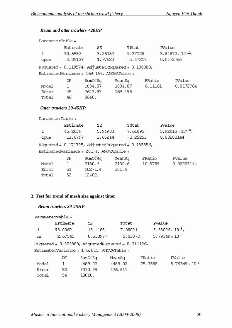
Bioeconomic analysis of the shrimp trawl fishery Nguyen Viet Thanh
Master in International Fishery Management (2004-2006) 50
Beam and otter trawlers <20HP
Otter trawlers 20-45HP
3. Test for trend of mesh size against time:
Beam trawlers 20-45HP
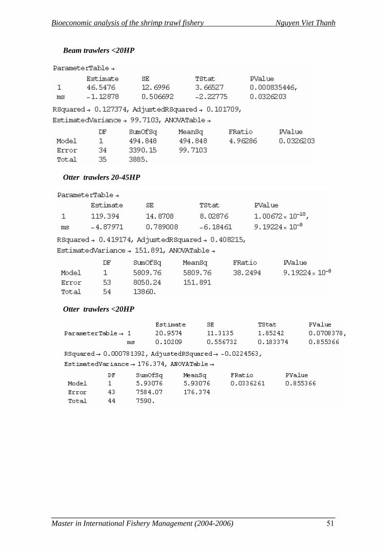
Bioeconomic analysis of the shrimp trawl fishery Nguyen Viet Thanh
Master in International Fishery Management (2004-2006) 51
Beam trawlers <20HP
Otter trawlers 20-45HP
Otter trawlers <20HP
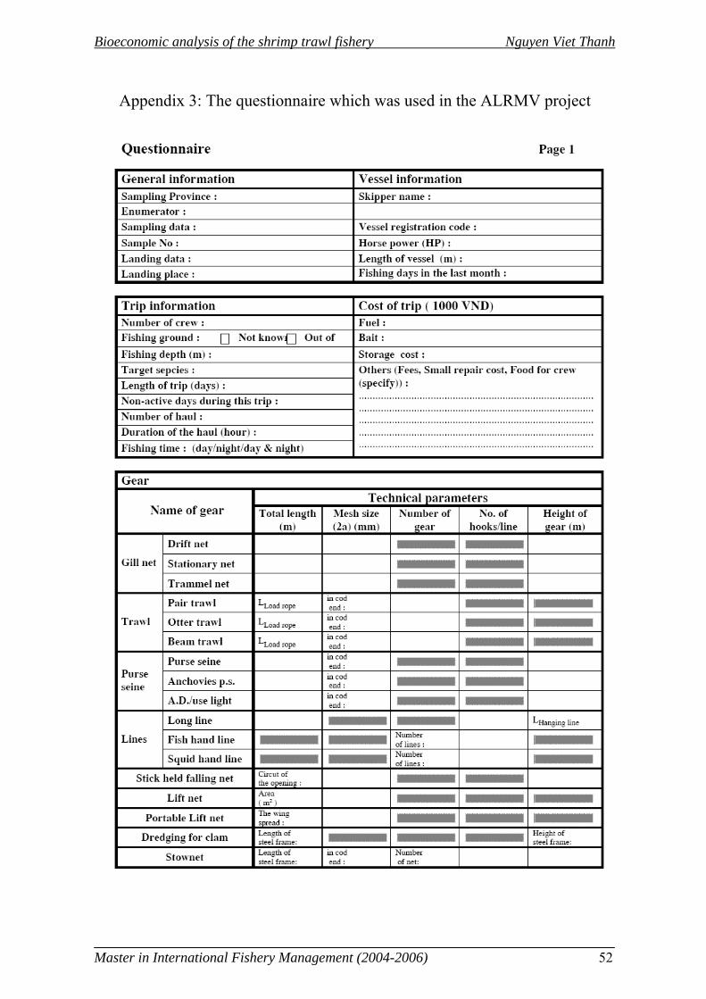
Bioeconomic analysis of the shrimp trawl fishery Nguyen Viet Thanh
Master in International Fishery Management (2004-2006) 52
Appendix 3: The questionnaire which was used in the ALRMV project

Bioeconomic analysis of the shrimp trawl fishery Nguyen Viet Thanh
Master in International Fishery Management (2004-2006) 53
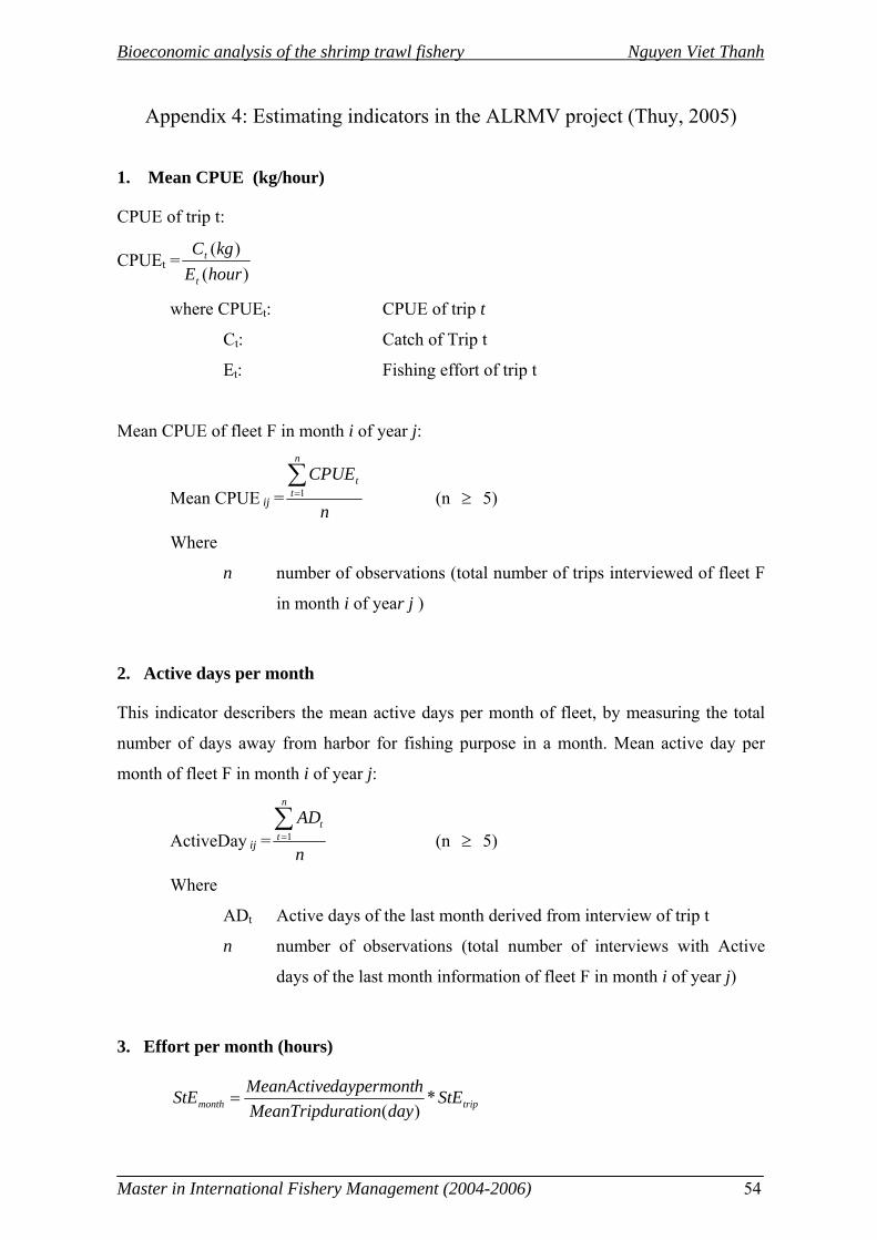
Bioeconomic analysis of the shrimp trawl fishery Nguyen Viet Thanh
Master in International Fishery Management (2004-2006) 54
Appendix 4: Estimating indicators in the ALRMV project (Thuy, 2005)
1. Mean CPUE (kg/hour)
CPUE of trip t:
CPUEt = )()(
hourEkgC
t
t
where CPUEt: CPUE of trip t
Ct: Catch of Trip t
Et: Fishing effort of trip t
Mean CPUE of fleet F in month i of year j:
Mean CPUE ij = n
CPUEn
tt∑
=1 (n ≥ 5)
Where
n number of observations (total number of trips interviewed of fleet F
in month i of year j )
2. Active days per month
This indicator describers the mean active days per month of fleet, by measuring the total
number of days away from harbor for fishing purpose in a month. Mean active day per
month of fleet F in month i of year j:
ActiveDay ij = n
ADn
tt∑
=1 (n ≥ 5)
Where
ADt Active days of the last month derived from interview of trip t
n number of observations (total number of interviews with Active
days of the last month information of fleet F in month i of year j)
3. Effort per month (hours)
tripmonth StEdayrationMeanTripdu
hdaypermontMeanActiveStE *)(
=

Bioeconomic analysis of the shrimp trawl fishery Nguyen Viet Thanh
Master in International Fishery Management (2004-2006) 55
Where:
onHaulDuratihaulNumberhStEtrip *)( =
4. Cost per hour (variable cost):
Cost per hour of trip t:
CostperHourt= )(hStECost
t
Tript
Where cost trip t:
Costt= CostIce + CostFuel + CostFood + CostSalary + ....
Cost per hour from fleet F in month i of year j:
MeanCostPerHour ij = n
rCostperHoun
tt∑
=1 (n ≥ 5)
Where
n number of observations (total number of trips interviewed with cost
information of fleet in month i of year j )
5. Catch composition
This indicator describer the catch composition by percentages of fish groups in the
monthly catches of fleets
Percentage of group A in the catches of fleet F in month i of year j:
PercentageOf GroupAij =∑
∑
=
=n
tt
m
tAt
C
C
1
1
Where
CAt Catch of fish group A in trip t
Ct Catch of trip t
m total number of trips interviewed of fleet F in month i of year j,
which have group A in their catches
n total number of trips interviewed of fleet F in month i of year j
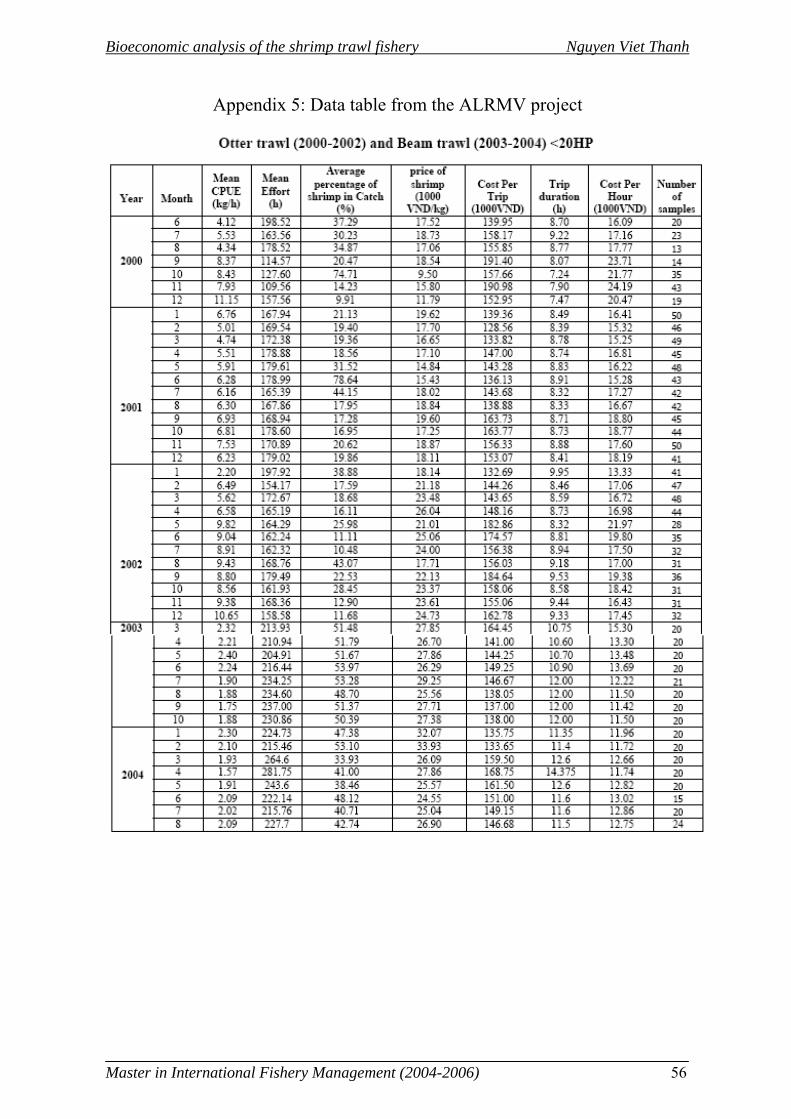
Bioeconomic analysis of the shrimp trawl fishery Nguyen Viet Thanh
Master in International Fishery Management (2004-2006) 56
Appendix 5: Data table from the ALRMV project
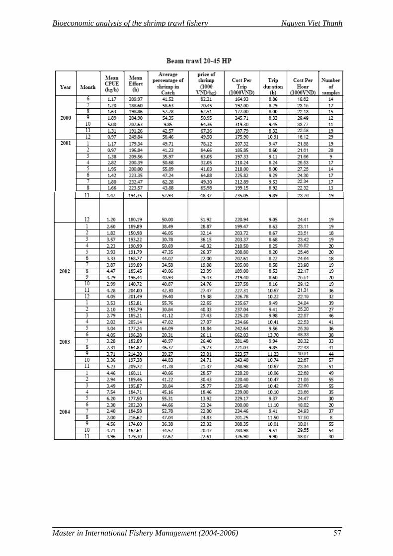
Bioeconomic analysis of the shrimp trawl fishery Nguyen Viet Thanh
Master in International Fishery Management (2004-2006) 57
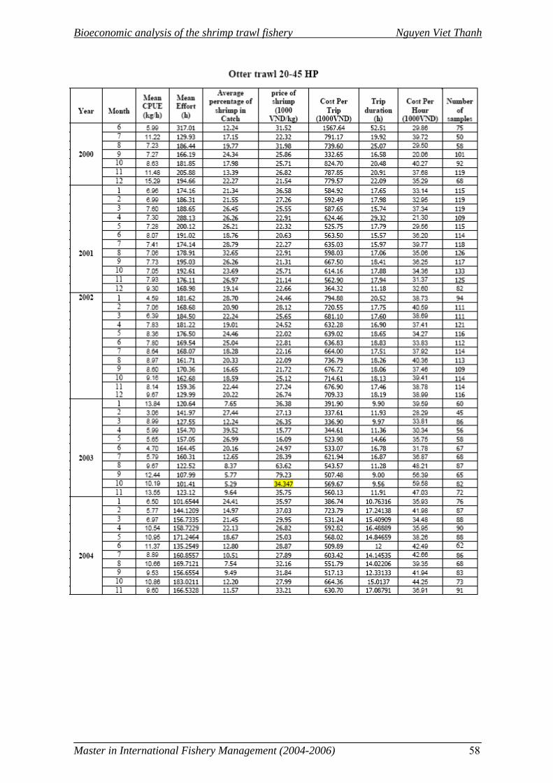
Bioeconomic analysis of the shrimp trawl fishery Nguyen Viet Thanh
Master in International Fishery Management (2004-2006) 58