Beyond the epsilon band: Polygonal modeling of gradation/uncertainty in area-class maps1

Barry J. Kronenfeld

Abstract: A spatial modeling technique is proposed to represent boundary uncertainty or gradation on area class maps using a simple polygon tessellation with designated zones of indeterminacy, or transition zones. The transition zone can be conceptualized as a dual of the epsilon band, but is more flexible and allows for a wide range of polygonal configurations, including polygons with sinuous boundaries, spurs, three-way transition zones and null polygons. The model is specified using the medial axis to capture the general shape characteristics of a transition zone. Graph theoretic representation of an extended version of the medial axis captures key junctions in both shape and classification, and is used to identify well-formed transition zones that can be logically and unambiguously handled by the model. A multivariate classification surface is specified by first defining degrees or probabilities of membership at every point on the medial axis and transition zone boundary. Degrees or probabilities of membership at all other points are defined by linear interpolation. The technique is illustrated with an example of a complex transition zone, and a simple isoline representation that can be derived from the model is presented. The proposed modeling technique promises to facilitate expert characterization of soil formations, ecological systems, and other types of areal units where gradation and/or boundary uncertainty are prevalent.

Keywords: Gradation, boundary uncertainty, area-class map, medial axis, epsilon band

1. Introduction

Area-class maps provide a powerful mechanism by which domain experts can express the spatial pattern of complex natural phenomena such as vegetation, soils, and climate. In these domains, manual delineation of regions is often advantageous over automated mapping methods due to the high costs of data acquisition as well as the challenges of developing formal models of causal inference. The exact locations of boundaries between regions are often indeterminate, however, and so there exists a need for spatial data models that allow expert cartographers to express this indeterminacy. The problem of indeterminate boundaries has led to various research volumes (Burrough and Frank 1996), specialist meetings (Peuquet et al. 1998, Bennett 2003), research priorities (Kronenfeld et al. 2002) and special journal issues (Goodchild 2000, Bennett 2003). Despite this body of research, spatial modeling of boundary indeterminacy is still limited essentially to a raster data model (e.g. Brown 1998, Zhang and Stuart 2001, Zhang et al. 2004, Goodchild et al. 2009). The purpose of the present research is to propose an alternative data model that is more conducive to manual cartographic production by domain experts.

Boundary indeterminacy often results from uncertain knowledge due to inaccurate, imprecise or incomplete observation (e.g. Zhang and Stuart 2001). Boundary indeterminacy may also exist under perfect knowledge, however, when the underlying phenomena change continuously across a gradient. In the latter case, indeterminacy results from the subjective process of defining classes and regions within a continuous landscape, and can be viewed as a form of cartographic generalization (Kronenfeld 2005). These two sources of boundary indeterminacy are referred to

1 This is an Author's Accepted Manuscript of an article published in International Journal of Geographical Information

Science, 2011, © Taylor & Francis, available online at: http://www.tandfonline.com/10.1080/13658816.2010.518317.

as boundary uncertainty and gradation respectively. They often occur simultaneously, and may be difficult to distinguish. Furthermore, both require a similar spatial representation framework in which a multivariate surface is specified across a gradient. Therefore, they are treated together in the present research.

Two general approaches exist to modeling boundary indeterminacy: the attribute-based approach and the location-based approach (Mark and Csillag 1989). The attribute-based approach begins with a set of predefined locations (e.g. cells in a raster grid), and proceeds by specifying a degree of uncertainty or gradation at each location. The process is reversed in the location-based approach: prescribed degrees of uncertainty or gradation are first defined, and then locations at which these occur are delineated. For example, a line might be drawn through the set of locations at which two classes are equally probable, or at which amiguous classification transitions to unambiguous classification. The two approaches differ in their sequence of specification and are appropriate in different situations.

The attribute-based approach is feasible when high-resolution attribute data is available and appropriate numerical classification methods can be developed. This approach has been employed to capture classification uncertainty in maps created from remote sensing imagery (e.g. Zhang and Stuart 2001), modern ground surveys (e.g. Zhang et al. 2004) and historical surveys (Brown 1998). Geostatistical techniques can be used to translate attribute uncertainty into classification uncertainty for map production (Goodchild et al. 2009).

In contrast, the location-based approach is appropriate when visual or experiential assessment by domain experts is required, either because quantitative attribute data is unavailable or appropriate numerical classification methods do not exist. Such situations are common in soil and ecological mapping (e.g. Foody 1992, Zhu 1997, Burrough et al. 1997, Brown 1998, Zhang et al. 2004). For example, soil mapping units are typically defined through expert inference of soil processes from visible features such as topography, drainage and vegetation, with only a small number of soil samples collected for validation purposes (Soil Survey Division Staff, 1993). Although automated inference systems to capture soil scientists’ knowledge have been developed, they depend on local knowledge that is not transferrable across broad regions (Shi et al. 2009). Similarly, the difficulty of developing formal, explicit models of causal relations between climate and vegetation over broad regions has resulted in widespread use of expert-delineated ecoregion maps in which such relations are implicitly expressed (Bailey 2005, Carr et al. 2005, Wotton and Martell 2005). Thus, despite the growing availability of quantitative data in both domains, numerical methods of classification are not always feasible or optimal, and manual delineation of area-class maps remains a standard method of geographic data creation.

When expert-drawn boundary lines are a primary data source, the location-based approach to modeling boundary indeterminacy is advantageous because manually drawing lines is an easier and more adaptable process than assigning values to cells in a raster grid. In practice, however, tools for implementing the location-based approach are lacking. The implementation most commonly cited is the epsilon band model, presented at a conference by Honeycutt (1987). More than two decades later, however, a publicly available implementation has yet to surface.

An alternative implementation of the location-based approach may be derived from polygonal regions of indeterminacy, within which probabilities or degrees of membership transition gradually from one class to another. Such zones of indeterminacy are referred to here as transition zones. The concept of the transition zone is common in vegetation mapping, and is appealing as a general model for two reasons. First, the model provides for straightforward cartographic modeling. In terms of spatial elements, all that is required from the cartographer is a tesselation of polygons, just like an ordinary area-class map except that some polygons are designated as transition zones. Second, the flexibility of the polygon representation allows for modeling of a wide variety of complex spatial configurations, a problem identified with the epsilon band model (Goodchild 2003, Goodchild et al. 2009).

The very flexibility of the model, however, poses challenges to model specification. Transition zones can be sinuous and branching, and may be adjacent to multiple classified polygons, other transition zones and unclassified regions in an infinite number of geometric and topological configurations. An acceptable modeling technique must be able to robustly handle any reasonable data configuration, and from this create values representing probabilities or degrees of class membership at every point. Development of this surface should follow a clearly defined and reasonably intuitive logic, so that the surface created by a cartographer corresponds to that which was intended. If some polygonal configurations cannot be handled by the model, then they should be flagged as ill-formed, and this should be governed by a logical set of rules so that both the determination and the rationale behind it are communicable to the cartographer.

In this paper, I develop a technique for modeling transition zones that I believe satisfactorily meets the above criteria. The technique uses the medial axis of a transition zone to specify a continuous multivariate surface of class probabilities or membership values. Five easily communicable principles are used to guide this specification. In addition, rules to identify well-formed and ill-formed transition zones are presented which can be used algorithmically to validate data input. With the proposed data modeling technique, a wide variety of non-trivial gradation surfaces can be modeled and the resulting data can be transformed into raster, TIN or isoline format.

The paper proceeds as follows. The next section reviews previous models of boundary indeterminacy and briefly describes the medial axis. Section three defines the components of the model, including polygon types and segmentation of the extended medial axis. In section four, rules are given to define a well-formed transition zone, and examples of well-formed and ill-formed transition zones are presented. Four corollaries to these rules are then derived. Specification of the class probability or membership value surface is defined in section five, and an example of a transition zone created using the proposed modeling technique is illustrated in section six. The final section concludes with a discussion of the limitations of the model, and proposes three perspectives on transition zones to guide future research.

2. Modeling Framework and Previous Work

Boundary indeterminacy can be modeled using a numerical system in which values between 0 and 1 are associated with every pair of {location, class}. Formally, a k-category classification system C applied to a spatial domain L is represented by assigning a value l,c to each location l in L and class c in C such that the following constraints hold:

0 , 1 (1)

, 1 (2)

This formalism may be used to produce a spatial representation of either boundary uncertainty or gradation. In the former case, l,c denotes the probability of location l belonging to class c (Shi et al. 1999), and the likelihood of a boundary occurring at l is implied. In the latter case l,c denotes a membership value indicating the degree to which location l belongs to class c, in which case the above formalism may be associated with fuzzy classification (Foody and Boyd 1999) or fuzzy set theory (McBratney & Odeh 1997, Fisher 2000, Robinson 2003). The unity sum constraint (eq. 2) distinguishes area-class maps with indeterminate boundaries from situations in which uncertainty exists in the location of boundaries of individual entities that are not part of a partition, such as mountain peaks (e.g. Deng and Wilson 2008). In what follows, the notation l,c will be abbreviated as c when the specific location l is obvious in context or irrelevant.

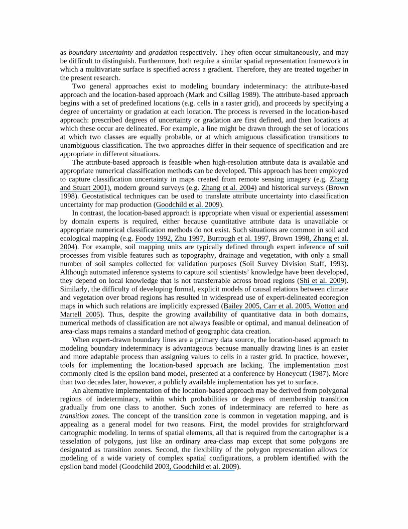
Three data models for representing the spatial distribution of c are depicted in Figure 1. Most prior spatially explicit representations of boundary uncertainty (e.g. Zhang et al. 2004,

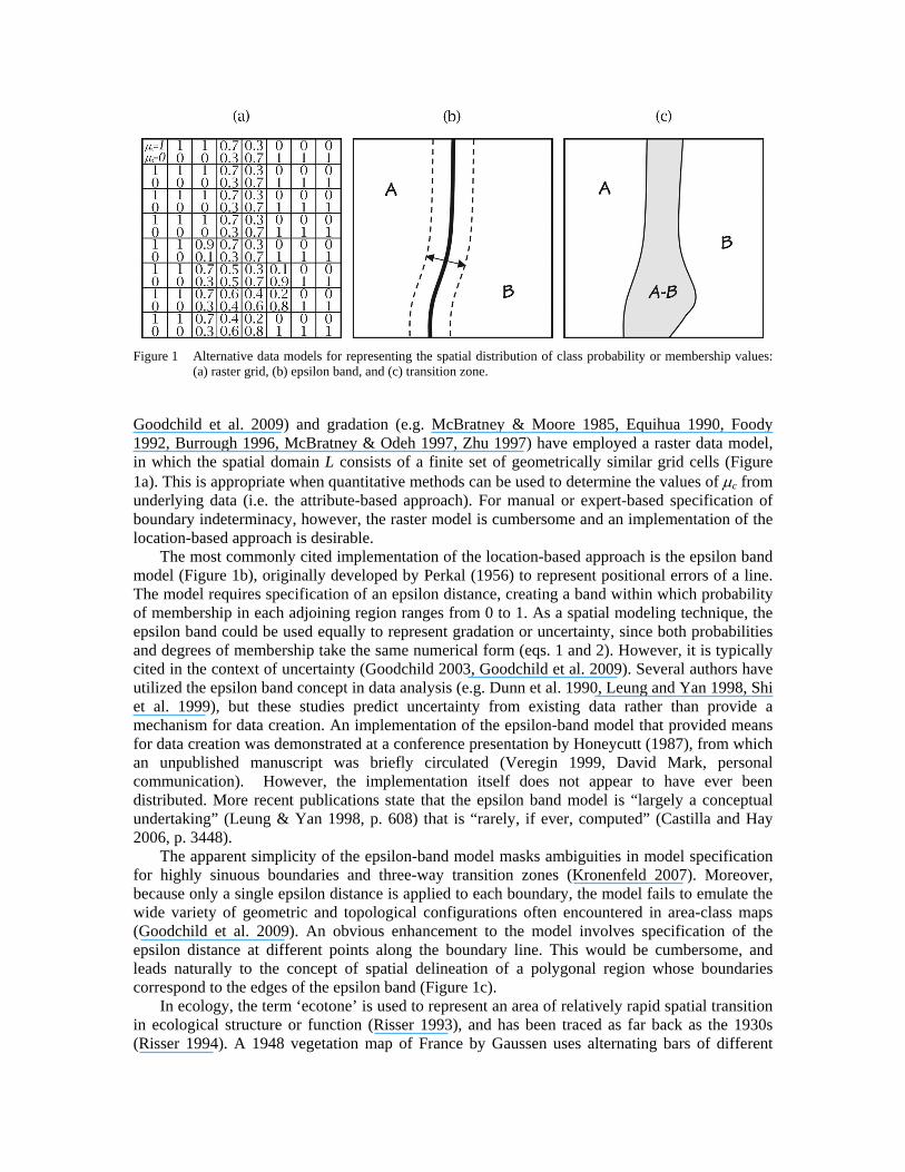
Figure 1 Alternative data models for representing the spatial distribution of class probability or membership values:

(a) raster grid, (b) epsilon band, and (c) transition zone.

Goodchild et al. 2009) and gradation (e.g. McBratney & Moore 1985, Equihua 1990, Foody 1992, Burrough 1996, McBratney & Odeh 1997, Zhu 1997) have employed a raster data model, in which the spatial domain L consists of a finite set of geometrically similar grid cells (Figure 1a). This is appropriate when quantitative methods can be used to determine the values of c from underlying data (i.e. the attribute-based approach). For manual or expert-based specification of boundary indeterminacy, however, the raster model is cumbersome and an implementation of the location-based approach is desirable.

The most commonly cited implementation of the location-based approach is the epsilon band model (Figure 1b), originally developed by Perkal (1956) to represent positional errors of a line. The model requires specification of an epsilon distance, creating a band within which probability of membership in each adjoining region ranges from 0 to 1. As a spatial modeling technique, the epsilon band could be used equally to represent gradation or uncertainty, since both probabilities and degrees of membership take the same numerical form (eqs. 1 and 2). However, it is typically cited in the context of uncertainty (Goodchild 2003, Goodchild et al. 2009). Several authors have utilized the epsilon band concept in data analysis (e.g. Dunn et al. 1990, Leung and Yan 1998, Shi et al. 1999), but these studies predict uncertainty from existing data rather than provide a mechanism for data creation. An implementation of the epsilon-band model that provided means for data creation was demonstrated at a conference presentation by Honeycutt (1987), from which an unpublished manuscript was briefly circulated (Veregin 1999, David Mark, personal communication). However, the implementation itself does not appear to have ever been distributed. More recent publications state that the epsilon band model is “largely a conceptual undertaking” (Leung & Yan 1998, p. 608) that is “rarely, if ever, computed” (Castilla and Hay 2006, p. 3448).

The apparent simplicity of the epsilon-band model masks ambiguities in model specification for highly sinuous boundaries and three-way transition zones (Kronenfeld 2007). Moreover, because only a single epsilon distance is applied to each boundary, the model fails to emulate the wide variety of geometric and topological configurations often encountered in area-class maps (Goodchild et al. 2009). An obvious enhancement to the model involves specification of the epsilon distance at different points along the boundary line. This would be cumbersome, and leads naturally to the concept of spatial delineation of a polygonal region whose boundaries correspond to the edges of the epsilon band (Figure 1c).

In ecology, the term ‘ecotone’ is used to represent an area of relatively rapid spatial transition in ecological structure or function (Risser 1993), and has been traced as far back as the 1930s (Risser 1994). A 1948 vegetation map of France by Gaussen uses alternating bars of different

color to depict gradation between homogeneous areas of vegetation (Küchler 1967). At a global scale, Walter et al. (1975) depict transition zones between zonobiomes, while Bailey (2005, p. S18) states that “major transitional zones (ecotones) should be delineated as separate ecoregions.” Despite its long history, however, the ecotone concept has remained largely informal from a spatial modeling perspective, and methods to determine class probability or membership values at individual locations within an ecotone are lacking.

A previous version of the modeling technique proposed here was presented in Kronenfeld (2007). Building on the Delauney triangulation of the vertices of the gradient polygon, the previous version was limited in flexibility, and was unable to handle ‘null’ polygons which lead to a variety of complex configurations. Also, no robust method was given to identify spatial configurations that could or could not be handled by the model. Finally, the Delauney triangulation of polygon vertices was unstable, leading to changes in the gradient surface when additional points were added along the existing boundary.

The present paper builds on the previous model by developing a graph theoretic representation of the medial axis to capture the essential geometric and topologic characteristics of a transition zone. The medial axis of a polygon (Blum 1967) is the set of interior points that have two or more equidistant closest points along the polygon boundary. It may be thought of as a centerline that extends outward to each convex boundary curve. An evocative analogy is often made to a grassfire (Chin et al. 1999): if the boundary points of a polygon are set on fire simultaneously, the medial axis will be formed by the set of points where two or more fire lines meet. The medial axis is a subset of the Voronoi diagram of a polygon, which is the dual of the Delauney triangulation of the infinitely dense set of boundary points. Computation can be performed by the software package VRONI (Held 2001).

The medial axis has been used in numerous cartographic applications ranging from representation and generalization of map features to terrain modeling, cartogram design and network optimization (Leymarie and Kimia 2008). Gold and Thibault (2000) employ the medial axis to capture the essential shape characteristics of polygons for the purpose of cartographic generalization. In terrain analyses, the medial axis has been used to eliminate ‘flat triangles’ that occur in the triangulation of adjacent contour lines (Thibault and Gold 2000). It will be used similarly in what follows to handle convoluted polygons and to develop a complete formulation of topological configurations considered to be well-formed transition zones

3. Model Components

The modeling process begins by sketching an area-class map composed of a set of classified core regions bridged by zones of transition which together form the spatial domain L; the map may also contain null polygons. Within each transition zone, the values of c (probabilities or degrees of membership in each class c) vary along a smooth gradient between adjacent core regions. To model this gradient, the medial axis and extended medial axis of the transition zone are created. Topological characteristics of the extended medial axis required to perform validity checks and specify values of c are captured in a segmentation graph. This section provides formal definitions for each of the above components.

3.1. Core Regions, Transition zones and Null Polygons

The transition zone model consists of a polygon tessellation in which each polygon is defined as one of three types: core region, transition zone or null polygon. A core region is a set of locations A={a}, contiguous or non-contiguous, such that A L and all values of a,c are the same for each class c. Ordinarily within a core region, c=1 for a single ‘core’ class (c=A) and c=0 for all other classes (cA). However, there is no restriction against other sets of values as long as they conform to the constraints given by equations (1) and (2).

Figure 2 Constructon of the segmentation graph: (a) medial axis of the transition zone; (b) extended medial axis with

segments (heavy dashed) added connecting triple boundary points (denoted by arrows) to the medial axis, dividing the transition zone into subdivisions within which all points share the same nearest core region (indicated in small letters); and (c) segmentation graph of the extended medial axis depicting the topological relationships in (b).

A transition zone is defined as a contiguous set of locations T={t} such that T L, within which t,c varies with t along a smooth gradient from one core region to another. It follows that transition zones must be adjacent to at least two different core regions. Transition zones may also be adjacent to null polygons that do not overlap the spatial domain being classified, i.e. sets of locations X for which X L = ∅. For example, in an area-class map of land cover classes, an ocean may be represented as a null polygon. If two transition zones are adjacent to each other, it is assumed that their separation indicates a sharp boundary, and each is treated as a null polygon from the perspective of the other. In all diagrams to follow, core regions are labeled A, B, C or D and null polygons are labeled X; the transition zone is shown in gray.

3.2. Medial Axis, Extended Medial Axis and Segmentation Graph

An example of the medial axis of a transition zone is shown in Figure 2a. The transition zone spans two core regions (A and B) and a null polygon. The medial axis consists of three segments (dashed lines) meeting at a junction (black dot) that is equidistant to three different boundary points.

Whereas the medial axis captures the shape characteristics of a single polygon, the transition zone is semantically defined in terms of its relation to adjacent polygons. These adjacent polygons meet at triple boundary points along the transition zone boundary, denoted by the small arrows in Figure 2b. Therefore, it is useful to extend the medial axis by adding a straight line segment from each triple boundary point to the location on the medial axis for which the triple boundary point is among the set of closest equidistant points. These extension segments are shown in Figure 2b as heavy dashed lines. The extended medial axis constructed in this manner divides the transition zone into subdivisions such that all points in the interior of a subdivision are nearest to the same adjacent polygon, denoted by small letters in Figure 2b. Note that more than one subdivision may be nearest to the same polygon.

If only the topological relationships of the extended medial axis and adjacent polygons are considered, a simple graph can be constructed. This graph will be referred to as the segmentation graph or S-graph. The S-graph shown in Figure 2c depicts the extended medial axis in Figure 2b, with lettered boxes representing the polygon adjacent to the transition zone subdivision on either side of each segment; junctions between two or more segments are shown as black dots.

In fact, as a result of the definition of the extended medial axis above, at least three segments must meet at each junction:

Lemma 1: On an S-graph, if at least two segments meet at a junction then at least three segments meet at that junction.

Proof: The proof is by counter-example. Suppose exactly two segments meet at a junction. Then, either each segment has the same adjacent polygons on each side or they have different polygons on at least one side. In the first case, the two segments are the same, and there is no junction. In the second case, the junction point has at least one triple-boundary point in its set of equidistant boundary points, to which a new segment must be extended.

In addition, since the extended medial axis divides the transition zone into regions with the same neighboring polygon, adjacent segments on the S-graph must share at least one neighboring polygon:

Lemma 2: All pairs of segments that meet at a junction of the S-graph have the same polygon on their shared side.

Proof: Again by counterexample, if two adjacent segments do not have the same polygon on their shared side, a triple boundary point must be associated with the junction point, and a new segment must be extended from this junction point to the triple boundary point.

These properties will be used to help define well-formed transition zones. Four types of segments on the S-graph may be distinguished: normal, flat, half-null and null

(Table 1). Normal segments represent the centerline between two different core regions, and thus indicate a typical transition from one region to another. The other three segment types are atypical in that they lie within subdivisions of the transition zone adjacent to at most one core region. Flat segments have the same core region on both sides; half-null segments have a null polygon on one side; and null segments have a null polygon on both sides. Examples of segments of each type can be seen in Figure 2c: [AB] and [BA] are normal segments, [AA] and [BB] are flat segments, [XA] and [XB] are half-null segments, and [XX] is a null segment.

Table 1 Types of segments in the medial axis and extended medial axis.

Segment Type Definition Example normal equidistant to two different core regions [AB] flat equidistant to two edges of the same core region [AA] half-null equidistant to a core region and a null polygon [AX] null equidistant to two null polygons [XX]

4. Well-Formed Transition zones

Not every possible configuration of core regions, transition zones and null polygons lends itself to a logical interpretation. The notion of a well-formed transition zone is introduced to identify those configurations that meet conditions required to specify class probabilities or membership values unambiguously at every interior point. The rules to define well-formed transition zones were arrived at after carefully examining the properties of the S-graph and working through the process of specifying values of c (section 5). In this section, the rules of well-formed transition zones are first stated. The rationale behind these rules is then illustrated by way of example. Lastly, some useful corollaries are derived.

4.1. Definition

A transition zone is defined to be well-formed if its S-graph conforms to the following three rules: 1. It is contiguous and contains at least one normal segment. 2. There are no junctions of more than three segments. 3. Every flat, half-null and null segment is part of a hierarchical tree for which:

3a. No normal segments are contained within or connected to the tree except at the root

3b. All descendants of null segments are null segments. 3c. All descendants of flat segments are flat segments.

4.2. Examples of well-formed transition zones

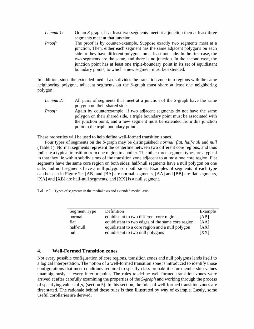
Some examples of well-formed transition zones and their corresponding S-graphs are depicted in 0. Well-formed transition zones may be adjacent to null polygons (Fig. 3a), contain irregular boundaries with spurs into either core regions (Fig. 3b) or null polygons (Fig. 3c), span three or more core regions (Fig. 3d), and/or contain cycles (Fig. 3e). In all of these examples, the transition zone is contiguous and contains at least one normal [AB] segment (rule 1); there are no junctions of more than three segments (rule 2); and every half-null [AX] and null [XX] segment is part of a valid hierachical tree (rule 3). An example of a valid hierarchical tree can be seen in Figure 3c. The root of the tree is the half-null [AX] segment in the center of the graph. This segment has two children, another half-null [XA] segment and a null [XX] segment. The tree is hierarchical and connected to a normal segment only at the root (rule 3a), the null segment has no descendants (rule 3b), and there are no flat segments (rule 3c). It is hypothesized that most transition zones drawn by experts will be well-formed.

4.3. Examples of ill-formed transition zones

Figure 4 shows a transition zone that violates the first rule. The transition zone has only one adjacent core region and therefore no normal segments. Such a configuration may represent a single region with indeterminate boundaries, but is not a transition zone between regions on an area-class map.

Figure 5 shows a transition zone that violates the second rule. Extensions of the medial axis coincidentally converge on a medial axis junction. Although this case is broadly plausible, it is considered a singularity and is not presently handled by the model. However, a simple work-around is suggested in the discussion.

Figure 6 shows four transition zones that violate the third rule. Figure 6a contains a cycle of flat segments, violating the definition of a hierarchical tree. Similar situations can occur with cycles of null or half-null segments. In Figure 6b, a flat segment spans two junctions with normal segments, violating condition 3a. Figure 6c shows two half-null descendants of a null segment, violating condition 3b. Similarly, Figure 6d shows a flat segment with two half-null descendants, violating condition 3c. In each of these configurations, there is a portion of the transition zone for which there is no natural and unique way to define A, B or both while preserving the continuous nature of each probability or membership value surface. For example, in Figure 6a, a natural interpretation suggests that A should increase and B should decrease along each branch from the root to point m midway through the cycle. However, there is no natural and unique value for m,A and m,B. It is tempting to assign values of m,A=1 and m,B=0, but this would create a non-intuitive situation in which there would be no uncertainty or gradation at a point in the middle of the transition zone. Similarly in Figures 6b, 6c and 6d, there exists a point m in the middle of the segments [BB], [XX] and [AA], respectively at which both A and B must reach either a minimum or a maximum, but no unique natural values exist for these minima and maxima.

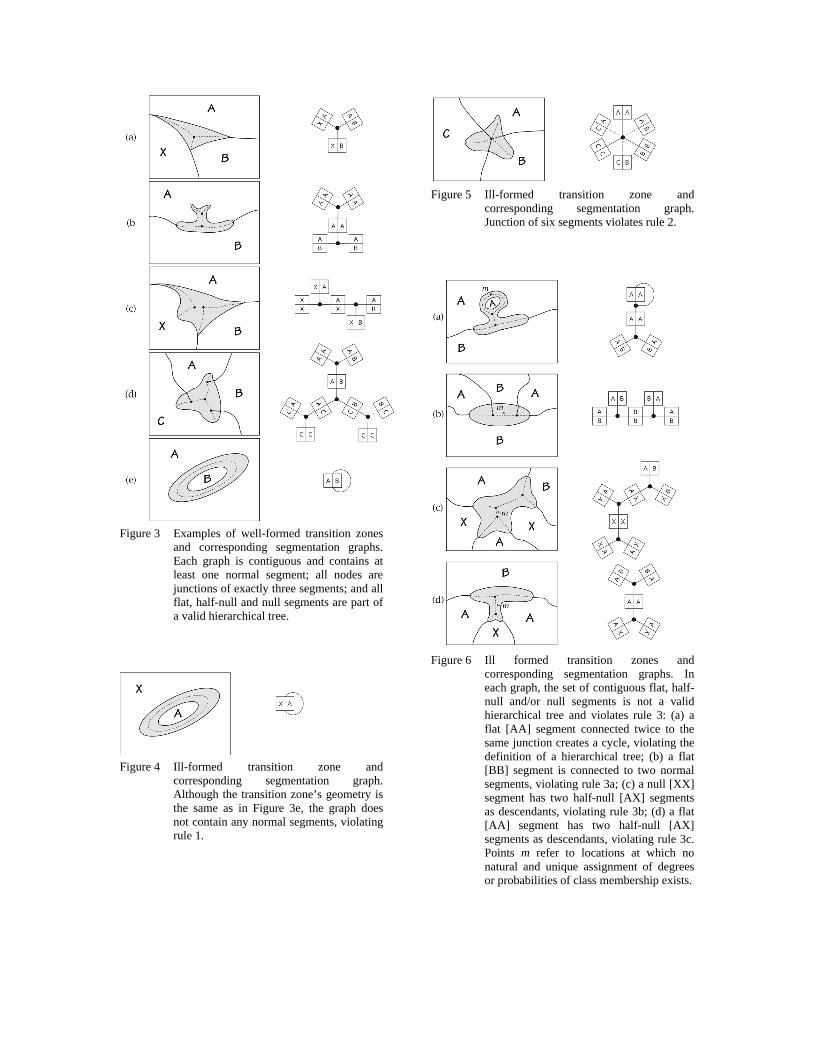
Figure 3 Examples of well-formed transition zones

and corresponding segmentation graphs. Each graph is contiguous and contains at least one normal segment; all nodes are junctions of exactly three segments; and all flat, half-null and null segments are part of a valid hierarchical tree.

Figure 4 Ill-formed transition zone and

corresponding segmentation graph. Although the transition zone’s geometry is the same as in Figure 3e, the graph does not contain any normal segments, violating rule 1.

Figure 5 Ill-formed transition zone and

corresponding segmentation graph. Junction of six segments violates rule 2.

Figure 6 Ill formed transition zones and

corresponding segmentation graphs. In each graph, the set of contiguous flat, half-null and/or null segments is not a valid hierarchical tree and violates rule 3: (a) a flat [AA] segment connected twice to the same junction creates a cycle, violating the definition of a hierarchical tree; (b) a flat [BB] segment is connected to two normal segments, violating rule 3a; (c) a null [XX] segment has two half-null [AX] segments as descendants, violating rule 3b; (d) a flat [AA] segment has two half-null [AX] segments as descendants, violating rule 3c. Points m refer to locations at which no natural and unique assignment of degrees or probabilities of class membership exists.

The rules defining a well-formed transition zone are tightly intertwined with the rules for specifying l,c presented in section 5, and guarantee that class probabilities can be specified at every point. To demonstrate this, several corollaries to these rules must first be derived.

4.4. Corollaries

Four useful corollaries regarding the configuration of half-null, null and flat segments are derived from the rules defined in section 4.1:

Corollary 1: All half-null segments are part of a linear chain (termed a half-null chain) extending between:

a junction of two half-null segments and a normal segment, and a triple boundary point between a core region, transition zone and

null polygon. Proof: First consider a single half-null segment. By the first lemma and rule 2, each

end of the segment must be connected either to two other segments at a junction, or to no other segments. By the construction of the S-graph, a half-null segment connected to no other segments on one end must be connected either to itself or to a triple boundary point between a core region, transition zone and null polygon. If the segment is connected to itself then the segment is on a cycle, which violates the definition of a hierarchical tree in rule 3. If the segment is connected to a triple boundary point on both ends, the transition zone contains no normal segments and rule 1 is violated. Therefore, every half-null segment is connected either to a junction and a triple boundary point or to two junctions.

Without loss of generality, assume that the half-null segment is [AX]. By the second lemma, its two neighbors at a 3-junction must be [*A] and [X*], and further, * must be the same for both neighbors. There are three relevant possibilities: [AA]-[AX]-[XA], [XA]-[AX]-[XX] or [BA]-[AX]-[XB]. The first two cases result in continuation of the half-null chain, from which a flat or null segment protrude respectively. The third case results in the chain ending at a junction of two half-null segments and a normal segment. Therefore, all half-null segments must be part of a linear chain of half-null segments.

By the above limitations, each end of a half-null chain must either be a junction or a triple boundary point of the type stated in the corollary. If both ends are junctions, then the tree is connected to a normal segment in two places and rule 3a is violated. If both ends are triple boundary points then the tree is not connected to any normal segment because, by rules 3b and 3c, the descendants of the flat and null segments that protrude from the half-null chain cannot be normal segments. Therefore, one end of the half-null chain must be a junction and the other must be a triple boundary point.

Corollary 2: Two half-null segments that meet at a junction must have different adjacent core regions.

Proof: By corollary 1, every half-null chain connects to a junction with the form [AX]-[XB]-[BA]. If the adjacent core regions of each half-null segment are the same (i.e. A=B), then the junction is of the form [AX]-[XA]-[AA]. However, this results in two half-null chains being descendants of a flat segment, violating rule 3c.

Corollary 3: All null segments are part of a hierarchical tree containing only null segments (termed a null tree), rooted in a half-null chain.

Proof: The second lemma dictates that null segments can only connect to junctions of the form [AX]-[XX]-[XA] and [XX]-[XX]-[XX]. By rule 3, all null segments must be contained within a hierarchical tree of null segments. If the tree is connected to more than one junction of the form [AX]-[XX]-[XA], then by corollaries 1 and 2 it must either be connected to two different pairs of half-null chains or to the same pair of half-null chains twice. In the first case, each pair of half-null chains is connected to a different normal segment, violating rule 3a. In the second case, the combination of null and half-null segments must form a cycle, violating the definition of a hierarchical tree. Therefore, the null segment tree can connect to a half-null chain in at most one location. If the null segment tree does not connect to a half-null chain at any location, then it is a graph that contains no normal segments, violating rule 1. Therefore, the null segment tree must connect to exactly one half-null chain.

Corollary 4: All flat segments are part of a hierarchical tree containing only flat segments (termed a flat tree), rooted either in a half-null chain or a junction of two normal segments and a flat segment.

Proof: The proof is similar to that of corollary 3.

From these corollaries, it follows that all segments of the extended medial axis must either be normal segments or belong to a half-null chain, null tree or flat tree. This fact will be used in the next section to ensure that all valid transition zones are fully specified.

5. Specification of the Probability or Membership Value Surface

In an ordinary area-class map, quantitative attribute values are considered to be the same everywhere within each polygon. The transition zone concept differs semantically and implies that attribute values vary within the polygon. A fully specified model of a transition zone should define these values at every location. In this section, rules for defining values of c representing either class probability or membership values are provided. These rules are derived from the configuration of neighboring core regions.

There are many ways in which the values of c could be specified within a transition zone. The following set of rules provides one such specification, and is based on five core concepts:

1) The surface of c should be smooth and everywhere at least 1st order differentiable, if possible.

2) c should be defined by relative Euclidean distance to core regions along ‘natural’ shortest-distance pathways.

3) Pathways used to measure relative Euclidean distance should lie wholly interior to the transition zone.

4) These pathways should follow the general shape characteristics of the transition zone, and not be influenced by the sinuosity of the boundary.

5) When a transition zone extends between three or more core regions, the influence of each core region should not extend beyond the distance across the transition zone to the opposing pair of core regions.

The above concepts seem intuitive and are flexible enough to allow creation of a wide variety of transition surfaces

To implement these concepts, it is useful to start with the simplest case of a rectangular transition zone between two core regions A and B. The concept of relative distance (2) suggests

that p,A and p,B at any interior point p can be defined by extending a straight line from one core region to the other through p to form a linear gradient. When the transition zone is convoluted, adjacent to more than two core regions, or adjacent to a null polygon, this is not generally possible. A more robust strategy is to construct the medial axis, define l,c at all locations along the transition zone boundary and medial axis as reference sets, and interpolate along linear gradients between these sets.

Formally, let r be a straight line segment extending through point p from point m on the medial axis to point b that is one of the 2 or more corresponding closest equidistant boundary points to q. For any interior point p, there exists exactly one such line segment that passes through it. Therefore, given reference sets that define m,k and b,k for all m and b along the medial axis and transition zone boundary, then p,k for any interior point p is defined via linear interpolation:

,,

, ,,

,

, ,, (3)

where dx,y denotes the Euclidean distance between two points x and y.

The remainder of this section defines c at seven sets of points on the medial axis and polygon boundary, which together comprise the reference set. Once the values of c have been established at these points, the values of c at any point in the interior of the transition zone can be calculated from eq. 3. Definitions for each subset of points are backwards referencing. For example, values of c at points along null polygon boundaries (def. 6) are defined with respect to values of c at the leaf nodes of null segment trees (def. 5) and points along core region boundaries (def. 1). Only definitions are provided in this section; the next section illustrates each rule by way of example. To conform to standard graph theory notation, junctions of the S-graph are referred to synonymously as nodes.

Definition 1: Values of c at points along core region boundaries

At triple boundary points between the transition zone and two adjacent core regions A and B, c is defined as the average of A,c and B,c. At all other points along the edge between the transition zone and an adjacent core region A, c=A,c.

Definition 2: Values of c at junctions of three normal segments

At the junction of three normal segments with adjacent core regions A, B and C, c is defined as the average of A,c, B,c and C,c.

At each point of the medial axis where it intersects the largest circle centered on the above junction and inscribed within the transition zone, c is defined as the average of A,c and B,c, where A and B are the core regions adjacent to the normal segment containing the point of intersection.

At all other points on a normal segment within the inscribed circle described above, c is calculated by linear interpolation between the above junction and point of intersection.

Definition 3: Values of c at all other points along normal segments

At all other points along normal segments of the medial axis, c is defined as the average of A,c and B,c, where A and B are the core regions adjacent to the normal segment.

Definition 4: Values of c on half-null segment chains

On all half-null chains, c is calculated by linear interpolation along segments between the end points of the chain. Note that one end of a half-null chain is always the endpoint of a normal segment (def. 3), and the other is always a point along a core region boundary (def. 1).

Definition 5: Values of c on null segment trees

Let the value of c at the root of each null segment tree where it joins a half-null segment chain (def. 4) be denoted as root, and values of c at the nearest junction or triple boundary point on either side of the root of a null segment tree be denoted as left and right. A reference range bounding c within each null segment tree is defined as {(left+root)/2, (right+root)/2}. The value of c at the child node of the root is defined as the value of c at the root. At each branching node of the null segment tree, the reference range is split on the value of c at that node, these new reference ranges are assigned to the corresponding child nodes, and c at each child node is defined as the mid-points of the assigned reference range. The process is repeated until the leaf nodes are reached.

Algorithmically, define: root the triple boundary point at the end of the left half-null chain rootLeft the next junction or triple boundary point to the left of the root along the half-

null chain rootRight the next junction or triple boundary point to the right of the root along the

half-null chain The range of values of c for the entire tree and the value of the root child are defined by the InitializeTree function:

1 rangeLeft (rootLeft,c + root,c)/2 2 rangeRight (rootRight,c + rootRight,c)/2 3 curNode child of root 4 curNode,c root,c 5 WorkChildren(curNode, rangeLeft, rangeRight)

Values at descendant nodes are then defined recursively through the WorkChildren function: 1 If curNode is a leafNode then Exit Else 2 curNode.leftChild,c (curNode,c + rangeLeft)/2 3 curNode.rightChild,c (curNode,c + rangeRight)/2 4 WorkChildren(curNode.leftChild, rangeLeft, curNode,c) 5 WorkChildren(curNode.rightChild, curNode,c, rangeRight)

Definition 6: Values of c at boundary points adjacent to null polygons

Along null polygon boundaries, c is calculated by linear interpolation between adjacent nodes of the extended medial axis that lie along the boundary. Note that every node on the boundary with a null polygon is either a triple-boundary point between a transition zone, null polygon and core region (def. 1), or a leaf node of a null segment tree (def. 5).

Definition 7: Values of c on flat segment trees

At each non-root node, c is calculated by linear interpolation along a path from the node’s parent to the furthest descendant (leaf) node. Note by corollary 4 that the root node of a flat segment tree will always lie either between two normal segments (def. 3) or along a half-null segment chain (def. 4).

To verify that the proposed model is fully specified, it must be shown that the above seven definitions ensure the values of c are defined at every point of a valid transition zone. It was argued above that the values of c at all interior points can be determined from eq. 3 if all points along the medial axis and boundary of the transition zone are defined. Section four concluded by noting that all segments of the medial axis must be normal segments or parts of half-null chains, null trees, or flat trees; values of c on these segments are defined in definitions 2-3, 4, 5, and 7 respectively. Along the transition zone boundary, all points must be adjacent to either a core region (def. 1) or a null polygon (def. 6). Therefore, the model is fully specified.

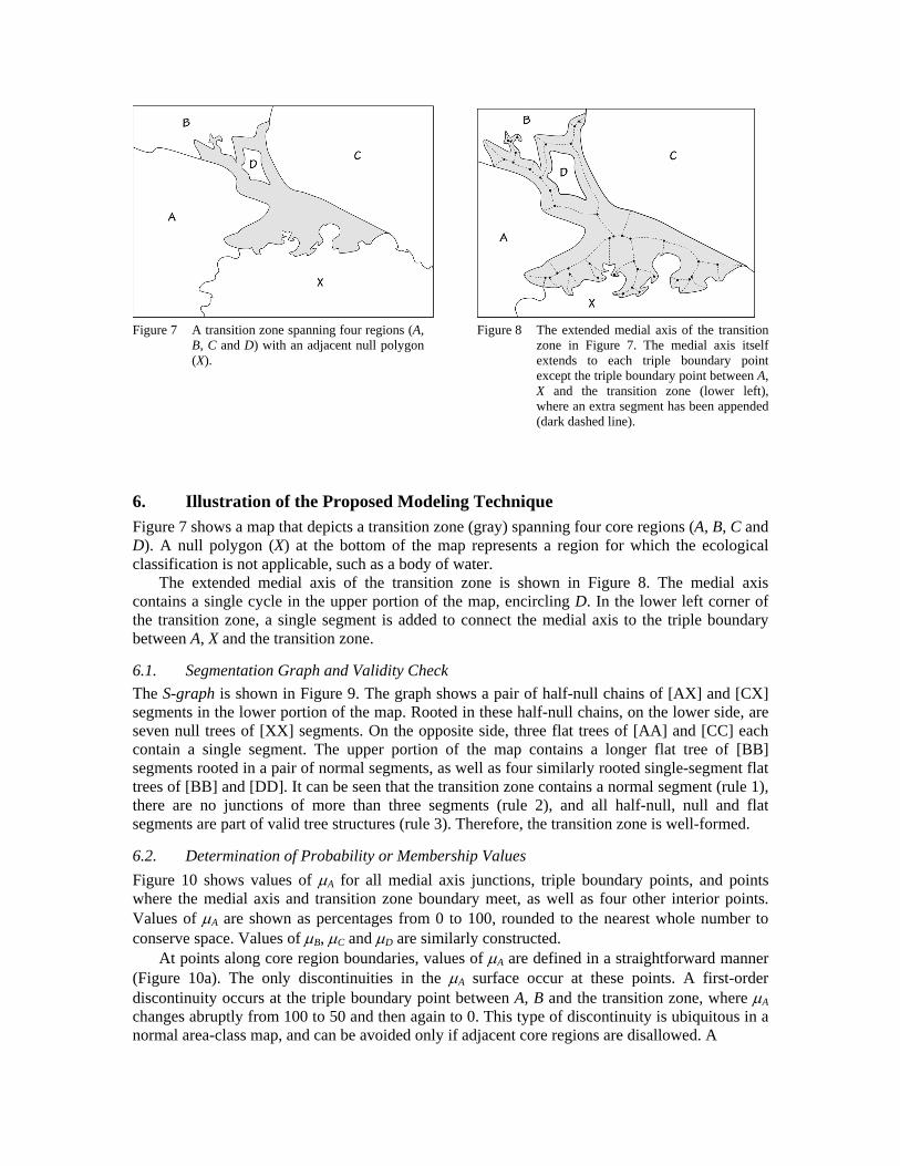
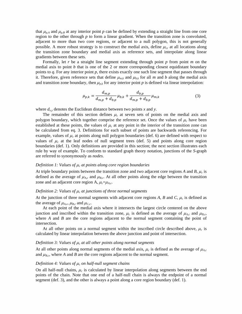
Figure 7 A transition zone spanning four regions (A,

B, C and D) with an adjacent null polygon (X).

Figure 8 The extended medial axis of the transition

zone in Figure 7. The medial axis itself extends to each triple boundary point except the triple boundary point between A, X and the transition zone (lower left), where an extra segment has been appended (dark dashed line).

6. Illustration of the Proposed Modeling Technique

Figure 7 shows a map that depicts a transition zone (gray) spanning four core regions (A, B, C and D). A null polygon (X) at the bottom of the map represents a region for which the ecological classification is not applicable, such as a body of water.

The extended medial axis of the transition zone is shown in Figure 8. The medial axis contains a single cycle in the upper portion of the map, encircling D. In the lower left corner of the transition zone, a single segment is added to connect the medial axis to the triple boundary between A, X and the transition zone.

6.1. Segmentation Graph and Validity Check

The S-graph is shown in Figure 9. The graph shows a pair of half-null chains of [AX] and [CX] segments in the lower portion of the map. Rooted in these half-null chains, on the lower side, are seven null trees of [XX] segments. On the opposite side, three flat trees of [AA] and [CC] each contain a single segment. The upper portion of the map contains a longer flat tree of [BB] segments rooted in a pair of normal segments, as well as four similarly rooted single-segment flat trees of [BB] and [DD]. It can be seen that the transition zone contains a normal segment (rule 1), there are no junctions of more than three segments (rule 2), and all half-null, null and flat segments are part of valid tree structures (rule 3). Therefore, the transition zone is well-formed.

6.2. Determination of Probability or Membership Values

Figure 10 shows values of A for all medial axis junctions, triple boundary points, and points where the medial axis and transition zone boundary meet, as well as four other interior points. Values of A are shown as percentages from 0 to 100, rounded to the nearest whole number to conserve space. Values of B, C and D are similarly constructed.

At points along core region boundaries, values of A are defined in a straightforward manner (Figure 10a). The only discontinuities in the A surface occur at these points. A first-order discontinuity occurs at the triple boundary point between A, B and the transition zone, where A changes abruptly from 100 to 50 and then again to 0. This type of discontinuity is ubiquitous in a normal area-class map, and can be avoided only if adjacent core regions are disallowed. A

Figure 9 The segmentation graph of the extended

medial axis in Figure 8.

Figure 10 Values of A at boundary points (a),

junctions of the extended medial axis (b)-(f) and interior points (g). Calculation of A for each labeled set is explained separately in the text.

discontinuity in the first derivative of A occurs along all points along the boundary of A and the transition zone; this type of discontinuity is inherent to the transition zone model.

Figure 10b shows a junction between [AD], [DC] and [CA] segments. The inscribing circle around the junction touches boundaries of each core region A, C and D. The junction itself is equidistant to all three core regions. Therefore, A is defined as 1/3 (33%). The diameter of the inscribing circle approximates the distance between each pair of core regions, and therefore marks a natural boundary for the influence of each region. At the point where this circle intersects the [DC] segment, A is equal to zero.

Figure 10c shows a sequence of normal segments between A and B in the upper left portion of the map. Since these are halfway between the two core regions and are outside the inscribing circle of every junction of three normal segments, A at all points on this sequence is equal to 50%.

Figure 10d shows two half-null segment chains at the bottom of the map which together span from A to C. These chains form a natural frame for the gradient in probability or membership values between the two regions. Along each chain, A is defined by linear interpolation from the junction of [AC], [CX] and [XA] segments in the center of the map to the triple boundary point at the end of the chain. Together, the two half-null chains define the shape of the broad gradient from A=100% (left) to A=0% (right).

This broad gradient is used to define the values of nodes along all null segments descending from the half-null chain. An example is shown in Figure 10e. Within this null chain, A is constrained to the range 48% (halfway between 52% and 44%) to 38% (halfway between 44% and 32%). The range is successively split into two parts down the tree to the leaf nodes, which are

Figure 11 Isoline representation of the transition zone in Figure 7. Each isoline covers a set of locations with equal

values of c in at least one adjacent core region. Outside the circular regions, each isoline is actually two coincident isolines. For example, isolines in the lower part of the transition zone covers a set of locations with equal values of A and C.

on the null polygon boundary. This results in relatively small changes along sinuous portions of the boundary, as compared to the straighter portions.

For flat segment trees (Figure 10f), the natural constraint on A is the length of the tree rather than the breadth. Tree branching creates multiple lengths from any given node to its descendant leaf nodes. In this case, short segments which have little descriptive value should be ignored, so the downstream length from any node is defined as the longest path from the node to a descendant leaf. The first node from the tree root in Figure 10f, for example, is more than half way along the shortest path from root to leaf but only about 30% of the way along the longest path; the latter distance is used, so that A = (0.7)*50% + (0.3)*0% = 35%.

Finally, values of c at interior points between the medial axis and transition zone boundary are shown in Figure 10g. By eq. 3, These values are calculated via linear interpolation between the value on the medial axis (m,A=50) and the transition zone boundary (b,A=0).

Probability or membership values for the other three classes are similarly calculated. Figure 11 displays the multivariate surface of A, B, C and D as a set of isolines. It can be seen that isolines generally run parallel to the boundary of each core region. Except for the areas within the inscribed circles around the junctions of three normal segments, each line in Figure 11 is actually two coincident isolines of probability or membership in different core regions. For example, the leftmost isoline just above the null polygon is actually two coincident isolines of A=12.5% and C=87.5%.

7. Discussion

Gradation and classification indeterminacy are ever present in area-class maps, and are caused by a multitude of factors including lack of data and reliance on qualitative rather than quantitative classification methods. The general research trend in modeling these phenomena has been to utilize a growing body of high-resolution geographic data, model error sources quantitatively and improve the logic behind numerical classification systems. While these are laudable goals, there will always be a role for qualitative map creation by experts in various fields who require tools for knowledge representation. Such experts in the fields of ecology and vegetation mapping have

developed theoretical constructs to differentiate regions of relative homogeneity from regions of relatively abrupt change. The transition zone therefore appears to be a natural and useful concept.

The proposed technique allows for modeling of a wide variety of transition zone configurations, including polygons with sinuous boundaries, spurs, null polygons and zones of non-zero probability or membership in three different core regions. It does have some limitations, however. Symmetry is enforced around the medial axis, and the area of transition between three core regions must be a circle. Further, simultaneous transition between more than three core regions cannot be modeled.

Greater flexibility can be achieved by the model through clever use of ‘core regions’ with non-zero probability or membership in more than one class. This method can be used, for example, to emulate a four way transition zone. The ill-formed transition zone depicted in Figure 5 can be transformed into a well-formed transition zone by inserting a single point (treated as a degenerate polygon) with values of A=B=C=33% at the central junction point. Similarly, asymmetrical transitions can be modeled by inserting a line (also treated as a degenerate polygon) with class probabilities of 0.5 in each adjacent core region at any appropriate position. Although such techniques can be used to expand the range of class probability or membership value surfaces that can be emulated, modeling techniques that more directly capture common gradational structures might be desirable if such structures can be identified.

As a technique for modeling a multivariate surface, the transition zone model is more flexible than the epsilon band but less flexible than a raster grid. The assumptions behind the model practically require the existence of broad regions of homogeneity and make it difficult to model fine scale salt-and-pepper spatial variation. This constraint is implicit in the concept of gradation, which derives its meaning from the assumption that there are entities between which gradation occurs. Many ecologists have questioned the existence of homogenous regions, however, so the assumption of homogeneous regions may reflect a cognitive rather than phenomenological structure. Nevertheless, the structure appears to be widespread in spatial reasoning, and so a model that captures its essential features is long overdue.

Three broad perspectives regarding the nature of transition zones and their appropriate modeling can be identified. First, the ontological perspective encompasses questions regarding the nature of boundary uncertainty and gradation in the real world. Research into this question has been undertaken by domain experts (e.g. Wilson et al. 1996), but geographic information scientists can contribute by building a general ontology that includes both concepts. Second, a cognitive perspective is needed to shed light on when and why boundary uncertainty and gradation are cognized, and how they contribute to spatial reasoning and communication. Finally, the modeling perspective looks at ways in which boundary uncertainty and gradation can be represented in data models and structures. The modeling technique proposed here offers a practical and workable solution to the problem of representation, but more research into ontological and cognitive issues will likely lead to improvements in the model.

References

Bailey, RG. 2005. Identifying ecoregion boundaries. Environmental Management, 34(1):S14-S26.

Bennett, B. 2003. Editorial (Introduction to special issue on spatial vagueness, uncertainty and granularity). Spatial Cognition and Computation, 3(2/3):93-96.

Blum, H. 1967. A transformation for extracting new descriptors of shape. In W.W. Dunn (ed.), Models for the Perception of Speech and Visual Form, MIT Press: Cambridge, MA, pp. 153-171.

Burrough, PA. 1996. Natural objects with indeterminate boundaries. In Burrough and Frank (eds.), Geographic Objects with Indeterminate Boundaries, London: Taylor & Francis.

Burrough, PA and Frank, AU. 1996. Geographic Objects with Indeterminate Boundaries. London: Taylor & Francis.

Burrough, PA, PFM van Gaans and R Hootsmans. 1997. Continuous classification in soil survey: spatial correlation, confusion and boundaries. Geoderma 77:115-135.

Carr, GM, PA Chambers and A Morin. 2005. Periphyton, water quality, and land use at multiple scales in Alberta rivers. Canadian Journal of Fisheries and Aquatic Sciences, 62(6):1309-1319.

Castilla, G and Hay, GJ. 2006. Uncertainties in land use data. Hydrology and Earth System Science Discussions, 3: 3439-3472.

Chin, F, J Snoeyink and CA Wang. 1999. Finding the medial axis of a simple polygon in linear time. Discrete Computational Geometry, 21(3):405-420.

Dunn, R, AR Harrison and JC White. 1990. Positional accuracy and measurement error in digital databases of land use: an empirical study. International Journal of Geographical Information Systems, 4:385-198.

Equihua, M. 1990. Fuzzy clustering of ecological data. Journal of Ecology, 78: 519-534. Fisher, PF. 2000. Sorites paradox and vague geographies. Fuzzy Sets and Systems, 113(1): 7-18. Foody, GM. 1992. A fuzzy sets approach to the representation of vegetation continua from

remotely sensed data: An example from lowland heath. Photogrammetric Engineering and Remote Sensing, 58: 221-225.

Foody, GM and DS Boyd. 1999. Fuzzy mapping of tropical land cover along an environmental gradient from remotely sensed data with an artificial neural network. Journal of Geographical Systems, 1:23-35.

Gold, CM and D Thibault. 2001. Map generalization by skeleton retraction. In Proceedings, International Cartographic Association, Beijing, China, pp.2072-2081.

Goodchild, MF. 2000. Introduction: Special issue on ‘Uncertainty in geographic information systems’. Fuzzy Sets and Systems, 113: 3-5.

Goodchild, MF. 2003. Models for uncertainty in area-class maps. In Shi W, Goodchild M F, and Fisher P F (eds), Proceedings of the Second International Symposium on Spatial Data Quality, Hong Kong, Hong Kong Polytechnic University, pp. 1–9.

Goodchild, MF, J Zhang and P Kyriakidis. 2009. Discriminant models of uncertainty in nominal fields. Transactions in GIS, 13(1):7-23.

Held, M. 2001. VRONI: An engineering approach to the reliable and efficient computation of Voronoi diagrams of points and line segments. Computational Geometry: Theory and Applications, 18:95-123.

Honeycutt, DM. 1987. Epsilon bands based on probability. Abstract presented at Auto-Carto VIII, Baltimore, MD.

Kronenfeld, BJ, Mark, DM and Smith, B. 2002. Gradation and Objects with Indeterminate Boundaries. Short-term research priority, University Consortium for Geographic Information Science (UCGIS).

Kronenfeld, BJ. 2007. Triangulation of gradient polygons: A spatial data model for categorical fields. Proceedings of the 8th International Conference on Spatial Information Theory (COSIT). Berlin: Springer Lecture Notes in Computer Science, pp. 21-37.

Leung, Y and J Yan. 1998. A locational error model for spatial features. International Journal of Geographical Information Science, 12(6):607-620.

Leymarie, FF and BB Kimia. From the infinitely large to the infinitely small: Applications of medial symmetry representation of shape. In Siddiqi and Pizer (eds.), Medial Representations: Mathematics, Algorithms and Applications, Netherlands: Springer, pp. 327-351.

McBratney, AB and Moore, AW. 1985. Application of fuzzy sets to climatic classification. Agricultural and Forest Meteorology, 35: 165-185.

McBratney, AB and Odeh, IOA. 1997. Applications of fuzzy sets in soil science: fuzzy logic, fuzzy measurements and fuzzy decisions. Geoderma, 77: 85-113.

Peuquet, DJ, Smith, B and Brogaard, B. 1998. The ontology of fields: Report of a specialist meeting held under the auspices of the Varenius Project. Santa Barbara: National Center for Geographic Information and Analysis.

Risser, PG. 1993. Ecotones at local to regional scales from around the world. Ecological Applications, 3(3):367-368.

Risser, PG. 1994. The status of the science examining ecotones. Bioscience, 45(5):318-325. Robinson, VB. 2003. A perspective on the fundamentals of fuzzy sets and their use in geographic

information systems. Transactions in GIS, 7(1): 3-30. Shi, X, Long, R, Dekett, R and Philippe, J. 2009. Integrating different types of knowledge for

digital soil mapping. Soil Science Society of America Journal, 73(5):1682-1692. Shi, WZ, M Ehlers and K Templi. 1999. Analytical modeling of positional and thematic

uncertainties in the integration of remote sensing and geographical information systems. Transactions in GIS, 3(2):119-136.

Soil Survey Division Staff. 1993. Soil Survey Manual. Soil Conservation Service, U.S. Department of Agriculture Handbook 18.

Thibault, D and CM Gold. 2000. Terrain reconstruction from contours by skeleton construction. GeoInformatica, 4(4):349-373.

Veregin, H. 1999. Data quality parameters. In PA Longley, MF Goodchild, DJ Maguire and DW Rhind (eds.), Geographicl Information Systems – Volume 1, Principles and Technical Issues. New York: John Wiley & Sons, pp. 177-189.

Walter, H, Harnickell, E, and Mueller-Dombois, D. 1975. Climate-diagram maps of the individual continents and the ecological climatic regions of the earth. Text volume (Vegetation Monographs; 36 pp.) and 9 folded maps issued together in a case. Berlin: Springer.

Wilson, JB, I Ullmann and P Bannister. 1996. Do species assemblages ever recur? Journal of Ecology, 84:471-474.

Wotton, BM and DL Martell. 2005. A lightning fire occurrence model for Ontaria. Canadian Journal of Forest Research, 35(6):1389-1401.

Zhang, J and Stuart, N. 2001. Fuzzy methods for categorical mapping with image-based land cover data. International Journal of Geographical Information Science, 15(2): 175-195.

Zhang, L, Liu, C, Davis, CJ, Solomon, DS, Brann, TB and Caldwell, LE. 2004. Fuzzy classification of ecological habitats from FIA data. Forest Science 50(1): 117-127.

Zhu, A. 1997. A similarity model for representing soil spatial information. Geoderma, 77: 217-242.