bayesian modelling of dupuytren disease using gaussian copula graphical models

Bayesian modeling of Dupuytren disease using

copula Gaussian graphical models

Abdolreza MohammadiUniversity of [email protected]

Fentaw AbegazUniversity of [email protected]

Edwin van den HeuvelEindhoven University of Technology

[email protected]

Ernst C. WitUniversity of Groningen

[email protected]

January 27, 2015

Abstract

Dupuytren disease is a fibroproliferative disorder with unknown eti-ology that often progresses and eventually can cause permanent contrac-tures of the affected fingers. Most of the researches on severity of thedisease and the phenotype of this disease are observational studies with-out concrete statistical analyses. There is a lack of multivariate analysisfor the disease taking into account potential risk factors. In this paper, weprovide a novel Bayesian framework to discover potential risk factors andwhich fingers are jointly affected. Copula Gaussian graphical modeling isone potential way to discover the underlying conditional independence ofvariables in mixed data. Our Bayesian approach is based on copula Gaus-sian graphical models. We embed a graph selection procedure inside asemiparametric Gaussian copula. We carry out the posterior inference byusing an efficient sampling scheme which is a trans-dimensional MCMCapproach based on birth-death process. We implemented the method asa general purpose in the R package BDgraph.

Keywords: Dupuytren disease; Risk factors; Bayesian inference; Cop-ula Gaussian graphical models; Bayesian model selection; Latent variablemodels; Birth-death process; Markov chain Monte Carlo

1 Introduction

Dupuytren disease is an inherited and presents worldwide but is more prevalentin people with northern European ancestry (Bayat and McGrouther, 2006). Thisdisease is an incurable fibroproliferative disorder that alters the palmar handand may causes progressive and permanent flextion contracture of the fingers.At the first stage of the disease, giving rise to the development of skin pittingand subcutaneous nodules in the palm; See picture 1 in the left side. At a laterstage, cords appear that connect the nodules and may contract the fingers intoa flexed position; See picture 1 in the right side. A contracture can arise isolatedin a single ray or even multiple rays. And it affects in a single or more joints of

1

arX

iv:1

501.

0484

9v1

[st

at.A

P] 2

0 Ja

n 20

15

the rays, in decreasing order. The disease mostly appears in the ulnar side of thehand, and peculiarly, it often affects the little finger and ring finger, see figure2. The main questions are: (1) Can one make recommendations for treatmentbased on the current stage of the disease? (2) Can we find what variables affectthe disease and how?

Empirical research has described the patterns of occurrence of Dupuytrendisease in multiple fingers. Meyerding (1936) have stated that most often thecombination of affected ring and little fingers occurred, followed by the combi-nation of an affected third, fourth, and fifth finger. Tubiana et al. (1982) foundthat Dupuytren disease rarely affects isolated radial side, and that radial effectoften associate with an affected ulnar side. Milner (2003) noticed that patientswho had required surgery because of firmly affected thumb were on average 8years older and had suffered significantly longer from the disease with comparewith patients with a mildly affected radial side. Moreover, these patients suf-fered from ulnar disease that repeatedly had required surgery, suggesting anintractable form of disease. More recently, Lanting et al. (2014), with a mul-tivariate ordinal logit model, suggested that the middle finger is substantiallycorrelated with other fingers on the ulnar side, and the thumb and index fingerare correlated. They taking into account age and sex, and tested hypotheses onindependence between groups of fingers. However, there is a lack of multivariateanalysis study for the disease with taking into account potential risk factors.

Essential risk factors of Dupuytren disease is vague. It has been variablyattributed to both phenotypic and genotypic factors (Shih and Bayat, 2010).Essential risk factors include genetic predisposition and ethnicity, as well assex and age. Research on family studies and twin studies recommended thatDupuytren disease has a potential genetic risk factors. However, until now, it isunclear whether Dupuytren disease is a complex oligogenic or a simple mono-genic Mendelian disorder. Several environmental risk factors (some consideredcontroversial) include smoking, excessive alcohol consumption, manual work,hand trauma, and several diseases, such as diabetes mellitus and epilepsy, arethought to play a role in the cause of Dupuytren disease. However, the role ofthese risk factors and diseases has not been fully elucidated, and the results ofdifferent studies are occasionally conflicting (Lanting et al., 2014).

In this paper we analyse the data which are collected in the north of Nether-lands from patients who have Dupuytren disease. Both hands of patients are ex-amined for signs of Dupuytren disease. These are tethering of the skin, nodules,cords, and finger contractures in patients with cords. Severity of the disease aremeasured by total angles on each of the 10 fingers. For the potential risk factors,in addition, we inquired about smoking habits, alcohol consumption, whetherparticipants had performed manual labor during a significant part of their life,and whether they had sustained hand injury in the past, including surgery. Inaddition, we inquired about the presence of Ledderhose diabetes, epilepsy, pey-ronie, knucklepade, and liver disease; familial occurrence of Dupuytren disease,defined as a first-degree relative with Dupuytren disease. In our dataset wehave 279 patients in which 79 of them, the disease affected on at least one oftheir fingers. Therefore, there are a lot of zeros in the data as shown in figure 2.Beside, there are 13 potential risk factors. This mixed data set contains binary(disease factors), discrete (alcohol and hand injury), and continuous variables(total angles for fingers).

The primary aim of this paper is to model the relationships between the

2

Figure 1: In the left is a hand image of a patient who has Dupuytren disease and hisfinger has been affected by the disease. Palmar nodules and small cords without signsof contracture. In the right is a hand image of a patient who has Dupuytren diseaseand his fingers has not been affected by the disease yet.

●

●

●

●

●

●●

●

●

●

●

●

●

●

●

●

● ●

●

●

●●

●

●

●

●

●

●

●

●

●

●

●

●

●

●

●

●

●

●

● ●●

●

●

●

●

●

●

●

●

●

●●

●●

●

●

●

●

●

●

●●●

●

●

●

●

●

●

●

●

●

●

●

●

●

●

●●

●

●

●

●●

●

●●

●

●●

●

●

●

●

●●

●

●

●

●

●

●

●

●

●

●

●●

●

●

●

●

●

●

●

Rig

ht1

Rig

ht2

Rig

ht3

Rig

ht4

Rig

ht5

Left1

Left2

Left3

Left4

Left5

0

50

100

150

Rig

ht1

Rig

ht2

Rig

ht3

Rig

ht4

Rig

ht5

Left1

Left2

Left3

Left4

Left5

0

5

10

15

20

25

30

35

Figure 2: In the left is a boxplot for all hand fingers which is based on the total anglesof the fingers. In the right is is occurrence of rays affected with Dupuytren disease forall 10 hand fingers.

risk factors and disease indicators for Dupuytren disease based on this mixeddataset. We propose an efficient Bayesian statistical methodology based oncopula Gaussian graphical models that can be applied to binary, ordinal orcontinuous variables simultaneously. We embed the graphical model inside asemiparametric framework, using extended rank likelihood (Hoff, 2007). Wecarry out posterior inference for the graph structure and the precision matrixby using an efficient sampling scheme which is a trans-dimensional MCMC ap-proach based on a continuous-time birth-death process (Mohammadi and Wit,2014b).

Graphical models provide an effective way to describe statistical patternsin data. In this context undirected Gaussian graphical models are commonly

3

used, since inference in such models is often tractable. In undirected Gaussiangraphical models, the graph structure is characterized by its precision matrix(the inverse of covariance matrix): the non-zero entries in the precision matrixshow the edges in the graph. In the real world, data are often non-Gaussian.For non-Gaussian continuous data, variables can be transformed to Gaussianlatent variables. For discrete data, however, the situation is more convoluted;there is no one-to-one transformation into latent Gaussian variables. A commonapproach is to apply a Markov chain Monte Carlo method (MCMC) to simulateboth the latent Gaussian variables and the posterior distributions (Hoff, 2007).Related approach is copula Gaussian graphical models has been developed byDobra and Lenkoski (2011). In their method, they have designed the sampleralgorithm which is based on reversible-jump MCMC approach. Here, in ourproposed method we implement the birth-death MCMC approach (Mohammadiand Wit, 2014b) which has several computational advantages with compare withreversible-jump MCMC approach; see (Mohammadi and Wit, 2014b, Section 4).

The paper is organized as follows. In Section 2, we introduce a comprehensiveBayesian framework based on copula Gaussian graphical models. In addition, weshow the performance of our methodology and we compare it with state-of-the-art alternatives. In section 3 we analyses Dupuytren disease dataset based onour proposed Bayesian statistical methodology. In this section, first we discoverthe potential phenotype risk factors for the Dupuytren disease. Moreover, weconsider the severity of Dupuytren disease between pairs of 10 hand fingers; Theresult help surgeons to decide weather they should operate one finger or theyshould operate multiple fingers simultaneously. In the last section, we discussthe connections to existing methods and possible future directions in the lastsection.

2 Methodology

2.1 Gaussian graphical models

In graphical models, conditional dependence relationships among random vari-ables are presented as a graph G. A graph G = (V,E) specifies a set of verticesV = {1, 2, ..., p}, where each vertex corresponds to a random variable, and aset of existing edges E ⊂ V × V (Lauritzen, 1996). E denotes the set of non-existing edges. We focus here on undirected graphical models in where (i, j) ∈ Eis equivalent with (j, i) ∈ E, also known as Markov random fields. The absenceof an edge between two vertices specifies the pairwise conditional independenceof these two variables given the remaining variables, while an edge between thetwo variables determines the conditional dependence of the variables.

For a p-dimensional variable exists in total 2p(p−1)/2 possible conditionalindependence graphs. Even with a relatively small number of variables, thesize of graph space is enormous. The graph space can be explored by stochasticsearch algorithms (Mohammadi and Wit, 2014b, Dobra et al., 2011, Jones et al.,2005). These types of algorithms explore the graph space by adding or deletingone edge at each step, known as a neighborhood search algorithm.

A graphical model that follows a multivariate normal distribution is called aGaussian graphical models, also known as a covariance selection model (Demp-ster, 1972). Zero entries in the precision matrix correspond to the absence of

4

edges on the graph and conditional independence between pairs of random vari-ables given all other variables. We define a zero mean Gaussian graphical modelwith respect to the graph G as

MG ={Np(0,Σ) | K = Σ−1 ∈ PG

},

where PG denotes the space of p × p positive definite matrices with entries(i, j) equal to zero whenever (i, j) ∈ E. Let z = (z1, ..., zn) be an independentand identically distributed sample of size n from model MG, where zi is a pdimensional vector of variables. Then, the likelihood is

P (z|K,G) ∝ |K|n/2 exp

{−1

2tr(KU)

}, (1)

where U = z′z.

2.2 Copula Gaussian graphical models

A copula is a multivariate cumulative distribution function whose uniform marginalsare on the interval [0, 1]. Copulas provide a flexible tool for understanding de-pendence among random variables, in particular for non-Gaussian multivariatedata. By Sklar’s theorem (Sklar, 1959) there exists a copula C such that any pdimensional distribution function H can be completely specified by its marginaldistributions and a copula C satisfying

H(y1, . . . , yp) = C (F1(y1), . . . , Fp(yp)) ,

where Fj are the univariate marginal distributions of H. If all Fj are all con-tinuous, then C is unique, otherwise it is uniquely determined on Ran(F1) ×· · · ×Ran(Fp) which is the cartesian product of the ranges of Fj . Conversely, acopula function can be extracted from any p dimension distribution function Hand marginal distributions Fj by

C(u1, . . . , up) = H(F−11 (y1), . . . , F−1p (yp)

),

where F−1j (s) = inf{t | Fj(t) ≥ s} are the pseudo-inverse of Fj .The decomposition of a joint distribution into marginal distributions and a

copula suggests that the copula captures the essential features of dependencebetween random variables. Moreover, the copula measure of dependence is in-variant to any monotone transformation of random variables. Thus, copulasallow one to model the marginal distributions and the dependence structure ofa multivariate random variables separately. In copula modeling, Genest et al.(1995) develop a popular semiparametric estimation approach or rank likeli-hood based estimation in which the association among variables is representedwith a parametric copula but the marginals are treated as nuisance parameters.The marginals are estimated non-parametrically using the scaled empirical dis-tribution function Fj(y) = n

n+1Fnj (y), where Fnj (y) = 1n

∑ni=1 I{yij ≤ y}.

As a result estimation and inference are robust to misspecification of marginaldistributions.

The semiparametric estimators are well-behaved for continuous data butfail for discrete data, for which the distribution of the ranks depends on theunivariate marginal distributions, making them somewhat inappropriate for the

5

analysis of mixed continuous and discrete data (Hoff, 2007). To remedy this,Hoff (2007) propose the extended rank likelihood which is a type of marginallikelihood that does not depend on the marginal distributions of the observedvariables. Under the extended rank likelihood approach the ranks are free ofthe nuisance parameters (or marginal distributions) of the discrete data. Thismakes the extended rank likelihood approach more focused on the determinationof graphical models (or multivariate association) and avoids the difficult problemof modeling the marginal distributions (Dobra and Lenkoski, 2011).

In case of ordered discrete and continuous variables, a Gaussian copula hasbeen considered to describe dependence pattern between heterogeneous vari-ables using the extended rank likelihood in copula Gaussian graphical modeling(Dobra and Lenkoski, 2011). Let Y be a collection of continuous, binary, ordinalor count variables with Fj the marginal distribution of Yj and F−1j its pseudoinverse. For constructing a joint distribution of Y , we introduce a multivariatenormal latent variable as follows

Z1, ..., Zniid∼ N (0,Γ),

and define the observed data as

Yij = F−1j (Φ(Zij)),

where Γ is the correlation matrix for a Gaussian copula. The joint distributionof Y is given by

P (Y1 ≤ y1, . . . , Yp ≤ yp) = C(F1(y1), . . . , Fp(yp) | Γ),

where C(·) is the Gaussian copula given by

C(u1, . . . , up | Γ) = Φp

(Φ−1(u1), . . . ,Φ−1(up) | Γ

),

where Φp(·) is the cumulative distribution of a multivariate normal distributionand Φ(·) is a cumulative distribution function of a univariate normal distribu-tion. Hence the joint cumulative distribution function is

P (Y1≤y1, . . . , Yp≤yp)=Φp

(Φ−1(F1(y1)), . . . ,Φ−1(F (yp)) |Γ

), (2)

In the semiparametric copula estimation, since the marginals are treated asnuisance parameters the joint distribution in (2) is parametrized only by thecorrelation matrix of the Gaussian copula, Γ.

Our aim is to infer the underlying graph structure G of the observed variablesY implied by the continuous latent variables Z. Since Zs are unobservable wefollow the idea of (Hoff, 2007) that relate them to the observed data as follows.Given the observed data Y from a sample of n observations, the latent samplesz are constrained to belong to the set

A(y) = {z ∈ Rn×p : lrj (z) < z(r)j < urj(z), r = 1, . . . , n; j = 1, . . . , p}.

where

lrj (z) = max{z(k)j : y

(s)j < y

(r)j

},

urj(z) = min{z(s)j : y

(r)j < y

(s)j

}. (3)

6

Further Hoff (2007) suggests that inference on the latent space can be per-formed by substituting the observed data y with the event A(y). For a givengraph G and precision matrix K = Γ−1, the likelihood is defined as:

P (y | K,G,F1, ..., Fp) = P (y, z ∈ A(y) | K,G,F1, ..., Fp)

= P (z ∈ A(y) | K,G)

×P (y | z ∈ A(y),K,G, F1, ..., Fp).

The only part of the observed data likelihood relevant for inference on K and Gis P (z ∈ A(y) | K,G). Thus, the extended rank likelihood function as referredby (Hoff, 2007) is given by

P(z ∈ A(y) |K,G)=P (z ∈ A(y) | K,G)=

∫A(y)

P (z |K,G)dz,

where the expression inside the integral for the Gaussian copula based distribu-tion given by (2) takes a similar form as in 1.

Therefore, we can infer about (K,G) by obtaining a posterior distributionP (K,G|z ∈ A(y)) ∝ P (z ∈ A(y)|K,G)P (K | G)P (G) which is discussed indetail in the next sections. Moreover, we evaluate the results induced by thelatent variables using posterior predictive analysis on the scale of the originalmixed variables.

2.3 Bayesian copula Gaussian graphical models

2.3.1 Prior specification

In this section we discuss the specification of prior distributions for the graph Gand the precision matrix K. For the prior distribution of the graph, we proposeto use the discrete uniform distribution over the graph space, P (G) ∝ 1, as anon-informative prior. Other choices of priors for the graph structure have beenconsidered by modeling the joint state of the edges (Scutari, 2013), encouragingsparse graphs (Jones et al., 2005) or a truncated Poisson distribution on thegraph size (Mohammadi and Wit, 2014b).

We consider the G-Wishart (Roverato, 2002) distribution for the prior dis-tribution of the precision matrix. The G-Wishart distributions is conjugate fornormally distributed data and places no probability mass on zero entries of theprecision matrix. Matrix K ∈ PG has the G-Wishart distribution WG(b,D), if

P (K|G) =1

IG(b,D)|K|(b−2)/2 exp

{−1

2tr(DK)

},

where b > 2 is the degree of freedom, D is a symmetric positive definite matrix,and IG(b,D) is the normalizing constant,

IG(b,D) =

∫PG

|K|(b−2)/2 exp

{−1

2tr(DK)

}dK.

If graph G is complete the G-Wishart distribution reduces to the usual Wishartdistribution. In that case, its normalizing constant has an explicit form (Muir-head, 1982). If a graph is decomposable, IG(b,D) can be calculated explicitly(Roverato, 2002). For non-decomposable graphs, we can approximate IG(b,D)

7

by a Monte Carlo approach (Atay-Kayis and Massam, 2005) or a Laplace ap-proximation (Lenkoski and Dobra, 2011).

The G-Wishart prior is conjugate to the likelihood (1), hence, the posteriordistribution of K is

P (K|Z ∈ A(y), G) =1

IG(b∗, D∗)|K|(b

∗−2)/2 exp

{−1

2tr(D∗K)

},

where b∗ = b + n and D∗ = D + S, that is, WG(b∗, D∗). For other choices ofpriors for the precision matrix see Wang and Pillai (2013), Wang (2014, 2012),Wong et al. (2003).

2.3.2 Posterior inference

Consider the joint posterior distribution of K ∈ PG and the graph G given by

P (K,G | Z ∈ A(y)) ∝ P (Z ∈ A(y) | K) P (K | G) P (G). (4)

Sampling from this joint posterior distribution can be done by a computationallyefficient birth-death MCMC sampler proposed in Mohammadi and Wit (2013)for Gaussian graphical models. Here we extend their algorithm for the moregeneral case of copula Gaussian graphical models. Our algorithm is based on acontinuous time birth-death Markov process in which the algorithm explores thegraph space by adding or removing an edge in a birth or death event. The birthand death rates of edges occur in continuous time with the rates determinedby the stationary distribution of the process. The algorithm is considered insuch a way that the stationary distribution equals the target joint posteriordistribution of the graph and the precision matrix (4).

The birth-death process is designed in such a way that the birth and deathevents are independent Poisson processes; the time between two successiveevents has an exponential distribution. Therefore, the probability of birth anddeath events are proportional to their rates.

Mohammadi and Wit (2014b, section 3) prove that by considering the follow-ing birth and death rates, the birth-death MCMC sampling algorithm convergesto the target joint posterior distribution of the graph and the precision matrix,

βe(K) =P (G+e,K+e \ (kij , kjj)|Z ∈ A(y))

P (G,K \ kjj |Z ∈ A(y)), for each e ∈ E, (5)

δe(K) =P (G−e,K−e \ kjj |Z ∈ A(y))

P (G,K \ (kij , kjj)|Z ∈ A(y)), for each e ∈ E, (6)

in which G+e = (V,E ∪ {e}), and K+e ∈ PG+e and similarly G−e = (V,E \{e}), and K−e ∈ PG−e . The extended birth-death MCMC algorithm for copulaGaussian graphical models are summarized in Algorithm 1.

In Algorithm 1, the first step is to sample from the latent variables giventhe observed data. Then, based on this sample, we calculate the birth anddeath rates and waiting times. Based on birth and death rates we calculate thetype of jump. Details of how to efficiently calculate the birth and death ratesare discussed in subsection 2.3.3. Finally in step 3, according to the new stateof jump, we sample from new precision matrix using a direct sampling scheme

8

Algorithm 1. Given a graph G = (V,E) with a precision matrix K, iteratethe following steps:

1. Sample the latent data. For each r ∈ V and j ∈ {1, 2, ..., n}, we update the

latent value z(j)r from its full conditional distribution

Zr|K,ZV \{r} = z(j)K,V \{r} ∼ N

(−∑r′

Krr′z(j)r′ /Krr, 1/Krr

),

truncated to the interval[Ljr, U

jr

]in (3).

2. Sample the graph based on birth and death process.

2.1. Calculate the birth rates by equation 5 and β(K) =∑

e∈E βe(K),

2.2. Calculate the death rates by equation 6 and δ(K) =∑

e∈E δe(K),

2.3. Calculate the waiting time by W(K) = 1/(β(K) + δ(K)),

2.4. Calculate the type of jump (birth or death),

3. Sample the new precision matrix, according to the type of jump, based onAlgorithm 2.

from the G-Wishart distribution which is described in Algorithm 2 in subsection2.3.4.

To calculate the posterior probability of a graph we compute the Rao-Blackwellized sample mean (Cappe et al., 2003, subsection 2.5). The Rao-Blackwellized estimate of the posterior graph probability is the proportion ofthe total waiting time for that graph (see Figure 3 in the right). The weightsare equal to the length of the waiting time in each state ( e.g. {W1,W2,W3, ...}in Figure 3).

2.3.3 Computing the birth and death rates

Calculating the birth and death rates (5 and 6) is the bottleneck of our BDM-CMC algorithm. Here, we explain how to calculate efficiently the death rates;the birth rates are calculated a similar manner.

Following Mohammadi and Wit (2014b) and after some simplification, foreach e = (i, j) ∈ E, we have

δe(K) =P (G−e)

P (G)

IG(b,D)

IG−e(b,D)(

D∗jj2π(kii − k111)

)12H(K,D∗), (7)

where

H(K,D∗) = exp

{−1

2

[tr(D∗e,e(K

0 −K1))− (D∗ii −(D∗ij)

2

D∗jj)(kii − k111)

]}.

in which

K0 =

[kii 00 Kj,V \j(KV \j,V \j)

−1KV \j,j

].

9

Figure 3: This image visualizes Algorithm 1. (Bottom left) Continuous time BDM-CMC algorithm where {W1,W2, ...} denote waiting times and {t1, t2, ...} denote jump-ing times. (Bottom right) Estimated posterior probability of the graphs which are pro-portional to sum of their waiting times.

and K1 = Ke,V \e(KV \e,V \e)−1KV \e,e. The computational bottleneck in (7) is

the ratio of normalizing constants.

Dealing with calculation of normalizing constants Calculating the ra-tio of normalizing constants has been a major issue in recent literature (Uhleret al., 2014, Wang and Li, 2012, Mohammadi and Wit, 2014b). To compute thenormalizing constants of a G-Wishart, Roverato (2002) proposed an importancesampling algorithm, while Atay-Kayis and Massam (2005) developed a MonteCarlo method. these methods can be computationally expensive and numericalinstable (Jones et al., 2005, Wang and Li, 2012). Wang and Li (2012), Chenget al. (2012), Mohammadi and Wit (2014b) developed an alternative approach,which borrows ideas from the exchange algorithm (Murray et al., 2012) and thedouble Metropolis-Hastings algorithm (Liang, 2010) to compute the ratio of suchnormalizing constants. When the dimension of the problem is high, the curseof dimensionality may be a serious difficulty for the double MH sampler (Liang,2010). More recently Uhler et al. (2014) derived an explicit representation ofthe normalizing constant ratio.

Theorem 2.1 (Uhler et al. 2014). Let G = (V,E) be an undirected graph andG−e = (V,E−e) denotes the graph G with one less edge e. Then

IG(b, Ip)

IG−e(b, Ip)= 2√π

Γ((b+ d+ 1)/2)

Γ((b+ d)/2),

where d denotes the number of triangles formed by the edge e and two otheredges in G and Ip denotes an identity matrix with p dimension.

10

Proof. it is immediate by using Uhler et al. (2014, theorem 3.7).Therefore, for the case of D = Ip, we have a simplified expression for the

death rates, given by

δe(K) =P (G−e)

P (G)

Γ((b+ d+ 1)/2)

Γ((b+ d)/2)(

2D∗jj(kii − k1ii)

)12H(K,D∗),

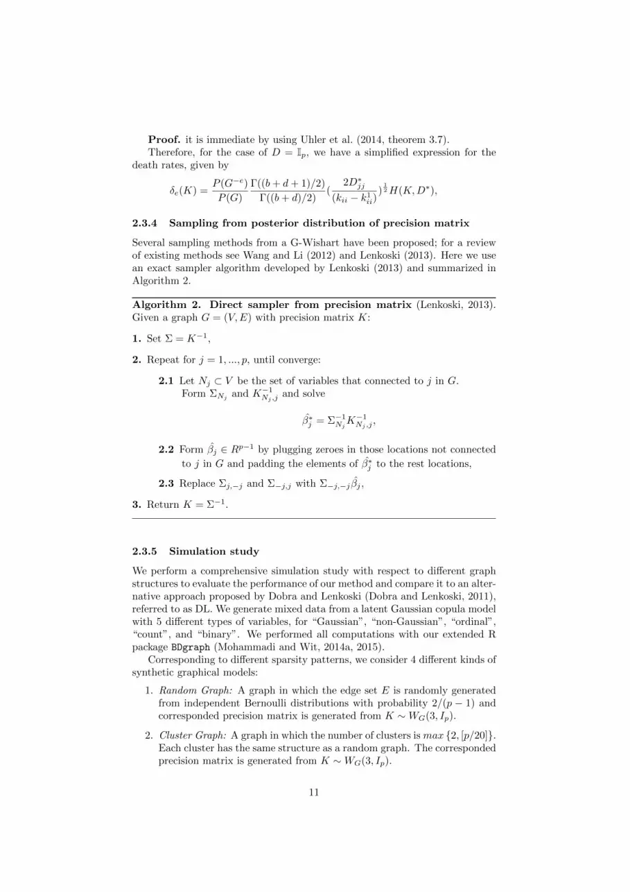
2.3.4 Sampling from posterior distribution of precision matrix

Several sampling methods from a G-Wishart have been proposed; for a reviewof existing methods see Wang and Li (2012) and Lenkoski (2013). Here we usean exact sampler algorithm developed by Lenkoski (2013) and summarized inAlgorithm 2.

Algorithm 2. Direct sampler from precision matrix (Lenkoski, 2013).Given a graph G = (V,E) with precision matrix K:

1. Set Σ = K−1,

2. Repeat for j = 1, ..., p, until converge:

2.1 Let Nj ⊂ V be the set of variables that connected to j in G.Form ΣNj

and K−1Nj ,jand solve

β∗j = Σ−1NjK−1Nj ,j

,

2.2 Form βj ∈ Rp−1 by plugging zeroes in those locations not connected

to j in G and padding the elements of β∗j to the rest locations,

2.3 Replace Σj,−j and Σ−j,j with Σ−j,−j βj ,

3. Return K = Σ−1.

2.3.5 Simulation study

We perform a comprehensive simulation study with respect to different graphstructures to evaluate the performance of our method and compare it to an alter-native approach proposed by Dobra and Lenkoski (Dobra and Lenkoski, 2011),referred to as DL. We generate mixed data from a latent Gaussian copula modelwith 5 different types of variables, for “Gaussian”, “non-Gaussian”, “ordinal”,“count”, and “binary”. We performed all computations with our extended Rpackage BDgraph (Mohammadi and Wit, 2014a, 2015).

Corresponding to different sparsity patterns, we consider 4 different kinds ofsynthetic graphical models:

1. Random Graph: A graph in which the edge set E is randomly generatedfrom independent Bernoulli distributions with probability 2/(p − 1) andcorresponded precision matrix is generated from K ∼WG(3, Ip).

2. Cluster Graph: A graph in which the number of clusters is max {2, [p/20]}.Each cluster has the same structure as a random graph. The correspondedprecision matrix is generated from K ∼WG(3, Ip).

11

3. Scale-free Graph: A scale-free graph has a power-low degree distributiongenerated by the Barabasi-Albert algorithm (Albert and Barabasi, 2002).The corresponded precision matrix is generated from K ∼WG(3, Ip).

4. Hub Graph: A graph in which every node is connected to one node, andcorresponded precision matrix is generated from K ∼WG(3, Ip).

For each graphical model, we consider four different scenarios: (1) dimensionp = 10 and sample size n = 30, (2) p = 10 and n = 100, (3) p = 30 and n = 100,(4) p = 30 and n = 500.

For each mixed data set, we fit our method and DL approach using a uniformprior for the graph and the G-Wishart prior WG(3, Ip) for the precision matrix.We run the two algorithms with the same starting points with 100, 000 iterationand 50, 000 as a burn in. Computations for this example were performed inparallel on a 235 batch nodes with 12 cores and 24 GB of memory, runningLinux.

To assess the performance of the graph structure, we compute the F1-scoremeasure (Powers, 2011) for MAP graph which defined as

F1-score =2TP

2TP + FP + FN, (8)

where TP, FP, and FN are the number of true positives, false positives, andfalse negatives, respectively. The F1-score score lies between 0 and 1, where 1stands for perfect identification and 0 for bad identification. Also, the meansquare error (MSE) is used, defined as

MSE =∑e

(pe − I(e ∈ Gtrue))2, (9)

where pe is the posterior pairwise edge inclusion probabilities and I(e ∈ Gtrue)is an indicator function, such that I(e ∈ Gtrue) = 1 if e ∈ Gtrue and zerootherwise. For our BDMCMC algorithm we calculate the posterior pairwiseedge inclusion probabilities based on the Rao-Blackwellization (Cappe et al.,2003, subsection 2.5) for each possible edge e = (i, j) as

pe =

∑Nt=1 I(e ∈ G(t))W(K(t))∑N

t=1W(K(t)), (10)

whereN is the number of iterations andW(K(t)) is the waiting time in the graphG(t) with the precision matrix K(t); See Mohammadi and Wit (2014b). Table 1reports comparisons of our method with DL (Dobra and Lenkoski, 2011), wherewe repeat the experiments 50 times and report the average F1-score and MSEwith their standard errors in parentheses. Our method performs well overall asits F1-score and its MSE are beter in most of the cases and mainly because ofits fast convergence rate. As we expected, the DL approach converges slowercompared to our method. From a theoretical point of view, both algorithmsconverge to the true posterior distribution, if we run them a sufficient amount oftime. Thus, the results from this table just indicate how quickly the algorithmsconverge.

12

F1-score MSE

p n graph BDMCMC DL BDMCMC DL

10 30

Random 0.37 (0.17) 0.33 (0.11) 7.0 (2.0) 9.2 (1.1)Cluster 0.35 (0.16) 0.30 (0.11) 6.9 (1.8) 9.6 (1.4)Scale-free 0.31 (0.13) 0.34 (0.08) 7.6 (1.2) 9.7 (1.0)Hub 0.26 (0.11) 0.31 (0.10) 8.3 (0.8) 10.2 (0.8)

10 100

random 0.33 (0.17) 0.32 (0.11) 7.7 (1.7) 9.9 (1.0)Cluster 0.30 (0.17) 0.28 (0.09) 6.8 (1.5) 9.5 (1.3)Scale-free 0.33 (0.16) 0.32 (0.12) 7.3 (1.4) 9.6 (1.0)Hub 0.26 (0.12) 0.31 (0.09) 8.3 (0.9) 10.0 (1.0)

30 100


30 500


Table 1: Summary of performance measures in simulation example 2.3.5 for ourmethod and DL (Dobra and Lenkoski, 2011). The table presents the F1-score, de-fined in (8) and MSE, defined in (9), with 100 replications and standard deviations inparenthesis. The F1-score reaches its best score at 1 and its worst at 0. The MSE ispositive value for which 0 is minimal and smaller is better. The best models for bothF1-score and MSE are boldfaced.

3 Analysis of Dupuytren disease dataset

The data set we analyses here are collected from patients who have Dupuytrendisease from north of Netherlands. Both hands of patients who were willingto participate and signed an informed consent from are examined for signsof Dupuytren disease and knuckle pads. Signs of Dupuytren disease includetethering of the skin, nodules, cords, and finger contractures in patients withcords. Participants who had at least one of these features were labeled as hav-ing Dupuytren disease. Severity of the disease are measured by total angles ofeach 10 fingers. The total angles is the sum of angles for metaccarpophalangealjoint, two interphalangeal joints (for thumb fingers are only two interphalangealjoints).

As potential risk factors, in addition, information is available about smokinghabits, alcohol consumption, whether participants performed manual labor dur-ing a significant part of their life, and whether they had sustained hand injuryin the past, including surgery. In addition, disease history information aboutthe presence of Ledderhose diabetes, epilepsy, peyronie, knucklepade, or liverdisease, and familial occurrence of Dupuytren disease (defined as a first-degreerelative with Dupuytren disease) is available.

The data consist of 279 patients who have Dupuytren disease (n = 279);

13

among those patients, 79 of them have an irreversible flexion contracture atleast one of their fingers. The severity of the disease in the all 10 fingers of thepatients is measured by total angles of each fingers (each fingers has 3 anglesexcept thumb finger which has 2 angles). To study the potential phenotype riskfactors of this disease, we consider the above mentioned 14 factors.

Lanting et al. (2014) analyzes the Dupuytren disease with a multivariateordinal logit model, taking into account age and sex, and tested hypotheses ofthe independence between groups of fingers. However, most of the studies on thephenotype of this disease have been observational studies without comprehensivestatistical analyses.

Phenotype risk factors previously described include alcohol consumption,smoking, manual labor, hand trauma, diabetes mellitus, and epilepsy (Shih andBayat, 2010, Lanting et al., 2013).

In subsection 3.1, we infer the Dupuytren disease network with 14 potentialrisk factors based on our Bayesian approach. In subsection 3.2, we consider onlythe 10 fingers to infer the interaction between the fingers.

3.1 Inference for Dupuytren disease with risk factors

We consider the severity of disease in all 10 fingers of the patients and 14 po-tential phenotype risk factors of the disease, so p = 24. The factors are: age,sex, smoking, amount of alcohol (Alcohol), relative (Relative), number of handinjury of patients (HandInjury), Manual labour (Labour), Ledderhose disease(Ledderhose), diabetes disease (Diabetes), epilepsy disease (Epilepsy), liver Dis-ease (LiverDisease), peyronie disease (Peyronie), knucklepade disease (Knuck-lepade). For each finger we measure angles of metaccarpophalangeal joint, twointerphalangeal joints (for thumb fingers we only measure two interphalangealjoints); Then we sum those angles for each fingers. The total angles could varyfrom 0 to 270 degrees; In this dataset the minimum degree is 0 and maximum157 degrees. The age of participants (in years) ranges from 40 to 89 years,with an average age of 66 years. Smoking is binned into 3 ordered categories.Amount of alcohol consumption is binned into 8 ordered categories. The othervariables are binary.

We apply our Bayesian framework to infer the conditional (in)dependenceamong the variables in order to identify the potential risk factors of the Dupuytrendisease and discover how they affect the disease. We place a uniform distribu-tion as an uninformative prior on the graph and the G-Wishart WG(3, I24) onthe precision matrix. We run our BDMCMC algorithm for 2, 000K iterationswith a 1, 000K sweeps burn-in.

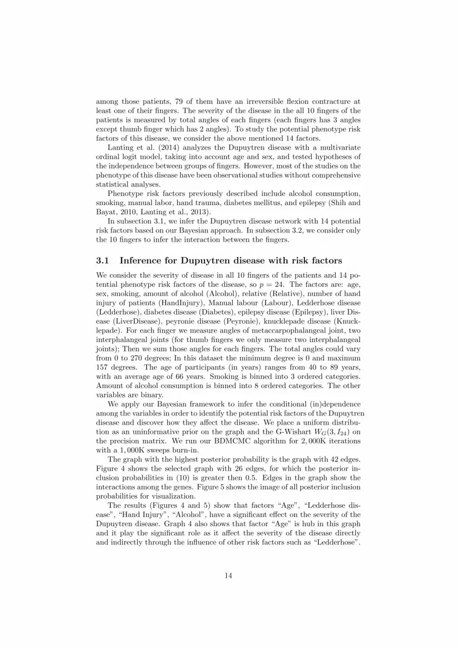
The graph with the highest posterior probability is the graph with 42 edges.Figure 4 shows the selected graph with 26 edges, for which the posterior in-clusion probabilities in (10) is greater then 0.5. Edges in the graph show theinteractions among the genes. Figure 5 shows the image of all posterior inclusionprobabilities for visualization.

The results (Figures 4 and 5) show that factors “Age”, “Ledderhose dis-ease”, “Hand Injury”, “Alcohol”, have a significant effect on the severity of theDupuytren disease. Graph 4 also shows that factor “Age” is hub in this graphand it play the significant role as it affect the severity of the disease directlyand indirectly through the influence of other risk factors such as “Ledderhose”.

14

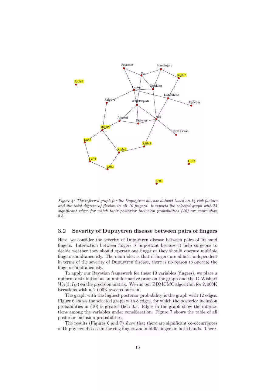
Figure 4: The inferred graph for the Dupuytren disease dataset based on 14 risk factorsand the total degrees of flexion in all 10 fingers. It reports the selected graph with 24significant edges for which their posterior inclusion probabilities (10) are more than0.5.

3.2 Severity of Dupuytren disease between pairs of fingers

Here, we consider the severity of Dupuytren disease between pairs of 10 handfingers. Interaction between fingers is important because it help surgeons todecide weather they should operate one finger or they should operate multiplefingers simultaneously. The main idea is that if fingers are almost independentin terms of the severity of Dupuytren disease, there is no reason to operate thefingers simultaneously.

To apply our Bayesian framework for these 10 variables (fingers), we place auniform distribution as an uninformative prior on the graph and the G-WishartWG(3, I10) on the precision matrix. We run our BDMCMC algorithm for 2, 000Kiterations with a 1, 000K sweeps burn-in.

The graph with the highest posterior probability is the graph with 12 edges.Figure 6 shows the selected graph with 8 edges, for which the posterior inclusionprobabilities in (10) is greater then 0.5. Edges in the graph show the interac-tions among the variables under consideration. Figure 7 shows the table of allposterior inclusion probabilities.

The results (Figures 6 and 7) show that there are significant co-occurrencesof Dupuytren disease in the ring fingers and middle fingers in both hands. There-

15

Posterior Edge Inclusion ProbabilitiesSex

Age

Labour

Smoking

Alcohol

Diabetes

Epilepsy

LiverDisease

Peyronie

Ledderhose

Knucklepads

HandInjury

Relative

Right1

Right2

Right3

Right4

Right5

Left1

Left2

Left3

Left4

Left5

Sex

Age

Labo

urS

mok

ing

Alc

ohol

Dia

bete

sE

pile

psy

Live

rDis

ease

Pey

roni

eLe

dder

hose

Knu

ckle

pads

Han

dInj

ury

Rel

ativ

eR

ight

1R

ight

2R

ight

3R

ight

4R

ight

5Le

ft1Le

ft2Le

ft3Le

ft4Le

ft5

0.0

0.2

0.4

0.6

0.8

Figure 5: Image visualization of the posterior pairwise edge inclusion probabilities ofall possible edges in the graph, for 10 fingers with 14 risk factors.

Figure 6: The inferred graph the Dupuytren disease dataset based on the total degreesof flexion in all 10 fingers. It reports the selected graph with 9 significant edges forwhich their posterior inclusion probabilities (10) are more than 0.5.

fore we can infer that middle finger substantially belong to ulnar side of hand.Surprisingly, our result show that there is significant relationship between mid-dle fingers in both hands. This result support the hypotheses the this disease isa genetic disease. Therefore, there should be some genotype risk factors for thisDupuytren disease. Moreover, it also shows that the joint interactions betweenfingers in both hand is almost symmetric.

16

Posterior Edge Inclusion Probabilities

Row

0

0.23

0.24

0.21

0.25

0.24

0.27

0.21

0.2

0.27

0.23

0

0.13

0.11

0.28

0.22

0.2

0.09

0.09

0.23

0.24

0.13

0

0.95

0.3

0.25

0.23

0.77

0.09

0.11

0.21

0.11

0.95

0

0.1

0.21

0.13

0.09

0.07

0.08

0.25

0.28

0.3

0.1

0

0.28

0.21

0.08

0.12

0.41

0.24

0.22

0.25

0.21

0.28

0

0.25

0.21

0.21

0.28

0.27

0.2

0.23

0.13

0.21

0.25

0

0.25

0.17

0.49

0.21

0.09

0.77

0.09

0.08

0.21

0.25

0

0.98

0.16

0.2

0.09

0.09

0.07

0.12

0.21

0.17

0.98

0

0.52

0.27

0.23

0.11

0.08

0.41

0.28

0.49

0.16

0.52

0Left5

Left4

Left3

Left2

Left1

Right5

Right4

Right3

Right2

Right1

Rig

ht1

Rig

ht2

Rig

ht3

Rig

ht4

Rig

ht5

Left1

Left2

Left3

Left4

Left5

0.00

0.25

0.50

0.75

1.00

Figure 7: Image visualization of the posterior pairwise edge inclusion probabilities ofall possible edges in the graph, for 10 fingers.

3.3 Fit of model to Dupuytren data

Posterior predictive checks can be used for checking the proposed Bayesianapproach fits the Dupuytren data set. If the model fits the Dupuytren data set,then simulated data generated under the model should look like to the observeddata.

Therefore, first, based on our estimated graph from our BDMCMC algo-rithm in section 3.1, we draw simulated values from the posterior predictivedistribution of replicated data. Then, we compare the samples to our observeddata. Any systematic differences between the simulations and the data deter-mine potential failings of the model.

In this regard and based on the result in subsection 3.1 (Figures 4 and 5),for both simulation and observed data, we obtain the conditional distributionsof the potential risk factors and fingers. We show that the result for finger 4in right hand and risk factor age in figure 8, for finger 5 in right hand andrisk factor relative in figure 9, and for finger 2 in right hand and risk factorLedderhose in figure 10.

Figure 8 plots the empirical and predictive distribution of variable finger 4in hand right conditional on variable “age”in four categories {(40, 50), (50, 60),(60, 70), (70, 90)}. For variable finger 4 in hand right, based on Tubiana Classi-fication, we categories it in 5 categories (category 1: 0 degree for total angle; 2:degree between (1, 45); 3: degree between (46, 90); 4: degree between (90, 135);5: degree more than 135).

Figure 9 plots the empirical and predictive distribution of variable finger 5in hand right conditional on variable “Relative”.

Figure 10 plots the empirical and predictive distribution of variable finger 2

17

1 2 3 4 5

0.0

0.2

0.4

0.6

0.8

1.0

P(Right4|40<age<50)

Index

NU

LLEmpricalPredictive

1 2 3 4 5

0.0

0.2

0.4

0.6

0.8

1.0

P(Right4|50<age<60)

Index

NU

LL

1 2 3 4 5

0.0

0.2

0.4

0.6

0.8

1.0

P(Right4|60<age<70)

NU

LL

1 2 3 4 5

0.0

0.2

0.4

0.6

0.8

1.0

P(Right4|70<age<90)

NU

LL

Figure 8: Empirical and predictive conditional distributions for total angle of finger 4in right hand condition on four different categories of variable “age”.

1 2 3 4 5

0.0

0.2

0.4

0.6

0.8

1.0

P(Right 5|Relative=0)

NU

LL

EmpricalPredictive

1 2 3 4 5

0.0

0.2

0.4

0.6

0.8

1.0

P(Right 5|Relative=1)

NU

LL

EmpricalPredictive

Figure 9: Empirical and predictive conditional distributions for total angles of finger5 in right hand condition on relative variable.

in hand right conditional on variable “Ledderhose”. Figures 10 and 9 show thatthe fit is good, since the predicted conditional distributions, in general, are thesame as the empirical distributions.

4 Conclusion

In this paper we have proposed a Bayesian methodology for discovering the effectof potential risk factors of Dupuytren disease and the underling relationships

18

1 2 3 4 5

0.0

0.2

0.4

0.6

0.8

1.0

Pr(Right2|Ledderhose=0)N

ULL

EmpricalPredictive

1 2 3 4 5

0.0

0.2

0.4

0.6

0.8

1.0

Pr(Right2|Ledderhose=1)

NU

LL

EmpricalPredictive

Figure 10: Empirical and predictive conditional distributions for total angles of finger2 in right hand condition on Ledderhose disease variable.

between fingers simultaneously.Of course, our proposed Bayesian methodology is not limited only to this

type of data. It can potentially be applied to any kind of mixed data wherethe observed variables are binary, ordinal or continuous. Our method does notwork with discrete variables that are not binary or ordinal.

We compare our Bayesian approach with an alternative Bayesian approach(Dobra and Lenkoski, 2011) using a simulation study on various types of networkstructures. Although, both approaches converge to the same posterior distri-bution our approach has some clear advantages on finite MCMC runs. Thisdifference is mainly due to our implementation of a computationally efficient al-gorithm. Our method is computationally more efficient because of two reasons.Firstly, our sampling algorithm is based on birth-death process which compareto the RJMCMC implemented in Dobra and Lenkoski (2011) is much more ef-ficient. Secondly, based on the theory which derived by Uhler et al. (2014), weused exact values for the ratio of normalizing constants which has been compu-tationally a bottleneck in the Bayesian approach. Moreover, we implementedthe code for our method in C++ which is linked to R; It is freely available onlineby R package BDgraph at http://CRAN.R-project.org/package=BDgraph.

References

Albert, R. and A.-L. Barabasi (2002). Statistical mechanics of complex net-works. Reviews of modern physics 74 (1), 47.

Atay-Kayis, A. and H. Massam (2005). A monte carlo method for comput-ing the marginal likelihood in nondecomposable gaussian graphical models.Biometrika 92 (2), 317–335.

Bayat, A. and D. McGrouther (2006). Management of dupuytren’s disease–clearadvice for an elusive condition. Annals of the Royal College of Surgeons ofEngland 88 (1), 3.

Cappe, O., C. Robert, and T. Ryden (2003). Reversible jump, birth-and-deathand more general continuous time markov chain monte carlo samplers. Jour-nal of the Royal Statistical Society: Series B (Statistical Methodology) 65 (3),679–700.

19

http://CRAN.R-project.org/package=BDgraph

Cheng, Y., A. Lenkoski, et al. (2012). Hierarchical gaussian graphical models:Beyond reversible jump. Electronic Journal of Statistics 6, 2309–2331.

Dempster, A. (1972). Covariance selection. Biometrics 28 (1), 157–175.

Dobra, A. and A. Lenkoski (2011). Copula gaussian graphical models and theirapplication to modeling functional disability data. The Annals of AppliedStatistics 5 (2A), 969–993.

Dobra, A., A. Lenkoski, and A. Rodriguez (2011). Bayesian inference for gen-eral gaussian graphical models with application to multivariate lattice data.Journal of the American Statistical Association 106 (496), 1418–1433.

Genest, C., K. Ghoudi, and L.-P. Rivest (1995). A semiparametric estimationprocedure of dependence parameters in multivariate families of distributions.Biometrika 82 (3), 543–552.

Hoff, P. D. (2007). Extending the rank likelihood for semiparametric copulaestimation. The Annals of Applied Statistics, 265–283.

Jones, B., C. Carvalho, A. Dobra, C. Hans, C. Carter, and M. West (2005). Ex-periments in stochastic computation for high-dimensional graphical models.Statistical Science 20 (4), 388–400.

Lanting, R., D. C. Broekstra, P. M. Werker, and E. R. van den Heuvel (2014). Asystematic review and meta-analysis on the prevalence of dupuytren diseasein the general population of western countries. Plastic and reconstructivesurgery 133 (3), 593–603.

Lanting, R., N. Nooraee, P. Werker, and E. van den Heuvel (2014). Patterns ofdupuytren disease in fingers; studying correlations with a multivariate ordinallogit model. Plastic and reconstructive surgery .

Lanting, R., E. R. van den Heuvel, B. Westerink, and P. M. Werker (2013).Prevalence of dupuytren disease in the netherlands. Plastic and reconstructivesurgery 132 (2), 394–403.

Lauritzen, S. (1996). Graphical models, Volume 17. Oxford University Press,USA.

Lenkoski, A. (2013). A direct sampler for g-wishart variates. Stat 2 (1), 119–128.

Lenkoski, A. and A. Dobra (2011). Computational aspects related to inference ingaussian graphical models with the g-wishart prior. Journal of Computationaland Graphical Statistics 20 (1), 140–157.

Liang, F. (2010). A double metropolis–hastings sampler for spatial models withintractable normalizing constants. Journal of Statistical Computation andSimulation 80 (9), 1007–1022.

Meyerding, H. W. (1936). Dupuytren’s contracture. Archives of Surgery 32 (2),320–333.

Milner, R. (2003). Dupuytrens disease affecting the thumb and first web of thehand. Journal of Hand Surgery (British and European Volume) 28 (1), 33–36.

20

Mohammadi, A. and E. Wit (2014a). BDgraph: Graph estimation based onbirth-death MCMC approach. R package version 2.12.

Mohammadi, A. and E. C. Wit (2014b). Bayesian structure learning in sparsegaussian graphical models. Bayesian Analysis accepted.

Mohammadi, A. and E. C. Wit (2015). Bdgraph: R package for bayesian struc-ture learning in graphical models. Arxiv .

Muirhead, R. (1982). Aspects of multivariate statistical theory, Volume 42.Wiley Online Library.

Murray, I., Z. Ghahramani, and D. MacKay (2012). Mcmc for doubly-intractable distributions. arXiv preprint arXiv:1206.6848 .

Powers, D. M. (2011). Evaluation: from precision, recall and f-measure toroc, informedness, markedness & correlation. Journal of Machine LearningTechnologies 2 (1), 37–63.

Roverato, A. (2002). Hyper inverse wishart distribution for non-decomposablegraphs and its application to bayesian inference for gaussian graphical models.Scandinavian Journal of Statistics 29 (3), 391–411.

Scutari, M. (2013). On the prior and posterior distributions used in graphicalmodelling. Bayesian Analysis 8 (1), 1–28.

Shih, B. and A. Bayat (2010). Scientific understanding and clinical managementof dupuytren disease. Nature Reviews Rheumatology 6 (12), 715–726.

Sklar, M. (1959). Fonctions de repartition a n dimensions et leurs marges.Universite Paris 8.

Tubiana, R., B. Simmons, and H. DeFrenne (1982). Location of dupuytren’sdisease on the radial aspect of the hand. Clinical orthopaedics and relatedresearch (168), 222.

Uhler, C., A. Lenkoski, and D. Richards (2014). Exact formulas for the normal-izing constants of wishart distributions for graphical models. arXiv preprintarXiv:1406.4901 .

Wang, H. (2012). Bayesian graphical lasso models and efficient posterior com-putation. Bayesian Analysis 7 (4), 867–886.

Wang, H. (2014). Scaling it up: Stochastic search structure learning in graphicalmodels.

Wang, H. and S. Li (2012). Efficient gaussian graphical model determinationunder g-wishart prior distributions. Electronic Journal of Statistics 6, 168–198.

Wang, H. and N. S. Pillai (2013). On a class of shrinkage priors for covariancematrix estimation. Journal of Computational and Graphical Statistics 22 (3),689–707.

Wong, F., C. K. Carter, and R. Kohn (2003). Efficient estimation of covarianceselection models. Biometrika 90 (4), 809–830.

21

bayesian modelling of dupuytren disease using gaussian copula graphical models

Documents