band-stop smoothing filter design - archive ouverte hal

HAL Id: hal-03147947https://hal.archives-ouvertes.fr/hal-03147947

Submitted on 21 Feb 2021

HAL is a multi-disciplinary open accessarchive for the deposit and dissemination of sci-entific research documents, whether they are pub-lished or not. The documents may come fromteaching and research institutions in France orabroad, or from public or private research centers.

L’archive ouverte pluridisciplinaire HAL, estdestinée au dépôt et à la diffusion de documentsscientifiques de niveau recherche, publiés ou non,émanant des établissements d’enseignement et derecherche français ou étrangers, des laboratoirespublics ou privés.

Band-stop Smoothing Filter DesignArman Kheirati Roonizi, Christian Jutten

To cite this version:Arman Kheirati Roonizi, Christian Jutten. Band-stop Smoothing Filter Design. IEEE Trans-actions on Signal Processing, Institute of Electrical and Electronics Engineers, 2021, pp.1-1.�10.1109/TSP.2021.3060619�. �hal-03147947�

https://hal.archives-ouvertes.fr/hal-03147947

https://hal.archives-ouvertes.fr

ACCEPTED PAPER FOR PUBLICATION IN IEEE TRANSACTIONS ON SIGNAL PROCESSING, DOI 10.1109/TSP.2021.3060619 1

Band-stop Smoothing Filter DesignArman Kheirati Roonizi∗, and Christian Jutten, Fellow, IEEE

Abstract—Smoothness priors and quadratic variation (QV)regularization are widely used techniques in many applicationsranging from signal and image processing, computer vision,pattern recognition, and many other fields of engineering andscience. In this contribution, an extension of such algorithms toband-stop smoothing filters (BSSFs) is investigated. For designinga BSSF, the most important parameters are the order and the cut-off frequencies. In this paper, we show that with the optimizationapproaches (smoothness priors or QV regularization), the cutofffrequencies are related to the regularized parameters and theorder can be directly (and easily) controlled with the numberof derivatives. We describe two ways to implement the BSSFsusing these approaches. First, we present a parallel structureto BSSF and then illustrate why it is less than ideal. Next, wepresent a novel approach regarding parallel structure to produceBSSFs with very sharp transition bands for high-performanceapplications. An improved optimization-based approach to BSSFdesign is introduced. The performance of the new BSSFs is nearlyideal.

Index Terms—Smoothness priors, Quadratic variation regular-ization, Least-squares optimization, Band-stop smoothing filter,Parallel structure

I. INTRODUCTION

THERE is no doubt that smoothing filters (i.e., smoothnesspriors and quadratic variation) have a respectable place

in signal and image processing, computer vision and patternrecognition, statistics, time series analysis, economics andmany other fields of engineering and science. Many papersand a number of books have appeared. In the following, somemajor contributions that have been developed in the design ofsmoothing filters are highlighted.

The conceptual structure of smoothing filter dates from1899 with Bohlmann’s work who studied the application ofregularized method for time series smoothing [1]. In 1923,Whittaker addressed the problem of estimating a smooth trendembedded in white noise and spoke about the method ofgraduating data [2]. Therefore, his method is known as themethod of graduating data [3]. At the same time, Hendersonhad presented a different solution which was widely extendedin North America [4]. So the method of graduating data isalso known as Whittaker-Henderson (WH) graduation [5]. In1973, Shiller worked on the same problem and introducedthe notation of “smoothness priors” [6]. It seems that hewas not aware of either Whittaker-Henderson graduation orBohlmann’s work. Subsequently, smoothness priors becamepopular in research communities. It was used in many appli-cations.

Manuscript received February 19, 2021. Asterisk indicates correspondingauthor.∗A. Kheirati Roonizi is with the Department of Computer Sci-

ence, Fasa University, Daneshjou blvd, 74616-86131 Fasa, Iran (e-mail:[email protected])

Christian Jutten is with Gipsa-Lab, CNRS, Univ. Grenoble Alpes, France

In time series analysis, smoothness priors was used formodeling nonstationary time series [7], [8], generalizing anonparametric estimator [9], [10] and exploring large-scaletime series [11]. Some developments, extensions and the least-squares computational framework of smoothness priors in timeseries analysis are presented in [12], [13].

In signal and image analysis, smoothness priors was used forsignal smoothing and detrending [14]–[18], image smoothingand restoration [19], [20], spectral estimation [21] and splinesmoothing [9], [22].

In pattern recognition, the second-order priors was used forsurface reconstruction [23], [24], dense stereo [25] and globalstereo reconstruction [26].

Some other connections to smoothness priors are quadraticvariation (QV) regularization [27], Hodrick-Prescott filtering[28], Savitzky-Golay filter [29] and the ill-posed inverseproblems of statistical Tikhonov regularization [30].

The smoothing approach based QV regularization orsmoothness priors is based on a penalized least-squaresoptimization which depends on a regularization factor thatneeds to be designed and weighted properly for getting goodperformance. There are several methods for designing theregularization factor and its weight (usually denoted as anhyperparameter). Some of them are briefly presented below.

• The L-curve method is a well-known heuristic method forchoosing the regularization parameter for ill-posed prob-lems by selecting it according to the maximal curvatureof the L-curve [31].

• Generalized cross validation is a popular tool for calculat-ing the parameters in the context of inverse problems andregularization techniques. It was initially used to tune thesmoothness parameter in ridge regression and smoothingsplines [32].

• Discrepancy principle is a posteriori parameter choicestrategies for Tikhonov regularization for solving non-linear ill-posed problems [33].

• Maximum likelihood estimation (MLE) algorithm whichis based on the concept of Bayesian likelihood, was firstintroduced by Akaike to determine the smoothness trade-off parameter [34].

• Stein’s unbiased risk estimate (SURE) regularization isanother approach that uses the Jacobian matrix of thereconstruction operator with respect to the data [35].

• Regularization factor design in terms of the cutofffrequency. Recently, we have derived a rather simpleclosed-form expression for the frequency response of thesmoothness priors and proposed a closed-form expressionfor the regularization factor. The design parameter wascalculated in terms of the cutoff frequency [36].

For extracting a signal within a predetermined frequency band,conventional linear filtering (digital filtering) techniques are

2 ACCEPTED PAPER FOR PUBLICATION IN IEEE TRANSACTIONS ON SIGNAL PROCESSING, DOI 10.1109/TSP.2021.3060619

commonly used [37]. There are many papers and many waysfor designing digital filters developed over the past decades.This technique is performed through linear time-invariant(LTI) systems which are characterized in time/frequency do-main by their impulse/frequency response. The frequencyresponse is the Fourier transform of the system’s impulseresponse.

In [17], [38], [39], it is shown that smoothness priors or QVregularization can be designed for linear filtering or smoothing.In other word, there is an equivalence between penalized least-squares optimization and zero-phase filtering. Especially, ina series of our recent papers, a general approach based ona regularized least-squares optimization framework has beenintroduced to signal denoising/smoothing [36], [38], [40] thatshows there is a strong connection between linear filteringtechniques and the current approach based on regularizedleast-squares optimization. We note that the main differencebetween them is that the designed filters based on regular-ized least-squares optimization handles smoothing/denoisingdirectly in the time domain while in the conventional linearfiltering techniques, the desired filter is first designed in thefrequency domain and then implemented in the time domainusing convolution operator. In the following, we briefly presentthe main results regarding the connection between penalizedleast-squares optimization and filtering reported in [36], [38],[40].

In [40], a general framework based on a regularized least-squares optimization has been introduced to signal smoothingwhen the signal is represented by an autoregressive movingaverage (ARMA) model. As an application, the frameworkwas used for ARMA filter design. It was shown that theframework can be driven from a forward-backward filtering,which is accomplished through LTI system. In [40], the designof a variable-Q 1 notch filter design has been discussed.Recent comparisons with many classical methods such assimple notch filter or narrow-band notch filter using feedbackstructure proposed by Pei et. al. [41] showed the superiorityof the current approach based on optimization with smoothingconstraints.

In [38], a framework for unification of the penalized least-squares optimization and forward-backward filtering schemewas presented. We showed that forward-backward filtering(zero-phase IIR filters) can be presented as instances of pe-nalized least-squares optimization. Against conventional linearfiltering that uses an IIR filter in its forward pass (followedby time reversing, filtering the reversed signal with the sameIIR filter and finally flipping the result), the approach pre-sented in [38] uses an FIR matrix filter in its forward passwhich has the advantage of being inherently stable. Com-parison with classical linear filtering showed the superiorityof the regularized approach. Therefore, the regularized least-squares optimization techniques (e.g., smoothness priors orQV regularization strategies) and zero-phase IIR filters can beconflated into one topic. In this paper, we propose a regularizedleast-squares optimization approach for BSSF design. The

1The quality factor or Q-factor of a filter is defined as the ratio of its centerfrequency over its bandwidth.

optimization problem used in this work is a linear least-squares optimization (or a convex optimization) problem. Itcan be solved by equating its derivative with respect to eachunknown variable to zero. The approach is different fromlinear time invariant (LTI) filter and matrix filter which canbe used to design BSSF. For more details on matrix filters,we refer the interested readers to [42]. In [42], the designand implementation of causal recursive filters in terms ofbanded matrices are discussed. It is based on the fact thata discrete-time filter is described by the difference equation.In this paper, we consider the problem of filtering finite-length signals, since signal processing problems are generallyformulated in terms of finite-length signals, and the developedalgorithms are targeted for the finite-length case. In [36], wehave shown that the regularized least-squares optimizationtechniques are also suitable for signal recovering even if thesignal of interest is (approximately) restricted to a knownfrequency band. We introduced a new way to the design andimplementation of smoothness priors and QV regularizationand discussed its application to low-pass, high-pass and band-pass smoothing filter design. Building on that result, in thispaper, we mainly focus on the design of band-stop smoothingfilter (BSSF). In [36], we have proposed a simple parallelstructure for band-pass smoothing filter (BPSF) or BSSFdesign. The simple band-stop smoothing filter is made out ofa low-pass smoothing filter and a high-pass smoothing filterby connecting the two smoothing filter sections in parallelwith each other. As it will be shown in Section III, thesimple parallel structure has some limitations for BSSF design.Especially, its cutoff frequencies are not exactly mapped onthe arbitrary cutoff frequencies and the amplitude at its centerfrequency is not exactly zero. Furthermore, it has a shallowfrequency transition band which is another limitation of thesimple parallel structure. It is known that the filters with steepfrequency transition bands can better separate signal and noisecomponents in adjacent frequency bands than filters with ashallow frequency transition band. To solve these issues, wepropose an improved parallel structure to BSSF design. Inthe proposed approach, we consider a modified model andinvestigate the role of noise correlation which represents thelink between two smoothing filter sections. Our results suggestthat the noise correlation increases the steepness of the role-off and boosts the performance. First we briefly review thesimple method described in [36] for BSSF design and thenshow its limitations. Next, we present an improved parallelstructure which yields nearly ideal BSSF: its cutoff frequenciesare exactly mapped on the arbitrary cutoff frequencies and ithas a sharp frequency transition band.

The remainder of the paper is organized as follows. InSection II, the relevant background on smoothness priors orQV regularization is reviewed. In Section III, we presenta naive BSSF using smoothness priors or QV regulariza-tion approach and show its limited performance. Section IVpresents an extension of such algorithms to BSSFs design,which can achieve nearly optimal performance. In SectionV, the proposed method is used to electrocardiogram (ECG)signal denoising and compared with conventional filters suchas zero-phase Butterworth filter. It is shown that the proposed

KHEIRATI ROONIZI AND JUTTEN: BAND-STOP SMOOTHING FILTER DESIGN 3

BSSF outperforms band-stop Butterworth filter. Finally, someconcluding remarks are presented in Section VI-B.

Throughout this paper, we use the following notations:boldface uppercase/lowercase letters are used to denote ma-trices/vectors and lowercase letters for scalars. The subscriptk stands for discrete time index while (·)T , (·)−1 and (·)�denote the matrix transpose, matrix inverse and deconvolution,respectively. Symbol Dn denotes the n-th order derivative withrespect to t, i.e., Dn = dn

dtn and ∗ denotes the convolution.

II. BACKGROUND

Formally, the objective of univariate smoothness priors andQV regularization strategies is to find an estimate of signalxlp(t), where the subscript lp stands for low-pass signal, fromits noisy measurement y(t) in the model

y (t) = xlp(t) + vlp(t), (1)

where vlp(t) is the unwanted additive noise signal, by solvingthe following optimization problem

xlp(t) = argminxlp(t)

∫[y(τ)− xlp(τ)]

2dτ+α2

∫ [dn

dtnxlp(τ)

]2dτ,

(2)where dn

dtn is the n-th order derivative and α denotes asmoothness tradeoff which balances the error variance andthe output smoothness. The subscript lp is used as a low-pass in the above equations since the mentioned methodsact as low-pass smoothing filter [36]. In order to digitallyprocess the signal at discrete time k, one needs to considery[k] = y[kTs], the discrete-time samples of y(t), where Tsis the sampling period, xlp[k] the sampled desired signal andvlp[k] the sampled observation noise:

y[k] = xlp[k] + vlp[k], k = 1, · · · , L.

The smoothing procedure (2) can be then expressed as

xlp[k] = argminxlp[k]

L∑j=1

(y[j]− xlp[j])2 + α2L∑j=1

(∇nxlp[j])2 ,

(3)for all k = 1, · · · , L, where ∇nxlp[k] is the n-th orderdifference approximation of the derivative. There are severalmethods that can be used for the difference approximation ofthe derivative operator. Some of them are forward, backward,central difference rule and bilinear transform. Without lossof generality, we consider the backward/forward differencerule for the difference approximation of the derivative. Inthis case, the first order difference is defined by ∇xlp[k] =xlp[k] − xlp[k ± 1], where one with “+” holds for forwarddifference rule and one with “−” holds for backward dif-ference rule. The n-th order difference is then computedas ∇nxlp[k] = ∇(∇n−1)xlp[k]. The n-th order difference,∇nxlp[k], can also be computed as

∇nxlp[k] =

n∑i=0

(−1)i(n

i

)xlp[k ± i], (4)

where(ni

)is the binomial coefficient. In the following, we use

the backward difference rule. It then means that, from now,

we used xlp[k − i] in (4). Hence, (3) can be written in thefollowing matrix notation [36]

xlp = ‖y − xlp‖2 + α2 ‖Dnxlp‖2 , (5)

where y = (y[1], · · · , y[L])T , xlp = (xlp[1], · · · , xlp[L])

T ,‖·‖2 denotes the Euclidean norm and Dn is the L×L Toeplitzmatrix, built from the backward difference operator dn:

dn ,

[1, −

(n

1

), · · · , (−1)n−1

(n

n− 1

), (−1)n

(n

n

)].

The difference operator dn can also be computed by thefollowing recursion:{

d1 , [+1, −1] n = 1

dn = dn−1 ∗ d1 n > 1, (6)

where ∗ denotes the convolution operator. Throughout thepaper, the second-order smoothness priors is of special interest.As a special case, for data on L samples, D2 is a L×L matrixdefined as:

D2 =

1 . . . 0 0 0 0−2 1 . . . 0 01 −2 1 0 . . . 0

0 1 −2 1. . .

......

. . . . . . . . . . . . 00 . . . 0 1 −2 1

L×L

. (7)

The solution that follows from the minimization of (5) is

xlp = (I + α2DTnDn)−1y.

Any component xlp[k] of the vector xlp can be written in thefollowing convolution form [36]:

xlp[k] =(δ[k] + α2dn[−k] ∗ dn[k]

)� ∗ y[k], (8)

where (·)� denotes the deconvolution. (8) can be implementedas

xlp[k] = Z−1

{1

1 + α2dn( 1z )dn(z)

}∗ y[k],

where Z−1 denotes the inverse Z-transform. The above reg-ularization method can be stated in terms of a zero-phase,linear time-invariant (LTI) smoothing filter (for more detailssee [17], [36]). It can be analyzed in the frequency domain. Tothis purpose by substituting y[k] with δ[k] in (8), and takingthe Z-transform, the frequency response of the smoothing filteris obtained as follows [36]H lpn (z) =

1

1 + α2dn(z)dn( 1z )

=1

1 + α2(1− z−1)n(1− z)n

H lpn (ejω) =

1

1 + α2(2 sin ω2 )2n

.

(9)

The transfer function of the smoothing filter, i.e., (9), is realand its phase is zero. It has a low-pass characteristic whichmakes it suited for extracting the low frequency componentsof the signal, hence the subscript lp in the previous equations.The regularization factor α determines at which frequency the


0 0.5 1

0

0.2

0.4

0.6

0.8

1

0 0.5 1

0

0.2

0.4

0.6

0.8

1

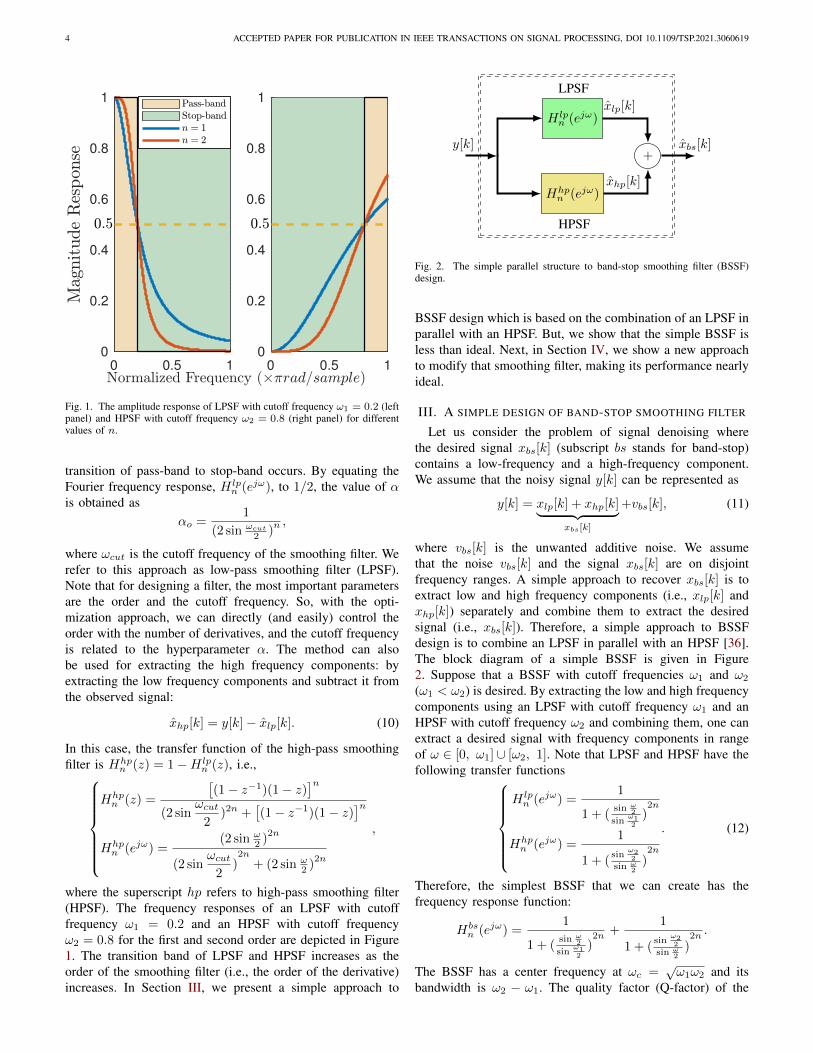
Fig. 1. The amplitude response of LPSF with cutoff frequency ω1 = 0.2 (leftpanel) and HPSF with cutoff frequency ω2 = 0.8 (right panel) for differentvalues of n.

transition of pass-band to stop-band occurs. By equating theFourier frequency response, H lp

n (ejω), to 1/2, the value of αis obtained as

αo =1

(2 sin ωcut

2 )n ,

where ωcut is the cutoff frequency of the smoothing filter. Werefer to this approach as low-pass smoothing filter (LPSF).Note that for designing a filter, the most important parametersare the order and the cutoff frequency. So, with the opti-mization approach, we can directly (and easily) control theorder with the number of derivatives, and the cutoff frequencyis related to the hyperparameter α. The method can alsobe used for extracting the high frequency components: byextracting the low frequency components and subtract it fromthe observed signal:

xhp[k] = y[k]− xlp[k]. (10)

In this case, the transfer function of the high-pass smoothingfilter is Hhp

n (z) = 1−H lpn (z), i.e.,

Hhpn (z) =

[(1− z−1)(1− z)

]n(2 sin

ωcut2

)2n +[(1− z−1)(1− z)

]nHhpn (ejω) =

(2 sin ω2 )

2n

(2 sinωcut

2)2n

+ (2 sin ω2 )

2n

,

where the superscript hp refers to high-pass smoothing filter(HPSF). The frequency responses of an LPSF with cutofffrequency ω1 = 0.2 and an HPSF with cutoff frequencyω2 = 0.8 for the first and second order are depicted in Figure1. The transition band of LPSF and HPSF increases as theorder of the smoothing filter (i.e., the order of the derivative)increases. In Section III, we present a simple approach to

H lpn (ejω)

Hhpn (ejω)

+y[k]

xlp[k]

xhp[k]

xbs[k]

LPSF

HPSF

Fig. 2. The simple parallel structure to band-stop smoothing filter (BSSF)design.

BSSF design which is based on the combination of an LPSF inparallel with an HPSF. But, we show that the simple BSSF isless than ideal. Next, in Section IV, we show a new approachto modify that smoothing filter, making its performance nearlyideal.

III. A SIMPLE DESIGN OF BAND-STOP SMOOTHING FILTER

Let us consider the problem of signal denoising wherethe desired signal xbs[k] (subscript bs stands for band-stop)contains a low-frequency and a high-frequency component.We assume that the noisy signal y[k] can be represented as

y[k] = xlp[k] + xhp[k]︸︷︷︸xbs[k]

+vbs[k], (11)

where vbs[k] is the unwanted additive noise. We assumethat the noise vbs[k] and the signal xbs[k] are on disjointfrequency ranges. A simple approach to recover xbs[k] is toextract low and high frequency components (i.e., xlp[k] andxhp[k]) separately and combine them to extract the desiredsignal (i.e., xbs[k]). Therefore, a simple approach to BSSFdesign is to combine an LPSF in parallel with an HPSF [36].The block diagram of a simple BSSF is given in Figure2. Suppose that a BSSF with cutoff frequencies ω1 and ω2

(ω1 < ω2) is desired. By extracting the low and high frequencycomponents using an LPSF with cutoff frequency ω1 and anHPSF with cutoff frequency ω2 and combining them, one canextract a desired signal with frequency components in rangeof ω ∈ [0, ω1] ∪ [ω2, 1]. Note that LPSF and HPSF have thefollowing transfer functions

H lpn (ejω) =

1

1 + (sin ω

2

sinω12

)2n

Hhpn (ejω) =

1

1 + (sin

ω22

sin ω2

)2n

. (12)

Therefore, the simplest BSSF that we can create has thefrequency response function:

Hbsn (ejω) =

1

1 + (sin ω

2

sinω12

)2n +

1

1 + (sin

ω22

sin ω2

)2n .

The BSSF has a center frequency at ωc =√ω1ω2 and its

bandwidth is ω2 − ω1. The quality factor (Q-factor) of the


0 0.2 0.4 0.6 0.8 1

0

0.2

0.4

0.6

0.8

1

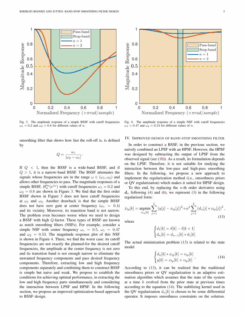
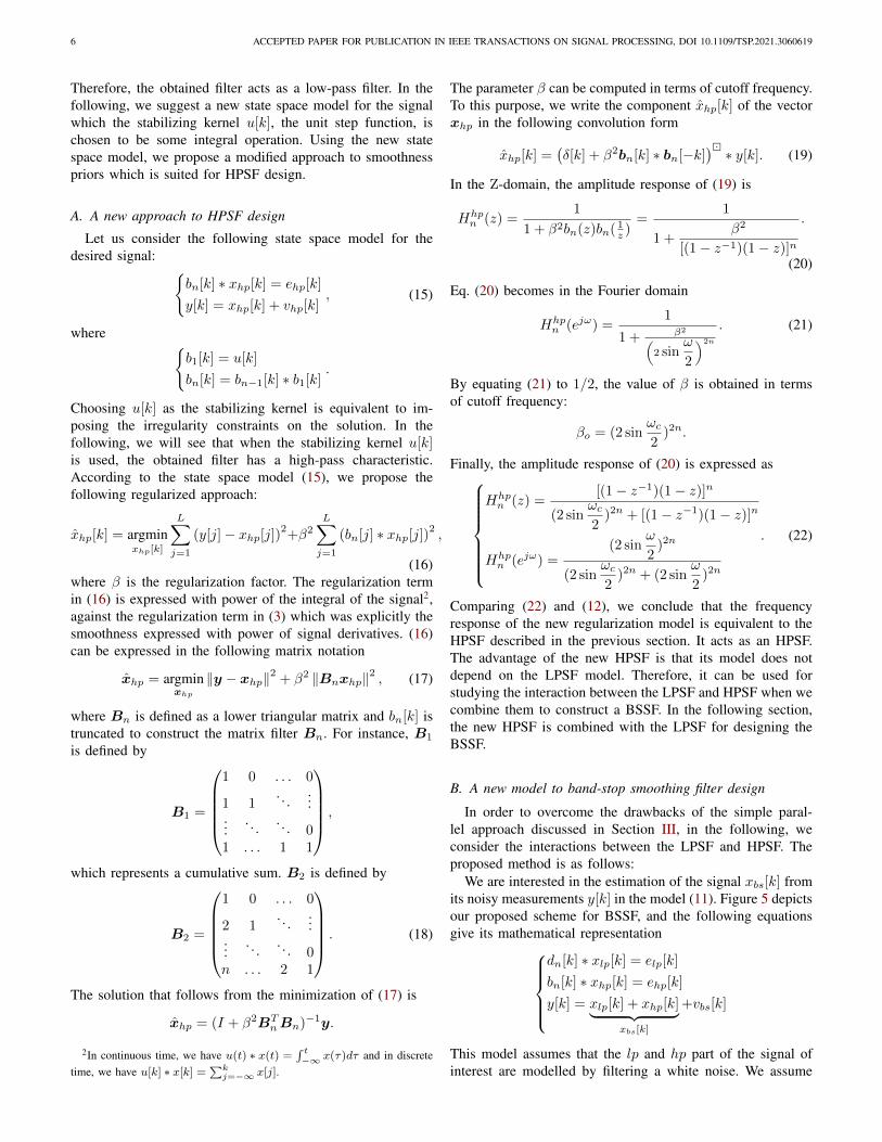
Fig. 3. The amplitude response of a simple BSSF with cutoff frequenciesω1 = 0.2 and ω2 = 0.8 for different values of n.

smoothing filter that shows how fast the roll-off is, is definedby

Q =ωc

|ω2 − ω1|.

If Q < 1, then the BSSF is a wide-band BSSF, and ifQ > 1, it is a narrow-band BSSF. The BSSF attenuates thesignals whose frequencies are in the range ω ∈ (ω1, ω2) andallows other frequencies to pass. The magnitude responses of asimple BSSF, Hbs

n (ejω) with cutoff frequencies ω1 = 0.2 andω2 = 0.8 are shown in Figure 3. We find that the first orderBSSF shown in Figure 3 does not have cutoff frequenciesat ω1 and ω2. Another drawback is that the simple BSSFdoes not have zero gain at center frequency (ωc = 0.4)and its vicinity. Moreover, its transition band is not narrow.The problem even becomes worse when we need to designa BSSF with high Q-factor. These types of BSSF are knownas notch smoothing filters (NSFs). For example, consider asimple NSF with center frequency ωc = 0.5, ω1 = 0.47and ω2 = 0.53. The magnitude response plot of this NSFis shown in Figure 4. There, we find the worst case: its cutofffrequencies are not exactly the planned-for the desired cutofffrequencies, the amplitude at the center frequency is not zeroand its transition band is not enough narrow to eliminate theunwanted frequency components and pass desired frequencycomponents. Therefore, extracting low and high frequencycomponents separately and combining them to construct BSSFis simple but naive and weak. We propose to establish theconditions for achieving optimal performance, in extracting thelow and high frequency parts simultaneously and consideringthe interaction between LPSF and HPSF. In the followingsection, we propose an improved optimization-based approachto BSSF design.

0 0.2 0.4 0.6 0.8 1

0

0.2

0.4

0.6

0.8

1

Fig. 4. The amplitude response of a simple NSF with cutoff frequenciesω1 = 0.47 and ω2 = 0.53 for different values of n.

IV. IMPROVED DESIGN OF BAND-STOP SMOOTHING FILTER

In order to construct a BSSF, in the previous section, wenaively combined an LPSF with an HPSF. However, the HPSFwas designed by subtracting the output of LPSF from theobserved signal (see (10)). As a result, its formulation dependson the LPSF. Therefore, it is not suitable for studying theinteraction between the low-pass and high-pass smoothingfilters. In the following, we propose a new approach toimplement the regularization method (i.e., smoothness priorsor QV regularization) which makes it suited for HPSF design.

To this end, by replacing the n-th order derivative usingdn following (4) and (6), we represent (3) in the followingregularized form:

xlp[k] = argminxlp[k]

L∑j=1

(y[j]− xlp[j])2+α2L∑j=1

(dn[j] ∗ xlp[j])2 ,

(13)where {

d1[k] = δ[k]− δ[k + 1]

dn[k] = dn−1[k] ∗ d1[k]

The actual minimization problem (13) is related to the statemodel {

dn[k] ∗ xlp[k] = elp[k]

y[k] = xlp[k] + vlp[k], (14)

According to (13), it can be realized that the traditionalsmoothness priors or QV regularization is an adaptive esti-mation algorithm which assumes that the state of the systemat a time k evolved from the prior state at previous timesaccording to the equation (14). The stabilizing kernel used inthe QV regularization dn[k] is chosen to be some differentialoperator. It imposes smoothness constraints on the solution.


Therefore, the obtained filter acts as a low-pass filter. In thefollowing, we suggest a new state space model for the signalwhich the stabilizing kernel u[k], the unit step function, ischosen to be some integral operation. Using the new statespace model, we propose a modified approach to smoothnesspriors which is suited for HPSF design.

A. A new approach to HPSF design

Let us consider the following state space model for thedesired signal: {

bn[k] ∗ xhp[k] = ehp[k]

y[k] = xhp[k] + vhp[k], (15)

where {b1[k] = u[k]

bn[k] = bn−1[k] ∗ b1[k].

Choosing u[k] as the stabilizing kernel is equivalent to im-posing the irregularity constraints on the solution. In thefollowing, we will see that when the stabilizing kernel u[k]is used, the obtained filter has a high-pass characteristic.According to the state space model (15), we propose thefollowing regularized approach:

xhp[k] = argminxhp[k]

L∑j=1

(y[j]− xhp[j])2+β2L∑j=1

(bn[j] ∗ xhp[j])2 ,

(16)where β is the regularization factor. The regularization termin (16) is expressed with power of the integral of the signal2,against the regularization term in (3) which was explicitly thesmoothness expressed with power of signal derivatives. (16)can be expressed in the following matrix notation

xhp = argminxhp

‖y − xhp‖2 + β2 ‖Bnxhp‖2 , (17)

where Bn is defined as a lower triangular matrix and bn[k] istruncated to construct the matrix filter Bn. For instance, B1

is defined by

B1 =

1 0 . . . 0

1 1. . .

......

. . . . . . 01 . . . 1 1

,

which represents a cumulative sum. B2 is defined by

B2 =

1 0 . . . 0

2 1. . .

......

. . . . . . 0n . . . 2 1

. (18)

The solution that follows from the minimization of (17) is

xhp = (I + β2BTnBn)−1y.

2In continuous time, we have u(t) ∗ x(t) =∫ t−∞ x(τ)dτ and in discrete

time, we have u[k] ∗ x[k] =∑k

j=−∞ x[j].

The parameter β can be computed in terms of cutoff frequency.To this purpose, we write the component xhp[k] of the vectorxhp in the following convolution form

xhp[k] =(δ[k] + β2bn[k] ∗ bn[−k]

)� ∗ y[k]. (19)

In the Z-domain, the amplitude response of (19) is

Hhpn (z) =

1

1 + β2bn(z)bn( 1z )

=1

1 +β2

[(1− z−1)(1− z)]n

.

(20)

Eq. (20) becomes in the Fourier domain

Hhpn (ejω) =

1

1 + β2(2 sin

ω

2

)2n

. (21)

By equating (21) to 1/2, the value of β is obtained in termsof cutoff frequency:

βo = (2 sinωc2

)2n.

Finally, the amplitude response of (20) is expressed as

Hhpn (z) =

[(1− z−1)(1− z)]n

(2 sinωc2

)2n + [(1− z−1)(1− z)]n

Hhpn (ejω) =

(2 sinω

2)2n

(2 sinωc2

)2n + (2 sinω

2)2n

. (22)

Comparing (22) and (12), we conclude that the frequencyresponse of the new regularization model is equivalent to theHPSF described in the previous section. It acts as an HPSF.The advantage of the new HPSF is that its model does notdepend on the LPSF model. Therefore, it can be used forstudying the interaction between the LPSF and HPSF when wecombine them to construct a BSSF. In the following section,the new HPSF is combined with the LPSF for designing theBSSF.

B. A new model to band-stop smoothing filter design

In order to overcome the drawbacks of the simple paral-lel approach discussed in Section III, in the following, weconsider the interactions between the LPSF and HPSF. Theproposed method is as follows:

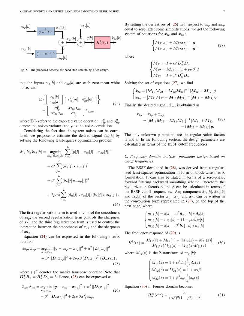
We are interested in the estimation of the signal xbs[k] fromits noisy measurements y[k] in the model (11). Figure 5 depictsour proposed scheme for BSSF, and the following equationsgive its mathematical representation

dn[k] ∗ xlp[k] = elp[k]

bn[k] ∗ xhp[k] = ehp[k]

y[k] = xlp[k] + xhp[k]︸︷︷︸xbs[k]

+vbs[k]

This model assumes that the lp and hp part of the signal ofinterest are modelled by filtering a white noise. We assume


1(1−z−1)n

(1− z−1)n

+

elp[k]

ehp[k]

xlp[k]

xhp[k]

xbs[k]+

vbs[k]

y[k]Hbsn (z)

xbs[k]

Fig. 5. The proposed scheme for band-stop smoothing filter design.

that the inputs elp[k] and ehp[k] are each zero-mean whitenoise, with

(23)E{[

elp[k]ehp[k]

] [e∗lp[m] e∗hp[m]

]}=

[σ2lp ρσlpσhp

ρσlpσhp σ2hp

]δk,m,

where E{} refers to the expected value operation, σ2lp and σ2

hp

denote the noises variance and ρ is the noise correlation.Considering the fact that the system noises can be corre-

lated, we propose to estimate the desired signal xbs[k] bysolving the following least-squares optimization problem

xlp[k], xhp[k] = argminxlp[j],xhp[j]

L∑j=1

(y[j]− xlp[j]− xhp[j])2

+ α2L∑j=1

(dn[j] ? xlp[j])2

+ β2L∑j=1

(bn[j] ? xhp[j])2

+ 2ραβ

L∑j=1

(dn[j] ? xlp[j]) (bn[j] ? xhp[j]) .

(24)

The first regularization term is used to control the smoothnessof xlp, the second regularization term controls the sharpnessof xhp and the third regularization term is used to control theinteraction between the smoothness of xlp and the sharpnessof xhp.

Equation (24) can be expressed in the following matrixnotation

xlp, xhp = argminxlp,xhp

‖y − xlp − xhp‖2 + α2 ‖Dnxlp‖2

+ β2 ‖Bnxhp‖2 + 2ραβ (Dnxlp)T

(Bnxhp) ,

(25)

where (·)T denotes the matrix transpose operator. Note thatDTnBn = BT

nDn = I . Hence, (25) can be expressed as

(26)xlp, xhp = argmin

xlp,xhp

‖y − xlp − xhp‖2 + α2 ‖Dnxlp‖2

+ β2 ‖Bnxhp‖2 + 2ραβxTlpxhp.

By setting the derivatives of (26) with respect to xlp and xhpequal to zero, after some simplifications, we get the followingsystem of equations for xlp and xhp:{

M11xlp + M12xhp = y

M21xlp + M22xhp = y, (27)

where M11 = I + α2DT

nDn

M12 = M21 = (1 + ραβ) I

M22 = I + β2BTnBn

Solving the set of equations (27), we find{xlp = [M11M22 −M12M21]

−1[M22 −M12]y

xhp = [M11M22 −M12M21]−1

[M11 −M21]y

Finally, the desired signal, xbs, is obtained as

(28)xbs = xlp + xhp

= [M11M22 −M12M21]−1

[M11 + M22

− (M12 + M21)]y.

The only unknown parameters are the regularization factorsα and β. In the following section, the design parameters arecalculated in terms of the BSSF cutoff frequencies.

C. Frequency domain analysis: parameter design based oncutoff frequencies

The BSSF developed in (28), was derived from a regular-ized least-squares optimization in form of block-wise matrixformulation. It can also be stated in terms of a zero-phase,forward filtering backward smoothing scheme. Therefore, theregularization factors α and β can be calculated in terms ofthe BSSF cutoff frequencies. Any component xlp[k], xhp[k]and xbs[k] of the vector xlp, xhp and xbs can be written inthe convolution form represented in (29), on the top of thenext page, where

m11[k] = δ[k] + α2dn[−k] ∗ dn[k]

m12[k] = m21[k] = (1 + ραβ)δ[k]

m22[k] = δ[k] + β2bn[−k] ∗ bn[k]

The frequency response of (29) is

Hbsn (z) =

M11(z) +M22(z)− [M12(z) +M21(z)]

M11(z)M22(z)−M12(z)M21(z), (30)

where Mij(z) is the Z-transform of mij [k]:M11(z) = 1 + α2dn(

1

z)dn(z)

M12(z) = M21(z) = 1 + ραβ

M22(z) = 1 + β2bn(1

z)bn(z)

Equation (30) in Fourier domain becomes

Hbsn (ejω) =

κ

(αβ)2(1− ρ2) + κ, (31)


xlp[k] = (m11[k] ∗m22[k]−m12[k] ∗m21[k])

� ∗ (m22[k]−m21[k]) ∗ y[k]

xhp[k] = (m11[k] ∗m22[k]−m12[k] ∗m21[k])� ∗ (m11[k]−m12[k]) ∗ y[k]

xbs[k] = (m11[k] ∗m22[k]−m12[k] ∗m21[k])� ∗ (m11[k] +m22[k]−m21[k]−m12[k]) ∗ y[k]

(29)

where

κ = α2(2 sinω

2)2n − 2ραβ +

β2

(2 sinω

2)2n

.

The magnitude response of the BSSF, (31), has two cutofffrequencies at ω1 and ω2 which are satisfying |Hbs

n (ejω)|= 12 .

Substituting each of these two points into equation (31) resultsa system of equations which contains two equations that sharetwo unknowns α and β:

α2(2 sinω1

2)2n − 2ραβ +

β2

(2 sin ω1

2 )2n= α2β2(1− ρ2)

α2(2 sinω2

2)2n − 2ραβ +

β2

(2 sin ω2

2 )2n= α2β2(1− ρ2)

(32)

Subtracting the second equation from the first one, we find

β = α[(2 sin

ω1

2)(2 sin

ω2

2)]n

(33)

Substituting (33) in the first equation of (32), the resultingequation is

(34)α222n[(sinω1

2)2n − 2ρ(sin

ω1

2sin

ω2

2)n + (sin

ω2

2)2n]

= α2β2(1− ρ2)

After some simplifications, we find

βo = 2n

√(sin ω1

2 )2n − 2ρ(sin ω1

2 sin ω2

2 )n + (sin ω2

2 )2n

1− ρ2(35)

From (33) and (35), the value of α is obtained as

αo =βo[

(2 sin ω1

2 )(2 sin ω2

2 )]n (36)

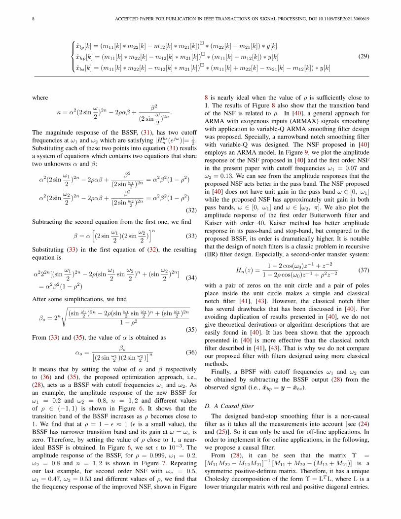
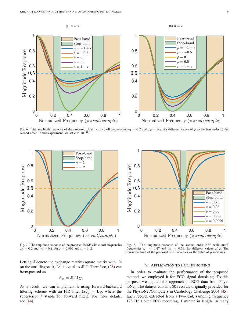
It means that by setting the value of α and β respectivelyto (36) and (35), the proposed optimization approach, i.e.,(28), acts as a BSSF with cutoff frequencies ω1 and ω2. Asan example, the amplitude response of the new BSSF forω1 = 0.2 and ω2 = 0.8, n = 1, 2 and different valuesof ρ ∈ (−1, 1) is shown in Figure 6. It shows that thetransition band of the BSSF increases as ρ becomes close to1. We find that at ρ = 1 − ε ≈ 1 (ε is a small value), theBSSF has narrower transition band and its gain at ω = ωc iszero. Therefore, by setting the value of ρ close to 1, a near-ideal BSSF is obtained. In Figure 6, we set ε to 10−3. Theamplitude response of the BSSF, for ρ = 0.999, ω1 = 0.2,ω2 = 0.8 and n = 1, 2 is shown in Figure 7. Repeatingour last example, for second order NSF with ωc = 0.5,ω1 = 0.47, ω2 = 0.53 and different values of ρ, we find thatthe frequency response of the improved NSF, shown in Figure

8 is nearly ideal when the value of ρ is sufficiently close to1. The results of Figure 8 also show that the transition bandof the NSF is related to ρ. In [40], a general approach forARMA with exogenous inputs (ARMAX) signals smoothingwith application to variable-Q ARMA smoothing filter designwas proposed. Specially, a narrowband notch smoothing filterwith variable-Q was designed. The NSF proposed in [40]employs an ARMA model. In Figure 9, we plot the amplituderesponse of the NSF proposed in [40] and the first order NSFin the present paper with cutoff frequencies ω1 = 0.07 andω2 = 0.13. We can see from the amplitude responses that theproposed NSF acts better in the pass band. The NSF proposedin [40] does not have unit gain in the pass band ω ∈ [0, ω1]while the proposed NSF has approximately unit gain in bothpass bands, ω ∈ [0, ω1] and ω ∈ [ω2, π]. We also plot theamplitude response of the first order Butterworth filter andKaiser with order 40. Kaiser method has better amplituderesponse in its pass-band and stop-band, but compared to theproposed BSSF, its order is dramatically higher. It is notablethat the design of notch filters is a classic problem in recursive(IIR) filter design. Especially, a second-order transfer system:

Hn(z) =1− 2 cos(ω0)z−1 + z−2

1− 2ρ cos(ω0)z−1 + ρ2z−2(37)

with a pair of zeros on the unit circle and a pair of polesplace inside the unit circle makes a simple and classicalnotch filter [41], [43]. However, the classical notch filterhas several drawbacks that has been discussed in [40]. Foravoiding duplication of results presented in [40], we do notgive theoretical derivations or algorithm descriptions that areeasily found in [40]. It has been shown that the approachpresented in [40] is more effective than the classical notchfilter described in [41], [43]. That is why we do not compareour proposed filter with filters designed using more classicalmethods.

Finally, a BPSF with cutoff frequencies ω1 and ω2 canbe obtained by subtracting the BSSF output (28) from theobserved signal (i.e., xbp = y − xbs).

D. A Causal filter

The designed band-stop smoothing filter is a non-causalfilter as it takes all the measurements into account [see (24)and (25)]. So it can only be used for off-line applications. Inorder to implement it for online applications, in the following,we propose a causal filter.

From (28), it can be seen that the matrix Υ =[M11M22 −M12M21]

−1[M11 +M22 − (M12 +M21)] is a

symmetric positive-definite matrix. Therefore, it has a uniqueCholesky decomposition of the form Υ = LTL, where L is alower triangular matrix with real and positive diagonal entries.


(a) n = 1

0 0.2 0.4 0.6 0.8 1

0

0.2

0.4

0.6

0.8

1

(b) n = 2

0 0.2 0.4 0.6 0.8 1

0

0.2

0.4

0.6

0.8

1

Fig. 6. The amplitude response of the proposed BSSF with cutoff frequencies ω1 = 0.2 and ω2 = 0.8, for different values of ρ a) the first order b) thesecond order. In this experiment, we set ε to 10−3.

0 0.2 0.4 0.6 0.8 1

0

0.2

0.4

0.6

0.8

1

Fig. 7. The amplitude response of the proposed BSSF with cutoff frequenciesω1 = 0.2 and ω2 = 0.8, for ρ = 0.999 and n = 1, 2.

Letting J denote the exchange matrix (square matrix with 1’son the anti-diagonal), LT is equal to JLJ. Therefore, (28) canbe expressed as

xbs = JLJLy,

As a result, we can implement it using forward-backwardfiltering scheme with an FIR filter (xfbs = Ly, where thesuperscript f stands for forward filter). For more details,see [44].

0 0.2 0.4 0.6 0.8 1

0

0.2

0.4

0.6

0.8

1

Fig. 8. The amplitude response of the second order NSF with cutofffrequencies ω1 = 0.47 and ω2 = 0.53, for different values of ρ. Thetransition band of the proposed NSF increases as the value of ρ increases.

V. APPLICATION TO ECG DENOISING

In order to evaluate the performance of the proposedmethod, we employed it for ECG signal denoising. To thispurpose, we applied the approach on ECG data from Phys-ioNet. The dataset contains 80 records, originally provided forthe PhysioNet/Computers in Cardiology Challenge 2004 [45].Each record, extracted from a two-lead, sampling frequency128 Hz Holter ECG recording, 1 minute in length. In many


0 0.2 0.4 0.6 0.8 1

0

0.2

0.4

0.6

0.8

1

Fig. 9. The amplitude response of the NSF proposed in [40] and the firstorder NSF proposed in the present paper with cutoff frequencies ω1 = 0.07and ω2 = 0.13. The proposed NSF has approximately unit gain in either passband. We also plot the amplitude response of the first order Butterworth filterand Kaiser with order 40.

applications of signal processing such as ECG denoising,linear time invariant (LTI) filters (e.g., Butterworth filter) arestill the standard choice for ECG system front-ends [46].Therefore, we also employed a band-stop Butterworth filter forextracting the ECG signals and compared it with our proposedmethod. In the following case studies, the BSSF order is setto n = 2, and the operators D2 and B2 are as defined in (7)and (18), respectively. The Butterworth filters were applied tothe data using the filtfilt function in Matlab to have zero-phaselag.

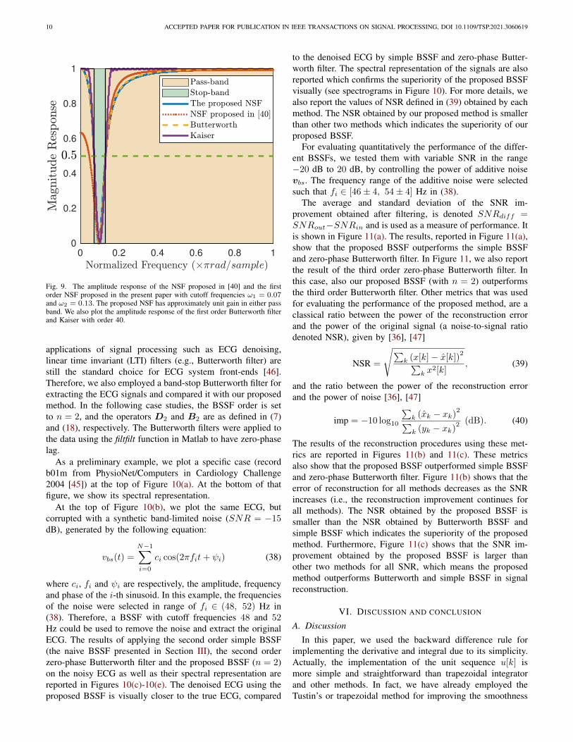
As a preliminary example, we plot a specific case (recordb01m from PhysioNet/Computers in Cardiology Challenge2004 [45]) at the top of Figure 10(a). At the bottom of thatfigure, we show its spectral representation.

At the top of Figure 10(b), we plot the same ECG, butcorrupted with a synthetic band-limited noise (SNR = −15dB), generated by the following equation:

vbs(t) =

N−1∑i=0

ci cos(2πfit+ ψi) (38)

where ci, fi and ψi are respectively, the amplitude, frequencyand phase of the i-th sinusoid. In this example, the frequenciesof the noise were selected in range of fi ∈ (48, 52) Hz in(38). Therefore, a BSSF with cutoff frequencies 48 and 52Hz could be used to remove the noise and extract the originalECG. The results of applying the second order simple BSSF(the naive BSSF presented in Section III), the second orderzero-phase Butterworth filter and the proposed BSSF (n = 2)on the noisy ECG as well as their spectral representation arereported in Figures 10(c)-10(e). The denoised ECG using theproposed BSSF is visually closer to the true ECG, compared

to the denoised ECG by simple BSSF and zero-phase Butter-worth filter. The spectral representation of the signals are alsoreported which confirms the superiority of the proposed BSSFvisually (see spectrograms in Figure 10). For more details, wealso report the values of NSR defined in (39) obtained by eachmethod. The NSR obtained by our proposed method is smallerthan other two methods which indicates the superiority of ourproposed BSSF.

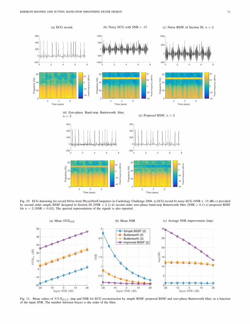
For evaluating quantitatively the performance of the differ-ent BSSFs, we tested them with variable SNR in the range−20 dB to 20 dB, by controlling the power of additive noisevbs. The frequency range of the additive noise were selectedsuch that fi ∈ [46± 4, 54± 4] Hz in (38).

The average and standard deviation of the SNR im-provement obtained after filtering, is denoted SNRdiff =SNRout−SNRin and is used as a measure of performance. Itis shown in Figure 11(a). The results, reported in Figure 11(a),show that the proposed BSSF outperforms the simple BSSFand zero-phase Butterworth filter. In Figure 11, we also reportthe result of the third order zero-phase Butterworth filter. Inthis case, also our proposed BSSF (with n = 2) outperformsthe third order Butterworth filter. Other metrics that was usedfor evaluating the performance of the proposed method, are aclassical ratio between the power of the reconstruction errorand the power of the original signal (a noise-to-signal ratiodenoted NSR), given by [36], [47]

NSR =

√∑k (x[k]− x[k])

2∑k x

2[k], (39)

and the ratio between the power of the reconstruction errorand the power of noise [36], [47]

imp = −10 log10

∑k (xk − xk)

2∑k (yk − xk)

2 (dB). (40)

The results of the reconstruction procedures using these met-rics are reported in Figures 11(b) and 11(c). These metricsalso show that the proposed BSSF outperformed simple BSSFand zero-phase Butterworth filter. Figure 11(b) shows that theerror of reconstruction for all methods decreases as the SNRincreases (i.e., the reconstruction improvement continues forall methods). The NSR obtained by the proposed BSSF issmaller than the NSR obtained by Butterworth BSSF andsimple BSSF which indicates the superiority of the proposedmethod. Furthermore, Figure 11(c) shows that the SNR im-provement obtained by the proposed BSSF is larger thanother two methods for all SNR, which means the proposedmethod outperforms Butterworth and simple BSSF in signalreconstruction.

VI. DISCUSSION AND CONCLUSION

A. Discussion

In this paper, we used the backward difference rule forimplementing the derivative and integral due to its simplicity.Actually, the implementation of the unit sequence u[k] ismore simple and straightforward than trapezoidal integratorand other methods. In fact, we have already employed theTustin’s or trapezoidal method for improving the smoothness


(a) ECG record.

0 2 4 6 8-200

0

200

400

600

2 4 6

Time (secs)

0

20

40

60

Fre

quency (

Hz)

-40

-20

0

20

Po

we

r/fr

eq

ue

ncy (

dB

/Hz)

(b) Noisy ECG with SNR = -15

0 2 4 6 8-1000

-500

0

500

1000

2 4 6

Time (secs)

0

20

40

60

Fre

quency (

Hz)

-40

-20

0

20

40

Po

we

r/fr

eq

ue

ncy (

dB

/Hz)

(c) Naive BSSF of Section III, n = 2

0 2 4 6 8-500

0

500

1000

2 4 6

Time (secs)

0

20

40

60

Fre

quency (

Hz)

-40

-20

0

20

40

Po

we

r/fr

eq

ue

ncy (

dB

/Hz)

(d) Zero-phase Band-stop Butterworth filter,n = 2

0 2 4 6 8-200

0

200

400

600

2 4 6

Time (secs)

0

20

40

60

Fre

quency (

Hz)

-40

-20

0

20

Po

we

r/fr

eq

ue

ncy (

dB

/Hz)

(e) Proposed BSSF, n = 2

0 2 4 6 8-200

0

200

400

600

2 4 6

Time (secs)

0

20

40

60

Fre

quency (

Hz)

-60

-40

-20

0

20

Po

we

r/fr

eq

ue

ncy (

dB

/Hz)

Fig. 10. ECG denoising for record b01m from PhysioNet/Computers in Cardiology Challenge 2004. a) ECG record b) noisy ECG (SNR = -15 dB) c) providedby second order simple BSSF designed in Section III (NSR = 2.1) d) second order zero-phase band-stop Butterworth filter (NSR = 0.1) e) proposed BSSFfor n = 2 (NSR = 0.02). The spectral representation of the signals is also reported.

(a) Mean SNRdiff

-20 -10 0 10 20

-20

-10

0

10

20

30

40

50

(b) Mean NSR

-20 -10 0 10 200

0.5

1

1.5

2

2.5

3Simple BSSF (2)

Butterworth (2)

Butterworth (3)

Improved BSSF (2)

(c) Average SNR improvement (imp)

-20 -10 0 10 20

0

5

10

15

20

25

30

Fig. 11. Mean values of SNRdiff , imp and NSR for ECG reconstruction by simple BSSF, proposed BSSF and zero-phase Butterworth filter, as a functionof the input SNR. The number between braces is the order of the filter.


0 0.5 1

0

0.2

0.4

0.6

0.8

1

0 0.5 1

0

0.2

0.4

0.6

0.8

1

0 0.5 1

0

0.2

0.4

0.6

0.8

1

0 0.5 1

0

0.2

0.4

0.6

0.8

1

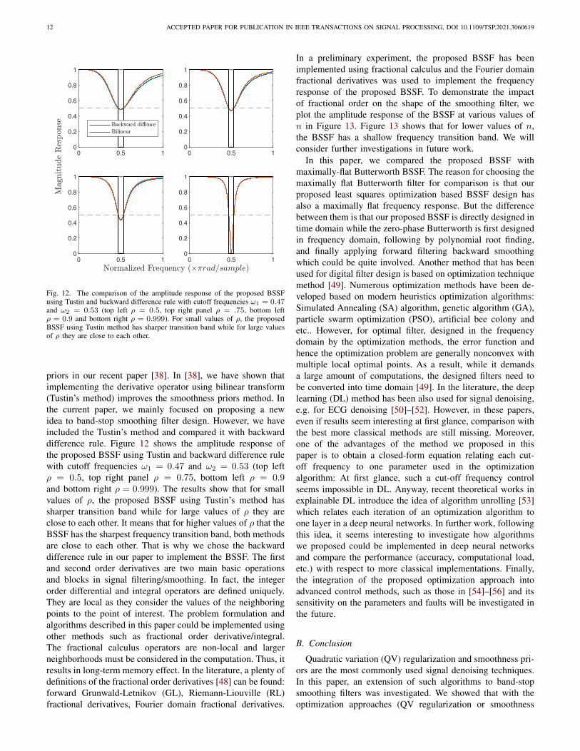
Fig. 12. The comparison of the amplitude response of the proposed BSSFusing Tustin and backward difference rule with cutoff frequencies ω1 = 0.47and ω2 = 0.53 (top left ρ = 0.5, top right panel ρ = .75, bottom leftρ = 0.9 and bottom right ρ = 0.999). For small values of ρ, the proposedBSSF using Tustin method has sharper transition band while for large valuesof ρ they are close to each other.

priors in our recent paper [38]. In [38], we have shown thatimplementing the derivative operator using bilinear transform(Tustin’s method) improves the smoothness priors method. Inthe current paper, we mainly focused on proposing a newidea to band-stop smoothing filter design. However, we haveincluded the Tustin’s method and compared it with backwarddifference rule. Figure 12 shows the amplitude response ofthe proposed BSSF using Tustin and backward difference rulewith cutoff frequencies ω1 = 0.47 and ω2 = 0.53 (top leftρ = 0.5, top right panel ρ = 0.75, bottom left ρ = 0.9and bottom right ρ = 0.999). The results show that for smallvalues of ρ, the proposed BSSF using Tustin’s method hassharper transition band while for large values of ρ they areclose to each other. It means that for higher values of ρ that theBSSF has the sharpest frequency transition band, both methodsare close to each other. That is why we chose the backwarddifference rule in our paper to implement the BSSF. The firstand second order derivatives are two main basic operationsand blocks in signal filtering/smoothing. In fact, the integerorder differential and integral operators are defined uniquely.They are local as they consider the values of the neighboringpoints to the point of interest. The problem formulation andalgorithms described in this paper could be implemented usingother methods such as fractional order derivative/integral.The fractional calculus operators are non-local and largerneighborhoods must be considered in the computation. Thus, itresults in long-term memory effect. In the literature, a plenty ofdefinitions of the fractional order derivatives [48] can be found:forward Grunwald-Letnikov (GL), Riemann-Liouville (RL)fractional derivatives, Fourier domain fractional derivatives.

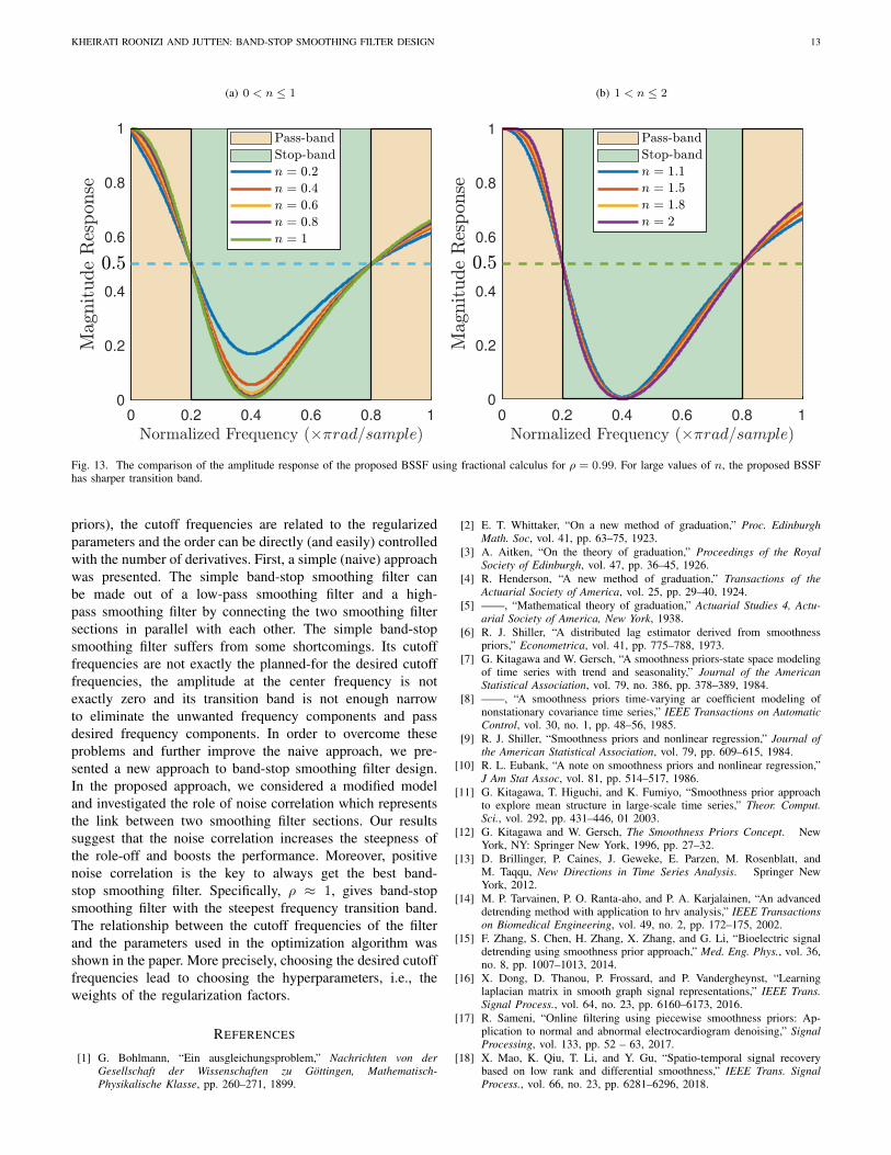
In a preliminary experiment, the proposed BSSF has beenimplemented using fractional calculus and the Fourier domainfractional derivatives was used to implement the frequencyresponse of the proposed BSSF. To demonstrate the impactof fractional order on the shape of the smoothing filter, weplot the amplitude response of the BSSF at various values ofn in Figure 13. Figure 13 shows that for lower values of n,the BSSF has a shallow frequency transition band. We willconsider further investigations in future work.

In this paper, we compared the proposed BSSF withmaximally-flat Butterworth BSSF. The reason for choosing themaximally flat Butterworth filter for comparison is that ourproposed least squares optimization based BSSF design hasalso a maximally flat frequency response. But the differencebetween them is that our proposed BSSF is directly designed intime domain while the zero-phase Butterworth is first designedin frequency domain, following by polynomial root finding,and finally applying forward filtering backward smoothingwhich could be quite involved. Another method that has beenused for digital filter design is based on optimization techniquemethod [49]. Numerous optimization methods have been de-veloped based on modern heuristics optimization algorithms:Simulated Annealing (SA) algorithm, genetic algorithm (GA),particle swarm optimization (PSO), artificial bee colony andetc.. However, for optimal filter, designed in the frequencydomain by the optimization methods, the error function andhence the optimization problem are generally nonconvex withmultiple local optimal points. As a result, while it demandsa large amount of computations, the designed filters need tobe converted into time domain [49]. In the literature, the deeplearning (DL) method has been also used for signal denoising,e.g. for ECG denoising [50]–[52]. However, in these papers,even if results seem interesting at first glance, comparison withthe best more classical methods are still missing. Moreover,one of the advantages of the method we proposed in thispaper is to obtain a closed-form equation relating each cut-off frequency to one parameter used in the optimizationalgorithm: At first glance, such a cut-off frequency controlseems impossible in DL. Anyway, recent theoretical works inexplainable DL introduce the idea of algorithm unrolling [53]which relates each iteration of an optimization algorithm toone layer in a deep neural networks. In further work, followingthis idea, it seems interesting to investigate how algorithmswe proposed could be implemented in deep neural networksand compare the performance (accuracy, computational load,etc.) with respect to more classical implementations. Finally,the integration of the proposed optimization approach intoadvanced control methods, such as those in [54]–[56] and itssensitivity on the parameters and faults will be investigated inthe future.

B. Conclusion

Quadratic variation (QV) regularization and smoothness pri-ors are the most commonly used signal denoising techniques.In this paper, an extension of such algorithms to band-stopsmoothing filters was investigated. We showed that with theoptimization approaches (QV regularization or smoothness


(a) 0 < n ≤ 1

0 0.2 0.4 0.6 0.8 1

0

0.2

0.4

0.6

0.8

1

(b) 1 < n ≤ 2

0 0.2 0.4 0.6 0.8 1

0

0.2

0.4

0.6

0.8

1

Fig. 13. The comparison of the amplitude response of the proposed BSSF using fractional calculus for ρ = 0.99. For large values of n, the proposed BSSFhas sharper transition band.

priors), the cutoff frequencies are related to the regularizedparameters and the order can be directly (and easily) controlledwith the number of derivatives. First, a simple (naive) approachwas presented. The simple band-stop smoothing filter canbe made out of a low-pass smoothing filter and a high-pass smoothing filter by connecting the two smoothing filtersections in parallel with each other. The simple band-stopsmoothing filter suffers from some shortcomings. Its cutofffrequencies are not exactly the planned-for the desired cutofffrequencies, the amplitude at the center frequency is notexactly zero and its transition band is not enough narrowto eliminate the unwanted frequency components and passdesired frequency components. In order to overcome theseproblems and further improve the naive approach, we pre-sented a new approach to band-stop smoothing filter design.In the proposed approach, we considered a modified modeland investigated the role of noise correlation which representsthe link between two smoothing filter sections. Our resultssuggest that the noise correlation increases the steepness ofthe role-off and boosts the performance. Moreover, positivenoise correlation is the key to always get the best band-stop smoothing filter. Specifically, ρ ≈ 1, gives band-stopsmoothing filter with the steepest frequency transition band.The relationship between the cutoff frequencies of the filterand the parameters used in the optimization algorithm wasshown in the paper. More precisely, choosing the desired cutofffrequencies lead to choosing the hyperparameters, i.e., theweights of the regularization factors.

REFERENCES

[1] G. Bohlmann, “Ein ausgleichungsproblem,” Nachrichten von derGesellschaft der Wissenschaften zu Gottingen, Mathematisch-Physikalische Klasse, pp. 260–271, 1899.

[2] E. T. Whittaker, “On a new method of graduation,” Proc. EdinburghMath. Soc, vol. 41, pp. 63–75, 1923.

[3] A. Aitken, “On the theory of graduation,” Proceedings of the RoyalSociety of Edinburgh, vol. 47, pp. 36–45, 1926.

[4] R. Henderson, “A new method of graduation,” Transactions of theActuarial Society of America, vol. 25, pp. 29–40, 1924.

[5] ——, “Mathematical theory of graduation,” Actuarial Studies 4, Actu-arial Society of America, New York, 1938.

[6] R. J. Shiller, “A distributed lag estimator derived from smoothnesspriors,” Econometrica, vol. 41, pp. 775–788, 1973.

[7] G. Kitagawa and W. Gersch, “A smoothness priors-state space modelingof time series with trend and seasonality,” Journal of the AmericanStatistical Association, vol. 79, no. 386, pp. 378–389, 1984.

[8] ——, “A smoothness priors time-varying ar coefficient modeling ofnonstationary covariance time series,” IEEE Transactions on AutomaticControl, vol. 30, no. 1, pp. 48–56, 1985.

[9] R. J. Shiller, “Smoothness priors and nonlinear regression,” Journal ofthe American Statistical Association, vol. 79, pp. 609–615, 1984.

[10] R. L. Eubank, “A note on smoothness priors and nonlinear regression,”J Am Stat Assoc, vol. 81, pp. 514–517, 1986.

[11] G. Kitagawa, T. Higuchi, and K. Fumiyo, “Smoothness prior approachto explore mean structure in large-scale time series,” Theor. Comput.Sci., vol. 292, pp. 431–446, 01 2003.

[12] G. Kitagawa and W. Gersch, The Smoothness Priors Concept. NewYork, NY: Springer New York, 1996, pp. 27–32.

[13] D. Brillinger, P. Caines, J. Geweke, E. Parzen, M. Rosenblatt, andM. Taqqu, New Directions in Time Series Analysis. Springer NewYork, 2012.

[14] M. P. Tarvainen, P. O. Ranta-aho, and P. A. Karjalainen, “An advanceddetrending method with application to hrv analysis,” IEEE Transactionson Biomedical Engineering, vol. 49, no. 2, pp. 172–175, 2002.

[15] F. Zhang, S. Chen, H. Zhang, X. Zhang, and G. Li, “Bioelectric signaldetrending using smoothness prior approach,” Med. Eng. Phys., vol. 36,no. 8, pp. 1007–1013, 2014.

[16] X. Dong, D. Thanou, P. Frossard, and P. Vandergheynst, “Learninglaplacian matrix in smooth graph signal representations,” IEEE Trans.Signal Process., vol. 64, no. 23, pp. 6160–6173, 2016.

[17] R. Sameni, “Online filtering using piecewise smoothness priors: Ap-plication to normal and abnormal electrocardiogram denoising,” SignalProcessing, vol. 133, pp. 52 – 63, 2017.

[18] X. Mao, K. Qiu, T. Li, and Y. Gu, “Spatio-temporal signal recoverybased on low rank and differential smoothness,” IEEE Trans. SignalProcess., vol. 66, no. 23, pp. 6281–6296, 2018.


[19] L. Xu, C. Lu, Y. Xu, and J. Jia, “Image smoothing via l0 gradientminimization,” ACM Trans. Graph., vol. 30, pp. 174:1–174:12, 2011.

[20] A. M. Thompson, J. C. Brown, J. W. Kay, and D. M. Titterington,“A study of methods of choosing the smoothing parameter in imagerestoration by regularization,” IEEE Transactions on Pattern Analysisand Machine Intelligence, vol. 13, no. 4, pp. 326–339, 1991.

[21] G. Kitagawa and W. Gersch, “A smoothness priors long ar model methodfor spectral estimation,” IEEE Transactions on Automatic Control,vol. 30, no. 1, pp. 57–65, 1985.

[22] P. H. C. Eilers and B. D. Marx, “Flexible smoothing with b-splines andpenalties,” Statistical Science, vol. 11, pp. 89 – 121, 1996.

[23] D. Terzopoulos, “Multilevel computational processes for visual surfacereconstruction,” Computer Vision, Graphics, and Image Processing,vol. 24, no. 1, pp. 52–96, 1983.

[24] W. Grimson, From Images to Surfaces: A Computational Study of theHuman Early Visual System. MIT Press, 1981.

[25] B. Horn, Robot Vision. MIT Press, 1986.[26] O. Woodford, P. Torr, I. Reid, and A. Fitzgibbon, “Global stereo recon-

struction under second-order smoothness priors,” IEEE Trans. PatternAnal. Mach. Intell., vol. 31, no. 12, pp. 2115–2128, Dec. 2009.

[27] A. Fasano and V. Villani, “Baselinewander removal for bioelectricalsignals by quadratic variation reduction,” Signal Processing, vol. 99,pp. 48–57, 2014.

[28] R. Hodrick and E. Prescott, “Postwar u.s. business cycles: An empiricalinvestigation,” JMCB, vol. 29, pp. 1–16, 1997.

[29] A. Savitzky and M. J. E. Golay, “Smoothing and differentiation of databy simplified least squares procedures.” Analytical Chemistry, vol. 36,no. 8, pp. 1627–1639, 1964.

[30] G. Golub, P. Hansen, and D. O’Leary, “Tikhonov regularization and totalleast squares,” SIAM J. Matrix Anal. Appl., vol. 21, pp. 185–194, 1999.

[31] S. Boyd and L. Vandenberghe, Convex Optimization. New York, NY,USA: Cambridge University Press, 2004.

[32] G. H. Golub, M. Heath, and G. Wahba, “Generalized cross-validation asa method for choosing a good ridge parameter,” Technometrics, vol. 21,no. 2, pp. 215–223, 1979.

[33] H. W. Engl, “Discrepancy principles for tikhonov regularization ofill-posed problems leading to optimal convergence rates,” Journal ofOptimization Theory and Applications, vol. 52, pp. 209–215, 1987.

[34] H. Akaike, “Factor analysis and AIC,” Psychometrika, vol. 52, no. 3,pp. 317–332, Sep 1987.

[35] Y. C. Eldar, “Generalized sure for exponential families: Applicationsto regularization,” IEEE Trans. Signal Process., vol. 57, pp. 471–481,2009.

[36] A. Kheirati Roonizi and C. Jutten, “Improved smoothness priors usingbilinear transform,” Signal Processing, vol. 169, p. 107381, 2020.

[37] A. Oppenheim and R. Schafer, Discrete-Time Signal Processing. Pear-son Education, 2011.

[38] A. Kheirati Roonizi and C. Jutten, “Forward-backward filtering andpenalized least-squares optimization: A unified framework,” SignalProcess., vol. 178, p. 107796, 2021.

[39] M. Unser, A. Aldroubi, and M. Eden, “Recursive regularization filters:design, properties, and applications,” IEEE Transactions on PatternAnalysis and Machine Intelligence, vol. 13, no. 3, pp. 272–277, 1991.

[40] A. Kheirati Roonizi, “A New Approach to ARMAX Signals Smoothing:Application to Variable-Q ARMA Filter Design,” IEEE Trans. SignalProcess., vol. 67, no. 17, pp. 4535–4544, 2019.

[41] S. Pei, B. Guo, and W. Lu, “Narrowband notch filter using feedbackstructure,” IEEE Signal Process. Mag., vol. 33, pp. 115–118, 2016.

[42] J. Smith, Introduction to Digital Filters: with Audio Applications. U.K.,Exeter:W3K Publishing, 2007.

[43] Chien-Cheng Tseng and Soo-Chang Pei, “Stable IIR notch filter designwith optimal pole placement,” IEEE Transactions on Signal Processing,vol. 49, no. 11, pp. 2673–2681, 2001.

[44] A. Kheirati Roonizi, “An efficient algorithm for manuvering targettracking,” IEEE Signal Process. Mag., vol. 37, pp. 122–130, 2021.

[45] G. Moody, “Spontaneous termination of atrial fibrillation: A challengefrom physionet and computers in cardiology 2004,” Computers inCardiology, vol. 31, pp. 101–104, 2004.

[46] A. Widmann, E. Schroger, and B. Maess, “Digital filter design for elec-trophysiological data – a practical approach,” Journal of NeuroscienceMethods, vol. 250, pp. 34 – 46, 2015.

[47] E. Kheirati Roonizi and R. Sassi, “A Signal Decomposition Model-Based Bayesian Framework for ECG Components Separation,” IEEETransactions on Signal Processing, vol. 64, no. 3, pp. 665–674, 2016.

[48] M. D. Ortigueira, “An introduction to the fractional continuous-timelinear systems: the 21st century systems,” IEEE Circuits and SystemsMagazine, vol. 8, no. 3, pp. 19–26, 2008.

[49] “Design of digital IIR filter: A research survey,” Applied Acoustics, vol.172, p. 107669, 2021.

[50] C. T. C. Arsene, R. Hankins, and H. Yin, “Deep learning modelsfor denoising ecg signals,” in 2019 27th European Signal ProcessingConference (EUSIPCO), 2019, pp. 1–5.

[51] V. Ravichandran, B. Murugesan, S. M. Shankaranarayana, K. Ram, P. S.P, J. Joseph, and M. Sivaprakasam, “Deep network for capacitive ECGdenoising,” CoRR, vol. abs/1903.12536, 2019.

[52] H. Chiang, Y. Hsieh, S. Fu, K. Hung, Y. Tsao, and S. Chien, “Noise re-duction in ecg signals using fully convolutional denoising autoencoders,”IEEE Access, vol. 7, pp. 60 806–60 813, 2019.

[53] V. Monga, Y. Li, and Y. C. Eldar, “Algorithm unrolling: Interpretable,efficient deep learning for signal and image processing,” To be appearedin IEEE Signal Processing Magazine, 2021.

[54] K. Sun, L. Liu, J. Qiu, and G. Feng, “Fuzzy adaptive finite-time fault-tolerant control for strict-feedback nonlinear systems,” IEEE Transac-tions on Fuzzy Systems, pp. 1–1, 2020.

[55] S. K., Q. Jianbin, H. R. Karimi, and Y. Fu, “Event-triggered robustfuzzy adaptive finite-time control of nonlinear systems with prescribedperformance,” IEEE Transactions on Fuzzy Systems, pp. 1–1, 2020.

[56] K. Sun, J. Qiu, H. R. Karimi, and H. Gao, “A novel finite-time controlfor nonstrict feedback saturated nonlinear systems with tracking errorconstraint,” IEEE Transactions on Systems, Man, and Cybernetics:Systems, pp. 1–12, 2019.

Arman Kheirati Roonizi received the Ph.D. de-gree in computer science from University of Mi-lan, Italy, in 2017. After graduating, he workedas Postdoctoral Researcher with GIPSA-lab at theUniversite Grenoble Alpes, France. Since February2018, he is an Assistant Professor at Fasa Uni-versity, Iran. His research interests include signalmodeling/decomposition, filtering and processing,cardiac modeling and simulation, multimodal signalprocessing and functional data analysis.

Christian Jutten (AM’92-M’03-SM’06-F’08) re-ceived Ph.D. (1981) and Doctor es Sciences (1987)degrees from Grenoble Institute of Technology,France. He was Associate Professor (1982-1989),Professor (1989-2019), and is Professor Emeritussince September 2019 at University Grenoble Alpes.Since 1980’s, his research interests are in machinelearning and source separation, including theoryand applications (brain and hyperspectral imaging,chemical sensing, speech). He is author/co-author offour books, 110+ papers in international journals and

250+ publications in international conferences. He is a fellow of the IEEE andEURASIP. He was a visiting professor at EPFL (Switzerland, 1989), RIKENlabs (Japan, 1999) and University of Campinas (Brazil, 2010). He servedas the head of the signal/image processing laboratory, scientific advisor forsignal/image processing at the French Ministry of Research (1996–1998) andCNRS (2003–2006 and 2012-2019). He was organizer or program chair ofmany international conferences, including the first Independent ComponentAnalysis Conference in 1999 and IEEE MLSP 2009. He was the technicalprogram co-chair ICASSP 2020. He was a member of the IEEE MLSP andSPTM Technical Committees. He was associate editor in Signal Processingand IEEE Trans. on Circuits and Systems, and guest co-editor for IEEE SignalProcessing Magazine (2014) and the Proceedings of the IEEE (2015). He hasbeen a Senior Member of Institut Universitaire de France since 2008, andthe recipient of the 2012 ERC Advanced Grant for the project Challenges inExtraction and Separation of Sources (CHESS). He received many awards, e.g.Best Paper Awards of EURASIP in 1992 and IEEE GRSS in 2012, MedalBlondel in 1997 from the French Electrical Engineering Society, and oneGrand Prix of the French Academie des Sciences in 2016. Since January2021, he is the editor-in-chief of IEEE Signal Processing Magazine.

band-stop smoothing filter design - archive ouverte hal

Documents