bachelor essay - diva portal

Bachelor Essay

How does municipality tax impact on net regional

mobility in Sweden?

Author: Björn Uddgård

Supervisor: Jonas Månsson

Examiner: Dominique Anxo

Semester: Spring-18

Subject: Bachelor essay

Course code: 2NA11E

of 32

Abstract

The primary objective of this essay is to test how the municipality tax rate affects net regional

migration in Sweden. All the 290 municipalities where included between the years 2008 to

2016. The relationship is estimated by panel data using a fixed effect model. The main

findings of this study suggest that there is no correlation between municipality tax rate and net

regional migration, ceteris paribus. The result is partly in line with theory and shows slightly

different finding than Edmark and Ågren (2008).

of 32

Table of content

1. Introduction 3

2. Theory 5

2.1 Horizontal tax competition 7

2.2 Resource-flow model 8

3. Literature review 9

4. Contextual aspects: The Swedish governmental structure 12

5. Data 12

5.1 Model 13

5.2 Data description 16

5.3 Method 18

6. Results 19

7. Conclusion 22

References 23

Appendix A, Correlation and the Hausman test 26

Appendix B, Robustness analysis 29

of 32

1. Introduction

”A central message of the tax competition literature is that

independent governments engage in wasteful competition for

scarce capital through reductions in tax rates and public

expenditure levels”

– Wilson (1999, p.269)

With a more open market amongst countries an increase in mobility between nations has

occurred. The focus has shifted towards how different nations organise and supply their welfare

and taxation, based on a mobile tax base. Higher education and better language skills amongst

individuals are two examples of why international mobility of labour has increased over the last

years. Within the European Union the mobility has greatly increased since the implementation

of the Schengen agreement. How should countries react to this new mobility between regions?

(Osmundsen et. al., 2000, p. 623)

According to Osmundsen et al. (2000) this kind of question might be new at a national level,

but it has been addressed earlier. Many of the problems now faced at the national level regarding

a mobile workforce have been addressed by municipalities for some time. Municipalities have

designed their welfare programs and level of taxation taking into account possible migration

between regions. However, the migrants could move back to the original region at any point

for example depending on taxes, welfare or carrier opportunities. According to Osmundsen et

al. (2000) this puts pressure on local governments to design their taxation and welfare systems

in an appropriate way.

Wilson (1999) also considers the mobility of the tax base as a common factor for different local

governments. According to Wilson (1999) municipalities decides on their tax rate and subsidies

so that the local residents will maximise their welfare. These choices and policies affects the

size of the tax base within the different regions. The tax bases often consist of mobile labour

and capital, hence the difference in its size depends on political choices and decisions.

Just like there is a theory about how supply and demand for households and firms predicts

behaviour on an open competitive market, Wildasin and Wilson (1996) argues that there is a

need for a predictable behaviour, or a theory, that explains how local municipality governments

of 32

will make their decisions. The decisions the authors concern the level of the local government’s

expenditures and tax rate as well as the overall efficiency versus equity properties.

According to Lipatov and Weichenrieder (2015), the world has become more globalized and

with this globalization it has become easier to move between countries. With the increase of

the open boarders the mobility of resources, such as people and goods, has also increased.

Hindriks (1999) and Wildasin and Wilson (1996) reflects over the question if the local

governments have the capacity to handle redistribution of the welfare without just attracting

low-skilled individuals and by doing so drive away the high-skilled. According to Hindriks

(1999) the local government have to take this possibility into consideration when they decide

on which factors, tax or transfer, to compete with. Depending on which one of the factors that

were chosen, an adjustment has to be made for the risk of only attracting low skilled individuals.

Due to more open regions on a national level, entering EU for example, and with no cost for

moving between municipalities within Sweden, the competition for able workers will tighten.

Which leads to that the municipalities have to compete amongst each other for that specific

resource. The municipalities could adjust the tax rate trying to influence individuals to move to

the given municipality. Hence, the level of taxation is one way for the municipality to influence

the migration patterns of individuals. There are numerous other reasons why individuals chose

to move between regions, such as job opportunities, living with friends and family or to live

with individuals of the same ethnic background. Since it is important for the local government

to know to what extent the tax rate influences the migration, the purpose with this essay will be

to estimate the effects a change in regional/municipal taxation will have on the net regional

migration.

The research question for this essay is:

How does municipality tax impact on net regional mobility in Sweden?

The essay is structured as follows. Section 1 introduces the subject at hand, followed by theories

in section 2. Section 3 presents what previous research has concluded. The framework for the

Swedish government system is covered in section 4. In section 5 the model, method and which

data that has been included is presented. Section 6 presents the results from the regressions in

addition to a discussion about the result. Conclusions are presented in section 7.

of 32

2. Theory

A theoretical model often used when addressing migration is the push-pull model (Schoorl et

al., 2000). In its most simple form this model consists of some negative and positive factors

influencing individual’s decisions regarding migration. The negative factors (push) and the

positive factors (pull) works in combination with each other. The size of respective factor will

determine the flow and magnitude of the migration. The push factors includes for example lack

of job opportunities and not being allowed to express religious and/or political point of view in

the poorer regions. In contrast to the pull factors which include the advantages existing in the

richer regions, better infrastructure, services and welfare system for example.

Early theories about migration used the framework of supply and demand with the wage as the

main driving force behind migration, acting both as pull and push factors. According to Hicks

(1932) the wages were the major argument for individual’s different preferences. These

preferences were based on individual’s different reservation wages, implying that the level of

income was the main argument for migration. In other words, the wages would respond to the

fluctuations of demand and supply over different regions and thus create migration.

Sjaastad (1962) expanded Hicks (1932) theory by including investments in human capital as

another source of influence for migration. This expanded model took into consideration that an

individual would make assessment of the future benefits and costs of migration (both monetary

and psychologically). The individual makes these “calculations” for all potential regions and

will migrate to the region with the highest net outcome.

In addition Sjaastad (1962) includes uncertainties and attitudes towards risk into the model.

This implies that it is more to the decision than reservation wage and job opportunities,

suggesting that mobility rate would differ between individuals as well as between groups.

Elderly individuals, for example, might be less prone to move since they have a shorter time

horizon from which they can benefit from potential better living conditions existing in the new

region.

According to Molho (2013) there is an important distinction to be made when addressing

migration, the distinction between different types of migrants. Molho (2013) mentions two

types of migration, ‘speculative migration’ and ‘contracted migration’. The first of the two

undertakes more of a leap of faith to find an opportunity, such as a job, after the migration has

taken place, making migration a part of the search process. The latter assumes that the individual

already have acquired an opportunity before moving.

of 32

The municipalities’ borders are not closed for migration. The residents are free to move between

them without any costs. Osmundsen et al. (2000) argue that where individuals chose to reside

could change over time as individuals’ preferences changes. These changes along with different

political policies are affecting individuals differently throughout the lifespan. The authors argue

that the individual’s utility maximisation problems are to be solved by municipalities to attract

more residents. According to Osmundsen et al. (2000) the way that municipalities solve this

problem is to put different weights on individuals, depending on if they are believed to be a

stayer or mover. Osmundsen et al. (2000) also discuss how redistribution, on a national level,

could be positive for municipalities which are receiving low income from taxation. Such a

redistribution could allow these municipalities to maintain a higher level of welfare in their

region, even after a decrease in the tax base has occurred.

According to Lipatov and Weichenrieder (2015) it is only rich individuals who have the

possibility to gain from the tax competition, by moving between regions. The risk associated

with the downward pressure on taxation is that it could push the level below the optimal efficacy

point. It could be seen as a compromise for the effects on the size of the government, putting a

stop to possible wastefulness. This regulation of political policies is called yardstick

competition and Edmark and Ågren (2008) argues that this kind of tax competition would

probably be more widespread during election years as well as when the political majority is

weak.

Hindriks (1999) used a game theoretical approach and considered two different strategic

variables during competition; tax and transfers. Based on the variables the author derives three

different Nash equilibriums, firstly only the tax rate, secondly only the transfers and thirdly

both tax rate and transfers. The author found that both variables had an impact on individual’s

decision to move or to stay. According to Hindriks (1999) it could be hard to differ the two

because only the stronger of the two effects would show and thus be the more realistic of the

two.

Hindriks (1999) way of arguing is consistent with a so called horizontal tax externality, there

also exists a vertical tax externality. The vertical externality arises from the interaction between

different levels of government within a country. In Sweden for example, it would be between

the municipality and the state. Moreover, the horizontal tax externalities take place amongst

different governments on the same level, i.e. between different municipalities (Wilson, 1999).

of 32

This essay will take into account the latter of the two externalities, i.e. that the tax competition

between municipalities will affect the individual’s incentive to migrate.

An extension of Hindriks (1999) is done by Dahlberg and Edmark (2008) who also consider

how municipalities would decide to what level they should set their welfare benefits. The

authors found that the level of welfare in one municipality was affected by the level of its

neighbouring municipalities’ welfare levels. This would imply, from a mobility point of view,

that the welfare level could also affect individual’s decisions to move or not to move.

2.1 Horizontal tax competition

The horizontal tax competition is a fiscal externality which arises from tax and expenditure

competition between regions, also called the spill-over model. The fiscal decisions for one

region to achieve an objective, and in the process affects other regions. A change in taxation to

attract residents from another municipality trying to expand their own tax base, or a cut in the

welfare to encourage the poor individuals to move to other regions, are example of such

decisions. The horizontal tax competition could be positive or negative for the region, thus

giving the local government an incentive to try to influence the outcome of the competition. By

doing so the municipalities are interfering with the resource allocation across the nation, hence

it could create an inefficiency in the nation’s resource allocation (Broadway, 2001, p.96).

Wilson (1999) argues that this unhealthy tax competition between municipalities occur when

interregional externalities exists. This phenomenon is called “fiscal externality” and arises

when the decision in one region affects the budget of another region. For example a decrease

in tax rate in one region could affect the second regions budget by a decrease in their tax base,

due to migration between the two regions. In other words, when one region acts to improve its

welfare the process leads to a decline in welfare in another region (Wilson, 1999, p. 272).

According to Wilson (1999), an adequate allocation of resources nationwide, cannot be

achieved as long as there are different taxation levels throughout the different municipalities.

A central government can achieve an effective redistribution of resources by demanding some

tax revenue from each region and reallocate the revenue. The most efficient way would be

through a lump-sum transfer to each region, size depending on the marginal benefit and

marginal cost for each region. An identical tax level for all regions would be another solution

to the problem. However, this would not take into account the different costs occurring when

producing different level of public goods/services (Wilson, 1999, p. 276).

of 32

2.2 Resource-flow model

The resource-flow model is another way of explaining mobility between regions. This model

tries to capture the indirect effects a region experience due to a result of other regions’ decisions

(Brueckner, 2003, pp.178-181).

Following Brueckner (2003), the objective function for region i is written as follows.

V (zi, si; Xi) (1)

Where zi is the decision variable, here the tax rate, for the municipality i. The Xi captures

municipality specific characteristics and the si is the level of resources within municipality i.

The si could be rewritten as shown below.

si = H (zi, z-i; Xi) (2)

si is a function of the tax rate in the municipality, zi, as well as the tax rate for the other

municipalities, z-i. The resource-flow model affects indirectly by the level of resources the

municipality has, which in turn is affected by the level of other municipality’s tax rate. This in

contrast to the horizontal tax competition which directly affects the municipalities. Inserting (2)

into (1) gives:

V [zi, H (zi, z-i; Xi); Xi)] ≡ V1 (zi, z-i; Xi) (3)

Equation (3) implies that the optimal tax rate for municipality i indirectly will be influenced by

neighbouring municipalities’ tax rate and Xi. Following this the municipality will maximise the

function.

V1 = Vzi + Vsi(dsi/dzi) = 0 (4)

Maximising of equation (4) for municipality i could be written as a reaction function as follow:

zi = R(t-i; Xi) (5)

The function R represents the best response a municipality could chose, given other

municipalities chosen tax rate and its own characteristics. Brueckner (2003) argues that the sign

of the response function is silent, meaning that we do not know which sign it will take. But

municipality i has to adjust a positive or a negative sign, depending on the preferences of

municipality i. If the municipality i do not adjust to neighbouring municipalities the risk of

of 32

losing tax base and/or capital will increase and by doing so putting the municipality i into a

possible worse situation than if an adjustment was made.

3. Literature review

Osmundsen et al. (2000) uses a theoretical model based on a utility function expressed in

monetary terms. The time spent in the home region is denoted t and time spent in other regions

is denoted (1-t) =T in addition the mobility of an individual is not known to the government.

Therefore, according to the authors the taxation can only be on individual income or time spent

in the region. Ɵ denotes the mobility for an individual and can take either a low (Ɵ) or a high

(Ɵ̅) value. Osmundsen et al. (2000) uses this mobility variable as an index of how individuals

values local goods/services as well as a preference for a specific region. The model is used as

follows:

u = z(t) – r + Y(T) + φ( t, T, Ɵ)

z(t) is the gross local income, r local tax rate, Y(T) is after tax income from other regions and φ

is the utility gained from time spent in a region. The two kinds of income are separated due to

that income from another region cannot be taxed in the home region. According to Osmundsen

et al. (2000) the utility gained from time spent in a specific region could be due to infrastructure,

culture or unharmed scenery, based on the individual’s preferences.

The authors assume that individuals compare taxes and public goods/services when distributing

time between different regions. Osmundsen et al. (2000) reaches the conclusion that optimal

taxation regarding mobile labour between regions, assuming that information of mobility is

private, could be negative, zero or positive. It is the welfare weights assigned by mobile

individuals that decide what sign it will be.

Lipatov and Weichenrieder (2015) used a pareto optimal taxation model. Into this model the

authors introduces a flexible objective function for the government, allowing for various

welfare preferences. For the closed economy the model gives the following function:

u (x, y), where x ≥ 0 for consumption and 0 ≤ y ≤ 1 for time worked.

For the open economy Lipatov and Weichenrieder (2015) assumes that high productive

individuals might migrate between regions to improve life-quality. The low productive

of 32

individuals are immobile in this scenario. The assumption changes the utility function for the

high productive individuals to include a migration cost for a region p, c (p).

u(x, y) – c (p), where c is strictly increasing.

According to Lipatov and Weichenrieder (2015), the government would enact and perfect

information tax onto the mobile individual to keep them from migrating. This governmental

behaviour was excluded from the research, by the authors, due to that most countries have some

kind of antidiscrimination laws.

Lipatov and Weichenrieder (2015) conclude that tax competition will restrict the wastefulness

of the government, but at the same time limits the redistribution. Hence, the effect from welfare

significantly depends on the redistribution preferences amongst the population and the

redistribution ability of the government.

Research on tax competition in Sweden has been conducted by Edmark and Ågren (2008). The

authors use panel data in a fixed effect model to identify the strategic interaction in local income

tax. The variables used by Edmark and Ågren (2008) in the regression are the unemployment

rate, the proportion of young and old individuals, population size and the share of the

population on welfare for the municipalities. Edmark and Ågren (2008) concluded that weak

evidence exists supporting that there is a correlation between taxes amongst different Swedish

local governments. Also that it can be explained by incentives to attract the mobile tax base.

But Edmark and Ågren (2008) did not find any indication that this pattern would change during

election years.

Hindriks (1999) minimal model contains two symmetric regions and a single private good.

Within these regions a large number of individuals exists who differ both in regional

preferences and income. A number of the individuals are poor (income set to 0) and some are

rich (income set to 1). Hindriks (1999) describes the preferences for a region by a taste

parameter, which is uniformly distributed in both groups (rich and poor). The two regions both

impose a per capita tax and pays a per capita transfer. The regions have to balance their budgets

and the individuals are free to move to the region that maximises the individual’s utility

function, given by:

z = (T, B), for home region

z* = (T*, B*), for other region.

of 32

The author applies the tax and transfer variables in different Nash equilibriums, depending on

what variable the regions compete with.

Hindriks (1999) concludes that the level of redistribution is depending on whether the region

compete with tax, transfers or tax and transfers. According to the author the competition with

transfers would be tougher for the region since it could attract poor individuals. Hindriks (1999)

also concludes that the mobility amongst rich individuals are harmful to the redistribution, when

competing with taxes. The author shows that when the regions compete with both tax and

transfers the equilibrium will be higher than pure tax competition and lower than a transfer

competition.

With a similar theory as Hindriks (1999), Dahlberg and Edmark (2008) researched if the local

governments take into consideration the levels of their neighbour’s welfare when they set their

own level of benefits, in Sweden. Dahlberg and Edmark (2008) used refugee placements as

exogenous variable for their research. To estimate the migration effect Dahlberg and Edmark

(2008) used a two stage OLS model with fixed effects. The explanatory variables included in

the model were benefit level, unemployment, tax base, grants (government equilibration grant),

the population (age 19-29), vacant rentals and refugees. They found a positive, significant,

effect from the welfare benefit levels of neighbouring municipalities on the decision for a given

municipality’s benefit levels. Dahlberg and Edmark (2008) concluded that this indicates that

there is a strategic interaction amongst the municipalities, when setting the welfare level.

of 32

4. Contextual aspects: The Swedish governmental structure

There are three levels of governance in Sweden: the state, the county councils and the

municipalities. For all three levels the income taxation is a large source of income. In this paper

the income taxation for the state will not be addressed since it is not relevant for the tax

competition models amongst municipalities. Sweden is divided into 21 counties and every

county is run by a county council. The main responsibility for the counties is the public health

care system which stands for about 80 percent of their expenditures. Members in the council

are elected every fourth year in a public election, at the same time as election for state and

municipality governments are elected. Sweden consist of 290 municipalities, which have the

responsibility to maintain and develop local schools, eldercare, roads, and the provision of

water, sanitation as well as energy issues (Regeringskansliet, 2017).

Swedish municipalities receive redistributive equilibration grants from the state (Sveriges

kommuner och landsting, 2017). According to Osmundsen et al. (2000) this kind of

redistribution is a form of resource reallocation nationwide, as mentioned earlier in this paper.

The municipalities receive three different types of re-distributional grants, income, cost and

structural. The first two are a pure redistribution between the municipalities. A municipality

with a higher income will transfer, through the state, a portion of their income to a less well-off

municipality. The last grant is purely a monetary income received from the state to the

municipality which for example, have a small population and thus could risk a lower level of

welfare (Sveriges kommuner och landsting, 2017).

5. Data

The data are collected from SCB (Statistic Sweden), Arbetsförmedlingen (Swedish Public

Employment Service) and Socialstyrelsen (The National Board of Health and Welfare). The

data set consists of yearly data covering all municipalities for a time period of 9 years (2008-

2016). The balanced panel data have 290x9 = 2610 observations. To identify neighbours to

the different municipalities a land connection between the municipalities have been used as

the main argument. Since Gotland has no neighbours connected by land, the neighbours have

been identified as the municipalities from which individuals can take the ferry to Gotland1.

1 The municipalities are Nynäshamn, Oskarshamn and Västervik.

of 32

5.1 Model

The dependent variable for the analysis is the net migration within Sweden (Net migi,t) for

municipality i, in time t, between 2008 to 20162

The main independent variable in the analysis is taxation in municipality i (Ti,t). According to

Edmark and Ågren (2008) there is a weak correlation between taxes in the different

municipalities in Sweden. This weak correlation could be explained by the incentives to attract

migrants. In accordance with the incentive found by Edmark and Ågren (2008), Osmundsen et

al. (2000) argues that the municipalities have to solve the utility maximisation problem for the

inhabitants. The solution for this problem aims to attract more migrants to the region and by

doing so expanding regional tax base. That is why the impact on net migration will depend on

how protective the inhabitants in the region are for their welfare, it could be both positive and

negative.

The average neighbouring municipalities’ tax rate (Σj≠iWijTjt) is part of the regression to capture

the effects of tax competition. According to Broadway (2001) the tax competition could affect

the region both positive and negative. Hence, giving the local government an incentive to try to

influence the outcome of this competition. This will be due to the spill-over model as well as

the resource-flow model, which gives an uncertainty on the affect it will have on the net

migration.

Unemployment rate (Unemp.i,t) for a given municipality during time period t. This variable

contains individuals who are openly unemployed and those individuals who are in some kind

of unemployment activation program. According to Molho (2013) migration consists of two

types of migrants, “speculative” and “contracted”. An unemployed individual might be more

of a speculative migrant having more to gain from moving than staying. In addition, Sjaastad

(1962) argues that individuals calculate the benefits and costs for migration before moving

implies that unemployment will have a positive impact on net migration.

Average income in a municipality (Incomei,t) is used to indicate if a municipality is wealthy or

poor. Lipatov and Weichenrieder (2015) argues that it is to a greater extent rich individuals that

2 The migration into and out of Sweden could also be included into this net migration. But including that into the

variable would force the research to take into account the tax competition between nations. This is not the

objective for this paper to address that issue, hence the net migration is limited to within Sweden

of 32

takes advantage of tax competition, due to of the possibility of moving. Therefore, Income is

expected to correlate positively with net migration.

Grant (Granti,t) represent the governmental equilibration grant every municipality receives to

maintain the same level of welfare across the nation. According to Wilson (1999) the fiscal

externality of tax competition hinders an effective allocation of resources nationwide. Hence,

arguing that this could be corrected by a central government who redistribute some of the

municipalities’ income. In Sweden the central government use this way of trying to correct the

misallocation of resources and therefore it is expected that Grant will correlate positively with

net migration.

House prices (House pricei,t) is the average price of houses sold during the time period t.

According to Sjaastad (1962) the individual calculates the costs and benefits of the migration

and the supply and demand in different municipalities affects the house prices. A more

attractive municipality will have higher prices on houses than a municipality where no one

wants to live, higher demand than supply. Buying a house is also often seen as an investment

and the buyer want some rent on this investment. Therefore, a region where the prices increases

would attract more buyers. The causality between the two factors are hard to differ, but both

drives the house price up. With the same frame of costs and benefits, the house price could

work as a deterrent. That is because individuals might not be able to afford to buy a house in

the given municipality as well as being an unpopular region. This means that depending on

which one of the forces is the stronger one House prices could give either a negative or a

positive correlation to the net migration.

Neighbouring municipalities’ average unemployment (Σj≠iWijUnempljt) is included to

investigate if the unemployment in neighbouring municipalities affects the net migration for a

given municipality. According to Sjaastad (1962) different individuals, as well as groups of

individuals, has different mobility rates. That is, individuals who are unemployed have a higher

mobility rate since this group have more to gain from moving than employed individuals.

Therefore, it is expected that Neighbouring municipalities’ average unemployment will have a

positive impact on the net migration for the given municipality.

Welfare is the total monetary cost for welfare benefits in a given municipality. Dahlberg and

Edmark (2008) conclude that there is a strategic interaction between the municipalities when

the level of welfare are decided upon. This implies that the job situation in the municipality

of 32

could be hard and the number of individuals on welfare benefits would work as a deterrent for

migrants. Therefore welfare is expected to be negatively correlated with net migration.

The model to be estimated is summarised as follows:

Net migi,t = β0 + β2 Ti,t +αΣj≠iWijTjt + β3 Unemp.i,t + β4 Incomei,t + β5 Granti,t + β6 House pricei,t

+ α2Σj≠iWijUnempljt +welfarei,t + δTt + γSi + εi,t

Net migi,t = the difference in numbers of individuals moving into and out of the

municipality i at time t, net migration.

Ti,t = gives the tax rate in municipality i at time period t.

Σj≠iWijTjt = will give the average tax rate for the municipalities describe as neighbours

to municipality i at time period t.

Unemp.i,t = the unemployment rate in municipality i at time period t.

Incomei,t = gives the average income per capita in thousands of Swedish kronor (SEK)

in municipality i at time period t.

Granti,t = gives the grant received from the state in thousands of Swedish kronor

(SEK) in municipality i at time period t.

House price = gives the average house prices in thousands of Swedish kronor (SEK) in

municipality i at time period t.

Σj≠iWijUnempljt = the average unemployment rate in percent for the municipalities

describe as neighbours to municipality i at time period t.

welfarei,t = total monetary cost for welfare benefits in municipality i at time period t.

Tt = reflects the time specific effects which affects all the municipalities in the same

way, in this case inflation.

Si = will give the municipality specific factor, such as culture.

εi,t = the error term for municipality i in time period t.

of 32

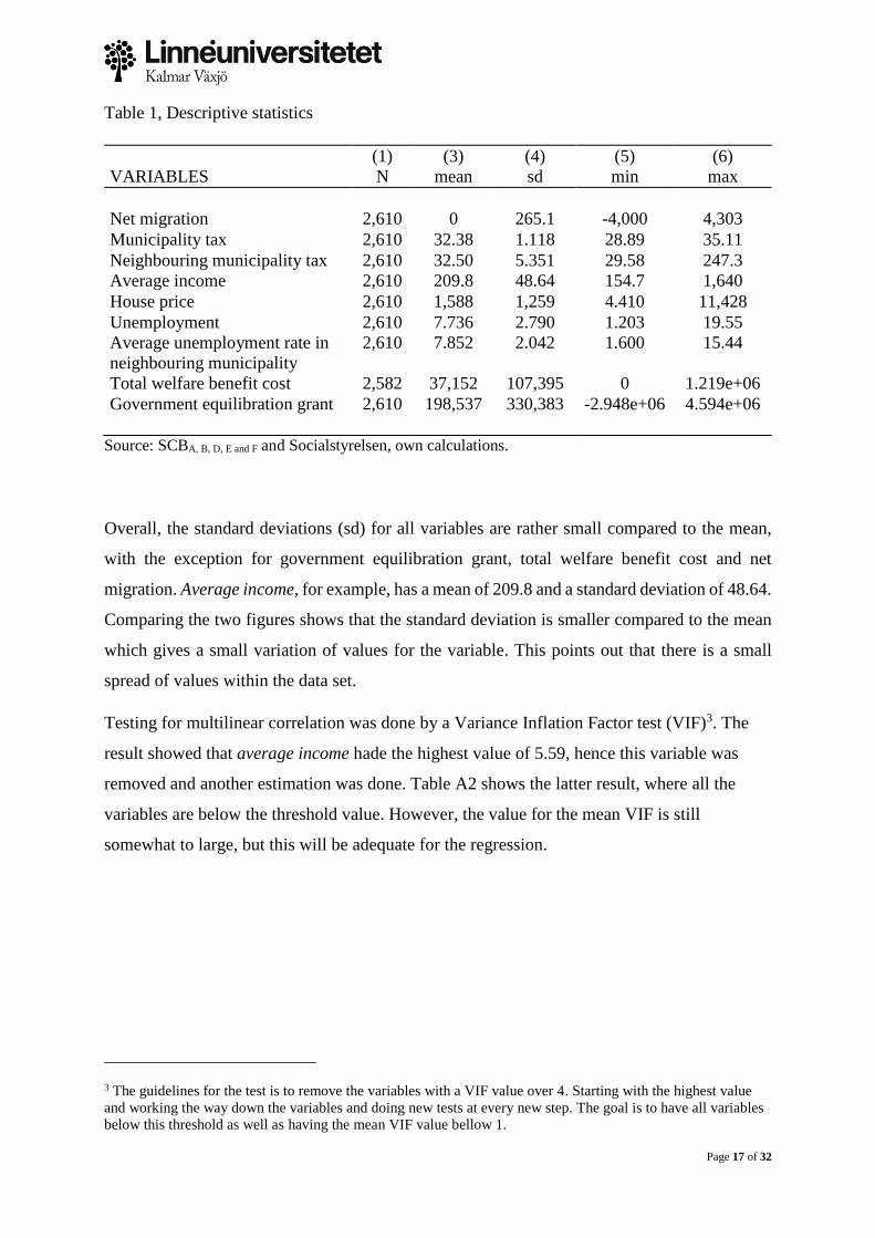
5.2 Data description

Table 1 displays some statistic descriptive for the data used in the regression analysis. As shown

by Table 1 all but one of the variables has 2610 (N) observations. The total monetary cost for

welfare benefits only have 2582 observations, due to missing values caused by inadequate

routines regarding documentation and reporting (Socialstyrelsen, 2018).

As shown by table1 the mean for net migration is zero, this is due to that in the research only

migration within Sweden is accounted for. This implies that there are no individuals entering

or exiting the country and thus the mean for migration is zero. Comparing the two tax variables,

municipality tax and neighbouring municipality tax, there is a standard deviation of 1.118 for

the given municipality specific tax and 5.351 for the neighbouring municipalities taxation. The

higher value for the neighbouring municipalities could be explained by that it is a somewhat

aggregated value. The average income has the largest mean amongst the variables and with a

small standard deviation it implies that the variation of the values for the variable are rather

small. The house price variable is measured in thousands of Swedish kronor (SEK) and with

this in mind table 1 shows that the average house price in Sweden for the time period, 2008-

2016, was 1,588,000 Swedish kronor. The mean for unemployment is 7.7 percent, meaning that

over all observations this is the average unemployment rate. Shown in table 1, the neighbouring

municipalities has a somewhat larger average unemployment then for the given municipality,

7.8 percent. This could be due to the same reason as for the difference between the tax rates.

The minimum for total welfare benefit cost is zero, could be due to the missing values.

Otherwise it would be highly unlikely that a municipality would have zero costs for the welfare

benefits. As for the government equilibration grant the minimum is negative, shown in table 1.

This supports that a resource reallocation between the municipalities have is occurring, where

some municipalities have to pay some of their tax revenue to the state for reallocation to other

municipalities.

of 32

Table 1, Descriptive statistics

(1) (3) (4) (5) (6)

VARIABLES N mean sd min max

Net migration 2,610 0 265.1 -4,000 4,303

Municipality tax 2,610 32.38 1.118 28.89 35.11

Neighbouring municipality tax 2,610 32.50 5.351 29.58 247.3

Average income 2,610 209.8 48.64 154.7 1,640

House price 2,610 1,588 1,259 4.410 11,428

Unemployment 2,610 7.736 2.790 1.203 19.55

Average unemployment rate in

neighbouring municipality

2,610 7.852 2.042 1.600 15.44

Total welfare benefit cost 2,582 37,152 107,395 0 1.219e+06

Government equilibration grant 2,610 198,537 330,383 -2.948e+06 4.594e+06

Source: SCBA, B, D, E and F and Socialstyrelsen, own calculations.

Overall, the standard deviations (sd) for all variables are rather small compared to the mean,

with the exception for government equilibration grant, total welfare benefit cost and net

migration. Average income, for example, has a mean of 209.8 and a standard deviation of 48.64.

Comparing the two figures shows that the standard deviation is smaller compared to the mean

which gives a small variation of values for the variable. This points out that there is a small

spread of values within the data set.

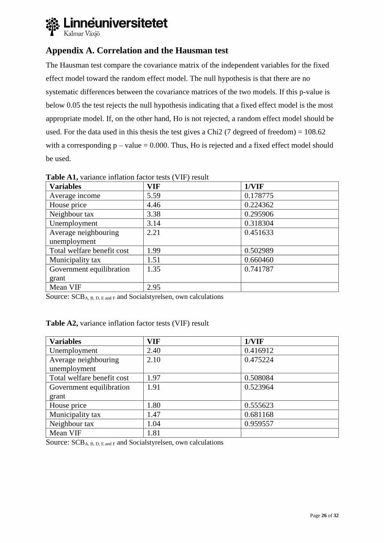
Testing for multilinear correlation was done by a Variance Inflation Factor test (VIF)3. The

result showed that average income hade the highest value of 5.59, hence this variable was

removed and another estimation was done. Table A2 shows the latter result, where all the

variables are below the threshold value. However, the value for the mean VIF is still

somewhat to large, but this will be adequate for the regression.

3 The guidelines for the test is to remove the variables with a VIF value over 4. Starting with the highest value

and working the way down the variables and doing new tests at every new step. The goal is to have all variables

below this threshold as well as having the mean VIF value bellow 1.

of 32

5.3 Method

The choice of using panel data instead of a cross section or a pure time series regression was

made because panel data gives the possibility for a more dynamics adjustment of the study. The

panel data allows for controlling for individual heterogeneity, whereas cross section and time

series studies do not control for such heterogeneity which in turn risks obtaining a biased result

(Baltagi, 2013, pp.6-7).

The first step when using panel data models is to decide if a fixed or random effect model is the

most appropriate. To do so a Hausman test is performed. 4,5 The test suggests that a fixed effect

model should be used.

Following the test two regressions will be done. The first model will contain the municipality

tax rate as variable in addition to the area and yearly fixed effects. The second model contains,

in addition to model 1, the neighbouring municipalities’ average tax rate, the unemployment,

neighbouring municipalities’ average unemployment, house prices and average income as

variables, in addition to the welfare variables total monetary welfare benefit cost and

government equilibration grant.

The fixed effect model was used and for the municipality specific effect we used an area

approach. For the time specific effect the yearly inflation was used, since it affects all the

municipalities in the same way.

The outcome of the three different regressions will be interpreted focusing on which variables

have an effect on the net regional migration. The interpretation will also show if this effect

changes between the different regressions.

4 The Hausman test examines the differences between the random effects model and fixed effect model. The null

hypothesis that no correlation exists between the explanatory variables and the error term (Hill et al., 2011,

p.420). If correlation exists the null hypothesis becomes rejected and the random effect model will produce a

bias estimate and violate one of the Gauss-Markov assumptions of unbiased estimator 5 The test results are reported in the appendix A

of 32

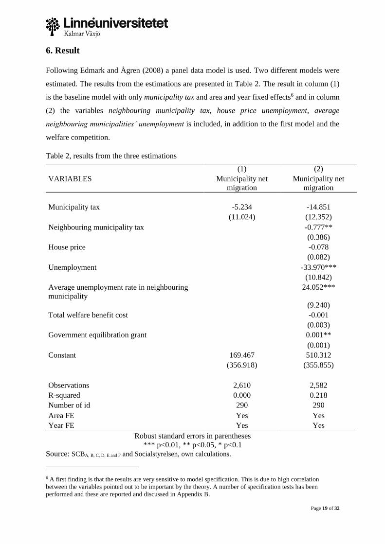
6. Result

Following Edmark and Ågren (2008) a panel data model is used. Two different models were

estimated. The results from the estimations are presented in Table 2. The result in column (1)

is the baseline model with only municipality tax and area and year fixed effects6 and in column

(2) the variables neighbouring municipality tax, house price unemployment, average

neighbouring municipalities’ unemployment is included, in addition to the first model and the

welfare competition.

Table 2, results from the three estimations

Robust standard errors in parentheses

*** p<0.01, ** p<0.05, * p<0.1

Source: SCBA, B, C, D, E and F and Socialstyrelsen, own calculations.

6 A first finding is that the results are very sensitive to model specification. This is due to high correlation

between the variables pointed out to be important by the theory. A number of specification tests has been

performed and these are reported and discussed in Appendix B.

(1) (2)

VARIABLES Municipality net

migration

Municipality net

migration

Municipality tax -5.234 -14.851

(11.024) (12.352)

Neighbouring municipality tax -0.777**

(0.386)

House price -0.078

(0.082)

Unemployment -33.970***

(10.842)

Average unemployment rate in neighbouring

municipality

24.052***

(9.240)

Total welfare benefit cost -0.001

(0.003)

Government equilibration grant 0.001**

(0.001)

Constant 169.467 510.312

(356.918) (355.855)

Observations 2,610 2,582

R-squared 0.000 0.218

Number of id 290 290

Area FE Yes Yes

Year FE Yes Yes

of 32

Throughout the two regressions the municipality tax rate is insignificant, i.e. no impact on the

net regional migration is identified, ceteris paribus. From theory the municipality tax rate could

be connected to the wage, a higher tax rate gives a lower net income. In this way the tax rate

work as a push factor which will push individuals to move from the given municipality. The

negative value produced by the regression indicates that the impact the municipality tax has on

net regional migration is in line with theory. Previous research shows that the municipality tax

rate should have an incentive to attract migrants according to Edmark and Ågren (2008). Both

Wilson (1999) and Broadway (2001) argues that the fiscal externality of tax competition is

connected to the municipalities desire to expand the tax base, hence migration. However, since

the tax never becomes significant we cannot say for certain that this is the case.

The neighbouring municipalities’ tax rate is significant in estimation (2). Indicating that an

increase in neighbouring municipalities’ tax rate by 1 percent decreases the municipality net

migration by 0.777 percent, ceteris paribus. This is somewhat unexpected since this variable

was expected to take a positive sign, for the given municipality. This due to that the tax rate

should work as a push factor for the neighbouring municipalities and thus give the given

municipality a positive correlation to net regional migration. The change in sign could be due

to the indirect effects of the Brueckner’s (2003) resource-flow model. It is possibility that the

effects of tax competition only shows in this variable and not in both tax variables. Hence, the

negative sign.

House price gives an insignificant negative result in the regression (2). This implies that the

outcome of the net regional migration is not statistically correlated with the level of house

prices for the given municipality. However, the negative sign could be interpreted as an

indication that if the house prices would increase the municipality could risking a decrease in

net regional migration.

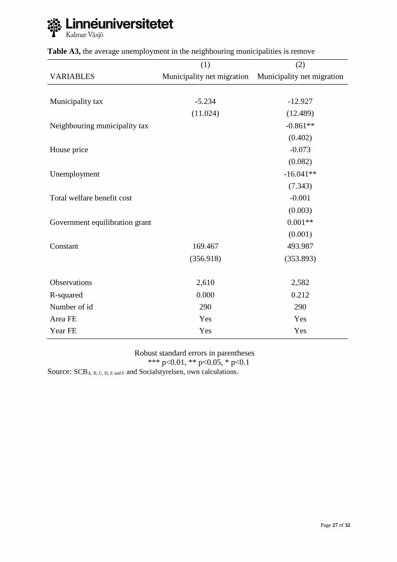
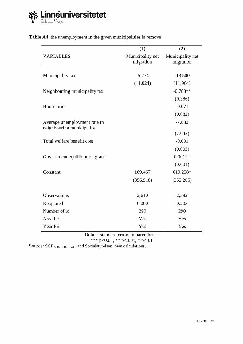
Unemployment has a highly significant, negative, impact on net regional migration. The value

-33.970 suggests that an increase by 1 percent in unemployment for the specific municipality

will decrease the net regional migration by nearly 34 percent, ceteris paribus. The size of the

impact on net regional migration is probably not correct, due to that the unemployment

variables has a high value in the VIF test, as shown in table A1 and A2, in Appendix A. Hence,

when removing any one of the unemployment variables the value of the other drops, shown in

table A3 and A4 in appendix A. We conclude that a negative impact on net migration can be

of 32

identified, but not to what degree. This would contradict the argument that unemployed

individuals have a higher mobility. Molho (2013) argues that most of the population are

contracted migrants, but that it might change when being unemployed. The result implies that

this is not the case, which in turn suggests that the individuals are still contracted migrants and

will not migrate before a new job have been secured. An increase in unemployment could

indicate that there are no vacant jobs in the municipality and thus the migrants into the

municipality will decline. At the same time the migration out of the municipality might increase

due to unemployment, hence give a negative outcome the net regional migration.

The neighbouring municipalities’ unemployment rate is also significant for the estimation. But

in contrast to the given municipality’s unemployment this is positively correlated to the net

regional migration. Therefore, when unemployment in neighbouring municipalities increase

the net regional migration in the given municipality increases. Due to the significant value a

positive correlation to the net regional migration do exist. However, due to the correlation with

the unemployment for the given municipality the degree of the impact cannot be concluded. In

accordance with both Sjaastad (1962) and Molho (2013) the unemployed individuals would

search for a new job, hence looking to the neighbouring municipalities. Since there are probably

more vacant jobs in the given municipality the inflow of migration is larger than the outflow.

For the given municipality this implies that net regional migration will increase.

The governmental equilibration grant is positive and significant for the net regional migration.

This is in accordance with Hindriks (1999) and Dahlberg and Edmark (2008) argument that a

strategic interaction exists between the municipalities when deciding on the welfare level.

Osmundsen et al. (2000) concluded that it is the welfare preferences that decided how mobile

an individual is and that this information is hidden for local government.

The total monetary cost for welfare benefits has a negative but statistically insignificant value.

The outcome of the regressions in this study indicates that are no impact on net regional

migration by the total monetary cost for welfare benefits. The negative sign implies that it could

still affect the net migration negatively but we cannot say that for certain, due to the insignificant

value.

of 32

7. Conclusion

The purpose of this essay has been to assess whether the municipality tax has any effect on net

regional migration in Sweden. The results of our estimations show that a direct effect does not

exist. The regression results imply that the two variables are not correlated. On the other hand

the neighbouring municipalities’ tax rate are statistically significant in all the regressions and

it could be that the effects of tax competition are absorbed into this variable. Nonetheless, there

is no correlation between the main variables. This indicates that an increase in the municipality

tax would not affect net regional migration. The result is significant at the 95 percent

confidence interval.

However, the correlation found between the neighbouring municipalities’ tax rate and the net

regional migration would indicate to the local government that it is important to be a part of

the tax competition. Thus, be able to adjust to the fluctuations within the competition. This is

in line with what Edmark and Ågren (2008) concluded that a weak evidence for tax competition

in Sweden does exist.

Dahlberg and Edmark (2008) found a positive correlation between neighbouring welfare level

and the decision taken by a given municipality’s benefits. Dahlberg and Edmark (2008), as well

as Hindriks (1999), indicate that there is a strategic interaction between municipalities,

regarding the net regional migration. However, the result regarding the welfare in this

investigation indicates that no such effect can be concluded from the results show in this paper

and thus the results for welfare are not in line with previous research.

Due to the large similarities between the governmental structure and autonomy of

municipalities, the results would be rather similar for the Nordic countries. In countries where

there is less autonomy for the local governments this result will most likely not stand.

In future studies it would be interesting to go deeper into the effects of municipality tax rate on

net migration, since the theory states that there should be a connection. In addition it would be

of interest to compare results from another country with less autonomy amongst the local

governments. Such a comparison would give an idea of what to expect if the autonomy would

be cut down.

of 32

8. References

Baltagi, Badi, H., (2013). Econometric analysis of panel data (5th ed.). Chichester, West

Sussex: John Wiley & Sons.

Boadway, R. (2001). Inter-Governmental Fiscal Relations: The Facilitator of Fiscal

Decentralization. Constitutional Political Economy, 12(2), 93-121.

Brueckner, J. (2003). Strategic Interaction Among Governments: An Overview of Empirical

Studies. International Regional Science Review, 26(2), 175-188.

Dahlberg, & Edmark. (2008). Is there a "race-to-the-bottom" in the setting of welfare benefit

levels? Evidence from a policy intervention. Journal of Public Economics, 92(5), 1193-1209.

Edmark, & Ågren. (2008). Identifying strategic interactions in Swedish local income tax

policies. Journal of Urban Economics, 63(3), 849-857.

Hill, Griffiths, Lim, William E, & Lim, G. C. (2011). Principles of econometrics (4th ed.).

Hoboken, N.J.: Wiley.

Hindriks, J. (1999). The consequences of labour mobility for redistribution: Tax vs. transfer

competition. Journal of Public Economics, 74(2), 215-234.

Hicks, J. (1963). The theory of wages (2nd ed.). London: Macmillan.

Lipatov, V., and Weichenrieder, A. (2015). Welfare and labor supply implications of tax

competition for mobile labor. Social Choice and Welfare, 45(2), 457-477.

Molho, I. (2013). Theories of migration a review. Scottish Journal of Political Economy: The

Journal of the Scottish Economic Society, 60(5), 526-556.

Osmundsen, P., Schjelderup, G., & Hagen, K. (2000). Personal income taxation under

mobility, exogenous and endogenous welfare weights, and asymmetric information. Journal of

Population Economics, 13(4), 623-637.

Schoorl, Jeannette, Heering Liesbeth, Esveldt, Ingrid, Groenewold, George, van der Erf, Rob,

Bosch, Alinda, de Valk, Helga and de Bruijn, Bart. Push and pull factors of international

migration: A comparative report (2000 ed., Eurostat. Theme 1, General statistics). (2000).

Luxembourg: Office for Official Publications of the European Communities.

of 32

Sjaastad, L. (1962). The Costs and Returns of Human Migration. Journal of Political

Economy, 70(5, Part 2), 80-93.

Wildasin, and Wilson. (1996). Imperfect mobility and local government behaviour in an

overlapping-generations model. Journal of Public Economics, 60(2), 177-198.

Wilson, J. (1999). Theories of tax competition. National Tax Journal, 52(2), pp. 269-304.

Arbetsförmedlingen, 2018

https://www.arbetsformedlingen.se/Om-oss/Statistik-och-publikationer/Statistik/Tidigare-

statistik.html

Accessed 2018-04-16

Regeringskansliet. 2017. Den nationella nivån - riksdag och regering

http://www.regeringen.se/sa-styrs-sverige/det-demokratiska-systemet-i-sverige/den-

nationella-nivan---riksdag-och-regering/

Accessed 2018-04-04

SCBA, 2018, Flyttningar efter region, ålder och kön. År 1997 - 2017

http://www.statistikdatabasen.scb.se/pxweb/sv/ssd/START__BE__BE0101__BE0101J/Flyttn

ingar97/?rxid=f45f90b6-7345-4877-ba25-9b43e6c6e299

Accessed 2018-04-17

SCBB, 2018, Försålda permanenta småhus efter region (län, riksområden, riket). År 2000 -

2017

http://www.statistikdatabasen.scb.se/pxweb/sv/ssd/START__BO__BO0501__BO0501B/Fast

prisPSRegAr/?rxid=f45f90b6-7345-4877-ba25-9b43e6c6e299

Accessed 2018-04-17

SCBC, 2018, Inflation i Sverige 1831–2017, 2018-01-12

http://www.scb.se/hitta-statistik/statistik-efter-amne/priser-och-

konsumtion/konsumentprisindex/konsumentprisindex-kpi/pong/tabell-och-

diagram/konsumentprisindex-kpi/inflation-i-sverige/

https://www.arbetsformedlingen.se/Om-oss/Statistik-och-publikationer/Statistik/Tidigare-statistik.html

https://www.arbetsformedlingen.se/Om-oss/Statistik-och-publikationer/Statistik/Tidigare-statistik.html

http://www.regeringen.se/sa-styrs-sverige/det-demokratiska-systemet-i-sverige/den-nationella-nivan---riksdag-och-regering/

http://www.regeringen.se/sa-styrs-sverige/det-demokratiska-systemet-i-sverige/den-nationella-nivan---riksdag-och-regering/

http://www.statistikdatabasen.scb.se/pxweb/sv/ssd/START__BE__BE0101__BE0101J/Flyttningar97/?rxid=f45f90b6-7345-4877-ba25-9b43e6c6e299

http://www.statistikdatabasen.scb.se/pxweb/sv/ssd/START__BE__BE0101__BE0101J/Flyttningar97/?rxid=f45f90b6-7345-4877-ba25-9b43e6c6e299

http://www.statistikdatabasen.scb.se/pxweb/sv/ssd/START__BO__BO0501__BO0501B/FastprisPSRegAr/?rxid=f45f90b6-7345-4877-ba25-9b43e6c6e299

http://www.statistikdatabasen.scb.se/pxweb/sv/ssd/START__BO__BO0501__BO0501B/FastprisPSRegAr/?rxid=f45f90b6-7345-4877-ba25-9b43e6c6e299

http://www.scb.se/hitta-statistik/statistik-efter-amne/priser-och-konsumtion/konsumentprisindex/konsumentprisindex-kpi/pong/tabell-och-diagram/konsumentprisindex-kpi/inflation-i-sverige/



of 32

Accessed 2018-04-19

SCBD, 2018, Kommunalekonomisk utjämning efter region, År 2005 - 2018

http://www.statistikdatabasen.scb.se/pxweb/sv/ssd/START__OE__OE0115/KomEkUtj/?rxid

=f45f90b6-7345-4877-ba25-9b43e6c6e299

Accessed 2018-04-18

SCBE, 2018, Kommunalskatteuppgifter efter region. År 2000 - 2018

http://www.statistikdatabasen.scb.se/pxweb/sv/ssd/START__OE__OE0101/Kommunalskatter

2000/?rxid=f45f90b6-7345-4877-ba25-9b43e6c6e299

Accessed 2018-04-18

SCBF, 2018, Nettoinkomst för boende i Sverige hela året (antal personer, medel- och

medianinkomst samt totalsumma) efter region, kön och ålder. År 2000 - 2016

http://www.statistikdatabasen.scb.se/pxweb/sv/ssd/START__HE__HE0110__HE0110A/NetI

nk02/?rxid=f45f90b6-7345-4877-ba25-9b43e6c6e299

Accessed 2018-04-17

Socialstyrelsen, 2018

http://www.socialstyrelsen.se/statistik/statistikdatabas/ekonomisktbistand

Accessed 2018-04-23

Sveriges kommuner och landsting, 2017

https://skl.se/ekonomijuridikstatistik/ekonomi/utjamningssystem.1917.html

Accessed 2018-04-04

http://www.statistikdatabasen.scb.se/pxweb/sv/ssd/START__OE__OE0115/KomEkUtj/?rxid=f45f90b6-7345-4877-ba25-9b43e6c6e299

http://www.statistikdatabasen.scb.se/pxweb/sv/ssd/START__OE__OE0115/KomEkUtj/?rxid=f45f90b6-7345-4877-ba25-9b43e6c6e299

http://www.statistikdatabasen.scb.se/pxweb/sv/ssd/START__OE__OE0101/Kommunalskatter2000/?rxid=f45f90b6-7345-4877-ba25-9b43e6c6e299

http://www.statistikdatabasen.scb.se/pxweb/sv/ssd/START__OE__OE0101/Kommunalskatter2000/?rxid=f45f90b6-7345-4877-ba25-9b43e6c6e299

http://www.statistikdatabasen.scb.se/pxweb/sv/ssd/START__HE__HE0110__HE0110A/NetInk02/?rxid=f45f90b6-7345-4877-ba25-9b43e6c6e299

http://www.statistikdatabasen.scb.se/pxweb/sv/ssd/START__HE__HE0110__HE0110A/NetInk02/?rxid=f45f90b6-7345-4877-ba25-9b43e6c6e299

http://www.socialstyrelsen.se/statistik/statistikdatabas/ekonomisktbistand

https://skl.se/ekonomijuridikstatistik/ekonomi/utjamningssystem.1917.html

of 32

Appendix A. Correlation and the Hausman test

The Hausman test compare the covariance matrix of the independent variables for the fixed

effect model toward the random effect model. The null hypothesis is that there are no

systematic differences between the covariance matrices of the two models. If this p-value is

below 0.05 the test rejects the null hypothesis indicating that a fixed effect model is the most

appropriate model. If, on the other hand, Ho is not rejected, a random effect model should be

used. For the data used in this thesis the test gives a Chi2 (7 degreed of freedom) = 108.62

with a corresponding p – value = 0.000. Thus, Ho is rejected and a fixed effect model should

be used.

Table A1, variance inflation factor tests (VIF) result

Variables VIF 1/VIF

Average income 5.59 0.178775

House price 4.46 0.224362

Neighbour tax 3.38 0.295906

Unemployment 3.14 0.318304

Average neighbouring

unemployment

2.21 0.451633

Total welfare benefit cost 1.99 0.502989

Municipality tax 1.51 0.660460

Government equilibration

grant

1.35 0.741787

Mean VIF 2.95

Source: SCBA, B, D, E and F and Socialstyrelsen, own calculations

Table A2, variance inflation factor tests (VIF) result

Variables VIF 1/VIF

Unemployment 2.40 0.416912

Average neighbouring

unemployment

2.10 0.475224

Total welfare benefit cost 1.97 0.508084

Government equilibration

grant

1.91 0.523964

House price 1.80 0.555623

Municipality tax 1.47 0.681168

Neighbour tax 1.04 0.959557

Mean VIF 1.81

Source: SCBA, B, D, E and F and Socialstyrelsen, own calculations

of 32

Table A3, the average unemployment in the neighbouring municipalities is remove


*** p<0.01, ** p<0.05, * p<0.1


(1) (2)

VARIABLES Municipality net migration Municipality net migration


(11.024) (12.489)


(0.402)

House price -0.073

(0.082)

Unemployment -16.041**

(7.343)


(0.003)


(0.001)

Constant 169.467 493.987

(356.918) (353.893)


R-squared 0.000 0.212


Area FE Yes Yes

Year FE Yes Yes

of 32

Table A4, the unemployment in the given municipalities is remove

(1) (2)


migration

Municipality net

migration


(11.024) (11.964)


(0.386)

House price -0.071

(0.082)



-7.832

(7.042)


(0.003)


(0.001)

Constant 169.467 619.238*

(356.918) (352.205)


R-squared 0.000 0.203


Area FE Yes Yes

Year FE Yes Yes


*** p<0.01, ** p<0.05, * p<0.1


of 32

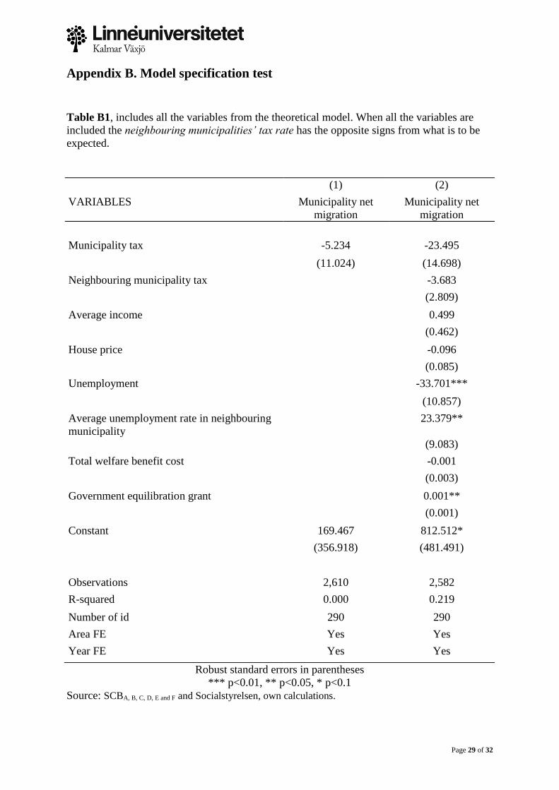
Appendix B. Model specification test

Table B1, includes all the variables from the theoretical model. When all the variables are

included the neighbouring municipalities’ tax rate has the opposite signs from what is to be

expected.

(1) (2)


migration

Municipality net

migration


(11.024) (14.698)

Neighbouring municipality tax -3.683

(2.809)

Average income 0.499

(0.462)

House price -0.096

(0.085)


(10.857)


municipality

23.379**

(9.083)


(0.003)


(0.001)

Constant 169.467 812.512*

(356.918) (481.491)


R-squared 0.000 0.219


Area FE Yes Yes

Year FE Yes Yes


*** p<0.01, ** p<0.05, * p<0.1


of 32

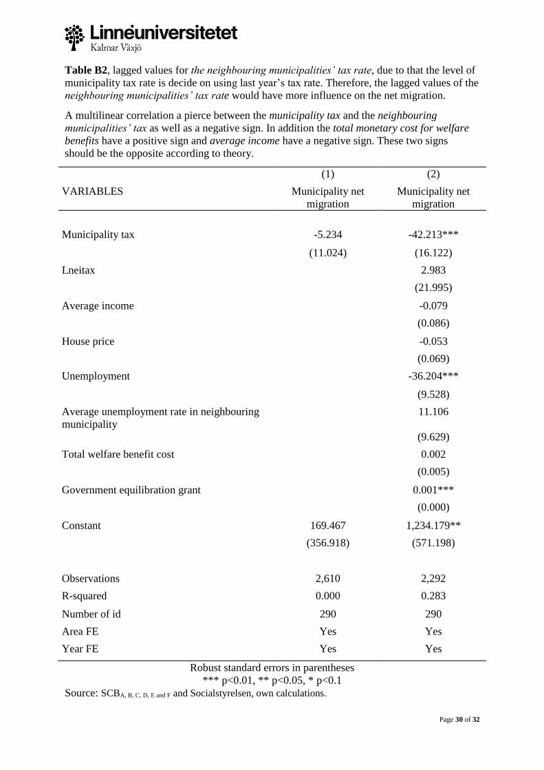
Table B2, lagged values for the neighbouring municipalities’ tax rate, due to that the level of

municipality tax rate is decide on using last year’s tax rate. Therefore, the lagged values of the

neighbouring municipalities’ tax rate would have more influence on the net migration.

A multilinear correlation a pierce between the municipality tax and the neighbouring

municipalities’ tax as well as a negative sign. In addition the total monetary cost for welfare

benefits have a positive sign and average income have a negative sign. These two signs

should be the opposite according to theory.

(1) (2)


migration

Municipality net

migration

Municipality tax -5.234 -42.213***

(11.024) (16.122)

Lneitax 2.983

(21.995)

Average income -0.079

(0.086)

House price -0.053

(0.069)


(9.528)


municipality

11.106

(9.629)

Total welfare benefit cost 0.002

(0.005)

Government equilibration grant 0.001***

(0.000)

Constant 169.467 1,234.179**

(356.918) (571.198)


R-squared 0.000 0.283


Area FE Yes Yes

Year FE Yes Yes


*** p<0.01, ** p<0.05, * p<0.1


of 32

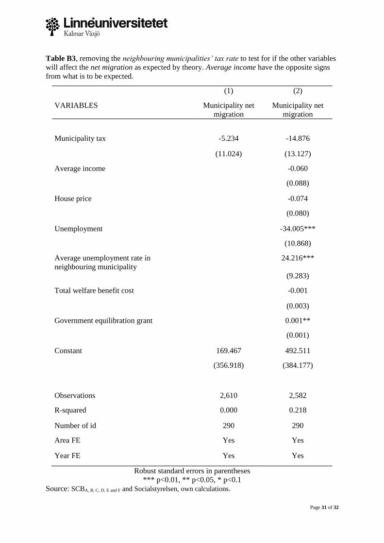
Table B3, removing the neighbouring municipalities’ tax rate to test for if the other variables

will affect the net migration as expected by theory. Average income have the opposite signs

from what is to be expected.

(1) (2)


migration

Municipality net

migration


(11.024) (13.127)


(0.088)

House price -0.074

(0.080)


(10.868)



24.216***

(9.283)


(0.003)


(0.001)

Constant 169.467 492.511

(356.918) (384.177)


R-squared 0.000 0.218


Area FE Yes Yes

Year FE Yes Yes


*** p<0.01, ** p<0.05, * p<0.1


of 32

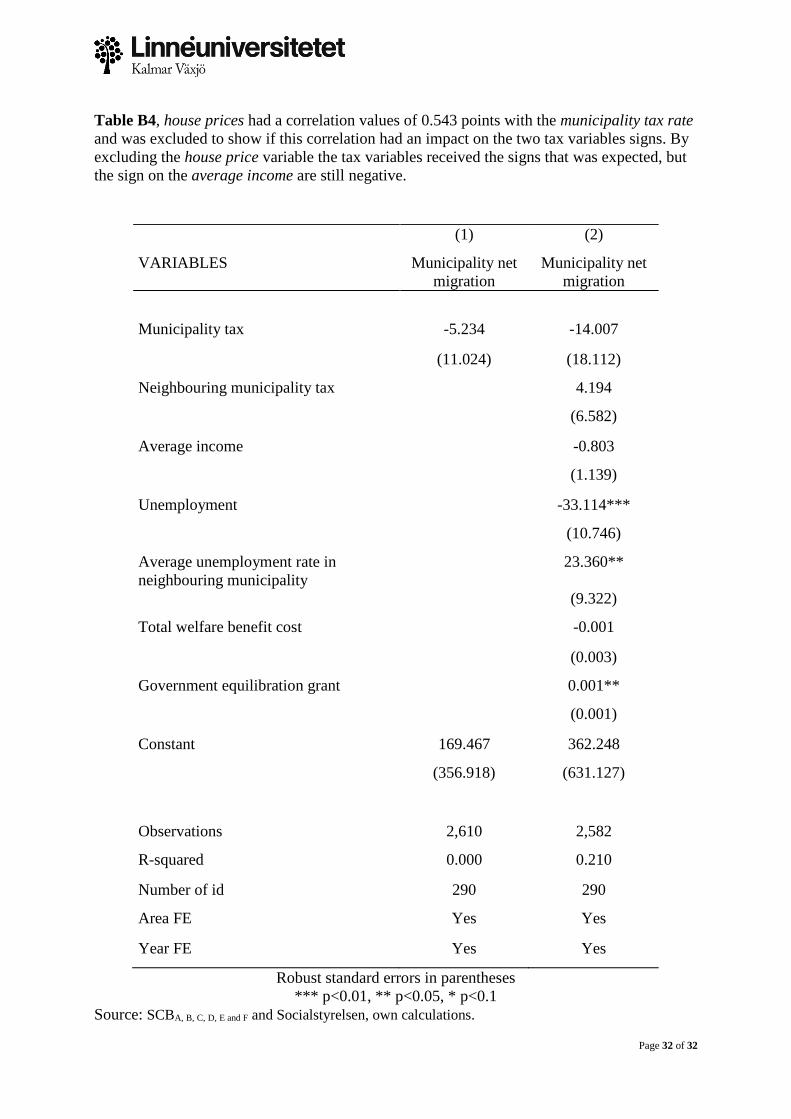
Table B4, house prices had a correlation values of 0.543 points with the municipality tax rate

and was excluded to show if this correlation had an impact on the two tax variables signs. By

excluding the house price variable the tax variables received the signs that was expected, but

the sign on the average income are still negative.

(1) (2)


migration

Municipality net

migration


(11.024) (18.112)

Neighbouring municipality tax 4.194

(6.582)


(1.139)


(10.746)



23.360**

(9.322)


(0.003)


(0.001)

Constant 169.467 362.248

(356.918) (631.127)


R-squared 0.000 0.210


Area FE Yes Yes

Year FE Yes Yes


*** p<0.01, ** p<0.05, * p<0.1


bachelor essay - diva portal

Documents