automatic calibration of a spiking head-direction network for representing robot orientation

Automatic Calibration of a Spiking Head-Direction Network for Representing Robot Orientation

Peter Stratton*†, Michael Milford*†, Janet Wiles†, Gordon Wyeth† *Queensland Brain Institute and

†School of Information Technology and Electrical Engineering The University of Queensland

St Lucia Queensland 4072 Australia {stratton, milford, wiles, wyeth@} itee.uq.edu.au

Abstract

Calibration of movement tracking systems is a difficult problem faced by both animals and robots. The ability to continuously calibrate changing systems is essential for animals as they grow or are injured, and highly desirable for robot control or mapping systems due to the possibility of component wear, modification, damage and their deployment on varied robotic platforms. In this paper we use inspiration from the animal head direction tracking system to implement a self-calibrating, neurally-based robot orientation tracking system. Using real robot data we demonstrate how the system can remove tracking drift and learn to consistently track rotation over a large range of velocities. The neural tracking system provides the first steps towards a fully neural SLAM system with improved practical applicability through self-tuning and adaptation.

1 Introduction

The problem of calibration is a key one in both nature and robotics; how can an animal or robot maintain accurate tracking of its movement when both it and its environment can change. In nature, an animal must maintain calibration of the neural and sensory systems used to track movement, rotation, grasping and striking, in the face of challenges such as growth, damage, and change in its environment. Likewise, in robotics, one might imagine an ideal robot control system that can be flexibly deployed on a range of varying robotic platforms without the need for manual fine-tuning of the tracking system parameters. If the tracking system could autocalibrate, not only would it not require exact initial parameters, but it would be able to adapt if the robot was damaged or modified. For example, a service robot which lost pressure in a tyre might recalibrate and continue to keep track of its location and orientation. A grasping robot which had an arm component bent or shortened

would be able to recalibrate and continue to perform its intended task.

In this paper we describe the first stage of work towards developing a completely self-tuning neural SLAM system; a self-calibrating, neurally-based robot orientation tracking system. We use a spiking neural network to address two of the key issues in self-calibration; removing drift, and developing consistent tracking for turns in both clockwise and counter-clockwise directions. The core network provides a significant increase in biological relevance over extant neurally-inspired systems such as RatSLAM [Milford et al., 2008, Milford, 2008, Milford et al., 2009], while providing a means for improved practical performance through self-tuning and adaptation.

The paper continues as follows. In Section 1.1 we briefly describe the anatomical background of the head direction tracking system in animals, and provide an overview of the typical modelling approaches in Section 1.2. Section 2 presents the network architecture and connectivity, while Section 3 details the autonomous calibration procedure. In Section 4 the experimental procedure is described with the results presented in Section 5. Section 6 discusses the results and details possible directions for future work.

1.1 Head Direction Neurons Head direction (HD) neurons are cells in the mammalian brain that fire when an animal is facing in a certain direction relative to cues in the environment [Taube, 2007]. A number of other neuron types perform computation to help maintain this representation of orientation state in the HD cells. Of particular relevance to the model presented in this paper is a class of neurons called angular head velocity (AHV) cells. There are two categories of AHV neuron – symmetric AHV neurons which fire to indicate rotational speed, responding to both clockwise and counter clockwise rotation, while asymmetric AHV neurons indicate rotational velocity, firing only for rotation in one direction.

Australasian Conference on Robotics and Automation (ACRA), December 2-4, 2009, Sydney, Australia

1.2 Network Models of Head-Direction Cells Computational models of the head direction system typically use a continuous attractor network [Sharp et al., 2001]. An attractor is a dynamical system that tends towards one or more equilibrium states over time; a continuous attractor is stable in a continuum of states instead of a set of discrete states. For HD networks, the attractor states are stable firing patterns able to represent any possible orientation across the population of HD units. These states are created by the interaction between two sets of weights, one excitatory and one inhibitory.

• Excitatory connections strongly connect neurons that encode similar orientations, so that groups of neurons encoding similar orientations are coopted into firing together. The group of firing neurons is often called an activity bump (see Figure 1).

• Inhibitory connections strongly connect neurons that encode dissimilar orientations, so that groups of neurons that encode dissimilar orientations cannot sustain firing together.

Figure 1 – A group of neurons firing together in a network are known as an activity bump or activity packet. When used to represent a head direction network, nearby neurons encode similar orientations.

The major computational models of head direction networks have used static network connections that were already perfectly balanced and tuned [Song et al., 2005, Skaggs et al., 1995, Redish et al., 1996, Goodridge et al., 2000, Xie et al., 2002]; we call these models the non-adaptive attractor models. Some studies have considered the calibration issue such as work by Zhang [Zhang, 1996], Stringer et al. [Stringer et al., 2002] and Hahnloser [Hahnloser, 2003]. However, most of these approaches have assumed the existence of visual cues in the environment that were already ‘mapped’ to specific animal or robot orientations.

2 Network Model Architecture

The network model (see Figure 2) consists of three different types of neurons:

• head direction (HD) cells, which encode the robot’s orientation,

• right and left turn angular head velocity (AHV) cells, which encode, respectively, clockwise and counter clockwise rotational velocity, and

• symmetric angular head velocity cells, which encode rotational speed.

Figure 2 – Network architecture. The head-direction cells encode the robot’s orientation, while the clockwise and counter-clockwise cells encode the robot’s angular velocity. The symmetric angular velocity cells encode the robot’s rotation speed in either direction.

2.1 Network connections The network contains three sets of connections; recurrent excitatory connections from each HD cell to other HD cells, excitatory connections from HD cells to the clockwise and counter-clockwise AHV cells, and inhibitory connections from the clockwise and counter-clockwise AHV cells to the HD cells (see Figure 3). We present equations for the recurrent HD connections, which change under the adaptation algorithm, and briefly describe the other connections. Recurrent HD Connections There are 100 HD cells in the network, each connected by recurrent excitatory weights, given by a Gaussian function of the distance between the cells (see Equation 1). The strength of the connection WHH from HD cell i to HD cell j is given by

(.)22

, 2, noise

rdexcit

HHij feGW HHij−= (1)

where rHH is the distance, in number of cells, of one standard deviation of the Gaussian (set to n/8 for all trials) and d is the circular distance (i.e. with wrapping at the ends) from cell j to cell i, given by

)],)mod((),),(min[mod(, njoinoijd iiij −−−−= (2)

where oi is a systematic shift which is applied to the direction of the initial Gaussian weights. It is this shift which causes a continuous drift in the attractor bump and which is corrected for by the adaptation algorithms presented in this study. fnoise(.) is a noise function defined as

(.).1(.) gaussfnoise λ+= (3)


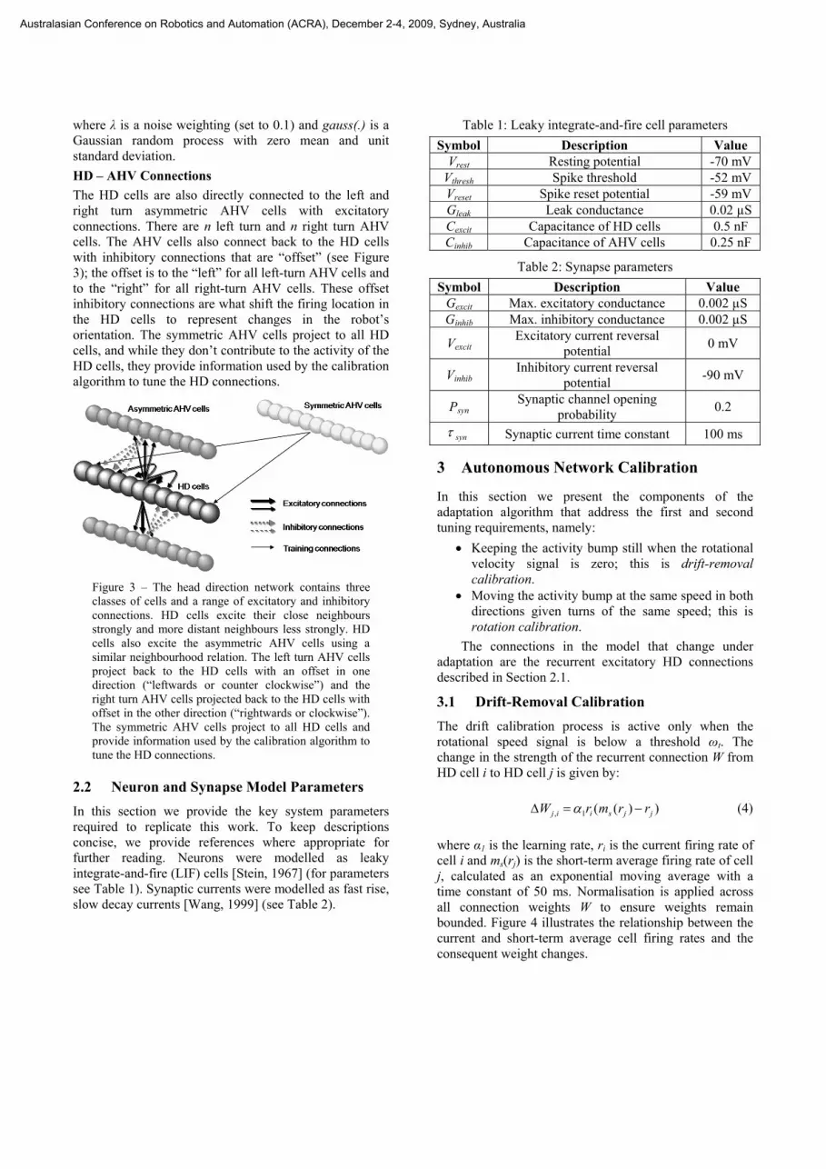
where λ is a noise weighting (set to 0.1) and gauss(.) is a Gaussian random process with zero mean and unit standard deviation. HD – AHV Connections The HD cells are also directly connected to the left and right turn asymmetric AHV cells with excitatory connections. There are n left turn and n right turn AHV cells. The AHV cells also connect back to the HD cells with inhibitory connections that are “offset” (see Figure 3); the offset is to the “left” for all left-turn AHV cells and to the “right” for all right-turn AHV cells. These offset inhibitory connections are what shift the firing location in the HD cells to represent changes in the robot’s orientation. The symmetric AHV cells project to all HD cells, and while they don’t contribute to the activity of the HD cells, they provide information used by the calibration algorithm to tune the HD connections.

Figure 3 – The head direction network contains three classes of cells and a range of excitatory and inhibitory connections. HD cells excite their close neighbours strongly and more distant neighbours less strongly. HD cells also excite the asymmetric AHV cells using a similar neighbourhood relation. The left turn AHV cells project back to the HD cells with an offset in one direction (“leftwards or counter clockwise”) and the right turn AHV cells projected back to the HD cells with offset in the other direction (“rightwards or clockwise”). The symmetric AHV cells project to all HD cells and provide information used by the calibration algorithm to tune the HD connections.

2.2 Neuron and Synapse Model Parameters In this section we provide the key system parameters required to replicate this work. To keep descriptions concise, we provide references where appropriate for further reading. Neurons were modelled as leaky integrate-and-fire (LIF) cells [Stein, 1967] (for parameters see Table 1). Synaptic currents were modelled as fast rise, slow decay currents [Wang, 1999] (see Table 2).

Table 1: Leaky integrate-and-fire cell parameters Symbol Description Value

Vrest Resting potential -70 mV Vthresh Spike threshold -52 mV Vreset Spike reset potential -59 mV Gleak Leak conductance 0.02 µS Cexcit Capacitance of HD cells 0.5 nF Cinhib Capacitance of AHV cells 0.25 nF

Table 2: Synapse parameters Symbol Description Value

Gexcit Max. excitatory conductance 0.002 µS Ginhib Max. inhibitory conductance 0.002 µS

Vexcit Excitatory current reversal

potential 0 mV

Vinhib Inhibitory current reversal

potential -90 mV

Psyn Synaptic channel opening

probability 0.2

synτ Synaptic current time constant 100 ms

3 Autonomous Network Calibration

In this section we present the components of the adaptation algorithm that address the first and second tuning requirements, namely:

• Keeping the activity bump still when the rotational velocity signal is zero; this is drift-removal calibration.

• Moving the activity bump at the same speed in both directions given turns of the same speed; this is rotation calibration.

The connections in the model that change under adaptation are the recurrent excitatory HD connections described in Section 2.1.

3.1 Drift-Removal Calibration The drift calibration process is active only when the rotational speed signal is below a threshold ωt. The change in the strength of the recurrent connection W from HD cell i to HD cell j is given by:

))((1, jjsiij rrmrW −=Δ α (4)

where α1 is the learning rate, ri is the current firing rate of cell i and ms(rj) is the short-term average firing rate of cell j, calculated as an exponential moving average with a time constant of 50 ms. Normalisation is applied across all connection weights W to ensure weights remain bounded. Figure 4 illustrates the relationship between the current and short-term average cell firing rates and the consequent weight changes.


Figure 4 – Learning to keep the activity bump encoding the robot’s orientation stationary when the velocity signal is zero. This graph shows the current bump across the HD cell population (black line) and the short term exponential moving average (grey line) which lags slightly behind. The bump is drifting to the right. Connections from the current bump to the region denoted with plus symbols are strengthened (thick curved arrow) which tends to pull the bump in the direction opposite to the direction of drift. Conversely, connections from the current bump to the region denoted with minus symbols are weakened (thin arrow) which tends to stop pulling the bump in the direction of drift.

3.2 Rotation Calibration When the rotational speed signal is above threshold ωt, the change in the strength of the recurrent connection W from HD cell i to HD cell j is given by:

jiisjij crrmrW ))((2, −=Δ α (5)

where r and ms(.) are as defined in Equation 4, α2 is the learning rate, and cj is a calibration term: which is zero if the rate of change of firing rate of neuron j, given the current velocity signal, is correct, positive if the rate of change of firing rate is too low (i.e. the bump is moving too slowly), and negative if the rate of change of firing rate is too large (i.e. the bump is moving too quickly). It is calculated as:

sym

jsjj AHV

rmrabsKc

))(( −−= (6)

where K is a constant that controls the overall speed of the bump through the HD network for given AHV input, and AHVsym is the current input from the symmetric AHV cells. K was chosen to be 25 in these studies, which results in reasonable bump movement speed for given AHV input. The value of cj is positive if rotational tracking is lagging and negative if rotational tracking is leading.

4 Experimental Procedure

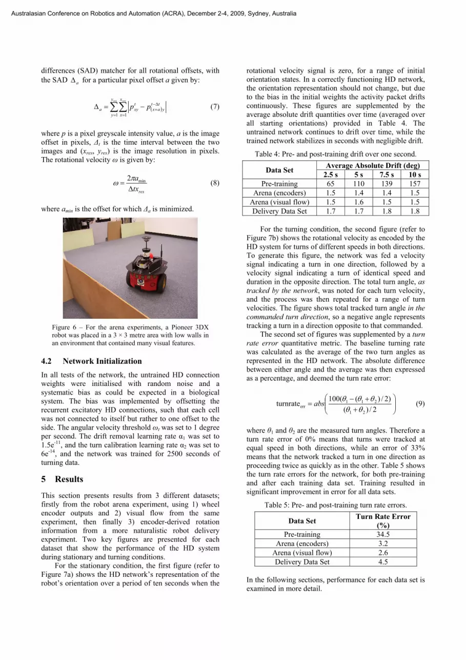
Rotational velocity data was generated using a Pioneer 3DX robot in two different scenarios. The first “arena” scenario consisted of the robot being placed in a walled 3 × 3 metre area rich in visual features. The movement scheme consisted of the robot randomly spinning on the spot or remaining still, with the breakdown given in Table 3. Each turn or stationary segment was performed for a random time duration between one and three seconds long, with an average duration of two seconds. Commanded turn velocities were fixed for any single turn segment and ranged randomly between 30 and 120 degrees per second.

Table 3: Arena Movement Types and Durations

Movement Type Percentage Active (desired)

Percentage Active

(achieved) Stationary 50% 41.44% Clockwise 25% 29.57% Counter-clockwise 25% 28.97%

The second scenario involved extracting rotational

velocity data from a robot performing exploration and delivery tasks over an entire office building floor, as described in [Milford et al., 2009]. The rotational data was extracted from a robot that was translating as well as turning and which did not have discrete turning / stationary modes as in the arena scenario. The velocities of the two datasets are compared with histograms in Figure 5.

Figure 5 – Rotational velocity histograms for the encoder derived velocities in the (a) arena and (b) delivery robot scenarios. The arena velocity histogram has clear stationary periods, while the delivery robot scenario has velocities distributed over the entire range, with relatively few completely stationary periods. The peaks at -27 and +27 degrees in (b) are caused by the robot’s movement scheme.

4.1 Velocity Extraction From Sensors Two rotational velocity signals were logged by the robot at a rate of 7 Hz. The first was extracted from the wheel encoders, while the second was taken by performing whole image offset matching on successive panoramic images taken by the robot’s camera and mirror setup. Images were compared using a sum of absolute


differences (SAD) matcher for all rotational offsets, with the SAD aΔ for a particular pixel offset a given by:

( )∑∑= =

Δ−+−=Δ

res resy

y

x

x

ttyax

txya pp

1 1 (7)

where p is a pixel greyscale intensity value, a is the image offset in pixels, Δt is the time interval between the two images and (xres, yres) is the image resolution in pixels. The rotational velocity ω is given by:

restx

aΔ

= min2πω (8)

where amin is the offset for which Δa is minimized.

Figure 6 – For the arena experiments, a Pioneer 3DX robot was placed in a 3 × 3 metre area with low walls in an environment that contained many visual features.

4.2 Network Initialization In all tests of the network, the untrained HD connection weights were initialised with random noise and a systematic bias as could be expected in a biological system. The bias was implemented by offsetting the recurrent excitatory HD connections, such that each cell was not connected to itself but rather to one offset to the side. The angular velocity threshold ωt was set to 1 degree per second. The drift removal learning rate α1 was set to 1.5e-11, and the turn calibration learning rate α2 was set to 6e-14, and the network was trained for 2500 seconds of turning data.

5 Results

This section presents results from 3 different datasets; firstly from the robot arena experiment, using 1) wheel encoder outputs and 2) visual flow from the same experiment, then finally 3) encoder-derived rotation information from a more naturalistic robot delivery experiment. Two key figures are presented for each dataset that show the performance of the HD system during stationary and turning conditions.

For the stationary condition, the first figure (refer to Figure 7a) shows the HD network’s representation of the robot’s orientation over a period of ten seconds when the

rotational velocity signal is zero, for a range of initial orientation states. In a correctly functioning HD network, the orientation representation should not change, but due to the bias in the initial weights the activity packet drifts continuously. These figures are supplemented by the average absolute drift quantities over time (averaged over all starting orientations) provided in Table 4. The untrained network continues to drift over time, while the trained network stabilizes in seconds with negligible drift.

Table 4: Pre- and post-training drift over one second.

Data Set Average Absolute Drift (deg) 2.5 s 5 s 7.5 s 10 s

Pre-training 65 110 139 157 Arena (encoders) 1.5 1.4 1.4 1.5

Arena (visual flow) 1.5 1.6 1.5 1.5 Delivery Data Set 1.7 1.7 1.8 1.8

For the turning condition, the second figure (refer to

Figure 7b) shows the rotational velocity as encoded by the HD system for turns of different speeds in both directions. To generate this figure, the network was fed a velocity signal indicating a turn in one direction, followed by a velocity signal indicating a turn of identical speed and duration in the opposite direction. The total turn angle, as tracked by the network, was noted for each turn velocity, and the process was then repeated for a range of turn velocities. The figure shows total tracked turn angle in the commanded turn direction, so a negative angle represents tracking a turn in a direction opposite to that commanded.

The second set of figures was supplemented by a turn rate error quantitative metric. The baseline turning rate was calculated as the average of the two turn angles as represented in the HD network. The absolute difference between either angle and the average was then expressed as a percentage, and deemed the turn rate error:

⎟⎟⎠

⎞⎜⎜⎝

⎛+

+−=

2/)()2/)((100turnrate

21

211err θθ

θθθabs (9)

where θ1 and θ2 are the measured turn angles. Therefore a turn rate error of 0% means that turns were tracked at equal speed in both directions, while an error of 33% means that the network tracked a turn in one direction as proceeding twice as quickly as in the other. Table 5 shows the turn rate errors for the network, for both pre-training and after each training data set. Training resulted in significant improvement in error for all data sets.

Table 5: Pre- and post-training turn rate errors.

Data Set Turn Rate Error (%)

Pre-training 34.5 Arena (encoders) 3.2

Arena (visual flow) 2.6 Delivery Data Set 4.5

In the following sections, performance for each data set is examined in more detail.


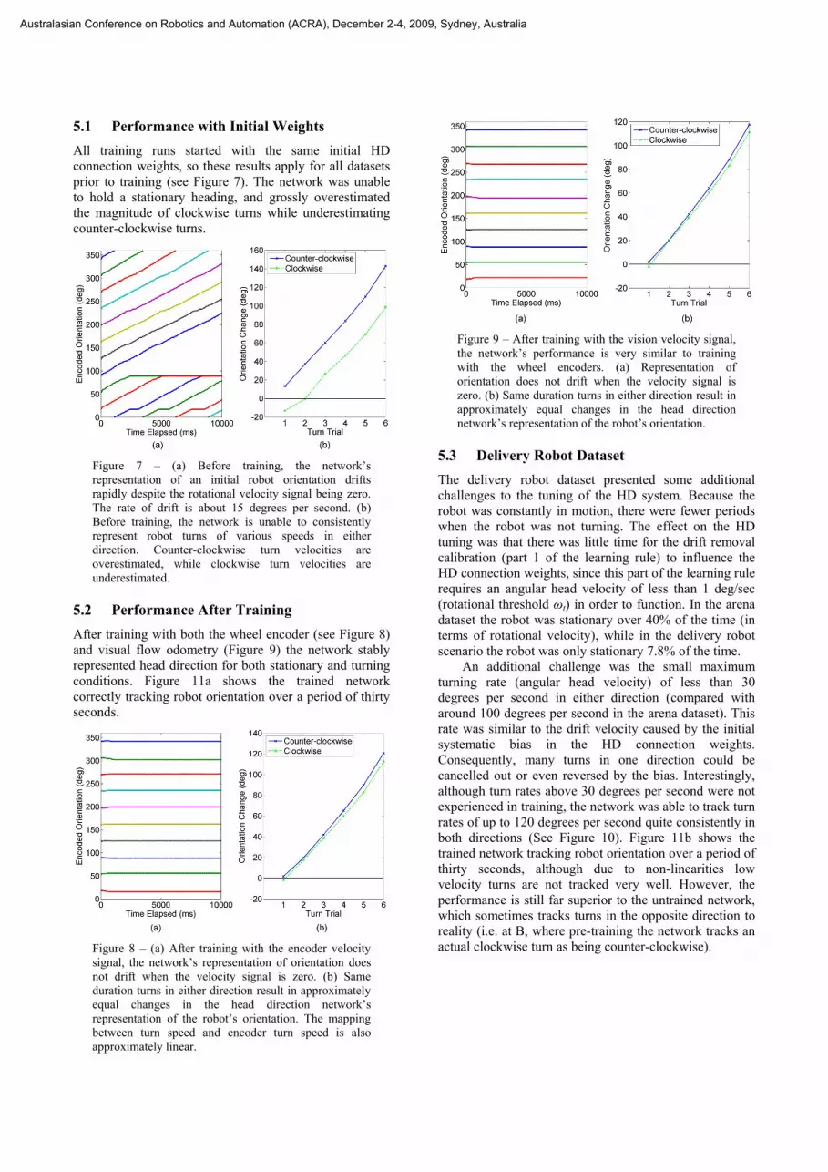
5.1 Performance with Initial Weights All training runs started with the same initial HD connection weights, so these results apply for all datasets prior to training (see Figure 7). The network was unable to hold a stationary heading, and grossly overestimated the magnitude of clockwise turns while underestimating counter-clockwise turns.

Figure 7 – (a) Before training, the network’s representation of an initial robot orientation drifts rapidly despite the rotational velocity signal being zero. The rate of drift is about 15 degrees per second. (b) Before training, the network is unable to consistently represent robot turns of various speeds in either direction. Counter-clockwise turn velocities are overestimated, while clockwise turn velocities are underestimated.

5.2 Performance After Training After training with both the wheel encoder (see Figure 8) and visual flow odometry (Figure 9) the network stably represented head direction for both stationary and turning conditions. Figure 11a shows the trained network correctly tracking robot orientation over a period of thirty seconds.

Figure 8 – (a) After training with the encoder velocity signal, the network’s representation of orientation does not drift when the velocity signal is zero. (b) Same duration turns in either direction result in approximately equal changes in the head direction network’s representation of the robot’s orientation. The mapping between turn speed and encoder turn speed is also approximately linear.

Figure 9 – After training with the vision velocity signal, the network’s performance is very similar to training with the wheel encoders. (a) Representation of orientation does not drift when the velocity signal is zero. (b) Same duration turns in either direction result in approximately equal changes in the head direction network’s representation of the robot’s orientation.

5.3 Delivery Robot Dataset The delivery robot dataset presented some additional challenges to the tuning of the HD system. Because the robot was constantly in motion, there were fewer periods when the robot was not turning. The effect on the HD tuning was that there was little time for the drift removal calibration (part 1 of the learning rule) to influence the HD connection weights, since this part of the learning rule requires an angular head velocity of less than 1 deg/sec (rotational threshold ωt) in order to function. In the arena dataset the robot was stationary over 40% of the time (in terms of rotational velocity), while in the delivery robot scenario the robot was only stationary 7.8% of the time.

An additional challenge was the small maximum turning rate (angular head velocity) of less than 30 degrees per second in either direction (compared with around 100 degrees per second in the arena dataset). This rate was similar to the drift velocity caused by the initial systematic bias in the HD connection weights. Consequently, many turns in one direction could be cancelled out or even reversed by the bias. Interestingly, although turn rates above 30 degrees per second were not experienced in training, the network was able to track turn rates of up to 120 degrees per second quite consistently in both directions (See Figure 10). Figure 11b shows the trained network tracking robot orientation over a period of thirty seconds, although due to non-linearities low velocity turns are not tracked very well. However, the performance is still far superior to the untrained network, which sometimes tracks turns in the opposite direction to reality (i.e. at B, where pre-training the network tracks an actual clockwise turn as being counter-clockwise).


Figure 10 – (a) After training with the delivery robot data set, the network’s representation of orientation does not drift when the velocity signal is zero. (b) Same duration turns in either direction result in approximately equal changes in the head direction network’s representation of the robot’s orientation.

6 Discussion and Future Work

There are several aspects of the work that warrant discussion. The first regards the faithfulness of the network model to the neural circuits it is based upon. The model presented in this paper represents a significant improvement in biological relevance compared to previous robot-based models of head direction cells such as that of Milford et al. [Milford et al., 2003]. Neurons are modelled using spiking neurons rather than rate-coded neurons, and most importantly, connectivity is not assumed to be perfectly pre-wired and static. Instead, an initially noisy, biased, drifting neural representation of head direction is calibrated using adaptive learning rules. The learning algorithms use biological plausible mechanisms such as total synaptic weight normalization [Royer et al., 2003] and mean firing rate normalization [Turrigiano et al., 2004].

Through the use of symmetric angular head velocity cells, the model differs from previous models [Song et al., 2005, Skaggs et al., 1995, Redish et al., 1996, Goodridge et al., 2000, Xie et al., 2002]. Furthermore, unlike previous approaches which have used simulated or highly idealized training data, we have trained and tested the network using real-world robot data obtained from both wheel encoder information and visual flow. The calibration relies only on equal-speed turns in either direction generating either equal-magnitude wheel encoder or visual flow input to the HD network. It is interesting to note that calibration can occur somewhat independently of the robot movement behaviour, as demonstrated by the use of data from two different robot schemes. The calibration scheme also tunes the robot’s orientation tracking system to track velocities far larger than encountered during its training phase, as demonstrated using the delivery robot dataset.

Figure 11 – Tracking performance over 30 seconds pre- (dotted line) and post (solid line) training, compared to the integral of the input velocity signal (dashed line) for the (a) arena dataset and (b) delivery robot dataset. Pre-training the network exaggerates counter-clockwise (positive) turns, tracks counter-clockwise turns when the robot is actually still (see A), and underestimates clockwise turns. For the delivery robot dataset the trained network struggles to track low rotational speeds (see B) but fares much better than the untrained network, which represents rotation in the opposite (and wrong) direction.

Exactly the same network (connectivity, learning rates, time constants, and initial conditions) was used for training with all three datasets, and despite the large differences in the magnitude and distribution of turn rates in the training data, the network converged well to a stable head direction representation in all cases. This flexible calibration suggests the potential for ‘out of the box’ operation on a variety of operating environments and robot hardware.

The specific subset of the navigation problem addressed in this paper is also solvable using current engineering approaches such as Kalman Filter techniques. However, navigation systems such as RatSLAM have demonstrated that pursuing a bio-inspired solution to engineering problems can eventually produce systems that outperform the state of the art engineering systems. No current engineering system as a whole navigates as well as a rat; our aim in this work is to understand how it may be possible to form a superior navigation system through modelling and understanding mechanisms of rat navigation.

One key improvement to the current HD system will be the addition of loop closure calibration. By introducing recognition of orientation loop closures – when the robot has rotated through 360 degrees and is facing the way it started, the system will have an additional means of calibration. Further extending the network to include


place cells and grid cells will enable calibration of translation tracking. The ultimate goal will be the development of a self-tuning, spiking neuron model of the current RatSLAM system. Combining the already capable robot mapping performance of RatSLAM with the improved neural models and self-tuning capability will provide a system that can be flexibly deployed on a range of platforms.

References [M. Milford, et al., 2008] M. Milford, et al., "Mapping a

Suburb with a Single Camera using a Biologically Inspired SLAM System," IEEE Transactions on Robotics, vol. 24, 2008.

[M. Milford, 2008] M. Milford, Robot Navigation from Nature: Simultaneous Localisation, Mapping, and Path Planning Based on Hippocampal Models, vol. 41, 2008.

[M. Milford, et al., 2009] M. Milford, et al., "Persistent Navigation and Mapping using a Biologically Inspired SLAM System " The International Journal of Robotics Research (in press), 2009.

[J. S. Taube, 2007] J. S. Taube, "The head direction signal: origins and sensory-motor integration," Annual Review of Neuroscience, vol. 30, pp. 181-207, 2007.

[P. E. Sharp, et al., 2001] P. E. Sharp, et al., "The anatomical and computational basis of the rat head-direction cell signal," Trends in Neurosciences, vol. 24, pp. 289-294, 2001.

[P. Song, et al., 2005] P. Song, et al., "Angular Path Integration by Moving Hill of Activity: A Spiking Neuron Model without Recurrent Excitation of the Head-Direction System," Journal of Neuroscience, vol. 25, pp. 1002-1014, 2005.

[W. E. Skaggs, et al., 1995] W. E. Skaggs, et al., "A model of the neural basis of the rat's sense of direction," Advances in Neural Information Processing Systems, 7, pp. 51-58, 1995.

[A. D. Redish, et al., 1996] A. D. Redish, et al., "A coupled attractor model of the rodent head direction system," Network: Computation in Neural Systems, vol. 7, pp. 671-685, 1996.

[J. P. Goodridge, et al., 2000] J. P. Goodridge, et al., "Modeling Attractor Deformation in the Rodent Head-Direction System," Journal of Neurophysiology, vol. 83, pp. 3402-3410, 2000.

[X. Xie, et al., 2002] X. Xie, et al., "Double-ring network model of the head-direction system," Physical Review E, vol. 66, pp. 41902(1-9), 2002.

[K. Zhang, 1996] K. Zhang, "Representation of spatial orientation by the intrinsic dynamics of the head-direction cell ensemble: a theory," Journal of Neuroscience, vol. 16, pp. 2112-2126, 1996.

[S. M. Stringer, et al., 2002] S. M. Stringer, et al., "Self-organizing continuous attractor networks and path integration: one-dimensional models of head direction cells," Network: Computation in Neural Systems, vol. 13, pp. 217-242, 2002.

[R. H. R. Hahnloser, 2003] R. H. R. Hahnloser, "Emergence of neural integration in the head-direction system by visual supervision," Neuroscience, vol. 120, pp. 877-891, 2003.

[R. B. Stein, 1967] R. B. Stein, "The Frequency of Nerve Action Potentials Generated by Applied Currents," Proceedings of the Royal Society of London. Series B, Biological Sciences (1934-1990), vol. 167, pp. 64-86, 1967.

[X. J. Wang, 1999] X. J. Wang, "Synaptic Basis of Cortical Persistent Activity: the Importance of NMDA Receptors to Working Memory," Journal of Neuroscience, vol. 19, pp. 9587-9603, 1999.

[M. J. Milford, et al., 2003] M. J. Milford, et al., "Hippocampal Models for Simultaneous Localisation and Mapping on an Autonomous Robot," presented at the Australasian Conference on Robotics and Automation, Brisbane, Australia, 2003.

[S. Royer, et al., 2003] S. Royer, et al., "Conservation of total synaptic weight through balanced synaptic depression and potentiation," Nature, vol. 422, pp. 518-522, 2003.

[G. G. Turrigiano, et al., 2004] G. G. Turrigiano, et al., "Homeostatic plasticity in the developing nervous system," Nature Reviews Neuroscience, vol. 5, pp. 97-107, 2004.


automatic calibration of a spiking head-direction network for representing robot orientation

Documents