University of Massachusetts Amherst University of Massachusetts Amherst

ScholarWorks@UMass Amherst ScholarWorks@UMass Amherst

Doctoral Dissertations Dissertations and Theses

Fall November 2014

Asymptotic Analysis of Random Wireless Networks: Asymptotic Analysis of Random Wireless Networks:

Broadcasting, Secrecy, and Hybrid Networks Broadcasting, Secrecy, and Hybrid Networks

Cagatay Capar University of Massachusetts - Amherst

Follow this and additional works at: https://scholarworks.umass.edu/dissertations_2

Part of the Digital Communications and Networking Commons, and the Systems and

Communications Commons

Recommended Citation Recommended Citation Capar, Cagatay, "Asymptotic Analysis of Random Wireless Networks: Broadcasting, Secrecy, and Hybrid Networks" (2014). Doctoral Dissertations. 163. https://doi.org/10.7275/2h3c-r762 https://scholarworks.umass.edu/dissertations_2/163

This Open Access Dissertation is brought to you for free and open access by the Dissertations and Theses at ScholarWorks@UMass Amherst. It has been accepted for inclusion in Doctoral Dissertations by an authorized administrator of ScholarWorks@UMass Amherst. For more information, please contact scholarworks@library.umass.edu.

ASYMPTOTIC ANALYSIS OF RANDOM WIRELESSNETWORKS: BROADCASTING, SECRECY, AND HYBRID

NETWORKS

A Dissertation Presented

by

CAGATAY CAPAR

Submitted to the Graduate School of theUniversity of Massachusetts Amherst in partial fulfillment

of the requirements for the degree of

DOCTOR OF PHILOSOPHY

September 2014

Electrical and Computer Engineering

c⃝ Copyright by Cagatay Capar 2014

All Rights Reserved

ASYMPTOTIC ANALYSIS OF RANDOM WIRELESSNETWORKS: BROADCASTING, SECRECY, AND HYBRID

NETWORKS

A Dissertation Presented

by

CAGATAY CAPAR

Approved as to style and content by:

Dennis L. Goeckel, Chair

Patrick A. Kelly, Member

Hossein Pishro-Nik, Member

Don Towsley, Member

C. V. Hollot, Department HeadElectrical and Computer Engineering

To my parents Zeliha and Eyyup, and my sister Betul.

ACKNOWLEDGMENTS

It is the people I have met here who have made my time at UMass such a great experi-

ence. First and foremost, I would like to thank my advisor Prof. Dennis Goeckel, whom I

owe so much. Throughout my many years here, I have always felt very lucky to have the

privilege to be working with him. In addition to his excellent academic guidance through

which I learned so much, he has always been also a source of great positive energy. It is

thanks to his support and guidance that I am remembering such a positive experience as

I reflect on my years here, and I leave here knowing that he is also a great friend I can

always count on. I would also like to thank all my past and present professors, especially

my committee members. In all my Ph.D. projects, I had the chance to work with Prof. Don

Towsley – an experience I count myself so fortunate to have. Professors Patrick Kelly and

Hossein Pishro-Nik have served also in my Master’s committee and I am so grateful to have

had the opportunity to learn from them for many years both as my committee members and

teachers. I would also like to thank all members of the department who helped me along

the way.

Throughout my years here, I have had the chance to make many great friendships that

I enjoy knowing that I am carrying with me as I move on to a next chapter. First of all, I

feel so grateful to have my current and former labmates who made my time here so much

fun. Outside the lab, I would like to thank especially my roommates, whom I was fortunate

to have not only as roommates but also as great friends. I would also like to thank all the

people I had the chance to meet and work with at my internships, and our collaborators

from all over the world. In addition, I would like to thank all the people I met at UMass,

people I took classes with, people I met on and off campus. I am also so grateful to have

v

wonderful friends whom I met before I came to UMass but have been so close that they

also made my time here so much better.

I would like to finish by thanking my family. My sister has always been such a great

source of support. I shared with her many things that I felt comfortable sharing with her

only. I don’t know how I can ever thank my parents. I have the most supportive parents

one can ever wish for. I guess I won’t try and just say “Thank you so much!”.

vi

ABSTRACT

ASYMPTOTIC ANALYSIS OF RANDOM WIRELESSNETWORKS: BROADCASTING, SECRECY, AND HYBRID

NETWORKS

SEPTEMBER 2014

CAGATAY CAPAR, B.S., BOGAZICI UNIVERSITY

M.S., UNIVERSITY OF MASSACHUSETTS AMHERST

Ph.D., UNIVERSITY OF MASSACHUSETTS AMHERST

Directed by: Professor Dennis L. Goeckel

This thesis work is concerned with communication in large random wireless ad hoc net-

works. We mathematically model the wireless network as a collection of randomly located

nodes, and explore how its performance scales as the network size increases. In particular,

we study three important properties: broadcasting ability, rate of information exchange,

and secret communication capability. In addition, we study connectivity properties of large

random graphs in a more general context, where the graph does not necessarily represent a

wireless communication network.

Broadcasting, i.e., delivering a message from a single node to the entire network in a

wireless ad hoc network can be achieved by nodes acting as relays. However, due to the

random placement of nodes, broadcasting gets more difficult as the network size increases.

We study how a stronger form of cooperation where nodes coordinate and transmit at the

same time to increase their collective transmit range can improve broadcast ability. We

vii

show that, in this case, broadcast performance strongly depends on the type of wireless

medium, in particular how fast the signal strength decays with distance. Specifically, we

establish that, with increasing network size, broadcast probability goes to zero unless the

attenuation in the medium is lower than a certain critical threshold.

We consider the case of a wireless ad hoc network that is supported by base stations

to improve data rate, which is referred to as a hybrid network. Although the availability

of base stations may improve the throughput between the wireless nodes by providing

access to an overlaid high-speed wired network, this improvement does not necessarily

bring a scaling advantage as the network gets larger. Motivated by work which suggests the

capacity increase depends on at what rate the number of base stations scales in comparison

to the number of wireless nodes, we study the ultimate constraints on the capacity of hybrid

networks. In particular, we prove upper bounds on the capacity scaling benefit the base

stations can provide and also show constructions that achieve these bounds in some cases.

We study secret communication capabilities of nodes in a large wireless ad hoc network

that also includes eavesdropper nodes. Under an information-theoretic secrecy framework,

we investigate whether nodes can exchange data while keeping bits secret from eaves-

dropper nodes without sacrificing on the data rate, and, most importantly, without location

information about the eavesdroppers. We show that this is indeed possible by employing a

combination of secret sharing, two-way communications and network coding, where nodes

perform simple coding operations on messages instead of simply forwarding them.

Finally, motivated by the results in the theory of random graphs that facilitate the un-

derstanding of the behavior of large wireless networks, we study connectivity in general

random graphs in more detail. In particular, we study the percolation phenomenon, which

refers to the abrupt transition of connectivity in large random graphs from a combination

of disconnected islands to a large cluster spanning the whole graph when a critical thresh-

old on the randomness parameter is exceeded. We study the extension of this percolation

behavior to the case of a multilayer graph, which is formed by merging different graphs on

viii

the same vertex set, each representing a different type of connection between vertices. A

multilayer graph, in general, is better connected than its individual layers, as vertices can be

connected through paths traversing many layers. We numerically calculate the critical con-

nectivity level on each layer such that the multilayer graph transitions to a well-connected

state, i.e., percolates. Furthermore, we study the exact asymptotic behavior of this critical

percolation threshold as the number of layers increases.

ix

TABLE OF CONTENTS

Page

ACKNOWLEDGMENTS . . . . . . . . . . . . . . . . . . . . . . . . . . . . . . . . . . . . . . . . . . . . . . . . . . . v

ABSTRACT . . . . . . . . . . . . . . . . . . . . . . . . . . . . . . . . . . . . . . . . . . . . . . . . . . . . . . . . . . . . . . vii

LIST OF TABLES . . . . . . . . . . . . . . . . . . . . . . . . . . . . . . . . . . . . . . . . . . . . . . . . . . . . . . . . xiv

LIST OF FIGURES . . . . . . . . . . . . . . . . . . . . . . . . . . . . . . . . . . . . . . . . . . . . . . . . . . . . . . . xv

CHAPTER

1. INTRODUCTION . . . . . . . . . . . . . . . . . . . . . . . . . . . . . . . . . . . . . . . . . . . . . . . . . . . . . . 1

1.1 Motivation . . . . . . . . . . . . . . . . . . . . . . . . . . . . . . . . . . . . . . . . . . . . . . . . . . . . . . . . . 11.2 Background . . . . . . . . . . . . . . . . . . . . . . . . . . . . . . . . . . . . . . . . . . . . . . . . . . . . . . . . 51.3 Contributions . . . . . . . . . . . . . . . . . . . . . . . . . . . . . . . . . . . . . . . . . . . . . . . . . . . . . . . 9

2. BACKGROUND . . . . . . . . . . . . . . . . . . . . . . . . . . . . . . . . . . . . . . . . . . . . . . . . . . . . . . . 13

2.1 Introduction . . . . . . . . . . . . . . . . . . . . . . . . . . . . . . . . . . . . . . . . . . . . . . . . . . . . . . . 132.2 Communication and Network Model . . . . . . . . . . . . . . . . . . . . . . . . . . . . . . . . . . 14

2.2.1 Communication Model . . . . . . . . . . . . . . . . . . . . . . . . . . . . . . . . . . . . . . . 142.2.2 Network Model . . . . . . . . . . . . . . . . . . . . . . . . . . . . . . . . . . . . . . . . . . . . . 16

2.3 Connectivity of Wireless Ad Hoc Networks . . . . . . . . . . . . . . . . . . . . . . . . . . . . . 172.4 Capacity of Wireless Ad Hoc Networks . . . . . . . . . . . . . . . . . . . . . . . . . . . . . . . . 22

2.4.1 Traffic Model . . . . . . . . . . . . . . . . . . . . . . . . . . . . . . . . . . . . . . . . . . . . . . . 232.4.2 Multihop Routing . . . . . . . . . . . . . . . . . . . . . . . . . . . . . . . . . . . . . . . . . . . 232.4.3 Optimal Capacity under Multihop Routing . . . . . . . . . . . . . . . . . . . . . . . 242.4.4 Improved Capacity . . . . . . . . . . . . . . . . . . . . . . . . . . . . . . . . . . . . . . . . . . 272.4.5 One-dimensional networks . . . . . . . . . . . . . . . . . . . . . . . . . . . . . . . . . . . . 30

2.5 Summary . . . . . . . . . . . . . . . . . . . . . . . . . . . . . . . . . . . . . . . . . . . . . . . . . . . . . . . . . 32

x

3. BROADCAST IN COOPERATIVE WIRELESS NETWORKS . . . . . . . . . . . . . . 33

3.1 Introduction . . . . . . . . . . . . . . . . . . . . . . . . . . . . . . . . . . . . . . . . . . . . . . . . . . . . . . . 333.2 Cooperative Network Model . . . . . . . . . . . . . . . . . . . . . . . . . . . . . . . . . . . . . . . . . 353.3 Broadcast Analysis . . . . . . . . . . . . . . . . . . . . . . . . . . . . . . . . . . . . . . . . . . . . . . . . . 37

3.3.1 1-D Networks . . . . . . . . . . . . . . . . . . . . . . . . . . . . . . . . . . . . . . . . . . . . . . . 383.3.2 2-D Networks . . . . . . . . . . . . . . . . . . . . . . . . . . . . . . . . . . . . . . . . . . . . . . . 433.3.3 Comparison with Continuum Analysis . . . . . . . . . . . . . . . . . . . . . . . . . . 46

3.4 Conclusion . . . . . . . . . . . . . . . . . . . . . . . . . . . . . . . . . . . . . . . . . . . . . . . . . . . . . . . . 473.5 Acknowledgment . . . . . . . . . . . . . . . . . . . . . . . . . . . . . . . . . . . . . . . . . . . . . . . . . . 48

4. CAPACITY OF HYBRID NETWORKS . . . . . . . . . . . . . . . . . . . . . . . . . . . . . . . . . . 49

4.1 Introduction . . . . . . . . . . . . . . . . . . . . . . . . . . . . . . . . . . . . . . . . . . . . . . . . . . . . . . . 494.2 Model and The Main Results . . . . . . . . . . . . . . . . . . . . . . . . . . . . . . . . . . . . . . . . . 51

4.2.1 Network Model . . . . . . . . . . . . . . . . . . . . . . . . . . . . . . . . . . . . . . . . . . . . . 514.2.2 Channel and Interference Model . . . . . . . . . . . . . . . . . . . . . . . . . . . . . . . 524.2.3 Main Results . . . . . . . . . . . . . . . . . . . . . . . . . . . . . . . . . . . . . . . . . . . . . . . 53

4.3 Cutset Bounds . . . . . . . . . . . . . . . . . . . . . . . . . . . . . . . . . . . . . . . . . . . . . . . . . . . . . 544.4 Maxima of a sequence of Poisson random variables . . . . . . . . . . . . . . . . . . . . . . 594.5 One-dimensional Network . . . . . . . . . . . . . . . . . . . . . . . . . . . . . . . . . . . . . . . . . . . 65

4.5.1 Achievability . . . . . . . . . . . . . . . . . . . . . . . . . . . . . . . . . . . . . . . . . . . . . . . 654.5.2 Upper Bound . . . . . . . . . . . . . . . . . . . . . . . . . . . . . . . . . . . . . . . . . . . . . . . 67

4.6 Two-dimensional Network . . . . . . . . . . . . . . . . . . . . . . . . . . . . . . . . . . . . . . . . . . . 68

4.6.1 Achievability . . . . . . . . . . . . . . . . . . . . . . . . . . . . . . . . . . . . . . . . . . . . . . . 684.6.2 Upper Bound . . . . . . . . . . . . . . . . . . . . . . . . . . . . . . . . . . . . . . . . . . . . . . . 69

4.7 Discussion . . . . . . . . . . . . . . . . . . . . . . . . . . . . . . . . . . . . . . . . . . . . . . . . . . . . . . . . 714.8 Acknowledgment . . . . . . . . . . . . . . . . . . . . . . . . . . . . . . . . . . . . . . . . . . . . . . . . . . 71

5. SECRET COMMUNICATION IN WIRELESS NETWORKS . . . . . . . . . . . . . . . 72

5.1 Introduction . . . . . . . . . . . . . . . . . . . . . . . . . . . . . . . . . . . . . . . . . . . . . . . . . . . . . . . 725.2 Model . . . . . . . . . . . . . . . . . . . . . . . . . . . . . . . . . . . . . . . . . . . . . . . . . . . . . . . . . . . . 76

5.2.1 Network and Channel Model . . . . . . . . . . . . . . . . . . . . . . . . . . . . . . . . . . 765.2.2 Performance Metrics . . . . . . . . . . . . . . . . . . . . . . . . . . . . . . . . . . . . . . . . . 78

5.3 One-dimensional Networks . . . . . . . . . . . . . . . . . . . . . . . . . . . . . . . . . . . . . . . . . . 78

xi

5.3.1 Coloring the Network . . . . . . . . . . . . . . . . . . . . . . . . . . . . . . . . . . . . . . . . 805.3.2 Routing Algorithm . . . . . . . . . . . . . . . . . . . . . . . . . . . . . . . . . . . . . . . . . . 825.3.3 Time Division Multiplexing Scheme . . . . . . . . . . . . . . . . . . . . . . . . . . . . 83

5.4 Two-dimensional Networks . . . . . . . . . . . . . . . . . . . . . . . . . . . . . . . . . . . . . . . . . . 87

5.4.1 Routing Algorithm . . . . . . . . . . . . . . . . . . . . . . . . . . . . . . . . . . . . . . . . . . 885.4.2 Time Division Multiplexing Scheme . . . . . . . . . . . . . . . . . . . . . . . . . . . . 89

5.5 Network Coding for Secrecy . . . . . . . . . . . . . . . . . . . . . . . . . . . . . . . . . . . . . . . . . 91

5.5.1 Model . . . . . . . . . . . . . . . . . . . . . . . . . . . . . . . . . . . . . . . . . . . . . . . . . . . . . 91

5.5.1.1 Wiretap Network . . . . . . . . . . . . . . . . . . . . . . . . . . . . . . . . . . . 915.5.1.2 Secrecy Graph . . . . . . . . . . . . . . . . . . . . . . . . . . . . . . . . . . . . . . 92

5.5.2 Network Coding Techniques to Aid Secrecy . . . . . . . . . . . . . . . . . . . . . 93

5.5.2.1 A simple two-way scheme. . . . . . . . . . . . . . . . . . . . . . . . . . . . 935.5.2.2 Non-collaborating eavesdroppers of known location . . . . . . 945.5.2.3 Eavesdroppers of Unknown Location . . . . . . . . . . . . . . . . . . 96

5.5.3 Scaling Results . . . . . . . . . . . . . . . . . . . . . . . . . . . . . . . . . . . . . . . . . . . . . . 97

5.5.3.1 Secrecy in a Square Lattice . . . . . . . . . . . . . . . . . . . . . . . . . . . 97

5.5.4 Secrecy Capacity Scaling . . . . . . . . . . . . . . . . . . . . . . . . . . . . . . . . . . . . . 99

5.5.4.1 Routing Algorithm . . . . . . . . . . . . . . . . . . . . . . . . . . . . . . . . . 1005.5.4.2 Time Division Multiplexing Scheme . . . . . . . . . . . . . . . . . . 103

5.6 Conclusion . . . . . . . . . . . . . . . . . . . . . . . . . . . . . . . . . . . . . . . . . . . . . . . . . . . . . . . 1055.7 Acknowledgment . . . . . . . . . . . . . . . . . . . . . . . . . . . . . . . . . . . . . . . . . . . . . . . . . 106

6. PERCOLATION IN MULTILAYER GRAPHS . . . . . . . . . . . . . . . . . . . . . . . . . . . 107

6.1 Introduction . . . . . . . . . . . . . . . . . . . . . . . . . . . . . . . . . . . . . . . . . . . . . . . . . . . . . . 1076.2 Multilayer Percolation . . . . . . . . . . . . . . . . . . . . . . . . . . . . . . . . . . . . . . . . . . . . . 1106.3 Numerical Results . . . . . . . . . . . . . . . . . . . . . . . . . . . . . . . . . . . . . . . . . . . . . . . . . 1116.4 Asymptotic behavior of qc(M) . . . . . . . . . . . . . . . . . . . . . . . . . . . . . . . . . . . . . . 1136.5 Conclusions . . . . . . . . . . . . . . . . . . . . . . . . . . . . . . . . . . . . . . . . . . . . . . . . . . . . . . 1176.6 Acknowledgment . . . . . . . . . . . . . . . . . . . . . . . . . . . . . . . . . . . . . . . . . . . . . . . . . 118

7. CONCLUSION . . . . . . . . . . . . . . . . . . . . . . . . . . . . . . . . . . . . . . . . . . . . . . . . . . . . . . . 119

xii

APPENDICES

A. SECRECY . . . . . . . . . . . . . . . . . . . . . . . . . . . . . . . . . . . . . . . . . . . . . . . . . . . . . . . . . . . 123

A.1 One-dimensional Networks . . . . . . . . . . . . . . . . . . . . . . . . . . . . . . . . . . . . . . . . . 123A.2 Two-dimensional Networks . . . . . . . . . . . . . . . . . . . . . . . . . . . . . . . . . . . . . . . . . 127A.3 The Number of Streams Arriving to a Cell in 2-D . . . . . . . . . . . . . . . . . . . . . . . 128

B. HYBRID NETWORKS . . . . . . . . . . . . . . . . . . . . . . . . . . . . . . . . . . . . . . . . . . . . . . . . 130

B.1 1-D Construction Details . . . . . . . . . . . . . . . . . . . . . . . . . . . . . . . . . . . . . . . . . . . 130B.2 1-D Cutset example with total unbounded throughput . . . . . . . . . . . . . . . . . . . 131

BIBLIOGRAPHY . . . . . . . . . . . . . . . . . . . . . . . . . . . . . . . . . . . . . . . . . . . . . . . . . . . . . . . . 136

xiii

LIST OF TABLES

Table Page

3.1 Broadcast probabilities of cooperative wireless networks (α: path lossexponent, λ: node density, B: event of broadcast, r: transmissionradius) . . . . . . . . . . . . . . . . . . . . . . . . . . . . . . . . . . . . . . . . . . . . . . . . . . . . . . . . . 35

xiv

LIST OF FIGURES

Figure Page

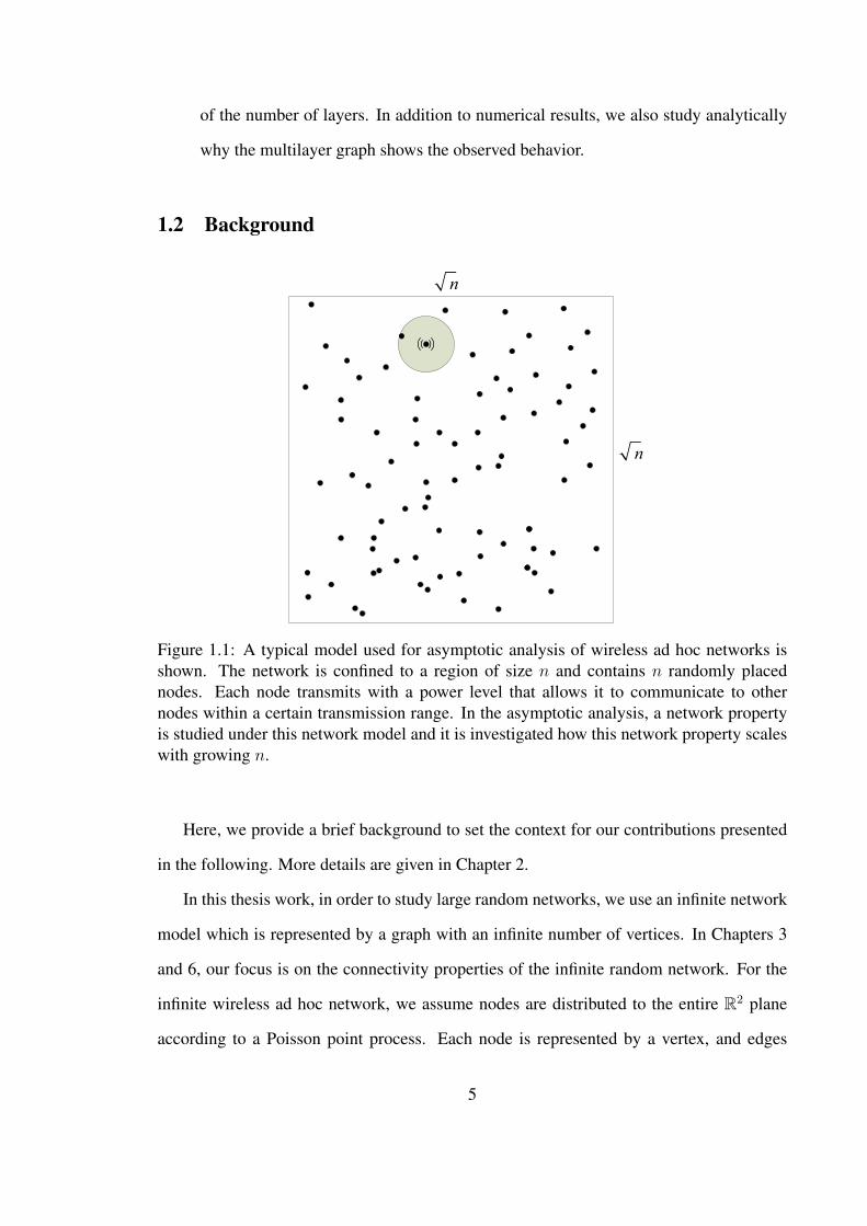
1.1 A typical model used for asymptotic analysis of wireless ad hoc networksis shown. The network is confined to a region of size n and contains nrandomly placed nodes. Each node transmits with a power level thatallows it to communicate to other nodes within a certain transmissionrange. In the asymptotic analysis, a network property is studied underthis network model and it is investigated how this network propertyscales with growing n. . . . . . . . . . . . . . . . . . . . . . . . . . . . . . . . . . . . . . . . . . . . . 5

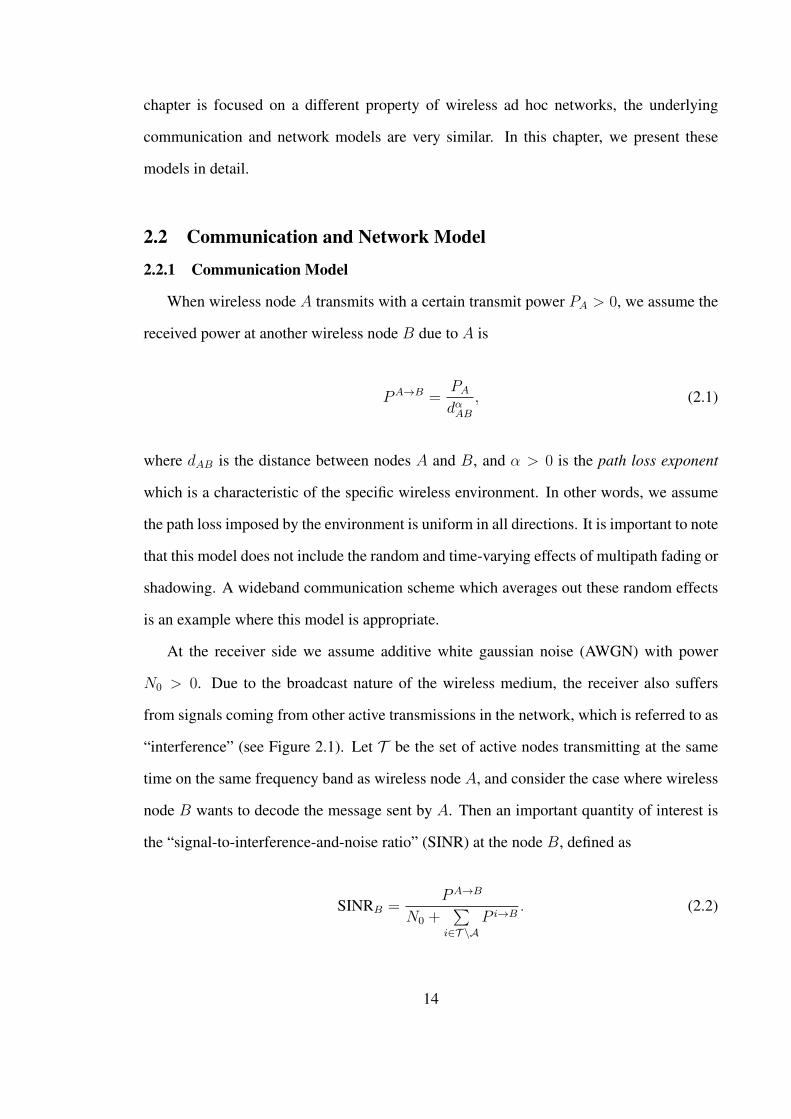
2.1 In the communication model, wireless nodes are assumed to be pointsources. The signal power received at a wireless node B due toanother node A decays with the distance dAB between nodes. Whentrying to decode A’s message, B suffers interference from signalscoming from other active nodes. . . . . . . . . . . . . . . . . . . . . . . . . . . . . . . . . . . . 15

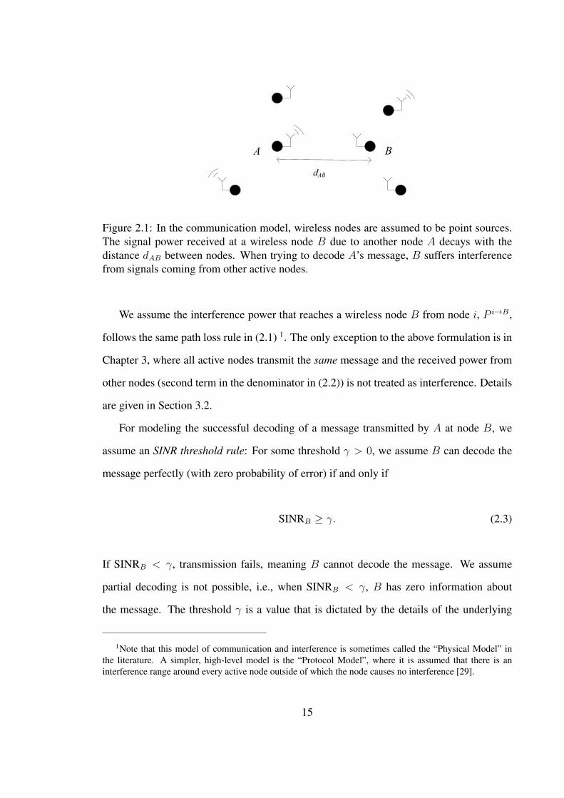
2.2 In the network model, we assume nodes to be placed randomly accordingto a Poisson point process in an infinite region. In the one-dimensionalcase, nodes are on the real line R (left figure). In the two-dimensionalcase, nodes are on the infinite plane R2 (right figure). . . . . . . . . . . . . . . . . . . 17

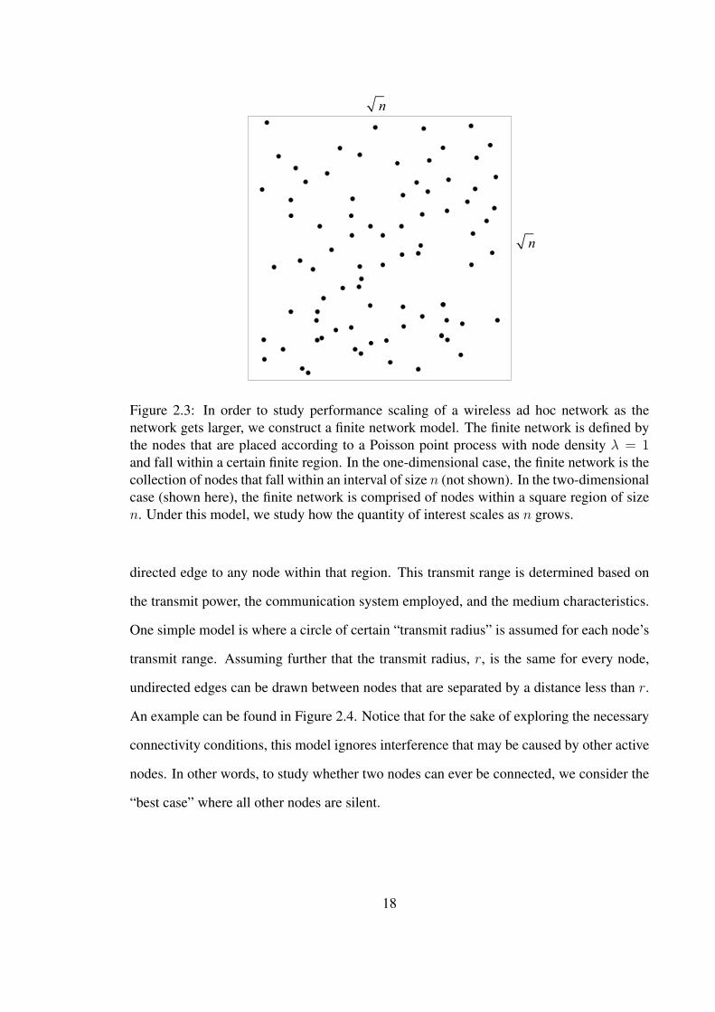
2.3 In order to study performance scaling of a wireless ad hoc network as thenetwork gets larger, we construct a finite network model. The finitenetwork is defined by the nodes that are placed according to a Poissonpoint process with node density λ = 1 and fall within a certain finiteregion. In the one-dimensional case, the finite network is thecollection of nodes that fall within an interval of size n (not shown). Inthe two-dimensional case (shown here), the finite network iscomprised of nodes within a square region of size n. Under thismodel, we study how the quantity of interest scales as n grows. . . . . . . . . . 18

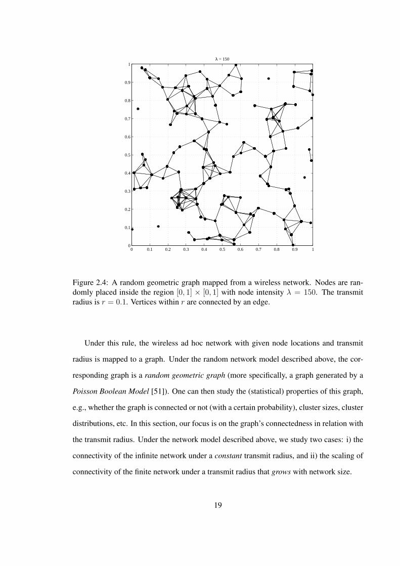
2.4 A random geometric graph mapped from a wireless network. Nodes arerandomly placed inside the region [0, 1]× [0, 1] with node intensityλ = 150. The transmit radius is r = 0.1. Vertices within r areconnected by an edge. . . . . . . . . . . . . . . . . . . . . . . . . . . . . . . . . . . . . . . . . . . . . 19

xv

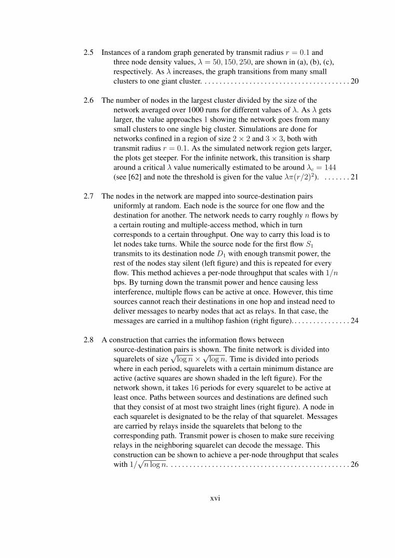
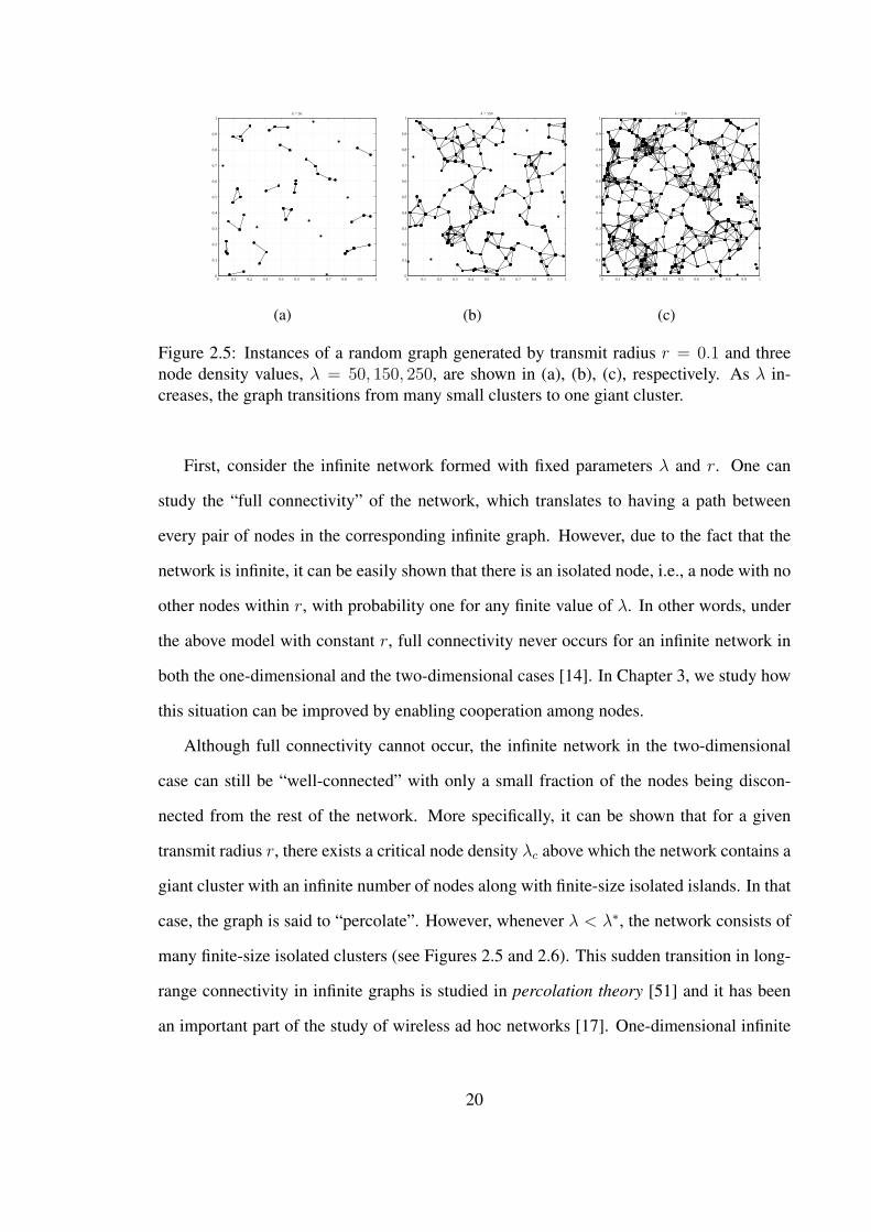
2.5 Instances of a random graph generated by transmit radius r = 0.1 andthree node density values, λ = 50, 150, 250, are shown in (a), (b), (c),respectively. As λ increases, the graph transitions from many smallclusters to one giant cluster. . . . . . . . . . . . . . . . . . . . . . . . . . . . . . . . . . . . . . . . 20

2.6 The number of nodes in the largest cluster divided by the size of thenetwork averaged over 1000 runs for different values of λ. As λ getslarger, the value approaches 1 showing the network goes from manysmall clusters to one single big cluster. Simulations are done fornetworks confined in a region of size 2× 2 and 3× 3, both withtransmit radius r = 0.1. As the simulated network region gets larger,the plots get steeper. For the infinite network, this transition is sharparound a critical λ value numerically estimated to be around λc = 144(see [62] and note the threshold is given for the value λπ(r/2)2). . . . . . . . 21

2.7 The nodes in the network are mapped into source-destination pairsuniformly at random. Each node is the source for one flow and thedestination for another. The network needs to carry roughly n flows bya certain routing and multiple-access method, which in turncorresponds to a certain throughput. One way to carry this load is tolet nodes take turns. While the source node for the first flow S1

transmits to its destination node D1 with enough transmit power, therest of the nodes stay silent (left figure) and this is repeated for everyflow. This method achieves a per-node throughput that scales with 1/nbps. By turning down the transmit power and hence causing lessinterference, multiple flows can be active at once. However, this timesources cannot reach their destinations in one hop and instead need todeliver messages to nearby nodes that act as relays. In that case, themessages are carried in a multihop fashion (right figure). . . . . . . . . . . . . . . . 24

2.8 A construction that carries the information flows betweensource-destination pairs is shown. The finite network is divided intosquarelets of size

√log n×

√log n. Time is divided into periods

where in each period, squarelets with a certain minimum distance areactive (active squares are shown shaded in the left figure). For thenetwork shown, it takes 16 periods for every squarelet to be active atleast once. Paths between sources and destinations are defined suchthat they consist of at most two straight lines (right figure). A node ineach squarelet is designated to be the relay of that squarelet. Messagesare carried by relays inside the squarelets that belong to thecorresponding path. Transmit power is chosen to make sure receivingrelays in the neighboring squarelet can decode the message. Thisconstruction can be shown to achieve a per-node throughput that scaleswith 1/

√n log n. . . . . . . . . . . . . . . . . . . . . . . . . . . . . . . . . . . . . . . . . . . . . . . . . 26

xvi

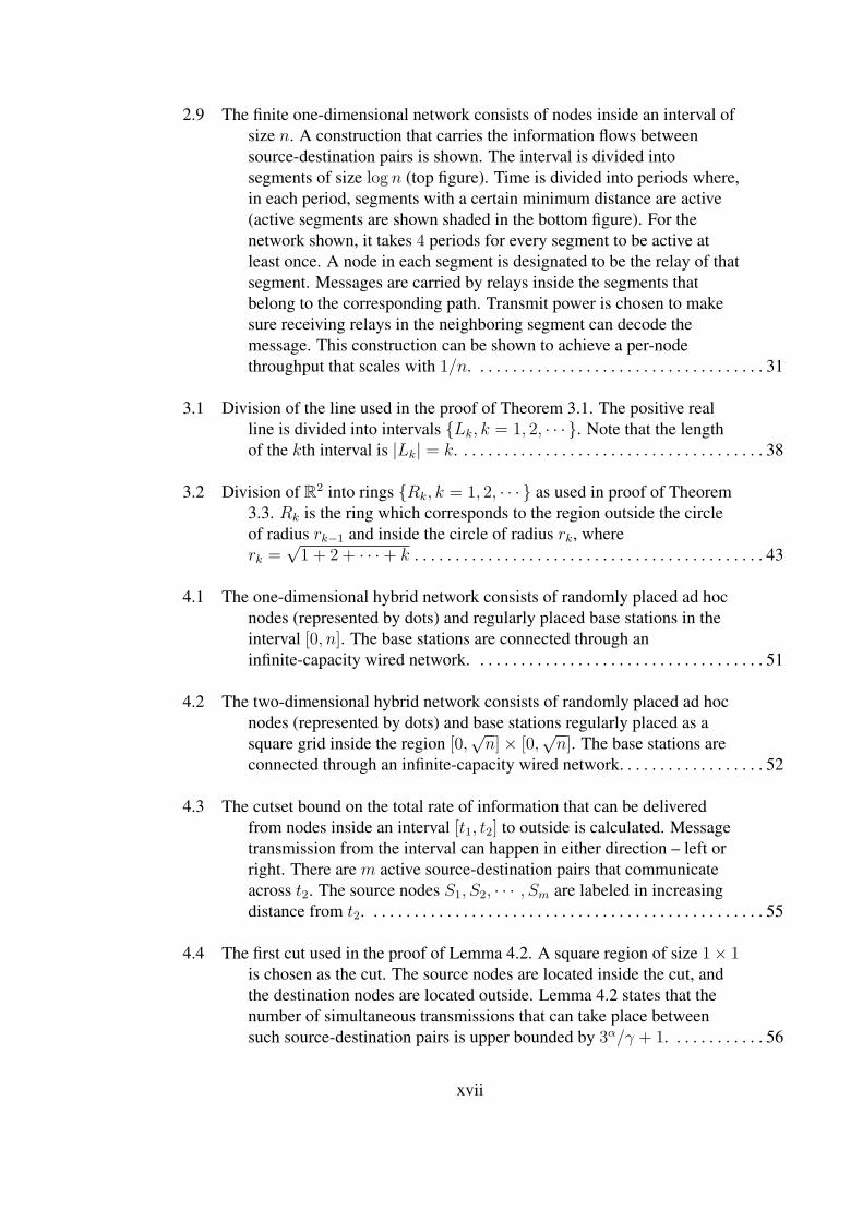
2.9 The finite one-dimensional network consists of nodes inside an interval ofsize n. A construction that carries the information flows betweensource-destination pairs is shown. The interval is divided intosegments of size log n (top figure). Time is divided into periods where,in each period, segments with a certain minimum distance are active(active segments are shown shaded in the bottom figure). For thenetwork shown, it takes 4 periods for every segment to be active atleast once. A node in each segment is designated to be the relay of thatsegment. Messages are carried by relays inside the segments thatbelong to the corresponding path. Transmit power is chosen to makesure receiving relays in the neighboring segment can decode themessage. This construction can be shown to achieve a per-nodethroughput that scales with 1/n. . . . . . . . . . . . . . . . . . . . . . . . . . . . . . . . . . . . 31

3.1 Division of the line used in the proof of Theorem 3.1. The positive realline is divided into intervals Lk, k = 1, 2, · · · . Note that the lengthof the kth interval is |Lk| = k. . . . . . . . . . . . . . . . . . . . . . . . . . . . . . . . . . . . . . 38

3.2 Division of R2 into rings Rk, k = 1, 2, · · · as used in proof of Theorem3.3. Rk is the ring which corresponds to the region outside the circleof radius rk−1 and inside the circle of radius rk, whererk =

√1 + 2 + · · ·+ k . . . . . . . . . . . . . . . . . . . . . . . . . . . . . . . . . . . . . . . . . . . 43

4.1 The one-dimensional hybrid network consists of randomly placed ad hocnodes (represented by dots) and regularly placed base stations in theinterval [0, n]. The base stations are connected through aninfinite-capacity wired network. . . . . . . . . . . . . . . . . . . . . . . . . . . . . . . . . . . . 51

4.2 The two-dimensional hybrid network consists of randomly placed ad hocnodes (represented by dots) and base stations regularly placed as asquare grid inside the region [0,

√n]× [0,

√n]. The base stations are

connected through an infinite-capacity wired network. . . . . . . . . . . . . . . . . . 52

4.3 The cutset bound on the total rate of information that can be deliveredfrom nodes inside an interval [t1, t2] to outside is calculated. Messagetransmission from the interval can happen in either direction – left orright. There are m active source-destination pairs that communicateacross t2. The source nodes S1, S2, · · · , Sm are labeled in increasingdistance from t2. . . . . . . . . . . . . . . . . . . . . . . . . . . . . . . . . . . . . . . . . . . . . . . . . 55

4.4 The first cut used in the proof of Lemma 4.2. A square region of size 1× 1is chosen as the cut. The source nodes are located inside the cut, andthe destination nodes are located outside. Lemma 4.2 states that thenumber of simultaneous transmissions that can take place betweensuch source-destination pairs is upper bounded by 3α/γ + 1. . . . . . . . . . . . 56

xvii

4.5 The strip used in the proof of Lemma 4.2. The number of simultaneoustransmissions that can take place from sources inside the strip todestinations to the right of the cut line is upper bounded by a constant.To prove the argument the division of the strip as in Figure 4.6 isused. . . . . . . . . . . . . . . . . . . . . . . . . . . . . . . . . . . . . . . . . . . . . . . . . . . . . . . . . . . 58

4.6 The strip is considered as the union of a square of size 1× 1 and a strip ofsize 1× ℓ− 1. The proof is obtained by upper bounding the number oftransmissions that can take place from source nodes within eachregion. . . . . . . . . . . . . . . . . . . . . . . . . . . . . . . . . . . . . . . . . . . . . . . . . . . . . . . . . . 59

4.7 The box of size ℓ× ℓ is considered as a union of four 1× ℓ strips for eachcut line. Hence, the number of transmissions through each cut line isupper bounded by a number proportional to ℓ. Considering all four cutlines that the transmissions can cross, the total rate of information thatcan be transmitted to the outside of the box is upper bounded by avalue proportional to the edge length ℓ. . . . . . . . . . . . . . . . . . . . . . . . . . . . . . 60

4.8 The 1-D network consists of b cells of length n/b. In the upload phase, thepacket is delivered to the closest base station through multihopcommunication (a). After the wired phase, the destination base stationdelivers the packet to the destination node following the reverse of theoperation in the upload phase (not shown). The cut Γs used to provethe upper bound is shown in (b). The cut is drawn around the ad hocnodes in a cell and can be crossed in three places. All these crossingshave constant capacity, bringing the overall cutset bound to aconstant. . . . . . . . . . . . . . . . . . . . . . . . . . . . . . . . . . . . . . . . . . . . . . . . . . . . . . . . 66

4.9 The region is divided into b cells, each of size√n/b×

√n/b (top figure).

A source node sends its packet to the destination in three steps. In theupload phase, the source node delivers the packet to the closest basestation through multihop communication (bottom figure). In the wiredphase, the packet is delivered from the source base station to thedestination base station. The download phase follows the reverseoperation of the upload phase (not shown). . . . . . . . . . . . . . . . . . . . . . . . . . . 69

4.10 Cut Γ has half of the ad hoc nodes on one side and the rest of the ad hocnodes and all base stations on the other side. Γ can be crossed into theb/2 base stations in addition to communication to other nodes throughthe middle line. Γs is drawn outside the nodes in a cell. This cut can becrossed to the base station and to nodes in other cells through ad hoccommunication. Crossings to each base station has constant capacity,while crossings through ad hoc have capacity proportional to thecorresponding edge length of the cut. . . . . . . . . . . . . . . . . . . . . . . . . . . . . . . . 70

xviii

5.1 The one-dimensional network consists of legitimate nodes (represented bydots) and eavesdroppers (represented by crosses) placed in the interval[0, n], divided into cells of length c(n) = log n, as part of the signalingconstruction. . . . . . . . . . . . . . . . . . . . . . . . . . . . . . . . . . . . . . . . . . . . . . . . . . . . . 80

5.2 The network is partitioned into regions (colors), where each region is acollection of cells regularly sampled in the linear grid. Cells in aregion are spaced (k + 1)(2l + 1)− 1 cells apart (k = 1, l = 2 in thefigure). Hence, the network consists of t = (k + 1)(2l + 1) regions(t = 10 in the figure). The network is shown here with four of those 10different regions highlighted. . . . . . . . . . . . . . . . . . . . . . . . . . . . . . . . . . . . . . . 80

5.3 The network is shown with one region Γi(n) highlighted as done in Figure5.2. Cj

i denotes the jth cell in region Γi(n). Around each cell, the“neighborhood” of that cell N(Cj

i ) is defined as the interval consistingof (2l + 1) cells (l = 2 above). So, neighborhoods are separated byk(2l + 1) cells (k = 1 above). . . . . . . . . . . . . . . . . . . . . . . . . . . . . . . . . . . . . . 82

5.4 (a) The route connecting a source node S to a destination node D isshown. At each hop, the packet is delivered to the next cell on theroute. (b) Whenever the route intersects a neighborhood N(Cj

i ), thepacket is transmitted such that it reaches over multiple cells at once. Atransmitting relay A inside the cell where the route enters N(Cj

i )transmits to a receiving relay B inside the cell where the route exitsN(Cj

i ), while a jammer node J inside Cji transmits artificial noise.

Hence, packets of color i are routed in a way that avoids entering theinteriors of neighborhoods N(Cj

i ). The only exception is possibly atthe start or the end of the route, as the source or the destination nodemay be located inside the interior of a neighborhood (destination nodeD is inside the interior of a neighborhood in (a)). . . . . . . . . . . . . . . . . . . . . . 83

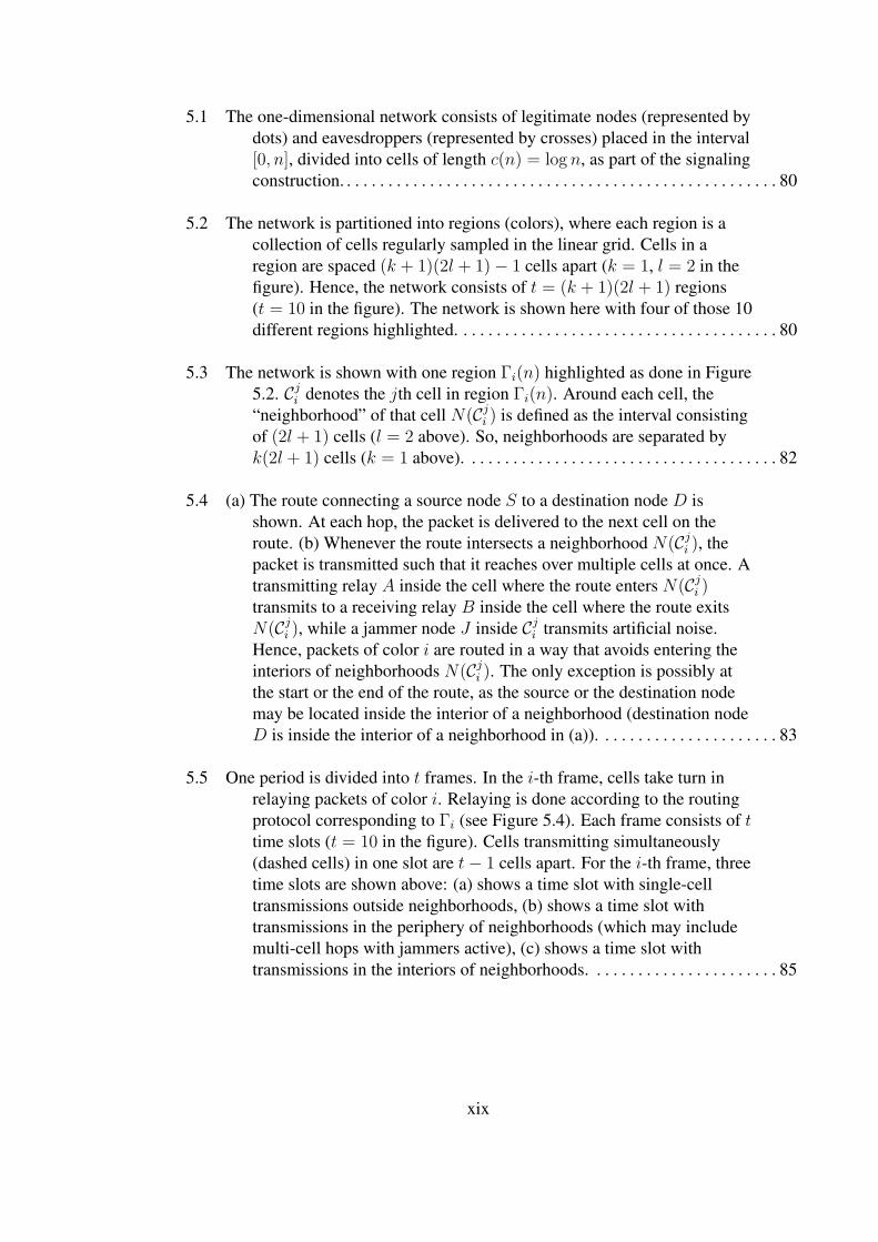
5.5 One period is divided into t frames. In the i-th frame, cells take turn inrelaying packets of color i. Relaying is done according to the routingprotocol corresponding to Γi (see Figure 5.4). Each frame consists of ttime slots (t = 10 in the figure). Cells transmitting simultaneously(dashed cells) in one slot are t− 1 cells apart. For the i-th frame, threetime slots are shown above: (a) shows a time slot with single-celltransmissions outside neighborhoods, (b) shows a time slot withtransmissions in the periphery of neighborhoods (which may includemulti-cell hops with jammers active), (c) shows a time slot withtransmissions in the interiors of neighborhoods. . . . . . . . . . . . . . . . . . . . . . . 85

xix

5.6 The two-dimensional network consists of legitimate nodes (represented bydots) and eavesdroppers (represented by crosses) placed in the square[0,

√n]× [0,

√n], divided into square cells of size c(n)× c(n), with

c(n) =√log n, as part of the signaling construction. . . . . . . . . . . . . . . . . . . 88

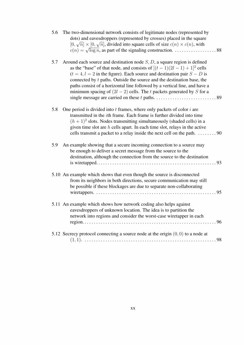
5.7 Around each source and destination node S,D, a square region is definedas the “base” of that node, and consists of [(t− 1)(2l − 1) + 1]2 cells(t = 4, l = 2 in the figure). Each source and destination pair S −D isconnected by t paths. Outside the source and the destination base, thepaths consist of a horizontal line followed by a vertical line, and have aminimum spacing of (2l − 2) cells. The t packets generated by S for asingle message are carried on these t paths. . . . . . . . . . . . . . . . . . . . . . . . . . . 89

5.8 One period is divided into t frames, where only packets of color i aretransmitted in the ith frame. Each frame is further divided into time(h+ 1)2 slots. Nodes transmitting simultaneously (shaded cells) in agiven time slot are h cells apart. In each time slot, relays in the activecells transmit a packet to a relay inside the next cell on the path. . . . . . . . . 90

5.9 An example showing that a secure incoming connection to a source maybe enough to deliver a secret message from the source to thedestination, although the connection from the source to the destinationis wiretapped. . . . . . . . . . . . . . . . . . . . . . . . . . . . . . . . . . . . . . . . . . . . . . . . . . . . 93

5.10 An example which shows that even though the source is disconnectedfrom its neighbors in both directions, secure communication may stillbe possible if these blockages are due to separate non-collaboratingwiretappers. . . . . . . . . . . . . . . . . . . . . . . . . . . . . . . . . . . . . . . . . . . . . . . . . . . . . 95

5.11 An example which shows how network coding also helps againsteavesdroppers of unknown location. The idea is to partition thenetwork into regions and consider the worst-case wiretapper in eachregion. . . . . . . . . . . . . . . . . . . . . . . . . . . . . . . . . . . . . . . . . . . . . . . . . . . . . . . . . . 96

5.12 Secrecy protocol connecting a source node at the origin (0, 0) to a node at(1, 1). . . . . . . . . . . . . . . . . . . . . . . . . . . . . . . . . . . . . . . . . . . . . . . . . . . . . . . . . . 98

xx

5.13 (Left) Around each source s, a “source base” is defined, which is a squareregion of size 7× 7 cells. The four (shaded) corner cells are the relaycells, where nodes are selected to help initiate the transmission. Thefour relays do two-way exchanges with the source to receive fourpackets that form the secret message. The locations of the relaysensure that (compared to the source) no eavesdropper can be locatedcloser to all relays at once, i.e., for any given eavesdropper e,d(s, ri) 6 d(e, ri) for some i ∈ 1, 2, 3, 4. (Right) The delivery of thefour packets to the destination is shown. As is the case for the drainingphase, due to the location of the relays, no eavesdropper can be closeenough to all relays at once to collect all four packets. . . . . . . . . . . . . . . . . 101

5.14 The source and the destination bases are connected with four paths, eachcarrying one of the packets. The paths have the same minimumspacing throughout the route; hence, no eavesdropper can be closeenough to all four paths at once. . . . . . . . . . . . . . . . . . . . . . . . . . . . . . . . . . . 103

6.1 Three instances of site percolation on a square lattice of size 41× 41 isshown. For ease of exposition, the sites labeled as unoccupied are notshown. The site occupation probabilities used for generating thegraphs in (a), (b), (c) are 0.4, 0.6, 0.8, respectively. As q increases, thegraph transitions from many small clusters to one giant cluster. . . . . . . . . 109

6.2 The number of nodes in the largest cluster divided by the size of thenetwork averaged over 100 runs for a square lattice graph plotted fordifferent values of site occupation probability q. As q gets larger, thevalue approaches one, showing that the network goes from many smallclusters to one single big cluster. Two plots are shown for lattices ofsize 51× 51 and 101× 101. As the simulated graph gets larger, theplots get steeper. For the infinite square lattice, this transition is sharparound a critical q value numerically estimated to be aroundqc = 0.59275 [54]. . . . . . . . . . . . . . . . . . . . . . . . . . . . . . . . . . . . . . . . . . . . . . 110

6.3 The multilayer graph is formed by combining subgraphs of the sameunderlying graph G. A two-layer graph G(2) is shown, which is theunion of the two layers G1 and G2. . . . . . . . . . . . . . . . . . . . . . . . . . . . . . . . . 111

6.4 The size of the largest cluster divided by the network size is plotted for anM -layer square lattice of size 512× 512 for different values ofsingle-layer site occupation probability q. The critical threshold qc(M)is estimated using the algorithm presented in [54] which is roughly thevalue where the curve makes a steep climb. The plots are drawn forvalues of M = 1, 2, · · · , 10. Percolation happens at smaller q values asM increases. . . . . . . . . . . . . . . . . . . . . . . . . . . . . . . . . . . . . . . . . . . . . . . . . . . 112

xxi

6.5 Critical site-occupation probability qc(M) for the M -layer graph plottedagainst the number of layers, M . As M increases, the multilayer graphpercolates for a smaller value of single-layer site occupationprobability q, hence qc(M) decreases. The values are numericallyestimated using an algorithm based on [54], on a square lattice and atriangular lattice of size both 512× 512. . . . . . . . . . . . . . . . . . . . . . . . . . . . 113

6.6 The multilayer graph is formed by combining subgraphs of the sameunderlying graph G. A two-layer graph G(2) is shown, which is theunion of the two layers G1 and G2. . . . . . . . . . . . . . . . . . . . . . . . . . . . . . . . . 114

6.7 Critical site-occupation probability qc(M) for the M -layer square latticegraph plotted against the number of layers, M , along with theconjectured upper bound. The plotted upper bound is given by√

1− (1− pc)1/M , where pc is the critical bond percolation threshold.pc = 0.5 for the square lattice. The upper bound gets tight as Mincreases. . . . . . . . . . . . . . . . . . . . . . . . . . . . . . . . . . . . . . . . . . . . . . . . . . . . . . 117

B.1 Source-destination pairs are placed inside the interval [−n, n], wheresource nodes are on one side of the point 0 and the destination nodesare on the other side. . . . . . . . . . . . . . . . . . . . . . . . . . . . . . . . . . . . . . . . . . . . . 131

B.2 Placement of source-destination pairs that lead to unbounded total ratethrough a single point as the network size increases. . . . . . . . . . . . . . . . . . . 132

xxii

CHAPTER 1

INTRODUCTION

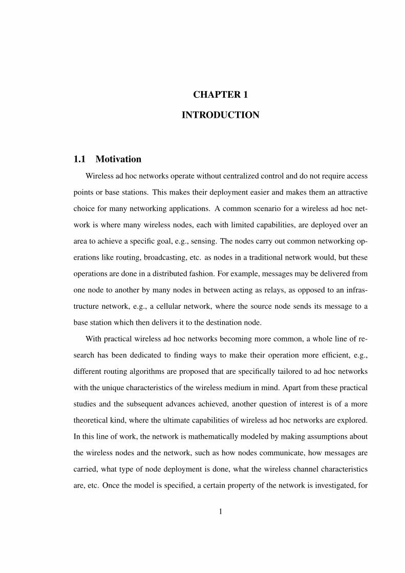
1.1 Motivation

Wireless ad hoc networks operate without centralized control and do not require access

points or base stations. This makes their deployment easier and makes them an attractive

choice for many networking applications. A common scenario for a wireless ad hoc net-

work is where many wireless nodes, each with limited capabilities, are deployed over an

area to achieve a specific goal, e.g., sensing. The nodes carry out common networking op-

erations like routing, broadcasting, etc. as nodes in a traditional network would, but these

operations are done in a distributed fashion. For example, messages may be delivered from

one node to another by many nodes in between acting as relays, as opposed to an infras-

tructure network, e.g., a cellular network, where the source node sends its message to a

base station which then delivers it to the destination node.

With practical wireless ad hoc networks becoming more common, a whole line of re-

search has been dedicated to finding ways to make their operation more efficient, e.g.,

different routing algorithms are proposed that are specifically tailored to ad hoc networks

with the unique characteristics of the wireless medium in mind. Apart from these practical

studies and the subsequent advances achieved, another question of interest is of a more

theoretical kind, where the ultimate capabilities of wireless ad hoc networks are explored.

In this line of work, the network is mathematically modeled by making assumptions about

the wireless nodes and the network, such as how nodes communicate, how messages are

carried, what type of node deployment is done, what the wireless channel characteristics

are, etc. Once the model is specified, a certain property of the network is investigated, for

1

example, how much information can be shared among the nodes per unit time, i.e., the

throughput capability of the network. These studies serve as guidance to practical algo-

rithms by showing what can be expected theoretically.

Many envisioned applications for wireless ad hoc networks involve very large networks

and a fundamental question is what happens to a certain network property as the network

gets larger; thus, one important characteristic these theoretical studies aim to extract is

how the network properties scale with increasing network size. For example, one may

investigate how the connectivity properties behave as a network with randomly located

nodes, each with a given transmission range, has an increasing number of nodes. Under

a given model, one can study, e.g., at what point connectivity breaks down, or how the

transmission ranges should scale with increasing network size to sustain connectivity of

the whole network.

This thesis work studies several scaling properties of wireless ad hoc networks where

nodes are randomly distributed to a region. Mainly, we focus on three important properties:

connectivity, information sharing capacity, and secret communication capabilities. In ad-

dition, we study the more general case of large random networks where the network is not

necessarily a prototypical communication network. Our work is comprised of four projects

summarized below.

1. We study the broadcast capabilities of nodes in a cooperative wireless ad hoc net-

work. Here the distinguishing property is the type of cooperation the nodes are able

to perform. In addition to simply relaying each other’s messages, we assume the

nodes are able to use a communication scheme where the same message is transmit-

ted by many nodes at once to combine the received power at the receiver node to

facilitate decoding. This cooperation improves the ability of nodes to broadcast their

message to the entire network, where the message is distributed in waves of nodes

transmitting together. We consider the extreme case of an infinite network, and ex-

plore whether by using this cooperation scheme, a message initiated at a node can

2

reach all nodes in the infinite network. Our work shows that the ability to broadcast

strongly depends on the type of wireless medium, in particular how fast the received

power decays with distance to the transmitting antenna. The probability of successful

broadcast is shown to be zero above a certain critical threshold on the exponent that

governs the relationship between the received power and the distance to the transmit-

ter node.

2. We consider capacity scaling in hybrid networks. Hybrid networks include both ad

hoc nodes and base stations. Here the wireless nodes have two options to deliver

messages to their destination nodes. They can operate as a pure ad hoc network where

other nodes are used as relays, or they can choose to switch to the wired network

via base stations for at least some part of the route. Obviously, the availability of

base stations may improve the communication capabilities of the wireless network

by increasing the rate at which data can be shared by wireless nodes. However, it is of

interest whether this improvement brings any scaling advantage as the network gets

larger. Previous work showed achievable results on the throughput scaling of hybrid

networks, hence showing a lower bound to the throughput benefit the base stations

can provide. In our work, we study upper bounds to explore the ultimate advantage

the base stations can realize. For a one-dimensional hybrid network where all nodes

are located on a line, we prove upper bounds that match previous achievable results,

hence completing the picture for the capacity of one-dimensional hybrid networks.

For two-dimensional hybrid networks, we establish analogous upper bounds, but we

have not shown these are achievable in all cases.

3. We consider scaling properties of secret communication in a wireless ad hoc network.

Here, the network includes eavesdropper nodes in addition to the wireless nodes that

share information. Starting with prior work that studies the fundamental communi-

cation capabilities, i.e., how many bits per second can be shared in a large wireless

3

network, we explore whether these limits can be achieved while also keeping the

messages secret from eavesdropper nodes. We show that this is indeed possible. In

particular, the throughput scaling shown in prior work can be achieved without re-

vealing the information to the eavesdropper nodes. We make use of network coding

tools to show this result, where nodes also perform simple coding operations instead

of only forwarding messages. Most importantly, our results show that this scaling

can be achieved without having to know where the eavesdroppers are located in the

network, which had been the common assumption in prior work studying secret com-

munication in wireless ad hoc networks.

4. We study connectivity properties of large random networks in general which do not

necessarily represent communication networks. For example, the graph may repre-

sent a social network where vertices represent people, and edges represent the rela-

tionship between them. We focus on the case of “multilayer graphs”, where different

types of edges may exist between vertices, e.g., representing work or family rela-

tionships. For each type of edge, a separate graph corresponding to that layer can be

formed, and the overall multilayer graph becomes the combination of these layers. In

our work, we study the connectivity properties of the multilayer graph. Note that even

when the layers are not well-connected individually, the multilayer graph can still be

well-connected. In the social network example, although two people A and B may

not be connected through a work-only chain, they may have a connection through

a chain that includes a person C in the family layer. We try to answer the question

how connected should each layer be so that the overall multilayer graph just starts to

be well-connected? The transition of large random graphs to a well-connected state

is studied in “percolation theory”. For traditional (single-layer) graphs, connectivity

behavior has been studied extensively in the literature. In our work, we extend these

results to multilayer graphs, and study the critical connectivity behavior as a function

4

of the number of layers. In addition to numerical results, we also study analytically

why the multilayer graph shows the observed behavior.

1.2 Background

n

n

Figure 1.1: A typical model used for asymptotic analysis of wireless ad hoc networks isshown. The network is confined to a region of size n and contains n randomly placednodes. Each node transmits with a power level that allows it to communicate to othernodes within a certain transmission range. In the asymptotic analysis, a network propertyis studied under this network model and it is investigated how this network property scaleswith growing n.

Here, we provide a brief background to set the context for our contributions presented

in the following. More details are given in Chapter 2.

In this thesis work, in order to study large random networks, we use an infinite network

model which is represented by a graph with an infinite number of vertices. In Chapters 3

and 6, our focus is on the connectivity properties of the infinite random network. For the

infinite wireless ad hoc network, we assume nodes are distributed to the entire R2 plane

according to a Poisson point process. Each node is represented by a vertex, and edges

5

are drawn between vertices that are within a certain transmission range. One fundamental

property of interest is whether this infinite graph has full connectivity, i.e., whether there

is a path between every pair of nodes. It can be shown that for this infinite graph, full

connectivity never occurs for any finite node density and transmission range, because an

isolated node can be found in the infinite network with probability one. In Chapter 3, we

study how this situation can be improved by cooperation between nodes.

An infinite graph which is not fully connected can still be “well-connected”, meaning

that although there are small isolated islands, there is a cluster spanning an infinite number

of nodes. In that case, this graph is said to “percolate”. Percolation theory studies the

connectivity properties of the infinite random graph. Central to percolation theory is the

phase transition phenomenon, in which as a local parameter is varied, the graph abruptly

transitions from a state of many small clusters to one giant cluster. The value at which this

transition happens is called the critical percolation threshold. Percolation is observed for

a wide range of infinite random graphs which do not necessarily represent communication

networks. An example is the infinite square lattice, where each vertex has four neighbors.

Consider a random process on this infinite graph, where each edge is independently deleted

with some probability. Clearly, as this deletion probability is varied from zero to one, the

resulting infinite network becomes less and less connected. What is less obvious is that,

there is a critical value at which the resulting graph suddenly transitions from one big

connected cluster to many small connected islands. This phase transition observed in the

infinite random graph is used to explain and model many real-life phenomena in a wide

range of fields. In Chapter 6, we study critical percolation thresholds for a special family

of graphs called multilayer graphs.

In order to study the asymptotic behavior of networks, we use an infinite network

model. However, sometimes it is also of interest to consider how the network converges to

its asymptotic behavior. In other words, the scaling properties of the network may be of in-

terest. This is the case in Chapters 4 and 5. In that case, we use a finite network model, and

6

study how a certain property of the network scales as the networks get larger. Figure 1.1

shows a typical model used for the asymptotic analysis of wireless ad hoc networks. Nodes

are randomly distributed to a two-dimensional box of size√n×

√nwith unit density, so the

region contains nwireless nodes on average. These n nodes form the wireless network. For

the traffic pattern, it is usually assumed that the nodes are randomly matched into source-

destination pairs, so that we have n pairs with their respective information flows. Because

nodes share the same medium, a fundamental property of wireless communication is inter-

ference. Whenever a node transmits, it creates interference to nearby nodes and degrades

the quality of the signal they receive. This puts a constraint on simultaneous transmissions,

which creates the fundamental limitation on the communication capacity of the network as

a whole.

In order to create as little interference as possible, one could limit the transmission

power of the wireless nodes so that nodes with enough separation between them can trans-

mit at the same time to improve the capacity of the network. However, with smaller transmit

power, it becomes harder for a source node to reach its destination directly, and therefore it

needs to use neighboring nodes as relays to forward its message. Hence, a message needs

to be transmitted many times before arriving at the destination, which decreases the capac-

ity. In other words, there is a trade-off between the spatial reuse of the band which helps

the capacity and the relaying burden caused by multihop transmission.

In their seminal paper [29], Gupta and Kumar study this trade-off and explore the fun-

damental limits on the rate data can be shared in multihop wireless networks. They show

that in to order to maximize capacity, it is optimal to reduce the transmit power as much

as possible. However, if the transmit power is too small, the connectivity of the network

itself breaks down. They establish that if the network is operated at the critical power

threshold for connectivity, the total throughput realized by the network scales proportional

to√n/ log n bits per second as n grows. This means the throughput available to each pair

goes down to zero with 1/√n log n, showing that wireless ad hoc networks in fact do not

7

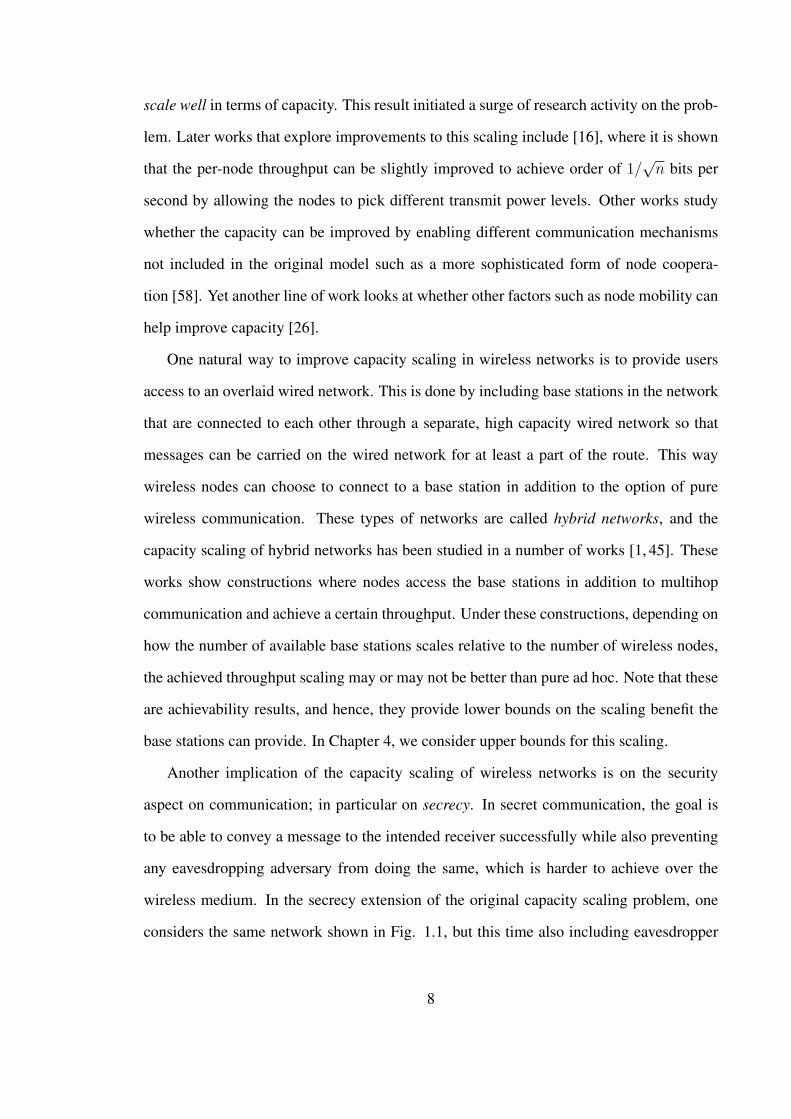
scale well in terms of capacity. This result initiated a surge of research activity on the prob-

lem. Later works that explore improvements to this scaling include [16], where it is shown

that the per-node throughput can be slightly improved to achieve order of 1/√n bits per

second by allowing the nodes to pick different transmit power levels. Other works study

whether the capacity can be improved by enabling different communication mechanisms

not included in the original model such as a more sophisticated form of node coopera-

tion [58]. Yet another line of work looks at whether other factors such as node mobility can

help improve capacity [26].

One natural way to improve capacity scaling in wireless networks is to provide users

access to an overlaid wired network. This is done by including base stations in the network

that are connected to each other through a separate, high capacity wired network so that

messages can be carried on the wired network for at least a part of the route. This way

wireless nodes can choose to connect to a base station in addition to the option of pure

wireless communication. These types of networks are called hybrid networks, and the

capacity scaling of hybrid networks has been studied in a number of works [1, 45]. These

works show constructions where nodes access the base stations in addition to multihop

communication and achieve a certain throughput. Under these constructions, depending on

how the number of available base stations scales relative to the number of wireless nodes,

the achieved throughput scaling may or may not be better than pure ad hoc. Note that these

are achievability results, and hence, they provide lower bounds on the scaling benefit the

base stations can provide. In Chapter 4, we consider upper bounds for this scaling.

Another implication of the capacity scaling of wireless networks is on the security

aspect on communication; in particular on secrecy. In secret communication, the goal is

to be able to convey a message to the intended receiver successfully while also preventing

any eavesdropping adversary from doing the same, which is harder to achieve over the

wireless medium. In the secrecy extension of the original capacity scaling problem, one

considers the same network shown in Fig. 1.1, but this time also including eavesdropper

8

nodes. Here, the fundamental question becomes whether achieving secret communication

is possible, and if it is, whether it will require compromise on the throughput scaling. The

secrecy notion adapted here is information-theoretic secrecy as originally studied for the

single-sender-single-receiver case in the framework of the wiretap channel [75]. In this

domain of research, [39] shows that the same construction used in [16] can be modified

and the same per-node throughput scaling of 1/√n bps can be achieved while keeping all

the information secret from eavesdroppers. In the proposed construction in [39], messages

are routed away from eavesdroppers to force them to have low received signal quality.

This requires the knowledge of eavesdropper locations, which is an undesired assumption.

In [73], it is shown that by using friendly jamming it is possible to achieve the same secrecy

scaling; however, the number of eavesdroppers that can be tolerated is limited to log n. We

consider in Chapter 5 whether this latter scaling result can be improved.

1.3 Contributions

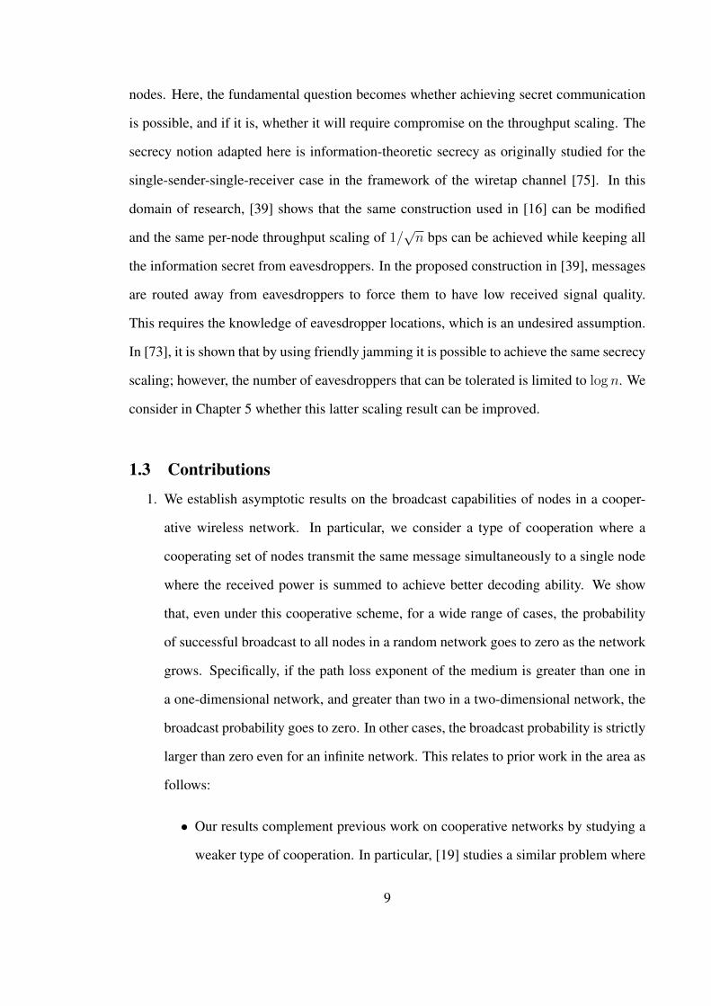
1. We establish asymptotic results on the broadcast capabilities of nodes in a cooper-

ative wireless network. In particular, we consider a type of cooperation where a

cooperating set of nodes transmit the same message simultaneously to a single node

where the received power is summed to achieve better decoding ability. We show

that, even under this cooperative scheme, for a wide range of cases, the probability

of successful broadcast to all nodes in a random network goes to zero as the network

grows. Specifically, if the path loss exponent of the medium is greater than one in

a one-dimensional network, and greater than two in a two-dimensional network, the

broadcast probability goes to zero. In other cases, the broadcast probability is strictly

larger than zero even for an infinite network. This relates to prior work in the area as

follows:

• Our results complement previous work on cooperative networks by studying a

weaker type of cooperation. In particular, [19] studies a similar problem where

9

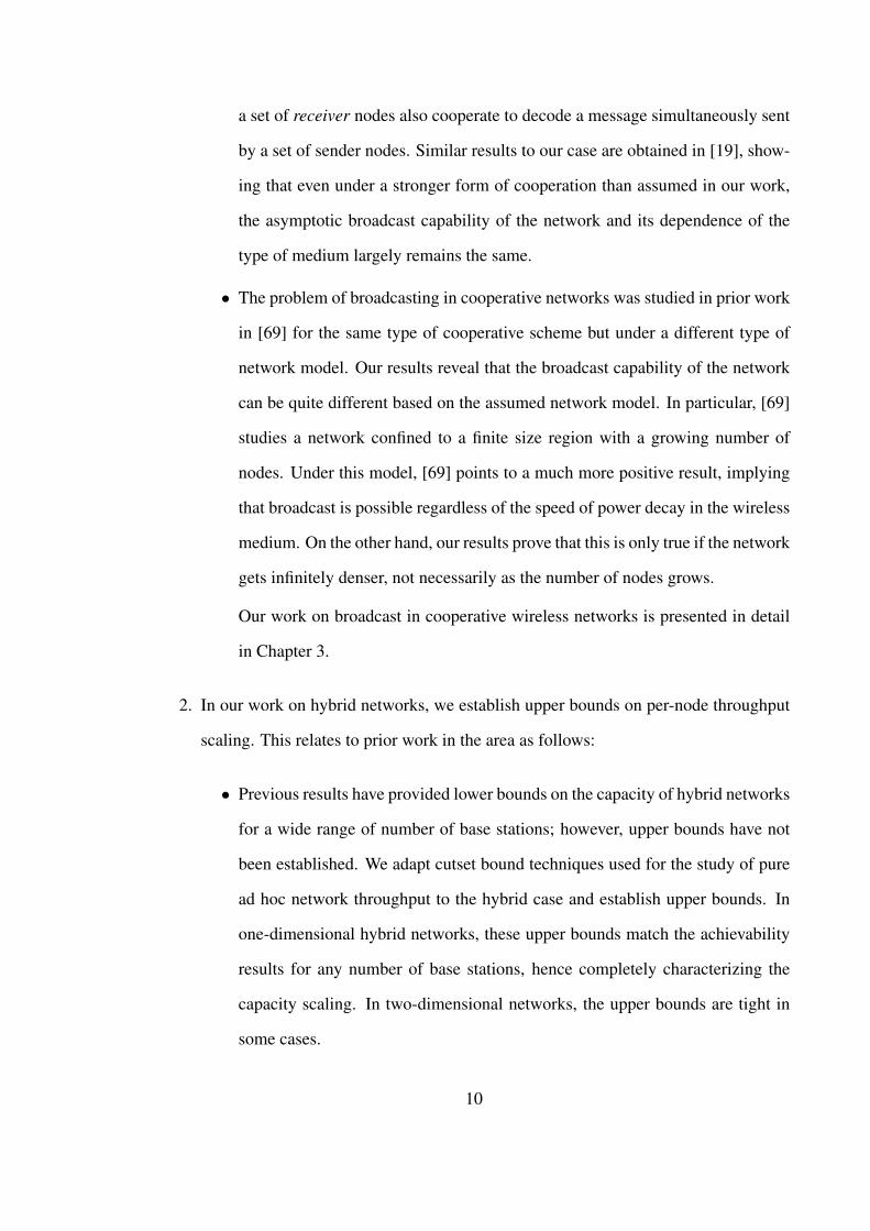
a set of receiver nodes also cooperate to decode a message simultaneously sent

by a set of sender nodes. Similar results to our case are obtained in [19], show-

ing that even under a stronger form of cooperation than assumed in our work,

the asymptotic broadcast capability of the network and its dependence of the

type of medium largely remains the same.

• The problem of broadcasting in cooperative networks was studied in prior work

in [69] for the same type of cooperative scheme but under a different type of

network model. Our results reveal that the broadcast capability of the network

can be quite different based on the assumed network model. In particular, [69]

studies a network confined to a finite size region with a growing number of

nodes. Under this model, [69] points to a much more positive result, implying

that broadcast is possible regardless of the speed of power decay in the wireless

medium. On the other hand, our results prove that this is only true if the network

gets infinitely denser, not necessarily as the number of nodes grows.

Our work on broadcast in cooperative wireless networks is presented in detail

in Chapter 3.

2. In our work on hybrid networks, we establish upper bounds on per-node throughput

scaling. This relates to prior work in the area as follows:

• Previous results have provided lower bounds on the capacity of hybrid networks

for a wide range of number of base stations; however, upper bounds have not

been established. We adapt cutset bound techniques used for the study of pure

ad hoc network throughput to the hybrid case and establish upper bounds. In

one-dimensional hybrid networks, these upper bounds match the achievability

results for any number of base stations, hence completely characterizing the

capacity scaling. In two-dimensional networks, the upper bounds are tight in

some cases.

10

• Previous work shows that the per-node throughput increases linearly in the

number of base stations for the case where the number of base stations grows

faster than the square root of the number of wireless nodes. This implies that in

the case where the number of base stations grows proportional to the number of

wireless nodes, it could potentially be possible to provide constant throughput

to nodes. By establishing a new result on the maxima of a sequence of Poisson

random variables, we show that this is not possible for some subset of nodes in

the network and their throughput goes to zero as the network grows. Further-

more, we provide a matching lower bound on per-node throughput, therefore

completing the capacity result in the case where the number of base stations is

proportional to the number of wireless nodes.

Our work on hybrid networks is given in Chapter 4.

3. In our work on secrecy, we show that secret communication in large wireless net-

works is possible without having to know the locations of the eavesdroppers. This

is a significant improvement to previous work, where knowledge of eavesdropper

locations has been the common assumption. Further, we show that secrecy can be

achieved without having to compromise on the throughput scaling. This relates to

prior work in the area as follows:

• Our results in secrecy reveal how coding techniques can be immensely useful

for secret communication in wireless ad hoc networks, which had previously

not been considered in the case of large wireless networks. Coding techniques

allow important problems to be tackled easily without resorting to expensive

physical-layer solutions such as the friendly jamming used in prior work. Fur-

thermore, for two-dimensional networks, we show that coding can also enable

secrecy in a more general case than typically considered in prior work by pro-

11

viding secrecy where an arbitrary number of eavesdroppers can be arbitrarily

located.

• We also study the case of secrecy in one-dimensional large networks, a prob-

lem not considered in previous work. Secrecy is especially challenging in this

case, as it is not possible to route around eavesdroppers, and a single eavesdrop-

per can practically disable secret communication between two sides of a point

on the line. We show that by using coding in addition to friendly jamming,

secret communication is possible, again without having to know eavesdropper

locations and without compromising on throughput scaling.

Details of our work on secrecy in wireless networks can be found in Chapter 5.

4. We study site percolation properties of the random multilayer graph. In site percola-

tion, vertices (sites) of a given graph are randomly labeled occupied or unoccupied,

and the edges incident on the unoccupied vertices are removed. Suppose each site is

occupied with probability q. Then there exists a critical value of q, qc, at which the

graph transitions from many small clusters to one giant cluster. This value is called

the site percolation threshold. The value of qc for many types of graphs has been

studied extensively in the literature. In our case, we generate several site percolation

instances of the same graph with some probability q, calling each of them a layer.

We call the union of these layers the multilayer graph, and we are interested in the

critical q value that makes the multilayer graph percolate. Obviously, this value is

smaller than the single-layer case, and decreases as the number of layers increase.

In our work, we show by simulations that the critical threshold value follows an in-

verse square root behavior. In particular, if the graph is formed by combining M

layers, the critical threshold scales with 1/√M . Moreover, we study analytically the

exact function that governs this behavior, and conjecture an asymptotic relation that

matches numerical results very closely.

12

CHAPTER 2

BACKGROUND

This chapter presents models for wireless communication networks, and discusses im-

portant previous results in the area of asymptotic analysis of wireless networks that serve

as a background for the following chapters.

2.1 Introduction

Wireless communication networks have been rapidly replacing their wired counterparts

in many applications. However, most current wireless networks are, in fact, a relatively

small appendage to a large traditional wired network. For example, in cellular networks,

cell phones communicate directly with base stations which are part of the traditional tele-

phone network. Similarly, in WiFi networks, wireless devices such as laptops and tablets

are just a single wireless connection away from the wired internet infrastructure.

The advances in wireless communications now also make it possible to form what are

called “wireless ad hoc networks”. In wireless ad hoc networks, wireless devices commu-

nicate with each other, possibly through multiple “hops”, without the need for centralized

control, e.g., a base station. An example is a collection of laptops in the same building

that form a wireless network to exchange messages without the need for an access point.

Wireless ad hoc networks bring greater flexibility and quick deployment of networks where

infrastructure may not be available or may be costly to deploy. This makes them an attrac-

tive choice for many applications including future generation wireless technologies [52].

The following chapters are concerned with modeling and performance analysis of large

wireless ad hoc networks, i.e., wireless ad hoc networks with many nodes. Although each

13

chapter is focused on a different property of wireless ad hoc networks, the underlying

communication and network models are very similar. In this chapter, we present these

models in detail.

2.2 Communication and Network Model

2.2.1 Communication Model

When wireless node A transmits with a certain transmit power PA > 0, we assume the

received power at another wireless node B due to A is

PA→B =PA

dαAB

, (2.1)

where dAB is the distance between nodes A and B, and α > 0 is the path loss exponent

which is a characteristic of the specific wireless environment. In other words, we assume

the path loss imposed by the environment is uniform in all directions. It is important to note

that this model does not include the random and time-varying effects of multipath fading or

shadowing. A wideband communication scheme which averages out these random effects

is an example where this model is appropriate.

At the receiver side we assume additive white gaussian noise (AWGN) with power

N0 > 0. Due to the broadcast nature of the wireless medium, the receiver also suffers

from signals coming from other active transmissions in the network, which is referred to as

“interference” (see Figure 2.1). Let T be the set of active nodes transmitting at the same

time on the same frequency band as wireless node A, and consider the case where wireless

node B wants to decode the message sent by A. Then an important quantity of interest is

the “signal-to-interference-and-noise ratio” (SINR) at the node B, defined as

SINRB =PA→B

N0 +∑

i∈T \AP i→B

. (2.2)

14

A B

dAB

Figure 2.1: In the communication model, wireless nodes are assumed to be point sources.The signal power received at a wireless node B due to another node A decays with thedistance dAB between nodes. When trying to decode A’s message, B suffers interferencefrom signals coming from other active nodes.

We assume the interference power that reaches a wireless node B from node i, P i→B,

follows the same path loss rule in (2.1) 1. The only exception to the above formulation is in

Chapter 3, where all active nodes transmit the same message and the received power from

other nodes (second term in the denominator in (2.2)) is not treated as interference. Details

are given in Section 3.2.

For modeling the successful decoding of a message transmitted by A at node B, we

assume an SINR threshold rule: For some threshold γ > 0, we assume B can decode the

message perfectly (with zero probability of error) if and only if

SINRB ≥ γ. (2.3)

If SINRB < γ, transmission fails, meaning B cannot decode the message. We assume

partial decoding is not possible, i.e., when SINRB < γ, B has zero information about

the message. The threshold γ is a value that is dictated by the details of the underlying

1Note that this model of communication and interference is sometimes called the “Physical Model” inthe literature. A simpler, high-level model is the “Protocol Model”, where it is assumed that there is aninterference range around every active node outside of which the node causes no interference [29].

15

communication system. For the problems in this thesis, it is assumed γ is given, and the

system parameters for the respective problem are designed around this value.

2.2.2 Network Model

In this work, we are interested in the asymptotic performance of wireless ad hoc net-

works. This means the network contains infinitely many nodes. We assume nodes are

at fixed, random locations. We study both one-dimensional and two-dimensional net-

works. In the one-dimensional case, the nodes are placed on the real line R, and in the

two-dimensional case, on the plane R2 (see Figure 2.2). Nodes are assumed to be placed

according to a homogeneous Poisson point process with node intensity λ > 0. Notice

that we model wireless nodes as point sources and enforce no minimum distance between

nodes. Under this model, we study how this infinite network performs. For example, in

Chapter 3 we study whether a node can broadcast its messages to the entire infinite region.

When we study asymptotic limits, we are sometimes also interested in how the quantity

of interest goes to that limit, i.e., the convergence rate may also be of concern. In that case,

we need to define a finite network model and study explicitly how this network performs as

it contains more and more nodes and gets closer to the infinite network defined above. This

is the case in Chapters 4 and 5, where we are interested in the performance scaling of the

network. In these works, we consider a certain region inside R or R2, and define the finite

network as the set of nodes that fall inside this region. In particular, for the variable n > 0,

we consider the interval [−n/2, n/2] and the box [−√n/2,

√n/2] × [−

√n/2,

√n/2], for

the one-dimensional and the two-dimensional cases, respectively (see Figure 2.3). Assum-

ing a node density of λ = 1, we study how the performance of the network scales as

n→ ∞.

Note that another way to do asymptotic analysis is to study a network with infinitely

many nodes in a finite size region. This model is often referred to as a “dense network”,

whereas our model described above is called an “extended network”.

16

n

n

Figure 2.2: In the network model, we assume nodes to be placed randomly according to aPoisson point process in an infinite region. In the one-dimensional case, nodes are on thereal line R (left figure). In the two-dimensional case, nodes are on the infinite plane R2

(right figure).

2.3 Connectivity of Wireless Ad Hoc Networks

One basic property of interest for any communication network is its “connectivity”.

Connectivity determines the network’s ability to carry information between its members.

In order to study connectivity, it is convenient to model the network as a graph with a set

of vertices and edges, where vertices represent the members of the network and an edge

exists between two vertices whenever the nodes representing them have a direct connection.

For wired networks, there is a natural mapping from the network to a graph as every edge

corresponds to a physical link.

Mapping a wireless ad hoc network to a graph to study its connectivity is not as obvious

as in the wired case. A direct link between two wireless nodes may be introduced depending

on the wireless signal quality. One basic way to do this is to assume a “transmit range” for

each node. Here, it is assumed that every node has a certain region around it and it has a

17

n

n

Figure 2.3: In order to study performance scaling of a wireless ad hoc network as thenetwork gets larger, we construct a finite network model. The finite network is defined bythe nodes that are placed according to a Poisson point process with node density λ = 1and fall within a certain finite region. In the one-dimensional case, the finite network is thecollection of nodes that fall within an interval of size n (not shown). In the two-dimensionalcase (shown here), the finite network is comprised of nodes within a square region of sizen. Under this model, we study how the quantity of interest scales as n grows.

directed edge to any node within that region. This transmit range is determined based on

the transmit power, the communication system employed, and the medium characteristics.

One simple model is where a circle of certain “transmit radius” is assumed for each node’s

transmit range. Assuming further that the transmit radius, r, is the same for every node,

undirected edges can be drawn between nodes that are separated by a distance less than r.

An example can be found in Figure 2.4. Notice that for the sake of exploring the necessary

connectivity conditions, this model ignores interference that may be caused by other active

nodes. In other words, to study whether two nodes can ever be connected, we consider the

“best case” where all other nodes are silent.

18

0 0.1 0.2 0.3 0.4 0.5 0.6 0.7 0.8 0.9 10

0.1

0.2

0.3

0.4

0.5

0.6

0.7

0.8

0.9

1λ = 150

Figure 2.4: A random geometric graph mapped from a wireless network. Nodes are ran-domly placed inside the region [0, 1] × [0, 1] with node intensity λ = 150. The transmitradius is r = 0.1. Vertices within r are connected by an edge.

Under this rule, the wireless ad hoc network with given node locations and transmit

radius is mapped to a graph. Under the random network model described above, the cor-

responding graph is a random geometric graph (more specifically, a graph generated by a

Poisson Boolean Model [51]). One can then study the (statistical) properties of this graph,

e.g., whether the graph is connected or not (with a certain probability), cluster sizes, cluster

distributions, etc. In this section, our focus is on the graph’s connectedness in relation with

the transmit radius. Under the network model described above, we study two cases: i) the

connectivity of the infinite network under a constant transmit radius, and ii) the scaling of

connectivity of the finite network under a transmit radius that grows with network size.

19

0 0.1 0.2 0.3 0.4 0.5 0.6 0.7 0.8 0.9 10

0.1

0.2

0.3

0.4

0.5

0.6

0.7

0.8

0.9

1λ = 50

(a)

0 0.1 0.2 0.3 0.4 0.5 0.6 0.7 0.8 0.9 10

0.1

0.2

0.3

0.4

0.5

0.6

0.7

0.8

0.9

1λ = 150

(b)

0 0.1 0.2 0.3 0.4 0.5 0.6 0.7 0.8 0.9 10

0.1

0.2

0.3

0.4

0.5

0.6

0.7

0.8

0.9

1λ = 250

(c)

Figure 2.5: Instances of a random graph generated by transmit radius r = 0.1 and threenode density values, λ = 50, 150, 250, are shown in (a), (b), (c), respectively. As λ in-creases, the graph transitions from many small clusters to one giant cluster.

First, consider the infinite network formed with fixed parameters λ and r. One can

study the “full connectivity” of the network, which translates to having a path between

every pair of nodes in the corresponding infinite graph. However, due to the fact that the

network is infinite, it can be easily shown that there is an isolated node, i.e., a node with no

other nodes within r, with probability one for any finite value of λ. In other words, under

the above model with constant r, full connectivity never occurs for an infinite network in

both the one-dimensional and the two-dimensional cases [14]. In Chapter 3, we study how

this situation can be improved by enabling cooperation among nodes.

Although full connectivity cannot occur, the infinite network in the two-dimensional

case can still be “well-connected” with only a small fraction of the nodes being discon-

nected from the rest of the network. More specifically, it can be shown that for a given

transmit radius r, there exists a critical node density λc above which the network contains a

giant cluster with an infinite number of nodes along with finite-size isolated islands. In that

case, the graph is said to “percolate”. However, whenever λ < λ∗, the network consists of

many finite-size isolated clusters (see Figures 2.5 and 2.6). This sudden transition in long-

range connectivity in infinite graphs is studied in percolation theory [51] and it has been

an important part of the study of wireless ad hoc networks [17]. One-dimensional infinite

20

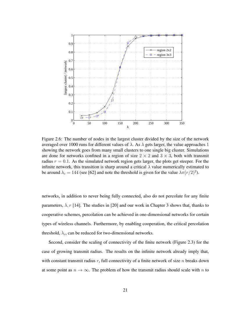
0 50 100 150 200 250 300 3500

0.1

0.2

0.3

0.4

0.5

0.6

0.7

0.8

0.9

1

λ

|larg

est c

lust

er| /

|net

wor

k|

region 2x2

region 3x3

Figure 2.6: The number of nodes in the largest cluster divided by the size of the networkaveraged over 1000 runs for different values of λ. As λ gets larger, the value approaches 1showing the network goes from many small clusters to one single big cluster. Simulationsare done for networks confined in a region of size 2 × 2 and 3 × 3, both with transmitradius r = 0.1. As the simulated network region gets larger, the plots get steeper. For theinfinite network, this transition is sharp around a critical λ value numerically estimated tobe around λc = 144 (see [62] and note the threshold is given for the value λπ(r/2)2).

networks, in addition to never being fully connected, also do not percolate for any finite

parameters, λ, r [14]. The studies in [20] and our work in Chapter 3 shows that, thanks to

cooperative schemes, percolation can be achieved in one-dimensional networks for certain

types of wireless channels. Furthermore, by enabling cooperation, the critical percolation

threshold, λc, can be reduced for two-dimensional networks.

Second, consider the scaling of connectivity of the finite network (Figure 2.3) for the

case of growing transmit radius. The results on the infinite network already imply that,

with constant transmit radius r, full connectivity of a finite network of size n breaks down

at some point as n → ∞. The problem of how the transmit radius should scale with n to

21

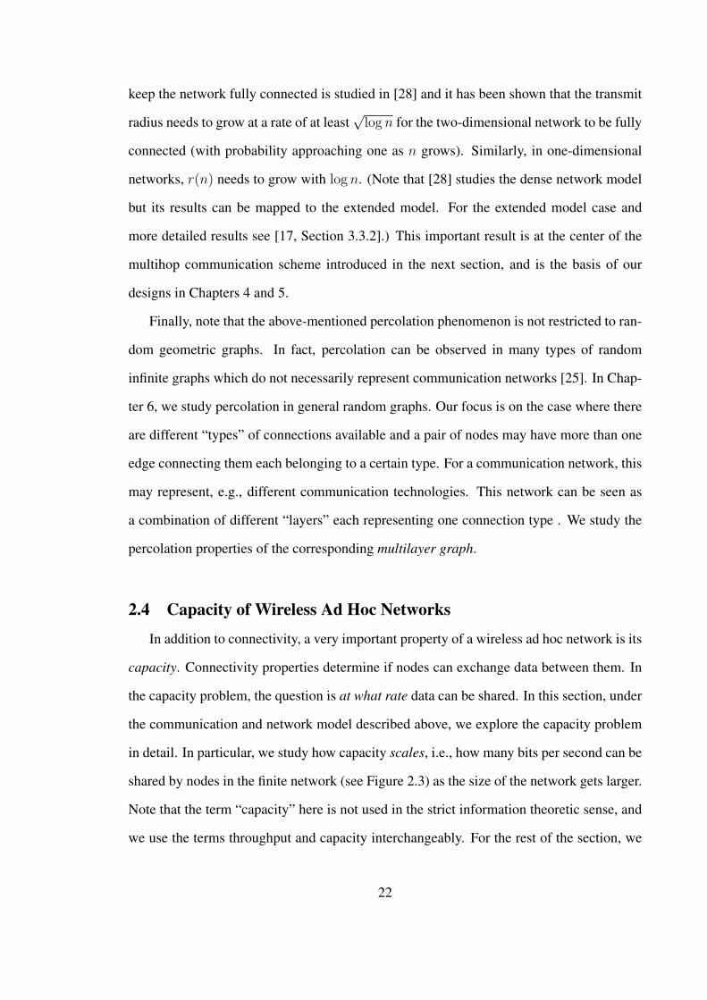
keep the network fully connected is studied in [28] and it has been shown that the transmit

radius needs to grow at a rate of at least√log n for the two-dimensional network to be fully

connected (with probability approaching one as n grows). Similarly, in one-dimensional

networks, r(n) needs to grow with log n. (Note that [28] studies the dense network model

but its results can be mapped to the extended model. For the extended model case and

more detailed results see [17, Section 3.3.2].) This important result is at the center of the

multihop communication scheme introduced in the next section, and is the basis of our

designs in Chapters 4 and 5.

Finally, note that the above-mentioned percolation phenomenon is not restricted to ran-

dom geometric graphs. In fact, percolation can be observed in many types of random

infinite graphs which do not necessarily represent communication networks [25]. In Chap-

ter 6, we study percolation in general random graphs. Our focus is on the case where there

are different “types” of connections available and a pair of nodes may have more than one

edge connecting them each belonging to a certain type. For a communication network, this

may represent, e.g., different communication technologies. This network can be seen as

a combination of different “layers” each representing one connection type . We study the

percolation properties of the corresponding multilayer graph.

2.4 Capacity of Wireless Ad Hoc Networks

In addition to connectivity, a very important property of a wireless ad hoc network is its

capacity. Connectivity properties determine if nodes can exchange data between them. In

the capacity problem, the question is at what rate data can be shared. In this section, under

the communication and network model described above, we explore the capacity problem

in detail. In particular, we study how capacity scales, i.e., how many bits per second can be

shared by nodes in the finite network (see Figure 2.3) as the size of the network gets larger.

Note that the term “capacity” here is not used in the strict information theoretic sense, and

we use the terms throughput and capacity interchangeably. For the rest of the section, we

22

confine ourselves mostly to two-dimensional networks and then finish by briefly presenting

the one-dimensional case.

2.4.1 Traffic Model

The nodes in the two-dimensional finite network are matched into source-destination

pairs uniformly at random. Hence, each node is the source for an information flow, and

also the destination for another (see Figure 2.7). This kind of traffic pattern is also called

multiple unicast. The network needs to carry roughly n information flows, and the question

of interest is at what rate these flows can be carried. There is a frequency band of fixed

bandwidth allocated for this traffic. Over this band, nodes can transmit atW bits per second

(bps) and this value is a constant (does not grow with n). In order to carry the traffic load,

a certain routing and multiple-access algorithm (which together we call a “construction”)

needs to be designed, and the selected construction determines the achieved throughput.

2.4.2 Multihop Routing

In order to get a sense of the capacity problem, consider the simple multiple-access al-

gorithm for carrying the n information flows where nodes simply take turns to deliver their

messages. Assuming that each node transmits with enough power to reach its destination,

i.e., with a single-hop routing algorithm, it takes on the order of n time slots to finish car-

rying the total load (see Figure 2.7). In other words, with this construction, a throughput

value that scales as 1/n bps is achieved per source-destination pair. Hence, as the network

gets larger, the number of bits that can be shared by each pair under this construction goes

down to zero at a rate reciprocal of the number of nodes.

The problem with the above construction is that the active node creates too much inter-

ference, and hence, the rest of the network needs to stay idle. In order to increase efficiency,

the transmit power of the nodes can be turned down to decrease interference so that nodes

with enough distance between them can be active simultaneously, i.e., the nodes can ben-

efit from the spatial reuse of the available band. However, this in turn makes the source

23

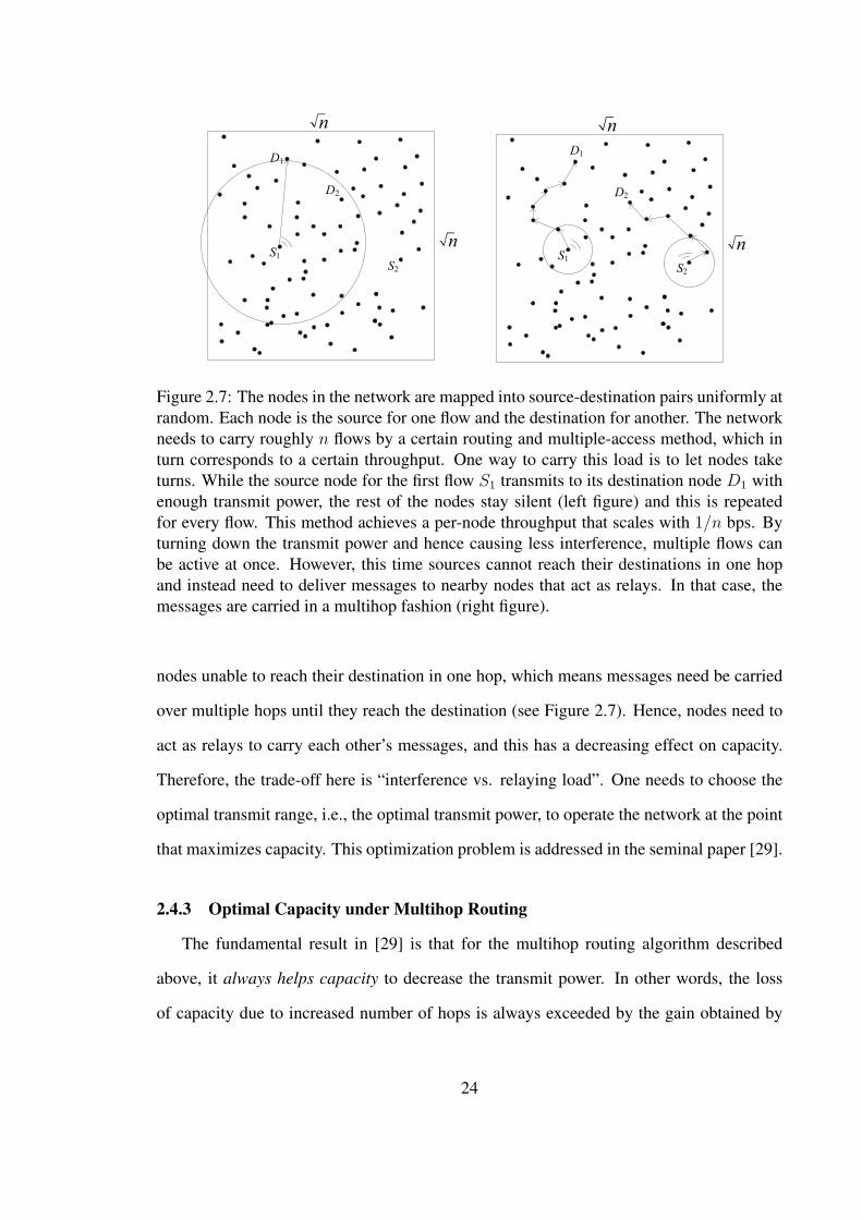
n

n

n

n

S1

S2

D1

D2

S1

D1

n

n

S1

D1

S2

D2

S2

D2

Figure 2.7: The nodes in the network are mapped into source-destination pairs uniformly atrandom. Each node is the source for one flow and the destination for another. The networkneeds to carry roughly n flows by a certain routing and multiple-access method, which inturn corresponds to a certain throughput. One way to carry this load is to let nodes taketurns. While the source node for the first flow S1 transmits to its destination node D1 withenough transmit power, the rest of the nodes stay silent (left figure) and this is repeatedfor every flow. This method achieves a per-node throughput that scales with 1/n bps. Byturning down the transmit power and hence causing less interference, multiple flows canbe active at once. However, this time sources cannot reach their destinations in one hopand instead need to deliver messages to nearby nodes that act as relays. In that case, themessages are carried in a multihop fashion (right figure).

nodes unable to reach their destination in one hop, which means messages need be carried

over multiple hops until they reach the destination (see Figure 2.7). Hence, nodes need to

act as relays to carry each other’s messages, and this has a decreasing effect on capacity.

Therefore, the trade-off here is “interference vs. relaying load”. One needs to choose the

optimal transmit range, i.e., the optimal transmit power, to operate the network at the point

that maximizes capacity. This optimization problem is addressed in the seminal paper [29].

2.4.3 Optimal Capacity under Multihop Routing

The fundamental result in [29] is that for the multihop routing algorithm described

above, it always helps capacity to decrease the transmit power. In other words, the loss

of capacity due to increased number of hops is always exceeded by the gain obtained by

24

reduced interference. The basic idea is that decreasing the transmit range r(n) increases

the number of hops linearly, however, it also frees up space for spatial reuse that increases

quadratically [29]. Although capacity increases with decreasing transmit radius, the trans-

mit radius cannot be decreased indefinitely. As discussed in the previous section, connec-

tivity breaks down for too small r(n). Hence, the optimal operating point for multihop

routing is exactly the critical transmit power required for connectivity. Assuming the same

transmit power for each node, this means a transmit range r(n) that scales as√log n max-

imizes capacity.

In order to see what capacity scaling is achieved under multihop routing with r(n) that

scales with√log n, we present a construction, i.e., a routing and multiple-access algo-

rithm, that uses this transmit power. We divide the finite network into “squarelets” of size√log n ×

√log n as shown in Figure 2.8. It can be easily shown that each squarelet con-

tains at least one node with high probability (w.h.p.), i.e., with probability going to one as

n increases. Inside each squarelet, we designate one node to be the relay of that squarelet.

For each information flow, we define a path between the source and the destination node

that consists of squarelets on straight lines (see Figure 2.8). Each message is carried on

this path by the corresponding relays until it reaches its destination. Because the transmit

radius is selected to grow with√log n, relays are able to reach the next node on the path.

The multiple-access algorithm is defined such that squarelets with a certain minimum

distance between them can be active at the same time. This minimum distance can be

determined by measuring the total interference at a receiving relay arriving from all active

squarelets. The important detail here is that for path loss exponents α > 2, this minimum

distance can be selected to be a constant value that is independent of n. Time is divided

into periods and the squarelets take turns. At the end of a constant number of periods, each

squarelet gets to be active once (see Figure 2.8).

The throughput achieved under this construction can be found by focusing on the relay-

ing load of a single relay in a given squarelet. Due to the way paths are defined, this relay

25

S

D

n n

n n

Figure 2.8: A construction that carries the information flows between source-destinationpairs is shown. The finite network is divided into squarelets of size

√log n×

√log n. Time

is divided into periods where in each period, squarelets with a certain minimum distanceare active (active squares are shown shaded in the left figure). For the network shown, ittakes 16 periods for every squarelet to be active at least once. Paths between sources anddestinations are defined such that they consist of at most two straight lines (right figure).A node in each squarelet is designated to be the relay of that squarelet. Messages arecarried by relays inside the squarelets that belong to the corresponding path. Transmitpower is chosen to make sure receiving relays in the neighboring squarelet can decode themessage. This construction can be shown to achieve a per-node throughput that scales with1/√n log n.

needs to carry messages that belong to source nodes that are located inside squarelets on

the same row or the column. The number of nodes inside that region can be easily shown to

scale as√n log n w.h.p. Hence, the total traffic load of this relay can be finished in a con-

stant factor of√n log n periods. Further, it can be shown that no relay has to deliver more

than a constant factor of√n log n messages. This means under the multihop routing case

with optimal transmit radius, the throughput achieved per source-destination pair scales as

1/√n log n bps.

In Chapter 5, we study scaling of the secrecy capacity in a wireless ad hoc network. The

only difference in the problem formulation is that now the network also includes eavesdrop-

ping nodes from which the bits need to be kept secret. We explore how many secret bits per

26

second the source-destination pairs can share. We show how a construction that is based on

the one described here (Figure 2.8) can achieve the throughput scaling of 1/√n log n bps

while keeping the bits secret from eavesdroppers.

We see that even under optimal transmit power, nodes can share data at 1/√n log n

bps, which shows the capacity of wireless ad hoc networks does not scale well. This result,

presented in [29], had a very important impact on the research activity in wireless ad hoc

networks as explained in the following section.

2.4.4 Improved Capacity

The finding that the capacity of wireless ad hoc networks does not scale well [29]

initiated a surge of research activity, especially in order to explore to what degree this

result is tied to the specific model in [29]. It is important to note that being a highly

theoretical study, there are many underlying assumptions to the capacity problem definition

which may each potentially change the answer. These include the modeling of the wireless

nodes, the network, the wireless environment, how interference is assumed to affect nodes,

what the underlying point-to-point communication method is, what the transmit power

contraints are, etc. A tabulated summary of some major results categorized according to

these assumptions can be found in [49] and [79, page 152].

The focus of many of the works following [29] has been on whether it is possible to

improve capacity scaling under a different set of assumptions, which could serve as an

important guideline to practical implementations of large wireless ad hoc networks. In

this section, we review a number of the important results that show how the capacity can

be improved. It should be noted, however, that the results of [29] have been shown to

generalize to a much broader set of assumptions and communication techniques [79].

The construction described above (see Figure 2.8) achieves a capacity scaling on the or-

der of 1/√n log n. It is further shown in [29] that, under their communication and network

model, no other construction employing multihop routing can achieve a better scaling than

27

1/√n. This small difference between the lower and upper bounds on capacity was closed

by the work in [16], which showed a construction that achieves 1/√n capacity scaling.

The main reason behind the loss of a factor of√log n is the transmit radius employed. As

discussed in the previous section, under a smaller transmit radius, the network is no longer

fully connected. However, the network can still be “well-connected” under a constant

transmit radius with only a relatively small number of nodes disconnected. The majority of

the nodes form a big connected cluster, and can serve as a traffic-carrying backbone, called

“percolation highways” in [16]. The construction in [16] employs power control, providing

a transmit radius of√log n to only the nodes that need it, and giving a constant radius to

the rest of the nodes. A construction that uses only the constant-radius nodes for relaying is

shown to achieve 1/√n scaling in [16], demonstrating that the capacity upper bound given

in [29] can be reached by employing power control.

Under our communication model, the throughput between a single source-destination

pair under ideal conditions is W bits per second. We have seen that due to the presence of

other active nodes, this throughput goes down with increasing network size n. An important

study which shows that a constant throughput can still be achieved in a large network

is [26]. The network model in [26] assumes mobile nodes as opposed to static nodes as in

our model. The fact that nodes are mobile dramatically changes how routing can be done,

as it is now possible that the source and destination nodes get closer in time. We have

seen that a constant factor of n simultaneous transmissions is indeed possible (see Figure

2.8). However, these transmissions are between nearby nodes who are not necessarily

source-destination pairs. When nodes are mobile, from time to time, the nearby nodes can

indeed be source-destination pairs. In other words, even with a small transmit radius, it is

possible to use single-hop routing in a wireless ad hoc network if the nodes are mobile. The

work in [26] considers this possibility. It is shown that, at a given time there may not be

enough number of nearby source-destination pairs to make full utilization of transmissions.

However, by using two-hop routing, i.e., by giving messages to nearby nodes which wait

28

until they get close to the destination, it is shown that constant throughput is possible. This

drastic capacity improvement, however, comes at the price of increased delay.

In addition to the network model, another important consideration is the communica-

tion model. Here, the question is whether capacity scaling can be improved by more ad-

vanced physical layer communication techniques than the simple point-to-point decoding

with fixed rate based on the SINR threshold rule. Hence, the ultimate throughput capac-

ity, regardless of the underlying physical layer communication scheme, is of interest. This

requires a more information-theoretic approach, and the first work that took this approach

is [77]. Here, it is shown that, for high-attenuation channels, the upper bound of 1/√n

actually holds for any communication scheme. More specifically, for path loss exponents

α > 6, the scaling achieved by the construction shown above with multihop decoding-and-

forwarding routing is indeed optimal in the order sense. This threshold was later improved

in [78] to α > 4. The question of whether any capacity scaling improvement is possi-

ble in low-attenuation regime was answered in [58]. It is shown in [58] that for path loss

exponents 2 ≤ α ≤ 3, improvement is indeed possible using a distributed multiple-input-

multiple-output (MIMO) scheme referred to as “hierarchical cooperation”. In particular,

they showed that this construction achieves a per-node scaling of n1−α/2, which is better

than the simple multihop routing construction for 2 ≤ α ≤ 3. Further, they showed that no

improvement was possible for α > 3. Note that, in the special case α = 2, this translates

to having constant per-node throughput. In other words, nodes do not suffer any capacity

loss in the scaling sense. This is an example of how the specific type of wireless medium

can significantly effect the capacity results [59].

Finally, another way to improve capacity scaling is by supporting the wireless ad hoc

network with an overlaid wired network, which together is called a hybrid network. This

is done by placing base stations in the network, so that wireless nodes have the option of

carrying the messages on the wired network for some part of the path. The wired network

does not have its own traffic, so it can only improve wireless network’s capacity. Whether

29

this improvement brings any scaling advantage is studied in works such as [45, 46]. These

works present constructions that improve capacity scaling, but only if the number of base

stations scale faster than√n. In Chapter 4, we prove upper bounds on the capacity scaling

of hybrid networks.

2.4.5 One-dimensional networks

Two-dimensional models are a good approximation to many real networks. However,

for some special configurations such as a collection of nodes in a narrow valley or a net-

work of cars on a road, the network is better modeled as one-dimensional. In addition

to modeling these networks, studying the one-dimensional case also has the added ben-

efit of providing a starting point to get insight into the two-dimensional case. Also, the

one-dimensional properties often carry over to the two-dimensional “strip” case, where the

region is significantly longer in one of the dimensions [15].

The infinite one-dimensional network model is shown in Figure 2.2. The nodes are

assumed to be point sources placed according to a homogeneous Poisson point process on

the real line. As stated in the connectivity discussion, one-dimensional networks are much

more restrictive compared to the two-dimensional case. In this section, we briefly cover the

capacity scaling of the one-dimensional network.

The finite one-dimensional network model is shown in Figure 2.9. The network is

comprised of nodes that fall within an interval of size n. Under the same traffic model de-

scribed above, we present a construction to carry the n information flows between source-

destination pairs. We divide the interval into “segments” of size log n. It can be shown that

each segment contains at least one node w.h.p. In each segment, one node is designated to

be the relay. Messages are carried from the source to the destination via relays inside the

segments that fall between the source and the destination. Similar to the two-dimensional

case, time is divided into periods and the segments take turns in being active (see Figure

2.9).

30

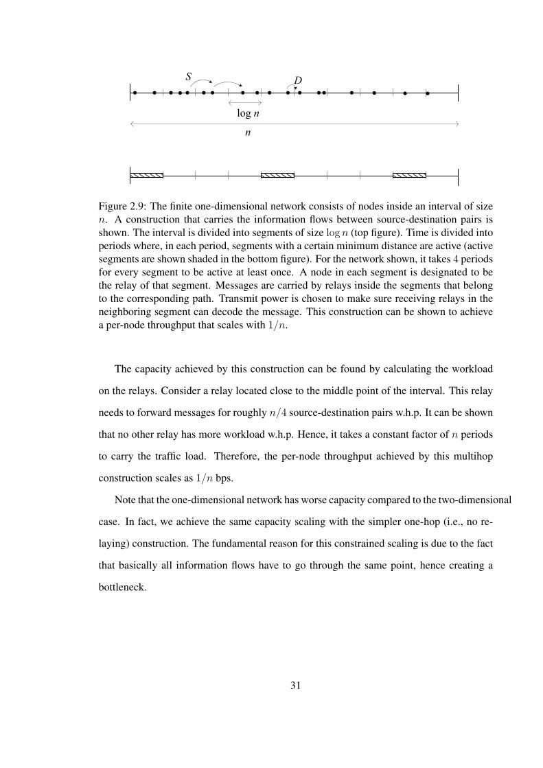
· · ·· · · · · ·n

· · ··· log n

· ·S

D

· ·

Figure 2.9: The finite one-dimensional network consists of nodes inside an interval of sizen. A construction that carries the information flows between source-destination pairs isshown. The interval is divided into segments of size log n (top figure). Time is divided intoperiods where, in each period, segments with a certain minimum distance are active (activesegments are shown shaded in the bottom figure). For the network shown, it takes 4 periodsfor every segment to be active at least once. A node in each segment is designated to bethe relay of that segment. Messages are carried by relays inside the segments that belongto the corresponding path. Transmit power is chosen to make sure receiving relays in theneighboring segment can decode the message. This construction can be shown to achievea per-node throughput that scales with 1/n.

The capacity achieved by this construction can be found by calculating the workload

on the relays. Consider a relay located close to the middle point of the interval. This relay

needs to forward messages for roughly n/4 source-destination pairs w.h.p. It can be shown

that no other relay has more workload w.h.p. Hence, it takes a constant factor of n periods

to carry the traffic load. Therefore, the per-node throughput achieved by this multihop

construction scales as 1/n bps.

Note that the one-dimensional network has worse capacity compared to the two-dimensional

case. In fact, we achieve the same capacity scaling with the simpler one-hop (i.e., no re-

laying) construction. The fundamental reason for this constrained scaling is due to the fact

that basically all information flows have to go through the same point, hence creating a

bottleneck.

31

2.5 Summary

This chapter has introduced the models and some of the important previous results

in the area of wireless ad hoc networks. These serve as a background for the following

chapters. In Chapter 3, we study broadcast connectivity in cooperative wireless ad hoc net-

works. In Section 2.3, we argued that full connectivity never occurs for infinite networks

with nodes with constant transmit radius. This means broadcast to the entire infinite net-

work is not possible. In Chapter 3, we explore whether node cooperation can improve this

situation. In the broadcast case, nodes transmit the same message, hence they can cooper-

ate by combining their transmit power to reach further distances. We show that although

this helps reaching a larger region, broadcast to the infinite network is still not possible ex-

cept for low-attenuation cases. Chapter 4 studies the capacity scaling of hybrid networks.

The addition of base stations helps improve the capacity of wireless ad hoc networks, and

in Chapter 4, we show limitations on this throughput benefit. Chapter 5 uses the capacity

results shown here, especially the construction in Figure 2.8, and extends them to the case

of secrecy capacity. We show how network coding techniques in addition to a construction

based on the one presented in Figure 2.8 can achieve secret communication from eaves-

droppers of unknown location in the network without any compromise on the throughput.

Finally, in Chapter 6, our focus is on the percolation phenomenon introduced here in Sec-

tion 2.3. The sudden transition from disconnected clusters to a well-connected network

occurs in many types of infinite graphs in addition to the random geometric graphs dis-

cussed above (see Figure 2.5). We study percolation in other types of infinite graphs for the

case where edges between nodes can be of different types. For each type of connection, we

can form a separate graph and the overall network can be seen as the combination of these

different “layers”. A node can have a path to another node that passes through multiple

layers. We study percolation of the overall multilayer graph. In particular, we explore the

minimum connectivity required for each layer in order to just start seeing a well-connected

multilayer graph.

32

CHAPTER 3

BROADCAST IN COOPERATIVE WIRELESS NETWORKS

3.1 Introduction

Cooperation among nodes is a powerful tool to improve the performance of wireless

networks. A simple example of cooperation is multihop forwarding, where intermediate

nodes transmit a source node’s message along a path to a receiver which is not within the

source’s direct reach. More powerful forms of cooperation have emerged in recent years.

For example, there has been interest in cooperative diversity, where nodes place a signal

simultaneously in the same frequency band to provide spatial diversity from the source to

a next-hop destination [41, 65]. Such cooperation improves link-level performance such as

reducing the probability of error, outage probability, etc. [65], [57], and has been considered

for improving connectivity [65] and capacity [58] in large wireless networks.

Broadcast is a common operation in wireless networks. Examples include the periodic

broadcast of routing updates and other control messages, and emergency signaling. It is

important that a network successfully deliver these messages to the entire network, as fail-

ure to do so may block other operations and can severely impact network functionality.

The important operation of broadcasting is especially challenging in a mobile ad hoc net-

work (MANET) in which each node typically has a very limited communication range and

broadcast messages have to be carried by nodes in a multihop fashion [55, 74]. A simple

approach to broadcast in a MANET is to require each node to retransmit the message once

it receives the message. However, flooding the network in this manner leads to frequent

collisions and wastes network resources.

33

As with other network functions, and, perhaps more so, broadcast operation can be

potentially enhanced by enabling a form of cooperative diversity. In particular, if the set

of nodes that has decoded the message transmits using a distributed space-time code, this

results in enhanced diversity against multipath fading and improved link performance rather

than collisions. In addition, by combining their resources (e.g., power), cooperating nodes

may be able to reach more distant nodes than would be possible without cooperation. In

accordance with these ideas, several studies report improvements in broadcast performance

in harsh environments [4,5]. It is therefore important to understand the theoretical limits of

broadcast performance gain that can be realized by cooperation. In this chapter, we study

the asymptotic limits of broadcast capabilities for large cooperative networks.

We investigate the ability of a source to transmit a message to the whole network when

nodes are randomly distributed according to a Poisson point process. The source transmits

the message with a given transmit power. The set of nodes that receive this signal with suf-

ficiently large signal-to-noise ratio (SNR) cooperatively transmit the message to reach the

next set of nodes, which again cooperate to reach further nodes and so forth. In this man-

ner, the broadcast message propagates through the network, and, if this wave of message

transmissions reaches the entire network, broadcast is said to be successful. In a random

network, for a given source node, the probability of successful broadcast is strictly less than

one, as there is always a nonzero probability that the source lacks any one-hop neighbors

with which to initiate broadcast in the first place. Clearly, the probability of successful

broadcast monotonically decreases as the size of the network grows. In our analysis, we

explore whether the broadcast probability is zero or strictly between zero and one, in a

network over an infinite-size region. The results, summarized in Table 3.1, show that the

broadcast capability of the network strongly depends on the path loss exponent. For ex-

ample, in an infinite 1-D network, the broadcast probability is zero for path loss exponents

larger than 1, and nonzero for path loss exponents less than 1, regardless of the node den-

sity. Note that path loss exponents α < 1 in 1-D and α < 2 in 2-D might seem to be of

34

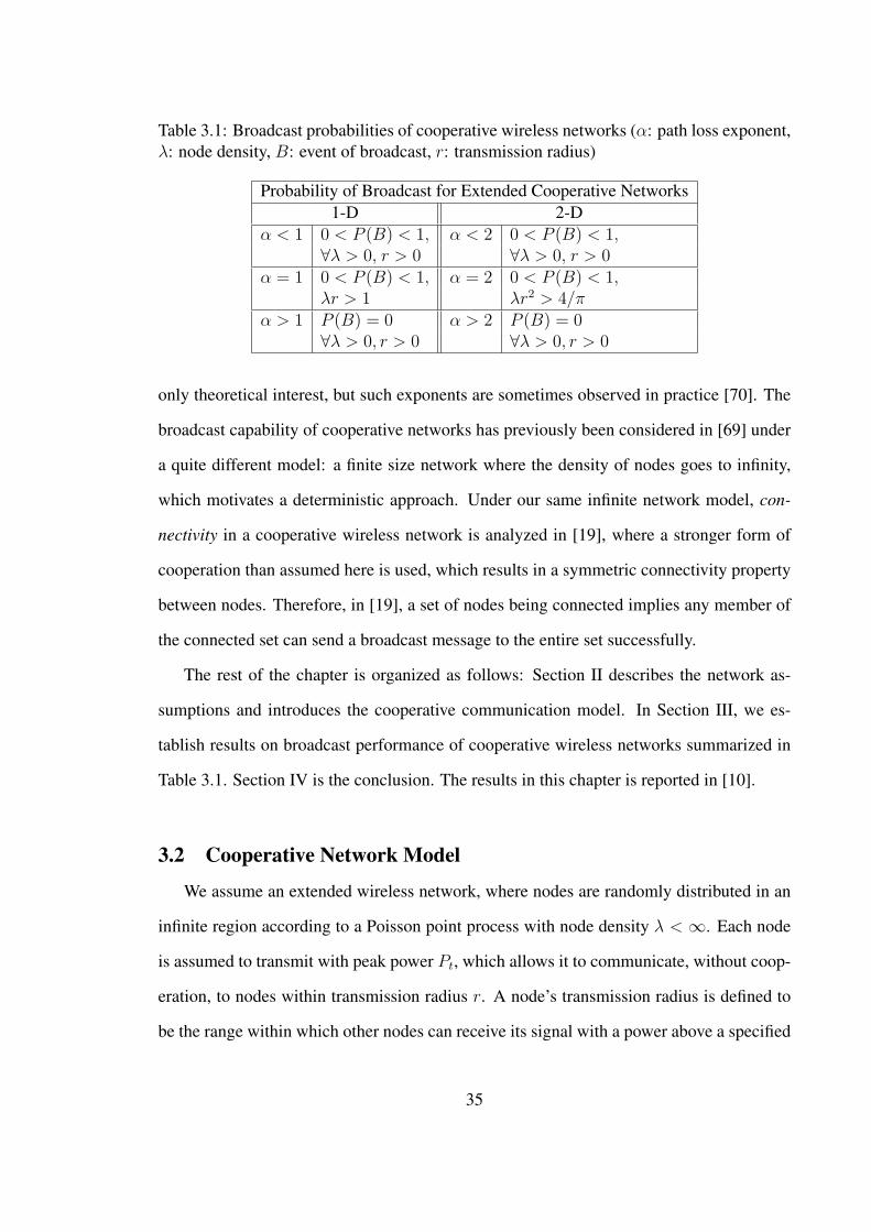
Table 3.1: Broadcast probabilities of cooperative wireless networks (α: path loss exponent,λ: node density, B: event of broadcast, r: transmission radius)

Probability of Broadcast for Extended Cooperative Networks1-D 2-D

α < 1 0 < P (B) < 1, α < 2 0 < P (B) < 1,∀λ > 0, r > 0 ∀λ > 0, r > 0

α = 1 0 < P (B) < 1, α = 2 0 < P (B) < 1,λr > 1 λr2 > 4/π

α > 1 P (B) = 0 α > 2 P (B) = 0∀λ > 0, r > 0 ∀λ > 0, r > 0

only theoretical interest, but such exponents are sometimes observed in practice [70]. The

broadcast capability of cooperative networks has previously been considered in [69] under

a quite different model: a finite size network where the density of nodes goes to infinity,

which motivates a deterministic approach. Under our same infinite network model, con-

nectivity in a cooperative wireless network is analyzed in [19], where a stronger form of

cooperation than assumed here is used, which results in a symmetric connectivity property

between nodes. Therefore, in [19], a set of nodes being connected implies any member of

the connected set can send a broadcast message to the entire set successfully.

The rest of the chapter is organized as follows: Section II describes the network as-

sumptions and introduces the cooperative communication model. In Section III, we es-

tablish results on broadcast performance of cooperative wireless networks summarized in

Table 3.1. Section IV is the conclusion. The results in this chapter is reported in [10].

3.2 Cooperative Network Model

We assume an extended wireless network, where nodes are randomly distributed in an

infinite region according to a Poisson point process with node density λ < ∞. Each node

is assumed to transmit with peak power Pt, which allows it to communicate, without coop-

eration, to nodes within transmission radius r. A node’s transmission radius is defined to

be the range within which other nodes can receive its signal with a power above a specified

35

decoding threshold, τ , which allows a receiver to satisfy a minimum signal-to-noise ratio

(SNR) for physical layer functionality so that the two nodes are connected. With these

definitions, r is given by:

Ptr−α = τ, (3.1)

where α is the path loss coefficient which determines the rate at which the received power

decays with distance.

When two or more nodes cooperate, they simultaneously transmit the same message

such that they can reach a greater distance than they would otherwise reach without co-

operation. In this work, we assume cooperation provides power summing at the receiver.

More formally, the condition for a cooperating set of nodes Ω to reach a node k is

Pt

∑j∈Ω

(dj,k)−α > τ, (3.2)

where dj,k is the distance between nodes j and k.

We assume that the source initiates cooperative broadcast by transmitting the message,

which is heard by nodes within the source’s transmit range. In the second step, those

nodes that have just received the message transmit cooperatively and reach a further set

of nodes. In successive steps, the set of nodes that have received the message from the

previous step cooperatively transmit. As in the maximum multihop diversity case in [69],

we assume that a receiving node accumulates power from all previous steps. Hence, a node

k can successfully decode the broadcast message, if this accumulated power satisfies (3.2),

with Ω being the set of nodes that have previously decoded the message. If a message

transmitted from a given node reaches all of the nodes in the network, then broadcast is

said to be achieved. Without loss of generality, we consider a source node at the origin.

We formally define the broadcast event B to be the event that the message sent from the

36

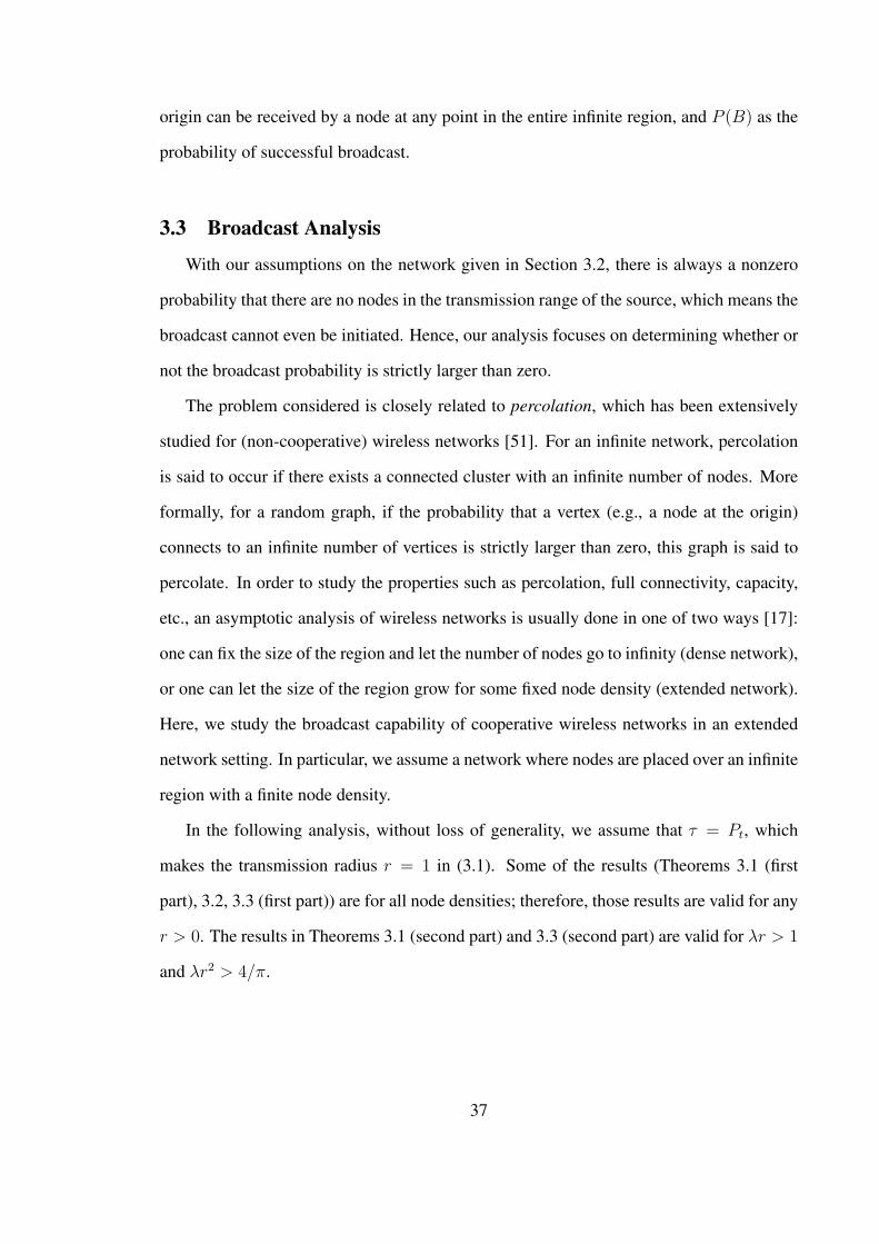
origin can be received by a node at any point in the entire infinite region, and P (B) as the

probability of successful broadcast.

3.3 Broadcast Analysis

With our assumptions on the network given in Section 3.2, there is always a nonzero

probability that there are no nodes in the transmission range of the source, which means the

broadcast cannot even be initiated. Hence, our analysis focuses on determining whether or

not the broadcast probability is strictly larger than zero.

The problem considered is closely related to percolation, which has been extensively

studied for (non-cooperative) wireless networks [51]. For an infinite network, percolation

is said to occur if there exists a connected cluster with an infinite number of nodes. More

formally, for a random graph, if the probability that a vertex (e.g., a node at the origin)

connects to an infinite number of vertices is strictly larger than zero, this graph is said to

percolate. In order to study the properties such as percolation, full connectivity, capacity,

etc., an asymptotic analysis of wireless networks is usually done in one of two ways [17]:

one can fix the size of the region and let the number of nodes go to infinity (dense network),

or one can let the size of the region grow for some fixed node density (extended network).

Here, we study the broadcast capability of cooperative wireless networks in an extended

network setting. In particular, we assume a network where nodes are placed over an infinite

region with a finite node density.

In the following analysis, without loss of generality, we assume that τ = Pt, which

makes the transmission radius r = 1 in (3.1). Some of the results (Theorems 3.1 (first

part), 3.2, 3.3 (first part)) are for all node densities; therefore, those results are valid for any

r > 0. The results in Theorems 3.1 (second part) and 3.3 (second part) are valid for λr > 1

and λr2 > 4/π.

37

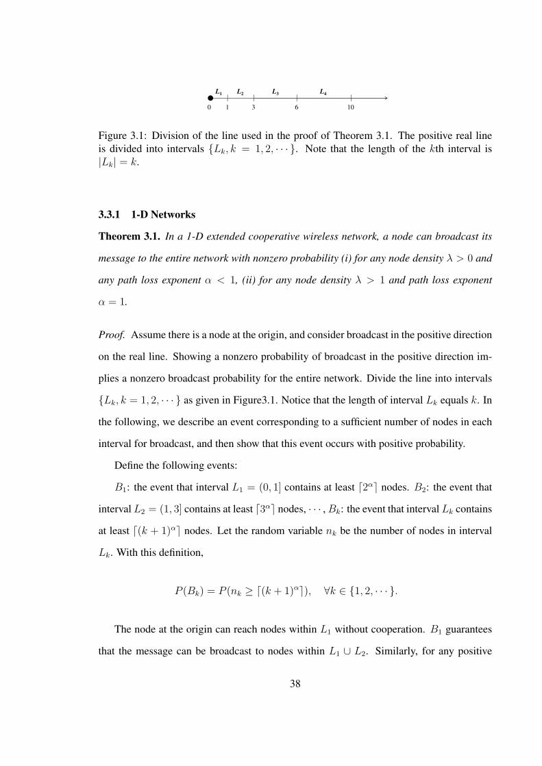
Source

Node

0 1 3 6 10

L1

L2

L3

L4

Figure 3.1: Division of the line used in the proof of Theorem 3.1. The positive real lineis divided into intervals Lk, k = 1, 2, · · · . Note that the length of the kth interval is|Lk| = k.

3.3.1 1-D Networks

Theorem 3.1. In a 1-D extended cooperative wireless network, a node can broadcast its

message to the entire network with nonzero probability (i) for any node density λ > 0 and

any path loss exponent α < 1, (ii) for any node density λ > 1 and path loss exponent

α = 1.

Proof. Assume there is a node at the origin, and consider broadcast in the positive direction

on the real line. Showing a nonzero probability of broadcast in the positive direction im-

plies a nonzero broadcast probability for the entire network. Divide the line into intervals

Lk, k = 1, 2, · · · as given in Figure3.1. Notice that the length of interval Lk equals k. In

the following, we describe an event corresponding to a sufficient number of nodes in each

interval for broadcast, and then show that this event occurs with positive probability.

Define the following events:

B1: the event that interval L1 = (0, 1] contains at least ⌈2α⌉ nodes. B2: the event that

interval L2 = (1, 3] contains at least ⌈3α⌉ nodes, · · · ,Bk: the event that interval Lk contains

at least ⌈(k + 1)α⌉ nodes. Let the random variable nk be the number of nodes in interval

Lk. With this definition,

P (Bk) = P (nk ≥ ⌈(k + 1)α⌉), ∀k ∈ 1, 2, · · · .

The node at the origin can reach nodes within L1 without cooperation. B1 guarantees

that the message can be broadcast to nodes within L1 ∪ L2. Similarly, for any positive

38

integer q, if∩q

k=1Bk occurs, this guarantees broadcast in∪q+1

k=1 Lk. This can be seen by

lower bounding the power received at the rightmost end of∪q+1

k=1 Lk by assuming all nodes

in∪q

k=1 Lk are located at the origin and recalling α 6 1. With all nodes assumed to be

located at the origin, the received power is:

Pt

(1 +

∑qk=1⌈(k + 1)α⌉

)|∪q+1

k=1 Lk|α≥Pt

(∑q+1k=1 k

α)(∑q+1

k=1 k)α ≥ τ. (3.3)

Note the simplifying assumption that Pt = τ . The next step is to show that the event∩∞k=1Bk, which enables broadcast, has nonzero probability.

Consider λ > 0 for α < 1, and λ > 1 for α = 1. The number of nodes nk in the interval

Lk has expected value kλ. Let N be the smallest integer such that this expected value is

greater than the number of nodes required for BN to occur; that is Nλ > ⌈(N + 1)α⌉. It is

always possible to find such an N because as k → ∞, ⌈(k + 1)α⌉/k → 0 for α < 1, and

⌈(k + 1)α⌉/k → 1 for α = 1. Now write

P (B∗) ≥ P (∞∩k=1

Bk) =N−1∏i=1

P (Bi)∞∏

k=N

P (Bk), (3.4)

where B∗ denotes the event that broadcast in the positive direction on the line happens.

Clearly∏N−1

i=1 P (Bi) > 0. Next consider∏∞

k=N P (Bk). Let δ ∈ (0, 1) be defined as:

(1− δ)E(nN) = (1− δ)λN = ⌈(N + 1)α⌉ (3.5)

Using a Chernoff bound, we find a lower bound for P (BN).

P (BN) = P (nN ≥ ⌈(N + 1)α⌉)

= P (nN ≥ (1− δ)λN)

≥ 1− exp(−λNδ2/2). (3.6)

39

The final step is to find lower bounds for P (Bk) for k > N . As k increases, the ratio of

the required number of nodes in interval Lk to the expected number kλ gets smaller. Thus,

using the same δ, which is constant given N as above,

P (Bk) = P (nk ≥ ⌈(k + 1)α⌉)

≥ 1− exp(−λkδ2/2) for k ≥ N. (3.7)

Then,

∞∏k=N

P (Bk) ≥∞∏

k=N

(1− exp(−λkδ2/2)) > 0. (3.8)

The last inequality above can be seen by noting that∑∞

k=N exp(−λkδ2/2) is a convergent

series and hence, the infinite product is convergent [32]. Finally,

P (B∗) ≥N−1∏i=1

P (Bi)∞∏

k=N

P (Bk) > 0, (3.9)

and P (B) > 0, where B is the event of broadcast to the entire line.

Remark 3.1. Theorem 3.1 states that a randomly selected node can broadcast to the entire

network with nonzero probability. It may also be of interest to consider the existence of a

node that can broadcast its message to the entire line with probability one. In fact, Theorem

3.1 indeed implies that, with probability one, there exists a node on the line which can

broadcast to the entire network. This argument can be shown by considering the network

as a disjoint union of finite size regions. For any given ε > 0, the length of the regions

can be selected large enough, so that if a node can broadcast to an entire region, it can

broadcast to the rest of the network with probability (1− ε). The result follows by noticing

that, with arbitrarily high probability, there exists a node inside a finite union of these

regions which can broadcast to its entire region.

40

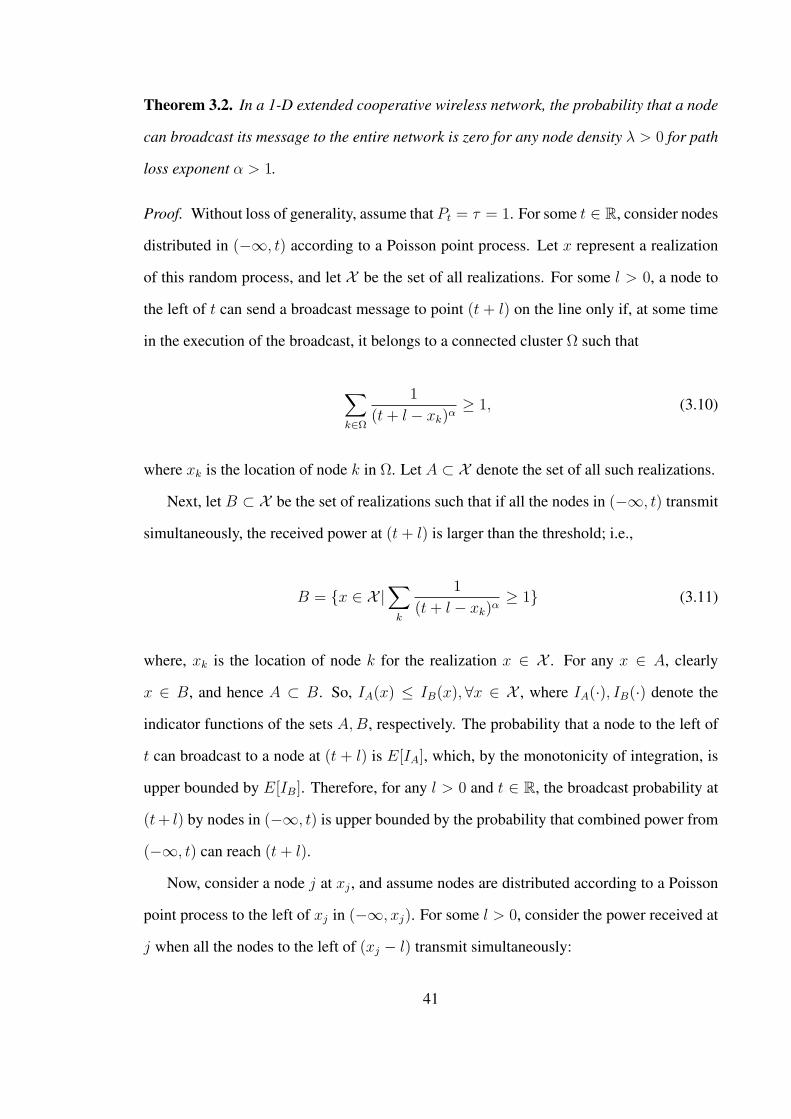
Theorem 3.2. In a 1-D extended cooperative wireless network, the probability that a node

can broadcast its message to the entire network is zero for any node density λ > 0 for path

loss exponent α > 1.

Proof. Without loss of generality, assume that Pt = τ = 1. For some t ∈ R, consider nodes

distributed in (−∞, t) according to a Poisson point process. Let x represent a realization

of this random process, and let X be the set of all realizations. For some l > 0, a node to

the left of t can send a broadcast message to point (t + l) on the line only if, at some time

in the execution of the broadcast, it belongs to a connected cluster Ω such that

∑k∈Ω

1

(t+ l − xk)α≥ 1, (3.10)

where xk is the location of node k in Ω. Let A ⊂ X denote the set of all such realizations.

Next, let B ⊂ X be the set of realizations such that if all the nodes in (−∞, t) transmit

simultaneously, the received power at (t+ l) is larger than the threshold; i.e.,

B = x ∈ X |∑k

1

(t+ l − xk)α≥ 1 (3.11)

where, xk is the location of node k for the realization x ∈ X . For any x ∈ A, clearly

x ∈ B, and hence A ⊂ B. So, IA(x) ≤ IB(x), ∀x ∈ X , where IA(·), IB(·) denote the

indicator functions of the sets A,B, respectively. The probability that a node to the left of

t can broadcast to a node at (t + l) is E[IA], which, by the monotonicity of integration, is

upper bounded by E[IB]. Therefore, for any l > 0 and t ∈ R, the broadcast probability at

(t+ l) by nodes in (−∞, t) is upper bounded by the probability that combined power from

(−∞, t) can reach (t+ l).

Now, consider a node j at xj , and assume nodes are distributed according to a Poisson

point process to the left of xj in (−∞, xj). For some l > 0, consider the power received at

j when all the nodes to the left of (xj − l) transmit simultaneously:

41

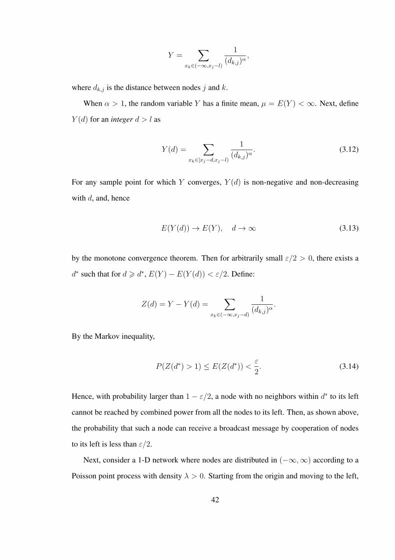
Y =∑

xk∈(−∞,xj−l)

1

(dk,j)α,

where dk,j is the distance between nodes j and k.

When α > 1, the random variable Y has a finite mean, µ = E(Y ) < ∞. Next, define

Y (d) for an integer d > l as

Y (d) =∑

xk∈[xj−d,xj−l)

1

(dk,j)α. (3.12)

For any sample point for which Y converges, Y (d) is non-negative and non-decreasing

with d, and, hence

E(Y (d)) → E(Y ), d→ ∞ (3.13)

by the monotone convergence theorem. Then for arbitrarily small ε/2 > 0, there exists a

d∗ such that for d > d∗, E(Y )− E(Y (d)) < ε/2. Define:

Z(d) = Y − Y (d) =∑

xk∈(−∞,xj−d)

1

(dk,j)α.

By the Markov inequality,

P (Z(d∗) > 1) ≤ E(Z(d∗)) <ε

2. (3.14)

Hence, with probability larger than 1 − ε/2, a node with no neighbors within d∗ to its left

cannot be reached by combined power from all the nodes to its left. Then, as shown above,

the probability that such a node can receive a broadcast message by cooperation of nodes

to its left is less than ε/2.

Next, consider a 1-D network where nodes are distributed in (−∞,∞) according to a

Poisson point process with density λ > 0. Starting from the origin and moving to the left,

42

Rk

Rk+1

rk

rk+1

Figure 3.2: Division of R2 into rings Rk, k = 1, 2, · · · as used in proof of Theorem 3.3.Rk is the ring which corresponds to the region outside the circle of radius rk−1 and insidethe circle of radius rk, where rk =

√1 + 2 + · · ·+ k

consider the first gap which is larger than d∗. For any ε > 0, such a gap exists within the

first N gaps with probability

1− (1− exp(−λd∗))N > 1− ε/2

for some integerN . Consider the node at the right end of this gap. By (3.14), the probability

that a broadcast message can be delivered to this node by nodes to its left is less than

ε/2. Hence, probability of broadcast to the whole network can be upper bounded by an

arbitrarily small number ε > 0.

3.3.2 2-D Networks

Theorem 3.3. In a 2-D extended cooperative wireless network, a node can broadcast its

message to the entire network with nonzero probability (i) for any node density λ > 0 and

43

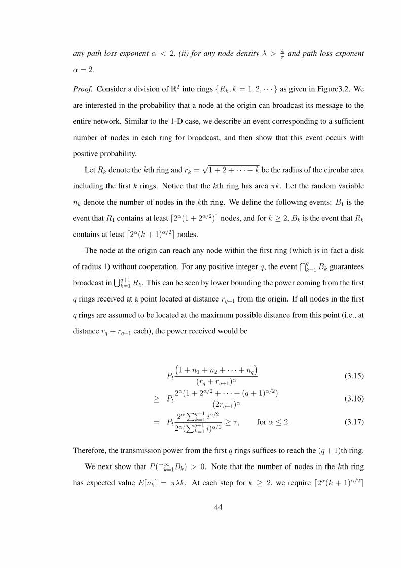
any path loss exponent α < 2, (ii) for any node density λ > 4π

and path loss exponent

α = 2.

Proof. Consider a division of R2 into rings Rk, k = 1, 2, · · · as given in Figure3.2. We

are interested in the probability that a node at the origin can broadcast its message to the

entire network. Similar to the 1-D case, we describe an event corresponding to a sufficient

number of nodes in each ring for broadcast, and then show that this event occurs with

positive probability.

Let Rk denote the kth ring and rk =√1 + 2 + · · ·+ k be the radius of the circular area

including the first k rings. Notice that the kth ring has area πk. Let the random variable

nk denote the number of nodes in the kth ring. We define the following events: B1 is the

event that R1 contains at least ⌈2α(1 + 2α/2)⌉ nodes, and for k ≥ 2, Bk is the event that Rk

contains at least ⌈2α(k + 1)α/2⌉ nodes.

The node at the origin can reach any node within the first ring (which is in fact a disk

of radius 1) without cooperation. For any positive integer q, the event∩q

k=1Bk guarantees

broadcast in∪q+1

k=1Rk. This can be seen by lower bounding the power coming from the first

q rings received at a point located at distance rq+1 from the origin. If all nodes in the first

q rings are assumed to be located at the maximum possible distance from this point (i.e., at

distance rq + rq+1 each), the power received would be

Pt

(1 + n1 + n2 + · · ·+ nq

)(rq + rq+1)α

(3.15)

≥ Pt2α(1 + 2α/2 + · · ·+ (q + 1)α/2)

(2rq+1)α(3.16)

= Pt2α∑q+1

k=1 iα/2

2α(∑q+1

k=1 i)α/2

≥ τ, for α ≤ 2. (3.17)

Therefore, the transmission power from the first q rings suffices to reach the (q+1)th ring.

We next show that P (∩∞k=1Bk) > 0. Note that the number of nodes in the kth ring

has expected value E[nk] = πλk. At each step for k ≥ 2, we require ⌈2α(k + 1)α/2⌉

44

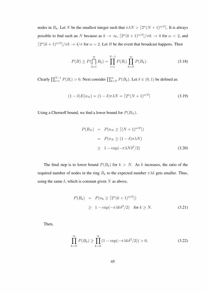
nodes in Rk. Let N be the smallest integer such that πλN > ⌈2α(N + 1)α/2⌉. It is always

possible to find such an N because as k → ∞, ⌈2α(k + 1)α/2⌉/πk → 0 for α < 2, and

⌈2α(k + 1)α/2⌉/πk → 4/π for α = 2. Let B be the event that broadcast happens. Then

P (B) ≥ P (∞∩k=1

Bk) =N−1∏i=1

P (Bi)∞∏

k=N

P (Bk). (3.18)

Clearly∏N−1

i=1 P (Bi) > 0. Next consider∏∞

k=N P (Bk). Let δ ∈ (0, 1) be defined as:

(1− δ)E(nN) = (1− δ)πλN = ⌈2α(N + 1)α/2⌉ (3.19)

Using a Chernoff bound, we find a lower bound for P (BN).

P (BN) = P (nN ≥ ⌈(N + 1)α/2⌉)

= P (nN ≥ (1− δ)πλN)

≥ 1− exp(−πλNδ2/2) (3.20)

The final step is to lower bound P (Bk) for k > N . As k increases, the ratio of the

required number of nodes in the ring Rk to the expected number πλk gets smaller. Thus,

using the same δ, which is constant given N as above,

P (Bk) = P (nk ≥ ⌈2α(k + 1)α/2⌉)

≥ 1− exp(−πλkδ2/2) for k ≥ N. (3.21)

Then,

∞∏k=N

P (Bk) ≥∞∏

k=N

(1− exp(−πλkδ2/2)) > 0, (3.22)

45

which implies

P (B) ≥N−1∏i=1

P (Bi)∞∏

k=N

P (Bk) > 0.

Theorem 3.4. In a 2-D extended cooperative wireless network, the probability that a node

can broadcast its message to the entire network is zero for any node density λ > 0 for path

loss exponent α > 2.

Proof. The proof is very similar to the proof of Theorem 3.2. It is based on the idea that

there exists a critical distance r∗ < ∞ such that, with high probability, the network cannot

deliver a broadcast message to a node that has no neighbors within a radius of r∗. As the

size of the network grows, it includes such an isolated node with high probability .

Thus, in a 2-D extended network with α > 2, broadcast to the entire network is not

possible. However, in contrast to a 1-D network with α > 1, it is possible (with nonzero

probability) for a node to broadcast its message to an infinite number of nodes in a 2-D

extended network with α > 2. This result follows from Theorem 4.3 of [19].

3.3.3 Comparison with Continuum Analysis

A theoretical analysis with the same goal of considering broadcast performance in co-

operative wireless networks has previously been considered in [69] for a dense network.

The key element of the analysis in [69] (and similarly in [34, 35, 68]) is that the random

network is approximated by a deterministic continuum model, where it is assumed that the

transmit power is distributed to the entire network as a continuum as opposed to separate

randomly placed nodes in discrete locations with some nonzero transmit power. For a 2-D

dense network where the transmit power coming from the cooperating nodes is assumed

to be summed at the receiver, [69] shows that broadcast performance depends on what

scale multihop diversity is exploited. In multihop diversity, power is accumulated from

46

m > 1 previous levels. If, as assumed here, power is accumulated from all previous levels

(m = ∞), it is shown (for path loss exponent α = 2) that the message is broadcast to the

whole network [69]. This result can be easily extended to arbitrary path loss exponents in

a 1-D network by observing that in the continuum limit, if nodes in a region of size 1 can

reach nodes within a region of size (1+ε1), ε1 > 0, in the next level, broadcast will reach a

region of size (1 + ε1 + ε2) with ε2 > ε1. Hence, the broadcast region grows to infinity for

all path loss exponents and power densities. The same result follows analogously in 2-D.

Thus, the results of [69] appear to be quite at odds with the results derived here. How-

ever, the dichotomy can be explained by carefully considering the assumptions in our work

and in [69]. In the continuum analysis of [69], one models the random network in the limit

of high node densities, where the distribution of nodes becomes deterministic, and then

checks whether broadcast is possible or not. As noted above, under the m = ∞ assump-

tion, this results in broadcast with probability one to the entire network, even in the limit

of very large networks, because of the deterministic uniformity of the node distribution.

Here, in contrast, we consider fixed node densities λ <∞, with the associated randomness

of node distributions, for infinitely large networks. Because of the randomness in the node

locations, for α > 1 (1-D) or α > 2 (2-D) it is very likely that one will find an isolated node

if the network is large enough, as formally described in the proofs of Theorems 3.2 and 3.4.

Hence, the probability of broadcast is zero regardless of the node density λ. Hence, it is

clear that one must be careful in choosing the appropriate model for a given application.

The model of [69] has been successfully employed in numerous works [11, 33, 35], but

our results would suggest caution in its application to very large random networks which

require many hops for broadcast to reach the entire network.

3.4 Conclusion

We analyze the theoretical limits of node broadcast in a cooperative wireless network.

For a network where nodes are distributed randomly to an infinite region, we calculate the

47

probability that a node can broadcast its message to the whole network. Using an exact

discrete model, we show that broadcast performance of the cooperative network strongly

depends on the path loss exponent, and that there is zero probability of broadcast for a large

range of path loss exponents regardless of the node density.

3.5 Acknowledgment

The work in this chapter was supported in part by the National Science Foundation

under grants CNS-0721861 and CNS-1018464, and in part by the U.S. Army Research

Laboratory and the U.K. Ministry of Defence, and was accomplished under Agreement

Number W911NF-06-3-0001.

48

CHAPTER 4

CAPACITY OF HYBRID NETWORKS

4.1 Introduction

Consider a wireless ad hoc network where n nodes are placed in a two-dimensional

region, and are randomly matched into n source-destination pairs. As reviewed in Chapter

2, Gupta and Kumar showed in [29] that the rate of information that can be shared by each

pair scales at most with 1/√n, which shows that the capacity of wireless networks does

not scale well. Successive works to [29] improved this scaling by considering cases not

assumed in the original network or communication model, such as node mobility [26], a

sophisticated physical layer scheme [58], etc.

One straightforward way to increase the capacity of an ad hoc network is to add in-

frastructure, i.e., an overlaid wired network connecting b base stations which help carry

information between the wireless nodes. This type of a network is commonly referred to

as a “hybrid network” [15, 45], and the capacity that can be achieved by ad hoc nodes in a

hybrid network is the problem of interest in this chapter.

The scaling of capacity in hybrid networks has been studied in a number of works under

different network and communication models starting with [40, 45]. Some of these works

observe that whether or not infrastructure improves capacity scaling depends on how the

number of base stations b scales as compared to n. In particular, the works of [45, 72, 80]

show that the per-node throughput scaling of 1/√n remains the same if b grows at most

with√n. Only after that point does the capacity start to increase. On the other hand, [1,40]

study the special case where b = Θ(n), and explore the possibility of providing each pair

Θ(1) throughput. In particular, [1] shows that this is indeed possible for a fraction of node

49

pairs arbitrarily close to one. The cases of mobile nodes [50], multicast communication

[12], and base stations with multiple antennas [67] in hybrid networks are studied in other

related work.

The work of most interest to us is that of [46]. Under the Physical Model [29], [46]

considers both one-dimensional and two-dimensional hybrid networks. A simple construc-

tion where each node gives their message to the closest base station via multihop is shown

in [46] to provide a per-node throughput scaling of b/n bits per second. Note that, for 1-D

networks, this is a significant improvement to pure ad hoc capacity of 1/n. However, in

2-D networks, only when b grows faster than√n, does b/n provide a better throughput

than pure ad hoc scaling of 1/√n, which is consistent with previous results. The through-

put scaling of b/n is shown to hold for values of b that satisfy b log b 6 n. When b scales

faster, e.g., when b = Θ(n), the construction is shown to achieve 1/ log b bits per second,

i.e., a value less than b/n. The reason for this change is the fact that the workload on base

stations is no longer uniformly bounded by their expected value. However, this result is an

achievability result and it is of interest whether the throughput can be further improved.

In this chapter, we study lower and upper bounds on per-node throughput in 1-D and

2-D hybrid networks under the Physical Model. We show that the construction proposed

in [46] in fact achieves better throughput than previously thought in the case where b log b

grows faster than n. In addition to improving the achievability results, we show upper

bounds on per-node throughput. Central to our work is a new result we establish on the

maxima of a sequence of Poisson random variables. The phase transition that happens

on the maxima of a sequence of Poisson random variables, namely that the maxima di-

verges from a constant factor of the mean for sequences with slowly growing mean values,

had been shown in the literature [3]. However, the exact value (or the distribution) that

the maxima takes was not identified, except for the special case of constant-mean Pois-

son sequences [37]. We establish how the maxima scales for the entire divergent range.

This result helps characterize more accurately the throughput achieved by the construction

50

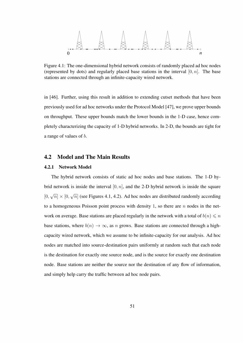
0 n

Figure 4.1: The one-dimensional hybrid network consists of randomly placed ad hoc nodes(represented by dots) and regularly placed base stations in the interval [0, n]. The basestations are connected through an infinite-capacity wired network.

in [46]. Further, using this result in addition to extending cutset methods that have been

previously used for ad hoc networks under the Protocol Model [47], we prove upper bounds

on throughput. These upper bounds match the lower bounds in the 1-D case, hence com-

pletely characterizing the capacity of 1-D hybrid networks. In 2-D, the bounds are tight for

a range of values of b.

4.2 Model and The Main Results

4.2.1 Network Model

The hybrid network consists of static ad hoc nodes and base stations. The 1-D hy-

brid network is inside the interval [0, n], and the 2-D hybrid network is inside the square

[0,√n]× [0,

√n] (see Figures 4.1, 4.2). Ad hoc nodes are distributed randomly according

to a homogeneous Poisson point process with density 1, so there are n nodes in the net-

work on average. Base stations are placed regularly in the network with a total of b(n) 6 n

base stations, where b(n) → ∞, as n grows. Base stations are connected through a high-

capacity wired network, which we assume to be infinite-capacity for our analysis. Ad hoc

nodes are matched into source-destination pairs uniformly at random such that each node

is the destination for exactly one source node, and is the source for exactly one destination

node. Base stations are neither the source nor the destination of any flow of information,

and simply help carry the traffic between ad hoc node pairs.

51

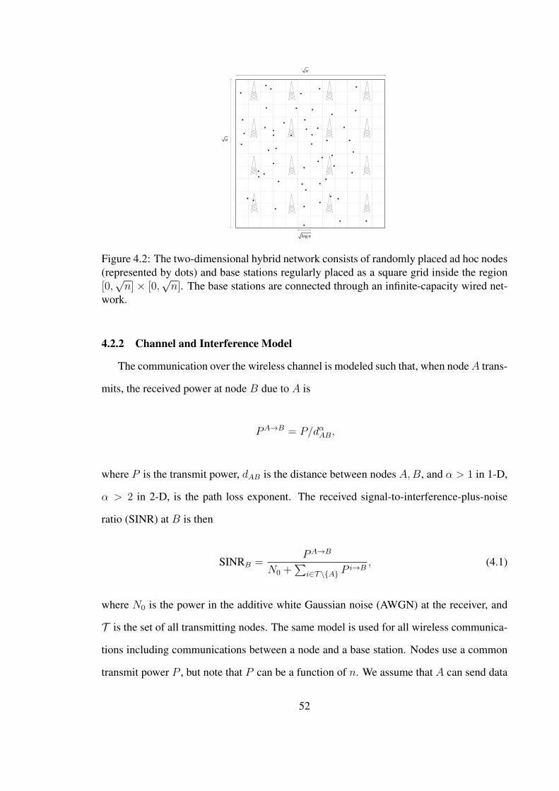
log n

n

n

Figure 4.2: The two-dimensional hybrid network consists of randomly placed ad hoc nodes(represented by dots) and base stations regularly placed as a square grid inside the region[0,

√n] × [0,

√n]. The base stations are connected through an infinite-capacity wired net-

work.

4.2.2 Channel and Interference Model

The communication over the wireless channel is modeled such that, when nodeA trans-

mits, the received power at node B due to A is

PA→B = P/dαAB,

where P is the transmit power, dAB is the distance between nodes A,B, and α > 1 in 1-D,

α > 2 in 2-D, is the path loss exponent. The received signal-to-interference-plus-noise

ratio (SINR) at B is then

SINRB =PA→B

N0 +∑

i∈T \A Pi→B

, (4.1)

where N0 is the power in the additive white Gaussian noise (AWGN) at the receiver, and

T is the set of all transmitting nodes. The same model is used for all wireless communica-

tions including communications between a node and a base station. Nodes use a common

transmit power P , but note that P can be a function of n. We assume that A can send data

52

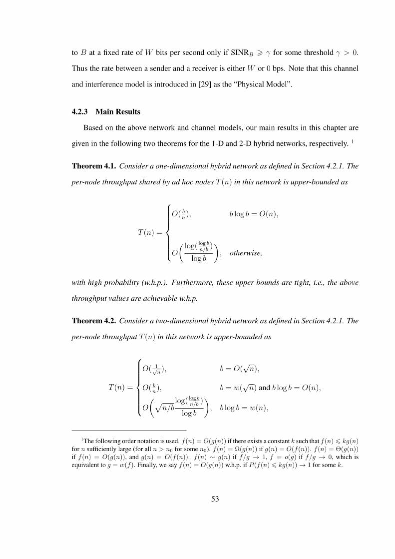
to B at a fixed rate of W bits per second only if SINRB > γ for some threshold γ > 0.

Thus the rate between a sender and a receiver is either W or 0 bps. Note that this channel

and interference model is introduced in [29] as the “Physical Model”.

4.2.3 Main Results

Based on the above network and channel models, our main results in this chapter are

given in the following two theorems for the 1-D and 2-D hybrid networks, respectively. 1

Theorem 4.1. Consider a one-dimensional hybrid network as defined in Section 4.2.1. The

per-node throughput shared by ad hoc nodes T (n) in this network is upper-bounded as

T (n) =

O( bn), b log b = O(n),

O

(log( log b

n/b)

log b

), otherwise,

with high probability (w.h.p.). Furthermore, these upper bounds are tight, i.e., the above

throughput values are achievable w.h.p.

Theorem 4.2. Consider a two-dimensional hybrid network as defined in Section 4.2.1. The

per-node throughput T (n) in this network is upper-bounded as

T (n) =

O( 1√n), b = O(

√n),

O( bn), b = w(

√n) and b log b = O(n),

O

(√n/b

log( log bn/b

)

log b

), b log b = w(n),

1The following order notation is used. f(n) = O(g(n)) if there exists a constant k such that f(n) 6 kg(n)for n sufficiently large (for all n > n0 for some n0). f(n) = Ω(g(n)) if g(n) = O(f(n)). f(n) = Θ(g(n))if f(n) = O(g(n)), and g(n) = O(f(n)). f(n) ∼ g(n) if f/g → 1, f = o(g) if f/g → 0, which isequivalent to g = w(f). Finally, we say f(n) = O(g(n)) w.h.p. if P (f(n) 6 kg(n)) → 1 for some k.

53

w.h.p. For b log b = O(n), these upper bounds are tight, i.e., the above throughput values

are achievable w.h.p. For b log b = w(n), T (n) = Ω(log( log b

n/b)/log b

).

Note that, in the two-dimensional case, a per-node throughput on the order of 1/√n log n

bps is already achievable via pure ad hoc communication as shown in Section 2.4.3, i.e.,

T (n) = Ω(1/√n log n) for all cases. Overall, we have the following achievability results

in the 2-D case:

T (n) =

Ω( 1√n logn

), b = O(√n/ log n),

Ω( bn), b = w(

√n/ log n) and b log b = O(n),

Ω

(log( log b

n/b)

log b

), b log b = w(n).

4.3 Cutset Bounds

In this section, we prove two cutset results for upper bounding the total rate of informa-

tion that can be achieved from a set of nodes inside a given region to nodes outside. Similar

cutset bounds under the Protocol Model were shown in [47]. Here, we extend these results

to the Physical Model. These results are used in proving the upper bounds in Theorems 4.1

and 4.2.

The following result establishes the fact that under the Physical Model, when nodes are

located on a line, at most a constant rate of information can be delivered across a given

point regardless of the number or the locations of the nodes.

Lemma 4.1. Consider an interval [t1, t2] on the real line (see Figure 4.3). Under the Phys-

ical Model, when nodes are located on the real line, the rate of information that can be

delivered from inside the interval to outside is upper bounded by 2W (1/γ + 1) bps.

Proof. For convenience, first consider only the source-destination pairs where the desti-

nation nodes are placed to the right of the cut. Suppose there are m such active source-

destination pairs. Let the set of source nodes be S1, S2, · · · , Sm, where the numbering

54

S1S2Sm D1D2 Dm

t1 t2

Figure 4.3: The cutset bound on the total rate of information that can be delivered fromnodes inside an interval [t1, t2] to outside is calculated. Message transmission from theinterval can happen in either direction – left or right. There are m active source-destinationpairs that communicate across t2. The source nodes S1, S2, · · · , Sm are labeled in increas-ing distance from t2.

is done in increasing order of distance from the point b (see Figure 4.3). Let Di be the

destination node of the source node Si, i = 1, 2, · · · ,m. Hence, the SINR condition is

satisfied for each pair Si, Di, and each pair shares W bits per second with a total of mW

bits per second crossing the cut through point t2.

Let P Si→Dj be the power received at Dj due to node Si. The SINR condition at Dm

requires

P Sm→Dm

N0 +∑m−1

i=1 P Si→Dm≥ γ.

Note that, P Si→Dm > P Sm→Dj , as nodes use common transmit power and the received

power monotonically decreases with distance. Hence,

P Sm→Dm > γ

m−1∑i=1

P Sm→Dm ≥ γ(m− 1)P Sm→Dm ,

which implies

m <1

γ+ 1.

Therefore, there can be at most 1γ+ 1 simultaneous transmissions crossing the cut

through point t2. A similar argument can be shown for transmissions through point t1.

Hence, the cutset capacity is upper-bounded by 2W (1/γ + 1) bps.

55

Si

Sj

Di

dii

dji

1

1

Figure 4.4: The first cut used in the proof of Lemma 4.2. A square region of size 1 × 1 ischosen as the cut. The source nodes are located inside the cut, and the destination nodesare located outside. Lemma 4.2 states that the number of simultaneous transmissions thatcan take place between such source-destination pairs is upper bounded by 3α/γ + 1.

The following result shows that, in the two-dimensional case, under the Physical Model,

the total rate of information that can be delivered from inside a given region to outside is

proportional to the “edge length” of the region regardless of the number or the locations of

nodes.

Lemma 4.2. Consider a box of size ℓ×ℓ on the two-dimensional plane. Under the Physical

Model, and with the constraint that the received power cannot exceed the transmit power,

the rate of information that can be delivered from inside the box to outside is upper bounded

by 4Wℓ(2 + 2α+3α

γ) bps.

Proof. We first show that the number of simultaneous transmissions outside a box of size

1 × 1 is upper bounded a constant. Again, we consider one-hop transmissions between

56

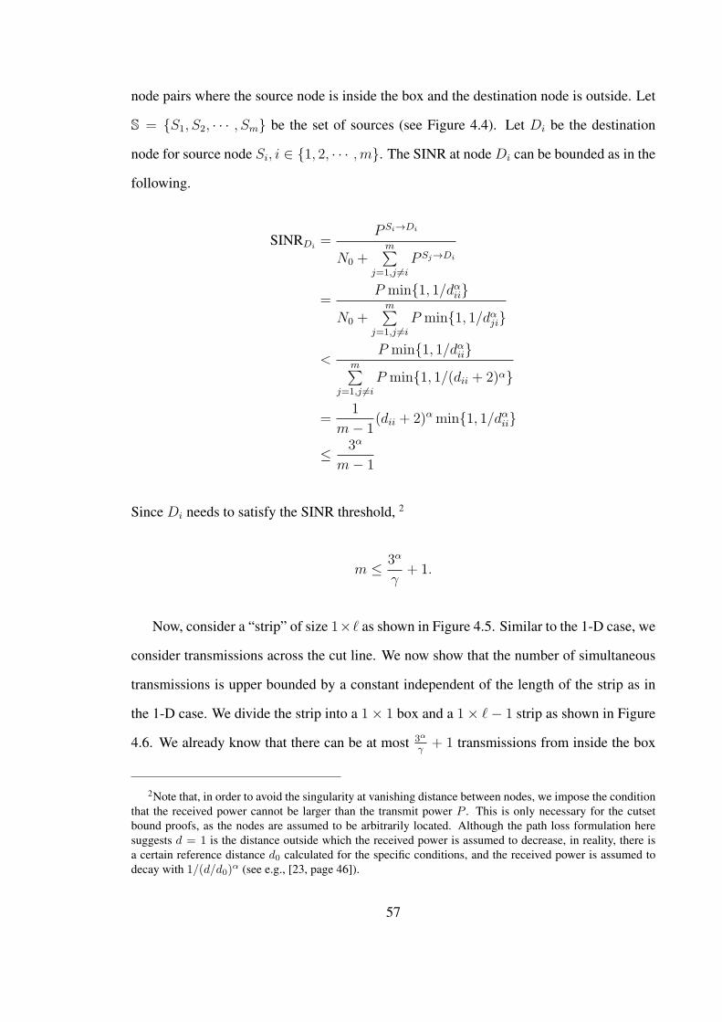
node pairs where the source node is inside the box and the destination node is outside. Let

S = S1, S2, · · · , Sm be the set of sources (see Figure 4.4). Let Di be the destination

node for source node Si, i ∈ 1, 2, · · · ,m. The SINR at node Di can be bounded as in the

following.

SINRDi=

P Si→Di

N0 +m∑

j=1,j =i

P Sj→Di

=P min1, 1/dαii

N0 +m∑

j=1,j =i

P min1, 1/dαji

<P min1, 1/dαii

m∑j=1,j =i

P min1, 1/(dii + 2)α

=1

m− 1(dii + 2)α min1, 1/dαii

≤ 3α

m− 1

Since Di needs to satisfy the SINR threshold, 2

m ≤ 3α

γ+ 1.

Now, consider a “strip” of size 1×ℓ as shown in Figure 4.5. Similar to the 1-D case, we

consider transmissions across the cut line. We now show that the number of simultaneous

transmissions is upper bounded by a constant independent of the length of the strip as in

the 1-D case. We divide the strip into a 1× 1 box and a 1× ℓ− 1 strip as shown in Figure

4.6. We already know that there can be at most 3α

γ+ 1 transmissions from inside the box

2Note that, in order to avoid the singularity at vanishing distance between nodes, we impose the conditionthat the received power cannot be larger than the transmit power P . This is only necessary for the cutsetbound proofs, as the nodes are assumed to be arbitrarily located. Although the path loss formulation heresuggests d = 1 is the distance outside which the received power is assumed to decrease, in reality, there isa certain reference distance d0 calculated for the specific conditions, and the received power is assumed todecay with 1/(d/d0)

α (see e.g., [23, page 46]).

57

S1S2Sm

D1

D2

Dm

1

d

Cut line

Figure 4.5: The strip used in the proof of Lemma 4.2. The number of simultaneous trans-missions that can take place from sources inside the strip to destinations to the right of thecut line is upper bounded by a constant. To prove the argument the division of the strip asin Figure 4.6 is used.

of size 1× 1 to outside. Suppose the strip of size 1× ℓ− 1 contains m′ active sources. We

label them in increasing order of their “horizontal distance” to the cut. Let d be the distance

between Sm′ and Dm′ . Consider the SINR value at Dm′ .

SINRDm′ =P Sm′→Dm′

N0 +m′−1∑j=1

P Sj→Dm′

=P/dα

N0 +m′−1∑j=1

P/|Sj −Dm′|

<P/dα

m′−1∑j=1

P/(2d)α

=1

m′ − 12α

Since Dm′ needs to satisfy the SINR threshold

58

S1S2Sm’

D1

D2

Dm’

1

d

1

Figure 4.6: The strip is considered as the union of a square of size 1× 1 and a strip of size1 × ℓ − 1. The proof is obtained by upper bounding the number of transmissions that cantake place from source nodes within each region.

m′ ≤ 2α

γ+ 1

Hence, the total number of transmissions from the 1×ℓ strip is upper bounded by 2α+3α

γ+2.

Finally consider the ℓ × ℓ box shown in Figure 4.7. Any destination node outside the

box has to be on the other side of one of the four cut lines shown. Hence, the number of

transmissions are upper bounded by the sum of the number of transmissions crossing these

four lines. For any cut line, the ℓ × ℓ box can be divided into ℓ strips of size 1 × ℓ. We

have shown above that there can be at most 2α+3α

γ+ 2 transmissions from a strip, so the

total number of transmissions from the ℓ × ℓ box crossing one cut line is upper bounded

by ℓ(2α+3α

γ+ 2). Considering all four cut lines, the total number of transmissions is upper

bounded by 4ℓ(2α+3α

γ+ 2).

4.4 Maxima of a sequence of Poisson random variables

The regularly-placed b base stations can be thought of as dividing the network into b

equal size “cells”. In 1-D, each cell is a subinterval of length n/b, [0, n/b] being the first

59

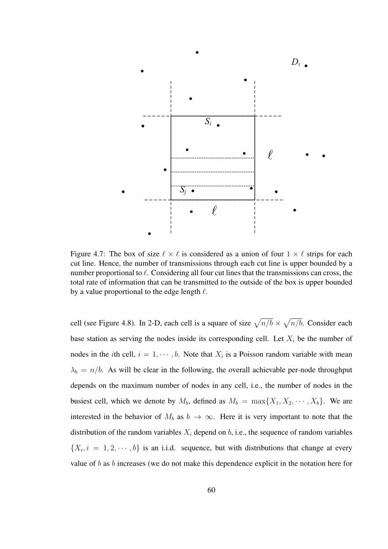
Si

Sj

Di

l

l

Figure 4.7: The box of size ℓ × ℓ is considered as a union of four 1 × ℓ strips for eachcut line. Hence, the number of transmissions through each cut line is upper bounded by anumber proportional to ℓ. Considering all four cut lines that the transmissions can cross, thetotal rate of information that can be transmitted to the outside of the box is upper boundedby a value proportional to the edge length ℓ.

cell (see Figure 4.8). In 2-D, each cell is a square of size√n/b ×

√n/b. Consider each

base station as serving the nodes inside its corresponding cell. Let Xi be the number of

nodes in the ith cell, i = 1, · · · , b. Note that Xi is a Poisson random variable with mean

λb = n/b. As will be clear in the following, the overall achievable per-node throughput

depends on the maximum number of nodes in any cell, i.e., the number of nodes in the

busiest cell, which we denote by Mb, defined as Mb = maxX1, X2, · · · , Xb. We are

interested in the behavior of Mb as b → ∞. Here it is very important to note that the

distribution of the random variables Xi depend on b, i.e., the sequence of random variables

Xi, i = 1, 2, · · · , b is an i.i.d. sequence, but with distributions that change at every

value of b as b increases (we do not make this dependence explicit in the notation here for

60

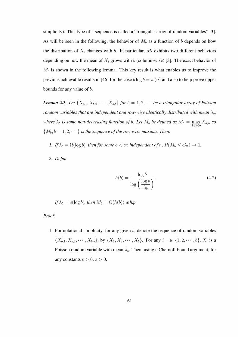
simplicity). This type of a sequence is called a “triangular array of random variables” [3].

As will be seen in the following, the behavior of Mb as a function of b depends on how

the distribution of Xi changes with b. In particular, Mb exhibits two different behaviors

depending on how the mean of Xi grows with b (column-wise) [3]. The exact behavior of

Mb is shown in the following lemma. This key result is what enables us to improve the

previous achievable results in [46] for the case b log b = w(n) and also to help prove upper

bounds for any value of b.

Lemma 4.3. Let Xb,1, Xb,2, · · · , Xb,b for b = 1, 2, · · · be a triangular array of Poisson

random variables that are independent and row-wise identically distributed with mean λb,

where λb is some non-decreasing function of b. Let Mb be defined as Mb = max16i6b

Xb,i, so

Mb, b = 1, 2, · · · is the sequence of the row-wise maxima. Then,

1. If λb = Ω(log b), then for some c <∞ independent of n, P (Mb ≤ cλb) → 1.

2. Define

h(b) =log b

log

(log b

λb

) . (4.2)

If λb = o(log b), then Mb = Θ(h(b)) w.h.p.

Proof:

1. For notational simplicity, for any given b, denote the sequence of random variables

Xb,1, Xb,2, · · · , Xb,b, by X1, X2, · · · , Xb. For any i =∈ 1, 2, · · · , b, Xi is a

Poisson random variable with mean λb. Then, using a Chernoff bound argument, for

any constants c > 0, s > 0,

61

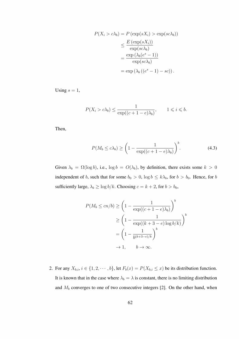
P (Xi > cλb) = P (exp(sXi) > exp(scλb))

≤ E (exp(sXi))

exp(scλb)

=exp (λb(e

s − 1))

exp(scλb)

= exp (λb ((es − 1)− sc)) .

Using s = 1,

P (Xi > cλb) ≤1

exp((c+ 1− e)λb), 1 6 i 6 b.

Then,

P (Mb ≤ cλb) ≥(1− 1

exp((c+ 1− e)λb)

)b

. (4.3)

Given λb = Ω(log b), i.e., log b = O(λb), by definition, there exists some k > 0

independent of b, such that for some b0 > 0, log b ≤ kλb, for b > b0. Hence, for b

sufficiently large, λb ≥ log b/k. Choosing c = k + 2, for b > b0,

P (Mb ≤ cn/b) ≥(1− 1

exp((c+ 1− e)λb)

)b

≥(1− 1

exp((k + 3− e) log b/k)

)b

=

(1− 1

b(k+3−e)/k

)b

→ 1, b→ ∞.

2. For any Xb,i, i ∈ 1, 2, · · · , b, let Fb(x) = P (Xb,i ≤ x) be its distribution function.

It is known that in the case where λb = λ is constant, there is no limiting distribution

and Mb converges to one of two consecutive integers [2]. On the other hand, when

62

λb grows with b, it is shown in [3] that the maximum Mb exhibits two different

behaviors depending on the growth rate of λb. The proof in the first part shows that

Mb is bounded by a constant factor of λb when λb = Ω(log b), which is consistent

with the result in [3]. In the case where λb = o(log b), [3] shows that Mb converges

to one of two integers. In other words, when λb = o(log n), there is a sequence of

integers Ib such that

P (Mb ∈ Ib, Ib + 1) → 1, as b→ ∞. (4.4)

However, it is of interest here to consider a question left open in the literature on

the maximum of Poisson random variables, which is how Mb, i.e., Ib, scales when

λb = o(log b). Note that for the special case of constant mean, λb = λ, it is shown

in [37] that Ib ∼ log b/ log log b, which, interestingly, is independent of the value of

λ.

First, define the tail function Fb = 1 − Fb. As in [37], we associate the following

continuous function to the exact function Fb, which agrees with Fb at integer values.

Fc,b(x) = e−λbλxb

∞∑j=1

λjb/Γ(x+ j + 1), (4.5)

where Γ is the gamma function. Second, define the sequence of real numbers βb, b =

1, 2, · · · by the following relation:

1/b = Fc,b(βb) (4.6)

Note that the function Fc,b is strictly decreasing, hence βb is a growing sequence.

In [2], it is shown that the integer sequence Ib is given by Ib = ⌊βb+1/2⌋. Therefore,

the asymptotic behavior of Ib can be found by finding the growth rate of βb.

63

By taking logarithms of both sides in (4.6),

log b = λb − βb log λb − log∞∑j=1

λjb/Γ(βb + j + 1) (4.7)

We do an asymptotic analysis on the above equation to analyze the growth rate of

βb. We first make the observation that, as b grows, the first term in the summation

in (4.7) dominates the sum of the rest of the terms. This can be found by using the

fact that for any y > 0, Fc,b(x)/Fc,b(x + y) → ∞, as x → ∞ [3, page 970]. The

dominance result then follows by using y = 1, x = βb. Hence, we may keep only the

first term in the summation above and get

log b ∼ λb − βb log λb − log λb + log Γ(βb + 2). (4.8)

Then we proceed similarly. First, keeping the most dominant term in Stirling’s ap-

proximation to the gamma function,

log b ∼ λb − βb log λb − log λb + βb log βb. (4.9)

For the terms on the right hand side above, we look for the most dominant term(s).

It is shown in [3] that βb is asymptotically dominant to λb. (Note that log βb does not

necessarily dominate log λb). Hence we are left with

log b ∼ βb log βb − βb log λb. (4.10)

From above, finally it can be shown that βb satisfies

βb ∼log b

log( log bλb

).

64

4.5 One-dimensional Network

Theorem 4.1 is our main result for the one-dimensional hybrid network. We present

its proof in the following. The proof is divided into two parts. The first part shows the

achievability result by presenting a construction. The second part shows the upper bound

by cutset arguments.

4.5.1 Achievability

We present a construction that describes how information is carried between source-

destination pairs, and then calculate the throughput achieved by this construction, which

gives a lower bound. Note that this construction is similar to the one presented in [46].

The interval [0, n] is divided into small “segments” of length log n, the first segment be-

ing [0, log n] (see Figure 4.8). It can be shown that each segment contains at least one node

w.h.p. (see Appendix B.1). For ad hoc communication, data is carried through multihop

where each time data is delivered to a node inside the next segment on the route. Note that

segments are different from “cells”, the subintervals of length n/b. Data is delivered from

a source node to a destination node in three steps.

1. Upload Phase: The source sends the packet to the closest base station through mul-

tihop, where the packet is delivered to the next segment at each hop until it reaches

the base station (see Figure 4.8). Note that the size of a cell becomes smaller than

the size of a segment in the case n/b ≤ log n, and nodes reach the base station in one

hop.

2. Wired Phase: The packet is carried through the wired network until it reaches the

base station that is closest to the destination node.

3. Download Phase: The base station closest to the destination node delivers the packet

to the destination node using multihop transmission by nodes in each segment. Note

that if the base stations have enough power to reach the whole cell, this phase can be

done with broadcast instead. However, this does not change the scaling result.

65

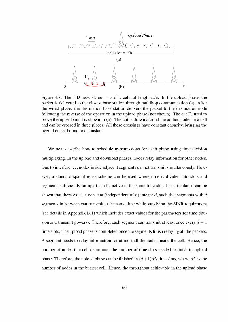
log n

cell size = n/b

Upload Phase

sΓ

0 n

(a)

(b)

Figure 4.8: The 1-D network consists of b cells of length n/b. In the upload phase, thepacket is delivered to the closest base station through multihop communication (a). Afterthe wired phase, the destination base station delivers the packet to the destination nodefollowing the reverse of the operation in the upload phase (not shown). The cut Γs used toprove the upper bound is shown in (b). The cut is drawn around the ad hoc nodes in a celland can be crossed in three places. All these crossings have constant capacity, bringing theoverall cutset bound to a constant.

We next describe how to schedule transmissions for each phase using time division

multiplexing. In the upload and download phases, nodes relay information for other nodes.

Due to interference, nodes inside adjacent segments cannot transmit simultaneously. How-

ever, a standard spatial reuse scheme can be used where time is divided into slots and

segments sufficiently far apart can be active in the same time slot. In particular, it can be

shown that there exists a constant (independent of n) integer d, such that segments with d

segments in between can transmit at the same time while satisfying the SINR requirement

(see details in Appendix B.1) which includes exact values for the parameters for time divi-

sion and transmit powers). Therefore, each segment can transmit at least once every d + 1

time slots. The upload phase is completed once the segments finish relaying all the packets.

A segment needs to relay information for at most all the nodes inside the cell. Hence, the

number of nodes in a cell determines the number of time slots needed to finish its upload

phase. Therefore, the upload phase can be finished in (d+1)Mb time slots, whereMb is the

number of nodes in the busiest cell. Hence, the throughput achievable in the upload phase

66

is Θ(1/Mb). As shown in Lemma 4.3, 1/Mb scales as b/n when b log b = O(n), and scales

with 1/h(b) otherwise, where h(b) is defined in (4.2). Note that the download phase brings

the same throughput constraint and the wired phase brings no constraint.

Finally, the throughput achieved by the construction is given by considering the through-

put constraint coming from all three phases, giving a lower bound of Ω(1/Mb) w.h.p.

4.5.2 Upper Bound

The construction presented above shows a way to share information between nodes,

where the nodes inside the busiest cell become the bottleneck and determine the achievable

throughput. A natural question of interest is whether this value can be further improved;

in particular, whether these nodes can achieve better throughput by some other scheme. In

this section, we answer this question by showing that, under the Physical Model, the nodes

inside a cell cannot achieve a rate that scales better than the rates shown above regardless

of the construction they use.

Let si = [(i − 1)n/b, in/b] be the ith cell 1 6 i 6 b. For any cell s, consider the cut

Γs that divides the network into two regions (see Figure 4.8): Γis, which includes the ad

hoc nodes inside s, and Γos which includes the rest of the nodes and all base stations. The

cut capacity of Γs in the direction from Γis to Γo

s upper bounds the rate of information that

can be carried away from the nodes inside s. This cut can be crossed in the direction to the

base station or by ad hoc transmission to neighboring cells. The base station can receive

W bps and is the only receiver for that crossing. For the crossings to the neighboring

cells, the question is whether the nodes can achieve a rate that grows with n to ad hoc

nodes outside the cell by some scheme. Lemma 4.1 shows that the total rate that can

be achieved from inside of an arbitrary 1-D interval to the outside is upper bounded by

a constant, namely 2W (1/γ + 1) bps, regardless of the number or placement of nodes

inside or outside the interval, as long as communication is subject to the model presented

in Section 4.2.2. Therefore, the nodes in any cell are bounded to have constant total rate

67

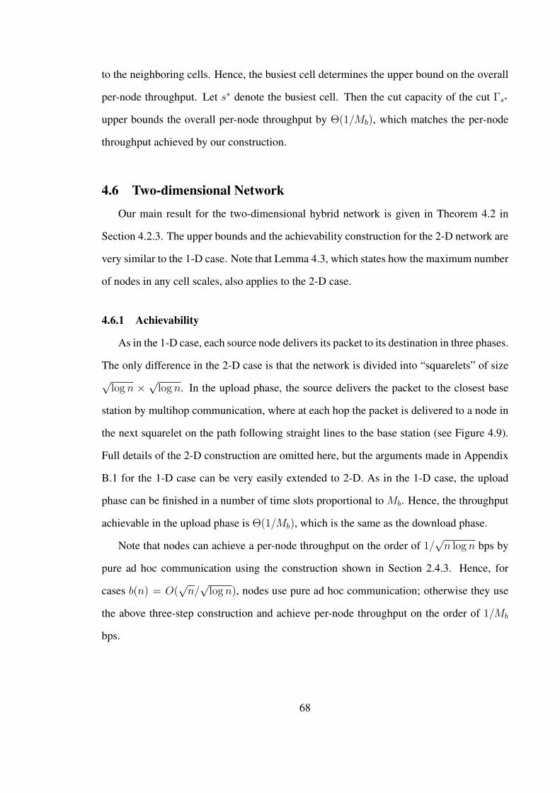
to the neighboring cells. Hence, the busiest cell determines the upper bound on the overall

per-node throughput. Let s∗ denote the busiest cell. Then the cut capacity of the cut Γs∗

upper bounds the overall per-node throughput by Θ(1/Mb), which matches the per-node

throughput achieved by our construction.

4.6 Two-dimensional Network

Our main result for the two-dimensional hybrid network is given in Theorem 4.2 in

Section 4.2.3. The upper bounds and the achievability construction for the 2-D network are

very similar to the 1-D case. Note that Lemma 4.3, which states how the maximum number

of nodes in any cell scales, also applies to the 2-D case.

4.6.1 Achievability

As in the 1-D case, each source node delivers its packet to its destination in three phases.

The only difference in the 2-D case is that the network is divided into “squarelets” of size√log n ×

√log n. In the upload phase, the source delivers the packet to the closest base

station by multihop communication, where at each hop the packet is delivered to a node in

the next squarelet on the path following straight lines to the base station (see Figure 4.9).

Full details of the 2-D construction are omitted here, but the arguments made in Appendix

B.1 for the 1-D case can be very easily extended to 2-D. As in the 1-D case, the upload

phase can be finished in a number of time slots proportional to Mb. Hence, the throughput

achievable in the upload phase is Θ(1/Mb), which is the same as the download phase.

Note that nodes can achieve a per-node throughput on the order of 1/√n log n bps by

pure ad hoc communication using the construction shown in Section 2.4.3. Hence, for

cases b(n) = O(√n/

√log n), nodes use pure ad hoc communication; otherwise they use

the above three-step construction and achieve per-node throughput on the order of 1/Mb

bps.

68

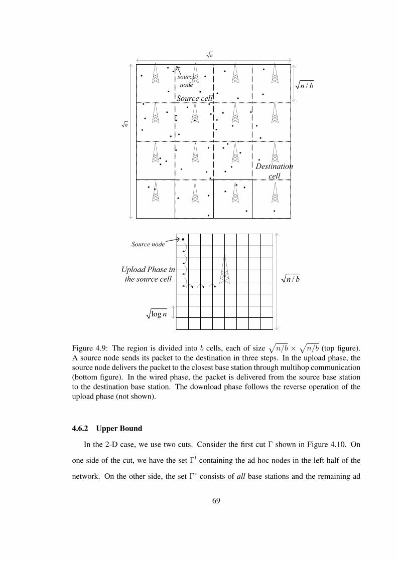
Source cell

n

n

Destination

cell

Upload Phase in

the source cell

Source node

log n

/n b

/n b

source

node

Figure 4.9: The region is divided into b cells, each of size√n/b ×

√n/b (top figure).

A source node sends its packet to the destination in three steps. In the upload phase, thesource node delivers the packet to the closest base station through multihop communication(bottom figure). In the wired phase, the packet is delivered from the source base stationto the destination base station. The download phase follows the reverse operation of theupload phase (not shown).

4.6.2 Upper Bound

In the 2-D case, we use two cuts. Consider the first cut Γ shown in Figure 4.10. On

one side of the cut, we have the set Γl containing the ad hoc nodes in the left half of the

network. On the other side, the set Γr consists of all base stations and the remaining ad

69

n

n

Γ

/n b

/n b

sΓ

Figure 4.10: Cut Γ has half of the ad hoc nodes on one side and the rest of the ad hocnodes and all base stations on the other side. Γ can be crossed into the b/2 base stationsin addition to communication to other nodes through the middle line. Γs is drawn outsidethe nodes in a cell. This cut can be crossed to the base station and to nodes in other cellsthrough ad hoc communication. Crossings to each base station has constant capacity, whilecrossings through ad hoc have capacity proportional to the corresponding edge length ofthe cut.

hoc nodes. The cut capacity in the direction from Γl to Γr consists of connections to the

b/2 base stations, each with a capacity of W bps, and the crossing through the middle line

which has capacity Θ(√n) bps which can be seen by considering Lemma 4.2. Hence, the

cut capacity of Γ is Θ(b+√n) which serves a constant fraction of all nodes w.h.p., resulting

in a per-node capacity of Θ(b/n+√n/n). The second cut Γs is defined similar to the 1-D

case around the nodes inside the cell s. This cut has one crossing of capacity W bps to the

base station, and other crossings through ad hoc connection to nodes outside the cell. Due

to Lemma 4.2, the ad hoc crossing has capacity proportional to the edge length of the cell,

i.e.,√n/b. Hence, the cut for the busiest cell, Γs∗ brings an overall per-node throughput

upper bound of Θ(√n/b/Mb) bps. Finally, due to cuts Γ,Γs, we have an overall upper

bound of Θ(minb/n+√n/n,

√n/b/Mb) which gives the values listed in Theorem 4.2.

70

4.7 Discussion

Capacity scaling laws strongly depend on the communication and network model cho-

sen. Achievability results presented in this chapter can be easily generalized to other mod-

els. For example, in contrast to the model assumed here, if nodes can perform power

control, per-node throughput on the order of 1/√n bps can be achieved by pure ad hoc

communication using the construction in [16]. However, we hasten to note that some of the

cutset bounds we prove in this chapter may not apply under other models. For example,

in contrast to the case shown in Lemma 4.1, under a model where the rate is a function of

the SINR (and without any constraint on minimum inter-node distance, as assumed here),

it is in fact possible for n nodes on a line to achieve a total rate that grows with n across a

single point. This is shown in Appendix B.2.

Note that some previous work on hybrid networks explored the possibility of providing

constant throughput to nodes [1, 40]. Our upper bounds show that (see Lemma 4.2), for

regularly placed base stations, even under the case b = n, a constant rate is not possible for

those nodes that occupy the busiest cell.

4.8 Acknowledgment

The work in this chapter was sponsored by the National Science Foundation under

grant CNS-1018464 and by the U.S. Army Research Laboratory and the U.K. Ministry of

Defence and was accomplished under Agreement Number W911NF-06-3-0001.

71

CHAPTER 5

SECRET COMMUNICATION IN WIRELESS NETWORKS

5.1 Introduction

Consider the transmission of a message from one party (Alice) to another (Bob), such

that it is kept secret from an eavesdropping adversary (Eve). Cryptographic solutions as-

sume that Eve will intercept the transmitted signal cleanly but impose a hard mathematical

problem on Eve that is beyond her computational power to solve. Information-theoretic

solutions do not rely on computational assumptions, but exploit the relative signal quality

achieved at Bob compared to Eve. Specifically, if the signal quality is better at Bob than

it is at Eve, a number of secret bits can be delivered to Bob [75] that is a function of the

difference in signal qualities. Whether information-theoretic or cryptographic secrecy is

employed in a system, there is utility in enhancing reception by the desired party while in-

hibiting reception by eavesdroppers. For information-theoretic security, the need is appar-

ent, since a positive secrecy capacity relies on such. From the viewpoint of cryptographic

security, inhibiting Eve’s reception of the encrypted signal can be used to hide its existence

or characteristics, or may be part of a defense-in-depth approach to information security.

Hence, here we consider constructions that achieve a high signal quality at system nodes

while providing a low signal quality to potential eavesdroppers. If a given high signal-to-

interference-plus-noise ratio (SINR) threshold is exceeded at the system nodes while the

eavesdroppers are unable to achieve a given (lower) SINR threshold, the communication

will be deemed secret.

Here, we consider the secrecy problem in large wireless networks, both in the one-

dimensional and the two-dimensional cases. In particular, we are interested in the amount

72

of information that can be carried by n (legitimate) nodes in a network while being kept

secret from m eavesdroppers also present in the network. This problem can be seen as a se-

curity extension of the original problem of capacity scaling in large wireless networks [29],

where an achievable per-node throughput that scales as O(1/√n log n) is shown for a 2-D

random network of n nodes. Since then, different strategies for achieving similar scaling

results and also upper bounds on the capacity have been shown [16, 43]. When consider-

ing secrecy in large networks, the ability of network nodes to be securely connected (i.e.,

without any constraint on the throughput value) is studied in [30, 61]. Secrecy throughput

scaling in a network with mobile nodes is studied in [44] using a one-hop transmission

scheme [26]. The secrecy capacity scaling with static nodes, as assumed in our work, is

studied in [39], where it is shown that if the eavesdropper locations are known, the eaves-

droppers can be effectively routed around, and a secure per-node throughput of order 1/√n

is feasible as long as the number of eavesdroppers in the network is o(n/(log n)2). The

case of eavesdroppers of unknown location is addressed in [73]. The trade-off between the

per-node throughput that can be achieved and the number of eavesdroppers that can be tol-

erated is explicitly given in [73], where it is shown that a secure throughput on the order of

1/√n log n is achieved if the number of eavesdroppers is on the order of (log n)c, for some

0 < c < 1. The construction that achieves this trade-off uses artificial noise generation

by legitimate nodes to degrade the signal quality at the potential eavesdropper locations,

and uses a multi-user diversity effect exploiting the fading characteristics of the wireless

channel.

A common assumption in most previous work in secrecy scaling is that the locations

of the eavesdroppers are known. However, this assumption is highly undesirable espe-

cially for passive eavesdroppers [21]. In this chapter, we address the issue of unknown

eavesdropper locations by requiring each source node to generate multiple “packets” for

a single message such that the message can only be decoded if all packets are received,

and no information about the message can be gained if even only one of the packets is

73

missing [63, 66]. These packets are sent in separate transmissions such that each packet is

delivered to the destination but kept secure from potential eavesdroppers in a certain region

of the network. Therefore, an eavesdropper anywhere in the network is guaranteed to miss

some non-empty subset of the packets, and hence will not be able to decode the message.

In the two-dimensional case, this is done by sending each packet on a different path, and

maintaining sufficient separation between paths. In other words, the “path diversity” avail-

able in the network is utilized [48] to provide resilience against the lack of knowledge of

the eavesdropper locations. From a graphical view, the eavesdropper has access to only a

subset of the edges connecting the source-destination pair, hence it is possible to deliver

secret bits by secret sharing at the source node and sending the pieces over the edges [6].

In the one-dimensional case, there exists only a single path connecting a source-destination

pair, hence the one-dimensional network itself is partitioned into segments, where each

packet is kept secure from eavesdroppers located in its corresponding segment.

We assume only path loss for the wireless channel, which means when a message is

transmitted, it cannot be securely received by another legitimate node if an eavesdropper

is closer to the transmitter compared to the receiver, since in that case, the SINR condi-

tion for secrecy cannot be satisfied. This makes achieving secret communication in the

one-dimensional case especially challenging, since an eavesdropper located on a point

on the line blocks any communication that has to be securely routed through this point.

This makes secret communication between all legitimate nodes impossible even with a

single eavesdropper in the network. In our work, we make use of the fact that enabling

cooperative jamming makes secret communication possible in the one-dimensional net-

work [8]. In cooperative jamming [22, 60], a legitimate node transmits artificial noise to

degrade the signal quality at the potential nearby eavesdroppers. However, a legitimate

node located far away from the jammer node can still achieve the required SINR, hence

the transmission can “jump over” the eavesdroppers near the jammer to reach its destina-

tion. We present a construction that utilizes cooperative jamming to keep packets secure

74

from eavesdroppers located in the corresponding segment. If the number of eavesdroppers

satisfies m(n) = o(n/log n), with this construction, almost all source-destination pairs

achieve secure throughput of order 1/n with high probability, i.e., with probability one as

the number of nodes n goes to infinity.

In the two-dimensional case, a fundamental advantage is the availability of many paths

connecting a single source-destination pair. We present a construction that utilizes this

path diversity and the fact that an eavesdropper cannot decode the packets that are trans-

mitted over far-away paths. Using our construction, we show that in a two-dimensional

network of n nodes, source-destination pairs can achieve a secure throughput on the order

of 1/√n log n if the number of eavesdroppers satisfies m(n) = o(n/ log n). Furthermore,

the throughput remains secure up to any constant number of eavesdroppers collaborating

by combining their received packets. Note that cooperative jamming is not used in the con-

struction in the two-dimensional case since the eavesdroppers with some minimum distance

to a path cannot achieve the SINR threshold. However, this assumes a certain minimum

noise level in the eavesdropper receivers, which may not be a desirable assumption in all

cases. This can be avoided by using cooperative jamming for the transmissions on the

paths, so that a noise floor is established at the potential eavesdroppers regardless of the

quality of their receivers.

Inspired by the extensive improvements enabled by network coding, we explore whether

additional coding techniques can provide further gains in secrecy in large wireless net-

works. The utility of network coding for secrecy has been recognized in previous work

[6, 31], where it was studied in a more abstract setting. This motivates a more careful

study of the application of general principles from the area of “secure network coding” to

the wireless security problem. While the field of secure network coding is relatively well

understood, the mapping of the wireless security problem to its framework is not clear. Se-

cure network coding is a graph-based approach in which eavesdroppers tap edges (or not),

which does not map well to the wireless environment where there are no edges but rather

75

there is a continuum of SNRs. Nevertheless, the coding methods proven to be useful to

secrecy can easily be replicated for the wireless case. We show that by employing addi-

tional coding, in the non-collaborating eavesdropper case, our secrecy capacity results can

be further improved by achieving a secure throughput on the order of 1/√n log n for any

number of eavesdroppers that may be arbitrarily located inside the network.

The rest of the chapter is organized as follows. We describe the network and channel

models in the next section, which are used in our secrecy capacity results presented in Sec-

tion 5.3 for the one-dimensional networks, and in Section 5.4 for the two-dimensional case.

Our focused study in the utility of network coding ideas to wireless secrecy is presented in

detail in Section 5.5, where we also present our improved results in the two-dimensional

case. Section 5.6 is the conclusion.

5.2 Model

5.2.1 Network and Channel Model

The wireless network is composed of legitimate nodes and eavesdroppers inside the

interval [0, n] in the one-dimensional case, and inside the square region [0,√n] × [0,

√n]

in the two-dimensional case. Legitimate nodes are distributed according to a homogeneous

Poisson point process with intensity λ = 1. All nodes are assumed to be static. Legitimate

nodes are matched into source-destination pairs uniformly at random, such that each node is

the destination of exactly one source node, and the source for exactly one destination node.

For each pair, we associate a stream of information that needs to flow from the source

to the destination. Eavesdroppers are assumed to be passive, and in the one-dimensional

case, operating independently of each other, i.e., they do not collaborate by sharing their

observations.

Only path loss is assumed for the wireless channels between transmitter and receiver

nodes. Hence, whenever a node A transmits with some transmit power P , the received

power at node B is modeled as

76

Prcv,B = P/dαAB,

where dAB is the distance between nodes A,B, and α > 1 in 1-D, α > 2 in 2-D, is the

path loss exponent. This model may be appropriate for a wideband system where fading

is averaged out due to frequency diversity, or an environment without significant multipath

effects.

We adopt a threshold model here, as motivated for both practical and information-

theoretic security in [20]. Thus, we assume a message is successfully decoded if the re-

ceived signal-to-interference-plus-noise ratio (SINR) exceeds a certain threshold γ > 0. In

other words, node B successfully decodes node A’s message if

SINRB , Prcv,B

N0 + IB> γ, (5.1)

where N0 is the power in the additive white Gaussian noise (AWGN) at the receiver, and

IB is the interference received at node B due to other transmissions in the network. In our

case, this interference may be due to other legitimate signal transmissions and/or artificial

noise generated by legitimate nodes.

As mentioned above, for a message to be securely received at B in the presence of

an eavesdropper E, we require the SINR at the eavesdropper SINRE to be smaller than

SINRB. Furthermore, it may be desirable to have some positive SINR gap between nodes

B and E. Hence, for some γe such that 0 < γe < γ, in our model, we require SINRE < γe,

where γe can be selected to be arbitrarily small. Note that, from an information-theoretic

secrecy perspective, this allows choosing some positive secrecy rate Rs given as [42]

Rs =1

2

(log(1 + SINRB)− log(1 + SINRE)

).

Therefore, for some region R in the network, a message is decoded by B while being

secret from eavesdroppers inside R if (1) SINRB > γ, and (2) any eavesdropper E inside

77

R has SINRE < γe. For multihop transmission from a source node to a destination node,

if this SINR condition is satisfied at every hop, we refer to the rate of information as the

secure throughput achieved by this pair. Note that secrecy at each hop over a multihop path

is shown to be sufficient for end-to-end secrecy in [39].

5.2.2 Performance Metrics

The network carries information streams to be delivered from the source nodes to their

respective destinations. We consider the network’s ability to carry these streams at a cer-

tain per-node throughput in the presence of eavesdroppers. Our performance metric is the

number of eavesdroppers that can be tolerated while legitimate nodes maintain some secure

throughput with high probability (w.h.p.).

5.3 One-dimensional Networks

The following theorem establishes security in the absence of eavesdroppers near the

source-destination nodes, which is then used in Theorem 5.2 to establish the number of

eavesdroppers that can be tolerated.

Theorem 5.1. Consider the one-dimensional network inside the interval [0, n], where eaves-

droppers are arbitrarily distributed. The locations of the eavesdroppers are unknown,

and they are assumed not to collaborate. Legitimate nodes can maintain a throughput

of Θ(1/n)

w.h.p. for all source-destination pairs, for any number of eavesdroppers. For

some fixed positive constant r, the throughput achieved is secure for the source-destination

pairs that satisfy the condition that no eavesdropper is placed within a distance r log n to

the source and to the destination node.

Overview of the Proof

We prove Theorem 5.1 by providing a construction summarized by the following steps:

78

1. In order to handle unknown eavesdropper locations, we partition the network into a

finite number t of interlaced regions (also referred in the following as “coloring”

the network), and treat each region (color) one by one, assuming each time that

eavesdroppers are all confined to that particular region.

2. For each message to be delivered to the destination node, the source node generates

t “packets”, with each packet corresponding to one of the regions. These packets

are generated in a way that ensures the message cannot be decoded by a node un-

less all packets are successfully received. These packets are delivered in separate

transmissions such that each packet is protected from potential eavesdroppers in its

corresponding region, thus guaranteeing that an eavesdropper located anywhere in

the network misses at least one of the packets.

3. We provide an algorithm that routes packets from source to destination in such a way

to ensure the secure transfer of the packet from potential eavesdroppers inside the

region corresponding to it. This is achieved by legitimate nodes inside the region

acting as “jammers” by transmitting random noise to prevent eavesdroppers in that

region from decoding the packet.

4. We use time division multiplexing, where time is considered as a sequence of “pe-

riods”. Each period consists of t “frames”, and packets corresponding to color

i, i ∈ 1, 2, · · · , t, are transmitted in the ith frame. Each frame is further divided

into slots, where a standard spatial reuse scheme (as in [29]) is employed.

The proof is completed by showing that this construction achieves the stated throughput

properties with probability one as the size of the network, n, goes to infinity.

Proof. Our construction consists of (1) partitioning of the network into regions (also re-

ferred to below as “coloring” the network), (2) a routing algorithm, and (3) a time-division

multiplexing scheme, which are given in detail in the following. The proof is completed

79

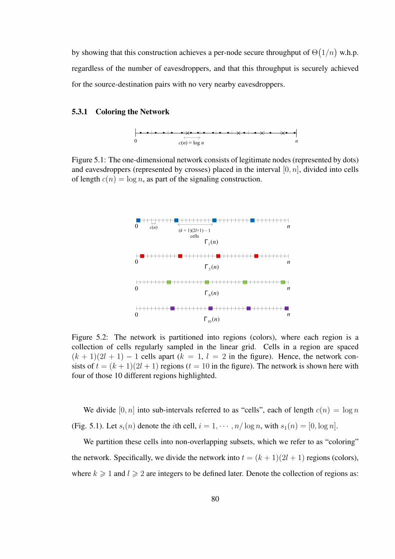
by showing that this construction achieves a per-node secure throughput of Θ(1/n)

w.h.p.

regardless of the number of eavesdroppers, and that this throughput is securely achieved

for the source-destination pairs with no very nearby eavesdroppers.

5.3.1 Coloring the Network

· · · · · · · · · · ··0 n

· · ···c(n) = log n

Figure 5.1: The one-dimensional network consists of legitimate nodes (represented by dots)and eavesdroppers (represented by crosses) placed in the interval [0, n], divided into cellsof length c(n) = log n, as part of the signaling construction.

(k + 1)(2l+1) – 1

cells

0 n

1( )nΓ

n

10( )nΓ

0

n

9( )nΓ

0

0 n

2( )nΓ

c(n)

Figure 5.2: The network is partitioned into regions (colors), where each region is acollection of cells regularly sampled in the linear grid. Cells in a region are spaced(k + 1)(2l + 1) − 1 cells apart (k = 1, l = 2 in the figure). Hence, the network con-sists of t = (k + 1)(2l + 1) regions (t = 10 in the figure). The network is shown here withfour of those 10 different regions highlighted.

We divide [0, n] into sub-intervals referred to as “cells”, each of length c(n) = log n

(Fig. 5.1). Let si(n) denote the ith cell, i = 1, · · · , n/ log n, with s1(n) = [0, log n].

We partition these cells into non-overlapping subsets, which we refer to as “coloring”

the network. Specifically, we divide the network into t = (k + 1)(2l + 1) regions (colors),

where k > 1 and l > 2 are integers to be defined later. Denote the collection of regions as:

80

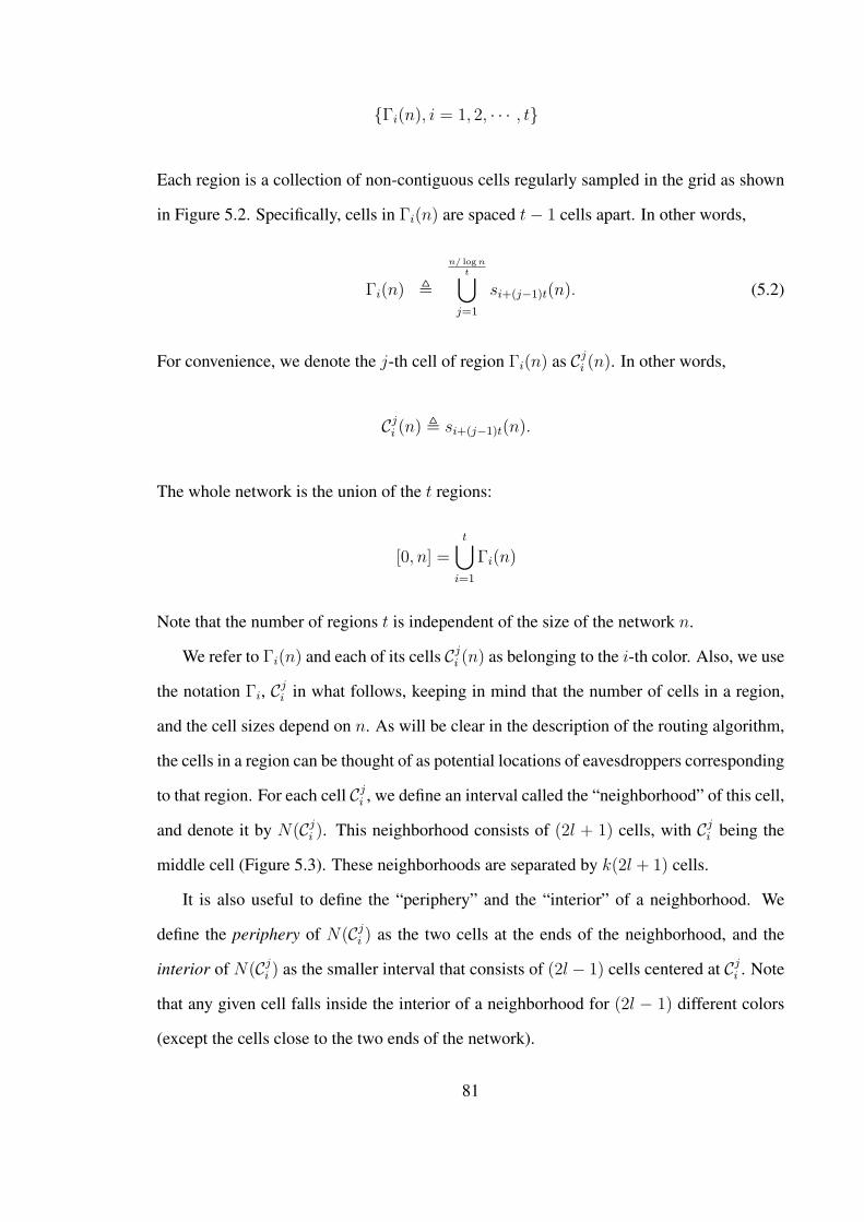
Γi(n), i = 1, 2, · · · , t

Each region is a collection of non-contiguous cells regularly sampled in the grid as shown

in Figure 5.2. Specifically, cells in Γi(n) are spaced t− 1 cells apart. In other words,

Γi(n) ,n/ logn

t∪j=1

si+(j−1)t(n). (5.2)

For convenience, we denote the j-th cell of region Γi(n) as Cji (n). In other words,

Cji (n) , si+(j−1)t(n).

The whole network is the union of the t regions:

[0, n] =t∪

i=1

Γi(n)

Note that the number of regions t is independent of the size of the network n.

We refer to Γi(n) and each of its cells Cji (n) as belonging to the i-th color. Also, we use

the notation Γi, Cji in what follows, keeping in mind that the number of cells in a region,

and the cell sizes depend on n. As will be clear in the description of the routing algorithm,

the cells in a region can be thought of as potential locations of eavesdroppers corresponding

to that region. For each cell Cji , we define an interval called the “neighborhood” of this cell,

and denote it by N(Cji ). This neighborhood consists of (2l + 1) cells, with Cj

i being the

middle cell (Figure 5.3). These neighborhoods are separated by k(2l + 1) cells.

It is also useful to define the “periphery” and the “interior” of a neighborhood. We

define the periphery of N(Cji ) as the two cells at the ends of the neighborhood, and the

interior of N(Cji ) as the smaller interval that consists of (2l− 1) cells centered at Cj

i . Note

that any given cell falls inside the interior of a neighborhood for (2l − 1) different colors

(except the cells close to the two ends of the network).

81

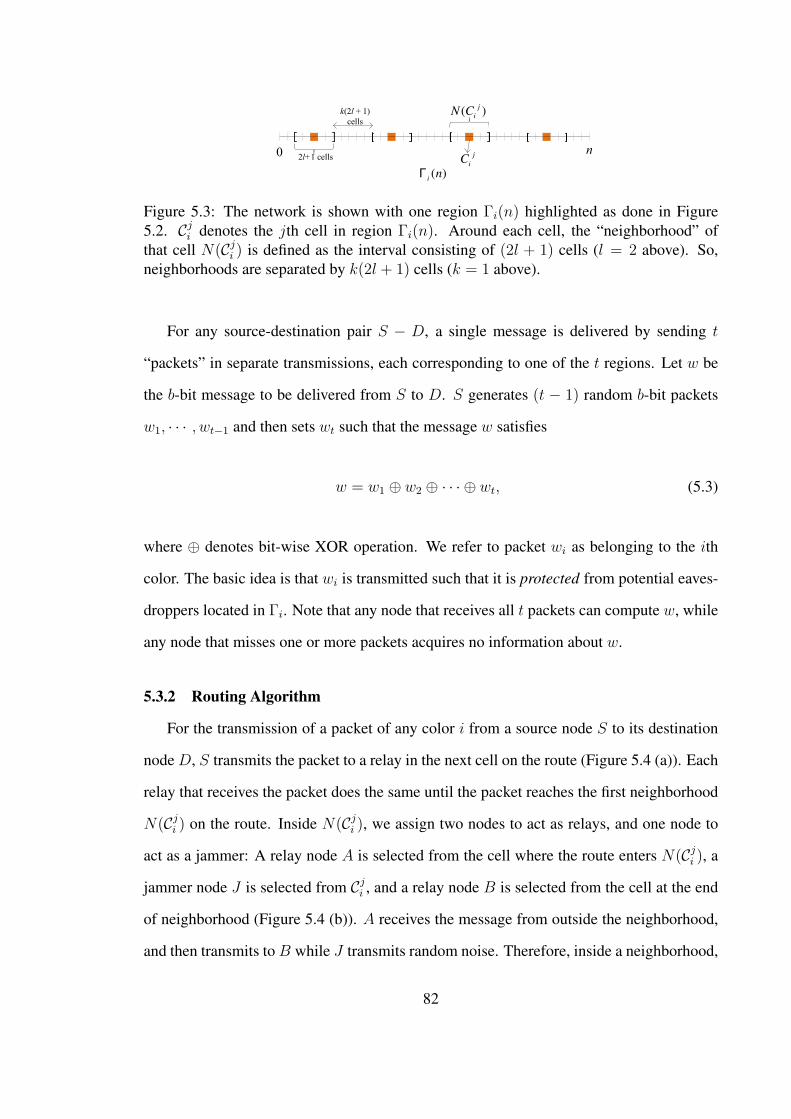
n

( )i

nΓ

0 2l+1 cells

k(2l + 1)

cells

j

iC

( )j

iN C

Figure 5.3: The network is shown with one region Γi(n) highlighted as done in Figure5.2. Cj

i denotes the jth cell in region Γi(n). Around each cell, the “neighborhood” ofthat cell N(Cj

i ) is defined as the interval consisting of (2l + 1) cells (l = 2 above). So,neighborhoods are separated by k(2l + 1) cells (k = 1 above).

For any source-destination pair S − D, a single message is delivered by sending t

“packets” in separate transmissions, each corresponding to one of the t regions. Let w be

the b-bit message to be delivered from S to D. S generates (t − 1) random b-bit packets

w1, · · · , wt−1 and then sets wt such that the message w satisfies

w = w1 ⊕ w2 ⊕ · · · ⊕ wt, (5.3)

where ⊕ denotes bit-wise XOR operation. We refer to packet wi as belonging to the ith

color. The basic idea is that wi is transmitted such that it is protected from potential eaves-

droppers located in Γi. Note that any node that receives all t packets can compute w, while

any node that misses one or more packets acquires no information about w.

5.3.2 Routing Algorithm

For the transmission of a packet of any color i from a source node S to its destination

node D, S transmits the packet to a relay in the next cell on the route (Figure 5.4 (a)). Each

relay that receives the packet does the same until the packet reaches the first neighborhood

N(Cji ) on the route. Inside N(Cj

i ), we assign two nodes to act as relays, and one node to

act as a jammer: A relay node A is selected from the cell where the route enters N(Cji ), a

jammer node J is selected from Cji , and a relay node B is selected from the cell at the end

of neighborhood (Figure 5.4 (b)). A receives the message from outside the neighborhood,

and then transmits to B while J transmits random noise. Therefore, inside a neighborhood,

82

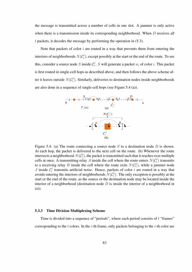
the message is transmitted across a number of cells in one slot. A jammer is only active

when there is a transmission inside its corresponding neighborhood. When D receives all

t packets, it decodes the message by performing the operation in (5.3).

Note that packets of color i are routed in a way that prevents them from entering the

interiors of neighborhoodsN(Cji ), except possibly at the start or the end of the route. To see

this, consider a source node S inside Cji . S will generate a packet wi of color i. This packet

is first routed in single-cell hops as described above, and then follows the above scheme af-

ter it leaves outside N(Cji ). Similarly, deliveries to destination nodes inside neighborhoods

are also done in a sequence of single-cell hops (see Figure 5.4 (a)).

n

( )i

nΓ0

j

iC

S D

j

iC

( )j

iN C

A BJ

(b)

(a)

Figure 5.4: (a) The route connecting a source node S to a destination node D is shown.At each hop, the packet is delivered to the next cell on the route. (b) Whenever the routeintersects a neighborhoodN(Cj

i ), the packet is transmitted such that it reaches over multiplecells at once. A transmitting relay A inside the cell where the route enters N(Cj

i ) transmitsto a receiving relay B inside the cell where the route exits N(Cj

i ), while a jammer nodeJ inside Cj

i transmits artificial noise. Hence, packets of color i are routed in a way thatavoids entering the interiors of neighborhoodsN(Cj

i ). The only exception is possibly at thestart or the end of the route, as the source or the destination node may be located inside theinterior of a neighborhood (destination node D is inside the interior of a neighborhood in(a)).

5.3.3 Time Division Multiplexing Scheme

Time is divided into a sequence of “periods”, where each period consists of t “frames”

corresponding to the t colors. In the i-th frame, only packets belonging to the i-th color are

83

transmitted. In each frame, a spatial reuse scheme is employed such that in the i-th frame,

every cell in the network transmits one packet of color i. This is done by further dividing

each frame into t time slots. In each slot, transmitting cells are t− 1 cells apart (see Figure

5.5). During the i-th frame, jammer nodes inside Γi may be active only during the two time

slots where relays in the periphery of neighborhoods transmit.

The streams arriving to a cell take turns being relayed. A node in a given cell has to

relay information for at most a constant factor of n streams w.h.p., hence a throughput of

Θ(1/n)

per stream is achieved w.h.p.

The route a packet takes contains the following types of hops: (1) single-cell hop out-

side neighborhoods, (2) multiple-cell hop inside a neighborhood, (3) single-cell hop inside

a neighborhood if it contains either the source or destination (see Figure 5.4). In Appendix

A.1, we show that the first two types of hops are achieved securely. We show that there

exist constants k, l for coloring the network, and transmit power values for relays and jam-

mer nodes, such that for any stream of color i, the destination node and the eavesdroppers

inside Γi satisfy the SINR requirement for secure transmission. Hence, the only possible

insecure transmissions are in the close proximity of the source and destination nodes (i.e.,

the third type above). For a source-destination pair, if no eavesdropper is within a distance

rc(n), r = l, to the source and the destination, then these hops will also be secure, hence

the result follows.

Theorem 5.2. Consider the one-dimensional network inside the interval [0, n], where the

eavesdroppers are placed according to a Poisson point process with some density λe > 0,

independent of the placement of the legitimate nodes. The locations of the eavesdrop-

pers are unknown, and they are assumed not to collaborate. Then, the fraction of source-

destination pairs that can maintain a per-node secure throughput of Θ(1/n)

is arbitrarily

close to one w.h.p, if λe = o(1/ log(n)).

84

n0(a)

n0(b)

n0(c)

Figure 5.5: One period is divided into t frames. In the i-th frame, cells take turn in relay-ing packets of color i. Relaying is done according to the routing protocol correspondingto Γi (see Figure 5.4). Each frame consists of t time slots (t = 10 in the figure). Cellstransmitting simultaneously (dashed cells) in one slot are t − 1 cells apart. For the i-thframe, three time slots are shown above: (a) shows a time slot with single-cell transmis-sions outside neighborhoods, (b) shows a time slot with transmissions in the periphery ofneighborhoods (which may include multi-cell hops with jammers active), (c) shows a timeslot with transmissions in the interiors of neighborhoods.

Proof. We use the same construction as that used to prove Theorem 5.1, which is shown

to achieve w.h.p. the stated secure throughput for source-destination pairs free from any

nearby eavesdroppers. The proof follows by showing that for λe = o(1/ log n), the fraction

of source-destination pairs that do not have any nearby eavesdroppers is arbitrarily close to

one w.h.p.

Let the random variable m(n) be the number of eavesdroppers in the network, which

has an expected value of λen. Let yi ∈ [0, n] be the location of the i-th eavesdropper, and

define Ai(n) = [yi − l log n, yi + l log n], with length ℓ(n) , |Ai(n)| = 2l log n,∀i. Let

A(n) be the total region covered by the eavesdroppers, i.e., any source or destination node

inside A(n) will not be able to communicate secretly.

A(n) ,m(n)∪i=1

Ai(n) (5.4)

Let Ni(n), No(n) be the random variables denoting the number of legitimate nodes

inside and outside A(n), respectively. For some ε > 0, define the event Cε(n) as

85

Cε(n) ,

Ni(n)

Ni(n) +No(n)< ε

. (5.5)

We can write P (Cε(n)) as

P (Cε(n)) = P (Cε(n) | |A(n)| ≤ 2λenℓ(n))P (|A(n)| ≤ 2λenℓ(n))

+ P (Cε(n) | |A(n)| > 2λenℓ(n))P (|A(n)| > 2λenℓ(n))

Define the random variable X(n) as

X(n) , Ni(n)/n

No(n)/n.

Given λe = o(1/log n), and |A(n)| ≤ 2λenℓ(n),

Ni(n)/n→ 0, No(n)/n→ 1, and X(n) → 0, a.s.

Then,

P(Cε(n) | |A(n)| ≤ 2λenℓ(n)

)=

P

(X(n)

1 +X(n)< ε | |A(n)| ≤ 2λenℓ(n)

)→ 1, n→ ∞ (5.6)

Since, by a Chernoff bound,

P (|A(n)| ≤ 2λenℓ(n)) ≥ P (m ≤ 2λen) → 1, n→ ∞,

P (Cε(n)) → 1, as n → ∞, for any ε > 0. Hence, with high probability, the fraction

of nodes inside A(n) is arbitrarily close to zero, which readily implies that the fraction of

source-destination pairs inside A(n) is arbitrarily close to zero w.h.p.

86

5.4 Two-dimensional Networks

Similar to the one-dimensional case, we first establish security in the absence of eaves-

droppers near the source-destination nodes in the following theorem by presenting a con-

struction, which is then used in Theorem 5.4 to establish the number of eavesdroppers that

can be tolerated.

Theorem 5.3. Consider the two-dimensional network inside the square [0,√n]× [0,

√n],

where the eavesdroppers are arbitrarily distributed, and the locations of the eavesdroppers

are unknown. Legitimate nodes can maintain a throughput of Θ(1/√n log n

)w.h.p. for

all source-destination pairs, for any number of eavesdroppers. For some fixed positive

constant r, the throughput achieved is secure for the source-destination pairs that satisfy

the condition that no eavesdropper is placed within a distance r√log n to the source and

to the destination node. For any given integer t < ∞, the throughput remains secure for

any number g < t of collaborating eavesdroppers arbitrarily chosen from the network.

Overview of the proof:

Similar to the one-dimensional case, the key technique adopted in the construction to

prove Theorem 5.3 is to require each source node to generate multiple packets to be sent in

separate transmissions. However, a fundamental advantage in the two-dimensional case is

that there exist many paths connecting each source-destination pair. By carefully selecting

paths, and sending each packet on a different path, it can be ensured that an eavesdropper

anywhere in the network cannot decode at least some of the packets since it is far from some

of the paths. Therefore, unlike the one-dimensional case, “coloring” is done across differ-

ent paths, rather than across different segments of a single path. By choosing the number

of paths accordingly, it is further ensured that for any number of collaborating eavesdrop-

pers up to some constant, the eavesdroppers cannot decode messages by combining their

received packets.

87

Proof. In the following, we present the construction and prove that the construction achieves

the stated properties.

5.4.1 Routing Algorithm

We divide [0,√n] × [0,

√n] into a square lattice of cells, each with a side of length

c(n) =√log n (Figure 5.6); hence, each cell contains a legitimate node w.h.p. (see Ap-

pendix A.1). For each source-destination pair S −D, S generates t packets w1, · · · , wt

for each message w to be sent. The packets are generated in the same way as done in the

one-dimensional case (see Section 5.3.1).

( ) logc n n=

n

n

×

×

×

× ×

×

×

× ×

Figure 5.6: The two-dimensional network consists of legitimate nodes (represented bydots) and eavesdroppers (represented by crosses) placed in the square [0,

√n] × [0,

√n],

divided into square cells of size c(n) × c(n), with c(n) =√log n, as part of the signaling

construction.

Consider square regions with (t − 1)(2l − 1) + 1 cells on each side with S, and D in

the center cells. We refer to these as S and D’s “bases” (Figure 5.7). We define t “paths”

connecting S to D, and packets of color i are sent on the i-th path. As shown in Figure 5.7,

each path exits the source base on a horizontal line, then follows a vertical line entering the

destination base. The first path exits the edge of the source base from the top cell on the

edge. Outside the bases, the paths have a minimum spacing of (2l − 2) cells. Inside the

88

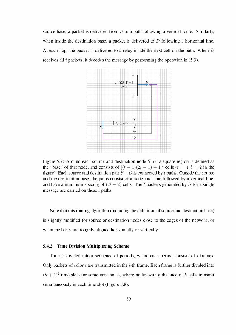
source base, a packet is delivered from S to a path following a vertical route. Similarly,

when inside the destination base, a packet is delivered to D following a horizontal line.

At each hop, the packet is delivered to a relay inside the next cell on the path. When D

receives all t packets, it decodes the message by performing the operation in (5.3).

DD

D

S

D

2l -2 cells

(t-1)(2l -1) + 1

cells

w1

w2

w3

w4

Figure 5.7: Around each source and destination node S,D, a square region is defined asthe “base” of that node, and consists of [(t − 1)(2l − 1) + 1]2 cells (t = 4, l = 2 in thefigure). Each source and destination pair S−D is connected by t paths. Outside the sourceand the destination base, the paths consist of a horizontal line followed by a vertical line,and have a minimum spacing of (2l − 2) cells. The t packets generated by S for a singlemessage are carried on these t paths.

Note that this routing algorithm (including the definition of source and destination base)

is slightly modified for source or destination nodes close to the edges of the network, or

when the bases are roughly aligned horizontally or vertically.

5.4.2 Time Division Multiplexing Scheme

Time is divided into a sequence of periods, where each period consists of t frames.

Only packets of color i are transmitted in the i-th frame. Each frame is further divided into

(h + 1)2 time slots for some constant h, where nodes with a distance of h cells transmit

simultaneously in each time slot (Figure 5.8).

89

h cells

h cells

Figure 5.8: One period is divided into t frames, where only packets of color i are trans-mitted in the ith frame. Each frame is further divided into time (h + 1)2 slots. Nodestransmitting simultaneously (shaded cells) in a given time slot are h cells apart. In eachtime slot, relays in the active cells transmit a packet to a relay inside the next cell on thepath.

In each cell, streams that have arrived to that cell take turns being relayed. As proved

in Appendix A.3, the number of streams arriving to each cell is at most a constant times√n log n w.h.p. Hence, a throughput value of Θ

(1/√n log n

)is achieved for each source-

destination pair w.h.p.

For the secrecy of the achieved throughput, consider the transfer of a message w to be

carried from node S toD, and focus on the transmission of a packetwi on its corresponding

path. Consider a hop where wi is transmitted from node A to B. It is shown that (Appendix

A.2), the receiving node B, and any eavesdropper E located at least a distance of (l − 1)

cells from the transmitting cell satisfy the SINR condition for secrecy. This shows that a

packet of color i is protected from all the eavesdroppers located outside a strip of width

(2l − 1) cells surrounding the path carrying that packet. Note that, outside the bases, an

eavesdropper can be located less than (l − 1) cells to at most one path due to the spacing

of the paths. If the source and the destination are free from eavesdroppers inside a radius

of r log n, for any r > 2tl, then the source and destination bases do not contain any eaves-

droppers. Hence, an eavesdropper in the network can decode at most one packet out of

the t packets. Therefore, any number g < t of collaborating eavesdroppers are not able to

decode the message by combining their received packets.

90

Theorem 5.4. Consider the two-dimensional network inside [0,√n] × [0,

√n], where the

eavesdroppers are placed according to a Poisson point process with some density λe > 0,

independent of the placement of the legitimate nodes. Then, almost all source-destination

pairs can maintain a per-node secure throughput of Θ(1/√n log n

)w.h.p, if λe = o(1/ log(n)),

and the throughput achieved remains secure for any number g < t of collaborating eaves-

droppers arbitrarily chosen from the network.

The proof is very similar to the proof of Theorem 5.2, and is omitted.

5.5 Network Coding for Secrecy

In this section, motivated by the results in Sections 5.3 and 5.4, we take a more general

view and study the utility of network coding approaches to help guarantee information-

theoretic secrecy in the wireless environment. We present “toy” examples in Section 5.5.2

to demonstrate the salient aspects, and then show in Section 5.5.4 how the insight gained

allows us to improve secrecy scaling results presented in Section 5.4.

5.5.1 Model

Here we describe the main tools used in the section. The first is the wiretap network

model [6], which is an abstract graph-based tool that allows a formal way to check whether

secure communication is possible using network coding [31]. The second is a very use-

ful tool called the secrecy graph [30] which allows one to map a given physical wireless

network topology (including eavesdroppers) to a graph which we study using the wiretap

network model.

5.5.1.1 Wiretap Network

Let G = (V,E) be a directed graph, where V is the set of legitimate wireless nodes

including one source node s, and one destination node d. E is the set of edges representing

the connections between the nodes. Assume that all nodes in V have a path to d. There is a

91

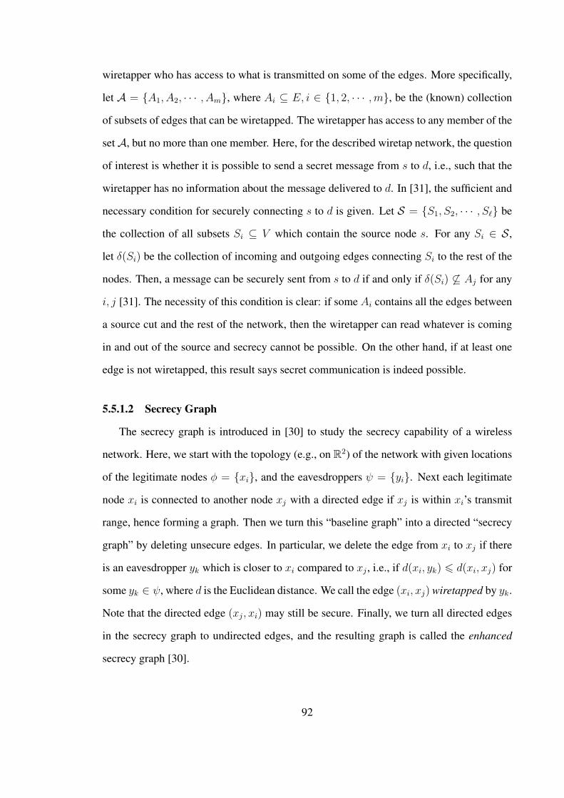
wiretapper who has access to what is transmitted on some of the edges. More specifically,

let A = A1, A2, · · · , Am, where Ai ⊆ E, i ∈ 1, 2, · · · ,m, be the (known) collection

of subsets of edges that can be wiretapped. The wiretapper has access to any member of the

set A, but no more than one member. Here, for the described wiretap network, the question

of interest is whether it is possible to send a secret message from s to d, i.e., such that the

wiretapper has no information about the message delivered to d. In [31], the sufficient and

necessary condition for securely connecting s to d is given. Let S = S1, S2, · · · , Sℓ be

the collection of all subsets Si ⊆ V which contain the source node s. For any Si ∈ S ,

let δ(Si) be the collection of incoming and outgoing edges connecting Si to the rest of the

nodes. Then, a message can be securely sent from s to d if and only if δ(Si) ⊆ Aj for any

i, j [31]. The necessity of this condition is clear: if some Ai contains all the edges between

a source cut and the rest of the network, then the wiretapper can read whatever is coming

in and out of the source and secrecy cannot be possible. On the other hand, if at least one

edge is not wiretapped, this result says secret communication is indeed possible.

5.5.1.2 Secrecy Graph

The secrecy graph is introduced in [30] to study the secrecy capability of a wireless

network. Here, we start with the topology (e.g., on R2) of the network with given locations

of the legitimate nodes ϕ = xi, and the eavesdroppers ψ = yi. Next each legitimate

node xi is connected to another node xj with a directed edge if xj is within xi’s transmit

range, hence forming a graph. Then we turn this “baseline graph” into a directed “secrecy

graph” by deleting unsecure edges. In particular, we delete the edge from xi to xj if there

is an eavesdropper yk which is closer to xi compared to xj , i.e., if d(xi, yk) 6 d(xi, xj) for

some yk ∈ ψ, where d is the Euclidean distance. We call the edge (xi, xj) wiretapped by yk.

Note that the directed edge (xj, xi) may still be secure. Finally, we turn all directed edges

in the secrecy graph to undirected edges, and the resulting graph is called the enhanced

secrecy graph [30].

92

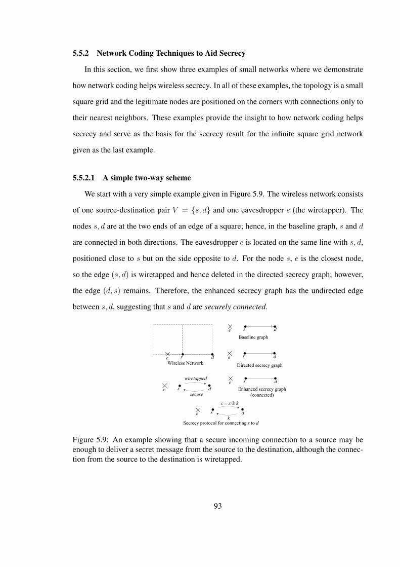
5.5.2 Network Coding Techniques to Aid Secrecy

In this section, we first show three examples of small networks where we demonstrate

how network coding helps wireless secrecy. In all of these examples, the topology is a small

square grid and the legitimate nodes are positioned on the corners with connections only to

their nearest neighbors. These examples provide the insight to how network coding helps

secrecy and serve as the basis for the secrecy result for the infinite square grid network

given as the last example.

5.5.2.1 A simple two-way scheme

We start with a very simple example given in Figure 5.9. The wireless network consists

of one source-destination pair V = s, d and one eavesdropper e (the wiretapper). The

nodes s, d are at the two ends of an edge of a square; hence, in the baseline graph, s and d

are connected in both directions. The eavesdropper e is located on the same line with s, d,

positioned close to s but on the side opposite to d. For the node s, e is the closest node,

so the edge (s, d) is wiretapped and hence deleted in the directed secrecy graph; however,

the edge (d, s) remains. Therefore, the enhanced secrecy graph has the undirected edge

between s, d, suggesting that s and d are securely connected.

s de

wiretapped

secure

s dek

s de

c x k= ⊕

s de

s de

s de

Baseline graph

Directed secrecy graph

Enhanced secrecy graph

(connected)

Wireless Network

Secrecy protocol for connecting s to d

Figure 5.9: An example showing that a secure incoming connection to a source may beenough to deliver a secret message from the source to the destination, although the connec-tion from the source to the destination is wiretapped.

93

Now consider this example with the wiretap network model. For the wiretapper, we

have the set A = A1, where A1 = (s, d). There is a single source cut S1 = s, and

δ(S1) = (s, d), (d, s). Hence, δ(S1) ⊆ A1, and the secrecy condition is satisfied, which

means there is a way to send a secret message from s to d. A secret message x is sent from

s to d in two steps. In the first step, d generates a random string k and sends it to s. In the

second step, s uses k as a one-time pad, and sends the string c = x ⊕ k, where ⊕ is the

XOR operation. In the end, d has the strings k, c and extracts x; however, e only has the

string c and can obtain no information about x. This example illustrates the powerful idea

that an incoming connection to the source can be very valuable for secrecy, and this will be

exploited in the examples below. The fact that two nodes can be securely connected as long

as one of the edges is secure was recognized in [30], and is the reason for the introduction

of the enhanced secrecy graph to check secure connectivity.

5.5.2.2 Non-collaborating eavesdroppers of known location

Here, we have four legitimate nodes V = s, a, b, d on the four corners of a square,

and two eavesdroppers e1, e2 located in the middle of the edges between the pairs s, a, and

s, b (Figure 5.10). The edges in both directions between s, a and s, b are wiretapped, hence

the resulting secrecy graph is disconnected. Although the source is disconnected from both

of its neighbors in both directions, we show that with the help of network coding, delivering

a secure message from s to d is possible.

We first check whether the secrecy condition is satisfied. Assuming the two eavesdrop-

pers do not collaborate, we have the following sets of wiretapped edges. A = A1, A2,

where

A1 = (s, a), (s, b), (a, s), (a, d) ,

A2 = (s, a), (s, b), (b, s), (b, d) .

Now consider the cuts S = S1, S2, S3, S4, where

94

s b

a d

e1

e2 s b

a d

e1

e2

s b

a d

e1

e2 s b

a d

e1

e2

k1

k2

k1 k2

c

c

1 2c x k k= ⊕ ⊕

Wireless Network Baseline graph

Enhanced secrecy graph

(disconnected) Secrecy protocol for connecting s to d

s b

a d

e1

e2

Directed secrecy graph

Figure 5.10: An example which shows that even though the source is disconnected from itsneighbors in both directions, secure communication may still be possible if these blockagesare due to separate non-collaborating wiretappers.

S1 = s, δ(S1) = (s, a), (s, b), (a, s), (b, s),

S2 = s, a, δ(S2) = (s, b), (a, d), (b, s), (d, a),

S3 = s, b, δ(S3) = (s, a), (b, d), (a, s), (d, b),

S4 = s, a, b, δ(S4) = (a, d), (b, d), (d, a), (d, b).

Notice that δ(Si) ⊆ Aj, for any i, j. Hence, the condition for secrecy is satisfied and it

is possible to securely connect s to d. In Figure 5.10, we describe a protocol that achieves

such. First, nodes a, b generate random strings k1, k2, respectively and send them over their

outgoing edges successively. Next, s calculates c = x ⊕ k1 ⊕ k2, and sends it. Finally, a

forwards the string c to d. The receiver d now has the strings c, k1, k2 and can extract the

secret message x. At the end of the protocol, the eavesdropper e1 has the strings k1, c, but

misses k2. Similarly, e2 has c, k2 but not k1. Therefore, the eavesdroppers do not have any

information about the message x. Also, note that the message is not revealed to the nodes

a, b.

95

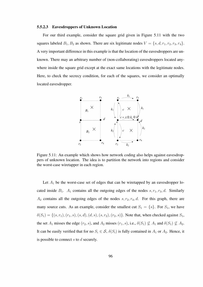
5.5.2.3 Eavesdroppers of Unknown Location

For our third example, consider the square grid given in Figure 5.11 with the two

squares labeled B1, B2 as shown. There are six legitimate nodes V = s, d, r1, r2, r3, r4.

A very important difference in this example is that the location of the eavesdroppers are un-

known. There may an arbitrary number of (non-collaborating) eavesdroppers located any-

where inside the square grid except at the exact same locations with the legitimate nodes.

Here, to check the secrecy condition, for each of the squares, we consider an optimally

located eavesdropper.

s

r1

s b

a d

e1

e2

d

r2

r3

r4

k1

k1

k2

k2

1 2c x k k= ⊕ ⊕

c

ck2

s

r1

d

r2

r3

r4

k1B1

B2

Figure 5.11: An example which shows how network coding also helps against eavesdrop-pers of unknown location. The idea is to partition the network into regions and considerthe worst-case wiretapper in each region.

Let A1 be the worst-case set of edges that can be wiretapped by an eavesdropper lo-

cated inside B1. A1 contains all the outgoing edges of the nodes s, r1, r3, d. Similarly

A2 contains all the outgoing edges of the nodes s, r2, r4, d. For this graph, there are

many source cuts. As an example, consider the smallest cut S1 = s. For S1, we have

δ(S1) = (s, r1), (r1, s), (s, d), (d, s), (s, r2), (r2, s). Note that, when checked against S1,

the set A1 misses the edge (r2, s), and A2 misses (r1, s), i.e., δ(S1) ⊆ A1 and δ(S1) ⊆ A2.

It can be easily verified that for no Si ∈ S , δ(Si) is fully contained in A1 or A2. Hence, it

is possible to connect s to d securely.

96

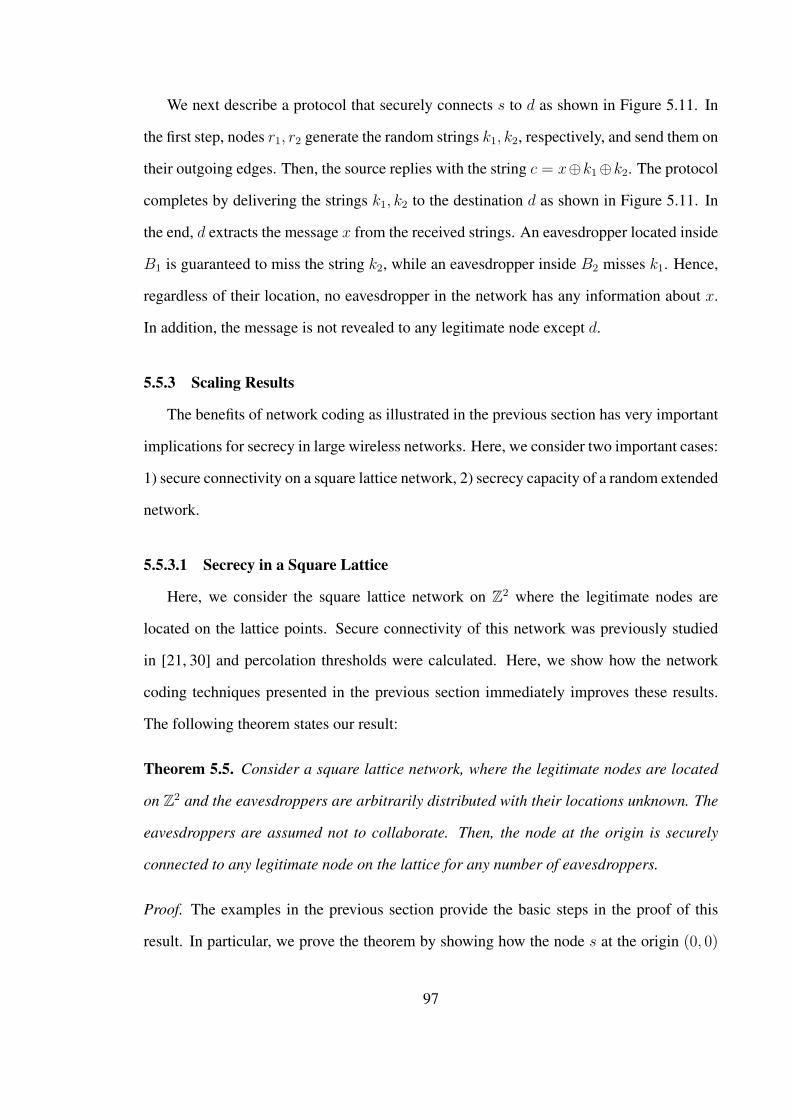
We next describe a protocol that securely connects s to d as shown in Figure 5.11. In

the first step, nodes r1, r2 generate the random strings k1, k2, respectively, and send them on

their outgoing edges. Then, the source replies with the string c = x⊕k1⊕k2. The protocol

completes by delivering the strings k1, k2 to the destination d as shown in Figure 5.11. In

the end, d extracts the message x from the received strings. An eavesdropper located inside

B1 is guaranteed to miss the string k2, while an eavesdropper inside B2 misses k1. Hence,

regardless of their location, no eavesdropper in the network has any information about x.

In addition, the message is not revealed to any legitimate node except d.

5.5.3 Scaling Results

The benefits of network coding as illustrated in the previous section has very important

implications for secrecy in large wireless networks. Here, we consider two important cases:

1) secure connectivity on a square lattice network, 2) secrecy capacity of a random extended

network.

5.5.3.1 Secrecy in a Square Lattice

Here, we consider the square lattice network on Z2 where the legitimate nodes are

located on the lattice points. Secure connectivity of this network was previously studied

in [21, 30] and percolation thresholds were calculated. Here, we show how the network

coding techniques presented in the previous section immediately improves these results.

The following theorem states our result:

Theorem 5.5. Consider a square lattice network, where the legitimate nodes are located

on Z2 and the eavesdroppers are arbitrarily distributed with their locations unknown. The

eavesdroppers are assumed not to collaborate. Then, the node at the origin is securely

connected to any legitimate node on the lattice for any number of eavesdroppers.

Proof. The examples in the previous section provide the basic steps in the proof of this

result. In particular, we prove the theorem by showing how the node s at the origin (0, 0)

97

can be connected to some selected lattice points in the first quadrant. Secure connectivity

to other points can be similarly shown.

Let d be located at (1, 0). s can send a secret message to d by simply using the proto-

col given in Figure 5.11, by employing the nodes at (0, 1), (0, –1), (1, 1), (1, –1) as relays.

Similarly s can send a secret message to a node located at (0, 1) by employing the four

nodes located at points (–1, 0), (–1, 1), (1, 0), (1, 1) and executing the same protocol. The

secrecy protocol to go from s at the origin to a node d at (1, 1) is given in Figure 5.12.

Again, roughly, the idea is that the source receives two keys k1, k2 from the relays on two

opposite directions, and these keys also arrive to d from two opposite directions. Connec-

tion to other points can be shown in a similar manner and therefore, the source is connected

to any node on the lattice.

s

dk1

k2

k2

c

k1 k2

1 2c x k k= ⊕ ⊕

k2

k2

k2

(0,0)

(1,1)

Figure 5.12: Secrecy protocol connecting a source node at the origin (0, 0) to a node at(1, 1).

Note that in the percolation results stated in [21, 30], the origin being connected to

another node refers to the existence of a “path” starting at the origin and ending at the

destination node. However, in our case, the connection to each node potentially requires a

different subset of nodes forming a network and employing network coding to reach that

node, which we refer to as the origin being “connected” to the destination node.

98

5.5.4 Secrecy Capacity Scaling

In our result given in Theorem 5.4, the requirement is that the number of eavesdroppers

(with unknown location) should grow more slowly than n/ log n for the achieved through-

put to remain secure. In this and other similar secrecy scaling results [39], the main feature

constraining the number of eavesdroppers that can be tolerated is the requirement that le-

gitimate nodes should be free from very nearby eavesdroppers, and this requirement still

applies even when the location of the eavesdroppers are assumed known [39].

The reason behind this major restriction is that whenever a node initiates the flow of

a secret message, a very nearby eavesdropper has a significant SNR advantage over any

receiver for any signal transmitted by this node. However, as shown in the previous section,

one major advantage of network coding techniques is that an incoming connection to a

source can be used to enable secrecy. For an incoming signal, the SNR values at a source

and a very nearby eavesdropper are almost the same, i.e., the use of network coding evens

out the SNR gap. Hence, a physical-layer secrecy scheme that achieves secrecy at equal

SNRs can be used to initiate the secure transmission.

The following theorem states our main result in this section which improves on the

result in Theorem 5.4 significantly in terms of the number of eavesdroppers tolerated. In

the construction used to prove this result, we assume a slightly modified secrecy scheme

than given in 5.2.1. Here we assume that, for all transmissions in the wireless network,

the sender node a employs a physical-layer secrecy scheme to deliver the message to the

receiver node b at some fixed rate, which is designed to guarantee secrecy from any eaves-

dropper e that has roughly the same signal quality with b (or worse). More precisely, for

some decoding threshold γ for the signal-to-interference-and-noise ratio (SINR), and some

(small) δ such that 0 < δ < 1, a sends bits to b at some fixed rate R bits per second, which

is kept secret from any eavesdropper e if 1) SINRb > γ, 2) SINRe 6 (1 + δ)SINRb. One

example of such a secrecy scheme is the low-complexity on-off method in [24], which uti-

lizes fading by sending only at instants when the main channel gain is larger than a certain

99

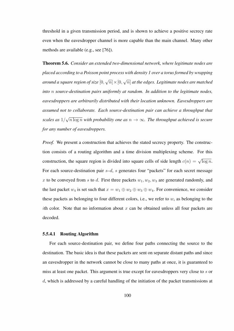
threshold in a given transmission period, and is shown to achieve a positive secrecy rate

even when the eavesdropper channel is more capable than the main channel. Many other

methods are available (e.g., see [76]).

Theorem 5.6. Consider an extended two-dimensional network, where legitimate nodes are

placed according to a Poisson point process with density 1 over a torus formed by wrapping

around a square region of size [0,√n]×[0,

√n] at the edges. Legitimate nodes are matched

into n source-destination pairs uniformly at random. In addition to the legitimate nodes,

eavesdroppers are arbitrarily distributed with their location unknown. Eavesdroppers are

assumed not to collaborate. Each source-destination pair can achieve a throughput that

scales as 1/√n log n with probability one as n → ∞. The throughput achieved is secure

for any number of eavesdroppers.

Proof. We present a construction that achieves the stated secrecy property. The construc-

tion consists of a routing algorithm and a time division multiplexing scheme. For this

construction, the square region is divided into square cells of side length c(n) =√log n.

For each source-destination pair s–d, s generates four “packets” for each secret message

x to be conveyed from s to d. First three packets w1, w2, w3 are generated randomly, and

the last packet w4 is set such that x = w1 ⊕ w2 ⊕ w3 ⊕ w4. For convenience, we consider

these packets as belonging to four different colors, i.e., we refer to wi as belonging to the

ith color. Note that no information about x can be obtained unless all four packets are

decoded.

5.5.4.1 Routing Algorithm

For each source-destination pair, we define four paths connecting the source to the

destination. The basic idea is that these packets are sent on separate distant paths and since

an eavesdropper in the network cannot be close to many paths at once, it is guaranteed to

miss at least one packet. This argument is true except for eavesdroppers very close to s or

d, which is addressed by a careful handling of the initiation of the packet transmissions at

100

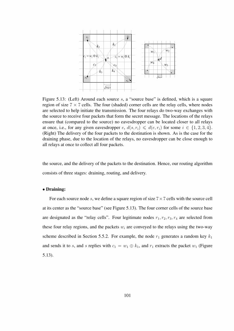
k

1 1 2c x k k= ⊕ ⊕

w2w1

w4w3

d

log n

k1

1 2c x k k= ⊕ ⊕

k1

1 1 1c w k= ⊕

k2

2 2 2c w k= ⊕

k3

c3

k4

c4

s

r1r2

r3r4

log n

Figure 5.13: (Left) Around each source s, a “source base” is defined, which is a squareregion of size 7 × 7 cells. The four (shaded) corner cells are the relay cells, where nodesare selected to help initiate the transmission. The four relays do two-way exchanges withthe source to receive four packets that form the secret message. The locations of the relaysensure that (compared to the source) no eavesdropper can be located closer to all relaysat once, i.e., for any given eavesdropper e, d(s, ri) 6 d(e, ri) for some i ∈ 1, 2, 3, 4.(Right) The delivery of the four packets to the destination is shown. As is the case for thedraining phase, due to the location of the relays, no eavesdropper can be close enough toall relays at once to collect all four packets.

the source, and the delivery of the packets to the destination. Hence, our routing algorithm

consists of three stages: draining, routing, and delivery.

• Draining:

For each source node s, we define a square region of size 7×7 cells with the source cell

at its center as the “source base” (see Figure 5.13). The four corner cells of the source base

are designated as the “relay cells”. Four legitimate nodes r1, r2, r3, r4 are selected from

these four relay regions, and the packets wi are conveyed to the relays using the two-way

scheme described in Section 5.5.2. For example, the node r1 generates a random key k1

and sends it to s, and s replies with c1 = w1 ⊕ k1, and r1 extracts the packet w1 (Figure

5.13).

101

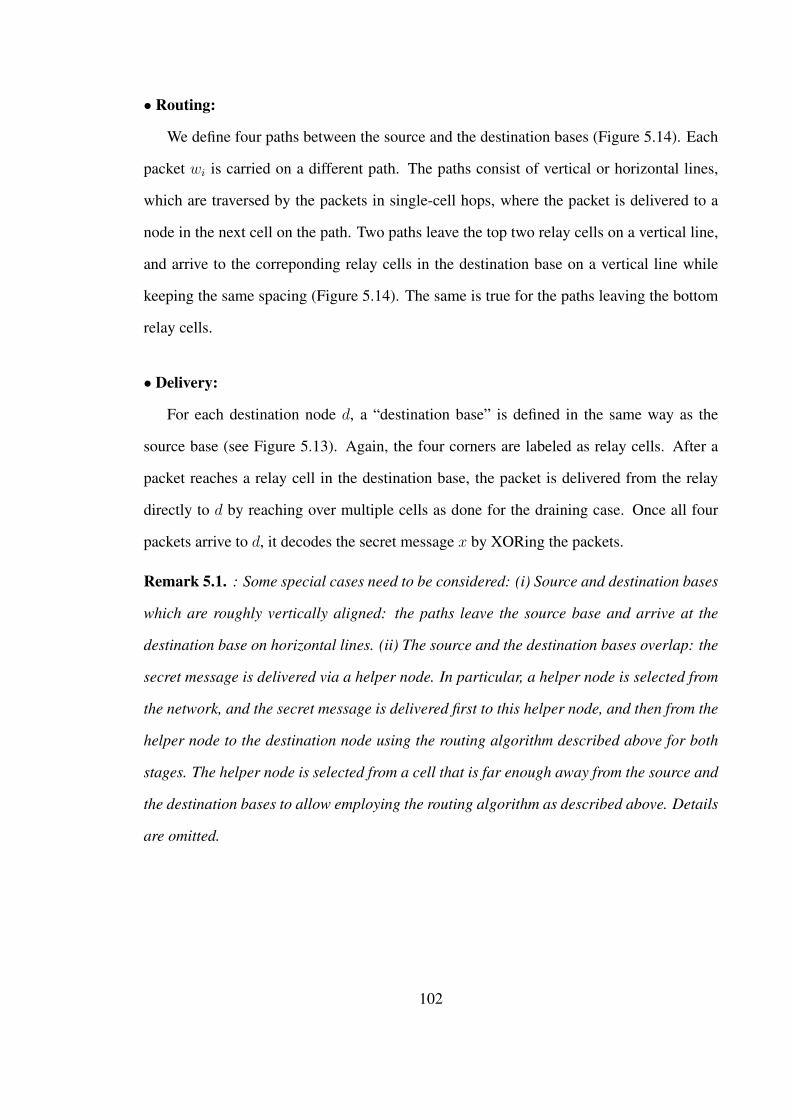
• Routing:

We define four paths between the source and the destination bases (Figure 5.14). Each

packet wi is carried on a different path. The paths consist of vertical or horizontal lines,

which are traversed by the packets in single-cell hops, where the packet is delivered to a

node in the next cell on the path. Two paths leave the top two relay cells on a vertical line,

and arrive to the correponding relay cells in the destination base on a vertical line while

keeping the same spacing (Figure 5.14). The same is true for the paths leaving the bottom

relay cells.

• Delivery:

For each destination node d, a “destination base” is defined in the same way as the

source base (see Figure 5.13). Again, the four corners are labeled as relay cells. After a

packet reaches a relay cell in the destination base, the packet is delivered from the relay

directly to d by reaching over multiple cells as done for the draining case. Once all four

packets arrive to d, it decodes the secret message x by XORing the packets.

Remark 5.1. : Some special cases need to be considered: (i) Source and destination bases

which are roughly vertically aligned: the paths leave the source base and arrive at the

destination base on horizontal lines. (ii) The source and the destination bases overlap: the

secret message is delivered via a helper node. In particular, a helper node is selected from

the network, and the secret message is delivered first to this helper node, and then from the

helper node to the destination node using the routing algorithm described above for both

stages. The helper node is selected from a cell that is far enough away from the source and

the destination bases to allow employing the routing algorithm as described above. Details

are omitted.

102

DD

D

s

w1

w2

w3

w4

d

Figure 5.14: The source and the destination bases are connected with four paths, eachcarrying one of the packets. The paths have the same minimum spacing throughout theroute; hence, no eavesdropper can be close enough to all four paths at once.

5.5.4.2 Time Division Multiplexing Scheme

Time is divided into three phases corresponding to the draining, routing, and delivery

stages.

• Draining:

The draining phase is divided into eight frames. The first four frames are for trans-

missions of the keys from the relays to the sources, and the last four frames are for the

responses of the sources. Each frame consists of a constant number of time slots, where

cells take turns for signal transmissions employing a standard spatial reuse scheme as as-

sumed in the similar construction in Section 5.4.1. Hence, at the end of each frame, it is

ensured that each cell has transmitted once.

• Routing:

The routing phase is divided into four frames for each type of packet. In the ith frame,

packets of color i are routed. Each frame is further divided into time slots again employing

103

a spatial reuse scheme. In each time slot, relaying nodes from the active cells deliver their

packets to the next cell on the path.

• Delivery:

The delivery phase consists of four frames for the transmission of the packets of four

colors. Again, each frame is divided into time slots, and transmissions are done as in the

draining phase.

The proof completes by showing that: (i) this construction is feasible, (ii) it achieves a

per-node throughput on the order of 1/√n log n, and (iii) the achieved throughput is secure.

The first two statements can be shown by standard arguments as used in Sections 5.3

and 5.4 and similar works (see e.g., [16, 73]), and we omit the detailed proof here. The

throughput achieved by the construction is found by considering the throughput constraint

imposed by each phase. For the draining and delivery phases, the difference in our con-

struction compared to a standard construction is that transmissions require multi-cell hops,

and that these phases complete in more than one transmissions. However, these both bring

only a constant factor to the throughput achieved and do not affect the scaling. The differ-

ence in the routing phase is that each message requires four packets to be carried, which

again does not affect the order. It can be shown that the performance bottleneck is due to

the routing phase, and since the relaying load in each cell grows with√n log n (see Ap-

pendix A.3), the overall per-node throughput scales as 1/√n log n. Finally, note that the

construction requires nodes to transmit with power that is proportonal to (log n)α/2, where

α > 2 is the path loss exponent of the medium.

Next we show that for each source-destination pair s–d, each message x is delivered

from s to d securely. For secrecy, we show that an eavesdropper located anywhere in the

network is guaranteed to miss at least one packet out of the four packets after listening to

all the transmissions required for the delivery of x. First consider the draining phase. Due

to the relative locations of the relays with respect to the source, any given eavesdropper e

104

satisfies d(e, ri) > d(s, ri) for some i ∈ 1, 2, 3, 4 (Figure 5.13). Hence, for the trans-

mission of ki from ri to s, the received signal power at s is larger than the received signal

power at e. In addition, even with the interference at e ignored, the spatial reuse scheme can

be designed such that the interference at s is low enough to allow SINRe 6 (1 + δ)SINRb.

Therefore, ki is delivered to s but not to e; hence, e misses the packet wi. Therefore, any

eavesdropper is guaranteed to miss at least one packet, and the message x is not leaked dur-

ing the draining phase. A similar argument can be made for the delivery phase. The four

packets arrive to d from four directions and any eavesdropper e satisfies d(e, ri) > d(d, ri)

for some i. Outside the bases, the packets are carried on paths with some minimum spac-

ing; hence, no eavesdropper can be close enough to many paths at once, thus establishing

secrecy during the routing phase. Also note that it can be ensured that an eavesdropper

cannot decode a packet by combining observations from all hops on the packet’s path as

proved in [39]. Finally, it can be easily verified that no eavesdropper can collect the four

packets by listening to all three phases.

Therefore, using this construction, as n grows, each source-destination pair can share on

the order of 1/√n log n secret bits per second for any number of independent eavesdroppers

arbitrarily distributed to the network.

5.6 Conclusion

We address the important problem of secure communication in a wireless network in

the presence of eavesdroppers. We present achievable scaling results on the rate of infor-

mation that can be securely carried in a network, when the size of the network becomes

large. In contrast to most of the previous work in this area, we assume the locations of the

eavesdroppers are unknown. Compared to previous works that consider unknown eaves-

dropper locations, our construction can achieve the same secure throughput scaling while

tolerating a significantly higher number of eavesdroppers. Our work shows the big poten-

tial network coding techniques have to improve information-theoretic secrecy in wireless

105

networks, most notably by enabling the secure connection of one node to another in the

presence of very nearby eavesdroppers.

This work partially completes a line of research that originated with the secrecy-capacity

tradeoffs in asymptotically large networks of [73]. In [73], even when multi-user diversity

and cooperative jamming were employed, the near eavesdropper problem severely limited

the number of uniformly distributed eavesdroppers that could be tolerated in the network.

In [8] and [9] (presented in previous sections), we began to realize the utility of modifica-

tions at higher layers in resolving difficult secrecy problems caused by certain geometries

of the system nodes and eavesdroppers, but we still were not able to address eavesdroppers

very near the nodes originating messages. The work presented in Section 5.5 (published

in [7]) addresses this last problem and thus allows for a secure per-session throughput of

O(1/√n log n) in the presence of an arbitrarily located set of non-collaborating eavesdrop-

pers.

5.7 Acknowledgment

The work in this chapter was supported by the National Science Foundation under

grants CNS-0721626, CNS-0721861, CNS-0905349, CNS-0953620, and CNS- 1018464,

and by the U.S. Army Research Laboratory and the U.K. Ministry of Defence under Agree-

ment Number W911NF-06-3-0001.

106

CHAPTER 6

PERCOLATION IN MULTILAYER GRAPHS

6.1 Introduction

Previous chapters are concerned with large wireless ad hoc networks. The network

model we use in those chapters contains an asymptotically large number of nodes, as we

are interested in the network’s limiting behavior. As discussed in Chapter 2, a network

can be studied by mapping it to a graph, and important asymptotic properties of a network

can be deduced by studying the corresponding infinite graph. In particular, some of the

important results in wireless ad hoc networks discussed in previous chapters make use

of percolation theory, which studies the connectivity behavior of infinite random graphs.

Central to percolation theory is the study of the “phase transition” that infinite random

graphs demonstrate. Phase transition here refers to the sudden change of the connectivity

properties of the network as a local parameter is varied. This behavior of the random infinite

graph is used to explain and model many real-life phase transition phenomena in diverse

fields such as soil physics, polymer science, and epidemiology [64].

In addition to the random geometric graphs used to model wireless ad hoc networks,

phase transition behavior can be observed on many other types of random graphs where

vertices may have fixed locations or, as studied in this chapter, there is no geometric (lo-

cation) notion to the graph. For example, consider a square lattice graph. Here, each

vertex has four edges connecting it to its four neighbors. One can run a random process

on this graph by independently and randomly deleting edges. Suppose deletion happens

with some probability 1 − p, so each edge survives with probability p. When p is large,

the resulting graph (subgraph of the original square lattice) will still be well-connected.

107

As p decreases, the square lattice will transition from a well-connected graph to one that

consists of many small connected islands. Here, the surprising result is that this transition

happens very abruptly. When the square lattice is very large, at a certain critical p value,

the graph suddenly changes state from having one big spanning cluster to having many

small clusters. Consider this lattice as modeling a physical structure; here, this sudden

transition corresponds to the structure “breaking down”. The critical value of p, called pc,

where this phase transition happens is of interest. In general, this critical value is very

difficult to calculate analytically, and, except for a few types of regular graphs, it has only

been numerically estimated. For the square lattice, calculating pc analytically was an open

problem for many years, and the result that pc is exactly 0.5 for the square lattice is one of

the famous results of percolation theory [36].

In percolation theory, the random process of deleting edges from a graph is referred to

as “bond percolation”. Another option is to delete vertices (or mark them as “unoccupied”)

randomly. The idea is that when a vertex is unoccupied, the edges arriving to it are blocked.

An equivalent way to consider this process is to assume all edges from an unoccupied vertex

are deleted. This process is called “site percolation” (see Figure 6.1). Suppose each vertex

remains occupied with probability q. Again, there is a critical value qc, called the “site

percolation threshold”, where the phase transition is observed. For the square lattice, qc

is numerically estimated to be around 0.59275 [54] (see Figure 6.2). In this chapter, we

extensively study site percolation.

In our work, we consider site percolation on “multilayer graphs”. Multilayer graphs

are formed by combining different graphs that share the same vertex set. An example of a

multilayer graph is one representing a social network of a set of people, where each vertex

represents a person, and an edge between two people represents a social relationship. In

a multilayer social network, each layer may represent a different type of relationship such

as “work” or “family”. The overall multilayer graph is formed by combining these layers.

Another example is a wireless network where nodes may be equipped with more than

108

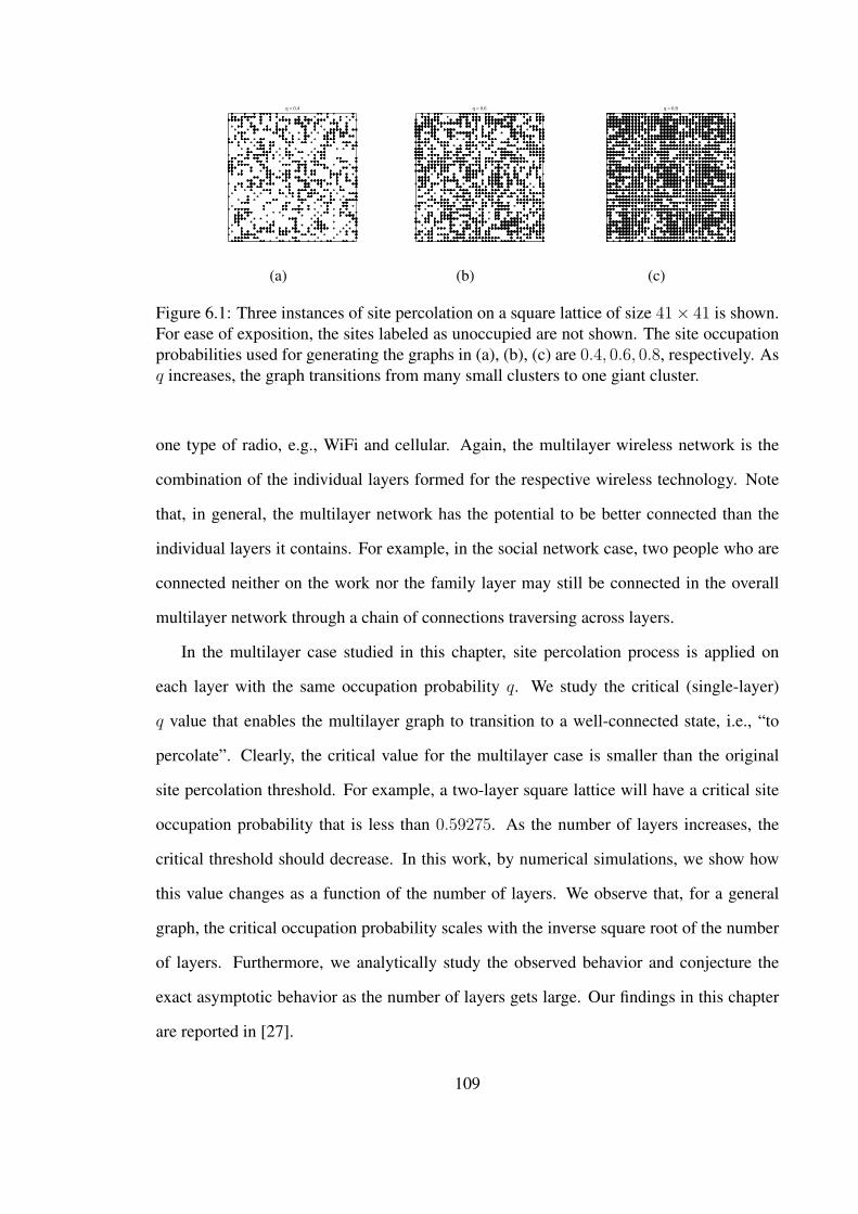
q = 0.4

(a)

q = 0.6

(b)

q = 0.8

(c)

Figure 6.1: Three instances of site percolation on a square lattice of size 41× 41 is shown.For ease of exposition, the sites labeled as unoccupied are not shown. The site occupationprobabilities used for generating the graphs in (a), (b), (c) are 0.4, 0.6, 0.8, respectively. Asq increases, the graph transitions from many small clusters to one giant cluster.

one type of radio, e.g., WiFi and cellular. Again, the multilayer wireless network is the

combination of the individual layers formed for the respective wireless technology. Note

that, in general, the multilayer network has the potential to be better connected than the

individual layers it contains. For example, in the social network case, two people who are

connected neither on the work nor the family layer may still be connected in the overall

multilayer network through a chain of connections traversing across layers.

In the multilayer case studied in this chapter, site percolation process is applied on

each layer with the same occupation probability q. We study the critical (single-layer)

q value that enables the multilayer graph to transition to a well-connected state, i.e., “to

percolate”. Clearly, the critical value for the multilayer case is smaller than the original

site percolation threshold. For example, a two-layer square lattice will have a critical site

occupation probability that is less than 0.59275. As the number of layers increases, the

critical threshold should decrease. In this work, by numerical simulations, we show how

this value changes as a function of the number of layers. We observe that, for a general

graph, the critical occupation probability scales with the inverse square root of the number

of layers. Furthermore, we analytically study the observed behavior and conjecture the

exact asymptotic behavior as the number of layers gets large. Our findings in this chapter

are reported in [27].

109

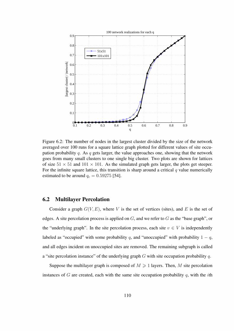
0.1 0.2 0.3 0.4 0.5 0.6 0.7 0.8 0.90

0.1

0.2

0.3

0.4

0.5

0.6

0.7

0.8

0.9

q

|larg

est c

lust

er| /

|net

wor

k|

100 network realizations for each q

51x51

101x101

Figure 6.2: The number of nodes in the largest cluster divided by the size of the networkaveraged over 100 runs for a square lattice graph plotted for different values of site occu-pation probability q. As q gets larger, the value approaches one, showing that the networkgoes from many small clusters to one single big cluster. Two plots are shown for latticesof size 51 × 51 and 101 × 101. As the simulated graph gets larger, the plots get steeper.For the infinite square lattice, this transition is sharp around a critical q value numericallyestimated to be around qc = 0.59275 [54].

6.2 Multilayer Percolation

Consider a graph G(V,E), where V is the set of vertices (sites), and E is the set of

edges. A site percolation process is applied on G, and we refer to G as the “base graph”, or

the “underlying graph”. In the site percolation process, each site v ∈ V is independently

labeled as “occupied” with some probability q, and “unoccupied” with probability 1 − q,

and all edges incident on unoccupied sites are removed. The remaining subgraph is called

a “site percolation instance” of the underlying graph G with site occupation probability q.

Suppose the multilayer graph is composed of M > 1 layers. Then, M site percolation

instances of G are created, each with the same site occupation probability q, with the ith

110

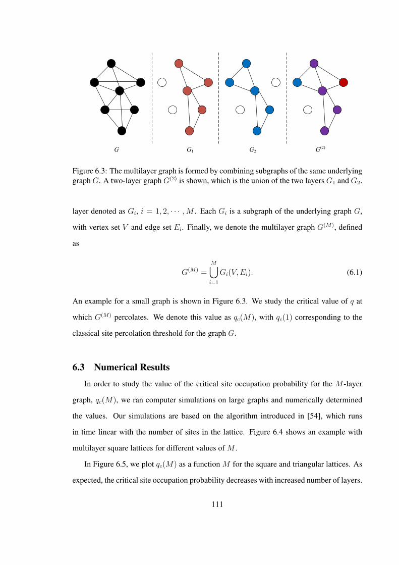
G G1 G2 G(2)

Figure 6.3: The multilayer graph is formed by combining subgraphs of the same underlyinggraph G. A two-layer graph G(2) is shown, which is the union of the two layers G1 and G2.

layer denoted as Gi, i = 1, 2, · · · ,M . Each Gi is a subgraph of the underlying graph G,

with vertex set V and edge set Ei. Finally, we denote the multilayer graph G(M), defined

as

G(M) =M∪i=1

Gi(V,Ei). (6.1)

An example for a small graph is shown in Figure 6.3. We study the critical value of q at

which G(M) percolates. We denote this value as qc(M), with qc(1) corresponding to the

classical site percolation threshold for the graph G.

6.3 Numerical Results

In order to study the value of the critical site occupation probability for the M -layer

graph, qc(M), we ran computer simulations on large graphs and numerically determined

the values. Our simulations are based on the algorithm introduced in [54], which runs

in time linear with the number of sites in the lattice. Figure 6.4 shows an example with

multilayer square lattices for different values of M .

In Figure 6.5, we plot qc(M) as a function M for the square and triangular lattices. As

expected, the critical site occupation probability decreases with increased number of layers.

111

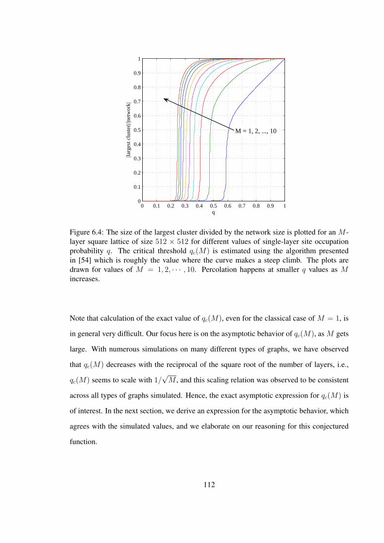
0 0.1 0.2 0.3 0.4 0.5 0.6 0.7 0.8 0.9 10

0.1

0.2

0.3

0.4

0.5

0.6

0.7

0.8

0.9

1

|larg

est c

lust

er|/|

netw

ork|

q

M = 1, 2, ..., 10

Figure 6.4: The size of the largest cluster divided by the network size is plotted for an M -layer square lattice of size 512 × 512 for different values of single-layer site occupationprobability q. The critical threshold qc(M) is estimated using the algorithm presentedin [54] which is roughly the value where the curve makes a steep climb. The plots aredrawn for values of M = 1, 2, · · · , 10. Percolation happens at smaller q values as Mincreases.

Note that calculation of the exact value of qc(M), even for the classical case of M = 1, is

in general very difficult. Our focus here is on the asymptotic behavior of qc(M), as M gets

large. With numerous simulations on many different types of graphs, we have observed

that qc(M) decreases with the reciprocal of the square root of the number of layers, i.e.,

qc(M) seems to scale with 1/√M , and this scaling relation was observed to be consistent

across all types of graphs simulated. Hence, the exact asymptotic expression for qc(M) is

of interest. In the next section, we derive an expression for the asymptotic behavior, which

agrees with the simulated values, and we elaborate on our reasoning for this conjectured

function.

112

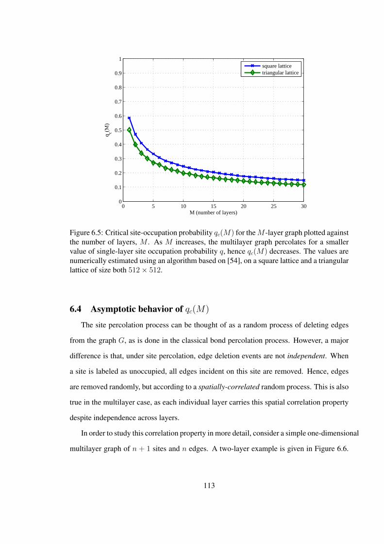
0 5 10 15 20 25 300

0.1

0.2

0.3

0.4

0.5

0.6

0.7

0.8

0.9

1

M (number of layers)

q c(M)

square latticetriangular lattice

Figure 6.5: Critical site-occupation probability qc(M) for theM -layer graph plotted againstthe number of layers, M . As M increases, the multilayer graph percolates for a smallervalue of single-layer site occupation probability q, hence qc(M) decreases. The values arenumerically estimated using an algorithm based on [54], on a square lattice and a triangularlattice of size both 512× 512.

6.4 Asymptotic behavior of qc(M)

The site percolation process can be thought of as a random process of deleting edges

from the graph G, as is done in the classical bond percolation process. However, a major

difference is that, under site percolation, edge deletion events are not independent. When

a site is labeled as unoccupied, all edges incident on this site are removed. Hence, edges

are removed randomly, but according to a spatially-correlated random process. This is also

true in the multilayer case, as each individual layer carries this spatial correlation property

despite independence across layers.

In order to study this correlation property in more detail, consider a simple one-dimensional

multilayer graph of n + 1 sites and n edges. A two-layer example is given in Figure 6.6.

113

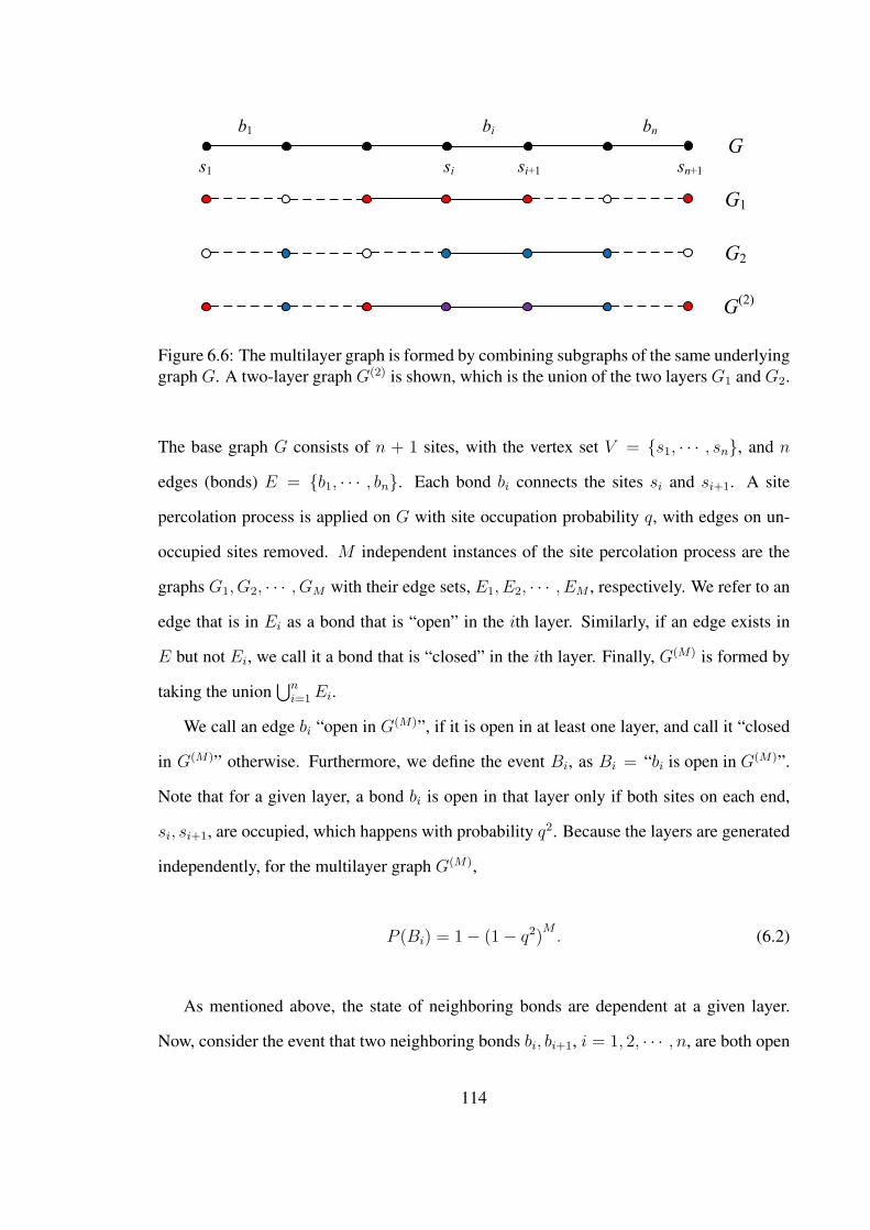
s1

Xi = R Xi+1 = BX0 = P X1 = U Yi+1 = 0Yi = 1

G

G1

G2

G(2)

si si+1 sn+1

b1 bi bn

Figure 6.6: The multilayer graph is formed by combining subgraphs of the same underlyinggraph G. A two-layer graph G(2) is shown, which is the union of the two layers G1 and G2.

The base graph G consists of n + 1 sites, with the vertex set V = s1, · · · , sn, and n

edges (bonds) E = b1, · · · , bn. Each bond bi connects the sites si and si+1. A site

percolation process is applied on G with site occupation probability q, with edges on un-

occupied sites removed. M independent instances of the site percolation process are the

graphs G1, G2, · · · , GM with their edge sets, E1, E2, · · · , EM , respectively. We refer to an

edge that is in Ei as a bond that is “open” in the ith layer. Similarly, if an edge exists in

E but not Ei, we call it a bond that is “closed” in the ith layer. Finally, G(M) is formed by

taking the union∪n

i=1Ei.

We call an edge bi “open in G(M)”, if it is open in at least one layer, and call it “closed

in G(M)” otherwise. Furthermore, we define the event Bi, as Bi = “bi is open in G(M)”.

Note that for a given layer, a bond bi is open in that layer only if both sites on each end,

si, si+1, are occupied, which happens with probability q2. Because the layers are generated

independently, for the multilayer graph G(M),

P (Bi) = 1− (1− q2)M. (6.2)

As mentioned above, the state of neighboring bonds are dependent at a given layer.

Now, consider the event that two neighboring bonds bi, bi+1, i = 1, 2, · · · , n, are both open

114

in G(M), i.e., Bi ∩Bi+1). The probability of this event can be written as

P (Bi ∩Bi+1) = 1− P (Bi ∪Bi+1)

= 1−(P (Bi) + P (Bi+1)− P (Bi ∩Bi+1)

). (6.3)

The event Bi ∩ Bi+1 corresponds to the event that bi and bi+1 are both closed in G(M),

which means bi, bi+1 are closed in all M layers. For any given layer j ∈ 1, 2, · · · ,M,

P (“bi and bi+1 closed in the jth layer”) = 1− 2q2 + q3. (6.4)

The above value can be easily found by enumerating all possible states of the sites si, si+1, si+2

and summing up the probabilities of states that correspond to both bonds being closed.

Therefore, for all i ∈ 1, 2, · · · , n,

P (Bi ∩Bi+1) = (1− 2q2 + q3)M. (6.5)

Finally, replacing the above value in (6.3),

P (Bi ∩Bi+1) = 1− 2(1− q2)M

+ (1− 2q2 + q3)M. (6.6)

Also note that,

P (B1)P (B2) =(1− (1− q2)

M)2= 1− 2(1− q2)

M+ (1− 2q2 + q4)

M. (6.7)

Therefore, for any finite M ,

P (Bi ∩Bi+1) ≥ P (Bi)P (Bi+1). (6.8)

Hence, as expected, events Bi and Bi+1 are positively correlated. Therefore, compared to

classical bond percolation where states of all edges are determined independently, we ex-

115

pect percolation to occur “sooner”, i.e., with a smaller marginal bond occupation probabil-

ity P (Bi). In addition, note that, for a given q value, P (Bi∩Bi+1) approaches P (Bi)P (Bi+1)

as M increases. In other words, correlation between neighboring bonds dies out with an

increasing number of layers. Hence, in the limit as M → ∞, the M -layer graph can be

thought of as a graph generated by a single-layer independent bond percolation process

with bond occupation probability P (Bi), which percolates at P (Bi) = pc. On the other

hand, for any finite M , the multilayer graph has a smaller critical threshold than a graph

generated with a bond percolation process of the same marginal bond occupation probabil-

ity. Therefore, we have the following conjecture:

Conjecture 6.1. Consider a graphG(V,E) with critical bond percolation threshold pc, and

the multilayer graph G(M) generated by combining M random site percolation instances

of G, each with site occupation probability q. Suppose G(M) percolates at some critical

value q = qc(M). Then the critical site percolation threshold qc(M) is upper bounded as

qc(M) ≤√1− (1− pc)1/M . (6.9)

Further, this upper bound is asymptotically tight as M → ∞.

Note that the upper bound above satisfies

√1− (1− pc)1/M ∼

√log(1− pc)√

M, (6.10)

which makes the inverse square root scaling explicit and shows that the scaling coefficient

is√

log(1− pc).

We compared the qc(M) values numerically estimated for many types of graphs (see

Figure 6.5) with the conjectured upper bound. All these simulations show perfect agree-

ment. Figure 6.7 shows the case of the square lattice graph.

116

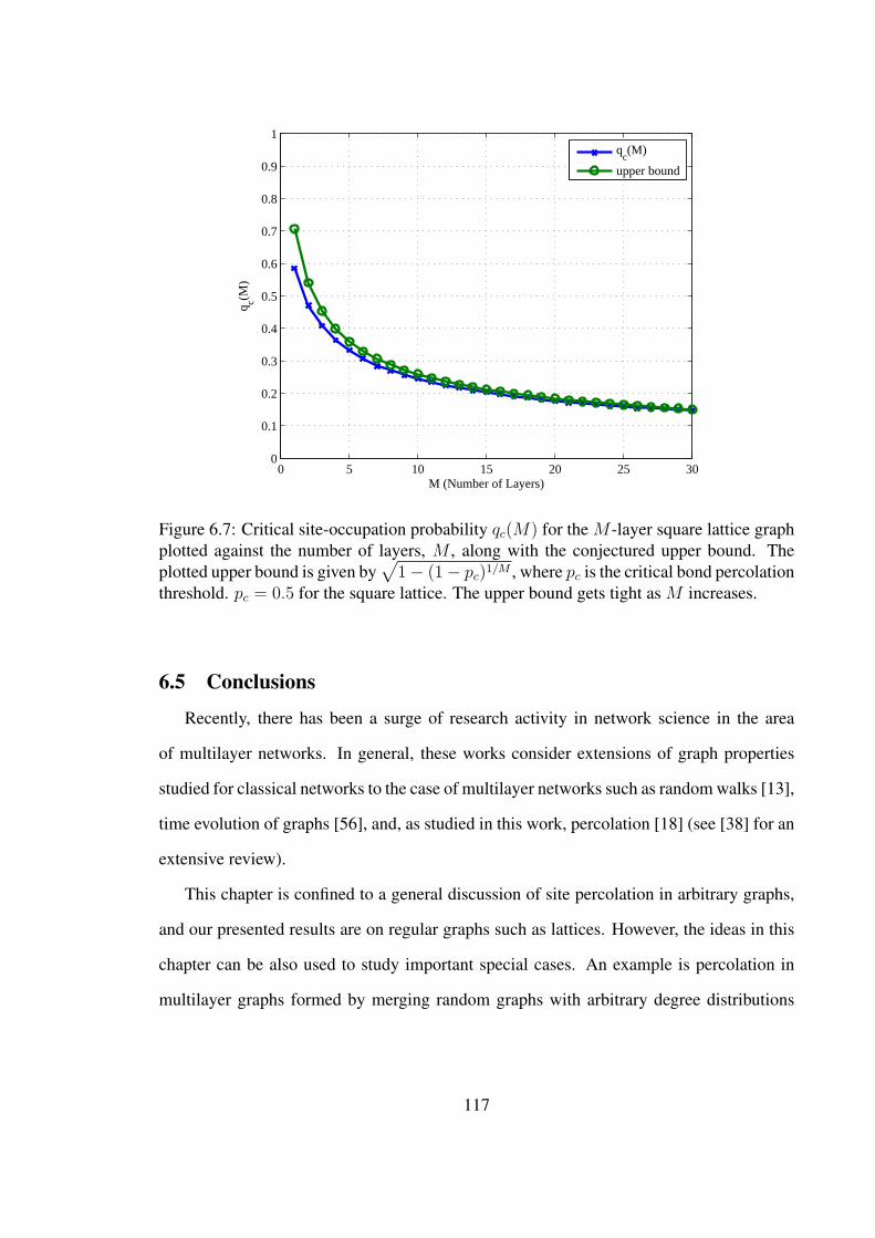
0 5 10 15 20 25 300

0.1

0.2

0.3

0.4

0.5

0.6

0.7

0.8

0.9

1

M (Number of Layers)

q c(M)

q

c(M)

upper bound

Figure 6.7: Critical site-occupation probability qc(M) for the M -layer square lattice graphplotted against the number of layers, M , along with the conjectured upper bound. Theplotted upper bound is given by

√1− (1− pc)1/M , where pc is the critical bond percolation

threshold. pc = 0.5 for the square lattice. The upper bound gets tight as M increases.

6.5 Conclusions

Recently, there has been a surge of research activity in network science in the area

of multilayer networks. In general, these works consider extensions of graph properties

studied for classical networks to the case of multilayer networks such as random walks [13],

time evolution of graphs [56], and, as studied in this work, percolation [18] (see [38] for an

extensive review).

This chapter is confined to a general discussion of site percolation in arbitrary graphs,

and our presented results are on regular graphs such as lattices. However, the ideas in this

chapter can be also used to study important special cases. An example is percolation in

multilayer graphs formed by merging random graphs with arbitrary degree distributions

117

[53]. In fact, contrary to the case of regular graphs discussed here, exact expressions for

the critical site occupation probability are found in this case [27].

One important insight gained in studying percolation in multilayer graphs is that impor-

tant properties can be deduced by considering the problem as a spatially-correlated bond

percolation process that converges to an independent bond percolation process as the num-

ber of layers increases. This also naturally ties the multilayer percolation problem to the

case of mixed “site-bond percolation” considered in the literature [71]. In site-bond perco-

lation, each site and bond in the graph is labeled as occupied or unoccupied independently,

with probabilities q and p, respectively, and only occupied bonds with occupied sites on its

both ends are declared open. Clearly, the special cases of q = 1 and p = 1 correspond to

site and bond percolation, respectively. Hence, the transition from site to bond percolation

for the multilayer graph as the number of layers increases is also observed in the site-bond

percolation problem as values of p, q are varied. This similarity allows us to adapt bounds

established for site-bond percolation to the multilayer percolation problem. In fact, these

adapted bounds show perfect agreement with the multilayer case as presented in [27].

For future work, we plan to rigorously prove Conjecture 6.1. This requires us to prove

the argument that under two probability measures with the same marginal bond occupa-

tion probabilities on the same infinite graph, the percolation probability is greater under

the measure which implies correlation between neighboring bonds than the one where the

states of all bonds are independent.

6.6 Acknowledgment

The work in this chapter was supported in part by the National Science Foundation

under grant CNS-1018464, and in part by the U.S. Army Research Laboratory and the

U.K. Ministry of Defence, and was accomplished under Cooperative Agreement Number

W911NF-09-2-0053 (the ARL Network Science CTA).

118

CHAPTER 7

CONCLUSION

This thesis work consists of four projects concerned with asymptotic analysis of large

random networks. In the first three projects, we focus on the asymptotic properties of

wireless ad hoc networks. In the last project, we study percolation properties of arbitrary

large random networks.

In the first project, we study broadcast in a large wireless ad hoc network. We model

the network as consisting of nodes randomly placed on the infinite real-line or, in the two-

dimensional case, on the infinite R2 plane. Because the locations of the nodes are random,

broadcasting a message to the entire infinite network is difficult. We explore how cooper-

ation between nodes can improve this situation. In particular, we study a special case of

cooperation where nodes that have decoded the broadcast message coordinate and transmit

the message at the same time so that their signal power is added at a receiver node. This

helps the broadcast message reach farther distances. We analytically calculate the proba-

bility that a node can broadcast its message to the entire infinite network when this type

of cooperation is enabled. We show that although cooperation helps increase the broadcast

range, for a wide range of cases, the probability that the message reaches every node in

the infinite region is zero. However, for mediums with low attenuation, cooperation indeed

makes broadcast possible.

In the second project we are interested in the rate data can be exchanged by nodes in

a large wireless ad hoc network. Wireless ad hoc networks are known to not scale well

in terms of capacity, meaning that the number of bits each node can share goes down to

zero as the network gets larger. Supporting the wireless network with a high-capacity

119

wired network through placement of base stations, thereby creating a hybrid network, is

a method to improve this situation. Previous work has shown capacity scaling results for

hybrid networks. These works show what capacity benefit is obtained through the use of

base stations; however, it is of interest whether even better capacity is possible. We show

upper bounds on hybrid network capacity, hence showing the limits on the capacity benefit

that can be provided.

The third project is also concerned with sharing of data in a large wireless ad hoc

network; however, this time our focus is on secret communication. We assume the network

contains eavesdropping nodes, and we explore whether nodes can share information while

keeping their messages secret from these eavesdroppers. Previous work has shown that this

is possible without any compromise on the achieved throughput. However, it is assumed

that the locations of the eavesdroppers are known. In our work, we show that it is possible

to achieve the same amount of secret information exchange without having to know the

locations of the eavesdroppers. Central to our solution is the use of coding techniques

for wireless secrecy. Our results highlight how upper layer solutions can address difficult

physical layer problems.

In the final project, we study percolation properties of large random multilayer net-

works. Members of a given network may have more than one type of relationship, and

each type of relationship can be represented by a separate network. Multilayer networks are

formed by combining these individual networks, called layers. We study the connectivity

of the corresponding multilayer graph as a function of the connectivity of individual lay-

ers. Because the multilayer graph is the combination of the layers, many poorly-connected

layers can form a well-connected union. We study the critical connectivity threshold for

the individual layers that enable the multilayer graph to percolate. In addition to showing

the behavior of the critical threshold numerically, we study analytically why this behavior

is observed.

120

Each project in this thesis involves theoretical analysis of the behavior of a large ran-

dom network. The main goal of such theoretical analysis is to gain insight into the net-

work’s real-life performance. Especially in the first three projects, where we study wireless

networks, the network needs to be mathematically modeled before such analysis can be

carried out. Modeling the network inevitably involves making simplifying assumptions to

yield theoretical study. In a complicated operation such as wireless networking, modeling

requires assumptions on many different aspects such as how each physical device is mod-

eled, how communication takes place, how interference affects communication, etc. An

important fact that has repeatedly demonstrated itself in these projects is that each detail

of this model has the potential to dramatically affect the conclusions one can draw from

analysis. One example of this is discussed in Chapter 4, where we show how two different

assumptions on the rate of information carried on a wireless link can lead to two different

conclusions on the total rate that can be achieved by nodes confined in a region. Therefore,

conclusions drawn from such theoretical analysis should always be carefully considered

with attention given to how they are tied to the underlying model.

In our project on secret communication presented in Chapter 5, the main tool behind

the solution that enabled secrecy in the presence of eavesdroppers is the coding techniques

employed. Simple coding techniques for enabling secrecy in a wiretapped network were

already considered in previous work; however, their application to wireless information-

theoretic secrecy has proved to be particularly useful as illustrated by our results. The main

reason behind that is, in wireless secrecy, uncertainty about the eavesdropper is of particular

concern. For example, the state of the channel to an eavesdropper, although central to the

secrecy performance, is very difficult to model and make assumptions on in the wireless

case. As demonstrated in our work, coding techniques help relax the assumptions that

have to be made about the eavesdropper, and help address very difficult questions such

as unknown eavesdropper location or the near-eavesdropper problem. Our results show

the usefulness of these techniques to enable secrecy in a large wireless network; however,

121

the coding techniques employed in fact do not require a large number of nodes for their

benefit to be realized. The techniques used in our work, such as secret sharing or two-

way communications, can be very easily employed in a small network scenario. Overall,

secrecy obtained through the use of coding techniques illustrate how upper layer solutions

can be useful to address difficult physical layer problems.

122

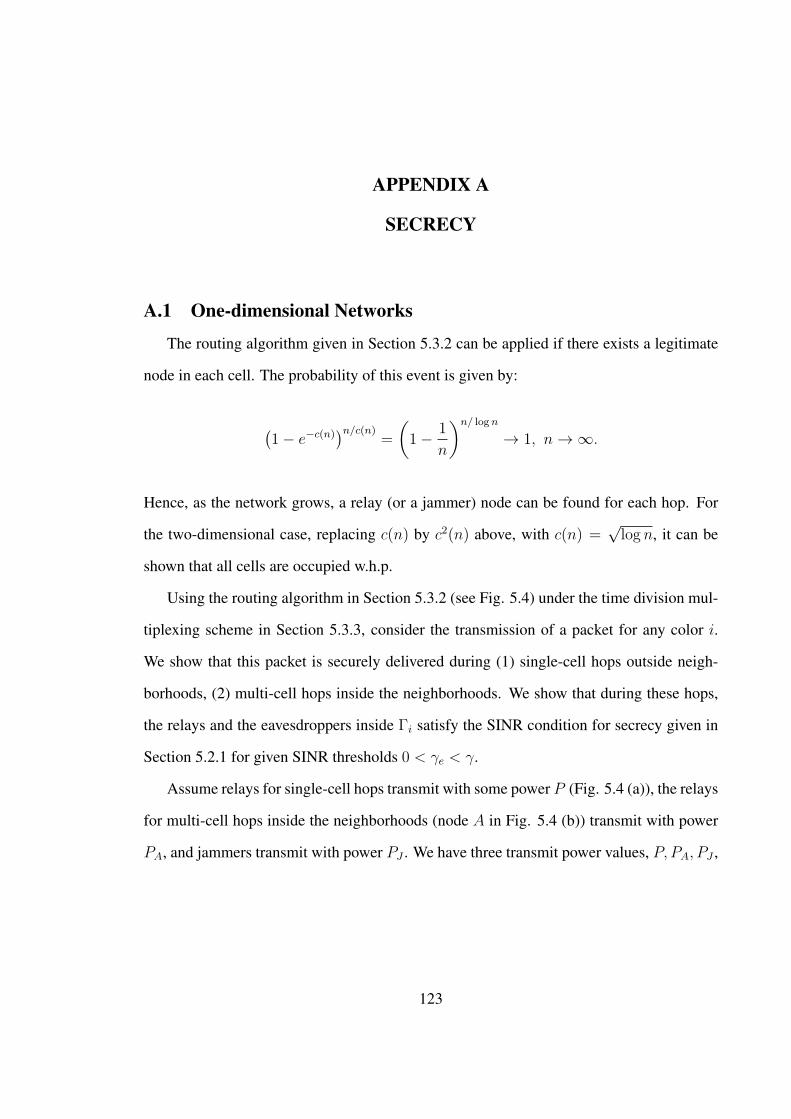
APPENDIX A

SECRECY

A.1 One-dimensional Networks

The routing algorithm given in Section 5.3.2 can be applied if there exists a legitimate

node in each cell. The probability of this event is given by:

(1− e−c(n)

)n/c(n)=

(1− 1

n

)n/ logn

→ 1, n→ ∞.

Hence, as the network grows, a relay (or a jammer) node can be found for each hop. For

the two-dimensional case, replacing c(n) by c2(n) above, with c(n) =√log n, it can be

shown that all cells are occupied w.h.p.

Using the routing algorithm in Section 5.3.2 (see Fig. 5.4) under the time division mul-

tiplexing scheme in Section 5.3.3, consider the transmission of a packet for any color i.

We show that this packet is securely delivered during (1) single-cell hops outside neigh-

borhoods, (2) multi-cell hops inside the neighborhoods. We show that during these hops,

the relays and the eavesdroppers inside Γi satisfy the SINR condition for secrecy given in

Section 5.2.1 for given SINR thresholds 0 < γe < γ.

Assume relays for single-cell hops transmit with some power P (Fig. 5.4 (a)), the relays

for multi-cell hops inside the neighborhoods (node A in Fig. 5.4 (b)) transmit with power

PA, and jammers transmit with power PJ . We have three transmit power values, P, PA, PJ ,

123

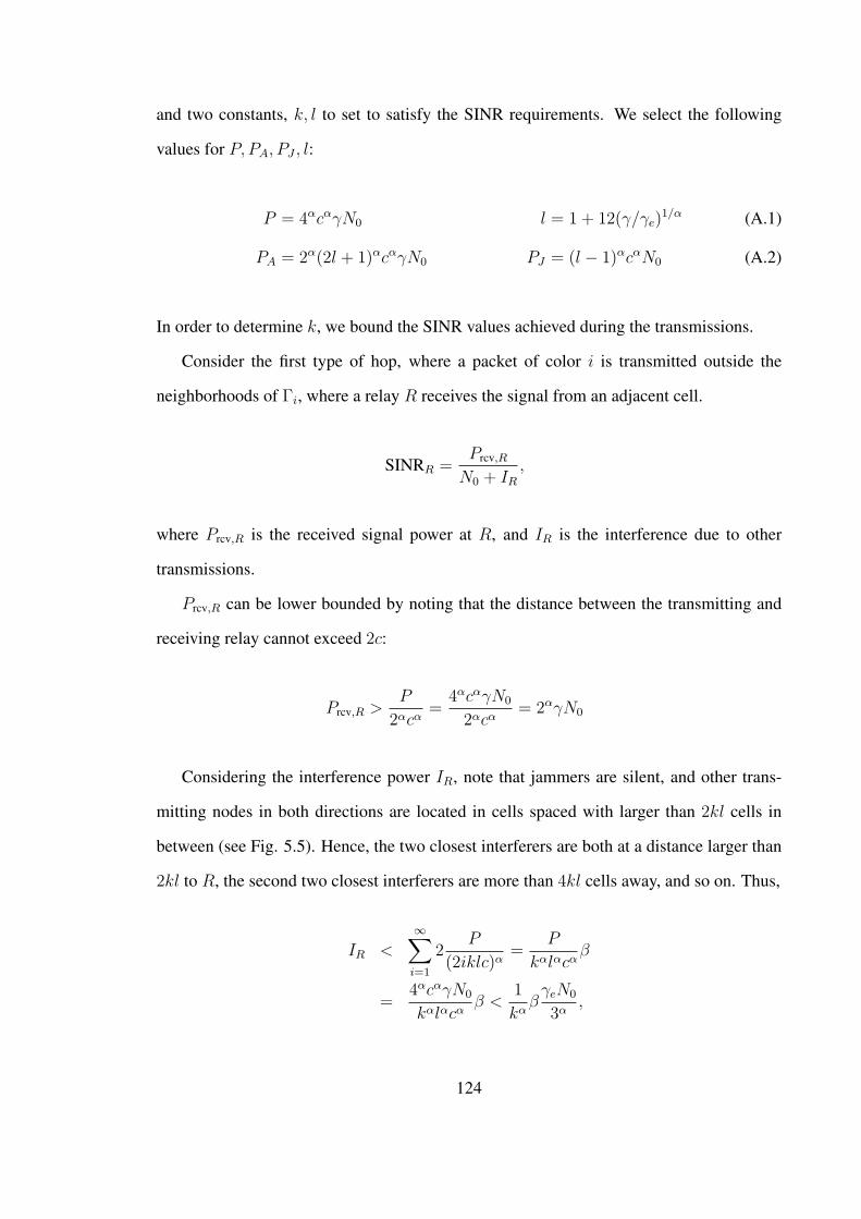
and two constants, k, l to set to satisfy the SINR requirements. We select the following

values for P, PA, PJ , l:

P = 4αcαγN0 l = 1 + 12(γ/γe)1/α (A.1)

PA = 2α(2l + 1)αcαγN0 PJ = (l − 1)αcαN0 (A.2)

In order to determine k, we bound the SINR values achieved during the transmissions.

Consider the first type of hop, where a packet of color i is transmitted outside the

neighborhoods of Γi, where a relay R receives the signal from an adjacent cell.

SINRR =Prcv,R

N0 + IR,

where Prcv,R is the received signal power at R, and IR is the interference due to other

transmissions.

Prcv,R can be lower bounded by noting that the distance between the transmitting and

receiving relay cannot exceed 2c:

Prcv,R >P

2αcα=

4αcαγN0

2αcα= 2αγN0

Considering the interference power IR, note that jammers are silent, and other trans-

mitting nodes in both directions are located in cells spaced with larger than 2kl cells in

between (see Fig. 5.5). Hence, the two closest interferers are both at a distance larger than

2kl to R, the second two closest interferers are more than 4kl cells away, and so on. Thus,

IR <∞∑i=1

2P

(2iklc)α=

P

kαlαcαβ

=4αcαγN0

kαlαcαβ <

1

kαβγeN0

3α,

124

where we define

β =2

2α

∞∑i=1

1

iα.

Note that β <∞ for α > 1. Hence,

SINRR >2αγN0

N0 +1

kαβγeN0

3α

> γ,

provided

kα >βγe

3α(2α − 1

) . (A.3)

During this single-cell hop for packet i, the SINR value at the closest eavesdropper E

inside Γi can be bounded as

SINRE <P/(l − 1)αcα

N0

=4αcαγN0

12α(γ/γe)cαN0

=γe3α

< γe.

Therefore, single-cell hops outside the neighborhoods satisfy the SINR requirements (with

k satisfying (A.3)).

Second, consider any multi-cell hop inside a neighborhood N(Cji ) (see Fig. 5.4 (b)),

where the transmitting relay A sends the packet to the receiving relay B.

SINRB =Prcv,B

N0 + IB + IB

Here, IB is the interference due to other relay transmissions, IB is the jamming noise

suffered due to all the active jammer nodes in the network. Prcv,B can be bounded by

noting the maximum distance between A and B.

Prcv,B ≥ PA

(2l + 1)αcα= 2αγN0

125

The interfering relays and jammers (with power PA, PJ , respectively) are located in the

network as in the single-cell hop case. Hence,

IB <∞∑i=1

2PA

(2iklc)α=

PA

kαlαcαβ <

1

kαβγN06

α,

and

IB <PJ

(l − 1)αcα+

∞∑i=1

2PJ

(2iklc)α

=PJ

(l − 1)αcα+

PJ

kαlαcαβ

≤ N0 +1

kαβN0,

where the first term in the upper bound for IB is due to the jammer node inside Cji . Hence,

SINRB >2αγN0

N0 +1kαβγN06α +N0 +

1kαβN0

> γ,

provided

kα >β(6αγ + 1)

2α − 2. (A.4)

The bound in (A.4) is stricter than the bound in (A.3).

The SINR value at an eavesdropper E inside Cji can be bounded as

SINRE ≤ PA/(l − 1)αcα

PJ/cα= γ2α

(2l + 1

l − 1

)α1

(l − 1)α

<6α

12αγ

γ/γe< γe.

The next closest eavesdropper E inside Γi has

SINRE <PA/(2klc)

α

N0

=1

kα

(2l + 1

l

)α

γ < γe,

126

provided

kα > 3α(γ/γe

)α. (A.5)

Thus, any value of k satisfying below can be used.

kα > max

β(6αγ + 1)

2α − 2, 3α(γ/γe

)α (A.6)

A.2 Two-dimensional Networks

Similar to the one-dimensional case, we show that the SINR condition is achieved in

the two-dimensional case for each hop. Consider the transmission of a packet under the

routing protocol (Fig. 5.7), where the signal is transmitted to a relay R from an adjacent

cell using a transmit power P with the value given in (A.1).

SINRR =Prcv,R

N0 + IR

The maximum distance between the relays is 2√2c, hence

Prcv,R >P

(2√2)αcα

=4αcαγN0

(2√2)αcα

= (√2)αγN0.

Considering the interference power IR, note that other transmitting nodes are placed

on the edges of concentric squares due to the time division multiplexing scheme. The first

such square contains 8 transmitting nodes (see Fig. 5.8), each with a distance larger than

(h− 1) cells to R, the next square contains 16 transmitting nodes, and so on. Thus,

IR <∞∑i=1

8iP

(i(h− 1)c)α= µ

P

(h− 1)αcα= µ

4αγN0

(h− 1)α,

127

where we define

µ = 8∞∑i=1

1

iα−1.

Note that µ <∞ for α > 2. Hence,

SINRR >(√2)αγN0

N0 + µ4αγN0

(h− 1)α

> γ,

provided

(h− 1)α > µ4αγ(

(√2)α − 1

) . (A.7)

During this transmission, consider any eavesdropper E that is located at a distance

larger than (l − 1) cells to the transmitting relay with l having the value in (A.1).

SINRE <P/(l − 1)αcα

N0

=4αcαγN0

N0(l − 1)αcα< γe (A.8)

Hence, the transmission of a packet on a path remains secure from any eavesdropper

that is located a distance of more than (l − 1) cells to any point on the path.

A.3 The Number of Streams Arriving to a Cell in 2-D

Consider any stream arriving at a cell sij(n), which is located on the ith row and jth

column in the square lattice, 1 6 i, j 6√n/ log n (see Fig. 5.6). The source node of this

stream has a path passing through sij(n), hence the source base should contain cells on the

ith row. Therefore, the source node is located on a row is such that (i− z) < is < (i+ z),

z = 4tl, so the sources of all the streams arriving to sij(n) is contained in a rectangular

region Ri of size z√log n×

√n. Similarly, the destination base of any stream contains a cell

128

on column j, therefore the destination nodes of all streams are contained in a rectangular

region Rj of size√n×z

√log n. Hence, the number of streams N arriving at sij(n) can be

upper-bounded by the number of nodes inside Ri∪Rj . Let the random variables Ni, Nj be

the number of nodes located in Ri,Rj , respectively. Ni, Nj are Poisson random variables

with parameter z√n log n. Note that N 6 Ni +Nj . Hence,

P (N < 4z√n log n) ≥ P (Ni +Nj < 4z

√n log n)

≥ P(Ni < 2z

√n log n

∩Nj < 2z√n log n

)≥ 1−

[P (Ni ≥ 2z

√n log n)

+P (Nj ≥ 2z√n log n)

]≥ 1− 2(e/4)z

√n logn → 1, n→ ∞,

where the third inequality is due to a union bound, and the last inequality is due to a

Chernoff bound. This shows N < 4z√n log n with high probability.

129

APPENDIX B

HYBRID NETWORKS

B.1 1-D Construction Details

Each segment has a Poisson number of nodes with mean log n. Hence,

P (”each segment has at least one node”) =(1− 1

n

)n/ logn

→ 1, n→ ∞

Each node (including base stations in the download phase) transmits with the same

power P . For b log b = O(n), nodes need to reach a node in the next segment, whereas

when b log b = w(n), nodes reach the closest base station in a single hop. The transmit

power is given by

P = 4αc(n)αγN0, (B.1)

where, c(n) = log n for the case b log b = O(n), and c(n) = n/b otherwise.

Consider a transmission from node A to node B which is in the next segment. The

SINR at node B is

SINRB =PA→B

N0 + IB,

where IB is the interference due to transmissions that take place in other segments. These

segments are regularly placed with d cells apart. Hence,

IB ≤ 2∞∑i=1

P

(idc(n))α= N0

1

dαη, (B.2)

130

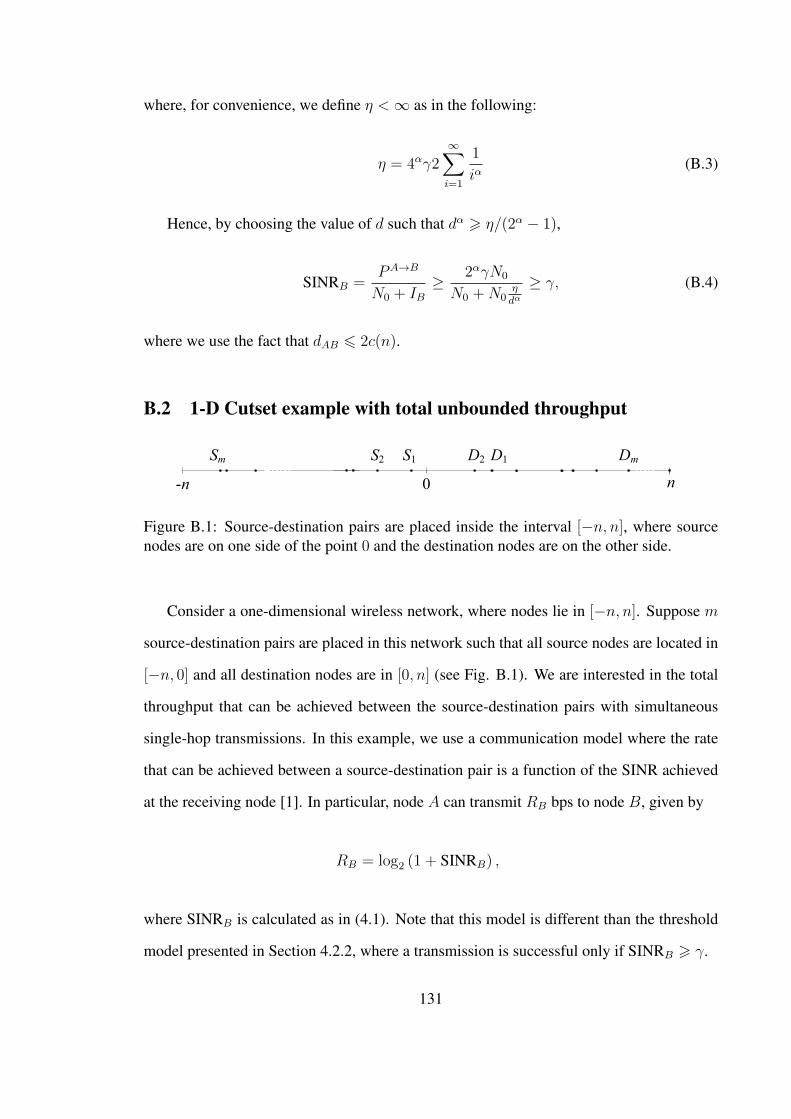
where, for convenience, we define η <∞ as in the following:

η = 4αγ2∞∑i=1

1

iα(B.3)

Hence, by choosing the value of d such that dα > η/(2α − 1),

SINRB =PA→B

N0 + IB≥ 2αγN0

N0 +N0ηdα

≥ γ, (B.4)

where we use the fact that dAB 6 2c(n).

B.2 1-D Cutset example with total unbounded throughput

n0-n

S1S2Sm D1D2 Dm

Figure B.1: Source-destination pairs are placed inside the interval [−n, n], where sourcenodes are on one side of the point 0 and the destination nodes are on the other side.

Consider a one-dimensional wireless network, where nodes lie in [−n, n]. Suppose m

source-destination pairs are placed in this network such that all source nodes are located in

[−n, 0] and all destination nodes are in [0, n] (see Fig. B.1). We are interested in the total

throughput that can be achieved between the source-destination pairs with simultaneous

single-hop transmissions. In this example, we use a communication model where the rate

that can be achieved between a source-destination pair is a function of the SINR achieved

at the receiving node [1]. In particular, node A can transmit RB bps to node B, given by

RB = log2 (1 + SINRB) ,

where SINRB is calculated as in (4.1). Note that this model is different than the threshold

model presented in Section 4.2.2, where a transmission is successful only if SINRB > γ.

131

Under this communication model, consider the following placement of nodes (see Fig.

B.2): We define the point +i as the “ith destination bin” for i = 1, 2, · · · , f(n), where

f(n) 6 n is the number of bins. At each destination bin, we place g(n) nodes. We denote

Dki as the kth destination node located at the ith bin, where i ∈ 1, 2, · · · , f(n) and

k ∈ 1, 2, · · · , g(n). The corresponding source node, Ski , is located at −i, which we

define as the “ith source bin”. Note that there are a total of m(n) = f(n)g(n) source-

destination pairs. Let PA→B be the power received at node B due to node A. Then, the

SINR achieved at Dki is:

-i n

Si1

0-n -1-2 +1 +2 +i

Si2 Di

1Di2

g(n) nodes at each integer location

-f(n) +f(n)

Figure B.2: Placement of source-destination pairs that lead to unbounded total rate througha single point as the network size increases.

SINRki =

P Ski →Dk

i

N0 +

(f(n)∑j=1

g(n)∑ℓ=1

P Sℓj→Dk

i

)− P Sk

i →Dki

The total rate achieved by these source-destination pairs is:

R(n) =

f(n)∑i=1

g(n)∑k=1

log2(1 + SINRk

i

)

In the following, we consider the total SINR instead of the total rate, and show that the

total SINR goes to infinity as n grows, which we later show that implies the total rate also

goes to infinity.

132

Let the distance between nodes A,B denoted as |A−B|. Then, SINRki can be bounded

as:

SINRki =

P |Ski −Dk

i |−α

N0 +

(f(n)∑j=1

g(n)∑ℓ=1

P |Sℓj −Dk

i |−α

)− P Sk

i →Dki

≥ P |Ski −Dk

i |−α

N0 +f(n)∑j=1

g(n)∑ℓ=1

P |Sℓj −Dk

i |−α

=|Sk

i −Dki |−α

Nr +f(n)∑j=1

g(n)∑ℓ=1

|Sℓj −Dk

i |−α

=1

|Ski −Dk

i |α(Nr +

f(n)∑j=1

g(n)∑ℓ=1

|Sℓj −Dk

i |−α

) ,

where we define Nr = N0/P for convenience. For the placement described above:

SINRki ≥

1

(2i)α

(Nr +

f(n)∑j=1

g(n)∑ℓ=1

(j + i)−α

)

=1

(2i)α

(Nr + g(n)

f(n)∑j=1

(j + i)−α

)

≥ 1

(2i)α(Nr + g(n)

n∫t=0

(t+ i)−αdt

)≥ 1

(2i)α(Nr +

g(n)

α− 1

1

iα−1

)

Let Y (n) be the total SINR. Then,

133

Y (n) =

f(n)∑i=1

g(n)∑k=1

SINRki

≥f(n)∑i=1

g(n)

(2i)α(Nr +

g(n)

α− 1

1

iα−1

)=

1

2α

f(n)∑i=1

1iαNr

g(n)+

i

α− 1

For the case where f(n)α−1 6 g(n), and f(n) → ∞, as n→ ∞,

Y (n) ≥ 1

2α

f(n)∑i=1

1iαNr

iα−1+

i

α− 1

=1

2α (Nr + 1/(α− 1))

f(n)∑i=1

1

i

→ ∞, as n→ ∞.

Therefore, it is possible to choose appropriate values for f(n), g(n), e.g., for α = 3,

f(n) = n1/3, g(n) = n2/3, so that the corresponding placement of m(n) = f(n)g(n)

nodes enable the total SINR grow to infinity with increasing network size. Finally, it can

be shown that the total rate also grows to infinity. For convenience, let us relabel the SINR

values in an arbitrary way as ai, i = 1, 2, · · · , n. Now consider the total rate:

R(n) =n∑

i=1

log2 (1 + ai)

= log2

(n∏

i=1

(1 + ai)

)

→ ∞, as n→ ∞,

where the divergence follows from the fact thatn∏

i=1

(1 + ai) diverges if the sumn∑

i=1

(1 + ai)

diverges [32].

134

Hence, the total rate through a single point can grow with the number of nodes. Con-

trasting this result with Lemma 4.1, we see that the cutset bounds can vary under different

communication models.

135

BIBLIOGRAPHY

[1] Agarwal, A., and Kumar, P. R. Capacity bounds for ad hoc and hybrid wirelessnetworks. ACM SIGCOMM Computer Communication Review (2004), 71–81.

[2] Anderson, C. W. Extreme value theory for a class of discrete distributions with appli-cations to some stochastic processes. Journal of Applied Probability (1970), 99–113.

[3] Anderson, C. W., Coles, S. G., and Husler, J. Maxima of Poisson-like variables andrelated triangular arrays. The Annals of Applied Probability (1997), 953–971.

[4] Blair, A., Brown, T., Chugg, K. M., Halford, T. R., and Johnson, M. Barrage relaynetworks for cooperative transport in tactical MANETs. In Proc. MILCOM 2008.

[5] Blair, A., Brown, T., Chugg, K. M., and Johnson, M. Tactical mobile mesh networksystem design. In Proc. MILCOM 2007.

[6] Cai, N., and Yeung, R.W. Secure network coding. In Proc. ISIT 2002.

[7] Capar, C., and Goeckel, D. Network coding for facilitating secrecy in large wirelessnetworks. In Proc. CISS 2012.

[8] Capar, C., Goeckel, D., Liu, B., and Towsley, D. Cooperative jamming to improvethe connectivity of the 1-D secrecy graph. In Proc. CISS 2011.

[9] Capar, C., Goeckel, D., Liu, B., and Towsley, D. Secret communication in large wire-less networks without eavesdropper location information. In Proc. IEEE INFOCOM2012.

[10] Capar, C., Goeckel, D., and Towsley, D. Broadcast analysis for extended cooperativewireless networks. IEEE Transactions on Information Theory (2013), 5805–5810.

[11] Chang, Y. J., Jung, H., and Ingram, M. A. Demonstration of a new degree of free-dom in wireless routing: Concurrent cooperative transmission. In Proc. HotEMNETS2010.

[12] Chen, X., Huang, W., Wang, X., and Lin, X. Multicast capacity in mobile wireless adhoc network with infrastructure support. In Proc. IEEE INFOCOM 2012.

[13] De Domenico, M., Sole, A., Gomez, S., and Arenas, A. Random Walks on MultiplexNetworks. arXiv:1306.0519.

[14] Dousse, O. Asymptotic properties of wireless multi-hop networks. PhD dissertation,EPFL, 2005.

136

[15] Dousse, O., Thiran, P., and Hasler, M. Connectivity in ad-hoc and hybrid networks.In Proc. IEEE INFOCOM 2002.

[16] Franceschetti, M., Dousse, O., Tse, D. N. C., and Thiran, P. Closing the gap in the ca-pacity of wireless networks via percolation theory. IEEE Transactions on InformationTheory (2007), 1009–1018.

[17] Franceschetti, M., and Meester, R. Random networks for communication: from sta-tistical physics to information systems. Cambridge University Press, 2007.

[18] Gao, J., Buldyrev, S. V., Stanley, H. E., Xu, X., and Havlin, S. Percolation of a generalnetwork of networks. Physical Review E (2013), 062816.

[19] Goeckel, D., Liu, B., Towsley, D., Wang, L., and Westphal, C. Asymptotic connec-tivity properties of cooperative wireless ad hoc networks. IEEE Journal on SelectedAreas in Communications (2009), 1226–1237.

[20] Goeckel, D., Vasudevan, S., Towsley, D., Adams, S., Ding, Z., and Leung, K. Artifi-cial noise generation from cooperative relays for everlasting secrecy in two-hop wire-less networks. IEEE Journal on Selected Areas in Communications (2011), 2067–2076.

[21] Goel, S., Aggarwal, V., Yener, A., and Calderbank, A. R. Modeling location uncer-tainty for eavesdroppers: A secrecy graph approach. In Proc. ISIT 2010.

[22] Goel, S., and Negi, R. Guaranteeing secrecy using artificial noise. IEEE Transactionson Wireless Communications (2008), 2180–2189.

[23] Goldsmith, A. Wireless Communications. Cambridge University Press, 2005.

[24] Gopala, P. K., Lai, L., and El Gamal, H. On the secrecy capacity of fading channels.IEEE Transactions on Information Theory (2008), 4687–4698.

[25] Grimmett, G. Percolation. Springer Verlag, 1999.

[26] Grossglauser, M., and Tse, D. N. C. Mobility increases the capacity of ad hoc wirelessnetworks. IEEE/ACM Transactions on Networking (2002), 477–486.

[27] Guha, S., Towsley, D., Capar, C., Swami, A., and Basu, P. Layered percolation.arXiv:1402.7057.

[28] Gupta, P., and Kumar, P. R. Critical power for asymptotic connectivity. In Proc. IEEEConference on Decision and Control (1998).

[29] Gupta, P., and Kumar, P. R. The capacity of wireless networks. IEEE Transactionson Information Theory (2000), 388–404.

[30] Haenggi, M. The secrecy graph and some of its properties. In Proc. ISIT 2008.

137

[31] Jain, K. Security based on network topology against the wiretapping attack. IEEEWireless Communications (2004), 68–71.

[32] Jeffrey, A., and Dai, H. H. Handbook of Mathematical Formulas and Integrals. Aca-demic Press, 2008.

[33] Jung, H., Chang, Y. J., and Ingram, M. A. Experimental range extension of concurrentcooperative transmission in indoor environments at 2.4GHz. In Proc. MILCOM 2010.

[34] Kailas, A., and Ingram, M. A. Analysis of a simple recruiting method for cooperativeroutes and strip networks. IEEE Transactions on Wireless Communications (2010),2415–2419.

[35] Kailas, A., Thanayankizil, L., and Ingram, M. A. A simple cooperative transmis-sion protocol for energy-efficient broadcasting over multi-hop wireless networks.KICS/IEEE Journal of Communication and Networks (2008), 213–220.

[36] Kesten, H. The critical probability of bond percolation on the square lattice equals1/2. Communications in Mathematical Physics (1980), 41–59.

[37] Kimber, A. C. A note on Poisson maxima. Probability Theory and Related Fields(1983), 551–552.

[38] Kivela, M., Arenas, A., Barthelemy, M., Gleeson, J. P., Moreno, Y., and Porter, M. A.Multilayer networks. arXiv:1309.7233.

[39] Koyluoglu, O. O., Koksal, C. E., and Gamal, H. E. On secrecy capacity scaling inwireless networks. IEEE Transactions on Information Theory (2012), 3000–3015.

[40] Kozat, U. C., and Tassiulas, L. Throughput capacity of random ad hoc networks withinfrastructure support. In Proc. MobiCom 2003.

[41] Laneman, J. N., Tse, D. N. C., and Wornell, G. W. Cooperative diversity in wirelessnetworks: Efficient protocols and outage behavior. IEEE Transactions on InformationTheory (2004), 3062–3080.

[42] Leung-Yan-Cheong, S. K., and Hellman, M. E. The gaussian wire-tap channel. IEEETransactions on Information Theory (1978), 451–456.

[43] Leveque, O., and Telatar, I. E. Information-theoretic upper bounds on the capacity oflarge extended ad hoc wireless networks. IEEE Transactions on Information Theory(2005), 858–865.

[44] Liang, Y., Poor, H. V., and Ying, L. Secrecy throughput of MANETs with maliciousnodes. In Proc. ISIT 2009.

[45] Liu, B., Liu, Z., and Towsley, D. On the capacity of hybrid wireless networks. InProc. IEEE INFOCOM 2003.

138

[46] Liu, B., Thiran, P., and Towsley, D. Capacity of a wireless ad hoc network withinfrastructure. In Proc. MobiHoc 2007.

[47] Liu, J., Goeckel, D., and Towsley, D. Bounds on the throughput gain of networkcoding in unicast and multicast wireless networks. IEEE Journal on Selected Areasin Communications (2009), 582–592.

[48] Lou, W., Liu, W., and Fang, Y. SPREAD: enhancing data confidentiality in mobile adhoc networks. In Proc. IEEE INFOCOM 2004.

[49] Lu, N., and Shen, X. S. Scaling laws for throughput capacity and delay in wirelessnetworks - a survey. IEEE Communications Surveys Tutorials (2014), 642–657.

[50] Mao, X. F., Li, X. Y., and Tang, S. J. Multicast capacity for hybrid wireless networks.In Proc. MobiHoc 2008.

[51] Meester, R., and Roy, R. Continuum Percolation. Cambridge University Press, 1996.

[52] Miorandi, D., Sicari, S., Pellegrini, F. D., and Chlamtac, I. Internet of things: Vision,applications and research challenges. Ad Hoc Networks (2012), 1497–1516.

[53] Newman, M. E. J., Strogatz, S. H., and Watts, D. J. Random graphs with arbitrarydegree distributions and their applications. Physical Review E (2001), 026118.

[54] Newman, M. E. J., and Ziff, R. M. Efficient monte carlo algorithm and high-precisionresults for percolation. Physical Review Letters (2000), 4104–4107.

[55] Ni, S.-Y., Tseng, Y.-C., Chen, Y.-S., and Sheu, J.-P. The broadcast storm problem ina mobile ad hoc network. In Proc. MobiCom 1999.

[56] Nicosia, V., Bianconi, G., Latora, V., and Barthelemy, M. Growing multiplex net-works. Physical Review Letters (2013), 058701.

[57] Nosratinia, A., Hunter, T. E., and Hedayat, A. Cooperative communication in wirelessnetworks. IEEE Communications Magazine (2004), 74–80.

[58] Ozgur, A., Leveque, O., and Tse, D. Hierarchical cooperation achieves optimal ca-pacity scaling in ad hoc networks. IEEE Transactions on Information Theory (2007),3549–3572.

[59] Ozgur, A., Leveque, O., and Tse, D. Operating regimes of large wireless networks.Foundations and Trends in Networking (2011), 1–107.

[60] Perron, E., Diggavi, S., and Telatar, E. On noise insertion strategies for wirelessnetwork secrecy. In Proc. ITA 2009.

[61] Pinto, P. C., Barros, J., and Win, M. Z. Wireless secrecy in large-scale networks. InProc. ITA 2011.

139

[62] Quintanilla, J. A., and Ziff, R. M. Asymmetry in the percolation thresholds of fullypenetrable disks with two different radii. Physical Review E (2007), 051115.

[63] Rabin, M. O. Efficient dispersal of information for security, load balancing, and faulttolerance. Journal of the ACM (1989), 335–348.

[64] Sahimi, M. Applications Of Percolation Theory. Taylor & Francis, 1994.

[65] Scaglione, A., Goeckel, D. L., and Laneman, J. N. Cooperative communications inmobile ad hoc networks. IEEE Signal Processing Magazine (Sept. 2006), 18–29.

[66] Shamir, A. How to share a secret. Communications of the ACM (1979).

[67] Shin, W. Y., Jeon, S. W., Devroye, N., Vu, M. H., Chung, S. Y., Lee, Y. H., andTarokh, V. Improved capacity scaling in wireless networks with infrastructure. IEEETransactions on Information Theory (2011), 5088–5102.

[68] Sirkeci-Mergen, B., and Scaglione, A. A continuum approach to dense wireless net-works with cooperation. In Proc. IEEE INFOCOM 2005.

[69] Sirkeci-Mergen, B., Scaglione, A., and Mergen, G. Asymptotic analysis of multi-stage cooperative broadcast in wireless networks. IEEE Transactions on InformationTheory (2006), 2531–2550.

[70] Sozer, E. M., Stojanovic, M., and Proakis, J. G. Underwater acoustic networks. IEEEJournal of Oceanic Engineering (2000), 72–83.

[71] Tarasevich, Y. Y., and van der Marck, S. C. An investigation of site-bond percolationon many lattices. International Journal of Modern Physics C (1999), 1193–1204.

[72] Toumpis, S. Capacity bounds for three classes of wireless networks: asymmetric,cluster, and hybrid. In Proc. MobiHoc 2004.

[73] Vasudevan, S., Goeckel, D., and Towsley, D. F. Security-capacity trade-off in largewireless networks using keyless secrecy. In Proc. MobiHoc 2010.

[74] Williams, B., and Camp, T. Comparison of broadcasting techniques for mobile adhoc networks. In Proc. MobiHoc 2002.

[75] Wyner, A. D. The wire-tap channel. Bell Systems Technical Journal (1975), 1355–1387.

[76] Xiao, S., Gong, W., and Towsley, D. Secure wireless communication with dynamicsecrets. In Proc. IEEE INFOCOM 2010.

[77] Xie, L.-L., and Kumar, P. R. A network information theory for wireless communica-tion: scaling laws and optimal operation. IEEE Transactions on Information Theory(2004), 748–767.

140

[78] Xie, L.-L., and Kumar, P. R. On the path-loss attenuation regime for positive costand linear scaling of transport capacity in wireless networks. IEEE Transactions onInformation Theory (2006), 2313–2328.

[79] Xue, F., and Kumar, P. R. Scaling laws for ad hoc wireless networks: An informationtheoretic approach. Foundations and Trends in Networking (2006), 145–270.

[80] Zemlianov, A., and de Veciana, G. Capacity of ad hoc wireless networks with infras-tructure support. IEEE Journal on Selected Areas in Communications (2005), 657–667.

141