assessing the suitability of central european landscapes for the reintroduction of eurasian lynx:...

Journal of Applied Ecology 2002 39, 189–203

© 2002 British Ecological Society

Blackwell Science LtdAssessing the suitability of central European landscapes for the reintroduction of Eurasian lynx

STEPHANIE SCHADT*†, ELOY REVILLA*‡, THORSTEN WIEGAND*, FELIX KNAUER§, PETRA KACZENSKY¶, URS BREITENMOSER**, LUDEK BUFKA††, JAROSLAV CERVENY‡‡, PETR KOUBEK‡‡, THOMAS HUBER¶, CVETKO STANISA§§ and LUDWIG TREPL†*Department of Ecological Modelling, UFZ Centre for Environmental Research, Permoser Str. 15, D-04318 Leipzig, Germany; †Department für Ökologie, Lehrstuhl für Landschaftsökologie, Technische Universität München, Am Hochanger 6, D-85350 Freising-Weihenstephan, Germany; ‡Department of Applied Biology, Estación Biológica de Doñana, Consejo Superior de Investigaciones Científicas, Avenida María Luisa s/n, E-41013 Sevilla, Spain; §Wildlife Research and Management Unit, Faculty of Forest Sciences, Technische Universität Munich, Field Research Station Linderhof, Linderhof 2, D-82488 Ettal, Germany; ¶Institute of Wildlife Biology and Game Management, Agricultural University of Vienna, Peter-Jordan-Str. 76, A-1190 Vienna, Austria; **Institute of Veterinary Virology, University of Bern, Länggass-Str. 122, CH-3012 Bern, Switzerland; ††Íumava National Park Administration, Sußická 399, CZ-34192 Kaßperské Hory, Czech Republic; ‡‡Institute of Vertebrate Biology, Academy of Sciences of the Czech Republic, Kv´tná 8, CZ-60365 Brno, Czech Republic; §§State Forest Service, Slovenia, Rozna ul. 36, SLO-1330 Kocevje, Slovenia

Summary

1. After an absence of almost 100 years, the Eurasian lynx Lynx lynx is slowly recover-ing in Germany along the German–Czech border. Additionally, many reintroductionschemes have been discussed, albeit controversially, for various locations. We present ahabitat suitability model for lynx in Germany as a basis for further management andconservation efforts aimed at recolonization and population development.2. We developed a statistical habitat model using logistic regression to quantify thefactors that describe lynx home ranges in a fragmented landscape. As no data wereavailable for lynx distribution in Germany, we used data from the Swiss Jura Mountainsfor model development and validated the habitat model with telemetry data from theCzech Republic and Slovenia. We derived several variables describing land use andfragmentation, also introducing variables that described the connectivity of forestedand non-forested semi-natural areas on a larger scale than the map resolution.3. We obtained a model with only one significant variable that described the connec-tivity of forested and non-forested semi-natural areas on a scale of about 80 km2. Thisresult is biologically meaningful, reflecting the absence of intensive human land use onthe scale of an average female lynx home range. Model testing at a cut-off level of P > 0·5correctly classified more than 80% of the Czech and Slovenian telemetry location data ofresident lynx. Application of the model to Germany showed that the most suitable habitatsfor lynx were large-forested low mountain ranges and the large forests in east Germany.4. Our approach illustrates how information on habitat fragmentation on a large scalecan be linked with local data to the potential benefit of lynx conservation in centralEurope. Spatially explicit models like ours can form the basis for further assessing thepopulation viability of species of conservation concern in suitable patches.

Key-words: GIS, large-scale approach, logistic regression, Lynx lynx, spatially explicitconnectivity index, species reintroduction, statistical habitat model.

Journal of Applied Ecology (2002) 39, 189–203

Correspondence: S. Schadt, Department of Ecological Modelling, UFZ Centre for Environmental Research, Permoser Str. 15,D-04318 Leipzig, Germany (fax + 49 341 235 3500; e-mail [email protected]).

190S. Schadt et al.

© 2002 British Ecological Society, Journal of Applied Ecology, 39,189–203

Introduction

Effective nature conservation and habitat restorationin human-dominated landscapes require an under-standing of how species respond to habitat fragmenta-tion. As anthropogenic activities such as agriculture orurban development become prevalent in a region,native habitats are reduced in area and exist ultimatelyas remnants in a highly altered matrix (Miller & Cale2000). Large carnivores provide some of the clearestexamples of the fate of species that have to cope withfragmented multi-use landscapes on a large scale. Cen-tral Europe was once covered by dense temperatedeciduous forests. However, after more than 5000 yearsof intense human activities only 2% of the originalprime forest remains. At the beginning of the 20th cen-tury, wolves Canis lupus, brown bears Ursus arctos andEurasian lynx Lynx lynx were almost extinct. Sincethen, there has been slow recovery of wolves in Spainand Italy (Boitani 2000), and bears and Eurasian lynxin Scandinavia, the Carpathians and the Balkan Penin-sula (Breitenmoser et al. 2000; Swenson et al. 2000).

The management and conservation of large carni-vores is particularly difficult due to their large require-ments for space. Intensive human land use is responsiblefor habitat fragmentation, which results in direct andindirect conflicts with those carnivores that competewith humans for the remaining semi-natural space andresources (Noss et al. 1996; Woodroffe & Ginsberg1998; Revilla, Palomares & Delibes 2001). Many suchspecies come into direct conflict with people because oftheir predatory habits. For example, the diet of lynx isbasically formed of valuable game such as roe deerCapreolus capreolus and chamois Rupicapra rupicapra,but also includes sheep and red deer Cervus elaphus(Breitenmoser & Haller 1993; Jedrzejewski et al. 1993;Okarma et al. 1997; Jobin, Molinari & Breitenmoser2000; Cerveny et al. 2002; Stahl et al. 2001). The patchydistribution of suitable habitat and construction of lin-ear barriers such as highways can lead to higher mor-tality (Kaczensky et al. 1996; Mace et al. 1996; Clevenger,Chruszcz & Gunson 2001). Therefore, conservationstrategies for large carnivores focus on the integrationof the species into multi-use landscapes inevitably domi-nated by people (Schröder 1998; Linnell, Swenson &Andersen 2000; Linnell et al. 2001).

Basic questions about the management and conser-vation of large carnivores still remain unanswered, forexample about minimum habitat requirements underthe new landscape conditions, and about whetherrecovery is only a local-scale phenomenon or can beexpected to a greater extent in areas with dense humanpopulations. These complex large-scale issues requireknowledge of the extent, spatial arrangement andconnectivity of potentially suitable habitat. In denselypopulated central Europe, the case of the reinvadingEurasian lynx poses exactly these questions. Since 1970several successful efforts have been made to reintroducelynx in Switzerland, France, Slovenia and the Czech

Republic (Herrenschmidt & Leger 1987; Breitenmoseret al. 1993; Cerveny, Koubek & Andera 1996; Cop &Frkovic 1998). In Germany there has been much contro-versy over lynx reintroduction, but natural immigrationhas already occurred into the Bavarian Forest due tothe expansion of a population reintroduced to the CzechBohemian Forest (Cerveny & Bufka 1996) (Fig. 1).

Given this situation, a large-scale assessment of hab-itat suitability is a necessary prerequisite for the evalu-ation of current initiatives for lynx reintroduction andmanagement actions. Although the suitability of someareas for lynx has been ardently and controversiallydiscussed in Germany, no quantitative habitat modelyet exists to support these discussions, particularly onethat can describe to what extent the species is tolerant oflarge-scale fragmentation. Some studies have modelledspatial factors that determine the distribution of theEurasian lynx, but restricted to local areas (Zimmermann& Breitenmoser 2001) or using algorithms that do notapply to fragmented areas (Corsi, Sinibaldi & Boitani1998). Schadt et al. (in press) developed a rule-basedhabitat model for lynx in Germany, but this model hasnot been validated with any field data.

We aimed to develop a home range suitability modelfor the lynx in central Europe based on current under-standing of its requirements. We wanted our model toquantify general predictors for lynx home ranges tocontribute to the design of a Germany-wide conservationplan by (i) identifying the broad distribution of suitablepatches; (ii) obtaining an estimate of possible lynx homeranges in Germany; and (iii) providing a basis for aspatially explicit population simulation model to assessrecolonization success and population development.

Methods

Habitat models using presence–absence data and logis-tic regression are useful in formalizing the relationshipbetween environmental conditions and species’ habitatrequirements, and in quantifying the amount of poten-tial habitat (Morrison, Marcot & Mannan 1992; Boyce& McDonald 1999); they have been widely applied fora variety of purposes and species (Buckland & Elston1993; FitzGibbon 1993; Wilson et al. 1997; Mace et al.1999; Mladenoff, Sickley & Wydeven 1999; Palma,Beja & Rodrigues 1999; Rodriguez & Andrén 1999;Bradbury et al. 2000; Gates & Donald 2000; Manel,Buckton & Ormerod 2000; Orrock et al. 2000; Suarez,Balbontin & Ferrer 2000). The principle of this methodis to contrast used habitat units vs. unused units inorder to determine habitat suitability with a set ofexplanatory variables (Hosmer & Lemeshow 1989;Tabachnick & Fidell 1996). The regression functioncan then be extrapolated and mapped over target areas,in our case Germany and its neighbouring forests. Wegenerated a home range suitability model based onlocal radio-tracking data obtained from lynx in theFrench and Swiss Jura Mountains (local study area), alandscape similar in fragmentation and population

191Lynx habitat suitability


density to the German low mountain ranges. Thismodel was then extrapolated to Germany (large-scalestudy area) and evaluated with independent radio-tracking data from the low mountain range along theGerman–Czech border and from the Dinaric Moun-tain Range of southern Slovenia.

To provide a range of comparable data for areas notinhabited by lynx, i.e. unused units or non-observations,we created random home ranges in the local study areathat we assumed to be in the general region of probablelynx movement and that lynx were likely to have visited,but where they had not settled as permanent residents.We assumed the resident home range areas to representmore desirable habitat than the non-occupied area.

The basic units for our analysis were raster cells basedon the total lynx home range area irrespective of theanimal, to avoid pseudoreplication due to home rangeoverlap. We did not use single lynx location data,although we also used the telemetry data to gain insightinto preferred land-use types. As the accuracy of thetelemetry location data was 1 km2, we defined this asthe spatial grain or landscape resolution. In order toconsider information that comprised forest fragmenta-tion on a larger scale than our grid cell, we introducedtwo spatially explicit connectivity indices that describedscale-dependent landscape properties to capture theindividual’s landscape perception over larger areas.

Local-scale data for model development

Model development was based on lynx radio-collaredand tracked in the Swiss Jura Mountains. The JuraMountains are a secondary limestone chain betweenSwitzerland and France with altitudes ranging between372 and 1679 m a.s.l. The highlands are 53% covered bydeciduous forest on the slopes, with coniferous forestson the ridges. Human population density reachesabout 120 inhabitants km–2, and the area is intensivelyused for recreation. Cultivated areas are typically pas-tures used for grazing cattle (Breitenmoser & Baettig1992; Breitenmoser et al. 1993).

We used 3402 radio-location data points publishedby Breitenmoser et al. (1993) from 13 individualstracked from 1988 to 1991, of which four were residentfemales and three were resident males. The rest weredispersing subadults. One resident female had a homerange shift during her observation period, and for ana-lytical purposes we considered her home range asbelonging to two different individuals (giving a total offive home ranges of female lynx). Following the meth-odology proposed by Breitenmoser et al. (1993), weremoved outlier locations before estimating the homeranges of the resident lynx using minimum convexpolygons (MCP). The average home range sizes werethen 169 km2 for females (n = 5) and 263 km2 formales (n = 3). For our analysis we defined the ‘closer

Fig. 1. Permanent lynx populations in central Europe, sporadic and undetermined lynx occurrence (modified after Breitenmoseret al. 2000) and reintroduction initiatives for lynx in Germany. The black rectangles show the places from where we obtainedtelemetry data for developing the habitat model. PF, Palatine Forest; BF, Black Forest; BBF, Bavarian/Bohemian Forest.

192S. Schadt et al.


study area’ (CSA) as the MCP enclosing all locations,including residents and dispersers, to create a generalregion of probable lynx movement, with a buffer of2·5 km, defined by the average daily distance moved(Fig. 2).

Local-scale data for model validation

German–Czech data. The forest cover of the low moun-tain chain along the German–Czech border (highestelevation at 1457 m) ranges from more than 90% in theinner parts (Sumava Mountains on the Czech side andInner Bavarian Forest on the German side) to below50% in the outer regions (e.g. Sumava Foothills, OuterBavarian Forest and Fichtelgebirge). Population dens-ity ranges from 20 to 100 inhabitants km–2 (Cerveny &Bufka 1996; Wölfl et al. 2001) (Fig. 1). From theSumava National Park we used the data of 714 radio-locations from five lynx observed between 1997 and1999 (Bufka et al. 2000), one of them being a residentfemale having most of the centre of her home range inthe Bavarian Forest on the German side. Two otherswere resident males and two were dispersing subadults.

Slovenian data. We used 677 telemetry locations fromtwo resident females and three resident males over theperiod 1994–96 (Stanis̆a 1998). The lynx were descend-ants of six lynx reintroduced in the region in 1973 (Cop& Frkovic 1998). The study area is part of the Dinaric

Mountain Range, stretching from Slovenia in the northto Albania in the south (Fig. 1). Elevations range from300 to 1200 m, forest cover averages 90%, and the dom-inating forest community is Abieti–Fagetum dinaricum.Human population density is low, averaging 22 inhab-itants km–2, and the main human activities of the regionare forestry, timber extraction and hunting with smallamounts of recreation.

Large-scale study area for model application

Germany comprises an area of about 358 000 km2 withan average population density of 230 inhabitants km–2,which drops to about 100 inhabitants km–2 in placessuch as the low mountain ranges (e.g. Black Forest,Palatine Forest and Thuringian Forest). Urbaniza-tion accounts for 5% of the total area, and 30% of thetotal area is forested. The forests are clustered in areasformerly unsuitable for human activity in the low moun-tain ranges and in areas with poor soils in the north-east. Of the total area 2·5% is protected by NationalPark status. Germany has a very dense traffic networkconsisting of 11 000 km of highways and more than50 000 km of interstate or main roads. We includedneighbouring forest areas in Poland, the Czech Repub-lic, France and Belgium in our large-scale study area.We excluded the Alps as the habitat requirements oflynx in alpine biomes differ from those in low mountainranges where we obtained our data.

Fig. 2. Swiss Jura Mountain chain: home ranges of resident lynx (polygons), random home ranges (circles) and locations ofdispersing lynx (triangles) in the closer study area (CSA). Light grey are grid cells that contain more than 66·6% of extensively usedland-use types, such as forest or heathland (classed as PExt cells); dark grey are cells of the applied model with P > 0·5 (see theresults of the logistic regression).



Data base

We used CORINE land use data (European TopicCenter on Land Cover, Environment Satellite DataCenter, Kiruna, Sweden), which classify the followingland use types on a 250-m grid. The CORINE classifica-tion names are provided in parentheses when differ-ent. (i) Urban areas (artificial territories); (ii) agriculturalland (strongly artificial vegetated areas); (iii) pasture(less artificial vegetated areas); (iv) forests; (v) non-wooded semi-natural areas, e.g. heathland; (vi) wet-lands; (vii) water surfaces. Information on roads wasdigitized from 1 : 250 000-scale road maps. Roadsincluded highways, transeuropean roads and mainroads. Other paved roads, unpaved roads, unimprovedforest roads and trails were not considered. All datawere georeferenced on a Transverse Mercator projec-tion (spheroid Bessel, x-shift 3 500 000).

Map preparation

We created a raster map of 1-km mesh size and clippedit with the land use and road maps of the CSA in Switzer-land. Each lynx home range was intersected with theraster map, and descriptive environmental variableswere extracted for each cell. We created five non-usedhome ranges for females and three for males of the aver-age size observed in the CSA. The position of these non-used home ranges was randomly assigned within theCSA, but without considering the area of lynx homeranges and big lakes (Bieler See and Neuenburger See)to help ensure that non-resident home range areas werelikely to have been visited by lynx. Point distances were7334 (9150) m from the edge, to avoid lying outside theCSA, and 14 668 (18 300) m between points, to avoidhome range overlap in the same sexes for females(males). These points were then buffered with a radiusof 7334 m (= area of 169 km2) for females and 9150 m(= area of 263 km2) for males. The random home rangesof the different sexes overlapped in two cases (Fig. 2).

To improve the biological interpretability of the finalmodel, we avoided choosing many potential landscapepredictors that a priori were not directly linked to thebiology of the species, and orthogonalizing them intoindependent axes with data aggregation techniques(e.g. with principal component or factor analysis;Tabachnick & Fidell 1996).

The Eurasian lynx is present in large continuous for-est areas, although the forests can be interrupted byother land-use types such as pastures or agriculture.Intensive land use is tolerated as long as there is enoughconnected forest for retreat (Haller & Breitenmoser1986; Breitenmoser & Baettig 1992; Haller 1992;

Breitenmoser et al. 1993; Schmidt, Jedrzejewski &Okarma 1997). Human activity may strongly affect thepresence of large carnivores by direct elimination orby individual avoidance of areas used by humans(Mladenoff et al. 1995; Woodroffe & Ginsberg 1998;Revilla, Palomares & Delibes 2001; Palomares et al.2001). Availability of prey may also be important.Unfortunately, uniform data on prey density do notexist, so we were not able to include this information inour model.

Local-scale variables

Initially we compiled a number of potential predictorvariables to describe fragmentation of large forest areasand intensive human land use (Table 1). We includedvariables related to the presence of forest within eachgrid cell, such as the percentage of forest, PFor, thenumber of forest patches, NPFor, and the perimeter offorest patches, PeriFor. We included other land usessuch as the percentages of arable land, PAgr, pastures,PPast, and other non-forested semi-natural areas,PNat (Table 1). We also included the total number ofpatches of any land use, NPTot, and the percentage ofextensive human land use, PExt. The latter was definedas the combined percentage of forest areas, PFor, andother non-forested semi-natural land cover, PNat,when the percentage of both land uses per cellwas ≥ 66·6% (Table 1). This ensured that we alsoincluded margin cells of extensively used areas. Humanvariables included the percentage of urban areas,PUrb, and the number of urban polygons per cell,NPUrb (Table 1). We also compiled the total length oftranseuropean and major roads, R50, per cell.

Large-scale variables

We introduced two spatial indices, RA and RC, thatdescribe the connectivity or fragmentation of extens-ively used areas on larger scales than map resolution(Fig. 3). We defined the index RA (x, y, r) as the pro-portion of extensively used cells, PExt, in the circularneighbourhood within radius r around a given extens-ively used cell (x, y). RA (x, y, r) = 1 indicates that allcells in the neighbourhood r of (x, y) are extensivelyused cells, i.e. the suitable habitat in the neighbourhoodr of (x, y) is non-fragmented, while RA (x, y, r) < < 1indicates that only a few cells in the neighbourhood r of(x, y) are extensively used. Alternatively, we mayassume that the average cover of extensive land uses inthe neighbourhood of a given cell determines habitatsuitability. Therefore we define the second index RC (x,y, r) as the proportion of extensive land-use types in thecircular neighbourhood with radius r around a givencell (x, y). Note that RC may not be zero for cells withlow cover of extensively used areas. If such cells, e.g.villages, are surrounded by larger forest areas, RC assignsthem a high index value. This assumption is reasonablebecause MCP representations of lynx home ranges

194S. Schadt et al.


may include villages. We calculated both indices forradius r = 1, 3, 5 and 7 km.

First, we used descriptive univariate analyses to testour data before entering them into the logistic model,as the ecological relevance of an explanatory variable isan important aspect of model evaluation (Noon 1986).Lynx home ranges created with the MCP method areconceptual approximations and may contain variablesthat do not make sense from the perspective of lynxbiology. Variables that are not plausible can beexcluded before being entered into the logistic regres-sion. However, we did not want to exclude variables

that may influence lynx presence or absence, such asagriculture, beforehand, as this would constitute datadredging (Burnham & Anderson 1998). We thereforecompared frequencies of telemetry data on the land-use classes with the same frequency of random pointsdistributed in the CSA with a frequency test. Addition-ally we compared rank differences of the variables ofthe eight home ranges to the eight random home rangeswith a non-parametric Kruskal–Wallis test.

As we divided the total home range area and also therandom home ranges into raster cells of 1 km2 (Fig. 3),we expected a high spatial autocorrelation in ourdependent variable, i.e. a high probability that a cellcontains the same information as its neighbouring cell(Lennon 1999). Therefore we could not include the data

Table 1. Means of the land-use variables per cell in the random home ranges (HR) (n = 8) and the home ranges of the residentlynx (n = 8). **Indicates differences of the Kruskal–Wallis tests at a significance level of P < 0·01, and * at a significance level ofP < 0·05, n = 16, d.f. = 1. Retained variables (RV) for the logistic regression are marked with an x

Variable Biological interpretation Random HR ± SD Lynx HR ± SD RV

PUrb (% of urban areas) Intensive human land use ** 3·3 ± 2·3 0·7 ± 0·3PAgr (% of agriculture) Intensive human land use 5·5 ± 8·8 10·2 ± 5·4PPast (% of pasture) Intensive human land use * 39·5 ± 20·8 11·2 ± 5PFor (% of forest) Extensive human land use * 40·9 ± 8·6 52·9 ± 2·5 xPNat (% of natural areas) Extensive human land use ** 8·9 ± 4·1 24 ± 6·9 xNPTot (total no. of polygons) Fragmentation 2·5 ± 0·4 2·5 ± 0·2 xNPFor (no. of forest polygons) Extensive human land use * 0·9 ± 0·1 1·1 ± 0·1 xNPUrb (no. of urban polygons) Intensive human land use ** 0·1 ± 0·1 0 ± 0 xPeriFor (perimeter of forest) Forest fragmentation * 2614·5 ± 420·7 3220·5 ± 209·5R50 (density of major roads in km/km2) Intensive human land use 0·6 ± 0·3 0·3 ± 0·2 xRA Radius 1 km Forest fragmentation ** 0·26 ± 0·17 0·66 ± 0·1 x

Radius 3 km Forest fragmentation ** 0·22 ± 0·16 0·58 ± 0·1 xRadius 5 km Forest fragmentation ** 0·2 ± 0·15 0·53 ± 0·1 xRadius 7 km Forest fragmentation ** 0·19 ± 0·14 0·47 ± 0·1 x

RC Radius 1 km Forest fragmentation ** 1·13 ± 0·26 1·7 ± 0·13 xRadius 3 km Forest fragmentation ** 1·11 ± 0·23 1·62 ± 0·12 xRadius 5 km Forest fragmentation ** 1·11 ± 0·19 1·51 ± 0·12 xRadius 7 km Forest fragmentation ** 1·11 ± 0·16 1·43 ± 0·13 x

Fig. 3. Example of the indices RA (left) and RC (right) with radii of 5 km each. RA only uses the predefined cells with extensively used areas and calculatesthe percentage of more cells of that type around, RC uses all cells and calculates the mean part of cells with extensively used areas around. Also shown isthe closer study area (CSA). The colours from white to black indicate increasing values of the indices. Cells outside the CSA were not considered. Fororientation the home ranges (polygons) of the resident lynx and the random home ranges (circles) are also shown.



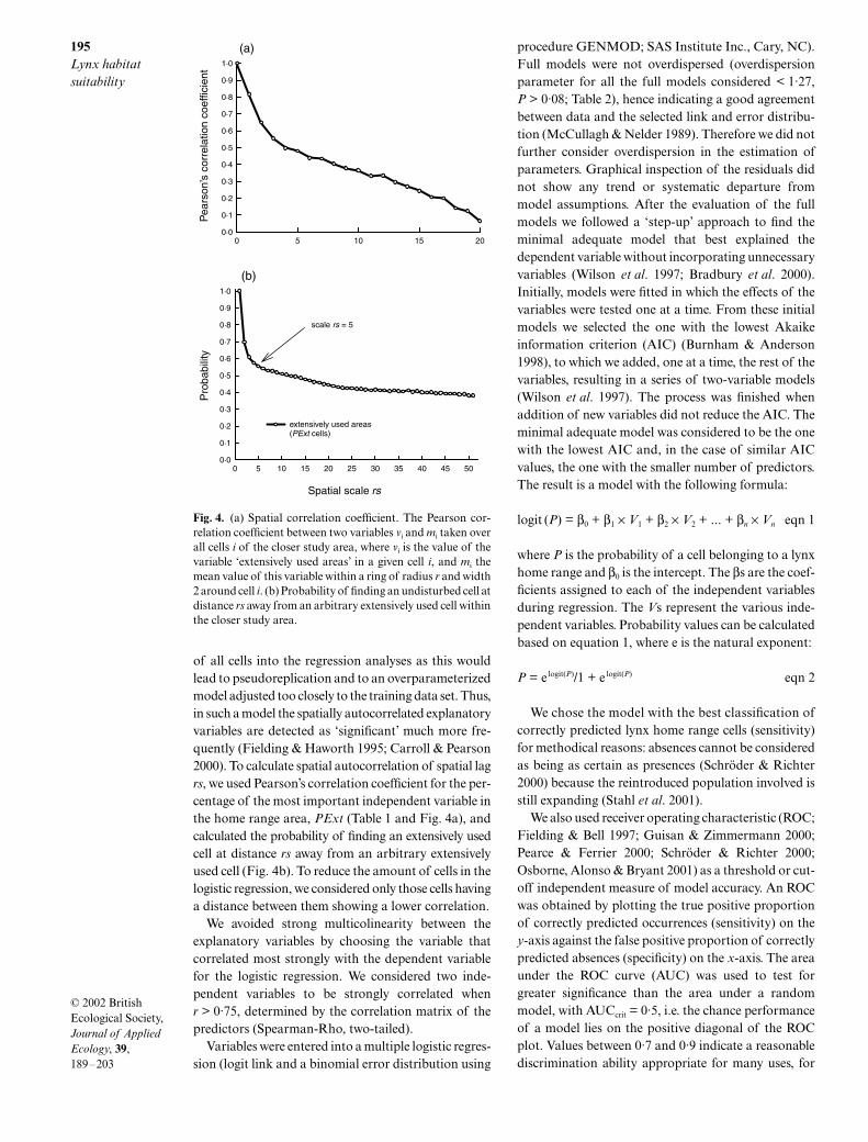
of all cells into the regression analyses as this wouldlead to pseudoreplication and to an overparameterizedmodel adjusted too closely to the training data set. Thus,in such a model the spatially autocorrelated explanatoryvariables are detected as ‘significant’ much more fre-quently (Fielding & Haworth 1995; Carroll & Pearson2000). To calculate spatial autocorrelation of spatial lagrs, we used Pearson’s correlation coefficient for the per-centage of the most important independent variable inthe home range area, PExt (Table 1 and Fig. 4a), andcalculated the probability of finding an extensively usedcell at distance rs away from an arbitrary extensivelyused cell (Fig. 4b). To reduce the amount of cells in thelogistic regression, we considered only those cells havinga distance between them showing a lower correlation.

We avoided strong multicolinearity between theexplanatory variables by choosing the variable thatcorrelated most strongly with the dependent variablefor the logistic regression. We considered two inde-pendent variables to be strongly correlated whenr > 0·75, determined by the correlation matrix of thepredictors (Spearman-Rho, two-tailed).

Variables were entered into a multiple logistic regres-sion (logit link and a binomial error distribution using

procedure GENMOD; SAS Institute Inc., Cary, NC).Full models were not overdispersed (overdispersionparameter for all the full models considered < 1·27,P > 0·08; Table 2), hence indicating a good agreementbetween data and the selected link and error distribu-tion (McCullagh & Nelder 1989). Therefore we did notfurther consider overdispersion in the estimation ofparameters. Graphical inspection of the residuals didnot show any trend or systematic departure frommodel assumptions. After the evaluation of the fullmodels we followed a ‘step-up’ approach to find theminimal adequate model that best explained thedependent variable without incorporating unnecessaryvariables (Wilson et al. 1997; Bradbury et al. 2000).Initially, models were fitted in which the effects of thevariables were tested one at a time. From these initialmodels we selected the one with the lowest Akaikeinformation criterion (AIC) (Burnham & Anderson1998), to which we added, one at a time, the rest of thevariables, resulting in a series of two-variable models(Wilson et al. 1997). The process was finished whenaddition of new variables did not reduce the AIC. Theminimal adequate model was considered to be the onewith the lowest AIC and, in the case of similar AICvalues, the one with the smaller number of predictors.The result is a model with the following formula:

logit (P) = β0 + β1 × V1 + β2 × V2 + ... + βn × Vn eqn 1

where P is the probability of a cell belonging to a lynxhome range and β0 is the intercept. The βs are the coef-ficients assigned to each of the independent variablesduring regression. The Vs represent the various inde-pendent variables. Probability values can be calculatedbased on equation 1, where e is the natural exponent:

P = e logit(P)/1 + e logit(P) eqn 2

We chose the model with the best classification ofcorrectly predicted lynx home range cells (sensitivity)for methodical reasons: absences cannot be consideredas being as certain as presences (Schröder & Richter2000) because the reintroduced population involved isstill expanding (Stahl et al. 2001).

We also used receiver operating characteristic (ROC;Fielding & Bell 1997; Guisan & Zimmermann 2000;Pearce & Ferrier 2000; Schröder & Richter 2000;Osborne, Alonso & Bryant 2001) as a threshold or cut-off independent measure of model accuracy. An ROCwas obtained by plotting the true positive proportionof correctly predicted occurrences (sensitivity) on they-axis against the false positive proportion of correctlypredicted absences (specificity) on the x-axis. The areaunder the ROC curve (AUC) was used to test forgreater significance than the area under a randommodel, with AUCcrit = 0·5, i.e. the chance performanceof a model lies on the positive diagonal of the ROCplot. Values between 0·7 and 0·9 indicate a reasonablediscrimination ability appropriate for many uses, for

Fig. 4. (a) Spatial correlation coefficient. The Pearson cor-relation coefficient between two variables vi and mi taken overall cells i of the closer study area, where vi is the value of thevariable ‘extensively used areas’ in a given cell i, and mi themean value of this variable within a ring of radius r and width2 around cell i. (b) Probability of finding an undisturbed cell atdistance rs away from an arbitrary extensively used cell withinthe closer study area.

196S. Schadt et al.


example a value of AUC = 0·8 means that, in 80% of allcases for a randomly chosen area with presence, agreater presence probability is being calculated than fora randomly chosen area with non-presence (Fielding &Haworth 1995; Pearce & Ferrier 2000).

To apply the model to our large-scale study area weselected the cut-off level for a given probability P of ourmodel ex posteriori by comparing the evolution ofpresence–absence prognosis. We chose a cut-off valuein between the optimum cut-off value, Popt (maximumof proportion of correct classifications), and the occur-rence probability value, Pfair (least error of the model),where false presence predictions and false absencepredictions have the same probability of occurring(Schröder & Richter 2000).

The predictive power of the model with the thusfound cut-off value P was then validated with a set oftelemetry data from the German–Czech border andSlovenia. For this we created home ranges with thesame method of outlier removal as used for the Swissdata (Breitenmoser et al. 1993). For assessing the aver-age number of lynx that could live in the patches of ourlarge-scale study area, we used the core area size plusone standard deviation (non-overlapping part of thehome range) of female lynx (99 km2) and the averagecore area size of male lynx (185 km2; Breitenmoseret al. 1993) to assess the possible number of lynx inGermany, and divided the suitable patches in Germanyby these areas.

Results

Lynx radio-locations were not randomly distributed,showing a clear tendency for avoidance of intensively

used land-use types (arable land and pastures) and apreference for forest (χ2 = 2740, d.f. = 7, P < 0·01),with almost 80% of the locations of resident lynx in for-est. Differences in the use of semi-natural non-forestedareas were minimal.

Lynx home ranges had significantly fewer urbanizedareas, PUrb and NPUrb, and significantly more areaswith semi-natural non-forested land cover, PNat, thanrandom home ranges (Table 1). Lynx home rangestended to have more forest cover, PFor, more forestpolygons, NPFor, and a greater perimeter of forest,PeriFor. As we might expect from lynx biology, com-bined variables had significantly higher index values, RA

and RC, within lynx home ranges. On the other hand,compared with the random home ranges, we foundtwice the percentage of arable land, PAgr, in lynxhome ranges and only a quarter of the percentage ofpastures, PPast. These variables reflect both the specificlandscape structure of the Jura Mountains and theMCP method for creating home ranges, and are notrelated to the known habitat preferences of lynx. There-fore they were excluded from the logistic regression.

The most important independent variable, extensivelyused areas, PExt, was highly autocorrelated at smallspatial scales (Table 1 and Fig. 4a,b). Thus, to obtain aset of data that were spatially independent we removedneighbouring cells, retaining one of 25 cells (i.e. rs = 5)and hence obtaining a sample size of n = 62 (RA

indices) and n = 86 (RC indices). For rs = 5 the spatialcorrelation coefficient of PExt was c = 0·5 (Fig. 4a),and the probability of finding an extensively used cell indistance rs = 5 from an arbitrary PExt cell in thecloser study site was 54% (Fig. 4b).

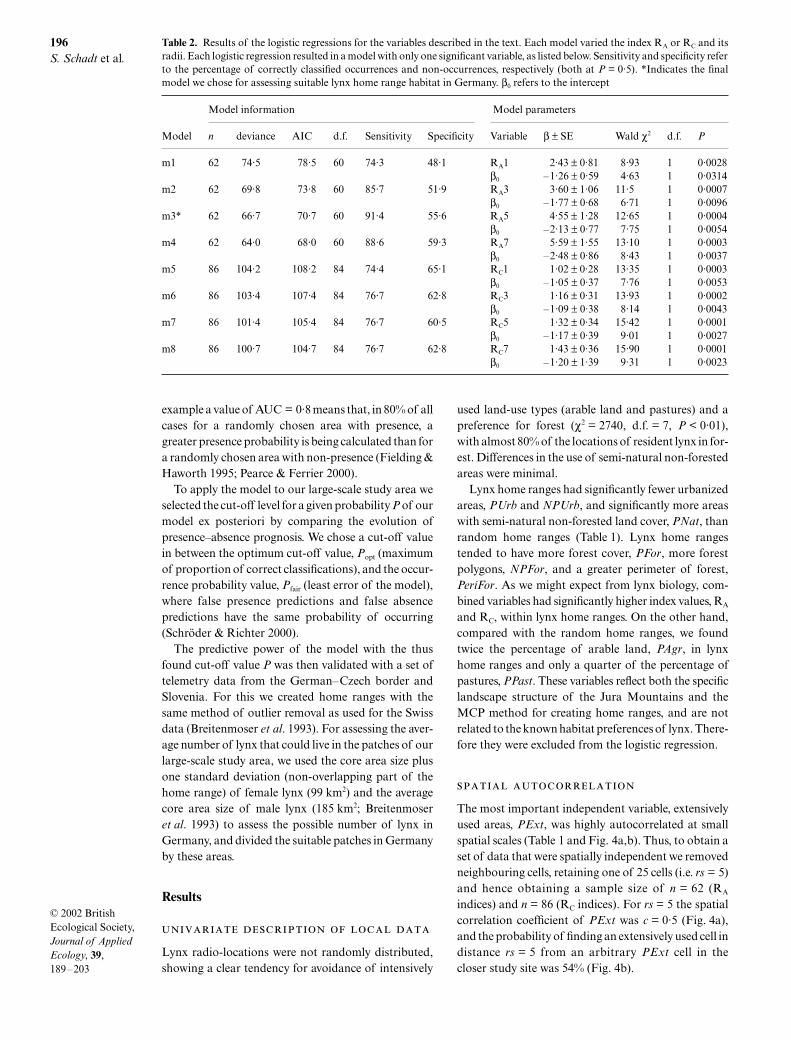
Table 2. Results of the logistic regressions for the variables described in the text. Each model varied the index RA or RC and itsradii. Each logistic regression resulted in a model with only one significant variable, as listed below. Sensitivity and specificity referto the percentage of correctly classified occurrences and non-occurrences, respectively (both at P = 0·5). *Indicates the finalmodel we chose for assessing suitable lynx home range habitat in Germany. β0 refers to the intercept

Model information Model parameters

Model n deviance AIC d.f. Sensitivity Specificity Variable β ± SE Wald χ2 d.f. P

m1 62 74·5 78·5 60 74·3 48·1 RA1 2·43 ± 0·81 8·93 1 0·0028β0 –1·26 ± 0·59 4·63 1 0·0314

m2 62 69·8 73·8 60 85·7 51·9 RA3 3·60 ± 1·06 11·5 1 0·0007β0 –1·77 ± 0·68 6·71 1 0·0096

m3* 62 66·7 70·7 60 91·4 55·6 RA5 4·55 ± 1·28 12·65 1 0·0004β0 –2·13 ± 0·77 7·75 1 0·0054

m4 62 64·0 68·0 60 88·6 59·3 RA7 5·59 ± 1·55 13·10 1 0·0003β0 –2·48 ± 0·86 8·43 1 0·0037

m5 86 104·2 108·2 84 74·4 65·1 RC1 1·02 ± 0·28 13·35 1 0·0003β0 –1·05 ± 0·37 7·76 1 0·0053

m6 86 103·4 107·4 84 76·7 62·8 RC3 1·16 ± 0·31 13·93 1 0·0002β0 –1·09 ± 0·38 8·14 1 0·0043

m7 86 101·4 105·4 84 76·7 60·5 RC5 1·32 ± 0·34 15·42 1 0·0001β0 –1·17 ± 0·39 9·01 1 0·0027

m8 86 100·7 104·7 84 76·7 62·8 RC7 1·43 ± 0·36 15·90 1 0·0001β0 –1·20 ± 1·39 9·31 1 0·0023



NPUrb and PUrb, and PeriFor and Pfor, were highlycorrelated, and therefore contained very similar infor-mation. The variables with the greatest explanatoryeffect in respect to the response variable, NPUrb andPFor, were retained. The indices for RA and RC of vari-able PExt were also highly inter- and intracorrelatedwithin the different radii. As the indices RA and RC rep-resent the connectivity of the same variable at differentscales, we calculated eight different models for both RA

and RC, each with the four different radii and the restof the predictors. With this we avoided the dangerof undertaking the kind of a priori screening that canlead to deleting the superior explanatory variable(MacNally 2000).

For the logistic regression using the RA index, we onlyused PExt cells, which explains the reduced amount ofcells (n = 62) in comparison with the models with theRC indices (n = 86). In all cases, the minimal adequatemodel chosen contained only one variable related to thefragmentation of forest and natural areas at differentscales, with a higher probability that a cell belonged toa lynx home range with decreasing fragmentation, whichmeans an increasing RA or RC value. The model withthe highest sensitivity included RA5 as a predictor(model 3 in Table 2). A circle with a radius of 5 km rep-resents an area of about 80 km2, which is approximatelythe size of the core area of a female lynx’s home range(72 ± 27 km2; Breitenmoser et al. 1993). Note that thisdoes not reflect a forest patch of this size, but a continuousconfiguration of forest and other semi-natural landcover types of at least 50% in a circle around any cell.

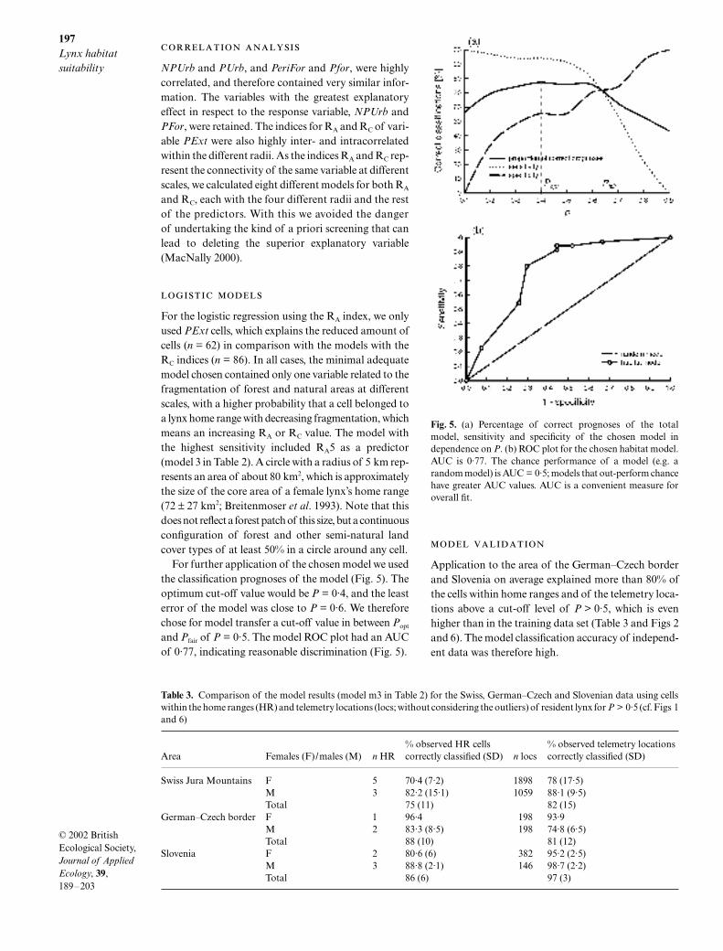
For further application of the chosen model we usedthe classification prognoses of the model (Fig. 5). Theoptimum cut-off value would be P = 0·4, and the leasterror of the model was close to P = 0·6. We thereforechose for model transfer a cut-off value in between Popt

and Pfair of P = 0·5. The model ROC plot had an AUCof 0·77, indicating reasonable discrimination (Fig. 5).

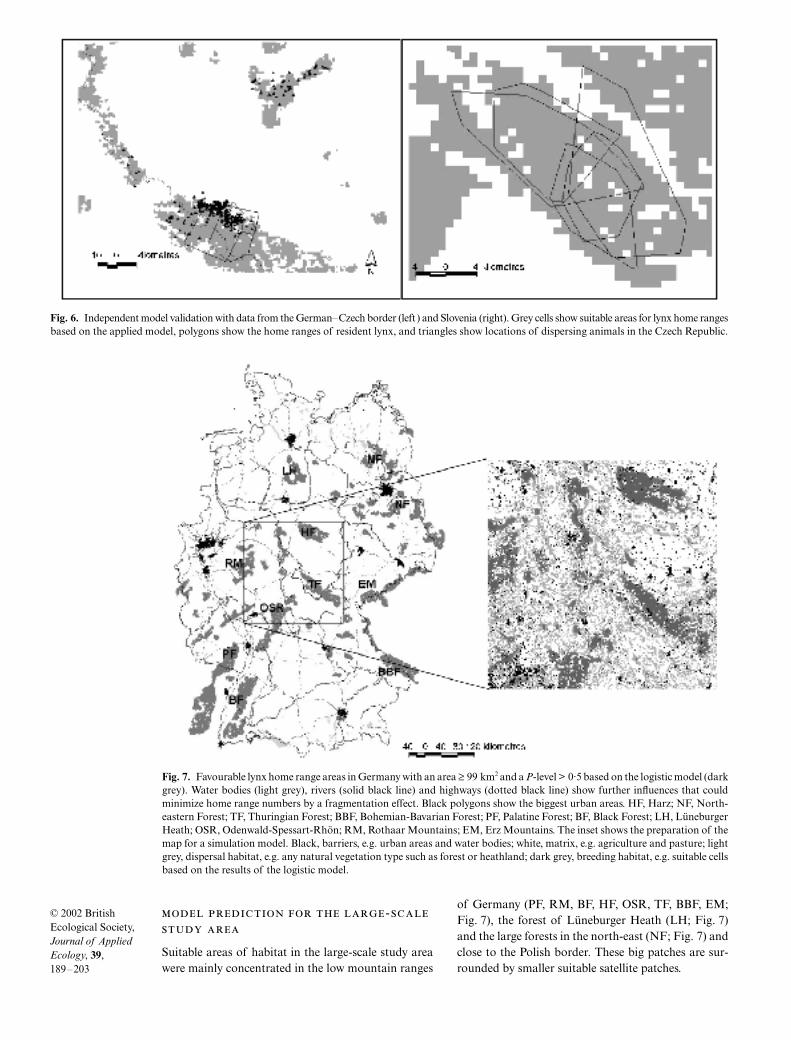
Application to the area of the German–Czech borderand Slovenia on average explained more than 80% ofthe cells within home ranges and of the telemetry loca-tions above a cut-off level of P > 0·5, which is evenhigher than in the training data set (Table 3 and Figs 2and 6). The model classification accuracy of independ-ent data was therefore high.

Fig. 5. (a) Percentage of correct prognoses of the totalmodel, sensitivity and specificity of the chosen model independence on P. (b) ROC plot for the chosen habitat model.AUC is 0·77. The chance performance of a model (e.g. arandom model) is AUC = 0·5; models that out-perform chancehave greater AUC values. AUC is a convenient measure foroverall fit.

Table 3. Comparison of the model results (model m3 in Table 2) for the Swiss, German–Czech and Slovenian data using cellswithin the home ranges (HR) and telemetry locations (locs; without considering the outliers) of resident lynx for P > 0·5 (cf. Figs 1and 6)

Area Females (F)/males (M) n HR% observed HR cells correctly classified (SD) n locs

% observed telemetry locations correctly classified (SD)

Swiss Jura Mountains F 5 70·4 (7·2) 1898 78 (17·5)M 3 82·2 (15·1) 1059 88·1 (9·5)Total 75 (11) 82 (15)

German–Czech border F 1 96·4 198 93·9M 2 83·3 (8·5) 198 74·8 (6·5)Total 88 (10) 81 (12)

Slovenia F 2 80·6 (6) 382 95·2 (2·5)M 3 88·8 (2·1) 146 98·7 (2·2)Total 86 (6) 97 (3)

198S. Schadt et al.


-

Suitable areas of habitat in the large-scale study areawere mainly concentrated in the low mountain ranges

of Germany (PF, RM, BF, HF, OSR, TF, BBF, EM;Fig. 7), the forest of Lüneburger Heath (LH; Fig. 7)and the large forests in the north-east (NF; Fig. 7) andclose to the Polish border. These big patches are sur-rounded by smaller suitable satellite patches.

Fig. 6. Independent model validation with data from the German–Czech border (left) and Slovenia (right). Grey cells show suitable areas for lynx home rangesbased on the applied model, polygons show the home ranges of resident lynx, and triangles show locations of dispersing animals in the Czech Republic.

Fig. 7. Favourable lynx home range areas in Germany with an area ≥ 99 km2 and a P-level > 0·5 based on the logistic model (darkgrey). Water bodies (light grey), rivers (solid black line) and highways (dotted black line) show further influences that couldminimize home range numbers by a fragmentation effect. Black polygons show the biggest urban areas. HF, Harz; NF, North-eastern Forest; TF, Thuringian Forest; BBF, Bohemian-Bavarian Forest; PF, Palatine Forest; BF, Black Forest; LH, LüneburgerHeath; OSR, Odenwald-Spessart-Rhön; RM, Rothaar Mountains; EM, Erz Mountains. The inset shows the preparation of themap for a simulation model. Black, barriers, e.g. urban areas and water bodies; white, matrix, e.g. agriculture and pasture; lightgrey, dispersal habitat, e.g. any natural vegetation type such as forest or heathland; dark grey, breeding habitat, e.g. suitable cellsbased on the results of the logistic model.



About 81% of Germany consists of unsuitable areafor lynx, and these grid cells were not considered in thelogistic regression because they contained less than66% of extensively used areas. Of the remaining67 024 km2 a total of 29 105 km2 (43%) reached a P-level above 0·5 (Fig. 8). Considering only those areaswith P > 0·5 that are ≥ 100 km2, we obtained a totalarea of 32 266 km2 for Germany and neighbouring for-est areas in France, the Czech Republic and Poland,which is reduced to 24 119 km2 for Germany only(Table 4 and Figs 6 and 8); at typical home range size,this leaves space for about 370 resident lynx in the suit-able patches in Germany.

Discussion

The use of models to predict the likely occurrence ordistribution of conservation target species is an import-ant first step in conservation planning and wildlifemanagement (Pearson, Drake & Turner 1999). Effect-ive and correct model assessment therefore has realsignificance to fundamental ecology as well as con-servation biology (Manel, Williams & Ormerod 2001).

Here we developed a statistical habitat model to pre-dict suitable areas for lynx in central Europe, basedon our current understanding of its biology; a modelthat can be applied to similar kinds of landscapes, forexample in Belgium, Scotland, the Netherlands andFrance. Although we have specifically addressed thesituation of the Eurasian lynx in central Europe, we areconfident that our approach may also be used for otherspecies and purposes, where only local data exist butlarge-scale information on fragmentation or the influ-ence of other land-use types is needed (Mladenoff et al.1995; Osborne, Alonso & Bryant 2001). The futureof large carnivores in central Europe will depend onour ability to protect and promote suitable areas andconnecting corridors where they can be managedeffectively (Corsi, Duprè & Boitani 1999; Palomareset al. 2000; Palomares 2001). It will also depend onthe correct management of reintroduction schemes,and the prior detection of potential areas whereconflicts with human economic activities and illegalhunting might occur.

A potential problem with our model is that it wasbuilt on data from an expanding population. It isunknown whether the unoccupied areas are reallyunsuitable or whether the population was not saturated

Probability classes

> 0·1 > 0·2 > 0·3 > 0·4 > 0·5 > 0·6 > 0·7 > 0·8 > 0·9

Favo

urab

le h

abita

t (km

2 )

0

2000

4000

6000

8000

10 000

12 000

6871

10 801 10 687

9560

74337806

6874

5705

1287

Fig. 8. Favourable habitat area in Germany based on probability levels from the logistic regression model. Of a total area of357 909 km2, 328 804 km2 (92%) was unsuitable for lynx home ranges.

Table 4. Suitable patches in Germany (cf. Fig. 7) based on the logistic regression model, with patches bigger than 99 km2 basedon maximum core area sizes of female lynx in the Swiss Jura Mountains (Breitenmoser et al. 1993). Home range (HR) numberscorrespond with core areas and are calculated by dividing the area by 99 km2

Suitable patch Size (km2) No. of female HR

Lüneburger Heath (LH) 1193 12North-eastern Forest (NE) 5185 52Odenwald-Spessart-Rhön (OSR) 2151 21German-Czech border (Bavarian/Bohemian

Forest, Erz Mountains) (BBF, EM)4637 46

Thuringian Forest (TF) 1676 17Black Forest (BF) 2974 30Palatine Forest (with Vosges Mountains) (PF) 5232 52Harz Forest (HF) 1566 16Rothaar Mountains (RM) 1551 16

200S. Schadt et al.


and would also spread into these areas when the bestareas are occupied. Lynx are also present in the Frenchpart of the Jura Mountains (Stahl et al. 2001), but it iscurrently not known if the sightings or findings of lynxprey remains correspond to resident lynx or to floaters.For our model we cannot be absolutely sure whetherour supposed absence data would be so in the future,but this only leads to an underestimate of the power ofthe independent variables (Boyce & McDonald 1999),i.e. an underestimate of suitable habitat in more frag-mented areas. If home ranges now occupied an areawith a high occurrence probability, this would ratherconfirm the validity of the model. For many threatened,rare and elusive species limited data only are available,and especially for rare and endangered species theirwhole range is never occupied. However, these are exactlythose species for which management decisions arerequired (Palma, Beja & Rodrigues 1999). We recom-mend updating our models for lynx with new data as soonas they are available in order to determine which otherhabitat variables could be constraining lynx presence.

Care must be taken with logistic regression as a pre-dictive tool. Many approaches with logistic regressioninclude a variety of landscape variables that are avail-able from maps rather than from biological require-ments of the species (Odom et al. 2001). Therefore theycannot be applied elsewhere and may not produce newinsights into the biology of the species. Our model con-stitutes an advance in that we analysed the species require-ments and eliminated variables that were not plausiblefrom lynx biology. We found a significantly high pro-portion of other non-wooded semi-natural land-covertypes within lynx home ranges. A fragmented forest areainterrupted by semi-natural non-wooded areas couldalso attract roe deer, which is the main prey of lynx. Wecan therefore assume that in the study area the absenceof intense human land use is the decisive factor forestablishing lynx home ranges. Distribution of forestalone was not important in this case, as we have a highdistribution of forest cover over the entire study area.

Local landscape variables were not significantly dif-ferent between lynx and random home ranges, but avariable comprising a regional scale (cf. Mladenoffet al. 1995; Massolo & Meriggi 1998; Carroll, Zielinski& Noss 1999). We can therefore assume that modelslike ours for the Eurasian lynx can be transferred toother areas without considering local structures suchas forest composition or distribution of prey. Small-scale structures are presumably more important forintraterritory use and for dispersal than for predictingregional home range distribution.

An additional problem in the context of logisticregression is dealing with spatial autocorrelation of thedependent variable, which leads to overparameterizedmodels that are not general habitat predictors for spe-cies presence (Lennon 1999). The selection of cells toavoid the effect of spatial autocorrelation could haveled to the exclusion of cells with a high percentage ofurban areas, so this variable was therefore not a signi-

ficant discriminator of lynx home ranges and randomhome ranges. This circumstance is reinforced by thefact that the MCP method for calculating lynx homeranges is a conceptual approximation. At the marginsof the MCP many cells with land-use types that are notused by lynx can be included in the logistic regression.However, in the RA models cells with less than 66%extensively used areas are excluded from the analysisbeforehand. Furthermore, the reduction of spatialautocorrelation leads to general predictions of habitatsuitability, which in our case was necessary for modelapplication at very large spatial scales.

A crucial question in applied biology is to whatextent information is transferable between geograph-ical areas (Rodriguez & Andrén 1999). If the transfer-ability of the model is not examined and verified, onlylocal applications are possible (Morrison, Marcot &Mannan 1992; Fielding & Haworth 1995; Rodriguez &Andrén 1999). General validity requires new applica-tions in space and time (Brooks 1997; Schröder &Richter 2000; Manel, Williams & Ormerod 2001).In our case, model validation with independent datafrom other regions like the German–Czech border andSlovenia showed accuracy of more than 80%. Com-paring our model results with data on populationdevelopment along the German–Czech border from1990 to 1995 (Cerveny, Koubek & Andera 1996) and withdata from 1999 (Wölfl et al. 2001), there is a very highconcordance with our model results. The high predic-tion accuracy is due to the fact that these areas are notvery fragmented and consist almost only of forest.

Our analysis provides insight into the distribution, theamount and the fragmentation of favourable lynx hab-itat in central Europe and especially Germany. Thepatches of suitable habitat are located mainly in the lowmountain ranges of south and central Germany and inthe large forests in the north and east of Germany.However, the distribution of suitable areas is patchyand many of them seem isolated (Lüneburger Heath,LH; Fig. 7) or fragmented by highways or rivers(Odenwald-Spessart-Rhön, OSR; Fig. 7), which makethem seem unsuitable as focal areas for reintroduction.Isolated patches can cause populations to suffer fromdemographic and genetic effects when they are toosmall and lack immigration. Experts estimate thatminimum numbers for viable populations are at least50–100 individuals (Seidensticker 1986; Shaffer 1987;Allen, Pearlstine & Kitchens 2001). Assuming an over-lap of one male per female, only the north-easternforests (NF), the Palatine Forest with the VosgesMountains (PF) and the German–Czech area(EM + BBF) can host up to 100 lynx, while the BlackForest (BF) could host up to 60 lynx, making these themost suitable target areas. However, local-scale factors,such as roads, could make these areas unsuitable, and



therefore we need to proceed with more detailedmodels at local scales before accepting an area assuitable for lynx reintroduction (Kaczensky et al. 1996;Mace et al. 1996; Trombulak & Frissell 2000).

Comparing the model results with a previous rule-based approach (Schadt et al., in press), we found ahigh concordance in the distribution and also thenumber of female home ranges within suitable areas.For example, for the Black Forest, the ThuringianForest, the Harz and the German–Czech border, wefound almost the same number of female home rangeswith deviations ±3 home ranges when comparing thetwo modelling approaches. But the number of femalehome ranges is reduced by approximately one-third inthe current model for the Rothaar Mountains andincreased by approximately one-third for the north-eastern forests. One reason for this is the fragmentationof the Rothaar Mountains, which was not consideredin the rule-based approach of Schadt et al. (in press).In addition, we had a high proportion of natural non-forested heathland in the north-eastern forest area,which increased the number of female home ranges notconsidered in the rule-based approach. This clearlyshows how important it is to counter-test and evaluatequalitative and quantitative models before basingmanagement schemes such as reintroductions on onlyone assessment.

Population viability analyses (Boyce 1992; Lindenmayeret al. 2001) should now be the next step in assessingwhether the existing habitat patches in Germany arelarge enough to host populations of lynx and to whatdegree viability is influenced by local-scale factors (e.g.road mortality). Our example shows how models canprovide a sound basis for a spatially explicit populationsimulation to answer questions on the viability of car-nivore populations under ‘real’ conditions.

Acknowledgements

This work is funded by the Deutsche BundesstiftungUmwelt, AZ 6000/596, and the Deutsche Wildtier Stiftungfor the main author. E. Revilla was supported by aMarie Curie Individual Fellowship provided by theEuropean Commission (Energy, Environment andSustainable Development Contract EVK2-CT-1999-50001). Thanks to M. Heurich (Bavarian ForestNational Park) for providing lynx telemetry data. Wethank S. J. Ormerod, S. Rushton, H. Griffiths and ananonymous referee for critically commenting on themanuscript. We are grateful to B. Reineking for assist-ance in statistical analyses.

References

Allen, C.R., Pearlstine, L.G. & Kitchens, W.M. (2001)Modeling viable mammal populations in gap analyses.Biological Conservation, 99, 135–144.

Boitani, L. (2000) The Action Plan for the Conservation of theWolf (Canis lupus) in Europe. Council of Europe, BernConvention Meeting, Bern, Switzerland.

Boyce, M.S. (1992) Population viability analysis. AnnualReview of Ecology and Systematics, 23, 481–506.

Boyce, M.S. & McDonald, L.L. (1999) Relating populationsto habitats using resource selection functions. Trends inEcology and Evolution, 14, 268–272.

Bradbury, R.B., Kyrkos, A., Morris, A.J., Clark, S.C.,Perkins, A.J. & Wilson, J.D. (2000) Habitat associationsand breeding success of yellowhammers on lowlandfarmland. Journal of Applied Ecology, 37, 789–805.

Breitenmoser, U. & Baettig, M. (1992) Wiederansiedlung undAusbreitung des Luchses (Lynx lynx) im Schweizer Jura.Revue Suisse de Zoologie, 99, 163–176.

Breitenmoser, U. & Haller, H. (1993) Patterns of predation byreintroduced European lynx in the Swiss Alps. Journal ofWildlife Management, 57, 135–144.

Breitenmoser, U., Breitenmoser-Würsten, C., Okarma, H.,Kaphegyi, T., Kaphegyi-Wallmann, U. & Müller, U.M.(2000) The Action Plan for the Conservation of the EurasianLynx (Lynx lynx) in Europe. Council of Europe, BernConvention Meeting, Bern, Switzerland.

Breitenmoser, U., Kaczensky, P., Dötterer, M., Breitenmoser-Würsten, C., Capt, S., Bernhart, F. & Liberek, M. (1993)Spatial organization and recruitment of lynx (Lynx lynx) ina re-introduced population in the Swiss Jura Mountains.Journal of Zoology (London), 231, 449–464.

Brooks, R.P. (1997) Improving habitat suitability indexmodels. Wildlife Society Bulletin, 25, 163–167.

Buckland, S.T. & Elston, D.K. (1993) Empirical models forthe spatial distribution of wildlife. Journal of AppliedEcology, 30, 478–495.

Bufka, L., Cerveny, J., Koubek, P. & Horn, P. (2000) Radio-telemetry research of the lynx (Lynx lynx) in Sumava –preliminary results. Proceedings ‘Predatori v. myslivosti2000’, Hranice.

Burnham, K.P. & Anderson, D.R. (1998) Model Selection andInference: A Practical Information-Theoretic Approach.Springer Verlag, New York, NY.

Carroll, C., Zielinski, W.J. & Noss, R.F. (1999) Usingpresence–absence data to build and test spatial habitatmodels for the fisher in the Klamath Region, USA. Con-servation Biology, 13, 1344–1359.

Carroll, S.S. & Pearson, D.L. (2000) Detecting and modelingspatial and temporal dependence in conservation biology.Conservation Biology, 14, 1893–1897.

Cerveny, J. & Bufka, L. (1996) Lynx (Lynx lynx) in south-western Bohemia. Lynx in the Czech and Slovak Republics(eds P. Koubek & J. Cerveny), pp. 16–33. Acta ScientiarumNaturalium Brno 30 (3).

Cerveny, J., Koubek, P. & Andera, M. (1996) Populationdevelopment and recent distribution of the lynx (Lynxlynx) in the Czech Republic. Lynx in the Czech and SlovakRepublics (eds P. Koubek & J. Cerveny), pp. 2–15. ActaScientiarum Naturalium Brno 30 (3).

Cerveny, J., Koubek, P., Bufka, L. & Fejková, P. (2001) Diet ofthe lynx (Lynx lynx) and its impact on populations of roedeer (Capreolus capreolus) in the Sumava Mts region (CzechRepublic). Folia Zoologica, in press.

Clevenger, A.P., Chruszcz, B. & Gunson, K. (2001) Drainageculverts as habitat linkages and factors affecting passage bymammals. Journal of Applied Ecology, 38, 1340–1349.

Cop, J. & Frkovic, A. (1998) The re-introduction of the lynx inSlovenia and its present status in Slovenia and Croatia.Hystrix, 10, 65–76.

Corsi, F., Duprè, E. & Boitani, L. (1999) A large-scale modelof wolf distribution in Italy for conservation planning. Con-servation Biology, 13, 150–159.

Corsi, F., Sinibaldi, I. & Boitani, L. (1998) Large CarnivoreConservation Areas in Europe: A Summary of the FinalReport. Istituto Ecologia Applicata, Roma, Italy.

Fielding, A.H. & Bell, J.F. (1997) A review of methods forassessment of prediction errors in conservation presence/

202S. Schadt et al.


absence models. Environmental Conservation, 24, 38–49.

Fielding, A.H. & Haworth, P.F. (1995) Testing the generalityof bird–habitat models. Conservation Biology, 9, 1466–1481.

FitzGibbon, C.D. (1993) The distribution of grey squirreldreys in farm woodland: the influence of wood area, isola-tion and management. Journal of Applied Ecology, 30, 736–742.

Gates, S. & Donald, P.F. (2000) Local extinction of Britishfarmland birds and the prediction of further loss. Journal ofApplied Ecology, 37, 806–820.

Guisan, A. & Zimmermann, N.E. (2000) Predictive habitatdistribution models in ecology. Ecological Modelling, 135,147–186.

Haller, H. (1992) Zur Ökologie des Luchses Lynx lynx imVerlauf seiner Wiederansiedlung in den Walliser Alpen.Mammalia Depicta, 15, 1–62.

Haller, H. & Breitenmoser, U. (1986) Zur Raumorganisa-tion der in den Schweizer Alpen wiederangesiedeltenPopulation des Luchses (Lynx lynx). Zeitschrift fürSäugetierkunde, 51, 289–311.

Herrenschmidt, V. & Leger, F. (1987) Le Lynx Lynx lynx (L.)dans le Nord-Est de la France. La colonisation du Massifjurassien francais et la réintroduction de l’espece dans leMassif vosgien. Premiers rèsultats. Ciconia, 11, 131–151.

Hosmer, D.W. & Lemeshow, S. (1989) Applied LogisticRegression. Wiley, New York, NY.

Jedrzejewski, W., Schmidt, K., Milkowski, L., Jedrzejewska,B. & Okarma, H. (1993) Foraging by lynx and its role inungulate mortality: the local (Bia8owieza Forest) and thePalaearctic viewpoints. Acta Theriologica, 38, 385–403.

Jobin, A., Molinari, P. & Breitenmoser, U. (2000) Prey spec-trum, prey preference and consumption rates of Eurasianlynx in the Swiss Jura Mountains. Acta Theriologica, 45,243–252.

Kaczensky, P., Knauer, F., Jonozovic, M., Huber, T. &Adamic, M. (1996) The Ljubljana–Postojna Highway –a deadly barrier for brown bears in Slovenia. Journal ofWildlife Research, 1, 263–267.

Lennon, J.L. (1999) Resource selection functions: takingspace seriously? Trends in Ecology and Evolution, 14, 399–400.

Lindenmayer, D.B., Ball, I., Possingham, H.P., McCarthy,M.A. & Pope, M.L. (2001) A landscape-scale test of thepredictive ability of a spatially explicit model for popu-lation viability analysis. Journal of Applied Ecology, 38,36–48.

Linnell, J.D.C., Andersen, R., Kvam, T., Andren, H., Liberg,O., Odden, J. & Moa, P.F. (2001) Home range size andchoice of management strategy for lynx in Scandinavia.Environmental Management, 27, 869–879.

Linnell, J.D.C., Swenson, J.E. & Andersen, R. (2000) Conser-vation of biodiversity in Scandinavian boreal forests: largecarnivores as flagships, umbrellas, indicators, or keystones?Biodiversity and Conservation, 9, 857–868.

McCullagh, P. & Nelder, J.A. (1989) Generalized Linear Mod-els. Chapman & Hall /CRC, Boca Raton, FL.

Mace, R.D., Waller, J.S., Manley, T.L., Ake, K. & Wittinger,W.T. (1999) Landscape evaluation of grizzly bear habitat inWestern Montana. Conservation Biology, 13, 367–377.

Mace, R.D., Waller, J.S., Manley, T.L., Lyon, L.J. & Zuuring,H. (1996) Relationships among grizzly bears, roads andhabitat in the Swan Mountains, Montana. Journal ofApplied Ecology, 33, 1395–1404.

MacNally, R. (2000) Regression and model-building inconservation biology, biogeography and ecology: the dis-tinction between – and reconciliation of – ‘predictive’ and‘explanatory’ models. Biodiversity and Conservation, 9,655–671.

Manel, S., Buckton, S.T. & Ormerod, S.J. (2000) Problems andpossibilities in large-scale surveys: the effects of land use on

the habitats, invertebrates and birds of Himalayan rivers.Journal of Applied Ecology, 37, 756–770.

Manel, S., Williams, H.C. & Ormerod, S.J. (2001) Evaluatingpresence–absence models in ecology: the need to accountfor prevalence. Journal of Applied Ecology, 38, 921–931.

Massolo, A. & Meriggi, A. (1998) Factors affecting habitatoccupancy by wolves in northern Apennines (northernItaly): a model of habitat suitability. Ecography, 21, 97–107.

Miller, J.R. & Cale, P. (2000) Behavioral mechanisms and hab-itat use by birds in a fragmented agricultural landscape.Ecological Applications, 10, 1732–1748.

Mladenoff, D.J., Sickley, T.A., Haight, R.G. & Wydeven, A.P.(1995) A regional landscape analysis and prediction offavorable gray wolf habitat in the Northern Great Lakesregion. Conservation Biology, 9, 279–294.

Mladenoff, D.J., Sickley, T.A. & Wydeven, A.P. (1999) Pre-dicting gray wolf landscape recolonization: logistic regres-sion models vs. new field data. Ecological Applications, 9,37–44.

Morrison, M.L., Marcot, B.G. & Mannan, R.W. (1992)Wildlife–Habitat Relationships – Concepts and Applications.The University of Wisconsin Press, Madison, WI.

Noon, B.R. (1986) Summary: biometric approaches tomodeling – the researcher’s viewpoint. Wildlife 2000:Modeling Habitat Relationships of Terrestrial Vertebrates(eds J. Verner, M.L. Morrison & C.J. Ralph), pp. 197–201.University of Wisconsin Press, Madison, WI.

Noss, R.F., Quigley, H.B., Hornocker, M.G., Merrill, T. &Paquet, P.C. (1996) Conservation biology and carnivoreconservation in the Rocky Mountains. Conservation Bio-logy, 10, 949–963.

Odom, R.H., Ford, W.M., Edwards, J.W., Stihler, C.W. &Menzel, J.M. (2001) Developing a habitat model for theendangered Virginia northern flying squirrel (Glaucomyssabrinus fuscus) in the Allegheny Mountain of WestVirginia. Biological Conservation, 99, 245–252.

Okarma, H., Jedrzejewski, W., Schmidt, K., Kowalczyk, R. &Jedrzejewska, B. (1997) Predation of Eurasian lynx on roedeer and red deer in Bia8owieza Primeval Forest, Poland.Acta Theriologica, 42, 203–224.

Orrock, J.L., Pagels, J.F., McShea, W.J. & Harper, E.K. (2000)Predicting presence and abundance of a small mammalspecies: the effect of scale and resolution. EcologicalApplications, 10, 1356–1366.

Osborne, P.E., Alonso, J.C. & Bryant, R.G. (2001) Modellinglandscape-scale habitat use using GIS and remote sensing:a case study with great bustards. Journal of Applied Eco-logy, 38, 458–471.

Palma, L., Beja, P. & Rodrigues, M. (1999) The use of sightingdata to analyse Iberian lynx habitat and distribution. Journalof Applied Ecology, 36, 812–824.

Palomares, F. (2001) Vegetation structure and preyabundance requirements of the Iberian lynx: implicationsfor the design of reserves and corridors. Journal of AppliedEcology, 38, 9–18.

Palomares, F., Delibes, M., Ferreras, P., Fedriani, J., Calzada,J. & Revilla, E. (2000) Iberian lynx in a fragmented land-scape: pre-dispersal, dispersal and post-dispersal habitats.Conservation Biology, 14, 809–818.

Palomares, F., Delibes, M., Revilla, E., Calzada, J. &Fedriani, J.M. (2001) Spatial ecology of the Iberian lynxand abundance of European Rabbit in southwestern Spain.Wildlife Monographs, 148, 1–36.

Pearce, J. & Ferrier, S. (2000) Evaluating the predictiveperformance of habitat models developed using logisticregression. Ecological Modelling, 133, 225–245.

Pearson, S.M., Drake, J.B. & Turner, M.G. (1999) Land-scape change and habitat availability in the southernAppalachian Highlands and Olympic Peninsula. EcologicalApplications, 9, 1288–1304.



Revilla, E., Palomares, F. & Delibes, M. (2001) Edge-coreeffects and the effectiveness of traditional reserves in con-servation: Eurasian badgers in Doñana National Park.Conservation Biology, 15, 148–158.

Rodriguez, A. & Andrén, H. (1999) A comparison of Eura-sian red squirrel distribution in different fragmentedlandscapes. Journal of Applied Ecology, 36, 649–662.

Schadt, S., Knauer, F., Kaczensky, P., Revilla, E., Wiegand, T.& Trepl, L. (in press) Dealing with limited resources inconservation planning: rule-based assessment of suitablehabitat and patch connectivity for the Eurasian lynx inGermany. Ecological Applications.

Schmidt, K., Jedrzejewski, W. & Okarma, H. (1997) Spatialorganization and social relations in the Eurasian lynxpopulation in Bia8owieza Primeval Forest, Poland. ActaTheriologica, 42, 289–312.

Schröder, B. & Richter, O. (2000) Are habitat models trans-ferable in space and time? Zeitschrift für Ökologie undNaturschutz, 8, 195–205.

Schröder, W. (1998) Challenges to wildlife management andconservation in Europe. Wildlife Society Bulletin, 26, 921–926.

Seidensticker, J. (1986) Large carnivores and the con-sequences of habitat insularization: ecology and conservationof tigers in Indonesia and Bangladesh. Cats of the World:Biology, Conservation and Management (eds S.D. Miller &D.D. Everett), pp. 1–42. National Wildlife Federation,Washington, DC.

Shaffer, M. (1987) Minimum viable populations: copingwith uncertainty. Viable Populations for Conservation (ed.M.E. Soulé), pp. 69–85. Cambridge University Press,Cambridge, UK.

Stahl, P., Vandel, J.M., Herrenschmidt, V. & Migot, P. (2001)Predation on livestock by an expanding reintroduced lynxpopulation: long-term trend and spatial variability. Journalof Applied Ecology, 38, 674–687.

Stanisa, C. (1998) Methodenvergleich zur Erhebung derAnwesenheit des Luchses (Lynx lynx). Schriftreihe desLandesverbandes Bayern, 5, 57–66.

Suarez, S., Balbontin, J. & Ferrer, M. (2000) Nesting habitatselection by booted eagles Hieraaetus pennatus and implica-tions for management. Journal of Applied Ecology, 37,215–223.

Swenson, J.E., Gerstl, N., Dahle, B. & Zedrosser, A. (2000)Final Draft Action Plan for the Conservation of the BrownBear (Ursus arctos ) in Europe. Council of Europe, BernConvention Meeting, Bern, Switzerland.

Tabachnick, B.G. & Fidell, L.S. (1996) Using MultivariateStatistics. Harper Collins, New York, NY.

Trombulak, S.C. & Frissell, C.A. (2000) Review of ecologicaleffects of roads on terrestrial and aquatic communities.Conservation Biology, 14, 18–30.

Wilson, J.D., Evans, J., Browne, S.J. & King, J.R. (1997)Territory distribution and breeding success of skylarksAlauda arvensis on organic and intensive farmland insouthern England. Journal of Applied Ecology, 34, 1462–1478.

Wölfl, M., Bufka, L., Cerveny, J., Koubek, P., Heurich, M.,Habel, H., Huber, T. & Poost, W. (2001) Distribution andstatus of lynx in the border region between Czech Republic,Germany and Austria. Acta Theriologica, 46, 181–194.

Woodroffe, R. & Ginsberg, J.R. (1998) Edge effects and theextinction of populations inside protected areas. Science,280, 2126–2128.

Zimmermann, F. & Breitenmoser, U. (2002) A distributionmodel for the Eurasian lynx (Lynx lynx) in the Jura Moun-tains, Switzerland. Predicting Species Occurrences: Issues ofAccuracy and Scale (eds J.M. Scott, P.J. Heglund, F. Samson,J. Haufler, M. Morrison, M. Raphael & B. Wal), in press.Island Press, Covelo, CA.

Received 5 July 2001; final copy received 12 November 2001

assessing the suitability of central european landscapes for the reintroduction of eurasian lynx:...

Documents