artificial neural networks for estimating the hydraulic performance of labyrinth-channel emitters
TRANSCRIPT
Computers and Electronics in Agriculture 114 (2015) 189–201
Contents lists available at ScienceDirect
Computers and Electronics in Agriculture
journal homepage: www.elsevier .com/locate /compag
Artificial neural networks for estimating the hydraulic performanceof labyrinth-channel emitters
http://dx.doi.org/10.1016/j.compag.2015.04.0070168-1699/� 2015 Elsevier B.V. All rights reserved.
⇑ Corresponding author at: Agricultural Engineering Department, College of Foodand Agriculture Sciences, King Saud University, PO Box 2460, Riyadh 11451, SaudiArabia. Tel.: +966 11 4676024; fax: +966 11 4678502.
E-mail addresses: [email protected], [email protected](M.A. Mattar).
Mohamed A. Mattar a,b,c,⇑, Ahmed I. Alamoud a,b
a Agricultural Engineering Department, College of Food and Agriculture Sciences, King Saud University, PO Box 2460, Riyadh 11451, Saudi Arabiab Prince Sultan Research Institute, and Prince Sultan International Prize for Water (PSIPW) Research Chair, King Saud University, Saudi Arabiac Agricultural Engineering Research Institute (AEnRI), Agricultural Research Center, PO Box 256, Giza, Egypt
a r t i c l e i n f o
Article history:Received 2 December 2014Received in revised form 4 April 2015Accepted 6 April 2015
Keywords:Artificial neural networkLabyrinth emitterEmitter flow variationManufacturer’s coefficient of variation
a b s t r a c t
In this paper, we examine the discharge of labyrinth-channel emitters under different operating pres-sures (P) and water temperatures (T). An artificial neural network (ANN) and multiple linear regression(MLR) model are developed for the emitter flow variation (qvar) and the manufacturer’s coefficient ofvariation (CV). As well as P and T, the structural parameters of the labyrinth emitter are considered asindependent variables. The ANN results demonstrate that a feed-forward back-propagation network withfive input neurons and 14 neurons in the hidden layer successfully model qvar and CV. The trapezoidalunit spacing and path length of the labyrinth emitter are found to be insignificant. In our ANN model,we use a hyperbolic tangent as the activation function in the hidden layer and the output layer.Statistical criteria indicate that the ANN is better at predicting the hydraulic performance of the labyrinthemitters than MLR. The root mean square errors for qvar and CV are 1.0497 and 0.0044, respectively, forthe ANN model, and 2.0703 and 0.0107, respectively, for the MLR model using a test dataset. The rela-tively low errors obtained by the ANN approach lead to high model predictability and are feasible formodeling the hydraulic performance of labyrinth emitters.
� 2015 Elsevier B.V. All rights reserved.
1. Introduction
Drip irrigation is the most efficient method of supplying waterto soil across a wide area. In this method, small-diameter plasticlateral pipes with various emission devices deliver water to the soilsurface near to the plant root zone. The applicability of drip irriga-tion can be extended to a wide range of agronomic, horticultural,and fruit crops by installing the lateral pipes below the soil surface.This subsurface drip irrigation generally operates with a similardischarge rate to surface drip irrigation. The water can be deliveredby a variety of devices, from simple orifice emitters to complexpressure-compensating emitters (ASABE, 2005; Singh et al.,2006a,b; Kumar and Singh, 2007).
All emitters with the same characteristics in a single irrigationsystem should deliver equal quantities of water. However, in rea-lity, there is some variation in discharge between different emit-ters. The main reason for this is the manufacturing variation. As
drip irrigation emission devices are designed to discharge waterat a low rate, small variations in dripper design cause a relativelylarge variation in discharge (Singh et al., 2006a). Therefore, theemitter is a key component, and plays a significant role in drip irri-gation systems. It is designed to discharge pressurized water fromthe pipes into the soil slowly and uniformly via energy dissipationin its internal structure. This structure has a great effect on thehydraulic performance of emitters (Nakayama and Bucks, 1986).
Temperature variations influence water properties, especiallyviscosity, and this may be a significant factor in an emitter flowchannel (Rodriguez-Sinobas et al., 1999). Emitters with labyrinthchannels are used because of their simple structures and low cost.The labyrinth structure is the most important section in an emit-ter’s performance. Different dimensions within the labyrinth emit-ter can produce various discharge rates depending on the waterpressure (Evans et al., 2007; Wei et al., 2007; Zhang et al., 2007;Zhang et al., 2011a).
The transitional flow characteristics of labyrinth-channel emit-ters indicate that the internal flow is turbulent under practicalpressure ranges (Evans et al., 2007; Zhao et al., 2009). Emitterswith a square labyrinth cross-section perform better than thosewith rectangular sections (Zhiqin and Lin, 2011).
Nomenclature
bi estimated regression coefficientsbo value of bY when all of the independent variables are
equal to zeroB1 biases in the hidden layerB2 biases in the output layerCV manufacturer’s coefficient of variationEi experimental valueEn minimum experimental valueEx maximum experimental valueE average experimental valuef activation (transfer) functionH trapezoidal unit heightL path lengthN trapezoidal unit numbersNi number of input neuronsNj number of output neuronsn total number of emitters along the lateral linen0 number of observationsP operating pressurePi predicted value
P average predicted valueqi discharge rate of emitter iqmax maximum emitter discharge rateqmin minimum emitter discharge rateqvar emitter flow variation�q average emitter discharge rateS trapezoidal unit spacingSd standard deviation of emitter discharge rateT water temperatureW path widthW1 weights between input and hidden layersW2 weights between hidden and output layersxi independent or predictor variablesXi input parametersXmax maximum valueXmin minimum valueXn normalized valueXo original value; andbY predicted or expected value of the dependent variable
190 M.A. Mattar, A.I. Alamoud / Computers and Electronics in Agriculture 114 (2015) 189–201
Two uniformity criteria used in drip irrigation design are theemitter flow variation (qvar) and the manufacturer’s coefficient ofvariation (CV). Tripathi et al. (2011) reported CVs of 4.0% withwastewater and 6.46% with groundwater for subsurface (15 cmdeep) lateral pipes after filtration with gravel and disk filters.Singh et al. (2006b) found that the qvar and CV of labyrinth-channelemitters were in the acceptable to excellent range across all lateralpipes, and this performance did not change significantly during2 years of study. Zapata et al. (2013) reported that the CV of dis-charge within irrigation events was 12%, while the CV of dischargebetween different irrigation events was 10%. In field conditions,any variation in flow channel area or shape away from a standardsize will cause qvar to vary. Other factors affecting qvar include fieldtopography, water temperature, soil hydraulic characteristics,emitter spacing, and emitter clogging (Nakayama and Bucks,1986; Mizyed and Kruse, 1989). Alamoud et al. (2014) showed thatthe structural parameters of the labyrinth emitters are correlatedwith their hydraulic performance, particularly the trapezoidal unit(dentations) number and height variables. Zhang et al. (2011b)proposed new method to evaluate hydraulic performance of thelabyrinth-channel emitter by using a pressure loss coefficient asthe evaluation index, which was derived from frictional and locallosses of the fluid in labyrinth channels.
The concept of neural network analysis was first reportednearly 50 years ago, but it is only in the last 20 years that softwarehas been developed to handle practical problems. An artificial neu-ral network (ANN) is a mathematical construction that is essen-tially analogous to the human brain. Basically, the highlyinterconnected and layered processing elements reflect thearrangement of neurons in the brain (ASCE, 2000; Kumar et al.,2002). ANNs, like people, learn by example. An ANN is configuredfor a specific application, such as pattern recognition or data clas-sification, through a process of learning or training. ANNs can pro-cess problems involving nonlinear and complex data, even if thedata are imprecise and noisy. Thus, they are ideally suited for themodeling of agricultural data, which are known to be complexand are often nonlinear.
ANNs have been used for a wide variety of applications. In theagricultural field alone, they have been used to classify irrigationplanning strategies (Raju et al., 2006), predict the soil water con-tent (Givi et al., 2004; Wanakule and Aly, 2005), calculate subsur-face wetting for drip irrigation (Hinnell et al., 2009), local pressure
losses produced by integrated emitters (Martí et al., 2010),reference evapotranspiration (Zanetti et al., 2007; Landeras et al.,2008, 2009; Cobaner et al., 2014; Gocic et al., 2015), and the infil-trated water volume under furrow irrigation (Mattar et al., 2015).
A poorly designed and managed drip irrigation system results innonuniform water distribution, and nonuniform irrigation resultsin poor crop development and lower yields. The structural designof the emitter is worthy of further investigation. However, to ourknowledge, no previous research has mapped the capability ofANNs to estimate the hydraulic performance of labyrinth emitters.Therefore, the objectives of our study are to (1) develop mathe-matical models to estimate the hydraulic performance (namely qvar
and CV) of emitters using ANNs; (2) evaluate the performance ofthese ANNs using a statistical comparison between the hydraulicperformance obtained from the model and experimental results;and (3) compare the ANNs with multiple linear regression (MLR)models in terms of their suitability for predicting hydraulicperformance.
2. Materials and methods
2.1. Experimental procedure
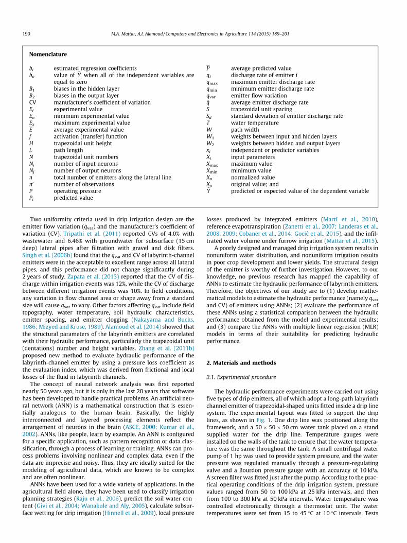
The hydraulic performance experiments were carried out usingfive types of drip emitters, all of which adopt a long-path labyrinthchannel emitter of trapezoidal-shaped units fitted inside a drip linesystem. The experimental layout was fitted to support the driplines, as shown in Fig. 1. One drip line was positioned along theframework, and a 50 � 50 � 50 cm water tank placed on a standsupplied water for the drip line. Temperature gauges wereinstalled on the walls of the tank to ensure that the water tempera-ture was the same throughout the tank. A small centrifugal waterpump of 1 hp was used to provide system pressure, and the waterpressure was regulated manually through a pressure-regulatingvalve and a Bourdon pressure gauge with an accuracy of 10 kPa.A screen filter was fitted just after the pump. According to the prac-tical operating conditions of the drip irrigation system, pressurevalues ranged from 50 to 100 kPa at 25 kPa intervals, and thenfrom 100 to 300 kPa at 50 kPa intervals. Water temperature wascontrolled electronically through a thermostat unit. The watertemperatures were set from 15 to 45 �C at 10 �C intervals. Tests
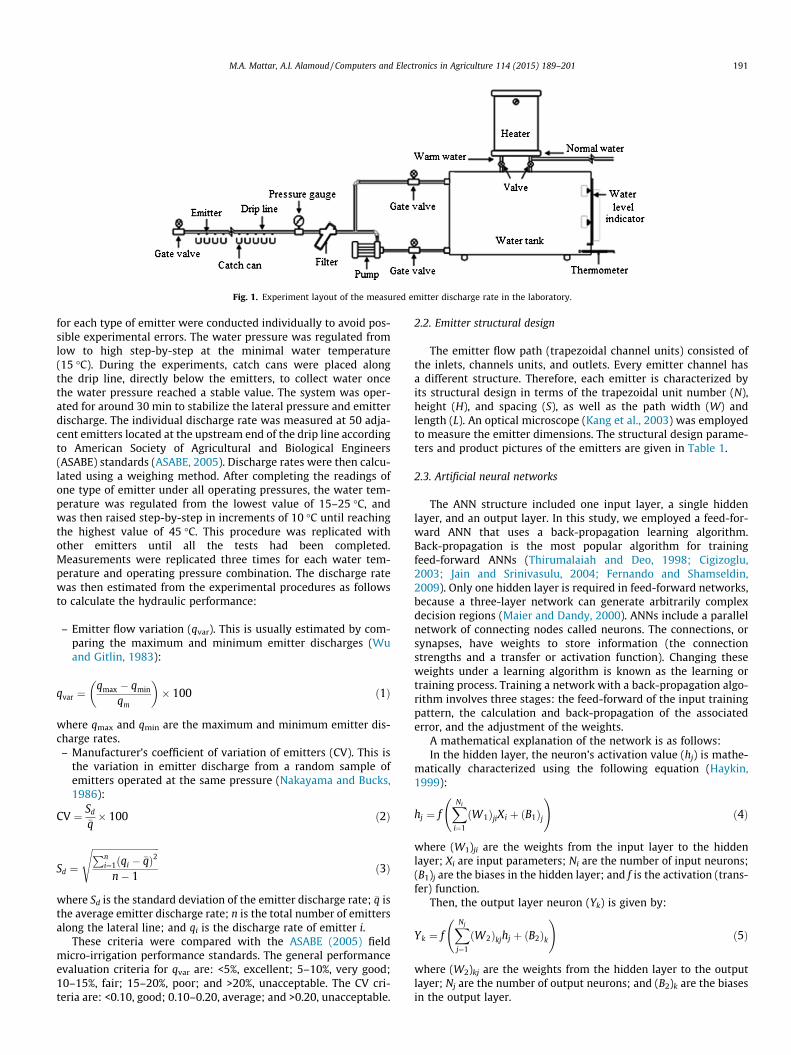
Fig. 1. Experiment layout of the measured emitter discharge rate in the laboratory.
M.A. Mattar, A.I. Alamoud / Computers and Electronics in Agriculture 114 (2015) 189–201 191
for each type of emitter were conducted individually to avoid pos-sible experimental errors. The water pressure was regulated fromlow to high step-by-step at the minimal water temperature(15 �C). During the experiments, catch cans were placed alongthe drip line, directly below the emitters, to collect water oncethe water pressure reached a stable value. The system was oper-ated for around 30 min to stabilize the lateral pressure and emitterdischarge. The individual discharge rate was measured at 50 adja-cent emitters located at the upstream end of the drip line accordingto American Society of Agricultural and Biological Engineers(ASABE) standards (ASABE, 2005). Discharge rates were then calcu-lated using a weighing method. After completing the readings ofone type of emitter under all operating pressures, the water tem-perature was regulated from the lowest value of 15–25 �C, andwas then raised step-by-step in increments of 10 �C until reachingthe highest value of 45 �C. This procedure was replicated withother emitters until all the tests had been completed.Measurements were replicated three times for each water tem-perature and operating pressure combination. The discharge ratewas then estimated from the experimental procedures as followsto calculate the hydraulic performance:
– Emitter flow variation (qvar). This is usually estimated by com-paring the maximum and minimum emitter discharges (Wuand Gitlin, 1983):
qvar ¼qmax � qmin
qm
� �� 100 ð1Þ
where qmax and qmin are the maximum and minimum emitter dis-charge rates.– Manufacturer’s coefficient of variation of emitters (CV). This is
the variation in emitter discharge from a random sample ofemitters operated at the same pressure (Nakayama and Bucks,1986):
CV ¼ Sd
�q� 100 ð2Þ
Sd ¼
ffiffiffiffiffiffiffiffiffiffiffiffiffiffiffiffiffiffiffiffiffiffiffiffiffiffiffiffiffiPni¼1ðqi � �qÞ2
n� 1
sð3Þ
where Sd is the standard deviation of the emitter discharge rate; �q isthe average emitter discharge rate; n is the total number of emittersalong the lateral line; and qi is the discharge rate of emitter i.
These criteria were compared with the ASABE (2005) fieldmicro-irrigation performance standards. The general performanceevaluation criteria for qvar are: <5%, excellent; 5–10%, very good;10–15%, fair; 15–20%, poor; and >20%, unacceptable. The CV cri-teria are: <0.10, good; 0.10–0.20, average; and >0.20, unacceptable.
2.2. Emitter structural design
The emitter flow path (trapezoidal channel units) consisted ofthe inlets, channels units, and outlets. Every emitter channel hasa different structure. Therefore, each emitter is characterized byits structural design in terms of the trapezoidal unit number (N),height (H), and spacing (S), as well as the path width (W) andlength (L). An optical microscope (Kang et al., 2003) was employedto measure the emitter dimensions. The structural design parame-ters and product pictures of the emitters are given in Table 1.
2.3. Artificial neural networks
The ANN structure included one input layer, a single hiddenlayer, and an output layer. In this study, we employed a feed-for-ward ANN that uses a back-propagation learning algorithm.Back-propagation is the most popular algorithm for trainingfeed-forward ANNs (Thirumalaiah and Deo, 1998; Cigizoglu,2003; Jain and Srinivasulu, 2004; Fernando and Shamseldin,2009). Only one hidden layer is required in feed-forward networks,because a three-layer network can generate arbitrarily complexdecision regions (Maier and Dandy, 2000). ANNs include a parallelnetwork of connecting nodes called neurons. The connections, orsynapses, have weights to store information (the connectionstrengths and a transfer or activation function). Changing theseweights under a learning algorithm is known as the learning ortraining process. Training a network with a back-propagation algo-rithm involves three stages: the feed-forward of the input trainingpattern, the calculation and back-propagation of the associatederror, and the adjustment of the weights.
A mathematical explanation of the network is as follows:In the hidden layer, the neuron’s activation value (hj) is mathe-
matically characterized using the following equation (Haykin,1999):
hj ¼ fXNi
i¼1
ðW1ÞjiXi þ ðB1Þj
!ð4Þ
where (W1)ji are the weights from the input layer to the hiddenlayer; Xi are input parameters; Ni are the number of input neurons;(B1)j are the biases in the hidden layer; and f is the activation (trans-fer) function.
Then, the output layer neuron (Yk) is given by:
Yk ¼ fXNj
j¼1
ðW2Þkjhj þ ðB2Þk
!ð5Þ
where (W2)kj are the weights from the hidden layer to the outputlayer; Nj are the number of output neurons; and (B2)k are the biasesin the output layer.
Table 1Dimensions and characteristics of emitters.
Emitter code Emitter labyrinth shape Drip linedimensions(mm)
Structural parameters Nominal emitter flow rate(L h�1)
Operating pressure(kPa)
IDa tb Nc Ld We Hf Sg
E1 16 1.1 61 53.59 1.22 2.37 2.40 4.0 70–207
E2 16 1.1 22 48.00 2.03 5.56 4.02 8.0 50–400
E3 16 1.1 52 134.84 1.88 3.48 3.73 3.0 50–400
E4 16 0.9 22 75.43 2.29 5.14 4.29 3.5 50–400
E5 16 1.1 12 28.92 1.69 3.51 2.96 4.0 50–400
a Inside diameter.b Thickness.c Number of units.d Length of water path (mm).e Path width (mm).f Unit height (mm).g Unit spacing (mm).
192M
.A.M
attar,A.I.A
lamoud
/Computers
andElectronics
inA
griculture114
(2015)189–
201
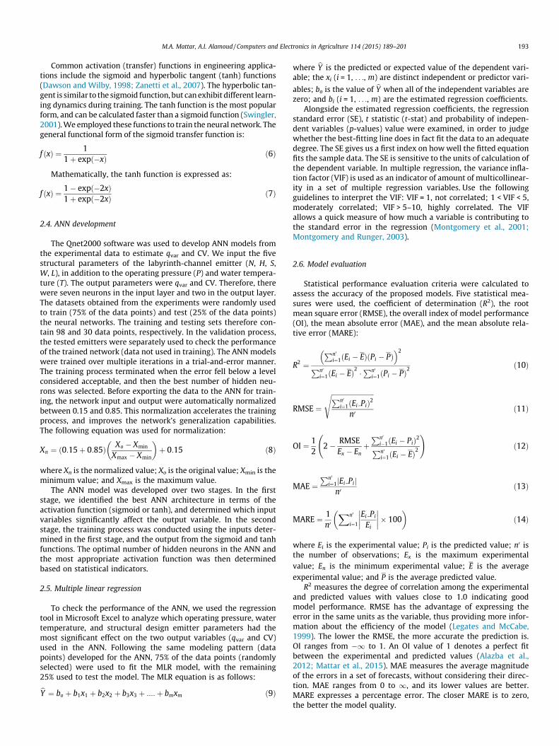
M.A. Mattar, A.I. Alamoud / Computers and Electronics in Agriculture 114 (2015) 189–201 193
Common activation (transfer) functions in engineering applica-tions include the sigmoid and hyperbolic tangent (tanh) functions(Dawson and Wilby, 1998; Zanetti et al., 2007). The hyperbolic tan-gent is similar to the sigmoid function, but can exhibit different learn-ing dynamics during training. The tanh function is the most popularform, and can be calculated faster than a sigmoid function (Swingler,2001). We employed these functions to train the neural network. Thegeneral functional form of the sigmoid transfer function is:
f ðxÞ ¼ 11þ expð�xÞ ð6Þ
Mathematically, the tanh function is expressed as:
f ðxÞ ¼ 1� expð�2xÞ1þ expð�2xÞ ð7Þ
2.4. ANN development
The Qnet2000 software was used to develop ANN models fromthe experimental data to estimate qvar and CV. We input the fivestructural parameters of the labyrinth-channel emitter (N, H, S,W, L), in addition to the operating pressure (P) and water tempera-ture (T). The output parameters were qvar and CV. Therefore, therewere seven neurons in the input layer and two in the output layer.The datasets obtained from the experiments were randomly usedto train (75% of the data points) and test (25% of the data points)the neural networks. The training and testing sets therefore con-tain 98 and 30 data points, respectively. In the validation process,the tested emitters were separately used to check the performanceof the trained network (data not used in training). The ANN modelswere trained over multiple iterations in a trial-and-error manner.The training process terminated when the error fell below a levelconsidered acceptable, and then the best number of hidden neu-rons was selected. Before exporting the data to the ANN for train-ing, the network input and output were automatically normalizedbetween 0.15 and 0.85. This normalization accelerates the trainingprocess, and improves the network’s generalization capabilities.The following equation was used for normalization:
Xn ¼ ð0:15þ 0:85Þ Xo � Xmin
Xmax � Xmin
� �þ 0:15 ð8Þ
where Xn is the normalized value; Xo is the original value; Xmin is theminimum value; and Xmax is the maximum value.
The ANN model was developed over two stages. In the firststage, we identified the best ANN architecture in terms of theactivation function (sigmoid or tanh), and determined which inputvariables significantly affect the output variable. In the secondstage, the training process was conducted using the inputs deter-mined in the first stage, and the output from the sigmoid and tanhfunctions. The optimal number of hidden neurons in the ANN andthe most appropriate activation function was then determinedbased on statistical indicators.
2.5. Multiple linear regression
To check the performance of the ANN, we used the regressiontool in Microsoft Excel to analyze which operating pressure, watertemperature, and structural design emitter parameters had themost significant effect on the two output variables (qvar and CV)used in the ANN. Following the same modeling pattern (datapoints) developed for the ANN, 75% of the data points (randomlyselected) were used to fit the MLR model, with the remaining25% used to test the model. The MLR equation is as follows:bY ¼ bo þ b1x1 þ b2x2 þ b3x3 þ ::::þ bmxm ð9Þ
where bY is the predicted or expected value of the dependent vari-able; the xi (i = 1, . . ., m) are distinct independent or predictor vari-
ables; bo is the value of bY when all of the independent variables arezero; and bi (i = 1, . . ., m) are the estimated regression coefficients.
Alongside the estimated regression coefficients, the regressionstandard error (SE), t statistic (t-stat) and probability of indepen-dent variables (p-values) value were examined, in order to judgewhether the best-fitting line does in fact fit the data to an adequatedegree. The SE gives us a first index on how well the fitted equationfits the sample data. The SE is sensitive to the units of calculation ofthe dependent variable. In multiple regression, the variance infla-tion factor (VIF) is used as an indicator of amount of multicollinear-ity in a set of multiple regression variables. Use the followingguidelines to interpret the VIF: VIF = 1, not correlated; 1 < VIF < 5,moderately correlated; VIF > 5–10, highly correlated. The VIFallows a quick measure of how much a variable is contributing tothe standard error in the regression (Montgomery et al., 2001;Montgomery and Runger, 2003).
2.6. Model evaluation
Statistical performance evaluation criteria were calculated toassess the accuracy of the proposed models. Five statistical mea-sures were used, the coefficient of determination (R2), the rootmean square error (RMSE), the overall index of model performance(OI), the mean absolute error (MAE), and the mean absolute rela-tive error (MARE):
R2 ¼Pn0
i¼1ðEi � EÞðPi � PÞ� �2
Pn0i¼1ðEi � EÞ2 �
Pn0i¼1ðPi � PÞ2
ð10Þ
RMSE ¼
ffiffiffiffiffiffiffiffiffiffiffiffiffiffiffiffiffiffiffiffiffiffiffiffiffiffiPn0i¼1ðEi PiÞ2
n0
sð11Þ
OI ¼ 12
2� RMSEEx � En
þPn0
i�1ðEi � PiÞ2Pn0i¼1ðEi � EÞ2
!ð12Þ
MAE ¼Pn0
i¼1jEi Pijn0
ð13Þ
MARE ¼ 1n0
Xn0
i¼1
Ei Pi
Ei
���� ����� 100� �
ð14Þ
where Ei is the experimental value; Pi is the predicted value; n0 isthe number of observations; Ex is the maximum experimentalvalue; En is the minimum experimental value; E is the averageexperimental value; and P is the average predicted value.
R2 measures the degree of correlation among the experimentaland predicted values with values close to 1.0 indicating goodmodel performance. RMSE has the advantage of expressing theerror in the same units as the variable, thus providing more infor-mation about the efficiency of the model (Legates and McCabe,1999). The lower the RMSE, the more accurate the prediction is.OI ranges from �1 to 1. An OI value of 1 denotes a perfect fitbetween the experimental and predicted values (Alazba et al.,2012; Mattar et al., 2015). MAE measures the average magnitudeof the errors in a set of forecasts, without considering their direc-tion. MAE ranges from 0 to 1, and its lower values are better.MARE expresses a percentage error. The closer MARE is to zero,the better the model quality.
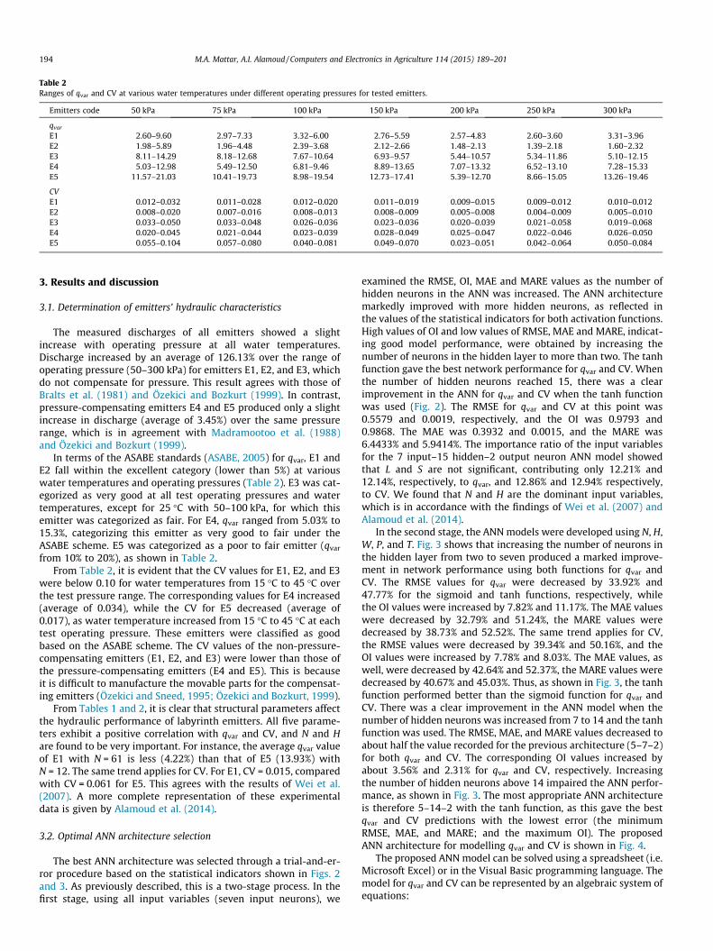
Table 2Ranges of qvar and CV at various water temperatures under different operating pressures for tested emitters.
Emitters code 50 kPa 75 kPa 100 kPa 150 kPa 200 kPa 250 kPa 300 kPa
qvar
E1 2.60–9.60 2.97–7.33 3.32–6.00 2.76–5.59 2.57–4.83 2.60–3.60 3.31–3.96E2 1.98–5.89 1.96–4.48 2.39–3.68 2.12–2.66 1.48–2.13 1.39–2.18 1.60–2.32E3 8.11–14.29 8.18–12.68 7.67–10.64 6.93–9.57 5.44–10.57 5.34–11.86 5.10–12.15E4 5.03–12.98 5.49–12.50 6.81–9.46 8.89–13.65 7.07–13.32 6.52–13.10 7.28–15.33E5 11.57–21.03 10.41–19.73 8.98–19.54 12.73–17.41 5.39–12.70 8.66–15.05 13.26–19.46
CVE1 0.012–0.032 0.011–0.028 0.012–0.020 0.011–0.019 0.009–0.015 0.009–0.012 0.010–0.012E2 0.008–0.020 0.007–0.016 0.008–0.013 0.008–0.009 0.005–0.008 0.004–0.009 0.005–0.010E3 0.033–0.050 0.033–0.048 0.026–0.036 0.023–0.036 0.020–0.039 0.021–0.058 0.019–0.068E4 0.020–0.045 0.021–0.044 0.023–0.039 0.028–0.049 0.025–0.047 0.022–0.046 0.026–0.050E5 0.055–0.104 0.057–0.080 0.040–0.081 0.049–0.070 0.023–0.051 0.042–0.064 0.050–0.084
194 M.A. Mattar, A.I. Alamoud / Computers and Electronics in Agriculture 114 (2015) 189–201
3. Results and discussion
3.1. Determination of emitters’ hydraulic characteristics
The measured discharges of all emitters showed a slightincrease with operating pressure at all water temperatures.Discharge increased by an average of 126.13% over the range ofoperating pressure (50–300 kPa) for emitters E1, E2, and E3, whichdo not compensate for pressure. This result agrees with those ofBralts et al. (1981) and Özekici and Bozkurt (1999). In contrast,pressure-compensating emitters E4 and E5 produced only a slightincrease in discharge (average of 3.45%) over the same pressurerange, which is in agreement with Madramootoo et al. (1988)and Özekici and Bozkurt (1999).
In terms of the ASABE standards (ASABE, 2005) for qvar, E1 andE2 fall within the excellent category (lower than 5%) at variouswater temperatures and operating pressures (Table 2). E3 was cat-egorized as very good at all test operating pressures and watertemperatures, except for 25 �C with 50–100 kPa, for which thisemitter was categorized as fair. For E4, qvar ranged from 5.03% to15.3%, categorizing this emitter as very good to fair under theASABE scheme. E5 was categorized as a poor to fair emitter (qvar
from 10% to 20%), as shown in Table 2.From Table 2, it is evident that the CV values for E1, E2, and E3
were below 0.10 for water temperatures from 15 �C to 45 �C overthe test pressure range. The corresponding values for E4 increased(average of 0.034), while the CV for E5 decreased (average of0.017), as water temperature increased from 15 �C to 45 �C at eachtest operating pressure. These emitters were classified as goodbased on the ASABE scheme. The CV values of the non-pressure-compensating emitters (E1, E2, and E3) were lower than those ofthe pressure-compensating emitters (E4 and E5). This is becauseit is difficult to manufacture the movable parts for the compensat-ing emitters (Özekici and Sneed, 1995; Özekici and Bozkurt, 1999).
From Tables 1 and 2, it is clear that structural parameters affectthe hydraulic performance of labyrinth emitters. All five parame-ters exhibit a positive correlation with qvar and CV, and N and Hare found to be very important. For instance, the average qvar valueof E1 with N = 61 is less (4.22%) than that of E5 (13.93%) withN = 12. The same trend applies for CV. For E1, CV = 0.015, comparedwith CV = 0.061 for E5. This agrees with the results of Wei et al.(2007). A more complete representation of these experimentaldata is given by Alamoud et al. (2014).
3.2. Optimal ANN architecture selection
The best ANN architecture was selected through a trial-and-er-ror procedure based on the statistical indicators shown in Figs. 2and 3. As previously described, this is a two-stage process. In thefirst stage, using all input variables (seven input neurons), we
examined the RMSE, OI, MAE and MARE values as the number ofhidden neurons in the ANN was increased. The ANN architecturemarkedly improved with more hidden neurons, as reflected inthe values of the statistical indicators for both activation functions.High values of OI and low values of RMSE, MAE and MARE, indicat-ing good model performance, were obtained by increasing thenumber of neurons in the hidden layer to more than two. The tanhfunction gave the best network performance for qvar and CV. Whenthe number of hidden neurons reached 15, there was a clearimprovement in the ANN for qvar and CV when the tanh functionwas used (Fig. 2). The RMSE for qvar and CV at this point was0.5579 and 0.0019, respectively, and the OI was 0.9793 and0.9868. The MAE was 0.3932 and 0.0015, and the MARE was6.4433% and 5.9414%. The importance ratio of the input variablesfor the 7 input–15 hidden–2 output neuron ANN model showedthat L and S are not significant, contributing only 12.21% and12.14%, respectively, to qvar, and 12.86% and 12.94% respectively,to CV. We found that N and H are the dominant input variables,which is in accordance with the findings of Wei et al. (2007) andAlamoud et al. (2014).
In the second stage, the ANN models were developed using N, H,W, P, and T. Fig. 3 shows that increasing the number of neurons inthe hidden layer from two to seven produced a marked improve-ment in network performance using both functions for qvar andCV. The RMSE values for qvar were decreased by 33.92% and47.77% for the sigmoid and tanh functions, respectively, whilethe OI values were increased by 7.82% and 11.17%. The MAE valueswere decreased by 32.79% and 51.24%, the MARE values weredecreased by 38.73% and 52.52%. The same trend applies for CV,the RMSE values were decreased by 39.34% and 50.16%, and theOI values were increased by 7.78% and 8.03%. The MAE values, aswell, were decreased by 42.64% and 52.37%, the MARE values weredecreased by 40.67% and 45.03%. Thus, as shown in Fig. 3, the tanhfunction performed better than the sigmoid function for qvar andCV. There was a clear improvement in the ANN model when thenumber of hidden neurons was increased from 7 to 14 and the tanhfunction was used. The RMSE, MAE, and MARE values decreased toabout half the value recorded for the previous architecture (5–7–2)for both qvar and CV. The corresponding OI values increased byabout 3.56% and 2.31% for qvar and CV, respectively. Increasingthe number of hidden neurons above 14 impaired the ANN perfor-mance, as shown in Fig. 3. The most appropriate ANN architectureis therefore 5–14–2 with the tanh function, as this gave the bestqvar and CV predictions with the lowest error (the minimumRMSE, MAE, and MARE; and the maximum OI). The proposedANN architecture for modelling qvar and CV is shown in Fig. 4.
The proposed ANN model can be solved using a spreadsheet (i.e.Microsoft Excel) or in the Visual Basic programming language. Themodel for qvar and CV can be represented by an algebraic system ofequations:
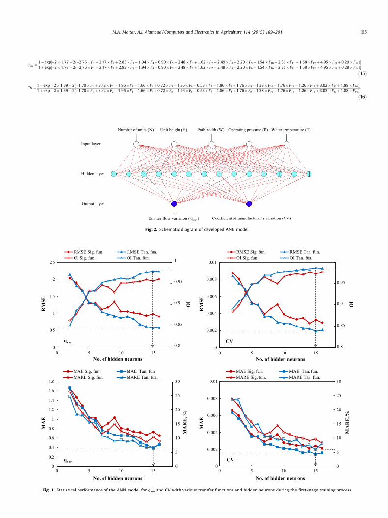
Fig. 2. Schematic diagram of developed ANN model.
0.8
0.85
0.9
0.95
1
0
0.5
1
1.5
2
2.5
0 5 10 15
OI
RM
SE
No. of hidden neurons
RMSE Sig. fun. RMSE Tan. fun.OI Sig. fun. OI Tan. fun.
0.8
0.85
0.9
0.95
1
0
0.002
0.004
0.006
0.008
0.01
0 5 10 15O
I
RM
SE
No. of hidden neurons
RMSE Sig. fun. RMSE Tan. fun.OI Sig. fun. OI Tan. fun.
0
5
10
15
20
25
30
0
0.2
0.4
0.6
0.8
1
1.2
1.4
1.6
1.8
0 5 10 15
MA
RE
, %
MA
E
No. of hidden neurons
MAE Sig. fun. MAE Tan. fun.MARE Sig. fun. MARE Tan. fun.
0
5
10
15
20
25
30
0
0.002
0.004
0.006
0.008
0.01
0 5 10 15
MA
RE
,%
MA
E
No. of hidden neurons
MAE Sig. fun. MAE Tan. fun.MARE Sig. fun. MARE Tan. fun.
qvar CV
qvar CV
Fig. 3. Statistical performance of the ANN model for qvar and CV with various transfer functions and hidden neurons during the first-stage training process.
qvar ¼1� exp �2� 1:77� 2 �2:76� F1 þ 2:97� F2 þ 2:83� F3 � 1:94� F4 þ0:90� F5 � 2:48� F6 þ1:62� F7 �2:49� F8 þ2:20� F9 �1:54� F10 � 2:36� F11 �1:58� F12 þ 4:95� F13 þ 0:29� F14ð Þ½ �1þ exp �2� 1:77� 2 �2:76� F1 þ 2:97� F2 þ 2:83� F3 � 1:94� F4 þ0:90� F5 � 2:48� F6 þ1:62� F7 �2:49� F8 þ2:20� F9 �1:54� F10 � 2:36� F11 �1:58� F12 þ 4:95� F13 þ 0:29� F14ð Þ½ �
ð15Þ
CV¼ 1� exp �2� 1:39� 2 �1:70� F1 þ 3:42� F2 þ 1:96� F3 � 1:66� F4 þ 0:72� F5 � 1:96� F6 �0:53� F7 �1:86� F8 þ1:76� F9 �1:38� F10 � 1:76� F11 �1:26� F12 þ 3:02� F13 þ 1:88� F14ð Þ½ �1þ exp �2� 1:39� 2ð�1:70� F1 þ 3:42� F2 þ 1:96� F3 � 1:66� F4 þ 0:72� F5 � 1:96� F6 �0:53� F7 �1:86� F8 þ1:76� F9 �1:38� F10 � 1:76� F11 �1:26� F12 þ 3:02� F13 þ 1:88� F14Þ½ �
ð16Þ
M.A. Mattar, A.I. Alamoud / Computers and Electronics in Agriculture 114 (2015) 189–201 195

0.8
0.85
0.9
0.95
1
0
0.5
1
1.5
2
2.5
0 5 10 15
OI
RM
SE
No. of hidden neurons
RMSE Sig. fun. RMSE Tan. fun.OI Sig. fun. OI Tan. fun.
qvar
0.8
0.85
0.9
0.95
1
0
0.002
0.004
0.006
0.008
0.01
0 5 10 15
OI
RM
SE
No. of hidden neurons
RMSE Sig. fun. RMSE Tan. fun.OI Sig. fun. OI Tan. fun.
CV
0
5
10
15
20
25
30
0
0.2
0.4
0.6
0.8
1
1.2
1.4
1.6
1.8
0 5 10 15
MA
RE
, %
MA
E
No. of hidden neurons
MAE Sig. fun. MAE Tan. fun.MARE Sig. fun. MARE Tan. fun.
qvar
0
5
10
15
20
25
30
0
0.002
0.004
0.006
0.008
0.01
0 5 10 15
MA
RE,
%
MA
E
No. of hidden neurons
MAE Sig. fun. MAE Tan. fun.MARE Sig. fun. MARE Tan. fun.
CV
Fig. 4. Statistical performance of the ANN model for qvar and CV with various transfer functions and hidden neurons during the second-stage training process.
Table 3Weights [(W1)ji ] and biases [(B1)j] between input and hidden layers for the developedANN model.
Hidden neurons (j) Input neurons (i) (B1)j
1 2 3 4 5
1 �0.80 3.25 �1.31 5.14 2.69 �4.242 �3.23 �0.14 �3.01 �5.15 �1.65 2.423 �0.05 �1.08 0.57 �1.88 2.13 0.334 �1.78 �1.21 �3.38 3.10 8.15 �4.755 �1.94 �3.62 �0.77 �6.41 5.05 0.916 0.96 2.43 �0.09 �2.46 �3.35 2.157 �0.45 0.34 0.51 0.07 �0.09 �0.418 0.14 0.81 �0.67 �2.39 �2.86 0.749 0.59 �1.41 �0.58 �2.86 �4.77 2.53
10 �1.79 1.60 0.06 1.54 3.02 �2.3511 2.64 1.54 �0.80 �5.14 �0.76 4.1812 �1.17 �1.09 �2.98 0.94 4.23 0.4913 �1.13 1.58 �0.73 3.53 1.45 �2.0414 �1.20 0.35 0.40 0.67 0.84 �0.30
196 M.A. Mattar, A.I. Alamoud / Computers and Electronics in Agriculture 114 (2015) 189–201
where the tanh function (Fj) used for this model is represented asfollows:
Fj ¼1� expð�2HjÞ1þ expð�2HjÞ
ð17Þ
where Hj is the sum of the product of the input parameters and theirweights. For Eqs. (15) and (16), this is:
Hj ¼ ðW1Þj1 � N þ ðW1Þj2 � H þ ðW1Þj3 �W þ ðW1Þj4 � P
þ ðW1Þj5 � T þ ðB1Þj ð18Þ
where the connection weights [(W1)ji] and hidden biases [(B1)j] arelisted in Table 3.
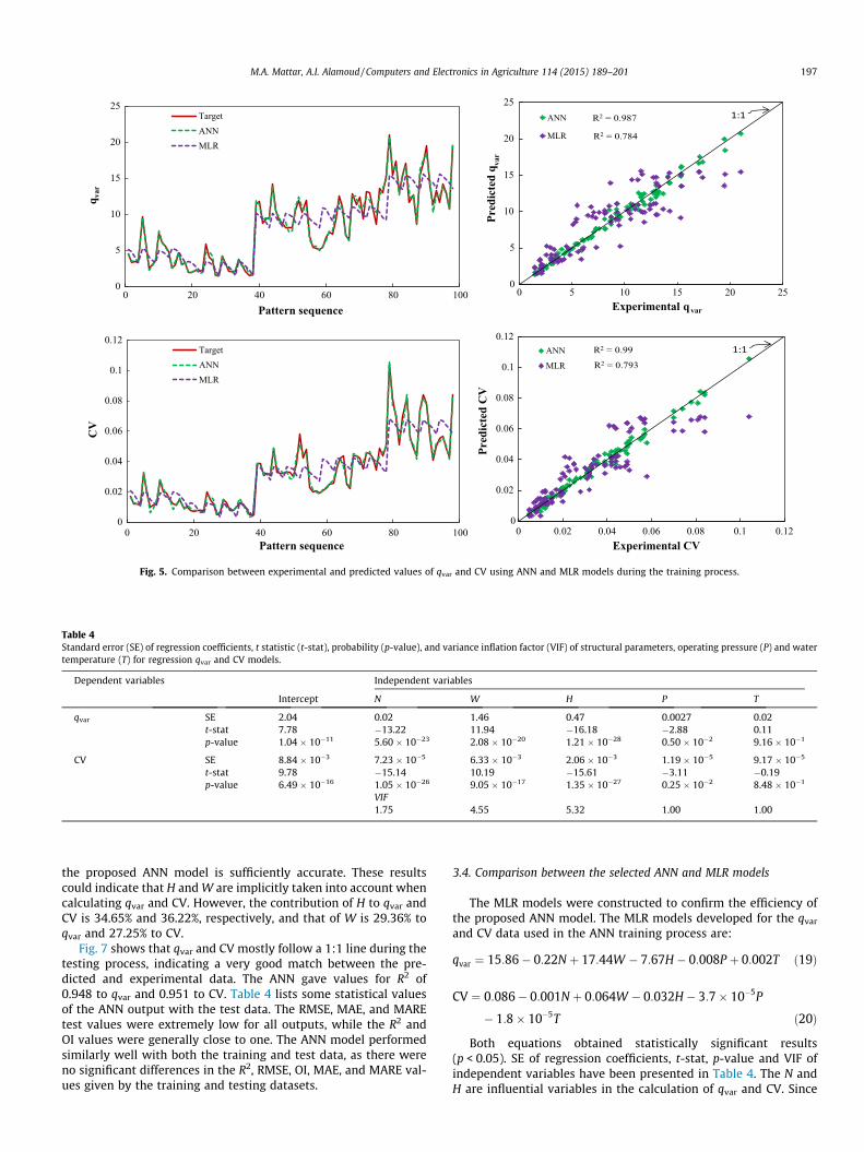
3.3. ANN model performance
A feed-forward back-propagation ANN with a tanh transferfunction in the hidden and output layers was selected to predictvalues of qvar and CV for labyrinth emitters. The 5–14–2 architec-ture obtained the best fit during the training process, as describedabove. To illustrate the goodness of fit, Fig. 5 compares the experi-mental and predicted qvar and CV values with the proposed ANN. Itis clear from this figure that the values predicted by the proposedANN fit perfectly with the observed values. The R2 (0.987 and 0.99)values are very close to one for qvar and CV, respectively. For thisnetwork, we obtained RMSE values of 0.5585 and 0.0022 for qvar
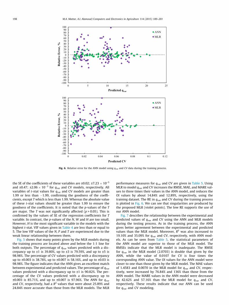
and CV, respectively, as presented in Table 4. These values are closeto zero. The corresponding OI values were 0.9793 and 0.9844,which are very close to one. The MAE values, as well, were0.4157 and 0.0017, which are very close to zero. The MARE valueswere 5.8987% and 7.3164%, which are less values. As Fig. 6 depicts,the relative errors (RE) of the predicted qvar and CV values (greenpoints) are mostly around ±10%, with the exception of a few datapoints. Thus, the R2, RMSE, OI, MAE, MARE, and RE indicate that
0
5
10
15
20
25
0 20 40 60 80 100
q var
Pattern sequence
TargetANNMLR
0
5
10
15
20
25
0 5 10 15 20 25
Pred
icte
d q va
r
Experimental qvar
ANN
MLR
1:1R2 = 0.987
R2 = 0.784
0
0.02
0.04
0.06
0.08
0.1
0.12
0 20 40 60 80 100
CV
Pattern sequence
TargetANNMLR
0
0.02
0.04
0.06
0.08
0.1
0.12
0 0.02 0.04 0.06 0.08 0.1 0.12
Pred
icte
d C
V
Experimental CV
ANN
MLR
1:1R2 = 0.99
R2 = 0.793
Fig. 5. Comparison between experimental and predicted values of qvar and CV using ANN and MLR models during the training process.
Table 4Standard error (SE) of regression coefficients, t statistic (t-stat), probability (p-value), and variance inflation factor (VIF) of structural parameters, operating pressure (P) and watertemperature (T) for regression qvar and CV models.
Dependent variables Independent variables
Intercept N W H P T
qvar SE 2.04 0.02 1.46 0.47 0.0027 0.02t-stat 7.78 �13.22 11.94 �16.18 �2.88 0.11p-value 1.04 � 10�11 5.60 � 10�23 2.08 � 10�20 1.21 � 10�28 0.50 � 10�2 9.16 � 10�1
CV SE 8.84 � 10�3 7.23 � 10�5 6.33 � 10�3 2.06 � 10�3 1.19 � 10�5 9.17 � 10�5
t-stat 9.78 �15.14 10.19 �15.61 �3.11 �0.19p-value 6.49 � 10�16 1.05 � 10�26 9.05 � 10�17 1.35 � 10�27 0.25 � 10�2 8.48 � 10�1
VIF1.75 4.55 5.32 1.00 1.00
M.A. Mattar, A.I. Alamoud / Computers and Electronics in Agriculture 114 (2015) 189–201 197
the proposed ANN model is sufficiently accurate. These resultscould indicate that H and W are implicitly taken into account whencalculating qvar and CV. However, the contribution of H to qvar andCV is 34.65% and 36.22%, respectively, and that of W is 29.36% toqvar and 27.25% to CV.
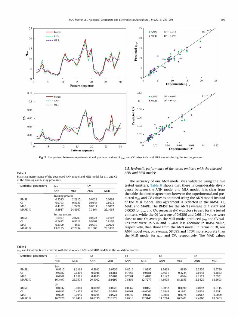
Fig. 7 shows that qvar and CV mostly follow a 1:1 line during thetesting process, indicating a very good match between the pre-dicted and experimental data. The ANN gave values for R2 of0.948 to qvar and 0.951 to CV. Table 4 lists some statistical valuesof the ANN output with the test data. The RMSE, MAE, and MAREtest values were extremely low for all outputs, while the R2 andOI values were generally close to one. The ANN model performedsimilarly well with both the training and test data, as there wereno significant differences in the R2, RMSE, OI, MAE, and MARE val-ues given by the training and testing datasets.
3.4. Comparison between the selected ANN and MLR models
The MLR models were constructed to confirm the efficiency ofthe proposed ANN model. The MLR models developed for the qvar
and CV data used in the ANN training process are:
qvar ¼ 15:86� 0:22N þ 17:44W � 7:67H � 0:008P þ 0:002T ð19Þ
CV ¼ 0:086� 0:001N þ 0:064W � 0:032H � 3:7� 10�5P
� 1:8� 10�5T ð20Þ
Both equations obtained statistically significant results(p < 0.05). SE of regression coefficients, t-stat, p-value and VIF ofindependent variables have been presented in Table 4. The N andH are influential variables in the calculation of qvar and CV. Since
-100-90-80-70-60-50-40-30-20-10
0102030405060708090
100
0 5 10 15 20 25
Rel
ativ
e E
rror
, %
Predicted qvar
ANNMLR
-100-90-80-70-60-50-40-30-20-10
0102030405060708090
100
0 0.02 0.04 0.06 0.08 0.1 0.12
Rel
ativ
e E
rror
, %
Predicted CV
ANNMLR
Fig. 6. Relative error for the ANN model using qvar and CV data during the training process.
198 M.A. Mattar, A.I. Alamoud / Computers and Electronics in Agriculture 114 (2015) 189–201
the SE of the coefficients of these variables are ±0.02; ±7.23 � 10–5
and ±0.47; ±2.06 � 10�3 for qvar and CV models, respectively. Allvariables of t-stat values for qvar and CV models are greater than1.99 or less than �1.99, confirming the goodness of the coeffi-cients, except T which is less than 1.99. Whereas the absolute valueof these t-stat values should be greater than 1.99 to ensure thegoodness of the coefficients. It is noted that the p-values of the Tare major. The T was not significantly affected (p > 0.05). This isconfirmed by the values of SE of the regression coefficients for Tvariable. In contrast, the p-values of the N, W and H are too small.However, H is the most significant variable in the models with thehighest t-stat. VIF values given in Table 4 are less than or equal to5. The low VIF values of the N, P and T are experienced due to theweak linear relationship between them.
Fig. 5 shows that many points given by the MLR models duringthe training process are located above and below the 1:1 line forboth outputs. The percentage of qvar values predicted with a dis-crepancy up to ±1 is 39.80%, up to ±3 is 79.59%, and up to ±5 is98.98%. The percentage of CV values predicted with a discrepancyup to ±0.003 is 38.78%, up to ±0.007 is 58.16%, and up to ±0.03 is98.98%. The figure indicates that the ANN gives an excellent matchbetween experimental and predicted values. The percentage of qvar
values predicted with a discrepancy up to ±1 is 90.82%. The per-centage of the CV values predicted with a discrepancy up to±0.003 is 85.71%, and up to ±0.007 is 97.96%. The ANN for qvar
and CV, respectively, had a R2 values that were about 25.89% and24.84% more accurate than those from the MLR models. The MLR
performance measures for qvar and CV are given in Table 5. UsingMLR to model qvar and CV increases the RMSE, MAE, and MARE val-ues to three times their values in the ANN model, and reduces theOI values by about 14.84% and 12.89%, respectively, using thetraining dataset. The RE in qvar and CV during the training processis plotted in Fig. 6. We can see that singularities are produced bythe proposed MLR (violet points). The low RE supports the use ofour ANN model.
Fig. 7 describes the relationship between the experimental andpredicted values of qvar and CV using the ANN and MLR modelsduring the testing process. As in the training process, the ANNgives better agreement between the experimental and predictedvalues than the MLR model. Moreover, R2 was also increased to19.10% and 35.09% for qvar and CV, respectively, with ANN mod-els. As can be seen from Table 5, the statistical parameters ofthe ANN model are superior to those of the MLR model. TheRMSEs indicate that the MLR model is inadequate. The RMSEfor qvar in the MLR model (2.0703) is double that given by theANN, while the value of 0.0107 for CV is four times thecorresponding ANN value. The OI values for the ANN model werecloser to one than those given by the MLR model. The MAE valuesof 1.4583 and 0.0070 in the MLR model for qvar and CV, respec-tively, were increased by 76.84% and 136% than those from theANN model. The MARE values in the ANN model were decreasedby 42.62% and 57.16% than the MLR model for qvar and CV,respectively. These results indicate that our ANN can be usedfor qvar and CV modeling.
0
5
10
15
20
25
0 5 10 15 20 25 30
q var
Pattern sequence
TargetANNMLR
0
5
10
15
20
25
0 5 10 15 20 25
Pred
icte
d q v
ar
Experimental qvar
ANN
MLR
1:1R2 = 0.948
R2 = 0.796
0
0.02
0.04
0.06
0.08
0.1
0.12
0 5 10 15 20 25 30
CV
Pattern sequence
TargetANNMLR
0
0.02
0.04
0.06
0.08
0.1
0.12
0 0.02 0.04 0.06 0.08 0.1 0.12
Pred
icte
d C
V
Experimental CV
ANN
MLR
1:1R2 = 0.951
R2 = 0.704
Fig. 7. Comparison between experimental and predicted values of qvar and CV using ANN and MLR models during the testing process.
Table 5Statistical performance of the developed ANN model and MLR model for qvar and CVin the training and testing processes.
Statistical parameters qvar CV
ANN MLR ANN MLR
Training processRMSE 0.5585 2.2815 0.0022 0.0099OI 0.9793 0.8339 0.9844 0.8675MAE 0.4157 1.7472 0.0017 0.0072MARE, % 5.8987 24.4667 7.3164 25.1065
Testing processRMSE 1.0497 2.0703 0.0024 0.0107OI 0.9472 0.8511 0.9661 0.8107MAE 0.8399 1.4853 0.0030 0.0070MARE, % 13.0155 22.2934 12.1605 28.3870
Table 6qvar and CV of the tested emitters with the developed ANN and MLR models in the valida
Statistical parameters E1 E2
ANN MLR ANN MLR
qvar
RMSE 0.9315 1.2168 0.5912 0.6556OI 0.6987 0.5239 0.6945 0.6383MAE 0.6961 1.0511 0.4833 0.5102MARE, % 16.3497 26.0575 20.1002 19.9299
CVRMSE 0.0037 0.0048 0.0020 0.0026OI 0.6493 0.4553 0.7001 0.5384MAE 0.0025 0.0045 0.0015 0.0021MARE, % 16.2620 33.9411 16.6735 23.2979
M.A. Mattar, A.I. Alamoud / Computers and Electronics in Agriculture 114 (2015) 189–201 199
3.5. Hydraulic performance of the tested emitters with the selectedANN and MLR models
The accuracy of our ANN model was validated using the fivetested emitters. Table 6 shows that there is considerable diver-gence between the ANN model and MLR model. It is clear fromthe table that better agreement between the experimental and pre-dicted qvar and CV values is obtained using the ANN model insteadof the MLR model. This agreement is reflected in the RMSE, OI,MAE, and MARE. The RMSE for the ANN (average of 1.2907 and0.0053 for qvar and CV, respectively) was close to zero for the testedemitters, while the OI (average of 0.6356 and 0.6611) values wereclose to one. On average, the MLR model produced qvar and CV val-ues that were 29.53% and 66.46% less accurate in RMSE value,respectively, than those from the ANN model. In terms of OI, ourANN model was, on average, 58.09% and 170% more accurate thanthe MLR model for qvar and CV, respectively. The MAE values
tion process.
E3 E4 E5
ANN MLR ANN MLR ANN MLR
0.8516 1.9255 1.7435 1.9880 2.3359 2.57390.7566 0.0381 0.4631 0.3234 0.5648 0.48630.7661 1.4186 1.3147 1.6964 2.1127 2.09317.8156 12.7277 14.1605 18.2655 15.5429 14.5603
0.0062 0.0159 0.0052 0.0090 0.0092 0.01150.6461 �0.4045 0.6848 0.1861 0.6251 0.45110.0042 0.0089 0.0038 0.0078 0.0067 0.00999.8716 17.3145 11.5214 26.2401 12.4200 18.5603
200 M.A. Mattar, A.I. Alamoud / Computers and Electronics in Agriculture 114 (2015) 189–201
(average of 1.0746 and 0.0038) for the ANN model were closer tozero than its values (average of 1.3539 and 0.0066) for the MLRmodel. The MARE values for the MLR model were almost 1.25and 1.8 times that of the values for the ANN model for qvar andCV, respectively. The RMSE, OI, MAE, and MARE for the two modelsconfirm that MLR performs poorly.
The statistical parameters indicate that the predicted hydraulicperformance of E1, E2, and E3 (non-pressure-compensating emit-ters) was better than those of E4 and E5 (pressure-compensatingemitters) when using the developed ANN model (Table 6). Theaverage RMSE for qvar in pressure-compensating emitters increasedby a factor of 2.5 (from 0.79 in non-pressure-compensating emit-ters to 2.04). The average RMSE for CV in pressure-compensatingemitters increased by about 80%, from 0.004 to 0.0072. The non-pressure-compensating emitters had OI values that were about39.42% and 1.57% more accurate for qvar and CV, respectively, com-pared with pressure-compensating emitters. Finally, the value ofMAE for the pressure-compensating emitters (average of 1.7137and 0.0052 for qvar and CV, respectively) was almost 2.5 and 2times that of the value for the non-pressure-compensatingemitters.
4. Conclusion
The hydraulic performance of emitters plays a significant role indrip irrigation systems, because the emitter is one of the mosteffective water-saving elements. We used an ANN to model thehydraulic performance of labyrinth-channel emitters. We consid-ered the qvar and CV at different operating pressures and watertemperatures. Our ANN model used the structural parameters ofthe labyrinth-emitters as inputs, and gave qvar and CV as output.A feed-forward back-propagation algorithm was preferred as theANN training algorithm. The results were compared with thosefrom MLR. The performance of the models was assessed by theR2, RMSE, OI, MAE, and MARE performance indicators. Several neu-ral network structures with different numbers of neurons in thehidden layer were trained and tested to determine which structuregave the minimal error.
Having 14 neurons in the hidden layer resulted in the optimalANN model performance in terms of RMSE, OI, MAE, and MARE.Thus, the 5–14–2 configuration was determined as the optimalANN architecture, with the S and L variables rejected. The hyper-bolic tangent was used as the activation function in the hiddenand output layers. As seen from the results, the ANN model exhib-ited better prediction performance than MLR, and displayed suffi-cient accuracy in the prediction of qvar and CV. Our study showsthat ANNs are a reliable and powerful tool for predicting thehydraulic performance of emitters. Moreover, using an ANN modelreduces the amount of input data, less time consuming, and resultsin higher performance and accuracy.
Acknowledgements
The authors would like to acknowledge the Prince SultanResearch Institute and PSIPW research chair for sponsoring thisresearch project. We would like to express deep thanks to theDeanship of Scientific Research, King Saud University andAgriculture Research Center, College of Food and AgricultureSciences for their financial support, sponsorship, andencouragement.
References
Alamoud, A.I., Mattar, M.A., Ateia, M., 2014. Impact of water temperature andstructural parameters on the hydraulic labyrinth-channel emitter performance.Span. J. Agric. Res. 12 (2), 580–593.
Alazba, A.A., Mattar, M.A., ElNesr, M.N., Amin, M.T., 2012. Field assessment offriction head loss and friction correction factor equations. J. Irrig. Drain. Eng.,ASCE 138 (2), 166–176.
ASABE, 2005. EP-458: Field evaluation of microirrigation systems. ASABE, St. Joseph,USA.
ASCE Task committee, 2000. Artificial neural networks in hydrology. I: preliminaryconcepts. J. Hydrol. Eng., ASCE 5 (2), 115–123.
Bralts, V.F., Wu, I.P., Gitlin, H.M., 1981. Manufacturing variation and drip irrigationuniformity. Trans. ASABE 24 (1), 113–119.
Cigizoglu, H.K., 2003. Estimation, forecasting and extrapolation of river flows byartificial neural networks. Hydrol. Sci. J. 48 (3), 349–361.
Cobaner, M., Citakoglu, H., Kis�i, Ö., Haktanir, T., 2014. Estimation of mean monthlyair temperatures in Turkey. Comput. Electron. Agric. 109 (8), 71–79.
Dawson, W.C., Wilby, R., 1998. An artificial neural networks approach to rainfall-runoff modeling. Hydrol. Sci. J. 43 (1), 47–66.
Evans, R.G., Wu, I., Smajstrala, A.G., 2007. Microirrigation systems. In: Design andOperation of Irrigation Systems, second ed. American Society of Agriculturaland Biological Engineers Special Monograph, pp. 632–683 (Chapter 17).
Fernando, D.A.K., Shamseldin, A.Y., 2009. Investigation of internal functioning of theradial-basis-function neural network river flow forecasting models. J. Hydrol.Eng., ASCE 14 (3), 286–292.
Givi, J., Prasher, S.O., Patel, R.M., 2004. Evaluation of pedotransfer functions inpredicting the soil water contents at field capacity and wilting point. Agric.Water Manage. 70 (2), 83–96.
Gocic, M., Motamedi, S., Shamshirband, S., Petkovic, D., Ch, S., Hashim, R., Arif, M.,2015. Soft computing approaches for forecasting reference evapotranspiration.Comput. Electron. Agric. 113 (2), 164–173.
Haykin, S., 1999. Neural Networks. A Comprehensive Foundation. Prentice HallInternational Inc., New Jersey.
Hinnell, A.C., Lazarovitch, N., Furman, A., Poulton, M., Warrick, A.W., 2009. Neuro-Drip: estimation of subsurface wetting patterns for drip irrigation using neuralnetworks. Irri. Sci. 28 (6), 535–544.
Jain, A., Srinivasulu, S., 2004. Development of effective and efficient rainfall-runoffmodels using integration of deterministic, real-coded genetic algorithms, andartificial neural network techniques. Water Resour. Res. 40 (4), W04302.
Kang, S., Yulong, Z., Zhuangde, J., 2003. Laser profilometer. Opt. Precis. Eng. 11 (3),245–248.
Kumar, S., Singh, P., 2007. Evaluation of hydraulic performance of drip irrigationsystem. J. Agric. Eng. 44 (2), 104–108.
Kumar, M., Raghuwanshi, N.S., Singh, R., Wallender, W.W., Pruitt, W.O., 2002.Estimating evapotranspiration using artificial neural network. J. Irrig. Drain.Eng., ASCE 128 (4), 224–233.
Landeras, G., Ortiz-Barredo, A., López, J.J., 2008. Comparison of artificial neuralnetwork models and empirical and semi-empirical equations for daily referenceevapotranspiration estimation in the Basque Country Northern Spain. Agric.Water Manage. 95 (5), 553–565.
Landeras, G., Ortiz-Barredo, A., López, J.J., 2009. Forecasting weeklyevapotranspiration with ARIMA and artificial neural network Models. J. Irrig.Drain. Eng., ASCE 135 (3), 323–334.
Legates, D.R., McCabe Jr., G.J., 1999. Evaluating the use of ‘‘goodness-of fit’’ measuresin hydrologic and hydroclimatic model validation. Water Resour. Res. 35 (1),233–241.
Madramootoo, C.A., Khatri, K.C., Rigby, M., 1988. Hydraulic performances of fivedifferent trickle irrigation emitters. Can. Agric. Eng. 30, 1–4.
Maier, H.R., Dandy, G.C., 2000. Neural networks for the prediction and forecasting ofwater resources variables: a review of modeling issues and application. Environ.Model. Software 15 (1), 101–124.
Martí, P., Provenzano, G., Royuela, Á., Palau-Salvador, G., 2010. Integrated emitterlocal loss prediction using artificial neural networks. J. Irrig. Drain. Eng., ASCE136 (1), 11–22.
Mattar, M.A., Alazba, A.A., Zin El-Abedin, T.K., 2015. Forecasting furrow irrigationinfiltration using artificial neural networks. Agric. Water Manage. 148 (1),63–71.
Mizyed, N., Kruse, E.G., 1989. Emitter discharge evaluation of subsurface trickleirrigation. Trans. ASABE 32 (4), 1223–1228.
Montgomery, D., Runger, G., 2003. Applied Statistics and Probability for Engineers.John Wiley & Sons Inc., United States of America.
Montgomery, D., Peck, E., Vining, G., 2001. Introduction to linear regression analysis,third ed. John Wiley, New York.
Nakayama, F.S., Bucks, D.A., 1986. Trickle Irrigation for Crop Production. ElsevierScience, Amsterdam, pp. 1–383.
Özekici, B., Bozkurt, S., 1999. Determination of hydraulic performances of in-lineemitters. Turk. J. Agric. Forest. 23 (1), 19–24.
Özekici, B., Sneed, R.E., 1995. Manufacturing variation for various trickle irrigationon-line emitter. Appl. Eng. Agric. 11 (2), 235–240.
Raju, S.K., Kumar, D.N., Duck, L., 2006. Artificial neural networks and multicriterionanalysis for sustainable irrigation planning. Comput. Oper. Res. 33, 1138–1153.
Rodriguez-Sinobas, L., Juana, L., Losada, A., 1999. Effects of temperature changes onemitter discharge. J. Irrig. Drain. Eng., ASCE 125 (2), 64–73.
Singh, A.K., Upadhyaya, A., Islam, A., Bharali, M.A., Roy, M., 2006a. Flow andmanufacturing variation of drippers. J. Agric. Eng. 43 (3), 27–30.
Singh, D.K., Rajput, T.B.S., Singh, D.K., Sikarwar, H.S., Sahoo, R.N., Ahmad, T., 2006b.Performance of subsurface drip irrigation system with line source of waterapplication in okra field. J. Agric. Eng. 43 (3), 23–26.
Swingler, K., 2001. Applying Neural Networks, A Practical Guide, third ed. AcademicPress, San Francisco, CA.

M.A. Mattar, A.I. Alamoud / Computers and Electronics in Agriculture 114 (2015) 189–201 201
Thirumalaiah, K., Deo, M.C., 1998. River stage forecasting using artificial neuralnetworks. J. Hydrol. Eng., ASCE 3 (1), 26–32.
Tripathi, V.K., Rajput, T.B.S., Patel, N., Lata, 2011. Hydraulic performance of dripirrigation system with municipal wastewater. J. Agric. Eng. 48 (2), 15–22.
Wanakule, N., Aly, A., 2005. Using groundwater artificial neural network models foradaptive water supply management. In: Proc., Impacts of Global ClimateChange, ASCE, Reston, Va., 173(40792), 89.
Wei, Z., Tang, Y., Zhao, W., Lu, B., 2007. Rapid structural design of drip irrigationemitters based on RP technology. Rapid. Prototyping J. 13 (5), 268–275.
Wu, I.P., Gitlin, H.M., 1983. Drip irrigation application efficiency and schedules.Trans. ASABE 28, 92–99.
Zanetti, S.S., Sousa, E.F., Oliveira, V.P.S., 2007. Estimating evapotranspiration usingartificial neural network and minimum climatological data. J. Irrig. Drain. Eng.,ASCE 133 (2), 83–89.
Zapata, N., Nerilli, E., Martinez-Cob, A., Chalghaf, I., Chalghaf, B., Fliman, D., Playan,E., 2013. Limitations to adopting regulated deficit irrigation in stone fruitorchards: a case study. Span. J. Agric. Res. 11 (2), 529–546.
Zhang, J., Zhao, W., Wei, Z., Tang, Y., Lu, B., 2007. Numerical and experimental studyon hydraulic performance of emitters with arc labyrinth channels. Comput.Electron. Agric. 56 (2), 120–129.
Zhang, J., Zhao, W., Tang, Y., Lu, B., 2011a. Structural optimization of labyrinth-channel emitters based on hydraulic and anti-clogging performances. Irri. Sci.29 (5), 351–357.
Zhang, J., Zhao, W., Lu, B., 2011b. New method of hydraulic performance evaluationon emitters with labyrinth channels. J. Irrig. Drain. Eng., ASCE 137 (12), 811–815.
Zhao, W., Zhang, J., Tang, Y., Wei, Z., Lu, B., 2009. In: Li, D., Chunjiang, Z. (Eds.), IFIPInternational Federation for Information Processing, Computer and ComputingTechnologies in Agriculture II, vol. 2. Springer, Boston, pp. 881–890.
Zhiqin, L., Lin, L., 2011. The influence of the sectional form of labyrinth emitter onthe hydraulic properties. In: Deng, H. et al. (Eds.), AICI 2011, CCIS 237. Springer-Verlag Berlin Heidelberg, pp. 499–505.