RESEARCH ARTICLE

Area Change and Thickness Variation over PensilungpaGlacier (J&K) using Remote Sensing

Arvind Chandra Pandey & Swagata Ghosh &

M. S. Nathawat & Reet Kamal Tiwari

Received: 6 October 2010 /Accepted: 25 May 2011# Indian Society of Remote Sensing 2011

Abstract Accurate representations of the Earth’ssurface in the form of digital elevation models(DEMs) are essential for a variety of applications inglaciological and remote-sensing research. In thepresent study area change and thickness variationover Pensilungpa glacier was attempted using remotesensing approach. It can be remarked that a net loss of9.23 sq. km. which is 38% of the glacier area mappedin 1962 indicate a drastic change over the glacier areaduring 1962–2007. Estimation of glacier thicknesschange on Pensilungpa glacier based on ASTERDEM (2003) and Survey of India (SOI) contourbased DEM (1962) indicated increase in the glacierelevation in the accumulation zone mainly by 30 to90 m and similar reduction by 30 to 90 m in theablation zone.

Keywords Area change . Topographic change .

Pensilungpa glacier. Himalaya . Remote sensing

Introduction

The Himalaya nourishes more than 12000 glaciers(Kaul 1999; Mool et al. 2001; Thayyen and Gergan2010) covering approximately 33000 sq km (Rai andGurung 2005; Thayyen and Gergan 2010) which isabout 17% of Himalayan mountain area (Ahmed et al.2004). Fresh water resources in the Himalayas arestored in the form of glaciers. During the last centurymost glaciers in the Himalayas have receded, inresponse to the climatic change (Kulkarni et al.2002; Hansen et al. 2005; Bhambri and Bolch 2009;Prasad et al. 2009) with annual rate of retreat varyingfrom 16 to 35 m (Dhobal et al. 2004) with a fewexceptions in the Karakoram region, which areadvancing since the late 1990s (Hewitt 2005, 2010).Due to 10% increase in the melting of the glaciers ofthe western Himalaya, the rivers fed by the Himalayanglaciers have shown 3–4% surplus water (Hasnain2008). Volume changes in glaciers are projected tomake the largest contribution, to sea-level rise in thecoming century (Meier et al. 2007; Herman et al.2011). The net shrinkage and retreat of glaciers iscausing the increase in size and number of glacial lakesand thereby the possibility of increase in frequency ofglacier lake outburst floods (GLOFs) in coming years(Bajracharya et al. 2008). Therefore understanding of

J Indian Soc Remote SensDOI 10.1007/s12524-011-0134-y

A. C. Pandey (*) : S. Ghosh :M. S. NathawatDepartment of Remote Sensing,Birla Institute of Technology, Mesra,Ranchi 835215, Indiae-mail: arvindchandrap@yahoo.com

S. Ghoshe-mail: swagata.gis@gmail.com

M. S. Nathawate-mail: msnathawat@yahoo.com

R. K. TiwariDepartment of Earth Sciences,Indian Institute of Technology Roorkee, Roorkee,Uttarakhand, India 247667e-mail: reetkamal@gmail.com

the temporal changes in the area of glaciers andvariation in their thickness is important to evaluatethe glaciers response to climatic changes as thechanges in glacier extent and mass are regarded ascrucial indicators of the effects of climate change(Oerlemans 2001) in a region where climatic series(temperature, precipitation) are rare and the climatechange signal is not clear (Yadav et al. 2004; Roy andBalling 2005; Hasnain 2008). To decipher the impactof climate forcing in Himalayas where hydro-meteorological observations are limited to selectedlocations, remote sensing appears to be the only meansof monitoring changes over glaciers if it is to be carriedout for a large number of Himalayan glaciers, wherefield methods are difficult to implement due to roughweather and terrain conditions (Li et al. 1998;Racoviteanu et al. 2008).

For the analysis of the glacier retreat and change in thethickness of glacier ice accurate representations of theEarth’s surface in the form of digital elevation models(DEMs) are essential (Barrand et al. 2009). Remotesensing derived glacier outlines combined with digitalelevation models (DEMs) in a geographic informationsystem (GIS) are used to derive topographic glacierinventory parameters such as hypsometry, minimum,maximum and mean elevations in an efficient manner(Paul 2002; Paul 2007; Racoviteanu et al. 2009).Surazakov and Aizen (2006) showed the applicabilityof the SRTM data for assessing mountain glacierthickness and volume changes and emphasized thatoccasional absence of data on steep slopes due tolayover and shadow during data acquisition hinderaccuracy of DEM. Comparing a photogrammetricdigital elevation model derived from ASTER satelliteoptical stereo to contour lines from a topographic mapof 1970s, Kaab (2007) obtained an overall thicknesschange of about −0.5 m/yr between 1970 and 2002 fortwo small ice caps in Eastern Svalbard, Kvalpyntfonnaand Digerfonna. Bahuguna et al. (2007) comparedelevations from the Survey of India (SOI) topographicalmap at a 1:50000 scale and DEM generated from IRSPAN stereo data to determine the thickness of theGangotri glacier ice during1962–2000.

Glaciers in the western Himalaya are of particularinterest because the region is influenced by two majorclimatic systems viz., the mid-latitude westerlies andsouth Asian summer monsoon (Hasnain 2008). Thepresent study describes the various morphometriccharacteristics of Pensilungpa glacier located in the

western Himalaya using multi-temporal satelliteimages along with the comparison of two time periodDEMs derived from digitized contours using Surveyof India (SOI) topographical maps at 1:50000 scale of1962 and ASTER GDEM (2003) to detect thetopographical variation for the estimation of changein the glacier thickness during 1962–2003.

Study Area

Pensilungpa glacier is located at the north westerncorner of Zanskar valley and extends between 76°16′E-76°19′E longitudes and 33°47′N-33°51′N latitudes.From the snout of this glacier river Suru originate.Mapping of glacier using satellite image (LISS-III) ofAugust 2007 revealed that seven percent of the glacierarea is covered by debris. The orientation of theglacier is NE-SW and the elevation varies from4700 m to 5500 m.

The Pensilungpa glacier selected for the presentstudy occur in the monsoon-arid transition zone andtherefore glaciers in this region is considered to be apotential indicator of the northern limits of theintensity of the monsoon. Moreover the small sizeof this glacier (appox. 16 sq. km.) is ideal formeasurement, quantification, analysis and standardi-zation of glacial parameters. Therefore this glacier hasbeen selected for this particular study.

Data Sources

Satellite Data

a) IRS-1C LISS III (August 2007)b) IRS-1C LISS III (August 2001)c) Landsat TM (September1992)d) Landsat MSS (October1975)

The sensor specifications of satellite imageries aregiven in Table 1

The LANDSAT Multispectral Scanner (MSS) wasfirst launched in July 1972 on board the LANDSAT-1satellite. It provided images at a pixel resolution of80 m, in four spectral bands within the visible andnear-infrared parts of the electromagnetic spectrum.The Thematic Mapper (TM) sensor was first carriedon the Landsat-3 satellite in 1982. It provided 28.5 m

J Indian Soc Remote Sens

pixel resolution images of the Earth’s surface in sevenspectral bands, ranging from visible to thermal-infrared part of the spectrum (Hall et al. 2003). TheIndian Remote Sensing Satellite (IRS–1C) wassuccessfully launched on December, 1995, whichprovided images at a pixel resolution of 23.5 m, infour spectral bands in the visible and near infraredparts of the electromagnetic spectrum (Srivastava andAlurkar 1997).

Elevation Data

In the present study two DEM (Digital ElevationModel) were created, one from ASTER (AdvancedSpace borne Thermal Emission and ReflectionRadiometer) GDEM (Global Digital ElevationMap) with spatial resolution of 30 m and anotherfrom digitized contours (contour interval of 40 m)obtained from Survey of India (SOI) topographicalmap on 1: 50000 scale (Surveyed in 1962–63 andpublished in 1965–66).

GDEM was produced by the Ministry of Economy,Trade and Industry (METI) of Japan and the UnitedStates National Aeronautics and Space Administration(NASA) from optical stereo data acquired by theAdvanced Spaceborne Thermal Emission and Reflec-tion Radiometer (ASTER). ASTER is an imaginginstrument built by METI and operates on the NASATerra platform. Images are acquired in 14 spectral

bands using three separate telescopes and sensorsystems. These include three visible and near-infrared (VNIR) bands with a spatial resolution of15 meters (m), six short-wave-infrared (SWIR) bandswith a spatial resolution of 30 m, and five thermalinfrared (TIR) bands that have a spatial resolution of90 m. ASTER GDEM was produced by automatedprocessing of the entire 1.5-million-scene ASTERarchive, including stereo-correlation to produce indi-vidual scene-based ASTER DEMs, cloud masking toremove cloudy pixels, stacking all scene-basedDEMs, removing residual bad values and outliers,averaging selected data to create final pixel values,and then correcting residual anomalies before parti-tioning the data into 1°-by-1° tiles. ASTER GDEM ispackaged in 1°-by-1° tiles, and covers land surfacesbetween 83°N and 83°S with estimated accuracies of20 m at 95% confidence for vertical data and 30 m at95% confidence for horizontal data (Aster GlobalDEM Validation Report 2009; Bolch 2004).

In the present the ASTER GDEM with 30 m spatialresolution was used to create contours at the interval of40m to obtain similar contour interval as available in theSOI topographical map. These contours were used tocreate the ASTER DEM. Another DEM was developedby digitizing contour lines from rectified Survey of India(SOI) topographical maps at 1:50000 scale of 1962 withan equidistance of 40 m, which represent the bestavailable maps for the study area. The DEM was

SatelliteImagery

SpatialResolution (m)

SpectralResolution (μm)

Year Cloud cover

IRS-1C

LISS-III 23.5 G : 0.5–0.6 August 2001 & 2007 NoR : 0.6–0.7

NIR: 0.7–0.8

MIR: 0.8–1.1

LANDSAT TM 28.5 B : 0.45–0.52 OCT. 1989/SEP. 1992 NoG :0.52–0.60

R :0.63–0.69

NIR :0.79–0.90

MIR :1.55–1.75

TIR :10.4–12.5

MIR :2.08–2.35

LANDSAT MSS 80 G :0.52–0.59 OCT. 1975 NoR :0.62–0.68

NIR :0.77–0.86

SWIR:1.55–1.70

Table 1 Salient specifica-tions of the satellite imagesused

J Indian Soc Remote Sens

developed in the Universal Transverse Mercator (UTM)projection, zone 43 N, WGS 84. For data interpolationtriangulated-irregular-networks interpolation (TIN) wasused. Kamp et al. (2005) achieved best results usingTIN as the interpolation technique for DEM generationfrom topographic map (1:50000).

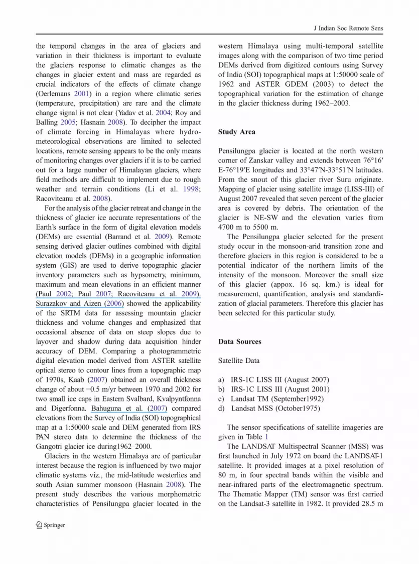
Methodology

To compute changes in the morphometric parametersbetween different time domains using multi temoporalsatellite images it is required that all the imagesshould be co-registered. The LANDSAT MSS imageof 1975, IRS LISS-III images of 2001 and 2007 wereregistered to the LANDSAT TM image of 1992(which is used as the base image). The mediumresolution sensors such as LANDSAT TM/ETM+

have no significant relief displacement (Konecny1979; Thakur et al. 2008) and therefore we selectedLANDSAT TM image-1992 as a base image. UTMprojection system was followed using WGS-84datum. To register the scenes, about 100 tie pointscommon between the LANDSAT TM image and otherimages were determined. A second order polynomialwas used to warp each image to the base image. Theregistration error were 1 pixel or 28.5 m and 0.5 pixelor 14 m while registering the 1975 MSS image (80 mresolution) and IRS LISS-III images (23.5 m resolu-tion) to the base image respectively.

The glacier inventory using different period satellitedata was performed by delineating the glacier boundary(Fig. 2) based on identification of the glacier featuresby visual on screen interpretation and their on screendigitization using Geographic Information System(GIS) on ArcGIS 8.3 platform. The adequate spatialresolution of 23.5 m of LISS-III satellite data allowedmapping of glacier boundaries using False ColourComposite (FCC) image with standard combination ofbands, 432 on RGB. The upper boundary of theglaciers at the accumulation area can be demarcated bythe ice divide. It is a line of division between twoadjacent glaciers and characterized by ice movement intwo different directions (Kulkarni 1991). In the area,ice divides associated with mountain cliff can bedelineated by using cliff shadow. Parts of the glaciercovered by moraines can be delineated on a LISS-IIISWIR, NIR and G (as RGB) composite image.Reflectance of rock in SWIR band is higher than that

of ice, which makes debris cover on glacier appear inreddish tone (Kulkarni et al. 2005). Ablation zone ofthe glacier was differentiated from the surroundingrocky terrain (which appears in bright reddish colour)by its colour and longitudinal pattern of moraines. Thepresence of small glacial lakes and ponds over someglaciers was also helpful in accurately demarcating theglacier boundary in the debris-covered glaciers. Thenon-glacier area present in front of the glacier snoutexhibiting bright tone with fine texture in contrast tocoarse and mottled texture over glacier surface helpedin the delineation of glacier lower limits.

In the present study a TM4/TM5 band-ratio image issegmented into two classes viz., ‘glacier’ and otherusing a threshold value of 2.0. Similar method was usedby Paul et al. (2004) in the study of debris coveredglaciers in Swiss Alps. Normalized Difference SnowIndex (NDSI) was applied to distinguish snow fromsimilarly bright soil and rock, as well as from clouds inTM imagery (Dozier 1989; Hall et al. 1995a). Itseffectiveness in mapping snow cover over ruggedterrain has been demonstrated by Hall et al. (1995b).It was found that demarcations of stream emerging atsnout and transverse crevasses developed near thesnout are also better identified in NDSI image.

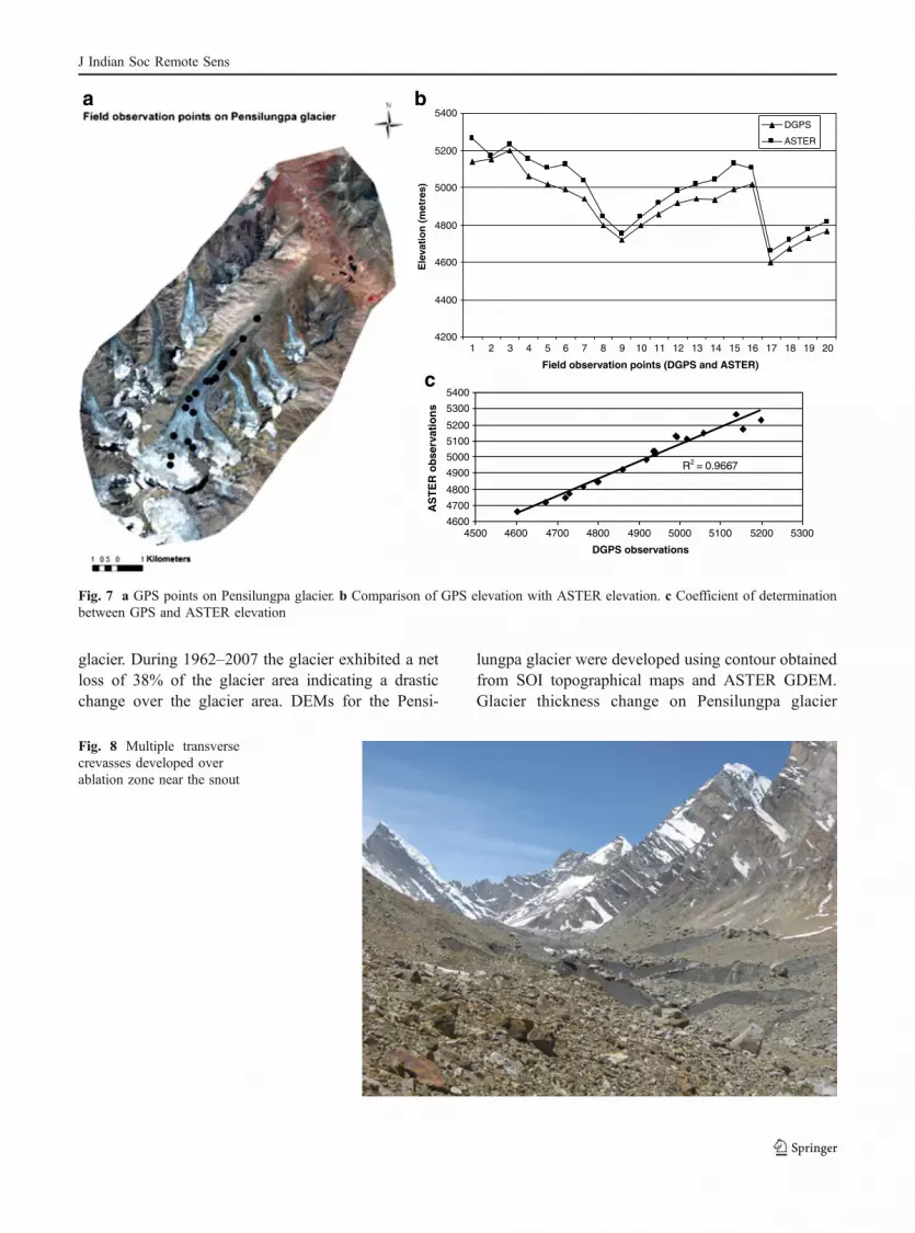
The study pertaining to glacier thickness changesinvolved creation of two DEMs representing topograph-ical variation over the Pensilungpa glacier during 1962(SOI DEM) and 2003 (ASTER DEM). To evaluatetopographic variability from snout to the top of theglacier longitudinal valley profile (Fig. 5b) along the lineAB (Fig. 5a) extending from the accumulation zone tothe snout of the glacier along the central line wasprepared using the two DEMs. Change detection inelevation (Fig. 6) over glacier using these DEMs washelpful in determining the topographic change over theglacier. The glacier locations (Fig. 7a) where fieldmeasurement of elevation using DGPS survey wasconducted in the month of August, 2007 were related tothe elevation values obtained from ASTER DEM.These elevation values (Fig. 7b) where used to calculatethe coefficient of determination (Fig. 7c) betweenglacier elevation recorded by DGPS and ASTERDEM. The methodology flowchart is given in Fig. 1.

Error Analysis

Williams et al. (1997), Hall et al. (2003), Jin et al.(2005), Wang et al. (2009) estimated the terminus

J Indian Soc Remote Sens

change uncertainty ‘U’ associating the spatial reso-lutions of the datasets and the errors in imageryregistration by the following equation

U ¼ pa2 þ b2� �þ s

Where ‘a’ and ‘b’ are the image resolutions of images‘a’ and ‘b’ respectively and σ is the error in imageregistration.

The registration error while registering 1975 MSSimage (80 m resolution) and IRS LISS-III images(23.5 m resolution) to the base image were 1 pixel or28.5 m (28.5*1=28.5) and 0.5 pixel or 14 m(28.5*0.5=14) respectively. The registration errorwas added up over the uncertainty value to computemeasured error between two images.

Changes in the snout position of glaciers wasmeasured digitally with an accuracy of ±85 mwhen registering 1975 MSS image to the baseimage and ±37 m when registering the LISS-IIIimages of 2001 and 2007 to the base image.Adding the registration error to the computeduncertainty, the overall accuracy becomes ±113 mfor the MSS data registration, ±51 m for the LISS-III data registration.

Changes in the areal extent of the glaciers weremeasured with an accuracy of ±0.0136 km2 usingMSS image, ±0.0017 km2 using the LISS III images

by using the following formula (Hall et al. 2003;Wang et al. 2009):

Uarea ¼ 2UV

Where ‘U’ is the terminus uncertainty and V is theimage pixel resolution.

The total uncertainty of glacier area on topographicmaps can be estimated by the following formula forerror propagation (Bevington 1969; Jin et al. 2005;Wang et al. 2009)

Uncertainty ¼ pS1»5%ð Þ2 þ S2»5%ð Þ2

�

þ . . . . . . . . . . . . . . . Sn»5%ð Þ2�

Where Sn is glacier area and n is the number of glaciers.Using this formula the total uncertainty of Pensilungpa

glacier area mapped from SOI topographical map of1962 was estimated. The whole glacierized area estimatefor the year 1962 is 23.82 sq km±1.2 sq km (Fig. 2).

Results

Morphometric Parametres

The glacier length is found to be 8.69 km in 1962,decreasing to 8.49 km in 2007 showing an overall

Data Sources

Satellite Data IRS-1C LISS III (2001 & 2007) Landsat TM (1992) Landsat MSS (1975)

Topographical Map (1962) Field Observation ASTER DEM

(2003)

Georeferencing

Glacier boundary delineation

Glacier Area Computation

Glacier Area Change Detection

Contour Extraction

DEM Generation

Longitudinal valley profile generation

Elevation Accuracy Estimation

Difference Map generation

Glacier topographic change detection

Glacier change evaluation

Fig. 1 Methodology flowchart

J Indian Soc Remote Sens

decrease of only 0.2 km during 1962–2007(Fig. 3a). During 1962–1975 the perimeter of theglacier was drastically decreased from 62 km to32 km probably due to detachment of tributaryglaciers or shrinkage of the glacier area in the upperablation zone of the glacier which also resulted in thechange of the shape of the glacier (Fig. 3b). Theglacier area is found to be 23.82 sq. km. in 1962,decreasing to 14.59 sq. km in 2007. The area of theglacier was continuously decreasing during 1975–2007 with an overall loss of 11.12 sq. km. (Fig. 3c).

It is inferred that a net loss of 9.23 sq. km. whichis 38% of the glacier area in 1962 indicate a drasticchange over the glacier area during 1962–2007.Computation of per year change percentage(Fig. 4a) over glacier area revealed that maximumpercentage area loss/year (2.8%) took place during1992–2001. There is a net loss of 0.86% per yearover the glacier area during 1962–2007. Analyzingthe contribution of the study periods (Fig. 4b)towards the area change over the glacier it wasevident that during 1992–2001 the area loss wasmaximum.

Topographical Change Detection

Longitudinal profile (Fig. 5b) was drawn along thecentral line (A-B in Fig. 5a) of the glacier from snoutto the highest point of the glacier. Comparison oflongitudinal profiles prepared from the SOI DEM andASTER DEM indicated that the glacier was occupy-ing lower topographic levels in the accumulation aswell as parts of upper ablation zone during the 1962period. On the contrary the entire lower and middleablation zone as well as a part of upper ablation zonewas occupying higher topographic levels during thesame period. This indicates that during the period of1962–2003 overall thickening in the glacier wasrecorded in the accumulation zone whereas a thinningwas recorded in the ablation zone. The elevationdifference obtained through procedure of imagesubtraction of two DEMS (Fig. 6) clearly depictstopographic rise in the accumulation zone and theupper ablation zone whereas topographic fall occursin middle ablation zone and lower ablation zone.

Estimation of glacier thickness change on Pensi-lungpa glacier based on ASTER DEM (2003) andSOI DEM (1962) indicated increase in the glacier

Fig. 2 Glacier boundary in 1962 and 2007

6.5

7

7.5

8

8.5

9

9.5

1962 1975 1992 2001 2007

Observation periods

1962 1975 1992 2001 2007

Observation periods

1962 1975 1992 2001 2007

Observation periods

Leng

th (

km)

0

10203040506070

Per

imet

re (

km)

a b

05

1015202530

Are

a (s

q km

)

c

Fig. 3 a–c Dimensions of the glacier during different periods

J Indian Soc Remote Sens

elevation in the accumulation zone up mainly by 30 to90 m and similar reduction by 30 to 90 m in ablationzone against area change of 9.23 sq km. Surazakovand Aizen (2006) reported thinning of Akshiirakglaciers (Tien Shan, Central Asia) up to 126 m onsimilar lines using the Shuttle Radar TopographyMission (SRTM) C-band data (2000) and a digitalelevation model (DEM) generated from topographicmaps. In the Basapa valley, Himachal PradeshBahuguna and Kulkarni (2005) estimated reductionin thickness of ice (35 m) in the deglaciated part ofthe Shaune garang glacier on the basis of change inthe elevations of the glacial surface from 1963 to1998 and supported this view by field verification.

Field verification over Pensilungpa glacier (Fig. 7a)was done to estimate the errors between the field basedelevation observation using Differential Global Posi-tioning System (DGPS) and the elevation recorded onASTER DEMs at the same place. These elevation

values (Fig. 7b) were used to calculate the coefficientof determination between DGPS and Aster DEMobservation. The R2 value (0.96) (Fig. 7c) indicated avery good correlation between the field based andsatellite based elevation observation indicating suit-ability of satellite based elevation measurement overthe glaciers even though the reported vertical accuracyof ASTER GDEM is 20 m.

Discussion

The use of multi temporal space imagery for glaciermonitoring is well known (Bolch et al. 2008). Since theadvent of satellite remote sensing and its data avail-ability to researchers from 1972 onwards, mapping andmonitoring of glaciers become more popular because ofits multi-spectral nature, temporal availability andgradual improvement in resolution. The area changes

Per year change % in glacierarea during different years

-3-2-101

1962-1975

1975-1992

1992-2001

2001-2007

Observation years

Per

yea

rch

ange

%

Glacier area change comparison between observation periods

-100%-80%-60%-40%-20%

0%20%

% c

ompa

rison

of o

bser

vatio

npe

riods

to a

rea

2001-2007

1992-2001

1975-1992

1962-1975

a bFig. 4 a–b Glacier areachange analysis

Lower ablation zone

Middle ablation zone

Upper ablation zone

Accumulation zone

Snout

A

B

Snout

Lower ablation Zone

Upper ablation Zone

Accumulation Zone

Middle ablation Zone

B

A

a b

Fig. 5 a False Colour Composite (FCC) image of thePensilungpa (Suru) glacier with standard combination of bands,432 as RGB. Longitudinal profile is drawn along the line A-B

to evaluate topographic variability from snout to the top of theglacier. b Showing longitudinal profile along the centre line ofthe glacier from snout to the highest point of the glacier

J Indian Soc Remote Sens

of the Pensilungpa glacier in the western Himalayabased on multi-temporal satellite images confirm theexpected and widely published retreat of glaciers in theregion. The variable rate of glacier area change duringthe study period (1962–2007) is comparable with thereported fluctuating glacial retreat rate in the adjacentbasins (Kulkarni et al. 2005). In the Chenab basinwestern Himalaya, the total area of Samudratapu glacierwas reduced by 13.7 sq km during 1963 to 2004(Shukla et al. 2009). The pronounced glacial area lossin the 1990s in the Pensilungpa glacier reflectingbehaviour similar to that of well investigated glaciersin the Naimona’nyi region of the western Himalaya (Yeet al. 2006) and in Khumbu Himal, Nepal (Bolch et al.2008).

Estimation of glacier thickness change on Pensi-lungpa glacier indicates increase in the glacier elevationin the accumulation zone and reduction in ablation zone.Similar results was shown by Kaab, (2007) indicatingloss of ice thickness of 25–50 m in the lower parts andincrease in the ice thickess in upper glacier part inEastern Svalbard. The topographic rise in the accumu-

lation zone and the upper ablation zone of thePensilungpa glacier obtained through procedure ofimage subtraction of SOI DEM and ASTER DEMcould be attributed to the increased snowfall over theglacier during this period. Accumulation of snow andresulted ice mass force down the glacier producingmore stress in glacier mass in the lower ablation zone.This could result in the development of deep crevassescausing defragmentation of glacier mass as recorded inthe field (Fig. 8).

It is well known that SOI maps are imprecise forglacier terrain in some instances (Bhambri and Bolch2009), but Survey of India (SOI) topographical mapsat 1:50000 scale of 1962 represents the best availabletopographic maps for the study area. Therefore thedigitized contours from SOI maps used to createDEM in the present study. Successful generation ofDEM using topographical maps at 1:50000 scale,1:100000 scale has also been reported in variouspublished work (Bolch 2004; Bahuguna et al. 2004;Kamp et al. 2005; Kaab 2007; Bahuguna et al. 2007).If no DEM of higher spatial resolution is available,information about topographic characteristics of gla-ciers can be obtained from ASTER GDEM (Frey andPaul 2011). Considering the spatial resolution of 30 m(1 arc-second), the ASTER GDEM provide thehighest resolution of freely available DEMs for theusers. The Shuttle Radar Topography Mission(SRTM) DEM and the Global Topographic Data(GTOPO30) are the other available global DEMreleased before ASTER GDEM with 90 m and1000 m posting interval, respectively (Arefi andReinartz 2010). Additionally the ASTER GDEM datais available for high latitude and steep mountainousareas which are not covered by SRTM due to radarshadowing and foreshortening effects (ERSDAC2010). The high cost of satellite data as well nonavailability of cloud free data over glaciers inHimalayas further hamper the remote sensing basedglacier research especially in elevation change studies.

Conclusions

The morphometric parameters derived from thesatellite image based glacier mapping and theircomparison with similar parameters obtained throughtopographical maps provided comparative assessmentof elevation changes vis-à-vis area changes over the

Fig. 6 Difference image between DEMs based on toposheetand ASTER

J Indian Soc Remote Sens

glacier. During 1962–2007 the glacier exhibited a netloss of 38% of the glacier area indicating a drasticchange over the glacier area. DEMs for the Pensi-

lungpa glacier were developed using contour obtainedfrom SOI topographical maps and ASTER GDEM.Glacier thickness change on Pensilungpa glacier

4200

4400

4600

4800

5000

5200

5400

1 2 3 4 5 6 7 8 9 10 11 12 13 14 15 16 17 18 19 20

Field observation points (DGPS and ASTER)

Ele

vati

on

(m

etre

s)

DGPS

ASTER

R2 = 0.9667

4600

4700

4800

4900

5000

5100

5200

5300

5400

4500 4600 4700 4800 4900 5000 5100 5200 5300

DGPS observations

AS

TE

R o

bse

rvat

ion

s

a b

c

Fig. 7 a GPS points on Pensilungpa glacier. b Comparison of GPS elevation with ASTER elevation. c Coefficient of determinationbetween GPS and ASTER elevation

Fig. 8 Multiple transversecrevasses developed overablation zone near the snout

J Indian Soc Remote Sens

based on ASTER DEM (2003) and SOI DEM(1962) indicated increase in the glacier elevation inthe accumulation zone mainly by 30 to 90 m andsimilar reduction by 30 to 90 m in ablation zoneagainst area change of 38% of glacier areameasured in 1962. The present study indicatedsuitability of present methodology for computingelevation changes over glaciers using DEMs of twodifferent periods. Although minor errors are evidentin the DEMs difference image, such errors can beminimized if DEMs with high spatial resolution likeIRS-Cartosat 2 can be utilized. The field validationconfirms the accuracy of elevation recorded throughDGPS and ASTER DEM. The non availability ofany satellite or ground based elevation measurementduring the 1962 period hinder the accuracy assess-ment of DEM derived from contours available onSOI topographical map.

References

Ahmed, S., Hasnain, S., & Selvan, M. (2004). Morpho-metriccharacteristic of glaciers in the Indian Himalayas. AsianJournal of Water, Environment and Pollution, 1(1 & 2),109–118.

Arefi, H., & Reinartz, P. (2010). Elimination of the Outliersfrom ASTER GDEM data. Canadian Geomatics. Conf.,Calgary, Canada, Jun. 14–18, 2010.

Bahuguna, I. M., & Kulkarni, A. V. (2005). Application ofdigital elevation model and orthoimages from IRS-1CPAN stereo data in monitoring variations in glacierdimensions. Journal of the Indian Society of RemoteSensing, 33(1), 107–112.

Bahuguna, I. M., Kulkarni, A. V., & Nayak, S. (2004).DEM from IRS-1C PAN stereo coverages over Hima-layan glaciated region—accuracy and its utility. Inter-national Journal of Remote Sensing, 25(19), 4029–4041.

Bahuguna, I. M., Kulkarni, A. V., Nayak, S., Rathore, B. P.,Negi, H. S., & Mathur, P. (2007). Himalayan glacier retreatusing IRS 1C PAN stereo data. International Journal ofRemote Sensing, 28(2), 437–442.

Bajracharya, S. R., Mool, P. K., & Shrestha, B. R. (2008).Global climate change and melting of Himalayan glaciers.In P. S. Ranade (Ed.), Melting Glaciers and Rising sealevels: Impacts and implications (pp. 28–46). India: TheIcfai’s University Press.

Barrand, N. E., Murray, T., James, T. D., Barr, S. L., & Mills, J.P. (2009). Instruments and methods: optimizing photo-grammetric DEMs for glacier volume change assessmentusing laser-scanning derived ground-control points. Jour-nal of Glaciology, 55(189), 106–116.

Bevington, P. R. (1969). Data reduction and error analysis forthe physical sciences. New York: McGraw-Hill.

Bhambri, R., & Bolch, T. (2009). Glacier mapping: a reviewwith special reference to the Indian Himalayas. Progress inPhysical Geography, 33(5), 672–704.

Bolch, T. (2004). Using ASTER and SRTM DEMS for studyingglaciers and Rockglaciers in northern Tien Shan. Proc.PartI of the Conf., Theoretical and applied problems ofgeography on a boundary of centuries, Almaty/Kasakhstan,Jun. 8–9, 2004, pp. 254–258.

Bolch, T., Buchroithner, M., Pieczonka, T., & Kunert, A.(2008). Planimetric and volumetric glacier changes in theKhumbu Himal, Nepal, since 1962 using Corona, LandsatTM and ASTER data. Journal of Glaciology, 54(187),592–600.

Dhobal, D. P., Gergan, J. T., & Thayyen, R. J. (2004). Recessionand morphogeometrical changes of Dokriani glacier(1962–1995), Garhwal Himalaya, India. Current Science,86(5), 692–696.

Dozier, J. (1989). Spectral signature of Alpine snow cover fromLandsat 5 TM. Remote Sensing of Environment, 28, 9–22.

ERSDAC (2010). Earth Remote Sensing Data Analysis Center.www.ersdac.or.jp.

Frey, H., & Paul, F. (2011). On the suitability of the SRTMDEM and ASTER GDEM for the compilation of topo-graphic parameters in glacier inventories. GeophysicalResearch Abstracts, 13.

Hall, D. K., Riggs, G. A., & Salomonson, V. V. (1995).Development of methods for mapping global snow coverusing Moderate Resolution Imaging Spectroradiometerdata. Remote Sensing of Environment, 54, 127–140.

Hall, D. K., Foster, J. L., Chein, J. Y. L., & Riggs, G. A. (1995).Determination of actual snow covered area using LandsatTM and digital model data in Glacier National Park,Montana. Polar Record, 31, 191–198.

Hall, D. K., Bayr, K. J., Schoner, W., Bindschadler, R. A., &Chien, J. Y. L. (2003). Consideration of the errors inherentin mapping historical glacier positions in Austria from theground and space (1893–2001). Remote Sensing ofEnvironment, 86(4), 566–577.

Hansen, J., Nazarenko, L., Ruedy, R., Sato, M., Willis, J.,Genio, A. D., et al. (2005). Earth’s energy imbalance:confirmation and implications. Science, 308, 1431–1435.

Hasnain, S. I. (2008). Impact of climate change on Himalayanglaciers and glacier lakes Proc. Taal2007: The 12th WorldLake Conf., Oct.29-Nov.2, 2007, pp. 1088–1091.

Herman, F., Anderson, B., & Leprince, S. (2011). Mountainglacier velocity variation during a retreat/advance cyclequantified using sub-pixel analysis of ASTER images.Journal of Glaciology, 57(202), 197–207.

Hewitt, K. (2005). The Karakoram Anomaly? Glacier Expan-sion and and the ‘Elevation Effect’, Karakoram Himalaya.Mountain Research and Development, 25(4), 332–340.

Hewitt, K. (2010). Understanding glacier changes. Chinadia-logue.

Jin, R., Li, X., Che, T., Wu, L., & Mool, P. (2005). Glacier areachanges in Pumqu river basin, Tibetan Plateau, betweenthe 1970s and 2001. Journal of Glaciology, 51(175), 607–610.

Kaab, A. (2007). Glacier volume changes using ASTER opticalstereo. ATest Study in Eastern Svalbard. Geoscience andRemote Sensing Symp., IGARSS, IEEE International, Jul.23–28, 2007, pp. 3994–3996.

J Indian Soc Remote Sens

Kamp, U., Bolch, T., & Olsenholler, J. (2005). Geomorphom-etry of Cerro Sillajhuay (Andes, Chile/Bolivia): compari-son of Digital Elevation Models (DEMs) from ASTERremote sensing data and contour maps. Geocarto Interna-tional, 20(1), 23–33.

Kaul, M. K. (1999). Inventory of Himalayan glaciers. Geolog-ical Survey of India, 34.

Konecny, G. (1979). Methods and possibilities for digitaldifferential rectification. Photogrammetric Engineeringand Remote Sensing, 6, 727–734.

Kulkarni, A. V. (1991). Glacier inventory in Himachal Pradeshusing satellite images. Journal of the Indian Society ofRemote Sensing, 19(3), 195–203.

Kulkarni, A. V., Mathur, P., Rathore, B. P., Alex, S., Thakur, N., &Kumar, M. (2002). Effect of global warming on snow ablationpattern in the Himalayas. Current Science, 83, 120–123.

Kulkarni, A. V., Rathore, B. P., Mahajan, S., & Mathur, P.(2005). Alarming retreat of Parbati Glacier, Beas basin,Himachal Pradesh. Current Science, 88, 1844–1850.

Li, Z., Sun, W., & Zeng, Q. (1998). Measurements of glaciervariation in the Tibetan plateau using Landsat data.Remote Sensing of Environment, 63, 258–264.

Meier, M. F., Dyurgerov, M. B., Rick, U. K., Neel, S. O.,Pfeffer, W. T., Anderson, R. S., et al. (2007). Glaciersdominate eustatic sea-level rise in the 21st century.Science, 317(5841), 1064–1067.

METI/ERSDAC, NASA/LPDAAC, USGS/EROS (2009). AS-TER GDEM Validation Summary Report.

Mool, P. K., Wangda, D., Bajracharya, S. R., Kunzang, K.,Gurung, D. R., & Joshi, S. P. (2001). Inventory of Glaciers,glacial Lakes and Glacial Lake outburst Floods, monitoringand early warning system in the Hindu Kush-Himalayanregion, Nepal, (UNEP/RCAP)/ICIMOD, Kathmandu.

Oerlemans, J. (2001). Glaciers and climatic change. Rotterdam:A.A Balkema Publishers.

Paul, F. (2002). Changes in glacier area in Tyrol, Austria,between1969 and 1992 derived from Landsat 5 thematicmapper and Austrian glacier inventory data. InternationalJournal of Remote Sensing, 23(4), 787–799.

Paul, F. (2007). The new Swiss glacier inventory 2000—Application of remote sensing and GIS. SchriftenreihePhysische Geographie, Universität Zürich, 52, 210.

Paul, F., Huggel, C., Kaab, A. (2004). Combining satellitemultispectral image data and a digital elevation model formapping debris-covered glaciers. Remote sensing ofEnvironment, 89, 510–518.

Prasad, A. K., Yang, K. H. S., El-Askary, H. M., & Kafatos, M.(2009). Melting of major Glaciers in the western Hima-layas: evidence of climatic changes from long term MSUderived tropospheric temperature trend (1979–2008).Annales Geophysicae, 27, 4505–4519.

Racoviteanu, A., Arnaud, Y., & Williams, M. (2008). Decadalchanges in glacier parameters in Cordillera Blanca, Peruderived from remote sensing. Journal of Glaciology, 54(186), 499–510.

Racoviteanu, A. E., Paul, F., Raup, B., Khalsa, S. J. S., &Armstrong, R. (2009). Challenges and recommendationsin mapping of glacier parameters from space: results of the2008 Global Land Ice Measurements from Space(GLIMS) workshop, Boulder, Colorado, USA. Annals ofGlaciology, 50(53), 53–69.

Rai, S. C., & Gurung, A. (2005). Raising awareness of theimpacts of climate changes. Mountain Research Develop-ment, 25(4), 316–320.

Roy, S. S., & Balling, R. C., Jr. (2005). Analysis of trends inmaximum and minimum temperature, diurnal temperaturerange, and cloud cover over India. Geophysical ResearchLetters, 32(12), 4.

Shukla, A., Gupta, R. P., & Arora, M. K. (2009). Instrumentsand Methods Estimation of debris cover and its temporalvariation using optical satellite sensor data: a case study inChenab basin, Himalaya. Journal of Glaciology, 55(191),444–452.

Srivastava, P. K., & Alurkar, M. S. (1997). Inflight calibrationof IRS-1C imaging geometry for data products. Journal ofPhotogrammetry & Remote Sensing, 52, 215–221.

Surazakov, A. B., & Aizen, V. B. (2006). Estimating volumechange of mountain glaciers using SRTM and map-basedtopographic data. IEEE Transactions on Geoscience andRemote Sensing, 44(10), 2991–2995.

Thakur, A. K., Singh, S., & Roy, P. S. (2008). Orthorectificationof IRS-P6 LISS IV data using Landsat ETM+ and SRTMdatasets in the Himalayas of Chamoli District, Uttarak-hand. Current Science, 95(10), 1458–1463.

Thayyen, R. J., & Gergan, J. T. (2010). Role of glaciers inWatershed Hydrology: a preliminary study of a Himalayancatchment. The Cryosphere, 4, 115–128.

Wang, Y., Hou, S., & Liu, Y. (2009). Glacier changes in theKarlik Shan, eastern Tien Shan, during 1971/72-2001/02.Annals of Glaciology, 50(53), 39–45.

Williams, R. S., Jr., Hall, D. K., Sigurdsson, O., & Chien, J. Y.L. (1997). Comparison of satellite-derived with ground-based measurements of the fluctuations of the margins ofVatnajo¨kull, Iceland, 1973–92. Annals of Glaciology, 24,72–80.

Yadav, R. R., Park, W. K., Singh, J., & Dubey, B. (2004). Do thewestern Himalayas defy global warming? GeophysicalResearch Letters, 31(17), 5.

Ye, Q., Yao, T., Kang, S., Chen, F., & Wang, J. (2006). Glaciervariations in the Naimona’nyi region, western Himalaya,in the last three decades. Annals of Glaciology, 43, 385–389.

J Indian Soc Remote Sens