A

Ta

b

c

a

ARA

KGVA

1

aat(mcetTcepsdoo

d1a

0h

International Journal of Applied Earth Observation and Geoinformation 28 (2014) 117–130

Contents lists available at ScienceDirect

International Journal of Applied Earth Observation andGeoinformation

jo ur nal home page: www.elsev ier .com/ locate / jag

rea-based and location-based validation of classified image objects

imothy G. Whitesidea,∗, Stefan W. Maierb, Guy S. Boggsc

Environmental Research Institute of the Supervising Scientist, Darwin, NT 0820, AustraliaResearch Institute of the Environment and Livelihoods, Charles Darwin University, Darwin, NT 0909, AustraliaWheatbelt NRM Inc, P.O. Box 311, Northam, WA 6401, Australia

r t i c l e i n f o

rticle history:eceived 19 June 2013ccepted 21 November 2013

eywords:eographic object-based image analysisalidationccuracy assessment

a b s t r a c t

Geographic object-based image analysis (GEOBIA) produces results that have both thematic and geomet-ric properties. Classified objects not only belong to particular classes but also have spatial properties suchas location and shape. Therefore, any accuracy assessment where quantification of area is required must(but often does not) take into account both thematic and geometric properties of the classified objects.By using location-based and area-based measures to compare classified objects to corresponding refer-ence objects, accuracy information for both thematic and geometric assessment is available. Our methodsprovide location-based and area-based measures with application to both a single-class feature detection

and a multi-class object-based land cover analysis. In each case the classification was compared to a GISlayer of associated reference data using randomly selected sample areas. Error is able to be pin-pointedspatially on per-object, per class and per-sample area bases although there is no indication whetherthe errors exist in the classification product or the reference data. This work showcases the utility ofthe methods for assessing the accuracy of GEOBIA derived classifications provided the reference data is

le sc

accurate and of comparab

. Introduction

Site-specific accuracy assessment methods typically associ-ted with per-pixel classifications (Congalton, 1991; Congaltonnd Green, 2009) have obvious limitations when applied withinhe geographic object-based image analysis (GEOBIA) paradigmClinton et al., 2010; Schöpfer and Lang, 2006). While these

ethods do provide information on the quality or accuracy of alassification at particular locations (x,y) across the image (Zhant al., 2005), when applied to the output of a GEOBIA, there is uncer-ainty about the extent of the reference class beyond that location.he assumption that the thematic value of that reference point isonsistent over the entire area of the object is therefore debatable,ven if the reference is large enough to be representative of thereferred block of pixels (Stehman and Wickham, 2011). In short,ingle pixel- and block-based approaches for accuracy assessmento not answer the following question: How well does the classifiedbject typify, both thematically and geometrically, the real worldbject it is meant to represent?

Methods of assessing image segmentation accuracy are well

ocumented (Clinton et al., 2010; Delves et al., 1992; Hoover et al.,996; Lucieer, 2004; Möller et al., 2007; Prieto and Allen, 2003),nd generally compare the output of a segmentation algorithm

∗ Corresponding author. Tel.: +61 8 89201161; fax: +61 8 89201195.E-mail address: tim.whiteside@environment.gov.au (T.G. Whiteside).

303-2434/$ – see front matter © 2013 Elsevier B.V. All rights reserved.ttp://dx.doi.org/10.1016/j.jag.2013.11.009

ale.© 2013 Elsevier B.V. All rights reserved.

to manually delineated features and their outlines in the imagery.Although segmentation accuracy can influence thematic accuracy,the methods do not assess thematic accuracy. Therefore, a methodof assessing both the thematic and geometric accuracy of classifiedobjects is needed (Schöpfer et al., 2008).

The accuracy assessment of GEOBIA outputs has been identifiedas an area of emerging research (Blaschke, 2010). One advantageof GEOBIA is an output (classified objects) that is claimed to beready for GIS implementation (Benz et al., 2004). While it is impor-tant to know how well an initial segmentation provides objectssuitable for classification (Clinton et al., 2010; Möller et al., 2007),the end result of objects also needs to be assessed particularlyif they are used as input into a GIS model or used in decisionmaking processes. For such an output to be valuable in GIS anal-ysis, the output would require an assessment of the geometricaccuracy (location and shape) of its classified objects (Schöpferet al., 2008). Traditional site-specific accuracy assessment methodsbased upon site-specific reference data, such as confusion matrices(Congalton and Green, 2009; Story and Congalton, 1986), do notprovide this type of information, and there has been very little workundertaken on determining suitable spatial accuracy measures forobject-based image analysis (Schöpfer et al., 2008; Weidner, 2008;Winter, 2000; Zhan et al., 2005). Much of the work has focussed

on the assessment of building detection where spatial accuracy is arequirement (Weidner, 2008; Winter, 2000). Very little researchhas been undertaken into the application of spatial accuracymeasures for object-based multi-class analysis (Lang et al., 2009;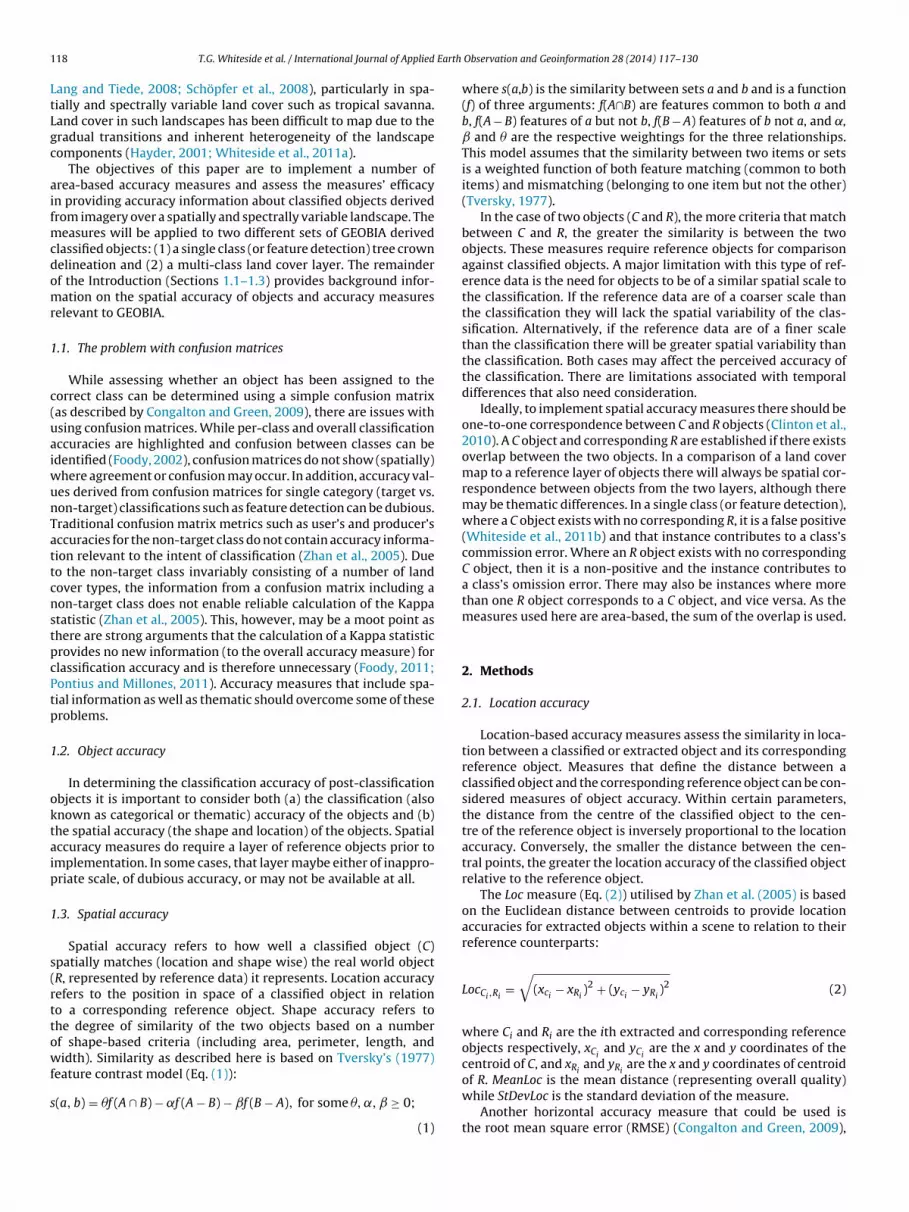

1 Earth

LtLgc

aifmcdomr

1

c(uaiwunTattcnstpcPtp

1

oktaip

1

s(rttowf

s

18 T.G. Whiteside et al. / International Journal of Applied

ang and Tiede, 2008; Schöpfer et al., 2008), particularly in spa-ially and spectrally variable land cover such as tropical savanna.and cover in such landscapes has been difficult to map due to theradual transitions and inherent heterogeneity of the landscapeomponents (Hayder, 2001; Whiteside et al., 2011a).

The objectives of this paper are to implement a number ofrea-based accuracy measures and assess the measures’ efficacyn providing accuracy information about classified objects derivedrom imagery over a spatially and spectrally variable landscape. The

easures will be applied to two different sets of GEOBIA derivedlassified objects: (1) a single class (or feature detection) tree crownelineation and (2) a multi-class land cover layer. The remainderf the Introduction (Sections 1.1–1.3) provides background infor-ation on the spatial accuracy of objects and accuracy measures

elevant to GEOBIA.

.1. The problem with confusion matrices

While assessing whether an object has been assigned to theorrect class can be determined using a simple confusion matrixas described by Congalton and Green, 2009), there are issues withsing confusion matrices. While per-class and overall classificationccuracies are highlighted and confusion between classes can bedentified (Foody, 2002), confusion matrices do not show (spatially)

here agreement or confusion may occur. In addition, accuracy val-es derived from confusion matrices for single category (target vs.on-target) classifications such as feature detection can be dubious.raditional confusion matrix metrics such as user’s and producer’sccuracies for the non-target class do not contain accuracy informa-ion relevant to the intent of classification (Zhan et al., 2005). Dueo the non-target class invariably consisting of a number of landover types, the information from a confusion matrix including aon-target class does not enable reliable calculation of the Kappatatistic (Zhan et al., 2005). This, however, may be a moot point ashere are strong arguments that the calculation of a Kappa statisticrovides no new information (to the overall accuracy measure) forlassification accuracy and is therefore unnecessary (Foody, 2011;ontius and Millones, 2011). Accuracy measures that include spa-ial information as well as thematic should overcome some of theseroblems.

.2. Object accuracy

In determining the classification accuracy of post-classificationbjects it is important to consider both (a) the classification (alsonown as categorical or thematic) accuracy of the objects and (b)he spatial accuracy (the shape and location) of the objects. Spatialccuracy measures do require a layer of reference objects prior tomplementation. In some cases, that layer maybe either of inappro-riate scale, of dubious accuracy, or may not be available at all.

.3. Spatial accuracy

Spatial accuracy refers to how well a classified object (C)patially matches (location and shape wise) the real world objectR, represented by reference data) it represents. Location accuracyefers to the position in space of a classified object in relationo a corresponding reference object. Shape accuracy refers tohe degree of similarity of the two objects based on a numberf shape-based criteria (including area, perimeter, length, andidth). Similarity as described here is based on Tversky’s (1977)

eature contrast model (Eq. (1)):

(a, b) = �f (A ∩ B) − ˛f (A − B) − ˇf (B − A), for some �, ˛, ≥ 0;

(1)

Observation and Geoinformation 28 (2014) 117–130

where s(a,b) is the similarity between sets a and b and is a function(f) of three arguments: f(A∩B) are features common to both a andb, f(A − B) features of a but not b, f(B − A) features of b not a, and ˛,

and � are the respective weightings for the three relationships.This model assumes that the similarity between two items or setsis a weighted function of both feature matching (common to bothitems) and mismatching (belonging to one item but not the other)(Tversky, 1977).

In the case of two objects (C and R), the more criteria that matchbetween C and R, the greater the similarity is between the twoobjects. These measures require reference objects for comparisonagainst classified objects. A major limitation with this type of ref-erence data is the need for objects to be of a similar spatial scale tothe classification. If the reference data are of a coarser scale thanthe classification they will lack the spatial variability of the clas-sification. Alternatively, if the reference data are of a finer scalethan the classification there will be greater spatial variability thanthe classification. Both cases may affect the perceived accuracy ofthe classification. There are limitations associated with temporaldifferences that also need consideration.

Ideally, to implement spatial accuracy measures there should beone-to-one correspondence between C and R objects (Clinton et al.,2010). A C object and corresponding R are established if there existsoverlap between the two objects. In a comparison of a land covermap to a reference layer of objects there will always be spatial cor-respondence between objects from the two layers, although theremay be thematic differences. In a single class (or feature detection),where a C object exists with no corresponding R, it is a false positive(Whiteside et al., 2011b) and that instance contributes to a class’scommission error. Where an R object exists with no correspondingC object, then it is a non-positive and the instance contributes toa class’s omission error. There may also be instances where morethan one R object corresponds to a C object, and vice versa. As themeasures used here are area-based, the sum of the overlap is used.

2. Methods

2.1. Location accuracy

Location-based accuracy measures assess the similarity in loca-tion between a classified or extracted object and its correspondingreference object. Measures that define the distance between aclassified object and the corresponding reference object can be con-sidered measures of object accuracy. Within certain parameters,the distance from the centre of the classified object to the cen-tre of the reference object is inversely proportional to the locationaccuracy. Conversely, the smaller the distance between the cen-tral points, the greater the location accuracy of the classified objectrelative to the reference object.

The Loc measure (Eq. (2)) utilised by Zhan et al. (2005) is basedon the Euclidean distance between centroids to provide locationaccuracies for extracted objects within a scene to relation to theirreference counterparts:

LocCi,Ri=

√(xci

− xRi)2 + (yci

− yRi)2 (2)

where Ci and Ri are the ith extracted and corresponding referenceobjects respectively, xCi

and yCiare the x and y coordinates of the

centroid of C, and xRiand yRi

are the x and y coordinates of centroid

of R. MeanLoc is the mean distance (representing overall quality)while StDevLoc is the standard deviation of the measure.

Another horizontal accuracy measure that could be used isthe root mean square error (RMSE) (Congalton and Green, 2009),

T.G. Whiteside et al. / International Journal of Applied Earth Observation and Geoinformation 28 (2014) 117–130 119

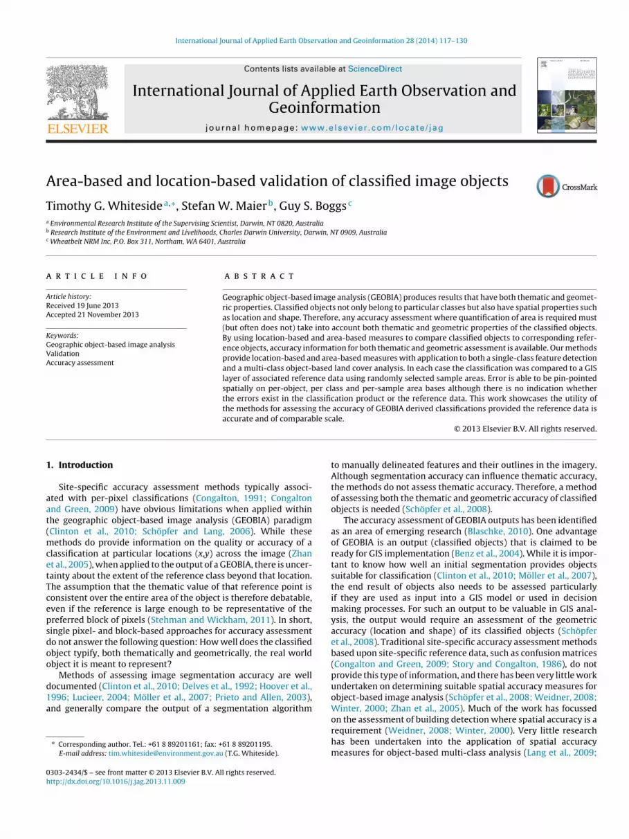
Fig. 1. Five topological relationships between two objects: (a) disjoint, (b) overlap, (c) contains, (d) contained by, and (e) equal. (For interpretation of the references to colorin text, the reader is referred to the web version of the article.)

F refert n of th

ar

R

w

br2

2

bWret2

i

ii

iv

v

f

∣∣C ∪ R∣∣ =

∣∣C ∩ R∣∣ +

∣∣C ∩ ¬R∣∣ +

∣∣¬C ∩ R∣∣ (4)

Using Eq. (4), the 5 spatial relationships between C and Robjects listed above and shown in Fig. 1 can be described relative

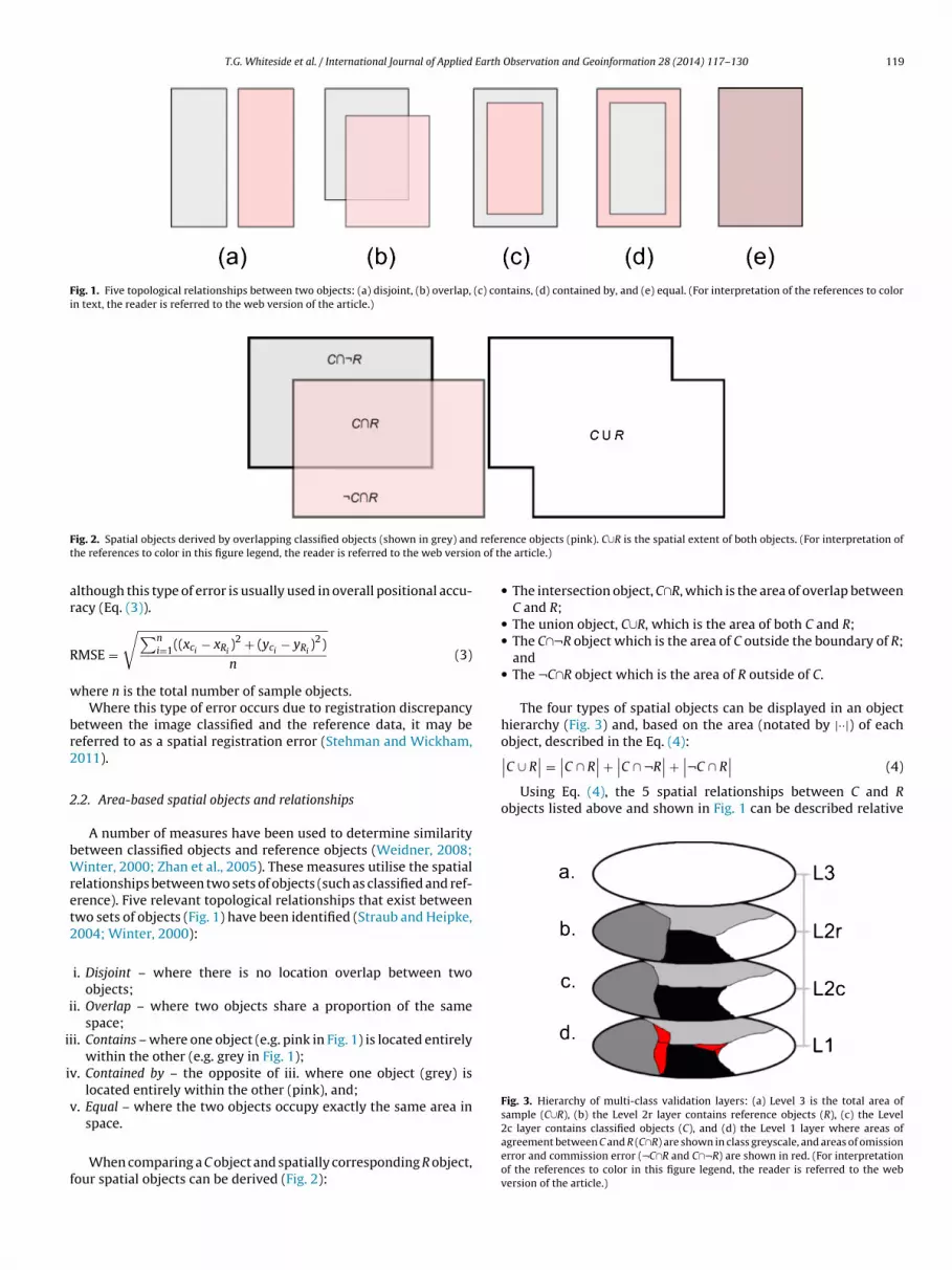
Fig. 3. Hierarchy of multi-class validation layers: (a) Level 3 is the total area ofsample (C∪R), (b) the Level 2r layer contains reference objects (R), (c) the Level

ig. 2. Spatial objects derived by overlapping classified objects (shown in grey) andhe references to color in this figure legend, the reader is referred to the web versio

lthough this type of error is usually used in overall positional accu-acy (Eq. (3)).

MSE =√∑n

i=1((xci− xRi

)2 + (yci− yRi

)2)

n(3)

here n is the total number of sample objects.Where this type of error occurs due to registration discrepancy

etween the image classified and the reference data, it may beeferred to as a spatial registration error (Stehman and Wickham,011).

.2. Area-based spatial objects and relationships

A number of measures have been used to determine similarityetween classified objects and reference objects (Weidner, 2008;inter, 2000; Zhan et al., 2005). These measures utilise the spatial

elationships between two sets of objects (such as classified and ref-rence). Five relevant topological relationships that exist betweenwo sets of objects (Fig. 1) have been identified (Straub and Heipke,004; Winter, 2000):

i. Disjoint – where there is no location overlap between twoobjects;

i. Overlap – where two objects share a proportion of the samespace;

i. Contains – where one object (e.g. pink in Fig. 1) is located entirelywithin the other (e.g. grey in Fig. 1);

. Contained by – the opposite of iii. where one object (grey) islocated entirely within the other (pink), and;

. Equal – where the two objects occupy exactly the same area in

space.

When comparing a C object and spatially corresponding R object,our spatial objects can be derived (Fig. 2):

ence objects (pink). C∪R is the spatial extent of both objects. (For interpretation ofe article.)

• The intersection object, C∩R, which is the area of overlap betweenC and R;

• The union object, C∪R, which is the area of both C and R;• The C∩¬R object which is the area of C outside the boundary of R;

and• The ¬C∩R object which is the area of R outside of C.

The four types of spatial objects can be displayed in an objecthierarchy (Fig. 3) and, based on the area (notated by |··|) of eachobject, described in the Eq. (4):

2c layer contains classified objects (C), and (d) the Level 1 layer where areas ofagreement between C and R (C∩R) are shown in class greyscale, and areas of omissionerror and commission error (¬C∩R and C∩¬R) are shown in red. (For interpretationof the references to color in this figure legend, the reader is referred to the webversion of the article.)

120 T.G. Whiteside et al. / International Journal of Applied Earth Observation and Geoinformation 28 (2014) 117–130

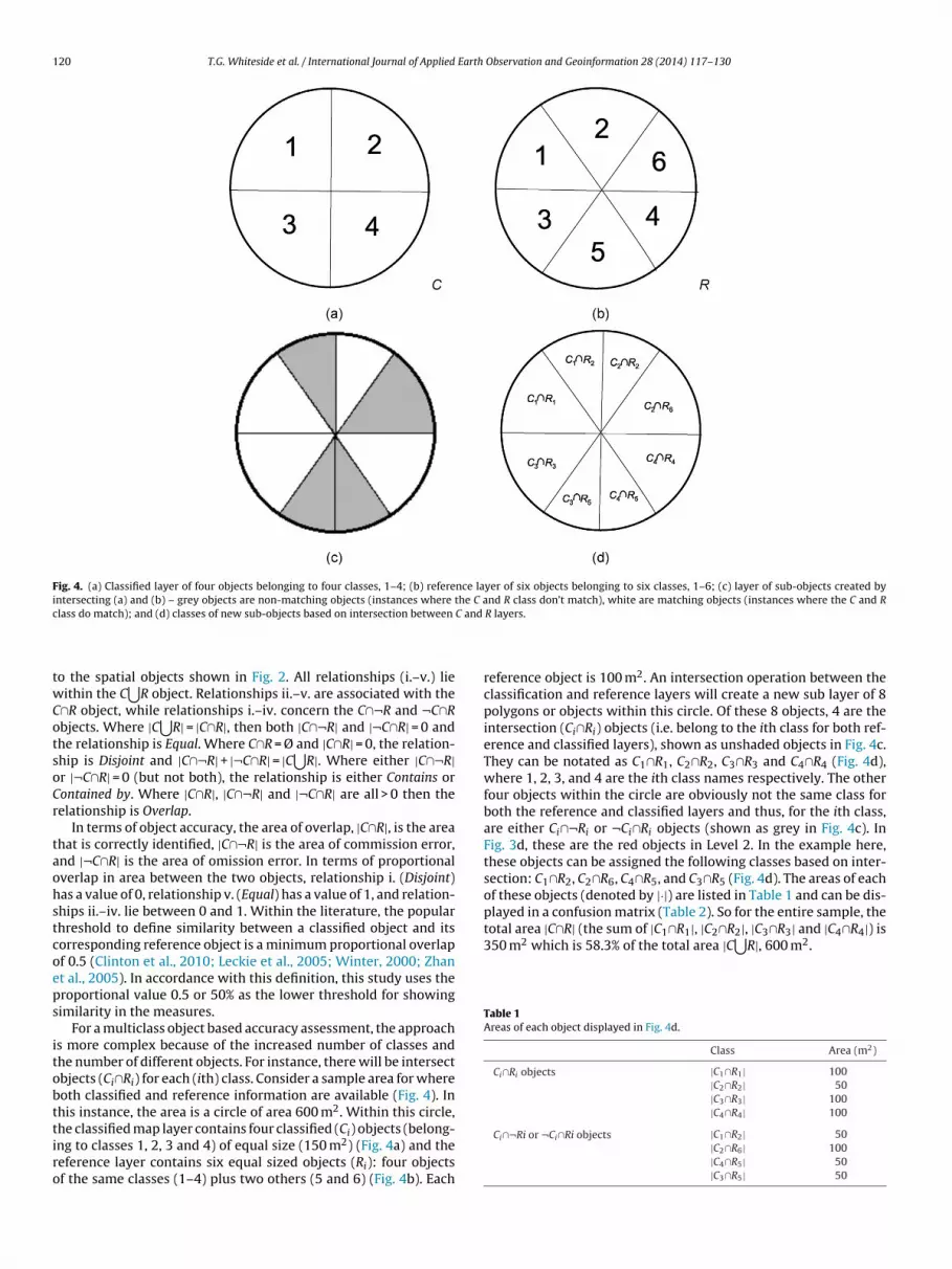
Fig. 4. (a) Classified layer of four objects belonging to four classes, 1–4; (b) reference layer of six objects belonging to six classes, 1–6; (c) layer of sub-objects created byintersecting (a) and (b) – grey objects are non-matching objects (instances where the C and R class don’t match), white are matching objects (instances where the C and Rc C and

twCotsoCr

taohstcoeps

itobttiro

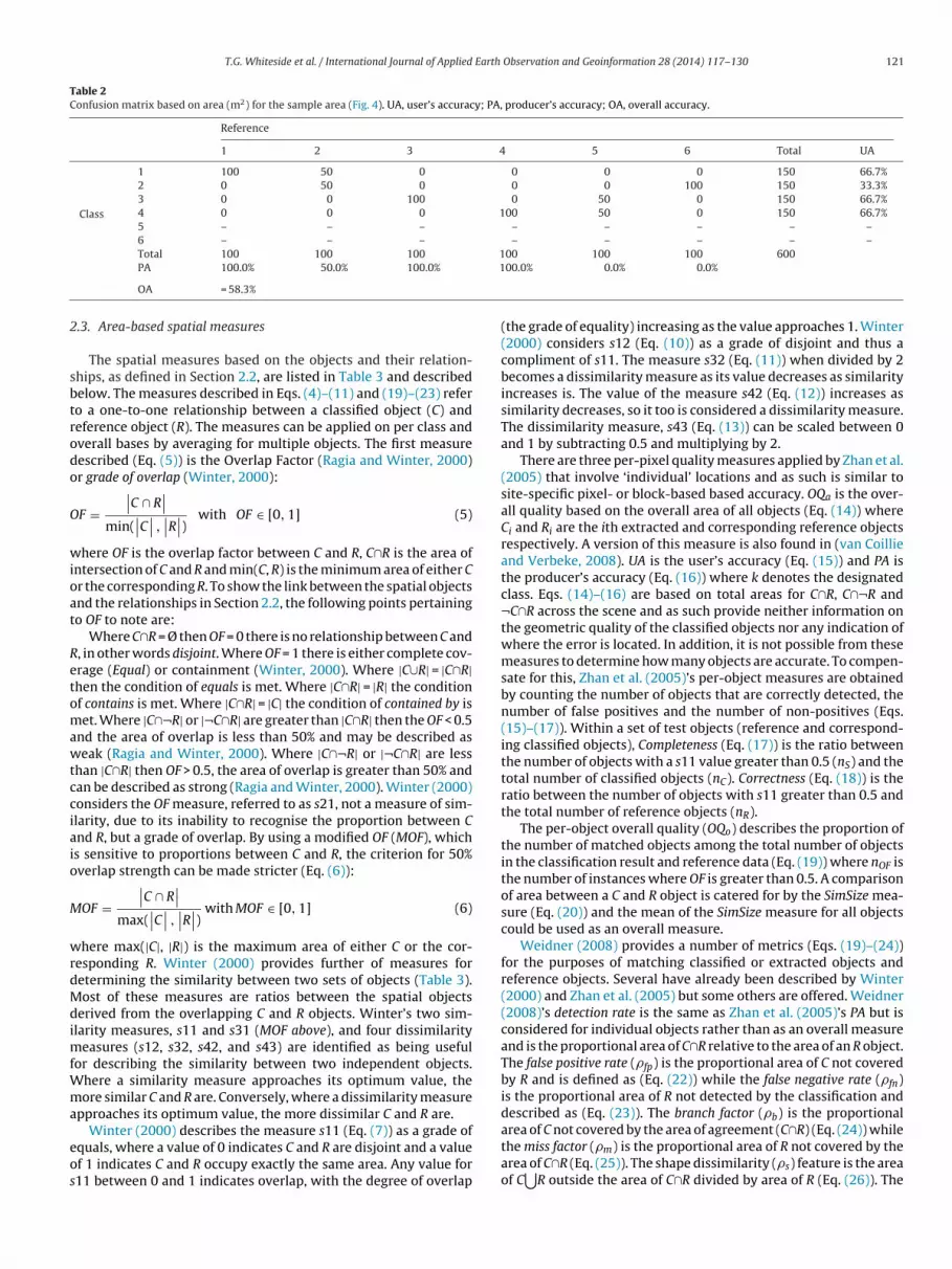
total area |C∩R| (the sum of |C1∩R1|, |C2∩R2|, |C3∩R3| and |C4∩R4|) is350 m2 which is 58.3% of the total area |C

⋃R|, 600 m2.

Table 1Areas of each object displayed in Fig. 4d.

Class Area (m2)

Ci∩Ri objects |C1∩R1| 100|C2∩R2| 50|C3∩R3| 100|C4∩R4| 100

lass do match); and (d) classes of new sub-objects based on intersection between

o the spatial objects shown in Fig. 2. All relationships (i.–v.) lieithin the C

⋃R object. Relationships ii.–v. are associated with the

∩R object, while relationships i.–iv. concern the C∩¬R and ¬C∩Rbjects. Where |C⋃

R| = |C∩R|, then both |C∩¬R| and |¬C∩R| = 0 andhe relationship is Equal. Where C∩R = Ø and |C∩R| = 0, the relation-hip is Disjoint and |C∩¬R| + |¬C∩R| = |C

⋃R|. Where either |C∩¬R|

r |¬C∩R| = 0 (but not both), the relationship is either Contains orontained by. Where |C∩R|, |C∩¬R| and |¬C∩R| are all > 0 then theelationship is Overlap.

In terms of object accuracy, the area of overlap, |C∩R|, is the areahat is correctly identified, |C∩¬R| is the area of commission error,nd |¬C∩R| is the area of omission error. In terms of proportionalverlap in area between the two objects, relationship i. (Disjoint)as a value of 0, relationship v. (Equal) has a value of 1, and relation-hips ii.–iv. lie between 0 and 1. Within the literature, the popularhreshold to define similarity between a classified object and itsorresponding reference object is a minimum proportional overlapf 0.5 (Clinton et al., 2010; Leckie et al., 2005; Winter, 2000; Zhant al., 2005). In accordance with this definition, this study uses theroportional value 0.5 or 50% as the lower threshold for showingimilarity in the measures.

For a multiclass object based accuracy assessment, the approachs more complex because of the increased number of classes andhe number of different objects. For instance, there will be intersectbjects (Ci∩Ri) for each (ith) class. Consider a sample area for whereoth classified and reference information are available (Fig. 4). Inhis instance, the area is a circle of area 600 m2. Within this circle,

he classified map layer contains four classified (Ci) objects (belong-ng to classes 1, 2, 3 and 4) of equal size (150 m2) (Fig. 4a) and theeference layer contains six equal sized objects (Ri): four objectsf the same classes (1–4) plus two others (5 and 6) (Fig. 4b). Each

R layers.

reference object is 100 m2. An intersection operation between theclassification and reference layers will create a new sub layer of 8polygons or objects within this circle. Of these 8 objects, 4 are theintersection (Ci∩Ri) objects (i.e. belong to the ith class for both ref-erence and classified layers), shown as unshaded objects in Fig. 4c.They can be notated as C1∩R1, C2∩R2, C3∩R3 and C4∩R4 (Fig. 4d),where 1, 2, 3, and 4 are the ith class names respectively. The otherfour objects within the circle are obviously not the same class forboth the reference and classified layers and thus, for the ith class,are either Ci∩¬Ri or ¬Ci∩Ri objects (shown as grey in Fig. 4c). InFig. 3d, these are the red objects in Level 2. In the example here,these objects can be assigned the following classes based on inter-section: C1∩R2, C2∩R6, C4∩R5, and C3∩R5 (Fig. 4d). The areas of eachof these objects (denoted by |·|) are listed in Table 1 and can be dis-played in a confusion matrix (Table 2). So for the entire sample, the

Ci∩¬Ri or ¬Ci∩Ri objects |C1∩R2| 50|C2∩R6| 100|C4∩R5| 50|C3∩R5| 50

T.G. Whiteside et al. / International Journal of Applied Earth Observation and Geoinformation 28 (2014) 117–130 121

Table 2Confusion matrix based on area (m2) for the sample area (Fig. 4). UA, user’s accuracy; PA, producer’s accuracy; OA, overall accuracy.

Reference

1 2 3 4 5 6 Total UA

Class

1 100 50 0 0 0 0 150 66.7%2 0 50 0 0 0 100 150 33.3%3 0 0 100 0 50 0 150 66.7%4 0 0 0 100 50 0 150 66.7%5 – – – – – – – –6 – – – – – – – –Total 100 100 100 100 100 100 600

1

2

sbtrodo

O

wioat

Retomawtcciaio

M

wrdMdimfWma

eos

PA 100.0% 50.0% 100.0%

OA = 58.3%

.3. Area-based spatial measures

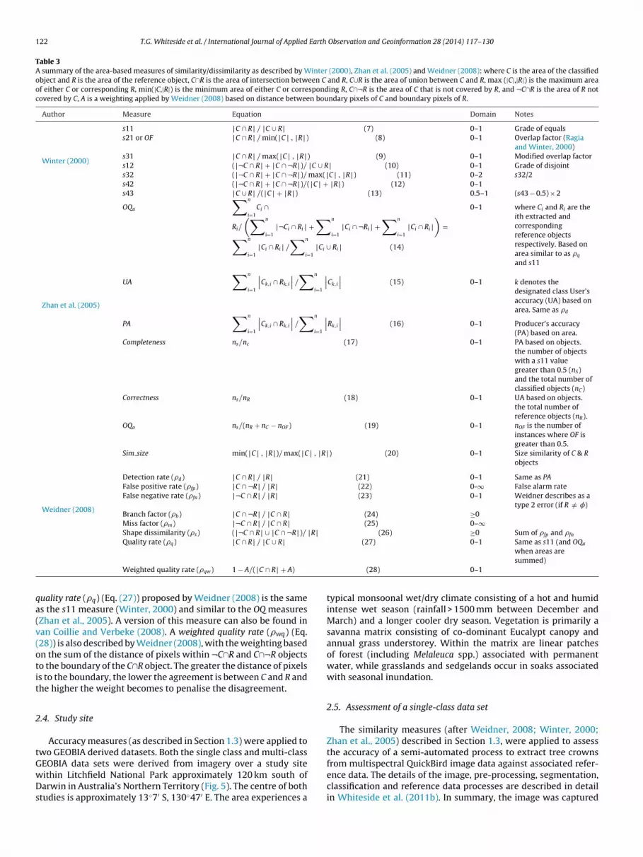
The spatial measures based on the objects and their relation-hips, as defined in Section 2.2, are listed in Table 3 and describedelow. The measures described in Eqs. (4)–(11) and (19)–(23) refero a one-to-one relationship between a classified object (C) andeference object (R). The measures can be applied on per class andverall bases by averaging for multiple objects. The first measureescribed (Eq. (5)) is the Overlap Factor (Ragia and Winter, 2000)r grade of overlap (Winter, 2000):

F =∣∣C ∩ R

∣∣min(

∣∣C∣∣ ,∣∣R∣∣) with OF ∈ [0, 1] (5)

here OF is the overlap factor between C and R, C∩R is the area ofntersection of C and R and min(C, R) is the minimum area of either Cr the corresponding R. To show the link between the spatial objectsnd the relationships in Section 2.2, the following points pertainingo OF to note are:

Where C∩R = Ø then OF = 0 there is no relationship between C and, in other words disjoint. Where OF = 1 there is either complete cov-rage (Equal) or containment (Winter, 2000). Where |C∪R| = |C∩R|hen the condition of equals is met. Where |C∩R| = |R| the conditionf contains is met. Where |C∩R| = |C| the condition of contained by iset. Where |C∩¬R| or |¬C∩R| are greater than |C∩R| then the OF < 0.5

nd the area of overlap is less than 50% and may be described aseak (Ragia and Winter, 2000). Where |C∩¬R| or |¬C∩R| are less

han |C∩R| then OF > 0.5, the area of overlap is greater than 50% andan be described as strong (Ragia and Winter, 2000). Winter (2000)onsiders the OF measure, referred to as s21, not a measure of sim-larity, due to its inability to recognise the proportion between Cnd R, but a grade of overlap. By using a modified OF (MOF), whichs sensitive to proportions between C and R, the criterion for 50%verlap strength can be made stricter (Eq. (6)):

OF =∣∣C ∩ R

∣∣max(

∣∣C∣∣ ,∣∣R∣∣) with MOF ∈ [0, 1] (6)

here max(|C|, |R|) is the maximum area of either C or the cor-esponding R. Winter (2000) provides further of measures foretermining the similarity between two sets of objects (Table 3).ost of these measures are ratios between the spatial objects

erived from the overlapping C and R objects. Winter’s two sim-larity measures, s11 and s31 (MOF above), and four dissimilarity

easures (s12, s32, s42, and s43) are identified as being usefulor describing the similarity between two independent objects.

here a similarity measure approaches its optimum value, theore similar C and R are. Conversely, where a dissimilarity measure

pproaches its optimum value, the more dissimilar C and R are.

Winter (2000) describes the measure s11 (Eq. (7)) as a grade of

quals, where a value of 0 indicates C and R are disjoint and a valuef 1 indicates C and R occupy exactly the same area. Any value for11 between 0 and 1 indicates overlap, with the degree of overlap

00.0% 0.0% 0.0%

(the grade of equality) increasing as the value approaches 1. Winter(2000) considers s12 (Eq. (10)) as a grade of disjoint and thus acompliment of s11. The measure s32 (Eq. (11)) when divided by 2becomes a dissimilarity measure as its value decreases as similarityincreases is. The value of the measure s42 (Eq. (12)) increases assimilarity decreases, so it too is considered a dissimilarity measure.The dissimilarity measure, s43 (Eq. (13)) can be scaled between 0and 1 by subtracting 0.5 and multiplying by 2.

There are three per-pixel quality measures applied by Zhan et al.(2005) that involve ‘individual’ locations and as such is similar tosite-specific pixel- or block-based based accuracy. OQa is the over-all quality based on the overall area of all objects (Eq. (14)) whereCi and Ri are the ith extracted and corresponding reference objectsrespectively. A version of this measure is also found in (van Coillieand Verbeke, 2008). UA is the user’s accuracy (Eq. (15)) and PA isthe producer’s accuracy (Eq. (16)) where k denotes the designatedclass. Eqs. (14)–(16) are based on total areas for C∩R, C∩¬R and¬C∩R across the scene and as such provide neither information onthe geometric quality of the classified objects nor any indication ofwhere the error is located. In addition, it is not possible from thesemeasures to determine how many objects are accurate. To compen-sate for this, Zhan et al. (2005)’s per-object measures are obtainedby counting the number of objects that are correctly detected, thenumber of false positives and the number of non-positives (Eqs.(15)–(17)). Within a set of test objects (reference and correspond-ing classified objects), Completeness (Eq. (17)) is the ratio betweenthe number of objects with a s11 value greater than 0.5 (nS) and thetotal number of classified objects (nC). Correctness (Eq. (18)) is theratio between the number of objects with s11 greater than 0.5 andthe total number of reference objects (nR).

The per-object overall quality (OQo) describes the proportion ofthe number of matched objects among the total number of objectsin the classification result and reference data (Eq. (19)) where nOF isthe number of instances where OF is greater than 0.5. A comparisonof area between a C and R object is catered for by the SimSize mea-sure (Eq. (20)) and the mean of the SimSize measure for all objectscould be used as an overall measure.

Weidner (2008) provides a number of metrics (Eqs. (19)–(24))for the purposes of matching classified or extracted objects andreference objects. Several have already been described by Winter(2000) and Zhan et al. (2005) but some others are offered. Weidner(2008)’s detection rate is the same as Zhan et al. (2005)’s PA but isconsidered for individual objects rather than as an overall measureand is the proportional area of C∩R relative to the area of an R object.The false positive rate (�fp) is the proportional area of C not coveredby R and is defined as (Eq. (22)) while the false negative rate (�fn)is the proportional area of R not detected by the classification anddescribed as (Eq. (23)). The branch factor (�b) is the proportional

area of C not covered by the area of agreement (C∩R) (Eq. (24)) whilethe miss factor (�m) is the proportional area of R not covered by thearea of C∩R (Eq. (25)). The shape dissimilarity (�s) feature is the areaof C

⋃R outside the area of C∩R divided by area of R (Eq. (26)). The

122 T.G. Whiteside et al. / International Journal of Applied Earth Observation and Geoinformation 28 (2014) 117–130

Table 3A summary of the area-based measures of similarity/dissimilarity as described by Winter (2000), Zhan et al. (2005) and Weidner (2008): where C is the area of the classifiedobject and R is the area of the reference object, C∩R is the area of intersection between C and R, C∪R is the area of union between C and R, max (|C|,|R|) is the maximum areaof either C or corresponding R, min(|C,|R|) is the minimum area of either C or corresponding R, C∩¬R is the area of C that is not covered by R, and ¬C∩R is the area of R notcovered by C, A is a weighting applied by Weidner (2008) based on distance between boundary pixels of C and boundary pixels of R.

Author Measure Equation Domain Notes

Winter (2000)

s11∣C ∩ R

∣/∣C ∪ R

∣(7) 0–1 Grade of equals

s21 or OF∣C ∩ R

∣/ min(

∣C∣

,∣R∣) (8) 0–1 Overlap factor (Ragia

and Winter, 2000)s31

∣C ∩ R

∣/ max(

∣C∣

,∣R∣) (9) 0–1 Modified overlap factor

s12 (∣¬C ∩ R

∣ + ∣C ∩ ¬R

∣)/

∣C ∪ R

∣(10) 0–1 Grade of disjoint

s32 (∣¬C ∩ R

∣ + ∣C ∩ ¬R

∣)/ max(

∣C∣

,∣R∣) (11) 0–2 s32/2

s42 (∣¬C ∩ R

∣ + ∣C ∩ ¬R

∣)/(

∣C∣ + ∣

R∣) (12) 0–1

s43∣C ∪ R

∣/(∣C∣ + ∣

R∣) (13) 0.5–1 (s43 − 0.5) × 2

OQa

∑n

i=1Ci ∩

Ri/

(∑n

i=1

∣¬Ci ∩ Ri∣ +

∑n

i=1

∣Ci ∩ ¬Ri

∣ +∑n

i=1

∣Ci ∩ Ri

∣) =∑n

i=1

∣Ci ∩ Ri

∣/∑n

i=1

∣Ci ∪ Ri

∣(14)

0–1 where Ci and Ri are theith extracted andcorrespondingreference objectsrespectively. Based onarea similar to as �q

and s11

Zhan et al. (2005)

UA∑n

i=1

∣∣Ck,i ∩ Rk,i

∣∣/∑n

i=1

∣∣Ck,i

∣∣ (15) 0–1 k denotes thedesignated class User’saccuracy (UA) based onarea. Same as �d

PA∑n

i=1

∣∣Ck,i ∩ Rk,i

∣∣/∑n

i=1

∣∣Rk,i

∣∣ (16) 0–1 Producer’s accuracy(PA) based on area.

Completeness ns/nc (17) 0–1 PA based on objects.the number of objectswith a s11 valuegreater than 0.5 (nS)and the total number ofclassified objects (nC)

Correctness ns/nR (18) 0–1 UA based on objects.the total number ofreference objects (nR).

OQo ns/(nR + nC − nOF ) (19) 0–1 nOF is the number ofinstances where OF isgreater than 0.5.

Sim size min(∣C∣

,∣R∣)/ max(

∣C∣

,∣R∣) (20) 0–1 Size similarity of C & R

objects

Weidner (2008)

Detection rate (�d)∣C ∩ R

∣/∣R∣

(21) 0–1 Same as PAFalse positive rate (�fp)

∣C ∩ ¬R

∣/∣R∣

(22) 0-∞ False alarm rateFalse negative rate (�fn)

∣¬C ∩ R∣

/∣R∣

(23) 0–1 Weidner describes as atype 2 error (if R /= �)

Branch factor (�b)∣C ∩ ¬R

∣/∣C ∩ R

∣(24) ≥0

Miss factor (�m)∣¬C ∩ R

∣/∣C ∩ R

∣(25) 0–∞

Shape dissimilarity (�s) (∣¬C ∩ R

∣ ∪ ∣C ∩ ¬R

∣)/

∣R∣

(26) ≥0 Sum of �fp and �fn

Quality rate (�q)∣C ∩ R

∣/∣C ∪ R

∣(27) 0–1 Same as s11 (and OQa

qa(v(otit

2

tGwDs

Weighted quality rate (�qw) 1 − A/(∣C ∩ R

∣ + A)

uality rate (�q) (Eq. (27)) proposed by Weidner (2008) is the sames the s11 measure (Winter, 2000) and similar to the OQ measuresZhan et al., 2005). A version of this measure can also be found inan Coillie and Verbeke (2008). A weighted quality rate (�wq) (Eq.28)) is also described by Weidner (2008), with the weighting basedn the sum of the distance of pixels within ¬C∩R and C∩¬R objectso the boundary of the C∩R object. The greater the distance of pixelss to the boundary, the lower the agreement is between C and R andhe higher the weight becomes to penalise the disagreement.

.4. Study site

Accuracy measures (as described in Section 1.3) were applied towo GEOBIA derived datasets. Both the single class and multi-class

EOBIA data sets were derived from imagery over a study siteithin Litchfield National Park approximately 120 km south ofarwin in Australia’s Northern Territory (Fig. 5). The centre of both

tudies is approximately 13◦7′ S, 130◦47′ E. The area experiences a

when areas aresummed)

(28) 0–1

typical monsoonal wet/dry climate consisting of a hot and humidintense wet season (rainfall > 1500 mm between December andMarch) and a longer cooler dry season. Vegetation is primarily asavanna matrix consisting of co-dominant Eucalypt canopy andannual grass understorey. Within the matrix are linear patchesof forest (including Melaleuca spp.) associated with permanentwater, while grasslands and sedgelands occur in soaks associatedwith seasonal inundation.

2.5. Assessment of a single-class data set

The similarity measures (after Weidner, 2008; Winter, 2000;Zhan et al., 2005) described in Section 1.3, were applied to assessthe accuracy of a semi-automated process to extract tree crowns

from multispectral QuickBird image data against associated refer-ence data. The details of the image, pre-processing, segmentation,classification and reference data processes are described in detailin Whiteside et al. (2011b). In summary, the image was captured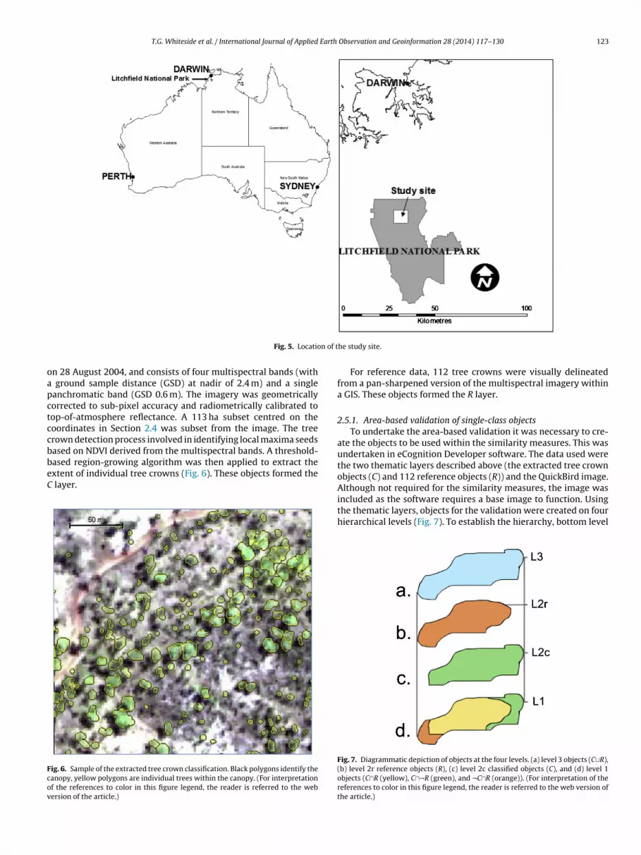

T.G. Whiteside et al. / International Journal of Applied Earth Observation and Geoinformation 28 (2014) 117–130 123

n of t

oapctccbbeC

Fcov

Fig. 5. Locatio

n 28 August 2004, and consists of four multispectral bands (with ground sample distance (GSD) at nadir of 2.4 m) and a singleanchromatic band (GSD 0.6 m). The imagery was geometricallyorrected to sub-pixel accuracy and radiometrically calibrated toop-of-atmosphere reflectance. A 113 ha subset centred on theoordinates in Section 2.4 was subset from the image. The treerown detection process involved in identifying local maxima seeds

ased on NDVI derived from the multispectral bands. A threshold-ased region-growing algorithm was then applied to extract thextent of individual tree crowns (Fig. 6). These objects formed the

layer.

ig. 6. Sample of the extracted tree crown classification. Black polygons identify theanopy, yellow polygons are individual trees within the canopy. (For interpretationf the references to color in this figure legend, the reader is referred to the webersion of the article.)

he study site.

For reference data, 112 tree crowns were visually delineatedfrom a pan-sharpened version of the multispectral imagery withina GIS. These objects formed the R layer.

2.5.1. Area-based validation of single-class objectsTo undertake the area-based validation it was necessary to cre-

ate the objects to be used within the similarity measures. This wasundertaken in eCognition Developer software. The data used werethe two thematic layers described above (the extracted tree crownobjects (C) and 112 reference objects (R)) and the QuickBird image.

Although not required for the similarity measures, the image wasincluded as the software requires a base image to function. Usingthe thematic layers, objects for the validation were created on fourhierarchical levels (Fig. 7). To establish the hierarchy, bottom level

Fig. 7. Diagrammatic depiction of objects at the four levels. (a) level 3 objects (C∪R),(b) level 2r reference objects (R), (c) level 2c classified objects (C), and (d) level 1objects (C∩R (yellow), C∩¬R (green), and ¬C∩R (orange)). (For interpretation of thereferences to color in this figure legend, the reader is referred to the web version ofthe article.)

124 T.G. Whiteside et al. / International Journal of Applied Earth Observation and Geoinformation 28 (2014) 117–130

F dom st .)

(timcdwmitcaarewlcaCCmw

tartaSdw

2

eeomtH

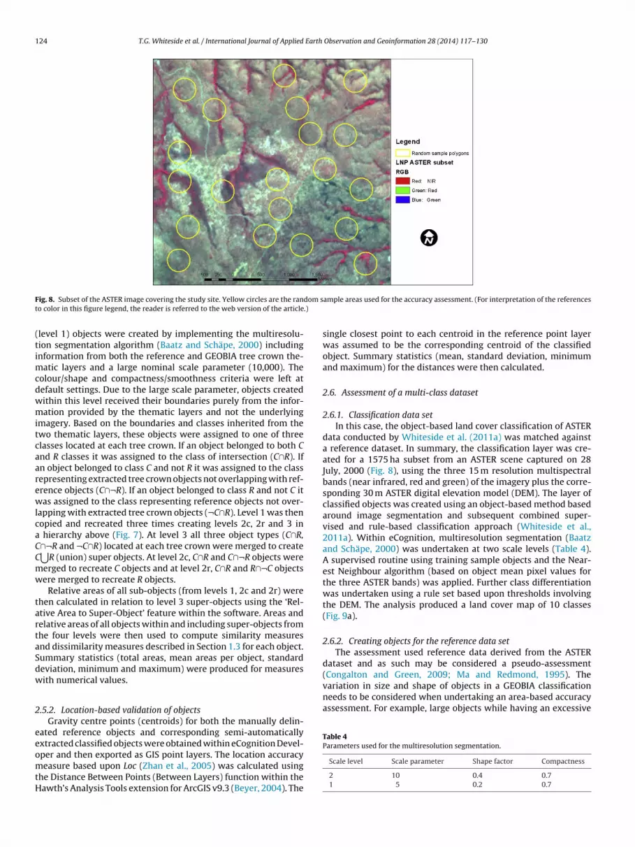
(Congalton and Green, 2009; Ma and Redmond, 1995). Thevariation in size and shape of objects in a GEOBIA classificationneeds to be considered when undertaking an area-based accuracyassessment. For example, large objects while having an excessive

Table 4Parameters used for the multiresolution segmentation.

ig. 8. Subset of the ASTER image covering the study site. Yellow circles are the rano color in this figure legend, the reader is referred to the web version of the article

level 1) objects were created by implementing the multiresolu-ion segmentation algorithm (Baatz and Schäpe, 2000) includingnformation from both the reference and GEOBIA tree crown the-

atic layers and a large nominal scale parameter (10,000). Theolour/shape and compactness/smoothness criteria were left atefault settings. Due to the large scale parameter, objects createdithin this level received their boundaries purely from the infor-ation provided by the thematic layers and not the underlying

magery. Based on the boundaries and classes inherited from thewo thematic layers, these objects were assigned to one of threelasses located at each tree crown. If an object belonged to both Cnd R classes it was assigned to the class of intersection (C∩R). Ifn object belonged to class C and not R it was assigned to the classepresenting extracted tree crown objects not overlapping with ref-rence objects (C∩¬R). If an object belonged to class R and not C itas assigned to the class representing reference objects not over-

apping with extracted tree crown objects (¬C∩R). Level 1 was thenopied and recreated three times creating levels 2c, 2r and 3 in

hierarchy above (Fig. 7). At level 3 all three object types (C∩R,∩¬R and ¬C∩R) located at each tree crown were merged to create⋃

R (union) super objects. At level 2c, C∩R and C∩¬R objects wereerged to recreate C objects and at level 2r, C∩R and R∩¬C objectsere merged to recreate R objects.

Relative areas of all sub-objects (from levels 1, 2c and 2r) werehen calculated in relation to level 3 super-objects using the ‘Rel-tive Area to Super-Object’ feature within the software. Areas andelative areas of all objects within and including super-objects fromhe four levels were then used to compute similarity measuresnd dissimilarity measures described in Section 1.3 for each object.ummary statistics (total areas, mean areas per object, standardeviation, minimum and maximum) were produced for measuresith numerical values.

.5.2. Location-based validation of objectsGravity centre points (centroids) for both the manually delin-

ated reference objects and corresponding semi-automaticallyxtracted classified objects were obtained within eCognition Devel-

per and then exported as GIS point layers. The location accuracyeasure based upon Loc (Zhan et al., 2005) was calculated using

he Distance Between Points (Between Layers) function within theawth’s Analysis Tools extension for ArcGIS v9.3 (Beyer, 2004). The

ample areas used for the accuracy assessment. (For interpretation of the references

single closest point to each centroid in the reference point layerwas assumed to be the corresponding centroid of the classifiedobject. Summary statistics (mean, standard deviation, minimumand maximum) for the distances were then calculated.

2.6. Assessment of a multi-class dataset

2.6.1. Classification data setIn this case, the object-based land cover classification of ASTER

data conducted by Whiteside et al. (2011a) was matched againsta reference dataset. In summary, the classification layer was cre-ated for a 1575 ha subset from an ASTER scene captured on 28July, 2000 (Fig. 8), using the three 15 m resolution multispectralbands (near infrared, red and green) of the imagery plus the corre-sponding 30 m ASTER digital elevation model (DEM). The layer ofclassified objects was created using an object-based method basedaround image segmentation and subsequent combined super-vised and rule-based classification approach (Whiteside et al.,2011a). Within eCognition, multiresolution segmentation (Baatzand Schäpe, 2000) was undertaken at two scale levels (Table 4).A supervised routine using training sample objects and the Near-est Neighbour algorithm (based on object mean pixel values forthe three ASTER bands) was applied. Further class differentiationwas undertaken using a rule set based upon thresholds involvingthe DEM. The analysis produced a land cover map of 10 classes(Fig. 9a).

2.6.2. Creating objects for the reference data setThe assessment used reference data derived from the ASTER

dataset and as such may be considered a pseudo-assessment

Scale level Scale parameter Shape factor Compactness

2 10 0.4 0.71 5 0.2 0.7

T.G. Whiteside et al. / International Journal of Applied Earth Observation and Geoinformation 28 (2014) 117–130 125

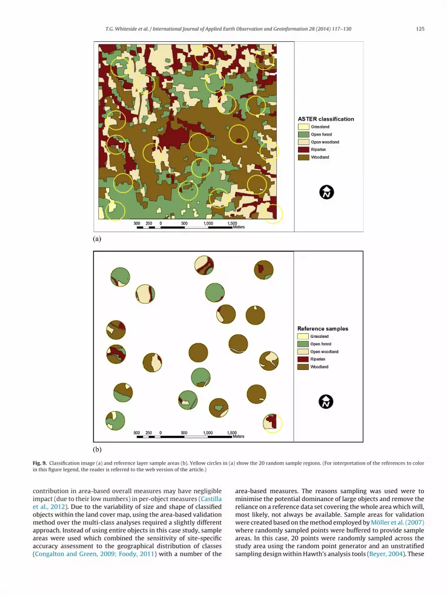
F in (a)

i

cieomaaa(

ig. 9. Classification image (a) and reference layer sample areas (b). Yellow circles

n this figure legend, the reader is referred to the web version of the article.)

ontribution in area-based overall measures may have negligiblempact (due to their low numbers) in per-object measures (Castillat al., 2012). Due to the variability of size and shape of classifiedbjects within the land cover map, using the area-based validationethod over the multi-class analyses required a slightly different

pproach. Instead of using entire objects in this case study, samplereas were used which combined the sensitivity of site-specificccuracy assessment to the geographical distribution of classesCongalton and Green, 2009; Foody, 2011) with a number of the

show the 20 random sample regions. (For interpretation of the references to color

area-based measures. The reasons sampling was used were tominimise the potential dominance of large objects and remove thereliance on a reference data set covering the whole area which will,most likely, not always be available. Sample areas for validationwere created based on the method employed by Möller et al. (2007)

where randomly sampled points were buffered to provide sampleareas. In this case, 20 points were randomly sampled across thestudy area using the random point generator and an unstratifiedsampling design within Hawth’s analysis tools (Beyer, 2004). These

126 T.G. Whiteside et al. / International Journal of Applied Earth Observation and Geoinformation 28 (2014) 117–130

Table 5Summary statistics (m2) for objects created to display relationships between two sets for application in the similarity/dissimilarity measures. |C

⋃R| and |C∩R| are the areas

of union and intersection objects respectively derived from the overlap of classified (C) and reference (R) objects. |C∩¬R| is the area of C objects not corresponding to R objectsand |¬C∩R| is the area of R objects not corresponding to C objects. Std Dev is standard deviation.

Object name

|C⋃

R| |C| |C∩¬R| |¬C∩R| |R| |C∩R|

Total 11,627 8999 1927 2629 9701 7072Percentage 100 77 17 23 83 61Mean 107 83 18 24 89 65

172

pAcbdtaidpd2to

tiecStT(((abowsteo(mtowmilt

TCp

Minimum 15 0

Maximum 482 467

Std Dev 73 74

oints were buffered to a 200 m radius creating the sample areas.lthough it was not necessary in this study, the random point toolan enforce a minimum distance between points to avoid overlapetween sample areas. This method provided sufficient and evenlyistributed sample areas to represent all the land covers withinhe study site. Under this sampling, 269 ha (17% of the entire studyrea) was assessed. Polygons of land cover classes were visuallydentified within the sample areas of the imagery and manuallyigitised to create a thematic layer within a GIS. These land coverolygons were verified against the multispectral QuickBird dataescribed in Section 2.5 and field observations (Whiteside et al.,011a) and further refined (Fig. 9b). The reference data werehen used to verify the geometric and thematic accuracy of thebject-based classification from Whiteside et al. (2011a).

The resulting 200 m radius circle polygons were used as a masko clip the classified layer resulting in 20 samples of correspond-ng C and R objects. These sample areas were then imported intoCognition Developer to undertake the analysis. Using the steps forreating an object hierarchy described in the single-class analysis inection 2.5, four levels of objects were created. However this time,he four types of objects were created for each class (as in Fig. 3).he top level of the hierarchy comprised the union super-objectC⋃

R) covering the entire sample area (Fig. 3a). Reference objectsR) were in the level directly below (Fig. 3b) and classified objectsC) occupy the next level (Fig. 3c). For the bottom level of the hier-rchy (Fig. 3d) sub-objects were created using the boundaries fromoth R and C objects. In instances where reference and classifiedbjects of the same class overlapped, the bottom level sub-objectsere classified as an agreement (C∩R) according to their class. For

ub-objects where the classified object’s class did not correspondo the class of the reference object (C∩¬R), and likewise, where ref-rence object’s class did not correspond to the class of the classifiedbject (¬C∩R), sub-objects were assigned to a non-agreement classdisplayed as red polygons in Fig. 3d). Using this sample method

any of the overall area-based measures were not applied due tohe overall area of classified objects, the overall area of referencebjects and the overall area of the classified objects being the sameithin each sample and across the image. The full suite of accuracy

easures were applied to per-class assessments. Due to the major-

ty of sample areas not containing entire objects (and affecting theocation of centroids), no location measures were considered forhe multi-class assessment.

able 6omparison of the similarity measures (Weidner, 2008; Winter, 2000; Zhan et al., 200arentheses for Correctness, Completeness and OQo are derived from Modified Overlap Fac

OF s11, �q , OQa MOF s41 × 2

Overall 0.79 0.61 0.73 0.76

Mean 0.90 0.59 0.62 0.72

Standard Deviation 0.17 0.20 0.21 0.19

Minimum 0.00 0.00 0.00 0.00

Maximum 1.00 0.93 0.96 0.96

No. objects >0.5 106 78 84 98

0 0 14 05 120 341 3259 25 56 53

3. Results

3.1. Results for single-class analysis

From comparing the extracted tree crown layer (C) and the ref-erence objects (R), the total number of crowns where overlap orcontainment occurred between C and R objects was 109 out of 112.The total area, |C

⋃R|, covered by all reference objects and corre-

sponding classified objects was 11,627 m2 (Table 5). Of that area,61% (7071 m2) is the intersection of C and R objects with a C∩Robject mean size of almost 65 m2.

3.1.1. Similarity measuresFor similarity measures, the overall area total (m2) for each

object class are calculated from the total areas of all objects whereasthe mean totals are the averages of the values for each object(Table 6). The overall quality area (OQa) measure is calculated usingthe areas of the C∩R and C

⋃R objects whereas overall quality per

object (OQo) is based upon the number of instances where the50% overlap threshold is exceeded. Within the OQo column, themain number is the proportion of instances where there is over50% overlap based on the OF measure (Eq. (5)) and the numberin parentheses is based on the MOF measure (Eq. (6)). Values arenoticeably higher for the OF derived Correctness, Completeness andOQo (0.97, 0.95 and 0.93 respectively) over the MOF derived values(0.77, 0.75 and 0.73). Overall similarity measures are based on totalarea covered by all objects within reference data and correspond-ing classified data (Table 6). Mean values are based on the values foreach measure for each object. The bottom row of Table 6 (numberof objects > 0.5) shows the number of objects where the value forthe particular measure is greater than 0.5 (50%). The same appliesfor the summary statistics for dissimilarity measures (Table 7).

As with the similarity measures, the dissimilarity measureswere provided as both an overall total area and per object (as amean) (Table 7). Apart from s32, the mean values for all measuresare higher than the overall measures. The most notable discrepancyis between the values for the miss factor (�m) suggesting a numberof instances are quite dissimilar and the reference object is larger

than the classified object. This is backed up by the maximum andstandard deviation values for this measure.

By undertaking regression analysis between a number of themeasures over all the objects it is clear there is a strong linear

5) applied for assessment of the single-class tree crown detection. The values intor (MOF) values.

�d Correctness Completeness OQo Simsize

0.73 0.97 (0.77) 0.95 (0.75) 0.93 (0.73) N/A0.71 – – – 0.680.26 – – – 0.230.00 – – – 0.001.00 – – – 1.00

87 – – – 91

T.G. Whiteside et al. / International Journal of Applied Earth Observation and Geoinformation 28 (2014) 117–130 127

Table 7Comparison of dissimilarity measures (Weidner, 2008; Winter, 2000) applied for assessment of the single-class tree crown detection. Std Dev is standard deviation andNo > 0.5 is the number of objects that have a value of greater than 0.5 for each measure.

s12 s32/2 s42 (s43 − 0.5/2) �fp �m �s

Overall 0.39 0.24 0.24 0.24 0.21 0.37 0.47Mean 0.42 0.22 0.28 0.28 0.27 0.68 0.50Minimum 0.07 0.04 0.04 0.04 0.00 0.00 0.07

1.00 1.45 9.93 1.450.19 0.27 1.33 0.25

11 11 42 45

rmurSumtrmn

3

rscoM(

3

t

Table 8Location measures summary statistics of Euclidean distances (in metres) betweencentroids of reference objects and corresponding classified objects.

Statistic Value

No. of events 104Mean distance (MeanLoc) 0.8Maximum distance 5.1

TC

Fcs

Maximum 1.00 0.50 1.00

Std Dev 0.20 0.10 0.19

No > 0.5 30 0 11

elationship between the measures. For example the similarityeasure s11 has a strong correlation to the s41 × 2 and s31 meas-

res (r2 = 0.96 and r2 = 0.98 respectively), while s31 shows a strongelationship to the size comparison measure, Simsize (r2 = 0.95).imilar linear relationships are shown for the dissimilarity meas-res. Therefore, there appears to be some redundancy in theeasures. The best measures for single class assessment are those

hat use per-object information (such as OQo, Completeness and Cor-ectness). These measures are preferred over overall area (per-pixel)easures as overall area assessments maybe influenced by a small

umber of poorly overlapping cases.

.1.2. Location measuresUsing the nearest location based distance measure (Loc), 104

elationships were identified between reference objects and corre-ponding classified objects (Table 8). The mean distance betweenentroids was 0.8 m and the error range (the mean plus or minusne standard deviation) was between 0 and 1.7 m (0 and 0.7 pixels).aximum distance between centroids was just over five metres

just over 2 pixels).

.2. Multi-class analysis results

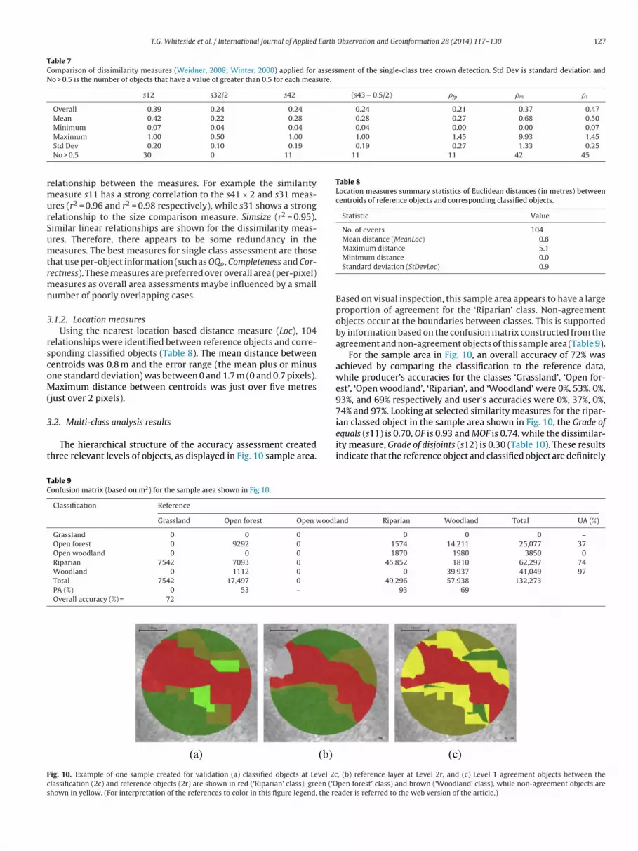
The hierarchical structure of the accuracy assessment createdhree relevant levels of objects, as displayed in Fig. 10 sample area.

able 9onfusion matrix (based on m2) for the sample area shown in Fig.10.

Classification Reference

Grassland Open forest Open woodl

Grassland 0 0 0

Open forest 0 9292 0

Open woodland 0 0 0

Riparian 7542 7093 0

Woodland 0 1112 0

Total 7542 17,497 0

PA (%) 0 53 –

Overall accuracy (%) = 72

ig. 10. Example of one sample created for validation (a) classified objects at Level 2classification (2c) and reference objects (2r) are shown in red (‘Riparian’ class), green (‘Ohown in yellow. (For interpretation of the references to color in this figure legend, the re

Minimum distance 0.0Standard deviation (StDevLoc) 0.9

Based on visual inspection, this sample area appears to have a largeproportion of agreement for the ‘Riparian’ class. Non-agreementobjects occur at the boundaries between classes. This is supportedby information based on the confusion matrix constructed from theagreement and non-agreement objects of this sample area (Table 9).

For the sample area in Fig. 10, an overall accuracy of 72% wasachieved by comparing the classification to the reference data,while producer’s accuracies for the classes ‘Grassland’, ‘Open for-est’, ‘Open woodland’, ‘Riparian’, and ‘Woodland’ were 0%, 53%, 0%,93%, and 69% respectively and user’s accuracies were 0%, 37%, 0%,74% and 97%. Looking at selected similarity measures for the ripar-

ian classed object in the sample area shown in Fig. 10, the Grade ofequals (s11) is 0.70, OF is 0.93 and MOF is 0.74, while the dissimilar-ity measure, Grade of disjoints (s12) is 0.30 (Table 10). These resultsindicate that the reference object and classified object are definitely

and Riparian Woodland Total UA (%)

0 0 0 –1574 14,211 25,077 371870 1980 3850 0

45,852 1810 62,297 740 39,937 41,049 97

49,296 57,938 132,27393 69

, (b) reference layer at Level 2r, and (c) Level 1 agreement objects between thepen forest’ class) and brown (‘Woodland’ class), while non-agreement objects areader is referred to the web version of the article.)

128 T.G. Whiteside et al. / International Journal of Applied Earth Observation and Geoinformation 28 (2014) 117–130

Table 10Selected similarity measures for the ‘Riparian’ object in sample area shown in Fig. 9.

Similarity measure

msti

(dwgo(c

a7d‘2w

o(tm

oudwa

Table 12Overall area-based measures of multiclass object-based classification includingOverall quality (OQa), another measure of similarity (s41/2), and measures of dis-similarity (s12, s32/2, s42, s43 and (s43 − 0.5) × 2) (Winter, 2000).

Measure Value

OQa 0.71s12 0.28s43 0.50(s43 − 0.5) × 2 0.01

of an object-based classification (Weidner, 2008; Winter, 2000;Zhan et al., 2005). By using sample areas, these measures are givensite-specificity, negating the insensitivity that whole of image area-based accuracy assessment has to the geographical distribution of

TC

Object class s11 OF MOF s12

Riparian 0.70 0.93 0.74 0.30

ore similar than they are dissimilar. The difference between the21 and s31 measure indicates that while there is overlap betweenhe reference object and the classified object, the reference objects much larger.

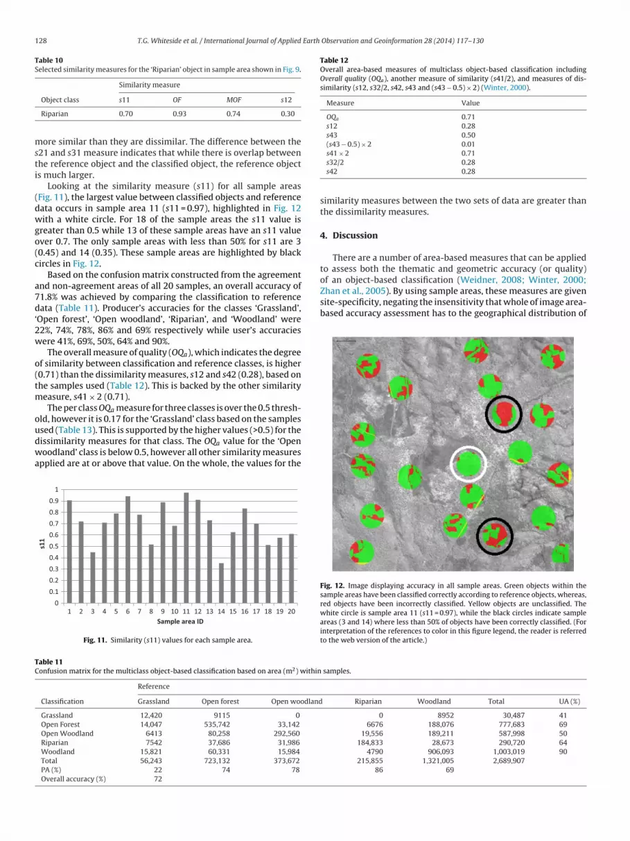
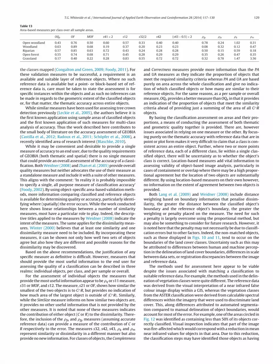
Looking at the similarity measure (s11) for all sample areasFig. 11), the largest value between classified objects and referenceata occurs in sample area 11 (s11 = 0.97), highlighted in Fig. 12ith a white circle. For 18 of the sample areas the s11 value is

reater than 0.5 while 13 of these sample areas have an s11 valuever 0.7. The only sample areas with less than 50% for s11 are 30.45) and 14 (0.35). These sample areas are highlighted by blackircles in Fig. 12.

Based on the confusion matrix constructed from the agreementnd non-agreement areas of all 20 samples, an overall accuracy of1.8% was achieved by comparing the classification to referenceata (Table 11). Producer’s accuracies for the classes ‘Grassland’,

Open forest’, ‘Open woodland’, ‘Riparian’, and ‘Woodland’ were2%, 74%, 78%, 86% and 69% respectively while user’s accuraciesere 41%, 69%, 50%, 64% and 90%.

The overall measure of quality (OQa), which indicates the degreef similarity between classification and reference classes, is higher0.71) than the dissimilarity measures, s12 and s42 (0.28), based onhe samples used (Table 12). This is backed by the other similarity

easure, s41 × 2 (0.71).The per class OQa measure for three classes is over the 0.5 thresh-

ld, however it is 0.17 for the ‘Grassland’ class based on the samples

sed (Table 13). This is supported by the higher values (>0.5) for theissimilarity measures for that class. The OQa value for the ‘Openoodland’ class is below 0.5, however all other similarity measures

pplied are at or above that value. On the whole, the values for the

00.10.20.30.40.50.60.70.80.91

1 2 3 4 5 6 7 8 9 10 11 12 13 14 15 16 17 18 19 20

s11

Samp le area ID

Fig. 11. Similarity (s11) values for each sample area.

able 11onfusion matrix for the multiclass object-based classification based on area (m2) within

Reference

Classification Grassland Open forest Open woodland

Grassland 12,420 9115 0

Open Forest 14,047 535,742 33,142

Open Woodland 6413 80,258 292,560

Riparian 7542 37,686 31,986

Woodland 15,821 60,331 15,984

Total 56,243 723,132 373,672

PA (%) 22 74 78

Overall accuracy (%) 72

s41 × 2 0.71s32/2 0.28s42 0.28

similarity measures between the two sets of data are greater thanthe dissimilarity measures.

4. Discussion

There are a number of area-based measures that can be appliedto assess both the thematic and geometric accuracy (or quality)

Fig. 12. Image displaying accuracy in all sample areas. Green objects within thesample areas have been classified correctly according to reference objects, whereas,red objects have been incorrectly classified. Yellow objects are unclassified. Thewhite circle is sample area 11 (s11 = 0.97), while the black circles indicate sampleareas (3 and 14) where less than 50% of objects have been correctly classified. (Forinterpretation of the references to color in this figure legend, the reader is referredto the web version of the article.)

samples.

Riparian Woodland Total UA (%)

0 8952 30,487 416676 188,076 777,683 69

19,556 189,211 587,998 50184,833 28,673 290,720 64

4790 906,093 1,003,019 90215,855 1,321,005 2,689,907

86 69

T.G. Whiteside et al. / International Journal of Applied Earth Observation and Geoinformation 28 (2014) 117–130 129

Table 13Area-based measures per class over all sample areas.

OQa OF MOF s41 × 2 s12 s32/2 s42 (s43 − 0.5) × 2 �fp �fn �b �m

Open woodland 0.43 0.76 0.50 0.60 0.57 0.33 0.40 0.40 0.78 0.24 1.02 0.31Woodland 0.63 0.89 0.68 0.19 0.37 0.20 0.23 0.23 0.08 0.32 0.12 0.47

0.240.280.55

ttaresbo

dtaat(r

motfiqaTt(oifhmtiudmad

ssar

psshwiotfrRrp

Riparian 0.57 0.85 0.63 0.72 0.43

Open forest 0.55 0.74 0.68 0.71 0.45

Grassland 0.17 0.40 0.22 0.28 0.83

he classes mapped (Congalton and Green, 2009; Foody, 2011). Forhese validation measures to be successful, a requirement is anvailable and suitable layer of reference objects. Where no sucheference data is available but a point- or block-based set of ref-rence data is, care must be taken to state the assessment is forpecific instances within the objects and as such no inferences cane made in regards to the geometric extent of the classified objectsr, for that matter, the thematic accuracy across entire objects.

While similar measures have been used for assessing tree crownetection previously (Leckie et al., 2005), the authors believe it ishe first known application using sample areas of classified objectsnd the first known application of such measures for multi-classnalysis of accuracy. Thus the work described here contributes tohe small body of literature on the accuracy assessment of GEOBIACastilla et al., 2012; Radoux et al., 2011; Schöpfer et al., 2008), aecently identified area of research interest (Blaschke, 2010).

While it may be convenient and desirable to provide a singleeasure of accuracy to an end user, due to the quality requirements

f GEOBIA (both thematic and spatial) there is no single measurehat could provide an overall assessment of the accuracy of a classi-cation. Both Weidner (2008) and Zhan et al. (2005) provide overalluality measures but neither advocates the use of their measure as

standalone measure and include it with a suite of other measures.his aligns with the comment: ‘In reality it is probably impossibleo specify a single, all purpose measure of classification accuracy’Foody, 2002). By using object-specific area-based validation meth-ds, more information comparing classified and reference objectss available for determining quality or accuracy, particularly identi-ying where (spatially) the error occurs. While the work conductedere shows linear relationships between a number of similarityeasures, most have a particular role to play. Indeed, the descrip-

ive titles applied to the measures by Weidner (2008) indicate thentent of the measures. The same applies for the dissimilarity meas-res. Winter (2000) believes that at least one similarity and oneissimilarity measure need to be included. By incorporating theseeasures, it can be shown not only how well two sets of objects

gree but also how they are different and possible reasons for theissimilarity may be discovered.

Based on the above recommendations, the justification of anypecific measure as definitive is difficult. However, measures thathould provide the most useful information to the end user forssessing the quality of a classification can be described in threeealms: individual objects, per class, and per sample or overall.

For the assessment of individual objects the measures thatrovide the most useful information appear to be �q or s11 measure,31 or MOF, and s12. The measure, s21 or OF, shows how similar themallest of the two objects is to C∩R, but provides no indication ofow much area of the largest object is outside of |C∩R|. Similarly,hile the SimSize measure informs on how similar two objects are,

t provides no other useful information that is not provided by thether measures. It is noted that none of these measures indicateshe contribution of either object (C or R) to the dissimilarity. There-ore, the inclusion of the �fn and �fp measures (assuming accurate

eference data) can provide a measure of the contribution of C or

respectively to the error. The measures s32, s42, s43, �b and �m

epresent similarity or dissimilarity in a different manner but alsorovide no new information. For classes of objects, the Completeness

0.28 0.28 0.50 0.15 0.59 0.18 0.29 0.29 0.35 0.26 0.47 0.35 0.72 0.72 0.32 0.78 1.47 3.56

and Correctness measures provide more information than the PAand UA measures as they indicate the proportion of objects thatmeet the required similarity criteria whereas PA and UA are basedpurely on area across the whole classification and give no indica-tion of which classified objects or how many are similar to theirreference objects. For the same reasons, as a per sample or overallmeasure, OQo provides a better measure than OQa in that it providesan indication of the proportion of objects that meet the similaritycriteria ahead of providing just a summing of the area of all C∩Robjects.

By basing the classification assessment on areas and their pro-portions, a means of conducting the assessment of both thematicand geometric quality together is provided. There are, howeverissues associated in relying on one measure or the other. By focus-ing purely on the thematic accuracy with reference data that are inpoint or plot form makes it very difficult to claim that a class is con-sistent across an entire object. Further, where two or more pointsof reference data, each of a different class, lie within a single clas-sified object, there will be uncertainty as to whether the object’sclass is correct. Location-based measures add vital information toassessing validity of object-based image analysis, particularly incases of containment or overlap where there may be a high propor-tional agreement but the location of two objects are substantiallydifferent. By using location-based measures on their own however,no information on the extent of agreement between two objects isprovided.

Both Lang et al. (2009) and Weidner (2008) include distanceweighting based on boundary information that penalise dissim-ilarity, the greater the distance between the classified object’sboundary and the reference object’s boundary, the greater theweighting or penalty placed on the measure. The need for sucha penalty is largely overcome using the proportional method, butmay also be something to consider for future research. However, itis noted here that the penalty may not necessarily be due to classifi-cation errors but to other factors. Indeed, the non-matched objects,such as those displayed in Figs. 10 and 11, tend to occur on theboundaries of the land cover classes. Uncertainty such as this maybe attributed to differences between human and machine percep-tion in the delineation of land cover boundaries, differences in scalebetween data sets, or registration discrepancies between the imageand reference data.

The methods used for assessment here appear to be viabledespite the issues associated with matching a classification tosuitable reference data. For example, the methods used in the delin-eation of vegetation classes were quite different. The reference datawas derived from the visual interpretation of a near infrared falsecolour image display within a GIS, whereas the vegetation classesfrom the ASTER classification were derived from calculable spectraldifferences within the imagery that were used to discriminate landcover. This, along differences attributed to automated segmenta-tion compared to manual delineation of object boundaries, wouldaccount for most of the error. For example, one of the areas circled inFig. 12 was identified as containing less than 50% of its objects cor-

rectly classified. Visual inspection indicates that part of the imagewas fire-affected which would correspond with a reduction in meannear infrared values for objects in that area. Due to this reduction,the classification steps may have identified those objects as having

1 Earth

lo

5

maeoaihorpwcshofiitdmsaToo

stataarieeeiv

R

B

B

B

B

C

C

C

Winter, S., 2000. Location similarity of regions. ISPRS Journal of Photogrammetry

30 T.G. Whiteside et al. / International Journal of Applied

ess vegetation and assigned those objects to a more vegetativelypen class.

. Conclusions

This paper has presented area-based methods for the assess-ent of the quality or accuracy of geographic object-based image

nalysis. These approaches have been used infrequently in the lit-rature, and prior to this research have not been used for assessingbject-based image analysis of heterogeneous land cover. Thepplicability of different methods to assess the accuracy or qual-ty of segmentations and subsequent object-based image analysisas been discussed. The methods used apply proportional measuresf overlap between classified objects and spatially correspondingeference objects. For the single class tree crown detection exam-le, it was found that 73% of tree crown objects were in agreementith the corresponding reference crowns. For the multiclass land

over map example, overall accuracy was 71% with 18 of the 20ample objects showing a similarity value of greater than 50%. Theigh similarity and low dissimilarity values overall show a degreef agreement, both spatially and thematically, between the classi-cation and the reference data. While it has been claimed, there

s no single measure that could provide an overall assessment ofhe accuracy of a classification; there is a subset of the measuresescribed here that can be used to provide an assessment. Theeasures most useful for assessing individual objects are the �q or

11, s31, �fn and �fp measures. Per class measures are Completenessnd Correctness, while for per sample or overall the measure is OQo.he inclusion of these measures provides a quantitative indicationf how well the classified objects match up against the referencebjects both spatially and thematically.

The approaches used here, provided that the reference data isuitable, showcase a number of advantages of the method overraditional site-specific pixel or point-based methods of accuracyssessment. Such advantages include the consideration of both spa-ial and thematic information in the accuracy assessment and thebility to spatially identify where there is error or uncertainty. Dis-dvantages of the method include the reliance on a set of suitableeference objects and the inability to determine whether the errordentified is associated with either the classification or the refer-nce data set. A challenge that has arisen from this research isstablishing protocols and methods for collecting appropriate ref-rence data for this type of assessment. Further research shouldnclude the testing of the efficacy of the accuracy measures in aariety of contexts and scenarios.

eferences

aatz, M., Schäpe, A., 2000. Multiresolution segmentation – an optimizationapproach for high quality multi-scale image segmentation. In: Strobl, J.,Blaschke, T., Griesebner, G. (Eds.), Angewandte Geographische Informationsver-arbeitung XII. Wichmann-Verlag, Heidelberg, pp. 12–23.

enz, U., Hofmann, P., Willhauck, G., Lingenfelder, I., Heynen, M., 2004. Multi-resolution, object-oriented fuzzy analysis of remote sensing data for GIS-readyinformation. ISPRS Journal of Photogrammetry and Remote Sensing 58,239–258.

eyer, H.L., 2004. Hawth’s analysis tools for ArcGIS, http://www.spatialecology.com/htools (last accessed 08.12.13).

laschke, T., 2010. Object based image analysis for remote sensing. ISPRS Journal ofPhotogrammetry and Remote Sensing 65, 2–16.

astilla, G., Hernando, A., Zhang, C., Mazumdar, D., McDermid, G.J., 2012. An inte-grated framework for assessing the accuracy of GEOBIA landcover products. In:Proceedings of Proceedings of the 4th GEOBIA, Rio de Janeiro, Brazil, May 7–9.

linton, N., Holt, A., Scarborough, J., Yan, L., Gong, P., 2010. Accuracy assessmentmeasures for object-based image segmentation goodness. PhotogrammetricEngineering and Remote Sensing 76, 289–299.

ongalton, R.G., 1991. A review of assessing the accuracy of classifications ofremotely sensed data. Remote Sensing of Environment 37, 35–46.

Observation and Geoinformation 28 (2014) 117–130

Congalton, R.G., Green, K., 2009. Assessing the Accuracy of Remotely Sensed Data:Principles and Practices, 2nd ed. CRC Press, Boca Raton, FL.

Delves, L.M., Wilkinson, R., Oliver, C.J., White, R.G., 1992. Comparing the performanceof SAR image segmentation algorithms. International Journal of Remote Sensing13, 2121–2149.

Foody, G.M., 2002. Status of land cover classification accuracy assessment. RemoteSensing of Environment 80, 185–201.

Foody, G.M., 2011. Classification accuracy assessment. In: IEEE Geoscience andRemote Sensing Newsletter, June, pp. 8–14.

Hayder, K., (Ph.D. thesis) 2001. Study of remote sensing and GIS for the assessmentof their capabilities in mapping the vegetation form and structure of tropicalsavannas in Northern Australia. Northern Territory University, Darwin.

Hoover, A., Jean-Baptiste, G., Jiang, X., Flynn, P.J., Bunke, H., Goldgof, D.B., Bowyer,K., Eggert, D.W., Fitzgibbon, A., Fisher, R.B., 1996. An experimental comparisonof range image segmentation algorithms. IEEE Transactions on Pattern Analysisand Machine Intelligence 18, 673–689.

Lang, S., Schöpfer, E., Langanke, T., 2009. Combined object-based classification andmanual interpretation-synergies for a quantitative assessment of parcels andbiotopes. Geocarto International 24, 99–114.

Lang, S., Tiede, D., 2008. Geons: establishing manageable geo-objects for spatial plan-ning and monitoring purposes. In: Proceedings of GEOBIA 2008 – Pixels, Objects,Intelligence: Geographic Object-Based Image Analysis for the 21st Century, Cal-gary, Alberta, August 6–7.

Leckie, D.G., Gougeon, F.A., Tinis, S., Nelson, T., Burnett, C.N., Paradine, D., 2005.Automated tree recognition in old growth conifer stands with high resolutiondigital imagery. Remote Sensing of Environment 94, 311–326.

Lucieer, A., (Ph.D. thesis) 2004. Uncertainties in segmentation and their visualisation.International Institute for Geo-Information Science and Earth Observation (ITC)and the University of Utrecht, Netherlands.

Ma, Z., Redmond, R.L., 1995. Tau coefficients for accuracy assessment of classificationof remote sensing data. Photogrammetric Engineering and Remote Sensing 61,435–439.

Möller, M., Lymburner, L., Volk, M., 2007. The comparison index: a tool for assessingthe accuracy of image segmentation. International Journal of Applied EarthObservation and Geoinformation 9, 311–321.

Pontius, R.G., Millones, M., 2011. Death to kappa: birth of quantity disagreementand allocation disagreement for accuracy assessment. International Journal ofRemote Sensing 32, 4407–4429.

Prieto, M.S., Allen, A.R., 2003. A similarity metric for edge images. IEEE Transactionson Pattern Analysis and Machine Intelligence 25, 1265–1273.

Radoux, J., Bogaert, P., Fasbender, D., Defourny, P., 2011. Thematic accuracy assess-ment of geographic object-based image classification. International Journal ofGeographical Information Science 25, 895–911.

Ragia, L., Winter, S., 2000. Contributions to a quality description of areal objectsin spatial data sets. ISPRS Journal of Photogrammetry and Remote Sensing 55,201–213.

Schöpfer, E., Lang, S., 2006. Object fate analysis – a virtual overlay method for thecategorisation of object transition and object-based accuracy assessment. In:Proceedings of 1st International Conference on Object-based Image Analysis(OBIA 2006), Salzburg, July 4–5.

Schöpfer, E., Lang, S., Albrecht, F., 2008. Object-fate analysis: spatial relationships forthe assessment of object transition and correspondence. In: Blaschke, T., Lang, S.,Hay, G.J. (Eds.), Object-Based Image Analysis: Spatial Concepts for Knowledge-Driven Remote Sensing Applications. Springer, Berlin, pp. 785–801.

Stehman, S.V., Wickham, J.D., 2011. Pixels, blocks of pixels, and polygons: choosing aspatial unit for thematic accuracy assessment. Remote Sensing of Environment115, 3044–3055.

Story, M., Congalton, R.G., 1986. Accuracy assessment: a user’s perspective. Pho-togrammetric Engineering and Remote Sensing 52, 397–399.

Straub, B.M., Heipke, C., 2004. Concepts for internal and external evaluation auto-matically delineated tree tops. In: International Archives of Photogrammetryand Remote Sensing, Vol. XXXVI-8/W2, Freiburg, pp. 62–65.

Tversky, A., 1977. Features of similarity. Psychological Review 84, 327–352.van Coillie, F.M.B., Verbeke, L.P.C., Wulf, R.R.D., 2008. Semi-automatic forest stand

delineation using wavelet based segmentation of very high resolution opticalimagery. In: Blaschke, T., Lang, S., Hay, G.J. (Eds.), Object-Based Image Analysis:Spatial Concepts for Knowledge-Driven Remote Sensing Applications. Springer,Berlin, pp. 237–256.

Weidner, U., 2008. Contribution to the assessment of segmentation quality forremote sensing applications. In: International Archives of the Photogrammetry,Remote Sensing and Spatial Information Sciences, Vol. XXXVII-B7, pp. 479–484.

Whiteside, T.G., Boggs, G.S., Maier, S.W., 2011a. Comparing object-based and pixel-based classifications for mapping savannas. International Journal of AppliedEarth Observation and Geoinformation 13, 884–893.

Whiteside, T.G., Boggs, G.S., Maier, S.W., 2011b. Extraction of tree crowns from highresolution imagery over Eucalypt dominant tropical savanna. PhotogrammetricEngineering and Remote Sensing 77, 813–824.

and Remote Sensing 55, 189–200.Zhan, Q., Molenaar, M., Tempfli, K., Shi, W., 2005. Quality assessment for geo-spatial

objects derived from remotely sensed data. International Journal of RemoteSensing 26, 2953–2974.