Are Revealed Intentions Possible1?

John D. Hey and Carmen Pasca

LUISS Italy and University of York UK and LUISS Italy

1

Abstract

This paper asks whether it is possible to design an Intentions Revealing Experiment – that is, an

experiment in which the early moves of the decision maker in a dynamic decision problem reveal

the intentions of that decision maker regarding later moves in the decision problem. If such a type

of experiment is possible, then it will enable economists to test whether individuals have plans and

implement them – a basic assumption of all economic theories of dynamic decision making.

Unfortunately the main finding of the paper is in the form of two Impossibility Theorems which

show that, unless one is prepared to make certain assumptions, such an Intentions Revealing

Experiment is impossible. However, the paper does have a positive side – it describes the type of

assumptions that one needs to make in order to make an Intentions Revealing Experiment possible.

JEL codes: D81, C91, D90

Keywords: dynamic decision making, experiments, planning, dynamic consistency.

Corresponding Address:

Department of Economics,

University of York,

York YO10 5DD, United Kingdom

e-mail address: jdh1@york.ac.uk

Are Revealed Intentions Possible1?

John D. Hey and Carmen Pasca

LUISS Italy and University of York UK and LUISS Italy

2

1. Introduction

Is it possible to design an experiment in which early decisions by the participants reveal the

intentions or plans of those individuals with respect to later decisions? To answer this question is

the purpose of this paper.

We should start with some motivation as to why the answer to this question is of interest.

This motivation comes from all economic theories of dynamic decision making, in which the

economic agent is envisaged, firstly, as having a plan as to what he or she will do later in the

decision problem, and secondly, as using this plan to determine the earlier decisions. This follows

from the structure of economic models of dynamic decision making. Virtually all such economic

theories of dynamic decision making involve two components: a procedure for reducing, either in

one move or several, a dynamic decision problem to one or several static decision problems; and a

preference functional for determining optimal choice in static decision problems.

There are three main alternative procedures for reducing a dynamic decision problem to a

(series of) static decision problem(s): (1) converting the dynamic decision problem into a strategy

choice problem (where a strategy is a set of conditional decisions at to what to do at each decision

node, conditional on having arrived at that node); (2) using backward induction with reduction to

eliminate choices that will not be taken in the future and then using the principle of the reduction of

compound lotteries to simplify the remaining portion of the decision tree; (3) using backward

1 I wish to thank the European Community under its TMR Programme Savings and Pensions (TMR

Network Contract number ERB FMR XCT 96 0016 (“Structural Analysis of Househld Savings and

Wealth Positions over the Life Cycle”)) for stimulating the research reported in this paper.

3

induction with certainty equivalents to eliminate choices that will not be taken in the future and

using certainty equivalents to replace the eliminated part of the decision tree with a certainty

equivalent. Each of these three procedures involves a plan – a set of conditional decisions at each

node, conditional on having arrived there. Procedure (1) does this explicitly; procedures (2) and (3)

implicitly.

There are many preference functionals in economic theory that attempt to describe optimal

decision making in static decision problems. The most popular is Expected Utility theory but there

are many alternatives and generalisations. Any of these preference functionals can be combined

with any of the three procedures (for reducing a dynamic decision problem to a (series of) static

decision problem(s)) described above. In general, the three different procedures will generate

different plans for tackling any given dynamic decision problem, though in the case of Expected

Utility theory this is not so: whichever procedure is used, the plan produced is the same. Many

economists regard this as a great normative strength of Expected Utility theory.

If an individual’s preference functional is not that of Expected Utility theory, it is possible

(though not inevitable) that different procedures (for reducing a dynamic decision problem to a

(series of) static decision problem(s)) will result in different plans. Because of this, it is possible

that a non-Expected-Utility-theory decision maker (henceforth non-EU person) will be dynamically

inconsistent – that is, they will want to do something different from their original plan at some point

in the decision tree.

There are two ways that a non-EU person can resolve this problem of potential dynamic

inconsistency: that of ‘resolution’ and that of ‘sophistication’. The first of these terms was coined

by McClennen (1990) and describes the behaviour of an individual who chooses the ex ante optimal

strategy (out of the set of all possible strategies) and who resolutely implements it without deviation

(perhaps he or she leaves instructions with his or her lawyer and then goes away on holiday). The

second of these terms (perhaps attributable to Machina (1989)) describes the behaviour of an

individual who works by backward induction (either with reduction or with certainty equivalents)

4

and therefore never places him- or her-self in a position of wanting to change his or her mind –

change the plan.

Non-EU people who are neither resolute nor sophisticated are described by

O’Donoghue and Rabin (1999) as ‘naïve’ – they will typically do something different in the future

than they had earlier planned to do. Most economists would describe this kind of behaviour (time

inconsistency) as irrational – particularly as the non-EU people who do this kind of thing know in

advance that they will do it – and yet disregard this fact. Yet casual empiricism would suggest that

such behaviour is not unusual: there seem to be people who either do not have a plan or who have a

plan and do not implement it. We are interested to learn whether in fact this is the case.

So the brief is simple: to ascertain whether individuals make plans and whether they

implement them. But the execution of the brief is far from simple – as it is difficult to observe

whether people have plans and what those plans are. First, there is a methodological problem in that

mentioning the word ‘plan’ to individuals may well affect their behaviour. We want to avoid this

problem. Secondly, even if we did not, there would be problems in motivating the response of

subjects. Suppose, for the moment that individuals do have plans, how do we ask them what those

plans are in a way that gives them an incentive to accurately reveal them? If we simply ask them,

there is a problem – how do we know whether the reply has any meaning? If, to make their reply to

have meaning, we force them then to implement whatever plan they have announced, then we have

not only forced them to have a plan but we have also forced them to implement it. Which rather

spoils the whole purpose of the exercise! We are very sceptical about the value of asking for

people’s plans: first, because the question itself suggests to individuals that they ought to have a

plan; secondly, there is no way that we can guarantee that what they say is their plan actually is

their plan.

Instead, we have the following suggestion: can we design an experiment in such a way that

the earlier decisions of individuals reveal their future intentions? If we can, then we can answer the

combination of the two questions above: do individuals have plans and implement them? While we

5

may not have answers to each question individually, it is the answer to the combination that is

important to economic theorists and practitioners.

2. Experimental Design

We deliberately work with a simple structure – in fact the simplest possible structure for a

genuinely dynamic decision problem under risk – a two decision-nodes, two chance-nodes decision

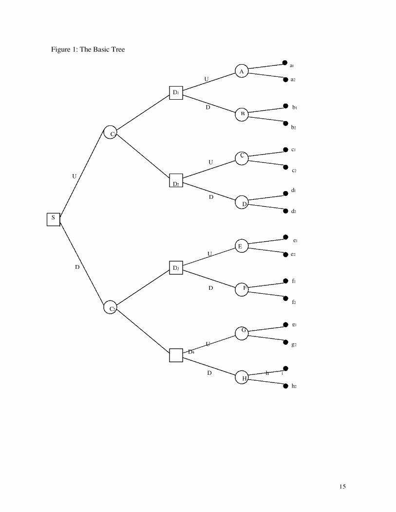
problem – as portrayed in Figure 1. Square boxes represent decision nodes and round boxes chance

nodes. To make the analysis as simple as possible we restrict the number of decisions at each

decision node to two - Up or Down, and we restrict the number of possibilities at each chance node

to two – Up or Down. We also, rather arbitrarily at this point assume that each of these two

possibilities are equally likely – so that the probability of moving Up at a chance node and the

probability of moving Down are both 0.5.

The tree in Figure 1 starts with a decision – whether to move Up or Down at node S. Then

follows a chance node – either C1 or C2 depending upon the decision taken at S. Then there is a

second decision node – either D1, D2, D3 or D4 depending on the previous moves by the decision

maker and by Nature. There are then choice nodes, labelled A through H, and finally there is a

payoff, one of the set P = {a1, a2, b1, b2, c1, c2, d1, d2, e1, e2,f1,f2,g1,g2, h1, h2}. For simplicity in what follows,

let me number the payoffs in such a way that x1 is at least as large as x2 for all x in the set a through h.

The participant in the experiment will end up paid one of the payoffs out of this set P – the precise

payoff depending upon his or her decisions and upon the moves by Nature. The question is: can

we choose the elements of the set P in such a way that the move by the individual at the first

decision node, S, reveals his or her plan as to what he or she will do at (the relevant ones of) the

decision nodes D1, D2, D3 or D4?

Obviously how we order the elements of the set is unimportant, so let us be more precise.

Let us ask: can we choose the elements of the set P in such a way that a decision to move Up at the

first choice node (S) reveals the intention to move Up at whichever of D1 or D2 is actually reached,

6

while a decision to move Down at the first choice node (S) reveals the intention to move Down at

whichever of D3 or D4 is actually reached? We should add to this that we want the experiment to be

non-trivial and, in particular, not driven by (first-order) dominance – so that all rational subjects all

take the same decisions. (Perhaps an extended note is needed at this stage: some of my colleagues

have argued that it is of interest to construct a tree where two strategies (one involving Up at the

first node and the second involving Down at the first node) dominate all the others, and therefore in

which violation of the revealed intentions reveals a violation of dominance. My response is that I

am testing to see whether plans are made and implemented. It may be the case that plans are not

made and implemented because dominance is violated – but I do not want an experiment in which

that is the only reason why plans are not made and implemented.) Moreover we want the decision

problem to be a genuinely dynamic one so we need that at least one of (A and B), (C and D), (E

and F) and (G and H) are different – otherwise the second decision would not be a genuine

decision. Similarly we need that either (A and B) are different from (C and D) or that (E and F) are

different from (G and H) – for otherwise the first chance node would not be a genuine chance node.

More crucially we do not want the decisions at any node to be driven purely by dominance. In

particular we do not want the decisions at the second decision node to be driven purely by

dominance. So, for at least one of the pairs (A and B), (C and D), (E and F) and (G and H) it must

be the case that neither member of the pair dominates the other member of the pair. Dominance in

this two-outcome case is clear – for example if a1 is at least as large as b1 and a2 is at least as large

as b2 then A dominates B.

As we will see, the answer to our question depends very much on what we can assume about

subjects. We consider various cases, becoming more and more restrictive as we proceed. Before we

start, it might be useful to propose a definition of what it is that we are after. This is an Intentions

Revealing Experiment – defined as an experiment in which some subjects move Up at the first node

and some move Down at the first node, and in which the decision to move Up at the first decision

node reveals the intention (for someone who makes plans) to move Up at the second decision node

7

(independently of what Nature does at the first chance node) and in which the decision to move

Down at the first decision node reveals the intention (for someone who makes plans) to move Down

at the second decision node (independently of what Nature does at the first chance node). In such an

Intentions Revealing Experiment a decision to move Up at the first decision node and Down at the

second, or a decision to move Down at the first and Up at the second, must be a decision by

someone who either does not have a plan, or who has a plan but fails to implement it. In other

words, such a pattern of decisions reveals a dynamically inconsistent individual.

Before concluding this section let us introduce some notation. A strategy is a decision at the

first decision node and a decision at both of the possible second decision nodes – depending upon

which decision node Nature moves to. We denote a strategy in the following form: {X ,YZ} – where

each of X, Y and Z are one of U or D – indicating Up or Down. The general strategy {X ,YZ}

indicates the decision to move X at the first node and then Y at the second if Nature moves Up at the

first chance node, or Z at the second if Nature moves Down at the first chance node. So one strategy

is {U,UU} – where the subject moves Up at the first node and then moves Up at the second node,

irrespective of what Nature does at C1. Another strategy is {U ,UD} - where the subject moves Up at

S and then moves Up if Nature moves Up at C1 and Down if Nature moves Down at C1. Associated

with any strategy is a probability distribution over either penultimate payoffs or final payoffs. For

example, the choice of strategy {U ,UU} will lead intermediately to one of A or C, each with equal

probability2, and will lead finally to one of a1, a2, c1 or c2, again each with equal probability. We

will denote a gamble with outcomes a, b, c, d, ..., each with equal probabilities by [a,b,c,d, ...J. The

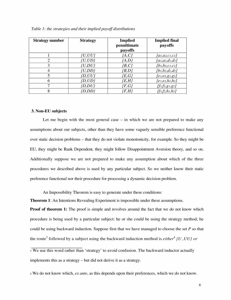
complete set of all possible strategies, and their associated intermediate and final outcomes, in this

simple experiment is shown in Table 1.

2 Recall that we have assumed that Nature moves Up or Down at each chance node with probability

0.5.

8

Table 1: the strategies and their implied payoff distributions

Strategy number Strategy Implied

penultimate

payoffs

Implied final

payoffs

1 {U,UU] [A,C] [a1,a2,c1,c2]

2 {U,UD} [A,D] [a1,a2,d1,d2]

3 {U,DU} [B,C] [b1,b2,c1,c2]

4 {U,DD} [B,D] [b1,b2,d1,d2]

5 {D,UU] [E,G] [e1,e2,g1,g2]

6 {D,UD} [E,H] [e1,e2,h1,h2]

7 {D,DU} [F,G] [f1,f2,g1,g2]

8 {D,DD} [F,H] [f1,f2,h1,h2]

3. Non-EU subjects

Let me begin with the most general case – in which we are not prepared to make any

assumptions about our subjects, other than they have some vaguely sensible preference functional

over static decision problems – that they do not violate monotonicity, for example. So they might be

EU, they might be Rank Dependent, they might follow Disappointment Aversion theory, and so on.

Additionally suppose we are not prepared to make any assumption about which of the three

procedures we described above is used by any particular subject. So we neither know their static

preference functional nor their procedure for processing a dynamic decision problem.

An Impossibility Theorem is easy to generate under these conditions:

Theorem 1: An Intentions Revealing Experiment is impossible under these assumptions.

Proof of theorem 1: The proof is simple and revolves around the fact that we do not know which

procedure is being used by a particular subject: he or she could be using the strategy method; he

could be using backward induction. Suppose first that we have managed to choose the set P so that

the route3 followed by a subject using the backward induction method is either

4 {U ,UU} or

3 We use this word rather than ‘strategy’ to avoid confusion. The backward inductor actually

implements this as a strategy – but did not derive it as a strategy.

4 We do not know which, ex ante, as this depends upon their preferences, which we do not know.

9

{D,DD}. Take a backward inductor subject for whom the preferred route is {U ,UU}5. Then this

subject prefers to move Up at node D1 and Up at node D2. That is, he or she prefers A to B at D1 and

prefers C to D at D2.

Let us now consider an individual with the same preferences but one who uses the strategy

method. Is the information we have obtained above sufficient to prove that he or she prefers the

strategy {U, UU} to {U,DU}, {U, UD} and {U,DD}? In other words is the fact that A is preferred to B

and that C is preferred to D sufficient to show that [A, C] is preferred to [B, C], [A,D] and [B,D]?

Unfortunately not. As we show in Appendix Theorem 1, for any A, B, C and D that satisfy

the conditions that we have stated above, we can always find some non-EU preferences for whom A

is preferred to B and C is preferred to D but either [B, C] is preferred to [A, C] or [A,D] is preferred

to [A, C] or both. In other words, even if all backward inductors are following the route {U, UU}

there may be strategy players with the same preferences for whom {U, UU} is not the best strategy.

3. EU Subjects

The problem above is that different procedures for reducing a dynamic problem to a static

decision problem may lead to different solutions for individuals with non-EU static preference

functionals. This, through Theorem 1, makes an Intentions Revealing Experiment impossible. Let

us therefore assume that all our subjects satisfy Expected Utility theory. Does this help us? The

answer is ‘no’ as the next theorem shows.

Theorem 2: An Intentions Revealing Experiment is impossible under these assumptions.

Proof of theorem 2: Consider A and B. We have assumed that a1 ? a2 and that b1 ? b2. Furthermore

we do not want our results to be driven by dominance so we want neither that A dominates B or that

B dominates A. This requires that we have either that a1 ? b1 and b2 ? a2 or that b1 ? a1 and a2 ? b2 .

Which way round is irrelevant (as will be seen) and so let us assume that a1 ? b1 and b2 ? a2. If you

5 The proof in the contrary case follows in a parallel manner.

10

like you can interpret this as saying that A is riskier than B – since A’s best outcome is better than

the best outcome of B and A’s worst outcome is worse than the worst outcome of B – but it is not

riskier in the Rothschild and Stiglitz sense, since A and B do not necessarily have the same mean6.

However we can say that someone sufficiently risk-loving will prefer A while someone

insufficiently risk-loving will prefer B. The question now is: can we choose A, B, C and D so that

some people prefer A to B and C to D, while the others prefer B to A and D to C? The problem is

that the pair (A and B) cannot be the same as the pair (C and D) – for otherwise the chance node at

C1 would not exist - and Appendix Theorem 2 shows that it does not follow that if A is preferred to

B then C is preferred to D or vice versa. So either even if someone is sufficiently risk-loving to

prefer A to B then it does not follow that they are sufficiently risk-loving to prefer C to D or even if

someone is sufficiently risk-loving to prefer C to D then it does not follow that they are sufficiently

risk-loving to prefer A to B. The problem is that (A and B) must differ from (C and D) and if we do

not know anything about an individual’s utility function other than either they prefer A to B or that

they prefer C to D that is not sufficient to tell us whether they prefer C to D (given that they prefer

A to B) or whether they prefer A to B (given that they prefer C to D).

4. EU subjects who are either everywhere risk-averse or everywhere risk-loving

The above result gives us a clue as to what assumptions we might need to design an

Intentions Revealing Experiment. Suppose we assume that all our subjects are either everywhere

risk-lovers or everywhere risk-averters. Then we can make A and B have the same mean – with A

riskier than B – and we can make C and D have the same mean –with C riskier than D. Then all the

risk-lovers will choose Up at the second decision node in the top part of the tree. This suggests that

we design the tree so that the risk-lovers go Up at the first decision node, and continue to play Up

6 It is riskier in the sense used by Hey and Lambert (1989) in generalizing the results of Rothschild

and Stiglitz.

11

thereafter, while all the risk-averters play Down at the first decision node and continue to play

Down thereafter. Using the same logic as that used to design the gambles A, B, C and D, we make

E and F have the same mean but E riskier than F and we make G and H have the same mean but G

riskier than H. This means that all risk-averters will play Down at the second decision node in the

bottom half of the tree.

We have not finished. We now want to persuade all the risk-lovers to choose Up at the first

decision node and all risk-averters to choose Down at the first decision node. How do we do this?

Well, we have already set things up so that, at the second decision node, risk-lovers everywhere

play Up while risk-averters everywhere play Down. So, as viewed from the first decision node the

risk-lovers are choosing between [A, C] and [E, G] while the risk-averters are choosing between

[B,D] and [F,H]. We therefore want to make [A, C] more attractive to risk-lovers than [E, G] and we

want to make [F,H] more attractive to risk-averters than [B,D]. At the same time, we want to

respect the conditions above: that A and B have the same mean but A is riskier; that C and D have

the same mean but C is riskier; that E and F have the same mean but E is riskier; and that G and H

have the same mean but G is riskier. The argument goes through in a more general case but let us

consider a rather special case – in which B, D, F and H are all certainties – that is b1 = b2 = b, d1 =

d2 = d, f1 = f2 = f and h1 = h2 = h. Then for all risk-averters to prefer to play Down at the first

decision node we require that [F,H] is more attractive to them than [B,D]. We could guarantee that

by putting f + h = b + d (thus guaranteeing that the means of [F,H] and [B,D] are equal) and then

by putting b > f > h > d - so that [F,H] is less risky than [B,D].

So the secret is to tempt the risk-averters Down by making the two certainties in the bottom

half of the tree jointly more attractive to risk-averters than the two certainties in the top half of the

tree. This entices the risk-averters Down at the first decision node. We then do a similar thing to

tempt the risk-lovers Up at the first decision node – make the risky prospects in the upper part of the

tree more attractive than the risky prospects in the bottom half of the tree. We can do this by

making them riskier.

12

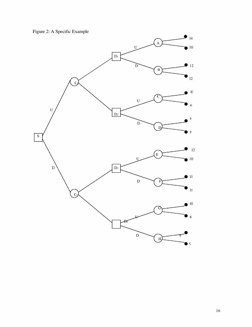
An example is presented in Figure 2. It will be seen from this that at all second decision

nodes D1 through D4 all risk-lovers will choose Up and all risk-averters will choose Down. So the

risk-averters know that if they choose Up at the first decision node they will end up either with 12

or with 8 – each equally likely – whereas if they choose Down at the first decision node they will

end up with either 11 or 9 – each equally likely. All risk-averters prefer [11,9] to [12,8] so all risk-

averters will choose Down at the first decision node and will continue to play Down thereafter.

Risk-lovers, on the other hand, knowing that they will play Up at any second decision node have a

choice between [14,10,10,6] by playing Up at the first node and [12,10,10,8] by playing Down at

the first node. For all risk-lovers the prospect [14,10,10,6] is more attractive than the prospect

[12,10,10,8] – because the former is riskier than the latter – so they will choose Up at the first

decision node and will continue to play Up thereafter.

We have seen, therefore, that if we are able to make a sufficiently strong assumption about

the preferences of our subjects – in this case, assuming that they are either everywhere risk-loving

or everywhere risk-averting – we can design an Intentions Revealing Experiment. (Of course, this

cannot work for the dividing case – the individual who is risk-neutral - for he or she is everywhere

indifferent.)

5. Generalisations

It should be clear that there are obvious generalisations of the ‘Possibility Theorem’ of

section 4. For instance we could take some reference individual – say an individual with utility

function R(.) and assume that all other individuals are either everywhere more risk-averse than the

reference individual or everywhere more risk-loving than the reference individual. This follows the

line of argument of Hey and Lambert (1989) in generalising the results of Rothschild and Stiglitz.

Then we amend what we have done above in Figure 2. Note that there the ‘reference individual’

was the risk-neutral individual. We made all the final choices between gambles with the same mean

but the Up decision riskier. In this current section’s generalisation we construct the tree so that in all

13

the final choices the reference individual is indifferent – and once again we make the Up decision

riskier. So all those agents everywhere more risk-loving than our reference individual will play Up

at the first node and continue to play Up thereafter while all those agents everywhere more risk-

averse than our reference individual will play Down at the first node and continue to play Down

thereafter. (Though, of course, this cannot work for our reference individual – who is everywhere

indifferent7.)

There are clearly countless other generalisations of this form. In Hey (2002) it was supposed

that if an individual prefers some gamble A to some other gamble B then he or she will also prefer

the gamble A+d to the gamble B+d – where by the notation A+d we mean a gamble which has the

same probabilities and outcomes as A except that all outcomes are increased by the constant d

(which could be negative). Notice that this assumption has the same type of structure as before: it

enables us to divide our subjects into two groups – one sub-group which is always in that sub-group

and the rest which are always in some other sub-group. This then enables us to design our tree.

So we have a way of designing an Intentions Revealing Experiment. We need to be able to

divide our subjects up into two groups – and be sure that they remain in these two subgroups at all

stages in the experiment. This appears to be difficult – without making what would appear to be

strong assumptions8.

7 But then he or she has mass zero in the population.

8 One possibility is that we use a modification of the Binary Lottery incentive mechanism – the

payoffs at the end of the tree are probability points to be used in a binary lottery. The trouble with

this is twofold: (1) the Binary Lottery mechanism is not viewed with favour by all experimental

economists; and (2) the addition of this “sting in the tail” complicates the experiment considerably.

14

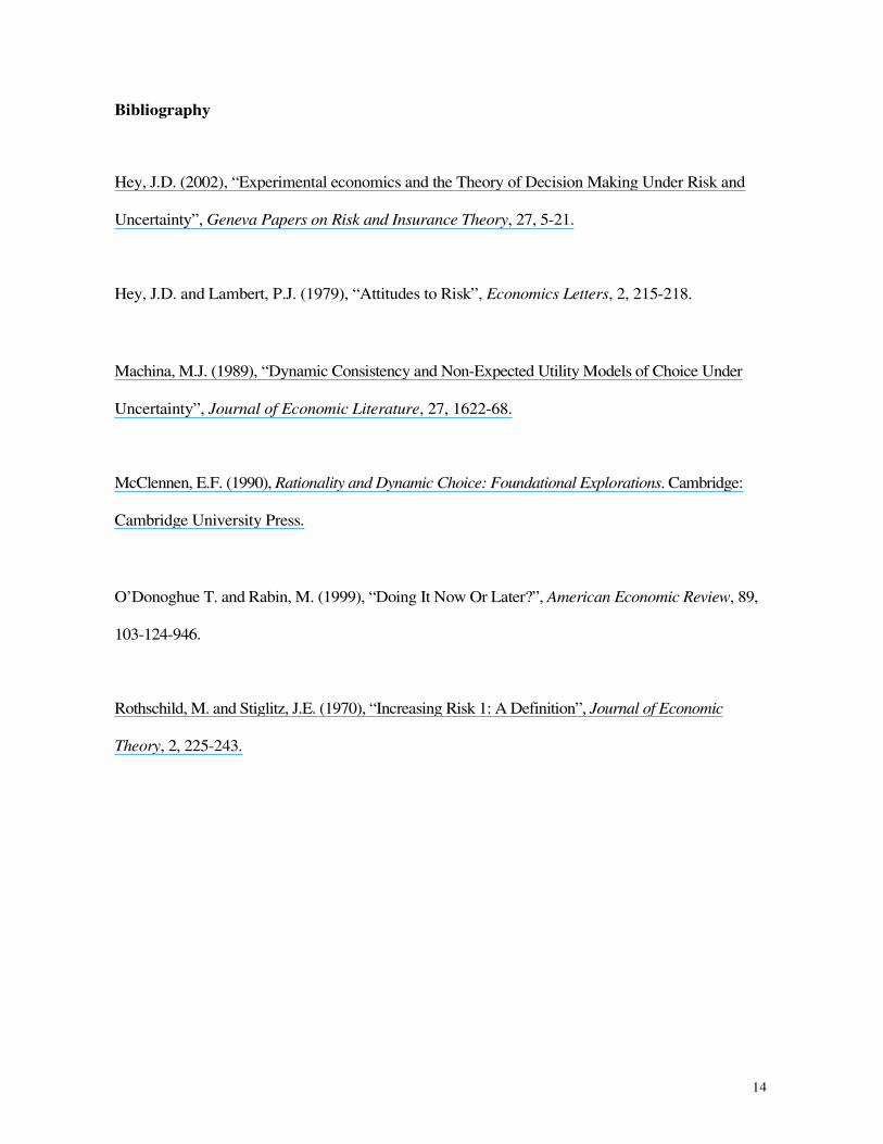
Bibliography

Hey, J.D. (2002), “Experimental economics and the Theory of Decision Making Under Risk and

Uncertainty”, Geneva Papers on Risk and Insurance Theory, 27, 5-21.

Hey, J.D. and Lambert, P.J. (1979), “Attitudes to Risk”, Economics Letters, 2, 215-218.

Machina, M.J. (1989), “Dynamic Consistency and Non-Expected Utility Models of Choice Under

Uncertainty”, Journal of Economic Literature, 27, 1622-68.

McClennen, E.F. (1990), Rationality and Dynamic Choice: Foundational Explorations. Cambridge:

Cambridge University Press.

O’Donoghue T. and Rabin, M. (1999), “Doing It Now Or Later?”, American Economic Review, 89,

103-124-946.

Rothschild, M. and Stiglitz, J.E. (1970), “Increasing Risk 1: A Definition”, Journal of Economic

Theory, 2, 225-243.

15

Figure 1: The Basic Tree

S

U

D

C2

C1

D1

D2

D3

D4

A

U a2

D b1

B

U g2

D h 1

H

E

U e2

U

D F

D

C

G

D

a1

b2

d1

d2

c1

h2

c2

f1

f2

g1

e1

16

Figure 2: A Specific Example

S

U

D

C2

C1

D1

D2

D3

D4

A U 10

D 12

B

U 8

D 9

H

E U 10

U

D F

D

C

G

D

14

12

9

11

11

10

8

8

10

6

12

17

Appendix Theorem 1

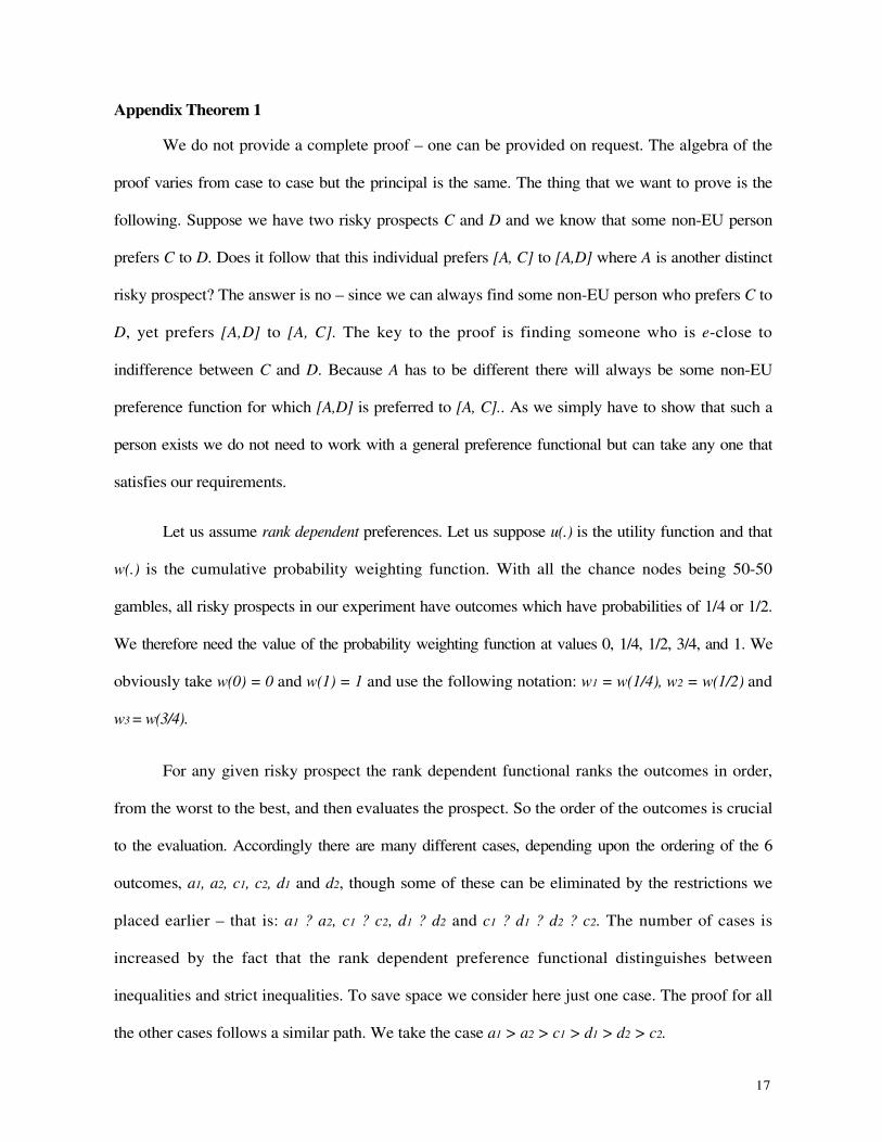
We do not provide a complete proof – one can be provided on request. The algebra of the

proof varies from case to case but the principal is the same. The thing that we want to prove is the

following. Suppose we have two risky prospects C and D and we know that some non-EU person

prefers C to D. Does it follow that this individual prefers [A, C] to [A,D] where A is another distinct

risky prospect? The answer is no – since we can always find some non-EU person who prefers C to

D, yet prefers [A,D] to [A, C]. The key to the proof is finding someone who is e-close to

indifference between C and D. Because A has to be different there will always be some non-EU

preference function for which [A,D] is preferred to [A, C].. As we simply have to show that such a

person exists we do not need to work with a general preference functional but can take any one that

satisfies our requirements.

Let us assume rank dependent preferences. Let us suppose u(.) is the utility function and that

w(.) is the cumulative probability weighting function. With all the chance nodes being 50-50

gambles, all risky prospects in our experiment have outcomes which have probabilities of 1/4 or 1/2.

We therefore need the value of the probability weighting function at values 0, 1/4, 1/2, 3/4, and 1. We

obviously take w(0) = 0 and w(1) = 1 and use the following notation: w1 = w(1/4), w2 = w(1/2) and

w3 = w(3/4).

For any given risky prospect the rank dependent functional ranks the outcomes in order,

from the worst to the best, and then evaluates the prospect. So the order of the outcomes is crucial

to the evaluation. Accordingly there are many different cases, depending upon the ordering of the 6

outcomes, a1, a2, c1, c2, d1 and d2, though some of these can be eliminated by the restrictions we

placed earlier – that is: a1 ? a2, c1 ? c2, d1 ? d2 and c1 ? d1 ? d2 ? c2. The number of cases is

increased by the fact that the rank dependent preference functional distinguishes between

inequalities and strict inequalities. To save space we consider here just one case. The proof for all

the other cases follows a similar path. We take the case a1 > a2 > c1 > d1 > d2 > c2.

18

We start with the supposition that we have an individual who (just) prefers C to D. It

follows that

{u(c2)(1-w2) + u(c1)w2} - {u(d2)(1-w2) + u(d1)w2} > ε (A1)

where ε is an arbitrarily small positive number – reflecting the fact the individual (just) prefers C to

D.

The question now is: can such an individual prefer [A,D] to [A,C]? The answer is ‘yes’ if

the expression in equation below is negative.

{u(c2) + [u(c1) – u(c2)]w3 + [u(a2) – u(c1)]w2 + [u(a1) – u(a2)]w1}–

{u(d2) + [u(d1) – u(d2)]w3 + [u(a2) – u(d1)]w2 + [u(a1) – u(a2)]w1}

We can simplify this. The above expression is negative if the expression below is negative.

{u(c2)(1-w3) + u(c1)(w3-w2)} - {u(d2)(1-w3) + u(d1)(w3-w2)}

We can write this as the difference between two weighted averages – just as (A1) above – as

follows:

{u(c2)[(1-w3)/(1-w2)] + u(c1)[(w3-w2)/(1-w2)]} – {u(d2)[(1-w3)/(1-w2)] + u(d1)[(w3-w2)/(1-w2)]} (A2)

Now examine (A1) – it is the difference between a weighted average of u(c2) and u(c1), with

weights (1-w2) and w2, and the same weighted average of u(d2) and u(d1). Expression (A1) says that

this difference is (just) positive. Expression (A2) is the difference between a weighted average of

u(c2) and u(c1), with weights (1-w3)/(1-w2) and (w3–w2)/(1-w2), and the same weighted average of

u(d2) and u(d1). The question is: whereas the weights in expression (A1) made the difference (just)

positive, can we have weights in expression (A2) that makes the difference negative? The answer is

yes in general. Why? Well, in the case of EU we have w1 = 1/4, w2 = 1/2 and w3 = 3/4, in which case

the weights in expression (A1) are exactly the same as the weights in expression (A2) - and so the

expression (A2) is (just) negative. In the case of non-EU preferences, we can either put more (less)

weight on c2 and d2 and less (more) on c1 and d1 by decreasing (increasing) w3 relative to its EU

value of 3/4. By so doing – depending upon the curvature of the utility function - we can make the

19

value of the expression (A2) (just) negative. Thus the individual prefers C to D yet prefers [A,D] to

[A,C].

20

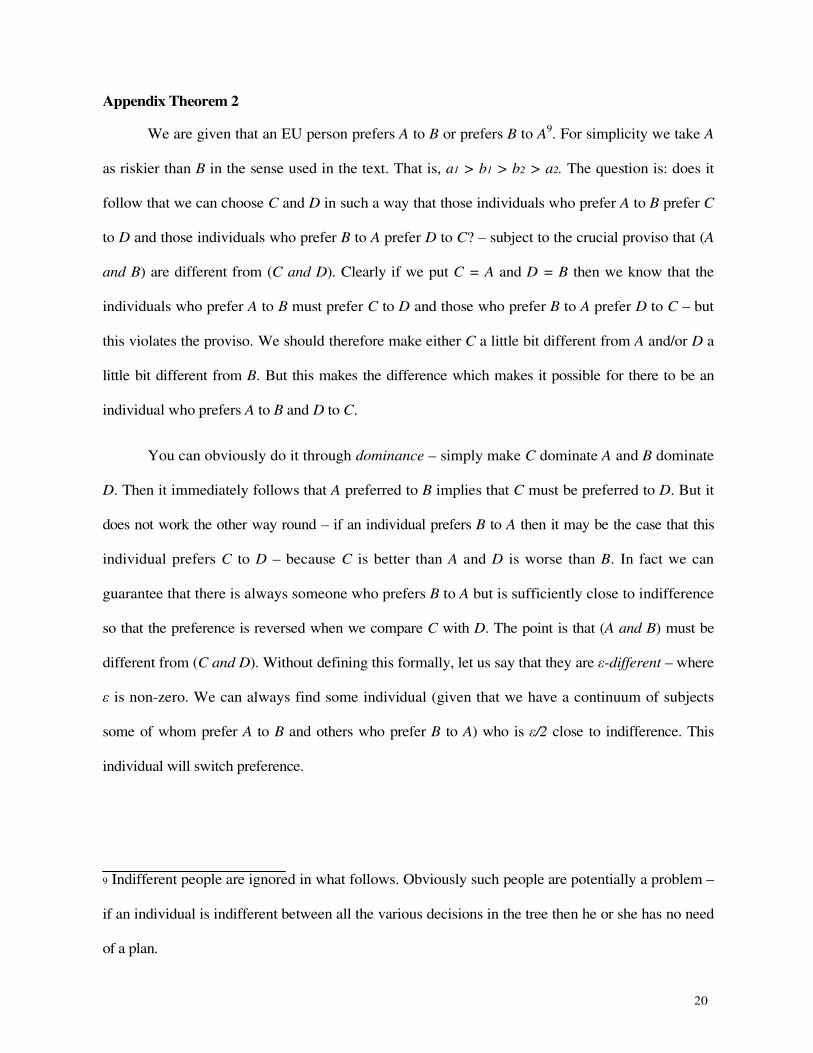
Appendix Theorem 2

We are given that an EU person prefers A to B or prefers B to A9. For simplicity we take A

as riskier than B in the sense used in the text. That is, a1 > b1 > b2 > a2. The question is: does it

follow that we can choose C and D in such a way that those individuals who prefer A to B prefer C

to D and those individuals who prefer B to A prefer D to C? – subject to the crucial proviso that (A

and B) are different from (C and D). Clearly if we put C = A and D = B then we know that the

individuals who prefer A to B must prefer C to D and those who prefer B to A prefer D to C – but

this violates the proviso. We should therefore make either C a little bit different from A and/or D a

little bit different from B. But this makes the difference which makes it possible for there to be an

individual who prefers A to B and D to C.

You can obviously do it through dominance – simply make C dominate A and B dominate

D. Then it immediately follows that A preferred to B implies that C must be preferred to D. But it

does not work the other way round – if an individual prefers B to A then it may be the case that this

individual prefers C to D – because C is better than A and D is worse than B. In fact we can

guarantee that there is always someone who prefers B to A but is sufficiently close to indifference

so that the preference is reversed when we compare C with D. The point is that (A and B) must be

different from (C and D). Without defining this formally, let us say that they are ε-different – where

ε is non-zero. We can always find some individual (given that we have a continuum of subjects

some of whom prefer A to B and others who prefer B to A) who is ε/2 close to indifference. This

individual will switch preference.

9 Indifferent people are ignored in what follows. Obviously such people are potentially a problem –

if an individual is indifferent between all the various decisions in the tree then he or she has no need

of a plan.

21

Furthermore, if neither A nor C dominate the other and neither B or D dominate the other10

it

is even easier to find utility functions for which A is preferred to B and D to C and other functions

for which B is preferred to A and C to D. A formal proof seems unnecessary but can be provided on

request.

10 Recall that we are assuming that a1 ≥ b1 and b2 ≥ a2.