are all species necessary to reveal ecologically important patterns?

Are all species necessary to reveal ecologically importantpatterns?Edwin Pos1,2, Juan Ernesto Guevara Andino3, Daniel Sabatier4, Jean-Franc�ois Molino4, NigelPitman5,6, Hugo Mogoll�on7, David Neill8, Carlos Cer�on9, Gonzalo Rivas10, Anthony Di Fiore11, RaquelThomas12, Milton Tirado13, Kenneth R. Young14, Ophelia Wang15, Rodrigo Sierra13, RooseveltGarc�ıa-Villacorta16,17, Roderick Zagt18, Walter Palacios19, Milton Aulestia20 & Hans ter Steege1,2

1Ecology and Biodiversity Group, Utrecht University, Utrecht, the Netherlands2Section Botany, Naturalis Biodiversity Center, Leiden, the Netherlands3Department of Integrative Biology, University of California, Berkeley, California 94720-31404IRD, UMR AMAP, Montpellier, France5The Field Museum, 1400 S. Lake Shore Drive, Chicago, Illinois 60605-24966Center for Tropical Conservation, Nicholas School of the Environment, Duke University, Durham, North Carolina 277087Endangered Species Coalition, 8530 Geren Rd., Silver Spring, Maryland 209018Universidad Estatal Amaz�onica, Puyo, Ecuador9Universidad Central Herbario Alfredo Paredes, Escuela de Biolog�ıa Herbario Alfredo Paredes, Ap. Postal 17.01.2177, Quito, Ecuador10Wildlife Ecology and Conservation & Quantitative Spatial Ecology, University of Florida, 110 Newins-Ziegler Hall, PO Box 110430, Gainesville,

Florida11Department of Anthropology, University of Texas at Austin, SAC 5.150, 2201 Speedway Stop C3200 Austin, Texas 7871212Iwokrama International Programme for Rainforest Conservation, Georgetown, Guyana13GeoIS, El D�ıa 369 y El Tel�egrafo, 3° Piso, Quito, Ecuador14Geography and the Environment, University of Texas, Austin, Texas 7871215Northern Arizona University, Flagstaff, Arizona 8601116Institute of Molecular Plant Sciences, University of Edinburgh, Mayfield Rd, Edinburgh EH3 5LR, UK17Royal Botanic Garden of Edinburgh, 20a Inverleith Row, Edinburgh EH3 5LR, UK18Tropenbos International, Lawickse Allee 11, PO Box 232, Wageningen, 6700 AE, the Netherlands19Universidad T�ecnica del Norte, Herbario Nacional del Euador, Quito, Ecuador20Herbario Nacional del Ecuador, Casilla 17-21-1787, Avenida R�ıo Coca E6-115, Quito, Ecuador

Keywords

Beta-diversity, Fisher’s alpha, indets, large-

scale ecological patterns, Mantel test,

morpho-species, nonmetric multidimensional

scaling, similarity of species composition,

spatial turnover.

Correspondence

Edwin T. Pos, Department of Biology,

Research group of Ecology & Biodiversity,

Utrecht University, Padualaan 8, 3584 CH,

Utrecht, the Netherlands.

Tel: +31302536837; E-mail: [email protected]

Funding Information

No funding information provided.

Received: 9 April 2014; Revised: 5 August

2014; Accepted: 24 August 2014

doi: 10.1002/ece3.1246

Abstract

While studying ecological patterns at large scales, ecologists are often unable to

identify all collections, forcing them to either omit these unidentified records

entirely, without knowing the effect of this, or pursue very costly and time-con-

suming efforts for identifying them. These “indets” may be of critical impor-

tance, but as yet, their impact on the reliability of ecological analyses is poorly

known. We investigated the consequence of omitting the unidentified records

and provide an explanation for the results. We used three large-scale indepen-

dent datasets, (Guyana/ Suriname, French Guiana, Ecuador) each consisting of

records having been identified to a valid species name (identified morpho-spe-

cies – IMS) and a number of unidentified records (unidentified morpho-species

– UMS). A subset was created for each dataset containing only the IMS, which

was compared with the complete dataset containing all morpho-species

(AMS: = IMS + UMS) for the following analyses: species diversity (Fisher’s

alpha), similarity of species composition, Mantel test and ordination (NMDS).

In addition, we also simulated an even larger number of unidentified records

for all three datasets and analyzed the agreement between similarities again with

these simulated datasets. For all analyses, results were extremely similar when

using the complete datasets or the truncated subsets. IMS predicted ≥91% of

the variation in AMS in all tests/analyses. Even when simulating a larger frac-

tion of UMS, IMS predicted the results for AMS rather well. Using only IMS

also out-performed using higher taxon data (genus-level identification) for sim-

ª 2014 The Authors. Ecology and Evolution published by John Wiley & Sons Ltd.

This is an open access article under the terms of the Creative Commons Attribution License, which permits use,

distribution and reproduction in any medium, provided the original work is properly cited.

1

ilarity analyses. Finding a high congruence for all analyses when using IMS

rather than AMS suggests that patterns of similarity and composition are very

robust. In other words, having a large number of unidentified species in a data-

set may not affect our conclusions as much as is often thought.

Introduction

In comparative ecology, the proper naming of species is

essential. Historically, ecological studies have assigned a

particular name to a particular entity based on the Dar-

winian species concept, which uses morphological charac-

ters to separate clusters of individuals into species

(Darwin 1859; Mallet 2008). While studying ecological

patterns at large scales, ecologists are often unable to

identify all individuals encountered in the field to species.

This leads to a potential problem: individuals that are

recorded in a dataset but which have no valid species

name (hereafter “indets”). As databases grow larger, so

does the number of indets, with each plot added to a

database also adding a number of new unidentified mor-

pho-species (UMS), which ecologists must either incorpo-

rate or ignore in analyses. Both of these options

potentially introduce errors of some sort, and there is no

agreement among ecologists how indets should be han-

dled or to what degree they might compromise the results

of large-scale analyses.

These questions have been addressed on multiple occa-

sions. Pitman et al. (1999), comparing tree species com-

munities, also raised the question what would be the

result of eliminating species that lacked taxonomic identi-

fication. In their view, the only variable that would sub-

stantially change with more individuals identified to a

species was the geographic range of a species (Pitman

et al. 1999). Following this statement, Ruokolainen et al.

(2002) focused on the geographical ranges of the identi-

fied versus unidentified species previously mentioned by

Pitman et al. (1999), agreed that this bias has the poten-

tial to greatly distort analyses, and added that it is not

necessarily confined to distributional patterns. Some

might be more obvious than others; species richness will

be underestimated when unidentified specimens belong to

new species, and this will also affect the relative abun-

dance distribution. Similarities of species composition

may also be affected, which will affect subsequent analyses

that depend on these similarities, importantly Mantel tests

and ordinations, tests that are often used by ecologists.

Many studies have sought a middle ground between

high-cost, taxonomically precise analyses and more cost-

effective methods without losing valuable ecological infor-

mation, for instance, by relaxing taxonomic resolution

(Terlizzi et al. 2003; and references therein) or by ran-

domly reassigning UMS to identified species present in

other plots or to itself again, in which case it was consid-

ered a new species (Cayuela et al. 2011). This, however,

unintentionally increases similarity between plots. In

several studies, correlations were in fact found between

different taxon-level approaches and the patterns in abun-

dance and composition in both marine and terrestrial

habitats (Vanderklift et al. 1998; Pik et al. 1999, 2002; En-

quist et al. 2002). In an attempt to abbreviate forest

inventories, Higgins & Ruokolainen also made use of

higher-taxon-level analyses by eliminating species identifi-

cations (Higgins and Ruokolainen 2004). While promis-

ing, these studies mostly dealt with unidentified species

by decreasing taxonomic resolution, allowing the use of

more individuals from a dataset without identification up

to species level. However, as Terlizzi et al. (2003) have

noted, many large-scale ecological questions (e.g., species

loss or the degradation of forest diversity) require species-

level analyses.

While new analytical tools offer some help in standard-

izing ecological datasets, removing synonyms, and check-

ing the validity of names (e.g., the Taxonomic Name

Resolution Service (TNRS: Boyle et al. 2013) and the R

packages taxize and taxonstand), they cannot help solve

the indet problem. In a theoretical approach, it was

shown that, by subsampling datasets at random, thereby

simulating a random sampling at a lower intensity, and

by making subsamples based on the difficulty in identify-

ing them, the outcome of analyses on species richness

and composition does not necessarily change (Vellend

et al. 2008). The first probably being the result of the rel-

ative abundance distribution theoretically remaining iden-

tical even with smaller subsamples, because of the

random sampling. To our knowledge, the effect of omit-

ting unidentified species has not yet been tested with

actual data containing unidentified records at a scale as

presented here.

Here, we use three independent large-scale harmonized

and standardized tree inventory datasets (Guyana/Suri-

name, French Guiana and Ecuador) to test whether eco-

logical patterns such as species diversity, richness,

composition, and underlying gradients in the full datasets,

using all morpho-species differ from those in subsets of

identified morpho-species. This was done using three

often-used analyses: species richness and Fisher’s alpha

(Fisher et al. 1943), to study patterns in tree species

diversity, the similarity of species composition between

samples for studying patterns in species turnover (Nekola

2 ª 2014 The Authors. Ecology and Evolution published by John Wiley & Sons Ltd.

Does it Hurt not to Know? E. T. Pos et al.

and White 1999) and nonmetric multidimensional scaling

(NMDS), an ordination technique designed to search for

patterns in community composition. We also tested the

similarities using a higher taxon level, in this case, genus-

level, against results generated by the complete dataset

(i.e., all morpho-species, the sum of the identified mor-

pho-species and unidentified morpho-species included).

These tests have significant practical implications, because

a finding of no difference between using only identified

morpho-species or all morpho-species would suggest a

simple solution to the indet problem: omitting them alto-

gether. In turn, this might make it possible to use large

datasets that are currently underutilized in ecology

because they contain large numbers of indets.

Methods

Species composition data

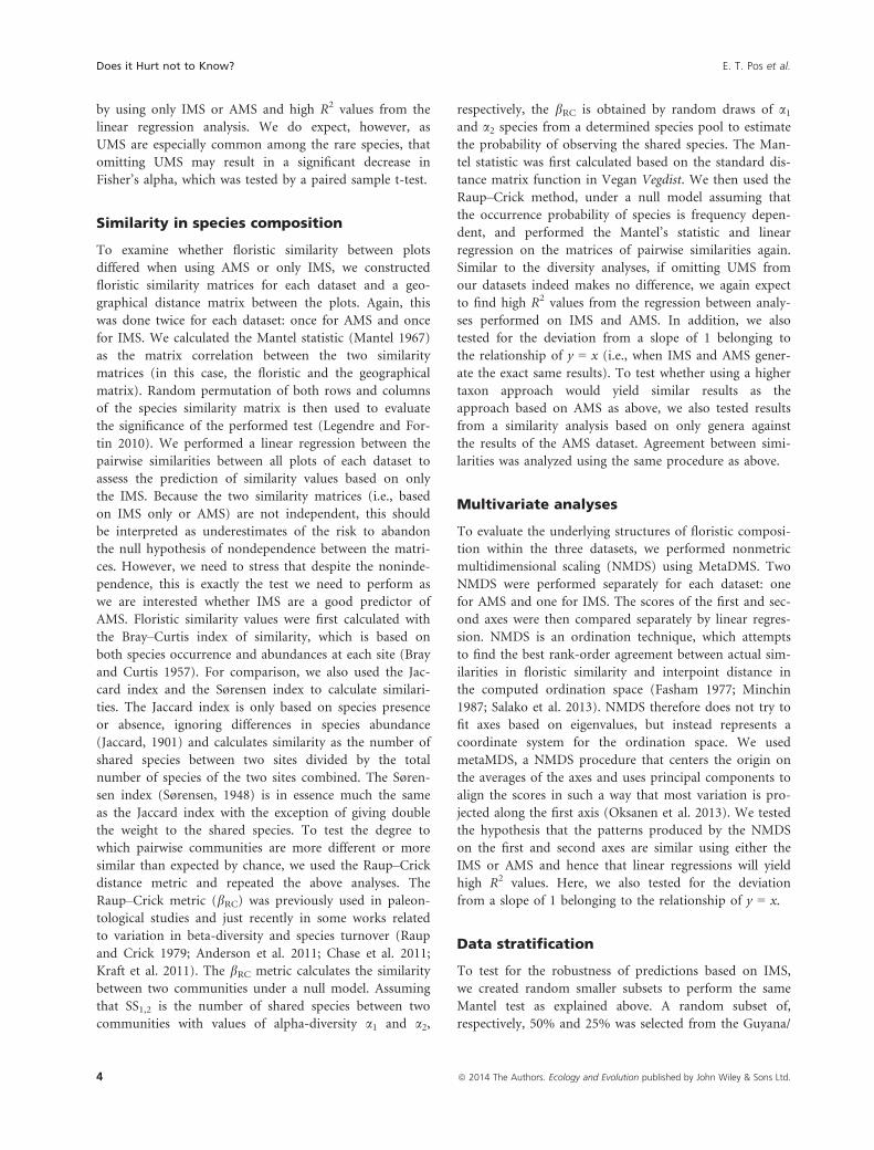
Three independent, nonoverlapping, tree inventory data-

sets were assembled: one from Guyana and Suriname, one

from Ecuador, and one from French Guiana (Fig. 1).

Each dataset consisted of 63–72 one-hectare plots, in

which all trees ≥10 cm DBH had been inventoried (see

Table 1 for details). Within each dataset, one or two per-

sons responsible for the majority of the collected material

harmonized all species names. Olaf B�anki and Juan Ernes-

to Guevara performed harmonization for the Guyana/

Suriname and Ecuador datasets, respectively, while Daniel

Sabatier and Jean-Franc�ois Molino together harmonized

the French Guianan dataset (hereafter referred to as OSB,

JEG, S-M). Harmonization was done by morphological

comparison of collections with reference to a “morpho-

holotype” for each morpho-species. Species names of all

subsets were standardized with the W3 Tropicos database,

using TNRS (Boyle et al. 2013). The three datasets were

harmonized independently of each other; no attempt was

made to harmonize the three datasets into one.

Three types of common ecological analyses (described

below) were performed for each dataset twice: once for

the all morpho-species (hereafter AMS) and once for a

subset composed of only identified morpho-species

(IMS), omitting the unidentified morpho-species of this

dataset (UMS – thus AMS = IMS + UMS). All tests were

performed in the “R” statistical and programming envi-

ronment (R Core Team 2012). To calculate the Mantel

statistics and metaMDS (a variant of NMDS), we used

the package “vegan” (Oksanen et al. 2013). All linear

models were tested for significance with a permutation

procedure from the package “lmperm” (Wheeler 2010).

Diversity analyses

To test how UMS influence analyses of alpha- and beta-

diversity, we calculated Fisher’s alpha values (Fisher et al.

1943) for every one-hectare plot twice: once with AMS

and once for only IMS. We then performed a linear

regression analysis between Fisher’s alpha calculated for

AMS and IMS to determine whether diversity patterns

remain the same when datasets are truncated like this.

Fisher’s alpha is a widely used diversity index, specifically

suited for species abundances following a logseries distri-

bution. Fisher’s alpha has been shown to be a very effi-

cient diversity index for discriminating between sites

(Taylor et al. 1976). This is a consequence of Fisher’s

alpha being theoretically independent of sample size, and

therefore, much less influenced by the abundances of the

more common species (Kempton 1979; Condit et al.

1998). If UMS can safely be excluded from the dataset,

we expect to find no deviation from the pattern predicted

Table 1. The number of one-hectare plots for each forest type listed

by country. Guyana and Suriname are used as one dataset. Type

abbreviations are Igap�o (IG), Podzol (PZ), Swamp (SW), Terra Firme

(TF), and V�arzea (VA). Minimum diameter at breast height (DBH) as

limit for measurement was 10 centimeters for all plots.

IG PZ SW TF VA Min. DBH

Nr. 1-Ha

plots

Guyana/

Suriname

0 21 0 45 1 10 67

Ecuador 2 3 4 53 10 10 72

French Guiana 0 0 0 63 0 10 63

Total 2 24 4 161 11 NA 202

–80 –75 –70 –65 –60 –55 –50 –45

–20

–15

–10

–50

510

Longitude

Latit

ude

500 km

Figure 1. Map showing location of all 202 plots belonging to the

Ecuador (blue), Guyana/Suriname (red), and French Guiana (black)

datasets.

ª 2014 The Authors. Ecology and Evolution published by John Wiley & Sons Ltd. 3

E. T. Pos et al. Does it Hurt not to Know?

by using only IMS or AMS and high R2 values from the

linear regression analysis. We do expect, however, as

UMS are especially common among the rare species, that

omitting UMS may result in a significant decrease in

Fisher’s alpha, which was tested by a paired sample t-test.

Similarity in species composition

To examine whether floristic similarity between plots

differed when using AMS or only IMS, we constructed

floristic similarity matrices for each dataset and a geo-

graphical distance matrix between the plots. Again, this

was done twice for each dataset: once for AMS and once

for IMS. We calculated the Mantel statistic (Mantel 1967)

as the matrix correlation between the two similarity

matrices (in this case, the floristic and the geographical

matrix). Random permutation of both rows and columns

of the species similarity matrix is then used to evaluate

the significance of the performed test (Legendre and For-

tin 2010). We performed a linear regression between the

pairwise similarities between all plots of each dataset to

assess the prediction of similarity values based on only

the IMS. Because the two similarity matrices (i.e., based

on IMS only or AMS) are not independent, this should

be interpreted as underestimates of the risk to abandon

the null hypothesis of nondependence between the matri-

ces. However, we need to stress that despite the noninde-

pendence, this is exactly the test we need to perform as

we are interested whether IMS are a good predictor of

AMS. Floristic similarity values were first calculated with

the Bray–Curtis index of similarity, which is based on

both species occurrence and abundances at each site (Bray

and Curtis 1957). For comparison, we also used the Jac-

card index and the Sørensen index to calculate similari-

ties. The Jaccard index is only based on species presence

or absence, ignoring differences in species abundance

(Jaccard, 1901) and calculates similarity as the number of

shared species between two sites divided by the total

number of species of the two sites combined. The Søren-

sen index (Sørensen, 1948) is in essence much the same

as the Jaccard index with the exception of giving double

the weight to the shared species. To test the degree to

which pairwise communities are more different or more

similar than expected by chance, we used the Raup–Crickdistance metric and repeated the above analyses. The

Raup–Crick metric (bRC) was previously used in paleon-

tological studies and just recently in some works related

to variation in beta-diversity and species turnover (Raup

and Crick 1979; Anderson et al. 2011; Chase et al. 2011;

Kraft et al. 2011). The bRC metric calculates the similarity

between two communities under a null model. Assuming

that SS1,2 is the number of shared species between two

communities with values of alpha-diversity a1 and a2,

respectively, the bRC is obtained by random draws of a1and a2 species from a determined species pool to estimate

the probability of observing the shared species. The Man-

tel statistic was first calculated based on the standard dis-

tance matrix function in Vegan Vegdist. We then used the

Raup–Crick method, under a null model assuming that

the occurrence probability of species is frequency depen-

dent, and performed the Mantel’s statistic and linear

regression on the matrices of pairwise similarities again.

Similar to the diversity analyses, if omitting UMS from

our datasets indeed makes no difference, we again expect

to find high R2 values from the regression between analy-

ses performed on IMS and AMS. In addition, we also

tested for the deviation from a slope of 1 belonging to

the relationship of y = x (i.e., when IMS and AMS gener-

ate the exact same results). To test whether using a higher

taxon approach would yield similar results as the

approach based on AMS as above, we also tested results

from a similarity analysis based on only genera against

the results of the AMS dataset. Agreement between simi-

larities was analyzed using the same procedure as above.

Multivariate analyses

To evaluate the underlying structures of floristic composi-

tion within the three datasets, we performed nonmetric

multidimensional scaling (NMDS) using MetaDMS. Two

NMDS were performed separately for each dataset: one

for AMS and one for IMS. The scores of the first and sec-

ond axes were then compared separately by linear regres-

sion. NMDS is an ordination technique, which attempts

to find the best rank-order agreement between actual sim-

ilarities in floristic similarity and interpoint distance in

the computed ordination space (Fasham 1977; Minchin

1987; Salako et al. 2013). NMDS therefore does not try to

fit axes based on eigenvalues, but instead represents a

coordinate system for the ordination space. We used

metaMDS, a NMDS procedure that centers the origin on

the averages of the axes and uses principal components to

align the scores in such a way that most variation is pro-

jected along the first axis (Oksanen et al. 2013). We tested

the hypothesis that the patterns produced by the NMDS

on the first and second axes are similar using either the

IMS or AMS and hence that linear regressions will yield

high R2 values. Here, we also tested for the deviation

from a slope of 1 belonging to the relationship of y = x.

Data stratification

To test for the robustness of predictions based on IMS,

we created random smaller subsets to perform the same

Mantel test as explained above. A random subset of,

respectively, 50% and 25% was selected from the Guyana/



Suriname, French Guiana, and Ecuador IMS pool. In

making the IMS dataset even smaller in comparison with

the complete dataset (by randomly omitting IMS), we

simulated a larger proportion of UMS. This was repeated

for 50 iterations from which mean values were calculated

for the similarity matrices using the same three indices as

used for the similarity analyses described above.

Results

Floristic composition and level of speciesidentification

The proportion of IMS varied in the three datasets from

44–77%. In Guyana and Suriname (OSB), 67 plots

yielded 37,446 individual trees, for a total of 1042 AMS

and 458 IMS (44%). The mean number of UMS per plot

was 27 with a median of 24. Mean fraction of IMS per

plot for Guyana/Suriname was 70%. Ecuador (JEG) with

a total of 72 plots yielded 34,544 individual trees, for a

total of 2021 AMS and 1391 IMS (69%), with a mean

number of 17 and a median of 16 UMS per plot. The

mean proportion of IMS for each plot in Ecuador was

90%. In French Guiana (S-M), 63 plots yielded 35,075

individuals of trees, for a total of 1204 AMS and 925 IMS

(77%). Mean number of UMS per plot was 15 with a

median of 15. The mean proportion of IMS per plot in

French Guiana was 91%. Linear regressions between the

number of AMS and the number of IMS were high, with

R2 values of 0.938, 0.976, and 0.959 for Guyana/Suriname,

Ecuador, and French Guiana, respectively.

Predicted species diversity based onidentified morpho-species

Linear regressions between Fisher’s alpha (FA) calcu-

lated using AMS and only the IMS were extremely

high, yielding R2 values of >0.95 for all three datasets

(Table 2). The slope of the linear model based on the

Guyana/Suriname was 1.6. Using a 95% confidence

interval for the slope showed that this was significantly

different from the relation y = x with slope 1 (i.e.,

when there is no difference between FA based on

AMS or just IMS). This was the case for Ecuador and

French Guiana as well, with slopes of 1.12 and 1.10,

respectively. As expected, FA showed an increase with

an increasing number of species per plot for both IMS

and AMS. FA calculated for just IMS ranged between

2.87–44.92 for Guyana/Suriname, 8.96–114.65 for Ecua-

dor, and 27.61–114.65 for French Guiana. When using

AMS, this was (in the same order) 4.65–78.17, 12.23–130.32, and 27.61–130.32. These differences were found

to be significant after performing a paired sample t-

test with significance levels for rejecting the H0 of

equal ranges with probabilities <0.005 for all three

datasets.

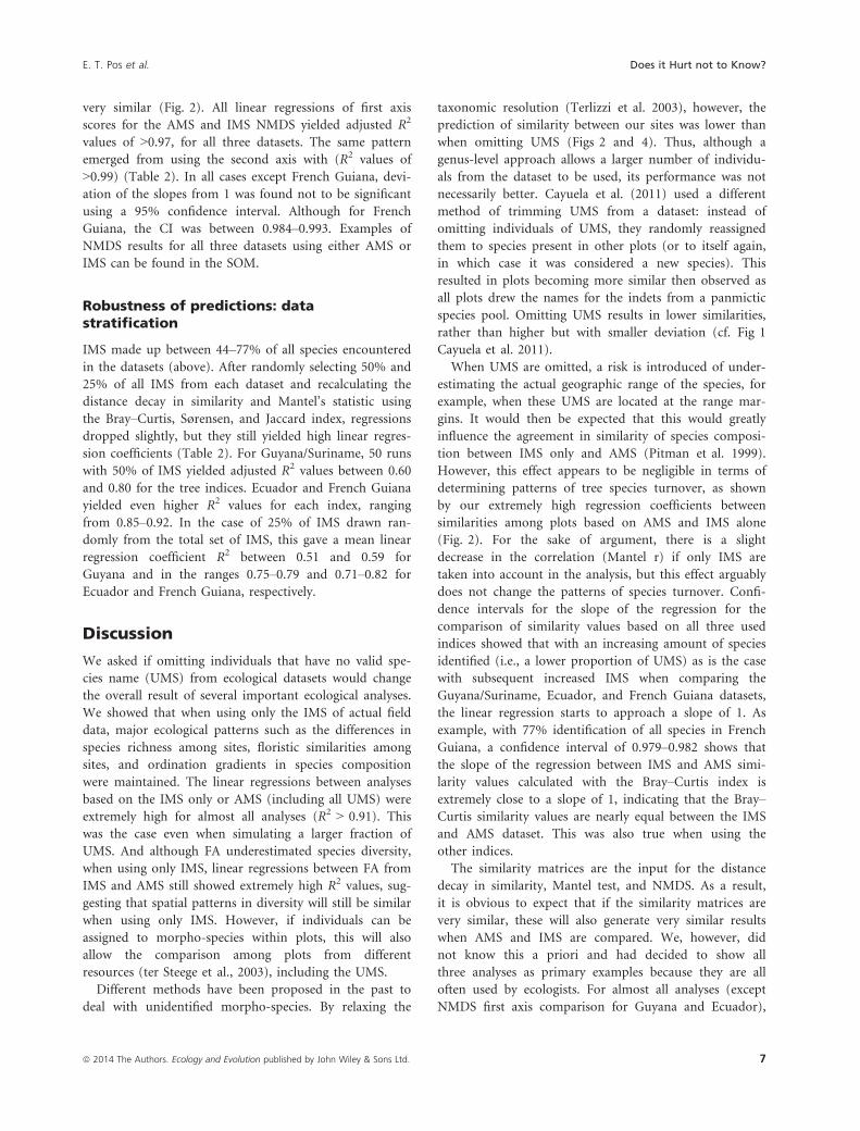
Patterns in morpho-species abundance

Because the slope between FA calculated for only the IMS

and AMS deviated significantly from 1, we examined the

rank abundance curves for both IMS and AMS for each

dataset. The AMS datasets were consistently richer in spe-

cies, especially the rare ones, when compared to the IMS

datasets (Fig. 3). Moving from the AMS dataset to the

IMS, more species were lost than individuals, significantly

affecting FA. For instance, the IMS dataset contains only

approximately 21% of the number of singletons

compared to the AMS dataset in Guyana/Suriname. For

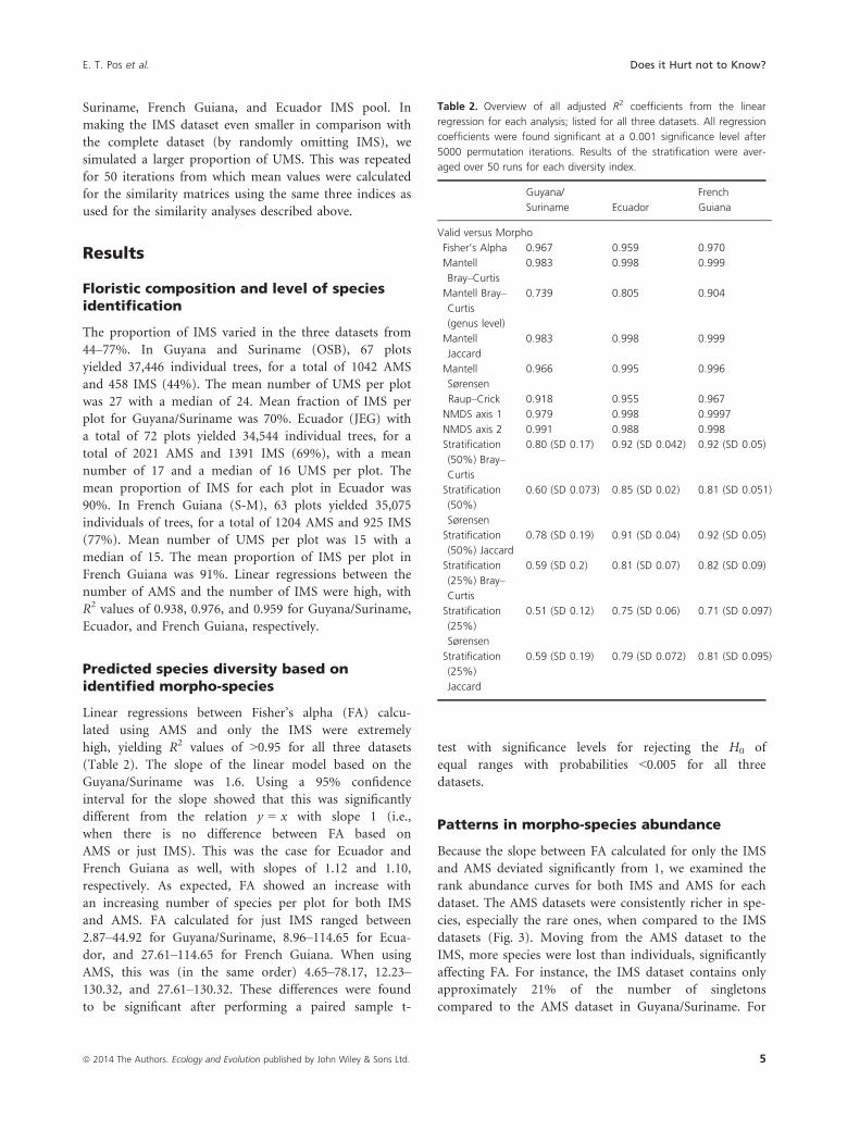
Table 2. Overview of all adjusted R2 coefficients from the linear

regression for each analysis; listed for all three datasets. All regression

coefficients were found significant at a 0.001 significance level after

5000 permutation iterations. Results of the stratification were aver-

aged over 50 runs for each diversity index.

Guyana/

Suriname Ecuador

French

Guiana

Valid versus Morpho

Fisher’s Alpha 0.967 0.959 0.970

Mantell

Bray–Curtis

0.983 0.998 0.999

Mantell Bray–

Curtis

(genus level)

0.739 0.805 0.904

Mantell

Jaccard

0.983 0.998 0.999

Mantell

Sørensen

0.966 0.995 0.996

Raup–Crick 0.918 0.955 0.967

NMDS axis 1 0.979 0.998 0.9997

NMDS axis 2 0.991 0.988 0.998

Stratification

(50%) Bray–

Curtis

0.80 (SD 0.17) 0.92 (SD 0.042) 0.92 (SD 0.05)

Stratification

(50%)

Sørensen

0.60 (SD 0.073) 0.85 (SD 0.02) 0.81 (SD 0.051)

Stratification

(50%) Jaccard

0.78 (SD 0.19) 0.91 (SD 0.04) 0.92 (SD 0.05)

Stratification

(25%) Bray–

Curtis

0.59 (SD 0.2) 0.81 (SD 0.07) 0.82 (SD 0.09)

Stratification

(25%)

Sørensen

0.51 (SD 0.12) 0.75 (SD 0.06) 0.71 (SD 0.097)

Stratification

(25%)

Jaccard

0.59 (SD 0.19) 0.79 (SD 0.072) 0.81 (SD 0.095)



Ecuador and French Guiana, this was 41% and 55%,

respectively. In terms of numbers, there are a total of only

44 singletons in the IMS dataset of Guyana/Suriname

against 210 in the AMS dataset (Ecuador = 212 vs. 518

and French Guiana = 114 vs. 208).

Similarity in species composition

Using IMS only, the similarity in species composition

based on Bray–Curtis was predicted very well for all three

datasets (R2 values of >0.98) (Table 2), and the slope in

all cases was almost identical to 1 (Fig. 2). Confidence

intervals showed, however, that, despite high adjusted R2

values, slopes from the linear regressions actually deviated

significantly from 1 for all datasets when using the Bray–Curtis index (Guyana/Suriname CI 0.917–0.927, Ecuador0.958–0.961, and French Guiana 0.979–0.982). The differ-

ence between using the Jaccard, Bray–Curtis, or Sørensen

index for calculating similarities among plots appeared to

be negligible, all resulted in adjusted R2 values of >0.96(Table 2) with slopes from the linear regressions all still

significantly deviating from 1 (for Jaccard: Guyana/Suri-

name CI 0.897–0.907, Ecuador 0.950–0.953, and French

Guiana 0.973–0.976 and for Sørensen Guyana/Suriname

CI 0.915–0.930, Ecuador 0.932–0.938, and French Guiana

0.969–0.974). Adjusted R2-values using the Raup–Crickdistance metric yielded values of >0.91 for all three

datasets. Examples of the patterns of distance decay with

AMS, and only IMS can be found for all three datasets in

the Supplementary Online Material (SOM). The Mantel’s

r coefficient for Guyana/Suriname using only IMS was

0.4695; when using AMS, this was slightly higher

(0.5092). The differences in Mantel’s r coefficient were

smaller for Ecuador (0.4029 and 0.4039) and French

Guiana (0.7944 and 0.7987).

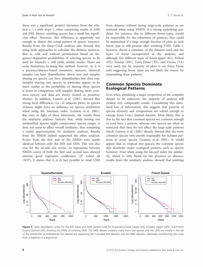
Using higher-taxon-level resolution incomparison with identified morpho-species

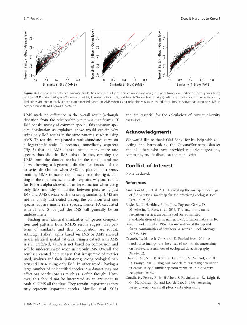
Using higher-taxon-level (genus-level) data, similarities

among communities are higher and much more deviant

from the expected similarities based on AMS (Fig. 4) than

with the IMS (Fig. 2). The latter shows a very strong lin-

ear regression, while regressions between similarities based

on genus level appear to predict the pattern generated by

AMS not as good (with R2 values ranging from 0.74–0.90,Table 2) as using only the IMS.

Predictions of Multivariate analyses

Nonmetric multidimensional scaling of all three subsets

showed good segregation along the first two axes of the

NMDS when using AMS as well as when using only IMS.

Axis 1 scores derived from only the IMS, and AMS were

Fisher's alpha in plot (IMS)

Fish

er's

alp

ha in

plo

t (A

MS

) Guyana/SurinameEcuadorFrench Guiana

Similarity (1-Bray) (IMS)

True

sim

ilarit

y (1

-Bra

y) (A

MS


NMDS axis 1 scores (IMS)

NM

DS

axi

s 1

scor

es (A

MS


0 50 100 150 200 250

050

100

150

200

250

0.0 0.2 0.4 0.6 0.8 1.0

0.0

0.2

0.4

0.6

0.8

1.0

–0.4 –0.2 0.0 0.2 0.4 0.6

–0.4

–0.2

0.0

0.2

0.4

0.6

0 50 100 150 200 250 300

050

100

150

200

250

300

Number of species per plot (IMS)

Num

ber o

f spe

cies

per

plo

t (A

MS

)Guyana/SurinameEcuadorFrench Guiana

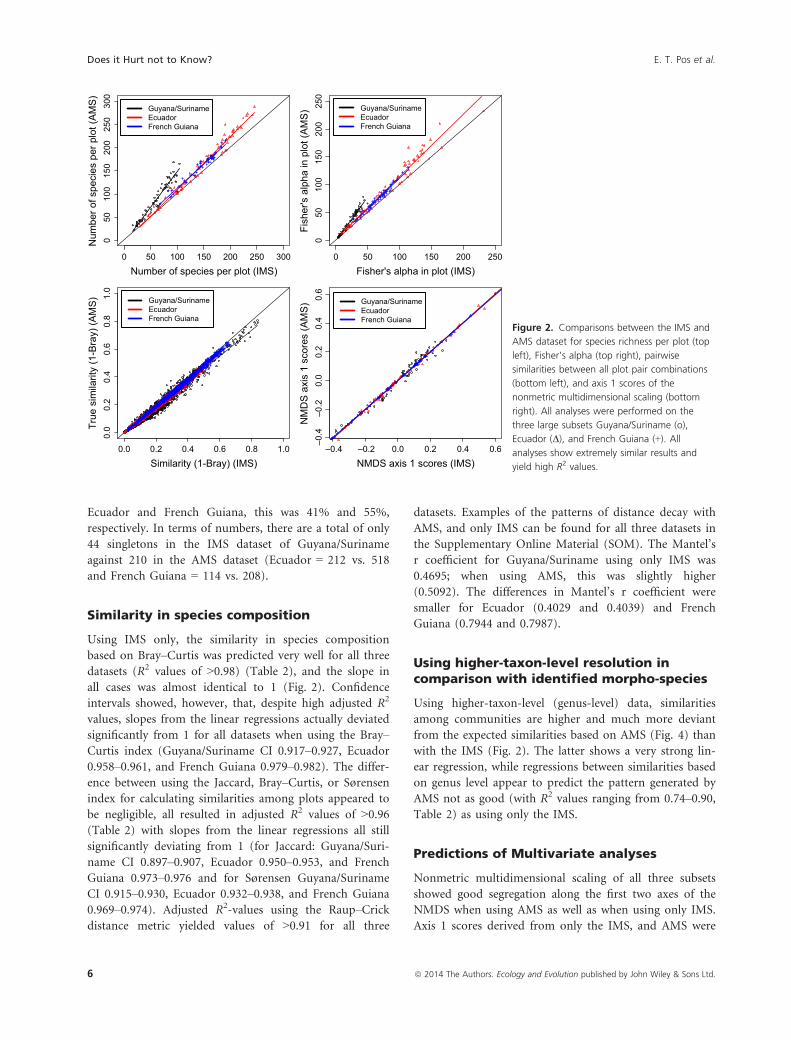
Figure 2. Comparisons between the IMS and

AMS dataset for species richness per plot (top

left), Fisher’s alpha (top right), pairwise

similarities between all plot pair combinations

(bottom left), and axis 1 scores of the

nonmetric multidimensional scaling (bottom

right). All analyses were performed on the

three large subsets Guyana/Suriname (o),

Ecuador (D), and French Guiana (+). All

analyses show extremely similar results and

yield high R2 values.



very similar (Fig. 2). All linear regressions of first axis

scores for the AMS and IMS NMDS yielded adjusted R2

values of >0.97, for all three datasets. The same pattern

emerged from using the second axis with (R2 values of

>0.99) (Table 2). In all cases except French Guiana, devi-

ation of the slopes from 1 was found not to be significant

using a 95% confidence interval. Although for French

Guiana, the CI was between 0.984–0.993. Examples of

NMDS results for all three datasets using either AMS or

IMS can be found in the SOM.

Robustness of predictions: datastratification

IMS made up between 44–77% of all species encountered

in the datasets (above). After randomly selecting 50% and

25% of all IMS from each dataset and recalculating the

distance decay in similarity and Mantel’s statistic using

the Bray–Curtis, Sørensen, and Jaccard index, regressions

dropped slightly, but they still yielded high linear regres-

sion coefficients (Table 2). For Guyana/Suriname, 50 runs

with 50% of IMS yielded adjusted R2 values between 0.60

and 0.80 for the tree indices. Ecuador and French Guiana

yielded even higher R2 values for each index, ranging

from 0.85–0.92. In the case of 25% of IMS drawn ran-

domly from the total set of IMS, this gave a mean linear

regression coefficient R2 between 0.51 and 0.59 for

Guyana and in the ranges 0.75–0.79 and 0.71–0.82 for

Ecuador and French Guiana, respectively.

Discussion

We asked if omitting individuals that have no valid spe-

cies name (UMS) from ecological datasets would change

the overall result of several important ecological analyses.

We showed that when using only the IMS of actual field

data, major ecological patterns such as the differences in

species richness among sites, floristic similarities among

sites, and ordination gradients in species composition

were maintained. The linear regressions between analyses

based on the IMS only or AMS (including all UMS) were

extremely high for almost all analyses (R2 > 0.91). This

was the case even when simulating a larger fraction of

UMS. And although FA underestimated species diversity,

when using only IMS, linear regressions between FA from

IMS and AMS still showed extremely high R2 values, sug-

gesting that spatial patterns in diversity will still be similar

when using only IMS. However, if individuals can be

assigned to morpho-species within plots, this will also

allow the comparison among plots from different

resources (ter Steege et al., 2003), including the UMS.

Different methods have been proposed in the past to

deal with unidentified morpho-species. By relaxing the

taxonomic resolution (Terlizzi et al. 2003), however, the

prediction of similarity between our sites was lower than

when omitting UMS (Figs 2 and 4). Thus, although a

genus-level approach allows a larger number of individu-

als from the dataset to be used, its performance was not

necessarily better. Cayuela et al. (2011) used a different

method of trimming UMS from a dataset: instead of

omitting individuals of UMS, they randomly reassigned

them to species present in other plots (or to itself again,

in which case it was considered a new species). This

resulted in plots becoming more similar then observed as

all plots drew the names for the indets from a panmictic

species pool. Omitting UMS results in lower similarities,

rather than higher but with smaller deviation (cf. Fig 1

Cayuela et al. 2011).

When UMS are omitted, a risk is introduced of under-

estimating the actual geographic range of the species, for

example, when these UMS are located at the range mar-

gins. It would then be expected that this would greatly

influence the agreement in similarity of species composi-

tion between IMS only and AMS (Pitman et al. 1999).

However, this effect appears to be negligible in terms of

determining patterns of tree species turnover, as shown

by our extremely high regression coefficients between

similarities among plots based on AMS and IMS alone

(Fig. 2). For the sake of argument, there is a slight

decrease in the correlation (Mantel r) if only IMS are

taken into account in the analysis, but this effect arguably

does not change the patterns of species turnover. Confi-

dence intervals for the slope of the regression for the

comparison of similarity values based on all three used

indices showed that with an increasing amount of species

identified (i.e., a lower proportion of UMS) as is the case

with subsequent increased IMS when comparing the

Guyana/Suriname, Ecuador, and French Guiana datasets,

the linear regression starts to approach a slope of 1. As

example, with 77% identification of all species in French

Guiana, a confidence interval of 0.979–0.982 shows that

the slope of the regression between IMS and AMS simi-

larity values calculated with the Bray–Curtis index is

extremely close to a slope of 1, indicating that the Bray–Curtis similarity values are nearly equal between the IMS

and AMS dataset. This was also true when using the

other indices.

The similarity matrices are the input for the distance

decay in similarity, Mantel test, and NMDS. As a result,

it is obvious to expect that if the similarity matrices are

very similar, these will also generate very similar results

when AMS and IMS are compared. We, however, did

not know this a priori and had decided to show all

three analyses as primary examples because they are all

often used by ecologists. For almost all analyses (except

NMDS first axis comparison for Guyana and Ecuador),



there was a significant positive deviation from the rela-

tion y = x with slope 1, when comparing results of AMS

and IMS. Hence, omitting species has a small but signifi-

cant effect. However, this difference is apparently not

enough to distort the actual pattern of species turnover.

Results from the Raup–Crick analyses also showed that

using both approaches to calculate the distance matrices,

that is, with and without permutation based on fre-

quency-dependent probabilities of selecting species to be

used for Mantel’s r, still yields similar results. There are

some limitations to using this method, however. As it is

a presence/absence-based nonmetric measure, identical

samples can have dissimilarities above zero and samples

sharing no species can have dissimilarities less than one.

Samples sharing rare species in particular appear to be

more similar as the probability of sharing these species

is lower in comparison with samples sharing more com-

mon species and data are always treated as presence/

absence. In addition, Lennon et al. (2001) showed that

strong local differences (i.e., in adjacent plots) in species

richness might have an influence on species similarities

when using the Sørensen index (Lennon et al. 2001).

But even in light of these limitations, the results from

the similarity analyses indicate that, while leaving out

unidentified species might compromise species ranges, it

does not seem to affect overall similarity, thus remaining

a useful approximation for similarity analyses. Results

from the NMDS indeed supported the other analyses.

Scores from the first axis of the NMDS were nearly

identical between only the IMS and AMS. This was also

true for the second axis scores. As regressions between

NMDS scores of both the first and second axes showed

extreme good regression coefficients (R2 values all

>0.97), it shows that it is in fact possible to omit UMS

from datasets without losing large-scale patterns as are

analyzed when using NMDS. If a strong underlying gra-

dient, for instance, due to different forest types, would

be responsible for the robustness of patterns, they could

be maintained if a large enough fraction of plots in each

forest type is still present after omitting UMS. Table 1,

however, shows a summary of the datasets used and the

types of forest incorporated in the analyses, and

although five different types of forest Igap�o (IG), Podzol

(PZ), Swamp (SW), Terra Firme (TF), and V�arzea (VA)

were used, the far majority of plots is on Terra Firme

soils suggesting forest types are not likely the reason for

maintaining these patterns.

Common Species DominateEcological Patterns

Even when simulating a larger proportion of the complete

dataset to be unknown, the majority of analyses still

yielded very comparable results. Considering this simu-

lated loss of information, this suggests that patterns of

species diversity and composition are robust enough to

emerge from (very) limited datasets. Most likely, this is

due to the fact that common species are common enough

to even have a pattern, whereas rare species are often so

restricted that they do not affect the large-scale patterns

much. Lennon et al. (2001) already showed that the more

common species were mostly responsible for richness pat-

terns in avian species (Lennon et al. 2001). It would

appear that in tropical tree species, the common species

also dominate major ecological patterns such as species

turnover. Even when using the Jaccard index for similar-

ity, which is only based on the presence or absence,

results from the similarity analyses showed that omitting

Guyana/Suriname

Rank

Log

(abu

ndan

ce)

IMSAMSBoundary IMS/AMS


Ecuador

Rank

Log

(abu

ndan

ce)

0 200 400 600 800 1000 0 500 1000 1500 2000

15

1050

500

15

1050

500


0 200 400 600 800 1000 1200

15

1050

100

500

French Guiana

Rank

Log

(abu

ndan

ce)

Figure 3. Rank abundance curves for the IMS (blue) and AMS dataset (red) for Guyana/Suriname (upper left), Ecuador (upper right), and French

Guiana (bottom left), showing the effect of omitting UMS. The AMS dataset contains many more rare species and the UMS are mostly in the tail

of the distribution as indicated by the dashed line separating the truncated IMS datasets and the AMS datasets, effectively transforming the curve

from a logseries to a lognormal.



UMS made no difference in the overall result (although

deviation from the relationship y = x was significant). If

IMS consist mostly of common species, this common spe-

cies domination as explained above would explain why

using only IMS results in the same patterns as when using

AMS. To test this, we plotted a rank abundance curve on

a logarithmic scale. It becomes immediately apparent

(Fig. 3) that the AMS dataset include many more rare

species than did the IMS subset. In fact, omitting the

UMS from the dataset results in the rank abundance

curve showing a lognormal distribution instead of the

logseries distribution when AMS are plotted. In a sense,

omitting UMS truncates the datasets from the right, cut-

ting of the rare species. This also explains why our results

for Fisher’s alpha showed an underestimation when using

only IMS and why similarities between plots using just

IMS and AMS deviate with increasing similarity. UMS are

not randomly distributed among the common and rare

species but are mostly rare species. Hence, FA calculated

with N and S for just the IMS will generally be an

underestimate.

Finding near identical similarities of species composi-

tion and patterns from NMDS results suggest that pat-

terns of similarity and thus composition are robust.

Although Fisher’s alpha based on IMS or AMS showed

nearly identical spatial patterns, using a dataset with AMS

is still preferred, as FA is not based on comparison and

will be underestimated when using only IMS. Overall, the

results presented here suggest that irrespective of metrics

used, analyses and their limitations; strong ecological pat-

terns still arise using only IMS. In other words, having a

large number of unidentified species in a dataset may not

affect our conclusions as much as is often thought. How-

ever, this should not be interpreted as an argument to

omit all UMS all the time. They remain important as they

may represent important species (Mouillot et al. 2013)

and are essential for the calculation of correct diversity

measures.

Acknowledgments

We would like to thank Olaf B�anki for his help with col-

lecting and harmonizing the Guyana/Suriname dataset

and all others who have provided valuable suggestions,

comments, and feedback on the manuscript.

Conflict of Interest

None declared.

References

Anderson M. J., et al. 2011. Navigating the multiple meanings

of b diversity: a roadmap for the practicing ecologist. Ecol.

Lett. 14:19–28.

Boyle, B., N. Hopkins, Z. Lu, J. A. Raygoza Garay, D.

Mozzherin, T. Rees, et al. 2013. The taxonomic name

resolution service: an online tool for automated

standardization of plant names. BMC Bioinformatics 14:16.

Bray, J., and J. Curtis. 1957. An ordination of the upland

forest communities of southern Wisconsin. Ecol. Monogr.

27:325–349.

Cayuela, L., M. de la Cruz, and K. Ruokolainen. 2011. A

method to incorporate the effect of taxonomic uncertainty

on multivariate analyses of ecological data. Ecography

34:94–102.

Chase, J. M., N. J. B. Kraft, K. G. Smith, M. Vellend, and B.

D. Inouye. 2011. Using null models to disentangle variation

in community dissimilarity from variation in a-diversity.

Ecosphere 2:art24.

Condit, R., Foster, R. B., Hubbell, S. P., Sukumar, R., Leigh, E.

G., Manokaran, N., and Loo de Lao, S. 1998. Assessing

forest diversity on small plots: calibration using

Similarity (1-Bray) (AMS)

True

sim

ilarit

y (1

-Bra

y) (G

enus

leve

l)

0.0 0.2 0.4 0.6 0.8

0.0

0.2

0.4

0.6

0.8


True

sim

ilarit

y (1

-Bra

y) (G

enus

leve

l)

0.0 0.2 0.4 0.6 0.8

0.0

0.2

0.4

0.6

0.8

0.0 0.2 0.4 0.6 0.8

0.0

0.2

0.4

0.6

0.8


True

sim

ilarit

y (1

-Bra

y) (G

enus

leve

l)

Figure 4. Comparisons between pairwise similarities between all plot pair combinations using a higher-taxon-level indicator (here genus level)

and the AMS dataset (Guyana/Suriname topright, Ecuador bottom left, and French Guiana bottom right). Although patterns still remain the same,

similarities are continuously higher than expected based on AMS when using only higher taxa as an indicator. Results show that using only IMS in

comparison with AMS gives a better fit.



species-individual curves from 50 ha plots. Pp. in 247–268

Forest Biodiversity Diversity Research, Monitoring, and

Modeling, Dallmeier, F. and Comiskey, J. A. (ed.). Paris,

UNESCO, the Parthenon Publishing Group.

Darwin, C. 1859. On the origin of the species by means of

natural selection, or the preservation of favoured races in

the struggle for life. John Murray, London.

Enquist, B. J., J. P. Haskell, and B. H. Tiffney. 2002. General

patterns of taxonomic and biomass partitioning in extant

and fossil plant communities. Nature 419:610–613.

Fasham, M. 1977. A comparison of nonmetric

multidimensional scaling, principal components and

reciprocal averaging for the ordination of simulated

coenoclines, and coenoplanes. Ecology 58:551–561.

Fisher, R. A., A. Steven Corbet, and C. B. Williams. 1943. The

relation between the number of species and the number of

individuals in a random sample of an animal population. J.

Anim. Ecol. :42–58.

Higgins, M. A., and K. Ruokolainen. 2004. Rapid tropical forest

inventory: a comparison of techniques based on inventory

data from western Amazonia. Conserv. Biol. 18:799–811.

Jaccard, Paul. Distribution de la Flore Alpine: dans le Bassin des

dranses et dans quelques r�egions voisines. Rouge, 1901.

Jari Oksanen, F., G. Blanchet, R. Kindt, P. Legendre, P. R.

Minchin, R. B. O’Hara, et al. (2013). vegan: Community

Ecology Package. R package version 2.0-7. http://CRAN.

R-project.org/package=vegan

Kempton, R. 1979. The structure of species abundance

measurement of diversity. Biometrics 35:307–321.

Kraft, N. J. B., L. S. Comita, J. M. Chase, N. J. Sanders, N. G.

Swenson, T. O. Crist, et al. 2011. Disentangling the drivers

of diversity along latitudinal and elevational gradients.

Science 333:1755–1758.

Legendre, P., and M.-J. Fortin. 2010. Comparison of the

Mantel test and alternative approaches for detecting

complex multivariate relationships in the spatial analysis of

genetic data. Mol. Ecol. Resour. 10:831–844.

Lennon, J. J., et al. 2001. The geographical structure of British

bird distributions: diversity, spatial turnover and scale. J.

Anim. Ecol. 70:966–979.

Mallet, J. 2008. Hybridization, ecological races and the nature

of species: empirical evidence for the ease of speciation.

Philos. Trans. R. Soc. Lond. B Biol. Sci. 363:2971–2986.

Mantel, N. 1967. The detection of disease clustering and a

generalized regression approach. Cancer Res. 27:209–220.

Minchin, P. R. 1987. An evaluation of the relative robustness

of techniques for ecological ordination. Vegetatio 69:89–107.

Mouillot, D., D. R. Bellwood, C. Baraloto, J. Chave, R. Galzin,

M. Harmelin-Vivien, et al. 2013. Rare species support

vulnerable functions in high-diversity ecosystems. PLoS Biol.

11:e1001569.

Nekola, J., and P. White. 1999. The distance decay of

similarity in biogeography and ecology. J. Biogeogr. 26:

867–878.

Pik, A. J., I. A. N. Oliver, and A. J. Beattie. 1999. Taxonomic

sufficiency in ecological studies of terrestrial invertebrates.

Aust. J. Ecol. 24:555–562.

Pik, A. J., J. M. Dangerfield, R. A. Bramble, C. Angus, and D.

A. Nipperess. 2002. The use of invertebrates to detect

small-scale habitat heterogeneity and its application to

restoration. Environ. Monit. Assess. 75:179–199.

Pitman, N., J. Terborgh, M. Silman, and V. P. N. Percy

Nu~nez. 1999. Tree species distributions in an upper

Amazonian forest. Ecology 80:2651–2661.

R Core Team (2012). R: A language and environment for

statistical computing. R Foundation for Statistical

Computing, Vienna, Austria. ISBN 3-900051-07-0, URL

http://www.R-project.org/

Raup, D. M., and R. E. Crick. 1979. Measurement of faunal

similarity in paleontology. J. Paleontol. 53:1213–1227.

Ruokolainen, K., et al. (2002). Two biases in estimating range

sizes of Amazonian plant species. J. Trop. Ecol. 18:

935–942.

Salako, V. K., A. Adebanji, and R. Gl�el�e Kaka€ı. 2013. On the

empirical performance of non-metric multidimensional

scaling in vegetation studies. Int. J. Appl. Math. Stat. 36:

54–67.

Sørensen, T. 1948. A method of establishing groups of equal

amplitude in plant sociology based on similarity of species

and its application to analyses of the vegetation on Danish

commons. Biol. skr. 5:1–34.

Taylor, L., R. Kempton, and I. Woiwod. 1976. Diversity

statistics and the log series model. J. Anim. Ecol. 45:

255–272.

Terlizzi, A., S. Bevilacqua, S. Fraschetti, and F. Boero. 2003.

Taxonomic sufficiency and the increasing insufficiency of

taxonomic expertise. Mar. Pollut. Bull. 46:556–561.

Ter Steege, H., et al. 2003. A spatial model of tree a-diversityand tree density for the Amazon. Biodivers. Conserv.

12:2255–2277.

Vanderklift, M. A., T. J. Ward, and J. C. Phillips. 1998. Use of

assemblages derived from different taxonomic levels to select

areas for conserving marine biodiversity. Biol. Conserv.

86:307–315.

Vellend, M., P. L. Lilley, and B. M. Starzomski. 2008. Using

subsets of species in biodiversity surveys. J. Appl. Ecol.

45:161–169.

Wheeler, R. E. (2010). multResp() lmPerm. The R project for

statistical computing http://www.r-project.org/

Supporting Information

Additional Supporting Information may be found in the

online version of this article:

Figure S1. Example showing the distance decay in simi-

larity (DDS) for the Guyana/Suriname dataset based on

the distance matrices calculated with the Bray-Curtis



index used for the Mantel statistic Analysis of DDS are

shown for only IMS (upperleft), AMS (upperright) and

the linear regression for Guyana/Suriname (lowerleft).


larity (DDS) for the Guyana/Suriname dataset using the

Raup-Crick analyses. Analysis of DDS are shown for only

IMS (upperleft), AMS (upperright) and the linear regres-

sion for Guyana/Suriname (lowerleft).


larity (DDS) for the Ecuador dataset based on the dis-

tance matrices calculated with the Bray-Curtis index used

for the Mantel statistic Analysis of DDS are shown for

only IMS (upperleft), AMS (upperright) and the linear

regression for Ecuador (lowerleft).

Figure S4. Example showing the distance decay in

similarity (DDS) for the Ecuador dataset using the Raup-

Crick analyses Analysis of DDS are shown for only IMS

(upperleft), AMS (upperright) and the linear regression

for Ecuador (lowerleft)


larity (DDS) for the French Guiana dataset based on the

distance matrices calculated with the Bray-Curtis index

used for the Mantel statistic Analysis of DDS are shown

for only IMS (upperleft), AMS (upperright) and the lin-

ear regression for French Guiana (lowerleft).


larity (DDS) for the French Guiana dataset using the

Raup-Crick analyses Analysis of DDS are shown for only

IMS (upperleft), AMS (upperright) and the linear regres-

sion for French Guiana (lowerleft).



are all species necessary to reveal ecologically important patterns?

Documents