arX

iv:2

008.

1265

6v1

[m

ath.

OC

] 2

8 A

ug 2

020

Approximation of null controls for semilinear heat equations

using a least-squares approach

Jerome Lemoine ∗, Irene Marın-Gayte†, Arnaud Munch‡

August 31, 2020

Abstract

The null distributed controllability of the semilinear heat equation yt−∆y+g(y) = f 1ω,

assuming that g satisfies the growth condition g(s)/(|s| log3/2(1 + |s|)) → 0 as |s| → ∞and that g′ ∈ L∞

loc(R) has been obtained by Fernandez-Cara and Zuazua in 2000. The

proof based on a fixed point argument makes use of precise estimates of the observability

constant for a linearized heat equation. It does not provide however an explicit construction

of a null control. Assuming that g′ ∈ W s,∞(R) for one s ∈ (0, 1], we construct an explicit

sequence converging strongly to a null control for the solution of the semilinear equation. The

method, based on a least-squares approach, generalizes Newton type methods and guarantees

the convergence whatever be the initial element of the sequence. In particular, after a finite

number of iterations, the convergence is super linear with a rate equal to 1 + s. Numerical

experiments in the one dimensional setting support our analysis.

AMS Classifications: 35Q30, 93E24.

Keywords: Semilinear heat equation, Null controllability, Least-squares approach.

1 Introduction

Let Ω ⊂ Rd, 1 ≤ d ≤ 3, be a bounded connected open set whose boundary ∂Ω is Lipschitz. Let

ω be any non-empty open set of Ω and let T > 0. We note QT = Ω × (0, T ), qT = ω × (0, T )

and ΣT = ∂Ω× (0, T ). We are concerned with the null controllability problem for the following

semilinear heat equation yt −∆y + g(y) = f1ω in QT ,

y = 0 on ΣT , y(·, 0) = u0 in Ω,(1)

∗Laboratoire de mathematiques Blaise Pascal, Universite Clermont Auvergne, UMR CNRS 6620, Campus des

Cezeaux, 3, place Vasarely, 63178 Aubiere, France. e-mail: jerome.lemoine@uca.fr.†Departamento EDAN, Universidad de Sevilla, Campus Reina Mercedes, 41012, Sevilla, Spain. e-mail: im-

gayte@us.es.‡Laboratoire de mathematiques Blaise Pascal, Universite Clermont Auvergne, UMR CNRS 6620, Campus des

Cezeaux, 3, place Vasarely, 63178 Aubiere, France. e-mail: arnaud.munch@uca.fr (Corresponding author).

1

where u0 ∈ L2(Ω) is the initial state of y and f ∈ L2(qT ) is a control function. We assume more-

over that the nonlinear function g : R 7→ R is, at least, locally Lipschitz-continuous. Following

[13], we will also assume for simplicity that g satisfies

|g′(s)| ≤ C(1 + |s|m) a.e., with 1 ≤ m ≤ 1 + 4/d. (2)

Under this condition, (1) possesses exactly one local in time solution. Moreover, under the

growth condition

|g(s)| ≤ C(1 + |s| log(1 + |s|)) ∀s ∈ R, (3)

the solutions to (1) are globally defined in [0, T ] and one has

y ∈ C0([0, T ];L2(Ω)) ∩ L2(0, T ;H10 (Ω)), (4)

see [3]. Recall that, without a growth condition of the kind (3), the solutions to (1) can blow

up before t = T ; in general, the blow-up time depends on g and the size of ‖u0‖L2(Ω).

The system (1) is said to be controllable at time T if, for any u0 ∈ L2(Ω) and any globally

defined bounded trajectory y⋆ ∈ C0([0, T ];L2(Ω)) (corresponding to the data u⋆0 ∈ L2(Ω) and

f⋆ ∈ L2(qT )), there exist controls f ∈ L2(qT ) and associated states y that are again globally

defined in [0, T ] and satisfy (4) and

y(x, T ) = y⋆(x, T ), x ∈ Ω. (5)

We refer to [5] for an overview of control problems in nonlinear situations. The uniform control-

lability strongly depends on the nonlinearity g. Fernandez-Cara and Zuazua proved in [13] that

if g is too “super-linear” at infinity, then, for some initial data, the control cannot compensate

the blow-up phenomenon occurring in Ω\ω:

Theorem 1 ([13]) There exist locally Lipschitz-continuous functions g with g(0) = 0 and

|g(s)| ∼ |s| logp(1 + |s|) as |s| → ∞, p > 2,

such that (1) fails to be controllable for all T > 0.

On the other hand, Fernandez-Cara and Zuazua also proved that if p is small enough, then the

controllability holds true uniformly.

Theorem 2 ([13]) Let T > 0 be given. Assume that (1) admits at least one solution y⋆, globally

defined in [0, T ] and bounded in QT . Assume that g : R 7→ R is locally Lipschitz-continuous and

satisfies (2) andg(s)

|s| log3/2(1 + |s|)→ 0 as |s| → ∞. (6)

Then (1) is controllable at time T .

Therefore, if |g(s)| does not grow at infinity faster than |s| logp(1+ |s|) for any p < 3/2, then (1)

is controllable. This result extends [9] obtaining the uniform controllability for any p < 1. We

also mention [1] which gives the same result assuming additional sign condition on g, namely

g(s)s ≥ −C(1 + s2) for all s ∈ R and some C > 0. The problem remains open when g behaves

2

at infinity like |s| logp(1 + |s|) with 3/2 ≤ p ≤ 2. We mention however the recent work of

LeBalc’h [16] where uniform controllability results are obtained for p ≤ 2 assuming additional

sign conditions on g, notably that g(s) > 0 for s > 0 and g(s) < 0 for s < 0. This condition is

not satisfied for g(s) = −s logp(1 + |s|). Let us also mention [6] in the context of Theorem 1

where a positive boundary controllability result is proved for a specific class of initial and final

data and T large enough.

In the sequel, for simplicity, we shall assume that g(0) = 0 and that f⋆ ≡ 0, u⋆0 ≡ 0 so that

y⋆ is the null trajectory. The proof given in [13] is based on a fixed point method. Precisely, it

is shown that the operator Λ : L∞(QT ) → L∞(QT ), where yz := Λz is a null controlled solution

of the linear boundary value problem

yz,t −∆yz + yz g(z) = fz1ω in QT

yz = 0 on ΣT , yz(·, 0) = u0 in Ω, g(s) :=

g(s)/s s 6= 0,

g′(0) s = 0,(7)

maps a closed ball B(0,M) ⊂ L∞(QT ) into itself, for someM > 0. The Kakutani’s theorem then

provides the existence of at least one fixed point for the operator Λ, which is also a controlled

solution for (1).

The main goal of this work is to determine an approximation of the controllability problem

associated to (1), that is to construct an explicit sequence (fk)k∈N converging strongly toward

a null control for (1). A natural strategy is to take advantage of the method used in [16, 13]

and consider the Picard iterates associated with the operator Λ: yk+1 = Λ(yk), k ≥ 0 initialized

with any element y0 ∈ B(0,M). The sequence of controls is then (fk)k∈N so that fk ∈ L2(qT ) is

a null control for yk solution of

yk,t −∆yk + yk g(yk−1) = fk1ω in QT ,

yk = 0 on ΣT , yk(·, 0) = u0 in Ω.(8)

Numerical experiments for d = 1 reported in [11] exhibit the non convergence of the sequences

(yk)k∈N and (fk)k∈N for some initial conditions large enough. This phenomenon is related to

the fact that the operator Λ is a priori not contractant. We also refer to [2] where this strategy

is implemented. Still in the one dimensional case, a least-squares type approach, based on

the minimization over L2(QT ) of the functional R : L2(QT ) → R+ defined by R(z) := ‖z −

Λ(z)‖L2(QT ) is introduced and analyzed in [11]. Assuming that g ∈ C1(R) and g′ ∈ L∞(R), it

is proved first that R ∈ C1(L2(QT );R+) and secondly that, if ‖u0‖L∞(Ω) is small enough, then

any critical point for R is a fixed point for Λ. Under this smallness assumption on the data,

numerical experiments reported in [11] display the convergence of minimizing sequences for R

(based on a gradient method) and a better behavior than the Picard iterates. The analysis of

convergence is however not performed. As is usual for nonlinear problems and considered in

[11], we may also employ a Newton type method to find a zero of the mapping F : Y 7→ W

defined by

F (y, f) = (yt −∆y + g(y) − f1ω, y(· , 0) − u0, y(·, T )) ∀(y, f) ∈ Y (9)

for some appropriate Hilbert spaces Y and W (see below). It is shown for d = 1 in [11]

that, if g ∈ C1(R) and g′ ∈ L∞(R), then F ∈ C1(Y ;W ) allowing to derive the Newton iterative

3

sequence: given (y0, f0) in Y , define the sequence (yk, fk)k∈N iteratively as follows (yk+1, fk+1) =

(yk, fk)− (Yk, Fk) where Fk is a control for Yk solution of

Yk,t −∆Yk + g′(yk)Yk = Fk 1ω + yk,t −∆yk + g(yk)− fk1ω, in QT ,

Yk = 0, on ΣT ,

Yk(·, 0) = u0 − yk(·, 0), in Ω

(10)

such that Yk(·, T ) = −yk(·, T ) in Ω. Once again, numerical experiments for d = 1 in [11] exhibits

the lack of convergence of the Newton method for large enough initial condition, for which the

solution y is not close enough to the zero trajectory. As far as we know, the construction of a

convergent approximation (fk)k∈N in the general case where the initial data to be controlled is

arbitrary in L2(Ω) remains an open issue. Still assuming that g′ ∈ L∞(R) and in addition that

there exists one s in (0, 1] such that supa,b∈R,a6=b|g′(a)−g′(b)|

|a−b|s < ∞, we construct, for any initial

data u0 ∈ L2(Ω), a strongly convergent sequence (fk)k∈N toward a control for (1). Moreover,

after a finite number of iterates related to the norm ‖g′‖L∞(R), the convergence is super linear

with a rate equal to 1 + s. This is done (following and improving [20] devoted to a linear

case) by introducing a quadratic functional which measures how a pair (y, f) ∈ Y is close to a

controlled solution for (1) and then by determining a particular minimizing sequence enjoying

the announced property. A natural example of so-called error (or least-squares) functional is

given by E(y, f) := 12‖F (y, f)‖2W to be minimized over Y . In view of controllability results for

(1), the non-negative functional E achieves its global minimum equal to zero for any control

pair (y, f) ∈ Y of (1).

The paper is organized as follows. In Section 2, we first derive a controllability result for

a linearized wave equation with potential in L∞(QT ) and source term in L2(0, T ;H−1(Ω)).

Then, in Section 3, we define the least-squares functional E and the corresponding optimization

problem (26) over the Hilbert space A. We show that E is Gateaux-differentiable over A and

that any critical point (y, f) for E for which g′(y) belongs to L∞(QT ) is also a zero of E (see

Proposition 4). This is done by introducing a descent direction (Y 1, F 1) for E(y, f) for which

E′(y, f) · (Y 1, F 1) is proportional to E(y, f). Then, assuming that the nonlinear function g is

such that g′ belongs to W s,∞(R) for one s in (0, 1], we determine a minimizing sequence based

on (Y 1, F 1) which converges strongly to a controlled pair for the semilinear heat equation (1).

Moreover, we prove that after a finite number of iterates, the convergence enjoys a rate equal

to 1 + s (see Theorem 3 for s = 1 and Theorem 4 for s ∈ (0, 1)). We also emphasize that this

least-squares approach coincides with the damped Newton method one may use to find a zero of

a mapping similar to F mentioned above; we refer to Remark 7. This explains the convergence

of our approach with a super-linear rate. Section 4 gives some numerical illustrations of our

result in the one dimensional case and a nonlinear function g for which g′ ∈ W 1,∞(R). We

conclude in Section 5 with some perspectives. As far as we know, the analysis of convergence

presented in this work, though some restrictive hypotheses on the nonlinear function g, is the

first one in the context of controllability for partial differential equations.

Along the text, we shall denote by ‖ ·‖∞ the usual norm in L∞(R), (·, ·)X the scalar product

of X (if X is a Hilbert space) and by 〈·, ·〉X,Y the duality product between the spaces X and Y .

4

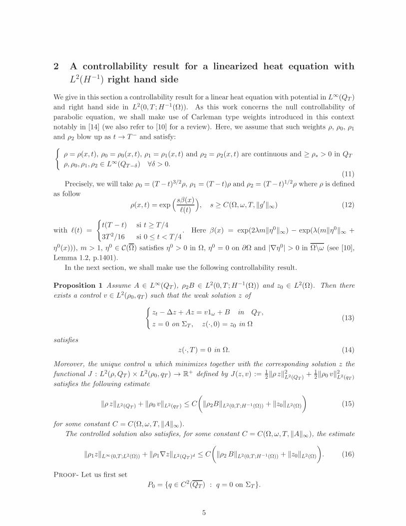
2 A controllability result for a linearized heat equation with

L2(H−1) right hand side

We give in this section a controllability result for a linear heat equation with potential in L∞(QT )

and right hand side in L2(0, T ;H−1(Ω)). As this work concerns the null controllability of

parabolic equation, we shall make use of Carleman type weights introduced in this context

notably in [14] (we also refer to [10] for a review). Here, we assume that such weights ρ, ρ0, ρ1and ρ2 blow up as t → T− and satisfy:

ρ = ρ(x, t), ρ0 = ρ0(x, t), ρ1 = ρ1(x, t) and ρ2 = ρ2(x, t) are continuous and ≥ ρ∗ > 0 in QT

ρ, ρ0, ρ1, ρ2 ∈ L∞(QT−δ) ∀δ > 0.

(11)

Precisely, we will take ρ0 = (T − t)3/2ρ, ρ1 = (T − t)ρ and ρ2 = (T − t)1/2ρ where ρ is defined

as follow

ρ(x, t) = exp(sβ(x)

ℓ(t)

), s ≥ C(Ω, ω, T, ‖g′‖∞) (12)

with ℓ(t) =

t(T − t) si t ≥ T/4

3T 2/16 si 0 ≤ t < T/4. Here β(x) = exp(2λm‖η0‖∞) − exp(λ(m‖η0‖∞ +

η0(x))), m > 1, η0 ∈ C(Ω) satisfies η0 > 0 in Ω, η0 = 0 on ∂Ω and |∇η0| > 0 in Ω\ω (see [10],

Lemma 1.2, p.1401).

In the next section, we shall make use the following controllability result.

Proposition 1 Assume A ∈ L∞(QT ), ρ2B ∈ L2(0, T ;H−1(Ω)) and z0 ∈ L2(Ω). Then there

exists a control v ∈ L2(ρ0, qT ) such that the weak solution z of

zt −∆z +Az = v1ω +B in QT ,

z = 0 on ΣT , z(·, 0) = z0 in Ω(13)

satisfies

z(·, T ) = 0 in Ω. (14)

Moreover, the unique control u which minimizes together with the corresponding solution z the

functional J : L2(ρ,QT ) × L2(ρ0, qT ) → R+ defined by J(z, v) := 1

2‖ρ z‖2L2(QT ) +12‖ρ0 v‖2L2(qT )

satisfies the following estimate

‖ρ z‖L2(QT ) + ‖ρ0 v‖L2(qT ) ≤ C

(‖ρ2B‖L2(0,T ;H−1(Ω)) + ‖z0‖L2(Ω)

)(15)

for some constant C = C(Ω, ω, T, ‖A‖∞).

The controlled solution also satisfies, for some constant C = C(Ω, ω, T, ‖A‖∞), the estimate

‖ρ1z‖L∞(0,T ;L2(Ω)) + ‖ρ1∇z‖L2(QT )d ≤ C

(‖ρ2 B‖L2(0,T ;H−1(Ω)) + ‖z0‖L2(Ω)

). (16)

Proof- Let us first set

P0 = q ∈ C2(QT ) : q = 0 on ΣT .

5

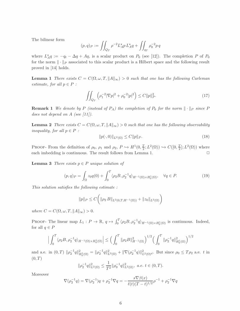
The bilinear form

(p, q)P :=

∫∫

QT

ρ−2L⋆ApL

⋆Aq +

∫∫

qT

ρ−20 p q

where L⋆Aq := −qt − ∆q + Aq, is a scalar product on P0 (see [12]). The completion P of P0

for the norm ‖ · ‖P associated to this scalar product is a Hilbert space and the following result

proved in [14] holds.

Lemma 1 There exists C = C(Ω, ω, T, ‖A‖∞) > 0 such that one has the following Carleman

estimate, for all p ∈ P :

∫∫

QT

(ρ−21 |∇p|2 + ρ−2

0 |p|2)≤ C‖p‖2P . (17)

Remark 1 We denote by P (instead of PA) the completion of P0 for the norm ‖ · ‖P since P

does not depend on A (see [11]).

Lemma 2 There exists C = C(Ω, ω, T, ‖A‖∞) > 0 such that one has the following observability

inequality, for all p ∈ P :

‖p(·, 0)‖L2(Ω) ≤ C‖p‖P . (18)

Proof- From the definition of ρ0, ρ1 and ρ2, P −→ H1(0, T2 ;L2(Ω)) −→ C([0, T2 ];L

2(Ω)) where

each imbedding is continuous. The result follows from Lemma 1.

Lemma 3 There exists p ∈ P unique solution of

(p, q)P =

∫

Ωz0q(0) +

∫ T

0〈ρ2B, ρ−1

2 q〉H−1(Ω)×H10 (Ω), ∀q ∈ P. (19)

This solution satisfies the following estimate :

‖p‖P ≤ C

(‖ρ2 B‖L2(0,T ;H−1(Ω)) + ‖z0‖L2(Ω)

)

where C = C(Ω, ω, T, ‖A‖∞) > 0.

Proof- The linear map L1 : P → R, q 7→∫ T0 〈ρ2B, ρ−1

2 q〉H−1(Ω)×H10 (Ω) is continuous. Indeed,

for all q ∈ P

∣∣∣∫ T

0〈ρ2B, ρ−1

2 q〉H−1(Ω)×H10 (Ω)

∣∣∣ ≤(∫ T

0‖ρ2B‖2H−1(Ω)

)1/2( ∫ T

0‖ρ−1

2 q‖2H10 (Ω)

)1/2

and a.e. in (0, T ) ‖ρ−12 q‖2

H10 (Ω)

= ‖ρ−12 q‖2L2(Ω) + ‖∇(ρ−1

2 q)‖2L2(Ω)d

. But since ρ0 ≤ Tρ2 a.e. t in

(0, T )

‖ρ−12 q‖2L2(Ω) ≤

1

T 2‖ρ−1

0 q‖2L2(Ω), a.e. t ∈ (0, T ).

Moreover

∇(ρ−12 q) = ∇(ρ−1

2 )q + ρ−12 ∇q = − s∇β(x)

ℓ(t)(T − t)1/2ρ−1 + ρ−1

2 ∇q

6

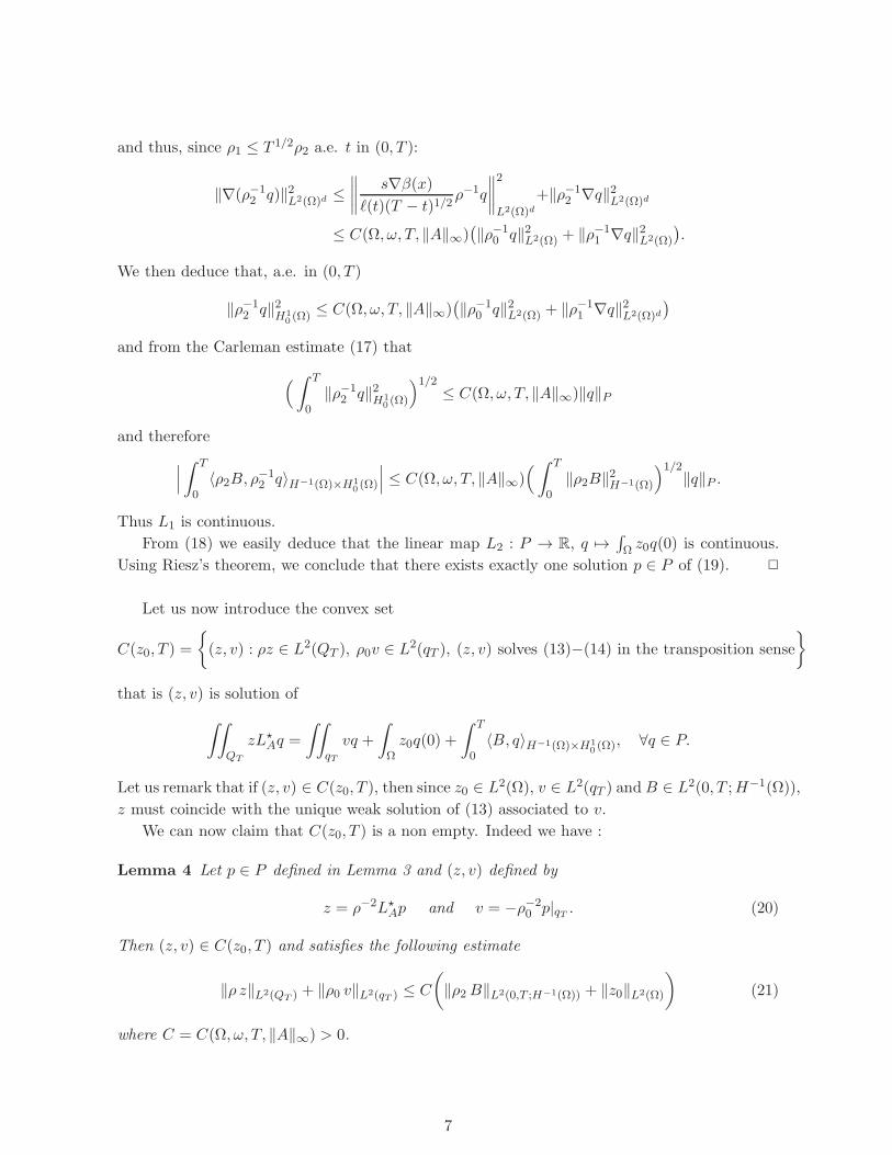
and thus, since ρ1 ≤ T 1/2ρ2 a.e. t in (0, T ):

‖∇(ρ−12 q)‖2L2(Ω)d ≤

∥∥∥∥s∇β(x)

ℓ(t)(T − t)1/2ρ−1q

∥∥∥∥2

L2(Ω)d+‖ρ−1

2 ∇q‖2L2(Ω)d

≤ C(Ω, ω, T, ‖A‖∞)(‖ρ−1

0 q‖2L2(Ω) + ‖ρ−11 ∇q‖2L2(Ω)

).

We then deduce that, a.e. in (0, T )

‖ρ−12 q‖2H1

0 (Ω) ≤ C(Ω, ω, T, ‖A‖∞)(‖ρ−1

0 q‖2L2(Ω) + ‖ρ−11 ∇q‖2L2(Ω)d

)

and from the Carleman estimate (17) that

(∫ T

0‖ρ−1

2 q‖2H10 (Ω)

)1/2≤ C(Ω, ω, T, ‖A‖∞)‖q‖P

and therefore

∣∣∣∫ T

0〈ρ2B, ρ−1

2 q〉H−1(Ω)×H10 (Ω)

∣∣∣ ≤ C(Ω, ω, T, ‖A‖∞)( ∫ T

0‖ρ2B‖2H−1(Ω)

)1/2‖q‖P .

Thus L1 is continuous.

From (18) we easily deduce that the linear map L2 : P → R, q 7→∫Ω z0q(0) is continuous.

Using Riesz’s theorem, we conclude that there exists exactly one solution p ∈ P of (19).

Let us now introduce the convex set

C(z0, T ) =

(z, v) : ρz ∈ L2(QT ), ρ0v ∈ L2(qT ), (z, v) solves (13)−(14) in the transposition sense

that is (z, v) is solution of

∫∫

QT

zL⋆Aq =

∫∫

qT

vq +

∫

Ωz0q(0) +

∫ T

0〈B, q〉H−1(Ω)×H1

0 (Ω), ∀q ∈ P.

Let us remark that if (z, v) ∈ C(z0, T ), then since z0 ∈ L2(Ω), v ∈ L2(qT ) andB ∈ L2(0, T ;H−1(Ω)),

z must coincide with the unique weak solution of (13) associated to v.

We can now claim that C(z0, T ) is a non empty. Indeed we have :

Lemma 4 Let p ∈ P defined in Lemma 3 and (z, v) defined by

z = ρ−2L⋆Ap and v = −ρ−2

0 p|qT . (20)

Then (z, v) ∈ C(z0, T ) and satisfies the following estimate

‖ρ z‖L2(QT ) + ‖ρ0 v‖L2(qT ) ≤ C

(‖ρ2 B‖L2(0,T ;H−1(Ω)) + ‖z0‖L2(Ω)

)(21)

where C = C(Ω, ω, T, ‖A‖∞) > 0.

7

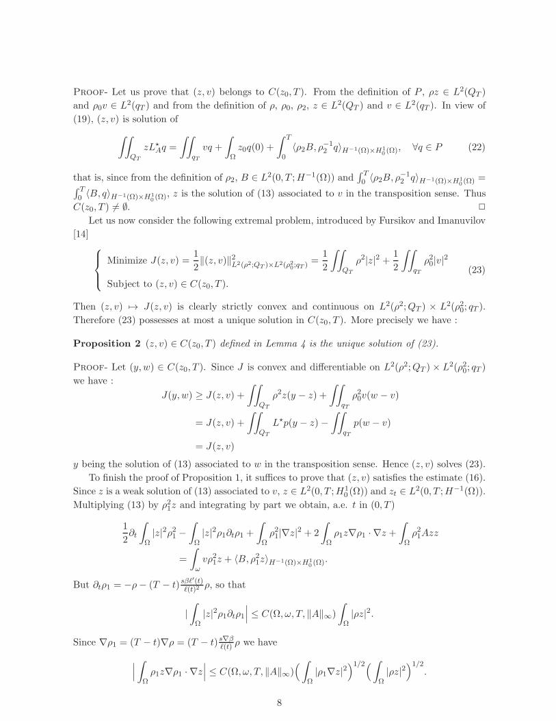
Proof- Let us prove that (z, v) belongs to C(z0, T ). From the definition of P , ρz ∈ L2(QT )

and ρ0v ∈ L2(qT ) and from the definition of ρ, ρ0, ρ2, z ∈ L2(QT ) and v ∈ L2(qT ). In view of

(19), (z, v) is solution of

∫∫

QT

zL⋆Aq =

∫∫

qT

vq +

∫

Ωz0q(0) +

∫ T

0〈ρ2B, ρ−1

2 q〉H−1(Ω)×H10 (Ω), ∀q ∈ P (22)

that is, since from the definition of ρ2, B ∈ L2(0, T ;H−1(Ω)) and∫ T0 〈ρ2B, ρ−1

2 q〉H−1(Ω)×H10 (Ω) =∫ T

0 〈B, q〉H−1(Ω)×H10 (Ω), z is the solution of (13) associated to v in the transposition sense. Thus

C(z0, T ) 6= ∅.

Let us now consider the following extremal problem, introduced by Fursikov and Imanuvilov

[14]

Minimize J(z, v) =1

2‖(z, v)‖2L2(ρ2;QT )×L2(ρ20;qT ) =

1

2

∫∫

QT

ρ2|z|2 + 1

2

∫∫

qT

ρ20|v|2

Subject to (z, v) ∈ C(z0, T ).

(23)

Then (z, v) 7→ J(z, v) is clearly strictly convex and continuous on L2(ρ2;QT ) × L2(ρ20; qT ).

Therefore (23) possesses at most a unique solution in C(z0, T ). More precisely we have :

Proposition 2 (z, v) ∈ C(z0, T ) defined in Lemma 4 is the unique solution of (23).

Proof- Let (y,w) ∈ C(z0, T ). Since J is convex and differentiable on L2(ρ2;QT ) × L2(ρ20; qT )

we have :

J(y,w) ≥ J(z, v) +

∫∫

QT

ρ2z(y − z) +

∫∫

qT

ρ20v(w − v)

= J(z, v) +

∫∫

QT

L⋆p(y − z)−∫∫

qT

p(w − v)

= J(z, v)

y being the solution of (13) associated to w in the transposition sense. Hence (z, v) solves (23).

To finish the proof of Proposition 1, it suffices to prove that (z, v) satisfies the estimate (16).

Since z is a weak solution of (13) associated to v, z ∈ L2(0, T ;H10 (Ω)) and zt ∈ L2(0, T ;H−1(Ω)).

Multiplying (13) by ρ21z and integrating by part we obtain, a.e. t in (0, T )

1

2∂t

∫

Ω|z|2ρ21 −

∫

Ω|z|2ρ1∂tρ1 +

∫

Ωρ21|∇z|2 + 2

∫

Ωρ1z∇ρ1 · ∇z +

∫

Ωρ21Azz

=

∫

ωvρ21z + 〈B, ρ21z〉H−1(Ω)×H1

0 (Ω).

But ∂tρ1 = −ρ− (T − t)sβℓ′(t)

ℓ(t)2ρ, so that

|∫

Ω|z|2ρ1∂tρ1

∣∣∣ ≤ C(Ω, ω, T, ‖A‖∞)

∫

Ω|ρz|2.

Since ∇ρ1 = (T − t)∇ρ = (T − t)s∇βℓ(t) ρ we have

∣∣∣∫

Ωρ1z∇ρ1 · ∇z

∣∣∣ ≤ C(Ω, ω, T, ‖A‖∞)(∫

Ω|ρ1∇z|2

)1/2(∫

Ω|ρz|2

)1/2.

8

The following estimates also hold

∣∣∣∫

Ωρ21Azz

∣∣∣ ≤ C(T, ‖A‖∞)

∫

Ω|ρz|2,

∣∣∣∫

ωvρ21z

∣∣∣ ≤ T 1/2∣∣∣∫

ωρ0vρz

∣∣∣ ≤ T 1/2(∫

ω|ρ0v|2

)1/.2( ∫

Ω|ρz|2

)1/2

and

|〈B, ρ21z〉H−1(Ω)×H10 (Ω)| = |〈ρ1B, ρ1z〉H−1(Ω)×H1

0 (Ω)| ≤ ‖ρ1B‖H−1(Ω)‖ρ1z‖H10 (Ω)

≤ C(Ω, ω, T, ‖A‖∞)‖ρ2B‖H−1(Ω)

(‖ρz‖L2(Ω) + ‖ρ1∇z‖L2(Ω)d

).

Thus we easily obtain that

∂t

∫

Ωρ21|z|2 +

∫

Ωρ21|∇z|2 ≤ C(Ω, ω, T, ‖A‖∞)

(‖ρ2B‖2H−1(Ω) +

∫

Ωρ2|z|2 +

∫

ω|ρ0v|2

)

and therefore, using (21), for all t ∈ [0, T ] :

( ∫

Ωρ21|z|2

)(t) +

∫∫

Qt

ρ21|∇z|2 ≤ C(Ω, ω, T, ‖A‖∞)

(‖ρ2 B‖2L2(0,T ;H−1(Ω)) + ‖z0‖2L2(Ω)

)

which gives (16) and concludes the proof of Proposition 1.

3 The least-squares method and its analysis

For any s ∈ [0, 1], we define the space

Ws =

g ∈ C(R), g(0) = 0, g′ ∈ L∞(R), sup

a,b∈R,a6=b

|g′(a)− g′(b)||a− b|s < ∞

.

The case s = 0 reduces to W0 = g ∈ C(R), g(0) = 0, g′ ∈ L∞(R) while the case s = 1

corresponds to W1 = g ∈ C(R), g(0) = 0, g′ ∈ L∞(R), g′′ ∈ L∞(R).In the sequel, we shall assume that there exists one s ∈ (0, 1] for which the nonlinear function

g belongs to Ws. Remark that g ∈ Ws for some s ∈ [0, 1] satisfies hypotheses (2) and (6). We

shall also assume that u0 ∈ L2(Ω).

3.1 The least-squares method

We introduce the vectorial space A0 as follows

A0 =

(y, f) : ρ y ∈ L2(QT ), ρ1∇y ∈ L2(QT )

d, ρ0f ∈ L2(qT ),

ρ2(yt −∆y − f 1ω) ∈ L2(0, T ;H−1(Ω)), y(·, 0) = 0 in Ω, y = 0 on ΣT

(24)

where ρ, ρ2, ρ1 and ρ0 are defined in (12). Since L2(0, T ;H−1(Ω)) is also a Hilbert space, A0

endowed with the following scalar product

((y, f), (y, f)

)A0

=(ρy, ρy

)2+

(ρ1∇y, ρ1∇y

)2+

(ρ0f, ρ0f

)2

+(ρ2(yt −∆y − f 1ω), ρ2(yt −∆y − f 1ω)

)L2(0,T ;H−1(Ω))

9

is a Hilbert space. The corresponding norm is ‖(y, f)‖A0 =√

((y, f), (y, f))A0 . We also consider

the convex space

A =

(y, f) : ρ y ∈ L2(QT ), ρ1 ∇y ∈ L2(QT )

d, ρ0f ∈ L2(qT ),

ρ2(yt −∆y − f 1ω) ∈ L2(0, T ;H−1(Ω)), y(·, 0) = u0 in Ω, y = 0 on ΣT

(25)

so that we can write A = (y, f) + A0 for any element (y, f) ∈ A. We endow A with the same

norm. Clearly, if (y, f) ∈ A, then y ∈ C([0, T ];L2(Ω)) and since ρ y ∈ L2(QT ), then y(·, T ) = 0.

The null controllability requirement is therefore incorporated in the spaces A0 and A.

For any fixed (y, f) ∈ A, we can now consider the following extremal problem :

min(y,f)∈A0

E(y + y, f + f) (26)

where E : A → R is defined as follows

E(y, f) :=1

2

∥∥∥∥ρ2(yt −∆y + g(y)− f 1ω

)∥∥∥∥2

L2(0,T ;H−1(Ω))

(27)

justifying the least-squares terminology we have used.

Let us remark that, if g ∈ Ws for one s ≥ 0, then g is Lipschitz and thus, since g(0) = 0,

there exists K > 0 such that |g(ξ)| ≤ K|ξ| for all ξ ∈ R. Consequently, ρ2g(y) ∈ L2(QT ) (and

then ρ2g(y) ∈ L2(0, T ;H−1(Ω))) since

‖ρ2g(y)‖L2(QT ) = ‖(ρ2ρ−1)ρg(y)‖L2(QT ) = ‖(T − t)1/2ρg(y)‖L2(QT ) ≤ T 1/2K‖ρy‖L2(QT ).

Since any g ∈ Ws satisfies hypotheses (2) and (6), the controllability result of Theorem

2 given in [13] implies the existence of at least one pair (y, f) ∈ A such that E(y, f) = 0.

The extremal problem (26) admits therefore solutions. Conversely, any pair (y, f) ∈ A for

which E(y, f) vanishes is a controlled pair of (1). In this sense, the functional E is a so-called

error functional which measures the deviation of (y, f) from being a solution of the underlying

nonlinear equation. We emphasize that the L2(0, T ;H−1(Ω)) norm in E indicates that we are

looking for weak solutions of the parabolic equation (1). We refer to [18] where a similar so-

called weak least-squares method is employed to approximate the solutions of the unsteady

Navier-Stokes equation.

A practical way of taking a functional to its minimum is through some clever use of descent

directions, i.e the use of its derivative. In doing so, the presence of local minima is always

something that may dramatically spoil the whole scheme. The unique structural property that

discards this possibility is the strict convexity of the functional E. However, for nonlinear

equation like (1), one cannot expect this property to hold for the functional E. Nevertheless, we

insist in that one may construct a particular minimizing sequence which cannot converge except

to a global minimizer leading E down to zero.

In order to construct such minimizing sequence, we look, for any (y, f) ∈ A, for a pair

(Y 1, F 1) ∈ A0 solution of the following formulationY 1t −∆Y 1 + g′(y)Y 1 = F 11ω +

(yt −∆y + g(y) − f 1ω

)in QT ,

Y 1 = 0 on ΣT , Y 1(·, 0) = 0 in Ω.(28)

Since (Y 1, F 1) ∈ A0, F1 is a null control for Y 1. We have the following property.

10

Proposition 3 Let any (y, f) ∈ A. There exists a pair (Y 1, F 1) ∈ A0 solution of (28) which

satisfies the following estimate:

‖(Y 1, F 1)‖A0 ≤ C√E(y, f) (29)

for some C = C(Ω, ω, T, ‖g′‖∞) > 0.

Proof- For all (y, f) ∈ A we have ρ2(yt−∆y+g(y)−f1ω) ∈ L2(0, T ;H−1(Ω)). The existence

of a null control F 1 is therefore given by Proposition 1. Choosing the control F 1 which minimizes

together with the corresponding solution Y 1 the functional J defined in Proposition 1, we get

the following estimate (since Y 1(·, 0) = 0)

‖ρ Y 1‖L2(QT ) + ‖ρ0F 1‖L2(qT ) ≤ C‖ρ2(yt −∆y + g(y)− f1ω)‖L2(0,T ;H−1(Ω))

≤ C√E(y, f)

(30)

and

‖ρ1 Y 1‖L∞(0,T ;L2(Ω)) + ‖ρ1∇Y 1‖L2(QT )d ≤ C‖ρ2(yt −∆y + g(y)− f1ω)‖L2(0,T ;H−1(Ω))

≤ C√E(y, f)

(31)

for some C = C(Ω, ω, T, ‖g‖∞) independent of Y 1, F 1 and y. Eventually, from the equation

solved by Y 1,

‖ρ2(Y 1t −∆Y 1 − F 1 1ω)‖L2(0,T ;H−1(Ω))

≤ ‖ρ2g′(y)Y 1‖L2(QT ) + ‖ρ2(yt −∆y + g(y)− f 1ω)‖L2(0,T ;H−1(Ω))

≤ ‖(T − t)1/2g′(y)‖∞‖ρY 1‖L2(QT ) +√

2E(y, f)

≤ max(1, ‖(T − t)1/2g′‖∞

)C√E(y, f)

(32)

which proves that (Y 1, F 1) belongs to A0.

Remark 2 From (28), z = y − Y 1 is a null controlled solution satisfying

zt −∆z + g′(y)z = (f − F 1)1ω − g(y) + g′(y)y in QT ,

z = 0 on ΣT , z(·, 0) = u0 in Ω(33)

by the control (f − F 1) ∈ L2(ρ0, qT ) := f ; ρ0f ∈ L2(qT ).

Remark 3 We emphasize that the presence of a right hand side in (28), namely yt − ∆y +

g(y)− f 1ω, forces us to introduce from the beginning the weights ρ0, ρ1, ρ2 and ρ in the spaces

A0 and A. This can be seen from the equality (19): since ρ−12 q belongs to L2(0, T ;H1(Ω)) for

all q ∈ P , we need to impose that ρ2B ∈ L2(0, T ;H−1(Ω)) with here B = yt −∆y+ g(y)− f 1ω.

Working with the linearized equation (7) (introduced in [13]) which does not make appear an

additional right hand side, we may avoid the introduction of Carleman type weights. Actually,

the authors in (7) consider controls of minimal L∞(qT ) norm. Introduction of weights allows

however the characterization (19), which is very convenient at the practical level. We refer to

[12] where this is discussed at length.

11

The interest of the pair (Y 1, F 1) ∈ A0 lies in the following result.

Proposition 4 Let (y, f) ∈ A and let (Y 1, F 1) ∈ A0 be a solution of (28). Then the deriva-

tive of E at the point (y, f) ∈ A along the direction (Y 1, F 1) given by E′(y, f) · (Y 1, F 1) :=

limη→0,η 6=0E((y,f)+η(Y 1,F 1))−E(y,f)

η satisfies

E′(y, f) · (Y 1, F 1) = 2E(y, f). (34)

Proof- We preliminary check that for all (Y, F ) ∈ A0, E is differentiable at the point (y, f) ∈ Aalong the direction (Y, F ) ∈ A0. For all λ ∈ R, simple computations lead to the equality

E(y + λY, f + λF ) = E(y, f) + λE′(y, f) · (Y, F ) + h((y, f), λ(Y, F ))

with

E′(y, f) · (Y, F ) :=

(ρ2(yt−∆y+g(y)−f 1ω), ρ2(Yt−∆Y +g′(y)Y −F 1ω)

)

L2(0,T ;H−1(Ω))

(35)

and

h((y, f), λ(Y, F )) =λ

(ρ2(Yt −∆Y + g′(y)Y − F 1ω), ρ2l(y, λY )

)

L2(0,T ;H−1(Ω))

+λ2

2‖ρ2(Yt −∆Y + g′(y)Y − F 1ω)‖2L2(0,T ;H−1(Ω))

+

(ρ2(yt −∆y + g(y)− f 1ω), ρ2l(y, λY )

)

L2(0,T ;H−1(Ω))

+1

2‖ρ2l(y, λY )‖2L2(0,T ;H−1(Ω))

where l(y, λY ) = g(y + λY )− g(y)− λg′(y)Y .

The application (Y, F ) → E′(y, f) ·(Y, F ) is linear and continuous from A0 to R as it satisfies

|E′(y, f) · (Y, F )|≤ ‖ρ2(yt −∆y + g(y) − f 1ω)‖L2(0,T ;H−1(Ω))‖ρ2(Yt −∆Y + g′(y)Y − F 1ω)‖L2(0,T ;H−1(Ω))

≤√

2E(y, f)

(‖ρ2(Yt −∆Y − F 1ω)‖L2(0,T ;H−1(Ω)) + ‖ρ2g′(y)Y ‖L2(QT )

)

≤√

2E(y, f)

(‖ρ2(Yt −∆Y − F 1ω)‖L2(0,T ;H−1(Ω)) + ‖(T − t)1/2g′(y)‖L∞(QT )‖ρY ‖L2(QT )

)

≤√

2E(y, f)max

(1, ‖(T − t)1/2g′‖∞

)‖(Y, F )‖A0 .

Similarly, for all λ ∈ R⋆

| 1λh((y, f), λ(Y, F ))| ≤

(λ‖ρ2(Yt −∆Y + g′(y)Y − F 1ω)‖L2(0,T ;H−1(Ω)) +

√2E(y, f)

+1

2‖ρ2l(y, λY )‖L2(0,T ;H−1(Ω))

)1

λ‖ρ2l(y, λY )‖L2(0,T ;H−1(Ω))

+λ

2‖ρ2(Yt −∆Y + g′(y)Y − F 1ω)‖2L2(0,T ;H−1(Ω)).

12

Since g′ ∈ L∞(R) we have for a.e. (x, t) ∈ QT :

ρ2|1

λl(y, λY )| = ρ2

∣∣∣g(y + λY )− g(y)

λ− g′(y)Y

∣∣∣ ≤ 2‖g′‖∞|ρ2Y |

and ρ2Y ∈ L2(QT ). Moreover, for a.e. (x, t) ∈ QT , ρ2| 1λ l(y, λY )| = ρ2|g(y+λY )−g(y)λ −g′(y)Y | → 0

as λ → 0; it follows from the Lebesgue’s Theorem that

1

λ‖ρ2l(y, λY )‖L2(QT ) → 0 as λ → 0.

It is now easy to see that

h((y, f), λ(Y, F )) = o(λ)

and that the functional E is differentiable at the point (y, f) ∈ A along the direction (Y, F ) ∈ A0.

Eventually, the equality (34) follows from the definition of the pair (Y 1, F 1) given in (28).

Remark that from the equality (35), the derivative E′(y, f) is independent of (Y, F ). We can

then define the norm ‖E′(y, f)‖(A0)′ := sup(Y,F )∈A0,(Y,F )6=(0,0)E′(y,f)·(Y,F )‖(Y,F )‖A0

associated to (A0)′,

the set of the linear and continuous applications from A0 to R.

Combining the equality (34) and the inequality (29), we deduce the following estimates of

E(y, f) in term of the norm of E′(y, f).

Proposition 5 For any (y, f) ∈ A, the inequalities holds true

C1(Ω, ω, T, ‖g′‖∞)‖E′(y, f)‖A′0≤

√E(y, f) ≤ C2(Ω, ω, T, ‖g′‖∞)‖E′(y, f)‖A′

0

for some constants C1, C2 > 0.

Proof- (34) rewrites E(y, f) = 12E

′(y, f) · (Y 1, F 1) where (Y 1, F 1) ∈ A0 is solution of (28) and

therefore, with (29)

E(y, f) ≤ 1

2‖E′(y, f)‖A′

0‖(Y 1, F 1)‖A0 ≤ C(Ω, ω, T, ‖g′‖∞)‖E′(y, f)‖A′

0

√E(y, f).

On the other hand, for all (Y, F ) ∈ A0 (see the proof of Proposition 4) :

|E′(y, f) · (Y, F )| ≤√

2E(y, f)max

(1, ‖(T − t)1/2g′‖∞

)‖(Y, F )‖A0

and thus

C1(Ω, ω, T, ‖g′‖∞)‖E′(y, f)‖A′0≤

√E(y, f).

In particular, any critical point (y, f) ∈ A for E (i.e. for which E′(y, f) vanishes) is a zero

for E, a pair solution of the controllability problem. In other words, any sequence (yk, fk)k>0

satisfying ‖E′(yk, fk)‖(A0)′ → 0 as k → ∞ is such that E(yk, fk) → 0 as k → ∞. We insist

that this property does not imply the convexity of the functional E (and a fortiori the strict

convexity of E, which actually does not hold here in view of the multiple zeros for E) but show

that a minimizing sequence for E can not be stuck in a local minimum. Far from the zeros of

E, in particular, when ‖(y, f)‖A → ∞, the right hand side inequality indicates that E tends to

be convex. On the other side, the left inequality indicates the functional E is flat around its

zero set. As a consequence, gradient based minimizing sequences may achieve a very low rate

of convergence (we refer to [20] and also [17] devoted to the Navier-Stokes equation where this

phenomenon is observed).

13

3.2 A strongly converging minimizing sequence for E

We now examine the convergence of an appropriate sequence (yk, fk) ∈ A. In this respect, we

observe that the equality (34) shows that −(Y 1, F 1) given by the solution of (28) is a descent

direction for the functional E. Therefore, we can define at least formally, for any m ≥ 1, a

minimizing sequence (yk, fk)k∈N as follows:

(y0, f0) ∈ A,

(yk+1, fk+1) = (yk, fk)− λk(Y1k , F

1k ), k ≥ 0,

λk = argminλ∈[0,m]E((yk, fk)− λ(Y 1

k , F1k ))

(36)

where (Y 1k , F

1k ) ∈ A0 is such that F 1

k is a null control for Y 1k , solution of

Y 1k,t −∆Y 1

k + g′(yk)Y1k = F 1

k 1ω + (yk,t −∆yk + g(yk)− fk1ω) in QT ,

Y 1k = 0 on ΣT , Y 1

k (·, 0) = 0 in Ω(37)

and minimizes the functional J defined in Proposition 1. The direction Y 1k vanishes when E

vanishes.

We first perform the analysis assuming the non linear function g in W1, notably that g′′ ∈L∞(R) (the derivatives here are in the sense of distribution). We first prove the following lemma.

Lemma 5 Assume g ∈ W1. Let (y, f) ∈ A and (Y 1, F 1) ∈ A0 defined by (28). For any λ ∈ R

and k ∈ N, the following estimate holds

E((y, f)− λ(Y 1, F 1)

)≤ E(y, f)

(|1− λ|+ λ2C(Ω, ω, T, ‖g′‖∞)‖g′′‖∞

√E(y, f)

)2

. (38)

Proof- With g ∈ W1, we write that

|l(y,−λY 1)| = |g(y − λY 1)− g(y) + λg′(y)Y 1| ≤ λ2

2‖g′′‖∞(Y 1)2 (39)

and obtain that

2E((y, f)− λ(Y 1, F 1)

)

=

∥∥∥∥ρ2(yt −∆yk + g(y) − f 1ω

)−

λρ2(Y 1t −∆Y 1 + g′(y)Y 1 − F 1ω

)+ ρ2l(y,−λY 1)

∥∥∥∥2

L2(0,T ;H−1(Ω))

=

∥∥∥∥ρ2(1− λ)(yt −∆y + g(y) − f 1ω

)+ ρ2l(y,−λY 1)

∥∥∥∥2

L2(0,T ;H−1(Ω))

≤(∥∥ρ2(1− λ)

(yt −∆y + g(y)− f 1ω

)∥∥L2(0,T ;H−1(Ω))

+∥∥ρ2l(y,−λY 1)

∥∥L2(0,T ;H−1(Ω))

)2

≤ 2

(|1− λ|

√E(y, f) +

λ2

2√2‖g′′‖∞‖ρ2(Y 1)2‖L2(0,T ;H−1(Ω))

)2

.

(40)

14

For d = 3 (similar estimates hold for d = 1 and d = 2), using the continuous embedding of

L6/5(Ω) into H−1(Ω), we have:

‖ρ2(Y 1)2‖2L2(0,T ;H−1(Ω)) ≤ C(Ω)‖ρ2(Y 1)2‖2L2(0,T ;L6/5(Ω))

≤ C(Ω)

∫ T

0‖ρ2Y 1‖2L3(Ω)‖Y 1‖2L2(Ω)

≤ C(Ω)

∫ T

0‖ρY 1‖L2(Ω)‖ρ1Y 1‖L6(Ω)‖Y 1‖2L2(Ω)

≤ C(Ω)

∫ T

0‖ρY 1‖L2(Ω)‖∇(ρ1Y

1)‖L2(Ω)d‖Y 1‖2L2(Ω).

From the definition of ρ and ρ1 we have ∇ρ1 =s∇β

ℓ(t)(T−t)ρ1 =s∇βℓ(t) ρ and therefore a.e. t in (0, T )

‖∇(ρ1Y1)‖L2(Ω)d ≤ ‖∇(ρ1)Y

1‖L2(Ω)d + ‖ρ1∇Y 1‖L2(Ω)d

≤ C(Ω, ω, T, ‖g′‖∞)‖ρY 1‖L2(Ω) + ‖ρ1∇Y 1‖L2(Ω)d

and thus

‖ρ2(Y 1)2‖2L2(0,T ;H−1(Ω)) ≤ C(Ω, ω, T, ‖g′‖∞)‖ρ1Y 1‖2L∞(0,T ;L2(Ω))‖ρY 1‖L2(QT )

×(‖ρY 1‖L2(QT ) + ‖ρ1∇Y 1‖L2(QT )d

).

Using (30) and (31), we obtain

‖ρ0(Y 1)2‖2L2(0,T ;H−1(Ω)) ≤ C(Ω, ω, T, ‖g′‖∞)E(y, f)2, (41)

from which we get (38).

Proceeding as in [19], we are now in position to prove the following convergence result for

the sequence (E(yk, fk))(k≥0).

Proposition 6 Assume g ∈ W1. Let (yk, fk)k∈N be the sequence defined by (36). Then E(yk, fk) →0 as k → ∞. Moreover, there exists k0 ∈ N such that the sequence (E(yk, fk))k≥k0 decays

quadratically.

Proof- We define the polynomial pk as follows

pk(λ) = |1− λ|+ λ2c1√

E(yk, fk) where c1 := C(Ω, ω, T, ‖g′‖∞)‖g′′‖∞.

Lemma 5 with (y, f) = (yk, fk) allows to write that

c1√

E(yk+1, fk+1) ≤ c1√

E(yk, fk)pk(λk), ∀k ≥ 0 (42)

with pk(λk) := minλ∈[0,m] pk(λ).

If c1√

E(y0, f0) < 1 (and thus c1√

E(yk, fk) < 1 for all k ∈ N) then

pk(λk) = minλ∈[0,m]

pk(λ) ≤ pk(1) = c1√

E(yk, fk)

and thus

c1√

E(yk+1, fk+1) ≤(c1√

E(yk, fk))2

(43)

15

implying that c1√

E(yk, fk) → 0 as k → ∞ with a quadratic rate.

If now c1√

E(y0, f0) ≥ 1, we check that I := k ∈ N, c1√

E(yk, fk) ≥ 1 is a finite subset of

N. For all k ∈ I, since c1√E(yk, fk) ≥ 1,

minλ∈[0,m]

pk(λ) = minλ∈[0,1]

pk(λ) = pk

( 1

2c1√

E(yk, fk)

)= 1− 1

4c1√

E(yk, fk)

and thus, for all k ∈ I,

c1√

E(yk+1, fk+1) ≤(1− 1

4c1√

E(yk, fk)

)c1√

E(yk, fk) = c1√

E(yk, fk)−1

4. (44)

This inequality implies that the sequence (c1√

E(yk, fk))k∈N strictly decreases and then that

the sequence (pk(λk)k∈N decreases as well. Thus the sequence (c1√

E(yk, fk))k∈N decreases to 0

at least linearly and there exists k0 ∈ N such that for all k ≥ k0, c1√

E(yk, fk) < 1, that is I is

a finite subset of N. Arguing as in the first case, it follows that c1√

E(yk, fk) → 0 as k → ∞.

In both cases, remark that pk(λk) decreases with respect to k.

Remark 4 Writing from (44) that c1√

E(yk, fk) ≤ c1√

E(y0, f0)−k4 for all k such that c1

√E(yk, fk) ≥

1, we obtain that

k0 ≤⌊4(c1

√E(y0, f0)− 1) + 1

⌋

where ⌊x⌋ denotes the integer part of x ∈ R+.

We also have the following convergence of the optimal sequence λkk>0.

Lemma 6 The sequence λkk>0 defined in (36) converges to 1 as k → ∞.

Proof- In view of (40), we have, as long as E(yk, fk) > 0, since λk ∈ [0,m]

(1 − λk)2 =

E(yk+1, fk+1)

E(yk, fk)− 2(1 − λk)

〈ρ2(yk,t +∆yk + g(yk)− fk 1ω

), ρ2l(yk, λkY

1k )〉L2(0,T ;H−1(Ω))

E(yk, fk)

−∥∥ρ2l(yk, λkY

1k )

∥∥2L2(0,T ;H−1(Ω))

2E(yk)

≤ E(yk+1, fk+1)

E(yk, fk)− 2(1 − λk)

〈ρ2(yk,t +∆yk + g(yk)− fk 1ω

), ρ2l(yk, λkY

1k )〉L2(0,T ;H−1(Ω))

E(yk, fk)

≤ E(yk+1, fk+1)

E(yk, fk)+ 2

√2m

√E(yk, fk)‖ρ2l(yk, λkY

1k )‖L2(0,T ;H−1(Ω))

E(yk, fk)

≤ E(yk+1, fk+1)

E(yk, fk)+ 2

√2m

‖ρ2l(yk, λkY1k )‖L2(0,T ;H−1(Ω))√E(yk, fk)

But, from (39) and (41)

‖ρ2l(yk, λkY1k )‖L2(0,T ;H−1(Ω)) ≤

λ2k

2√2‖g′′‖∞‖ρ2(Y 1

k )2‖L2(0,T ;H−1(Ω))

≤ m2‖g′′‖∞C(T,Ω, ω, ‖g′‖∞)E(yk, fk)

16

and thus

(1− λk)2 ≤ E(yk+1, fk+1)

E(yk, fk)+m2‖g′′‖∞C(Ω, ω, T, ‖g′‖∞)

√E(yk, fk).

Consequently, since E(yk, fk) → 0 andE(yk+1,fk+1)

E(yk,fk)→ 0, we deduce that (1− λk)

2 → 0.

We are now in position to prove the following convergence result.

Theorem 3 Assume g ∈ W1. Let (yk, fk)k∈N be the sequence defined by (36). Then, (yk, fk)k∈N →(y, f) in A where f is a null control for y solution of (1). Moreover, the convergence is quadratic

after a finite number of iterates.

Proof- For all k ∈ N, let Fk = −∑kn=0 λnF

1n and Yk =

∑kn=0 λnY

1n . Let us prove that(

(Yk, Fk))k∈N

converge in A0, i.e. that the series∑

λn(F1n , Y

1n ) converges in A0. Using that

‖(Y 1k , F

1k )‖A0 ≤ C

√E(yk, fk) for all k ∈ N (see (29)), we write

k∑

n=0

λn‖(Y 1n , F

1n)‖A0 ≤ m

k∑

n=0

‖(Y 1n , F

1n)‖A0 ≤ C

k∑

n=0

√E(yn, fn).

But(√

E(yn, fn))k∈N

and(pk(λk)

)k∈N

are decreasing sequences so that

√E(yn, fn) ≤ pn(λn)

√E(yn−1, fn−1) ≤ p0(λ0)

√E(yn−1, fn−1) ≤ p0(λ0)

n√

E(y0, f0)

so that, since p0(λ0) < 1 :

k∑

n=0

√E(yn, fn) ≤

√E(y0, f0)

1− p(λ0)k+1

1− p(λ0)≤

√E(y0, f0)

1

1− p(λ0).

We deduce that the series∑

n λn(Y1n , F

1n) is normally convergent and so convergent. Conse-

quently, there exists (Y, F ) ∈ A0 such that (Yk, Fk)k∈N converges to (Y, F ) in A0.

Denoting y = y0 + Y and f = f0 + F , we then have that (yk, fk)k∈N = (y0 + Yk, f0 + Fk)k∈Nconverges to (y, f) in A.

It suffices now to verify that the limit (y, f) satisfies E(y, f) = 0. We write that (Y 1k , F

1k ) ∈ A0

and (yk, fk) ∈ A solve the

Y 1k,t −∆Y 1

k + g′(yk) · Y 1k = F 1

k 1ω − (yk,t −∆yk + g(yk)− fk1ω) in QT ,

Y 1k = 0 on ΣT , Y 1

k (·, 0) = 0 in Ω.(45)

Using that (Y 1k , F

1k ) goes to zero in A0 as k → ∞, we pass to the limit in (45) and get, since

g ∈ W1, that (y, f) ∈ A solves (1), that is E(y, f) = 0.

In particular, along the sequence (yk, fk)k defined by (36), we have the following coercivity

property for E, which confirms the strong convergence of the sequence (yk, fk)k>0. In view of

the non uniqueness of the zeros of E, remark that this property is not true in general for all

(y, f) in A.

Proposition 7 Let (yk, fk)k>0 defined by (36) and (y, f) its limit. Then, there exists a positive

constant C such that

‖(y, f)− (yk, fk)‖A0 ≤ C√E(yk, fk), ∀k > 0. (46)

17

Proof- We write that

‖(y, f)− (yk, fk)‖A0 = ‖∞∑

p=k+1

λp(Y1p , F

1p )‖A ≤ m

∞∑

p=k+1

‖(Y 1p , F

1p ‖A0

≤ mC∞∑

p=k+1

√E(yp, fp)

≤ mC

∞∑

p=k+1

p0(λ0)p−k

√E(yk, fk)

≤ mCp0(λ0)

1− p0(λ0)

√E(yk, fk).

We emphasize, in view of the non uniqueness of the zeros of E, that an estimate (similar

to (46)) of the form ‖(y, f) − (y, f)‖A0 ≤ C√

E(y, f) does not hold for all (y, f) ∈ A. We also

mention the fact that the sequence (yk, fk)k>0 and its limits (y, f) are uniquely determined from

the initial guess (y0, f0) and from our criterion of selection of the control F 1. In other words,

the solution (y, f) is unique up to the element (y0, f0) and the functional J .

3.3 The case g ∈ Ws, 0 ≤ s < 1 and additional remarks

The results of the previous subsection devoted to the case s = 1 still hold if we assume only

that g ∈ Ws for one s ∈ (0, 1). For any g ∈ Ws, we introduce the notation ‖g′‖W s,∞(R)

:=

supa,b∈R,a6=b|g′(a)−g′(b)|

|a−b|s . We have the following result.

Theorem 4 Assume that there exists s ∈ (0, 1) such that g ∈ Ws. Let (yk, fk)k∈N be the

sequence defined by (36). Then, (yk, fk)k∈N → (y, f) in A where f is a null control for y

solution of (1). Moreover, after a finite number of iterates, the rate of convergence is equal to

1 + s.

Proof- We briefly sketch the proof, close to the proof of Theorem 3 for the case s = 1.

-We first prove for any (y, f) ∈ A and λ ∈ R the following inequality (similar to the inequality

(38))

E((y, f)− λ(Y 1, F 1)

)≤ E(y, f)

(|1− λ|+ λ1+sc1E(y, f)s/2

)2

(47)

with c1 = C(T,Ω, ω, ‖g′‖∞)‖g′‖W s,∞(R)

and (Y 1, F 1) ∈ A0 the solution of (37) which minimizes

J . For any (x, y) ∈ R2 and λ ∈ R, we write g(x+ λy)− g(x) =

∫ λ0 yg′(x+ ξy)dξ leading to

|g(x + λy)− g(x)− λg′(x)y| ≤∫ λ

0|y||g′(x+ ξy)− g′(x)|dξ

≤∫ λ

0|y|1+s|ξ|s |g

′(x+ ξy)− g′(x)||ξy|s dξ

≤ ‖g′‖W s,∞(R)

|y|1+s λ1+s

1 + s.

18

It follows that

|l(y,−λY 1)| = |g(y − λY 1)− g(y) + λg′(y)Y 1| ≤ ‖g′‖W s,∞(R)

λ1+s

1 + s|Y 1|1+s

and ∥∥ρ2l(y, λY 1)∥∥L2(0,T ;H−1(Ω))

≤∥∥ρ2l(y, λY 1)

∥∥L2(0,T ;L6/5(Ω))

≤ ‖g′‖W s,∞(R)

λ1+s

1 + s

∥∥ρ2|Y 1|1+s∥∥L2(0,T ;L6/5(Ω))

.

But

∥∥ρ2|Y 1|1+s∥∥2L2(0,T ;L6/5(Ω))

=

∫ T

0

∥∥ρ2|Y 1|1+s∥∥2L6/5(Ω)

≤∫ T

0

∥∥ρ2Y 1∥∥2L3(Ω)

∥∥|Y 1|s∥∥2L2(Ω)

≤∫ T

0

∥∥ρY 1∥∥L2(Ω)

∥∥ρ1Y 1∥∥L6(Ω)

∥∥Y 1∥∥2sL2s(Ω)

≤ C(Ω)

∫ T

0

∥∥ρY 1∥∥L2(Ω)

∥∥∇(ρ1Y1)∥∥L2(Ω)d

∥∥Y 1∥∥2sL2s(Ω)

≤ C(Ω)∥∥ρY 1

∥∥L2(QT )

∥∥∇(ρ1Y1)∥∥L2(QT )d

∥∥Y 1∥∥2sL∞(0,T ;L2s(Ω))

≤ C(Ω)∥∥ρY 1

∥∥L2(QT )

∥∥∇(ρ1Y1)∥∥L2(QT )d

∥∥Y 1∥∥2sL∞(0,T ;L2(Ω))

.

Since ‖∇(ρ1Y1)‖L2(Ω)d ≤ C(Ω, ω, T, ‖g′‖∞)‖ρY 1‖L2(Ω) + ‖ρ1∇Y 1‖L2(Ω)d , we finally get

∥∥ρ2|Y 1|1+s∥∥2L2(0,T ;L6/5(Ω))

≤ C(Ω, ω, T, ‖g′‖∞)‖ρY 1‖L2(QT )

×(‖ρY 1‖L2(QT ) + ‖ρ1∇Y 1‖L2(QT )d

)‖ρ1Y ‖2sL∞(0,T ;L2(Ω)).

The first inequality of (40) then leads to (47).

- We then check that the sequence (E(yk, fk))k∈N goes to zero as k → ∞. We define pk as

follows

pk(λ) = |1− λ|+ λ1+sc1E(yk, fk)s/2

so that √E(yk+1, fk+1) ≤

√E(yk, fk)pk(λk), ∀k ≥ 0

with pk(λk) = minλ∈[0,m] pk(λ). We have pk(λk) := minλ∈[0,m] pk(λ) ≤ pk(1) = c1E(yk, fk)s/2

and thus

c2√

E(yk+1, fk+1) ≤(c2√E(yk, fk)

)1+s, c2 := c

1/s1 .

If c2√

E(y0, f0) < 1 (and thus c2√

E(yk, fk) < 1 for all k ∈ N) then the above inequal-

ity implies that c2√

E(yk, fk) → 0 as k → ∞. If c2√

E(y0, f0) ≥ 1 then let I = k ∈N, c2

√E(yk, fk) ≥ 1. I is a finite subset of N; for all k ∈ I, since c2

√E(yk, fk) ≥ 1

minλ∈[0,m]

pk(λ) = minλ∈[0,1]

pk(λ) = pk

( 1

(1 + s)1/sc2√

E(yk, fk)

)= 1− s

(1 + s)1s+1

1

c2√

E(yk, fk)

and thus, for all k ∈ I,

c2√

E(yk+1, fk+1) ≤(1− s

(1 + s)1s+1

1

c2√

E(yk, fk)

)c2√

E(yk, fk) = c2√

E(yk, fk)−s

(1 + s)1s+1

.

19

This inequality implies that the sequence (c2√

E(yk, fk))k∈N strictly decreases and then that

the sequence (pk(λk))k∈N decreases as well. Thus the sequence (c2√

E(yk, fk))k∈N decreases to

0 at least linearly and there exists k0 ∈ N such that for all k ≥ k0, c2√

E(yk, fk) < 1, that is I

is a finite subset of N. Similarly, the optimal parameter λk goes to one as k → ∞.

- Using that the sequence (E(yk, fk))k∈N goes to zero, we conclude exactly as in the proof of

Theorem 3.

On the other hand, if we assume only that g belongs to W0, then we can not expect the

convergence of the sequence (yk, fk)k>0 if ‖g′‖∞ is too large.

Remark 5 Assume that g ∈ W0. Let any (y, f) ∈ A and (Y 1, F 1) the solution of (28) which

minimizes J . The following inequality holds :

E((y, f)− λ(Y 1, F 1)

)≤ E(y, f)

(|1− λ|+ λC(Ω, ω, T, ‖g′‖∞)‖g′‖∞

)2

for all λ ∈ R where C(Ω, ω, T, ‖g′‖∞) ≥ 0 increases with ‖g′‖∞. Indeed, this is a consequence of

the following inequality, for all (y, f) ∈ A, (Y, F ) ∈ A0 :

2E((y, f)− λ(Y 1, F 1)

)≤

(∥∥ρ2(1− λ)(yt −∆y + g(y)− f 1ω

)∥∥L2(0,T ;H−1(Ω))

+∥∥ρ2l(y, λY 1)

∥∥L2(0,T ;H−1(Ω))

)2

≤(|1− λ|

√2E(y, f) + 2λ‖(T − t)1/2g′(y)‖L∞(QT )‖ρY ‖L2(QT )

)2

.

As a consequence, we get that the sequence (E(yk, fk))k≥0 decreases to 0 if g satisfies

C(Ω, ω, T, ‖g′‖∞)‖g′‖∞ < 1.

Remark 6 The estimate (29) is a key point in the convergence analysis and is independent

of the choice of the functional J defined by J(Y 1, F 1) = 12‖ρ0F 1‖2L2(qT ) +

12‖ρY ‖2L2(QT ) (see

Proposition 1) in order to select a pair (Y 1, F 1) in A0. Thus, we may consider other weighted

functionals, for instance J(Y 1, F 1) = 12‖ρ0F 1‖2L2(qT ) as discussed in [21].

Remark 7 If we introduce F : A → L2(0, T ;H−1(Ω)) by F (y, f) := ρ−2(yt−∆y+ g(y)− f 1ω),

we get that E(y, f) = 12‖F (y, f)‖2L2(0,T ;H−1(Ω)) and observe that, for λk = 1, the algorithm (36)

coincides with the Newton algorithm associated to the mapping F . This explains notably the

quadratic convergence of Theorem 3 in the case g ∈ W1 for which we have a control of g′′

in L∞(QT ). The optimization of the parameter λk allows to get a global convergence of the

algorithm and leads to the so-called damped Newton method (for F ). Under general hypothesis,

global convergence for this kind of method is achieved, with a linear rate (for instance; we refer

to [7, Theorem 8.7]). As far as we know, the analysis of damped type Newton methods for partial

differential equations has deserved very few attention in the literature. We mention [18, 22] in

the context of fluids mechanics.

20

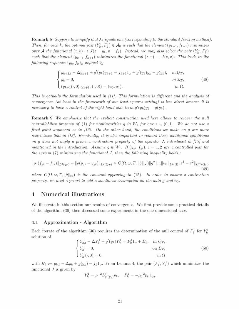
Remark 8 Suppose to simplify that λk equals one (corresponding to the standard Newton method).

Then, for each k, the optimal pair (Y 1k , F

1k ) ∈ A0 is such that the element (yk+1, fk+1) minimizes

over A the functional (z, v) → J(z − yk, v − fk). Instead, we may also select the pair (Y 1k , F

1k )

such that the element (yk+1, fk+1) minimizes the functional (z, v) → J(z, v). This leads to the

following sequence yk, fkk defined by

yk+1,t −∆yk+1 + g′(yk)yk+1 = fk+11ω + g′(yk)yk − g(yk), in QT ,

yk = 0, on ΣT ,

(yk+1(·, 0), yk+1,t(·, 0)) = (u0, u1), in Ω.

(48)

This is actually the formulation used in [11]. This formulation is different and the analysis of

convergence (at least in the framework of our least-squares setting) is less direct because it is

necessary to have a control of the right hand side term g′(yk)yk − g(yk).

Remark 9 We emphasize that the explicit construction used here allows to recover the null

controllability property of (1) for nonlinearities g in Ws for one s ∈ (0, 1]. We do not use a

fixed point argument as in [13]. On the other hand, the conditions we make on g are more

restrictives that in [13]. Eventually, it is also important to remark these additional conditions

on g does not imply a priori a contraction property of the operator Λ introduced in [13] and

mentioned in the introduction. Assume g ∈ W1. If (yzi , fzi), i = 1, 2 are a controlled pair for

the system (7) minimizing the functional J , then the following inequality holds :

‖ρ0(fz1 − fz2)‖L2(qT ) + ‖ρ(yz1 − yz2)‖L2(QT ) ≤ C(Ω, ω, T, ‖g‖∞)‖g′′‖∞‖u0‖L2(Ω)‖z1 − z2‖L∞(QT )

(49)

where C(Ω, ω, T, ‖g‖∞) is the constant appearing in (15). In order to ensure a contraction

property, we need a priori to add a smallness assumption on the data g and u0.

4 Numerical illustrations

We illustrate in this section our results of convergence. We first provide some practical details

of the algorithm (36) then discussed some experiments in the one dimensional case.

4.1 Approximation - Algorithm

Each iterate of the algorithm (36) requires the determination of the null control of F 1k for Y 1

k

solution of

Y 1k,t −∆Y 1

k + g′(yk)Y1k = F 1

k 1ω +Bk, in QT ,

Y 1k = 0, on ΣT ,

Y 1k (·, 0) = 0, in Ω

(50)

with Bk := yk,t −∆yk + g(yk) − fk1ω. From Lemma 4, the pair (F 1k , Y

1k ) which minimizes the

functional J is given by

Y 1k = ρ−2L⋆

g′(yk)pk, F 1

k = −ρ−20 pk 1qT

21

where pk ∈ P solves the formulation

∫∫

QT

ρ−1L⋆g′(yk)

pk ρ−1L⋆

g′(yk)p+

∫∫

qT

ρ−10 pk ρ

−10 p =

∫ T

0< ρ2Bk, ρ

−12 p >H−1(Ω),H1

0 (Ω) dt ∀p ∈ P.

(51)

The numerical approximation of this variational formulation (of second order in time and fourth

order in space) has been discussed at length in [12]. In order, first to avoid numerical instabilities

(due to the presence of exponential functions in the formulation), and second to make appear

explicitly the controlled solution, we introduce the new variables

mk = ρ−10 p, zk = ρ−1L⋆

g′(yk)pk.

Since ρ−12 p ∈ L2(0, T ;H1

0 (Ω)), we obtain notably that ρ−12 p = ρ−1

2 ρ0m = (T−t)m ∈ L2(0, T ;H10 (Ω)).

From (51), the pair (mk, zk) ∈ M× L2(QT ) with M := ρ−10 P solves

∫∫

QT

zk z+

∫∫

qT

mk m =

∫ T

0< ρ2Bk, (T−t)m >H−1(Ω),H1

0 (Ω) dt ∀(m, z) ∈ M×L2(QT ) (52)

subject to the constraint zk = ρ−1L⋆g′(yk)

(ρ0mk). This constraint leads to the following well-

posed mixed formulation : find (mk, zk, λk) ∈ M× L2(QT )× L2(QT ) solution of

∫∫

QT

zk z +

∫∫

qT

mk m+

∫∫

QT

λk

(z − ρ−1L⋆

g′(y)(ρ0 m)

)

=

∫ T

0< ρ2Bk, (T − t)m >H−1(Ω),H1

0 (Ω) dt, ∀(m, z) ∈ M× L2(QT ),

∫∫

QT

λ

(zk − ρ−1L⋆

g′(yk)(ρ0 m)

)= 0, ∀λ ∈ L2(QT ).

(53)

The variable λk ∈ L2(QT ) is a Lagrange multiplier. Moreover, from the unique solution (mk, zk),

we get the explicit form of the controlled pair (Y 1k , F

1k ) as follows:

Y 1k = ρ−1zk, F 1

k = −ρ−10 mk 1qT .

The algorithm associated to the sequence (yk, fk)k>0 (see (36)) may be developed as follows:

given ǫ > 0 and m ≥ 1,

1. We determine the controlled pair (y0, f0) which minimizes the functional J associated to

the linear case (for which g ≡ 0 in (1)). (y0, f0) is given by

(y0, f0) = (ρ−1z0,−ρ−10 m0 1qT )

where (z0,m0) solves the formulation :

∫∫

QT

z z +

∫∫

qT

mm+

∫∫

QT

λ

(z − ρ−1L⋆

0(ρ0 m)

)=

∫∫

Ωρ0(·, 0)u0 m(·, 0),

∀(m, z) ∈ M× L2(QT ),∫∫

QT

λ

(z − ρ−1L⋆

0(ρ0 m)

)= 0, ∀λ ∈ L2(QT ).

(54)

In view of Proposition 1, we check that (y0, f0) belongs to A.

22

2. Assume now that (λk, fk) is computed for some k ≥ 0. We then compute ck ∈ L2(0, T ;H10 (Ω)),

unique solution of

∫

QT

∇ck·∇c =

∫ T

0< ρ2(yk,t−∆yk+g(yk)−fk 1ω), c >H−1(Ω),H1

0 (Ω), ∀c ∈ L2(0, T ;H10 (Ω))

(55)

and then E(yk, fk) =12‖ρ2(yk,t −∆yk + g(yk)− fk 1ω)‖2L2(0,T ;H−1(Ω)) =

12‖∇ck‖2L2(QT ).

3. If E(yk, fk) < ǫ, the approximate controlled pair is given by (y, f) = (yk, fk) and the

algorithm stops. Otherwise, we determine the solution (Y 1k , F

1k ) = (ρ−1zk,−ρ−1

0 mk 1qT )

where (zk,mk) solves (53).

4. Set (yk+1, fk+1) = (yk, fk)−λk(Y1k , F

1k ) where λk minimizes over [0,m] the scalar functional

λ → E((yk, fk)− λ(Y 1k , F

1k )) defined by (see (40))

2E((yk, fk)− λ(Y 1

k , F1k ))=

∥∥∥∥ρ2(1− λ)(yk,t −∆yk + g(yk)− fk 1ω

)+ ρ2l(yk,−λY 1

k )

∥∥∥∥2

L2(0,T ;H−1(Ω))

(56)

with l(yk,−λY 1k ) = g(yk−λY 1

k )−g(yk)+λg′(yk)Y1k . The minimization is performed using

a line search method. Return to step 2.

We use the conformal space-time finite element method described in [12]. We consider a

regular family T = Th;h > 0 of triangulation of QT such that QT = ∪K∈ThK. The family

T is indexed by h = maxK∈Thdiam(K). The variable zk and λk are approximated with the

space Ph = ph ∈ C(QT ); ph|K ∈ P1(K),∀K ∈ Th ⊂ L2(QT ) where P1(K) denotes the space

of affine functions both in x and t. The variable mk is approximated with the space Vh =

vh ∈ C1(QT ); vh|K ∈ P(K),∀K ∈ Th ⊂ M where P(K) denotes the Hsieh-Clough-Tocher C1

element (we refer to [4] page 356). These conformal approximation leads to a strong convergent

approximation of the control and the controlled solution with respect to the parameter h.

4.2 Experiments

We present some numerical experiments in the one dimensional setting with Ω = (0, 1). The

control is located on ω = (0.1, 0.3). We consider T = 1/2; moreover, in order to reduce the

dissipation of the solution of (1) when g ≡ 0, we replace the term −∆y in (1) by −ν∆y with

ν > 0 small, here ν = 10−1. We consider the nonlinear even function g as follows

g(s) =

l(s), s ∈ [−a, a],

− |s|α log3/2(1 + |s|), |s| ≥ a(57)

with a, α ∈ (0, 1). l denotes the (even) polynomial of order two such that l(0) = 0, l(a) =

−|a|α log3/2(1 + |a|) and (−|s|α log3/2(1 + |s|))′(s = a) = l′(a). We use in the sequel the values

a = 10−1 and α = 0.95. We check that g belongs to W1, in particular g′′ ∈ L∞(R) in the sense

of distribution. Remark as well that g is sublinear.

As for the initial condition to be controlled, we consider simply u0(x) = β sin(πx) parametrized

by β > 0.

23

The experiments are performed with the Freefem++ package developed at the Sorbonne

university (see [15]), very well-adapted to the space-time formulation we employ. The algorithm

is stopped when the value E(yk, fk) is less than ǫ = 10−6. The optimal steps λk are searched in

the interval [0, 1].

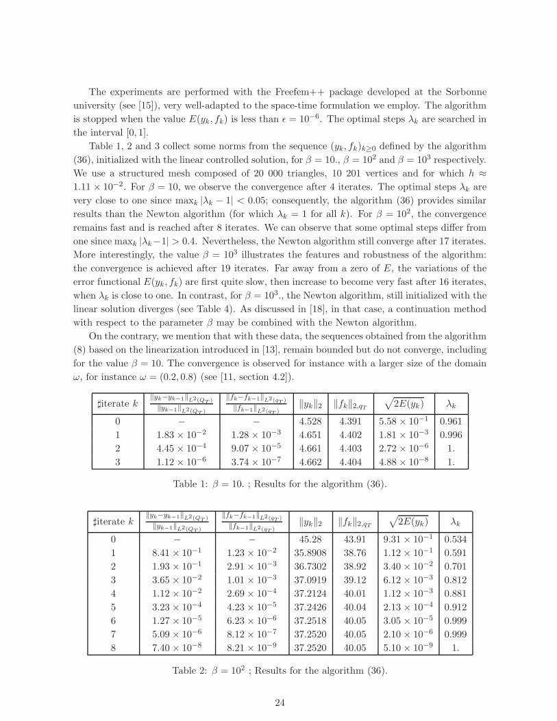
Table 1, 2 and 3 collect some norms from the sequence (yk, fk)k≥0 defined by the algorithm

(36), initialized with the linear controlled solution, for β = 10., β = 102 and β = 103 respectively.

We use a structured mesh composed of 20 000 triangles, 10 201 vertices and for which h ≈1.11 × 10−2. For β = 10, we observe the convergence after 4 iterates. The optimal steps λk are

very close to one since maxk |λk − 1| < 0.05; consequently, the algorithm (36) provides similar

results than the Newton algorithm (for which λk = 1 for all k). For β = 102, the convergence

remains fast and is reached after 8 iterates. We can observe that some optimal steps differ from

one since maxk |λk−1| > 0.4. Nevertheless, the Newton algorithm still converge after 17 iterates.

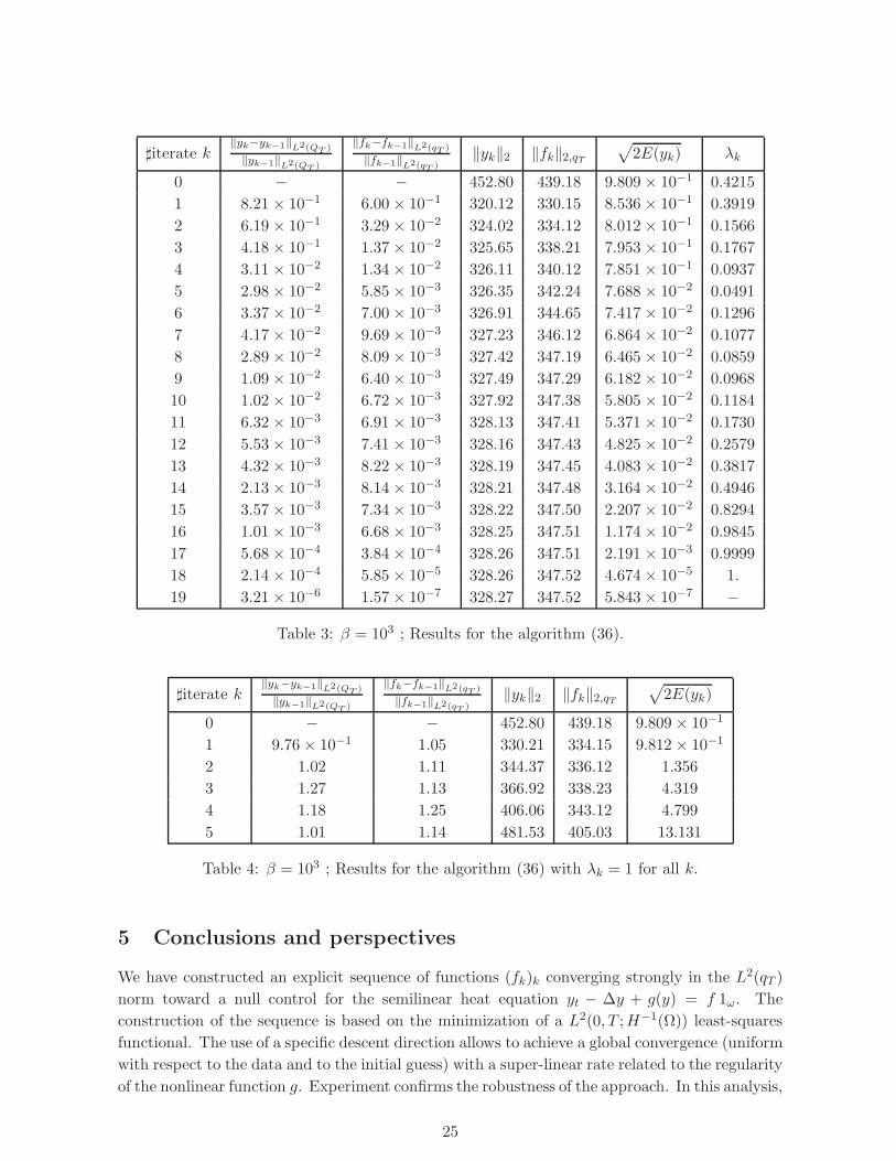
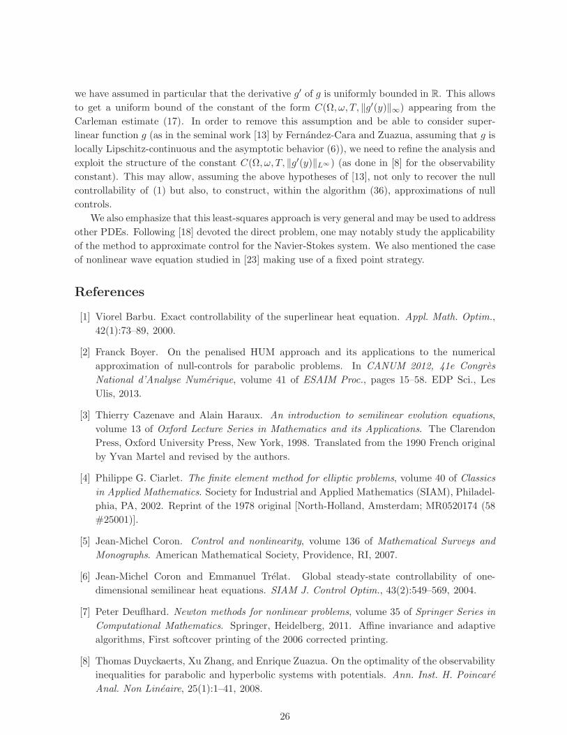
More interestingly, the value β = 103 illustrates the features and robustness of the algorithm:

the convergence is achieved after 19 iterates. Far away from a zero of E, the variations of the

error functional E(yk, fk) are first quite slow, then increase to become very fast after 16 iterates,

when λk is close to one. In contrast, for β = 103., the Newton algorithm, still initialized with the

linear solution diverges (see Table 4). As discussed in [18], in that case, a continuation method

with respect to the parameter β may be combined with the Newton algorithm.

On the contrary, we mention that with these data, the sequences obtained from the algorithm

(8) based on the linearization introduced in [13], remain bounded but do not converge, including

for the value β = 10. The convergence is observed for instance with a larger size of the domain

ω, for instance ω = (0.2, 0.8) (see [11, section 4.2]).

♯iterate k‖yk−yk−1‖L2(QT )

‖yk−1‖L2(QT )

‖fk−fk−1‖L2(qT )

‖fk−1‖L2(qT )‖yk‖2 ‖fk‖2,qT

√2E(yk) λk

0 − − 4.528 4.391 5.58 × 10−1 0.961

1 1.83 × 10−2 1.28 × 10−3 4.651 4.402 1.81 × 10−3 0.996

2 4.45 × 10−4 9.07 × 10−5 4.661 4.403 2.72 × 10−6 1.

3 1.12 × 10−6 3.74 × 10−7 4.662 4.404 4.88 × 10−8 1.

Table 1: β = 10. ; Results for the algorithm (36).

♯iterate k‖yk−yk−1‖L2(QT )

‖yk−1‖L2(QT )

‖fk−fk−1‖L2(qT )

‖fk−1‖L2(qT )‖yk‖2 ‖fk‖2,qT

√2E(yk) λk

0 − − 45.28 43.91 9.31 × 10−1 0.534

1 8.41 × 10−1 1.23 × 10−2 35.8908 38.76 1.12 × 10−1 0.591

2 1.93 × 10−1 2.91 × 10−3 36.7302 38.92 3.40 × 10−2 0.701

3 3.65 × 10−2 1.01 × 10−3 37.0919 39.12 6.12 × 10−3 0.812

4 1.12 × 10−2 2.69 × 10−4 37.2124 40.01 1.12 × 10−3 0.881

5 3.23 × 10−4 4.23 × 10−5 37.2426 40.04 2.13 × 10−4 0.912

6 1.27 × 10−5 6.23 × 10−6 37.2518 40.05 3.05 × 10−5 0.999

7 5.09 × 10−6 8.12 × 10−7 37.2520 40.05 2.10 × 10−6 0.999

8 7.40 × 10−8 8.21 × 10−9 37.2520 40.05 5.10 × 10−9 1.

Table 2: β = 102 ; Results for the algorithm (36).

24

♯iterate k‖yk−yk−1‖L2(QT )

‖yk−1‖L2(QT )

‖fk−fk−1‖L2(qT )

‖fk−1‖L2(qT )‖yk‖2 ‖fk‖2,qT

√2E(yk) λk

0 − − 452.80 439.18 9.809 × 10−1 0.4215

1 8.21 × 10−1 6.00 × 10−1 320.12 330.15 8.536 × 10−1 0.3919

2 6.19 × 10−1 3.29 × 10−2 324.02 334.12 8.012 × 10−1 0.1566

3 4.18 × 10−1 1.37 × 10−2 325.65 338.21 7.953 × 10−1 0.1767

4 3.11 × 10−2 1.34 × 10−2 326.11 340.12 7.851 × 10−1 0.0937

5 2.98 × 10−2 5.85 × 10−3 326.35 342.24 7.688 × 10−2 0.0491

6 3.37 × 10−2 7.00 × 10−3 326.91 344.65 7.417 × 10−2 0.1296

7 4.17 × 10−2 9.69 × 10−3 327.23 346.12 6.864 × 10−2 0.1077

8 2.89 × 10−2 8.09 × 10−3 327.42 347.19 6.465 × 10−2 0.0859

9 1.09 × 10−2 6.40 × 10−3 327.49 347.29 6.182 × 10−2 0.0968

10 1.02 × 10−2 6.72 × 10−3 327.92 347.38 5.805 × 10−2 0.1184

11 6.32 × 10−3 6.91 × 10−3 328.13 347.41 5.371 × 10−2 0.1730

12 5.53 × 10−3 7.41 × 10−3 328.16 347.43 4.825 × 10−2 0.2579

13 4.32 × 10−3 8.22 × 10−3 328.19 347.45 4.083 × 10−2 0.3817

14 2.13 × 10−3 8.14 × 10−3 328.21 347.48 3.164 × 10−2 0.4946

15 3.57 × 10−3 7.34 × 10−3 328.22 347.50 2.207 × 10−2 0.8294

16 1.01 × 10−3 6.68 × 10−3 328.25 347.51 1.174 × 10−2 0.9845

17 5.68 × 10−4 3.84 × 10−4 328.26 347.51 2.191 × 10−3 0.9999

18 2.14 × 10−4 5.85 × 10−5 328.26 347.52 4.674 × 10−5 1.

19 3.21 × 10−6 1.57 × 10−7 328.27 347.52 5.843 × 10−7 −

Table 3: β = 103 ; Results for the algorithm (36).

♯iterate k‖yk−yk−1‖L2(QT )

‖yk−1‖L2(QT )

‖fk−fk−1‖L2(qT )

‖fk−1‖L2(qT )‖yk‖2 ‖fk‖2,qT

√2E(yk)

0 − − 452.80 439.18 9.809 × 10−1

1 9.76 × 10−1 1.05 330.21 334.15 9.812 × 10−1

2 1.02 1.11 344.37 336.12 1.356

3 1.27 1.13 366.92 338.23 4.319

4 1.18 1.25 406.06 343.12 4.799

5 1.01 1.14 481.53 405.03 13.131

Table 4: β = 103 ; Results for the algorithm (36) with λk = 1 for all k.

5 Conclusions and perspectives

We have constructed an explicit sequence of functions (fk)k converging strongly in the L2(qT )

norm toward a null control for the semilinear heat equation yt − ∆y + g(y) = f 1ω. The

construction of the sequence is based on the minimization of a L2(0, T ;H−1(Ω)) least-squares

functional. The use of a specific descent direction allows to achieve a global convergence (uniform

with respect to the data and to the initial guess) with a super-linear rate related to the regularity

of the nonlinear function g. Experiment confirms the robustness of the approach. In this analysis,

25

we have assumed in particular that the derivative g′ of g is uniformly bounded in R. This allows

to get a uniform bound of the constant of the form C(Ω, ω, T, ‖g′(y)‖∞) appearing from the

Carleman estimate (17). In order to remove this assumption and be able to consider super-

linear function g (as in the seminal work [13] by Fernandez-Cara and Zuazua, assuming that g is

locally Lipschitz-continuous and the asymptotic behavior (6)), we need to refine the analysis and

exploit the structure of the constant C(Ω, ω, T, ‖g′(y)‖L∞) (as done in [8] for the observability

constant). This may allow, assuming the above hypotheses of [13], not only to recover the null

controllability of (1) but also, to construct, within the algorithm (36), approximations of null

controls.

We also emphasize that this least-squares approach is very general and may be used to address

other PDEs. Following [18] devoted the direct problem, one may notably study the applicability

of the method to approximate control for the Navier-Stokes system. We also mentioned the case

of nonlinear wave equation studied in [23] making use of a fixed point strategy.

References

[1] Viorel Barbu. Exact controllability of the superlinear heat equation. Appl. Math. Optim.,

42(1):73–89, 2000.

[2] Franck Boyer. On the penalised HUM approach and its applications to the numerical

approximation of null-controls for parabolic problems. In CANUM 2012, 41e Congres

National d’Analyse Numerique, volume 41 of ESAIM Proc., pages 15–58. EDP Sci., Les

Ulis, 2013.

[3] Thierry Cazenave and Alain Haraux. An introduction to semilinear evolution equations,

volume 13 of Oxford Lecture Series in Mathematics and its Applications. The Clarendon

Press, Oxford University Press, New York, 1998. Translated from the 1990 French original

by Yvan Martel and revised by the authors.

[4] Philippe G. Ciarlet. The finite element method for elliptic problems, volume 40 of Classics

in Applied Mathematics. Society for Industrial and Applied Mathematics (SIAM), Philadel-

phia, PA, 2002. Reprint of the 1978 original [North-Holland, Amsterdam; MR0520174 (58

#25001)].

[5] Jean-Michel Coron. Control and nonlinearity, volume 136 of Mathematical Surveys and

Monographs. American Mathematical Society, Providence, RI, 2007.

[6] Jean-Michel Coron and Emmanuel Trelat. Global steady-state controllability of one-

dimensional semilinear heat equations. SIAM J. Control Optim., 43(2):549–569, 2004.

[7] Peter Deuflhard. Newton methods for nonlinear problems, volume 35 of Springer Series in

Computational Mathematics. Springer, Heidelberg, 2011. Affine invariance and adaptive

algorithms, First softcover printing of the 2006 corrected printing.

[8] Thomas Duyckaerts, Xu Zhang, and Enrique Zuazua. On the optimality of the observability

inequalities for parabolic and hyperbolic systems with potentials. Ann. Inst. H. Poincare

Anal. Non Lineaire, 25(1):1–41, 2008.

26

[9] Enrique Fernandez-Cara. Null controllability of the semilinear heat equation. ESAIM

Control Optim. Calc. Var., 2:87–103, 1997.

[10] Enrique Fernandez-Cara and Sergio Guerrero. Global Carleman inequalities for parabolic

systems and applications to controllability. SIAM J. Control Optim., 45(4):1399–1446,

2006.

[11] Enrique Fernandez-Cara and Arnaud Munch. Numerical null controllability of semi-linear

1-D heat equations: fixed point, least squares and Newton methods. Math. Control Relat.

Fields, 2(3):217–246, 2012.

[12] Enrique Fernandez-Cara and Arnaud Munch. Strong convergent approximations of null

controls for the 1D heat equation. SeMA J., 61:49–78, 2013.

[13] Enrique Fernandez-Cara and Enrique Zuazua. Null and approximate controllability for

weakly blowing up semilinear heat equations. Ann. Inst. H. Poincare Anal. Non Lineaire,

17(5):583–616, 2000.

[14] A. V. Fursikov and O. Yu. Imanuvilov. Controllability of evolution equations, volume 34 of

Lecture Notes Series. Seoul National University, Research Institute of Mathematics, Global

Analysis Research Center, Seoul, 1996.

[15] Frederic Hecht. New development in Freefem++. J. Numer. Math., 20(3-4):251–265, 2012.

[16] Kevin Le Balc’h. Global null-controllability and nonnegative-controllability of slightly su-

perlinear heat equations. J. Math. Pures Appl. (9), 135:103–139, 2020.

[17] J. Lemoine, A. Munch, and P. Pedregal. Analysis of continuous H−1-least-squares ap-

proaches for the steady Navier-Stokes system. To appear in Applied Mathematics and

Optimization.

[18] Jerome Lemoine and Arnaud Munch. A fully space-time least-squares method for the

unsteady Navier-Stokes system. Preprint. arXiv:1909.05034.

[19] Jerome Lemoine and Arnaud Munch. Resolution of the implicit Euler scheme for the

Navier-Stokes equation through a least-squares method. Preprint - https://hal.uca.fr/hal-

01996429, 2020.

[20] Arnaud Munch and Pablo Pedregal. Numerical null controllability of the heat equation

through a least squares and variational approach. European J. Appl. Math., 25(3):277–306,

2014.

[21] Arnaud Munch and Diego A. Souza. A mixed formulation for the direct approximation of

L2-weighted controls for the linear heat equation. Adv. Comput. Math., 42(1):85–125, 2016.

[22] Pierre Saramito. A damped Newton algorithm for computing viscoplastic fluid flows. J.

Non-Newton. Fluid Mech., 238:6–15, 2016.

[23] Enrique Zuazua. Exact controllability for semilinear wave equations in one space dimension.

Ann. Inst. H. Poincare Anal. Non Lineaire, 10(1):109–129, 1993.

27