approximate algorithms for neural-bayesian approaches

Theoretical Computer Science 287 (2002) 219–238www.elsevier.com/locate/tcs

Approximate algorithms forneural-Bayesian approachesTom Heskes∗, Bart Bakker, Bert Kappen

SNN, University of Nijmegen, Geert Grooteplein 21, 6525 EZ Nijmegen, The Netherlands

Abstract

We describe two speci.c examples of neural-Bayesian approaches for complex modeling tasks:survival analysis and multitask learning. In both cases, we can come up with reasonable priorson the parameters of the neural network. As a result, the Bayesian approaches improve their(maximum likelihood) frequentist counterparts dramatically. By illustrating their application onthe models under study, we review and compare algorithms that can be used for Bayesianinference: Laplace approximation, variational algorithms, Monte Carlo sampling, and empiricalBayes.c© 2002 Elsevier Science B.V. All rights reserved.

PACS: 02.50.Ng; 02.70.Lg; 07.05.Mh

Keywords: Neural networks; Bayesian inference; Survival analysis; Multitask learning; Monte Carlosampling; Variational approximation

1. Introduction

Feedforward neural networks, also called multi-layered perceptrons, have becomepopular tools for solving complex prediction and classi.cation problems. More andmore people start to realize that there is nothing magical about neural networks: theyare “just” nonlinear models, not principally di>erent from many others. The so-calledweights are the parameters of the model. The error function one tries to minimize canoften be interpreted as (minus) the loglikelihood of the data given the parameters. Thefamous backpropagation rule is nothing but an e?cient way to compute the gradientof this error function.

∗ Corresponding author.E-mail address: [email protected] (T. Heskes).URL: http://www.mbfys.kun.nl/people/tom

0304-3975/02/$ - see front matter c© 2002 Elsevier Science B.V. All rights reserved.PII: S0304 -3975(02)00132 -9

220 T. Heskes et al. / Theoretical Computer Science 287 (2002) 219–238

This insight has led to a welcome cross-fertilization between neural network researchand advanced statistics. Neural networks are now standardly trained with better opti-mization procedures as Levenberg–Marquardt and conjugate gradient. Frequentist toolssuch as bootstrapping and cross-validation generate ensembles of neural networks withmuch better and more reliable performance than single ones. Algorithms have been de-veloped for computing con.dence and prediction intervals (errorbars) on the networkoutcomes.The introduction of Bayesian methodology for neural networks has been another

important advance. Training became Bayesian inference and popular strategies such as“weight decay” could be interpreted in terms of Bayesian priors. Now there seemsto be a status-quo between the frequentist and Bayesian approaches for training stan-dard multi-layered perceptrons. The Bayesian approach seems to be more principledand elegant, but the frequentist one more practical, yielding about the sameperformance.In this article we describe two examples of multi-layered perceptrons solving a spe-

ci.c problem: survival analysis and multitask learning. We will see that in both casesthe Bayesian approach is de.nitely better than its frequentist alternative. The reason isthat in these speci.c cases we can come up with sensible priors. These priors spec-ify reasonable assumptions about the weights of the neural network. The Bayesianinference machine can be used to infer the appropriate strength of these priors. Inmost cases, however, exact Bayesian inference is intractable and we have to resortto approximations. We highlight and compare the approximations that are currently inuse.In Section 2 we describe our neural network model for survival analysis.

Section 3 treats appropriate approximations for Bayesian inference of the parametersof this model: Monte Carlo sampling, the variational approach, and the Laplace ap-proximation. In Section 4 the di>erent approaches are applied and compared on a largereal-world database involving patients with ovarian cancer. Our model for multitasklearning is introduced in Section 5. Section 6 discusses empirical Bayes, also called“evidence framework”, an approximation that seems particularly suited for multitasklearning. Results obtained on a huge dataset involving magazine sales are described inSection 7. We end with a discussion and conclusions in Section 8. Detailed mathematicsis treated in Appendix A.

2. Multi-layered perceptrons for survival analysis

2.1. The model and the likelihood

The purpose of survival analysis is to estimate a patient’s chances of survival asa function of time, given the available medical information at the time the patient isadmitted to the study. This information (e.g., age, given treatment, outcome of medicaltests) is quanti.ed by an ninp-dimensional input vector x. Time is discretized into nequal time intervals of length It. The output yi stands for the (estimated) probabilityto survive a time ti after entering the study. It is modeled through a multi-layered

T. Heskes et al. / Theoretical Computer Science 287 (2002) 219–238 221

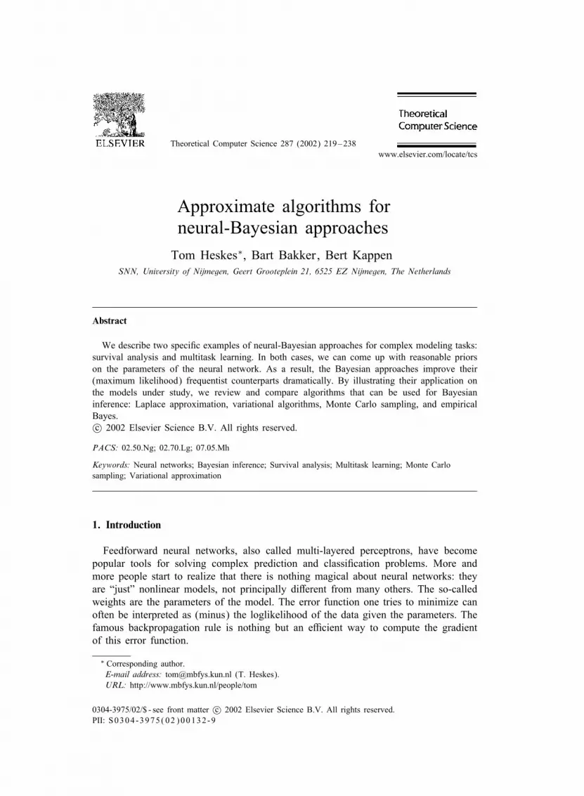
Fig. 1. Neural interpretation of survival analysis. See the text for an explanation.

perceptron with exponential transfer functions as sketched in Fig. 1:

yi(x) = exp

[nhid∑jwjihj(x)

]and hj(x) = exp

[ninp∑kvkjxk

]: (1)

In [1] it is shown that the case of a single hidden unit corresponds to a discretizedversion of Cox proportional hazards model [8], which is the standard in the .eld of sur-vival analysis. hj(x) is called the proportional hazard and only depends on the patient’scharacteristics; wj is the baseline hazard, a function of time t, here discretized as ti. Byadding hidden units (the dashed lines in Fig. 1), we can in principle extend our modelbeyond proportional hazards to allow for more complex input–output relationships.Our database D consists of a set of N patients with characteristics x� and corre-

sponding times t�, the time that the patient leaves the study after entering it, eitherbecause the patient dies (uncensored) or because the study ended when the patient wasstill alive (censored). In computing the likelihood of the data, we have to make thisdistinction between censored and uncensored patients. We have

P(D|v; w) = ∏�∈uncensored

fi(�)(x�)∏

�∈censoredyi(�)(x�) (2)

with i(�) such that ti(�)−1¡t�6ti(�), and

fi(x) = − 1It

∑j[wji − wj;i−1]hj(x)yi(x);

the probability density for a patient with characteristics x to die between ti−1 andti (fi(x) is minus the derivative of yi(x) with respect to time).Standard Cox now corresponds to a maximum likelihood (ML) approach: try and .nd

the parameters v and w that maximize the likelihood of the data D. An advantage ofCox analysis is that the optimal parameters v of the proportional and w of the time-dependent hazard can be found sequentially. Disadvantages of this approach are thehazard’s tendency to become highly non-smooth, and the danger of strongly over.ttingthe data. Here we suggest a Bayesian approach to overcome these weaknesses.

https://www.researchgate.net/publication/237344014_Analysis_of_survival_data?el=1_x_8&enrichId=rgreq-6c4e14ba-7439-4f36-a49b-7c1109a5d577&enrichSource=Y292ZXJQYWdlOzIyMjY4ODE1MTtBUzoxMDM3MjQ4NDAxMjg1MjdAMTQwMTc0MTMzODMyMw==

https://www.researchgate.net/publication/2300244_A_neural-Bayesian_approach_to_survival_analysis?el=1_x_8&enrichId=rgreq-6c4e14ba-7439-4f36-a49b-7c1109a5d577&enrichSource=Y292ZXJQYWdlOzIyMjY4ODE1MTtBUzoxMDM3MjQ4NDAxMjg1MjdAMTQwMTc0MTMzODMyMw==


0 900 1800 2700 36000

0.02

0.04

0.06

0.08

0.1

time (days)

base

line

haza

rd

standard Cox

0 900 1800 2700 36000

0.01

0.02

0.03

0.04

0.05

0.06

time (days)

base

line

haza

rd

with Bayesian priors

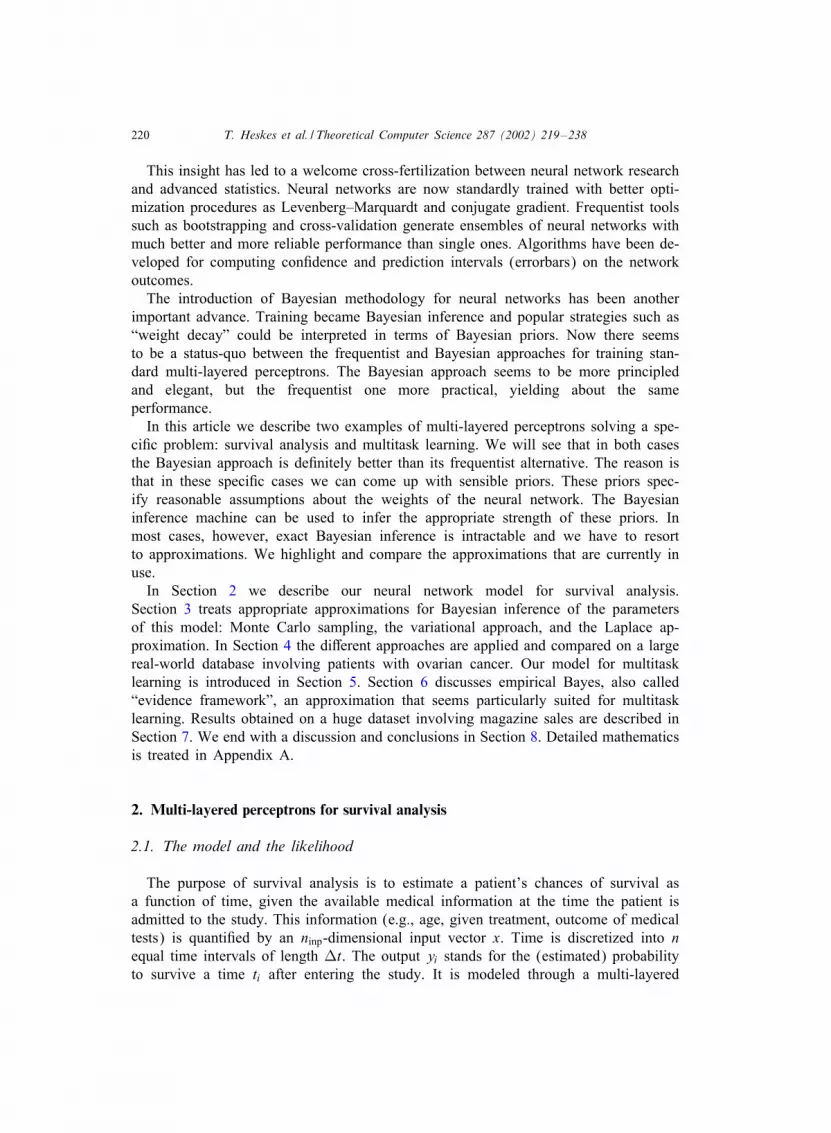
Fig. 2. The baseline hazard wi as obtained in maximum likelihood Cox analysis (left), and the maximum aposteriori solutions resulting from the Bayesian approach incorporating the prior on q (right). In both caseswi is optimized on a training set of 600 patterns, chosen randomly from our database. The e>ect of the prioris a considerable smoothing of the hazard function.

2.2. Sensible priors

In a Bayesian approach we seek to construct a probability distribution over all pos-sible values of the parameters, here v and w. This distribution not only depends on thedata D, but also on prior knowledge about the nature of the problem. This prior knowl-edge can be expressed as prior probabilities on the model parameters. Using Bayes’formula the priors and the data likelihood are combined into a posterior distribution.For ease of notation, we consider the case of one hidden unit and make a transfor-

mation of variables by de.ning qi= log(wi − wi−1) and q1= log(w1). The .rst prior

P(q|�) ∝ exp

[− �2∑ij

g(|i − j|)[qi − qj]2]∝ exp

[− �2qT�q

]

with �ij= − g(|i− j|); �ii=∑

j �=i g(|i− j|), and g(x)=e−x2=�, prevents the hazard frombecoming too sharp as a function of time. Since P(q|�) assigns the highest likelihood toa hazard function that is constant in time (independent of i), it smoothes out the hazardfunction, and introduces a preference for survivor functions which decay exponentially.Its e>ect is visualized in Fig. 2. The hazard function in the ML Cox approach is ajagged function, due to the limited information in the database. After incorporating theprior P(q|�) this function becomes much more smooth. This smoother function is notonly more plausible a priori, but, as we will see below, also improves the model’spredictive performance.The second prior

P(v|�) ∝ exp[−�2vT�v

]; where � =

1N∑�

x�x�T

prevents large activities of hidden units (high values for the proportional hazard), i.e.,prefers small weights. This prior corresponds to a ridge-type estimator, as discussed


_2 _1 0 1 20

5

10

15

20

25

30standard Cox

log(h(x))

# co

unts

_2 _1 0 1 20

5

10

15

20

25

30

log(h(x))

with Bayesian priors

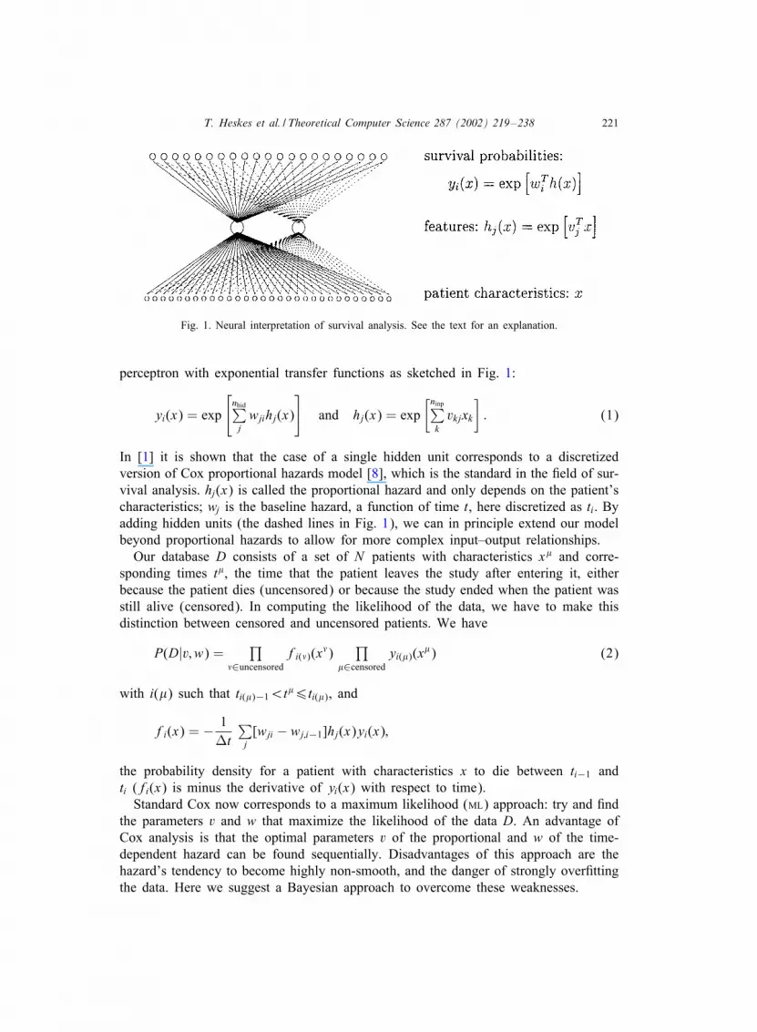
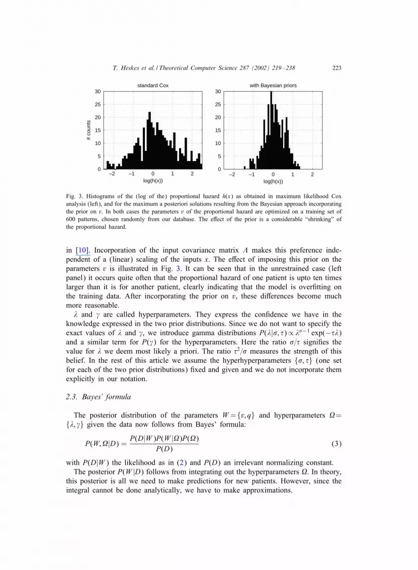
Fig. 3. Histograms of the (log of the) proportional hazard h(x) as obtained in maximum likelihood Coxanalysis (left), and for the maximum a posteriori solutions resulting from the Bayesian approach incorporatingthe prior on v. In both cases the parameters v of the proportional hazard are optimized on a training set of600 patterns, chosen randomly from our database. The e>ect of the prior is a considerable “shrinking” ofthe proportional hazard.

in [10]. Incorporation of the input covariance matrix � makes this preference inde-pendent of a (linear) scaling of the inputs x. The e>ect of imposing this prior on theparameters v is illustrated in Fig. 3. It can be seen that in the unrestrained case (leftpanel) it occurs quite often that the proportional hazard of one patient is upto ten timeslarger than it is for another patient, clearly indicating that the model is over.tting onthe training data. After incorporating the prior on v, these di>erences become muchmore reasonable.

� and � are called hyperparameters. They express the con.dence we have in theknowledge expressed in the two prior distributions. Since we do not want to specify theexact values of � and �, we introduce gamma distributions P(�|�; �)∝ ��−1 exp(−��)and a similar term for P(�) for the hyperparameters. Here the ratio �=� signi.es thevalue for � we deem most likely a priori. The ratio �2=� measures the strength of thisbelief. In the rest of this article we assume the hyperhyperparameters {�; �} (one setfor each of the two prior distributions) .xed and given and we do not incorporate themexplicitly in our notation.

2.3. Bayes’ formula

The posterior distribution of the parameters W ={v; q} and hyperparameters �={�; �} given the data now follows from Bayes’ formula:

P(W;�|D) = P(D|W )P(W |�)P(�)P(D)

(3)

with P(D|W ) the likelihood as in (2) and P(D) an irrelevant normalizing constant.The posterior P(W |D) follows from integrating out the hyperparameters �. In theory,

this posterior is all we need to make predictions for new patients. However, since theintegral cannot be done analytically, we have to make approximations.

https://www.researchgate.net/publication/266953700_Ridge_Type_Estimators_for_Regression_Analysis?el=1_x_8&enrichId=rgreq-6c4e14ba-7439-4f36-a49b-7c1109a5d577&enrichSource=Y292ZXJQYWdlOzIyMjY4ODE1MTtBUzoxMDM3MjQ4NDAxMjg1MjdAMTQwMTc0MTMzODMyMw==


3. Approximations of the posterior

Fortunately, an ample arsenal of methods to approximate P(W |D) is available. Thesemethods have become popular tools in the neural network community. In this sectionwe describe three such methods: Monte Carlo sampling, a variational approach and theLaplace approximation.

3.1. Monte Carlo sampling

Since the posterior P(W;�|D) is not a simple analytic function of the model param-eters, it is hard to draw samples from it. We can use a combination of Gibbs samplingand Hybrid Markov Chain Monte Carlo Sampling (HMCMC) to make it tractable.Gibbs sampling is used to iterate between drawing samples for the model param-

eters W and for the hyperparameters �. As we will see, drawing hyperparameters isstraightforward for two reasons.• The probability of the hyperparameters � given a particular sample W and the data

D is independent of the latter:

P(�|W;D) =P(D;W |�)P(�)

P(D;W )=

P(D|W )P(W |�)P(�)P(D|W )P(W ) = P(�|W ):

• The resulting distributions P(�|v) and P(�|q) are again gamma distributions. In sta-tistical terms, the gamma prior is the natural conjugate of the Gaussian. Standardtricks to sample from a gamma distribution can be found in any textbook on Bayesiananalysis (see e.g. [9]).

Now, given a new set of hyperparameters �, we have to draw a new W from

P(W |�;D) =P(D|W )P(W |�)

P(D|�) ∝ P(D|W )P(W |�);

the product of the likelihood and the priors, with .xed values for the hyperparameters.The data likelihood P(D|W ) and priors P(W |�) are easy to compute; the problem

is in the normalization P(D|�). Monte Carlo sampling circumvents computations ofthis normalization term. A Monte Carlo sampling procedure works as follows:(1) Starting from a sample W use the “jumping distribution” J (W ′|W ) to generate a

candidate sample W ′. In its simplest version, the jumping distribution is symmetric,i.e., J (W ′|W )=J (W |W ′).

(2) Compute the ratio

r =P(W ′|�;D)P(W |�;D)

:

Note that computation of this ratio is doable, since the normalizations of the sep-arate probabilities drop out.

(3) Accept the new state W ′ if r¿1 or with probability r if r¡1. Otherwise keep theprevious state W . Return to the .rst step.


The essence of a good Monte Carlo sampling algorithm is in the “jumping distribution”:you want to have a distribution that makes large steps in the space of your parameters,such that subsequent samples are more or less independent, with a high acceptancerate.A very popular sampling algorithm is Hybrid Markov Chain Monte Carlo sampling

(see e.g. [16]). The basic idea is to double the parameter space, introducing an ex-tra canonical parameter for each original one. Jumps are de.ned on both original andcanonical parameters, such that the joint probability of the candidate sample is, upto numerical errors, equal to that of the one started from: the candidate has a highacceptance rate. Since the canonical parameters and the original ones are by construc-tion independent, sampling of the joint distribution also corresponds to sampling of thedistribution of the parameters we are interested in: the values of the canonical ones aresimply neglected.A disadvantage of Monte Carlo sampling is that generating (independent) samples

can be quite time-consuming. Even more important, it is di?cult to tell when su?cientsamples have been drawn. It might for example be that one is sampling in just one partof the parameter space, with a very small probability of jumping to another relevantpart. Advantages are that Monte Carlo sampling algorithms, in the limit of an in.nitenumber of samples and except for singular cases, converge to the exact probabilitydistribution. Furthermore, they are easy to implement for many probability distributions.

3.2. Variational approach

The variational approach o>ers an alternative. It has been introduced under the term“ensemble learning” in [12] and has been applied to learning in multi-layered percep-trons and radial basis function networks in [2,3].Recall that we are interested in the joint posterior P(W;�|D) of model parameters

and hyperparameters. Knowing that we cannot describe it in an analytical form, thebest we can do is to try and approximate it with an analytical distribution. Here wetake

P∗(W;�) = Q(W )R(�)

with 1 Q(W )=$(W |W ; C), a Gaussian distribution, and R(�) for the moment unspec-i.ed.A natural distance between the probabilitiesP(W;�|D) andP∗(W;�) is the Kullback–

Leibler divergence

KL[Q; R] =∫dW d�Q(W )R(�) log

[Q(W )R(�)P(W;�|D)

]

= 〈log[Q(W )R(�)]〉Q;R − 〈log[P(D|W )P(W |�)P(�)]〉Q;R; (4)

1 $(W |W ; C)∝ exp[− 12 (W − W )TC−1(W − W )].


where in the second line we substituted (3) and neglected irrelevant constants. The goalof the variational approach is now to .nd the parameters of the distribution Q(W ) andthe distribution R(�) that minimize this distance.The steps to be taken are quite similar to those in the Gibbs algorithm explained in

the previous section. Suppose .rst that we know the distribution Q(W ) and would liketo .nd the optimal R(�). Collecting the terms in (4) that depend on R(�), we obtain

KL[R] = 〈logR(�)〉R − 〈logP(�)〉R − 〈logP(W |�)〉Q;R: (5)

Note that, as in the Gibss sampling procedure, none of the terms involves the data D.Furthermore, we have the same kind of “conjugacy”: with a Gaussian prior P(W |�)and a gamma distribution for P(�), the optimal R(�) is also gamma distributed. Itsaverage Q� only depends on the parameters QW and C of the distribution Q(W ) (seeAppendix for details).Next we assume that R(�) is known and try to optimize the parameters of Q(W ).

The terms in (4) depending on Q(W ) and thus on the variational parameters {W ; C}are

KL[Q] = 〈logQ(W )〉Q − 〈logP(D|W )〉Q − 〈logP(W |�)〉Q;R: (6)

In Appendix A we show that, for our survival analysis model, all these terms can becomputed analytically as a function of the data D and the average Q� for the hyperpa-rameters. Computing the new QW and C boils down to a straightforward optimizationprocedure, to be solved e.g. using a conjugate gradient method.Iterating back and forth as in the Gibbs sampler, the variational procedure converges

to an (at least locally) optimal distribution P∗(W;�). The advantage of the variationalapproach is that we arrive at a relatively simple distribution to work with. Further-more, in the above application to survival analysis all computations to arrive at thisdistribution can be done analytically. In most cases however, numerical integrationsare unavoidable (see e.g. [2] for the case of multi-layered perceptrons with sigmoidaltransfer functions). Also here, with more than one hidden unit, we have to resort tonumerical integrations, scaling with the number of added hidden units.

3.3. Laplace approximation

The variational procedure can be simpli.ed by replacing the minimization of theKullback–Leibler divergence KL[Q] by a Laplace approximation. That is, instead of.tting the parameters of Q(W ) against the distribution P(W | Q�;D), we can take theLaplace approximation

W = argmaxW

P(W | Q�;D)

and C the Hessian of − log(P(W | Q�;D)). Based on these new parameters W and C,new values for Q� can be computed as in (A.1).


An advantage of the Laplace approximation over the full variational approach is thatit does not require the evaluation of integrals, just minimization, and is therefore ofteneasier to compute. One would expect the variational approach to be more accurate, sinceit not only considers the peak of the probability distribution, but might also take intoaccount some of its mass. Note that what we call Laplace approximation is somewhatdi>erent from the “evidence framework” introduced by MacKay (see e.g. [14,15]). Wediscuss the evidence framework in more detail below.

4. Results for survival analysis

We test the standard ML approach and the three (approximate) Bayesian approacheson a database of 929 ovarian cancer patients (see [13] for details). The database israndomly divided in a training and test set. As an error criterion we take minus theloglikelihood on the test set, i.e., the logarithm of (2), with � running over the test set.To get a clear indication of the relative strengths of the methods, we scale the errorsrelative to a “minimum error” Emin and the “Cox error” Ecox:

Erel =E − Emin

Ecox − Emin: (7)

The minimum error is de.ned as the test error of the maximum likelihood Cox solutionwhen the ML parameters are optimized on this same test set. The Cox error is the testerror of the ML solution computed by optimizing on the training set. So, a relative errorof 1 means just as good as the ML Cox method. A relative error of 0.5 means twiceas close to the error of the ML solution on the test set.Let us .rst consider the results for a training set of 600 patients and testing on

the remaining 329 (Fig. 4c). The errors in any of the approximations to the Bayesianposterior are signi.cantly (p≈ 1× 10−5) smaller than the error in the ML Cox approach.Looking more closely at the di>erence between the three Bayesian approaches, theerror in the variational approach happens to be slightly (but signi.cantly) larger thanthe error in the sampling approach. The Laplace approximation, which takes aboutan equal amount of computation time as the variational approach, does not performsigni.cantly better or worse than the variational approach.The size of our database (929 patients) is much larger than common in survival anal-

ysis (typically 100–200 patients). Therefore, we also compared the four approacheswhen applied on smaller parts (120 and 200 patients), results of which are shownin Figs. 4a and b. Note that we used the values Ecox and Emin obtained on thetraining set of 600 patterns to de.ne the relative errors. For lower and lower num-bers of training patterns, the error in the ML Cox method increases dramatically. Theerror in the Bayesian approaches also increases slightly, but much more gradually:the less data, the higher the impact of the priors, which here yield an enormousimprovement.We notice a similar e>ect when considering more complex models. After adding

an extra hidden unit, which doubles the number of model parameters, the error corre-sponding to the ML solution increases dramatically, even with a training set of 600


1 2 3 40.1

1

10

120 training patternsre

lativ

e er

ror

1 2 3 40.1

1

10

200 training patterns

1 2 3 40.1

1

10

600 training patterns

(a) (b) (c)

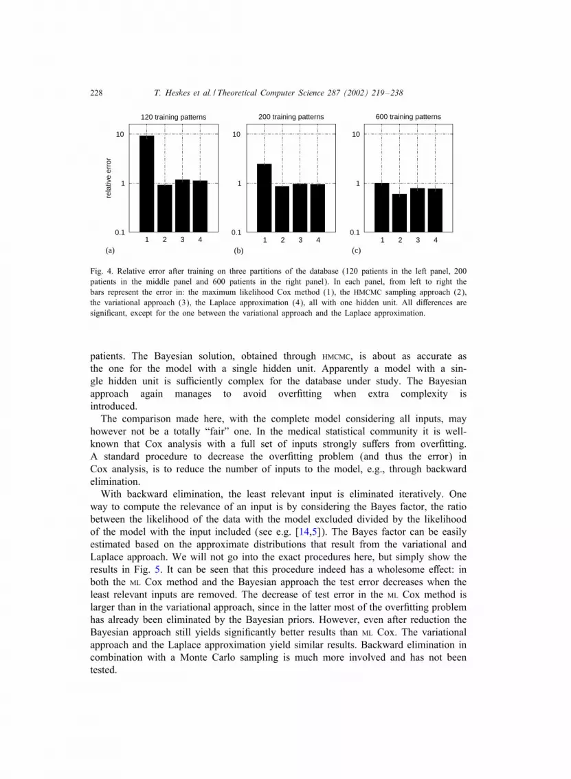
Fig. 4. Relative error after training on three partitions of the database (120 patients in the left panel, 200patients in the middle panel and 600 patients in the right panel). In each panel, from left to right thebars represent the error in: the maximum likelihood Cox method (1), the HMCMC sampling approach (2),the variational approach (3), the Laplace approximation (4), all with one hidden unit. All di>erences aresigni.cant, except for the one between the variational approach and the Laplace approximation.

patients. The Bayesian solution, obtained through HMCMC, is about as accurate asthe one for the model with a single hidden unit. Apparently a model with a sin-gle hidden unit is su?ciently complex for the database under study. The Bayesianapproach again manages to avoid over.tting when extra complexity isintroduced.The comparison made here, with the complete model considering all inputs, may

however not be a totally “fair” one. In the medical statistical community it is well-known that Cox analysis with a full set of inputs strongly su>ers from over.tting.A standard procedure to decrease the over.tting problem (and thus the error) inCox analysis, is to reduce the number of inputs to the model, e.g., through backwardelimination.With backward elimination, the least relevant input is eliminated iteratively. One

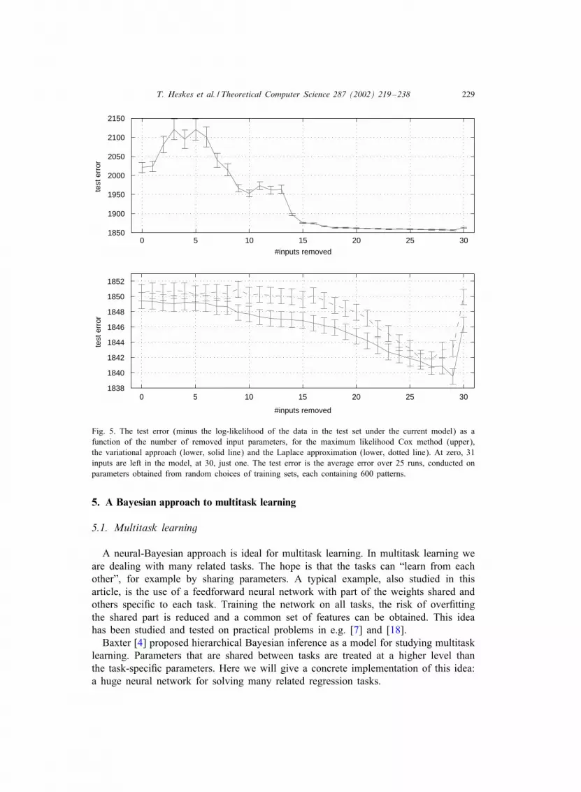
way to compute the relevance of an input is by considering the Bayes factor, the ratiobetween the likelihood of the data with the model excluded divided by the likelihoodof the model with the input included (see e.g. [14,5]). The Bayes factor can be easilyestimated based on the approximate distributions that result from the variational andLaplace approach. We will not go into the exact procedures here, but simply show theresults in Fig. 5. It can be seen that this procedure indeed has a wholesome e>ect: inboth the ML Cox method and the Bayesian approach the test error decreases when theleast relevant inputs are removed. The decrease of test error in the ML Cox method islarger than in the variational approach, since in the latter most of the over.tting problemhas already been eliminated by the Bayesian priors. However, even after reduction theBayesian approach still yields signi.cantly better results than ML Cox. The variationalapproach and the Laplace approximation yield similar results. Backward elimination incombination with a Monte Carlo sampling is much more involved and has not beentested.


0 5 10 15 20 25 301850

1900

1950

2000

2050

2100

2150

#inputs removed

test

err

or

0 5 10 15 20 25 301838

1840

1842

1844

1846

1848

1850

1852

#inputs removed

test

err

or

Fig. 5. The test error (minus the log-likelihood of the data in the test set under the current model) as afunction of the number of removed input parameters, for the maximum likelihood Cox method (upper),the variational approach (lower, solid line) and the Laplace approximation (lower, dotted line). At zero, 31inputs are left in the model, at 30, just one. The test error is the average error over 25 runs, conducted onparameters obtained from random choices of training sets, each containing 600 patterns.

5. A Bayesian approach to multitask learning

5.1. Multitask learning

A neural-Bayesian approach is ideal for multitask learning. In multitask learning weare dealing with many related tasks. The hope is that the tasks can “learn from eachother”, for example by sharing parameters. A typical example, also studied in thisarticle, is the use of a feedforward neural network with part of the weights shared andothers speci.c to each task. Training the network on all tasks, the risk of over.ttingthe shared part is reduced and a common set of features can be obtained. This ideahas been studied and tested on practical problems in e.g. [7] and [18].Baxter [4] proposed hierarchical Bayesian inference as a model for studying multitask

learning. Parameters that are shared between tasks are treated at a higher level thanthe task-speci.c parameters. Here we will give a concrete implementation of this idea:a huge neural network for solving many related regression tasks.


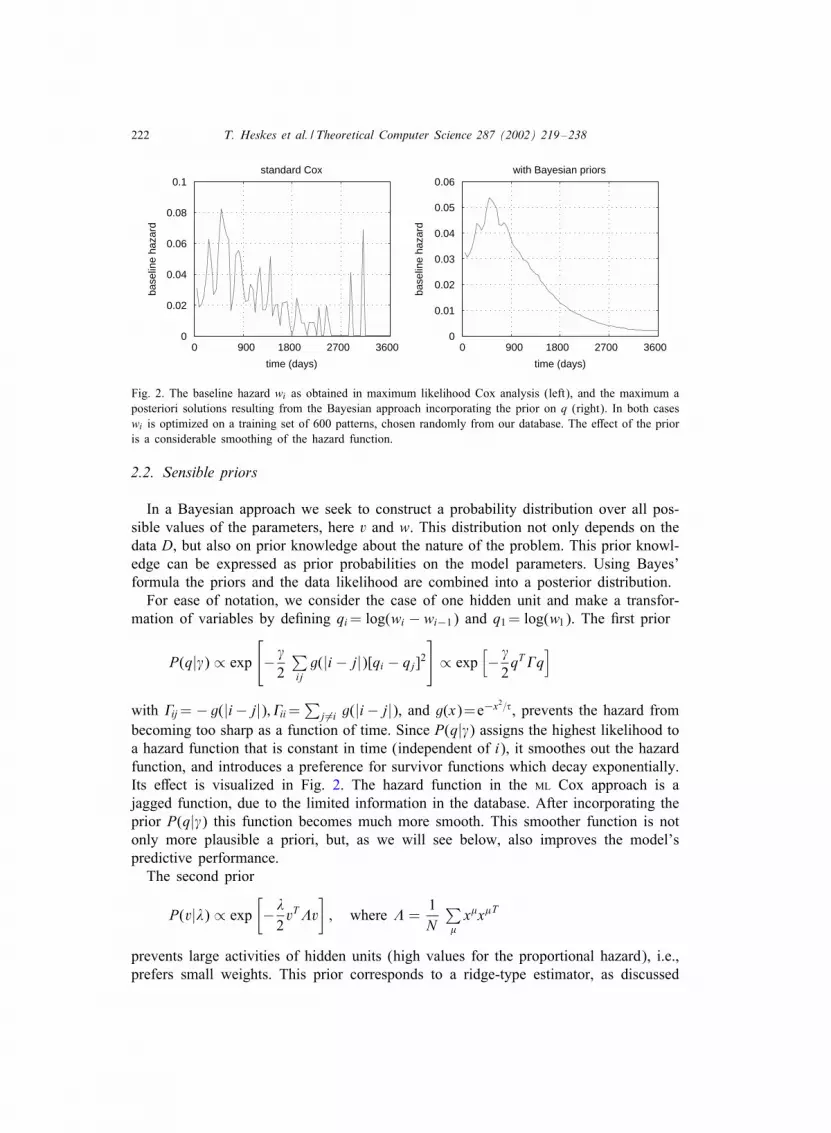
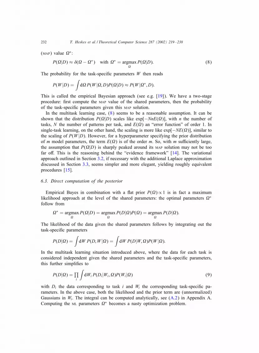
Fig. 6. Sketch of the architecture of the neural network for multitask learning. Each output corresponds toa di>erent task. Input-to-hidden weights are shared; hidden-to-output weights speci.c.

5.2. The network architecture

The model that we study is sketched in Fig. 6. It has n outputs, each correspondingto a di>erent task i. Given the input vector x, the output yi(x) follows from [comparewith (1)]

yi(x) =nhid∑jwjihj(x) and hj(x) = g

(ninp∑kvkjxk

)

with g(·) the hidden unit’s transfer function. The ninp× nhid matrix v with the weightsfrom the input to the hidden units is shared by all tasks. The nhid × n matrix w, withcolumn vectors wi, contains the weights from the hidden to the output units speci.c toeach task. Typically we have nhid¡ninp�n, i.e., a bottleneck of hidden units. The ideabehind multitask learning is that after training the input-to-hidden weights v implementa low-dimensional (feature) representation of the inputs that is useful for all tasks. Therisk of over.tting v is small since the data for all tasks can be used to infer this partof the model.Our total database D consists of n sets Di, one for each task, each containing N

combinations of input vectors x�(i) and observed outputs y�i . We assume that the

observed outputs y�i are given by the outputs yi(x�(i)) of the neural network, corrupted

with Gaussian noise of zero mean and standard deviation �, independent of i. Thelikelihood of all data Di for task i given the weights v and wi thus reads

P(Di|wi; v; �) =∏�$(y�

i |wTi g(v

T x�(i)); �2)

with $(·|·; ·) the normal distribution de.ned in Section 3.2. The likelihood of all datais the product

P(D|w; v; �) =∏iP(Di|wi; v; �):


5.3. Priors

The weights wi determine the impact of the hidden units on output i. We considerthe Gaussian prior

P(wi|m;+) = $(wi|m;+2)

with m a vector of length nhid and +2 an nhid × nhid covariance matrix. This correspondsto a so-called exchangeability assumption (the same m for all tasks) and introduces atendency for similar weights across tasks. How similar is determined by the covariancematrix +2.In a full hierarchical Bayesian analysis, we should also specify priors for the pa-

rameters � and v and even “hyperpriors” for the parameters m and +. In the empiricalBayesian approach, to be discussed next, we simply take an improper “Rat” prior,giving equal a priori weight to all possible values.

6. Empirical Bayes for multitask learning

6.1. Task-speci<c parameters and shared parameters

In the (single-task) survival analysis case, we divided our total set of parameters intotwo sets: hyperparameters � and model parameters W . Hyperparameters � speci.edthe prior distribution for the model parameters W , but had no direct e>ect on the data.The resulting conditional independence P(�|W;D)=P(�|W ) simpli.ed both the Gibbssampling and the variational approach considerably.We could make the same subdivision here, but the resulting procedures would

be extremely time-consuming. The empirical Bayesian approach introduced belowdistinguishes between parameters W ={w} that are task-speci.c and parameters �={v; �; m; +} that are shared between tasks. With this subdivision we lose the conditionalindependence in P(�|W;D): P(�|W;D) =P(�|W ). Instead we will make the assump-tion that the posterior probability of the shared parameters is sharply peaked around itsmaximum a posteriori (MAP) solution. This approximation is particularly suited for themultitask learning situation (see also e.g. [6] for similar approximations in the .eld ofmultilevel analysis), but can also be used in other contexts.

6.2. Empirical Bayes

We are interested in the probability P(W;�|D) of all parameters given all data andwrite

P(W;�|D) = P(W |�;D)P(�|D):

Since all data can be used to infer the probability of the shared parameters �, we makethe assumption that P(�|D) is very sharply peaked around its maximum a posteriori


(MAP) value �∗:

P(�|D) ≈ ,(� − �∗) with �∗ = argmax�

P(�|D): (8)

The probability for the task-speci.c parameters W then reads

P(W |D) =∫d�P(W |�;D)P(�|D) ≈ P(W |�∗; D):

This is called the empirical Bayesian approach (see e.g. [19]). We have a two-stageprocedure: .rst compute the MAP value of the shared parameters, then the probabilityof the task-speci.c parameters given this MAP solution.In the multitask learning case, (8) seems to be a reasonable assumption. It can be

shown that the distribution P(�|D) scales like exp[−NnE(�)], with n the number oftasks, N the number of patterns per task, and E(�) an “error function” of order 1. Insingle-task learning, on the other hand, the scaling is more like exp[−NE(�)], similar tothe scaling of P(W |D). However, for a hyperparameter specifying the prior distributionof m model parameters, the term E(�) is of the order m. So, with m su?ciently large,the assumption that P(�|D) is sharply peaked around its MAP solution may not be toofar o>. This is the reasoning behind the “evidence framework” [14]. The variationalapproach outlined in Section 3.2, if necessary with the additional Laplace approximationdiscussed in Section 3.3, seems simpler and more elegant, yielding roughly equivalentprocedures [15].

6.3. Direct computation of the posterior

Empirical Bayes in combination with a Rat prior P(�)∝ 1 is in fact a maximumlikelihood approach at the level of the shared parameters: the optimal parameters �∗

follow from

�∗ = argmax�

P(�|D) = argmax�

P(D|�)P(�) = argmax�

P(D|�):

The likelihood of the data given the shared parameters follows by integrating out thetask-speci.c parameters

P(D|�) =∫dW P(D;W |�) =

∫dW P(D|W;�)P(W |�):

In the multitask learning situation introduced above, where the data for each task isconsidered independent given the shared parameters and the task-speci.c parameters,this further simpli.es to

P(D|�) =∏i

∫dWi P(Di|Wi; �)P(Wi|�) (9)

with Di the data corresponding to task i and Wi the corresponding task-speci.c pa-rameters. In the above case, both the likelihood and the prior term are (unnormalized)Gaussians in Wi. The integral can be computed analytically, see (A.2) in Appendix A.Computing the ML parameters �∗ becomes a nasty optimization problem.


6.4. EM algorithm

For slightly more complex models (e.g., non-Gaussian noise or nonlinear transferfunction for the outputs), the integrals in (9) can no longer be computed analytically.But even if they can, as in our case, direct optimization of (9) may not be the smartestthing to do. The variational approach, outlined in Section 3.2, provides an alternative.Here we take as an approximating distribution

P∗(W;�) = Q(W )R(�) with R(�) = ,(� − �∗):

The (parameters specifying the) distribution Q(W ) and �∗ have to be optimized suchthat the KL-divergence between the approximation and the true posterior is P(W;�|D)is minimized.Minimization of the part KL[R] in (5) given the current distribution Q(W ) now

amounts to .nding

�∗ = argmax�

∫dW Q(W ) logP(W;�|D)

= argmax�

∫dW Q(W ) logP(D|W;�)P(W |�):

Substituting R(�)=,(� − �∗), the term KL[Q] of (6) reads

KL[Q] =∫dW Q(W ) log

[P(W |�∗; D)

Q(W )

]:

If we leave Q(W ) completely free, we directly obtain Q(W )=P(W |�∗; D). This cor-responds to a standard EM algorithm for optimizing (9): in the E-step we computethe expectation of the “hidden variables” W given the current parameters �∗; in theM-step we use this probability to optimize for the next set of shared parameters. Ascan be seen in Appendix A, the two separate expectation and optimization steps aremuch simpler and easier to interpret than the direct integration of (9). Furthermore, byrestricting Q(W ) to be of a speci.c form, we can obtain useful approximations whenthe exact integral is undoable. More on the link between variational approaches andEM algorithms can be found in [17].

7. Results for multitask learning

We illustrate multitask learning in combination with a Bayesian approach on a hugedata set involving the sales of weekly magazines. Each task corresponds to a di>erentoutlet. The nine inputs taken into account include recent sales .gures, holiday andprice information, and season. Sales .gures are normalized per task to have zero meanand unit variance. Magazine and newspapers sales is extremely noisy and thus di?cultto predict. Since the same problem reoccurs week after week on a huge number ofoutlets, any performance improvement is signi.cant. The technical di?culty is to avoidthe risk of over.tting, while still being able to consider several input variables.


0 2 4 6 8 10

0.88

0.89

0.9

0.91

0.92

0.93

0.94

0.95

number of hidden units

mea

n_sq

uare

d er

ror

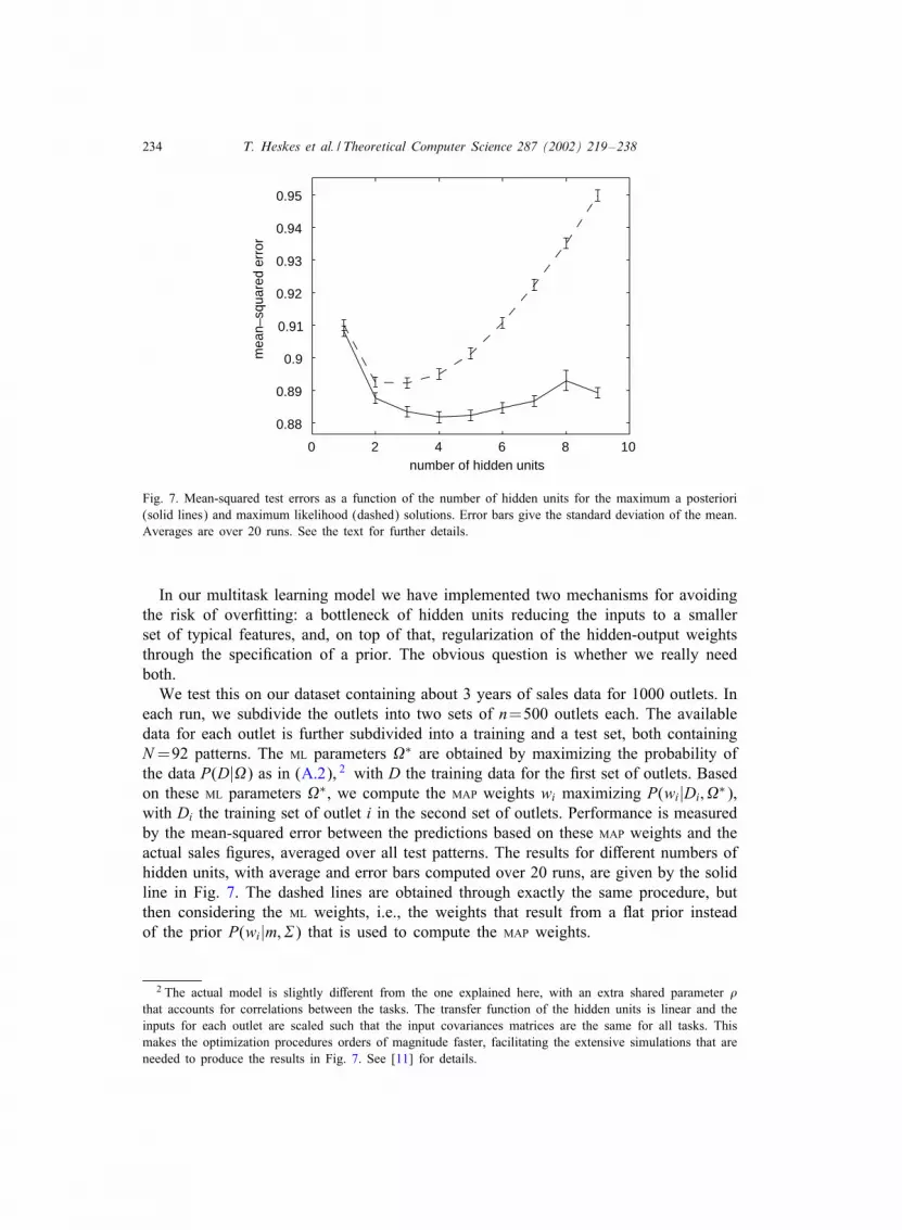
Fig. 7. Mean-squared test errors as a function of the number of hidden units for the maximum a posteriori(solid lines) and maximum likelihood (dashed) solutions. Error bars give the standard deviation of the mean.Averages are over 20 runs. See the text for further details.

In our multitask learning model we have implemented two mechanisms for avoidingthe risk of over.tting: a bottleneck of hidden units reducing the inputs to a smallerset of typical features, and, on top of that, regularization of the hidden-output weightsthrough the speci.cation of a prior. The obvious question is whether we really needboth.We test this on our dataset containing about 3 years of sales data for 1000 outlets. In

each run, we subdivide the outlets into two sets of n=500 outlets each. The availabledata for each outlet is further subdivided into a training and a test set, both containingN=92 patterns. The ML parameters �∗ are obtained by maximizing the probability ofthe data P(D|�) as in (A.2), 2 with D the training data for the .rst set of outlets. Basedon these ML parameters �∗, we compute the MAP weights wi maximizing P(wi|Di; �∗),with Di the training set of outlet i in the second set of outlets. Performance is measuredby the mean-squared error between the predictions based on these MAP weights and theactual sales .gures, averaged over all test patterns. The results for di>erent numbers ofhidden units, with average and error bars computed over 20 runs, are given by the solidline in Fig. 7. The dashed lines are obtained through exactly the same procedure, butthen considering the ML weights, i.e., the weights that result from a Rat prior insteadof the prior P(wi|m;+) that is used to compute the MAP weights.

2 The actual model is slightly di>erent from the one explained here, with an extra shared parameter -that accounts for correlations between the tasks. The transfer function of the hidden units is linear and theinputs for each outlet are scaled such that the input covariances matrices are the same for all tasks. Thismakes the optimization procedures orders of magnitude faster, facilitating the extensive simulations that areneeded to produce the results in Fig. 7. See [11] for details.


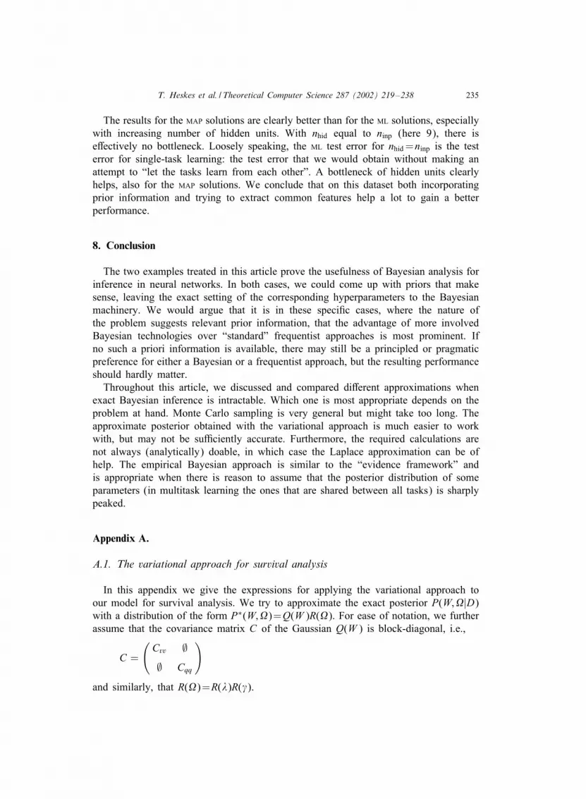
The results for the MAP solutions are clearly better than for the ML solutions, especiallywith increasing number of hidden units. With nhid equal to ninp (here 9), there ise>ectively no bottleneck. Loosely speaking, the ML test error for nhid =ninp is the testerror for single-task learning: the test error that we would obtain without making anattempt to “let the tasks learn from each other”. A bottleneck of hidden units clearlyhelps, also for the MAP solutions. We conclude that on this dataset both incorporatingprior information and trying to extract common features help a lot to gain a betterperformance.

8. Conclusion

The two examples treated in this article prove the usefulness of Bayesian analysis forinference in neural networks. In both cases, we could come up with priors that makesense, leaving the exact setting of the corresponding hyperparameters to the Bayesianmachinery. We would argue that it is in these speci.c cases, where the nature ofthe problem suggests relevant prior information, that the advantage of more involvedBayesian technologies over “standard” frequentist approaches is most prominent. Ifno such a priori information is available, there may still be a principled or pragmaticpreference for either a Bayesian or a frequentist approach, but the resulting performanceshould hardly matter.Throughout this article, we discussed and compared di>erent approximations when

exact Bayesian inference is intractable. Which one is most appropriate depends on theproblem at hand. Monte Carlo sampling is very general but might take too long. Theapproximate posterior obtained with the variational approach is much easier to workwith, but may not be su?ciently accurate. Furthermore, the required calculations arenot always (analytically) doable, in which case the Laplace approximation can be ofhelp. The empirical Bayesian approach is similar to the “evidence framework” andis appropriate when there is reason to assume that the posterior distribution of someparameters (in multitask learning the ones that are shared between all tasks) is sharplypeaked.

Appendix A.

A.1. The variational approach for survival analysis

In this appendix we give the expressions for applying the variational approach toour model for survival analysis. We try to approximate the exact posterior P(W;�|D)with a distribution of the form P∗(W;�)=Q(W )R(�). For ease of notation, we furtherassume that the covariance matrix C of the Gaussian Q(W ) is block-diagonal, i.e.,

C =

(Cvv ∅∅ Cqq

)

and similarly, that R(�)=R(�)R(�).


The optimization of the function R(�) given the current parameters QW and C isgiven in [2]. The resulting distributions R(�) and R(�) both happen to be gammadistributions. The average Q� reads

Q� = 〈�〉R =(ninp2+ �)[12QvT� Qv+

12Tr(Cvv�) + �

]−1(A.1)

and similarly, with n instead of ninp and � instead of �, for �.Computation of the functional (6) is more involved. We treat the terms one by one

and neglect irrelevant constants. Straightforward manipulations yield (|C| stands for thedeterminant of the matrix C)

−〈logQ(W )〉Q = 12 log |C| = 1

2 log |Cvv|+ 12 log |Cqq|;

−〈logP(v|�)〉Q;R = −〈logP(v| Q�)〉Q =Q�2[vT�v+ Tr(Cvv�)]

and a similar expression for 〈logP(w|�)〉Q;R. The term 〈logP(D|W )〉Q for the dataloglikelihood can again be decomposed into two terms, see (2): a term involving onlyuncensored patients and a term to which all patients contribute. Both contributions canbe computed analytically, starting from (2) and the transformation

wi =i∑

i′=1eqi′ :

The uncensored patients � contribute terms of the form

〈log[eqievT x� ]〉Q = qi + vT x� for ti−1¡t� 6 ti:

For both censored and uncensored patients we get contributions

−〈eqievT x�〉Q = − exp[vT x� + qi +12x

�TCvvx� + 12Cqiqi ]:

Here we used the equality∫dy $(y|m;+2)ey

T z = exp[mTz + 12 z

T+2z];

where we substitute {v; q} for y and the vector {x; [: : : ; 0; 0; 1; 0; 0; : : :]}, with 1 at theposition of i, for z.

A.2. Mathematics of multitask learning

Computation of the likelihood P(Di|�) boils down to the evaluation of Gaussian inte-grals, since both P(Di|Wi; �) and P(Wi|�) are, up to normalization constants, Gaussiansin Wi. With de.nitions

Ci = 〈hhT 〉i = 1N∑�

h(x�(i))hT (x�(i));


the covariance matrix of the hidden unit activities, and

wi = C−1i 〈hy〉i = C−1

i1N∑�

h(x�(i))y�i ;

the maximum likelihood solutions of the weights, we arrive at

− logP(Di|�) = N − nhid2

log �2 + 12 log |Ci|+ 1

2 log

∣∣∣∣∣+2 +(NCi

�2

)−1∣∣∣∣∣+

N2�2

[〈y2〉i − wTi Ciwi]

+ 12 (wi − m)T

[+2 +

(NCi

�2

)−1]−1(wi − m): (A.2)

Note that both wi and Ci are in fact functions of the input-to-hidden weights v. Directoptimization of (A.2) happens to be extremely unstable.In the optimization step of the variational (EM) approach, we have to compute terms

of the form 〈logP(Di|wi; �)〉Q and 〈logP(wi|�)〉Q. We easily obtain, up to irrelevantconstants,

−〈logP(Di|wi; �; v)〉Q = 12�2

∑�〈[y� − wT

i h(x�(i))]2〉Q + N

2log �2;

−〈logP(wi|m;+2)〉Q = 12 〈(wi − m)T+−2(wi − m)〉Q + 1

2 log∣∣+2∣∣ : (A.3)

Both terms only depend on the .rst and second moments of Q(wi). Furthermore,optimization of each shared parameter can be done separately: � after v and + afterm. In the expectation step, we have to compute

P(wi|Di; �∗) ∝ P(Di|wi; �∗)P(wi|�∗):

The expressions for P(Di|wi; �∗) and P(wi|�∗) are similar to those in (A.3), but thenwithout the average over Q(wi). Combining both we get a simple Gaussian distributionP(wi|Di; �∗).

References

[1] B. Bakker, T. Heskes, A neural-Bayesian approach to survival analysis, Proc. of ICANN99, 1999,pp. 832–837.

[2] D. Barber, C. Bishop, Ensemble learning for multi-layer networks, Advances in Neural InformationProcessing Systems, Vol. 10, MIT Press, Cambridge, 1997, pp. 395–401.

[3] D. Barber, B. Schottky, Radial basis functions: a Bayesian treatment, Advances in Neural InformationProcessing Systems, Vol. 10, MIT Press, Cambridge, 1997, pp. 402–408.

[4] J. Baxter, A Bayesian=information theoretic model of learning to learn via multiple task sampling, Mach.Learning 28 (1997) 7–39.

[5] J. Berger, M. Delampady, Testing precise hypotheses, Statist. Sci. 2 (1987) 317–352.


[6] A. Bryk, S. Raudenbusch, Hierarchical Linear Models, Sage, Newbury Park, 1992.[7] R. Caruana, Multitask learning, Mach. Learning 28 (1997) 41–75.[8] D. Cox, D. Oakes, Analysis of Survival Data, Chapman & Hall, London, 1984.[9] A. Gelman, J. Carlin, H. Stern, D. Rubin, Bayesian Data Analysis, Chapman & Hall, London, 1995.[10] M. Goldstein, A. Smith, Ridge-type estimators for regression analysis, J. Roy. Statist. Soc. 36 (1974)

284–291.[11] T. Heskes, Empirical Bayes for learning to learn, in: P. Langley (Ed.), Proc. 17th International

Conference on Machine Learning, Morgan Kaufmann, San Francisco, CA, 2000, pp. 367–374.[12] G. Hinton, D. van Camp, Keeping neural networks simple by minimizing the description length

of the weights, in: Proc. Sixth Annual Workshop on Computational Learning Theory, ACM Press,New York, 1993, pp. 5–13.

[13] H. Kappen, J. Neijt, Neural network analysis to predict treatment outcome, Ann. Oncol. 4 (1993)S31–S34.

[14] D. MacKay, Probable networks and plausible predictions—a review of practical Bayesian methodsfor supervised neural networks, Network 6 (1995) 469–505.

[15] D. MacKay, Comparison of approximate methods for handling hyper-parameters, Neural Comput. 11(1999) 1035–1068.

[16] R. Neal, Bayesian Learning for Neural Networks, Springer, New York, 1996.[17] R. Neal, G. Hinton, A view of the EM algorithm that justi.es incremental, sparse, and other variants,

in: M. Jordan (Ed.), Learning in Graphical Models, Kluwer Academic Publishers, Dordrecht, MA, 1998,pp. 355–368.

[18] L. Pratt, B. Jennings, A survey of transfer between connectionist networks, Connection Sci. 8 (1996)163–184.

[19] C. Robert, The Bayesian Choice: A Decision-Theoretic Motivation, Springer, New York, 1994.

approximate algorithms for neural-bayesian approaches

Documents