applying value-at-risk model in vietnam security market

VIETNAM NATIONAL UNIVERSITY OF HANOI

UNIVERSITY OF ECONOMICS AND BUSINESS

FINANCE AND BANKING FALCULTY

GRADUATION THESIS

APPLYING VALUE-AT-RISK MODEL IN VIETNAM

SECURITY MARKET

Supervisor: Dr. Nguyen The Hung

Student: Nguyen Khanh

Class: QH-2011-E TCNH CLC

Hanoi – Nov, 2015

1

VIETNAM NATIONAL UNIVERSITY OF HANOI

UNIVERSITY OF ECONOMICS AND BUSINESS

FINANCE AND BANKING FACULTY

GRADUATION THESIS

APPLYING VALUE-AT-RISK MODEL IN VIETNAM

SECURITY MARKET

Supervisor: Dr. Nguyen The Hung

Student: Nguyen Khanh

Class: QH-2011-E TCNH CLC

Graduation Thesis Nguyen Khanh - QH-2011E TCNH CLC

2

ACKNOWLEDGEMENT

With profound gratitude, I would like to sincerely thanks my lecturers for helping me

doing the thesis: Applying VaR model in Vietnam Securities Investment especially my

supervisor, Dr. Nguyen The Hung, for his heartedly direction as well as his detailed

instruction during all the phases of the research, from the selection of practical topic to

the final submission. If it had not been for his help, I would not have been able to finish

this thesis.

I also want to thank my family and friends for their incredibly amount of support during

the time of the research. They have been supporting me, both materially and spiritually.

Without their encouragement and help, I would not be patient enough to finish my work.

In addition, I would like to thank LR Global for giving me the access to the database

used in this thesis.

I also want to thank my family and friends for their incredibly amount of support during

the time of the research. They have been supporting me, both materially and spiritually.

Without their encouragement and help, I would not be patient enough to finish my work.

In addition, I would like to thank LR Global, where I used to work, for giving me the

access to the database used in this thesis.


3

Finally, I would like to thank all of the authors whose books and articles have been used

as references materials in my thesis for their works have been my guidelines throughout

the work.

Hanoi, Dec 2015


4

Table of contentsList of Tables.......................................................................................................................6

List of Figures......................................................................................................................6

List of Abreviation...............................................................................................................7

Abstract................................................................................................................................8

Chapter I :Introduction........................................................................................................9

1.1 Statement of Problem and Rationale for the thesis....................................................9

1.2Aims and objectives of the thesis..............................................................................10

1.3 Significance of the thesis..........................................................................................10

1.4 Scope of Thesis........................................................................................................11

1.5 Organization.............................................................................................................12

Chapter II : Literature Review...........................................................................................14

2.1 What is Value at risk?..............................................................................................14

2.1.1 History and Definition of VaR...........................................................................14

2.1.2 Element of Measuring Value at risk..................................................................16

2.1.3 The choice of technique.....................................................................................16

2.2 The VaR measurement method................................................................................17

2.2.1 The Delta Normal Method.................................................................................17

2.2.2. Monte Carlo Simulation....................................................................................19

2.2.3 Historical Simulation Method............................................................................19

2.3 Benefits and Drawback of Method...........................................................................20

2.3.1 Delta-Normal Method........................................................................................20

2.3.2. Historical VaR..................................................................................................21

2.3.3. Monte Carlo Simulation Method......................................................................22

2.4 Backtesting...............................................................................................................22

2.4.1 Definition...........................................................................................................22

2.4.2 Model Vertification Based on Failure Case.......................................................24

2.5 Problem with Complicated Portfolio........................................................................25

2.5.1 Problem with Correlation...................................................................................25


5

2.5.2 Problem with the weight in portfolio.................................................................27

Chapter III:Application in VN Index.................................................................................28

3.1 A brief of history and database.................................................................................28

3.2 Applying delta-normal method................................................................................28

3.2.1 A short describe.................................................................................................28

3.2.2 Test for assumption............................................................................................32

3.2.3. Test for assumption in VN Index......................................................................37

3.3. Historical Distribution.............................................................................................39

3.3.1 Remind problems of historical distribution.......................................................39

3.3.2 Solute problem...................................................................................................39

3.3.3 GARCH Estimation for Volatility.....................................................................41

3.4 Monte Carlo Simulation...........................................................................................43

3.5 Backtesting VN-Index..............................................................................................43

Chapter IV: Conclusion and Further Thesis......................................................................44

4.1 First conclusion: Answer the first question..............................................................44

4.2 Second conclusion: Answer the second question.....................................................44

4.3 Third conclusion: Anwser the third question...........................................................45

4.4 Limitation of research..............................................................................................45

4.5 Further suggestion: Stress testing.............................................................................45

Reference...........................................................................................................................47


6

List of Tables

Table Page

Table 1.2.3 :The distribution of return 15

Table 1.3.3 : REE Corporation historical monthly return 18

Table 2.5.1: Combined portfolio 24

Table 3.2.1.a: Histogram Table of VN-Index daily return 29

Table 3.1.b: Histogram Statistic of VN-Index daily return 29

Table 2.2.2.1.a:JB-test for normal distribution 32

Table 4.2.2.1b: Shapiro-Wilk test for normally distribution 34

Table 3.2.3.2 The result of normal distribution test for VN-Index daily return 36

Table 3.3.2 : Test for ARCH phenomenon 39

Table 3.3.3 :GRACH (1,1) Estimation 40

List of Figures

Figure Page

Figure 2.1.1 Definition of VaR 14

Figure 3.1. Histogram Plot of VN-Index Return 31

Figure 3.2.2.1b : Q-Q plot method 34

Figure 3.2.2.1 c. Anderson-Darling (Doornick –Chi square Method) test for

normal distribution method 36


7

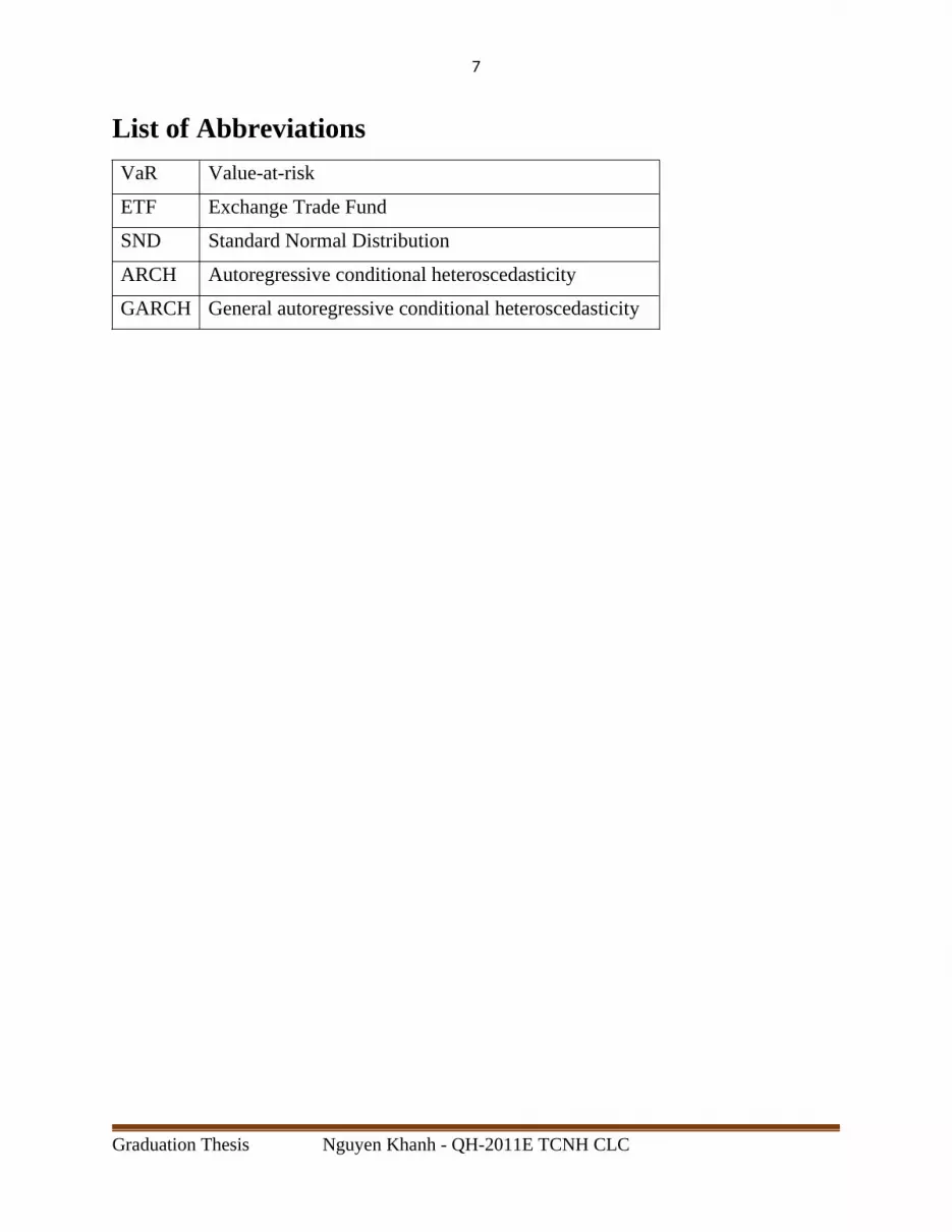
List of AbbreviationsVaR Value-at-risk

ETF Exchange Trade Fund

SND Standard Normal Distribution

ARCH Autoregressive conditional heteroscedasticity

GARCH General autoregressive conditional heteroscedasticity


8

AbstractSo far, in Vietnam security market, investors usually focus more on return and

price of securities. However, the other side of return- risk does not focus effectively. For

instance, CAPM model bases on market risk and risk free to evaluate asset. Another

traditional tools such as Z-score just concentrates on credit risk. In addition, Z-score is

difficult to compare and depend on internal factors of portfolio. Another point is other

type of risks such as operational risk and market risk are concentrated inadequately. In

general, Vietnam securities market do not have enough tools for risk measurement.

Moreover, Vietnam securities market is developing. In 2014, VFMVN30, the first

ETF fund was operated. Besides, according to derivative securities law draft, Vietnam

will start derivative trading in securities market in 2016. Consequently, it is necessary to

apply an effective tool in securities market-risk.

In the world, Value-at-risk has been existed has been existed from 1970s. In

Vietnam until recent years , when State Bank of Vietnam required several banks to apply

Basel II condition, Value-at-risk , a required condition in Basel II condition, has received

more attention. However, VaR is limited in banking system. Although, the VaR’s

common idea is applied to portfolio management it rarely is applied in securities market.

VaR is an effective tool because it focuses in market risk and price instead of

internal factors of company or portfolio to measure risk. Therefore, it is a probably

candidate to measure market risk of Vietnam Securities Market.

From perspective of an undergraduate student, I hope to provide an useful tool and

way to apply it in practice.


9

Chapter I :Introduction

1.1 Statement of Problem and Rationale for the thesis

The Vietnam Stock Index or VN-Index is a capitalization-weighted index of all the

companies listed on the Ho Chi Minh City Stock Exchange. The index was created with a

base index value of 100 as of July 28, 2000. The main purpose of this indicator is indicate

the situation of Vietnam Securities Market.

In general, investors usually consider price indexes such as VN-Index are return-

related indicator, which means that VN-Index shows how much return could earn in

certain period of time. Investors rarely consider problem about risk that could include in

that index.

In traditional risk measurement method, we usually use STD or another indicator

such as: Sharpe-ratio, M2 to analysis risk. However, many disadvantages have still

existed.

In addition, many old-type of risk measurement tools usually relate to credit risk.

For example, Z-score or credit ranking system just focus on the intrinsic financial

problem of portfolio, not their price in market and bring a quality determination instead

of quantitative results.

Value-at-risk is not only applied for banking sector but also applied to securities.

That is why the study is demanded in order to provide valuable risk-measurement tool

and illustrate how it can be done in Vietnam market-risk.

1.2Aims and objectives of the thesis

There are three major objective accomplished in this thesis. The first one is

definition of Value-at-risk model and how that model could be applied. Second, giving an

alternative to measure market risk of Vietnam security market. The third is giving the

drawbacks of model and how to limit disadvantages in reality.

In other word , the thesis focus on dealing with three following questions:


10

1. What is Value-at-risk model and how to apply it .

2. If Value-at-risk could be applied in Vietnam, what the optimal way could be

suitable for Vietnam Securities market.

3. What is model drawback and we how to solute this limitation.

1.3 Significance of the thesis

In the world, Value-at-risk model has been used from 1970s. However, until

1990s, when investor needed to a more reliable tool for risk assessment, Value-at-risk

(VaR) became a distinct concept. In 2000s, VaR was one of the most prominent concept

of risk because it was assigned as risk measurement tool in banking, according to Basel II

and Basel III Committee.

VaR was put into many risk course books. The most valuable work that gives the

basic foundation of VaR is: “Value at risk-The New Benchmark for Managing Financial

Risk-Third Edition”(2007) by Professor Philippe Jorion. He revealed all the ways to

measure VaR and how to apply VaR in practice. He also gave various tools to limit

drawbacks of model. In addition, “Financial Institution and Risk Management” by

Professor John Hull, mentioned how to apply VaR in financial institution. Although,

being researched globally, VaR has been an unfamiliar concept in Vietnam. Only several

researches were taken in Vietnam such as : “ A research on predictability of capital

market risk management models - case of value-at-risk models” by professor Dang Huu

Man, which indicated the suitability of VaR model when applying Vietnam. The other is

“Applying VaR to manage risk in portfolio in Vietnam” only stated the way to measure

risk in VaR model. However, it was not backtested for suitability.

Therefore, from perspective of an undergraduate student, I hope to combine both research

and give a way to measure market risk and limit the disadvantage of this model.

1.4 Scope of Thesis

Research Subject


11

VaR mesuares market-risk. It is presented through VN-Index- an indicator

represent price and return of market portfolio. As a result, this thesis focus on whole risk

Vietnam Market.

Time period

The thesis will focus on daily data of VN-Index from starting point of Vietnam

Security Market -2000 to July -2015. The number of samples hold nearly all of VN-

Index population will give sufficient data to analyze.

Data

Data of this thesis is the input database collected from authorized documents or

trustworthy sources, such as well-known stock brokerage firms and companies and

famous risk material .

1.5 Organization

The thesis contain 5 different chapters for different focus :

• Chapter One: Introduction.

This is a concise introduction of the case thesis, including: the statement of the

problem and the rationale of the thesis, its aims and objectives, the scope of the thesis and

the overall organization.

• Chapter Two: Literature Review.

Briefly providing general knowledge of risk analysis, containing various theories,

models, methods and formulas used in the thesis as well as their meanings in risk

analysis.

• Chapter Three: Applying Value-at-risk in Vietnam Securities Market.

Applying process of VaR theory to the case of Vietnam Securities Market and

draw conclusions of the market daily risk. In addition, indicating drawbacks of model.

• Chapter Four: Conclusion.


12

This chapter answers the request from chapter 1 and concluse the result for the

whole thesis, summarize with findings, limitations and suggestions for further studies.


13

Chapter II : Literature Review2.1 What is Value at risk?

2.1.1 History and Definition of VaR

During the 1990s, value at risk- or VaR, as it is commonly known- emerged as the

financial service industry’s premier risk management technique. JP Morgan developed

the original concept for internal use but later published the tools it had developed for

managing risk (as well as related information). Probably no other risk management topic

has generated as much as much attention and controversy as has value at risk. In this

section, we take an introductory look at value at risk, examine an application, and lock at

VaR’s strength and limitations.

VaR is a probability-based measure of loss potential for a company, a fund, a

portfolio, a transaction or a strategy. It is usually expressed either as a percentage or in

units of currency. Any position that exposes one to loss is the potentially a candidate for

VaR measurement. VaR is most widely and easily used to measure the loss from market

risk, but it can also be used –subject- to much greater complexity-to measure the loss

from credit risk and other type of exposures

We have note that VaR is probability based measure of loss potential. This

definition is very general, however, and we need something more specific. More

formally: Value at risk (VaR) is an estimate of the loss (in money term) that we expect to

be exceeded with a given level of probability over a specified time period.

The actual loss may be much worse without necessarily impugning the VaR

model’s accuracy. Secondly, If we lower the probability from 5% to 1% the value will be

larger because we now referring to a loss that we expect to be exceeded with only 1%

probability. VaR cannot be compared directly the share with the same interval.


14

Figure 2.1.1 Definition of VaR

We assume that daily return of VN-Index distributed as normal distribution (see

figure 2.1.1), 10% of lowest sample will get z-score less than -1.28, 5% lowest of

population will get z-score less than -1.65 and 1% lowest of population will get z-score

less than -2.33.

The VaR is similar to this definition. 10% VaR daily return will get a lower certain

return, this is similar to z-score in normal distribution. 5% VaR daily return will get a

lower return than 10%VaR. It is similar to -1.65 z-score <-1.28 z-score.

Another example is the VaR for a portfolio is $1.5 million for one day with a

probability of 5%. Recall what this statement says: There is a 5% chance that portfolio

will lose at least 1.5 million in a single day. The emphasis here should be on the fact that

the $1.5 million loss is a minimum. Equivalently, the possibility is 95% that portfolio will

lose no more than 1.5 million in a single day. In conclusion, we express VaR in form of a

minimum loss with a given probability.


15

2.1.2 Element of Measuring Value at risk

1.1.2.1 Picking a probability level

Typically, the probability is chosen 5% or 1% (corresponding to a 95% or 90%

confidence level, respectively). The use of 1% lead to a more conservative VaR risk

estimate, because it sets the figure at the level where there should be only a percent

chance that a given loss will be worse than the calculated VaR. The trade-off however, is

that the VaR risk estimate will be larger with a 1% probability than it will be for a 5%.

2.1.2.2. Time period

The second important decision for VaR users is choosing the time period. VaR is

often measure over a day, but other longer time periods are common. Banking regulators

prefer two week period intervals. Many companies report quarterly and annual VaR to

match their performance reporting cycle.

2.1.3 The choice of technique

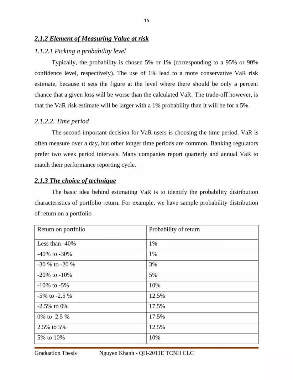
The basic idea behind estimating VaR is to identify the probability distribution

characteristics of portfolio return. For example, we have sample probability distribution

of return on a portfolio

Return on portfolio Probability of return

Less than -40% 1%

-40% to -30% 1%

-30 % to -20 % 3%

-20% to -10% 5%

-10% to -5% 10%

-5% to -2.5 % 12.5%

-2.5% to 0% 17.5%

0% to 2.5 % 17.5%

2.5% to 5% 12.5%

5% to 10% 10%


16

10% to 20% 5%

20% to 30% 3%

30% to 40% 1%

Greater than 40% 1%

Total:100%

Table 1.2.3 The distribution of return

Consider the information in table, which is a simple probability distribution for the

return on portfolio over a specified time period. Suppose we were interested in the VaR at

5% of probability .Observe that the probability is 1 % that the portfolio will lose at least

40%, 1% that the portfolio will lose between 30% and 40%, 3% that the portfolio will

lose between 20% and 30%. Thus, the portfolio will lose at least 20%

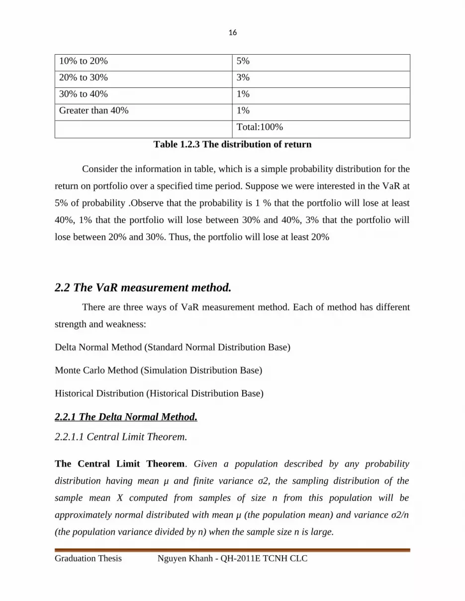
2.2 The VaR measurement method. There are three ways of VaR measurement method. Each of method has different

strength and weakness:

Delta Normal Method (Standard Normal Distribution Base)

Monte Carlo Method (Simulation Distribution Base)

Historical Distribution (Historical Distribution Base)

2.2.1 The Delta Normal Method .

2.2.1.1 Central Limit Theorem.

The Central Limit Theorem. Given a population described by any probability

distribution having mean μ and finite variance σ2, the sampling distribution of the

sample mean X computed from samples of size n from this population will be

approximately normal distributed with mean μ (the population mean) and variance σ2/n

(the population variance divided by n) when the sample size n is large.


17

The central limit theorem allows us to make an assumption about the distribution

of market return to apply in Delta-Normal method.

2.2.1.2 Delta- Normal Method.

The most important of the Central Limit Theorem is the ability to assume that the interest

rate is normally distributed with the extreme sample size.

The delta-normal method for estimating VaR requires the assumption of a normal

distribution. This is because the result of centre limit theorem. For example, in

calculating a daily VaR, we calculate the standard deviation of daily returns in the past

and assume it will be applicable to the future. Than using the asset’s expected 1-day

return and standard deviation, we estimate the 1-day VaR at th desired level of

significance.

The assumption of normality is troublesome because many assets exhibit skewed return

distribution(e.g., option), and equity return frequently exhibit leptokurtosis ( fat tails).

When a distribution has “fat tails”, VaR will tend to underestimate the lossadn its

associated probability. Also know that delta-normal VaR is calculated using the historical

standard deviation, which may not be appropriate if the composition of the portfolio

changes, if the estimation period contained unusual events, or if economics conditions

have changed.

For example, the expected 1-day return for a Vp=$100,000,000 portfolio is x=0.00085

and the historical standard deviation of daily return is σ=¿ 0.0011. To locate the value for

a 5% VaR, we use the z-table in the appendix to this thesis. In this case, we want 5% in

the lower tail, which would leave 45% below the mean that is not in the tail. Searching

for 0.45, we find the value 0.4505 ( the closet value we will find). Adding the z-value in

the left hand margin and the z-value at the top of the column in which 0.4505 lies, we get

1.6 + 0.05 =1.65, so the z-value coinciding with a 95% VaR is 1.65.

VaR= [X-(z)×σ ]×Vp


18

=[ 0.00085-1.65(0.0011)](100,000,000)

=-96,500

The interpretation of this VaR that there is a 5% chance the minimum 1-day loss is

0.0965% or 96,500. ( there is 5% probability that the 1-day lteross will exceed $96,500).

Alternatively, we could say we are 95% confident the 1-day loss will not exceed 96,500.

2.2.2. Monte Carlo Simulation .

Monte Carlo has been controversial topic. It is applied in not only economics but also

many other sector. This method created thousands to millions case of inputs to solve and

return the outcomes.

In Monte Carlo simulation, we have to depend on distribution of computer. In many way,

this distribution is usually standard normal distribution.

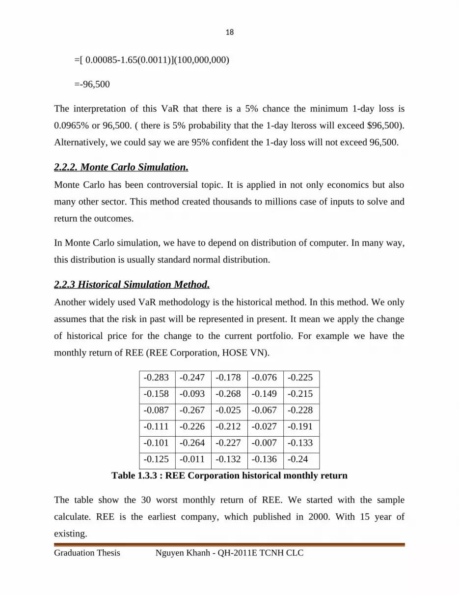
2.2.3 Historical Simulation Method .

Another widely used VaR methodology is the historical method. In this method. We only

assumes that the risk in past will be represented in present. It mean we apply the change

of historical price for the change to the current portfolio. For example we have the

monthly return of REE (REE Corporation, HOSE VN).

-0.283 -0.247 -0.178 -0.076 -0.225

-0.158 -0.093 -0.268 -0.149 -0.215

-0.087 -0.267 -0.025 -0.067 -0.228

-0.111 -0.226 -0.212 -0.027 -0.191

-0.101 -0.264 -0.227 -0.007 -0.133

-0.125 -0.011 -0.132 -0.136 -0.24

Table 1.3.3 : REE Corporation historical monthly return

The table show the 30 worst monthly return of REE. We started with the sample

calculate. REE is the earliest company, which published in 2000. With 15 year of

existing.


19

We assume the portfolio that comprise all of REE securities will replicated as past. It

mean 5% of worst case in past will use to find 5% VaR in month. In 15 year of existing,

the population consists of 180 samples. 5% of 180 cases is 9 th worst case, which is -

22.6%.Therefore, we conclude VaR at 5% in month is 22.6%. In other word, portfolio

have 5% of probability to lose at least 22.6% value.

Similarly, VaR at 1% is 1.8th worst cases. Simply, we direct the 1st worst, which is 28.3%,

as 1% VaR. We conclude that 1% of probability the portfolio will lose 28.3%. An

alternative is working with average of 1st and 2nd worst. VaR is (28.3+26.8)/2= 27.5%.

2.3 Benefits and Drawback of Method.

2.3.1 Delta-Normal Method .

Advantages of delta-normal method include the following:

Easy to implement.

Calculations can be performed quickly.

Conductive to analysis because risk factors, correlation and volatilities are

identified.

Disadvantages of delta-normal method include the following:

Samples data need to be assumed as normal distribution.

The method is unable to properly account for distributions with fat tails, either

because of unidentified risk factor and/or correlation.

Nonlinear relationship of options-like positions are not adequately, described

by the delta normal method. VaR is misstated because the instability of option

deltas is not captured.

2.3.2. Historical VaR

Advantages of the historical simulation method include the following :

The model is easy to implement when historical data is readily available.


20

Calculations are simple and can be perform quickly.

Horizon is positive choice based on the intervals of historical data used.

Full valuation of portfolio is based on actual price.

It is not exposed to model risk.

It include all correlations as embedded in market price changes.

Disadvantages of the historical simulation method include following:

It may not be enough historical data for all assets.

Only one path of events is used, which includes change in correlation and

volatilities that may have occurred only in that historical period.

Time Variation of risk in the past may not present Variation in the future.

The model may not recognize change in volatility and correlations from structural

change.

A small number of actual observations may lead to insufficiently defined

distribution tails.

It is slow to adapt to new volatility and correlations as old data carries the same

weight as more recent data. However, exponentially average (EWMA) models can

be used to weight recent observations more heavily

2.3.3. Monte Carlo Simulation Method

Advantages of the Monte Carlo simulation method include the following:

It is most powerful model.

It can account for both linear and nonlinear risk.

It can include time variations in risk and correlations by aging positions over chosen

horizons.

It is extremely flexible and can incorporate additional risk factor easily.

Nearly unlimited numbers of scenarios can produce well-described distributions.

Disadvantages of the Monte Carlo simulation method include following:


21

There is a lengthy computation time as the number of valuations escalates quickly.

It is expensive because of intellectual and technology skill required.

It is subject to model risk of the stochastic processes chosen.

It is subject to sampling variations at lower number of simulations.

It is base on model of computer. As a result , it could not happened in reality.

2.4 Backtesting

2.4.1 Definition

Backtesting is the process of comparing losses predicted by the value at risk (VaR) model

to those actually experienced over the sample testing period. If the model were

completely accurate, we would expect VaR to be exceed with the same frequency

predicted by the confidence level used in the VaR model. In other word, the probability

of observing a loss amount greater than VaR is equal to the significance level (x%). This

value is also obtained by calculating one minus the level confidence level.

For example, if VaR of $10 million is calculated at a 95% of confidence level we expect

to have exceptions ( losses exceeding $10 million ) 5% of the time. If exception are

occurring with greater frequency, we may be underestimating the actual risk. If exception

is occurring less frequently. We may overestimating risk.

There are three desirable attribute of VaR estimates that can be evaluate when using a

backtesting approach. The first desirable attribute is that the VaR estimate should be

unbiased. To test this property, we use an indicator variable to record the number of time

an exception occurs during a sample period. For each sample return, this indicator

variable is record as 1 for exception or 0 for non-exception. The average of indicators

over the sample period should be equal x% for VaR estimate to be unbiased.

A second desirable attribute is that the VaR estimate is adaptable. For example , if a large

return increase the size of the tail of the return distribution, the VaR amount should also

be increased. Given a large loss amount, VaR must be adjusted so that the probability of


22

the next loss amount again equal x%. This suggest that the indicator variables, discussed

account for new information in the face of increasing volatility.

A third desirable attribute, which is closely related to the first to attributes, is for the VaR

estimate to be robust. A strong VaR estimate produces only a small deviation between the

number of expected exceptions during the sample period and actual number of

exceptions. This attribute is measure by examining the statistical significance of the

autocorrelation of extreme events over backtesting period. A significant autocorrelation

would indicate a less reliable VaR measure.

By examining historical return data, we can gain some clarity regarding which VaR

method actually produces a more reliable estimate in practice. In reality, VaR approaches

that are nonparametric ( historical simulation) do a better job at producing VaR amounts

that mimic actual observations when compared to parametric( delta-normal distribution)

method.

2.4.2 Model Verification Based on Failure Case

The simplest method to verify the accuracy of model is to record the failure rate which

give the proportion of times VaR is exceeded in a given simple. Suppose a bank provides

a VaR figure at the 1 percent left- tail level (p=1-c) for a total of T days the user then

count how many times the actual loss exceeds the previous days VaR. Define N as the

number of exceptions and N/T as the failure rate. Ideally, the failure rate should give an

unbiased measure of p, that is, should convert to p as the sample size increase.

We want to know, at a given confidence level, whether N is too small or too large under

the null hypothesis that p=0.01 in a sample of size T. Note that this test makes no

assumption about the return distribution. The distribution could be normal, or skewed, or

with heavy tails, or time VaRying. We simply count the number of exceptions.

The setup for this test is the classic testing framework for sequence of success and failure

also call Bernoulli trails. Under the null hypothesis that model is correctly calibrated the

number of exceptions x follows a binominal probability distribution:


23

f ( x )=(Tx ) px(1−p)

We also know that x has expected value of E(x) =pT and variance V(x)=p(1-p)T. When T

is large, we can use the central limit theorem and approximate the binominal distribution

by the normal distribution.

z=( x−pT√ p (1−p ) T )≈ N (0,1)

Which provides a convenient shortcut. If the decision rule is defined ate two-tailed 95%

test confidence level, then the cutoff value |z| is 1.96.

For instance, JP Morgan’s exceptions. In its 1998 annual report, the US, commercial

bank JPMorgan explained that:

“In 1998 daily revenue fell short of downside ( 95% VaR) band on 20 days, or more than

5% of the time. Nine of these 20 occurrences fell within the August to October period”.

We can test this was bad luck or a faulty model, assuming 252 days in the year. Based on

Equation we have z=20−0.05 ×252√0.05 (0.95 )252

=¿2.14.This is larger than the cut-off value of 1.96.

Therefore we reject the hypothesis that the VaR model is unbiased. It is unlikely( at the

95% test confidence level) that this was bad luck bank suffered too many exceptions

which must have to a search for better model. The flaw probably was due to the

assumption of a normal distribution, which does not model tail risk adequately. Indeed,

during the fourth quarter of 1998, the bank reported having switched to a "historical

simulation" model that better account for fate tails. This episode illustrates how

backtesting can lead to improved models.

However, the backtesting based on historical data is only effective to delta-normal

method and Monte Carlo simulation method. In historical simulation method, the


24

backtesting depend on future data instead of historical data, because the principal rule of

historical simulation is following the historical data.

2.5 Problem with Complicated Portfolio.

2.5.1 Problem with Correlation .

In all example we usually assume that our assets consist of one asset. In real the portfolio

usually consist more than 1. The method of VaR still is applied for this case. We use

variance-covariance to solve this problem.

Simply, we assume the portfolio will consist of 2 asset: 1 bond and 1 security. The

expected return of bond is:

Rp=w1 R1+w2 R2=[ w1 w2 ] [R1

R2]V ( Rp )=(w¿¿1σ1)

2+(w¿¿2 σ 2)2+2 w1 σ1 w2 σ2 ×σ 1,2¿¿

With the 2 factors return and standard deviation we could simply calculate VaR in 2

method delta-normal method and Monte Carlo simulation. In historical simulation. Only

Rp is enough to install model.

In case of more than 2 factors we could generalize by this. Assume portfolio have N

assets:

Rp=∑i=1

N

wi μi

V ( Rp )=σ p2=∑

i=1

N

wi2 σ j

2+∑I=1

N

∑j<i

N

wi w j σ ij

σ p2=[w1…wN ] [ σ1

2 ⋯ σ 1 N

⋮ ⋱ ⋮σN 1 ⋯ σ N

2] [ w1

⋮wN

]In which, σ 1 N is the correlation of first portfolio with the assets N.


25

In practice we could use function CORR in Excel to solve it.

For example:

Suppose the portfolio contains two asset classes, with 75% of the money invested in an

asset class represented by VN Index and 25% invested in an asset class represented by

NASDAQ Composite Index. Recall that a portfolio’s expected return is a weighted

average of the expected returns of its component stocks or asset classes.

VN Index NASDAQ Combined Portfolio

Percentage invested(w) 0.75 0.25 1

Expected annual

return(µ)

0.12 0.18 0.135a

Standard Deviation(σ) 0.2 0.4 0.244b

Correlation(ρ) 0.9

Table 2.5.1: Combined portfolio

a.Expected Return of Portfolio μp=μv wv+μn wn=¿0.75 ×0.12+0.25×0.18=0.135 ¿.

b.Standard deviation of portfolio:

σ p2=w v

2σ v2+wn

2 σn2+2 wv wnσ v σn ρ=0.244

VaR at 5% of portfolio calculate as 0.135- 1.65×√0.244=¿-0.68.

As a result, the portfolio have 5% of probability loss at least 68%.

2.5.2 Problem with the weight in portfolio

The prominent problem with portfolio is the weight of an asset will be not constant. Each

asset value will create the change in both its weight and required return.

In practice, we still keep the database, add new statistic and recalculate VaR. It is not a

problem with a small portfolio such as: individual portfolio; but in term of mutual fund’s


26

portfolios, which consist of hundreds to thousands assets, we have to use professional

software such as R to back up database.


27

Chapter III: Application in VN Index.

3.1 A brief of history and database.The Vietnam Stock Index or VN-Index is a capitalization-weighted index of all the

companies listed on the Ho Chi Minh City Stock Exchange. The index was created with a

base index value of 100 as of July 28, 2000. Prior to March 1, 2002, the market only

traded on alternate days.

The thesis aims to apply a new method in market-risk management. In order to limit

effectively market-risk, market data has to be calculated at frequent level. It is reason

why we chose daily data instead of weekly or monthly data.

The VN-Index from the first day published in 28-7-2000 to 31-7-2015 consist of 3539

samples. It means that we nearly approach a perfect statistic to calculate VaR.

We will measure VaR according to 3 ways that we discuss on chapter II

3.2 Applying delta-normal method

3.2.1 A short describe

First we have the distribution of VaR through table diagram and histogram plot

Histogra

m Table

Interval

number=

77

µ=0.00037

87

Δ=0.016580

71

Bin LL UL Center FreeCum.

FreqNormal

1 -0.13 -0.12 -0.12 0.00% 0.00% 0.00%

2 -0.12 -0.12 -0.12 0.00% 0.00% 0.00%

3 -0.12 -0.11 -0.12 0.00% 0.00% 0.00%

4 -0.11 -0.11 -0.11 0.00% 0.00% 0.00%

5 -0.11 -0.11 -0.11 0.00% 0.00% 0.00%


28

6 -0.11 -0.10 -0.11 0.00% 0.00% 0.00%

7 -0.10 -0.10 -0.10 0.00% 0.00% 0.00%

8 -0.10 -0.10 -0.10 0.00% 0.00% 0.00%

9 -0.10 -0.09 -0.09 0.00% 0.00% 0.00%

10 -0.09 -0.09 -0.09 0.00% 0.00% 0.00%

11 -0.09 -0.08 -0.09 0.00% 0.00% 0.00%

12 -0.08 -0.08 -0.08 0.00% 0.00% 0.00%

13 -0.08 -0.08 -0.08 0.00% 0.10% 0.00%

14 -0.08 -0.07 -0.08 0.00% 0.10% 0.00%

15 -0.07 -0.07 -0.07 0.20% 0.30% 0.00%

16 -0.07 -0.07 -0.07 0.10% 0.40% 0.00%

17 -0.07 -0.06 -0.06 0.10% 0.50% 0.00%

18 -0.06 -0.06 -0.06 0.00% 0.60% 0.00%

19 -0.06 -0.05 -0.06 0.00% 0.60% 0.00%

20 -0.05 -0.05 -0.05 0.10% 0.70% 0.10%

21 -0.05 -0.05 -0.05 0.30% 1.00% 0.10%

22 -0.05 -0.04 -0.05 0.60% 1.60% 0.20%

23 -0.04 -0.04 -0.04 0.70% 2.30% 0.40%

24 -0.04 -0.04 -0.04 0.60% 2.80% 0.60%

25 -0.04 -0.03 -0.03 0.80% 3.60% 1.00%

26 -0.03 -0.03 -0.03 1.00% 4.60% 1.60%

27 -0.03 -0.02 -0.03 1.20% 5.80% 2.40%

28 -0.02 -0.02 -0.02 1.60% 7.50% 3.40%

29 -0.02 -0.02 -0.02 2.30% 9.80% 4.50%

30 -0.02 -0.01 -0.02 4.60% 14.40% 5.80%

31 -0.01 -0.01 -0.01 5.30% 19.60% 7.00%

32 -0.01 -0.01 -0.01 6.80% 26.40% 8.00%

33 -0.01 0.00 0.00 12.70% 39.10% 8.70%

34 0.00 0.00 0.00 16.20% 55.30% 9.00%

35 0.00 0.01 0.00 11.80% 67.10% 8.90%


29

36 0.01 0.01 0.01 9.50% 76.70% 8.30%

37 0.01 0.01 0.01 5.70% 82.40% 7.40%

38 0.01 0.02 0.01 4.60% 87.00% 6.20%

39 0.02 0.02 0.02 5.50% 92.50% 5.00%

40 0.02 0.02 0.02 1.90% 94.30% 3.80%

41 0.02 0.03 0.03 1.40% 95.70% 2.70%

42 0.03 0.03 0.03 0.90% 96.60% 1.90%

43 0.03 0.04 0.03 1.00% 97.60% 1.20%

44 0.04 0.04 0.04 0.80% 98.40% 0.80%

45 0.04 0.04 0.04 0.60% 99.00% 0.40%

46 0.04 0.05 0.04 0.60% 99.60% 0.30%

47 0.05 0.05 0.05 0.00% 99.60% 0.10%

48 0.05 0.05 0.05 0.00% 99.60% 0.10%

49 0.05 0.06 0.06 0.00% 99.70% 0.00%

50 0.06 0.06 0.06 0.10% 99.80% 0.00%

51 0.06 0.07 0.06 0.20% 99.90% 0.00%

52 0.07 0.07 0.07 0.00% 99.90% 0.00%

53 0.07 0.07 0.07 0.00% 99.90% 0.00%

54 0.07 0.08 0.07 0.00% 100.00% 0.00%

55 0.08 0.08 0.08 0.00% 100.00% 0.00%

56 0.08 0.08 0.08 0.00% 100.00% 0.00%

57 0.08 0.09 0.09 0.00% 100.00% 0.00%

58 0.09 0.09 0.09 0.00% 100.00% 0.00%

59 0.09 0.10 0.09 0.00% 100.00% 0.00%

60 0.10 0.10 0.10 0.00% 100.00% 0.00%

61 0.10 0.10 0.10 0.00% 100.00% 0.00%

62 0.10 0.11 0.10 0.00% 100.00% 0.00%

63 0.11 0.11 0.11 0.00% 100.00% 0.00%

64 0.11 0.11 0.11 0.00% 100.00% 0.00%


30

65 0.11 0.12 0.12 0.00% 100.00% 0.00%

66 0.12 0.12 0.12 0.00% 100.00% 0.00%

67 0.12 0.13 0.12 0.00% 100.00% 0.00%

68 0.13 0.13 0.13 0.00% 100.00% 0.00%

69 0.13 0.13 0.13 0.00% 100.00% 0.00%

70 0.13 0.14 0.14 0.00% 100.00% 0.00%

71 0.14 0.14 0.14 0.00% 100.00% 0.00%

72 0.14 0.14 0.14 0.00% 100.00% 0.00%

73 0.14 0.15 0.15 0.00% 100.00% 0.00%

74 0.15 0.15 0.15 0.00% 100.00% 0.00%

75 0.15 0.16 0.15 0.00% 100.00% 0.00%

76 0.16 0.16 0.16 0.00% 100.00% 0.00%

77 0.16 0.16 0.16 0.00% 100.00% 0.00%

Table 3.2.1.a: Histogram Table of VN-Index daily return

Average 0.038%

variance 0.0275%

Standard Deviation 1.66%

Kurtosis 5.865720774

Skewers -0.173466893

n 3539

Table 3.1.b Histogram Statistic of VN-Index daily return


31

-0.124351478510544

-0.109312887039994

-0.0942742955694432

-0.0792357040988926

-0.064197112628342

-0.0491585211577914

-0.0341199296872408

-0.0190813382166902

-0.00404274674613955

0.0109958447244111

0.0260344361949617

0.0410730276655123

0.0561116191360629

0.0711502106066135

0.0861888020771641

0.101227393547715

0.116265985018265

0.131304576488816

0.146343167959367

0.1613817594299170%

2%

4%

6%

8%

10%

12%

14%

16%

18%

Histogram Plot of VN-Index daily return

FrequencyNormal

Figure 3.1. Histogram Plot of VN-Index Return.

3.2.2 Test for assumption .

The delta-normal method will become useless if the distribution of expected daily

interest rate of VN Index is not standard normal distribution. Therefore, we have to

test to affirm that the distribution of interest is standard normal.

3.2.2.1. Hypothesis Test.

Let’s assume we have a data set of a univariate ( ), and we wish to determine whether

the data set is well-modeled by a Gaussian distribution.

Where

null hypothesis (X is normally distributed)

alternative hypothesis (X distribution deviates from Gaussian)


32

Gaussian or normal distribution.

In essence, the normality test is a regular test of a hypothesis that can have two possible

outcomes: (1) rejection of the null hypothesis of normality ( ), or (2) failure to reject the

null hypothesis.

In practice, when we can’t reject the null hypothesis of normality, it means that the test

fails to find deviance from a normal distribution for this sample. Therefore, it is possible

the data is normally distributed.

The problem we typically face is that when the sample size is small, even large

departures from normality are not detected; conversely, when your sample size is large,

even the smallest deviations from normality will lead to a rejected null.

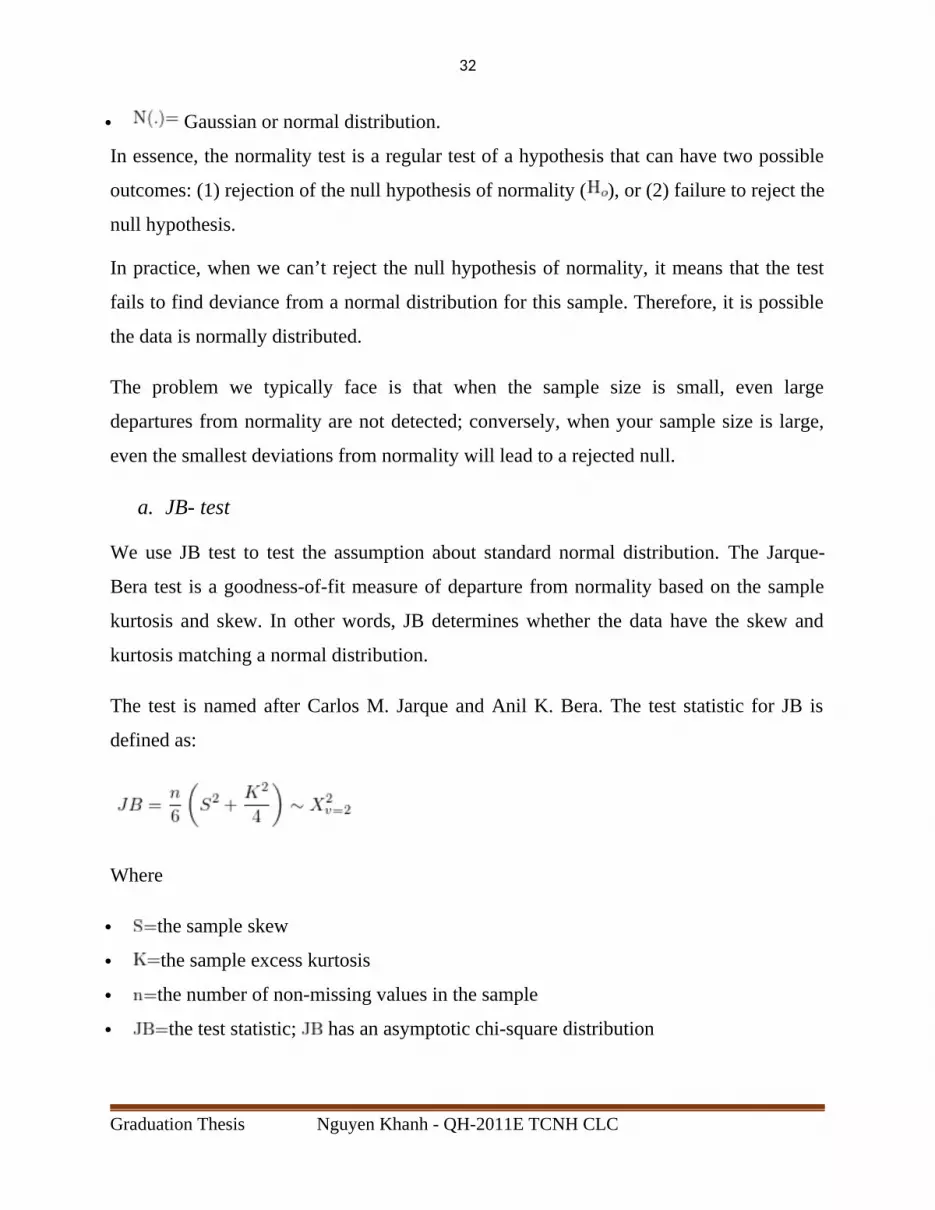
a. JB- test

We use JB test to test the assumption about standard normal distribution. The Jarque-

Bera test is a goodness-of-fit measure of departure from normality based on the sample

kurtosis and skew. In other words, JB determines whether the data have the skew and

kurtosis matching a normal distribution.

The test is named after Carlos M. Jarque and Anil K. Bera. The test statistic for JB is

defined as:

Where

the sample skew

the sample excess kurtosis

the number of non-missing values in the sample

the test statistic; has an asymptotic chi-square distribution


33

Table 2.2.2.1.a JB-test for normal distribution.

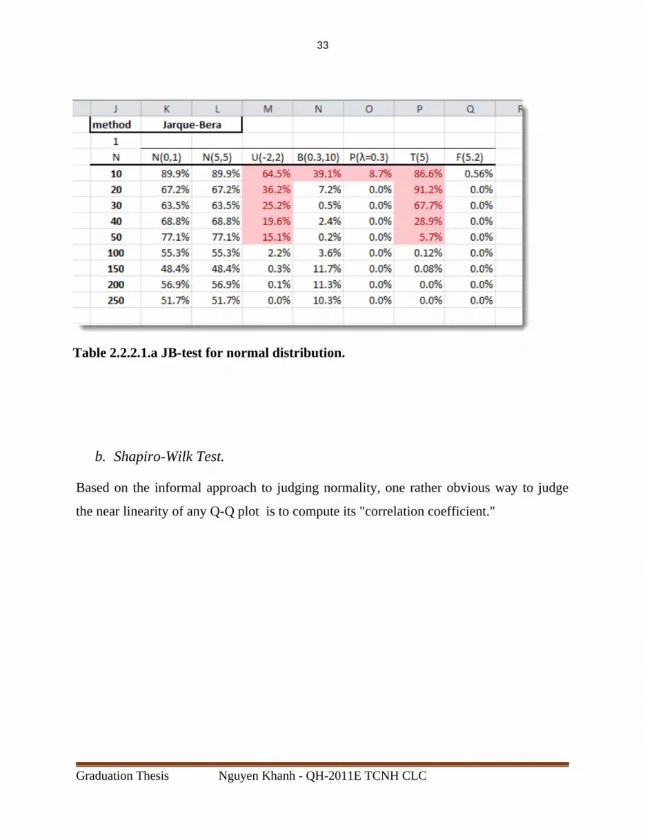
b. Shapiro-Wilk Test.

Based on the informal approach to judging normality, one rather obvious way to judge

the near linearity of any Q-Q plot is to compute its "correlation coefficient."


34

Figure 3.2.2.1b : Q-Q plot method.

When this is done for normal probability (Q-Q) plots, a formal test can be obtained that is

essentially equivalent to the powerful Shapiro-Wilk test W and its approximation W.

Where

the order (smallest number in the sample)

a constant given by

the expected values of the order statistics of independent and identical distributed

random Variables sampled from Gaussian distribution.

the covariance matric of order statistics.


35

Table 3.2.2.1b Shapiro-Wilk test for normally distribution.

In the table above, the SW P-values are significantly better for small sample sizes ( )

in detecting departure from normality, but exhibit similar issues with symmetric

distribution (e.g. Uniform, Student’s t).

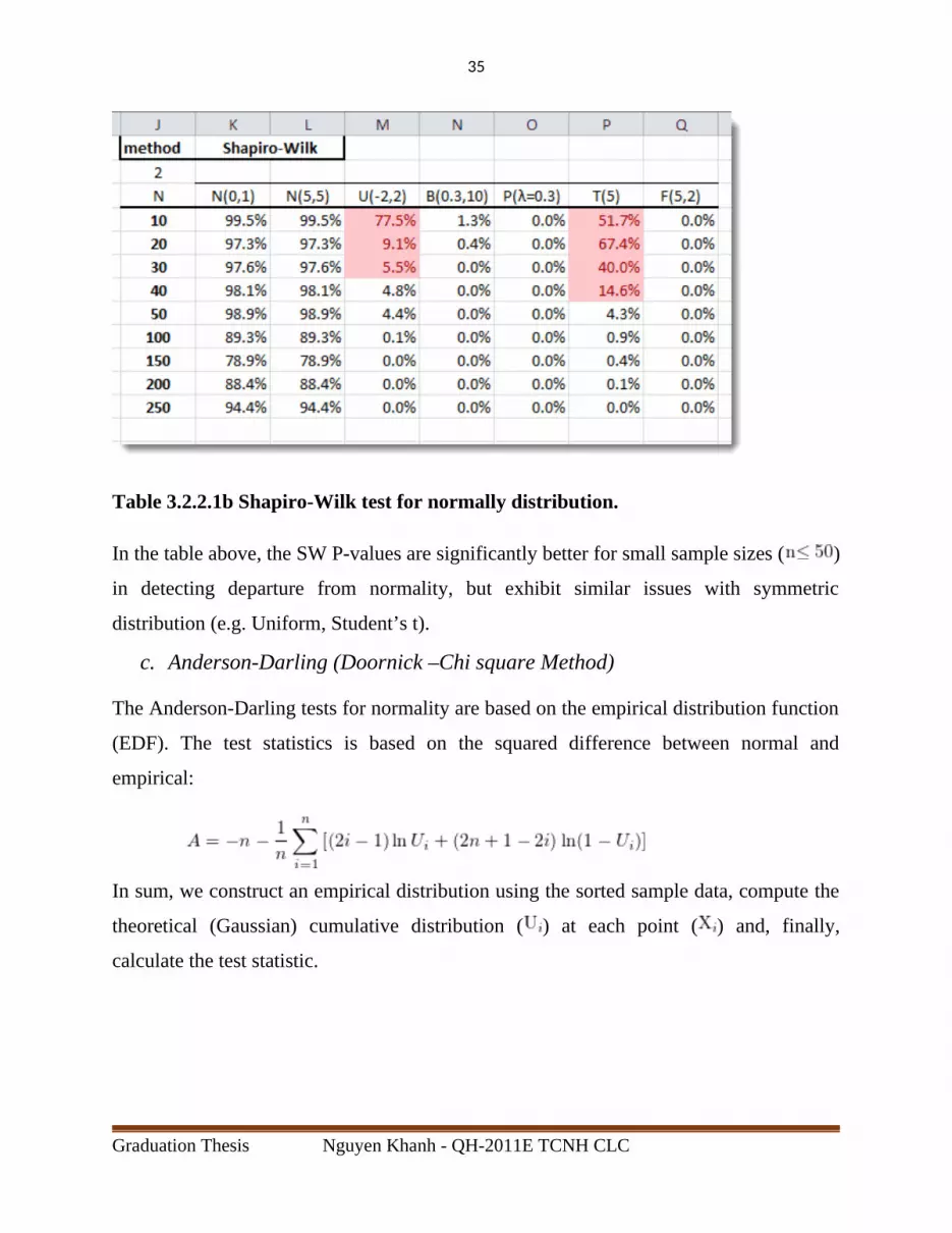
c. Anderson-Darling (Doornick –Chi square Method)

The Anderson-Darling tests for normality are based on the empirical distribution function

(EDF). The test statistics is based on the squared difference between normal and

empirical:

In sum, we construct an empirical distribution using the sorted sample data, compute the

theoretical (Gaussian) cumulative distribution ( ) at each point ( ) and, finally,

calculate the test statistic.


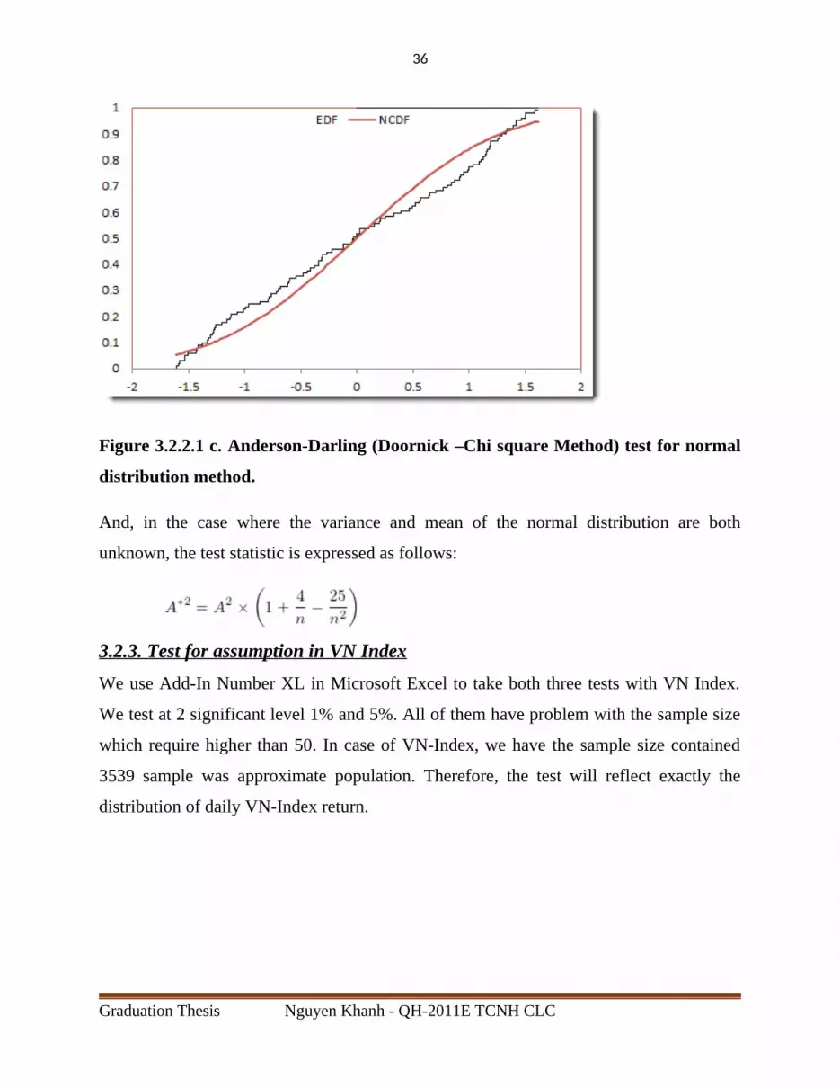
36

Figure 3.2.2.1 c. Anderson-Darling (Doornick –Chi square Method) test for normal

distribution method.

And, in the case where the variance and mean of the normal distribution are both

unknown, the test statistic is expressed as follows:

3.2.3. Test for assumption in VN Index

We use Add-In Number XL in Microsoft Excel to take both three tests with VN Index.

We test at 2 significant level 1% and 5%. All of them have problem with the sample size

which require higher than 50. In case of VN-Index, we have the sample size contained

3539 sample was approximate population. Therefore, the test will reflect exactly the

distribution of daily VN-Index return.


37

Table 3.2.3.2 The result of normal distribution test for VN-Index daily return

According to this result, at 5% of significant level , p-value of all three methods were

approximately to 0%, which are lower than 5%. As a result, VN-Index daily return data is

not normally distributed at 5%

At 1% of significant level, p-value of all three methods were approximate to 0% which

are lower than 1%. As a result, VN-Index daily return data is not normally distributed at

1%

3.2.2.3. Conclusion.

To sum up, it means that interest rates of VN-Index in both 1% and 5% with three

methods shows that the VN-Index is not normally distribution. Therefore, the first

method of measurement VaR, which is delta-normal (which assumes that return will be

normally distributed), will be pointless in measuring.


38

3.3. Historical Distribution.3.3.1 Remind problems of historical distribution.

Problem 1: It may not be enough historical data for all assets.

Problem 2: Only one path of events is used, which includes change in correlation

and volatilities that may have occurred only in that historical period.

Problem 3: Time VaRiation of risk in the past may not present VaRiation in the

future.

Problem 4: The model may not recognize change in volatility and correlations from

structural change.

Problem 5: A small number of actual observations may lead to insufficiently defined

distribution tails.

Problem 6: It is slow to adapt to new volatility and correlations as old data carries

the same weight as more recent data. However, exponentially average (EWMA)

models can be used to weight recent observations more heavily.

3.3.2 Solute problem :

Problem 1 and Problem 5: the sample size is not enough.

The data of this thesis is absolutely adequate. We have sample size of 3539 samples.

It spreads from the first day of VN Index to the nearly contemporary. Therefore, it

is almost the same as population.

Problem 2, problem 3, problem 4, and problem 6: Relate to the sample variations. It

means that the valuation of variance will change as the time series change or in

econometrics side, this problem is heteroscedasticity.

The first and foremost, we have to test the change in variations in a time series. It means

that if the change in variance influences significantly to the change in future value of


39

interest rate, the VaR will be underestimated or overestimated. If the current volatility is

more than it in past, VaR will be under estimate. On the other hand, if the current

volatility is less than it in past, VaR according to historical valuation will be

overestimate.

Robert F.Engle in 1982 first suggested a way of testing whether the variance of the error

in a particular time-series model in one period depend on the variance of the error in

previous periods. He called this type of heteroscedasticity is autoregressive conditional

heteroscedasticity (ARCH).

As an example consider the ARCH (1) model:

ε t N (0 , a0+a1ε t−12)

Where the distribution of ε t, conditional on its value in the previous period normal with

mean 0 and variance a0+a1 εt−12. If a1 = 0, the VaR of the error in every period is just a0.

The VaR is constant over time and does not depend on past errors. Now suppose that a1 >

0. Then the VaR of the error in one period depends on how large the squared error was in

the previous period. If a large error occurs in one period, the variance of the error in the

next period will be even larger.

Engle shows that we can test whether a time series is ARCH(1,1) by regressing the

squared residuals from a previously estimated time-series model (AR, MA, or ARMA) on

a constant and one lag of the squared residuals. We can estimate the linear regression

equation:

Equation (18) :

ε̂ t2¿ a0+a1 ε̂t−1

2+u t


40

Where ut is an error term. If the estimate of a1 is statistically significantly different from

zero, we conclude that the time series is ARCH (1). If a time-series model has ARCH (1)

errors, then the variance of the errors in period t + 1 can be predicted in period t using the

formula:

.

Using excel tool to test for heteroscedasticity autoregressive conditional

heteroscedasticity and it effect to daily interest rate of VN Index series.

Table 3.3.2 : Test for ARCH phenomenon

Conclusion of ARCH:

First, the phenomenon of ARCH is exhibited significantly on daily interest of VN

Index. As a result, the VaR estimation will be changed overtime. This volatility

makes the measurement fluctuate. To estimate this change we use the new model.

3.3.3 GARCH Estimation for Volatility.

GARCH model proposed by Engle (1982) and Bollerslev (1986). The simplest model are

GARCH (1, 1) the conditional variance depends on the latest innovation but also on the

previous conditional variance. Define ht as the conditional variance using information up


41

to time t-1 and rt-1 as previous day’s return. The simplest such model is the GARCH (1, 1)

process, that is:

ht=α 0+α 1rt−12+β ht−1

The beauty of this model is specification is that it provides a parsimonious model with

few parameters that seem to fit the data quite well. GARCH model have become a

mainstay of time-series analysis of financial markets that systematically display volatility

clustering. There are literally thousands of papers applying GARCH models to financial

series.

Appling GARCH(1,1) model to VN Index we have the result:

Table 3.3.3 GRACH (1,1) Estimation

So we have the result is:

ht=0.019 %+16.004 r t−12+16.004 h t−1

With ht mean is 0.038%.

3.3.4 VaR with historical simulation.Back to the VN-Index from the first day published in 28-7-2000 to 31-7-2015 consisting

of 3539 samples.

The 5% of 3539: 5 %× 3539=179.95 .

As a result the VaR at 5% of VN Index is 180th lowest return.


42

180th lowest is -0.027264.

We could conclude that there is 5% of probability that daily interest lose will be equal or

lower than 2.726% with the standard variance of h =0.038%.

Similarly VaR at 1% of VN Index is 35.39th lowest return.

We could also conclude that there is 1% of probability that daily interest return will be

equal or lower than 4.7664% with the standard variance of h = 0.038%

3.4 Monte Carlo Simulation.The most disadvantages of Monte Carlo Simulation is the same as Delta Normal method.

We have to simulate the distribution of each case of Simulation. In many current model

of Monte Carlo, we usually assume that it distributes as standard normal distribution.

Consequently, VaR is underestimated or overestimated. In this case, VN-Index is not

normally distributed. Eventually, Monte Carlo Simulation is also worthless.

3.5 Backtesting VN-IndexIn last part, we tested for the most appropriate model of VaR method. The test showed

that the only way we could adjust its drawback is historical distribution.

However, only this method is following historical distribution, as a result, it will be true

in history. A disadvantage of this model is we could not use the current data to backtest

it. Only the future data could conclude accuracy of model.


43

Chapter IV: Conclusion and Further Thesis

4.1 First conclusion: Answer the first question. What is VaR model and how to apply it?

VaR model is an risk management tool which measure market-risk. We have to be taken

at certain probability(1%, 5% …).

VaR could be applied through the three method :

1. Delta-Normal Method (Base on the assumption about standard normal

distribution).

2. Monte Carlo Simulation Method (Base on the simulation of computer).

3. Historical Simulation Method (Base on the assumption of historical).

4.2 Second conclusion: Answer the second question.If Value-at-risk model could be applied in Vietnam, what is the optimal method for

Vietnam Securities market index ?

Value-at-risk model could be applied in Vietnam Securities Index, at only 1 method:

Historical Simulation Method. In order to limit the volatility of measuring in whole long

period of time, we applied GARCH (1,1) model to measure the volatility of model.

The result of historical simulation is:

VaR at 5% of daily return of VN Index is 2.726%. It means Vietnam securities market

have 5% of probability loss 2.726% a day with the average standard deviation of

h=0.038%.

VaR at 1% of daily return of VN Index is 4.7664% It means Vietnam securities market

have 1% of probability loss 4.764% a day with the average standard deviation of

h=0.038%.

The volatility of estimate is h =0.038%. This result derives from GRACH (1,1) model.


44

4.3 Third conclusion: Answer the third question.

What is the model drawback and how to solve this?

The drawback of historical simulation method in VaR is it could not be backtested.

Possible application depends on for future data to verify this model in future.

4.4 Limitation of thesis. This thesis have two limitations :

1. The thesis only finds the ways to measure risk. However, the thesis could not find

the method to avoid risk for portfolio.

2. The thesis is usually pointless in crisis situation when the volatility tends to be

more than the level of VaR estimation.

4.5 Further suggestion: Stress testingTradition VaR methodology relies on historical data to generate a distribution of possible

return. A high confidence level ( typically 99%) is chosen to characterize typical market

conditions and allows the analyst to make statements such as, “ I expected losses to

exceed the threshold only 1% of the time over the next ( arbitrary) time period.” Why

VaR is useful for normal market conditions, history clearly tell us that large and

unexpected losses do occur. VaR cannot make predictions about the magnitude of the

losses beyond the threshold, and it cannot identify the causes or conditions that can lead

to the large loss. The use of stress testing addresses these shortcomings in VaR. It is

apparent that stress testing should be used as a complement to VaR measure, rather than

subsitute.

In stress test model, portfolio are usually put in a stress sceenario. In this stiuation, the

portfolios’ outside-factors (for example : GDP, inflation.) could change dramatically.

After that, they measure the change in value of portfolios and the required conditions of

portfolios to keep a stable threshold.


45

In conclusion, stress testing could be a good complement to VaR model. Additionally, it

calcultes the condition to avoid risk instead of only measure risk. I hope that this research

will become a base for futher research.


46

Reference English Material

[1]]Hendricks, D. “Evaluation of Value-at-Risk Models Using Historical Data,”

Economic Policy Review, Federal Reserve Bank of New York, vol. 2 (April 1996): pp39–

69.

[2]Hull, J. C., and A. White. “Incorporating Volatility Updating into the Historical

Simulation Method for Value at Risk,” Journal of Risk 1, no. 1 (1998):pp 5–19.

[3]. Christoffersen, P.F, Hahn J., and Inoue, A. (2001), “Testing and Comparing Value at

Risk Measures”, Journal of Empirical Finance, 8, pp. 325-342.

[4]. Duffie, D., and Pan, J. (1997), “An Overview of Value at Risk”, Journal of

Derivatives 4,3, pp. 28-49.

[5]. John C.Hull (2012) “Risk Management and Financial Institution 3rd -Edition”,

McGraw-Hill, 2012, 14, pp 303-345

[6]. Philippe Jorion (2007), “Value at risk ,The new benmark for managing financial risk-

3rd Edition”, New York: McGraw-Hill, 2001, 5,6,8,9,10 pp.150-277

[7]. Pritsker, M. (1997), “Evaluating Value at Risk Methodologies”, Journal of Financial

Services Research, 12, pp. 201-242.

[8]. Sarma, M., Thomas S., and Shah., A. (2003), “Selection of VaR models”, Journal of

Forecasting, 22, pp. 337-358.

Vietnames Material

[1]Ứng dụng lý thuyết giá trị cực đoan (Extreme Value Theory) trong đo lường rủi ro tài

chính- Chu Lục Ninh- Đại học Ngoại Thương

[2] Nghiên cứu chất lượng dự báo của những mô hình quản trị rủi ro thị trường vốn -

trường hợp của value-at-risk models –Đặng Gia Mẫn-Đại học Đà Nẵng


47

[3]Ứng dụng Value-at-risk trong việc cảnh báo và giám sát rủi ro thị trường đối với hệ

thống ngân hàng thương mại- Trần Mạnh Hà- Học viện Ngân Hàng

[4] Kiểm tra độ ổn định của các ngân hàng thương mại lớn Việt Nam – Phùng Đức

Quyền- Đại học Kinh tế- Đại học Quốc Gia Hà Nội

WEBSITE

-Riskmetric.com

-Cafef.com

-Bloomberg.com

- Rmmagazine.com

- GARP.org


applying value-at-risk model in vietnam security market

Documents