Applying econometric methods to decision cost models for Expected Utility violations David E. Buschena* Montana State University David Zilberman University of California at Berkeley Joseph A. Atwood Montana State University *David Buschena©

Dept. of Ag. Econ. and Econ. Montana State University Bozeman, MT 59717 (406) 994-5623 (phone) (406) 994-4838 (fax) buschena@montana.edu

Abstract Recent work proposes a decision cost argument for the occurrence of expected utility violations. These cost models suggest measures over the risky pairs that define these decision costs, but there is more than one form of these cost measures. These proposed measures are furthermore non-nested. This paper assesses, using information criteria, the relative modeling success of these candidate measures in explaining risky choice behavior giving rise to violations. Although the candidate models exhibit some degree of substitutability, our results indicate support for a candidate model that uses relatively simple measures to instrument for decision costs. Keywords: risk, expected utility, similarity, information criteria JEL classification: D810, C520, C900

Applying econometric methods to decision cost models for EU violations

Maximization of expected utility (EU) has been the dominant explanation for risky

choices. However, the violations were first suggested by Allais (1953), famously

addressed by Kahneman and Tversky (1979), and have become a topic of considerable

interest in economics, psychology, and management science, and led to a search for

alternative models. One major approach, the non-expected utility models (see the survey

article by Starmer)., has modified the assumptions regarding decision-making

preferences, but has assumed one-step maximizing behavior

Another approach to EU violations is the similarity approach (Rubinstein, Leland,

Buschena & Zilberman, Loomes (2006)), which assumes that decision makers may use

different decision-making criteria that depend on the risky choices they have available.

They apply a two-stage decision process: first, selecting a decision rule, and then making

the actual risky choice. The decision algorithm is affected by the similarity between the

risky choices. A simpler decision algorithm is chosen when the alternatives are more

similar, and a more complex algorithm (EU) when outcomes are less similar.

This similarity approach can be interpreted as taking into account the mental

transaction costs associated with making risky choices, as well as the cost of making the

wrong choice. In this way the similarity approach has much in common with bounded

rationality models for risky choice such as Payne, Bettman and Johnson and also Conlisk.

These similarity models also relate to a growing literature for error frameworks for risky

choice in Ballinger and Wilcox, Hey and Orme, Hey, Loomes and Sudgen, and Loomes

(2005) that support heteroscedastic error across decision task as opposed to the constant

2

(Fechner type) error suggested in Harless and Camerer.

One major challenge for this similarity framework is finding the appropriate

measures of similarity that explain observed behavior, i.e., whether similarity can be best

explained by intuitive measures based on Euclidean distance, by measures of difference

of information content of different distributions, reflected by the cross-entropy measure,

or by measures that weight distances non-linearly to reflect decreasing marginal utility,

such as Loomes’ non-linear definition for similarity.

This paper attempts to develop a methodology to resolve this problem empirically, and to

apply it to a large data set, using results of experiments done with 300 undergraduate

students facing a series of risky choices, over gambles offering risk-return tradeoffs. The

similarity among the alternatives vary for the different choices, resulting in several

thousand observations of risky choices that vary in the similarity of the outcomes and

other characteristics.

After first assessing the state of the econometric methods used to assess EU

violations and the decision limitation explanations for them, we test three candidate

models for decision limitation as an explanatory measure for risky choice patterns. These

tests utilize maximum likelihood linear and nonlinear in parameter logit models across

individual’s choices for a large set of respondents. Because the models tested are

nonnested, various information criteria are utilized.

I. The pioneers: Simple means tests across two risky pairs

Von Neumann and Morgenstern’s (1953) EU model provided an axiomatized model to

describe risk-return tradeoffs commonly observed in a host of economic settings. Their

3

model of choice provides the EU for a probability vector p that defines a risky alternative

over a vector of outcomes x as:

∑=

•=n

iii xuppEU

1)()( . (1)

The EU model remains a powerful and widely used tool for the analysis of choice under

risk.

Shortly after von Neuman and Morgenstern’s 1944 paper, Allais (1953) published

findings of systematic departures from EU. Allais’ results and a body of supporting

evidence have become known as independence violations. These violations, in addition

to other behavior inconsistent with EU, came to the fore in economics by the publication

of Kahneman and Tversky’s (1979) seminal paper. The nature of these EU violations,

and especially what to do about them, remains the topic of considerable interest within

economics, psychology, management science, and other fields.

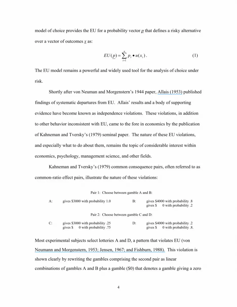
Kahneman and Tversky’s (1979) common consequence pairs, often referred to as

common-ratio effect pairs, illustrate the nature of these violations:

Pair 1: Choose between gamble A and B: A: gives $3000 with probability 1.0 B: gives $4000 with probability .8 gives $ 0 with probability .2

Pair 2: Choose between gamble C and D: C: gives $3000 with probability .25 D: gives $4000 with probability .2 gives $ 0 with probability .75 gives $ 0 with probability .8.

Most experimental subjects select lotteries A and D, a pattern that violates EU (von

Neumann and Morgenstern, 1953; Jensen, 1967; and Fishburn, 1988). This violation is

shown clearly by rewriting the gambles comprising the second pair as linear

combinations of gambles A and B plus a gamble ($0) that denotes a gamble giving a zero

4

payoff with certainty. Under EU, if A is preferred to B, then C must be preferred to D

because:

C = 1/4 * A + 3/4 * ($0) and D = 1/4 * B + 3/4 * ($0).

The empirical analysis of these original EU violations consisted of means tests of

choice proportions between pair AB and CD. These tests are simple, and in a sense

powerful. These tests, however, offer a limited view of the nature of these violations, and

in particular how robust they are to gambles that differ in the probabilities of the

alternative outcomes.

II. The developers: Multiple choices per person and panel data

In response to the simple EU violations above, a substantial number of competing

Generalized EU models (GEU) weaken the von Neumann-Morgenstern axioms to allow

for choice patterns violating EU. These GEU models essentially introduced a nonlinear

treatment, through a function π( · ), of the probabilities for the valuation of risky

alternatives. This nonlinear function π( · ) is introduced into the EU formulation in

equation (1), defining:

∑=

=n

iii xuppGEU

1)()()( π (2)

The specific nature of π(· ) distinguishes the competing GEU models. Virtually all of

these models retain some of the EU axioms (chiefly transitivity), while weakening others

in order to allow for common patterns of EU violations. Particularly good summaries of

these models can be found in Fishburn (1988), and in Harless and Camerer (1994).

In order to test between the many competing GEU models, Harless and Camerer

(1994), Hey and Orme (1994), Hey (1995), Wilcox (1993), Ballinger and Wilcox (1997),

and others extended the set of risky choices considered. Some of these empirical

estimations apply maximum likelihood methods and information criteria to the analysis

5

of the competing GEU and related models, providing evidence for the relative predictive

power of the alternative GEU models. Ballinger and Wilcox and also Hey additionally

explored the role of heteroscedastic error structures for explaining risky choice.

III. A decision cost explanation: Similarity models

In contrast to the “reduced form” treatment of choice patterns through the weighting

function π( · ) under the GEU models, an alternative approach establishes instruments for

decision costs and benefits based on the importance and/or the difficulty of risky choice

selection. To motivate this approach, consider again the Kahneman and Tversky pairs

AB and CD. The similarity approach (Rubinstein, 1988, 2003; Leland, 1994; Buschena

and Zilberman, 1995, 1999, 2000), and related work in Coretto (2002) posits that the

difference in the relative importance in choice between pair AB (important or dissimilar)

and pair CD (unimportant or similar) explains patterns of choice violating EU.

In this similarity approach, respondents are held to place less importance on the

choice between pair CD relative to the choice between pair AB, with a resulting higher

likelihood of selection of the more risky alternative D over C than for the more risky

alternative B over A. The similarity approach holds that, when choices between

dissimilar pair AB (which is taken to more accurately reflect actual attitudes regarding

risk return tradeoffs) and pair CD are compared, the increased likelihood of selection of

alternative D relative to alternative B appears to reflect non-EU preferences. Rather than

changing the preference axioms as in the GEU models, these similarity models suggest a

structural approach whereby choice models are augmented with a measure that reflects

the importance and difficulty of choice. Specifically, assuming that computation extracts

mental cost, and the decision maker can select from two algorithms, one more effort

intensive (EU), and the other less effort intensive (e.g. choosing the outcome with the

highest expected value). The similarity approach can be interpreted as the outcome of an

optimization process where a decision maker maximizes expected utility of choice less

6

mental cost of calculation. When outcomes are similar, and the loss for making the wrong

choice is small, the decision maker may prefer the less effort intensive approach. On the

other hand, when outcomes are dissimilar, and the loss for making the wrong choice is

large, the decision maker may prefer the more effort intensive, and more accurate,

approach.

Thus, the similarity approach assumes that optimization includes two elements.

First, selection of an algorithm, and then, the actual choice using the selected algorithm.

This two-stage procedure may be consistent with some of the new findings of

neuroeconomics (Camerer, et. al). By observing where actions occur in the brain, it was

found that distinct brain processes may serve the same function in different situations,

one of the processes being a control process (effortful), the other being an automatic

process (effortless). Studies also found that the brain is able to do assigned tasks

efficiently, using the specialized systems it has at its disposal. The neuroeconomic

literature also suggests that switching algorithms may result in non-optimal outcomes in

certain situations. That implies a decision making approach that is consistent with our

similarity model. If both the cost of effort and the cost of mistakes are taken into account,

the decision rule resulting in these mistakes may be optimal.

Hey (1995) and Ballinger and Wilcox (1997) found some support for similarity

effects in their exploration of heteroscedastic error structures and risky choice. Buschena

and Zilberman (1995, 1999) tested a similarity model against GEU models, and found

support for similarity effects through a structural approach. Buschena and Zilberman

(2000) additionally found that incorporating similarity measures in an EU model with a

heteroscedastic error framework.

One difficulty with the similarity approach is in defining the similarity measure.

Rubinstein (1988) considers fairly simple gambles that offer only one nonzero outcome.

In his model, the more risky gamble offers a p chance at outcome x, while the safer

7

gamble offers a q chance of y (p < q and x > y). Rubinstein provides an axiomatized

model for choice under EU preference with similarity effects, and considers two

measures for similarity on both outcomes and probabilities (defined here for

probabilities).

Rubinstein’s first measure is the absolute difference measure between the

probabilities, |p - q|. His relative difference measure is the ratio of the probabilities, p/q.

Rubinstein also includes a qualitative similarity criterion; probability q is dissimilar to p

if q = 1 and p < 1; that is, degenerate probabilities that offer an outcome with certainty

are viewed as dissimilar to probabilities with less than certainty.

Because many risky pairs offer more than one nonzero outcome, a few more

general similarity measures have been proposed. Three similarity models are considered

in this paper, because the definition of “similarity” is subjective. All of the models used

nonlinear measures over the probability vectors to define similarity and differ in how

they handle qualitative similarity (lotteries offering certainty of a positive payoff), with

one model including it directly as an additional and separate explanatory term and the

other two models incorporating certainty into their functional form.

Candidate Model 1: Distance-based similarity. This similarity model is relatively

simple, using the Euclidian distance between the probability vectors p and q to describe

differences between gambles (Buschena and Zilberman, 1995, 1996, 2000). This

distance measure is reasonably applied for the set of gambles considered here that offer

nontrivial risk-return tradeoffs. We have also explored a more generalized difference

measure based on absolute differences in the distributions’ Cumulative Distribution

Functions, with this CDF measure is empirically comparable to the Euclidian distance

8

measure.

In this paper’s empirical estimation below, both the distance measure and its

square will be considered. In addition to the distance measure, some of these estimates

also include 0 - 1 similarity measure, quasi-certainty, that generalizes the qualitative

component in Rubinstein’s similarity definition. Quasi-certainty in this definition takes

the value 1 if the less risky of the two gambles in the pair gives greater than a zero payoff

with certainty.

Candidate Model 2: (Dis)similarity as defined through cross entropy. Entropy

provides a useful alternative measure for describing the differences between probability

distributions. Specifically, the cross-entropy measure described below over the

distributions serves to define the similarity between risky alternatives.

Shannon’s (1948) entropy stems from information theory and serves as a measure

of how a particular distribution differs from a uniform distribution. The entropy measure

for a discrete distribution is:

)ln()(1

i

n

ii pppEnt ∑

=

−= . (3)

A uniform distribution is in a sense the least informative over a range of outcomes, so the

smaller a distribution’s entropy, the more information it contains. A uniform distribution

has maximum entropy, while a degenerate (pi = 1, 0) distribution has minimum entropy

and is clearly most informative. Coretto (2002) develops a risky choice model combining

EU with Shannon’s entropy as an explanation of EU violations.

More useful than Shannon’s entropy for our application is the Kullback-Leiber

(1951) cross entropy that measures how two distributions (our p and q) differ from one

another:

9

)/ln(),(1

ii

n

ii qppqpCrossEnt ∑

=

−= . (4)

Two identical (extremely similar) distributions would have a cross-entropy value of 0.

As the distributions differ more from one another (are dissimilar), the cross-entropy

measure increases.

Under this candidate model for similarity, the cross entropy of distributions is

used to define the similarity of the pairs in our empirical estimations. For our empirical

application, qi never takes the value 0. If pi takes the value 0, the value inside the sum is

set to zero for our estimations.

The monograph by Golan, Judge, and Miller (1996) provides a very thorough

treatment of the use of entropy in econometrics. Preckel (2001) provides a useful

summary of entropy and cross entropy. To our knowledge, this paper offers the first

extensive test of cross entropy for explaining EU independence violations. In our

empirical application, we consider subsets of models including the risky pairs’ cross

entropy, its square, and the previously defined quasi-certainty measure.

Candidate Model 3: Loomes’ nonlinear similarity. Loomes (2006) recently

introduced a nonlinear similarity measure (φ ). This measure allows for both the ratio of

the gamble probabilities and the difference in the probabilities to affect choice. The

relative effects of the probability ratios and differences can vary across individuals in

Loomes’ measure, with these relative effects defined through two parameters, α and β, in

the following formulation. Loomes’ model allows for gambles over as many as three

outcomes, with these gambles defined through their probability vectors p and q:

10

f = [1− (p1 / q1)]g = [1− (q2 / p2)]h = [1− (p3 / q3)]aI = (q1 − p1)aJ = (q3 − p3)

φ(α ,β, p,q) = ( fgh)β[(aI / aJ )(aI +aJ )α ].

(5)

Loomes development of φ ( · ) includes a discussion of its two component parts,

relating to the two coefficients α and β. The coefficient α is restricted to be nonpositive

and defines the degree of divergence between the perceived (subjective) and objective

(actual) probability ratios. If α = 0, there is no difference between these ratios; as α

declines, this perceived vs. objective difference becomes larger. In Loomes’

development, α differs across individuals.

The component of φ( · ) “scales down” the bracketed portion that relates to

how close the less risky alternative is to certainty. In particular, Loomes’ is working to

define qualitative certainty-type effects more generally than in the candidate models

using the Euclidian distance or the cross-entropy measures. A value of β = 0 in (5)

indicates that the ratio of probabilities does not affect choice, while β values of larger

absolute value indicate a person strongly affected by these ratios, and thus more affected

by the less risky gamble’s relationship to certainty. As for α, the β coefficient likely

differs across individuals in Loomes’ formulation.

β)( fgh

A priori, if we assume that decision makers account for the computational effort

associated with the choice of algorithm, then perhaps and the more easily interpreted

Euclidian distance similarity measure has additional merit over the cross-entropy and

power function measures such as Loomes. [David Z, I’m still not sure that we can say

much about this, and wonder if it’s necessary.]

11

IV. The data: “Industrial strength” probability triangle with real payoffs

Our experiment was designed to test for similarity effects on EU violations intensively.

The risky pairs allow for clear tests of both quantitative (such as measured by Euclidian

distance) and quantitative effects (such as measured by quasi-certainty) across a large set

of risky pairs. The set of gamble pairs given to each respondent was devised so that

parametric estimation of the three candidate similarity models in explaining EU

violations should be possible. Each respondent faced both hypothetical and “real”

gambles, but we found no significant effects of real payoffs on choices for estimation

using individual choice.

More than 300 undergraduate students faced a series of risky choices over gamble

pairs offering a risk/return tradeoff for which EU predicts the same qualitative choice.

EU would predict that (1) either the less risky choice would always be selected for every

choice pair by an individual, or (2) the more risky choice would always be selected. Only

a few (27, 8.5%) of subjects had choices completely consistent with EU in that they

always selected the least risky option in every pair (no subject always selected the most

risky option). For the other (288) subjects who had some choices violating EU, we use

the candidate similarity models to explain when the riskier choice is more likely. With

this approach, we focus on measuring the characteristics of the risky pairs that give rise to

the risk-taking behavior and thus for many respondents EU violations when their choices

over similar pairs is compared with their choices over dissimilar pairs. This experiment

and data are additionally described in Buschena and Zilberman (1999).

The risky pairs in the experimental design differed considerably in their

quantitative and qualitative similarity, allowing an extensive test of how similarity

12

(defined through our three candidate measures) relates to the occurrence of EU

violations. The gamble pairs used in the design are illustrated in Figure 1. Gamble p =

(p1, p2, p3) and q = (q1, q2, q3) were defined for each subject over a common set of

outcomes x = (x1, x2, x3) for all questions.

The data set considered from each subject consisted of their choices over 26 risky

pairs. Gambles are defined by a choice between two vectors of discrete probabilities over

a common set of outcomes, either ($0, $15, $20) or ($0, $30, $40). The pattern for these

gambles began with Kahneman and Tversky’s (1979) certainty effect pairs described at

the outset of our paper. Kahneman and Tversky’s four original gambles are included in

the set of risky pairs we use, but are augmented by an additional 104 gamble pairs. In

each of these pairs, one gamble (s) is less risky (lower expected value and variance) than

the other gamble (r) is. An important design feature is that EU predicts the same choice

pattern for each pair, the same prediction made use of by Kahneman and Tversky in

showing their well-known patterns of EU violations.

The gamble pairs are illustrated in Figure 1. Lotteries on the borders of the unit

triangle are listed in the table below Figure 1, with each border pair defined by the

probability vectors b1 and b2. Kahneman and Tversky’s pairs are RV and kℓ in this

Figure. Every other lottery on the locus of points is defined using a scalar α ∈(0, 1), as a

linear combination of the border pairs: α b1 + 1 −α( )b2 . For example, gamble B in the

figure is a combination of border pairs A and C where α = 0.5. For interior pairs on the

DH, RV, and fj loci, α takes values 0.25, 0.5, and 0.75. For interior pairs on the IQ and

We loci, α takes values 0.125, 0.25, 0.375, 0.5, 0.625, 0.75, and 0.875. A risky pair was

defined for every possible combination of points on each locus—e.g., additional pairs on

13

the DH locus were DE, DF, DG, EF, EG, EH, FG, FH, and GH. There were 106 gamble

pairs in total to be selected from. This set of risky pairs varies considerably in their

values for the candidate similarity measures. The EU model predicts consistent choice for

each one of the 106 pairs—either always r or always s.

V. What do decision makers view as similar?

Our three candidate models for risky pair similarity were designed to explain choice

patterns violating EU, and that explanation is our primary interest. Another subject of

interest is to what degree these measures relate to how respondents view the pairs. To

assess these views, we make use of a set of subjective responses regarding the similarity

of the gamble pairs, elicited using a visual scale on the computer screen over a subset of

risky choice pairs (5-6 per person). Respondents moved a cursor over a computer screen

to indicate their subjective similarity level on the scale below:

1______________________________________________________________10 very moderately very dissimilar similar similar Estimation. The three candidate models were used to assess the subjective responses via

OLS regression, n = 1672. The error structure did not exhibit any apparent

heteroscedasticity or time series problems.

The Euclidian distance model included a constant, distance, its square, and the

quasi-certainty measure. The cross-entropy model included a constant, the pairs’ cross

entropy, its square, and the quasi-certainty measure. The Loomes’ power function model

included a constant and the function φ( · ) in (5).

14

The results of the estimation for the subjective similarity responses under the

Euclidian distance model are given in Table 1. The subjects viewed a pair as

increasingly less similar at a decreasing rate as the pair’s distance increases.

The results of the cross-entropy model in Table 2 are comparable to those for the

Euclidian distance, with the pairs decreasing at a decreasing rate in subjective similarity

as the cross entropy increases.

The results of the Loomes’ model reported in Table 3 indicate some estimation

problems. The estimated alpha and beta coefficients were outside the range allowed

(alpha must be nonnegative and beta must be nonpositive). Estimations were

unsuccessful when alpha and beta were restricted to the ranges required in Loomes.

These results were robust to an alternative model excluding the constant, and to a model

restricting beta to zero.

In short, the candidate models for subjective similarity use the Euclidian distance

and the cross-entropy terms we estimated with the anticipated signs, while Loomes’

Power function model was estimated with parameter values outside their allowable range.

Information criteria measures such as Akaike’s show a slight explanatory advantage for

the Euclidian distance model over the cross-entropy model.

VI. Estimated effects of candidate models on choice

A. The model

Variants of each of the three candidate similarity models were estimated in a logit

framework for discrete choice (0 = the less risky lottery selected, 1 = the more risky

15

lottery selected). These were estimated separately for each respondent’s choices, where

there were 26 observations per respondent.

Estimations were carried using the public domain software R. This has become a

powerful statistical tool that is particularly good at data management and model

diagnostics. We estimated (not always successfully for each respondent) a total of 10

different models based on the three candidate models above. This fairly extensive

coverage of the various models was used in order to give as extensive a test of each three

candidate models’ predictive power. The 10 candidate models are given in Table 4, with

the variable list omitting the constant terms that were included for each estimation.

The standard logit estimation was carried out for the linear in parameter models 1-8. We

carried out a maximum likelihood grid search for the nonlinear in parameter models

based on Loomes’ similarity approach for models 9 and 10. Model 10 was selected after

previous runs over model 9 gave rise to numerous cases of β estimates near zero.

Diagnostic tests showed that a comparable grid search approach provided virtually exact

results as did the standard estimation for models 1-8. There were some subjects who had

no risky lotteries on the border of Figure 1, so none of their observed choices had a value

other than 0 for the quasi-certainty variable. For these subjects, models 3, 4, 7, and 8

were estimated omitting that variable; for example, for these subjects, model 1 was

estimated instead of model 3.

Information criteria provide a useful method of fit comparison for the multiple

non-nested models we consider. These information criteria are based on the estimated

log-likelihood functions for each model, but also include a penalty for the number of

parameters in each model.

16

We report two information criteria for completeness, with relatively consistent

results. Akaike’s (1973) criteria for model j, respondent i is for a sample size n and

model parameter k, is:

AICji = 2*[-LLFji( ) + kji]/n. (6)

The lower the AIC, the higher the model’s rank. The AIC measure is asymptotically

efficient, but we have only 26 observations. This measure is biased toward models with

higher dimension (Hannan and Quinn, 1979; Hurvich and Tsai, 1989; Schwartz, 1978).1

Suguira (1978) suggests a bias corrected version of the AIC. This corrected measure was

extended to nonlinear models by Hurvich and Tsai as:

AIC Cji = AIC + [2*( kji + 1)( kji + 2)]\[n – kji - 2]. (7)

Schwartz develops an asymptotically optimal Bayesian-based information criterion. This

SIC criterion favors models with fewer parameters relative to the AIC (Schwartz, 1978).

Note that for our data the penalty relative to the log-likelihood under the SIC is

approximately twice that of the AIC C. The Schwartz information criterion is2:

SICji = [-LLFji( ) + 1/2kji * log(n)]. (8)

Clearly, all of the information criteria are asymptotically equivalent. Their differences

may be important for small samples such as our relatively small sample of 26

observations.

1 Note however that the AIC is justified under somewhat weaker assumptions regarding the underlying model through a maximum entropy approach (White, 1982; Bozdogan, 2000). 2 We break with convention by using “SIC” to acknowledge Schwartz, rather than the commonly used “BIC” for Bayesian information criteria.

17

B. Results

Information from the information criteria rankings for each model over every individual’s

choices is given in Tables 5 and 6 for the AIC C, and the SIC criterion. We provide the

results of both of these rankings to illustrate how they differ for evaluation of these

relatively small sample estimations. Note also that although the AIC and AIC C values

themselves differed, their rankings did not.

For both ranking methods, we report (1) the average ranking across individuals

for the 10 models; (2) the percentage of subjects for which each model had the first,

second, and third ranks; and (3) the percentage of subjects for which the model ranked in

the top five models.

A. AIC C tanking results, Table 5.

The AIC C results from the Logit models provide a fairly clear picture of the relative

predictive power of the risky pairs’ Euclidian distance over the probabilities to describe

choice patterns. This distance measure has low average rank when used singly in model

1. Loomes’ restricted power function model with β = 0 (model 10) and the model using

cross entropy (model 4) also perform well in terms of AIC C ranks. The evidence

regarding the full version of Loomes’ model (model 9) is very clear; the restricted version

of this model has considerably more support under both the AIC C ranking and the SIC

ranking below. Under any of the three candidate formulations, higher dimension models

are penalized quite heavily by the AIC C measure. This penalization is likely related to

our relatively small sample size, but note that the unreported AIC rankings were virtually

identical to the AIC C rankings that include an additional penalty for higher dimension

models.

18

B. SIC ranking results, Table 6.

In contrast to the AIC C ranking results in Table 5, the SIC results offer less clarity in

terms of model selection. The uninformative prior and the apparent close substitutability

between models tend to show less of a distinction between models. All of the models

save one (model 9) are now favored by at least some subjects. As a candidate model, the

family of Euclidian distance-based models (1-4) receives support from the SIC rankings

in that they have somewhat lower average ranks than other models do. The cross-entropy

model in a quadratic form (model 6) also has relatively low average rank. The restricted

Loomes’ power formulation model is not compared as favorably to the other models

under the SIC ranking.

C. Posterior probabilities using the SIC measures.

The Bayesian structure of the SIC statistic in equation (8) allows construction of an

approximate measure of the (posterior) probability for observing the estimated SIC

conditional on a uniform (uninformative) prior. This interpretation makes the SIC quite

attractive in terms of model selection, as these posterior probabilities provide information

on the models beyond the rankings in Tables 5 and 6. We construct and estimate these

estimated posterior probabilities for the 10 candidate models.

The constructed approximate posterior conditional probabilities, the SIC weights,

for model j and respondent i are constructed as:

. (9) SIC Weight ji = exp(-SIC ji ) / exp(SICki )k∑

As shown in Schwartz, these SIC weights are the approximate posterior probabilities of

19

observing the sample conditional on an uninformative prior (see also Ramsey and

Schafer, 1978). Strictly speaking, this interpretation is developed for linear models such

as the Euclidian distance and cross-entropy candidate models. We provide summary

statistics for these SIC weights across the set of respondents for each of the candidate

models in Table 7a. The minimums for these approximate posterior probabilities were

uniformly zero for each model.

The posterior probabilities again illustrate the substitutability between the

candidate models, particularly for the Euclidian distance based models (1-4), and the

models using cross entropy (6 and 7). There is more limited support for the full cross-

entropy model (model 8), and the restricted Loomes power formulation (model 10).

In order to better assess the posterior probabilities of these candidate models, we

recalculated them using a selected subset of models, with one model from each of these

three nested “families.” We selected what appeared (from Tables 6 and 7a) to be the

most promising models from (a) those using the Euclidian distance measure (model 1),

(b) those using the cross-entropy measure (model 4), and (c) the most promising from

those using the Loomes power formulation (model 10).

The summary statistics for the posterior probabilities for this restricted set of

models are given in Table 7b. The models again appear to substitute for one another on

average, with model 1 from the Euclidian distance family having a somewhat higher

mean posterior probability. The restricted Loomes power function model (model 10) has

somewhat more support in this table than was illustrated in Table 7a. Note also that each

model appears to have strong support for particular subjects, as evidenced by the

maximum posterior probabilities in Table 7b.

20

In order to reduce the potential for selection bias in favor of the Euclidian

distance- and cross-entropy-based model families, we reproduced the subset approach by

selecting what appeared to be the “worst” two models from these families. The summary

statistics for these models (models 2 and 5) compared with Loomes’ restricted model

(model 10) are given in Table 7c. Clearly the potential for selection bias based on the

results in Table 7a is imperfectly understood. There is again support for the Euclidian

distance family, here model 2.

D. Summary of the information criteria rankings.

Somewhat as expected, the three-candidate models for measuring similarity effects on

choice appear to serve as substitutes. There is support (particularly under the AIC C

criteria) for the relatively simple Euclidian distance-based models over the cross entropy

and the Loomes’ power formulation. The AIC C criteria provided quite clear ranking

results, while the SIC criteria indicated that the models within one and to some extent

between the three-candidate families showed considerable substitution with one another.

These findings may depend on the particular set of experimental data. In

particular, we estimate the underlying likelihood functions using a per-respondent sample

size of 26 for a large number (n = 288) respondents. Additional analysis using alternative

data sets may provide more refinement of these results.

VII. Conclusion

Both the experimental studies and neuroeconomics suggest that the traditional

frameworks for analyzing decision making under uncertainty have to be modified. The

21

similarity approach can explain some of the behavioral paradoxes detected by

experimental studies, and it also suggests that different algorithms are used for different

choices under uncertainty, which is consistent with the new findings in neuroeconomics.

In particular, this similarity approach suggests that EU is used when choices are

dissimilar and the stakes are higher, and a simpler rule is used when outcomes are more

similar, and the stakes are correspondingly lower. The task, then, is to identify which

measure of similarity is triggering the algorithm choice. The empirical analysis suggests

that the intuitive Euclidean distance measure is most consistent with the observed data.

The cross-entropy measure, which measures relative distributional information content,

also performs well, while the Loomes’ measure, which combines probabilities and

outcomes in a non-linear fashion is least likely to predict observed choices.

The econometric methodology presented here allows for selection between

similarity measures using (1) robust grid search maximum likelihood estimation routines

over the full set of choices made by a respondent, and (2) several information criteria.

These methods are to our mind superior to the analysis of subsets of choices taken to

support or reject a particular theory. In this regard we extend work by Hey and Orme,

and by Hey, to which risk analysts are substantially indebted.

[David Z, I deleted the above because it seemed to repeat the first paragraph in the

conclusions, but maybe you had a separate point in mind. I would like to acknowledge

Hey here as I see his work as providing some statistical honesty to this issue].

22

References

Akaike, H., 1973, Information theory and an extension of the maximum likelihood

principle, in: B. N. Petrov and F. Csaki (Eds.), Second international symposium

on information theory. Akademiai Kiado, Budapest, pp. 267-281.

Allais, M., 1953, Le comportement de l'homme rationnel devant le risque: Critique

de postulats et axiomes de l'ecole américaine. Econometrica 21, 503-546.

Ballinger, T. P. and N. T. Wilcox, 1997, Decisions, error, and heterogeneity. The

Economic Journal 107, 1090-1105.

Bozdogan, H., 2000, Akaike’s information criterion and recent developments in

information complexity. Journal of Mathematical Psychology. 44, 62-91.

Buschena, D. E. and D. Zilberman, 1995, Performance of the similarity hypothesis

relative to existing models of risky choice. Journal of Risk and Uncertainty 11,

233-262.

Buschena, D. E. and D. Zilberman, 1999, Testing the effects of similarity on risky choice:

Implications for violations of expected utility. Theory and Decision 46, 253-280.

Buschena, D. E. and D. Zilberman, 2000, Generalized expected utility, heteroscedastic

error, and path dependence in risky choice. Journal of Risk and Uncertainty 20,

67-88.

Conlisk, J. 1996, Why bounded rationality. Journal of Economic Literature 34, 669-700.

Coretto, P., 2002, A theory of decidability: Entropy and choice under uncertainty. Rivista

di Politica Economica 92, 29-62.

23

Fishburn, P. C., 1988, Nonlinear preference and utility theory, Johns Hopkins University

Press, Baltimore, MD.

Golan, A., G. Judge, and D. Miller, 1996, Maximum entropy econometrics: Robust

estimation with limited data, John Wiley and Sons, New York.

Hannan, E. J. and B. G. Quinn, 1979, The determination of the order of an

autoregression. Journal of the Royal Statistical Association 41, 190-195.

Harless, D. and C. F. Camerer, 1994, The predictive utility of generalized expected utility

theory. Econometrica 62, 1251-1290.

Hey, J. D., 1995, Experimental investigations of errors in decision making under risk.

European Economic Review 39, 633-640.

Hey, J. D. and C. Orme, 1994, Investigating generalizations of expected utility theory

using experimental data. Econometrica 62, 1291-1326.

Hurvich, C. M. and G.-L. Tsai, 1989, Regression and time series model selection in small

samples. Biometrika 76, 297-307.

Jensen, N. E., 1967, An introduction to Bernoullian utility theory: I. utility functions.

Swedish Journal of Economics 69, 163-183.

Kahneman, D. and A. Tversky, 1979, Prospect theory: An analysis of decision under risk.

Econometrica 47, 263-291.

Kullback, S. and R. A. Leibler, 1951, On information and sufficiency. Annals of

Mathematical Statistics 22, 79-86.

Leland, J. W., 1994, Generalized similarity judgments: An alternative explanation for

choice anomalies. Journal of Risk and Uncertainty 9, 151-172.

24

Loomes, G. 2005, Modeling the stochastic component of behaviour in experiments:

some issues for the interpretation of data. Experimental Economics 8, 301-323

Loomes, G., 2006, The improbability of a general, rational and descriptively adequate

theory of decision under risk. Working Paper. School of Economics, University

of East Anglia.

Loomes, G. and R. Sudgen, 1998, Testing different stochastic specifications of risky

choice. Economica 65, 581-598.

Payne, J.W., J.R. Bettmann, and E. J. Johnson, 1993, The adaptive decision maker,

Cambridge University Press, Cambridge, United Kingdom.

Preckel, P., 2001, Least squares and entropy: A penalty function perspective. American

Journal of Agricultural Economics 83, 366-377.

Ramsey, F. L. and D. W. Schafer, 2002, The statistical sleuth: A course in methods of

data analysis, 2nd ed., Duxbury, Thompson Learning, Belmont, CA.

Rubinstein, A., 1988, Similarity and decision making under risk: Is there a utility theory

resolution to the Allais Paradox? Journal of Economic Theory 46, 145-153.

Rubinstein, A., 2003, ‘Economics and Psychology’?: The case of hyperbolic discounting.

International Economic Review 44, 1207-1216.

Schwartz, G., 1978, Estimating the dimension of a model. The Annals of Statistics 6,

461-464.

Shannon, C. E., 1948, A mathematical theory of communication. Bell System Technical

Journal 27, 379-423, 623-59.

Starmer, C., 2000, Developments in non-expected utility theory: the hunt for a descriptive

theory of choice under risk. Journal of Economic Literature 38, 332-382.

25

Suguira, N., 1978, Further analysis of the data by Akaike’s information criterion and the

finite corrections. Communications in Statistics A7, 13-26.

von Neumann, J. and O. Morgenstern, 1953, Theory of games and economic behavior,

3rd ed., Princeton University Press, Princeton, NJ.

White, H., 1982, Maximum likelihood estimation of misspecified models. Econometrica 50,1-26.

Wilcox, N. T., 1993, Lottery choice: Incentives, complexity and decision time. Economic

Journal 103, 1397-1417.

26

Fig. 1. Probability triangle for experimental risky choice pairs

0 0.2 0.6 0.75 1.00

0.2

0.4

0.6

0.8

1.0

pH

pL

Z

Y

X

W

V

F

R

N

a

B

A

Q

E

j

Oe

D

C

L

K

J

I

H

G

M

P

b

c

d

Rh

k

S

T

U

fg

i

Probabilities of the border pairs

Pair pL pM pH qL qM qH

AC .00 .40 .60 .08 .00 .92

DH .00 .60 .40 .12 .00 .88

IQ .00 .80 .20 .16 .00 .84

RV .00 1.00 .00 .20 .00 .80

We .20 .80 .00 .36 .00 .64

fj .60 .40 .00 .68 .00 .32

Kl .75 .25 .00 .80 .00 .20

27

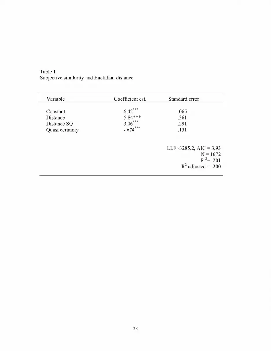
Table 1 Subjective similarity and Euclidian distance

Variable Coefficient est. Standard error Constant

6.42***

.065

Distance -5.84*** .361 Distance SQ 3.06*** .291 Quasi certainty -.674*** .151

LLF -3285.2, AIC = 3.93 N = 1672R 2= .201

R2 adjusted = .200

28

Table 2 Subjective similarity and cross entropy

Variable Coefficient est. Standard error Constant

6.42***

.065

Cross entropy -5.84*** .361 Cross entropy squared 3.06*** .291 Quasi certainty -.674*** .151

LLF -3414.1, AIC = 4.09 N = 1672R 2= .068

R2 adjusted = .067

29

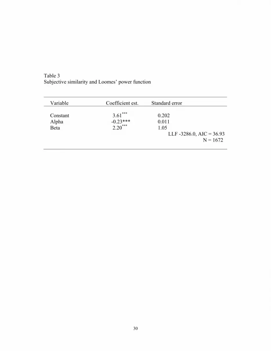
Table 3 Subjective similarity and Loomes’ power function

Variable Coefficient est. Standard error Constant

3.61***

0.202

Alpha -0.23*** 0.011 Beta 2.20*** 1.05

LLF -3286.0, AIC = 36.93 N = 1672

30

Table 4 List of candidate models

Model

Basic measure Variables (in addition to a constant)

1

Euclidian distance

Distance

2 Euclidian distance Distance, distance squared

3 Euclidian distance Distance, quasi-certainty

4 Euclidian distance Distance, distance squared, quasi certainty

5 Cross entropy Cross entropy

6 Cross entropy Cross entropy, cross entropy squared

7 Cross entropy Cross entropy, quasi certainty

8 Cross entropy Cross entropy, cross entropy squared, quasi certainty

9 Loomes’ full Loomes power function, unrestricted model

10 Loomes’ restricted Loomes power function, β restricted to zero

31

Table 5 Akaike information criteria (small sample) corrected ranks for logit models explaining choice under risk, N = 288 Proportion of Subjects with AIC C Rank Average Model Rank = 1 Rank = 2 Rank = 3 Rank 1-5 rank 1. Euclidian distance 40% 44% 15% 100% 1.79 2. Euclidian distance, distance squared 49% 5.51 3. Euclidian distance, quasi-certainty 2% 1% 3% 61% 5.08 4. Euclidian distance, distance squared, quasi-certainty 9.29 5. Cross entropy 33% 17% 46% 100% 2.20 6. Cross entropy, cross entropy squared 47% 5.57 7. Cross entropy, quasi-certainty 3% 0% 0% 45% 5.57 8. Cross entropy, cross entropy squared, quasi-certainty 9.34 9. Loomes’ power formulation, full model 8.1210. Loomes’ power formulation, restricted model 27% 32% 38% 100% 2.18

32

Table 6 Schwartz information criteria ranks for logit models explaining choice under risk, N = 288 Proportion of Subjects with SIC Rank Average Model Rank = 1 Rank = 2 Rank = 3 Rank 1-5 Rank 1. Euclidian distance 18% 15% 9% 69% 4.11 2. Euclidian distance, distance squared 10% 11% 12% 59% 4.88 3. Euclidian distance, quasi-certainty 12% 13% 13% 14% 4.53 4. Euclidian distance, distance squared, quasi- certainty 5% 15% 9% 69% 5.16 5. Cross entropy 18% 14% 13% 57% 5.41 6. Cross entropy, cross entropy squared 12% 6% 14% 35% 4.84 7. Cross entropy, quasi-certainty 6% 11% 11% 43% 5.54 8. Cross entropy, cross entropy squared, quasi- certainty 17% 11% 8% 57% 5.09 9. Loomes’ power formulation, full model 9.8910. Loomes’ power formulation, restricted model 11% 6% 8% 53% 5.21

33

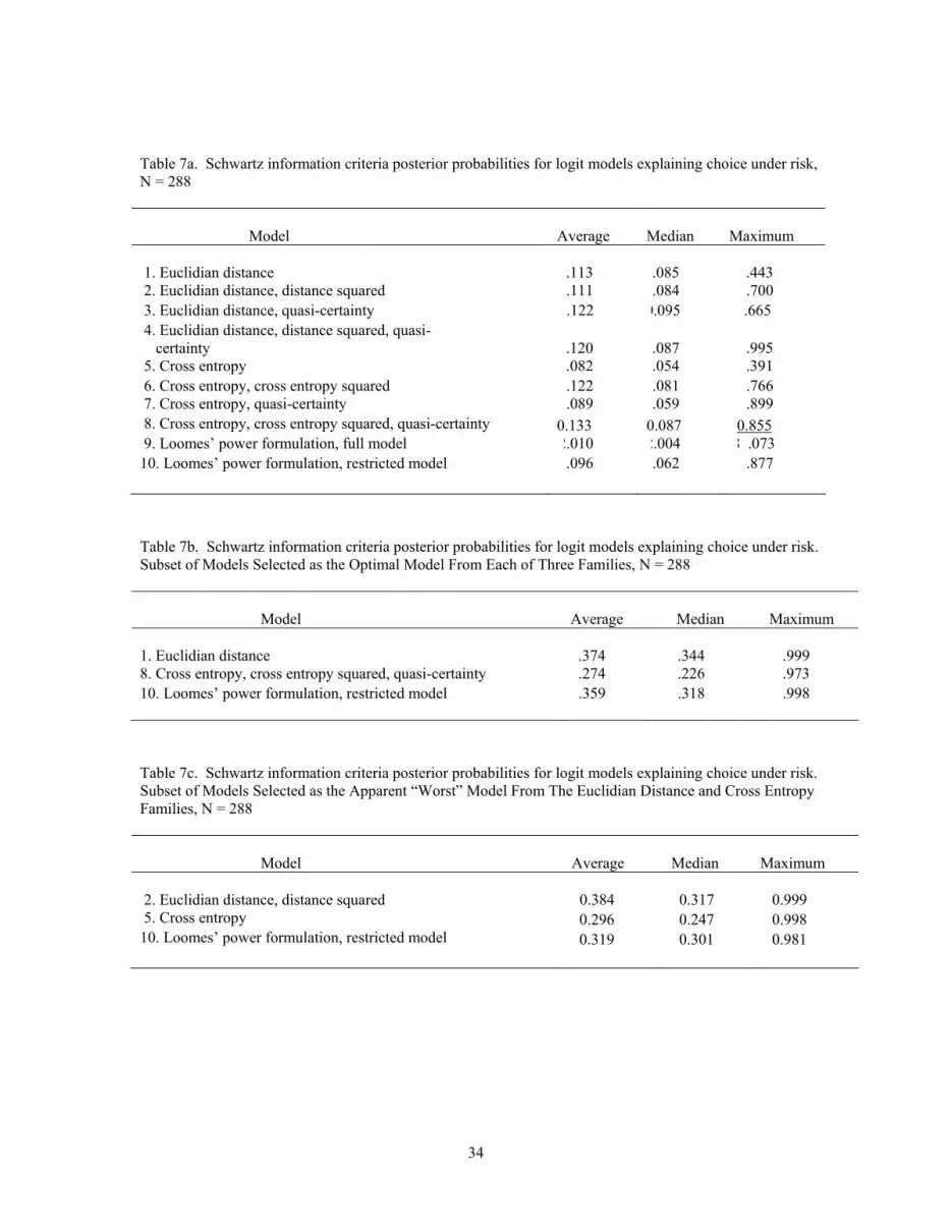
Table 7a. Schwartz information criteria posterior probabilities for logit models explaining choice under risk, N = 288 Model

Average

Median

Maximum

1. Euclidian distance

.113

.085

.443

2. Euclidian distance, distance squared .111 .084 .700 3. Euclidian distance, quasi-certainty .122 0.095 .665 4. Euclidian distance, distance squared, quasi- certainty

.120

.087

.995

5. Cross entropy .082 .054 .391 6. Cross entropy, cross entropy squared .122 .081 .766 7. Cross entropy, quasi-certainty .089 .059 .899 8. Cross entropy, cross entropy squared, quasi-certainty 0.133 0.087 0.855 9. Loomes’ power formulation, full model 2.010 2.004 8 .073 10. Loomes’ power formulation, restricted model .096 .062 .877

Table 7b. Schwartz information criteria posterior probabilities for logit models explaining choice under risk. Subset of Models Selected as the Optimal Model From Each of Three Families, N = 288 Model

Average

Median

Maximum

1. Euclidian distance

.374

.344

.999

8. Cross entropy, cross entropy squared, quasi-certainty .274 .226 .973 10. Loomes’ power formulation, restricted model .359 .318 .998

Table 7c. Schwartz information criteria posterior probabilities for logit models explaining choice under risk. Subset of Models Selected as the Apparent “Worst” Model From The Euclidian Distance and Cross Entropy Families, N = 288 Model

Average

Median

Maximum

2. Euclidian distance, distance squared 0.384 0.317 0.999 5. Cross entropy 0.296 0.247 0.998 10. Loomes’ power formulation, restricted model 0.319 0.301 0.981

34