DINCON’ 2008

7 Brazilian Conference on Dynamics, Control and Applicationsth

May 07 - 09, 2008FCT - Unesp at Presidente Prudente, SP, Brazil

x(i) y(i)

z(i)

6

5

4

3

2

1

-4-2

02

4-3-2

-10

12

3

APPLICATIONS OF PIEZOELECTRIC SENSORS AND ACTUATORS FORACTIVE AND PASSIVE VIBRATION CONTROL

Marcelo A. Trindade1

1Department of Mechanical Engineering, São Carlos School of Engineering, University of São Paulo, Av. Trabalhador São-Carlense, 400,São Carlos-SP, 13566-590, Brazil, trindade@sc.usp.br

Abstract: The present article provides a brief review of theopen literature concerning applications of piezoelectric sen-sors and actuators for active and passive vibration control.Then, some recent advances on this subject are presented.In particular, the following topics are discussed in detail: i)modeling of structures with piezoelectric sensors and actu-ators, ii) evaluation of the effective electromechanical cou-pling coefficient, iii) applications for active and passive vi-bration control.

Keywords: Piezoelectric Materials, Active Vibration Con-trol, Passive Vibration Control

1. INTRODUCTION

When incorporated into a laminated composite structure,piezoelectric materials can be used as distributed means forsensing and/or actuating the structure’s response. This isachieved thanks to the electromechanical interaction thatoccurs in a piezoelectric material for which the applica-tion of a force or pressure produces electric charge/voltage(direct piezoelectric effect) and the application of electriccharge/voltage is responded by induced strain (conversepiezoelectric effect). Therefore, the dynamic response of astructure with incorporated piezoelectric layers/patches canbe both monitored, through the measure of the charge/voltageinduced in the piezoelectric element(s) acting as sensor(s),and controlled, through the application of an appropriatecharge/voltage to the piezoelectric element(s) acting as ac-tuator(s). It is clear that to effectively control the structure’sresponse using piezoelectric sensors and actuators, one mustbe able not only to sense and actuate the structure’s responsebut also to evaluate the appropriate charge/voltage to be ap-plied to the actuator(s) based on the measured charge/voltageinduced in the sensor(s). This is achieved by a control sys-tem that connects the sensor(s) and actuator(s) and can bedesigned to induce the required response to the structure.

Over the past two decades, several research works haveshown that the use of integrated piezoelectric patches act-ing as sensors and/or actuators allows effective control of

the structure’s vibrations [1–4]. These laminated compositestructures with integrated piezoelectric sensors and actuatorsform a class of “smart structures” that has been widely usedfor structural vibration control in the recent years. The piezo-electric layers/patches can be either bonded to the surfacesof the host structure or embedded into a laminate structure.Surface-bonded, also known as surface-mounted, actuatorshave the advantage of ease in construction, access and main-tainability but may be subjected to high longitudinal stressesand contact with surrounding objects that may be detrimentalto normally brittle piezoceramic materials. Embedding thepiezoelectric layers/patches alleviate these problems and alsoenables good mechanical and electrical link with the struc-tural element and gluing materials may be unnecessary. Onthe other hand, embedding may lead to complex manufactur-ing and electrical insulation.

1.1. Piezoelectric extension and shear actuation andsensing modes

Surface-mounted piezoelectric actuators are normallypoled in the thickness direction so that the application of athrough-thickness electric field forces an elongation or con-traction of the actuators. If the actuators are well-bonded tothe surface of the host structure, their elongation or contrac-tion causes a deformation of the host structure. This may berepresented as the application of axial forces on the struc-ture’s surface at the actuator edges leading to bending mo-ments applied to the structure’s neutral line. That is why,surface-mounted actuators are also known as extension orextension-bending actuators. They been widely used on ac-tive [1], passive [2] and hybrid active-passive [5] control ap-plications. Although extension actuators can be very effec-tive when surface-mounted on the host structure, they are notvery effective when embedded in a laminate structure. Thisis because they induce smaller bending moments when theyare close to the structure’s neutral line.

Sun and Zhang [6] proposed the use of the thickness-shear mode of piezoelectric actuators embedded in a sand-wich beam. In this case, the piezoelectric patches are poled

in the axial direction and, when subjected to the standardthrough-thickness electric field, induce thickness shear stressin the sandwich structure’s core. These piezoelectric ac-tuators are known as shear actuators and are produced bysome piezoceramic manufacturers normally in the form ofplates poled in the length or width direction. Benjeddou,Trindade, and Ohayon [7–9] showed that shear actuators in-duce distributed actuation moments in the structure unlikeextension actuators which induce boundary forces. There-fore, shear actuation mechanism may lead to less problemsof debonding in actuators boundaries and to minor depen-dence of the control performance on actuators position andlength. Aldraihem and Khdeir [10–12] presented exact so-lutions for sandwich beams with shear and extension actua-tors using equivalent single layer models based on first-orderand third-order shear deformation theories. Trindade, Ben-jeddou, and Ohayon [13] presented a comparison betweenactive control performances of shear and extension actuationmechanisms using a sandwich beam finite element model.They showed that shear actuators are generally more suit-able to control bending vibrations of stiff structures. Raja,Sreedeep, and Prathap [14] have presented a finite elementstatic analysis of sandwich beams actuated simultaneouslyby shear and extension actuators for several boundary con-ditions. Recent experiments and numerical simulations per-formed by Baillargeon and Vel [15] have shown that shearactuators can provide significant reduction on the vibrationsof a sandwich beam. Vel and Batra [16] presented an ex-act 3D solution for the static cylindrical bending of simplysupported laminated plates with embedded shear piezoelec-tric actuators. Edery-Azulay and Abramovich [17] also pre-sented closed-form solutions for the static analysis of lami-nate/sandwich beams with embedded extension and shear ac-tuators. It has been observed that extension actuators are gen-erally more effective for very flexible host structures whileshear actuators are more effective for stiffer structures (e.g.short beams). Also, the effectiveness of extension actuatorsis more dependent on the position along the beam than shearactuators. These and other distinctive features of extensionand shear actuators may be exploited to study their simulta-neous use and to design a combined extension-shear actuatedbeam [18]. These and other aspects of the shear actuationmechanism are reviewed in [19].

1.2. Effective electromechanical coupling coefficient

It is well known that the sensing and actuation perfor-mances of piezoelectric materials depend highly on the effec-tive electromechanical coupling provided to the structure towhich they are attached. This coupling itself is known to bedependent on the intrinsic electromechanical coupling coef-ficient (EMCC) of the piezoelectric material and on the me-chanical coupling between the piezoelectric sensor/actuatorand the rest of the structure. In particular, the effectiveEMCC of a structure with piezoelectric elements should beexpected to be smaller than the material EMCC of the piezo-electric material embedded into the structure [20].

The EMCC of a piezoelectric material was first intro-duced by Mason [21] and can be defined as the square root of

the ratio of electrical energy stored in the volume of a piezo-electric body to the total mechanical energy supplied to thebody (or vice-versa). The EMCC is an important measure ofthe effectiveness of the electromechanical coupling and, thus,of the effectiveness of a piezoelectric material for a given ap-plication. Several formulas and methods were proposed toevaluate numerically or measure experimentally the EMCCof a piezoelectric material [21–23]. Most of them refer to thematerial EMCC, which is only function of the material prop-erties and normally requires an assumption of homogeneousdeformation throughout the piezoelectric body [24].

Some attempts to evaluate the effective EMCC of a struc-ture with piezoelectric elements were previously publishedin the literature [25–27]. Most of them make use of the for-mulas proposed by Mason [21] and Ulitko [22], which mea-sure variations in the resulting electromechanical structurewhen the electric boundary conditions are changed. Theseformulas are intended to account automatically for nonho-mogeneous deformations in the piezoelectric elements, cor-responding to an integration of electromechanical couplingthroughout the volume of piezoelectric bodies. This leads toa quite simple methodology when applying these formulas toevaluate the effective EMCC from experimentally measuredquantities. However, when applying these formulas to the-oretical models, care should be taken as to whether the the-oretical model accounts properly for the electric boundaryconditions [28].

1.3. Modeling of structures with piezoelectric sensorsand actuators

The first model proposed for structures with piezoelectricactuators was quite simple considering that an induced strain,proportional to the voltage applied to the actuator, was ap-plied to the host structure [29]. Improvements of this modelwere then proposed by Crawley and de Luis [30], accountingalso for the position of the actuator along the thickness direc-tion and the shear lag due to the adhesive layer. A somewhatmore sophisticated model based on a Bernoulli-Euler beamtheory was presented in [31]. Herman Shen [32] presenteda Timoshenko beam model to account for the shear strainsinduced by the piezoelectric actuator. Lee [33] proposed aclassical laminate theory, that is Kirchoff plate hypothesesfor an equivalent single layer. From the mid 90s on, severalmodeling methodologies were proposed for general laminatestructures with piezoelectric layers/patches bonded to, or em-bedded in, the host structure [34, 35]. Several finite elementmodels with and without electric degrees of freedom werealso proposed in the literature [36].

1.4. Passive vibration control using shunted piezoelec-tric materials

The idea of connecting piezoelectric patches to shunt cir-cuits is basically to control the mechanical energy via theelectrical energy induced in the shunt circuit due to elec-tromechanical coupling in the piezoelectric [37, 38]. Mostof the recent studies focus on optimizing the shunt circuitsby including resistances, inductances and capacitances in se-ries and/or parallel [3, 39, 40]. Nevertheless, few studies

focus on the optimization of the electromechanical couplingin the piezoelectric material. It has been shown that piezo-electric actuators using their thickness-shear mode can bemore effective than surface-mounted extension piezoelectricactuators for vibration damping [13, 15, 18, 41]. However,their use in connection to shunt circuits to provide passivevibration control is much less explored. In particular, it wasshown that the use of piezoelectric patches in thickness-shearmode may be more interesting since the electromechanicalcoupling is higher than that in extension mode [19, 42–44].

1.5. Active-passive vibration control using piezoelectricmaterials

In the last two decades, research was redirected to com-bined active and passive vibration control techniques [45].One of these techniques, so-called Active-Passive Piezoelec-tric Networks (APPN), integrates an active voltage sourcewith a passive resistance-inductance shunt circuit to a piezo-electric sensor/actuator [46]. This technique allows to simul-taneously dissipate passively vibratory energy through theshunt circuit and actively control the structural vibrations. Ithas been shown that combined active-passive vibration con-trol allows better performance with smaller cost than separateactive and passive control, provided the simultaneous actionis optimized. On the other hand, it has been shown in previ-ous studies [18, 47] that both purely active and purely passivedamping performance can be improved by properly selectingbetween, or combining, extension and thickness-shear actu-ation mechanisms of piezoelectric actuators/sensors. Hence,it is expected that the choice between actuation mechanismsshould be important as well for active-passive vibration con-trol.

2. MODELING OF STRUCTURES WITH PIEZO-ELECTRIC MATERIALS

In this section, a general methodology for the variationalformulation of coupled equations of motion for structureswith piezoelectric materials is presented. Equations are writ-ten in terms of both electric potential and electric charge inthe piezoelectric elements. Equipotentiality over each piezo-electric element electrodes is accounted for in both formula-tions. Finally, a methodology for coupling the piezoelectricelements with electric circuits is presented.

2.1. Electric potential formulation

First, a formulation considering electric potential in thepiezoelectric elements as variables is proposed. For that,let us start by denoting the generalized displacements of thestructure as u. Hence, the virtual work done by inertial andexternal forces can be written as

δT =−∫

Ω

δutρ ¨u dΩ (1)

δW =∫

Ω

δut f dΩ (2)

where ¨u and f stand for the generalized accelerations and ap-plied body forces vectors, respectively. ρ is the volumetric

mass density and Ω is the volume of the structure. The vir-tual work done by internal forces can be found from the vir-tual variation of the electromechanic potential energy. In thisfirst formulation, it is chosen to write the potential energyas the electric Gibbs energy, written in terms of mechanicalstrains ε and electric fields E, such that its variation reads

δU(ε,E) =∫

Ω

(δεt cEε−δεt eE−δEt etε−δEtεεE

)dΩ

(3)where cE , e and εε are the matrices of elastic (for constantelectric field), piezoelectric and dielectric (for constant me-chanical strain) constants of the material.

These virtual work expressions can be spatially dis-cretized through the discretization of the displacementsfields, and thus of the corresponding strains, such that

u(x1,x2,x3, t) = Nu(x1,x2,x3)u(t) (4)

ε(x1,x2,x3, t) = B(x1,x2,x3)u(t) (5)

The electric fields appearing in (3) can also be discretizedand written in terms of difference of electric potential (volt-age) as

E(x1,x2,x3, t) = NV (x1,x2,x3)V(t) (6)

Then, replacing discretized fields into the virtual work ex-pressions yields

δT =−δut Mu ; M =∫

Ω

ρNtuNu dΩ (7)

δW = δut Fm ; Fm =∫

Ω

Ntuf dΩ (8)

δU = δut KEu u−δut KuvV−δVt Kt

uvu−δVt KvV (9)

where the elastic (for constant electric field), piezoelectricand dielectric (for constant mechanical strain) stiffness ma-trices are

KEu =

∫Ω

BtcEB dΩ ; Kuv =∫

Ω

BteNV dΩ

Kv =∫

Ω

NtVεεNV dΩ

(10)

The equations of motion can then be derived fromD’Alembert’s principle,

δT −δU +δW = 0 (11)

such that

δut [(Ms +Mp)u+(Kus +KEup)u−KuvV−Fm

]+δVt (−Kt

uvu−KvV)

= 0 (12)

or in matrix form

[Ms +Mp 0

0 0

]uV

+[

Kus +KEup −Kuv

−Ktuv −Kv

]uV

=

Fm0

(13)

where Ms and Kus are the mass and elastic stiffness matricesof the structure (without piezoelectric elements) and Mp andKE

up are the mass and elastic (for constant electric fields) stiff-ness matrices of the piezoelectric elements. Kuv and Kv arethe piezoelectric and dielectric stiffnesses of the piezoelec-tric elements. Fm is a vector of the mechanical loads appliedto the structure. The degrees of freedom (dofs) u are the gen-eralized displacements and V are the generalized differencesof electric potentials (voltages) on the piezoelectric material.

To account for the equipotential condition on the elec-trodes of each piezoelectric element, let us define the vectorsof differences of electric potentials Vp induced or applied tothe electrodes of the piezoelectric elements, such that

V = LpVp (14)

The boolean matrix Lp has dimension N×Np, where N isthe number of spatial (nodal) points and Np is the number ofindependent piezoelectric elements. Lp allows to set an equalvalue to selected nodal differences of electric potentials.

Substituting equation (14) in equation (13) and pre-multiplying the second line of the resulting equation by Lt

pleads to

[Ms +Mp 0

0 0

]u

Vp

+[

Kus +KEup −Kuv

−Ktuv −Kv

]u

Vp

=

Fm0

(15)

whereKuv = KuvLp ; Kv = Lt

pKvLp (16)

Now, it is worthwhile to investigate three separate cases.If the piezoelectric elements are short-circuited, the differ-ences of electric potentials between their electrodes vanishand, hence, the first line of (15) reduces to

(Ms +Mp)u+(Kus +KEup)u = Fm (17)

On the other hand, if the piezoelectric elements are open-circuited, the differences of electric potentials between theirelectrodes are unknown and can be evaluated using the sec-ond line of equation (15), such that

Vp =−K−1v Kt

uvu (18)

Replacing equation (18) in the first line of equation (15) leadsto the following condensed equations of motion

(Ms +Mp)u+[Kus +(KE

up + KuvK−1v Kt

uv)]

u = Fm (19)

From equation (19), the generalized displacements u canbe evaluated. Then, the electric potentials Vp induced in thepiezoelectric elements can be found using equation (18). It

is worthwhile to notice, from equation (19), that the inducedpotentials in the sensors due to the direct piezoelectric effectlead to an increase in their constant electric field stiffnesses.This is due to an equivalent electric load generated in thepiezoelectric layer by the induced potential.

Finally, if differences of electric potential are applied tothe piezoelectric elements, the second equation in (15) is au-tomatically satisfied, since δVp = 0, and the first equation in(15) can be written as

(Ms +Mp)u+(Kus +KEup)u = Fm +Fp (20)

whereFp = KuvVp (21)

In this case, the piezoelectric elements act as actuatorsapplying piezoelectric equivalent forces on the structure andtheir stiffnesses are those for constant electric field.

2.2. Electric charge formulation

An electric charge formulation can be obtained by usingthe Helmholz free energy, written in terms of mechanicalstrains ε and electric displacements D, as potential energyinstead of the electric Gibbs energy, such that the virtual vari-ation of the potential energy is

δU(ε,D) =∫

Ω

(δεt cDε−δεt hD−δDt htε−δDtβεD

)dΩ

(22)where cD, h and βε are the matrices of elastic (for constantelectric displacement), piezoelectric and dielectric (for con-stant mechanical strain) constants of the material.

In this case, the discretization of mechanical quantities(displacements and strains) is the same as in the previoussection. The difference is on electrical quantities, that is,the electric displacements appearing in (22), which are dis-cretized as

D = NDDn (23)

Hence, the discretized version of the potential energy iswritten as

δU = δut KDu u−δut KudDn−δDt

nKtudu+δDt

nKdDn (24)

where the elastic (for constant electric displacement), piezo-electric and dielectric stiffness matrices are

KDu =

∫Ω

BtcDB dΩ ; Kud =∫

Ω

BthND dΩ

Kd =∫

Ω

NtDβ

εND dΩ

(25)

Again, from D’Alembert’s principle (11), the equationsof motion are now written in terms of the generalized dis-placements u and electric displacements Dn, such that

δut [(Ms +Mp)u+(Kus +KDup)u−KudDn−Fm

]+δDt

n(−Kt

udu+KdDn)

= 0 (26)

or in matrix form

[Ms +Mp 0

0 0

]u

Dn

+[

Kus +KDup −Kud

−Ktud Kd

]u

Dn

=

Fm0

(27)

where, as in the previous case, Ms and Kus are the massand elastic stiffness matrices of the structure (without piezo-electric elements) and Mp and KD

up are the mass and elastic(for constant electric displacements) stiffness matrices of thepiezoelectric elements. Kud and Kd are the piezoelectric anddielectric stiffnesses of the piezoelectric elements.

To account for the equipotential condition on the elec-trodes of each piezoelectric element, let us define the vectorsof electric charges qp on the electrodes of the piezoelectricelements, such that

Dn = Bpqp ; Bp = LpA−1p (28)

The boolean matrix Lp has dimension N×Np, where Nis the number of spatial (nodal) points and Np is the numberof independent piezoelectric elements. Lp allows to set anequal value to selected nodal electric displacements. Ap is adiagonal matrix with the surface area of the electrodes of thepiezoelectric elements.

Substituting equation (28) in equation (27) and pre-multiplying the second line of the resulting equation by Bt

pleads to

[Ms +Mp 0

0 0

]uqp

+[

Kus +KDup −Kuq

−Ktuq Kq

]uqp

=

Fm0

(29)

whereKuq = KudBp ; Kq = Bt

pKdBp (30)

Now, it is worthwhile to investigate two separate cases.If the piezoelectric elements are open-circuited, the electriccharge flux between their electrodes vanish and, hence, thefirst line of (29) reduces to

(Ms +Mp)u+(Kus +KDup)u = Fm (31)

On the other hand, if the piezoelectric elements are short-circuited, the electric charge flux between their electrodes areunknown and can be evaluated using the second line of equa-tion (29), such that

qp = K−1q Kt

uqu (32)

Replacing equation (32) in the first line of equation (29) leadsto the following condensed equations of motion

(Ms +Mp)u+[Kus +(KD

up−KuqK−1q Kt

uq)]

u = Fm (33)

From equation (33), the generalized displacements u canbe evaluated. Then, the electric charges qp flowing between

electrodes of the piezoelectric elements can be found usingequation (32). It is worthwhile to notice, from equation (33),that the induced electric displacements in the sensors due tothe direct piezoelectric effect lead to a decrease in their stiff-nesses. This is due to the relaxation of the equivalent electricload generated in the piezoelectric layer by the induced po-tential.

Finally, if electric charges are applied to the piezoelectricelements, the second equation in (29) is automatically sat-isfied, since δqp = 0, and the first equation in (29) can bewritten as

(Ms +Mp)u+(Kus +KDup)u = Fm +Fp (34)

whereFp = Kuqqp (35)

in this case, the piezoelectric elements act as charge actuatorsapplying piezoelectric equivalent forces on the structure andtheir stiffnesses are those for constant electric displacement.

2.3. Connection to electric circuits

It is worthwhile to analyze the connection of piezoelec-tric elements to electric circuits, specially when shunt circuitsare considered for passive vibration control. To this end, itseems that an electric charge formulation is more appropri-ate since it is possible to relate the electric charges flowingbetween the piezoelectric elements electrodes with the elec-tric charges flowing through the electric circuit. First, let usconsider a set of simple but quite general electric circuitscomposed of an inductor, a resistor and a voltage source.The equations of motion for such circuits can be found us-ing d’Alembert’s principle, such that the virtual work doneby the inductors δTL j, resistors, δWR j, and voltage sources,δWV j, of the j-th electric circuit are

δTL j =−δqc jLc jqc j ; δWR j =−δqc jRc jqc j ;δWV j = δqc jVc j

(36)

where Lc j, Rc j e Vc j are the inductance, resistance and ap-plied voltage of the j-th electric circuit. qc j is the electriccharge flowing through the j-th electric circuit. Combiningthe virtual work done by all circuits leads to

δTL =n

∑j=1δTL j =−δqt

cLcqc

δWR =n

∑j=1δWR j =−δqt

cRcqc

δWV =n

∑j=1δWV j = δqt

cVc

(37)

where qc is the vector of electric charges, Lc and Rc are di-agonal matrices with the inductances and resistances of eachcircuit, and Vc is the vector of applied voltages.

Adding these virtual works to the electromechanical vir-tual works of previous section, such that

δT −δU +δW +δTL +δWR +δWV = 0 (38)

or, in terms of the generalized displacements,

δut [(Ms +Mp)u+(Kus +KDup)u−Kuqqp−Fm

]+δqt

p(−Ktuqu+Kqqp)+δqt

c(Lcqc +Rcqc−Vc) = 0(39)

Then, the connection between each piezoelectric elementand a corresponding electric circuit is done by stating that theelectric charges flowing from the piezoelectric element enterthe circuit and vice-versa, such that

qc = qp (40)

Thus, replacing qc by qp in (39) leads to the followingcoupled equations of motion

[Ms +Mp 0

0 Lc

]uqp

+[

0 00 Rc

]uqp

+[

Kus +KDup −Kuq

−Ktuq Kq

]uqp

=

FmVc

(41)

In this case, the solution for u and qp must be simulta-neous, that is accounting for the electromechanical and cir-cuit equations of motion. Notice that the passive componentsof the electric circuit Lc and Rc affect the equivalent piezo-electric force applied to the structure when an actuator withapplied voltage is considered. For a simple actuator with ap-plied voltage, that is with only a voltage source in the circuit(Lc = Rc = 0), the second equation in (41) can be solved forqp leading to

qp = K−1q Vc +K−1

q Ktuqu (42)

which can be substituted in (41) such that it reduces to

(Ms +Mp)u+[Kus +(KD

up−KuqK−1q Kt

uq)]

u = Fm +Fp(43)

where the equivalent piezoelectric force Fp applied to thestructure by the piezoelectric actuators is

Fp = KuqK−1q Vc (44)

From equation (43), the generalized displacements u in-duced by mechanical and piezoelectric equivalent forces canbe evaluated. Then, the electric charges qp flowing betweenelectrodes of the piezoelectric elements can be found usingequation (42).

3. EVALUATION OF THE EFFECTIVE ELEC-TROMECHANICAL COUPLING COEFFICIENT

3.1. Evaluation of material EMCC

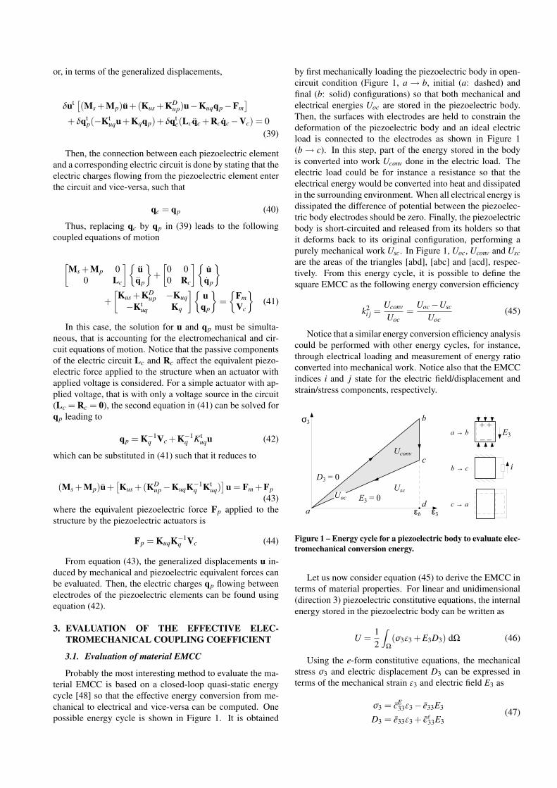
Probably the most interesting method to evaluate the ma-terial EMCC is based on a closed-loop quasi-static energycycle [48] so that the effective energy conversion from me-chanical to electrical and vice-versa can be computed. Onepossible energy cycle is shown in Figure 1. It is obtained

by first mechanically loading the piezoelectric body in open-circuit condition (Figure 1, a→ b, initial (a: dashed) andfinal (b: solid) configurations) so that both mechanical andelectrical energies Uoc are stored in the piezoelectric body.Then, the surfaces with electrodes are held to constrain thedeformation of the piezoelectric body and an ideal electricload is connected to the electrodes as shown in Figure 1(b→ c). In this step, part of the energy stored in the bodyis converted into work Uconv done in the electric load. Theelectric load could be for instance a resistance so that theelectrical energy would be converted into heat and dissipatedin the surrounding environment. When all electrical energy isdissipated the difference of potential between the piezoelec-tric body electrodes should be zero. Finally, the piezoelectricbody is short-circuited and released from its holders so thatit deforms back to its original configuration, performing apurely mechanical work Usc. In Figure 1, Uoc, Uconv and Uscare the areas of the triangles [abd], [abc] and [acd], respec-tively. From this energy cycle, it is possible to define thesquare EMCC as the following energy conversion efficiency

k2i j =

Uconv

Uoc=

Uoc−Usc

Uoc(45)

Notice that a similar energy conversion efficiency analysiscould be performed with other energy cycles, for instance,through electrical loading and measurement of energy ratioconverted into mechanical work. Notice also that the EMCCindices i and j state for the electric field/displacement andstrain/stress components, respectively.

D3 = 0

E3 = 0Usc

Uconv

σ3

ε3εba

b

c

a → b

b → c

c → a

+

–

+

–E3

i

Uocd

Figure 1 – Energy cycle for a piezoelectric body to evaluate elec-tromechanical conversion energy.

Let us now consider equation (45) to derive the EMCC interms of material properties. For linear and unidimensional(direction 3) piezoelectric constitutive equations, the internalenergy stored in the piezoelectric body can be written as

U =12

∫Ω

(σ3ε3 +E3D3) dΩ (46)

Using the e-form constitutive equations, the mechanicalstress σ3 and electric displacement D3 can be expressed interms of the mechanical strain ε3 and electric field E3 as

σ3 = cE33ε3− e33E3

D3 = e33ε3 +εε33E3(47)

where cE33, e33 and εε33 are the elastic (at constant electric

field), piezoelectric and dielectric (at constant strain) con-stants. One can notice that during the first (a→ b) and third(c→ a) phases of the energy cycle of Figure 1, that is unidi-mensional contraction (extension) in direction 3 with D3 = 0(E3 = 0), the constitutive equations (47) can be reduced to:

First phase of energy cycle (a→ b)

σ3 = cD33ε3 with cD

33 = cE33 +(e2

33/εε33)

E3 =−(e33/εε33)ε3 and D3 = 0

(48)

Third phase of energy cycle (c→ a)

σ3 = cE33ε3

D3 = e33ε3 and E3 = 0(49)

Hence, the total energy stored in the piezoelectric body inthe first and third phases of the energy cycle can be evaluatedfrom equations (46), (48) and (49), such that

Uoc =12

∫Ω

cD33ε

23 dΩ (50)

Usc =12

∫Ω

cE33ε

23 dΩ (51)

Considering homogeneous deformation throughout thepiezoelectric body, the square EMCC for this mode of de-formation can be written from equations (45), (50) and (51)as

k233 =

cD33− cE

33

cD33

(52)

which, from equation (48), can be simplified to

k233 =

e233

cD33ε

ε33

=e2

33

cE33ε

σ33

(53)

A similar expression can be obtained using the formulaproposed in [49] and based on the ratio between the square ofa so-called mutual elasto-dielectric energy Um and the prod-uct of the stored elastic Ue and dielectric Ud energies, suchthat

k233 =

U2m

UeUd(54)

where the mutual, elastic and dielectric energies should bedefined as

Um =12

∫Ω

d33σ3E3 dΩ ; Ue =12

∫Ω

sE33σ

23 dΩ ;

Ud =12

∫Ω

εσ33E23 dΩ

(55)

Although the energy cycle (Figure 1) and the EMCC def-inition (Equation (45)) are defined for quasi-static defor-mation, this analysis may be extended to resonant vibra-tions. However, in such cases, the deformation throughoutthe piezoelectric body may not be homogeneous and, thus,both open-circuit and short-circuit energies must be evalu-ated through integration over the volume of the piezoelectric

body. Supposing that the displacement u3 and, consequentlythe mechanical strain ε3, along the x3 direction are written as

u3(x3, t) =φ(x3)cosωt ; ε3(x3, t) =φ′(x3)cosωt, (56)

the strain, as in (50) and (51), and kinetic energies of thepiezoelectric body are

U =12

cos2ωt∫

Ω

c33φ′(x3)2 dΩ ;

T =12ω2 sin2ωt

∫Ω

ρφ(x3)2 dΩ

(57)

Recalling that, for resonant vibrations, the maximum ki-netic energy equals the maximum strain energy, and sup-posing that the vibration mode φ(x3) remains unchangedfor open-circuit and short-circuit conditions, the maximumstrain energy in these electric conditions reads

Umaxoc =

12

∫Ω

cD33φ

′(x3)2 dΩ =12ω2

ocT ;

Umaxsc =

12

∫Ω

cE33φ

′(x3)2 dΩ =12ω2

scT(58)

whereT =

∫Ω

ρφ(x3)2 dΩ (59)

Notice that the integrals in Umaxoc and Umax

sc can be seenas the modal stiffness in open and short circuit conditionswhereas T is the modal mass. The square EMCC, for thisparticular vibration mode, can then be defined as

k233 =

Umaxoc −Umax

sc

Umaxoc

=ω2

oc−ω2sc

ω2oc

(60)

For homogeneous properties throughout the piezoelectricbody, equation (60) reduces to equation (45). This analysis,however, is only valid under the assumption that the electricfield E3 and displacement D3 can be set to zero throughoutthe piezoelectric body in short-circuit and open-circuit con-ditions, respectively.

3.2. Evaluation of effective EMCC

It is also worthwhile to evaluate the effective EMCC fora general mechanical structure with bonded and/or embed-ded piezoelectric elements. In this case, the effective EMCCshould account not only for the material EMCC of eachpiezoelectric element but also for the mechanical couplingbetween the piezoelectric elements and the rest of the struc-ture. Indeed, a satisfactory measure of the effective squareEMCC for a structure with piezoelectric elements should bethe ratio of electrical energy stored in the piezoelectric ele-ments to the total mechanical (strain) energy supplied to thestructure. However, the evaluation of such effective EMCCrequires accounting for non-homogeneous properties and de-formation. Hence, a general procedure based on a model ofthe structure with piezoelectric elements is proposed.

Starting from the reduced equations of motion (17) and(19), the i-th eigenmode and eigenfrequency of the structurewith piezoelectric elements in short-circuit and open-circuitcan be evaluated, respectively, by

[−ωi

sc2M+(Ks +Ksc

p )]

Tisc = 0 (61)

[−ωi

oc2M+(Ks +Koc

p )]

Tioc = 0 (62)

where, for the sake of clarity, the matrices M, Ks, Kscp and

Kocp are defined as

M = Ms +Mp ; Ks = Kus ; Kscp = KE

up ;

Kocp = KE

up + KuvK−1v Kt

uv(63)

Supposing that the short-circuit and open-circuit condi-tions of the piezoelectric elements do not yield large varia-tions in the structure eigenmodes (Ti

sc = Tioc = Ti), which

should be valid for relatively small piezoelectric elements,and for mass-normalized eigenmodes, the i-th short-circuitand open-circuit eigenfrequencies can be written as

ωisc

2 = Tti (Ks +Ksc

p )Ti (64)

andωi

oc2 = Tt

i (Ks +Kocp )Ti (65)

Therefore, the effective square EMCC for the structurewith piezoelectric elements, vibrating in the i-th mode, canbe defined as

K2i =

ωioc

2−ωisc

2

ωioc

2 =Tt

i (Kocp −Ksc

p )Ti

Tti (Ks +Koc

p )Ti(66)

Equation (66) provides a relatively simple technique toevaluate the effective EMCC in terms of the open-circuit andshort-circuit eigenfrequencies, which may be measured fora given experimental setup or numerically calculated for agiven structural model. Notice that this equation provides anaverage effective EMCC for a structure with several piezo-electric elements and may even account for the electrome-chanical coupling provided by a set of piezoelectric elementsworking in different deformation modes (e.g. 33, 31, 15).Hence, if the objective is to evaluate the effective EMCCprovided by a single piezoelectric element, this evaluationshould be done by imposing a short-circuit condition for theother piezoelectric elements, so that the only electrically-stiffened element will be the element under study.

Notice that, for the analysis of a single piezoelectric el-ement with homogeneous properties and working mainly inone deformation mode, Ksc

p ≈ (1− k2jl)K

ocp , where k2

jl is thematerial square EMCC for the specific deformation mode.Thus, in this case, K2

i may be approximated as

K2i = k2

jlTt

i Kocp Ti

Tti (Ks +Koc

p )Ti(67)

This expression can be interpreted as the product of thematerial square EMCC by the ratio of the OC strain en-ergy stored in the piezoelectric element to the total strainenergy. This formula is similar to that in the Modal StrainEnergy method, proposed in [50] for the evaluation of ef-fective modal loss factors for structures with viscoelastic el-ements. An analysis of equation (67) indicates that there

are two main levers to maximize the effective EMCC: i) thematerial EMCC for the main deformation mode, and ii) theenergy ratio stored in the piezoelectric element for a givenstructural eigenmode.

3.3. Comparison with experimental results for a can-tilever beam

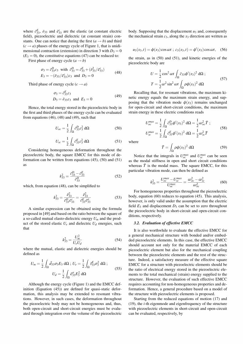
A comparative analysis is performed in this subsectionfor an aluminum cantilever beam with two thickness-poledpiezoelectric patches bonded symmetrically on its top andbottom surfaces near the clamp (Figure 2). The beam hasa length of 243.5 mm, a thickness of 2 mm and a widthof 30 mm, and its material properties are: Young modu-lus 69 GPa, mass density 2790 kg m−3 and Poisson ra-tio 0.3. The piezoelectric patches are identical and madeof a PIC255 piezoceramic with thickness 0.25 mm, width20 mm, length 25 mm, mass density 7800 kg m−3, equiv-alent SC Young modulus 62.1 GPa, equivalent piezoelec-tric coefficient e31 = 11.2 C m−2 and dielectric coefficientεσ33 = 15.5 nF m−1. These data were adapted from [51]. No-tice, however, that the piezoceramics width was consideredequal to that of the beam (30 mm) in the calculations usingthe present beam model.

25

2.000.25PIC255 Piezoceramic

Aluminum

17 243.50PIC255 Piezoceramic 0.25

20 30

Figure 2 – Representation of the cantilever beam with bondedpiezoelectric patches (dimensions in mm).

Experimental measurements of the two first bendingeigenfrequencies of the cantilever beam with short-circuitand open-circuit piezoelectric patches were presented in [51].The authors then used the measured eigenfrequencies to eval-uate the effective EMCC and predicted shunted damping ra-tios. The short-circuit and open-circuit eigenfrequencies andthe resulting EMCC, taken from [51], are presented in Ta-ble 1. The corresponding results obtained with the presentFE model, accounting for the equipotentiality condition forboth piezoelectric patches, are also presented. It is possibleto observe that the numerical eigenfrequencies match quitewell with the experimental ones (up to 10% error for the firsteigenfrequency). Possible reasons for the error could be thelack of precise knowledge on the material properties and thedifference between theoretical and real clamped-free bound-ary conditions. As a result, the numerically evaluated EMCCdo not match exactly the experimental ones. However, it ispossible to observe from Table 1 that both numerical andexperimental results indicate a higher EMCC for the firsteigenmode, as expected, since the piezoelectric patches werebonded near the clamped end where the normal strains arehigher for the first eigenmode. It is also noticeable that 2/3of the evaluated square EMCC, to adjust for the difference

of piezoelectric volume, matches quite well the experimentalvalues. As for the previous case, equation (67) provides agood approximation for the EMCC.

3.4. Evaluation of equipotential effect on EMCC

0 100 2000

2

4

PZT length (mm)

Squ

are

EM

CC

M1

(%)

0 100 2000

2

4

PZT length (mm)

Squ

are

EM

CC

M2

(%)

0 100 2000

2

4

PZT length (mm)S

quar

e E

MC

C M

3 (%

)

0 100 2000

2

4

PZT length (mm)

Squ

are

EM

CC

M4

(%)

0 100 2000

2

4

PZT length (mm)

Squ

are

EM

CC

M5

(%)

0 100 2000

2

4

PZT length (mm)

Squ

are

EM

CC

M6

(%)

0 100 2000

2

4

PZT length (mm)

Squ

are

EM

CC

M7

(%)

0 100 2000

2

4

PZT length (mm)

Squ

are

EM

CC

M8

(%)

0 100 2000

2

4

PZT length (mm)

Squ

are

EM

CC

M9

(%)

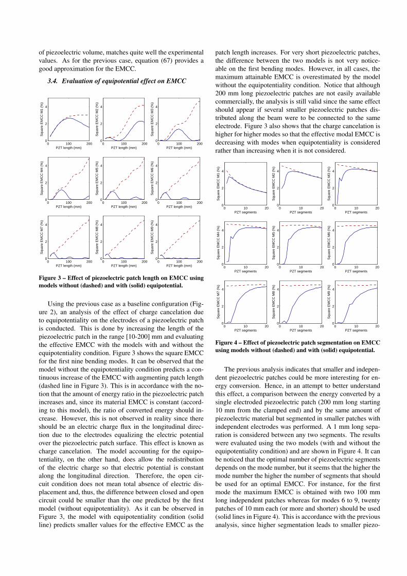
Figure 3 – Effect of piezoelectric patch length on EMCC usingmodels without (dashed) and with (solid) equipotential.

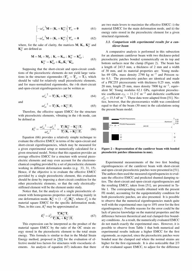
Using the previous case as a baseline configuration (Fig-ure 2), an analysis of the effect of charge cancelation dueto equipotentiality on the electrodes of a piezoelectric patchis conducted. This is done by increasing the length of thepiezoelectric patch in the range [10-200] mm and evaluatingthe effective EMCC with the models with and without theequipotentiality condition. Figure 3 shows the square EMCCfor the first nine bending modes. It can be observed that themodel without the equipotentiality condition predicts a con-tinuous increase of the EMCC with augmenting patch length(dashed line in Figure 3). This is in accordance with the no-tion that the amount of energy ratio in the piezoelectric patchincreases and, since its material EMCC is constant (accord-ing to this model), the ratio of converted energy should in-crease. However, this is not observed in reality since thereshould be an electric charge flux in the longitudinal direc-tion due to the electrodes equalizing the electric potentialover the piezoelectric patch surface. This effect is known ascharge cancelation. The model accounting for the equipo-tentiality, on the other hand, does allow the redistributionof the electric charge so that electric potential is constantalong the longitudinal direction. Therefore, the open cir-cuit condition does not mean total absence of electric dis-placement and, thus, the difference between closed and opencircuit could be smaller than the one predicted by the firstmodel (without equipotentiality). As it can be observed inFigure 3, the model with equipotentiality condition (solidline) predicts smaller values for the effective EMCC as the

patch length increases. For very short piezoelectric patches,the difference between the two models is not very notice-able on the first bending modes. However, in all cases, themaximum attainable EMCC is overestimated by the modelwithout the equipotentiality condition. Notice that although200 mm long piezoelectric patches are not easily availablecommercially, the analysis is still valid since the same effectshould appear if several smaller piezoelectric patches dis-tributed along the beam were to be connected to the sameelectrode. Figure 3 also shows that the charge cancelation ishigher for higher modes so that the effective modal EMCC isdecreasing with modes when equipotentiality is consideredrather than increasing when it is not considered.

0 10 200

2

4

PZT segments

Squ

are

EM

CC

M1

(%)

0 10 200

2

4

PZT segments

Squ

are

EM

CC

M2

(%)

0 10 200

2

4

PZT segments

Squ

are

EM

CC

M3

(%)

0 10 200

2

4

PZT segments

Squ

are

EM

CC

M4

(%)

0 10 200

2

4

PZT segmentsS

quar

e E

MC

C M

5 (%

)

0 10 200

2

4

PZT segments

Squ

are

EM

CC

M6

(%)

0 10 200

2

4

PZT segments

Squ

are

EM

CC

M7

(%)

0 10 200

2

4

PZT segments

Squ

are

EM

CC

M8

(%)

0 10 200

2

4

PZT segmentsS

quar

e E

MC

C M

9 (%

)

Figure 4 – Effect of piezoelectric patch segmentation on EMCCusing models without (dashed) and with (solid) equipotential.

The previous analysis indicates that smaller and indepen-dent piezoelectric patches could be more interesting for en-ergy conversion. Hence, in an attempt to better understandthis effect, a comparison between the energy converted by asingle electroded piezoelectric patch (200 mm long starting10 mm from the clamped end) and by the same amount ofpiezoelectric material but segmented in smaller patches withindependent electrodes was performed. A 1 mm long sepa-ration is considered between any two segments. The resultswere evaluated using the two models (with and without theequipotentiality condition) and are shown in Figure 4. It canbe noticed that the optimal number of piezoelectric segmentsdepends on the mode number, but it seems that the higher themode number the higher the number of segments that shouldbe used for an optimal EMCC. For instance, for the firstmode the maximum EMCC is obtained with two 100 mmlong independent patches whereas for modes 6 to 9, twentypatches of 10 mm each (or more and shorter) should be used(solid lines in Figure 4). This is accordance with the previousanalysis, since higher segmentation leads to smaller piezo-

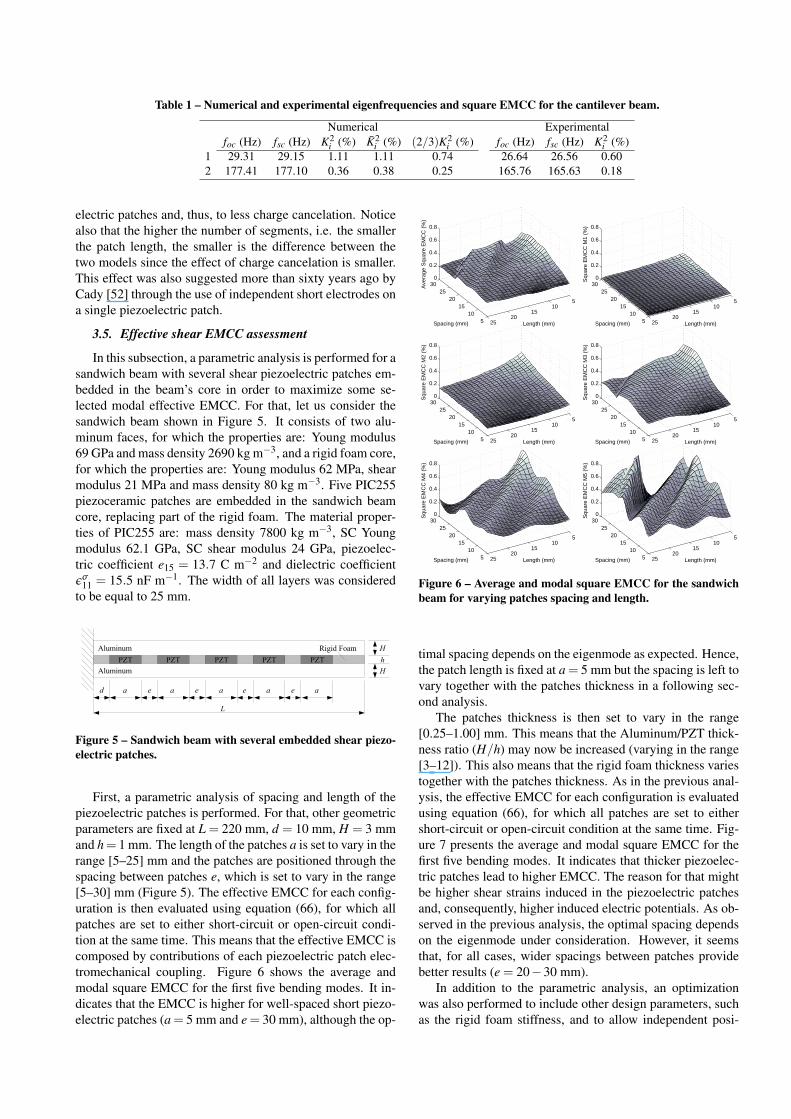
Table 1 – Numerical and experimental eigenfrequencies and square EMCC for the cantilever beam.

Numerical Experimentalfoc (Hz) fsc (Hz) K2

i (%) K2i (%) (2/3)K2

i (%) foc (Hz) fsc (Hz) K2i (%)

1 29.31 29.15 1.11 1.11 0.74 26.64 26.56 0.602 177.41 177.10 0.36 0.38 0.25 165.76 165.63 0.18

electric patches and, thus, to less charge cancelation. Noticealso that the higher the number of segments, i.e. the smallerthe patch length, the smaller is the difference between thetwo models since the effect of charge cancelation is smaller.This effect was also suggested more than sixty years ago byCady [52] through the use of independent short electrodes ona single piezoelectric patch.

3.5. Effective shear EMCC assessment

In this subsection, a parametric analysis is performed for asandwich beam with several shear piezoelectric patches em-bedded in the beam’s core in order to maximize some se-lected modal effective EMCC. For that, let us consider thesandwich beam shown in Figure 5. It consists of two alu-minum faces, for which the properties are: Young modulus69 GPa and mass density 2690 kg m−3, and a rigid foam core,for which the properties are: Young modulus 62 MPa, shearmodulus 21 MPa and mass density 80 kg m−3. Five PIC255piezoceramic patches are embedded in the sandwich beamcore, replacing part of the rigid foam. The material proper-ties of PIC255 are: mass density 7800 kg m−3, SC Youngmodulus 62.1 GPa, SC shear modulus 24 GPa, piezoelec-tric coefficient e15 = 13.7 C m−2 and dielectric coefficientεσ11 = 15.5 nF m−1. The width of all layers was consideredto be equal to 25 mm.

L

d a e a e a e a e a

H

Hh

Aluminum

AluminumPZT

Rigid FoamPZT PZT PZT PZT

Figure 5 – Sandwich beam with several embedded shear piezo-electric patches.

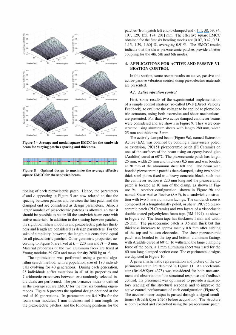
First, a parametric analysis of spacing and length of thepiezoelectric patches is performed. For that, other geometricparameters are fixed at L = 220 mm, d = 10 mm, H = 3 mmand h = 1 mm. The length of the patches a is set to vary in therange [5–25] mm and the patches are positioned through thespacing between patches e, which is set to vary in the range[5–30] mm (Figure 5). The effective EMCC for each config-uration is then evaluated using equation (66), for which allpatches are set to either short-circuit or open-circuit condi-tion at the same time. This means that the effective EMCC iscomposed by contributions of each piezoelectric patch elec-tromechanical coupling. Figure 6 shows the average andmodal square EMCC for the first five bending modes. It in-dicates that the EMCC is higher for well-spaced short piezo-electric patches (a = 5 mm and e = 30 mm), although the op-

510

1520

2530

510

1520

25

0

0.2

0.4

0.6

0.8

Length (mm)Spacing (mm)

Ave

rage

Squ

are

EM

CC

(%

)

510

1520

2530

510

1520

25

0

0.2

0.4

0.6

0.8

Length (mm)Spacing (mm)

Squ

are

EM

CC

M1

(%)

510

1520

2530

510

1520

25

0

0.2

0.4

0.6

0.8

Length (mm)Spacing (mm)

Squ

are

EM

CC

M2

(%)

510

1520

2530

510

1520

25

0

0.2

0.4

0.6

0.8

Length (mm)Spacing (mm)

Squ

are

EM

CC

M3

(%)

510

1520

2530

510

1520

25

0

0.2

0.4

0.6

0.8

Length (mm)Spacing (mm)

Squ

are

EM

CC

M4

(%)

510

1520

2530

510

1520

25

0

0.2

0.4

0.6

0.8

Length (mm)Spacing (mm)

Squ

are

EM

CC

M5

(%)

Figure 6 – Average and modal square EMCC for the sandwichbeam for varying patches spacing and length.

timal spacing depends on the eigenmode as expected. Hence,the patch length is fixed at a = 5 mm but the spacing is left tovary together with the patches thickness in a following sec-ond analysis.

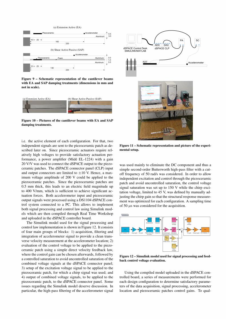
The patches thickness is then set to vary in the range[0.25–1.00] mm. This means that the Aluminum/PZT thick-ness ratio (H/h) may now be increased (varying in the range[3–12]). This also means that the rigid foam thickness variestogether with the patches thickness. As in the previous anal-ysis, the effective EMCC for each configuration is evaluatedusing equation (66), for which all patches are set to eithershort-circuit or open-circuit condition at the same time. Fig-ure 7 presents the average and modal square EMCC for thefirst five bending modes. It indicates that thicker piezoelec-tric patches lead to higher EMCC. The reason for that mightbe higher shear strains induced in the piezoelectric patchesand, consequently, higher induced electric potentials. As ob-served in the previous analysis, the optimal spacing dependson the eigenmode under consideration. However, it seemsthat, for all cases, wider spacings between patches providebetter results (e = 20−30 mm).

In addition to the parametric analysis, an optimizationwas also performed to include other design parameters, suchas the rigid foam stiffness, and to allow independent posi-

0.20.4

0.60.8

10

20

300

0.2

0.4

0.6

0.8

Thickness (mm)Spacing (mm)

Ave

rage

Squ

are

EM

CC

(%

)

0.20.4

0.60.8

10

20

300

0.2

0.4

0.6

0.8

Thickness (mm)Spacing (mm)

Squ

are

EM

CC

M1

(%)

0.20.4

0.60.8

10

20

300

0.2

0.4

0.6

0.8

Thickness (mm)Spacing (mm)

Squ

are

EM

CC

M2

(%)

0.20.4

0.60.8

10

20

300

0.2

0.4

0.6

0.8

Thickness (mm)Spacing (mm)

Squ

are

EM

CC

M3

(%)

0.20.4

0.60.8

10

20

300

0.2

0.4

0.6

0.8

Thickness (mm)Spacing (mm)

Squ

are

EM

CC

M4

(%)

0.20.4

0.60.8

10

20

300

0.2

0.4

0.6

0.8

Thickness (mm)Spacing (mm)

Squ

are

EM

CC

M5

(%)

Figure 7 – Average and modal square EMCC for the sandwichbeam for varying patches spacing and thickness.

Figure 8 – Optimal design to maximize the average effectivesquare EMCC for the sandwich beam.

tioning of each piezoelectric patch. Hence, the parametersd and e appearing in Figure 5 are now relaxed so that thespacing between patches and between the first patch and theclamped end are considered as design parameters. Also, alarger number of piezoelectric patches is allowed, so that itshould be possible to better fill the sandwich beam core withactive materials. In addition to the spacing between patches,the rigid foam shear modulus and piezoelectric patches thick-ness and length are considered as design parameters. For thesake of simplicity, however, the length a is considered equalfor all piezoelectric patches. Other geometric properties, ac-cording to Figure 5, are fixed at L = 220 mm and H = 3 mm.Material properties of the two aluminum faces are fixed atYoung modulus 69 GPa and mass density 2690 kg m−3.

The optimization was performed using a genetic algo-rithm search method, with a population size of 180 individ-uals evolving for 40 generations. During each generation,25 individuals suffer mutations in all of its properties and7 arithmetic crossovers between two randomly selected in-dividuals are performed. The performance index is definedas the average square EMCC for the first six bending eigen-modes. Figure 8 presents the optimal design obtained at theend of 40 generations. Its parameters are 0.4 MPa for thefoam shear modulus, 1 mm thickness and 5 mm length forthe piezoelectric patches, and the following positions for the

patches (from patch left end to clamped end): [11, 38, 59, 84,107, 129, 155, 174, 201] mm. The effective square EMCCobtained for the first six bending modes are [0.07, 0.42, 0.81,1.15, 1.39, 1.60] %, averaging 0.91%. The EMCC resultsindicate that the shear piezoceramic patches provide a bettercoupling for the 4th, 5th and 6th modes.

4. APPLICATIONS FOR ACTIVE AND PASSIVE VI-BRATION CONTROL

In this section, some recent results on active, passive andactive-passive vibration control using piezoelectric materialsare presented.

4.1. Active vibration control

First, some results of the experimental implementationof a simple control strategy, so-called DVF (Direct VelocityFeedback), to evaluate the voltage to be applied to piezoelec-tric actuators, using both extension and shear mechanisms,are presented. For that, two active damped cantilever beamswere considered and are shown in Figure 9. They were con-structed using aluminum sheets with length 280 mm, width25 mm and thickness 3 mm.

The actively damped beam (Figure 9a), named ExtensionActive (EA), was obtained by bonding a transversely poled,or extension, PIC151 piezoceramic patch (PI Ceramic) onone of the surfaces of the beam using an epoxy-based glue(Araldite) cured at 60oC. The piezoceramic patch has length25 mm, width 25 mm and thickness 0.5 mm and was bondedat 70 mm of the aluminum sheet left end. The beam withbonded piezoceramic patch is then clamped, using two boltedthick steel plates fixed to a heavy concrete block, such thatthe cantilever section is 220 mm long and the piezoceramicpatch is located at 10 mm of the clamp, as shown in Fig-ure 9a. Another configuration, shown in Figure 9b andnamed Shear Active-Passive (SAP), is a sandwich construc-tion with two 3 mm aluminum facings. The sandwich core iscomposed of a longitudinally poled, or shear, PIC255 piezo-ceramic patch (PI Ceramic) and two layers of a viscoelasticdouble coated polyethylene foam tape (3M 4494), as shownin Figure 9d. The foam tape has thickness 1 mm and width25 mm. The piezoceramic patch is 0.5 mm thick but thisthickness increases to approximately 0.8 mm after cablingof the top and bottom electrodes. The shear piezoceramicpatch was bonded to the top and bottom aluminum facingswith Araldite cured at 60oC. To withstand the large clampingforce of the bolts, a 1 mm aluminum sheet was used for the60 mm long clamped section core. The experimental designsare depicted in Figure 10.

A general schematic representation and picture of the ex-perimental setup are depicted in Figure 11. An accelerom-eter (Brüel&Kjær 4375) was considered for both measure-ment and observation of the structural response and feedbackcontrol. Its placement was optimized to provide a satisfac-tory reading of the structural response and to improve theactive control performance of each configuration (Figure 9).The accelerometer output is passed through a signal condi-tioner (Brüel&Kjær 2626) before acquisition. The structureis both excited and controlled using the piezoceramic patch,

(a) Extension Active (EA)

16025

220

3.00.5AccelerometerPiezoceramic

Aluminum

10

(b) Shear Active-Passive (SAP)

13025

220

3.01.0

Accelerometer

Piezoceramic Aluminum

Aluminum 3.0

Foam

10

Figure 9 – Schematic representation of the cantilever beamswith EA and SAP damping treatments (dimensions in mm andnot in scale).

(a) Extension Active (EA) (b) Shear Active-Passive (SAP)

Figure 10 – Pictures of the cantilever beams with EA and SAPdamping treatments.

i.e. the active element of each configuration. For that, twoindependent signals are sent to the piezoceramic patch as de-scribed later on. Since piezoceramic actuators require rel-atively high voltages to provide satisfactory actuation per-formance, a power amplifier (Midé EL-1224) with a gain20 V/V was used to connect the dSPACE output to the piezo-ceramic patches. The dSPACE connector panel (CLP) inputand output connectors are limited to ±10 V. Hence, a max-imum voltage amplitude of 200 V could be applied to thepiezoceramic patches. Since the piezoceramic patches are0.5 mm thick, this leads to an electric field magnitude upto 400 V/mm, which is sufficient to achieve significant ac-tuation forces. Both accelerometer input and piezoceramicoutput signals were processed using a DS1104 dSPACE con-trol system connected to a PC. This allows to implementboth signal processing and control law using Simulink mod-els which are then compiled through Real Time Workshopand uploaded in the dSPACE controller board.

The Simulink model used for the signal processing andcontrol law implementation is shown in Figure 12. It consistsof four main groups of blocks: 1) acquisition, filtering andintegration of accelerometer signal to provide a clean trans-verse velocity measurement at the accelerometer location; 2)evaluation of the control voltage to be applied to the piezo-ceramic patch using a simple direct velocity feedback law,where the control gain can be chosen afterwards, followed bya controlled saturation to avoid uncontrolled saturation of thecombined voltage signals at the dSPACE connector panel;3) setup of the excitation voltage signal to be applied to thepiezoceramic patch, for which a chirp signal was used; and4) output of combined voltage signals, to be applied to thepiezoceramic patch, to the dSPACE connector panel. Someissues regarding the Simulink model deserve discussion. Inparticular, the high-pass filtering of the accelerometer signal

ADC DAC

PA SC

dSPACE CLPdSPACE Control DeskSIMULINK/MATLAB

PZT Accelerometer

Figure 11 – Schematic representation and picture of the experi-mental setup.

was used mainly to eliminate the DC component and thus asimple second-order Butterworth high-pass filter with a cut-off frequency of 50 rad/s was considered. In order to allowindependent excitation and control through the piezoceramicpatch and avoid uncontrolled saturation, the control voltagesignal saturation was set up to 150 V while the chirp exci-tation voltage, limited to 45 V, was defined by manually ad-justing the chirp gain so that the structural response measure-ment was optimized for each configuration. A sampling timeof 50 µs was considered for the acquisition.

Velocity Totalvoltage

Saturation

−K−

SC gain

RTI Data

1/20

PA gain

0.1

Output gain

1s

Integrator

10

Input gain

s 2

den(s)

High−pass "lter(50 rad/s)

Delay Chirp

DAC

DS1104DAC_C1

ADC

DS1104ADC_C6

−K−

Control gain

Controlvoltage

20

Chirp gain

Chirpvoltage

Acceleration

1 2

3

4

Figure 12 – Simulink model used for signal processing and feed-back control voltage evaluation.

Using the compiled model uploaded in the dSPACE con-trolled board, a series of measurements were performed foreach design configuration to determine satisfactory parame-ters of the data acquisition, signal processing, accelerometerlocation and piezoceramic patches control gains. To qual-

ify the measurements and the damping performance, the fre-quency response function (FRF) between the chirp excita-tion voltage and the transverse velocity at the accelerometerlocation was evaluated. For that, a routine was developed inMATLAB to process data recorded by the dSPACE interface.It consists mainly of evaluating and plotting the FRF for eachrun, recording N selected satisfactory FRFs, and evaluating,plotting and recording the average FRF. In this work, N = 20selected FRFs were used to evaluate the average FRF. A FRFestimator equal to the cross-spectrum, between input (chirpvoltage) and output (velocity), divided by the autospectrumof the input was considered. The input and output spectrawere obtained using the fast fourier transform algorithm ofMATLAB.

102

103

−150

−140

−130

−120

−110

−100

−90

−80

−70

−60

−50

−40

Vel

ocity

/Vol

tage

(m

/s/V

, dB

)

Frequency (Hz)

k0k1k2k3

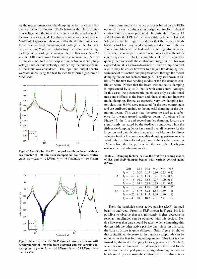
Figure 13 – FRF for the EA damped cantilever beam with ac-celerometer at 160 mm from clamped end for various controlgains: k0 = 0, k1 =−2 kVs/m, k2 =−6 kVs/m, k3 =−10 kVs/m.

102

103

−150

−140

−130

−120

−110

−100

−90

−80

−70

Vel

ocity

/Vol

tage

(m

/s/V

, dB

)

Frequency (Hz)

k0k1k2k3

Figure 14 – FRF for the SAP damped sandwich beam withaccelerometer at 130 mm from clamped end for various con-trol gains: k0 = 0, k1 = −10 kVs/m, k2 = −25 kVs/m, k3 =−40 kVs/m.

Some damping performance analyses based on the FRFsobtained for each configuration design and for four selectedcontrol gains are now presented. In particular, Figures 13and 14 show the FRF for the two cantilever beams: EA andSAP, respectively. Figure 13 shows that the velocity feed-back control law may yield a significant decrease in the re-sponse amplitude at the first and second eigenfrequencies.However, the same performance is not observed at the othereigenfrequencies. In fact, the amplitude at the fifth eigenfre-quency increases with the control gain magnitude. This wasexpected and it is a known downside of such a simple controllaw. It may be easier however to analyze the damping per-formance of this active damping treatment through the modaldamping factors for each control gain. They are shown in Ta-ble 3 for the first five bending modes of the EA damped can-tilever beam. Notice that the beam without active dampingis represented by k0 = 0, that is with zero control voltage.In this case, the piezoceramic patch acts only as additionalmass and stiffness to the beam and, thus, should not improvemodal damping. Hence, as expected, very low damping fac-tors (less than 0.4%) were measured for the zero control gainand are attributed mainly to the material damping of the alu-minum beam. This case may therefore be used as a refer-ence for the non-treated cantilever beam. As observed inFigure 13, the first and second modes damping factors aresignificantly increased by the feedback controller, while thefifth mode damping factor has a small overall decrease for thelarger control gain. Notice that, as it is well-known for directvelocity feedback controllers, this damping performance isvalid only for this selected position of the accelerometer, at160 mm from the clamp, for which the controller clearly pri-oritizes the first vibration mode.

Table 2 – Damping factors (%) for the first five bending modesof EA and SAP damped beams with various control gains(kVs/m).

Gain M 1 M 2 M 3 M 4 M 5k0 = 0 0.39 0.17 0.16 0.25 0.25

EA k1 = −2 4.12 1.29 0.21 0.63 0.32k2 = −6 10.9 3.83 0.27 1.20 0.27k3 =−10 14.9 6.99 0.33 1.71 0.22k0 = 0 3.49 1.85 0.90 0.98 1.25

SAP k1 =−10 5.75 5.22 1.84 1.39 1.18k2 =−25 8.17 11.3 4.09 1.90 1.13k3 =−40 10.8 18.7 9.91 2.41 1.02

Then, the sandwich shear active-passive (SAP) dampedbeam is analyzed. From its FRF, shown in Figure 14, it ispossible to observe that a significantly higher decrease inresonant amplitudes can be obtained with this design. No-tice however that care should be taken when comparing thisdesign with the other active-passive ones since, in this case,the base structure is quite different. Still, Figure 14 showsthat a significant decrease in the response amplitude can beobtained at the first four eigenfrequencies. This fact is con-firmed by the modal damping factors, presented in Table 3,where it can be observed that, although the third and fourthmodes are less damped passively, large damping factors canbe obtained by increasing the control gain. It is also notice-

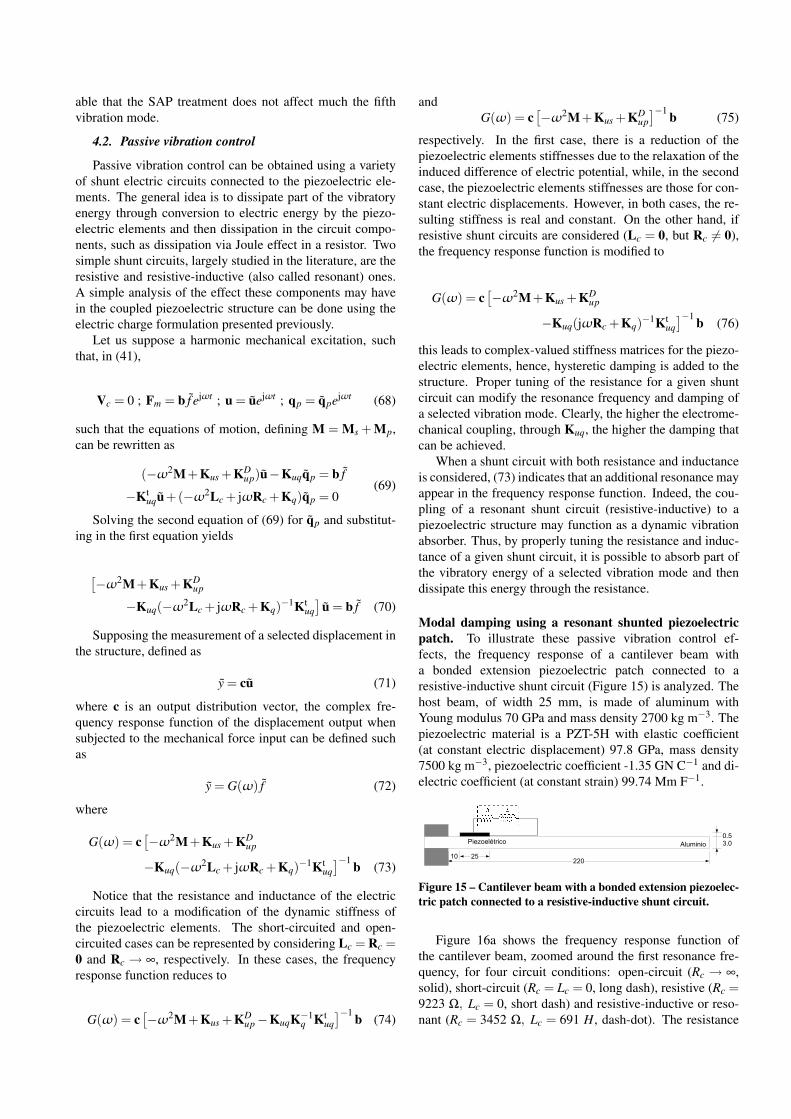
able that the SAP treatment does not affect much the fifthvibration mode.

4.2. Passive vibration control

Passive vibration control can be obtained using a varietyof shunt electric circuits connected to the piezoelectric ele-ments. The general idea is to dissipate part of the vibratoryenergy through conversion to electric energy by the piezo-electric elements and then dissipation in the circuit compo-nents, such as dissipation via Joule effect in a resistor. Twosimple shunt circuits, largely studied in the literature, are theresistive and resistive-inductive (also called resonant) ones.A simple analysis of the effect these components may havein the coupled piezoelectric structure can be done using theelectric charge formulation presented previously.

Let us suppose a harmonic mechanical excitation, suchthat, in (41),

Vc = 0 ; Fm = b f ejωt ; u = uejωt ; qp = qpejωt (68)

such that the equations of motion, defining M = Ms + Mp,can be rewritten as

(−ω2M+Kus +KDup)u−Kuqqp = b f

−Ktuqu+(−ω2Lc + jωRc +Kq)qp = 0

(69)

Solving the second equation of (69) for qp and substitut-ing in the first equation yields

[−ω2M+Kus +KD

up

−Kuq(−ω2Lc + jωRc +Kq)−1Ktuq]

u = b f (70)

Supposing the measurement of a selected displacement inthe structure, defined as

y = cu (71)

where c is an output distribution vector, the complex fre-quency response function of the displacement output whensubjected to the mechanical force input can be defined suchas

y = G(ω) f (72)

where

G(ω) = c[−ω2M+Kus +KD

up

−Kuq(−ω2Lc + jωRc +Kq)−1Ktuq]−1 b (73)

Notice that the resistance and inductance of the electriccircuits lead to a modification of the dynamic stiffness ofthe piezoelectric elements. The short-circuited and open-circuited cases can be represented by considering Lc = Rc =0 and Rc → ∞, respectively. In these cases, the frequencyresponse function reduces to

G(ω) = c[−ω2M+Kus +KD

up−KuqK−1q Kt

uq]−1 b (74)

andG(ω) = c

[−ω2M+Kus +KD

up]−1 b (75)

respectively. In the first case, there is a reduction of thepiezoelectric elements stiffnesses due to the relaxation of theinduced difference of electric potential, while, in the secondcase, the piezoelectric elements stiffnesses are those for con-stant electric displacements. However, in both cases, the re-sulting stiffness is real and constant. On the other hand, ifresistive shunt circuits are considered (Lc = 0, but Rc 6= 0),the frequency response function is modified to

G(ω) = c[−ω2M+Kus +KD

up

−Kuq(jωRc +Kq)−1Ktuq]−1 b (76)

this leads to complex-valued stiffness matrices for the piezo-electric elements, hence, hysteretic damping is added to thestructure. Proper tuning of the resistance for a given shuntcircuit can modify the resonance frequency and damping ofa selected vibration mode. Clearly, the higher the electrome-chanical coupling, through Kuq, the higher the damping thatcan be achieved.

When a shunt circuit with both resistance and inductanceis considered, (73) indicates that an additional resonance mayappear in the frequency response function. Indeed, the cou-pling of a resonant shunt circuit (resistive-inductive) to apiezoelectric structure may function as a dynamic vibrationabsorber. Thus, by properly tuning the resistance and induc-tance of a given shunt circuit, it is possible to absorb part ofthe vibratory energy of a selected vibration mode and thendissipate this energy through the resistance.

Modal damping using a resonant shunted piezoelectricpatch. To illustrate these passive vibration control ef-fects, the frequency response of a cantilever beam witha bonded extension piezoelectric patch connected to aresistive-inductive shunt circuit (Figure 15) is analyzed. Thehost beam, of width 25 mm, is made of aluminum withYoung modulus 70 GPa and mass density 2700 kg m−3. Thepiezoelectric material is a PZT-5H with elastic coefficient(at constant electric displacement) 97.8 GPa, mass density7500 kg m−3, piezoelectric coefficient -1.35 GN C−1 and di-electric coefficient (at constant strain) 99.74 Mm F−1.

25220

3.00.5

Piezoelétrico Aluminio

10

Figure 15 – Cantilever beam with a bonded extension piezoelec-tric patch connected to a resistive-inductive shunt circuit.

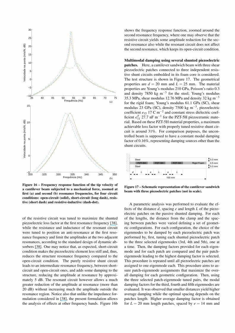
Figure 16a shows the frequency response function ofthe cantilever beam, zoomed around the first resonance fre-quency, for four circuit conditions: open-circuit (Rc → ∞,solid), short-circuit (Rc = Lc = 0, long dash), resistive (Rc =9223 Ω, Lc = 0, short dash) and resistive-inductive or reso-nant (Rc = 3452 Ω, Lc = 691 H, dash-dot). The resistance

35 40 45 50 55 60 65 70 75−10

−5

0

5

10

15

20

25

30

Vel

ocid

ade

na p

onta

(m

/s/N

, dB

)

Frequência (Hz) (a)

320 325 330 335 340 345 350−5

0

5

10

15

Vel

ocid

ade

na p

onta

(m

/s/N

, dB

)

Frequência (Hz) (b)

Figure 16 – Frequency response function of the tip velocity ofa cantilever beam subjected to a mechanical force, zoomed atfirst (a) and second (b) resonance frequencies, for four circuitconditions: open-circuit (solid), short-circuit (long dash), resis-tive (short dash) and resistive-inductive (dash-dot).

of the resistive circuit was tuned to maximize the shuntedpiezoelectric loss factor at the first resonance frequency [38],while the resistance and inductance of the resonant circuitwere tuned to position an anti-resonance at the first reso-nance frequency and limit the amplitudes at the two adjacentresonances, according to the standard design of dynamic ab-sorbers [38]. One may notice that, as expected, short-circuitcondition makes the piezoelectric element less stiff and, thus,reduces the structure resonance frequency compared to theopen-circuit condition. The purely resistive shunt circuitleads to an intermediate resonance frequency, between short-circuit and open-circuit ones, and adds some damping to thestructure, reducing the amplitude at resonance by approxi-mately 5 dB. The resonant circuit however allows a muchgreater reduction of the amplitude at resonance (more than20 dB) without increasing much the amplitude outside theresonance region. Notice also that unlike the impedance for-mulation considered in [38], the present formulation allowsthe analysis of effects at other frequency bands. Figure 16b

shows the frequency response function, zoomed around thesecond resonance frequency, where one may observe that theresistive circuit yields some amplitude reduction for the sec-ond resonance also while the resonant circuit does not affectthe second resonance, which keeps its open-circuit condition.

Multimodal damping using several shunted piezoelectricpatches. Here, a cantilever sandwich beam with three shearpiezoelectric patches connected to three independent resis-tive shunt circuits embedded in its foam core is considered.The test structure is shown in Figure 17. The geometricalproperties are d = 20 mm and L = 25 mm. The materialproperties are Young’s modulus 210 GPa, Poisson’s ratio 0.3and density 7850 kg m−3 for the steel; Young’s modulus35.3 MPa, shear modulus 12.76 MPa and density 32 kg m−3

for the rigid foam; Young’s modulus 61.1 GPa (SC), shearmodulus 23 GPa (SC), density 7500 kg m−3, piezoelectriccoefficient e15 17 C m−2 and constant stress dielectric coef-ficient εT

11 27.7 nF m−1 for the PZT-5H piezoceramic mate-rial. Based on these PZT-5H material properties, a maximumachievable loss factor with properly tuned resistive shunt cir-cuit is around 31%. For comparison purposes, the uncon-trolled beam is supposed to have a constant modal dampingfactor of 0.16%, representing damping sources other than theshunt circuits.

100 mm

d L e L e L

5.0 mm

5.0 mm0.5 mm

Steel

SteelPZT-5H Rigid FoamPZT-5H PZT-5H

Figure 17 – Schematic representation of the cantilever sandwichbeam with three piezoelectric patches (not in scale).

A parametric analysis was performed to evaluate the ef-fects of the distance d, spacing e and length L of the piezo-electric patches on the passive shunted damping. For eachof the lengths, the distance from the clamp and the spac-ing between patches were varied defining a set of geomet-ric configurations. For each configuration, the choice of theeigenmodes to be damped by each piezoelectric patch wasperformed by, first, tuning each shunted piezoelectric patchto the three selected eigenmodes (3rd, 4th and 5th), one ata time. Then, the damping factors provided for each eigen-mode and for each patch are compared and the pair patch-eigenmode leading to the highest damping factor is selected.This procedure is repeated until all piezoelectric patches areassigned to one eigenmode each. This procedure aims to as-sure patch-eigenmode assignments that maximize the over-all damping for each geometric configuration. Then, usingthe three selected patch-eigenmode tuned pairs, the modaldamping factors for the third, fourth and fifth eigenmodes areevaluated. It was observed that smaller distances yield higheraverage damping while the optimal spacing depends on thepatches length. Higher average damping factor is obtainedfor L = 20 mm length patches, spaced by e = 14 mm and

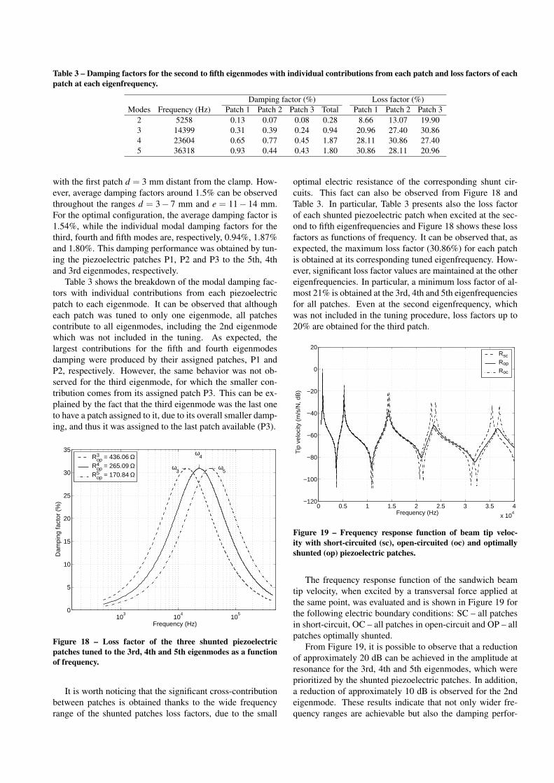
Table 3 – Damping factors for the second to fifth eigenmodes with individual contributions from each patch and loss factors of eachpatch at each eigenfrequency.

Damping factor (%) Loss factor (%)Modes Frequency (Hz) Patch 1 Patch 2 Patch 3 Total Patch 1 Patch 2 Patch 3

2 5258 0.13 0.07 0.08 0.28 8.66 13.07 19.903 14399 0.31 0.39 0.24 0.94 20.96 27.40 30.864 23604 0.65 0.77 0.45 1.87 28.11 30.86 27.405 36318 0.93 0.44 0.43 1.80 30.86 28.11 20.96

with the first patch d = 3 mm distant from the clamp. How-ever, average damping factors around 1.5% can be observedthroughout the ranges d = 3− 7 mm and e = 11− 14 mm.For the optimal configuration, the average damping factor is1.54%, while the individual modal damping factors for thethird, fourth and fifth modes are, respectively, 0.94%, 1.87%and 1.80%. This damping performance was obtained by tun-ing the piezoelectric patches P1, P2 and P3 to the 5th, 4thand 3rd eigenmodes, respectively.

Table 3 shows the breakdown of the modal damping fac-tors with individual contributions from each piezoelectricpatch to each eigenmode. It can be observed that althougheach patch was tuned to only one eigenmode, all patchescontribute to all eigenmodes, including the 2nd eigenmodewhich was not included in the tuning. As expected, thelargest contributions for the fifth and fourth eigenmodesdamping were produced by their assigned patches, P1 andP2, respectively. However, the same behavior was not ob-served for the third eigenmode, for which the smaller con-tribution comes from its assigned patch P3. This can be ex-plained by the fact that the third eigenmode was the last oneto have a patch assigned to it, due to its overall smaller damp-ing, and thus it was assigned to the last patch available (P3).

103

104

105

0

5

10

15

20

25

30

35

Frequency (Hz)

Dam

ping

fact

or (

%)

ω3 →

ω4

↓ ← ω5

Rop3 = 436.06 Ω

Rop4 = 265.09 Ω

Rop5 = 170.84 Ω

Figure 18 – Loss factor of the three shunted piezoelectricpatches tuned to the 3rd, 4th and 5th eigenmodes as a functionof frequency.

It is worth noticing that the significant cross-contributionbetween patches is obtained thanks to the wide frequencyrange of the shunted patches loss factors, due to the small

optimal electric resistance of the corresponding shunt cir-cuits. This fact can also be observed from Figure 18 andTable 3. In particular, Table 3 presents also the loss factorof each shunted piezoelectric patch when excited at the sec-ond to fifth eigenfrequencies and Figure 18 shows these lossfactors as functions of frequency. It can be observed that, asexpected, the maximum loss factor (30.86%) for each patchis obtained at its corresponding tuned eigenfrequency. How-ever, significant loss factor values are maintained at the othereigenfrequencies. In particular, a minimum loss factor of al-most 21% is obtained at the 3rd, 4th and 5th eigenfrequenciesfor all patches. Even at the second eigenfrequency, whichwas not included in the tuning procedure, loss factors up to20% are obtained for the third patch.

0 0.5 1 1.5 2 2.5 3 3.5 4

x 104

−120

−100

−80

−60

−40

−20

0

20

Frequency (Hz)

Tip

vel

ocity

(m

/s/N

, dB

)

Rsc

Rop

Roc

Figure 19 – Frequency response function of beam tip veloc-ity with short-circuited (sc), open-circuited (oc) and optimallyshunted (op) piezoelectric patches.

The frequency response function of the sandwich beamtip velocity, when excited by a transversal force applied atthe same point, was evaluated and is shown in Figure 19 forthe following electric boundary conditions: SC – all patchesin short-circuit, OC – all patches in open-circuit and OP – allpatches optimally shunted.

From Figure 19, it is possible to observe that a reductionof approximately 20 dB can be achieved in the amplitude atresonance for the 3rd, 4th and 5th eigenmodes, which wereprioritized by the shunted piezoelectric patches. In addition,a reduction of approximately 10 dB is observed for the 2ndeigenmode. These results indicate that not only wider fre-quency ranges are achievable but also the damping perfor-

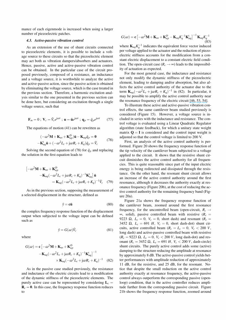
mance of each eigenmode is increased when using a largernumber of piezoelectric patches.

4.3. Active-passive vibration control

As an extension of the use of shunt circuits connectedto piezoelectric elements, it is possible to include a volt-age source to these circuits so that the piezoelectric elementmay act both as vibration dampers/absorbers and actuators.Hence, passive, active and active-passive vibration controlcan be obtained. In the particular case of the circuit pro-posed previously, composed of a resistance, an inductanceand a voltage source, it is worthwhile to analyze the activeand active-passive action, since the passive action is obtainedby eliminating the voltage source, which is the case treated inthe previous section. Therefore, a harmonic excitation anal-ysis similar to the one presented in the previous section canbe done here, but considering an excitation through a singlevoltage source, such that

Fm = 0 ; Vc = Vcejωt ; u = uejωt ; qp = qpejωt (77)

The equations of motion (41) can be rewritten as

(−ω2M+Kus +KDup)u−Kuqqp = 0

−Ktuqu+(−ω2Lc + jωRc +Kq)qp = Vc

(78)

Solving the second equation of (78) for qp and replacingthe solution in the first equation leads to

[−ω2M+Kus +KD

up

−Kuq(−ω2Lc + jωRc +Kq)−1Ktuq]

u

= Kuq(−ω2Lc + jωRc +Kq)−1Vc (79)

As in the previous section, supposing the measurement ofa selected displacement in the structure, defined as

y = cu (80)

the complex frequency response function of the displacementoutput when subjected to the voltage input can be definedsuch as

y = G(ω)Vc (81)

where

G(ω) = c[−ω2M+Kus +KD

up

−Kuq(−ω2Lc + jωRc +Kq)−1Ktuq]−1

×Kuq(−ω2Lc + jωRc +Kq)−1 (82)

As in the passive case studied previously, the resistanceand inductance of the electric circuits lead to a modificationof the dynamic stiffness of the piezoelectric elements. Thepurely active case can be represented by considering Lc =Rc = 0. In this case, the frequency response function reducesto

G(ω) = c[−ω2M+Kus +KD

up−KuqK−1q Kt

uq]−1 KuqK−1

q(83)

where KuqK−1q indicates the equivalent force vector induced

per voltage applied to the actuator and the reduction of piezo-electric stiffness accounts for the modification from a con-stant electric displacement to a constant electric field condi-tion. The open-circuit case (Rc→∞) leads to the impossibil-ity of actuation as expected.

For the most general case, the inductance and resistancenot only modify the dynamic stiffness of the piezoelectricelement, leading to damping and/or absorption, but also af-fects the active control authority of the actuator due to theterm Kuq(−ω2Lc + jωRc + Kq)−1 in (82). In particular, itmay be possible to amplify the active control authority nearthe resonance frequency of the electric circuit [46, 53, 54].

To illustrate these active and active-passive vibration con-trol effects, the same cantilever beam studied previously isconsidered (Figure 15). However, a voltage source is in-cluded in series with the inductance and resistance. The con-trol voltage is evaluated using a Linear Quadratic Regulatoralgorithm (state feedback), for which a unitary state weightmatrix Q = I is considered and the control input weight isadjusted so that the control voltage is limited to 200 V.

First, an analysis of the active control authority is per-formed. Figure 20 shows the frequency response function ofthe tip velocity of the cantilever beam subjected to a voltageapplied to the circuit. It shows that the resistive shunt cir-cuit diminishes the active control authority for all frequen-cies. This is quite reasonable since part of the input electricenergy is being redirected and dissipated through the resis-tance. On the other hand, the resonant shunt circuit allowsan increase of the active control authority around the firstresonance, although it decreases the authority exactly at res-onance frequency (Figure 20b), at the cost of reducing the ac-tive control authority for the remaining frequency band (Fig-ure 20a).

Figure 21a shows the frequency response function ofthe cantilever beam, zoomed around the first resonancefrequency, for the uncontrolled beam (open-circuit, Rc →∞, solid), passive controlled beam with resistive (Rc =9223 Ω, Lc = 0, Vc = 0, short dash) and resonant (Rc =3452 Ω, Lc = 691 H, Vc = 0, short dash-dot) shunt cir-cuits, active controlled beam (Rc = Lc = 0, Vc < 200 V ,long dash) and active-passive controlled beam with resistive(Rc = 9223 Ω, Lc = 0, Vc < 200 V , long dash-dot) and res-onant (Rc = 3452 Ω, Lc = 691 H, Vc < 200 V , dash-circle)shunt circuits. The purely active control adds some (active)damping to the structure reducing the amplitude at resonanceby approximately 8 dB. The active-passive control yields bet-ter performances with amplitude reduction of approximately11 dB, for the resistive, and 25 dB, for the resonant. No-tice that despite the small reduction on the active controlauthority exactly at resonance frequency, the active-passivecontrol always outperform the corresponding passive (open-loop) condition, that is the active controller reduces ampli-tude further from the corresponding passive circuit. Figure21b shows the frequency response function, zoomed around

102

103

−160

−140

−120

−100

−80

−60

−40

Vel

ocid

ade

na p

onta

(m

/s/V

, dB

)

Frequência (Hz) (a)

20 30 40 50 60 70 80 90 100−90

−85

−80

−75

−70

−65

−60

−55

−50

−45

−40

−35

Vel

ocid

ade

na p

onta

(m

/s/V

, dB

)

Frequência (Hz) (b)

Figure 20 – Comparison of active control authority for thepurely active and resistive and inductive active-passive circuitsfor whole frequency range (a) and zoomed around the first res-onance frequency.

the second resonance frequency, where one may observe thatthe purely active and resistive, passive, active and active-passive, circuits yield some amplitude reduction for the sec-ond resonance also while the resonant circuit does not allowcontrol of the second resonance, since it limits both activeand passive effects to a narrow frequency-band around thefirst resonance, for which the inductance was tuned.

5. CONCLUDING REMARKS

The present article has presented a brief review of theopen literature concerning applications of piezoelectric sen-sors and actuators for active and passive vibration control.Some recent advances on this subject were also presentedwith special attention to the following aspects: i) modeling ofstructures with piezoelectric sensors and actuators, ii) evalu-ation of the effective electromechanical coupling coefficient,iii) applications for active and passive vibration control. Itwas shown that piezoelectric materials can be quite effec-tive as distributed sensors and actuators for active, passive

35 40 45 50 55 60 65 70 75−10

−5

0

5

10

15

20

25

30

Vel

ocid

ade

na p

onta

(m

/s/N

, dB

)

Frequência (Hz) (a)

320 325 330 335 340 345 350−5

0

5

10

15

Vel

ocid

ade

na p

onta

(m

/s/N

, dB

)

Frequência (Hz) (b)

Figure 21 – Frequency response function of the tip velocityof a cantilever beam subjected to a mechanical force, zoomedat first (a) and second (b) resonance frequencies, for: open-circuit (solid), passive resistive (short dash), passive resistive-inductive (short dash-dot), active (long dash), active-passiveresistive (long dash-dot) and active-passive resistive-inductive(dash-circle).

and active-passive vibration control. In particular, impor-tant design parameters include: effective electromechanicalcoupling coefficient, actuation/sensing mechanism or mode,patches size and location. It was also shown that proper de-sign should include electromechanical coupled models forthe ensemble structure-patches-circuits.

ACKNOWLEDGEMENTS

This research was supported by the State of São PauloResearch Foundation (FAPESP), through research grant04/10255-7, which is gratefully acknowledged. The authoralso thanks Prof. Ayech Benjeddou for his valuable inputsand the authors’ students Heinsten Santos, Rafael Azevedo,Carlos Maio for generating part of the presented results.

REFERENCES

[1] M. Sunar and S.S. Rao. Recent advances in sensing andcontrol of flexible structures via piezoelectric materi-als technology. Applied Mechanics Review, 52(1):1–16,1999.

[2] M. Ahmadian and A.P. DeGuilio. Recent advances inthe use of piezoceramics for vibration suppression. TheShock and Vibration Digest, 33(1):15–22, 2001.

[3] S.O. Reza Moheimani. A survey of recent innovationsin vibration damping and control using shunted piezo-electric transducers. IEEE Transactions on Control Sys-tems Technology, 11(4):482–494, 2003.

[4] I. Chopra. Review of state of art of smart structures andintegrated systems. AIAA Journal, 40(11):2145–2187,2002.

[5] M.A. Trindade and A. Benjeddou. Hybrid active-passive damping treatments using viscoelastic andpiezoelectric materials: review and assessment. Jour-nal of Vibration and Control, 8(6):699–746, 2002.

[6] C.T. Sun and X.D. Zhang. Use of thickness-shear modein adaptive sandwich structures. Smart Materials andStructures, 4(3):202–206, 1995.

[7] A. Benjeddou, M.A. Trindade, and R. Ohayon. A uni-fied beam finite element model for extension and shearpiezoelectric actuation mechanisms. Journal of Intel-ligent Material Systems and Structures, 8(12):1012–1025, 1997.

[8] A. Benjeddou, M.A. Trindade, and R. Ohayon. Newshear actuated smart structure beam finite element.AIAA Journal, 37(3):378–383, 1999.

[9] A. Benjeddou, M.A. Trindade, and R. Ohayon. Piezo-electric actuation mechanisms for intelligent sandwichstructures. Smart Materials and Structures, 9(3):328–335, 2000.

[10] O.J. Aldraihem and A.A. Khdeir. Smart beams withextension and thickness-shear piezoelectric actuators.Smart Materials and Structures, 9(1):1–9, 2000.

[11] A.A. Khdeir and O.J. Aldraihem. Deflection analysis ofbeams with extension and shear piezoelectric patchesusing discontinuity functions. Smart Materials andStructures, 10(2):212–220, 2001.

[12] O.J. Aldraihem and A.A. Khdeir. Exact deflection solu-tions of beams with shear piezoelectric actuators. Inter-national Journal of Solids and Structures, 40(1):1–12,2003.

[13] M.A. Trindade, A. Benjeddou, and R. Ohayon. Para-metric analysis of the vibration control of sandwichbeams through shear-based piezoelectric actuation.Journal of Intelligent Material Systems and Structures,10(5):377–385, 1999.

[14] S. Raja, R. Sreedeep, and G. Prathap. Bending behav-ior of hybrid-actuated piezoelectric sandwich beams.Journal of Intelligent Material Systems and Structures,

15(8):611–619, 2004.

[15] B.P. Baillargeon and S.S. Vel. Active vibration suppres-sion of sandwich beams using piezoelectric shear actu-ators: experiments and numerical simulations. Jour-nal of Intelligent Material Systems and Structures,16(6):517–530, 2005.

[16] S.S. Vel and R.C. Batra. Exact solution for the cylindri-cal bending of laminated plates with embedded piezo-electric shear actuators. Smart Materials and Struc-tures, 10(2):240–251, 2001.

[17] L. Edery-Azulay and H. Abramovich. Piezoelectricactuation and sensing mechanisms - closed form solu-tions. Composite Structures, 64(3-4):443–453, 2004.

[18] M.A. Trindade. Simultaneous extension and shearpiezoelectric actuation for active vibration control ofsandwich beams. Journal of Intelligent Material Sys-tems and Structures, 18(6):591–600, 2007.

[19] A. Benjeddou. Shear-mode piezoceramic advanced ma-terials and structures: a state of the art. Mechanicsof Advanced Materials and Structures, 14(4):263–275,2007.

[20] G.A. Lesieutre and C.L. Davis. Can a coupling coeffi-cient of a piezoelectric device be higher than those ofits active material? Journal of Intelligent Material Sys-tems and Structures, 8(10):859–867, 1997.

[21] W.P. Mason. Piezoelectric crystals and their applica-tion to ultrasonics. Van Nostrand, New York, 1950.

[22] A.F. Ulitko. On the theory of electromechanical con-version of energy in nonuniformly deformed piezoce-ramic bodies. Prikladnaya Mekhanika, 13(10):115–123, 1977.

[23] S.H. Chang, N.N. Rogacheva, and C.C. Chou. Analysisof methods for determining electromechanical couplingcoefficients of piezoelectric elements. IEEE Trans-actions on Ultrasonics, Ferroelectrics, and FrequencyControl, 42(4):630–640, 1995.

[24] B. Aronov. On the optimization of the effective elec-tromechanical coupling coefficients of a piezoelectricbody. Journal of the Acoustical Society of America,114(2):792–800, 2003.

[25] N.N. Rogacheva, C.C. Chou, and S.H. Chang. Elec-tromechanical analysis of a symmetric piezoelec-tric/elastic laminate structure: theory and experiment.IEEE Transactions on Ultrasonics, Ferroelectrics, andFrequency Control, 45(2):285–294, 1998.

[26] S. Basak, A. Raman, and S.V. Garimella. Dynamicresponse optimization of piezoelectrically excited thinresonant beams. Journal of Vibration and Acoustics,127(1):18–27, 2005.

[27] H. Boudaoud, A.Benjeddou, E.M. Daya, and S. Belou-ettar. Analytical evaluation of the effective emcc ofsandwich beams with a shear-mode piezoceramic core.In Proceedings of Second International Conference onDesing and Modelling of Mechanical Systems, Monas-

tir, Tunisia, March 19-21 2007.

[28] M. Naillon, R.H. Coursant, and F. Besnier. Analyse destructures piézoélectriques par une méthode d’élémentsfinis. Acta Electronica, 25(4):341–362, 1983.

[29] T. Bailey and J.E. Hubbard Jr. Distributedpiezoelectric-polymer active vibration control of a can-tilever beam. Journal of Guidance, 8(5):605–, 1985.

[30] E.F. Crawley and J. deLuis. Use of piezoelectric actua-tors as elements of intelligent structures. AIAA Journal,25(10):1373–1385, 1987.

[31] E.F. Crawley and E.H. Anderson. Detailed models ofpiezoceramic actuation of beams. Journal of IntelligentMaterial Systems and Structures, 1(1):4–25, 1990.

[32] M.-H. Herman Shen. Analysis of beams containingpiezoelectric sensors and actuators. Smart Materialsand Structures, 3(4):439–447, 1994.

[33] C.K. Lee. Theory of laminated piezoelectric plates forthe design of distributed sensors/actuators. part i: gov-erning equations and reciprocal relationships. Journalof the Acoustical Society of America, 87:1145U1157,1990.

[34] D.A. Saravanos and P.R. Heyliger. Mechanics and com-putational models for laminated piezoelectric beams,plates, and shells. Applied Mechanics Review,52(10):305–320, 1999.

[35] S.V. Gopinathan, V.V. Varadan, and V.K. Varadan. Areview and critique of theories for piezoelectric lami-nates. Smart Materials and Structures, 9:24–48, 2000.

[36] A. Benjeddou. Advances in piezoelectric finite el-ements modeling of adaptive structural elements: asurvey. Computers and Structures, 76(1-3):347–363,2000.

[37] R.L. Forward. Electronic damping of vibrations in op-tical structures. Applied Optics, 18(5):690–697, 1979.

[38] N.W. Hagood and A. von Flotow. Damping of struc-tural vibrations with piezoelectric materials and passiveelectrical networks. Journal of Sound and Vibration,146(2):243–268, 1991.

[39] C.H. Park and D.J. Inman. Enhanced piezoelectricshunt design. Shock and Vibration, 10:127–133, 2003.

[40] F.A.C. Viana and V. Steffen Jr. Multimodal vibrationdamping through piezoelectric patches and optimal res-onant shunt circuits. Journal of the Brazilian Society ofMechanical Sciences, 28(3):293–310, 2006.

[41] S. Raja, G. Prathap, and P.K. Sinha. Active vibrationcontrol of composite sandwich beams with piezoelec-tric extension-bending and shear actuators. Smart Ma-terials and Structures, 11(1):63–71, 2002.

[42] A. Benjeddou and J.-A. Ranger-Vieillard. Passive vi-bration damping using shunted shear-mode piezoce-ramics. In B.H.V. Topping and C.A. Mota Soares, ed-itors, Proceedings of the Seventh International Confer-ence on Computational Structures Technology, page #4,

Stirling, Scotland, 2004. Civil-Comp Press.

[43] M.A. Trindade and C.E.B. Maio. Passive vibration con-trol of sandwich beams using shunted shear piezoelec-tric actuators. In IV ABCM National Congress of Me-chanical Engineering, Recife, Brazil, August 2006.

[44] M.A. Trindade and C.E.B. Maio. Multimodal passivevibration control of sandwich beams with shunted shearpiezoelectric materials. In 19th International Congressof Mechanical Engineering (COBEM), Brasília, 2007.

[45] J. Tang, Y. Liu, and K.W. Wang. Semiactive and active-passive hybrid structural damping treatments via piezo-electric materials. The Shock and Vibration Digest,32(3):189–200, 2000.

[46] M.S. Tsai and K.W. Wang. On the structural damp-ing characteristics of active piezoelectric actuatorswith passive shunt. Journal of Sound and Vibration,221(1):1–22, 1999.

[47] A. Benjeddou and J.-A. Ranger. Use of shunted shear-mode piezoceramics for structural vibration passivedamping. Computers and Structures, 84:1415–1425,2006.

[48] The Institute of Electrical and Electronics EngineersInc. IEEE Standard on Piezoelectricity n.176-1987.1987.

[49] The Institute of Radio Engineers. IRE standards onpiezoelectric crystals: Determination of the elastic,piezoelectric, and dielectric constants - the electrome-chanical coupling factor. Proceedings of the IRE,46(4):764–778, 1958.

[50] C.D. Johnson, D.A. Kienholz, and L.C. Rogers. Fi-nite element prediction of damping in beams with con-strained viscoelastic layers. Shock and Vibration Bul-letin, 50(1):71–81, 1981.

[51] G. Chevallier, J.-A. Ranger, A.Benjeddou, and H. Seb-bah. Passive vibration damping using resistivelyshunted piezoceramics: an experimental performanceevaluation. In Proceedings of Second InternationalConference on Desing and Modelling of MechanicalSystems, Monastir, Tunisia, March 19-21 2007.

[52] W.G. Cady. Piezoelectricity: An introduction to the the-ory and applications of electromechanical phenomenain crystals. McGraw-Hill, New York, 1946.

[53] C. Niezrecki and H.H. Cudney. Improving the powerconsumption characteristics of piezoelectric actuators.Journal of Intelligent Material Systems and Structures,5(4):522–529, 1994.

[54] J. Sirohi and I. Chopra. Actuator power reduction usingL-C oscillator circuits. Journal of Intelligent MaterialSystems and Structures, 12(12):867–877, 2001.