Engineering Applications of Computational Fluid Mechanics Vol. 7, No. 4, pp. 486–495 (2013)

Received: 9 Apr. 2013; Revised: 4 Jul. 2013; Accepted: 29 Jul. 2013

486

APPLICATION OF GENERALIZED RNG TURBULENCE MODEL TO

FLOW IN MOTORED SINGLE-CYLINDER PFI ENGINE

Fang Wang *, Rolf D. Reitz **, Cecile Pera #, Zhi Wang *† and Jianxin Wang *

* Department of Automotive Engineering, Tsinghua University, Beijing, 100084, P.R. China † E-Mail: wangzhi@tsinghua.edu.cn (Corresponding Author)

** Department of Mechanical Engineering, University of Wisconsin-Madison, 1018A Engineering

Research Building ,1500 Engineering Drive , Madison, WI 53706, USA # IFP Energies Nouvelles, 1 & 4, Avenue de Bois-Awning ,92852 Rueil-Malmaison Cedex, France

ABSTRACT: This paper describes a generalized renormalization group (RNG) turbulence model applied to

simulate non-reacting flows in an optical single-cylinder PFI engine. A structured computational mesh of the

combustion system with complex geometry was generated by ICEM-CFD in conjunction with KIVA-3V code.

Turbulent flow in the 4-valve engine, including the exhaust, intake, compression and expansion strokes, was

simulated with the standard k and a generalized RNG turbulence model using the KIVA-3V code. Crank angle-

resolved results from available experimental data were used as the boundary and initial conditions for the calculation

setup. Pressure traces of the simulation results were compared to the phase-averaged measured pressure trace.

Predicted radial and vertical velocities along a horizontal line at BDC and radial velocities along the cylinder axis at

four crank angles were compared with the experimental measurements. In addition, the velocity field calculated by

the generalized RNG turbulence model was compared with experimental data from Particle Image Velocimetry

(PIV) measurements. Good agreement was found between the experiment results and simulation results with the

generalized RNG turbulence model.

Keywords: internal combustion engine, RANS, generalized RNG model, structured grids

1. INTRODUCTION

In internal combustion (IC) engines, a highly

transient flow field is accompanied with

geometric complexity, which makes it still one of

the most difficult applications of turbulence

prediction. Thanks to the rapid development in

computer technology for computational fluid

dynamics (CFD), three-dimensional numerical

simulation is rapidly becoming a powerful tool

for engine design and optimization. In spite of

much progress in the development of CFD

models, choosing an appropriate turbulence

model for a certain problem to obtain results

consistent with experimental measurements is still

an arduous process for engineers.

Generally, there are three methods for turbulent

flow prediction: direct numerical simulation

(DNS), large eddy simulation (LES) and

Reynolds average Navier-Stokes (RANS)

simulation. In DNS (Pope, 2000), the Navier-

Stokes equations are highly resolved to simulate

the flow. DNS is computational expensive as all

length scales and time scales have to be resolved,

with the result that this approach is limited to

flows with low-to-moderate Reynolds numbers.

In LES, the equations are solved for a filtered

velocity field which represents the larger-scale

turbulent motions, and the influence of the

smaller-scale motions, which are not directly

represented, are calculated by a subgrid

turbulence model. Although it offers advantages

for engine simulations, including higher-fidelity

and the potential of predicting cycle-to-cycle

variations in flow structures compared to the

RANS method, LES is still under development

for industrial applications and engine design due

to the high computational overload. In addition,

there is the need to modify other corresponding

models such as spray models and turbulent

combustion models to achieve satisfying

simulations of the mixture formation and

combustion process in IC engines.

In RANS, the two-equation k model is the

most widely used. For the relatively simple two-

equation k model, a simple constitutive

relation is adopted for the turbulence stresses

which may introduce inaccuracies, however, it

has been shown to correctly predict many

measurements of engine performance and it is

currently the most widely used turbulence model

for combustion system optimization and design

using CFD simulations.

Engineering Applications of Computational Fluid Mechanics Vol. 7, No. 4 (2013)

487

Despite over three decades of use, in some cases

associated with the prediction of flows with bulk

compression, the prediction results are not fully

satisfactory (Miles et al., 2007; Miles, 2010;

Morel and Mansour, 1982; Tian and Lu, 2013;

Wu et al., 1985). Specifically, the modeling of the

dissipation rate of turbulent kinetic energy, when

the model constants of the transport equation are

optimized for the compression process, leads to

an unrealistic growth of turbulent time and length

scales during the expansion process (Miles et al.,

2007; Miles, 2010). One promising approach to

solving this problem is to employ model

coefficients that vary with the characteristic strain

rate of the compression flow. The model

coefficients of the dissipation rate transport

equation, which are modeled based on such

analysis have shown the potential for better

predictions. Based on the„dimensionality‟ of the

flow strain rate, a generalized RNG closure model

was proposed by Wang and Reitz (Wang et al.,

2011) to improve the predictions of turbulence

quantities for compressible flows. In this

turbulence model, the model coefficients C1, C2,

and C3 in the transport equation of the turbulent

kinetic energy dissipation rate are all functions of

the local flow strain rate. This modeling approach

was validated using the results of direct numerical

simulation (DNS) analysis and the model was

also applied to compressible jet flows and

complex diesel engine flows. The results agreed

well with experimental data, and significant

improvements were found.

In the present work, the generalized RNG

turbulence model is further applied to a single-

cylinder PFI engine. Averaged in-cylinder

pressure traces of the simulation results were

compared to the experimental data to verify the

set up for the predictions. Predicted radial and

vertical velocities at different crank angles with

the standard k model and the generalized

RNG turbulence model were compared with the

experimental measurements. In addition, the

velocity fields calculated by the generalized RNG

turbulence model were compared with the

experimental data from PIV measurements. In

addition, „dimensionality‟ analysis and

comparison of averaged predictions of intake

flows with the two turbulence models was made

to futher investigate the performance of the

generalized RNG turbulence model.

2. TURBULENCE MODELING

2.1 Standard k model

For the standard k model applied to a

compressible turbulent flow, two transport

equations are solved for the turbulence quantities

k and .

kDiffusion

DP

Dt (1)

2

1 2 3 ( ) DiffusionD P

C C CDt k k

u

(2)

where u is the mean velocity vector. The

production of turbulent kinetic energy is

calculated by

i j ijP u u S (3)

Based on the turbulent-viscosity hypothesis,

2 12 ( ( u) )

3 3i j ij t ij iju u k S (4)

where ijS is the mean strain rate calculated by

1( / / ),

2i j j iu x u x and the turbulent

viscosity t is given by 2 /C k ,where C , 1C ,

2C and 3C are model constants with standard

values due to Lauder and Sharma (1974).

However, the accuracy of simulation results can

be improved by adjusting the values of the k

model constants for any particular case.

Therefore, it is of inherent necessity to explore

more general turbulence model treatments.

2.2 Generalized RNG closure mode

An improved two equation eddy viscosity

turbulence model based on a generalized RNG

closure proposed by Wang et al. (2011) is

described in this section. By averaging the

equations of motion over infinitesimal bands of

small scales and collecting the effect of the scale

removal process in a modified viscosity, the

Renormalization Group (RNG) method of Yakhot

and Orszag (1986), Yakhot and Smith (1992), and

Smith and Reynolds (1992) successfully removes

the impact of smaller scale structures on the larger

ones. This approach has been used to derive the

k and equation from the N-S equations,

including providing numerical values for the

Engineering Applications of Computational Fluid Mechanics Vol. 7, No. 4 (2013)

488

model constants in the transport equations. The

transport equation finally becomes

2

1 2 DiffusionD P

C C RDt k k

(5)

where the additional term, R, represents the effect

of flow strain rate on the dissipation rate, and is

modeled by Yakhot et al. (1992) as:

3 20

3

(1 / )

1

CR

k

(6)

where the ratio of the turbulent-to-mean strain

time scale is given by / ,Sk and 1/2(2 )i j i jS S S is the magnitude of the mean

strain. To consider compressibility in the RNG

analysis, Han and Reitz (1995) introduced an

extra term 3 ( )C u in the equation under

the spherical compression assumption, where

11 22 33 ( ).S S S u The behavior of the

RNG turbulence model was examined in the rapid

distortion limit, and the model coefficient 3C was

given by

1 03

0 0

64 2 1 1( 1)

3 ( u) 3

1 ( ) 0

0 ( ) 0

CC dC

dt

if

if

u

u

(7)

where 0 is the fluid molecular viscosity which

depends on mT for isentropic compression of a

fluid with a specific heat ratio , where T

represents the fluid temperature and the

superscript m us a variable exponent. With

1.4 and 0.5m the second term on the

right hand side of Equation (7) is approximated as

0

0

1 11 ( 1) 0.8

( u)

dm

dt

(8)

Finally, the equation of the standard RNG

turbulence model is written as

2

1 2 3 ( ) DiffusionD P

C C C RDt k k

u

(9)

A generalized RNG turbulence model based on

the local „dimensionality‟ of the flow field was

proposed by Wang and Reitz (Wang et al., 2011)

to improve the predictions of turbulent flow. In

this turbulence model, the model constants in the

equation are all assumed to be functions of the

flow strain rate. The generalized RNG turbulence

model showed more accurate predictions when

compared to experimental data for two pure

compression cases: a 1-D unidirectional axial

compression and a 2-D cylinder-radial

compression.

The final version of the dissipation rate equation

is

22

1 1 2

3

' ( u)

( u)

t n

Diffusion

D PC C C

Dt k k k

C R

(10)

where the model coefficients 1 'C and 3C are

calculated by

1 1

2' (1 )

3C a C (11)

3 1

1 2 2(1 )( 1)

3 3

n aC C C C

n

(12)

where, a and n are parameters determined by the

local „dimensionality‟ of the flow compression,

which is given by

11

2 2 2 2

22 33 11 22 333( ) / ( ) 1a S S S S S S

(13)

3 2n a (14)

The indices “1”, “2”, “3” in Equation (13)

represent the three directions in a Cartersian

coordinate system. For a given compression case,

the recommended “dimensionality” a and n of the

strain rate field would be 2.0 and 1.0 for

unidirectional 1-D compression, 0.5 and 2.0 for

cylindrical-radial 2-D compression, 0.0 and 3.0

for spherical 3-D compression, respectively.

The model coefficient 2nC which governs the rate

of decay of isotropic turbulence was suggested to

be

2

2 0 1 2nC b b n b n (15)

Based on calibrations using incompressible jet

flows (Wang et al., 2011), the model constants

0 ,b 1,b 2b are 2.0725, -0.3865 and 0.083,

respectively.

In the R term defined by Equation (6), the fixed

point equilibrium value 0 and the model

coefficient are determined in the same way as

in the standard RNG closure model suggested by

Yakhot and Orszag (1986).

Engineering Applications of Computational Fluid Mechanics Vol. 7, No. 4 (2013)

489

The fixed point equilibrium value 0 is given by

1/2

0 2 1[( 1) / ( 1)]C C C (16)

and the model coefficient is modeled by

establishing a direct constraint relationship with

the von Karman constant with an assumption

of a turbulent log layer and

neglect of convection effects as follows:

1/202 1 3

(1 / )[( ( )) / ]

1C C C

(17)

For the simulation of near-wall turbulence, the

traditional wall function approach (Reitz, 1991)

was applied to give reasonable wall heat transfer

with affordable grid sizes for engineering

predictions. With the assumption that the

turbulence production is that of a turbulent

boundary layer, the boundary conditions for k

and are

= 0k n (18)

and

3/4 3/2

=C k

y

(19)

where n is the unit vector normal to the wall, and

y is the physical distance from the nearest wall.

3. EXPERIMENTAL AND CALCULATION

SETUP

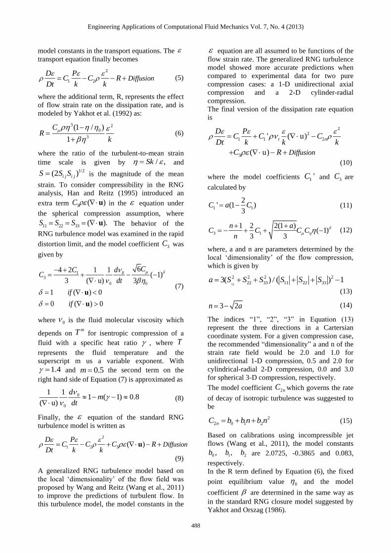
The complete SGEmac engine test bench set-up

of Lacour and Pera (2011) is shown in Fig. 1. Air

is introduced into the intake volume while fuel is

injected into a large mixing plenum for fired

engine cases. As the result of the two large

volumes in the intake path, perturbation at the

intake volume inlet is avoided, and the boundary

conditions are considered to be nearly constant at

this location. Similarly, the exhaust line involves

a large volume for the purpose of dampening

exhaust perturbations. The experimental engine is

a single-cylinder SI engine equipped with a 4-

valve pent-roof combustion chamber and a flat

piston head. The main engine specifications are

shown in Table 1. Several pressure transducers

are used to record at one crank angle resolution

the pressure evolution along the intake and

exhaust ports. The in-cylinder velocity field is

measured using a PIV method. Velocities are

measured under motored operation through a

quartz cylinder liner in a vertical plane, since the

in-cylinder fluid motion is mainly a tumble

Fig. 1 SGEmac engine test bench.

Table 1 Main engine specifications.

Engine Type Single-cylinder

Number of Valves 4

Displacement 441 cm3

Stroke 83.5 mm

Bore 82 mm

Connecting Rod 144 mm

Compression Ratio 9.9:1

IVO (at 0.7 mm) 372 CAD

IVC (at 0.7 mm) 578 CAD

EVO (at 0.7 mm) 140 CAD

EVC (at 0.7 mm) 348 CAD

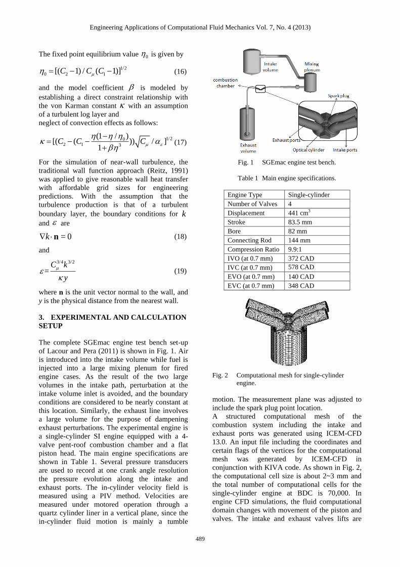
Fig. 2 Computational mesh for single-cylinder

engine.

motion. The measurement plane was adjusted to

include the spark plug point location.

A structured computational mesh of the

combustion system including the intake and

exhaust ports was generated using ICEM-CFD

13.0. An input file including the coordinates and

certain flags of the vertices for the computational

mesh was generated by ICEM-CFD in

conjunction with KIVA code. As shown in Fig. 2,

the computational cell size is about 2~3 mm and

the total number of computational cells for the

single-cylinder engine at BDC is 70,000. In

engine CFD simulations, the fluid computational

domain changes with movement of the piston and

valves. The intake and exhaust valves lifts are

Engineering Applications of Computational Fluid Mechanics Vol. 7, No. 4 (2013)

490

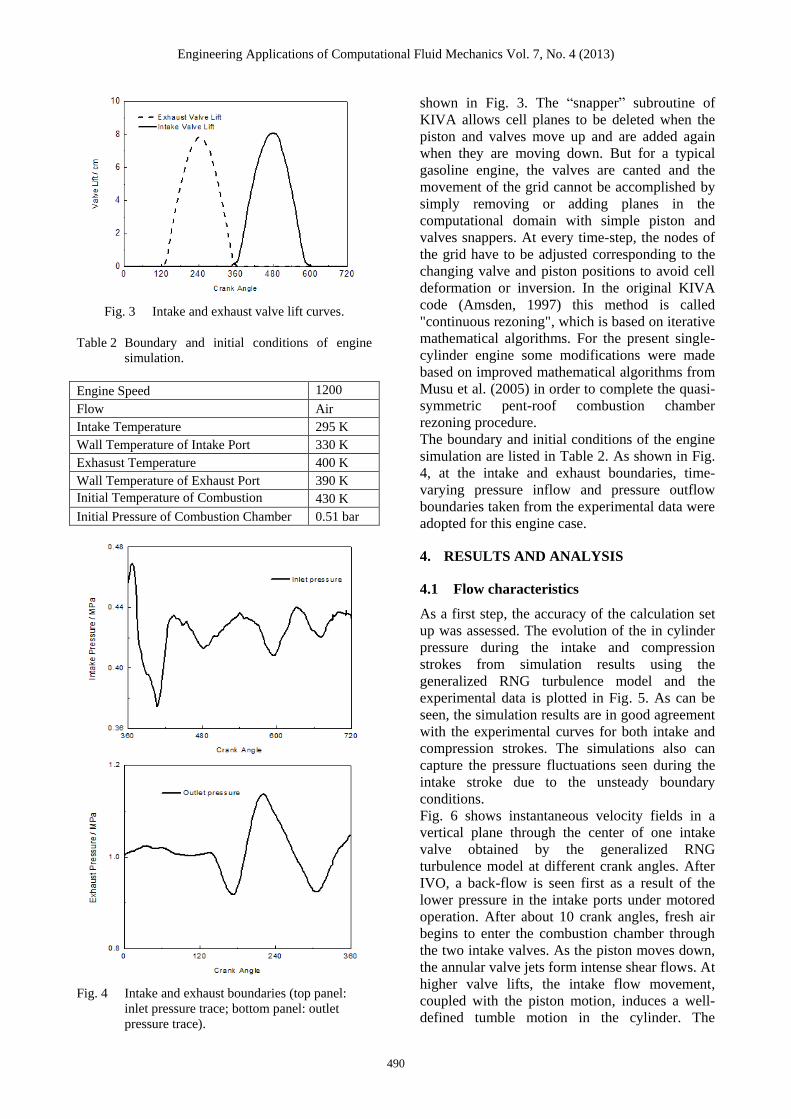
Fig. 3 Intake and exhaust valve lift curves.

Table 2 Boundary and initial conditions of engine

simulation.

Engine Speed 1200

r/min Flow Air

Intake Temperature 295 K

Wall Temperature of Intake Port 330 K

Exhasust Temperature 400 K

Wall Temperature of Exhaust Port 390 K

Initial Temperature of Combustion

Chamber 430 K

Initial Pressure of Combustion Chamber 0.51 bar

Fig. 4 Intake and exhaust boundaries (top panel:

inlet pressure trace; bottom panel: outlet

pressure trace).

shown in Fig. 3. The “snapper” subroutine of

KIVA allows cell planes to be deleted when the

piston and valves move up and are added again

when they are moving down. But for a typical

gasoline engine, the valves are canted and the

movement of the grid cannot be accomplished by

simply removing or adding planes in the

computational domain with simple piston and

valves snappers. At every time-step, the nodes of

the grid have to be adjusted corresponding to the

changing valve and piston positions to avoid cell

deformation or inversion. In the original KIVA

code (Amsden, 1997) this method is called

"continuous rezoning", which is based on iterative

mathematical algorithms. For the present single-

cylinder engine some modifications were made

based on improved mathematical algorithms from

Musu et al. (2005) in order to complete the quasi-

symmetric pent-roof combustion chamber

rezoning procedure.

The boundary and initial conditions of the engine

simulation are listed in Table 2. As shown in Fig.

4, at the intake and exhaust boundaries, time-

varying pressure inflow and pressure outflow

boundaries taken from the experimental data were

adopted for this engine case.

4. RESULTS AND ANALYSIS

4.1 Flow characteristics

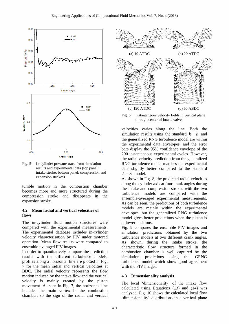
As a first step, the accuracy of the calculation set

up was assessed. The evolution of the in cylinder

pressure during the intake and compression

strokes from simulation results using the

generalized RNG turbulence model and the

experimental data is plotted in Fig. 5. As can be

seen, the simulation results are in good agreement

with the experimental curves for both intake and

compression strokes. The simulations also can

capture the pressure fluctuations seen during the

intake stroke due to the unsteady boundary

conditions.

Fig. 6 shows instantaneous velocity fields in a

vertical plane through the center of one intake

valve obtained by the generalized RNG

turbulence model at different crank angles. After

IVO, a back-flow is seen first as a result of the

lower pressure in the intake ports under motored

operation. After about 10 crank angles, fresh air

begins to enter the combustion chamber through

the two intake valves. As the piston moves down,

the annular valve jets form intense shear flows. At

higher valve lifts, the intake flow movement,

coupled with the piston motion, induces a well-

defined tumble motion in the cylinder. The

Engineering Applications of Computational Fluid Mechanics Vol. 7, No. 4 (2013)

491

Fig. 5 In-cylinder pressure trace from simulation

results and experimental data (top panel:

intake stroke; bottom panel: compression and

expansion strokes).

tumble motion in the combustion chamber

becomes more and more structured during the

compression stroke and disappears in the

expansion stroke.

4.2 Mean radial and vertical velocities of

flows

The in-cylinder fluid motion structures were

compared with the experimental measurements.

The experimental database includes in-cylinder

velocity characterisation by PIV under motored

operation. Mean flow results were compared to

ensemble-averaged PIV images.

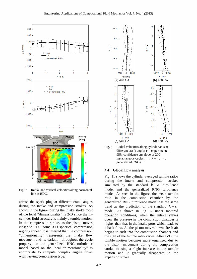
In order to quantitatively compare the prediction

results with the different turbulence models,

profiles along a horizontal line are plotted in Fig.

7 for the mean radial and vertical velocities at

BDC. The radial velocity represents the flow

motion induced by the intake flow and the vertical

velocity is mainly created by the piston

movement. As seen in Fig. 7, the horizontal line

includes the main vortex in the combustion

chamber, so the sign of the radial and vertical

(a) 10 ATDC (b) 20 ATDC

(c) 120 ATDC (d) 60 ABDC

Fig. 6 Instantaneous velocity fields in vertical plane

through center of intake valve.

velocities varies along the line. Both the

simulation results using the standard k and

the generalized RNG turbulence model are within

the experimental data envelopes, and the error

bars display the 95% confidence envelope of the

200 instantaneous experimental cycles. However,

the radial velocity prediction from the generalized

RNG turbulence model matches the experimental

data slightly better compared to the standard

k model.

As shown in Fig. 8, the predicted radial velocities

along the cylinder axis at four crank angles during

the intake and compression strokes with the two

turbulence models are compared with the

ensemble-averaged experimental measurements.

As can be seen, the predictions of both turbulence

models are mainly within the experimental

envelopes, but the generalized RNG turbulence

model gives better predictions when the piston is

at lower positions.

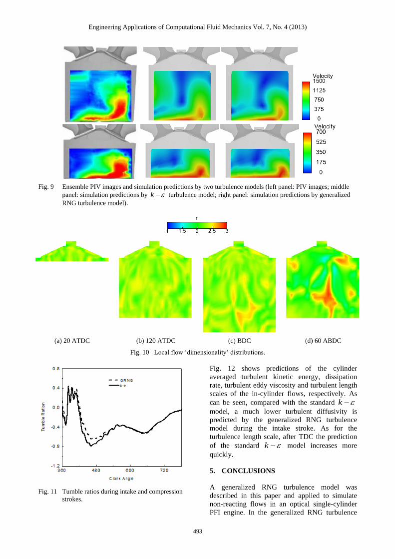
Fig. 9 compares the ensemble PIV images and

simulation predictions obtained by the two

turbulence models at two different crank angles.

As shown, during the intake stroke, the

characteristic flow structure formed in the

combustion chamber is well captured by the

simulation predictions using the GRNG

turbulence model which show good agreement

with the PIV images.

4.3 Dimensionality analysis

The local „dimensionality‟ of the intake flow

calculated using Equations (13) and (14) was

analyzed. Fig. 10 shows the calculated local flow

„dimensionality‟ distributions in a vertical plane

Engineering Applications of Computational Fluid Mechanics Vol. 7, No. 4 (2013)

492

Fig. 7 Radial and vertical velocities along horizontal

line at BDC.

across the spark plug at different crank angles

during the intake and compression strokes. As

shown in the figure, during the intake stroke most

of the local “dimensionality” is 2-D since the in-

cylinder fluid structure is mainly a tumble motion.

In the compression stroke, as the piston moves

closer to TDC some 3-D spherical compression

regions appear. It is inferred that the compression

“dimensionality” represents the intake flow

movement and its variation throughout the cycle

properly, so the generalized RNG turbulence

model based on the local “dimensionality” is

appropriate to compute complex engine flows

with varying compression type.

(a) 440 CA (b) 480 CA

(c) 540 CA (d) 620 CA

Fig. 8 Radial velocities along cylinder axis at

different crank angles ( : experiment; :

95% confidence envelope of 200

instantaneous cycles; : k ; :

generalized RNG).

4.4 Global flow analysis

Fig. 11 shows the cylinder averaged tumble ratios

during the intake and compression strokes

simulated by the standard k turbulence

model and the generalized RNG turbulence

model. As seen in the figure, the mean tumble

ratio in the combustion chamber by the

generalized RNG turbulence model has the same

trend as the prediction of the standard k

model. As shown in Fig. 6, under motored

operation conditions, when the intake valves

open, the pressure in the combustion chamber is

higher than that in the intake ports which leads to

a back flow. As the piston moves down, fresh air

begins to rush into the combustion chamber and

the sign of the tumble ratio varies. After IVO, the

tumble motion becomes more organized due to

the piston movement during the compression

stroke, causing a slight increase in the tumble

motion and it gradually disappears in the

expansion stroke.

Engineering Applications of Computational Fluid Mechanics Vol. 7, No. 4 (2013)

493

Fig. 9 Ensemble PIV images and simulation predictions by two turbulence models (left panel: PIV images; middle

panel: simulation predictions by k turbulence model; right panel: simulation predictions by generalized

RNG turbulence model).

(a) 20 ATDC (b) 120 ATDC (c) BDC (d) 60 ABDC

Fig. 10 Local flow „dimensionality‟ distributions.

Fig. 11 Tumble ratios during intake and compression

strokes.

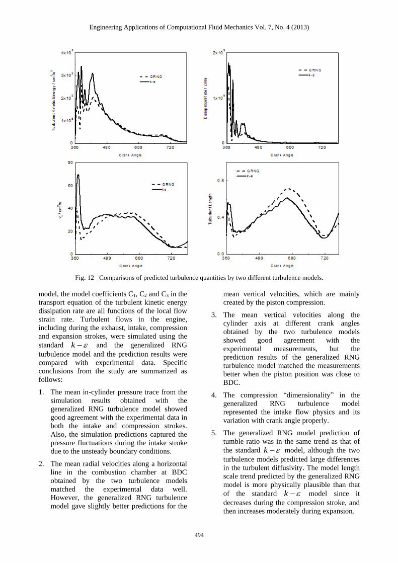
Fig. 12 shows predictions of the cylinder

averaged turbulent kinetic energy, dissipation

rate, turbulent eddy viscosity and turbulent length

scales of the in-cylinder flows, respectively. As

can be seen, compared with the standard k

model, a much lower turbulent diffusivity is

predicted by the generalized RNG turbulence

model during the intake stroke. As for the

turbulence length scale, after TDC the prediction

of the standard k model increases more

quickly.

5. CONCLUSIONS

A generalized RNG turbulence model was

described in this paper and applied to simulate

non-reacting flows in an optical single-cylinder

PFI engine. In the generalized RNG turbulence

Engineering Applications of Computational Fluid Mechanics Vol. 7, No. 4 (2013)

494

Fig. 12 Comparisons of predicted turbulence quantities by two different turbulence models.

model, the model coefficients C1, C2 and C3 in the

transport equation of the turbulent kinetic energy

dissipation rate are all functions of the local flow

strain rate. Turbulent flows in the engine,

including during the exhaust, intake, compression

and expansion strokes, were simulated using the

standard k and the generalized RNG

turbulence model and the prediction results were

compared with experimental data. Specific

conclusions from the study are summarized as

follows:

1. The mean in-cylinder pressure trace from the

simulation results obtained with the

generalized RNG turbulence model showed

good agreement with the experimental data in

both the intake and compression strokes.

Also, the simulation predictions captured the

pressure fluctuations during the intake stroke

due to the unsteady boundary conditions.

2. The mean radial velocities along a horizontal

line in the combustion chamber at BDC

obtained by the two turbulence models

matched the experimental data well.

However, the generalized RNG turbulence

model gave slightly better predictions for the

mean vertical velocities, which are mainly

created by the piston compression.

3. The mean vertical velocities along the

cylinder axis at different crank angles

obtained by the two turbulence models

showed good agreement with the

experimental measurements, but the

prediction results of the generalized RNG

turbulence model matched the measurements

better when the piston position was close to

BDC.

4. The compression “dimensionality” in the

generalized RNG turbulence model

represented the intake flow physics and its

variation with crank angle properly.

5. The generalized RNG model prediction of

tumble ratio was in the same trend as that of

the standard k model, although the two

turbulence models predicted large differences

in the turbulent diffusivity. The model length

scale trend predicted by the generalized RNG

model is more physically plausible than that

of the standard k model since it

decreases during the compression stroke, and

then increases moderately during expansion.

Engineering Applications of Computational Fluid Mechanics Vol. 7, No. 4 (2013)

495

6. In this paper, the GRNG turbulence model

was only applied to simulate non-reacting

flows in an optical single-cylinder PFI engine.

The simulation of reacting flows in this

optical engine by the GRNG turbulence

model combined with ignition model,

combustion model and chemical mechanism

could be the future direction of this work.

ACKNOWLEDGEMENTS

The authors would like to acknowledge the

scholarship provided by the National Science

Foundation of China under Grant No. 51036004

and financial support provided by China-US clean

vehicle project 2010DFA72760. The authors

thank w-erc.com for use of the mesh generation

manual.

REFERENCES

1. Amsden AA (1997). KIVA-3V: A Block-

Structured KIVA Program for Engines with

Vertical or Canted Values. Los Alamos

National Laboratory Technical Report, LA-

13313-MS.

2. Han Z, Reitz RD (1995). Turbulence

modeling of internal combustion engines

using RNG k models. Combustion

Science and Technology 106:267-295.

3. Lacour C, Pera C (2011). An experimental

database dedicated to the study and modelling

of cyclic variability in spark-ignition engines

with LES. SAE Paper 2011-01-1282.

4. Lauder BE, Sharma BI (1974).Application of

the energy dissipation model of turbulence to

the calculation of flow near a spinning disc.

Letters in Heat Mass Transfer 1:131-138.

5. Miles PC (2010). Experimental assessment of

Reynolds-averaged dissipation modeling in

compressible flows employing RNG

turbulence closures. The 15th Int Symp on

Application of Laser Techniques to Fluid

Mechanics. Lisbon, Portugal, 5-8 July.

6. Miles PC, Rempelewert BH, Reitz RD

(2007). Experiment assessment of Reynolds-

averaged dissipation modeling in engine

flows. SAE Paper 2007-24-0046.

7.

8. Morel T, Mansour NN (1982). Modeling of

turbulence in internal combustion engines.

SAE Paper 820040.

9. Musu E, Gentili R, Zanforlin S (2005). Four

stroke engine geometry for stratified charge

combustion. ASME 2005 Internal Combustion

Engine Division Fall Technical Conference.

Ottawa, Ontario, Canada, 11–14 Sep, 447-

457.

10. Pope SB (2000). Turbulence Flows.

Cambridge: Cambridge University.

11. Reitz RD (1991). Assessment of wall heat

transfer models for premixed-charge engine

combustion computations. SAE Paper

910267.

12. Smith LM, Reynolds WC (1992). On the

Yakhot-Orszag renormalization group method

for deriving turbulence statistics and models.

Physics of Fluids A 4:364-390.

13. Tian C, Lu YJ (2013). Turbulence models of

separated flows in shock wave thrust vector

nozzle. Engineering Applications of

Computational Fluid Mechanics 7(2):182-

192.

14. Wang BL, Miles PC, Reitz RD, Han Z,

Petersen BR (2011). Assessment of RNG

turbulence modeling and the development of

a generalized RNG closure model. SAE Paper

2011-01-0829.

15. Wu CT, Ferziger JH, Chapman DR (1985).

Simulation and Modeling of Homogeneous,

Compressed Turbulence. Report,

Thermosciences Division. Stanford

University, USA.

16. Yakhot V, Orszag SA (1986).

Renormalization group analysis of turbulence

I. Basic theory. Journal of Scientific

Computing 1(1):3-51.

17. Yakhot V, Orszag SA, Thangam S, Gatski

TB, Speziale CG (1992). Development of

turbulence models for shear flows by a double

expansion technique. Physics of Fluids A

4:1510-1520.

18. Yakhot V, Smith LM (1992). The

Renormalization Group, the -expansion

and derivation of turbulence models. Journal

of Scientific Computing 7(1):35-61.