apex calculus lt - college of arts & sciences
TRANSCRIPT
APEX CALCULUS IILate Transcendentals
University of North Dakota
Adapted from APEX Calculus byGregory Hartman, Ph.D.
Department of Applied MathematicsVirginia Military Institute
Revised June 2019

Contributing AuthorsTroy Siemers, Ph.D.Department of Applied MathematicsVirginia Military Institute
Michael CorralMathematicsSchoolcraft College
Brian Heinold, Ph.D.Department of Mathematicsand Computer ScienceMount Saint Mary’s University
Paul Dawkins, Ph.D.Department of MathematicsLamar University
Dimplekumar Chalishajar, Ph.D.Department of Applied MathematicsVirginia Military Institute
EditorJennifer Bowen, Ph.D.Department of Mathematicsand Computer ScienceThe College of Wooster
Copyright© 2015 Gregory Hartman© 2019 Department of Mathematics,University of North Dakota
This work is licensed under aCreative CommonsAttribution‐NonCommercial4.0 International License.Resale and reproduction restricted.
CONTENTSPreface vii
Calculus I 1
1 Limits 71.1 An Introduction To Limits . . . . . . . . . . . . . . . . . . . . 71.2 Epsilon‐Delta Definition of a Limit . . . . . . . . . . . . . . . 151.3 Finding Limits Analytically . . . . . . . . . . . . . . . . . . . . 251.4 One Sided Limits . . . . . . . . . . . . . . . . . . . . . . . . 391.5 Limits Involving Infinity . . . . . . . . . . . . . . . . . . . . . 471.6 Continuity . . . . . . . . . . . . . . . . . . . . . . . . . . . . 59
2 Derivatives 792.1 Instantaneous Rates of Change: The Derivative . . . . . . . . 792.2 Interpretations of the Derivative . . . . . . . . . . . . . . . . 942.3 Basic Differentiation Rules . . . . . . . . . . . . . . . . . . . 1012.4 The Product and Quotient Rules . . . . . . . . . . . . . . . . 1102.5 The Chain Rule . . . . . . . . . . . . . . . . . . . . . . . . . 1222.6 Implicit Differentiation . . . . . . . . . . . . . . . . . . . . . 133
3 The Graphical Behavior of Functions 1453.1 Extreme Values . . . . . . . . . . . . . . . . . . . . . . . . . 1453.2 The Mean Value Theorem . . . . . . . . . . . . . . . . . . . . 1543.3 Increasing and Decreasing Functions . . . . . . . . . . . . . . 1603.4 Concavity and the Second Derivative . . . . . . . . . . . . . . 1713.5 Curve Sketching . . . . . . . . . . . . . . . . . . . . . . . . . 179
4 Applications of the Derivative 1894.1 Related Rates . . . . . . . . . . . . . . . . . . . . . . . . . . 1894.2 Optimization . . . . . . . . . . . . . . . . . . . . . . . . . . . 1974.3 Differentials . . . . . . . . . . . . . . . . . . . . . . . . . . . 2054.4 Newton’s Method . . . . . . . . . . . . . . . . . . . . . . . . 213
5 Integration 2215.1 Antiderivatives and Indefinite Integration . . . . . . . . . . . 2215.2 The Definite Integral . . . . . . . . . . . . . . . . . . . . . . 2315.3 Riemann Sums . . . . . . . . . . . . . . . . . . . . . . . . . 2425.4 The Fundamental Theorem of Calculus . . . . . . . . . . . . . 262
iii
5.5 Substitution . . . . . . . . . . . . . . . . . . . . . . . . . . . 277
6 Applications of Integration 2916.1 Area Between Curves . . . . . . . . . . . . . . . . . . . . . . 2926.2 Volume by Cross‐Sectional Area; Disk and Washer Methods . . 3006.3 The Shell Method . . . . . . . . . . . . . . . . . . . . . . . . 3116.4 Work . . . . . . . . . . . . . . . . . . . . . . . . . . . . . . . 3216.5 Fluid Forces . . . . . . . . . . . . . . . . . . . . . . . . . . . 332
Calculus II 341
7 Inverse Functions and L’Hôpital’s Rule 3437.1 Inverse Functions . . . . . . . . . . . . . . . . . . . . . . . . 3437.2 Derivatives of Inverse Functions . . . . . . . . . . . . . . . . 3497.3 Exponential and Logarithmic Functions . . . . . . . . . . . . . 3557.4 Hyperbolic Functions . . . . . . . . . . . . . . . . . . . . . . 3647.5 L’Hôpital’s Rule . . . . . . . . . . . . . . . . . . . . . . . . . 375
8 Techniques of Integration 3838.1 Integration by Parts . . . . . . . . . . . . . . . . . . . . . . . 3838.2 Trigonometric Integrals . . . . . . . . . . . . . . . . . . . . . 3948.3 Trigonometric Substitution . . . . . . . . . . . . . . . . . . . 4078.4 Partial Fraction Decomposition . . . . . . . . . . . . . . . . . 4178.5 Integration Strategies . . . . . . . . . . . . . . . . . . . . . . 4278.6 Improper Integration . . . . . . . . . . . . . . . . . . . . . . 4368.7 Numerical Integration . . . . . . . . . . . . . . . . . . . . . . 447
9 Sequences and Series 4619.1 Sequences . . . . . . . . . . . . . . . . . . . . . . . . . . . . 4619.2 Infinite Series . . . . . . . . . . . . . . . . . . . . . . . . . . 4769.3 The Integral Test . . . . . . . . . . . . . . . . . . . . . . . . . 4909.4 Comparison Tests . . . . . . . . . . . . . . . . . . . . . . . . 4969.5 Alternating Series and Absolute Convergence . . . . . . . . . 5059.6 Ratio and Root Tests . . . . . . . . . . . . . . . . . . . . . . . 5159.7 Strategy for Testing Series . . . . . . . . . . . . . . . . . . . . 5219.8 Power Series . . . . . . . . . . . . . . . . . . . . . . . . . . . 5259.9 Taylor Polynomials . . . . . . . . . . . . . . . . . . . . . . . 5439.10 Taylor Series . . . . . . . . . . . . . . . . . . . . . . . . . . . 553
10 Curves in the Plane 57310.1 Arc Length and Surface Area . . . . . . . . . . . . . . . . . . 57310.2 Parametric Equations . . . . . . . . . . . . . . . . . . . . . . 58310.3 Calculus and Parametric Equations . . . . . . . . . . . . . . . 59610.4 Introduction to Polar Coordinates . . . . . . . . . . . . . . . 61010.5 Calculus and Polar Functions . . . . . . . . . . . . . . . . . . 623
Calculus III 637
11 Vectors 63911.1 Introduction to Cartesian Coordinates in Space . . . . . . . . 63911.2 An Introduction to Vectors . . . . . . . . . . . . . . . . . . . 65611.3 The Dot Product . . . . . . . . . . . . . . . . . . . . . . . . . 67011.4 The Cross Product . . . . . . . . . . . . . . . . . . . . . . . . 68311.5 Lines . . . . . . . . . . . . . . . . . . . . . . . . . . . . . . . 69611.6 Planes . . . . . . . . . . . . . . . . . . . . . . . . . . . . . . 706
12 Vector Valued Functions 71512.1 Vector‐Valued Functions . . . . . . . . . . . . . . . . . . . . 71512.2 Calculus and Vector‐Valued Functions . . . . . . . . . . . . . 72112.3 The Calculus of Motion . . . . . . . . . . . . . . . . . . . . . 73512.4 Unit Tangent and Normal Vectors . . . . . . . . . . . . . . . . 74812.5 The Arc Length Parameter and Curvature . . . . . . . . . . . 757
13 Functions of Several Variables 76913.1 Introduction to Multivariable Functions . . . . . . . . . . . . 76913.2 Limits and Continuity of Multivariable Functions . . . . . . . . 77713.3 Partial Derivatives . . . . . . . . . . . . . . . . . . . . . . . . 79013.4 Differentiability and the Total Differential . . . . . . . . . . . 80113.5 The Multivariable Chain Rule . . . . . . . . . . . . . . . . . . 80913.6 Directional Derivatives . . . . . . . . . . . . . . . . . . . . . 81813.7 Tangent Lines, Normal Lines, and Tangent Planes . . . . . . . 82913.8 Extreme Values . . . . . . . . . . . . . . . . . . . . . . . . . 84013.9 Lagrange Multipliers . . . . . . . . . . . . . . . . . . . . . . 851
14 Multiple Integration 85914.1 Iterated Integrals and Area . . . . . . . . . . . . . . . . . . . 85914.2 Double Integration and Volume . . . . . . . . . . . . . . . . . 86914.3 Double Integration with Polar Coordinates . . . . . . . . . . . 88114.4 Center of Mass . . . . . . . . . . . . . . . . . . . . . . . . . 88914.5 Surface Area . . . . . . . . . . . . . . . . . . . . . . . . . . . 90114.6 Volume Between Surfaces and Triple Integration . . . . . . . . 908
14.7 Triple Integration with Cylindrical and Spherical Coordinates . 929
15 Vector Analysis 94715.1 Introduction to Line Integrals . . . . . . . . . . . . . . . . . . 94815.2 Vector Fields . . . . . . . . . . . . . . . . . . . . . . . . . . . 95815.3 Line Integrals over Vector Fields . . . . . . . . . . . . . . . . 96815.4 Flow, Flux, Green’s Theorem and the Divergence Theorem . . 98115.5 Parameterized Surfaces and Surface Area . . . . . . . . . . . 99215.6 Surface Integrals . . . . . . . . . . . . . . . . . . . . . . . . . 100415.7 The Divergence Theorem and Stokes’ Theorem . . . . . . . . 1013
Solutions To Selected Problems A.3
Index A.17
PREFACEA Note on Using this TextThank you for reading this short preface. Allow us to share a few key pointsabout the text so that youmay better understand what you will find beyond thispage.
This text comprises a three‐volume series on Calculus. The first part coversmaterial taught in many “Calculus 1” courses: limits, derivatives, and the basicsof integration, found in Chapters 1 through 6. The second text covers mate‐rial often taught in “Calculus 2”: integration and its applications, along with anintroduction to sequences, series and Taylor Polynomials, found in Chapters 7through 10. The third text covers topics common in “Calculus 3” or “Multivari‐able Calculus”: parametric equations, polar coordinates, vector‐valued func‐tions, and functions of more than one variable, found in Chapters 11 through15. All three are available separately for free.
Printing the entire text as one volumemakes for a large, heavy, cumbersomebook. One can certainly only print the pages they currently need, but someprefer to have a nice, bound copy of the text. Therefore this text has been splitinto these three manageable parts, each of which can be purchased separately.
A result of this splitting is that sometimes material is referenced that is notcontained in the present text. The context should make it clear whether the“missing” material comes before or after the current portion. Downloading theappropriate pdf, or the entireAPEXCalculus LT pdf, will give access to these topics.
For Students: How to Read this TextMathematics textbooks have a reputation for being hard to read. High‐levelmathematical writing often seeks to say much with few words, and this styleoften seeps into texts of lower‐level topics. This book was written with the goalof being easier to read than many other calculus textbooks, without becomingtoo verbose.
Each chapter and section starts with an introduction of the coming mate‐rial, hopefully setting the stage for “why you should care,” and ends with a lookahead to see how the just‐learned material helps address future problems. Ad‐ditionally, each chapter includes a section zero, which provides a basic reviewand practice problems of pre‐calculus skills. Since this content is a pre‐requisitefor calculus, reviewing and mastering these skills are considered your responsi‐bility. This means that it is your responsibility to seek assistance outside of classfrom your instructor, a math resource center or other math tutoring availableon‐campus. A solid understanding of these skills is essential to your success insolving calculus problems.
Please read the text; it is written to explain the concepts of Calculus. Thereare numerous examples to demonstrate the meaning of definitions, the truthof theorems, and the application of mathematical techniques. When you en‐counter a sentence you don’t understand, read it again. If it still doesn’t makesense, read on anyway, as sometimes confusing sentences are explained by latersentences.
You don’t have to read every equation. The examples generally show “all”the steps needed to solve a problem. Sometimes reading through each step ishelpful; sometimes it is confusing. When the steps are illustrating a new tech‐nique, one probably should follow each step closely to learn the new technique.When the steps are showing the mathematics needed to find a number to be
used later, one can usually skip ahead and see how that number is being used,instead of getting bogged down in reading how the number was found.
Some proofs have been delayed until later (or omitted completely). In math‐ematics, proving something is always true is extremely important, and entailsmuch more than testing to see if it works twice. However, students often areconfused by the details of a proof, or become concerned that they should havebeen able to construct this proof on their own. To alleviate this potential prob‐lem, we do not include the more difficult proofs in the text. The interestedreader is highly encouraged to find other proofs online or from their instruc‐tor. In most cases, one is very capable of understanding what a theoremmeansand how to apply it without knowing fully why it is true.
Work through the examples. The best way to learn mathematics is to do it.Reading about it (or watching someone else do it) is a poor substitute. For thisreason, every page has a place for you to put your notes so that you can workout the examples. That being said, sometimes it is useful to watch someonework through an example. For this reason, this text also provides links to onlinevideos where someone is working through a similar problem. If you want evenmore videos, these are generally chosen from
• Khan Academy: https://www.khanacademy.org/• Math Doctor Bob: http://www.mathdoctorbob.org/• Just Math Tutorials: http://patrickjmt.com/ (unfortunately, they’renot well organized)
Some other sites you may want to consider are• LarryGreen’s Calculus Videos: http://www.ltcconline.net/greenl/
courses/105/videos/VideoIndex.htm• Mathispower4u: http://www.mathispower4u.com/• Yay Math: http://www.yaymath.org/ (for prerequisite material)
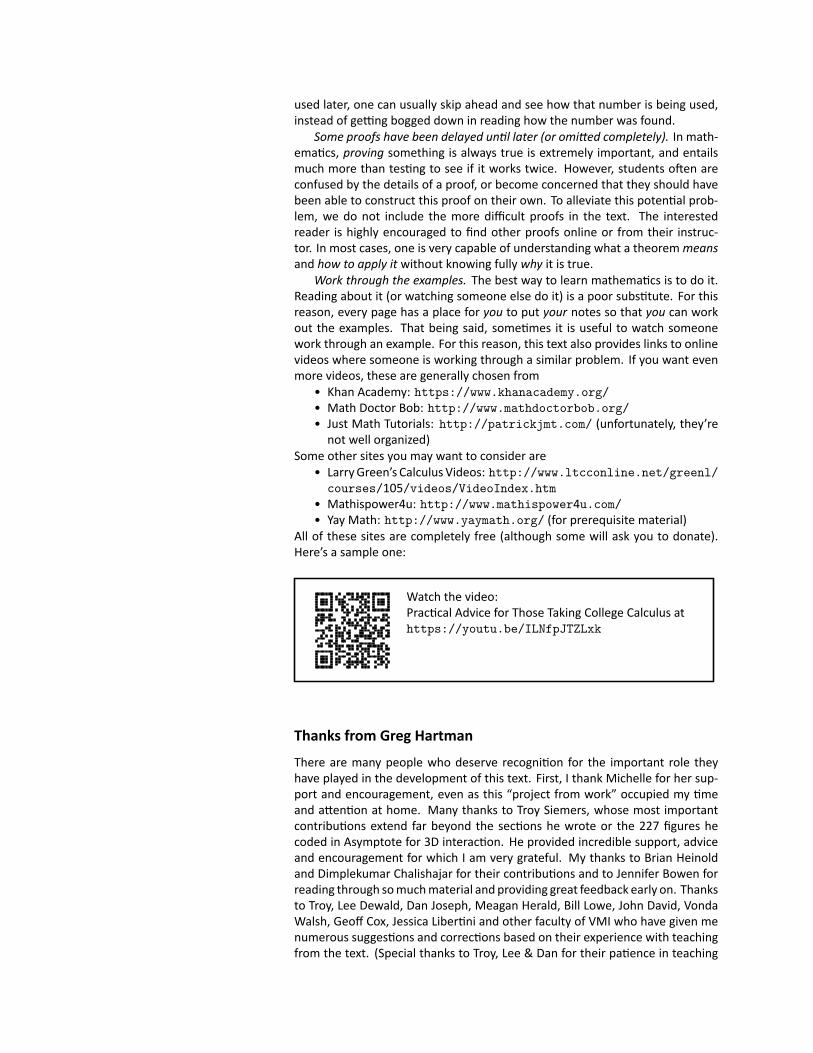
All of these sites are completely free (although some will ask you to donate).Here’s a sample one:
Watch the video:Practical Advice for Those Taking College Calculus athttps://youtu.be/ILNfpJTZLxk
Thanks from Greg HartmanThere are many people who deserve recognition for the important role theyhave played in the development of this text. First, I thank Michelle for her sup‐port and encouragement, even as this “project from work” occupied my timeand attention at home. Many thanks to Troy Siemers, whose most importantcontributions extend far beyond the sections he wrote or the 227 figures hecoded in Asymptote for 3D interaction. He provided incredible support, adviceand encouragement for which I am very grateful. My thanks to Brian Heinoldand Dimplekumar Chalishajar for their contributions and to Jennifer Bowen forreading through somuchmaterial and providing great feedback early on. Thanksto Troy, Lee Dewald, Dan Joseph, Meagan Herald, Bill Lowe, John David, VondaWalsh, Geoff Cox, Jessica Libertini and other faculty of VMI who have given menumerous suggestions and corrections based on their experience with teachingfrom the text. (Special thanks to Troy, Lee & Dan for their patience in teaching
Calc III while I was still writing the Calc III material.) Thanks to Randy Cone forencouraging his tutors of VMI’s Open Math Lab to read through the text andcheck the solutions, and thanks to the tutors for spending their time doing so.A very special thanks to Kristi Brown and Paul Janiczek who took this opportu‐nity far above & beyond what I expected, meticulously checking every solutionand carefully reading every example. Their comments have been extraordinarilyhelpful. I am also thankful for the support provided by Wane Schneiter, who asmy Dean provided me with extra time to work on this project. I am blessed tohave so many people give of their time to make this book better.
APEX — Affordable Print and Electronic teXtsAPEX is a consortiumof authorswho collaborate to produce high‐quality, low‐costtextbooks. The current textbook‐writing paradigm is facing a potential revolu‐tion as desktop publishing and electronic formats increase in popularity. How‐ever, writing a good textbook is no easy task, as the time requirements aloneare substantial. It takes countless hours of work to produce text, write exam‐ples and exercises, edit and publish. Through collaboration, however, the costto any individual can be lessened, allowing us to create texts that we freely dis‐tribute electronically and sell in printed form for an incredibly low cost. Havingsaid that, nothing is entirely free; someone always bears some cost. This text“cost” the authors of this book their time, and that was not enough. APEX Cal‐culuswould not exist had not the Virginia Military Institute, through a generousJackson‐Hope grant, given the lead author significant time away from teachingso he could focus on this text.
Each text is available as a free .pdf, protected by a Creative Commons Attri‐bution — Noncommercial 4.0 copyright. That means you can give the .pdf toanyone you like, print it in any form you like, and even edit the original contentand redistribute it. If you do the latter, you must clearly reference this work andyou cannot sell your edited work for money.
We encourage others to adapt this work to fit their own needs. One mightadd sections that are “missing” or remove sections that your students won’tneed. The source files can be found at https://github.com/APEXCalculus.
You can learn more at www.vmi.edu/APEX.Greg Hartman
Creating APEX LTStarting with the source at https://github.com/APEXCalculus, faculty atthe University of North Dakota made several substantial changes to create APEXLate Transcendentals. The most obvious change was to rearrange the text todelay proving the derivative of transcendental functions until Calculus 2. UNDadded Sections 7.1 and 7.3, adapted several sections from other resources, cre‐ated the prerequisite sections, included links to videos andGeogebra, and addedseveral examples and exercises. In the end, every section had some changes(some more substantial than others), resulting in a document that is about 10%longer. The source files can now be found athttps://github.com/teepeemm/APEXCalculusLT_Source.
Extra thanks are due to Michael Corral for allowing us to use portions of hisVector Calculus, available at www.mecmath.net/ (specifically, section 13.9 andthe Jacobian in section 14.7) and to Paul Dawkins for allowing us to use portionsof his online math notes from tutorial.math.lamar.edu/ (specifically, Sec‐tions 8.5 and 9.7, as well as “Area with Parametric Equations” in section 10.3).The work on Calculus III was partially supported by the NDUS OER Initiative.
Electronic ResourcesA distinctive feature of APEX is interactive, 3D graphics in the .pdf version. Nearlyall graphs of objects in space can be rotated, shifted, and zoomed in/out so thereader can better understand the object illustrated.
Currently, the only pdf viewers that support these 3D graphics for comput‐ers are Adobe Reader & Acrobat. To activate the interactive mode, click on theimage. Once activated, one can click/drag to rotate the object and use the scrollwheel on a mouse to zoom in/out. (A great way to investigate an image is tofirst zoom in on the page of the pdf viewer so the graphic itself takes up muchof the screen, then zoom inside the graphic itself.) A CTRL‐click/drag pans theobject left/right or up/down. By right‐clicking on the graph one can access amenu of other options, such as changing the lighting scheme or perspective.One can also revert the graph back to its default view. If you wish to deactivatethe interactivity, one can right‐click and choose the “Disable Content” option.
The situation is more interesting for tablets and smart‐phones. The 3D graphics files have been arrayed at https://sites.und.edu/timothy.prescott/apex/prc/. Atthe bottom of the page are links to Android and iOS appsthat can display the interactive files. The QR code to theright will take you to that page.
Additionally, aweb version of the book is available at https://sites.und.edu/timothy.prescott/apex/web/. While we have striven to make the pdfaccessible for non‐print formats, html is far better in this regard.
Part
Calculus II
341

7: INVERSE FUNCTIONS ANDL’HÔPITAL’S RULEThis chapter completes our differentiation toolkit. The first and most importanttool will be how to differentiate inverse functions. We’ll be able to use this todifferentiate exponential and logarithmic functions, which we stated in Theo‐rem 2.3.1 but did not prove.
7.1 Inverse FunctionsWe say that two functions f and g are inverses if g(f(x)) = x for all x in thedomain of f and f(g(x)) = x for all x in the domain of g. A function can onlyhave an inverse if it is one‐to‐one, i.e. if we never have f(x1) = f(x2) for differentelements x1 and x2 of the domain. This is equivalent to saying that the graph ofthe functionpasses the horizontal line test. The inverse of f is denoted f−1, whichshould not be confused with the function 1/f(x).
Key Idea 7.1.1 Inverse FunctionsFor a one‐to–one function f,
• The domain of f−1 is the range of f; the range of f−1 is the domainof f.
• f−1(f(x)) = x for all x in the domain of f.
• f(f−1(x)) = x for all x in the domain of f−1.
• The graph of y = f−1(x) is the reflection across y = x of the graphof y = f(x).
• y = f−1(x) if and only if f(y) = x and y is in the domain of f.
Watch the video:Finding the Inverse of a Function or Showing OneDoes not Exist, Ex 3 athttps://youtu.be/BmjbDINGZGg
Notes:
343
Chapter 7 Inverse Functions and L’Hôpital’s Rule
To determine whether or not f and g are inverses for each other, we checkto see whether or not g(f(x)) = x for all x in the domain of f,and f(g(x)) = x forall x in the domain of g.
−1 1 2
−1
1
(−0.5, 0.375)
(0.375,−0.5)
(1, 1.5)
(1.5, 1)
x
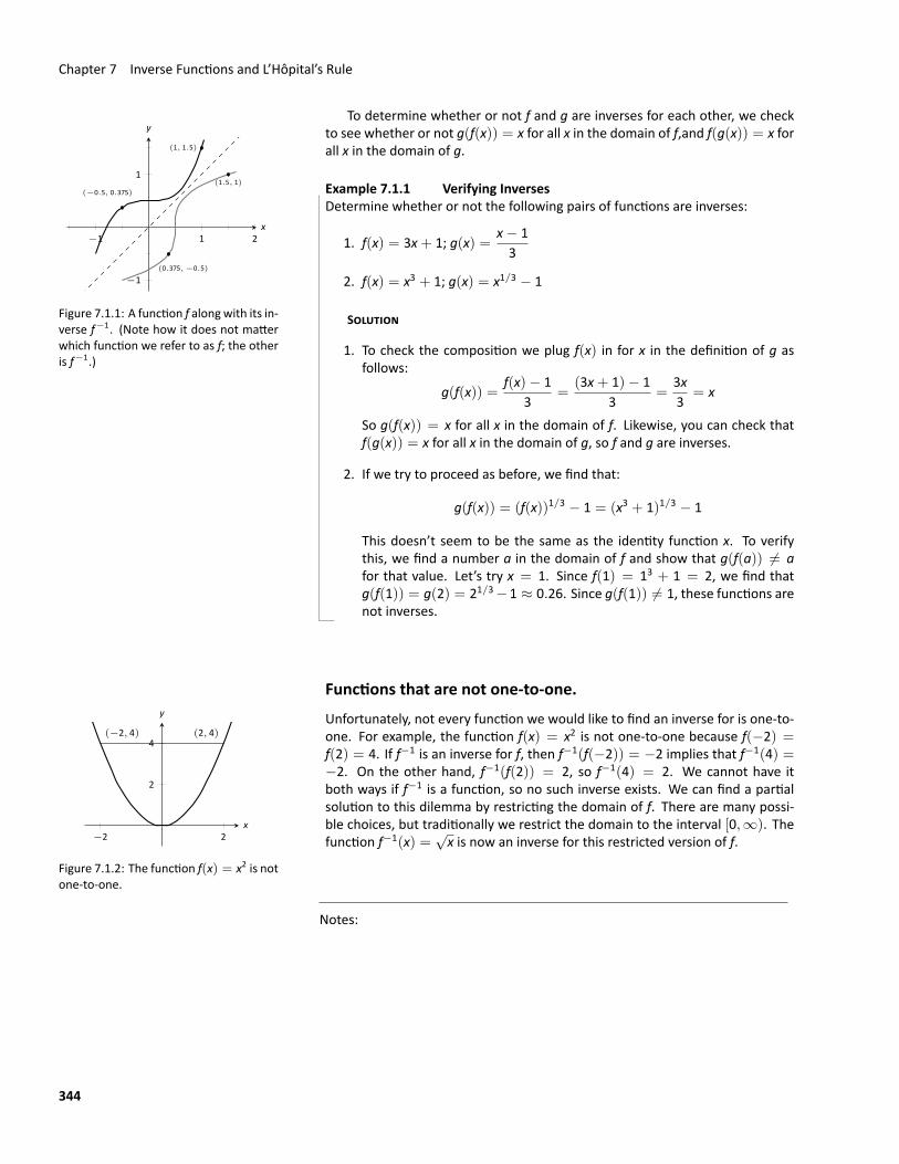
y
Figure 7.1.1: A function f alongwith its in‐verse f−1. (Note how it does not matterwhich function we refer to as f; the otheris f−1.)
Example 7.1.1 Verifying InversesDetermine whether or not the following pairs of functions are inverses:
1. f(x) = 3x+ 1; g(x) =x− 13
2. f(x) = x3 + 1; g(x) = x1/3 − 1
SOLUTION
1. To check the composition we plug f(x) in for x in the definition of g asfollows:
g(f(x)) =f(x)− 1
3=
(3x+ 1)− 13
=3x3
= x
So g(f(x)) = x for all x in the domain of f. Likewise, you can check thatf(g(x)) = x for all x in the domain of g, so f and g are inverses.
2. If we try to proceed as before, we find that:
g(f(x)) = (f(x))1/3 − 1 = (x3 + 1)1/3 − 1
This doesn’t seem to be the same as the identity function x. To verifythis, we find a number a in the domain of f and show that g(f(a)) ̸= afor that value. Let’s try x = 1. Since f(1) = 13 + 1 = 2, we find thatg(f(1)) = g(2) = 21/3−1 ≈ 0.26. Since g(f(1)) ̸= 1, these functions arenot inverses.
Functions that are not one‐to‐one.
−2 2
2
4(−2, 4) (2, 4)
x
y
Figure 7.1.2: The function f(x) = x2 is notone‐to‐one.
Unfortunately, not every function we would like to find an inverse for is one‐to‐one. For example, the function f(x) = x2 is not one‐to‐one because f(−2) =f(2) = 4. If f−1 is an inverse for f, then f−1(f(−2)) = −2 implies that f−1(4) =−2. On the other hand, f−1(f(2)) = 2, so f−1(4) = 2. We cannot have itboth ways if f−1 is a function, so no such inverse exists. We can find a partialsolution to this dilemma by restricting the domain of f. There are many possi‐ble choices, but traditionally we restrict the domain to the interval [0,∞). Thefunction f−1(x) =
√x is now an inverse for this restricted version of f.
Notes:
344
7.1 Inverse Functions
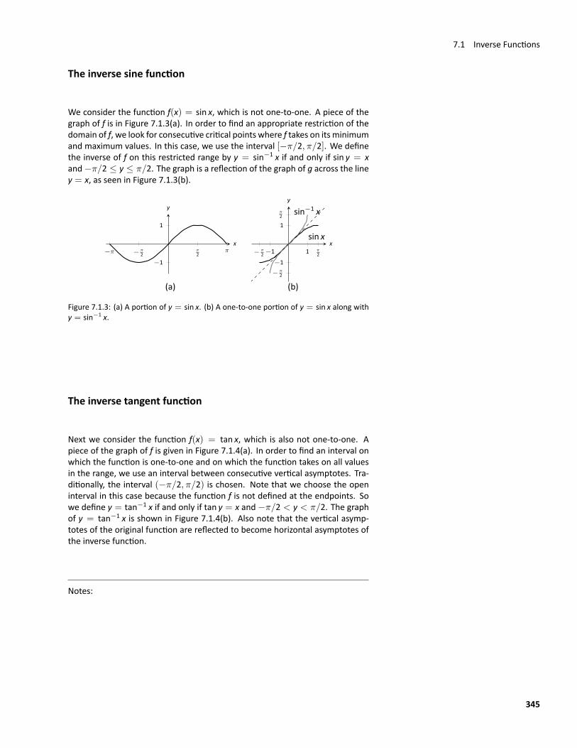
The inverse sine function
We consider the function f(x) = sin x, which is not one‐to‐one. A piece of thegraph of f is in Figure 7.1.3(a). In order to find an appropriate restriction of thedomain of f, we look for consecutive critical points where f takes on its minimumand maximum values. In this case, we use the interval [−π/2, π/2]. We definethe inverse of f on this restricted range by y = sin−1 x if and only if sin y = xand−π/2 ≤ y ≤ π/2. The graph is a reflection of the graph of g across the liney = x, as seen in Figure 7.1.3(b).
−π − π2
π2
π
−1
1
x
y
− π2 −1 1 π
2
− π2
−1
1
π2
sin x
sin−1 x
x
y
(a) (b)
Figure 7.1.3: (a) A portion of y = sin x. (b) A one‐to‐one portion of y = sin x along withy = sin−1 x.
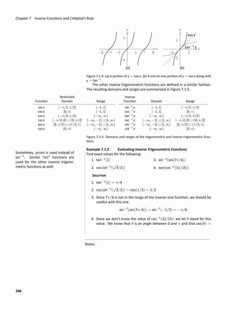
The inverse tangent function
Next we consider the function f(x) = tan x, which is also not one‐to‐one. Apiece of the graph of f is given in Figure 7.1.4(a). In order to find an interval onwhich the function is one‐to‐one and on which the function takes on all valuesin the range, we use an interval between consecutive vertical asymptotes. Tra‐ditionally, the interval (−π/2, π/2) is chosen. Note that we choose the openinterval in this case because the function f is not defined at the endpoints. Sowe define y = tan−1 x if and only if tan y = x and−π/2 < y < π/2. The graphof y = tan−1 x is shown in Figure 7.1.4(b). Also note that the vertical asymp‐totes of the original function are reflected to become horizontal asymptotes ofthe inverse function.
Notes:
345
Chapter 7 Inverse Functions and L’Hôpital’s Rule
− 3π2
−π − π2
π2
π 3π2
−2
2
x
y
− π2
π2
− π2
π2
tan x
tan−1 x x
y
(a) (b)
Figure 7.1.4: (a) A portion of y = tan x. (b) A one‐to‐one portion of y = tan x along withy = tan−1.
The other inverse trigonometric functions are defined in a similar fashion.The resulting domains and ranges are summarized in Figure 7.1.5.
FunctionRestrictedDomain Range
InverseFunction Domain Range
sin x [−π/2, π/2] [−1, 1] sin−1 x [−1, 1] [−π/2, π/2]cos x [0, π] [−1, 1] cos−1 x [−1, 1] [0, π]tan x (−π/2, π/2) (−∞,∞) tan−1 x (−∞,∞) (−π/2, π/2)csc x [−π/2, 0) ∪ (0, π/2] (−∞,−1] ∪ [1,∞) csc−1 x (−∞,−1] ∪ [1,∞) [−π/2, 0) ∪ (0, π/2]sec x [0, π/2) ∪ (π/2, π] (−∞,−1] ∪ [1,∞) sec−1 x (−∞,−1] ∪ [1,∞) [0, π/2) ∪ (π/2, π]cot x (0, π) (−∞,∞) cot−1 x (−∞,∞) (0, π)
Figure 7.1.5: Domains and ranges of the trigonometric and inverse trigonometric func‐tions.
Example 7.1.2 Evaluating Inverse Trigonometric FunctionsFind exact values for the following:Sometimes, arcsin is used instead of
sin−1. Similar “arc” functions areused for the other inverse trigono‐metric functions as well.
1. tan−1(1)
2. cos(sin−1(√3/2))
3. sin−1(sin(7π/6))
4. tan(cos−1(11/15))
SOLUTION
1. tan−1(1) = π/4
2. cos(sin−1(√3/2)) = cos(π/3) = 1/2
3. Since 7π/6 is not in the range of the inverse sine function, we should becareful with this one.
sin−1(sin(7π/6)) = sin−1(−1/2) = −π/6.
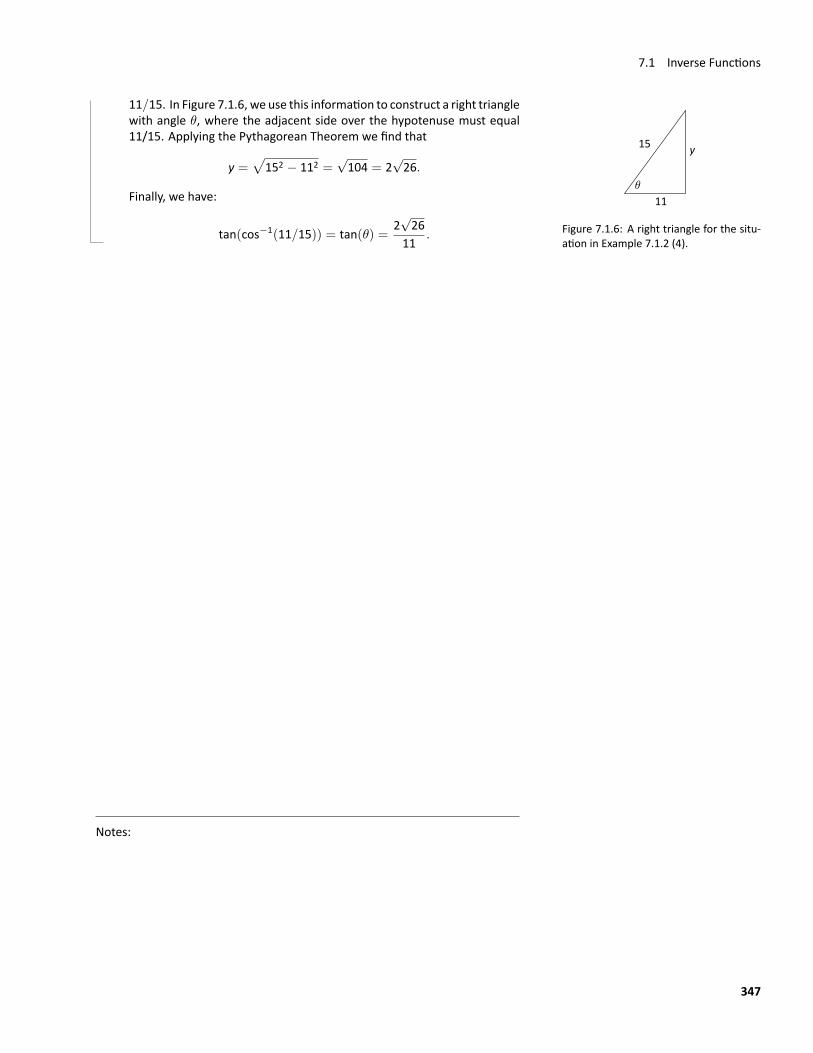
4. Since we don’t know the value of cos−1(11/15), we let θ stand for thisvalue. We know that θ is an angle between 0 and π and that cos(θ) =
Notes:
346
7.1 Inverse Functions
11/15. In Figure 7.1.6, we use this information to construct a right trianglewith angle θ, where the adjacent side over the hypotenuse must equal11/15. Applying the Pythagorean Theorem we find that
θ
11
y15
Figure 7.1.6: A right triangle for the situ‐ation in Example 7.1.2 (4).
y =√
152 − 112 =√104 = 2
√26.
Finally, we have:
tan(cos−1(11/15)) = tan(θ) =2√26
11.
Notes:
347
Exercises 7.1Terms and Concepts1. T/F: Every function has an inverse.2. In your own words explain what it means for a function to
be “one to one.”3. If (1, 10) lies on the graph of y = f(x), what can be said
about the graph of y = f−1(x)?4. If a function doesn’t have an inverse, what can we do to
help it have an inverse?
ProblemsIn Exercises 5–6, given the graph of f, sketch the graph of f−1.
5.
−9−8−7−6−5−4−3−2−1 1 2 3 4 5 6 7 8 9
−8−7−6−5−4−3−2−1
12345678
f(x)
x
y
6.
−9−8−7−6−5−4−3−2−1 1 2 3 4 5 6 7 8 9
−8−7−6−5−4−3−2−1
12345678
f(x)
x
y
In Exercises 7–10, verify that the given functions are inverses.
7. f(x) = 2x+ 6 and g(x) = 12 x− 3
8. f(x) = x2 + 6x + 11, x ≥ −3 and g(x) =√x− 2 − 3,
x ≥ 2
9. f(x) = 3x− 5
, x ̸= 5 and g(x) = 3+ 5xx
, x ̸= 0
10. f(x) = x+ 1x− 1
, x ̸= 1 and g(x) = f(x)
In Exercises 11–14, find a restriction of the domain of the givenfunction on which the function will have an inverse.
11. f(x) =√16− x2
12. g(x) =√x2 − 16
13. r(t) = t2 − 6t+ 9
14. f(x) = 1−√x
1+√x
In Exercises 15–18, find the inverse of the given function.
15. f(x) = x+ 1x− 2
16. f(x) = x2 + 4
17. f(x) = ex+3 − 2
18. f(x) = ln(x− 5) + 1
In Exercises 19–28, find the exact value.
19. tan−1(0)
20. tan−1(tan(π/7))
21. cos(cos−1(−1/5))
22. sin−1(sin(8π/3))
23. sin(tan−1(1))
24. sec(sin−1(−3/5))
25. cos(tan−1(3/7))
26. sin−1(−√3/2)
27. cos−1(−√2/2)
28. cos−1(cos(8π/7))
In Exercises 29–32, simplify the expression.
29. sin(tan−1 x√
4−x2
)30. tan
(sin−1 x√
x2+4
)31. cos
(sin−1 5√
x2+25
)32. cot
(cos−1 3√
x
)
348
7.2 Derivatives of Inverse Functions
7.2 Derivatives of Inverse FunctionsIn this section we will figure out how to differentiate the inverse of a function.To do so, we recall that if f and g are inverses, then f(g(x)) = x for all x in thedomain of f. Differentiating and simplifying yields:
f(g(x)) = xf ′(g(x))g ′(x) = 1
g ′(x) =1
f ′(g(x))assuming f ′(x) is nonzero
Note that the derivation above assumes that the function g is differentiable. Itis possible to prove that gmust be differentiable if f ′ is nonzero, but the proof isbeyond the scope of this text. However, assuming this fact we have shown thefollowing:
Theorem 7.2.1 Derivatives of Inverse FunctionsLet f be differentiable and one‐to‐one on an open interval I, wheref ′(x) ̸= 0 for all x in I, let J be the range of f on I, let g be the inversefunction of f, and let f(a) = b for some a in I. Then g is a differentiablefunction on J, and in particular,(
f−1)′ (b) = g ′(b) =1
f ′(a)(f−1)′ (x) = g ′(x) =
1f ′(g(x))
The results of Theorem7.2.1 are not trivial; the notationmay seemconfusingat first. Careful consideration, along with examples, should earn understanding.
Watch the video:Derivative of an Inverse Function, Ex 2 athttps://youtu.be/RKfGMX0pn2k
In the next example we apply Theorem 7.2.1 to the arcsine function.
Example 7.2.1 Finding the derivative of an inverse trigonometric functionLet y = sin−1 x. Find y ′ using Theorem 7.2.1.
Notes:
349
Chapter 7 Inverse Functions and L’Hôpital’s Rule
SOLUTION Adopting our previously defined notation, let g(x) = sin−1 xand f(x) = sin x. Thus f ′(x) = cos x. Applying Theorem 7.2.1, we have
g ′(x) =1
f ′(g(x))
=1
cos(sin−1 x).
y√1 − x2
x1
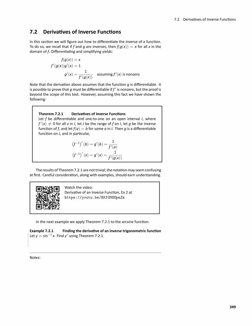
Figure 7.2.1: A right triangle defined byy = sin−1(x/1) with the length of thethird leg found using the PythagoreanTheorem.
This last expression is not immediately illuminating. Drawing a figure willhelp, as shown in Figure 7.2.1. Recall that the sine function can be viewed astaking in an angle and returning a ratio of sides of a right triangle, specifically,the ratio “opposite over hypotenuse.” Thismeans that the arcsine function takesas input a ratio of sides and returns an angle. The equation y = sin−1 x can berewritten as y = sin−1(x/1); that is, consider a right triangle where the hy‐potenuse has length 1 and the side opposite of the angle with measure y haslength x. This means the final side has length
√1− x2, using the Pythagorean
Theorem.Therefore cos(sin−1 x) = cos y =
√1− x2/1 =
√1− x2, resulting in
ddx(sin−1 x
)= g ′(x) =
1√1− x2
.
Remember that the input x of the arcsine function is a ratio of a side of aright triangle to its hypotenuse; the absolute value of this ratio will be less than1. Therefore 1− x2 will be positive.
− π2 − π
4π4
π2
−1
1
y = sin x
( π3 ,
√3
2 )
x
y
−2 −1 1 2
− π2
− π4
π4
π2
y = sin−1 x
(√
32 , π
3 )
Figure 7.2.2: Graphs of y = sin x and y =sin−1 x along with corresponding tangentlines.
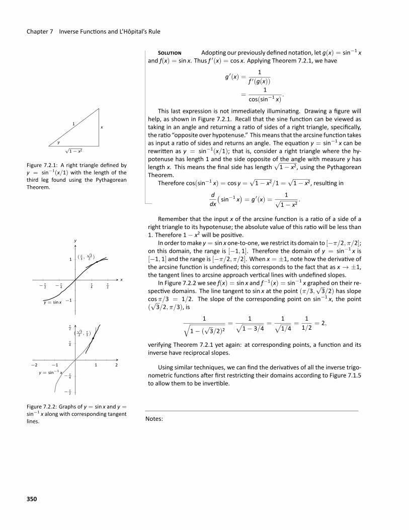
In order tomake y = sin x one‐to‐one, we restrict its domain to [−π/2, π/2];on this domain, the range is [−1, 1]. Therefore the domain of y = sin−1 x is[−1, 1] and the range is [−π/2, π/2]. When x = ±1, note how the derivative ofthe arcsine function is undefined; this corresponds to the fact that as x → ±1,the tangent lines to arcsine approach vertical lines with undefined slopes.
In Figure 7.2.2 we see f(x) = sin x and f−1(x) = sin−1 x graphed on their re‐spective domains. The line tangent to sin x at the point (π/3,
√3/2) has slope
cos π/3 = 1/2. The slope of the corresponding point on sin−1 x, the point(√3/2, π/3), is
1√1− (
√3/2)2
=1√
1− 3/4=
1√1/4
=1
1/2= 2,
verifying Theorem 7.2.1 yet again: at corresponding points, a function and itsinverse have reciprocal slopes.
Using similar techniques, we can find the derivatives of all the inverse trigo‐nometric functions after first restricting their domains according to Figure 7.1.5to allow them to be invertible.
Notes:
350
7.2 Derivatives of Inverse Functions
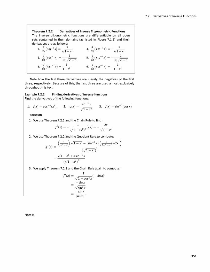
Theorem 7.2.2 Derivatives of Inverse Trigonometric FunctionsThe inverse trigonometric functions are differentiable on all opensets contained in their domains (as listed in Figure 7.1.5) and theirderivatives are as follows:
1. ddx(sin−1 x
)=
1√1− x2
2. ddx(sec−1 x
)=
1|x|
√x2 − 1
3. ddx(tan−1 x
)=
11+ x2
4. ddx(cos−1 x
)= − 1√
1− x2
5. ddx(csc−1 x
)= − 1
|x|√x2 − 1
6. ddx(cot−1 x
)= − 1
1+ x2
Note how the last three derivatives are merely the negatives of the firstthree, respectively. Because of this, the first three are used almost exclusivelythroughout this text.
Example 7.2.2 Finding derivatives of inverse functionsFind the derivatives of the following functions:
1. f(x) = cos−1(x2) 2. g(x) =sin−1 x√1− x2
3. f(x) = sin−1(cos x)
SOLUTION
1. We use Theorem 7.2.2 and the Chain Rule to find:
f ′(x) = − 1√1− (x2)2
(2x) = − 2x√1− x4
2. We use Theorem 7.2.2 and the Quotient Rule to compute:
g ′(x) =
(1√1−x2
)√1− x2 − (sin−1 x)
(1
2√1−x2 (−2x)
)(√
1− x2)2
=
√1− x2 + x sin−1 x(√
1− x2)3
3. We apply Theorem 7.2.2 and the Chain Rule again to compute:
f ′(x) =1√
1− cos2 x(− sin x)
=− sin x√sin2 x
=− sin x|sin x|
.
Notes:
351
Chapter 7 Inverse Functions and L’Hôpital’s Rule
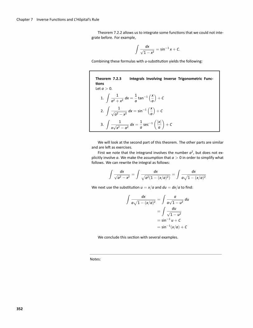
Theorem 7.2.2 allows us to integrate some functions that we could not inte‐grate before. For example,∫
dx√1− x2
= sin−1 x+ C.
Combining these formulas with u‐substitution yields the following:
Theorem 7.2.3 Integrals Involving Inverse Trigonometric Func‐tionsLet a > 0.
1.∫
1a2 + x2
dx =1atan−1
( xa
)+ C
2.∫
1√a2 − x2
dx = sin−1( xa
)+ C
3.∫
1x√x2 − a2
dx =1asec−1
(|x|a
)+ C
We will look at the second part of this theorem. The other parts are similarand are left as exercises.
First we note that the integrand involves the number a2, but does not ex‐plicitly involve a. We make the assumption that a > 0 in order to simplify whatfollows. We can rewrite the integral as follows:∫
dx√a2 − x2
=
∫dx√
a2(1− (x/a)2)=
∫dx
a√
1− (x/a)2
We next use the substitution u = x/a and du = dx/a to find:∫dx
a√
1− (x/a)2=
∫a
a√1− u2
du
=
∫du√1− u2
= sin−1 u+ C= sin−1(x/a) + C
We conclude this section with several examples.
Notes:
352
7.2 Derivatives of Inverse Functions
Example 7.2.3 Finding antiderivatives involving inverse functionsFind the following integrals.
1.∫
dx100+ x2
2.∫
sin−1 x√1− x2
dx 3.∫
dxx2 + 2x+ 5
SOLUTION
1.∫
dx100+ x2
=
∫dx
102 + x2=
110
tan−1(x/10) + C
2. We use the substitution u = sin−1 x and du = dx√1−x2 to find:∫
sin−1 x√1− x2
dx =∫
u du =12u2 + C =
12(sin−1 x
)2+ C
3. This does not immediately look like one of the forms in Theorem 7.2.3,but we can complete the square in the denominator to see that∫
dxx2 + 2x+ 5
=
∫dx
(x2 + 2x+ 1) + 4=
∫dx
4+ (x+ 1)2
We now use the substitution u = x+ 1 and du = dx to find:∫dx
4+ (x+ 1)2=
∫du
4+ u2=
12tan−1(u/2)+C =
12tan−1
(x+ 12
)+C.
Notes:
353
Exercises 7.2Terms and Concepts1. If (1, 10) lies on the graph of y = f(x) and f ′(1) = 5, what
can be said about y = f−1(x)?2. Since d
dx (sin−1 x + cos−1 x) = 0, what does this tell us
about sin−1 x+ cos−1 x?
ProblemsIn Exercises 3–8, an invertible function f(x) is given along witha point that lies on its graph. Using Theorem 7.2.1, evaluate(f−1)′ (x) at the indicated value.
3. f(x) = 5x+ 10Point= (2, 20)Evaluate
(f−1)′ (20)
4. f(x) = x2 − 2x+ 4, x ≥ 1Point= (3, 7)Evaluate
(f−1)′ (7)
5. f(x) = sin 2x,−π/4 ≤ x ≤ π/4Point= (π/6,
√3/2)
Evaluate(f−1)′ (√3/2)
6. f(x) = x3 − 6x2 + 15x− 2Point= (1, 8)Evaluate
(f−1)′ (8)
7. f(x) = 11+ x2
, x ≥ 0Point= (1, 1/2)Evaluate
(f−1)′ (1/2)
8. f(x) = 6e3xPoint= (0, 6)Evaluate
(f−1)′ (6)
In Exercises 9–18, compute the derivative of the given func‐tion.
9. h(t) = sin−1(2t)10. f(t) = sec−1(2t)11. g(x) = tan−1(2x)12. f(x) = x sin−1 x
13. g(t) = sin t cos−1 t
14. f(t) = et ln t
15. h(x) = sin−1 xcos−1 x
16. g(x) = tan−1(√x)
17. f(x) = sec−1(1/x)18. f(x) = sin(sin−1 x)
In Exercises 19–22, compute the derivative of the given func‐tion in two ways:
(a) By simplifying first, then taking the derivative, and
(b) by using the Chain Rule first then simplifying.
Verify that the two answers are the same.
19. f(x) = sin(sin−1 x)
20. f(x) = tan−1(tan x)
21. f(x) = sin(cos−1 x)
22. f(x) = sin(tan−1 x)
In Exercises 23–24, find the equation of the line tangent to thegraph of f at the indicated x value.
23. f(x) = sin−1 x at x =√
22
24. f(x) = cos−1(2x) at x =√
34
In Exercises 25–30, compute the indicated integral.
25.∫ 1/2
1/√
2
2√1− x2
dx
26.∫ √
3
0
49+ x2
dx
27.∫
sin−1 r√1− r2
dr
28.∫
x3
4+ x8dx
29.∫
et√10− e2t
dt
30.∫
1√x(1+ x)
dx
31. A regulation hockey goal is 6 feet wide. If a player is skat‐ing towards the end line on a line perpendicular to the endline and 10 feet from the imaginary line joining the centerof one goal to the center of the other, the angle betweenthe player and the goal first increases and then begins todecrease. In order tomaximize this angle, how far from theend line should the player be when they shoot the puck?
θ
6 ft
10 ft
354
7.3 Exponential and Logarithmic Functions
7.3 Exponential and Logarithmic Functions
In this section we will define general exponential and logarithmic functions andfind their derivatives.
General exponential functions
1
1
2
x
y
Figure 7.3.1: The function 2x for rationalvalues of x.
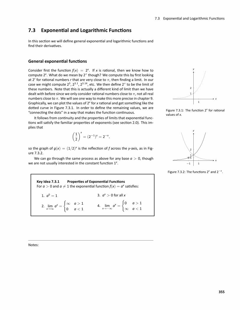
Consider first the function f(x) = 2x. If x is rational, then we know how tocompute 2x. What do we mean by 2π though? We compute this by first lookingat 2r for rational numbers r that are very close to π, then finding a limit. In ourcase we might compute 23, 23.1, 23.14, etc. We then define 2π to be the limit ofthese numbers. Note that this is actually a different kind of limit than we havedealt with before since we only consider rational numbers close to π, not all realnumbers close to π. Wewill see one way tomake this more precise in chapter 9.Graphically, we can plot the values of 2x for x rational and get something like thedotted curve in Figure 7.3.1. In order to define the remaining values, we are“connecting the dots” in a way that makes the function continuous.
It follows from continuity and the properties of limits that exponential func‐tions will satisfy the familiar properties of exponents (see section 2.0). This im‐plies that
−1 1
0.51
2
x
y
Figure 7.3.2: The functions 2x and 2−x.
(12
)x
= (2−1)x = 2−x,
so the graph of g(x) = (1/2)x is the reflection of f across the y‐axis, as in Fig‐ure 7.3.2.
We can go through the same process as above for any base a > 0, thoughwe are not usually interested in the constant function 1x.
Key Idea 7.3.1 Properties of Exponential FunctionsFor a > 0 and a ̸= 1 the exponential function f(x) = ax satisfies:
1. a0 = 1
2. limx→∞
ax =
{∞ a > 10 a < 1
3. ax > 0 for all x
4. limx→−∞
ax =
{0 a > 1∞ a < 1
Notes:
355
Chapter 7 Inverse Functions and L’Hôpital’s Rule
Derivatives of exponential functions
Suppose f(x) = ax for some a > 0. We can use the rules of exponents to findthe derivative of f:
f ′(x) = limh→0
f(x+ h)− f(x)h
= limh→0
ax+h − ax
h
= limh→0
axah − ax
h
= limh→0
ax(ah − 1)h
= ax limh→0
ah − 1h
(since ax does not depend on h)
So we know that f ′(x) = ax limh→0
ah − 1h
, but can we say anything about thatremaining limit? First we note that
f ′(0) = limh→0
a0+h − a0
h= lim
h→0
ah − 1h
,
so we have f ′(x) = axf ′(0). The actual value of the limit limh→0
ah − 1h
dependson the base a, but it can be proved that it does exist. Wewill figure out just whatthis limit is later, but for now we note that the easiest differentiation formulas
come from using a base a that makes limh→0
ah − 1h
= 1. This base is the numbere ≈ 2.71828 and the exponential function ex is called the natural exponentialfunction. This leads to the following result.
Theorem 7.3.1 Derivative of Exponential FunctionsFor any base a > 0, the exponential function f(x) = ax has deriva‐tive f ′(x) = axf ′(0). The natural exponential function g(x) = ex hasderivative g ′(x) = ex.
Notes:
356

7.3 Exponential and Logarithmic Functions
Watch the video:Derivatives of Exponential Functions athttps://youtu.be/U3PyUcEd7IU
General logarithmic functions
Before reviewing general logarithmic functions, we’ll first remind ourselves ofthe laws of logarithms.
Key Idea 7.3.2 Properties of LogarithmsFor a, x, y > 0 and a ̸= 1, we have1. loga(xy) = loga x+ loga y 2. loga
xy= loga x− loga y
3. logx y =loga yloga x
, when x ̸= 1 4. loga xy = y loga x
5. loga 1 = 0 6. loga a = 1
1 e
1
e
x
y
Figure 7.3.3: The functions y = ax andy = loga x for a > 1.
Let us consider the function f(x) = ax where a ̸= 1. We know that f ′(x) =f ′(0)ax, where f ′(0) is a constant that depends on the base a. Since ax > 0 for allx, this implies that f ′(x) is either always positive or always negative, dependingon the sign of f ′(0). This in turn implies that f is strictly monotonic, so f is one‐to‐one. We can now say that f has an inverse. We call this inverse the logarithmwith base a, denoted f−1(x) = loga x. When a = e, this is the natural logarithmfunction ln x. So we can say that y = loga x if and only if ay = x. Since the rangeof the exponential function is the set of positive real numbers, the domain ofthe logarithm function is also the set of positive real numbers. Reflecting thegraph of y = ax across the line y = x we find that (for a > 1) the graph of thelogarithm looks like Figure 7.3.3.
Notes:
357
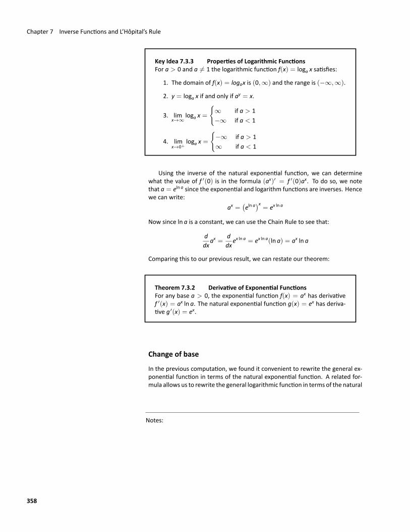
Chapter 7 Inverse Functions and L’Hôpital’s Rule
Key Idea 7.3.3 Properties of Logarithmic FunctionsFor a > 0 and a ̸= 1 the logarithmic function f(x) = loga x satisfies:
1. The domain of f(x) = logax is (0,∞) and the range is (−∞,∞).
2. y = loga x if and only if ay = x.
3. limx→∞
loga x =
{∞ if a > 1−∞ if a < 1
4. limx→0+
loga x =
{−∞ if a > 1∞ if a < 1
Using the inverse of the natural exponential function, we can determinewhat the value of f ′(0) is in the formula (ax)′ = f ′(0)ax. To do so, we notethat a = eln a since the exponential and logarithm functions are inverses. Hencewe can write:
ax =(eln a)x
= ex ln a
Now since ln a is a constant, we can use the Chain Rule to see that:
ddx
ax =ddx
ex ln a = ex ln a(ln a) = ax ln a
Comparing this to our previous result, we can restate our theorem:
Theorem 7.3.2 Derivative of Exponential FunctionsFor any base a > 0, the exponential function f(x) = ax has derivativef ′(x) = ax ln a. The natural exponential function g(x) = ex has deriva‐tive g ′(x) = ex.
Change of base
In the previous computation, we found it convenient to rewrite the general ex‐ponential function in terms of the natural exponential function. A related for‐mula allows us to rewrite the general logarithmic function in terms of the natural
Notes:
358
7.3 Exponential and Logarithmic Functions
logarithm. To see how this works, suppose that y = loga x, then we have:
ay = xln(ay) = ln xy ln a = ln x
y =ln xln a
loga x =ln xln a
.
This change of base formula allows us to use facts about the natural logarithmto derive facts about the general logarithm.
Derivatives of logarithmic functionsSince the natural logarithm function is the inverse of the natural exponentialfunction, we can use the formula (f−1(x))′ =
1f ′(f−1(x))
to find the derivative
of y = ln x. We know thatddx
ex = ex, so we get:
ddx
ln x =1ey
=1
eln x=
1x.
Nowwe can apply the change of base formula to find the derivative of a generallogarithmic function:
ddx
loga x =ddx
(ln xln a
)=
1ln a
(ddx
ln x)
=1
x ln a.
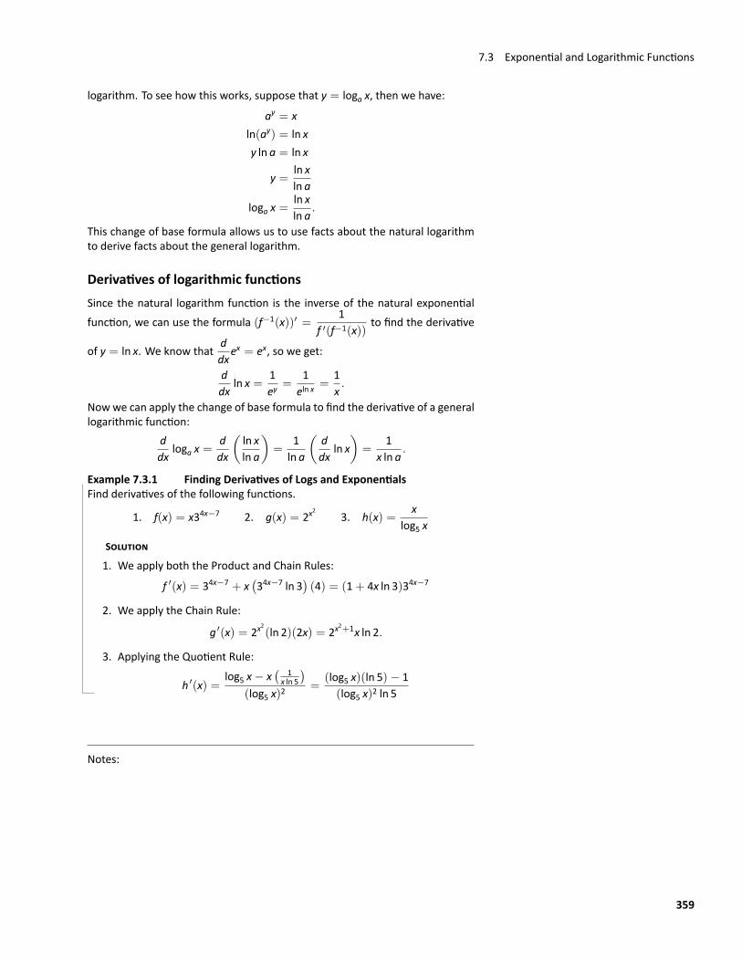
Example 7.3.1 Finding Derivatives of Logs and ExponentialsFind derivatives of the following functions.
1. f(x) = x34x−7 2. g(x) = 2x2
3. h(x) =x
log5 x
SOLUTION
1. We apply both the Product and Chain Rules:
f ′(x) = 34x−7 + x(34x−7 ln 3
)(4) = (1+ 4x ln 3)34x−7
2. We apply the Chain Rule:
g ′(x) = 2x2(ln 2)(2x) = 2x
2+1x ln 2.
3. Applying the Quotient Rule:
h ′(x) =log5 x− x
( 1x ln 5)
(log5 x)2=
(log5 x)(ln 5)− 1(log5 x)2 ln 5
Notes:
359
Chapter 7 Inverse Functions and L’Hôpital’s Rule
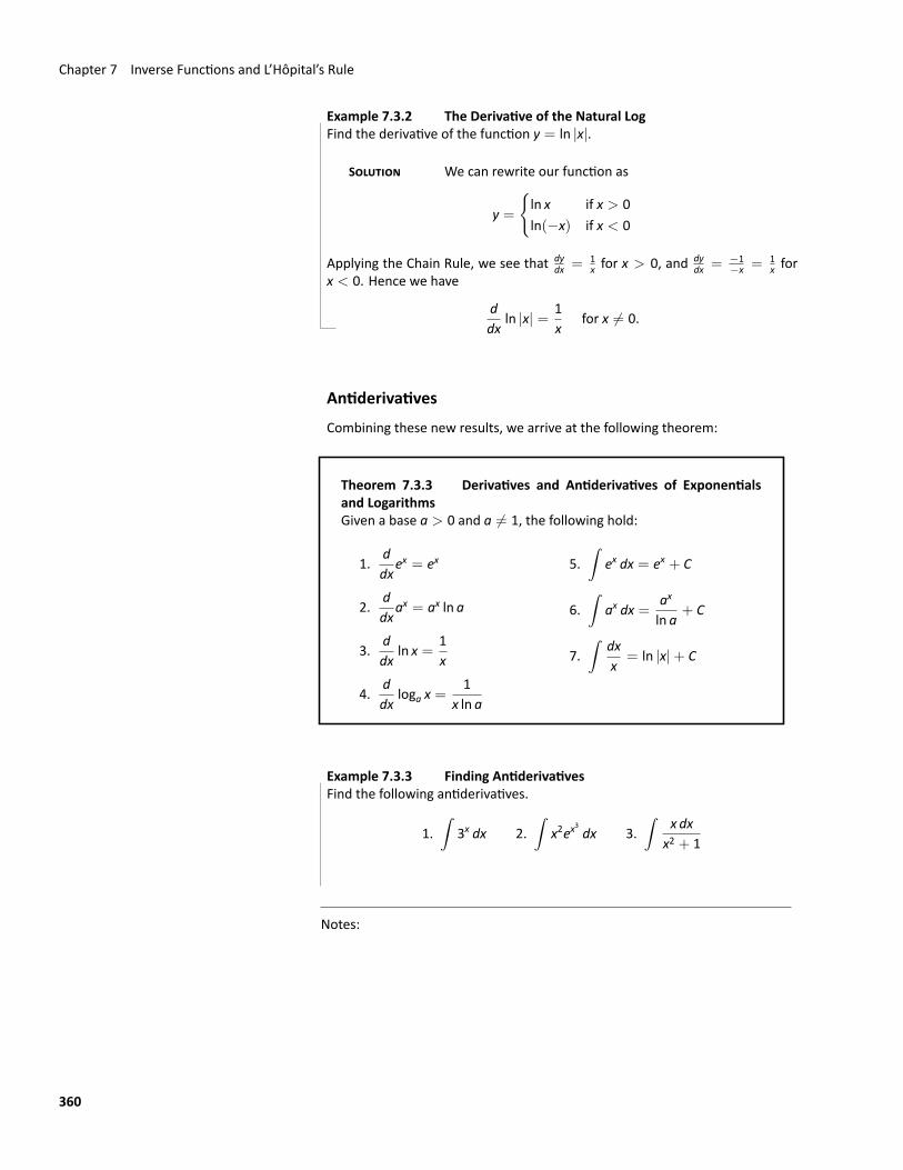
Example 7.3.2 The Derivative of the Natural LogFind the derivative of the function y = ln |x|.
SOLUTION We can rewrite our function as
y =
{ln x if x > 0ln(−x) if x < 0
Applying the Chain Rule, we see that dydx = 1
x for x > 0, and dydx = −1
−x = 1x for
x < 0. Hence we have
ddx
ln |x| = 1x
for x ̸= 0.
AntiderivativesCombining these new results, we arrive at the following theorem:
Theorem 7.3.3 Derivatives and Antiderivatives of Exponentialsand LogarithmsGiven a base a > 0 and a ̸= 1, the following hold:
1.ddx
ex = ex
2.ddx
ax = ax ln a
3.ddx
ln x =1x
4.ddx
loga x =1
x ln a
5.∫
ex dx = ex + C
6.∫
ax dx =ax
ln a+ C
7.∫
dxx
= ln |x|+ C
Example 7.3.3 Finding AntiderivativesFind the following antiderivatives.
1.∫
3x dx 2.∫
x2ex3dx 3.
∫x dx
x2 + 1
Notes:
360
7.3 Exponential and Logarithmic Functions
SOLUTION
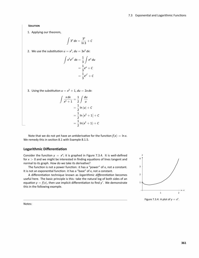
1. Applying our theorem, ∫3x dx =
3x
ln 3+ C
2. We use the substitution u = x3, du = 3x2 dx:∫x2ex
3dx =
13
∫eu du
=13eu + C
=13ex
3+ C
3. Using the substitution u = x2 + 1, du = 2x dx:∫x dx
x2 + 1=
12
∫duu
=12ln |u|+ C
=12ln∣∣x2 + 1
∣∣+ C
=12ln(x2 + 1) + C
Note that we do not yet have an antiderivative for the function f(x) = ln x.We remedy this in section 8.1 with Example 8.1.5.
Logarithmic Differentiation
1 2
1
2
3
4
x
y
Figure 7.3.4: A plot of y = xx.
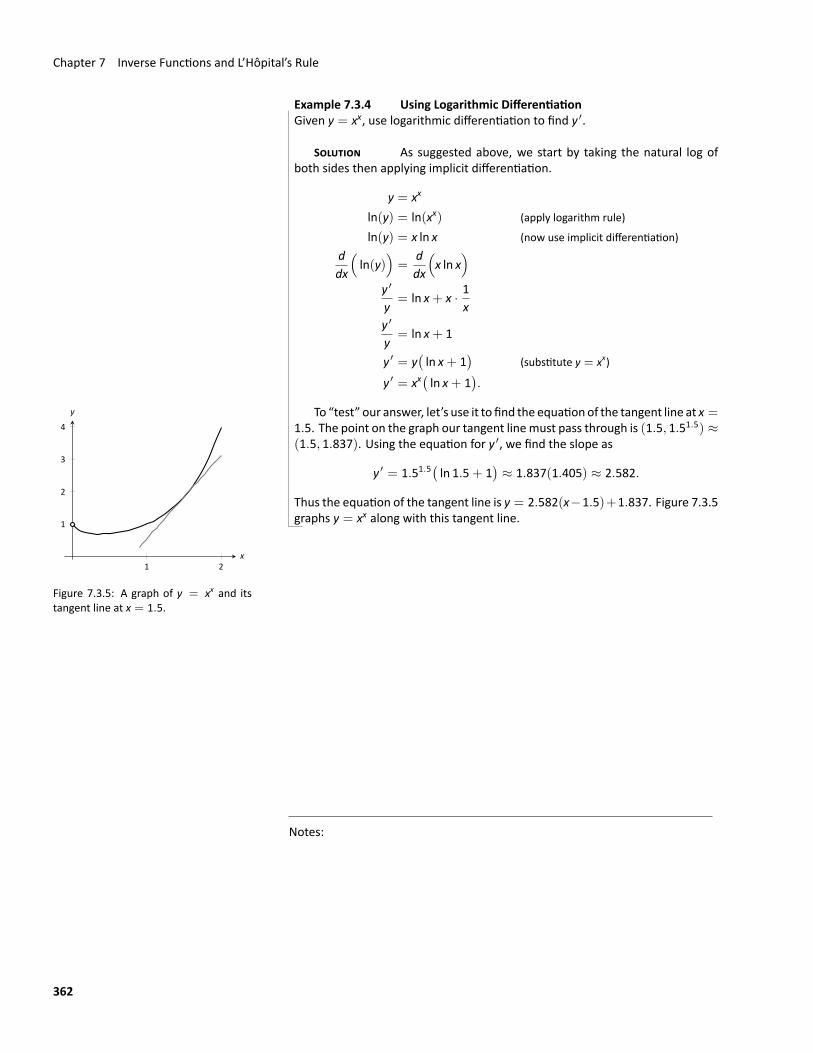
Consider the function y = xx; it is graphed in Figure 7.3.4. It is well‐definedfor x > 0 and we might be interested in finding equations of lines tangent andnormal to its graph. How do we take its derivative?
The function is not a power function: it has a “power” of x, not a constant.It is not an exponential function: it has a “base” of x, not a constant.
A differentiation technique known as logarithmic differentiation becomesuseful here. The basic principle is this: take the natural log of both sides of anequation y = f(x), then use implicit differentiation to find y ′. We demonstratethis in the following example.
Notes:
361
Chapter 7 Inverse Functions and L’Hôpital’s Rule
Example 7.3.4 Using Logarithmic DifferentiationGiven y = xx, use logarithmic differentiation to find y ′.
SOLUTION As suggested above, we start by taking the natural log ofboth sides then applying implicit differentiation.
y = xx
ln(y) = ln(xx) (apply logarithm rule)
ln(y) = x ln x (now use implicit differentiation)ddx
(ln(y)
)=
ddx
(x ln x
)y ′
y= ln x+ x · 1
xy ′
y= ln x+ 1
y ′ = y(ln x+ 1
)(substitute y = xx)
y ′ = xx(ln x+ 1
).
1 2
1
2
3
4
x
y
Figure 7.3.5: A graph of y = xx and itstangent line at x = 1.5.
To “test” our answer, let’s use it to find the equationof the tangent line at x =1.5. The point on the graph our tangent linemust pass through is (1.5, 1.51.5) ≈(1.5, 1.837). Using the equation for y ′, we find the slope as
y ′ = 1.51.5(ln 1.5+ 1
)≈ 1.837(1.405) ≈ 2.582.
Thus the equation of the tangent line is y = 2.582(x−1.5)+1.837. Figure 7.3.5graphs y = xx along with this tangent line.
Notes:
362
Exercises 7.3ProblemsIn Exercises 1–4, find the domain of the function.
1. f(x) = ex2+1
2. f(t) = ln(1− t2)
3. g(x) = ln(x2)
4. f(x) = 2log3(x2 + 1)
In Exercises 5–12, find the derivative of the function.
5. f(t) = et3−1
6. g(r) = r2 log2 r
7. f(x) = log5 x5x
8. f(x) = 4x5
9. f(x) = 7log7 x
10. g(x) = ex2sin(x− ln x)
11. h(r) = tan−1(3r)
12. h(x) = log10(x2 + 1x4
)In Exercises 13–20, evaluate the integral.
13.∫ 2
05x dx
14.∫ 3
1
log3 xx
dx
15.∫
x3x2−1 dx
16.∫
cos(ln x)x
dx
17.∫
ex sin(ex) cos(ex) dx
18.∫ 8
1log2 x dx
19.∫ 5
0
3x
3x + 2dx
20.∫
1(1+ x2) tan−1 x
dx
21. Find the two values of n so that the function y = enx satis‐fies the differential equation y ′′ + y ′ − 6y = 0.
22. Let f(x) = x2 and g(x) = 2x.
(a) Since f(2) = 22 = 4 and g(2) = 22 = 4,f(2) = g(2). Find a positive number c > 2 so thatf(c) = g(c).
(b) Explain how you can be sure that there is at least onenegative number a so that f(a) = g(a).
(c) Use the Bisection Method to estimate the number aaccurate to within .05.
(d) Assume youwere to graph f(x) and g(x) on the samegraph with unit length equal to 1 inch along both co‐ordinate axes. Approximately how high is the graphof f when x = 18? The graph of g?
In Exercises 23–30, use logarithmic differentiation to find dydx
,then find the equation of the tangent line at the indicated x‐value.
23. y = (1+ x)1/x, x = 1
24. y = (2x)x2, x = 1
25. y = xx
x+ 1, x = 1
26. y = xsin(x)+2, x = π/2
27. y = x+ 1x+ 2
, x = 1
28. y = (x+ 1)(x+ 2)(x+ 3)(x+ 4)
, x = 0
29. y = xex, x = 1
30. y = (cot x)cos x, x = π
363
Chapter 7 Inverse Functions and L’Hôpital’s Rule
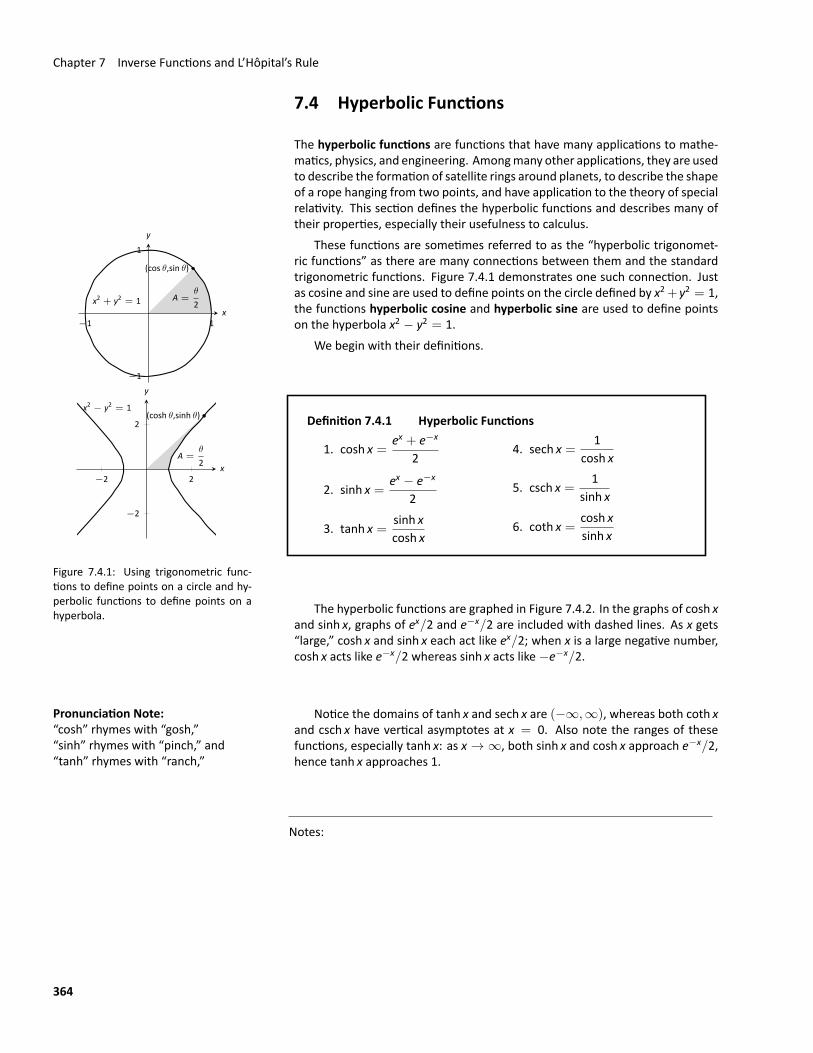
7.4 Hyperbolic Functions
The hyperbolic functions are functions that have many applications to mathe‐matics, physics, and engineering. Amongmany other applications, they are usedto describe the formation of satellite rings around planets, to describe the shapeof a rope hanging from two points, and have application to the theory of specialrelativity. This section defines the hyperbolic functions and describes many oftheir properties, especially their usefulness to calculus.
(cos θ,sin θ)
A =θ
2x2 + y2 = 1
−1 1
−1
1
x
y
(cosh θ,sinh θ)
A =θ
2
x2 − y2 = 1
−2 2
−2
2
x
y
Figure 7.4.1: Using trigonometric func‐tions to define points on a circle and hy‐perbolic functions to define points on ahyperbola.
These functions are sometimes referred to as the “hyperbolic trigonomet‐ric functions” as there are many connections between them and the standardtrigonometric functions. Figure 7.4.1 demonstrates one such connection. Justas cosine and sine are used to define points on the circle defined by x2+y2 = 1,the functions hyperbolic cosine and hyperbolic sine are used to define pointson the hyperbola x2 − y2 = 1.
We begin with their definitions.
Definition 7.4.1 Hyperbolic Functions
1. cosh x =ex + e−x
2
2. sinh x =ex − e−x
2
3. tanh x =sinh xcosh x
4. sech x =1
cosh x
5. csch x =1
sinh x
6. coth x =cosh xsinh x
The hyperbolic functions are graphed in Figure 7.4.2. In the graphs of cosh xand sinh x, graphs of ex/2 and e−x/2 are included with dashed lines. As x gets“large,” cosh x and sinh x each act like ex/2; when x is a large negative number,cosh x acts like e−x/2 whereas sinh x acts like−e−x/2.
Pronunciation Note:“cosh” rhymes with “gosh,”“sinh” rhymes with “pinch,” and“tanh” rhymes with “ranch,”
Notice the domains of tanh x and sech x are (−∞,∞), whereas both coth xand csch x have vertical asymptotes at x = 0. Also note the ranges of thesefunctions, especially tanh x: as x → ∞, both sinh x and cosh x approach e−x/2,hence tanh x approaches 1.
Notes:
364
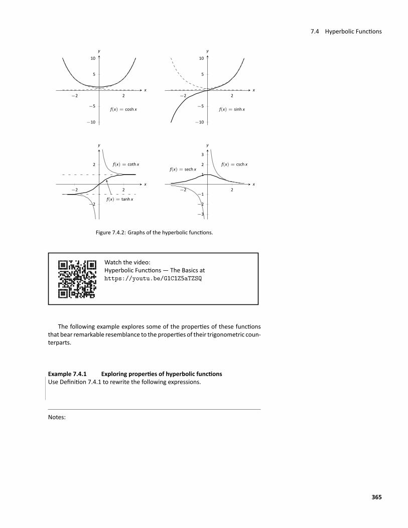
7.4 Hyperbolic Functions
f(x) = cosh x
−2 2
−10
−5
5
10
x
y
f(x) = sinh x
−2 2
−10
−5
5
10
x
y
f(x) = tanh x
f(x) = coth x
−2 2
−2
2
x
y
f(x) = sech xf(x) = csch x
−2 2
−3
−2
−1
1
2
3
x
y
Figure 7.4.2: Graphs of the hyperbolic functions.
Watch the video:Hyperbolic Functions — The Basics athttps://youtu.be/G1C1Z5aTZSQ
The following example explores some of the properties of these functionsthat bear remarkable resemblance to the properties of their trigonometric coun‐terparts.
Example 7.4.1 Exploring properties of hyperbolic functionsUse Definition 7.4.1 to rewrite the following expressions.
Notes:
365
Chapter 7 Inverse Functions and L’Hôpital’s Rule
1. cosh2 x− sinh2 x
2. tanh2 x+ sech2 x
3. 2 cosh x sinh x
4. ddx
(cosh x
)5. d
dx
(sinh x
)6. d
dx
(tanh x
)SOLUTION
1. cosh2 x− sinh2 x =(ex + e−x
2
)2
−(ex − e−x
2
)2
=e2x + 2exe−x + e−2x
4− e2x − 2exe−x + e−2x
4
=44= 1.
So cosh2 x− sinh2 x = 1.
2. tanh2 x+ sech2 x =sinh2 xcosh2 x
+1
cosh2 x
=sinh2 x+ 1cosh2 x
Now use identity from #1.
=cosh2 xcosh2 x
= 1.
So tanh2 x+ sech2 x = 1.
3. 2 cosh x sinh x = 2(ex + e−x
2
)(ex − e−x
2
)= 2 · e
2x − e−2x
4
=e2x − e−2x
2= sinh(2x).
Thus 2 cosh x sinh x = sinh(2x).
4. ddx(cosh x
)=
ddx
(ex + e−x
2
)=
ex − e−x
2= sinh x.
So ddx
(cosh x
)= sinh x.
Notes:
366
7.4 Hyperbolic Functions
5. ddx(sinh x
)=
ddx
(ex − e−x
2
)=
ex + e−x
2= cosh x.
So ddx
(sinh x
)= cosh x.
6. ddx(tanh x
)=
ddx
(sinh xcosh x
)=
cosh x cosh x− sinh x sinh xcosh2 x
=1
cosh2 x= sech2 x.
So ddx
(tanh x
)= sech2 x.
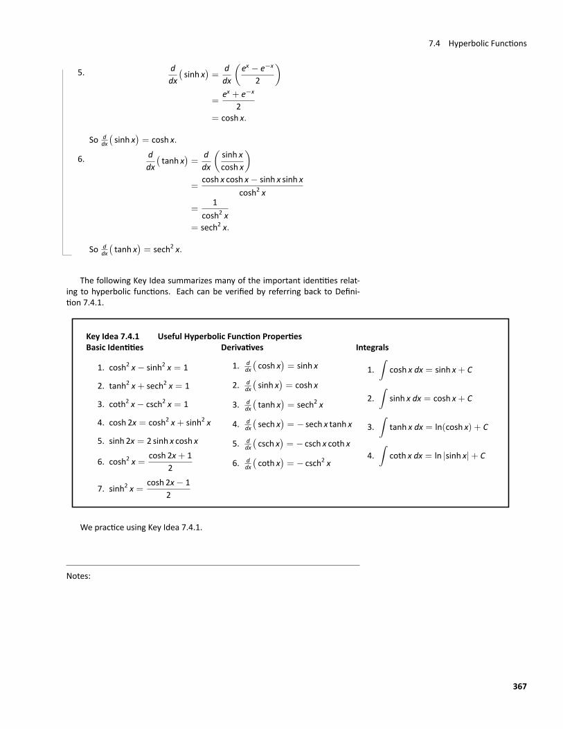
The following Key Idea summarizes many of the important identities relat‐ing to hyperbolic functions. Each can be verified by referring back to Defini‐tion 7.4.1.
Key Idea 7.4.1 Useful Hyperbolic Function PropertiesBasic Identities
1. cosh2 x− sinh2 x = 1
2. tanh2 x+ sech2 x = 1
3. coth2 x− csch2 x = 1
4. cosh 2x = cosh2 x+ sinh2 x
5. sinh 2x = 2 sinh x cosh x
6. cosh2 x =cosh 2x+ 1
2
7. sinh2 x =cosh 2x− 1
2
Derivatives
1. ddx
(cosh x
)= sinh x
2. ddx
(sinh x
)= cosh x
3. ddx
(tanh x
)= sech2 x
4. ddx
(sech x
)= − sech x tanh x
5. ddx
(csch x
)= − csch x coth x
6. ddx
(coth x
)= − csch2 x
Integrals
1.∫
cosh x dx = sinh x+ C
2.∫
sinh x dx = cosh x+ C
3.∫
tanh x dx = ln(cosh x) + C
4.∫
coth x dx = ln |sinh x|+ C
We practice using Key Idea 7.4.1.
Notes:
367
Chapter 7 Inverse Functions and L’Hôpital’s Rule
Example 7.4.2 Derivatives and integrals of hyperbolic functionsEvaluate the following derivatives and integrals.
1.ddx(cosh 2x
)2.∫
sech2(7t− 3) dt
3.∫ ln 2
0cosh x dx
SOLUTION
1. Using the Chain Rule directly, we have ddx
(cosh 2x
)= 2 sinh 2x.
Just to demonstrate that it works, let’s also use the Basic Identity found inKey Idea 7.4.1: cosh 2x = cosh2 x+ sinh2 x.
ddx(cosh 2x
)=
ddx(cosh2 x+ sinh2 x
)= 2 cosh x sinh x+ 2 sinh x cosh x
= 4 cosh x sinh x.
Using another Basic Identity, we can see that 4 cosh x sinh x = 2 sinh 2x.We get the same answer either way.
2. We employ substitution, with u = 7t − 3 and du = 7dt. Applying KeyIdea 7.4.1 we have:∫
sech2(7t− 3) dt =17tanh(7t− 3) + C.
3. ∫ ln 2
0cosh x dx = sinh x
∣∣∣ln 20
= sinh(ln 2)− sinh 0 = sinh(ln 2).
We can simplify this last expression as sinh x is based on exponentials:
sinh(ln 2) =eln 2 − e− ln 2
2=
2− 1/22
=34.
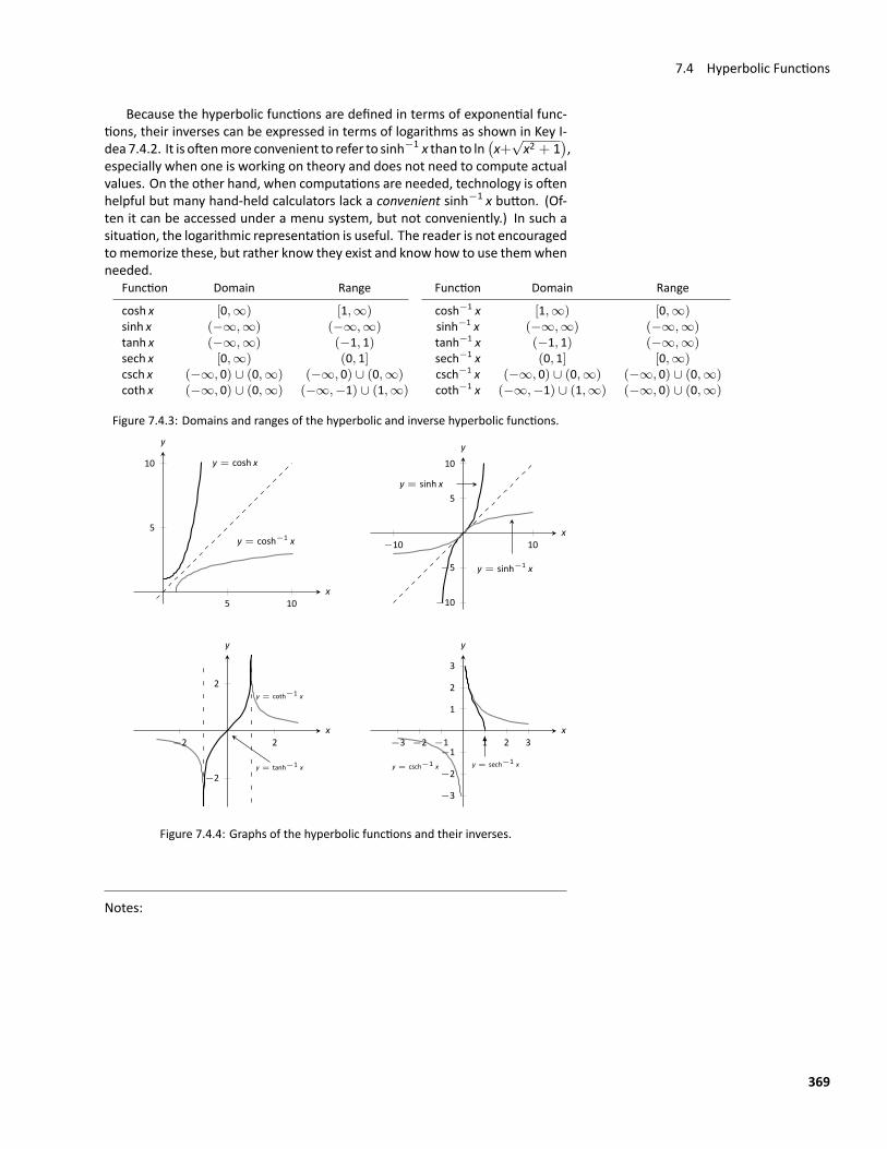
Inverse Hyperbolic FunctionsJust as the inverse trigonometric functions are useful in certain integrations, theinverse hyperbolic functions are useful with others. Figure 7.4.3 shows the re‐strictions on the domains to make each function one‐to‐one and the resultingdomains and ranges of their inverse functions. Their graphs are shown in Fig‐ure 7.4.4.
Notes:
368
7.4 Hyperbolic Functions
Because the hyperbolic functions are defined in terms of exponential func‐tions, their inverses can be expressed in terms of logarithms as shown in Key I‐dea 7.4.2. It is oftenmore convenient to refer to sinh−1 x than to ln
(x+
√x2 + 1
),
especially when one is working on theory and does not need to compute actualvalues. On the other hand, when computations are needed, technology is oftenhelpful but many hand‐held calculators lack a convenient sinh−1 x button. (Of‐ten it can be accessed under a menu system, but not conveniently.) In such asituation, the logarithmic representation is useful. The reader is not encouragedtomemorize these, but rather know they exist and know how to use themwhenneeded.
Function Domain Range Function Domain Range
cosh x [0,∞) [1,∞) cosh−1 x [1,∞) [0,∞)sinh x (−∞,∞) (−∞,∞) sinh−1 x (−∞,∞) (−∞,∞)tanh x (−∞,∞) (−1, 1) tanh−1 x (−1, 1) (−∞,∞)sech x [0,∞) (0, 1] sech−1 x (0, 1] [0,∞)csch x (−∞, 0) ∪ (0,∞) (−∞, 0) ∪ (0,∞) csch−1 x (−∞, 0) ∪ (0,∞) (−∞, 0) ∪ (0,∞)coth x (−∞, 0) ∪ (0,∞) (−∞,−1) ∪ (1,∞) coth−1 x (−∞,−1) ∪ (1,∞) (−∞, 0) ∪ (0,∞)
Figure 7.4.3: Domains and ranges of the hyperbolic and inverse hyperbolic functions.
y = cosh−1 x
y = cosh x
5 10
5
10
x
y
y = sinh x
y = sinh−1 x
−10 10
−10
−5
5
10
x
y
y = coth−1 x
y = tanh−1 x
−2 2
−2
2
x
y
y = sech−1 xy = csch−1 x
−3 −2 −1 1 2 3
−3
−2
−1
1
2
3
x
y
Figure 7.4.4: Graphs of the hyperbolic functions and their inverses.
Notes:
369
Chapter 7 Inverse Functions and L’Hôpital’s Rule
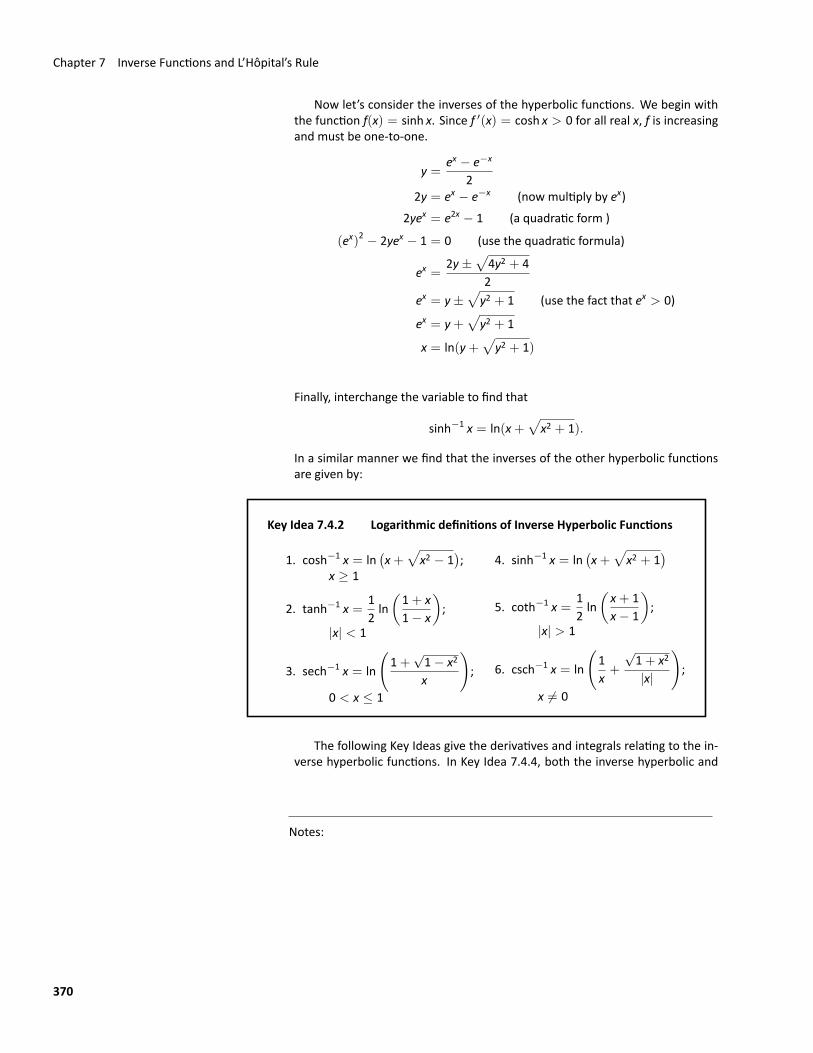
Now let’s consider the inverses of the hyperbolic functions. We begin withthe function f(x) = sinh x. Since f ′(x) = cosh x > 0 for all real x, f is increasingand must be one‐to‐one.
y =ex − e−x
22y = ex − e−x (now multiply by ex)
2yex = e2x − 1 (a quadratic form )
(ex)2 − 2yex − 1 = 0 (use the quadratic formula)
ex =2y±
√4y2 + 42
ex = y±√
y2 + 1 (use the fact that ex > 0)
ex = y+√
y2 + 1
x = ln(y+√
y2 + 1)
Finally, interchange the variable to find that
sinh−1 x = ln(x+√
x2 + 1).
In a similar manner we find that the inverses of the other hyperbolic functionsare given by:
Key Idea 7.4.2 Logarithmic definitions of Inverse Hyperbolic Functions
1. cosh−1 x = ln(x+
√x2 − 1
);
x ≥ 1
2. tanh−1 x =12ln(1+ x1− x
);
|x| < 1
3. sech−1 x = ln
(1+
√1− x2
x
);
0 < x ≤ 1
4. sinh−1 x = ln(x+
√x2 + 1
)5. coth−1 x =
12ln(x+ 1x− 1
);
|x| > 1
6. csch−1 x = ln
(1x+
√1+ x2
|x|
);
x ̸= 0
The following Key Ideas give the derivatives and integrals relating to the in‐verse hyperbolic functions. In Key Idea 7.4.4, both the inverse hyperbolic and
Notes:
370
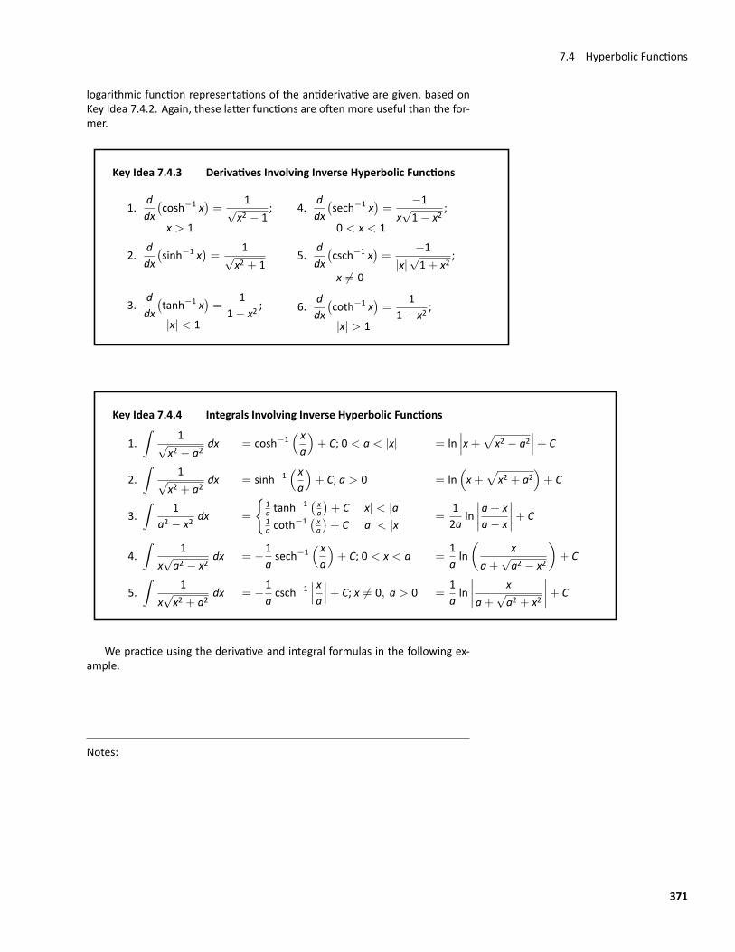
7.4 Hyperbolic Functions
logarithmic function representations of the antiderivative are given, based onKey Idea 7.4.2. Again, these latter functions are often more useful than the for‐mer.
Key Idea 7.4.3 Derivatives Involving Inverse Hyperbolic Functions
1.ddx(cosh−1 x
)=
1√x2 − 1
;x > 1
2.ddx(sinh−1 x
)=
1√x2 + 1
3.ddx(tanh−1 x
)=
11− x2
;|x| < 1
4.ddx(sech−1 x
)=
−1x√1− x2
;
0 < x < 1
5.ddx(csch−1 x
)=
−1|x|
√1+ x2
;
x ̸= 0
6.ddx(coth−1 x
)=
11− x2
;|x| > 1
Key Idea 7.4.4 Integrals Involving Inverse Hyperbolic Functions
1.∫
1√x2 − a2
dx = cosh−1( xa
)+ C; 0 < a < |x| = ln
∣∣∣x+√x2 − a2∣∣∣+ C
2.∫
1√x2 + a2
dx = sinh−1( xa
)+ C; a > 0 = ln
(x+
√x2 + a2
)+ C
3.∫
1a2 − x2
dx =
{1a tanh
−1 ( xa
)+ C |x| < |a|
1a coth
−1 ( xa
)+ C |a| < |x|
=12a
ln∣∣∣∣a+ xa− x
∣∣∣∣+ C
4.∫
1x√a2 − x2
dx = −1asech−1
( xa
)+ C; 0 < x < a =
1aln(
xa+
√a2 − x2
)+ C
5.∫
1x√x2 + a2
dx = −1acsch−1
∣∣∣ xa ∣∣∣+ C; x ̸= 0, a > 0 =1aln∣∣∣∣ xa+
√a2 + x2
∣∣∣∣+ C
We practice using the derivative and integral formulas in the following ex‐ample.
Notes:
371
Chapter 7 Inverse Functions and L’Hôpital’s Rule
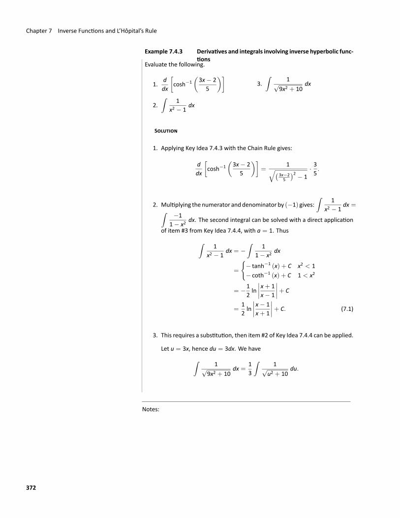
Example 7.4.3 Derivatives and integrals involving inverse hyperbolic func‐tions
Evaluate the following.
1.ddx
[cosh−1
(3x− 2
5
)]2.∫
1x2 − 1
dx
3.∫
1√9x2 + 10
dx
SOLUTION
1. Applying Key Idea 7.4.3 with the Chain Rule gives:
ddx
[cosh−1
(3x− 2
5
)]=
1√( 3x−25)2 − 1
· 35.
2. Multiplying the numerator anddenominator by (−1) gives:∫
1x2 − 1
dx =∫−1
1− x2dx. The second integral can be solved with a direct application
of item #3 from Key Idea 7.4.4, with a = 1. Thus∫1
x2 − 1dx = −
∫1
1− x2dx
=
{− tanh−1 (x) + C x2 < 1− coth−1 (x) + C 1 < x2
= −12ln∣∣∣∣x+ 1x− 1
∣∣∣∣+ C
=12ln∣∣∣∣x− 1x+ 1
∣∣∣∣+ C. (7.1)
3. This requires a substitution, then item #2 of Key Idea 7.4.4 can be applied.
Let u = 3x, hence du = 3dx. We have∫1√
9x2 + 10dx =
13
∫1√
u2 + 10du.
Notes:
372
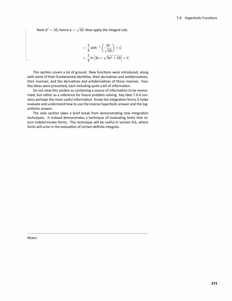
7.4 Hyperbolic Functions
Note a2 = 10, hence a =√10. Now apply the integral rule.
=13sinh−1
(3x√10
)+ C
=13ln∣∣∣3x+√9x2 + 10
∣∣∣+ C.
This section covers a lot of ground. New functions were introduced, alongwith some of their fundamental identities, their derivatives and antiderivatives,their inverses, and the derivatives and antiderivatives of these inverses. FourKey Ideas were presented, each including quite a bit of information.
Do not view this section as containing a source of information to be memo‐rized, but rather as a reference for future problem solving. Key Idea 7.4.4 con‐tains perhaps the most useful information. Know the integration forms it helpsevaluate and understand how to use the inverse hyperbolic answer and the log‐arithmic answer.
The next section takes a brief break from demonstrating new integrationtechniques. It instead demonstrates a technique of evaluating limits that re‐turn indeterminate forms. This technique will be useful in section 8.6, wherelimits will arise in the evaluation of certain definite integrals.
Notes:
373

Exercises 7.4Terms and Concepts
1. In Key Idea 7.4.1, the equation∫
tanh x dx = ln(cosh x)+
C is given. Why is “ln |cosh x|” not used — i.e., why are ab‐solute values not necessary?
2. The hyperbolic functions are used to define points on theright hand portion of the hyperbola x2 − y2 = 1, as shownin Figure 7.4.1. How can we use the hyperbolic functionsto define points on the left hand portion of the hyperbola?
ProblemsIn Exercises 3–10, verify the given identity using Defini‐tion 7.4.1, as done in Example 7.4.1.
3. coth2 x− csch2 x = 14. cosh 2x = cosh2 x+ sinh2 x
5. cosh2 x = cosh 2x+ 12
6. sinh2 x = cosh 2x− 12
7. ddx
[sech x] = − sech x tanh x
8. ddx
[coth x] = − csch2 x
9.∫
tanh x dx = ln(cosh x) + C
10.∫
coth x dx = ln |sinh x|+ C
In Exercises 11–22, find the derivative of the given function.
11. f(x) = sinh 2x12. f(x) = cosh2 x13. f(x) = tanh(x2)14. f(x) = ln(sinh x)15. f(x) = sinh x cosh x16. f(x) = x sinh x− cosh x17. f(x) = sech−1(x2)
18. f(x) = sinh−1(3x)
19. f(x) = cosh−1(2x2)
20. f(x) = tanh−1(x+ 5)
21. f(x) = tanh−1(cos x)
22. f(x) = cosh−1(sec x)
In Exercises 23–28, find the equation of the line tangent to thefunction at the given x‐value.
23. f(x) = sinh x at x = 0
24. f(x) = cosh x at x = ln 2
25. f(x) = tanh x at x = − ln 3
26. f(x) = sech2 x at x = ln 3
27. f(x) = sinh−1 x at x = 0
28. f(x) = cosh−1 x at x =√2
In Exercises 29–36, evaluate the given indefinite integral.
29.∫
tanh(2x) dx
30.∫
cosh(3x− 7) dx
31.∫
sinh x cosh x dx
32.∫
19− x2
dx
33.∫
2x√x4 − 4
dx
34.∫ √
x√1+ x3
dx
35.∫
ex
e2x + 1dx
36.∫
sech x dx (Hint: multiply by cosh xcosh x ; set u = sinh x.)
In Exercises 37–38, evaluate the given definite integral.
37.∫ 1
−1sinh x dx
38.∫ ln 2
− ln 2cosh x dx
374
7.5 L’Hôpital’s Rule
7.5 L’Hôpital’s Rule
This section is concerned with a technique for evaluating certain limits that willbe useful in later chapters.
Our treatment of limits exposedus to “0/0”, an indeterminate form. If limx→c
f(x) =0 and lim
x→cg(x) = 0, we do not conclude that lim
x→cf(x)/g(x) is 0/0; rather, we use
0/0 as notation to describe the fact that both the numerator and denominatorapproach 0. The expression 0/0 has no numeric value; other workmust be doneto evaluate the limit.
Other indeterminate forms exist; they are: ∞/∞, 0 ·∞,∞−∞, 00, 1∞ and∞0. Just as “0/0” does not mean “divide 0 by 0,” the expression “∞/∞” doesnot mean “divide infinity by infinity.” Instead, it means “a quantity is growingwithout bound and is being divided by another quantity that is growing withoutbound.” We cannot determine from such a statement what value, if any, resultsin the limit. Likewise, “0 ·∞” does not mean “multiply zero by infinity.” Instead,it means “one quantity is shrinking to zero, and is being multiplied by a quantitythat is growing without bound.” We cannot determine from such a descriptionwhat the result of such a limit will be.
This section introduces L’Hôpital’s Rule, a method of resolving limits thatproduce the indeterminate forms 0/0 and∞/∞. We’ll also show how algebraicmanipulation can be used to convert other indeterminate expressions into oneof these two forms so that our new rule can be applied.
Theorem 7.5.1 L’Hôpital’s Rule, Part 1Let f and g be differentiable functions on an open interval I containinga.
1. If limx→a
f(x) = 0, limx→a
g(x) = 0, and g ′(x) ̸= 0 except possibly atx = a, then
limx→a
f(x)g(x)
= limx→a
f ′(x)g ′(x)
,
assuming that the limit on the right exists.
2. If limx→a
f(x) = ±∞ and limx→a
g(x) = ±∞, then
limx→a
f(x)g(x)
= limx→a
f ′(x)g ′(x)
,
assuming that the limit on the right exists.
Notes:
375
Chapter 7 Inverse Functions and L’Hôpital’s Rule
A similar statement holds if we just look at the one sided limits limx→a−
andlim
x→a+.
Theorem 7.5.2 L’Hôpital’s Rule, Part 2Let f and g be differentiable functions on the open interval (c,∞) forsome value c and g ′(x) ̸= 0 on (c,∞).
1. If limx→∞
f(x) = 0 and limx→∞
g(x) = 0, then
limx→∞
f(x)g(x)
= limx→∞
f ′(x)g ′(x)
,
assuming that the limit on the right exists.
2. If limx→∞
f(x) = ±∞ and limx→∞
g(x) = ±∞, then
limx→∞
f(x)g(x)
= limx→∞
f ′(x)g ′(x)
,
assuming that the limit on the right exists.
Similar statements can be made where x approaches−∞.
We demonstrate the use of L’Hôpital’s Rule in the following examples; wewill often use “LHR” as an abbreviation of “L’Hôpital’s Rule.”
Example 7.5.1 Using L’Hôpital’s RuleEvaluate the following limits, using L’Hôpital’s Rule as needed.
1. limx→0
sin xx
2. limx→1
√x+ 3− 21− x
3. limx→0
x2
1− cos x
4. limx→−3
x3 + 27x2 + 9
5. limx→∞
3x2 − 100x+ 24x2 + 5x− 1000
6. limx→∞
ex
x3
SOLUTION
1. This has the indeterminate form 0/0. We proved this limit is 1 in Exam‐ple 1.3.4 using the Squeeze Theorem. Here we use L’Hôpital’s Rule to
Notes:
376
7.5 L’Hôpital’s Rule
show its power.limx→0
sin xx
by LHR= lim
x→0
cos x1
= 1.
While this seems easier than using the Squeeze Theorem to find this limit,we note that applying L’Hôpital’s Rule here requires us to know the deriva‐tive of sin x. We originally encountered this limit when we were trying tofind that derivative.
2. This has the indeterminate form 0/0.
limx→1
√x+ 3− 21− x
by LHR= lim
x→1
12 (x+ 3)−1/2
−1= −1
4.
3. This has the indeterminate form 0/0.
limx→0
x2
1− cos xby LHR= lim
x→0
2xsin x
.
This latter limit also evaluates to the 0/0 indeterminate form. To evaluateit, we apply L’Hôpital’s Rule again.
limx→0
2xsin x
by LHR=
2cos x
= 2.
Thus limx→0
x2
1− cos x= 2.
4. limx→−3
x3 + 27x2 + 9
=018
= 0
We cannot use L’Hôpital’s Rule in this case because the original limit doesnot return an indeterminate form, so L’Hôpital’s Rule does not apply. Infact, the inappropriate use of L’Hôpital’s Rule here would result in the in‐correct limit− 9
2 .
5. We can evaluate this limit already using Key Idea 1.5.2; the answer is 3/4.We apply L’Hôpital’s Rule to demonstrate its applicability.
limx→∞
3x2 − 100x+ 24x2 + 5x− 1000
by LHR= lim
x→∞
6x− 1008x+ 5
by LHR= lim
x→∞
68=
34.
6. limx→∞
ex
x3by LHR= lim
x→∞
ex
3x2by LHR= lim
x→∞
ex
6xby LHR= lim
x→∞
ex
6= ∞.
Recall that this means that the limit does not exist; as x approaches ∞,the expression ex/x3 grows without bound. We can infer from this thatex grows “faster” than x3; as x gets large, ex is far larger than x3. (Thishas important implications in computing when considering efficiency ofalgorithms.)
Notes:
377
Chapter 7 Inverse Functions and L’Hôpital’s Rule
Indeterminate Forms 0 · ∞ and∞−∞L’Hôpital’s Rule can only be applied to ratios of functions. When faced with anindeterminate form such as 0 · ∞ or∞−∞, we can sometimes apply algebrato rewrite the limit so that L’Hôpital’s Rule can be applied. We demonstrate thegeneral idea in the next example.
Watch the video:L’Hop̂ital’s Rule — Indeterminate Powers athttps://youtu.be/kEnwac_9lyg
Example 7.5.2 Applying L’Hôpital’s Rule to other indeterminate formsEvaluate the following limits.
1. limx→0+
x · e1/x
2. limx→0−
x · e1/x
3. limx→∞
(ln(x+ 1)− ln x)
4. limx→∞
(x2 − ex
)SOLUTION
1. As x → 0+, note that x → 0 and e1/x → ∞. Thus we have the indeter‐
minate form 0 · ∞. We rewrite the expression x · e1/x as e1/x
1/x; now, as
x → 0+, we get the indeterminate form ∞/∞ to which L’Hôpital’s Rulecan be applied.
limx→0+
x · e1/x = limx→0+
e1/x
1/xby LHR= lim
x→0+
(−1/x2)e1/x
−1/x2= lim
x→0+e1/x = ∞.
Interpretation: e1/x grows “faster” than x shrinks to zero, meaning theirproduct grows without bound.
2. As x → 0−, note that x → 0 and e1/x → e−∞ → 0. The the limitevaluates to 0 · 0 which is not an indeterminate form. We conclude thenthat
limx→0−
x · e1/x = 0.
Notes:
378
7.5 L’Hôpital’s Rule
3. This limit initially evaluates to the indeterminate form∞−∞. By applyinga logarithmic rule, we can rewrite the limit as
limx→∞
(ln(x+ 1)− ln x) = limx→∞
ln(x+ 1x
).
As x → ∞, the argument of the natural logarithm approaches ∞/∞, towhich we can apply L’Hôpital’s Rule.
limx→∞
x+ 1x
by LHR= lim
x→∞
11= 1.
Since x → ∞ impliesx+ 1x
→ 1, it follows that
x → ∞ implies ln(x+ 1x
)→ ln 1 = 0.
Thus
limx→∞
(ln(x+ 1)− ln x) = limx→∞
ln(x+ 1x
)= 0.
Interpretation: since this limit evaluates to 0, it means that for large x,there is essentially no difference between ln(x + 1) and ln x; their differ‐ence is essentially 0.
4. The limit limx→∞
(x2 − ex
)initially returns the indeterminate form∞−∞.
We can rewrite the expression by factoring out x2; x2−ex = x2(1− ex
x2
).
We need to evaluate how ex/x2 behaves as x → ∞:
limx→∞
ex
x2by LHR= lim
x→∞
ex
2xby LHR= lim
x→∞
ex
2= ∞.
Thus limx→∞ x2(1− ex/x2) evaluates to∞ · (−∞), which is not an inde‐terminate form; rather, ∞ · (−∞) evaluates to −∞. We conclude thatlimx→∞
(x2 − ex
)= −∞.
Interpretation: as x gets large, the difference between x2 and ex growsvery large.
Notes:
379
Chapter 7 Inverse Functions and L’Hôpital’s Rule
Indeterminate Forms 00, 1∞, and∞0
When faced with a limit that returns one of the indeterminate forms 00, 1∞, or∞0, it is often useful to use the natural logarithm to convert to an indeterminateform we already know how to find the limit of, then use the natural exponentialfunction find the original limit. This is possible because the natural logarithmand natural exponential functions are inverses and because they are both con‐tinuous. The following Key Idea expresses the concept, which is followed by anexample that demonstrates its use.
Key Idea 7.5.1 Evaluating Limits Involving Indeterminate Forms00, 1∞ and∞0
If limx→c
ln(f(x))= L, then lim
x→cf(x) = lim
x→celn(f(x)) = e L.
Example 7.5.3 Using L’Hôpital’s Rule with indeterminate forms involvingexponents
Evaluate the following limits.
1. limx→∞
(1+
1x
)x
2. limx→0+
xx.
SOLUTION
1. This is equivalent to a special limit given in Theorem 1.3.6; these limitshave important applications in mathematics and finance. Note that theexponent approaches ∞ while the base approaches 1, leading to the in‐determinate form 1∞. Let f(x) = (1+1/x)x; the problem asks to evaluatelimx→∞
f(x). Let’s first evaluate limx→∞
ln(f(x)).
limx→∞
ln(f(x))= lim
x→∞ln(1+
1x
)x
= limx→∞
x ln(1+
1x
)= lim
x→∞
ln(1+ 1
x
)1/x
Notes:
380
7.5 L’Hôpital’s Rule
This produces the indeterminate form 0/0, so we apply L’Hôpital’s Rule.
= limx→∞
11+1/x · (−1/x2)
(−1/x2)
= limx→∞
11+ 1/x
= 1.
Thus limx→∞
ln(f(x))= 1. We return to the original limit and apply Key I‐
dea 7.5.1.
limx→∞
(1+
1x
)x
= limx→∞
f(x) = limx→∞
eln(f(x)) = e1 = e.
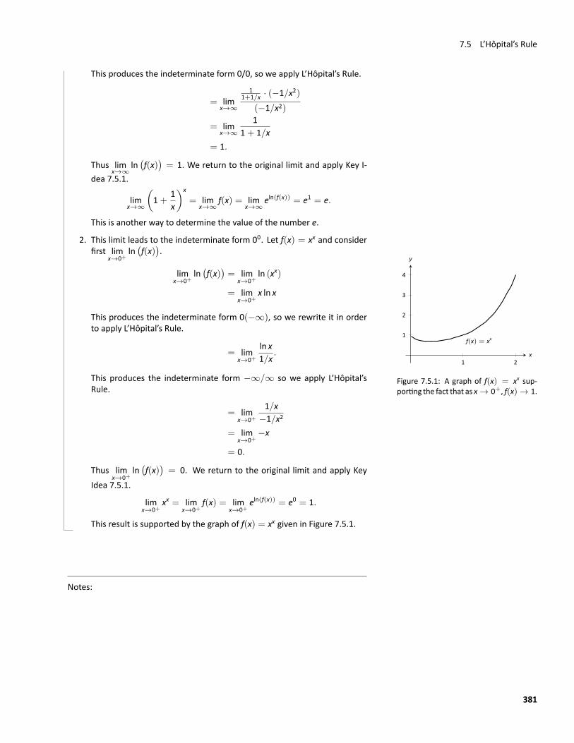
This is another way to determine the value of the number e.
2. This limit leads to the indeterminate form 00. Let f(x) = xx and considerfirst lim
x→0+ln(f(x)).
f(x) = xx
1 2
1
2
3
4
x
y
Figure 7.5.1: A graph of f(x) = xx sup‐porting the fact that as x → 0+, f(x) → 1.
limx→0+
ln(f(x))= lim
x→0+ln (xx)
= limx→0+
x ln x
This produces the indeterminate form 0(−∞), so we rewrite it in orderto apply L’Hôpital’s Rule.
= limx→0+
ln x1/x
.
This produces the indeterminate form −∞/∞ so we apply L’Hôpital’sRule.
= limx→0+
1/x−1/x2
= limx→0+
−x
= 0.
Thus limx→0+
ln(f(x))= 0. We return to the original limit and apply Key
Idea 7.5.1.
limx→0+
xx = limx→0+
f(x) = limx→0+
eln(f(x)) = e0 = 1.
This result is supported by the graph of f(x) = xx given in Figure 7.5.1.
Notes:
381
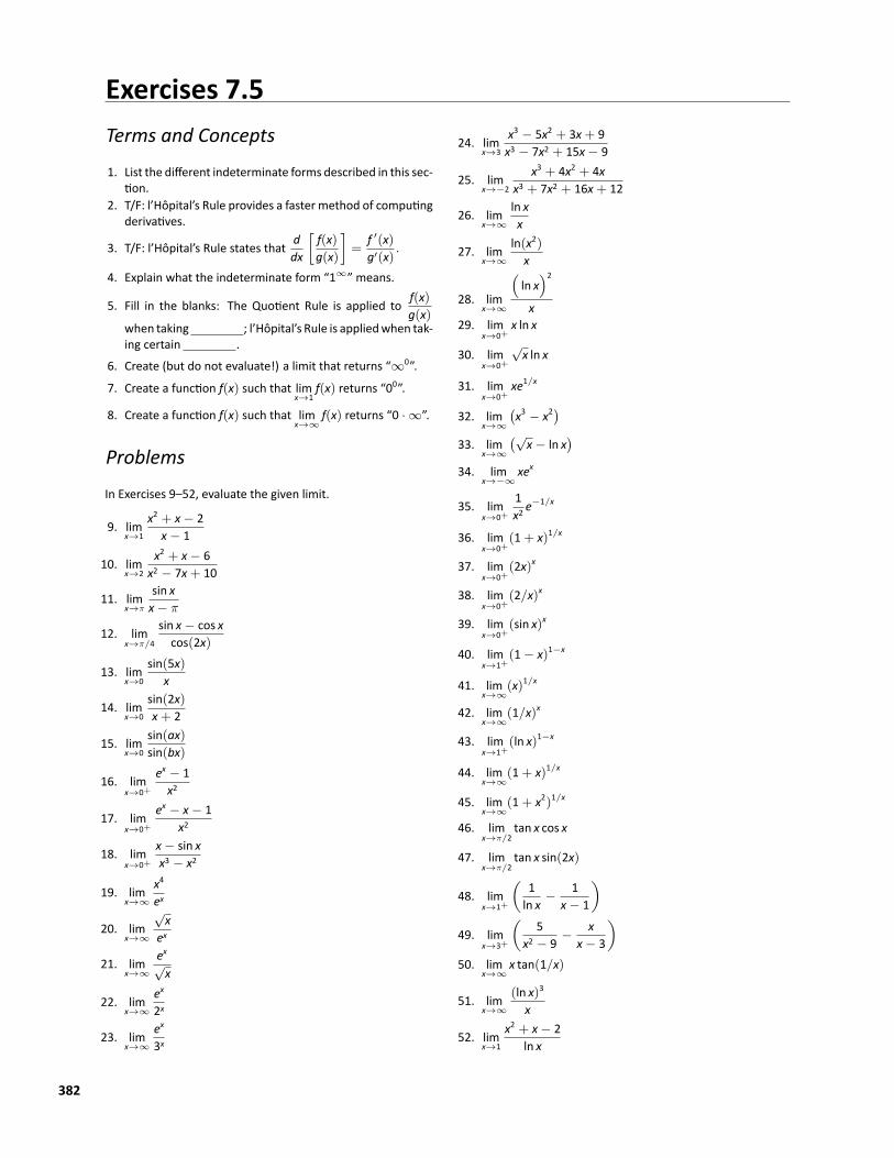
Exercises 7.5Terms and Concepts
1. List the different indeterminate forms described in this sec‐tion.
2. T/F: l’Hôpital’s Rule provides a faster method of computingderivatives.
3. T/F: l’Hôpital’s Rule states that ddx
[f(x)g(x)
]=
f ′(x)g′(x)
.
4. Explain what the indeterminate form “1∞” means.
5. Fill in the blanks: The Quotient Rule is applied to f(x)g(x)
when taking ; l’Hôpital’s Rule is appliedwhen tak‐ing certain .
6. Create (but do not evaluate!) a limit that returns “∞0”.
7. Create a function f(x) such that limx→1
f(x) returns “00”.
8. Create a function f(x) such that limx→∞
f(x) returns “0 · ∞”.
Problems
In Exercises 9–52, evaluate the given limit.
9. limx→1
x2 + x− 2x− 1
10. limx→2
x2 + x− 6x2 − 7x+ 10
11. limx→π
sin xx− π
12. limx→π/4
sin x− cos xcos(2x)
13. limx→0
sin(5x)x
14. limx→0
sin(2x)x+ 2
15. limx→0
sin(ax)sin(bx)
16. limx→0+
ex − 1x2
17. limx→0+
ex − x− 1x2
18. limx→0+
x− sin xx3 − x2
19. limx→∞
x4
ex
20. limx→∞
√x
ex
21. limx→∞
ex√x
22. limx→∞
ex
2x
23. limx→∞
ex
3x
24. limx→3
x3 − 5x2 + 3x+ 9x3 − 7x2 + 15x− 9
25. limx→−2
x3 + 4x2 + 4xx3 + 7x2 + 16x+ 12
26. limx→∞
ln xx
27. limx→∞
ln(x2)x
28. limx→∞
(ln x)2
x29. lim
x→0+x ln x
30. limx→0+
√x ln x
31. limx→0+
xe1/x
32. limx→∞
(x3 − x2
)33. lim
x→∞
(√x− ln x
)34. lim
x→−∞xex
35. limx→0+
1x2e−1/x
36. limx→0+
(1+ x)1/x
37. limx→0+
(2x)x
38. limx→0+
(2/x)x
39. limx→0+
(sin x)x
40. limx→1+
(1− x)1−x
41. limx→∞
(x)1/x
42. limx→∞
(1/x)x
43. limx→1+
(ln x)1−x
44. limx→∞
(1+ x)1/x
45. limx→∞
(1+ x2)1/x
46. limx→π/2
tan x cos x
47. limx→π/2
tan x sin(2x)
48. limx→1+
(1ln x
− 1x− 1
)49. lim
x→3+
(5
x2 − 9− x
x− 3
)50. lim
x→∞x tan(1/x)
51. limx→∞
(ln x)3
x
52. limx→1
x2 + x− 2ln x
382
8: TECHNIQUES OF INTEGRATIONchapter 5 introduced the antiderivative and connected it to signed areas un‐der a curve through the Fundamental Theorem of Calculus. The chapter afterexplored more applications of definite integrals than just area. As evaluatingdefinite integrals will become even more important, we will want to find an‐tiderivatives of a variety of functions.
This chapter is devoted to exploring techniques of antidifferentiation. Whilenot every function has an antiderivative in terms of elementary functions, wecan still find antiderivatives of a wide variety of functions.
8.1 Integration by PartsHere’s a simple integral that we can’t yet evaluate:∫
x cos x dx.
It’s a simple matter to take the derivative of the integrand using the ProductRule, but there is no Product Rule for integrals. However, this section introducesIntegration by Parts, a method of integration that is based on the Product Rulefor derivatives. It will enable us to evaluate this integral.
The Product Rule says that ifu and v are functions of x, then (uv)′ = u ′v+uv ′.For simplicity, we’ve written u for u(x) and v for v(x). Suppose we integrate bothsides with respect to x. This gives∫
(uv)′ dx =∫(u ′v+ uv ′) dx.
By the Fundamental Theoremof Calculus, the left side integrates to uv. The rightside can be broken up into two integrals, and we have
uv =∫
u ′v dx+∫
uv ′ dx.
Solving for the second integral we have∫uv ′ dx = uv−
∫u ′v dx.
Using differential notation, we can write
u ′ =dudx
v ′ =dvdx
⇒du = u ′dxdv = v ′dx.
Notes:
383
Chapter 8 Techniques of Integration
Thus, the equation above can be written as follows:∫u dv = uv−
∫v du.
This is the Integration by Parts formula. For reference purposes, we state this ina theorem.
Theorem 8.1.1 Integration by PartsLet u and v be differentiable functions of x on an interval I containing aand b. Then ∫
u dv = uv−∫
v du,
and applying FTC part 2 we have∫ x=b
x=au dv = uv
∣∣∣ba−∫ x=b
x=av du.
Watch the video:Integration by Parts — Definite Integral athttps://youtu.be/zGGI4PkHzhI
Let’s try an example to understand our new technique.
Example 8.1.1 Integrating using Integration by PartsEvaluate
∫x cos x dx.
SOLUTION The key to Integration by Parts is to identify part of the in‐tegrand as “u” and part as “dv.” Regular practice will help one make good iden‐tifications, and later we will introduce some principles that help. For now, letu = x and dv = cos x dx.
It is generally useful to make a small table of these values.
u = x dv = cos x dxdu = ? v = ?
⇒u = x dv = cos x dx
du = dx v = sin x
Notes:
384
8.1 Integration by Parts
Right now we only know u and dv as shown on the left; on the right we fill inthe rest of what we need. If u = x, then du = dx. Since dv = cos x dx, v is anantiderivative of cos x, so v = sin x.
Now substitute all of this into the Integration by Parts formula, giving∫x cos x dx = x sin x−
∫sin x dx.
We can then integrate sin x to get− cos x+ C and overall our answer is∫x cos x dx = x sin x+ cos x+ C.
We have two important notes here: (1) notice how the antiderivative containsthe product, x sin x. This product is what makes integration by parts necessary.And (2) antidifferentiating dv does result in v+ C. The intermediate+Cs are alladded together and represented by one+C in the final answer.
The example above demonstrates how Integration by Parts works in general.We try to identify u and dv in the integral we are given, and the key is that weusually want to choose u and dv so that du is simpler than u and v is hopefullynot too much more complicated than dv. This will mean that the integral on theright side of the Integration by Parts formula,
∫v du will be simpler to integrate
than the original integral∫u dv.
In the example above, we chose u = x and dv = cos x dx. Then du = dxwassimpler than u and v = sin x is no more complicated than dv. Therefore, insteadof integrating x cos x dx, we could integrate sin x dx, which we knew how to do.
If we had chosen u = cos x and dv = x dx, so that du = − sin x dx andv = 1
2x2, then ∫
x cos x dx =12x2 cos x−
(−12
)∫x2 sin x dx.
We then need to integrate x2 sin x, which is more complicated than our originalintegral, making this an unproductive choice.
We now consider another example.
Example 8.1.2 Integrating using Integration by PartsEvaluate
∫xex dx.
SOLUTION Notice that x becomes simpler when differentiated and exis unchanged by differentiation or integration. This suggests that we should letu = x and dv = ex dx:
u = x dv = ex dxdu = ? v = ?
⇒u = x dv = ex dx
du = dx v = ex
Notes:
385
Chapter 8 Techniques of Integration
The Integration by Parts formula gives∫xex dx = xex −
∫ex dx.
The integral on the right is simple; our final answer is∫xex dx = xex − ex + C.
Note again how the antiderivatives contain a product term.
Example 8.1.3 Integrating using Integration by PartsEvaluate
∫x2 cos x dx.
SOLUTION Let u = x2 instead of the trigonometric function, hencedv = cos x dx. Then du = 2x dx and v = sin x as shown below.
u = x2 dv = cos x dxdu = ? v = ?
⇒u = x2 dv = cos x dx
du = 2x dx v = sin x
The Integration by Parts formula gives∫x2 cos x dx = x2 sin x−
∫2x sin x dx.
At this point, the integral on the right is indeed simpler than the one we startedwith, but to evaluate it, we need to do Integration by Parts again. Here wechoose u = 2x and dv = sin x and fill in the rest below.
u = 2x dv = sin x dxdu = ? v = ?
⇒u = 2x dv = sin x dx
du = 2 dx v = − cos x
This means that∫x2 cos x dx = x2 sin x−
(−2x cos x−
∫−2 cos x dx
).
The integral all the way on the right is now something we can evaluate. It eval‐uates to −2 sin x. Then going through and simplifying, being careful to keep allthe signs straight, our answer is∫
x2 cos x dx = x2 sin x+ 2x cos x− 2 sin x+ C.
Notes:
386
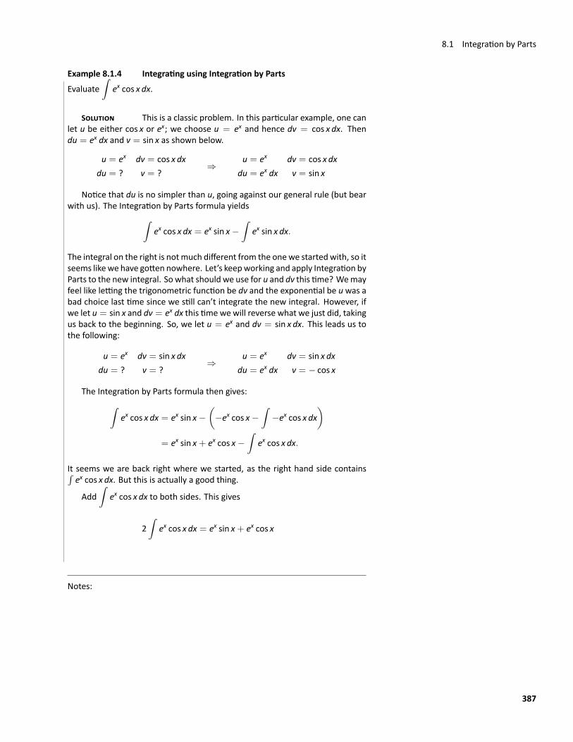
8.1 Integration by Parts
Example 8.1.4 Integrating using Integration by PartsEvaluate
∫ex cos x dx.
SOLUTION This is a classic problem. In this particular example, one canlet u be either cos x or ex; we choose u = ex and hence dv = cos x dx. Thendu = ex dx and v = sin x as shown below.
u = ex dv = cos x dxdu = ? v = ?
⇒u = ex dv = cos x dx
du = ex dx v = sin x
Notice that du is no simpler than u, going against our general rule (but bearwith us). The Integration by Parts formula yields∫
ex cos x dx = ex sin x−∫
ex sin x dx.
The integral on the right is notmuch different from the onewe startedwith, so itseems likewe have gotten nowhere. Let’s keepworking and apply Integration byParts to the new integral. So what should we use for u and dv this time? Wemayfeel like letting the trigonometric function be dv and the exponential be uwas abad choice last time since we still can’t integrate the new integral. However, ifwe let u = sin x and dv = ex dx this time wewill reverse what we just did, takingus back to the beginning. So, we let u = ex and dv = sin x dx. This leads us tothe following:
u = ex dv = sin x dxdu = ? v = ?
⇒u = ex dv = sin x dx
du = ex dx v = − cos x
The Integration by Parts formula then gives:∫ex cos x dx = ex sin x−
(−ex cos x−
∫−ex cos x dx
)= ex sin x+ ex cos x−
∫ex cos x dx.
It seems we are back right where we started, as the right hand side contains∫ex cos x dx. But this is actually a good thing.
Add∫
ex cos x dx to both sides. This gives
2∫
ex cos x dx = ex sin x+ ex cos x
Notes:
387
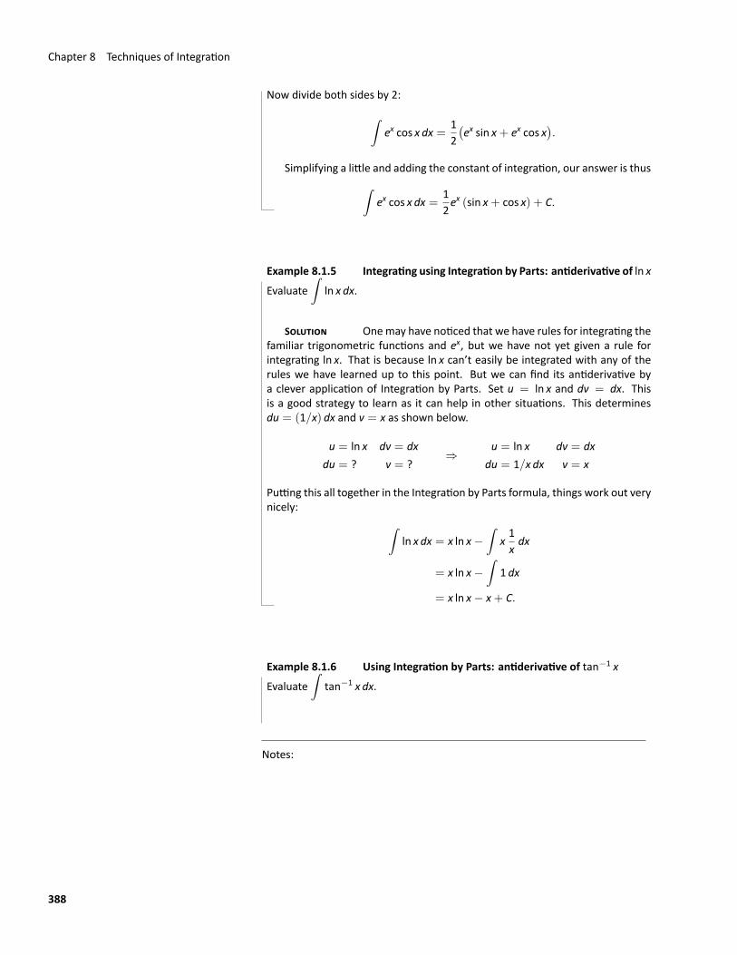
Chapter 8 Techniques of Integration
Now divide both sides by 2:∫ex cos x dx =
12(ex sin x+ ex cos x
).
Simplifying a little and adding the constant of integration, our answer is thus∫ex cos x dx =
12ex (sin x+ cos x) + C.
Example 8.1.5 Integrating using Integration by Parts: antiderivative of ln xEvaluate
∫ln x dx.
SOLUTION Onemay have noticed that we have rules for integrating thefamiliar trigonometric functions and ex, but we have not yet given a rule forintegrating ln x. That is because ln x can’t easily be integrated with any of therules we have learned up to this point. But we can find its antiderivative bya clever application of Integration by Parts. Set u = ln x and dv = dx. Thisis a good strategy to learn as it can help in other situations. This determinesdu = (1/x) dx and v = x as shown below.
u = ln x dv = dxdu = ? v = ?
⇒u = ln x dv = dx
du = 1/x dx v = x
Putting this all together in the Integration by Parts formula, things work out verynicely: ∫
ln x dx = x ln x−∫
x1xdx
= x ln x−∫
1 dx
= x ln x− x+ C.
Example 8.1.6 Using Integration by Parts: antiderivative of tan−1 x
Evaluate∫
tan−1 x dx.
Notes:
388
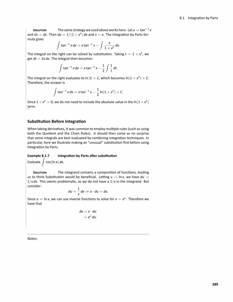
8.1 Integration by Parts
SOLUTION The same strategyweused aboveworks here. Letu = tan−1 xand dv = dx. Then du = 1/(1+ x2) dx and v = x. The Integration by Parts for‐mula gives ∫
tan−1 x dx = x tan−1 x−∫
x1+ x2
dx.
The integral on the right can be solved by substitution. Taking t = 1 + x2, weget dt = 2x dx. The integral then becomes∫
tan−1 x dx = x tan−1 x− 12
∫1tdt.
The integral on the right evaluates to ln |t|+ C, which becomes ln(1+ x2) + C.Therefore, the answer is∫
tan−1 x dx = x tan−1 x− 12ln(1+ x2) + C.
Since 1+ x2 > 0, we do not need to include the absolute value in the ln(1+ x2)term.
Substitution Before IntegrationWhen taking derivatives, it was common to employ multiple rules (such as usingboth the Quotient and the Chain Rules). It should then come as no surprisethat some integrals are best evaluated by combining integration techniques. Inparticular, here we illustrate making an “unusual” substitution first before usingIntegration by Parts.
Example 8.1.7 Integration by Parts after substitutionEvaluate
∫cos(ln x) dx.
SOLUTION The integrand contains a composition of functions, leadingus to think Substitution would be beneficial. Letting u = ln x, we have du =1/x dx. This seems problematic, as we do not have a 1/x in the integrand. Butconsider:
du =1xdx ⇒ x · du = dx.
Since u = ln x, we can use inverse functions to solve for x = eu. Therefore wehave that
dx = x · du= eu du.
Notes:
389
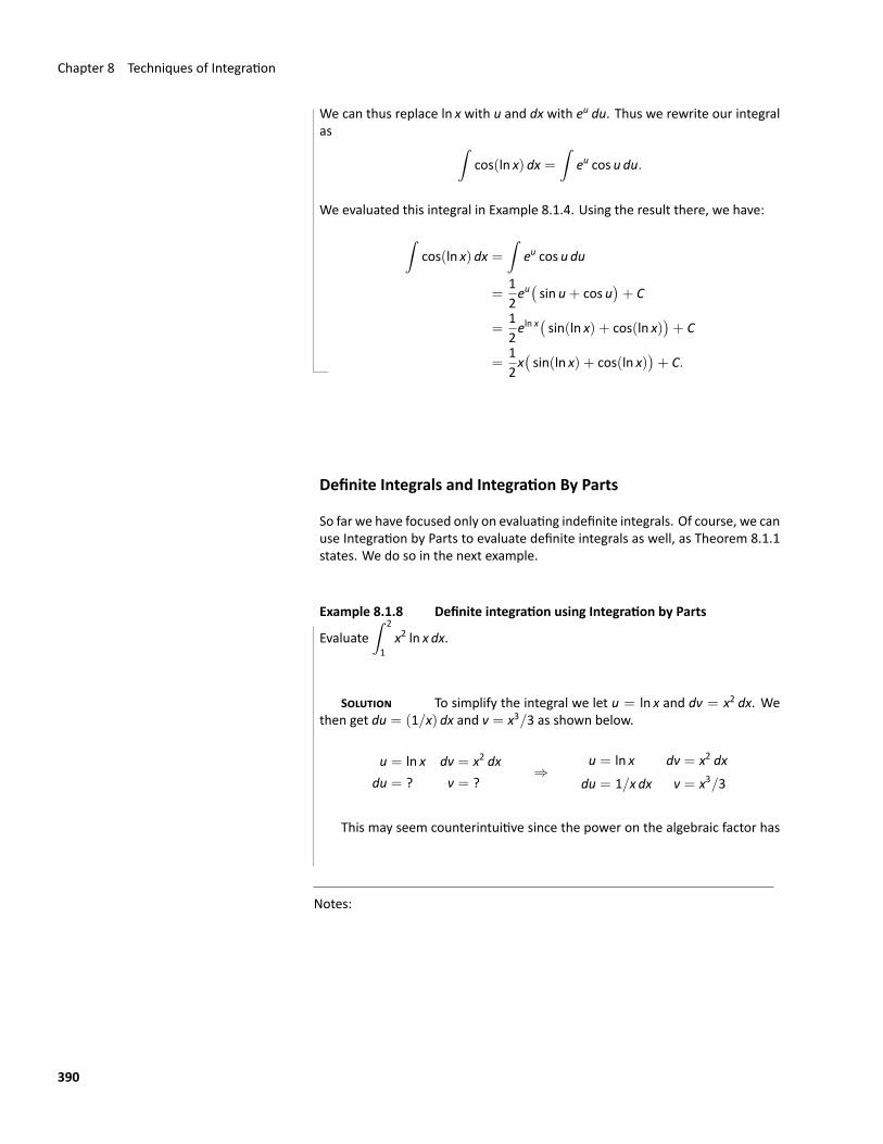
Chapter 8 Techniques of Integration
We can thus replace ln x with u and dx with eu du. Thus we rewrite our integralas ∫
cos(ln x) dx =∫
eu cos u du.
We evaluated this integral in Example 8.1.4. Using the result there, we have:
∫cos(ln x) dx =
∫eu cos u du
=12eu(sin u+ cos u
)+ C
=12eln x(sin(ln x) + cos(ln x)
)+ C
=12x(sin(ln x) + cos(ln x)
)+ C.
Definite Integrals and Integration By Parts
So far we have focused only on evaluating indefinite integrals. Of course, we canuse Integration by Parts to evaluate definite integrals as well, as Theorem 8.1.1states. We do so in the next example.
Example 8.1.8 Definite integration using Integration by Parts
Evaluate∫ 2
1x2 ln x dx.
SOLUTION To simplify the integral we let u = ln x and dv = x2 dx. Wethen get du = (1/x) dx and v = x3/3 as shown below.
u = ln x dv = x2 dxdu = ? v = ?
⇒u = ln x dv = x2 dx
du = 1/x dx v = x3/3
This may seem counterintuitive since the power on the algebraic factor has
Notes:
390
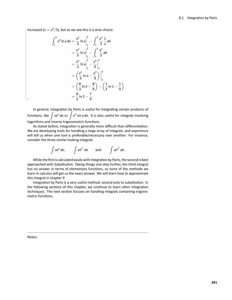
8.1 Integration by Parts
increased (v = x3/3), but as we see this is a wise choice:∫ 2
1x2 ln x dx =
x3
3ln x∣∣∣∣21−∫ 2
1
x3
31xdx
=x3
3ln x∣∣∣∣21−∫ 2
1
x2
3dx
=x3
3ln x∣∣∣∣21− x3
9
∣∣∣∣21
=
(x3
3ln x− x3
9
) ∣∣∣∣21
=
(83ln 2− 8
9
)−(13ln 1− 1
9
)=
83ln 2− 7
9.
In general, Integration by Parts is useful for integrating certain products offunctions, like
∫xex dx or
∫x3 sin x dx. It is also useful for integrals involving
logarithms and inverse trigonometric functions.As stated before, integration is generally more difficult than differentiation.
We are developing tools for handling a large array of integrals, and experiencewill tell us when one tool is preferable/necessary over another. For instance,consider the three similar‐looking integrals∫
xex dx,∫
xex2dx and
∫xex
3dx.
While the first is calculated easilywith Integrationby Parts, the second is bestapproached with Substitution. Taking things one step further, the third integralhas no answer in terms of elementary functions, so none of the methods welearn in calculus will get us the exact answer. We will learn how to approximatethis integral in chapter 9
Integration by Parts is a very useful method, second only to substitution. Inthe following sections of this chapter, we continue to learn other integrationtechniques. The next section focuses on handling integrals containing trigono‐metric functions.
Notes:
391
Exercises 8.1Terms and Concepts1. T/F: Integration by Parts is useful in evaluating integrands
that contain products of functions.2. T/F: Integration by Parts can be thought of as the “opposite
of the Chain Rule.”
ProblemsIn Exercises 3–36, evaluate the given indefinite integral.
3.∫
x sin x dx
4.∫
xe−x dx
5.∫
x2 sin x dx
6.∫
x3 sin x dx
7.∫
xex2dx
8.∫
x3ex dx
9.∫
xe−2x dx
10.∫
ex sin x dx
11.∫
e2x cos x dx
12.∫
e2x sin(3x) dx
13.∫
e5x cos(5x) dx
14.∫
sin x cos x dx
15.∫
sin−1 x dx
16.∫
tan−1(2x) dx
17.∫
x tan−1 x dx
18.∫
cos−1 x dx
19.∫
x ln x dx
20.∫
(x− 2) ln x dx
21.∫
x ln(x− 1) dx
22.∫
x ln(x2) dx
23.∫
x2 ln x dx
24.∫
(ln x)2 dx
25.∫
(ln(x+ 1))2 dx
26.∫
x sec2 x dx
27.∫
x csc2 x dx
28.∫
x√x− 2 dx
29.∫
x√x2 − 2 dx
30.∫
sec x tan x dx
31.∫
x sec x tan x dx
32.∫
x csc x cot x dx
33.∫
x cosh x dx
34.∫
x sinh x dx
35.∫
sinh−1 x dx
36.∫
tanh−1 x dx
In Exercises 37–42, evaluate the indefinite integral after firstmaking a substitution.
37.∫
sin(ln x) dx
38.∫
sin(√x) dx
39.∫
ln(√x) dx
40.∫
e√
x dx
41.∫
eln x dx
42.∫
x3ex2dx
In Exercises 43–52, evaluate the definite integral. Note: thecorresponding indefinite integrals appear in Exercises 3–12.
43.∫ π
0x sin x dx
44.∫ 1
−1xe−x dx
45.∫ π/4
−π/4x2 sin x dx
46.∫ π/2
−π/2x3 sin x dx
392
47.∫ √
ln 2
0xex
2dx
48.∫ 1
0x3ex dx
49.∫ 2
1xe−2x dx
50.∫ π
0ex sin x dx
51.∫ π/2
−π/2e2x cos x dx
52.∫ π/3
0e2x sin(3x) dx
393
Chapter 8 Techniques of Integration
8.2 Trigonometric Integrals
Trigonometric functions are useful for describing periodic behavior. This sectiondescribes several techniques for finding antiderivatives of certain combinationsof trigonometric functions.
Integrals of the form∫
sinm x cosn x dx
In learning the technique of Substitution, we saw the integral∫sin x cos x dx in
Example 5.5.4. The integration was not difficult, and one could easily evaluatethe indefinite integral by letting u = sin x or by letting u = cos x. This integral iseasy since the power of both sine and cosine is 1.
Wegeneralize this integral and consider integrals of the form∫sinm x cosn x dx,
where m, n are nonnegative integers. Our strategy for evaluating these inte‐grals is to use the identity cos2 x + sin2 x = 1 to convert high powers of onetrigonometric function into the other, leaving a single sine or cosine term in theintegrand. We summarize the general technique in the following Key Idea.
Watch the video:Trigonometric Integrals — Part 2 of 6 athttps://youtu.be/zyg9k1je7Fg
Notes:
394
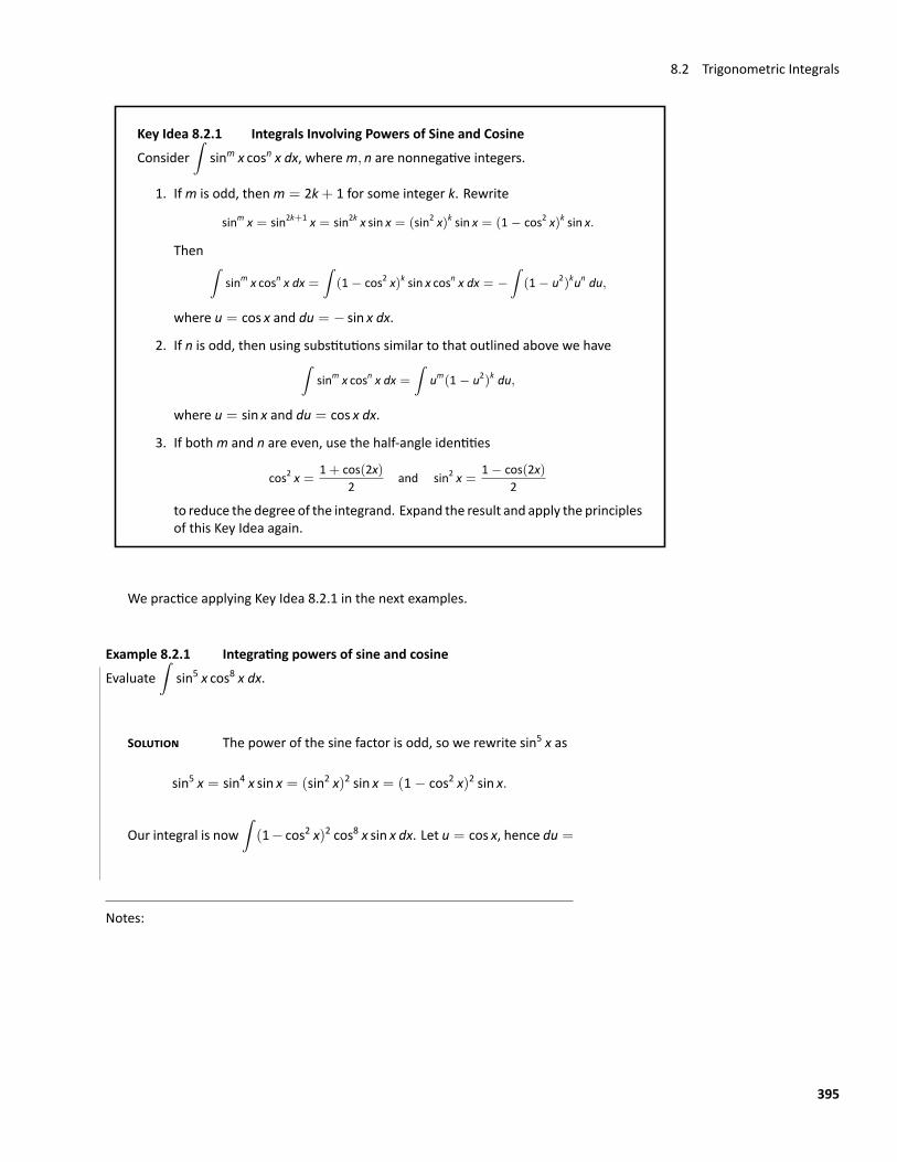
8.2 Trigonometric Integrals
Key Idea 8.2.1 Integrals Involving Powers of Sine and CosineConsider
∫sinm x cosn x dx, wherem, n are nonnegative integers.
1. Ifm is odd, thenm = 2k+ 1 for some integer k. Rewrite
sinm x = sin2k+1 x = sin2k x sin x = (sin2 x)k sin x = (1− cos2 x)k sin x.
Then ∫sinm x cosn x dx =
∫(1− cos2 x)k sin x cosn x dx = −
∫(1− u2)kun du,
where u = cos x and du = − sin x dx.
2. If n is odd, then using substitutions similar to that outlined above we have∫sinm x cosn x dx =
∫um(1− u2)k du,
where u = sin x and du = cos x dx.
3. If bothm and n are even, use the half‐angle identities
cos2 x = 1+ cos(2x)2
and sin2 x = 1− cos(2x)2
to reduce the degree of the integrand. Expand the result and apply the principlesof this Key Idea again.
We practice applying Key Idea 8.2.1 in the next examples.
Example 8.2.1 Integrating powers of sine and cosineEvaluate
∫sin5 x cos8 x dx.
SOLUTION The power of the sine factor is odd, so we rewrite sin5 x as
sin5 x = sin4 x sin x = (sin2 x)2 sin x = (1− cos2 x)2 sin x.
Our integral is now∫(1− cos2 x)2 cos8 x sin x dx. Let u = cos x, hence du =
Notes:
395
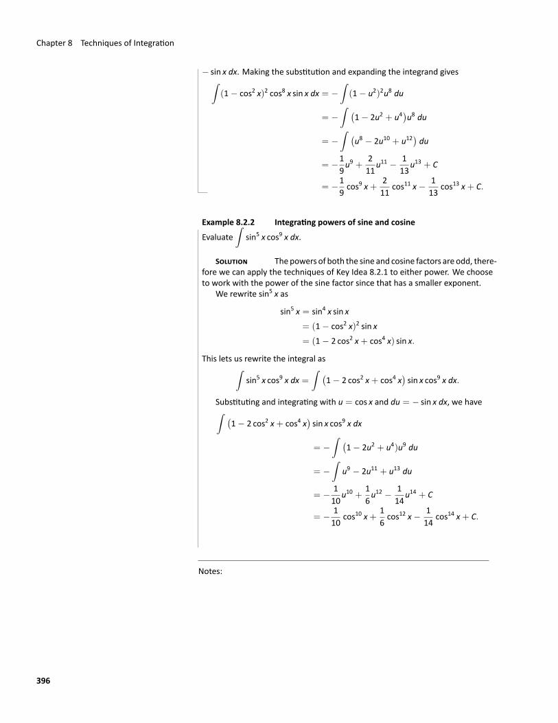
Chapter 8 Techniques of Integration
− sin x dx. Making the substitution and expanding the integrand gives∫(1− cos2 x)2 cos8 x sin x dx = −
∫(1− u2)2u8 du
= −∫ (
1− 2u2 + u4)u8 du
= −∫ (
u8 − 2u10 + u12)du
= −19u9 +
211
u11 − 113
u13 + C
= −19cos9 x+
211
cos11 x− 113
cos13 x+ C.
Example 8.2.2 Integrating powers of sine and cosineEvaluate
∫sin5 x cos9 x dx.
SOLUTION Thepowers of both the sine and cosine factors are odd, there‐fore we can apply the techniques of Key Idea 8.2.1 to either power. We chooseto work with the power of the sine factor since that has a smaller exponent.
We rewrite sin5 x as
sin5 x = sin4 x sin x= (1− cos2 x)2 sin x= (1− 2 cos2 x+ cos4 x) sin x.
This lets us rewrite the integral as∫sin5 x cos9 x dx =
∫ (1− 2 cos2 x+ cos4 x
)sin x cos9 x dx.
Substituting and integrating with u = cos x and du = − sin x dx, we have∫ (1− 2 cos2 x+ cos4 x
)sin x cos9 x dx
= −∫ (
1− 2u2 + u4)u9 du
= −∫
u9 − 2u11 + u13 du
= − 110
u10 +16u12 − 1
14u14 + C
= − 110
cos10 x+16cos12 x− 1
14cos14 x+ C.
Notes:
396
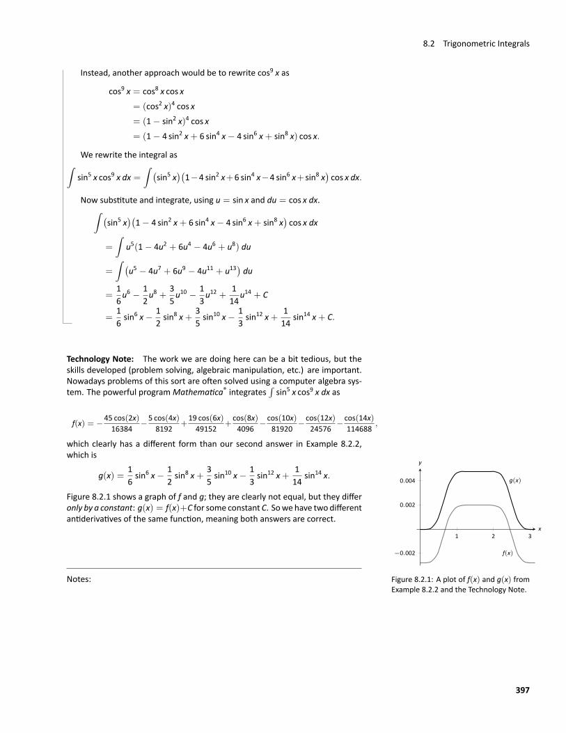
8.2 Trigonometric Integrals
Instead, another approach would be to rewrite cos9 x as
cos9 x = cos8 x cos x= (cos2 x)4 cos x= (1− sin2 x)4 cos x= (1− 4 sin2 x+ 6 sin4 x− 4 sin6 x+ sin8 x) cos x.
We rewrite the integral as∫sin5 x cos9 x dx =
∫ (sin5 x
)(1−4 sin2 x+6 sin4 x−4 sin6 x+ sin8 x
)cos x dx.
Now substitute and integrate, using u = sin x and du = cos x dx.∫ (sin5 x
)(1− 4 sin2 x+ 6 sin4 x− 4 sin6 x+ sin8 x
)cos x dx
=
∫u5(1− 4u2 + 6u4 − 4u6 + u8) du
=
∫ (u5 − 4u7 + 6u9 − 4u11 + u13
)du
=16u6 − 1
2u8 +
35u10 − 1
3u12 +
114
u14 + C
=16sin6 x− 1
2sin8 x+
35sin10 x− 1
3sin12 x+
114
sin14 x+ C.
Technology Note: The work we are doing here can be a bit tedious, but theskills developed (problem solving, algebraic manipulation, etc.) are important.Nowadays problems of this sort are often solved using a computer algebra sys‐tem. The powerful programMathematica® integrates
∫sin5 x cos9 x dx as
f(x) = −45 cos(2x)16384
−5 cos(4x)8192
+19 cos(6x)49152
+cos(8x)4096
− cos(10x)81920
− cos(12x)24576
− cos(14x)114688
,
which clearly has a different form than our second answer in Example 8.2.2,which is
g(x)
f(x)
1 2 3
−0.002
0.002
0.004
x
y
Figure 8.2.1: A plot of f(x) and g(x) fromExample 8.2.2 and the Technology Note.
g(x) =16sin6 x− 1
2sin8 x+
35sin10 x− 1
3sin12 x+
114
sin14 x.
Figure 8.2.1 shows a graph of f and g; they are clearly not equal, but they differonly by a constant: g(x) = f(x)+C for some constant C. Sowehave twodifferentantiderivatives of the same function, meaning both answers are correct.
Notes:
397
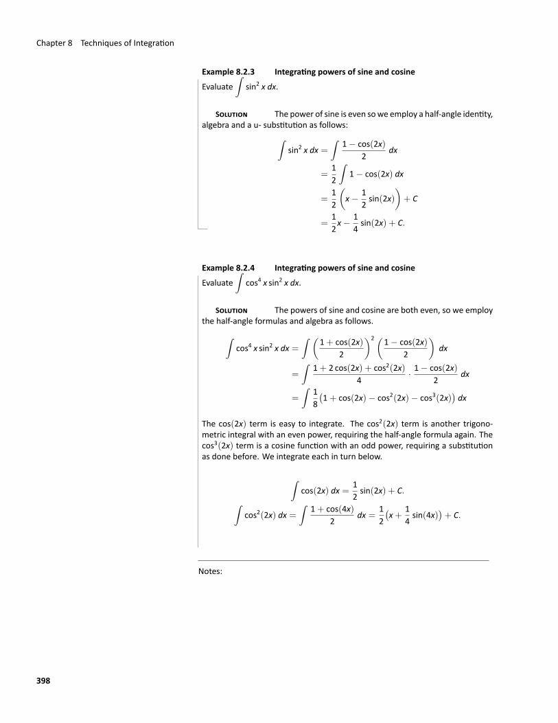
Chapter 8 Techniques of Integration
Example 8.2.3 Integrating powers of sine and cosineEvaluate
∫sin2 x dx.
SOLUTION The power of sine is even sowe employ a half‐angle identity,algebra and a u‐ substitution as follows:∫
sin2 x dx =∫
1− cos(2x)2
dx
=12
∫1− cos(2x) dx
=12
(x− 1
2sin(2x)
)+ C
=12x− 1
4sin(2x) + C.
Example 8.2.4 Integrating powers of sine and cosineEvaluate
∫cos4 x sin2 x dx.
SOLUTION The powers of sine and cosine are both even, so we employthe half‐angle formulas and algebra as follows.∫
cos4 x sin2 x dx =∫ (
1+ cos(2x)2
)2(1− cos(2x)2
)dx
=
∫1+ 2 cos(2x) + cos2(2x)
4· 1− cos(2x)
2dx
=
∫18(1+ cos(2x)− cos2(2x)− cos3(2x)
)dx
The cos(2x) term is easy to integrate. The cos2(2x) term is another trigono‐metric integral with an even power, requiring the half‐angle formula again. Thecos3(2x) term is a cosine function with an odd power, requiring a substitutionas done before. We integrate each in turn below.
∫cos(2x) dx =
12sin(2x) + C.∫
cos2(2x) dx =∫
1+ cos(4x)2
dx =12(x+
14sin(4x)
)+ C.
Notes:
398
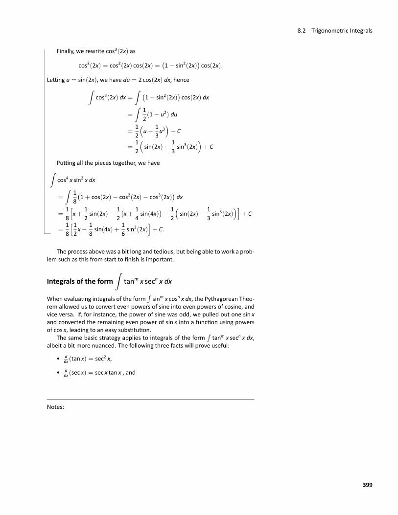
8.2 Trigonometric Integrals
Finally, we rewrite cos3(2x) as
cos3(2x) = cos2(2x) cos(2x) =(1− sin2(2x)
)cos(2x).
Letting u = sin(2x), we have du = 2 cos(2x) dx, hence∫cos3(2x) dx =
∫ (1− sin2(2x)
)cos(2x) dx
=
∫12(1− u2) du
=12
(u− 1
3u3)+ C
=12
(sin(2x)− 1
3sin3(2x)
)+ C
Putting all the pieces together, we have∫cos4 x sin2 x dx
=
∫18(1+ cos(2x)− cos2(2x)− cos3(2x)
)dx
=18
[x+
12sin(2x)− 1
2(x+
14sin(4x)
)− 1
2
(sin(2x)− 1
3sin3(2x)
)]+ C
=18
[12x− 1
8sin(4x) +
16sin3(2x)
]+ C.
The process above was a bit long and tedious, but being able to work a prob‐lem such as this from start to finish is important.
Integrals of the form∫
tanm x secn x dx
When evaluating integrals of the form∫sinm x cosn x dx, the Pythagorean Theo‐
rem allowed us to convert even powers of sine into even powers of cosine, andvice versa. If, for instance, the power of sine was odd, we pulled out one sin xand converted the remaining even power of sin x into a function using powersof cos x, leading to an easy substitution.
The same basic strategy applies to integrals of the form∫tanm x secn x dx,
albeit a bit more nuanced. The following three facts will prove useful:
• ddx (tan x) = sec2 x,
• ddx (sec x) = sec x tan x , and
Notes:
399
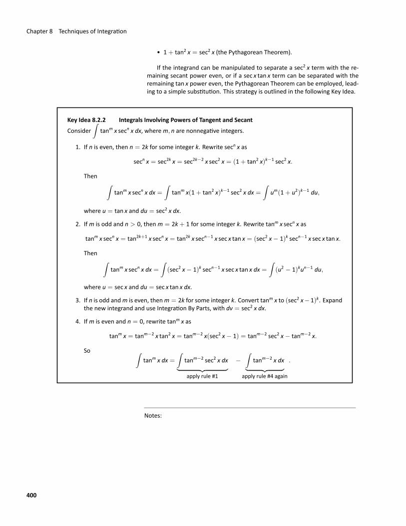
Chapter 8 Techniques of Integration
• 1+ tan2 x = sec2 x (the Pythagorean Theorem).
If the integrand can be manipulated to separate a sec2 x term with the re‐maining secant power even, or if a sec x tan x term can be separated with theremaining tan x power even, the Pythagorean Theorem can be employed, lead‐ing to a simple substitution. This strategy is outlined in the following Key Idea.
Key Idea 8.2.2 Integrals Involving Powers of Tangent and SecantConsider
∫tanm x secn x dx, wherem, n are nonnegative integers.
1. If n is even, then n = 2k for some integer k. Rewrite secn x as
secn x = sec2k x = sec2k−2 x sec2 x = (1+ tan2 x)k−1 sec2 x.
Then ∫tanm x secn x dx =
∫tanm x(1+ tan2 x)k−1 sec2 x dx =
∫um(1+ u2)k−1 du,
where u = tan x and du = sec2 x dx.
2. Ifm is odd and n > 0, thenm = 2k+ 1 for some integer k. Rewrite tanm x secn x as
tanm x secn x = tan2k+1 x secn x = tan2k x secn−1 x sec x tan x = (sec2 x− 1)k secn−1 x sec x tan x.
Then ∫tanm x secn x dx =
∫(sec2 x− 1)k secn−1 x sec x tan x dx =
∫(u2 − 1)kun−1 du,
where u = sec x and du = sec x tan x dx.
3. If n is odd andm is even, thenm = 2k for some integer k. Convert tanm x to (sec2 x− 1)k. Expandthe new integrand and use Integration By Parts, with dv = sec2 x dx.
4. Ifm is even and n = 0, rewrite tanm x as
tanm x = tanm−2 x tan2 x = tanm−2 x(sec2 x− 1) = tanm−2 sec2 x− tanm−2 x.
So ∫tanm x dx =
∫tanm−2 sec2 x dx︸ ︷︷ ︸apply rule #1
−∫
tanm−2 x dx︸ ︷︷ ︸apply rule #4 again
.
Notes:
400
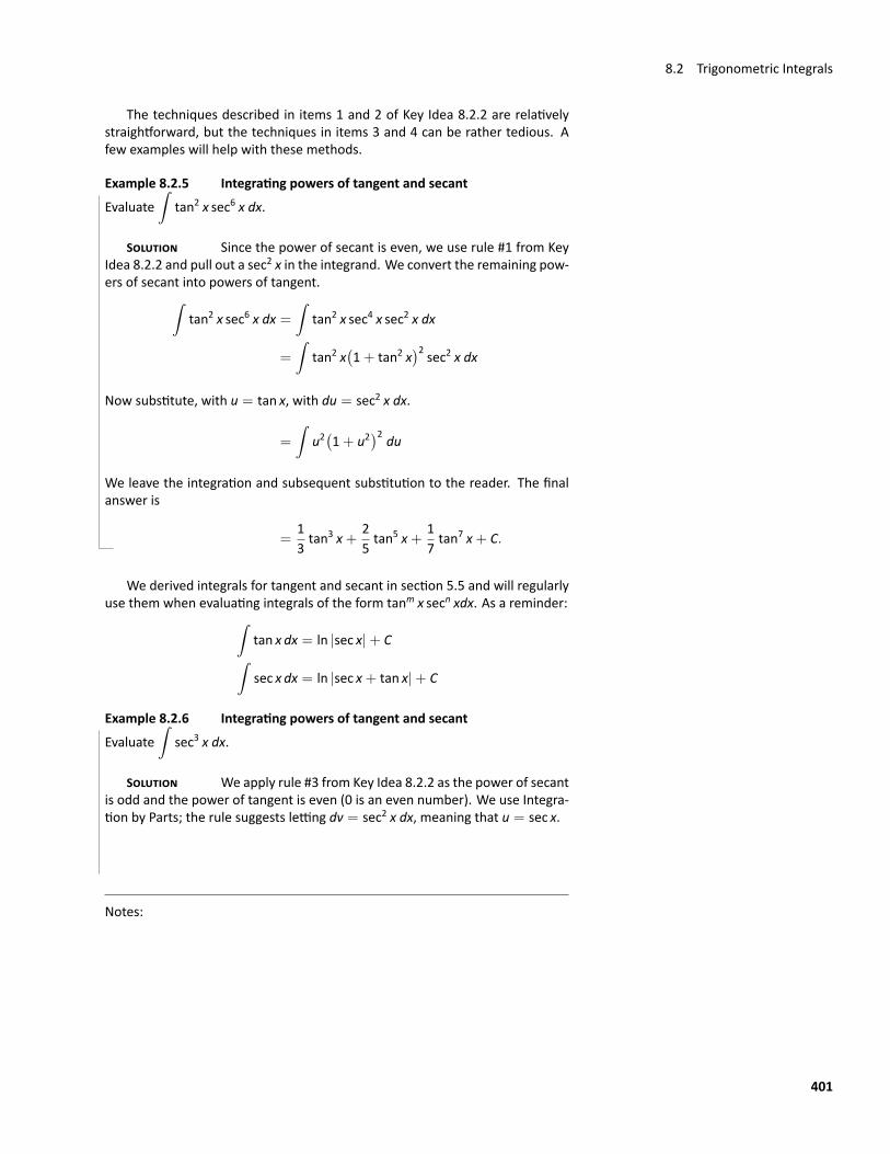
8.2 Trigonometric Integrals
The techniques described in items 1 and 2 of Key Idea 8.2.2 are relativelystraightforward, but the techniques in items 3 and 4 can be rather tedious. Afew examples will help with these methods.
Example 8.2.5 Integrating powers of tangent and secantEvaluate
∫tan2 x sec6 x dx.
SOLUTION Since the power of secant is even, we use rule #1 from KeyIdea 8.2.2 and pull out a sec2 x in the integrand. We convert the remaining pow‐ers of secant into powers of tangent.∫
tan2 x sec6 x dx =∫
tan2 x sec4 x sec2 x dx
=
∫tan2 x
(1+ tan2 x
)2 sec2 x dxNow substitute, with u = tan x, with du = sec2 x dx.
=
∫u2(1+ u2
)2 duWe leave the integration and subsequent substitution to the reader. The finalanswer is
=13tan3 x+
25tan5 x+
17tan7 x+ C.
We derived integrals for tangent and secant in section 5.5 and will regularlyuse them when evaluating integrals of the form tanm x secn xdx. As a reminder:∫
tan x dx = ln |sec x|+ C∫sec x dx = ln |sec x+ tan x|+ C
Example 8.2.6 Integrating powers of tangent and secantEvaluate
∫sec3 x dx.
SOLUTION We apply rule #3 from Key Idea 8.2.2 as the power of secantis odd and the power of tangent is even (0 is an even number). We use Integra‐tion by Parts; the rule suggests letting dv = sec2 x dx, meaning that u = sec x.
Notes:
401
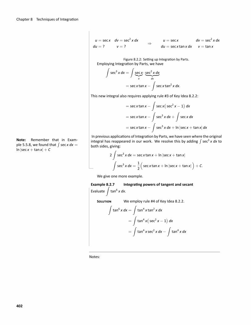
Chapter 8 Techniques of Integration
u = sec x dv = sec2 x dxdu = ? v = ?
⇒u = sec x dv = sec2 x dx
du = sec x tan x dx v = tan x
Figure 8.2.2: Setting up Integration by Parts.Employing Integration by Parts, we have∫
sec3 x dx =∫
sec x︸︷︷︸u
· sec2 x dx︸ ︷︷ ︸dv
= sec x tan x−∫
sec x tan2 x dx.
This new integral also requires applying rule #3 of Key Idea 8.2.2:
= sec x tan x−∫
sec x(sec2 x− 1
)dx
= sec x tan x−∫
sec3 x dx+∫
sec x dx
= sec x tan x−∫
sec3 x dx+ ln |sec x+ tan x| dx
In previous applications of Integration by Parts, we have seenwhere the originalNote: Remember that in Exam‐ple 5.5.8, we found that
∫sec x dx =
ln |sec x+ tan x|+ C
integral has reappeared in our work. We resolve this by adding∫sec3 x dx to
both sides, giving:
2∫
sec3 x dx = sec x tan x+ ln |sec x+ tan x|∫sec3 x dx =
12
(sec x tan x+ ln |sec x+ tan x|
)+ C.
We give one more example.
Example 8.2.7 Integrating powers of tangent and secantEvaluate
∫tan6 x dx.
SOLUTION We employ rule #4 of Key Idea 8.2.2.∫tan6 x dx =
∫tan4 x tan2 x dx
=
∫tan4 x
(sec2 x− 1
)dx
=
∫tan4 x sec2 x dx−
∫tan4 x dx
Notes:
402
8.2 Trigonometric Integrals
We integrate the first integral with substitution, u = tan x and du = sec2 x dx;and the second by employing rule #4 again.
=
∫u4 du−
∫tan2 x tan2 x dx
=15tan5 x−
∫tan2 x
(sec2 x− 1
)dx
=15tan5 x−
∫tan2 x sec2 x dx+
∫tan2 x dx
Again, use substitution for the first integral and rule #4 for the second.
=15tan5 x− 1
3tan3 x+
∫ (sec2 x− 1
)dx
=15tan5 x− 1
3tan3 x+ tan x− x+ C.
Integrals of the form∫
cotm x cscn x dx
Not surprisingly, evaluating integrals of the form∫cotm x cscn x dx is similar to
evaluating∫tanm x secn x dx. The guidelines from Key Idea 8.2.2 and the follow‐
ing three facts will be useful:
ddx
(cot x) = − csc2 x
ddx
(csc x) = − csc x cot x, and
csc2 x = cot2 x+ 1
Example 8.2.8 Integrating powers of cotangent and cosecantEvaluate
∫cot2 x csc4 x dx
SOLUTION Since the power of cosecant is evenwewill let u = cot x andsave a csc2 x for the resulting du = − csc2 x dx.∫
cot2 x csc4 x dx =∫
cot2 x csc2 x csc2 x dx
=
∫cot2 x(1+ cot2 x) csc2 x dx
= −∫
u2(1+ u2) du.
Notes:
403
Chapter 8 Techniques of Integration
The integration and substitution required to finish this example are similar tothat of previous examples in this section. The result is
−13cot3 x− 1
5cot5 x+ C.
Integrals of the form∫
sin(mx) sin(nx) dx,∫
cos(mx) cos(nx) dx,
and∫
sin(mx) cos(nx) dx.
Functions that contain products of sines and cosines of differing periods are im‐portant in many applications including the analysis of sound waves. Integrals ofthe form∫
sin(mx) sin(nx) dx,∫
cos(mx) cos(nx) dx and∫
sin(mx) cos(nx) dx
are best approached by first applying the Product to Sum Formulas of Trigonom‐etry found in the back cover of this text, namely
sin(mx) sin(nx) =12
[cos((m− n)x
)− cos
((m+ n)x
)]cos(mx) cos(nx) =
12
[cos((m− n)x
)+ cos
((m+ n)x
)]sin(mx) cos(nx) =
12
[sin((m− n)x
)+ sin
((m+ n)x
)]Example 8.2.9 Integrating products of sin(mx) and cos(nx)
Evaluate∫
sin(5x) cos(2x) dx.
SOLUTION The application of the formula and subsequent integrationare straightforward:∫
sin(5x) cos(2x) dx =∫
12
[sin(3x) + sin(7x)
]dx
= −16cos(3x)− 1
14cos(7x) + C.
Notes:
404
8.2 Trigonometric Integrals
Integrating other combinations of trigonometric functionsCombinations of trigonometric functions thatwehavenot discussed in this chap‐ter are evaluated by applying algebra, trigonometric identities and other integra‐tion strategies to create an equivalent integrand that we can evaluate. To eval‐uate “crazy” combinations, those not readily manipulated into a familiar form,one should use integral tables. A table of “common crazy” combinations can befound at the end of this text.
These latter examples were admittedly long, with repeated applications ofthe same rule. Try to not be overwhelmed by the length of the problem, butrather admire how robust this solution method is. A trigonometric function ofa high power can be systematically reduced to trigonometric functions of lowerpowers until all antiderivatives can be computed.
The next section introduces an integration technique known as Trigonomet‐ric Substitution, a clever combination of Substitution and the Pythagorean The‐orem.
Notes:
405
Exercises 8.2Terms and Concepts
1. T/F:∫
sin2 x cos2 x dx cannot be evaluated using the tech‐niques described in this section since both powers of sin xand cos x are even.
2. T/F:∫
sin3 x cos3 x dx cannot be evaluated using the tech‐niques described in this section since both powers of sin xand cos x are odd.
3. T/F: This section addresses how to evaluate indefinite inte‐grals such as
∫sin5 x tan3 x dx.
4. T/F: Sometimes computer programs evaluate integrals in‐volving trigonometric functions differently than one wouldusing the techniques of this section. When this is the case,the techniques of this section have failed and one shouldonly trust the answer given by the computer.
ProblemsIn Exercises 5–32, evaluate the indefinite integral.
5.∫
sin3 x cos x dx
6.∫
cos2 x dx
7.∫
cos4 x dx
8.∫
sin3 x cos2 x dx
9.∫
sin3 x cos3 x dx
10.∫
sin6 x cos5 x dx
11.∫
cos2 x tan3 x dx
12.∫
sin2 x cos2 x dx
13.∫
sin3 x√cos x dx
14.∫
sin(x) cos(2x) dx
15.∫
sin(3x) sin(7x) dx
16.∫
sin(πx) sin(2πx) dx
17.∫
cos(x) cos(2x) dx
18.∫
cos(π2x)cos(πx) dx
19.∫
tan2 x dx
20.∫
tan2 x sec4 x dx
21.∫
tan3 x sec4 x dx
22.∫
tan3 x sec2 x dx
23.∫
tan3 x sec3 x dx
24.∫
tan5 x sec5 x dx
25.∫
tan4 x dx
26.∫
sec5 x dx
27.∫
tan2 x sec x dx
28.∫
tan2 x sec3 x dx
29.∫
csc x dx
30.∫
cot3 x csc3 x dx
31.∫
cot3 x dx
32.∫
cot6 x csc4 x dx
In Exercises 33–40, evaluate the definite integral.
33.∫ π
0sin x cos4 x dx
34.∫ π
−π
sin3 x cos x dx
35.∫ π/2
−π/2sin2 x cos7 x dx
36.∫ π/2
0sin(5x) cos(3x) dx
37.∫ π/2
−π/2cos(x) cos(2x) dx
38.∫ π/4
0tan4 x sec2 x dx
39.∫ π/4
−π/4tan2 x sec4 x dx
40.∫ π
2
π6
cot2 x dx
406
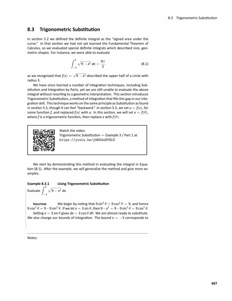
8.3 Trigonometric Substitution
8.3 Trigonometric SubstitutionIn section 5.2 we defined the definite integral as the “signed area under thecurve.” In that section we had not yet learned the Fundamental Theorem ofCalculus, so we evaluated special definite integrals which described nice, geo‐metric shapes. For instance, we were able to evaluate∫ 3
−3
√9− x2 dx =
9π2
(8.1)
as we recognized that f(x) =√9− x2 described the upper half of a circle with
radius 3.We have since learned a number of integration techniques, including Sub‐
stitution and Integration by Parts, yet we are still unable to evaluate the aboveintegral without resorting to a geometric interpretation. This section introducesTrigonometric Substitution, amethod of integration that fills this gap in our inte‐gration skill. This techniqueworks on the sameprinciple as Substitution as foundin section 5.5, though it can feel “backward.” In section 5.5, we set u = f(x), forsome function f, and replaced f(x) with u. In this section, we will set x = f(θ),where f is a trigonometric function, then replace x with f(θ).
Watch the video:Trigonometric Substitution — Example 3 / Part 1 athttps://youtu.be/yW6Odu0YHL0
We start by demonstrating this method in evaluating the integral in Equa‐tion (8.1). After the example, we will generalize the method and give more ex‐amples.
Example 8.3.1 Using Trigonometric Substitution
Evaluate∫ 3
−3
√9− x2 dx.
SOLUTION We begin by noting that 9 sin2 θ + 9 cos2 θ = 9, and hence9 cos2 θ = 9−9 sin2 θ. If we let x = 3 sin θ, then 9−x2 = 9−9 sin2 θ = 9 cos2 θ.
Setting x = 3 sin θ gives dx = 3 cos θ dθ. We are almost ready to substitute.We also change our bounds of integration. The bound x = −3 corresponds to
Notes:
407
Chapter 8 Techniques of Integration
θ = −π/2 (for when θ = −π/2, x = 3 sin θ = −3). Likewise, the bound ofx = 3 is replaced by the bound θ = π/2. Thus
∫ 3
−3
√9− x2 dx =
∫ π/2
−π/2
√9− 9 sin2 θ(3 cos θ) dθ
=
∫ π/2
−π/23√9 cos2 θ cos θ dθ
=
∫ π/2
−π/23 |3 cos θ| cos θ dθ.
On [−π/2, π/2], cos θ is always positive, so we can drop the absolute value bars,then employ a half‐angle formula:
=
∫ π/2
−π/29 cos2 θ dθ
=
∫ π/2
−π/2
92(1+ cos(2θ)
)dθ
=92
(θ +
12sin(2θ)
)∣∣∣∣π/2−π/2
=92π.
This matches our answer from before.
We now describe in detail Trigonometric Substitution. This method excelswhen dealing with integrands that contain
√a2 − x2,
√x2 − a2 and
√x2 + a2.
The following Key Idea outlines the procedure for each case, followed by moreexamples.
Notes:
408
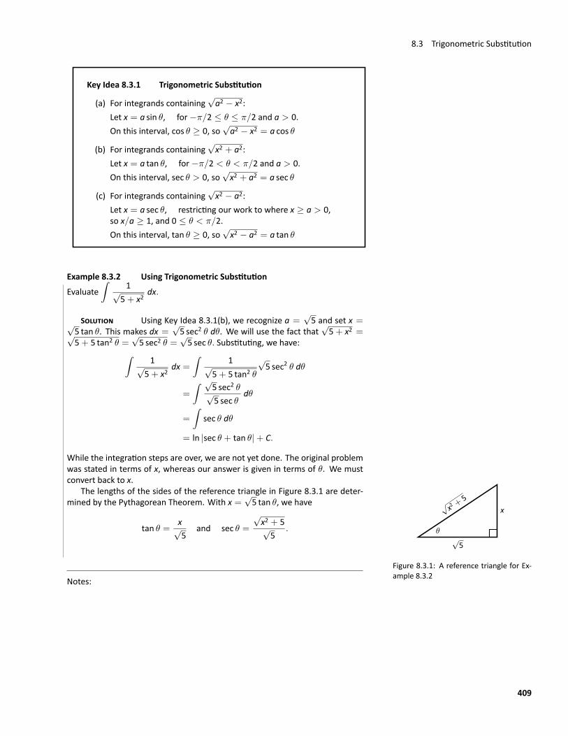
8.3 Trigonometric Substitution
Key Idea 8.3.1 Trigonometric Substitution
(a) For integrands containing√a2 − x2:
Let x = a sin θ, for−π/2 ≤ θ ≤ π/2 and a > 0.On this interval, cos θ ≥ 0, so
√a2 − x2 = a cos θ
(b) For integrands containing√x2 + a2:
Let x = a tan θ, for−π/2 < θ < π/2 and a > 0.On this interval, sec θ > 0, so
√x2 + a2 = a sec θ
(c) For integrands containing√x2 − a2:
Let x = a sec θ, restricting our work to where x ≥ a > 0,so x/a ≥ 1, and 0 ≤ θ < π/2.On this interval, tan θ ≥ 0, so
√x2 − a2 = a tan θ
Example 8.3.2 Using Trigonometric SubstitutionEvaluate
∫1√
5+ x2dx.
SOLUTION Using Key Idea 8.3.1(b), we recognize a =√5 and set x =√
5 tan θ. This makes dx =√5 sec2 θ dθ. We will use the fact that
√5+ x2 =√
5+ 5 tan2 θ =√5 sec2 θ =
√5 sec θ. Substituting, we have:∫
1√5+ x2
dx =∫
1√5+ 5 tan2 θ
√5 sec2 θ dθ
=
∫ √5 sec2 θ√5 sec θ
dθ
=
∫sec θ dθ
= ln |sec θ + tan θ|+ C.
While the integration steps are over, we are not yet done. The original problemwas stated in terms of x, whereas our answer is given in terms of θ. We mustconvert back to x.
√5
x√ x2 +5
θ
Figure 8.3.1: A reference triangle for Ex‐ample 8.3.2
The lengths of the sides of the reference triangle in Figure 8.3.1 are deter‐mined by the Pythagorean Theorem. With x =
√5 tan θ, we have
tan θ =x√5
and sec θ =
√x2 + 5√
5.
Notes:
409
Chapter 8 Techniques of Integration
This gives ∫1√
5+ x2dx = ln |sec θ + tan θ|+ C
= ln
∣∣∣∣∣√x2 + 5√
5+
x√5
∣∣∣∣∣+ C.
We can leave this answer as is, or we can use a logarithmic identity to simplifyit. Note:
ln
∣∣∣∣∣√x2 + 5√
5+
x√5
∣∣∣∣∣+ C = ln∣∣∣∣ 1√
5
(√x2 + 5+ x
)∣∣∣∣+ C
= ln∣∣∣∣ 1√
5
∣∣∣∣+ ln∣∣∣√x2 + 5+ x
∣∣∣+ C
= ln∣∣∣√x2 + 5+ x
∣∣∣+ C,
where the ln(1/
√5)term is absorbed into the constant C. (In section 7.4 we
learned another way of approaching this problem.)
Example 8.3.3 Using Trigonometric SubstitutionEvaluate
∫ √4x2 − 1 dx.
SOLUTION Westart by rewriting the integrand so that it looks like√x2 − a2
for some value of a:
√4x2 − 1 =
√4(x2 − 1
4
)
= 2
√x2 −
(12
)2
.
So we have a = 1/2, and following Key Idea 8.3.1(c), we set x = 12 sec θ, and
hence dx = 12 sec θ tan θ dθ. We now rewrite the integral with these substitu‐
Notes:
410
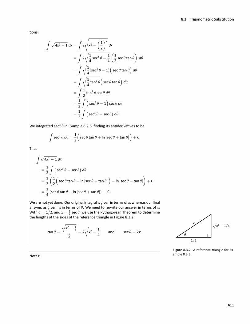
8.3 Trigonometric Substitution
tions:
∫ √4x2 − 1 dx =
∫2
√x2 −
(12
)2
dx
=
∫2√
14sec2 θ − 1
4
(12sec θ tan θ
)dθ
=
∫ √14(sec2 θ − 1)
(sec θ tan θ
)dθ
=
∫ √14tan2 θ
(sec θ tan θ
)dθ
=
∫12tan2 θ sec θ dθ
=12
∫ (sec2 θ − 1
)sec θ dθ
=12
∫ (sec3 θ − sec θ
)dθ.
We integrated sec3 θ in Example 8.2.6, finding its antiderivatives to be∫sec3 θ dθ =
12
(sec θ tan θ + ln |sec θ + tan θ|
)+ C.
Thus∫ √4x2 − 1 dx
=12
∫ (sec3 θ − sec θ
)dθ
=12
(12
(sec θ tan θ + ln |sec θ + tan θ|
)− ln |sec θ + tan θ|
)+ C
=14(sec θ tan θ − ln |sec θ + tan θ|) + C.
Weare not yet done. Our original integral is given in terms of x, whereas our finalanswer, as given, is in terms of θ. We need to rewrite our answer in terms of x.With a = 1/2, and x = 1
2 sec θ, we use the Pythagorean Theorem to determinethe lengths of the sides of the reference triangle in Figure 8.3.2.
1/2
√x2 − 1/4
x
θ
Figure 8.3.2: A reference triangle for Ex‐ample 8.3.3
tan θ =
√x2 − 1
412
= 2√
x2 − 14
and sec θ = 2x.
Notes:
411
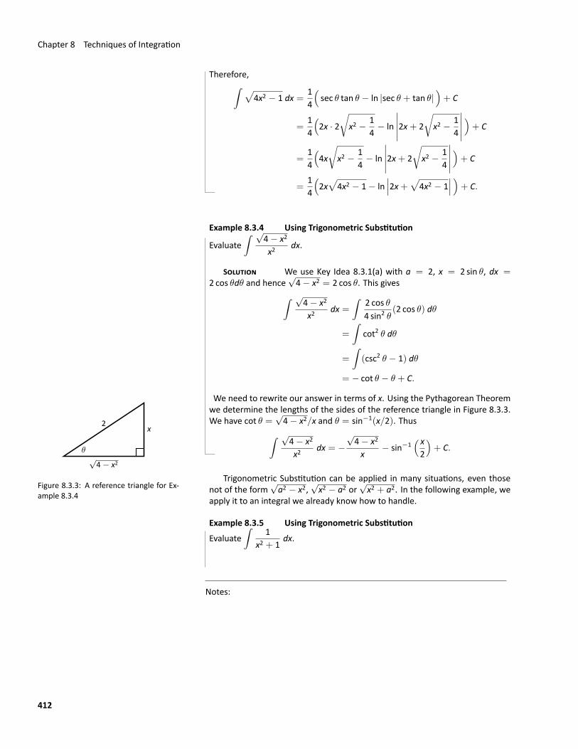
Chapter 8 Techniques of Integration
Therefore,∫ √4x2 − 1 dx =
14
(sec θ tan θ − ln |sec θ + tan θ|
)+ C
=14
(2x · 2
√x2 − 1
4− ln
∣∣∣∣∣2x+ 2√
x2 − 14
∣∣∣∣∣ )+ C
=14
(4x√
x2 − 14− ln
∣∣∣∣∣2x+ 2√
x2 − 14
∣∣∣∣∣ )+ C
=14
(2x√
4x2 − 1− ln∣∣∣2x+√4x2 − 1
∣∣∣ )+ C.
Example 8.3.4 Using Trigonometric Substitution
Evaluate∫ √
4− x2
x2dx.
SOLUTION We use Key Idea 8.3.1(a) with a = 2, x = 2 sin θ, dx =2 cos θdθ and hence
√4− x2 = 2 cos θ. This gives∫ √4− x2
x2dx =
∫2 cos θ4 sin2 θ
(2 cos θ) dθ
=
∫cot2 θ dθ
=
∫(csc2 θ − 1) dθ
= − cot θ − θ + C.
We need to rewrite our answer in terms of x. Using the Pythagorean Theorem
√4− x2
x2
θ
Figure 8.3.3: A reference triangle for Ex‐ample 8.3.4
we determine the lengths of the sides of the reference triangle in Figure 8.3.3.We have cot θ =
√4− x2/x and θ = sin−1(x/2). Thus∫ √4− x2
x2dx = −
√4− x2
x− sin−1
( x2
)+ C.
Trigonometric Substitution can be applied in many situations, even thosenot of the form
√a2 − x2,
√x2 − a2 or
√x2 + a2. In the following example, we
apply it to an integral we already know how to handle.
Example 8.3.5 Using Trigonometric SubstitutionEvaluate
∫1
x2 + 1dx.
Notes:
412
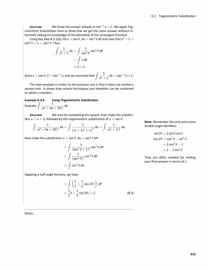
8.3 Trigonometric Substitution
SOLUTION We know the answer already as tan−1 x+ C. We apply Trig‐onometric Substitution here to show that we get the same answer without in‐herently relying on knowledge of the derivative of the arctangent function.
Using Key Idea 8.3.1(b), let x = tan θ, dx = sec2 θ dθ and note that x2 + 1 =tan2 θ + 1 = sec2 θ. Thus∫
1x2 + 1
dx =∫
1sec2 θ
sec2 θ dθ
=
∫1 dθ
= θ + C.
Since x = tan θ, θ = tan−1 x, and we conclude that∫
1x2 + 1
dx = tan−1 x+C.
The next example is similar to the previous one in that it does not involve asquare‐root. It shows how several techniques and identities can be combinedto obtain a solution.
Example 8.3.6 Using Trigonometric SubstitutionEvaluate
∫1
(x2 + 6x+ 10)2dx.
SOLUTION We start by completing the square, then make the substitu‐tion u = x+ 3, followed by the trigonometric substitution of u = tan θ:
Note: Remember the sine and cosinedouble angle identities:
sin 2θ = 2 sin θ cos θcos 2θ = cos2 θ − sin2 θ
= 2 cos2 θ − 1= 1− 2 sin2 θ
They are often needed for writingyour final answer in terms of x.
∫1
(x2 + 6x+ 10)2dx =
∫1(
(x+ 3)2 + 1)2 dx =
∫1
(u2 + 1)2du.
Now make the substitution u = tan θ, du = sec2 θ dθ:
=
∫1
(tan2 θ + 1)2sec2 θ dθ
=
∫1
(sec2 θ)2sec2 θ dθ
=
∫cos2 θ dθ.
Applying a half‐angle formula, we have
=
∫ (12+
12cos(2θ)
)dθ
=12θ +
14sin(2θ) + C. (8.2)
Notes:
413
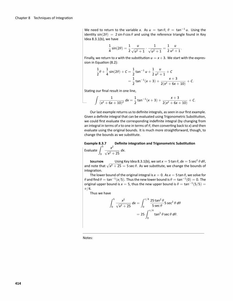
Chapter 8 Techniques of Integration
We need to return to the variable x. As u = tan θ, θ = tan−1 u. Using theidentity sin(2θ) = 2 sin θ cos θ and using the reference triangle found in KeyIdea 8.3.1(b), we have
14sin(2θ) =
12
u√u2 + 1
· 1√u2 + 1
=12
uu2 + 1
.
Finally, we return to xwith the substitution u = x+3. We start with the expres‐sion in Equation (8.2):
12θ +
14sin(2θ) + C =
12tan−1 u+
12
uu2 + 1
+ C
=12tan−1(x+ 3) +
x+ 32(x2 + 6x+ 10)
+ C.
Stating our final result in one line,∫1
(x2 + 6x+ 10)2dx =
12tan−1(x+ 3) +
x+ 32(x2 + 6x+ 10)
+ C.
Our last example returns us to definite integrals, as seen in our first example.Given a definite integral that can be evaluated using Trigonometric Substitution,we could first evaluate the corresponding indefinite integral (by changing froman integral in terms of x to one in terms of θ, then converting back to x) and thenevaluate using the original bounds. It is much more straightforward, though, tochange the bounds as we substitute.
Example 8.3.7 Definite integration and Trigonometric Substitution
Evaluate∫ 5
0
x2√x2 + 25
dx.
SOLUTION Using Key Idea 8.3.1(b), we set x = 5 tan θ, dx = 5 sec2 θ dθ,and note that
√x2 + 25 = 5 sec θ. As we substitute, we change the bounds of
integration.The lower bound of the original integral is x = 0. As x = 5 tan θ, we solve for
θ and find θ = tan−1(x/5). Thus the new lower bound is θ = tan−1(0) = 0. Theoriginal upper bound is x = 5, thus the new upper bound is θ = tan−1(5/5) =π/4.
Thus we have∫ 5
0
x2√x2 + 25
dx =∫ π/4
0
25 tan2 θ5 sec θ
5 sec2 θ dθ
= 25∫ π/4
0tan2 θ sec θ dθ.
Notes:
414
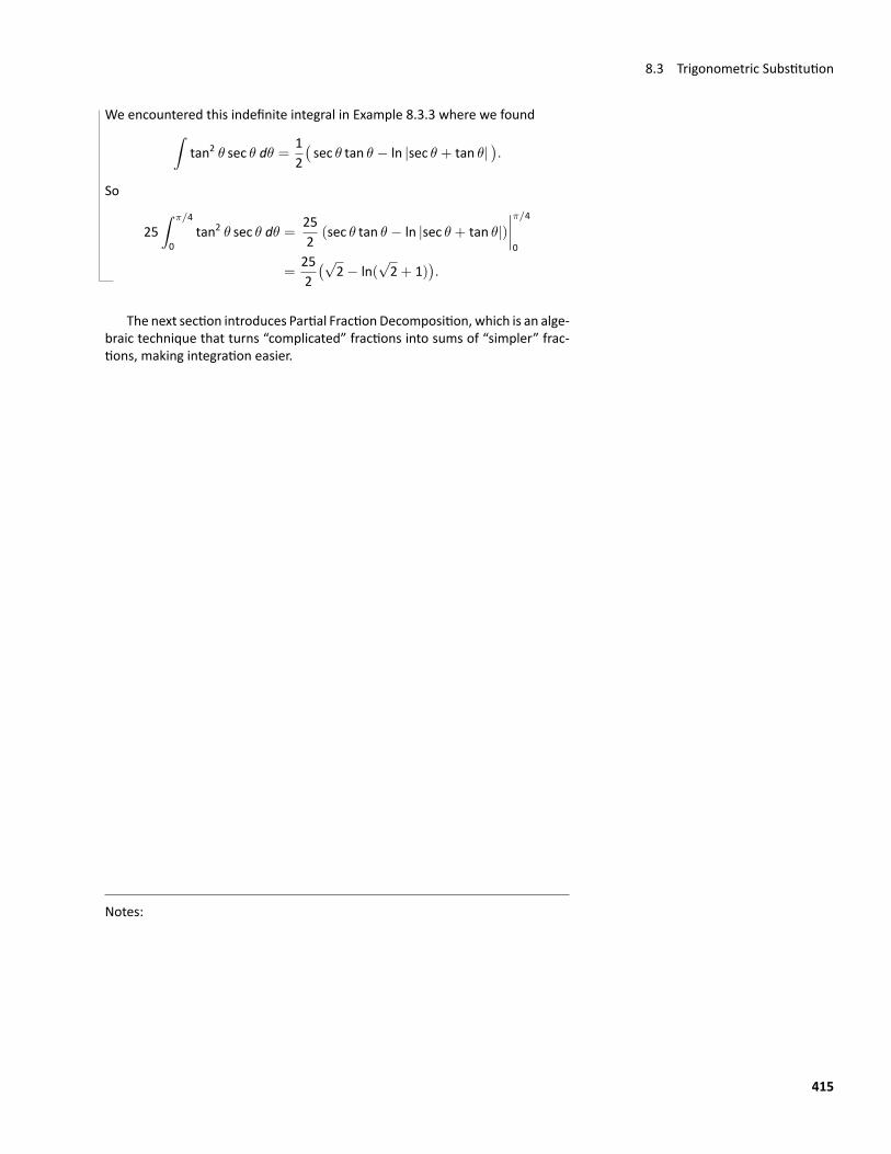
8.3 Trigonometric Substitution
We encountered this indefinite integral in Example 8.3.3 where we found∫tan2 θ sec θ dθ =
12(sec θ tan θ − ln |sec θ + tan θ|
).
So
25∫ π/4
0tan2 θ sec θ dθ =
252
(sec θ tan θ − ln |sec θ + tan θ|)∣∣∣∣π/40
=252(√
2− ln(√2+ 1)
).
The next section introduces Partial FractionDecomposition, which is an alge‐braic technique that turns “complicated” fractions into sums of “simpler” frac‐tions, making integration easier.
Notes:
415
Exercises 8.3Terms and Concepts
1. Trigonometric Substitutionworks on the sameprinciples asIntegration by Substitution, though it can feel “ ”.
2. If one uses Trigonometric Substitution on an integrand con‐taining
√25− x2, then one should set x = .
3. Consider the Pythagorean Identity sin2 θ + cos2 θ = 1.
(a) What identity is obtained when both sides are di‐vided by cos2 θ?
(b) Use the new identity to simplify 9 tan2 θ + 9.
4. Why does Key Idea 8.3.1(a) state that√a2 − x2 = a cos θ,
and not |a cos θ|?
Problems
In Exercises 5–12, apply Trigonometric Substitution to evaluatethe indefinite integrals.
5.∫ √
x2 + 1 dx
6.∫ √
x2 − 1 dx
7.∫ √
4x2 + 1 dx
8.∫ √
1− 9x2 dx
9.∫ √
16x2 − 1 dx
10.∫
8√x2 + 2
dx
11.∫
3√7− x2
dx
12.∫
5√x2 − 8
dx
In Exercises 13–20, evaluate the indefinite integrals. Somemaybe evaluated without Trigonometric Substitution.
13.∫ √
x2 − 11x
dx
14.∫
x√x2 − 3
dx
15.∫
x(x2 + 9)3/2
dx
16.∫
5x2√x2 − 10
dx
17.∫
1(x2 + 4x+ 13)2
dx
18.∫
x2(1− x2)−3/2 dx
19.∫ √
5− x27x2
dx
20.∫
x2√x2 + 3
dx
In Exercises 21–26, evaluate the definite integrals by mak‐ing the proper trigonometric substitution and changing thebounds of integration.
21.∫ 1
−1
√1− x2 dx
22.∫ 8
4
√x2 − 16 dx
23.∫ 2
0
√x2 + 4 dx
24.∫ 1
−1
1(x2 + 1)2
dx
25.∫ 1
−1
√9− x2 dx
26.∫ 1
−1x2√1− x2 dx
416
8.4 Partial Fraction Decomposition
8.4 Partial Fraction DecompositionIn this sectionwe investigate the antiderivatives of rational functions. Recall thatrational functions are functions of the form f(x) = p(x)
q(x) , where p(x) and q(x) arepolynomials and q(x) ̸= 0. Such functions arise in many contexts, one of whichis the solving of certain fundamental differential equations.
We begin with an example that demonstrates the motivation behind thissection. Consider the integral
∫1
x2 − 1dx. We do not have a simple formula
for this (if the denominator were x2 + 1, we would recognize the antiderivativeas being the arctangent function). It can be solved using Trigonometric Substi‐tution, but note how the integral is easy to evaluate once we realize:
1x2 − 1
=1/2x− 1
− 1/2x+ 1
.
Thus ∫1
x2 − 1dx =
∫1/2x− 1
dx−∫
1/2x+ 1
dx
=12ln |x− 1| − 1
2ln |x+ 1|+ C.
This section teaches how to decompose
1x2 − 1
into1/2x− 1
− 1/2x+ 1
.
We start with a rational function f(x) =p(x)q(x)
, where p and q do not have
any common factors. We first consider the degree of p and q.
• If the deg(p) ≥ deg(q) then we use polynomial long division to divide qinto p to determine a remainder r(x) where deg(r) < deg(q). We then
write f(x) = s(x)+r(x)q(x)
and apply partial fraction decomposition tor(x)q(x)
.
• If the deg(p) < deg(q) we can apply partial fraction decomposition top(x)q(x)
without additional work.
Partial fraction decomposition is based on an algebraic theorem that guar‐antees that any polynomial, and hence q, can use real numbers to factor intothe product of linear and irreducible quadratic factors. The following Key Idea An irreducible quadratic is one that
cannot factor into linear terms withreal coefficients.
states how to decompose a rational function into a sum of rational functionswhose denominators are all of lower degree than q.
Notes:
417
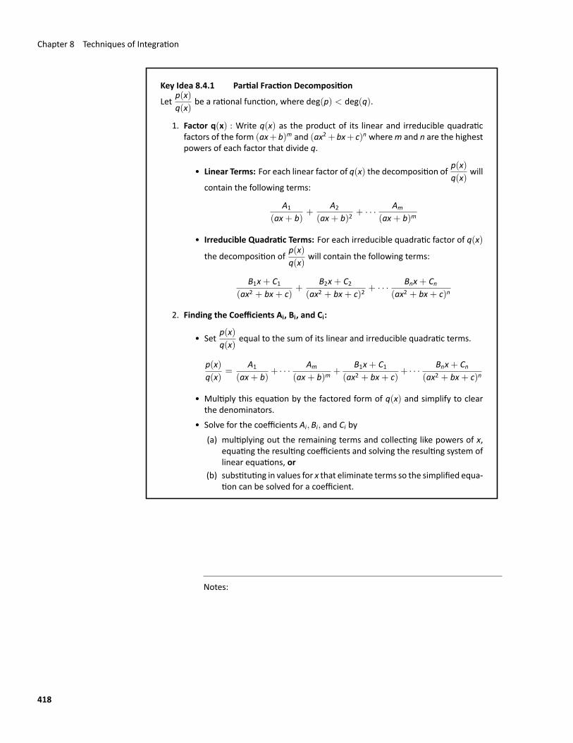
Chapter 8 Techniques of Integration
Key Idea 8.4.1 Partial Fraction Decomposition
Letp(x)q(x)
be a rational function, where deg(p) < deg(q).
1. Factor q(x) : Write q(x) as the product of its linear and irreducible quadraticfactors of the form (ax+b)m and (ax2+bx+ c)n wherem and n are the highestpowers of each factor that divide q.
• Linear Terms: For each linear factor of q(x) the decomposition ofp(x)q(x)
will
contain the following terms:
A1
(ax+ b)+
A2
(ax+ b)2+ · · · Am
(ax+ b)m
• Irreducible Quadratic Terms: For each irreducible quadratic factor of q(x)
the decomposition ofp(x)q(x)
will contain the following terms:
B1x+ C1(ax2 + bx+ c)
+B2x+ C2
(ax2 + bx+ c)2+ · · · Bnx+ Cn
(ax2 + bx+ c)n
2. Finding the Coefficients Ai, Bi, and Ci:
• Setp(x)q(x)
equal to the sum of its linear and irreducible quadratic terms.
p(x)q(x)
=A1
(ax+ b)+ · · · Am
(ax+ b)m+
B1x+ C1(ax2 + bx+ c)
+ · · · Bnx+ Cn(ax2 + bx+ c)n
• Multiply this equation by the factored form of q(x) and simplify to clearthe denominators.
• Solve for the coefficients Ai, Bi, and Ci by(a) multiplying out the remaining terms and collecting like powers of x,
equating the resulting coefficients and solving the resulting system oflinear equations, or
(b) substituting in values for x that eliminate terms so the simplified equa‐tion can be solved for a coefficient.
Notes:
418
8.4 Partial Fraction Decomposition
Watch the video:Integration Using method of Partial Fractions athttps://youtu.be/6qVgHWxdlZ0
The following examples will demonstrate how to put this Key Idea into prac‐tice. In Example 8.4.1, we focus on the setting up the decomposition of a rationalfunction.
Example 8.4.1 Decomposing into partial fractionsDecompose f(x) =
1(x+ 5)(x− 2)3(x2 + x+ 2)(x2 + x+ 7)2
without solving
for the resulting coefficients.
SOLUTION The denominator is already factored, as both x2+ x+ 2 andx2+x+7 are irreducible quadratics. We need to decompose f(x) properly. Since(x+ 5) is a linear factor that divides the denominator, there will be a
Ax+ 5
term in the decomposition.As (x− 2)3 divides the denominator, we will have the following terms in the
decomposition:B
x− 2,
C(x− 2)2
andD
(x− 2)3.
The x2 + x+ 2 term in the denominator results in aEx+ F
x2 + x+ 2term.
Finally, the (x2 + x+ 7)2 term results in the termsGx+ H
x2 + x+ 7and
Ix+ J(x2 + x+ 7)2
.
All together, we have
1(x+ 5)(x− 2)3(x2 + x+ 2)(x2 + x+ 7)2
=
Ax+ 5
+B
x− 2+
C(x− 2)2
+D
(x− 2)3+
Ex+ Fx2 + x+ 2
+Gx+ H
x2 + x+ 7+
Ix+ J(x2 + x+ 7)2
Solving for the coefficients A, B, …, Jwould be a bit tedious but not “hard.” In thenext example we demonstrate solving for the coefficients using both methodsgiven in Key Idea 8.4.1.
Notes:
419
Chapter 8 Techniques of Integration
Example 8.4.2 Decomposing into partial fractionsPerform the partial fraction decomposition of
1x2 − 1
.
SOLUTION The denominator can bewritten as the product of two linearfactors: x2 − 1 = (x− 1)(x+ 1). Thus
1x2 − 1
=A
x− 1+
Bx+ 1
. (8.3)
Using the method described in Key Idea 8.4.1 2(a) to solve for A and B, firstmultiply through by x2 − 1 = (x− 1)(x+ 1):
1 =A(x− 1)(x+ 1)
x− 1+
B(x− 1)(x+ 1)x+ 1
= A(x+ 1) + B(x− 1) (8.4)= Ax+ A+ Bx− B= (A+ B)x+ (A− B) collect like terms.
The next step is key. For clarity’s sake, rewrite the equality we have as
0x+ 1 = (A+ B)x+ (A− B).
On the left, the coefficient of the x term is 0; on the right, it is (A+B). Since bothsides are equal for all values of x, we must have that 0 = A + B. Likewise, onthe left, we have a constant term of 1; on the right, the constant term is (A−B).Therefore we have 1 = A− B.
We have two linear equations with two unknowns. This one is easy to solveby hand, leading to
A+ B = 0A− B = 1
⇒A = 1/2B = −1/2.
Thus1
x2 − 1=
1/2x− 1
− 1/2x+ 1
.
Before solving for A and B using themethod described in Key Idea 8.4.1 2(b),we note that Equations (8.3) and (8.4) are not equivalent. Only the second equa‐tion holds for all values of x, including x = −1 and x = 1, by continuity of poly‐nomials. Thus, we can choose values for x that eliminate terms in the polynomialto solve for A and B.
1 = A(x+ 1) + B(x− 1).
Notes:
420
8.4 Partial Fraction Decomposition
If we choose x = −1,
1 = A(0) + B(−2)
B = −12.
Next choose x = 1:
1 = A(2) + B(0)
A =12.
Resulting in the same decomposition as above.
In Example 8.4.3, we solve for the decomposition coefficients using the sys‐tem of linear equations (method 2a). The margin note explains how to solveusing substitution (method 2b).
Example 8.4.3 Integrating using partial fractionsUse partial fraction decomposition to integrate
∫1
(x− 1)(x+ 2)2dx.
SOLUTION Wedecompose the integrand as follows, as described by KeyIdea 8.4.1:
1(x− 1)(x+ 2)2
=A
x− 1+
Bx+ 2
+C
(x+ 2)2. (8.5)
To solve for A, B and C, we multiply both sides by (x− 1)(x+ 2)2 and collect liketerms:
Note: Equations (8.5) and (8.6) arenot equivalent for x = 1 and x =−2. However, due to the continuityof polynomials we can let x = 1 tosimplify the right hand side to A(1 +2)2 = 9A. Since the left hand sideis still 1, we have 1 = 9A, so thatA = 1/9.Likewise,when x = −2; this leads tothe equation 1 = −3C. Thus C =−1/3.Knowing A and C, we can find thevalue of B by choosing yet anothervalue of x, such as x = 0, and solvingfor B.
1 = A(x+ 2)2 + B(x− 1)(x+ 2) + C(x− 1) (8.6)= Ax2 + 4Ax+ 4A+ Bx2 + Bx− 2B+ Cx− C= (A+ B)x2 + (4A+ B+ C)x+ (4A− 2B− C)
We have
0x2 + 0x+ 1 = (A+ B)x2 + (4A+ B+ C)x+ (4A− 2B− C)
leading to the equations
A+ B = 0, 4A+ B+ C = 0 and 4A− 2B− C = 1.
These three equations of three unknowns lead to a unique solution:
A = 1/9, B = −1/9 and C = −1/3.
Notes:
421
Chapter 8 Techniques of Integration
Thus∫1
(x− 1)(x+ 2)2dx =
∫1/9x− 1
dx+∫
−1/9x+ 2
dx+∫
−1/3(x+ 2)2
dx.
Each can be integratedwith a simple substitutionwith u = x−1 or u = x+2.The end result is∫
1(x− 1)(x+ 2)2
dx =19ln |x− 1| − 1
9ln |x+ 2|+ 1
3(x+ 2)+ C.
Example 8.4.4 Integrating using partial fractions
Use partial fraction decomposition to integrate∫
x3
(x− 5)(x+ 3)dx.
SOLUTION Key Idea 8.4.1 presumes that the degree of the numeratoris less than the degree of the denominator. Since this is not the case here, webegin by using polynomial division to reduce the degree of the numerator. Weomit the steps, but encourage the reader to verify that
x3
(x− 5)(x+ 3)= x+ 2+
19x+ 30(x− 5)(x+ 3)
.
Using Key Idea 8.4.1, we can rewrite the new rational function as:
19x+ 30(x− 5)(x+ 3)
=A
x− 5+
Bx+ 3
for appropriate values of A and B. Clearing denominators, we have
19x+ 30 = A(x+ 3) + B(x− 5).
As in the previous examples we choose values of x to eliminate terms in thepolynomial. If we choose x = −3,
19(−3) + 30 = A(0) + B(−8)
B =278.
Next choose x = 5:
19(5) + 30 = A(8) + B(0)
A =1258
.
Notes:
422
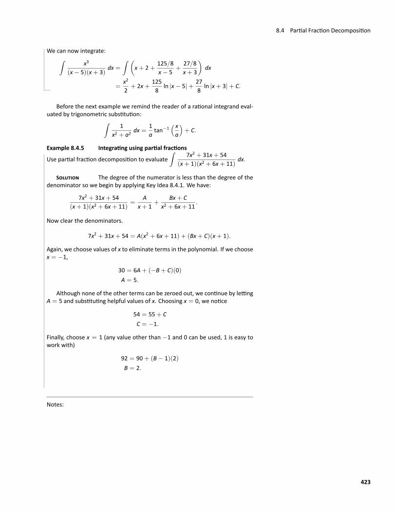
8.4 Partial Fraction Decomposition
We can now integrate:∫x3
(x− 5)(x+ 3)dx =
∫ (x+ 2+
125/8x− 5
+27/8x+ 3
)dx
=x2
2+ 2x+
1258
ln |x− 5|+ 278
ln |x+ 3|+ C.
Before the next example we remind the reader of a rational integrand eval‐uated by trigonometric substitution:∫
1x2 + a2
dx =1atan−1
( xa
)+ C.
Example 8.4.5 Integrating using partial fractions
Use partial fraction decomposition to evaluate∫
7x2 + 31x+ 54(x+ 1)(x2 + 6x+ 11)
dx.
SOLUTION The degree of the numerator is less than the degree of thedenominator so we begin by applying Key Idea 8.4.1. We have:
7x2 + 31x+ 54(x+ 1)(x2 + 6x+ 11)
=A
x+ 1+
Bx+ Cx2 + 6x+ 11
.
Now clear the denominators.
7x2 + 31x+ 54 = A(x2 + 6x+ 11) + (Bx+ C)(x+ 1).
Again, we choose values of x to eliminate terms in the polynomial. If we choosex = −1,
30 = 6A+ (−B+ C)(0)A = 5.
Although none of the other terms can be zeroed out, we continue by lettingA = 5 and substituting helpful values of x. Choosing x = 0, we notice
54 = 55+ CC = −1.
Finally, choose x = 1 (any value other than −1 and 0 can be used, 1 is easy towork with)
92 = 90+ (B− 1)(2)B = 2.
Notes:
423
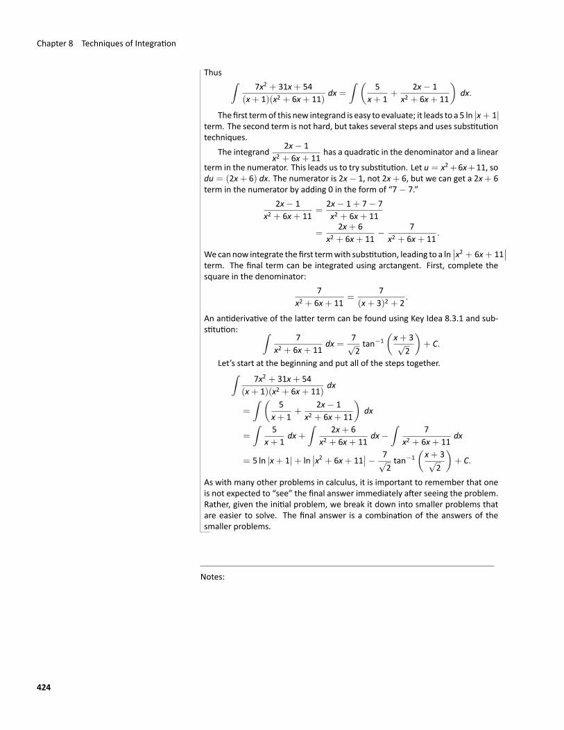
Chapter 8 Techniques of Integration
Thus ∫7x2 + 31x+ 54
(x+ 1)(x2 + 6x+ 11)dx =
∫ (5
x+ 1+
2x− 1x2 + 6x+ 11
)dx.
Thefirst termof this new integrand is easy to evaluate; it leads to a 5 ln |x+ 1|term. The second term is not hard, but takes several steps and uses substitutiontechniques.
The integrand2x− 1
x2 + 6x+ 11has a quadratic in the denominator and a linear
term in the numerator. This leads us to try substitution. Let u = x2+6x+11, sodu = (2x+ 6) dx. The numerator is 2x− 1, not 2x+ 6, but we can get a 2x+ 6term in the numerator by adding 0 in the form of “7− 7.”
2x− 1x2 + 6x+ 11
=2x− 1+ 7− 7x2 + 6x+ 11
=2x+ 6
x2 + 6x+ 11− 7
x2 + 6x+ 11.
Wecannow integrate the first termwith substitution, leading to a ln∣∣x2 + 6x+ 11
∣∣term. The final term can be integrated using arctangent. First, complete thesquare in the denominator:
7x2 + 6x+ 11
=7
(x+ 3)2 + 2.
An antiderivative of the latter term can be found using Key Idea 8.3.1 and sub‐stitution: ∫
7x2 + 6x+ 11
dx =7√2tan−1
(x+ 3√
2
)+ C.
Let’s start at the beginning and put all of the steps together.∫7x2 + 31x+ 54
(x+ 1)(x2 + 6x+ 11)dx
=
∫ (5
x+ 1+
2x− 1x2 + 6x+ 11
)dx
=
∫5
x+ 1dx+
∫2x+ 6
x2 + 6x+ 11dx−
∫7
x2 + 6x+ 11dx
= 5 ln |x+ 1|+ ln∣∣x2 + 6x+ 11
∣∣− 7√2tan−1
(x+ 3√
2
)+ C.
As with many other problems in calculus, it is important to remember that oneis not expected to “see” the final answer immediately after seeing the problem.Rather, given the initial problem, we break it down into smaller problems thatare easier to solve. The final answer is a combination of the answers of thesmaller problems.
Notes:
424

8.4 Partial Fraction Decomposition
Partial Fraction Decomposition is an important tool when dealing with ratio‐nal functions. Note that at its heart, it is a technique of algebra, not calculus,as we are rewriting a fraction in a new form. Regardless, it is very useful in therealm of calculus as it lets us evaluate a certain set of “complicated” integrals.The next sectionwill require the reader to determine an appropriatemethod forevaluating a variety of integrals.
Notes:
425
Exercises 8.4Terms and Concepts1. Fill in the blank: Partial Fraction Decomposition is a
method of rewriting functions.2. T/F: It is sometimes necessary to use polynomial division
before using Partial Fraction Decomposition.
3. Decompose 1x2 − 3x
without solving for the coefficients, asdone in Example 8.4.1.
4. Decompose 7− xx2 − 9
without solving for the coefficients, asdone in Example 8.4.1.
5. Decompose x− 3x2 − 7
without solving for the coefficients, asdone in Example 8.4.1.
6. Decompose 2x+ 5x3 + 7x
without solving for the coefficients, asdone in Example 8.4.1.
ProblemsIn Exercises 7–32, evaluate the indefinite integral.
7.∫
7x+ 7x2 + 3x− 10
dx
8.∫
7x− 2x2 + x
dx
9.∫
−43x2 − 12
dx
10.∫
x+ 7(x+ 5)2
dx
11.∫
−3x− 20(x+ 8)2
dx
12.∫
9x2 + 11x+ 7x(x+ 1)2
dx
13.∫
−12x2 − x+ 33(x− 1)(x+ 3)(3− 2x)
dx
14.∫
94x2 − 10x(7x+ 3)(5x− 1)(3x− 1)
dx
15.∫
x2 + x+ 1x2 + x− 2
dx
16.∫
x3
x2 − x− 20dx
17.∫
2x2 − 4x+ 6x2 − 2x+ 3
dx
18.∫
1x3 + 2x2 + 3x
dx
19.∫
dxx4 − x2
20.∫
x2 + x+ 5x2 + 4x+ 10
dx
21.∫
12x2 + 21x+ 3(x+ 1)(3x2 + 5x− 1)
dx
22.∫
6x2 + 8x− 4(x− 3)(x2 + 6x+ 10)
dx
23.∫
1− x+ 2x2 − x3
x(x2 + 1)2dx
24.∫
2x2 + x+ 1(x+ 1)(x2 + 9)
dx
25.∫
x2 − 20x− 69(x− 7)(x2 + 2x+ 17)
dx
26.∫
x3 + x2 + 2x+ 1(x2 + 1)(x2 + 2)
dx
27.∫
xx4 + 4x2 + 3
dx
28.∫
x− 3(x2 + 2x+ 4)2
dx
29.∫
9x2 − 60x+ 33(x− 9)(x2 − 2x+ 11)
dx
30.∫
6x2 + 45x+ 121(x+ 2)(x2 + 10x+ 27)
dx
31.∫
1x4 − 16
dx
32.∫
1x2 + x
dx
In Exercises 33–36, evaluate the definite integral.
33.∫ 2
1
8x+ 21(x+ 2)(x+ 3)
dx
34.∫ 5
0
14x+ 6(3x+ 2)(x+ 4)
dx
35.∫ 1
−1
x2 + 5x− 5(x− 10)(x2 + 4x+ 5)
dx
36.∫ 1
0
x(x+ 1)(x2 + 2x+ 1)
dx
426

8.5 Integration Strategies
8.5 Integration StrategiesWe’ve now seen a fair number of different integration techniques and so weshould probably pause at this point to talk a little bit about a strategy to use fordetermining the correct technique to use when faced with an integral.
There are a couple of points that need to be made about this strategy. First,it isn’t a hard and fast set of rules for determining the method that should beused. It is really nothing more than a general set of guidelines that will help usto identify techniques that may work. Some integrals can be done in more thanone way and so depending on the path you take through the strategy you mayend up with a different technique than someone else who also went throughthis strategy.
Second, while the strategy is presented as a way to identify the techniquethat could be used on an integral keep in mind that, for many integrals, it canalso automatically exclude certain techniques as well. When going through thestrategy keep two lists in mind. The first list is integration techniques that simplywon’t work and the second list is techniques that look like they might work.After going through the strategy, if the second list has only one entry then thatis the technique to use. If on the other hand, there is more than one possibletechnique to use we will have to decide on which is liable to be the best for usto use. Unfortunately there is no way to teach which technique is the best asthat usually depends upon the person and which technique they find to be theeasiest.
Third, don’t forget thatmany integrals can be evaluated inmultiple ways andsomore than one techniquemay be used on it. This has already beenmentionedin each of the previous points, but is important enough to warrant a separatemention. Sometimes one technique will be significantly easier than the othersand so don’t just stop at the first technique that appears towork. Always identifyall possible techniques and then go back and determine which you feel will bethe easiest for you to use.
Next, it’s entirely possible that you will need to use more than one methodto completely evaluate an integral. For instance a substitutionmay lead to usingintegration by parts or partial fractions integral.
Notes:
427
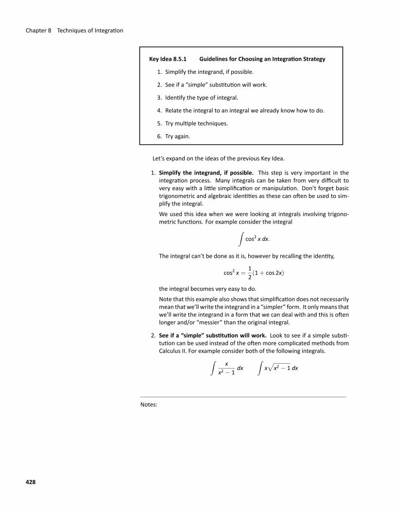
Chapter 8 Techniques of Integration
Key Idea 8.5.1 Guidelines for Choosing an Integration Strategy
1. Simplify the integrand, if possible.
2. See if a “simple” substitution will work.
3. Identify the type of integral.
4. Relate the integral to an integral we already know how to do.
5. Try multiple techniques.
6. Try again.
Let’s expand on the ideas of the previous Key Idea.
1. Simplify the integrand, if possible. This step is very important in theintegration process. Many integrals can be taken from very difficult tovery easy with a little simplification or manipulation. Don’t forget basictrigonometric and algebraic identities as these can often be used to sim‐plify the integral.We used this idea when we were looking at integrals involving trigono‐metric functions. For example consider the integral∫
cos2 x dx.
The integral can’t be done as it is, however by recalling the identity,
cos2 x =12(1+ cos 2x)
the integral becomes very easy to do.Note that this example also shows that simplification does not necessarilymean thatwe’ll write the integrand in a “simpler” form. It onlymeans thatwe’ll write the integrand in a form that we can deal with and this is oftenlonger and/or “messier” than the original integral.
2. See if a “simple” substitution will work. Look to see if a simple substi‐tution can be used instead of the often more complicated methods fromCalculus II. For example consider both of the following integrals.∫
xx2 − 1
dx∫
x√
x2 − 1 dx
Notes:
428
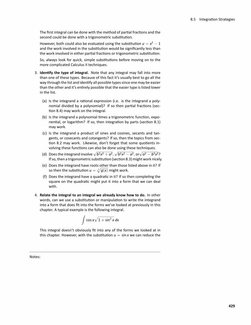
8.5 Integration Strategies
The first integral can be done with the method of partial fractions and thesecond could be done with a trigonometric substitution.However, both could also be evaluated using the substitution u = x2 − 1and the work involved in the substitution would be significantly less thanthe work involved in either partial fractions or trigonometric substitution.So, always look for quick, simple substitutions before moving on to themore complicated Calculus II techniques.
3. Identify the type of integral. Note that any integral may fall into morethan one of these types. Because of this fact it’s usually best to go all theway through the list and identify all possible types since onemay be easierthan the other and it’s entirely possible that the easier type is listed lowerin the list.
(a) Is the integrand a rational expression (i.e. is the integrand a poly‐nomial divided by a polynomial)? If so then partial fractions (sec‐tion 8.4) may work on the integral.
(b) Is the integrand a polynomial times a trigonometric function, expo‐nential, or logarithm? If so, then integration by parts (section 8.1)may work.
(c) Is the integrand a product of sines and cosines, secants and tan‐gents, or cosecants and cotangents? If so, then the topics from sec‐tion 8.2 may work. Likewise, don’t forget that some quotients in‐volving these functions can also be done using these techniques.
(d) Does the integrand involve√b2x2 + a2,
√b2x2 − a2, or
√a2 − b2x2?
If so, then a trigonometric substitution (section8.3)mightwork nicely.(e) Does the integrand have roots other than those listed above in it? If
so then the substitution u = n√
g(x)might work.(f) Does the integrand have a quadratic in it? If so then completing the
square on the quadratic might put it into a form that we can dealwith.
4. Relate the integral to an integral we already know how to do. In otherwords, can we use a substitution or manipulation to write the integrandinto a form that does fit into the forms we’ve looked at previously in thischapter. A typical example is the following integral.∫
cos x√
1+ sin2 x dx
This integral doesn’t obviously fit into any of the forms we looked at inthis chapter. However, with the substitution u = sin x we can reduce the
Notes:
429
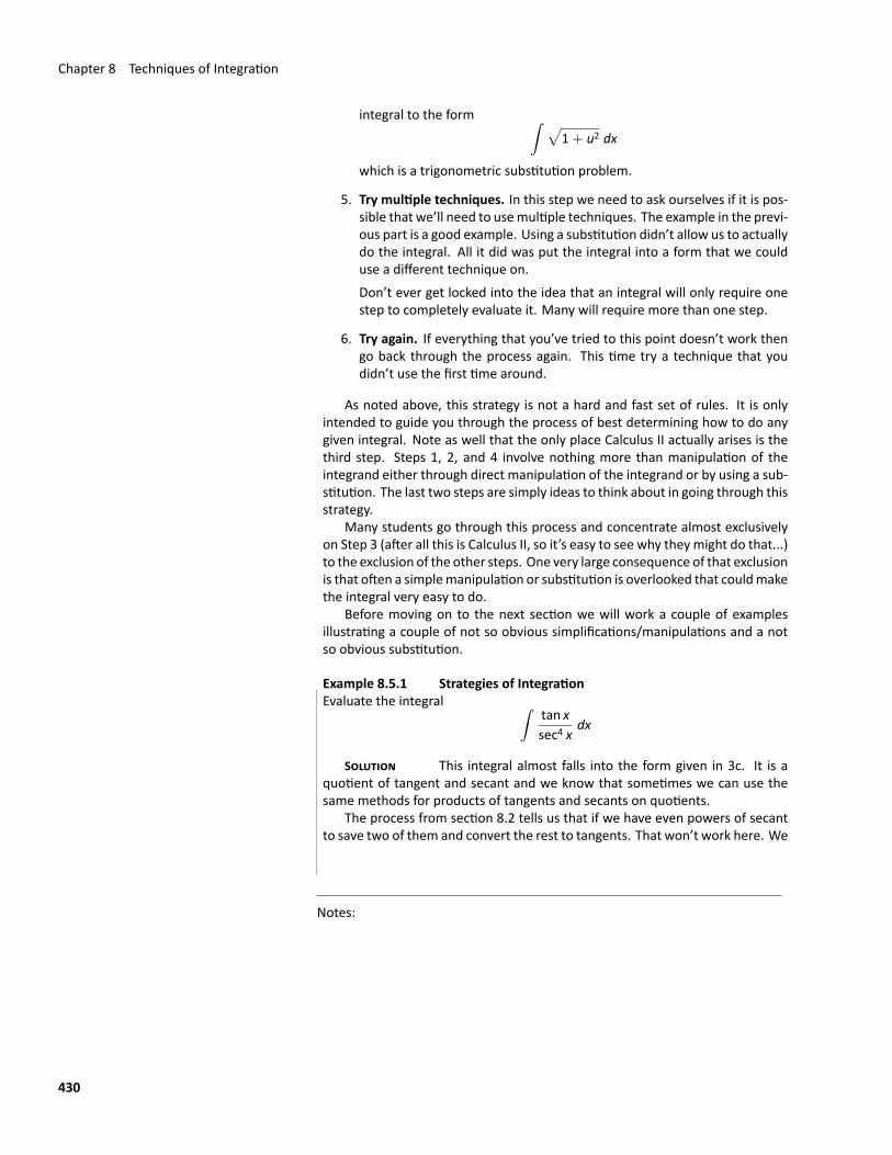
Chapter 8 Techniques of Integration
integral to the form ∫ √1+ u2 dx
which is a trigonometric substitution problem.
5. Try multiple techniques. In this step we need to ask ourselves if it is pos‐sible that we’ll need to usemultiple techniques. The example in the previ‐ous part is a good example. Using a substitution didn’t allow us to actuallydo the integral. All it did was put the integral into a form that we coulduse a different technique on.Don’t ever get locked into the idea that an integral will only require onestep to completely evaluate it. Many will require more than one step.
6. Try again. If everything that you’ve tried to this point doesn’t work thengo back through the process again. This time try a technique that youdidn’t use the first time around.
As noted above, this strategy is not a hard and fast set of rules. It is onlyintended to guide you through the process of best determining how to do anygiven integral. Note as well that the only place Calculus II actually arises is thethird step. Steps 1, 2, and 4 involve nothing more than manipulation of theintegrand either through direct manipulation of the integrand or by using a sub‐stitution. The last two steps are simply ideas to think about in going through thisstrategy.
Many students go through this process and concentrate almost exclusivelyon Step 3 (after all this is Calculus II, so it’s easy to see why they might do that...)to the exclusion of the other steps. One very large consequence of that exclusionis that often a simplemanipulation or substitution is overlooked that couldmakethe integral very easy to do.
Before moving on to the next section we will work a couple of examplesillustrating a couple of not so obvious simplifications/manipulations and a notso obvious substitution.
Example 8.5.1 Strategies of IntegrationEvaluate the integral ∫
tan xsec4 x
dx
SOLUTION This integral almost falls into the form given in 3c. It is aquotient of tangent and secant and we know that sometimes we can use thesame methods for products of tangents and secants on quotients.
The process from section 8.2 tells us that if we have even powers of secantto save two of them and convert the rest to tangents. That won’t work here. We
Notes:
430
8.5 Integration Strategies
can save two secants, but they would be in the denominator and they won’t dous any good here. Remember that the point of saving them is so they could bethere for the substitution u = tan x. That requires them to be in the numerator.So, that won’t work. We need to find another solution method.
There are in fact two solution methods to this integral depending on howyou want to go about it.
Solution 1 In this solution method we could just convert everything tosines and cosines and see if that gives us an integral we can deal with.∫
tan xsec4 x
dx =∫
sin xcos x
cos4 x dx
=
∫sin x cos3 x dx substitute u = cos x
= −∫
u3 du
= −14cos4 x+ C
Note that just converting to sines and cosines won’t always work and if itdoes it won’t always work this nicely. Often there will be a lot more work thatwould need to be done to complete the integral.
Solution 2 This solution method goes back to dealing with secants andtangents. Let’s notice that if we had a secant in the numerator we could just useu = sec x as a substitution and it would be a fairly quick and simple substitutionto use. We don’t have a secant in the numerator. However we could very easilyget a secant in the numerator by multiplying the numerator and denominatorby secant (i.e. we multiply the integrand by “1”).∫
tan xsec4 x
dx =∫
tan x sec xsec5 x
dx substitute u = sec x
=
∫1u5
du
= −14
1sec4 x
+ C
= −14cos4 x+ C
In the previous examplewe saw two “simplifications” that allowed us to eval‐uate the integral. The first was using identities to rewrite the integral into termswe could deal with and the second involved multiplying the numerator and de‐nominator by something to again put the integral into terms we could deal with.
Notes:
431
Chapter 8 Techniques of Integration
Using identities to rewrite an integral is an important “simplification” andweshould not forget about it. Integrals can often be greatly simplified or at leastput into a form that can be dealt with by using an identity.
The second “simplification” is not used as often, but does show up on oc‐casion so again, it’s best to remember it. In fact, let’s take another look at anexample in which multiplying the integrand by “1” will allow us to evaluate anintegral.
Example 8.5.2 Strategy for IntegrationEvaluate the integral ∫
11+ sin x
dx
SOLUTION This is an integral which if we just concentrate on the thirdstep we won’t get anywhere. This integral doesn’t appear to be any of the kindsof integrals that we worked on in this chapter. We can evaluate the integralhowever, if we do the following,∫
11+ sin x
dx =∫
11+ sin x
1− sin x1− sin x
dx
=
∫1− sin x1− sin2 x
dx
This does not appear to have done anything for us. However, if we nowremember the first “simplification” we looked at above we will notice that wecan use an identity to rewrite the denominator. Once we do that we can furthermanipulate the integrand into something we can evaluate.∫
11+ sin x
dx =∫
1− sin xcos2 x
dx
=
∫1
cos2 x− sin x
cos x1
cos xdx
=
∫sec2 x− tan x sec x dx
= tan x− sec x+ C
So, we’ve just seen once again that multiplying by a helpful form of “1” canput the integral into a form we can integrate. Notice as well that this exam‐ple also showed that “simplifications” do not necessarily put an integral into asimpler form. They only put the integrand into a form that is easier to integrate.
Let’s now take a quick look at an example of a substitution that is not soobvious.
Notes:
432
8.5 Integration Strategies
Example 8.5.3 Strategy for IntegrationEvaluate the integral ∫
cos√x dx
SOLUTION We introduced this integral by saying that the substitutionwas not so obvious. However, this is really an integral that falls into the formgiven by 3e in Key Idea 8.5.1. Many people miss that form and so don’t thinkabout it. So, let’s try the following substitution.
u =√x x = u2 dx = 2u du
With this substitution the integral becomes,∫cos
√x dx = 2
∫u cos u du
This is now an integration by parts. Remember that often we will need to usemore than one technique to completely do the integral. This is a fairly simpleintegration by parts problem so we’ll leave the remainder of the details for youto check. ∫
cos√x dx = 2(cos
√x+
√x sin
√x) + C.
It will be possible to integrate every integral assigned in this class, but it is im‐portant to note that there are integrals that just can’t be evaluated. We shouldalso note that after we look at series in chapter 9 we will be able to write downa series representation of many of these types of integrals.
Notes:
433
Exercises 8.5ProblemsIn Exercises 1–51, compute the indefinite integral.
1.∫
sin−1 x dx
2.∫
cos3 2x sin2 2x dx
3.∫
4x2 − 12x− 10(x− 2)(x2 − 4x+ 3)
dx
4.∫
tan x sec5 x dx
5.∫
1(x2 + 25)3/2
dx
6.∫ √
4− x2x
dx
7.∫
x3 + 1x(x− 1)3
dx
8.∫
x√4+ 4x− x2
dx
9.∫
x3ex2dx
10.∫ 3√x+ 8
xdx
11.∫
e2x sin 3x dx
12.∫
cos3 x sin3 x dx
13.∫
x√4− x2
dx
14.∫
x5 − x3 + 1x3 + 2x2
dx
15.∫
1x3/2 + x1/2
dx
16.∫
ex sec ex dx
17.∫
x2 sin 3x dx
18.∫
sin3 x√cos x dx
19.∫
ex√ex + 1 dx
20.∫
x2√4x2 + 9
dx
21.∫
sec2 x tan2 x dx
22.∫
x csc x cot x dx
23.∫
x2(8− x3)1/3 dx
24.∫
sin√x dx
25.∫
x√3− 2x dx
26.∫
e3x
1+ exdx
27.∫
x2 − 4x+ 3√x
dx
28.∫
x3√16− x2
dx
29.∫
1− 2xx2 + 12x+ 35
dx
30.∫
tan−1 5x dx
31.∫
etan x
cos2 xdx
32.∫
1√7+ 5x2
dx
33.∫
cot6 x dx
34.∫
x3√x2 − 25 dx
35.∫
(x2 − sech2 4x) dx
36.∫
x2e−4x dx
37.∫
3√11− 10x− x2
dx
38.∫
x3 − 20x2 − 63x− 198x4 − 1
dx
39.∫
tan3 x sec x dx
40.∫
(x3 + 1) cos x dx
41.∫ √
9− 4x2x2
dx
42.∫
(5− cot 3x)2 dx
43.∫
1x(√x− 4
√x)
dx
44.∫
sin x√1+ cos x
dx
45.∫
x2
(25+ x2)2dx
46.∫
2x3 + 4x2 + 10x+ 13x4 + 9x2 + 20
dx
47.∫
(x2 − 2)2
xdx
48.∫
x3/2 ln x dx
49.∫
x23√2x+ 3
dx
434
50.∫
xex
(x+ 1)2dx
51.∫
tan 7x cos 7x dx
52. Show that if t = tan θ2 , then
sin θ =2t
1+ t2cos θ =
1− t2
1+ t2and dθ
dt=
21+ t2
.
Explain how this substitution transforms a rational trigono‐metric function into a rational function. (This is known asthe tangent half‐angle substitution and sometimes knownas the Weierstrass substitution.)
53. Use the substitution of the previous exercise to evaluate∫sec θ dθ.
54. Use the substitution of the previous exercise to evaluate∫1
sin θ + tan θdθ.
435
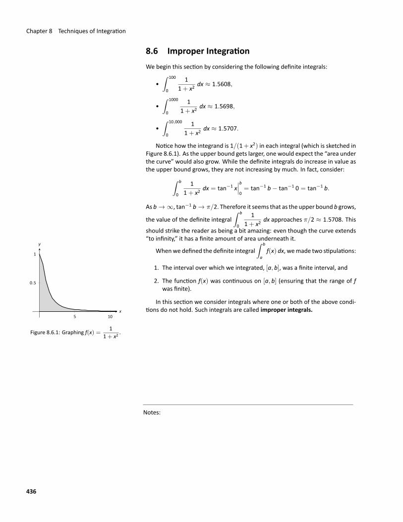
Chapter 8 Techniques of Integration
8.6 Improper IntegrationWe begin this section by considering the following definite integrals:
•∫ 100
0
11+ x2
dx ≈ 1.5608,
•∫ 1000
0
11+ x2
dx ≈ 1.5698,
•∫ 10,000
0
11+ x2
dx ≈ 1.5707.
Notice how the integrand is 1/(1+ x2) in each integral (which is sketched inFigure 8.6.1). As the upper bound gets larger, one would expect the “area underthe curve” would also grow. While the definite integrals do increase in value asthe upper bound grows, they are not increasing by much. In fact, consider:∫ b
0
11+ x2
dx = tan−1 x∣∣∣b0= tan−1 b− tan−1 0 = tan−1 b.
As b → ∞, tan−1 b → π/2. Therefore it seems that as the upper bound b grows,
the value of the definite integral∫ b
0
11+ x2
dx approaches π/2 ≈ 1.5708. This
should strike the reader as being a bit amazing: even though the curve extends“to infinity,” it has a finite amount of area underneath it.
5 10
0.5
1
x
y
Figure 8.6.1: Graphing f(x) = 11+ x2
.
Whenwe defined the definite integral∫ b
af(x) dx, wemade two stipulations:
1. The interval over which we integrated, [a, b], was a finite interval, and
2. The function f(x) was continuous on [a, b] (ensuring that the range of fwas finite).
In this section we consider integrals where one or both of the above condi‐tions do not hold. Such integrals are called improper integrals.
Notes:
436
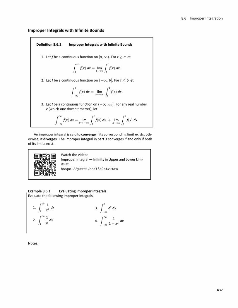
8.6 Improper Integration
Improper Integrals with Infinite Bounds
Definition 8.6.1 Improper Integrals with Infinite Bounds
1. Let f be a continuous function on [a,∞). For t ≥ a let∫ ∞
af(x) dx = lim
t→∞
∫ t
af(x) dx.
2. Let f be a continuous function on (−∞, b]. For t ≤ b let∫ b
−∞f(x) dx = lim
t→−∞
∫ b
tf(x) dx.
3. Let f be a continuous function on (−∞,∞). For any real numberc (which one doesn’t matter), let∫ ∞
−∞f(x) dx = lim
a→−∞
∫ c
af(x) dx + lim
b→∞
∫ b
cf(x) dx.
An improper integral is said to converge if its corresponding limit exists; oth‐erwise, it diverges. The improper integral in part 3 converges if and only if bothof its limits exist.
Watch the video:Improper Integral— Infinity in Upper and Lower Lim‐its athttps://youtu.be/f6cGotvktxs
Example 8.6.1 Evaluating improper integralsEvaluate the following improper integrals.
1.∫ ∞
1
1x2
dx
2.∫ ∞
1
1xdx
3.∫ 0
−∞ex dx
4.∫ ∞
−∞
11+ x2
dx
Notes:
437
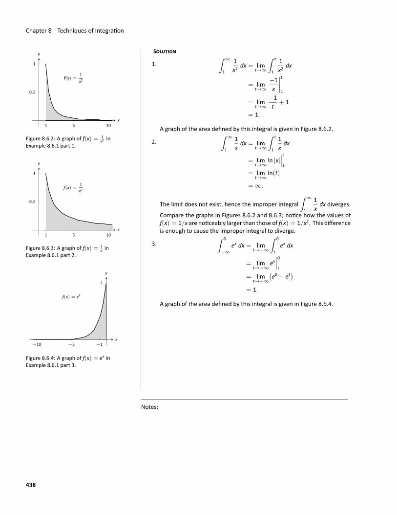
Chapter 8 Techniques of Integration
SOLUTION
1.
f(x) =1x2
1 5 10
0.5
1
x
y
Figure 8.6.2: A graph of f(x) = 1x2 in
Example 8.6.1 part 1.
∫ ∞
1
1x2
dx = limt→∞
∫ t
1
1x2
dx
= limt→∞
−1x
∣∣∣∣t1
= limt→∞
−1t
+ 1
= 1.
A graph of the area defined by this integral is given in Figure 8.6.2.
2.
f(x) =1x2
1 5 10
0.5
1
x
y
Figure 8.6.3: A graph of f(x) = 1x in
Example 8.6.1 part 2.
∫ ∞
1
1xdx = lim
t→∞
∫ t
1
1xdx
= limt→∞
ln |x|∣∣∣t1
= limt→∞
ln(t)
= ∞.
The limit does not exist, hence the improper integral∫ ∞
1
1xdx diverges.
Compare the graphs in Figures 8.6.2 and 8.6.3; notice how the values off(x) = 1/x are noticeably larger than those of f(x) = 1/x2. This differenceis enough to cause the improper integral to diverge.
3.
f(x) = ex
−1−5−10
1
x
y
Figure 8.6.4: A graph of f(x) = ex inExample 8.6.1 part 3.
∫ 0
−∞ex dx = lim
t→−∞
∫ 0
tex dx
= limt→−∞
ex∣∣∣0t
= limt→−∞
(e0 − et
)= 1.
A graph of the area defined by this integral is given in Figure 8.6.4.
Notes:
438
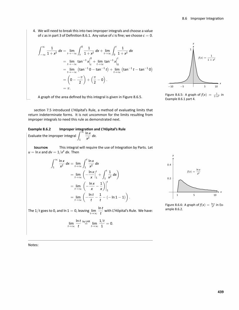
8.6 Improper Integration
4. We will need to break this into two improper integrals and choose a valueof c as in part 3 of Definition 8.6.1. Any value of c is fine; we choose c = 0.
f(x) =1
1 + x2
−10 −5 5 10
1
x
y
Figure 8.6.5: A graph of f(x) = 11+x2 in
Example 8.6.1 part 4.
∫ ∞
−∞
11+ x2
dx = limt→−∞
∫ 0
t
11+ x2
dx+ limt→∞
∫ t
0
11+ x2
dx
= limt→−∞
tan−1 x∣∣∣0t+ lim
t→∞tan−1 x
∣∣∣t0
= limt→−∞
(tan−1 0− tan−1 t
)+ lim
t→∞
(tan−1 t− tan−1 0
)=
(0− −π
2
)+(π2− 0).
= π.
A graph of the area defined by this integral is given in Figure 8.6.5.
section 7.5 introduced L’Hôpital’s Rule, a method of evaluating limits thatreturn indeterminate forms. It is not uncommon for the limits resulting fromimproper integrals to need this rule as demonstrated next.
Example 8.6.2 Improper integration and L’Hôpital’s Rule
Evaluate the improper integral∫ ∞
1
ln xx2
dx.
SOLUTION This integral will require the use of Integration by Parts. Letu = ln x and dv = 1/x2 dx. Then
f(x) =ln xx2
1 5 10
0.2
0.4
x
y
Figure 8.6.6: A graph of f(x) = ln xx2 in Ex‐
ample 8.6.2.
∫ ∞
1
ln xx2
dx = limt→∞
∫ t
1
ln xx2
dx
= limt→∞
(− ln x
x
∣∣∣t1+
∫ t
1
1x2
dx)
= limt→∞
(− ln x
x− 1
x
)∣∣∣∣t1
= limt→∞
(− ln t
t− 1
t− (− ln 1− 1)
).
The 1/t goes to 0, and ln 1 = 0, leaving limt→∞
ln tt
with L’Hôpital’s Rule. We have:
limt→∞
ln tt
by LHR= lim
t→∞
1/t1
= 0.
Notes:
439
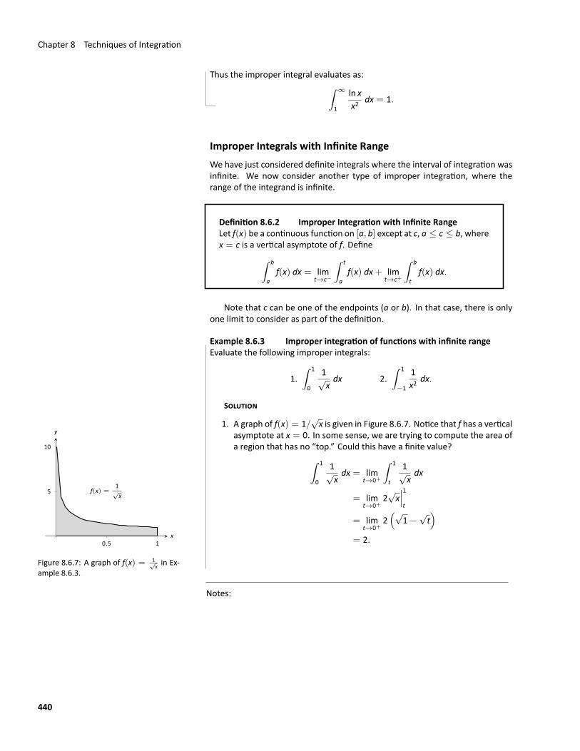
Chapter 8 Techniques of Integration
Thus the improper integral evaluates as:∫ ∞
1
ln xx2
dx = 1.
Improper Integrals with Infinite RangeWe have just considered definite integrals where the interval of integration wasinfinite. We now consider another type of improper integration, where therange of the integrand is infinite.
Definition 8.6.2 Improper Integration with Infinite RangeLet f(x) be a continuous function on [a, b] except at c, a ≤ c ≤ b, wherex = c is a vertical asymptote of f. Define∫ b
af(x) dx = lim
t→c−
∫ t
af(x) dx+ lim
t→c+
∫ b
tf(x) dx.
Note that c can be one of the endpoints (a or b). In that case, there is onlyone limit to consider as part of the definition.
Example 8.6.3 Improper integration of functions with infinite rangeEvaluate the following improper integrals:
1.∫ 1
0
1√xdx 2.
∫ 1
−1
1x2
dx.
SOLUTION
1. A graph of f(x) = 1/√x is given in Figure 8.6.7. Notice that f has a vertical
f(x) =1√x
0.5 1
5
10
x
y
Figure 8.6.7: A graph of f(x) = 1√x in Ex‐
ample 8.6.3.
asymptote at x = 0. In some sense, we are trying to compute the area ofa region that has no “top.” Could this have a finite value?∫ 1
0
1√xdx = lim
t→0+
∫ 1
t
1√xdx
= limt→0+
2√x∣∣∣1t
= limt→0+
2(√
1−√t)
= 2.
Notes:
440
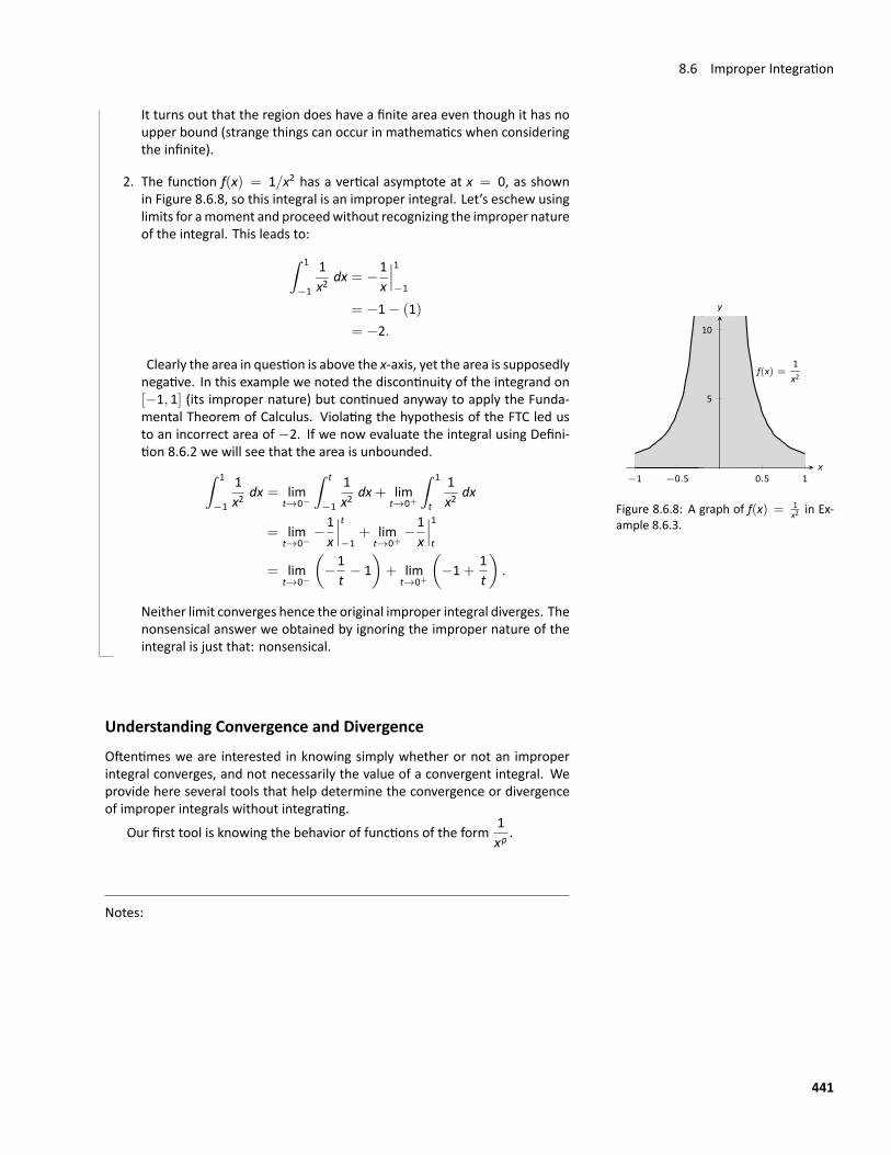
8.6 Improper Integration
It turns out that the region does have a finite area even though it has noupper bound (strange things can occur in mathematics when consideringthe infinite).
2. The function f(x) = 1/x2 has a vertical asymptote at x = 0, as shownin Figure 8.6.8, so this integral is an improper integral. Let’s eschew usinglimits for amoment and proceedwithout recognizing the improper natureof the integral. This leads to:∫ 1
−1
1x2
dx = −1x
∣∣∣1−1
= −1− (1)= −2.
Clearly the area in question is above the x‐axis, yet the area is supposedly f(x) =1x2
−1 −0.5 0.5 1
5
10
x
y
Figure 8.6.8: A graph of f(x) = 1x2 in Ex‐
ample 8.6.3.
negative. In this example we noted the discontinuity of the integrand on[−1, 1] (its improper nature) but continued anyway to apply the Funda‐mental Theorem of Calculus. Violating the hypothesis of the FTC led usto an incorrect area of −2. If we now evaluate the integral using Defini‐tion 8.6.2 we will see that the area is unbounded.∫ 1
−1
1x2
dx = limt→0−
∫ t
−1
1x2
dx+ limt→0+
∫ 1
t
1x2
dx
= limt→0−
−1x
∣∣∣t−1
+ limt→0+
−1x
∣∣∣1t
= limt→0−
(−1
t− 1)+ lim
t→0+
(−1+
1t
).
Neither limit converges hence the original improper integral diverges. Thenonsensical answer we obtained by ignoring the improper nature of theintegral is just that: nonsensical.
Understanding Convergence and DivergenceOftentimes we are interested in knowing simply whether or not an improperintegral converges, and not necessarily the value of a convergent integral. Weprovide here several tools that help determine the convergence or divergenceof improper integrals without integrating.
Our first tool is knowing the behavior of functions of the form1xp
.
Notes:
441
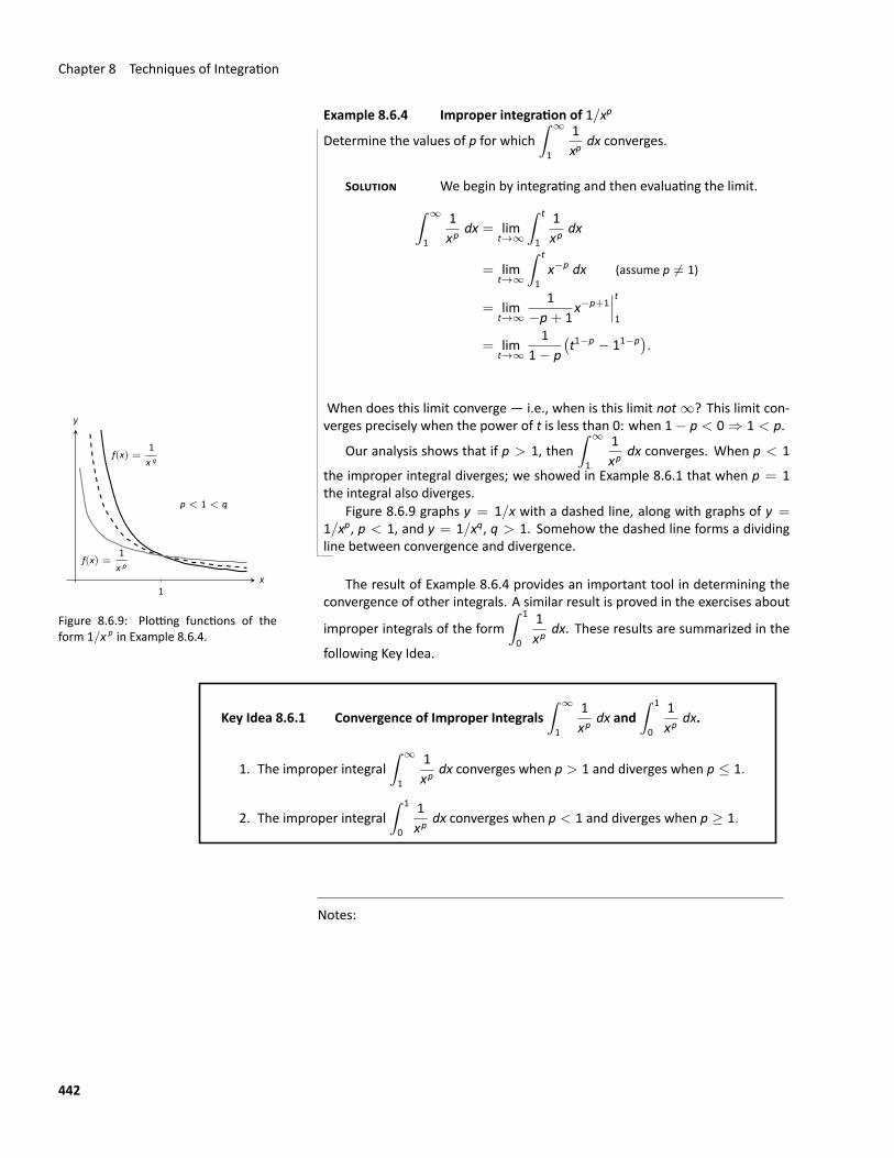
Chapter 8 Techniques of Integration
Example 8.6.4 Improper integration of 1/xp
Determine the values of p for which∫ ∞
1
1xp
dx converges.
SOLUTION We begin by integrating and then evaluating the limit.∫ ∞
1
1xp
dx = limt→∞
∫ t
1
1xp
dx
= limt→∞
∫ t
1x−p dx (assume p ̸= 1)
= limt→∞
1−p+ 1
x−p+1∣∣∣t1
= limt→∞
11− p
(t1−p − 11−p).
When does this limit converge — i.e., when is this limit not ∞? This limit con‐
f(x) =1x q
f(x) =1x p
p < 1 < q
1x
y
Figure 8.6.9: Plotting functions of theform 1/x p in Example 8.6.4.
verges precisely when the power of t is less than 0: when 1− p < 0 ⇒ 1 < p.
Our analysis shows that if p > 1, then∫ ∞
1
1xp
dx converges. When p < 1
the improper integral diverges; we showed in Example 8.6.1 that when p = 1the integral also diverges.
Figure 8.6.9 graphs y = 1/x with a dashed line, along with graphs of y =1/xp, p < 1, and y = 1/xq, q > 1. Somehow the dashed line forms a dividingline between convergence and divergence.
The result of Example 8.6.4 provides an important tool in determining theconvergence of other integrals. A similar result is proved in the exercises about
improper integrals of the form∫ 1
0
1xp
dx. These results are summarized in the
following Key Idea.
Key Idea 8.6.1 Convergence of Improper Integrals∫ ∞
1
1xp
dx and∫ 1
0
1xp
dx.
1. The improper integral∫ ∞
1
1xp
dx converges when p > 1 and diverges when p ≤ 1.
2. The improper integral∫ 1
0
1xp
dx converges when p < 1 and diverges when p ≥ 1.
Notes:
442
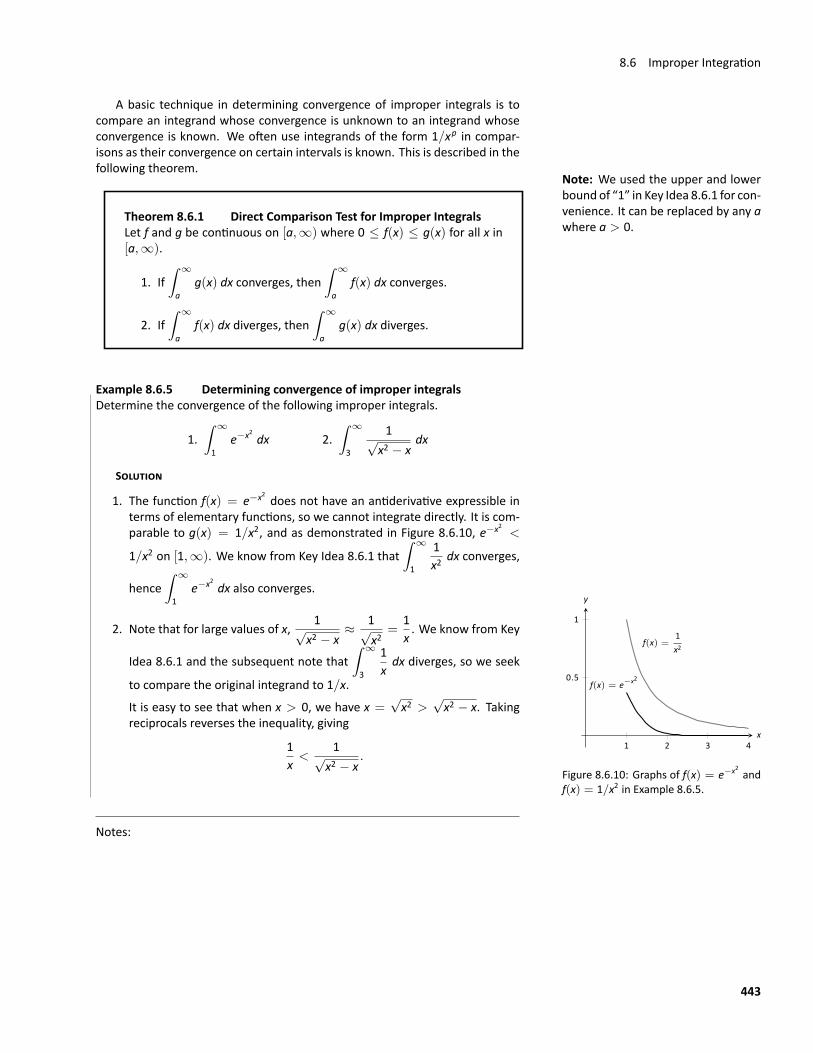
8.6 Improper Integration
A basic technique in determining convergence of improper integrals is tocompare an integrand whose convergence is unknown to an integrand whoseconvergence is known. We often use integrands of the form 1/xp in compar‐isons as their convergence on certain intervals is known. This is described in thefollowing theorem.
Note: We used the upper and lowerbound of “1” in Key Idea 8.6.1 for con‐venience. It can be replaced by any awhere a > 0.
Theorem 8.6.1 Direct Comparison Test for Improper IntegralsLet f and g be continuous on [a,∞) where 0 ≤ f(x) ≤ g(x) for all x in[a,∞).
1. If∫ ∞
ag(x) dx converges, then
∫ ∞
af(x) dx converges.
2. If∫ ∞
af(x) dx diverges, then
∫ ∞
ag(x) dx diverges.
Example 8.6.5 Determining convergence of improper integralsDetermine the convergence of the following improper integrals.
1.∫ ∞
1e−x2 dx 2.
∫ ∞
3
1√x2 − x
dx
SOLUTION
1. The function f(x) = e−x2 does not have an antiderivative expressible interms of elementary functions, so we cannot integrate directly. It is com‐parable to g(x) = 1/x2, and as demonstrated in Figure 8.6.10, e−x2 <
1/x2 on [1,∞). We know from Key Idea 8.6.1 that∫ ∞
1
1x2
dx converges,
hence∫ ∞
1e−x2 dx also converges.
f(x) = e−x2
f(x) =1x2
1 2 3 4
0.5
1
x
y
Figure 8.6.10: Graphs of f(x) = e−x2 andf(x) = 1/x2 in Example 8.6.5.
2. Note that for large values of x,1√
x2 − x≈ 1√
x2=
1x. We know from Key
Idea 8.6.1 and the subsequent note that∫ ∞
3
1xdx diverges, so we seek
to compare the original integrand to 1/x.
It is easy to see that when x > 0, we have x =√x2 >
√x2 − x. Taking
reciprocals reverses the inequality, giving
1x<
1√x2 − x
.
Notes:
443
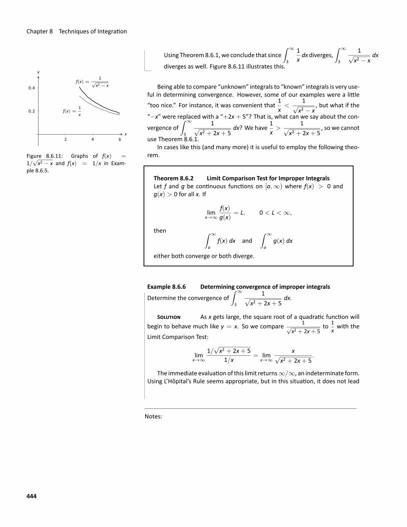
Chapter 8 Techniques of Integration
Using Theorem8.6.1, we conclude that since∫ ∞
3
1xdxdiverges,
∫ ∞
3
1√x2 − x
dx
diverges as well. Figure 8.6.11 illustrates this.
f(x) =1
√x2 − x
f(x) =1x
2 4 6
0.2
0.4
x
y
Figure 8.6.11: Graphs of f(x) =1/
√x2 − x and f(x) = 1/x in Exam‐
ple 8.6.5.
Being able to compare “unknown” integrals to “known” integrals is very use‐ful in determining convergence. However, some of our examples were a little“too nice.” For instance, it was convenient that
1x<
1√x2 − x
, but what if the
“−x” were replaced with a “+2x+ 5”? That is, what can we say about the con‐
vergence of∫ ∞
3
1√x2 + 2x+ 5
dx? We have1x>
1√x2 + 2x+ 5
, so we cannot
use Theorem 8.6.1.In cases like this (and many more) it is useful to employ the following theo‐
rem.
Theorem 8.6.2 Limit Comparison Test for Improper IntegralsLet f and g be continuous functions on [a,∞) where f(x) > 0 andg(x) > 0 for all x. If
limx→∞
f(x)g(x)
= L, 0 < L < ∞,
then ∫ ∞
af(x) dx and
∫ ∞
ag(x) dx
either both converge or both diverge.
Example 8.6.6 Determining convergence of improper integrals
Determine the convergence of∫ ∞
3
1√x2 + 2x+ 5
dx.
SOLUTION As x gets large, the square root of a quadratic function willbegin to behave much like y = x. So we compare 1√
x2 + 2x+ 5to 1
xwith the
Limit Comparison Test:
limx→∞
1/√x2 + 2x+ 51/x
= limx→∞
x√x2 + 2x+ 5
.
The immediate evaluationof this limit returns∞/∞, an indeterminate form.Using L’Hôpital’s Rule seems appropriate, but in this situation, it does not lead
Notes:
444
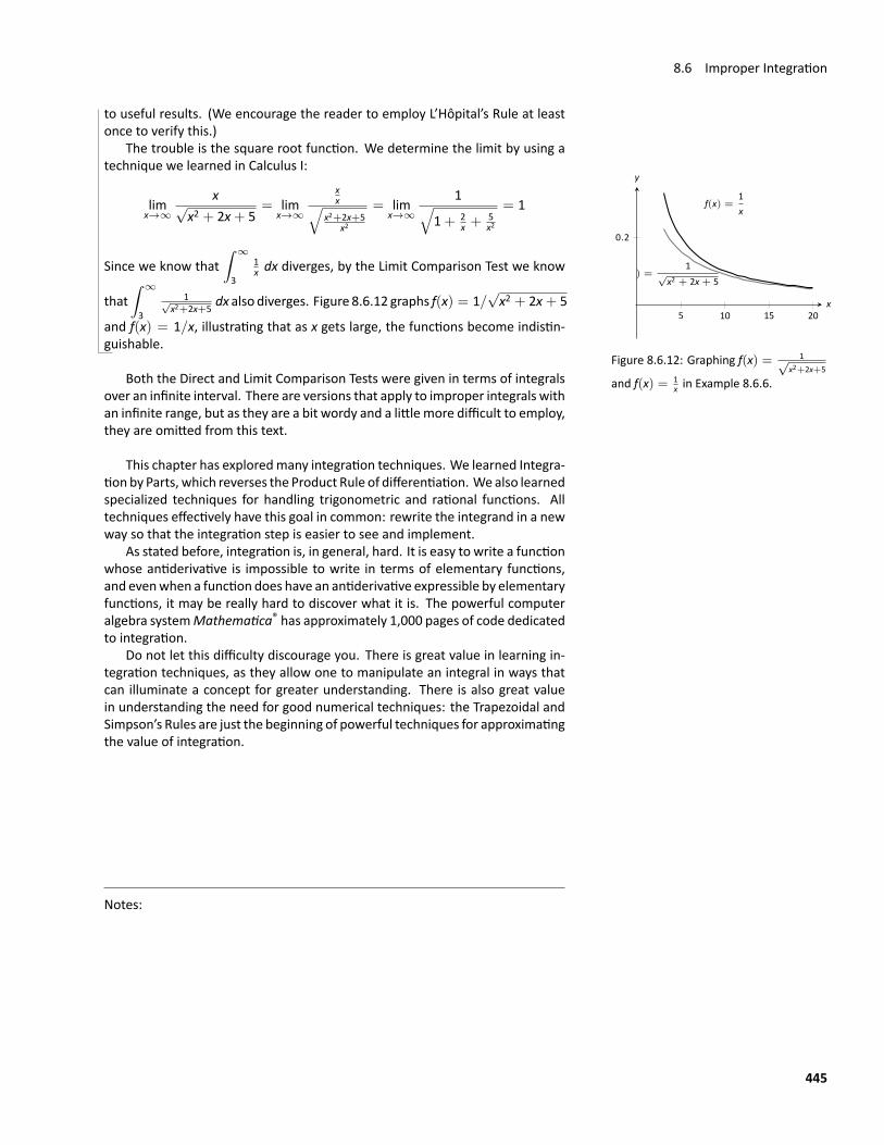
8.6 Improper Integration
to useful results. (We encourage the reader to employ L’Hôpital’s Rule at leastonce to verify this.)
The trouble is the square root function. We determine the limit by using atechnique we learned in Calculus I:
f(x) =1x
f(x) =1
√x2 + 2x + 5
5 10 15 20
0.2
x
y
Figure 8.6.12: Graphing f(x) = 1√x2+2x+5
and f(x) = 1x in Example 8.6.6.
limx→∞
x√x2 + 2x+ 5
= limx→∞
xx√
x2+2x+5x2
= limx→∞
1√1+ 2
x +5x2
= 1
Since we know that∫ ∞
3
1x dx diverges, by the Limit Comparison Test we know
that∫ ∞
3
1√x2+2x+5 dx also diverges. Figure 8.6.12 graphs f(x) = 1/
√x2 + 2x+ 5
and f(x) = 1/x, illustrating that as x gets large, the functions become indistin‐guishable.
Both the Direct and Limit Comparison Tests were given in terms of integralsover an infinite interval. There are versions that apply to improper integrals withan infinite range, but as they are a bit wordy and a little more difficult to employ,they are omitted from this text.
This chapter has exploredmany integration techniques. We learned Integra‐tion by Parts, which reverses the Product Rule of differentiation. Wealso learnedspecialized techniques for handling trigonometric and rational functions. Alltechniques effectively have this goal in common: rewrite the integrand in a newway so that the integration step is easier to see and implement.
As stated before, integration is, in general, hard. It is easy to write a functionwhose antiderivative is impossible to write in terms of elementary functions,and evenwhen a function does have an antiderivative expressible by elementaryfunctions, it may be really hard to discover what it is. The powerful computeralgebra systemMathematica® has approximately 1,000 pages of code dedicatedto integration.
Do not let this difficulty discourage you. There is great value in learning in‐tegration techniques, as they allow one to manipulate an integral in ways thatcan illuminate a concept for greater understanding. There is also great valuein understanding the need for good numerical techniques: the Trapezoidal andSimpson’s Rules are just the beginning of powerful techniques for approximatingthe value of integration.
Notes:
445
Exercises 8.6Terms and Concepts1. The definite integral was defined with what two stipula‐
tions?
2. If limb→∞
∫ b
0f(x) dx exists, then the integral
∫ ∞
0f(x) dx is
said to .
3. If∫ ∞
1f(x) dx = 10, and 0 ≤ g(x) ≤ f(x) for all x, then we
know that∫ ∞
1g(x) dx .
4. For what values of p will∫ ∞
1
1xp
dx converge?
5. For what values of p will∫ ∞
10
1xp
dx converge?
6. For what values of p will∫ 1
0
1xp
dx converge?
ProblemsIn Exercises 7–36, evaluate the given improper integral.
7.∫ ∞
0e5−2x dx
8.∫ ∞
1
1x3
dx
9.∫ ∞
1x−4 dx
10.∫ ∞
−∞
1x2 + 9
dx
11.∫ 0
−∞2x dx
12.∫ 0
−∞
(12
)x
dx
13.∫ ∞
−∞
xx2 + 1
dx
14.∫ ∞
−∞
xx2 + 4
dx
15.∫ ∞
2
1(x− 1)2
dx
16.∫ 2
1
1(x− 1)2
dx
17.∫ ∞
2
1x− 1
dx
18.∫ 2
1
1x− 1
dx
19.∫ 3
0
1xdx
20.∫ 1
−1
1xdx
21.∫ 5
2
dx√x− 2
22.∫ 9
1
dx3√9− x
23.∫ 3
1
1x− 2
dx
24.∫ π
0sec2 x dx
25.∫ π
2
0sec x dx
26.∫ 1
−2
1√|x|
dx
27.∫ ∞
0xe−x dx
28.∫ ∞
0xe−x2 dx
29.∫ ∞
−∞xe−x2 dx
30.∫ ∞
−∞
1ex + e−x dx
31.∫ 1
0x ln x dx
32.∫ ∞
1
ln xx
dx
33.∫ 1
0ln x dx
34.∫ ∞
1
ln xx2
dx
35.∫ ∞
1
ln x√xdx
36.∫ ∞
0e−x sin x dx
In Exercises 37–46, use the Direct Comparison Test or the LimitComparison Test to determine whether the given definite inte‐gral converges or diverges. Clearly statewhat test is being usedand what function the integrand is being compared to.
37.∫ ∞
10
3√3x2 + 2x− 5
dx
38.∫ ∞
2
4√7x3 − x
dx
39.∫ ∞
0
√x+ 3√
x3 − x2 + x+ 1dx
40.∫ ∞
1e−x ln x dx
41.∫ ∞
5e−x2+3x+1 dx
42.∫ ∞
0
√x
exdx
43.∫ ∞
2
1x2 + sin x
dx
44.∫ ∞
0
xx2 + cos x
dx
45.∫ ∞
0
1x+ ex
dx
46.∫ ∞
0
1ex − x
dx
446
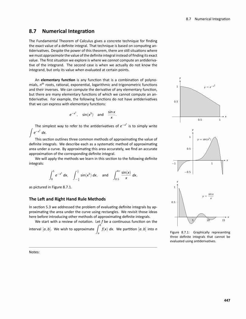
8.7 Numerical Integration
8.7 Numerical IntegrationThe Fundamental Theorem of Calculus gives a concrete technique for findingthe exact value of a definite integral. That technique is based on computing an‐tiderivatives. Despite the power of this theorem, there are still situations wherewemustapproximate the value of the definite integral instead of finding its exactvalue. The first situation we explore is where we cannot compute an antideriva‐tive of the integrand. The second case is when we actually do not know theintegrand, but only its value when evaluated at certain points.
An elementary function is any function that is a combination of polyno‐mials, nth roots, rational, exponential, logarithmic and trigonometric functionsand their inverses. We can compute the derivative of any elementary function,but there are many elementary functions of which we cannot compute an an‐tiderivative. For example, the following functions do not have antiderivativesthat we can express with elementary functions:
e−x2 , sin(x3) andsin xx
.
The simplest way to refer to the antiderivatives of e−x2 is to simply write∫e−x2 dx.
y = e−x2
0.5 1
0.5
1
x
y
y = sin(x3)
−1 1
−0.5
0.5
1
x
y
y =sin xx
5 10 15
0.5
1
x
y
Figure 8.7.1: Graphically representingthree definite integrals that cannot beevaluated using antiderivatives.
This section outlines three common methods of approximating the value ofdefinite integrals. We describe each as a systematic method of approximatingarea under a curve. By approximating this area accurately, we find an accurateapproximation of the corresponding definite integral.
We will apply the methods we learn in this section to the following definiteintegrals: ∫ 1
0e−x2 dx,
∫ π2
− π4
sin(x3) dx, and∫ 4π
0.5
sin(x)x
dx,
as pictured in Figure 8.7.1.
The Left and Right Hand Rule MethodsIn section 5.3 we addressed the problem of evaluating definite integrals by ap‐proximating the area under the curve using rectangles. We revisit those ideashere before introducing other methods of approximating definite integrals.
We start with a review of notation. Let f be a continuous function on the
interval [a, b]. We wish to approximate∫ b
af(x) dx. We partition [a, b] into n
Notes:
447
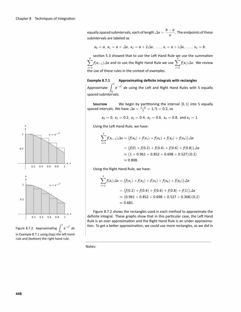
Chapter 8 Techniques of Integration
equally spaced subintervals, each of length∆x =b− an
. The endpoints of thesesubintervals are labeled as
x0 = a, x1 = a+∆x, x2 = a+ 2∆x, . . . , xi = a+ i∆x, . . . , xn = b.
section 5.3 showed that to use the Left Hand Rule we use the summationn∑
i=1
f(xi−1)∆x and to use the Right Hand Rule we usen∑
i=1
f(xi)∆x. We review
the use of these rules in the context of examples.
Example 8.7.1 Approximating definite integrals with rectangles
Approximate∫ 1
0e−x2 dx using the Left and Right Hand Rules with 5 equally
spaced subintervals.
SOLUTION We begin by partitioning the interval [0, 1] into 5 equallyspaced intervals. We have∆x = 1−0
5 = 1/5 = 0.2, so
x0 = 0, x1 = 0.2, x2 = 0.4, x3 = 0.6, x4 = 0.8, and x5 = 1.
y = e−x2
0.2 0.4 0.6 0.8 1
0.5
1
x
y
y = e−x2
0.2 0.4 0.6 0.8 1
0.5
1
x
y
Figure 8.7.2: Approximating∫ 1
0e−x2 dx
in Example 8.7.1 using (top) the left handrule and (bottom) the right hand rule.
Using the Left Hand Rule, we have:
n∑i=1
f(xi−1)∆x =(f(x0) + f(x1) + f(x2) + f(x3) + f(x4)
)∆x
=(f(0) + f(0.2) + f(0.4) + f(0.6) + f(0.8)
)∆x
≈(1+ 0.961+ 0.852+ 0.698+ 0.527)(0.2)
≈ 0.808.
Using the Right Hand Rule, we have:
n∑i=1
f(xi)∆x =(f(x1) + f(x2) + f(x3) + f(x4) + f(x5)
)∆x
=(f(0.2) + f(0.4) + f(0.6) + f(0.8) + f(1)
)∆x
≈(0.961+ 0.852+ 0.698+ 0.527+ 0.368)(0.2)
≈ 0.681.
Figure 8.7.2 shows the rectangles used in each method to approximate thedefinite integral. These graphs show that in this particular case, the Left HandRule is an over approximation and the Right Hand Rule is an under approxima‐tion. To get a better approximation, we could use more rectangles, as we did in
Notes:
448
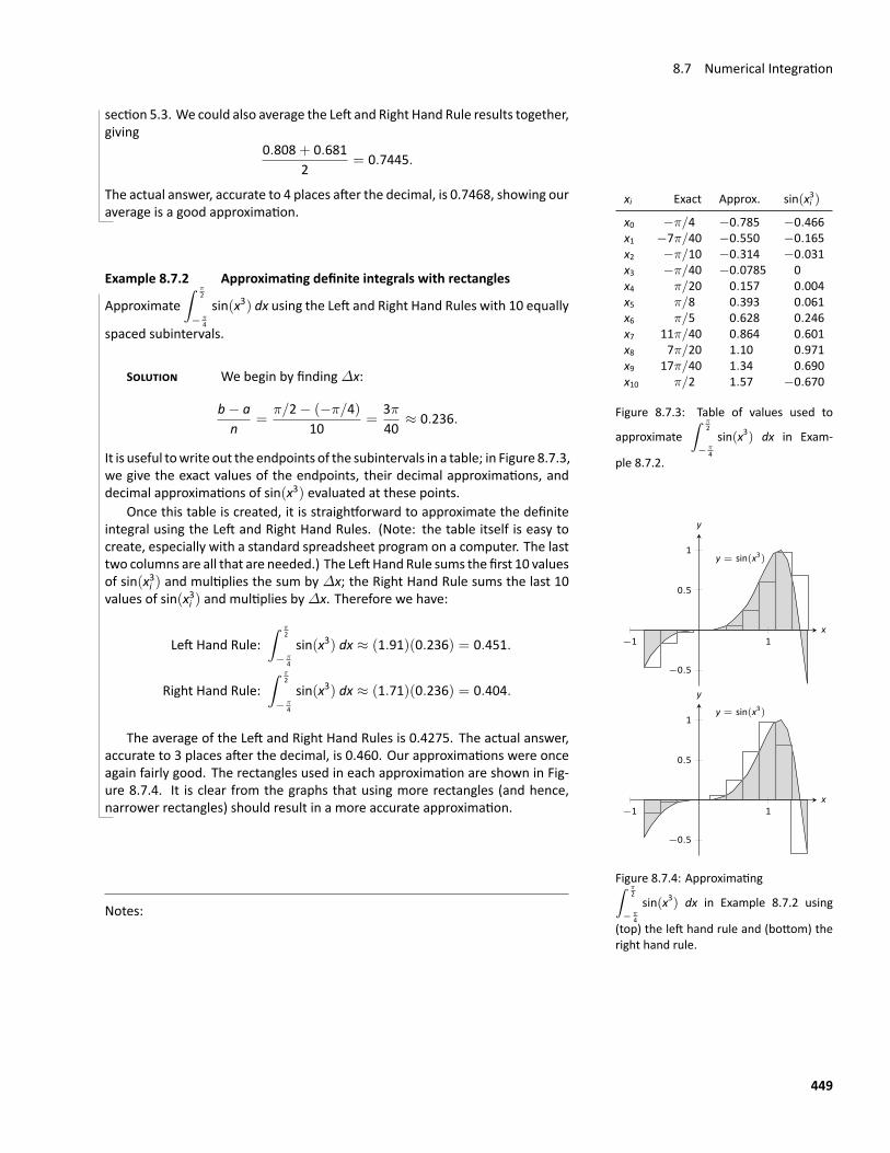
8.7 Numerical Integration
section 5.3. We could also average the Left and Right Hand Rule results together,giving
0.808+ 0.6812
= 0.7445.
The actual answer, accurate to 4 places after the decimal, is 0.7468, showing ouraverage is a good approximation.
xi Exact Approx. sin(x3i )
x0 −π/4 −0.785 −0.466x1 −7π/40 −0.550 −0.165x2 −π/10 −0.314 −0.031x3 −π/40 −0.0785 0x4 π/20 0.157 0.004x5 π/8 0.393 0.061x6 π/5 0.628 0.246x7 11π/40 0.864 0.601x8 7π/20 1.10 0.971x9 17π/40 1.34 0.690x10 π/2 1.57 −0.670
Figure 8.7.3: Table of values used to
approximate∫ π
2
− π4
sin(x3) dx in Exam‐
ple 8.7.2.
Example 8.7.2 Approximating definite integrals with rectangles
Approximate∫ π
2
− π4
sin(x3) dx using the Left and Right Hand Rules with 10 equally
spaced subintervals.
SOLUTION We begin by finding∆x:
b− an
=π/2− (−π/4)
10=
3π40
≈ 0.236.
It is useful towrite out the endpoints of the subintervals in a table; in Figure 8.7.3,we give the exact values of the endpoints, their decimal approximations, anddecimal approximations of sin(x3) evaluated at these points.
y = sin(x3)
−1 1
−0.5
0.5
1
x
y
y = sin(x3)
−1 1
−0.5
0.5
1
x
y
Figure 8.7.4: Approximating∫ π2
− π4
sin(x3) dx in Example 8.7.2 using
(top) the left hand rule and (bottom) theright hand rule.
Once this table is created, it is straightforward to approximate the definiteintegral using the Left and Right Hand Rules. (Note: the table itself is easy tocreate, especially with a standard spreadsheet program on a computer. The lasttwo columns are all that are needed.) The LeftHand Rule sums the first 10 valuesof sin(x3i ) and multiplies the sum by ∆x; the Right Hand Rule sums the last 10values of sin(x3i ) and multiplies by∆x. Therefore we have:
Left Hand Rule:∫ π
2
− π4
sin(x3) dx ≈ (1.91)(0.236) = 0.451.
Right Hand Rule:∫ π
2
− π4
sin(x3) dx ≈ (1.71)(0.236) = 0.404.
The average of the Left and Right Hand Rules is 0.4275. The actual answer,accurate to 3 places after the decimal, is 0.460. Our approximations were onceagain fairly good. The rectangles used in each approximation are shown in Fig‐ure 8.7.4. It is clear from the graphs that using more rectangles (and hence,narrower rectangles) should result in a more accurate approximation.
Notes:
449
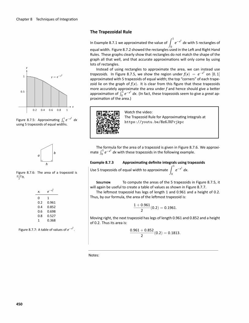
Chapter 8 Techniques of Integration
The Trapezoidal Rule
In Example 8.7.1 we approximated the value of∫ 1
0e−x2 dx with 5 rectangles of
equal width. Figure 8.7.2 showed the rectangles used in the Left and Right HandRules. These graphs clearly show that rectangles do not match the shape of thegraph all that well, and that accurate approximations will only come by usinglots of rectangles.
y = e−x2
0.2 0.4 0.6 0.8 1
0.5
1
x
y
Figure 8.7.5: Approximating∫ 10 e−x2 dx
using 5 trapezoids of equal widths.
Instead of using rectangles to approximate the area, we can instead usetrapezoids. In Figure 8.7.5, we show the region under f(x) = e−x2 on [0, 1]approximated with 5 trapezoids of equal width; the top “corners” of each trape‐zoid lie on the graph of f(x). It is clear from this figure that these trapezoidsmore accurately approximate the area under f and hence should give a betterapproximation of
∫ 10 e−x2 dx. (In fact, these trapezoids seem to give a great ap‐
proximation of the area.)
Watch the video:The Trapezoid Rule for Approximating Integrals athttps://youtu.be/8z6JRFvjkpc
ab
h
Figure 8.7.6: The area of a trapezoid isa+b2 h.
The formula for the area of a trapezoid is given in Figure 8.7.6. We approxi‐mate
∫ 10 e−x2 dx with these trapezoids in the following example.
Example 8.7.3 Approximating definite integrals using trapezoids
Use 5 trapezoids of equal width to approximate∫ 1
0e−x2 dx.
SOLUTION To compute the areas of the 5 trapezoids in Figure 8.7.5, itwill again be useful to create a table of values as shown in Figure 8.7.7.
xi e−x2i
0 10.2 0.9610.4 0.8520.6 0.6980.8 0.5271 0.368
Figure 8.7.7: A table of values of e−x2 .
The leftmost trapezoid has legs of length 1 and 0.961 and a height of 0.2.Thus, by our formula, the area of the leftmost trapezoid is:
1+ 0.9612
(0.2) = 0.1961.
Moving right, the next trapezoid has legs of length 0.961 and 0.852 and a heightof 0.2. Thus its area is:
0.961+ 0.8522
(0.2) = 0.1813.
Notes:
450
8.7 Numerical Integration
The sum of the areas of all 5 trapezoids is:
1+ 0.9612
(0.2) +0.961+ 0.852
2(0.2) +
0.852+ 0.6982
(0.2)
+0.698+ 0.527
2(0.2) +
0.527+ 0.3682
(0.2) = 0.7445.
We approximate∫ 1
0e−x2 dx ≈ 0.7445.
There are many things to observe in this example. Note how each term inthe final summationwasmultiplied by both 1/2 and by∆x = 0.2. We can factorthese coefficients out, leaving a more concise summation as:
12(0.2)
[(1+0.961)+(0.961+0.852)+(0.852+0.698)+(0.698+0.527)+(0.527+0.368)
].
Now notice that all numbers except for the first and the last are added twice.Therefore we can write the summation even more concisely as
0.22
[1+ 2(0.961+ 0.852+ 0.698+ 0.527) + 0.368
].
This is the heart of the Trapezoidal Rule, wherein a definite integral∫ b
af(x)dx
is approximated by using trapezoids of equal widths to approximate the corre‐sponding area under f. Using n equally spaced subintervals with endpoints x0,x1, …, xn, we again have∆x =
b− an
. Thus:
∫ b
af(x) dx ≈
n∑i=1
f(xi−1) + f(xi)2
∆x
=∆x2
n∑i=1
(f(xi−1) + f(xi)
)=
∆x2
[f(x0) + 2
n−1∑i=1
f(xi) + f(xn)
].
Example 8.7.4 Using the Trapezoidal Rule
Revisit Example 8.7.2 and approximate∫ π
2
− π4
sin(x3) dx using the Trapezoidal Rule
and 10 equally spaced subintervals.
Notes:
451
Chapter 8 Techniques of Integration
SOLUTION Werefer back to Figure 8.7.3 for the table of values of sin(x3).Recall that∆x = 3π/40 ≈ 0.236. Thus we have:∫ π
2
− π4
sin(x3) dx
≈ 0.2362
[− 0.466+ 2
(− 0.165+ (−0.031) + · · ·+ 0.69
)+ (−0.67)
]= 0.4275.
Notice how “quickly” the Trapezoidal Rule can be implemented once the ta‐ble of values is created. This is true for all the methods explored in this section;the real work is creating a table of xi and f(xi) values. Once this is completed, ap‐proximating the definite integral is not difficult. Again, using technology is wise.Spreadsheets can make quick work of these computations and make using lotsof subintervals easy.
Also notice the approximations the Trapezoidal Rule gives. It is the averageof the approximations given by the Left and Right Hand Rules! This effectivelyrenders the Left and Right Hand Rules obsolete. They are useful when first learn‐ing about definite integrals, but if a real approximation is needed, one is gener‐ally better off using the Trapezoidal Rule instead of either the Left or Right HandRule.
We will also show that the Trapezoidal Rule makes using the Midpoint Ruleobsolete as well. With much more work, it will turn out that the Midpoint Rulehas only a marginal gain in accuracy. But we will include it in our results for thesake of completeness.
How can we improve on the Trapezoidal Rule, apart from using more andmore trapezoids? The answer is clear once we look back and consider what wehave really done so far. The Left Hand Rule is not really about using rectangles toapproximate area. Instead, it approximates a function f with constant functionson small subintervals and then computes the definite integral of these constantfunctions. The Trapezoidal Rule is really approximating a function fwith a linearfunction on a small subinterval, then computes the definite integral of this linearfunction. In both of these cases the definite integrals are easy to compute ingeometric terms.
So we have a progression: we start by approximating fwith a constant func‐tion and then with a linear function. What is next? A quadratic function. Byapproximating the curve of a function with lots of parabolas, we generally getan even better approximation of the definite integral. We call this process Simp‐son’s Rule, named after Thomas Simpson (1710‐1761), even though others hadused this rule as much as 100 years prior.
Notes:
452
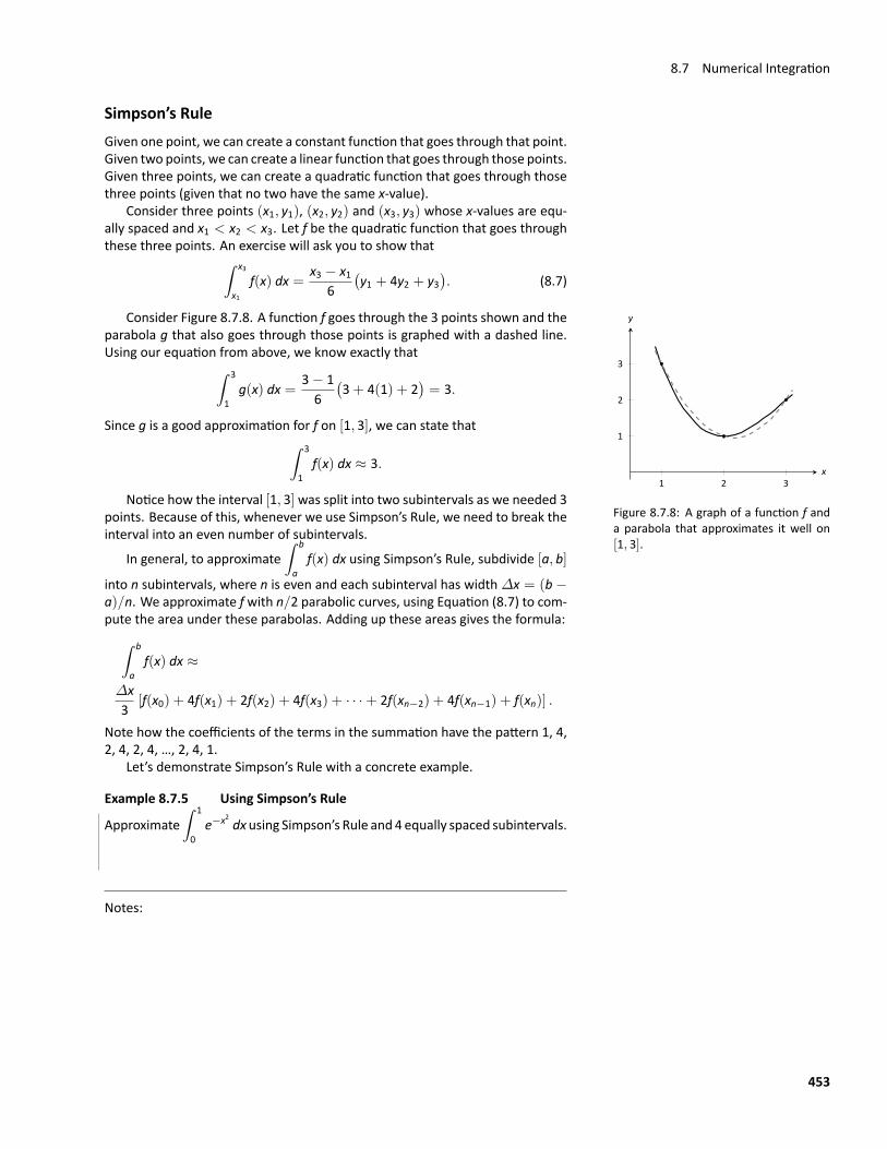
8.7 Numerical Integration
Simpson’s RuleGiven one point, we can create a constant function that goes through that point.Given two points, we can create a linear function that goes through those points.Given three points, we can create a quadratic function that goes through thosethree points (given that no two have the same x‐value).
Consider three points (x1, y1), (x2, y2) and (x3, y3) whose x‐values are equ‐ally spaced and x1 < x2 < x3. Let f be the quadratic function that goes throughthese three points. An exercise will ask you to show that∫ x3
x1f(x) dx =
x3 − x16
(y1 + 4y2 + y3
). (8.7)
1 2 3
1
2
3
x
y
Figure 8.7.8: A graph of a function f anda parabola that approximates it well on[1, 3].
Consider Figure 8.7.8. A function f goes through the 3 points shown and theparabola g that also goes through those points is graphed with a dashed line.Using our equation from above, we know exactly that∫ 3
1g(x) dx =
3− 16(3+ 4(1) + 2
)= 3.
Since g is a good approximation for f on [1, 3], we can state that∫ 3
1f(x) dx ≈ 3.
Notice how the interval [1, 3]was split into two subintervals as we needed 3points. Because of this, whenever we use Simpson’s Rule, we need to break theinterval into an even number of subintervals.
In general, to approximate∫ b
af(x) dx using Simpson’s Rule, subdivide [a, b]
into n subintervals, where n is even and each subinterval has width∆x = (b−a)/n. We approximate fwith n/2 parabolic curves, using Equation (8.7) to com‐pute the area under these parabolas. Adding up these areas gives the formula:∫ b
af(x) dx ≈
∆x3
[f(x0) + 4f(x1) + 2f(x2) + 4f(x3) + · · ·+ 2f(xn−2) + 4f(xn−1) + f(xn)] .
Note how the coefficients of the terms in the summation have the pattern 1, 4,2, 4, 2, 4, …, 2, 4, 1.
Let’s demonstrate Simpson’s Rule with a concrete example.
Example 8.7.5 Using Simpson’s Rule
Approximate∫ 1
0e−x2 dxusing Simpson’s Rule and 4 equally spaced subintervals.
Notes:
453
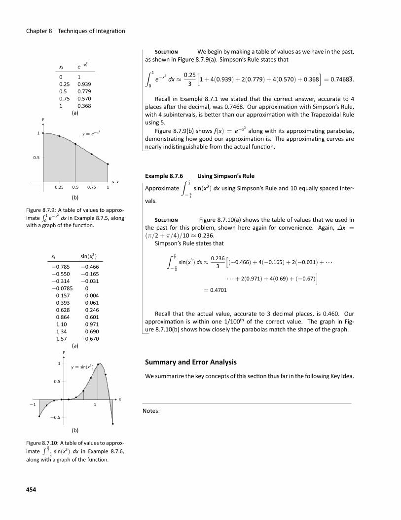
Chapter 8 Techniques of Integration
SOLUTION We begin bymaking a table of values as we have in the past,as shown in Figure 8.7.9(a). Simpson’s Rule states that
xi e−x2i
0 10.25 0.9390.5 0.7790.75 0.5701 0.368
(a)
y = e−x2
0.25 0.5 0.75 1
0.5
1
x
y
(b)
Figure 8.7.9: A table of values to approx‐imate
∫ 10 e−x2 dx in Example 8.7.5, along
with a graph of the function.
∫ 1
0e−x2 dx ≈ 0.25
3
[1+ 4(0.939) + 2(0.779) + 4(0.570) + 0.368
]= 0.74683.
Recall in Example 8.7.1 we stated that the correct answer, accurate to 4places after the decimal, was 0.7468. Our approximation with Simpson’s Rule,with 4 subintervals, is better than our approximation with the Trapezoidal Ruleusing 5.
Figure 8.7.9(b) shows f(x) = e−x2 along with its approximating parabolas,demonstrating how good our approximation is. The approximating curves arenearly indistinguishable from the actual function.
Example 8.7.6 Using Simpson’s Rule
Approximate∫ π
2
− π4
sin(x3) dx using Simpson’s Rule and 10 equally spaced inter‐
vals.
SOLUTION Figure 8.7.10(a) shows the table of values that we used in
xi sin(x3i )
−0.785 −0.466−0.550 −0.165−0.314 −0.031−0.0785 00.157 0.0040.393 0.0610.628 0.2460.864 0.6011.10 0.9711.34 0.6901.57 −0.670
(a)
y = sin(x3)
−1 1
−0.5
0.5
1
x
y
(b)
Figure 8.7.10: A table of values to approx‐imate
∫ π2
− π4sin(x3) dx in Example 8.7.6,
along with a graph of the function.
the past for this problem, shown here again for convenience. Again, ∆x =(π/2+ π/4)/10 ≈ 0.236.
Simpson’s Rule states that∫ π2
− π4
sin(x3) dx ≈ 0.2363
[(−0.466) + 4(−0.165) + 2(−0.031) + · · ·
· · ·+ 2(0.971) + 4(0.69) + (−0.67)]
= 0.4701
Recall that the actual value, accurate to 3 decimal places, is 0.460. Ourapproximation is within one 1/100th of the correct value. The graph in Fig‐ure 8.7.10(b) shows how closely the parabolas match the shape of the graph.
Summary and Error Analysis
We summarize the key concepts of this section thus far in the following Key Idea.
Notes:
454
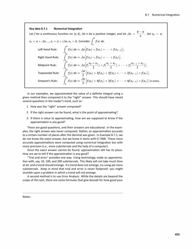
8.7 Numerical Integration
Key Idea 8.7.1 Numerical IntegrationLet f be a continuous function on [a, b], let n be a positive integer, and let ∆x =
b− an
. Set x0 = a,
x1 = a+∆x, …, xi = a+ i∆x, xn = b. Consider∫ b
af(x) dx.
Left Hand Rule:∫ b
af(x) dx ≈ ∆x
[f(x0) + f(x1) + · · ·+ f(xn−1)
].
Right Hand Rule:∫ b
af(x) dx ≈ ∆x
[f(x1) + f(x2) + · · ·+ f(xn)
].
Midpoint Rule:∫ b
af(x) dx ≈ ∆x
[f(x0 + x1
2)+ f(x1 + x2
2)+ · · ·+ f
(xn−1 + xn2
)].
Trapezoidal Rule:∫ b
af(x) dx ≈ ∆x
2
[f(x0) + 2f(x1) + 2f(x2) + · · ·+ 2f(xn−1) + f(xn)
].
Simpson’s Rule:∫ b
af(x) dx ≈ ∆x
3
[f(x0) + 4f(x1) + 2f(x2) + · · ·+ 4f(xn−1) + f(xn)
](n even).
In our examples, we approximated the value of a definite integral using agiven method then compared it to the “right” answer. This should have raisedseveral questions in the reader’s mind, such as:
1. How was the “right” answer computed?
2. If the right answer can be found, what is the point of approximating?
3. If there is value to approximating, how are we supposed to know if theapproximation is any good?
These are good questions, and their answers are educational. In the exam‐ples, the right answer was never computed. Rather, an approximation accurateto a certain number of places after the decimal was given. In Example 8.7.1, wedo not know the exact answer, but we know it starts with 0.7468. These moreaccurate approximations were computed using numerical integration but withmore precision (i.e., more subintervals and the help of a computer).
Since the exact answer cannot be found, approximation still has its place.How are we to tell if the approximation is any good?
“Trial and error” provides one way. Using technology, make an approxima‐tion with, say, 10, 100, and 200 subintervals. This likely will not take much timeat all, and a trend should emerge. If a trend does not emerge, try using yet moresubintervals. Keep in mind that trial and error is never foolproof; you mightstumble upon a problem in which a trend will not emerge.
A second method is to use Error Analysis. While the details are beyond thescope of this text, there are some formulas that give bounds for how good your
Notes:
455
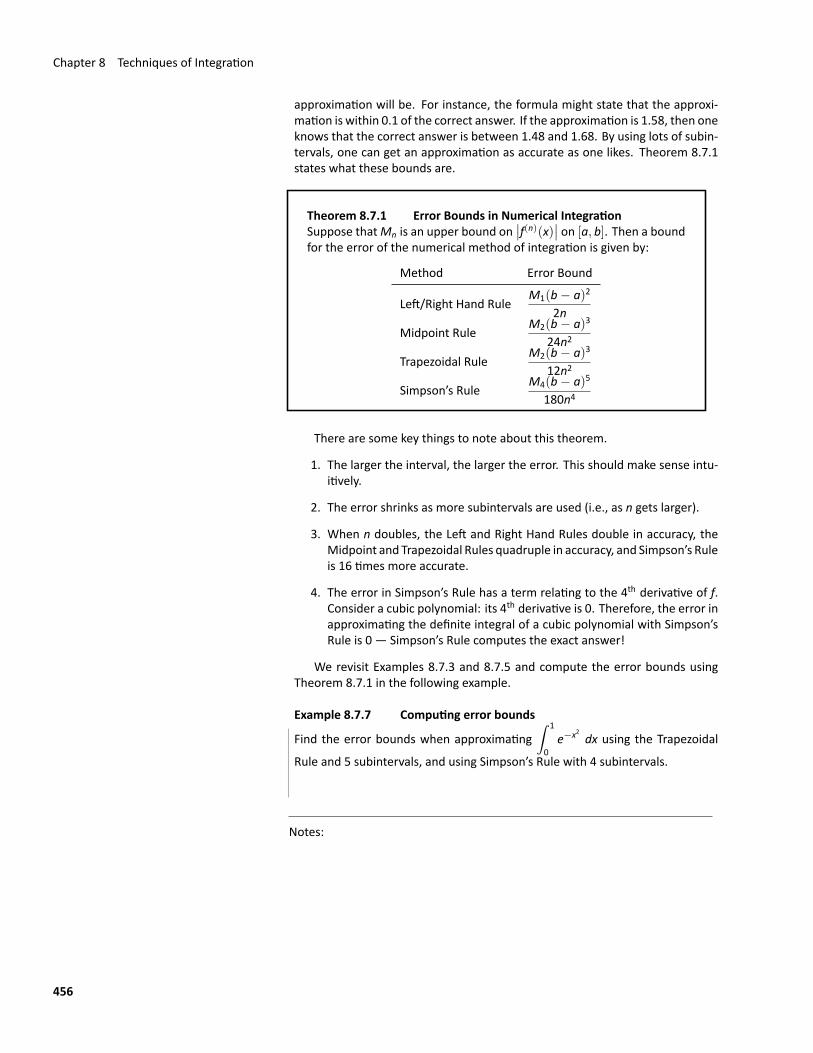
Chapter 8 Techniques of Integration
approximation will be. For instance, the formula might state that the approxi‐mation is within 0.1 of the correct answer. If the approximation is 1.58, then oneknows that the correct answer is between 1.48 and 1.68. By using lots of subin‐tervals, one can get an approximation as accurate as one likes. Theorem 8.7.1states what these bounds are.
Theorem 8.7.1 Error Bounds in Numerical IntegrationSuppose thatMn is an upper bound on
∣∣f(n)(x)∣∣ on [a, b]. Then a boundfor the error of the numerical method of integration is given by:
Method Error Bound
Left/Right Hand RuleM1(b− a)2
2nMidpoint Rule
M2(b− a)3
24n2
Trapezoidal RuleM2(b− a)3
12n2
Simpson’s RuleM4(b− a)5
180n4
There are some key things to note about this theorem.
1. The larger the interval, the larger the error. This should make sense intu‐itively.
2. The error shrinks as more subintervals are used (i.e., as n gets larger).
3. When n doubles, the Left and Right Hand Rules double in accuracy, theMidpoint and Trapezoidal Rules quadruple in accuracy, and Simpson’s Ruleis 16 times more accurate.
4. The error in Simpson’s Rule has a term relating to the 4th derivative of f.Consider a cubic polynomial: its 4th derivative is 0. Therefore, the error inapproximating the definite integral of a cubic polynomial with Simpson’sRule is 0 — Simpson’s Rule computes the exact answer!
We revisit Examples 8.7.3 and 8.7.5 and compute the error bounds usingTheorem 8.7.1 in the following example.
Example 8.7.7 Computing error bounds
Find the error bounds when approximating∫ 1
0e−x2 dx using the Trapezoidal
Rule and 5 subintervals, and using Simpson’s Rule with 4 subintervals.
Notes:
456
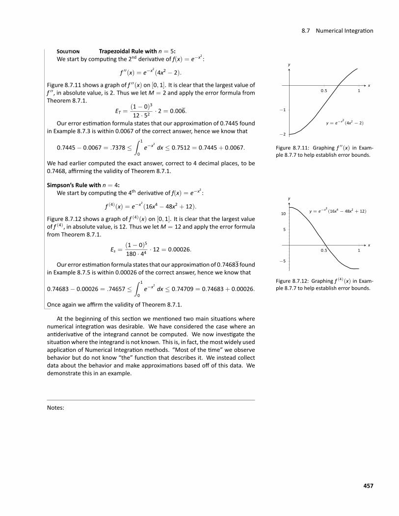
8.7 Numerical Integration
SOLUTION Trapezoidal Rule with n = 5:We start by computing the 2nd derivative of f(x) = e−x2 :
y = e−x2 (4x2 − 2)
0.5 1
−2
−1
x
y
Figure 8.7.11: Graphing f ′′(x) in Exam‐ple 8.7.7 to help establish error bounds.
f ′′(x) = e−x2(4x2 − 2).
Figure 8.7.11 shows a graph of f ′′(x) on [0, 1]. It is clear that the largest value off ′′, in absolute value, is 2. Thus we letM = 2 and apply the error formula fromTheorem 8.7.1.
ET =(1− 0)3
12 · 52· 2 = 0.006.
Our error estimation formula states that our approximation of 0.7445 foundin Example 8.7.3 is within 0.0067 of the correct answer, hence we know that
0.7445− 0.0067 = .7378 ≤∫ 1
0e−x2 dx ≤ 0.7512 = 0.7445+ 0.0067.
We had earlier computed the exact answer, correct to 4 decimal places, to be0.7468, affirming the validity of Theorem 8.7.1.
Simpson’s Rule with n = 4:We start by computing the 4th derivative of f(x) = e−x2 :
y = e−x2 (16x4 − 48x2 + 12)
0.5 1
−5
5
10
x
y
Figure 8.7.12: Graphing f (4)(x) in Exam‐ple 8.7.7 to help establish error bounds.
f (4)(x) = e−x2(16x4 − 48x2 + 12).
Figure 8.7.12 shows a graph of f (4)(x) on [0, 1]. It is clear that the largest valueof f (4), in absolute value, is 12. Thus we letM = 12 and apply the error formulafrom Theorem 8.7.1.
Es =(1− 0)5
180 · 44· 12 = 0.00026.
Our error estimation formula states that our approximationof 0.74683 foundin Example 8.7.5 is within 0.00026 of the correct answer, hence we know that
0.74683− 0.00026 = .74657 ≤∫ 1
0e−x2 dx ≤ 0.74709 = 0.74683+ 0.00026.
Once again we affirm the validity of Theorem 8.7.1.
At the beginning of this section we mentioned two main situations wherenumerical integration was desirable. We have considered the case where anantiderivative of the integrand cannot be computed. We now investigate thesituationwhere the integrand is not known. This is, in fact, themost widely usedapplication of Numerical Integration methods. “Most of the time” we observebehavior but do not know “the” function that describes it. We instead collectdata about the behavior and make approximations based off of this data. Wedemonstrate this in an example.
Notes:
457
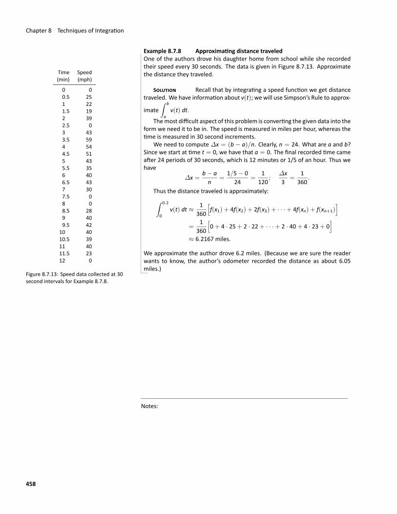
Chapter 8 Techniques of Integration
Example 8.7.8 Approximating distance traveledOne of the authors drove his daughter home from school while she recordedtheir speed every 30 seconds. The data is given in Figure 8.7.13. Approximate
Time Speed(min) (mph)
0 00.5 251 221.5 192 392.5 03 433.5 594 544.5 515 435.5 356 406.5 437 307.5 08 08.5 289 409.5 42
10 4010.5 3911 4011.5 2312 0
Figure 8.7.13: Speed data collected at 30second intervals for Example 8.7.8.
the distance they traveled.
SOLUTION Recall that by integrating a speed function we get distancetraveled. We have information about v(t); we will use Simpson’s Rule to approx‐
imate∫ b
av(t) dt.
Themost difficult aspect of this problem is converting the given data into theform we need it to be in. The speed is measured in miles per hour, whereas thetime is measured in 30 second increments.
We need to compute∆x = (b − a)/n. Clearly, n = 24. What are a and b?Since we start at time t = 0, we have that a = 0. The final recorded time cameafter 24 periods of 30 seconds, which is 12 minutes or 1/5 of an hour. Thus wehave
∆x =b− an
=1/5− 0
24=
1120
;∆x3
=1
360.
Thus the distance traveled is approximately:∫ 0.2
0v(t) dt ≈ 1
360
[f(x1) + 4f(x2) + 2f(x3) + · · ·+ 4f(xn) + f(xn+1)
]=
1360
[0+ 4 · 25+ 2 · 22+ · · ·+ 2 · 40+ 4 · 23+ 0
]≈ 6.2167 miles.
We approximate the author drove 6.2 miles. (Because we are sure the readerwants to know, the author’s odometer recorded the distance as about 6.05miles.)
Notes:
458
Exercises 8.7Terms and Concepts1. T/F: Simpson’s Rule is a method of approximating an‐
tiderivatives.2. What are the twobasic situationswhere approximating the
value of a definite integral is necessary?3. Why are the Left and Right Hand Rules rarely used?4. Why is the Midpoint Rule rarely used?
ProblemsIn Exercises 5–12, a definite integral is given.
(a) Approximate the definite integral with the TrapezoidalRule and n = 4.
(b) Approximate the definite integral with Simpson’s Ruleand n = 4.
(c) Find the exact value of the integral.
5.∫ 1
−1x2 dx
6.∫ 10
05x dx
7.∫ π
0sin x dx
8.∫ 4
0
√x dx
9.∫ 3
0(x3 + 2x2 − 5x+ 7) dx
10.∫ 1
0x4 dx
11.∫ 2π
0cos x dx
12.∫ 3
−3
√9− x2 dx
In Exercises 13–20, approximate the definite integral with theTrapezoidal Rule and Simpson’s Rule, with n = 6.
13.∫ 1
0cos(x2)dx
14.∫ 1
−1ex
2dx
15.∫ 5
0
√x2 + 1 dx
16.∫ π
0x sin x dx
17.∫ π/2
0
√cos x dx
18.∫ 4
1ln x dx
19.∫ 1
−1
1sin x+ 2
dx
20.∫ 6
0
1sin x+ 2
dx
In Exercises 21–24, find n such that the error in approximatingthe given definite integral is less than 0.0001 when using:
(a) the Trapezoidal Rule
(b) Simpson’s Rule
21.∫ π
0sin x dx
22.∫ 4
1
1√xdx
23.∫ π
0cos(x2)dx
24.∫ 5
0x4 dx
In Exercises 25–26, a region is given. Find the area of the re‐gion using Simpson’s Rule:
(a) where the measurements are in centimeters, taken in 1cm increments, and
(b) where the measurements are in hundreds of yards,taken in 100 yd increments.
25. 4.7
6.3
6.9
6.6
5.1
26. 3.6
3.6
4.5 6.6
5.6
27. Let f be the quadratic function that goes through the points(x1, y1), (x1 + ∆x, y2) and (x1 + 2∆x, y3). Show that∫ x1+2∆x
x1f(x)dx = ∆x
3(y1 + 4y2 + y3).
459

9: SEQUENCES AND SERIESThis chapter introduces sequences and series, important mathematical con‐structions that are useful when solving a large variety of mathematical prob‐lems. The content of this chapter is considerably different from the content ofthe chapters before it. While the material we learn here definitely falls underthe scope of “calculus,” we will make very little use of derivatives or integrals.Limits are extremely important, though, especially limits that involve infinity.
One of the problems addressed by this chapter is this: suppose we knowinformation about a function and its derivatives at a point, such as f(1) = 3,f ′(1) = 1, f ′′(1) = −2, f ′′′(1) = 7, and so on. What can I say about f(x) itself?Is there any reasonable approximation of the value of f(2)? The topic of TaylorSeries addresses this problem, and allows us to make excellent approximationsof functions when limited knowledge of the function is available.
9.1 SequencesWe commonly refer to a set of events that occur one after the other as a se‐quence of events. In mathematics, we use the word sequence to refer to anordered set of numbers, i.e., a set of numbers that “occur one after the other.”
For instance, the numbers 2, 4, 6, 8, . . . , form a sequence. The order is im‐portant; the first number is 2, the second is 4, etc. It seems natural to seek a for‐mula that describes a given sequence, and often this can be done. For instance,the sequence above could be described by the function a(n) = 2n, for the val‐ues of n = 1, 2, . . . (it could also be described by n4−10n3+35n2−48n+24, togive one of infinitelymany other options). To find the 10th term in the sequence,we would compute a(10). This leads us to the following, formal definition of asequence.
Notation: We use N to describe theset of natural numbers, that is, the in‐tegers 1, 2, 3, . . .Definition 9.1.1 Sequence
A sequence is a function a(n) whose domain is N. The range of asequence is the set of all distinct values of a(n).
The terms of a sequence are the values a(1), a(2), . . . , which areusually denoted with subscripts as a1, a2, . . . .
A sequence a(n) is often denoted as {an}.
Notes:
461
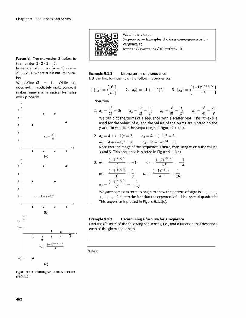
Chapter 9 Sequences and Series
Watch the video:Sequences — Examples showing convergence or di‐vergence athttps://youtu.be/9K1xx6wfN-U
Factorial: The expression 3! refers tothe number 3 · 2 · 1 = 6.In general, n! = n · (n − 1) · (n −2) · · · 2 · 1, where n is a natural num‐ber.We define 0! = 1. While thisdoes not immediately make sense, itmakes many mathematical formulaswork properly.
an =3n
n!
1 2 3 4
1
2
3
4
5
n
y
(a)
an = 4 + (−1)n
1 2 3 4
1
2
3
4
5
n
y
(b)
an =(−1)n(n+1)/2
n2
1 2 3 4 5
−1
1/2
1/4
n
y
(c)
Figure 9.1.1: Plotting sequences in Exam‐ple 9.1.1.
Example 9.1.1 Listing terms of a sequenceList the first four terms of the following sequences.
1. {an} =
{3n
n!
}2. {an} = {4+ (−1)n} 3. {an} =
{(−1)n(n+1)/2
n2
}SOLUTION
1. a1 =31
1!= 3; a2 =
32
2!=
92; a3 =
33
3!=
92; a4 =
34
4!=
278
We can plot the terms of a sequence with a scatter plot. The “x”‐axis isused for the values of n, and the values of the terms are plotted on they‐axis. To visualize this sequence, see Figure 9.1.1(a).
2. a1 = 4+ (−1)1 = 3; a2 = 4+ (−1)2 = 5;a3 = 4+ (−1)3 = 3; a4 = 4+ (−1)4 = 5.Note that the range of this sequence is finite, consisting of only the values3 and 5. This sequence is plotted in Figure 9.1.1(b).
3. a1 =(−1)1(2)/2
12= −1; a2 =
(−1)2(3)/2
22= −1
4
a3 =(−1)3(4)/2
32=
19
a4 =(−1)4(5)/2
42=
116
;
a5 =(−1)5(6)/2
52= − 1
25.
We gave one extra term to begin to show the pattern of signs is “−,−,+,+,−,−, …”, due to the fact that the exponent of−1 is a special quadratic.This sequence is plotted in Figure 9.1.1(c).
Example 9.1.2 Determining a formula for a sequenceFind the nth term of the following sequences, i.e., find a function that describeseach of the given sequences.
Notes:
462
9.1 Sequences
1. 2, 5, 8, 11, 14, . . .
2. 2,−5, 10,−17, 26,−37, . . .
3. 1, 1, 2, 6, 24, 120, 720, . . .
4.52,52,158,54,2532
, . . .
SOLUTION We should first note that there is never exactly one functionthat describes a finite set of numbers as a sequence. There are many sequencesthat start with 2, then 5, as our first example does. We are looking for a simpleformula that describes the terms given, knowing there is possiblymore than oneanswer.
1. Note how each term is 3 more than the previous one. This implies a linearfunction would be appropriate: a(n) = an = 3n+b for some appropriatevalue of b. As we want a1 = 2, we set b = −1. Thus an = 3n− 1.
2. First notice how the sign changes from term to term. This is most com‐monly accomplished bymultiplying the terms by either (−1)n or (−1)n+1.Using (−1)n multiplies the odd terms by (−1); using (−1)n+1 multipliesthe even terms by (−1). As this sequence has negative even terms, wewill multiply by (−1)n+1.After this, we might feel a bit stuck as to how to proceed. At this point,we are just looking for a pattern of some sort: what do the numbers 2, 5,10, 17, etc., have in common? There are many correct answers, but theone that we’ll use here is that each is one more than a perfect square.That is, 2 = 12 + 1, 5 = 22 + 1, 10 = 32 + 1, etc. Thus our formula isan = (−1)n+1(n2 + 1).
3. One who is familiar with the factorial function will readily recognize thesenumbers. They are 0!, 1!, 2!, 3!, etc. Since our sequences start with n = 1,we cannot write an = n!, for this misses the 0! term. Instead, we shift by1, and write an = (n− 1)!.
4. This one may appear difficult, especially as the first two terms are thesame, but a little “sleuthing” will help. Notice how the terms in the nu‐merator are always multiples of 5, and the terms in the denominator arealways powers of 2. Does something as simple as an = 5n
2n work?When n = 1, we see that we indeed get 5/2 as desired. When n = 2,we get 10/4 = 5/2. Further checking shows that this formula indeedmatches the other terms of the sequence.
A common mathematical endeavor is to create a new mathematical object(for instance, a sequence) and then apply previously knownmathematics to thenew object. We do so here. The fundamental concept of calculus is the limit, sowe will investigate what it means to find the limit of a sequence.
Notes:
463
Chapter 9 Sequences and Series
Definition 9.1.2 Limit of a Sequence, Convergent, DivergentLet {an} be a sequence and let L be a real number. Given any ε > 0,if an m can be found such that |an − L| < ε for all n > m, then we saythe limit of {an}, as n approaches infinity, is L, denoted
limn→∞
an = L.
If limn→∞
an exists, we say the sequence converges; otherwise, the se‐quence diverges.
This definition states, informally, that if the limit of a sequence is L, then ifyou go far enough out along the sequence, all subsequent terms will be reallyclose to L. Of course, the terms “far enough” and “really close” are subjectiveterms, but hopefully the intent is clear.
This definition is reminiscent of the ε‐δ proofs of chapter 1. In that chapterwe developed other tools to evaluate limits apart from the formal definition; wedo so here as well.
Theorem 9.1.1 Limit of a SequenceLet {an} be a sequence and let f(x) be a function whose domaincontains the positive real numbers where f(n) = an for all n in N.
If limx→∞
f(x) = L, then limn→∞
an = L.
Theorem 9.1.1 allows us, in certain cases, to apply the tools developed inchapter 1 to limits of sequences. Note two things not stated by the theorem:
1. If limx→∞
f(x) does not exist, we cannot conclude that limn→∞
an does not exist.It may, or may not, exist. For instance, we can define a sequence {an} ={cos(2πn)}. Let f(x) = cos(2πx). Since the cosine function oscillatesover the real numbers, the limit lim
x→∞f(x) does not exist.
However, for every positive integer n, cos(2πn) = 1, so limn→∞
an = 1.
2. If we cannot find a function f(x) whose domain contains the positive realnumbers where f(n) = an for all n inN, we cannot conclude lim
n→∞an does
not exist. It may, or may not, exist.
Notes:
464
9.1 Sequences
Example 9.1.3 Determining convergence/divergence of a sequenceDetermine the convergence or divergence of the following sequences.
an =3n2 − 2n + 1n2 − 1000
20 40 60 80 100
−10
−5
5
10
n
y
(a)
20 40 60 80 100
−1
−0.5
0.5
1
n
yan = cos n
(b)
an =(−1)n
n
5 10 15 20
−1
−0.5
0.5
1
n
y
(c)
Figure 9.1.2: Scatter plots of the se‐quences in Example 9.1.3.
1. {an} =
{3n2 − 2n+ 1n2 − 1000
}2. {an} = {cos n} 3. {an} =
{(−1)n
n
}SOLUTION
1. Using Key Idea 1.5.2, we can state that limx→∞
3x2 − 2x+ 1x2 − 1000
= 3. (We couldhave also directly applied L’Hôpital’s Rule.) Thus the sequence {an} con‐verges, and its limit is 3. A scatter plot of every 5 values of an is given inFigure 9.1.2 (a). The values of an vary widely near n = 30, ranging fromabout−73 to 125, but as n grows, the values approach 3.
2. The limit limx→∞
cos x does not exist, as cos x oscillates (and takes on ev‐ery value in [−1, 1] infinitely many times). Thus we cannot apply Theo‐rem 9.1.1.The fact that the cosine function oscillates strongly hints that cos n, whenn is restricted toN, will also oscillate. Figure 9.1.2 (b), where the sequenceis plotted, shows that this is true. Because only discrete values of cosineare plotted, it does not bear strong resemblance to the familiar cosinewave.Based on the graph, we suspect that lim
n→∞an does not exist, but we have
not decisively proven it yet.
3. We cannot actually apply Theorem 9.1.1 here, as the function f(x) =
(−1)x/x is not well defined. (What does (−1)√2 mean? In actuality, there
is an answer, but it involves complex analysis, beyond the scope of thistext.) So for now we say that we cannot determine the limit. (But we willbe able to very soon.) By looking at the plot in Figure 9.1.2 (c), we wouldlike to conclude that the sequence converges to 0. That is true, but at thispoint we are unable to decisively say so.
It seems that {(−1)n/n} converges to 0 but we lack the formal tool to proveit. The following theorem gives us that tool.
Theorem 9.1.2 Absolute Value TheoremLet {an} be a sequence. If lim
n→∞|an| = 0, then lim
n→∞an = 0
Notes:
465
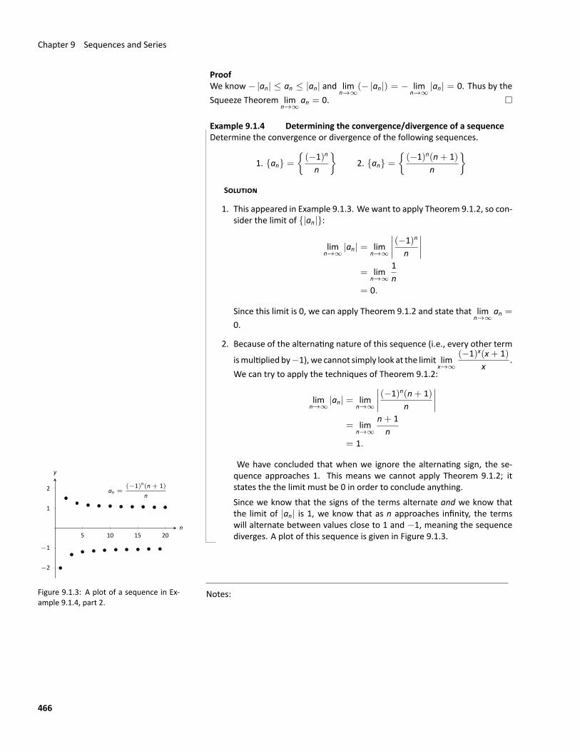
Chapter 9 Sequences and Series
ProofWe know − |an| ≤ an ≤ |an| and lim
n→∞(− |an|) = − lim
n→∞|an| = 0. Thus by the
Squeeze Theorem limn→∞
an = 0. □
Example 9.1.4 Determining the convergence/divergence of a sequenceDetermine the convergence or divergence of the following sequences.
1. {an} =
{(−1)n
n
}2. {an} =
{(−1)n(n+ 1)
n
}SOLUTION
1. This appeared in Example 9.1.3. We want to apply Theorem 9.1.2, so con‐sider the limit of {|an|}:
limn→∞
|an| = limn→∞
∣∣∣∣ (−1)n
n
∣∣∣∣= lim
n→∞
1n
= 0.
Since this limit is 0, we can apply Theorem 9.1.2 and state that limn→∞
an =0.
2. Because of the alternating nature of this sequence (i.e., every other term
ismultiplied by−1), we cannot simply look at the limit limx→∞
(−1)x(x+ 1)x
.We can try to apply the techniques of Theorem 9.1.2:
limn→∞
|an| = limn→∞
∣∣∣∣ (−1)n(n+ 1)n
∣∣∣∣= lim
n→∞
n+ 1n
= 1.
We have concluded that when we ignore the alternating sign, the se‐
an =(−1)n(n + 1)
n
5 10 15 20
−1
−2
1
2
n
y
Figure 9.1.3: A plot of a sequence in Ex‐ample 9.1.4, part 2.
quence approaches 1. This means we cannot apply Theorem 9.1.2; itstates the the limit must be 0 in order to conclude anything.Since we know that the signs of the terms alternate and we know thatthe limit of |an| is 1, we know that as n approaches infinity, the termswill alternate between values close to 1 and −1, meaning the sequencediverges. A plot of this sequence is given in Figure 9.1.3.
Notes:
466
9.1 Sequences
We continue our study of the limits of sequences by considering some of theproperties of these limits.
Theorem 9.1.3 Properties of the Limits of SequencesLet {an} and {bn} be sequences such that lim
n→∞an = L and lim
n→∞bn = K,
where L and K are real numbers, and let c be a real number.
1. limn→∞
(an ± bn) = L± K
2. limn→∞
(an · bn) = L · K
3. limn→∞
(an/bn) = L/K, K ̸= 0
4. limn→∞
(c · an) = c · L
Example 9.1.5 Applying properties of limits of sequencesLet the following limits be given:
• limn→∞
an = 0;
• limn→∞
bn = e; and
• limn→∞
cn = 5.
Evaluate the following limits.
1. limn→∞
(an + bn) 2. limn→∞
(bn · cn) 3. limn→∞
(1000 · an)
SOLUTION We will use Theorem 9.1.3 to answer each of these.
1. Since limn→∞
an = 0 and limn→∞
bn = e, we conclude that limn→∞
(an + bn) =
0+ e = e. So even though we are adding something to each term of thesequence bn, we are adding something so small that the final limit is thesame as before.
2. Since limn→∞
bn = e and limn→∞
cn = 5, we conclude that limn→∞
(bn · cn) =
e · 5 = 5e.
3. Since limn→∞
an = 0, we have limn→∞
1000an = 1000 · 0 = 0. It does notmatter that wemultiply each term by 1000; the sequence still approaches0. (It just takes longer to get close to 0.)
Notes:
467
Chapter 9 Sequences and Series
Definition 9.1.3 Geometric SequenceFor a constant r, the sequence {rn} is known as a geometric sequence.
Theorem 9.1.4 Convergence of Geometric SequencesThe sequence {rn} is convergent if −1 < r ≤ 1 and divergent for allother values of r. Furthermore,
limn→∞
rn =
{0 −1 < r < 11 r = 1
ProofWe can see from Key Idea 7.3.1 and by letting a = r that
limn→∞
rn =
{∞ r > 10 0 < r < 1.
We also know that limx→∞
1n = 1 and limx→∞
0n = 0. If −1 < r < 0, we know0 < |r| < 1 so lim
x→∞|rn| = lim
x→∞|r|n = 0 and thus by Theorem 9.1.2, lim
x→∞rn = 0.
If r ≤ −1, limx→∞
rn does not exist. Therefore, the sequence {rn} is convergent if−1 < r ≤ 1 and divergent for all other values of r. □
There is more to learn about sequences than just their limits. We will alsostudy their range and the relationships terms have with the terms that follow.We start with some definitions describing properties of the range.
Definition 9.1.4 Bounded and Unbounded SequencesA sequence {an} is said to be bounded if there exist real numbers mandM such thatm < an < M for all n in N.
A sequence {an} is said to be unbounded if it is not bounded.
A sequence {an} is said to be bounded above if there exists anM suchthat an < M for all n inN; it is bounded below if there exists anm suchthatm < an for all n in N.
Notes:
468
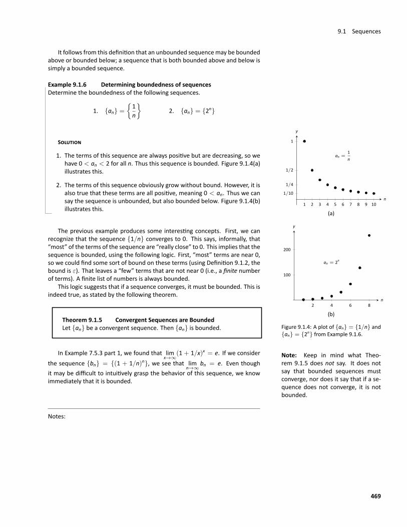
9.1 Sequences
It follows from this definition that an unbounded sequencemay be boundedabove or bounded below; a sequence that is both bounded above and below issimply a bounded sequence.
Example 9.1.6 Determining boundedness of sequencesDetermine the boundedness of the following sequences.
1. {an} =
{1n
}2. {an} = {2n}
an =1n
1 2 3 4 5 6 7 8 9 10
1
1/2
1/4
1/10n
y
(a)
an = 2n
2 4 6 8
100
200
n
y
(b)
Figure 9.1.4: A plot of {an} = {1/n} and{an} = {2n} from Example 9.1.6.
SOLUTION
1. The terms of this sequence are always positive but are decreasing, so wehave 0 < an < 2 for all n. Thus this sequence is bounded. Figure 9.1.4(a)illustrates this.
2. The terms of this sequence obviously grow without bound. However, it isalso true that these terms are all positive, meaning 0 < an. Thus we cansay the sequence is unbounded, but also bounded below. Figure 9.1.4(b)illustrates this.
The previous example produces some interesting concepts. First, we canrecognize that the sequence {1/n} converges to 0. This says, informally, that“most” of the terms of the sequence are “really close” to 0. This implies that thesequence is bounded, using the following logic. First, “most” terms are near 0,so we could find some sort of bound on these terms (using Definition 9.1.2, thebound is ε). That leaves a “few” terms that are not near 0 (i.e., a finite numberof terms). A finite list of numbers is always bounded.
This logic suggests that if a sequence converges, it must be bounded. This isindeed true, as stated by the following theorem.
Theorem 9.1.5 Convergent Sequences are BoundedLet {an} be a convergent sequence. Then {an} is bounded.
Note: Keep in mind what Theo‐rem 9.1.5 does not say. It does notsay that bounded sequences mustconverge, nor does it say that if a se‐quence does not converge, it is notbounded.
In Example 7.5.3 part 1, we found that limx→∞
(1 + 1/x)x = e. If we considerthe sequence {bn} = {(1 + 1/n)n}, we see that lim
n→∞bn = e. Even though
it may be difficult to intuitively grasp the behavior of this sequence, we knowimmediately that it is bounded.
Notes:
469
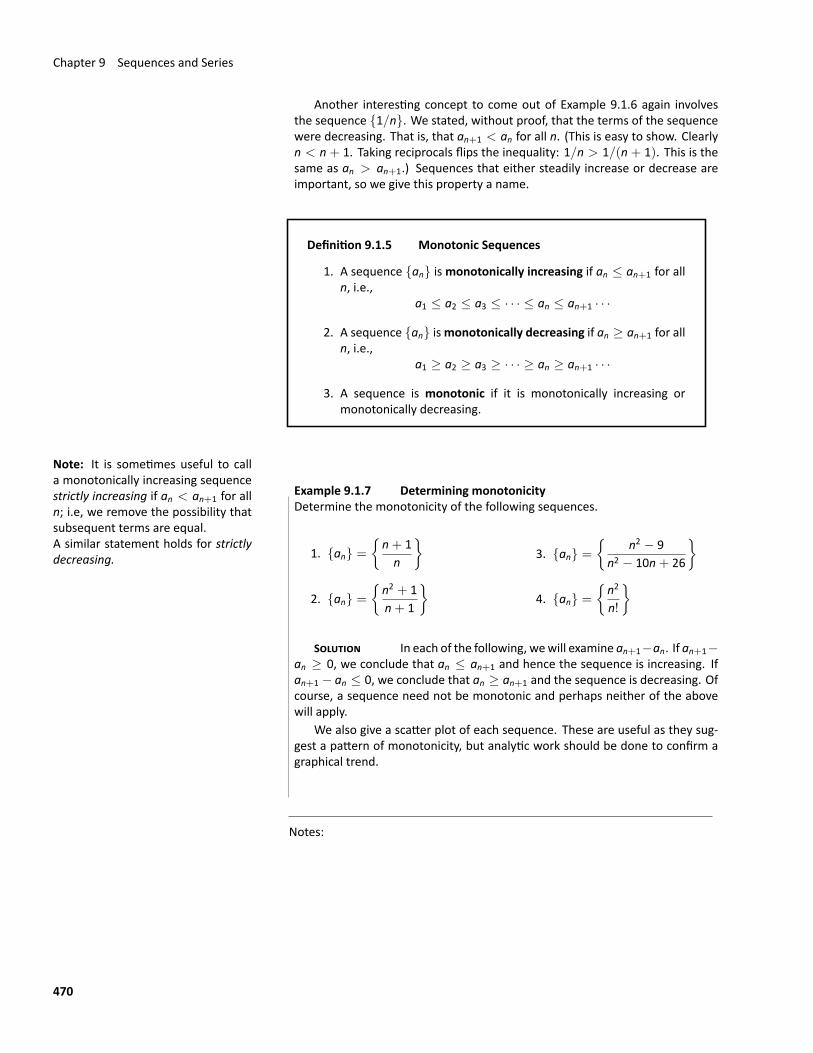
Chapter 9 Sequences and Series
Another interesting concept to come out of Example 9.1.6 again involvesthe sequence {1/n}. We stated, without proof, that the terms of the sequencewere decreasing. That is, that an+1 < an for all n. (This is easy to show. Clearlyn < n + 1. Taking reciprocals flips the inequality: 1/n > 1/(n + 1). This is thesame as an > an+1.) Sequences that either steadily increase or decrease areimportant, so we give this property a name.
Definition 9.1.5 Monotonic Sequences
1. A sequence {an} ismonotonically increasing if an ≤ an+1 for alln, i.e.,
a1 ≤ a2 ≤ a3 ≤ · · · ≤ an ≤ an+1 · · ·
2. A sequence {an} ismonotonically decreasing if an ≥ an+1 for alln, i.e.,
a1 ≥ a2 ≥ a3 ≥ · · · ≥ an ≥ an+1 · · ·
3. A sequence is monotonic if it is monotonically increasing ormonotonically decreasing.
Note: It is sometimes useful to calla monotonically increasing sequencestrictly increasing if an < an+1 for alln; i.e, we remove the possibility thatsubsequent terms are equal.A similar statement holds for strictlydecreasing.
Example 9.1.7 Determining monotonicityDetermine the monotonicity of the following sequences.
1. {an} =
{n+ 1n
}
2. {an} =
{n2 + 1n+ 1
}3. {an} =
{n2 − 9
n2 − 10n+ 26
}
4. {an} =
{n2
n!
}
SOLUTION In each of the following, wewill examine an+1−an. If an+1−an ≥ 0, we conclude that an ≤ an+1 and hence the sequence is increasing. Ifan+1 − an ≤ 0, we conclude that an ≥ an+1 and the sequence is decreasing. Ofcourse, a sequence need not be monotonic and perhaps neither of the abovewill apply.
We also give a scatter plot of each sequence. These are useful as they sug‐gest a pattern of monotonicity, but analytic work should be done to confirm agraphical trend.
Notes:
470
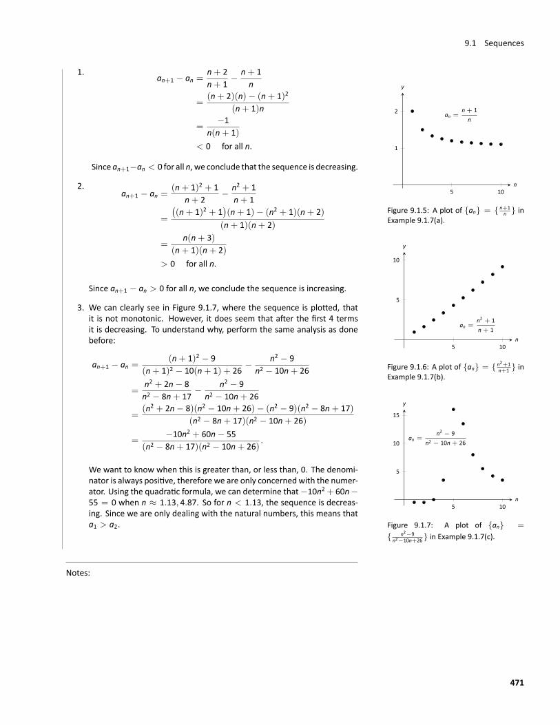
9.1 Sequences
1.an+1 − an =
n+ 2n+ 1
− n+ 1n
=(n+ 2)(n)− (n+ 1)2
(n+ 1)n
=−1
n(n+ 1)< 0 for all n.
Since an+1−an < 0 for all n, we conclude that the sequence is decreasing.
an =n + 1n
5 10
1
2
n
y
Figure 9.1.5: A plot of {an} = { n+1n } in
Example 9.1.7(a).
2.
an =n2 + 1n + 1
5 10
5
10
n
y
Figure 9.1.6: A plot of {an} = { n2+1n+1 } in
Example 9.1.7(b).
an+1 − an =(n+ 1)2 + 1
n+ 2− n2 + 1
n+ 1
=
((n+ 1)2 + 1
)(n+ 1)− (n2 + 1)(n+ 2)
(n+ 1)(n+ 2)
=n(n+ 3)
(n+ 1)(n+ 2)> 0 for all n.
Since an+1 − an > 0 for all n, we conclude the sequence is increasing.
an =n2 − 9
n2 − 10n + 26
5 10
5
10
15
n
y
Figure 9.1.7: A plot of {an} =
{ n2−9n2−10n+26} in Example 9.1.7(c).
3. We can clearly see in Figure 9.1.7, where the sequence is plotted, thatit is not monotonic. However, it does seem that after the first 4 termsit is decreasing. To understand why, perform the same analysis as donebefore:
an+1 − an =(n+ 1)2 − 9
(n+ 1)2 − 10(n+ 1) + 26− n2 − 9
n2 − 10n+ 26
=n2 + 2n− 8n2 − 8n+ 17
− n2 − 9n2 − 10n+ 26
=(n2 + 2n− 8)(n2 − 10n+ 26)− (n2 − 9)(n2 − 8n+ 17)
(n2 − 8n+ 17)(n2 − 10n+ 26)
=−10n2 + 60n− 55
(n2 − 8n+ 17)(n2 − 10n+ 26).
We want to know when this is greater than, or less than, 0. The denomi‐nator is always positive, therefore we are only concerned with the numer‐ator. Using the quadratic formula, we can determine that−10n2 + 60n−55 = 0 when n ≈ 1.13, 4.87. So for n < 1.13, the sequence is decreas‐ing. Since we are only dealing with the natural numbers, this means thata1 > a2.
Notes:
471
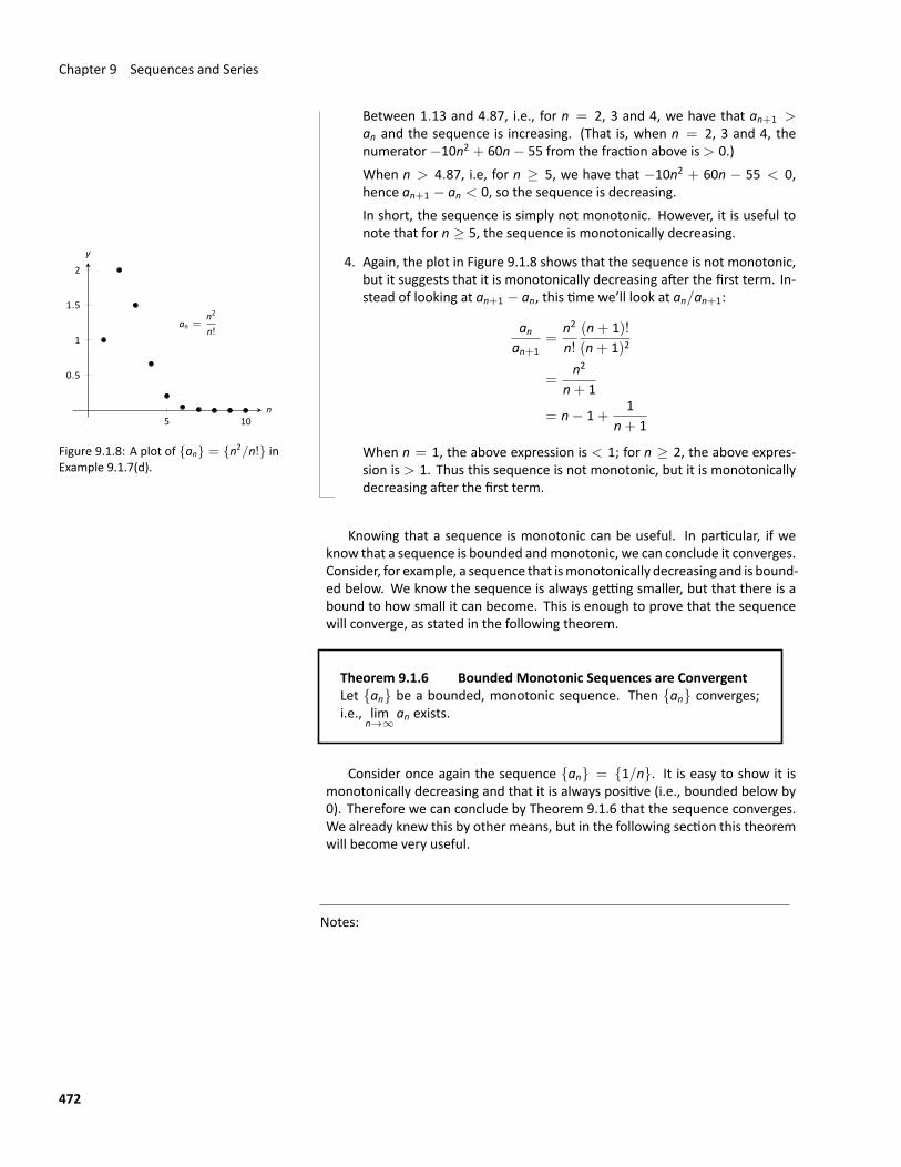
Chapter 9 Sequences and Series
Between 1.13 and 4.87, i.e., for n = 2, 3 and 4, we have that an+1 >an and the sequence is increasing. (That is, when n = 2, 3 and 4, thenumerator−10n2 + 60n− 55 from the fraction above is> 0.)When n > 4.87, i.e, for n ≥ 5, we have that −10n2 + 60n − 55 < 0,hence an+1 − an < 0, so the sequence is decreasing.In short, the sequence is simply not monotonic. However, it is useful tonote that for n ≥ 5, the sequence is monotonically decreasing.
an =n2
n!
5 10
0.5
1
1.5
2
n
y
Figure 9.1.8: A plot of {an} = {n2/n!} inExample 9.1.7(d).
4. Again, the plot in Figure 9.1.8 shows that the sequence is not monotonic,but it suggests that it is monotonically decreasing after the first term. In‐stead of looking at an+1 − an, this time we’ll look at an/an+1:
anan+1
=n2
n!(n+ 1)!(n+ 1)2
=n2
n+ 1
= n− 1+1
n+ 1
When n = 1, the above expression is < 1; for n ≥ 2, the above expres‐sion is > 1. Thus this sequence is not monotonic, but it is monotonicallydecreasing after the first term.
Knowing that a sequence is monotonic can be useful. In particular, if weknow that a sequence is bounded andmonotonic, we can conclude it converges.Consider, for example, a sequence that ismonotonically decreasing and is bound‐ed below. We know the sequence is always getting smaller, but that there is abound to how small it can become. This is enough to prove that the sequencewill converge, as stated in the following theorem.
Theorem 9.1.6 Bounded Monotonic Sequences are ConvergentLet {an} be a bounded, monotonic sequence. Then {an} converges;i.e., lim
n→∞an exists.
Consider once again the sequence {an} = {1/n}. It is easy to show it ismonotonically decreasing and that it is always positive (i.e., bounded below by0). Therefore we can conclude by Theorem 9.1.6 that the sequence converges.We already knew this by other means, but in the following section this theoremwill become very useful.
Notes:
472
9.1 Sequences
Convergence of a sequence does not depend on the first N terms of a se‐quence. For example, we could adapt the sequence of the previous paragraphto be
1, 10, 100, 1000,15,16,17,18,19,
110
, . . .
Because we only changed three of the first 4 terms, we have not affected whe‐ther the sequence converges or diverges.
Sequences are a great source of mathematical inquiry. The On‐Line Ency‐clopedia of Integer Sequences (http://oeis.org) contains thousands of se‐quences and their formulae. (As of this writing, there are 257,537 sequencesin the database.) Perusing this database quickly demonstrates that a single se‐quence can represent several different “real life” phenomena.
Interesting as this is, our interest actually lies elsewhere. We are more in‐terested in the sum of a sequence. That is, given a sequence {an}, we are veryinterested in a1+a2+a3+ · · · . Of course, one might immediately counter with“Doesn’t this just add up to ‘infinity’?” Many times, yes, but there are many im‐portant cases where the answer is no. This is the topic of series, which we beginto investigate in the next section.
Notes:
473
Exercises 9.1Terms and Concepts1. Use your own words to define a sequence.2. The domain of a sequence is the numbers.3. Use your own words to describe the range of a sequence.4. Describe what it means for a sequence to be bounded.
ProblemsIn Exercises 5–8, give the first five terms of the given sequence.
5. {an} =
{4n
(n+ 1)!
}6. {bn} =
{(−32
)n}7. {cn} =
{− nn+1
n+ 2
}8. {dn} =
{1√5
((1+
√5
2
)n
−(1−
√5
2
)n)}
In Exercises 9–12, determine the nth term of the given se‐quence.
9. 4, 7, 10, 13, 16, . . .
10. 3, −32,34, −3
8, . . .
11. 10, 20, 40, 80, 160, . . .
12. 1, 1, 12,16,
124
,1
120, . . .
In Exercises 13–16, use the following information to determinethe limit of the given sequences.
• {an} =
{2n − 20
2n
}; lim
n→∞an = 1
• {bn} =
{(1+ 2
n
)n}; lim
n→∞bn = e2
• {cn} = {sin(3/n)}; limn→∞
cn = 0
13. {dn} =
{2n − 207 · 2n
}14. {dn} = {3bn − an}
15. {dn} =
{sin(3/n)
(1+ 2
n
)n}16. {dn} =
{(1+ 2
n
)2n}
In Exercises 17–38, determine whether the sequence con‐verges or diverges. If convergent, give the limit of the se‐quence.
17. {an} =
{(−1)n n
n+ 1
}18. {an} =
{4n2 − n+ 53n2 + 1
}
19. {an} =
{4n
5n
}20. {an} =
{(n− 3)!(n+ 1)!
}21. {an} =
{n− 1n
− nn− 1
}, n ≥ 2
22. {an} =
{6n+3
8n
}23. {an} = {ln(n)}
24. {an} =
{3n√n2 + 1
}25. {an} =
{(1+ 1
n
)n}26. {an} =
{(2n+ 1)!(2n− 1)!
}27. {an} =
{5− 1
n
}28. {an} =
{(−1)n+1
n
}29. {an} =
{1.1n
n
}30. {an} =
{2n
n+ 1
}31. {an} =
{(−1)n n2
2n − 1
}32. {an} =
{2+ 9n
8n
}33. {an} =
{(n− 1)!(n+ 1)!
}34. {an} = {ln(3n+ 2)− ln n}
35. {an} = {ln(2n2 + 3n+ 1)− ln(n2 + 1)}
36. {an} =
{n sin
(1n
)}37. {an} =
{en + e−n
e2n − 1
}38. {an} =
{ln nln 2n
}In Exercises 39–42, determine whether the sequence isbounded, bounded above, bounded below, or none of theabove.
39. {an} = {sin n}
40. {an} =
{(−1)n 3n− 1
n
}41. {an} =
{3n2 − 1
n
}42. {an} = {2n − n!}
474
In Exercises 43–48, determine whether the sequence is mono‐tonically increasing or decreasing. If it is not, determine ifthere is anm such that it is monotonic for all n ≥ m.
43. {an} =
{n
n+ 2
}44. {an} =
{n2 − 6n+ 9
n
}45. {an} =
{(−1)n 1
n3
}46. {an} =
{n2
2n
}47. {an} =
{cos(nπ2
)}
48. {an} = {ne−n}
49. Prove Theorem 9.1.2; that is, use the definition of thelimit of a sequence to show that if lim
n→∞|an| = 0, then
limn→∞
an = 0.
50. Let {an} and {bn} be sequences such that limn→∞
an = L andlim
n→∞bn = K.
(a) Show that if an < bn for all n, then L ≤ K.
(b) Give an example where an < bn for all n but L = K.
51. Prove the Squeeze Theorem for sequences: Let {an} and{bn} be such that lim
n→∞an = L and lim
n→∞bn = L, and let
{cn} be such that an ≤ cn ≤ bn for all n. Then limn→∞
cn = L
475
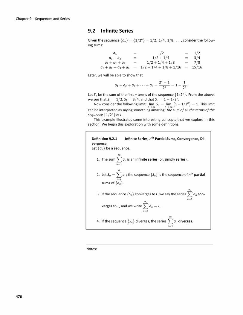
Chapter 9 Sequences and Series
9.2 Infinite SeriesGiven the sequence {an} = {1/2n} = 1/2, 1/4, 1/8, . . . , consider the follow‐ing sums:
a1 = 1/2 = 1/2a1 + a2 = 1/2+ 1/4 = 3/4
a1 + a2 + a3 = 1/2+ 1/4+ 1/8 = 7/8a1 + a2 + a3 + a4 = 1/2+ 1/4+ 1/8+ 1/16 = 15/16
Later, we will be able to show that
a1 + a2 + a3 + · · ·+ an =2n − 12n
= 1− 12n
.
Let Sn be the sum of the first n terms of the sequence {1/2n}. From the above,we see that S1 = 1/2, S2 = 3/4, and that Sn = 1− 1/2n.
Now consider the following limit: limn→∞
Sn = limn→∞
(1−1/2n
)= 1. This limit
can be interpreted as saying something amazing: the sum of all the terms of thesequence {1/2n} is 1.
This example illustrates some interesting concepts that we explore in thissection. We begin this exploration with some definitions.
Definition 9.2.1 Infinite Series, nth Partial Sums, Convergence, Di‐vergenceLet {an} be a sequence.
1. The sum∞∑n=1
an is an infinite series (or, simply series).
2. Let Sn =n∑
i=1
ai ; the sequence {Sn} is the sequence of nth partial
sums of {an}.
3. If the sequence {Sn} converges to L, we say the series∞∑n=1
an con‐
verges to L, and we write∞∑n=1
an = L.
4. If the sequence {Sn} diverges, the series∞∑n=1
an diverges.
Notes:
476
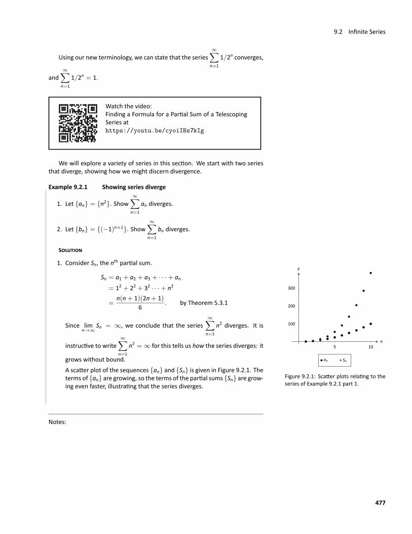
9.2 Infinite Series
Using our new terminology, we can state that the series∞∑n=1
1/2n converges,
and∞∑n=1
1/2n = 1.
Watch the video:Finding a Formula for a Partial Sum of a TelescopingSeries athttps://youtu.be/cyoiIBs7kIg
We will explore a variety of series in this section. We start with two seriesthat diverge, showing how we might discern divergence.
Example 9.2.1 Showing series diverge
1. Let {an} = {n2}. Show∞∑n=1
an diverges.
2. Let {bn} = {(−1)n+1}. Show∞∑n=1
bn diverges.
SOLUTION
1. Consider Sn, the nth partial sum.
5 10
100
200
300
n
y
an Sn
Figure 9.2.1: Scatter plots relating to theseries of Example 9.2.1 part 1.
Sn = a1 + a2 + a3 + · · ·+ an= 12 + 22 + 32 · · ·+ n2
=n(n+ 1)(2n+ 1)
6. by Theorem 5.3.1
Since limn→∞
Sn = ∞, we conclude that the series∞∑n=1
n2 diverges. It is
instructive to write∞∑n=1
n2 = ∞ for this tells us how the series diverges: it
grows without bound.A scatter plot of the sequences {an} and {Sn} is given in Figure 9.2.1. Theterms of {an} are growing, so the terms of the partial sums {Sn} are grow‐ing even faster, illustrating that the series diverges.
Notes:
477
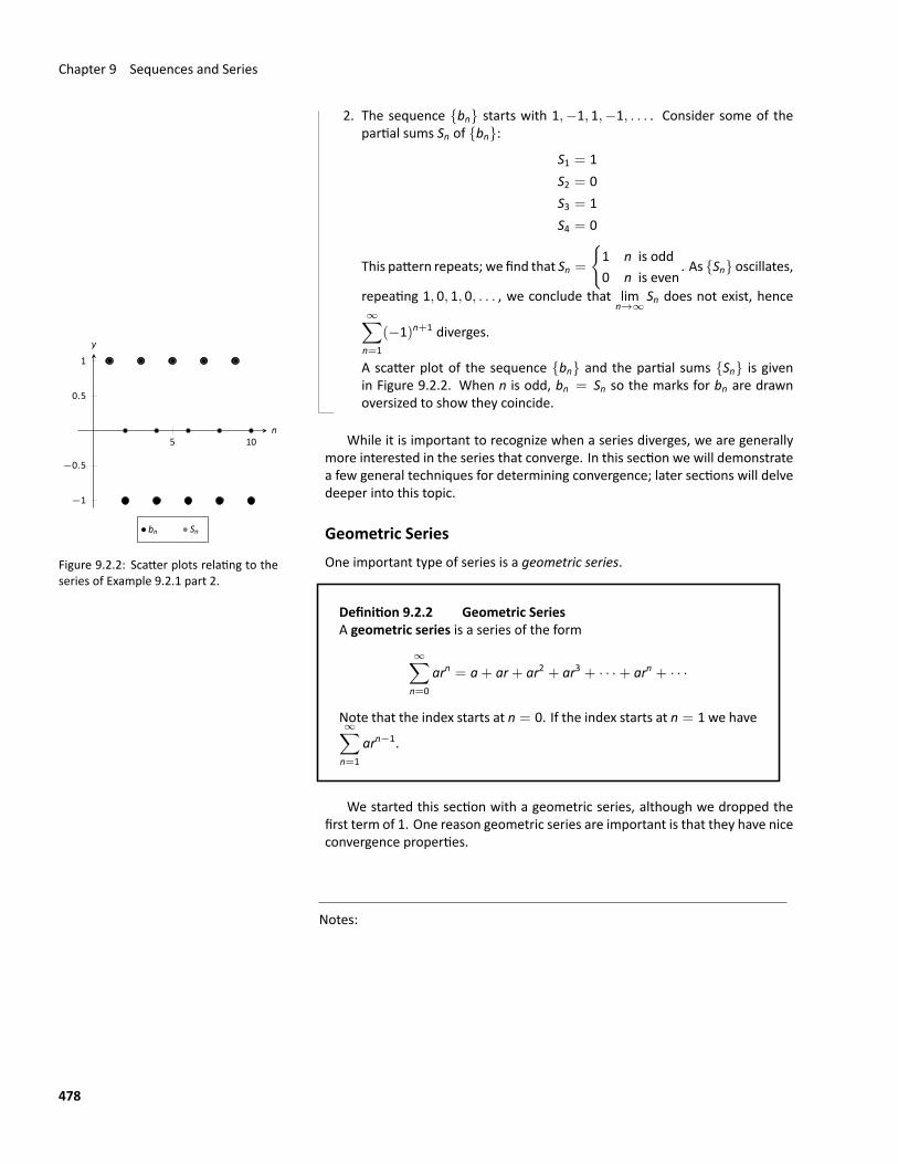
Chapter 9 Sequences and Series
2. The sequence {bn} starts with 1,−1, 1,−1, . . . . Consider some of thepartial sums Sn of {bn}:
S1 = 1S2 = 0S3 = 1S4 = 0
This pattern repeats; we find that Sn =
{1 n is odd0 n is even
. As {Sn} oscillates,
repeating 1, 0, 1, 0, . . . , we conclude that limn→∞
Sn does not exist, hence∞∑n=1
(−1)n+1 diverges.
5 10
−1
−0.5
0.5
1
n
y
bn Sn
Figure 9.2.2: Scatter plots relating to theseries of Example 9.2.1 part 2.
A scatter plot of the sequence {bn} and the partial sums {Sn} is givenin Figure 9.2.2. When n is odd, bn = Sn so the marks for bn are drawnoversized to show they coincide.
While it is important to recognize when a series diverges, we are generallymore interested in the series that converge. In this section we will demonstratea few general techniques for determining convergence; later sections will delvedeeper into this topic.
Geometric SeriesOne important type of series is a geometric series.
Definition 9.2.2 Geometric SeriesA geometric series is a series of the form
∞∑n=0
arn = a+ ar+ ar2 + ar3 + · · ·+ arn + · · ·
Note that the index starts at n = 0. If the index starts at n = 1 we have∞∑n=1
arn−1.
We started this section with a geometric series, although we dropped thefirst term of 1. One reason geometric series are important is that they have niceconvergence properties.
Notes:
478
9.2 Infinite Series
Theorem 9.2.1 Convergence of Geometric Series
Consider the geometric series∞∑n=0
arn.
1. If r ̸= 1, the nth partial sum is: Sn =n−1∑k=0
ark =a(1− r n)1− r
.
2. The series converges if, and only if, |r| < 1. When |r| < 1,
∞∑n=0
arn =a
1− r.
ProofIf r = 1, then Sn = a+a+a+· · ·+a = na. Since lim
n→∞Sn = ±∞, the geometric
series diverges.If r ̸= 1, we have
Sn = a+ ar+ ar2 + · · ·+ arn−1.
Multiply each term by r and we have
rSn = ar+ ar2 + ar3 · · ·+ arn.
Subtract these two equations and solve for Sn.
Sn − rSn = a− arn
Sn =a(1− rn)1− r
From Theorem 9.1.4, we know that if−1 < r < 1, then limn→∞
rn = 0 so
limn→∞
Sn = limn→∞
=a(1− rn)1− r
=a
1− r− a
1− rlim
n→∞rn =
a1− r
.
So when |r| < 1 the geometric series converges and its sum isa
1− r.
If either r ≤ −1 or r > 1, the sequence {rn} is divergent by Theorem 9.1.4.Thus lim
n→∞Sn does not exist, so the geometric series diverges if r ≤ −1 or r >
1. □
Notes:
479
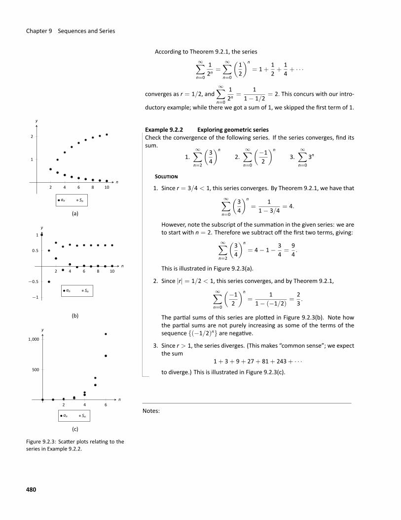
Chapter 9 Sequences and Series
According to Theorem 9.2.1, the series∞∑n=0
12n
=
∞∑n=0
(12
)n
= 1+12+
14+ · · ·
converges as r = 1/2, and∞∑n=0
12n
=1
1− 1/2= 2. This concurs with our intro‐
ductory example; while there we got a sum of 1, we skipped the first term of 1.
2 4 6 8 10
1
2
n
y
an Sn
(a)
2 4 6 8 10
−1
−0.5
0.5
1
n
y
an Sn
(b)
2 4 6
500
1,000
n
y
an Sn
(c)
Figure 9.2.3: Scatter plots relating to theseries in Example 9.2.2.
Example 9.2.2 Exploring geometric seriesCheck the convergence of the following series. If the series converges, find itssum.
1.∞∑n=2
(34
)n
2.∞∑n=0
(−12
)n
3.∞∑n=0
3n
SOLUTION
1. Since r = 3/4 < 1, this series converges. By Theorem 9.2.1, we have that∞∑n=0
(34
)n
=1
1− 3/4= 4.
However, note the subscript of the summation in the given series: we areto start with n = 2. Therefore we subtract off the first two terms, giving:
∞∑n=2
(34
)n
= 4− 1− 34=
94.
This is illustrated in Figure 9.2.3(a).
2. Since |r| = 1/2 < 1, this series converges, and by Theorem 9.2.1,∞∑n=0
(−12
)n
=1
1− (−1/2)=
23.
The partial sums of this series are plotted in Figure 9.2.3(b). Note howthe partial sums are not purely increasing as some of the terms of thesequence {(−1/2)n} are negative.
3. Since r > 1, the series diverges. (This makes “common sense”; we expectthe sum
1+ 3+ 9+ 27+ 81+ 243+ · · ·to diverge.) This is illustrated in Figure 9.2.3(c).
Notes:
480
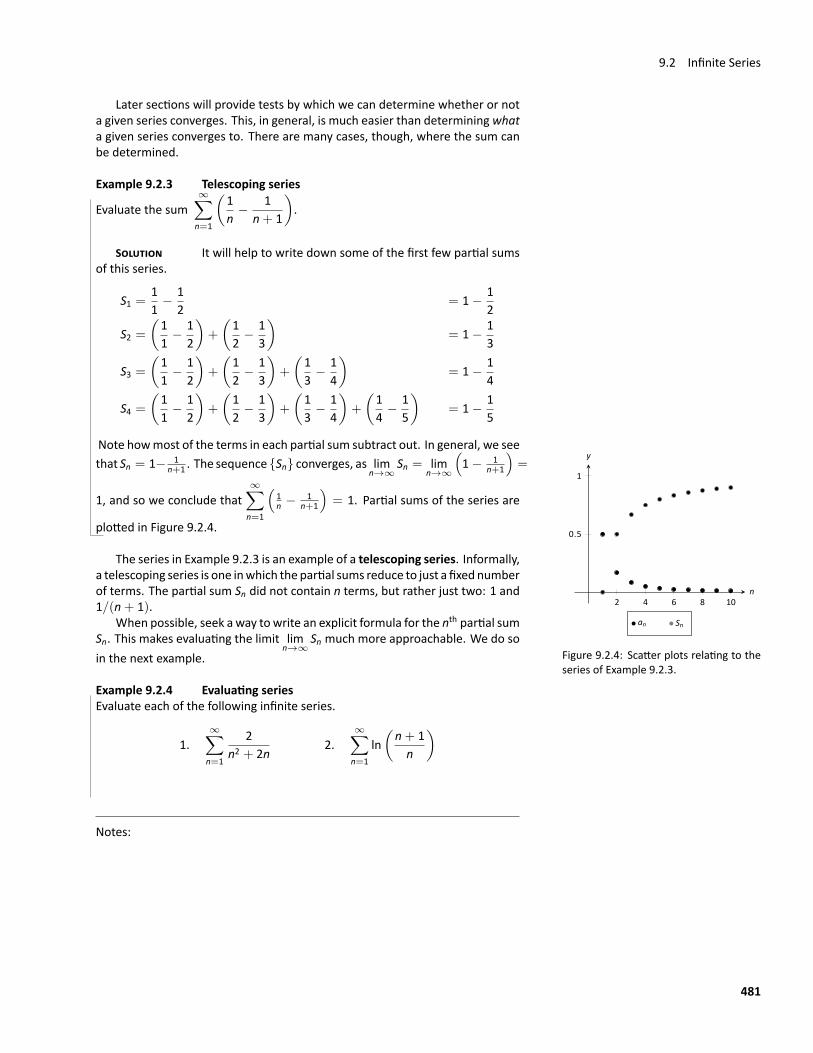
9.2 Infinite Series
Later sections will provide tests by which we can determine whether or nota given series converges. This, in general, is much easier than determiningwhata given series converges to. There are many cases, though, where the sum canbe determined.
Example 9.2.3 Telescoping series
Evaluate the sum∞∑n=1
(1n− 1
n+ 1
).
SOLUTION It will help to write down some of the first few partial sumsof this series.
S1 =11− 1
2= 1− 1
2
S2 =(11− 1
2
)+
(12− 1
3
)= 1− 1
3
S3 =(11− 1
2
)+
(12− 1
3
)+
(13− 1
4
)= 1− 1
4
S4 =(11− 1
2
)+
(12− 1
3
)+
(13− 1
4
)+
(14− 1
5
)= 1− 1
5
Note howmost of the terms in each partial sum subtract out. In general, we see
2 4 6 8 10
0.5
1
n
y
an Sn
Figure 9.2.4: Scatter plots relating to theseries of Example 9.2.3.
that Sn = 1− 1n+1 . The sequence {Sn} converges, as lim
n→∞Sn = lim
n→∞
(1− 1
n+1
)=
1, and so we conclude that∞∑n=1
(1n −
1n+1
)= 1. Partial sums of the series are
plotted in Figure 9.2.4.
The series in Example 9.2.3 is an example of a telescoping series. Informally,a telescoping series is one inwhich the partial sums reduce to just a fixednumberof terms. The partial sum Sn did not contain n terms, but rather just two: 1 and1/(n+ 1).
When possible, seek away towrite an explicit formula for the nth partial sumSn. This makes evaluating the limit lim
n→∞Sn much more approachable. We do so
in the next example.
Example 9.2.4 Evaluating seriesEvaluate each of the following infinite series.
1.∞∑n=1
2n2 + 2n
2.∞∑n=1
ln(n+ 1n
)
Notes:
481
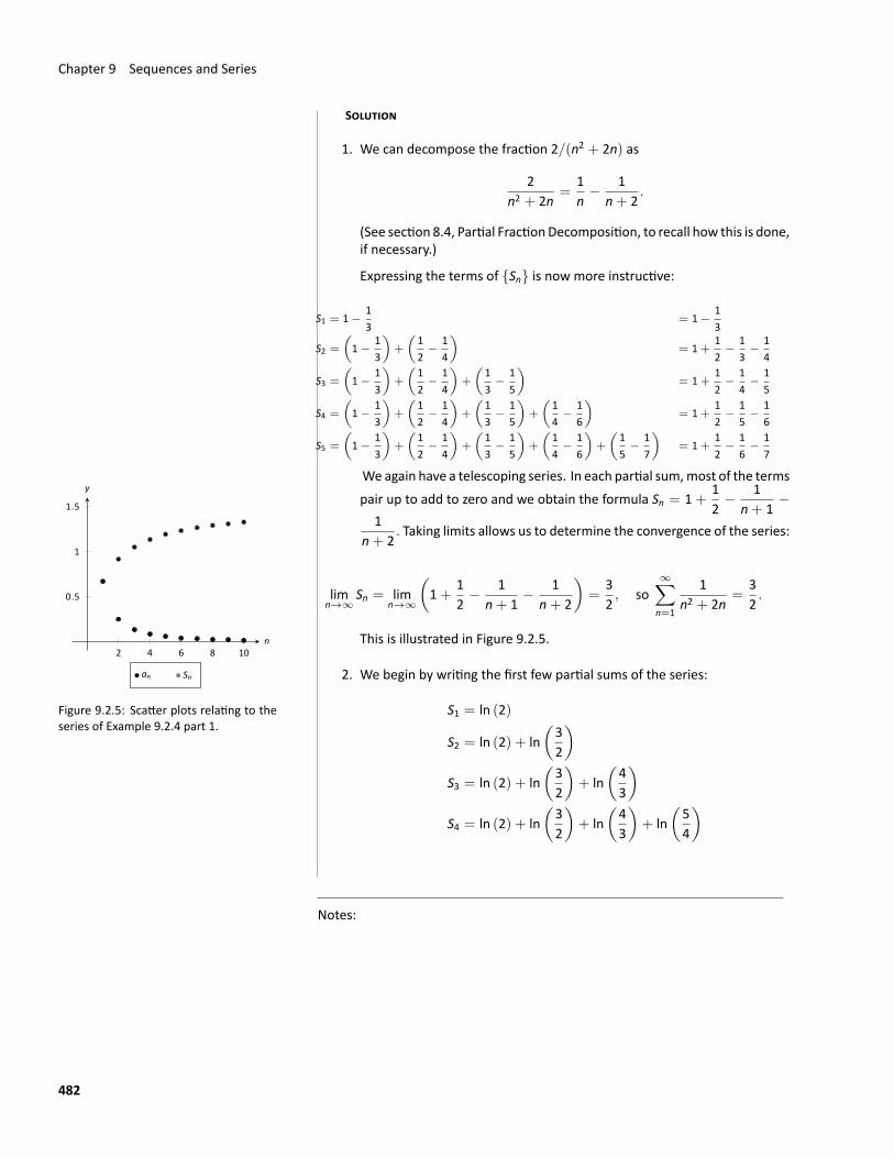
Chapter 9 Sequences and Series
SOLUTION
1. We can decompose the fraction 2/(n2 + 2n) as
2n2 + 2n
=1n− 1
n+ 2.
(See section 8.4, Partial FractionDecomposition, to recall how this is done,if necessary.)
Expressing the terms of {Sn} is now more instructive:
S1 = 1−13
= 1−13
S2 =
(1−
13
)+
(12−
14
)= 1+
12−
13−
14
S3 =
(1−
13
)+
(12−
14
)+
(13−
15
)= 1+
12−
14−
15
S4 =
(1−
13
)+
(12−
14
)+
(13−
15
)+
(14−
16
)= 1+
12−
15−
16
S5 =
(1−
13
)+
(12−
14
)+
(13−
15
)+
(14−
16
)+
(15−
17
)= 1+
12−
16−
17
Weagain have a telescoping series. In each partial sum,most of the terms
2 4 6 8 10
0.5
1
1.5
n
y
an Sn
Figure 9.2.5: Scatter plots relating to theseries of Example 9.2.4 part 1.
pair up to add to zero and we obtain the formula Sn = 1+12− 1
n+ 1−
1n+ 2
. Taking limits allows us to determine the convergence of the series:
limn→∞
Sn = limn→∞
(1+
12− 1
n+ 1− 1
n+ 2
)=
32, so
∞∑n=1
1n2 + 2n
=32.
This is illustrated in Figure 9.2.5.
2. We begin by writing the first few partial sums of the series:
S1 = ln (2)
S2 = ln (2) + ln(32
)S3 = ln (2) + ln
(32
)+ ln
(43
)S4 = ln (2) + ln
(32
)+ ln
(43
)+ ln
(54
)
Notes:
482
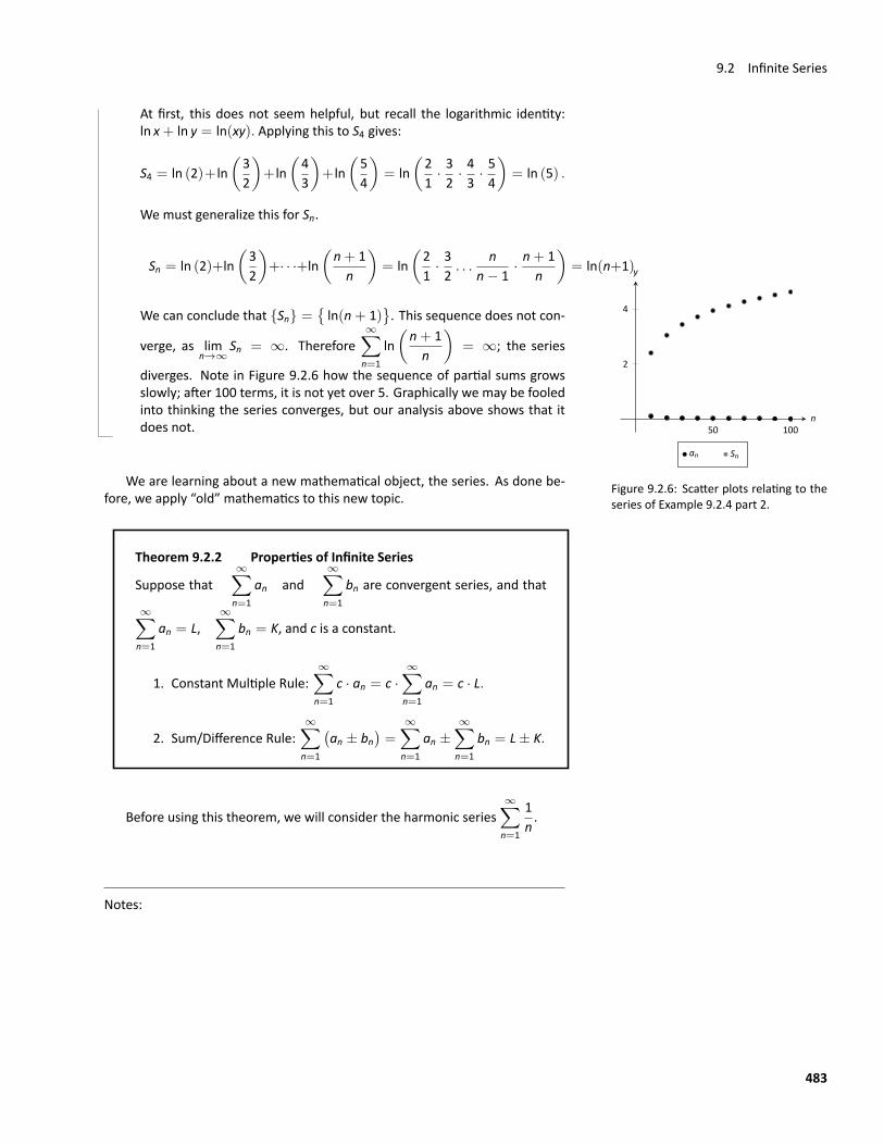
9.2 Infinite Series
At first, this does not seem helpful, but recall the logarithmic identity:ln x+ ln y = ln(xy). Applying this to S4 gives:
S4 = ln (2)+ ln(32
)+ ln
(43
)+ ln
(54
)= ln
(21· 32· 43· 54
)= ln (5) .
We must generalize this for Sn.
Sn = ln (2)+ln(32
)+· · ·+ln
(n+ 1n
)= ln
(21· 32. . .
nn− 1
· n+ 1n
)= ln(n+1)
50 100
2
4
n
y
an Sn
Figure 9.2.6: Scatter plots relating to theseries of Example 9.2.4 part 2.
We can conclude that {Sn} ={ln(n+ 1)
}. This sequence does not con‐
verge, as limn→∞
Sn = ∞. Therefore∞∑n=1
ln(n+ 1n
)= ∞; the series
diverges. Note in Figure 9.2.6 how the sequence of partial sums growsslowly; after 100 terms, it is not yet over 5. Graphically we may be fooledinto thinking the series converges, but our analysis above shows that itdoes not.
We are learning about a new mathematical object, the series. As done be‐fore, we apply “old” mathematics to this new topic.
Theorem 9.2.2 Properties of Infinite Series
Suppose that∞∑n=1
an and∞∑n=1
bn are convergent series, and that
∞∑n=1
an = L,∞∑n=1
bn = K, and c is a constant.
1. Constant Multiple Rule:∞∑n=1
c · an = c ·∞∑n=1
an = c · L.
2. Sum/Difference Rule:∞∑n=1
(an ± bn
)=
∞∑n=1
an ±∞∑n=1
bn = L± K.
Before using this theorem, we will consider the harmonic series∞∑n=1
1n.
Notes:
483
Chapter 9 Sequences and Series
Example 9.2.5 Divergence of the Harmonic Series
Show that the harmonic series∞∑n=1
1ndiverges.
SOLUTION We will use a proof by contradiction here. Suppose the har‐monic series converges to S. That is
S = 1+12+
13+
14+
15+
16+
17+
18+ · · ·
We then have
S ≥ 1+12+
14+
14+
16+
16+
18+
18+ · · ·
= 1+12+
12
+13
+14
+ · · ·
=12+ S
This gives us S ≥ 12 + S which can never be true, thus our assumption that
the harmonic series converges must be false. Therefore, the harmonic seriesdiverges.
It may take a while before one is comfortable with this statement, whosetruth lies at the heart of the study of infinite series: it is possible that the sum ofan infinite list of nonzero numbers is finite. We have seen this repeatedly in thissection, yet it still may “take some getting used to.”
As one contemplates the behavior of series, a few facts become clear.
1. In order to add an infinite list of nonzero numbers and get a finite result,“most” of those numbers must be “very near” 0.
2. If a series diverges, it means that the sum of an infinite list of numbers isnot finite (it may approach±∞ or it may oscillate), and:
(a) The series will still diverge if the first term is removed.(b) The series will still diverge if the first 10 terms are removed.(c) The series will still diverge if the first 1,000,000 terms are removed.(d) The series will still diverge if any finite number of terms from any‐
where in the series are removed.
These concepts are very important and lie at the heart of the next two the‐orems.
Notes:
484
9.2 Infinite Series
Theorem 9.2.3 Convergence of Sequence
If the series∞∑n=1
an converges, then limn→∞
an = 0.
ProofLet Sn = a1 + a2 + · · ·+ an. We have
Sn = a1 + a2 + · · ·+ an−1 + anSn = Sn−1 + anan = Sn − Sn−1
Since∑n→∞
an converges, the sequence {Sn} converges. Let limn→∞
Sn = S. As
n → ∞, n− 1 also goes to∞, so limn→∞
Sn−1 = S. We now have
limn→∞
an = limn→∞
(Sn − Sn−1)
= limn→∞
Sn − limn→∞
Sn−1
= S− S = 0 □
Theorem 9.2.4 Test for Divergence
If limn→∞
an does not exist or limn→∞
an ̸= 0, then the series∞∑n=1
an diverges.
The Test for Divergence follows from Theorem 9.2.3. If the series does notdiverge, it must converge and therefore lim
n→∞an = 0.
Note that the two statements in Theorems 9.2.3 and 9.2.4 are really thesame. In order to converge, the terms of the sequence must approach 0; if theydo not, the series will not converge.
Looking back, we can apply this theorem to the series in Example 9.2.1. Inthat example, we had {an} = {n2} and {bn} = {(−1)n+1}.
limn→∞
an = limn→∞
n2 = ∞
andlim
n→∞bn = lim
n→∞(−1)n+1 which does not exist.
Notes:
485
Chapter 9 Sequences and Series
Thus by the Test for Divergence, both series will diverge.
Important! This theorem does not state that if limn→∞
an = 0 then∞∑n=1
an con‐
verges. The standard example of this is the Harmonic Series, as given in Exam‐ple 9.2.5. The Harmonic Sequence, {1/n}, converges to 0; the Harmonic Series,∞∑n=1
1/n, diverges.
Theorem 9.2.5 Infinite Nature of SeriesThe convergence or divergence of a series remains unchanged by theinsertion or deletion of any finite number of terms. That is:
1. A divergent series will remain divergent with the insertion ordeletion of any finite number of terms.
2. A convergent series will remain convergent with the insertion ordeletion of any finite number of terms. (Of course, the sum willlikely change.)
In other words, when we are only interested in the convergence or diver‐gence of a series, it is safe to ignore the first few billion terms.
Example 9.2.6 Removing Terms from the Harmonic Series
Consider once more the Harmonic Series∞∑n=1
1nwhich diverges; that is, the par‐
tial sums SN =
N∑n=1
1ngrow (very, very slowly) without bound. One might think
that by removing the “large” terms of the sequence that perhaps the series willconverge. This is simply not the case. For instance, the sum of the first 10 mil‐lion terms of the Harmonic Series is about 16.7. Removing the first 10 millionterms from the Harmonic Series changes the partial sums, effectively subtract‐ing 16.7 from the sum. However, a sequence that is growing without bound willstill grow without bound when 16.7 is subtracted from it.
The equation below illustrates this. Even though we have subtracted off thefirst 10 million terms, this only subtracts a constant off of an expression that is
Notes:
486
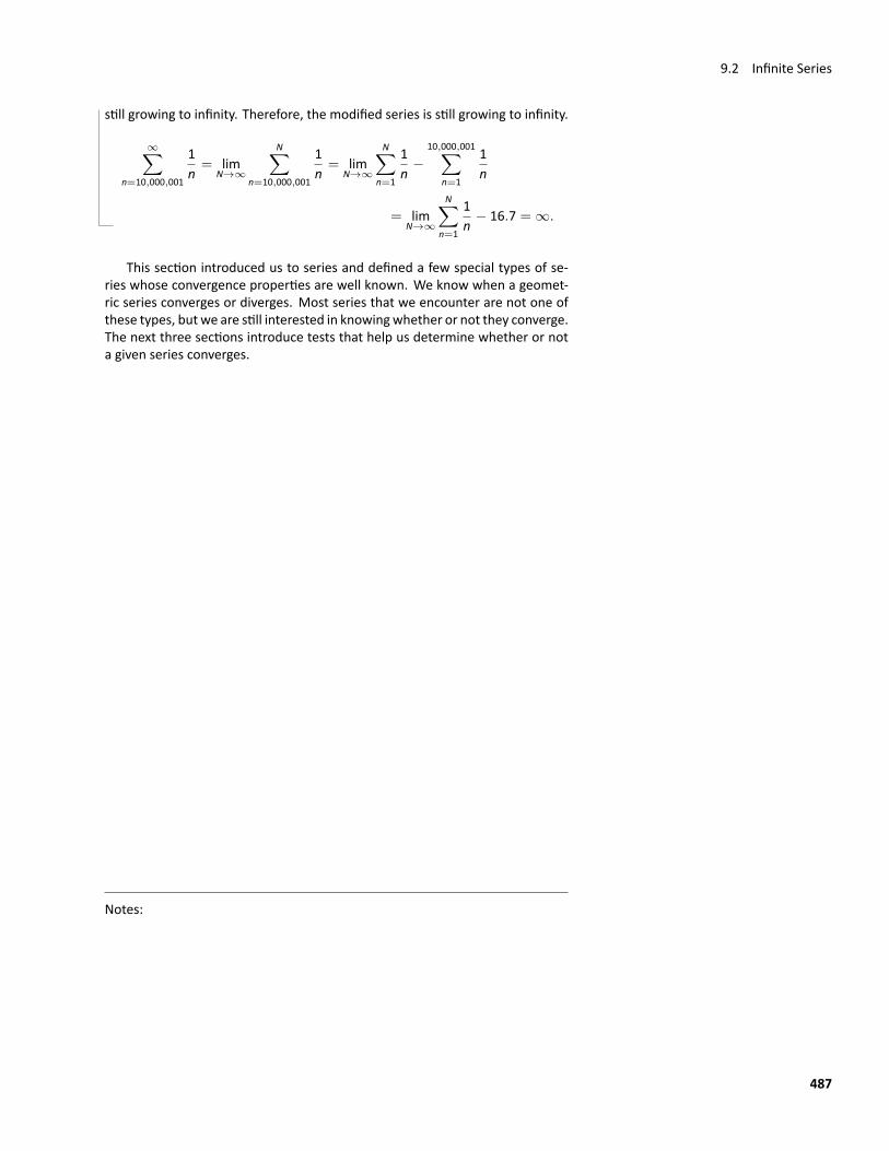
9.2 Infinite Series
still growing to infinity. Therefore, the modified series is still growing to infinity.
∞∑n=10,000,001
1n= lim
N→∞
N∑n=10,000,001
1n= lim
N→∞
N∑n=1
1n−
10,000,001∑n=1
1n
= limN→∞
N∑n=1
1n− 16.7 = ∞.
This section introduced us to series and defined a few special types of se‐ries whose convergence properties are well known. We know when a geomet‐ric series converges or diverges. Most series that we encounter are not one ofthese types, but we are still interested in knowingwhether or not they converge.The next three sections introduce tests that help us determine whether or nota given series converges.
Notes:
487
Exercises 9.2Terms and Concepts1. Use your ownwords to describe how sequences and series
are related.2. Use your own words to define a partial sum.
3. Given a series∞∑n=1
an, describe the two sequences related
to the series that are important.4. Use your own words to explain what a geometric series is.
5. T/F: If {an} is convergent, then∞∑n=1
an is also convergent.
6. T/F: If {an} converges to 0, then∞∑n=0
an converges.
Problems
In Exercises 7–14, a series∞∑n=1
an is given.
(a) Give the first 5 partial sums of the series.(b) Give a graph of the first 5 terms of an and Sn on the same
axes.
7.∞∑n=1
(−1)n
n
8.∞∑n=1
1n2
9.∞∑n=1
cos(πn)
10.∞∑n=1
n
11.∞∑n=1
1n!
12.∞∑n=1
13n
13.∞∑n=1
(− 910
)n
14.∞∑n=1
(110
)n
In Exercises 15–32, state whether the given series convergesor diverges and provide justification for your conclusion.
15.∞∑n=0
15n
16.∞∑n=1
3n2
n(n+ 2)
17.∞∑n=0
6n
5n
18.∞∑n=1
2n
n2
19.∞∑n=1
√n
20.∞∑n=0
(ln(4n+ 2)− ln(7n+ 5))
21.∞∑n=1
5n − n5
5n + n5
22.∞∑n=1
(1n!
+1n
)
23.∞∑n=1
12n
24.∞∑n=1
2n + 12n+1
25.∞∑n=1
12n− 1
26.∞∑n=1
n√3
27.∞∑n=1
(1+ 1
n
)n
28.∞∑n=1
πn
3n+1
29.∞∑n=1
3n + 2n
6n
30.∞∑n=1
4n + 2n
6n
31.∞∑n=1
4n + 5n
6n
32.∞∑n=1
(3
n(n+ 1)+
54n
)In Exercises 33–48, a series is given.
(a) Find a formula for Sn, the nth partial sum of the series.(b) Determine whether the series converges or diverges. If
it converges, state what it converges to.
33.∞∑n=0
14n
34. 13 + 23 + 33 + 43 + · · ·
35.∞∑n=1
(−1)nn
36.∞∑n=0
52n
37.∞∑n=1
e−n
488
38. 1− 13+
19− 1
27+
181
+ · · ·
39.∞∑n=1
1n(n+ 1)
40.∞∑n=1
3n(n+ 2)
41.∞∑n=1
1(2n− 1)(2n+ 1)
42.∞∑n=1
ln(
nn+ 1
)
43.∞∑n=1
2n+ 1n2(n+ 1)2
44. 11 · 4 +
12 · 5 +
13 · 6 +
14 · 7 + · · ·
45. 2+(12+
13
)+
(14+
19
)+
(18+
127
)+ · · ·
46.∞∑n=2
1n2 − 1
47.∞∑n=0
(sin 1
)n48.
∞∑n=1
(2
n(n+ 2)+
54n
)In Exercises 49–52, find the values of x for which the seriesconverges.
49.∞∑n=1
xn
3n
50.∞∑n=1
(x+ 3)n
2n
51.∞∑n=1
4n
xn
52.∞∑n=1
(x+ 2)n
53. Show the series∞∑n=1
n(2n− 1)(2n+ 1)
diverges.
489
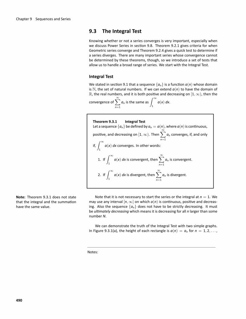
Chapter 9 Sequences and Series
9.3 The Integral TestKnowing whether or not a series converges is very important, especially whenwe discuss Power Series in section 9.8. Theorem 9.2.1 gives criteria for whenGeometric series converge and Theorem 9.2.4 gives a quick test to determine ifa series diverges. There are many important series whose convergence cannotbe determined by these theorems, though, so we introduce a set of tests thatallow us to handle a broad range of series. We start with the Integral Test.
Integral TestWe stated in section 9.1 that a sequence {an} is a function a(n) whose domainis N, the set of natural numbers. If we can extend a(n) to have the domain ofR, the real numbers, and it is both positive and decreasing on [1,∞), then the
convergence of∞∑n=1
an is the same as∫ ∞
1a(x) dx.
Theorem 9.3.1 Integral TestLet a sequence {an} be defined by an = a(n), where a(n) is continuous,
positive, and decreasing on [1,∞). Then∞∑n=1
an converges, if, and only
if,∫ ∞
1a(x) dx converges. In other words:
1. If∫ ∞
1a(x) dx is convergent, then
∞∑n=1
an is convergent.
2. If∫ ∞
1a(x) dx is divergent, then
∞∑n=1
an is divergent.
Note: Theorem 9.3.1 does not statethat the integral and the summationhave the same value.
Note that it is not necessary to start the series or the integral at n = 1. Wemay use any interval [n,∞] on which a(n) is continuous, positive and decreas‐ing. Also the sequence {an} does not have to be strictly decreasing. It mustbe ultimately decreasing which means it is decreasing for all n larger than somenumber N.
We can demonstrate the truth of the Integral Test with two simple graphs.In Figure 9.3.1(a), the height of each rectangle is a(n) = an for n = 1, 2, . . . ,
Notes:
490
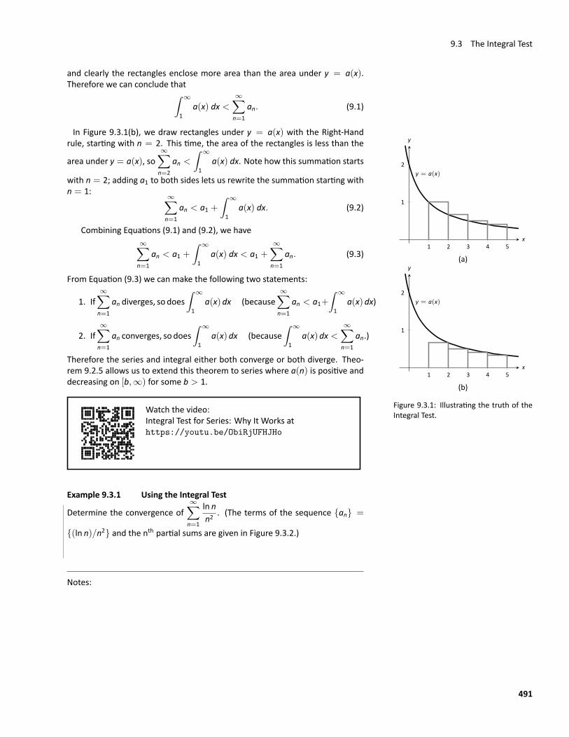
9.3 The Integral Test
and clearly the rectangles enclose more area than the area under y = a(x).Therefore we can conclude that∫ ∞
1a(x) dx <
∞∑n=1
an. (9.1)
In Figure 9.3.1(b), we draw rectangles under y = a(x) with the Right‐Hand
1 2 3 4 5
1
2y = a(x)
x
y
(a)
1 2 3 4 5
1
2y = a(x)
x
y
(b)
Figure 9.3.1: Illustrating the truth of theIntegral Test.
rule, starting with n = 2. This time, the area of the rectangles is less than the
area under y = a(x), so∞∑n=2
an <∫ ∞
1a(x) dx. Note how this summation starts
with n = 2; adding a1 to both sides lets us rewrite the summation starting withn = 1:
∞∑n=1
an < a1 +∫ ∞
1a(x) dx. (9.2)
Combining Equations (9.1) and (9.2), we have∞∑n=1
an < a1 +∫ ∞
1a(x) dx < a1 +
∞∑n=1
an. (9.3)
From Equation (9.3) we can make the following two statements:
1. If∞∑n=1
an diverges, so does∫ ∞
1a(x)dx (because
∞∑n=1
an < a1+∫ ∞
1a(x)dx)
2. If∞∑n=1
an converges, so does∫ ∞
1a(x)dx (because
∫ ∞
1a(x)dx <
∞∑n=1
an.)
Therefore the series and integral either both converge or both diverge. Theo‐rem 9.2.5 allows us to extend this theorem to series where a(n) is positive anddecreasing on [b,∞) for some b > 1.
Watch the video:Integral Test for Series: Why It Works athttps://youtu.be/ObiRjUFHJHo
Example 9.3.1 Using the Integral Test
Determine the convergence of∞∑n=1
ln nn2
. (The terms of the sequence {an} =
{(ln n)/n2} and the nth partial sums are given in Figure 9.3.2.)
Notes:
491
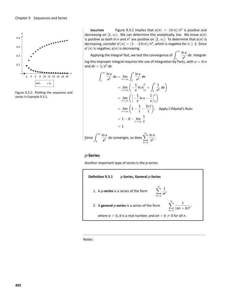
Chapter 9 Sequences and Series
SOLUTION Figure 9.3.2 implies that a(n) = (ln n)/n2 is positive and
2 4 6 8 10 12 14 16 18 20
0.2
0.4
0.6
0.8
n
y
an Sn
Figure 9.3.2: Plotting the sequence andseries in Example 9.3.1.
decreasing on [2,∞). We can determine this analytically, too. We know a(n)is positive as both ln n and n2 are positive on [2,∞). To determine that a(n) isdecreasing, consider a′(n) = (1− 2 ln n)/n3, which is negative for n ≥ 2. Sincea′(n) is negative, a(n) is decreasing.
Applying the Integral Test, we test the convergence of∫ ∞
1
ln xx2
dx. Integrat‐
ing this improper integral requires the use of Integration by Parts, with u = ln xand dv = 1/x2 dx.∫ ∞
1
ln xx2
dx = limt→∞
∫ t
1
ln xx2
dx
= limt→∞
(−1xln x∣∣∣t1+
∫ t
1
1x2
dx)
= limt→∞
([−1xln x− 1
x
]t1
)= lim
t→∞
(1− 1
t− ln t
t
). Apply L’Hôpital’s Rule:
= 1− 0− limt→∞
1t
= 1
Since∫ ∞
1
ln xx2
dx converges, so does∞∑n=1
ln nn2
.
p‐SeriesAnother important type of series is the p‐series.
Definition 9.3.1 p‐Series, General p‐Series
1. A p‐series is a series of the form∞∑n=1
1np
.
2. A general p‐series is a series of the form∞∑n=1
1(an+ b)p
,
where a > 0, b is a real number, and an+ b ̸= 0 for all n.
Notes:
492
9.3 The Integral Test
Like geometric series, one of the nice things about p‐series is that they haveeasy to determine convergence properties.
Theorem 9.3.2 Convergence of General p‐SeriesAssume a and b are real numbers and an+ b ̸= 0 for all n.
A general p‐series∞∑n=1
1(an+ b)p
will converge if, and only if, p > 1.
ProofConsider the integral
∫ ∞
1
1(ax+ b)p
dx; assuming p ̸= 1,
∫ ∞
1
1(ax+ b)p
dx = limt→∞
∫ t
1
1(ax+ b)p
dx
= limt→∞
1a(1− p)
(ax+ b)1−p∣∣∣t1
= limt→∞
1a(1− p)
((at+ b)1−p − (a+ b)1−p).
This limit converges if and only if, p > 1. It is easy to show that the integral alsodiverges in the case of p = 1. (This result is similar to the work preceding KeyIdea 8.6.1.)
Therefore∞∑n=1
1(an+ b)p
converges if, and only if, p > 1. □
Example 9.3.2 Determining convergence of seriesDetermine the convergence of the following series.
1.∞∑n=1
1n
2.∞∑n=1
1n2
3.∞∑n=1
1√n
4.∞∑n=1
(−1)n
n
5.∞∑
n=11
1( 12n− 5)3
6.∞∑n=1
12n
SOLUTION
1. This is a p‐series with p = 1. By Theorem 9.3.2, this series diverges.This series is a famous series, called the Harmonic Series, so named be‐cause of its relationship to harmonics in the study of music and sound.
Notes:
493
Chapter 9 Sequences and Series
2. This is a p‐series with p = 2. By Theorem 9.3.2, it converges. Note thatthe theorem does not give a formula by which we can determine whatthe series converges to; we just know it converges. A famous, unexpectedresult is that this series converges to π2/6.
3. This is a p‐series with p = 1/2; the theorem states that it diverges.
4. This is not a p‐series; the definition does not allow for alternating signs.Therefore we cannot apply Theorem 9.3.2. We will consider this seriesagain in section 9.5. (Another famous result states that this series, theAlternating Harmonic Series, converges to− ln 2.)
5. This is a general p‐series with p = 3, therefore it converges.
6. This is not a p‐series, but a geometric series with r = 1/2. It converges.
In the next section we consider two more convergence tests, both compari‐son tests. That is, we determine the convergence of one series by comparing itto another series with known convergence.
Notes:
494
Exercises 9.3Terms and Concepts1. In order to apply the Integral Test to a sequence {an}, the
function a(n) = an must be , and .2. T/F: The Integral Test can be used to determine the sum of
a convergent series.
ProblemsIn Exercises 3–10, use the Integral Test to determine the con‐vergence of the given series.
3.∞∑n=1
12n
4.∞∑n=1
1n4
5.∞∑n=1
nn2 + 1
6.∞∑n=2
1n ln n
7.∞∑n=1
1n2 + 1
8.∞∑n=2
1n(ln n)2
9.∞∑n=1
n2n
10.∞∑n=1
ln nn3
In Exercises 11–14, find the value(s) of p for which the series isconvergent.
11.∞∑n=2
1n(ln n)p
12.∞∑n=1
n(1+ n2)p
13.∞∑n=1
ln nnp
14.∞∑n=3
1n ln n[ln(ln n)]p
495
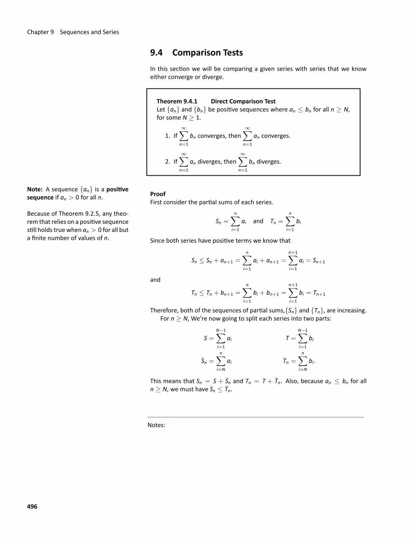
Chapter 9 Sequences and Series
9.4 Comparison TestsIn this section we will be comparing a given series with series that we knoweither converge or diverge.
Theorem 9.4.1 Direct Comparison TestLet {an} and {bn} be positive sequences where an ≤ bn for all n ≥ N,for some N ≥ 1.
1. If∞∑n=1
bn converges, then∞∑n=1
an converges.
2. If∞∑n=1
an diverges, then∞∑n=1
bn diverges.
Note: A sequence {an} is a positivesequence if an > 0 for all n.
Because of Theorem 9.2.5, any theo‐rem that relies on a positive sequencestill holds truewhen an > 0 for all buta finite number of values of n.
ProofFirst consider the partial sums of each series.
Sn =n∑
i=1
ai and Tn =n∑
i=1
bi
Since both series have positive terms we know that
Sn ≤ Sn + an+1 =
n∑i=1
ai + an+1 =
n+1∑i=1
ai = Sn+1
and
Tn ≤ Tn + bn+1 =
n∑i=1
bi + bn+1 =
n+1∑i=1
bi = Tn+1
Therefore, both of the sequences of partial sums,{Sn} and {Tn}, are increasing.For n ≥ N, We’re now going to split each series into two parts:
S =N−1∑i=1
ai T =
N−1∑i=1
bi
S̄n =n∑
i=N
ai T̄n =n∑
i=N
bi.
This means that Sn = S + S̄n and Tn = T + T̄n. Also, because an ≤ bn for alln ≥ N, we must have S̄n ≤ T̄n.
Notes:
496
9.4 Comparison Tests
For the first part of the theorem, assume that∞∑n=1
bn converges. Since bn ≥ 0
we know that
Tn =n∑
i=1
bi ≤∞∑i=1
bi
From above we know that S̄n ≤ T̄n for all n ≥ N so we also have
Sn = S+ S̄n ≤ S+ T̄n = S+ Tn − T = S− T+∞∑i=1
bi
Because∞∑i=1
bi converges it must have a finite value and {Sn} is bounded above.
We also showed that {Sn} is increasing so by Theorem 9.1.6 we know {Sn} con‐
verges and so∞∑n=1
an converges.
For the second part, assume that∞∑n=1
an diverges. Because an ≥ 0 we must
have limn→∞
Sn = ∞. We also know that for all n ≥ N, S̄n ≤ T̄n. This means that
limn→∞
Tn = limn→∞
(T+ T̄n)
≥ T+ limn→∞
S̄n = T+ limn→∞
(Sn − S) = T− S+ limn→∞
Sn = ∞.
Therefore, {Tn} is a divergent sequence and so∞∑i=1
bn diverges. □
Watch the video:Direct Comparison Test / Limit Comparison Test forSeries — Basic Info athttps://youtu.be/LAHKu3B-1zE
Example 9.4.1 Applying the Direct Comparison Test
Determine the convergence of∞∑n=1
13n + n2
.
Notes:
497
Chapter 9 Sequences and Series
SOLUTION This series is neither a geometric or p‐series, but seems re‐lated. We predict it will converge, so we look for a series with larger terms thatconverges. (Note too that the Integral Test seems difficult to apply here.)
Since 3n < 3n + n2,13n
>1
3n + n2for all n ≥ 1. The series
∞∑n=1
13n
is a
convergent geometric series; by Theorem 9.4.1,∞∑n=1
13n + n2
converges.
Example 9.4.2 Applying the Direct Comparison Test
Determine the convergence of∞∑n=2
n3
n4 − 1.
SOLUTION We know the Harmonic Series∞∑n=1
1ndiverges, and it seems
that the given series is closely related to it, hence we predict it will diverge.
We haven3
n4 − 1>
n3
n4=
1nfor all n ≥ 1.
The Harmonic Series,∞∑n=1
1n, diverges, so we conclude that
∞∑n=1
n3
n4 − 1di‐
verges as well.
The concept of direct comparison is powerful and often relatively easy toapply. Practice helps one develop the necessary intuition to quickly pick a properseries with which to compare. However, it is easy to construct a series for whichit is difficult to apply the Direct Comparison Test.
Consider∞∑n=1
n3
n4 + 1. It is very similar to the divergent series given in Exam‐
ple 9.4.2. We suspect that it also diverges, as1n
≈ n3
n4 + 1for large n. How‐
ever, the inequality that we naturally want to use “goes the wrong way”: sincen3
n4 + 1<
n3
n4=
1nfor all n ≥ 1. The given series has terms less than the terms
of a divergent series, and we cannot conclude anything from this.Fortunately, we can apply another test to the given series to determine its
convergence.
Notes:
498
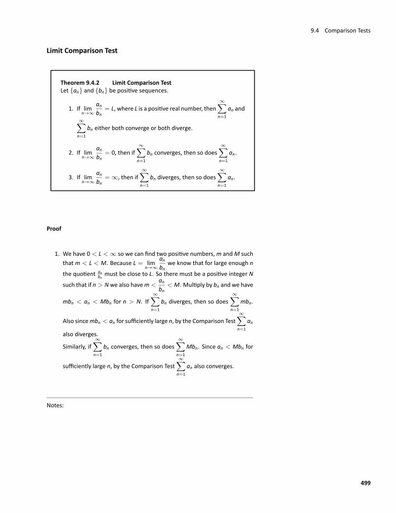
9.4 Comparison Tests
Limit Comparison Test
Theorem 9.4.2 Limit Comparison TestLet {an} and {bn} be positive sequences.
1. If limn→∞
anbn
= L, where L is a positive real number, then∞∑n=1
an and
∞∑n=1
bn either both converge or both diverge.
2. If limn→∞
anbn
= 0, then if∞∑n=1
bn converges, then so does∞∑n=1
an.
3. If limn→∞
anbn
= ∞, then if∞∑n=1
bn diverges, then so does∞∑n=1
an.
Proof
1. We have 0 < L < ∞ so we can find two positive numbers,m andM suchthatm < L < M. Because L = lim
n→∞
anbn
we know that for large enough n
the quotient anbn must be close to L. So there must be a positive integer N
such that if n > Nwe also havem <anbn
< M. Multiply by bn and we have
mbn < an < Mbn for n > N. If∞∑n=1
bn diverges, then so does∞∑n=1
mbn.
Also sincembn < an for sufficiently large n, by the Comparison Test∞∑n=1
an
also diverges.
Similarly, if∞∑n=1
bn converges, then so does∞∑n=1
Mbn. Since an < Mbn for
sufficiently large n, by the Comparison Test∞∑n=1
an also converges.
Notes:
499
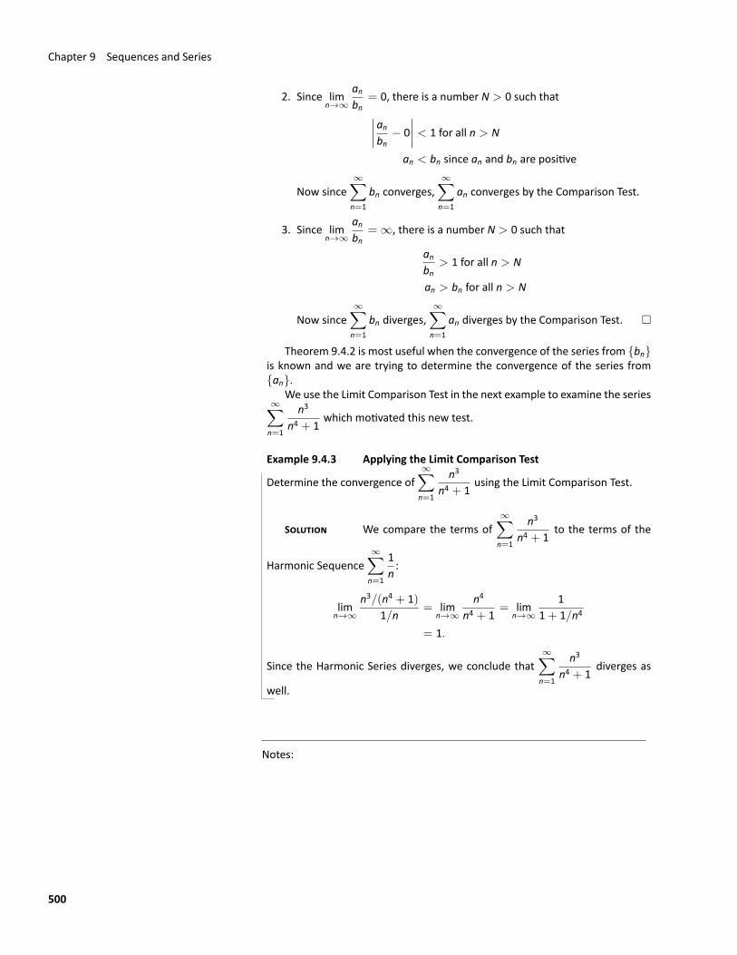
Chapter 9 Sequences and Series
2. Since limn→∞
anbn
= 0, there is a number N > 0 such that∣∣∣∣anbn − 0∣∣∣∣ < 1 for all n > N
an < bn since an and bn are positive
Now since∞∑n=1
bn converges,∞∑n=1
an converges by the Comparison Test.
3. Since limn→∞
anbn
= ∞, there is a number N > 0 such that
anbn
> 1 for all n > N
an > bn for all n > N
Now since∞∑n=1
bn diverges,∞∑n=1
an diverges by the Comparison Test. □
Theorem 9.4.2 is most useful when the convergence of the series from {bn}is known and we are trying to determine the convergence of the series from{an}.
We use the Limit Comparison Test in the next example to examine the series∞∑n=1
n3
n4 + 1which motivated this new test.
Example 9.4.3 Applying the Limit Comparison Test
Determine the convergence of∞∑n=1
n3
n4 + 1using the Limit Comparison Test.
SOLUTION We compare the terms of∞∑n=1
n3
n4 + 1to the terms of the
Harmonic Sequence∞∑n=1
1n:
limn→∞
n3/(n4 + 1)1/n
= limn→∞
n4
n4 + 1= lim
n→∞
11+ 1/n4
= 1.
Since the Harmonic Series diverges, we conclude that∞∑n=1
n3
n4 + 1diverges as
well.
Notes:
500
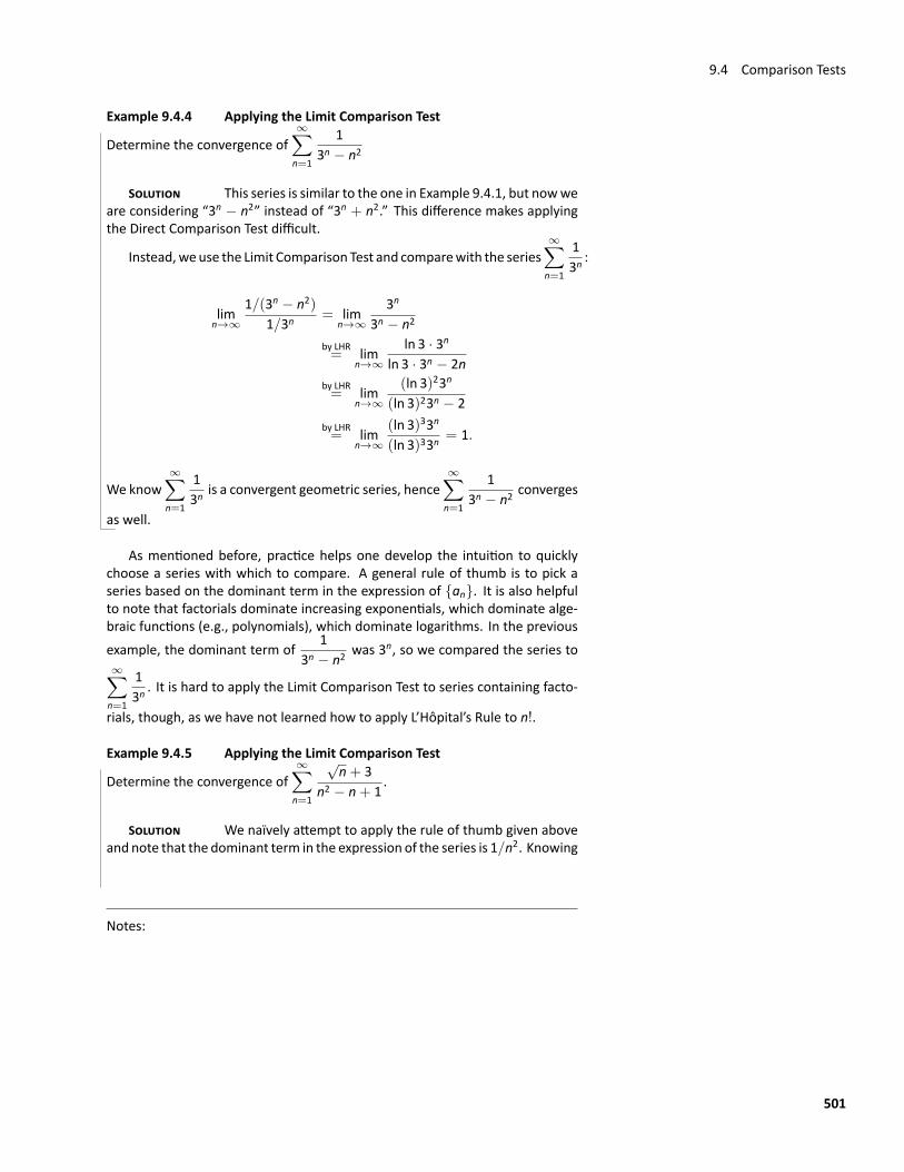
9.4 Comparison Tests
Example 9.4.4 Applying the Limit Comparison Test
Determine the convergence of∞∑n=1
13n − n2
SOLUTION This series is similar to the one in Example 9.4.1, but nowweare considering “3n − n2” instead of “3n + n2.” This difference makes applyingthe Direct Comparison Test difficult.
Instead, weuse the Limit Comparison Test and comparewith the series∞∑n=1
13n
:
limn→∞
1/(3n − n2)1/3n
= limn→∞
3n
3n − n2
by LHR= lim
n→∞
ln 3 · 3n
ln 3 · 3n − 2nby LHR= lim
n→∞
(ln 3)23n
(ln 3)23n − 2by LHR= lim
n→∞
(ln 3)33n
(ln 3)33n= 1.
We know∞∑n=1
13n
is a convergent geometric series, hence∞∑n=1
13n − n2
converges
as well.
As mentioned before, practice helps one develop the intuition to quicklychoose a series with which to compare. A general rule of thumb is to pick aseries based on the dominant term in the expression of {an}. It is also helpfulto note that factorials dominate increasing exponentials, which dominate alge‐braic functions (e.g., polynomials), which dominate logarithms. In the previousexample, the dominant term of
13n − n2
was 3n, so we compared the series to∞∑n=1
13n
. It is hard to apply the Limit Comparison Test to series containing facto‐
rials, though, as we have not learned how to apply L’Hôpital’s Rule to n!.
Example 9.4.5 Applying the Limit Comparison Test
Determine the convergence of∞∑n=1
√n+ 3
n2 − n+ 1.
SOLUTION We naïvely attempt to apply the rule of thumb given aboveand note that the dominant term in the expression of the series is 1/n2. Knowing
Notes:
501
Chapter 9 Sequences and Series
that∞∑n=1
1n2
converges, we attempt to apply the Limit Comparison Test:
limn→∞
(√n+ 3)/(n2 − n+ 1)
1/n2= lim
n→∞
n2(√n+ 3)
n2 − n+ 1= ∞ (Apply L’Hôpital’s Rule).
Theorem 9.4.2 part (3) only applies when∞∑n=1
bn diverges; in our case, it con‐
verges. Ultimately, our test has not revealed anything about the convergenceof our series.
The problem is that we chose a poor series with which to compare. Sincethe numerator and denominator of the terms of the series are both algebraicfunctions, we should have compared our series to the dominant term of thenumerator divided by the dominant term of the denominator.
The dominant term of the numerator is n1/2 and the dominant term of thedenominator is n2. Thus we should compare the terms of the given series ton1/2/n2 = 1/n3/2:
limn→∞
(√n+ 3)/(n2 − n+ 1)
1/n3/2= lim
n→∞
n3/2(√n+ 3)
n2 − n+ 1= 1 (Apply L’Hôpital’s Rule).
Since the p‐series∞∑n=1
1n3/2
converges, we conclude that∞∑n=1
√n+ 3
n2 − n+ 1con‐
verges as well.
The tests we have encountered so far have required that we analyze seriesfrom positive sequences (the absolute value of the ratio and the root tests ofsection 9.6 will convert the sequence into a positive sequence). The next sectionrelaxes this restriction by considering alternating series, where the underlyingsequence has terms that alternate between being positive and negative.
Notes:
502
Exercises 9.4Terms and Concepts
1. Suppose∞∑n=0
an is convergent, and there are sequences
{bn} and {cn} such that 0 ≤ bn ≤ an ≤ cn for all n. What
can be said about the series∞∑n=0
bn and∞∑n=0
cn?
2. Suppose∞∑n=0
an is divergent, and there are sequences {bn}
and {cn} such that 0 ≤ bn ≤ an ≤ cn for all n. What can
be said about the series∞∑n=0
bn and∞∑n=0
cn?
ProblemsIn Exercises 3–8, use the Direct Comparison Test to determinethe convergence of the given series; state what series is usedfor comparison.
3.∞∑n=1
1n2 + 3n− 5
4.∞∑n=1
14n + n2 − n
5.∞∑n=1
ln nn
6.∞∑n=1
1n! + n
7.∞∑n=2
1√n2 − 1
8.∞∑n=5
1√n− 2
In Exercises 9–14, use the Limit Comparison Test to determinethe convergence of the given series; state what series is usedfor comparison.
9.∞∑n=1
1n2 − 3n+ 5
10.∞∑n=1
14n − n2
11.∞∑n=4
ln nn− 3
12.∞∑n=1
1√n2 + n
13.∞∑n=1
1n+
√n
14.∞∑n=1
sin(1/n)
In Exercises 15–24, use the Direct Comparison Test or the LimitComparison Test to determine the convergence of the givenseries. State which series is used for comparison.
15.∞∑n=1
n2 + n+ 1n3 − 5
16.∞∑n=1
n− 10n2 + 10n+ 10
17.∞∑n=1
2n
5n + 10
18.∞∑n=1
n+ 5n3 − 5
19.∞∑n=1
nn4 + 1
20.∞∑n=1
n− 1n4n
21.∞∑n=2
nn2 − 1
22.∞∑n=1
1√n+ 100
23.∞∑n=2
1n2 ln n
24.∞∑n=1
√n+ 3
n2 + 17
In Exercises 25–32, determine the convergence of the givenseries. State the test used; more than one test may be appro‐priate.
25.∞∑n=1
n2
2n
26.∞∑n=1
1(2n+ 5)3
27.∞∑n=1
n!10n
28.∞∑n=1
ln nn!
29.∞∑n=1
13n + n
30.∞∑n=1
n− 210n+ 5
31.∞∑n=1
3n
n3
32.∞∑n=1
cos(1/n)√n
503
33. Given that∞∑n=1
an converges, state which of the following
series converges, may converge, or does not converge.
(a)∞∑n=1
ann
(b)∞∑n=1
anan+1
(c)∞∑n=1
(an)2
(d)∞∑n=1
nan
(e)∞∑n=1
1an
504
9.5 Alternating Series and Absolute Convergence
9.5 Alternating Series and Absolute ConvergenceThe series convergence tests we have used require that the underlying sequence{an} be a positive sequence. (We can relax this with Theorem 9.2.5 and statethat there must be an N > 0 such that an > 0 for all n > N; that is, {an} ispositive for all but a finite number of values of n.)
In this section we explore series whose summation includes negative terms.We start with a very specific form of series, where the terms of the summationalternate between being positive and negative.
Definition 9.5.1 Alternating SeriesLet {bn} be a positive sequence. An alternating series is a series ofeither the form
∞∑n=1
(−1)nbn or∞∑n=1
(−1)n+1bn.
We want to think that an alternating sequence {an} is related to a positivesequence {bn} by an = (−1)nbn.
Recall the termsofHarmonic Series come from theHarmonic Sequence {bn} ={1/n}. An important alternating series is the Alternating Harmonic Series:
∞∑n=1
(−1)n+1 1n= 1− 1
2+
13− 1
4+
15− 1
6+ · · ·
Geometric Series can also be alternating series when r < 0. For instance, ifr = −1/2, the geometric series is
∞∑n=0
(−12
)n
= 1− 12+
14− 1
8+
116
− 132
+ · · ·
Theorem 9.2.1 states that geometric series converge when |r| < 1 and gives
the sum:∞∑n=0
rn =1
1− r. When r = −1/2 as above, we find
∞∑n=0
(−12
)n
=1
1− (−1/2)=
13/2
=23.
Apowerful convergence theoremexists for other alternating series thatmeeta few conditions.
Notes:
505
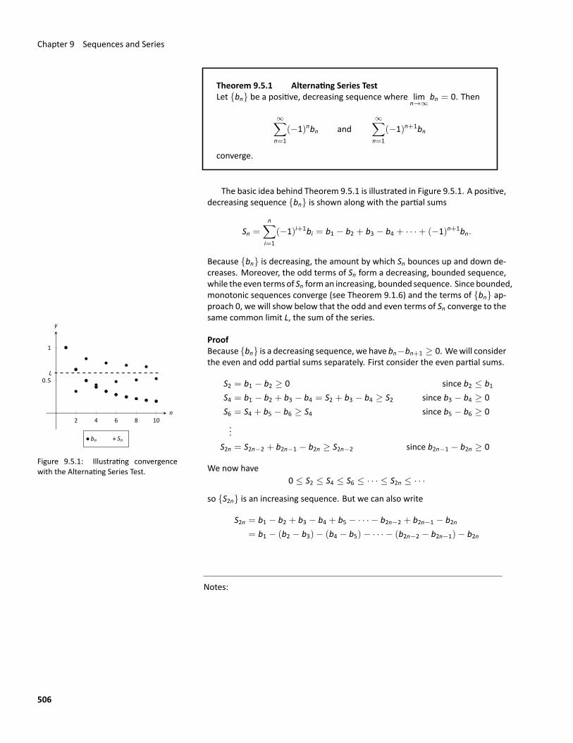
Chapter 9 Sequences and Series
Theorem 9.5.1 Alternating Series TestLet {bn} be a positive, decreasing sequence where lim
n→∞bn = 0. Then
∞∑n=1
(−1)nbn and∞∑n=1
(−1)n+1bn
converge.
The basic idea behind Theorem 9.5.1 is illustrated in Figure 9.5.1. A positive,decreasing sequence {bn} is shown along with the partial sums
Sn =n∑
i=1
(−1)i+1bi = b1 − b2 + b3 − b4 + · · ·+ (−1)n+1bn.
Because {bn} is decreasing, the amount by which Sn bounces up and down de‐creases. Moreover, the odd terms of Sn form a decreasing, bounded sequence,while the even termsof Sn forman increasing, bounded sequence. Since bounded,monotonic sequences converge (see Theorem 9.1.6) and the terms of {bn} ap‐proach 0, we will show below that the odd and even terms of Sn converge to thesame common limit L, the sum of the series.
L
2 4 6 8 10
0.5
1
n
y
bn Sn
Figure 9.5.1: Illustrating convergencewith the Alternating Series Test.
ProofBecause {bn} is a decreasing sequence, we have bn−bn+1 ≥ 0. Wewill considerthe even and odd partial sums separately. First consider the even partial sums.
S2 = b1 − b2 ≥ 0 since b2 ≤ b1S4 = b1 − b2 + b3 − b4 = S2 + b3 − b4 ≥ S2 since b3 − b4 ≥ 0S6 = S4 + b5 − b6 ≥ S4 since b5 − b6 ≥ 0...
S2n = S2n−2 + b2n−1 − b2n ≥ S2n−2 since b2n−1 − b2n ≥ 0
We now have0 ≤ S2 ≤ S4 ≤ S6 ≤ · · · ≤ S2n ≤ · · ·
so {S2n} is an increasing sequence. But we can also write
S2n = b1 − b2 + b3 − b4 + b5 − · · · − b2n−2 + b2n−1 − b2n= b1 − (b2 − b3)− (b4 − b5)− · · · − (b2n−2 − b2n−1)− b2n
Notes:
506
9.5 Alternating Series and Absolute Convergence
Each term in parentheses is positive and b2n is positive so we have S2n ≤ b1for all n. We now have the sequence of even partial sums, {S2n}, is increasingand bounded above so by Theorem 9.1.6 {S2n} converges. Since we know itconverges, we will assume it’s limit is L or
limn→∞
S2n = L
Next we determine the limit of the sequence of odd partial sums.
limn→∞
S2n+1 = limn→∞
(S2n + b2n+1)
= limn→∞
S2n + limn→∞
b2n+1
= L+ 0= L
Both the even and odd partial sums converge to L so we have limn→∞
Sn = L, whichmeans the series is convergent. □
Watch the video:Alternating Series — Another Example 4 athttps://youtu.be/aOiZvfFAMW8
Example 9.5.1 Applying the Alternating Series TestDetermine if the Alternating Series Test applies to each of the following series.
1.∞∑n=1
(−1)n+1 1n
2.∞∑n=2
(−1)nln nn
3.∞∑n=1
(−1)n+1 |sin n|n2
SOLUTION
1. This is the Alternating Harmonic Series as seen previously. The underlyingsequence is {bn} = {1/n}, which is positive, decreasing, and approaches0 as n → ∞. Therefore we can apply the Alternating Series Test andconclude this series converges.While the test does not state what the series converges to, we will see
later that∞∑n=1
(−1)n+1 1n= ln 2.
Notes:
507
Chapter 9 Sequences and Series
2. The underlying sequence is {bn} = {(ln n)/n}. This is positive for n ≥ 2
and limn→∞
ln nn
= limn→∞
1n
= 0 (use L’Hôpital’s Rule). However, the se‐quence is not decreasing for all n. It is straightforward to compute b1 ≈0.347, b2 ≈ 0.366, and b3 ≈ 0.347: the sequence is increasing for at leastthe first 2 terms.
We do not immediately conclude that we cannot apply the AlternatingSeries Test. Rather, consider the long‐term behavior of {bn}. Treatingbn = b(n) as a continuous function of n defined on [2,∞), we can takeits derivative:
b ′(n) =1− ln n
n2.
The derivative is negative for all n ≥ 3 (actually, for all n > e), mean‐ing b(n) = bn is decreasing on [3,∞). We can apply the AlternatingSeries Test to the series when we start with n = 3 and conclude that∞∑n=3
(−1)nln nn
converges; adding the terms with n = 2 does not change
the convergence (i.e., we apply Theorem 9.2.5).
The important lesson here is that as before, if a series fails to meet thecriteria of the Alternating Series Test on only a finite number of terms, wecan still apply the test.
3. The underlying sequence is {bn} = {|sin n| /n2}. This sequence is positiveand approaches 0 as n → ∞. However, it is not a decreasing sequence;the value of |sin n| oscillates between 0 and 1 as n → ∞. We cannotremove a finite number of terms to make {bn} decreasing, therefore wecannot apply the Alternating Series Test.
Keep in mind that this does not mean we conclude the series diverges;in fact, it does converge. We are just unable to conclude this based onTheorem 9.5.1.
One of the famous results of mathematics is that the Harmonic Series,∞∑n=1
1n
diverges, yet the Alternating Harmonic Series,∞∑n=1
(−1)n+1 1n, converges. The
notion that alternating the signs of the terms in a series can make a series con‐verge leads us to the following definitions.
Notes:
508
9.5 Alternating Series and Absolute Convergence
Definition 9.5.2 Absolute and Conditional Convergence
1. A series∞∑n=1
an converges absolutely if∞∑n=1
|an| converges.
2. A series∞∑n=1
an converges conditionally if∞∑n=1
an converges but
∞∑n=1
|an| diverges.
Note: In Definition 9.5.2,∞∑n=1
an is
not necessarily an alternating series;it justmay have some negative terms.
Thus we say the Alternating Harmonic Series converges conditionally.
Example 9.5.2 Determining absolute and conditional convergence.Determine if the following series converge absolutely, conditionally, or diverge.
1.∞∑n=1
(−1)nn+ 3
n2 + 2n+ 52.
∞∑n=3
(−1)n3n− 35n− 10
SOLUTION
1. We can show the series∞∑n=1
∣∣∣∣(−1)nn+ 3
n2 + 2n+ 5
∣∣∣∣ = ∞∑n=1
n+ 3n2 + 2n+ 5
diverges using the Limit Comparison Test, comparing with 1/n.
The sequence { n+ 3n2 + 2n+ 5
} is monotonically decreasing, so that the se‐
ries∞∑n=1
(−1)nn+ 3
n2 + 2n+ 5converges using the Alternating Series Test; we
conclude it converges conditionally.
2. The series∞∑n=3
∣∣∣∣(−1)n3n− 35n− 10
∣∣∣∣ = ∞∑n=3
3n− 35n− 10
diverges using the Test for Divergence, so it does not converge absolutely.
The series∞∑n=3
(−1)n3n− 35n− 10
fails the conditions of the Alternating Series
Test as (3n− 3)/(5n− 10) does not approach 0 as n → ∞. We can state
Notes:
509
Chapter 9 Sequences and Series
further that this series diverges; as n → ∞, the series effectively adds andsubtracts 3/5 over and over. This causes the sequence of partial sums tooscillate and not converge.
Therefore the series∞∑n=1
(−1)n3n− 35n− 10
diverges.
Knowing that a series converges absolutely allows us to make two impor‐tant statements, given in the following theorem. The first is that absolute con‐
vergence is “stronger” than regular convergence. That is, just because∞∑n=1
an
converges, we cannot conclude that∞∑n=1
|an| will converge, but knowing a series
converges absolutely tells us that∞∑n=1
an will converge.
Theorem 9.5.2 Absolute Convergence Theorem
Let∞∑n=1
an be a series that converges absolutely.
1.∞∑n=1
an converges.
2. Let {bn} be any rearrangement of the sequence {an}. Then
∞∑n=1
bn =∞∑n=1
an.
One reason this is important is that our convergence tests all require that theunderlying sequence of terms be positive. By taking the absolute value of theterms of a series where not all terms are positive, we are often able to apply anappropriate test and determine absolute convergence. This, in turn, determinesthat the series we are given also converges.
The second statement relates to rearrangements of series. When dealingwith a finite set of numbers, the sum of the numbers does not depend on theorder which they are added. (So 1+2+3 = 3+1+2.) Onemay be surprised tofind out that when dealing with an infinite set of numbers, the same statementdoes not always hold true: some infinite lists of numbers may be rearranged indifferent orders to achieve different sums. The theorem states that the terms of
Notes:
510
9.5 Alternating Series and Absolute Convergence
an absolutely convergent series can be rearranged in any way without affectingthe sum.
The theorem states that rearranging the terms of an absolutely convergentseries does not affect its sum. This implies that perhaps the sum of a condition‐ally convergent series can change based on the arrangement of terms. Indeed,it can. The Riemann Rearrangement Theorem (named after Bernhard Riemann)states that any conditionally convergent series can have its terms rearranged sothat the sum is any desired value or infinity.
Before we consider an example, we state the following theorem that illus‐trates how the alternating structure of an alternating series is a powerful toolwhen approximating the sum of a convergent series.
Theorem 9.5.3 The Alternating Series Approximation TheoremLet {bn} be a sequence that satisfies the hypotheses of the AlternatingSeries Test, and let Sn and L be the nth partial sum and sum, respectively,
of either∞∑n=1
(−1)nbn or∞∑n=1
(−1)n+1bn. Then
1. |Sn − L| < bn+1, and
2. L is between Sn and Sn+1.
Part 1 of Theorem 9.5.3 states that the nth partial sum of a convergent al‐ternating series will be within bn+1 of its total sum. Consider the alternating
series we looked at before the statement of the theorem,∞∑n=1
(−1)n+1
n2. Since
b14 = 1/142 ≈ 0.0051, we know that S13 is within 0.0051 of the total sum.Moreover, Part 2 of the theorem states that since S13 ≈ 0.8252 and S14 ≈
0.8201, we know the sum L lies between 0.8201 and 0.8252. One use of this isthe knowledge that S14 is accurate to two places after the decimal.
Some alternating series converge slowly. In Example 9.5.1 we determined
the series∞∑n=2
(−1)n+1 ln nn
converged. With n = 1001, we find (ln n)/n ≈
0.0069, meaning that S1000 ≈ 0.1633 is accurate to one, maybe two, places afterthe decimal. Since S1001 ≈ 0.1564, we know the sum L is 0.1564 ≤ L ≤ 0.1633.
Example 9.5.3 Approximating the sums of convergent alternating seriesApproximate the sum of the following series, accurate to within 0.001.
1.∞∑n=1
(−1)n+1 1n3
2.∞∑n=1
(−1)n+1 ln nn
.
Notes:
511
Chapter 9 Sequences and Series
SOLUTION
1. Using Theorem 9.5.3, we want to find n where 1/n3 ≤ 0.001:
1n3
≤ 0.001 =1
1000n3 ≥ 1000
n ≥ 3√1000
n ≥ 10.
Let L be the sum of this series. By Part 1 of the theorem, |S9 − L| < b10 =1/1000. We can compute S9 = 0.902116, which our theorem states iswithin 0.001 of the total sum.We can use Part 2 of the theorem to obtain an even more accurate result.Aswe know the 10th termof the series is−1/1000, we can easily computeS10 = 0.901116. Part 2 of the theorem states that L is between S9 and S10,so 0.901116 < L < 0.902116.
2. Wewant to find nwhere (ln n)/n ≤ 0.001. We start by solving (ln n)/n =0.001 for n. This cannot be solved algebraically, so we will use Newton’sMethod to approximate a solution.Let f(x) = ln(x)/x− 0.001; we want to know where f(x) = 0. We make aguess that xmust be “large,” so our initial guess will be x1 = 1000. Recallhow Newton’s Method works: given an approximate solution xn, our nextapproximation xn+1 is given by
xn+1 = xn −f(xn)f ′(xn)
.
We find f ′(x) =(1− ln(x)
)/x2. This gives
x2 = 1000− ln(1000)/1000− 0.001(1− ln(1000)
)/10002
= 2000.
Using a computer, we find that Newton’s Method seems to converge to asolution x = 9118.01 after 8 iterations. Taking the next integer higher, wehave n = 9119, where ln(9119)/9119 = 0.000999903 < 0.001.Again using a computer, we find S9118 = −0.160369. Part 1 of the theo‐rem states that this is within 0.001 of the actual sum L. Already knowingthe 9,119th term, we can compute S9119 = −0.159369, meaning
−0.160369 < L < −0.159369.
Notes:
512
9.5 Alternating Series and Absolute Convergence
Notice how the first series converged quite quickly, where we needed only 10terms to reach the desired accuracy, whereas the second series took over 9,000terms.
We now consider the Alternating Harmonic Series once more. We havestated that
∞∑n=1
(−1)n+1 1n= 1− 1
2+
13− 1
4+
15− 1
6+
17· · · = ln 2,
(see Example 9.5.1).Consider the rearrangement where every positive term is followed by two
negative terms:
1− 12− 1
4+
13− 1
6− 1
8+
15− 1
10− 1
12· · ·
(Convince yourself that these are exactly the same numbers as appear in theAlternating Harmonic Series, just in a different order.) Now group some termsand simplify:(
1− 12
)− 1
4+
(13− 1
6
)− 1
8+
(15− 1
10
)− 1
12+ · · · =
12− 1
4+
16− 1
8+
110
− 112
+ · · · =
12
(1− 1
2+
13− 1
4+
15− 1
6+ · · ·
)=
12ln 2.
By rearranging the terms of the series, we have arrived at a different sum.(One could try to argue that the Alternating Harmonic Series does not actuallyconverge to ln 2, because rearranging the terms of the series shouldn’t changethe sum. However, the Alternating Series Test proves this series converges to L,for some number L, and if the rearrangement does not change the sum, thenL = L/2, implying L = 0. But the Alternating Series Approximation Theoremquickly shows that L > 0. The only conclusion is that the rearrangement didchange the sum.) This is an incredible result.
We mentioned earlier that the Integral Test did not work well with seriescontaining factorial terms. The next section introduces the Ratio Test, whichdoes handle such series well. We also introduce the Root Test, which is good forseries where each term is raised to a power.
Notes:
513
Exercises 9.5Terms and Concepts
1. Why is∞∑n=1
sin n not an alternating series?
2. A series∞∑n=1
(−1)nan convergeswhen {an} is ,
and limn→∞
an = .
3. Give an example of a series where∞∑n=0
an converges but∞∑n=0
|an| does not.
4. The sum of a convergent series can be changed byrearranging the order of its terms.
Problems
In Exercises 5–18, an alternating series∞∑n=i
an is given.
(a) Determine if the series converges or diverges.
(b) Determine if∞∑n=0
|an| converges or diverges.
(c) If∞∑n=0
an converges, determine if the convergence is
conditional or absolute.
5.∞∑n=1
(−1)n+1
n2
6.∞∑n=0
(−e)−n
7.∞∑n=0
(−1)n n+ 53n− 5
8.∞∑n=1
(−1)n 2n
n2
9.∞∑n=0
(−1)n+1 3n+ 5n2 − 3n+ 1
10.∞∑n=1
(−1)n
ln n+ 1
11.∞∑n=2
(−1)n nln n
12.∞∑n=1
(−1)n+1
1+ 3+ 5+ · · ·+ (2n− 1)
13.∞∑n=1
cos(πn)
14.∞∑n=2
sin((n+ 1/2)π
)n ln n
15.∞∑n=0
(−23
)n
16.∞∑n=0
(−1)n2−n2
17.∞∑n=1
(−1)n√n
18.∞∑n=2
(−1)n
n(ln n)2
Let Sn be the nth partial sum of a series. In Exercises 19–22, aconvergent alternating series is given and a value of n. Com‐pute Sn and Sn+1 and use these values to find bounds on thesum of the series.
19.∞∑n=1
(−1)n
ln(n+ 1), n = 5
20.∞∑n=1
(−1)n+1
n4, n = 4
21.∞∑n=0
(−1)n
n!, n = 6
22.∞∑n=0
(−12
)n
, n = 9
In Exercises 23–26, a convergent alternating series is givenalong with its sum and a value of ε. Use Theorem 9.5.3 to findn such that the nth partial sum of the series is within ε of thesum of the series.
23.∞∑n=1
(−1)n+1
n4=
7π4
720, ε = 0.001
24.∞∑n=0
(−1)n
n!=
1e, ε = 0.0001
25.∞∑n=0
(−1)n
2n+ 1=
π
4, ε = 0.001
26.∞∑n=0
(−1)n
(2n)!= cos 1, ε = 10−8
514
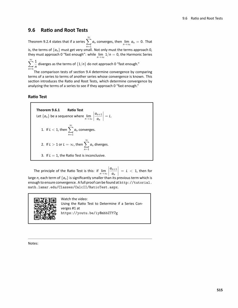
9.6 Ratio and Root Tests
9.6 Ratio and Root Tests
Theorem 9.2.4 states that if a series∞∑n=1
an converges, then limn→∞
an = 0. That
is, the terms of {an}must get very small. Not only must the terms approach 0,they must approach 0 “fast enough”: while lim
n→∞1/n = 0, the Harmonic Series
∞∑n=1
1ndiverges as the terms of {1/n} do not approach 0 “fast enough.”
The comparison tests of section 9.4 determine convergence by comparingterms of a series to terms of another series whose convergence is known. Thissection introduces the Ratio and Root Tests, which determine convergence byanalyzing the terms of a series to see if they approach 0 “fast enough.”
Ratio Test
Theorem 9.6.1 Ratio TestLet {an} be a sequence where lim
n→∞
∣∣∣∣an+1
an
∣∣∣∣ = L.
1. If L < 1, then∞∑n=1
an converges.
2. If L > 1 or L = ∞, then∞∑n=1
an diverges.
3. If L = 1, the Ratio Test is inconclusive.
The principle of the Ratio Test is this: if limn→∞
∣∣∣∣an+1
an
∣∣∣∣ = L < 1, then for
large n, each term of {an} is significantly smaller than its previous term which isenough to ensure convergence. A full proof canbe found athttp://tutorial.math.lamar.edu/Classes/CalcII/RatioTest.aspx.
Watch the video:Using the Ratio Test to Determine if a Series Con‐verges #1 athttps://youtu.be/iy8mhbZTY7g
Notes:
515
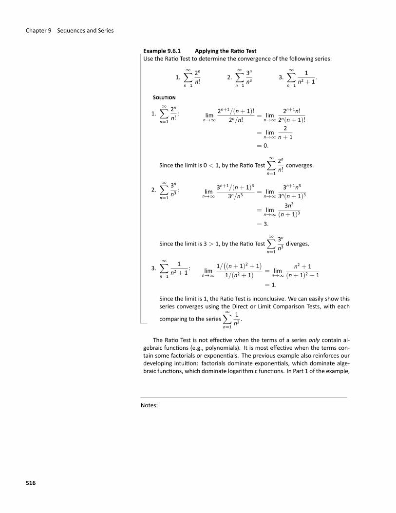
Chapter 9 Sequences and Series
Example 9.6.1 Applying the Ratio TestUse the Ratio Test to determine the convergence of the following series:
1.∞∑n=1
2n
n!2.
∞∑n=1
3n
n33.
∞∑n=1
1n2 + 1
.
SOLUTION
1.∞∑n=1
2n
n!: lim
n→∞
2n+1/(n+ 1)!2n/n!
= limn→∞
2n+1n!2n(n+ 1)!
= limn→∞
2n+ 1
= 0.
Since the limit is 0 < 1, by the Ratio Test∞∑n=1
2n
n!converges.
2.∞∑n=1
3n
n3: lim
n→∞
3n+1/(n+ 1)3
3n/n3= lim
n→∞
3n+1n3
3n(n+ 1)3
= limn→∞
3n3
(n+ 1)3
= 3.
Since the limit is 3 > 1, by the Ratio Test∞∑n=1
3n
n3diverges.
3.∞∑n=1
1n2 + 1
: limn→∞
1/((n+ 1)2 + 1
)1/(n2 + 1)
= limn→∞
n2 + 1(n+ 1)2 + 1
= 1.
Since the limit is 1, the Ratio Test is inconclusive. We can easily show thisseries converges using the Direct or Limit Comparison Tests, with each
comparing to the series∞∑n=1
1n2
.
The Ratio Test is not effective when the terms of a series only contain al‐gebraic functions (e.g., polynomials). It is most effective when the terms con‐tain some factorials or exponentials. The previous example also reinforces ourdeveloping intuition: factorials dominate exponentials, which dominate alge‐braic functions, which dominate logarithmic functions. In Part 1 of the example,
Notes:
516
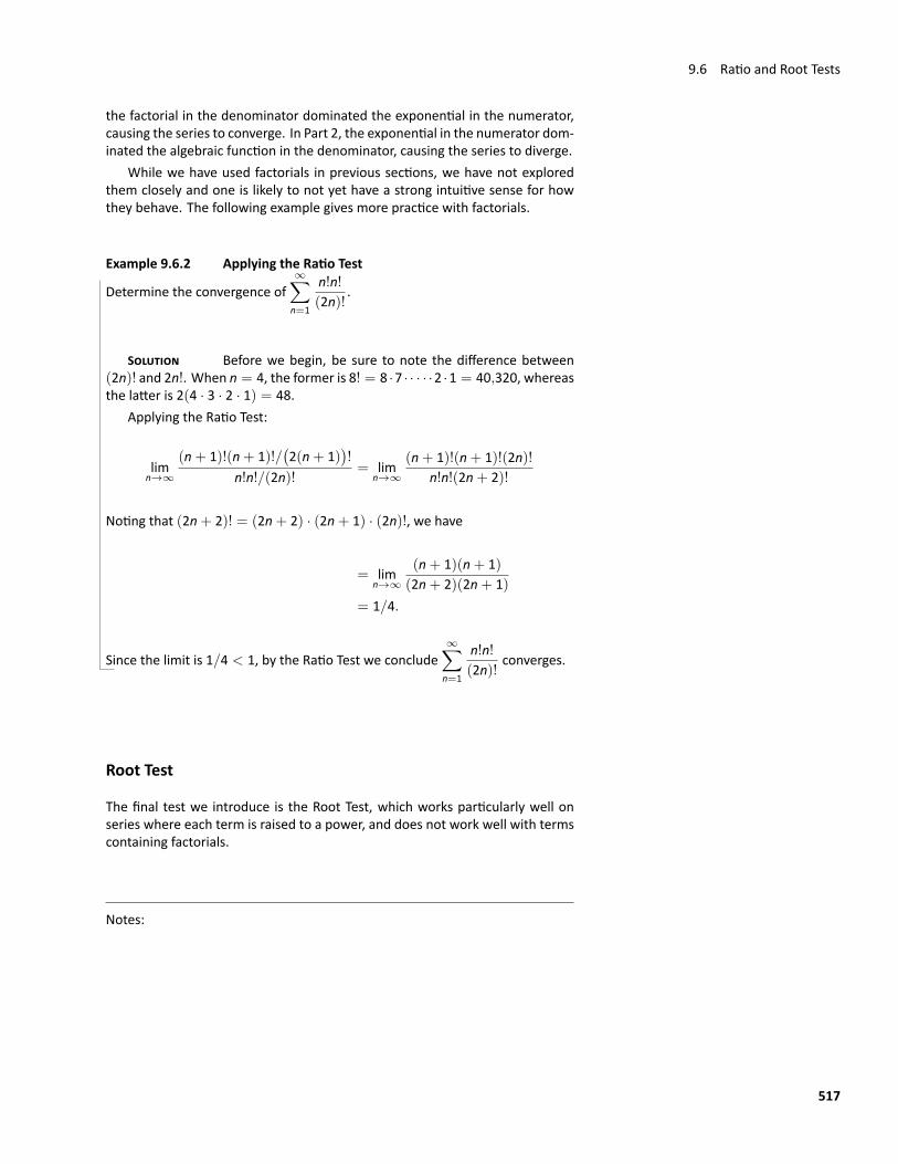
9.6 Ratio and Root Tests
the factorial in the denominator dominated the exponential in the numerator,causing the series to converge. In Part 2, the exponential in the numerator dom‐inated the algebraic function in the denominator, causing the series to diverge.
While we have used factorials in previous sections, we have not exploredthem closely and one is likely to not yet have a strong intuitive sense for howthey behave. The following example gives more practice with factorials.
Example 9.6.2 Applying the Ratio Test
Determine the convergence of∞∑n=1
n!n!(2n)!
.
SOLUTION Before we begin, be sure to note the difference between(2n)! and 2n!. When n = 4, the former is 8! = 8 ·7 · · · · ·2 ·1 = 40,320, whereasthe latter is 2(4 · 3 · 2 · 1) = 48.
Applying the Ratio Test:
limn→∞
(n+ 1)!(n+ 1)!/(2(n+ 1)
)!
n!n!/(2n)!= lim
n→∞
(n+ 1)!(n+ 1)!(2n)!n!n!(2n+ 2)!
Noting that (2n+ 2)! = (2n+ 2) · (2n+ 1) · (2n)!, we have
= limn→∞
(n+ 1)(n+ 1)(2n+ 2)(2n+ 1)
= 1/4.
Since the limit is 1/4 < 1, by the Ratio Test we conclude∞∑n=1
n!n!(2n)!
converges.
Root Test
The final test we introduce is the Root Test, which works particularly well onseries where each term is raised to a power, and does not work well with termscontaining factorials.
Notes:
517
Chapter 9 Sequences and Series
Theorem 9.6.2 Root TestLet {an} be a sequence where lim
n→∞|an|1/n = L.
1. If L < 1, then∞∑n=1
an converges.
2. If L > 1 or L = ∞, then∞∑n=1
an diverges.
3. If L = 1, the Root Test is inconclusive.
Example 9.6.3 Applying the Root TestDetermine the convergence of the following series using the Root Test:
1.∞∑n=1
(3n+ 15n− 2
)n
2.∞∑n=2
n4
(ln n)n3.
∞∑n=1
2n
n2.
SOLUTION
1. limn→∞
((3n+ 15n− 2
)n)1/n
= limn→∞
3n+ 15n− 2
=35.
Since the limit is less than 1, we conclude the series converges. Note: it isdifficult to apply the Ratio Test to this series.
2. limn→∞
(n4
(ln n)n
)1/n
= limn→∞
(n1/n
)4ln n
.
As n grows, the numerator approaches 1 (apply L’Hôpital’s Rule) and thedenominator grows to infinity. Thus
limn→∞
(n1/n
)4ln n
= 0.
Since the limit is less than 1, we conclude the series converges.
3. limn→∞
(2n
n2
)1/n
= limn→∞
2(n1/n
)2 = 2.
Since this is greater than 1, we conclude the series diverges.
Notes:
518

9.6 Ratio and Root Tests
We end here our study of tests to determine convergence. The next sec‐tion of this text provides strategies for testing series, while the back of the bookcontains a table summarizing the tests that one may find useful.
While series are worthy of study in and of themselves, our ultimate goalwithin calculus is the study of Power Series, whichwewill consider in section 9.8.We will use power series to create functions where the output is the result ofan infinite summation.
Notes:
519
Exercises 9.6Terms and Concepts1. The Ratio Test is not effective when the terms of a se‐
quence only contain functions.2. The Ratio Test is most effective when the terms of a se‐
quence contains and/or functions.3. What three convergence tests do not work well with terms
containing factorials?4. The Root Test works particularly well on series where each
term is to a .
ProblemsIn Exercises 5–16, determine the convergence of the given se‐ries using the Ratio Test. If the Ratio Test is inconclusive, stateso and determine convergence with another test.
5.∞∑n=0
2nn!
6.∞∑n=0
5n − 3n4n
7.∞∑n=0
n!10n
(2n)!
8.∞∑n=1
5n + n4
7n + n2
9.∞∑n=1
1n
10.∞∑n=1
13n3 + 7
11.∞∑n=1
10 · 5n
7n − 3
12.∞∑n=1
n ·(35
)n
13.∞∑n=1
2 · 4 · 6 · 8 · · · 2n3 · 6 · 9 · 12 · · · 3n
14.∞∑n=1
n!5 · 10 · 15 · · · (5n)
15.∞∑n=1
e−nn!
16.∞∑n=1
e1/n
n3
In Exercises 17–26, determine the convergence of the given se‐ries using the Root Test. If the Root Test is inconclusive, stateso and determine convergence with another test.
17.∞∑n=1
(2n+ 53n+ 11
)n
18.∞∑n=1
(.9n2 − n− 3n2 + n+ 3
)n
19.∞∑n=1
2nn2
3n
20.∞∑n=1
1nn
21.∞∑n=1
3n
n22n+1
22.∞∑n=1
4n+7
7n
23.∞∑n=1
(n2 − nn2 + n
)n
24.∞∑n=1
(1n− 1
n2
)n
25.∞∑n=2
1(ln n)n
26.∞∑n=2
n2(ln n)n
520
9.7 Strategy for Testing Series
9.7 Strategy for Testing SeriesWe have now covered all of the tests for determining the convergence or diver‐gence of a series, which we summarize here. Because more than one test mayapply to a given series, you should always go completely through the guidelinesand identify all possible tests that you can use. Once you’ve done this, you canidentify the test that will be the easiest for you to use.
1. With a quick glance does it look like the series terms don’t converge tozero in the limit, i.e. does lim
n→∞an ̸= 0? If so, use the Test for Divergence.
Note that you should only use the Test for Divergence if a quick glancesuggests that the series terms may not converge to zero in the limit.
2. Is the series a p‐series(∑
n−p)or a geometric series
(∑arn)? If so,
use the fact that p‐series will converge only if p > 1 and a geometric serieswill only converge if |r| < 1. Remember as well that often some algebraicmanipulation is required to get a geometric series into the correct form.
3. Is the series similar to a p‐series or a geometric series? If so, try the Com‐parison Test.
4. Is the series a rational expression involving only polynomials or polynomi‐als under radicals? If so, try the Comparison test or the Limit ComparisonTest. Remember however, that in order to use the Comparison Test andthe Limit Comparison Test the series terms all need to be positive.
5. Is the series of the form∑
(−1)nan? If so, then the Alternating SeriesTest may work.
6. Does the series contain factorials or constants raised to powers involvingn? If so, then the Ratio Testmaywork. Note that if the series term containsa factorial then the only test that we have that will work is the Ratio Test.
7. Can the series terms be written in the form an = (bn)n? If so, then theRoot Test may work.
8. If an = f(n) for some positive, decreasing function and∫ ∞
af(x) dx is easy
to evaluate then the Integral Test may work.
Again, remember that these are only a set of guidelines and not a set of hardand fast rules to use when trying to determine the best test to use on a series.If more that one test can be used, try to use the test that will be the easiest foryou to use. These guidelines are also summarized in a table in the back of thebook.
We now consider several examples.
Notes:
521
Chapter 9 Sequences and Series
Example 9.7.1 Testing SeriesDetermine whether the given series converges absolutely, converges condition‐ally, or diverges.
1.∞∑n=2
(−1)nnn2 + 3
2.∞∑n=1
n2 − 3n4n2 − 2n+ 1
3.∞∑n=2
en
(n+ 3)!
SOLUTION
1. We see that this series is alternating so we use the alternating series test.The underlying sequence is {an} = { n
n2+3}which is positive and decreas‐
ing since a′(n) =3− n2
(n2 + 3)2< 0 for n ≥ 2. We also see lim
n→∞
nn2 + 3
=
0 so by the Alternating Series Test∞∑n=2
(−1)nnn2 + 3
converges. We now de‐
termine if it converges absolutely. Consider the series∞∑n=2
∣∣∣∣ (−1)nnn2 + 3
∣∣∣∣ =∞∑n=2
nn2 + 3
. Using the Limit Comparison Test with the divergent p‐series
∞∑n=2
nn2
=
∞∑n=2
1n,
∞∑n=2
nn2 + 3
diverges. Therefore,∞∑n=2
(−1)nnn2 + 3
converges
conditionally.
2. limn→∞
n2 − 3n4n2 − 2n+ 1
=14so by the Test for Divergence
∞∑n=1
n2 − 3n4n2 − 2n+ 1
diverges.
3. We see the factorial and use the Ratio Test. All terms of the series are
Notes:
522
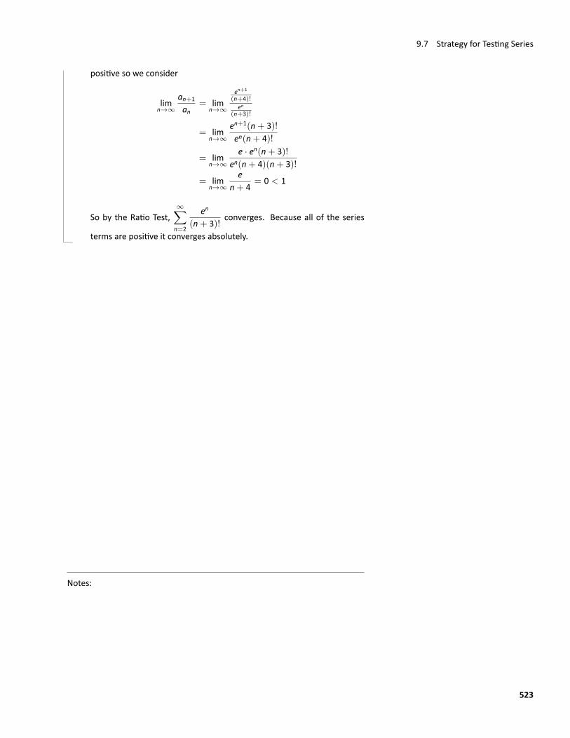
9.7 Strategy for Testing Series
positive so we consider
limn→∞
an+1
an= lim
n→∞
en+1
(n+4)!en
(n+3)!
= limn→∞
en+1(n+ 3)!en(n+ 4)!
= limn→∞
e · en(n+ 3)!en(n+ 4)(n+ 3)!
= limn→∞
en+ 4
= 0 < 1
So by the Ratio Test,∞∑n=2
en
(n+ 3)!converges. Because all of the series
terms are positive it converges absolutely.
Notes:
523
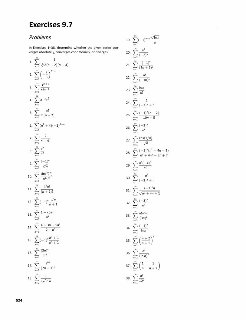
Exercises 9.7Problems
In Exercises 1–38, determine whether the given series con‐verges absolutely, converges conditionally, or diverges.
1.∞∑n=1
13√
n(n+ 2)(n+ 4)
2.∞∑n=1
(−23
)n−1
3.∞∑n=1
32n+1
n5n−1
4.∞∑n=1
n−2e1n
5.∞∑n=1
n!ln(n+ 2)
6.∞∑n=1
(n2 + 4)(−2)1−n
7.∞∑n=1
2n+ 4n
8.∞∑n=1
en
ne
9.∞∑n=1
(−1)n4√n
10.∞∑n=1
sin( 4πn3 )
n4π/3
11.∞∑n=1
3nn!(n+ 2)!
12.∞∑n=1
(−1)n√n
n+ 1
13.∞∑n=1
1− cos nn3
14.∞∑n=1
4+ 3n− 5n3
2+ n3
15.∞∑n=1
(−1)n n2 + 1
n4 + 1
16.∞∑n=1
(3n)n
n3n
17.∞∑n=1
e2n
(2n− 1)!
18.∞∑n=2
1n√ln n
19.∞∑n=2
(−1)n−1√ln nn
20.∞∑n=1
n2
(−2)n
21.∞∑n=1
(−1)n
(2n+ 5)3
22.∞∑n=1
n!(−10)n
23.∞∑n=1
ln nn!
24.∞∑n=1
1(−3)n + n
25.∞∑n=1
(−1)n(n− 2)10n+ 5
26.∞∑n=1
(−3)n
n3
27.∞∑n=1
cos(1/n)√n
28.∞∑n=1
(−1)n(n2 + 4n− 2)n3 + 4n2 − 3n+ 7
29.∞∑n=1
n4(−4)n
n!
30.∞∑n=1
n2
(−3)n + n
31.∞∑n=1
(−1)nn√n2 + 4n+ 1
32.∞∑n=1
(−3)n
nn
33.∞∑n=1
n!n!n!(3n)!
34.∞∑n=2
(−1)n
ln n
35.∞∑n=1
(n+ 2n+ 1
)n
36.∞∑n=2
n3(ln n)n
37.∞∑n=1
(1n− 1
n+ 2
)
38.∞∑n=1
n!10n
524
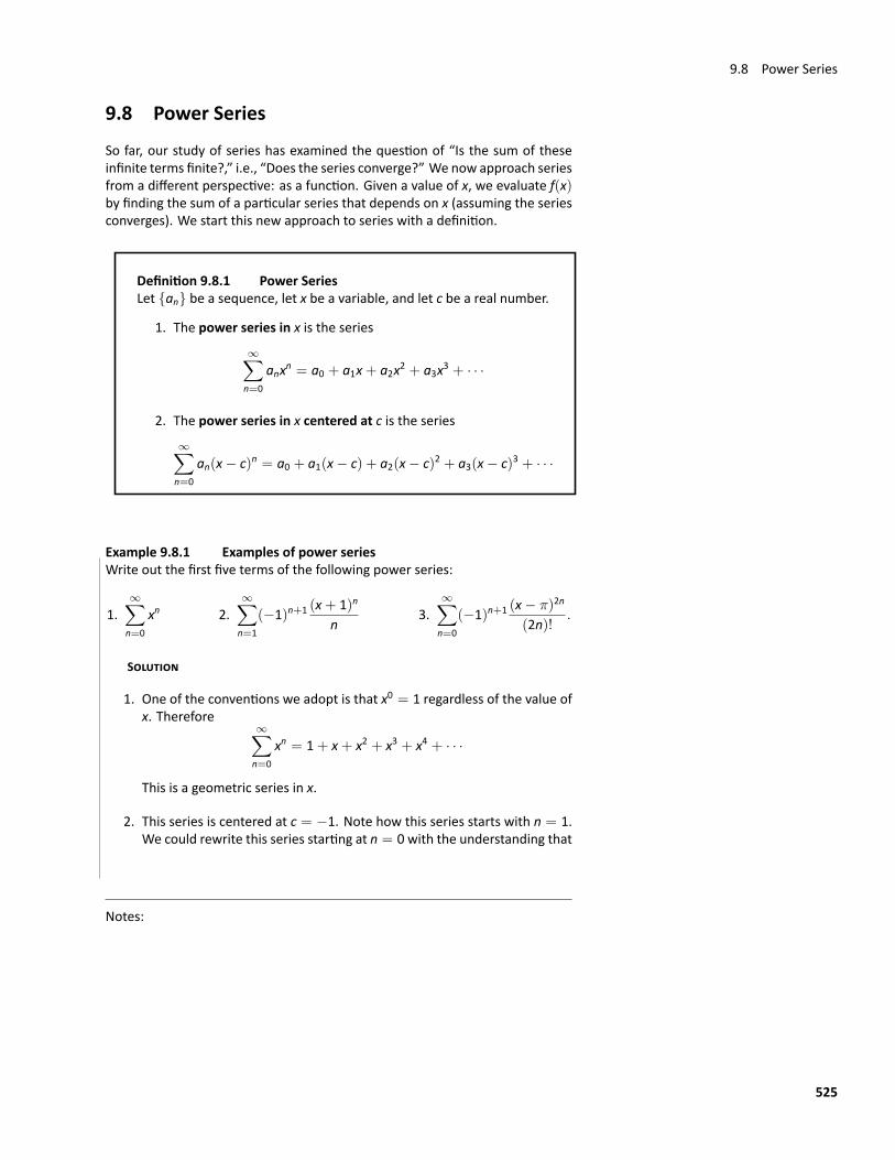
9.8 Power Series
9.8 Power SeriesSo far, our study of series has examined the question of “Is the sum of theseinfinite terms finite?,” i.e., “Does the series converge?” We now approach seriesfrom a different perspective: as a function. Given a value of x, we evaluate f(x)by finding the sum of a particular series that depends on x (assuming the seriesconverges). We start this new approach to series with a definition.
Definition 9.8.1 Power SeriesLet {an} be a sequence, let x be a variable, and let c be a real number.
1. The power series in x is the series
∞∑n=0
anxn = a0 + a1x+ a2x2 + a3x3 + · · ·
2. The power series in x centered at c is the series∞∑n=0
an(x− c)n = a0 + a1(x− c) + a2(x− c)2 + a3(x− c)3 + · · ·
Example 9.8.1 Examples of power seriesWrite out the first five terms of the following power series:
1.∞∑n=0
xn 2.∞∑n=1
(−1)n+1 (x+ 1)n
n3.
∞∑n=0
(−1)n+1 (x− π)2n
(2n)!.
SOLUTION
1. One of the conventions we adopt is that x0 = 1 regardless of the value ofx. Therefore
∞∑n=0
xn = 1+ x+ x2 + x3 + x4 + · · ·
This is a geometric series in x.
2. This series is centered at c = −1. Note how this series starts with n = 1.We could rewrite this series starting at n = 0 with the understanding that
Notes:
525
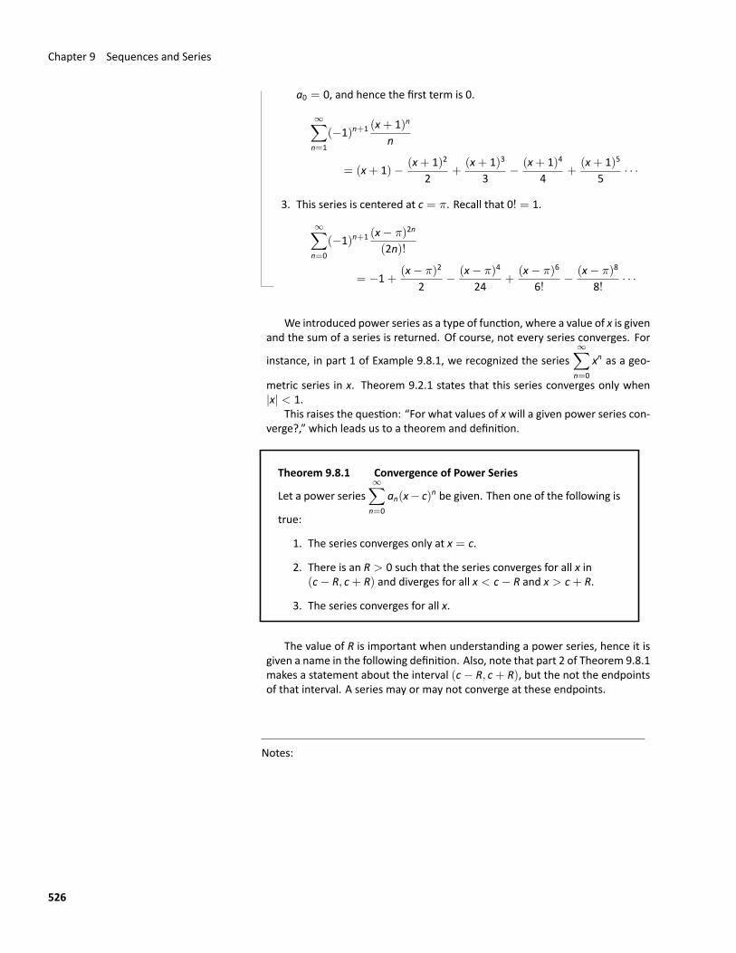
Chapter 9 Sequences and Series
a0 = 0, and hence the first term is 0.
∞∑n=1
(−1)n+1 (x+ 1)n
n
= (x+ 1)− (x+ 1)2
2+
(x+ 1)3
3− (x+ 1)4
4+
(x+ 1)5
5· · ·
3. This series is centered at c = π. Recall that 0! = 1.
∞∑n=0
(−1)n+1 (x− π)2n
(2n)!
= −1+(x− π)2
2− (x− π)4
24+
(x− π)6
6!− (x− π)8
8!· · ·
We introduced power series as a type of function, where a value of x is givenand the sum of a series is returned. Of course, not every series converges. For
instance, in part 1 of Example 9.8.1, we recognized the series∞∑n=0
xn as a geo‐
metric series in x. Theorem 9.2.1 states that this series converges only when|x| < 1.
This raises the question: “For what values of xwill a given power series con‐verge?,” which leads us to a theorem and definition.
Theorem 9.8.1 Convergence of Power Series
Let a power series∞∑n=0
an(x− c)n be given. Then one of the following is
true:
1. The series converges only at x = c.
2. There is an R > 0 such that the series converges for all x in(c− R, c+ R) and diverges for all x < c− R and x > c+ R.
3. The series converges for all x.
The value of R is important when understanding a power series, hence it isgiven a name in the following definition. Also, note that part 2 of Theorem 9.8.1makes a statement about the interval (c− R, c+ R), but the not the endpointsof that interval. A series may or may not converge at these endpoints.
Notes:
526
9.8 Power Series
Definition 9.8.2 Radius and Interval of Convergence
1. The number R given in Theorem 9.8.1 is the radius of conver‐gence of a given series. When a series converges for only x = c,we say the radius of convergence is 0, i.e., R = 0. When a se‐ries converges for all x, we say the series has an infinite radius ofconvergence, i.e., R = ∞.
2. The interval of convergence is the set of all values of x for whichthe series converges.
To find the values of x for which a given series converges, wewill use the con‐vergence tests we studied previously (especially the Ratio Test). However, thetests all required that the terms of a series be positive. The following theoremgives us a work‐around to this problem.
Theorem 9.8.2 The Radius of Convergence of a Series and Abso‐lute Convergence
The series∞∑n=0
an(x − c)n and∞∑n=0
|an(x− c)n| have the same radius of
convergence R.
Theorem 9.8.2 allows us to find the radius of convergence R of a series byapplying the Ratio Test (or any applicable test) to the absolute value of the termsof the series. We practice this in the following example.
Watch the video:Power Series — Finding the Interval of Convergenceathttps://youtu.be/01LzAU__J-0
Example 9.8.2 Determining the radius and interval of convergence.Find the radius and interval of convergence for each of the following series:
1.∞∑n=0
xn
n!2.
∞∑n=1
(−1)n+1 xn
n3.
∞∑n=0
2n(x− 3)n 4.∞∑n=0
n!xn
Notes:
527
Chapter 9 Sequences and Series
SOLUTION
1. We apply the Ratio Test to the series∞∑n=0
∣∣∣∣xnn!∣∣∣∣:
limn→∞
∣∣xn+1/(n+ 1)!∣∣
|xn/n!|= lim
n→∞
∣∣∣∣xn+1
xn· n!(n+ 1)!
∣∣∣∣= lim
n→∞
∣∣∣∣ xn+ 1
∣∣∣∣= 0 for all x.
The Ratio Test shows us that regardless of the choice of x, the series con‐verges. Therefore the radius of convergence is R = ∞, and the interval ofconvergence is (−∞,∞).
2. We apply the Ratio Test to the series∞∑n=1
∣∣∣∣(−1)n+1 xn
n
∣∣∣∣ = ∞∑n=1
∣∣∣∣xnn∣∣∣∣:
limn→∞
∣∣xn+1/(n+ 1)∣∣
|xn/n|= lim
n→∞
∣∣∣∣xn+1
xn· nn+ 1
∣∣∣∣= lim
n→∞|x| n
n+ 1= |x| .
The Ratio Test states a series converges if the limit of |an+1/an| = L < 1.We found the limit above to be |x|; therefore, the power series convergeswhen |x| < 1, or when x is in (−1, 1). Thus the radius of convergence isR = 1.To determine the interval of convergence, we need to check the endpointsof (−1, 1). When x = −1, we have the opposite of the Harmonic Series:
∞∑n=1
(−1)n+1 (−1)n
n=
∞∑n=1
(−1)2n+1
n
=
∞∑n=1
−1n
= −∞.
The series diverges when x = −1.
When x = 1, we have the series∞∑n=1
(−1)n+1 (1)n
n, which is the Alternating
Harmonic Series, which converges. Therefore the interval of convergenceis (−1, 1].
Notes:
528
9.8 Power Series
3. We apply the Ratio Test to the series∞∑n=0
|2n(x− 3)n|:
limn→∞
∣∣2n+1(x− 3)n+1∣∣
|2n(x− 3)n|= lim
n→∞
∣∣∣∣2n+1
2n· (x− 3)n+1
(x− 3)n
∣∣∣∣= lim
n→∞|2(x− 3)| .
According to theRatioTest, the series convergeswhen |2(x− 3)| < 1 =⇒|x− 3| < 1/2. The series is centered at 3, and x must be within 1/2 of 3in order for the series to converge. Therefore the radius of convergenceis R = 1/2, and we know that the series converges absolutely for all x in(3− 1/2, 3+ 1/2) = (2.5, 3.5).We check for convergence at the endpoints to find the interval of conver‐gence. When x = 2.5, we have:
∞∑n=0
2n(2.5− 3)n =∞∑n=0
2n(−1/2)n
=
∞∑n=0
(−1)n,
which diverges. A similar process shows that the series also diverges atx = 3.5. Therefore the interval of convergence is (2.5, 3.5).
4. We apply the Ratio Test to∞∑n=0
|n!xn|:
limn→∞
∣∣(n+ 1)!xn+1∣∣
|n!xn|= lim
n→∞|(n+ 1)x|
= ∞ for all x, except x = 0.
The Ratio Test shows that the series diverges for all x except x = 0. There‐fore the radius of convergence is R = 0.
Power Series as FunctionsWe can use a power series to define a function:
f(x) =∞∑n=0
anxn
Notes:
529
Chapter 9 Sequences and Series
where the domain of f is a subset of the interval of convergence of the powerseries. One can apply calculus techniques to such functions; in particular, wecan find derivatives and antiderivatives.
Theorem9.8.3 Derivatives and Indefinite Integrals of Power SeriesFunctions
Let f(x) =∞∑n=0
an(x− c)n be a function defined by a power series, with
radius of convergence R.
1. f(x) is continuous and differentiable on (c− R, c+ R).
2. f ′(x) =∞∑n=1
ann(x− c)n−1, with radius of convergence R.
3.∫
f(x) dx = C+∞∑n=0
an(x− c)n+1
n+ 1, with radius of convergence R.
A few notes about Theorem 9.8.3:
1. The theorem states that differentiation and integration do not change theradius of convergence. It does not state anything about the interval ofconvergence. They are not always the same.
2. Notice how the summation for f ′(x) starts with n = 1. This is because theconstant term a0 of f(x) goes to 0.
3. Differentiation and integration are simply calculated term‐by‐term usingprevious rules of integration and differentiation.
Example 9.8.3 Derivatives and indefinite integrals of power series
Let f(x) =
∞∑n=0
xn. Find the following along with their respective intervals of
convergence.
1. f ′(x) and 2. F(x) =∫
f(x) dx
SOLUTION We find the derivative and indefinite integral of f(x), follow‐ing Theorem 9.8.3.
Notes:
530
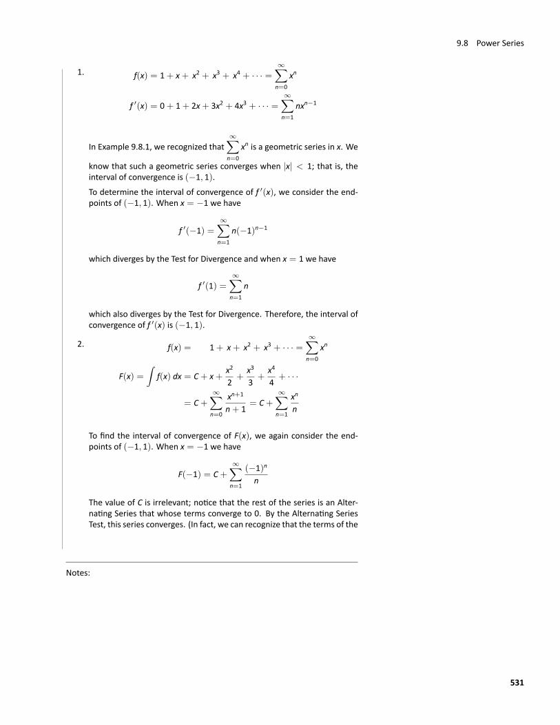
9.8 Power Series
1. f(x) = 1+ x+ x2 + x3 + x4 + · · · =∞∑n=0
xn
f ′(x) = 0+ 1+ 2x+ 3x2 + 4x3 + · · · =∞∑n=1
nxn−1
In Example 9.8.1, we recognized that∞∑n=0
xn is a geometric series in x. We
know that such a geometric series converges when |x| < 1; that is, theinterval of convergence is (−1, 1).To determine the interval of convergence of f ′(x), we consider the end‐points of (−1, 1). When x = −1 we have
f ′(−1) =∞∑n=1
n(−1)n−1
which diverges by the Test for Divergence and when x = 1 we have
f ′(1) =∞∑n=1
n
which also diverges by the Test for Divergence. Therefore, the interval ofconvergence of f ′(x) is (−1, 1).
2. f(x) = 1+ x+ x2 + x3 + · · · =∞∑n=0
xn
F(x) =∫
f(x) dx = C+ x+x2
2+
x3
3+
x4
4+ · · ·
= C+∞∑n=0
xn+1
n+ 1= C+
∞∑n=1
xn
n
To find the interval of convergence of F(x), we again consider the end‐points of (−1, 1). When x = −1 we have
F(−1) = C+∞∑n=1
(−1)n
n
The value of C is irrelevant; notice that the rest of the series is an Alter‐nating Series that whose terms converge to 0. By the Alternating SeriesTest, this series converges. (In fact, we can recognize that the terms of the
Notes:
531
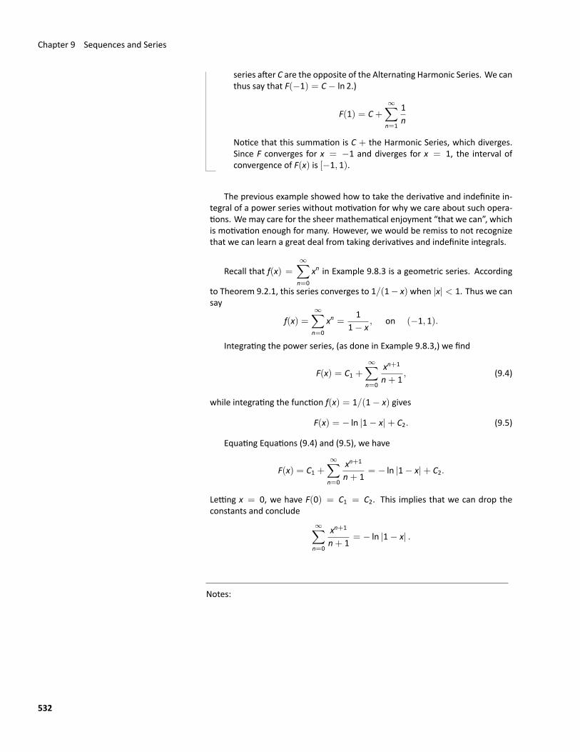
Chapter 9 Sequences and Series
series after C are the opposite of the Alternating Harmonic Series. We canthus say that F(−1) = C− ln 2.)
F(1) = C+∞∑n=1
1n
Notice that this summation is C + the Harmonic Series, which diverges.Since F converges for x = −1 and diverges for x = 1, the interval ofconvergence of F(x) is [−1, 1).
The previous example showed how to take the derivative and indefinite in‐tegral of a power series without motivation for why we care about such opera‐tions. Wemay care for the sheer mathematical enjoyment “that we can”, whichis motivation enough for many. However, we would be remiss to not recognizethat we can learn a great deal from taking derivatives and indefinite integrals.
Recall that f(x) =
∞∑n=0
xn in Example 9.8.3 is a geometric series. According
to Theorem 9.2.1, this series converges to 1/(1− x) when |x| < 1. Thus we cansay
f(x) =∞∑n=0
xn =1
1− x, on (−1, 1).
Integrating the power series, (as done in Example 9.8.3,) we find
F(x) = C1 +∞∑n=0
xn+1
n+ 1, (9.4)
while integrating the function f(x) = 1/(1− x) gives
F(x) = − ln |1− x|+ C2. (9.5)
Equating Equations (9.4) and (9.5), we have
F(x) = C1 +∞∑n=0
xn+1
n+ 1= − ln |1− x|+ C2.
Letting x = 0, we have F(0) = C1 = C2. This implies that we can drop theconstants and conclude
∞∑n=0
xn+1
n+ 1= − ln |1− x| .
Notes:
532
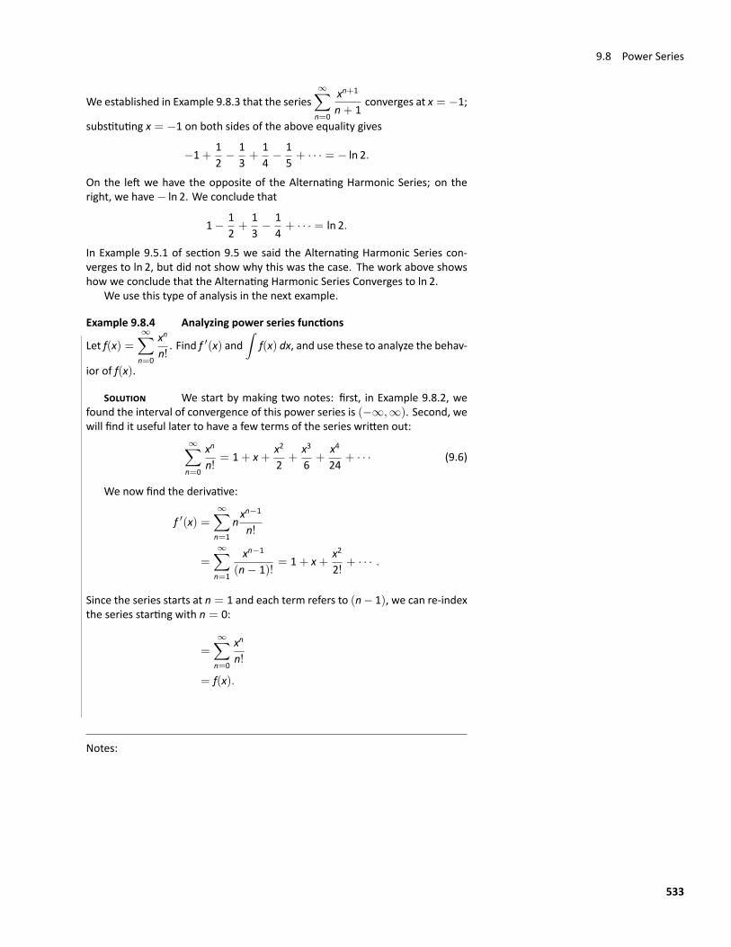
9.8 Power Series
We established in Example 9.8.3 that the series∞∑n=0
xn+1
n+ 1converges at x = −1;
substituting x = −1 on both sides of the above equality gives
−1+12− 1
3+
14− 1
5+ · · · = − ln 2.
On the left we have the opposite of the Alternating Harmonic Series; on theright, we have− ln 2. We conclude that
1− 12+
13− 1
4+ · · · = ln 2.
In Example 9.5.1 of section 9.5 we said the Alternating Harmonic Series con‐verges to ln 2, but did not show why this was the case. The work above showshow we conclude that the Alternating Harmonic Series Converges to ln 2.
We use this type of analysis in the next example.
Example 9.8.4 Analyzing power series functions
Let f(x) =∞∑n=0
xn
n!. Find f ′(x) and
∫f(x) dx, and use these to analyze the behav‐
ior of f(x).
SOLUTION We start by making two notes: first, in Example 9.8.2, wefound the interval of convergence of this power series is (−∞,∞). Second, wewill find it useful later to have a few terms of the series written out:
∞∑n=0
xn
n!= 1+ x+
x2
2+
x3
6+
x4
24+ · · · (9.6)
We now find the derivative:
f ′(x) =∞∑n=1
nxn−1
n!
=
∞∑n=1
xn−1
(n− 1)!= 1+ x+
x2
2!+ · · · .
Since the series starts at n = 1 and each term refers to (n− 1), we can re‐indexthe series starting with n = 0:
=
∞∑n=0
xn
n!
= f(x).
Notes:
533
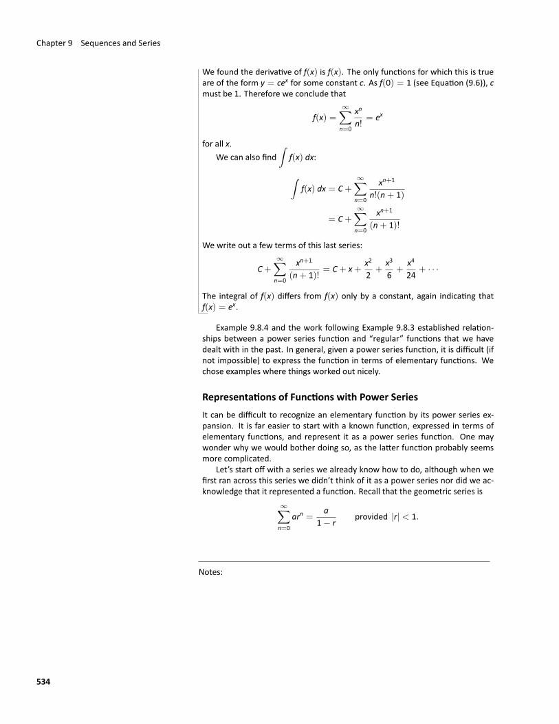
Chapter 9 Sequences and Series
We found the derivative of f(x) is f(x). The only functions for which this is trueare of the form y = cex for some constant c. As f(0) = 1 (see Equation (9.6)), cmust be 1. Therefore we conclude that
f(x) =∞∑n=0
xn
n!= ex
for all x.We can also find
∫f(x) dx:
∫f(x) dx = C+
∞∑n=0
xn+1
n!(n+ 1)
= C+∞∑n=0
xn+1
(n+ 1)!
We write out a few terms of this last series:
C+∞∑n=0
xn+1
(n+ 1)!= C+ x+
x2
2+
x3
6+
x4
24+ · · ·
The integral of f(x) differs from f(x) only by a constant, again indicating thatf(x) = ex.
Example 9.8.4 and the work following Example 9.8.3 established relation‐ships between a power series function and “regular” functions that we havedealt with in the past. In general, given a power series function, it is difficult (ifnot impossible) to express the function in terms of elementary functions. Wechose examples where things worked out nicely.
Representations of Functions with Power SeriesIt can be difficult to recognize an elementary function by its power series ex‐pansion. It is far easier to start with a known function, expressed in terms ofelementary functions, and represent it as a power series function. One maywonder why we would bother doing so, as the latter function probably seemsmore complicated.
Let’s start off with a series we already know how to do, although when wefirst ran across this series we didn’t think of it as a power series nor did we ac‐knowledge that it represented a function. Recall that the geometric series is
∞∑n=0
arn =a
1− rprovided |r| < 1.
Notes:
534
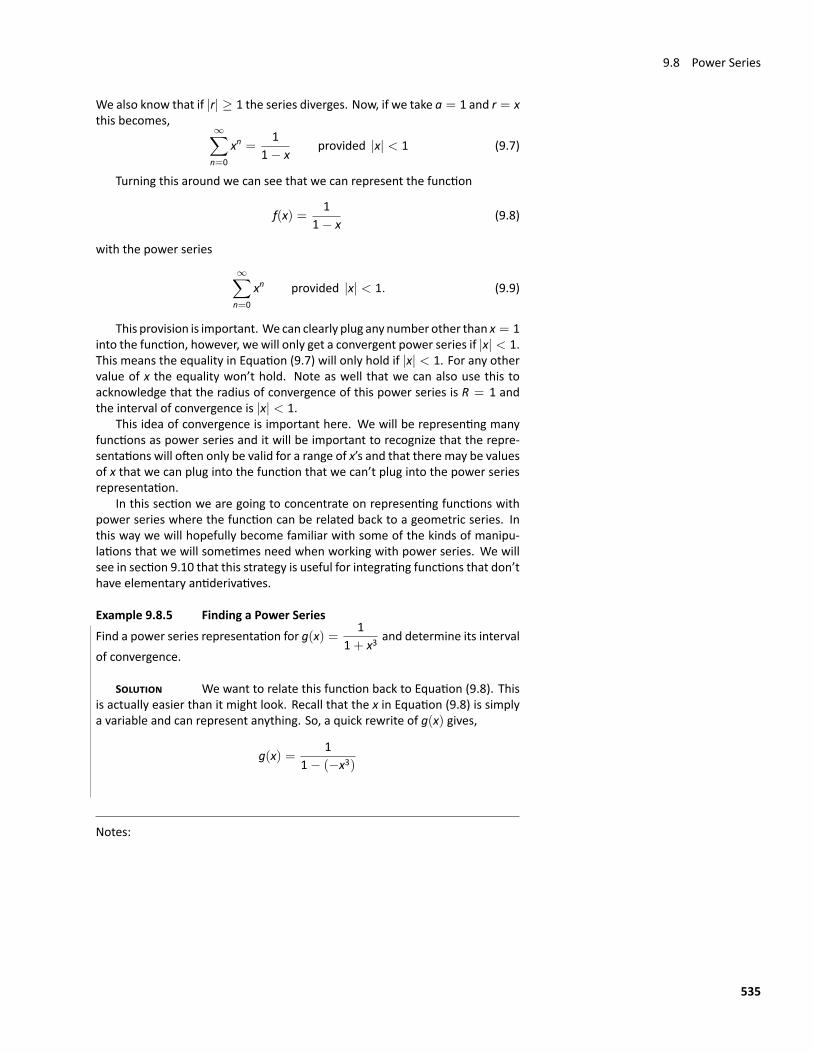
9.8 Power Series
We also know that if |r| ≥ 1 the series diverges. Now, if we take a = 1 and r = xthis becomes,
∞∑n=0
xn =1
1− xprovided |x| < 1 (9.7)
Turning this around we can see that we can represent the function
f(x) =1
1− x(9.8)
with the power series
∞∑n=0
xn provided |x| < 1. (9.9)
This provision is important. We can clearly plug any number other than x = 1into the function, however, we will only get a convergent power series if |x| < 1.This means the equality in Equation (9.7) will only hold if |x| < 1. For any othervalue of x the equality won’t hold. Note as well that we can also use this toacknowledge that the radius of convergence of this power series is R = 1 andthe interval of convergence is |x| < 1.
This idea of convergence is important here. We will be representing manyfunctions as power series and it will be important to recognize that the repre‐sentations will often only be valid for a range of x’s and that there may be valuesof x that we can plug into the function that we can’t plug into the power seriesrepresentation.
In this section we are going to concentrate on representing functions withpower series where the function can be related back to a geometric series. Inthis way we will hopefully become familiar with some of the kinds of manipu‐lations that we will sometimes need when working with power series. We willsee in section 9.10 that this strategy is useful for integrating functions that don’thave elementary antiderivatives.
Example 9.8.5 Finding a Power SeriesFind a power series representation for g(x) =
11+ x3
and determine its intervalof convergence.
SOLUTION We want to relate this function back to Equation (9.8). Thisis actually easier than it might look. Recall that the x in Equation (9.8) is simplya variable and can represent anything. So, a quick rewrite of g(x) gives,
g(x) =1
1− (−x3)
Notes:
535
Chapter 9 Sequences and Series
and so the −x3 holds the same place as the x in Equation (9.8). Therefore, allwe need to do is replace the x in Equation (9.9) and we’ve got a power seriesrepresentation for g(x).
g(x) =∞∑n=0
(−x3
)n provided∣∣−x3
∣∣ < 1
Notice that we replaced both the x in the power series and in the interval ofconvergence. All we need to do now is a little simplification.
g(x) =∞∑n=0
(−1)n x3n provided |x| < 1
So, in this case the interval of convergence is the same as the original powerseries. This usually won’t happen. More often than not the new interval ofconvergence will be different from the original interval of convergence.
Example 9.8.6 Finding a Power Series
Find a power series representation for h(x) =2x2
1+ x3and determine its interval
of convergence.
SOLUTION This function is similar to the previous function, however thenumerator is different. Since Equation (9.8) doesn’t have an x in the numerator itappears that we can’t relate this function back to that. However, now that we’veworked the first example this one is actually very simple since we can use theresult of the answer from that example. To see how to do this let’s first rewritethe function a little.
h(x) = 2x21
1+ x3.
Now, from the first example we’ve already got a power series for the secondterm so let’s use that to write the function as,
h(x) = 2x2∞∑n=0
(−1)n x3n provided |x| < 1
Notice that the presence of x’s outside of the series will NOT affect its con‐vergence and so the interval of convergence remains the same. The last stepis to bring the coefficient into the series and we’ll be done. When we do this,make sure to combine the x’s as well. We typically onlywant a single x in a powerseries.
h(x) =∞∑n=0
2 (−1)n x3n+2 provided |x| < 1.
Notes:
536
9.8 Power Series
As we saw in the previous example we can often use previous results to help usout. This is an important idea to remember as it can often greatly simplify ourwork.
Example 9.8.7 Finding a Power SeriesFind a power series representation for f(x) =
x5− x
and determine its intervalof convergence.
SOLUTION So again, we have an x in the numerator. As with the lastexample factor x out and we have f(x) = x
15− x
. If we had a power series
representation for g(x) =1
5− xwe could get a power series representation for
f(x). We need the number in the denominator to be a one so we rewrite thedenominator.
g(x) =15
11− x
5
Now all we need to do to get a power series representation is to replace thex in Equation (9.9) with
x5. Doing this gives
g(x) =15
∞∑n=0
( x5
)nprovided
∣∣∣ x5 ∣∣∣ < 1.
Now simplify the series.
g(x) =15
∞∑n=0
xn
5n
=
∞∑n=0
xn
5n+1
The interval of convergence for this series is∣∣∣ x5 ∣∣∣ < 1 ⇒ 15|x| < 1 ⇒ |x| < 5
We now have a power series representation for g(x) but we need to find apower series representation for the original function. All we need to do for this
Notes:
537
Chapter 9 Sequences and Series
is to multiply the power series representative for g(x) by x and we’ll have it.
f(x) = x1
5− x
= x∞∑n=0
xn
5n+1
=
∞∑n=0
xn+1
5n+1
The interval of convergence doesn’t change and so it will be |x| < 5.
Example 9.8.8 Re‐indexing a Power SeriesFind a power series representation for f(x) =
1+ x1− x
.
SOLUTION We can start by writing this as
f(x) = (1+ x)∞∑n=0
xn.
The problem with this representation is that the 1 + x makes this not a powerseries —we only want a single occurrence of x. The proceed, we’ll split this intotwo sums
f(x) =∞∑n=0
xn + x∞∑n=0
xn =∞∑n=0
xn +∞∑n=0
xn+1.
Because the second sum uses n+1, we can re‐index it to get a sum involving xn,which is our power series
f(x) =∞∑n=0
xn + x∞∑n=0
xn =∞∑n=0
xn +∞∑n=1
xn = 1+ 2∞∑n=1
xn.
We now consider several examples where differentiation and integration ofpower series from Theorem 9.8.3 are used to write the power series for a func‐tion.
Example 9.8.9 Differentiating a Power SeriesFind a power series representation for g(x) =
1(1− x)2
and determine its radius
of convergence.
Notes:
538

9.8 Power Series
SOLUTION We know that
1(1− x)2
=ddx
(1
1− x
).
Since we have a power series representation for1
1− x, we can differentiate that
power series to get a power series representation for g(x).
g(x) =1
(1− x)2
=ddx
(1
1− x
)=
ddx
( ∞∑n=0
xn)
=
∞∑n=1
nxn−1
Since the original power series had a radius of convergence of R = 1 thederivative, and hence g(x), will also have a radius of convergence of R = 1.
Example 9.8.10 Integrating a Power SeriesFind a power series representation for h(x) = ln(5−x) and determine its radiusof convergence.
SOLUTION In this case we need the fact that∫1
5− xdx = − ln(5− x).
Recall that we found a power series representation for1
5− xin Example 9.8.7.
We now have
ln(5− x) = −∫
15− x
dx
= −∫ ∞∑
n=0
xn
5n+1 dx where |x| < 5
= C−∞∑n=0
xn+1
(n+ 1)5n+1 where |x| < 5
Notes:
539
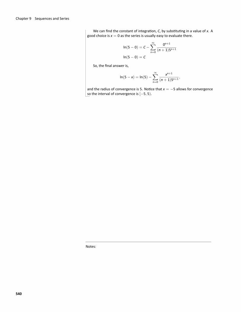
Chapter 9 Sequences and Series
We can find the constant of integration, C, by substituting in a value of x. Agood choice is x = 0 as the series is usually easy to evaluate there.
ln(5− 0) = C−∞∑n=0
0n+1
(n+ 1)5n+1
ln(5− 0) = C
So, the final answer is,
ln(5− x) = ln(5)−∞∑n=0
xn+1
(n+ 1)5n+1 ,
and the radius of convergence is 5. Notice that x = −5 allows for convergenceso the interval of convergence is [−5, 5).
Notes:
540
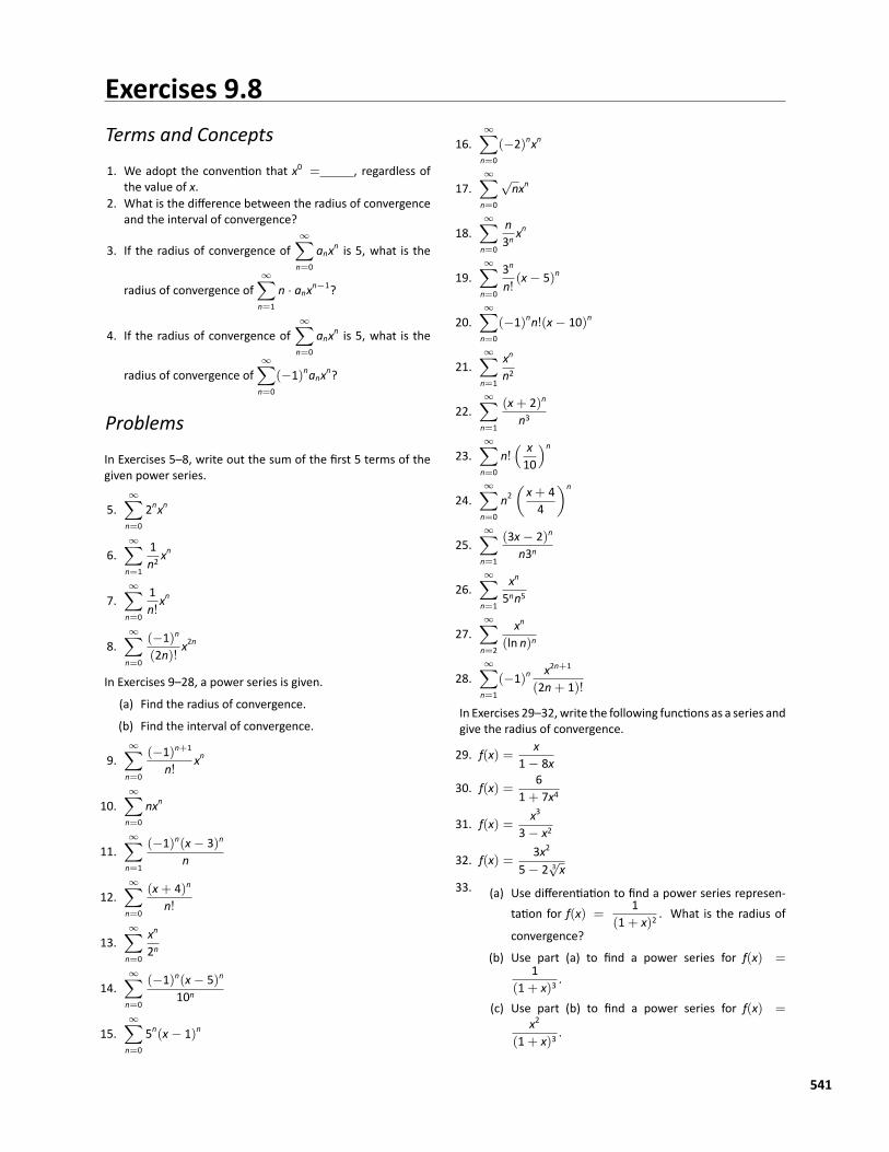
Exercises 9.8Terms and Concepts1. We adopt the convention that x0 = , regardless of
the value of x.2. What is the difference between the radius of convergence
and the interval of convergence?
3. If the radius of convergence of∞∑n=0
anxn is 5, what is the
radius of convergence of∞∑n=1
n · anxn−1?
4. If the radius of convergence of∞∑n=0
anxn is 5, what is the
radius of convergence of∞∑n=0
(−1)nanxn?
ProblemsIn Exercises 5–8, write out the sum of the first 5 terms of thegiven power series.
5.∞∑n=0
2nxn
6.∞∑n=1
1n2
xn
7.∞∑n=0
1n!xn
8.∞∑n=0
(−1)n
(2n)!x2n
In Exercises 9–28, a power series is given.
(a) Find the radius of convergence.
(b) Find the interval of convergence.
9.∞∑n=0
(−1)n+1
n!xn
10.∞∑n=0
nxn
11.∞∑n=1
(−1)n(x− 3)n
n
12.∞∑n=0
(x+ 4)n
n!
13.∞∑n=0
xn
2n
14.∞∑n=0
(−1)n(x− 5)n
10n
15.∞∑n=0
5n(x− 1)n
16.∞∑n=0
(−2)nxn
17.∞∑n=0
√nxn
18.∞∑n=0
n3n
xn
19.∞∑n=0
3n
n!(x− 5)n
20.∞∑n=0
(−1)nn!(x− 10)n
21.∞∑n=1
xn
n2
22.∞∑n=1
(x+ 2)n
n3
23.∞∑n=0
n!( x10
)n
24.∞∑n=0
n2(x+ 44
)n
25.∞∑n=1
(3x− 2)n
n3n
26.∞∑n=1
xn
5nn5
27.∞∑n=2
xn
(ln n)n
28.∞∑n=1
(−1)n x2n+1
(2n+ 1)!
In Exercises 29–32, write the following functions as a series andgive the radius of convergence.
29. f(x) = x1− 8x
30. f(x) = 61+ 7x4
31. f(x) = x3
3− x2
32. f(x) = 3x2
5− 2 3√x
33. (a) Use differentiation to find a power series represen‐tation for f(x) =
1(1+ x)2
. What is the radius of
convergence?
(b) Use part (a) to find a power series for f(x) =1
(1+ x)3.
(c) Use part (b) to find a power series for f(x) =x2
(1+ x)3.
541
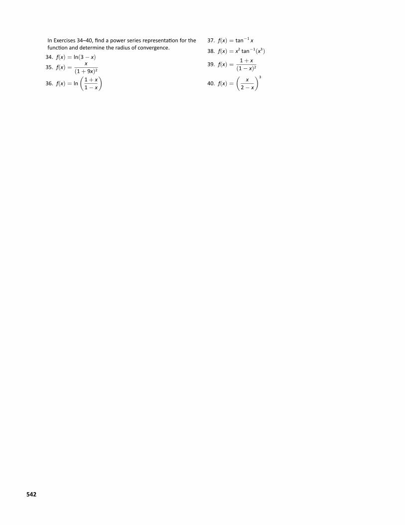
In Exercises 34–40, find a power series representation for thefunction and determine the radius of convergence.34. f(x) = ln(3− x)
35. f(x) = x(1+ 9x)2
36. f(x) = ln(1+ x1− x
)
37. f(x) = tan−1 x
38. f(x) = x2 tan−1(x3)
39. f(x) = 1+ x(1− x)2
40. f(x) =(
x2− x
)3
542
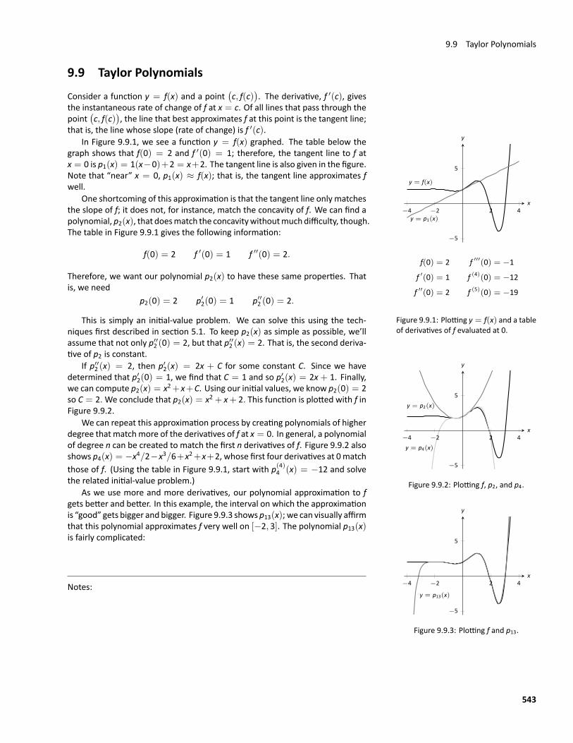
9.9 Taylor Polynomials
9.9 Taylor PolynomialsConsider a function y = f(x) and a point
(c, f(c)
). The derivative, f ′(c), gives
the instantaneous rate of change of f at x = c. Of all lines that pass through thepoint
(c, f(c)
), the line that best approximates f at this point is the tangent line;
that is, the line whose slope (rate of change) is f ′(c).
y = f(x)
y = p1(x)−4 −2 2 4
−5
5
x
y
f(0) = 2 f ′′′(0) = −1
f ′(0) = 1 f (4)(0) = −12
f ′′(0) = 2 f (5)(0) = −19
Figure 9.9.1: Plotting y = f(x) and a tableof derivatives of f evaluated at 0.
In Figure 9.9.1, we see a function y = f(x) graphed. The table below thegraph shows that f(0) = 2 and f ′(0) = 1; therefore, the tangent line to f atx = 0 is p1(x) = 1(x−0)+2 = x+2. The tangent line is also given in the figure.Note that “near” x = 0, p1(x) ≈ f(x); that is, the tangent line approximates fwell.
One shortcoming of this approximation is that the tangent line only matchesthe slope of f; it does not, for instance, match the concavity of f. We can find apolynomial, p2(x), that doesmatch the concavitywithoutmuchdifficulty, though.The table in Figure 9.9.1 gives the following information:
f(0) = 2 f ′(0) = 1 f ′′(0) = 2.
Therefore, we want our polynomial p2(x) to have these same properties. Thatis, we need
p2(0) = 2 p′2(0) = 1 p′′2 (0) = 2.
This is simply an initial‐value problem. We can solve this using the tech‐niques first described in section 5.1. To keep p2(x) as simple as possible, we’llassume that not only p′′2 (0) = 2, but that p′′2 (x) = 2. That is, the second deriva‐tive of p2 is constant.
y = p2(x)
y = p4(x)−4 −2 2 4
−5
5
x
y
Figure 9.9.2: Plotting f, p2, and p4.
y = p13(x)
−4 −2 2 4
−5
5
x
y
Figure 9.9.3: Plotting f and p13.
If p′′2 (x) = 2, then p′2(x) = 2x + C for some constant C. Since we havedetermined that p′2(0) = 1, we find that C = 1 and so p′2(x) = 2x + 1. Finally,we can compute p2(x) = x2+x+C. Using our initial values, we know p2(0) = 2so C = 2.We conclude that p2(x) = x2 + x+ 2. This function is plotted with f inFigure 9.9.2.
We can repeat this approximation process by creating polynomials of higherdegree that matchmore of the derivatives of f at x = 0. In general, a polynomialof degree n can be created to match the first n derivatives of f. Figure 9.9.2 alsoshows p4(x) = −x4/2−x3/6+x2+x+2, whose first four derivatives at 0matchthose of f. (Using the table in Figure 9.9.1, start with p(4)4 (x) = −12 and solvethe related initial‐value problem.)
As we use more and more derivatives, our polynomial approximation to fgets better and better. In this example, the interval on which the approximationis “good” gets bigger and bigger. Figure 9.9.3 shows p13(x); we can visually affirmthat this polynomial approximates f very well on [−2, 3]. The polynomial p13(x)is fairly complicated:
Notes:
543
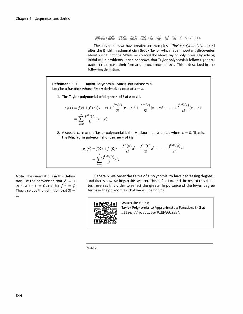
Chapter 9 Sequences and Series
16901x136227020800+
13x121209600−
1321x1139916800−
779x101814400−
359x9362880+
x8240+
139x75040 + 11x6
360 − 19x5120 − x4
2 − x36 +x2+x+2.
Thepolynomialswehave created are examples of Taylor polynomials, namedafter the British mathematician Brook Taylor who made important discoveriesabout such functions. While we created the above Taylor polynomials by solvinginitial‐value problems, it can be shown that Taylor polynomials follow a generalpattern that make their formation much more direct. This is described in thefollowing definition.
Definition 9.9.1 Taylor Polynomial, Maclaurin PolynomialLet f be a function whose first n derivatives exist at x = c.
1. The Taylor polynomial of degree n of f at x = c is
pn(x) = f(c) + f ′(c)(x− c) +f ′′(c)2!
(x− c)2 +f ′′′(c)3!
(x− c)3 + · · ·+ f (n)(c)n!
(x− c)n
=
n∑k=0
f (k)(c)k!
(x− c)k.
2. A special case of the Taylor polynomial is the Maclaurin polynomial, where c = 0. That is,theMaclaurin polynomial of degree n of f is
pn(x) = f(0) + f ′(0)x+f ′′(0)2!
x2 +f ′′′(0)3!
x3 + · · ·+ f (n)(0)n!
xn
=
n∑k=0
f (k)(0)k!
xk.
Note: The summations in this defini‐tion use the convention that x0 = 1even when x = 0 and that f(0) = f.They also use the definition that 0! =1.
Generally, we order the terms of a polynomial to have decreasing degrees,and that is how we began this section. This definition, and the rest of this chap‐ter, reverses this order to reflect the greater importance of the lower degreeterms in the polynomials that we will be finding.
Watch the video:Taylor Polynomial to Approximate a Function, Ex 3 athttps://youtu.be/UINFWG0ErSA
Notes:
544
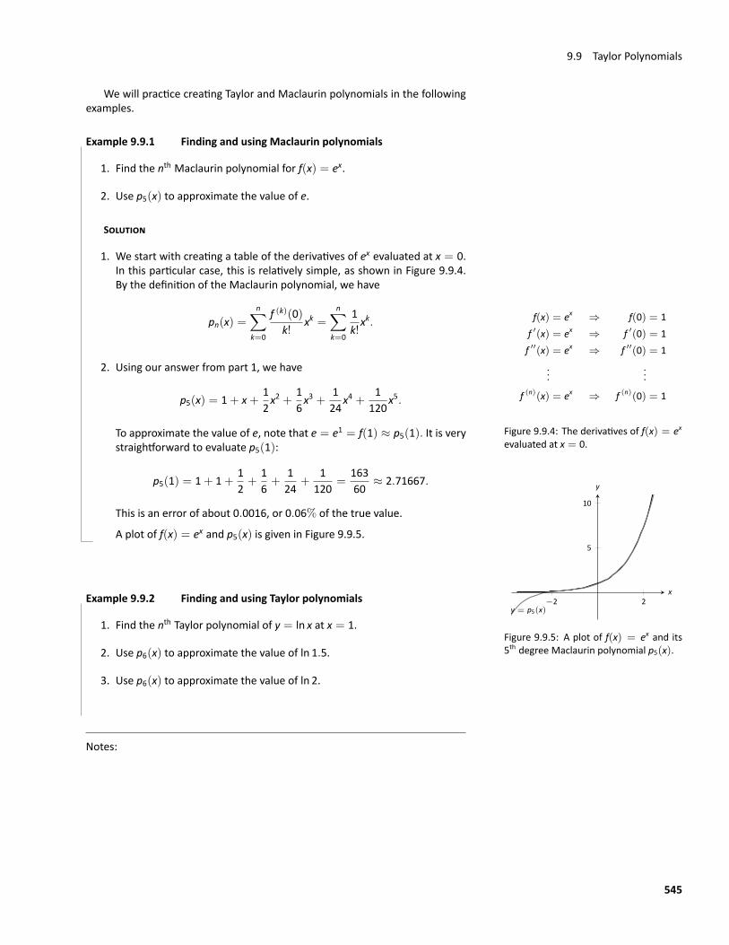
9.9 Taylor Polynomials
We will practice creating Taylor and Maclaurin polynomials in the followingexamples.
Example 9.9.1 Finding and using Maclaurin polynomials
1. Find the nth Maclaurin polynomial for f(x) = ex.
2. Use p5(x) to approximate the value of e.
SOLUTION
1. We start with creating a table of the derivatives of ex evaluated at x = 0.In this particular case, this is relatively simple, as shown in Figure 9.9.4.By the definition of the Maclaurin polynomial, we have
f(x) = ex ⇒ f(0) = 1f ′(x) = ex ⇒ f ′(0) = 1f ′′(x) = ex ⇒ f ′′(0) = 1
......
f (n)(x) = ex ⇒ f (n)(0) = 1
Figure 9.9.4: The derivatives of f(x) = ex
evaluated at x = 0.
pn(x) =n∑
k=0
f (k)(0)k!
xk =n∑
k=0
1k!xk.
2. Using our answer from part 1, we have
p5(x) = 1+ x+12x2 +
16x3 +
124
x4 +1
120x5.
To approximate the value of e, note that e = e1 = f(1) ≈ p5(1). It is verystraightforward to evaluate p5(1):
y = p5(x)−2 2
5
10
x
y
Figure 9.9.5: A plot of f(x) = ex and its5th degree Maclaurin polynomial p5(x).
p5(1) = 1+ 1+12+
16+
124
+1
120=
16360
≈ 2.71667.
This is an error of about 0.0016, or 0.06% of the true value.
A plot of f(x) = ex and p5(x) is given in Figure 9.9.5.
Example 9.9.2 Finding and using Taylor polynomials
1. Find the nth Taylor polynomial of y = ln x at x = 1.
2. Use p6(x) to approximate the value of ln 1.5.
3. Use p6(x) to approximate the value of ln 2.
Notes:
545
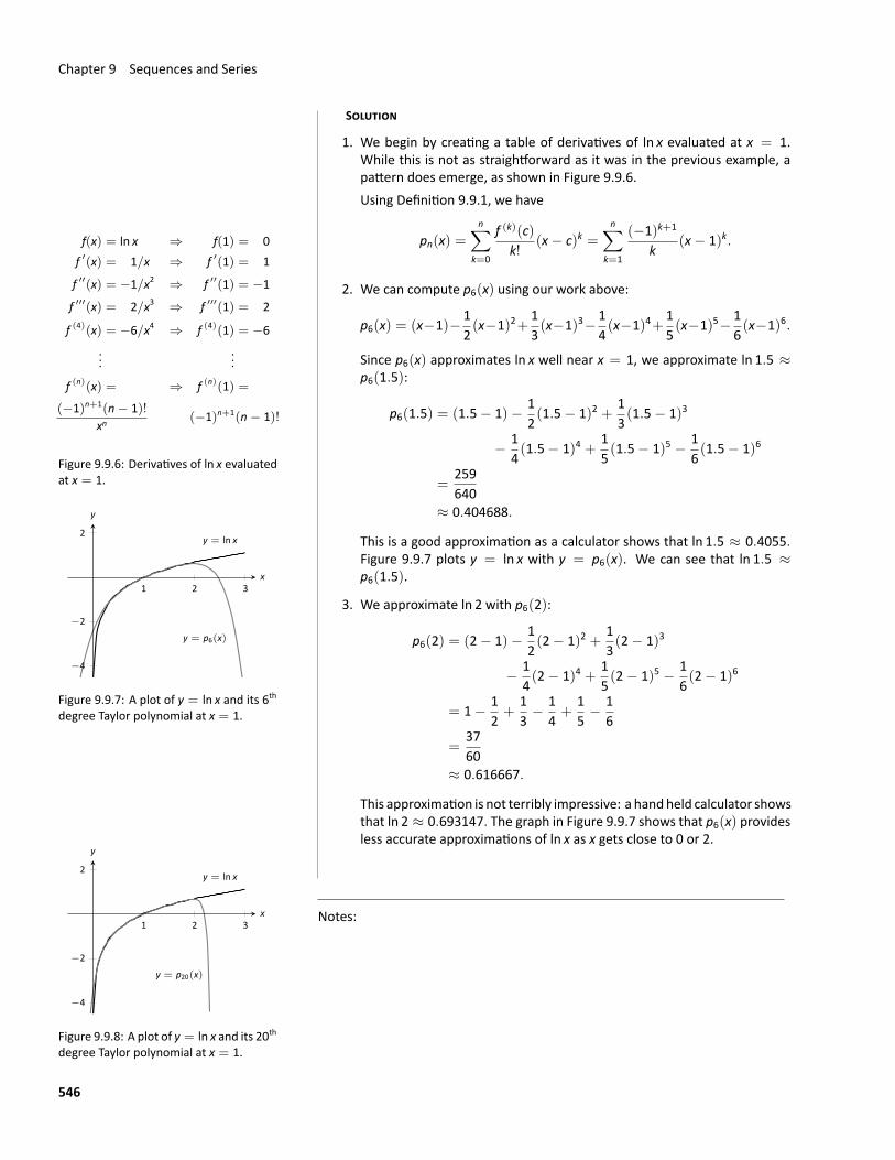
Chapter 9 Sequences and Series
SOLUTION
1. We begin by creating a table of derivatives of ln x evaluated at x = 1.While this is not as straightforward as it was in the previous example, apattern does emerge, as shown in Figure 9.9.6.Using Definition 9.9.1, we have
pn(x) =n∑
k=0
f (k)(c)k!
(x− c)k =n∑
k=1
(−1)k+1
k(x− 1)k.
2. We can compute p6(x) using our work above:
f(x) = ln x ⇒ f(1) = 0f ′(x) = 1/x ⇒ f ′(1) = 1
f ′′(x) = −1/x2 ⇒ f ′′(1) = −1
f ′′′(x) = 2/x3 ⇒ f ′′′(1) = 2
f (4)(x) = −6/x4 ⇒ f (4)(1) = −6...
...
f (n)(x) = ⇒ f (n)(1) =(−1)n+1(n− 1)!
xn(−1)n+1(n− 1)!
Figure 9.9.6: Derivatives of ln x evaluatedat x = 1.
p6(x) = (x−1)− 12(x−1)2+
13(x−1)3− 1
4(x−1)4+
15(x−1)5− 1
6(x−1)6.
Since p6(x) approximates ln x well near x = 1, we approximate ln 1.5 ≈p6(1.5):
y = ln x
y = p6(x)
1 2 3
−4
−2
2
x
y
Figure 9.9.7: A plot of y = ln x and its 6thdegree Taylor polynomial at x = 1.
p6(1.5) = (1.5− 1)− 12(1.5− 1)2 +
13(1.5− 1)3
− 14(1.5− 1)4 +
15(1.5− 1)5 − 1
6(1.5− 1)6
=259640
≈ 0.404688.
This is a good approximation as a calculator shows that ln 1.5 ≈ 0.4055.Figure 9.9.7 plots y = ln x with y = p6(x). We can see that ln 1.5 ≈p6(1.5).
3. We approximate ln 2 with p6(2):
p6(2) = (2− 1)− 12(2− 1)2 +
13(2− 1)3
− 14(2− 1)4 +
15(2− 1)5 − 1
6(2− 1)6
= 1− 12+
13− 1
4+
15− 1
6
=3760
≈ 0.616667.
This approximation is not terribly impressive: a handheld calculator showsthat ln 2 ≈ 0.693147. The graph in Figure 9.9.7 shows that p6(x) providesless accurate approximations of ln x as x gets close to 0 or 2.
y = ln x
y = p20(x)
1 2 3
−4
−2
2
x
y
Figure 9.9.8: A plot of y = ln x and its 20thdegree Taylor polynomial at x = 1.
Notes:
546
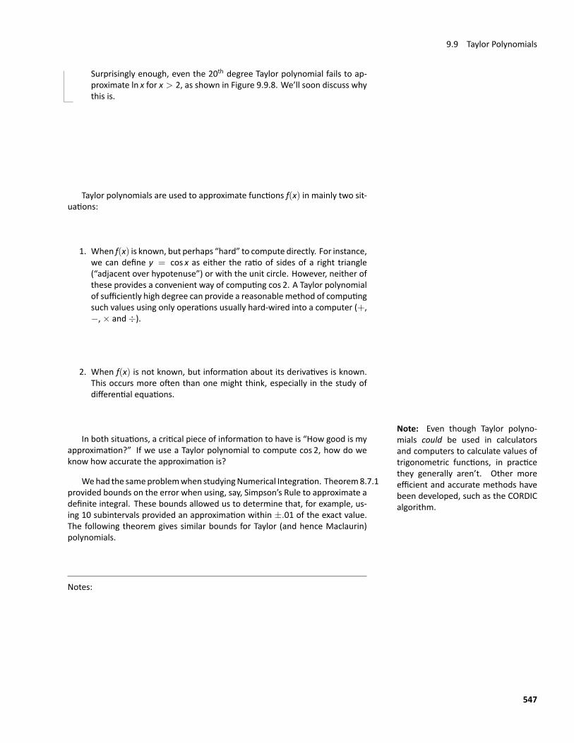
9.9 Taylor Polynomials
Surprisingly enough, even the 20th degree Taylor polynomial fails to ap‐proximate ln x for x > 2, as shown in Figure 9.9.8. We’ll soon discuss whythis is.
Taylor polynomials are used to approximate functions f(x) in mainly two sit‐uations:
1. When f(x) is known, but perhaps “hard” to compute directly. For instance,we can define y = cos x as either the ratio of sides of a right triangle(“adjacent over hypotenuse”) or with the unit circle. However, neither ofthese provides a convenient way of computing cos 2. A Taylor polynomialof sufficiently high degree can provide a reasonablemethod of computingsuch values using only operations usually hard‐wired into a computer (+,−,× and÷).
2. When f(x) is not known, but information about its derivatives is known.This occurs more often than one might think, especially in the study ofdifferential equations.
Note: Even though Taylor polyno‐mials could be used in calculatorsand computers to calculate values oftrigonometric functions, in practicethey generally aren’t. Other moreefficient and accurate methods havebeen developed, such as the CORDICalgorithm.
In both situations, a critical piece of information to have is “How good is myapproximation?” If we use a Taylor polynomial to compute cos 2, how do weknow how accurate the approximation is?
Wehad the sameproblemwhen studyingNumerical Integration. Theorem8.7.1provided bounds on the error when using, say, Simpson’s Rule to approximate adefinite integral. These bounds allowed us to determine that, for example, us‐ing 10 subintervals provided an approximation within ±.01 of the exact value.The following theorem gives similar bounds for Taylor (and hence Maclaurin)polynomials.
Notes:
547
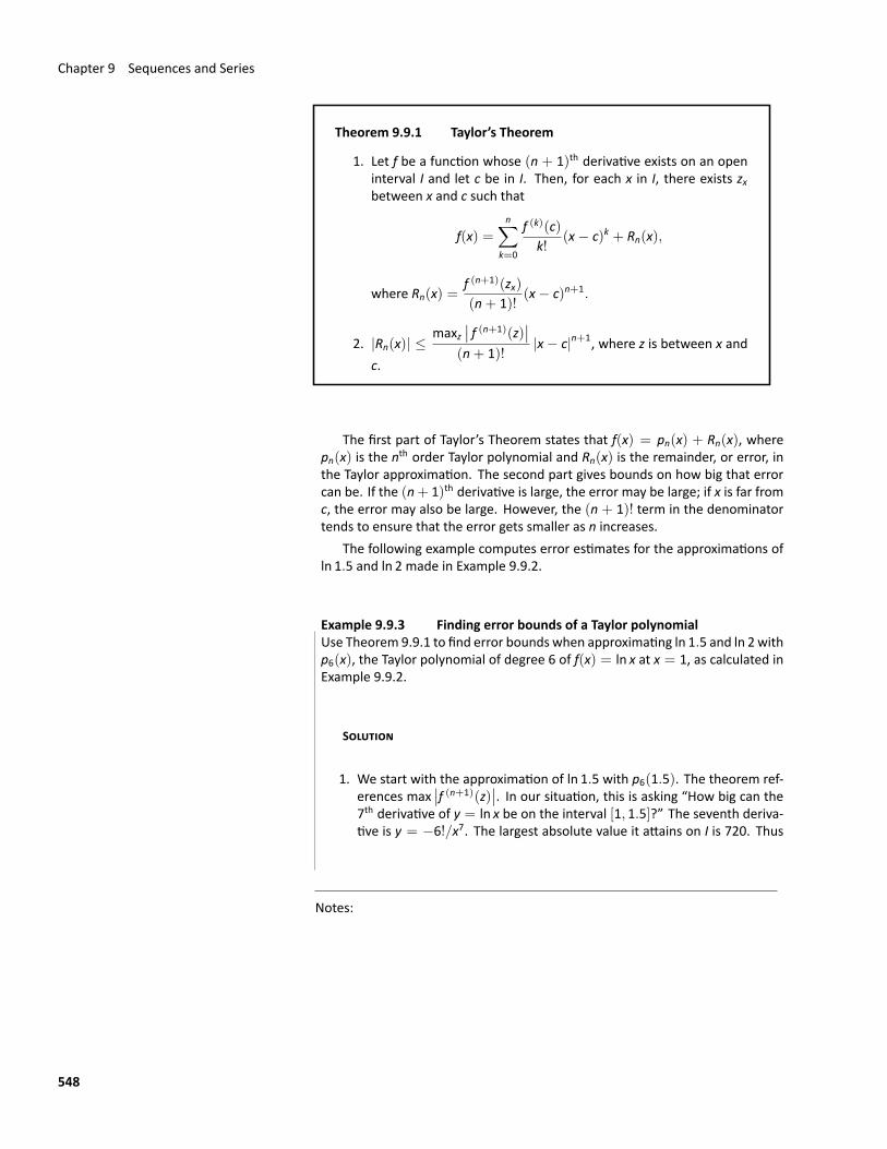
Chapter 9 Sequences and Series
Theorem 9.9.1 Taylor’s Theorem
1. Let f be a function whose (n + 1)th derivative exists on an openinterval I and let c be in I. Then, for each x in I, there exists zxbetween x and c such that
f(x) =n∑
k=0
f (k)(c)k!
(x− c)k + Rn(x),
where Rn(x) =f (n+1)(zx)(n+ 1)!
(x− c)n+1.
2. |Rn(x)| ≤maxz
∣∣ f (n+1)(z)∣∣
(n+ 1)!|x− c|n+1, where z is between x and
c.
The first part of Taylor’s Theorem states that f(x) = pn(x) + Rn(x), wherepn(x) is the nth order Taylor polynomial and Rn(x) is the remainder, or error, inthe Taylor approximation. The second part gives bounds on how big that errorcan be. If the (n+ 1)th derivative is large, the error may be large; if x is far fromc, the error may also be large. However, the (n + 1)! term in the denominatortends to ensure that the error gets smaller as n increases.
The following example computes error estimates for the approximations ofln 1.5 and ln 2 made in Example 9.9.2.
Example 9.9.3 Finding error bounds of a Taylor polynomialUse Theorem 9.9.1 to find error bounds when approximating ln 1.5 and ln 2 withp6(x), the Taylor polynomial of degree 6 of f(x) = ln x at x = 1, as calculated inExample 9.9.2.
SOLUTION
1. We start with the approximation of ln 1.5 with p6(1.5). The theorem ref‐erences max
∣∣f (n+1)(z)∣∣. In our situation, this is asking “How big can the
7th derivative of y = ln x be on the interval [1, 1.5]?” The seventh deriva‐tive is y = −6!/x7. The largest absolute value it attains on I is 720. Thus
Notes:
548
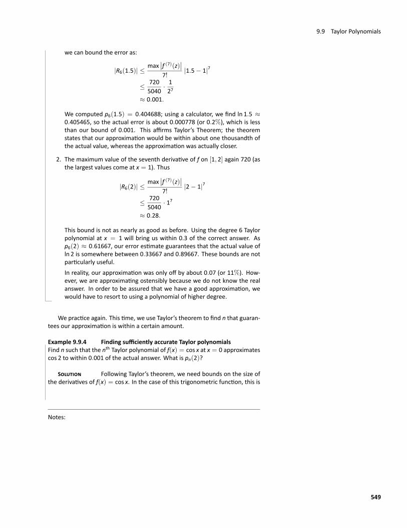
9.9 Taylor Polynomials
we can bound the error as:
|R6(1.5)| ≤max
∣∣f (7)(z)∣∣7!
|1.5− 1|7
≤ 7205040
· 127
≈ 0.001.
We computed p6(1.5) = 0.404688; using a calculator, we find ln 1.5 ≈0.405465, so the actual error is about 0.000778 (or 0.2%), which is lessthan our bound of 0.001. This affirms Taylor’s Theorem; the theoremstates that our approximation would be within about one thousandth ofthe actual value, whereas the approximation was actually closer.
2. The maximum value of the seventh derivative of f on [1, 2] again 720 (asthe largest values come at x = 1). Thus
|R6(2)| ≤max
∣∣f (7)(z)∣∣7!
|2− 1|7
≤ 7205040
· 17
≈ 0.28.
This bound is not as nearly as good as before. Using the degree 6 Taylorpolynomial at x = 1 will bring us within 0.3 of the correct answer. Asp6(2) ≈ 0.61667, our error estimate guarantees that the actual value ofln 2 is somewhere between 0.33667 and 0.89667. These bounds are notparticularly useful.In reality, our approximation was only off by about 0.07 (or 11%). How‐ever, we are approximating ostensibly because we do not know the realanswer. In order to be assured that we have a good approximation, wewould have to resort to using a polynomial of higher degree.
We practice again. This time, we use Taylor’s theorem to find n that guaran‐tees our approximation is within a certain amount.
Example 9.9.4 Finding sufficiently accurate Taylor polynomialsFind n such that the nth Taylor polynomial of f(x) = cos x at x = 0 approximatescos 2 to within 0.001 of the actual answer. What is pn(2)?
SOLUTION Following Taylor’s theorem, we need bounds on the size ofthe derivatives of f(x) = cos x. In the case of this trigonometric function, this is
Notes:
549
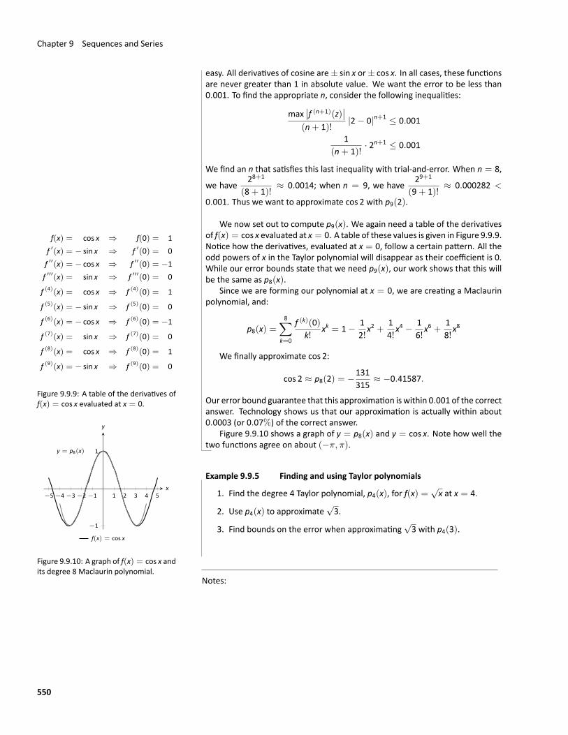
Chapter 9 Sequences and Series
easy. All derivatives of cosine are± sin x or± cos x. In all cases, these functionsare never greater than 1 in absolute value. We want the error to be less than0.001. To find the appropriate n, consider the following inequalities:
max∣∣f (n+1)(z)
∣∣(n+ 1)!
|2− 0|n+1 ≤ 0.001
1(n+ 1)!
· 2n+1 ≤ 0.001
We find an n that satisfies this last inequality with trial‐and‐error. When n = 8,
we have28+1
(8+ 1)!≈ 0.0014; when n = 9, we have
29+1
(9+ 1)!≈ 0.000282 <
0.001. Thus we want to approximate cos 2 with p9(2).
We now set out to compute p9(x). We again need a table of the derivativesof f(x) = cos x evaluated at x = 0. A table of these values is given in Figure 9.9.9.Notice how the derivatives, evaluated at x = 0, follow a certain pattern. All theodd powers of x in the Taylor polynomial will disappear as their coefficient is 0.While our error bounds state that we need p9(x), our work shows that this willbe the same as p8(x).
f(x) = cos x ⇒ f(0) = 1f ′(x) = − sin x ⇒ f ′(0) = 0f ′′(x) = − cos x ⇒ f ′′(0) = −1f ′′′(x) = sin x ⇒ f ′′′(0) = 0
f (4)(x) = cos x ⇒ f (4)(0) = 1
f (5)(x) = − sin x ⇒ f (5)(0) = 0
f (6)(x) = − cos x ⇒ f (6)(0) = −1
f (7)(x) = sin x ⇒ f (7)(0) = 0
f (8)(x) = cos x ⇒ f (8)(0) = 1
f (9)(x) = − sin x ⇒ f (9)(0) = 0
Figure 9.9.9: A table of the derivatives off(x) = cos x evaluated at x = 0.
Since we are forming our polynomial at x = 0, we are creating a Maclaurinpolynomial, and:
p8(x) =8∑
k=0
f (k)(0)k!
xk = 1− 12!x2 +
14!x4 − 1
6!x6 +
18!x8
y = p8(x)
−5 −4 −3 −2 −1 1 2 3 4 5
−1
1
x
y
f(x) = cos x
Figure 9.9.10: A graph of f(x) = cos x andits degree 8 Maclaurin polynomial.
We finally approximate cos 2:
cos 2 ≈ p8(2) = −131315
≈ −0.41587.
Our error bound guarantee that this approximation is within 0.001 of the correctanswer. Technology shows us that our approximation is actually within about0.0003 (or 0.07%) of the correct answer.
Figure 9.9.10 shows a graph of y = p8(x) and y = cos x. Note how well thetwo functions agree on about (−π, π).
Example 9.9.5 Finding and using Taylor polynomials
1. Find the degree 4 Taylor polynomial, p4(x), for f(x) =√x at x = 4.
2. Use p4(x) to approximate√3.
3. Find bounds on the error when approximating√3 with p4(3).
Notes:
550
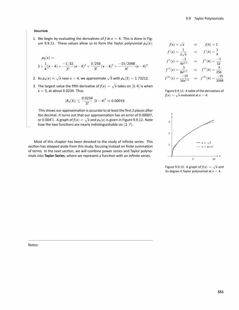
9.9 Taylor Polynomials
SOLUTION
1. We begin by evaluating the derivatives of f at x = 4. This is done in Fig‐ure 9.9.11. These values allow us to form the Taylor polynomial p4(x): f(x) =
√x ⇒ f(4) = 2
f ′(x) = 12√x
⇒ f ′(4) = 14
f ′′(x) = −14x3/2
⇒ f ′′(4) = −132
f ′′′(x) = 38x5/2
⇒ f ′′′(4) = 3256
f (4)(x) = −1516x7/2
⇒ f (4)(4) = −152048
Figure 9.9.11: A table of the derivatives off(x) =
√x evaluated at x = 4.
p4(x) =
2+14(x−4)+
−1/322!
(x−4)2+3/2563!
(x−4)3+−15/2048
4!(x−4)4.
2. As p4(x) ≈√x near x = 4, we approximate
√3 with p4(3) = 1.73212.
3. The largest value the fifth derivative of f(x) =√x takes on [3, 4] is when
x = 3, at about 0.0234. Thus
|R4(3)| ≤0.0234
5!|3− 4|5 ≈ 0.00019.
This shows our approximation is accurate to at least the first 2 places after
y =√x
y = p4(x)
5 10
1
2
3
x
y
Figure 9.9.12: A graph of f(x) =√x and
its degree 4 Taylor polynomial at x = 4.
the decimal. It turns out that our approximation has an error of 0.00007,or 0.004%. A graph of f(x) =
√x and p4(x) is given in Figure 9.9.12. Note
how the two functions are nearly indistinguishable on (2, 7).
Most of this chapter has been devoted to the study of infinite series. Thissection has stepped aside from this study, focusing instead on finite summationof terms. In the next section, we will combine power series and Taylor polyno‐mials into Taylor Series, where we represent a function with an infinite series.
Notes:
551

Exercises 9.9Terms and Concepts1. What is the difference between a Taylor polynomial and a
Maclaurin polynomial?2. T/F: In general, pn(x) approximates f(x) better and better
as n gets larger.3. For some function f(x), the Maclaurin polynomial of de‐
gree 4 is p4(x) = 6+ 3x− 4x2 + 5x3 − 7x4. What is p2(x)?4. For some function f(x), the Maclaurin polynomial of de‐
gree 4 is p4(x) = 6+3x−4x2+5x3−7x4. What is f ′′′(0)?
ProblemsIn Exercises 5–12, find the Maclaurin polynomial of degree nfor the given function.
5. f(x) = e−x, n = 36. f(x) = sin x, n = 87. f(x) = x · ex, n = 58. f(x) = tan x, n = 69. f(x) = e2x, n = 4
10. f(x) = 11− x
, n = 4
11. f(x) = 11+ x
, n = 4
12. f(x) = 11+ x
, n = 7
In Exercises 13–20, find the Taylor polynomial of degree n, atx = c, for the given function.
13. f(x) =√x, n = 4, c = 1
14. f(x) = ln(x+ 1), n = 4, c = 115. f(x) = cos x, n = 6, c = π/416. f(x) = sin x, n = 5, c = π/6
17. f(x) = 1x, n = 5, c = 2
18. f(x) = 1x2, n = 8, c = 1
19. f(x) = 1x2 + 1
, n = 3, c = −1
20. f(x) = x2 cos x, n = 2, c = π
In Exercises 21–24, approximate the function value with theindicated Taylor polynomial and give approximate bounds onthe error.
21. Approximate sin 0.1 with the Maclaurin polynomial of de‐gree 3.
22. Approximate cos 1 with the Maclaurin polynomial of de‐gree 4.
23. Approximate√10 with the Taylor polynomial of degree 2
centered at x = 9.24. Approximate ln 1.5 with the Taylor polynomial of degree 3
centered at x = 1.
Exercises 25–28 ask for an n to be found such that pn(x) ap‐proximates f(x) within a certain bound of accuracy.
25. Find n such that the Maclaurin polynomial of degree n off(x) = ex approximates ewithin 0.0001 of the actual value.
26. Find n such that the Taylor polynomial of degree n of f(x) =√x, centered at x = 4, approximates
√3 within 0.0001 of
the actual value.27. Find n such that the Maclaurin polynomial of degree n of
f(x) = cos x approximates cos π/3 within 0.0001 of theactual value.
28. Find n such that the Maclaurin polynomial of degree n off(x) = sin x approximates cos πwithin 0.0001 of the actualvalue.
In Exercises 29–34, find the xn term of the indicated Taylorpolynomial.
29. Find a formula for the xn term of theMaclaurin polynomialfor f(x) = ex.
30. Find a formula for the xn term of theMaclaurin polynomialfor f(x) = cos x.
31. Find a formula for the xn term of theMaclaurin polynomialfor f(x) = sin x.
32. Find a formula for the xn term of theMaclaurin polynomialfor f(x) = 1
1− x.
33. Find a formula for the xn term of theMaclaurin polynomialfor f(x) = 1
1+ x.
34. Find a formula for the xn term of the Taylor polynomial forf(x) = ln x centered at c = 1.
In Exercises 35–36, approximate the solution to the given dif‐ferential equation with a degree 4 Maclaurin polynomial.
35. y′ = y, y(0) = 1
36. y′ = 2y, y(0) = 1
552
9.10 Taylor Series
9.10 Taylor SeriesIn section 9.8, we showed how certain functions can be represented by a powerseries function. In section 9.9, we showed how we can approximate functionswith polynomials, given that enough derivative information is available. In thissection we combine these concepts: if a function f(x) is infinitely differentiable,we show how to represent it with a power series function.
Definition 9.10.1 Taylor and Maclaurin SeriesLet f(x) have derivatives of all orders at x = c.
1. The Taylor Series of f(x), centered at c is
∞∑n=0
f (n)(c)n!
(x− c)n.
2. Setting c = 0 gives theMaclaurin Series of f(x):
∞∑n=0
f (n)(0)n!
xn.
Watch the video:Taylor and Maclaurin Series — Example 2 athttps://youtu.be/Os8OtXFBLkY
The difference between a Taylor polynomial and a Taylor series is the formeris a polynomial, containing only a finite number of terms, whereas the latteris a series, a summation of an infinite set of terms. When creating the Taylorpolynomial of degree n for a function f(x) at x = c, we needed to evaluate f, andthe first n derivatives of f, at x = c. When creating the Taylor series of f, we needto find a pattern that describes the nth derivative of f at x = c. We demonstratethis in the next two examples.
Example 9.10.1 The Maclaurin series of f(x) = cos xFind the Maclaurin series of f(x) = cos x.
Notes:
553
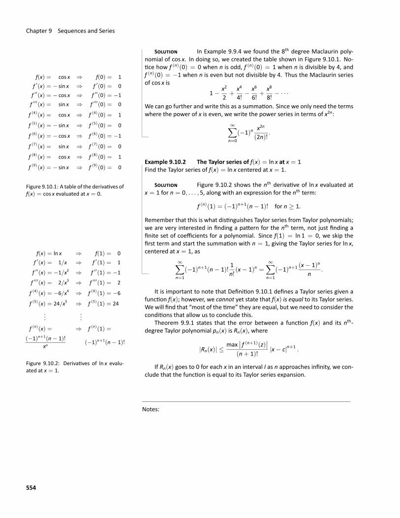
Chapter 9 Sequences and Series
SOLUTION In Example 9.9.4 we found the 8th degree Maclaurin poly‐nomial of cos x. In doing so, we created the table shown in Figure 9.10.1. No‐
f(x) = cos x ⇒ f(0) = 1f ′(x) = − sin x ⇒ f ′(0) = 0f ′′(x) = − cos x ⇒ f ′′(0) = −1f ′′′(x) = sin x ⇒ f ′′′(0) = 0
f (4)(x) = cos x ⇒ f (4)(0) = 1
f (5)(x) = − sin x ⇒ f (5)(0) = 0
f (6)(x) = − cos x ⇒ f (6)(0) = −1
f (7)(x) = sin x ⇒ f (7)(0) = 0
f (8)(x) = cos x ⇒ f (8)(0) = 1
f (9)(x) = − sin x ⇒ f (9)(0) = 0
Figure 9.10.1: A table of the derivatives off(x) = cos x evaluated at x = 0.
tice how f (n)(0) = 0 when n is odd, f (n)(0) = 1 when n is divisible by 4, andf (n)(0) = −1 when n is even but not divisible by 4. Thus the Maclaurin seriesof cos x is
1− x2
2+
x4
4!− x6
6!+
x8
8!− · · ·
We can go further and write this as a summation. Since we only need the termswhere the power of x is even, we write the power series in terms of x2n:
∞∑n=0
(−1)nx2n
(2n)!.
Example 9.10.2 The Taylor series of f(x) = ln x at x = 1Find the Taylor series of f(x) = ln x centered at x = 1.
SOLUTION Figure 9.10.2 shows the nth derivative of ln x evaluated atx = 1 for n = 0, . . . , 5, along with an expression for the nth term:
f (n)(1) = (−1)n+1(n− 1)! for n ≥ 1.
Remember that this is what distinguishes Taylor series from Taylor polynomials;we are very interested in finding a pattern for the nth term, not just finding afinite set of coefficients for a polynomial. Since f(1) = ln 1 = 0, we skip the
f(x) = ln x ⇒ f(1) = 0f ′(x) = 1/x ⇒ f ′(1) = 1
f ′′(x) = −1/x2 ⇒ f ′′(1) = −1
f ′′′(x) = 2/x3 ⇒ f ′′′(1) = 2
f (4)(x) = −6/x4 ⇒ f (4)(1) = −6
f (5)(x) = 24/x5 ⇒ f (5)(1) = 24...
...
f (n)(x) = ⇒ f (n)(1) =(−1)n+1(n− 1)!
xn(−1)n+1(n− 1)!
Figure 9.10.2: Derivatives of ln x evalu‐ated at x = 1.
first term and start the summation with n = 1, giving the Taylor series for ln x,centered at x = 1, as
∞∑n=1
(−1)n+1(n− 1)!1n!(x− 1)n =
∞∑n=1
(−1)n+1 (x− 1)n
n.
It is important to note that Definition 9.10.1 defines a Taylor series given afunction f(x); however, we cannot yet state that f(x) is equal to its Taylor series.We will find that “most of the time” they are equal, but we need to consider theconditions that allow us to conclude this.
Theorem 9.9.1 states that the error between a function f(x) and its nth‐degree Taylor polynomial pn(x) is Rn(x), where
|Rn(x)| ≤max
∣∣ f (n+1)(z)∣∣
(n+ 1)!|x− c|n+1
.
If Rn(x) goes to 0 for each x in an interval I as n approaches infinity, we con‐clude that the function is equal to its Taylor series expansion.
Notes:
554
9.10 Taylor Series
Theorem 9.10.1 Function and Taylor Series EqualityLet f(x) have derivatives of all orders at x = c, let Rn(x) be as stated inTheorem 9.9.1, and let I be an interval on which the Taylor series of f(x)converges. If lim
n→∞Rn(x) = 0 for all x in I, then
f(x) =∞∑n=0
f (n)(c)n!
(x− c)n on I.
We demonstrate the use of this theorem in an example.
Example 9.10.3 Establishing equality of a function and its Taylor seriesShow that f(x) = cos x is equal to itsMaclaurin series, as found in Example 9.10.1,for all x.
SOLUTION Given a value x, the magnitude of the error term Rn(x) isbounded by
|Rn(x)| ≤max
∣∣ f (n+1)(z)∣∣
(n+ 1)!|x|n+1
.
Since all derivatives of cos x are± sin xor± cos x, whosemagnitudes are boundedby 1, we can state
|Rn(x)| ≤1
(n+ 1)!|x|n+1
which implies
− |x|n+1
(n+ 1)!≤ Rn(x) ≤
|x|n+1
(n+ 1)!. (9.10)
For any x, limn→∞
xn+1
(n+ 1)!= 0. Applying the Squeeze Theorem to Equation (9.10),
we conclude that limn→∞
Rn(x) = 0 for all x, and hence
cos x =∞∑n=0
(−1)nx2n
(2n)!for all x.
It is natural to assume that a function is equal to its Taylor series on theseries’ interval of convergence, but this is not the case. In order to properlyestablish equality, one must use Theorem 9.10.1. This is a bit disappointing, aswe developed beautiful techniques for determining the interval of convergenceof a power series, and proving that Rn(x) → 0 can be cumbersome as it dealswith high order derivatives of the function.
Notes:
555
Chapter 9 Sequences and Series
There is good news. A function f(x) that is equal to its Taylor series, centeredat any point the domain of f(x), is said to be an analytic function, andmost, if notall, functions that we encounterwithin this course are analytic functions. Gener‐ally speaking, any function that one creates with elementary functions (polyno‐mials, exponentials, trigonometric functions, etc.) that is not piecewise definedis probably analytic. For most functions, we assume the function is equal to itsTaylor series on the series’ interval of convergence and only use Theorem 9.10.1when we suspect something may not work as expected. The converse is alsotrue: if a function is equal to some power series on an interval, then that powerseries is the Taylor series of the function.
We develop the Taylor series for one more important function, then give atable of the Taylor series for a number of common functions.
Example 9.10.4 The Binomial SeriesFind the Maclaurin series of f(x) = (1+ x)k, k ̸= 0.
SOLUTION When k is a positive integer, the Maclaurin series is finite.For instance, when k = 4, we have
f(x) = (1+ x)4 = 1+ 4x+ 6x2 + 4x3 + x4.
The coefficients of x when k is a positive integer are known as the binomial co‐efficients, giving the series we are developing its name.
When k = 1/2, we have f(x) =√1+ x. Knowing a series representation of
this function would give a useful way of approximating√1.3, for instance.
To develop the Maclaurin series for f(x) = (1 + x)k for any value of k ̸= 0,we consider the derivatives of f evaluated at x = 0:
f(x) = (1+ x)k f(0) = 1f ′(x) = k(1+ x)k−1 f ′(0) = k
f ′′(x) = k(k− 1)(1+ x)k−2 f ′′(0) = k(k− 1)f ′′′(x) = k(k− 1)(k− 2)(1+ x)k−3 f ′′′(0) = k(k− 1)(k− 2)
......
f (n)(x) = k(k− 1) · · ·(k− (n− 1)
)(1+ x)k−n f (n)(0) = k(k− 1) · · ·
(k− (n− 1)
)Thus the Maclaurin series for f(x) = (1+ x)k is
1+kx+k(k− 1)
2!x2+
k(k− 1)(k− 2)3!
x3+· · ·+k(k− 1) · · ·
(k− (n− 1)
)n!
xn+· · ·
It is important to determine the interval of convergence of this series. With
an =k(k− 1) · · ·
(k− (n− 1)
)n!
xn,
Notes:
556
9.10 Taylor Series
we apply the Ratio Test:
limn→∞
|an+1||an|
= limn→∞
∣∣∣ k(k−1)···(k−n)(n+1)! xn+1
∣∣∣∣∣∣∣ k(k−1)···(k−(n−1)
)n! xn
∣∣∣∣= lim
n→∞
∣∣∣∣ k− nn+ 1
x∣∣∣∣
= |x| .
The series converges absolutely when the limit of the Ratio Test is less than1; therefore, we have absolute convergence when |x| < 1.
While outside the scope of this text, the interval of convergence dependson the value of k. When k > 0, the interval of convergence is [−1, 1]. When−1 < k < 0, the interval of convergence is (−1, 1]. If k ≤ −1, the interval ofconvergence is (−1, 1).
We learned that Taylor polynomials offer a way of approximating a “difficultto compute” function with a polynomial. Taylor series offer a way of exactlyrepresenting a function with a series. One probably can see the use of a goodapproximation; is there any use of representing a function exactly as a series?
Whilewe should not overlook themathematical beauty of Taylor series (whichis reason enough to study them), there are practical uses as well. They providea valuable tool for solving a variety of problems, including problems relating tointegration and differential equations.
In Key Idea 9.10.1 (on the following page) we give a table of the Maclaurinseries of a number of common functions. We then give a theorem about the“algebra of power series,” that is, how we can combine power series to createpower series of new functions. This allows us to find the Taylor series of func‐tions like f(x) = ex cos x by knowing the Taylor series of ex and cos x.
Before we investigate combining functions, consider the Taylor series for thearctangent function (see Key Idea 9.10.1). Knowing that tan−1(1) = π/4, wecan use this series to approximate the value of π:
π
4= tan−1(1) = 1− 1
3+
15− 1
7+
19− · · ·
π = 4(1− 1
3+
15− 1
7+
19− · · ·
)Unfortunately, this particular expansion of π converges very slowly. The first 100terms approximate π as 3.13159, which is not particularly good.
Notes:
557
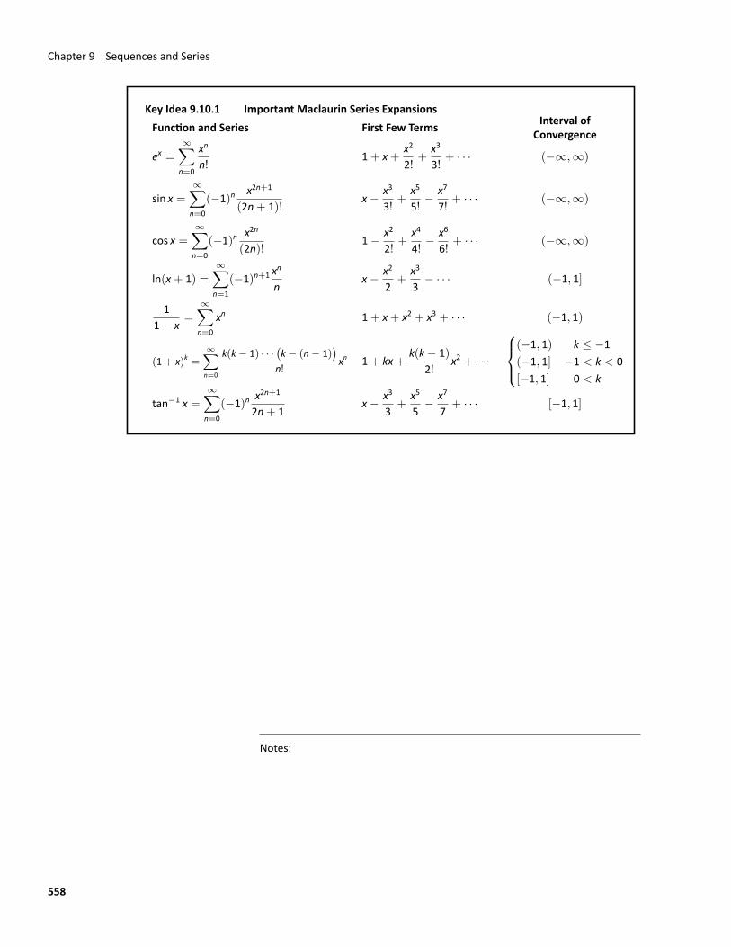
Chapter 9 Sequences and Series
Key Idea 9.10.1 Important Maclaurin Series ExpansionsFunction and Series First Few Terms Interval of
Convergence
ex =∞∑n=0
xn
n!1+ x+
x2
2!+
x3
3!+ · · · (−∞,∞)
sin x =∞∑n=0
(−1)nx2n+1
(2n+ 1)!x− x3
3!+
x5
5!− x7
7!+ · · · (−∞,∞)
cos x =∞∑n=0
(−1)nx2n
(2n)!1− x2
2!+
x4
4!− x6
6!+ · · · (−∞,∞)
ln(x+ 1) =∞∑n=1
(−1)n+1 xn
nx− x2
2+
x3
3− · · · (−1, 1]
11− x
=
∞∑n=0
xn 1+ x+ x2 + x3 + · · · (−1, 1)
(1+ x)k =∞∑n=0
k(k− 1) · · ·(k− (n− 1)
)n!
xn 1+ kx+k(k− 1)
2!x2 + · · ·
(−1, 1) k ≤ −1(−1, 1] −1 < k < 0[−1, 1] 0 < k
tan−1 x =∞∑n=0
(−1)nx2n+1
2n+ 1x− x3
3+
x5
5− x7
7+ · · · [−1, 1]
Notes:
558
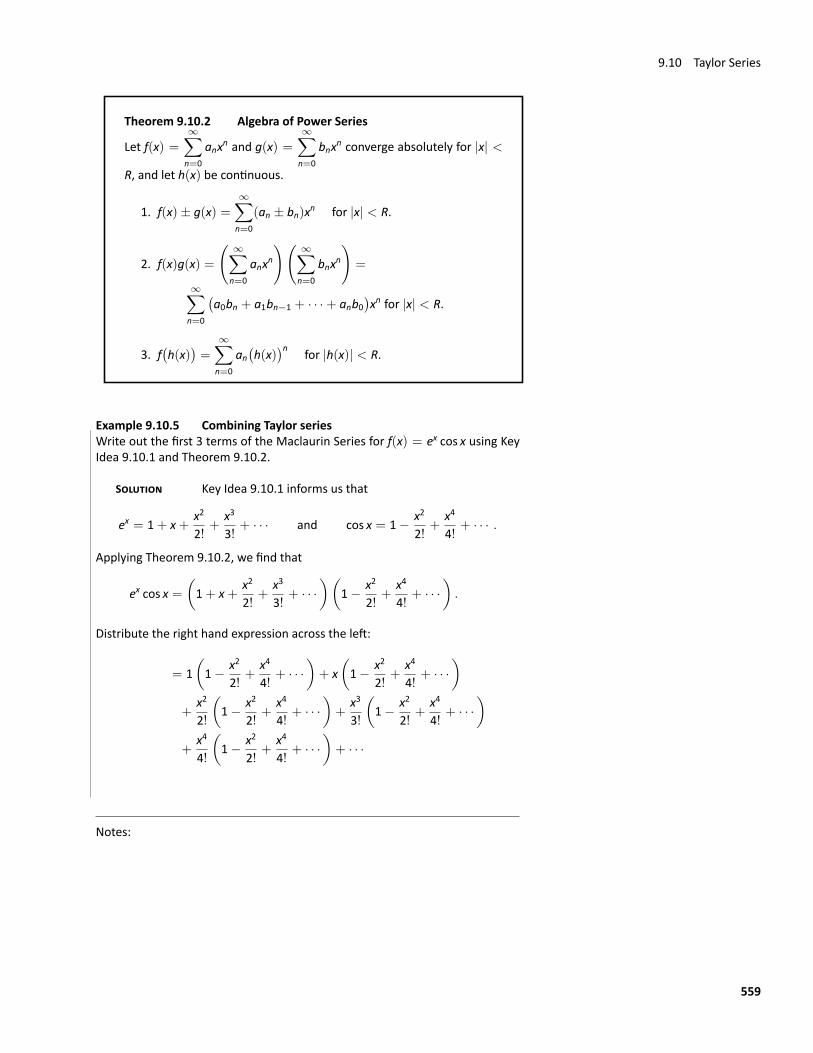
9.10 Taylor Series
Theorem 9.10.2 Algebra of Power Series
Let f(x) =∞∑n=0
anxn and g(x) =∞∑n=0
bnxn converge absolutely for |x| <
R, and let h(x) be continuous.
1. f(x)± g(x) =∞∑n=0
(an ± bn)xn for |x| < R.
2. f(x)g(x) =
( ∞∑n=0
anxn)( ∞∑
n=0bnxn
)=
∞∑n=0
(a0bn + a1bn−1 + · · ·+ anb0
)xn for |x| < R.
3. f(h(x)
)=
∞∑n=0
an(h(x)
)n for |h(x)| < R.
Example 9.10.5 Combining Taylor seriesWrite out the first 3 terms of the Maclaurin Series for f(x) = ex cos x using KeyIdea 9.10.1 and Theorem 9.10.2.
SOLUTION Key Idea 9.10.1 informs us that
ex = 1+ x+x2
2!+
x3
3!+ · · · and cos x = 1− x2
2!+
x4
4!+ · · · .
Applying Theorem 9.10.2, we find that
ex cos x =(1+ x+
x2
2!+
x3
3!+ · · ·
)(1− x2
2!+
x4
4!+ · · ·
).
Distribute the right hand expression across the left:
= 1(1− x2
2!+
x4
4!+ · · ·
)+ x
(1− x2
2!+
x4
4!+ · · ·
)+
x2
2!
(1− x2
2!+
x4
4!+ · · ·
)+
x3
3!
(1− x2
2!+
x4
4!+ · · ·
)+
x4
4!
(1− x2
2!+
x4
4!+ · · ·
)+ · · ·
Notes:
559
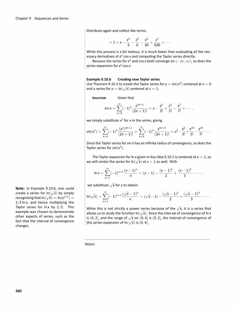
Chapter 9 Sequences and Series
Distribute again and collect like terms.
= 1+ x− x3
3− x4
6− x5
30+
x7
630+ · · ·
While this process is a bit tedious, it is much faster than evaluating all the nec‐essary derivatives of ex cos x and computing the Taylor series directly.
Because the series for ex and cos x both converge on (−∞,∞), so does theseries expansion for ex cos x.
Example 9.10.6 Creating new Taylor seriesUse Theorem 9.10.2 to create the Taylor series for y = sin(x2) centered at x = 0and a series for y = ln(
√x) centered at c = 1.
SOLUTION Given that
sin x =∞∑n=0
(−1)nx2n+1
(2n+ 1)!= x− x3
3!+
x5
5!− x7
7!+ · · · ,
we simply substitute x2 for x in the series, giving
sin(x2) =∞∑n=0
(−1)n(x2)2n+1
(2n+ 1)!=
∞∑n=0
(−1)nx4n+2
(2n+ 1)!= x2− x6
3!+x10
5!− x14
7!· · · .
Since the Taylor series for sin x has an infinite radius of convergence, so does theTaylor series for sin(x2).
The Taylor expansion for ln x given in Key Idea 9.10.1 is centered at x = 1, sowe will center the series for ln(
√x) at x = 1 as well. With
ln x =∞∑n=1
(−1)n+1 (x− 1)n
n= (x− 1)− (x− 1)2
2+
(x− 1)3
3− · · · ,
we substitute√x for x to obtain
Note: In Example 9.10.6, one couldcreate a series for ln(
√x) by simply
recognizing that ln(√x) = ln(x1/2) =
1/2 ln x, and hence multiplying theTaylor series for ln x by 1/2. Thisexample was chosen to demonstrateother aspects of series, such as thefact that the interval of convergencechanges.
ln(√x) =
∞∑n=1
(−1)n+1 (√x− 1)n
n= (
√x−1)− (
√x− 1)2
2+
(√x− 1)3
3−· · · .
While this is not strictly a power series because of the√x, it is a series that
allows us to study the function ln(√x). Since the interval of convergence of ln x
is (0, 2], and the range of√x on (0, 4] is (0, 2], the interval of convergence of
this series expansion of ln(√x) is (0, 4].
Notes:
560
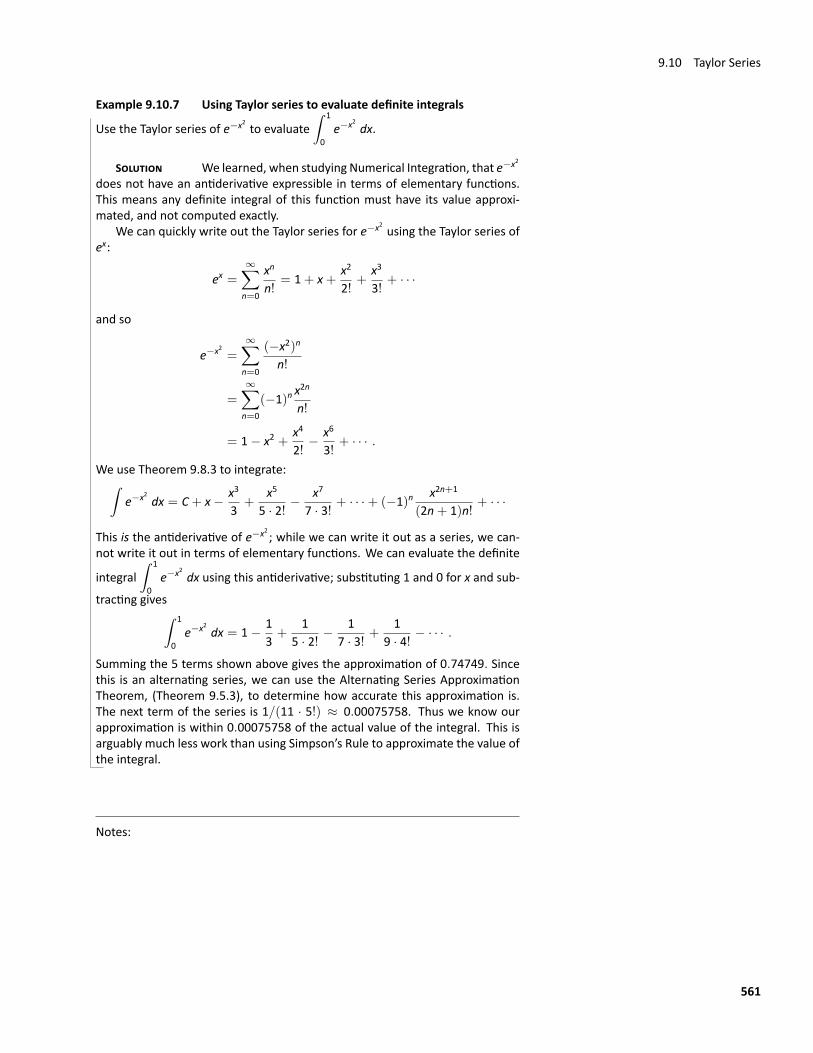
9.10 Taylor Series
Example 9.10.7 Using Taylor series to evaluate definite integrals
Use the Taylor series of e−x2 to evaluate∫ 1
0e−x2 dx.
SOLUTION We learned, when studying Numerical Integration, that e−x2
does not have an antiderivative expressible in terms of elementary functions.This means any definite integral of this function must have its value approxi‐mated, and not computed exactly.
We can quickly write out the Taylor series for e−x2 using the Taylor series ofex:
ex =∞∑n=0
xn
n!= 1+ x+
x2
2!+
x3
3!+ · · ·
and so
e−x2 =
∞∑n=0
(−x2)n
n!
=
∞∑n=0
(−1)nx2n
n!
= 1− x2 +x4
2!− x6
3!+ · · · .
We use Theorem 9.8.3 to integrate:∫e−x2 dx = C+ x− x3
3+
x5
5 · 2!− x7
7 · 3!+ · · ·+ (−1)n
x2n+1
(2n+ 1)n!+ · · ·
This is the antiderivative of e−x2 ; while we can write it out as a series, we can‐not write it out in terms of elementary functions. We can evaluate the definite
integral∫ 1
0e−x2 dx using this antiderivative; substituting 1 and 0 for x and sub‐
tracting gives∫ 1
0e−x2 dx = 1− 1
3+
15 · 2!
− 17 · 3!
+1
9 · 4!− · · · .
Summing the 5 terms shown above gives the approximation of 0.74749. Sincethis is an alternating series, we can use the Alternating Series ApproximationTheorem, (Theorem 9.5.3), to determine how accurate this approximation is.The next term of the series is 1/(11 · 5!) ≈ 0.00075758. Thus we know ourapproximation is within 0.00075758 of the actual value of the integral. This isarguably much less work than using Simpson’s Rule to approximate the value ofthe integral.
Notes:
561
Chapter 9 Sequences and Series
Another advantage to using Taylor series instead of Simpson’s Rule is formaking subsequent approximations. We found in Example 8.7.7 that the er‐
ror in using Simpson’s Rule for∫ 1
0e−x2 dx with four intervals was 0.00026. If
we wanted to decrease that error, we would need to use more intervals, es‐sentially starting the problem over. Using a Taylor series, if we wanted a moreaccurate approximation, we can just subtract the next term 1/(11 · 5!) to get anapproximation of 0.7467, with an error of at most 1/(13 · 6!) ≈ 0.0001.
Finding a pattern in the coefficients that match the series expansion of aknown function, such as those shown in Key Idea 9.10.1, can be difficult. Whatif the coefficients are given in their reduced form; how could we still recover thefunction?
Suppose that all we know is that
a0 = 1, a1 = 2, a2 = 2, a3 =43, a4 =
23.
Definition 9.10.1 states that each term of the Taylor expansion of a function in‐cludes an n!. This allows us to say that
a2 = 2 =b22!, a3 =
43=
b33!, and a4 =
23=
b44!
for some values b2, b3 and b4. Solving for these values, we see that b2 = 4,b3 = 8 and b4 = 16. That is, we are recovering the pattern bn = 2n, allowing usto write
f(x) =∞∑n=0
anxn =∞∑n=0
bnn!xn
= 1+ 2x+42!x2 +
83!x3 +
164!
x4 + · · ·
From here it is easier to recognize that the series is describing an exponentialfunction.
This chapter introduced sequences, which are ordered lists of numbers, fol‐lowed by series, wherein we add up the terms of a sequence. We quickly sawthat such sums do not always add up to “infinity,” but rather converge. We stud‐ied tests for convergence, then ended the chapter with a formal way of definingfunctions based on series. Such “series‐defined functions” are a valuable tool insolving a number of different problems throughout science and engineering.
Coming in the next chapters are new ways of defining curves in the planeapart from using functions of the form y = f(x). Curves created by these newmethods can be beautiful, useful, and important.
Notes:
562
Exercises 9.10Terms and Concepts1. What is the difference between a Taylor polynomial and a
Taylor series?2. What theoremmustweuse to show that a function is equal
to its Taylor series?
ProblemsKey Idea 9.10.1 gives the nth term of the Taylor series of com‐mon functions. In Exercises 3–6, verify the formula given inthe Key Idea by finding the first few terms of the Taylor seriesof the given function and identifying a pattern.
3. f(x) = ex; c = 0
4. f(x) = sin x; c = 0
5. f(x) = 1/(1− x); c = 0
6. f(x) = tan−1 x; c = 0
In Exercises 7–12, find a formula for the nth term of the Taylorseries of f(x), centered at c, by finding the coefficients of thefirst few powers of x and looking for a pattern. (The formulasfor several of these are found in Key Idea 9.10.1; show workverifying these formula.)
7. f(x) = cos x; c = π/2
8. f(x) = 1/x; c = 1
9. f(x) = e−x; c = 0
10. f(x) = ln(1+ x); c = 0
11. f(x) = x/(x+ 1); c = 1
12. f(x) = sin x; c = π/4
In Exercises 13–16, show that the Taylor series for f(x), as givenin Key Idea 9.10.1, is equal to f(x) by applying Theorem 9.10.1;that is, show lim
n→∞Rn(x) = 0.
13. f(x) = ex
14. f(x) = sin x
15. f(x) = ln(x+ 1) (show equality only on (0, 1)).
16. f(x) = 1/(1− x) (show equality only on (−1, 0))
In Exercises 17–20, use the Taylor series given in Key I‐dea 9.10.1 to verify the given identity.
17. cos(−x) = cos x
18. sin(−x) = − sin x
19. ddx
(sin x
)= cos x
20. ddx
(cos x
)= − sin x
In Exercises 21–24, write out the first 5 terms of the Binomialseries with the given k‐value.
21. k = 1/2
22. k = −1/2
23. k = 1/3
24. k = 4
In Exercises 25–30, use the Taylor series given in Key I‐dea 9.10.1 to create the Taylor series of the given functions.
25. f(x) = cos(x2)
26. f(x) = e−x
27. f(x) = sin(2x+ 3
)28. f(x) = tan−1(x/2)29. f(x) = ex sin x (only find the first non‐zero 4 terms)
30. f(x) = (1 + x)1/2 cos x (only find the first non‐zero 4terms)
In Exercises 31–32, approximate the value of the given definiteintegral by using the first 4 nonzero terms of the integrand’sTaylor series.
31.∫ √
π
0sin(x2)dx
32.∫ π2/4
0cos(√
x)dx
563

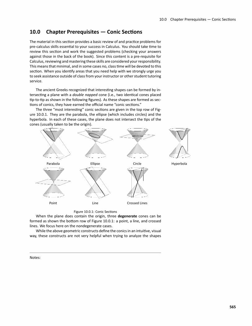
10.0 Chapter Prerequisites — Conic Sections
10.0 Chapter Prerequisites — Conic SectionsThe material in this section provides a basic review of and practice problems forpre‐calculus skills essential to your success in Calculus. You should take time toreview this section and work the suggested problems (checking your answersagainst those in the back of the book). Since this content is a pre‐requisite forCalculus, reviewing andmastering these skills are considered your responsibility.Thismeans thatminimal, and in some cases no, class timewill be devoted to thissection. When you identify areas that you need help with we strongly urge youto seek assistance outside of class from your instructor or other student tutoringservice.
The ancient Greeks recognized that interesting shapes can be formed by in‐tersecting a plane with a double napped cone (i.e., two identical cones placedtip‐to‐tip as shown in the following figures). As these shapes are formed as sec‐tions of conics, they have earned the official name “conic sections.”
The three “most interesting” conic sections are given in the top row of Fig‐ure 10.0.1. They are the parabola, the ellipse (which includes circles) and thehyperbola. In each of these cases, the plane does not intersect the tips of thecones (usually taken to be the origin).
Parabola Ellipse Circle Hyperbola
Point Line Crossed Lines
Figure 10.0.1: Conic SectionsWhen the plane does contain the origin, three degenerate cones can be
formed as shown the bottom row of Figure 10.0.1: a point, a line, and crossedlines. We focus here on the nondegenerate cases.
While the above geometric constructs define the conics in an intuitive, visualway, these constructs are not very helpful when trying to analyze the shapes
Notes:
565
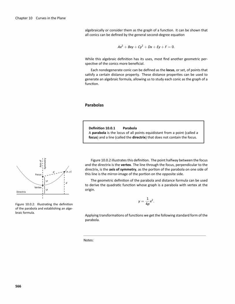
Chapter 10 Curves in the Plane
algebraically or consider them as the graph of a function. It can be shown thatall conics can be defined by the general second‐degree equation
Ax2 + Bxy+ Cy2 + Dx+ Ey+ F = 0.
While this algebraic definition has its uses, most find another geometric per‐spective of the conics more beneficial.
Each nondegenerate conic can be defined as the locus, or set, of points thatsatisfy a certain distance property. These distance properties can be used togenerate an algebraic formula, allowing us to study each conic as the graph of afunction.
Parabolas
Definition 10.0.1 ParabolaA parabola is the locus of all points equidistant from a point (called afocus) and a line (called the directrix) that does not contain the focus.
Directrix
Focus
Vertex
}p}p
(x, y)d
d
Axisof
Symmetry
Figure 10.0.2: Illustrating the definitionof the parabola and establishing an alge‐braic formula.
Figure 10.0.2 illustrates this definition. The point halfway between the focusand the directrix is the vertex. The line through the focus, perpendicular to thedirectrix, is the axis of symmetry, as the portion of the parabola on one side ofthis line is the mirror‐image of the portion on the opposite side.
The geometric definition of the parabola and distance formula can be usedto derive the quadratic function whose graph is a parabola with vertex at theorigin.
y =14p
x2.
Applying transformations of functions we get the following standard form of theparabola.
Notes:
566
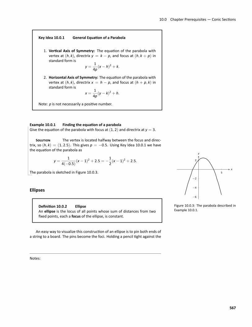
10.0 Chapter Prerequisites — Conic Sections
Key Idea 10.0.1 General Equation of a Parabola
1. Vertical Axis of Symmetry: The equation of the parabola withvertex at (h, k), directrix y = k − p, and focus at (h, k + p) instandard form is
y =14p
(x− h)2 + k.
2. Horizontal Axis of Symmetry: The equation of the parabola withvertex at (h, k), directrix x = h − p, and focus at (h + p, k) instandard form is
x =14p
(y− k)2 + h.
Note: p is not necessarily a positive number.
Example 10.0.1 Finding the equation of a parabolaGive the equation of the parabola with focus at (1, 2) and directrix at y = 3.
SOLUTION The vertex is located halfway between the focus and direc‐trix, so (h, k) = (1, 2.5). This gives p = −0.5. Using Key Idea 10.0.1 we havethe equation of the parabola as
5
−6
−4
−2
2
x
y
Figure 10.0.3: The parabola described inExample 10.0.1.
y =1
4(−0.5)(x− 1)2 + 2.5 = −1
2(x− 1)2 + 2.5.
The parabola is sketched in Figure 10.0.3.
Ellipses
Definition 10.0.2 EllipseAn ellipse is the locus of all points whose sum of distances from twofixed points, each a focus of the ellipse, is constant.
An easy way to visualize this construction of an ellipse is to pin both ends ofa string to a board. The pins become the foci. Holding a pencil tight against the
Notes:
567
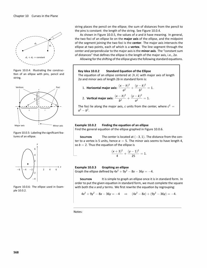
Chapter 10 Curves in the Plane
string places the pencil on the ellipse; the sum of distances from the pencil tothe pins is constant: the length of the string. See Figure 10.0.4.
As shown in Figure 10.0.5, the values of a and b have meaning. In general,the two foci of an ellipse lie on the major axis of the ellipse, and the midpointof the segment joining the two foci is the center. The major axis intersects theellipse at two points, each of which is a vertex. The line segment through thecenter and perpendicular to the major axis is theminor axis. The “constant sumof distances” that defines the ellipse is the length of the major axis, i.e., 2a.
d1d2
d1 + d2 = constant
Figure 10.0.4: Illustrating the construc‐tion of an ellipse with pins, pencil andstring.
Major axis Minor axis
Vertices Foci
︸ ︷︷ ︸a
︸ ︷︷ ︸c
b
Figure 10.0.5: Labeling the significant fea‐tures of an ellipse.
Allowing for the shifting of the ellipse gives the following standard equations.
Key Idea 10.0.2 Standard Equation of the EllipseThe equation of an ellipse centered at (h, k) with major axis of length2a and minor axis of length 2b in standard form is:
1. Horizontal major axis:(x− h)2
a2+
(y− k)2
b2= 1.
2. Vertical major axis:(x− h)2
b2+
(y− k)2
a2= 1.
The foci lie along the major axis, c units from the center, where c2 =a2 − b2.
Example 10.0.2 Finding the equation of an ellipseFind the general equation of the ellipse graphed in Figure 10.0.6.
−6 −4 −2 2 4 6
−4
−2
2
4
6
x
y
Figure 10.0.6: The ellipse used in Exam‐ple 10.0.2.
SOLUTION The center is located at (−3, 1). The distance from the cen‐ter to a vertex is 5 units, hence a = 5. The minor axis seems to have length 4,so b = 2. Thus the equation of the ellipse is
(x+ 3)2
4+
(y− 1)2
25= 1.
Example 10.0.3 Graphing an ellipseGraph the ellipse defined by 4x2 + 9y2 − 8x− 36y = −4.
SOLUTION It is simple to graph an ellipse once it is in standard form. Inorder to put the given equation in standard form, we must complete the squarewith both the x and y terms. We first rewrite the equation by regrouping:
4x2 + 9y2 − 8x− 36y = −4 ⇒ (4x2 − 8x) + (9y2 − 36y) = −4.
Notes:
568
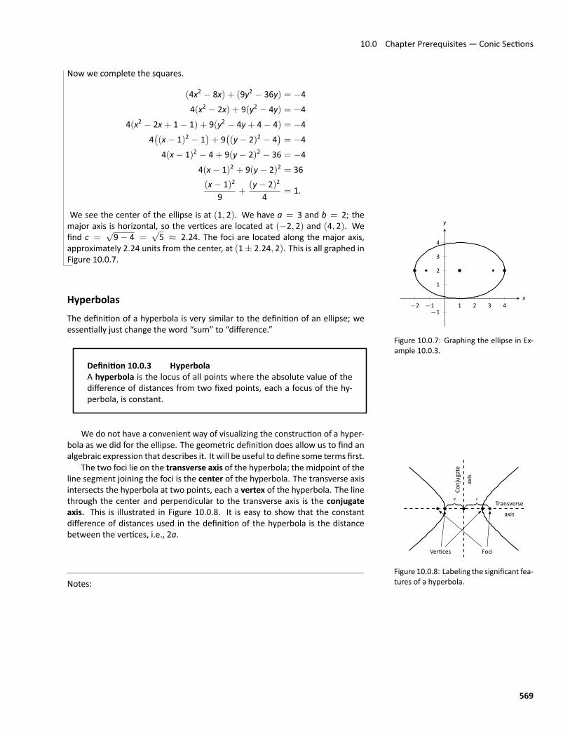
10.0 Chapter Prerequisites — Conic Sections
Now we complete the squares.
(4x2 − 8x) + (9y2 − 36y) = −44(x2 − 2x) + 9(y2 − 4y) = −4
4(x2 − 2x+ 1− 1) + 9(y2 − 4y+ 4− 4) = −44((x− 1)2 − 1
)+ 9((y− 2)2 − 4
)= −4
4(x− 1)2 − 4+ 9(y− 2)2 − 36 = −44(x− 1)2 + 9(y− 2)2 = 36(x− 1)2
9+
(y− 2)2
4= 1.
We see the center of the ellipse is at (1, 2). We have a = 3 and b = 2; the
−2 −1 1 2 3 4−1
1
2
3
4
x
y
Figure 10.0.7: Graphing the ellipse in Ex‐ample 10.0.3.
major axis is horizontal, so the vertices are located at (−2, 2) and (4, 2). Wefind c =
√9− 4 =
√5 ≈ 2.24. The foci are located along the major axis,
approximately 2.24 units from the center, at (1± 2.24, 2). This is all graphed inFigure 10.0.7.
HyperbolasThe definition of a hyperbola is very similar to the definition of an ellipse; weessentially just change the word “sum” to “difference.”
Definition 10.0.3 HyperbolaA hyperbola is the locus of all points where the absolute value of thedifference of distances from two fixed points, each a focus of the hy‐perbola, is constant.
We do not have a convenient way of visualizing the construction of a hyper‐bola as we did for the ellipse. The geometric definition does allow us to find analgebraic expression that describes it. It will be useful to define some terms first.
Transverseaxis
axis
Conjugate
FociVertices
a︷ ︸︸ ︷ c︷ ︸︸ ︷
Figure 10.0.8: Labeling the significant fea‐tures of a hyperbola.
The two foci lie on the transverse axis of the hyperbola; the midpoint of theline segment joining the foci is the center of the hyperbola. The transverse axisintersects the hyperbola at two points, each a vertex of the hyperbola. The linethrough the center and perpendicular to the transverse axis is the conjugateaxis. This is illustrated in Figure 10.0.8. It is easy to show that the constantdifference of distances used in the definition of the hyperbola is the distancebetween the vertices, i.e., 2a.
Notes:
569
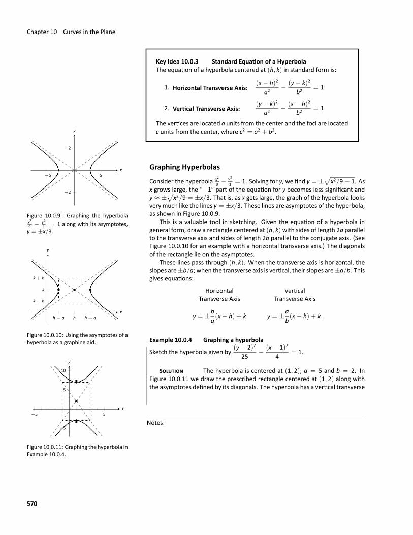
Chapter 10 Curves in the Plane
Key Idea 10.0.3 Standard Equation of a HyperbolaThe equation of a hyperbola centered at (h, k) in standard form is:
1. Horizontal Transverse Axis:(x− h)2
a2− (y− k)2
b2= 1.
2. Vertical Transverse Axis:(y− k)2
a2− (x− h)2
b2= 1.
The vertices are located a units from the center and the foci are locatedc units from the center, where c2 = a2 + b2.
Graphing Hyperbolas−5 5
−2
2
x
y
Figure 10.0.9: Graphing the hyperbolax29 − y2
1 = 1 along with its asymptotes,y = ±x/3.
Consider the hyperbola x29 − y2
1 = 1. Solving for y, we find y = ±√
x2/9− 1. Asx grows large, the “−1” part of the equation for y becomes less significant andy ≈ ±
√x2/9 = ±x/3. That is, as x gets large, the graph of the hyperbola looks
verymuch like the lines y = ±x/3. These lines are asymptotes of the hyperbola,as shown in Figure 10.0.9.
h − a h + ah
k − b
k
k + b
x
y
Figure 10.0.10: Using the asymptotes of ahyperbola as a graphing aid.
This is a valuable tool in sketching. Given the equation of a hyperbola ingeneral form, draw a rectangle centered at (h, k)with sides of length 2a parallelto the transverse axis and sides of length 2b parallel to the conjugate axis. (SeeFigure 10.0.10 for an example with a horizontal transverse axis.) The diagonalsof the rectangle lie on the asymptotes.
These lines pass through (h, k). When the transverse axis is horizontal, theslopes are±b/a; when the transverse axis is vertical, their slopes are±a/b. Thisgives equations:
HorizontalTransverse Axis
VerticalTransverse Axis
y = ±ba(x− h) + k y = ±a
b(x− h) + k.
−5 5
−5
5
10
x
y
Figure 10.0.11: Graphing the hyperbola inExample 10.0.4.
Example 10.0.4 Graphing a hyperbola
Sketch the hyperbola given by(y− 2)2
25− (x− 1)2
4= 1.
SOLUTION The hyperbola is centered at (1, 2); a = 5 and b = 2. InFigure 10.0.11 we draw the prescribed rectangle centered at (1, 2) along withthe asymptotes defined by its diagonals. The hyperbola has a vertical transverse
Notes:
570
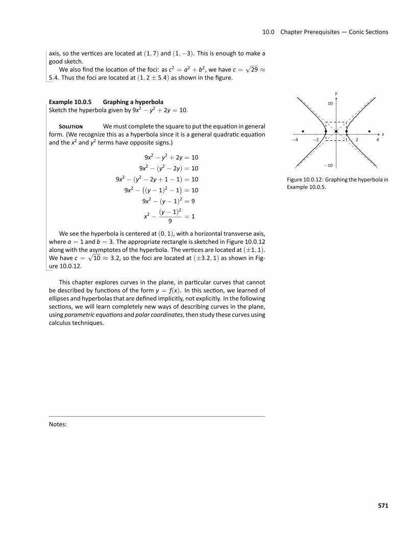
10.0 Chapter Prerequisites — Conic Sections
axis, so the vertices are located at (1, 7) and (1,−3). This is enough to make agood sketch.
We also find the location of the foci: as c2 = a2 + b2, we have c =√29 ≈
5.4. Thus the foci are located at (1, 2± 5.4) as shown in the figure.
−4 −2 2 4
−10
10
x
y
Figure 10.0.12: Graphing the hyperbola inExample 10.0.5.
Example 10.0.5 Graphing a hyperbolaSketch the hyperbola given by 9x2 − y2 + 2y = 10.
SOLUTION Wemust complete the square to put the equation in generalform. (We recognize this as a hyperbola since it is a general quadratic equationand the x2 and y2 terms have opposite signs.)
9x2 − y2 + 2y = 109x2 − (y2 − 2y) = 10
9x2 − (y2 − 2y+ 1− 1) = 109x2 −
((y− 1)2 − 1
)= 10
9x2 − (y− 1)2 = 9
x2 − (y− 1)2
9= 1
We see the hyperbola is centered at (0, 1), with a horizontal transverse axis,where a = 1 and b = 3. The appropriate rectangle is sketched in Figure 10.0.12along with the asymptotes of the hyperbola. The vertices are located at (±1, 1).We have c =
√10 ≈ 3.2, so the foci are located at (±3.2, 1) as shown in Fig‐
ure 10.0.12.
This chapter explores curves in the plane, in particular curves that cannotbe described by functions of the form y = f(x). In this section, we learned ofellipses and hyperbolas that are defined implicitly, not explicitly. In the followingsections, we will learn completely new ways of describing curves in the plane,using parametric equations and polar coordinates, then study these curves usingcalculus techniques.
Notes:
571
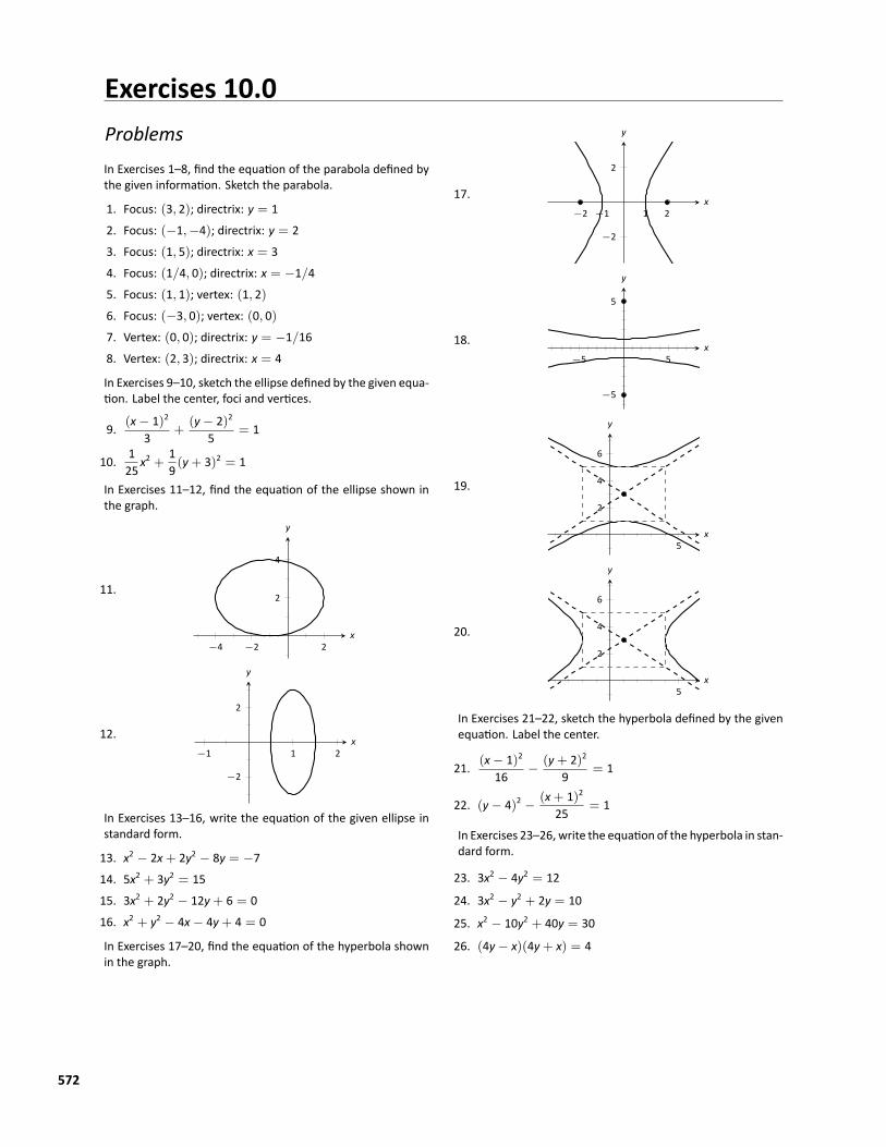
Exercises 10.0ProblemsIn Exercises 1–8, find the equation of the parabola defined bythe given information. Sketch the parabola.
1. Focus: (3, 2); directrix: y = 12. Focus: (−1,−4); directrix: y = 23. Focus: (1, 5); directrix: x = 34. Focus: (1/4, 0); directrix: x = −1/45. Focus: (1, 1); vertex: (1, 2)6. Focus: (−3, 0); vertex: (0, 0)7. Vertex: (0, 0); directrix: y = −1/168. Vertex: (2, 3); directrix: x = 4
In Exercises 9–10, sketch the ellipse defined by the given equa‐tion. Label the center, foci and vertices.
9. (x− 1)2
3+
(y− 2)2
5= 1
10. 125
x2 + 19(y+ 3)2 = 1
In Exercises 11–12, find the equation of the ellipse shown inthe graph.
11.
−4 −2 2
2
4
x
y
12.−1 1 2
−2
2
x
y
In Exercises 13–16, write the equation of the given ellipse instandard form.
13. x2 − 2x+ 2y2 − 8y = −714. 5x2 + 3y2 = 1515. 3x2 + 2y2 − 12y+ 6 = 016. x2 + y2 − 4x− 4y+ 4 = 0
In Exercises 17–20, find the equation of the hyperbola shownin the graph.
17.−1 1 2−2
−2
2
x
y
18.−5 5
−5
5
x
y
19.
5
2
4
6
x
y
20.
5
2
4
6
x
y
In Exercises 21–22, sketch the hyperbola defined by the givenequation. Label the center.
21. (x− 1)2
16− (y+ 2)2
9= 1
22. (y− 4)2 − (x+ 1)2
25= 1
In Exercises 23–26, write the equation of the hyperbola in stan‐dard form.
23. 3x2 − 4y2 = 12
24. 3x2 − y2 + 2y = 10
25. x2 − 10y2 + 40y = 30
26. (4y− x)(4y+ x) = 4
572
10.1 Arc Length and Surface Area
10: CURVES IN THE PLANEWe have explored functions of the form y = f(x) closely throughout this text.We have explored their limits, their derivatives and their antiderivatives; wehave learned to identify key features of their graphs, such as relative maximaandminima, inflection points and asymptotes; we have found equations of theirtangent lines, the areas between portions of their graphs and the x‐axis, and thevolumes of solids generated by revolving portions of their graphs about a hori‐zontal or vertical axis.
Despite all this, the graphs created by functions of the form y = f(x) arelimited. Since each x‐value can correspond to only 1 y‐value, common shapeslike circles cannot be fully described by a function in this form. Fittingly, the“vertical line test” excludes vertical lines from being functions of x, even thoughthese lines are important in mathematics.
In this chapter we’ll explore new ways of drawing curves in the plane. We’llstill workwithin the framework of functions, as an inputwill still only correspondto one output. However, our new techniques of drawing curves will render thevertical line test pointless, and allow us to create important — and beautiful —new curves. Once these curves are defined, we’ll apply the concepts of calculusto them, continuing to find equations of tangent lines and the areas of enclosedregions.
One aspect that we’ll be interested in is “how long is this curve?” Beforewe explore that idea for these new ways to draw curves, we’ll start by exploringhow long a curve is when we’ve gotten it from a regular y = f(x) function.
10.1 Arc Length and Surface Area
π4
π2
3π4
π
1
x
y
(a)
π4
π2
3π4
π
1√2
1
x
y
(b)
Figure 10.1.1: Graphing y = sin x on[0, π] and approximating the curve withline segments.
In previous sectionswe have used integration to answer the following questions:
1. Given a region, what is its area?
2. Given a solid, what is its volume?
In this section, we address a related question: Given a curve, what is itslength? This is often referred to as arc length.
Consider the graph of y = sin x on [0, π] given in Figure 10.1.1 (a). How longis this curve? That is, if we were to use a piece of string to exactly match theshape of this curve, how long would the string be?
As we have done in the past, we start by approximating; later, we will refineour answer using limits to get an exact solution.
Notes:
573
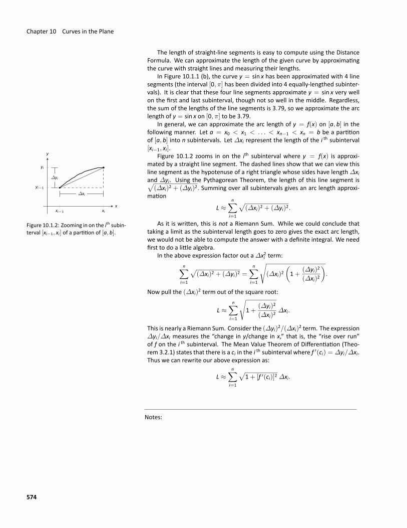
Chapter 10 Curves in the Plane
The length of straight‐line segments is easy to compute using the DistanceFormula. We can approximate the length of the given curve by approximatingthe curve with straight lines and measuring their lengths.
In Figure 10.1.1 (b), the curve y = sin x has been approximated with 4 linesegments (the interval [0, π] has been divided into 4 equally‐lengthed subinter‐vals). It is clear that these four line segments approximate y = sin x very wellon the first and last subinterval, though not so well in the middle. Regardless,the sum of the lengths of the line segments is 3.79, so we approximate the arclength of y = sin x on [0, π] to be 3.79.
In general, we can approximate the arc length of y = f(x) on [a, b] in thefollowing manner. Let a = x0 < x1 < . . . < xn−1 < xn = b be a partitionof [a, b] into n subintervals. Let ∆xi represent the length of the i th subinterval[xi−1, xi].
∆yi
∆xi
xi−1 xi
yi−1
yi
x
y
Figure 10.1.2: Zooming in on the ith subin‐terval [xi−1, xi] of a partition of [a, b].
Figure 10.1.2 zooms in on the ith subinterval where y = f(x) is approxi‐mated by a straight line segment. The dashed lines show that we can view thisline segment as the hypotenuse of a right triangle whose sides have length∆xiand ∆yi. Using the Pythagorean Theorem, the length of this line segment is√(∆xi)2 + (∆yi)2. Summing over all subintervals gives an arc length approxi‐
mation
L ≈n∑
i=1
√(∆xi)2 + (∆yi)2.
As it is written, this is not a Riemann Sum. While we could conclude thattaking a limit as the subinterval length goes to zero gives the exact arc length,we would not be able to compute the answer with a definite integral. We needfirst to do a little algebra.
In the above expression factor out a∆x2i term:n∑
i=1
√(∆xi)2 + (∆yi)2 =
n∑i=1
√(∆xi)2
(1+
(∆yi)2
(∆xi)2
).
Now pull the (∆xi)2 term out of the square root:
L ≈n∑
i=1
√1+
(∆yi)2
(∆xi)2∆xi.
This is nearly a Riemann Sum. Consider the (∆yi)2/(∆xi)2 term. The expression∆yi/∆xi measures the “change in y/change in x,” that is, the “rise over run”of f on the i th subinterval. The Mean Value Theorem of Differentiation (Theo‐rem 3.2.1) states that there is a ci in the i th subinterval where f ′(ci) = ∆yi/∆xi.Thus we can rewrite our above expression as:
L ≈n∑
i=1
√1+ [f ′(ci)]2 ∆xi.
Notes:
574
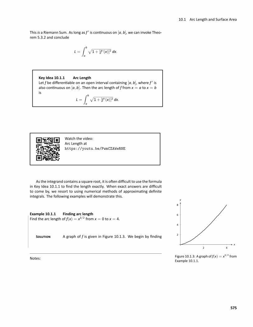
10.1 Arc Length and Surface Area
This is a Riemann Sum. As long as f ′ is continuous on [a, b], we can invoke Theo‐rem 5.3.2 and conclude
L =∫ b
a
√1+ [f ′(x)]2 dx.
Key Idea 10.1.1 Arc LengthLet f be differentiable on an open interval containing [a, b], where f ′ isalso continuous on [a, b]. Then the arc length of f from x = a to x = bis
L =∫ b
a
√1+ [f ′(x)]2 dx.
Watch the video:Arc Length athttps://youtu.be/PwmCZAWeRNE
As the integrand contains a square root, it is often difficult to use the formulain Key Idea 10.1.1 to find the length exactly. When exact answers are difficultto come by, we resort to using numerical methods of approximating definiteintegrals. The following examples will demonstrate this.
2 4
2
4
6
8
x
y
Figure 10.1.3: A graph of f(x) = x3/2 fromExample 10.1.1.
Example 10.1.1 Finding arc lengthFind the arc length of f(x) = x3/2 from x = 0 to x = 4.
SOLUTION A graph of f is given in Figure 10.1.3. We begin by finding
Notes:
575
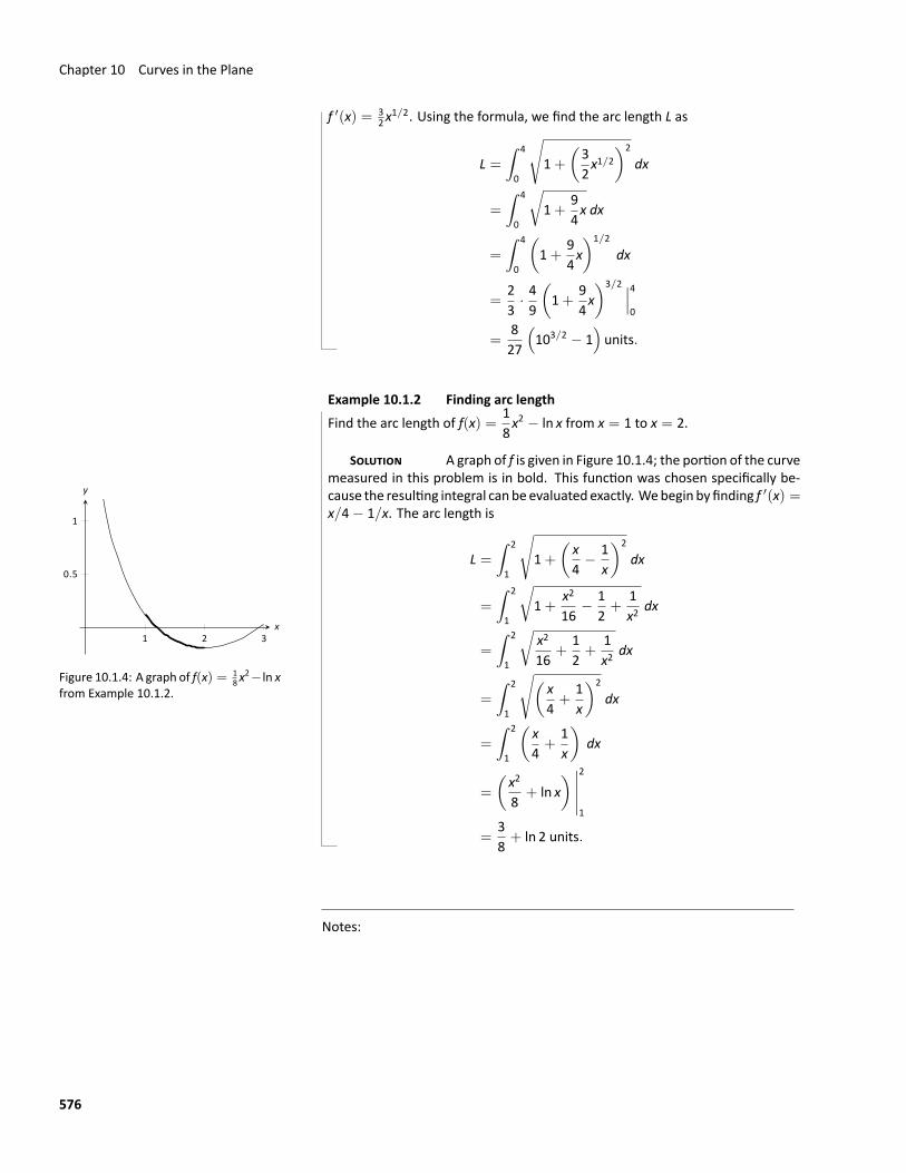
Chapter 10 Curves in the Plane
f ′(x) = 32x
1/2. Using the formula, we find the arc length L as
L =∫ 4
0
√1+
(32x1/2
)2
dx
=
∫ 4
0
√1+
94x dx
=
∫ 4
0
(1+
94x)1/2
dx
=23· 49
(1+
94x)3/2 ∣∣∣4
0
=827
(103/2 − 1
)units.
Example 10.1.2 Finding arc lengthFind the arc length of f(x) =
18x2 − ln x from x = 1 to x = 2.
SOLUTION A graph of f is given in Figure 10.1.4; the portion of the curvemeasured in this problem is in bold. This function was chosen specifically be‐
1 2 3
0.5
1
x
y
Figure 10.1.4: A graph of f(x) = 18 x
2− ln xfrom Example 10.1.2.
cause the resulting integral canbe evaluated exactly. Webegin byfinding f ′(x) =x/4− 1/x. The arc length is
L =∫ 2
1
√1+
(x4− 1
x
)2
dx
=
∫ 2
1
√1+
x2
16− 1
2+
1x2
dx
=
∫ 2
1
√x2
16+
12+
1x2
dx
=
∫ 2
1
√(x4+
1x
)2
dx
=
∫ 2
1
(x4+
1x
)dx
=
(x2
8+ ln x
) ∣∣∣∣∣2
1
=38+ ln 2 units.
Notes:
576
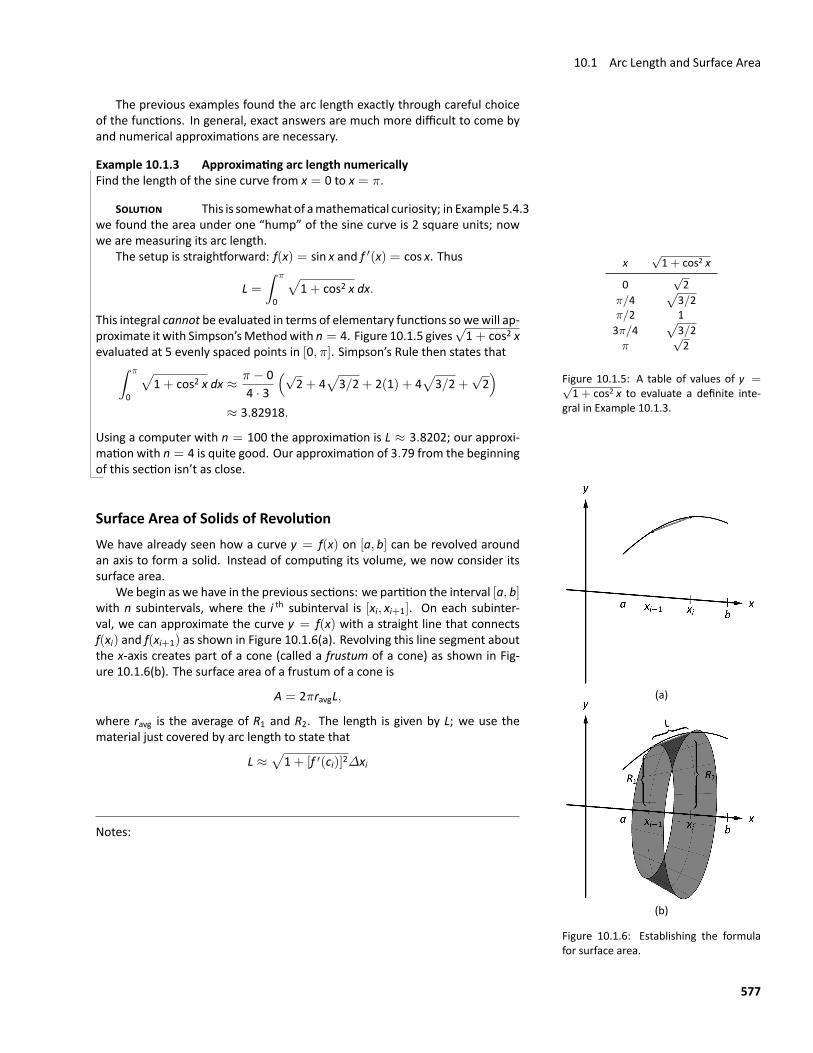
10.1 Arc Length and Surface Area
The previous examples found the arc length exactly through careful choiceof the functions. In general, exact answers are much more difficult to come byand numerical approximations are necessary.
Example 10.1.3 Approximating arc length numericallyFind the length of the sine curve from x = 0 to x = π.
SOLUTION This is somewhat of amathematical curiosity; in Example 5.4.3we found the area under one “hump” of the sine curve is 2 square units; nowwe are measuring its arc length.
x√1+ cos2 x
0√2
π/4√
3/2π/2 13π/4
√3/2
π√2
Figure 10.1.5: A table of values of y =√1+ cos2 x to evaluate a definite inte‐
gral in Example 10.1.3.
The setup is straightforward: f(x) = sin x and f ′(x) = cos x. Thus
L =∫ π
0
√1+ cos2 x dx.
This integral cannot be evaluated in terms of elementary functions sowewill ap‐proximate it with Simpson’sMethodwith n = 4. Figure 10.1.5 gives
√1+ cos2 x
evaluated at 5 evenly spaced points in [0, π]. Simpson’s Rule then states that∫ π
0
√1+ cos2 x dx ≈ π − 0
4 · 3
(√2+ 4
√3/2+ 2(1) + 4
√3/2+
√2)
≈ 3.82918.
Using a computer with n = 100 the approximation is L ≈ 3.8202; our approxi‐mation with n = 4 is quite good. Our approximation of 3.79 from the beginningof this section isn’t as close.
Surface Area of Solids of Revolution
(a)
(b)
Figure 10.1.6: Establishing the formulafor surface area.
We have already seen how a curve y = f(x) on [a, b] can be revolved aroundan axis to form a solid. Instead of computing its volume, we now consider itssurface area.
We begin as we have in the previous sections: we partition the interval [a, b]with n subintervals, where the i th subinterval is [xi, xi+1]. On each subinter‐val, we can approximate the curve y = f(x) with a straight line that connectsf(xi) and f(xi+1) as shown in Figure 10.1.6(a). Revolving this line segment aboutthe x‐axis creates part of a cone (called a frustum of a cone) as shown in Fig‐ure 10.1.6(b). The surface area of a frustum of a cone is
A = 2πravgL,
where ravg is the average of R1 and R2. The length is given by L; we use thematerial just covered by arc length to state that
L ≈√
1+ [f ′(ci)]2∆xi
Notes:
577
Chapter 10 Curves in the Plane
for some ci in the i th subinterval. The radii are just the function evaluated at theendpoints of the interval: f(xi−1) and f(xi). Thus the surface area of this samplefrustum of the cone is approximately
2πf(xi−1) + f(xi)
2√
1+ [f ′(ci)]2∆xi.
Since f is a continuous function, the IntermediateValue Theoremstates there
is some di in [xi−1, xi] such that f(di) =f(xi−1) + f(xi)
2; we can use this to rewrite
the above equation as
2πf(di)√
1+ [f ′(ci)]2∆xi.
Summing over all the subintervals we get the total surface area to be approxi‐mately
Surface Area ≈n∑
i=1
2πf(di)√
1+ [f ′(ci)]2∆xi,
which is a Riemann Sum. Taking the limit as the subinterval lengths go to zerogives us the exact surface area, given in the upcoming Key Idea.
If instead we revolve y = f(x) about the y‐axis, the radii of the resultingfrustumare xi−1 and xi; their average value is simply themidpoint of the interval.In the limit, this midpoint is just x. This gives the second part of Key Idea 10.1.2.
Key Idea 10.1.2 Surface Area of a Solid of RevolutionLet f be differentiable on an open interval containing [a, b] where f ′ isalso continuous on [a, b].
1. The surface area of the solid formed by revolving the graph ofy = f(x), where f(x) ≥ 0, about the x‐axis is
Surface Area = 2π∫ b
af(x)√
1+ [f ′(x)]2 dx.
2. The surface area of the solid formed by revolving the graph ofy = f(x) about the y‐axis, where a, b ≥ 0, is
Surface Area = 2π∫ b
ax√
1+ [f ′(x)]2 dx.
Notes:
578
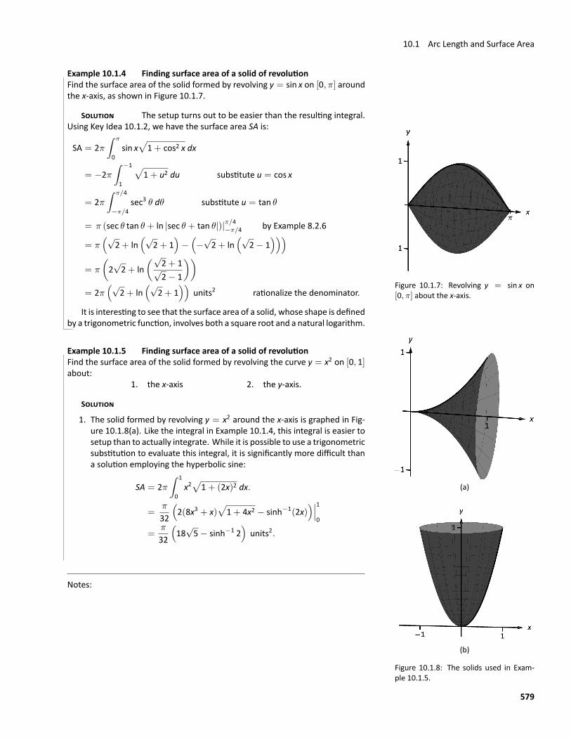
10.1 Arc Length and Surface Area
Example 10.1.4 Finding surface area of a solid of revolutionFind the surface area of the solid formed by revolving y = sin x on [0, π] aroundthe x‐axis, as shown in Figure 10.1.7.
SOLUTION The setup turns out to be easier than the resulting integral.Using Key Idea 10.1.2, we have the surface area SA is:
Figure 10.1.7: Revolving y = sin x on[0, π] about the x‐axis.
SA = 2π∫ π
0sin x
√1+ cos2 x dx
= −2π∫ −1
1
√1+ u2 du substitute u = cos x
= 2π∫ π/4
−π/4sec3 θ dθ substitute u = tan θ
= π (sec θ tan θ + ln |sec θ + tan θ|)|π/4−π/4 by Example 8.2.6
= π(√
2+ ln(√
2+ 1)−(−√2+ ln
(√2− 1
)))= π
(2√2+ ln
(√2+ 1√2− 1
))= 2π
(√2+ ln
(√2+ 1
))units2 rationalize the denominator.
It is interesting to see that the surface area of a solid, whose shape is definedby a trigonometric function, involves both a square root and a natural logarithm.
(a)
(b)
Figure 10.1.8: The solids used in Exam‐ple 10.1.5.
Example 10.1.5 Finding surface area of a solid of revolutionFind the surface area of the solid formed by revolving the curve y = x2 on [0, 1]about:
1. the x‐axis 2. the y‐axis.
SOLUTION
1. The solid formed by revolving y = x2 around the x‐axis is graphed in Fig‐ure 10.1.8(a). Like the integral in Example 10.1.4, this integral is easier tosetup than to actually integrate. While it is possible to use a trigonometricsubstitution to evaluate this integral, it is significantly more difficult thana solution employing the hyperbolic sine:
SA = 2π∫ 1
0x2√
1+ (2x)2 dx.
=π
32
(2(8x3 + x)
√1+ 4x2 − sinh−1(2x)
)∣∣∣10
=π
32
(18
√5− sinh−1 2
)units2.
Notes:
579
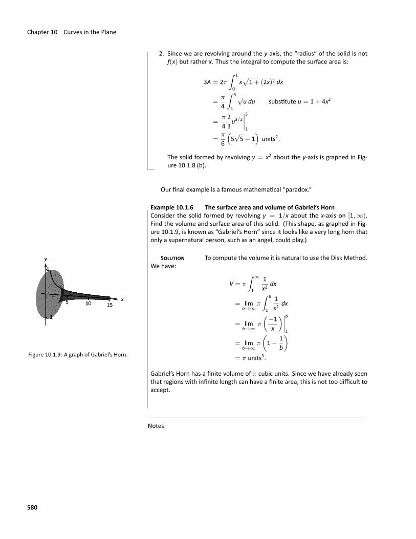
Chapter 10 Curves in the Plane
2. Since we are revolving around the y‐axis, the “radius” of the solid is notf(x) but rather x. Thus the integral to compute the surface area is:
SA = 2π∫ 1
0x√
1+ (2x)2 dx
=π
4
∫ 5
1
√u du substitute u = 1+ 4x2
=π
423u3/2
∣∣∣∣51
=π
6
(5√5− 1
)units2.
The solid formed by revolving y = x2 about the y‐axis is graphed in Fig‐ure 10.1.8 (b).
Our final example is a famous mathematical “paradox.”
Example 10.1.6 The surface area and volume of Gabriel’s HornConsider the solid formed by revolving y = 1/x about the x‐axis on [1,∞).Find the volume and surface area of this solid. (This shape, as graphed in Fig‐ure 10.1.9, is known as “Gabriel’s Horn” since it looks like a very long horn thatonly a supernatural person, such as an angel, could play.)
Figure 10.1.9: A graph of Gabriel’s Horn.
SOLUTION To compute the volume it is natural to use the Disk Method.We have:
V = π
∫ ∞
1
1x2
dx
= limb→∞
π
∫ b
1
1x2
dx
= limb→∞
π
(−1x
)∣∣∣∣b1
= limb→∞
π
(1− 1
b
)= π units3.
Gabriel’s Horn has a finite volume of π cubic units. Since we have already seenthat regions with infinite length can have a finite area, this is not too difficult toaccept.
Notes:
580
10.1 Arc Length and Surface Area
We now consider its surface area. The integral is straightforward to setup:
SA = 2π∫ ∞
1
1x√
1+ 1/x4 dx.
Integrating this expression is not trivial. We can, however, compare it to otherimproper integrals. Since 1 <
√1+ 1/x4 on [1,∞), we can state that
2π∫ ∞
1
1xdx < 2π
∫ ∞
1
1x√
1+ 1/x4 dx.
By Key Idea 8.6.1, the improper integral on the left diverges. Since the integralon the right is larger, we conclude it also diverges, meaning Gabriel’s Horn hasinfinite surface area.
Hence the “paradox”: we can fill Gabriel’s Hornwith a finite amount of paint,but since it has infinite surface area, we can never paint it.
Somehow this paradox is striking when we think about it in terms of volumeand area. However, we have seen a similar paradox before, as referenced above.We know that the area under the curve y = 1/x2 on [1,∞) is finite, yet theshape has an infinite perimeter. Strange things can occur when we deal withthe infinite.
Notes:
581
Exercises 10.1Terms and Concepts1. T/F: The integral formula for computing Arc Length was
found by first approximating arc length with straight linesegments.
2. T/F: The integral formula for computingArc Length includesa square‐root, meaning the integration is probably easy.
ProblemsIn Exercises 3–12, find the arc length of the function on thegiven interval.
3. f(x) = x on [0, 1].4. f(x) =
√8x on [−1, 1].
5. f(x) = 13x3/2 − x1/2 on [0, 1].
6. f(x) = 112
x3 + 1xon [1, 4].
7. f(x) = 2x3/2 − 16√x on [0, 9].
8. f(x) = cosh x on [− ln 2, ln 2].
9. f(x) = 12(ex + e−x) on [0, ln 5].
10. f(x) = 112
x5 + 15x3
on [.1, 1].
11. f(x) = ln(sin x
)on [π/6, π/2].
12. f(x) = ln(cos x
)on [0, π/4].
In Exercises 13–20, set up the integral to compute the arclength of the function on the given interval. Do not evaluatethe integral.
13. f(x) = x2 on [0, 1].14. f(x) = x10 on [0, 1].15. f(x) =
√x on [0, 1].
16. f(x) = ln x on [1, e].
17. f(x) =√1− x2 on [−1, 1]. (Note: this describes the top
half of a circle with radius 1.)
18. f(x) =√
1− x2/9 on [−3, 3]. (Note: this describes thetop half of an ellipse with a major axis of length 6 and aminor axis of length 2.)
19. f(x) = 1xon [1, 2].
20. f(x) = sec x on [−π/4, π/4].
In Exercises 21–28, use Simpson’s Rule, with n = 4, to approxi‐mate the arc length of the function on the given interval. Note:these are the same problems as in Exercises 13–20.
21. f(x) = x2 on [0, 1].
22. f(x) = x10 on [0, 1].
23. f(x) =√x on [0, 1]. (Note: f ′(x) is not defined at x = 0.)
24. f(x) = ln x on [1, e].
25. f(x) =√1− x2 on [−1, 1]. (Note: f ′(x) is not defined at
the endpoints.)
26. f(x) =√
1− x2/9 on [−3, 3]. (Note: f ′(x) is not definedat the endpoints.)
27. f(x) = 1xon [1, 2].
28. f(x) = sec x on [−π/4, π/4].
In Exercises 29–32, find the surface area of the described solidof revolution.
29. The solid formed by revolving y = 2x on [0, 1] about thex‐axis.
30. The solid formed by revolving y = x3 on [0, 1] about thex‐axis.
31. The solid formed by revolving y =√x on [0, 1] about the
x‐axis.32. The sphere formed by revolving y =
√1− x2 on [−1, 1]
about the x‐axis.
582
10.2 Parametric Equations
10.2 Parametric Equations
We are familiar with sketching shapes, such as parabolas, by following this basicprocedure:
Choosex
−→Use a function
f to find y(y = f(x)
) −→Plot point(x, y)
In the rectangular coordinate system, the rectangular equation y = f(x)works well for some shapes like a parabola with a vertical axis of symmetry, butin precalculus and the review of conic sections in section 10.0, we encounteredseveral shapes that could not be sketched in thismanner. (To plot an ellipse usingthe above procedure, we need to plot the “top” and “bottom” separately.)
In this section we introduce a new sketching procedure:
Chooset
Use a functionf to find x(x = f(t)
)Use a functiong to find y(y = g(t)
)Plot point(x, y)
Here, x and y are found separately but then plotted together. This leads usto a definition.
Definition 10.2.1 Parametric Equations and CurvesLet f and g be continuous functions on an interval I. The graph of theparametric equations x = f(t) and y = g(t) is the set of all points(x, y)=(f(t), g(t)
)in the Cartesian plane, as the parameter t varies
over I. A curve is a graph along with the parametric equations that de‐fine it.
Notes:
583
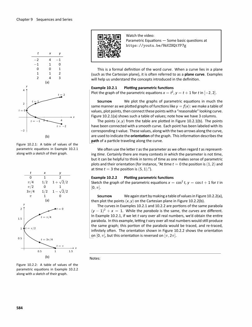
Chapter 9 Sequences and Series
Watch the video:Parametric Equations — Some basic questions athttps://youtu.be/9kKZHQtYP7g
This is a formal definition of the word curve. When a curve lies in a plane(such as the Cartesian plane), it is often referred to as a plane curve. Exampleswill help us understand the concepts introduced in the definition.
t x y
−2 4 −1−1 1 00 0 11 1 22 4 3
(a)
2 4
−2
2
4
t = −2
t = −1
t = 0
t = 1
t = 2
x
y
(b)
Figure 10.2.1: A table of values of theparametric equations in Example 10.2.1along with a sketch of their graph.
Example 10.2.1 Plotting parametric functionsPlot the graph of the parametric equations x = t2, y = t+ 1 for t in [−2, 2].
SOLUTION We plot the graphs of parametric equations in much thesamemanner as we plotted graphs of functions like y = f(x): wemake a table ofvalues, plot points, then connect these pointswith a “reasonable” looking curve.Figure 10.2.1(a) shows such a table of values; note how we have 3 columns.
The points (x, y) from the table are plotted in Figure 10.2.1(b). The pointshave been connected with a smooth curve. Each point has been labeled with itscorresponding t‐value. These values, alongwith the two arrows along the curve,are used to indicate the orientation of the graph. This information describes thepath of a particle traveling along the curve.
We often use the letter t as the parameter as we often regard t as represent‐ing time. Certainly there are many contexts in which the parameter is not time,but it can be helpful to think in terms of time as one makes sense of parametricplots and their orientation (for instance, “At time t = 0 the position is (1, 2) andat time t = 3 the position is (5, 1).”).
t x y0 1 2
π/4 1/2 1+√2/2
π/2 0 13π/4 1/2 1−
√2/2
π 1 0(a)
0.5 1 1.5
0.5
1
1.5
2 t = 0
t = π/4
t = π/2
t = 3π/4
t = πx
y
(b)
Figure 10.2.2: A table of values of theparametric equations in Example 10.2.2along with a sketch of their graph.
Example 10.2.2 Plotting parametric functionsSketch the graph of the parametric equations x = cos2 t, y = cos t + 1 for t in[0, π].
SOLUTION Weagain start bymaking a table of values in Figure 10.2.2(a),then plot the points (x, y) on the Cartesian plane in Figure 10.2.2(b).
The curves in Examples 10.2.1 and 10.2.2 are portions of the same parabola(y − 1)2 + x = 1. While the parabola is the same, the curves are different.In Example 10.2.1, if we let t vary over all real numbers, we’d obtain the entireparabola. In this example, letting t vary over all real numbers would still producethe same graph; this portion of the parabola would be traced, and re‐traced,infinitely often. The orientation shown in Figure 10.2.2 shows the orientationon [0, π], but this orientation is reversed on [π, 2π].
Notes:
584
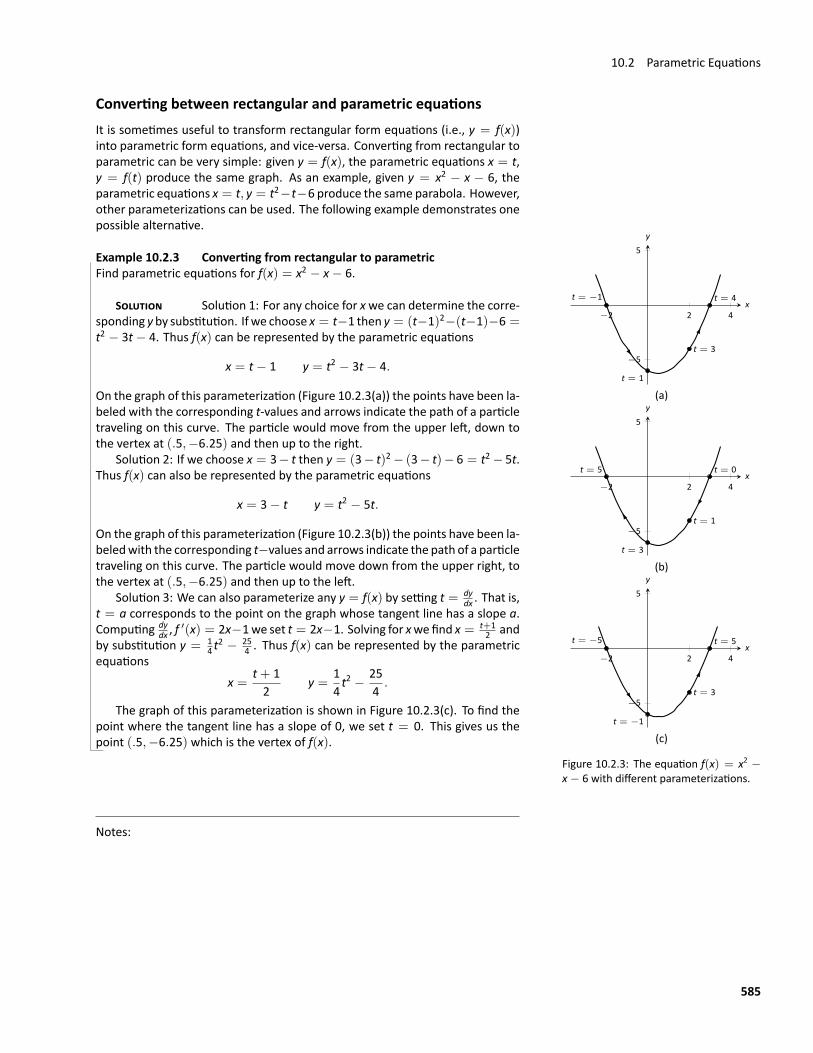
10.2 Parametric Equations
Converting between rectangular and parametric equationsIt is sometimes useful to transform rectangular form equations (i.e., y = f(x))into parametric form equations, and vice‐versa. Converting from rectangular toparametric can be very simple: given y = f(x), the parametric equations x = t,y = f(t) produce the same graph. As an example, given y = x2 − x − 6, theparametric equations x = t, y = t2−t−6 produce the same parabola. However,other parameterizations can be used. The following example demonstrates onepossible alternative.
−2 2 4
−5
5
t = −1
t = 1
t = 3
t = 4x
y
(a)
−2 2 4
−5
5
t = 5
t = 3
t = 1
t = 0x
y
(b)
−2 2 4
−5
5
t = −5
t = −1
t = 3
t = 5x
y
(c)
Figure 10.2.3: The equation f(x) = x2 −x− 6 with different parameterizations.
Example 10.2.3 Converting from rectangular to parametricFind parametric equations for f(x) = x2 − x− 6.
SOLUTION Solution 1: For any choice for xwe can determine the corre‐sponding y by substitution. If we choose x = t−1 then y = (t−1)2−(t−1)−6 =t2 − 3t− 4. Thus f(x) can be represented by the parametric equations
x = t− 1 y = t2 − 3t− 4.
On the graph of this parameterization (Figure 10.2.3(a)) the points have been la‐beled with the corresponding t‐values and arrows indicate the path of a particletraveling on this curve. The particle would move from the upper left, down tothe vertex at (.5,−6.25) and then up to the right.
Solution 2: If we choose x = 3− t then y = (3− t)2− (3− t)− 6 = t2− 5t.Thus f(x) can also be represented by the parametric equations
x = 3− t y = t2 − 5t.
On the graph of this parameterization (Figure 10.2.3(b)) the points have been la‐beledwith the corresponding t−values and arrows indicate the path of a particletraveling on this curve. The particle would move down from the upper right, tothe vertex at (.5,−6.25) and then up to the left.
Solution 3: We can also parameterize any y = f(x) by setting t = dydx . That is,
t = a corresponds to the point on the graph whose tangent line has a slope a.Computing dy
dx , f′(x) = 2x−1we set t = 2x−1. Solving for xwefind x = t+1
2 andby substitution y = 1
4 t2 − 25
4 . Thus f(x) can be represented by the parametricequations
x =t+ 12
y =14t2 − 25
4.
The graph of this parameterization is shown in Figure 10.2.3(c). To find thepoint where the tangent line has a slope of 0, we set t = 0. This gives us thepoint (.5,−6.25) which is the vertex of f(x).
Notes:
585
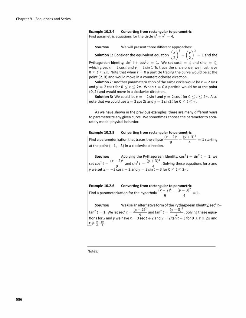
Chapter 9 Sequences and Series
Example 10.2.4 Converting from rectangular to parametricFind parametric equations for the circle x2 + y2 = 4.
SOLUTION We will present three different approaches:
Solution 1: Consider the equivalent equation(x2
)2
+
(y2
)2
= 1 and the
Pythagorean Identity, sin2 t + cos2 t = 1. We set cos t = x2 and sin t = y
2 ,which gives x = 2 cos t and y = 2 sin t. To trace the circle once, we must have0 ≤ t ≤ 2π. Note that when t = 0 a particle tracing the curve would be at thepoint (2, 0) and would move in a counterclockwise direction.
Solution 2: Another parameterization of the same circle would be x = 2 sin tand y = 2 cos t for 0 ≤ t ≤ 2π. When t = 0 a particle would be at the point(0, 2) and would move in a clockwise direction.
Solution 3: We could let x = −2 sin t and y = 2 cos t for 0 ≤ t ≤ 2π. Alsonote that we could use x = 2 cos 2t and y = 2 sin 2t for 0 ≤ t ≤ π.
As we have shown in the previous examples, there are many different waysto parameterize any given curve. We sometimes choose the parameter to accu‐rately model physical behavior.
Example 10.2.5 Converting from rectangular to parametric
Find a parameterization that traces the ellipse(x− 2)2
9+
(y+ 3)2
4= 1 starting
at the point (−1,−3) in a clockwise direction.
SOLUTION Applying the Pythagorean Identity, cos2 t + sin2 t = 1, we
set cos2 t =(x− 2)2
9and sin2 t =
(y+ 3)2
4. Solving these equations for x and
y we set x = −3 cos t+ 2 and y = 2 sin t− 3 for 0 ≤ t ≤ 2π.
Example 10.2.6 Converting from rectangular to parametric
Find a parameterization for the hyperbola(x− 2)2
9− (y− 3)2
4= 1.
SOLUTION Weuse an alternative formof the Pythagorean Identity, sec2 t−
tan2 t = 1. We let sec2 t =(x− 2)2
9and tan2 t =
(y− 3)2
4. Solving these equa‐
tions for x and y we have x = 3 sec t+ 2 and y = 2 tan t+ 3 for 0 ≤ t ≤ 2π andt ̸= π
2 ,3π2 .
Notes:
586
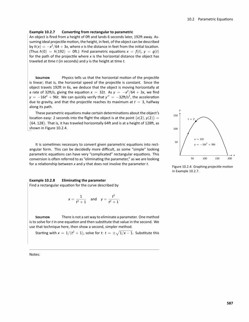
10.2 Parametric Equations
Example 10.2.7 Converting from rectangular to parametricAn object is fired from a height of 0ft and lands 6 seconds later, 192ft away. As‐suming ideal projectilemotion, the height, in feet, of the object can be describedby h(x) = −x2/64+ 3x, where x is the distance in feet from the initial location.(Thus h(0) = h(192) = 0ft.) Find parametric equations x = f(t), y = g(t)for the path of the projectile where x is the horizontal distance the object hastraveled at time t (in seconds) and y is the height at time t.
SOLUTION Physics tells us that the horizontal motion of the projectileis linear; that is, the horizontal speed of the projectile is constant. Since theobject travels 192ft in 6s, we deduce that the object is moving horizontally ata rate of 32ft/s, giving the equation x = 32t. As y = −x2/64 + 3x, we findy = −16t2 + 96t. We can quickly verify that y ′′ = −32ft/s2, the accelerationdue to gravity, and that the projectile reaches its maximum at t = 3, halfwayalong its path.
50 100 150 200
50
100
150t = 2
x = 32t
y = −16t2 + 96t
x
y
Figure 10.2.4: Graphing projectile motionin Example 10.2.7.
These parametric equationsmake certain determinations about the object’slocation easy: 2 seconds into the flight the object is at the point
(x(2), y(2)
)=(
64, 128). That is, it has traveled horizontally 64ft and is at a height of 128ft, as
shown in Figure 10.2.4.
It is sometimes necessary to convert given parametric equations into rect‐angular form. This can be decidedly more difficult, as some “simple” lookingparametric equations can have very “complicated” rectangular equations. Thisconversion is often referred to as “eliminating the parameter,” as we are lookingfor a relationship between x and y that does not involve the parameter t.
Example 10.2.8 Eliminating the parameterFind a rectangular equation for the curve described by
x =1
t2 + 1and y =
t2
t2 + 1.
SOLUTION There is not a setway to eliminate a parameter. Onemethodis to solve for t in one equation and then substitute that value in the second. Weuse that technique here, then show a second, simpler method.
Starting with x = 1/(t2 + 1), solve for t: t = ±√
1/x− 1. Substitute this
Notes:
587
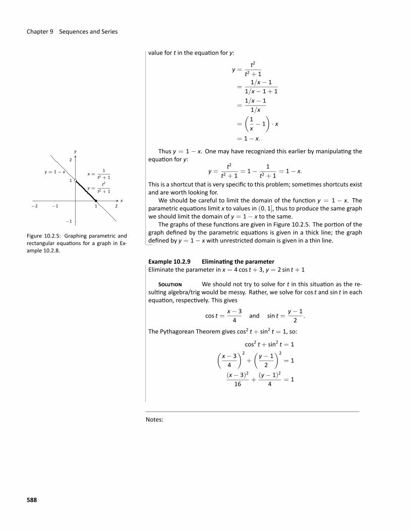
Chapter 9 Sequences and Series
value for t in the equation for y:
y =t2
t2 + 1
=1/x− 1
1/x− 1+ 1
=1/x− 11/x
=
(1x− 1)· x
= 1− x.
−2 −1 1 2
−1
1
2
x =1
t2 + 1
y =t2
t2 + 1
y = 1 − x
x
y
Figure 10.2.5: Graphing parametric andrectangular equations for a graph in Ex‐ample 10.2.8.
Thus y = 1 − x. One may have recognized this earlier by manipulating theequation for y:
y =t2
t2 + 1= 1− 1
t2 + 1= 1− x.
This is a shortcut that is very specific to this problem; sometimes shortcuts existand are worth looking for.
We should be careful to limit the domain of the function y = 1 − x. Theparametric equations limit x to values in (0, 1], thus to produce the same graphwe should limit the domain of y = 1− x to the same.
The graphs of these functions are given in Figure 10.2.5. The portion of thegraph defined by the parametric equations is given in a thick line; the graphdefined by y = 1− x with unrestricted domain is given in a thin line.
Example 10.2.9 Eliminating the parameterEliminate the parameter in x = 4 cos t+ 3, y = 2 sin t+ 1
SOLUTION We should not try to solve for t in this situation as the re‐sulting algebra/trig would be messy. Rather, we solve for cos t and sin t in eachequation, respectively. This gives
cos t =x− 34
and sin t =y− 12
.
The Pythagorean Theorem gives cos2 t+ sin2 t = 1, so:
cos2 t+ sin2 t = 1(x− 34
)2
+
(y− 12
)2
= 1
(x− 3)2
16+
(y− 1)2
4= 1
Notes:
588
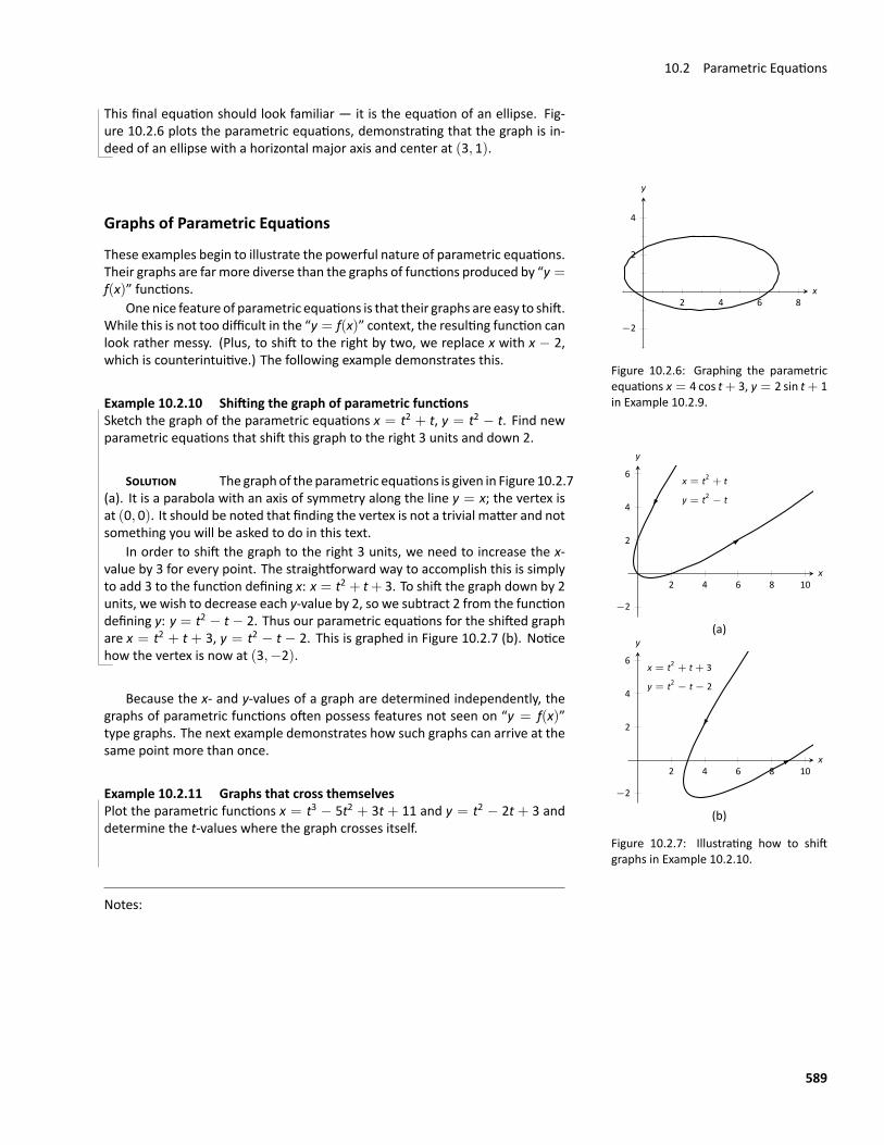
10.2 Parametric Equations
This final equation should look familiar — it is the equation of an ellipse. Fig‐ure 10.2.6 plots the parametric equations, demonstrating that the graph is in‐deed of an ellipse with a horizontal major axis and center at (3, 1).
2 4 6 8
−2
2
4
x
y
Figure 10.2.6: Graphing the parametricequations x = 4 cos t+ 3, y = 2 sin t+ 1in Example 10.2.9.
Graphs of Parametric Equations
These examples begin to illustrate the powerful nature of parametric equations.Their graphs are far more diverse than the graphs of functions produced by “y =f(x)” functions.
Onenice feature of parametric equations is that their graphs are easy to shift.While this is not too difficult in the “y = f(x)” context, the resulting function canlook rather messy. (Plus, to shift to the right by two, we replace x with x − 2,which is counterintuitive.) The following example demonstrates this.
2 4 6 8 10
−2
2
4
6x = t2 + t
y = t2 − t
x
y
(a)
2 4 6 8 10
−2
2
4
6x = t2 + t + 3
y = t2 − t − 2
x
y
(b)
Figure 10.2.7: Illustrating how to shiftgraphs in Example 10.2.10.
Example 10.2.10 Shifting the graph of parametric functionsSketch the graph of the parametric equations x = t2 + t, y = t2 − t. Find newparametric equations that shift this graph to the right 3 units and down 2.
SOLUTION The graphof the parametric equations is given in Figure 10.2.7(a). It is a parabola with an axis of symmetry along the line y = x; the vertex isat (0, 0). It should be noted that finding the vertex is not a trivial matter and notsomething you will be asked to do in this text.
In order to shift the graph to the right 3 units, we need to increase the x‐value by 3 for every point. The straightforward way to accomplish this is simplyto add 3 to the function defining x: x = t2 + t+ 3. To shift the graph down by 2units, we wish to decrease each y‐value by 2, so we subtract 2 from the functiondefining y: y = t2 − t− 2. Thus our parametric equations for the shifted graphare x = t2 + t + 3, y = t2 − t − 2. This is graphed in Figure 10.2.7 (b). Noticehow the vertex is now at (3,−2).
Because the x‐ and y‐values of a graph are determined independently, thegraphs of parametric functions often possess features not seen on “y = f(x)”type graphs. The next example demonstrates how such graphs can arrive at thesame point more than once.
Example 10.2.11 Graphs that cross themselvesPlot the parametric functions x = t3 − 5t2 + 3t + 11 and y = t2 − 2t + 3 anddetermine the t‐values where the graph crosses itself.
Notes:
589
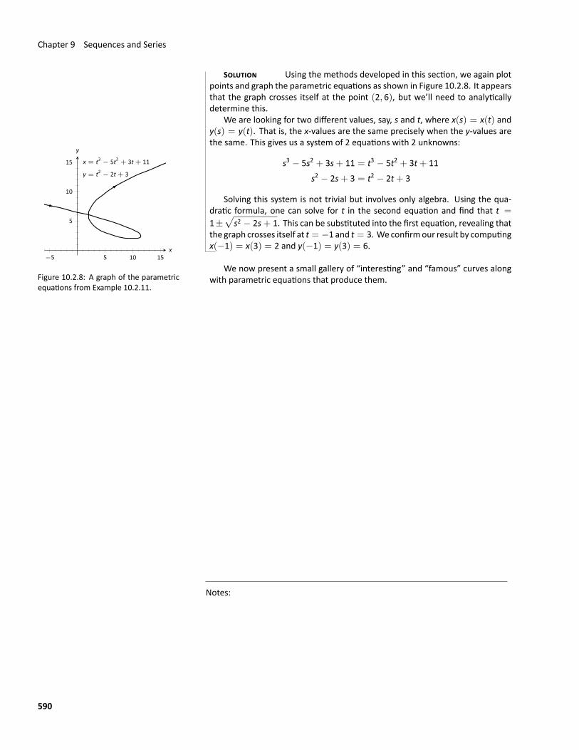
Chapter 9 Sequences and Series
SOLUTION Using the methods developed in this section, we again plotpoints and graph the parametric equations as shown in Figure 10.2.8. It appearsthat the graph crosses itself at the point (2, 6), but we’ll need to analyticallydetermine this.
We are looking for two different values, say, s and t, where x(s) = x(t) andy(s) = y(t). That is, the x‐values are the same precisely when the y‐values arethe same. This gives us a system of 2 equations with 2 unknowns:
−5 5 10 15
5
10
15 x = t3 − 5t2 + 3t + 11
y = t2 − 2t + 3
x
y
Figure 10.2.8: A graph of the parametricequations from Example 10.2.11.
s3 − 5s2 + 3s+ 11 = t3 − 5t2 + 3t+ 11s2 − 2s+ 3 = t2 − 2t+ 3
Solving this system is not trivial but involves only algebra. Using the qua‐dratic formula, one can solve for t in the second equation and find that t =
1±√
s2 − 2s+ 1. This can be substituted into the first equation, revealing thatthe graph crosses itself at t = −1 and t = 3. We confirmour result by computingx(−1) = x(3) = 2 and y(−1) = y(3) = 6.
We now present a small gallery of “interesting” and “famous” curves alongwith parametric equations that produce them.
Notes:
590
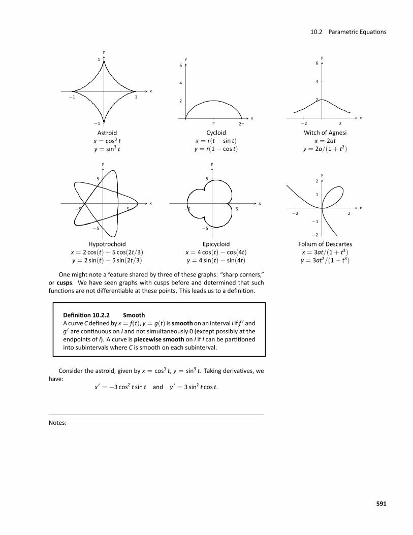
10.2 Parametric Equations
−1 1
−1
1
x
y
π 2π
2
4
6
x
y
−2 2
2
4
6
x
y
Astroidx = cos3 ty = sin3 t
Cycloidx = r(t− sin t)y = r(1− cos t)
Witch of Agnesix = 2at
y = 2a/(1+ t2)
−5 5
−5
5
x
y
−5 5
−5
5
x
y
−2 2
−2
−1
1
2
x
y
Hypotrochoidx = 2 cos(t) + 5 cos(2t/3)y = 2 sin(t)− 5 sin(2t/3)
Epicycloidx = 4 cos(t)− cos(4t)y = 4 sin(t)− sin(4t)
Folium of Descartesx = 3at/(1+ t3)y = 3at2/(1+ t3)
One might note a feature shared by three of these graphs: “sharp corners,”or cusps. We have seen graphs with cusps before and determined that suchfunctions are not differentiable at these points. This leads us to a definition.
Definition 10.2.2 SmoothA curveCdefinedby x = f(t), y = g(t) is smoothon an interval I if f ′ andg ′ are continuous on I and not simultaneously 0 (except possibly at theendpoints of I). A curve is piecewise smooth on I if I can be partitionedinto subintervals where C is smooth on each subinterval.
Consider the astroid, given by x = cos3 t, y = sin3 t. Taking derivatives, wehave:
x ′ = −3 cos2 t sin t and y ′ = 3 sin2 t cos t.
Notes:
591
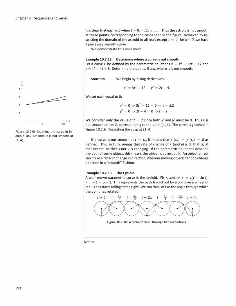
Chapter 9 Sequences and Series
It is clear that each is 0 when t = 0, π/2, π, . . . . Thus the astroid is not smoothat these points, corresponding to the cusps seen in the figure. However, by re‐stricting the domain of the astroid to all reals except t = kπ
2 for k ∈ Z we havea piecewise smooth curve.
We demonstrate this once more.
Example 10.2.12 Determine where a curve is not smoothLet a curve C be defined by the parametric equations x = t3 − 12t + 17 andy = t2 − 4t+ 8. Determine the points, if any, where it is not smooth.
SOLUTION We begin by taking derivatives.
5 10
2
4
6
8
x
y
Figure 10.2.9: Graphing the curve in Ex‐ample 10.2.12; note it is not smooth at(1, 4).
x ′ = 3t2 − 12, y ′ = 2t− 4.
We set each equal to 0:
x ′ = 0 ⇒ 3t2 − 12 = 0 ⇒ t = ±2y ′ = 0 ⇒ 2t− 4 = 0 ⇒ t = 2
We consider only the value of t = 2 since both x′ and y′ must be 0. Thus C isnot smooth at t = 2, corresponding to the point (1, 4). The curve is graphed inFigure 10.2.9, illustrating the cusp at (1, 4).
If a curve is not smooth at t = t0, it means that x ′(t0) = y ′(t0) = 0 asdefined. This, in turn, means that rate of change of x (and y) is 0; that is, atthat instant, neither x nor y is changing. If the parametric equations describethe path of some object, this means the object is at rest at t0. An object at restcanmake a “sharp” change in direction, whereas moving objects tend to changedirection in a “smooth” fashion.
Example 10.2.13 The CycloidA well‐known parametric curve is the cycloid. Fix r, and let x = r(t − sin t),y = r(1 − cos t). This represents the path traced out by a point on a wheel ofradius r as starts rolling to the right. We can think of t as the angle throughwhichthe point has rotated.
t = 0 t = 2π t = 4πt = 2π3 t = 4π
3 t = 8π3 t = 10π
3
Figure 10.2.10: A cycloid traced through two revolutions.
Notes:
592
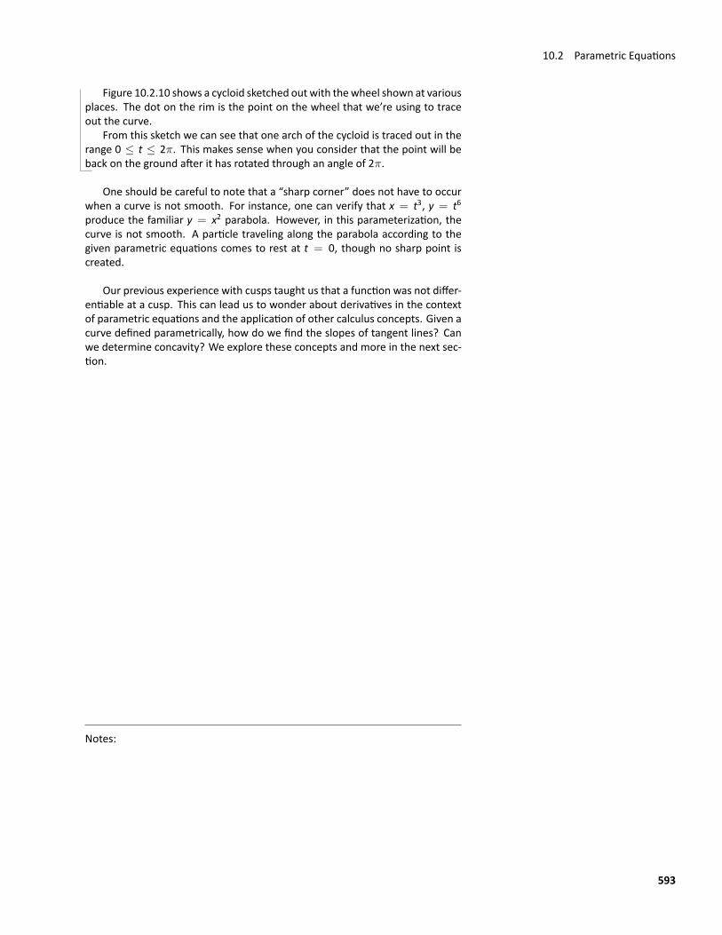
10.2 Parametric Equations
Figure 10.2.10 shows a cycloid sketched out with thewheel shown at variousplaces. The dot on the rim is the point on the wheel that we’re using to traceout the curve.
From this sketch we can see that one arch of the cycloid is traced out in therange 0 ≤ t ≤ 2π. This makes sense when you consider that the point will beback on the ground after it has rotated through an angle of 2π.
One should be careful to note that a “sharp corner” does not have to occurwhen a curve is not smooth. For instance, one can verify that x = t3, y = t6produce the familiar y = x2 parabola. However, in this parameterization, thecurve is not smooth. A particle traveling along the parabola according to thegiven parametric equations comes to rest at t = 0, though no sharp point iscreated.
Our previous experience with cusps taught us that a function was not differ‐entiable at a cusp. This can lead us to wonder about derivatives in the contextof parametric equations and the application of other calculus concepts. Given acurve defined parametrically, how do we find the slopes of tangent lines? Canwe determine concavity? We explore these concepts and more in the next sec‐tion.
Notes:
593
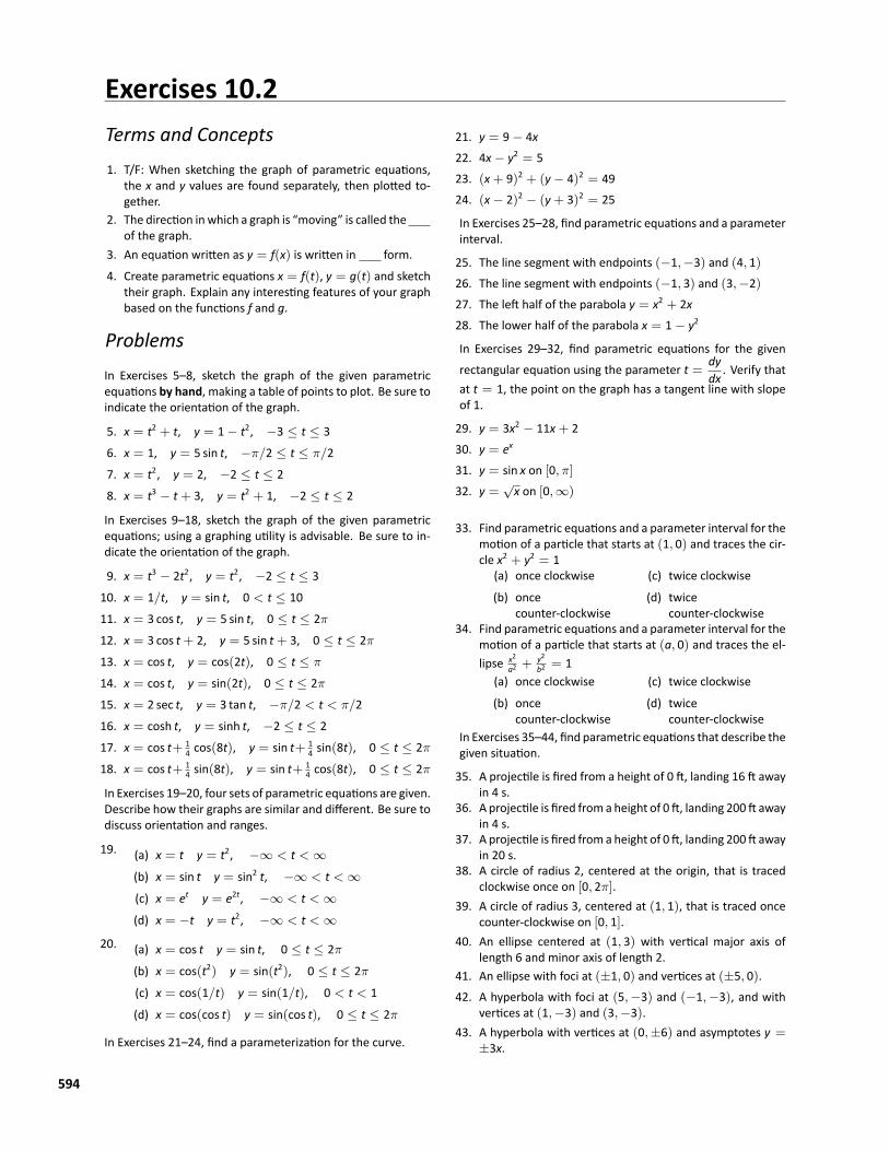
Exercises 10.2Terms and Concepts1. T/F: When sketching the graph of parametric equations,
the x and y values are found separately, then plotted to‐gether.
2. The direction inwhich a graph is “moving” is called theof the graph.
3. An equation written as y = f(x) is written in form.4. Create parametric equations x = f(t), y = g(t) and sketch
their graph. Explain any interesting features of your graphbased on the functions f and g.
ProblemsIn Exercises 5–8, sketch the graph of the given parametricequations by hand, making a table of points to plot. Be sure toindicate the orientation of the graph.
5. x = t2 + t, y = 1− t2, −3 ≤ t ≤ 36. x = 1, y = 5 sin t, −π/2 ≤ t ≤ π/27. x = t2, y = 2, −2 ≤ t ≤ 28. x = t3 − t+ 3, y = t2 + 1, −2 ≤ t ≤ 2
In Exercises 9–18, sketch the graph of the given parametricequations; using a graphing utility is advisable. Be sure to in‐dicate the orientation of the graph.
9. x = t3 − 2t2, y = t2, −2 ≤ t ≤ 310. x = 1/t, y = sin t, 0 < t ≤ 1011. x = 3 cos t, y = 5 sin t, 0 ≤ t ≤ 2π12. x = 3 cos t+ 2, y = 5 sin t+ 3, 0 ≤ t ≤ 2π13. x = cos t, y = cos(2t), 0 ≤ t ≤ π
14. x = cos t, y = sin(2t), 0 ≤ t ≤ 2π15. x = 2 sec t, y = 3 tan t, −π/2 < t < π/216. x = cosh t, y = sinh t, −2 ≤ t ≤ 217. x = cos t+ 1
4 cos(8t), y = sin t+ 14 sin(8t), 0 ≤ t ≤ 2π
18. x = cos t+ 14 sin(8t), y = sin t+ 1
4 cos(8t), 0 ≤ t ≤ 2π
In Exercises 19–20, four sets of parametric equations are given.Describe how their graphs are similar and different. Be sure todiscuss orientation and ranges.
19. (a) x = t y = t2, −∞ < t < ∞(b) x = sin t y = sin2 t, −∞ < t < ∞(c) x = et y = e2t, −∞ < t < ∞(d) x = −t y = t2, −∞ < t < ∞
20. (a) x = cos t y = sin t, 0 ≤ t ≤ 2π
(b) x = cos(t2) y = sin(t2), 0 ≤ t ≤ 2π
(c) x = cos(1/t) y = sin(1/t), 0 < t < 1
(d) x = cos(cos t) y = sin(cos t), 0 ≤ t ≤ 2π
In Exercises 21–24, find a parameterization for the curve.
21. y = 9− 4x22. 4x− y2 = 523. (x+ 9)2 + (y− 4)2 = 4924. (x− 2)2 − (y+ 3)2 = 25
In Exercises 25–28, find parametric equations and a parameterinterval.
25. The line segment with endpoints (−1,−3) and (4, 1)26. The line segment with endpoints (−1, 3) and (3,−2)27. The left half of the parabola y = x2 + 2x28. The lower half of the parabola x = 1− y2
In Exercises 29–32, find parametric equations for the givenrectangular equation using the parameter t = dy
dx. Verify that
at t = 1, the point on the graph has a tangent line with slopeof 1.
29. y = 3x2 − 11x+ 230. y = ex
31. y = sin x on [0, π]32. y =
√x on [0,∞)
33. Find parametric equations and a parameter interval for themotion of a particle that starts at (1, 0) and traces the cir‐cle x2 + y2 = 1
(a) once clockwise
(b) oncecounter‐clockwise
(c) twice clockwise
(d) twicecounter‐clockwise
34. Find parametric equations and a parameter interval for themotion of a particle that starts at (a, 0) and traces the el‐lipse x2
a2 + y2b2 = 1
(a) once clockwise
(b) oncecounter‐clockwise
(c) twice clockwise
(d) twicecounter‐clockwise
In Exercises 35–44, find parametric equations that describe thegiven situation.
35. A projectile is fired from a height of 0 ft, landing 16 ft awayin 4 s.
36. A projectile is fired froma height of 0 ft, landing 200ft awayin 4 s.
37. A projectile is fired froma height of 0 ft, landing 200ft awayin 20 s.
38. A circle of radius 2, centered at the origin, that is tracedclockwise once on [0, 2π].
39. A circle of radius 3, centered at (1, 1), that is traced oncecounter‐clockwise on [0, 1].
40. An ellipse centered at (1, 3) with vertical major axis oflength 6 and minor axis of length 2.
41. An ellipse with foci at (±1, 0) and vertices at (±5, 0).42. A hyperbola with foci at (5,−3) and (−1,−3), and with
vertices at (1,−3) and (3,−3).43. A hyperbola with vertices at (0,±6) and asymptotes y =
±3x.
594
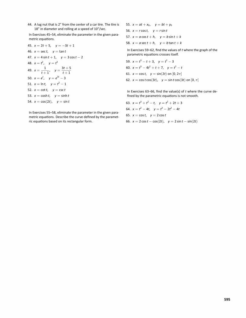
44. A lug nut that is 2” from the center of a car tire. The tire is18” in diameter and rolling at a speed of 10”/sec.
In Exercises 45–54, eliminate the parameter in the given para‐metric equations.
45. x = 2t+ 5, y = −3t+ 146. x = sec t, y = tan t47. x = 4 sin t+ 1, y = 3 cos t− 248. x = t2, y = t3
49. x = 1t+ 1
, y = 3t+ 5t+ 1
50. x = et, y = e3t − 351. x = ln t, y = t2 − 152. x = cot t, y = csc t53. x = cosh t, y = sinh t54. x = cos(2t), y = sin t
In Exercises 55–58, eliminate the parameter in the given para‐metric equations. Describe the curve defined by the paramet‐ric equations based on its rectangular form.
55. x = at+ x0, y = bt+ y056. x = r cos t, y = r sin t
57. x = a cos t+ h, y = b sin t+ k
58. x = a sec t+ h, y = b tan t+ k
In Exercises 59–62, find the values of t where the graph of theparametric equations crosses itself.
59. x = t3 − t+ 3, y = t2 − 3
60. x = t3 − 4t2 + t+ 7, y = t2 − t
61. x = cos t, y = sin(2t) on [0, 2π]
62. x = cos t cos(3t), y = sin t cos(3t) on [0, π]
In Exercises 63–66, find the value(s) of t where the curve de‐fined by the parametric equations is not smooth.
63. x = t3 + t2 − t, y = t2 + 2t+ 3
64. x = t2 − 4t, y = t3 − 2t2 − 4t
65. x = cos t, y = 2 cos t
66. x = 2 cos t− cos(2t), y = 2 sin t− sin(2t)
595
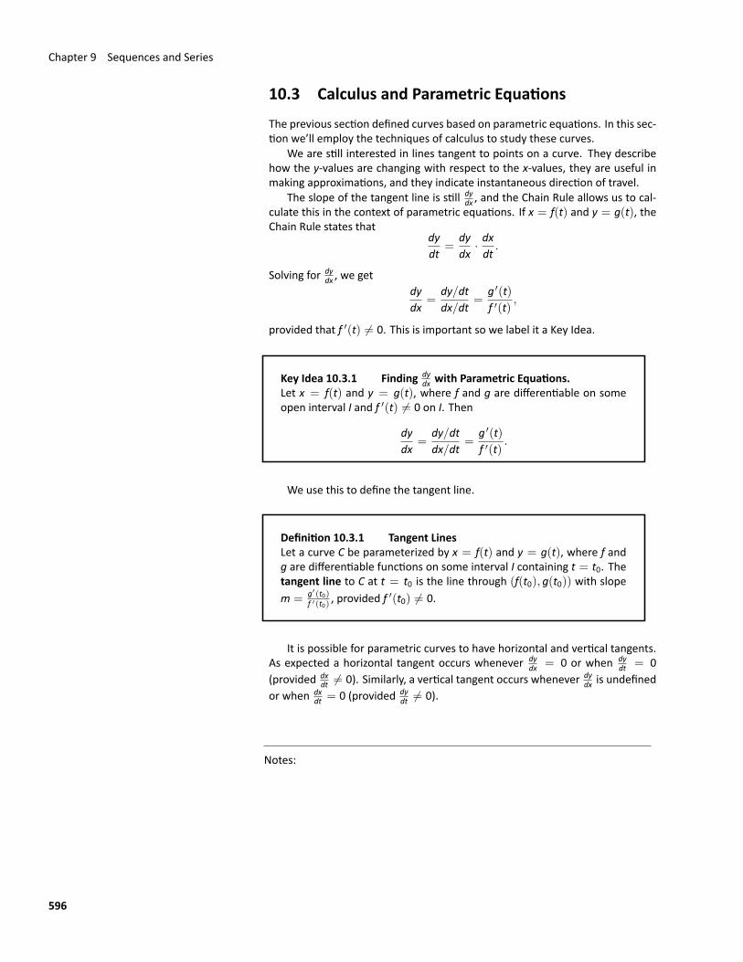
Chapter 9 Sequences and Series
10.3 Calculus and Parametric EquationsThe previous section defined curves based on parametric equations. In this sec‐tion we’ll employ the techniques of calculus to study these curves.
We are still interested in lines tangent to points on a curve. They describehow the y‐values are changing with respect to the x‐values, they are useful inmaking approximations, and they indicate instantaneous direction of travel.
The slope of the tangent line is still dydx , and the Chain Rule allows us to cal‐
culate this in the context of parametric equations. If x = f(t) and y = g(t), theChain Rule states that
dydt
=dydx
· dxdt
.
Solving for dydx , we get
dydx
=dy/dtdx/dt
=g ′(t)f ′(t)
,
provided that f ′(t) ̸= 0. This is important so we label it a Key Idea.
Key Idea 10.3.1 Finding dydx with Parametric Equations.
Let x = f(t) and y = g(t), where f and g are differentiable on someopen interval I and f ′(t) ̸= 0 on I. Then
dydx
=dy/dtdx/dt
=g ′(t)f ′(t)
.
We use this to define the tangent line.
Definition 10.3.1 Tangent LinesLet a curve C be parameterized by x = f(t) and y = g(t), where f andg are differentiable functions on some interval I containing t = t0. Thetangent line to C at t = t0 is the line through (f(t0), g(t0)) with slopem = g′(t0)
f ′(t0) , provided f ′(t0) ̸= 0.
It is possible for parametric curves to have horizontal and vertical tangents.As expected a horizontal tangent occurs whenever dy
dx = 0 or when dydt = 0
(provided dxdt ̸= 0). Similarly, a vertical tangent occurs whenever dy
dx is undefinedor when dx
dt = 0 (provided dydt ̸= 0).
Notes:
596
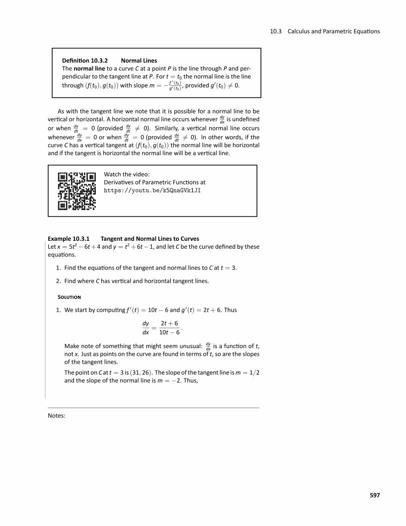
10.3 Calculus and Parametric Equations
Definition 10.3.2 Normal LinesThe normal line to a curve C at a point P is the line through P and per‐pendicular to the tangent line at P. For t = t0 the normal line is the linethrough (f(t0), g(t0)) with slopem = − f ′(t0)
g′(t0) , provided g′(t0) ̸= 0.
As with the tangent line we note that it is possible for a normal line to bevertical or horizontal. A horizontal normal line occurs whenever dy
dx is undefinedor when dx
dt = 0 (provided dydt ̸= 0). Similarly, a vertical normal line occurs
whenever dydx = 0 or when dy
dt = 0 (provided dxdt ̸= 0). In other words, if the
curve C has a vertical tangent at (f(t0), g(t0)) the normal line will be horizontaland if the tangent is horizontal the normal line will be a vertical line.
Watch the video:Derivatives of Parametric Functions athttps://youtu.be/k5QnaGVk1JI
Example 10.3.1 Tangent and Normal Lines to CurvesLet x = 5t2−6t+4 and y = t2+6t−1, and let C be the curve defined by theseequations.
1. Find the equations of the tangent and normal lines to C at t = 3.
2. Find where C has vertical and horizontal tangent lines.
SOLUTION
1. We start by computing f ′(t) = 10t− 6 and g ′(t) = 2t+ 6. Thus
dydx
=2t+ 610t− 6
.
Make note of something that might seem unusual: dydx is a function of t,
not x. Just as points on the curve are found in terms of t, so are the slopesof the tangent lines.The point on C at t = 3 is (31, 26). The slope of the tangent line ism = 1/2and the slope of the normal line ism = −2. Thus,
Notes:
597
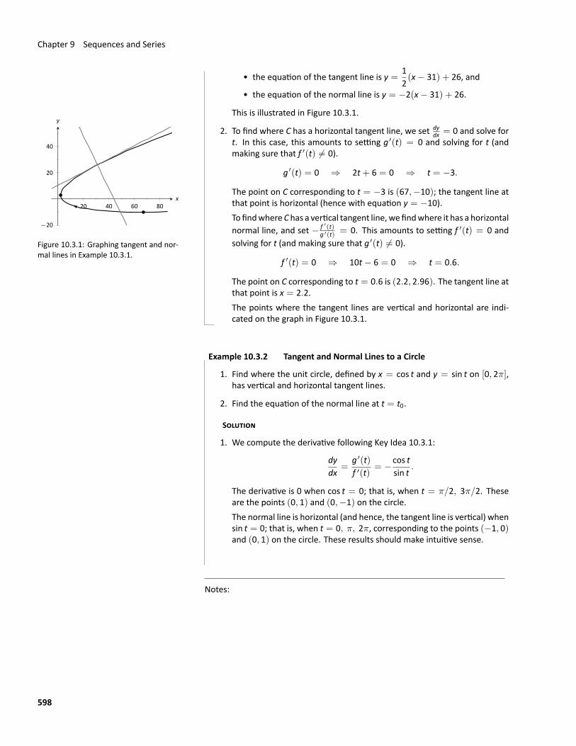
Chapter 9 Sequences and Series
• the equation of the tangent line is y =12(x− 31) + 26, and
• the equation of the normal line is y = −2(x− 31) + 26.
This is illustrated in Figure 10.3.1.
20 40 60 80
−20
20
40
x
y
Figure 10.3.1: Graphing tangent and nor‐mal lines in Example 10.3.1.
2. To find where C has a horizontal tangent line, we set dydx = 0 and solve for
t. In this case, this amounts to setting g ′(t) = 0 and solving for t (andmaking sure that f ′(t) ̸= 0).
g ′(t) = 0 ⇒ 2t+ 6 = 0 ⇒ t = −3.
The point on C corresponding to t = −3 is (67,−10); the tangent line atthat point is horizontal (hence with equation y = −10).To findwhereChas a vertical tangent line, wefindwhere it has a horizontalnormal line, and set − f ′(t)
g ′(t) = 0. This amounts to setting f ′(t) = 0 andsolving for t (and making sure that g ′(t) ̸= 0).
f ′(t) = 0 ⇒ 10t− 6 = 0 ⇒ t = 0.6.
The point on C corresponding to t = 0.6 is (2.2, 2.96). The tangent line atthat point is x = 2.2.The points where the tangent lines are vertical and horizontal are indi‐cated on the graph in Figure 10.3.1.
Example 10.3.2 Tangent and Normal Lines to a Circle
1. Find where the unit circle, defined by x = cos t and y = sin t on [0, 2π],has vertical and horizontal tangent lines.
2. Find the equation of the normal line at t = t0.
SOLUTION
1. We compute the derivative following Key Idea 10.3.1:
dydx
=g ′(t)f ′(t)
= −cos tsin t
.
The derivative is 0 when cos t = 0; that is, when t = π/2, 3π/2. Theseare the points (0, 1) and (0,−1) on the circle.The normal line is horizontal (and hence, the tangent line is vertical) whensin t = 0; that is, when t = 0, π, 2π, corresponding to the points (−1, 0)and (0, 1) on the circle. These results should make intuitive sense.
Notes:
598
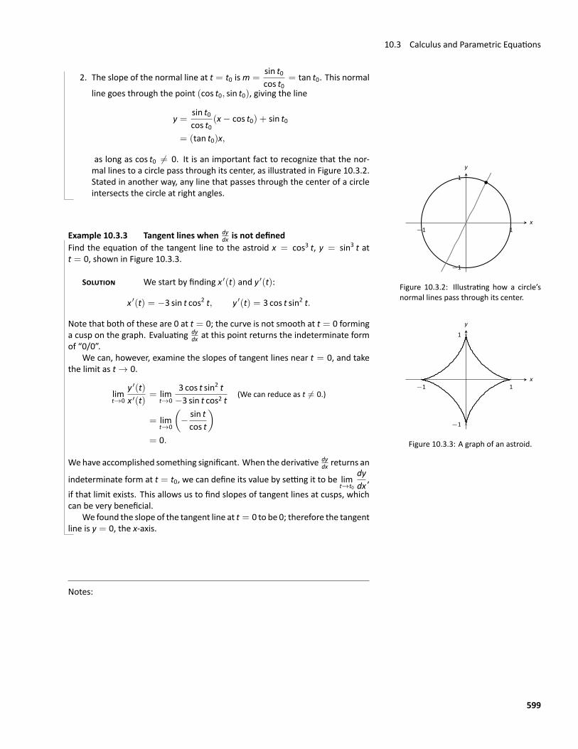
10.3 Calculus and Parametric Equations
2. The slope of the normal line at t = t0 ism =sin t0cos t0
= tan t0. This normal
line goes through the point (cos t0, sin t0), giving the line
y =sin t0cos t0
(x− cos t0) + sin t0
= (tan t0)x,
as long as cos t0 ̸= 0. It is an important fact to recognize that the nor‐
−1 1
−1
1
x
y
Figure 10.3.2: Illustrating how a circle’snormal lines pass through its center.
mal lines to a circle pass through its center, as illustrated in Figure 10.3.2.Stated in another way, any line that passes through the center of a circleintersects the circle at right angles.
Example 10.3.3 Tangent lines when dydx is not defined
Find the equation of the tangent line to the astroid x = cos3 t, y = sin3 t att = 0, shown in Figure 10.3.3.
−1 1
−1
1
x
y
Figure 10.3.3: A graph of an astroid.
SOLUTION We start by finding x ′(t) and y ′(t):
x ′(t) = −3 sin t cos2 t, y ′(t) = 3 cos t sin2 t.
Note that both of these are 0 at t = 0; the curve is not smooth at t = 0 forminga cusp on the graph. Evaluating dy
dx at this point returns the indeterminate formof “0/0”.
We can, however, examine the slopes of tangent lines near t = 0, and takethe limit as t → 0.
limt→0
y ′(t)x ′(t)
= limt→0
3 cos t sin2 t−3 sin t cos2 t
(We can reduce as t ̸= 0.)
= limt→0
(− sin tcos t
)= 0.
Wehave accomplished something significant. When the derivative dydx returns an
indeterminate form at t = t0, we can define its value by setting it to be limt→t0
dydx
,if that limit exists. This allows us to find slopes of tangent lines at cusps, whichcan be very beneficial.
We found the slope of the tangent line at t = 0 to be 0; therefore the tangentline is y = 0, the x‐axis.
Notes:
599
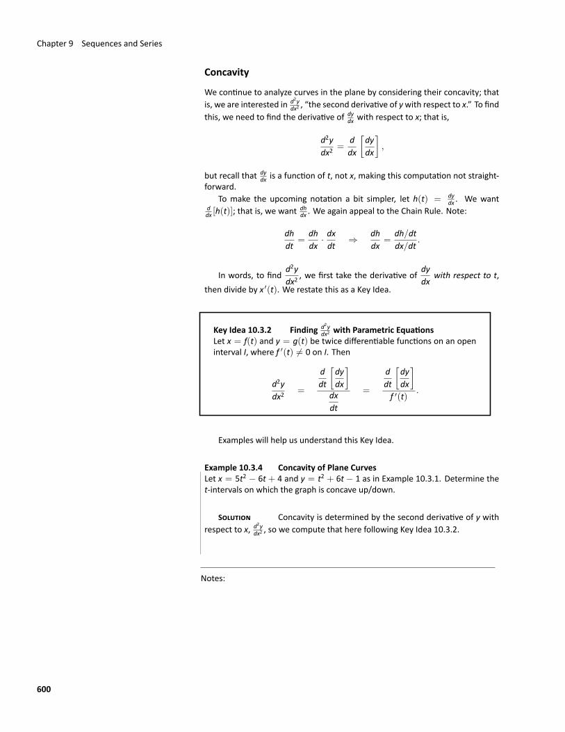
Chapter 9 Sequences and Series
Concavity
We continue to analyze curves in the plane by considering their concavity; thatis, we are interested in d2y
dx2 , “the second derivative of ywith respect to x.” To findthis, we need to find the derivative of dy
dx with respect to x; that is,
d2ydx2
=ddx
[dydx
],
but recall that dydx is a function of t, not x, making this computation not straight‐
forward.To make the upcoming notation a bit simpler, let h(t) = dy
dx . We wantddx [h(t)]; that is, we want
dhdx . We again appeal to the Chain Rule. Note:
dhdt
=dhdx
· dxdt
⇒ dhdx
=dh/dtdx/dt
.
In words, to findd2ydx2
, we first take the derivative ofdydx
with respect to t,then divide by x ′(t). We restate this as a Key Idea.
Key Idea 10.3.2 Finding d2ydx2 with Parametric Equations
Let x = f(t) and y = g(t) be twice differentiable functions on an openinterval I, where f ′(t) ̸= 0 on I. Then
d2ydx2
=
ddt
[dydx
]dxdt
=
ddt
[dydx
]f ′(t)
.
Examples will help us understand this Key Idea.
Example 10.3.4 Concavity of Plane CurvesLet x = 5t2 − 6t + 4 and y = t2 + 6t − 1 as in Example 10.3.1. Determine thet‐intervals on which the graph is concave up/down.
SOLUTION Concavity is determined by the second derivative of y withrespect to x, d2y
dx2 , so we compute that here following Key Idea 10.3.2.
Notes:
600

10.3 Calculus and Parametric Equations
In Example 10.3.1, we founddydx
=2t+ 610t− 6
and f ′(t) = 10t− 6. So:
d2ydx2
=
ddt
[2t+610t−6
]10t− 6
=− 72
(10t−6)2
10t− 6
= − 72(10t− 6)3
= − 9(5t− 3)3
20 40 60 80
−20
20
40
t >3/5
; concave
down
t < 3/5; concave up
x
y
Figure 10.3.4: Graphing the parametricequations in Example 10.3.4 to demon‐strate concavity.
The graph of the parametric functions is concave up when d2ydx2 > 0 and con‐
cave down when d2ydx2 < 0. We determine the intervals when the second deriva‐
tive is greater/less than 0 by first finding when it is 0 or undefined.As the numerator of − 9
(5t− 3)3is never 0, d2y
dx2 ̸= 0 for all t. It is undefined
when 5t − 3 = 0; that is, when t = 3/5. Following the work established insection 3.4, we look at values of t greater or less than 3/5 on a number line:
35
xf ′′ + −
f CU CD
Reviewing Example 10.3.1, we see that when t = 3/5 = 0.6, the graph ofthe parametric equations has a vertical tangent line. This point is also a point ofinflection for the graph, illustrated in Figure 10.3.4.
Example 10.3.5 Concavity of Plane CurvesFind the points of inflection of the graph of the parametric equations x =
√t,
y = sin t, for 0 ≤ t ≤ 16.
SOLUTION We need to compute dydx and
d2ydx2 .
dydx
=y ′(t)x ′(t)
=cos t
1/(2√t)
= 2√t cos t.
d2ydx2
=ddt
[ dydx
]x ′(t)
=cos t/
√t− 2
√t sin t
1/(2√t)
= 2 cos t− 4t sin t.
Notes:
601
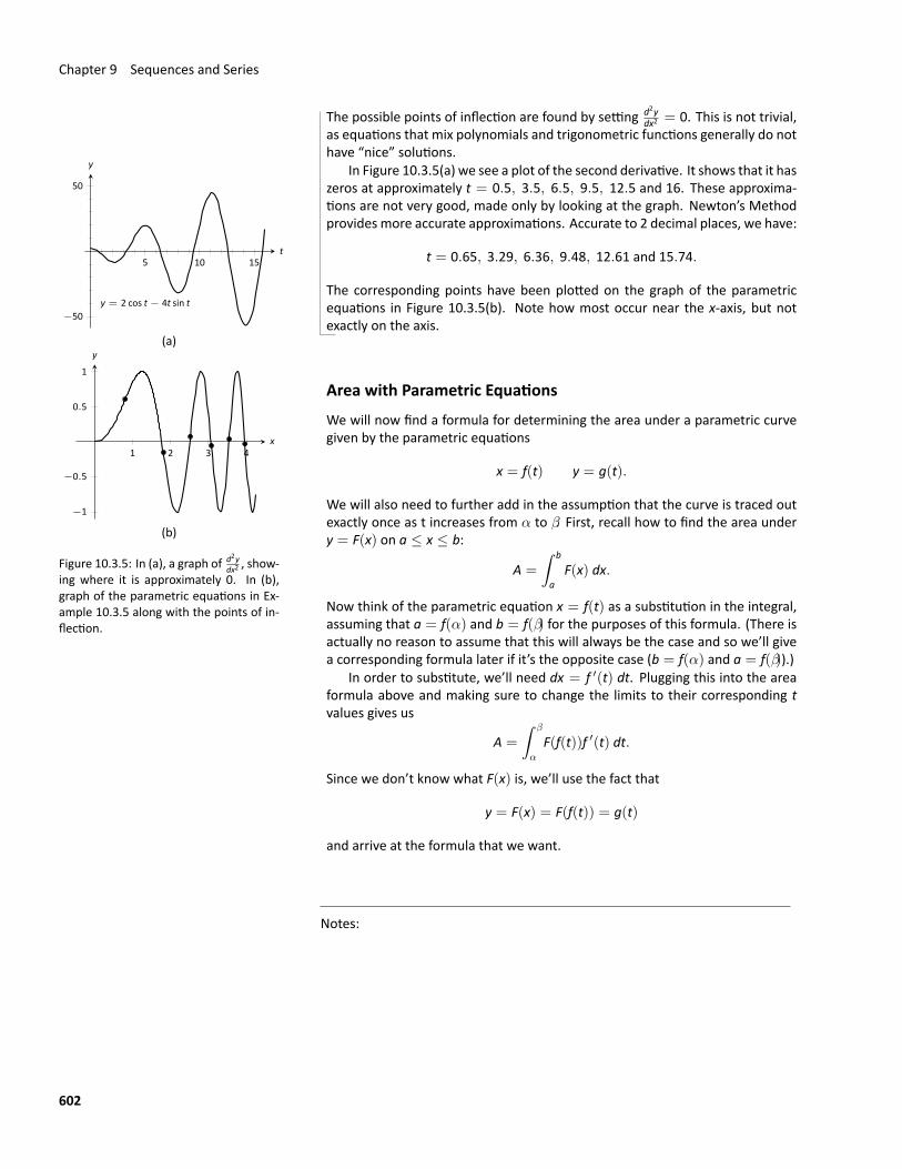
Chapter 9 Sequences and Series
The possible points of inflection are found by setting d2ydx2 = 0. This is not trivial,
as equations that mix polynomials and trigonometric functions generally do nothave “nice” solutions.
5 10 15
−50
50
y = 2 cos t − 4t sin t
t
y
(a)
31 2 4
−1
−0.5
0.5
1
x
y
(b)
Figure 10.3.5: In (a), a graph of d2ydx2 , show‐
ing where it is approximately 0. In (b),graph of the parametric equations in Ex‐ample 10.3.5 along with the points of in‐flection.
In Figure 10.3.5(a) we see a plot of the second derivative. It shows that it haszeros at approximately t = 0.5, 3.5, 6.5, 9.5, 12.5 and 16. These approxima‐tions are not very good, made only by looking at the graph. Newton’s Methodprovides more accurate approximations. Accurate to 2 decimal places, we have:
t = 0.65, 3.29, 6.36, 9.48, 12.61 and 15.74.
The corresponding points have been plotted on the graph of the parametricequations in Figure 10.3.5(b). Note how most occur near the x‐axis, but notexactly on the axis.
Area with Parametric EquationsWe will now find a formula for determining the area under a parametric curvegiven by the parametric equations
x = f(t) y = g(t).
We will also need to further add in the assumption that the curve is traced outexactly once as t increases from α to β. First, recall how to find the area undery = F(x) on a ≤ x ≤ b:
A =
∫ b
aF(x) dx.
Now think of the parametric equation x = f(t) as a substitution in the integral,assuming that a = f(α) and b = f(β) for the purposes of this formula. (There isactually no reason to assume that this will always be the case and so we’ll givea corresponding formula later if it’s the opposite case (b = f(α) and a = f(β)).)
In order to substitute, we’ll need dx = f ′(t) dt. Plugging this into the areaformula above and making sure to change the limits to their corresponding tvalues gives us
A =
∫ β
α
F(f(t))f ′(t) dt.
Since we don’t know what F(x) is, we’ll use the fact that
y = F(x) = F(f(t)) = g(t)
and arrive at the formula that we want.
Notes:
602
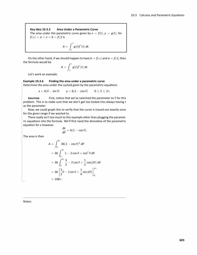
10.3 Calculus and Parametric Equations
Key Idea 10.3.3 Area Under a Parametric CurveThe area under the parametric curve given by x = f(t), y = g(t), forf(α) = a < x < b = f(β) is
A =
∫ β
α
g(t)f ′(t) dt.
On the other hand, if we should happen to have b = f(α) and a = f(β), thenthe formula would be
A =
∫ α
β
g(t)f ′(t) dt.
Let’s work an example.
Example 10.3.6 Finding the area under a parametric curveDetermine the area under the cycloid given by the parametric equations
x = 6(θ − sin θ) y = 6(1− cos θ) 0 ≤ θ ≤ 2π.
SOLUTION First, notice that we’ve switched the parameter to θ for thisproblem. This is to make sure that we don’t get too locked into always having tas the parameter.
Now, we could graph this to verify that the curve is traced out exactly oncefor the given range if we wanted to.
There really isn’t toomuch to this example other than plugging the paramet‐ric equations into the formula. We’ll first need the derivative of the parametricequation for x however.
dxdθ
= 6(1− cos θ).
The area is then
A =
∫ 2π
036(1− cos θ)2 dθ
= 36∫ 2π
01− 2 cos θ + cos2 θ dθ
= 36∫ 2π
0
32− 2 cos θ +
12cos(2θ) dθ
= 36[32θ − 2 sin θ +
14sin(2θ)
]2π0
= 108π.
Notes:
603
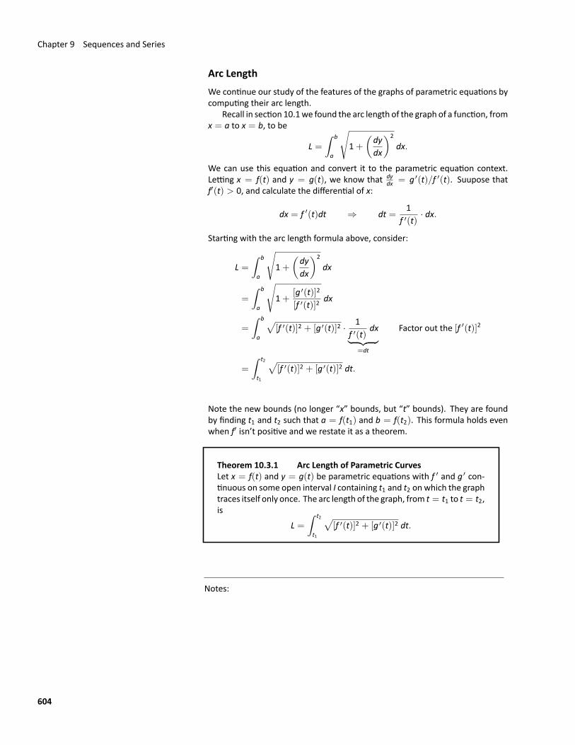
Chapter 9 Sequences and Series
Arc LengthWe continue our study of the features of the graphs of parametric equations bycomputing their arc length.
Recall in section 10.1we found the arc length of the graph of a function, fromx = a to x = b, to be
L =∫ b
a
√1+
(dydx
)2
dx.
We can use this equation and convert it to the parametric equation context.Letting x = f(t) and y = g(t), we know that dy
dx = g ′(t)/f ′(t). Suupose thatf′(t) > 0, and calculate the differential of x:
dx = f ′(t)dt ⇒ dt =1
f ′(t)· dx.
Starting with the arc length formula above, consider:
L =∫ b
a
√1+
(dydx
)2
dx
=
∫ b
a
√1+
[g ′(t)]2
[f ′(t)]2dx
=
∫ b
a
√[f ′(t)]2 + [g ′(t)]2 · 1
f ′(t)dx︸ ︷︷ ︸
=dt
Factor out the [f ′(t)]2
=
∫ t2
t1
√[f ′(t)]2 + [g ′(t)]2 dt.
Note the new bounds (no longer “x” bounds, but “t” bounds). They are foundby finding t1 and t2 such that a = f(t1) and b = f(t2). This formula holds evenwhen f′ isn’t positive and we restate it as a theorem.
Theorem 10.3.1 Arc Length of Parametric CurvesLet x = f(t) and y = g(t) be parametric equations with f ′ and g ′ con‐tinuous on some open interval I containing t1 and t2 onwhich the graphtraces itself only once. The arc length of the graph, from t = t1 to t = t2,is
L =∫ t2
t1
√[f ′(t)]2 + [g ′(t)]2 dt.
Notes:
604
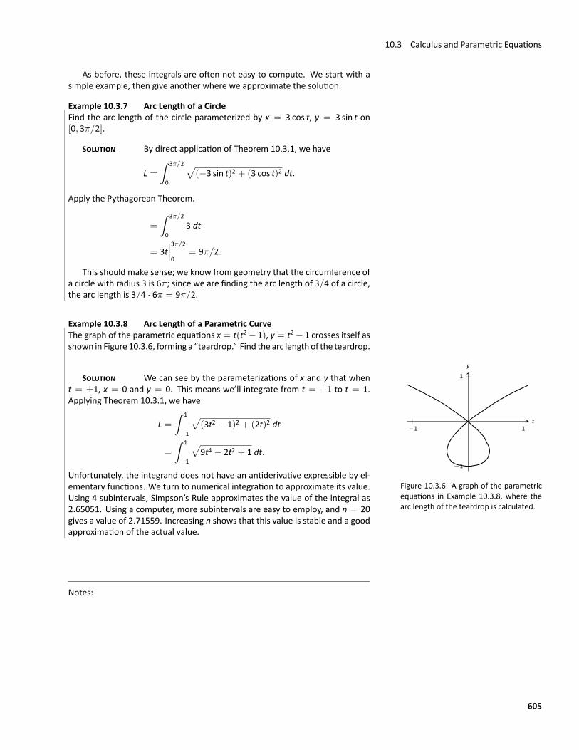
10.3 Calculus and Parametric Equations
As before, these integrals are often not easy to compute. We start with asimple example, then give another where we approximate the solution.
Example 10.3.7 Arc Length of a CircleFind the arc length of the circle parameterized by x = 3 cos t, y = 3 sin t on[0, 3π/2].
SOLUTION By direct application of Theorem 10.3.1, we have
L =∫ 3π/2
0
√(−3 sin t)2 + (3 cos t)2 dt.
Apply the Pythagorean Theorem.
=
∫ 3π/2
03 dt
= 3t∣∣∣3π/20
= 9π/2.
This should make sense; we know from geometry that the circumference ofa circle with radius 3 is 6π; since we are finding the arc length of 3/4 of a circle,the arc length is 3/4 · 6π = 9π/2.
Example 10.3.8 Arc Length of a Parametric CurveThe graph of the parametric equations x = t(t2 − 1), y = t2 − 1 crosses itself asshown in Figure 10.3.6, forming a “teardrop.” Find the arc length of the teardrop.
1−1
−1
1
t
y
Figure 10.3.6: A graph of the parametricequations in Example 10.3.8, where thearc length of the teardrop is calculated.
SOLUTION We can see by the parameterizations of x and y that whent = ±1, x = 0 and y = 0. This means we’ll integrate from t = −1 to t = 1.Applying Theorem 10.3.1, we have
L =∫ 1
−1
√(3t2 − 1)2 + (2t)2 dt
=
∫ 1
−1
√9t4 − 2t2 + 1 dt.
Unfortunately, the integrand does not have an antiderivative expressible by el‐ementary functions. We turn to numerical integration to approximate its value.Using 4 subintervals, Simpson’s Rule approximates the value of the integral as2.65051. Using a computer, more subintervals are easy to employ, and n = 20gives a value of 2.71559. Increasing n shows that this value is stable and a goodapproximation of the actual value.
Notes:
605
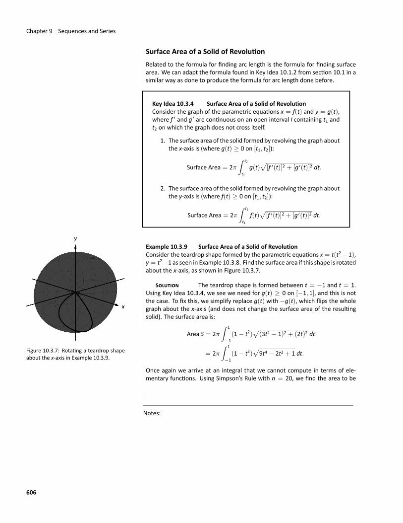
Chapter 9 Sequences and Series
Surface Area of a Solid of RevolutionRelated to the formula for finding arc length is the formula for finding surfacearea. We can adapt the formula found in Key Idea 10.1.2 from section 10.1 in asimilar way as done to produce the formula for arc length done before.
Key Idea 10.3.4 Surface Area of a Solid of RevolutionConsider the graph of the parametric equations x = f(t) and y = g(t),where f ′ and g ′ are continuous on an open interval I containing t1 andt2 on which the graph does not cross itself.
1. The surface area of the solid formed by revolving the graph aboutthe x‐axis is (where g(t) ≥ 0 on [t1, t2]):
Surface Area = 2π∫ t2
t1g(t)
√[f ′(t)]2 + [g ′(t)]2 dt.
2. The surface area of the solid formed by revolving the graph aboutthe y‐axis is (where f(t) ≥ 0 on [t1, t2]):
Surface Area = 2π∫ t2
t1f(t)√
[f ′(t)]2 + [g ′(t)]2 dt.
Figure 10.3.7: Rotating a teardrop shapeabout the x‐axis in Example 10.3.9.
Example 10.3.9 Surface Area of a Solid of RevolutionConsider the teardrop shape formed by the parametric equations x = t(t2− 1),y = t2−1 as seen in Example 10.3.8. Find the surface area if this shape is rotatedabout the x‐axis, as shown in Figure 10.3.7.
SOLUTION The teardrop shape is formed between t = −1 and t = 1.Using Key Idea 10.3.4, we see we need for g(t) ≥ 0 on [−1, 1], and this is notthe case. To fix this, we simplify replace g(t) with −g(t), which flips the wholegraph about the x‐axis (and does not change the surface area of the resultingsolid). The surface area is:
Area S = 2π∫ 1
−1(1− t2)
√(3t2 − 1)2 + (2t)2 dt
= 2π∫ 1
−1(1− t2)
√9t4 − 2t2 + 1 dt.
Once again we arrive at an integral that we cannot compute in terms of ele‐mentary functions. Using Simpson’s Rule with n = 20, we find the area to be
Notes:
606

10.3 Calculus and Parametric Equations
S = 9.44. Using larger values of n shows this is accurate to 2 places after thedecimal.
After defining a new way of creating curves in the plane, in this sectionwe have applied calculus techniques to the parametric equation defining thesecurves to study their properties. In the next section, we define another way offorming curves in the plane. To do so, we create a new coordinate system, calledpolar coordinates, that identifies points in the plane in a manner different thanfrom measuring distances from the y‐ and x‐ axes.
Notes:
607
Exercises 10.3Terms and Concepts1. T/F: Given parametric equations x = f(t) and y = g(t),
dydx = f ′(t)/g′(t), as long as g′(t) ̸= 0.
2. Given parametric equations x = f(t) and y = g(t), thederivative dy
dx as given in Key Idea 10.3.1 is a function of?
3. T/F: Given parametric equations x = f(t) and y = g(t), tofind d2y
dx2 , one simply computes ddt
(dydx
).
4. T/F: If dydx = 0 at t = t0, then the normal line to the curve
at t = t0 is a vertical line.
ProblemsIn Exercises 5–12, parametric equations for a curve are given.
(a) Find dydx
.
(b) Find the equations of the tangent and normal line(s) atthe point(s) given.
(c) Sketch the graph of the parametric functions along withthe found tangent and normal lines.
5. x = t, y = t2; t = 16. x =
√t, y = 5t+ 2; t = 4
7. x = t2 − t, y = t2 + t; t = 18. x = t2 − 1, y = t3 − t; t = 0 and t = 19. x = sec t, y = tan t on (−π/2, π/2); t = π/4
10. x = cos t, y = sin(2t) on [0, 2π]; t = π/411. x = cos t sin(2t), y = sin t sin(2t) on [0, 2π]; t = 3π/412. x = et/10 cos t, y = et/10 sin t; t = π/2
In Exercises 13–20, find t‐values where the curve defined bythe given parametric equations has horizontal or vertical tan‐gent lines. Note: these are the same equations as in Exer‐cises 5–12.
13. x = t, y = t2
14. x =√t, y = 5t+ 2
15. x = t2 − t, y = t2 + t
16. x = t2 − 1, y = t3 − t
17. x = sec t, y = tan t on (−π/2, π/2)18. x = cos t, y = sin(2t) on [0, 2π]19. x = cos t sin(2t), y = sin t sin(2t) on [0, 2π]20. x = et/10 cos t, y = et/10 sin t on [−π, π]
In Exercises 21–24, find t = t0 where the graph of the givenparametric equations is not smooth, then find lim
t→t0
dydx
.
21. x = 1t2 + 1
, y = t3
22. x = −t3 + 7t2 − 16t+ 13, y = t3 − 5t2 + 8t− 223. x = t3 − 3t2 + 3t− 1, y = t2 − 2t+ 1
24. x = cos2 t, y = 1− sin2 t
In Exercises 25–32, parametric equations for a curve are given.Find d2y
dx2 , then determine the intervals on which the graph ofthe curve is concave up/down. Note: these are the same equa‐tions as in Exercises 5–12.
25. x = t, y = t2
26. x =√t, y = 5t+ 2
27. x = t2 − t, y = t2 + t
28. x = t2 − 1, y = t3 − t
29. x = sec t, y = tan t on (−π/2, π/2)30. x = cos t, y = sin(2t) on [0, 2π]31. x = cos t sin(2t), y = sin t sin(2t) on [−π/2, π/2]32. x = et/10 cos t, y = et/10 sin t
In Exercises 33–40, find the arc length of the graph of the para‐metric equations on the given interval(s).
33. x = −3 sin(2t), y = 3 cos(2t) on [0, π]34. x = et/10 cos t, y = et/10 sin t on [0, 2π] and [2π, 4π]35. x = 5t+ 2, y = 1− 3t on [−1, 1]36. x = 2t3/2, y = 3t on [0, 1]37. x = cos t, y = sin t on [0, 2π]38. x = 1+ 3t2, y = 4+ 2t3 on [0, 1]
39. x = t1+ t
, y = ln(1+ t) on [0, 2]
40. x = et − t, y = 4e−t/2 on [−8, 3]
In Exercises 41–44, numerically approximate the given arclength.
41. Approximate the arc length of one petal of the rose curvex = cos t cos(2t), y = sin t cos(2t) using Simpson’s Ruleand n = 4.
42. Approximate the arc length of the “bow tie curve” x =cos t, y = sin(2t) using Simpson’s Rule and n = 6.
43. Approximate the arc length of the parabola x = t2 − t,y = t2 + t on [−1, 1] using Simpson’s Rule and n = 4.
44. A common approximate of the circumference of an ellipse
given by x = a cos t, y = b sin t is C ≈ 2π√
a2 + b22
.Use this formula to approximate the circumference of x =5 cos t, y = 3 sin t and compare this to the approxima‐tion given by Simpson’s Rule and n = 6.
In Exercises 45–50, a solid of revolution is described. Find orapproximate its surface area as specified.
45. Find the surface area of the sphere formed by rotating thecircle x = 2 cos t, y = 2 sin t about:
(a) the x‐axis and
(b) the y‐axis.
46. Find the surface area of the torus (or “donut”) formed byrotating the circle x = cos t + 2, y = sin t about they‐axis.
608
47. Find the surface area of the solid formed by rotating thecurve x = a cos3 θ, y = a sin3 θ on [0, π/2] about thex−axis
48. Find the surface area of the solid formed by rotating thecurve x = 3t2, y = 2t3 on [0, 5] about the y−axis
49. Approximate the surface area of the solid formed by rotat‐ing the “upper right half” of the bow tie curve x = cos t,y = sin(2t) on [0, π/2] about the x‐axis, using Simpson’sRule and n = 4.
50. Approximate the surface area of the solid formed by ro‐tating the one petal of the rose curve x = cos t cos(2t),y = sin t cos(2t) on [0, π/4] about the x‐axis, using Simp‐son’s Rule and n = 4.
609
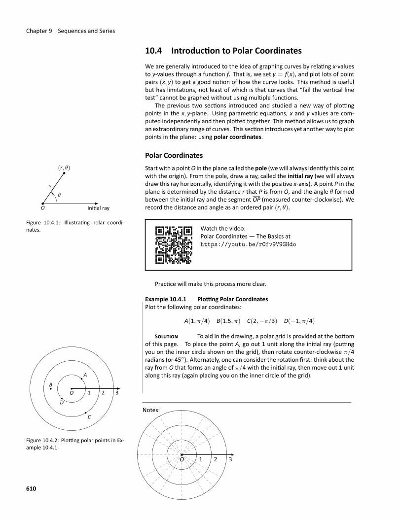
Chapter 9 Sequences and Series
10.4 Introduction to Polar CoordinatesWe are generally introduced to the idea of graphing curves by relating x‐valuesto y‐values through a function f. That is, we set y = f(x), and plot lots of pointpairs (x, y) to get a good notion of how the curve looks. This method is usefulbut has limitations, not least of which is that curves that “fail the vertical linetest” cannot be graphed without using multiple functions.
The previous two sections introduced and studied a new way of plottingpoints in the x, y‐plane. Using parametric equations, x and y values are com‐puted independently and then plotted together. This method allows us to graphan extraordinary range of curves. This section introduces yet anotherway to plotpoints in the plane: using polar coordinates.
Polar Coordinates
O initial ray
r
(r, θ)
θ
Figure 10.4.1: Illustrating polar coordi‐nates.
Start with a pointO in the plane called the pole (wewill always identify this pointwith the origin). From the pole, draw a ray, called the initial ray (we will alwaysdraw this ray horizontally, identifying it with the positive x‐axis). A point P in theplane is determined by the distance r that P is from O, and the angle θ formedbetween the initial ray and the segment OP (measured counter‐clockwise). Werecord the distance and angle as an ordered pair (r, θ).
Watch the video:Polar Coordinates — The Basics athttps://youtu.be/r0fv9V9GHdo
Practice will make this process more clear.
Example 10.4.1 Plotting Polar CoordinatesPlot the following polar coordinates:
A(1, π/4) B(1.5, π) C(2,−π/3) D(−1, π/4)
SOLUTION To aid in the drawing, a polar grid is provided
O 1 2 3
at the bottomof this page. To place the point A, go out 1 unit along the initial ray (putting
O 1 2 3
A
B
C
D
Figure 10.4.2: Plotting polar points in Ex‐ample 10.4.1.
you on the inner circle shown on the grid), then rotate counter‐clockwise π/4radians (or 45◦). Alternately, one can consider the rotation first: think about theray from O that forms an angle of π/4 with the initial ray, then move out 1 unitalong this ray (again placing you on the inner circle of the grid).
Notes:
610
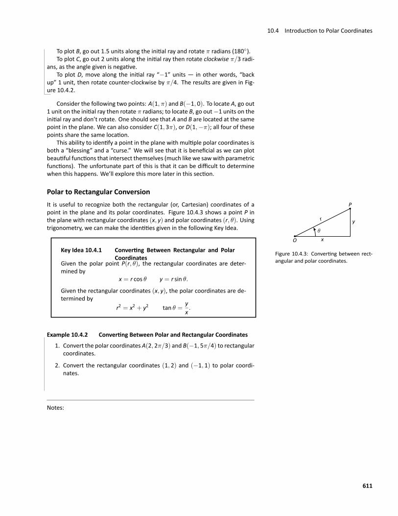
10.4 Introduction to Polar Coordinates
To plot B, go out 1.5 units along the initial ray and rotate π radians (180◦).To plot C, go out 2 units along the initial ray then rotate clockwise π/3 radi‐
ans, as the angle given is negative.To plot D, move along the initial ray “−1” units — in other words, “back
up” 1 unit, then rotate counter‐clockwise by π/4. The results are given in Fig‐ure 10.4.2.
Consider the following two points: A(1, π) and B(−1, 0). To locate A, go out1 unit on the initial ray then rotate π radians; to locate B, go out−1 units on theinitial ray and don’t rotate. One should see that A and B are located at the samepoint in the plane. We can also consider C(1, 3π), or D(1,−π); all four of thesepoints share the same location.
This ability to identify a point in the plane with multiple polar coordinates isboth a “blessing” and a “curse.” We will see that it is beneficial as we can plotbeautiful functions that intersect themselves (much like we sawwith parametricfunctions). The unfortunate part of this is that it can be difficult to determinewhen this happens. We’ll explore this more later in this section.
Polar to Rectangular Conversion
x
yr
θ
O
P
Figure 10.4.3: Converting between rect‐angular and polar coordinates.
It is useful to recognize both the rectangular (or, Cartesian) coordinates of apoint in the plane and its polar coordinates. Figure 10.4.3 shows a point P inthe plane with rectangular coordinates (x, y) and polar coordinates (r, θ). Usingtrigonometry, we can make the identities given in the following Key Idea.
Key Idea 10.4.1 Converting Between Rectangular and PolarCoordinates
Given the polar point P(r, θ), the rectangular coordinates are deter‐mined by
x = r cos θ y = r sin θ.
Given the rectangular coordinates (x, y), the polar coordinates are de‐termined by
r2 = x2 + y2 tan θ =yx.
Example 10.4.2 Converting Between Polar and Rectangular Coordinates1. Convert the polar coordinates A(2, 2π/3) and B(−1, 5π/4) to rectangular
coordinates.
2. Convert the rectangular coordinates (1, 2) and (−1, 1) to polar coordi‐nates.
Notes:
611
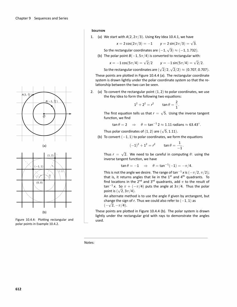
Chapter 9 Sequences and Series
SOLUTION
1. (a) We start with A(2, 2π/3). Using Key Idea 10.4.1, we have
x = 2 cos(2π/3) = −1 y = 2 sin(2π/3) =√3.
So the rectangular coordinates are (−1,√3) ≈ (−1, 1.732).
(b) The polar point B(−1, 5π/4) is converted to rectangular with:
x = −1 cos(5π/4) =√2/2 y = −1 sin(5π/4) =
√2/2.
So the rectangular coordinates are (√2/2,
√2/2) ≈ (0.707, 0.707).
These points are plotted in Figure 10.4.4 (a). The rectangular coordinatesystem is drawn lightly under the polar coordinate system so that the re‐lationship between the two can be seen.
O
A(2, 2π3 )
B(−1, 5π4 )
(a)
(0, 0)
(1, 2)
(−1, 1)
3π43π4
−π4
1.11
(b)
Figure 10.4.4: Plotting rectangular andpolar points in Example 10.4.2.
2. (a) To convert the rectangular point (1, 2) to polar coordinates, we usethe Key Idea to form the following two equations:
12 + 22 = r2 tan θ =21.
The first equation tells us that r =√5. Using the inverse tangent
function, we find
tan θ = 2 ⇒ θ = tan−1 2 ≈ 1.11 radians ≈ 63.43◦.
Thus polar coordinates of (1, 2) are (√5, 1.11).
(b) To convert (−1, 1) to polar coordinates, we form the equations
(−1)2 + 12 = r2 tan θ =1−1
.
Thus r =√2. We need to be careful in computing θ: using the
inverse tangent function, we have
tan θ = −1 ⇒ θ = tan−1(−1) = −π/4.
This is not the angle we desire. The range of tan−1 x is (−π/2, π/2);that is, it returns angles that lie in the 1st and 4th quadrants. Tofind locations in the 2nd and 3rd quadrants, add π to the result oftan−1 x. So π + (−π/4) puts the angle at 3π/4. Thus the polarpoint is (
√2, 3π/4).
An alternate method is to use the angle θ given by arctangent, butchange the sign of r. Thus we could also refer to (−1, 1) as(−
√2,−π/4).
These points are plotted in Figure 10.4.4 (b). The polar system is drawnlightly under the rectangular grid with rays to demonstrate the anglesused.
Notes:
612
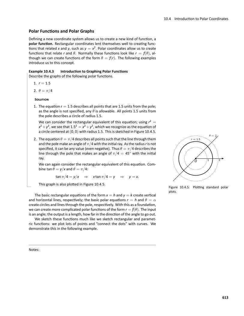
10.4 Introduction to Polar Coordinates
Polar Functions and Polar GraphsDefining a new coordinate system allows us to create a new kind of function, apolar function. Rectangular coordinates lent themselves well to creating func‐tions that related x and y, such as y = x2. Polar coordinates allow us to createfunctions that relate r and θ. Normally these functions look like r = f(θ), al‐though we can create functions of the form θ = f(r). The following examplesintroduce us to this concept.
Example 10.4.3 Introduction to Graphing Polar FunctionsDescribe the graphs of the following polar functions.
1. r = 1.5
2. θ = π/4
SOLUTION
1. The equation r = 1.5 describes all points that are 1.5 units from the pole;as the angle is not specified, any θ is allowable. All points 1.5 units fromthe pole describes a circle of radius 1.5.We can consider the rectangular equivalent of this equation; using r2 =x2+y2, we see that 1.52 = x2+y2, which we recognize as the equation ofa circle centered at (0, 0)with radius 1.5. This is sketched in Figure 10.4.5.
O 1 2
r = 1.5θ = π
4
Figure 10.4.5: Plotting standard polarplots.
2. The equation θ = π/4 describes all points such that the line through themand the polemake an angle of π/4with the initial ray. As the radius r is notspecified, it can be any value (even negative). Thus θ = π/4 describes theline through the pole that makes an angle of π/4 = 45◦ with the initialray.We can again consider the rectangular equivalent of this equation. Com‐bine tan θ = y/x and θ = π/4:
tan π/4 = y/x ⇒ x tan π/4 = y ⇒ y = x.
This graph is also plotted in Figure 10.4.5.
The basic rectangular equations of the form x = h and y = k create verticaland horizontal lines, respectively; the basic polar equations r = h and θ = αcreate circles and lines through the pole, respectively. With this as a foundation,we can create more complicated polar functions of the form r = f(θ). The inputis an angle; the output is a length, how far in the direction of the angle to go out.
We sketch these functions much like we sketch rectangular and paramet‐ric functions: we plot lots of points and “connect the dots” with curves. Wedemonstrate this in the following example.
Notes:
613
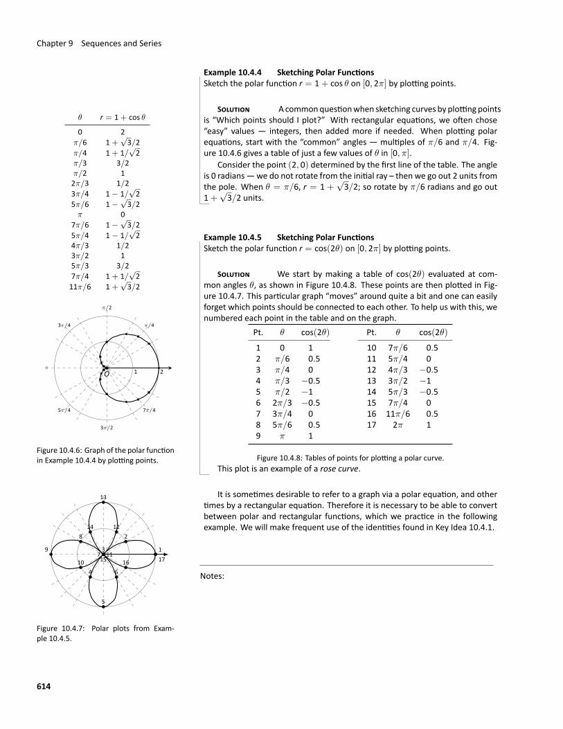
Chapter 9 Sequences and Series
Example 10.4.4 Sketching Polar FunctionsSketch the polar function r = 1+ cos θ on [0, 2π] by plotting points.
SOLUTION Acommonquestionwhen sketching curves by plottingpointsθ r = 1+ cos θ
0 2π/6 1+
√3/2
π/4 1+ 1/√2
π/3 3/2π/2 12π/3 1/23π/4 1− 1/
√2
5π/6 1−√3/2
π 07π/6 1−
√3/2
5π/4 1− 1/√2
4π/3 1/23π/2 15π/3 3/27π/4 1+ 1/
√2
11π/6 1+√3/2
O 1 2
π/4
π/2
3π/4
π
5π/4
3π/2
7π/4
Figure 10.4.6: Graph of the polar functionin Example 10.4.4 by plotting points.
is “Which points should I plot?” With rectangular equations, we often chose“easy” values — integers, then added more if needed. When plotting polarequations, start with the “common” angles — multiples of π/6 and π/4. Fig‐ure 10.4.6 gives a table of just a few values of θ in [0, π].
Consider the point (2, 0) determined by the first line of the table. The angleis 0 radians—we do not rotate from the initial ray – then we go out 2 units fromthe pole. When θ = π/6, r = 1 +
√3/2; so rotate by π/6 radians and go out
1+√3/2 units.
Example 10.4.5 Sketching Polar FunctionsSketch the polar function r = cos(2θ) on [0, 2π] by plotting points.
SOLUTION We start by making a table of cos(2θ) evaluated at com‐mon angles θ, as shown in Figure 10.4.8. These points are then plotted in Fig‐ure 10.4.7. This particular graph “moves” around quite a bit and one can easilyforget which points should be connected to each other. To help us with this, wenumbered each point in the table and on the graph.
1
2
3
4
5
6
7
8
9
1011
12
13
14
15 16 17
Figure 10.4.7: Polar plots from Exam‐ple 10.4.5.
Pt. θ cos(2θ) Pt. θ cos(2θ)
1 0 1 10 7π/6 0.52 π/6 0.5 11 5π/4 03 π/4 0 12 4π/3 −0.54 π/3 −0.5 13 3π/2 −15 π/2 −1 14 5π/3 −0.56 2π/3 −0.5 15 7π/4 07 3π/4 0 16 11π/6 0.58 5π/6 0.5 17 2π 19 π 1
Figure 10.4.8: Tables of points for plotting a polar curve.This plot is an example of a rose curve.
It is sometimes desirable to refer to a graph via a polar equation, and othertimes by a rectangular equation. Therefore it is necessary to be able to convertbetween polar and rectangular functions, which we practice in the followingexample. We will make frequent use of the identities found in Key Idea 10.4.1.
Notes:
614
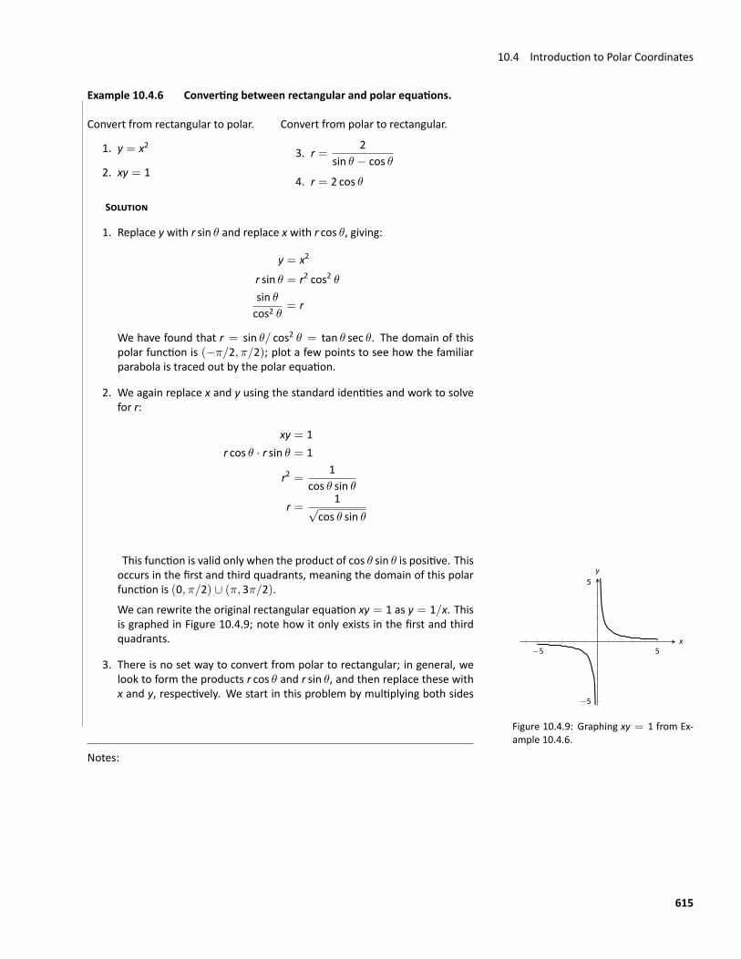
10.4 Introduction to Polar Coordinates
Example 10.4.6 Converting between rectangular and polar equations.
Convert from rectangular to polar.
1. y = x2
2. xy = 1
Convert from polar to rectangular.
3. r =2
sin θ − cos θ
4. r = 2 cos θ
SOLUTION
1. Replace y with r sin θ and replace x with r cos θ, giving:
y = x2
r sin θ = r2 cos2 θsin θcos2 θ
= r
We have found that r = sin θ/ cos2 θ = tan θ sec θ. The domain of thispolar function is (−π/2, π/2); plot a few points to see how the familiarparabola is traced out by the polar equation.
2. We again replace x and y using the standard identities and work to solvefor r:
xy = 1r cos θ · r sin θ = 1
r2 =1
cos θ sin θ
r =1√
cos θ sin θ
This function is valid only when the product of cos θ sin θ is positive. This
−5 5
−5
5
x
y
Figure 10.4.9: Graphing xy = 1 from Ex‐ample 10.4.6.
occurs in the first and third quadrants, meaning the domain of this polarfunction is (0, π/2) ∪ (π, 3π/2).
We can rewrite the original rectangular equation xy = 1 as y = 1/x. Thisis graphed in Figure 10.4.9; note how it only exists in the first and thirdquadrants.
3. There is no set way to convert from polar to rectangular; in general, welook to form the products r cos θ and r sin θ, and then replace these withx and y, respectively. We start in this problem by multiplying both sides
Notes:
615
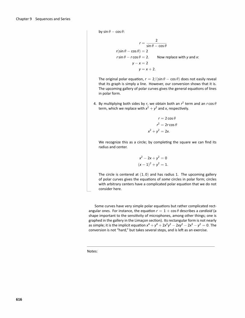
Chapter 9 Sequences and Series
by sin θ − cos θ:
r =2
sin θ − cos θr(sin θ − cos θ) = 2r sin θ − r cos θ = 2. Now replace with y and x:
y− x = 2y = x+ 2.
The original polar equation, r = 2/(sin θ − cos θ) does not easily revealthat its graph is simply a line. However, our conversion shows that it is.The upcoming gallery of polar curves gives the general equations of linesin polar form.
4. By multiplying both sides by r, we obtain both an r2 term and an r cos θterm, which we replace with x2 + y2 and x, respectively.
r = 2 cos θr2 = 2r cos θ
x2 + y2 = 2x.
We recognize this as a circle; by completing the square we can find itsradius and center.
x2 − 2x+ y2 = 0(x− 1)2 + y2 = 1.
The circle is centered at (1, 0) and has radius 1. The upcoming galleryof polar curves gives the equations of some circles in polar form; circleswith arbitrary centers have a complicated polar equation that we do notconsider here.
Some curves have very simple polar equations but rather complicated rect‐angular ones. For instance, the equation r = 1 + cos θ describes a cardioid (ashape important to the sensitivity of microphones, among other things; one isgraphed in the gallery in the Limaçon section). Its rectangular form is not nearlyas simple; it is the implicit equation x4 + y4 + 2x2y2 − 2xy2 − 2x3 − y2 = 0. Theconversion is not “hard,” but takes several steps, and is left as an exercise.
Notes:
616
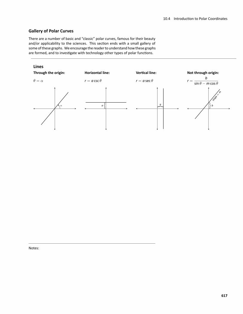
10.4 Introduction to Polar Coordinates
Gallery of Polar CurvesThere are a number of basic and “classic” polar curves, famous for their beautyand/or applicability to the sciences. This section ends with a small gallery ofsomeof these graphs. Weencourage the reader to understandhow these graphsare formed, and to investigate with technology other types of polar functions.
LinesThrough the origin: Horizontal line: Vertical line: Not through origin:
θ = α r = a csc θ r = a sec θ r =b
sin θ −m cos θ
α a{ ︷︸︸ ︷a
slope=m
}b
Notes:
617
Circles SprialCentered on origin: (x− a
2 )2 + y2 = a2
4 x2 + (y− a2 )
2 = a24 Archimedean spiral
r = a r = a cos θ r = a sin θ r = θ
︷ ︸︸ ︷a ︷ ︸︸ ︷a
a
LimaçonsSymmetric about x‐axis: r = a± b cos θ; Symmetric about y‐axis: r = a± b sin θ; a, b > 0With inner loop: Cardioid: Dimpled: Convex:ab< 1
ab= 1 1 <
ab< 2
ab> 2
Rose CurvesSymmetric about x‐axis: r = a cos(nθ); Symmetric about y‐axis: r = a sin(nθ)Curve contains 2n petals when n is even and n petals when n is odd.r = a cos(2θ) r = a sin(2θ) r = a cos(3θ) r = a sin(3θ)
Special CurvesRose curves Lemniscate: Eight Curve:r = a sin(θ/5) r = a sin(2θ/5) r2 = a2 cos(2θ) r2 = a2 sec4 θ cos(2θ)
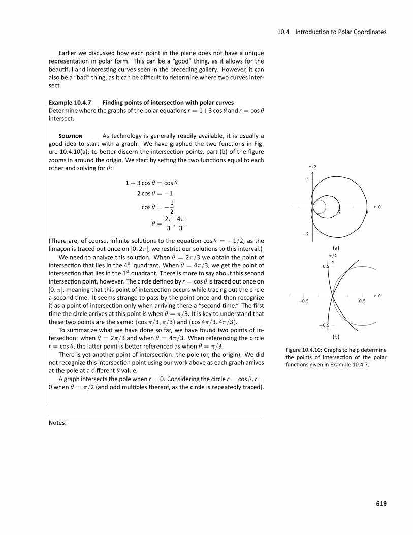
10.4 Introduction to Polar Coordinates
Earlier we discussed how each point in the plane does not have a uniquerepresentation in polar form. This can be a “good” thing, as it allows for thebeautiful and interesting curves seen in the preceding gallery. However, it canalso be a “bad” thing, as it can be difficult to determine where two curves inter‐sect.
Example 10.4.7 Finding points of intersection with polar curvesDeterminewhere the graphs of the polar equations r = 1+3 cos θ and r = cos θintersect.
SOLUTION As technology is generally readily available, it is usually agood idea to start with a graph. We have graphed the two functions in Fig‐ure 10.4.10(a); to better discern the intersection points, part (b) of the figurezooms in around the origin. We start by setting the two functions equal to each
2 4
−2
2
0
π/2
(a)
−0.5 0.5
−0.5
0.5
0
π/2
(b)
Figure 10.4.10: Graphs to help determinethe points of intersection of the polarfunctions given in Example 10.4.7.
other and solving for θ:
1+ 3 cos θ = cos θ2 cos θ = −1
cos θ = −12
θ =2π3,4π3.
(There are, of course, infinite solutions to the equation cos θ = −1/2; as thelimaçon is traced out once on [0, 2π], we restrict our solutions to this interval.)
We need to analyze this solution. When θ = 2π/3 we obtain the point ofintersection that lies in the 4th quadrant. When θ = 4π/3, we get the point ofintersection that lies in the 1st quadrant. There is more to say about this secondintersection point, however. The circle defined by r = cos θ is traced out once on[0, π], meaning that this point of intersection occurs while tracing out the circlea second time. It seems strange to pass by the point once and then recognizeit as a point of intersection only when arriving there a “second time.” The firsttime the circle arrives at this point is when θ = π/3. It is key to understand thatthese two points are the same: (cos π/3, π/3) and (cos 4π/3, 4π/3).
To summarize what we have done so far, we have found two points of in‐tersection: when θ = 2π/3 and when θ = 4π/3. When referencing the circler = cos θ, the latter point is better referenced as when θ = π/3.
There is yet another point of intersection: the pole (or, the origin). We didnot recognize this intersection point using our work above as each graph arrivesat the pole at a different θ value.
A graph intersects the pole when r = 0. Considering the circle r = cos θ, r =0 when θ = π/2 (and odd multiples thereof, as the circle is repeatedly traced).
Notes:
619
Chapter 9 Sequences and Series
The limaçon intersects the pole when 1+ 3 cos θ = 0; this occurs when cos θ =−1/3, or for θ = cos−1(−1/3). This is a nonstandard angle, approximatelyθ = 1.9106 radians ≈ 109.47◦. The limaçon intersects the pole twice in [0, 2π];the other angle at which the limaçon is at the pole is the reflection of the firstangle across the x‐axis. That is, θ = 4.3726 ≈ 250.53◦.
If all one is concernedwith is the (x, y) coordinates at which the graphs inter‐sect, much of the above work is extraneous. We know they intersect at (0, 0);we might not care at what θ value. Likewise, using θ = 2π/3 and θ = 4π/3can give us the needed rectangular coordinates. However, in the next sectionwe apply calculus concepts to polar functions. When computing the area of aregion bounded by polar curves, understanding the nuances of the points ofintersection becomes important.
Notes:
620
Exercises 10.4Terms and Concepts1. In your own words, describe how to plot the polar point
P(r, θ).2. T/F: When plotting a point with polar coordinate P(r, θ), r
must be positive.3. T/F: Every point in the Cartesian plane can be represented
by a polar coordinate.4. T/F: Every point in the Cartesian plane can be represented
uniquely by a polar coordinate.
Problems5. Plot the points with the given polar coordinates.
(a) A(2, 0)
(b) B(1, π)
(c) C(−2, π/2)
(d) D(1, π/4)6. Plot the points with the given polar coordinates.
(a) A(2, 3π)
(b) B(1,−π)
(c) C(1, 2)
(d) D(1/2, 5π/6)7. For each of the given points give two sets of polar coordi‐
nates that identify it, where 0 ≤ θ ≤ 2π.
O 1 2 3
A
B
C
D
8. For each of the given points give two sets of polar coordi‐nates that identify it, where−π ≤ θ ≤ π.
O 1 2 3
A
B
C
D
9. Convert the polar coordinates A and B to rectangular, andthe rectangular coordinates C and D to polar.
(a) A(2, π/4)
(b) B(2,−π/4)
(c) C(2,−1)
(d) D(−2, 1)10. Convert the polar coordinates A and B to rectangular, and
the rectangular coordinates C and D to polar.
(a) A(3, π)
(b) B(1, 2π/3)
(c) C(0, 4)
(d) D(1,−√3)
In Exercises 11–32, graph the polar function on the given in‐terval.
11. r = 2, 0 ≤ θ ≤ π/2
12. θ = π/6, −1 ≤ r ≤ 213. r = 1− cos θ, [0, 2π]14. r = 2+ sin θ, [0, 2π]15. r = 2− sin θ, [0, 2π]16. r = 1− 2 sin θ, [0, 2π]17. r = 1+ 2 sin θ, [0, 2π]18. r = cos(2θ), [0, 2π]19. r = sin(3θ), [0, π]20. r = cos(θ/3), [0, 3π]21. r = cos(2θ/3), [0, 6π]22. r = θ/2, [0, 4π]23. r = 3 sin(θ), [0, π]24. r = −4 sin(θ), [0, π]25. r = −2 cos(θ), [0, π]
26. r = 32cos(θ), [0, π]
27. r = cos θ sin θ, [0, 2π]28. r = θ2 − (π/2)2, [−π, π]
29. r = 35 sin θ − cos θ
, [0, 2π]
30. r = −23 cos θ − 2 sin θ
, [0, 2π]
31. r = 3 sec θ, (−π/2, π/2)32. r = 3 csc θ, (0, π)
In Exercises 33–44, convert the polar equation to a rectangularequation.
33. r = 2 cos θ34. r = −4 sin θ35. r = 3 sin θ
36. r = −32cos θ
37. r = cos θ + sin θ
38. r = 75 sin θ − 2 cos θ
39. r = 3cos θ
40. r = 4sin θ
41. r = tan θ42. r = cot θ43. r = 244. θ =
π
6In Exercises 45–52, convert the rectangular equation to a polarequation.
45. y = x46. y = 4x+ 747. x = 548. y = 5
621
49. x = y2
50. x2y = 1
51. x2 + y2 = 7
52. (x+ 1)2 + y2 = 1
In Exercises 53–60, find the points of intersection of the polargraphs.
53. r = sin(2θ) and r = cos θ on [0, π]
54. r = cos(2θ) and r = cos θ on [0, π]
55. r = 2 cos θ and r = 2 sin θ on [0, π]
56. r = sin θ and r =√3+ 3 sin θ on [0, 2π]
57. r = sin(3θ) and r = cos(3θ) on [0, π]
58. r = 3 cos θ and r = 1+ cos θ on [−π, π]
59. r = 1 and r = 2 sin(2θ) on [0, 2π]
60. r = 1− cos θ and r = 1+ sin θ on [0, 2π]
61. Pick a integer value for n, where n ̸= 2, 3, and use tech‐nology to plot r = sin
(mnθ)for three different integer
values of m. Sketch these and determine a minimal inter‐val on which the entire graph is shown.
62. Create your own polar function, r = f(θ) and sketch it. De‐scribe why the graph looks as it does.
622
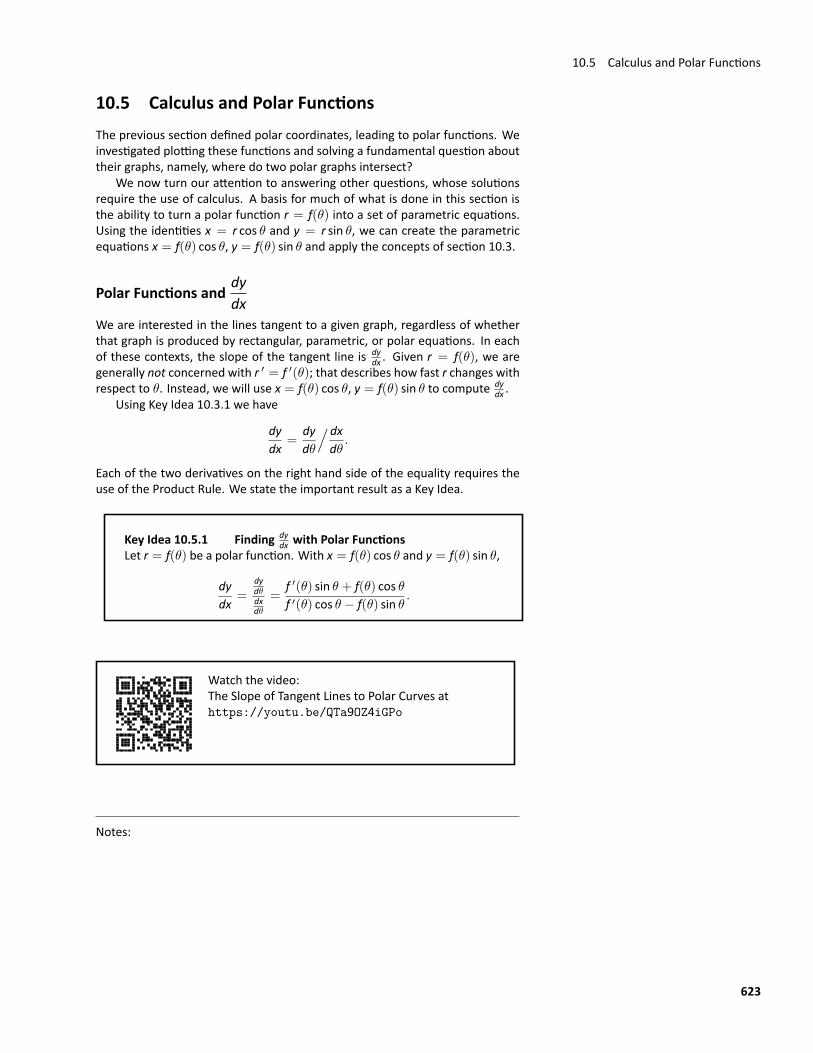
10.5 Calculus and Polar Functions
10.5 Calculus and Polar FunctionsThe previous section defined polar coordinates, leading to polar functions. Weinvestigated plotting these functions and solving a fundamental question abouttheir graphs, namely, where do two polar graphs intersect?
We now turn our attention to answering other questions, whose solutionsrequire the use of calculus. A basis for much of what is done in this section isthe ability to turn a polar function r = f(θ) into a set of parametric equations.Using the identities x = r cos θ and y = r sin θ, we can create the parametricequations x = f(θ) cos θ, y = f(θ) sin θ and apply the concepts of section 10.3.
Polar Functions anddydx
We are interested in the lines tangent to a given graph, regardless of whetherthat graph is produced by rectangular, parametric, or polar equations. In eachof these contexts, the slope of the tangent line is dy
dx . Given r = f(θ), we aregenerally not concerned with r ′ = f ′(θ); that describes how fast r changes withrespect to θ. Instead, we will use x = f(θ) cos θ, y = f(θ) sin θ to compute dy
dx .Using Key Idea 10.3.1 we have
dydx
=dydθ
/dxdθ
.
Each of the two derivatives on the right hand side of the equality requires theuse of the Product Rule. We state the important result as a Key Idea.
Key Idea 10.5.1 Finding dydx with Polar Functions
Let r = f(θ) be a polar function. With x = f(θ) cos θ and y = f(θ) sin θ,
dydx
=dydθdxdθ
=f ′(θ) sin θ + f(θ) cos θf ′(θ) cos θ − f(θ) sin θ
.
Watch the video:The Slope of Tangent Lines to Polar Curves athttps://youtu.be/QTa9OZ4iGPo
Notes:
623
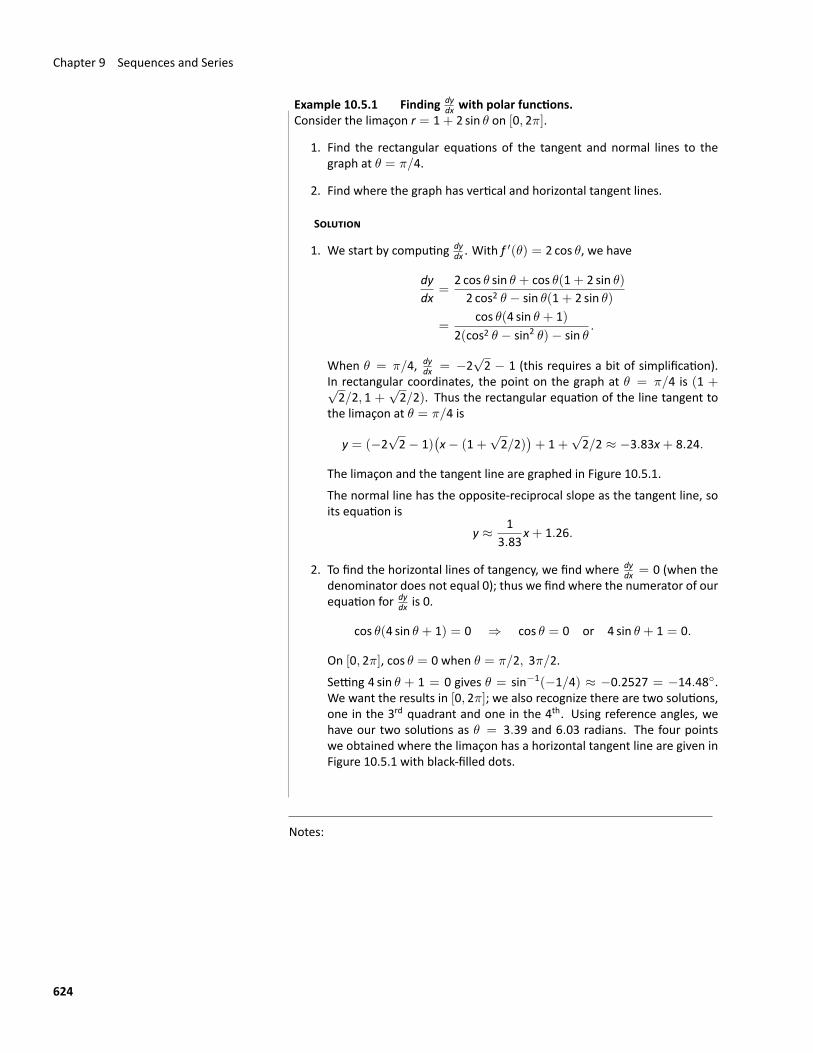
Chapter 9 Sequences and Series
Example 10.5.1 Finding dydx with polar functions.
Consider the limaçon r = 1+ 2 sin θ on [0, 2π].
1. Find the rectangular equations of the tangent and normal lines to thegraph at θ = π/4.
2. Find where the graph has vertical and horizontal tangent lines.
SOLUTION
1. We start by computing dydx . With f ′(θ) = 2 cos θ, we have
dydx
=2 cos θ sin θ + cos θ(1+ 2 sin θ)2 cos2 θ − sin θ(1+ 2 sin θ)
=cos θ(4 sin θ + 1)
2(cos2 θ − sin2 θ)− sin θ.
When θ = π/4, dydx = −2
√2 − 1 (this requires a bit of simplification).
In rectangular coordinates, the point on the graph at θ = π/4 is (1 +√2/2, 1 +
√2/2). Thus the rectangular equation of the line tangent to
the limaçon at θ = π/4 is
y = (−2√2− 1)
(x− (1+
√2/2)
)+ 1+
√2/2 ≈ −3.83x+ 8.24.
The limaçon and the tangent line are graphed in Figure 10.5.1.The normal line has the opposite‐reciprocal slope as the tangent line, soits equation is
y ≈ 13.83
x+ 1.26.
2. To find the horizontal lines of tangency, we find where dydx = 0 (when the
denominator does not equal 0); thus we find where the numerator of ourequation for dy
dx is 0.
cos θ(4 sin θ + 1) = 0 ⇒ cos θ = 0 or 4 sin θ + 1 = 0.
On [0, 2π], cos θ = 0 when θ = π/2, 3π/2.Setting 4 sin θ + 1 = 0 gives θ = sin−1(−1/4) ≈ −0.2527 = −14.48◦.We want the results in [0, 2π]; we also recognize there are two solutions,one in the 3rd quadrant and one in the 4th. Using reference angles, wehave our two solutions as θ = 3.39 and 6.03 radians. The four pointswe obtained where the limaçon has a horizontal tangent line are given inFigure 10.5.1 with black‐filled dots.
Notes:
624
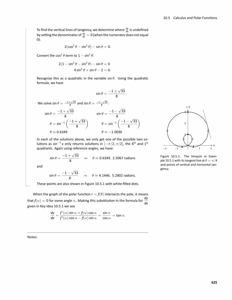
10.5 Calculus and Polar Functions
To find the vertical lines of tangency, we determine where dydx is undefined
by setting the denominator of dydx = 0 (when the numerator does not equal
0).
2(cos2 θ − sin2 θ)− sin θ = 0.
Convert the cos2 θ term to 1− sin2 θ:
2(1− sin2 θ − sin2 θ)− sin θ = 04 sin2 θ + sin θ − 2 = 0.
Recognize this as a quadratic in the variable sin θ. Using the quadraticformula, we have
sin θ =−1±
√33
8.
We solve sin θ = −1+√33
8 and sin θ = −1−√33
8 :
−2 −1 1 2
1
2
3
0
π/2
Figure 10.5.1: The limaçon in Exam‐ple 10.5.1 with its tangent line at θ = π/4and points of vertical and horizontal tan‐gency.
sin θ =−1+
√33
8sin θ =
−1−√33
8
θ = sin−1(−1+
√33
8
)θ = sin−1
(−1−
√33
8
)θ ≈ 0.6349 θ ≈ −1.0030
In each of the solutions above, we only get one of the possible two so‐lutions as sin−1 x only returns solutions in [−π/2, π/2], the 4th and 1stquadrants. Again using reference angles, we have:
sin θ =−1+
√33
8⇒ θ ≈ 0.6349, 2.5067 radians
and
sin θ =−1−
√33
8⇒ θ ≈ 4.1446, 5.2802 radians.
These points are also shown in Figure 10.5.1 with white‐filled dots.
When the graph of the polar function r = f(θ) intersects the pole, it means
that f(α) = 0 for some angle α. Making this substitution in the formula fordydx
given in Key Idea 10.5.1 we see
dydx
=f ′(α) sinα+ f(α) cosαf ′(α) cosα− f(α) sinα
=sinαcosα
= tanα.
Notes:
625
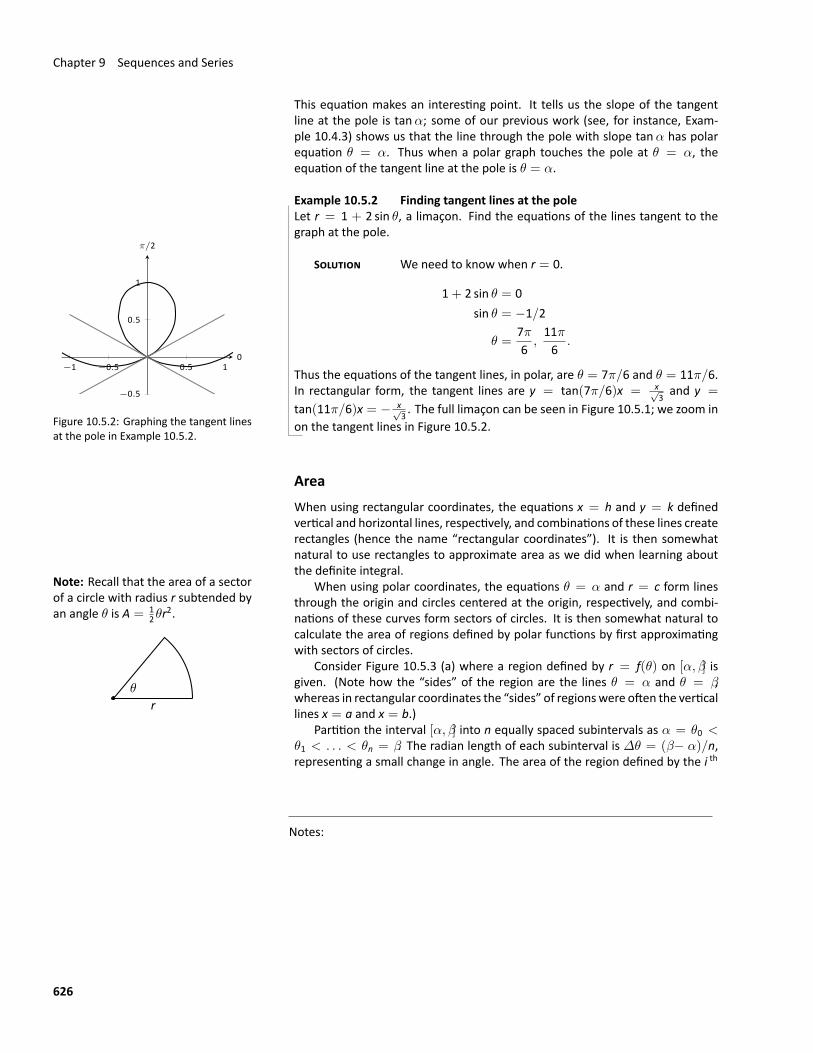
Chapter 9 Sequences and Series
This equation makes an interesting point. It tells us the slope of the tangentline at the pole is tanα; some of our previous work (see, for instance, Exam‐ple 10.4.3) shows us that the line through the pole with slope tanα has polarequation θ = α. Thus when a polar graph touches the pole at θ = α, theequation of the tangent line at the pole is θ = α.
Example 10.5.2 Finding tangent lines at the poleLet r = 1 + 2 sin θ, a limaçon. Find the equations of the lines tangent to thegraph at the pole.
−1 −0.5 0.5 1
−0.5
0.5
1
0
π/2
Figure 10.5.2: Graphing the tangent linesat the pole in Example 10.5.2.
SOLUTION We need to know when r = 0.
1+ 2 sin θ = 0sin θ = −1/2
θ =7π6,11π6
.
Thus the equations of the tangent lines, in polar, are θ = 7π/6 and θ = 11π/6.In rectangular form, the tangent lines are y = tan(7π/6)x = x√
3 and y =
tan(11π/6)x = − x√3 . The full limaçon can be seen in Figure 10.5.1; we zoom in
on the tangent lines in Figure 10.5.2.
AreaWhen using rectangular coordinates, the equations x = h and y = k definedvertical and horizontal lines, respectively, and combinations of these lines createrectangles (hence the name “rectangular coordinates”). It is then somewhatnatural to use rectangles to approximate area as we did when learning aboutthe definite integral.
Note: Recall that the area of a sectorof a circle with radius r subtended byan angle θ is A = 1
2θr2.
rθ
When using polar coordinates, the equations θ = α and r = c form linesthrough the origin and circles centered at the origin, respectively, and combi‐nations of these curves form sectors of circles. It is then somewhat natural tocalculate the area of regions defined by polar functions by first approximatingwith sectors of circles.
Consider Figure 10.5.3 (a) where a region defined by r = f(θ) on [α, β] isgiven. (Note how the “sides” of the region are the lines θ = α and θ = β,whereas in rectangular coordinates the “sides” of regionswere often the verticallines x = a and x = b.)
Partition the interval [α, β] into n equally spaced subintervals as α = θ0 <θ1 < . . . < θn = β. The radian length of each subinterval is ∆θ = (β− α)/n,representing a small change in angle. The area of the region defined by the i th
Notes:
626
10.5 Calculus and Polar Functions
subinterval [θi−1, θi] can be approximated with a sector of a circle with radiusf(ci), for some ci in [θi−1, θi]. The area of this sector is 1
2 [f(ci)]2∆θ. This is shown
in part (b) of the figure, where [α, β] has been divided into 4 subintervals. Weapproximate the area of the whole region by summing the areas of all sectors:
0.5 1
0.5
1
θ = α
θ=
β
r = f(θ)
0
π/2
(a)
0.5 1
0.5
1
θ=
β
r = f(θ)
θ = α
0
π/2
(b)
Figure 10.5.3: Computing the area of apolar region.
Area ≈n∑
i=1
12[f(ci)]2∆θ.
This is a Riemann sum. By taking the limit of the sum as n → ∞, we find theexact area of the region in the form of a definite integral.
Theorem 10.5.1 Area of a Polar RegionLet f be continuous and non‐negative on [α, β], where 0 ≤ β− α ≤ 2π.The area A of the region bounded by the curve r = f(θ) and the linesθ = α and θ = βis
A =12
∫ β
α
[f(θ)]2 dθ =12
∫ β
α
r 2 dθ
The theorem states that 0 ≤ β− α ≤ 2π. This ensures that region does notoverlap itself, which would give a result that does not correspond directly to thearea.
Example 10.5.3 Area of a polar regionFind the area of the circle defined by r = cos θ. (Recall this circle has radius 1/2.)
SOLUTION This is a direct application of Theorem 10.5.1. The circle istraced out on [0, π], leading to the integral
Note: Example 10.5.3 requires theuse of the integral
∫cos2 θ dθ. This
is handledwell by using the half angleformula as found in the back of thistext. Due to the nature of the areaformula, integrating cos2 θ and sin2 θis required often. We offer here theseindefinite integrals as a time‐savingmeasure.∫
cos2 θ dθ =12θ +
14sin(2θ) + C∫
sin2 θ dθ =12θ − 1
4sin(2θ) + C
Area =12
∫ π
0cos2 θ dθ
=12
∫ π
0
1+ cos(2θ)2
dθ
=14(θ +
12sin(2θ)
)∣∣∣∣∣π
0
=π
4.
Of course, we already knew the area of a circle with radius 1/2. We did thisexample to demonstrate that the area formula is correct.
Notes:
627
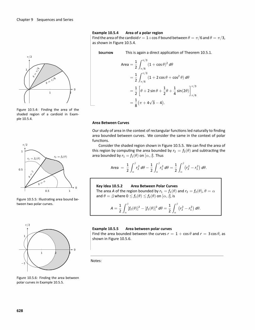
Chapter 9 Sequences and Series
Example 10.5.4 Area of a polar regionFind the area of the cardioid r = 1+cos θ bound between θ = π/6 and θ = π/3,as shown in Figure 10.5.4.
SOLUTION This is again a direct application of Theorem 10.5.1.
1 2
1
θ =π/
6θ=
π/3
0
π/2
Figure 10.5.4: Finding the area of theshaded region of a cardioid in Exam‐ple 10.5.4.
Area =12
∫ π/3
π/6(1+ cos θ)2 dθ
=12
∫ π/3
π/6(1+ 2 cos θ + cos2 θ) dθ
=12
[θ + 2 sin θ +
12θ +
14sin(2θ)
]π/3π/6
=18(π + 4
√3− 4
).
Area Between Curves
Our study of area in the context of rectangular functions led naturally to findingarea bounded between curves. We consider the same in the context of polarfunctions.
0.5 1
0.5
1
r2 = f2(θ)r1 = f1(θ)
θ =α
θ=
β
0
π/2
Figure 10.5.5: Illustrating area bound be‐tween two polar curves.
Consider the shaded region shown in Figure 10.5.5. We can find the area ofthis region by computing the area bounded by r2 = f2(θ) and subtracting thearea bounded by r1 = f1(θ) on [α, β]. Thus
Area =12
∫ β
α
r 22 dθ − 12
∫ β
α
r 21 dθ =12
∫ β
α
(r 22 − r 21
)dθ.
Key Idea 10.5.2 Area Between Polar CurvesThe area A of the region bounded by r1 = f1(θ) and r2 = f2(θ), θ = αand θ = β, where 0 ≤ f1(θ) ≤ f2(θ) on [α, β], is
A =12
∫ β
α
[f2(θ)]2 − [f1(θ)]2 dθ =12
∫ β
α
(r 22 − r 21
)dθ.
1 2 3
−1
1
0
π/2
Figure 10.5.6: Finding the area betweenpolar curves in Example 10.5.5.
Example 10.5.5 Area between polar curvesFind the area bounded between the curves r = 1 + cos θ and r = 3 cos θ, asshown in Figure 10.5.6.
Notes:
628
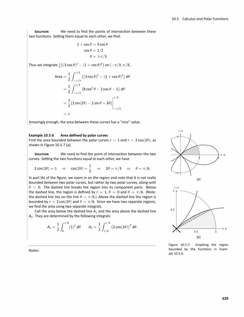
10.5 Calculus and Polar Functions
SOLUTION We need to find the points of intersection between thesetwo functions. Setting them equal to each other, we find:
1+ cos θ = 3 cos θcos θ = 1/2
θ = ±π/3
Thus we integrate 12((3 cos θ)2 − (1+ cos θ)2
)on [−π/3, π/3].
Area =12
∫ π/3
−π/3
((3 cos θ)2 − (1+ cos θ)2
)dθ
=12
∫ π/3
−π/3
(8 cos2 θ − 2 cos θ − 1
)dθ
=12(2 sin(2θ)− 2 sin θ + 3θ
)∣∣∣∣∣π/3
−π/3
= π.
Amazingly enough, the area between these curves has a “nice” value.
1 2
−1
1
0
π/2
(a)
0.5 1
0.5
1
0
π/2
(b)
Figure 10.5.7: Graphing the regionbounded by the functions in Exam‐ple 10.5.6.
Example 10.5.6 Area defined by polar curvesFind the area bounded between the polar curves r = 1 and r = 2 cos(2θ), asshown in Figure 10.5.7 (a).
SOLUTION We need to find the point of intersection between the twocurves. Setting the two functions equal to each other, we have
2 cos(2θ) = 1 ⇒ cos(2θ) =12
⇒ 2θ = π/3 ⇒ θ = π/6.
In part (b) of the figure, we zoom in on the region and note that it is not reallybounded between two polar curves, but rather by two polar curves, along withθ = 0. The dashed line breaks the region into its component parts. Belowthe dashed line, the region is defined by r = 1, θ = 0 and θ = π/6. (Note:the dashed line lies on the line θ = π/6.) Above the dashed line the region isbounded by r = 2 cos(2θ) and θ = π/6. Since we have two separate regions,we find the area using two separate integrals.
Call the area below the dashed line A1 and the area above the dashed lineA2. They are determined by the following integrals:
A1 =12
∫ π/6
0(1)2 dθ A2 =
12
∫ π/4
π/6
(2 cos(2θ)
)2 dθ.
Notes:
629
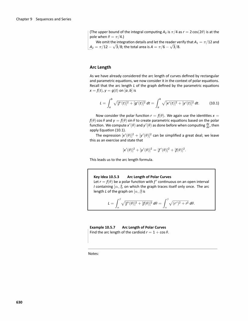
Chapter 9 Sequences and Series
(The upper bound of the integral computing A2 is π/4 as r = 2 cos(2θ) is at thepole when θ = π/4.)
We omit the integration details and let the reader verify that A1 = π/12 andA2 = π/12−
√3/8; the total area is A = π/6−
√3/8.
Arc Length
As we have already considered the arc length of curves defined by rectangularand parametric equations, we now consider it in the context of polar equations.Recall that the arc length L of the graph defined by the parametric equationsx = f(t), y = g(t) on [a, b] is
L =∫ b
a
√[f ′(t)]2 + [g ′(t)]2 dt =
∫ b
a
√[x ′(t)]2 + [y ′(t)]2 dt. (10.1)
Now consider the polar function r = f(θ). We again use the identities x =f(θ) cos θ and y = f(θ) sin θ to create parametric equations based on the polarfunction. We compute x ′(θ) and y ′(θ) as done before when computing dy
dx , thenapply Equation (10.1).
The expression [x ′(θ)]2 + [y ′(θ)]2 can be simplified a great deal; we leavethis as an exercise and state that
[x ′(θ)]2 + [y ′(θ)]2 = [f ′(θ)]2 + [f(θ)]2.
This leads us to the arc length formula.
Key Idea 10.5.3 Arc Length of Polar CurvesLet r = f(θ) be a polar function with f ′ continuous on an open intervalI containing [α, β], on which the graph traces itself only once. The arclength L of the graph on [α, β] is
L =∫ β
α
√[f ′(θ)]2 + [f(θ)]2 dθ =
∫ β
α
√(r ′)2 + r2 dθ.
Example 10.5.7 Arc Length of Polar CurvesFind the arc length of the cardioid r = 1+ cos θ.
Notes:
630
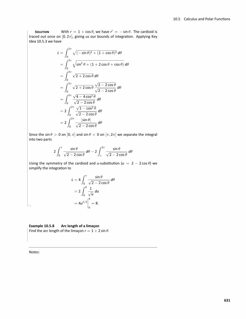
10.5 Calculus and Polar Functions
SOLUTION With r = 1 + cos θ, we have r′ = − sin θ. The cardioid istraced out once on [0, 2π], giving us our bounds of integration. Applying KeyIdea 10.5.3 we have
L =∫ 2π
0
√(− sin θ)2 + (1+ cos θ)2 dθ
=
∫ 2π
0
√sin2 θ + (1+ 2 cos θ + cos θ) dθ
=
∫ 2π
0
√2+ 2 cos θ dθ
=
∫ 2π
0
√2+ 2 cos θ
√2− 2 cos θ√2− 2 cos θ
dθ
=
∫ 2π
0
√4− 4 cos2 θ√2− 2 cos θ
dθ
= 2∫ 2π
0
√1− cos2 θ√2− 2 cos θ
dθ
= 2∫ 2π
0
|sin θ|√2− 2 cos θ
dθ
Since the sin θ > 0 on [0, π] and sin θ < 0 on [π, 2π] we separate the integralinto two parts
2∫ π
0
sin θ√2− 2 cos θ
dθ − 2∫ 2π
π
sin θ√2− 2 cos θ
dθ
Using the symmetry of the cardioid and u‐substitution (u = 2 − 2 cos θ) wesimplify the integration to
L = 4∫ π
0
sin θ√2− 2 cos θ
dθ
= 2∫ 4
0
1√udu
= 4u1/2∣∣∣∣40= 8.
Example 10.5.8 Arc length of a limaçonFind the arc length of the limaçon r = 1+ 2 sin θ.
Notes:
631
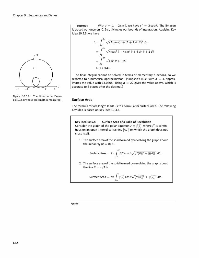
Chapter 9 Sequences and Series
SOLUTION With r = 1 + 2 sin θ, we have r ′ = 2 cos θ. The limaçonis traced out once on [0, 2π], giving us our bounds of integration. Applying KeyIdea 10.5.3, we have
L =∫ 2π
0
√(2 cos θ)2 + (1+ 2 sin θ)2 dθ
=
∫ 2π
0
√4 cos2 θ + 4 sin2 θ + 4 sin θ + 1 dθ
=
∫ 2π
0
√4 sin θ + 5 dθ
≈ 13.3649.
The final integral cannot be solved in terms of elementary functions, so we
−2 −1 1 2
1
2
3
0
π/2
Figure 10.5.8: The limaçon in Exam‐ple 10.5.8 whose arc length is measured.
resorted to a numerical approximation. (Simpson’s Rule, with n = 4, approx‐imates the value with 13.0608. Using n = 22 gives the value above, which isaccurate to 4 places after the decimal.)
Surface AreaThe formula for arc length leads us to a formula for surface area. The followingKey Idea is based on Key Idea 10.3.4.
Key Idea 10.5.4 Surface Area of a Solid of RevolutionConsider the graph of the polar equation r = f(θ), where f ′ is contin‐uous on an open interval containing [α, β] on which the graph does notcross itself.
1. The surface area of the solid formed by revolving the graph aboutthe initial ray (θ = 0) is:
Surface Area = 2π∫ β
α
f(θ) sin θ√
[f ′(θ)]2 + [f(θ)]2 dθ.
2. The surface area of the solid formed by revolving the graph aboutthe line θ = π/2 is:
Surface Area = 2π∫ β
α
f(θ) cos θ√
[f ′(θ)]2 + [f(θ)]2 dθ.
Notes:
632
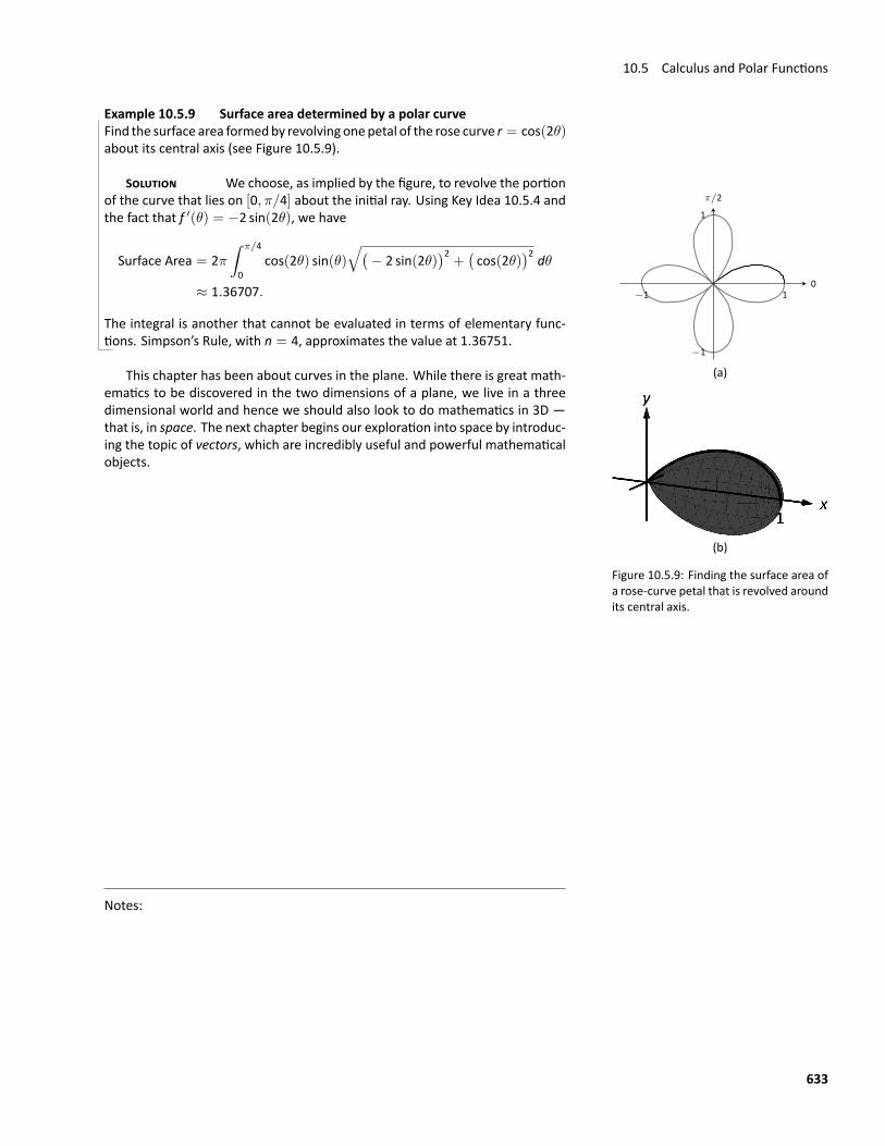
10.5 Calculus and Polar Functions
Example 10.5.9 Surface area determined by a polar curveFind the surface area formedby revolving onepetal of the rose curve r = cos(2θ)about its central axis (see Figure 10.5.9).
SOLUTION We choose, as implied by the figure, to revolve the portion
−1 1
−1
1
0
π/2
(a)
(b)
Figure 10.5.9: Finding the surface area ofa rose‐curve petal that is revolved aroundits central axis.
of the curve that lies on [0, π/4] about the initial ray. Using Key Idea 10.5.4 andthe fact that f ′(θ) = −2 sin(2θ), we have
Surface Area = 2π∫ π/4
0cos(2θ) sin(θ)
√(− 2 sin(2θ)
)2+(cos(2θ)
)2 dθ≈ 1.36707.
The integral is another that cannot be evaluated in terms of elementary func‐tions. Simpson’s Rule, with n = 4, approximates the value at 1.36751.
This chapter has been about curves in the plane. While there is great math‐ematics to be discovered in the two dimensions of a plane, we live in a threedimensional world and hence we should also look to do mathematics in 3D —that is, in space. The next chapter begins our exploration into space by introduc‐ing the topic of vectors, which are incredibly useful and powerful mathematicalobjects.
Notes:
633
Exercises 10.5Terms and Concepts1. Given polar equation r = f(θ), how can one create para‐
metric equations of the same curve?2. With rectangular coordinates, it is natural to approximate
area with ; with polar coordinates, it is natural toapproximate area with .
ProblemsIn Exercises 3–10, find:
(a) dydx
(b) the equation of the tangent and normal lines to thecurve at the indicated θ‐value.
3. r = 1; θ = π/4
4. r = cos θ; θ = π/4
5. r = 1+ sin θ; θ = π/6
6. r = 1− 3 cos θ; θ = 3π/4
7. r = θ; θ = π/2
8. r = cos(3θ); θ = π/6
9. r = sin(4θ); θ = π/3
10. r = 1sin θ − cos θ
; θ = π
In Exercises 11–14, find the values of θ in the given intervalwhere the graph of the polar function has horizontal and ver‐tical tangent lines.
11. r = 3; [0, 2π]
12. r = 2 sin θ; [0, π]
13. r = cos(2θ); [0, 2π]
14. r = 1+ cos θ; [0, 2π]
In Exercises 15–18, find the equation of the lines tangent tothe graph at the pole.
15. r = sin θ; [0, π]
16. r = cos 3θ; [0, π]
17. r = cos 2θ; [0, 2π]
18. r = sin 2θ; [0, 2π]
In Exercises 19–30, find the area of the described region.
19. Enclosed by the circle: r = 4 sin θ, π3 ≤ θ ≤ 2π
3
20. Enclosed by the circle r = 5
21. Enclosed by one petal of r = sin(3θ)
22. Enclosed by one petal of the rose curve r = cos(n θ),where n is a positive integer.
23. Enclosed by the cardioid r = 1− sin θ
24. Enclosed by the inner loop of the limaçon r = 1+ 2 cos θ
25. Enclosed by the outer loop of the limaçon r = 1 + 2 cos θ(including area enclosed by the inner loop)
26. Enclosed between the inner and outer loop of the limaçonr = 1+ 2 cos θ
27. Enclosed by r = 2 cos θ and r = 2 sin θ, as shown:
−1 1 2
−1
1
2
x
y
28. Enclosed by r = cos(3θ) and r = sin(3θ), as shown:
1
0.5
x
y
29. Enclosed by r = cos θ and r = sin(2θ), as shown:
1
1
x
y
30. Enclosed by r = cos θ and r = 1− cos θ, as shown:
−2 −1 1
−1
1
x
y
In Exercises 31–36, answer the questions involving arc length.31. Let x(θ) = f(θ) cos θ and y(θ) = f(θ) sin θ. Show, as sug‐
gested by the text, that
x ′(θ)2 + y ′(θ)2 = f ′(θ)2 + f(θ)2.
32. Use the arc length formula to compute the arc length ofthe circle r = 2.
33. Use the arc length formula to compute the arc length ofthe circle r = 4 sin θ.
34. Use the arc length formula to compute the arc length ofr = cos θ + sin θ.
35. Approximate the arc length of one petal of the rose curver = sin(3θ) with Simpson’s Rule and n = 4.
36. Approximate the arc length of the cardioid r = 1 + cos θwith Simpson’s Rule and n = 6.
634
In Exercises 37–42, answer the questions involving surfacearea.37. Use Key Idea 10.5.4 to find the surface area of the sphere
formed by revolving the circle r = 2 about the initial ray.38. Use Key Idea 10.5.4 to find the surface area of the sphere
formed by revolving the circle r = 2 cos θ about the initialray.
39. Find the surface area of the solid formed by revolving thecardioid r = 1+ cos θ about the initial ray.
40. Find the surface area of the solid formed by revolving thecircle r = 2 cos θ about the line θ = π/2.
41. Find the surface area of the solid formed by revolving theline r = 3 sec θ, −π/4 ≤ θ ≤ π/4, about the lineθ = π/2.
42. Find the surface area of the solid formed by revolving theline r = 3 sec θ, 0 ≤ θ ≤ π/4, about the initial ray.
635

Chapter 9 Sequences and Series
Notes:
636

Appendices

SOLUTIONS TO SELECTED PROBLEMS
Chapter 7Exercises 7.11. F
3. The point (10, 1) lies on the graph of y = f−1(x) (assumingf is invertible).
5.
−9−8−7−6−5−4−3−2−1 1 2 3 4 5 6 7 8 9
−8−7−6−5−4−3−2−1
12345678
f(x)
x
y
7. Compose f(g(x)) and g(f(x)) to confirm that each equalsx.
9. Compose f(g(x)) and g(f(x)) to confirm that each equalsx.
11. [−4, 0] or [0, 4]
13. (−∞, 3] or [3,∞)
15. f−1(x) = 2x+ 1x− 1
17. f−1(x) = ln(x+ 2)− 3
19. 0
21. −1/5
23. 1/√2
25. 7/√58
27. 3π/4
29. x/2
31. x/√x2 + 25
Exercises 7.21. The point (10, 1) lies on the graph of y = f−1(x) (assuming
f is invertible) and (f−1)′(10) = 1/5.
3.(f−1)′ (20) = 1
f ′(2) = 1/5
5.(f−1)′ (√3/2) = 1
f ′(π/6) = 1
7.(f−1)′ (1/2) = 1
f ′(1) = −2
9. h′(t) = 2√1−4t2
11. g′(x) = 21+4x2
13. g′(t) = cos−1(t) cos(t)− sin(t)√1−t2
15. h′(x) = sin−1 x+cos−1 x√1−x2(cos−1 x)2
17. f ′(x) = − 1√1−x2
19. (a) f(x) = x, so f ′(x) = 1
(b) f ′(x) = cos(sin−1 x) 1√1−x2
= 1.
21. (a) f(x) =√1− x2, so f ′(x) = −x√
1−x2
(b) f ′(x) = cos(cos−1 x)( 1√1−x2
) = −x√1−x2
23. y =√2(x−
√2/2) + π/4
25. −π/6
27. 12
(sin−1 r
)2+ C
29. sin−1(et/√10) + C
31.√91 ≈ 9.54 feet
Exercises 7.31. (−∞,∞)
3. (−∞, 0) ∪ (0,∞)
5. f ′(t) = 3t2et3−1
7. f ′(x) = 1− x ln 5 ln xx5x ln 5
9. f ′(x) = 1
11. h ′(r) = 3r ln 31+ 32r
13. 24ln 5
15. 3x2−1
2ln3 + C
17. 12 sin
2(ex) + C
19. ln 245ln 3
− 1
21. n = −3, 2
23. y′ = (1+ x)1/x( 1x(x+1) −
ln(1+x)x2
)Tangent line: y = (1− 2 ln 2)(x− 1) + 2
25. y′ = xxx+1
(ln x+ 1− 1
x+1
)Tangent line: y = (1/4)(x− 1) + 1/2
27. y′ = x+1x+2
( 1x+1 −
1x+2
)Tangent line: y = 1/9(x− 1) + 2/3
29. y′ = xex−1ex(1+ x ln x)
Tangent line: y = ex− e+ 1
A.3
Exercises 7.41. Because cosh x is always positive.
3. coth2 x− csch2 x =(ex + e−x
ex − e−x
)2
−(
2ex − e−x
)2
=(e2x + 2+ e−2x)− (4)
e2x − 2+ e−2x
=e2x − 2+ e−2x
e2x − 2+ e−2x
= 1
5. cosh2 x =(ex + e−x
2
)2
=e2x + 2+ e−2x
4
=12(e2x + e−2x) + 2
2
=12
(e2x + e−2x
2+ 1)
=cosh 2x+ 1
2.
7. ddx
[sech x] = ddx
[2
ex + e−x
]=
−2(ex − e−x)
(ex + e−x)2
= − 2(ex − e−x)
(ex + e−x)(ex + e−x)
= − 2ex + e−x ·
ex − e−x
ex + e−x
= − sech x tanh x
9.∫
tanh x dx =∫
sinh xcosh x
dx
Let u = cosh x; du = (sinh x)dx
=
∫1udu
= ln |u|+ C= ln(cosh x) + C.
11. 2 cosh 2x13. 2x sech2(x2)15. sinh2 x+ cosh2 x17. −2x
(x2)√
1−x4
19. 4x√4x4−1
21. − csc x23. y = x25. y = 9
25 (x+ ln 3)− 45
27. y = x29. 1
2 ln(cosh(2x)) + C
31. 12 sinh
2 x+ C or 1/2 cosh2 x+ C
33. cosh−1(x2/2) + C = ln(x2 +√x4 − 4) + C
35. tan−1(ex) + C37. 0
Exercises 7.51. 0/0,∞/∞, 0 · ∞,∞−∞, 00, 1∞,∞0
3. F
5. derivatives; limits
7. Answers will vary.
9. 3
11. −1
13. 5
15. a/b
17. 1/2
19. 0
21. ∞23. 0
25. −2
27. 0
29. 0
31. ∞33. ∞35. 0
37. 1
39. 1
41. 1
43. 1
45. 1
47. 2
49. −∞51. 0
Chapter 8Exercises 8.11. T
3. sin x− x cos x+ C
5. −x2 cos x+ 2x sin x+ 2 cos x+ C
7. 1/2ex2+ C
9. − 12 xe
−2x − e−2x
4 + C
11. 1/5e2x(sin x+ 2 cos x) + C
13. 110e
5x(sin(5x) + cos(5x)) + C
15.√1− x2 + x sin−1(x) + C
17. 12 x
2 tan−1(x)− x2 +
12 tan
−1(x) + C
19. 12 x
2 ln |x| − x24 + C
21. − x24 + 1
2 x2 ln |x− 1| − x
2 −12 ln |x− 1|+ C
23. 13 x
3 ln |x| − x39 + C
A.4
25. 2x + x (ln |x+ 1|)2 + (ln |x+ 1|)2 − 2x ln |x+ 1| −2 ln |x+ 1|+ 2+ C
27. ln |sin x| − x cot x+ C
29. 13 (x
2 − 2)3/2 + C
31. x sec x− ln |sec x+ tan x|+ C
33. x sinh x− cosh x+ C
35. x sinh−1 x−√x2 + 1+ C
37. 1/2x(sin(ln x)− cos(ln x)
)+ C
39. 12 x ln |x| −
x2 + C
41. 1/2x2 + C
43. π
45. 0
47. 1/2
49. 34e2 − 5
4e4
51. 15
(eπ + e−π
)
Exercises 8.21. F
3. F
5. 14 sin
4 x+ C
7. 38 x+
14 sin 2x+
132 sin 4x+ C
9. 16 cos
6 x− 14 cos
4 x+ C
11. 12 cos
2 x− ln |cos x|+ C
13.( 27 cos
3 x− 23 cos x
)√cos x+ C
15. 12
( 14 sin(4x)−
110 sin(10x)
)+ C
17. 12
(sin(x) + 1
3 sin(3x))+ C
19. tan x− x+ C
21. tan6(x)6 + tan4 x
4 + C
23. sec5(x)5 − sec3 x
3 + C
25. 13 tan
3 x− tan x+ x+ C
27. 12 (sec x tan x− ln |sec x+ tan x|) + C
29. ln |csc x− cot x|+ C
31. − 12 cot
2 x+ ln |csc x|+ C
33. 25
35. 32/315
37. 2/3
39. 16/15
Exercises 8.31. backwards3. (a) tan2 θ + 1 = sec2 θ
(b) 9 sec2 θ.
5. 12
(x√x2 + 1+ ln
∣∣√x2 + 1+ x∣∣)+ C
7. x√
x2 + 1/4+ 14 ln∣∣∣2√x2 + 1/4+ 2x
∣∣∣+ C
= 12 x√4x2 + 1+ 1
4 ln∣∣√4x2 + 1+ 2x
∣∣+ C
9. 4(
12 x√
x2 − 1/16− 132 ln
∣∣∣4x+ 4√
x2 − 1/16∣∣∣) + C =
12 x√16x2 − 1− 1
8 ln∣∣4x+√
16x2 − 1∣∣+ C
11. 3 sin−1(
x√7
)+ C (Trig. Subst. is not needed)
13.√x2 − 11−
√11 sec−1(x/
√11) + C
15. − 1√x2+9
+ C (Trig. Subst. is not needed)
17. 118
x+2x2+4x+13 +
154 tan
−1 ( x+23
)+ C
19. 17
(−√
5−x2x − sin−1(x/
√5))+ C
21. π/223. 2
√2+ 2 ln(1+
√2)
25. 9 sin−1(1/3) + 2√2 Note: the new bounds of integra‐
tion are sin−1(−1/3) < θ < sin−1(1/3). The final answercomeswith recognizing that sin−1(−1/3) = − sin−1(1/3)and that cos
(sin−1(1/3)
)= cos
(sin−1(−1/3)
)=
2√2/3.
Exercises 8.41. rational3. A
x +B
x−3
5. Ax−
√7 +
Bx+
√7
7. 3 ln |x− 2|+ 4 ln |x+ 5|+ C9. 1
3 (ln |x+ 2| − ln |x− 2|) + C11. − 4
x+8 − 3 ln |x+ 8|+ C13. − ln |2x− 3|+ 5 ln |x− 1|+ 2 ln |x+ 3|+ C15. x+ ln |x− 1| − ln |x+ 2|+ C17. 2x+ C
19. 1x +
12 ln∣∣∣ x−1x+1
∣∣∣+ C
21. ln∣∣3x2 + 5x− 1
∣∣+ 2 ln |x+ 1|+ C23. ln |x| − 1
2 ln(x2 + 1)− tan−1 x− 1
2(x2+1) + C
25. 12
(3 ln∣∣x2 + 2x+ 17
∣∣− 4 ln |x− 7|+ tan −1 ( x+14
))+ C
27. − 14 ln(x
2 + 3) + 14 ln(x
2 + 1) + C = 14 ln
x2+1x2+3 + C
29. 3(ln∣∣x2 − 2x+ 11
∣∣+ ln |x− 9|)+3√
25 tan
−1(
x−1√10
)+C
31. 132 ln |x− 2| − 1
32 ln |x+ 2| − 116 tan
−1(x/2) + C33. ln(2000/243) ≈ 2.10835. −π/4+ tan−1 3− ln(11/9) ≈ 0.263
A.5
Exercises 8.51. x sin−1 x+
√1− x2 + C
3. 18 ln |x− 2| − 9 ln |x− 1| − 5 ln |x− 3|+ C
5. x25
√x2 + 25
+ C
7. 2 ln |x− 1| − ln |x| − 1x− 1
− 1(x− 1)2
+ C
9. 12ex
2(x2 − 1) + C
11. 113
e2x(2 sin 3x− 3 cos 3x) + C
13. −√4− x2 + C
15. 2 tan−1 √x+ C
17. 127
[6x sin 3x− (9x2 − 2) cos 3x] + C
19. 23(1+ ex)3/2 + C
21. 13tan3 x+ C
23. −14(8− x3)4/3 + C
25. 110
(3− 2x)5/2 − 12(3− 2x)3/2 + C
27. 25x5/2 − 8
3x3/2 + 6x1/2 + C
29. 112
ln |x+ 5| − 152
ln |x+ 7|+ C
31. etan x + C
33. −15cot5 x+ 1
3cot3 x− cot x− x+ C
35. 13x3 − 1
4tanh 4x+ C
37. 3 sin−1( x+ 56)+ C
39. 13sec3 x− sec x+ C
41. −2 sin−1(2x3)− 1
x√9− 4x2 + C
43. − ln x+ 44√x+ 4 ln
∣∣1− 4√x∣∣+ C
45. −x2(25+ x2)
+110
tan−1( x5)+ C
47. 14x4 − 2x2 + 4 ln |x|+ C
49. 364
(2x+ 3)8/3 − 920
(2x+ 3)5/3 + 2716
(2x+ 3)2/3 + C
51. −17cos 7x+ C
53. ln∣∣1+ tan θ
2
∣∣− ln∣∣1− tan θ
2
∣∣+ C
Exercises 8.61. The interval of integration is finite, and the integrand is
continuous on that interval.3. converges; could also state≤ 10.5. p > 17. e5/29. 1/3
11. 1/ ln 213. diverges15. 117. diverges19. diverges21. 2
√3
23. diverges25. diverges27. 129. 031. −1/433. −135. diverges37. diverges; Limit Comparison Test with 1/x.39. diverges; Limit Comparison Test with 1/x.41. converges; Direct Comparison Test with e−x.43. converges; Direct Comparison Test with 1/(x2 − 1).45. converges; Direct Comparison Test with 1/ex.
Exercises 8.71. F3. They are superseded by the Trapezoidal Rule; it takes an
equal amount of work and is generally more accurate.5. (a) 3/4
(b) 2/3
(c) 2/3
7. (a) 14 (1+
√2)π ≈ 1.896
(b) 16 (1+ 2
√2)π ≈ 2.005
(c) 2
9. (a) 38.5781
(b) 147/4 ≈ 36.75
(c) 147/4 ≈ 36.75
11. (a) 0
(b) 0
(c) 0
13. Trapezoidal Rule: 0.9006Simpson’s Rule: 0.90452
A.6
15. Trapezoidal Rule: 13.9604Simpson’s Rule: 13.9066
17. Trapezoidal Rule: 1.1703Simpson’s Rule: 1.1873
19. Trapezoidal Rule: 1.0803Simpson’s Rule: 1.077
21. (a) n = 161 (using max(f ′′(x)
)= 1)
(b) n = 12 (using max(f (4)(x)
)= 1)
23. (a) n = 1004 (using max(f ′′(x)
)= 39)
(b) n = 62 (using max(f (4)(x)
)= 800)
25. (a) Area is 30.8667 cm2.
(b) Area is 308, 667 yd2.
27. Let f(x) = a(x−x1)2+b(x−x1)+c, so that f(x1) = c = y1,f(x1 +∆x) = a∆x2 + b∆x + c = y2, and f(x1 + 2∆x) =4a∆x2 + 2b∆x + c = y3. Therefore, a = y1−2y2+y3
2(∆x)2 and
b = 4y2−y3−3y12∆x , and
∫ x1+2∆x
x1a(x−x1)2+b(x−x1)+cdx =
a(2∆x)3
3+
b(2∆x)2
2+ c(2∆x) = 4(y1 − 2y2 + y3)∆x
3+
(4y2 − y3 − 3y1)∆x + 2y1∆x =∆x3
(4y1 − 8y2 + 4y3 +
12y2 − 3y3 − 9y1 + 6y1) =∆x3
(y1 + 4y2 + y3).
Chapter 9Exercises 9.11. Answers will vary.3. Answers will vary.5. 2, 8
3 ,83 ,
3215 ,
6445
7. − 13 ,−2,− 81
5 ,−5123 ,− 15625
7
9. an = 3n+ 111. an = 10 · 2n−1
13. 1/715. 017. diverges19. converges to 021. converges to 023. diverges25. converges to e
27. converges to 529. diverges31. converges to 033. converges to 035. converges to ln 237. converges to 039. bounded
41. bounded below43. monotonically increasing45. never monotonic47. never monotonic49. Let {an} be given such that lim
n→∞|an| = 0. By the defi‐
nition of the limit of a sequence, given any ε > 0, thereis a m such that for all n > m, | |an| − 0| < ε. Since| |an| − 0| = |an − 0|, this directly implies that for alln > m, |an − 0| < ε, meaning that lim
n→∞an = 0.
51. Left to reader
Exercises 9.21. Answers will vary.3. One sequence is the sequence of terms {an}. The other is
the sequence of nth partial sums, {Sn} = {∑n
i=1 ai}.5. F7. (a) −1,− 1
2 ,−56 ,−
712 ,−
4760
(b) Plot omitted
9. (a) −1, 0,−1, 0,−1
(b) Plot omitted
11. (a) 1, 32 ,
53 ,
4124 ,
10360
(b) Plot omitted
13. (a) −0.9,−0.09,−0.819,−0.1629,−0.75339
(b) Plot omitted
15. Converges because it is a geometric series with r = 15 .
17. Diverges by Theorem 9.2.419. Diverges21. lim
n→∞an = 1; by Theorem 9.2.4 the series diverges.
23. Diverges25. Diverges27. lim
n→∞an = e; by Theorem 9.2.4 the series diverges.
29. Converges31. Converges33. (a) Sn = 1−(1/4)n
3/4
(b) Converges to 4/3.
35.(a) Sn =
{− n+1
2 n is oddn2 n is even
(b) Diverges
37. (a) Sn = 1−(1/e)n+1
1−1/e .
(b) Converges to 1/(1− 1/e) = e/(e− 1).
39. (a) With partial fractions, an = 1n −
1n+1 .
Thus Sn = 1− 1n+1 .
(b) Converges to 1.
A.7
41. (a) Use partial fraction decomposition to recognize thetelescoping series: an = 1
2
(1
2n−1 −1
2n+1
), so that
Sn = 12
(1− 1
2n+1
)= n
2n+1 .
(b) Converges to 1/2.
43. (a) Sn = 1− 1(n+1)2
(b) Converges to 1.
45. (a) an = 1/2n + 1/3n for n ≥ 0. Thus Sn = 1−1/221/2 +
1−1/3n2/3 .
(b) Converges to 2+ 3/2 = 7/2.
47. (a) Sn = 1−(sin 1)n+1
1−sin 1
(b) Converges to 11−sin 1 .
49. (−3, 3)
51. (−∞,−4) ∪ (4,∞)
53. Using partial fractions, we can show that an =14
(1
2n−1 +1
2n+1
). The series is effectively twice the sum
of the odd terms of the Harmonic Series which was shownto diverge in Example 9.2.5. Thus this series diverges.
Exercises 9.31. continuous, positive and decreasing
3. Converges
5. Diverges
7. Converges
9. Converges
11. p > 1
13. p > 1
Exercises 9.4
1.∞∑n=0
bn converges; we cannot conclude anything about
∞∑n=0
cn
3. Converges; compare to∞∑n=1
1n2
, as 1/(n2+3n−5) ≤ 1/n2
for all n > 1.
5. Diverges; compare to∞∑n=1
1n, as 1/n ≤ ln n/n for all n ≥ 3.
7. Diverges; compare to∞∑n=1
1n. Since n =
√n2 >
√n2 − 1,
1/n ≤ 1/√n2 − 1 for all n ≥ 2.
9. Converges; compare to∞∑n=1
1n2
.
11. Diverges; compare to∞∑n=1
ln nn
.
13. Diverges; compare to∞∑n=1
1n.
15. Diverges; compare to∞∑n=1
1n:
1n=
n2
n3<
n2 + n+ 1n3
<n2 + n+ 1n3 − 5
,
for all n ≥ 1.
17. Converges; compare to∞∑n=1
(25
)n
, as 2n/(5n + 10) <
2n/5n for all n ≥ 1.
19. Converges by Comparison Test with∑ 1
n3
21. Diverges; compare to∞∑n=1
1n. Note that
nn2 − 1
=n2
n2 − 1· 1n>
1n,
as n2n2−1 > 1, for all n ≥ 2.
23. Converges; compare to∞∑n=1
1n2
, as 1/(n2 ln n) ≤ 1/n2 for
all n ≥ 3.25. Converges; Integral Test
27. Diverges; the nth Term Test and Direct Comparison Test canbe used.
29. Converges; the Direct Comparison Test can be used withsequence 1/3n.
31. Diverges; the nth Term Test can be used, along with the In‐tegral Test.
33. (a) Converges; use Direct Comparison Test as ann < an.
(b) Converges; since original series converges, we knowlimn→∞ an = 0. Thus for large n, anan+1 < an.
(c) Converges; similar logic to part (b) so (an)2 < an.
(d) May converge; certainly nan > an but that does notmean it does not converge.
(e) Does not converge, using logic from (b) and nth TermTest.
Exercises 9.51. The signs of the terms do not alternate; in the given series,
some terms are negative and the others positive, but theydo not necessarily alternate.
3. Many examples exist; one common example is an =(−1)n/n.
5. (a) converges
(b) converges (p‐Series)
(c) absolute
A.8
7. (a) diverges (limit of terms is not 0)
(b) diverges
(c) n/a; diverges
9. (a) converges
(b) diverges (Limit Comparison Test with 1/n)
(c) conditional
11. (a) diverges (limit of terms is not 0)
(b) diverges
(c) n/a; diverges
13. (a) diverges (terms oscillate between±1)
(b) diverges
(c) n/a; diverges
15. (a) converges
(b) converges (Geometric Series with r = 2/3)
(c) absolute
17. (a) converges
(b) diverges (p‐Series Test with p = 1/2)
(c) conditional
19. S5 = −1.1906; S6 = −0.6767;
−1.1906 ≤∞∑n=1
(−1)n
ln(n+ 1)≤ −0.6767
21. S6 = 0.3681; S7 = 0.3679;
0.3681 ≤∞∑n=0
(−1)n
n!≤ 0.3679
23. n = 525. Using the theorem, we find n = 499 guarantees the sum
is within 0.001 of π/4. (Convergence is actually faster, asthe sum is within ε of π/24 when n ≥ 249.)
Exercises 9.61. algebraic, or polynomial.3. Integral Test, Limit Comparison Test, and Root Test5. Converges7. Converges9. The Ratio Test is inconclusive; the p‐Series Test states it di‐
verges.11. Converges13. Converges; note the summation can be rewritten as
∞∑n=1
2nn!3nn!
, from which the Ratio Test can be applied.
15. Diverges17. Converges19. Converges21. Diverges
23. Diverges. The Root Test is inconclusive, but the nth‐TermTest shows divergence. (The terms of the sequence ap‐proach e−2, not 0, as n → ∞.)
25. Converges
Exercises 9.71. Diverges3. Diverges5. Diverges7. Absolutely converges9. Conditionally converges
11. Diverges13. Absolutely converges15. Absolutely converges17. Absolutely converges19. Conditionally converges21. Absolutely converges23. Absolutely converges25. Diverges27. Diverges29. Absolutely converges31. Diverges33. Absolutely converges35. Diverges37. Absolutely converges
Exercises 9.81. 13. 55. 1+ 2x+ 4x2 + 8x3 + 16x4
7. 1+ x+ x22 + x3
6 + x424
9. (a) R = ∞(b) (−∞,∞)
11. (a) R = 1
(b) (2, 4]
13. (a) R = 2
(b) (−2, 2)
15. (a) R = 1/5
(b) (4/5, 6/5)
17. (a) R = 1
(b) (−1, 1)
19. (a) R = ∞(b) (−∞,∞)
A.9
21. (a) R = 1
(b) [−1, 1]
23. (a) R = 0
(b) x = 0
25. (a) R = 1
(b) [− 13 ,
53 )
27. (a) R = ∞(b) (−∞,∞)
29.∞∑n=0
8nxn+1, R = 1/8
31.∞∑n=0
x2n+3
3n+1 , R =√3
33. (a)∑∞
n=0 xn(−1)n(1+ n); R = 1
(b)∑∞
n=1 xn−1(−1)n−1(1+ n)n/2
=∑∞
n=0 xn(−1)n(2+ n)(1+ n)/2
(c)∑∞
n=1 xn+1(−1)n−1(1+ n)n/2
=∑∞
n=0 xn+2(−1)n(2+ n)(1+ n)/2
=∑∞
n=2 xn(−1)nn(−1+ n)/2
35.∞∑n=1
n(−9)n−1xn, R = 1/9
37.∞∑n=0
(−1)n x2n+1
2n+ 1; R = 1
39.∞∑n=0
(2n+ 1)xn; R = 1
Exercises 9.91. TheMaclaurin polynomial is a special case of Taylor polyno‐
mials. Taylor polynomials are centered at a specific x‐value;when that x‐value is 0, it is a Maclaurin polynomial.
3. p2(x) = 6+ 3x− 4x2.5. p3(x) = 1− x+ 1
2 x3 − 1
6 x3
7. p8(x) = x+ x2 + 12 x
3 + 16 x
4 + 124 x
5
9. p4(x) = 2x43 + 4x3
3 + 2x2 + 2x+ 111. p4(x) = x4 − x3 + x2 − x+ 113. p4(x) = 1 + 1
2 (−1 + x) − 18 (−1 + x)2 + 1
16 (−1 + x)3 −5
128 (−1+ x)4
15. p6(x) = 1√2 −
− π4 +x√
2 − (− π4 +x)2
2√
2 +(− π
4 +x)3
6√
2 +(− π
4 +x)4
24√
2 −(− π
4 +x)5
120√
2 − (− π4 +x)6
720√
2
17. p5(x) = 12 −
x−24 + 1
8 (x− 2)2 − 116 (x− 2)3 + 1
32 (x− 2)4 −164 (x− 2)5
19. p3(x) = 12 +
1+x2 + 1
4 (1+ x)2
21. p3(x) = x − x36 ; p3(0.1) = 0.09983. Error is bounded by
14! · 0.1
4 ≈ 0.000004167.
23. p2(x) = 3+ 16 (−9+x)− 1
216 (−9+x)2; p2(10) = 3.16204.The third derivative of f(x) =
√x is bounded on [9, 10] by
0.0015. Error is bounded by 0.00153! · 13 = 0.0003.
25. The nth derivative of f(x) = ex is bounded by e on [0, 1].Thus |Rn(1)| ≤ e
(n+1)!1(n+1). When n = 7, this is less than
0.0001.
27. The nth derivative of f(x) = cos x is bounded by 1on intervals containing 0 and π/3. Thus |Rn(π/3)| ≤
1(n+1)! (π/3)
(n+1). When n = 7, this is less than 0.0001.Since the Maclaurin polynomial of cos x only uses evenpowers, we can actually just use n = 6.
29. 1n! x
n
31. When n even, 0; when n is odd, (−1)(n−1)/2
n! xn.
33. (−1)nxn
35. 1+ x+ 12x2 + 1
6x3 + 1
24x4
Exercises 9.10
1. A Taylor polynomial is a polynomial, containing a finitenumber of terms. A Taylor series is a series, the summa‐tion of an infinite number of terms.
3. All derivatives of ex are ex which evaluate to 1 at x = 0.The Taylor series starts 1+ x+ 1
2 x2 + 1
3! x3 + 1
4! x4 + · · · ;
the Taylor series is∞∑n=0
xn
n!
5. The nth derivative of 1/(1−x) is f (n)(x) = (n)!/(1−x)n+1,which evaluates to n! at x = 0.The Taylor series starts 1+ x+ x2 + x3 + · · · ;
the Taylor series is∞∑n=0
xn
7. The Taylor series starts 0−(x−π/2)+0x2+ 16 (x−π/2)3+
0x4 − 1120 (x− π/2)5;
the Taylor series is∞∑n=0
(−1)n+1 (x− π/2)2n+1
(2n+ 1)!
9. f (n)(x) = (−1)ne−x; at x = 0, f (n)(0) = −1 when n is oddand f (n)(0) = 1 when n is even.The Taylor series starts 1− x+ 1
2 x2 − 1
3! x3 + · · · ;
the Taylor series is∞∑n=0
(−1)n xn
n!.
11. f (n)(x) = (−1)n+1 n!(x+1)n+1 ; at x = 1, f (n)(1) =
(−1)n+1 n!2n+1
The Taylor series starts 12 +
14 (x− 1)− 1
8 (x− 1)2 + 116 (x−
1)3 · · · ;
the Taylor series is 12+
∞∑n=1
(−1)n+1 (x− 1)n
2n+1 .
A.10
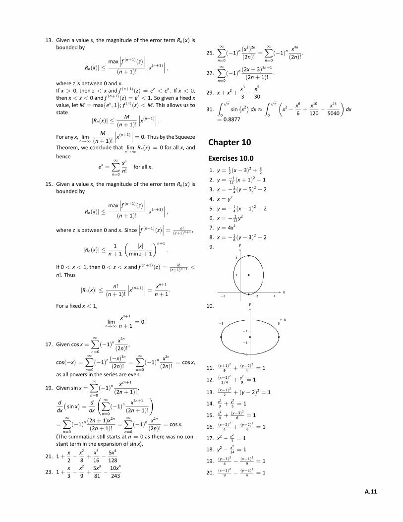
13. Given a value x, the magnitude of the error term Rn(x) isbounded by
|Rn(x)| ≤max
∣∣∣f (n+1)(z)∣∣∣
(n+ 1)!
∣∣∣x(n+1)∣∣∣ ,
where z is between 0 and x.If x > 0, then z < x and f (n+1)(z) = ez < ex. If x < 0,then x < z < 0 and f (n+1)(z) = ez < 1. So given a fixed xvalue, letM = max{ex, 1}; f (n)(z) < M. This allows us tostate
|Rn(x)| ≤M
(n+ 1)!
∣∣∣x(n+1)∣∣∣ .
For any x, limn→∞
M(n+ 1)!
∣∣∣x(n+1)∣∣∣ = 0. Thus by the Squeeze
Theorem, we conclude that limn→∞
Rn(x) = 0 for all x, andhence
ex =∞∑n=0
xn
n!for all x.
15. Given a value x, the magnitude of the error term Rn(x) isbounded by
|Rn(x)| ≤max
∣∣∣f (n+1)(z)∣∣∣
(n+ 1)!
∣∣∣x(n+1)∣∣∣ ,
where z is between 0 and x. Since∣∣∣f (n+1)(z)
∣∣∣ = n!(z+1)n+1 ,
|Rn(x)| ≤1
n+ 1
(|x|
min z+ 1
)n+1
.
If 0 < x < 1, then 0 < z < x and f (n+1)(z) = n!(z+1)n+1 <
n!. Thus
|Rn(x)| ≤n!
(n+ 1)!
∣∣∣x(n+1)∣∣∣ = xn+1
n+ 1.
For a fixed x < 1,
limn→∞
xn+1
n+ 1= 0.
17. Given cos x =∞∑n=0
(−1)n x2n
(2n)!,
cos(−x) =
∞∑n=0
(−1)n (−x)2n
(2n)!=
∞∑n=0
(−1)n x2n
(2n)!= cos x,
as all powers in the series are even.
19. Given sin x =∞∑n=0
(−1)n x2n+1
(2n+ 1)!,
ddx(sin x
)=
ddx
(∞∑n=0
(−1)n x2n+1
(2n+ 1)!
)
=
∞∑n=0
(−1)n (2n+ 1)x2n
(2n+ 1)!=
∞∑n=0
(−1)n x2n
(2n)!= cos x.
(The summation still starts at n = 0 as there was no con‐stant term in the expansion of sin x).
21. 1+ x2− x2
8+
x3
16− 5x4
128
23. 1+ x3− x2
9+
5x3
81− 10x4
243
25.∞∑n=0
(−1)n (x2)2n
(2n)!=
∞∑n=0
(−1)n x4n
(2n)!.
27.∞∑n=0
(−1)n (2x+ 3)2n+1
(2n+ 1)!.
29. x+ x2 + x3
3− x5
30
31.∫ √
π
0sin(x2)dx ≈
∫ √π
0
(x2 − x6
6+
x10
120− x14
5040
)dx
= 0.8877
Chapter 10Exercises 10.01. y = 1
2 (x− 3)2 + 32
2. y = −112 (x+ 1)2 − 1
3. x = − 14 (y− 5)2 + 2
4. x = y2
5. y = − 14 (x− 1)2 + 2
6. x = − 112y
2
7. y = 4x2
8. x = − 18 (y− 3)2 + 2
9.
−2 2 4
2
4
x
y
10.
−5 5
−6
−4
−2
x
y
11. (x+1)29 + (y−2)2
4 = 1
12. (x−1)21/4 + y2
9 = 1
13. (x−1)22 + (y− 2)2 = 1
14. x23 + y2
5 = 1
15. x24 + (y−3)2
6 = 1
16. (x−2)24 + (y−2)2
4 = 1
17. x2 − y23 = 1
18. y2 − x224 = 1
19. (y−3)24 − (x−1)2
9 = 1
20. (x−1)29 − (y−3)2
4 = 1
A.11
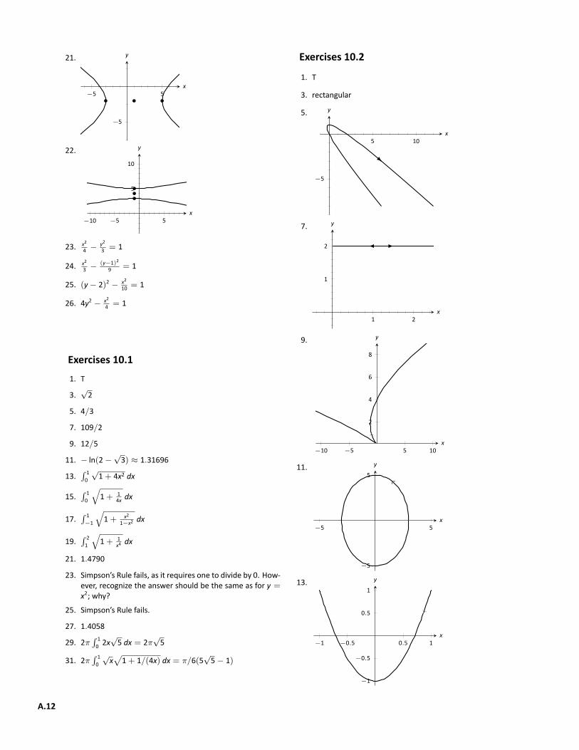
21.
−5 5
−5
x
y
22.
−10 −5 5
5
10
x
y
23. x24 − y2
3 = 1
24. x23 − (y−1)2
9 = 1
25. (y− 2)2 − x210 = 1
26. 4y2 − x24 = 1
Exercises 10.11. T
3.√2
5. 4/3
7. 109/2
9. 12/5
11. − ln(2−√3) ≈ 1.31696
13.∫ 10
√1+ 4x2 dx
15.∫ 10
√1+ 1
4x dx
17.∫ 1−1
√1+ x2
1−x2 dx
19.∫ 21
√1+ 1
x4 dx
21. 1.4790
23. Simpson’s Rule fails, as it requires one to divide by 0. How‐ever, recognize the answer should be the same as for y =x2; why?
25. Simpson’s Rule fails.
27. 1.4058
29. 2π∫ 10 2x
√5 dx = 2π
√5
31. 2π∫ 10√x√
1+ 1/(4x) dx = π/6(5√5− 1)
Exercises 10.2
1. T
3. rectangular
5.
5 10
−5
x
y
7.
1 2
1
2
x
y
9.
−10 −5 5 10
2
4
6
8
x
y
11.
−5 5
−5
5
x
y
13.
−1 −0.5 0.5 1
−1
−0.5
0.5
1
x
y
A.12
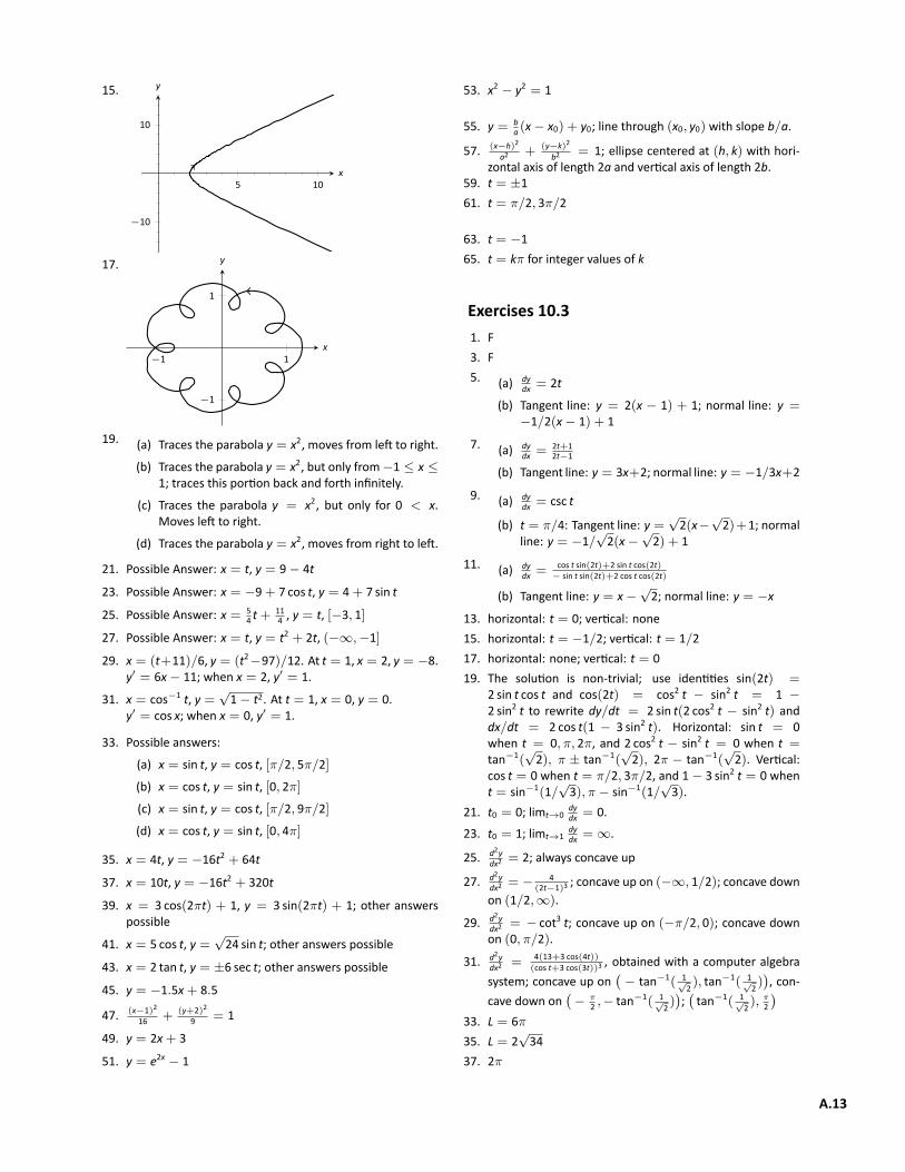
15.
5 10
−10
10
x
y
17.
−1 1
−1
1
x
y
19. (a) Traces the parabola y = x2, moves from left to right.
(b) Traces the parabola y = x2, but only from−1 ≤ x ≤1; traces this portion back and forth infinitely.
(c) Traces the parabola y = x2, but only for 0 < x.Moves left to right.
(d) Traces the parabola y = x2, moves from right to left.
21. Possible Answer: x = t, y = 9− 4t
23. Possible Answer: x = −9+ 7 cos t, y = 4+ 7 sin t
25. Possible Answer: x = 54 t+
114 , y = t, [−3, 1]
27. Possible Answer: x = t, y = t2 + 2t, (−∞,−1]
29. x = (t+11)/6, y = (t2−97)/12. At t = 1, x = 2, y = −8.y′ = 6x− 11; when x = 2, y′ = 1.
31. x = cos−1 t, y =√1− t2. At t = 1, x = 0, y = 0.
y′ = cos x; when x = 0, y′ = 1.
33. Possible answers:
(a) x = sin t, y = cos t, [π/2, 5π/2]
(b) x = cos t, y = sin t, [0, 2π]
(c) x = sin t, y = cos t, [π/2, 9π/2]
(d) x = cos t, y = sin t, [0, 4π]
35. x = 4t, y = −16t2 + 64t
37. x = 10t, y = −16t2 + 320t
39. x = 3 cos(2πt) + 1, y = 3 sin(2πt) + 1; other answerspossible
41. x = 5 cos t, y =√24 sin t; other answers possible
43. x = 2 tan t, y = ±6 sec t; other answers possible
45. y = −1.5x+ 8.5
47. (x−1)216 + (y+2)2
9 = 1
49. y = 2x+ 3
51. y = e2x − 1
53. x2 − y2 = 1
55. y = ba (x− x0) + y0; line through (x0, y0) with slope b/a.
57. (x−h)2
a2 + (y−k)2
b2 = 1; ellipse centered at (h, k) with hori‐zontal axis of length 2a and vertical axis of length 2b.
59. t = ±161. t = π/2, 3π/2
63. t = −165. t = kπ for integer values of k
Exercises 10.31. F3. F5. (a) dy
dx = 2t
(b) Tangent line: y = 2(x − 1) + 1; normal line: y =−1/2(x− 1) + 1
7. (a) dydx = 2t+1
2t−1
(b) Tangent line: y = 3x+2; normal line: y = −1/3x+2
9. (a) dydx = csc t
(b) t = π/4: Tangent line: y =√2(x−
√2)+1; normal
line: y = −1/√2(x−
√2) + 1
11. (a) dydx = cos t sin(2t)+2 sin t cos(2t)
− sin t sin(2t)+2 cos t cos(2t)
(b) Tangent line: y = x−√2; normal line: y = −x
13. horizontal: t = 0; vertical: none15. horizontal: t = −1/2; vertical: t = 1/217. horizontal: none; vertical: t = 019. The solution is non‐trivial; use identities sin(2t) =
2 sin t cos t and cos(2t) = cos2 t − sin2 t = 1 −2 sin2 t to rewrite dy/dt = 2 sin t(2 cos2 t − sin2 t) anddx/dt = 2 cos t(1 − 3 sin2 t). Horizontal: sin t = 0when t = 0, π, 2π, and 2 cos2 t − sin2 t = 0 when t =tan−1(
√2), π ± tan−1(
√2), 2π − tan−1(
√2). Vertical:
cos t = 0 when t = π/2, 3π/2, and 1− 3 sin2 t = 0 whent = sin−1(1/
√3), π − sin−1(1/
√3).
21. t0 = 0; limt→0dydx = 0.
23. t0 = 1; limt→1dydx = ∞.
25. d2ydx2 = 2; always concave up
27. d2ydx2 = − 4
(2t−1)3 ; concave up on (−∞, 1/2); concave downon (1/2,∞).
29. d2ydx2 = − cot3 t; concave up on (−π/2, 0); concave downon (0, π/2).
31. d2ydx2 = 4(13+3 cos(4t))
(cos t+3 cos(3t))3 , obtained with a computer algebrasystem; concave up on
(− tan−1( 1√
2 ), tan−1( 1√
2 )), con‐
cave down on(− π
2 ,− tan−1( 1√2 ));(tan−1( 1√
2 ),π2
)33. L = 6π35. L = 2
√34
37. 2π
A.13
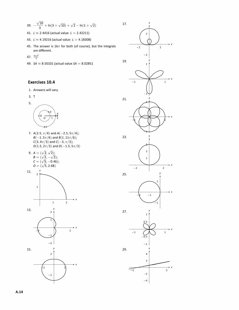
39. −√103
+ ln(3+√10) +
√2− ln(1+
√2)
41. L ≈ 2.4416 (actual value: L = 2.42211)
43. L ≈ 4.19216 (actual value: L = 4.18308)
45. The answer is 16π for both (of course), but the integralsare different.
47. 6πa25
49. SA ≈ 8.50101 (actual value SA = 8.02851
Exercises 10.41. Answers will vary.
3. T
5.
1 2OA
B
C
D
7. A(2.5, π/4) and A(−2.5, 5π/4);B(−1, 5π/6) and B(1, 11π/6);C(3, 4π/3) and C(−3, π/3);D(1.5, 2π/3) and D(−1.5, 5π/3)
9. A = (√2,√2);
B = (√2,−
√2);
C = (√5,−0.46);
D = (√5, 2.68)
11.
1 2
1
2
x
y
13.
−2 2
−2
−1
1
2
x
y
15.
−2 2
−2
2
x
y
17.
−2 2
−2
2
x
y
19.
−1 1
−1
1
x
y
21.
−1 1
−1
1
x
y
23.
−2 2
2
3
1
x
y
25.
−2 −1
−1
1
x
y
27.
−1 1
−1
−0.5
0.5
1
x
y
29.
−5 5
−4
−2
2
4
x
y
A.14
31.
−5 5
−4
−2
2
4
x
y
33. (x− 1)2 + y2 = 135. x2 + (y− 3
2 )2 = 9
4
37. (x− 1/2)2 + (y− 1/2)2 = 1/239. x = 341. x4 + x2y2 − y2 = 043. x2 + y2 = 445. θ = π/447. r = 5 sec θ49. r = cos θ/ sin2 θ51. r =
√7
53. P(√3/2, π/6), P(0, π/2), P(−
√3/2, 5π/6)
55. P(0, 0) = P(0, π/2), P(√2, π/4)
57. P(√2/2, π/12), P(−
√2/2, 5π/12), P(
√2/2, 3π/4), and
the origin.59. For all points, r = 1;
θ = π12 ,
5π12 ,
7π12 ,
11π12 ,
13π12 ,
17π12 ,
19π12 ,
23π12 .
61. Answers will vary. Ifm and n do not have any common fac‐tors, then an interval of 2nπ is needed to sketch the entiregraph.
Exercises 10.51. Using x = r cos θ and y = r sin θ, we can write x =
f(θ) cos θ, y = f(θ) sin θ.3. (a) dy
dx = − cot θ
(b) tangent line: y = −(x −√2/2) +
√2/2; normal
line: y = x
5. (a) dydx = cos θ(1+2 sin θ)
cos2 θ−sin θ(1+sin θ)
(b) tangent line: x = 3√3/4; normal line: y = 3/4
7. (a) dydx = θ cos θ+sin θ
cos θ−θ sin θ
(b) tangent line: y = −(2/π)x + π/2; normal line:y = (π/2)x+ π/2
9. (a) dydx = 4 sin(θ) cos(4θ)+sin(4θ) cos(θ)
4 cos(θ) cos(4θ)−sin(θ) sin(4θ)
(b) tangent line: y = 5√3(x +
√3/4) − 3/4; normal
line: y = −1/5√3(x+
√3/4)− 3/4
11. horizontal: θ = π/2, 3π/2;vertical: θ = 0, π, 2π
13. horizontal: θ = tan−1(1/√5), π/2,
π − tan−1(1/√5), π + tan−1(1/
√5), 3π/2, 2π −
tan−1(1/√5);
vertical: θ = 0, tan−1(√5), π − tan−1(
√5), π, π +
tan−1(√5), 2π − tan−1(
√5)
15. In polar: θ = 0 ∼= θ = πIn rectangular: y = 0
17. In polar: θ = π4 and θ = − π
4In rectangular: y = x and y = −x.
19. area = 4π3 + 2
√3
21. area = π/12
23. area = 3π/2
25. area = 2π + 3√3/2
27. area = 1
29. area = 132 (4π − 3
√3)
31. x ′(θ) = f ′(θ) cos θ − f(θ) sin θ, y ′(θ) = f ′(θ) sin θ +f(θ) cos θ. Square each and add; applying the PythagoreanTheorem twice achieves the result.
33. 4π
35. L ≈ 2.2592; (actual value L = 2.22748)
37. SA = 16π
39. SA = 32π/5
41. SA = 36π
A.15

INDEX!, see factorial
Absolute Convergence Theorem, 510Absolute Value Theorem, 465Alternating Harmonic Series, 508, 533Alternating Series Test
for series, 506analytic function, 556arc length, 575, 604, 630
Binomial Series, 556bounded sequence, 468
convergence, 469
concavity, 600conic sections, 565
degenerate, 565ellipse, 567hyperbola, 569parabola, 566
Constant Multiple Ruleof series, 483
convergenceabsolute, 509, 510Alternating Series Test, 506conditional, 509Direct Comparison Test, 496
for integration, 443Integral Test, 490interval of, 527Limit Comparison Test, 499
for integration, 444of geometric series, 479of improper int., 437, 442–444of monotonic sequences, 472of p‐series, 493of power series, 526of sequence, 464, 469of series, 476radius of, 527Ratio Comparison Test, 515Root Comparison Test, 518
curveparametrically defined, 583rectangular equation, 583smooth, 591
cusp, 591
derivativehyperbolic funct., 367inverse hyper., 371inverse trig., 351parametric equations, 596power series, 530
Direct Comparison Testfor integration, 443for series, 496
directrix, 566
divergenceAlternating Series Test, 506Direct Comparison Test, 496
for integration, 443Integral Test, 490Limit Comparison Test, 499
for integration, 444of geometric series, 479of improper int., 437, 442–444of p‐series, 493of sequence, 464of series, 476Ratio Comparison Test, 515Root Comparison Test, 518
elementary function, 447ellipse
definition, 567standard equation, 568
factorial, 462focus, 566, 567, 569
Gabriel’s Horn, 580geometric sequence, 468geometric series, 478, 479
hyperboladefinition, 569standard equation, 570
hyperbolic functiondefinition, 364derivatives, 367identities, 367integrals, 367inverse, 368
derivative, 371integration, 371logarithmic def., 370
improper integration, 437, 440indeterminate form, 378, 380Integral Test, 490integration
arc length, 575by parts, 384hyperbolic funct., 367improper, 437, 440, 443, 444inverse hyper., 371numerical, 447
Left Hand Rule, 455, 456Left/Right Hand Rule, 447Midpoint Rule, 455, 456Right Hand Rule, 455, 456Simpson’s Rule, 453, 455, 456Trapezoidal Rule, 450, 455, 456
of power series, 530of trig. powers, 400
A.17

of trig. powers, 395surface area, 578, 606, 632trig. subst., 409
interval of convergence, 527irreducible quadratic, 417
Left Hand Rule, 447Left/Right Hand Rule, 455
error bounds, 456limit
Absolute Value Theorem, 465indeterminate form, 378, 380of sequence, 464
Limit Comparison Testfor integration, 444for series, 499
logarithmic differentiation, 361
Maclaurin Polynomial, see also Taylor Polynomialdefinition, 544
Maclaurin Series, see also Taylor Seriesdefinition, 553
Midpoint Rule, 455error bounds, 456
monotonic sequence, 470
normal line, 597numerical integration, 447
Left Hand Rule, 455error bounds, 456
Left/Right Hand Rule, 447Midpoint Rule, 455
error bounds, 456Right Hand Rule, 455
error bounds, 456Simpson’s Rule, 453, 455
error bounds, 456Trapezoidal Rule, 450, 455
error bounds, 456
p‐series, 492, 493parabola
definition, 566general equation, 567
parametric equationsarc length, 604concavity, 600definition, 583finding d2y
dx2 , 600finding dy
dx , 596normal line, 597surface area, 606tangent line, 596
polarcoordinates, 610function
arc length, 630gallery of graphs, 617surface area, 632
functions, 613area, 626
area between curves, 628finding dy
dx , 623graphing, 613
polar coordinates, 610plotting points, 610
power series, 525algebra of, 559convergence, 526derivatives and integrals, 530
radius of convergence, 527Ratio Comparison Test
for series, 515rearrangements of series, 510Right Hand Rule, 447Root Comparison Test
for series, 518
sequenceAbsolute Value Theorem, 465positive, 496
sequencesboundedness, 468convergent, 464, 469, 472definition, 461divergent, 464limit, 464limit properties, 467monotonic, 470
seriesabsolute convergence, 509Absolute Convergence Theorem, 510alternating, 505
Approximation Theorem, 511Alternating Series Test, 506Binomial, 556conditional convergence, 509convergent, 476definition, 476Direct Comparison Test, 496divergent, 476geometric, 478, 479Integral Test, 490interval of convergence, 527Limit Comparison Test, 499Maclaurin, 553p‐series, 492, 493partial sums, 476power, 525, 526
derivatives and integrals, 530properties, 483radius of convergence, 527Ratio Comparison Test, 515rearrangements, 510Root Comparison Test, 518Taylor, 553telescoping, 481
Simpson’s Rule, 453, 455error bounds, 456
smooth curve, 591
Sum/Difference Ruleof series, 483
surface areasolid of revolution, 578, 606, 632
tangent half‐angle substitution, 435tangent line, 596, 623Taylor Polynomial
definition, 544Taylor’s Theorem, 548
Taylor Seriescommon series, 558definition, 553equality with generating function, 555
Taylor’s Theorem, 548telescoping series, 481Trapezoidal Rule, 450, 455
error bounds, 456
unbounded sequence, 468

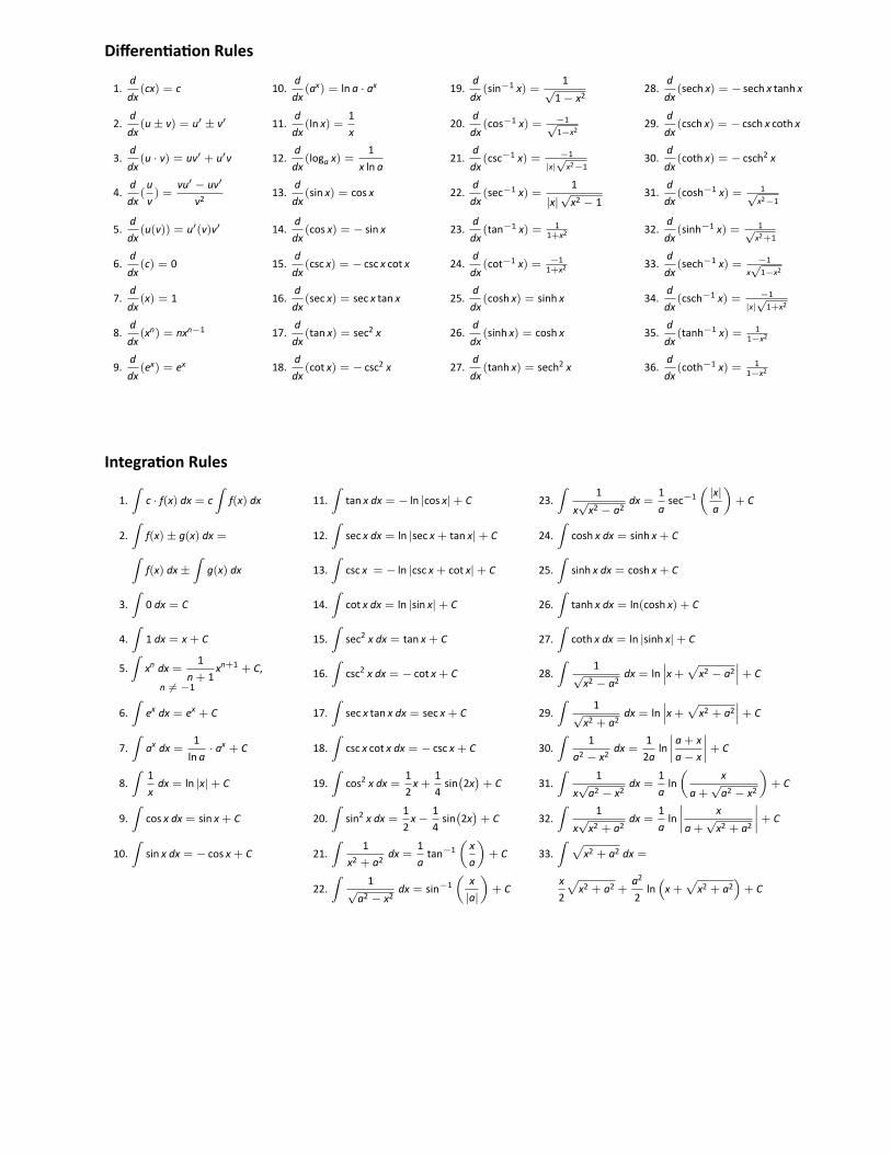
Differentiation Rules
1.ddx
(cx) = c 10.ddx
(ax) = ln a · ax 19.ddx
(sin−1 x) =1
√1− x2
28.ddx
(sech x) = − sech x tanh x
2.ddx
(u± v) = u′ ± v′ 11.ddx
(ln x) =1x
20.ddx
(cos−1 x) = −1√1−x2
29.ddx
(csch x) = − csch x coth x
3.ddx
(u · v) = uv′ + u′v 12.ddx
(loga x) =1
x ln a21.
ddx
(csc−1 x) = −1|x|√
x2−130.
ddx
(coth x) = − csch2 x
4.ddx
(uv) =
vu′ − uv′
v213.
ddx
(sin x) = cos x 22.ddx
(sec−1 x) =1
|x|√x2 − 1
31.ddx
(cosh−1 x) = 1√x2−1
5.ddx
(u(v)) = u′(v)v′ 14.ddx
(cos x) = − sin x 23.ddx
(tan−1 x) = 11+x2 32.
ddx
(sinh−1 x) = 1√x2+1
6.ddx
(c) = 0 15.ddx
(csc x) = − csc x cot x 24.ddx
(cot−1 x) = −11+x2 33.
ddx
(sech−1 x) = −1x√
1−x2
7.ddx
(x) = 1 16.ddx
(sec x) = sec x tan x 25.ddx
(cosh x) = sinh x 34.ddx
(csch−1 x) = −1|x|√
1+x2
8.ddx
(xn) = nxn−1 17.ddx
(tan x) = sec2 x 26.ddx
(sinh x) = cosh x 35.ddx
(tanh−1 x) = 11−x2
9.ddx
(ex) = ex 18.ddx
(cot x) = − csc2 x 27.ddx
(tanh x) = sech2 x 36.ddx
(coth−1 x) = 11−x2
Integration Rules
1.∫
c · f(x) dx = c∫
f(x) dx 11.∫
tan x dx = − ln |cos x|+ C 23.∫ 1
x√x2 − a2
dx =1asec−1
(|x|a
)+ C
2.∫
f(x)± g(x) dx = 12.∫
sec x dx = ln |sec x+ tan x|+ C 24.∫
cosh x dx = sinh x+ C∫f(x) dx±
∫g(x) dx 13.
∫csc x = − ln |csc x+ cot x|+ C 25.
∫sinh x dx = cosh x+ C
3.∫
0 dx = C 14.∫
cot x dx = ln |sin x|+ C 26.∫
tanh x dx = ln(cosh x) + C
4.∫
1 dx = x+ C 15.∫
sec2 x dx = tan x+ C 27.∫
coth x dx = ln |sinh x|+ C
5.∫
xn dx =1
n+ 1xn+1 + C,
n ̸= −116.
∫csc2 x dx = − cot x+ C 28.
∫ 1√x2 − a2
dx = ln∣∣∣x+√
x2 − a2∣∣∣+ C
6.∫
ex dx = ex + C 17.∫
sec x tan x dx = sec x+ C 29.∫ 1
√x2 + a2
dx = ln∣∣∣x+√
x2 + a2∣∣∣+ C
7.∫
ax dx =1ln a
· ax + C 18.∫
csc x cot x dx = − csc x+ C 30.∫ 1
a2 − x2dx =
12a
ln∣∣∣∣a+ xa− x
∣∣∣∣+ C
8.∫ 1
xdx = ln |x|+ C 19.
∫cos2 x dx =
12x+
14sin
(2x)+ C 31.
∫ 1x√a2 − x2
dx =1aln(
xa+
√a2 − x2
)+ C
9.∫
cos x dx = sin x+ C 20.∫
sin2 x dx =12x−
14sin
(2x)+ C 32.
∫ 1x√x2 + a2
dx =1aln∣∣∣∣ xa+
√x2 + a2
∣∣∣∣+ C
10.∫
sin x dx = − cos x+ C 21.∫ 1
x2 + a2dx =
1atan−1
(xa
)+ C 33.
∫ √x2 + a2 dx =
22.∫ 1
√a2 − x2
dx = sin−1(
x|a|
)+ C
x2
√x2 + a2 +
a2
2ln(x+
√x2 + a2
)+ C
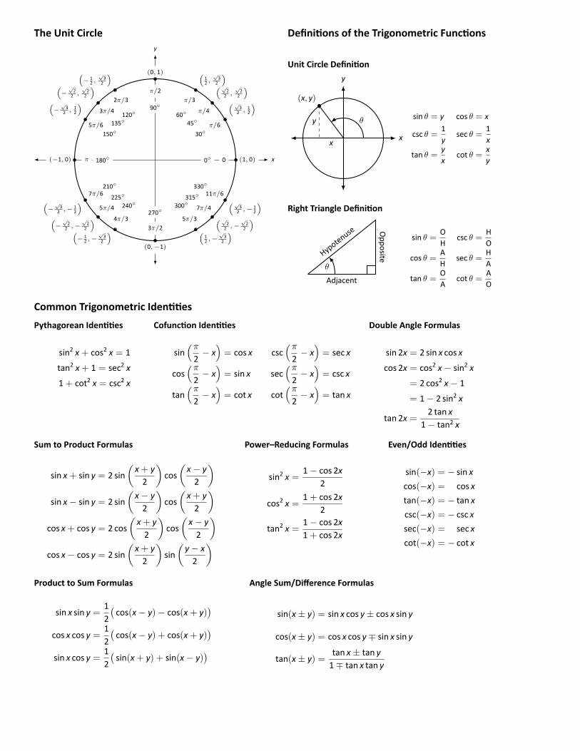
The Unit Circle
x
y
0◦ 0 (1, 0)
30◦π/6
(√3
2 , 12
)45◦
π/4
(√2
2 ,√
22
)60◦
π/3
(12 ,
√3
2
)
90◦
π/2
(0, 1)
120◦
2π/3
(− 1
2 ,√
32
)
135◦3π/4
(−
√2
2 ,√
22
)
150◦5π/6
(−
√3
2 , 12
)
180◦π(−1, 0)
210◦7π/6(
−√
32 ,− 1
2
) 225◦
5π/4(−
√2
2 ,−√
22
)240◦
4π/3
(− 1
2 ,−√
32
)270◦
3π/2
(0,−1)
300◦
5π/3
(12 ,−
√3
2
)
315◦
7π/4 (√2
2 ,−√
22
)
330◦11π/6 (√
32 ,− 1
2
)
Definitions of the Trigonometric Functions
Unit Circle Definition
x
y
(x, y)
y
x
θ sin θ = y cos θ = x
csc θ =1y
sec θ =1x
tan θ =yx
cot θ =xy
Right Triangle Definition
Adjacent
OppositeHypot
enuse
θ
sin θ =OH
csc θ =HO
cos θ =AH
sec θ =HA
tan θ =OA
cot θ =AO
Common Trigonometric IdentitiesPythagorean Identities
sin2 x+ cos2 x = 1tan2 x+ 1 = sec2 x1+ cot2 x = csc2 x
Cofunction Identities
sin(π2− x)= cos x csc
(π2− x)= sec x
cos(π2− x)= sin x sec
(π2− x)= csc x
tan(π2− x)= cot x cot
(π2− x)= tan x
Double Angle Formulas
sin 2x = 2 sin x cos xcos 2x = cos2 x− sin2 x
= 2 cos2 x− 1= 1− 2 sin2 x
tan 2x =2 tan x
1− tan2 x
Sum to Product Formulas
sin x+ sin y = 2 sin(x+ y2
)cos(x− y2
)sin x− sin y = 2 sin
(x− y2
)cos(x+ y2
)cos x+ cos y = 2 cos
(x+ y2
)cos(x− y2
)cos x− cos y = 2 sin
(x+ y2
)sin(y− x2
)
Power–Reducing Formulas
sin2 x =1− cos 2x
2
cos2 x =1+ cos 2x
2
tan2 x =1− cos 2x1+ cos 2x
Even/Odd Identities
sin(−x) = − sin xcos(−x) = cos xtan(−x) = − tan xcsc(−x) = − csc xsec(−x) = sec xcot(−x) = − cot x
Product to Sum Formulas
sin x sin y =12(cos(x− y)− cos(x+ y)
)cos x cos y =
12(cos(x− y) + cos(x+ y)
)sin x cos y =
12(sin(x+ y) + sin(x− y)
)
Angle Sum/Difference Formulas
sin(x± y) = sin x cos y± cos x sin y
cos(x± y) = cos x cos y∓ sin x sin y
tan(x± y) =tan x± tan y1∓ tan x tan y
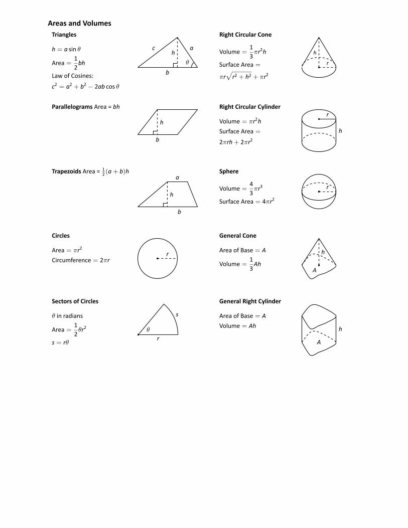
Areas and VolumesTriangles
h = a sin θ
Area =12bh
Law of Cosines:c2 = a2 + b2 − 2ab cos θ
bθ
ach
Right Circular Cone
Volume =13πr2h
Surface Area =
πr√
r2 + h2 + πr2
h
r
Parallelograms Area = bh
b
h
Right Circular Cylinder
Volume = πr2hSurface Area =
2πrh+ 2πr2h
r
Trapezoids Area = 12 (a+ b)h
b
a
h
Sphere
Volume =43πr3
Surface Area = 4πr2
r
Circles
Area = πr2
Circumference = 2πrr
General Cone
Area of Base = A
Volume =13Ah
h
A
Sectors of Circles
θ in radians
Area =12θr2
s = rθ r
s
θ
General Right Cylinder
Area of Base = AVolume = Ah h
A
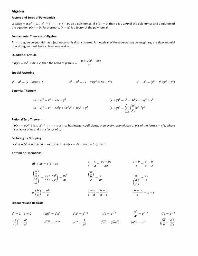
AlgebraFactors and Zeros of Polynomials
Let p(x) = anxn + an−1xn−1 + · · ·+ a1x+ a0 be a polynomial. If p(a) = 0, then a is a zero of the polynomial and a solution ofthe equation p(x) = 0. Furthermore, (x− a) is a factor of the polynomial.
Fundamental Theorem of Algebra
An nth degree polynomial has n (not necessarily distinct) zeros. Although all of these zerosmay be imaginary, a real polynomialof odd degree must have at least one real zero.
Quadratic Formula
If p(x) = ax2 + bx+ c, then the zeros of p are x =−b±
√b2 − 4ac2a
Special Factoring
x2 − a2 = (x− a)(x+ a) x3 ± a3 = (x± a)(x2 ∓ ax+ a2) x4 − a4 = (x2 − a2)(x2 + a2)
Binomial Theorem
(x+ y)2 = x2 + 2xy+ y2 (x+ y)3 = x3 + 3x2y+ 3xy2 + y3
(x+ y)4 = x4 + 4x3y+ 6x2y2 + 4xy3 + y4 (x+ y)n =n∑
k=0
(nk
)xn−kyk
Rational Zero Theorem
If p(x) = anxn + an−1xn−1 + · · ·+ a1x+ a0 has integer coefficients, then every rational zero of p is of the form x = r/s, wherer is a factor of a0 and s is a factor of an.
Factoring by Grouping
acx3 + adx2 + bcx+ bd = ax2(cx+ d) + b(cx+ d) = (ax2 + b)(cx+ d)
Arithmetic Operations
ab+ ac = a(b+ c)ab+
cd=
ad+ bcbd
a+ bc
=ac+
bc(
ab
)( cd
) =(ab
)(dc
)=
adbc
(ab
)c
=abc
a(bc
) =acb
a(bc
)=
abc
a− bc− d
=b− ad− c
ab+ aca
= b+ c
Exponents and Radicals
a0 = 1, a ̸= 0 (ab)x = axbx axay = ax+y √a = a1/2
ax
ay= ax−y n
√a = a1/n(a
b
)x=
ax
bxn√am = am/n a−x =
1ax
n√ab = n
√a n√b (ax)y = axy n
√ab=
n√a
n√b
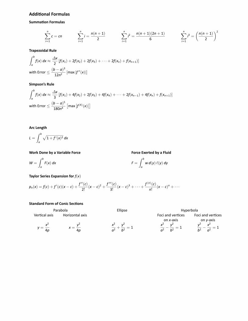
Additional FormulasSummation Formulas
n∑i=1
c = cnn∑
i=1
i =n(n+ 1)
2
n∑i=1
i2 =n(n+ 1)(2n+ 1)
6
n∑i=1
i3 =(n(n+ 1)
2
)2
Trapezoidal Rule∫ b
af(x) dx ≈ ∆x
2[f(x1) + 2f(x2) + 2f(x3) + · · ·+ 2f(xn) + f(xn+1)]
with Error ≤ (b− a)3
12n2[max |f ′′(x)|]
Simpson’s Rule∫ b
af(x) dx ≈ ∆x
3[f(x1) + 4f(x2) + 2f(x3) + 4f(x4) + · · ·+ 2f(xn−1) + 4f(xn) + f(xn+1)]
with Error ≤ (b− a)5
180n4[max
∣∣f(4)(x)∣∣]
Arc Length
L =∫ b
a
√1+ f ′(x)2 dx
Work Done by a Variable Force
W =
∫ b
aF(x) dx
Force Exerted by a Fluid
F =∫ b
awd(y) ℓ(y) dy
Taylor Series Expansion for f(x)
pn(x) = f(c) + f ′(c)(x− c) +f ′′(c)2!
(x− c)2 +f ′′′(c)3!
(x− c)3 + · · ·+ f (n)(c)n!
(x− c)n + · · ·
Standard Form of Conic SectionsParabola Ellipse Hyperbola
Vertical axis Horizontal axis Foci and vertices Foci and verticeson x‐axis on y‐axis
y =x2
4px =
y2
4px2
a2+
y2
b2= 1
x2
a2− y2
b2= 1
y2
b2− x2
a2= 1
Summary of Tests for Series
Test Series Condition(s) ofConvergence
Condition(s) ofDivergence Comment
nth‐TermTest for
Divergence
∞∑n=1
an limn→∞
an ̸= 0 cannot showconvergence.
AlternatingSeries
∞∑n=1
(−1)nbn limn→∞
bn = 0bn must bepositive anddecreasing
GeometricSeries
∞∑n=0
arn |r| < 1 |r| ≥ 1 Sum=a
1− r
TelescopingSeries
∞∑n=1
bn − bn+m limn→∞
bn = LSum=(m∑
n=1bn
)− L
p‐Series∞∑n=1
1(an+ b)p
p > 1 p ≤ 1
p‐Series ForLogarithms
∞∑n=1
1(an+ b)(log n)p
p > 1 p ≤ 1logarithm’s basedoesn’t affectconvergence.
IntegralTest
∞∑n=1
an∫ ∞
1a(n) dn
converges
∫ ∞
1a(n) dn
diverges
an = a(n)mustbe positive anddecreasing
DirectComparison
∞∑n=1
an∞∑n=0
bn
converges and0 ≤ an ≤ bn
∞∑n=0
bn
diverges and0 ≤ bn ≤ an
LimitComparison
∞∑n=1
an∞∑n=0
bn
converges andlim
n→∞an/bn < ∞
∞∑n=0
bn
diverges andlim
n→∞an/bn > 0
or = ∞
an, bn > 0
Ratio Test∞∑n=1
an limn→∞
∣∣∣∣an+1
an
∣∣∣∣ < 1lim
n→∞
∣∣∣∣an+1
an
∣∣∣∣ > 1
or = ∞
limit of 1 isindeterminate
Root Test∞∑n=1
an limn→∞
|an|1/n < 1lim
n→∞|an|1/n > 1
or = ∞limit of 1 is
indeterminate