1

UNIT – I - Antenna Fundamentals and Wire

Antennas – SECA1504

SCHOOL OF ELECTRICAL AND ELECTRONICS

DEPARTMENT OF ECE

2

I.INTRODUCTION

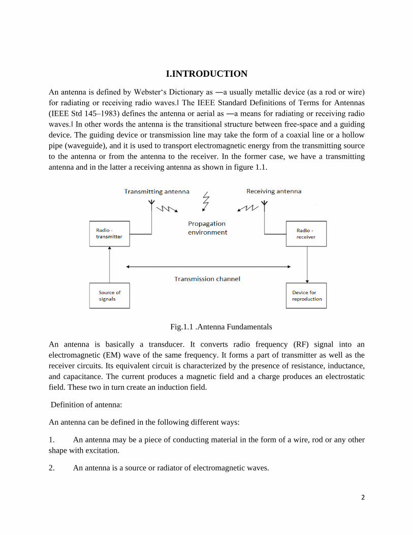
An antenna is defined by Webster‘s Dictionary as ―a usually metallic device (as a rod or wire)

for radiating or receiving radio waves.‖ The IEEE Standard Definitions of Terms for Antennas

(IEEE Std 145–1983) defines the antenna or aerial as ―a means for radiating or receiving radio

waves.‖ In other words the antenna is the transitional structure between free-space and a guiding

device. The guiding device or transmission line may take the form of a coaxial line or a hollow

pipe (waveguide), and it is used to transport electromagnetic energy from the transmitting source

to the antenna or from the antenna to the receiver. In the former case, we have a transmitting

antenna and in the latter a receiving antenna as shown in figure 1.1.

Fig.1.1 .Antenna Fundamentals

An antenna is basically a transducer. It converts radio frequency (RF) signal into an

electromagnetic (EM) wave of the same frequency. It forms a part of transmitter as well as the

receiver circuits. Its equivalent circuit is characterized by the presence of resistance, inductance,

and capacitance. The current produces a magnetic field and a charge produces an electrostatic

field. These two in turn create an induction field.

Definition of antenna:

An antenna can be defined in the following different ways:

1. An antenna may be a piece of conducting material in the form of a wire, rod or any other

shape with excitation.

2. An antenna is a source or radiator of electromagnetic waves.

3

3. An antenna is a sensor of electromagnetic waves.

4. An antenna is a transducer.

5. An antenna is an impedance matching device.

6. An antenna is a coupler between a generator and space or vice-versa.

The radiation from the antenna takes place when the Electromagnetic field generated by the

source is transmitted to the antenna system through the Transmission line and separated from the

Antenna into free space.

1.1ANTENNA PARAMETERS :

1.Field patterns:

The energy radiated in a particular direction is measured in terms of field strength at a

point

Radiation pattern- graph which shows the variation in actual field strength of

electromagnetic field at all points ,equal distance from the antenna

If the radiation from the antenna is expressed in terms of field strength E (V/m)- Field

strength pattern

If the radiation in a given direction is expressed in terms of power per unit solid-power

pattern

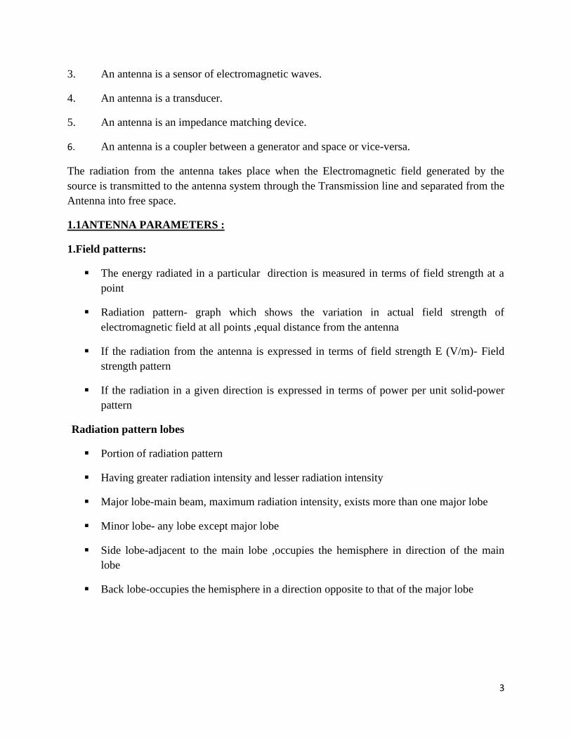
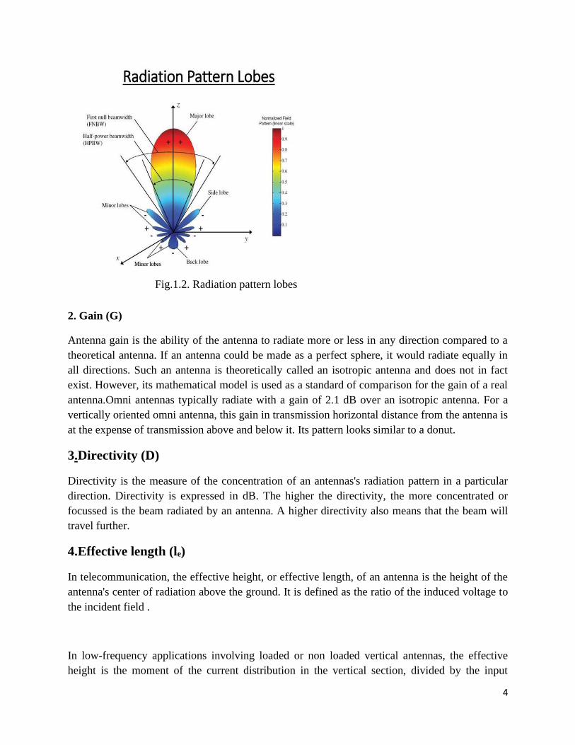
Radiation pattern lobes

Portion of radiation pattern

Having greater radiation intensity and lesser radiation intensity

Major lobe-main beam, maximum radiation intensity, exists more than one major lobe

Minor lobe- any lobe except major lobe

Side lobe-adjacent to the main lobe ,occupies the hemisphere in direction of the main

lobe

Back lobe-occupies the hemisphere in a direction opposite to that of the major lobe

4

2. Gain (G)

Antenna gain is the ability of the antenna to radiate more or less in any direction compared to a

theoretical antenna. If an antenna could be made as a perfect sphere, it would radiate equally in

all directions. Such an antenna is theoretically called an isotropic antenna and does not in fact

exist. However, its mathematical model is used as a standard of comparison for the gain of a real

antenna.Omni antennas typically radiate with a gain of 2.1 dB over an isotropic antenna. For a

vertically oriented omni antenna, this gain in transmission horizontal distance from the antenna is

at the expense of transmission above and below it. Its pattern looks similar to a donut.

3.Directivity (D)

Directivity is the measure of the concentration of an antennas's radiation pattern in a particular

direction. Directivity is expressed in dB. The higher the directivity, the more concentrated or

focussed is the beam radiated by an antenna. A higher directivity also means that the beam will

travel further.

4.Effective length (le)

In telecommunication, the effective height, or effective length, of an antenna is the height of the

antenna's center of radiation above the ground. It is defined as the ratio of the induced voltage to

the incident field .

In low-frequency applications involving loaded or non loaded vertical antennas, the effective

height is the moment of the current distribution in the vertical section, divided by the input

Fig.1.2. Radiation pattern lobes

5

current. For an antenna with a symmetrical current distribution, the center of radiation is the

center of the distribution. For an antenna with asymmetrical current distribution, the center of

radiation is the center of current moments when viewed from points near the direction of

maximum radiation.

5.Effective Aperture (Ae):

• Effective area or capture area

• Tr.antenna-transmits EM waves

• Receiving Antenna-receives fraction of the same

• Cross sectional area over which it extracts EM energy from the travelling EM waves.

6.Radiation Resistance:

It is a equivalent resistance which would dissipate the same amount of power as the

antenna radiates when the current in that resistance equals the input current at the antenna

terminals.

7.Antenna Impedance:

Impedance at the point where the transmission line carrying RF power from the

transmitter is connected

At this point input to the antenna is supplied-Antenna Input Impedance

Driving point impedance or Terminal impedance

Represented by a two terminal network

8.Polarization:

Described in terms of electric vector E

Defined by the direction in which the electric vector E is aligned during the passage of

atleast one cycle

Refers to the physical orientation of the radiated EM waves in space

E and H are mutually perpendicular

Magnetic fields surround the wire and perpendicular to it, it means the electric field is

parallel to the wire

Types of polarization:

a)Linear polarization: E as a function of time remains along a straight line

b) Circular polarization: E traces a circle

6

c) Elliptical polarization: Tip of electric field vector traces an ellipse

9.Bandwidth:

Defines the width or the working range of frequencies over which the antenna maintain

its characteristics and parameters like gain, Radiation pattern , Directivity, impedance

and so on without considerable changes

1.2 Basic Antenna Elements:

Short Dipole:

• Hertzian dipole, alternating current element, oscillating current element

• consists of co-linear conductors that are placed end to end, but with a small gap

between them for the feeder

• current may be assumed to be constant throughout its length

• length L < /10

• current distribution is triangular

Short Monopole:

- Length L < /8

- current distribution is triangular

Half wave dipole:

- Length L= /2

- current distribution is sinusoidal

Quarter wave monopole:

- Length L=/4

- current distribution is sinusoidal

1.3 Retarded potential

• Definition: The retarded potentials are the electromagnetic potential for the

electromagnetic field generated by time varying electric current or charge distribution in

the past

• Bio-Savart’s Law: Magnetic field due to a current carrying element is directly

proportional to the current and the vector product of length vector. It relates magnetic

fields to the currents which are their sources.

7

1.4 Radiation from an alternating current element

- Oscillating electric dipole, Hertzian dipole

- An infinite small current carrying element

- Useful to calculate the field of a large wire antenna

- Long wire antenna-large number of Hertzian dipoles connected in series

- current is constant along the length whenever it is excited by a RF current

- Concept of retarded vector potential is used to find these fields everywhere around in

free space

- elemental length of wire is placed at the origin of the spherical coordinate systems

- current in a dipole is accompanied by magnetic field surrounding the region of short

dipole

- Built upon on three mutually perpendicular axes x , y and z and a radial displacement (r)

- and two angular displacements ( and ) are used to describe the spherical coordinates

1.5 Antenna Field Zones

The energy is stored in the magnetic field in the surrounding zone of the current element and it

is alternatively stored in field and returned to the source (Idl) during each half cycle.

Electromagnetic radiation is impossible

a) Near field region:electromagnetic field created by an antenna that is only significant at

distances of less than 2D/λ from the antenna, where D is the longest dimension of the

antenna.

b) Far field region:electromagnetic field created by the antenna that extends throughout

all space. At distances greater than 2D/λ from the antenna, it is the only field. It is the

field used for communications

A distance is reached from the conductor at which both the induction and radiation fields

becomes equal and the particular distance depends on the wavelength used

It is given by = 0.15

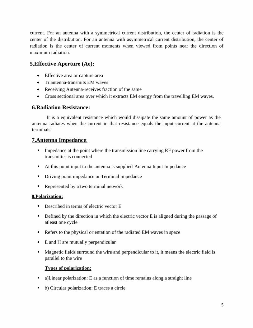
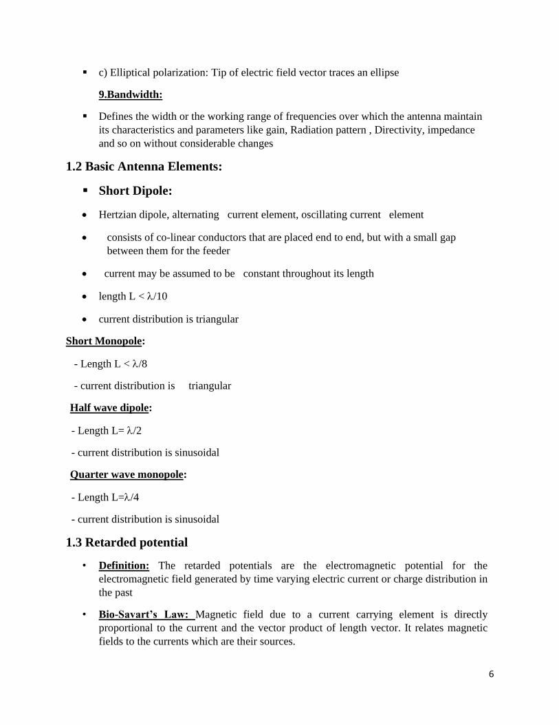
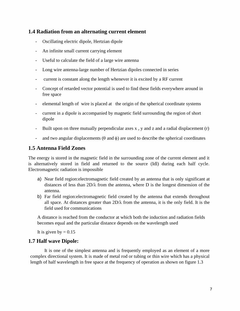
1.7 Half wave Dipole:

It is one of the simplest antenna and is frequently employed as an element of a more

complex directional system. It is made of metal rod or tubing or thin wire which has a physical

length of half wavelength in free space at the frequency of operation as shown on figure 1.3

8

A dipole antenna is defined as a symmetrical antenna in which the two ends are at equal potential

relative to mid point

Let us consider a centre fed half wave dipole system, the asymptotic current distribution is

I=I(z)=Imsinβ(h-Z) ;z>+0 (1)

I=I(z)=Imsinβ(h+Z) ;z<0 (2)

Im is the maximum current at the current loop

Power radiated by a half wave dipole is given by

W=73.140 I2rms Watts

The radiation resistance Rr=73 Ω

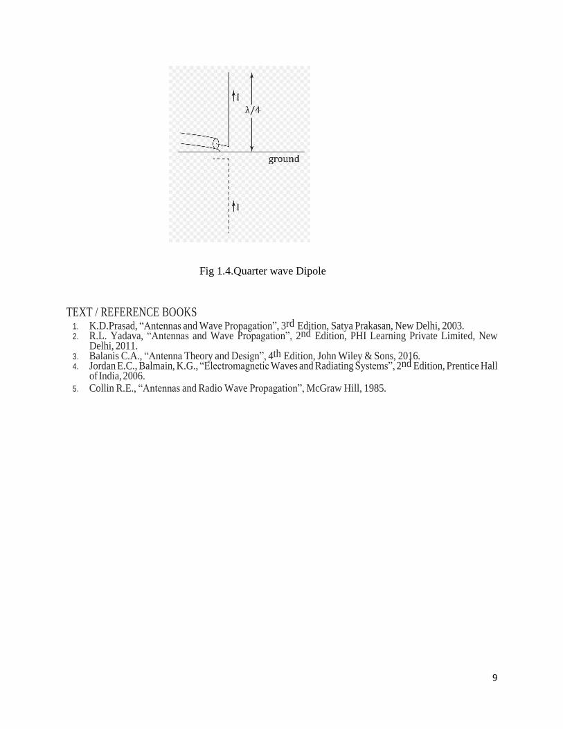
1.8 Quarter wave monopole

/4 antenna

Marconi Antenna

Consists of one half of a half wave dipole antenna located on a conducting ground plane

Perpendicular to the plane which is usually assumed to be infinite and perfectly

conducting

Fed by a coaxial cable connected to its base as shown in figure 1.4

Fig 1.3.Half wave Dipole

9

Fig 1.4.Quarter wave Dipole

TEXT / REFERENCE BOOKS 1. K.D.Prasad, “Antennas and Wave Propagation”, 3rd Edition, Satya Prakasan, New Delhi, 2003. 2. R.L. Yadava, “Antennas and Wave Propagation”, 2nd Edition, PHI Learning Private Limited, New

Delhi, 2011. 3. Balanis C.A., “Antenna Theory and Design”, 4th Edition, John Wiley & Sons, 2016. 4. Jordan E.C., Balmain, K.G., “Electromagnetic Waves and Radiating Systems”, 2nd Edition, Prentice Hall

of India, 2006. 5. Collin R.E., “Antennas and Radio Wave Propagation”, McGraw Hill, 1985.

10

PART A

1. State Directivity.

2. State Polarization.

3. Interpret Radiation Intensity.

4. Explain retarded potential

5. What is radiation resistance?

6. Find the angle of half wave dipole at 30 MHz.

7. Give the significance of radiation resistance of an antenna.

8. Define Effective length.

9. Illustrate the radiation resistance of a ʎ/2 dipole?

10. Define a Hertzian dipole.

PART B

1. Apply the expression for field components of an alternating current element.

2. Develop the expression for power radiated and find the radiation resistance of a half wave

dipole.

3. Interpret a) Radiation pattern b) Beam width c) Gain.

4. Explain a) Directivity b) Effective Aperture c) Polarization.

5. a) Summarize retarded potential

b) Compare the characteristics of half wave dipole and quarter wave monopole

6. Demonstrate the expression for the near and far fields due to short dipole. Find also the

distance at near and far fields are equal.

7. Elaborate notes on a) Field patterns b) Effective Aperture c) Self and Mutual Impedance

8. a) Compare Gain and directivity and state the relation between them

b) Develop equations and explain different types of polarization.

9. A thin dipole is λ/15 long. If it has loss resistance of 1.5 Ω, calculate directivity, gain,

effective aperture, beam solid angle and radiation resistance.

10. Estimate the power radiated and radiation resistance of current element.

11

UNIT – II – Antenna Arrays- SECA1504

12

2.1.Antenna Array

To increase the field strength in the desired direction by using group of antennas excited

simultaneously such a group of antennas are called as antenna arrays

Purpose of using antenna array:

• Increase field strength

• Increase directivity

• Point to Point communication

• Long distance communication

Array of two point sources

Point source

Also called as volume less radiator, isotropic radiator, hypothetical antenna

Conditions

Based on amplitude and phase are

Condition 1-Equal amplitude and in phase

Condition 2-Equal amplitude and out of phase

Condition 3-Equal amplitude amp and any phase

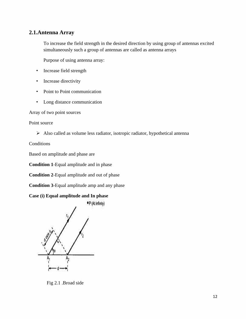
Case (i) Equal amplitude and In phase

Fig 2.1 .Broad side

array

13

Consider two point sources having equal amplitude and same phase

Step :1

Path difference between point source 1&2

Path diff=d/2 Cos θ +d/2 Cos θ

=d Cos θ (2.1)

Path difference in wavelength

=d Cos θ/ƛ (2.2)

Step :2

Phase angle difference Ψ

Ψ =2∏ [path difference]

Ψ =2∏ [d/ƛ Cosθ]

Ψ = 2∏d/ƛ Cos θ

Ψ= βd Cos θ (2.3)

Step :3

Total electric field strength of 2 pt source array is vector sum of individual elements in the array

[-ive sign---pt 1 lags, +ive sign –pt 2 leads]

Both phase angles are same

E t =E02 Cos ψ/2

E t =2E0 Cos[ βd Cos θ /2]

2E0=1

E t = Cos[ βd Cos θ /2]

E t = Cos ∏ /2 Cos θ (2.4)

Step:4 Graphical representation

(i)Direction of maxima:-

Total field strength will be maximum and the direction of maxima is obtained when

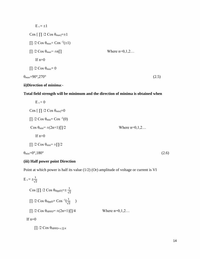
14

E t = ±1

Cos [ ∏ /2 Cos θmax]=±1

∏ /2 Cos θmax= Cos -1(±1)

∏ /2 Cos θmax= ±n∏ Where n=0,1,2…

If n=0

∏ /2 Cos θmax= 0

θmax=90°,270° (2.5)

ii)Direction of minima:-

Total field strength will be minimum and the direction of minima is obtained when

E t = 0

Cos [ ∏ /2 Cos θmin]=0

∏ /2 Cos θmin= Cos -1(0)

Cos θmin= ±(2n+1)∏/2 Where n=0,1,2…

If n=0

∏ /2 Cos θmin= ±∏/2

θmin=0°,180° (2.6)

(iii) Half power point Direction

Point at which power is half its value (1/2) (Or) amplitude of voltage or current is VI

E t = ±1

√2

Cos [∏ /2 Cos θHppD]=± 1

√2

∏ /2 Cos θHppD= Cos -1(1

√2 )

∏ /2 Cos θHPPD= ±(2n+1)∏/4 Where n=0,1,2…

If n=0

∏ /2 Cos θHPPD=± ∏/4

15

Cos θHPPD=±∏/4 *2/∏

θHPPD=±1/2

θHPPD=60°,120°,240°,300° (2.7)

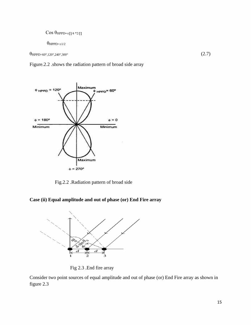
Figure.2.2 .shows the radiation pattern of broad side array

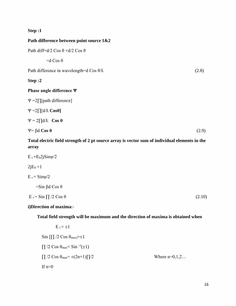
Case (ii) Equal amplitude and out of phase (or) End Fire array

Consider two point sources of equal amplitude and out of phase (or) End Fire array as shown in

figure 2.3

Fig.2.2 .Radiation pattern of broad side

array

Fig 2.3 .End fire array

16

Step :1

Path difference between point source 1&2

Path diff=d/2 Cos θ +d/2 Cos θ

=d Cos θ

Path difference in wavelength=d Cos θ/ƛ (2.8)

Step :2

Phase angle difference Ψ

Ψ =2∏[path difference]

Ψ =2∏[d/ƛ Cosθ]

Ψ = 2∏d/ƛ Cos θ

Ψ= βd Cos θ (2.9)

Total electric field strength of 2 pt source array is vector sum of individual elements in the

array

E t =E02jSinψ/2

2jE0 =1

E t = Sinψ/2

=Sin βd Cos θ

E t = Sin ∏ /2 Cos θ (2.10)

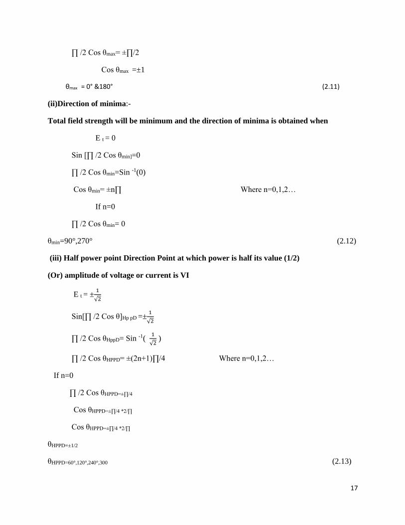
i)Direction of maxima:-

Total field strength will be maximum and the direction of maxima is obtained when

E t = ±1

Sin [∏ /2 Cos θmax]=±1

∏ /2 Cos θmax= Sin -1(±1)

∏ /2 Cos θmax= ±(2n+1)∏/2 Where n=0,1,2…

If n=0

17

∏ /2 Cos θmax= ±∏/2

Cos θmax =±1

θmax = 0° &180° (2.11)

(ii)Direction of minima:-

Total field strength will be minimum and the direction of minima is obtained when

E t = 0

Sin [∏ /2 Cos θmin]=0

∏ /2 Cos θmin=Sin -1(0)

Cos θmin= ±n∏ Where n=0,1,2…

If n=0

∏ /2 Cos θmin= 0

θmin=90°,270° (2.12)

(iii) Half power point Direction Point at which power is half its value (1/2)

(Or) amplitude of voltage or current is VI

E t = ±1

√2

Sin[∏ /2 Cos θ]Hp pD =±1

√2

∏ /2 Cos θHppD= Sin -1( 1

√2 )

∏ /2 Cos θHPPD= ±(2n+1)∏/4 Where n=0,1,2…

If n=0

∏ /2 Cos θHPPD=±∏/4

Cos θHPPD=±∏/4 *2/∏

Cos θHPPD=±∏/4 *2/∏

θHPPD=±1/2

θHPPD=60°,120°,240°,300 (2.13)

18

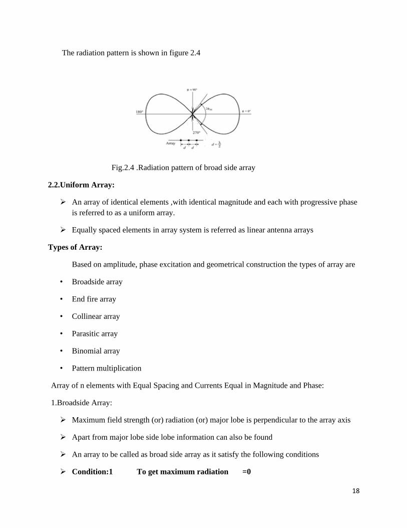
The radiation pattern is shown in figure 2.4

Fig.2.4 .Radiation pattern of broad side array

2.2.Uniform Array:

An array of identical elements ,with identical magnitude and each with progressive phase

is referred to as a uniform array.

Equally spaced elements in array system is referred as linear antenna arrays

Types of Array:

Based on amplitude, phase excitation and geometrical construction the types of array are

• Broadside array

• End fire array

• Collinear array

• Parasitic array

• Binomial array

• Pattern multiplication

Array of n elements with Equal Spacing and Currents Equal in Magnitude and Phase:

1.Broadside Array:

Maximum field strength (or) radiation (or) major lobe is perpendicular to the array axis

Apart from major lobe side lobe information can also be found

An array to be called as broad side array as it satisfy the following conditions

Condition:1 To get maximum radiation =0

19

Condition:2 For in phase α =0

=βd Cosθ+α

Condition:3 According to the definition of broad side array

θ max=90°

Condition:4 Minimum field strength is found to be

θ min=0°

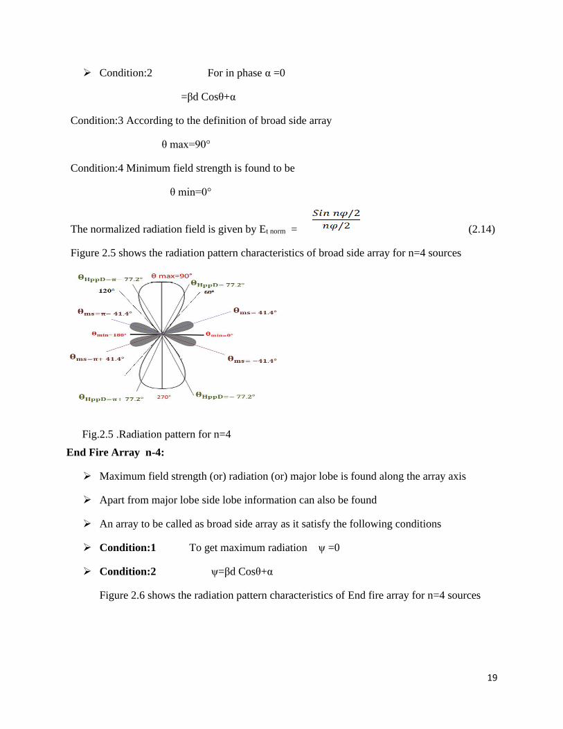
The normalized radiation field is given by Et norm = (2.14)

Figure 2.5 shows the radiation pattern characteristics of broad side array for n=4 sources

End Fire Array n-4:

Maximum field strength (or) radiation (or) major lobe is found along the array axis

Apart from major lobe side lobe information can also be found

An array to be called as broad side array as it satisfy the following conditions

Condition:1 To get maximum radiation ψ =0

Condition:2 ψ=βd Cosθ+α

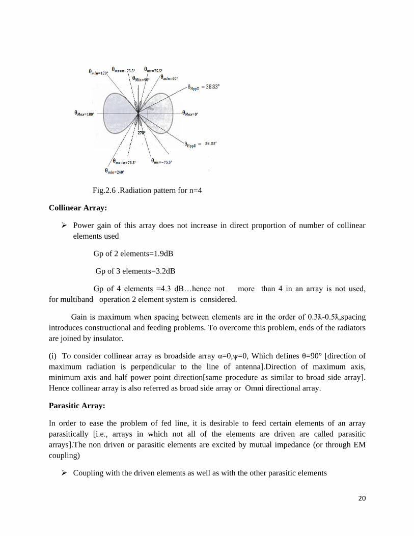
Figure 2.6 shows the radiation pattern characteristics of End fire array for n=4 sources

Fig.2.5 .Radiation pattern for n=4

20

Fig.2.6 .Radiation pattern for n=4

Collinear Array:

Power gain of this array does not increase in direct proportion of number of collinear

elements used

Gp of 2 elements=1.9dB

Gp of 3 elements=3.2dB

Gp of 4 elements =4.3 dB…hence not more than 4 in an array is not used,

for multiband operation 2 element system is considered.

Gain is maximum when spacing between elements are in the order of 0.3ƛ-0.5ƛ,spacing

introduces constructional and feeding problems. To overcome this problem, ends of the radiators

are joined by insulator.

(i) To consider collinear array as broadside array α=0,ψ=0, Which defines θ=90° [direction of

maximum radiation is perpendicular to the line of antenna].Direction of maximum axis,

minimum axis and half power point direction[same procedure as similar to broad side array].

Hence collinear array is also referred as broad side array or Omni directional array.

Parasitic Array:

In order to ease the problem of fed line, it is desirable to feed certain elements of an array

parasitically [i.e., arrays in which not all of the elements are driven are called parasitic

arrays].The non driven or parasitic elements are excited by mutual impedance (or through EM

coupling)

Coupling with the driven elements as well as with the other parasitic elements

21

The design of parasitic elements mainly dependent with

Mutual impedances, elemental length, applied wavelength and optimum spacing

Binomial Array:

Binomial array is an array of non uniform amplitudes and the amplitude of the radiating

sources are arranged according to the coefficient of successive term of the following

binomial series and hence the name.

Pattern Multiplication:

The principle of pattern multiplication

The principle of pattern multiplication states that “the radiation pattern of an array is the

product of the pattern of the individual antenna with the array pattern of isotropic point

sources each located at the phase centre of the individual source.”

The array pattern is a function of the location of the antennas in the array and their

relative complex excitation amplitudes.

The phase center of the array is the reference point for total phase pattern

Advantage:

It helps to sketch the radiation pattern of array antennas rapidly from the simple product of

element pattern and array pattern

Disadvantage

This principle is only applicable for arrays containing identical elements.

The principle of pattern multiplication is true for any number of similar sources.

Total phase pattern is the addition of the phase pattern of the individual sources and that

of the array of isotropic point sources.

TEXT / REFERENCE BOOKS 1. K.D.Prasad, “Antennas and Wave Propagation”, 3rd Edition, Satya Prakasan, New Delhi, 2003. 2. R.L. Yadava, “Antennas and Wave Propagation”, 2nd Edition, PHI Learning Private Limited, New

Delhi, 2011. 3. Balanis C.A., “Antenna Theory and Design”, 4th Edition, John Wiley & Sons, 2016. 4. Jordan E.C., Balmain, K.G., “Electromagnetic Waves and Radiating Systems”, 2nd Edition, Prentice Hall

of India, 2006. 5. Collin R.E., “Antennas and Radio Wave Propagation”, McGraw Hill, 1985.

22

PART A

1. Interpret beam width of major lobe?

2. State broadside array.

3. State end fire array?

4. Give the directivity expression for broadside array.

5. Give the directivity expression for end fire array.

6. Identify pattern multiplication?

7. Classify binomial array with necessary diagram.

8. State the calculation of beam width in two point array of equal amplitude and spacing.

9. List the purpose of antenna array?

10. How to convert broad side array radiation pattern into unidirectional?

PART B

1. Develop the expression for broadside array and draw the radiation pattern for the same.

2. Analyze the expression for end fire array and draw the radiation pattern for the same.

3. Demonstrate the expressions for electric field of a broad side array of two point sources and

alsofind the maxima directions, minima directions and half-power point direction.

4. Develop the beam width and draw the radiation pattern for two point sources with equal

amplitude and opposite phase.

5. Illustrate the following with neat sketch (a) binomial array (b) pattern multiplication.

6. a) Compare broad side and end fire arrays.

b) Categorize the various types of antenna arrays.

7. Develop the expression for directions of maxima of broad side array. Comment on the

expressions and draw the radiation pattern.

8.Illustrate an expression for field strength of an n-element linear isotropic array.

9. Analyze the field pattern of end fire array of 4-isotropic point source of same amplitude and

λ/2 spacing apart.

10. Summarize the following a) Collinear arrays b) Parasitic arrays

23

UNIT – III – Travelling Wave and Broadband

Antennas- SECA1504

24

3.1Loop Antennas

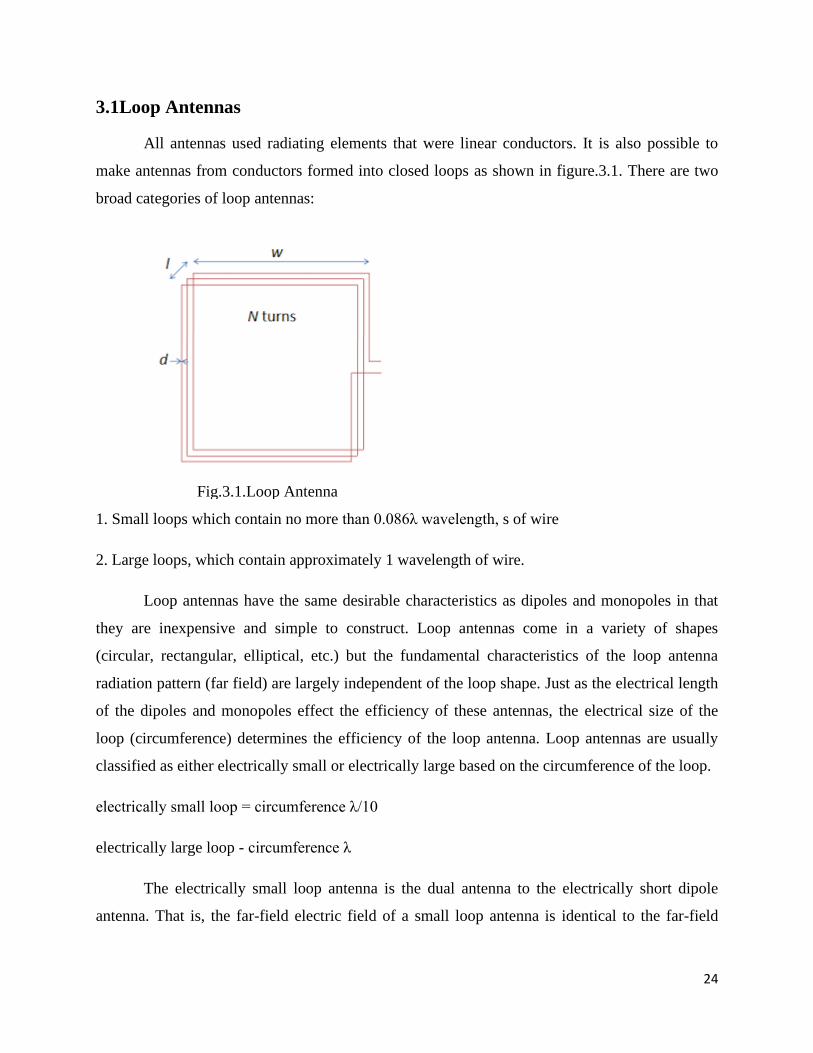
All antennas used radiating elements that were linear conductors. It is also possible to

make antennas from conductors formed into closed loops as shown in figure.3.1. There are two

broad categories of loop antennas:

1. Small loops which contain no more than 0.086λ wavelength, s of wire

2. Large loops, which contain approximately 1 wavelength of wire.

Loop antennas have the same desirable characteristics as dipoles and monopoles in that

they are inexpensive and simple to construct. Loop antennas come in a variety of shapes

(circular, rectangular, elliptical, etc.) but the fundamental characteristics of the loop antenna

radiation pattern (far field) are largely independent of the loop shape. Just as the electrical length

of the dipoles and monopoles effect the efficiency of these antennas, the electrical size of the

loop (circumference) determines the efficiency of the loop antenna. Loop antennas are usually

classified as either electrically small or electrically large based on the circumference of the loop.

electrically small loop = circumference λ/10

electrically large loop - circumference λ

The electrically small loop antenna is the dual antenna to the electrically short dipole

antenna. That is, the far-field electric field of a small loop antenna is identical to the far-field

Fig.3.1.Loop Antenna

25

magnetic field of the short dipole antenna and the far-field magnetic field of a small loop antenna

is identical to the far-field electric field of the short dipole antenna.

Advantages

1. A small loop is generally used as magnetic dipole.

2. A loop antenna has directional properties whereas a simple vertical antenna not has the same.

3. The induced e.m.f around the loop must be equal to the difference between the two vertical

sides only.

4. No e.m.f is produced in case of horizontal arms of a loop antenna.

5. The radiation pattern of the loop antenna does not depend upon the shape of the loop (for

small loops).

6. The currents are at same magnitude and phase, throughout the loop.

Disadvantages

1. Transmission efficiency of the loop is very poor.

2. It is suitable for low and medium frequencies and not for high frequencies.

3. In loop antenna, the two nulls of the pattern result in 180° ambiguity.

4. Loop antennas used as direction finders are unable to distinguish between bearing of a

Distant transmitter and its reciprocal bearing

3.2 Yagi-Uda Array

A Yagi-Uda array is an example of a parasitic array. Any element in an array which is not

connected to the source (in the case of a transmitting antenna) or the receiver (in the case of a

receiving antenna) is defined as a parasitic element. A parasitic array is any array which employs

parasitic elements. The general form of the N-element Yagi-Uda array is shown in figure 3.2.

26

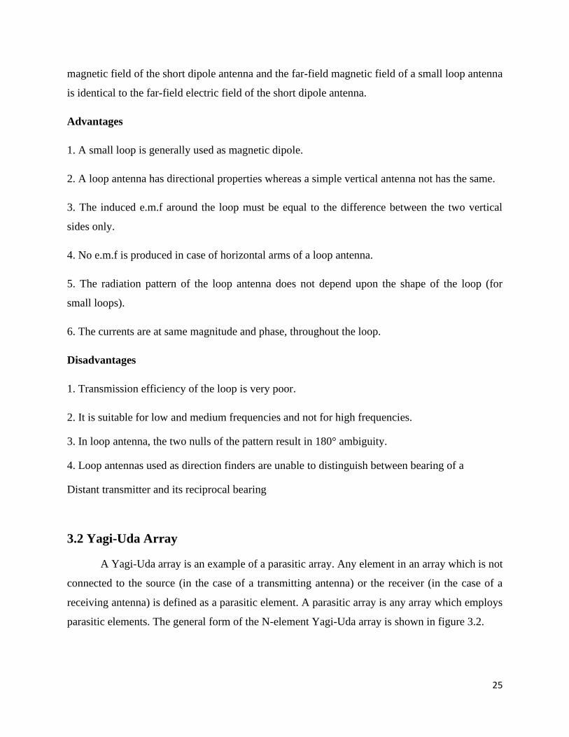
Driven element - usually a resonant dipole or folded dipole , folded dipoles are employed as

driven elements to increase the array input impedance

Reflector - slightly longer than the driven element so that it is inductive (its current lags that of

the driven element).Approximately 5 to 10 % longer than the driven element.

Director - slightly shorter than the driven element so that it is capacitive (its current leads that of

the driven element).Approximately 10 to 20 % shorter than the driven element), not necessarily

uniform.

Advantages

1. Light weight, Low cost

2.Simple construction

3.Unidirectional beam (front-to-back ratio)

4.Increased directivity over other simple wire antennas

5.Practical for use at HF (3-30 MHz), VHF (30-300 MHz), andUHF (300 MHz - 3 GHz)

Reflector spacing 0.1 to 0.258

3.3 V- Traveling Wave Antenna

The main beam of single electrically long wire guiding waves in one direction (traveling

wave segment) was found to be inclined at an angle relative to the axis of the wire as shown in

figure 3.3. Traveling wave antennas are typically formed by multiple traveling wave segments.

These traveling wave segments can be oriented such that the main beams of the component wires

combine to enhance the directivity of the overall antenna. A V- traveling wave antenna is formed

Fig.3.2.Loop Antenna

27

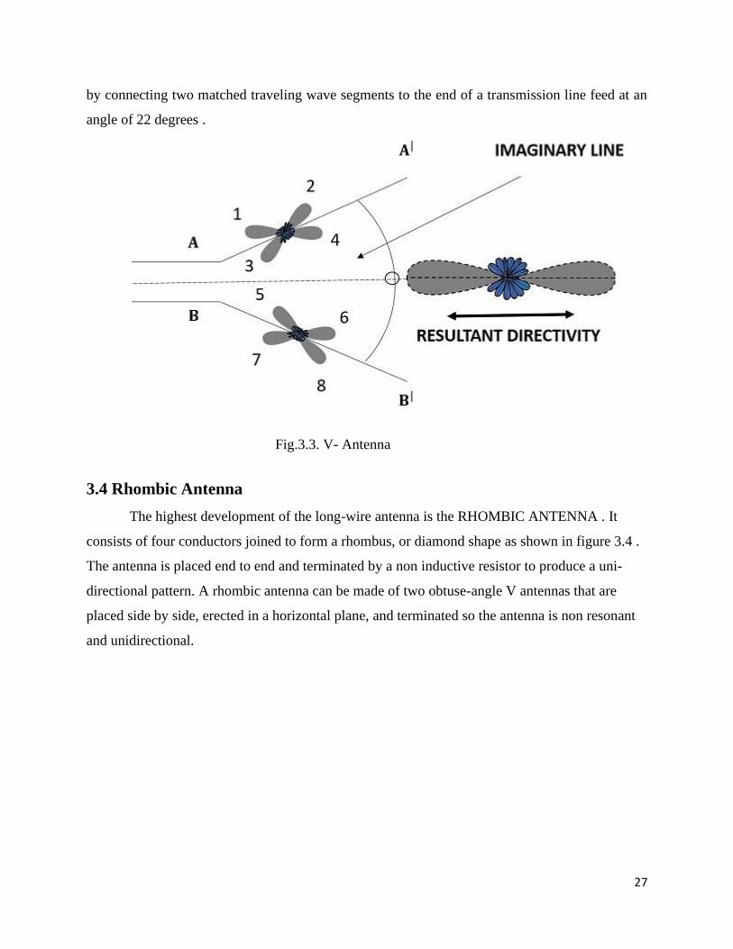
by connecting two matched traveling wave segments to the end of a transmission line feed at an

angle of 22 degrees .

3.4 Rhombic Antenna

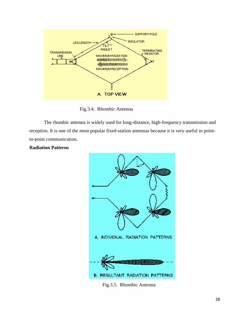
The highest development of the long-wire antenna is the RHOMBIC ANTENNA . It

consists of four conductors joined to form a rhombus, or diamond shape as shown in figure 3.4 .

The antenna is placed end to end and terminated by a non inductive resistor to produce a uni-

directional pattern. A rhombic antenna can be made of two obtuse-angle V antennas that are

placed side by side, erected in a horizontal plane, and terminated so the antenna is non resonant

and unidirectional.

Fig.3.3. V- Antenna

28

The rhombic antenna is widely used for long-distance, high-frequency transmission and

reception. It is one of the most popular fixed-station antennas because it is very useful in point-

to-point communication.

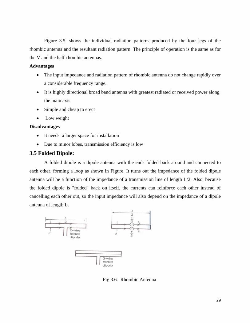
Radiation Patterns

Fig.3.5. Rhombic Antenna

Fig.3.4. Rhombic Antenna

29

Figure 3.5. shows the individual radiation patterns produced by the four legs of the

rhombic antenna and the resultant radiation pattern. The principle of operation is the same as for

the V and the half-rhombic antennas.

Advantages

• The input impedance and radiation pattern of rhombic antenna do not change rapidly over

a considerable frequency range.

• It is highly directional broad band antenna with greatest radiated or received power along

the main axis.

• Simple and cheap to erect

• Low weight

Disadvantages

• It needs a larger space for installation

• Due to minor lobes, transmission efficiency is low

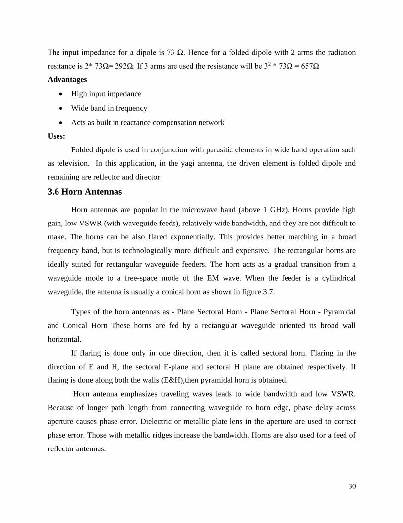
3.5 Folded Dipole:

A folded dipole is a dipole antenna with the ends folded back around and connected to

each other, forming a loop as shown in Figure. It turns out the impedance of the folded dipole

antenna will be a function of the impedance of a transmission line of length L/2. Also, because

the folded dipole is "folded" back on itself, the currents can reinforce each other instead of

cancelling each other out, so the input impedance will also depend on the impedance of a dipole

antenna of length L.

Fig.3.6. Rhombic Antenna

30

The input impedance for a dipole is 73 Ω. Hence for a folded dipole with 2 arms the radiation

resitance is 2* 73Ω= 292Ω. If 3 arms are used the resistance will be 32 * 73Ω = 657Ω

Advantages

• High input impedance

• Wide band in frequency

• Acts as built in reactance compensation network

Uses:

Folded dipole is used in conjunction with parasitic elements in wide band operation such

as television. In this application, in the yagi antenna, the driven element is folded dipole and

remaining are reflector and director

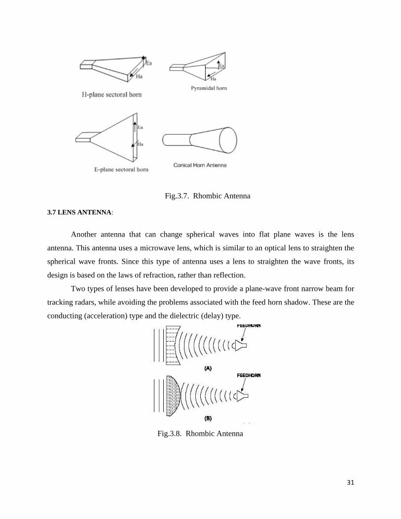
3.6 Horn Antennas

Horn antennas are popular in the microwave band (above 1 GHz). Horns provide high

gain, low VSWR (with waveguide feeds), relatively wide bandwidth, and they are not difficult to

make. The horns can be also flared exponentially. This provides better matching in a broad

frequency band, but is technologically more difficult and expensive. The rectangular horns are

ideally suited for rectangular waveguide feeders. The horn acts as a gradual transition from a

waveguide mode to a free-space mode of the EM wave. When the feeder is a cylindrical

waveguide, the antenna is usually a conical horn as shown in figure.3.7.

Types of the horn antennas as - Plane Sectoral Horn - Plane Sectoral Horn - Pyramidal

and Conical Horn These horns are fed by a rectangular waveguide oriented its broad wall

horizontal.

If flaring is done only in one direction, then it is called sectoral horn. Flaring in the

direction of E and H, the sectoral E-plane and sectoral H plane are obtained respectively. If

flaring is done along both the walls (E&H),then pyramidal horn is obtained.

Horn antenna emphasizes traveling waves leads to wide bandwidth and low VSWR.

Because of longer path length from connecting waveguide to horn edge, phase delay across

aperture causes phase error. Dielectric or metallic plate lens in the aperture are used to correct

phase error. Those with metallic ridges increase the bandwidth. Horns are also used for a feed of

reflector antennas.

31

Fig.3.7. Rhombic Antenna

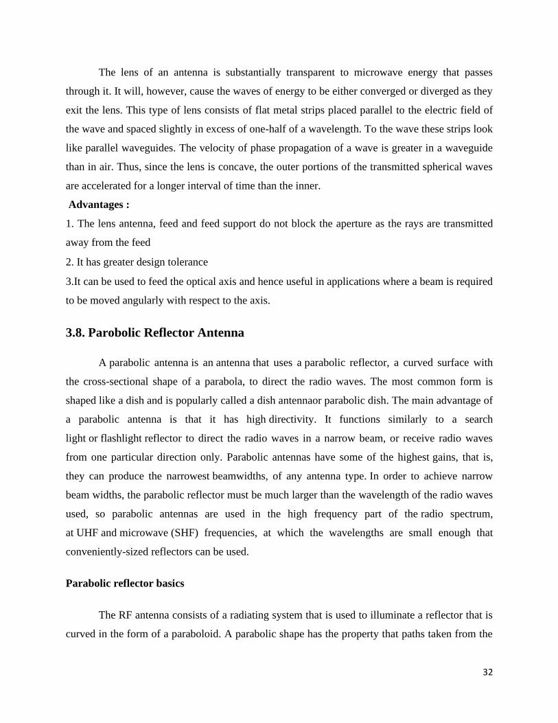
3.7 LENS ANTENNA:

Another antenna that can change spherical waves into flat plane waves is the lens

antenna. This antenna uses a microwave lens, which is similar to an optical lens to straighten the

spherical wave fronts. Since this type of antenna uses a lens to straighten the wave fronts, its

design is based on the laws of refraction, rather than reflection.

Two types of lenses have been developed to provide a plane-wave front narrow beam for

tracking radars, while avoiding the problems associated with the feed horn shadow. These are the

conducting (acceleration) type and the dielectric (delay) type.

Fig.3.8. Rhombic Antenna

32

The lens of an antenna is substantially transparent to microwave energy that passes

through it. It will, however, cause the waves of energy to be either converged or diverged as they

exit the lens. This type of lens consists of flat metal strips placed parallel to the electric field of

the wave and spaced slightly in excess of one-half of a wavelength. To the wave these strips look

like parallel waveguides. The velocity of phase propagation of a wave is greater in a waveguide

than in air. Thus, since the lens is concave, the outer portions of the transmitted spherical waves

are accelerated for a longer interval of time than the inner.

Advantages :

1. The lens antenna, feed and feed support do not block the aperture as the rays are transmitted

away from the feed

2. It has greater design tolerance

3.It can be used to feed the optical axis and hence useful in applications where a beam is required

to be moved angularly with respect to the axis.

3.8. Parobolic Reflector Antenna

A parabolic antenna is an antenna that uses a parabolic reflector, a curved surface with

the cross-sectional shape of a parabola, to direct the radio waves. The most common form is

shaped like a dish and is popularly called a dish antennaor parabolic dish. The main advantage of

a parabolic antenna is that it has high directivity. It functions similarly to a search

light or flashlight reflector to direct the radio waves in a narrow beam, or receive radio waves

from one particular direction only. Parabolic antennas have some of the highest gains, that is,

they can produce the narrowest beamwidths, of any antenna type. In order to achieve narrow

beam widths, the parabolic reflector must be much larger than the wavelength of the radio waves

used, so parabolic antennas are used in the high frequency part of the radio spectrum,

at UHF and microwave (SHF) frequencies, at which the wavelengths are small enough that

conveniently-sized reflectors can be used.

Parabolic reflector basics

The RF antenna consists of a radiating system that is used to illuminate a reflector that is

curved in the form of a paraboloid. A parabolic shape has the property that paths taken from the

33

feed point at the focus to the reflector and then outwards are in parallel, but more importantly the

paths taken are all the same length and therefore the outgoing waveform will form a plane wave

and the energy taken by all paths will all be in phase. This shape enables a very accurate beam to

be obtained. In this way, the feed system forms the actual radiating section of the antenna, and

the reflecting parabolic surface is purely passive.

When looking at parabolic reflector antenna systems there are a number of parameters

and terms that are of importance:

•Focus: The focus or focal point of the parabolic reflector is the point at which any

incoming signals are concentrated. When radiating from this point the signals will be reflected

by the reflecting surface and travel in a parallel beam and to provide the required gain and beam

width.

•Vertex: This is the innermost point at the centre of the parabolic reflector.

•Focal length: The focal length of a parabolic antenna is the distance from its focus to its

vertex. Read more about the focal length

Design

The operating principle of a parabolic antenna is that a point source of radio waves at

the focal point in front of a paraboloidal reflector of conductive material will be reflected into

a collimated plane wave beam along the axis of the reflector. Conversely, an incoming plane

wave parallel to the axis will be focused to a point at the focal point.

A typical parabolic antenna consists of a metal parabolic reflector with a small feed

antenna suspended in front of the reflector at its focus, pointed back toward the reflector. The

reflector is a metallic surface formed into a paraboloid of revolution and usually truncated in a

circular rim that forms the diameter of the antenna. In a transmitting antenna, radio

frequency current from a transmitter is supplied through a transmission line cable to the feed

antenna, which converts it into radio waves. The radio waves are emitted back toward the dish by

the feed antenna and reflect off the dish into a parallel beam. In a receiving antenna the incoming

radio waves bounce off the dish and are focused to a point at the feed antenna, which converts

them to electric currents which travel through a transmission line to the radio receiver.

34

Advantages:

• High gain: Parabolic reflector antennas are able to provide very high levels of gain. The

larger the 'dish' in terms of wavelengths, the higher the gain.

• High directivity: As with the gain, so too the parabolic reflector or dish antenna is able to

provide high levels of directivity. The higher the gain, the narrower the beam width. This can

be a significant advantage in applications where the power is only required to be directed

over a small area. This can prevent it, for example causing interference to other users, and

this is important when communicating with satellites because it enables satellites using the

same frequency bands to be separated by distance or more particularly by angle at the

antenna.

Disadvantages:

Like all forms of antenna, the parabolic reflector has its, limitations and drawbacks:

• Requires reflector and drive element: the parabolic reflector itself is only part of the

antenna. It requires a feed system to be placed at the focus of the parabolic reflector.

• Cost : The antenna needs to be manufactured with care. A paraboloid is needed to

reflect the radio signals which must be made carefully. In addition to this a feed system is also

required. This can add cost to the system

• Size: The antenna is not as small as some types of antenna, although many used for

satellite television reception are quite compact.

Parabolic reflector antenna applications

There are many areas in which the parabolic / dish antenna may be used. Its performance

enables it to be used almost exclusively in some areas.

• Direct broadcast television: Direct broadcast or satellite television has become a major

form of distribution for television material. The wide and controllable coverage areas

available combined with the much larger bandwidths for more channels available mean

that satellite television is very attractive.

35

• Satellite communications: Many satellite uplinks, or those for communication satellites

require high levels of gain to ensure the optimum signal conditions and that transmitted

power from the ground does not affect other satellites in close angular proximity. Again

the ideal antenna for most applications is the parabolic reflector antenna.

• Aperture : The aperture of a parabolic reflector is what may be termed its "opening" or

the area which it covers. For a circular reflector, this is described by its diameter. It can

be likened to the aperture of an optical lens.

• Gain: The gain of the parabolic reflector is one of the key parameters and it depends on

a number of factors including the diameter of the dish, wavelength and other factors.

• Feed systems: The parabolic reflector or dish antenna can be fed in a variety of ways.

Axial or front feed, off axis, Cassegrain, and Gregorian are the four main methods. Read

more about Parabolic reflector feed types.

Parabolic reflector feed types

There are several different types of parabolic reflector feed systems that can be used. Each

has its own characteristics that can be matched to the requirements of the application.

• Focal feed - often also known as axial or front feed system

• Cassegrain feed system

• Gregorian feed system

• Off Axis or offset feed

Focal feed system

The parabolic reflector or dish antenna consists of a radiating element which may be a

simple dipole or a waveguide horn antenna as shown in figure .3.9. This is placed at the focal

point of the parabolic reflecting surface. The energy from the radiating element is arranged so

that it illuminates the reflecting surface. Once the energy is reflected it leaves the antenna system

in a narrow beam. As a result considerable levels of gain can be achieved.

Achieving this is not always easy because it is dependent upon the radiator that is used.

For lower frequencies a dipole element is often employed whereas at higher frequencies a

36

circular waveguide may be used. In fact the circular waveguide provides one of the optimum

sources of illumination.

Fig.3.9.Diagram of a focal feed parabolic reflector antenna

The focal feed system is one of the most widely used feed system for larger parabolic

reflector antennas as it is straightforward. The major disadvantage is that the feed and its

supports block some of the beam, and this typically limits the aperture efficiency to only about

55 to 60%.

Cassegrain feed system

The Cassegrain feed system, although requiring a second reflecting surface has the

advantage that the overall length of the dish antenna between the two reflectors is shorter than

the length between the radiating element and the parabolic reflector as shown in figure.3.10 .This

is because there is a reflection in the focusing of the signal which shortens the physical length.

This can be an advantage in some systems.

Fig.3.10.Diagram of a Cassegrain feed parabolic reflector or dish antenna

37

Typical efficiency levels of 65 to 70% can be achieved using this form of parabolic

reflector feed system.The Cassegrain parabolic reflector antenna design and feed system gains its

name because the basic concept was adapted from the Cassegrain telescope. This was reflecting

telescope which was developed around 1672 and attributed to French priest Laurent Cassegrain.

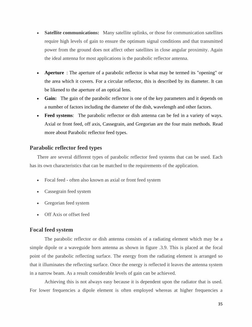
Gregorian parabolic reflector feed

The Gregorian parabolic reflector feed technique is very similar to the Cassegrain design.

The major difference is that except that the secondary reflector is concave or more correctly

ellipsoidal in shape as shown in figure.3.11 .

Fig.3.11.Diagram of a Gregorian feed parabolic reflector or dish antenna

Typical aperture efficiency levels of over 70% can be achieved because the system is able

to provide a better illumination of all of the reflector surface.

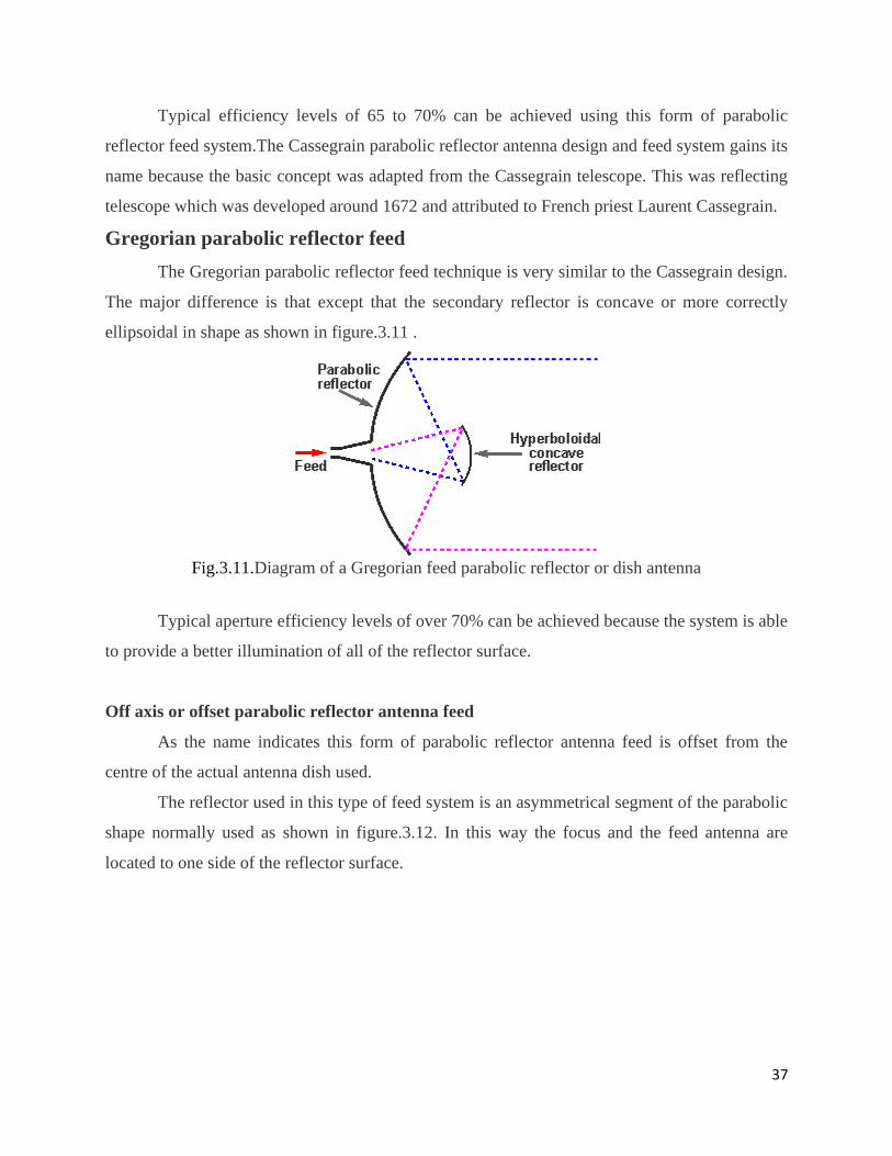
Off axis or offset parabolic reflector antenna feed

As the name indicates this form of parabolic reflector antenna feed is offset from the

centre of the actual antenna dish used.

The reflector used in this type of feed system is an asymmetrical segment of the parabolic

shape normally used as shown in figure.3.12. In this way the focus and the feed antenna are

located to one side of the reflector surface.

38

Fig.3.12.Diagram of an Offset feed parabolic reflector or dish antenna

The advantage of using this approach to the parabolic reflector feed system is to move the

feed structure out of the beam path. In this way it does not block the beam.

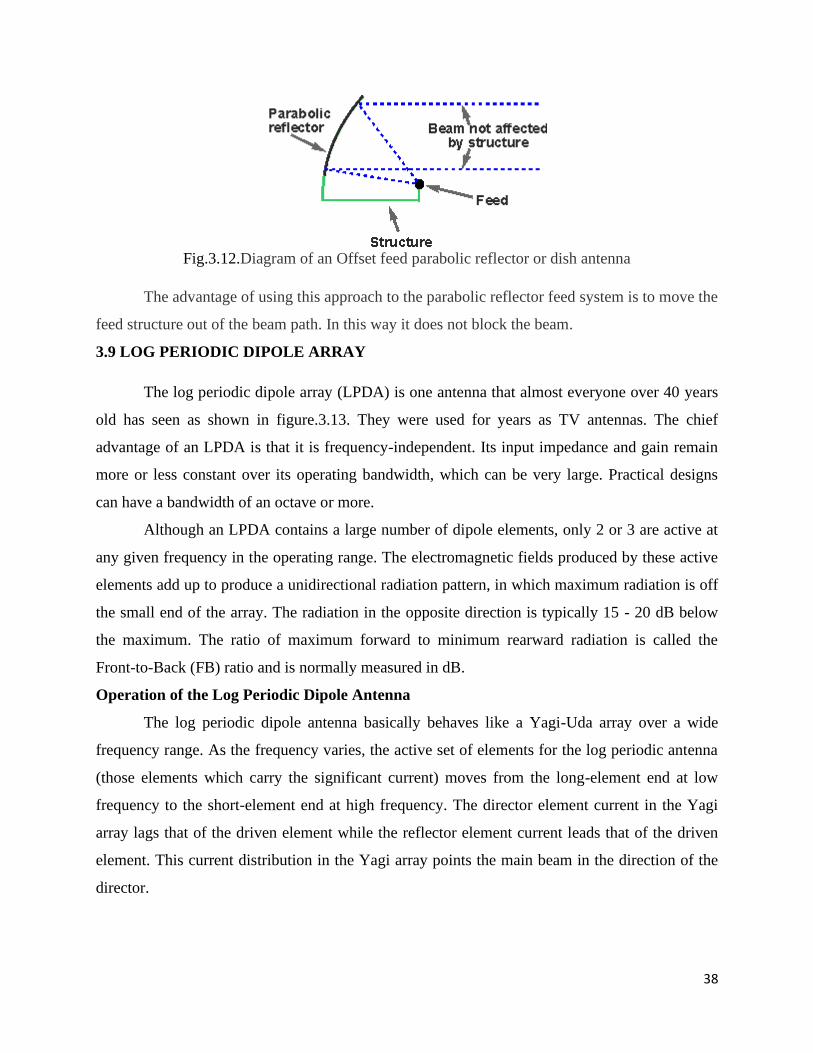
3.9 LOG PERIODIC DIPOLE ARRAY

The log periodic dipole array (LPDA) is one antenna that almost everyone over 40 years

old has seen as shown in figure.3.13. They were used for years as TV antennas. The chief

advantage of an LPDA is that it is frequency-independent. Its input impedance and gain remain

more or less constant over its operating bandwidth, which can be very large. Practical designs

can have a bandwidth of an octave or more.

Although an LPDA contains a large number of dipole elements, only 2 or 3 are active at

any given frequency in the operating range. The electromagnetic fields produced by these active

elements add up to produce a unidirectional radiation pattern, in which maximum radiation is off

the small end of the array. The radiation in the opposite direction is typically 15 - 20 dB below

the maximum. The ratio of maximum forward to minimum rearward radiation is called the

Front-to-Back (FB) ratio and is normally measured in dB.

Operation of the Log Periodic Dipole Antenna

The log periodic dipole antenna basically behaves like a Yagi-Uda array over a wide

frequency range. As the frequency varies, the active set of elements for the log periodic antenna

(those elements which carry the significant current) moves from the long-element end at low

frequency to the short-element end at high frequency. The director element current in the Yagi

array lags that of the driven element while the reflector element current leads that of the driven

element. This current distribution in the Yagi array points the main beam in the direction of the

director.

39

Fig.3.13.Log Periodic Dipole antenna

In order to obtain the same phasing in the log periodic antenna with all of the elements in

parallel, the source would have to be located on the long-element end of the array.The log

periodic dipole array must be driven from the short element end. But this arrangement gives the

exact opposite phasing required to point the beam in the direction of the shorter elements. It can

be shown that by alternating the connections from element to element, the phasing of the log

periodic dipole elements points the beam in the proper direction.

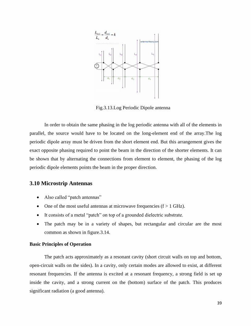
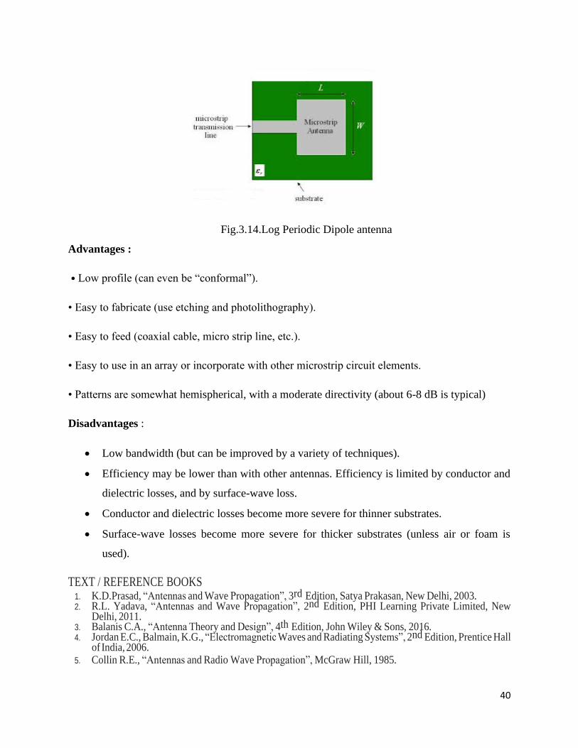
3.10 Microstrip Antennas

• Also called “patch antennas”

• One of the most useful antennas at microwave frequencies (f > 1 GHz).

• It consists of a metal “patch” on top of a grounded dielectric substrate.

• The patch may be in a variety of shapes, but rectangular and circular are the most

common as shown in figure.3.14.

Basic Principles of Operation

The patch acts approximately as a resonant cavity (short circuit walls on top and bottom,

open-circuit walls on the sides). In a cavity, only certain modes are allowed to exist, at different

resonant frequencies. If the antenna is excited at a resonant frequency, a strong field is set up

inside the cavity, and a strong current on the (bottom) surface of the patch. This produces

significant radiation (a good antenna).

40

Fig.3.14.Log Periodic Dipole antenna

Advantages :

• Low profile (can even be “conformal”).

• Easy to fabricate (use etching and photolithography).

• Easy to feed (coaxial cable, micro strip line, etc.).

• Easy to use in an array or incorporate with other microstrip circuit elements.

• Patterns are somewhat hemispherical, with a moderate directivity (about 6-8 dB is typical)

Disadvantages :

• Low bandwidth (but can be improved by a variety of techniques).

• Efficiency may be lower than with other antennas. Efficiency is limited by conductor and

dielectric losses, and by surface-wave loss.

• Conductor and dielectric losses become more severe for thinner substrates.

• Surface-wave losses become more severe for thicker substrates (unless air or foam is

used).

TEXT / REFERENCE BOOKS 1. K.D.Prasad, “Antennas and Wave Propagation”, 3rd Edition, Satya Prakasan, New Delhi, 2003. 2. R.L. Yadava, “Antennas and Wave Propagation”, 2nd Edition, PHI Learning Private Limited, New

Delhi, 2011. 3. Balanis C.A., “Antenna Theory and Design”, 4th Edition, John Wiley & Sons, 2016. 4. Jordan E.C., Balmain, K.G., “Electromagnetic Waves and Radiating Systems”, 2nd Edition, Prentice Hall

of India, 2006. 5. Collin R.E., “Antennas and Radio Wave Propagation”, McGraw Hill, 1985.

41

PART A

1. List the advantages of Rhombic Antenna?

2. List out the uses of loop antenna?

3 .Evaluate the elements of Yagi-Uda Antenna?

4. Enumerate the application of Horn antenna?

5.List out high frequency antennas.

6. Explain grounded antennas?

7. Estimate the loop antennas?

8. Give the types of horn antenna.

9. Evaluate log periodic antenna?

10. List the advantages of parabolic reflectors?

PART B

1.Describe the construction, principle of operation and design of rhombic antenna.

2.Explain the principle of operation of Log-Periodic antennas and its applications

3. Illustrate the working principle of loop antenna, with neat sketch

4. Categorize the various feeding techniques for parabolic reflector antenna

5. Demonstrate the operation of rectangular microstrip antenna

6. Estimate the principle of operation of horn antenna with neat sketch

7. Determine a three element yagi-uda antenna which operates at 5 GHz in free space

8. Estimate a detailed account of antennas used for high, medium and low frequency

applications.

9. Illustrate rhombic antenna with maximum field intensity design with a neat sketch.

10. Analyze the construction and working of frequency independent antenna and give their

applications.

42

UNIT – IV – Propagation- SECA1504

43

4.1.FACTORS AFFECTING THE RADIO WAVES PROPAGATION

There exist a number of factors which affect the propagation of radio waves in actual

environment. The most important of these are –

(a) Spherical shape of the earth:- since the radio waves travel in a straight line path in free space,

communication between any two points on the surface of earth is limited by the distance to

horizon. Therefore, for establishing a communication link beyond the horizon, the radio waves

need to undergo a change in the direction of propagation. Several mechanisms can be made use

of to effect the change.

(B) The atmosphere:- The earth's atmosphere extends all the way up to about 600 km. The

atmosphere is divided into several layers, viz., troposphere, stratosphere, mesosphere, and

ionosphere. The propagation of the radio waves near the surface of earth is affected mostly by

the troposphere which extends up to height of 8-15 km. Higher up in the atmosphere; it is the

ionosphere which interacts with radio waves.

(C) Interaction with the objects on the ground:- The radio waves travelling close to the surface of

earth encounter many obstacles such as building, trees, hills, valleys, water bodies, etc. The

interaction of such objects with the radio waves is mostly manifested as the phenomena of

reflection, refraction, diffraction, and scattering.

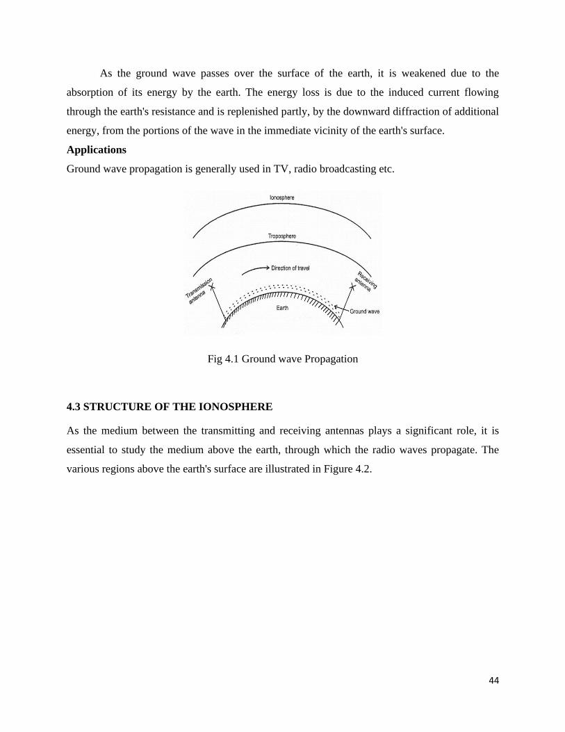
4.2. GROUND WAVE PROPAGATION

The ground wave is a wave that is guided along the surface of the earth just as an

electromagnetic wave is guided by a wave guide or transmission line as shown in figure 4.1. This

ground wave propagation takes place around the curvature of the earth in the frequency bands up

to 2 MHz. This also called as surface wave propagation The ground wave is vertically polarized,

as any horizontal component of the E field in contact with the earth is short-circuited by it. In

this mode, the wave glides over the surface of the earth and induces charges in the earth which

travel with the wave, thus constituting a current, while carrying this current, the earth acts as a

leaky capacitor. Hence it can be represented by a resistance or conductance shunted by a

capacitive reactance.

44

As the ground wave passes over the surface of the earth, it is weakened due to the

absorption of its energy by the earth. The energy loss is due to the induced current flowing

through the earth's resistance and is replenished partly, by the downward diffraction of additional

energy, from the portions of the wave in the immediate vicinity of the earth's surface.

Applications

Ground wave propagation is generally used in TV, radio broadcasting etc.

Fig 4.1 Ground wave Propagation

4.3 STRUCTURE OF THE IONOSPHERE

As the medium between the transmitting and receiving antennas plays a significant role, it is

essential to study the medium above the earth, through which the radio waves propagate. The

various regions above the earth's surface are illustrated in Figure 4.2.

45

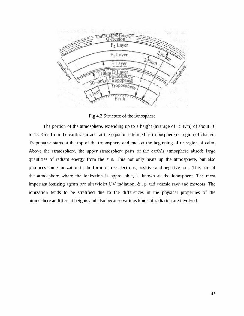
Fig 4.2 Structure of the ionosphere

The portion of the atmosphere, extending up to a height (average of 15 Km) of about 16

to 18 Kms from the earth's surface, at the equator is termed as troposphere or region of change.

Tropopause starts at the top of the troposphere and ends at the beginning of or region of calm.

Above the stratosphere, the upper stratosphere parts of the earth’s atmosphere absorb large

quantities of radiant energy from the sun. This not only heats up the atmosphere, but also

produces some ionization in the form of free electrons, positive and negative ions. This part of

the atmosphere where the ionization is appreciable, is known as the ionosphere. The most

important ionizing agents are ultraviolet UV radiation, ά , β and cosmic rays and meteors. The

ionization tends to be stratified due to the differences in the physical properties of the

atmosphere at different heights and also because various kinds of radiation are involved.

46

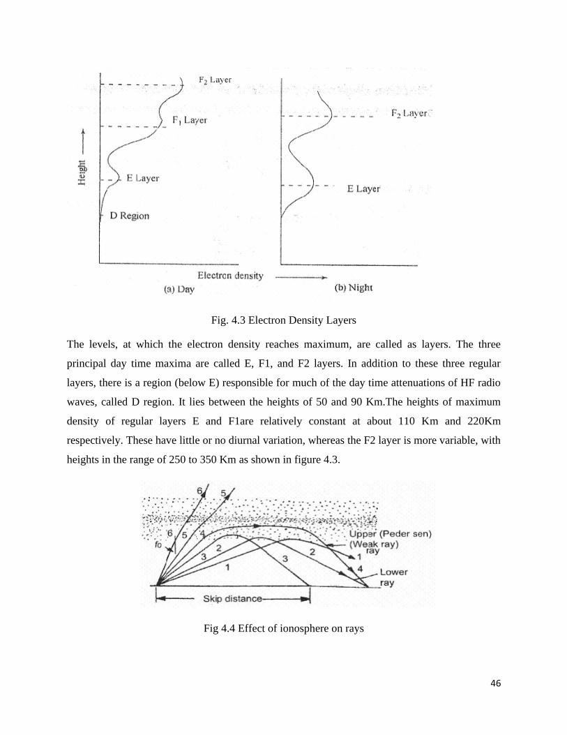
Fig. 4.3 Electron Density Layers

The levels, at which the electron density reaches maximum, are called as layers. The three

principal day time maxima are called E, F1, and F2 layers. In addition to these three regular

layers, there is a region (below E) responsible for much of the day time attenuations of HF radio

waves, called D region. It lies between the heights of 50 and 90 Km.The heights of maximum

density of regular layers E and F1are relatively constant at about 110 Km and 220Km

respectively. These have little or no diurnal variation, whereas the F2 layer is more variable, with

heights in the range of 250 to 350 Km as shown in figure 4.3.

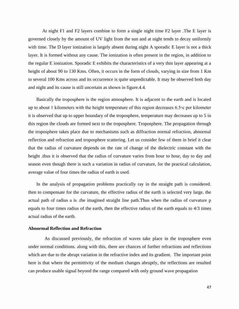
Fig 4.4 Effect of ionosphere on rays

47

At night F1 and F2 layers combine to form a single night time F2 layer .The E layer is

governed closely by the amount of UV light from the sun and at night tends to decay uniformly

with time. The D layer ionization is largely absent during night A sporadic E layer is not a thick

layer. It is formed without any cause. The ionization is often present in the region, in addition to

the regular E ionization. Sporadic E exhibits the characteristics of a very thin layer appearing at a

height of about 90 to 130 Kms. Often, it occurs in the form of clouds, varying in size from 1 Km

to several 100 Kms across and its occurrence is quite unpredictable. It may be observed both day

and night and its cause is still uncertain as shown in figure.4.4.

Basically the troposphere is the region atmosphere. It is adjacent to the earth and is located

up to about 1 kilometers with the height temperature of this region decreases 6.5c per kilometer

it is observed that up to upper boundary of the troposphere, temperature may decreases up to 5 in

this region the clouds are formed next to the troposphere. Troposphere. The propagation through

the troposphere takes place due to mechanisms such as diffraction normal refraction, abnormal

reflection and refraction and troposphere scattering. Let us consider few of them in brief it clear

that the radius of curvature depends on the rate of change of the dielectric constant with the

height .thus it is observed that the radius of curvature varies from hour to hour, day to day and

season even though there is such a variation in radius of curvature, for the practical calculation,

average value of four times the radius of earth is used.

In the analysis of propagation problems practically ray in the straight path is considered.

then to compensate for the curvature, the effective radius of the earth is selected very large. the

actual path of radius a is .the imagined straight line path.Thus when the radius of curvature p

equals to four times radius of the earth, then the effective radius of the earth equals to 4/3 times

actual radius of the earth.

Abnormal Reflection and Refraction

As discussed previously, the refraction of waves take place in the troposphere even

under normal conditions. along with this, there are chances of further refractions and reflections

which are due to the abrupt variation in the refractive index and its gradient. The important point

here is that where the permittivity of the medium changes abruptly, the reflections are resulted

can produce usable signal beyond the range compared with only ground wave propagation

48

Reflection

Reflection occurs when an electromagnetic wave falls on an object, which has very large

dimensions as compared to the wavelength of the propagating wave. For example, such objects

can be the earth, buildings and walls. When a radio wave falls on another medium having

different electrical properties, a part of it is transmitter into it, while some energy is reflected

back. Let us see some special cases. If the medium on which the EM wave is incident is a

dielectric, some energy is reflected back and some energy is transmitted. If the medium is a

perfect conductor, all energy is reflected back to the first medium. The amount of energy that is

reflected back depends on the polarization of the EM wave particular case of interest arises in

parallel polarization, when no reflection occurs in the medium of origin. This would occur, when

the incident angle would be such that the reflection coefficient is equal to zero. This angle is the

Brewster’s angle.

Mechanism of ionospheric propagation _reflection &refraction

Ionospheric propagation involves reflection of wave by the ionosphere .In actual

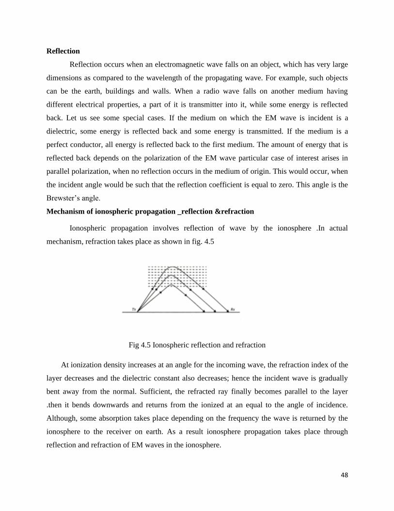
mechanism, refraction takes place as shown in fig. 4.5

Fig 4.5 Ionospheric reflection and refraction

At ionization density increases at an angle for the incoming wave, the refraction index of the

layer decreases and the dielectric constant also decreases; hence the incident wave is gradually

bent away from the normal. Sufficient, the refracted ray finally becomes parallel to the layer

.then it bends downwards and returns from the ionized at an equal to the angle of incidence.

Although, some absorption takes place depending on the frequency the wave is returned by the

ionosphere to the receiver on earth. As a result ionosphere propagation takes place through

reflection and refraction of EM waves in the ionosphere.

49

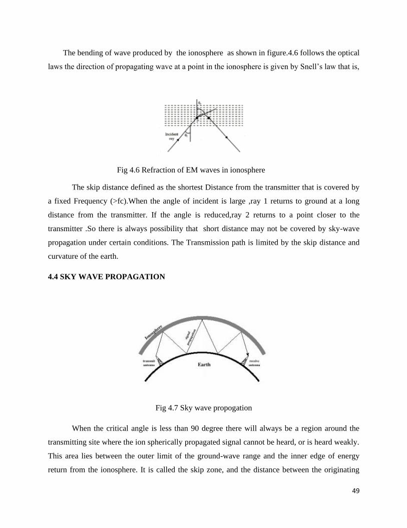
The bending of wave produced by the ionosphere as shown in figure.4.6 follows the optical

laws the direction of propagating wave at a point in the ionosphere is given by Snell’s law that is,

Fig 4.6 Refraction of EM waves in ionosphere

The skip distance defined as the shortest Distance from the transmitter that is covered by

a fixed Frequency (>fc).When the angle of incident is large ,ray 1 returns to ground at a long

distance from the transmitter. If the angle is reduced,ray 2 returns to a point closer to the

transmitter .So there is always possibility that short distance may not be covered by sky-wave

propagation under certain conditions. The Transmission path is limited by the skip distance and

curvature of the earth.

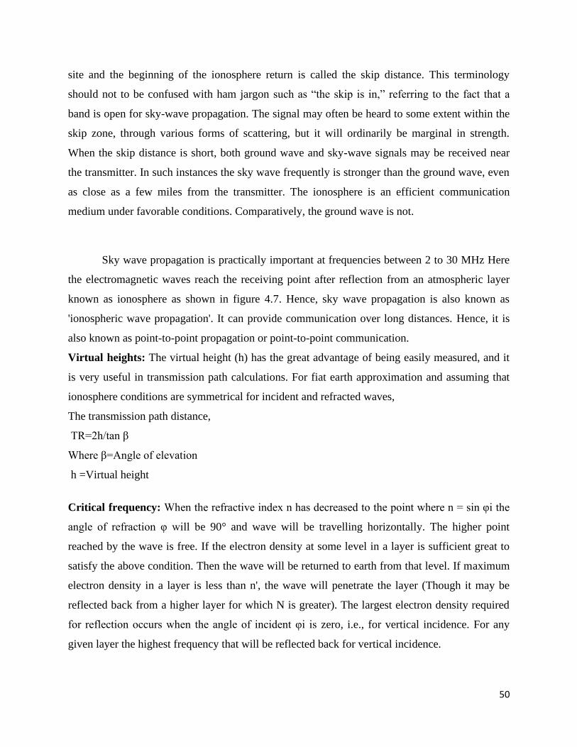
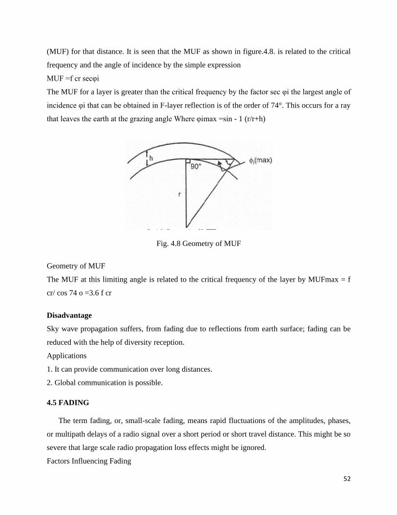
4.4 SKY WAVE PROPAGATION

Fig 4.7 Sky wave propogation

When the critical angle is less than 90 degree there will always be a region around the

transmitting site where the ion spherically propagated signal cannot be heard, or is heard weakly.

This area lies between the outer limit of the ground-wave range and the inner edge of energy

return from the ionosphere. It is called the skip zone, and the distance between the originating

50

site and the beginning of the ionosphere return is called the skip distance. This terminology

should not to be confused with ham jargon such as “the skip is in,” referring to the fact that a

band is open for sky-wave propagation. The signal may often be heard to some extent within the

skip zone, through various forms of scattering, but it will ordinarily be marginal in strength.

When the skip distance is short, both ground wave and sky-wave signals may be received near

the transmitter. In such instances the sky wave frequently is stronger than the ground wave, even

as close as a few miles from the transmitter. The ionosphere is an efficient communication

medium under favorable conditions. Comparatively, the ground wave is not.

Sky wave propagation is practically important at frequencies between 2 to 30 MHz Here

the electromagnetic waves reach the receiving point after reflection from an atmospheric layer

known as ionosphere as shown in figure 4.7. Hence, sky wave propagation is also known as

'ionospheric wave propagation'. It can provide communication over long distances. Hence, it is

also known as point-to-point propagation or point-to-point communication.

Virtual heights: The virtual height (h) has the great advantage of being easily measured, and it

is very useful in transmission path calculations. For fiat earth approximation and assuming that

ionosphere conditions are symmetrical for incident and refracted waves,

The transmission path distance,

TR=2h/tan β

Where β=Angle of elevation

h =Virtual height

Critical frequency: When the refractive index n has decreased to the point where n = sin φi the

angle of refraction φ will be 90° and wave will be travelling horizontally. The higher point

reached by the wave is free. If the electron density at some level in a layer is sufficient great to

satisfy the above condition. Then the wave will be returned to earth from that level. If maximum

electron density in a layer is less than n', the wave will penetrate the layer (Though it may be

reflected back from a higher layer for which N is greater). The largest electron density required

for reflection occurs when the angle of incident φi is zero, i.e., for vertical incidence. For any

given layer the highest frequency that will be reflected back for vertical incidence.

51

The characteristics of the ionosphere layers are usually described in terms of their virtual

heights and critical frequencies, as these quantities can be readily measured. The virtual height is

the height that would be reached by a short pulse of energy showing the same time delay as the

actual pulse reflected from the layer travelling with the speed of light. The virtual height is

always greater than the true height of reflection, because the interchange of energy taking place

between the wave and electrons of the ionosphere causes the velocity of propagation to be

reduced. The extent of this difference is influenced, by the electron distributions in the regions

below the level of reflection. It is usually very small, but on occasions may be as large as 100

Kms or so.

The critical frequency is the highest frequency that is returned by a layer at vertical

incidence. For regular layers,

fc =√max electron density in the layer

i.e. fc =√Ne

The critical frequencies of the E and F1 layers primarily depend on the zenith angle of the sun. It,

therefore, follows a regular diurnal cycle, being maximum at noon and tapering off an either

side. The fc of the F2 layer shows much larger seasonal variation and also changes more from

day to day. It can be seen that the critical frequencies of the regular layers decrease greatly

during night as a result of recombination in the absence of solar radiation. But the fc of sporadic

E shows regular variation throughout the day and night suggesting that sporadic E is affected

strongly by factors other than solar radiation. There is a long term variation in all ionosphere

characteristics closely associated with the 11 year sunspot cycle. From the minimum to

maximum of the cycle, fc of F2 layer varies from about 6 to 11 MHz (ratio of 1:1.8), fc of E

layer varies from 3.1 to 3.8 MHz (a ratio of mere 1 to 1.2). Long term predictions of ionosphere

characteristics are based on predictions of the sunspot number.

Maximum usable Frequency: Although the critical frequency for any layer represents the

highest frequency that will be reflected back from that layer at vertical incidence, it is not the

highest frequency that can be reflected from the layer. The highest frequency that can be

reflected depends also upon the angle of incidence, and hence, for a given layer height, upon the

distance between the transmitting and receiving points. The maximum, frequency that can be

reflected back for a given distance of transmission is called the maximum usable frequency

52

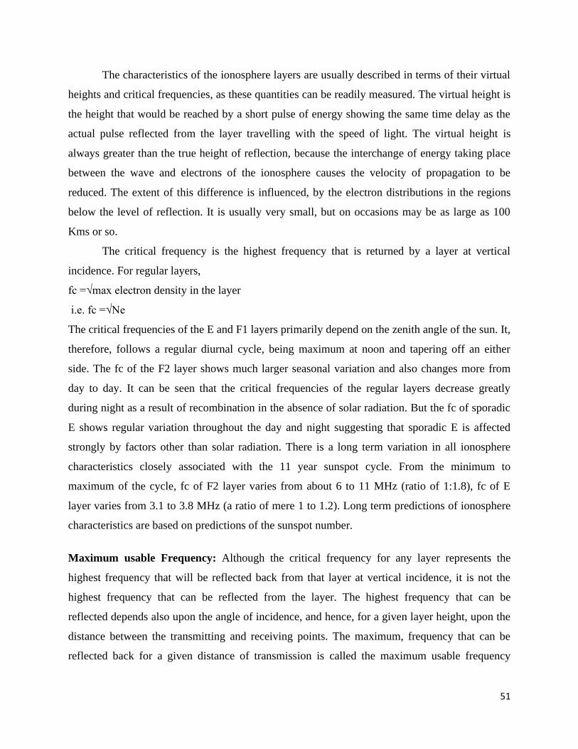
(MUF) for that distance. It is seen that the MUF as shown in figure.4.8. is related to the critical

frequency and the angle of incidence by the simple expression

MUF =f cr secφi

The MUF for a layer is greater than the critical frequency by the factor sec φi the largest angle of

incidence φi that can be obtained in F-layer reflection is of the order of 74°. This occurs for a ray

that leaves the earth at the grazing angle Where φimax =sin - 1 (r/r+h)

Fig. 4.8 Geometry of MUF

Geometry of MUF

The MUF at this limiting angle is related to the critical frequency of the layer by MUFmax = f

cr/ cos 74 o =3.6 f cr

Disadvantage

Sky wave propagation suffers, from fading due to reflections from earth surface; fading can be

reduced with the help of diversity reception.

Applications

1. It can provide communication over long distances.

2. Global communication is possible.

4.5 FADING

The term fading, or, small-scale fading, means rapid fluctuations of the amplitudes, phases,

or multipath delays of a radio signal over a short period or short travel distance. This might be so

severe that large scale radio propagation loss effects might be ignored.

Factors Influencing Fading

53

The following physical factors influence small-scale fading in the radio propagation channel:

(1) Multipath propagation – Multipath is the propagation phenomenon that results in radio

signals reaching the receiving antenna by two or more paths. The effects of multipath include

constructive and destructive interference, and phase shifting of the signal.

(2) Speed of the mobile – The relative motion between the base station and the mobile results in

random frequency modulation due to different doppler shifts on each of the multipath

components.

(3) Speed of surrounding objects – If objects in the radio channel are in motion, they induce a

time varying Doppler shift on multipath components. If the surrounding objects move at a

greater rate than the mobile, then this effect dominates fading.

(4) Transmission Bandwidth of the signal – If the transmitted radio signal bandwidth is greater

than the “bandwidth” of the multipath channel (quantified by coherence bandwidth), the received

signal will be distorted.

Selective Fading

This type of fading produces serious distortion in modulated signal. Selective fading is important

at higher frequencies. Selective fading generally occurs in amplitude modulated signals. SSB

signals become less distorted compared to the AM signals due to selective fading.

Interference Fading

Interference fading occurs due to the variation in different layers of ionosphere region. This type

of fading is very serious and produces interference between the upper and lower rays of sky

wave propagation. Interference fading can be reduced with the help of frequency and space

diversity reception.

4.6 DIVERSITY RECEPTION

• To reduce fading effects, diversity reception techniques are used. Diversity means the

provision of two or more uncorrelated (independent) fading paths from transmitter to

receiver

• These uncorrelated signals are combined in a special way, exploiting the fact that it is

unlikely that all the paths are poor at the same time. The probability of outage is thus

reduced.

54

• Uncorrelated paths are created using polarization, space, frequency, and time diversity

Frequency Diversity

Different frequencies mean different wavelengths. The hope when using frequency diversity is

that the same physical multipath routes will not produce simultaneous deep fades at two separate

wavelengths.

Space Diversity

Deep multipath fade have unlucky occurrence when the receiving antenna is in exactly in the

‘wrong’ place. One method of reducing the likelihood of multipath fading is by using two

receive antennas and using a switch to select the better signal. If these are physically separated

then the probability of a deep fade occurring simultaneously at both of these antennas is

significantly reduced. ·

Angle Diversity: In this case the receiving antennas are co-located but have different principal

directions. ·

Polarization Diversity: This involves simultaneously transmitting and receiving on two

orthogonal polarizations (e.g. horizontal and vertical). The hope is that one polarization will be

less severely affected when the other experiences a deep fade. ·

Time Diversity: This will transmit the desired signal in different periods of time. The intervals

between transmissions of the same symbol should be at least the coherence time so that different

copies of the same symbol undergo independent fading.

4.7 FREE SPACE RADIO WAVE PROPAGATION

There are two basic ways of transmitting an electro-magnetic (EM) signal, through a guided

medium or through an unguided medium. Guided mediums such as coaxial cables and fiber optic

cables are far less hostile toward the information carrying EM signal than the wireless or the

unguided medium. It presents challenges and conditions which are unique for this kind of

transmissions. A signal, as it travels through the wireless channel, undergoes many kinds of

propagation effects such as reflection, diffraction and scattering, due to the presence of buildings,

55

mountains and other such obstructions. Reflection occurs when the EM waves impinge on

objects which are much greater than the wavelength of the traveling wave. Diffraction is a

phenomena occurring when the wave interacts with a surface having sharp irregularities.

Scattering occurs when the medium through the wave is traveling contains objects which are

much smaller than the wavelength of the EM wave. These varied phenomena’s lead to large

scale and small scale propagation losses. Due to the inherent randomness associated with such

channels they are best described with the help of statistical models. Models which predict the

mean signal strength for arbitrary transmitter receiver distances are termed as large scale

propagation models. These are termed so because they predict the average signal strength for

large Tx-Rx separations, typically for hundreds of kilometers.

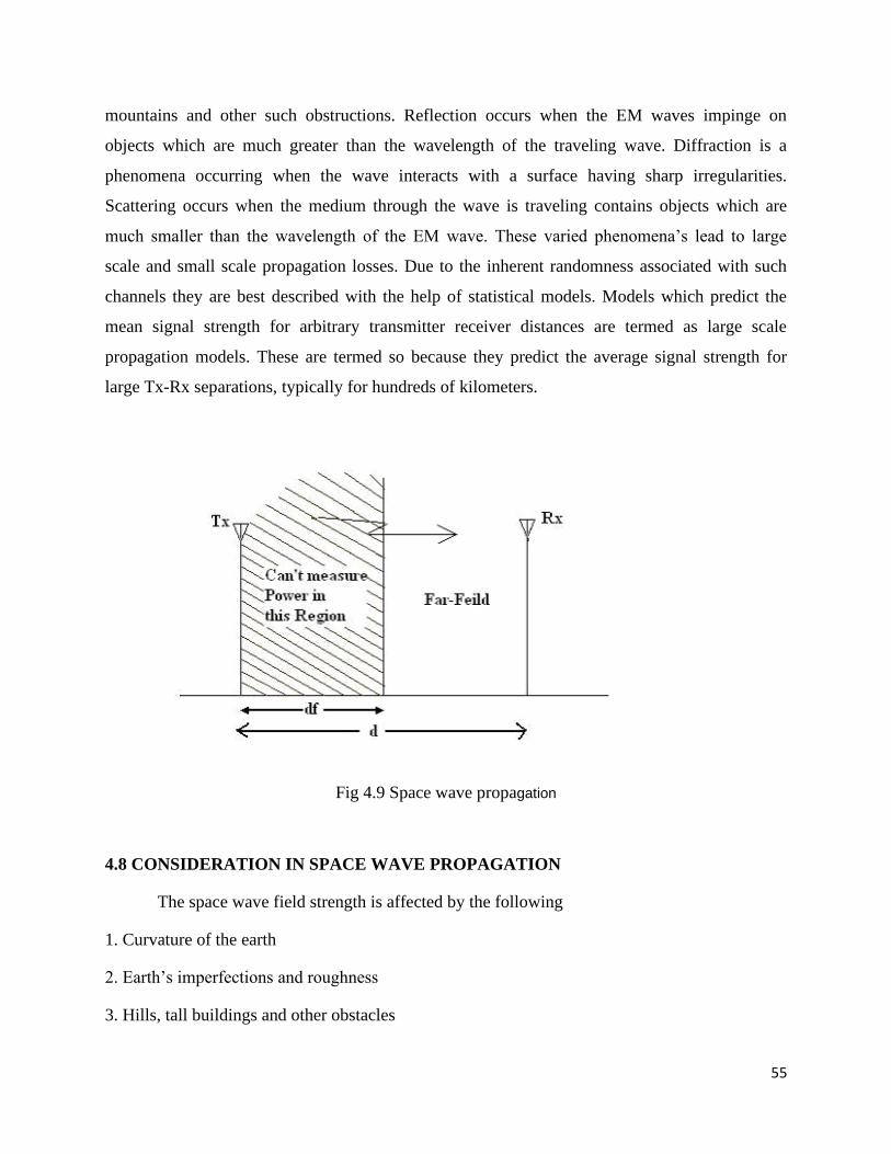
Fig 4.9 Space wave propagation

4.8 CONSIDERATION IN SPACE WAVE PROPAGATION

The space wave field strength is affected by the following

1. Curvature of the earth

2. Earth’s imperfections and roughness

3. Hills, tall buildings and other obstacles

56

4. Height above the earth.

5. Transition between ground and space wave

6. Polarization

4.9 ATMOSPHERIC EFFECTS IN SPACE WAVE PROPAGATION

There is a significant effect of the atmosphere through which the space wave

travels on the propagation. This is basically because of presence of gas molecules particularly of

a water vapor. Water vapor has a high dielectric constant and its presence causes the air of the

troposphere to have a dielectric constant and its presence causes the air of troposphere to have a

dielectric constant slightly greater than unity. the distribution of water vapor is not uniform

through out of the air and along with it the density of the air varies with height .As a

consequence of the dielectric constant and in turn the refractive index of air also depend upon the

height it is in general observed to be deceasing with increasing height gives rise to a variety of

phenomena like reflection,refraction ,scattering, duct transmission and fading of signals. The

behavior of the space wave under the different conditions can be better studied by changing the

co - ordinates in such a manner that the particular ray path of interest is a straight line instead of

a curve. for this , the radius of curvature of the earth is required to be simultaneously readjusted

to preserve the correct relative relation.

4.10 DUCT PROPAGATION

Duct propagation is phenomenon of propagation making use of the atmospheric duct region. The

duct region exits between two levels where the variation of modified refractive index with height

is minimum . It is also said to exist between a level .where the variation of modified refractive

index and a surface bounding the atmosphere. The higher frequencies or microwaves are

continuously reflected in the duct and reflected by the ground.So that they propagate around the

curvature for beyond the line of sight. This special refraction electromagnetic waves is called

super refraction and the process is called duct propagation. Duct propagation is also known as

super refraction. Consider the figure .4.10

57

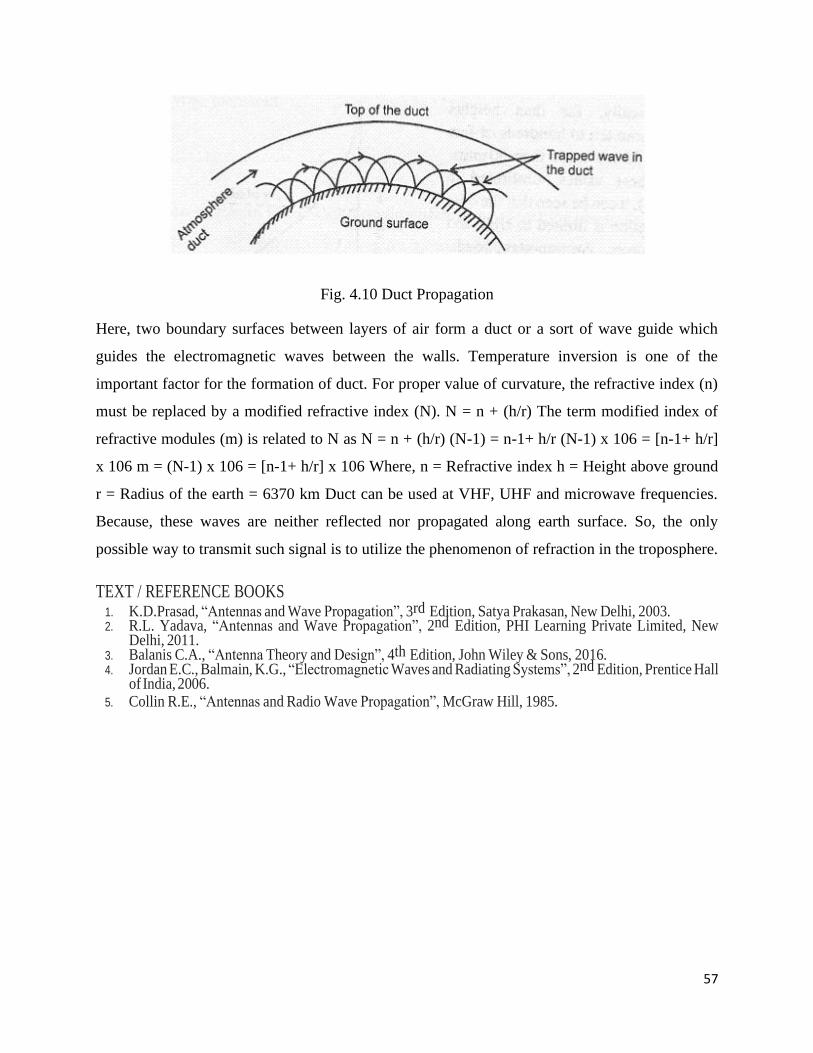
Fig. 4.10 Duct Propagation

Here, two boundary surfaces between layers of air form a duct or a sort of wave guide which

guides the electromagnetic waves between the walls. Temperature inversion is one of the

important factor for the formation of duct. For proper value of curvature, the refractive index (n)

must be replaced by a modified refractive index (N). N = n + (h/r) The term modified index of

refractive modules (m) is related to N as N = n + (h/r) (N-1) = n-1+ h/r (N-1) x 106 = [n-1+ h/r]

x 106 m = (N-1) x 106 = [n-1+ h/r] x 106 Where, n = Refractive index h = Height above ground

r = Radius of the earth = 6370 km Duct can be used at VHF, UHF and microwave frequencies.

Because, these waves are neither reflected nor propagated along earth surface. So, the only

possible way to transmit such signal is to utilize the phenomenon of refraction in the troposphere.

TEXT / REFERENCE BOOKS 1. K.D.Prasad, “Antennas and Wave Propagation”, 3rd Edition, Satya Prakasan, New Delhi, 2003. 2. R.L. Yadava, “Antennas and Wave Propagation”, 2nd Edition, PHI Learning Private Limited, New

Delhi, 2011. 3. Balanis C.A., “Antenna Theory and Design”, 4th Edition, John Wiley & Sons, 2016. 4. Jordan E.C., Balmain, K.G., “Electromagnetic Waves and Radiating Systems”, 2nd Edition, Prentice Hall

of India, 2006. 5. Collin R.E., “Antennas and Radio Wave Propagation”, McGraw Hill, 1985.

58

PART A

1. Explain fading?

2. Define skip distance.

3. Classify propagation of radio waves.

4. State diversity reception?

5. State MUF.

6. Analyze super refraction?

7. List the factors that affect the propagation of radio waves?

8. State duct propagation?

9. Interpret critical frequency?

10. Define Gyro frequency.

PART B

1. Demonstrate an expression for effective dielectric constant of the Ionosphere.

2. Illustrate the following : a) skip distance b) Fading c) Duct-wave propagation

3. Compare the space wave and sky wave propagation.

4. Give explanation about the Ground wave propagation.

5. Analyze and explain the mechanism of Ionospheric propagation and the different layers in it.

6. Interpret fading of signal and its types.

7. Demonstrate the expression for the refractive index of the ionosphere.

8. Summarize the effects of earth’s magnetic field on ionosphere radio wave propagation.

9. Illustrate the various diversity reception methods.

10. Demonstrate the troposphere and explain how ducts can be used for microwave propagation.

59

UNIT – V – Antenna Measurement-

SECA1504

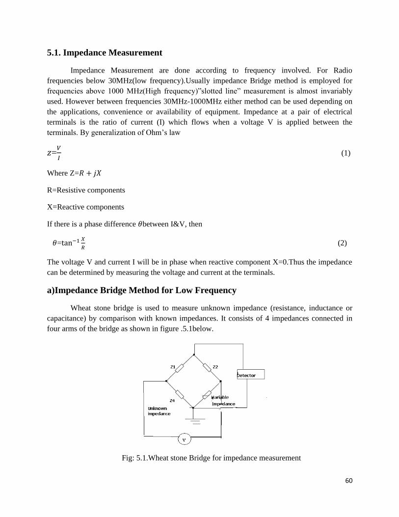
60

5.1. Impedance Measurement

Impedance Measurement are done according to frequency involved. For Radio

frequencies below 30MHz(low frequency).Usually impedance Bridge method is employed for

frequencies above 1000 MHz(High frequency)”slotted line” measurement is almost invariably

used. However between frequencies 30MHz-1000MHz either method can be used depending on

the applications, convenience or availability of equipment. Impedance at a pair of electrical

terminals is the ratio of current (I) which flows when a voltage V is applied between the

terminals. By generalization of Ohm’s law

𝑧=𝑉

𝐼 (1)

Where Z=𝑅 + 𝑗𝑋

R=Resistive components

X=Reactive components

If there is a phase difference 𝜃between I&V, then

𝜃=tan−1 𝑋

𝑅 (2)

The voltage V and current I will be in phase when reactive component X=0.Thus the impedance

can be determined by measuring the voltage and current at the terminals.

a)Impedance Bridge Method for Low Frequency

Wheat stone bridge is used to measure unknown impedance (resistance, inductance or

capacitance) by comparison with known impedances. It consists of 4 impedances connected in

four arms of the bridge as shown in figure .5.1below.

Fig: 5.1.Wheat stone Bridge for impedance measurement

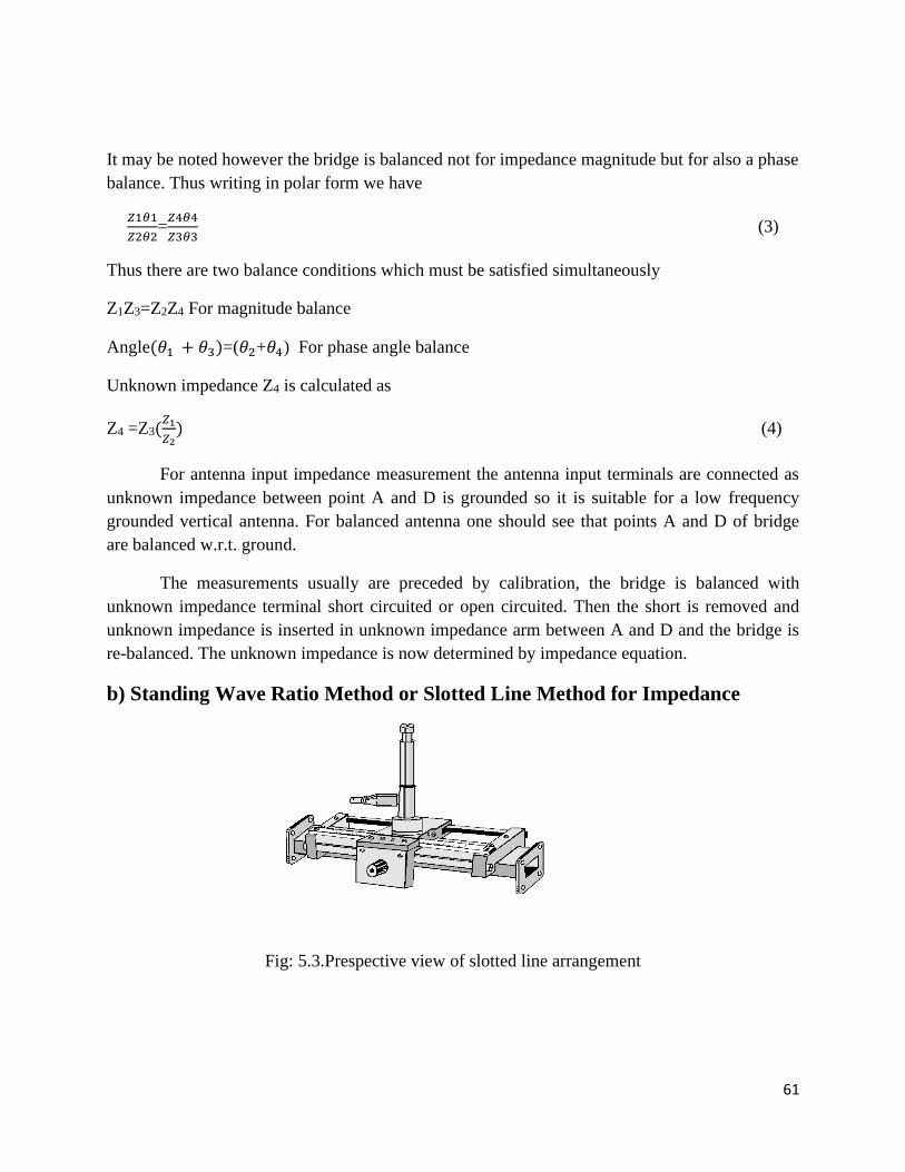
61

It may be noted however the bridge is balanced not for impedance magnitude but for also a phase

balance. Thus writing in polar form we have

𝑍1𝜃1

𝑍2𝜃2=

𝑍4𝜃4

𝑍3𝜃3 (3)

Thus there are two balance conditions which must be satisfied simultaneously

Z1Z3=Z2Z4 For magnitude balance

Angle(𝜃1 + 𝜃3)=(𝜃2+𝜃4) For phase angle balance

Unknown impedance Z4 is calculated as

Z4 =Z3(𝑍1

𝑍2) (4)

For antenna input impedance measurement the antenna input terminals are connected as

unknown impedance between point A and D is grounded so it is suitable for a low frequency

grounded vertical antenna. For balanced antenna one should see that points A and D of bridge

are balanced w.r.t. ground.

The measurements usually are preceded by calibration, the bridge is balanced with

unknown impedance terminal short circuited or open circuited. Then the short is removed and

unknown impedance is inserted in unknown impedance arm between A and D and the bridge is

re-balanced. The unknown impedance is now determined by impedance equation.

b) Standing Wave Ratio Method or Slotted Line Method for Impedance

Fig: 5.3.Prespective view of slotted line arrangement

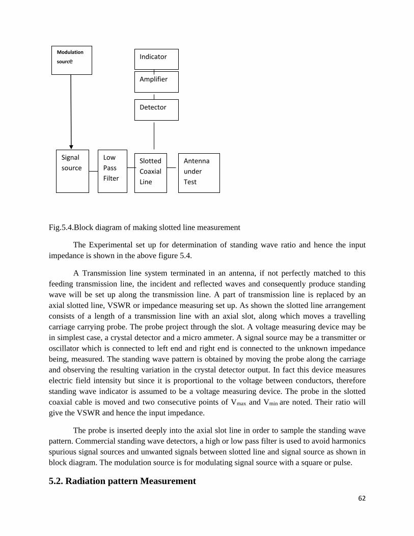
62

Fig.5.4.Block diagram of making slotted line measurement

The Experimental set up for determination of standing wave ratio and hence the input

impedance is shown in the above figure 5.4.

A Transmission line system terminated in an antenna, if not perfectly matched to this

feeding transmission line, the incident and reflected waves and consequently produce standing

wave will be set up along the transmission line. A part of transmission line is replaced by an

axial slotted line, VSWR or impedance measuring set up. As shown the slotted line arrangement

consists of a length of a transmission line with an axial slot, along which moves a travelling

carriage carrying probe. The probe project through the slot. A voltage measuring device may be

in simplest case, a crystal detector and a micro ammeter. A signal source may be a transmitter or

oscillator which is connected to left end and right end is connected to the unknown impedance

being, measured. The standing wave pattern is obtained by moving the probe along the carriage

and observing the resulting variation in the crystal detector output. In fact this device measures

electric field intensity but since it is proportional to the voltage between conductors, therefore

standing wave indicator is assumed to be a voltage measuring device. The probe in the slotted

coaxial cable is moved and two consecutive points of Vmax and Vmin are noted. Their ratio will

give the VSWR and hence the input impedance.

The probe is inserted deeply into the axial slot line in order to sample the standing wave

pattern. Commercial standing wave detectors, a high or low pass filter is used to avoid harmonics

spurious signal sources and unwanted signals between slotted line and signal source as shown in

block diagram. The modulation source is for modulating signal source with a square or pulse.

5.2. Radiation pattern Measurement

Signal

source

Low

Pass

Filter

Slotted

Coaxial

Line

Antenna

under

Test

Detector

Amplifier

Indicator Modulation

source

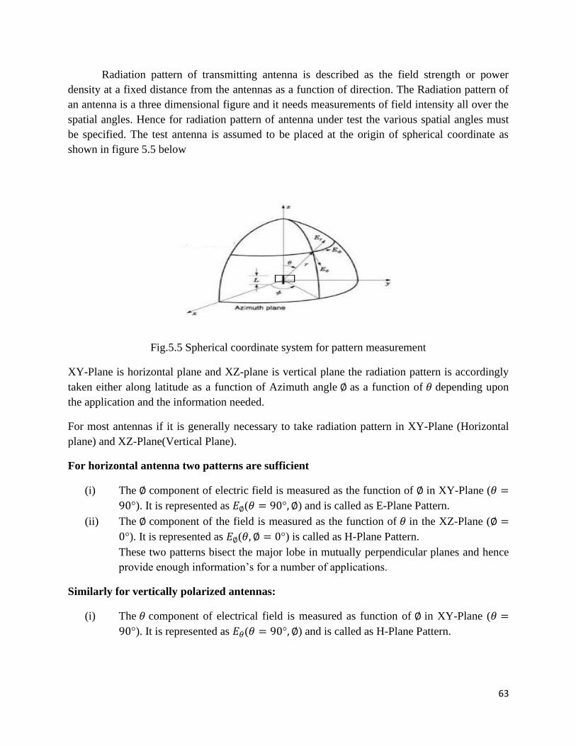
63

Radiation pattern of transmitting antenna is described as the field strength or power

density at a fixed distance from the antennas as a function of direction. The Radiation pattern of

an antenna is a three dimensional figure and it needs measurements of field intensity all over the

spatial angles. Hence for radiation pattern of antenna under test the various spatial angles must

be specified. The test antenna is assumed to be placed at the origin of spherical coordinate as

shown in figure 5.5 below

Fig.5.5 Spherical coordinate system for pattern measurement

XY-Plane is horizontal plane and XZ-plane is vertical plane the radiation pattern is accordingly

taken either along latitude as a function of Azimuth angle ∅ as a function of 𝜃 depending upon

the application and the information needed.

For most antennas if it is generally necessary to take radiation pattern in XY-Plane (Horizontal

plane) and XZ-Plane(Vertical Plane).

For horizontal antenna two patterns are sufficient

(i) The ∅ component of electric field is measured as the function of ∅ in XY-Plane (𝜃 =

90°). It is represented as 𝐸∅(𝜃 = 90°, ∅) and is called as E-Plane Pattern.

(ii) The ∅ component of the field is measured as the function of 𝜃 in the XZ-Plane (∅ =

0°). It is represented as 𝐸∅(𝜃, ∅ = 0°) is called as H-Plane Pattern.

These two patterns bisect the major lobe in mutually perpendicular planes and hence

provide enough information’s for a number of applications.

Similarly for vertically polarized antennas:

(i) The 𝜃 component of electrical field is measured as function of ∅ in XY-Plane (𝜃 =

90°). It is represented as 𝐸𝜃(𝜃 = 90°, ∅) and is called as H-Plane Pattern.

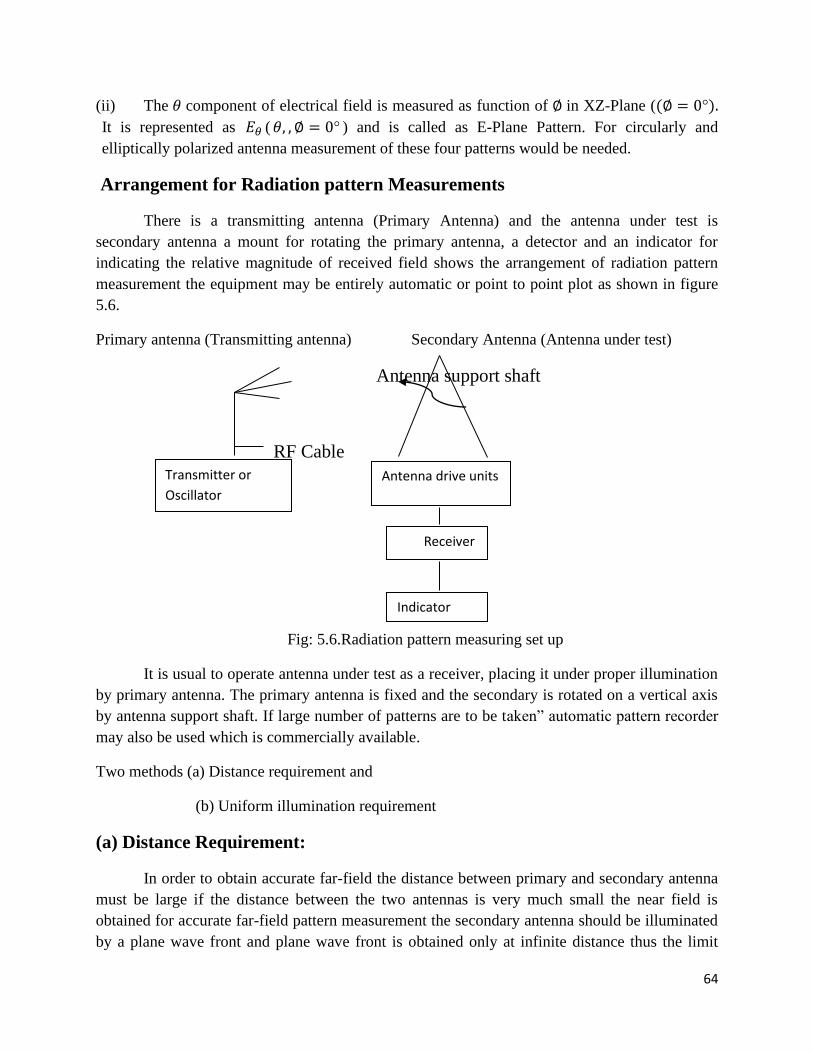
64

(ii) The 𝜃 component of electrical field is measured as function of ∅ in XZ-Plane ((∅ = 0°).

It is represented as 𝐸𝜃 ( 𝜃, , ∅ = 0° ) and is called as E-Plane Pattern. For circularly and

elliptically polarized antenna measurement of these four patterns would be needed.

Arrangement for Radiation pattern Measurements

There is a transmitting antenna (Primary Antenna) and the antenna under test is

secondary antenna a mount for rotating the primary antenna, a detector and an indicator for

indicating the relative magnitude of received field shows the arrangement of radiation pattern

measurement the equipment may be entirely automatic or point to point plot as shown in figure

5.6.

Primary antenna (Transmitting antenna) Secondary Antenna (Antenna under test)

Antenna support shaft

RF Cable

Fig: 5.6.Radiation pattern measuring set up

It is usual to operate antenna under test as a receiver, placing it under proper illumination

by primary antenna. The primary antenna is fixed and the secondary is rotated on a vertical axis

by antenna support shaft. If large number of patterns are to be taken” automatic pattern recorder

may also be used which is commercially available.

Two methods (a) Distance requirement and

(b) Uniform illumination requirement

(a) Distance Requirement:

In order to obtain accurate far-field the distance between primary and secondary antenna

must be large if the distance between the two antennas is very much small the near field is

obtained for accurate far-field pattern measurement the secondary antenna should be illuminated

by a plane wave front and plane wave front is obtained only at infinite distance thus the limit

Transmitter or

Oscillator

Antenna drive units

Receiver

Indicator

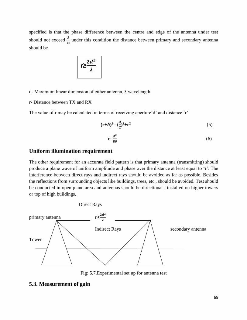
65

specified is that the phase difference between the centre and edge of the antenna under test

should not exceed 𝜆

16 under this condition the distance between primary and secondary antenna

should be

d- Maximum linear dimension of either antenna, λ wavelength

r- Distance between TX and RX

The value of r may be calculated in terms of receiving aperture‘d’ and distance ‘r’

(r+𝜹)2 =(𝒅

𝟐)2+r2 (5)

r=𝒅𝟐

𝟖𝜹 (6)

Uniform illumination requirement

The other requirement for an accurate field pattern is that primary antenna (transmitting) should

produce a plane wave of uniform amplitude and phase over the distance at least equal to ‘r’. The

interference between direct rays and indirect rays should be avoided as far as possible. Besides

the reflections from surrounding objects like buildings, trees, etc., should be avoided. Test should

be conducted in open plane area and antennas should be directional , installed on higher towers

or top of high buildings.

Direct Rays

primary antenna r≥𝟐𝒅𝟐

𝝀

Indirect Rays secondary antenna

Tower

Fig: 5.7.Experimental set up for antenna test

5.3. Measurement of gain

r≥𝟐𝒅𝟐

𝝀

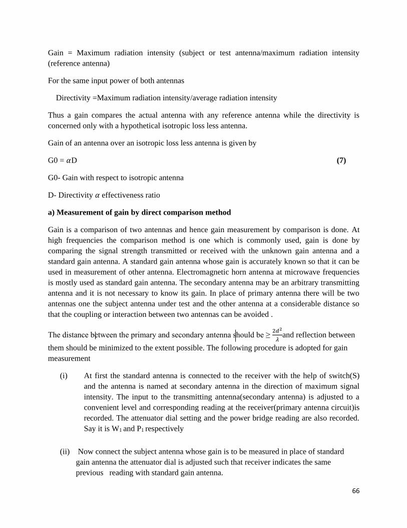
66

Gain = Maximum radiation intensity (subject or test antenna/maximum radiation intensity

(reference antenna)

For the same input power of both antennas

Directivity =Maximum radiation intensity/average radiation intensity

Thus a gain compares the actual antenna with any reference antenna while the directivity is

concerned only with a hypothetical isotropic loss less antenna.

Gain of an antenna over an isotropic loss less antenna is given by

G0 = 𝛼D (7)

G0- Gain with respect to isotropic antenna

D- Directivity 𝛼 effectiveness ratio

a) Measurement of gain by direct comparison method

Gain is a comparison of two antennas and hence gain measurement by comparison is done. At

high frequencies the comparison method is one which is commonly used, gain is done by

comparing the signal strength transmitted or received with the unknown gain antenna and a

standard gain antenna. A standard gain antenna whose gain is accurately known so that it can be

used in measurement of other antenna. Electromagnetic horn antenna at microwave frequencies

is mostly used as standard gain antenna. The secondary antenna may be an arbitrary transmitting

antenna and it is not necessary to know its gain. In place of primary antenna there will be two

antennas one the subject antenna under test and the other antenna at a considerable distance so

that the coupling or interaction between two antennas can be avoided .

The distance between the primary and secondary antenna should be ≥ 2𝑑2

𝜆and reflection between

them should be minimized to the extent possible. The following procedure is adopted for gain

measurement

(i) At first the standard antenna is connected to the receiver with the help of switch(S)

and the antenna is named at secondary antenna in the direction of maximum signal

intensity. The input to the transmitting antenna(secondary antenna) is adjusted to a

convenient level and corresponding reading at the receiver(primary antenna circuit)is

recorded. The attenuator dial setting and the power bridge reading are also recorded.

Say it is W1 and P1 respectively

(ii) Now connect the subject antenna whose gain is to be measured in place of standard

gain antenna the attenuator dial is adjusted such that receiver indicates the same

previous reading with standard gain antenna.

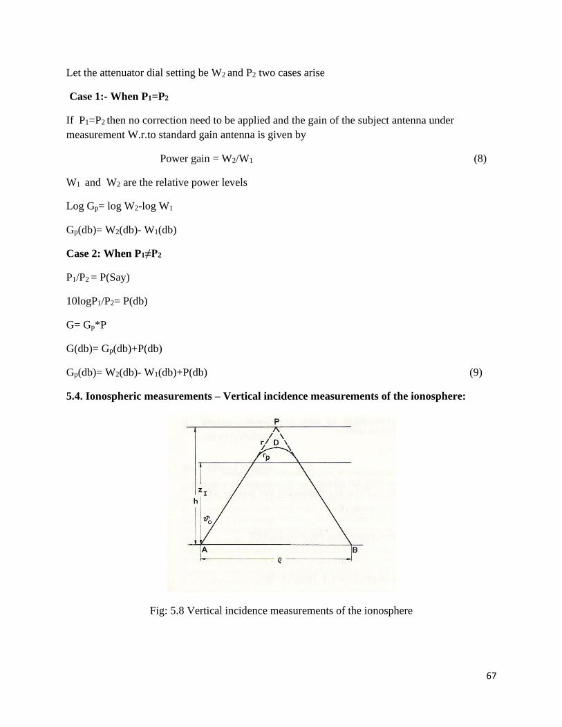
67

Let the attenuator dial setting be W2 and P2 two cases arise

Case 1:- When P1=P2

If P1=P2 then no correction need to be applied and the gain of the subject antenna under

measurement W.r.to standard gain antenna is given by

Power gain = W2/W1 (8)

W1 and W2 are the relative power levels

Log Gp= log W2-log W1

Gp(db)= W2(db)- W1(db)

Case 2: When P1≠P2

P1/P2 = P(Say)

10logP1/P2= P(db)

G= Gp*P

G(db)= Gp(db)+P(db)

Gp(db)= W2(db)- W1(db)+P(db) (9)

5.4. Ionospheric measurements – Vertical incidence measurements of the ionosphere:

Fig: 5.8 Vertical incidence measurements of the ionosphere

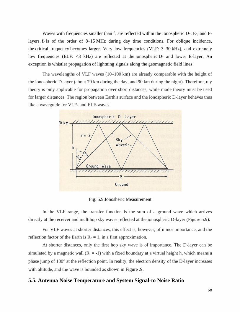
68

Waves with frequencies smaller than fc are reflected within the ionospheric D-, E-, and F-

layers. fc is of the order of 8–15 MHz during day time conditions. For oblique incidence,

the critical frequency becomes larger. Very low frequencies (VLF: 3–30 kHz), and extremely

low frequencies (ELF: <3 kHz) are reflected at the ionospheric D- and lower E-layer. An

exception is whistler propagation of lightning signals along the geomagnetic field lines

The wavelengths of VLF waves (10–100 km) are already comparable with the height of

the ionospheric D-layer (about 70 km during the day, and 90 km during the night). Therefore, ray

theory is only applicable for propagation over short distances, while mode theory must be used

for larger distances. The region between Earth's surface and the ionospheric D-layer behaves thus

like a waveguide for VLF- and ELF-waves.

Fig: 5.9.Ionosheric Measurement

In the VLF range, the transfer function is the sum of a ground wave which arrives

directly at the receiver and multihop sky waves reflected at the ionospheric D-layer (Figure 5.9).

For VLF waves at shorter distances, this effect is, however, of minor importance, and the

reflection factor of the Earth is Re = 1, in a first approximation.

At shorter distances, only the first hop sky wave is of importance. The D-layer can be

simulated by a magnetic wall (Ri = -1) with a fixed boundary at a virtual height h, which means a

phase jump of 180° at the reflection point. In reality, the electron density of the D-layer increases

with altitude, and the wave is bounded as shown in Figure .9.

5.5. Antenna Noise Temperature and System Signal-to Noise Ratio

69

Antenna temperature :

The performance of a telecommunication system depends very much on the signal-to-

noise ratio (SNR) at the receiver’s input. The electronic circuitry of the receiver (amplifiers,

mixers, etc.) has its own contribution to the noise generation. However, the antenna itself is a

significant source of noise. The antenna noise can be divided into two types of noise according to

its physical source: - noise due to the loss resistance of the antenna itself; and - noise, which the

antenna picks up from the surrounding environment. Any object whose temperature is above the

absolute zero radiates EM energy. Thus, each antenna is surrounded by noise sources, which

create noise power at the antenna terminals. Here, we will not be concerned with technological

sources of noise, which are a subject of the electromagnetic interference science. We are also not

concerned with intentional sources of electromagnetic interference. We are concerned with

natural sources of EM noise, such as sky noise and ground noise. The concept of antenna

temperature is not only associated with the EM noise. The relation between the object’s

temperature and the power it can create at the antenna terminals is used in passive remote

sensing (radiometry). A radiometer can create temperature images of objects. Typically, the

remote object’s temperature is measured by comparison with the noise due to background

sources and the receiver itself.

System signal-to-noise ratio (SNR)

Signal-to-noise ratio (abbreviated SNR or S/N) is a measure used in science and

engineering that compares the level of a desired signal to the level of background noise. It is

defined as the ratio of signal power to the noise power, often expressed in decibels. A ratio

higher than 1:1 (greater than 0 dB) indicates more signal than noise. While SNR is commonly

quoted for electrical signals, it can be applied to any form of signal (such as isotope levels in

an ice core or biochemical between cells).

Signal-to-noise ratio is defined as the ratio of the power of a signal (meaningful

information) and the power of background noise (unwanted signal)

SNR=𝐏𝐬𝐢𝐠𝐧𝐚𝐥

𝐩𝐧𝐨𝐢𝐬𝐞 (10)

A link budget is accounting of all of the gains and losses from the transmitter, through

the medium (free space, cable, waveguide, fiber, etc.) to the receiver in

70

telecommunication system. It accounts for the attenuation of the transmitted signal due to

propagation, as well as the antenna gains, feed line and miscellaneous losses. Randomly varying

channel gains such as fading are taken into account by adding some margin depending on the

anticipated severity of its effects. The amount of margin required can be reduced by the use of

mitigating techniques such as antenna diversity or frequency hopping.

A simple link budget equation looks like this:

Received Power (dB) = Transmitted Power (dB) + Gains (dB) − Losses (dB)

A link budget equation including all these effects, expressed logarithmically, might be

𝐏𝐑𝐗=𝐏𝐓𝐗+𝐆𝐓𝐗-𝐋𝐓𝐗-𝐋𝐅𝐒-𝐋𝐌+𝐆𝐑𝐗-𝐋𝐑𝐗which is given by

𝐏𝐑𝐗= received power (dBm)

𝐏𝐓𝐱= transmitter output power (dBm)

𝐆𝐓𝐗 = transmitter antenna gain (dBi)

𝐋𝐓𝐗 = transmitter losses (coax, connectors...) (dB)

𝐋𝐅𝐬 = path loss, usually free space loss (dB)

𝐋𝐦 = miscellaneous losses (fading margin, body loss, polarization mismatch, other

losses...) (dB)

𝐆𝐑𝐗 = receiver antenna gain (dBi)

𝐋𝐑𝐗 = receiver losses (coax, connectors...) (dB)

TEXT / REFERENCE BOOKS 1. K.D.Prasad, “Antennas and Wave Propagation”, 3rd Edition, Satya Prakasan, New Delhi, 2003. 2. R.L. Yadava, “Antennas and Wave Propagation”, 2nd Edition, PHI Learning Private Limited, New

Delhi, 2011. 3. Balanis C.A., “Antenna Theory and Design”, 4th Edition, John Wiley & Sons, 2016. 4. Jordan E.C., Balmain, K.G., “Electromagnetic Waves and Radiating Systems”, 2nd Edition, Prentice Hall

of India, 2006. 5. Collin R.E., “Antennas and Radio Wave Propagation”, McGraw Hill, 1985.

71

PART A

1. List out the requirements for accurate field pattern measurement?

2. Distinguish the two methods used for measuring impedance

3. Analyze the factors we need to find in the measurements of antenna?

4. List the methods available to measure gain of an antenna?

5. Give the methods of impedance measurement of antenna?

6. Examine the minimum distance between primary and secondary antennas to get accurate

far field patterns?

7. State vertical incidence.

8. Organize the relation between oblique and vertical incidence.

9. Examine radiation pattern of an antenna?

10. Interpret the methods used for antenna efficiency?

PART B

1. Illustrate a suitable experimental setup and the procedure to be followed for determining

the impedance.

2.Develop the relation between oblique and vertical incidence transmission.

3. Determine radiation pattern and beam width measurement of a given antenna.

4. Estimate short notes on a) Antenna noise b) Link Budget

5. Determine the measurement of gain of the antenna.

6. Evaluate the details about vertical incidence measurements of the ionosphere.

7. Interpret Ionospheric measurements.

8. Categorize the various measurements of antennas.

9. Analyze the two methods of measuring radiation pattern of an antenna.

10. Organize the measurement of antenna efficiency of an antenna.